Atmos. Meas. Tech., 5, 2469–2480, 2012www.atmos-meas-tech.net/5/2469/2012/doi:10.5194/amt-5-2469-2012© Author(s) 2012. CC Attribution 3.0 License.

AtmosphericMeasurement

Techniques

1 km fog and low stratus detection using pan-sharpened MSGSEVIRI data

H. M. Schulz1, B. Thies1, J. Cermak2, and J. Bendix1

1Laboratory for Climatology and Remote Sensing, Faculty of Geography, Philipps-University, Marburg, Germany2Institute of Geography, Ruhr University Bochum, Bochum, Germany

Correspondence to:H. M. Schulz (martin.schulz@geo.uni-marburg.de)

Received: 30 March 2012 – Published in Atmos. Meas. Tech. Discuss.: 26 June 2012Revised: 24 September 2012 – Accepted: 25 September 2012 – Published: 22 October 2012

Abstract. In this paper a new technique for the detection offog and low stratus in 1 km resolution from MSG SEVIRIdata is presented. The method relies on the pan-sharpeningof 3 km narrow-band channels using the 1 km high-resolutionvisible (HRV) channel. As solar and thermal channels had tobe sharpened for the technique, a new approach based on anexisting pan-sharpening method was developed using localregressions. A fog and low stratus detection scheme origi-nally developed for 3 km SEVIRI data was used as the basisto derive 1 km resolution fog and low stratus masks from thesharpened channels. The sharpened channels and the fog andlow stratus masks based on them were evaluated visually andby various statistical measures. The sharpened channels devi-ate only slightly from reference images regarding their pixelvalues as well as spatial features. The 1 km fog and low stra-tus masks are therefore deemed of high quality. They containmany details, especially where fog is restricted by complexterrain in its extent, that cannot be detected in the 3 km reso-lution.

1 Introduction

Fog and low stratus (FLS) have operationally been detectedfrom AVHRR and MODIS data for quite some time (firstapproach for fog detection at nighttime using AVHRR 3.7–10.8 µm differences: Eyre et al., 1984; Daytime approaches:e.g. Bendix and Bachmann, 1991; Kudoh and Noguchi,1991; Bendix et al., 2006). Also for geostationary satel-lite systems, which have the advantage of a high tempo-ral resolution, many reliable approaches for FLS detec-tion exist (e.g. Lee et al., 1997; comprehensive overview

in Gultepe et al., 2007). For Meteosat Second Genera-tion (MSG) Spinning-Enhanced Visible and Infrared Im-ager (SEVIRI) data the Satellite-based Operational Fog Ob-servation Scheme (SOFOS) developed by Cermak (2006)is a recent and reliable algorithm for FLS detection. It hasbeen extensively validated and proven its suitability for op-erational deployment (Cermak and Bendix, 2008), which iswhy it was used as the underlying FLS detection scheme inthis study.

However, for the detection of fog under certain conditionssuch as small-valley fog in a lower mountain range topog-raphy as found in many parts of Central Europe, the cur-rent scheme has some disadvantages, particularly becausethe nominal spatial resolution of 3 km at the sub-satellitepoint (this corresponds to a resolution of about 3× 6 km forCentral Europe) of the SEVIRI instrument’s multispectralbands is too coarse to detect these small-scale FLS phenom-ena. On the other hand, a panchromatic high resolution vis-ible (HRV) channel with a nominal resolution of 1 km perpixel is available on MSG, which could generally help toovercome this resolution problem. The high potential of theHRV channel in FLS detection was already highlighted byBugliaro and Mayer (2004) using two different approaches.Since their first approach, the simple application of radiancethresholds in the HRV channel, is not transferrable to a com-plex multi-channel classification scheme such as SOFOS, themore promising method for 1 km FLS detection is their sec-ond approach; this uses the HRV channel’s high-resolutioninformation to sharpen the SEVIRI 3 km channels. However,this procedure has major limitations regarding the quality ofthe resulting FLS masks and needs comprehensive manual

Published by Copernicus Publications on behalf of the European Geosciences Union.

2470 H. M. Schulz et al.: 1 km fog and low stratus detection

corrections so that it cannot be used for operational applica-tions.

The main aim of the current paper is to develop an auto-matic method that can be used operationally without man-ual post-processing. The technique is based on a specificpan-sharpening approach, also including the SEVIRI ther-mal bands. This is an innovation in comparison to com-mon pan-sharpening algorithms (see Strait et al., 2008 for anoverview). However, statistical downscaling approaches thatcould most probably be used in the context of FLS detec-tion do exist but have not proven their ability for the sharp-ening of thermal channels yet (Deneke and Roebeling, 2010)or cannot be used for SEVIRI data as multidimensional high-resolution input is needed (Liu and Pu, 2008). The newly de-veloped technique presented in this paper is based on a localregression approach presented by Hill et al. (1999). Sharp-ened solar and thermal channels are then used to detect FLSby using the SOFOS approach.

Data and techniques used for this study are described inSect. 2. The results are shown and discussed in Sect. 3. InSect. 4, a conclusion is drawn and a short outlook given.

2 Data and methods

2.1 SEVIRI data

SEVIRI raw data distributed via EUMETCast (EUMETSAT,2012) is operationally received at the Marburg Satellite Sta-tion. The data is decoded, unpacked and further processedby the FMet package (Cermak et al., 2008). Radiances inW m−2 sr−1, reflectance and blackbody temperatures (BBTs)in K are calculated for a section of the SEVIRI full diskshowing Europe. Several products, such as the SOFOS 3 kmFLS mask, are computed operationally from these data. Inthis study 144 daytime scenes from 17 November 2008,10 December 2008, 22 December 2008 and 17 January 2011showing Europe were incorporated.

2.2 METAR data

For validation purposes 6799 METereological AerodromeReports (METAR) from 21 points in time on the same days,obtained from a freely available online archive (Berge, 2012)were used. Geographic coordinates of the 982 European sta-tions (Fig. 1) that have published these METARs were takenfrom Thompson (2011).

2.3 FLS identification via SOFOS

1 km FLS masks were created from pan-sharpened chan-nels using SOFOS. SOFOS generally checks every pixel of ascene for FLS cloud properties using a range of tests (Cermakand Bendix, 2008, 2011). Most of these tests are conductedon a per-pixel basis:

Fig. 1.Positions of the METARs stations used in this study.

– cloud identification (application of a threshold derivedfrom a histogram analysis on the difference between the3.9 and 10.8 µm BBT);

– snow pixel elimination (application of thresholds on the0.8 and 10.8 µm channels as well as on the Normal-ized Difference Snow Index (NDSI), which is calculatedfrom the 0.6 and the 1.6 µm channel);

– test for liquid phase (application of a threshold of 230 Kon the 10.8 µm BBT. Further tests exclude warmer iceclouds and thin cirrus clouds which are not detected bythis simple threshold approach);

– test for small droplet size (application of a dynamicallyderived threshold on the 3.9 µm channel).

Pixels which do not pass all of these tests are rejected asobviously non-FLS. Further tests checking for spatial param-eters do not consider single pixels’ properties but propertiesof spatially coherent entities of cloud. For this purpose spa-tially connected pixels that were not rejected as obviouslynon-FLS are grouped together in entities (cf. Cermak andBendix, 2008). The following tests are performed on theseentities:

– test for stratiformity (A threshold of 2 K is applied onthe standard deviation of the 10.8 µm BBT for each en-tity);

– test for low clouds (cloud top height< 1000 m. Thecloud top height is derived from the 10.8 µm BBT orin some cases interpolated from the height of the sur-rounding terrain).

Entities which do not pass both tests are excluded fromthe resulting mask. Altogether SOFOS utilizes reflectance at0.6, 0.8 and 1.6 µm and BBTs at 3.9, 8.7, 10.8 and 12.0 µmto derive FLS masks from SEVIRI data, which now has tobe provided in 1 km spatial resolution by the pan-sharpeningalgorithm described below.

Atmos. Meas. Tech., 5, 2469–2480, 2012 www.atmos-meas-tech.net/5/2469/2012/

H. M. Schulz et al.: 1 km fog and low stratus detection 2471

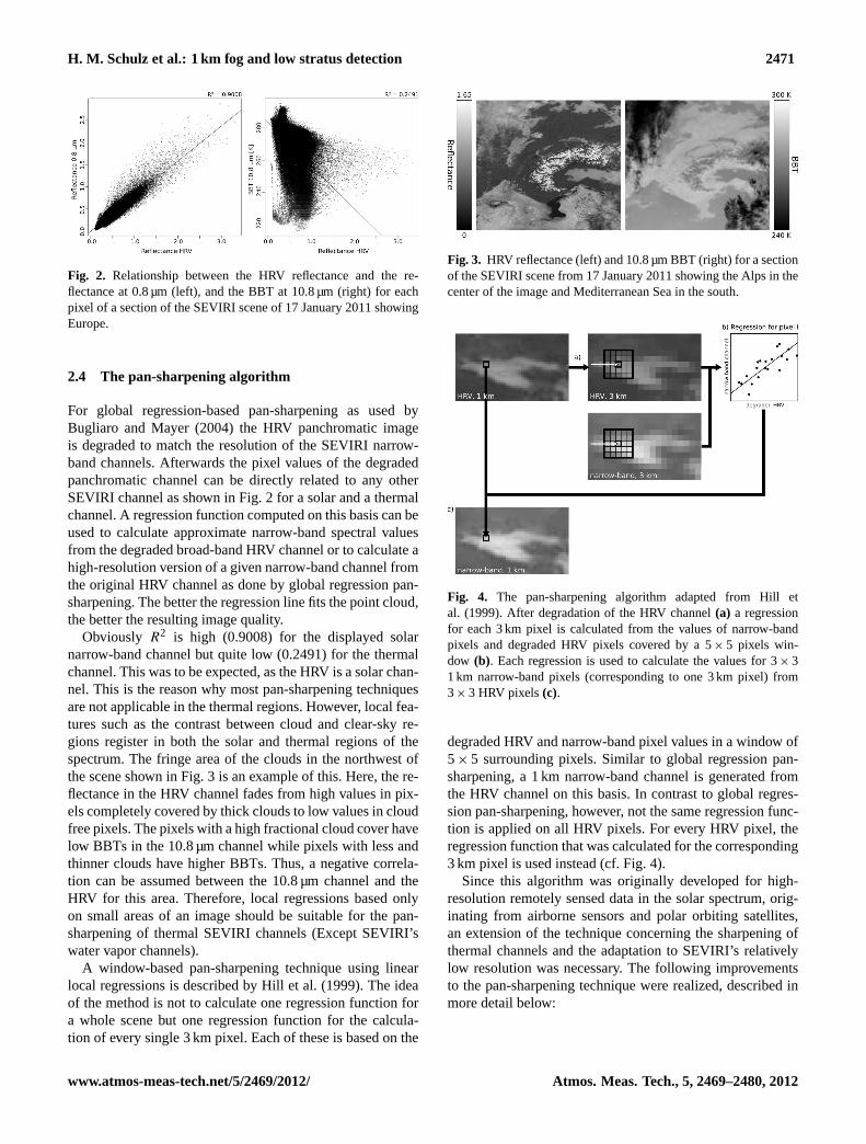
Fig. 2. Relationship between the HRV reflectance and the re-flectance at 0.8 µm (left), and the BBT at 10.8 µm (right) for eachpixel of a section of the SEVIRI scene of 17 January 2011 showingEurope.

2.4 The pan-sharpening algorithm

For global regression-based pan-sharpening as used byBugliaro and Mayer (2004) the HRV panchromatic imageis degraded to match the resolution of the SEVIRI narrow-band channels. Afterwards the pixel values of the degradedpanchromatic channel can be directly related to any otherSEVIRI channel as shown in Fig. 2 for a solar and a thermalchannel. A regression function computed on this basis can beused to calculate approximate narrow-band spectral valuesfrom the degraded broad-band HRV channel or to calculate ahigh-resolution version of a given narrow-band channel fromthe original HRV channel as done by global regression pan-sharpening. The better the regression line fits the point cloud,the better the resulting image quality.

Obviously R2 is high (0.9008) for the displayed solarnarrow-band channel but quite low (0.2491) for the thermalchannel. This was to be expected, as the HRV is a solar chan-nel. This is the reason why most pan-sharpening techniquesare not applicable in the thermal regions. However, local fea-tures such as the contrast between cloud and clear-sky re-gions register in both the solar and thermal regions of thespectrum. The fringe area of the clouds in the northwest ofthe scene shown in Fig. 3 is an example of this. Here, the re-flectance in the HRV channel fades from high values in pix-els completely covered by thick clouds to low values in cloudfree pixels. The pixels with a high fractional cloud cover havelow BBTs in the 10.8 µm channel while pixels with less andthinner clouds have higher BBTs. Thus, a negative correla-tion can be assumed between the 10.8 µm channel and theHRV for this area. Therefore, local regressions based onlyon small areas of an image should be suitable for the pan-sharpening of thermal SEVIRI channels (Except SEVIRI’swater vapor channels).

A window-based pan-sharpening technique using linearlocal regressions is described by Hill et al. (1999). The ideaof the method is not to calculate one regression function fora whole scene but one regression function for the calcula-tion of every single 3 km pixel. Each of these is based on the

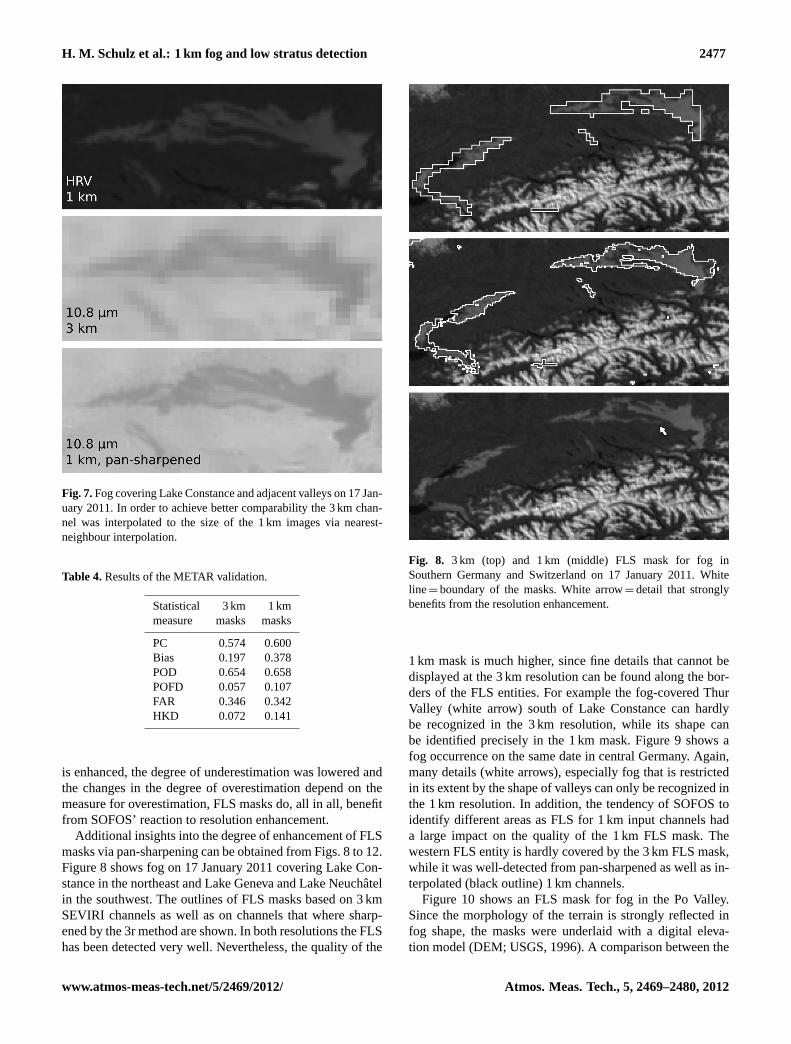
Fig. 3. HRV reflectance (left) and 10.8 µm BBT (right) for a sectionof the SEVIRI scene from 17 January 2011 showing the Alps in thecenter of the image and Mediterranean Sea in the south.

Fig. 4. The pan-sharpening algorithm adapted from Hill etal. (1999). After degradation of the HRV channel(a) a regressionfor each 3 km pixel is calculated from the values of narrow-bandpixels and degraded HRV pixels covered by a 5× 5 pixels win-dow (b). Each regression is used to calculate the values for 3× 31 km narrow-band pixels (corresponding to one 3 km pixel) from3× 3 HRV pixels(c).

degraded HRV and narrow-band pixel values in a window of5× 5 surrounding pixels. Similar to global regression pan-sharpening, a 1 km narrow-band channel is generated fromthe HRV channel on this basis. In contrast to global regres-sion pan-sharpening, however, not the same regression func-tion is applied on all HRV pixels. For every HRV pixel, theregression function that was calculated for the corresponding3 km pixel is used instead (cf. Fig. 4).

Since this algorithm was originally developed for high-resolution remotely sensed data in the solar spectrum, orig-inating from airborne sensors and polar orbiting satellites,an extension of the technique concerning the sharpening ofthermal channels and the adaptation to SEVIRI’s relativelylow resolution was necessary. The following improvementsto the pan-sharpening technique were realized, described inmore detail below:

www.atmos-meas-tech.net/5/2469/2012/ Atmos. Meas. Tech., 5, 2469–2480, 2012

2472 H. M. Schulz et al.: 1 km fog and low stratus detection

i. application of a potential regression;

ii. distance weighting;

iii. different combinations of window sizes and shapes.

(i) The first improvement is related to the type of regressionused by the pan-sharpening algorithm. In Fig. 5 the pixel val-ues of solar and thermal channels were plotted against thedegraded HRV channel for different single windows to deter-mine the nature of the relationship between these channels.Some relationships (a and b) can be described well by linearas well as potential regressions. For other windows (c and d)they can much better be described by potential regressionsand in a few windows there is no relationship between bothchannels at all (e). The latter case is reflected in locally dete-riorated sharpening quality (see Sect. 3). The other findingssuggest improving the algorithm by using a potential regres-sion in the form of

y = a × xb (1)

with

b =

n ×

n∑i=1

(ln(xi) × ln(yi)) −

n∑i=1

ln(xi) ×

n∑i=1

ln(yi)

n ×

n∑i=1

ln(xi)2−

(n∑

i=1ln(xi)

)2(2)

and

a =

n∑i=1

ln(yi) − b ×

n∑i=1

ln(xi)

n(3)

wherexi is the degraded HRV value andyi is the narrow-band channel value for a window pixeli. n is the number ofpixels in the current window (some windows next to an im-age’s border are cut off and therefore consist of fewer pixels).

(ii) The second change to Hill et al.’s (1999) algorithm wasimplemented to account for Tobler’s (1970) first law of ge-ography saying that near things are more related than distantthings. In this context this means that a window’s regressionshould particularly be affected by pixels close to the windowcenter. Therefore we introduced a weighting factorwi foreach window pixeli that depends on the Euclidean distancedi (measured in pixels) to a window’s central pixel:

wi =

{1di

if di > 01

0.5 if di=0. (4)

Sincedi is 0 for the central pixel and therefore this pixelwould be weighted infinitely,di is set to 0.5 for these pixels.To account forwi in such a way that window pixels nearer to

Fig. 5. Types of relationships between different narrow-band chan-nels and the HRV channel for single windows in a SEVIRI scenefrom 30 September 2003. The relationship shown in the upper rowcan be described well by a linear(a) and a potential regression(b).The relationship shown in the middle row is better described by apotential regression(d) than by a linear regression(c), while the re-lationship shown in(e) cannot be explained by the HRV values atall.

the window’s center have a stronger influence on the centralpixel. Eqs. (2) and (3) were altered, such that:

b =

n∑i=1

wi ×

n∑i=1

(ln(xi) × ln(yi) × wi) −

n∑i=1

(ln(xi) × wi) ×

n∑i=1

(ln(yi) × wi)

n∑i=1

wi ×

n∑i=1

(ln(xi)

2× wi

)−

(n∑

i=1(ln(xi) × wi)

)2(5)

and

a =

n∑i=1

(ln(yi) × wi) − b ×

n∑i=1

(ln(xi) × wi)

n∑i=1

wi

. (6)

(iii) Since relationships between the degraded HRV chan-nel and narrow-band channels are spatially limited, windows

Atmos. Meas. Tech., 5, 2469–2480, 2012 www.atmos-meas-tech.net/5/2469/2012/

H. M. Schulz et al.: 1 km fog and low stratus detection 2473

of only 3× 3 pixels in size, and windows of a roughly roundshape were tested (round windows cannot be achieved withonly a few pixels. For 3×3 pixels a cruciform shape is there-fore the nearest possible approximation to a round window.For 5× 5 pixel a better approximation is possible).

Besides the use of a potential regression and the changesregarding the window shape and size, the basic idea of thepan-sharpening algorithm described by Hill et al. (1999) andshown in Fig. 4 was not altered.

2.5 Methodology of validation

Several variations of the pan-sharpening approach describedin Sect. 2.4 are possible since the different window sizes andshapes, distance weighting and the two types of regressioncan be combined in various ways. To find the best-suitedversion for 1 km FLS detection, several steps of validationwere necessary. First, the spectral as well as the spatial qual-ity of pan-sharpened channels were measured for each possi-ble combination (see Sect. 2.5.1). The most promising vari-ations of the pan-sharpening technique were used to sharpenSEVIRI channels for FLS masking. These masks were com-pared to reference masks and METARs (see Sect. 2.5.2). Theadditional METAR validation was necessary to account forsome special characteristics of SOFOS regarding its reactionto an increased resolution of its input channels.

For the statistical validation of the pan-sharpened chan-nels and the comparison of FLS masks with reference masks,144 daylight scenes under various illumination conditionsfrom (randomly chosen) FLS appearances on 17 Novem-ber 2008, 10 December 2008, 22 December 2008 and 17 Jan-uary 2011 were utilized. For the METAR validation the num-ber of scenes was reduced to 21 to avoid overload of the usedonline archive.

Besides the validation using statistical measures, the qual-ity of sharpened channels and FLS masks based on themwas additionally assessed visually for individual scenes. FLSmasks based on channels, the resolution of which was in-creased by using a nearest-neighbour interpolation, wereincluded in this visual validation to be able to judge towhat degree differences between 3 km and 1 km channelswere caused by SOFOS’ above-mentioned reaction to high-resolution input channels.

The validation study on the performance of the pan-sharpening was conducted including all seven SEVIRI chan-nels used as input for SOFOS (see Sect. 2.3).

2.5.1 Validation of pan-sharpened channels

In order to validate the spectral quality of the sharpenedchannels the average Root Mean Square Error (RMSE, seeStrait et al., 2008) was calculated for all 144 scenes. Sinceit is a measure for the average difference between a data se-ries and a reference data series, it can be used for measuringthe difference between the pixel values of an image and the

corresponding pixel values in a reference image. As it is inthe nature of pan-sharpening that images in a resolution inwhich the corresponding channels did not priorly exist arecreated, the RMSE cannot be calculated in the SEVIRI 1 kmresolution for lack of a reference image. To overcome thisproblem a method suggested by Thomas and Wald (2004)was utilized. According to their approach (hereinafter re-ferred to as “validation approach A”) the narrow-band chan-nels as well as the HRV channel are downsampled by thefactor 3. The 3 km HRV channel obtained in this way isused to sharpen the degraded 9 km narrow-band channels.The resulting 3 km narrow-band channels can be comparedto the original ones as reference. The area on the Earth’ssurface covered by a window of a certain pixel size is de-pendent on the resolution of the image. As spatial aspectsare taken into account by the new pan-sharpening algorithmin many ways, the validation via approach A, in which thepan-sharpening algorithm is applied on channels in a reducedresolution, may lead to wrong results regarding the windowshape and size as well as the distance weighting. Therefore ina second validation approach (further referred to as “valida-tion approach B”) the narrow-band channels were sharpenedto the HRV channel’s resolution and afterwards degraded totheir original size, in which they were compared to the un-altered channels as reference images. Validation approach Bhas the disadvantage that information from individual pix-els is lost when the sharpened images are degraded to theoriginal resolution. Thus, errors affecting only isolated pix-els cannot be accounted for by this approach. For this reasonboth approaches were used.

The spatial quality, a measure of the degree of similaritybetween the geometry of a sharpened channel and a referenceimage, for the different variations of the pan-sharpening al-gorithm was calculated using a slightly modified variation ofa method developed by Zhou et al. (1998). By application ofa Laplacian filter using the convolution mask

Dxy =

−1 −1 −1−1 8 −1−1 −1 −1

, (7)

the high-frequency component of each sharpened channelwas extracted and compared to the high-frequency compo-nent of a reference image using the Pearson product-momentcorrelation coefficient of the pixel values of both high fre-quency images. Since Zhou et al. (1998) apply their methodon sharpened solar channels only, they use the panchromaticchannel as the reference image. This method is not suited forthermal channels as their high frequency components differfrom those of solar channels. So, analogous to validation ap-proach A, the high frequency component was calculated forchannels that were first degraded and sharpened afterwards,and compared to the high frequency component of the un-altered channels. The average value of the product-momentcorrelation was calculated for all 144 scenes.

www.atmos-meas-tech.net/5/2469/2012/ Atmos. Meas. Tech., 5, 2469–2480, 2012

2474 H. M. Schulz et al.: 1 km fog and low stratus detection

Table 1.Layout of the confusion matrices used to calculate the dif-ferent statistical measures.n is the number of occurrences.

FLS in reference mask FLS in validated mask

True/1 False/0

True/1 n11 n10False/0 n01 n00

2.5.2 Validation of FLS masks

FLS masks based on sharpened channels were validated intwo different ways. First, channels treated according to val-idation approaches A and B were used to create 3 km FLSmasks via SOFOS. These masks were compared with refer-ence masks calculated by SOFOS from unaltered 3 km chan-nels. Confusion matrices (cf. Table 1) based on each pixeland each of the 144 scenes used were calculated. From thesetables the following statistical measures (Wilks, 1995; Joliffeand Stephenson, 2003) were calculated (see Appendix A forformulas):

– Proportion Correct (PC);

– Bias;

– Probability of Detection (POD);

– Probability of False Detection (POFD);

– False Alarm Rate (FAR);

– Hanssen-Kuipers Discriminant (HKD);

– Additionally a new measure, the Edge Precision (EP),was developed. It describes how well the positions ofedge pixels of FLS entities in the validated masks fitthe positions of edge pixels of the corresponding entitiesin the reference mask. For this purpose the convolutionmaskDxy was applied on each mask and each referencemask, in order to gain images showing only the edgesof each mask’s FLS entities. For these edge images andreference edge images contingency tables were createdand the POD, which in this context describes the frac-tion of edges pixels that are on the correct position, wascalculated.

For purposes of comparison, these measures were also cal-culated for masks based on channels, the resolution of whichwas increased after degradation by using a simple nearest-neighbour interpolation instead of pan-sharpening. A com-parison with interpolated data was done for validation ap-proach A only since approach B would gain perfect resultsfor masks based on channels that were interpolated using anearest-neighbour approach and degenerated afterwards.

The second approach to validate the FLS masks was nec-essary as SOFOS shows a tendency to identify different

(mostly larger) areas as FLS when the input channels’ res-olution is increased. This tendency is not caused by spec-tral errors that appear during sharpening as it can also be ob-served for channels whose resolution was increased by sim-ple nearest-neighbour interpolation (see Sect. 3). To checkwhether this behaviour affects the FLS masks negativelyMETAR data was utilized. A contingency table was calcu-lated for FLS masks based on 1 km pan-sharpened as wellas on unaltered 3 km channels using the METARs as refer-ence for all scenes used. From these tables the same statis-tical measures as used for the first approach for FLS valida-tion were calculated (except the Edge Precision, as it doesnot make sense for the comparison with point data).

A principal problem when validating a satellite-basedcloud product by making use of METAR data is mentionedby Cermak and Bendix (2007): As the instruments at ground-based stations publishing METARs are below the cloudsthey have another perspective on the clouds than satellites.To eliminate this problem as far as possible, not only thecloud base height but also the fractional cloud cover, therange of sight and (if included) the cloud type were uti-lized. Assuming a typical cloud thickness of 200 m for FLS(this value was empirically determined from random sam-ples taken from a cloud thickness product which was calcu-lated as described in Cermak and Bendix, 2011), METARswith cloud base heights of less than 800 m were interpretedas showing FLS presence if no cumulonimbus or cumuluscongestus with a large vertical extent had been reported. Ad-ditionally, METARs reporting a line of sight of less than1000 m were interpreted as indicating ground fog. Reportsmentioning additional cloud layers above the 800 m thresh-old were interpreted as FLS-free since the additional layerswould block the view from the satellite on underlying layers.Finally, METARs with a fractional cloud coverage of lessthan 3/8 were interpreted as free of FLS since it is very un-likely for such a low coverage that the respective pixel wouldbe cloud-covered.

Due to the small sample size the METAR validation hereshould not be seen as a general validation of SOFOS’ sharp-ening quality. For a detailed METAR validation of SOFOSbased on 1030 scenes see Cermak’s (2006) original work.

3 Results and discussion

3.1 The quality of sharpened channels

The validation of the sharpened channels showed that the useof a potential regression as well as distance weighting signif-icantly improve the pan-sharpening quality, regardless of thewindow size and shape. The validation results for the originalalgorithm by Hill et al. (1999) and the most promising vari-ations of the new algorithm are given in Table 2. The spec-tral quality is the highest if potential regression and distanceweighting are used in combination with a 3×3 pixels “round”

Atmos. Meas. Tech., 5, 2469–2480, 2012 www.atmos-meas-tech.net/5/2469/2012/

H. M. Schulz et al.: 1 km fog and low stratus detection 2475

Table 2.Validation results for the spectral and spatial quality of different variations of the pan-sharpening approach. The RMSE is given inabsolute values (Reflectance for solar channels, blackbody temperature for thermal channels) as well as in % of the mean pixel value of eachvalidated scene.

Method of validation 0.6 µm 0.8 µm 1.6 µm 3.9 µm 8.7 µm 10.8 µm 12.0 µm

RMSE, approach AHill et al. 0.038/11.147 % 0.046/14.476 % 0.047/16.457 % 4.576/1.677 % 2.905/1.094 % 3.096/1.160 % 3.134/1.176 %5s 0.037/10.749 % 0.045/12.152 % 0.044/15.518 % 4.268/1.564 % 2.471/0.931 % 2.620/0.981 % 2.645/0.993 %3r 0.037/10.719 % 0.045/12.093 % 0.042/14.887 % 4.025/1.475 % 2.134/0.803 % 2.243/0.840 % 2.254/0.846 %

RMSE, approach BHill et al. 0.029/8.422 % 0.036/9.652 % 0.032/11.383 % 2.814/1.031 % 1.437/0.541 % 1.493/0.559 % 1.497/0.562 %5s 0.025/7.324 % 0.031/8.394 % 0.028/9.846 % 2.546/0.934 % 1.193/0.415 % 1.141/0.427 % 1.142/0.428 %3r 0.019/5.339 % 0.023/6.096 % 0.021/7.383 % 2.118/0.777 % 0.570/0.214 % 0.580/0.217 % 0.580/0.217 %

Spatial qualityHill et al. 0.689 0.665 0.635 0.185 0.381 0.389 0.3685s 0.693 0.668 0.644 0.217 0.403 0.413 0.3963r 0.683 0.657 0.618 0.197 0.361 0.369 0.354

window (further referred to as 3r). The algorithm version us-ing a 5× 5 pixels square window (further referred to as 5s),which yields a lower spectral quality (but is still better thanthat of the unaltered algorithm by Hill et al., 1999), yieldsthe highest spatial quality. The spatial as well as the spec-tral quality of the other algorithm versions using potentialregression and distance weighting (5× 5 pixels round win-dow and 3× 3 pixels square window, not shown in Table 2)lies between the quality of 3r and 5s. These findings are notsurprising: the spectral quality improves for smaller windowsconsistent with the consideration that relationships betweenthe HRV channel and the narrow-band channels are mostlyspatially limited. As the sample size of each regression getssmaller for smaller windows, the regression calculated a 3 kmpixels is of low significance in some cases and cannot be usedfor every corresponding 1 km pixel. The resulting failuresoccur rarely and only affect single pixels, which is why theoverall spectral quality is hardly affected. Since these singlepixel errors have impact on the high frequency componentof an image, they strongly affect the spatial quality. Due tothe trade-off between the spatial and the spectral quality thewindow size and shape has to be chosen depending on theintended use. In order to check whether the spatial or spec-tral quality of SOFOS input channels is more important forthe quality of the FLS detection, the validation of the result-ing masks was necessary to choose the best version of thepan-sharpening algorithm.

Figure 6 shows the quality of the new algorithm using 5sand 3r for the sharpening of each of the SOFOS input chan-nels. For the 3r version the mentioned errors in individualpixels can be clearly identified. Since the lowered spectralquality of the 5s variation cannot be recognized by the hu-man eye, a 5×5 pixels window seems to be a suitable choicefor visualization purposes. The scene shows fog in the PoValley in the center and the snow-covered Alps in the north.North of the fog in the plain Lake Iseo can be recognized. Foreach channel these different surfaces were sharpened well.The fog margin is very sharp and even small valleys, alongwhich the fog reaches into the northern parts of the Apen-nine Mountains, can be recognized. In the southeast of the

scene there are high clouds above the FLS, which are shownin dark shades in the thermal channels (low temperature). Inthe thermal spectrum the spatial quality of the scene is low-ered for these clouds by some weakly pronounced rectangu-lar artifacts in the original 3 km resolution. These artifacts arecaused by a situation as shown in Fig. 5e. As no relationshipbetween the narrow-band channel and the degraded HRVchannel can be established, a more or less horizontal regres-sion function is assumed, which is why for these areas quitesimilar values are assigned to all 1 km pixels covered by thesame 3 km pixel. These flaws do not affect the spectral qual-ity. Further they are rare and can mostly be observed for highclouds, especially for cumuliform clouds where the bright-ness of the HRV channel is strongly influenced by the illu-mination geometry. Therefore they should only minimallyaffect the quality of FLS masks based on sharpened chan-nels. In addition to Fig. 6, the pan-sharpening quality of 5sis demonstrated for a thermal channel in Fig. 7 showing anFLS entity covering Lake Constance and adjacent valleys.

3.2 The quality of FLS masks based on sharpenedchannels

The validation results for FLS masks based on sharpenedSEVIRI channels are given in Table 3 for the original sharp-ening technique by Hill et al. (1999) as well as for 3r and5s. Additionally the quality measures according to validationapproach A (see Sect. 2.5.2) are given for the masks basedon interpolated channels. The PC is almost 1 for each pan-sharpening technique as well as for each validation approach.This is no surprise since even the simple nearest-neighbourinterpolation achieves such high values. The reason for that isthat the majority of the pixels of each mask are far away fromthe boundaries of any FLS entity, but the resolution enhance-ment is only important to classify pixels near boundaries cor-rectly. Since the interpolation does not cause any spectral er-rors, the mask quality inside and outside of the FLS entitiesis very good, while it is low on boundary pixels. All in allthis causes a high PC, which is slightly better than that ofthe original algorithm by Hill et al. and the 5s variation. The

www.atmos-meas-tech.net/5/2469/2012/ Atmos. Meas. Tech., 5, 2469–2480, 2012

2476 H. M. Schulz et al.: 1 km fog and low stratus detection

Fig. 6.Sharpening results for different variations of the pan-sharpening algorithm and each of SOFOS’ input channels showing fog in the PoValley on 22 December 2008. In order to achieve better comparability the 3 km channels were interpolated to the size of the 1 km images vianearest-neighbour interpolation.

Table 3. Statistical measures describing the quality of FLS masks based on channels that were sharpened by different variations of thepan-sharpening algorithm as well as on interpolated channels.

Method of validation PC Bias POD POFD FAR HKD EP

Validation approach A

Hill et al. 0.933 0.987 0.746 0.038 0.244 0.708 0.3365s 0.936 1.045 0.787 0.040 0.246 0.747 0.3563r 0.950 1.0002 0.816 0.029 0.184 0.787 0.425Interpolation 0.948 1.001 0.807 0.030 0.194 0.777 0.372

Validation approach BHill et al. 0.956 1.011 0.842 0.026 0.167 0.816 0.5025s 0.966 1.013 0.880 0.021 0.132 0.859 0.6123r 0.974 1.002 0.904 0.015 0.098 0.888 0.703

Best Possible Result 1 1 1 0 0 1 1

same can be observed for the bias, the POD, the POFD, theFAR and the HKD. Although Figs. 6 and 7 show that thespatial quality of the 5s method is much higher than that of asimple interpolation, even the Edge Precision (EP) of sharp-ened masks is lower than that of masks based on interpolatedchannels. All of these findings are most probably caused byan insufficient spectral quality of the original algorithm andthe 5s version. This hypothesis is supported by the fact thatonly the 3r variation, which has the best spectral quality, out-performs the interpolation for all statistical measures. In ad-dition this variant delivers a spatial quality (cf. Fig. 6) thatis much higher than that of a simple interpolation and thusgains the best Edge Precision. Therefore it is the best choicefor the sharpening of SOFOS input channels.

3.3 Comparison of 3 km and 1 km FLS masks

In order to determine whether the mentioned differences be-tween the FLS area in masks on base of 3 km channel andon base of 1 km channels are altogether advantageous or dis-advantageous, the METAR validation was performed. Theresults are shown in Table 4. As the bias is low for bothresolutions, the area of FLS is apparently underestimatedby SOFOS in general. The better overall quality (PC andHKD) and a higher probability of detection in combinationwith a bias closer to 1 imply that the 1 km masks’ quality isenhanced due to a lowered degree of underestimation. ThePOFD, on the other hand, is a little bit higher than for 3 kmmasks (but still on a low level), which means that the areaof FLS is overestimated in some additional cases. However,the FAR, which is another measure for overestimation, isslightly better for the 1 km resolution. As the overall quality

Atmos. Meas. Tech., 5, 2469–2480, 2012 www.atmos-meas-tech.net/5/2469/2012/

H. M. Schulz et al.: 1 km fog and low stratus detection 2477

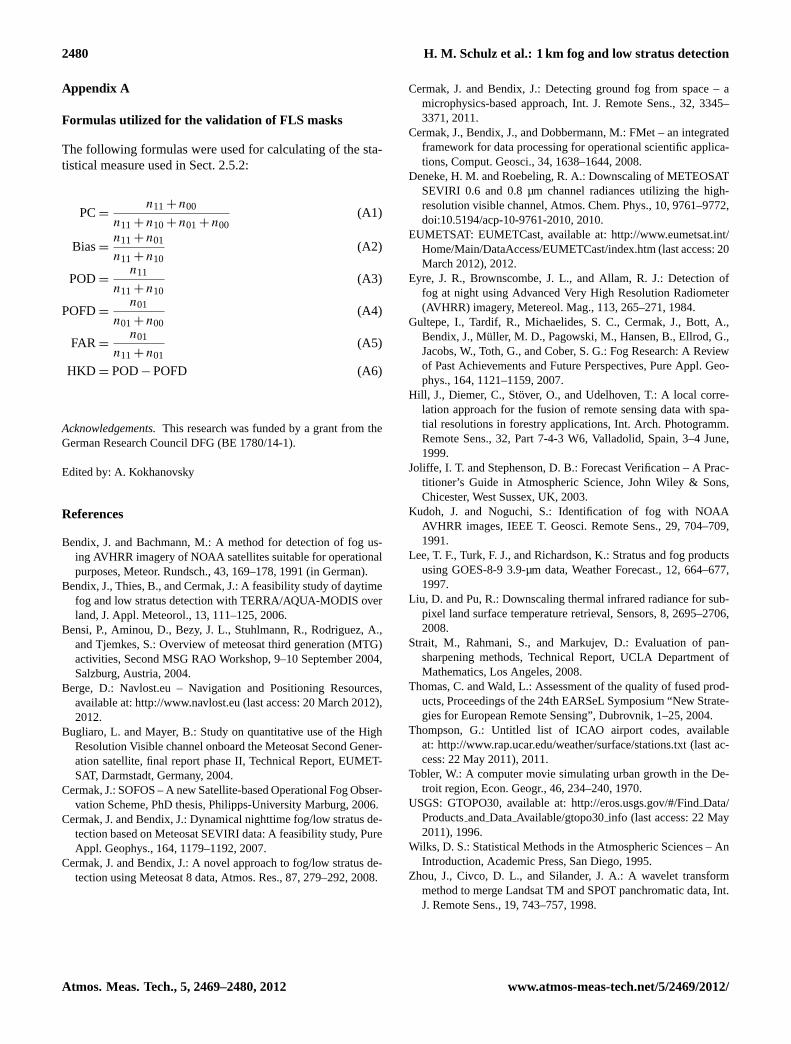
Fig. 7.Fog covering Lake Constance and adjacent valleys on 17 Jan-uary 2011. In order to achieve better comparability the 3 km chan-nel was interpolated to the size of the 1 km images via nearest-neighbour interpolation.

Table 4.Results of the METAR validation.

Statistical 3 km 1 kmmeasure masks masks

PC 0.574 0.600Bias 0.197 0.378POD 0.654 0.658POFD 0.057 0.107FAR 0.346 0.342HKD 0.072 0.141

is enhanced, the degree of underestimation was lowered andthe changes in the degree of overestimation depend on themeasure for overestimation, FLS masks do, all in all, benefitfrom SOFOS’ reaction to resolution enhancement.

Additional insights into the degree of enhancement of FLSmasks via pan-sharpening can be obtained from Figs. 8 to 12.Figure 8 shows fog on 17 January 2011 covering Lake Con-stance in the northeast and Lake Geneva and Lake Neuchatelin the southwest. The outlines of FLS masks based on 3 kmSEVIRI channels as well as on channels that where sharp-ened by the 3r method are shown. In both resolutions the FLShas been detected very well. Nevertheless, the quality of the

Fig. 8. 3 km (top) and 1 km (middle) FLS mask for fog inSouthern Germany and Switzerland on 17 January 2011. Whiteline= boundary of the masks. White arrow= detail that stronglybenefits from the resolution enhancement.

1 km mask is much higher, since fine details that cannot bedisplayed at the 3 km resolution can be found along the bor-ders of the FLS entities. For example the fog-covered ThurValley (white arrow) south of Lake Constance can hardlybe recognized in the 3 km resolution, while its shape canbe identified precisely in the 1 km mask. Figure 9 shows afog occurrence on the same date in central Germany. Again,many details (white arrows), especially fog that is restrictedin its extent by the shape of valleys can only be recognized inthe 1 km resolution. In addition, the tendency of SOFOS toidentify different areas as FLS for 1 km input channels hada large impact on the quality of the 1 km FLS mask. Thewestern FLS entity is hardly covered by the 3 km FLS mask,while it was well-detected from pan-sharpened as well as in-terpolated (black outline) 1 km channels.

Figure 10 shows an FLS mask for fog in the Po Valley.Since the morphology of the terrain is strongly reflected infog shape, the masks were underlaid with a digital eleva-tion model (DEM; USGS, 1996). A comparison between the

www.atmos-meas-tech.net/5/2469/2012/ Atmos. Meas. Tech., 5, 2469–2480, 2012

2478 H. M. Schulz et al.: 1 km fog and low stratus detection

Fig. 9. 3 km (top) and 1 km (center) FLS mask for fog in Cen-tral Germany on 17 January 2011. White line= boundary of the3 km and 1 km masks. Black line= boundary of an additional FLSmask based on channels interpolated to 1 km resolution (Notice thatthis mask matches the 3 km mask perfectly for the eastern FLSentity, which is why the black outline is not visible here). Whitearrows= details that strongly benefit from the resolution enhance-ment.

masks and the DEM shows that many terrain features affect-ing the shape of the fog entity (white arrows) like many smallvalleys in the northern Apennines, the Superga hill range ris-ing from the middle of the fog or the remnants of a morainearc in the northwest of the scene, are hardly reflected in the3 km mask. In the 1 km mask, all of these features can be dis-tinguished easily. In addition, the 3 km mask does not coverthe western part of the fog, while the 1 km mask does. Adrawback of the sharpened mask is marked by a black ar-row. A hole in the mask, where the FLS was not recognized,can be found here. Again, these differences to the 3 km maskwere not caused by a low quality of the sharpening but bythe effect of the increased resolution of its input channels onSOFOS. For interpolated input channels (black outline) thehole in the mask is even bigger.

Fig. 10. FLS masks (indicated by the white outline) in 3 km (left)and 1 km (center) resolution for fog in the Po Valley on 22 De-cember 2008. The masks’ outlines are underlaid by a DEM. Whiteline= boundary of the 3 km and 1 km masks. Black line= boundaryof an additional FLS mask based on channels interpolated to 1 kmresolution. White arrows= details that strongly benefit from the res-olution enhancement. Black Arrow= area where FLS was not de-tected.

Figure 11 shows FLS in Southern Germany delimited bythe northern margin of the Alps. Again, the topography-induced shape of the FLS, including many valleys (white ar-rows), can be much better identified in the 1 km mask than inthe 3 km mask. There are also some areas where FLS couldonly be identified on the basis of the 1 km channels (dark-grey arrow) or on the basis of the 3 km channels (light-greyarrow). A comparison of the 1 km mask with a mask based oninterpolated channels (black outline) shows that these differ-ences are, again, caused by the reaction of SOFOS to high-resolution input channels, which has (as the METAR valida-tion has shown) a positive overall influence.

Snow close to fog areas in Figs. 8, 10 and 11 was notmisidentified as FLS in any case, which is a big advantage ofthe new method over a threshold approach. However, if fogand snow or other clouds are situated directly side by side,they fall into common windows and therefore the algorithmtries to describe the dependency of a narrow-band channelfrom the pan channel by the same regressions for both mate-rials. Since this is not reasonable in many cases, a situationsimilar to that shown in Fig. 5e could occur and thereforedrawbacks in the spatial quality of the sharpened channelsand in the resulting mask should be possible. 3 km artifactsin the 1 km FLS mask caused by this could not be observedfor the margins of snow-covered areas or for any entity ofground fog. In the margin area of FLS without ground con-tact, however, this kind of artifacts could be observed in rarecases (cf. Fig. 12).

A general disadvantage of every algorithm using local re-gressions is the fact that only those pixel types can be sharp-ened that are accounted for by the regression used to sharpenthem. This means that a 1 km narrow-band pixel can only becalculated from the corresponding HRV pixel by using a re-gression that was calculated on the basis of at least one 3 kmpixel the value of which is linked to the HRV pixel valuesin the same way as the 1 km narrow-band pixel value. Thus,FLS entities that are not visible in the 3 km resolution andnot in the same window as bigger entities cannot be detectedby this approach.

Atmos. Meas. Tech., 5, 2469–2480, 2012 www.atmos-meas-tech.net/5/2469/2012/

H. M. Schulz et al.: 1 km fog and low stratus detection 2479

Fig. 11.3 km (top) and 1 km (center) FLS masks (indicated by thewhite outline) for fog north of the Alps on 2 February 2011. Themasks’ outlines are underlaid by a DEM. White line= boundary ofthe 3 km and 1 km masks. Black line= boundary of an additionalFLS mask based on channels interpolated to 1 km resolution. Whitearrows= details that strongly benefit from the resolution enhance-ment. Black arrows= Areas that were not identified as FLS regard-less of the resolution. Light grey arrow= an area that was only de-tected as FLS in 3 km resolution. Dark grey arrow= an area thatwas only detected as FLS in 1 km resolution.

4 Conclusion and outlook

A method for the creation of 1 km fog and low stratus (FLS)masks from MSG SEVIRI data was presented. The newmethod uses an innovative application for a further devel-oped version of an existing pan-sharpening algorithm suit-able to enhance the spatial quality of solar as well as ther-mal 3 km SEVIRI channels to 1 km by using the instru-ment’s panchromatic HRV channel. The resulting 1 km syn-thetic narrow-band channels are used as input for the well-validated FLS detection scheme SOFOS in order to produce1 km FLS masks. The pan-sharpening approach strongly im-proves the spatial quality of the resulting masks. As the shapeof many small valleys cannot be distinguished at a 3 km

Fig. 12.FLS masks (indicated by the white outline) for low stratuswithout ground contact over Central France on 10 December 2008based on 3 km (left) and 1 km (right) SEVIRI channels. The spatialquality of the 1 km mask is reduced by rectangular artifacts in the3 km resolution.

spatial resolution, this is especially important for the propermapping of FLS entities delimited by topography. The newapproach combines a relatively high spatial resolution withthe high temporal resolution of a geostationary instrument.Therefore it offers new possibilities for short-range forecast-ing and the creation of fog climatologies. Errors in the high-resolution FLS masks caused by a low spectral quality of thesharpened input channels could not be found. The only flawswhich can be traced back to the pan-sharpening algorithm arelocal reductions of the spatial quality reflected in rectangularartifacts in the mask border. These artifacts are rare and couldonly be observed for the fuzzy border of FLS without groundcontact. As they never reduce the spatial quality of the maskto a level lower than that of 3 km masks, a sharpening ofSOFOS input channels using the improved pan-sharpeningalgorithm seems to be a suitable method to gain high quality1 km FLS masks.

Meteosat Second Generation is going to be replaced bythe Meteosat Third Generation in 2015 (Bensi et al., 2004).Several adaptations of the pan-sharpening algorithm to theMTG’s main instrument Flexible Combined Imager (FCI)are conceivable. As the FCI will have 5 panchromatic chan-nels, a variation of the algorithm using multiple regressionswould be useful to improve the sharpening quality. Addi-tionally, multiple panchromatic channels could be utilizedto classify pixels by their spectral signature. Therefore notonly spatially adjacent pixels but also pixels that are similarto each other in their spectral signatures could be groupedtogether for each regression. For each spectral signature ineach window an individual regression could be calculated.When the regressions are used to transfer panchromatic chan-nel information into the high resolution version of a narrow-band channel, there would be several regressions to be cho-sen from depending on the spectral signature of each 1 kmpixel.

www.atmos-meas-tech.net/5/2469/2012/ Atmos. Meas. Tech., 5, 2469–2480, 2012

2480 H. M. Schulz et al.: 1 km fog and low stratus detection

Appendix A

Formulas utilized for the validation of FLS masks

The following formulas were used for calculating of the sta-tistical measure used in Sect. 2.5.2:

PC=n11+ n00

n11+ n10+ n01+ n00(A1)

Bias=n11+ n01

n11+ n10(A2)

POD=n11

n11+ n10(A3)

POFD=n01

n01+ n00(A4)

FAR =n01

n11+ n01(A5)

HKD = POD− POFD (A6)

Acknowledgements.This research was funded by a grant from theGerman Research Council DFG (BE 1780/14-1).

Edited by: A. Kokhanovsky

References

Bendix, J. and Bachmann, M.: A method for detection of fog us-ing AVHRR imagery of NOAA satellites suitable for operationalpurposes, Meteor. Rundsch., 43, 169–178, 1991 (in German).

Bendix, J., Thies, B., and Cermak, J.: A feasibility study of daytimefog and low stratus detection with TERRA/AQUA-MODIS overland, J. Appl. Meteorol., 13, 111–125, 2006.

Bensi, P., Aminou, D., Bezy, J. L., Stuhlmann, R., Rodriguez, A.,and Tjemkes, S.: Overview of meteosat third generation (MTG)activities, Second MSG RAO Workshop, 9–10 September 2004,Salzburg, Austria, 2004.

Berge, D.: Navlost.eu – Navigation and Positioning Resources,available at:http://www.navlost.eu(last access: 20 March 2012),2012.

Bugliaro, L. and Mayer, B.: Study on quantitative use of the HighResolution Visible channel onboard the Meteosat Second Gener-ation satellite, final report phase II, Technical Report, EUMET-SAT, Darmstadt, Germany, 2004.

Cermak, J.: SOFOS – A new Satellite-based Operational Fog Obser-vation Scheme, PhD thesis, Philipps-University Marburg, 2006.

Cermak, J. and Bendix, J.: Dynamical nighttime fog/low stratus de-tection based on Meteosat SEVIRI data: A feasibility study, PureAppl. Geophys., 164, 1179–1192, 2007.

Cermak, J. and Bendix, J.: A novel approach to fog/low stratus de-tection using Meteosat 8 data, Atmos. Res., 87, 279–292, 2008.

Cermak, J. and Bendix, J.: Detecting ground fog from space – amicrophysics-based approach, Int. J. Remote Sens., 32, 3345–3371, 2011.

Cermak, J., Bendix, J., and Dobbermann, M.: FMet – an integratedframework for data processing for operational scientific applica-tions, Comput. Geosci., 34, 1638–1644, 2008.

Deneke, H. M. and Roebeling, R. A.: Downscaling of METEOSATSEVIRI 0.6 and 0.8 µm channel radiances utilizing the high-resolution visible channel, Atmos. Chem. Phys., 10, 9761–9772,doi:10.5194/acp-10-9761-2010, 2010.

EUMETSAT: EUMETCast, available at:http://www.eumetsat.int/Home/Main/DataAccess/EUMETCast/index.htm(last access: 20March 2012), 2012.

Eyre, J. R., Brownscombe, J. L., and Allam, R. J.: Detection offog at night using Advanced Very High Resolution Radiometer(AVHRR) imagery, Metereol. Mag., 113, 265–271, 1984.

Gultepe, I., Tardif, R., Michaelides, S. C., Cermak, J., Bott, A.,Bendix, J., Muller, M. D., Pagowski, M., Hansen, B., Ellrod, G.,Jacobs, W., Toth, G., and Cober, S. G.: Fog Research: A Reviewof Past Achievements and Future Perspectives, Pure Appl. Geo-phys., 164, 1121–1159, 2007.

Hill, J., Diemer, C., Stover, O., and Udelhoven, T.: A local corre-lation approach for the fusion of remote sensing data with spa-tial resolutions in forestry applications, Int. Arch. Photogramm.Remote Sens., 32, Part 7-4-3 W6, Valladolid, Spain, 3–4 June,1999.

Joliffe, I. T. and Stephenson, D. B.: Forecast Verification – A Prac-titioner’s Guide in Atmospheric Science, John Wiley & Sons,Chicester, West Sussex, UK, 2003.

Kudoh, J. and Noguchi, S.: Identification of fog with NOAAAVHRR images, IEEE T. Geosci. Remote Sens., 29, 704–709,1991.

Lee, T. F., Turk, F. J., and Richardson, K.: Stratus and fog productsusing GOES-8-9 3.9-µm data, Weather Forecast., 12, 664–677,1997.

Liu, D. and Pu, R.: Downscaling thermal infrared radiance for sub-pixel land surface temperature retrieval, Sensors, 8, 2695–2706,2008.

Strait, M., Rahmani, S., and Markujev, D.: Evaluation of pan-sharpening methods, Technical Report, UCLA Department ofMathematics, Los Angeles, 2008.

Thomas, C. and Wald, L.: Assessment of the quality of fused prod-ucts, Proceedings of the 24th EARSeL Symposium “New Strate-gies for European Remote Sensing”, Dubrovnik, 1–25, 2004.

Thompson, G.: Untitled list of ICAO airport codes, availableat: http://www.rap.ucar.edu/weather/surface/stations.txt(last ac-cess: 22 May 2011), 2011.

Tobler, W.: A computer movie simulating urban growth in the De-troit region, Econ. Geogr., 46, 234–240, 1970.

USGS: GTOPO30, available at:http://eros.usgs.gov/#/FindData/ProductsandDataAvailable/gtopo30info (last access: 22 May2011), 1996.

Wilks, D. S.: Statistical Methods in the Atmospheric Sciences – AnIntroduction, Academic Press, San Diego, 1995.

Zhou, J., Civco, D. L., and Silander, J. A.: A wavelet transformmethod to merge Landsat TM and SPOT panchromatic data, Int.J. Remote Sens., 19, 743–757, 1998.

Atmos. Meas. Tech., 5, 2469–2480, 2012 www.atmos-meas-tech.net/5/2469/2012/