Air temperature estimation with MSG-SEVIRI data: Calibration and validation of the TVX algorithm for...

This article appeared in a journal published by Elsevier. The attachedcopy is furnished to the author for internal non-commercial researchand education use, including for instruction at the authors institution

and sharing with colleagues.

Other uses, including reproduction and distribution, or selling orlicensing copies, or posting to personal, institutional or third party

websites are prohibited.

In most cases authors are permitted to post their version of thearticle (e.g. in Word or Tex form) to their personal website orinstitutional repository. Authors requiring further information

regarding Elsevier’s archiving and manuscript policies areencouraged to visit:

http://www.elsevier.com/copyright

http://www.elsevier.com/copyright

Author's personal copy

Air temperature estimation with MSG-SEVIRI data: Calibration and validation of theTVX algorithm for the Iberian Peninsula

Héctor Nieto a,b,⁎, Inge Sandholt b, Inmaculada Aguado a, Emilio Chuvieco a, Simon Stisen c

a Department of Geography, University of Alcalá, Colegios 2, 28801, Alcalá de Henares, Spainb Department of Geography and Geology, University of Copenhagen, Øster Volgade 10, 1350, Copenhagen K, Denmarkc GEUS, Geological Survey of Denmark and Greenland, Øster Volgade 10, 1350, Copenhagen K, Denmark

a b s t r a c ta r t i c l e i n f o

Article history:Received 26 October 2009Received in revised form 12 August 2010Accepted 14 August 2010

Keywords:MSG-SEVIRIAir temperatureTVX algorithmLand Surface TemperatureNDVI

Air temperature can be estimated from remote sensing by combining information in thermal infrared andoptical wavelengths. The empirical TVX algorithm is based on an estimated linear relationship betweenobserved Land Surface Temperature (LST) and a Spectral Vegetation Index (NDVI). Air temperature isassumed to be equal to the LST corresponding to the effective full vegetation cover, and is found byextrapolating the line to a maximum value of NDVImax. The algorithm has been tested and reported in theliterature previously. However, the effect of vegetation types and climates and the potential variation in NDVIof the effective full cover has not been subject for investigation. The present study proposes a novelmethodology to estimate NDVImax that uses observed air temperature to calibrate the NDVImax for eachvegetation type. To assess the validity of this methodology, we have compared the accuracy of estimates usingthe new NDVImax and the previous NDVImax that have been proposed in literature with MSG-SEVIRI images inSpain during the year 2005. In addition, a spatio-temporal assessment of residuals has been performed toevaluate the accuracy of retrievals in terms of daily and seasonal variation, land cover, landscapeheterogeneity and topography. Results showed that the new calibrated NDVImax perform well, with a MeanAbsolute Error ranging between 2.8 °C and 4 °C. In addition, vegetation-specific NDVImax improve the accuracycompared with a unique NDVImax.

© 2010 Elsevier Inc. All rights reserved.

1. Introduction

Air temperature is one of the most important variables in climateresearch and global change. Air temperature controls many biologicaland physical processes between the Earth surface and the atmosphere,including respiration, transpiration and photosynthesis (Prihodko &Goward, 1997). Many land surface process models require airtemperature as a driving variable. These models include globalproduction models (Prince et al., 1998), Soil-Vegetation-Atmosphere-Transfer (SVAT) models (Olioso et al., 1999), and distributed hydrolog-ical models (Stisen et al., 2008a). In wildfire danger assessment airtemperature is a key variable in the calculation of most firemeteorological danger indices (Bradshaw & Deeming, 1983; Keetch &Byram, 1968; VanWagner, 1987), since it regulates the heat and vaporexchange between fuels and the surrounding atmosphere.

Air temperature has traditionally been measured at meteorologicalstations. However these measurements are not usually placed withenough spatial density for accurate climate research (Vogt et al., 1997;Willmott et al., 1991) and for application of spatially distributedmodels(Stisen et al., 2007). In addition, meteorological stations tend to be instrategic places to be operational and thus they do not optimallyrepresent all the environments (Prihodko & Goward, 1997). The lack ofsufficient spatial coverage anddensity can result in inaccurate estimatesthat affect the knowledge of global climate and the assessment ofbiophysical processes such as water and carbon fluxes (Prihodko &Goward, 1997). Remote sensing techniques may be a sound alternativeto provide spatially distributed information, since they enable theassessment of environmental conditions in ecosystems (Czajkowskiet al., 1997; Goward et al., 1994). Several studies have empiricallyderived the near surface air temperature by means of thermal remotesensing (Chokmani & Viau, 2006; Jang et al., 2004). However,applicability of empirical relationships, are limited by the difficulty ofspatial and temporal generalization and the need of a training dataset(Stisen et al., 2007). For instance, Cresswell et al. (1999) appliedempirical hour-specificmodels to estimate the air temperature from theLand Surface Temperature and the sun zenith angle. In another study,Vogt et al. (1997) used linear regressions between surface temperature

Remote Sensing of Environment 115 (2011) 107–116

⁎ Corresponding author. Department of Geography and Geology, University ofCopenhagen, Øster Volgade 10, 1350, Copenhagen K, Denmark.

E-mail addresses: [email protected] (H. Nieto), [email protected] (I. Sandholt),[email protected] (I. Aguado), [email protected] (E. Chuvieco),[email protected] (S. Stisen).

0034-4257/$ – see front matter © 2010 Elsevier Inc. All rights reserved.doi:10.1016/j.rse.2010.08.010

Contents lists available at ScienceDirect

Remote Sensing of Environment

j ourna l homepage: www.e lsev ie r.com/ locate / rse


and air temperature for data from 31 meteorological stations inAndalusia (Spain). They suggested that accuracies would be improvedby grouping the stations by environmental characteristics and thencalibrating the subgroups separately.

An interesting approach to estimate air temperature with remotesensing data is based on the correlation between Land SurfaceTemperature (LST) and Spectral Vegetation Index measurements (SVI)(Goward et al., 1994; Prihodko & Goward, 1997). This approach toestimate near surface air temperature, called the Temperature-VegetationIndex (TVX), was proposed by Nemani and Running (1989) and Gowardet al. (1994) and it includes as additional variable the NormalizedDifference Vegetation Index (NDVI). This method assumes that thetemperature of a full cover canopy approaches the temperature of the airwithin the canopy (Czajkowski et al., 1997; Prihodko & Goward, 1997),evenwithout evapotranspiration takingplace (Goward et al., 1994; Princeet al., 1998). On the contrary, soils have a much greater mass per unitvolume than vegetation canopies (Czajkowski et al., 1997; Goward et al.,1994; Prihodko & Goward, 1997) and consequently they are significantlyhotter thancanopies at the samemeteorological forcing (Czajkowski et al.,2000). Besides, the thermal conductivity of canopies is not much largerthan air, whereas soil thermal conductivity is one order of magnitudelarger than in vegetation (Prihodko&Goward, 1997). Therefore, LST tendsto approach air temperature with increasing SVI (Czajkowski et al., 1997;Goward et al., 1994). If an estimate of a full cover SVI is found, itscorresponding LST will be near to the shelter height air temperature(Czajkowski et al., 2000; Prince et al., 1998).

One of the main assumptions of this approach is that both uniformatmospheric forcing and soil moisture conditions must take place(Stisen et al., 2007). This assumption is presumably fulfilled by applyingthis approach in a relatively small pixel array. However, this contextualapproach might induce too low variations in the retrieved airtemperatureover themovingwindow(Stisen et al., 2007) and thereforespatial autocorrelation of air temperature is expected (Prince et al.,1998; Stisen et al., 2007). Thismethod ismore suitable inwindowswithheterogeneous covers (Czajkowski et al., 2000; Czajkowski et al., 1997)since a high variance in SVI within the moving window is desired toavoid noisy linear relationships (Czajkowski et al., 1997; Prince et al.,1998; Stisen et al., 2007). On the other hand, the landscape elementsshould have a similar size to the pixel resolution, due to the non-linearity of surface temperature (Stisen et al., 2007). This approach alsoassumes that there are no differences in aerodynamic resistance withinthe moving window due to different surface types (Stisen et al., 2007).It seems that the air temperature is estimated more accurately insurfaces closely coupled with the atmosphere (Prince et al., 1998).Differences of sun illumination caused by topography reduce theLST/SVI relation (Czajkowski et al., 1997) and shadowing caused by thetopography is assumed to be negligible (Stisen et al., 2007). In addition,significant variations in altitude within the moving window lead tospatial variations in air temperature due to the adiabatic cooling andthus it compromises the assumption of spatially correlated airtemperatures. Intra-pixel variability in altitude makes the estimationof the pixel averaged air temperature difficult. Timing is an additionalfactor that affects the estimates, since the algorithm requires thatsurface and air temperature are not out of phase (Stisen et al., 2007).In addition, since the algorithm requires as input a Spectral VegetationIndex, the algorithm is only suitable for daylight hours. The accuracy ofthemethodhas been shown to bevariable according to the season of theyear, Goward et al. (1994) observed higher residuals during winter,which were attributed to presence of snow cover beneath the canopy.

The vegetation index that has typically been plotted against the LSTis the NDVI. If all previous assumptions are met, a linear relationshipbetween the NDVI and LST within the window can be expressed byEq. (1)

LST = at;i + bt;i⋅NDVI ð1Þ

where the subscripts t and i indicate that the relationship is timedependent and variable in each moving window i.

A critical issue in the TVX approach is the definition of the value forthe full cover NDVI (hereafter called NDVImax). Once a value forNDVImax

has been established the air temperature can be estimated byextrapolating Eq. (1) to NDVImax (Eq. (2)):

Tt;i = at;i + bt;i⋅NDVImax ð2Þ

where Tt, i is the estimated air temperature of the pixel centered at themoving window i in time t.

Several values for NDVImax have been proposed in the literature.Prihodko and Goward (1997) measured the leaf reflectance andtransmittance of different herbaceous species and applied a radiativetransfer model to derive a NDVImax of 0.86 for AVHRRimages. Czajkowski et al. (1997) and Czajkowski et al. (2000) reducedtheNDVImaxof Prihodko andGoward (1997) to 0.7 and 0.65 respectivelyin order to account for atmospheric effects. More recently, Stisen et al.(2007) adapted the TVX algorithm to be used with Meteosat SecondGeneration SEVIRI images in the Senegal River Basin using anNDVImax of0.65. Their purpose was to obtain the air temperature at a highertemporal resolution and thus enable the use of these estimates as inputsfor specific models such as Soil-Vegetation-Atmosphere-Transfer(SVAT) models. Stisen et al. (2007) pointed out that differences inchannels and pixel resolution between sensors should make theNDVImax sensor specific. Besides, Prihodko and Goward (1997) andStisen et al. (2007) stated the need to address the value of NDVImax indifferent vegetation types.

This study continues the work of Stisen et al. (2007) and its mainobjective is to propose a novel methodology to estimate the NDVImax

based on measured air temperatures. The NDVImax was computed andvalidated for different vegetation types along the Iberian Peninsula. Toassess theperformanceof thismethodology, thenewcalibratedNDVImax

values have been comparedwith previously proposed NDVImax over thesame validation set, covering data during the year 2005. In addition wehave evaluated the effects that vegetation type, topography, landscapehomogeneity, and timing have on the accuracy of estimations.

2. Study area and data

2.1. Study area

The Iberian Peninsula (Fig. 1) is located at the south-west limit of theEuropean continent. TheWest and part of theNorth are bounded by theAtlantic Ocean whereas the East coast is washed by the Mediterranean.According to the Köppen classification, three climates can be distin-guished. The north coast has an Oceanic climate (Cfb), with mildtemperatures and abundant rainfall with no dry season. The naturallimit of this climate is the Cantabric Ranges. The dominant vegetationtypes are deciduous broadleaved and mixed forests with evergreenneedleleaved forest. South of the Cantabric Ranges, the dominantclimate is the Mediterranean (Csa), with a hot and dry season duringsummer and mild winters. In this zone we find mainly evergreenbroadleaved and needleleaved forests. A third climate can be found, theMid-latitude steppe (BSk),withverydry andhot summers andvery coldwinters, located in the interior of the Peninsula in plateau zones. Thevegetation in this climate is very adapted to these extreme conditions,with shrublands and, sometimes, sparse trees.

2.2. MSG-SEVIRI images

SEVIRI sensor provides images every 15 min in 12 spectral channelscovering both optical and thermal spectrumat a spatial sampling of 3kmat nadir (Schmetz et al., 2002). Visible, thermal, and the cloud maskimages were acquired and preprocessed at the Department ofGeography and Geology at the University of Copenhagen (Denmark).

108 H. Nieto et al. / Remote Sensing of Environment 115 (2011) 107–116


The data consist of subsets of the Iberian Peninsula (upper left corner:44.393968°N, 10.894700°W; lower right corner: 35.184872°N,1.616629°E) spanning the year 2005 and resampled at a resolution of4km. Atmospheric correction of visible channels was performed byusing the Simplified Method for the Atmospheric Correction (SMAC) ofsatellitemeasurements in the solar spectrum(Rahman&Dedieu, 1994),more details of this correction process can be found in Fensholt et al.(2006) and in Stisen et al. (2007). Several additional products areprovided by the EUMETCAST service, among these the cloud maskproduct was also acquired for the same period. The EUMETSAT cloudmask product is a simplification of the Cloud Analysis Image productwhich is based on a series of threshold tests to detect and characterizeclouds (EUMETSAT, 2007).

2.3. Meteorological data

Two different datasets of air temperature were available forthis study. 1) Hourly air temperature at an agromeoteorogical station,and 2) gridded interpolated daily maximum air temperature coveringthe Iberian Peninsula at 3×3 km resolution. The hourly dataset matchaccordingly to the MSG-SEVIRI temporal resolution enabling thus atemporal assessment of the proposed methodology, whereas thegridded daily data has been used to explore the spatial issues of thealgorithm.

2.3.1. Cabañeros agrometeorological stationThe agrometeorological station is located at the Cabañeros National

Park (39.319758°N, 4.394824°W). Air temperature, as well as relativehumidity, incoming solar radiation, wind speed and precipitation, werestored in an hourly and daily basis in a CR10X datalogger. The data areavailable since 1998, but a failure in sensors caused a loss of data duringthe year 2004. Only data from 2005 were thus used in this study. Thestation is located in flat terrain over a savanna with evergreen oak(Quercus ilex L.) and therefore shows the best conditions for theapplication of the TVX algorithm.

2.3.2. 3×3 km daily interpolated gridThis database is provided by the Spanish company Meteológica. It

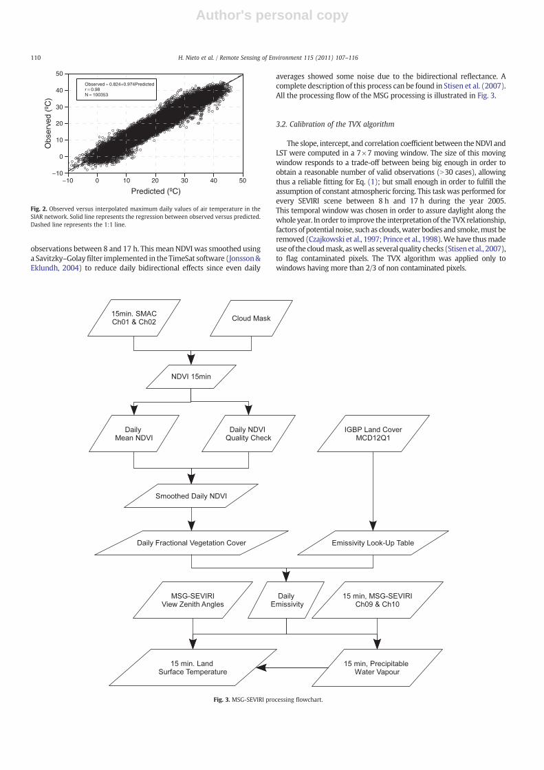
includes maximum and minimum daily temperatures from thereanalysis of the European Centre for Medium-rangeWeather Forecast,and interpolated at a spatial resolution of 3×3 km(Aguado et al., 2007).Thedatabase covers the years 2002 to2005. To check the integrityof thisdataset, themaximum interpolated daily air temperaturewas validatedwith daily data ranging the year 2005 from the Agro-climaticInformation System for Irrigation (SIAR; Sistema de InformaciónAgroclimática para el Regadío, http://www.mapa.es/siar/). This data-base comprises 361 automatic agrometeorological stations, which aremainly located over agricultural areas. Therefore, these stations do notcover the whole range of biomes found in the Iberian Peninsula. Theresults show that the interpolated data agree very closely with theobservations during year 2005 (Fig. 2), with a Mean Absolute Error of1.3 °C and Root Mean Square Error of 1.8 °C.

3. Methods

3.1. MSG-SEVIRI pre-processing

SMAC corrected radiances of channels 1 and 2, centered at 0.6 μmand 0.8 μm respectively, were used to compute NDVI values every15 min (Fensholt et al., 2006). Land Surface Temperaturewas computedusing the algorithm proposed by Sobrino and Romaguera (2004) forMSG-SEVIRI. This algorithm requires brightness temperatures andsurface emissivity estimates for channels centered in 10.8 and 12 μm,as well as precipitable water vapor and view zenith angles. Precipitablewater vaporwas estimated using a split-windowalgorithm(Choudhuryet al., 1995) originally developed for AVHRR data. The algorithm hasbeen successfully applied for SEVIRI data (Stisen et al., 2007; Stisen,Sandholt, et al., 2008). Daily emissivitymapswere produced combininganemissivity LookUpTable (Trigo et al., 2008) anddaily fractional coverderived fromNDVI values (Nishida et al., 2003). For this purpose, a dailyNDVI was produced from the 15 min data by averaging all cloud free

Fig. 1. The Iberian Peninsula and location of the 2000 random points used for calibration of validation of the algorithm. Source of annual mean temperatures: Digital Climatic Atlas ofthe Iberian Peninsula (Ninyerola et al., 2005).

109H. Nieto et al. / Remote Sensing of Environment 115 (2011) 107–116


observations between 8 and 17 h. This mean NDVI was smoothed usinga Savitzky–Golayfilter implemented in the TimeSat software (Jonsson&Eklundh, 2004) to reduce daily bidirectional effects since even daily

averages showed some noise due to the bidirectional reflectance. Acomplete description of this process can be found in Stisen et al. (2007).All the processing flow of the MSG processing is illustrated in Fig. 3.

3.2. Calibration of the TVX algorithm

The slope, intercept, and correlation coefficient between theNDVI andLST were computed in a 7×7 moving window. The size of this movingwindow responds to a trade-off between being big enough in order toobtain a reasonable number of valid observations (N30 cases), allowingthus a reliable fitting for Eq. (1); but small enough in order to fulfill theassumption of constant atmospheric forcing. This task was performed forevery SEVIRI scene between 8 h and 17 h during the year 2005.This temporal window was chosen in order to assure daylight along thewhole year. In order to improve the interpretation of the TVX relationship,factors of potential noise, suchas clouds,water bodies and smoke,must beremoved (Czajkowski et al., 1997; Prince et al., 1998).Wehave thusmadeuseof the cloudmask, aswell as several quality checks (Stisenet al., 2007),to flag contaminated pixels. The TVX algorithm was applied only towindows having more than 2/3 of non contaminated pixels.

Fig. 2. Observed versus interpolated maximum daily values of air temperature in theSIAR network. Solid line represents the regression between observed versus predicted.Dashed line represents the 1:1 line.

Fig. 3. MSG-SEVIRI processing flowchart.



In order to estimate NDVImax we can rewrite Eq. (2) as:

Tt;i−at;i = bt;i⋅NDVImax ð3Þ

Knowing Tt, i (the observed air temperature), at, i and bt, i, the onlyunknown variable isNDVImax, which can be solved by the least squaresmethod.

An a priori NDVImax must be assumed in order to compute apreliminary 15 min. SEVIRI air temperature and thus compare theobserved hourly (daily) temperature with the retrieved 15 min.regression parameters. Every hour, the corresponding TVX parameters(at, i and bt, i) to the maximum retrieved air temperature are chosen tocalibrate the new NDVImax with the observed hourly maximumtemperature. Similarly, the corresponding TVX parameters to themaximum retrieved air temperature between 12 h and 17 h(the temporal window when it is expected to occur the maximumdaily air temperature) were chosen to calibrate the NDVImax with theinterpolated daily temperature. The a priori NDVImax was 0.65, whichwas initially proposed by Czajkowski et al. (2000) and gave good resultsin the Senegal River Basin study carried out by Stisen et al. (2007).In addition, only regression parameters corresponding to a good linearrelationship between NDVI and LST were taken into account to performthe calibration. We have thus filtered all cases where the correlationcoefficient between NDVI and LST is less than or equal to −0.95(the relationship between the NDVI and the LST must be negative).

The NDVImax was calibrated for the hourly observations of theCabañeros site, as well as for the daily interpolated temperature in the3×3km UTM grid. The calibration and validation in this latter case wasperformed by sampling 2000 random points over all peninsular Spainalong thewhole year 2005. These 2000 locationswill allow thus to coverthe whole range of biomes in the Iberian Peninsula for the calibration/validation tasks.Wehave calibrated a uniqueNDVImaxbyusing all pointstogether, as well as an NDVImax for each biome by splitting the randompoints according to the MODIS IGBP Land Cover product, MCD12Q1(Friedl et al., 2002).

3.3. Validation

Several statistics were computed in order to assess the accuracy of theretrieved air temperature. These error measurements have beencalculated for an NDVImax of 0.65 (hereafter called NDVISTI), the valueproposed by Prihodko and Goward (1997) of 0.86 (hereafter calledNDVIPRI), and the new calibrated NDVImax. Different measures werecomputed to assess the performance of models. According to Fox (1981)two types of measures can be computed to evaluate the performance of amodel,measures based on residuals, andmeasures of correlation. Thefirstset of measures represents a quantification of the difference between theobserved and the predicted values. The second set represents thequantification of the agreement between predictions and observations.The followingmeasures have been computed to perform the comparisonof models: 1) mean of observed (Ō) versus mean of predicted (P), whichshows us the mean bias between observed and predicted. 2) Standarddeviation of observed versus standard deviation of predicted, whichreflects the capacity of themodel to explain the variability of the observedtemperature. 3) The slope and intercept between the observed andpredicted according to Piñeiro et al. (2008), under the hypothesis that agood model should follow the 1:1 line (slope unity and no intercept). 4)the index of agreement (d, Eq. (4)), which is more appropriate than thecorrelation index since the latter is not consistently related to theaccuracy, in terms of magnitude, between the observed and predictedvalues (Willmott, 1982).

d = 1− ∑ Pi−Oið Þ2∑ jPi− �

Oj + jOi−�Oj� �2 ð4Þ

5) The Root Mean Square Error (RMSE) and its systematic (RMSEs)and unsystematic (RMSEu) components. According to Willmott(1982), in a good model, the RMSEs should approach zero while theRMSEu approaches the RMSE. 6) The Mean Absolute Error (MAE),which is less sensitive to extreme values than RMSE. This latter tendsto inflate when extreme values are present (Willmott, 1982).Willmott and Matsuura (2005) recommended to use this measurerather than RMSE since the latter is not a true measure of averageerror since it also measures the variability of the errors. And 7) thepercentage of estimations that fall within ±3 °C and within ±5 °C,since it is a measure that has been used in previous studies, andtherefore it has been included for comparison purposes with otherstudies.

The final task of this study was to evaluate the spatio-temporalperformance of the algorithm. We have compared the residuals interms of daily and seasonal evolution, biome, topography, andlandscape homogeneity. Topographic variations within theMSG-pixeland within the 7×7 moving window were evaluated. The standarddeviation of altitudes, derived from a DTM at 250 m (source: NationalCartographic Database), was computed at the extension of the SEVIRIpixels as well as in the 7×7 moving window. The landscapeheterogeneity was evaluated with the Shannon's Entropy indexh (Eq. (5) (Ricotta et al., 2006))

h = ∑n

i=1pi⋅lnpi ð5Þ

where the relative abundance pi of the class ni is pi=ni /∑ni.For each of the 2000 random points, this index was computed

using a reclassification of the Corine Land Cover 2000 (EuropeanEnvironment Agency, 1999) into the IGBP land cover classes (Belward& Loveland, 1995). This source was chosen since it provides a higherspatial resolution than other global products such as MODIS LandCover (with a resolution of 1000 m), and therefore heterogeneity ismore accurately estimated at the SEVIRI pixel scale. Table 1 shows thetotal area covered by each class in Spain.

Analyses of Variance were performed to test whether time, season,and biome affects the residuals between observed and estimated airtemperatures. The factor time was tested with the Cabañeros hourlydata, whereas the other two factors, season and biome, were testedwith the gridded interpolated daily data. In addition, Spearmancorrelation coefficient was computed between the residuals and theintra-pixel topographic variability, moving window topographicvariability, and landscape heterogeneity.

Table 1Surface occupied for each IGBP class in Spain.Corine Land Cover 2000.

Code Class Area (ha)

1 Evergreen needleleaved forests 3,910,2112 Evergreen broadleaved forests 1,437,9174 Deciduous broadleaved forests 2,121,8125 Mixed forests 1,498,1256 Closed shrublands 10,380,2367 Open shrublands 14258 Woody savannas 2,452,6779 Savannas 2,616,77310 Grasslands 620,14711 Permanent wetlands 85,37112 Croplands 16,955,95013 Urban and built-up 1,020,88514 Cropland/natural vegetation mosaic 5,060,49115 Permanent snow and ice 30216 Barren or sparsely vegetated 1,197,841



4. Results

4.1. Cabañeros data

A total of 982 valid observations centered in the meteorologicalstation were obtained during the year 2005. For calibration purposes,705 of these cases fulfilled the criteria of having a correlation coefficientless or equal than −0.95. Therefore 420 cases were finally selected forcalibrating (≈60% of 705), leaving the remaining 562 observations forvalidation.

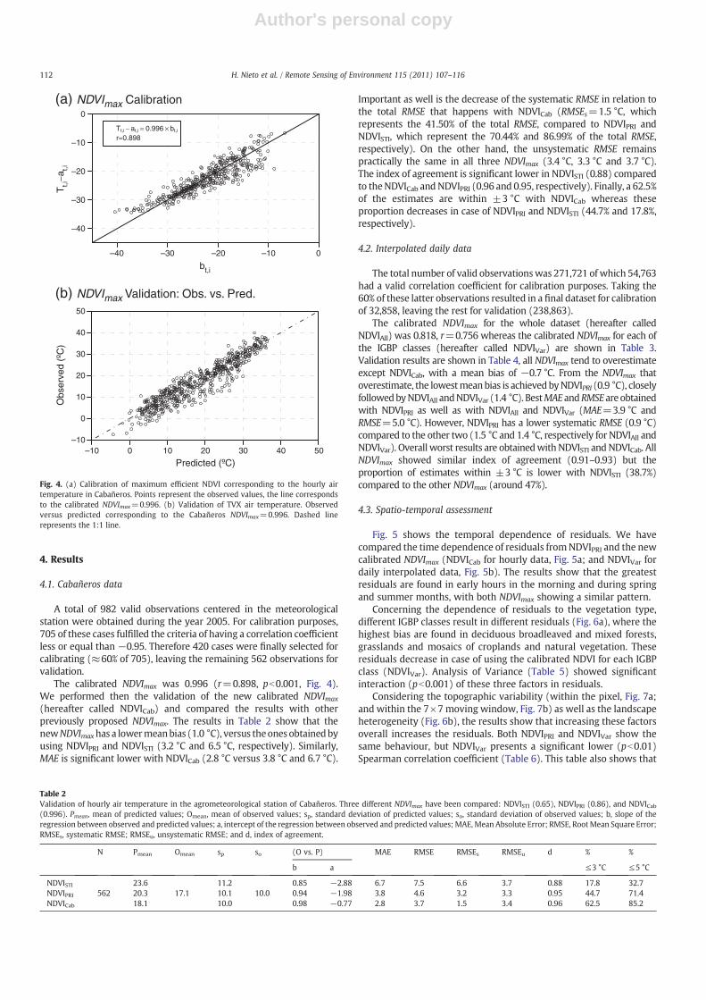
The calibrated NDVImax was 0.996 (r=0.898, pb0.001, Fig. 4).We performed then the validation of the new calibrated NDVImax

(hereafter called NDVICab) and compared the results with otherpreviously proposed NDVImax. The results in Table 2 show that thenewNDVImaxhas a lowermeanbias (1.0 °C), versus theones obtainedbyusing NDVIPRI and NDVISTI (3.2 °C and 6.5 °C, respectively). Similarly,MAE is significant lower with NDVICab (2.8 °C versus 3.8 °C and 6.7 °C).

Important as well is the decrease of the systematic RMSE in relation tothe total RMSE that happens with NDVICab (RMSEs=1.5 °C, whichrepresents the 41.50% of the total RMSE, compared to NDVIPRI andNDVISTI, which represent the 70.44% and 86.99% of the total RMSE,respectively). On the other hand, the unsystematic RMSE remainspractically the same in all three NDVImax (3.4 °C, 3.3 °C and 3.7 °C).The index of agreement is significant lower in NDVISTI (0.88) comparedto theNDVICab andNDVIPRI (0.96 and 0.95, respectively). Finally, a 62.5%of the estimates are within ±3 °C with NDVICab whereas theseproportion decreases in case of NDVIPRI and NDVISTI (44.7% and 17.8%,respectively).

4.2. Interpolated daily data

The total number of valid observationswas 271,721 of which 54,763had a valid correlation coefficient for calibration purposes. Taking the60% of these latter observations resulted in a final dataset for calibrationof 32,858, leaving the rest for validation (238,863).

The calibrated NDVImax for the whole dataset (hereafter calledNDVIAll) was 0.818, r=0.756 whereas the calibrated NDVImax for each ofthe IGBP classes (hereafter called NDVIVar) are shown in Table 3.Validation results are shown in Table 4, all NDVImax tend to overestimateexcept NDVICab, with a mean bias of −0.7 °C. From the NDVImax thatoverestimate, the lowestmeanbias is achievedbyNDVIPRI (0.9 °C), closelyfollowedbyNDVIAll andNDVIVar (1.4 °C). BestMAE andRMSEareobtainedwith NDVIPRI as well as with NDVIAll and NDVIVar (MAE=3.9 °C andRMSE=5.0 °C). However, NDVIPRI has a lower systematic RMSE (0.9 °C)compared to the other two (1.5 °C and 1.4 °C, respectively for NDVIAll andNDVIVar). Overall worst results are obtainedwithNDVISTI andNDVICab. AllNDVImax showed similar index of agreement (0.91–0.93) but theproportion of estimates within ±3 °C is lower with NDVISTI (38.7%)compared to the other NDVImax (around 47%).

4.3. Spatio-temporal assessment

Fig. 5 shows the temporal dependence of residuals. We havecompared the time dependence of residuals fromNDVIPRI and the newcalibrated NDVImax (NDVICab for hourly data, Fig. 5a; and NDVIVar fordaily interpolated data, Fig. 5b). The results show that the greatestresiduals are found in early hours in the morning and during springand summer months, with both NDVImax showing a similar pattern.

Concerning the dependence of residuals to the vegetation type,different IGBP classes result in different residuals (Fig. 6a), where thehighest bias are found in deciduous broadleaved and mixed forests,grasslands and mosaics of croplands and natural vegetation. Theseresiduals decrease in case of using the calibrated NDVI for each IGBPclass (NDVIVar). Analysis of Variance (Table 5) showed significantinteraction (pb0.001) of these three factors in residuals.

Considering the topographic variability (within the pixel, Fig. 7a;and within the 7×7 moving window, Fig. 7b) as well as the landscapeheterogeneity (Fig. 6b), the results show that increasing these factorsoverall increases the residuals. Both NDVIPRI and NDVIVar show thesame behaviour, but NDVIVar presents a significant lower (pb0.01)Spearman correlation coefficient (Table 6). This table also shows that

–40 –30 –20 –10 0

–40

–30

–20

–10

0

bt,i

Tt,i

−at,i

Tt,i − at,i = 0.996 × bt,i

r=0.898

–10 0 10 20 30 40 50

Predicted (ºC)

–10

0

10

20

30

40

50

Obs

erve

d (º

C)

(a) NDVImax Calibration

(b) NDVImax Validation: Obs. vs. Pred.

Fig. 4. (a) Calibration of maximum efficient NDVI corresponding to the hourly airtemperature in Cabañeros. Points represent the observed values, the line correspondsto the calibrated NDVImax=0.996. (b) Validation of TVX air temperature. Observedversus predicted corresponding to the Cabañeros NDVImax=0.996. Dashed linerepresents the 1:1 line.

Table 2Validation of hourly air temperature in the agrometeorological station of Cabañeros. Three different NDVImax have been compared: NDVISTI (0.65), NDVIPRI (0.86), and NDVICab(0.996). Pmean, mean of predicted values; Omean, mean of observed values; sp, standard deviation of predicted values; so, standard deviation of observed values; b, slope of theregression between observed and predicted values; a, intercept of the regression between observed and predicted values; MAE, Mean Absolute Error; RMSE, RootMean Square Error;RMSEs, systematic RMSE; RMSEu, unsystematic RMSE; and d, index of agreement.

N Pmean Omean sp so (O vs. P) MAE RMSE RMSEs RMSEu d % %

b a ≤3 °C ≤5 °C

NDVISTI 23.6 11.2 0.85 −2.88 6.7 7.5 6.6 3.7 0.88 17.8 32.7NDVIPRI 562 20.3 17.1 10.1 10.0 0.94 −1.98 3.8 4.6 3.2 3.3 0.95 44.7 71.4NDVICab 18.1 10.0 0.98 −0.77 2.8 3.7 1.5 3.4 0.96 62.5 85.2



the residuals are less related to spatial heterogeneity as well as totopographic heterogeneity with the use of NDVIVar.

5. Discussion

The results show that overall the TVX algorithm performs adequatelyin the Mediterranean climate. We have achieved an MAE of 2.8 °C andRMSE of 3.7 °C with the hourly dataset, which is similar to the error of2.96 °C found with the same sensor in Senegal (Stisen et al., 2007).However, an overestimation of 1.0 °C was found compared to theunderestimationof 1.1 °C in Senegal. The dailymaximumair temperaturealso showed a good accuracy with an RMSE=5 °C and an overestimationof 1.0 °C to 1.5 °C, depending of the adopted NDVImax. Similar results arefound with AVHRR data by (Goward et al., 1994) in Oregon,RMSE=5.4 °C; by (Czajkowski et al., 1997) in Canada, RMSE=4.2 °Cand bias of 3.2 °C; (Prihodko & Goward, 1997) in Kansas, MAE=2.9 °C;and (Czajkowski et al., 2000) in Oklahoma, RMSE=2.08 °C.

The new calibrated NDVImax showed a good performance,improving in general the results with other NDVImax proposed in theliterature. In particular, NDVICab, NDVIAll and NDVIVar outperform theresults obtained with the proposed NDVImax of Stisen et al. (2007) forMSG-SEVIRI. In both studies, SEVIRI scenes have been atmosphericallycorrected, but Stisen et al. (2007) adopted the value 0.65 assuming aresidual atmospheric effect on the SEVIRI images. If that residualatmospheric effect is disregarded, the NDVImax should be obviouslyhigher than 0.65 and closer to the value of 0.86 of Pridhodko andGoward (1997). On the other hand, Table 4 shows that NDVIPRIperforms slightly better than the new NDVImax. NDVIAll and NDVIVarhave similar error measurements and are close to NDVIPRI. This isexplained by the fact that most of the cases (85%) have an NDVIVarranging between 0.80 and 0.85 (Table 3). Although NDVIPRI showsbetter error measurements than NDVIVar, the distribution of residualsbetween IGBP classes is more homogeneous with NDVIVar (Fig. 6a),

considerably reducing the errors in classes such as evergreen anddeciduous broadleaved forests, mixed forests, grasslands andmosaics.These categories have the highest NDVImax (above 0.93), but they onlyrepresent nearly the 5% of the total cases and thus they barelycontribute to the global error measurements showed in Table 4.

At this point it is worth noting that the NDVImax for deciduousbroadleaved forests present an unrealistic value (1.16). The purelyempirical approach to derive the NDVImax together with the few validcases available to calibrate this IGBP class (70 cases) can be responsible ofthis value. However, an analysis performedwith the total number of casesfor broadleaved forest (262 cases) lead to a similar result in the calibratedNDVImax, with a value of 1.23. Table 3 also shows the 99th percentile of themeasured NDVI as a measure of the maximum observed NDVI for eachIGBP class. This statistic was used instead of the absolutemaximumNDVIin order to avoid a possible influence of outliers due to noise effects.Overall, the observed maximum NDVI are in agreement with theestimated NDVImax with exception of broadleaved forests, closed shrub-lands and grasslands, with observedmaximumNDVI sensible lower thanthe calibrated NDVImax. These classes are precisely among the ones withfewervalid cases toperformthe calibrationofNDVImaxand therefore thesevalues should be taken with care. In addition, Prince et al. (1998)suggested a tendency to estimate T more accurately in areas where thevegetation is more closely coupled with the atmosphere. Therefore,another factor that could have influenced the anomalous NDVImax inbroadleaved forest, is the leaf-in/leaf-out seasons that could contribute tonoisy values. However, a calibration performed taking only into accountspringandsummercasesgave thesameresults. Finally, Stisenetal. (2007)pointed out that there is always a small canopy heat flux, even atmaximum full cover, which induces the true air temperature to be belowthe canopy temperature. This minimum canopy heat flux is related to theminimum canopy resistance, which is directly proportional to theminimum leaf stomatal resistance and inversely to the Leaf Area Index(Monteith, 1973). In future research itwould be interesting to explore therelationship between minimum canopy resistance and the retrievedNDVImax.

Taking into account the unsystematic part of the RMSE it can be seenthat independently of the adopted NDVImax this RMSEu is almostconstant (3.5 °C and5 °C forhourly anddaily interpolated temperatures,respectively). According to Willmott (1982), these values of RMSEu arerepresentative of the model noise level, and can be interpreted as ameasure of potential accuracy. This noise canbe causedby split-windowestimates of LST— including satellite calibration, surface emissivity andprecipitable water estimation — as well as radiometric errors in NDVI,residual cloud-contamination and the size of the contextual window(Czajkowski et al., 1997; Prihodko & Goward, 1997; Prince et al., 1998).The algorithm for LST retrieval proposed by Sobrino and Romaguera(2004) showed an accuracy of 3 °C in Senegal (Stisen et al., 2007).Surface emissivity retrieval has been pointed out to be a great source oferror in LST estimation (Goward et al., 1994; Sobrino & Romaguera,2004). On the other hand, Prihodko and Goward (1997) estimated thatuncertainty in themeasurements ofNDVIwithAVHRR images can resultin air temperature errors of±4 °C. In addition errors in the observed airtemperature can be added to this noise level (Czajkowski et al., 1997).

Table 3Calibrated NDVImax for daily interpolated temperature corresponding to each of theIGBP biomes. N obs., number of cases for calibration/total number of cases; Obs. NDVI99,99th percentile of the observed NDVI; NDVImax, calibrated maximum efficient NDVI; r,correlation coefficient.

Code IGBP class N obs Obs.NDVI99

NDVImax r

1 Evergreen needleleaved forest 1139/9160 0.896 0.849 0.782 Evergreen broadleave forest 111/3857 0.949 0.934 0.964 Deciduous broadleaved forest 70/262 0.658 1.162 0.805 Mixed forests 1032/7971 0.934 0.995 0.846 Closed shrublands 270/2559 0.752 0.915 0.727 Open shrublands 7373/69,757 0.821 0.803 0.778 Woody savannas 8239/59,344 0.852 0.835 0.799 Savannas 2039/18,216 0.851 0.777 0.7610 Grasslands 116/1056 0.809 0.985 0.6412 Croplands 11,633/94,425 0.849 0.800 0.7113 Urban and built-up 678/3767 0.835 0.780 0.8814 Cropland/natural vegetation

mosaic158/1359 0.946 0.937 0.93

Table 4Validation of daily interpolated air temperature. Five different NDVImax have been compared: NDVISTI (0.65), NDVIPRI (0.86), NDVICab (0.996), NDVIAll (0.818), and NDVIVar (variableaccording to Table 3). Pmean, mean of predicted values; Omean, mean of observed values; sp, standard deviation of predicted values; so, standard deviation of observed values; b, slopeof the regression between observed and predicted values; a, intercept of the regression between observed and predicted values; MAE, Mean Absolute Error; RMSE, Root Mean SquareError; RMSEs, systematic RMSE; RMSEu, unsystematic RMSE; and d, index of agreement.

N Pmean Omean sp so (O vs. P) MAE RMSE RMSEs RMSEu d % %

b a ≤3 °C ≤5 °C

NDVISTI 26.0 11.0 0.74 3.39 4.8 6.0 3.5 4.8 0.91 38.7 59.9NDVIPRI 23.5 10.3 0.77 4.36 3.9 5.0 0.9 4.9 0.93 48.5 70.9NDVICab 238,863 21.9 22.6 10.0 9.1 0.78 5.53 4.0 5.2 0.9 5.1 0.92 46.4 69.0NDVIAll 24.0 10.4 0.77 4.09 3.9 5.0 1.5 4.8 0.93 47.5 69.9NDVIAll 24.0 10.4 0.77 4.08 3.9 5.0 1.4 4.8 0.93 48.1 70.4



This is particularly important in our maximum daily air temperature,since they represent interpolated data and therefore are subject tomodel errors. Moreover, maximum air temperature estimated withMSG-SEVIRI is likely to be biased since the assessment of the dailytemperature cycle will be subject to gaps due to the presence of cloudsand failures to fulfill the quality criteria applied in the TVX algorithm.

In another study, Nieto et al. (2010) validated the algorithm usinghourly ground data across different biomes using several agrometeor-ological stations in La Rioja (Spain). Their results showed aMAE=2.9 °Cand RMSE=3.5 °C, throwing some evidence on the actual accuracy ofthe algorithm. Further studies will thus be validated with ground datainstead of modeled air temperature. Finally, as it was stated before, thesize of the moving windowwas established according to a compromisebetween having enough valid observations within the window andassure the assumption of uniform atmospheric forcing following theworkof Stisen et al. (2007). Futureworkwill address theperformanceofthe TVX algorithm for different moving window sizes.

An increasing bias in estimated air temperature was found withincreasing pixel heterogeneity. This confirms the observations of Princeet al. (1998) and Czajkowski et al. (2000). However, accuracy,measuredby the Mean Absolute Error showed no tendency related to landscapeheterogeneity. On the other hand, TVX performance is clearlydependent on topographic variability within the pixel and within themoving window, as it was expected. The higher variation in altitudeswithin the pixel and within the moving window enhances theprobability of different atmospheric forcing, caused either bydifferencesin solar radiation and wind speed, as well as the adiabatic cooling of airwith altitude. BothNDVImax that have been analyzed in this step showedsimilarpatterns butNDVIVar tends to overestimate compared toNDVIPRI.

Finally, a temporal dependence of residuals has been observed.In termsof thediurnal cycle, highest accuracies are foundduring thehoursaroundmidday (12 h–13 h),when the Land Surface Temperature reachesits maximum, and coinciding with the steepest slopes of the TVXrelationship. Angular effects on observedNDVI and LST can be responsibleof this trend (Prince et al., 1998; Stisen et al., 2007). Besides, Czajkowskiet al. (1997) showed that the TVX slope decreases with high solar zenithangles and, therefore, the slope should be smaller during themorning andtheafternoon.Afternoon, accuracybegins todecrease, probablydue to thedecoupling between the Land Surface Temperature and the air temper-ature (Stisen et al., 2007). It has been seen aswell that bias decreaseswithtime, being negative after noon. The underestimation has itsmaximum at16–17 h, in coincidence with the air temperature peak of our study site.

On the other hand, annual variability showed that the lowest accuracyand the highest bias are found during spring and summer. The bias can becausedby the influenceof physiological activity of vegetationduring thesemonths, since vegetation canopies always cause a small sensible heatflux,evenatmaximumcanopycover andmoisture content (Stisenet al., 2007).Assuming that bulk surface resistance is inversely proportional to LeafArea Index (Allen et al., 2006; Noilhan & Planton, 1989), the sensible heatfluxwill be negligiblewhen LAI tends to infinite. In addition,meteorology

8 10 11 12 13 14 15 16

−4

−2

0

2

4

6

Hour

Err

or (

ºC)

−19

−17

−15

−13

−11

Slo

pe

Bias NDVIPRI

Bias NDVICab

MAE NDVIPRI

MAE NDVICab

Slope

−4

−2

0

2

4

6

Month

Err

or (

ºC)

JAN

FE

B

MA

R

AP

R

MA

Y

JUN

JUL

AU

G

SE

P

OC

T

NO

V

DE

C

−19

−16

−13

−10

−7

−4

Slo

peBias NDVIPRI

Bias NDVIVar

MAE NDVIPRI

MAE NDVIVar

Slope

9

(a) Hourly dependence

(b) Monthly dependence

Fig. 5. Temporal dependence of residuals. (a) Hourly dependence; (b) monthlydependence. For each factor two different NDVImax have been analysed in comparisonwith NDVIPRI (0.86): NDVICab (0.996), in a, and NDVIVar (IGBP variable NDVI), in b.The crosses represent the mean slope of the TVX relationship (secondary y-axis).

Table 5Analysis of variance of residuals for NDVIPRI (0.86), NDVICab (0.996) and NDVIVar (NDVImax variable according to Table 3).

Factor NDVImax Sum of squares d.f. Mean square F Sig.

Hour NDVIPRI Between groups 4147.7 8 518.5 106.1 0.00Within groups 4756.2 973 4.9Total 8903.9 981

NDVICab Between groups 4150.4 8 518.8 80.2 0.00Within groups 6296.7 973 6.5Total 10,447.1 981

Month NDVIPRI Between groups 299,732.7 11 27,248.4 1213.8 0.00Within groups 6,099,498.0 271,709 22.4Total 6,399,230.7 271,720

NDVIVar Between groups 420,770.9 11 38,251.9 1826.9 0.00Within groups 5,689,175.8 271,709 20.9Total 6,109,946.7 271,720

IGBP NDVIPRI Between groups 116,314.7 11 10,574.1 457.3 0.00Within groups 6,282,916.0 271,709 23.1Total 6,399,230.7 271,720

NDVIVar Between groups 12,421.2 11 1129.2 50.3 0.00Within groups 6,097,525.5 271,709 22.4Total 6,109,946.7 271,720



during the year 2005 in Spain was significantly anomalous, with warmertemperatures than usual during the spring months, April, May, andespecially June (Instituto Nacional de Meteorología, 2005). Prihodko andGoward (1997) found that lower errors occur with decreasing tempera-tures and thus it is expected that better accuracies had been found inwinter and autumn. Finally, that year was extremely dry in the IberianPeninsula (491.4 mm accumulated rainfall in average), with historicalminimums beginning in November 2004 until September 2005 (InstitutoNacional deMeteorología, 2005). Fig. 5.b shows that the highest monthlymean of the TVX slope are found from April until September. Since theslope of the TVX relationship can be related to surface wetness(Czajkowski et al., 1997; Goward et al., 1994; Prihodko & Goward,1997), the temporal evolution of the slope is in agreement with thedrought suffered in 2005.

6. Conclusion

Amethodology to estimate the full cover NDVI has been developed tobetter compute air temperature using the TVX algorithm. This empirical

approach only needs ground measurements of air temperature and theretrieved parameters (slope and intercept) of the TVX relationship. Thisallows us to easily obtain a differentNDVImax depending on the vegetationtype. All retrieved NDVImax values were coherent with exception of thedeciduous broadleaved forest value that had an unrealistic value of1.2,probably due to insufficient data for calibration.

The retrieved air temperature can be used as an input for a largerange of models such as energy and water flux models, ecosystemfunctioning, etc. Since the accuracy of the algorithm ranged between3 °C and 5 °C, the error transmission of the retrieved temperature into amodel depends largely on the model sensitivity to the air temperature.Therefore, in very sensitive models to air temperature, the TVXalgorithm could not be accurate enough to be used instead of groundmeasurements. For instance, Nieto et al. (2010) estimated theEquilibrium Moisture Content (Simard, 1968; Van Wagner & Pickett,1985) for wildfire danger assessment with MSG-SEVIRI data. Theauthors found biased estimates of the Equilibrium Moisture Contentcaused by an overestimation of the TVX air temperature.

The results showed similar performances compared to previousstudies and previous NDVImax but the application of a NDVImax

dependent with vegetation type improved the estimations in severalland covers, homogenising thus the accuracy between vegetation types.Although we have used exactly the same methodology as Stisen et al.(2007) for image processing, great differences have been found in termsof the relationship betweenNDVImax and the residuals. Further researchwould address the viability of this approach at global scales, testing thevariability of the NDVImax and the accuracy of the TVX algorithmbetween different climates.

Using the appropriate NDVImax most of the error to estimate the airtemperature can be attributed to noise (RMSEu near 4 °C). Therefore,

Table 6Spearman correlation coefficient between residuals and binned topographic variability(intra-pixel and moving window) and Shannon's h index of entropy. Significantcorrelations (pb0.01) are marked with an asterisk (*).

NDVIPRI NDVIVar

Residual Abs. residual Residual Abs. residual

STD Pixel 0.14* 0.06* 0.09* 0.06*STD Window 0.13* 0.07* 0.10* 0.07*h Shannon 0.07* 0.00 0.05* 0.00

0

2

4

6

IGBP class

Err

or (

ºC)

1 10 12 13 14

Bias NDVIPRI

Bias NDVIVar

MAE NDVIPRI

MAE NDVIVar

10

0

2

4

6

Landscape heterogeneity class

Err

or (

ºC)

Bias NDVIPRI

Bias NDVIVar

MAE NDVIPRI

MAE NDVIVar

9876542

1 98765423

(a) Land cover dependence

(b) Landscape heterogeneity dependence

Fig. 6. Spatial dependence corresponding to variations in land cover and landscapeheterogeneity. (a) IGBP classes; (b) equal size interval Shannon's h bins.

1 2 3 4 5 6 7 8 9 10

−4

−2

0

2

4

6

Intra−pixel topographic variability class

Err

or (

ºC)

Bias NDVIPRI

Bias NDVIVar

MAE NDVIPRI

MAE NDVIVar

1 2 3 4 5 6 7 8 9 10

−4

−2

0

2

4

6

Moving window topographic variability class

Err

or (

ºC)

Bias NDVIPRI

Bias NDVIVar

MAE NDVIPRI

MAE NDVIVar

(a) Intra-pixel topographic dependence

(b) Moving window topographic dependence

Fig. 7. Spatial dependence corresponding to variations topography. (a) Equal size intervalintra-pixel variability bins; (b) equal size interval moving window variability bins.



future efforts should be focused on improving the input variables.Firstly, the performed calibration/validation with interpolated airtemperature is subject to uncertainties because of inaccuracies in theweather model. Secondly, additional noise is caused by the satelliteinput data. Several factors affect the accuracy of Land SurfaceTemperature and NDVI and their correlation. A cloud screening iscrucial for this method since it affects LST, NDVI and the regressionbetween both (Prihodko & Goward, 1997; Prince et al., 1998).Atmospheric correction for aerosols and water vapor are needed foraddressing the effects of the atmosphere on the radiometric signal.Emissivity estimation is a key factor for accurate retrievals of LST(Sobrino & Romaguera, 2004). Finally, if hourly variations of airtemperature are required, it would be necessary to take into accountthe bidirectional effects on the NDVI as well as the diurnal cycle oftemperature.

Acknowledgements

This research has been done during a visiting stay at the Departmentof Geography and Geology of Copenhagen (Denmark). The first authorhas been funded by the Spanish Ministry of Science through the FPIscholarship BES-2005-7801. Special thanks to Flemming Andersen ofthe University of Copenhagen for providing the atmosphericallycorrected images, and to Meteológica for providing the daily interpo-lated meteorological database. Finally, usefull comments from theanonymous reviewers have improved the final version of themanuscript.

References

Aguado, I., Chuvieco, E., Borén, R., & Nieto, H. (2007). Estimation of dead fuel moisturecontent from meteorological data in Mediterranean areas. Applications in firedanger assessment. International Journal of Wildland Fire, 16, 390−397.

Allen, R. G., Pruitt, W. O., Wright, J. L., Howell, T. A., Ventura, F., Snyder, R., Itenfisu, D.,Steduto, P., Berengena, J., Yrisarry, J. B., Smith, M., Pereira, L. S., Raes, D., Perrier, A.,Alves, I., Walter, I., & Elliott, R. (2006). A recommendation on standardized surfaceresistance for hourly calculation of reference ETo by the FAO56 Penman-Monteithmethod. Agricultural Water Management, 81, 1−22.

Belward, A., & Loveland, T. R. (1995). The IGBP-DIS 1 km land cover project: Remotesensing in action. 21st Annual Conference of the Remote Sensing Society(pp. 1099−1106). Southampton, UK..

Bradshaw, B. S., & Deeming, J. E. (1983). The 1978 national fire danger rating system.Technical Report USDA Forest Service Ogden, Utah: Technical documentation.

Chokmani, K., & Viau, A. A. (2006). Estimation of the air temperature and the vapourquantity in atmosphericwaterwith the help of theAVHRRdata of theNOAA.CanadianJournal of Remote Sensing, 32, 1−14.

Choudhury, B. J., Dorman, T. J., & Hsu, A. Y. (1995). Modeled and observed relationsbetween the AVHRR split window temperature difference and atmosphericprecipitable water over land surfaces. Remote Sensing of Environment, 51, 281−290.

Cresswell, M. P., Morse, A. P., Thomson, M. C., & Connor, S. J. (1999). Estimating surfaceair temperatures, from Meteosat land surface temperatures, using an empiricalsolar zenith angle model. International Journal of Remote Sensing, 20, 1125−1132.

Czajkowski, K. P., Goward, S. N., Stadler, S. J., &Walz, A. (2000). Thermal remote sensingof near surface environmental variables: Application over the Oklahoma Mesonet.Professional Geographer, 52, 345−357.

Czajkowski, K. P.,Mulhern, T., Goward, S. N., Cihlar, J., Dubayah, R. O., & Prince, S. D. (1997).Biospheric environmentalmonitoring at BOREASwith AVHRR observations. Journal ofGeophysical Research, [Atmospheres], 102, 29,651−29,662.

EUMETSAT (2007). Cloud detection for MSG — Algorithm theoretical basis document.Technical Report EUM/MET/REP/07/0132 EUMETSAT Darmstadt, Germany.

European Environment Agency (1999). CORINE land cover 2000. Technical guide.Technical Report European Commission, Joint Research Centre.

Fensholt, R., Sandholt, I., Stisen, S., & Tucker, C. (2006). Analysing NDVI for the Africancontinent using the geostationary Meteosat Second Generation SEVIRI sensor.Remote Sensing of Environment, 101, 212−229.

Fox, D. G. (1981). Judging air quality model performance. Bulletin of the AmericanMeteorological Society, 62, 599−609.

Friedl, M. A., McIver, D. K., Hodges, J. C. F., Zhang, X. Y., Muchoney, D., Strahler, A. H.,Woodcock, C. E., Gopal, S., Schneider, A., Cooper, A., Baccini, A., Gao, F., & Schaaf, C.(2002). Global land covermapping fromMODIS: Algorithms and early results. RemoteSensing of Environment, 83, 287−302.

Goward, S. N., Waring, R. H., Dye, D. G., & Yang, J. L. (1994). Ecological remote-sensing atOTTER: Satellite macroscale observations. Ecological Applications, 4, 322−343.

Instituto Nacional deMeteorología (2005). Resumen Anual Climatológico del Año 2005.Technical Report Ministerio de Medio Ambiente Madrid.

Jang, J. D., Viau, A. A., & Anctil, F. (2004). Neural network estimation of air temperaturesfrom AVHRR data. International Journal of Remote Sensing, 25, 4541−4554.

Jonsson, P., & Eklundh, L. (2004). TIMESAT — A program for analyzing timeseries ofsatellite sensor data. Computers and Geosciences, 30, 833−845.

Keetch, J., & Byram, G. (1968). A drought index for forest fire control. Technical ReportUSDA Forest Service. Asheville, NC: Southeastern Forest Experiment Station.

Monteith, J. L. (1973). Principles of environmental physics. London: Edward Arnold.Nemani, R. R., & Running, J. W. (1989). Estimation of regional surface resistance to

evapotranspiration from NDVI and thermal-IR AVHRR data. Journal of AppliedMeteorology, 28, 276−284.

Nieto, H., Aguado, I., Chuvieco, E., & Sandholt, I. (2010). Dead fuel moisture estimationwith MSG-SEVIRI data. Retrieval of meteorological data for the calculation of theequilibrium moisture content. Agricultural and Forest Meteorology, 150, 861−870.

Ninyerola, M., Pons, X., & Roure, J. M. (2005). Atlas climático digital de la Península Ibérica.Metodología y aplicaciones en bioclimatología y geobotánica. Bellaterra. Spain:Universidad Autónoma de Barcelona (http://www.opengis.uab.es/wms/iberia/english/en cartografia.htm).

Nishida, K., Nemani, R., Running, S., & Glassy, J. (2003). An operational remote sensingalgorithm of land surface evaporation. Journal of Geophysical Research, [Atmospheres],108, D4270.

Noilhan, J., & Planton, S. (1989). A simple parameterization of land surface processes formeteorological models. Monthly Weather Review, 117, 536−549.

Olioso, A., Chauki, H., Courault, D., & Wigneron, J. P. (1999). Estimation ofevapotranspiration and photosynthesis by assimilation of remote sensing datainto SVAT models. Remote Sensing of Environment, 68, 341−356.

Piñeiro, G., Perelman, S., Guerschman, J. P., & Paruelo, J. M. (2008). How to evaluatemodels: Observed vs. predicted or predicted vs. observed? Ecological Modelling,216, 316−322.

Prihodko, L., & Goward, S. N. (1997). Estimation of air temperature from remotelysensed surface observations. Remote Sensing of Environment, 60, 335−346.

Prince, S. D., Goetz, S. J., Dubayah, R. O., Czajkowski, K. P., & Thawley, M. (1998).Inference of surface and air temperature, atmospheric precipitable water and vaporpressure deficit using Advanced Very High-Resolution Radiometer satelliteobservations: Comparison with field observations. Journal of Hydrology, 213,230−249.

Rahman, H., & Dedieu, G. (1994). SMAC — A simplified method for the atmosphericcorrection of satellite measurements in the solar spectrum. International Journal ofRemote Sensing, 15, 123−143.

Ricotta, C., Corona, P., Marchetti, M., & Chirici, G. (2006). On parametric fragmentationmeasures. European Journal of Forest Research, 125, 441−444.

Schmetz, J., Pili, P., Tjemkes, S., Just, D., Kerkmann, J., Rota, S., & Ratier, A. (2002). Anintroduction to Meteosat Second Generation (MSG). Bulletin of the AmericanMeteorological Society, 83, 977−992.

Simard, A. (1968). The moisture content of forest fuels — A review of the basic concepts.Forest Service Ottawa, Ontario: Technical Report USDA.

Sobrino, J. A., & Romaguera, M. (2004). Land surface temperature retrieval fromMSG1-SEVIRI data. Remote Sensing of Environment, 92, 247−254.

Stisen, S., Jensen, K. H., Sandholt, I., & Grimes, D. I. F. (2008). A remote sensing drivendistributed hydrological model of the Senegal River basin. Journal of Hydrology,354, 131−148.

Stisen, S., Sandholt, I., Norgaard, A., Fensholt, R., & Eklundh, L. (2007). Estimation ofdiurnal air temperature using MSG SEVIRI data in West Africa. Remote Sensing ofEnvironment, 110, 262−274.

Stisen, S., Sandholt, I., Norgaard, A., Fensholt, R., & Jensen, K. H. (2008). Combining thetriangle method with thermal inertia to estimate regional evapotranspiration —

Applied toMSG-SEVIRI data in the Senegal River basin. Remote Sensing of Environment,112, 1242−1255.

Trigo, I. F., Peres, L. F., DaCamara, C. C., & Freitas, S. C. (2008). Thermal land surfaceemissivity retrieved from SEVIRI/Meteosat. IEEE Transactions on Geoscience andRemote Sensing, 46, 307−315.

Van Wagner, C. E. (1987). Development and structure of the Canadian Forest FireWeather Index System. Technical Report Canadian Forest Service Otawa..

Van Wagner, C. E., & Pickett, T. L. (1985). Equations and FORTRAN program for theCanadian Forest Fire Weather Index System. Technical Report Canadian ForestService Ottawa.

Vogt, J. V., Viau, A. A., & Paquet, F. (1997). Mapping regional air temperature fields usingsatellite-derived surface skin temperatures. International Journal of Climatology, 17,1559−1579.

Willmott, C. J. (1982). Some comments on the evaluation of model performance.Bulletin of the American Meteorological Society, 63, 1309−1313.

Willmott, C. J., & Matsuura, K. (2005). Advantages of the mean absolute error (MAE)over the root mean square error (RMSE) in assessing average model performance.Climate Research, 30, 79−82.

Willmott, C. J., Robeson, S. M., & Feddema, J. J. (1991). Influence of spatially-variableinstrument networks on climatic averages. Geophysical Research Letters, 18,2249−2251.


Air temperature estimation with MSG-SEVIRI data: Calibration and validation of the TVX algorithm for...

Documents

Transcript of Air temperature estimation with MSG-SEVIRI data: Calibration and validation of the TVX algorithm for...