
Assessment of virtual design and manufacturing techniques ...
185
ASSESSMENT OF VIRTUAL DESIGN AND MANUFACTURING TECHNIQUES FOR FIBRE REINFORCED COMPOSITE MATERIALS Marc GASCONS TARRÉS Dipòsit legal: GI-74-2012 http://hdl.handle.net/10803/52864 ADVERTIMENT. La consulta d’aquesta tesi queda condicionada a l’acceptació de les següents condicions d'ús: La difusió d’aquesta tesi per mitjà del servei TDX ha estat autoritzada pels titulars dels drets de propietat intel·lectual únicament per a usos privats emmarcats en activitats d’investigació i docència. No s’autoritza la seva reproducció amb finalitats de lucre ni la seva difusió i posada a disposició des d’un lloc aliè al servei TDX. No s’autoritza la presentació del seu contingut en una finestra o marc aliè a TDX (framing). Aquesta reserva de drets afecta tant al resum de presentació de la tesi com als seus continguts. En la utilització o cita de parts de la tesi és obligat indicar el nom de la persona autora. ADVERTENCIA. La consulta de esta tesis queda condicionada a la aceptación de las siguientes condiciones de uso: La difusión de esta tesis por medio del servicio TDR ha sido autorizada por los titulares de los derechos de propiedad intelectual únicamente para usos privados enmarcados en actividades de investigación y docencia. No se autoriza su reproducción con finalidades de lucro ni su difusión y puesta a disposición desde un sitio ajeno al servicio TDR. No se autoriza la presentación de su contenido en una ventana o marco ajeno a TDR (framing). Esta reserva de derechos afecta tanto al resumen de presentación de la tesis como a sus contenidos. En la utilización o cita de partes de la tesis es obligado indicar el nombre de la persona autora. WARNING. On having consulted this thesis you’re accepting the following use conditions: Spreading this thesis by the TDX service has been authorized by the titular of the intellectual property rights only for private uses placed in investigation and teaching activities. Reproduction with lucrative aims is not authorized neither its spreading and availability from a site foreign to the TDX service. Introducing its content in a window or frame foreign to the TDX service is not authorized (framing). This rights affect to the presentation summary of the thesis as well as to its contents. In the using or citation of parts of the thesis it’s obliged to indicate the name of the author.
-
Upload
khangminh22 -
Category
Documents
-
view
1 -
download
0
Transcript of Assessment of virtual design and manufacturing techniques ...

ASSESSMENT OF VIRTUAL DESIGN AND MANUFACTURING TECHNIQUES FOR FIBRE
REINFORCED COMPOSITE MATERIALS
Marc GASCONS TARRÉS
Dipòsit legal: GI-74-2012 http://hdl.handle.net/10803/52864
ADVERTIMENT. La consulta d’aquesta tesi queda condicionada a l’acceptació de les següents condicions d'ús: La difusió d’aquesta tesi per mitjà del servei TDX ha estat autoritzada pels titulars dels drets de propietat intel·lectual únicament per a usos privats emmarcats en activitats d’investigació i docència. No s’autoritza la seva reproducció amb finalitats de lucre ni la seva difusió i posada a disposició des d’un lloc aliè al servei TDX. No s’autoritza la presentació del seu contingut en una finestra o marc aliè a TDX (framing). Aquesta reserva de drets afecta tant al resum de presentació de la tesi com als seus continguts. En la utilització o cita de parts de la tesi és obligat indicar el nom de la persona autora. ADVERTENCIA. La consulta de esta tesis queda condicionada a la aceptación de las siguientes condiciones de uso: La difusión de esta tesis por medio del servicio TDR ha sido autorizada por los titulares de los derechos de propiedad intelectual únicamente para usos privados enmarcados en actividades de investigación y docencia. No se autoriza su reproducción con finalidades de lucro ni su difusión y puesta a disposición desde un sitio ajeno al servicio TDR. No se autoriza la presentación de su contenido en una ventana o marco ajeno a TDR (framing). Esta reserva de derechos afecta tanto al resumen de presentación de la tesis como a sus contenidos. En la utilización o cita de partes de la tesis es obligado indicar el nombre de la persona autora. WARNING. On having consulted this thesis you’re accepting the following use conditions: Spreading this thesis by the TDX service has been authorized by the titular of the intellectual property rights only for private uses placed in investigation and teaching activities. Reproduction with lucrative aims is not authorized neither its spreading and availability from a site foreign to the TDX service. Introducing its content in a window or frame foreign to the TDX service is not authorized (framing). This rights affect to the presentation summary of the thesis as well as to its contents. In the using or citation of parts of the thesis it’s obliged to indicate the name of the author.

Universitat de Girona
Escola Politècnica Superior
Dept. d’Enginyeria Mecànica i de la Construcció Industrial
Assessment of virtual design and
manufacturing techniques for fibre
reinforced composite materials
A thesis submitted for the degree of Doctor of Philosophy
by
Marc Gascons i Tarrés
2011

Universitat de Girona
Escola Politècnica Superior
Dept. d’Enginyeria Mecànica i de la Construcció Industrial
Assessment of virtual design and
manufacturing techniques for fibre
reinforced composite materials
A thesis submitted for the degree of Doctor of Philosophy
by
Marc Gascons i Tarrés
2011
Advisors
Dr. Norbert Blanco Dr. Koen Matthys
Universitat de Girona, Spain Brunel University London, United Kingdom

To whom it might concern,
Dr. Norbert Blanco, Assistant Professor of the Department of Mechanical En-
gineering and Industrial Construction of Universitat de Girona.
Dr. Koen Matthys, Lecturer in the School of Engineering and Design at Brunel
University London.
CERTIFY that the study entitled “Assessment of virtual design and manufac-
turing techniques for fibre reinforced composite materials“ has been carried
out under their supervision by Marc Gascons i Tarrés to obtain the doctoral
degree, and accomplishes all the requirements to be considered for the Euro-
pean Mention.
Girona, June 2011

Acknowledgements - Agraïments
The author of this work wants to acknowledge the Department of Mechani-
cal Engineering and Industrial Construction of the University of Girona for the
support provided throughout the doctorate period, and particularly to the re-
search group Analysis of Advanced Materials for Structural Design (AMADE)
for the opportunity given. The author further acknowledges the support of
the Mechanical Engineering Subject Area from the School of Engineering and
Design at Brunel University London.
Also, this thesis would not have been possible without the expertise of Prof.
Suresh Advani and the computational support of Dr. Pavel Simacek of the Cen-
ter for Composite Materials of the University of Delaware, both of whom kindly
acted as external advisor to the project.
The experimental work was realized with kind assistance of Mr. Jaume
Vives in the laboratories of the Parc Científic i Tecnològic of the Universitat
de Girona, and in the facilities of Airborne Composites B.V., The Hague, The
Netherlands, through collaboration with Mr. Marco Brinkman, Mr. Alex Ver-
duyn and Mr. Maarten van Vliet.
This doctoral research endeavour has been funded through the research
group AMADE; however, partial funding and specific support have been re-
ceived from private companies such as Poltank SAU or Airborne Composites
B.V., and public funding bodies such as the Spanish government (through re-
search projects CICYT MAT2006-14159-C02-01 and MAT2009-07918).

Vull que aquesta pàgina serveixi per retornar tot el que he rebut durant
aquests anys i que no puc escriure en els capítols que venen a continuació.
Agraeixo als meus tutors el temps invertit en aquest projecte, el qual no
hagués sortit endavant sense la seva especial implicació. A en Joan Andreu,
per la oportunitat i a en Norbert i en Koen per la implicació i l’esforç.
Vull remarcar el mèrit de tots els que m’han hagut d’aguantar els crits,
emprenyades i canvis d’humor d’aquells dies que costa tant tirar endavant.
Pep, Marta, Elio, Jordi, Albert, Pere, tota la gent del galliner i dels despatxos
de dalt... neu n’hi dó quina paciència que teniu! Gràcies!. També remarcar
tots els moments de desconnexió que m’han ofert els meus amics, a en Xavi i
en Carles, a la Natàlia i la Eli, a en Jan, els Jordis, en Xevi i la Jordina, als nois
i noies del Club Rem Casinet i molt especialment a la Lierni per aquesta recta
final. A tots i totes, moltes gràcies.
Per acabar, vull que aquesta pàgina sigui per aquells que m’han servit de
patró. Pels que m’han ensenyat una actitud i una forma de fer, a ser massell
i a no rendir-me. Per aquells que m’han escoltat quan calia i m’han plantat
cara quan tocava. Al pare, a l’Anna, a en Ramon i a la mare. Tot el que implica
aquest document és un reflex del que m’heu transmès.
Un cop més, al meu pare.

SummaryVirtual tools are commonly used nowadays to optimize product design and
manufacturing process of fibre reinforced composite materials. The present
work focuses on two areas of interest to forecast the part performance and
the production process particularities.
The first part proposes a multi-physical optimization tool to support the
concept stage of a composite part. The strategy is based on the strategic
handling of information and, through a single control parameter, is able to
evaluate the effects of design variations throughout all these steps in parallel.
The second part targets the resin infusion process and the impact of ther-
mal effects. The numerical and experimental approach allowed the identifica-
tion of improvement opportunities regarding the implementation of algorithms
in commercially available simulation software.
SumariLes eines de disseny virtual son usades de forma habitual per optimitzar el
disseny i el procés productiu de peces de material compòsit reforçades amb
fibra. Aquest treball es centra en dos àrees d’interès per la predicció de les
prestacions de la peça i les particularitats del seu procés productiu.
La primera part proposa una eina d’optimització multi-física per recolzar
l’etapa de desenvolupament d’una nova peça. La estratègia es basa en la
gestió intel·ligent de la informació a través d’un paràmetre de control comú,
permeten l’avaluació dels canvis en totes les etapes en paral·lel.
La segona part es centra en la infusió de resina, i particularment en l’impacte
dels efectes tèrmics. Aquesta investigació numèrica i experimental ha permès
la identificació de possibilitats de millora en la implementació d’algoritmes
usats actualment en codis comercials de simulació.

Preface
The initial motivation of this PhD thesis was due to the fact that the re-
search group AMADE, Universitat de Girona, felt the necessity to complement
its research and technology transference capabilities in the virtual assess-
ment of structural performance of composite materials for aeronautical and
aerospace applications with expertise in manufacturing processes of fibre re-
inforced thermoset materials.
The group sensed an increasing demand for knowledge in the manufac-
turing and design areas, both from its academic and industrial partners. In
collaboration with Professor Suresh G. Advani, an identification of suitable re-
search topics and the development of research activity was made. The support
of industrial partners, such as Poltank SAU and Airborne Composites has been
also vital to understand the real need of the surrounding industry, focus the
new research activities and transfer the developed topics directly to the sur-
rounding area, testing it in a real industrial environment.
The conclusion of this work supposes the achievement of a milestone for
the hosting research group, AMADE, not only for the opening of a new re-
search line, but also for the experience acquired in this field and the develop-
ment of a manufacturing equipment for further research. The present work
also establishes the bases for a production process research line, closely re-
lated to companies, as well as the establishment of an European collaborative
framework of technology transfer between the hosting Universitat de Girona,
the University of Brunel and the European companies that support this initia-
tive.

Contents
1 Introduction 9
2 List of Papers 13
I Part I. Production and design optimization 15
3 Manufacturing processes for FRP vessels 17
3.1 Introduction . . . . . . . . . . . . . . . . . . . . . . . . . . . . . . . 18
3.2 Early beginnings . . . . . . . . . . . . . . . . . . . . . . . . . . . . 23
3.2.1 Hand laminating . . . . . . . . . . . . . . . . . . . . . . . . . 23
3.2.2 Spray up . . . . . . . . . . . . . . . . . . . . . . . . . . . . . 24
3.3 The impact of regulation . . . . . . . . . . . . . . . . . . . . . . . . 26
3.3.1 Preform making . . . . . . . . . . . . . . . . . . . . . . . . . 27
3.3.2 Double-sided closed mould infusion systems . . . . . . . . . 28
3.3.3 One-sided closed mould infusion systems . . . . . . . . . . . 30
3.4 A need for volume . . . . . . . . . . . . . . . . . . . . . . . . . . . . 32
3.4.1 Compression moulding systems . . . . . . . . . . . . . . . . 32
3.5 A drive for quality . . . . . . . . . . . . . . . . . . . . . . . . . . . . 33
3.5.1 Pre-preg lay-up systems . . . . . . . . . . . . . . . . . . . . . 34
3.6 A push for automation . . . . . . . . . . . . . . . . . . . . . . . . . 35
3.6.1 Filament winding . . . . . . . . . . . . . . . . . . . . . . . . 35
3.7 The impact of innovation . . . . . . . . . . . . . . . . . . . . . . . . 37
3.7.1 Fibre placement . . . . . . . . . . . . . . . . . . . . . . . . . 38
3.7.2 Roll wrapping . . . . . . . . . . . . . . . . . . . . . . . . . . 39
3.8 Discussion . . . . . . . . . . . . . . . . . . . . . . . . . . . . . . . . 39
1

2
3.9 Summary . . . . . . . . . . . . . . . . . . . . . . . . . . . . . . . . . 44
4 Strategy to support design processes 55
4.1 Introduction . . . . . . . . . . . . . . . . . . . . . . . . . . . . . . . 56
4.2 Methodology . . . . . . . . . . . . . . . . . . . . . . . . . . . . . . . 58
4.3 Case study. Supporting the decisions into the design process . . . 62
4.3.1 Design step: Material selection and configuration . . . . . . 62
4.3.2 Design step: Structural analysis . . . . . . . . . . . . . . . . 66
4.3.3 Design step: Production process . . . . . . . . . . . . . . . . 67
4.3.4 Design step: Production rates and costs . . . . . . . . . . . 71
4.3.5 Design step: Strategy application . . . . . . . . . . . . . . . 73
4.4 Discussion . . . . . . . . . . . . . . . . . . . . . . . . . . . . . . . . 75
4.5 Conclusions . . . . . . . . . . . . . . . . . . . . . . . . . . . . . . . 77
II Part II. Thermal effects in virtual manufacturing 85
5 Fibre bed impact on resin viscosity 87
5.1 Introduction . . . . . . . . . . . . . . . . . . . . . . . . . . . . . . . 88
5.2 Background . . . . . . . . . . . . . . . . . . . . . . . . . . . . . . . 90
5.3 Methodology . . . . . . . . . . . . . . . . . . . . . . . . . . . . . . . 94
5.3.1 Analytical model . . . . . . . . . . . . . . . . . . . . . . . . . 94
5.3.2 Experimental work . . . . . . . . . . . . . . . . . . . . . . . 98
5.3.3 Experiment vs. simulation . . . . . . . . . . . . . . . . . . . 102
5.4 Results . . . . . . . . . . . . . . . . . . . . . . . . . . . . . . . . . . 104
5.5 Discussion . . . . . . . . . . . . . . . . . . . . . . . . . . . . . . . . 105
5.6 Case Study . . . . . . . . . . . . . . . . . . . . . . . . . . . . . . . . 108
5.7 Conclusions . . . . . . . . . . . . . . . . . . . . . . . . . . . . . . . 111
6 Through-the-thickness temperature model 117
6.1 Introduction . . . . . . . . . . . . . . . . . . . . . . . . . . . . . . . 118
6.2 Methods . . . . . . . . . . . . . . . . . . . . . . . . . . . . . . . . . 121
6.2.1 Analytical background . . . . . . . . . . . . . . . . . . . . . 121
6.2.2 Implementation . . . . . . . . . . . . . . . . . . . . . . . . . 123
6.3 Experimental set-up . . . . . . . . . . . . . . . . . . . . . . . . . . 126

Contents 3
6.4 Results . . . . . . . . . . . . . . . . . . . . . . . . . . . . . . . . . . 131
6.4.1 Outputs of the numerical analysis . . . . . . . . . . . . . . . 131
6.4.2 Data treatment and post processing . . . . . . . . . . . . . . 132
6.4.3 Resin heated configuration . . . . . . . . . . . . . . . . . . . 134
6.4.4 Mould heated configuration . . . . . . . . . . . . . . . . . . 137
6.5 Discussion . . . . . . . . . . . . . . . . . . . . . . . . . . . . . . . . 138
6.6 Conclusions . . . . . . . . . . . . . . . . . . . . . . . . . . . . . . . 140
7 Heat dispersion coefficient analysis 147
7.1 Introduction . . . . . . . . . . . . . . . . . . . . . . . . . . . . . . . 148
7.2 Analytical background . . . . . . . . . . . . . . . . . . . . . . . . . 150
7.2.1 Model considered . . . . . . . . . . . . . . . . . . . . . . . . 150
7.2.2 Term by term analysis . . . . . . . . . . . . . . . . . . . . . . 153
7.3 Experimental setup . . . . . . . . . . . . . . . . . . . . . . . . . . . 154
7.4 Results . . . . . . . . . . . . . . . . . . . . . . . . . . . . . . . . . . 157
7.4.1 Data handling . . . . . . . . . . . . . . . . . . . . . . . . . . 157
7.4.2 Through-the-thickness conduction and dispersion . . . . . . 160
7.4.3 Output analysis . . . . . . . . . . . . . . . . . . . . . . . . . 160
7.4.4 Discussion . . . . . . . . . . . . . . . . . . . . . . . . . . . . 165
7.5 Conclusions . . . . . . . . . . . . . . . . . . . . . . . . . . . . . . . 166
III Conclusions 171


List of Figures
3.1 Hand layup production scheme . . . . . . . . . . . . . . . . . . . . 24
3.2 Spray up production scheme . . . . . . . . . . . . . . . . . . . . . 25
3.3 Preform production . . . . . . . . . . . . . . . . . . . . . . . . . . . 28
3.4 Resin Transfer Moulding . . . . . . . . . . . . . . . . . . . . . . . . 29
3.5 Compression moulding . . . . . . . . . . . . . . . . . . . . . . . . . 33
3.6 Autoclave cure cycle . . . . . . . . . . . . . . . . . . . . . . . . . . 34
3.7 Filament winding . . . . . . . . . . . . . . . . . . . . . . . . . . . . 36
3.8 Fibre placement machine . . . . . . . . . . . . . . . . . . . . . . . 38
3.9 Suggested techniques vs. volumes . . . . . . . . . . . . . . . . . . 42
4.1 Block diagram for usual simulation-aided design process. . . . . . 59
4.2 Block diagram of the background of the proposed strategy. . . . . 60
4.3 Range analysis representative example . . . . . . . . . . . . . . . 61
4.4 Main elastic properties . . . . . . . . . . . . . . . . . . . . . . . . . 64
4.5 Relative thickness decrease as a function of Vf . . . . . . . . . . . 67
4.6 Gate and vent placement . . . . . . . . . . . . . . . . . . . . . . . 69
4.7 Filling time for the different infusions considered. . . . . . . . . . 70
4.8 Variation of the thickness along the filling path . . . . . . . . . . . 70
4.9 Scheme and layout of the production process. . . . . . . . . . . . 72
4.10Cost and production time variation vs control parameter Vf . . . . 73
4.11Blocks of data handled in the proposed strategy. . . . . . . . . . . 74
4.12Chart illustrating the strategy for the specific case study. . . . . . 75
5.1 Thermoset polymer viscosity behaviour . . . . . . . . . . . . . . . 90
5.2 Two-dimensional mesh . . . . . . . . . . . . . . . . . . . . . . . . . 98
5.3 RTM6 viscosity behaviour . . . . . . . . . . . . . . . . . . . . . . . 99
5

6
5.4 Resin flow front vs. infusion time . . . . . . . . . . . . . . . . . . . 101
5.5 Schematic of the infused flat panel . . . . . . . . . . . . . . . . . . 102
5.6 Experimental flow front position vs. time . . . . . . . . . . . . . . 105
5.7 Fibre volume distribution over mesh elements . . . . . . . . . . . 106
5.8 Flow front prediction with different fibre volumes . . . . . . . . . 107
5.9 Effect of permeability on predictions accuracy . . . . . . . . . . . 108
5.10Vessel mesh geometry . . . . . . . . . . . . . . . . . . . . . . . . . 109
5.11Filling isochrones . . . . . . . . . . . . . . . . . . . . . . . . . . . . 110
6.1 RIFT and RTM schematics . . . . . . . . . . . . . . . . . . . . . . . 119
6.2 Representation of the expected temperature profile . . . . . . . . 126
6.3 Real setup overview . . . . . . . . . . . . . . . . . . . . . . . . . . 127
6.4 Transversal section detail . . . . . . . . . . . . . . . . . . . . . . . 129
6.5 Resin potlife according to accelerator content . . . . . . . . . . . 130
6.6 Numerical temperature prediction . . . . . . . . . . . . . . . . . . 132
6.7 Comparison of results for resin heated configuration . . . . . . . 133
6.8 Infrared image, resin heated sample . . . . . . . . . . . . . . . . . 136
6.9 Comparison of infrared camera data vs analytical solution . . . . 136
6.10Comparison of results for the heated mould configuration . . . . . 137
6.11Infrared image, mould heated sample . . . . . . . . . . . . . . . . 139
6.12Comparison of infrared camera data vs analytical solution . . . . 139
7.1 Schematic representation of RIFT techniques . . . . . . . . . . . . 148
7.2 Scheme of a longitudinal cut of the experimental rig . . . . . . . . 155
7.3 Detail of a transversal section of the sample . . . . . . . . . . . . 156
7.4 Detail of a longitudinal cut of the sample . . . . . . . . . . . . . . 159
7.5 Infrared image of the upper surface of one of the samples . . . . 159
7.6 Temperature recorded from one of the infused samples . . . . . . 161
7.7 Velocity profiles for the different infusions conducted. . . . . . . . 162
7.8 Result comparison with and without the fourth term . . . . . . . . 163
7.9 Through-the-thickness heat dispersion term vs. Péclet number . 163
7.10Different conduction and dispersion terms vs. Péclet number . . . 164

List of Tables
3.1 Application and pressures . . . . . . . . . . . . . . . . . . . . . . . 21
3.2 Temperature ranges . . . . . . . . . . . . . . . . . . . . . . . . . . 30
3.3 Comparison of evaluative parameters . . . . . . . . . . . . . . . . 40
3.4 Mechanical performance . . . . . . . . . . . . . . . . . . . . . . . . 41
3.5 Cost selection chart . . . . . . . . . . . . . . . . . . . . . . . . . . 41
4.1 Main mechanical properties . . . . . . . . . . . . . . . . . . . . . . 63
4.2 Production scenarios considered in the case study. . . . . . . . . . 72
5.1 Basic non-linear viscosity expressions . . . . . . . . . . . . . . . . 92
5.2 Advanced non-linear viscosity expressions . . . . . . . . . . . . . . 92
5.3 Main panel dimensions and material description . . . . . . . . . . 100
5.4 Values for the time-dependent viscosity expressions . . . . . . . . 104
5.5 Filling times for three different vessel sizes . . . . . . . . . . . . . 110
6.1 Properties of the used materials . . . . . . . . . . . . . . . . . . . 129
6.2 Main dimensions and experimental program information . . . . . 131
7.1 Main dimensions and experimental program description . . . . . 157
7.2 Auxiliary data extracted from the test configuration. . . . . . . . . 158
7


Chapter 1
Introduction
The presence of thermoset reinforced composite materials in an ever-growing
list of engineering applications has today brought forward the need to better
understand, control and improve the step-by-step aspects of the composites
design process and the related manufacturing techniques. In this matter, vir-
tual design and manufacturing simulation tools play an important role and are
increasingly deployed in the industrial environment. The extent to which de-
tails of all process steps are to be modelled in order to obtain industrial useful
results and the significance of including more physical phenomena such as
thermal and curing effects are key focus points for the on-going research in
this field.
The present work investigates the benefits of virtual design and manufac-
turing tools for composite production in a two-part approach.
In the first part of this study, optimization opportunities for the complete
composite design and manufacturing process are explored by means of two
studies. First, a review of state-of-the-art composite manufacturing techniques
is presented. Its findings have been composed from an extensive literature re-
view enhanced with valuable practical insights, gained from initiating hands-
on manufacturing experience through support of local composite manufactur-
ers such as Poltank SAU and Airborne Composites, B.V.. The review makes use
of a common industrial application, pressure vessels, as a leitmotif through-
out the story and touches upon aspects of historical evolution, properties of
currently used techniques, and future tendencies.
9

10
Next, a virtual design and manufacturing optimization scheme is put for-
ward that proposes to tweak every step of the entire process through the care-
ful selection and use of a single control parameter. The proposed optimization
strategy encompasses indeed the step of constituent and reinforcement archi-
tecture selection, manufacturing process simulation, structural analysis, as
well as the cost and production volume validation. Also here a practical as-
pect sides with the proposed methodology: with fibre volume fraction as the
chosen control parameter, the various steps in a composite design and liq-
uid injection moulding manufacturing case study are being subjected to the
theoretical optimization scheme.
The second part of this study targets specifically the composite manufac-
turing process of liquid injection moulding and the particular impact that the
inclusion of thermal and curing effects can have on the results from a virtual
design and manufacturing cycle. In turn, this approach also allowed identifi-
cation of improvement opportunities regarding the implementation of selected
algorithms in current commercially available simulation software. This second
part is composed of three studies.
A first study pinpoints the precision drop observed in the prediction of resin
flow front advance when filling time starts approaching resin gel time. A non-
linear, empirically-based viscosity model is proposed which is able to take into
account the fibre bed effect on resin parameters during flow propagation. It
is demonstrated that the use of this model results in better flow propagation
predictions than traditional non-linear models based on neat resin characteri-
zation.
A second study covers the existence of temperature gradients in non isother-
mal set-ups for thick composite parts. A 3D temperature prediction model is
presented. This model has been constructed as a further evolution of an ex-
isting 2D temperature module module in the research code LIMS from the
collaborating institute Center of Composite Materials (CCM), University of
Delaware.. Experimental model validation was performed by infusion of com-
posite specimens under different non-isothermal conditions. The developed
3D tool provides a temperature plot during infusion that can be used onwards
in the virtual design and manufacturing process when residual stress predic-

Introduction 11
tions are to be made.
Finally, a third study investigates the predictive power of a local thermal
equilibrium energy balance model, specifically targeting the impact in RIFT
set-ups. The work is based around an experimental analysis of the thermal
behaviour during infusion of thick composite specimens instrumented with
thermocouples. Findings report on the capability of the energy balance model
to accurately reproduce the experimental trends.
With this work, the research group AMADE of Universitat de Girona (Spain)
has met its objective to explore a new composites research area and diversify
beyond their established endeavours in structural analysis. Through partner-
ship with Brunel University London (UK), an initial knowledge transfer in vir-
tual composites design and manufacturing has been achieved. Under contin-
ued joint supervision, a blend of analytical, computational and experimental
results were produced by the PhD. candidate, thus enabling him to present
this research work and lay a foundation for future efforts in this particular
field of composites.


Chapter 2
List of Papers
The body of this dissertation consists of the following five manuscripts:
• M. Gascons, N. Blanco, J.A. Mayugo, K. Matthys, A strategy to support
design processes for fibre reinforced thermoset composite materials, Ap-
plied Composite Materials. Accepted 20 April 2011.
DOI 10.1080/0740817X.2011.590177
• M. Gascons, N. Blanco, K. Matthys, Evolution of manufacturing pro-
cesses for fiber reinforced thermoset tanks, vessels and silos: A review.
IIE Transactions. Accepted 11 May 2011.
DOI 10.1007/s10443-011-9203-1
• M. Gascons, N. Blanco, P. Simacek, J. Peiro, S. Advani, K. Matthys, Impact
of the fibre bed on resin viscosity in liquid composite moulding simula-
tions. Applied Composite Materials. Accepted 28 June 2011.
DOI 10.1007/s10443-011-9218-7
• M. Gascons, N. Blanco, J. Vives, K. Matthys, Numerical implementa-
tion and experimental validation of a through-the-thickness temperature
model for non-isothermal vacuum bagging infusion. Journal of Rein-
forced Plastics and Composites. Accepted 17 Aug 2011.
DOI 10.1177/0731684411423321
13

14
• M.Gascons, N.Blanco, K.Matthys, Study of through-the-thickness heat
conduction and dispersion in Resin Infusion under Flexible Tooling (RIFT).
To be submitted to International Journal of Heat and Mass Transfer

Part I
Production and design
optimization techniques
15


Chapter 3
Evolution of manufacturing
processes for fibre reinforced
thermoset tanks, vessels and
silos: A review
17

18
M. Gascons, N. Blanco, K. Matthys, Evolution of manufacturing processes
for fiber reinforced thermoset tanks, vessels and silos: A review, IIE Transac-
tions. Accepted 11 May 2011.
DOI 10.1007/s10443-011-9203-1
3.1 Introduction
Tanks, vessels and silos come in all shapes and sizes and are defined in this pa-
per as receptacles containing a fluid, solid or gas. Thermoset fibre reinforced
polymer (FRP) composite vessels firstly emerged in the chemical industry in
the 1950s and expanded from there towards a wide range of different appli-
cations such as storage and handling of flammable and combustible liquids
[1], sewage systems [2], pressurized operator equipment [3], offshore infras-
tructure [4], aerospace fuel recipients [5], etc. It was during the 1960s that
manufacturers began to develop recognized design standards and test meth-
ods for FRP storage. Today, there are a number of internationally recognized
standards and specifications for FRP storage containers, such as the ones cre-
ated by the the American Society for Testing and Materials (ASTM)[6, 7], the
American Society of Mechanical Engineers (ASME)[8], the Steel Tank Institute
(STI) [9] and others entities [10, 11].
During the formation of design approach and the selection of manufactur-
ing process for the production of a vessel, several criteria have to be taken
into account concurrently. In what follows, we address shape, size, service
position, strength, materials and the working environment as key areas of im-
portance. Regarding shape, vessel geometries are in most of cases achieved
by a revolution of a defined section around a central axis, which ends either
with a flat lid or with a spherical or dome-shaped end. The latter offers ad-
vantages in terms of load distribution, but requires special attention as it con-
stitutes a critical point in the structural design analysis [12, 13]. Regarding
size, vessel diameters can range from a few centimetres to a couple of me-
ters. Indeed, some processing techniques will not achieve sharp curvatures
as found on small tanks, and smart fibre draping strategies for such products
will be critical for successful manufacturing. For large diameter vessels, the

Manufacturing processes for FRP vessels 19
amount of bulk material necessary has to be considered in order to propose a
cost-efficient manufacturing solution for them.
As an example, consider the selection of resin material. It is found that
small diameter or high performance vessels requiring a high strength-to-weight
ratio will commonly use an epoxy resin system. This is the case for off-shore,
cryogenic or high pressure vessels. The cost of the high-quality resin is justi-
fied because not much of it is needed and performance (such as damage toler-
ance) is a critical design parameter. Polyester and vinylester systems, on the
other hand, are applied in large diameter vessels with less critical strength-
to-weight ratio. Examples of applications could be water tanks or large in-
dustrial, atmospherical, storage tanks. Indeed, despite adding weight, me-
chanical strength can still be achieved using more volume of a less-expensive
resin-type [14, 15]. Apart from Epoxy, Polyesters and Vinylesters, which repre-
sent the most commonly used resin families on the market, other thermosets
are less common such as Cyanate Esters, Bismaleinide and Polyamide.
Composite vessels are further extremely resistant to a variety of corrosive
environments, and that gives them a clear advantage over vessels constructed
with a more traditional material such as steel. A commonmisconception is that
FRP is unaffected by corrosion for all applications. Instead, corrosion resis-
tance is a property that needs to be introduced by design via careful selection
of composite constituents for a targeted application. In terms of such mate-
rial selection, the reinforcement choice is based mainly on filament materials
and the fibre arrangement. As an example, C-type glass fibre is often used in
chemically resistant environments [16], E-type glass fibre is applied in alkali
environments [17], while carbon fibre is found mostly for applications where
the design is driven by a critical final weight or pressure accommodation [18].
In addition, properties of constituents can be altered by the way they are
held, manipulated and consolidated during manufacturing. High resistance to
corrosion is directly related to low maintenance and more favourable ageing
properties, which is a critical point in large vessels, due to the difficulty to
move, replace or repair once in service.
Apart from suitability to the working environment, the design brief for a
composite vessel also enlists requirements from a purely mechanical perspec-

20
tive [19], with the most important item being the accommodation of an internal
vessel pressure. The mechanical strength of an FRP product depends upon the
amount, type and arrangement of fibre reinforcement. As FRP materials can
be mainly considered as shell structures, in-plane and out-of-plane properties
are generally defined. Several research groups, such Air Force Materials Lab-
oratory Wright-Patterson, Washington University or West Virginia University,
put their efforts to obtain different micromechanical models. The reader is
invited to read the book of Barbero et al. [20] to obtain more information.
As an example, the model presented in Equations 3.1-3.6 is often used by the
authors of this work.
Ein−plane = C∗
11 −2C∗
12
2C∗
22 + 2C∗
23
(3.1)
Eout−of−plane =(2C∗
11C∗
22 + 2C∗
11C∗
23 − 4C∗212)(C
∗
22 − 2C∗
23 + 2C∗
44)
3C∗
11C∗
22 + C∗
11C∗
23 + 2C∗
11C∗
44 − 4C∗
12
(3.2)
Gin−plane = C∗
66 (3.3)
Gout−of−plane =C∗
22
4−
C∗
23
4+
C∗
44
2=
Eout−of−plane
2(1− νout−of−plane)(3.4)
νin−plane =C∗
12
C∗
22 + C∗
23
(3.5)
νout−of−plane =C∗
11C∗
22 + 3C∗
11C∗
23 − 2C∗
11C∗
44 − 4C∗212
3C∗
11C∗
22 + C∗
11C∗
23 + 2C∗
11C∗
44 − 4C∗212
(3.6)
In equations 3.1-3.6, E stands for the Elastic Modulus, G for the Shear
Modulus and ν for the Poisson ratio. The terms C∗ij correspond to the po-
sitions i-j of the stiffness matrix determined using an approach based on the
periodic microstructure supposition.
Mechanical design efforts are focused on the avoidance of localized high
stress areas and zones prone to localized leakage such as vessel connection
ports [21]. As strength requirements are mainly imposed by a hydrostatic

Manufacturing processes for FRP vessels 21
pressure load case, low anisotropy is desired in the material configuration.
For low pressure applications, a short fibre reinforced thermoset matrix such
as mat or similar can be considered for the construction of the section with
the most important structural load. For high pressure applications, a reinforc-
ing strategy can be used consisting in the placement of extra, more structural
resistant, material, such as multi-axial fabrics, in order to create localized
reinforcement and avoid stress concentration problems. Limitations and suit-
ability of this technique will be determined by the shape, service position and
location of connection ports and any joints in the vessel wall. An evaluation of
pressure limits as the critical design parameter is summarized in Table 3.1, as
a function of manufacturing techniques and its typical applications.
Technique Reference pressure Typical applications
Hand Lay-up 10 bar Storage tanks, Water deposits
Spray-up 10 bar Grain silos, Septic tanks
RTM 200 bar Immersion bottle, Food industry
RIFT 100 bar Water storage , Underground tank
Compression moulding 50 bar Industrial supply, Air storage
Pre-preg layup 700 bar Aerospace tank , Fuel tank (high-end)
Filament winding 700 bar Hydrogen storage, Truck transport
Roll wrapping 50 bar Motorsport , Underwater tank
Adv. fibre placement 700 bar Cryogenic, Aeronautical
Table 3.1: Typical applications and reference pressures for different manufac-
turing techniques.
For large vessels, weight and position also become important variables to
include in the assessment of material selection and manufacturing process.
Vessel position while in service is of great importance for static-placed prod-
ucts. Weight must be included as an additional key load in the design, so if
the central axis is placed vertically, one lid must be reinforced to support the
internal pressure and the weight of the vessel. Should the vessel be placed
horizontally, central reinforcements (rings) must be placed on the long edge
to ensure mechanical strength. In safety critical applications such as vessels
used to store gas or liquid aboard a transport vehicle, pressure (including neg-

22
ative pressure for vacuum service tanks) but also storage and environmental
temperature will influence the structural design [22].
In conclusion, by carefully selecting a combination of resin, fibres, addi-
tives, design approach and manufacturing technique, the manufacturer can
create a part that meets the desired design specifications and manufactur-
ing standards for a specific industrial application. Different authors such as
Srinivasan et al. [23] or Gascons et al. [24] now work on analytical procedures
and strategies to obtain an efficient virtual design and manufacturing tool that
merges all of the selection and decision making.
The development of simulation tools to support the selection of the most
adequate technique has notably increased in the past years. Simulation is
able to forecast final results with little investment, which is of great attrac-
tion to industries. Simulation tools invite and accelerate further research
into manufacturing techniques and have already resulted in notable improve-
ments, leading to evolved processes and the breaking of traditional working
limits and operational barriers. As manufacturing techniques are extremely
varied and also often consist of different stages, several software tools are
used for the simulation of different activities in different stages of the process.
Among them, closed mould processes are dominated by resin flow simulation
codes such as PAM-RTM (ESI Group, Paris, France [25] or LIMS (University
of Delaware, Newark, DE, USA) [26], and the winding family can be covered
with CADWIND (Material, Brussels, Belgium) [27] or CADFIL (Crescent Con-
sultants Ltd, Derby, UK) [28]. The latest state-of-the-art robotised techniques
are equipped with bespoke control and automation software. Finally, FEA
analysis remains the standard for structural evaluation and for assessment
of the manufacturing process itself on the performance of the final part (e.g.
induced distortions or residual stresses).
But as different approaches can lead to similar results, there is still no real
consensus on the ideal pathway for the determination of an optimal design and
manufacturing technique for a given application. In what follows, the most rel-
evant techniques for FRP composite vessel manufacturing are reviewed. The
evolution of change is described from the first basic manufacturing process to
the current automated, shaped-based accurate and high-tech processes.

Manufacturing processes for FRP vessels 23
3.2 Early beginnings
The fundamentals of FRP composite manufacturing include the correct mix-
ture of the two constituents (matrix and reinforcement), and the subsequent
consolidation of the matrix by means of an exothermic reaction that changes
the matrix state from liquid to solid (this work targets thermoset composite
applications). The selection of different manufacturing processes described
here represents a range of different strategies to achieve these two concep-
tual steps (i.e. the constituent mixture and the consolidation). Limitations of a
specific manufacturing process originate not only from the technique or tool-
ing itself but also from the product design specification (i.e. level of quality,
precision, finish,...) and processing regulations (environmental, health and
safety). Craftsman hand laminating techniques were used at the beginning,
which soon were improved via the introduction of automation, such as spray
up, settling the initial milestones of a long development path.
3.2.1 Hand laminating
The first technique used in the manufacturing of FRP composite vessels was
hand laminating. Also known as hand lay-up, the technique is still in use nowa-
days to produce low cost composite parts. The process, represented in Figure
3.1, is operator intensive, and consists of pouring resin over a dry fibre fabric
or mat, spreading the resin with hand rollers, and letting it cure in an open
mould setup (although it can be combined with closed mould techniques). In
the hand lay-up process, the quality of the final part is closely related to the
ability of the operator. Several studies, such as the analytical work conducted
by the Polymer Composites Group of the University of Nottingham by Long et
al. [29] and Rudd et al. [30] or Hancock et al. [31] in the University of Bristol,
address the importance of the placing and draping of the dry preform to en-
sure best fitting of the fabric inside the mould cavity. The increase of material
compaction with a roller hand tool is the only way to reduce void spots and
air bubbles, creating a better mixture between components. Also, exceeds
of resin can be removed with the roller, which will increase the low level of
fibre volume of the process, and consequently, achieve better final material

24
properties. A major disadvantage of hand lay-up is the hefty health and safety
implications in the workshop to protect the workers from the harmful styrene
emissions produced by the crosslinking of the resin during curing.
Figure 3.1: Hand lamination scheme [33]. 1 Mould. 2 Release agent. 3 Gel-
coat. 4 Resin layer previously poured. 5 Rolling. (removing air for good fibre
wetting). 6 Fabric layer.
Widely used for storage tanks or for water treatment vessels [32], hand
lamination is usually associated with E-glass mat and Polyester, but various
physical properties can be enhanced by selection of a different resin and rein-
forcement type. Considered a relatively inexpensive method for vessel manu-
facturing due to its low equipment and tooling cost, its main limitation is not
being able to achieve high repeatability in mechanical and accuracy require-
ments due to its high dependence on operator skills.
3.2.2 Spray up
A first improvement, mainly related to multi-directional fabrics, consists on
introducing stacked layers or plies of woven roving fabric where the resin has
already been poured over in a previous stage [34]. Squeegees, rollers and
brushes are used to impregnate these various textile layers. Additional resin
is then applied to the outside of the stack until there is a clean surface fin-
ish without air bubbles or other deformities. This manufacturing process still
needs a high degree of skill from the operator to obtain a part that extracts
maximum strength from the fibre architecture. However, having the layers
wetted before stack enhances the mixture of the two components. Imper-
fections, such as dry zones into the thickness of the wall, decreases and the

Manufacturing processes for FRP vessels 25
distribution of resin over the fabric becomes more homogeneous, reducing
also the number of undesirable poor resin zones.
The spray-up process is a second improvement and the first automation
step for the hand lay-up process. A spray-gun, which can be operated manually
or by a robotic arm as shown in Figure 3.2, sprays fibre and resin over the
mould.
The spray-gun is one of the key elements of the process, as it handles the
fibres, mixes them with the resin and projects the compound mixture into the
mould. Although the cost of the spray-up equipment is relatively low compared
to the raw material, labour and overhead cost, correct equipment selection is
still vital to ensure that chopping and mixing of the components is effective.
Different kinds of guns can be used for this task [35, 36], such as airless in-
ternal mixing, turbulent mixing or distributive mixing. After projection into
the mould, consolidation is achieved using a roller to ensure the compaction
of the mixture.
Figure 3.2: Schematics of spray-up process [37]. 1 Mould. 2 Release agent.
3 Gelcoat. 4 Deposit fibre resin mixture. 5 Rolling. (removing air for good
fibre wetting). 6 Trimming. A Supply resin (A component). B Supply resin
(B component). C Supply air pressure. D Supply fibre. E Spray-up / Chopper
gun.
The spray-up process [38] is much faster than the hand lay-up process and
is also a less expensive alternative, because it starts from a raw, low pro-
cessed material such as fibre reels, which represent a cheaper reinforcement

26
constituent than carefully constructed reinforcement layers. After the mix-
ing process, the compound produced with spray-up is very close to a chopped
strand mat composite, but presents more flexibility in terms of fibre-to-resin
ratio as well as better malleability to the curvatures of the mould (the rein-
forcement is built up immediately in the mould and does not need draping).
While spray-up does not solve the styrene emission problem, it is a cleaner
technique than the manual wet lay-up. Indeed, the interaction between com-
posite constituents and operator is highly reduced due to the material charge
being carried by the chop gun. Regarding mechanical strength, part prop-
erties can be enhanced and part-to-part differences reduced by controlling
the spray-gun with a robotic arm that is programmed with the exact spray
sequence prior to the process initiation.
Typical applications of the spray-up process are the production of big sur-
faces for parts that do not have high mechanical strength requirements, such
as storage silos, water or waste tanks [39]. The spray-up technique is con-
sidered one of the most economical processes to produce large to middle-size
tanks, with diameters between half a meter to several meters.
Low investment in moulds and tooling, the relative simplicity of the pro-
cess and the delivery of cheap parts were the main drivers for the initial suc-
cess of the hand lay-up and spray-up processes. However, with the hazardous
emission of volatiles from resin curing still remaining, a different fundamental
technical approach was needed.
3.3 The impact of regulation
Worker’s unions and health organizations widen the repercussion of research
about the effects on workers of the volatile organic compounds (VOC) and
fibreglass handling. Studies such as the ones of Minamoto et al. [40] and
Dement [41] lead to restrictive environmental regulations from governments
[42–44], forcing companies to invest heavily in process modifications so as to
comply with new regulations and face the pressures of interest groups. The
change to a more stringent regulated manufacturing landscape triggered an
increase in research to improve the manufacturing techniques, not only by

Manufacturing processes for FRP vessels 27
reducing waste material via recycling methods [45], but also by adapting to
market requirements through variability reduction in part-to-part quality [46].
Therefore, the spray-up process, though versatile and low-cost, was soon re-
placed with a closed mould preform infusion technique. Preform infusion con-
sists of injecting resin into a fibre sheet reinforcement with a shape close to
the final part [47]. After creation of the preform reinforcement, the subse-
quent infusion process can be achieved with a closed mould technique. There
is a large list of nomenclatures for different closed mould techniques. Resin
transfer moulding (RTM), vacuum assisted resin transfer moulding (VARTM),
vacuum bagging moulding (VBM), Resin Film Infusion (RFI), Seeman Compos-
ite Resin Infusion Process (SCRIMP) or RTM-light, are techniques that can be
classified depending on whether they have one or two rigid mould halves. The
techniques enumerated can be considered natural evolutionary variations of
the RTM or VBM process, described next, and therefore present slight differ-
ences that can be further explored in manufacturing handbooks [48].
All resin infusion processes have in common that a pressure difference is
maintained over the mould, usually via a pump on the inlet, a vacuum pump
on the vent or a combination of both. The propagation of injected resin into
the dry fabric can be estimated by Darcy’s Law. (Equation 3.7).
q = K/µ · ∇P (3.7)
In Equation 3.7, µ stands for resin viscosity, K represents the permeability
tensor inherent to the preform, and ∇P is the pressure gradient inside the
mould cavity. For more information on resin modelling, it is suggested to
consult the work by Rudd et al. [29] or Simacek et al. [26].
3.3.1 Preform making
The infusion preform can be obtained by projecting roving fibre with a binder
(e.g. unsaturated polyester) over a perforated mould, which is under a neg-
ative pressure (vacuum). As shown in Figure 3.3, this method is popular for
applications involving small-to-medium dimensions with a relatively uniform
reinforcement cross section, e.g. filter deposits for water or chemical prod-

28
ucts [49].
Figure 3.3: Scheme of the production process for a preform.
The process of preform creation can be instrumented to achieve a high
level of automation with the implementation of robotics, giving the possibil-
ity to control the fibre angle and the fibre content on every zone of the part.
Such a preform production system allows the creation of locally reinforced
areas, such as ribs. The capability to deliver more complex composite parts
under highly controlled conditions allowed meeting tougher market demands
such as from the aeronautical and aerospace sector where sizeable compos-
ite parts with high mechanical performance became an important target. As
an example, a subsidiary of Owens Corning Fibreglass developed a sophisti-
cated preform production system, the Applicator P4 [50], for an automotive
composite consortium. Large series of parts have to be produced to recover
the investment cost, which is why such automated tooling is currently only in
use by companies aiming at very large product series or by companies sharing
manufacturing capabilities.
3.3.2 Double-sided closed mould infusion systems
Resin transfer moulding (RTM) is a widely implemented manufacturing pro-
cess [51] that consists of manually placing dry preforms, mat or fabrics in a
rigid double-sided mould, which is closed by clamping the two mould parts
firmly together. The catalysed resin is then pumped into the mould cavity via

Manufacturing processes for FRP vessels 29
dispensing tooling equipment. Typical injection pressures are kept within 1 to
10 bar. The relatively low injection pressure allows a slow liquid impregnation,
which results in better part quality but at the expense of a longer production
time. Faster filling times can be achieved through single or multiple injection
ports, allowing a better resin impregnation of the reinforcement placed inside
the mould. Once filling is completed, an exothermic curing reaction is initi-
ated that causes the solidification of the impregnated composite part. Heat
can be applied to the mould to shorten the cure-time after curing initiation.
After curing, the part is removed from the mould.
Figure 3.4: Scheme of resin transfer moulding processes. 1 Upper mould. 2
Lower Mould. 3 Clamp. 4 Pump. 5 Fibre reinforcement. 6 Mixed resin. 7
Base Resin. 8 Hardener. [52].
Structural parts that need a surface finish on both sides can be obtained
with this method, unlike with the open mould processes as described before.
RTM offers production of cost-effective structural vessels in medium-to-high
volume series using relatively low-cost tooling and with an increase of fibre
volume levels as compared to open mould techniques, allowing also the control
of fibre directions. The capability of using continuous fibre fabrics and the
increase of the fibre volume fraction offers improved mechanical properties
over already presented techniques.
Further development of the RTM technique has been inhibited by the lack
of efficient and cost-effective preforming technology and too long cycle times
(infusion is a slow process). The introduction of heat during the infusion stage
is a common industrial strategy. Heat reduces viscosity and results in a better

30
and faster resin propagation. In the following Table 3.2, reference tempera-
ture ranges for most used resins can be observed.
Resin type Process temperature [ºC]
Polyester 20-80
Vinylester 20-80
Epoxy 20-150
Phenolic 20-100
BMI 100-180
Table 3.2: Temperature ranges of operability for major thermoset resin sys-
tems.
Research institutions affiliated to the University of Delaware, Nottingham,
Delft or Auckland, in collaboration with leading companies such as Magnum
Venus Plastech or Quickstep, work on improvements that are focused on an
injection mixing head technology and lay-up automation. Also PLC-based hard-
ware and software are being developed to better control the injection param-
eters, such as pressure or resin flow rate, and thus providing control to avoid
so-called washing effects (undesired fibre movement due to resin injection),
dry zones or simply unnecessary extra filling.
3.3.3 One-sided closed mould infusion systems
The tooling cost associated with the RTM infusion stage can be reduced by
moving away from the double sided mould and introducing a vacuum bagging
film in place of one of the mould halves (VBM). A dry-laminate is then placed
over a mould with some ancillary material that must be included to facilitate
the infusion process, and the mould cavity is closed by sealing it with a plastic
bagging film. The ancillary material consists of a flow enhancement sheet to
help the resin flow through the preform, a bleeder cloth to absorb the excess
of resin from the fibre laminate and also to ensure that vacuum pressure is dis-
tributed evenly and uniformly over the part, and a release film to help remove
all from the final part. After sealing and the insertion of vacuum pressure, the

Manufacturing processes for FRP vessels 31
whole set-up can be introduced into an oven or an autoclave for temperature
and pressure curing.
The lack of a rigid mould half results in a mould cavity that is affected by
suction, causing a variation in thickness that should be taken into account
when analysing the infusion process. After the work conducted at the Lab-
oratory for Manufacturing and Productivity of the Massachusetts Institute of
Technology, Gutowski et al. [53], suggest the expression to evaluate this thick-
ness variation:
∂h
∂t=
1
u
[
(
Kdh
dP+ h
dK
dP
)(
∂P
∂x
)2
+ hK
(
∂2P
∂x2
)
]
(3.8)
In Equation 3.8, h is the thickness of the mould cavity, x is the flow front
distance, K is the permeability and P is the compaction pressure. The expres-
sion can be implemented by means of an iterative finite element method to
compute the pressure field, from which flow front progression can be deter-
mined using Darcy’s law (Equation 3.7).
In the case of oven curing, consolidation time is reduced with the introduc-
tion of heat. Standard composite ovens operate in a typical range from room
temperature up to 250ºC, in cycle times of 2 to 24 hours. The main issues
regard the appropriate distribution of temperature in the oven to ensure uni-
formity of the curing process and avoid residual stresses. Gascons et al. [24]
are working in advanced analytical models that reproduce thermal evolution
inside the mould cavity.
Comparing to open mould techniques, the advantages of vacuum bagging
are similar to those that RTM can offer (quality increase, reduced emissions,
etc). Though Vacuum Bagging Moulding (VBM) has a significantly lower tool-
ing cost than RTM, some attention in infusion set-up preparation is needed if
VBM is to challenge the quality and structural strength obtained via double-
sided rigid mould techniques. The positive effect of compression on part qual-
ity during infusion and curing cycle is clearly recognized, and as there is far
less pressure build-up being achieved with VBM than with RTM, the consol-
idation of constituents is one of the main issues that needs attention in the
vacuum bagging manufacturing process. Indeed, studies as made by Palardy

32
et al. [54] underline the notable increase in quality and mechanical strength
from the part when interchanging the flexible tooling bag with a rigid tool in
selected manufacturing processes.
However, many applications do not have strength and surface finish as the
most critical design needs. For example, the manufacturing of two-half vessels
can take profit of the more cost-effective vacuum bagging technique as the
internal vessel sides have no surface finish quality requirements. True, VBM
does imply a greater waste in ancillary material, which can not be reused.
However, silicon or rubber bags can sometimes provide a solution if there is a
need to re-use the same bagging material more than once.
3.4 A need for volume
Environmental regulations effectuated a first substantial change in manufac-
turing methods (i.e. from manual or semi-automated open mould techniques
to closed mould techniques). Closed mould techniques are indeed more envi-
ronmentally friendly and healthier for the operators but still have an inherent
limitation to high volume manufacturing due to the nature of the (slow) in-
jection process. Therefore, a second wave of change was related to the need
for higher manufacturing rates and was characterized by the introduction of
fundamentally different processing techniques.
3.4.1 Compression moulding systems
A good example away from classic injection is the creation of the compression
moulding technique [55]. Compression moulding is a manufacturing method
in which the moulding material, commonly referred to as moulding compound,
is placed in an open, heated and matched metal mould cavity. The mould is
typically made from machined steel that will ensure a long service life. The
compound consists on a mixture of fibre and resin prepared beforehand in
the exact proportion and amount to satisfy the material needs of the part. In
the compression moulding process, the mould is closed with extreme pres-
sure to force the fibre and resin compound into contact with all areas of the

Manufacturing processes for FRP vessels 33
mould. Heat and pressure are maintained until the compound material has
cured. A representative compression moulding cycles uses clamping forces
up to 30 tones and temperatures in range of 100ºC to 300ºC. The process em-
ploys thermosetting resins with short or long chopped fibres, such as random
mat and/or preforms, but a similar process has been developed for the use of
thermoplastic resins.
Figure 3.5: Compression moulding processes scheme in three steps (A,B,C). 1
Lower Mould. 2 Reinfocement fibres. 3 Resin 4 Upper Mould. 5 Area to trim.
6 Final Part [56].
Compression moulding is a high-volume, high-pressure method suitable
for manufacturing complex fibre reinforced components. A distinctive ad-
vantage of compression moulding is its ability to mould small to large intri-
cate parts with features such as holes that would otherwise have to be post-
machined with other workshop processes. Compression moulding produces
fewer knit lines and less fibre-length degradation than injection moulding.
Carbon, aramid and fibreglass are suitable fibres for this composite manufac-
turing process. The technique negatively affects the mechanical strength of
the vessel when compared to RTM or vacuum bagged products, so it is usually
related to low requirements-high volume series applications as for example
atmospheric pressure vessels.
3.5 A drive for quality
The difficulty of controlling resin diffusion through a dry fibre architecture is
one of the predominant causes of rejecting parts in a quality control process.
To avoid the need of resin flow through the reinforcement fabric, a production
process using previously impregnated (pre-pregs) fabrics was developed.

34
3.5.1 Pre-preg lay-up systems
Pre-preg layers are a combination of fibres and an uncured resin that only
needs temperature to be activated (which is why pre-preg laminates have to be
stored in a cold and controlled environment). In the pre-preg lay-up process,
the readily impregnated layers are cut and laid down in an open mould, in the
desired fibre orientation, and then vacuum bagged. After vacuum bagging,
the composite with the mould is put inside an oven or autoclave where heat
and/or pressure are applied for curing and consolidation of the part. The cure
cycle is strongly determined by the resin typology. A typical autoclave cycle
comprises a 2 to 48h period, with temperatures between 25ºC to 250ºC and
pressures up to 7 bar. Ramps and dwells are planned during the cycle in order
to reduce the residual stresses and improve the consolidation process. Figure
3.6 represents a classic two dwell curing process for an epoxy pre-preg.
Figure 3.6: Example of an autoclave curing cycle for a epoxy resin part.
Although pre-peg lay-up is a very labour-intensive process, the supreme
final quality of the part makes it a worthy investment for low series, high-
performance products. Pre-preg lay-up facilitated the introduction of FRP
tanks in the aerospace industry, where complex shapes and high mechanical
strength requirements (associated with high fibre volumes) are mandatory.

Manufacturing processes for FRP vessels 35
The curing process causing matrix consolidation has been clearly improved
in the last years by reformulating the composition and by using cure activation
techniques such as UV-lights or ultrasound [57] to eliminate VOC emission and
to increase part repeatability and quality. The introduction of further process
control technology and new manufacturing philosophies (including continu-
ous fibre position control) will drive future innovation in the pre-preg lay-up
process. At present, new pre-preg materials are being developed by major
producing companies such as Cytec, Gurit, Hexcel or Toray in order to avoid
the need of autoclave curing without reducing the final quality of the part.
Room temperature curing will make pre-preg technology more accessible for
other markets that currently cannot invest in expensive autoclave equipment.
3.6 A push for automation
A final step towards cutting-edge manufacturing processes for FRP composite
vessels includes taking profit of the specific vessel geometry. Control strate-
gies and robotic applications, like filament winding, were introduced to substi-
tute human intervention in the manufacturing process, ensuring best quality
of each part as well as high repeatability.
3.6.1 Filament winding
The filament winding technique has been strongly developed after the initial
work of Rosato and Grove [58] in 1963. In this process, a bundle of resin-
impregnated fibres [59] are wound at a desired angle over a rotating mandrel,
as shown in Figure 3.7. A carriage unit moves forward and backwards as the
mandrel rotates, generating a relative, time-dependent, position and angle
between carriage and mandrel. Numerical expressions, such as the one devel-
oped in the Production Technology section of the Delft University (Equation
3.9) can be used to analytically track this position [60].
G {E3}+ λ∆G {E3} = p {E0} (3.9)
In the Equation, G is the fibre position vector, λ is the length of the free

36
hanging fibre, ∆G is the orientation of the tangent vector and p {E0} is the
position of the delivery eye. Hereby is {E0} the general coordinate system,
and {E3} the local (part) coordinate system.
The control of the winding speed (between 60 to 90 metres/minute) as well
as the relative motion angle between parts allows the definition of the fibre
angle at each point. The technique has a high capability of determination of
the exact position of the reinforcement at any point on the part. Filament
winding is the preferred method for high-performance vessels such as rocket
vessels or accumulators [4, 61] and can be run with a high level of automation.
Restrictions to this technique are the difficulty to achieve low fibre angles
in reference to the longitudinal axis of the part (0º to 15º), which can be a
problem for certain geometries such as elongated bodies with small cross-
sectional diameters.
Figure 3.7: Filament winding tanks and its production technique.
In the filament winding process, fibre roving is pulled from large spools
through a resin bath, such as epoxy, and wound upon specially designed man-
drels. The mandrel itself is often a template and remaining part of the final
vessel, as it can serve as a waterproof internal liner. While the mandrel is
wound, a carriage containing the fibre spools and resin matrix travels back
and forth down the length of the mandrel and the epoxy fibre matrix is ap-
plied at a precise rate to ensure proper winding. The process is automated

Manufacturing processes for FRP vessels 37
and monitored by specifically designed computer-controlled filament winding
programs. These software ensure that the composite filament substance, now
a series of laminate plies, is applied accurately with regards to fibre orienta-
tion and precise fibre-to-resin volume, which is usually around 60 % with this
method [62]. Once the composite filaments are applied, a special non-stick
plastic film is wrapped under tension around the part to provide additional
compaction to the composite, and is easily removed after the curing process.
The mandrel is subsequently placed in a computer-controlled oven in which
targeted heating profiles harden the polymeric resin, solidifying the compos-
ite material. If necessary, the mandrel is then pulled from the composite part
using an extracting machine. In this case, a release agent must be applied to
mandrels prior to winding to aid the extraction process. The part can then be
machined, finished, and painted into its final form as per customer specifica-
tion.
Various patents are applicable to the filament winding method for vessel
manufacturing, such as [63–65], so as to ensure protection of the industrial
benefits of the adaption of a general purpose winding process to the specifics
of the vessel geometry. The vessel filament winding process was mainly devel-
oped to manufacture vessels with tensed (glass) fibres [66] oriented to bear
the combination of the hoop and axial force. Filament winding with a dual
angle configuration can be used to obtain layers of fibre in a near axial orien-
tation and is used to obtain high-pressurized vessels [67], such as the pressure
tanks manufactured by EDO Fibre Science [68].
3.7 The impact of innovation
With growing technological innovation, the vessel manufacturing processes
continue to progress. Refinements are introduced and techniques naturally
evolve to deliver ever better composite parts. The higher described filament
winding technique is for example evolving into a controlled fibre or tow place-
ment process. Cross-over also occurs as existing techniques are combined to
extract and merge the best properties into a new manufacturing system. An
example of this evolution is the creation of the roll wrapping process.

38
3.7.1 Fibre placement
Fibre (or tow) placement was developed in 1970 by Hercules Aerospace Co.
(now Alliant Techsystems). The process consists on heating and compacting
resin pre-impregnated non-metallic fibres on typically complex tooling man-
drels. The process is comparable to some extent with filament winding [69],
although clear differences can be observed. Meanwhile in filament winding
the fibre comes in circular tows, in fibre placement the fibre usually comes
in a tape shape consisting in aligned tows of fibres impregnated with epoxy
resin. Fibre placement machines (FPM) generally have a capacity of 12 to 32
tows, which are fed to a heater and compaction roller on the FPM head and
through robotised machine movements, which are placed in courses across
a tool surface. Some machines can control each bundle independently, so
more complex surface or laminate types can be achieved. Courses are gen-
erally placed in orientations of 0º, +45º, -45º and 90º to build up plies which
in combination, have good properties in all directions. This system, showed
in Figure 3.8, combines high fibre volumes with the accuracy on placement
of the filament winding process, which is very suitable for the production of
double-curved domes of the ends of some vessels. Also some wider lines can
be obtained with a variation of the technique called Tape Placement, where
several bundles are placed together at the same time.
Figure 3.8: Mtorres Fibre placement machine.
Advanced fibre placement machines [70] are used for the manufacturing

Manufacturing processes for FRP vessels 39
of large-scale, complex shaped, high-performance composite vessels and are
mainly developed by and for the aerospace and aeronautical industry, where
absolute control and accuracy in the manufacturing process is crucial. Still,
the technique had to face with batch production limitations.
3.7.2 Roll wrapping
The mostly cylindrical vessel shape has also allowed for the creation of the
roll-wrapping technique. Roll wrapping [48] is born from a combination of
pre-preg lay-up and fibre placement, widely used for manufacturing pipes and
sport goods. In this process, the pre-preg laminate is rolled over a removable
mandrel and covered with a shrink tape, which is wrapped for consolidation.
The entire assembly is then cured for solidification, assisted by the pressure
applied via the shrink tape. Suitable for manufacturing the main body of cylin-
drical vessels, roll wrapping is a more simple and lower cost alternative to fil-
ament winding. It is applicable to recover internal linings, offering aesthetics
and structural protection. Vessel extremities can be manufactured separately
from the main vessel body and glued together in a later step.
3.8 Discussion
In most common tank applications, fibre reinforced thermosets were originally
not considered as a first choice material, but as an alternative to other more
traditional materials, such as the metals family, which is still used as a refer-
ence. However, the introduction of fibre reinforced thermosets over the past
decades in multiple industrial fields has consolidated their great potential, and
it is now common to see them substituting original design materials, as they
have proven their advantages in durability, cost and weight. The higher spe-
cific strength of FRPs definitely positions them in front of their alternatives.
However, the more complicated composite manufacturing process is still im-
peding wide-scale infiltration into some markets. In Table 3.3 a ranking is
established between properties of fibre reinforced thermoset vessels versus
properties of vessels made with alternative materials.

40
Metallic Plastic Concrete Fibre reinforced
Weight M to H M H L
Cost M L to M M L to H
Durability M M to H M H
Ease of Manufacture H H M M to H
L=Low M=Medium H=High
Table 3.3: Comparison of different evaluative parameters for vessels materials
decision.
On manufacturing cost terms, plastic and metal tanks will still be costless
options due to its more optimized production process. Concrete option is a
candidate for extra-large tanks where weight is not an issue and there are no
compatibility problems between the tank and the stored product.
As this document states, a vast range of techniques exist that can be used
for the production of thermoset resin reinforced vessels. This does compro-
mise the definition of general characteristics for the entire materials family
and one would have to perform in-depth analysis into each of them in order to
better understand and classify their properties. In any case, the final perfor-
mance of the product is highly dependent on its manufacturing technique.
One can now evaluate the performance capability of a manufacturing tech-
nique by analysing the typical fibre content and void fraction associated with
it. In Table 3.4, typical ranges for both parameters can be observed. With this,
one can position manufacturing techniques in terms of which is more suitable
from a structural performance point of view.
The technical evaluation of a candidate production process for a vessel has
then to be contrasted with its economical viability. A compromise solution be-
tween both performance and cost will enable or restrict the application of a
production method for a predetermined design brief or market requirement.
In addition, one should consider whether other restrictions such as size lim-
itations or surface requirements can be satisfied by the process. Table 3.5
deploys key cost factors and typical restrictions as a function of the different
production techniques presented. It provides a comprehensive overview of

Manufacturing processes for FRP vessels 41
Manufacturing Fibre volume Void fraction Mechanical
technique typical range typical ranges performance
Hand Lay-up 15% to 30% 5% to 10% Low
Spray-up 15% to 30% 5% to 10% Low
RTM 50% to 60% < 2% High
RIFT 40% to 60% 1% to 3% High
Compression moulding 30% to 40% < 3% Medium
Pre-preg Lay-up 50% to 65% < 2% Top
Filament winding 50% to 70% 1% to 10% High
Adv. Fibre placement 50% to 65% < 2% Top
Roll wrapping 45% to 55% 3% to 5% Medium
Table 3.4: Evaluation of typical indicatives of mechanical performance for
each manufacturing technique.
the cost associated to processes as well as possible limitations and final part
appearance.
Manufacturing Labour Tooling Equipment Unit Shape & size Surfacetechnique cost cost[$] cost[$] cost limitations finish
Hand Lay-up H < 25k 5k H Mould 1. Fairto 50k to 25k to good
Spray-up M 50k 100k H Mould 1. Fairto 200k to good
RTM M 100k 100k M to Mould and 2. Good toto 250k to 200k H inj. pump excellent
RIFT M 50k 25k M Mould 1. Good toto 50k excellent
Compression L 100k 100k M to Press rate 2. Good tomoulding to 250k to 250k L and size excellentPre-preg H < 250k 250k H Mould and 1. Good toLay-up autoclave excellentFilament L 100k 100k M to Machine 2. Mediumwinding H size to goodAdv. Fibre L < 250k 250k H Machine 2. Good toplacement size excellent
Roll L 50k 50k M Machine 1. Good towrapping to 100k to 100k size excellentL=Low M=Medium H=High
Table 3.5: Key cost parameters for the selection of a manufacturing technique
for composite vessels.
Another constraint to be included to determinate the economic viability

42
of the candidate technique will be its production rate capability. Vessels for
applications requiring large series will necessarily have to be manufactured
by compression moulding or roll wrapping technique while short series, usu-
ally referred to prototyping or high-end applications, should be obtained with
hand-layup or fibre placement techniques. In the following Figure 3.9 one can
observe suggested techniques depending on the required production rate.
Figure 3.9: Suggested techniques for production of composite tanks depend-
ing on the produced volumes.
Different analytical evaluations can be used to determine the best manu-
facturing process depending on different constraints, although the industrial
sector mainly defines structural [71] or cost [72] optimizations. An interesting
procedure is presented by Bader ([73]), where base material and process are
defined as interdependent, and expressions for selection strategies based on
scale of production, tooling, part size, automation level or structural perfor-
mance can be found.
Bader defines a feedstock cost Cf (Equation 3.10), and a process cost
subdivided into tooling CT , labour CL and operations CP (Equations 3.11 to
3.13 respectively).

Manufacturing processes for FRP vessels 43
CF = 100mPF/u (3.10)
CT = PT/NT (3.11)
CL = thPL/60 (3.12)
CP = tpPp(1/w + i)/(W ) + P0 (3.13)
Where m stands for mass, PF is the raw material cost per kilo and u is the
percentage of feedstock utilization. PT is the tooling cost and NT is the total
number of parts to be produced. th is the operator labour time (in minutes)
and PL corresponds to its hourly economic retribution. In the last equation, tp
is the operating time, Pp is the capital value, w is the return period, i stands
for global interest rates, W stands yearly working hours and P0 is the cost
related to power, maintenance, etc. of the installation.
This should be used together with an evaluation of the desired perfor-
mance. For this aspect, and coincident with Ashby [74], a value function
(Equation 3.14) where E$ represents an exchange constant that relates mass
m and the cost C of the part is used. In the same manner, the expression can
be shifted to include specific strength or other performance evaluators.
Vi = E$ ·m− C (3.14)
The careful consideration of the enumerated constraints has led to today’s
success of many fibre reinforced thermoset vessel products. As an example of
a high-end application, the optimization of filament winding and fibre place-
ment machines has led to the successful implementation of storage vessels
in transport vehicles, e.g. as used in hydrogen cars. In this application, car-
bon fibre reinforced epoxy tanks have surpassed alternative materials due to
their high strength and low weight properties, while having solved issues with
damage propagation. For fibre reinforced thermoset vessel products, this has
resulted into an attractive position in the transportation market, which is fore-
casted to become a key area for growth for vessels in the future.

44
Simulation techniques have helped both research centres and industry
solving particular processing limitations and extend their range of application.
Tanks produced via an RTM technique are used in off-shore applications, with
significant cost reductions when compared to winded products, and achieving
larger diameters and sizes. The flexibility of the fibre placement process also
allows the development of newly optimized geometries that can better han-
dle cryogenic temperatures or match complex fitting structures as commonly
found in aerospace applications.
3.9 Summary
Since the initial introduction of the hand laminating techniques, it is clear that
a great deal of technological advancement has filtered into the manufacturing
process for FRP composite vessels. Following shy attempts to semi-automatize
the labour-intensive hand laminating, it was really the introduction of envi-
ronmental regulations that effectuated a major drive for change and brought
closed mould infusion techniques onto the scene.
The possibility of more process control and the directly related higher
repeatability ensured the successful spread of the closed mould techniques.
At the same time, more high-performance applications in expanding markets
such as aerospace were developing. This increased the amount of companies
and industries that became interested in acquiring the then state-of-the-art
manufacturing technology, causing an exponential growth of composites ves-
sel manufacturing throughout.
Soon however, the need for higher volume manufacturing started challeng-
ing the further development of closed-mould resin infusion techniques, and al-
ternatives such as compression moulding were sought and found. A need for
high-quality, controlled resin impregnation also brought about the pre-preg
lay-up process, another move away from infusion methods.
Further automation and innovation led to advanced processes (filament
winding) and the combination of techniques (fibre placement and roll wrap-
ping). These advanced techniques are now experiencing a clear evolution
in terms of consumer markets, moving from initially high-end aerospace and

Manufacturing processes for FRP vessels 45
aeronautical applications to more and more generic and cost-restricted con-
sumer products.
Despite the inspiring evolution from simple hand methods to fully-automated
processes over the last fifty years, it appears that due to the variety of design
needs that are to be satisfied a place for many of the here described processes
will remain. The array of different vessel sizes, shapes and applications is
vast, and it seems unlikely that a one-fits-all manufacturing process will come
about any time soon. Perhaps we should not be worried or confused about this.
In fact, we are better to embrace the very co-existence of different technolo-
gies in various stages of automation and innovation, as it provides the perfect
feeding ground for further technological change and innovation in composites
design and manufacturing.


Bibliography
[1] J. M. Starbuck, Low cost manufacturing for composite natural gas vehi-
cle (NGV) fuel tanks (1997).
[2] D. Jones, FRP improves design of sewage treatment equipment, Rein-
forced Plastics 42 (8) (1998) 44–46.
[3] T. Messager, M. Pyrz, B. Gineste, P. Chauchot, Optimal laminations of
thin underwater composite cylindrical vessels, Composite Structures
1 (58) (2002) 529–537.
[4] O. O. Ochoa, M. Salama, Offshore composites: Transition barriers to an
enabling technology, Composites science and technology 1 (65) (2005)
2588–2596.
[5] J. C. Williams, E. S. Starke Jr., Progress in structural materials for
aerospace systems, Acta materialia 1 (51) (2003) 5775–5799.
[6] ASTM, D 4097-88 Contact-moulded glass-fibre-reinforced thermoset
resin chemical-resistant tanks. American Society for Testing and Ma-
terials (1998).
[7] ASTM, D 3299-88 Filament-wound glass-fibre-reinforced thermoset
resin chemical-resistant tanks. American Society for Testing and Ma-
terials (1988).
[8] ASME, Rpt-1 Reinforced thermoset plastic corrosion resistant equip-
ment. American Society of Mechanical Engineers (1989).
[9] STI, Act-100 Specification for external corrosion protection of FRP com-
posite underground storage tanks (2001).
47

48
[10] AWWA, D120-84 Thermosetting fibreglass-reinforced plastic tanks.
American Water Works Association (1984).
[11] E. Comitte, Directive 97/23/EC of the European parliament and of the
council of 29 May 1997 on the approximation of the laws of the member
states concerning pressure equipment (1997).
[12] M. Hojjati, V. S. Ardebili, S. V. Hoa, Design of domes for polymeric com-
posite pressure-vessels, Composites Engineering 5 (5) (1995) 51–59.
[13] C. C. Liang, H. Chen, C. Wang, Optimum design of dome contour for
filament-wound composite pressure vessel based on a shape factor,
Composite Structures 58 (4) (2002) 469–482.
[14] A. Newbery, P.Gunung, World’s largest FRP acid storage tanks, Rein-
forced Plastics 49 (10) (2005) 26–29.
[15] A. Newbery, Large diameter FRP tanks mark progress in Mexico, Rein-
forced Plastics 45 (11) (2001) 40–42.
[16] A. Kootsookos, P. Burchill, The effect of the degree of cure on the corro-
sion resistance of vinyl ester/glass fibre composites, Composites Part A:
Applied Science and Manufacturing 1 (35) (2004) 501–508.
[17] M. Farshad, A. Necola, Strain corrosion of glass fibre-reinforced plastic
pipes, Polymer testing 1 (23) (2004) 517–521.
[18] R. Mohan, High pressure vessel construction (1987).
[19] P. Levend, N. Katirci, Design of fibre-reinforced composite pressure ves-
sels under various loading conditions, Composite Structures 58 (58)
(2002) 83–95.
[20] E. Barbero, introduction to composite materials design, Taylor and
Francis, Philadelphia, PA, USA, 1999.
[21] P. Mertiny, A. Gold, Quantification of leakage damage in high-pressure
fibre-reinforced polymer composite tubular vessels, Polymer Testing
26 (26) (2007) 172–179.

Bibliography 49
[22] K. Myung-Gon, K. Sang-Guk, K. Chun-Gon, Tensile response of
graphite/epoxy composites at low temperatures, Composite Structures
79 (1) (2007) 84–89.
[23] R. Srinivasan, H. M. Karandikar, F. Mistree, Understanding design and
manufacture interaction using compromise decision support problems.
1-A formulation for composite pressure vessels, Computers and Struc-
tures 40 (3) (1991) 679–692.
[24] M.Gascons, N.Blanco, K.Matthys, Mechanical and manufacturing opti-
mization of a large vessel through simulations, in: Proceedings Texcomp
9 Conference, 2008, 151–164.
[25] M. L. Skinner, New applications and approaches expand market for
composites software, Reinforced Plastics 50 (6) (2006) 24–28.
[26] P. Simacek, S. Advani, Desirable features in mould filling simulations for
liquid composite molding processes, Polymer Composite 25 (4) (2004)
355–367.
[27] Material, Cadwind (2010).
[28] Crescent Consultants limited, Cadfil (2010).
[29] A. C. Long, C. D. Rudd, M. Blagdon, P. Smith, Characterizing the pro-
cessing and performance of aligned reinforcements during preform
manufacture, Composites Part A: Applied Science and Manufacturing
27 (4) (1996) 247–253.
[30] C. D. Rudd, M. R. Turner, A. C. Long, V. Middleton, Tow placement stud-
ies for liquid composite moulding, Composites Part A: Applied Science
and Manufacturing 30 (9) (1999) 1105–1121.
[31] S. Hancock, K.D.Potter, The use of kinematic drape modelling to in-
form the hand lay-up of complex composite components using woven
reinforcements, Composites Part A: Applied Science and Manufactur-
ing 3 (37) (2006) 413–422.

50
[32] Poltank SAU, www.poltank.com (2006).
[33] L. van Lieshout, Hand lay-up moulding. Visualization of the hand lay-up
process (2007).
[34] L. Stringer, Optimization of the wet lay-up/vacuum bag process for the
fabrication of carbon fibre epoxy composites with high fibre fraction and
low void content, Composites 5 (20) (1989) 441–452.
[35] A. Jacob, Spray-up offers process improvements, Reinforced Plastics
46 (1) (2002) 32–34.
[36] J. Bert, Plural component external mix spray gun and method (1990).
[37] L. van Lieshout, Spray lay-up moulding (2009).
[38] J. Mansvile, Roving designed for spray-up processing, Reinforced Plas-
tics 5 (48) (2004) 21.
[39] DSM, Automatic spray-up of GRP silos, Composites 1 (5) (1970) 321.
[40] K. Minamoto, M. Nagano, T. Inaoka, T. Kitano, K. Ushijima, Y. Fukuda,
M. Futatsuka, Skin problems among fibreglass reinforced plastics fac-
tory workers in japan, Industrial Health 40 (40) (2002) 42–50.
[41] J. M. Dement, Environmental aspects of fibrous glass production and
utilization, Environmental Research (9) (1975) 295–312.
[42] E. Parliament, Directive 2004/42/ce of the European parliament and of
the council of 21 April 2004 on the limitation of emissions of volatile
organic compounds due to the use of organic solvents in certain paints
and varnishes and vehicle refinishing products and amending directive
1999/13/ec (April 2004).
[43] Department of Enviromental Quality, State of Oregon, Fibreglass man-
ufacturing and the environment (2010).
[44] Division of pollution prevention, Environmental assistance, Fibreglass
and Composite Manufacturing (2010).

Bibliography 51
[45] S. Wilkinson, Research into using recycled mixed plastics-fibreglass to
produce coil carriers for the steel industry, Techinal Report PLA0007-
11, WRAP (2002).
[46] J.Keim, Crude awakening: rising resin costs have driven up fibreglass
pool prices. What are builders and manufacturers doing to soften the
blow, Pool and Spa News retrieved .
[47] R. Crutchlow, Changing from open to closed moulding, Reinforced Plas-
tics 48 (8) (2004) 40–41.
[48] S.Mazumdar, Composites Manufacturing: Materials, Product, and Pro-
cess Engineering, CRC Press, Boca Raton, FL (USA), 2002.
[49] Pentair INC., Triton series of pentair inc. (2009).
[50] Applicator System AB, www.applicator.se (2010).
[51] J.Li, C.Zhang, R.Liang, B.Wang, Statistical characterization and robust
design of RTM processes, Composites Part A: Applied Science and Man-
ufacturing 36 (5) (2005) 564–580.
[52] L. van Lieshout, Resin transfer moulding (2006).
[53] T. G. Gutowski, G. Dillon, The elastic-deformation of lubricated carbon-
fibre bundles - comparison of theory and experiments, Journal of Com-
posite Materials 26 (16) (1992) 2330–2347.
[54] G. Palardy, P. Hubert, M. Haider, L. Lessard, Optimization of RTM pro-
cessing parameters for class a surface finish, Composites Part B: Engi-
neering 39 (7-8) (2008) 1280–1286.
[55] C. Rudd, A. Long, K. Kendall, C. Mangin, Liquid Moulding Technologies,
Woodhead Publishing Limited, Cambridge (UK), 1997.
[56] L. van Lieshout, Wet compression moulding (2009).
[57] F. Guasti, E. Rosi, Pressure vessels: A possible application of low energy
e-beam curing, SAMPE Journal 36 (36) (2000) 25–30.

52
[58] D. Rosato, C. Grove, Filament winding: Its development, manufacture,
application and design (1964).
[59] F. C. Shen, A filament-wound structure technology overview, Materials
Chemistry and Physics 42 (2) (1995) 96–100.
[60] S. Koussios, O. K. Bergsma, A. Beukers, Filament winding. Part 2:
generic kinematic model and its solutions, Composites Part A: Applied
Science and Manufacturing 35 (1) (2004) 197–212.
[61] V. Vasiliev, A.Krikanov, A. Razin, New generation of filament-wound
composite pressure vessels for commercial applications, Composite
Structures 62 (3-4) (2003) 449–459.
[62] D. Cohen, S. Mantell, L. Zhao, The effect of fibre volume fraction on
filament wound composite pressure vessel strength, Composites Part
B-Engineering 32 (5) (2001) 411–427.
[63] W. Goldsworthy, G. Korzeniowski, C. Carter, Method for fabricating com-
posite pressure vessels (2003).
[64] B. Avni, L. Lukov, Y. Liberman, O. Bachmutsky, Methods for manufacture
of reinforced composite vessel (2000).
[65] J. Marks, Process for lining composite vessels (1986).
[66] T. Hwang, C. Hong, C. Kim, Size effect on the fibre strength of composite
pressure vessels, Composite Structures 59 (4) (2003) 489–498.
[67] S. Peters, Improvements in FEA of composite overwrapped pressure
vessels, in: Proceedings of the 41st ISTC, 2003, pp. 44–48.
[68] E. F. Corporation, http://www.edocorp.com/edofiberscience.htm (2009).
[69] S. Beckwith, Filament winding vs. fibre placement manufacturing tech-
nologies, SAMPE Journal 44 (44) (2008) 54–55.
[70] B.Shirinzadeh, G.Alici, C.W.Foong, G.Cassidy, Fabrication process of
open surfaces by robotic fibre placement, Robotics and Computer-
Integrated Manufacturing 20 (1) (2004) 17–28.

Bibliography 53
[71] C. Monroy, A. Skordos, M. Sutcliffe, Design selection methodology for
composite structures, Materials and Design 29 (2) (2008) 418–426.
[72] K. Wang, D. Kely, S. Dutton, Multi-objective optimisation of composite
aerospace structures, Composite Structures 57 (1-4) (2002) 141–148.
[73] M. Bader, Selection of composite materials and manufacturing routes
for cost-effective performance, Composites Part A: Applied Science and
Manufacturing 33 (7) (2002) 913–934.
[74] M. F. Ashby, Multi-objective optimization in material design and selec-
tion, Acta Materialia 48 (1) (2000) 349–369.


Chapter 4
A strategy to support design
processes for fibre reinforced
thermoset composite materials
55

56
M. Gascons, N. Blanco, J.A. Mayugo, K. Matthys, A strategy to support
design processes for fibre reinforced thermoset composite materials, Applied
Composite Materials. Accepted 20 April 2011.
DOI 10.1080/0740817X.2011.590177
4.1 Introduction
Fibre reinforced thermoset polymers (FRP) are a type of composite materials
that are adopted more and more in a variety of industries and markets. FRP
materials offer great design flexibility and enviable mechanical strength prop-
erties. However, these materials are also challenging from a manufacturing
point of view, mainly due to the complexity of mixing two or more components
together under specific manufacturing conditions. It is thus vital to design the
manufacturing process in parallel with the component itself, making the con-
ceptual development of a new composite part one of the most important stages
of the entire process. It is a crucial step where a wide range of decisions need
to be taken in a short amount of time. Time and resource limitations usually
do not allow to experimentally test every potential design-to-manufacturing
solution. Virtual design and manufacturing tools have thus become more ap-
pealing to industry [1–4], as they offer valuable (virtual) test or prototyping
information in a short lead time and for a relatively low investment.
Responding to the industrial need, highly specialized codes have been de-
veloped over time that can cover almost every single step of the design pro-
cess. Software packages such as Esacomp [5] or Cadec [6] provide microme-
chanical models that can give virtual design support in the selection of con-
stituent materials and configuration of the composite architecture. Part ge-
ometry can be designed via advanced CAD programs such as CATIA, ProE,
Inventor, SolidWorks, NX, to name but the most widely used. Subsequent sim-
ulations of structural behaviour can be conducted using finite element analysis
(FEA) software such as MSC.MARC [7], ABAQUS [8], etc. Following, the part
model can be passed to simulation software for the manufacturing process.
Manufacturing process simulations of fibre reinforced composite parts are
focused on techniques that make use of a resin infusion process. Simulations

Strategy to support design processes 57
are used to localize gates and vents, avoid dry spots and optimize the process
parameters such as filling time, flow front propagation, mould temperature,
etc. Virtual manufacturing software tools for composites are less established
than CAD or FEA structural analysis software, but some commercial packages
exist [9] and some research codes are also available [10].
A final virtual design step can be conducted using enterprise resource plan-
ning software, which allows for e.g. material requirements planning [11] and
manufacturing resource planning [12]. Currently available software packages
for resource planning are highly configurable to the size and business objec-
tives of the company and can be provided by e.g. SAP, SAGE, NAVISION, etc.
Although there are several software codes to assist each design step, indus-
trial practice confirms that insufficient integration exists between the different
virtual design tools, even from the same provider. This makes it a laborious
task to work through an optimized solution that covers the entire process. In-
deed, one can immediately envisage many difficulties in acquiring a multitude
of different software platforms, and subsequently maintaining the infrastruc-
ture and operating across it.
Attempts have been made to create multi-platform packages that are able
to support the design process via integration of two or more design steps, and
some even tackle the complete process from material selection to manufactur-
ing. However, such integrated packages mainly focus on improving exchange
of information (e.g. file formats, data types, ...) between subsequent design
steps and hardly offer a solution for iterative optimization across the design
process. A linear path is followed that enables the sequential evaluation of
changes in each step of the design. However, such a linear progression path
quickly becomes limited. Designers first need to work through all the steps
in order to get a complete picture (i.e. shape, strength, cost,..) of a first esti-
mate solution. Subsequent changes then imply that the design process has to
be reconsidered in a series of sequential (rather than simultaneous) re-design
efforts, making the whole process tedious and impractical. There is currently
no software commercially available that is able to conduct a truly integrated
and simultaneous full path analysis, and this is certainly a hot working topic
for major software companies [13].

58
While efforts towards fully integrated environments are progressing fast,
it remains of fundamental interest to develop design decision making strate-
gies that are independent of software packages altogether. Many authors have
reviewed and contributed to this problem. Several partial or more comprehen-
sive solutions have been proposed, though no consensus exists. Some reports
focus on a specific step in the design path, such as classification and defini-
tion strategies [14], material selection to structural optimization [15], or cost
optimization strategies [16, 17]. Other reports cover strategies that tackle the
entire design path, but are linked to a specific part geometry, such as the work
presented by Srinivasan et al. [18–20].
The work proposed here aims to provide a design decision-making strategy
for virtual composites design and manufacturing. It recognizes that highly
specialized software is able to provide project tailored tools and better results
than generic multi-platform software. Its key feature is that it attempts to
move away from a sequential or linear process progression and instead links
all design process steps together through an identified common control pa-
rameter. Changes to the control parameter propagate simultaneously through
all the design stages, hereby making significant efficiency gains during re-
design efforts. The proposed strategy has been developed as a generic design
philosophy. It can be tailored to the requirements of any specific industry and
made applicable to a variety of materials and manufacturing processes. For
illustration purposes, a case study is added here that involves resin infusion
process and FRP materials.
4.2 Methodology
Many virtual design and manufacturing efforts abide by a sequential or linear
progression scheme as presented in Figure 4.1. This is rooted in conventional
design theory and methodology, and sustained in practice by the use of differ-
ent software packages in the different design stages.
The strategy put forward in this paper aims not to hand over results of one
software package to the next along a sequential path of design steps. Instead,
it promotes a parallel approach that seeks simultaneous optimization of design

Strategy to support design processes 59
Figure 4.1: Block diagram for usual simulation-aided design process.
steps by connecting the design steps and the overall design constraints via a
common control parameter.
First, the strategy identifies the different design steps or process mile-
stones that have to be covered. The design steps usually consist of: mate-
rial configuration, part geometry, structural analysis, manufacturing process
analysis, production volume analysis and cost validation. Next, the necessary
inputs, as well as the desired outputs for each milestone are identified. All
inputs and outputs are analysed in order to identify a common control pa-
rameter whose variation impacts directly or indirectly on the results of each
design step. The control parameter then becomes the pivotal for further opti-
mization.
The scheme in Figure 4.2 represents the principle behind the proposed
strategy. All the different design steps are linked together around a single
control parameter. The variation of the control parameter must lead to a di-
rect or indirect variation in the results of each of the design stages. After
identification of the pivotal parameter, the next step is the definition of the
working range of the control parameter for each of the steps to be covered.

60
Figure 4.2: Block diagram of the background of the proposed strategy.
Each analysis is not solved for a single working point, but for a feasible range
that is limited by the overall objectives or constraints of the design brief. Solv-
ing the problem for a determined range instead of a single working point does
imply an initial increase of simulation time and cost, but later on, efficiency
is gained in the decision making process. After obtaining simulation results
in each of the different design steps separately over the identified working
range of the control parameter, an output chart is created (see Figure 4.3)
that can be used to easily identify an optimized design scenario. Indeed, all
that is needed further is to select a value for the control parameter that is
compatible with the overall design objectives or constraints and that lies in
the working ranges identified per design step on the output chart. Once such
a value for the control parameter is selected, the optimized design path be-
comes immediately clear.
In fibre reinforced polymers, volume fraction (Vf ) is defined as the amount
of reinforcement inside the composite. It can serve as the control parameter
for a virtual composite design and manufacturing simulations, as it is a pa-
rameter that is present in all the different design steps of a composite part.
Indeed, material cost and mechanical properties of a composite material are

Strategy to support design processes 61
Figure 4.3: Scheme of a representative example of range analysis through a
single parameter.
strongly and directly influenced by the amount of reinforcement Vf . For the
manufacturing process, fibre volume fraction has a proportional relation with
the reinforcement permeability value, which in its turn can be directly related
to infusion time. Vf is also a key parameter in the selection of available man-
ufacturing processes and the determination of the volume production capabil-
ity. Due to the nature of composite material, not any value of Vf is suitable.
Structurally, materials with extremely high fibre volume ratios will not have
enough matrix to recover and ensure the consistency of the composite. From
the production point of view, a mould cavity packed tight with fibres will not
let the resin flow easily. On the other side, poor fibre composite will not ben-
efit from the advantages of reinforced materials. Considering all the steps to
cover in the project and references of practice in experienced industries, a
fibre volume range from 25 % to 55 % is used in the following case study.
As an illustration of the potential of the presented strategy, a real case
study regarding a fibre reinforced thermoset tank for industrial applications
is presented next.

62
4.3 Case study. Supporting the decisions into
the design process
The final goal of the proposed methodology is to reduce time and cut costs in
the crucial stage of new products development. Cost sensitive and production
driven markets (e.g. industrial supplies) have been targeted as primary objec-
tives of the methodology. There, the application of straightforward and sim-
plifying techniques can bring back great returns. The methodology deals with
material design, overpass structural analysis, select among different candi-
date productive strategies and evaluate its viability through production rates
and costs. Initially a set of inputs that will be used as boundary conditions
through all the steps of the project are required. For instance, the customer
must provide production rates and cost limits to achieve according to own ca-
pabilities and objectives. Requirements for the structural analysis are dictated
by the desired application regulations.
In this case study, the design and viability analysis of manufacturing a mat
fibre reinforced thermoset tank for industrial application is covered. For this
type of application, Resin Transfer Moulding (RTM) [21] and Resin Infusion
under Flexible Tooling (RIFT) [22] are the two main infusion techniques used.
In both systems, a thermoset resin is driven through a reinforcement con-
sisting in a mat fibrous preform. For most applications, constituents such as
polyester resin and E-Glass short fibres are commonly used although vinyl es-
ter or epoxy resins and carbon or aramid fibres can also be used to improve
the quality and performance of the infused part.
4.3.1 Design step: Material selection and configuration
Elastic and mechanical properties
Different analytical and numerical techniques have been developed to obtain
the elastic properties of a composite laminate, avoiding costly and time con-
suming experimental characterizations. Among these, different micromechan-
ical models have been formulated, capable to derive laminate properties from
standard values and configuration of the constituents. Analysing the mate-

Strategy to support design processes 63
rial configuration, composites are formed mainly by laminae of transversely-
isotropic materials. Consequently, only 6 different elastic properties (5 in-
dependents + 1 dependent) need to be determined. These properties can be
either obtained experimentally or determined from technical data sheets, gen-
eral reference books [21], or even internal libraries of software used with that
aim. A summary of used inputs in this case study is presented in Table 4.1.
Value E11 G12 ν12 Flexural
Modulus
Unit [MPa] [MPa] [ - ] [MPa]
Fibreglass 72345 29649 0.22 7600
Polyester 3400 1231 0.38 13500
Value Tensile Compressive Shear Density
Strength Strength Strength
Unit [MPa] [MPa] [MPa] [ Kg/m3]
Fibreglass 3450 117.2 75.9 2605
Polyester 76 200 n.a. 1120
Table 4.1: Main mechanical properties of the material constituents [21].
In our case study, a computing subroutine has been used to compare dif-
ferent micromechanical models for the six elastic properties of a transverse-
isotropic layer [23, 24]. Theories developed for unidirectional or bidirectional
laminates, such as the ones based on Halpin-Tsai, Rule of Mixtures, Matrix
Dominated, Self-Consistent or Periodic Microstructure approaches have been
compared as well as theories developed for continuous strand mats.
After the comparative analysis, the work from Luciano and Barbero [24]
was found most appropriate and has been used to obtain the lamina properties
of the material. Indeed, the model of Luciano and Barbero has been developed
to be used for unidirectional composites. The fact that in our case study the
material is a mat reinforcement with fibres randomly distributed is taken into
account with the introduction of a ζ efficiency factor, which is determined as
a function of the number of fibres orientated in the considered direction. The
use of this reduction coefficient in the fibre-related properties reflects the sup-

64
position that only a percentage of the fibres is in the presupposed direction.
Application of this supposition is in good agreement with experimental data
available from recorded tests according to ASTM D-3039 standard [25].
As for most micromechanical models, the model used here predicts the dif-
ferent elastic properties in function of the degree of mixture of constituents
or fibre volume fraction (Vf ) or, in some cases, porosity φ, which is an indi-
rect expression of the fibre volume (φ=1-Vf ). The fibre volume range can be
determined using literature guidance to limit the improvements that can be
achieved with its variation. Figure 4.4 summarises the variation of the six
elastic properties of the composite material as a function of the fibre volume.
It is observed that although the Poisson ratio slightly decreases, the elastic
modulus and the shear modulus outline a notable improvement when fibre
contents is increased.
Figure 4.4: Main elastic properties variation as a function of the control pa-
rameter.
Production process properties
To obtain mat reinforcement, dry sized fibres are chopped and randomly pro-
jected over a mould to produce either dry fibre preforms for the specific part
[26] or flat layers of reinforcement material that need to be patterned later.

Strategy to support design processes 65
Next, the whole laminate is closed into a mould cavity and the selected matrix
is infused.
To numerically evaluate the infusion step of that production scheme, two
different inputs are needed: reinforcement permeability and matrix viscosity.
Permeability is related to reinforcement and is defined as the ability of the
fabric to accommodate fluid penetration and propagation. This parameter is
traditionally determined experimentally for each case because it is highly in-
fluenced by different parameters inherent to the fabric. Several techniques
are available for its determination, such as the radial airflow proposed by
Pomeroy et al. [27] or the linear flow proposed by Lee et al. [28]. However,
there is no unanimity due to the lack of precision observed in all methods.
For this reason, in this work the evaluation of the variation of the permeabil-
ity is determined by using the analytical Kozeny-Carmann model [21], which
is widely accepted and presented below in Equation 4.1. In the equation, φ
stands for the porosity, dg is the equivalent fibre diameter and A is the Kozeny
constant which is usually determined experimentally.
K =φ3d2g
A(1− φ)2(4.1)
For the correct simulation of non-laminated preforms, some variations with
respect to the previously considered assumptions must be taken into account
[29]. For instance, lower superficial density and a higher number of fibres
orientated through the thickness lead to higher permeability levels than those
obtained for the general case. In addition, the uniformity of the material in the
through-the-thickness direction allows neglecting the through-the-thickness
permeability effects and conduct 2D analysis instead.
The second parameter, related to the matrix, is viscosity. Although viscosity
can be affected by temperature variations [30], it is commonly considered
constant for thermoset materials. A fixed, non-temperature dependent, value
of viscosity can be set depending only on the type of resin used.
For the production design step, the amount of fibre inside the cavity (Vf )
can be used to establish a relation between all the necessary data to conduct
the analysis. Keeping viscosity as a fixed term, a straightforward relation be-
tween the filling time and the amount of fibre in the cavity can be determined

66
for rigid mould setups. However, for processes with a flexible mould in one
side (RIFT), the compaction effect has to be taken into account as well, as
detailed later.
4.3.2 Design step: Structural analysis
The finite element method is a powerful technique that allows obtaining pre-
cise local information of the analysed part. Bidimensional representations of
the geometry, using shell elements, allow versatility and agility on the design
iterations; simplifying the problem with the use of an unique mesh through
both the structural and production process simulations. Thickness and pre-
viously obtained material properties of each element are introduced in the
pre-processor step.
In our case study, MSC software was used. MSC.Patran [31] was selected
to build the mesh and MSC.MARC [7] to conduct the structural failure analy-
sis.
The definition of correct boundary conditions is essential to conduct the
analysis. For our case study, the displacements in the upper lid of the filter
are restricted. The load condition considered for the analysis corresponds to
the watertight test, where the tank undergoes load cycles with an internal
pressure of 5 bars. Maximum strain or minimum displacement are the two
more extended failure criteria in composites industry although specifically de-
veloped criteria such as Tsai Wu [32], Hashin [33], Puck [34] or LaRC [35] offer
better precision. In the present case study, mechanical limits to validate the
design have been extracted from international regulation codes of reference
in composite analyisis [36–38].
This type of analysis has as an objective the reduction of the amount of
used materials, traditionally by modifying the thickness of the part wherever
is possible. In our strategy we change the iteration over the thickness for
iterations over the control parameter (Vf ). To achieve this, a first analysis is
made to set the limit thickness for a fixed base configuration of the material,
creating a start point to conduct a second iteration which improves this value
shifting the mixture of constituents.

Strategy to support design processes 67
Iterations over the control parameter, the fibre volume fraction, provides
an opportunity for improving the efficient use of material in the vessel, as it
can be observed in Figure 4.5. The variation of the thickness that can be
achieved only by modifying the mixture of the constituents is plotted for the
constrained range. It is observed how a fibre increase allows a reduction of the
necessary material without compromising the structural resistance, relating
structural improvement with the pivotal variable of the methodology.
.
Figure 4.5: Relative decrease of the thickness of the vessel as a function of Vf
4.3.3 Design step: Production process
The following step to cover in the design process of a new composite part
is the assessment on the selection of the right infusion technique, evaluating
the gate and vent strategy, infusion time and, when necessary, the thickness
variation due to the specific process.
Infusion techniques can be classified in two different families depending on
the mould typology, imposing different restrictions to the design process. For
rigid mould techniques, mainly known as Resin Transfer Moulding, commer-
cially available numerical codes can provide direct solutions for the simulation
of the entire process [39],[40]. For techniques using one flexible mould, such
as in Resin Infusion under Flexible Tooling (RIFT), the behaviour of the flexi-

68
ble mould introduces a further complexity in the prediction of the production
step, as different parameters must be specified affecting the obtained result.
For instance, the mould cavity undergoes a compaction pressure during the
process which modifies different parameters such as thickness, permeability
or fibre volume, decreasing the flow front velocity [41–44].
LIMS [10], a finite element/control volume simulation code developed at
the University of Delaware is used in the present case study. LIMS also in-
cludes LBASIC, a built-in script language to modify different conditions dur-
ing simulations. The RTM process can be simulated directly with the user
interface LIMS-UI. For RIFT, a LBASIC script is used to update the required
changes and iteratively check for convergence by resolving the pressure field
under the new conditions.
Compaction models based on the previously cited studies are included in
the governing flow equation, to take into account the particularities of this
boundary condition. Expressions are fitted to the particular part geometry and
fibre volume range considered in this work. Previous studies of Robitaille et
al. [45] and Kessels et al. [46], demonstrate that the variation of the thickness
of the part is related to the position of the flow front, decreasing from inlet to
vents. Most of the expressions used for compaction have been unified in the
work of Correia et al. [47].
In order to avoid dry spots caused by incomplete filling, a correct gate
and vent strategy is a key factor during the production step, as well as in the
determination of the infusion time. Using the largest path along the part is a
good approach to start with this iterative process. Mould geometry must be
also taken into account to ensure that simulation points for gates and vents
are feasible in a real setup.
For RIFT mould setups, compaction is dependent on the pressure differ-
ence and is recalculated based on the percentage of mould cavity already
filled with resin. Hence, the size of the cavity and the path do not affect the
thickness variation and, consequently, the permeability.
The benefits of a correct gate and vent strategy can be observed in Figure
4.6. If inlets are placed in the central areas of the part instead of towards the
edge, filling time is reduced by almost two as the distance to be covered is

Strategy to support design processes 69
also halved. When the inlet is placed at the central area of the part, the flow
front advance can expand in a circumferential pattern, while when located in
an edge the expansion is limited in one direction.
Figure 4.6: Gate and vent placement for the two infusion strategies proposed.
Time in seconds.
In Figure 4.7, the infusion time results can be observed for the conducted
simulations using different combinations of initial fibre volumes (our selected
control parameter), and relative compaction models. It is observed in the
figure that time is clearly affected by the compaction model used in the case
of the RIFT setup. Consequently, from the production point of view, the RTM
technique will always provide a faster filling alternative.
The thickness variation of the preform during the infusion process is a
phenomenon associated to flexible mould setups. Figure 4.8 shows the di-
mensionless variation of thickness versus the flow front advance for the RTM
setup and three different compaction models for the RIFT setup. As it can be
observed in the figure, the thickness of the preform remains constant from
gates to vents for the RTM case. However, the compaction behaviour clearly
affects the final thickness of the preform as the flow front develops from the
gate to the vent in the case of the RIFT setup. The compaction can result
in a thickness decrement between 36 and 41% depending on the considered
model. As a consequence, permeability is also affected which results in slower

70
Figure 4.7: Filling time for the different infusions considered.
infusion processes.
Figure 4.8: Variation of the thickness along the filling path, 0 inlet and 1 vent.
In conclusion, the infusion time to produce the part is linked to gate and
vent configuration and to permeability, compaction and thickness decrement,
which in turn are related to the pivotal variable of the analysis, fibre volume.
In this way, the expected structural behaviour of the part and its production

Strategy to support design processes 71
process are linked through this control parameter.
4.3.4 Design step: Production rates and costs
Production rates and its associated costs are the main constraints considered
in the project. The aim is to illustrate the methodology as clear as possible
using our control parameter, fibre volume. Part viability in this preliminary
stage is evaluated through two different constraints, described below, among
the many possible different economic factors that one can consider.
To define this step, information about the production layout needs to be
provided. Typical composite production processes differentiate two produc-
tion zones. All the preform cutting and preparation is conducted in a so-called
clean room zone. Afterwards, the preform is introduced into a mould, closed
and infused in the infusion zone. The key aspect that defines this process is the
infusion step (Figure 4.9), as usually there is only one mould and the material
stays there during the infusion and most of the consolidation process.
This typical lay-out shown in Figure 4.9 is used together with the produc-
tion capabilities and the desired production rates for the product to define
the work plan and size up the production rate for the selected process. Rates
must fit three production stages that represent the introduction, growth and
mature stage of the part, setting the production time.
Material costs and its repercussion into the project are also covered in this
strategy, with the objective to keep them as low as possible.
Material cost is determined through the evaluation of the price of the con-
stituents of the final composite material, fibre and resin. In this case, as fibre
preforms are obtained from fibre spools, the fibre is less expensive than the
resin. As the fibre volume increases, mechanical properties of the part are
improved while the resultant composite is less expensive.
The second factor used to illustrate the methodology is production time.
The variation on preform cutting time, moulding and demoulding time and
other related periods associated to each of the fibre volume configuration con-
sidered has to be taken into account. However, it has been found that all this
time variations are of little importance when compared to infusion time. An

72
Figure 4.9: Scheme and layout of the production process.
increase of the fibre volume results in large infusion times for each part, which
is added to the rest of process times. Three different productions scenarios
that reflect the product life cycle have been considered for this application
case: market introduction, growth and mature stage. These are detailed in
Table 4.2 along with the available production time for each vessel considering
a standard production capability of 1752 hours per year.
Production scenario Stage Units Time available
Low production rate Growth 500 210 minutes
Medium production rate Market 2000 52 minutes
High production rate Mature 3500 30 minutes
Table 4.2: Production scenarios considered in the case study.
The evolution of the material cost as well as the time increase on the infu-
sion time as a function of our control parameter, fibre volume, for both pro-
duction methods considered, RTM and RIFT, is represented in Figure 4.10,
demonstrating how the pivotal variable of the analysis Vf can be used to ob-
tain an evaluative image of the production rate and costs of the project.

Strategy to support design processes 73
Figure 4.10: Cost and production time variation vs control parameter Vf .
4.3.5 Design step: Strategy application
The previous points provided an overview of the large amount of information
that has to be handled through the entire process. However, with the proposed
strategy all this information coming from different milestones is provided as
a function of a single control parameter which makes simplifies its use. In
Figure 4.11, this information is conceptually presented, identifying three dif-
ferent blocks of information.
The first block of data consists on inputs needed to conduct the numerical
work in the different milestones of the project. The second block stands for
the type of analysis that need to be fulfilled, representative of each step of
the process. The third block contains the output obtained from each of the
milestones using this strategy. The design range of the pivotal variable is
covered with the help of user subroutines that automate the different analysis,
running them in parallel. This allows multiplying the amount of information of
the process with a slight increase in effort. This block is used to determine and
validate the proposed solution according to previously selected constraints.
The deployment of the outputs (included in the right rectangle of Figure
4.11) in a clever disposition allows an easy introduction of the constraints that
relate the different fields in a straightforward manner. Therefore, designers

74
Figure 4.11: Blocks of data handled in the proposed strategy.
can evaluate at a glance the validity of the proposed solution, the weak points
of the strategy or the possible conflicts in particular areas. The strategy is
illustrated with the two different constraints presented in the previous point.
The first constraint reflects limitations on the production capabilities of the
company. Therefore, the maximum allowable time to produce the part is used
as a restriction (30 minutes, according to Table 4.2).
The second constraint, related to the economical point of view, is intro-
duced to evaluate the capacity of the strategy to provide assessment in cost
reduction. With the aim of simplicity, the maximum cost of all the possible con-
figurations has been referred as the unit, and any cost reduction is presented
as a percentage of it. A numerical example is deployed in Figure 4.12 for the
two different constraints considered.
The selection of the optimized solution according to each constraint is pre-
sented as a path through all the different design steps in Figure 4.12 chart.
For the first constraint, production time, one starts the path in the highlighted

Strategy to support design processes 75
Figure 4.12: Chart illustrating the strategy for the specific case study.
time square of the specific production design step. Moving up, one can ob-
tain the associated thickness required to meet the structural analysis require-
ments, and the related fibre volume ratio, depending on the production tech-
nique used. Moving down, one obtains the associated material cost.
For the material cost restriction, the starting point is highlighted in the
material cost line. Here the constraint creates even a more straightforward
path, as one material configuration is associated with one cost and thickness
independently of the technique used. Therefore, a single straight line defines
the best alternative for both options.
4.4 Discussion
With the objective to provide as much information as possible at a low invest-
ment cost, a strategy based on a common control parameter for all the stages
involved in a part development process has been introduced. This strategy is
set out as a tool to focus and guide the initial development stage of a prod-
uct. It can be used to guide and optimize the prototyping task and reduce the

76
amount of effort spent in this crucial stage of the project.
The most critical point in this type of strategies is to evaluate the possi-
ble inaccuracy that exists between the numerical methods used and the real
data provided by experimental trials. Errors may come from the difference of
the ideal data extracted from handbooks and references and the real material
used. The extensive number of tests documented for several material config-
urations, as well as the numerical strategies to adapt one from another offers
a reasonable approach to the final solution, but not an exact one. The use of
micromechanical models and numerically based models in the finite element
codes are also sources of error that must be taken into account into the re-
sults, which should be understood as guide limits to conduct the experimental
work to finally validate the solution.
The precision in the cost determination has been carefully treated to pro-
vide reliable information about the economical feasibility of previous mile-
stones. As real material data can be provided from suppliers, the material
cost strategy has a high level of confidence. However, the most critical dis-
crepancies might come from the time estimation obtained in the production
process simulation stage.
The proposed strategy is highly oriented to support real cases in industrial
environments. It has been illustrated by a case delimited by different param-
eters such as one material type, two different production techniques and very
concise times due to market requirements.
The rationale of this delimitation is to reflect the situation that a company
faces when developing a new product. Companies know what their production
alternatives and capabilities are and they need decision strategies that handle
all the information and return the best possible alternative for the available
resources.
Although the family of composite materials and the industrial supplies mar-
ket has been selected here for the demonstration case, the strategy can be also
applied to other industrial sectors and materials by selecting the correct con-
trol parameter and link all the information managed in all the involved steps.

Strategy to support design processes 77
4.5 Conclusions
A comprehensive design strategy is presented that simultaneously optimizes
different design steps from material configuration, over structural analysis,
to production process costs. The strategy is based on the identification of a
control parameter common to all stages of a typical industrial design process.
A case study promotes the fibre volume ratio as the control parameter
for the virtual design and manufacturing of resin infusion processes and FRP
materials.
Nevertheless, the strategy is a generic, parallel decision-making tool, pro-
posed as an alternative to the conventional sequential design iteration ap-
proaches found in many fields and applications.
This strategy can support and improve the efficiency and performance of
design engineers that face the reality of working across several stand-alone
software packages in the most expensive and time pressured stage of a prod-
uct development, namely the initial conception and prototyping.


Bibliography
[1] A. Delaplace, R. Desmorat, Discrete 3D model as complimentary nu-
merical testing for anisotropic damage, International Journal Fracture
2 (148) (2007) 115–128.
[2] B. Farahmand, K. Nikbin, Predicting fracture and fatigue crack growth
properties using tensile properties. Engineering Fracture Mechanics
75 (8) (2008) 2144–2155
[3] C. Gonzalez, J. Llorca, Virtual fracture testing of composites: A com-
putational micromechanics approach, Engineering Fracture Mechanics
74 (7) (2007) 1126–1138.
[4] L. Mishnaevsky, N. Lippmann, S. Schmauder, Computational modelling
of crack propagation in real microstructures of steels and virtual test-
ing of artificially designed materials, International Journal of Fracture
120 (4) (2003) 581–600.
[5] D. B. Miracle, S. L. Donaldson, ASM Handbook, ASM International, Ma-
terials Park, OH, USA, 2001.
[6] E. Barbero, Computer aided design environment for composites
(CADEC) (2008).
[7] MSC. Software, Marc User’s Guide, Vol. Marc Manuals, 2007.
[8] Dassault Systemes, Abaqus 6.7 documentation (2007).
[9] M. L. Skinner, New applications and approaches expand market for
composites software, Journal of Reinforced Plastics and Composites
50 (6) (2006) 24–28.
79

80
[10] P. Simacek, S. Advani, Desirable features in mould filling simulations for
liquid composite moulding processes, Polymer Composites 25 (4) (2004)
355–367.
[11] T. Loh, S. C. L. Koh, Critical elements for a successful ERP implemen-
tation in SMEs, International Journal of Production Research 17 (42)
(2004) 3433–3455.
[12] E. Monk, B. Wagner, Concepts in enterprise resource planning, Course
Technology, Cengage Learning, Boston, MA, USA, 2008.
[13] V. McConnell, Software delivers faster time-to-part and reduced testing,
Journal of Reinforced Plastics and Composites 8 (51) (2007) 24–28.
[14] M. F. Ashby, Multi-objective optimization in material design and selec-
tion, Acta Materialia 48 (1) (2000) 349–369.
[15] C. Monroy, A. Skordos, M. Sutcliffe, Design selection methodology for
composite structures, Materials Design 29 (2) (2008) 418–426.
[16] M. Bader, Selection of composite materials and manufacturing routes
for cost-effective performance, Composites Part A: Applied Science and
Manufacturing 33 (7) (2002) 913–934.
[17] K. Wang, D. Kely, S. Dutton, Multi-objective optimisation of composite
aerospace structures, Composites and Structures 57 (1-4) (2002) 141–
148.
[18] R. Srinivasan, H. M. Karandikar, F. Mistree, Understanding design and
manufacture interaction using compromise decision support problems.
1 A formulation for composite pressure vessels, Computers and Struc-
tures 40 (3) (1991) 679–692.
[19] R. Srinivasan, H. M. Karandikar, F. Mistree, Understanding design and
manufacture interaction using compromise decision support problems.
2 Preliminary synthesis of composite pressure vessels, Computers and
Structures 40 (3) (1991) 693–703.

Bibliography 81
[20] R. Srinivasan, H. M. Karandikar, F. Mistree, Understanding design and
manufacture interaction using compromise decision support problems.
3 Design for manufacture of composite pressure vessels, Computers and
Structures 40 (3) (1991) 705–717.
[21] C. Rudd, A. Long, K. Kendall, C. Mangin, Liquid Moulding Technologies,
Woodhead Publishing and SAE International, Warrendale, PA, USA,
1997.
[22] C. Williams, J. Summerscales, S. Grove, Resin infusion under flexible
tooling(RIFT). A review, Composites Part A: Applied Science and Manu-
facturing 27 (7) (1996) 517–524.
[23] E. Barbero, introduction to composite materials design, Taylor and
Francis, Philadelphia, PA, USA, 1999.
[24] R. Luciano, E. Barbero, Formulas for the stiffness of composites with
periodic microstructure, International Journal of Solids and Structures
31 (21) (1994) 2933–2944.
[25] ASTM International, D3039-D3039M standard test method for tensile
properties of polymer matrix composite materials (2007).
[26] Aplicator systems AB, www.aplicator.se (retrieved March 2010).
[27] R. Pomeroy, S. Grove, J. Summerscales, Y. Wang, A. Harper, Measure-
ment of permeability of continuous filament mat glass-fibre reinforce-
ments by saturated radial airflow, Composites Part A: Applied Science
and Manufacturing 38 (5) (2007) 1439–1443.
[28] Y. J. Lee, J. H. Wu, Y. Hsu, C. H. Chung, A prediction method on in-plane
permeability of mat/roving fibres laminates in vacuum assisted resin
transfer moulding, Polymer Composites 27 (6) (2006) 665–670.
[29] K. A. Olivero, Y. K. Hamidi, L. Aktas, M. C. Altan, Effect of preform thick-
ness and volume fraction on injection pressure and mechanical proper-
ties of resin transfer molded composites, Journal of Composite Materials
38 (11) (2004) 937–957.

82
[30] C. J. Seeton, Viscosity temperature correlation for liquids, Tribology Let-
ters 22 (1) (2006) 67–78.
[31] MSCSoftware (2008) Patran Manuals. Patran User’s Guide.
Msc.Software, Santa Ana,CA, USA
[32] S. Tsai, E. Wu, A general theory of strength for anisotropic materials,
Journal of Composite Materials 5 (1) (1971) 58–80.
[33] Z. Hashin, Failure criteria for unidirectional fibre composites, Journal
of Applied Mechanics 47 (2) (1980) 329–334.
[34] A. Puck, A. Schürmann, Failure analysis of FRP laminates by means
of physically-based phenomenological models, Composites Science and
Technology 62 (12-13) (2002) 1633–1662.
[35] C. Davila, P. Camanho, C. Rose, Failure criteria for FRP laminates, Jour-
nal of Composite Materials 39 (4) (2005) 323–345.
[36] ASME. Boiler and Pressure Vessel Committee, ASME boiler and pres-
sure vessel code, Part 1, American Society of Mechanical Engineers
(1971).
[37] International Standard Organization, ISO 16528-1:2007 boilers and
pressure vessels, Part 1: Performance requirements (2007).
[38] G. Lloyd, Regulations for the certification of wind energy conversion
system (1999).
[39] M. Lin, H. T. Hahn, H. Huh, A finite element simulation of resin transfer
moulding based on partial nodal saturation and implicit time integra-
tion, Composites Part A: Applied Science and Manufacturing 29 (5-6)
(1998) 541–550.
[40] J. A. Garcia, L. Gascon, F. Chinesta, A fixed mesh numerical method
for modelling the flow in liquid composites moulding processes using
a volume of fluid technique, Computer Methods Applied to Mechanics
192 (7-8) (2003) 877–893.

Bibliography 83
[41] N. C. Correia, F. Robitaille, A. C. Long, C. D. Rudd, P. Simacek, S. G.
Advani, Use of resin transfer moulding simulation to predict flow, sat-
uration, and compaction in the VARTM process, Journal of Fluids in
Engineering-Transactions of the ASME 126 (2) (2004) 210–215.
[42] T. G. Gutowski, G. Dillon, The elastic-deformation of lubricated carbon-
fibre bundles - comparison of theory and experiments, Journal of Com-
posite Materials 26 (16) (1992) 2330–2347.
[43] P. Simacek, S. G. Advani, A numerical model to predict fibre tow satu-
ration during liquid composite moulding, Composites Science and Tech-
nology 63 (12) (2003) 1725–1736.
[44] P. Simacek, S. G. Advani, Modeling resin flow and fiber tow saturation
induced by distribution media collapse in VARTM, Composites Science
and Technology 67 (13) (2007) 2757–2769.
[45] F. Robitaille, R. Gauvin, Compaction of textile reinforcements for com-
posites manufacturing 2: Compaction and relaxation of dry and H2O-
saturated woven reinforcements, Polymer Composites 19 (5) (1998)
543–557.
[46] J. F. A. Kessels, A. S. Jonker, R. Akkerman, Fully 2,5 d flow modelling
of resin infusion under flexible tooling using unstructured meshes and
wet and dry compaction properties, Compos Part A-Appl S 38 (1) (2007)
51–60.
[47] N. C. Correia, F. Robitaille, A. C. Long, C. D. Rudd, P. Simacek, S. G.
Advani, Analysis of the vacuum infusion moulding process: I. analyti-
cal formulation, Composites Part A: Applied Science and Manufacturing
36 (12) (2005) 1645–1656.


Part II
Impact of thermal effects in
virtual design manufacturing
85


Chapter 5
Impact of the fibre bed on resin
viscosity in liquid composite
moulding simulations.
87

88
M. Gascons, N. Blanco, P. Simacek, J. Peiro, S. Advani, K. Matthys, Impact
of the fibre bed on resin viscosity in liquid composite moulding simulations,
Applied Composite Materials. Accepted 28 June 2011.
DOI 10.1007/s10443-011-9218-7
5.1 Introduction
In Liquid Composite Moulding processes (LCM) [1–3], a dry fibre reinforce-
ment is placed in a closed mould and a liquid thermoset resin is driven through
via a pressure gradient applied between mould inlet gate and outlet vent.
Though other (newer) manufacturing methods for composites are on the hori-
zon [4, 5], a keen interest in the advancement of conventional closed mould
manufacturing techniques still exists given their widespread use in key com-
posite markets such as the aerospace, automotive, marine and defense indus-
tries.
For a composite part to consolidate, LCM processes rely on the curing and
hardening capability of the infused resin. Knowledge about curing character-
istics and changing resin properties during consolidation is therefore critical
to the success of the moulding process.
Gel time (also known as ’pot life’) [6] is defined as the time interval re-
quired for a colloidal solution to become a solid or a semi-solid gel. Within
fibre reinforced thermoset moulding processes, this term denotes the work-
ing period defined between the moment that the resin starts impregnating
the reinforcement and the moment when the resin initiates its polymerization
process.
It is common practice in LCM process control to consider the infusion pe-
riod smaller than the gel time. Under this condition, polymerization effects
during infusion can be neglected and the assumption of a constant value for
viscosity is a valid approach [7–9]. However, in reality, this premise cannot
always be accomplished due to limitations of the LCM technique applied, or
due to physical and chemical constraints of the constituent materials involved.
For one-shot infusion of large parts, the long propagation path to be cov-
ered by the resin implies a long infusion period, as propagation velocity is lim-

Fibre bed impact on resin viscosity 89
ited by reinforcement permeability, resin viscosity and driving pressure. This
can cause the polymerization process to start before the resin reaches the end
of the mould, causing a noticeable viscosity variation of the resin liquid during
infusion.
The problem of early polymerization is particularly notorious in sizeable
parts. More and more, very large composite parts are made by infusion and
this is mostly done using the Resin Infusion under Flexible Tooling (RIFT) tech-
nique [10]. RIFT can only accommodate a limited pressure gradient over the
mould section as it is based on vacuum suction. Therefore, this technique will
always imply a slow resin front advance compared to other infusion processes
such as closed mould Resin Transfer Moulding (RTM) [3], and the production
of sizeable parts via RIFT is thus prone to run beyond the gel time.
The specific performance requirements of high-end composite markets,
such as the aerospace and automotive sectors, have led to the creation of
a range of resins that need heat so as to lower viscosity before becoming suit-
able for infusion. An example of such a resin is RTM6 [11]. For these resins,
gel time is a critical issue, as the polymerization process is directly affected
by the required working temperature.
Several academic research codes [12, 13] as well as commercial software
packages [14] are available nowadays to describe resin infusion processes via
numerical simulation. For advanced simulations, one can already implement
process parameter (mainly temperature) dependent viscosity models, which
should assist the simulation of processes whereby infusion time exceeds gel
time. However, especially near the end of infusion, such models still do not
seem to provide a very accurate prediction of flow front progression when
compared to real production set-ups.
These process dependent viscosity models are thus far still based on neat
(i.e. outside the mould) experimental characterizations of resin cure kinetics.
The hypothesis of this investigation is that the inaccuracy of the infusion sim-
ulation may be attributed to the fact that resin properties (mainly viscosity)
are measured and modelled in the absence of an enclosing fibre architecture,
thereby not mimicking true viscosity behaviour as deemed present in the in-
fusion set-up under process conditions and with the reinforcement in place in

90
the mould.
5.2 Background
To describe the viscosity changes of a thermoset polymer, one must study its
behaviour over time at a given temperature. Such a chemoviscosity study
relies on the use of Differential Scanning Calorimetries (DSC) or Dynamic
Mechanic/Dielectric Analysis (DMA-DEA) in order to obtain viscosity variation
and cure kinetics of neat (i.e. outside the mould and thus without the presence
of fibres) resin in a controlled environment.
Figure 5.1 illustrates a typical viscosity evolution under isothermal condi-
tions for a pre-heated thermoset polymer resin. As can be seen in this figure,
three stages can be clearly distinguished.
Figure 5.1: Viscosity behaviour of an epoxy-based thermoset polymer as a
function of time for a constant temperature.
In a first stage, resin viscosity (µ0) starts from an initial value and sub-
sequently decreases. This is a transient effect that follows the temperature
increase due to pre-heating.
During the second stage, the viscosity reduction due to heating is compen-
sated by the formation of a cross-linked network in the resin polymer. The

Fibre bed impact on resin viscosity 91
viscosity value remains relatively stable over time, pointing out this period as
the target time window for using the resin polymer in an infusion moulding
process.
The third and last identifiable stage is marked by the start of the curing
phase, in which viscosity increases dramatically. A macroscopic ’lump’ with
gel-like features can be observed in-situ as the liquid resin starts its rapid
conversion into a solid substance. In the beginning of this last stage, the gel
point, or more commonly, the gel time or pot life (tgel) is defined. From this
moment onward, viscosity tends to infinity; the resin loses its flow capabilities
and becomes a solid.
The described viscosity evolution over time can be influenced by external
parameters and it is a topic in literature that has been concisely reviewed by
many authors in the field of thermoset polymers [15–18]. Pressure P, shear
rate γ, temperature T, time t, and the presence of additives and fillers in the
resin are parameters identified as having significant influence on viscosity.
The application of heat when processing thermoset polymers has become
common practice across the composite moulding industry [19]. Heating the
resin polymer up to a certain temperature has the most direct influence on vis-
cosity. Several mathematical expressions have been validated in the literature
to express the general non-linear variation of viscosity with temperature for
different thermoset materials and processing conditions [20–22]. A selection
of basic expressions commonly used is summarized in Table 5.1. All expres-
sions model the viscosity change using an exponential law. In the first example
(Table 5.1, Empirical), the exponential law is built around temperature and a
model parameter b fitted by an empirical process. Other authors [23] related
the variation of viscosity with time using its dependence on the chemical re-
action and activation energy through the Arrhenius relationship (Table 5.1,
Arrhenius) or the Williams-Landel-Ferry expression (Table 5.1, WLF).
The increase of high performance applications and the development of
new materials have emphasized the need for highly application specific an-
alytical expressions to characterize the viscosity evolution. Several studies
have therefore adapted or modified the basic expressions with other factors,
such as the presence of fillers, sizings, additives or even specific processing

92
Non-linear viscosity expressions
Model Expresion
Empirical µ(T ) = µ0e(−bT )
Arrhenius µ(T ) = µ0e( ERT )
WLF µ(T ) = µ0e
(
−C1(T−Tr)C2+T−Tr
)
Table 5.1: Basic non-linear viscosity expressions used in simulation codes
(WLF stands for William-Landel-Ferry). µ0 stands for the initial viscosity at
the considered reference temperature, b is an empirically derived coefficient,
T stands for temperature, E is the activation energy, R is the universal gas con-
stant and C1, C2 and Tr, are independent empirical parameters. For further
information the reader is referred to the work by Halley and Mackay, 1996
[16]
conditions. This has led to the development of more empirical fittings [24],
probability and molecular based models [25], gelation models [26], advanced
Arrhenius models and detailed models based on free volume analysis [27]. A
list of representative advanced expressions is provided in Table 5.2.
Advanced non-linear viscosity expressions
Model Expression
Molecular µc = Ae(D/RT )(M/M0)(C/RT+S)
Empirical 1nµc=1nµv + Ev/RT + kα + kα
Gel Model µc
µ0 =(
1+kT1−T/T ∗
)
Modified WLF ln µc(T )µc(Tg)
= C1(α)[T−Tg(α)]
C2(α)+T−Tg(α)
Table 5.2: Advanced non-linear viscosity expressions. In the equations, param-
eters µ0, b, T, E, R, C1, C2 and Tr are as in Table 5.1. Additional parameters
stand for gelation temperature (Tg), viscosities (µc, µv, µ0), degree of cure (α),
viscous activation energy (Ev), molecular weights (M, M0), and model con-
stants (k, A, D, C, S). For further information, the reader is referred to the
work by Halley and Mackay, 1996 [16].

Fibre bed impact on resin viscosity 93
All these viscosity expressions have in common that they are adjusted
through parameters associated with the specific constituent materials or the
constraints of the infusion process. Initial resin parameter information is ob-
tained via experimental characterization of neat resin samples. Using this
technique, also the inclusion of resin fillers and additives can be covered [28],
obtaining detailed information about the rheokinetics of the thermoset resin
polymer.
Although such non-linear viscosity expressions have certainly increased the
accuracy of mould filling simulations, they tend to lose predictive power as
the flow front reaches the end of the mould. The fact that resin characteriza-
tion cannot take into account the influence of the reinforcement in the actual
moulding process might be a possible cause for this (so-called ’fibre bed ef-
fect’).
Apart from the fibre bed effect, another element relating to the fibre re-
inforcement is worthy of further consideration. Special material coatings (re-
ferred to as ’sizing’) are applied to the fibre reinforcement in order to safe-
guard the quality of the dry textile and also to promote bonding between resin
and fibre during the moulding process. Though resin system compatibility is
normally taken into account during sizing formulation, it is possible for resin
properties to be affected when sizing dissolves into the resin, potentially trig-
gering a change in resin cure kinetics.
This work aims to present a novel investigation regarding the effect of
the fibre bed and fibre sizing on thermoset polymer resin viscosity charac-
terisation for the purpose of improving accuracy of infusion moulding simula-
tions. This investigation is of special interest for design of infusion processes
whereby filling time gets close to or becomes equal to the resin gel time. A
new simulation method is presented next that allows to obtain an effective
viscosity expression for liquid composite moulding processes that apply ther-
moset resins and make use of long fibre bed preforms.
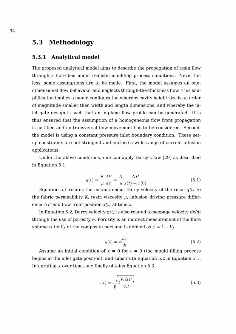
94
5.3 Methodology
5.3.1 Analytical model
The proposed analytical model aims to describe the propagation of resin flow
through a fibre bed under realistic moulding process conditions. Neverthe-
less, some assumptions are to be made. First, the model assumes an one-
dimensional flow behaviour and neglects through-the-thickness flow. This sim-
plification implies a mould configuration whereby cavity height size is an order
of magnitude smaller than width and length dimensions, and whereby the in-
let gate design is such that an in-plane flow profile can be generated. It is
thus ensured that the assumption of a homogeneous flow front propagation
is justified and no transversal flow movement has to be considered. Second,
the model is using a constant pressure inlet boundary condition. These set-
up constraints are not stringent and enclose a wide range of current infusion
applications.
Under the above conditions, one can apply Darcy’s law [29] as described
in Equation 5.1.
q(t) =K
µ
dP
dx=
K
µ
∆P
x(t)− x(0)(5.1)
Equation 5.1 relates the instantaneous Darcy velocity of the resin q(t) to
the fabric permeability K, resin viscosity µ, infusion driving pressure differ-
ence ∆P and flow front position x(t) at time t.
In Equation 5.2, Darcy velocity q(t) is also related to seepage velocity dx/dt
through the use of porosity φ. Porosity is an indirect measurement of the fibre
volume ratio Vf of the composite part and is defined as φ = 1− Vf .
q(t) = φdx
dt(5.2)
Assume an initial condition of x = 0 for t = 0 (the mould filling process
begins at the inlet gate position), and substitute Equation 5.2 in Equation 5.1.
Integrating x over time, one finally obtains Equation 5.3.
x(t) =
√
2K∆P
φµt (5.3)

Fibre bed impact on resin viscosity 95
Equation 5.3 describes the flow front propagation x(t) as a function of time
t, constituent material properties (resin viscosity µ, preform permeability K,
porosity φ) and specific process parameters (driving pressure difference ∆P ).
Step 1 - Model initialisation.
One defines a period of time when the effect of the initial resin cross-linking
and fibre sizing can still be considered negligible. As a rule of thumb, a quar-
ter of the gel time of the employed resin can be used as a conservative es-
timate. Over the chosen time window, the flow process can be treated as a
basic isothermal infusion, which is accurately reproduced by currently avail-
able simulation codes based on Darcy’s law (Equation 5.1). For this initializing
simulation step, one can implement constant model parameters (∆ P, φ, K and
µ). The value of ∆ P is controlled by the process operator and φ can be de-
rived from mould dimensions and lay-up thickness information. Model input
parameters ∆ P and φ can thus readily be obtained from the design of the
process that is to be simulated. Further, a permeability value needs to be de-
termined. Numerical techniques described in literature [30, 31] can be used
to determine the permeability of the fabric. However, the high dependence
of permeability on material parameters such as reinforcement architecture,
lay-up sequence, etc., results in considerable variation when evaluating this
parameter through analytical or numerical methods. As an alternative, the
strategy proposed here is to simply describe permeability as a function of vis-
cosity using the model applied for the analysis of the flow front propagation.
Given an ideal one-dimensional infusion trial, a valid assumption within the
initial time window as described above, the isolation of permeability results
from Darcy’s law as in Equation 5.4.
K =qµL
∆P(5.4)
Hereby is q defined as the quotient of flow rate and mould cavity cross-
sectional area (Q/A) and L is the distance travelled by the flow front from the
start. A constant viscosity estimate can be obtained from the resin supplier
data sheets, which then allows to perform an initialisation run with constant
parameters, based on Darcy’s law and valid for the chosen time window.

96
Step 2 - Viscosity expression
The next step in the model is the adoption of a non-linear description for the
resin viscosity evolution over time. As can be seen from Table 5.1 and Table 5.2
in Section 5.2, all models used to reproduce non-linear viscosity expressions
are based on power laws, albeit each with different levels of sophistication
and based on a variety of different process parameters. For our purpose,
setting forward an exponential law to express viscosity as a function of time is
therefore an appropriate start.
In fact, we propose to apply the empirical model from Table 5.1 but with
viscosity as a function of time, represented in Equation 5.5, where µ0 is the
viscosity at the initial stage of the injection process for the considered tem-
perature and b is the time constant to be empirically fitted.
µ(t) = µ0ebt (5.5)
Substitution of Equation 5.5 in Equation 5.3 and the posterior integration
of x over time, results in Equation 5.6, which represents the change of the
flow front position through the mould cavity.
x =
√
2K∆P
φ
(
−1
µ0b(e−bt − 1)
)
(5.6)
One can now describe the flow front propagation as a function of the pa-
rameters stated in Equation 5.6 and the viscosity time constant b. The present
work aims to use two different approaches to determine a value for b.
The first approach is based on a neat resin characterization outside the
mould without the presence of fibres. The initial viscosity µ0 can be extracted
from supplier datasheets, and parameter b can be determined using an isother-
mal time-viscosity chart.
The second approach consists of the determination of parameter b through
an empirical fitting based on a time-flow front propagation diagram extracted
from an experimental trial, that should be set up to be representative of the
real injection moulding process.
Using this last approach, one obtains a value for b that takes into account
the real situation in the mould cavity, including the presence of a fibre bed

Fibre bed impact on resin viscosity 97
architecture and a coating on the fibre reinforcement (sizing).
Model implementation
The two-step analytical model has been implemented as a numerical routine
in the Liquid Injection Moulding Simulation (LIMS) software [12, 13], a finite
element/control volume simulation code with thermal and cure prediction ca-
pabilities developed by the Center for Composite Materials at the University of
Delaware. Having obtained Equation 5.6, one might try to directly implement
this function into LIMS using a user subroutine. But, considering viscosity as
a function of time, in LIMS one must recalculate the entire matrix system of
the numerical algorithm at each time-step to do so [13]. In order to obtain a
more efficient simulation tool with low computational cost (i.e. avoiding heavy
matrix recalculations), a different approach was considered here. Though the
implementation is rather LIMS specific, the thought process behind the ap-
proach is generic and is therefore included here. Reviewing the governing
equations of flow through porous media (Equation 5.1), one observes that per-
meability K and viscosity µ always appear as a ratio. One can use this ratio
to transpose the viscosity change over time to an artificial change in fabric
permeability as in Equation 5.7.
K
µ(t)=
K
µ0ebt=
K(t)
µ0
(5.7)
Applying this method to Equation 5.6, one can keep the viscosity constant
to its initial value µ0 and reset the permeability value K for each time step
instead. In LIMS, the additional numerical cost of this approach is - unlike
changing viscosity per time step - without significant impact on the system
solution, as the modification of permeability can be easily inserted via a user
routine and entire matrix recalculations are not necessary.
Further, in order to determine the empirical parameter b for the analytical
model as expressed in Equation 5.5, an infusion process of a flat composite
panel has been considered in this investigation as an example (details are de-
scribed in the next section). For the numerical implementation, the panel was
represented via a rectangular mesh formed by 200 nodes and 171 shell type

98
elements. Figure 5.2 depicts an image of the used mesh and the placement
of the infusion gates, considered to be constant pressure inlet gates that com-
bine together to form a line gate along the short panel side, thus ensuring a
homogeneous and one-dimensional flow front propagation.
Figure 5.2: Representative plot of the two-dimensional mesh used for the nu-
merical implementation
5.3.2 Experimental work
Experimental trial data for the determination of model parameter b was ob-
tained with assistance of aerospace industry partners. As described in Step 2
of the analytical model, two approaches are needed for b determination, so as
to allow comparison between modelling techniques based on resin characteri-
sation outside the mould with the proposed model based on in-situ resin char-
acterisation. So, a neat characterization of a monocomponent, epoxy based
resin was conducted first, and a controlled infusion with the same resin was
performed after. The infusion set-up selected was for a two-dimensional rect-
angular composite panel made out of a non-crimp carbon fibre fabric. How-
ever, the selection of resin, part shape and fabric materials were merely made
for reasons of availability and relevance to real part applications of assisting
industrial partners, and the specific set-up properties of the experimental trial
do not influence the general nature of the study findings.

Fibre bed impact on resin viscosity 99
Neat resin characterization
Neat resin characterisation data was obtained for Hexflow RTM6 [11] from
supplier Hexcel (Hexcel, Cambridge, UK). Characterization tests were per-
formed of the RTM6 resin to obtain a viscosity chart under isothermal curing
conditions. The results of these tests are shown in Figure 5.3. They provide
the time-dependent viscosity behaviour over a discrete range of curing tem-
peratures (100ºC to 180ºC) and up to the point that the resin cross-linking
starts and the conversion into a solid substance takes place. Figure 5.3 con-
firms, as can be expected, that resin viscosity increase over time is accelerated
at higher temperatures due to the earlier activation of the exothermic reac-
tion.
Figure 5.3: RTM6 isothermal time-dependent viscosity behaviour over a tem-
perature range of 100-180ºC (Courtesy of resin supplier Hexcel)
Experimental trial
Long, flat panel samples were subjected to an isothermal, one-dimensional
flow infusion setup (RIFT). Aluminium mould tooling was used with controlled
electric heating capability. The fibre reinforcement preform for the samples
consisted of 8 layers of multi-axial carbon fabric, creating a quasi-isotropic
laminate lay-up. The monocomponent, epoxy based Hexflow RTM6 resin, as

100
characterised before, was used to consolidate the fibre architecture. Details
about panel dimensions and used materials are given in Table 5.3.
Sample information summary
Panel dimensions
DimensionsLength Width Thickness
2060 mm 590 mm 2.9±0.1 mm
Constituent materials
Fabric
Hexcel G0926 Carbon Fabric
5 harness, 6k (370 g/m2)
lay-up (0, 90,±45,±45, 0, 90)s
Resin
Hexflow RTM6
Monocomponent
Aerospace qualified
Table 5.3: Main panel dimensions and description of constituent materials as
used in the experimental infusion trial[11, 32]
Resin was injected via a line gate from the short left side of the panel. A line
vent was used on the short right side of the panel to establish a vacuum in the
mould and have the possibility to extract exceeding resin. Infusion pressure
was set to 552 kPa and vacuum level prior to infusion was approximately 0.4
kPa.
The acquisition system used in the tests recorded pressure throughout the
filling stage, and amount of resin transferred into the mould was registered
using a weighting scale on the resin supply. To track the position of the flow
front, pressure sensors were embedded in the mould tooling. A pressure read-
ing step change occurred when resin passed over the sensor location.
Tooling temperature was held constant at 120ºC during infusion. Due to
the low thickness of the panel, the transversal temperature gradient was con-
sidered negligible, and the set-up considered as isothermal. The resin pot
temperature was kept constant at 80ºC during infusion. On first contact with
the mould, a resin temperature variation occurs due to the difference in resin

Fibre bed impact on resin viscosity 101
pot and tooling temperature. However, this initial resin temperature adjust-
ment is a transient effect that only exists over a very short period of time. As
this investigation focuses on the end of infusion when resin polymerisation is
likely to occur, the small transient effect at the start of infusion can safely be
neglected. Note that, in line with these considerations, the analytical models
in this study also do not have a transient effect for resin temperature coming
out of a resin pot embedded, though it has been implemented that resin ini-
tially starts from the average temperature between pot and tooling at mould
entry.
In Figure 5.4, the evolution of the flow front position during the infusion
process can be observed. It highlights the decrease of flow front propagation
as the process reaches the later stages of infusion. The length of the time in-
terval between consecutive data points was gradually increased from approx-
imately 3 minutes to 6, 12 and finally 24 minutes. The infusion trial reached a
final flow front position of 1.98 m after 10020 seconds (167 minutes).
Figure 5.4: Resin flow front position vs. infusion time as derived from the
experimental trial
Information on fibre volume fraction Vf was additionally extracted from
the experiment. To obtain Vf , discrete thickness measurements on the dry
preform and the infused final part were conducted. In Figure 5.5, the position

102
of the control points and their thickness values are displayed. From these
thickness measurements the fibre volume fraction Vf was obtained, giving an
average Vf value of 58.14% throughout the entire mould cavity.
Figure 5.5: Schematic of the infused flat panel. Results of discrete thickness
measurements are presented (in inches)
5.3.3 Experiment vs. simulation
The flow front propagation as derived in the experimental trial (section 5.3.2)
was compared against numerical predictions (section 5.3.1). Apart from per-
forming a simulation using a constant viscosity parameter to provide a base-
line numerical prediction, two further simulations were made. These simula-
tions made use of a non-linear viscosity expression based on neat resin charac-
terisation data and in-situ resin characterisation from flow front propagation
data respectively.
Based on the experimental trial, empirical and process-related parameters
for the simulation are derived. In order to set the initial simulation working
point (see section 5.3.1), one assumes constant values for all parameters in-
volved in the infusion process (φ, ∆P , K and µ). The acquisition and control
system used in the experimental rig can derive porosity φ and driving pressure
∆P , but not fabric permeability K and resin viscosity µ.
An initial value for viscosity µ can be obtained from the neat resin charac-
terisation curves. As resin pot temperature was kept at 80ºC and the tooling
at 120ºC, an initial value of 0.057 Pa·s was determined from isothermal curves
of Figure 5.3.

Fibre bed impact on resin viscosity 103
An estimation for permeability K can be obtained from the one-dimensional
description of Darcy’s law, as stated in Equation 5.4. Parameters involved
are: permeability K [m2], viscosity µ [Pa·s], sample length L [m], pressure P
[Pa] and specific discharge or Darcy velocity q [m/s], which consists of flow
Q [m3/s] through area A [m2]. Darcy velocity can be obtained from the ex-
perimental trial data. A value of 0.3 mm/s was estimated from the time vs.
flow front position data displayed in Figure 5.4. Substituting this value into
Equation 5.4, one obtains a permeability value of 1.31·10−11 m2, for the initial
period of infusion time. This value is consistent with consulted material data
sheets of the same fibre fabric and similar lay-up [33], and can be applied to
the entire infusion plane due to the quasi-isotropic state of the prepared lam-
inate. As the permeability property is inherent to the fabric and should not
change throughout the infusion, the value of the obtained permeability K is
kept for the entire filling simulation.
With permeability addressed, only the changing behaviour of viscosity over
the duration of the simulation needs to be determined. The approach as de-
scribed in section 5.3.1 can now be considered and simulations based on dif-
ferent viscosity expressions compared: (i) the first case is a simulation with
a time-independent or constant viscosity value throughout, (ii) the second
case is a simulation with a time-dependent viscosity expression based on neat
resin characterisation data and (iii) the third case is a simulation with a time-
dependent viscosity expression based on in-situ resin characterisation via flow
front propagation data.
In the first simulation case, the value of resin viscosity is considered con-
stant during the entire process and is set equal to 0.057 Pa·s, the initial value
interpolated earlier from the neat resin characterisation curves (Figure 5.3).
In the second simulation case, a time-dependent viscosity expression (Equa-
tion 5.5) is used. Unknown parameter µ0 could be extracted from resin sup-
plier datasheets, but is here given the interpolated value as derived in the first
simulation case. Unknown parameter b can be derived from fitting Equation
5.5 onto the curves of the neat resin characterisation experiment available in
Figure 5.3. Table 5.4 lists the values of parameters µ0 and b, together with an
R2 precision value for the fitting.

104
In the third simulation case, the initial viscosity value µ0 is again main-
tained but now the flow front propagation data of the experimental trial are
used to establish empirical parameter b for the time-dependent viscosity ex-
pression in the form of Equation 5.5. Empirical parameter b can be derived
by matching the flow front position of the numerical prediction (Equation 5.6)
with the experimental trial data for all control time intervals using optimiza-
tion techniques and sensibility analysis [34]. The derived viscosity expression
parameter values are again given in Table 5.4.
Parameter Neat resin fit Flow front fit
µ0 [mPa·s] 57.4 57.4
b [ - ] 0.6·10−4 8.2·10−5
R2 0.985 0.985
Table 5.4: Expression parameters and R2 fitting precision values for the time-
dependent viscosity given by Equation 5.5, based on neat resin characterisa-
tion data fitting and on in-situ resin characterisation using flow front propaga-
tion data fitting from the experimental trial
5.4 Results
Figure 5.6 summarises the flow front propagation over time as observed dur-
ing the experimental trial, together with three numerical predictions, each
based on a different approach to incorporate resin viscosity into the simula-
tion.
One can observe in Figure 5.6 that the consideration of a constant viscos-
ity value leads to inaccurate predictions of the flow front propagation after the
first stages of infusion. Although initially the numerical prediction with con-
stant viscosity is excellent and matches well the experimental results, as the
infusion advances, the resin ends its ’gel time’ and viscosity starts increasing
its value to the point that a constant parameter assumption can no longer be
upheld. This is when the flow front prediction starts to deviate from the exper-

Fibre bed impact on resin viscosity 105
Figure 5.6: Experimental flow front position vs. time and numerical predic-
tions obtained with three different viscosity models
imental trend, which shows a clear propagation slow-down as time advances
that is not reproduced in the numerical result with constant viscosity.
It can be seen that a clear improvement is achieved in the numerical pre-
diction when the time-dependent viscosity model based on neat resin charac-
terisation data is used instead of the constant viscosity model. However, the
improvement still does not match the experimental trend to the very end of
the infusion period.
Finally, the numerical prediction obtained with the time-dependent viscos-
ity model based on flow front propagation data does reach the end of the fill-
ing stage in excellent agreement with the experimental trial. This is because
with this model one can reproduce in the simulation an in-situ resin viscosity
characterisation that incorporates the effect of having a fibre reinforcement
present in the mould, with its specific fibre sizing and fibre bed architecture,
which cannot be taken into account using neat resin characterization data.
5.5 Discussion
So far, this study has looked at changes over time of process or material pa-
rameters. However, some parameters, such as fibre volume fraction (Vf ), can

106
display a spatial variability over the sample investigated. As Vf is related
to permeability [35], and permeability is an input parameter for Darcy’s law
upon which the proposed analytical model is based, it is worth investigating
whether the spatial variability of Vf has any impact on the presented findings.
In the presented simulations, fibre volume fraction (Vf ) was set for all ele-
ments to an average value of 58.14%, extracted from various thickness mea-
surements across the sample before and after infusion. The collected data
presented a standard deviation of 1.56%. Though the small variations in Vf
were not expected to have any significant effect on the final simulation re-
sults, this has nevertheless been verified by comparing results for a specific
sample preform using detailed Vf values assigned to each element in the mesh
with results based on having an average value assigned for all the elements in
the mesh.
The spatial distribution of Vf was derived from discrete thickness measure-
ments, as can be seen in Figure 5.2. The mapping of the distribution to the
mesh elements is provided in Figure 5.7. Mesh elements that could not benefit
from direct Vf measurement mapping were assigned an interpolated Vf value
based on values of adjacent elements.
Figure 5.7: Mesh element distribution of fibre volume fraction Vf based on
experimental thickness measurements and interpolation. Paths used for the
fibre volume variability analysis are indicated with row numbers
Flow front propagation has been calculated separately for each of the 9
horizontal rows in the mesh using the flow front fitted viscosity model, allow-
ing for investigation of 9 different scenarios. Results have been compared
with the simulation based on a mesh with averaged Vf value as well as with
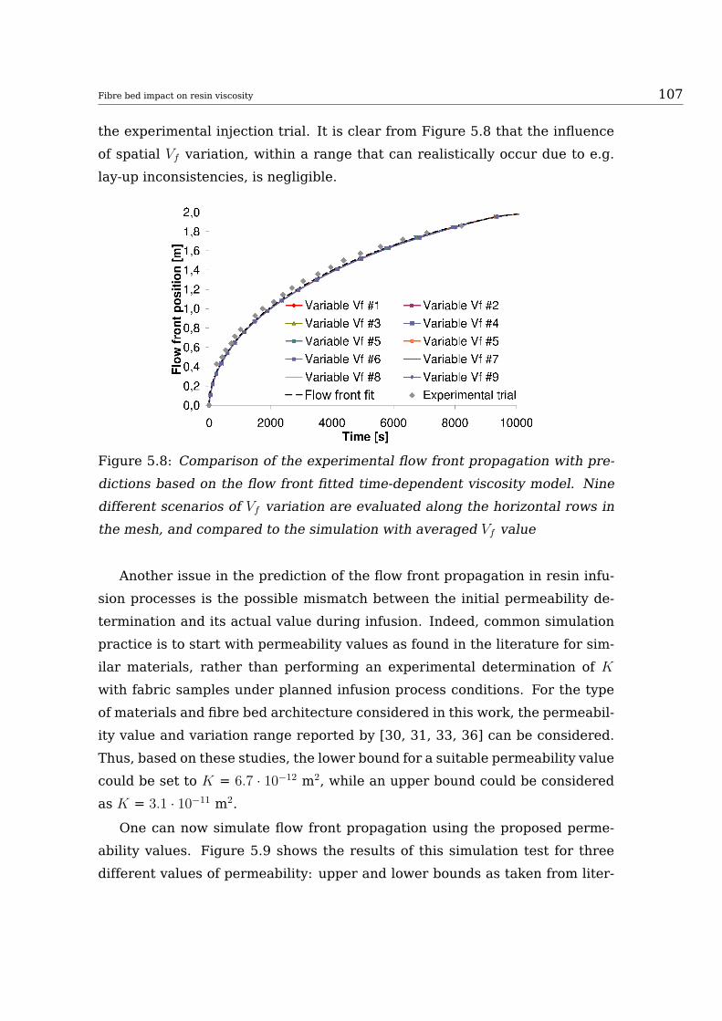
Fibre bed impact on resin viscosity 107
the experimental injection trial. It is clear from Figure 5.8 that the influence
of spatial Vf variation, within a range that can realistically occur due to e.g.
lay-up inconsistencies, is negligible.
Figure 5.8: Comparison of the experimental flow front propagation with pre-
dictions based on the flow front fitted time-dependent viscosity model. Nine
different scenarios of Vf variation are evaluated along the horizontal rows in
the mesh, and compared to the simulation with averaged Vf value
Another issue in the prediction of the flow front propagation in resin infu-
sion processes is the possible mismatch between the initial permeability de-
termination and its actual value during infusion. Indeed, common simulation
practice is to start with permeability values as found in the literature for sim-
ilar materials, rather than performing an experimental determination of K
with fabric samples under planned infusion process conditions. For the type
of materials and fibre bed architecture considered in this work, the permeabil-
ity value and variation range reported by [30, 31, 33, 36] can be considered.
Thus, based on these studies, the lower bound for a suitable permeability value
could be set to K = 6.7 · 10−12 m2, while an upper bound could be considered
as K = 3.1 · 10−11 m2.
One can now simulate flow front propagation using the proposed perme-
ability values. Figure 5.9 shows the results of this simulation test for three
different values of permeability: upper and lower bounds as taken from liter-

108
ature, as well as the permeability value derived from the actual experimental
trial (see section 5.3.3). While the simulation result obtained with the ex-
perimentally determined permeability value aligns well with the experimental
trial result for the complete infusion process, the predictions obtained with
the upper and lower permeability bounds as taken from literature only agree
with the experimental data at the very beginning of the process, but further
display poor agreement with the experimental curve throughout. The poor
predictions based on the upper and lower permeability bounds indicate that
though permeability value estimates can usually be obtained from literature
for similar materials and similar fibre architectures, the simulation results
are sensitive to variations of K and high accuracy simulations do require the
in-situ experimental determination of permeability under actual process pa-
rameters.
Figure 5.9: Effect of permeability determination on accuracy of numerical
predictions for flow front propagation. Permeability values in m2
5.6 Case Study
To underline the industrial relevance of the presented simulation methodology
based on flow front fitted time-dependent viscosity, a case study is given here.
The simulation was used to assist the manufacturing process design of three
different sizes of a cylindrical, flat lid ended vessel. The vessels are to be used

Fibre bed impact on resin viscosity 109
for water treatment in industrial environments. A vessel is composed of two
symmetrical parts held together by means of a metallic clamp. Figure 5.10
depicts the vessel half geometry considered for the analysis.
Figure 5.10: Representative mesh of a vessel half geometry as used in the
case study
The boundary conditions of the vessel infusion scheme are consistent with
the experimental trial on long, flat panels described earlier in this study. The
resin gate is placed in the middle of the top of the lid, creating a circumfer-
ential but homogeneous flow pattern. A line vent is placed at the end contour
of the cylindrical vessel half. Considered vessel diameters are 1000, 1200 and
1400 mm, respectively. Constituent materials match in type and lay-up with
the fibre fabric used in the experimental flat panel trial, of which details are
given in Table 5.3.
Filling simulations with three different viscosity models have been con-
ducted for each size, using a constant viscosity, a time-dependent neat resin
characterisation based viscosity and a time-dependent flow front based viscos-
ity expression. Table 5.5 summarizes the final filling times for each scenario.
Results show noticeable differences between the predictions made by the
different models. The predictions also become more disparate as the size of
the geometry grows, which underlines the rationale for this work (i.e. that
infusion simulation inaccuracies are more dominant with large parts working
close to the end of the resin gel time).

110
Diameter 1000 1200 1400 [mm]
Constant viscosity 6067 8800 13007 [s]
Neat resin fit 6181 9877 18245 [s]
Flow front fit 6731 11552 28719 [s]
Table 5.5: Filling times for three different vessel sizes and three different
viscosity models
Time-dependent viscosity based predictions are clearly differentiated from
constant viscosity predictions, which is in line with expectations, but results
also point to a clear distinction between the two time-dependent models, which
is further discussed through the analysis of the filling isochrones as shown in
Figure 5.11.
Figure 5.11: Filling isochrones [s] for the 1400 mmm vessel using different
time-dependent viscosity models.
Figure 5.11 depicts a lateral view of the 1400 mm vessel half geometry
as well as isochrones of the resin filling process, calculated with the viscosity
time-dependent models based on neat resin characterisation (left), and based
on flow front propagation, (right). The 1400 mm vessel has been selected for
this comparison as it represents the critical case of the three sizes (see also
Table 5.5 demonstrating the most disparate values for the 1400 mm diameter).
The difference in flow front propagation prediction is particularly notice-
able in the later stages of the infusion, when the resin reaches the end of
its gel time. Both models indeed exhibit a similar propagation pattern un-
til the vessel’s bottom half section. However, the model based on neat resin

Fibre bed impact on resin viscosity 111
characterisation demonstrates a significant slow down in flow front propaga-
tion only from the lower quarter of the vessel geometry, whereas for the flow
front propagation based model the flow front velocity is already dramatically
reduced when still one third of the vessel remains to be infused.
The sudden increase of viscosity, occurring during the initial cross-linking,
almost stops the resin flow front propagation, resulting in a high risk of voids
and dry spots for the last section of the part. The flow front propagation
based time-dependent model (5.11, right) captures this effect and thus pro-
vides more conservative simulation results than the neat resin characteriza-
tion time-dependent model (5.11, left), reducing the possibility of underesti-
mating infusion time and avoiding incompletely infused parts with consequent
loss of material and time.
5.7 Conclusions
A keen interest in liquid composite moulding processes still exists in strategic
markets such as the aerospace, automotive and defence industries. More and
more, very large one-shot infusion composite parts are attempted and their
manufacturing is therefore prone to run beyond the gel time of available resin
systems, hereby increasing the risk of voids, dry spots and incomplete part
infusion. Current infusion simulation strategies have already started to move
away from constant viscosity based models, but even advanced viscosity ex-
pressions seem to not always provide a very accurate prediction of flow front
progression in real infusion processes, especially in cases where filling time
reaches or extends beyond resin gel time.
This study has now proposed a two-step analytical simulation model based
on Darcy’s law, making use of an exponential time-dependent viscosity ex-
pression that incorporates an in-situ resin viscosity characterization. This was
achieved through an empirical parameter fitting using a flow front propaga-
tion trial under actual infusion process conditions. The method incorporates
the impact of the fibre reinforcement presence in the mould on resin viscos-
ity, which cannot be taken into account by a traditional neat resin charac-
terization test. It has been validated by comparison with an experimental

112
trial that the proposed model can predict flow front propagation results more
accurately than methods based on neat resin characterization, especially in
the later stages of large part infusion processes when resin cross-linking can
drastically increase resin viscosity and hamper flow front propagation. The
sensitivity to variations in process and material parameters such as fibre vol-
ume fraction and permeability were discussed. Finally, a real application case
study was included, highlighting the industrial relevance of adopting the pro-
posed model over other non-linear viscosity based infusion simulation models,
by demonstrating results that gave a more conservative prediction of flow
front propagation behaviour, thus avoiding potential filling time underestima-
tion that could lead to loss of material and time in subsequent manufacturing
trials.

Bibliography
[1] R.S. Dave, A.C. Loos, Processing of Composites, Hanser Publishers,
Cincinnati, OH, USA, (1999).
[2] F. Campbell Jr., Manufacturing Processes for Advanced Composites, El-
sevier Science, Amsterdam, NL, (2003).
[3] S. Mazumdar, Composites Manufacturing. Materials, Product and Pro-
cess Engineering, CRC Press, Boca Raton, FL, USA, (1997).
[4] B. Shirinzadeh, G. Alici, C. Foong, G. Cassidy, Fabrication process
of open surfaces by robotic fibre placement, Robotics and Computer-
Integrated Manufacturing 20 (1) (2004) 17–28.
[5] G. Newell, R. Buckingham, K.Khodabandehloo, The automated manu-
facture of prepreg broadgoods components. A review of literature, Com-
posites Part A: Applied Science and Manufacturing 27 (3) (1996) 211–
217.
[6] P. W. Schuessler, W. J. Dobbin, Gel time measurement of resins, Analyti-
cal Chemistry 53 (-) (1981) 2380–2381.
[7] S. Advani, E. Murat Sozer, Process Modelling in Composites Manufac-
turing, Marcel Dekker Inc., Taylor and Francis, UK, (2003).
[8] C. Tucker III, Fundamentals of Computer Modelling for Polymer Pro-
cessing, Hanser Publishers, New York, NJ, USA, (1989).
[9] M. Bruschke, S. Advani, A finite element/control volume approach to
mould filling in anisotropic porous media, Polymer Composites 11 (6)
(1990) 398–405.
113

114
[10] C. Williams, J. Summerscales, S. Grove, Resin infusion under flexible
tooling (RIFT). A review, Composites Part A:Applied Science and Manu-
facturing 27 (7) (1996) 517–524.
[11] Hexcel Composites, HexFlow RTM6 Datasheet, Publication ITA 065e,
Hexcel Composites, Stanford, CO, USA, (2009).
[12] P. Simacek, S. Advani, Desirable features in mould filling simulations for
liquid composite moulding processes, Polymer Composite 25 (4) (2004)
355–367.
[13] S. Advani, P. Simacek, Programming in LBasic. Lims 5.0.4 Software Doc-
umentation, Center for Composite Materials, UDel, Newark, DE, USA,
(2003).
[14] M. L. Skinner, New applications and approaches expand market for
composites software, Reinforced Plastics 50 (6) (2006) 24–28.
[15] J. Bear, Dynamics of Fluids in Porous Media, Dover Books, New York,
NJ, USA, (1989).
[16] P. Halley, M. E. Mackay, Chemorheology of thermosets-an overview,
Polymer Engineering and Science 36 (5) (1996) 593–609.
[17] N. Kiuna, C. Lawrence, Q. Fontana, P. Lee, T. Selerland, P. Spelt, A model
for resin viscosity during cure in the resin transfer moulding process,
Composites Part A-Applied Science and Manufacturing 33 (11) (2002)
1497–1503.
[18] Q. Fontana, Viscosity: thermal history treatment in resin transfer
moulding process modelling, Composites Part A-Applied Science and
Manufacturing 29 (1-2) (1998) 153–158.
[19] C. Seeton, Viscosity temperature correlation for liquids, Tribology Let-
ters 22 (1) (2006) 67–78.
[20] A. Malkin, S. G. Kulichikhin, Rheokinetics of curing, Springer
Berlin/Heidelberg, Berlin, DE, (1991).

Bibliography 115
[21] M. Kamal, S. Sourur, Kinetics and thermal characterization of thermoset
cure, Polymer Engineering and Science 13 (1) (1973) 59–64.
[22] F. Mussati, C. Macosko, Rheology of network forming systems, Polymer
Engineering and Science 13 (3) (1973) 236–240.
[23] M. L. Williams, R. F. Landel, J. Ferry, The temperature dependence of
relaxation mechanism in amorphous polymers and other glass-forming
liquids, Journal of American Chemical Society 77 (1955) 3701–3707.
[24] A. M. Stolin, A. G. Merzhanov, A. Y. Malkin, Non-isothermal phenomena
in polymer engineering and science: A review. part I: Non-isothermal
polymerization, Polymer Engineering and Science 19 (15) (1979) 1065–
1073.
[25] S. D. Lipshitz, C. W. Macosko, Kinetics and energetics of a fast
polyurethane cure, Journal of Applied Polymer Science 21 (8) (1976)
2029–2039.
[26] J. Mijovi, C. H. Lee, A comparison of chemorheological models for ther-
moset cure, Journal of Applied Polymer Science 38 (12) (1989) 2155–
2170.
[27] P. L. Chiou, A. Letton, Modelling the chemorheology of an epoxy resin
system exhibiting complex curing behaviour, Polymer 33 (18) (1992)
3925–3931.
[28] J. Martin, J. Laza, M. Morras, M. Rodriguez, L. Leon, Study of the cur-
ing process of a vinyl ester resin by means of TSR and DMTA, Polymer
41 (11) (2000) 4203–4211.
[29] S. Advani, M. Bruschke, R. Parnas, Resin Transfer moulding flow phe-
nomena in polymeric composites. In Flow and Rheology in Polymer
Composites Manufacturing, S.G. Advani, Amsterdam, NE, (1994).
[30] E. Heardman, C. Lekakou, M. Bader, Flow monitoring and permeability
measurement under constant and transient flow conditions, Composites
Science and Technology 64 (9) (2004) 1239–1249.

116
[31] C. Wong, A. Long, M. Sherburn, F. Robitaille, P. Harrison, C. Rudd, Com-
parisons of novel and efficient approaches for permeability prediction
based on the fabric architecture, Composites Part A-Applied Science
and Manufacturing 37 (6) (2006) 847–857.
[32] Hexcel Composites, G0926 Carbon Fabric Product Data, Hexcel Com-
posites, Stamford, CO, USA,(2009).
[33] A. Endruweit, K. S. Matthys, J. Peiro, A. C. Long, Effect of differential
compression on in-plane permeability tensor of heterogeneous multi-
layer carbon fibre preforms, Plastics, Rubber and Composites 38 (1)
(2009) 1–9.
[34] B. J. Henz, K. Tamma, R. Kanapady, N. Ngo, P. Chung, Process Mod-
eling of Composites by Resin Transfer Moulding: Sensitivity Analysis
for Isothermal Considerations ARL-TR-2686, Army Research Laboratory
(ARL), University of Minessota, MN, USA, 2002.
[35] H. C. Stadtfeld, M. Erninger, S. Bickterton, S. G. Advani, An experimen-
tal method to continuously measure permeability of fiber preforms as
a function of fiber volume fraction, Journal of Reinforced Plastics and
Composites 21 (10) (2002) 879–899.
[36] E. Heardman, C. Lekakou, M. Bader, In-plane permeability of sheared
fabrics, Composites Part A-Applied Science and Manufacturing 32 (7)
(2001) 933–940.

Chapter 6
Numerical implementation and
experimental validation of a
through-the-thickness
temperature model for
non-isothermal vacuum bagging
infusion.
117

118
M. Gascons, N. Blanco, J. Vives, K. Matthys, Numerical implementation
and experimental validation of a through-the-thickness temperature model for
non-isothermal vacuum bagging infusion, Journal of Reinforced Plastics and
Composites. Accepted 17 Aug 2011.
DOI 10.1177/0731684411423321
6.1 Introduction
In performance driven applications as found in the aerospace and high-end au-
tomotive sector, autoclaving techniques with prepreg composite materials are
an established code of practice. Liquid moulding techniques are however in-
creasingly considered as a lower-cost alternative, especially with demand for
thicker monolithic composite parts rapidly rising. Liquid Composite Mould-
ing (LCM) can be divided into two categories defined by mould typology, as
represented in Figure 6.1. The first category is that of Resin Transfer Mould-
ing (RTM) [1], whereby the mould cavity is formed between two rigid mould
halves. The second category is defined as Resin Infusion under Flexible Tool-
ing (RIFT) [2], also known as Vacuum Bagging Moulding (VBM), whereby one
of the rigid mould halves is replaced by a layer of flexible ’bagging’ mate-
rial. RIFT techniques are gaining importance over RTM [3], mainly due to
the lower tooling investment needed, which is of particular importance for the
manufacturing of large or thick composite parts.
As many variations exist on the RTM and RIFT processes, different nomen-
clature can be found, such as Resin Film Infusion (RFI), Vacuum Assisted RTM
(VARTM), Liquid Resin Infusion (LRI), Seeman Composite Resin Infusion Pro-
cess (SCRIMP) and RTM-Light. The essence of all LCM processes is however
that resin in liquid form is driven through the dry fibre preform by means of
a pressure difference between an inlet and an outlet or vent gate. The pres-
sure difference is maintained via a pump on the inlet, a vacuum pump on the
vent or a combination of both, and it drives the resin flow front propagation
and impacts part filling and impregnation time. Following impregnation, resin
curing starts and the part is consolidated.
The introduction of a heat source in the infusion process is a common tech-

Through-the-thickness temperature model 119
Figure 6.1: Schematic representation of the RTM (left) and RIFT (right) in-
fusion techniques. 1:Vents, 2:Mixing pump, 3:Rigid tool, 4:Resin pressurized
pot, 5:Catalyst pressurized pot, 6: Mould cavity, 7:Vacuum Bag, 8:Resin non-
pressurized pot, 9:Vacuum pump connection.
nique to reduce resin viscosity and enhance resin propagation. For sizeable
parts the resin itself is heated rather than applying mould temperature con-
trol. Thermal interventions are important and often vital for the manufactur-
ing of thick parts. Even with the evolution of low or non-reactive resins into
the market, thermal gradients caused by the external heat supply are still gen-
erated as the resin advances. This can lead to inhomogeneous cure of the part,
which is a potential source of residual stresses or deformation [4–6].
Heat transfer management in LCM is a complex topic of study due to the
interaction of many physical phenomena. As resin flows through the mould,
it exchanges heat with the dry preform and the mould by conduction but also
transports the heat inside the mould cavity by convection. In addition, changes
in resin flow propagation due to temperature dependence of the resin viscosity
are to be considered.
Heat transfer phenomena have been thoroughly described in literature for
double sided rigid mould infusion techniques, as found in RTM [7–10], but
are still less explored for single sided rigid mould infusions, as found in RIFT
techniques. The nature of RIFT techniques implies that one side of the mould
is closed with an element of little thermal inertia (bag) onto which the external
temperature will have more influence.
In the case of autoclave processing of vacuum bagged composites, the as-
sumption of a constant temperature boundary condition for the entire system

120
is appropriate, due to the forced air convection in the autoclave environment.
However, in the case of infusion by means of non-isothermal out-of-autoclave
vacuum bagging, forced air circulation is lacking and the constant tempera-
ture boundary assumption cannot be maintained. Instead, to resolve this, a
heat transfer coefficient might be used to reproduce the passive carry of heat
by natural convection phenomena. The accuracy of such simplification will be
discussed further.
Regarding thickness, in thin composite plates the temperature gradient
through-the-thickness can be neglected, but the difference of temperature in
a thick part, object of this study, can rise up to several degrees. For heated
resin set-ups, the preform can provide insulation to the entering heat, leaving
the inside of the part hotter than the edges. For the heated mould set-up,
heat propagates from the source at the bottom (mould side) to the top of the
specimen (bag side). Temperature will decrease accordingly from bottom to
top of the specimen.
In the absence, to our knowledge, of an adequate analytical thermal model
for RIFT manufacturing, it is suggested here to draw from thermal models
that were originally designed for RTM.
An experimental protocol has been developed to validate the fitness of pur-
pose of such RTM models for the prediction of temperature distribution and
evolution during the filling stage of thick monolithic shell parts produced in
a RIFT set-up. In order to single out the effect of external thermal interven-
tions, low-reactive epoxy resin has been used, but this is still representing a
considerable range of the available thermosets resin used in industrial envi-
ronments.
The analytical model is based on an estimated through-the-thickness tem-
perature profile, this allows the reduction of the fully three-dimensional prob-
lem to a two-dimensional one. Under this supposition, one can solve first
a two-dimensional discretization in the plane of the flow, currently available
in simulation codes, and later apply the desired profile. Extruding the two-
dimensional plane under the guidance of this profile provides the temperature
gradient in all directions for the real geometry. This supposition significantly
improves the computational efficiency in the process and avoids the difficulty

Through-the-thickness temperature model 121
of gathering all necessary parameters to run the full three-dimensional analy-
sis, a key point in infusion simulations of large structures.
In what follows, the analytical background of the RTM modelling work is
explained, the implementation of the models for a RIFT set-up is clarified and
the experimental validation protocol is presented. It will be shown that the
analytical solution is approximate but of practical use for RIFT applications.
6.2 Methods
6.2.1 Analytical background
A detailed overview of non-isothermal LCM modelling can be found in reviews
by e. g. Advani et al. [11] or Tucker and Dessenberger [12]. For RTM pro-
cesses, two different heat transfer models are commonly used [13]. The first
one is the Non Local Thermal Equilibrium (NLTE) model, also known as the
two equations model (Equation 6.1 and Equation 6.2). In this model the en-
ergy balance is considered independently for the two components present in
the mould cavity, the fluid (resin) and the solid (fibre). In the following equa-
tions the subscripts f and s refer to the fluid and the solid respectively.
φ(ρCp)f∂ 〈Tf〉
∂t+ (ρCp)f∇ (〈υf〉 〈Tf〉) =
= ∇ (Kf • ∇ 〈Tf〉) +H(Tf − Ts) + φs
(6.1)
(1− φ)(ρCp)s∂ 〈Ts〉
∂t= ∇(Ks • ∇ 〈Ts〉)− αfshfs(Tf − Ts) (6.2)
In both equations, ρ, Cp, 〈υf〉, T, K, H, φ, s and hfs are the density, the heat
capacity of the materials, the local averaged velocity of fluid, the temperature,
the heat conductivity tensor, the heat exchange parameter, the porosity, the
curing reaction heat and the heat exchange coefficient between fluid and solid
respectively. αfs is the specific area representing the laminate architecture at
tow scale and is defined in Equation 6.3.
αfs =4
dp
ǫ
1− ǫ(6.3)

122
In Equation 6.3, dp corresponds to the diameter of a fibre tow and ǫ to the
bed or fabric porosity.
Difficulties appear when all the necessary data to use these equations
needs to be gathered experimentally. The necessity of fully characterizing
both resin and fibre independently, in addition to the complex set-ups needed
to obtain particular data, such as the heat exchange coefficients or the con-
ductivity tensor, makes the NLTE model impractical for industrial use.
An alternative and simplified method is the Local Thermal Equilibrium
(LTE) or one equation model (Equation 6.4).
(φ(ρCp)f + (1− φ)(ρCp)s)∂ 〈T 〉
∂t+ (ρCp)f 〈υf〉 · ∇ 〈T 〉 =
= ∇ · ((φKf + (1− φ)Ks) · ∇ 〈T 〉) + φs
(6.4)
The LTE model is obtained under the assumption that local temperatures
of resin and fibre become equal as soon as resin and fibre come into contact
with each other. In the resulting equation, each term stands for a phenomena
occurring in the heat transfer process.
The first term represents the internal energy term (heating of the resin),
followed by the convection term (heat transport due to moving resin). This
equals to the heat generation (due to dissipation and chemical reaction) and
the conduction/dispersion term (due to diffusion of heat from the mould walls
into the resin and the microscopic resin motion not taken into account in the
convection term).
The simplification of the NLTEmodel into the LTE model is not always valid,
as it is constrained by certain assumptions regarding e.g. the fluid velocity.
However, computing cost can be reduced with LTE.
Regarding the velocity of the fluid going through the mould cavity, one can
evaluate the effect of filling speed through the Graetz number [14]. It defines
a dimensionless relation between the convection in the flow direction and the
transverse conduction.
A small Graetz number corresponds to a filling speed that is slow compared
to heat conduction. The conduction terms are then large compared to the con-
vection term, so they dominate the energy equation. For infusion processes

Through-the-thickness temperature model 123
with Graetz number much larger than one (Gz >>1), the LTE model becomes
imprecise [13, 15, 16], and is thus only suitable for low speed infusion manu-
facturing. RIFT processes utilize vacuum suction to pull the resin through the
mould. Resin velocities achieved by pressure gradients from vacuum suction
are limited; therefore the Graetz number for RIFT processes is always small,
and the LTE model is applicable.
Regarding computing cost, some authors [9, 17, 18] developed fully three-
dimensional models for non-isothermal infusion processes. Many others have
dealt with the extensive computational cost issue and have tested and vali-
dated the feasibility of applying many simplifications in the three-dimensional
model to obtain the so called "two and a half" dimensional models [19] or even
two-dimensional models that explain the full evolution of the flow.
The last option has been commonly used in industrial environments, as
most of the composite parts produced can be defined as shell parts (a thick-
ness to in-plane ratio less than 1/100). However the need from companies
to produce thicker parts reopens the necessity to obtain an accurate predic-
tion of temperature gradients and its evolution in the through-the-thickness
direction at a reasonable computational cost.
6.2.2 Implementation
The proposed method here has been implemented using the thermal module of
the Liquid Injection Moulding Simulation (LIMS) software (version 4.2) [20],
a finite element/control volume code with thermal and cure prediction capa-
bilities developed by the Center for Composite Materials of the University of
Delaware.
As a core solver, LIMS deals with the resin flow front advance using Darcy’s
law (Equation 6.5).
〈Vf〉 =K
η∇〈pf〉 (6.5)
In the previous equation,K stands for the permeability of the fabric, η is the
resin viscosity and pf is the fluid volume-averaged pressure. Using Equation
6.5 in the mass conservation equation, it results in the Laplacean equation for

124
the fluid pressure (Equation 6.6), which will be used together with the energy
equation (Equation 6.4) to solve the temperature during filling stage.
∇ ·
(
K
η∇〈pf〉
)
= 0 (6.6)
The particular production technique focus of this work, RIFT, presents spe-
cific peculiarities when modelling flow front advance. A flexible mould half
supposes an uncontrolled mould cavity, as thickness is affected by compaction,
caused by the driving suction.
Compaction of the fibre bed inside the mould cavity causes a thickness
variation that influences fibre volume and consequently the permeability of the
fabric. Different approaches and models are available in literature [21–23] to
implement compaction into Darcy’s law. In the present work, the compaction
effect has been evaluated and introduced into the system by shifting the value
of permeability used in the analytical models. However, advanced models
were not considered in the present work due to the low thickness variation
detected in the tested samples, keeping the main focus on the macro evolution
of temperature during the filling stage. In this manner, dry compaction and
wet unloading are considered, but not the post-filling compaction.
In addition, this technique allows the determination, beforehand, of some
parameters in the general LTE equation (Equation 6.4). The low resin flow
propagation velocity into the mould allows neglecting the in-plane conduction
and dispersion term. The pressure and the velocity profile can be assumed uni-
form through-the-thickness, and the variation of the viscosity once the working
temperature is achieved is not strongly dependent on temperature, which is
acceptable for most of the thermoset formulated resins.
Regarding the thermal boundary conditions, in the rigid mould side one
can consider that the heat transfer between elements occurs mainly by con-
ductivity and a fixed temperature can be supposed.
On the other side of the mould, where the vacuum bag is used, convection
needs to be taken into account in addition to the thermal conduction. Convec-
tion effects can be expressed as hconv·(T- Tout) where hconv is the coefficient
of convection and Tout the temperature of the external media. Conduction can
be expressed as -k·(dT/dz), where T is the temperature inside the mould, z the

Through-the-thickness temperature model 125
through-the-thickness direction (perpendicular to the surface of the mould)
and k the thermal conductivity coefficient of the material. To achieve equilib-
rium, both expressions are handled together leading to Equation 6.7. If the
temperature in the mould surface (T) and the surrounding temperature ( Tout)
are the same, it can be considered that k and hconv are the only parameters
that determine the heat transfer.
(T − Tout) =−k
hconv
dT
dz(6.7)
Previous statements are used into a first iteration using a two-dimensional
representation of the geometry. The temperature at midplane of the equiva-
lent thickness is obtained by means of the previously presented LTE equation
(Equation 6.4). Midplane temperature is determined mainly as a function of
diffusivity and conductivity of the preform and the resin.
Boundary conditions at top and bottom of the mould will determine the
temperatures at each side, depending on the set-up and the prevailing heat
transfer phenomena. In Figure 6.2, a dimensionless plot of the temperature
gradient (T*) is represented against a dimensionless representation of the
thickness of the mould cavity (h*). The two expected profiles for the heated
mould and the heated resin configuration are represented. In the vertical axis
of the graph, 0 stands for the bottom of the mould cavity (rigid mould), and 1
stands for the top of the mould (vacuum bag).
The polynomial profile used for the through-the-thickness temperature gra-
dient is suggested in the work of Advani and Simacek [24–26] and is described
by Equations 6.8, 6.9 and 6.10.
T (z; x, y, t) = T1(z) · Tm(x, y, t) + T2(z) (6.8)
T1(z) = 4z · (h− z)
h2(6.9)
T2(z) = 2T0(h− z)(h/2− z)
h2+ 2Th
z(z − h/2)
h2(6.10)
x stands for the longitudinal direction (flow front advance), y for the transver-
sal direction, defining the plane, Tm is the temperature at midplane, T0 is the

126
Figure 6.2: Representation of the expected temperature gradient profile (T*)
through the normalised thickness of the sample (h*) (0 for bottom, rigid mould,
1 for top, vacuum bag).
temperature at the bottom mould and Th is the temperature at the top of the
mould. z stands for the desired point of the thickness and h stands for the
mould height.
6.3 Experimental set-up
A specific experimental rig was designed to extract the necessary information
to validate the proposed model. The rig used is able to reproduce two differ-
ent non-isothermal set-ups, which are representative of the methods used to
introduce heat into an infusion process. The first set-up allows the introduc-
tion of heat by means of a heated resin entering into the mould cavity and the
second set-up allows the introduction of heat via a heat source from the mould
side. A schematic view of the set-up can be observed in Figure 6.3(a) together
with a real top view of the set-up (Figure 6.3(c)).
The resin is placed in an open bucket (T3) and is driven to the mould cavity,
where a distribution channel creates a linear gate across the entire edge. The
resin fills the mould, which consists of a thick aluminium slab on one side,

Through-the-thickness temperature model 127
(a) Scheme of a longitudinal cut of the experimental rig. T1, T2, T3 and T4 stand for
the different temperatures involved in the set-up
(b) Three-dimensional view of the sample, in-
cluding filling isochrones. Control sections
and direction of flow front advance high-
lighted
(c) Real image of the upper surface of one
of the samples produced heating the resin.
Linear flow front advance observed
Figure 6.3: Real set-up overview. (a) Scheme of the set-up, (b) 3D representa-
tion, and (c) top view of the real set-up

128
as a rigid tool, and a vacuum bag on the other side, as a flexible tool. No
flow enhancement layers or other ancillary materials were used during the
infusion. As the resin flow advances, the resin goes through the different
control sections (Section 1, Section 2 and Section 3) and finally reaches the
end of the mould cavity, connected to the vacuum pump.
Type K thermocouples were embedded in three different sections of the
preform (Section 1 to 3 in Figure 6.3(b)) at different heights to monitor the
evolution of temperature. The thermocouples were placed in the central ar-
eas of the sections in the width direction to avoid possible boundary effects.
Thermocouples were lined up in layers corresponding to midplane, first quar-
ter and third quarter of the thickness of the sample. Once the entire pre-
form is assembled, the disposition of the thermocouples configures a 9 points
grid. Three different control points are in the longitudinal axis for each in-
strumented layer and three control points are in the through-the-thickness
direction for each section.
These thermocouples are used first to determine the temperature of the dry
preform (T2), and later to determine the evolution of the temperature during
the infusion process.
In addition, temperatures at top and bottom of the sample need to be
recorded to monitor the interaction of the mould and the part. To this pur-
pose, three thermocouples were embedded in the surface of the aluminium
slab in contact with the part (T4), and an infrared camera was placed on top.
This camera not only verified the evolution of the temperature on the analysed
top layer but was also useful to monitor flow front advance and temperature
on the entire sample surface. Linear advance of the resin through the sample
was controlled visually, as shown in Figure 6.3(c).
Two extra thermocouples were used to monitor the room temperature (T1)
and the temperature of the resin at the inlet point (T3) during the infusion
stage. A detailed transversal view of a control section (Section 1 in Figure
6.3(a)), can be observed in Figure 6.4, where the position of each control
point in the section and its nomenclature is detailed.
All signals of the tests are handled through a data acquisition device. An
acquisition GUI was developed in-house using a Labview environment. Tem-

Through-the-thickness temperature model 129
Figure 6.4: Representative (not scaled) detail of the transversal section of the
sample with position and nomenclature of the recorded points.
perature was recorded in real time at 1Hz frequency. Synchronized with the
thermocouple measurement, the amount of resin transferred to the mould cav-
ity was controlled placing the resin bucket over a precision weighing scale to
obtain the exact flow rate and flow front velocity at any time of the test. A de-
scription of the material used during the infusion of the glass fibre reinforced
epoxy rectangular plates is provided in Table 6.1.
Materials properties (Multi axial fibreglass + Epoxy resin)
SP Gurit Epolam 5020
(QE1174) (amine hardener)
Conductivity 1.05 0.25 W/mK
Specific heat 344 1800 KJ/KgK
Density 2550 1275 Kg/ m3
Superficial density 1273 - g/ m2
Fibre volume 48 - %
Permeability(dry) 1.5−10 - m2
Number of layers 40 -
Hardener content - 34 %
Viscosity - 0.225 Pa·s
Table 6.1: Properties of the materials used in the tests conducted.
Regarding the resin, a low-reactive resin (Epolam 2020) with no accelera-
tor in the mixture was used for this purpose. Figure 6.5 show the pot life of
the used resin for the available range of accelerator content. As the average

130
time of the infusion process for all tests performed was 15 minutes, the graph
is supportive for the decision of not taking into account the heat reaction and
therefore focus on the external thermal interventions.
For the first configuration tested, the resin and the catalyzer were heated
up in a controlled temperature oven beforehand, and mixed into an insulated
bucket. An insulated tube was used to connect the bucket with the inlet of
the mould to ensure the temperature stability of the incoming resin. A ther-
mocouple is placed at the mould cavity inlet to provide the temperature in the
entrance of the system, which is needed for the analytical model. This point
is chosen to avoid heat loss from the short path between the bucket and the
entrance of the mould cavity. Data provided from this thermocouple confirms
the supposition of a constant temperature at the entrance.
Figure 6.5: Potlife of the resin according to accelerator content [27].
For the second configuration, an electric heating device was attached un-
derneath the aluminium slab with a close loop feedback calibration system to
keep a constant surface temperature. As the thickness of the rigid aluminium
tool used is also considerable (40 mm), the thermal inertia ensures the sta-
bility of the temperature on the contact surface. An extremely thick sample
was used in order to reproduce the goal of this study, thick shells. For each
configuration, six infusions were conducted following the details described in
Table 6.2.

Through-the-thickness temperature model 131
Sample dimensions and test plan
Repetitions Length Width Thickness
6 250 mm. 150 mm. 30 mm.
Heated Mould Temp. Fibre Temp. Resin Temp.
Resin Room Room 60ºC
Mould 60ºC Variable Room
Details of the experimental equipment
Infrared cameraModel Work Range Precision
NEC-TH7800N -20ºC to 250ºC min[-2ºC or 2%]
ThermocouplesModel Work Range Precision
Type K 0ºC to 200ºC min[2ºC or 0.75%]
Table 6.2: Main dimensions and experimental program information for con-
ducted tests, both for heating the resin and for heating the mould.
Difficulties were found when dealing with non-controlled parameters such
as difference in day-to-day room temperature, which was proven to affect the
final temperature profiles. To solve this problem and summarize the results, all
the temperatures were normalised to filter out such factors from the presented
results.
6.4 Results
6.4.1 Outputs of the numerical analysis
After the simulations, the temperature distribution in all the samples can be
extracted from the previously stated Equation 6.10 for any point of the sample
during the entire process. In Figure 6.6, the plot showing the temperature dis-
tribution at the end of filling stage of a mould heated configuration is shown.
In addition to the end-of-stage temperatures, the numerical analysis is also
able to provide the temperature throughout all the infusion stage in any de-
sired point. The highlighted central longitudinal cut corresponds to the plane
where the tracers were placed during the experimental program.

132
Figure 6.6: Numerical prediction of the temperature for a heated resin con-
figuration injected from the left top edge. Highlighted, the longitudinal cut
where tracers are placed. Temperature in ºC
6.4.2 Data treatment and post processing
The acquisition process starts with a conditioning period where the bag leak-
age is tested and (when necessary) the mould is heated to the desired temper-
ature and allowed to stabilize. Later on, the complete infusion, including cure
and cool-down stages, is recorded. The process stops in the instant just prior
to demould, when the part is fully consolidated.
To compare the results from the experimental data and the analytical pre-
diction, a preliminary set of inputs, such as the flow rate and the temperatures
at the start point of the analysis are provided to the analytical model. Flow
rate is extracted from a scale placed under the resin bucket and temperature
from the thermocouples inside the system.
Once the data is introduced to the code, the analysis is executed and the
implemented subroutines provide the temperature profile. The analysis con-
siders only the temperature of the fibre until the resin reaches the tracer point;
therefore, it is expected to provide a flat line and a sudden increase as soon
as the resin reaches the point. This results in a mismatch in the data shown
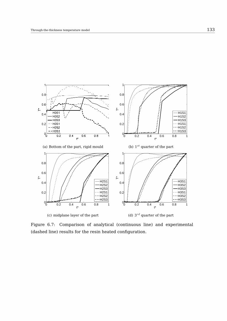
Through-the-thickness temperature model 133
(a) Bottom of the part, rigid mould
0 0.2 0.4 0.6 0.8 10
0.2
0.4
0.6
0.8
1
t*
T*
H1S1H1S2H1S3H1S1H1S2H1S3
(b) 1st quarter of the part
0 0.2 0.4 0.6 0.8 10
0.2
0.4
0.6
0.8
1
t*
T*
H2S1H2S2H2S3H2S1H2S2H2S3
(c) midplane layer of the part
0 0.2 0.4 0.6 0.8 10
0.2
0.4
0.6
0.8
1
t*
T*
H3S1H3S2H3S3H3S1H3S2H3S3
(d) 3rd quarter of the part
Figure 6.7: Comparison of analytical (continuous line) and experimental
(dashed line) results for the resin heated configuration.

134
on the pictures 6.7, 6.9, 6.10 and 6.12, but is considered irrelevant as it is
a limitation of the numerical formulation that does not influence the infusion
period of the process, which is the real objective of this work.
For both configurations, resin or mould heated, the data is provided nor-
malized. It presents a normalization of the temperature (T*) against a nor-
malization of the total filling time (t*). The legend on the graph identifies
the different tracers in the same layer, corresponding to each of the quarters
in height of the sample. Continuous lines represent the numerical data, and
dashed lines the experimental results. H stands for height, with zero being
the mould and four the top layer, and S stands for the section, with one being
the closest to the gate and three the closest to the vent.
The most critical aspect of the set-up, the flexible mould, is taken into
account by the analysis of the images provided by the infrared camera. Figure
6.8 shows a representative snapshot of the test, where temperature at the
external side of the bag can be observed. The image justifies the convection
boundary condition instead of a fixed temperature, as temperature gradients
occurring are clearly observed. Numerical information has been extracted
from the camera snapshots for the control points to be compared with the
values provided by the analytical model.
6.4.3 Resin heated configuration
For this configuration, the mould cavity, the rigid mould and the flexible mould
stay at the same temperature. A different temperature is introduced into this
isothermal system when the resin enters the cavity.
The comparison between the analytical results and the data extracted from
the infusions conducted are shown in the multiple graphic of Figure 6.7.
The temperature evolution at the mould side measured by the thermocou-
ples and predicted by the model can be observed In Figure 6.7(a). In the case
of the experimental data, the recorded values present significant oscillations
because the measuring accuracy of the employed thermocouples is 2 ºC and
the maximum variation in temperature in this case is of only 4 ºC. Such a
small variation of temperature during the test is due to the fact that the ther-

Through-the-thickness temperature model 135
mal capacity of the entering hot resin is not capable of overcoming the thermal
inertia of the cold mould. Therefore, the experimental curves show that the
temperature increases slightly once the resin reaches each section but it de-
creases after a while. This is especially true for sections 1 and 2, while for
section 3 the inherent precision of the thermocouple hides this tendency. Con-
cerning the numerical predictions, the tracers are able to follow the general
trend of the temperature, denoting slight increases in the first and second sec-
tion and, at the latest stage, detect the cooling effect of the rigid part of the
mould.
Figure 6.7(b), provides the results for the 1st quarter in thickness of the
sample. The temperature trend is followed in all the tracers. Imprecision is
observed in the analytical prediction of the first tracer and also in the start
point of the third tracer, attributed to the variability of the permeability of the
preform.
In Figure 6.7(c) the results for the midplane configuration are shown, di-
rectly extracted from the two-dimensional simulation of LIMS. The level of
accuracy in this case is similar to the previous ones, increasing as the resin
advances through the mould cavity.
The bottom right image, Figure 6.7(d), provides the trend for the layer of
thermocouples closest to the top of the preform. Best results are shown for
the prediction of the second and third tracers.
Temperatures extracted from the infrared camera (Figure 6.8) and the an-
alytical prediction are presented in Figure 6.9. Data presented in this figure
shows the same level of confidence as previous analysis for the second and
third tracer but a clear mismatch for the first tracer, where the temperature
is clearly over predicted.
The infrared data can also be contrasted with the real top view image,
previously depicted in Figure 6.3(c), which confirms the premise of the line
front advance through the complete specimen.
Comparing the four subfigures in Figure 6.7 it can be observed that the
evolution of the temperature for the hot resin configuration is different de-
pending on the considered height inside the mould, especially in the side of
the rigid mould. This is an effect that the the proposed model can reproduce

136
Figure 6.8: Infrared image of the upper surface of one of the samples pro-
duced heating the resin. Temperature in ºC
0 0.2 0.4 0.6 0.8 10
0.2
0.4
0.6
0.8
1
t*
T*
H4S1H4S2H4S3H4S1H4S2H4S3
Figure 6.9: Comparison of the temperatures extracted from the infrared cam-
era (dashed line) and the solution provided by the analytical model (continuous
line) for the resin heated case.
while the so-called two and "two and a half" dimensional temperature models
used in different simulation codes can not.

Through-the-thickness temperature model 137
0 0.2 0.4 0.6 0.8 10
0.2
0.4
0.6
0.8
1
t*
T*
H0S1H0S2H0S3H0S1H0S2H0S3
(a) Bottom of the part, rigid mould
0 0.2 0.4 0.6 0.8 10
0.2
0.4
0.6
0.8
1
t*
T*
H1S1H1S2H1S3H1S1H1S2H1S3
(b) 1st quarter of the part
0 0.2 0.4 0.6 0.8 10
0.2
0.4
0.6
0.8
1
t*
T*
H2S1H2S2H2S3H2S1H2S2H2S3
(c) midplane layer of the part
0 0.2 0.4 0.6 0.8 10
0.2
0.4
0.6
0.8
1
t*
T*
H3S1H3S2H3S3H3S1H3S2H3S3
(d) 3rd quarter of the part
Figure 6.10: Comparison of analytical (continuous line) and experimental
(dashed line) results for the mould heated configuration
6.4.4 Mould heated configuration
In the case of the heated mould, the resin is expected to absorb the temper-
ature of the preform. The through-the-thickness temperature decreases as
the height of the preform increases, which causes a difference between the
temperature of the resin entering into the system (constant) and the different
temperature at each height of the mould. The determination of this temper-
ature gradient at each height has to be done beforehand and introduced as
an input in the analytical model to be able to predict the full temperature
evolution.
For the tracer comparison of this case, Figure 6.10, the resin temperature

138
causes the reference temperature increase or decrease depending on the sec-
tion that is considered.
For the image of the mould tracers, Figure 6.10(a), the same tendency
as in the predictions of the resin heated configuration is observed, with a
clear change at the moment that the resin reaches each thermocouple section.
Some disturbances are observed in the experimental trend, caused by the own
thermocouple precision range.
Next two figures, corresponding to the 1st quarter (Figure 6.10(b)) and
midplane (Figure 6.10(c)), show the same pattern of evolution. Temperature
of the tracers decreases in the first section as the resin, which is at lower tem-
perature than the preform, cools it down. In the next two sections, the resin
advancing has lost cooling capacity, causing an increase of the temperature
when the tracer is reached.
The insulating nature of fibreglass is broken as soon as it is impregnated
by the resin causing a change in the heat conductivity of the mould cavity.
In the Figure corresponding to the 3rd quarter, temperature of the resin
entering the mould is slightly higher than the temperature of the preform at
the first tracer. It causes an increase of the temperature in this point and a
latter, more pronounced increase of the temperature for the second and third
tracers.
Figure 6.11 depicts one image representative of the information given by
the infrared camera. A comparison between the data extracted from these
images and the experimental trend is presented in Figure 6.12.
6.5 Discussion
As it is observed in (Figures 6.7(a) and 6.10(a)), the experimental data of the
mould tracers present some disturbances. The finite precision of the thermo-
couples has been corroborated as its inherent cause. The supposition of a
constant temperature in the mould side for both techniques is therefore ac-
cepted as adequate.
Analysing the other comparative images, it is observed that the accuracy
tends to increase as the resin advances, being more accurate in the second

Through-the-thickness temperature model 139
Figure 6.11: Infrared image of the upper surface of one of the samples pro-
duced heating the mould. Temperature in ºC
0 0.2 0.4 0.6 0.8 10
0.2
0.4
0.6
0.8
1
t*
T*
H4S1H4S2H4S3H4S1H4S2H4S3
Figure 6.12: Comparison of the temperatures extracted from the infrared cam-
era (dashed line) and the solution provided by the analytical model (continuous
line) for the mould heated case.
and third tracers than in the first one. The transient to steady state process is
pointed to as the cause of the under and over prediction in the results. Accu-
racy is achieved more properly at the end of the stage than in the beginning
of the fill period, which matches with the observations of Simacek and Advani
[24] in the two-dimensional validation of the method.

140
This can be attributed to the limitations of the LTE method, as indicated in
[13]. As the process advances, the velocity of the resin slows down and the
precision of the proposed method increases. As resin travels faster through
the first tracer than the second and third ones, the precision in the first de-
creases when compared with the other two, where the trend is more accu-
rately followed.
Regarding the analysis of the bag side, although imprecisions could be par-
tially attributed to the fact that the analytical model and the infrared camera
are providing information from different sides of the bag, the insulation effect
of the bag can be neglected due to its limited thickness. Therefore, bag in-
sulation can be discarded as the cause of differences between predicted and
measured temperature evolutions in the bag side of the mould.
The difference between the trend of the first tracer in Figure 6.12 and the
those observed for the first tracers in each height in Figure 6.10 points to the
influence of the convection boundary condition on this side of the mould.
The general observation of the trends in the midplane and the 3rd quarter
already shows a slight increase of the temperature when the resin reaches the
first tracer. On the surface of the sample, the higher exchange of temperature
with the room provides a different pattern, leaving the heat transported by
the resin with more importance than in the other tracers.
6.6 Conclusions
The capability of an analytical model to reproduce the experimental data in
non-isothermal vacuum bagged set-ups has been validated through the mea-
surement of the spatial temperature distribution and time evolution during a
sample infusion process.
Results show that the numerical implementation of the analytical model via
the use of a convection boundary condition on the flexible mould side offers a
good level of agreement between experiment and simulation.
Fast resin propagation in the entrance of the mould cavity is pointed to as
the cause of the temperature overprediction in zones close to the resin inlet,
obtained when using the LTE as a base for the calculation

Through-the-thickness temperature model 141
It has been demonstrated that a prediction of the thermal map in space
and time for a thick shell composite part infusion can be obtained with a sim-
ple analytical approach. The accuracy of the prediction is limited due to the
simplifications made in the numerical formulation, but the method can be con-
sidered to give an adequate solution for industrial applications. Moreover, the
work represents an opportunity for improvement of further analysis. As an
example, the thermal map can be used as a more precise initial condition for
the investigation of inhomogeneous cure gradients as well as for mechanical
issues regarding part distortions and residual stresses.


Bibliography
[1] C. Rudd, A. Long, K. Kendall, C. Mangin, Liquid Moulding Technologies,
Woodhead Publishing and SAE International, Warrendale, PA, USA,
1997.
[2] C. Williams, J. Summerscales, S. Grove, Resin infusion under flexible
tooling (rift). A review, Composites Part A: Applied Science and Manu-
facturing 27 (7) (1996) 517–524.
[3] S. Mazumdar, Composites Manufacturing. Materials, Product and Pro-
cess Engineering, CRC Press, Boca Raton, FL, USA, 1997.
[4] W. Schulz, D. Myers, T. Singer, P. Ifju, R. Haftka, Determination of resid-
ual stress and thermal history for im7/977-2 composite laminates, Com-
posites Science and Technology 65 (13) (2005) 2104–2024.
[5] J. Xiong, R. Shenoi, J. Gao, An analytical model to predict residual ther-
mal stress in 2d orthogonal plain weave fabric composites, International
Journal of Solids and Structures 46 (9) (2009) 1872–1883.
[6] L. You, X. You, A unified numerical approach for thermal analysis of
transversely isotropic fibre-reinforced composites containing inhomo-
geneous interphase, Composites: Part A-Applied Science and Manufac-
turing 36 (6) (2005) 728–738.
[7] A. Abbassi, M. Shahnazari, Numerical modelling of mould filling and
curing in non-isothermal RTM process, Applied thermal engineering
24 (16) (2004) 2453–2465.
143

144
[8] M. Lin, M. Kang, H. Hahn, A finite element analysis of convection prob-
lems in RTM using internal nodes, Composites Part A-Applied Science
and Manufacturing 31 (4) (2000) 373–383.
[9] A. Shojaei, S. Ghaffarian, S. Karimian, Simulation of the three-
dimensional non-isothermal mould filling process in resin transfer mold-
ing, Composites Science and Technology 63 (13) (2003) 1931–1948.
[10] K. Pillai, M. Munagavalasa, Governing equations for unsaturated flow
through woven fibre mats. Part 2. Non-isothermal reactive flows, Com-
posites Part Part A-Applied Science and Manufacturing 35 (4) (2004)
403–415.
[11] S. Advani, M. Bruschke, R. Parnas, Resin Transfer molding flow phe-
nomena in polymeric composites. In Flow and Rheology in Polymer
Composites Manufacturing, S.G. Advani, Amsterdam, NE, 1994.
[12] C.L. Tucker III, R. Dessenberger, Governing equations for flow and heat
transfer in stationary fibre beds in Flow and Rheology in Polymer Com-
posites Manufacturing, S.G. Advani, Amsterdam, NE, 1994.
[13] M. Deleglise, C. Binetruy, P. Castaing, P. Krawczak, Use of non local equi-
librium theory to predict transient temperature during non- resin flow
in a fibrous medium, International Journal of Heat and Mass Transfer
50 (11-12) (2007) 2317–2324.
[14] C.L.Tucker III, Heat transfer and reaction issues in liquid composite
moulding, Polymer Composites 17 (1) (1996) 60–72.
[15] H. Chiu, B. Yu, S. Chen, L. Lee, Heat transfer during flow and resin reac-
tion through fibre reinforcement, Chemical Engineering Science 55 (17)
(2000) 3365–3376.
[16] M. Quintard, S. Whitaker, Local thermal equilibrium for transient heat
conduction: theory and comparison with numerical experiments, Inter-
national Journal of Heat and Mass Transfer 38 (15) (1995) 2779–2796.

Bibliography 145
[17] O. Mai, A. Couniot, F. Dupret, Non-isothermal simulation of the resin
transfer moulding process, Composites Part A-Applied Science and
Manufacturing 29 (1-2) (1998) 189–198.
[18] W. Chang, N. Kikuchi, Analysis of non-isothermal mould filling moulding
and structural reaction process in resin transfer moulding (RTM) and
structural reaction injection moulding (SRIM), Computational mechan-
ics 16 (1) (1995) 22–35.
[19] J. Kessels, A. Jonker, R. Akkerman, Fully 2,5 d flow modelling of resin in-
fusion under flexible tooling using unstructured meshes and wet and dry
compaction properties, Composites Part A-Applied Science and Manu-
facturing 38 (1) (2007) 51–60.
[20] P. Simacek, S. Advani, Desirable features in mould filling simulations for
liquid composite moulding processes, Polymer Composite 25 (4) (2004)
355–367.
[21] B.Yenilmez and E. Murat Sozer, Compaction of e-glass fabric preforms
in the Vacuum Infusion Process. A: Characterization experiments, Com-
posites Part A-Applied Science and Engineering 40 (4), (2009) 499-510
[22] Q. Govignon and S.Bickerton and P.A. Kelly, Simulation of the reinforce-
ment compaction and resin flow during the complete resin infusion pro-
cess, Composites Part A-Applied Science and Engineering, 41(1), (2010)
45-57.
[23] A. Hammami and B.R. Gebart, Analysis of the Vacuum Infusion Mould-
ing Process, Polymer Composites, 21(1), (2000) 28-40
[24] P. Simacek, S. Advani, Approximate numerical method for prediction of
temperature distribution in flow through narrow gaps containing porous
media, Computational Mechanics 32 (1-2) (2003) 1–9.
[25] P. Simacek, S. Advani, An analytic solution for the temperature distribu-
tion in flow through porous media in narrow gaps I . Linear injection,
Heat and Mass Transfer 38 (1-2) (2001) 25–33.

146
[26] P. Simacek, S. Advani, An analytic solution for the temperature distri-
bution in flow through porous media in narrow gap II. Radial injection,
Heat and Mass Transfer 38 (6) (2001) 497–505.
[27] Epolam 2020 Epoxy laminating system with variable reactivity technical
datasheet. Axson, UK, 2005

Chapter 7
Study of the influence of the
in-plane conduction and
convection term in the
determination of the temperature
distribution in non-isothermal
setups
147

148
M.Gascons, N.Blanco, K.Matthys, Study of through-the-thickness heat con-
duction and dispersion in Resin Infusion under Flexible Tooling (RIFT). To be
submitted to International Journal of Heat and Mass Transfer.
7.1 Introduction
Resin Infusion under Flexible Tooling (RIFT) [1], is a specific method used
for the industrial production of fibre reinforced thermosets. This moulding
technique makes use of a flexible "bagging" material to enclose the mould
cavity as shown in Figure 7.1.
Figure 7.1: Schematic representation of the RIFT infusion technique. 1:Vac-
uum bag, 2: Mould cavity, 3:Resin non-pressurized pot, 4:Vacuum pump con-
nection 5:Rigid tool.
Although RIFT has already been a proven technique for many years in se-
lected industrial environments, it has been infiltrating into a broader range of
applications [2]. For example, RIFT is increasingly used for the manufacturing
of thick and large structural parts due to the lower cost of the flexible mould
compared to the tooling price of alternative methods, but this new application
also poses new technical challenges to the process.
RIFT has matured through steady evolution and continued improvement.

Heat dispersion coefficient analysis 149
The physical underlying principle, i.e. the suction of a liquid matrix through
a sealed mould cavity in which a reinforcement fabric is placed, has been re-
fined by research groups and industrial users, and has led to many variations
such as Vacuum assisted RTM (VARTM) or Seeman Composite Infusion Pro-
cess (SCRIMP).
Inside the mould cavity, the reinforcement fibres are being compressed
by the vacuum suction and the resin propagation is affected by the imposed
pressure gradient, which conditions the part filling and affects impregnation
time. In order to accelerate or influence the filling process, the introduction
of heat is commonly used [3].
Heat is either introduced via a temperature controlled mould or heated
resin. The first option is directly derived from Resin Transfer Moulding (RTM)
[4], where the mould cavity is formed by two solid halves. Heating of both
sides of the mould allows optimal temperature control and good thermal sta-
bility of the process.
However, with RIFT set-ups only disposing over one solid mould halve, heat
is only introduced unilaterally. This one-sided heat introduction causes ther-
mal gradients that can lead to inhomogenous cure, which is a potential source
for the formation of residual stresses and distortions in the injected part [5–
7]. In the case of very large parts or complex geometries it is sometimes not
even practically feasible to heat the solid mould half, and for these cases, heat
introduction via heated resin is the selected option.
Many physical phenomena are involved in the heat transfer inside Liquid
Composite Moulding (LCM) processes. As resin flows through the mould, it
exchanges heat with the dry preform and the mould by conduction but also
transports the heat inside the mould cavity by convection. In addition, changes
in resin flow propagation due to temperature dependence of the resin viscosity
are to be considered. The thermal boundary conditions of the mould cavity
also affect heat transfer during infusion [8].
Resin flow simulations codes [9, 10] do implement the non-isothermal en-
vironment using the Thermal Equilibrium equations [11]. Existing software
packages can provide approximate solutions but are subjected to impracti-
cally high computing costs for more accurate simulation studies.

150
Published scientific works on this matter presents two different alterna-
tives to model the heat transfer phenomena for flow through fibre beds [12]:
the Non Local Thermal Equilibrium (NLTE) and the Local Thermal Equilib-
rium (LTE) models. The LTE model is widely used in many thermoset resin
flow processes, mainly due to its simplicity. Many authors have reported its
use to describe the thermal evolution in RTM processes [13–16].
However, though established for RTM, the validity of the LTE model still
needs to be checked for RIFT due to the greater temperature gradient caused
by the small thermal inertia of the flexible mould.
The feasibility of extending the LTEmodel as used in RTM to non-isothermal
RIFT manufacturing processes will be discussed in this work. Although the
LTE equation can include microscale flow phenomena, it requires knowledge
of parameter values that are difficult to determine. This work assumes that
the influence of the heat dispersion coefficients in this technique is not signif-
icant and that neglecting these terms does not cause a remarkable impact in
the final accuracy of the analytical method. This is a fair assumption because
of the typical slow velocity of this method. Under this assumption, the neglec-
tion of these terms will not cause a significant impact on the overall accuracy
of the proposed analytical method.
7.2 Analytical background
7.2.1 Model considered
The Non-Local Thermal Equilibrium (NLTE) model, alternatively known as the
two equations model, (presented in Equation 7.1 and Equation 7.2), explicitly
reproduces the heat transfer phenomena inside the mould cavity by means of
independent expressions for each of the constituents inside the mould cavity.
φ(ρCp)f∂ 〈Tf〉
∂t+ (ρCp)f∇ (〈υf〉 〈Tf〉) =
= ∇ (Kf • ∇ 〈Tf〉) +H(Tf − Ts) + φs
(7.1)
(1− φ)(ρCp)s∂ 〈Ts〉
∂t= ∇(Ks • ∇ 〈Ts〉)− αfshfs(Tf − Ts) (7.2)

Heat dispersion coefficient analysis 151
In the equations above, the subscripts f and s stand for the fluid (resin)
and the solid (fibre) respectively.
In these equations, ρ stands for density, Cp for the heat capacity of the ma-
terials, 〈υf〉 for the injection average velocity, T for the temperature, K for the
heat conductivity tensor, H for the heat exchange parameter, φ for the poros-
ity , s for the curing reaction heat and hfs for the heat exchange coefficient
between fluid and solid respectively. αfs is the specific area representing the
laminate architecture at tow scale and is defined in Equation 7.3.
αfs =4
dp
φ
1− φ(7.3)
In Equation 7.3, dp corresponds to the diameter of a fibre tow and φ to the
bed or fabric porosity.
Although this equation system has been proven as an accurate model to
reproduce the heat transfer inside the mould cavity, difficulties arise in the
determination of all the involved parameters for each constituent. The need of
complex laboratory task to obtain the full characterization of the constituents
pushed the necessity of alternative models to become suitable for industrial
applications.
Under the principle that resin and fibre local temperature become equal as
soon as they come into contact with each other, the Local Thermal Equilibrium
(LTE) model (Equation 7.4) is the proposed alternative to the NLTE model. The
LTE model stands for simplicity in the determination of involved parameters
but has some limitations with the applicability range and precision [17].
(φ(ρCp)f + (1− φ)(ρCp)s)∂ 〈T 〉
∂t+ (ρCp)f 〈υf〉 · ∇ 〈T 〉 =
= (kzz +KDzz)∂2T
∂z2∇ · (((φKf + (1− φ)Ks) +KD) · ∇ 〈T 〉) + φs
(7.4)
Terms of the equation will be carefully described in the following chapter.
The background behind the modelling of non-isothermal infusion techniques
has solid foundations established in works of Advani et al. [18], Tucker and
Dessenberger [19] or Chang et al. [20]. These works discuss the suitability of
the previously stated Equations 7.1 and 7.2 to reproduce the thermal evolution
inside mould cavities enclosed in rigid moulds.

152
It has been reported that the LTE model loses accuracy as the velocity of
the fluid moving inside the cavity increases [21, 22]. At larger velocities, local
convection phenomena become dominant over conduction, causing usually an
over prediction of the temperatures in the mould. For the specific produc-
tion process addressed in this publication, the resin velocity is limited by the
pressure gradient inside the mould cavity, driven by vacuum suction.
To define an applicability range as a function of the fluid velocity, dimen-
sionless parameters are proposed, such as the Graetz number or the Péclet
number [23, 24].
The Graetz number is a relationship between the filling speed and the heat
conduction. When the filling speed is slow in comparison with the heat con-
duction, the conduction terms are larger than the convection terms, and they
dominate the energy equation. Imprecision for Graetz numbers larger than
one (Gz >>1) have been reported for temperature predictions using LTE mod-
els [25].
The Péclet number is a dimensionless evaluation of the fluid velocity, usu-
ally expressed as the product of the Prandtl number and the Reynolds number
[26]. Alternatively, the Péclet number can be expressed as defined in Equation
7.5.
Pe = Pr ·Re =w · L
a(7.5)
Where w stands for flow front velocity, L is the characteristic length and a
the thermal diffusivity of the resin as stated in Equation 7.6.
a =kT
ρr · Cp,r
(7.6)
In equation 7.6 Discussion opens at this point for the selection of the right
parameters for the definition of the Péclet number. Many author do use the
fibre tow diameter as a representative length (L) in Equation 7.5, while other
do use the mould cavity thickness [23]. The determination of the right Péclet
number needs consensus for the definition of the analysis scale. According to
that, in this work tow diameter is used as reference.

Heat dispersion coefficient analysis 153
7.2.2 Term by term analysis
The Local Thermal Equilibrium model is composed by five different terms rep-
resenting different phenomena occurring inside the mould cavity.
The first term of the equation, (Equation 7.7) corresponds to the change of
internal energy occurring in the process (heating of the resin). The term con-
sists in a law-of-mixtures of the specific heat and density of both constituents,
as a function of the temperature evolution over time. For most of the materials
used and usual temperature ranges (25ºC to 200ºC), the specific heat and the
density are considered as a constant.
(φ(ρCp)f + (1− φ)(ρCp)s)∂ 〈T 〉
∂t(7.7)
Second term of the equation, (Equation 7.7) stands for convection of heat in
the plane due to averaged Darcy velocity (heat transport due to moving resin).
Dependent of velocity and the resin gradient of temperature, it can be affected
by the slight velocity differences occurring due to the inhomogeneity of the
fibre bed. However, considering the macroscale level, the velocity variation
can be tracked easily and implemented in the model, restricting the possible
uncertainty of this term.
(ρCp)f 〈υf〉 · ∇ 〈T 〉 (7.8)
Third term (Equation 7.9) is for the through-the-thickness conduction and
dispersion (due to dissipation and chemical reaction). The term reflects the
gradient of temperature through the thickness of the sample. As in RIFT one
mould presents little thermal inertia, the through-the-thickness gradient is of
notable consideration and can be a possible source of accuracy improvement
for this specific setup.
(kzz +KDzz)∂2T
∂z2(7.9)
Fourth term (Equation 7.10) corresponds to the in plane conduction and
dispersion (due to diffusion of heat from the mould walls into the resin and
microscopic resin motion not accounted for convection). It is also presented
in this equation as a law-of-mixtures for conductivities, as a square function

154
of temperature evolution. Previous studies [17] advice discarding this term as
the effects caused by the square dependency are small when compared to the
rest of the terms for slow velocities.
∇ · (φKf + (1− φ)Ks) · ∇ (〈T 〉) (7.10)
Finally, the last term (Equation 7.11) stands for the heat generation due
to the exothermic process of the resin cure. Usual production process design
methodologies agree in the use of filling periods smaller than the resin life
time, in order to avoid the sudden viscosity increase related to the crosslinking
of the resin. Therefore, it is a safe decision to neglect this term under the
assumption that crosslinking will never occur during the infusion period of
time.
φs (7.11)
The third term, (Equation 7.9, arises as a discussion motive due to the
preform structure in which the resin flows. The laminar flow is disturbed
creating local convection effects. In the term description, the conductivity is
presented as (kzz +KDzz), but usually the thermal dispersion coefficient KDzz
is neglected in its implementation.
7.3 Experimental setup
In order to investigate the applicability of the model for the specific produc-
tion setup proposed, an experimental rig was developed to extract thermal
information of RIFT produced samples.
The rig was designed to conduct non-isothermal infusions using a RIFT
configuration. Heat is introduced into the system from the rigid mould side by
means of an electric heating device. The device is placed underneath the rigid
mould (aluminium slab) with a close loop feedback calibration system to keep
a constant surface temperature. The aluminium slab used as a mould has a
considerable thickness (40 mm.) which gives thermal inertia to the system,
ensuring thermal stability of the mould and a constant temperature at the

Heat dispersion coefficient analysis 155
mould surface. If needed, the resin itself can be heated beforehand in an oven
and infused through an isolated gate. A scheme of the entire setup is depicted
in Figure 7.2.
Figure 7.2: Scheme of a longitudinal cut of the experimental rig. T1, T2, T3
and T4 stand for the different temperatures involved in the set-up.
Resin is placed in a bucket and is driven to the mould cavity, where a dis-
tribution channel configures a linear gate across the entire edge. The rigid
mould tool consists in a flat thick aluminium slab on one side, and a vacuum
bag is used as a flexible tool in the other side. The resin goes through the dif-
ferent control section (Section 1, Section 2 and Section 3) and finally reaches
the end of the mould cavity, where a vacuum pump is connected.
Type K thermocouples were embedded in these sections of the preform,
lined up in layers corresponding to midplane, first quarter and third quarter
of the thickness of the sample. Once the entire preform is assembled, the
disposition of the thermocouples configures a 9 points grid. Three different
control points are in the longitudinal axis for each instrumented layer and
three control points are in the through-the-thickness direction for each sec-
tion. These thermocouples are used first to determine the temperature of the
dry preform (T2), and later to determine the evolution of the temperature dur-
ing the infusion and cure processes.
In addition, temperatures at top and bottom of the sample need to be
recorded to monitor the interaction of the mould and the part. To this pur-
pose, three thermocouples were embedded in the surface of the aluminium

156
slab in contact with the part (T4), and an infrared camera was placed on top.
This camera not only verified the evolution of the temperature on the analysed
top layer but was also useful to monitor the shape of the flow front advance
and the temperature on the entire sample surface. Linear advance of the resin
through the sample was controlled visually.
Two extra thermocouples were used to monitor the room temperature (T1)
and the temperature of the resin at the inlet point (T3) during the infusion
stage. A detailed transversal view of a control section (Section 1 in Figure
7.2), can be observed in Figure 7.3, where the position of each control point
and its nomenclature its detailed.
Figure 7.3: Representative (not scaled) detail of the transversal section of the
sample with position and nomenclature of the recorded points.
All signals of the tests are handled through a data acquisition device. An
acquisition GUI was developed in-house using a Labview environment. Tem-
perature was recorded in real time at 1Hz frequency. Synchronized with the
thermocouple measurement, the amount of resin transferred to the mould cav-
ity is recorded to obtain the exact flow rate and flow front velocity at any time
of the test.
An insulated tube was used to connect the bucket with the inlet of the
mould to ensure the temperature stability of the incoming resin. A thermo-
couple is placed at the mould cavity inlet to provide the temperature in the
entrance of the system. This point is chosen to avoid temperature variations
in the short path between the bucket and the entrance of the mould cavity.
Data provided from this thermocouple confirms the supposition of a constant
temperature at the entrance.

Heat dispersion coefficient analysis 157
Six samples were infused according to the details described in Table 7.1.
Sample dimensions and materials
DimensionsLength Width Thickness
250 mm. 150 mm. 30 mm.
MaterialsFibreglass multi-axial/non-crimp fabric
Epoxy resin with amine base hardener
Details of the experimental program
Repetitions Mould Tº Fibre Tº Resin Tº
6 60ºC variable Room
Table 7.1: Main dimensions, material description and experimental program
information.
The samples used for the tests consisted of glass fibre reinforced epoxy
rectangular plates. Extremely thick samples were used in order to insulate
the measurement points of the direct influence of the boundary condition in
the measurements. No flow enhancement layers or other ancillary materials
are used.
7.4 Results
7.4.1 Data handling
From the LTE equation, (Equation 7.1), terms on the left are dependent on
properties inherent to the own material. These properties can be directly ex-
tracted from material data sheet, and are obtained conducting common tests
in material characterization process. The following Table 7.2 summarizes the
used data.
Terms on the right side present variables such as the through-the-thickness
conduction and dispersion term, which can be obtained with this setup.
Last term in the right side of the equation, corresponding to the exother-
mic reaction, is ruled out due to the supposition that no curing occur during

158
Material data
Resin Fibre
Heat capacity [KJ/KgK] 1800 344
Density [Kg/m3] 1245 2550
Conductivity [W/mK] 0.25 1
Porosity [%] 50
Table 7.2: Auxiliary data extracted from the test configuration.
infusion process. Consequently, the third and fourth term (Equations 7.9 and
7.10) are left to be discussed.
Other simplifications should be considered when using the LTE equation to
simulate RIFT infusions. The pressure and the velocity profile is assumed uni-
form through the thickness, and the variation of the viscosity once the working
temperature is achieved is not strongly dependent on temperature, which is
acceptable for most of the thermoset formulated resins.
Temperatures needed for the evaluation of this two terms are extracted
directly from the data provided by the computing grid, depicted in Figure 7.4.
In this figure, the disposition of the points and its nomenclature inside the
system is presented.
H is the height, with zero being the mould and four the top layer, and
S standing for section, being 1 the closest to the gate and 3 the closest to
the vent. Distances between control points (thermocouples) can be found in
Table 7.2. The vertical distance between points is 6.25 mm and the horizontal
distance between sections is 75 mm.
The test developed is designed to understand the thermal evolution of the
central point (H2S2). Taking this point as a reference, one can obtain the time
partial derivation of temperatures from the values recorded at 1Hz frequency.
For the distance partial derivation of temperature as a function of longitudinal
displacement, one can use the data recorded at the point H2S1.
As the test is designed to provide a linear flow front advance of the resin,
only one longitudinal path is evaluated in this direction, by means of the tem-
perature at points H2S1 and H2S3. For the through-the-thickness tempera-

Heat dispersion coefficient analysis 159
Figure 7.4: Detail of a longitudinal cut of the sample, where the disposition of
the control points, and the through-the-thickness grid that they configure can
be observed.
ture evolution, one uses control points H1S2 and H3S2. Figure 7.5 shows an
infrared image of the infusion process, where the linear flow front advance
during the process can be verified.
Figure 7.5: Infrared image of the upper surface of one of the samples. Tem-
perature in ºC

160
7.4.2 Through-the-thickness conduction and dispersion eval-
uation
It is proposed to study the through-the-thickness conduction and dispersion
term by means of its isolation in the general LTE model as is shown in the
following Equation 7.12.
(kzz +KDzz) =Se
∂T∂t
+ (ρCp)f 〈υf〉 − ∇ (Ke +KD) · ∇ 〈T 〉∂2T∂z2
(7.12)
Where Se refers to the volumetric heat capacity as described in following
Equation 7.13
Se = (φ(ρCp)f + (1− φ)(ρCp)s) (7.13)
and Ke as it is defined in Equation 7.14
Ke = Ks · φ+Kf · (1− φ) (7.14)
One can now evaluate the magnitude of the in-plane conduction and dis-
persion term. Its square dependence should suppose a small influence when
compared to the rest of the terms. For the tests conducted, it is confirmed that
the magnitude of this term is of 2 orders of magnitude smaller than the rest of
terms. One can then obviate this term from the general equation and present
the following variable isolation of Equation 7.15 to evaluate the through-the-
thickness conduction and dispersion term.
(kzz +KDzz) =Se
∂T∂t
+ (ρCp)f 〈υf〉∂2T∂z2
(7.15)
7.4.3 Output analysis
The data extracted from the thermocouples provides a thermal map of the
sample while the resin flows, depicted in Figure 7.6.
In Figure 7.6, the trends of the temperature evolution can be observed.
Knowing the position of the thermocouples, one can use the temperature evo-
lution to derive the flow front position and verify the linear advance of the flow

Heat dispersion coefficient analysis 161
Figure 7.6: Temperature recorded from one of the infused samples, illustrative
of the temperature profile typology.
in the studied direction. This is verified by the alignment in the time-scale of
the tracers corresponding to Section 2.
Velocity profiles were extracted with mass loss measurements of the infu-
sion bucket, placed over a precision scale. After data treatment, the following
velocity profiles, presented in Figure 7.7 were obtained.
Velocity trends correspond with typical quadratic velocity expressions, char-
acteristic of constant pressure infusions. Using these profiles, the different
Péclet numbers were extracted for any instant of the infusion time, according
to its previously stated definition. For all tests, low Péclet numbers ( < 1) were
obtained. Therefore, for all cases, the flow typology is slow and laminar, and
matches the scope of this work.
For the purpose of this study, a limited period of time needs to be defined.
This period encompasses from the first instant were resin has gone through all
thermocouples until the resin reaches the mould end. This time period lasts
an average of 250 seconds ± 20 seconds for all tests.
Analysing the obtained profiles, the outputs remains constant until the
resin reaches the thermocouples. At this moment, a transient period in which

162
Figure 7.7: Velocity profiles for the different infusions conducted.
some thermocouples are wet and some not occurs. After that, the value stabi-
lizes again, and the resin flow through all the control points.
The energy equation that dominates the temperature field have been for-
mulated with and without the fourth term, related to the heat dispersion. The
difference between them is unnoticeable as can be shown in the trends de-
picted in the following Figure 7.8.
During tests, thermal lab conditions as well as infusion procedure was kept
as constant as possible. However, different profiles were obtained for different
infusions, which is reasonable due to the lack of control of some parameters
such as room temperature.
In addition, one must notice the existing variability in infusions 3 and 5.
The analysis of the data logs does not provide any specific reason for these
disturbances, so the variability was suggested to come from a physical prob-
lem. Incorrect wire connection in the measurement point or equipment end
arises as the most probable cause. This leads to results with large oscillations
when using this data for calculation.
After a comparative overview of the tests, the analysis of the heat disper-
sion term for each infusion is evaluated. The term is presented for each test as
a function of the Péclet number in order to check for its variation as a function
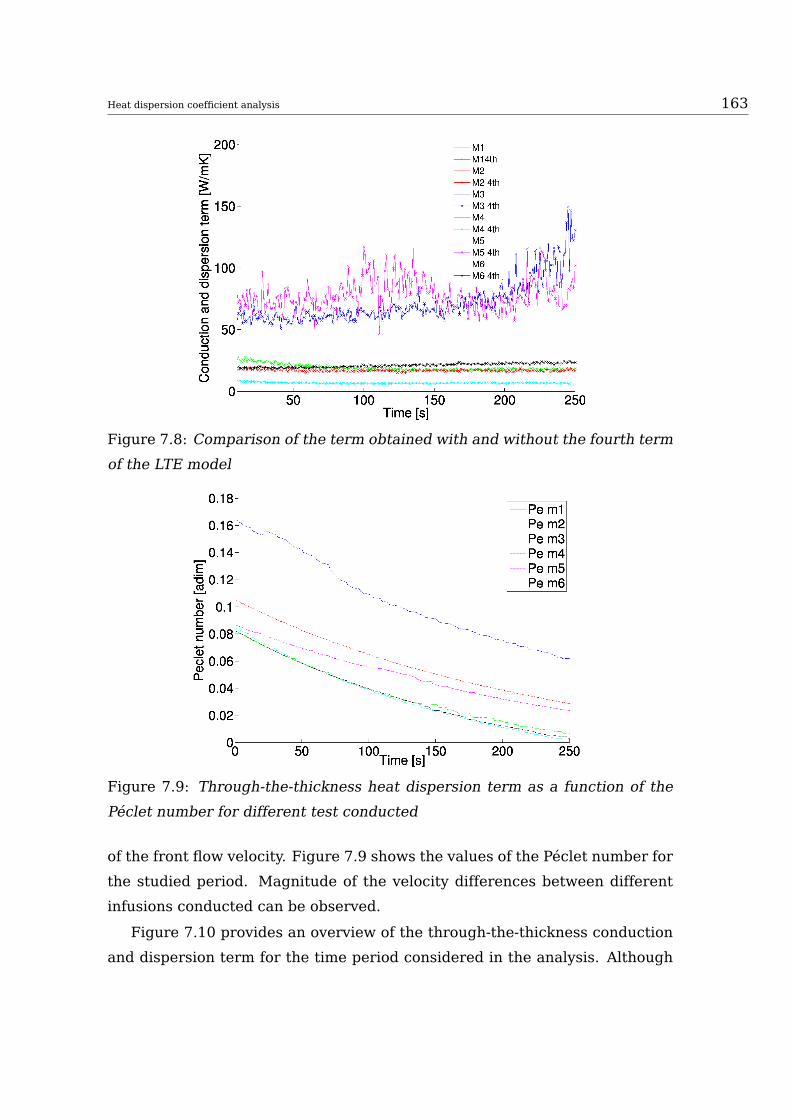
Heat dispersion coefficient analysis 163
Figure 7.8: Comparison of the term obtained with and without the fourth term
of the LTE model
Figure 7.9: Through-the-thickness heat dispersion term as a function of the
Péclet number for different test conducted
of the front flow velocity. Figure 7.9 shows the values of the Péclet number for
the studied period. Magnitude of the velocity differences between different
infusions conducted can be observed.
Figure 7.10 provides an overview of the through-the-thickness conduction
and dispersion term for the time period considered in the analysis. Although

164
(a) Infusion number 1 (b) Infusion number 2
(c) Infusion number 3 (d) Infusion number 4
(e) Infusion number 5 (f) Infusion number 6
Figure 7.10: Presentation of the different conduction and dispersion terms as
a function of the Péclet number for the different tests conducted

Heat dispersion coefficient analysis 165
different values are obtained for each test, the shape of the term along the
Péclet range considered in vacuum bagged infusion processes remains stable.
The author points the high dispersion range observed in image 7.10(e), to
the previously stated causes. Even considering this dispersion, a flat trend is
observed, in accordance with the results of the rest of tests.
7.4.4 Discussion
According to the observations described in literature [25, 26], one should ex-
pect a dependency between the heat dispersion coefficient and the Péclet num-
ber.
Metzger et al. [27] illustrate a methodology to obtain typology and shape
of heat dispersion coefficient by means of thermocouples lectures. Although
their work shows the linear evolution of the heat dispersion coefficient as a
function of the Péclet number, it considered a Péclet range much larger (ade-
quate for RTM) than the one used in the selected infusion technique.
Hsiao et Advani [28], also state the dependence of the heat convection on
the Péclet number. They also notice that, for low Péclet numbers, the heat
transfer is dominated by conduction, while as it increases the convection term
gains weight and becomes dominant in heat transfer. However, the specific
production technique cover in this work is different that the one used in the
work of Hsia et Advani (RTM). With the presented data, one can confirm the
validity of extending the proposed methodology to this production technique.
Their work [28], proposes a modified thermal conductivity parameter to
include these phenomena and cover the entire range of production processes
for composite materials, results obtained in this work show that in the specific
studied technique one can obviate the convective term.
For RIFT technique, the low velocity that is used (due to the limited suction
that can be done by vacuum pump), situates the value of the heat dispersion
coefficient in a range were the velocity influence can be almost negligible,
and therefore it is not dependent of the resin velocity. The stability of the
obtained term points conduction as the main source of heat transfer for this
production process. If the dispersion effect were noticeable one should expect

166
a linear tendency in the obtained results, which only can be identified in Figure
7.10(c), which has the larger Péclet numbers.
7.5 Conclusions
An experimental validation of proposed simplifications for the Local Thermal
Equilibrium equation has been proposed in the present work.
The results confirm the low Péclet number associated to this production
process which results in a heat transmission process based mainly in the con-
duction phenomena. Local convection is therefore negligible and the suppres-
sion of its related term is consistent with obtained results, leaving a simple,
easy to implement, version of the general equation.
The obtained simplified method will suppose lighter computing expressions
in simulation codes which will result in faster prediction without critical loss
of precision. This fact is of great interest for the prediction of thermal maps
in sizeable parts, which are every time more common of being produced with
this technique.
Future work will include the implementation of this thermal simulation ex-
pression in a full-scale model in order to check its application in a real part.

Bibliography
[1] C. Williams, J. Summerscales, S. Grove, Resin infusion under flexible
tooling (RIFT). A review, Composites Part A: Applied Science and Man-
ufacturing 27 (7) (1996) 517–524.
[2] S. Mazumdar, Composites Manufacturing. Materials, Product and Pro-
cess Engineering, CRC Press, Boca Raton, FL, USA, 1997.
[3] C. Seeton, Viscosity temperature correlation for liquids, Tribology Let-
ters 22 (1) (2006) 67–78.
[4] C. Rudd, A. Long, K. Kendall, C. Mangin, Liquid Moulding Technologies,
Woodhead Publishing and SAE International, Warrendale, PA, USA,
1997.
[5] W. Schulz, D. Myers, T. Singer, P. Ifju, R. Haftka, Determination of resid-
ual stress and thermal history for im7/977-2 composite laminates, Com-
posites Science and Technology 65 (13) (2005) 2104–2024.
[6] J. Xiong, R. Shenoi, J. Gao, An analytical model to predict residual ther-
mal stress in 2d orthogonal plain weave fabric composites, International
Journal of Solids and Structures 46 (9) (2009) 1872–1883.
[7] L. You, X. You, A unified numerical approach for thermal analysis of
transversely isotropic fiber-reinforced composites containing inhomo-
geneous interphase, Composites: Part A-Applied Science and Manufac-
turing 36 (6) (2005) 728–738.
[8] R. Gauvin, F. Trochu, Key issues in Numerical simulation for liquid com-
posite moulding processes, Polymer Composites, 19(3) (1998) 233–240.
167

168
[9] P. Simacek, S. Advani, Desirable features in mould filling simulations for
liquid composite moulding processes, Polymer Composite 25 (4) (2004)
355–367.
[10] M. Skinner, New application and approaches expand market for com-
posite software, Reinforced Plastics, 50 (6) (2006) 24–28.
[11] O. Mai, A. Couniot, F. Dupret, Non-isothermal simulation of the resin
transfer moulding process, Composites Part A-Applied Science and
Manufacturing 29 (1-2) (1998) 189–198.
[12] M. Deleglise, C. Binetruy, P. Castaing, P. Krawczak, Use of non local equi-
librium theory to predict transient temperature during non- resin flow
in a fibrous medium, International Journal of Heat and Mass Transfer
50 (11-12) (2007) 2317–2324.
[13] A. Abbassi, M. Shahnazari, Numerical modelling of mold filling and
curing in non-isothermal RTM process, Applied thermal engineering
24 (16) (2004) 2453–2465.
[14] M. Lin, M. Kang, H. Hahn, A finite element analysis of convection prob-
lems in RTM using internal nodes, Composites Part A-Applied Science
and Manufacturing 31 (4) (2000) 373–383.
[15] A. Shojaei, S. Ghaffarian, S. Karimian, Simulation of the three-
dimensional non-isothermal mold filling process in resin transfer mold-
ing, Composites Science and Technology 63 (13) (2003) 1931–1948.
[16] K. Pillai, M. Munagavalasa, Governing equations for unsaturated flow
through woven fiber mats. Part 2. non-isothermal reactive flows, Com-
posites Part Part A-Applied Science and Manufacturing 35 (4) (2004)
403–415.
[17] P. Simacek, S. Advani, Approximate numerical method for prediction of
temperature distribution in flow through narrow gaps containing porous
media, Computational Mechanics 32 (1-2) (2003) 1–9.

Bibliography 169
[18] S. Advani, M. Bruschke, R. Parnas, Resin Transfer molding flow phe-
nomena in polymeric composites. In Flow and Rheology in Polymer
Composites Manufacturing, S.G. Advani, Amsterdam, NE, 1994.
[19] C.L. Tucker III, R. Dessenberger, Governing equations for flow and heat
transfer in stationary fiber beds. In Flow and Rheology in Polymer Com-
posites Manufacturing, S.G. Advani, Amsterdam, NE, 1994.
[20] W. Chang, N. Kikuchi, Analysis of non-isothermal mold filling molding
and structural reaction process in resin transfer molding (RTM) and
structural reaction injection molding (SRIM), Computational mechanics
16 (1) (1995) 22–35.
[21] C.L.Tucker III, Heat transfer and reaction issues in liquid composite
moulding, Polymer Composites 17 (1) (1996) 60–72.
[22] H. Chiu, B. Yu, S. Chen, L. Lee, Heat transfer during flow and resin reac-
tion through fibre reinforcement, Chemical Engineering Science 55 (17)
(2000) 3365–3376.
[23] M. Huysmans, A. Dassargues, Review of the use of Peclet numbers to
determine the relative importance of advection and diffusion in low per-
meability environments, Hydrogeology Journal 13 (2005) 895–904
[24] A. Caba, Verification of a three-dimensional resin film infusion process
simulation model, Master thesis, Virginia State University (1998).
[25] M. Quintard, S. Whitaker, Local thermal equilibrium for transient heat
conduction: theory and comparison with numerical experiments, Inter-
national Journal of Heat and Mass Transfer 38 (15) (1995) 2779–2796.
[26] M. Henne, P. Ermanni, M. Deléglise, P. Krawczak, Heat transfer of fibre
beds in resin transfer moulding: an experimental approach, Composites
Science and Technology 64 (9) (2004) 1191–1202
[27] T. Metzger, S. Didierjean, D. Maillet, Optimal experimental estimation
of thermal dispersion coefficients in porous media, International Journal
of Heat and Mass Transfer 47 (2004) 3341–3353.

170
[28] K. Hsiao, S. Advani, Modified effective thermal conductivity due to heat
dispersion in fibrous porous, International Journal of Heat and Mass
Transfer 42 (1999) 1237–1254.

Part III
Conclusions
171


173
The field of design and manufacturing of fibre reinforced thermoset com-
posite parts is known to encompass a wide variety of methods and a broad
selection of process variations. The work presented here tries not to embrace
the full range of study within this field. Instead, it focuses on selected top-
ics that are of importance and particular interest to both the industrial user
who is faced with technical challenges in changing markets as to the scien-
tific community that investigates the underlying physical phenomena of the
manufacturing process.
Following an introduction in Chapter 1 accompanied by a list of scientific
papers in Chapter 2, Chapter 3 reviews the current state-of-the-art in the dom-
inant manufacturing methods available by using the example of a widely used
industrial part i.e. pressurised vessels. The study places fibre reinforced ther-
moset vessels against tanks made of different materials, as well as compares
the prevailing manufacturing techniques from a structural, production pro-
cess, and economical point of view. One can extract from this chapter the ne-
cessity of co-existence of different methods with various degrees of automa-
tion to best answer the current market needs of extended range of product
sizes, shapes and structural requirements.
Although in the review, cutting edge technologies such as Advanced Fibre
Placement or Pre-preg moulding are analysed, special attention is given to
a currently mature technology, liquid composite moulding. Two main fami-
lies, Resin Transfer Moulding (RTM) and Resin Infusion under Flexible Tool-
ing (RIFT) are specifically covered. Due to the pressure on energy savings
in manufacturing, such out-of-autoclave techniques are being considered as
cost-effective alternatives to AFP and Pre-preg moulding for the production of
structural parts in aeronautic and aerospace markets.
A method to select the best liquid composite moulding method for a partic-
ular part is proposed in Chapter 4. Although it is of a generic nature, the mul-
tidisciplinary decision tool proposed improves the efficiency and performance
of design engineers. The evaluation of the material configuration, structural
performance, cost analysis and production rates by means of single variable
optimization makes the decision tool a valuable assistant in the time and cost
consuming stage of initial conception and prototyping of a new industrial com-

174
posite product.
The necessity to ensure quality and repeatability has now increased the
need of virtual assessment tools for RTM and RIFT to fully characterize and
simulate the entire manufacturing process. Virtual tools can also help to adapt
the established LCM processes to new sector requirements. Thus, based on
the research and experience acquired in the first part of the dissertation,
deeper analysis of the two main representative families of liquid composite
moulding (RTM and RIFT) is conducted, in order to contribute to the develop-
ment of advanced simulation tools for each technique.
For RTM, a strategy to obtain more precise viscosity expressions has been
developed in Chapter 5. The work concludes that implementing in-situ char-
acterization of the viscosity value considering the effect of the surrounding fi-
bre provides more accurate injection simulation results than using traditional
expressions, based on neat resin characterizations. The method, experimen-
tally validated, discusses the sensitivity to variations in process and material
parameters such as fibre volume fraction and permeability. Finally, a real
application case study was included, highlighting the industrial relevance of
adopting the proposed model over other non-linear viscosity models.
Moving to RIFT, advanced virtual simulation techniques are starting to in-
clude temperature effects to model the flow front advance in non-isothermal
setups. An efficient, low cost algorithm is vital to encourage the practical
adoption in industrial environment. So, Chapter 6 proposes a through-the-
thickness temperature prediction technique that evolves from a bi-dimensional
thermal analysis and extrudes the temperature profile constrained by the
mould boundary conditions. The result offers a good level of agreement be-
tween experiment and simulation across the temperature range, with the ex-
ception of a slight overprediction tendency in zones close to the inlet gate.
Finally, a term by term analysis of the LTEmodel used for the determination
of the energy balance occurring inside the mould is conducted. The analysis
determines that the dominant heat transfer phenomenon during the infusion
process is thermal conduction. An experimental validation of the possible sim-
plification for the LTE equations is presented. The study demonstrates that
neglecting local convection and therefore suppressing its related term in the

175
LTE model is consistent with obtained experimental results, thus leaving a
simple, easy-to-implement version of the general equation without a critical
loss of accuracy.
Main Contributions
The main contributions presented in this thesis are listed below
• A state of the art of the current manufacturing techniques including an
analysis from its initial application to cutting edge technologies through
one of the most common products for the industrial environment, pres-
sure tanks. The state of the art includes technique analysis and general
evaluation from a performance, production rate and economic point of
view.
• The creation of a strategy to handle the information needed in each step
of the design process into a multidisciplinary tool, through a single con-
trol parameter. The strategy links together material selection, structural
performance, production process analysis, production rates and costs.
The output evaluates the effects of design variations throughout the de-
sign steps in parallel and provides numerical support to the decision pro-
cess.
• The development of a time-dependent resin viscosity expression, incor-
porating non-linear viscosity behaviour, which takes into account the
impact of reinforcement fibre sizing and fibre bed architecture. These
are not identifiable in neat resin viscosity characterization tests but are
thought to have substantial impact on in-situ viscosity values during in-
fusion, especially for large parts and slow infusion processes.
• The proposal of an analytical through-the-thickness temperature gradi-
ent model derived for resin transfer moulding, and its numerical imple-
mentation. An experimental validation study has been performed using
representative set-ups of typical vacuum bagging processes and denotes
the correct precision of the methodology despite is simplified nature.

176
• An analysis to validate the consideration of a conduction-dominant heat
transfer process using the LTE equation for parts produced using heated
mould setups. The analysis is done through an experimental task de-
signed with this aim and confirms that the effect of heat dispersion caused
by micro scale flow can be neglected due to the low velocity characteris-
tic of this technique.
• The design, development and construction of a fibre reinforced ther-
moset composites manufacturing facility for the research group AMADE.
The facility includes an instrumented vacuum bagging mould and and
RTM setup with temperature control capability, to be used for further
research and consolidation of the line activities.

177
Future Work
Based on both the results obtained and the difficulties found during the
conducted research, the following points are proposed as future investiga-
tions lines.
• The introduction of effects related to the exothermic nature of the resin
is an improvement to be included to the presented numerical tools. The
models are thought for low-exothermic resins, which currently cover a
wide range of the available thermoset resins in the market. The pro-
posed improvement can make the tools extensible to exothermic and
high-exothermic resins, where the cure effects are more noticeable and
can have a considerable effect on the viscosity variation.
• The experimental validation of the proposed virtual assessment tools
have been carried out at sample levels due to the limitations of the re-
search group. A next step of the process encompasses experimental test-
ing at sub-component and component level in order to test the viscosity
model and temperature prediction precision when used in large parts.
• To continue the process of a complete virtual assessment tool to ensure
the repeatability and quality of LCM produced part, the effects of the
production process into the final part should be taken into account. Cou-
pling the temperature history obtained for the infusions with structural
information of the material will lead to a multi-physical tool capable to
predict distortions caused by the production process into final part, as
well as thermal and cure related residual stresses. This continuation
work is considered as an actual topic of research for the main industrial
partners of the aeronautical and aerospace sectors, as well as a specific
funding topic of European research programs.