Assessment of a contactless drilling tool and its development ...
311
DISS. ETH NO. 24021 Assessment of a contactless drilling tool and its development to access deep underground resources A thesis submitted to attain the degree of DOCTOR OF SCIENCES of ETH ZURICH (Dr. sc. ETH Zurich) presented by THIERRY MEIER MSc ETH PE, ETH Zurich born on 18.12.1988 citizen of Uster (ZH), Coinsins (VD) Switzerland accepted on the recommendation of Prof. Dr. Philipp Rudolf von Rohr , examiner Prof. Dr. Dimos Poulikakos , co-examiner Prof. Dr. Panagiotis Stathopoulos , co-examiner Ing. Frédéric Guinot , co-examiner 2017
-
Upload
khangminh22 -
Category
Documents
-
view
2 -
download
0
Transcript of Assessment of a contactless drilling tool and its development ...

DISS. ETH NO. 24021
Assessment of a contactless drilling
tool and its development to access deep
underground resources
A thesis submitted to attain the degree of
DOCTOR OF SCIENCES of ETH ZURICH
(Dr. sc. ETH Zurich)
presented by
THIERRY MEIERMSc ETH PE, ETH Zurich
born on 18.12.1988citizen of
Uster (ZH), Coinsins (VD)Switzerland
accepted on the recommendation of
Prof. Dr. Philipp Rudolf von Rohr , examinerProf. Dr.Dimos Poulikakos , co-examiner
Prof. Dr. Panagiotis Stathopoulos , co-examinerIng. Frédéric Guinot , co-examiner
2017

c© Thierry Meier, 2016

À ma maman que le hasard de la vie a enlevé brûtalement et sans prévenir,il y de ça un peu plus de deux ans! Je t’aime de tout mon coeur et je tevois souvent, là-haut, depuis le bateau ou les skis, quand le soleil brille!


Preface
I find the preface of most thesis to give only minimum information aboutthe author and the spirit with which the project was conducted. Thus, Iwill try to depart from the usual structure and entertain you with anecdotesto provide this additional information.
Engineering is a school of life
Let me introduce myself with the narration of a symbolic episode. I remem-ber the year during secondary school to be divided in three terms. Eachconsists in typically three tests per course being averaged in the end, lead-ing to a full point grade. These term grades were once more averaged togive a final annual grade, or appreciation as they used to call it for a whileto depart from the usual formalism of the Swiss contonal institutions. Backthen, as lazy and arrogant as a twelve year old kid can be, my goal was al-ways to get a series of 2 (worst grade) during the first two tests and a final6 to be averaged and rounded to 4 (pass) - at least in the subjects wheremy capacities would allow me to be so arrogant which was unfortunatelyonly limited to mathematics. This worked fantastically and thinking aboutthe strategy I used to follow, I can tell you that I did not learn much duringthe past 15 years regarding work efficiency.
As I read the thesis preamble of a US colleague, Chad Augustine, who citedthe words of his colleague’s father:
If good is enough, better is not necessary
I smile because this is exactly in line with the way I think!
I

Preface
Before moving on to the acknowledgments, I would like to share with youone of my favorite sentences I used to say during my time at ETH andcarries a part of my philosophy:
There is only one way to know. . .
This represents this thesis well and the way I used to conduct research,mixing a rational and systematic method with more empiric approach basedon perception. And with that respect I belong to these kinesthetic people,who need to feel physics to grasp knowledge, whenever such descriptionmakes sense.
Acknowledgments
This piece of work results from a long series of circumstances. For theseI would like to address my deepest thanks to my parents and my sisterfor the education they gave me and the endless support in every decisionI took. My thanks also go to Prof. Dr. Philipp Rudolf von Rohr, whowas already my tutor during the Master’s. I could not have imaginedchosing someone else to write this thesis with. I will always remember whyI first chose you and how you reacted to my initial study plan. Thanksfor the passion driving you and the freedom you give us. It is certainlyone of the most difficult task to manage it while the will to do well andbe successful are legitimate. The support he gave me and our discussionswere very important, not only concerning this work but generally. I learnta lot during these years by his side.
I would like to express sincere thanks to Prof. Dr. Dimos Poulikakos,who accepted to be co-examiner of this work despite his tight schedule andto every co-referee, who spent time to proof read and suggest infinitelyvaluable comments: Frédéric and Panos. I met Panos the first time as Iwas completing my semester project with his office colleague. We rapidlyshared some beers on the way from the office to the train station earlyfriday afternoon. Panos commuting to Xenia in Berlin and me commutingto Aline and my relatives in Nyon. This tradition continues regularly withFrédéric, who is commuting to Geneva.
II

Acknowledgments
I would like to thank my colleagues, present and past from the Laboratory
of Transport Processes and Reactions (LTR). I had a lot of fun duringthe Christmas dinners, binge drinking with Yannick, during the many latelunch break with Thomas and our frequent visits to Martin. . . . During theyearly LTR summer program as Philipp would be on vacation, skinningat night on Gulmen, crossing the Oberalppass, visiting the Monte Ceneritunnel or the Grimsel underground laboratory, driving karts as if they werebumper cars, floating on the river, including on the newly “LTR offshoreplatform”, etc. A special thanks goes to you Richard, despite you decidedin the end to stop talking to me with certainly some good reasons. . . I had alot of fun discussing various unconventional ideas with you, staring at thetopless chicks sunbathing while drinking beers and chilling on our tubesalong the Limmat, jogging up the very steep Leistchamm or hoisting theUSA flag on top of ETH. You are a very particular and engaged personand I wish you all the best for your life, with your wife and twins.Along the four and a half years spent on the thesis, I had the chance toshare some times with students with whom I worked directly or indirectlyin the context of one of their projects. I always had a lot of fun discussingwith all of you, skiing or drinking beers. Thank you Roman, Andreas,Ruiyi, Ashwin, Damian, Georgios, Bastien and Oliver for contributing tothis thesis and pushing me to my limits.There are also the technicians from the workshop, Daniel, René, Peter,Bruno and Stefan with whom I always liked to discuss, make jokes andvisit our underground cellar, full of treasures. You were always kind to helpme with the different atypic ideas I had, to develop them and make themwork. I will always remember the discussion with Bruno, when I proposedto squeeze the rock in between two flanges tightened to the greatest torque- far beyond recommended service values. I will also remember these timeswith Daniel, trying to repair electronics we would find in the waste disposalor repairing bicycles. With you René, discussing sealing gland tolerancesand technical details for the largest burner we built, prior to the laboratorydemonstration of flame-jet drilling. You were all very important for thesuccess of this work.
There are also these geologists, Marcel, Dave, Keith and Thomas Spillmannwho were sometimes difficult to reach, because they are always up to the
III

Preface
field but who provided considerable support to many aspects of this work,thank you!
Aline, my partner deserves special acknowledgments, for the additional timethis work took me away from her and for being such a kind and attentiveperson. Our current life, full of ventures, laugh and sometimes cries iscertainly far from any standards, but its ours and we shall always try toget the best out of it. I am looking forward to move into our new house inYverdon-les-bains with the one I love!
To conclude the preface, I very much appreciated this journey in researchand development, punctuated by highs and lows and hope to share withyou my enthusiasm for the material and reflections presented in this thesis.
Zürich, July 10, 2016Thierry Meier
IV
Abstract
In the scope of Switzerland’s current energy turnaround, this work intro-duces geothermal well construction, local resources and techniques intendedfor underground heat mining. In this context flame-jet drilling, an estab-lished contactless drilling technique is substantially developed and technicalsolutions are demonstrated at the conditions prevailing in a well, severalkilometers deep.
To achieve this ambitious objective, custom sensors to ignite flames in anaqueous environment at conditions exceeding the critical pressure of waterhave been successfully developed, tested and patented. The dual functionsof the igniter thermocouple allowing: (i) to ignite the flame in a particu-larly relevant manner and, (ii) to monitor combustion. This is essential totrigger the operation of the contactless drill remotely while minimizing in-trinsic hazards.A novel confinement system to simulate the vertical stress downhole hasbeen conceived, developed and tested on laboratory rock samples. The con-finement system does not only allow to mimic the vertical stress at variousdepths, up to several kilometers, it is essential to drill in the laboratory.Using a specific finite element code written and tuned to analyze the de-velopment of thermal stresses in the rock probes, it is shown that thermaldrilling techniques require less energy at depth because the natural stressis beneficial for the drilling process. Additionally, the finite element codecontributes to the understanding of the mechanism driving the micro-scaleprocesses induced by the thermal shock and to explain the reasons whyigneous rocks are very sensitive to thermal stresses.
As a definite proof that ETH Zurich has the knowledge and technical skillsto drill hard rocks in a practically relevant manner, a large scale demon-stration of the technology has been performed using a system specifically
V

Abstract
designed and constructed to drill pilot holes in the field. The demonstrationproved that if spalls are removed rapidly from the surface, the propagationof the thermal front is essentially prevented (i.e. temperature gradientsare limited to the spall thickness) and the thermal process sustained with-out any reduction in the rate of penetration. Qualitative relations betweennozzle diameter, spall size and burner diameter, which are practically rele-vant to optimize the technique in the field have also been elucidated in thisscope.
In the end and in relation with the motivation of reducing well constructioncosts to promote the development of geothermal projects, two concepts toimplement the technology in deep wells are presented and discussed. Basedon an established costs distribution and an evaluation of the rock reduc-tion costs, the impact of the technology is reviewed. It turns out that up to39% of the rock reduction costs can be saved using the concepts presentedand that most of the economy is achieved by limiting tripping and drillingtime. Conversely due to the complex design of deep geothermal wells andthe restrained number of wells per field - leading to perpetual explorationand significant unexpected costs - the extensive savings in rock reductionhave a limited impact on the overall well and project costs, respectively10% and 7%.Even though the technology may contribute to reduce costs, it will not re-sult in a breakthrough for electricity production in Switzerland. The prin-cipal bottleneck remaining related to the construction of the undergroundheat exchanger, i.e. stimulation. The others being the intrinsic lack oftemperature in the underground and unattractive specific investment.
Besides the development related to a practical implementation of the tech-nique, novel heat flux sensors have been developed in an attempt to char-acterize the flame-jets. To date, such sensors for high temperature, highpressure, high heat flux applications do not exist on the market openingup new possibilities in different fields.
VI

Zusammenfassung
Im Rahmen der derzeitige Energiewende der Schweiz werden in diese Arbeitgeothermische Tiefbohrungenbau, lokale Ressourcen und Techniken für denWärmeabbau eingeführt. In diesem Kontext ist Flammstrahlbohrung, eineetablierte berührungslose Bohrtechnik, entwickelt worden und technischeLösungen werden unter den Bedingungen gezeigt, die in einem Bohrloch,mehrere Kilometer tief, vorherrschen.Um dieses Ziel zu erreichen, wurden spezifische Sensoren zur Zündung in ei-ner Wasserumgebung unter Bedingungen, die den kritischen Wasserdruckübersteigen, erfolgreich entwickelt, getestet und patentiert. Die Doppel-funktionen des Zündthermoelementes erlauben: (i) die Flamme in relevan-ter Weise zu zünden und (ii) die Verbrennung zu überwachen. Dies istnotwendig, um den Betrieb des berührungslosen Bohrers auszusteuern undgleichzeitig die Gefahren zu minimieren.Ein neuartiges Beschränkungsystem zur Simulation der vertikalen Span-nungen wurde konzipiert, entwickelt und auf Gesteinsproben getestet. DasSystem erlaubt nicht nur, die vertikalen Spannungen in verschiedenen Tie-fen bis zu mehreren Kilometern zu reproduzieren, sondern ist es auchwichtig, um im Labor bohren zu können. Mit einem spezifischen Finite-Elemente-Codes, der geschrieben und abgestimmt ist, um die Entwicklungvon thermischen Spannungen in den Gesteinsproben zu analysieren, wirdgezeigt, dass thermische Bohrtechniken weniger Energie in der Tiefe be-nötigen, da die natürliche Spannungen für den Bohrprozess nützlich sind.Darüber hinaus trägt das Finite-Elemente-Code zum Verständnis des Me-chanismus bei, der die durch den thermischen Schock induzierten mikrosko-pischen Prozesse antreibt und erklärt die Gründe, warum die magmatischenGesteine sehr empfindlich gegenüber thermischen Belastungen sind.
Als Beweis, dass die ETH Zürich über die Kenntnisse und technischen Fä-
VII

Zusammenfassung
higkeiten verfügt, harte Gesteine praktisch relevant zu bohren, wurde eineDemonstration der Technik mit einem System durchgeführt. Dieses Sys-tem wurde entwickelt und konstruiert, um Pilotlöcher im Feld zu bohren.Die Demonstration bewies, dass bei einer raschen Entfernung von Spä-nen aus der Oberfläche die Ausbreitung der thermischen Front verhindertwird (d.h. Temperaturgradienten sind auf die Spänedicke begrenzt) undder thermische Bohrprozess ohne Verringerung der Bohrgeschwindigkeitaufrechterhalten. Die qualitativen Verhältnisse zwischen Düsendurchmes-ser, Spänegröße und Brennerdurchmesser, die praktisch zur Optimierungder Technik im Feld dienen, wurden in diesem Bereich ebenfalls abgeklärt.Am Ende und in Bezug auf die Motivation, die Bohrkosten zu senken, umdie Entwicklung von geothermischen Projekten zu fördern, werden zweiKonzepte zur Umsetzung der Technologie in Tiefbohrllöcher vorgestelltund diskutiert. Basierend auf einer etablierten Kostenverteilung und einerBewertung der Grabungskosten werden die Auswirkungen der Technolo-gie überprüft. Es stellt sich heraus, dass bis zu 39% der Grabungskostenmit den dargestellten Konzepten eingespart werden können und dass derGroßteil der Wirtschaft durch die Begrenzung der Trippeln- und Bohr-zeit erreicht wird. Umgekehrt haben aufgrund der komplexen Gestaltunggeothermischer Tiefbohrlöcher und der zurückhaltenden Anzahl von Tief-bohrungen pro Feld - was zu einer kontinuierlichen Erkundung und erhebli-chen unerwarteten Kosten führt - die umfangreichen Einsparungen bei derGrabung nur einen begrenzten Einfluss auf die Gesamt Bohr- und Projekt-kosten von 10% bzw. 7%.
Schließlich - obwohl die Technologie dazu beitragen kann, die Kosten zusenken - wird es keinen Durchbruch für die Stromerzeugung in der Schweizgeben. Der Hauptflaschenhals bleibt im Zusammenhang mit dem Aufbaudes unterirdischen Wärmetauschers, d.h. die hydraulische Stimulation. DieAnderen sind die intrinsischen schwachen Temperaturgefälle in dem Unter-grund und die unattraktiven spezifischen Investitionen.
Neben der Entwicklung im Zusammenhang mit einer praktischen Um-setzung der Bohrtechnik wurden neuartige Wärmestromsensoren fürHochtemperatur-, Hochdruck- und Hochwärmeflussanwendungen ent-wickelt. Bisher gibt es keine solche Sensoren auf dem Markt, die neueMöglichkeiten in verschiedenen Bereichen eröffnen.
VIII

Résumé
Dans le cadre du tournant énergétique Suisse, ce travail introduit laconstruction de puits pour la géothermie, les ressources locales et les tech-niques utilisées pour extraire la chaleur du sous-sol. Dans ce contexte,une méthode de forage sans contact, à la flamme, est considérablementdéveloppée et des solutions techniques sont présentées à des conditionsreprésentant celles d’un puits profond.
Pour atteindre cet objectif ambitieux, un capteur étudié pour allumer lesflammes dans un environnement aqueux à des conditions excédant la pres-sion critique de l’eau a été développé, testé et breveté. La double fonctionde l’allumeur-thermocouple permet : l’allumage et de surveiller la combus-tion. Ceci est essentiel pour contrôler l’opération du foret à distance touten minimisant les risques.Un nouveau système de confinement pour simuler la contrainte verticale aété conçu, développé et testé sur des échantillons de roche au laboratoire.Le système de contraintes permet non seulement de reproduire la com-posante verticale à différentes profondeurs - jusqu’à plusieurs kilomètres -mais il est primordial pour forer de petits échantillons de roche.
En utilisant un code d’éléments finis adapté pour analyser le développe-ment des contraintes, il a été démontré que les techniques de forage ther-miques demandent moins d’énergie en profondeur car la contrainte verticaleaméliore les performances du procédé. De plus, le code d’éléments finis acontribué à l’étude du mécanisme induit par le choc thermique à l’échellemicroscopique et à expliquer les raisons pour lesquels les roches ignées sonttrès sensibles à ce type de contraintes.
Comme preuve finale que l’EPFZ a les connaissances et les compétencestechniques pour forer des roches dures efficacement, une démonstration à
IX

Résumé
l’échelle pilote a été effectué en utilisant un système conçu et construitspécifiquement pour le terrain. La démonstration a permis de mettre enévidence que si les éclats de roche sont évacués rapidement de la surface, lapropagation du front thermique peut être évitée. C’est à dire que les gra-dients de température sont limités à l’épaisseur des éclats et le procédé estcontinu, sans réduction de la vitesse de pénétration. Des relations quali-tatives entre le diamètre de la buse, la taille des éclats et le diamètre del’outil, qui ont une importance pour l’optimisation de la technique sur leterrain, ont pu également être élucidées dans le cadre de la démonstration.
À la fin et en relation avec l’objectif de réduire les coûts de construction despuits pour promouvoir le développement de projets de géothermie profonde,deux concepts pour implémenter la technologie au fond d’un puits sont pré-sentés et discutés. En se basant sur une répartition des coûts connue et uneévaluation des coûts de réduction de la roche, l’impact de la technologie estexaminé. Il en ressort que jusqu’à 39% de ces coûts peuvent être épargnésen utilisant les concepts présentés et que l’économie est principalement ob-tenue en limitant le temps de manœuvre et de forage. Cependant, à causedu design complexe des puits de géothermie profonde et de leur nombrerestreint par champs, l’impact sur les coûts totaux du puits et du projetde géothermie associé est moindre, 10% et 7% respectivement. Ceci est duau fait que le forage se fait en exploration perpétuelle, ce qui peut engen-drer des coûts inattendus importants. De plus, alors que la technique peutcontribuer à réduire le coût des puits de géothermie, elle ne va pas contri-buer de façon majeure à la production d’électricité en Suisse. Le problèmeprincipal pour la production d’électricité géothermique en Suisse restantlié à la construction de l’échangeur de chaleur souterrain. L’autre étantle faible gradient de température dans le sous-sol se traduisant par uneefficacité de conversion limitée et des investissements initiaux élevés.
Outre le développement pratique de la technologie, des nouveaux capteursde chaleur ont été développés pour des applications à haute température,pression et flux de chaleur, dans un effort de caractériser les jets de flammes.De tels capteurs étaient pour le moment inexistant sur le marché et ouvrentpar conséquent de nouvelles possibilités dans différents domaines.
X

Table of Contents
Preface I
Abstract V
Zusammenfassung VII
Résumé IX
Nomenclature XVII
1 Introduction 1
1.1 Context and motivation . . . . . . . . . . . . . . . . . . . . 11.1.1 Energy resources . . . . . . . . . . . . . . . . . . . . 11.1.2 Access to the resources . . . . . . . . . . . . . . . . . 21.1.3 Evolution of the Swiss energy mix . . . . . . . . . . 3
1.2 Project goals . . . . . . . . . . . . . . . . . . . . . . . . . . 51.3 Thesis outline . . . . . . . . . . . . . . . . . . . . . . . . . . 7
2 Basics 9
2.1 Geothermal energy . . . . . . . . . . . . . . . . . . . . . . . 92.1.1 Resources in Switzerland . . . . . . . . . . . . . . . 11
2.2 Well construction . . . . . . . . . . . . . . . . . . . . . . . . 132.2.1 Drilling rig . . . . . . . . . . . . . . . . . . . . . . . 132.2.2 State of the art in rock reduction techniques . . . . 172.2.3 Casing and cementing . . . . . . . . . . . . . . . . . 23
2.3 Well construction costs . . . . . . . . . . . . . . . . . . . . . 262.3.1 Rock reduction costs . . . . . . . . . . . . . . . . . . 302.3.2 Closing remarks . . . . . . . . . . . . . . . . . . . . 36
XI

Table of Contents
2.4 Alternative drilling techniques . . . . . . . . . . . . . . . . . 372.4.1 Thermal spallation . . . . . . . . . . . . . . . . . . . 42
2.5 Specific thermodynamics . . . . . . . . . . . . . . . . . . . . 522.5.1 Heat equation . . . . . . . . . . . . . . . . . . . . . . 552.5.2 Ethanol combustion at high pressure . . . . . . . . . 572.5.3 Wet flame-jets . . . . . . . . . . . . . . . . . . . . . 64
3 Custom heat flux sensors 73
3.1 Convective calibration setup . . . . . . . . . . . . . . . . . . 753.1.1 Heat flux microsensor . . . . . . . . . . . . . . . . . 76
3.2 Transverse heat flux sensor . . . . . . . . . . . . . . . . . . 803.2.1 Design and construction . . . . . . . . . . . . . . . . 813.2.2 Tensorial description . . . . . . . . . . . . . . . . . . 833.2.3 Radiative and convective calibrations . . . . . . . . . 853.2.4 Summary and assessment . . . . . . . . . . . . . . . 92
3.3 High temperature heat flux sensor . . . . . . . . . . . . . . 943.3.1 Construction and description . . . . . . . . . . . . . 943.3.2 Convective calibration . . . . . . . . . . . . . . . . . 973.3.3 Summary and assessment . . . . . . . . . . . . . . . 100
3.4 Universal heat flux sensor . . . . . . . . . . . . . . . . . . . 1003.4.1 Construction and description . . . . . . . . . . . . . 1013.4.2 Industrial prototypes . . . . . . . . . . . . . . . . . . 1023.4.3 Summary and assessment . . . . . . . . . . . . . . . 104
3.5 Closing remarks . . . . . . . . . . . . . . . . . . . . . . . . . 104
4 Wet flame-jet spallation drilling facility 107
4.1 Process lines . . . . . . . . . . . . . . . . . . . . . . . . . . 1074.1.1 Fuel . . . . . . . . . . . . . . . . . . . . . . . . . . . 1084.1.2 Oxygen . . . . . . . . . . . . . . . . . . . . . . . . . 1104.1.3 Cooling water . . . . . . . . . . . . . . . . . . . . . . 1134.1.4 Effluent . . . . . . . . . . . . . . . . . . . . . . . . . 117
4.2 Pressure vessel . . . . . . . . . . . . . . . . . . . . . . . . . 1184.2.1 Mass and energy balance . . . . . . . . . . . . . . . 1194.2.2 Jet temperature – sensitivity analysis . . . . . . . . 1214.2.3 Jet velocity – order of magnitudes analysis . . . . . 122
4.3 High pressure positioning systems . . . . . . . . . . . . . . . 124
XII

Table of Contents
4.4 Electronic and control . . . . . . . . . . . . . . . . . . . . . 1254.5 Safety . . . . . . . . . . . . . . . . . . . . . . . . . . . . . . 127
4.5.1 Maintenance and guidelines . . . . . . . . . . . . . . 1274.5.2 Emergency procedure . . . . . . . . . . . . . . . . . 1294.5.3 Potential improvements . . . . . . . . . . . . . . . . 130
4.6 Closing remarks . . . . . . . . . . . . . . . . . . . . . . . . . 130
5 Hydrothermal flame ignition and monitoring 133
5.1 Coil igniter and igniter thermocouple . . . . . . . . . . . . . 1335.1.1 Coil igniter calibration . . . . . . . . . . . . . . . . . 1355.1.2 Evolution towards the igniter thermocouple . . . . . 1355.1.3 Igniter thermocouple calibration . . . . . . . . . . . 1405.1.4 Igniter thermocouple aging . . . . . . . . . . . . . . 141
5.2 Ignition below the critical point of water . . . . . . . . . . . 1435.2.1 Specific motivation . . . . . . . . . . . . . . . . . . . 1435.2.2 Experimental setup and procedure . . . . . . . . . . 1465.2.3 Results and discussion . . . . . . . . . . . . . . . . . 148
5.3 Internal temperature profile . . . . . . . . . . . . . . . . . . 1575.3.1 Specific motivation . . . . . . . . . . . . . . . . . . . 1575.3.2 Experimental setup and procedure . . . . . . . . . . 1575.3.3 Results and discussion . . . . . . . . . . . . . . . . . 160
5.4 Closing remarks . . . . . . . . . . . . . . . . . . . . . . . . . 168
6 High pressure rock drilling and confinement 171
6.1 First series of attempts . . . . . . . . . . . . . . . . . . . . . 1716.2 Second series of attempts . . . . . . . . . . . . . . . . . . . 172
6.2.1 Measurement procedure . . . . . . . . . . . . . . . . 1736.2.2 Results and discussion . . . . . . . . . . . . . . . . . 1746.2.3 Assessment . . . . . . . . . . . . . . . . . . . . . . . 178
6.3 Confinement system . . . . . . . . . . . . . . . . . . . . . . 1796.3.1 Development . . . . . . . . . . . . . . . . . . . . . . 1796.3.2 Calibration of the confining assembly . . . . . . . . . 1816.3.3 Assessment . . . . . . . . . . . . . . . . . . . . . . . 182
6.4 Third series of attempts . . . . . . . . . . . . . . . . . . . . 1836.4.1 Results and discussion . . . . . . . . . . . . . . . . . 1836.4.2 Assessment . . . . . . . . . . . . . . . . . . . . . . . 185
XIII
Table of Contents
6.5 Closing remarks . . . . . . . . . . . . . . . . . . . . . . . . . 185
7 Numerical investigation of thermal spallation drilling 187
7.1 Governing equations . . . . . . . . . . . . . . . . . . . . . . 1877.2 Numerical method . . . . . . . . . . . . . . . . . . . . . . . 190
7.2.1 Domain . . . . . . . . . . . . . . . . . . . . . . . . . 1907.2.2 Discretization . . . . . . . . . . . . . . . . . . . . . . 1917.2.3 Energy conservation – initial and boundary conditions1927.2.4 Momentum conservation – boundary conditions . . . 193
7.3 Verification of the finite element method . . . . . . . . . . . 1947.4 Numerical investigation . . . . . . . . . . . . . . . . . . . . 197
7.4.1 Energy conservation . . . . . . . . . . . . . . . . . . 1977.4.2 Momentum conservation . . . . . . . . . . . . . . . . 1977.4.3 Thermal spallation drilling and vertical stress . . . . 201
7.5 Closing remarks . . . . . . . . . . . . . . . . . . . . . . . . . 204
8 Flame-jet drilling pilot scale demonstration 205
8.1 Experimental setup . . . . . . . . . . . . . . . . . . . . . . . 2088.1.1 Process lines . . . . . . . . . . . . . . . . . . . . . . 2088.1.2 Burner characteristics . . . . . . . . . . . . . . . . . 2098.1.3 Wellhead and cyclone . . . . . . . . . . . . . . . . . 2138.1.4 Control system . . . . . . . . . . . . . . . . . . . . . 2148.1.5 Safety . . . . . . . . . . . . . . . . . . . . . . . . . . 214
8.2 Results . . . . . . . . . . . . . . . . . . . . . . . . . . . . . . 2158.2.1 Data reduction and igniter thermocouple calibration 2158.2.2 Ignition and temperature evolution over time . . . . 2188.2.3 Flame-jet drilling demonstration . . . . . . . . . . . 221
8.3 Closing remarks . . . . . . . . . . . . . . . . . . . . . . . . . 226
9 Drilling concepts and techno-economic feasibility 229
9.1 Flame-jet coil tubing rig . . . . . . . . . . . . . . . . . . . . 2299.2 Enhanced fixed cutter bit . . . . . . . . . . . . . . . . . . . 2359.3 Economic assessment . . . . . . . . . . . . . . . . . . . . . . 2389.4 Closing remarks . . . . . . . . . . . . . . . . . . . . . . . . . 241
10 Conclusions 243
10.1 Geothermal energy . . . . . . . . . . . . . . . . . . . . . . . 243
XIV
Table of Contents
10.2 Drilling geothermal wells using flame-jets . . . . . . . . . . 24410.3 Major technical achievements . . . . . . . . . . . . . . . . . 245
11 Outlook 249
11.1 Flame-jet drilling . . . . . . . . . . . . . . . . . . . . . . . . 24911.1.1 Fundamental development . . . . . . . . . . . . . . . 24911.1.2 Application-oriented development . . . . . . . . . . . 251
11.2 Wet flame-jet spallation drilling facility . . . . . . . . . . . 25211.3 Geothermal energy . . . . . . . . . . . . . . . . . . . . . . . 254
A Appendix 255
A.1 Wet flame-jet spallation drilling facility . . . . . . . . . . . 255A.1.1 Recommended service torque values . . . . . . . . . 255A.1.2 Additional temperature profiles . . . . . . . . . . . . 256A.1.3 Operating procedure . . . . . . . . . . . . . . . . . . 258
A.2 Pilot scale burner . . . . . . . . . . . . . . . . . . . . . . . . 262A.3 Numerical investigation of thermal spallation drilling . . . . 262
Bibliography 263
Awards and publications 282
Curiculum vitae 285
XV


Nomenclature
Common abbreviations
ASTM American Society for Testing and MaterialsAWG American wire gaugeBHA bottom hole assemblyBOP blow out preventerDAQ data acquisition systemDC direct currentDTH down the holeDWD diagnostic while drillingEGS enhanced or engineered geothermal systemEMF electromotive forceEU European UnionGUI graphical user interfaceHFS heat flux sensorHWDP heavy weight drill pipeIADC international association of drilling contractorsKOP kick off pointMSE mechanical specific energyMWD measurment while drillingNBR nitrile butadiene rubberNiCr nichromeNPT national pipe threadPDC polycrystalline diamond compactPDM positive displacement motorPLC programmable logical controllerROP rate of penetration (m/h)
XVII

Nomenclature
RPM rotation-per-minuteRRCi rock reduction costs for section i (USD)SCWO supercritical water oxidationSOD stand-off distance (nozzle to target by nozzle diame-
ter ratio)SSR solid state relayTCI tungesten carbide insertTSE thermal specific energyTSP thermally stable polycrystalline diamond compactVLE vapor liquid equilibriumWCHB-i wall cooled hydrothermal burner, i = 1, 2, 3, 4
WOB weight-on-bitZTA zirconia toughened alumina
Roman symbols
a mm sensing element dimensionA m2 free cross sectional areab mm sensing element dimensionCp J/(kgK) heat capacityD mm diameter of the fuel injection holesEi µV/m electric fieldE J energyE Pa Young’s modulusE(Ω) − integrated error over Ω
fi N/m3 force densityH m heating coil heighth W/(m2 K) heat transfer coefficientI A currentk W/(mK) thermal conductivityL m characterisitc length, centerline axial flame lengthl m crack lengthm Ω/C calibration slopem kg/h mass flow
XVIII

Greek symbols
ni − unit outward pointing normal vectorn − number of radial holes in the fuel injection nozzlenz − number of nodes along z
Pmax W nominal laser powerp bar pressurep kW combustion powerpi − regression coefficientq W/m2 heat fluxrh USD/h total spread hourly rateR Ω resistanceS µVm2/kW sensitivitySi µV/C Seebeck coefficient of is m grid spacingT C temperaturet s timeti − unit tangent vectorU V voltageu − systematic uncertaintyuc(x) − combined uncertainty on xu variable analytical solutionus variable numerical solution for a grid spacing s
ui m displacementVair Nm3/h air volumetric flow rateve m/s velocity of dilatational wavesw wt.% fuel contentxi m dimensionzk m ordinate of node k
z mm normal distance to fuel injection
Greek symbols
α 1/K thermal expansion coefficientα angle between fuel injection and main axis
XIX

Nomenclature
α W/(m C) thermal conductivityαj − binary parameter for the rock reduction costsβ − coefficient for the MMSβ angle formed by the heat flux in the anisotropic materialβj − binary parameter for the rock reduction costsγj − binary parameter for the rock reduction costsΓ − segment of ∂Ω∆t s time stepδij − Kronecker deltaδ − dimensionless parameter∆ m crack to free surface distanceδi m layer widthεij − strain tensorηj − binary parameter for the rock reduction costsθ angle formed by the layers with respect to the surfaceλ nm wavelengthλ − oxygen to fuel ratioµD − dynamic friction coefficientµS − static friction coefficientν − Poisson’s ratioρ kg/m3 densityσij Pa stress tensorσ Pa uniaxial loadτ Pa frictionΩ − numerical domain∂Ω − boundary of Ω
Dimensionless numbers
Bi = h dλr
− Biot numberDa = τreaction
τmixing− Damkohler number
Nu = hLα − Nusselt number
Pr = να − Prantle number
XX

Dimensionless numbers
Re = ρ uLµ − Reynolds number
Constants and physical constants
R 8.3145 J/(molK) universal gas constantσ 5.67× 10⁻⁸ W/(m2 K4) Stefan Boltzman constant
Subscripts
ad adiabaticc at the thermodynamic critical pointf fluid propertym mixturerx reactionw wire property
Superscripts
standard thermodynamic stateefcb enhanced fixed cutter bitfcb fixed cutter bitfjb flame-jet bitrcb roller cone bitref reference sensorrot rotatingtrip tripping
XXI

1 Introduction
A footprint of the
financial support is
necessarily present in
every project. . .
This work builds up on a basic knowledge of geothermal energy and drillingand refers to the introductory textbooks by Tester et al. [1] on geothermalenergy and about drilling by Nguyen [2] for general background informa-tion and definitions on these respective topics.In this first chapter the situation around the evolution of the Swiss electric-ity mix and drilling are introduced to position the perspective (Sec. 1.1).The goals of the project are explained (Sec. 1.2) and an outline is presented(Sec. 1.3).
1.1 Context and motivation
1.1.1 Energy resources
A significant part of the energy available on Earth is stored in the under-ground: either in the form of fossil fuels (e.g. crude oil, shale gas, bituminoussands, etc.), radioactive minerals (e.g. Uranium) or heat (e.g. hot rocks).In order to access it, drilling is required and currently allows to gather asubstantial excess of the overall energy consumed.
1
1 Introduction
1.1.2 Access to the resources
The conventional approach to access underground resources involves differ-ent time consuming operations such as: reducing the rock by hammering,crushing or cutting [3, 4] and, inserting casing strings to stabilize the well.These processes are slow (several days to months) and costly (800-5000USD (yr. 2009)/m [5]) but well known and used by the drilling indus-try. As most of the development is performed by oil and gas companieswhich chiefly target hydrocarbon reservoirs, only moderate interest existsin developing specific techniques for hard and crystalline rocks, i.e. igneous;because most of the hydrocarbons are located in the upper layers (≤ 3 km)which are essentially composed of sediments and metamorphic rocks. Inthese soft formations, drilling and completion costs are driven by kicksand cementing problems [6]. Furthermore, the lack of vertical integrationof this industry, requiring cooperation between the client, the drilling con-tractor and a service company, etc., does not promote the development oftechnologies dedicated to well construction.
During the empirical development of drilling, driven at its infancy by theneed to tap ground-water reservoirs and later by the increasing need incrude oil and rare minerals and refereed by costs, improvements have beenmade over the initial rotary drill bits (Auger bits). As a result, the time todrill to a certain depth has been significantly reduced, diminishing therebywell construction costs and risks associated with drilling operations. Themajor improvements over the initial drilling operations are numerous, e.g.top drive, drilling mud, drag bits incl. polycrystalline diamond compacts(PDC) bits and thermally stable polycrystalline (TSP) diamond bits, rollercone bits and the control system, etc.Presently, only empirical improvements in conventional drilling techniquesare expected:
• further advances in material to increase the hardness of the cutters,inserts and other crushers [7] installed onto the metal-based drill bit,
• advances in technics to weaken hard rocks [8] and reduce the wear-rateof polycrystalline diamond cutters (e.g. diagnostics-while-drilling [9])and,
2

1.1 Context and motivation
• advances in tripping rates (e.g. continuous motion rig, coil tubing).
Therefore, significant breakthroughs in the drilling rate are no longer ex-pected. Note the distinction between penetration rate, which reports theadvance of the drill bit in meter per hour and the drilling rate, which refersto the average advancing rate: including logging and stabilizing the welli.e. lowering the casing and cementing operations. As improvements in thedrilling rate are essential to decrease well construction costs significantly, asole improvement in the penetration rate is less important.
1.1.3 Evolution of the Swiss energy mix
The Kyoto protocol and more recently the COP21 agreement stem fromglobal warming scenario and place stringent restrictions on CO2 emissions.Although currently hydrocarbon prices are expected to stabilize [10], thevolatile rising costs of oil and gas also favors the development of alterna-tive energy sources.These facts promote the utilization of energies like nuclear, wind, solar,hydro, geothermal, etc. and hinder fuel fired processes. In Switzerland, fol-lowing the severe accident at the Fukushima Daiichi nuclear power plantearly 2011 the Federal Council decided to update the energy strategy hori-zon 2035 [11]. This strategy relies on four pillars including the constructionof new large power plants and the slow phase out of the country nuclear in-stallations at the end of their safe operating period (∼ 40 years). The firststep being the complete phase out of the Mühleberg power plant, subtract-ing its 350MWe of installed capacity at the end of 2019. Following this,two main scenarios subsist:
(1) The stepwise decommissioning of the nuclear installations is compen-sated on a one-to-one basis by baseload renewable energy, i.e. hydroor geothermal and other renewables, i.e. photo-voltaic and wind tur-bines with the necessary energy storage systems.
(2) The stepwise decommissioning of nuclear power plants is initiallycompensated by imports during the construction and commission-ing of new fossil fired power plants, e.g. gas fired combined cycles andco-generation. Despite the Kyoto protocol, such temporary solution
3

1 Introduction
is required for geopolitical reasons. The fossil fired power plants arethen gradually phased out as the combination of the grid develop-ment - to enhance storage capacity and enable two way power flow -and the increasing renewable energy production stabilize.
Presently, Switzerland cannot pursue the first scenario due to the difficultiesto harvest high enthalpy geothermal energy for electricity production, thelimited additional hydro power resources available and the stress imposedto the grid by a decentralized and non-continuous electricity production(e.g. photo-voltaic and wind turbines). In fact, up to now only abundantgeothermal resources are exploited for electricity generation, i.e. mostlyIceland and Italy in Europe. The grid issue is related to the redundantproblematic of energy storage and will probably be solved sooner or lateras it is a topic of active research (e.g. thermoelectric energy storage [12],compressed air storage [13], hydro pumped storage [14], etc. [15]).
The second scenario relies at short term on additional energy import fromneighboring countries, limiting Switzerland’s flexibility to negotiate. It alsoinvolves an upgrade of the electrical grid to accommodate changes froma baseload, centralized energy production to a more fluctuating (intermit-tent) and local energy mix and, to support the development of renewableenergies. In this case, the time constraint set by the decommissioning ofthe nuclear installations is flexible and the opportunity to modify slowlythe grid to accommodate this new dynamic and localized energy mix re-mains.In 2015, the annual baseload electricity production in Switzerland repre-sented more than 100% of its domestic needs but this will decrease to about95% by the end of 2019 and to 60% as all nuclear power plants will be re-tired. According to Nasiri [16], this should still allow a stable electricitysupply provided that: (i) the necessary storage capacity exists and, (ii)peak-load demand is covered by intermittent sources. Finally, electricityimport and export remain necessary to cope with the yearly fluctuationsof the domestic production and seasonal consumption variations. That isexchange policies with neighboring countries are primary.
4

1.2 Project goals
Geothermal energy
Geothermal energy is an essentially infinite resource with a renewable timeconstant in the range of several hundred years, depending on the naturalheat flow, the exchange area, the harvesting technique, etc. It is a po-tential candidate to produce a part of the future Swiss energy mix butcurrently and in the near future it is mostly interesting as a heat sourcefor district heating (e.g. Riehen (Switzerland)) and industries. This is aconsequence of the absence of known high enthalpy hydrothermal resourceand the mediocre Carnot efficiency in the power conversion for moderatefluid temperatures. Assuming an optimistic temperature of 180 C at theproduction wellhead and an injection temperature of 50 C, the conversionefficiency is thermodynamically limited to 28.7%.On a long term perspective and with the experience acquired at shallowdepth (1 to 3 km), especially with stimulation work, deep (≥ 5 km) geother-mal energy remains attractive as a universal solution for power generation.
1.2 Project goals
Since the beginning of this work and even earlier, there is the motivationat the Laboratory of Transport Processes and Reactions to develop flame-jet drilling for hard rock drilling operations. This technique could be ableto drill large and deep wells continuously [17] and rapidly [18] reducingone part of the drilling time and the corresponding rock reduction costssubstantially. This motivation arose from a study published by MIT (Mas-sachusetts Institute of Technology) in 2006 [1] depicting well constructioncosts as one of the key challenges hindering the exploitation and the de-velopment of high enthalpy enhanced or engineered geothermal systems(EGS).
This motivation still exists and extends more generally to all miningprojects. The reduction of the well construction costs will allow to accessresources - fossil fuels, minerals (lithium, copper, gold, silicon, etc. . . ) orheat - which are presently economically out of reach. In this logic and inthe context of geothermal systems, it will allow to prospect for aquifers
5

1 Introduction
which production is currently not sustainable (i.e. too small or too deep,etc.). Concerning EGS, it will promote field trials and ease the access tothe bottleneck issue of this technology: the construction of an appropriateunderground heat exchanger.It should be mentioned that none of the EGS projects to date met pro-duction targets [19] to be viable and this cannot be imputed to the wellconstruction costs but is attributed to stimulation which remains at itsinfancy and is widely arbitrary. This is an additional reason to discardgeothermal as a quick and reliable fix to cope with trend policies of de-commissioning nuclear and fossil fired power plants, especially in poorhydrothermal resources areas. Conversely it should be part of a long termenergy strategy aiming to reduce greenhouse gas emissions. Note that un-like photovoltaic, geothermal energy is virtually greenhouse gases free andwill irrevocably become a trend, provided that technical solutions existand investment per MWe are competitive (e.g. by promoting feed-in tariffsincentives).
Intrinsic goals of this particular project add to the general mining motiva-tion and the project objectives can be formulated as follows:
• Prove that flame-jet drilling functions at realistic downhole conditions(pore fluid pressure up to 260 bar). This implies following fundamen-tal investigations:
(a) Flame ignition at relevant process conditions
(b) Flame and combustion monitoring
(c) Flame characterization, i.e. heat flux measurements
• Investigate the effects of the hydrostatic pressure on the drilling pro-cess.
• Contribute to the understanding of the mechanism.
• Assess the potential of flame-jet drilling to reduce well constructioncosts.
• Provide insights and contribute to the development of the technique.
6

1.3 Thesis outline
1.3 Thesis outline
Following the motivation and the project goals, chapter 2 presents the nec-essary basics for a meticulous assessment of flame-jet drilling. Chapter 3introduces the development of custom made sensors for the characteriza-tion of the flame-jets. Chapter 4 describes the main experimental facilityand chapter 5 depicts the construction, calibration and utilization of theheating coils developed to ignite and monitor hydrothermal flames. Thesesensors are practically relevant for the field development of the technology.Chapter 6 reports on the development and the results of the high pressuredrilling experiments. Chapter 7 provides an insight on the evolution of thestresses inside the rock before the onset of spallation. Chapter 8 focuses onthe pilot scale demonstration of the drilling technology.Each chapter (2 to 8) forms an independent story contributing to the de-velopment of flame-jet drilling and can be read independently. The rigorousassessment is finally presented in chapter 9 and the conclusions are drawnin chapter 10. Chapter 11 introduces some ideas to further develop severalconcepts either initiated or further developed during this work. Relevantpractical information is finally provided in the appendix A.
7


2 Basics
There does not exist one
solution to any single
problem, rather a number
of solutions are being
developed, evaluated and
tested.
A. J. Mansure, 2005
In this chapter, the first section introduces geothermal energy and the re-sources in Switzerland. Section 2.2 presents well construction on the basisof an example as Sec. 2.3 presents the corresponding costs and the in-fluence of different operations. Section 2.4 deals with alternative drillingtechniques. The necessary thermodynamics to discuss flame-jet drilling atdownhole conditions and the build up of thermal stresses in the rock areintroduced in section 2.5. In particular, the heat equation is developpedin a solid (2.5.1), the wet ethanol combustion used to produce flames isanalyzed and discussed (2.5.2) and the major physical properties of theflame-jets are presented (2.5.3).
2.1 Geothermal energy
In this section, the origin of geothermal energy is introduced, followed byharvesting techniques and applications. Geothermal energy refers to theheat stored in the underground and originates from the gravitational col-lapse of dust and gas and the decay of radioactive isotopes in the minerals.Both phenomena accounting for roughly half of the heat flux reaching the
9

2 Basics
surface [20]. Hence, as Earth’s core steadily cools down, the resource is andwill be continuously repleted by radioactive decay (i.e. until stable isotopesare formed). Considering that 99 wt.% of the Earth mass is hotter than1000 C, the resource is essentially infinite [19].
Heat is however not distributed homogeneously over the surface of theglobe and in continental Europe, the geothermal gradient is on average30 C/km with some anomalies in volcanic active areas, e.g. Larderello(Italy), or Iceland. The average heat flow over the continental crust is65.1± 1.6 mW/m2 [21].
Heat mining
In order to access this energy resource in the underground wells are drilled(Sec. 2.2). Then if the location is suitable and there is a reservoir of hotwater available, i.e. an aquifer, pumping of the hot fluid can start. To post-pone the depletion of the resource it is common to reinject the geothermalfluid once heat has been extracted on surface. It permits to maintain thepressure in the reservoir and to preserve the productivity of the geothermalfield (e.g. Larderello (Italy), the Gysers (USA) or Paris (France)). However,despite the fact that production can be maintained by stabilizing the pres-sure in the aquifer this leads sooner or latter to thermal breakthrough. Thishappens when the water injected in the geothermal system is produced be-fore its temperature has stabilized. From a practical point of view it implieseither: that the reinjection location is not appropriate (e.g. too close to theproduction well), or that the exploitation of the system is not sustainable(i.e. more heat is harvested than the natural heat flow times a projectedreservoir area).
In case no aquifer exists in the underground (e.g. St-Gallen (SG), Thonex(GE)), stimulation procedures can be used to enhance the permeabilityof the rock and these systems are termed enhanced geothermal systems(EGS). Depending on the properties of the formation different stimulationtechniques exist, e.g. involving acids to dissolve carbonates in limestone, orwater at high pressure to drive and enlarge pre-existing fractures. The goalbeing to create a heat exchanger with the largest swept area and the least
10

2.1 Geothermal energy
pressure drop such that the productivity index (L/(sMPa)) of the systemis maximized. Of course, the reservoir should be deep enough to reach aresource of an appropriate grade. Unlike hydrothermal systems which arenatural and where heat is already stored in a medium (i.e the brine), theEGS technology requires a fluid to be pumped down one well, throughthe heat exchanger and up along the production well. This technology,once established, would enable the use of geothermal energy essentiallyeverywhere.The hot fluid at the production wellhead can be used directly in a districtheating system (e.g. Riehen (BS)) or transformed into electricity.
Electricity generation
To generate electricity from the hot brine, different methods exist accord-ing to the temperature of the resource. Typically one differentiates betweendirect use e.g. Italy and the USA, flash systems e.g. Iceland and El Sal-vador [22] and binary organic rankine cycle or Kalina systems e.g. Franceand Germany.
As the heat to power conversion is thermodynamically limited by theCarnot efficiency:
η = 1−Ti
Tp,
where Ti [K] denotes the injection temperature and Tp [K] is the productionwellhead temperature. The higher the Tp, the better the system efficiency.
2.1.1 Resources in Switzerland
In Switzerland the average heat flux in the North of the Alps is beyondthe average continental crust and reaches 80 to 100mW/m2 [23] as thetemperature gradient lies between 30 − 35 C/km. Hence as heat can beharvested at shallow depth (e.g. heat pumps), to contribute to the powerproduction of Switzerland and considering that no high enthalpy aquifer isknown, EGS are necessary.
11

2 Basics
Renewable time constant
Geothermal energy is often identified as a renewable source of energy, whichis true considering the resource is continuously repleted by the decay of ra-dioactive isotopes and the cooling of the core. However, the manner inwhich it is harvested, especially for an EGS is not renewable [24] and ismatter of controversy. Based on an average heat flux of 100mW/m2 andassuming a temperature at the production wellhead of 180 C and an in-jection temperature of 50 C, the Carnot efficiency is η = 0.28. Hence toproduce 5MWe, which is the worldwide average per well and the objectiveof the Geo Energie Suisse geothermal project, 17.5MWth thermal powershould be continuously extracted. However, the area of the heat exchangerintersecting the heat flow should be 175 km2, which is impractical. Thusthe system is not going to be operated at steady state and depletion ofthe resource will occur. Note that for the project of Geo Energy Suisse, aprojected reservoir surface of 4 km2 is considered to be stimulated.
The renewable time constant is evaluated here assuming the temperature ofa generic rock volume is reduced by 20 C and observing the time requireduntil it recovers 63.2% of this difference. Assuming pure conduction, a con-stant thermal diffusivity of the rock, an initial temperature of 200 C anda heat flux of 100mW/m2, the time constant is 400 yr. Therefore, geother-mal energy harvested using EGS is renewable, but not on a human timescale.
In the end, geothermal energy seems particularly suitable in regions whereit is abundant, e.g. New Zealand, Iceland, Italy, USA, Japan, Philippines,Kenya, El Salvador and other countries along the fire ring. Conversely inregions where only low grade resources are available the transformationof heat to mechanical energy and then to electricity, considering its origin(50% nuclear) and its renewability, should be studied carefully.
12

2.2 Well construction
2.2 Well construction
Well construction is an important step in every project aiming to mineunderground resources, e.g. tap water, hydrocarbons, minerals, heat. It isvery complex, empiric, risky - up to 30% of the well construction costs arerelated to troubles [25] - and subject to continuous development, drivenmostly by oil and gas companies and hydrocarbon prices. This is becauserig daily rates are typically indirectly indexed on hydrocarbon prices [26].Despite the rather proprietary mindset of the industry, drilling has been thesubject of many textbooks and handbooks [6,27,28]. The last reference [28]deserves a special attention for those who appreciate to investigate toolsand operations in light of technical details.As this thesis deals with the assessment of an alternative drilling technique,it is necessary to describe rotary drilling using a real field example to give anidea of the equipment usually present, needed and readily available on site.At the beginning of this section, the main components and the functioningof a Soilmec mobile rig MR8000 used recently to drill a geothermal doubletin le Blanc-Mesnil (France) are described. The Soilmec MR8000 is not alast generation rig and therefore has limited automation but performs thesame operations, yet probably not as efficiently, as the most recent rigs.Then, the state of the art drill bits is introduced followed by casing andcementing operations.
2.2.1 Drilling rig
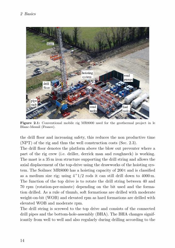
A drilling rig consists of multiple equipment and is designed to constructwells in different environments (i.e. off-shore, on-shore) and rock formations(i.e. sediment, metamorphic and igneous). Despite the variety of drilling op-erations, most of the hardware on a rig is similar. The land rig (Fig. 2.1)used for the geothermal project in Paris consists of a mast and its hoistingsystem, a pipe rack to store pre-assembled double stand drill pipes and atop-drive, mud pumps, shakers, compressors, etc.Newest advance by West Drilling (Norway) includes a second mast andtop-drive for continuous tripping - at velocities up to 1m/s in cased sec-tions - and rapid casing run. Besides diminishing the number of people on
13
2 Basics
Figure 2.1: Conventional mobile rig MR8000 used for the geothermal project in leBlanc-Mesnil (France).
the drill floor and increasing safety, this reduces the non productive time(NPT) of the rig and thus the well construction costs (Sec. 2.3).The drill floor denotes the platform above the blow out preventer where apart of the rig crew (i.e. driller, derrick man and roughneck) is working.The mast is a 35m iron structure supporting the drill string and allows theaxial displacement of the top-drive using the drawworks of the hoisting sys-tem. The Soilmec MR8000 has a hoisting capacity of 200 t and is classifiedas a medium size rig; using 4 ”1/2 rods it can still drill down to 4000m.The function of the top drive is to rotate the drill string between 40 and70 rpm (rotation-per-minute) depending on the bit used and the forma-tion drilled. As a rule of thumb, soft formations are drilled with moderateweight-on-bit (WOB) and elevated rpm as hard formations are drilled withelevated WOB and moderate rpm.The drill string is screwed to the top drive and consists of the connecteddrill pipes and the bottom-hole-assembly (BHA). The BHA changes signif-icantly from well to well and also regularly during drilling according to the
14

2.2 Well construction
well trajectory, the formation properties and, the needs to characterize thestratigraphic column while drilling as well as other factors.
Simple BHAs for vertical or slanted well can be directly assembled by thedrilling contractor which operates the rig and more complex BHAs fordirectional wells involving measurement while drilling (MWD) or reservoircharacterization while drilling (LWD) usually require a service company.
Hereafter, a 30 t bottom-hole-assembly (Tab. 2.1) prepared by the servicecompany Weatherford R© to build-up an angle from vertical in the produc-tion well (GBMN-3) at le Blanc-Mesnil in the Paris sedimentary pile isdescribed. As a matter of comparison, the 255m long BHA is only slightlyshorter than the upper platform of the top level of the Eiffel tower, whichstands 276m above ground.
Table 2.1: Item composing the bottom hole assembly prepared by the service companyWeatherfordR© and used by the drilling contractor Entrepose drilling.
O.D. Item Length [m] Cum. [m]
5” drill pipes - -5” HWDP 5” 65.56 255.45
6”1/2 Hydraulic jar 9.67 189.895” HWDP 5” 37.37 180.22
6”1/2 Union 4”IF pin x 4”1/2 IF box 0.88 142.856”1/2 DC 6”1/2 92.39 141.97
8” Union 6”5/8 REG pin x 4” IF box 0.78 49.588” DC 8” 18.17 48.808” Spiraled NMDC 8.55 30.63
7”3/4 MWD - emitting sub 3.38 22.088” MWD - tool carrier 6.00 18.708” Union pin x pin 0.49 12.70
12” × 8” Non magnetic stabilizer 2.21 12.218” Downhole motor 9.65 10.00
12”1/8 Bearing stabilizer 0.00 0.0012”1/4 PDC drill bit 0.35 0.35
Below the last drill pipe (Tab. 2.1), 102.93m of heavy weight drill pipes(HWDP) are used to sandwich a hydraulic jar.The jar produces impact loads to the downhole equipment in the critical
15

2 Basics
case where the BHA is stuck in the formation. It should suffice here to saythat different types of jars exist, operating either mechanically or hydrauli-cally and being designed for drilling or fishing operations. Fishing denotesthe trials to fetch the BHA downhole following a twist-off of the drill string,before one part of the well is cemented and a side track drilled. Such prob-lem happens relatively frequently especially during the early explorationof a new field which is unfortunately the usual situation in the geothermalsector.The lower set of HWDP (37.37m) is then screwed to a union, itself con-nected to about 92m of drill collars joined with a second union to about20m of 8” collars. A spiraled non-magnetic one is connected before theMWD sub-assemblies (emitter and tool carrier).A usual way to transmit information to the surface is by pulsing the mudflow at various frequency (mud pulse telemetry), which can then be recordedon surface with a receiver and digitalized to useful information. In the par-ticular case of le Blanc-Mesnil, information was transmitted directly byelectromagnetic waves through the ground [29].Below the MWD subs, a union and a non-magnetic stabilizer are connectedto center the tool and to prevent disturbing the azimuth measurements. Un-derneath is the positive displacement motor, in this case capable of adding245 kW to the bit. Below the mud motor, an additional stabilizer is used tocenter the bearings with the wellbore. At the bottom, a 12”1/4 PDC tool(model SDHE516S) from NOV (National Oilwell Varco) is mounted.
A water based mud flow of 2.6m3/min is circulated by two triplex pumpsin the drill pipes and flows up the annulus between the string and thewellbore. Along the circuit, the drilling fluid completes different tasks:
• It cools down the measurement tools and the bit. During operations,depending on the formation hardness, rpm, WOB and other parame-ters, the surface of the PDC cutters can be exposed to temperaturesin excess of 400 C [30].
• It drives the mud motor and other power generation equipment.
• It stabilizes the well. Most of the formation related drilling problemsappear while the drill string is out of the well or during tripping,when no circulation occurs.
16

2.2 Well construction
• It transports the cuttings.
• It lubricates the drill string in directional sections, when the stringlies against the wellbore or casing surface.
To separate the cuttings and clean the returning mud flow, large shakingunits are used on surface. The mud is then stored in pits where its chemistryis adjusted before being pumped back in the drill string.
With respect to mud chemistry, different additives (i.e. organic and inor-ganic) exist to adjust its chemical and rheological properties according tothe requirements of the formation (e.g. water soluble zones) and that of thedrilling process, i.e. cuttings transport, lubrication of the drill string, etc.Generally drilling mud are classified as water or oil based depending on thenature of the continuous phase forming the fluid. The whole point about themud is to produce a hydrostatic pressure between formation pressure (i.e.to prevent inflows) and the fracking pressure of the formation. Variationsin the pressure along the well will determine the set depth of the casingstrings, in addition to the strings set for environmental reasons. In the end,the mud density is designed to produce a certain hydrostatic pressure andthe viscosity to limit the flow rate cleaning the bit face and lifting the cut-tings in the annulus. It should be mentioned that often in soft formations,bit face cleaning and cuttings lifting limit the rate of penetration.
2.2.2 State of the art in rock reduction techniques
A common mistake in the
bit selection is the use of
rate of penetration rather
than cost per meter.
B. Mehri, Saudi Aramco,
2015
The state of the art in rock reduction represents the current most economicand applied drilling methods. This essentially means the use of drag bits(i.e. fixed cutter bits) in soft formations and roller cones in hard formations(e.g. igneous rock) [31] but depends as well on other parameters.
17

2 Basics
(b)(a)
cooling water
nozzle
lubricant
reservoir
bit axis
bit axis
bit body
cone
axis
tooth
blade
pilot bit
section
reaming
section
PDC
inserts
shank
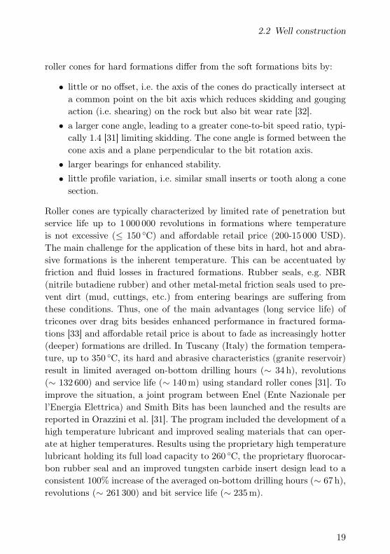
Figure 2.2: (a) HerculesTM roller cone drill bit (NOV) specifically developed for hardrock and challenging drilling environments. (b) SpeedDrillTM polycrystalline diamondcompact drag bit (NOV) with a pilot bit releasing formation stresses. This fixed cutterbit was used to drill the production well GBMN-3 in le Blanc-Mesnil (France).
Roller cone bits
Roller cone bits (Fig. 2.2(a)) are used in every type of drilling operations,reducing the rock by a common action of crushing, gouging and skidding.Crushing takes place when WOB forces the inserts into the formation.Skidding and gouging take place since the motion of the bit does not permitan insert to rotate out of a crushed zone it has created without inducingdamage over its perimeter. The effect is amplified by the offset between thecones and the bit axis, i.e. the cone axis do not converge on the bit axis.
Current roller cone bits usually consist of three cones (tricones) with eitherlarge milled steel tooth for soft to medium formations or shorter tungstencarbide inserts for medium to hard formations. The different roller coneclasses following the international association of drilling contractors arepresented in the drilling data handbook [28]. Besides the material, typical
18
2.2 Well construction
roller cones for hard formations differ from the soft formations bits by:
• little or no offset, i.e. the axis of the cones do practically intersect ata common point on the bit axis which reduces skidding and gougingaction (i.e. shearing) on the rock but also bit wear rate [32].
• a larger cone angle, leading to a greater cone-to-bit speed ratio, typi-cally 1.4 [31] limiting skidding. The cone angle is formed between thecone axis and a plane perpendicular to the bit rotation axis.
• larger bearings for enhanced stability.
• little profile variation, i.e. similar small inserts or tooth along a conesection.
Roller cones are typically characterized by limited rate of penetration butservice life up to 1 000 000 revolutions in formations where temperatureis not excessive (≤ 150 C) and affordable retail price (200-15 000 USD).The main challenge for the application of these bits in hard, hot and abra-sive formations is the inherent temperature. This can be accentuated byfriction and fluid losses in fractured formations. Rubber seals, e.g. NBR(nitrile butadiene rubber) and other metal-metal friction seals used to pre-vent dirt (mud, cuttings, etc.) from entering bearings are suffering fromthese conditions. Thus, one of the main advantages (long service life) oftricones over drag bits besides enhanced performance in fractured forma-tions [33] and affordable retail price is about to fade as increasingly hotter(deeper) formations are drilled. In Tuscany (Italy) the formation tempera-ture, up to 350 C, its hard and abrasive characteristics (granite reservoir)result in limited averaged on-bottom drilling hours (∼ 34 h), revolutions(∼ 132 600) and service life (∼ 140m) using standard roller cones [31]. Toimprove the situation, a joint program between Enel (Ente Nazionale perl’Energia Elettrica) and Smith Bits has been launched and the results arereported in Orazzini et al. [31]. The program included the development of ahigh temperature lubricant and improved sealing materials that can oper-ate at higher temperatures. Results using the proprietary high temperaturelubricant holding its full load capacity to 260 C, the proprietary fluorocar-bon rubber seal and an improved tungsten carbide insert design lead to aconsistent 100% increase of the averaged on-bottom drilling hours (∼ 67 h),revolutions (∼ 261 300) and bit service life (∼ 235m).
19

2 Basics
Roller cones will continuously benefit from improvements in bearings, seals,high temperature lubricant and harder inserts (e.g. diamond enhanced in-serts).Another example is a recent proprietary innovation [34] for roller cones re-ported in [35]. It consists of using tapered roller bearings instead of usualcylindrical bearings or journal bearings (i.e. friction bearings) to reduceaxial and radial play between the cone and the bit body. With these newbearings, extended service life (1 600 000 revolutions) is reached in a forma-tion where earlier bits would fail on average after 852 000 revolutions.Following such advance, more aggressive roller cones with:
• smaller cone angle (increasing the bit aggressiveness),
• larger offset (increasing skidding),
• larger and harder inserts (e.g. diamond enhanced inserts)
resulting in enhanced shearing and improved ROP might be able to oper-ate in hard rocks for extended service life.Finally and primarily because of the intrinsic disadvantages of moving partsand inefficiency of crushing rocks with high compressive strength, break-throughs in the penetration rate associated with roller cones are not ex-pected.
Fixed cutter bits
Presently, mostly two types of drag bits are used in drilling operations. Thediamond bits are equipped with small natural diamonds partially encapsu-lated in the bit body and reduce the rock by grinding. These bits requireturbodrill motors (i.e. high frequencies mud turbines) and function withmoderate WOB. The second type of drag bits has larger and synthetic cut-ting elements brazed onto the bit body (Fig. 2.2(b)). These are the onesconsidered most interesting as they are intrinsically superior to roller conesand diamond bits:
• no moving parts (e.g. cone bearings), which are fragile and need lu-brication and,
• rock is reduced by a shearing mechanism which is more effective (less
20

2.2 Well construction
J/cm3 of excavated rock) compared to the crushing, gauging andskidding action of roller cones or the grinding action of diamond bits.
These drag bits usually consist in a metal or a tungsten carbide matrix bodyequipped with blades, the position and size of which influence cuttingsformation and removal, as well as other factors. On the blades, PDC orthermally stable polycrystalline diamond compact (TSP) inserts are brazed.Both types of inserts are prepared the same way, but cobalt, used as a binderin PDC is either leached or replaced by a temperature compatible binderin the production of TSP.
Many structural parameters of fixed cutter bits can be tuned for specificdrilling operations and hard rock bits are essentially characterized by:
• A relatively flat body shape (Fig. 2.2(b)) which allows to spread theWOB evenly on the cutters and obtain a homogeneous wear rate.The expense is to limit the number of cutters on the bit because lesssurface is available in comparison to a parabolic bit profile.
• Fewer blades typically 6 to 8 [9,36] depending on the bit nominal di-ameter lead to an optimal balance between cuttings size and removalrate (i.e. bit hydraulics).
• A higher cutter density on each blade. Usually and similarly to rollercones, a higher density of smaller cutting elements is preferred forhard and abrasive formations, resulting as a trade-off in lower pene-tration rates and higher mechanical specific energy (MSE).
• A greater back rake angle, which is formed between the cutter face andthe normal to the formation being drilled. The larger angle enhancesthe cleaning of the cutters and reduces vibrations. It also results inless aggressiveness (i.e. reduced cutter penetration depth) and thuslower ROP.
Fixed cutter bits seem better suited with the multiple design parametersthat can be adjusted, the inherently more efficient rock reduction mech-anism and the absence of any moving part, limiting failure possibilities.Conversely the main disadvantages of drag bits with synthetic diamondcompact inserts are (i) their expensive retail price, up to 100 000 USD,which drill bit suppliers try to cope with by offering bits for rent [36] and,
21

2 Basics
(ii) the important wear rate experienced in hard and abrasive formationsby standard cutters. The shearing process releases a lot of heat and cutterswear increases typically exponentially above 372 C until PDC eventuallyfail at about 750 C [37]. This is connected with the use of a cobalt (Co)catalyst during the high temperature high pressure sintering process to pro-duce the compact. Indeed, the thermal expansion coefficient of cobalt anddiamond mismatches, resulting in differential expansion, thermal stressesand eventually flaws. Cobalt also catalyzes the reverse transformation ofsynthetic diamond into carbon at elevated temperature, e.g. produced byfriction heating [30].TSP cutters are essentially produced in a similar manner as PDC, i.e. hightemperature high pressure sintering but either cobalt is leached or a ther-mally compatible binder (e.g. silicon carbide) is used. In the case of leaching,the diamond table is first detached from its tungsten carbide support, thenleached and the TSP material is brazed or bonded at high temperature andhigh pressure to a substrate, typically containing tungsten carbide. Despitebeing able to operate at higher temperatures with reduced wear, TSP usedto suffer from a lower fracture toughness in comparison to PDC and resid-ual thermal stresses built during the cooling following the brazing process.Solutions to braze TSP inserts and to enhance fracture toughness have nowbeen developed and are reported by Radtke et al. [38].
An other common source of wear for both cutters (i.e. PDC and TSP) arebit vibrations which occur principally in hard and abrasive formations [39]and are enhanced in fractured or interbedded lithologies and at elevatedWOB. To reduce vibrations, shock absorbers [40] and DWD tools [9] pro-viding high frequencies downhole data have been investigated. Using DWDtool, Sandia could show consistent improvements in bit performance (i.e.ROP and service life). Wired drill pipes (e.g. IntelliServ, NOV) might alsopromote the use of such systems avoiding the usual troubles related withwet wirelines. However either every drill string component is compatible,which is currently very restrictive or the DWD is located fairly away fromthe bit (2.2.1).In an other development from Sandia [40], a shock absorber consisting of aspring and a magneto rheological fluid is used to mitigate axial bit vibra-tions and improve service life and drilling performance. Additionally, Smith
22

2.2 Well construction
Bits developed a novel conical diamond element positioned at the center offixed cutter bits to limit vibrations and extend service life [30].
Drag bits will therefore benefit from advances in manufacturing techniquesto produce inserts at reduced costs and improved characteristics. Recentadvances include cutting elements able to rotate at 360 spreading wearand heat along the entire circumference of the cutter and extending servicelife [30].
In conclusion, there is still no bit of either type (roller cones and fixed cut-ter) that permits to drill sections as long as casing intervals (50 - 1500m) inevery rock formation at an acceptable penetration rate (5 - 10m/h). Bothtypes of bits have advantages and drawbacks and ultimately, the minimiza-tion of the rock reduction costs (Sec. 2.3) should be used to choose theappropriate bit. The section length, its location (i.e. depth and lithologies),the steering requirements of the BHA, etc., are all elements that have to beaccounted for and weighted appropriately for an optimized bit choice. Prac-tically, it is also very likely that each driller has his favorite drill bit type.Such factors although superficial have to be considered in an effort to mini-mize rock reduction costs. From a strategic point of view, it seems generallyconvenient to drill exploration wells with roller cones which are tougher,cheaper, less sensitive to interbedded formations and characterized by anextended service life. For the upcoming wells, appropriate fixed cutters bitcan be purchased with the geological information (e.g. stratigraphy, rockultimate compressive strength, loss circulation zones, kicks, etc. . . ) such asto reduce durably the well construction costs in this field.
2.2.3 Casing and cementing
Because casing and cementing operations are expensive and risky, besidesthe sections which are compulsory from an environmental point of view, i.e.to avoid spoiling aquifers and contaminate freshwater resources, a minimumnumber of casing strings are installed along a well path. These operations oflowering the casing and cementing are time consuming and critical, because:
• there is no possibility to rotate the string,
23

2 Basics
• the space between the open hole and the casing string is tight and,
• cementing is a no return operation, once started (i.e. the annulus hasto be filled up before cement starts to dry).
Additionally, for each casing string the open hole diameter of the well is re-duced correspondingly limiting production flow rates by increasing the wellimpedance. In principle, set depths are determined in advance accountingfor the lithology and the difference between the formation and the hydro-static pressure created by the drilling fluid. The general idea is to preventinflows of formation fluid during drilling, while maintaining the well in-tegrity and preventing fracking. Hence it is required to change the drillingfluid periodically and the hole is cased beforehand. As soon as a set depthis reached, the drill string is pulled out of the hole, caliper and temperaturelogs are run to determine the cement volume and composition. Meanwhile,it might be necessary to adjust the rheological properties (i.e. density andviscosity) of the drilling fluid filling the hole to prevent fracking the for-mation while the casing string is lowered. Then the casing string equippedat its bottom with its shoe, which acts as a guide and helps to reduce thehook load on the drawworks by a system of non return valve, is slowly (i.e.150m/h) lowered into the well to manage the pressure surge. The differ-ent joints are either screwed - similarly to drill pipes - or welded together.Scratchers and centralizers are added regularly to center the string and helpcementing. Welding of the casing is preferred when the well is completedfor a high temperature production fluid (≥ 200 C), as the thermal expan-sion leads to extreme requirements on the threads. This is for instance astandard procedure in Iceland1.
Once the casing string has reached its set depth, the cementing head ismounted. The procedure begins using an appropriate set of plugs to pre-vent contamination of the cement by the drilling fluid used to force thecement in the annulus between the casing and the wellbore. Unlike for oiland gas wells, the casing is cemented along its whole length in geothermalcompletion, using specific high temperature cements. This is to cope withaxial dilatation of the casing as it is slowly heated up by the productionfluid and problems related with a pressure surge if water is trapped along
1Personal communication with Sverrir Thorhallsson, Iceland GeoSurvey, January 2016.
24

2.2 Well construction
the string [6]. After an appropriate drying time, varying upon the cement,its volume and composition, logs are run to ensure the operation was suc-cessful. Following the control, the blow out preventer (BOP) is lifted up andthe top of the casing string is drained and cut. Then the BOP is removedand hangers are installed before the BOP is nippled up and drilling can re-sume. For the production well in le Blanc-Mesnil two casing sections have
KOP, 500 m
section length, li [m] /
casing dia. [inch]
200 / 18 5/8
1096 / 13 3/8
bit dia. [inch] /
initial section depth di,1
[m]
24 / 0
17 1/2 / 200
12 1/4 / 1296
TVD 1815 m
MD 2071 m
1454 / 9 8/5
8 1/2 / 1894
Figure 2.3: Well design with casing and drill bit diameters for the production wellGBMN-3 in le Blanc-Mesnil (France). KOP denotes the kick-off point, TVD the truevertical depth and MD the measured depth. Plain lines denote casing strings and linersas the dash line denotes the open hole section.
been lowered and cemented in place as well as a production liner (Fig. 2.3).The liner is essentially a casing string which does not extend up to surfaceleaving space to accommodate the production pump. Connection with thereservoir is achieved along an open hole section, located below the liner.
It should finally be noted that the procedure described is for a single stagecementing using two plugs and a standard cementing head. According to thelength of the open hole section to be cased and other formation parameters(e.g. losses), it might be necessary to proceed to a two-stage cementing, thedetails of which are out of the scope of this work.
25

2 Basics
2.3 Well construction costs
depth is not all one needs
to know to determine well
costs.
A. J. Mansure, Sandia,
2006
After the presentation of a drilling rig, the conventional drill bits and out-lined the complexity of casing and cementing operations, it is important toaddress well construction costs. Their distribution determining the impactof the rock reduction on the overall well expenses. In the following, the liter-ature about well costs is briefly reviewed and a model to compute the rockreduction costs is presented and illustrated. More results of the costs cal-culation used in the techno-economic feasibility assessment are presentedin chapter 9.
In the literature, large discrepancies exist concerning the influence of dif-ferent operations and parameters on well construction costs. Among thestudies reviewed, concerning mostly geothermal wells, some attribute up to30% of the total construction costs to troubles (e.g. loss circulation, fishing,etc. . . ) in developed geothermal fields [25]. Some others attribute it only acontingency of 10% [41].Denninger et al. [42] claim that the way a drill bit is used is more impor-tant than the bit itself as Raymond et al. [36] established that expensivefixed cutter bits can contribute to reduce the costs of geothermal wells.On the top of that, different operators have different policies to reportcosts, increasing variation between data. This could be limited by a com-mon procedure to report costs providing at the same time a refined basis foranalyzing driving factors for averaged geothermal wells. This is for instancedone by the API (American Petroleum Institute) within the JAS (Joint As-sociation Survey on Drilling Costs) annually or by Rushmore Reviews forthe hydrocarbon industry. Fig. 2.4 presents the average well constructioncosts in the geothermal (blue [5], green [43]) and oil and gas (black [5])sectors. Hydrocarbon wells data are based on the yearly report of the APIJAS over the period 1976-2009 for well depths ranging from 381 to 6096m.
26

2.3 Well construction costs
0 2000 4000 6000 8000
measured depth, MD [m]
0
1000
2000
3000
4000
5000
6000
7000
cost
per
met
er,
[20
09
US
D]
Geothermal wells [5]Oil and gas wells [5]
Geothermal wells [43]
0
5
10
15
20
25
30
35
wel
lco
nst
ruct
ion
cost
s,[M
io.
20
09
US
D]
Figure 2.4: Average well construction costs and average cost per meter in 2009 USD.Plain lines refer to the overall well expenses as dash lines denote the costs per meter. Anyextrapolation from [43] beyond 6000m is abusive and presented here just for information.
The average geothermal well construction costs reported in [5] is primar-ily based on the data of 104 EGS and hydrothermal wells drilled between1972 and 2002 and 42 wells drilled between 2008 and 2013. The data are forwells between 732 and 5101m deep and are supplemented by a series of 29hydrothermal and EGS wells which costs are calculated using the WellCostLite software [25]. Finally, data reported in [43] are based on 33 propri-etary geothermal wells drilled on average in 1994 which data were providedto Sandia by industry. Note that the data from [43] are originally reportedin year 2000 USD and are updated here to 2009 USD using the US BLS(Bureau of Labor Statistics) “Drilling oil, gas, dry or service wells” indexfrom the database 8512. The influences of the cost index on well costs dataare discussed by the same authors [5, 41, 44] and details of the functionsrepresented in Fig. 2.4 are reported in Tab. 2.2. Lukawski et al. [5] explainthat shallow wells are less expensive in the oil and gas sector (Fig. 2.4) be-cause these wells are generally smaller in diameter. Beyond a certain depth
27

2 Basics
Table 2.2: Mathematical functions illustrated in Fig. 2.4. x denotes the measured depthin meter.
Oil and gas Geothermal
Lukawski et al. [5]C(x) [Mio. 2009 USD] 1.65× 10−5x1.607 1.72× 10−7x2+
2.3× 10⁻³x− 0.62∂C∂x [2009 USD] 26.5155x0.607 0.344x+ 2300
Mansure et al. [43]C(x) [Mio. 2009 USD] 1.92591853eαx
∂C∂x [2009 USD] 1925918.53αeαx
α [1/m] = 0.000125× 3.28084.
(around 6000m), this is counter-balanced by the ever increasing costs ofoil and gas wells, which require stronger (i.e. thicker, higher steel grades)casing strings and BOP. The claim that smaller diameter wells are less ex-pensive corroborates with the opinion of a senior drilling engineer2 whoclaimed that large diameter wells take the same time to drill but are up to30% more expensive than standard wells: the larger casings and the morepowerful rig and auxiliaries accounting essentially for the difference. Basedon Fig. 2.4, the cheaper wells beyond a certain depth is questionable, espe-cially considering that every geothermal well used in [5] for fitting beyond5101m results from calculated data for trouble-free wells. The same authorsalso observed, based on the API JAS 1976-2009 data, that oil and gas de-velopment wells are on average 8% less expensive than exploratory wells.This learning capacity could be higher in the geothermal sector because cor-responding lithologies are generally less homogeneous and less predictablethan sedimentary formations, out of which most of the hydrocarbons areproduced. This has however to be balanced with the usually limited num-ber of wells drilled in a geothermal field. Thus the learning curve in ageothermal field has to be very steep to result into costs reduction.
From Fig. 2.4, the only clear trend is an increase beyond linearity of wellconstruction costs with depth in both sectors. This is related to the follow-ing cumulative effects:
• deep formations are in general harder and a greater lithostatic stressreduces rock porosity, both contributing to lower ROP and bit service
2Personal communication with Sverrir Thorhallsson, Iceland GeoSurvey, January 2016.
28
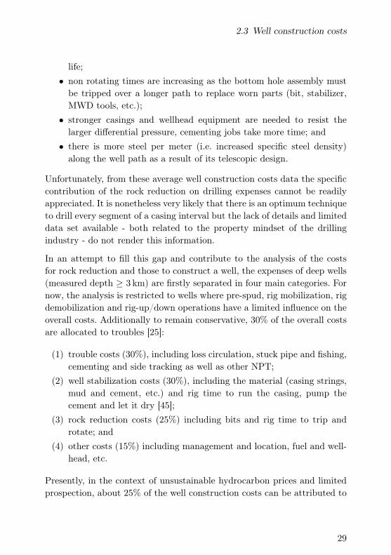
2.3 Well construction costs
life;
• non rotating times are increasing as the bottom hole assembly mustbe tripped over a longer path to replace worn parts (bit, stabilizer,MWD tools, etc.);
• stronger casings and wellhead equipment are needed to resist thelarger differential pressure, cementing jobs take more time; and
• there is more steel per meter (i.e. increased specific steel density)along the well path as a result of its telescopic design.
Unfortunately, from these average well construction costs data the specificcontribution of the rock reduction on drilling expenses cannot be readilyappreciated. It is nonetheless very likely that there is an optimum techniqueto drill every segment of a casing interval but the lack of details and limiteddata set available - both related to the property mindset of the drillingindustry - do not render this information.
In an attempt to fill this gap and contribute to the analysis of the costsfor rock reduction and those to construct a well, the expenses of deep wells(measured depth ≥ 3 km) are firstly separated in four main categories. Fornow, the analysis is restricted to wells where pre-spud, rig mobilization, rigdemobilization and rig-up/down operations have a limited influence on theoverall costs. Additionally to remain conservative, 30% of the overall costsare allocated to troubles [25]:
(1) trouble costs (30%), including loss circulation, stuck pipe and fishing,cementing and side tracking as well as other NPT;
(2) well stabilization costs (30%), including the material (casing strings,mud and cement, etc.) and rig time to run the casing, pump thecement and let it dry [45];
(3) rock reduction costs (25%) including bits and rig time to trip androtate; and
(4) other costs (15%) including management and location, fuel and well-head, etc.
Presently, in the context of unsustainable hydrocarbon prices and limitedprospection, about 25% of the well construction costs can be attributed to
29
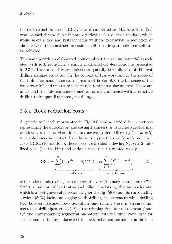
2 Basics
the rock reduction costs (RRC). This is supported by Mansure et al. [25]who claimed that with a ultimately perfect rock reduction method, whichwould allow a free and instantaneous wellbore excavation, a reduction ofabout 33% in the construction costs of a 6096m deep trouble-free well canbe achieved.
To come up with an elaborated opinion about the saving potential associ-ated with rock reduction, a simple mathematical description is presentedin 2.3.1. Then a sensitivity analysis to quantify the influence of differentdrilling parameters is run. In the context of this work and in the scope ofthe techno-economic assessment presented in Sec. 9.3, the influence of thebit service life and its rate of penetration is of particular interest. These arein the end the only parameters one can directly influence with alternativedrilling techniques like flame-jet drilling.
2.3.1 Rock reduction costs
A generic well path represented in Fig. 2.5 can be divided in m sectionsrepresenting the different bit and casing diameters. A usual deep geothermalwell involves four cased sections plus one completed differently (i.e. m = 5)to enable reservoir contact. In order to compute the specific rock reductioncosts (RRCi) for section i, these costs are divided following Nguyen [2] intofixed costs (i.e. the bits) and variable costs (i.e. rig related costs):
RRCi =
n∑
j=1
(αjC
fcb + βjCrcb)
︸ ︷︷ ︸
fixed costs
+ rh
n∑
j=1
(
ttripj + trotj
)
︸ ︷︷ ︸
variable costs
(2.1)
with n the number of segments in section i; α, β binary parameters; Cfcb,Crcb the unit cost of fixed cutter and roller cone bits; rh the rig-hourly-rate,which is a best guess value accounting for the rig (50%) and its surroundingservices (50%) including logging while drilling, measurement while drilling(e.g. bottom hole assembly orientation) and renting the drill string equip-ment (e.g. drill pipes, etc. . . ); ttripj the tripping time to drill segment j andtrotj the corresponding segmental on-bottom rotating time. Note that forsake of simplicity any influence of the rock reduction technique on the hole
30

2.3 Well construction costs
shape and stability (which might influence stabilization, troubles or othercosts) is neglected.
section (i) ... section (m)
segment (j-1) segment (j) segment (n)...
α=0, β=1 α=1, β=0
well pathli
srcb sfcb
Figure 2.5: Generic well path divided in m sections (1, . . . ,m) which are divided in nsegments (1, . . . , n) where the bit is represented by the value of the binary parameters(α, β). The superscripts “fcb” and “rcb” denote fixed cutter and roller cone bits.
The segmental on-bottom rotating time (trotj ) is defined by the minimumof the ratio between the intrinsic bit service lives (s) to its penetration rate(ROP) and the left-over length to drill in section i:
trotj = min
(sfcb
ROPfcbαj +
srcb
ROPrcbβj ;
|di+1,1 − di,j |
ROPfcbαj +
|di+1,1 − di,j |
ROPrcbβj
)
.
This means that when the casing set depth is reached the bit is pulledout and the casing string is run, cemented and controlled before drillingis resumed. These costs are imputed to the stabilization category (30%).Note that average ROP and service life are used neglecting the influenceof different geologies. With this respect Mansure et al. [44] showed thataccounting for specific geology can reduce the variation between field costdata and calculations, but only by 10%. The cumulative (i.e. up and down)segmental tripping time (ttripj in Eq. (2.1)) accounts for the bit choice andits corresponding rotating time (trotj ):
ttripj =di,jv︸︷︷︸
trip down
+di,j +ROPfcbtrotj
vαj +
di,j +ROPrcbtrotj
vβj
︸ ︷︷ ︸
trip up
with di,j the initial depth of segment j in section i and v is the trippingrate. In the context of a minimization of the rock reduction costs, Eq. (2.1)
31

2 Basics
Table 2.3: Bit data to analyze the rock reduction costs. All the values are gatheredfrom [36] besides the roller cone bit retail price. In [36], re-run bits are purchased at adiscount price and the cost applied here corresponds to a new bit.
Roller cone bit Fixed cutter bit
service life, s [m] 120 170cost, C [USD] 10 000 50 000
rate of penetration, ROP [m/h] 3 6
is an objective function subject to the following (n+ 1) linear constraints:
n∑
j=1
(αjs
fcb+ βjsrcb)≥ li (2.2)
αj+βj ≤ 1 (2.3)
where li denotes the length of section i. The first constraint (Eq. (2.2))requires the maximum cumulative segments length to be at least as longas the section and the second series of n constraints (Eq. (2.3)) preventthe unrealistic utilization of both bits for the segment j. The optimal bitchoice is obtained by minimizing Eq. (2.1) varying the values of the binaryparameters α and β. The first binary parameter α is true (or 1) if a fixedcutter bit is used and the second parameter β is true (or 1) when a rollercone bit is used.
Table 2.4: Basecase parameters to analyze the specific rock reduction costs and examplevalues for a virtual section i = 1.
Parameter Value
Basecaserig-daily-rate, rd [USD] 80’000
tripping rate, v [m/h] 500Example
initial section depth, d1,1 [m] 650section length, l1 [m] 290
It results in a problem where the order in which the drill bits are used hasan impact on costs. For example, for the virtual section i = 1 starting at
32

2.3 Well construction costs
650m (d1,1) and 290m long (l1 in Tab. 2.4), which suggests the use of onefixed cutter bit and one roller cone featuring a cumulative service life equalto the section length (l1), it is more economical to use the roller cone firstas this limits the overall tripping time and hence the variable costs. Overa 290m section with alike bit service life (Tab. 2.3), the economy is notvery significant, about 12min or 666USD using the data and parameterspresented in Tabs. 2.3 and 2.4, but this illustrates the details accounted forin the calculation.
In the end the cumulative rock reduction costs (RRCc) along the well pathare given by:
RRCc =
m∑
i=1
RRCi,
with m the total number of sections drilled (Fig. 2.5). The estimated rockreduction costs for the well presented in Fig. 2.6 are presented in Tab. 2.5when either roller cone or fixed cutter bits are used.
KOP, 3900 m
section length, li [m] /
casing dia. [inch]
80 / 26
320 / 18 5/8
1850 / 13 3/8
2550 / 9 8/5
bit dia. [inch] /
initial section length di,1
[m]
- / 0
24 / 80
17 1/2 / 400
8 1/2 / 4800
TVD 4500 m
MD 6300 m
12 1/4 / 2250
Figure 2.6: Generic EGS well for continental Europe with an average temperaturegradient in the range of 40 C/km. KOP denotes the kick-off point, TVD the true verticaldepth and MD the measured depth. Plain lines denote casing strings and liners as thedash line denotes the open hole section.
33

2 Basics
Table 2.5: Summary of the costs for the generic EGS well (Fig. 2.6). This well is suitablefor a region with a mean temperature gradient in the range of 40 C/km.
Roller cone Fixed cutter Diff. %
tripping time, ttrip [h] 694 473 -32rotation time, trot [h] 2100 1050 -50
fixed costs [Mio. USD] 0.55 1.9 +245RRCc [Mio. USD] 9.86 6.97 -29
well costs [Mio. USD] 39.44 36.55 -7project costs (2 wells) [Mio. USD] 106.59 100.81 -5
investment costs [Mio. USD/MWe] 21.32 20.16 -5
The RRC constitute 25% of the well costs.The well costs constitute 74% of the project costs [46].The investment costs assume 5MWe/project.
From Tab. 2.5 one observes that a change from roller cone towards fixedcutter bits helps to reduce the tripping time (ttrip) and the on-bottomrotating time (trot) significantly at the expense of increased fixed costs. Thismeans that the RRC are more coupled to the hydrocarbon prices (hencetotal spread daily rate) than bit performance and any long-term forecast ofRRC is truly speculative. Neglecting these hypothetical price variations andbased on both cases presented here, the RRC can be reduced by almost 30%using fixed cutter instead of roller cone bits. This change occurred alreadyin the oil and gas sector and in 2014 fixed cutter bits drilled more than 80%of the total footage [47]. Conservative people will legitimately claim thatmost rocks drilled in the oil and gas sectors are thus far softer comparedto geothermal formations, which is a fact.
In conclusion operators try to limit expenditure of geothermal drilling byusing cheap roller cone bits (e.g. re-run bits) and this might turn out tobe more expensive than using new fixed cutter bits (e.g. [36]). But again,the bit choice will vary according to many factors (e.g. driller, formation,diameter, trajectory, etc.) and the daily-rate, which is the most sensible pa-rameter of the costs for rock reduction and is closely linked to hydrocarbonprices.
Considering the fixed cutter column in Tab. 2.5 as a basecase, Fig. 2.7presents the influence of different parameters on the RRC as they depart
34

2.3 Well construction costs
from their initial values (Tabs. 2.3 and 2.4). Note that for each individualvalue the RRC are minimized varying α and β using a multiple binaryoptimization routine [48].
−40 −20 0 20 40 60 80 100
% change from basecase
4
5
6
7
8
9
10
11
rock
red
uct
ion
cost
s,R
RC
c[M
io.
US
D]
roller cone bits
fixed cutter bits
tripping rate
daily rate
ROPfcb
ROPrcb
sfcb
srcb
Figure 2.7: Influence of different parameters with respect to the basecase values(Tabs. 2.3 and 2.4) on the cumulative rock reduction costs for the well presented inFig. 2.6.
From Fig. 2.7, the most significant parameter influencing the cumulativerock reduction costs (RRCc) is the rig daily rate. A 50% increase in rig dailyrate, keeping every other parameter constant results in a 40% increase of theRRCc. Improvements in the tripping rate has only an asymptotic influenceon the costs and using a novel continuous motion rig able to reach trippingvelocity up to 3600m/h in cased sections can only limit the the RRCc byabout 15%. Improvements of the roller cones characteristics (i.e. rate ofpenetration, ROPrcb and service life, srcb) have both a limited impact on
35

2 Basics
the RRCc, which is related to the superior initial performance of the fixedcutter bits (Tab. 2.3). Roller cones eventually reduce the RRCc as their rateof penetration exceeds 4.5m/h which is well above current field average,especially in hard rocks. Similarly, a twofold increase in the roller cone bitservice life does not lead to any savings with respect to the basecase.Conversely, improving the rate of penetration and service life of fixed cutterbits have both a similar impact on costs. By doubling the ROP or servicelife of fixed cutter bits, the RRCc are reduced by 24% and the overall wellcosts by 4.5%. These figures are in agreement with the calculations of Pettyet al. [49] who claimed, based on the work of Augustine [41], that a twofoldincrease in ROP would permit to reduce deep borehole costs by 2 to 7%.Note the discontinuous savings associated with an improved fixed cutterbit service life (sfcb). This is related to the well design and is a practicaltradeoff. Once the casing set depth is reached, the drill string is pulledout of the well and the casing string is installed before drilling can resumeusing a smaller diameter bit. Sometimes an increase of a few percent inthe service life does not limit neither the number of drill bit required for asection, nor the tripping time, producing the pattern.
2.3.2 Closing remarks
The takeaway messages from Sec. 2.3 can be summarized as follows:
• The construction costs of deep wells can presently be broken in fourmain categories and the RRC account for about 25%.
• The RRC can be decomposed in fixed costs and variable costs, ex-pressed mathematically and minimized.
• The most significant parameter to reduce the RRC is the rig dailyrate. Fortunately deterministic, it can be negotiated but fluctuateswith hydrocarbon prices.
• The a-priori important savings related to doubling the ROP or servicelife of fixed cutter bits (-24%) has to be considered into perspective.It corresponds only to 4.5% of the total well costs or about 3.3% ofan EGS project tapping into bedrock at 4.5 km with a well design aspresented in Fig. 2.6.
36

2.4 Alternative drilling techniques
This 5-10% savings is the range of the well construction costs reductionexpected to be reached with the development of alternative drilling tech-niques, presuming the rest of the well costs (75%) are not affected.
It is important to mention that in an effort to reduce well constructioncosts, by modifying the design towards a monobore requiring one casingsection less, about 20% of the well construction costs could be saved [49].Therefore, alternative drilling techniques which allow to drill an under-reamed well permitting to case while drilling (e.g. expandable tubulars)are most promising, together with manage gradient drilling (e.g. Reelwell).
2.4 Alternative drilling techniques
Alternative drilling techniques refer to rock reduction methods which areconceptually different from rotary drilling. Over the years numerous ideashave been tested which are conceptually very diverse: using explosives,high pressure water jets, flame-jets, plasma, airplane engines, electropulses,micro waves, electron beams and even nuclear reactors, etc. [50–52]. Allthese concepts share two common characteristics: (i) they drilled rocksmore or less rapidly and, (ii) none of them replaced conventional rotarydrilling. This is attributed to the moderate complexity and great versatilityof conventional rotary drilling coupled with the long (i.e. several years [53,54]) and expensive empirical development of a new method and the longpayback period. Remember that having a rock reduction technique whichwould be free and excavate the well instantaneously, only 25% of the wellconstruction costs can be saved [25].In the following, the discussion is limited to few techniques which are at anadvanced development stage.
Electropusle drilling
Electropulse drilling uses a head consisting of several electrodes (Fig. 2.8(a))charged with an increasing voltage eventually resulting in a breakdown.Depending on the rising time and the peak magnitude of the pulse, the di-
37

2 Basics
(a) (b) (c)
Figure 2.8: (a) 12 1/4” electropulse drill bit [55]. (b) 6” laser enhanced rotarydrilling [56]. (c) 6” hammer system equipped with a 7 1/4” drill bit [57].
electric strength of the rock and of the drilling fluid vary. As the dielectricstrength of the rock is initially lower and essentially constant over time,the dielectric strength of the fluid decreases with the pulse rising time, be-cause charged fluid particles tend to align along the field lines. This wayits dielectric strength is reduced and it results in a discharge propagat-ing preferably across the fluid. For this technique to work, the dielectricstrength of the drilling fluid should be kept as high as possible and oilbased mud are typically easier to handle than water based drilling fluids.
The technical challenges for electropulse drilling are related to the necessityto load the electrodes with a high voltage, in the range of 500 kV, leading toa discharge current of 10 kA [55]. A convenient solution is to have the highvoltage generator directly downhole and driven by a submerged positivedisplacement motor. This alternative is currently under development [58],but has its own limitations. If the torque to drive the positive displacementmotor is excessive the stator which is designed to remain static starts torotate and drives the whole drill string. Besides the submerged high voltagepower generator, an other important challenge is related to the propertiesof the mud. Finally, electronic able to operate at high temperature, likelybeyond 200 C, when the well is not circulated is needed.
Conversly the advantages of this technique are the high ROP, up to 35m/h,the limited wear rate [55, 58] and the possibility to case the well whiledrilling because the hole is underreamed. This considers that technical so-lutions exist on surface to add casing strings simultaneously with a new
38

2.4 Alternative drilling techniques
drill pipe stand. The possibility to case the well while drilling extends thepotential savings associated with this drilling technique to both the RRCand the well stabilization costs. These account on average for 55% of thetotal well construction costs in deep geothermal projects (Sec. 2.3). As thewell is cased while drilling much of the risk is reduced: kicks occurenceand loss circulation are limited to the near-bit area. Breakouts risks arealso diminished as the formation is continuously stabilized. Developmentof this technique is still carried out by different institutes in Norway [55],Germany [58] and Russia [59].
Laser enhanced mechanical drilling
The laser enhanced mechanical bit (Fig. 2.8(b)) is based on the princi-ple that an inhomogeneous temperature generates thermal stresses in asolid. These stresses promote the combination and expansion of inherentweaknesses and cracks (i.e. flaws) in crystalline rocks, thereby reducing sig-nificantly its strength. It results that the laser enhanced mechanical bit [56]needs twenty times less WOB and ten times less torque to sustain the ROPof the corresponding unassisted mechanical bit. These softer requirementson the mechanical parts lead to a longer bit service life limiting the num-ber of trips to replace worn parts and reducing the corresponding variablecosts, part of the RRC (2.3.1). The drawbacks of the laser enhanced me-chanical drill are related to the power losses in optical fibers, the rotaryoptical bearing and the diffraction of the beam between the drill head andthe rock surface. This requires to use nitrogen as a drilling fluid. The beamreflexion on the rock surface and the necessity to use the bit with a coiltubing to pass the optical fibers to the head - from the laser unit on sur-face - add to the former difficulties to utilize the system. Additionally, coiltubing rigs have no way to rotate the drill string from surface and requirea positive displacement motor (PDM) which usually runs on mud. Con-ventional coil tubing cannot lower casing strings, requiring a hybrid rigequipped with a mast and these rigs have problems to drill horizontal sec-tions as the flexible coil has to be kept in tension to prevent friction on thewellbore.
39

2 Basics
Percussion drilling
The most advanced alternative method is percussion drilling used in min-ing, excavation work and for shallow geological survey, where pressurizedair drives the percussion hammer and flushes the cuttings. Development toenable the technology to operate with liquid based mud (i.e. incompress-ible fluid) is ongoing and currently only hammers running with clear tapwater are reported (e.g. Wassara and Hanjin D&B) [57]. Down the hole(DTH) hammers (Fig. 2.8(c)) use a reciprocating piston driven directly orindirectly (i.e. secondary fluid circuit) by the drilling fluid which in turnacts on an anvil to transfer impulse and mechanical energy to the tool face.The fluid is either air or water and uses its compressibility or a set of checkvalves to drive the hammer. Mostly like conventional rotary drill bits, tung-sten carbide inserts (TCI) and PDC inserts are set or sintered on the bitface.
These systems are increasingly used for hard rock drilling operations [57]where they have demonstrated ROPs near or above 10m/h. The maindisadvantages of DTH hammers lie in the difficulty to operate them withanything else than air or clean water and the important fluid consumption.Filtration of the return water for a closed loop design, which would solve theproblem of the large waste water volumes is still under development [57].
Flame-jet drilling
A contactless drilling method already applied extensively in the 20th cen-tury for taconite mining and other hard rock drilling operations [60, 61] isflame-jet drilling. It uses the low thermal conductivities of hard rocks andthe resulting differential expansion induced by local heating to break themin disc-like fragments (spalls) [62]. The greater the initial state of stress, thebetter the performance of the flame-jet drill by opposition to conventionaltechniques which makes it especially interesting at great depth.
In the early 1940’s, three companies in the U.S. exploited flame-jet drillingand were commercially viable. An interesting point to highlight is the dif-ferent combustion processes and nozzle geometries used by each company
40
2.4 Alternative drilling techniques
to generate the high temperature flame-jet required for spallation.
The Linde Division of Union Carbide Corporation used a liquid hydrocar-bon fuel, pure gaseous oxygen and a rocket type nozzle to accelerate theflame-jet. Over the years, the burner was improved with multiple outletsand additional cooling water. The water fulfilled two tasks: temperaturecontrol and extra momentum to transport the cuttings. Eventually, legshave been added on the burner to remove non-spallable rocks by ream-ing [18]. At its peak in 1966, a total of 37 machines from Linde were inservice removing approximately 100 million tons of rock per year [60].
Browning Engineering Inc. used different oxidizers to adjust the flame tem-perature with respect to the characteristics of the mineral. Browning etal. [61] highlighted that oxygen-flames are favorable for the working of ex-tremely hard and dense (i.e. few internal fractures) rocks. Air-flames aremore appropriate to process softer materials in which deeper heat penetra-tion is required, often resulting in thicker spalls. To address the problemof soft rocks and fractures encountered while drilling, Browning et al. [61]proposed to use the kinetic energy of the flame-jet to accelerate abrasiveparticles to high velocities. The role of the particles is to provide the nec-essary momentum to sweep the molten rock and grind rock around frac-tures. Eventually, this system has been used to drill numerous wells, amongothers the deepest well ever drilled by an unassisted, single-orifice flame-jet (Tab. 2.6) [18].
Flame Jet Partners Ltd. was the last company to consider business withflame-jets using a rocket engine burning chamber with hydrazine as fuel andnitrogen tetroxide as oxidizer. The hypergolic reaction creates ignition ofthe mixture. The extreme temperature of the exhaust gas, about 4000 C,is used to spall and melt the rock. Whenever rock is melted the scrapingaction of the lugs on the combustion chamber shield can get ridd of thefused rock [18]. Only one drilling rig was built by the company and its useremained mainly experimental.
Finally due to the shut down of most taconite quarries (iron extraction)in which spallation rigs and channeling tools were used they gradually dis-appeared [18]. In 1990, Maurer [51] concluded that the use of flame-jetdrilling is impossible at depth due to the inoperability of flames in water
41

2 Basics
Table 2.6: Characteristics of the deepest well ever drilled by an unassissted flame-jet [18].
Coleman QuarryConway, N. Hampshire
date august, 1981type of rock hard granite
Hole shapemaximum 50.80 cmminimum 19.05 cm
average 26.67 cmhole depth 331.01m
Penetration ratesmaximum 30.48m/hminimum 6.10m/h
average 15.85m/hEstimations
flame temperature 1816 Cflame-jet speed 1585m/s
filled boreholes. Since then, no large scale use of flame-jet has been reportedanymore.
2.4.1 Thermal spallation
The actual phenomenon happening on the rock surface during exposure toan intense heat source is called thermal spallation.Although the principle was used in the ancient times to quarry granite [63],its systematic investigation and description started with the work of Nor-ton [64] in 1925 and the ones of Preston and White [65,66]. Norton aimedat developing a general theory allowing the choice of an appropriate brickmaterial according to its ability to resist to thermal stresses. Among oth-ers, Norton observed that the phenomenon is proportional to the temper-ature gradients within a material free of external stresses. Solving the heatequation in a semi-infinite homogeneous material suddenly exposed to atemperature change on one face, Norton showed that at a certain depththermal gradients are increasing with time. This was attributed as one of
42

2.4 Alternative drilling techniques
the reasons why spallation does not occur directly at the surface as a heatflux is applied but later on and is initiated at a certain depth.
A few years later, Preston and White [66] imposed suddenly clay spheresto the intense heating of a furnace. Fig. 2.9 presents the spall thickness,determined using a micrometer, as a function of the time required to spall.The authors observed spallation after a finite time following the immer-sion in the furnace. Moreover the hotter the furnace the shorter the timeintervals between the events and the thinner the spalls (Fig. 2.9). Finally,as the temperature of the furnace was lowered spallation was not observedanymore but diametral fissures splitting the clay spheres in two pieces. The
0 10 20 30 40 50 60
time required to spall, ts [s]
550
600
650
700
750
800
850
900
950
init
ial
tem
per
atu
red
iffe
ren
ce,
∆T
0[
C]
0.0
0.5
1.0
1.5
2.0
2.5
3.0
3.5
4.0
spal
lth
ick
nes
s,d[m
m]
Figure 2.9: Experimental results obtained by exposing suddenly clay spheres to theintense heating of a furnace (adapted from [66]).
initial temperature difference (∆T0) between the furnace and the interior ofthe clay sphere is a direct measure of the average thermal shock. Figure 2.9shows that the heat flux has a direct influence on spallation frequency andthe more intense the heat flux, the higher the spalling frequency. Moreoverit shows that the larger the spall thickness the more time is required to
43

2 Basics
spall.
Finally, the authors present an equation to express the resistance to thermalrupture (R) of a material:
R =M
E α
(κ t
D2
) 1a
, (2.4)
where R is expressed in degrees and a is a constant depending on thematerial. M is the modulus of rupture, E is Young’s modulus, α is thecoefficient of linear expansion, κ is the thermal diffusivity, t is the time andD the diameter. For refractory materials, a = 2 is suggested.The larger the R the more resistant a material is to thermal stersses andtherefore spallation is enhanced in materials with large Young’s modulus(E) and thermal expansion coefficient (α).
In 1965, Browning et al. [61] reported experimental results and guidelines touse spallation in quarrying operations using a single nozzle burner. Amongothers removal rates of cuttings as a function of the heat flux (Fig. 2.10) foran air-fuel mixture were reported. In the report, the heat flux is defined asthe fuel heating power times its mass flow and divided by the cross sectionalarea of the burner throat. Therefore, absolute values are highly case specificand depend among others on the burner geometry and the nozzle-to-rockdistance, i.e. entrainment of the surrounding fluid. As observed by Browningwhen working on a flat surface larger removal rates are reached at moderateheat fluxes (Fig. 2.10). Conversely in drilling operations, larger heat fluxesand therefore larger mass flows of both reactants are required to providethe momentum necessary to flush and transport cuttings up to the surface.It is interesting to highlight that the authors did not attempt to modelspallation directly. However, the thermal process was linked to the depthat which a significant amount of heat penetrates as well as the steepness ofthe temperature profile in the rock measured by embedding thermocouplesalong the flame path. The authors concluded that heat should penetrateabout 3mm to maximize penetration rate in granite. For larger heat fluxesand therefore steeper temperature profiles “dusting” of the rock is reportedwhereas for lower heat flux, spalling is prevented and the fusion temperatureof the rock is reached.
44

2.4 Alternative drilling techniques
0 200 400 600 800 1000
heat flux, q [MW/m2]
0.0
0.2
0.4
0.6
0.8
1.0
1.2
rem
ova
lra
te[d
m3/
m3O
2]
workingof flatsurfaces
channeling
drilling
uF = 240m/s
Figure 2.10: Performance curve for an air-fuel internal burner showing recommendedregions for typical mineral working operations (adapted from [61]).
At the same time, Gray et al. [67] proposed a simplistic description ofthermal stresses formed during spallation assuming an homogeneous semi-infinite body with a planar surface:
σ =−E α (T − T0)
1− ν(2.5)
where ν is Poisson’s ratio, T is the temperature and σ represents the ther-mal stress in addition to the variables defined for Eq. (2.4). When a smalllayer at the surface of the body is heated to temperature T , the resultingthermal stress are given by Eq. (2.5). Note that the negative sign denotescompressive stresses. However during laboratory tests, the rock cannot beconsidered infinite. In such a case, Gray et al. [67] claimed that the condi-tion of complete constraints (responsible for the stresses) continues to holdas long as the thickness of the heated layer is much smaller than its radius.It remains to determine what much smaller actually means.
45

2 Basics
In 1968, Calaman et al. [60] defined the major thermo-physical parametersinfluencing the spallability of rocks:
Spallability ∝(thermal diffusivity × expansion (at Tp)× grain Size
compressive strength (at Tp)
)
with Tp the critical temperature at which, it is believed, a rock becomessufficiently plastic to prevent any further spalling action. This temperatureis pressure dependent. As a rule of thumb, the larger the temperature andpressure, the larger the plastic character of the rock.
In 1969 Thirumalai [68] published an exploratory study on the thermalfragmentation of rocks. Considering the rock as a semi-infinite homogeneousmaterial the thermal stresses are expressed similarly to Gray et al. [67] inplanes parallel to the outer surface on which a constant heat flux is applied:
σxx = σyy =−E αTδ
1− ν, σzz = 0, (2.6)
where Tδ represents the ∆T across the heated layer. As shown in Eq. (2.6),the expansion normal to the surface does not induce any stress on thematerial (σzz = 0) and therefore the stress field during spalling can beanalyzed as a two-dimensional thermoelastic problem.
In order to determine Tδ, the author built a small experimental setup us-ing an oxy-hydrogen torch. The heat flux required for the experiment waspreviously determined using a calorimeter. Care was taken to uncouplethe momentum effect by ensuring heat fluxes were generated at low gaspressure. To determine the thickness of the heated layer (δ) and the tem-perature difference across it (Tδ), K-type thermocouples were positioned atpre-defined locations in the rock samples (Fig. 2.11). For the determinationof the heated layer thickness, only thermocouple A is used. The spallationtemperature corresponds to the temperature when the flame reaches thesensor.Intense thermal gradients over the heated layer thickness were reported bythe author on Sioux quartzite samples. The temperature gradients wereranging from 175 to 260 C/mm as the spallation temperature from 150 to
46

2.4 Alternative drilling techniques
255 C and the heat flux produced by the flame was about 1.7MW/m2.To conclude, the author claimed that the spallation mechanism cannot berelated to the α − β transition of quartz occurring at around 573 C andtherefore, it must be linked to the coefficient of linear thermal expansion.To substantiate this result, the thermal expansion coefficient and the shearmodulus of the corresponding quartzite have been measured.
0.0 0.5 1.0 1.5 2.0
depth of progression by spalling, z [mm]
0
50
100
150
200
250
300
350
init
ial
tem
per
atu
red
iffe
ren
ce,
∆T
0[
C]
A
B
C
heat layerthickness
depth of placement A B C
of thermocouple mm 1.6 3.2 6.3
area of flame
incidence
AB C
Figure 2.11: Example of a measurement of the heated layer thickness in Sioux quartzite(adapted from [68]). The scale on the y-axis is valid for thermocouple A. For thermo-couple B and C, the offset at z = 0 has to be substracted for to get ∆T0.
One of the most complete work on thermal spallation is the Ph.D. thesisof Rauenzahn [17]. Unlike Gray et al. [67] or Thirumalai [68], Rauenzahnaccounted for the weaknesses already present in the rock before the com-pressive stresses are generated by the heat flux. The approach was alreadyadopted by Dey and Kranz earlier [69]. The idea arose because accord-ing to the authors, the compressive stresses induced by the local heating ofthe rock cannot be responsible alone for its subsequent bursting. Indeed un-der uniaxial compression the mode of rock failure is splitting parallel to the
47

2 Basics
surface [70] and such fracture is driven by the flaws under compression [69].
The compression induced by heating increases the size of a flaw in direc-tions parallel to the surface. Once the flaw size reaches a critical value -corresponding to a spall with a length-to-thickness ratio in the range of10:1 to 15:1 - it starts to buckle. The spall is finally ejected because of thetension generated on its contact planes.
Weibull’s statistical theory provides a convenient description of the weak-nesses (or flaws) already present in heterogeneous materials and wasadopted by Dey and Kranz [69] and Rauenzahn [17] to find the sur-face temperature and heat flux (Fig. 2.12) required to maintain a givenpenetration rate:
q = ρCp1− ν
αEσ0
(0.693
50π
)1/m (m
κ
)3/m
(u0 cos θ)1+3/m (2.7a)
Ts − Ts,0 =1− ν
αEσ0
(0.693
50π
)1/m(mu0 cos θ
κ
)3/m
, (2.7b)
where ρ is the density, Cp is the heat capacity, σ0 is the uniaxial compressivestrength of a sample one unit in dimension, m is Weibull’s distributionparameter and θ is the angle between the hole axis and the normal to thehole surface. Every rock parameter can be determined by usual mechanicaltests except the Weibull parameter m. It describes the variation of rockstrength and has a higher value the smaller the variation. For a materialcompletely homogeneous m = ∞. In such a case Eq. (2.7b) reverts tothe ones presented by Gray et al. [67] (Eq. (2.5)) and Thirumalai [68](Eq. (2.6)). In 1985, Dey et al. [69] evaluated m with a test mimicking thestress field during spallation. The authors found 15 ≤ m ≤ 25 for graniteand verified this mechanism later using a high-speed camera.
Most importantly Rauenzahn provided two important qualitative insightsconcerning spallation based on observations and the work of Preston andWhite [66]:
(1) for an unconfined sample, the heated area must not exceed 10% of thetotal area: if no external confinement is present the far-field expansionmust approach zero providing a sort of confinement for the heated
48

2.4 Alternative drilling techniques
0.6 0.8 1.0 1.2 1.4 1.6 1.8
heat flux, q [MW/m2]
200
300
400
500
600
700
800
900
1000
init
ial
tem
per
atu
red
iffe
ren
ce,
∆T
0[
C]
m = 15
m = 25
highσc(1−ν)
βrε
lowσc(1−ν)
βrε
Barre granite
Westerly granite
Figure 2.12: Experimental rock surface temperature rise as a function of applied heatflux, with reasonable theoretical bounds determined using most probable rock propertiesestimate (adapted from [17]).
spot and,
(2) the heat flux to the surface must be large enough to reach high surfacetemperatures before an appreciable fraction (≈ 10%) of the samplevolume is affected by heating.
These two conditions were later used by some researchers to design exper-imental facilities to study spallation [71,72].
Along the years different authors did not always agree on the details ofthe fracturing mechanism neither on the physical parameters influencingspallation. However they generally agreed that the necessary stresses aregenerated by differential expansion. Accordingly, they agreed that the heatflux through the material is a crucial parameter for thermal fragmentation.Indeed, together with the surface temperature the incident heat flux fullydefine the temperature profile in a material and therefore its state of ther-mal stress. However, realistic boundary conditions are difficult to measure
49

2 Basics
and most of the time, no analytical solution of the heat equation exists. Thelack of knowledge of the system on a microscopic level prevents accuratenumerical simulations. For this reason different authors developed variousphenomenological models, some of them more advanced than others.
Heat spallable rocks
A prerequisite for a rock to be sensitive to thermal stresses is its crystallinestructure. As individual minerals are inherently crystalline, the crystallinityof a rock or its degree of organization depends on the temperature andpressure conditions at which it formed. Most like other crystal structureswhen magma cools down slowly, large crystals enclosed in a lattice arepreferentially formed (Fig. 2.13). Metamorphism describes the process oftransforming this initial structure through the effect of pressure, temper-ature and shear. It dislocates individual minerals leading to a preferentialtridimensional arrangement, or a metamorphic rock, such as a gneiss. Ifmetamorphism further proceeds to completely tear off individual mineralsfrom the lattice, sand like crystals result which may be hold together bysome clay minerals. This results in a sedimentary rock. These rocks are usu-ally more porous and do not necessarily feature a macroscopic crystallinity.Thus they are less sensitive to thermal stresses. Rocks which are incom-pressible are in the end heat spallable, like granite, dolomite and hard rocksin general.
Spallation mechanism
Thermal spallation drilling uses the low thermal conductivity and the re-sulting thermal stresses induced by local heating (e.g. concentrated flame-jet, laser, etc.) to burst incompressible rocks rapidly into fragments of di-verse dimensions (spalls) [17,62, 64–66,73] - their size depending upon theinitial stress of the formation, the intensity of the thermal shock, as well asother factors.
Generally, the literature agrees on the dynamics of the rock spalling process,illustrated in Fig. 2.14 and summarized below:
50

2.4 Alternative drilling techniques
Simplification
spring model
Granite
crystalline grains
intergranular crystal lattice
Granite
sensitive to thermal stresses
Sandstone
crystalline grains
amorphous material in intergranular space
Simplification
spring model
intergranular
crystal lattice
intragranular
crystals
amorphous minerals
(e.g. clay etc.)
Sandstone
less sensitive to thermal stresses
Figure 2.13: Left column: Illustration of the structure of igneous rocks (top) and ofsedimentary rocks (bottom). Right column: Simplified model considering the crystallinestructure as a spring network.
(a) Pre-existing flaws, crevices and micro-cracks (e.g. crystal-crystal,grain-grain boundaries) reduce locally the resistance of crystallinerocks to compression.
(b) The action of an intense compression at the heated layer, generatedby a heat shock, induces weaknesses to grow and combine by tensilefractures parallel to the direction of compression [66,74,75]. For crackscharacterized by l ≪ ∆, with l the crack length and ∆ its distanceto the nearest free surface, the crack growth is stable and each cracksize increment inducts a local stress increase. Conversely, for crackswith l ≈ ∆, the propagation is unstable due to the interactions with
51

2 Basics
the nearest free-surface.
(c) Eventually, during the unstable crack growth, surface starts bucklingin reaction to compression - resulting in a further unstable extension.
(d) This finally ends in the flaking of the surface and the spall ejection.
(a) flaws in the rock (b) combination and growth
(c) surface buckling (d) surface flaking
4. Ejecion of spall spall
σrr
σrr
3. Buckling of surfaceσrr
σrr
2. Combinaion and growth σrr
σrrl
ΔΔ< l
Δ> l
Figure 2.14: Illustration of the spallation mechanism as presented in the literature(adapted from [76]). l denotes the crack length and ∆ its distance to the nearest freesurface.
For spalling to be continuous, stresses have to be contained in the vicin-ity of the free surface such that flaking and melting are the only possi-ble stress-relieving mechanisms. Supposing the rock surface temperature ismaintained below its softening temperature and the incident heat flux (e.g.1 − 10MW/m2 [75]) generates the necessary surface compression, flakingis preferred.
On the other hand, when the heat flux is too low, a heat wave propa-gates through the rock and induces tensile volume stresses which eventu-ally result in the axial splitting of the rock core. Such a behavior was oftenobserved during laboratory scale experiments in the absence of externalconstraints [17,62,77].
2.5 Specific thermodynamics
The laws of thermodynamics form the basics for the transfer of energy -work and heat - between a system and its environment. Here, the most
52

2.5 Specific thermodynamics
important energy transfer occurs as a hot fluid (e.g. a flame-jet) flows overa colder surface (i.e. convective heat transfer), typically the surface of arock probe or a heat flux sensor. The first law of thermodynamics states
Q
m1,v
1, p
1, A
1
m2, v
2, p
2, A
2
control volume
environment
Q
impingement plate
axis of symmetry
Figure 2.15: Illustration of the first law of thermodynamics for an open system. Astream is discharged from a nozzle and impinges on a plate.
the conservation of the energy and has its general form for an open systemas in Fig. 2.15:
dU
dt= Q− W + m1
(
u1 +v212
+ gz1
)
− m2
(
u2 +v222
+ gz2
)
, (2.8)
where the left hand term describes the change in internal energy of thecontrol volume. The first two terms on the right describe the heat exchangedbetween the system and its environment and the work done by the fluid. Itincludes one part performed by the control volume on its surrounding andanother named the flow work which corresponds to the work performed bythe fluid as it is sucked and ejected from the control volume. The remainingterms describe the internal energy (m1u1), the kinetic energy (m1v
21/2) and
the potential energy (m1gz1) of the fluid entering and exiting the controlvolume.For convenience, the flow work (p2A2v2 − p1A1v1) is usually subtractedfrom the total work; the difference is performed by the control volume onits surrounding. The combination of the flow work with the internal energyresults in the specific enthalpy (hi = ui + pi/ρi, i = 1, 2) of the fluid.At steady state and assuming: (1) no work is performed by the controlvolume and, (2) the height difference (z2−z1) is negligible, the conservation
53

2 Basics
equation for the open system in Fig. 2.15 reads:
Q = m2
(
h2 +v222
)
− m1
(
h1 +v212
)
, (2.9)
where Q describes the heat flux to the impingement plate. Using Eq. (2.9),the heat flux to the plate can be estimated at steady state provided thatadequate measurements or educated guesses are made for the remainingunknowns.
environment
qconv
qrad
qcond
closed system
x
y
qx
qx
qy
qy
Ω
∂Ω
Ωi
Figure 2.16: Schematic representation of the energy balance around a solid surface(adapted from [78]). The system boundaries are selected such that the incident heat(qconv + qrad) is conducted away along one coordinate.
In the case of a closed system (Fig. 2.16), no matter is exchanged with thesurrounding. Furthermore, if no work is performed and the system is atsteady state, Eq. (2.8) enforces the heat entering and exiting the system tobe balanced:
qcond = qconv + qrad. (2.10)
Eq. (2.10) can be used to conceptualize heat flux sensors, e.g. [78], when thesensor is designed to measure the conduction across its body and Eq. (2.10)is used to estimate the incident radiative heat transfer and, or convection.Such that qcond equals the incident heat flux it has to be measured in thevicinity of the surface before the flux relaxes. In some specific cases themeasurement can be performed further away from the surface.
54

2.5 Specific thermodynamics
2.5.1 Heat equation
The first step for a microscopic understanding of the thermal stresses is thetemperature distribution in the rock. As the thermophysical properties ofthe rock are known, only the boundary conditions are required to charac-terize the temperature profile.The case of a fluid impinging onto a surface is a classic convective heattransfer problem involving the exchange of thermal energy between thefluid and the solid. This energy transfer occurs in the vicinity of the sur-face (Fig. 2.16) and can involve complex phenomena e.g. intense propertiesvariation, turbulent heat transfer, radicals recombination, catalytic reac-tion, wall enhanced heat transfer (adiabatic compression), phase change,etc.
The development presented here refers to some extent specifically to theproblem of an axis-symmetric cylindrical rock impinged by a highly ener-getic flame-jet. In this case, the incident radiation is neglected as it accountsat most for 1% of the overall incident heat flux.
2D heat equation
environment
x
y
ρCp
k
qx|x+∆xq
x|x
qy|y+∆y
qy|y
Ωi
Figure 2.17: Closed thermodynamic system inside a solid.
Considering the closed thermodynamic system highlighted in light greyin Fig. 2.16 and reproduced with details in Fig. 2.17. The system has athickness (∆l) perpendicularly to both x and y and a constant and non-
55

2 Basics
trivial density (ρ), heat capacity (Cp) and thermal conductivity (k). Nowork is exchanged by the system and its environment and thus the firstlaw of thermodynamics reads:
∆U = Q. (2.11)
It states that the variation of the internal energy of the thermodynamicsystem has to be equal to its exchange of heat with the environment. Fora solid which does not expand nor contract, the heat capacity at constantvolume (Cv) is equal to its heat capacity at constant pressure (Cp) andthus ∆U = mCp∆T is valid. Using the fluxes expressed in Fig. 2.17 and therelation between the heat capacity and the internal energy of the system,Eq. (2.11) reads:
ρCp∆x∆y∆l [T |t+∆t − T |t ] = [qx |x− qx |x+∆x ] ∆t∆y∆l+
[qy |y− qy |y+∆y ] ∆t∆x∆l(2.12)
where the left hand term represents the rate at which the internal energyof the system changes (i.e. accumulation of heat in the system) during thetime ∆t as the right hand terms represent the inward and outward heatflux over the boundary surfaces. Provided that: (i) Fourier’s law:
qi = −k∂T
∂xi(2.13)
is substituted, (ii) the entire equation is divided by (∆x∆y∆l∆t) and,(iii) the limit as these dimensions approach zero is applied, it results apartial differential equation describing the temperature evolution in thesolid material:
ρCp∂T
∂t= k
∂2T
∂xi∂xi. (2.14)
Note that repeated indices imply the Einstein summation convention. Theuniqueness of the solution (T (xi, t)) is provided by two boundary conditionson (∂Ω) for each dimension (xi) along which heat conduction occurs and aninitial condition on (Ω) [79]. As the initial condition is typically a uniformtemperature in the whole domain, boundary conditions are mostly of threetypes [80]:
56

2.5 Specific thermodynamics
(1) Dirichlet corresponds to the temperature boundary condition, wherea defined value of the temperature (T ) is specified at the boundary(∂Ω).
(2) Neumann corresponds to the heat flux boundary condition (i.e. ra-diation, Joule heating, etc.), where a defined heat flux is specified atthe boundary (q = −k∂T/∂n), with n denoting the outward normaldirection to the boundary.
(3) Robin corresponds to a heat flux boundary condition, given in termsof convective heat transfer coefficient (h) and a reference fluid tem-perature (Tf ):
qconv = h(Tf − Ts). (2.15)
This semi-empirical relationship has a driving force (Tf − Ts) anda proportionality coefficient (h) which captures all effects related tothe interaction between the flow and the surface. The proportionalitycoefficient being itself occasionally dependent of the driving force.
As an analytical solution of the heat equation exists only for a limitednumber of ideal cases (geometry and boundary conditions), the equation iscommonly solved on a numerical grid (Ch. 7).
2.5.2 Ethanol combustion at high pressure
An other important theme of thermodynamics to address is the high pres-sure ethanol combustion used as a heat source to generate a hot-jet dis-charged through a nozzle on the surface of a rock probe.
The combustion of aqueous ethanol with pure oxygen in a system pres-surized to 260 bar involves complex phenomena which depend on mixing,temperature, the combustion chamber geometry, pressure and its fluctua-tions, etc. In the following, it is not the aim to describe and analyze thecombustion as it actually occurs at hydrothermal conditions but to presenta simplified description to estimate the maximum temperature the flamecould ideally reach (constant pressure adiabatic flame temperature) and toassess theoretically the combustion product (i.e. the flame-jet) composition.
57

2 Basics
Reaction mechanism
The ethanol oxidation is assumed irreversible and to follow a single stepreaction:
CH3CH2OH(l) + 3O2(g) +1− x
xH2O(l) → 2CO2(g)+
2x+ 1
xH2O(l) (2.16)
where x denotes the mole fraction of ethanol in the fuel stream and (1−x)that of water. The mole fraction of ethanol in the fuel stream is directlyrelated to its mass fraction (w) by the molar mass (M) of both reactantssuch that:
x =wM(H2O)
wM(H2O) + (1− w)M(CH3CH2OH)
holds. Multiplying w with the mass flow and the ∆Hrx gives the thermalpower. Depending on temperature and pressure, the oxidation can be morecomplex and involve the dissociation of both products (CO2 and H2O).However, the experimental pressure (260 bar) and the moderate flame tem-peratures (≈ 2200 C for wEtOH = 35 wt.%) strongly prevent dissociationas a consequence of:
• Le Châtelier’s principle. As the dissociation of both H2O(g) andCO2(g) involve the formation of a greater mole number of gaseousspecies, these are limited at high pressure.
• Endothermic dissociations must absorb a large amount of energy tobreak stable molecules and form less stable species. This requires tem-peratures greater than 2000 C at ambient pressure and even higherat 260 bar.
To illustrate the effect of temperature and pressure on dissociation, theequilibrium composition for a stoichiometric wet ethanol combustion atconstant enthalpy and pressure is presented in Tab. 2.7.
The equilibrium composition is calculated following two approaches: (i)using the NASA - Chemical Equilibrium and Applications (CEA) code,described in the reports [81, 82] and, (ii) assuming complete combustionwithout further dissociation of the products. This proves to be sufficientfor a mass fraction of ethanol in the fuel stream wEtOH ≤ 40 wt.%. Suffi-
58

2.5 Specific thermodynamics
cient means in this case an over-prediction of the ideal calculation by about11% with respect to the NASA code.The CEA code solves the system of non-linear equations describing thechemical equilibrium and the energy conservation. The approach consistsin the minimization of the system Gibbs’ free energy subject to n equalityconstraints expressed by Lagrange multipliers. These constraints representthe conservation of chemical elements and for ethanol oxidation, n = 3 (i.e:C, H, O). In addition to the chemical equilibrium condition, the conser-vation of energy has to be fulfilled. This is however not an explicit func-tion of temperature, rather temperature is present in the enthalpies of themolecules which complicates the system of equations to be solved. The so-lution is obtained numerically using a multi-dimensional Newton-Raphsonmethod.Note that below the critical temperature, the flash-calculations do not con-verge within the iteration limit. This is however not problematic as abovean ethanol content of 10 wt.% in the fuel stream, the code converges rapidly.
Table 2.7: Mass fraction [wt.%] of the species at equilibrium for two pressures and twoethanol content in the fuel stream. Mass fractions less than 1× 10⁻⁴ wt.% are not listed.
Method NASA-CEAIrreversiblecombustion
wEtOH [wt.%] 20 20 35 35 20 35pressure [bar] 1 260 1 260 260
Equilibrium composition [wt.%]H - - 5.35× 10⁻³ 3.50× 10⁻⁴ 0HO2 - - 4.44× 10⁻⁴ 1.07× 10⁻³ 0H2 1.98× 10⁻³ 3.14× 10⁻⁴ 1.25× 10⁻¹ 3.30× 10⁻² 0H2O 73.0 73.0 59.7 60.9 73.0 61.3O - - 4.30× 10⁻² 3.16× 10⁻³ 0OH 4.43× 10⁻³ 7.05× 10⁻⁴ 8.75× 10⁻¹ 2.66× 10⁻¹ 0O2 2.01× 10⁻² 3.18× 10⁻³ 1.92 5.38× 10⁻¹ 0CO 1.13× 10⁻² 1.79× 10⁻³ 2.34 7.04× 10⁻¹ 0CO2 27.0 27.0 35.0 37.6 27.0 38.7
Adiabatic flame temperatureTad [C] 1257 1259 2037 2187 1250 2213
With 20 wt.% ethanol in the fuel stream and independently of the pres-sure, the adiabatic flame temperature (Tad ≈ 1250 C) fails to dissociatethe combustion products. Therefore, the equilibrium composition (NASA-
59

2 Basics
CEA in Tab. 2.7) is mostly the same as for the irreversible, stoichiometricethanol oxidation where no dissociation is considered (Irreversible combus-tion in Tab. 2.7).With 35 wt.% ethanol in the fuel stream and atmospheric pressure, theadiabatic flame temperature (Tad = 2037 C) leads to 3% and 10% disso-ciation for water and carbon dioxide, respectively. Although these degreesof dissociation are minor they influence the final flame temperature. Thisis because both carbon dioxide and water are stable and thus their disso-ciation is strongly endothermic.
The 260-fold pressure increase reduces dissociation to 0.7% and 3%, re-spectively. These degrees of dissociation are low enough to be neglectedand use the composition of the complete and stoichiometric ethanol ox-idation - where no dissociation is considered - for the calculation of theadiabatic flame temperature.
Note that independently of the pressure, dissociated species might recom-bine on colder surfaces (i.e. heat flux sensor and rock probe) releasing heat.
Adiabatic flame temperature – complete combustion
While in the case of the NASA-CEA code, the heat of reaction is part ofthe system of non-linear equations, in the case of the complete and wetethanol combustion the reaction enthalpy has to be evaluated to determinethe adiabatic flame temperature. In Eq. (2.16), the subscripts representthe standard state of the compound, either liquid (l) or gaseous (g) and x
denotes the mole fraction of ethanol in the fuel stream and ranges from 0to 1. The reaction enthalpy is evaluated following Hess’ law:
∆Hrx =
∑
prod,i
νi∆Hf −
∑
react,j
νj∆Hf , (2.17)
where the superscript “” is a standard thermodynamic quantity at298.15K and 1 bar and νj , νi are the stoichiometric coefficients of thereactants (j) and the products (i). The formation enthalpies (∆H
f ) aregathered from [83] for water and carbon dioxide and from [84] for ethanol.
60

2.5 Specific thermodynamics
Table 2.8: Standard heat of formation of the species involved in the wet ethanol com-bustion when no dissociation occurs. The values are given at 298.15K and 1 bar.
∆Hf [kJ/mol]
CH3CH3OH(l) -277.6O2(g) 0H2O(l) -285.83CO2(g) -393.522
The enthalpy of reaction ∆Hrx corresponds to the energy released by the
combustion at 1 bar as the products are allowed to cool down to theirstandard state at 298.15K. In Fig. 2.18, the formation enthalpy of water ispresented as a function of pressure. There is no significant variation between1 bar and 500 bar which is explained by a single phase over this pressurerange [85]. As neither ethanol nor carbon dioxide undergo a phase changebetween 1 and 260 bar, the standard enthalpy of reaction (∆H
rx) will alsodescribe the heat released by the reaction at 260 bar and 298.15K. This isthe approximation followed here.
At 260 bar, the enthalpy of the ethanol combustion is therefore: ∆Hrx =
−1366.934 kJ/(mol EtOH). When evaluating the adiabatic flame tempera-ture this energy is solely devoted to heat up the equilibrium composition(i.e. the products) from 298.15K to the adiabatic flame temperature (Tad)such that:
∆Hrx =2x+ 1
x
(
hH2O(Tad)− hH2O(298.15))
+2(
hCO2(Tad)− hCO2
(298.15)) (2.18)
holds. In Eq. (2.18), the enthalpies (h) of the products are gathered fromRefProp R© at 260 bar with respect to the default reference state, i.e. p0 =
0.01 bar, T0 = 273.15K. It is important to stress that the values from Ref-prop v9.1 are generally valid up to 2000K and the range beyond 2000K
results simply from the extrapolation of the equations; which is not rigor-ously validated.
In Fig. 2.19, the adiabatic flame temperature as a function of the ethanolcontent in the fuel stream is presented (plain lines). Additionally, the wa-
61

2 Basics
10−2 10−1 100 101 102 103
pressure, p [MPa]
−300
−295
−290
−285
−280
−275
−270
enth
alpy
of
form
atio
n,
∆H
0 f[k
J/m
ol] H2O
Figure 2.18: Formation enthalpy of water at 298.15K as a function of pressure [83].
ter content in the products as a function of the ethanol content in thefuel stream is added (dash-lines). Beyond a certain ethanol mass fractionwhich increases with pressure, the amount of dissociated species influencesthe flame temperature and the simple irreversible combustion - withoutdissociation - analysis leads to large deviations. These deviations are upto 25% for the adiabatic flame temperature of a pure ethanol fuel stream(wEtOH = 100 wt.%).
Practical aspects
It is desired to obtain an irreversible ethanol combustion to maximize thepower density and for safety reasons, i.e. no fuel is present beyond the com-bustion chamber. Two parameters can be observed during an experimentto monitor the efficiency of the ethanol combustion: (i) the outlet temper-ature of the pressure vessel (TIAH-3, see Fig. 4.8 on page 117) and, (ii)the ethanol concentration at the outlet of the experimental facility using
62

2.5 Specific thermodynamics
0.0 0.2 0.4 0.6 0.8 1.0
ethanol mass fraction, wEtOH [−]
0.0
0.2
0.4
0.6
0.8
1.0
wat
erm
ass
frac
tio
n(p
rod
uct
s),
wH
2O[−
]
0
1000
2000
3000
4000
5000
adia
bat
icfl
ame
tem
per
atu
re,
Tad[
C]
NASA0.1MPa
NASA26MPa
irreversi
ble&
no dissociatio
n
irreversi
ble&
no dissociatio
n
Figure 2.19: Adiabatic flame temperature (plain lines) and water fraction in the prod-ucts (dash-lines). The values obtained with the NASA-CEA are added at two differentpressures for comparison (thin weight). The shaded area corresponds to the range ofethanol mass fractions used here.
high pressure liquid chromatography. Provided that the composition of theoutlet stream is not of interest, the first solution is preferred.
The major factors directly influencing the efficiency of the ethanol com-bustion are: (i) mixing, (ii) the residence time in the combustion chamberand, (iii) preheating. The recess length denotes the distance between thetip of the fuel injection nozzle and the tip of the burner (Fig. 5.16) and isthe length where fuel and oxidizer are in close proximity.Practically, the easiest parameter to influence is the preheating tempera-ture. Indeed, with the help of the 76 kW heating power installed it is easyto preheat the reactants at temperatures in excess of 400 C. From an ap-plication point of view, it is however not the recommended as one desiresto keep the preheating temperatures as low as possible and work - if pos-sible - without heaters. This is driven by the determination to simplify theexperimental facility, respectively the drilling rig.
63

2 Basics
The second parameter easily adjustable is the recess length of the com-bustion chamber but as there is no optical access, it is difficult to makea quantitative statement related to its influence on mixing efficiency. As arule of thumb, it is better to overestimate the recess length as it will stabi-lize the combustion process at minor heat losses. These are related to thecontact area of the combustion chamber with the cold cooling water whichincreases linearly with the length of the chamber.
For the experimental conditions presented here (20 ≤ wEtOH ≤ 32.5
wt.%), the product composition and adiabatic flame temperature can bedescribed by the solution assuming irreversible combustion without disso-ciation. Moreover the combustion products which consist of 63 to 73 wt.%water for a fuel stream with 20 to 32.5 wt.% ethanol are considered as purewater. It permits to discuss the flame-jet properties in a simplistic mannerand to avoid the definition of a mixing rule which describes the affinity ofthe different constituents and requires the knowledge of the mixture com-position. Note that this is a function of the position, the pressure and thetemperature and thus the assumption greatly simplifies the reality.
2.5.3 Wet flame-jets
Supposing a well is drilled using a flame-jet, the temperature of the fluiddischarged on the rock will be in higher than 500 C, which correspondsapproximately to the temperature reached during flame-jet drilling [17].The jet will be composed of water, carbon dioxide, oxygen, unburnt fueland some additional decomposition products and will vary during opera-tion (i.e. oxygen to fuel ratio, pressure, fuel, etc...).For the irreversible combustion of organics with oxygen the products arecomposed of water and carbon dioxide and depend on the carbon to hydro-gen ratio in the reactants. For most organics, the carbon to hydrogen ratiois similar, leading to a comparable composition of the product stream; i.e.the analysis presented hereafter is not only valid for ethanol but for everycompound which hydrogen to carbon ratio is about 2. As an example, forthe stoichiometric combustion of methane with oxygen, about 42 wt.% ofthe products consist of water, as for a stoichiometric ethanol combustionthe water content is in the range of 38 wt.%.
64

2.5 Specific thermodynamics
Table 2.9: Ethanol content in the fuel stream and water content in the products as-suming an irreversible stoichiometric combustion with no dissociation.
Fuel, wEtOH [wt. %] Products, wH2O [wt. %]
100 3850 5340 5830 6520 7310 840 100
In case of wet-flames the fuel is diluted with water allowing a better controlof the temperature and to increase the jet momentum and heat transfercapabilities. The hydrostatic pressure in the well (phydro = ρgh) increaseswhile drilling, i.e. about 10 bar per 100m for a drilling fluid with 103 kg/m3.The critical pressure of water (220.6 bar) is reached at around 2 km as atthe depth of the Kola superdeep borehole SG-3 (12 262m - the deepest everdrilled [86]) pressure reaches 1200 bar and temperature is about 180 C.
Fig. 2.20 presents one part of the phase diagram of water. As liquid waterbecomes steam (S. in Fig. 2.20) along an isobar crossing the vapor-liquidequilibrium (VLE), heat is used to break some intermolecular hydrogenbonds (bond energy: 5− 30 kJ/mol) without any temperature increase (i.e.the heat capacity, Cp, is infinite). At a greater temperature the smaller clus-ters of molecules contain more microscopic kinetic energy and are furtherapart resulting in a gas-like phase.
The changes in the hydrogen bonds (H-bonds) along an isobar with a pres-sure greater than the critical pressure are similar but, as the network isalready damaged by the high pressure the amount of energy required toperform the pseudo-phase change is reduced.At the pseudo-critical point the heat capacity has a definite value. It resultsthat an addition of heat keeping the pressure constant will break a part ofthe H-bond network and increase the fluid temperature unlike across thevapor-liquid equilibrium line.
In the following, some important thermophysical properties of water for
65

2 Basics
0 300 600 900
temperature, T [C]
0
20
40
60
80
100
pre
ssu
re,
p[M
Pa]
VLE
Pse
udoc
riti
cal
line
Tc = 373.95C
pc = 22.06MPa
Compressed fluid Supercritical fluid
t
High density(liquid-like)
Low density(gas-like)
Liquid
S.
Superheated steamc
Figure 2.20: Fluid part of the water phase diagram as a function of pressure andtemperature from the triple point (t : 0 C and 1 bar) to the dense gas-like supercriticalfluid at 900 C and 1000 bar. VLE is the vapor-liquid equilibrium line and S. denotessteam.
this project are presented and discussed. These properties are gatheredfrom Refprop R© (v9.1) [87], itself based on different sources. The density,the heat capacity and the specific enthalpy have been published by Wagneret Pruss [88] and the dynamic viscosity has been published by Huber etal. [89].
Density
The bulk density of water as a function of pressure and temperature is pre-sented in Fig. 2.21(a) and Fig. 2.21(b) presents some isobars. In Fig. 2.21(a),the separation between liquid and gas-like density is clear and follows thevapor-liquid equilibrium line (plain) until the critical point (circle). Beyond,the limit is the pseudo-critical line and the density is continuously differ-entiable (Fig. 2.21(b)). In the supercritical region at temperatures greater
66

2.5 Specific thermodynamics
0 300 600 900 1200 1500
temperature, T [C]
0
20
40
60
80
100
pre
ssu
re,
p[M
Pa]
0
200
400
600
800
1000
kg
/m3
(a) p, T plane with the vapor-liquid equi-librium line (plain), the critical point (cir-cle) and the pseudo-critical line (plain). Thedash line denotes 10% deviation betweenthe ideal gas law and RefpropR©.
0 300 600 900 1200 1500
temperature, T [C]
0
200
400
600
800
1000
den
sity
,ρ[k
g/m
3]
0.1
MP
a
10
2650
100
isobars
equilibrium line
ideal gas density
(b) Five isobars with the correspondingideal gas density (dashed), the vapor-liquid equilibrium density (dash-dot)and the critical point (circle).
Figure 2.21: Bulk density of water as a function of temperature and pressure [88].
than the pseudo-critical temperature the density remains mostly constantand takes values in the order of 102 kg/m3. As a matter of comparison, airat 900 C and 260 bar has a density of 72 kg/m3.
In the pressure and temperature range interesting for wet flame-jet drilling(1 ≤ p ≤ 1000 bar) and (500 ≤ T ≤ 2000 C) the density follows the idealgas law (Fig. 2.21(b)) and this simple equation of state might be usedwithout large deviations. A criteria leading to deviations lesser than 10%is mathematically expressed as:
ρ(p, T ) =pM
RT, if
0 ≤ T ≤ 2000 C
0 ≤ p ≤ max(6× 10⁻⁹T 3.4MPa, 100MPa)(2.19)
It results that at the largest working pressure of 260 bar and provided thatthe wet flame-jet has a temperature greater than 700 C it has a gas-likedensity and it behaves as an ideal gas.
67

2 Basics
At the conditions where Eq. (2.19) is valid water fulfills the assumptionsof an ideal gas, that is: (i) its internal energy is volume independent and(ii) its enthalpy is pressure independent [90] (see also Fig. 2.23). This idealbehavior is a consequence of the reduced intermolecular interactions insteam and supercritical water. These are highlighted by the spectroscopicmeasurements and molecular dynamics simulations of Sahle et al. [85]. Asthe average number of hydrogen-bonds (H-bonds) per molecule is 4 at 22 C
and 0.1MPa, it reduces to about 0.6 at 600 C and 134MPa. Moreover, thenumber of nearest neighboring oxygen atom within a sphere with a radiusof 3.6Å from the oxygen of interest drops from 5 to 2 at the same p andT conditions. Sahle et al. interpret the greater average number of nearestoxygen neighbors at the high p and T condition as a sign of a gas-likebehavior.
Heat capacity at constant pressure
0 300 600 900 1200 1500
temperature, T [C]
0
20
40
60
80
100
pre
ssu
re,
p[M
Pa]
0
3
6
9
12
15
kJ/(k
gK)
(a) p, T plane with the vapor-liquid equi-librium line (plain), the critical point (cir-cle) and the pseudo-critical line (plain).The dash line denotes 20% deviation be-tween the heat capacity of an ideal gas andRefpropR©.
0 300 600 900 1200 1500
temperature, T [C]
0
3
6
9
12
15
hea
tca
pac
ity,
Cp[k
J/(k
gK)]
0.1MPa
10 26
50
100
isobars
phase boundary
ideal gas law
(b) Five isobars with the correspond-ing ideal gas heat capacity (dash) andthe specific heat capacity at the vapor-liquid equilibrium (dash-dot).
Figure 2.22: Specific heat capacity of water as a function of temperature and pres-sure [88].
68

2.5 Specific thermodynamics
The bulk heat capacity as a function of pressure and temperature [88] ispresented in Fig. 2.22(a) and Fig. 2.22(b) presents some isobars. As liquidwater becomes steam along an isobar crossing the vapor-liquid equilibriumline, its Cp is infinite. It means that the heat needed for the phase change(i.e. latent heat of evaporation) is completely absorbed to overcome thebond energy of the dense H-bond network of the liquid phase. The heatcapacity of steam and superheated steam is lower than that of liquid waterbecause of its sparser H-bond network.
Along an isobar at a pressure beyond the critical pressure, the maximumheat capacity defines the pseudo critical line. This peak corresponds to theenergy needed to distort and break the H-bond network from liquid-liketo gas-like densities. As pressure rises, the pseudo-critical temperature isshifted towards higher temperature and the peak intensity decreases be-cause the strength of the H-bond network is increasingly limited at thesehigh temperature conditions.
For wet flame-jet drilling, the heat capacity (Cp) of the jet is important aspart of the Nusselt number (Eq. (2.20)).
Nu = C1PrβReγ =hL
α(2.20)
In Eq. (2.20), C1, β and γ are scaling factors which depend on the geomet-rical parameters of the system. Pr is the Prantle number describing theratio of momentum to thermal diffusivity and Re is the Reynolds numberwhich describes the ratio of momentum to viscous forces.In the liquid state at temperatures below 200 C and when the temperatureis above 900 C, water behaves as a thermally perfect gas (i.e. its heat ca-pacity is only temperature dependent) as in the near-critical region, largevariations are observed. The heat capacity of the wet flame-jet can be esti-mated using Eq. (2.21), valid on the same range as Eq. (2.19) and with atmost 20% deviations compared to the Refprop R© data.
69

2 Basics
Cp(T ) [kJ/(kgK)] = 2+5× 10⁻⁴T, if
0 ≤ T ≤ 2000 C
0 ≤ p ≤ max(6× 10⁻⁹T 3.4MPa, 100MPa)
(2.21)
Enthalpy
0 300 600 900 1200 1500
temperature, T [C]
0
20
40
60
80
100
pre
ssu
re,
p[M
Pa]
0
2
4
6
8
MJ/k
g
(a) p, T plane with the vapor-liquid equi-librium line (plain), the critical point(circle) and the pseudo critical line(plain).
0 300 600 900 1200 1500
temperature, T [C]
0
1
2
3
4
5
6
7
8
enth
alpy,
h[M
J/k
g]
0.1
MP
a
10
100
50
25
isobars
phase boundary
(b) Five isobars with the vapor-liquidequilibrium enthalpy (dash-dot) andthe critical point (circle).
Figure 2.23: Enthalpy of water as a function of temperature and pressure [88]. Thereference state for a trivial enthalpy is defined at p0 = 0.01 bar and T0 = 273.15K.
The water enthalpy as a function of pressure and temperature is presentedin Fig. 2.23(a) as Fig. 2.23(b) presents some isobars. Below the criticalpoint the phase change corresponds to a sudden increase in the enthalpy,the magnitude of which is the latent heat of evaporation. At the criticalpoint, no phase change occurs anymore and the enthalpy is continuouslydifferentiable with respect to the temperature.For flame-jet drilling, it is interesting to note that in order to reach a flame-jet with a temperature in excess 900 C, a similar amount of energy has tobe released by the combustion, independently of the pressure conditions.
70

2.5 Specific thermodynamics
Dynamic viscosity
0 300 600 900 1200 1500
temperature, T [C]
0
20
40
60
80
100
pre
ssu
re,
p[M
Pa]
10−5
10−4
10−3
Pa
s
(a) p, T plane with the vapor-liquid equilib-rium line (plain), the critical point (circle)and the pseudo critical line (plain).
0 300 600 900 1200 1500
temperature, T [C]
10−6
10−5
10−4
10−3
10−2
dy
n.
vis
cosi
ty,
µ[P
as]
0.1
MP
a
10
2650
100
isobars
phase boundary
(b) Five isobars with the vapor-liquidequilibrium dynamic viscosity (dash-dot) and the critical point (circle).
Figure 2.24: Dynamic viscosity of water as a function of temperature and pressure [89].
The dynamic viscosity of water is presented in Fig. 2.24(a) as Fig. 2.24(b)presents some isobars. Below the critical point, the phase change corre-sponds to a sudden decrease in viscosity the magnitude of which decreaseswith increasing pressure. At the critical point, no phase change occurs any-more and the viscosity is continuously differentiable. As a matter of com-parison air at standard conditions has a viscosity of 1.73× 10⁻⁵ Pa s.
For flame-jet drilling, at the same temperature a higher pressure will resultin a smaller Reynolds number (i.e. the ratio between convective forces toviscous forces) and therefore a smaller Nusselt number (i.e. dimensionlessratio between heat transferred by convection and by conduction).To summarize, the properties of water (Cp, ρ) depend generally weaklyon pressure over the range interesting for flame-jet drilling. Water mostlybehaves as an ideal gas when its temperature is beyond about 900 C nomatter the pressure conditions (Fig. 2.21). This implies that for the samemass flow a water jet (p = 26MPa, T = 900 C) and a dry air-jet (p =
26MPa, T = 900 C) will have a similar velocity.
71

3 Custom heat flux sensors
At the beginning of this chapter, the material properties of the nickel alloysused for the construction of the sensors is presented, then the convectivecalibration facility used to analyze, test and calibrate the prototypes isintroduced (Sec. 3.1). Finally, the three most promising sensors designed,developed, investigated and characterized are presented (Secs. 3.2, 3.3, 3.4).
As flame-jet drilling can be associated with lower drill wear rate and ex-tended service life of the tool, the penetration rate is a driving factor equallyimportant for the rock reduction costs (Fig. 2.7) and depends on the heatflux. According to Browning [61] there is for each situation (i.e. rock typeand stress conditions) an optimum incident heat flux, respectively temper-ature gradient to maximize the ROP of the drill. This can be appreciatedconsidering that the incident heat flux contributes to trigger the intensityof the stresses in the rock and the size of the rock chips. As a higher temper-ature gradient is associated with an increased frequency of spall ejection,it also causes spall size to decrease.In addition to the objective of an optimal penetration rate, there is anotherpractical interest in controlling the spall size distribution: particle trans-port. While larger chips require less specific energy to form, only particleswith a free-fall velocity lower than the fluid velocity can be excavated, whilelarger particles will settle and might disturb the drilling process.
In the end the heat flux is the parameter to modify from surface dur-ing drilling operation, a little like WOB and torque during conventionaldrilling. In an effort to resolve the interaction between penetration rate,spall size and heat flux, this chapter presents a contribution towards thisobjective. As introduced beforehand, flame-jet drilling is studied in a highpressure, high temperature environment with the aim to demonstrate thefeasibility of the method to drill deep, fluid filled borehole. In this envi-
73

3 Custom heat flux sensors
ronment, no commercially available heat flux sensor exists requiring theconstruction of specific sensors.
Material properties
The important physical properties of two high grade nickel alloys and alu-mina are depicted in Fig. 3.1. These materials, selected for their resistanceto oxidation, Seebeck coefficient and price are used for the manufacturingof the custom made sensors.
0 200 400 600 800 1000
temperature, T [C]
0
10
20
30
40
50
60
ther
mal
con
du
ctii
vty
,k[W
/(m
C)] Alumel®
Chromel®
Alumina
20
25
30
35
40
45
50
55
60
See
bec
kco
effi
cien
t,S
Al/
Cr[
C]
Figure 3.1: Properties of the materials used to manufacture the heat flux sensors.References are [91,92] for the thermal conductivities (dash) of AlumelR© and ChromelR©
and [93] for the thermal conductivity of alumina. The Seebeck coefficient of an Al/Crthermoelectric junction (dash) is based on [94].
74

3.1 Convective calibration setup
3.1 Convective calibration setup
Once a measuring concept for a sensor has been defined and positively eval-uated, testing and calibration are performed. A particular concern to beclarified for heat flux sensors intended for a convective environment is apotential dependency to the heat transfer coefficient. Thus, it is recom-mended that sensors designed for convective heat transfer investigationsare calibrated in the same heat transfer mode [78].
Figure 3.2: Convective calibration setup [95].
HX-2
18 kW
HX-1
3 kW
air
6 bar(g)
FMIC-1
3WV-1
TIC-1
TIC-2
TI
QI
FI-1TI-1
TI-2
water
DI
water
hot
water
impin
gem
ent
pla
te
V-1
Figure 3.3: Simplified scheme of the calibration setup. FMIC-1 is the air mass flowcontroller, 3WV-1 the three-way valve to switch between heaters. The valves on theright hand side allow to adjust the temperature of the cooling water (TI-1) and its flowrate (FI-1). QI and TI denote the quantities measured by the heat flux sensor.
The calibration setup (Fig. 3.3) has been initially designed and built by
75

3 Custom heat flux sensors
Hofmann [95]. It consists of a gas flow meter, a process air heater featuringa heating power of 3 kW and a solid stream nozzle with a bore diameterof 5.33mm (Fig. 3.2). A second 18 kW process air heater has been addedduring a retrofitting stage with the objective to reach higher heat fluxes andsurface temperatures. The heat sink capacity is controlled with a system ofball valves and needle valves connected to different water supply (Fig. 3.3).An infrared pyrometer and an infrared camera (Optris) are used to recordthe surface temperature of the sensors during tests and calibration. Finally,the most recent detailed description of the calibration setup is presentedby Fernandes [96].
3.1.1 Heat flux microsensor
For the secondary convective calibration of the custom heat flux sensors,reference sensors are necessary to characterize the heat transfer coefficientcorresponding to defined process parameters (Tab. 3.2). To this end fourheat flux microsensors (thermopiles) from Vatell Corp.TMhave been used asreference sensors (Tab. 3.1) [97]. All microsensors measurements are trace-
Table 3.1: Different commercial heat flux microsensors used for the secondary calibra-tion.
Date of order Type Serial number Coating
04.2010 HFM-8E/H 2890 zynolite10.2013 HFM-8E/H 2490 pyromark 120004.2014 HFM-6D/H 3365 pyromark 120006.2014 HFM-8E/H 2485 pyromark 1200
able to the NIST (National Institute of Standards and Technology) and arecalibrated following the Vatell Corp.
TM
procedure MAP006. The procedureinvolves the radiative calibration of a master sensor in a blackbody cavity,which temperature is controlled and recorded using a NIST-traceable py-rometer. Afterwards the master is used to calibrate a transfer sensor in aspecial apparatus consisting of a graphite heater. To this end, both sen-sors are exposed at the same distance from the flat graphite heater. Then,the temperature sensor of the commercial units (i.e either a RTS (resis-
76

3.1 Convective calibration setup
tance temperature sensor) or an E-Type thermocouple) is calibrated in acomputer controlled oven before the calibration versus the NIST-traceabletransfer sensor. The latter is performed using the same flat graphite heateras to calibrate the transfer sensor with respect to the master.
Because the platinum metallurgy of the HFM-6D/H (Tab. 3.1) is lessprompt to oxidation this sensor can tolerate surface temperatures up to600 C as the HFM-8E/H is rated for surface temperatures up to 400 C.Unfortunately the sensitivity of the 6D series is significantly lower (∼1 µV2 m/kW) and its RTS requires an excitation voltage, leading to a re-strictive trade-off between the two reference sensors. Besides, the µm-thickconductors are deposited onto the same aluminum nitride substrate utiliz-ing vacuum sputtering techniques. A 50 µm thick thermal resistance padallows to build a tiny temperature differential amplified by the number ofconsecutive junctions (Fig. 3.4). For both microsensor models, the calibra-tion accuracy is ±5% with a 95% level of confidence. Practically, during
(a) Close-up of the sen-sor surface, pattern diameter:4.8mm.
lower
thermocouple
upper
thermocouple
lead
connection
thermal
resistance
pad
(b) Schematic of the thermopile pattern showingthe thermocouples as well as the 50 µm thermalresistance pads.
Figure 3.4: Vatell thermopile HFM-8 E/H.
the calibration runs in the convective facility, the high emissivity paintstarted to peel off for the most demanding setpoints and the substrate un-dergone sometimes irreversible modifications (i.e. thermal stresses), leadingto a faulty sensor. This essentially explains the number of microsensors inTab. 3.1.
77

3 Custom heat flux sensors
Setpoints and performance of the calibration setup
The setpoints for the calibration are presented in Tab. 3.2. For all measure-
Table 3.2: Setpoints achieved during the convective calibration of the heat flux sensors.
SOD [−] Tf [C]Vair [Nm3/h]
(3 kW) (18 kW)
2 400 4 134 500 5 166 600 6 19
700 7 2210 25
ments at the three stand-off distances of 1.2, 2.2 and 3.2 cm, 60 of themare performed with the 3 kW process air heater and the remaining 60 withthe 18 kW heater. To highlight the variety of conditions potentially reachedduring calibration, the dimensionless Stanton number, characterizing thecapacity of the fluid to transfer heat by convection (Eq. (3.1)) is presentedin Fig. 3.5 as a function of the heater electric power.
St =h
ρCpv(3.1)
In Eq. (3.1), h is the heat transfer coefficient, ρ the density of air, Cp isthe specific heat capacity and v is the air velocity. Note that the physicalproperties of air are taken from [87] at Tf and represent the conditions atthe outlet of the nozzle without accounting for gas expansion.The heater electric power, p in Fig. 3.5, is calculated following a procedurefrom the heater manufacturer, i.e.
p =V (Tf − Tin)
2500, (3.2)
where p [kW] is the power, V [Nm3/h] is the air flow, Tf [C] is the air tem-perature at the heater exit, Tin [C] is the air temperature at the heaterinlet, typically room temperature and 2500 is a unit conversion factor in-cluding: the heat capacity, the density and 20% of energy losses.
78

3.1 Convective calibration setup
0 1 2 3 4 5 6 7 8
heater electric power, p [kW]
0.4
0.6
0.8
1.0
1.2
1.4
Sta
nto
nn
um
ber
,St[−
]
×10−2
3 kW
18 kW
Figure 3.5: Stanton number (St) as a function of the electric power (p) for both heaters(Fig. 3.3).
From Fig. 3.5, a decrease of the Stanton number with the heater power (p)is observed. At higher power, i.e. at higher jet temperatures or volumetricflow rates, there is more entrainment of the surrounding air owing to theincreasing density and velocity difference between the hot air-jet and thecold surrounding air. Hence, the shearing rate is increased and mixing isenhanced, cooling the hot air-jet intensively.
From Fig. 3.5, one observes that the 3 kW heater is used at its limit inthe current set of measurements. This means that no additional power canbe drawn by increasing either temperature or flow. The 18 kW heater is onthe other hand well below its maximum capacity and a mass flow controllerwith a higher flow limit than the current one (27Nm3/h) could be used todraw a larger thermal power. Therefore higher surface temperatures andheat flux could be reached on the sensors under investigation.
79

3 Custom heat flux sensors
3.2 Transverse heat flux sensor
Among the former sensors developed in the laboratory [71,98,99], the trans-verse heat flux sensor seemed, based on a review performed in the contextof a Focus Project [100], the most promising choice for the measurementof the impinging heat flux from a hydrothermal flame. This is because thesensing element consists only of high grade nickel thermoelectric materials(Alumel R© and Chromel R©) welded together by diffusion.
Since the discovery of the anisotropic thermal and electrical properties ofa single crystal of bismuth [101], naturally anisotropic elements have beenused in a wide range of applications such as heat flux sensors [102], self-powered detectors for laser radiation [103], resistance temperature mea-surements [104], shear stress and volume flow rate, thermal conductivity aswell as surface emissivity determination [104]. In 1974, anisotropic thermo-electric elements were synthesized extending their potential to applicationsas cooling [105,106] and power generation [106].Nowadays, anisotropic thermoelectrics are used extensively for the con-struction of heat flux sensors [102, 107–109]. Sensors based on the trans-verse Seebeck effect feature many advantages over other types of gauge. Inparticular, as the electric field and the heat flux are not collinear, no ther-mal resistive layer is required and the sensing element can be as thin as0.5 µm [110], resulting in small time constants and limited disruption of thetemperature field. On the other hand, thicker sensors feature enhanced me-chanical robustness and the sensitivity remains unaffected.Moreover, the synthesis of anisotropic thermoelectric elements allows theuse of several conductor/semi-conductor couples to manufacture the sens-ing element. Therefore suitable materials for most applications are likelyto exist. Finally, the relative simple fabrication of macroscopic anisotropicthermoelectrics reduces considerably the manufacturing costs of the sen-sor.Up to now, such type of sensors, also referred to as gradient heat flux sen-sors have been successfully applied for radiation [104], conduction [111] andlarge scale convection heat transfer [112], where the temperature distribu-tion in the sensor resulted only from its anisotropic properties. This sectionreports on a gradient type sensor where layers in the millimeter range are
80

3.2 Transverse heat flux sensor
used to form a stack of tilted elements. The manufactured sensor is cal-ibrated with a radiative heat source and then against a thermopile fromVatell Corp.TM in a stagnation heat transfer facility (Fig. 3.3). As the ra-diative calibration serves to compare the sensor with similar gauges, theconvective calibration intends to study its behavior in a highly convectiveenvironment, a pre-requisite for its use in convection heat transfer [78]. Fi-nally, the potential of gradient type heat flux sensors to characterize theimpingement heat transfer a few stand-off distances (2 ≤ SOD ≤ 6) down-stream of a nozzle with similar dimensions as the sensor is demonstrated.
3.2.1 Design and construction
The sensor is designed to measure the jet stagnation heat transfer. Itsmillimeter dimensions and the high grade nickel alloys used to build itsanisotropic sensing element lead to a robust sensor, chemically resistantand able to operate at surface temperatures in excess of 400 C.The building blocks of the sensing element are layers (10× 8× 0.8mm) ofAlumel R© and Chromel R©. Eight layers are welded by diffusion to form astack of alternating K-type thermoelement material.An eroding wire is used to shape the sensing element (6.3×5.5×2mm) at an
Alumel®
Chromel®
47°
2
Utrans
Ttrans
4.3
Figure 3.6: Section cut of the sensing element, the white areas are ChromelR© layersas the black are AlumelR©. Dimensions are in mm.
angle of 47 with respect to the layers (Fig. 3.6), enhancing the transversecomponent of the electric field [107]. Three contacts (Fig. 3.6) are laser-
81

3 Custom heat flux sensors
welded on the sensing element and allow the simultaneous determinationof its transverse voltage (U trans) and the sensor temperature (T trans).
90 mm
sensing elementceramic substrate
Kovar®
housing
fixation screw
cooling
channels
(a)
(b)
Figure 3.7: (a) Isometric section cut of the complete sensor assembly. (b) View of thesensor in its ceramic insulator and KovarR© guard. The outlets of the cooling water canbe observed and the thread at the end of the guard is used to flush-mount the sensor onthe KovarR© housing.
The thermocouple serves to use the gauge as a Nusselt meter (Nu = hL/α)
in environments where surface temperature measurements are not possi-ble [102]. It also allows to correct the sensitivity with respect to tempera-ture, reducing thereby the corresponding systematic uncertainty.The sensing element is then soldered under vacuum to a ceramic sub-strate (Fig. 3.7(a)) allowing its electrical insulation from the external
82

3.2 Transverse heat flux sensor
Kovar R© guard (Fig. 3.7(b)). The housing features two orthogonal cool-ing channels - 5mm in diameter - positioned 20mm below the surface,which form an active heat sink. Finally the sensing element is coated us-ing a black paint with a spectral emissivity of 0.94 and constant over thewavelengths of interest.
3.2.2 Tensorial description
E1
heat flux
b
a
θβx
1
x3
δ1
δ2
Figure 3.8: Layout of a typical sensing element from a transverse heat flux sensor.
A stack of alternating homogeneous layers is often described as a macro-scopic homogeneous material featuring anisotropic thermoelectric proper-ties [105,113]. The electric field (Ei) and the heat flux (qi) in such a materialcan be described as:
Ei = Sij(θ, T )∂T
∂xj, qi = kij(θ, T )
∂T
∂xj(3.3)
where Sij(θ, T ) denotes the Seebeck tensor, ∂T/∂xj the temperature gra-dient in the reference frame defined in Fig. 3.8 and kij(θ, T ) the thermalconductivity.For a synthetic anisotropic material, Eq. (3.3) is valid whenever the lay-ers width (δi=1,2) which form the stack are thin compared to the overallsensor thickness (b). In particular, Nitsovich et al. [114] suggested that themagnitude of the transverse component of the electric field might deviategreatly from the values predicted by the conservation of energy and elec-tric charge for b/(δ1 + δ2) ≤ 1. In the present study: b/(2δ) = 5/4, which
83

3 Custom heat flux sensors
justifies the use of the simple tensorial description.
Parametric model of the sensitivity
The sensitivity of a heat flux sensor is commonly expressed as the ratio ofits response to the absorbed heat flux. A model of the form:
S(β, T ) = S11k33 cos(β)− k13 sin(β)
k11k33 − k213a+S13
k11 sin(β)− k31 cos(β)
k11k33 − k213a (3.4)
with β the angle between the heat flux and the impingement plate and a
the distance between the two connections is adequate provided that: (i) thelead connections are in one x1x2 plane, (ii) the temperature profile alongx2 is constant and, (iii) the different material properties do not change sig-nificantly over the size of the sensor. The predicted sensitivity using thetemperature dependent material properties is presented in Fig. 3.13 fortwo characteristic angles, respectively β = 47, 90. In the limiting casewhere a heat flux collinear to x3 can be assumed (β = 90) and consideringk13 ≪ k11, the predicted sensitivity reverts to the model used by Knausset al. [112] and Fischer et al. [115].In both cases the simplification was adequate, either because of the atomicsize of the gauge or because of comparatively weak heat transfer rates cou-pled with an appropriate heat sink, inducing thereby a negligible heat fluxwithin the x1x2 plane. However, when a robust and therefore macroscopicsensor is used at large heat fluxes, a considerable transverse temperaturegradient might be present - when the heat sink impedes the overall heattransfer - and therefore the contribution of S11 to the electric field can-not be neglected anymore. During the convective calibration, a transversetemperature difference (∆Tx1
≤ 15 C) was observed on the surface of thesensor resulting from its anisotropic properties.
84

3.2 Transverse heat flux sensor
3.2.3 Radiative and convective calibrations
Data Reduction
The analysis is based on the guidelines presented by Coleman andSteele [116], while a 95% level of confidence is specified on the statisti-cal fluctuations and the systematic uncertainties presuming data followa t-distribution. Every signal, except the temperature and voltage of thetransverse sensor, was recorded using a 16-bit National Instruments DataAcquisition System (DAQ) directly connected to a computer. The tem-perature and the voltage from the transverse sensor were recorded using anano-volt meter (Agilent, 34420A). The sampling frequency of the DAQwas 200Hz and 5Hz for the nano-volt meter. Steady state measurementsfrom both devices - averaged to 1 s intervals - were recorded during 60 s
to minimize the precision error. The statistical fluctuation of any quan-tity was always below 2% for the radiative experiments and below 5%
for the convective measurements. In the error propagation, both the sys-tematic uncertainties and the statistical fluctuations were accounted forand the different variables assumed independent from each other. For the
Table 3.3: Systematic uncertainties of the devices used during the calibrations andprecision errors.
Sys. uncertainty Stat. fluctuation
Radiative calibrationU trans 0.012 µV 2%
Convective calibrationqref 5% 0.002%
U trans 0.012 µV 5%Tf 3 C 2%
T |x3=0 3 C 2%
convective calibration, the combined uncertainty resulting from the total
85

3 Custom heat flux sensors
differentiation of Eq. (3.8) leads to:
u2c(Sconv)
S2conv
=
(u(qref)
qref
)2
+
(
u(T reff )
T reff − T |refx3=0
)2
+
(
u(T |refx3=0)
T reff − T |refx3=0
)2
+
(u(U trans)
U trans
)2
(3.5)
+
(
u(T transf )
T transf − T |transx3=0
)2
+
(
u(T |transx3=0)
T transf − T |transx3=0
)2
and the corresponding uncertainties are presented in Tab. 3.3.
Radiative calibrations
The transverse sensor is analyzed by means of a radiative heat source in asetup similar to the ones presented in [104,112] which features an additionalcooling system to control the heat sink (Fig. 3.9). The mass flow and thetemperature of the cooling water are controlled by a thermostatic bath andleft constant during the experiments. A cw-argon laser manufactured byLexel (Pmax = 3W) equipped with a wavelength selector (λ = 488 nm)is used as a radiative heat source. The laser is mounted orthogonally tothe heat flux sensor at a distance of 400mm and the beam path consistsof a beam expander featuring a magnification ratio of 3 which allows theadjustment of the target area to a circle of about 5mm in diameter.
The radiative response of the sensor is presented in Fig. 3.10 along with aleast-squares fit having a correlation coefficient (r2) of 0.999. The typicallinear radiative response of a transverse heat flux sensor has already beenreported in several studies [104,113,115,117]. The present transverse sensorfeatures a radiative sensitivity Srad = 64.3± 0.8 µV/W similar to the onesreported by Zahner et al. [113] and Fischer et al. [115].
In a second investigation, the radiative response of the transverse sensoris presented with respect to the specific absorbed power determined in aseparate experiment using a thermopile calibrated for radiation (Fig. 3.11).The specific absorbed power is transferred by adjusting the cooling capacity
86

3.2 Transverse heat flux sensor
Figure 3.9: Radiative calibration setup. The beam is directed from the cw-argon laserthrough a beam expander towards the orthogonally mounted heat flux sensor surface.
0 400 800 1200 1600
laser power [mW]
0
20
40
60
80
100
resp
on
se,U
tran
s[µ
V]
least-squares fit
Figure 3.10: Gauge response as a function of the laser power. The statistical fluctuationremains below 1.4% and the systematic uncertainty is below 0.02%. The weighted least-squares fit features a correlation coefficient (r2) of 0.999.
87

3 Custom heat flux sensors
of the heat sink until the surface temperature of both sensors matcheswithin 0.6 C.The sensitivity determined experimentally Srad = 1.35 ± 0.03 µVm2/kW
deviates by less than 5% from the model. Moreover, the linear behavior ofthe response from a transverse heat flux sensor over the specific absorbedpower was already reported in [112,113].
Secondary convective calibration
The present sensor is primarily designed to investigate the stagnation heattransfer produced by an impinging jet. To verify that its sensitivity is inde-pendent of the heat transfer coefficient, a convective calibration is necessary(Sec. 3.1). Before the experiments, the transverse heat flux sensor is posi-tioned orthogonally to the nozzle at the required SOD. Similarly as for theradiative experiments, the heat sink capacity is left constant during themeasurements and a calibration point is obtained through the followingsteps:
(1) The transverse sensor is exposed to a specific stagnating air-jet. Itsoutput voltage U trans, the sensor temperature T trans and its surfacetemperature T |transx3=0 are recorded.
(2) The reference sensor (HFM-8E/H, S/N 2890) from Vatell Corp.TM isexposed to the same jet and the heat sink capacity is adjusted untilits surface temperature T |refx3=0 matches T |transx3=0 within 10%.
(3) The absorbed heat flux qref and the surface temperature T |refx3=0 arerecorded and the average heat transfer coefficient over the surface ofthe sensor is calculated by Eq. (3.6):
h =qref
(
T reff − T |refx3=0
) . (3.6)
The value of the jet temperature as measured at the outlet of theheater is used as reference fluid temperature (Tf ).
(4) Following the invariant-h-concept [118], which states that the convec-tive heat transfer coefficient depends only on the fluid side conditions,
88

3.2 Transverse heat flux sensor
the absorbed heat flux to the transverse sensor is expressed as:
qtrans = h(T transf − T |transx3=0
). (3.7)
(5) The sensitivity Sconv of the transverse sensor is obtained from themeasured voltage U trans and the heat flux qtrans. Equation (3.8) ex-presses the sensitivity as a function of measured parameters:
Sconv =U trans
qref
(
T reff − T |refx3=0
T transf − T |transx3=0
)
. (3.8)
In the scope of the convective calibration, the surface temperature differ-ence between the two sensors was always kept within 25 C (Fig. 3.14).Parameters like the fluid temperature (Tf ), the air volumetric flow rate(Vair) and SODs were varied to obtain a wide range of heat transfer coeffi-cients (Tab. 3.2). Note that for this calibration run only the 3 kW processair heater was used. For each SOD, all the jet temperatures were exam-ined and for each temperature all the air volumetric flow rates, resulting in60 experiments. Fig. 3.11 presents the gauge response as a function of theheat flux for two different heat transfer modes. The response increases lin-early up to 275 kW/m2 and flattens thereafter. For near-room temperatureradiation, the sensitivity is mostly independent of the heat flux directionin the anisotropic element resulting in a linear response. At higher gaugetemperatures, when the heat flux ranges from 175 kW/m2 to 275 kW/m2,the heat sink capacity limits the overall heat transfer and an undefinedheat flux direction results (47 ≤ β ≤ 90). For a heat flux greater than275 kW/m2, the conduction through the anisotropic element limits increas-ingly the overall heat transfer, resulting in a heat flux eventually orientedalong x3 (β = 90). At the corresponding temperature (≈ 200 C), this re-sults in a lower sensitivity as predicted by the parametric model (Eq. (3.4))and presented in Fig. 3.13.
In Fig. 3.12, the sensitivity is presented as a function of the heat transfercoefficient. The arbitrary spread of the data in the range Sconv = 1.3± 0.5
µVm2/kW for the three SODs and the radiative sensitivity (Srad = 1.35±
0.03 µVm2/kW) suggest the independence of the sensitivity on the con-
89

3 Custom heat flux sensors
0 100 200 300 400 500 600
heat flux, qtrans [kW/m2]
0
100
200
300
400
500
resp
on
se,U
tran
s[µ
V]
radiative
convective
Figure 3.11: Response of the transverse sensor as a function of the heat flux for twoheat transfer modes. The systematic uncertainty remains below 0.005% as the statisticalfluctuation is below 5% with 95% confidence.
vective heat transfer coefficient over three orders of magnitude. It followsthat the sensor can be used in both radiative and convective heat trans-fer regardless of the value of the convective heat transfer coefficient usingits temperature dependent sensitivity. Nevertheless, the necessary care hasto be taken to ensure that the actual heat transfer conditions are repre-sentative of the ones met during calibration. Especially, the heat transferdetermining step has to be the same in order to provide most accurateresults. Finally, the sensitivity as a function of the sensor temperature ispresented in Fig. 3.13. This allows to account for the variation of the mate-rial properties with temperature. A weighted least-squares fit of a sigmoidfunction is presented together with the data and both remain bounded bythe parametric model over the temperature range investigated during cali-bration. Indeed, further sensitivity measurement will lie within 30% of thesigmoid with a 95% level of confidence. Moreover, the parametric modelsuggests an angle between the heat flux and the impingement plate (β)
90

3.2 Transverse heat flux sensor
0.0 0.2 0.4 0.6 0.8 1.0 1.2 1.4 1.6
heat transfer coefficient, h [kW/(m2 C)]
0.0
0.5
1.0
1.5
2.0
2.5
3.0
3.5
4.0
sen
siti
vit
y,S
tran
s[µ
Vm
2/
kW]
SOD = 2
SOD = 4
SOD = 6
Figure 3.12: Sensitivity as a function of the convective heat transfer coefficient (h).The systematic uncertainty of the measurements remains below 12% as the statisticalfluctuation is below 8% with 95% confidence.
ranging from 47 to 90, i.e. between the angle formed by the layers (θ)
and the normal to the impingement surface. The angle (β) is attributed tothe overall heat transfer conditions: when the incident heat flux or the con-duction through the sensor are limiting the overall heat transfer, the heatflux is collinear to x3. Otherwise it tends to have non-negligible lateralcomponents resulting in an increased sensitivity.
To conclude the convective calibration, Fig. 3.14 presents the surface tem-perature difference between the reference and the transverse sensor and itseffect on the convective heat transfer coefficient (h) for a typical air-jet usedduring the calibration. The normalized heat transfer coefficient h/h0 doesnot decrease more than 2% of its value over 25 C for h0 defined as h when|∆T | = 0. As the temperature difference between both sensors during cal-ibration remained below 25 C, the invariant-h-concept is assumed to holdwithout any significant contribution to the overall uncertainty.
91

3 Custom heat flux sensors
0 100 200 300 400
temperature, T trans [C]
0.0
0.5
1.0
1.5
2.0
2.5
3.0
sen
siti
vit
y,S
tran
s[µ
Vm
2/
kW]
β = 90°
β = 47°
least-squares fit
parametric model
Figure 3.13: Sensitivity as a function of the sensor temperature (T trans) appendedby a weighted least-squares fit and a parametric model. The systematic uncertainty ofthe sensitivity remains below 12% as the statistical fluctuation is below 8% with 95%confidence.
3.2.4 Summary and assessment
Summary
A transverse heat flux sensor able to sustain the extreme environmentsmet in convective heat transfer has been designed and constructed. Thehigh grade nickel alloys ensure chemical compatibility of the sensing ele-ment with most chemicals as its millimeter dimensions provide mechanicalrobustness. The materials used to build the sensing element allow a simulta-neous temperature measurement and therefore permits: (i) to use the sensoras a Nusselt meter in applications impeding the use of surface thermometryand, (ii) to correct its sensitivity with respect to temperature and thereforereduce the associated systematic uncertainty. A radiative calibration wascarried out as a means to compare the performance of the gauge against
92

3.2 Transverse heat flux sensor
0 5 10 15 20 25
temperature difference [C]
0
50
100
150
200
250
300
350
400
450
tem
per
atu
re,
Ttr
ans[
C]
0.80
0.85
0.90
0.95
1.00
hea
ttr
ansf
erco
effi
cien
t[−
]
h/h0
| ∆T |
Figure 3.14: Surface temperature difference between the transverse and the referencesensor for all the calibration points and the convective heat transfer coefficient (h/h0)as a function of the temperature difference.
other transverse heat flux sensors. Eventually, the sensor was calibratedin a convective environment with surface temperatures above 400 C andheat fluxes above 550 kW/m2 resulting in sensitivities ranging from 0.8 to1.8 µVm2/kW. A parametric model able to represent the sensor in both ra-diative and convective environments is presented together with the results.It predicts enhanced sensitivities at large transverse temperature gradients,conditions typically met when the heat sink impedes the overall heat trans-fer.At the end, provided that the heat transfer limiting step is clarified duringcalibration and the sensor is centered with respect to the heat flux source,transverse heat flux sensors are promising candidates for forced convectiveheat transfer studies.
93

3 Custom heat flux sensors
Assessment of the transverse sensor
For the purpose of this project, i.e. characterize the impinging heat fluxof hydrothermal flames at elevated pressures, the transverse sensor is notsuitable. Its anisotropic thermoelectric properties confer to the sensor anasymmetric behavior requiring perfect centering of the probe with respectto the heat flux source. This cannot be guaranteed in the wall cooled hy-drothermal burner (Sec. 4.2) due to limited visual access and the difficultyto center the long rod of the lower positioning device (Sec. 4.3) with theaxis of the combustion chamber. Nevertheless, the sensor operated suc-cessfully in front of a hydrothermal flame conveying a thermal power of86.5 kW [119], demonstrating its robustness and the chemical compatibil-ity of the nickel alloys.
Hence, a symmetric sensor design is mandatory for reliable measurementsin the pressure vessel and a sensor of this kind is presented in the nextsection.
3.3 High temperature heat flux sensor
The high temperature heat flux sensor (HTHFS) has been developed byDiller et al. [120] at Virginia Tech to carry out measurements in variousdemanding applications. Gifford et al. [120] claimed that the sensor is sta-ble until temperatures up to 1000 C and therefore it seems a promisingcandidate for the measurement of the heat flux produced by an impinginghydrothermal flame.
3.3.1 Construction and description
The sensing element is composed of alternating Alumel R© (3.4 × 4.8 ×
0.34mm) and Chromel R© (3.0 × 4.8 × 0.81mm) layers as well as zirco-nia toughened alumina (ZTA, 15 vol.% zirconia, 85 vol.% alumina) stripes(Fig. 3.15). The thermoelectric elements are connected in series by resis-tance welding and the thin stripes of ZTA are used to insulate adjacent
94

3.3 High temperature heat flux sensor
Alumel® Chromel® ZTA
heat flux
Tbot
Ttop
x1
x3
Figure 3.15: Sectional scheme of the high temperature heat flux sensor and its leadwires. ZTA denotes zirconia toughened alumina.
conductors and form localized connection lines (thermoelectric junctions)on the hot and cold surfaces. The prototype sensing element is built atVirginia Tech and sent to ETH to proceed with its characterization.
Two bare Chromel R© and Alumel R© wires are laser welded onto diagonallyopposite ends of the sensor for heat flux as well as surface and bottomtemperature measurements. These wires are about 10 cm long and insulatedindividually using thin ceramic tubes. Then the sensing element is glued toan alumina substrate (Al995) using a ceramic glue (Resbond 989) allowingits electrical insulation from the external, 90mm in diameter, stainless steelguard (Fig. 3.16(a)). The housing features two orthogonal cooling channels- 5mm in diameter - positioned 20mm below the surface, which form anactive heat sink. Kapton R© insulated wires (AWG18) of the same materialsare laser welded to the corresponding bare wires and exit the housing viathe cooling water channel and through a sealing gland assembly to theDAQ.
Finally and similarly as for the transverse sensor, its surface is coated us-ing a black paint of known spectral emissivity which is constant over thewavelengths of interest. This extra coating is needed for the secondary con-vective calibration.
95

3 Custom heat flux sensors
sensing element
ceramic substratecooling
channels
stainless steel housing
guide for
positioning rod
90 mm
(a)
(b)
Figure 3.16: (a) Isometric section cut of the complete sensor assembly. (b) View of thesensor in its ceramic insulator and stainless steel guard. The outlets of the cooling waterand the guides for the positioning rods can be observed.
Theoretical sensitivity
According to Gifford et al. [120] and Pullins and Diller [121], the theoreticalsensitivity of the high temperature heat flux sensor can be expressed as:
S =NSCr/All
k∗, (3.9)
96

3.3 High temperature heat flux sensor
where N represents the total number of thermoelectric pairs and is 5 or 6 forthe prototype sensor delivered. This depends on the set of twin wires used togather signals (Fig. 3.15). SAl/Cr is the Seebeck coefficient of an Alumel R©-Chromel R© thermoelectric junction (∼ 40 µV/C, Fig. 3.1), l the sensorthickness (3.4mm) and k∗ its net thermal conductivity. It is computedbased on the temperature dependent thermal conductivities of its differentconstituents following a method presented by Fernandes [96].
3.3.2 Convective calibration
The calibration of the high temperature heat flux sensor is performed byfollowing a similar procedure as for the transverse heat flux sensor (3.2.3).In this case, the high temperature heat flux sensor is exposed to a stagnationair-jet, while ensuring a sufficient and constant cooling of its cold surface.Then the reference sensor (HFM-8E/H, S/N 2490) is exposed to the sameair-jet and the heat sink capacity is adjusted to match as closely as possiblethe surface temperatures. This procedure is repeated for the 120 setpointspresented in Tab 3.2.
In Fig. 3.17, the theoretical and experimental sensitivity of the high tem-perature heat flux sensor is reported. The deviation between the theoreticalvalue (N = 5) and the measurements is significant and might be attributedto the following:
• Some of the thermoelectric junctions are short circuited reducing N
in Eq. (3.9) correspondingly. Assuming two junctions are active, thetheoretical sensitivity lies as reported in Fig. 3.17 for N = 2.
• According to Diller [122], the discrepancy between experimental dataand theory (N = 5) can also be explained by a non-uniform con-tact resistance. Either between the sensor and its substrate or be-tween the substrate and the heat sink causing a multi-dimensionaltemperature distribution in the sensing element leading to a reducedsensitivity [123].
97

3 Custom heat flux sensors
0 100 200 300 400
temperature, T HTHFS [C]
5
10
15
20
25
30
35
40
sen
siti
vit
y,S
HT
HF
S[µ
Vm
2/k
W] N = 2
N = 5
Figure 3.17: Theoretical and experimental sensitivity of the high temperature heat fluxsensor as a function of temperature. The theoretical sensitivity is computed for N = 2and N = 5.
Measurements double check
Unlike the transverse heat flux sensor, the high temperature heat flux sensoroffers the possibility to double check the measurements based on unidimen-sional heat conduction across its sensing element. This has been performedand is presented in Fig 3.18 for the 120 measurements. The incident heatflux, i.e. convective, is calculated using the heat transfer coefficient mea-sured with the reference heat flux microsensor and the temperature differ-ence between the air-jet and the surface of the HTHFS. These convectivefluxes correlate with the unidimensional conduction calculations, indicatingthat the heat transfer coefficient measured with the microsensor is represen-tative of that on the HTHFS - despite discrepancies in cross-sectional areaand geometry. As the high temperature heat flux sensor has a rectangularcross-section and an area of 50mm2, the reference sensor is circular and
98

3.3 High temperature heat flux sensor
0 1 2 3 4 5 6 7 8
heater electric power, p [kW]
0
200
400
600
800
1000
hea
tfl
ux
,q[k
W/m
2]
convective heat flux
conductive heat flux
Figure 3.18: Conductive and convective heat fluxes plotted against the air heaterelectric power (p). Measurements for the 3 and 18 kW heaters are presented in the figure(adapted from [96]).
has a cross-sectional area of approximately 18mm2. Ideally, both shouldhave the same geometry and area for calibration purposes. A second obser-vation is that heat transfer is mostly unidimensional and nearly the wholeheat incident on the sensor surface diffuses across its thickness emphasiz-ing: (i) conduction across the sensor and its substrate is the heat transferlimiting step and, (ii) radiative heat losses are negligible, i.e. the incidentheat flux is fully absorbed.This final claim is supported by the calculations presented in Tab. 3.4,where the radiative energy emitted by the sensors at the setpoint wherethe highest surface temperatures are reached is presented. The radiation iscomputed following Boltzman equation:
qrad = σε (T |x3=0 − Tamb)4
99
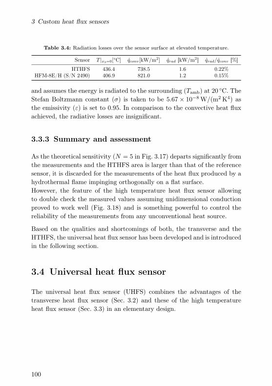
3 Custom heat flux sensors
Table 3.4: Radiation losses over the sensor surface at elevated temperature.
Sensor T |x3=0[C] qconv[kW/m2] qrad [kW/m2] qrad/qconv [%]
HTHFS 436.4 738.5 1.6 0.22%HFM-8E/H (S/N 2490) 406.9 821.0 1.2 0.15%
and assumes the energy is radiated to the surrounding (Tamb) at 20 C. TheStefan Boltzmann constant (σ) is taken to be 5.67× 10⁻⁸ W/(m2 K4) asthe emissivity (ε) is set to 0.95. In comparison to the convective heat fluxachieved, the radiative losses are insignificant.
3.3.3 Summary and assessment
As the theoretical sensitivity (N = 5 in Fig. 3.17) departs significantly fromthe measurements and the HTHFS area is larger than that of the referencesensor, it is discarded for the measurements of the heat flux produced by ahydrothermal flame impinging orthogonally on a flat surface.However, the feature of the high temperature heat flux sensor allowingto double check the measured values assuming unidimensional conductionproved to work well (Fig. 3.18) and is something powerful to control thereliability of the measurements from any unconventional heat source.
Based on the qualities and shortcomings of both, the transverse and theHTHFS, the universal heat flux sensor has been developed and is introducedin the following section.
3.4 Universal heat flux sensor
The universal heat flux sensor (UHFS) combines the advantages of thetransverse heat flux sensor (Sec. 3.2) and these of the high temperatureheat flux sensor (Sec. 3.3) in an elementary design.
100

3.4 Universal heat flux sensor
3.4.1 Construction and description
The sensing element of the UHFS is solely built with thermoelectric ma-terials. The central 800 µm thick cylindrical pad (Alumel R©) is prepared bywater cutting and is laser welded to its three lead wires (Fig. 3.19(a)). Twoof which consist of Chromel R© and are connected across the 800 µm thickpad. The last one is connected to the cold side of the pad and is made ofAlumel R©. This way the temperature across the pad is known as well as adifferential voltage between the twin Chromel R© leads. The differential volt-age is calibrated similarly as the two heat flux sensors previously presentedand the mean pad temperature is used to account for the variation of thesensitivity with temperature.
The substrate of the universal heat flux sensor is a 10mm in diameter ×
6mm ceramic substrate (Al995) manufactured with precision by diamondmachining (grinding and drilling). It serves as an electrical insulator to amounting guard made in Kovar R©. The sensing element is soldered undervacuum to its ceramic substrate and the latter is soldered to the Kovar R©.In this way it can be mounted in a similar housing as the transverse sensoror the high temperature heat flux sensor for calibration and measurementpurposes.
Theoretical sensitivity
Similarly to the high temperature heat flux sensor, the sensitivity of theuniversal heat flux sensor can be expressed as:
S =SAl/Crl
kAl(3.10)
where SAl/Cr is the Seebeck coefficient of an Alumel R©-Chromel R© junction,l is the thickness of the Alumel R© pad (800 µm) and kAl is the thermal con-ductivity of Alumel R©. From Eq. (3.10) the sensitivity can be increased bymanufacturing thicker sensors at the expense of increasing the sensor timeconstant and radial heat losses. Based on the different material propertiesdepicted in Fig. 3.1, the sensitivity of the universal heat flux sensor is cal-culated and the results are presented in Fig. 3.20. For a heat flux in the
101
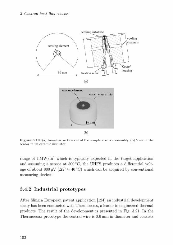
3 Custom heat flux sensors
cooling
channelssensing element
ceramic substrate
Kovar®
housingfixation scew90 mm
(a)
(b)
Figure 3.19: (a) Isometric section cut of the complete sensor assembly. (b) View of thesensor in its ceramic insulator.
range of 1MW/m2 which is typically expected in the target applicationand assuming a sensor at 500 C, the UHFS produces a differential volt-age of about 800 µV (∆T ≈ 40 C) which can be acquired by conventionalmeasuring devices.
3.4.2 Industrial prototypes
After filing a European patent application [124] an industrial developmentstudy has been conducted with Thermocoax, a leader in engineered thermalproducts. The result of the development is presented in Fig. 3.21. In theThermocoax prototype the central wire is 0.6mm in diameter and consists
102

3.4 Universal heat flux sensor
0 200 400 600 800 1000
temperature, T [C]
0
1
2
3
4
5
6
7
8
9
sen
siti
vit
y,S
UH
FS[µ
Vm
2/k
W]
ETH prototype
Thermocoax prototype
Figure 3.20: Theoretical sensitivity of the universal heat flux sensor as a function oftemperature. The ETH and the Thermocoax prototypes are presented.
5.3 mm
5.6 mm Chromel®
Alumel®
Figure 3.21: (a) Schematic principle of the Thermocoax prototype with dimensionsbetween the thermoelectric junctions. (b) X-Ray scan.
103
3 Custom heat flux sensors
of Alumel R©, as the twin Chromel R© wires are 0.45mm in diameter. Theinsulator between the universal heat flux sensor and the 3mm in diameterInconel 600 sheath is MgO, which thermal conductivity is similar to thatof alumina [125]. Because of the higher thermal conductivity of Alumel R©
and the larger wire diameter, heat predominantly flows through the centralwire allowing an accurate measurement of the axial temperature difference,respectively the heat flux.
3.4.3 Summary and assessment
An elementary heat flux sensor design built exclusively with thermoelectricmaterials is investigated. The sensor merges the advantages of both sen-sors previously presented at the expense of a limited sensitivity (Fig. 3.20).However, considering the electronic presently available, this is a minor con-cern.
In the end, all preliminary investigations lead to the common and positiveconclusion that this sensing principle works and should sustain operationin supercritical water.
3.5 Closing remarks
In the context of the heat flux sensors development, different concepts havebeen evaluated and one transverse heat flux sensor has operated successfullyin close proximity to a hydrothermal flame. Hence, proving the robustnessand enhanced chemical compatibility of nickel alloys in contact with super-critical water. Through these tests, shortcomings of this sensor principlehave been detected and it has been determined that a symmetric sensor ismandatory. Thus, a sensor from Virginia Tech has been implemented andconvective calibration runs were performed. Discrepancies between mea-surements and theory as well as deviations in cross sectional area betweenthe high temperature heat flux sensor and the reference microsensor, leadto discard this sensor for the intended measurements. However it broughtup an essential characteristic every heat flux sensor should have, the pos-
104

3.5 Closing remarks
sibility to double check the values by a simple means (e.g. unidimensionalconduction).
Based on the solid experience acquired in sensor construction, concept eval-uation and testing, the universal heat flux sensor has been conceived, lead-ing to a European patent. Following a development study involving in-dustry, the first universal heat flux sensors of industrial quality have beensuccessfully constructed and are now available for thorough characteriza-tion, calibration and measurements. The simple and reliable concept onwhich this sensor is based is very promising in different applications in-volving harsh environment and demanding conditions, such as in internalcombustion engines and in turbomachinery applications.
105


4 Wet flame-jet spallation
drilling facility
In this chapter, the high pressure facility used to perform the core exper-imental work is introduced. The facility is a scale up of a former setuppresented in the work of Weber [126] and has been built and commissionedby Stathopoulos [71]. As it was initially tailored for the study of continu-ous turbulent diffusion hydrothermal flames, the setup has been retrofittedthroughout this work to enable the demonstration of wet flame-jet drillingat supercritical pressure. The focus of this chapter is on the description andfunctioning of the updated setup.
4.1 Process lines
This facility occupies a space of 70m3 on two floors (Fig. 4.1). It consistsof four main fluid networks leading to the wall cooled hydrothermal burner(WCHB-4), core of the experimental setup. Two high pressure plungerpumps (WP-1, WP-2) ensure redundancy of the cooling water. A triplehead metering membrane pump (FP-1) pressurizes the fuel - an aqueousethanol mixture (wEtOH wt.%) - as two gas boosters pressurize the oxy-gen (OC-1). Two electrical heaters (HX-1, HX-2) serve to preheat the fueland the oxygen streams to the desired temperatures before their mixingand subsequent ignition by a custom made heating coil (Ch. 5). The vesselpressure can be adjusted between 50 bar and 260 bar by throttling a triplestem needle valve (RV-10). The effluent stream leaving the pressure ves-sel is mixed with the water provided by one water pump (CW 3) to coolthe mixture well below its flash point before the back pressure regulator
107

4 Wet flame-jet spallation drilling facility
(RV-10). Details of the different process lines are presented in the following.
Oxygen
Heater
HX-2
Back pressure
regulator RV-10
Oxygen
compressor OC-1
Fuel
CW 1
DI water
CW 3
Fuel
CW 2
Heater
HX-1O
2
FMI-1
PIC-5
Fuel pump
FP-1
Water pump
WP-1
3WV-1
FC-2
DI
water
FMI-2
2nd floor
TIC-2
TIC-1
FMIC-1
WCH
B-4
Water pump
WP-2
Figure 4.1: Simplified scheme of the wet flame-jet spallation drilling facility presentingonly its major components [71].
4.1.1 Fuel
The fuel is supplied with ethanol from three plastic tanks having a cumu-lative capacity of 120L and located about 3m above the three-way valve(3WV-1 in Fig. 4.3). Deionized water is delivered at a pressure of 6 bar(g) inthe hall where the facility is located and its pressure is reduced to 1 bar(g)
by a pressure reduction valve (PRV-1) - limiting thereby the pressure cou-pling of the delivery line and the water used to prepare the fuel mixture.This improves the control of the density by the 3WV-1. In the three-wayvalve, deionized water and ethanol are mixed to produce the fuel mixtureflowing through a triple head, variable speed, metering membrane pump(FP-1) - able to pressurize up to 100 kg/h of fuel to 350 bar. The mass flowdelivered by the pump is controlled by the frequency of its 3 kW electro-
108

4.1 Process lines
Figure 4.2: Wet flame-jet spallation drilling facility [71].
motor and the stroke length of its plungers. The latter can be adjustedmanually on each head. Then, the fuel flows through a pressure dampener(PD-1 in Fig. 4.3) before a piezo resistive pressure indicator (PI-1) and abursting disc (BS-3) set to 350± 10% bar. The flow is then monitored by aCoriolis flow meter (FMI-1 in Fig. 4.3) the amplitude signal of which (i.e.mass flow) is used to control the frequency of the FP-1 electro motor andthe frequency signal of which (i.e. density) is used to control the positionof the 3WV-1 and adjust the fuel composition. The fuel flows then througha non-return valve (NRV-5) before the 65 kW heating unit, a second valve(NRV-6) and its injection in the pressure vessel.
The density measured by the Coriolis flow meter (FMI-1) is linked to theethanol content in the fuel by calibrating the density of known ethanol-water mixtures at the working pressure. Such a calibration curve, measuredat 260 bar while 20 kg/h of mixture is flowing through the Coriolis flowmeter is presented in Fig. 4.4.
109
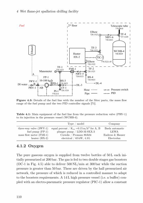
4 Wet flame-jet spallation drilling facility
PD-1
PI-1770.614
FMI-1
FP-1
10-100 kg/h
TF-2720.1523
BS-4720.5023
Elbow720.1522
Elbow720.1522
Heater
HX-2
TF-4727.1220
Telescopic tube779.0010
NRV-5720.8323
BS-3720.5023
TF-1720.1523
Manometer
Eth
anol
3WV-1
DI water
NRV-6720.4421
TF-3720.1523 WCHB-4
740.8029
DL-4DL-3
CF-1720.1524 Hose
Pipe
Pressure switch
PID
PRV-1
B
A
AB
Fuel 2nd floor
770.5221-45
TIC-2
Figure 4.3: Details of the fuel line with the number of the Sitec parts, the mass flowrange of the fuel pump and the two PID controller signals [71].
Table 4.1: Main equipment of the fuel line from the pressure reduction valve (PRV-1)to its injection in the pressure vessel (WCHB-4).
Type / model Company
three-way valve (3WV-1) equal percent / Kvs =0.15m/h3 for A, B Baelz automaticfuel pump (FP-1) plunger pump / LDD-M-9XX-3 LEWA
mass flow meter (FMI-1) Coriolis / Promass 80A04 Endress & Hauserheater (HX-2) electrical / 65 kW, 4.3L Electrolux
4.1.2 Oxygen
The pure gaseous oxygen is supplied from twelve bottles of 50L each ini-tially pressurized at 200 bar. The gas is fed to two double stages gas boosters(OC-1 in Fig. 4.5) able to deliver 500NL/min at 300 bar while the suctionpressure is greater than 50 bar. These are driven by the hall pressurized airnetwork, the pressure of which is reduced in a controlled manner to adaptto the boosters requirements. A 14L high pressure vessel (i.e. a buffer) cou-pled with an electro-pneumatic pressure regulator (PIC-1) allow a constant
110

4.1 Process lines
0 10 20 30 40 50
fuel concentration, w [wt.%EtOH]
930
940
950
960
970
980
990
1000
1010
1020
fuel
den
sity
,ρ[k
g/m
3]
least-squares fit
Figure 4.4: Density of the fuel measured by the Coriolis flow meter FMI-1 at 260 barfor different ethanol content. The reproducibility of the measurements is ±0.5 kg/m3.
inlet pressure in the gas line. Note that the setpoint of PIC-1 is one of themost important parameter to stabilize the system during its operation atelevated pressure.
The compressor is protected from over-pressure by a bursting disc (BS-1) and the stream is directed to a thermal mass flow controller (FMIC-1)which controls the flow (0 < VO2
< 600NL/min). The stream flows througha specially designed non-return valve (NRV-3) before its pressure is indi-cated by a manometer. Subsequently a bursting disc (BS-2) is implementedto protect the system locally. The gas is then directed to the upper leveland flows through an electrical heater (HX-1) followed by a temperaturemeasurement (TIC-1). To prevent unnecessary thermal fatigue in the line,a stress relieving mechanism is implemented in the pipe downstream of theheater. A second in-line non-return valve (NRV-4) follows and the super-critical oxygen is injected in the vessel head through a single port.
Every component of the oxygen line is carefully cleaned following ASTM
111

4 Wet flame-jet spallation drilling facility
Hose
Pipe
Pressure switch
PID
TF-3720.1423
BS-1720.5023
Heater
HX-1
NRV-4720.4423-1-O2
TF-4720.1423
OC-1
0-500 NL/min
PIC - 1
O2
BS-2720.5023
TF-1720.1423
FMIC-1V-22710.3230-O2
Manometer
V-1
N2 V-2
O2
F-3
SF-1729.2230-1
SF-2729.2230-1
WCHB-4740.8029
DL-1
DL-2
TIC-1
NRV-3720.4421-O2
2nd floorOxygen
Figure 4.5: Details of the oxygen line with the number of the Sitec parts, the volumetricrange of the compressor (OC-1) and the two PID controller signals [71].
recommendations for oxygen service [127] prior to their installation in theline or after maintenance. The sequence of the non-return valves with re-spect to the manometer (Fig. 4.5) permits to detect leakages upstream ofNRV-3 before the mass flow controller (FMIC-1) is flooded by the aqueousstream.
Relevant information about the main equipment of the oxygen line is sum-marized in Tab. 4.2.
112

4.1 Process lines
Table 4.2: Main equipment of the oxygen line from the gas bundle to its injection inthe pressure vessel.
Type / model Company
compressor (OC-1) double stage gas boosters / DLE 30-2 Maximatorfront pressure (PIC-1) linear / Kvs = 0.05 SCFM Tescom
mass flow controller (FMIC-1) thermal / F-133M-AAD-55-V Bronkhrostcontrol valve (FMIC-1) linear / Kvs = 0.026 Nm3/h of air at STP Badger meter
heater (HX-1) electrical / 11 kW, 0.8L Electrolux
4.1.3 Cooling water
CW 1 and 3
Hose
Pipe
Pressure switch
PID
CW 1DI water
tank (2.5 m3)
V-5 V-6 NRV-7
drinking
water
WP-2
47 L/min
Manometer
Connection
with CW-2
Connection
with CW-2
CF-5
CF-3
SV-1
Pswitch 2
PI-2
Pswitch 3
PI-3
CF-2
BS-5
V-10
V-12
FC-2
DL-3
V-7710.3112
B
Manometer
V-32
WCHB-4740.8029
CF-1
CW 3
CF-4
CW 1
TF-1TF-2 NRV-9FMI-2
PD-2A
NRV-8
Figure 4.6: Details of the cooling water lines 1 and 3 with the number of the Sitec parts,the mass flow of the WP-2 and two pressure switches connected to V-10 and V-12 [71].
The cooling water is supplied from the 6 bar(g) deionized line of the buildingand fills a 2.5m3 storage tank (i.e. buffer) which permits to run the waterpump 2 (WP-2 in Fig. 4.6) for about 50min in case no water is suppliedby the building line anymore. The water stream is then pressurized by the37 kW high pressure plunger pump (WP-2) equipped with a booster beforethe suction flange and a safety valve set to 350 bar on the pressure side.A cross junction connected to a pressure dampener (PD-2) separates theflow between the facility and a recirculation line. Note that the pressuredampener is set to about 80% of the operating pressure to absorb the
113

4 Wet flame-jet spallation drilling facility
fluctuations generated by the three plungers of the pump. The water inthe recirculation line flows through a pressure indicator and switch (PI-2)and then through a manually actuated micro metering valve (V-7). Thelatter permits to regulate the pressure drop of the line and to control theamount of water which flows through the facility. Its nominal setpoint is1mm. The greater the pressure drop across V-7, the more water flows tothe facility but V-7 cannot be completely opened, because the temperatureof the water entering the pump will start to rise. The water directed to thefacility flows through a series of three cross fittings (2 to 4) connected to:
CF-2 The cooling water 2 lines (CW 2) and the drinking water lineof the building - in the absence of electricity,
CF-3 A safety valve (SV-1) and the cooling water line 3 and,
CF-4 The manometer and a bursting disc (BS-5).
The connection to the cooling water 2 line is a safety measure and V-10and V-12 remain open as long as the pressure switches, controlled by thevalue of the three pressure sensors (PI-2, 3, 4), are open. The hardwareswitches controlled by the resistance of a potentiometer will close as thethree pressure sensors indicate a value above a threshold. For the opera-tion at 260 bar, this value is 250 bar. The cooling water 3 line flows thenthrough a non-return valve (NRV-8) before its mixing with the effluent ofthe pressure vessel (Fig. 4.8).
Downstream of the cross-fitting 4 the water flows through a Coriolis massflow meter (FMI-2) which signal is used to actuate the needle valve (FC-2)and control the mass flow of cooling water through the combustion cham-ber (CW 1). Before its injection in the combustion chamber, the streamflows through a T-fitting connected to: the manometer, a pressure sensor(PI-3) and a non-return valve (NRV-9) followed by a cross-fitting, con-nected through V-12 to the cooling water 2 line (CW 2) and splitting thecombustion chamber cooling water into two streams.
Obviously, the greater the pressure drop across FC-2, the less water iscooling the combustion chamber (CW 1) and the more water is directlyquenching the effluent stream of the pressure vessel (CW 3). The mini-mum flow tolerated through CW 1 is 200 kg/h before the facility enters its
114
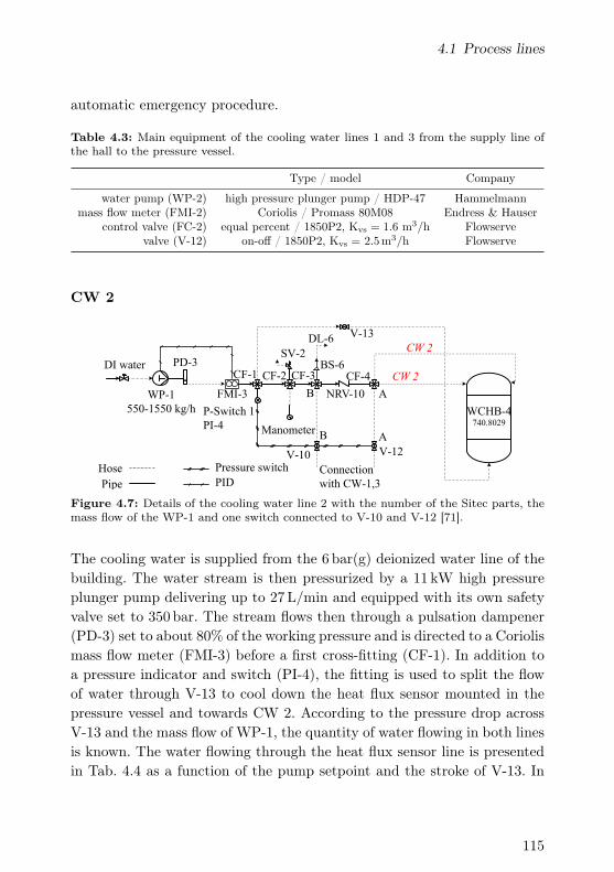
4.1 Process lines
automatic emergency procedure.
Table 4.3: Main equipment of the cooling water lines 1 and 3 from the supply line ofthe hall to the pressure vessel.
Type / model Company
water pump (WP-2) high pressure plunger pump / HDP-47 Hammelmannmass flow meter (FMI-2) Coriolis / Promass 80M08 Endress & Hauser
control valve (FC-2) equal percent / 1850P2, Kvs = 1.6 m3/h Flowservevalve (V-12) on-off / 1850P2, Kvs = 2.5m3/h Flowserve
CW 2
Hose
Pipe
Pressure switch
PID
DI water
V-12
PD-3
FMI-3WP-1
550-1550 kg/h
SV-2
V-10
Connection
with CW-1,3
CF-4
P-Switch 1
PI-4 Manometer
CF-1
V-13
CW 2
A
AB
B
CW 2CF-3CF-2
DL-6
WCHB-4740.8029
NRV-10
BS-6
Figure 4.7: Details of the cooling water line 2 with the number of the Sitec parts, themass flow of the WP-1 and one switch connected to V-10 and V-12 [71].
The cooling water is supplied from the 6 bar(g) deionized water line of thebuilding. The water stream is then pressurized by a 11 kW high pressureplunger pump delivering up to 27L/min and equipped with its own safetyvalve set to 350 bar. The stream flows then through a pulsation dampener(PD-3) set to about 80% of the working pressure and is directed to a Coriolismass flow meter (FMI-3) before a first cross-fitting (CF-1). In addition toa pressure indicator and switch (PI-4), the fitting is used to split the flowof water through V-13 to cool down the heat flux sensor mounted in thepressure vessel and towards CW 2. According to the pressure drop acrossV-13 and the mass flow of WP-1, the quantity of water flowing in both linesis known. The water flowing through the heat flux sensor line is presentedin Tab. 4.4 as a function of the pump setpoint and the stroke of V-13. In
115

4 Wet flame-jet spallation drilling facility
case the facility is used without heat flux sensor, a blind is installed andthe cross junction is reduced to a T-junction.
Table 4.4: Water pump (WP-1) and valve (V-13) setpoints to adjust the cooling ofthe heat flux sensor in the pressure vessel. The details of the calibration are reportedin [128].
WP-1 [kg/h] V-13 [%] mHFS [kg/h] WP-1 [kg/h] V-13 [%] mHFS [kg/h]
550
0 309.1
650
0 319.910 297.0 10 310.120 268.2 20 284.630 missing 30 258.940 214.3 40 226.150 192.8 50 205.960 158.8 60 168.370 125.8 70 133.880 97.8 80 104.190 59.3 90 63.6100 27.8 100 29.9
600
0 312.5
700
0 323.610 302.0 10 314.720 276.1 20 290.430 249.4 30 261.240 220.7 40 228.450 199.1 50 207.260 164.1 60 170.670 129.5 70 136.480 101.6 80 101.690 62.9 90 65.4100 29.0 100 30.3
The water exiting the first cross-fitting (CF-1) is directed towards a secondcross (CF-2), connected to a safety valve (SV-2) and the manometer. Down-stream, a third cross-fitting connects the line with V-10 and a bursting disc(BS-6) set to 350 bar ± 10%. Thereafter, a non-return valve (NRV-10) isinstalled and the flow is directed to a last cross where it is connected acrossV-12 to the CW 1, 3 lines and split into two streams towards the coolingmantle of the pressure vessel (CW 2).
116

4.1 Process lines
Table 4.5: Main equipment of the cooling water line 2 from the supply line of the hallto the pressure vessel.
Type / model Company
water pump (WP-1) high pressure plunger pump / HDP-27 Hammelmannmass flow meter (FMI-3) Coriolis / Promass 80M08 Endress & Hauser
valve (V-10) equal-percent / 1850P2, Kvs = 2.5m3/h Flowservevalve (V-13) linear / 1850P2, Kvs = 0.25m3/h Flowserve
4.1.4 Effluent
Hose
Pipe
Pressure switch
PID
RV-10
CW 3
F-2
PT-1
TIAH-3
To sink
TIAH-4
770.5212
Elbow725.1322
770.5221
Elbow720.1412
CF-3BS-8
Elbow725.1322
WCHB-4740.8029
CF-2
SF-1725.2240
CF-1
PIC-5
DL-8
F-1F-1
TF-1
TF-2
TF-3
TIA
H–
1T
IAH
–2
SV-3
NRV-8
Elbow725.1322
Elbow720.1412
Effluent
Figure 4.8: Details of the effluent lines with the number of the Sitec parts [71].
The effluent lines describe the outflows of the pressure vessel, which leavethe vessel into two times two streams. The upper streams correspond tothe outlet of the main volume (Fig. 4.9). Both flow through a coarse filter(F-1) with a cut-off of 1mm to remove large rock chips, before their mix-ing in the cross-fitting (CF-1) where temperature is measured (TIAH-3).
117

4 Wet flame-jet spallation drilling facility
The lower streams correspond to the outlet of the cooling mantle (CW2, fed by WP-1 in Fig. 4.7) and are merged together in the cross-fitting(CF-2) where temperature is measured (TIAH-4). The resulting streamsare mixed in the cross-fitting (CF-3) also connected to a bursting disc(BS-8) and are directed to a T-junction (TF-1) connected to a safety valve(SV-3). This stream flows through a fitting and is then quenched in a T-junction (TF-2) with the CW 3 stream. The result, about 3500 kg/h ismostly composed of water with traces of combustion products and some-times spalls flows through a micro-meter filter with a cut-off of 40 µm (F-2)before a T-junction (TF-3) where a combined pressure and temperaturesensor (PT-1) is connected. The mixture flows through the back-pressureregulator (RV-10) of the facility and is directed through a hose to the sinkof the hall.
Table 4.6: Main equipment of the effluent lines from the pressure vessel to the sink ofthe experimental hall.
Type / model Company
pressure vessel 740.8029 / 5.83L Sitecin-line filter (F-1) coarse / 1mm cut-off Sitecfilter tower (F-2) fine / 40 µm cut-off Mahle
triple stem valve (RV-10) linear / 110P3, Kvs(i=1,2,3) = 0.47, 0.88, 2m3/h Flowserve
4.2 Pressure vessel
The wall-cooled hydrothermal burner (WCHB-4) is a pressure vessel of 4th
generation (Fig. 4.9) manufactured by Sitec and tailored for the study ofturbulent diffusion hydrothermal flames [71]. A concise review of the pre-vious designs (WCHB-1, 2, 3) is presented by Augustine and Tester [129].The vessel has a volume of 5.83L and its pressure bearing walls are de-signed to sustain 650 bar at a temperature of 500 C. It consists of a mainvolume (Ø = 100mm) surrounded by a cooling jacket (Ø =140mm). Bothare separated by a cylinder perforated with 12 holes to balance pressure.
118
4.2 Pressure vessel
CW 1
exit to
TIAH-3
combustion
chamber
confining
assembly
rock
probe
exit to
TIAH-4
254 mm
Figure 4.9: Isometric breakout view of the pressure vessel in drilling operation mode.The rock is positioned to face the tip of the combustion chamber, where the flame-jetexits.
4.2.1 Mass and energy balance
A simple mass and energy balance to get an insight in the jet temperatureand its velocity at the exit of the combustion chamber is presented in thefollowing. The control volume is located inside the pressure vessel and is
119

4 Wet flame-jet spallation drilling facility
represented in Fig. 4.10. The combustion products (mF ) and the coolingwater of the combustion chamber (CW 1) enter the control volume andare assumed to exit at a temperature TE corresponding to TIAH-3. Theheat exchange to CW 2 is discarded and the control volume is consideredadiabatic. Additionally, a water-jet is used to mimic the flame-jet whichgreatly simplifies the calculations with moderate impact on the system asthe combustion products consist mostly of water (2.5.3). Remember thatwhen wEtOH = 30 wt.%, the combustion products consist of 65 wt.% water(Fig. 2.19). Similarly as in 2.5.3, the properties of pure water are gatheredfrom Refprop R© (v9.1) [130].
mF
hF
mCW1
hCW1
mE
hE
control volume
Q
uF
exit at
TIAH-3
combustion chamber
Figure 4.10: Illustration of the control volume where the energy and the mass balanceare solved.
The resulting coupled system of equations is:
mF + mCW1 = mE
mFhF (TF ) + mCW1hCW1(TCW1) = mEhE(TE)(4.1)
where the unknowns are the enthalpy of the hot water-jet (hF ) and themass flow exiting the control volume (mE). It results a closed system withno degree of freedom.
120

4.2 Pressure vessel
4.2.2 Jet temperature – sensitivity analysis
Using Eqs. (4.1), a sensitivity analysis on the outlet temperature (TE) ofthe control volume for discrete values of the water-jet mass flow (mF ) isperformed for the conditions presented in Tab. 4.7. This analysis is impor-tant to have an educated guess about the exit temperature of the flame-jetknowing the mass flow fed to the combustion chamber (process parame-ter) and monitoring the temperature at the outlet of the pressure vessel(TIAH-3).
Table 4.7: Parameters of the sensitivity analysis.
Parameter Value
water-jet mass flow, mF 40 ≤ mF ≤ 100 kg/hCW 1 mass flow, mCW1 350 kg/hCW 1 temperature, TCW1 298 Kexit temperature, TE 298 ≤ TE ≤ 500 K
The water-jet temperature (TF ) as a function of the control volume exittemperature (TE) is presented in Fig. 4.11 for different mass flow (mF ).
It is important to mention that the water-jet temperature (TF ) presentedhere is likely to be lower than the one of the flame-jet (for the same mF andTE) because: (i) the system is considered adiabatic with no heat transfer tothe surrounding and, (ii) the enthalpy of a pure water-jet is higher comparedto the one of the flame-jet at the same temperature.Indeed, the temperature of the cooling water 2 at the exit of the pressurevessel cooling mantle is measured by TIAH-4. For the default CW 2 massflow of 600 kg/h, temperatures in the range of 80 C are common for a flamepower of 132 kW. Following a simple mixing rule to express the mixtureenthalpy (hmix = 0.3hCO2+0.7hH2O), the difference between the enthalpyof the mixture and that of pure water increases with temperature to reacha deviation of about 17% at 5000K.
121

4 Wet flame-jet spallation drilling facility
0 50 100 150 200 250 300 350 400
exit temperature, TE [C]
0
500
1000
1500
2000
2500
wat
er-j
ette
mp
erat
ure
,T
F[
C]
40kg/h
60
80
100
Figure 4.11: Temperature of the water-jet (TF ) at the outlet of the combustion chamberas a function of its temperature when it exits the control volume (TE) for different massflow (mF ). The dash-lines represent the critical temperature of water (373.95 C).
throat
100 mm
main volume
fuel
O2
Figure 4.12: Isometric breakout view of the combustion chamber generating the flame-jet.
4.2.3 Jet velocity – order of magnitudes analysis
The water-jet velocity (uF ) as it exits the combustion chamber throat(Fig. 4.12) is calculated based on its mass flow (mF ), its density (ρ) and
122

4.2 Pressure vessel
the diameter (d) according to Eq. (4.2):
uF =4mF
ρ(TF )πd2. (4.2)
It results that the most important parameter to adjust the water-jet ve-locity is the combustion chamber throat diameter (d). The importance ofthe different parameters is best illustrated in Fig 4.13. For the purpose of
0 500 1000 1500 2000 2500
water-jet temperature, TF [C]
10−1
100
101
102
103
wat
er-j
etvel
oci
ty,
uF[m
/s]
100kg/h80 40
10080 40
10080 40
Ø10 mm
Ø5 mm
Ø2.5 mm
Figure 4.13: The velocity (uF ) of a water-jet accelerated through a throat with adiameter (d) as a function of its temperature (TF ) and for different mass flows (mF ).
flame-jet drilling, a large flame-jet velocity is favored to enhance the heattransfer to the rock. A small throat diameter will concentrate the heat andmaximize the intensity of the thermal stresses.
123

4 Wet flame-jet spallation drilling facility
4.3 High pressure positioning systems
To position the measurement probes inside the pressure vessel, two tele-scopic tubes fixed on the lower and upper flanges of the vessel and drivenby linear motors are used (Fig. 4.14). Typically, the lower positioning de-vice serves to move rock probes (Ch. 6), an axial thermocouple (Secs. 5.2and 5.3) or a heat flux sensor (Sec. 3.2). On the other hand, the upperpositioning device is employed to move the heating coil used to ignite thehydrothermal flames (Secs. 5.2 and 5.3).The positioning accuracy of the linear actuators is 0.1mm and the tele-scopic tubes have been designed by Sitec to sustain 300 bar at temperaturesup to 420 C.
upper
position
lower
position
pressure vessel
sealing point
for the heating coil
100 m
m
(a) Upper positioning device.
350 m
m
sealing point
or cooling water
thread for rock or
heat flux sensor
pressure
vessel
upper
position
lower
position
(b) Lower positioning device.
Figure 4.14: The telescopic tubes used to position the probes in the pressure vessel.The accuracy of the positioning is 0.1mm.
124

4.4 Electronic and control
4.4 Electronic and control
The control and monitoring of the setup has been developed and imple-mented by the company M+S Automation Technology [71]. It is based ona programmable logic controller (PLC) from Saia Burgess with a dedicatedIP address for external access as well as data monitoring and sampling.The objective of this section is not to present the exhaustive electrical dia-gram established by M+S but to introduce the architecture of the hardwareand the logic to control and operate the setup (Fig. 4.15). All pressure, tem-
PIC-1
PC
Labview card
Moxa hub Saia (PLC)
FMIC-1
Wago
LI-1
LI-2
Frequency converter-1
Frequency converter-2
HX-1 HX-2
V-10
V-12
P&S-1
P&S-2
P&S-3
PI-1
AI
USB
RJ45
High freq. AOProfibus
PI-5AI
Beckhoff
Igniter V
Igniter
power supply
AI
FP-1
WP-1WP-2
Wago I/O
system
Control cabinet
GUIInternet FMI-3
FMI-1
FC-2
F-2
PT-1
TIAH-1,2,3,4
RV-10
Figure 4.15: Architecture of the control system of the wet flame-jet spallation drillingfacility.
perature sensors and control valves of the setup are physically connectedto the different modules of a Wago input/output system which is locatedon the ceiling below the pressure vessel floor. There the DI (digital inputs)and AI (analog inputs) of the different sensors are sent over to the PLCas the AO (analog outputs) and DO (digital outputs) are transmitted tothe devices. Besides FMIC-1 (Fig. 4.5) where the Badger meter controlvalve (Tab. 4.2) is directly pneumatically connected to the thermal massflow controller, all values of the software PID controllers are presented in
125
4 Wet flame-jet spallation drilling facility
Tab. 4.8. Note that FMIC-1 triggers the position of the normally closedvalve with a 4 . . . 20mA, regulated by its internal PID controller.Based on the constant data flow reaching the PLC, continuous evaluationof a series of conditions is performed triggering the response of the setupin case one parameter departs from its expected range. For instance if atemperature beyond a certain threshold is recorded by one thermocouplemonitoring the facility, the PLC enters the irreversible emergency proce-dure (4.5.2). These predefined tasks are written as instructions list andare dedicated to machine safety, respectively to the automatic startup andshutdown of the facility.From Fig. 4.15, the communication between the PLC, the Wago, the lin-ear actuators (LI-1, 2) and the Bronkhorst thermal mass flow controller(FMIC-1) is performed digitally using a Profibus-DP protocol, where thePLC is the master and the others are slaves. The cooling water pump WP-2
Table 4.8: PID controller values. The differential component for all controllers is trivial.
Proportional Integral Dead band
RV-10 0.009 1.2 2FC-2 0.155 0.71 -3WV-1 0.7 100 -
is controlled via a digital signal, switching on and off its electro motor atthe nominal frequency and flow control is ensured by throttling manuallythe metering needle valve in the recirculation line (4.1.3). A digital outputof the PLC defines the state of WP-1 (on/off). Its setpoint is conveyed byan analog signal (4 . . . 20mA) which is internally controlled by the corre-sponding frequency converter based on the feedback information providedby FMI-3. Communication between the PLC and the frequency converterof the fuel pump (FP-1) is performed similarly but using the informationfrom FMI-1. Communication with both heaters (HX-1, 2) is achieved witha digital output and analog signals (4. . . 20mA) transmitting the setpointsfrom the PLC to the two external control racks.The PLC from Saia is equipped with internal memory sticks, allowing toupload locally the compiled program and the pages displayed by the GUI.It has its dedicated touch panel for operation without any computer. This
126

4.5 Safety
means that the control and the electronic of the facility are self-sustainedand independent. Additionally, low frequency monitoring of the main pro-cess parameters is performed by the PLC and saved locally on the memorysticks; these data can be downloaded anytime from another machine.As the highest sampling frequency of the data monitored using the pro-prietary software of the PLC is 1Hz, it is additionally equipped with twomodules having four analog outputs each. These outputs are connectedto a Labview card (Fig. 4.15) enabling the monitoring of specific processparameters with a higher sampling frequency. Finally, the Beckhoff I/Omodule (Fig. 4.15) is equipped with different terminals allowing voltages,current, resistance measurements and the connection of K-Type thermo-couples. This subsystem is independent of the PLC and is used to controlthe heating coil and acquire its data (Secs. 5.2 and 5.3).
In the end, the industrial PLC from Saia is a guarantee for a high reliabilityof the system, behaving independently from any computer limiting therebycritical situations. Additionally, the versatile Beckhoff I/O module providesthe necessary flexibility in data acquisition.
4.5 Safety
Safety is a critical concern in a large facility involving long residence time(≥ 10min) of concentrated fuel and pure oxygen, simultaneously at highpressure (i.e. up to 260 bar) and temperature (i.e. up to 2000 C).
4.5.1 Maintenance and guidelines
Keeping the setup clean and tidy is the first step to enhance safety dur-ing operation and enable the operator to react accordingly in case anythingunexpected happens. Additionally, the wet flame-jet spallation drilling fa-cility requires periodic control of its components and strict dismantling andinstallation procedures. An overview of the current maintenance and con-trol measures is given in the following, starting with recommended periodicinspections:
127

4 Wet flame-jet spallation drilling facility
• Control the oil level of the positive displacement pumps (WP-1, WP-2and FP-1) and refill as necessary. Note that an oil changed has to becarried out every 1000 h of operation.
• Check the oxygen gas boosters (OC-1) for oil and dust. Surfaces incontact with oxygen must remain perfectly clean.
• Control each high pressure valve near their stem for leakages, espe-cially after long stop. Tighten the cap to squeeze the glide rings asnecessary to reachieve sealing.
• Control the wear out of the high pressure hydraulic rubber hoses.These components are aging and have to be changed if flaws arespotted, or at least every 6 years according to DIN 20066.
• Control the pressure of the dampener (PD-1,2,3) and refill as neces-sary. The dampening pressure should be around 80% of the workingpressure for best attenuation.
In addition to these periodic checks, whenever fittings are disassembled ornew pieces are mounted, care must be taken to reassemble as before. Spe-cial care has to be taken with the fittings exposed to high temperatures, inorder to prevent galling. Typically, hard and milder alloys are in contact tolimit the process.Generally, threads should be torqued up, but (i) without exceeding recom-mended service values (A.1.1), (ii) after greasing every high pressure cylin-drical threads (mostly Sitec fittings) or, (iii) after applying Teflon tape onconical NTP threads. Fittings directly in contact with oxygen are cleanedfollowing ASTM recommendations for oxygen service [127] and kept grease-free. Thorough pressure tests including leakages check using appropriatedetection sprays are necessary every time the system is opened. The gasline and the pressure vessel should be purged using nitrogen at the end ofeach experimental day and stagnant water in the facility should be avoidedin full measure. Storing high pressure oxygen in the 14L buffer for morethan a day should be avoided.
128

4.5 Safety
4.5.2 Emergency procedure
Hazard probability is limited owing to the sound design of the setup and in-tensive HAZOP analysis performed by Stathopoulos [71]. Nevertheless, riskstill exists due to the nature of the process potentially leading to extremeconditions in the wall cooled hydrothermal burner. Therefore the PLC con-tinuously monitors a series of process values which are compared to presetthresholds. If a certain value exceeds its limit, the PLC enters a fully auto-matic emergency procedure, where the operator does not have any controlon the setup anymore, besides by switching the main power off. As this iscertainly not recommended, it might be necessary. In that case all pumpsare stopped and valves take their default positions, i.e normally closed ornormally opened, hence releasing pressure rapidly.The steps performed by the PLC during the emergency procedure are listedbelow:
Step 1. Switch off both heaters.
Step 2. Close 3WV-1.
Step 3. Wait 15min.
Step 4. Switch off the compressor (OC-1).
Step 5. Open RV-10.
Step 6. Wait for p ≤ 50 bar.
Step 7. Switch off WP-1, WP-2 and FP-1.
The main idea of the procedure is to initiate the cool down of fuel andoxygen, purge the facility from remaining fuel meanwhile ensuring com-plete oxidation. As the residence time of the fuel in the system is less than10min for a fuel mass flow of 20 kg/h - which is the least flow used - 15min
allow to ensure the system is fuel-free. Afterwards the oxygen compressor(OC-1) is switched off and the pressure released. Once the pressure falls be-low 50 bar, all positive displacement pumps are switched off leading to nearatmospheric pressure conditions in the system. Intense boiling, dependingon the temperatures of the preheaters results but this is typically a sec-ond concern. Besides the automatic monitoring performed by the PLC, theoperator can activate the emergency procedure by pressing one of the mul-
129

4 Wet flame-jet spallation drilling facility
tiple emergency stop buttons, easily accessible around the facility. Notethat this was never performed, besides for testing purposes. During exper-iments, this should be reserved for extreme cases, where the hall has to beevacuated.
4.5.3 Potential improvements
The lack of adequate equipment fulfilling the process requirements increasesthe potential consequences of hazard, e.g. no flame arrestor for high tem-perature, high pressure oxygen service exists. Presently a set of non-returnvalves is used, but these are not designed to prevent flashbacks and do notreact to a sudden temperature increase. In case the oxygen preheater isnot required for future experiments and is decommissioned, proper flamearrestors complying with international safety standard could be mountedand increase the system safety.Presently in case of a pump outage the pressure in the system will suddenlydrop, resulting in RV-10 closing completely in an attempt to maintain thesetpoint. At the next pump stroke, the pressure will rise beyond the burst-ing pressure of the safety disc (350 bar ± 10%) potentially leading to acritical situation. To cope with that, in case of a pump outage the auto-matic control of the back pressure regulator should be temporarily switchedoff for a certain time lapse, e.g. 30 s, giving time to the system to adapt.Depending of the future process requirements, it should be considered tobypass the fuel heater, reducing consequently the quantity of high pressure- high temperature fuel in the facility. Additionally, as the residence timeof the fuel would be reduced by 99%, the reactivity of the system is im-proved significantly. In such a case the emergency exit procedure which isdescribed in 4.5.2 should be reconsidered in agreement with the updatedHAZOP study.
4.6 Closing remarks
The wet flame-jet spallation drilling facility is a large experimental setupbuilt and commissioned by Stathopoulos [71]. It fulfills all the required in-
130

4.6 Closing remarks
dustrial standards in terms of safety, control and equipment. Among othersit permits to simulate the pressure, temperature and fluid dynamic condi-tions in a 2.6 km deep well filled with water. In the course of this work,it has been retroffitted to assess wet flame-jet drilling at supercritical con-ditions. No major problem occurred with the facility during this thesis,proving once more the quality of the design and construction of the setup.In the end, the facility has been used at its full extent, having a combus-tion power of 132 kW at 260 bar. To sustain this flame, 500NL/min ofpure oxygen have been delivered to the combustion chamber, without ma-jor troubles. Finally, the operating instructions for a typical experiment areprovided in A.1.3.
131


5 Hydrothermal flame ignition
and monitoring
In this chapter a series of sensors developed, calibrated and used to igniteand monitor hydrothermal flames is presented. Section 5.1 introduces thedesign and its evolution. These sensors have been initially developed toreduce the experimental time and to solve a practical problem: ignite aflame remotely in a controlled manner with the electrical power possiblyavailable downhole. In the end, other intrinsic benefits are associated withthese hot surface igniters: like the possibility to monitor the combustion,a significant reduction in the number of fittings exposed to heating andcooling cycles and mitigate potential hazards. This is related to a smallervolume of high temperature, high pressure oxygen and fuel in the facility.Sections 5.2 and 5.3 present two sets of measurements performed usingthese sensors and 5.4 briefly concludes this chapter.
5.1 Coil igniter and igniter thermocouple
The coil igniter and the igniter thermocouple describe two generations ofa sensor used to initiate the combustion of hydrothermal oxygen-ethanolflames and atmospheric methane-air flames. Several prototypes of thesehave been constructed. Among others NiCr-60/15, NiCr-80/20 and NiCr-90/10 alloys were considered for the electrical resistance and K-Type ther-mocouple alloys and copper for the lead wires. The assembly of the differ-ent igniters is similar and only the raw materials consisting the heating coiland the leads vary. The manufacturing procedure remained essentially thesame, although some shortcomings have been resolved with time. The coil
133

5 Hydrothermal flame ignition and monitoring
NiCr coilAl
2O
3
Copper or Alumel®
(base-junction)Alumel®
(tip-junction)30 mm
Figure 5.1: Igniter thermocouple consisting of a NiCr coil, a tip leg (AlumelR©) and abase leg. The coil height is about 30mm.
(Fig. 5.1) has a height of 30mm and consists of a wire which diameter iscomprised between 0.35 and 0.4mm. The diameter differs according to theresistivity of its material to maximize the energy dissipated once the systemis powered. Besides maximizing the resistance contribution of the coil, theoverall resistance (coil and leads) is designed to match the characteristicsof the power supply (10A at 65V) at the expected ignition temperature.Each lead wire consists of two pieces and the part near the coil is enclosedin a 400mm long ceramic tube 2.8mm in diameter with two holes, each0.8mm in diameter. The material of these near coil extensions can vary inorder to form different thermoelectric junctions at both ends (tip and basejunction in Fig. 5.1) of the heating wire. Typically Alumel R© is used for thetip leg forming at the same time a sensitive junction. Note that the part ofthe Alumel R© wire passing through the coil is insulated using a 35mm longalumina tube 1.7 × 1.1mm in diameter. The material of the base exten-sion varies for the two different designs presented here. For the original coiligniter which is based on a design presented in [131], Alumel R© is used. Itis chosen because of its low electrical resistivity (27.7 µΩcm at 22 C [92])and its high temperature properties resulting in an extended service life insupercritical water. In the latest version of the coil igniter referred to asigniter thermocouple, copper is used to have a weak thermoelectric basejunction allowing to measure the tip temperature when the sensor is notpowered.
In every design the bare wires fed through the 2.8mm in diameter aluminatube are laser welded to Kapton R© insulated copper wires (AWG20). Thelatter are fed through a high pressure gland (Conax, PL-20-A2-V-XX) toseal the assembly.
134

5.1 Coil igniter and igniter thermocouple
5.1.1 Coil igniter calibration
Resistance calibration
The igniter resistance gives its average temperature provided that: its cal-ibration function is known and, it does not oxidize during an ignition ex-periment.To limit oxidation during calibration an oxide layer is first built in a hightemperature oven (Nabertherm, L 3/11) at 600 C for 8 h. Subsequently thecalibration is performed, similarly as presented by Buckel et al. [132]. Thesetpoint of the high temperature oven is increased in steps of 50 C fromroom temperature to 450 C and steady state measurements are performed.The resistance of the igniter (R) is recorded using a micro-ohm meter (Ag-ilent, 34420A) and transmitted at 5Hz. The corresponding thermocoupletemperature (Toven) are sampled with a 16-bit DAQ at 250Hz. Data arefinally time averaged and saved in a text file every second during 60 s.
Table 5.1: Uncertainties during the heating wire resistance calibration.
Sys. uncertainty Stat. fluctuation
R 200 µΩ 0.1%Toven 3.75 C 0.7%
A least-squares fit of the resistance as a function of temperature is per-formed over the corresponding temperature range (Fig. 5.2). The statis-tical fluctuations and the systematic uncertainties (Tab. 5.1) of both, thethermocouple and the micro-ohm meter, are neglected during fitting.
This linear calibration function is then used to obtain the average temper-ature of the coil and the average energy dissipated at ignition. These dataare presented in Sec. 5.2.
5.1.2 Evolution towards the igniter thermocouple
Unlike the original igniter and its possibility to monitor an average temper-ature by measuring its resistance [133–135], the igniter thermocouple allows
135

5 Hydrothermal flame ignition and monitoring
0 100 200 300 400
temperature, Toven [C]
7.7
7.8
7.9
8.0
8.1
8.2
8.3
8.4
ign
iter
resi
stan
ce,
R[Ω
]
R = R0 +mT
Figure 5.2: Resistance-temperature calibration of a NiCr-60/15 igniter. The least-squares fit has a correlation coefficient (r2) of 0.997.
to get the tip temperature based on the electromotive force contributionsfrom the different alloys consisting the sensor. The main advantages of thisprinciple over the resistance measurements are:
• The measurement is local, i.e. it allows to investigate the effect ofdifferent flow and geometrical parameters on the flame-front position(Sec. 5.3).
• After the annealing process, the electromotive forces (emf) generatedas a function of temperature are not influenced by oxidation, unlikethe resistance.
• The sensor is self-energized and therefore fail-safe.
The igniter thermocouple gives its tip temperature (T4 in Fig. 5.3), pro-vided that: its base thermoelectric junction does not influence the measuredvoltage and, the emf-temperature function is known.
Considering the igniter thermocouple as presented in Fig. 5.3, the voltage
136

5.1 Coil igniter and igniter thermocouple
Cu
Cu
Cu
Al
NiCr
Tflame
Kapton
insulated leads
Alumina
insulated leads
heating
coil
T1
T2 T
3T
4
T5
T6
Figure 5.3: Scheme of the igniter thermocouple consisting of a NiCr heating coil, anAlumelR© (Al) and a copper (Cu) leg. The background temperature distribution repre-sents the case of a sensor tip exposed to the back of a flame (measurement configuration).
generated at the end of the copper leads can be expressed as:
∆V =
∫ T2
T1
SCu(T ) dT +
∫ T3
T2
SCu(T ) dT
+
∫ T4
T3
SNiCr(T ) dT +
∫ T5
T4
SAl(T ) dT
+
∫ T6
T5
SCu(T ) dT .
(5.1)
In Eq. (5.1), S denotes the Seebeck coefficient and its subscript refers tothe material. During the measurements inside the pressure vessel (5.3.3),provided that the feeds enter the combustion chamber at room temperatureevery junction - besides T4 - can be considered at room temperature. Hence,Eq. (5.1) simplifies to:
∆V =
∫ T4(Tflame)
T3(20C)
SNiCr(T ) − SAl(T ) dT (5.2)
and if the calibration function describing the relationship between (∆V )and T4 exists, the flame temperature (Tflame) can be back calculated.
Unfortunately, during calibration of the igniter thermocouple in a hightemperature oven (Fig. 5.4) the temperature distribution is significantlydifferent than during the measurements (Fig. 5.3).
From Fig. 5.4 and provided that the temperature in the oven is homoge-neous, i.e. T3 = T4, Eq. (5.1) simplifies to:
137

5 Hydrothermal flame ignition and monitoring
Cu
Cu
Cu
Al
NiCr
Toven
Kapton
insulated leads
Alumina
insulated leads
heating
coil
T1
T2 T
3T
4
T5
T6
Figure 5.4: Scheme of the igniter thermocouple consisting of a NiCr coil, an AlumelR©
(Al) and a copper (Cu) leg. The background temperature distribution represents thecase when the sensor is inserted in an oven (calibration configuration).
∆V =
∫ T3(Toven)
T2(20C)
SCu(T )− SAl(T ) dT . (5.3)
To compensate for the different temperature distribution between the cali-bration and the measurements, the Seebeck coefficient of copper should beas close as possible to NiCr, such that the sensor produces the same signalwhen Toven = Tflame. As the thermoelectric properties of copper are wellknown and tabulated, some of the different NiCr alloys considered are not.
To summarize, the NiCr alloy sought for to manufacture the coil of theigniter thermocouple has a high resistivity - to maximize the energy dissi-pated - and a Seebeck coefficient ideally equal to that of copper. Based onthe electromotive force measurements reported by Michalski [136] and pre-sented in Fig. 5.5, the emfs of NiCr-60/15 and NiCr-80/20 are expected tolie between Chromel R© (NiCr-90/10) and Iron.
To conclude univocally, a model igniter is constructed to evaluate exper-imentally the impact of any difference between copper and NiCr on thetemperature measurements. The model mimics the dimensions of the realsensor but the NiCr section extends all the way up to T2 (Fig. 5.6). As thissensor cannot be used to initiate the hydrothermal combustion, it permitsto study the impact of the different Seebeck coefficients. From Fig. 5.7 whichreports the voltage measured by both sensors when arranged as presentedin Fig. 5.6, the position of the base junction relative to the temperaturedistribution has a negligible influence on the measurement. Thus, the cali-bration function determined in the high temperature oven (5.1.3) is suitableto convert the voltage measured in the high pressure vessel to the tip tem-
138

5.1 Coil igniter and igniter thermocouple
−300 0 300 600 900 1200 1500
temperature, T [C]
−15
−10
−5
0
5
10
15
20
25
30
ther
mal
emf[m
V]
Chr
omel
Cop
per
Iron
Platinum
Alumel
Figure 5.5: Thermal electromotive force (emf) as a function of temperature for variousmetals using platinum as the reference material (adapted from Michalski [136]).
Cu
Cu
Cu
Cu
Cu
Al
NiCr
NiCr
Al
1000°C
Oven
1000°C
Oven
original igniter thermocouple
model igniter thermocouple
T1
T6 (20 °C)
T2
T3
T4
T5
T1
T6 (20 °C)
T2
T3
T4
T5
Figure 5.6: Sketch of the original and model igniter thermocouple to study the influenceof the position of the base thermoelectric junction on the measured voltage. The positionof the sensors in the oven is indicated.
perature (e.g. flame temperature) without any significant contribution tothe measurement uncertainty. For practical reasons this contribution is alsoneglected in the combined uncertainty reported in Sec. 5.3. Accordingly, the
139

5 Hydrothermal flame ignition and monitoring
excellent match of the emf from both sensors over a large range (20-1000 C)supports a similar Seebeck coefficient of copper and NiCr-60/15.
0 200 400 600 800 1000
temperature, Toven [C]
0
5
10
15
20
25
30th
erm
oco
up
leig
nit
ervo
ltag
e,U
[mV]
cal. I26 02.16
cal. I26-m 02.16
Figure 5.7: Voltage produced by the original thermocouple igniter (I26 02.16) and themodel thermocouple igniter (I26-m 02.16).
Table 5.2: Estimated fitting parameters for a polynomial of the form (U = p1T 2+p2T )on the data presented in Fig. 5.7.
sensor p1[µV/C2] p2[µV/C]
original (I26 02.16) 0.01162 14.96model (I26-m 02.16) 0.01125 15.39
5.1.3 Igniter thermocouple calibration
The igniter thermocouple gives its tip temperature (T4), provided that:its weak thermoelectric junction does not influence the measured voltage
140
5.1 Coil igniter and igniter thermocouple
(5.1.2) and, the emf-temperature function is known.To prevent changes in the igniter thermocouple emf between the calibra-tion and measurements, it is first furnace annealed in air at 600 C during8 h. Then, the calibration is performed similarly as recommended by Burnsand Scroger [137]. The setpoint of the oven is increased in steps of 100 C
from room temperature to 1000 C and steady state measurements are per-formed. The voltage produced by the igniter thermocouple (U) is recordedusing a nano-volt meter (Agilent, 34420A) and transmitted at 5Hz. Thecorresponding thermocouple temperature (Toven) are sampled with a 16-bitDAQ at 250Hz. Data are finally time averaged and saved in a text file everysecond during 60 s.
A least-squares fit of the emf as a function of temperature is performed overthe corresponding temperature range (Fig. 5.8). The statistical fluctuationsand the systematic uncertainties (Tab. 5.3) of both, the thermocouple andthe nano-volt meter, are neglected during fitting. Note also that the fittingresiduals are distributed randomly over the entire temperature range.
Table 5.3: Uncertainties during the igniter thermocouple emf calibration.
Sys. uncertainty Stat. fluctuation
U 2 µV 0.13%Toven 0.0075× T 0.13%
5.1.4 Igniter thermocouple aging
According to theory, the voltage generated by the Seebeck effect is expectedto be stable after an initial change, related to a modification in the crystal-lographic structure of Chromel R© [138]. To verify this experimentally, theigniter thermocouple used for the study (Sec. 5.3) has been initially cali-brated in July 2015, previous to the measurements and again in February2016, in the context of the study presented in 5.1.2. Fig. 5.9 allows a quali-tative comparison. In Tab. 5.4 the parameters corresponding to the fittingof (U = p1T
2+p2T ) in the sense of the least-squares are presented for bothcalibrations. Both sets of coefficients are almost identical, proving stable
141
5 Hydrothermal flame ignition and monitoring
0 200 400 600 800 1000
temperature, Toven [C]
0
5
10
15
20
25
30
35
ther
mo
cou
ple
ign
iter
vo
ltag
e,U
[mV]
quad. least-squares fit
Figure 5.8: Electromotive force - temperature calibration of the NiCr-60/15 igniterthermocouple. The least-squares fit has a correlation coefficient (R2) of 0.9999.
properties of the sensor over time as expected from theory [138].
Table 5.4: Estimated fitting parameters for a polynomial of the form (U = p1T 2+p2T )on the data presented in Fig. 5.9.
Date p1[µV/C2] p2[µV/C]
july 2015 0.01209 14.69february 2016 0.01162 14.96
142

5.2 Ignition below the critical point of water
0 200 400 600 800 1000
temperature, Toven [C]
0
5
10
15
20
25
30
ther
mo
cou
ple
ign
iter
vo
ltag
e,U
[mV]
cal. July 15
cal. Feb. 16
Figure 5.9: Voltage generated by the igniter thermocouple over an interval of 8 monthson the calibration temperature range.
5.2 Ignition below the critical point of water
5.2.1 Specific motivation
Flame-jet drilling is a contactless rock reduction method economically at-tractive compared to conventional rotary mechanical techniques, in partic-ular for drilling the crystalline basement because the wear rate of the drillbit is significantly reduced, resulting in less NPT and, thermal spallationbenefits from the surrounding lithostatic stress [54,139]. However to sustainthe borehole and excavate the cuttings from a great depth, a dense drillingfluid is necessary. In case of a water based drilling fluid, this means com-bustion takes place underwater. At some depth the hydrostatic pressureof the fluid filled borehole exceeds the critical pressure of water (221 bar)and beyond hydrothermal flames can be used. Hydrothermal combustionrefers to mixtures burning in an aqueous supercritical environment [129]
143

5 Hydrothermal flame ignition and monitoring
and different methods exist to ignite these flames: (i) auto-ignition by pre-heating reactants above the mixture self-ignition point [140,141], (ii) usinga spark plug [142] and, (iii) a hot surface dissipating energy by Joule heat-ing [143,144]. From a practical point of view, only local ignition techniquescan be used to start the oxidation during drilling. An advantage of a heat-ing wire compared to a spark is its additional potential to monitor thecombustion: either by measuring its mean temperature through the resis-tance [135, 143, 144] or by measuring a local temperature when the sensoris manufactured with thermoelectric materials (Sec. 5.3).
If flame-jet drilling in any of its form is to be implemented in deep wells,a remotely activated mechanism or a passive solution to initiate the oxida-tion reaction without preheating the feeds is mandatory. A passive methodbased on the decomposition of hydrogen peroxide (H2O2) mixed with aliquid fuel and simultaneously oxidized over a platinum catalyst was im-plemented by Potter Drilling Inc. [54]. An accurate control of the mixturecomposition on surface allowed to guarantee safe operation as well as limitthe temperature of the hot-jet and prevent rock softening or melting. Onthe other hand, this system did not offer the possibility to monitor thereaction and to answer the critical question:
Is there an intense exothermic oxidation occurring downhole?
such that an additional sensor has to be implemented downhole to fulfillthis task.
In this section, an active ignition method based on the coil igniter in-troduced in Sec. 5.1 is presented. Using the sensor, combustion can beinitiated by circulating a current through the coil resistance - dissipatingheat by Joule heating. Monitoring the resistance of the sensor allows to as-sess whether any strongly exothermic reaction occurs. The expense of thismethod is the necessity to have downhole electronic, potentially powered bya battery or with a downhole electrical power generator (e.g. [145]). Thesecomponents have to operate in harsh downhole conditions and consist inan additional step where the process can fail.
A further motivation for the development of this ignition method is thepotential to reduce the costs of supercritical water oxidation (SCWO) fa-
144

5.2 Ignition below the critical point of water
cilities, used industrially to treat waste water [146–148]. As the sludge pro-cessed with SCWO might contain different chemicals, hydrogen peroxideis generally not an appropriate oxidizer due to its tendency to decomposerapidly in contact with many compounds. A benefit of SCWO over conven-tional waste destruction processes is the zero-emission of dioxins, NOx andother harmful products as a result of the relatively low reaction tempera-ture [148]. Moreover, compared to conventional combustion which often re-quires a drying process beforehand, the wet destruction of aqueous waste isenergetically favorable. Despite these intrinsic advantages over other wastedestruction processes, SCWO is hindered by corrosion problems, pluggingand high running costs [148–152]. The running costs and corrosion prob-lems are related to the direct proximity of a highly-corrosive fluid with theequipment. In addition to corrosion, heating and cooling cycles, as a resultof the preheating necessary to start the waste oxidation, induce extreme re-quirements on the material. This often results in leakages and galling of thehigh pressure fittings. The utilization of an igniter could reduce the surfaceof material in contact with the highly corrosive working fluid - as no pre-heating units are required - and permit reliable ignition of hydrothermalflames.
Literature review
Up to date, forced ignition systems are not common in the scope of highpressure combustion: in 1981, Chen et al. [144] used NiCr wires chargedwith a capacitor to initiate decomposition waves in liquid ethylene ox-ide at high pressure - up to 250 bar. In 1995, Steinle et al. [143] used athin NiCr wire electrically heated and determined its temperature at ig-nition from its temperature-dependent resistance. Augustine et al. [142]used a high voltage spark plug to ignite a supercritical H2/O2 mixturein an aqueous environment at 100 bar. Finally, in a study by Stathopou-los et al. [134] in the WCHB-4, a heating coil has been used to supportthe ignition of turbulent diffusion hydrothermal flames at 260 bar, reducingtherefore preheating. Using the hot surface igniter, preheating temperaturesaround 370 C for an aqueous mixture containing only 12.5 wt.% ethanol(Pc ≈ 200 bar, Tc ≈ 350 C [153]) were necessary. At ignition, wire temper-
145

5 Hydrothermal flame ignition and monitoring
atures up to 850 C for mixtures containing up to 17.5 wt.% ethanol in thefuel stream were reported.
Nevertheless, supercritical injection of the reactants was required to igniteturbulent diffusion flames under high pressure. This considerably hindersthe development of spallation drilling and SCWO until an improved mech-anism is developed to further reduce this preheating demand.In the following, the hot surface ignition of oxygen-ethanol flames of differ-ent concentrations is presented in the WCHB-4 at 260 bar. The mixturesare injected in the combustion chamber at near-room temperatures andat ignition, energies up to 200 J are dissipated through the electrical resis-tance. This results in a wire temperature around 360 C.
5.2.2 Experimental setup and procedure
The experimental facility used for this study is presented in Ch. 4 andthe specific parts, which influence directly the measurements are describedhere.
Combustion chamber
The combustion chamber (Fig. 5.10(a)) is composed of two 100mm longconcentric tubes. The bore of the inner one (Ø = 10mm) discharges thehydrothermal flame in the main volume of the pressure vessel and the in-termediate space permits to cool down its internal wall with 475 kg/h ofdeionized water - initially at 20 C (CW 1). In its main volume, a class 1K-type thermocouple (Ø = 3mm) is positioned to measure the feed tem-perature (Tfeed).
Fuel injection nozzle
The fuel injection nozzle consists of a tube (Fig. 5.10(a)) and its tip(Fig. 5.10(b)). The tube is manufactured conventionally in Inconel 625 anddifferent tips are made in a cobalt-chrome-molybdenum superalloy powderby selective laser melting. The resulting rough surfaces are then improved
146

5.2 Ignition below the critical point of water
axial displacement
of the igniter
combustion
chamber
main
volume
K-Type thermocouple
heating coil
(a) (b)
5
103
CW 1
oxygen
A
fuel
2.5
4.1
60
15 mm30 mm
CW 1
H
Tw
Tfeed
100140
Figure 5.10: (a) Upper section of the pressure vessel (WCHB-4) with its combustionchamber and a 3mm K-Type thermocouple. The axial displacement of the igniter isindicated by the double arrow. (b) Detailed view of the fuel injection nozzle and itsdiverging ports. The heating coil is presented at its lower end position. Dimensions arein mm and angles in degree.
by standard machining - turning and drilling operations - and finally thetip is laser welded on a tube.
The fuel injection nozzle (Fig. 5.10(b)) is responsible for the mixing ofthe reactants and plays a crucial role in the following experiments. Itsdesign is based on the know-how of our laboratory with SCWO processes[71,99,140,141] and is a combination of a coaxial and a radial nozzle wherethe fuel is injected at an angle with respect to the oxygen flow. As thecoaxial nozzle retards ignition, the radial can produce intermittent pressurefluctuations for injection angles of 90 [141]. In this section, the fuel isinjected through 12 ports (Ø = 1mm) oriented at 30 with respect to thecoaxial flow of oxygen, producing therefore a turbulent diffusion flame. The
147

5 Hydrothermal flame ignition and monitoring
central hole (Ø = 4.1mm) in Fig. 5.10(b) remains blocked by the igniterthroughout the experiments.
Hot surface igniter and positioning system
For this set of experiments, a coil with a height of 30mm (H in Fig. 5.10(a))made of NiCr-60/15 (wire Ø = 0.35mm) and featuring a nominal resistanceof 7.7Ω at room temperature is used. Bare Alumel R© wires (Ø = 0.8mm)allow to feed the current to the igniter. Besides, the construction is aspresented in Sec. 5.1. The ceramic tube provides stiffness and allows theaxial displacement of the igniter (Fig. 5.10(a)). For this purpose, the upperlinear actuator moves a high pressure telescopic tube fixed on the pressurevessel. The telescopic tube has a travel distance of 100mm and is designedto sustain 300 bar at 420 C (4.14). Among others this positioning systemallows to retrieve the heating coil away from the flame after ignition, suchthat combustion proceeds without any external heat input.
Measuring chain
The hot surface igniter is powered with a power supply (EA-PS 8065 TDC) capable of delivering 10A at a maximum rated voltage of 65V. Thecurrent sent to the circuit (Fig. 5.11) is digitalized by the power supply asthe voltage drop over the igniter is measured using a digital multi-meterterminal (EL3681) from Beckhoff. A solid state relay (SSR in Fig. 5.11)is installed to: open the circuit directly as ignition occurs and protect theigniter from overheating and, use the igniter as a temperature sensor in casespecific alloys are used for the manufacturing. The temperature it provides- once the SSR is open - is used to monitor the reaction (Sec. 5.3).
5.2.3 Results and discussion
Hereafter are the experimental results using the calibration presented inSec. 5.1.1. The calibration permits to correlate the resistance of the wirewith its average temperature (Tw). This allows to determine both its mean
148

5.2 Ignition below the critical point of water
V
+
-
DC
SSR
Figure 5.11: Electrical diagram of the circuit used to power the igniter module. Thepower supply (DC), the solid state relay (SSR), the heating coil (resistance symbol) andthe voltage measurement device (V) are shown.
temperature and heat dissipated by limiting the current (I) and measuringthe voltage drop (U) over the igniter.
Data reduction
The analysis is based on the guidelines presented by Coleman andSteele [116] and the ISO 8466-1 [154], while a 95% level of confidence isspecified on the statistical fluctuations and the systematic uncertaintiespresuming data follow a t-distribution. The uncertainties on the directmeasurements are summarized in Tab. 5.5, while the combined uncer-tainty on the electrical energy (uc(E)) dissipated along the hot surface isexpressed as:
uc(E) = 2 E
(u2(U)
U2+
u2(I)
I2
) 12
, (5.4)
neglecting the uncertainties associated with: H [m], ρm [kg/m3], A [m2]
and m [kg/h] with respect to Eq. (5.6).Similarly, the combined uncertainty on the wire temperature (uc(Tw))reads:
uc(Tw) =2
m
(u2(U)
I2+
U2
I4u2(I)
) 12
, (5.5)
with m [Ω/C] being the slope of the calibration line (Fig. 5.2), I [A] thecurrent flowing through the circuit and U [V] the voltage drop over the hotsurface igniter. Note that: (i) to derive Eq. (5.5), R = R + m
(T − T
)is
149

5 Hydrothermal flame ignition and monitoring
used instead of the direct calibration equation (R = R0+mT ) as m and R0
are correlated [155] and, (ii) the uncertainty on the mean of the calibrationresponse (R) and the uncertainty of the calibration slope (m) are neglectedas both are two orders of magnitude lower than the uncertainty of theresistance measurement.
Table 5.5: Uncertainties during the ignition experiments.
Sys. uncertainty Stat. fluctuation
Tfeed 1.5 C 8.4%I 20mA 0.8%U 30mV 0.1%
Ignition experiments
After the calibration of a coil igniter, it is inserted in the pressure ves-sel. During every ignition experiment, a 20 kg/h aqueous ethanol stream(wEtOH) is prepared by adjusting the setpoint of the three-way valve(3WV-1 in Fig. 4.1) with respect to the mixture density measured bythe Coriolis flow meter (FMI-1). The fuel and oxygen streams are thenpreheated to the target temperature (Theaters). The gas flow is adjustedusing FMIC-1 to ensure 20% oxygen excess with respect to stoichiometry(fuel-lean conditions). Once the desired mixture at the predefined temper-ature is reached, the hot surface igniter is placed at its lower position inthe flow field (Fig. 5.10) and acts as an additional element where the flowcan attach. Previous to any Joule heating, the feed temperature is sampledat 1 kHz and saved with 10Hz during 30 s; its average value is reported inTab. 5.6. In the table, the deviations between the target heaters tempera-ture and the feed temperature are due to heat losses along the pipes andthe on/off character of the heaters controller.
The heating wire is then charged with 65V where the limiting current israised in steps of 0.2A every 15 s until either ignition or the 65V is reached.During this period, the electric current and the voltage drop across the ig-niter are sampled at 1 kHz and averaged values are saved with 10Hz. Theheating wire temperature (Tw), respectively the electrical energy (E) re-
150

5.2 Ignition below the critical point of water
ported (Fig. 5.12-5.14) correspond to an average of the last five values(500ms) before either: a step increase of the heating wire resistance - cor-responding to ignition - occurs or 65V is reached. After ignition, the solidstate relay is opened and the igniter is moved upstream inside the fuel in-jection nozzle.Throughout the experiments, the preheating temperature of both streamsis varied simultaneously between room temperature and 100 C and theethanol content of the fuel stream is varied between 20 and 32.5 wt.%(Tab. 5.6). Additionally, the true wire temperature lies at most 30 C apartof the value reported and the true energy within 10 J with 95% confidence.
Table 5.6: Feed temperatures (Tfeed) for the different ethanol mass fractions and pre-heating temperatures investigated during the ignition experiments.
Tfeed [C]wEtOH [wt.%]
20 22.5 25 27.5 30 32.5
100 81 83 82 82 79 8280 72 73 70 74 70 6660 55 57 54 52 50 5040 45 44 41 42 45 43
Theaters
[C
]
20 23 23 23 23 24 24
Fig. 5.12 presents the heating wire temperature (Tw) as a function of thefeed temperature (Tfeed). The feed temperature (Tab. 5.6) is measured withthe 3mm K-Type thermocouple 5mm inside the combustion chamber pre-vious to any Joule heating (Fig. 5.10(a)). In the context of hydrothermalflames, the ignition temperatures reported in the literature for differentflow regimes, ignition sources, burner geometries, mixing rates, oxidizers,fuels and pressures vary between 350 C [156, 157] and 510 C [158]. Thisrange is highlighted in Fig. 5.12 for comparison. Over the temperaturerange (23 ≤ Tfeed ≤ 83 C) investigated, the wire temperature at ignitionremains within 360 ± 40 C. This temperature is close to the autoignitiontemperature (AIT) of ethanol (368.8 ± 7.4 C) measured at atmosphericconditions following standardized protocols [159].
Fig. 5.13 presents the temperature as a function of the fuel content inthe fuel stream. For the successful ignitions (solid circles), the wire tem-
151

5 Hydrothermal flame ignition and monitoring
0 20 40 60 80 100
feed temperature, Tfeed [C]
0
100
200
300
400
500
wir
ete
mp
erat
ure
,T
w[
C]
ignition
no ignition
Steeper et al. (1992)
Sobhy et al. (2007)
Figure 5.12: Heating wire temperature (Tw) as a function of the feed temperature(Tfeed) for various ethanol content in the fuel stream (see Tab. 5.6). The solid circlesrepresent the heating wire temperature for successful ignition and the systematic uncer-tainty of the wire temperature is at most 30 C with 95% confidence. The autoignitiontemperature range reported in literature is added for comparison.
perature remains constant (360 ± 40 C). This suggests that the ignitiontemperature is a weak function of the fuel content for wEtOH ≥ 22.5 wt.%;a similar observation was already highlighted by Steeper et al. [158]. In aformer study by Stathopoulos et al. [134], higher wire temperatures - upto 850 C - were reported at ignition for mixtures containing between 12.5and 17.5 wt.% ethanol in the fuel stream. The higher wire temperaturesare related to lower ethanol contents and correspondingly higher ignitiontemperatures. Indeed, as every mixture is injected at elevated temperaturein [134], the heating wire reached higher temperatures at equivalent Jouleheating - compared to the present data - and thus mixtures with a lowerethanol content could be ignited here. Note that the data reported in [134]are not presented in Fig. 5.13 to keep an acceptable y-axis.The empty circles represent the wire temperatures at the limit of the powersupply (65V); in these cases ignition was not observed. The autoignition
152
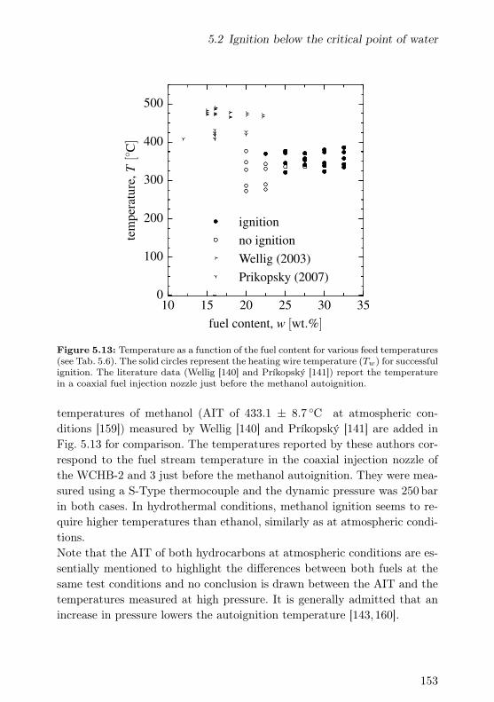
5.2 Ignition below the critical point of water
10 15 20 25 30 35
fuel content, w [wt.%]
0
100
200
300
400
500
tem
per
atu
re,
T[
C]
ignition
no ignition
Wellig (2003)
Prikopsky (2007)
Figure 5.13: Temperature as a function of the fuel content for various feed temperatures(see Tab. 5.6). The solid circles represent the heating wire temperature (Tw) for successfulignition. The literature data (Wellig [140] and Príkopský [141]) report the temperaturein a coaxial fuel injection nozzle just before the methanol autoignition.
temperatures of methanol (AIT of 433.1 ± 8.7 C at atmospheric con-ditions [159]) measured by Wellig [140] and Príkopský [141] are added inFig. 5.13 for comparison. The temperatures reported by these authors cor-respond to the fuel stream temperature in the coaxial injection nozzle ofthe WCHB-2 and 3 just before the methanol autoignition. They were mea-sured using a S-Type thermocouple and the dynamic pressure was 250 bar
in both cases. In hydrothermal conditions, methanol ignition seems to re-quire higher temperatures than ethanol, similarly as at atmospheric condi-tions.Note that the AIT of both hydrocarbons at atmospheric conditions are es-sentially mentioned to highlight the differences between both fuels at thesame test conditions and no conclusion is drawn between the AIT and thetemperatures measured at high pressure. It is generally admitted that anincrease in pressure lowers the autoignition temperature [143,160].
153

5 Hydrothermal flame ignition and monitoring
The critical temperature and pressure of an aqueous mixture containing 20wt.% ethanol are estimated to be 348.8 C and 187.2 bar by linear interpo-lation of the data of Abdurashidova et al. [153]. A higher ethanol contentresults in a lower critical pressure and temperature. Moreover, the addi-tion of supercritical oxygen to the mixture further reduces both the criticaltemperature and the critical pressure. In a previous work conducted inthe WCHB-4 [133], the forced convection of an electrically heated surfaceto a ternary water-ethanol-nitrogen mixture was reported. Extrapolatingthese data, the pseudo-critical temperature of a mixture containing 20 wt.%ethanol in the fuel stream and 20% excess oxygen at 260 bar is estimated tobe around 310 C. It results in an even lower thermodynamic critical point.As the current experiments are performed at a pressure significantly greaterthan the critical pressure of the ternary mixture, the physical propertychange generally observed across the pseudo-critical point and responsiblefor unusual heat transfer phenomena [161] is not highlighted in these data.The heating wire temperatures at ignition are above the pseudo-criticaltemperature of the ternary mixture, i.e. where no phase boundary existsbetween the reactants anymore.
The electrical energy (E) dissipated to the fluid as a function of the heaterstemperature (Theaters) is presented in Fig. 5.14. The energy transferred tothe mixture while it flows along the coil igniter is estimated according to:
E = H
(ρmA
m
)
UI. (5.6)
In Eq. (5.6), H is the height of the heating coil, ρm the mixture density, Athe free cross sectional area available along the heating coil (Fig. 5.10), mthe overall mass flow of the fuel and oxygen and UI the electrical power.The mixture density is estimated at the tip of the fuel injection nozzle(Fig. 5.10(b)) - before any oxidation occurs - at 260 bar and the feed tem-perature (Tfeed) using Refprop (v8.0) [87]. The calculation is performed ona mass basis following a simple mixing rule (ρm = ρiwi) and the density ofthe individual components (ρi) are gathered from [88], [162] and [163] forwater, ethanol and oxygen respectively.As a significant share of this energy is used to heat up the mixture beyond
154

5.2 Ignition below the critical point of water
0 20 40 60 80 100 120 140
heaters temperature, Theaters [C]
100
120
140
160
180
200
220
240
elec
tric
alen
erg
y,E[J] 20 wt.%
22.5
25
27.5
3032.5 wt.%
ignition
no ignition
Figure 5.14: Electrical energy dissipated to the fluid as a function of the heaters tem-perature for mixtures with different ethanol content (wt.%). The systematic uncertaintyof the energy is at most 10 J with 95% confidence.
the feed temperature, the leftover can allow to overcome the energy inputrequired by the ethanol combustion (solid circles).
Finally the ignition map of the system at 260 bar and the conditions givenin Tab. 5.6 is presented in Fig. 5.15. The rational function interpolatesthe heaters temperature required for ignition and is highly specific tothe present geometry, ignition system and experimental conditions. Nofuel with an ethanol content lower than 22.5 wt.% could be ignited withthe available electrical power (10A at 65V) and preheating temperatures(Theaters). Mixtures containing more than 30 wt.% ethanol could be ignitedwithout preheating.
This result is important in the scope of hydrothermal spallation drilling,where a flame burning in a water based-drilling fluid has to be ignited sev-eral hundred meters downhole [142].For SCWO and more generally the study of hydrothermal flames, the imple-
155

5 Hydrothermal flame ignition and monitoring
15 20 25 30 35
fuel content, wEtOH [wt. %]
0
20
40
60
80
100
120
hea
ters
tem
per
atu
re,
Thea
ters[
C] T (w) = 4w+60
w−21
ignition
no ignition
Figure 5.15: Ignition map of the system at 260 bar using a power supply capable ofdelivering 10A at 65V. Solid circles denote an ethanol fuel content and feed temperaturewhere hot surface ignition is possible. The feed temperatures can be found in Tab. 5.6.
mentation of a hot surface igniter in the system would allow the reductionof the investment costs of the corresponding facilities. As an example, thecosts of both heaters present in the wet flame-jet spallation drilling facil-ity (Ch. 4) represents 25% of the total equipment expenses. Moreover, therunning costs are also reduced as the 76 kW electrical power consumed byboth heaters can be minimized. Indeed, the ignition system consumes lessthan 1% of this electrical power. Eventually, as a result of the shorter res-idence time of hot and pressurized fuel and oxygen in the system, safetyhazards are minimized. Finally, the local ignition allows for a common feedline containing both fuel and oxidizer and thus premixed flames can beconsidered.
For the waste water treatment (SCWO), in case the content in organicsdoes not allow hot surface ignition or in case the waste is not soluble insubcritical water, a pulse of a low grade fuel, as suggested by Bermejo etal. [150] can be injected in the system to ease ignition. Indeed, a stream
156

5.3 Internal temperature profile
with a higher organics content is easier to ignite with limited electricalpower as its heat capacity is lower. Once the flame steadily burns, wastewith a lower organic content can be processed and the tubing in contactwith supercritical liquid is limited.
5.3 Internal temperature profile
After ignition, an additional temperature measurement in the combustionchamber permits to control the mass flows (e.g. fuel and oxidizer) withrespect to the flame characteristics and optimize the overall burner powerdensity or hazardous chemicals destruction efficiency.
5.3.1 Specific motivation
In this section, data acquired with the improved sensor (Sec. 5.1) to igniteand monitor locally the temperature of the hydrothermal flame are pre-sented. After ignition of the feed at room temperature (20 C) using thecustom made sensor, it is used to investigate the influence of the fuel in-jection geometry and the equivalence ratio on the centerline temperatureprofile at 260 bar. This information is then analyzed to extrapolate theflame-front position, the flame length, recirculation zones, the power den-sity and the combustion robustness. Hence, this combined sensor for flameignition and monitoring can be used in: SCWO where local ignition andtemperature monitoring can permit to reduce investment and indirectlyoperating costs and, flame-jet drilling where flame ignition and flame mon-itoring are essential.
5.3.2 Experimental setup and procedure
The experimental facility used for this study is presented in Ch. 4 andthe specific parts which influence directly the following measurements aredescribed hereafter.
157

5 Hydrothermal flame ignition and monitoring
oxygen
axial displacement of the
igniter thermocouple
main
volume
igniter
thermocouple
(a) (b)
fueloxygen
140 mm
100 mm
z = 2
z = 26
z = 148 exit to TIAH-4
30 mm 15 mm
CW 2
K-Type thermocouple
CW 1
exit to TIAH-3CW 1
Figure 5.16: (a) Upper section of the pressure vessel (WCHB-4) with its combustionchamber and a 3 mm K-Type thermocouple. The axial displacement of the igniter ther-mocouple is indicated by the double arrow and the 3mm thermocouple is positionedsimilarly. (b) Detailed view of the combustion chamber. The igniter thermocouple ispresented at its upper end position and the measurement locations are indicated withred dots. Dimensions are in mm.
Combustion chamber
The combustion chamber is composed of two 130mm long concentric tubes(Fig. 5.16(b)). The bottom end of the inner space (Ø=10mm) dischargesthe hydrothermal flame in the main volume of the pressure vessel and theintermediate space cools its internal wall with 400 kg/h of deionized water -initially at 20 C (CW 1). The cooling water stream exits through 6 holes -2mm in diameter - located 10mm upstream of the flame discharge location
158

5.3 Internal temperature profile
and oriented at 135 with respect to the main flow direction. In the vesselmain volume, the class-1 K-type thermocouple (Ø = 3mm) is positionedusing the linear actuator mounted on a telescopic tube to measure thedownstream temperature profile.
Fuel injection nozzles
12 x 1 mm x 30° 18 x 1 mm x 30° 12 x 1.5 mm x 30° 12 x 1 mm x 45°
4.1 mm
2α
D
A B C D
Figure 5.17: Different geometries of the fuel injection tip used for this experimentalstudy. The numbers below the fuel injection tip represent the number of holes (n), theholes diameter (D) and the angle (α).
For this set of experiments, the fuel injection nozzle geometries presentedin Fig. 5.17 are used. The injection angle (α) and the free cross section (a =
nπD2/4) available to the fuel essentially influence its injection velocity andthe ratio of its axial and radial components. Downstream of the injector, aflow field with two main recirculation zones results: a central recirculationzone generated by the flow around the bluff body and a circumferentialone (corner recirculation zone) generated by the sudden expansion [164].The igniter thermocouple is positioned in the central recirculation zoneto promote ignition. The fuel injection nozzle is located to leave a recess-length of 98mm, 40% more than in the former experiments (Sec. 5.2) andthis length denotes the distance over which both, the fuel and the oxygenare in contact along the combustion chamber. Note that the central hole(4.1mm in Fig. 5.17) remains mostly blocked by a ceramic insert whichelectrically insulates the igniter thermocouple from the fuel injection nozzle(Fig. 5.16(b)).
159

5 Hydrothermal flame ignition and monitoring
Igniter thermocouple layout and principle
The igniter thermocouple used for this set of measurements consists of a30mm coil made of NiCr-60/15 (Ø = 0.35mm) featuring a nominal resis-tance of 7.7Ω at room temperature (Fig. 5.1). The tip-junction is formedbetween the coil and a 435mm long Alumel R© wire (Ø = 0.8mm). At thesecond coil end (base-junction), it is welded to a 400mm long copper wire(Ø = 0.8mm) forming a weaker thermoelectric junction. This set of dif-ferent thermoelectric junctions essentially differentiate the igniter thermo-couple from the initial design presented in Sec. 5.1 and used in Sec. 5.2.Otherwise, the igniter thermocouple is as described in Sec. 5.1.
5.3.3 Results and discussion
Hereafter the experimental results are presented discussing firstly the datareduction. Then the temperature profiles for the various fuel injection ge-ometries (Fig. 5.17), two mass flows (m) and three different equivalenceratios (λ) are presented and discussed.Note that no correction is applied for radiative or convective losses for bothsensors (i.e. igniter thermocouple and K-Type thermocouple) and thus sen-sors temperature are reported rather than the local fluid temperature inthe following. Additionally, any catalytic effect on the surface of the ther-mocouple igniter is very unlikely [165].
Data reduction
The reduction of the experimental data is based on the guidelines pre-sented by Coleman and Steele [116] and the ISO 8466-2 [166], while a 95%
level of confidence is specified on the systematic uncertainties presumingdata follow a t-distribution. The uncertainties on the direct measurementsare summarized in Tab. 5.7. The combined systematic uncertainty on the
160

5.3 Internal temperature profile
igniter thermocouple temperature (uc(Ti)) is:
uc(Ti) =
2
[(∂Ti
∂p2
)2
u2(p2) +
(∂Ti
∂U
)2
u2(U) +
(∂Ti
∂U
)2
u2(U)
]1/2
,(5.7)
with p2 [µV/C] the coefficient of the polynomial least-squares regression(Fig. 5.8), U [µV] the voltage generated by the thermoelectric junction oncethe SSR is opened and U [µV] the mean response of the calibration. Notethat to derive Eq. (5.7),
U =
(U − p2T
T 2
)
T 2 + p2T
is used instead of the direct calibration equation (U = p1T2 + p2T ) as p1
and p2 are correlated [155] and, the partial derivatives (Eq. (5.7)) are eval-uated analytically. Finally the combined systematic uncertainty (±10 C)is negligible compared to the temperature fluctuations during the measure-ments along the axis of the combustion chamber.
Table 5.7: Uncertainties during the temperature profile measurements.
Sys. uncertainty Stat. fluctuation
Tk 0.004× T 55%U 30 µV 16%
Temperature profiles
After the determination of the calibration function for the igniter thermo-couple (5.1.3), the sensor is inserted in the pressure vessel (Fig. 5.16). Forevery experiment, the vessel pressure is set to 260 bar and a 20 kg/h aque-ous ethanol stream (32.5 wt.% EtOH) is prepared by adjusting the setpointof the three-way-valve (3WV-1 in Fig. 4.1). The oxygen flow is adjusted us-ing FMIC-1 to ensure 20% excess with respect to stoichiometry (λ = 1.2,fuel-lean condition).
161

5 Hydrothermal flame ignition and monitoring
Once the desired mixture is reached, the igniter thermocouple is moved atits lower position in the flow field (z = 28.5mm) and acts as an additionalelement where the flow can attach. It is then charged with 65VDC and thelimiting current - initially 6A - is raised in steps of 0.2A every 15 s untilignition occurs. Subsequently the SSR is opened such that no heat is dissi-pated anymore and the igniter thermocouple is retrieved 2mm downstreamof the fuel injection tip (z = 2mm, as presented in Fig. 5.16).
Subsequently, the temperatures downstream of the combustion chamberare measured using the 3mm, class-1, K-Type thermocouple. The firstmeasurement is performed 148mm away of the fuel injection tip and thethermocouple is moved sequentially in steps of 10mm towards the fuelinjection nozzle. Its temperature (Tk) is measured during 30 s at each posi-tion. The data are acquired with a sampling frequency of 100Hz and savedevery 100ms. Similarly, the measurements in the upper flame region areperformed using the igniter thermocouple (Ti). The first measurement isperformed 2mm below the fuel injection tip and the sensor is moved insteps of 3mm until the position 26mm below the injector is reached or thenext temperature is expected to be higher than 1000 C. Then, the flow pa-rameters (m, λ) are adjusted and the measurement procedure is repeated.Note that: (i) for 50 kg/h the temperature profile (Tk) extends only un-til z = 108mm because during preliminary experiments, the thermocouplemelted once at 98mm, (ii) all profiles are measured with the same set ofsensors ensuring maximum consistency in their positions and calibrationsand, (iii) the temperatures reported correspond to the time average over30 s.
Based on the temperature profile the axial extent of the flame is deter-mined considering combustion occurs at temperatures beyond 600 C. Thisis a lower threshold temperature compared to the value proposed by Augus-tine and Tester [129] (1000 C) but it is needed in order to use a consistentmethod for every set of flow regimes (m, λ) and geometrical parameters(a, α). Finally over the measurement series, the maximum intermittenttemperature recorded by the igniter thermocouple is 1005 C as the maxi-mum time averaged (30 s) temperature lies at 900 C.
Figs. 5.18 and 5.19 present the temperature profile along the centerline of
162

5.3 Internal temperature profile
0 20 40 60 80 100 120 140
distance to the injector tip, z, [mm]
0
200
400
600
800
1000
1200
tem
per
ature
,T[
C]
0 20 40 60 80 100 120 140
distance to the injector tip, z, [mm]
0
200
400
600
800
1000
1200
tem
per
ature
,T[
C]
λ = 1.2
λ = 1
λ = 0.8
Figure 5.18: Temperature profiles for different oxygen to fuel ratios (λ) and the fuelinjection nozzle A (see Fig. 5.17). Left panel: 20 kg/h and measurement positions alongthe combustion chamber indicated with red dots. Right panel: 50 kg/h and labels.
0 20 40 60 80 100 120 140
distance to the injector tip, z, [mm]
0
200
400
600
800
1000
1200
tem
per
ature
,T[
C]
0 20 40 60 80 100 120 140
distance to the injector tip, z, [mm]
0
200
400
600
800
1000
1200
tem
per
ature
,T[
C]
λ = 1.2
λ = 1
λ = 0.8
Figure 5.19: Temperature profiles for different oxygen to fuel ratios (λ) and the fuelinjection nozzle B (see Fig. 5.17). Left panel: 20 kg/h and measurement positions alongthe combustion chamber indicated with red dots. Right panel: 50 kg/h and labels.
the combustion chamber for the fuel injection nozzles A and B (Fig. 5.17).For both injectors and 20 kg/h, a greater equivalence (λ) results in lower
163

5 Hydrothermal flame ignition and monitoring
temperatures near the fuel injection tip and a shorter axial flame length de-spite a larger combustion power (see Tab. 5.8). The larger oxygen velocityis likely to lift up the flame, shifting recirculation zones, the flame-front andthe pseudo phase change downstream. By linear interpolation of the datapresented in [153], the critical temperature and pressure of an aqueous mix-ture containing 32.5 wt% ethanol are 333.5 C and 166.3 bar respectively.The addition of oxygen to the mixture further reduces both the critical tem-perature and pressure. Based on a former work performed in the WCHB-4 [133] using a ternary water-ethanol-nitrogen mixture, the pseudo criticaltemperature of the mixture is estimated - previous to combustion - to bearound 290 C at the working pressure depending on the oxygen equivalence(λ), the local pressure and composition variations. Therefore the pseudophase change position varies dynamically along z influencing combustion(power density and axial flame length, Tabs. 5.8 and 5.9). Compared tothe fuel injection nozzle A, the lower fuel injection velocity of nozzle B re-sults in a shorter induction length, especially highlighted for 50 kg/h. Thisis supported by an improved attachment of the fluid on the tip of the fuelinjection nozzle at lower velocities. The induction length is used to describethe axial distance from the fuel injection tip (z = 0) where essentially noreaction occurs until the z-location with a temperature in excess of 600 C.This information can be readily extrapolated from the figures by interpolat-ing linearly between adjacent temperatures, if necessary. Fig. 5.20 presentsthe temperature profile for nozzle C. Compared to nozzle B (Fig. 5.19), thefree cross section (a) available to the fuel flow is increased by 50% - therebycomparatively reducing its injection velocity. It results a shorter inductionlength for both mass flows. The lower fuel velocity shortens and weakensthe central recirculation zone, despite the axial flame length is generallylonger and the released power is larger (Tabs. 5.8 and 5.9). For 20% oxy-gen excess and 20 kg/h, the thermocouple igniter temperature profile has aplateau: it is attributed to a lack of mixing linked to the low fuel velocityand large oxygen velocity.
Fig. 5.21 presents the temperature profile using nozzle D. As the free crosssection remains the same as for nozzle A (Fig. 5.18), the larger injection an-gle promotes the formation of a wider and shorter central recirculation zonedownstream of the injection tip, as suggested by Ma et al. [167]. Because of
164

5.3 Internal temperature profile
0 20 40 60 80 100 120 140
distance to the injector tip, z, [mm]
0
200
400
600
800
1000
1200
tem
per
ature
,T[
C]
0 20 40 60 80 100 120 140
distance to the injector tip, z, [mm]
0
200
400
600
800
1000
1200
tem
per
ature
,T[
C]
λ = 1.2
λ = 1
λ = 0.8
Figure 5.20: Temperature profiles for different oxygen to fuel ratios (λ) and the fuelinjection nozzle C (see Fig. 5.17). Left panel: 20 kg/h and measurement positions alongthe combustion chamber indicated with red dots. Right panel: 50 kg/h and labels.
0 20 40 60 80 100 120 140
distance to the injector tip, z, [mm]
0
200
400
600
800
1000
1200
tem
per
ature
,T[
C]
0 20 40 60 80 100 120 140
distance to the injector tip, z, [mm]
0
200
400
600
800
1000
1200
tem
per
ature
,T[
C]
λ = 1.2
λ = 1
λ = 0.8
Figure 5.21: Temperature profile for different oxygen to fuel ratio (λ) and the fuelinjection nozzle D (see Fig. 5.17). Left panel: 20 kg/h and measurement positions alongthe combustion chamber indicated with red dots. Right panel: 50 kg/h and labels.
the radial confinement, this strengthens mixing, resulting in a short induc-tion length respectively a rapid temperature increase and an extended axial
165

5 Hydrothermal flame ignition and monitoring
flame length compared to A. As the temperature measured in the chambergives an indication on the flame position (flame-front) and its length (Lin Tabs. 5.8 and 5.9) along the central axis, the temperature measured inthe sub-cooled environment gives an indication on the penetration lengthof the supercritical plume. The supercritical plume penetration length inthe sub-cooled water increases substantially with the fuel mass flow fromabout 3 to 15mm and is largely independent of the fuel injection geometryand the oxygen to fuel ratio (λ). Especially when considering the fluctua-tions of the temperature measured with the K-Type thermocouple, up to45% with 95% confidence for 50 kg/h.
Eventually, all the injectors produced mixtures that could be ignited bythe igniter thermocouple and a robust combustion for different mass flowsand equivalence ratios (λ). For most geometries and flow conditions theflame remained anchored on the fuel injection nozzle enhancing combus-tion robustness. For the injector D, intermittent pressure fluctuations (i.e.explosions) are observed for a mass flow of 50 kg/h.Finally, the power p required to heat up the combustion chamber coolingwater (CW 1), the aqueous part of the fuel stream from room temperature(20 C) to TIAH-3 and the cooling water of the reactor mantle (CW 2)from room temperature to TIAH-4 (Fig. 5.16(a)) is presented in Tabs. 5.8and 5.9 for 20 and 50 kg/h of fuel respectively.
The water enthalpies are based on the data from the international associa-tion for the properties of water and steam which are reported in the workof Wagner and Pruss [88] and gathered from [130]. Note that the powervalues (p) reported do not completely represent the energy released by thereaction and are underestimated: the energy needed to heat up the com-bustion products is not accounted for as products composition is unknownand involves reactants.
Considering the combustion power fluctuations (σ95(p) in Tabs. 5.8 and5.9) as a measure of the combustion robustness, nozzle B leads cumula-tively to the most stable combustion and performs always best for a fuelrich combustion (λ = 0.8).Besides flame stability, the power density (kW/m3) of the burner is impor-tant and indicates its combustion efficiency. In the present case it reduces
166

5.3 Internal temperature profile
Table 5.8: Power (p), power fluctuations (σ95(p)) and axial flame length (L) for 20 kg/hof fuel, the different fuel injection geometries (a, α) and equivalence ratios (λ) investi-gated.
20 kg/h fuel injection nozzleλ A B C D
p [kW]1.2
24.73 23.52 24.49 26.48σ95(p) [kW] 1.30 1.08 1.24 1.58
L [mm] 39 26 29 64
p [kW]1
23.08 22.20 22.32 23.94σ95(p) [kW] 1.04 1.06 1.30 1.20
L [mm] 44 35 81 69
p [kW]0.8
18.03 18.36 18.56 20.95σ95(p) [kW] 7.06 1.02 1.30 1.82
L [mm] 47 69 79 54
Table 5.9: Power (p), power fluctuations (σ95(p)) and axial flame length (L) for 50 kg/hof fuel, the different fuel injection geometries (a, α) and equivalence ratios (λ) investi-gated.
50 kg/h fuel injection nozzleλ A B C D
p [kW]1.2
85.91 68.86 72.30 79.27σ95(p) [kW] 6.04 3.78 3.44 4.54
L [mm] 74 103 101 103
p [kW]1
76.03 64.62 68.28 73.00σ95(p) [kW] 3.12 3.36 3.30 3.74
L [mm] 54 93 101 101
p [kW]0.8
67.68 58.55 59.46 65.56σ95(p) [kW] 4.54 3.02 6.36 4.06
L [mm] 45 93 101 98
to the combustion power as volumes are constant. As presented in Tabs. 5.8and 5.9, for the same fuel injection geometry, the power p increases with theequivalence ratio even beyond stoichiometry. It implies that more ethanolreacts at greater equivalence (λ > 1) and an incomplete combustion, lim-ited by mixing or residence time. Along the axial extent of the combustion
167

5 Hydrothermal flame ignition and monitoring
chamber, three regimes characterized by different Damköhler numbers (Da)are distinguished:
(1) Upstream of the flame front, the reaction kinetics is slow resulting ina large Damköhler number (Da ≫ 1).
(2) Along the flame, the chemical time is expected to be similar as themixing time, resulting in Da ≈ 1.
(3) As the flame-jet penetrates the sub-cooled environment, the sur-rounding water quenches it rapidly, thus increasing significantly thechemical time and resulting in Da ≪ 1.
Concerning power, the injection nozzles A and D perform best despite acomparatively large induction length. Therefore the nozzle featuring thehighest power (Tabs. 5.8 and 5.9) is not the one featuring the least powerfluctuations (σ95(p)) resulting in a tradeoff in the choice of the fuel injectiongeometry, according to the process requirements. Typically for supercriticalwater oxidation where the maximum waste conversion in the least amountof time is desired, the injector leading to the maximum power density shouldbe chosen. On the contrary, for hydrothermal spallation drilling, wherecombustion occurs up to several kilometers downhole, flame stability shouldbe favored. In case the igniter thermocouple displacement is impossible, theinjector featuring 12 holes 1mm in diameter and diverging by 30 is the bestchoice: allowing flame ignition and, the protection of the sensor by operatingthe system at larger mass flow (lifting up the flame) and monitoring thetemperature in one location. It is likely that temperatures recorded in adifferent system will diverge, leading to a different fuel injection nozzleperforming best.
5.4 Closing remarks
In this chapter, the heating coil and its evolution is presented. The coiligniter is used to ignite hydrothermal flames (22.5 ≤ wEtOH ≤ 32.5 wt.%)in Sec. 5.2.Mixtures with an alcohol content larger or equal to 30 wt.% can be ignitedin absence of preheaters by releasing up to 520W through the heating wire
168

5.4 Closing remarks
reaching a temperature around 385 C.
The refined design of the igniter thermocouple presents extended servicelife at 900 C and is able to sustain intermittent temperatures in excess of1000 C. After calibration, this sensor has a mean sensitivity of 27 µV/C
and an absolute systematic uncertainty of ±10 C with 95% confidence fromroom temperature to its maximum operating temperature (1000 C).Based on the different temperature profiles determined along the combus-tion chamber axis, the flame-front position, the flame length, recirculationzones, the power and combustion robustness are discussed qualitatively(Sec. 5.3). For the experimental range investigated, if combustion robust-ness is primary, the injection nozzle A is most suitable. Conversely, tomaximize the power of the chamber, nozzles B and D perform best.
Generally for supercritical water oxidation, local ignition allows to reduceinvestment and operating costs. The combined measurement of the up-stream temperature can permit to adjust waste water and oxidizer flowrates entering the vessel to maintain constant and optimized process pa-rameters and reduce start up times.The hot surface igniter presented in this chapter is primary for flame-jetdrilling. Indeed, with the electrical power available downhole (i.e. muddriven downhole electric power generator or a battery), aqueous ethanolflames can be ignited and monitored at pressures exceeding the thermody-namic critical point of the mixture. Therefore, a major issue foreseen in theimplementation of spallation drilling to drill deep wells is solved [51].
169


6 High pressure rock drilling and
confinement
The first attempt to drill a core sample at a fluid pressure of 260 bar
occurred on February 4th 2013. The results of these preliminary exper-iments are summarized here (Sec. 6.1) to motivate the following steps(Secs. 6.2, 6.3) and to highlight the development stage of the drilling tech-nique at the beginning of this work. In Sec. 6.4, the proof-of-concept offlame-jet drilling at downhole conditions is presented.
6.1 First series of attempts
The rock cores (83mm in diameter and 150mm long) presented in Fig. 6.1were exposed to a hydrothermal flame conveying a thermal power of86.5 kW (60 kg/h of a fuel mixture with 17.5 wt.% ethanol) at a stand-offdistance of 15mm for increasing time from left to right (1, 10, 30min).The preheating temperatures were 410 C and 250 C for HX-1 and HX-2respectively, resulting in an adiabatic flame temperature in the rangeof 1600 C and a flame-jet composed of up to 75 wt.% water. Note thetendency to reduce the preheating temperatures, starting with O2, withrespect to the experiments presented in Stathopoulos [71]. The velocityof the flame-jet through the 10mm hole of the combustion chamber isestimated in the range of 10-15m/s using the mass and energy balancespresented in 4.2.1. The mass flow of cooling water through the combus-tion chamber was 350 kg/h and when the exposure time is greater than10min, the surface silica grains are oxidized over a circular area covering≈ 700mm2. Therefore the planar confinement requiring less than 10% of
171

6 High pressure rock drilling and confinement
the surface of an unconfined sample to be heated up [17] is not fulfilledanymore and the stresses released through the volume expansion of therock. After these results, which showed the onset of spallation on Iragna
Figure 6.1: Rock probes after different exposure time at a distance of 15mm from thecombustion chamber. The exposure time is from left to right: 1, 10, 30min. The thermalpower of the flame is 86.5 kW and the mass flow of cooling water exiting the combustionchamber is 350 kg/h.
gneiss samples from Tessin (Switzerland), the ignition experiments fol-lowed (Sec. 5.2). The goal was to lower as much as possible the preheatingtemperatures to: (i) reduce the residence time of hot oxygen and fuel in thefacility, (ii) safely increase the mass fraction of ethanol in the fuel streamand, (iii) reduce the experimental time.
Then, the development reported in Sec. 6.2 was carried out to continue theinvestigation of flame-jet drilling at high pressure.
6.2 Second series of attempts
The starting point is the experience acquired during the former tests de-scribed in Sec. 6.1. Unlike the ignition experiments which resulted froma defined measurement plan, the results presented in this section describethe evolution of the combustion chamber - where modifications were con-sidered after each experiment.Since the preliminary rock experiments (Sec. 6.1), the experimental facilityis used at its limits. This means a combustion load of 132 kW which is lim-ited by the volumetric flow rate the gas boosters can deliver at the workingpressure (500NL/min, 4.1.2).This choice is driven by two facts based on the experiments reported in
172

6.2 Second series of attempts
Sec. 6.1: (i) spallation did not start directly as the rock was exposed to theflame-jet, an indication for a lack of heat [17] and, (ii) as the preheatingtemperatures are reduced (410 C for HX-1 and 250 C for HX-2 to about100 C and 20 C respectively) with respect to the process parameters usedin [128], higher fuel content is used to compensate the reduction of thermalpower in the jet.
For the experiments, a hard polycrystalline Grimsel granite, the main con-stituents (vol.%) of which are: quartz (28), plagioclase (29), K-feldsparr(24), sheet-silicates (18) and minor accessory minerals [168] is used. Thequarry is located on the northern side of the Grimsel pass at the Swiss co-ordinate (667’730, 161’250). According to Prof. Diamond Larryn1, this rocktype is representative of the geology expected to be encountered in deepgeothermal projects in Switzerland.
6.2.1 Measurement procedure
For a lab-scale drilling experiment, the cylindrical core, 84.5mm in diame-ter and 151mm long is first positioned in the pressure vessel (Fig. 4.9). Thedistance between the tip of the combustion chamber and the rock surfaceis initially kept as large as possible. For an unconfined rock core sample(Secs. 6.1 and 6.2), this is 100mm, whereas for a confined sample (Sec. 6.4)it reduces to 70mm. The three-way valve (3WV-1) is positioned at 65% ofits stroke to prepare a mixture containing 32.5 wt.% ethanol. Once the den-sity is close to the target value (968 kg/m3), the PID controller is switchedon and set to the target for the fine tuning of the stroke of its needle. Oncethe desired density is reached, the procedure described in 5.2.3 is followedto ignite the flame. Afterwards, the setpoint of the fuel pump is increasedby steps of 10 kg/h until the target mass flow is reached. The oxygen volumeflow is set accordingly to keep a 20% excess with respect to stoichiometry.
In every experiment, the nominal thermal power of the flame is 132 kW
which corresponds to: 50 kg/h of a fuel stream with 32.5 wt.% ethanolcombusted with 475NL/min of pure oxygen. For the results presented in
1Personal communication with Prof. Larryn W. Diamond, University of Bern, Septem-ber 2013.
173

6 High pressure rock drilling and confinement
this section the oxygen heater is always off and the fuel heater set to 100 C
to extend the life time of the heating coil by reducing the electrical powerneeded for ignition. Note that the fuel injection nozzle used in these ex-periments is the same as presented in 5.2.2. It features 12 holes with 1mm
diameter oriented at 30 with respect to the co-annular flow of oxygen(Fig. 5.17).
6.2.2 Results and discussion
Starting with the combustion chamber A (Fig. 6.2) used during the ignitionexperiments (Sec. 5.2) and the first attempts (Sec. 6.1), seven changes tothe geometry have been necessary in order to reach a sufficient cavity within10min.The combustion chamber A has a length of 100mm and a 10mm throatdiameter. Its cooling water (CW 1 in Fig. 4.1) is flowing through a 200 µmcircular slit before its injection at 45 with respect to the chamber axis.The recess length of the chamber is 68mm. The first trial of this series
100 mmØ 10 mm
3 x 2 mm6 x 2 mm
A B
C D6 x 2 mm
6 x 2 mm
350 µm
cooling water slit
Figure 6.2: Combustion chambers A, B, C and D with the different cooling waterconfiguration. Note that the slit in A and B is sealed off in C and D.
is performed on a Grimsel core during 10min at a stand-off distance of10mm. The visual inspection of the core sample revealed a larger cavitycompared to the gneiss attempts (Sec. 6.1). The difference is attributedto the different rock, the greater ethanol content and the shorter stand-offdistance. The adiabatic flame temperature is now in the range of 2100 C
and the outlet velocity of the flame-jet in the range of 20m/s.
174

6.2 Second series of attempts
As no satisfactory cavity is built the rock core is pre-drilled to concentratethe heat and six holes of 2mm are drilled in the outer tube consisting thecombustion chamber to reduce the amount of cooling water reaching theimpinging area (Fig. 6.2).In the following, despite otherwise mentioned, a cylindrical cavity with adiameter of 40mm and a depth of 40mm is pre-drilled in every rock probewith a diamond core drill.The modified combustion chamber is labeled B. Using B, the pre-drilledcore remained unaffected by the flame-jet. This is attributed to a directquenching of the 90 kg/h flame-jet by the 350 kg/h cooling water stream(CW 1) inside the pre-drilled cavity.
To reduce the quenching of the flame-jet, the circular slit for the cooling wa-ter injection present in B is sealed and the position of the 6 holes is movedupstream - such that a large part of the cooling water is injected outside thepre-drilled cavity. For safety reasons, three holes located 10mm upstream ofthe injection are kept. This results in the chamber C presented in Fig. 6.2.As its geometry is similar to the chamber A, the flame-jet velocity and tem-perature estimated are also valid. Both the large fissure (horizontal) at thebottom of the pre-drilled section (Fig. 6.3) and the vertical crack extend-ing up to the core sample surface, give evidence for intense temperaturegradients. In addition, three symmetric spots have been excavated withinthe pre-drilled cavity. Due to the symmetry of the cooling holes injectingthe water, it is difficult to draw deterministic conclusions on whether thesespots are located near the cooling injection, where heat accumulates or inbetween.
In the literature whereas most combustion chambers have a single flame-jetoutlet to discharge the fluid on the rock [61] some can rotate with multipleflame injection ports (e.g. Linde system [18, 169]). Others can even rotatewith multiple injection ports: some discharging a cold stream (e.g. coolingwater) and some discharging the hot fluid (e.g. a flame-jet) [170]. Accordingto these authors, alternating heating / cooling can prevent saturation ofthe rock, potentially responsible for the reduction of the excavation ratewith the duration of the drilling operation. In the present case, to keepthe system as simple as possible and because: (i) most of the knowledge isavailable for a single outlet flame-jet [17,18,62] and, (ii) there is no evidence
175

6 High pressure rock drilling and confinement
Figure 6.3: Upper part of core sample number 6. Large fissures are observed in thepre-drilled region after its exposure to the flame-jet.
that drilling stops because the rock is saturated, a single throat chamberis used. Note that to test the effect of a rotating chamber, it would bepossible to use the cooling water pumped by WP-1 and flowing throughV-13 to allow the rock sample to rotate using a dynamic bearing similarlyas a rotary sprinkler.
As no evidence for excessive heat on the combustion chamber C is observed,the three holes located 10mm upstream of the chamber tip are sealed -resulting in combustion chamber D (Fig. 6.2).
Using D, the spalls were generally smaller compared to the former tests sup-porting the assumption that heat was more concentrated. Conversely theoverall mass removed is comparable to the former experiment and no univo-cal distinction could be observed. Additionally, no large fractures appearedon the core sample supporting surface localized stresses. The increase inoutlet temperature (TIAH-3 in Fig. 4.8) starting at about 8min (drillingtime, Fig. 6.4) suggests that combustion was not complete and after a while,the pre-drilled cavity became an extension of the chamber. Therefore, thecombustion chamber is modified to the version E (Fig. 6.5) which featuresa smaller throat diameter (2.5mm). The smaller diameter permits: (i) toconcentrate the heat source and, (ii) to accelerate the flame-jet by a factorof about 16. The resulting flame-jet velocity exiting E is estimated in therange of 250m/s. However, using chamber E nothing happened to the rock
176

6.2 Second series of attempts
0 5 10 15 20 25 30 35 40
time, t [min]
0
100
200
300
400
500
960
980
1000
1020
1040
fuel
den
sity
,ρ[k
g/
m3]
p [bar]
V [NL/min]
T [C]
SOD [mm]
Figure 6.4: Experimental logs. The pressure (p) is measured by PIC-5 (see Fig. 4.1)as the temperature (T ) is measured at the outlet of the pressure vessel (TIAH-3). Thevolumetric flow rate (V ) corresponds to the oxygen flow rate measured by the flowcontroller (FMIC-1) and the red line corresponds to the fuel density (FMI-1). Finally thegreen dots represents the stand-off-distance (SOD) between the outlet of the combustionchamber and the rock surface. Every line and symbol refers to the left y-axis besides thefuel density (red line).
core and therefore the recess length is extended by about 50% to enhancecombustion and reduce the amount of unburnt fuel (F). Again the temper-ature at the outlet of the pressure vessel (TIAH-3) is lower (T ≈ 160 C),despite: (i) the same mass flow of cooling water flows through CW 1 and,(ii) a greater thermal power is supposed to be released due to the extendedrecess length.
Unfortunately nothing happened to the rock core and close inspection re-vealed a malfunction in the chamber leading to a direct quenching of thereaction by CW 1. This is assumed to prevent the proper combustion of the
177

6 High pressure rock drilling and confinement
E F
G H
Ø 2.5 mm6 x 2 mm 6 x 2 mm
6 x 2 mm
130 mm100 mm
6 x 2 x 45°
Ø 10 mm
Figure 6.5: Combustion chambers E, F, G and H with the different cooling waterconfigurations and throat diameters.
ethanol and to cancel any beneficial effect of the extended recess length.
6.2.3 Assessment
So far, the flame-jet produced enough heat to initiate spallation in theGrimsel core and to create a cavity larger than presented in Sec. 6.1. Usingthe chamber with a recess length of 68mm (A to E) limits the combustion ofethanol. Finally, by adjusting the throat diameter between 2.5 and 10mm,the velocity range reached by the flame-jet could be adjusted over threeorders of magnitude (Fig. 4.13) and the local heat transfer conditions onthe rock core surface can be modified.
However, besides Potter Drilling Inc. [73] which performed impressive lab-scale drilling experiments in which up to 200mL were excavated within3min in a wet environment at a fluid pressure varying from near-ambientto 241 bar, no other lab-scale drilling experiment could proceed beyond theonset of spallation [17,62,77]. The major difference between Potter DrillingInc. and the others is the 41.3MPa axial load provided by a hydraulic pressand the 20.6MPa produced by an external pump acting radially againstthe granite core. Note that the rock core used by Potter Drilling Inc. hasan outer diameter of 101.6mm and is 152.4mm long. These dimensions aresimilar to the rock core used here.
Unfortunately as the experimental facility (Ch. 4) was designed to workwith fluid pressures up to 260 bar [71], it is not designed to prestress the
178

6.3 Confinement system
rock core. To cope with that, a simple confinement system is developed andpresented in Sec. 6.3.
6.3 Confinement system
The confinement system should prevent the volumetric expansion of therock and macroscopic fractures. It is necessary to proceed beyond the onsetof spallation similarly as a rock drilled by mechanical means needs to behold firmly in place to transmit shear stresses imposed by the drill.Despite the fact that rock confinement to simulate natural conditions (e.g.different depth and rock formations) is an old idea [17], no technical solutiondirectly applicable in the experimental facility is presented in literature.
Literature review
For the stress-strain relationship in triaxial compression, Smith et al. [171]placed a rock core sealed in a heat-shrinkable jacket inside a pressure vessel.A first hydraulic press is used to pump oil and produce a confining stress(i.e. radial compression). A second hydraulic press is used to produce theaxial load on the rock core. The authors recorded stress-strain behaviorsusing strain gauges and curves at confining pressure up to 620MPa arereported. A hydraulic system was also favored by Potter Drilling Inc. toapply an axial load on the rock cores [73].
6.3.1 Development
In our case, the use of an hydraulic system would require major changesto the experimental facility. Since the beginning of this project volumetriccracks are considered as a serious challenge and different radial confine-ment solutions have been tested. With the concepts presented in Fig. 6.6the recurrent problem is the limited radial load applied to the sample,considering the space available in the pressure vessel and the significantlylarger thermal expansion of steel compared to rock. A second possibility to
179

6 High pressure rock drilling and confinement
Figure 6.6: Preliminary radial confinement concepts on rock probes with a diameterof 83mm. Left panel: Metallic jacket. Right panel: Press fitting assembly.
stress, at least axially, the core sample is to use two flanges and threadedrods, resulting in the system presented in Fig. 6.7. This mechanical solu-tion is preferred here due to its simplicity and its capability to be fitted inrestricted volumes.
With the system presented in Fig. 6.7, each threaded rod (M16x1.5,strength class 4.6) supports 108 kN in tension and therefore a force ofabout 432 kN is applied on the surface of the rock. It results in an axialstress of 77MPa, twice as much as Potter Drilling Inc. applied.Although conceived in the scope of this work, this confinement systemhas been tested for the first time in an experimental facility built by Dra-gana Höser [72] allowing direct visual access of the drilling process. Asintuitively expected, volumetric expansion is hindered and drilling notablypromoted. Towards the end of this initial test (<2min), the wall thicknessof the sample was too thin to hold the compression imposed by the axialload, resulting in large axial fractures (Fig. 6.7).
Unfortunately this system is too voluminous to be used in the pressurevessel (Fig. 4.9). Indeed, as the rock core has a diameter of 84.5mm and the
180

6.3 Confinement system
Figure 6.7: Mechanical clamping system to apply an axial load on a rock core. In thiscase, about 82MPa are applied.
main volume of the pressure vessel is 100mm in diameter a more compactsystem presented in Fig. 6.9 is built. Once the rock core is inserted in theaxial confinement system, the second cap where six standard M12 classA4-80 threads are tapered is welded.
6.3.2 Calibration of the confining assembly
To estimate the axial force (F ) applied on the rock as a function of thetightening torque (M), a calibration is performed using a load cell. For thepurpose, a torque is applied to the thread and the corresponding axial loadis recorded. According to the manufacturer, the Induk load cell HKMD 29D0 has a systematic uncertainty of 2%. The result of the calibration for aM10 and a M12 threads are presented in Fig. 6.8 whereas Tab. 6.1 reportsthe coefficients of the calibration functions (F = p1M + p2).
181

6 High pressure rock drilling and confinement
0 20 40 60 80
Torque, M [Nm]
0
20
40
60
80
100F
orc
e,F[k
N]
0 20 40 60 80
Torque, M [Nm]
0
20
40
60
80
100
Forc
e,F[k
N]
Figure 6.8: Calibration data and weighted linear least-squares fit appended by a 95%confidence interval on the observations. Left panel: M10 threads, the correlation coeffi-cient (r2) is 0.9795. Right panel: M12 threads, the correlation coefficient (r2) is 0.9867.
Table 6.1: Linear calibration function coefficients (F = p1M + p2) for both threadsM10 and M12 as well as the reproducibility on the clamping force per thread.
ThreadCoeff. of the regression
Reproducibility [kN]p1[kN/(Nm)] p2[kN]
M10 0.6291 17.79 ±8.3M12 0.7673 3.499 ±5
6.3.3 Assessment
The axial load permits to reproduce the overburden pressure at variousdepths and prevents volumetric stresses to build up. It also allows to ho-mogenize the initial state of stress (i.e. stress history) between successiverock cores, reducing variability between experimental runs. This simplemethod can be used to develop flame-jet drilling using samples of conve-nient size and weight.
182
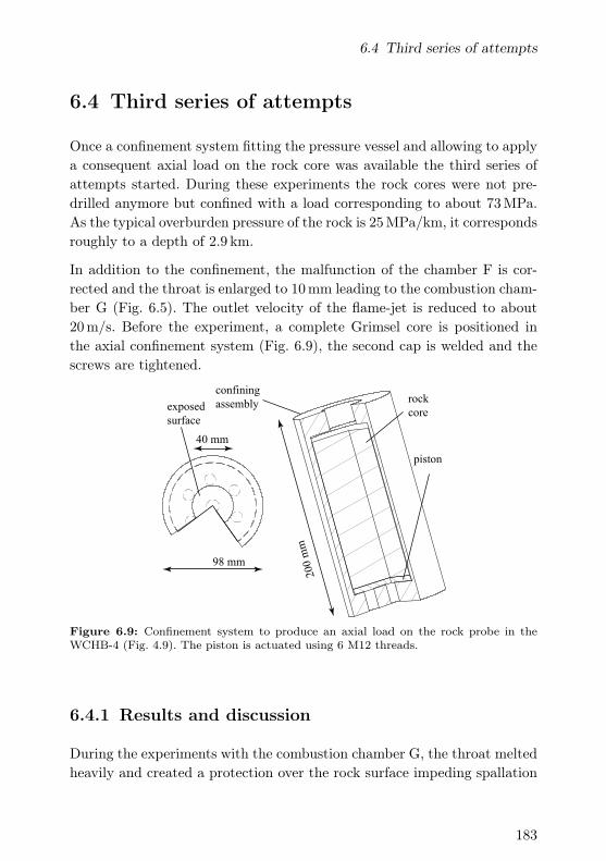
6.4 Third series of attempts
6.4 Third series of attempts
Once a confinement system fitting the pressure vessel and allowing to applya consequent axial load on the rock core was available the third series ofattempts started. During these experiments the rock cores were not pre-drilled anymore but confined with a load corresponding to about 73MPa.As the typical overburden pressure of the rock is 25MPa/km, it correspondsroughly to a depth of 2.9 km.
In addition to the confinement, the malfunction of the chamber F is cor-rected and the throat is enlarged to 10mm leading to the combustion cham-ber G (Fig. 6.5). The outlet velocity of the flame-jet is reduced to about20m/s. Before the experiment, a complete Grimsel core is positioned inthe axial confinement system (Fig. 6.9), the second cap is welded and thescrews are tightened.
200 m
m
98 mm
rock
core
confining
assembly
piston
40 mm
exposed
surface
Figure 6.9: Confinement system to produce an axial load on the rock probe in theWCHB-4 (Fig. 4.9). The piston is actuated using 6 M12 threads.
6.4.1 Results and discussion
During the experiments with the combustion chamber G, the throat meltedheavily and created a protection over the rock surface impeding spallation
183

6 High pressure rock drilling and confinement
to proceed. The fact that chamber G melted is an indication that the ad-ditional recess length, compared to chamber D, enhanced the ethanol oxi-dation.
Examining the rock core, large fractures were present over its whole lengthdespite the axial load. This is an evidence for its exposure to extremetemperature gradients.
To better cool the throat, the six cooling water injection holes are movedagain 10mm upstream of the tip. To reduce the quenching of the flame,the holes are oriented backwards with an angle of 45 with respect to theaxis of the chamber. The resulting combustion chamber H is presented inFig. 6.5. A final lab-scale drilling test is then performed. Examining theGrimsel core after the usual 10min impingement at a stand-off-distanceof 10mm, an appreciable cavity is formed (Fig. 6.10). The mass removed,about 30 g is at least three times larger than in the former experiments. Inaddition, no axial fracture is present in the rock core, an indication thatstresses were contained near the surface.
Figure 6.10: Upper part of core sample number 10. A cavity is formed by the flame-jetafter an exposure of 10min.
184
6.5 Closing remarks
6.4.2 Assessment
With help of the confinement system used during this third series of lab-scale drilling experiments, a certain cavity could be formed in the rock core.The additional recess length of chambers F, G and H enhanced the powerdischarged by the combustion chamber and the confinement system helpedcontaining the stresses near the exposed surface.
Finally, while the fluid pressure has relatively minor impact on spallation,the initial state of stress is very important for the thermal drilling process.Correspondingly, the mechanism can be classified as true thermal stressspallation in opposition to pore pressure spallation [172] which is substan-tiated by: the impact of the external confinement and the particle sizedistribution of the cuttings collected (Ch. 8). Note finally that no specificsize analysis of the cuttings could be performed for these tests but rangesare similar as those presented in Ch. 8.
6.5 Closing remarks
Following the preliminary tests performed in the garden and the recog-nition that some sort of confinement could help the drilling process, twoyears have been necessary to conceive the practical solution presented inSec. 6.4, which is applicable in the wet flame-jet spallation drilling facil-ity. During this time, a practically relevant manner to ignite hydrother-mal flames downhole has been developed (Ch. 5) and different combustionchamber geometries have been tested.
Combining these different developments for the final experiment, it hasbeen shown that hydrothermal spallation drilling or wet flame-jet drillingat the conditions prevailing in a deep wells is feasible. In the future, effortsshould be concentrated to accelerate the flame-jet reaching the rock. Forinstance by reducing the outlet bore of the chamber (e.g. chambers C andD).
185


7 Numerical investigation of
thermal spallation drilling
In order to describe the influence of the clamping action produced by theconfinement on the rock probe, a numerical investigation is reported in thischapter. Specifically a two-dimensional axisymmetric finite elements for-mulation of the thermoelastic equations is introduced (Secs. 7.1 and 7.2)to analyze and explain the laboratory drilling experiments. After verifica-tion of the implementation using the method of manufactured solutions(Sec. 7.3), the results of the numerical investigation are reported (Sec. 7.4).The results highlight the differences between flame-jet drilling lab-scaleexperiments, which generally failed [17, 62, 76, 77, 99] and early field-scaleattempts, which were usually successful [60, 61, 68, 169] and highlight anincreasing efficiency of thermal spallation drilling methods at depth.
7.1 Governing equations
In many engineering problems, hard and crystalline rocks are modelled as alinearly elastic, isotropic and homogeneous, non porous and brittle medium.This is generally acceptable when the sample size is much larger than itsgrains and temperature and pressure are moderate, i.e. the medium re-mains brittle. For the study of thermal spallation, Lauriello and Chen [173]tested this assumption and observed a close correlation between analyt-ically predicted fracture zones and experimentally fractured volumes. Insuch an idealized medium, the coupled, quasi-static thermoelastic equa-tions with initial and boundary conditions describe: (i) the generation ofthermal stresses due to spatial and temporal temperature variations and,
187
7 Numerical investigation of thermal spallation drilling
(ii) the thermoelastic dissipation, i.e. the generation of heat by strain. Ina domain Ω, the coupled, quasi-static thermoelastic equations are given byfollowing conservation equations for energy and momentum respectively:
ρCpT +E
1− 2ναT0εkk =
∂
∂xi
(
k∂T
∂xi
)
, (7.1a)
∂σij
∂xj+ fi = 0, (7.1b)
where ρ is the density, Cp is the heat capacity, E is Young’s modulus,ν is the Poisson ratio, α is the coefficient of thermal expansion, T is thetemperature, T0 is the stress free temperature, k is the thermal conductivity,εij is the strain tensor, σij is the stress tensor, fi is an external body forceper volume and dotted terms denote time derivatives.
For the isotropic, linearly elastic medium considered, the constitutive rela-tionship is given by:
σij =Eν
(1− 2ν)(1 + ν)εkkδij +
E
(1 + ν)εij −
E
(1− 2ν)α(T − T0)δij , (7.2)
where δij is the Kronecker delta and the strain tensor (εij) is given by:
εij =1
2
(∂ui
∂xj+
∂uj
∂xi
)
. (7.3)
In Eq. (7.1a), the term E1−2ναT0εkk represents the thermoelastic dissipa-
tion. According to Boley and Weiner [174], it can be discarded providedthat the temperature distribution in the solid is influenced mostly by itsinitial temperature and the external heat flux contributions. In the case ofa rock exposed to a flame-jet on one part of its faces, the contribution ofthe thermoelastic dissipation to the temperature is intuitively negligible, asstrains originate from the non-uniform temperature distribution imposedby the flame-jet.
188

7.1 Governing equations
Following Boley and Weiner [174] the dimensionless parameter δ:
δ =E2T0α
2
Cpρ2v2e(2ν − 1)2(7.4)
is introduced in which the velocity of propagation of dilatational waves (ve)in an elastic medium is defined by:
ve =
√
E(ν − 1)
ρ(ν + 1)(2ν − 1). (7.5)
Using Eqs. (7.4), (7.5), the conservation of energy (Eq. (7.1a)) can be ex-pressed as:
ρCpT
[
1 + δ(1− ν)
(1 + ν)
εkk
αT
]
=∂
∂xi
(
k∂T
∂xi
)
. (7.6)
where:
δ(1− ν)
(1 + ν)
εkk
αT,
represents the coupling term. The coupling term in Eq. (7.6) is negligibleif:
εkk
αT≪
(1 + ν)
δ(1− ν).
Referring to Tab. 7.1 for the material properties and assuming T0 = 298.15
K, for this type of granite δ = 0.0012 and ve = 3832 m/s. From the value of
Table 7.1: Material properties of a typical Grimsel granite (Switzerland).
Symbol Description Value
k thermal conductivity 1.5 W/(mK)ρ density 2750 kg/m3
Cp heat capacity 790 J/(kgK)E Young’s modulus 30 GPaν Poisson’s ratio 0.3α thermal expansion coefficient 8× 10⁻⁶ 1/K
δ and ν, the coupling term is small provided εkk
3αT≪ 500. As mentioned by
Boley and Weiner, for temperature distributions with no sharp temporal
189

7 Numerical investigation of thermal spallation drilling
variations or discontinuities, e.g. powerful explosions, it is expected thatthe time rate of change of the dilatation (εkk) is of the same order ofmagnitude as that of the thermal expansion (3αT ) [17]; thus the omissionof the coupling is a reasonable assumption here. Note that the force densityterm (fi in Eq. (7.1b)) is neglected because the dimensions of the numericaldomain considered are small and thus normal stresses due to gravitationalloading are negligible.
Therefore, the set of governing equations for the material considered canbe simplified to the quasi-static, uncoupled thermoelastic equations in theabsence of body forces:
ρCpT =∂
∂xi
(
k∂T
∂xi
)
, (7.7a)
∂σij
∂xj= 0. (7.7b)
7.2 Numerical method
7.2.1 Domain
The domain Ω in which the equations are solved is presented in Fig. 7.1.It represents a cylindrical rock core as used during drilling experiments(Ch. 6). Note that although Cartesian coordinates are used occasionally inthe text for convenience of the index notation, the symmetry of the prob-lem is recognized and the corresponding 2D axisymmetric torsionless (i.e.uθ = 0) formulation is implemented. The core is surrounded by a metallicassembly equipped at its bottom with a piston allowing to pre-stress therock core uniaxially. As the core is loaded uniaxially in the simulations toreproduce laboratory experiments, an anisotropic stress is naturally presentin the underground. The free space on top of the confining assembly allowsto bring the flame-jet, used as heat source during the experiments, close tothe rock core.
190

7.2 Numerical method
refT
r
z
Ω
confining
assembly
r=42.5
axis of symmetry
θ
r=0
z∆
r∆
1 2, ,e m m
n n nΓ Γ Γ
1 2, ,e m m
n n nΓ Γ Γ
1 2, ,e m m
n d dΓ Γ Γ
1 2, ,e m m
n d nΓ Γ Γ
1 2, ,e m m
r n nΓ Γ Γ
150z =
0z =
Rock core
Figure 7.1: Illustration of the two-dimensional axisymmetric domain (Ω) where theuncoupled, quasi-static thermoelastic equations are solved using a mix of Dirichlet (Γd),Neumann (Γn) and Robin (Γr) boundary conditions. Dimensions are in millimeters andthe superscripts e refers to the energy conservation and m to the momentum conserva-tion.
7.2.2 Discretization
The governing equations (Eqs. (7.7a) and (7.7b)) are expressed in cylin-drical coordinates and discretized in space using the finite elementmethod [175]. The 2D axisymmetric computational domain (Fig. 7.1) isdecomposed into 128 700 quadrilateral elements. The same mesh is usedfor solving the energy and momentum conservation. Over each element,the temperature and displacements are approximated using bilinear shapefunctions. All volume integrals in the weak form are evaluated using a2× 2 Gauss-Legendre quadrature scheme.
In the vicinity of the flame-jet impingement area on the upper surface of
191
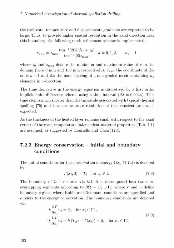
7 Numerical investigation of thermal spallation drilling
the rock core, temperature and displacements gradients are expected to belarge. Thus, to provide higher spatial resolution in the axial direction nearthis boundary, the following mesh refinement scheme is implemented:
zk+1 = zmax
tan−1(20k ∆z + z0)
tan−1(20zmax), k = 0, 1, 2, . . . , nz − 1,
where z0 and zmax denote the minimum and maximum value of z in thedomain (here 0 mm and 150 mm respectively), zk+1 the coordinate of thenode k + 1 and ∆z the node spacing of a non graded mesh containing nz
elements in z-direction.
The time derivative in the energy equation is discretized by a first orderimplicit finite difference scheme using a time interval (∆t = 0.002 s). Thistime step is much shorter than the timescale associated with typical thermalspalling [75] and thus an accurate resolution of the transient process isexpected.
As the thickness of the heated layer remains small with respect to the axialextent of the rock, temperature independent material properties (Tab. 7.1)are assumed, as suggested by Lauriello and Chen [173].
7.2.3 Energy conservation – initial and boundary
conditions
The initial conditions for the conservation of energy (Eq. (7.7a)) is denotedby:
T (xi, 0) = T0 for xi ∈ Ω. (7.8)
The boundary of Ω is denoted via ∂Ω. It is decomposed into two non-overlapping segments according to ∂Ω = Γe
r ∪ Γen where r and n define
boundary regions where Robin and Neumann conditions are specified ande refers to the energy conservation. The boundary conditions are denotedvia:
−k∂T
∂xini = qn for xi ∈ Γe
n,
−k∂T
∂xini = h (Tref − T (xi)) = qr for xi ∈ Γe
r,
(7.9)
192

7.2 Numerical method
where ni is the unit outward pointing normal vector to ∂Ω, Tref is a referencetemperature and h is the heat transfer coefficient.
Adiabatic boundaries (qn = 0) are considered all around the rock core,including along the axis of symmetry (Fig. 7.1), unless the rock is in con-tact with the flame-jet, i.e. for r < 20 mm and z = 150 mm. Indeed, asthe thermal conductivity of the rock is low, no significant amount of heatwhich diffuses through the rock reaches any outer surface over the simula-tion time (t ≤ 10 s). A Robin boundary condition (qr) is implemented todescribe the flame-jet: the reference temperature Tref = 1000K is constantand represents the flame-jet temperature as the heat transfer coefficient isspecified as h = 10 kW/(m2 K). These are rather conservative values to de-scribe the powerful flame-jets commonly used for drilling [73]. The initialtemperature, i.e. stress free temperature, of the rock core is set to roomtemperature (T0 = 298.15K).
On the upper surface, the temperature associated with the Robin conditionis discretized via a two-node linear element. The surface integral arisingfrom the weak form of the governing equations - which forms part of theRobin condition - is evaluated using a two point Gauss-Legendre quadraturescheme.
7.2.4 Momentum conservation – boundary conditions
Each equation associated with the conservation of momentum (Eq. (7.7b))requires the specification of a boundary condition. It is convenient to definethese in terms of values applied normal to, or in the tangent direction to∂Ω. Dirichlet boundary conditions are considered for the displacement:
uini = u for xi ∈ Γmd1, uiti = v for xi ∈ Γm
d2(7.10)
and Neumann boundary conditions for the normal and shear stress:
niσijnj = σ for xi ∈ Γmn1, tiσijnj = τ for xi ∈ Γm
n2, (7.11)
where ti and ni are the unit vectors tangent and normal to ∂Ω.
193

7 Numerical investigation of thermal spallation drilling
Free traction (σ = τ = 0) is applied on the upper surface in the regionwhere the rock core is not in contact with the confining assembly, i.e. forr < 20 mm, z = 150 mm and along the right boundary. On the symmetryaxis, “free slip” is implemented which defines that the displacement normalto the boundary is zero (u = 0) and the tangential shear stress vanishes(τ = 0). Along the entire lower boundary, “no-slip” conditions are specifiedfor the displacements such that u = v = 0. On the upper surface where therock core is in contact with the confining assembly (r ≥ 20 mm), a normalstress boundary condition (σ 6= 0) of different magnitudes and a frictionalboundary condition (i.e. a tangential stress, τ) are imposed. The form ofthe frictional boundary condition used is given by:
τ =
µDσ, ifE
2(1 + ν)
∂ur
∂z
∣∣∣∣z=150
≥ µS σ
−E
2(1 + ν)
∂ur
∂z
∣∣∣∣z=150
otherwise,(7.12)
with µS and µD being the static and dynamic friction coefficients of granite-stainless steel. Both friction coefficients are determined experimentally us-ing a Newton balance (Pesola R©, Medio-Line 42500) and a laboratory scale(Mettler Toledo PE11). Values are 0.4± 0.1 and 0.32± 0.07 for the staticand dynamic friction coefficients appended with an uncertainty expandedto a 95% level of confidence assuming data follow a t-distribution. Notethat the systematic uncertainty of both the scale and the Newton balanceare negligible compared to the statistical fluctuation of the traction mea-surements (Newton balance) and are therefore neglected in the reporteduncertainties.
For the non-zero Neumann boundary conditions, the surface integrals inthe weak form are evaluated using a two point Gauss-Legendre quadraturescheme.
7.3 Verification of the finite element method
To check the accuracy of the discretized equations, the method of manufac-tured solutions (MMS) [176] is applied independently to the dimensionless
194

7.3 Verification of the finite element method
2D axisymmetric: (i) steady state energy conservation and, (ii) conserva-tion of momentum for an isotropic elastic solid.
To verify the energy conservation, an equation of the form:
∂2u
∂x2i
= fmms, (7.13)
is solved. A function u which is at least twice differentiable is chosen to man-ufacture the right hand side (fmms) by evaluating the differential operatoron the left hand side of Eq. (7.13). Eq. (7.13) is closed by the Neumannboundary condition:
qn = −∂u
∂xini,
along the symmetry axis, right and lower boundaries and, the Robin typeboundary condition:
qr = −∂u
∂xini = β (u− u0) ,
on the upper boundary. To implement the Neumann condition, the value forqn is directly computed by evaluating the gradient of the chosen solution u.To impose the Robin condition, u0 = 1 is set and, β is computed using thechosen solution u and the surface flux − ∂u
∂xi
ni. In the numerical procedure,u is left as an unknown. Note that the same type of boundary conditionsare used for both the code verification and the numerical investigation.
The numerical code is set up to solve this steady state problem on a se-quence of different meshes with a uniform grid spacing (∆r = ∆z = s).
For each mesh, the L2 error:
E(Ω) =
√∫
Ω
|u− us|2 dV , (7.14)
is evaluated, where us is the numerical solution obtained with a grid spacings. The integral in Eq. (7.14) is evaluated using a 2 × 2 Gauss-Legendrequadrature scheme.
195

7 Numerical investigation of thermal spallation drilling
In Fig. 7.2 (left panel) the log-log plot of E(Ω) for the energy conservationversus s is reported, thereby highlighting the decrease of the discretiza-tion error as the mesh is refined. From the slope of this line, the spatialdiscretization for the energy conservation is determined to be second or-der convergence rate (slope ∼ 2.0020). This is the theoretically expectedaccuracy given bilinear shape functions are used.
The same procedure is followed to verify the axisymmetric discretizationof the momentum conservation. That is, a function for each displacementui and T is chosen, E = 10, µ = 0.3, α = 0.05, T0 = 600 are set and theconstitutive relation in Eq. (7.2) is evaluated using the chosen functionsand parameters. The differential operator in Eq. (7.7b) is then evaluatedto manufacture the right hand side. To remain consistent with the axisym-metric formulation of the thermoelastic equations, the radial displacement(ur) is chosen to vanish at r = 0. For this test Dirichlet boundary condi-tions are used for both displacements (ur, uz)
T on the symmetry axis, thelower and, the right boundaries. Along the upper boundary, Neumann typeboundary conditions are used for the normal and shear components of thestress. The Dirichlet displacements u, v are defined by evaluating the cho-sen displacement functions. The components of the stress (σ, τ) requiredfor the Neumann conditions are defined through the constitutive relation-ship and by evaluating the gradients of ui. Like in the energy conservationverification test, the same type of boundary conditions as those used forthe numerical investigation are employed.
In Fig. 7.2 (right panel) the log-log plot of E(Ω) for the momentum con-servation versus s is shown. As before, the theoretically expected order ofaccuracy, namely E ∼ O(s2) is obtained.
196

7.4 Numerical investigation
100 101 102 103
grid spacing, s [−]
10−7
10−6
10−5
10−4
10−3
10−2
num
eric
aler
ror,
E(Ω
)[−
]
100 101 102 103
grid spacing, s [−]
10−7
10−6
10−5
10−4
10−3
10−2
num
eric
aler
ror,
E(Ω
)[−
]Figure 7.2: Discretization errors (E(Ω)) as a function of element size (s). Left panel:Errors for the energy conservation. The slope is 2.0020 with a correlation coefficient (r2)of 1.0000. Right panel: Errors for the momentum conservation. The slope of the line is2.0014 with a correlation coefficient (r2) of 1.0000.
7.4 Numerical investigation
7.4.1 Energy conservation
After the verification procedure, the code is used to reproduce and ana-lyze the corresponding laboratory scale flame-jet drilling experiments. Thetemperature profiles at four selected times: 0.01, 0.1, 1 and 10 s, along thecenterline of the rock core, are presented in Fig. 7.3.
As the temperature gradients are steepest in the vicinity of the flame-jetexposed surface, the surface temperature rises already to 90% of the ref-erence fluid temperature (Tref) within 1 s. The local volumetric expansion,strongly coupled with the rapid temperature rise in the vicinity of the freesurface induces an intense compression.
7.4.2 Momentum conservation
In the following, stress profiles along the centerline of the rock core are pre-sented and discussed with respect to laboratory observations. The mechani-cal strains, composing the thermal stress tensor (Eq. (7.2)) are proportional
197

7 Numerical investigation of thermal spallation drilling
140 145 150
centerline coordinates, z [mm]
0
100
200
300
400
500
600
700
tem
per
atu
re,
T[
C]
10s
1s
Figure 7.3: Temperature profiles along the centerline in the last 10mm of the rockcore for four different time step: 0.01, 0.1, 1 and 10 s. The heat transfer coefficient (h) is10 kW/(m2 K) and the reference temperature (Tref) is 1000K.
to spatial derivatives of the displacements (discretized with bilinear shapefunctions) and therefore have linear variations over an element. The directcombination of the linear strains with a bilinear temperature in the ther-mal stress tensor leads to fluctuations [177]. These fluctuations linked tothe fields inconsistency can be damped using an element-averaged temper-ature for the thermal stresses calculation (Eq. (7.2)) as suggested by Pittrand Hartl [178] and Prathap and Naganarayana [177].
Fig. 7.4 presents the labels which denote the different normal stresses incylindrical coordinates where tension is considered positive, whereas com-pression is negative.
The first stress component in the direction parallel to the free surface (σrr)is presented in Fig. 7.5 for three axial loads (σ) and the four temperaturedistributions corresponding to the transient solution of the energy con-servation (Fig. 7.3). The different uniaxial loads mimic the vertical stress
198

7.4 Numerical investigation
z
θrr
σθθσ
rrσ
θθσ
r
Figure 7.4: Labels of the different normal stresses in cylindrical coordinates.
corresponding to a geological environment at a depth of 0, 1 and 2 km re-spectively. Note that in a concern to reproduce experiments, the lateralcomponents of the stresses at the right boundary are explicitely neglectedin the simulations: these are not only depth dependent but vary with thegeological conditions.
In the far field region (z ≈ 100mm) away from the exposed surface, thenormal stress (σrr) is not influenced by the external load (σ), regardless ofits magnitude. Slightly below the exposed surface, there is a zone of tension,resulting from: the temperature induced compression at the surface and,the uniaxial load (σ). This tensile stress, whose magnitude can alreadyexceed the tensile strength of most granite (≪ 10MPa), helps indirectlybuckling by fracturing the rock below the exposed layers - promoting surfaceflaking. The tension intensifies and moves away from the free surface as heatflows in the core. Note that the greater σ, the weaker the influence of thetemperature distribution on the magnitude of the tensile stress. Similarresults are reported in the literature based on the analytical solution of asemi-infinite body subject to a sudden temperature increase on one of itsface: a thin zone of intense compression is built in the vicinity the heatedsurface whereas a larger region of tension exists underneath [75].
The second normal stress, i.e. hoop stress (σθθ), is presented in Fig. 7.6.It essentially behaves the same as σrr emphasizing the symmetry of theinvestigated problem.
At equivalent time (e.g. t = 10 s) and assuming strain energy is not previ-ously released, the portion of an unconfined core (σ = 0) affected by tension
199

7 Numerical investigation of thermal spallation drilling
−20
0
20
10s1s
σ = 50 MPa
−20
0
20
no
rmal
stre
ss,
σrr[M
Pa]
10s1s
σ = 25 MPa
100 110 120 130 140 150
centerline coordinates, z [mm]
−20
0
20
10s1s
σ = 0 MPa
Figure 7.5: Normal stress (σrr) along the centerline of one third of the rock core forthree different axial loads (σ) and four different times (0.01, 0.1, 1 and 10 s). Symbolsare placed every 40 elements to highlight the resolution of the numerical grid.
is significantly larger than in a confined sample, promoting mode 1 crackpropagation and the axial splitting of the rock core. This phenomenon hasbeen often observed during laboratory scale experiments of mechanicallyunconfined samples [17,62].
The last normal stress (σzz) is presented in Fig. 7.7. In the far field region(z ≈ 100mm), the magnitude of the external load (σ) influences the normalstress in the axial direction (σzz). It results in a compressive stress whichfirst increases before relaxing towards the bottom of the rock core - due tothe elastic character of the material. In the first 4mm below the flame-jetexposed surface (z = 150mm), the normal stress in the axial direction isnegligible and thus will not have any influence on surface flaking.
At this point, it is important to emphasize that the presented profiles arenot completely representative of the reality as a result of the precedingassumptions; but probably the most significant deviation is related to the
200

7.4 Numerical investigation
−20
0
20
10s1s
σ = 50 MPa
−20
0
20
no
rmal
stre
ss,
σθ
θ[M
Pa]
10s1s
σ = 25 MPa
100 110 120 130 140 150
centerline coordinates, z [mm]
−20
0
20
10s1s
σ = 0 MPa
Figure 7.6: Normal stress (σθθ) along the centerline of one third of the rock core forthree different axial loads (σ) and four different times (0.01, 0.1, 1 and 10 s). Symbolsare placed every 40 elements to highlight the resolution of the numerical grid.
fact that as the surface flakes, strains and heat are released reducing themagnitude of the stress and temperature. However, before surface flakingoccurs the presented profiles should approximately represent reality andthus the time span of this numerical investigation is limited to 10 s.
7.4.3 Thermal spallation drilling and vertical stress
The compression in the vicinity of the free surface, causing indirectly cracksand flaws to combine and grow, is closely related to the sudden surfacetemperature increase. The tension below the free surface is mostly drivenby the initial state of stress of the rock surrounding the exposed surface -at least initially. This tensile stress fractures the rock below the exposedsurface promoting indirectly buckling.
Hence thermal spallation drilling is expected to be more efficient at depth
201
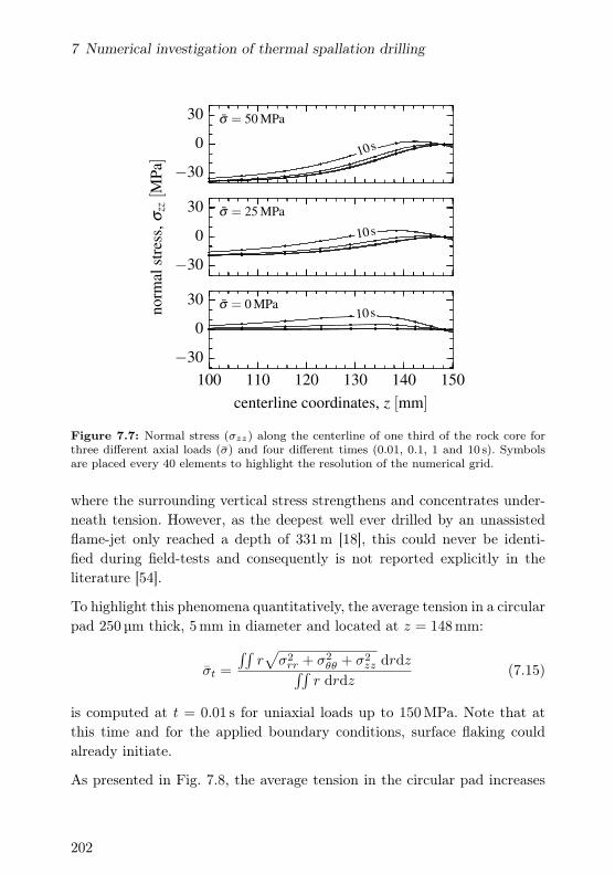
7 Numerical investigation of thermal spallation drilling
−30
0
30
10s
σ = 50 MPa
−30
0
30
no
rmal
stre
ss,
σzz[M
Pa]
10s
σ = 25 MPa
100 110 120 130 140 150
centerline coordinates, z [mm]
−30
0
3010s
σ = 0 MPa
Figure 7.7: Normal stress (σzz) along the centerline of one third of the rock core forthree different axial loads (σ) and four different times (0.01, 0.1, 1 and 10 s). Symbolsare placed every 40 elements to highlight the resolution of the numerical grid.
where the surrounding vertical stress strengthens and concentrates under-neath tension. However, as the deepest well ever drilled by an unassistedflame-jet only reached a depth of 331m [18], this could never be identi-fied during field-tests and consequently is not reported explicitly in theliterature [54].
To highlight this phenomena quantitatively, the average tension in a circularpad 250 µm thick, 5mm in diameter and located at z = 148mm:
σt =
∫∫r√
σ2rr + σ2
θθ + σ2zz drdz
∫∫r drdz
(7.15)
is computed at t = 0.01 s for uniaxial loads up to 150MPa. Note that atthis time and for the applied boundary conditions, surface flaking couldalready initiate.
As presented in Fig. 7.8, the average tension in the circular pad increases
202
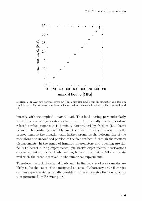
7.4 Numerical investigation
0 20 40 60 80 100 120 140 160
uniaxial load, σ [MPa]
0
5
10
15
20
25
30
35
mea
nte
nsi
on
,σ
t[M
Pa]
Figure 7.8: Average normal stress (σt) in a circular pad 5mm in diameter and 250 µmthick located 2mm below the flame-jet exposed surface as a function of the uniaxial load(σ).
linearly with the applied uniaxial load. This load, acting perpendicularlyto the free surface, generates static tension. Additionally the temperaturerelated surface expansion is partially constrained by friction (i.e. shear)between the confining assembly and the rock. This shear stress, directlyproportional to the uniaxial load, further promotes the deformation of therock along the unconfined portion of the free surface. Although the induceddisplacements, in the range of hundred micrometers and buckling are dif-ficult to detect during experiments, qualitative experimental observationsconducted with uniaxial loads ranging from 0 to about 80MPa correlatewell with the trend observed in the numerical experiments.
Therefore, the lack of external loads and the limited size of rock samples arelikely to be the cause of the mitigated success of laboratory scale flame-jetdrilling experiments, especially considering the impressive field demonstra-tion performed by Browning [18].
203

7 Numerical investigation of thermal spallation drilling
The static tension, produced by the external mechanical load and amplifiedby surface friction is expected to play a crucial role in the surface bucklingand surface flaking process and thus on the efficiency of thermal spallationdrilling. Based on the linear increase of the static tension for increasinguniaxial load, which fractures and weakens the near surface region, theefficiency of thermal spallation drilling is expected to increase with depthwhich makes the technique especially interesting for deep boreholes.
7.5 Closing remarks
The uncoupled, quasi-static thermoelastic code developed for this numer-ical investigation captures flame-jet drilling experimental trends observedwith different uniaxial loads from 0 to approximately 80MPa. The ben-eficial effects of the vertical confining stress, representing one part of thenatural stress at depth on the process is explained: the uniaxial load ampli-fies near surface tension, promoting indirectly surface flaking by fracturingthe rock underneath the compressed layer. Additionally, the uniaxial loadlimits volumetric tension responsible for the axial splitting of mechanicallyunconfined rock samples.
Finally, in contrary to conventional drilling techniques, flame-jet drillingand associated thermal drilling methods make use of the vertical stress pro-duced by the upper layers surrounding the borehole to concentrate stressestowards the free surface - enhancing surface flaking. Such a technique, whichefficiency is expected to increase with depth, have the potential to outper-form conventional drilling; especially for deep boreholes in hard crystallinerock formations where thermal spallation is reported to work best.
204

8 Flame-jet drilling pilot scale
demonstration
There is only one way to
know. . .
As introduced in Sec. 2.4, flame-jet drilling has been used industrially dur-ing almost thirty years for shallow depths hard rock drilling operations.In the end, due to the development of conventional rock reduction tech-niques and the increasing costs of fuel and oxygen, flame-jet rigs have beenslowly decommissioned, even though the performance (i.e. penetration rate)demonstrated in hard rocks remained very appealing.Since the sixties, there is an irregular development of this alternative rockreduction technique, essentially performed by research institutes and astart-up [17, 54, 62, 77]. The main driver being the potential to limit therock reduction costs regularly associated - by amalgam - with drilling orwell construction costs. These costs are usually pointed out as a major prob-lem impeding the widespread development of deep geothermal systems [1].Additionally, this sporadic and segregated development was mostly basedon fairly small laboratory rock samples (e.g. 85mm in diameter × 150mm
in length) and only one experimental setup has been fully dedicated to sim-ulate both the in-situ fluid pressure and the stresses prevailing in a deepwell [54]. In the end, the results reported by Potter et al. [54] proved univo-cally that the mechanism driving thermal spallation functions at relevantdownhole conditions (i.e. jet and in-situ fluid pressure as well as exter-nal stresses). The recent development, presented in Ch. 6, supports theseresults using hydrothermal flames as heat source, ignited and monitoredin a practically relevant manner for downhole operation. Thus a major
205

8 Flame-jet drilling pilot scale demonstration
problem foreseen for the application of flame-jet drilling at depth, i.e. theinoperability of the technique in a fluid filled borehole [51] is resolved. Asan intermediate step towards field tests, a demonstration of the processon a meter-scale is reported in this chapter. To highlight the relevance ofthe demonstration, the influence of two main external parameters varyingwhile drilling is first analyzed, namely the influence of (1) increasing pres-sure with depth and, (2) modification of the formation stress with locationand burial depth. Remember that for questions of hole stability and cut-tings transport, a dense drilling fluid (e.g. water based) is necessary to drillbeyond several hectometers and thus combustion should essentially takeplace in an aqueous environment.
(1) Along the well path fluid pressure increases with depth at a rateproportional to its density.
(a) The influence of this parameter on combustion is not trivial andhas been addressed in 2.5.2. It turns out that pressure will influ-ence the kinetics of the oxidation and that of the decompositionreactions. It will also influence mass transfer.Besides viscosity and the dielectric constant, the most importantjet properties (density, heat capacity) are mostly independent ofpressure, especially at high temperature. Provided that combus-tion can be initiated and supported - which is not trivial whenfeeds are gaseous (e.g. O2) - and dissociation remains limited,the exhaust stream properties are pressure independent. For thesame mass flow, the volumetric flow varies with pressure follow-ing mass conservation. It is therefore possible that a geometrysuitable at shallow depth (i.e. low to moderate pressure, high in-jection velocity and enhanced mixing), will have to be adjustedfor deeper conditions (i.e. higher pressure, lower velocity andpoor mixing).
(b) The in-situ fluid pressure trapped in the formation has a moder-ate impact on the stresses because rocks are porous. Local forcestend to balance over the length-scale of a grain or pore result-ing in no particular differential stress. While drilling hard rocks,the contribution of pore pressure spalling [172] is even negligi-ble based on the cuttings collected (Sec. 8.2) and from the time
206

scale of the process.Pore pressure spallation occurs when the pressure build up ratedue to evaporation is greater than that of crack propagationconnecting the pore network [172].
(2) The second parameter considered is the evolution of the stress fieldwhile drilling. As the vertical component can be readily estimatedbased on rock density and burial depth, horizontal components varyupon location according to the lithology and the presence of geolog-ical structures (e.g. faults, folds, caverns, etc.). Usually, the verticalcomponent of the stress field is reported and demonstrated to supportflame-jet drilling [54, 179] by magnifying and concentrating thermalstresses towards the exposed surface (Ch. 7).
Therefore a demonstration with ambient pressure conditions and usinggaseous feed is more challenging than what is expected downhole. In theend, it should be noted that the gaseous feeds used here are not consideredto be used at depth in the field. This considers pumping energy, drill pipeconnections, i.e. no circulation and risks of gas expansions, potentially lead-ing to a blowout. Liquid systems are preferred [54,73] for wells deeper thanabout 100m. For the pilot scale demonstration, it is however particularlyconvenient.
An additional motivation for the demonstration arises from the experimentsperformed in the laboratory so far [17,62,77], where spalling only initiated.In every case, the process stopped after some time and independently of theconditions, i.e. the stand-off distance, burner power or uniaxial load appliedto the rock cores. It remains to determine if the process can be sustained orif the rate of penetration drops as a result of heating the rock volume [77].This chapter documents the results of the demonstration starting with adescription of the experimental facility and the burner (Sec. 8.1). Then thedemonstration and the results are presented in details, focusing on relevantparameters for further development (Sec. 8.2).
207

8 Flame-jet drilling pilot scale demonstration
8.1 Experimental setup
The system presented in this section is dimensioned to drill 10m deep wellsin the field using a construction compressor for air delivery and gas bottleson site.The experimental setup consists of the process lines, the burner, the well-head, a drawworks system and a 660 kg rock block of granite from theGrimsel pass (Fig. 8.1). For the purpose of the demonstration, the rockblock is loaded symmetrically resulting in equal horizontal stresses i.e.SminH = Smax
H ≈ 1MPa. Note that this is meant to prevent axial split-ting of the block rather than to support spallation or mimic any downholecondition.Each process line (Fig. 8.2) extends on the pre-existing equipment belong-ing to a facility built by Dragana Höser [72]. The burner, the wellhead andthe umbilical coil tubing as well as the cyclone to separate the cuttingsfrom the exhaust stream have been specifically designed and constructedfor the demonstration.
8.1.1 Process lines
Methane is supplied from a 50L bottle initially at 200 bar and its pipingis equipped with a pressure reduction valve, a thermal mass flow controllerand a non-return valve. A manometer fitted upstream of the non-returnvalve allows to estimate the pressure in the combustion chamber.The air is supplied directly from the building delievery system at a pressureof 6 bar(g) and flows through a thermal mass flow controller where its flowis set according to methane to maintain a predefined oxygen to fuel ratio(λ).The contactless drilling tool is cooled with water, the flow rate of whichis adjusted to 160L/h using a rotameter as its temperature is monitoredusing a set of K-Type thermocouples installed upstream and downstreamof the drilling tool. Sufficient cooling water is also provided to the wellheadwhich temperature is monitored by an infrared camera to ensure it remainsat near room temperature during operation.
208

8.1 Experimental setup
burner
wellhead
660 kg
rock block
0.7 m
pads to apply
symmetrical
load
Figure 8.1: Three dimensional view of the 660 kg Grimsel granite block (∆x = ∆y =0.7m, ∆z = 0.5m) and breakout view of the wellhead with the burner enclosed.
8.1.2 Burner characteristics
The contactless burner (Fig. 8.3) is the first drilling tool designed and con-structed at LTR to drill pilot holes in the field. The detailed technicaldrawings of the burner are available in the appendix (A.2) and this sectiondescribes the function of its different parts. In total, it is about 850mm
long and weights 15 kg, keeping the coil essentially in tension using thedrawworks. Its length ensures smooth and vertical progression of the drill,due to gravity. The versatile design of the burner allows rapid adjustmentof different geometrical parameters impacting the combustion efficiency, itsrobustness or even the air and fuel velocities and the extent of the recircu-lation zones.The injection flange (Fig. 8.3) constitutes the link between the hoses en-
209

8 Flame-jet drilling pilot scale demonstration
vacuum
pumpCH
4
CW
CW
T
T
air
6 bar(g)
BHA
cyclone
cuttings
exhaust
T
coil
tubingwellhead
PI
FI
ground
CW
CW
Figure 8.2: Simplified scheme of the experimental facility. The BHA represents theburner assembly.
~505 m
m
CH4
CW
air
fuel injection nozzle
burner
feet
Laval
nozzle
cooling
mantle
CWin
axial
swirler
injection
flange
mixing
spacers
combustion
chamberchamber
shield
50 mm
coil
tubing
fitting
Figure 8.3: Isometric breakout view of the pilot scale burner.
210

8.1 Experimental setup
closed in the coil tubing and the combustion chamber. It features a sym-metric double air intake, limiting air velocity along with vibrations andother resonance phenomena potentially generated by a high fluid velocity.In the present case, pressure in this line is limiting the combustion cham-ber pressure (i.e. the combustion power) for a given nozzle outlet diameterand thus, pressure losses in the air line are minimized in full measure. Toprevent flashbacks, a short and narrow axial section, characterized by ve-locities beyond the flame speed is implemented.The chamber shield (Fig. 8.3) is a 5mm thick cylindrical tube meant toprotect the internal combustion chamber from impacts and erosion on theside of the borehole. Its mass helps holding the burner in a vertical posi-tion and steady while drilling.The cooling mantle is a 1mm tube fitted with 10 holes, 3mm in diameterand equally distributed at its bottom end in order to drive the water flowbetween the combustion chamber and the mantle - to return through theinjection flange.The pressure bearing wall of the chamber is 2.5mm thick, leaving an in-ternal space of 56mm in diameter and 545mm long (i.e. volume of 1.34L)for combustion and is rated for pressures up to 100 bar at room tempera-ture. An axial swirler (Fig. 8.4) is used to add a radial velocity component
39 m
m
24 mm
Figure 8.4: Isometric view of the axial swirler. The angle between the trailing edge andthe swirler axis is 62.
to the air stream before its injection and increase the turbulence intensityand combustion robustness. The angle formed by the trailing edge and theswirler axis is 62, resulting in a ratio of radial to axial velocity of about1.88.A set of mixing spacers (Fig. 8.3) can be inserted while assembling the
211

8 Flame-jet drilling pilot scale demonstration
contacless drilling tool to lift either the fuel injection location in the coax-ial air flow or the position of the axial swirler. Hence, combustion can beupgraded from a pure turbulent diffusion flame to a turbulent, partiallypremixed flame. For the present experiment no mixing spacers are used re-sulting in a pure turbulent diffusion flame.The fuel injection nozzle consists of a tube and its tip and is similar to theinjectors used in the pressure vessel (Ch. 5). In the present case, a fuel injec-tion nozzle featuring 12 holes, 1mm in diameter and departing by 30 fromthe central axis is used. Similarly as in the experiments in the WCHB-4and presented in Secs. 5.2 and 5.3, a ceramic insert is used to insulate theigniter thermocouple from the fuel injection nozzle.The combustion products are accelerated through a converging-divergingnozzle (Laval shape) designed by Zimmermann [180]. Besides the pressuredifference driving the flow, the geometry of the nozzle is optimized to en-sure a smooth velocity profile along its extent. Note that in the presentcase, the outlet bore of the nozzle is 7.1mm in diameter.To prevent the outlet of the burner to be blocked and to direct the drill,burner feet are used to keep a distance between the nozzle and the exposedrock surface. In the present case, the feet height leads to a dimensionlessstand off distance of 7 - using the outlet diameter of the nozzle as reference- which generally leads to optimal heat transfer conditions [181].
Hot surface ignition and its electrical circuit
The igniter thermocouple to ignite and monitor the combustion is based onthe series used for the hydrothermal flame ignition and monitoring (Ch. 5).The present sensor is as documented in Sec. 5.1 besides that the lengthof its ceramic insulation tube is shorter to fit the particular geometricalconstraints of this burner (Fig. 8.3). The coil protrudes about 33mm fromthe tip of the fuel injection nozzle and its tip-thermoelectric junction is4.5mm ahead of the coil. Thus, the igniter thermocouple is positioned inthe central recirculation of the purely diffusion flame used for the test.
212
8.1 Experimental setup
8.1.3 Wellhead and cyclone
The wellhead assembly is presented in Fig. 8.1. It serves on the one handto stabilize the drill until sufficient penetration in the hole and on the otherhand to partially seal the latter from the environment.At the top of the assembly is a long pipe through which the burner andthe feed lines - enclosed in the coil - are lowered into the hole. The tube iswelded to a flange equipped with connections for the exhaust, a burstingdisc (10 bar at 100 C), a manometer and a thermocouple. This flange isconnected by two - water cooled - concentric circular sections to a baseplatehaving a larger diameter to stabilize the construction. For the operation inthe laboratory, the wellhead is glued on the rock block using a mastic (ad-heseal, PCS Innotec) which seals any discontinuity. Conversely it is foreseenthat in the field, depending on the drawworks system, it might be neces-sary to anchor the wellhead firmly to the rock base and thus a set of holesto fit threaded rods and bolts are prepared in the base of the construction.Sealing is then achieved using a temperature resistant mastic or concrete.To separate the cuttings from the exhaust gas leaving the wellhead, thestream is directed with a metallic hose to a cyclone. The cyclone has beendesigned by Zimmerman [180] based on the recommendations of Muschelk-nautz [182]. The basic parameters used to design the device are its volume,the pressure drop across its inner tube and the separation limit, which isthe smallest size of solid particle that will be separated from the gas stream.In the present case, it is designed to separate any particle larger than 10 µmand has a volume of 23L. At its bottom, the cyclone is equipped with apolyamide rope bag to collect the cuttings. Finally, the outlet (i.e. innertube) of the cyclone is connected to a second metallic hose the pressure ofwhich can be reduced using an industrial vacuum cleaner. This permits toavoid over pressure in the system and outflows between the burner and thewellhead tube until sufficient penetration is reached. At this point a strip-per rubber can be installed on the coil tubing to better seal the system.
213
8 Flame-jet drilling pilot scale demonstration
8.1.4 Control system
The operation of the setup is done using a computer and the remote controlof the crane of the experimental hall. Each mass flow of the process linesis controlled using the electronic built by Dragana Höser and presentedin [72]. Temperature sensors are recorded with the same equipment be-sides the igniter thermocouple. The latter is supplied and used to monitorthe temperature in the combustion chamber with the same Beckhoff I/Omodule and power supply as for the high pressure experiments (Ch. 5).The current supplying the heating the coil is digitalized directly by theDC power supply. During the demonstration, these electronic parts werelocated more than 10m away from the heating coil - proving that the igni-tion system met the design purposes of the system (i.e. 10m deep wells inthe field).
8.1.5 Safety
Because of the inherent risks related to the use of a large and powerful in-ternal combustion chamber designed to drill rocks and moving dynamicallyduring operation, different safety measures were implemented to ensure asmooth and sound operation of the contactless drilling tool. These actionsare based on an HAZOP study of the burner, its feed lines and the exhaustsystem.The procedure is extensively documented in the work of Zimmermann [180]and the resulting actions are summarized below. Besides cooling water forboth the internal combustion chamber and the wellhead, emergency but-tons - to stop the gas feeds - are positioned adequately around the setup.Additionally the methane concentration is continuously monitored by twosensors, actuating a normally closed magnetic valve in the methane line. Inaddition to the flow of methane and air, temperatures inside the combustionchamber and on the wellhead are continuously monitored. The surface tem-perature of the wellhead is also controlled with an infrared camera to bearany burn hazard. A bursting disc implemented on the wellhead preventspressure buildup in the system and hazardous failure of any mechanicalpart. In addition to the axial position of the burner (tracked with a pattern
214

8.2 Results
marked on the coil tubing at 10 cm intervals) and the hook provided by thecrane (measured with a crane scale), the polyamide rope bag - underneaththe cyclone - lies on a scale to confirm the accumulation of spalls and thesmooth progression of the burner. A thermocouple is taped below the rockblock to stop the experiment as soon as full penetration is achieved. Thecombustion chamber of the burner is also expressively oversized to ensurecomplete combustion of the fuel and prevent any high enthalpy oxidationin the annulus formed with the open hole. Finally, a strict operational pro-cedure is worked out and followed to minimize hazardous scenarios.
8.2 Results
Hereafter the experimental results are reported, discussing firstly the datareduction and the temperature-emf calibration of the igniter thermocouple.Then, the power ramp for ignition and the temperature evolution insidethe combustion chamber are presented as a function of time. Note thatthe sensor temperature is reported rather than the local fluid temperature,i.e no correction is applied for radiation and convection losses. Afterwards,the average penetration rate, the thermal specific energy, hole shape andthe particle size distribution of the cuttings are presented. In the end,concluding remarks related to the demonstration and field trials are drawn.
8.2.1 Data reduction and igniter thermocouple
calibration
The reduction of the igniter thermocouple calibration data is performedfollowing the same methodology as presented in 5.3.3 which is based on theguidelines presented by Coleman and Steele [116] and the ISO 8466-2 [166].A 95% level of confidence is specified on the systematic uncertainties andthe statistical fluctuations presuming data follow a t-distribution and theuncertainties on the direct measurements are summarized in Tab. 8.1. Thecombined systematic uncertainty on the igniter thermocouple temperature
215

8 Flame-jet drilling pilot scale demonstration
(uc(Ti)) is:
uc(Ti) =
2
[(∂Ti
∂p2
)2
u2(p2) +
(∂Ti
∂U
)2
u2(U) +
(∂Ti
∂U
)2
u2(U)
]1/2
,(8.1)
with p2 [µV/C] the coefficient of the polynomial least-squares regression(Fig. 8.5), U [µV] the voltage generated by the thermoelectric junction oncethe SSR is opened and U [µV] the mean response of the calibration. Notethat to derive Eq. (8.1),
U =
(U − p2T
T 2
)
T 2 + p2T
is used instead of the direct calibration equation (U = p1T2 + p2T ) as p1
and p2 are correlated [155] and, the partial derivatives (Eq. (8.1)) are eval-uated analytically. Finally, the combined systematic uncertainty (±15 C)is negligible compared to the temperatures recorded by the custom madesensor and measurements are accurate.
Table 8.1: Uncertainties during the igniter thermocouple (NiCr-80/20) calibration andmeasurements.
Sys. uncertainty Stat. fluctuation
Voltage-temperature calibrationU 2 µV 3.77%T 0.0075× T 0.16%
Temperature profile measurementsU 30 µV -
The calibration of the igniter thermocouple is performed according to themethodology presented in 5.1.3 and a test to study the influence of the basecopper NiCr-80/20 thermoelectric junction, as introduced in 5.1.2, is alsoperformed.The results of the test and the calibration function for the thermocou-ple igniter are depicted in Fig. 8.5. The discrepancy between the originaland the model data suggests that NiCr-80/20 has a distinct Seebeck co-
216

8.2 Results
0 200 400 600 800 1000
temperature, Toven [C]
0
5
10
15
20
25
30
35
ther
mo
cou
ple
ign
iter
vo
ltag
e,U
[mV]
quad. least-squares fit
original data
model data
Figure 8.5: Temperature response of the NiCr-80/20 thermocouple igniter (originaldata) and its model (model data). The quadratic least-squares fit (calibration function)has a correlation coefficient (R2) of 0.9999.
efficient than copper (Fig. 5.5). Hence, different temperature distributionsenforced during the calibration (i.e. uniform temperature between the tipand the base-junction, see Fig. 5.4) and the measurements (i.e. monoton-ically increasing towards the tip-junction, see Fig. 5.3) are accounted forby using the model igniter data to determine the calibration function. Forthe model igniter in the oven, the temperature drop occurs along the NiCr-80/20 and Alumel R© segments, which best represents the conditions of theigniter thermocouple NiCr-80/20 during the temperature measurements in-side the combustion chamber. Therefore no contribution to the combineduncertainty (Eq. (8.1)) is added.
217

8 Flame-jet drilling pilot scale demonstration
8.2.2 Ignition and temperature evolution over time
The electrical circuit (5.2.2) consists of the copper extensions (> 10m) con-nected to the lead wires. A SSR mounted in series allows to open the circuitrapidly after ignition and a digital multimeter terminal mounted in paral-lel to the igniter thermocouple (Fig. 5.11) enables voltage measurementsover multiple scales (i.e. 0 . . . 30mV, 0 . . . 300V).
Ignition of the pure turbulent diffusion flame
0 20 40 60 80 100 120 140
time, tign [s]
7.0
7.2
7.4
7.6
7.8
8.0
ign
iter
resi
stan
ce,
Rig
n[Ω
]
0
20
40
60
80
100
120
140
ign
itio
np
ower
,p
ign[W
]
Figure 8.6: Electric power dissipated through the heating coil and its lead wires. Eachstep increase correspond to an additional 0.2A increase in the limiting current besidesthe first two steps which correspond to a 1A increase each.
Previous to ignition, 0.11 kg/h of methane and the necessary air to ensurefuel-lean conditions (λ = 1.2) are fed to the burner. The igniter thermo-couple is then charged using the same circuit as presented in 5.2.2. Due tothe lower heat capacity of the gaseous mixture, it is initially charged with
218

8.2 Results
0.2A and the current is increasingly limited in steps of 0.2A every 15 s
until ignition occurs. About 100W are necessary to ignite this mixture,which is significantly less than to ignite hydrothermal flames (Ch. 5).
Temperature time series
The temporal evolution of the temperature is presented in Fig. 8.7 (top)for the first phase of the demonstration and in Fig. 8.7 (bottom) for thesecond phase of the demonstration. The break in between is related to theinstallation of a vacuum cleaner at the end of the exhaust line, setting theexhaust line, the wellhead and the open hole in rough vacuum. The flowdirection in the circular gap between the burner and the wellhead is there-fore reversed and no spall is dragged out of the system. From both figures,the same trends are observed, highlighting the reproducibility of the exper-imental procedure. After ignition, the solid state relay is opened, breakingthe main circuit. Simultaneously, the voltage measuring terminal switchesscale in order to acquire the lower voltages generated by the thermoelec-tric junctions, resulting in the temperature log (Fig. 8.7).The mass flows of air and methane are then simultaneously increased step-wise, according to a procedure defined by Dragana Höser [72] to preventvibrations in the feed lines. At a certain mass flow of methane (∼1 kg/h)and air (∼20.8 kg/h), the temperature drops significantly, corresponding tothe flame detachment from the fuel injection nozzle. Thereafter, the flame islifted up. This behavior leads to the protection of the injection system andthe heating coil while drilling extending the service life of these uncooledparts and reducing risks of flashbacks.
Then, the temperature evolution reaches a plateau earlier than the massflows, supporting a steady position of the flame along the combustion cham-ber. Hence as the axial velocity is constant (resp. the flame front position)but the mass flows are increased, pressure necessarily increases to satisfythe mass balance. During drilling, the temperature log is relatively steady,despite the constant axial acceleration imposed to the burner by the draw-works, which is necessary to keep the drill free. Important fluctuations in thetemperature log while drilling are all related to rapid variations in the air
219

8 Flame-jet drilling pilot scale demonstration
0 300 600 900 1200 1500 1800
0.00.20.40.60.81.0
drillingphase 1
647 s
0 300 600 900 1200 1500 1800
time, t [s]
0.00.20.40.60.81.0
T/(1
16
3C);
mC
H4/(
2.4
7k
g/
h);
mai
r/(5
2k
g/
h)
drillingphase 2
736 s
igniter thermocouple
CH4
air
Figure 8.7: Relative temperature, methane and air mass flow during the demonstration.Ignition occurs at around 50 s and the drilling time for both phases is shaded. Top panel:First phase. Bottom panel: Second phase.
flowrate. From Fig. 8.7, a sudden decrease in the air mass flow (t = 1250 s)leads to consequent temperature fluctuations, certainly resulting from analteration of the mixing and the dynamic repositioning of the combustion.In the end, the temperatures recorded by the igniter thermocouple duringboth procedures to reach the setpoint are very similar, supporting the re-producibility of the mixing conditions and, the combustion robustness inthe burner. In addition to allow flame ignition and monitoring, the tem-poral evolution of the temperature informs qualitatively and relatively onthe flame structure inside the combustion chamber. This permits a con-trol over any unexpected trend. Finally, the intermittent and rough axialdisplacement of the chamber while drilling did not influence significantlycombustion.
220

8.2 Results
8.2.3 Flame-jet drilling demonstration
Penetration rate
The penetration rate is determined by analyzing the burner position withrespect to the top of the wellhead. The hook load (viz. crane scale) givingevidence whether the burner hangs or lies on the rock. During the demon-stration, an average and constant penetration rate of 1.5m/h has beenreached. Hence, disapproving Silva et al. [77] according to whom the rateof penetration decreases as a consequence of residual heat in the rock vol-ume. On the other hand, the rate of penetration achieved is considerablylower than former values reported in literature (Tab. 8.2). But as the com-bustion power is two order of magnitude lower, penetration rates cannotbe compared directly. The thermal specific energy is a convenient basis tocompare this demonstration with former field tests and conventional me-chanical drilling.
Thermal specific energy
The mechanical specific energy is a concept used to monitor the perfor-mance of the rock reduction process and adjust parameters such as weighton bit and rpm [50]. Adapting this concept to thermal spallation drilling,the thermal specific energy (TSE) is defined as:
TSE [J/mm3] =thermal energy inputrock volume removed
.
In order to determine the TSE during the demonstration, the total exca-vated volume (3.42L) is estimated by filling the hole with water and thethermal energy input is calculated using the methane enthalpy of combus-tion (higher heating value). The TSE is reported in Tab. 8.2 together withliterature values for flame-jet drilling. Although the ROP achieved in thepresent demonstration is significantly lower than values reached in the field(Tab. 8.2), the thermal specific energy has the same order of magnitudes.Hence, the efficiency of the conversion from thermal energy (combustion) tomechanical energy (thermal stresses) complies between the different tests.
221

8 Flame-jet drilling pilot scale demonstration
Table 8.2: Comparison of the demonstration with literature data. ROP denotes therate of penetration, D the hole diameter, p the combustion power and TSE the thermalspecific energy.
Rock ROP [m/h] D [mm] p [kW] TSE [J/mm3]
Fleming [169] Aurora 4.5 to 9 165 1600 30 to 60Browning [183] Barre 4 to 9 400 1600 30 to 60Browning [183] Conway 16 230 1600 8.7demonstration Grimsel 1.5 85 38 15.4
Therefore it is likely that the penetration rate was limited by the power ofthe combustion and not by poor heat transfer or any other factor duringthe demonstration, which would affect negatively the thermal specific en-ergy compared to former tests.In an attempt to increase ROP, increasing solely the combustion power us-ing the same nozzle (Fig. 8.3) characterized by a 6mm throat, is inefficient.This is because the advancing geometry of the hole would look like a halfelongated spheroid but not necessarily be directly large enough to enablesmooth and rapid progression of the drill. To optimize the system for thepenetration rate, the thermal stresses induced over the whole surface un-derneath the burner should be maximized.The specific energy of the thermal process is generally higher than thatof mechanical drilling (2.1 J/mm3 [184]). These numbers are only indica-tive as they depend on the rock type and size [185], the load applied orburial depth [184] as well as other external factors. The values reportedin Tab. 8.2 are for crystalline rocks at shallow depth without consideringthe impact of the chip hold down effect [51], nor that of the external con-straints at great depth.Accordingly, the higher specific energy of the thermal process can onlybe explained by dusting, i.e. dust size cuttings, often observed in ther-mal spallation (Fig. 8.10). This is because if the cuttings size would bethe same, thermal spallation is inherently more efficient than mechanicaldrilling (i.e. crushing and shearing), as the rock tensile strength is lowerthan its compressive or shear strength. Remember that although the de-tails of the mechanism are still not resolved, crack growth, buckling andspall ejection are driven by tension in the rock mass.To reduce the thermal specific energy, the heat generated during combus-
222

8.2 Results
tion should be invested to remove larger rock volumes which could beachieved using larger nozzles. As the diameter of the drill controls thesmallest hole diameter, the diameter of the nozzle sets an upper limit tothe surface heated by the concentrated jet and thus the maximal spall size,provided that sufficient heat reaches the rock surface over the correspond-ing area. As the typical flake-like shape of the spalls is found to be moreor less constant and characterized by diameter to thickness ratio rangingfrom 8 to 15 [186], larger spalls lead higher penetration rate [61] assumingthe rate at which they are expelled is steady.Provided that the supply is sized accordingly, nozzle diameters in the rangeof 10 to 30% of the drill diameter should be considered as a starting pointfor a finer optimization, based on TSE.Finally, even though the specific energy of thermal spallation is larger thanthat for mechanical drilling on surface, it should be inputed to the relativelack of optimization of the thermal process rather than to its potential. Itis also likely that this trend reverses at depth, owing to the increasing effi-ciency of the thermal process (Ch. 7). Thus thermal drilling techniques arefrom an energetic point of view favored at great depth which correspondswith the location at which crystalline rocks are encountered where thermalspallation drilling is reported to work best.
Hole shape
The hole shape is cylindrical and calibrated as illustrated in Fig. 8.8. It isgenerally only slightly underreamed allowing: the necessary clearance forthe contactless burner to advance under the effect of gravity and, suffi-cient velocity of the exhaust stream to drag the cuttings out of the hole.At about 10 cm from the top, there is an underreamed section which wasinduced by holding the burner steady for several seconds instead of con-tinuously advancing the drill. Hence different tolerances on the hole shapecan be achieved by adjusting design parameters, process parameters andoperating conditions.In the present case the burner was designed to produce straight and verticalholes and the clearance to the hole is adjusted by changing the advancingrate of the drill. The section shown in Fig. 8.8 corresponds to the orien-
223

8 Flame-jet drilling pilot scale demonstration
Figure 8.8: Section of the Grimsel rock block (0.7× 0.5m). A thermally altered area isvisible on the side of the hole. It corresponds to the dewatering of the minerals, oxidationas well as other factors.
tation East-North-East to South-South-West of the optical televiewer log(Fig. 8.9). The log covers the first 40 cm the of hole and the necessary carehas been taken to minimize any electro-magnetic distortion.
Particule size distribution
The spalls are collected in a polyamide bag underneath the cyclone. Atthe end of the demonstration, a fraction of 82% of the spalls had beencollected, which is representative of the complete size distribution besidesthe finest fractions dragged by the exhaust stream through the cyclone.The collected fraction is then sieved through a 500 µm mesh and the finefraction (72% of the initial mass) is analyzed by laser diffraction. The resultsare presented in Fig. 8.10. This is certainly the most direct indication ofthe stresses in the rock at the instant where it spalls and the only onepractically available in the field. Furthermore, this avoids the demandingand approximative determination of the heat transfer coefficient, followedby simulation (e.g. Ch. 7 or [187–189]) and the definition of a microscopicfailure criteria. Attempts to observe the micro-scale process at very highfrequencies (12 500Hz) to clarify the details of the mechanism (e.g. [190])remained up to date unsuccessful.
224

8.2 Results
Figure 8.9: Image from the optical televiewer log of the demonstration hole. The imagecovers the first 40 cm of the hole.
From Fig. 8.10, the average particle size is less than 100 µm and 90% ofthe particles are smaller than 300 µm. This is smaller than the particle sizeobtained by Potter et al. [54] during similar tests, where the average size liesat around 200 µm. The factor two is possibly explained by higher thermalstresses at the moment of the spall ejection, which could be attributed tothe small throat diameter (6mm).
As the particles are smaller than typical grains (∼ 2mm [191]), fractures areintra-crystalline and not only along grain boundaries (i.e. inter-crystalline).This is associated to thermal stress spallation and supports the minor con-tribution of pore pressure spallation [172].
225

8 Flame-jet drilling pilot scale demonstration
0 200 400 600 800
particle size, [µm]
0
20
40
60
80
100
cum
.d
istr
ibu
tio
nQ
3,
[%]
Figure 8.10: Particle size distribution of the spalls collected during phase 1 and 2. Thedistribution is representative of 60% of the total mass.
8.3 Closing remarks
In this section the contactless drilling tool to demonstrate flame-jet drillingon the meter-scale is presented. Based on the successful demonstrationusing the drill, every original milestone:
• flame ignition,
• monitoring,
• stable combustion and,
• drilling a calibrated and cylindrical hole through the rock block
has been achieved. The custom made igniter, initially constructed to forcethe ignition of hydrothermal flames (Ch. 5) has been successfully retrofittedin the design of the drilling tool. This allowed the constant combustionmonitoring during the demonstration, an essential information for safetyand to observe the lifting of the flame front beyond certain mass flows.
226

8.3 Closing remarks
Additionally, the system has been proven to work with wires longer thanthe measured depth for which it has been designed, giving confidence inthe capacity to achieve its target in the field.The thermal specific energy reported during the demonstration compareswell with similar tests of flame-jet drilling performed in the field, despitethose reached significantly larger penetration rates. This discrepancy isattributed to a lack of combustion power in the present demonstration anda poor utilization of the thermal energy.To maximize the penetration rate of the drill, an optimum between thedrill diameter, the nozzle bore diameter and the operating conditions hasto be found based on the information available in the field (i.e. particlesize distribution, thermal specific energy, process parameters and flamemonitoring (e.g. temperature)).In the end, one should aim at minimizing the thermal specific energy, orcontinuously try to optimize the figure to clarify the correlation between thespall size, different rocks, external constraints (e.g. depth), nozzle diameter,drill diameter and thermal stresses.As a rough guideline for designing flame-jet drilling tool, it is better tooverestimate the length of the burner and under dimension the outer borediameter of the nozzle. More specifically and assuming that the supply issized appropriately, nozzle diameters in the range of 10 to 30% of the drilldiameter should be considered as a starting point for a finer optimization,based on thermal specific energy. Additionally, the system should be limitedby the bore diameter of the nozzle. If, on the other hand, the supply linesare limiting, it might lead to a lack of heat with respect to the nozzle tosustain the thermal process.
227

9 Drilling concepts and
techno-economic feasibility
It was easy to drill in the
lab and it gets much
harder in the field. . . one
of the big issue is of
course that you can’t see
what you are doing. . .
T. Wideman, former
CTO at Potter Drilling
Inc., 2016
In this chapter two concepts to implement flame-jet drilling are introduced(Secs. 9.1 and 9.2). Section 9.3 presents the impact of both concepts on therock reduction costs, the well costs and finally to overall EGS project costs.To this aim, it is assumed that the concepts are on the one hand feasible (i.e.technically and practically) and that operating conditions exist to reach theaverage performances estimated (i.e. ROP and service life).
9.1 Flame-jet coil tubing rig
The flame-jet coil tubing system breaks the rock by thermal stresses withminor assistance from mechanical forces e.g. to penetrate through prob-lematic zones. Hence the hole drilled is underreamed but not perfectly cal-ibrated. At this point, it is important to clarify that a flame-jet describesany hot fluid jet able to spall rock or damage it by thermal shocks. In prin-
229

9 Drilling concepts and techno-economic feasibility
ciple, the flame remains confined in a combustion chamber or similar andonly the high temperature, high velocity exhaust stream is directed ontothe rock (jet).
Conceptual description
The system consists of a bottom hole assembly, a coil with an umbilical hoseto carry the reactants, the wellhead, potentially a mast (e.g. hybrid coiltubing rig) and feed auxiliaries (i.e. pumps and compressors). Commercialshakers and filtration units as well as mud coolers are used on surface toseparate solid particles from the return flow and cool the drilling fluid downbefore it is pumped back downhole (Fig. 9.2).Such a system is indeed a wet version of the one used for the demonstration(Ch. 8) with recirculation of the drilling fluid. It is illustrated in Fig. 9.1with the modified coil tubing rig used by Potter Drilling Inc. during fieldtests [54]. The BHA consists of the reaction zone or combustion chamber,the MWD and DWD tools as well as centralizers, collars and HWDP whichare located above the reaction sub to add weight on the tool. The length ofthe BHA is critical as it might determine a dogleg pattern along the well.
Feasibility assessment
The system requires a fairly limited number of additional units and is verycompact, light and elementary in comparison to the mobile rig MR8000(Fig. 2.1), especially in the standard coil tubing version. Additionally andcompared to conventional drilling rigs, it complies with the highest noisepolicies and seems very suitable for urban areas (i.e. no surface rotationnor drill pipe connection and minimum lift operation). Unlike the systemused for the demonstration of the technology (Ch. 8), it is convenient tohave both fuel and oxidizer in liquid form with densities close to that ofwater. The chemicals should be premixed on surface and enclosed in the coilseparately from the drilling fluid. The drilling fluid fills the space betweenthe umbilical hose carrying the reactants and the coil itself. This designconsiders the practical requirements related to:
230

9.1 Flame-jet coil tubing rig
Figure 9.1: Modified coil tubing rig used by Potter Drilling Inc. for the field test of wetflame-jet drilling [54].
• the energy needed to compress gases beyond the hydrostatic pressureat the bottom of a well - several kilometers deep - filled with waterand additives;
• safety concern: if pressure is lost on surface, it prevents hazardousexpansion of the feed line (i.e. a blowout);
• it is cumbersome to manufacture a long coil with several umbilicalhoses to transport fuel and oxidizer separately.
In the present thesis, flame-jet coil tubing rigs are further classified in twocategories, according to the core mechanism of the process, viz. the ignition:
(1) the first is based on passive ignition e.g. the decomposition of hy-drogen peroxide coupled with the oxidation of a hydrocarbon-watermixture (e.g. methanol-water) over a platinum catalyst bed [54,73].
(2) the second is active and based on the igniter thermocouple, or a highvoltage spark plug to initiate a rapid oxidation downhole [142].
231

9 Drilling concepts and techno-economic feasibility
additional surface
equipment
mud
pumpmud
tank
bottom hole
assembly
flame-jet bit
CT reel
pumpfuel
tank
pumpoxidizer
tank
Figure 9.2: Components of the flame-jet coil tubing rig. The additional units for thisspecific operation are highlighted in red.
Oxidation initiated over a catalyst bed
Potter Drilling Inc. relied on the decomposition of hydrogen peroxide as-sociated with the oxidation of a methanol-water mixture (38 wt.% H2O2,12 wt.% CH3OH, 50 wt.% H2O) to produce superheated steam or a su-percritical water jet (T ∼ 800 C) [73]. This mechanism is technically andpractically feasible backed up by a series of field tests [54]. Finally, a down-hole sensor is required to monitor continuously the exothermic reaction.
Oxidation initiated using the igniter thermocouple
The second mechanism uses an external sensor, e.g. a hot surface (Ch. 5),to initiate combustion or a self-sustained flameless oxidation. An advantageis the absence of catalyst, hence the system has constant performance overtime. Additionally, a sensor to monitor the reaction is available downhole.
232

9.1 Flame-jet coil tubing rig
Such a sensor could be powered employing a similar circuit as in Ch. 5 andsupplied by a downhole generator or a battery. Data to and from the sensorare exchanged with surface by usual mud pulse telemetry or based on theelectrical conductivity of the ground [29]. Additionally for the high pres-sure rock drilling experiments presented in Ch. 6 no specific seal is used toseparate the exhaust stream from the cooling water. The exclusion of thesurrounding cold water is naturally achieved by keeping the pressure in thereaction zone above hydrostatic and injecting the cooling water of the com-bustion chamber upwards (Fig. 5.16).As the temperature of the jet exciting the combustion chamber (32.5 wt.%EtOH) is higher (∼ 1000 C) than that from the catalyzed reaction, thissystem tolerates greater inflows from the surrounding cooling water. Fur-thermore, the extensive range of temperatures obtained by varying the fuelconcentration and the different flame power, by modifying the pumpingrate, lead to a great versatility and the possibility to comply with the se-vere requirements (e.g. drilling fluid density and pumping rate, formation,state of stress) while drilling.The disadvantage of this second solution is the need of an igniter to initi-ate the reaction downhole. Additionally, the highest temperature (Tad, seeFig. 2.19) produced with this system can be higher and potentially morehazardous. In the end, this concept is technically feasible and it remains todetermine whether it is also practically feasible.
Common characteristics
A fundamental limitation of the standalone system arises from the difficultyto drill through fissures [61] and direct the drill1 along with the impossi-bility to drill non heat spallable rocks or the casing shoe (Ch. 2). To piercenon heat spallable rocks and fissures, mechanical reamers [18] and abra-sive particles seeded in the feeds have been implemented successfully in thepast [61]. Concerning piercing the casing shoe no practical solution has beenproposed yet and the problem appears to be discussed nowhere. Hence, itseems there is no practical solution besides melting completely the metallic
1Personal communication with Tom Wideman, former CTO at Potter Drilling Inc.,April 2016
233

9 Drilling concepts and techno-economic feasibility
component of the shoe or changing significantly its design and composi-tion. Furthermore, the standard coil tubing rigs are not suitable to lowercasing strings, which requires the use of a hybrid rig (i.e. equipped with amast). These rigs are typically rated with lower hook load capacities thanconventional rigs which limits correspondingly the length of the sections.Coil tubing flame-jet drilling rigs are currently suitable to drill shallowwells [18], slim exploration holes, for mining operations [169] and to drillopen hole sections in the basement rock but cannot be used as a standalonerig to construct deep wells. For the open hole section, an adequate combi-nation of nozzles can be used to produce an elliptical underreamed sectionalong the reservoir, resulting in two significant benefits: (i) by aligning themajor axis of the ellipse with the maximum stress, the stability of the openhole section is enhanced and, (ii) the larger interface between the open holeand the formation reduces the near wall impedance [192]. A similar solu-tion has been proposed earlier by Guinot et al. [193] in order to improvethe stability and productivity of perforations for the production of oil fromsands.Practically, it seems challenging to do this along horizontal sections as it iscurrently impractical to have WOB beyond a lock-up point. The horizontalreach for small diameter (2”) coil is currently in the range of 1500m. Addi-tionally for workover operations, coil tubing rigs are generally appreciateddue to the limited mobilization costs, compatibility with stripper rubbers,etc. Hence, flame-jet coil tubing rigs could be employed to enhance thepermeability of the vertical open section in a well [192] by modifying itscircular shape which is convenient to drill and lower the casing, but notoptimized from a production (low surface to volume ratio) and stabilitypoint of view. An other problem of flame-jet drilling is to have fuel and ox-idant downhole in case hydrocarbons are met, especially if the oxidationis fuel-lean. On the other hand, a benefit might arise in cuttings transportas the CO2 from the combustion products degasses along the annulus. Inthe end, the flame-jet coil tubing concept permits to use many advantagesof these rigs (i.e. high tripping rate, small rig, easily transportable, limitedmobilization costs, enhanced cuttings transport by continuous circulation,hence reducing the risks of getting stuck, etc.) without suffering from theirusual flaws (i.e. no top drive, limited WOB, etc.).
234

9.2 Enhanced fixed cutter bit
9.2 Enhanced fixed cutter bit
Unlike the concept introduced in the preceding section, this one builds ona conventional rotary drilling rig (e.g. MR8000 in Ch. 2). It additionallyrequires: a delivery line connected to the main mud flow (Fig. 9.3) and,specific cooling nozzles in a fixed cutter bit (Fig. 9.4).
Conceptual description
The relative performance of fixed cutter bits in hard rocks is essentiallyrelated to frictional heating, leading to the early rupture (i.e. delamination)of the diamond table and vibrations related to slick and slip as well as otherphenomena (2.2.2). Hence, the concept of the enhanced fixed cutter bit isto initiate the spalling process (i.e. inherent cracks and flaws combinationand growth) to weaken crystalline rocks. Thereby vibrations and frictionalheating are reduced and the service life and ROP of these bits improved.To be optimum, the weathering (or weakening) caused by the flame-jethas to propagate to the cutting depth of the inserts over a revolution ofthe bit. This system keeps the flexibility to drill soft formations with theestablished ROP of fixed cutter bits and every nozzle for cooling. Theadditional chemicals are pumped intermittently in the drilling fluid to formslugs - when hard rocks are reached - and maintain an extended service lifeand ROP. Additionally, it permits to differentiate on a bit-to-bit (Fig. 9.4)basis which nozzles are dedicated to cool or to discharge a hot-jet.
Feasibility assessment
The idea of combining the flame-jet with mechanical means has been al-ready developed for different drilling and tunneling applications [73, 194,195], although no field tests have been performed using chemicals as a heatsource to date.Presently, there is one system industrially available using a laser to weakenthe rock [56]. The 20 kW laser assisted fixed cutter bit (6”) needs twentytimes less WOB and ten times less torque, to sustain the penetration rateof the corresponding unassisted drill bit in hard rocks. Thus highlighting
235

9 Drilling concepts and techno-economic feasibility
mud
pump
mud
tank
derrick
drill pipe
bottom hole
assembly
enhanced fixed
cutter bit
pump
pump
fuel
tank
oxidizer
tank
swiveladditional surface
equipment
Figure 9.3: Scheme of the drilling fluid circuit for a rotary rig equipped with an en-hanced fixed cutter bit. The additional units for this specific operation are highlightedin red.
the efficiency of the concept [56] despite the laser system uses nitrogen asa drilling fluid.
Unlike the flame-jet coil tubing rig where two ignition mechanisms are con-sidered, a passive mechanism is preferred for this concept. This way, anyoff-the-shell fixed cutter bit can be modified by the drilling contractor ora service company depending on the bit records, i.e. service life and ROP.The modification consists to exchange some of the original cooling nozzlesby ones having a catalyst bed (Fig. 9.4) to enable the exothermic reaction.Monitoring of the reaction is then achieved using a temperature sensor inthe BHA as close as possible to the bit. Compared to the laser assisted
236

9.2 Enhanced fixed cutter bit
Ø 12 1/4”
490
mm
bit body
shank
PDC or
TSP table
tungsten carbide or
thermally stable
support
cooling
nozzle
heating
nozzle
Figure 9.4: Isometric breakout view of a 12 1/4” fixed cutter bit.
drill bit, the use of heat stored in chemicals and intermittently pumpeddown - by slugs - with the main mud flow is convenient. No wirelines, nopower losses, etc. and the system is versatile. On the top of that, its com-patibility with a conventional rotary rig enables the possibility to construct(drill and stabilize) deep wells with long horizontal reach. Unfortunately,like the flame-jet coil tubing rig this concept has certain limitations. Thedecomposition of hydrogen peroxide [73], is also catalyzed by rust locatedeverywhere along the drill pipes. Requiring either: special handling (e.g.coating, intensive cleaning) of the equipment in contact with the slugs dis-persed in the mud or specific equipment (e.g. aluminum drill pipes). Inaddition to that, it remains to prove whether the mud motor can by drivenby the reactive fluid (e.g. ATEX) and, if the weathering induced on the rockcompared to the additional requirements set on the bit (e.g. delaminationof the diamond table) leads to an improved service life. Hence, providedthat the axial dispersion of the slug is limited and that the concept is rel-evant, no other major problem is foreseen.Note finally that the same concept can by readily adapted to roller conesand DTH hammers [73], although adding an issue related to the tempera-ture resistance of the elastomers and bearings of these bits as the reactiveslugs flow onto the catalyst bed.
237

9 Drilling concepts and techno-economic feasibility
9.3 Economic assessment
In this section the potential of both concepts to limit the RRC for a de-sign representative of an eventual EGS well in Switzerland (Fig. 2.6) isdiscussed. These costs are then extrapolated to the complete well construc-tion expenses using the cost breakdown presented in Sec. 2.3 and finallyto the EGS project investment based on a distribution for EGS projectspresented by Tester et al. [46]. This final extrapolation considers a uniformtemperature gradient of 40 C/km on the spot and a doublet well systemto access the resource. In this case the well construction costs account for74% of the overall project costs [46].
Coil tubing flame-jet drilling
The coil tubing flame-jet drilling rig is assumed to be able to drill the openhole section of the well (8 1/2” section in Fig. 2.6). This supposes there is apractical solution to have enough WOB using e.g. pads on the wellbore orthe Agitator
TM
oscillation tool from NOV. For the purpose of the economicassessment, this concept is associated with a service life of 500m and acost of 35 000 USD per bit. These estimations account for the simplicityof the bit design and very limited wear resulting from contactless drilling.The mobilization costs of the coil tubing are assumed to be 400 000 USD,which is representative of the current situation. A rate of penetration of6m/h is used for the tool which is conservative compared to the maximumreached in the field (Sec. 2.4). The tripping velocity of the coil tubing rigis set according to the value of the conventional rig (500m/h).
Enhanced fixed cutter bit
The enhanced fixed cutter bit is installed at the bottom of the BHA of aconventional drilling rig (e.g. MR8000 in 2.2.1). The penetration rate ofthis bit is assumed to be the same as the mean penetration rate of fixedcutter bits (6 m/h) and its cost accounts for the modification of the coolingnozzles (58 000 USD). In the end, the weakening of the rock - following
238

9.3 Economic assessment
the intermittent heating induced by the chemical slugs reaching the bit - isassumed to extend the service life of the bit by 25% to 210m.
The extended service life is based on the records of the laser assisted bit [56]and assumes no negative impact of the heat generated in the bit. Note thatthis is likely to be the case considering the massive flow of mud required totransport the cuttings (2-3m3/min). Finally, the important bit parametersfor both concepts are summarized in Tab. 9.1. The rock reduction costs
Table 9.1: Best guess bit parameters corresponding to the concepts introduced inSecs. 9.1 and 9.2. The bit parameters for the roller cone and the fixed cutter bits aregiven in Tab. 2.3.
Flame-jet bitEnhanced
fixed cutter bit
service life, s [m] 500 210cost, C [USD] 35 000 58 000
rate of penetration, ROP [m/h] 6 6
(RRCi) for section i along the well path (Fig. 2.6) can be expressed as:
RRCi =
n∑
j=1
(αjC
fcb + βjCrcb + γjC
efcb + ηjCfjb)
︸ ︷︷ ︸
fixed costs
+ rh
n∑
j=1
(
ttripj + trotj
)
︸ ︷︷ ︸
variable costs
,
which includes the possibility to use the enhanced fixed cutter bit (γ) andthe coil tubing rig equipped for flame-jet (η) compared to Eq. (2.1). InFig. 9.5 (resp. Tab. 9.2), case A and B correspond to drilling all sectionsusing roller cones and fixed cutter bits. Case C corresponds to the mini-mization of the rock reduction costs (-32%) using an optimal combinationof roller cone (α), fixed cutter (β) and enhanced fixed cutter bits (γ). Fi-nally, case D corresponds to the optimized drilling of all cased sections(i = 1, . . . , 4) and the use of the coil tubing rig equipped with standaloneflame-jet bits for the open hole section (i = 5). Note that the estimated
239

9 Drilling concepts and techno-economic feasibility
case A case B case C case D0
20
40
60
80
100re
lati
ve
cost
s,%
71
93
95
68
92
94
61
90
93
rock reduction costs
estimated well costs
overall project costs
Figure 9.5: Relative rock reduction, well and project costs using different combinationof drill bits for four distinct cases.
well construction costs and the overall project costs are based on case A,subtracting the savings associated with cases B, C and D.
Based on Fig. 2.7, it is foreseen that the RRC can be significantly reducedby increasing the rate of penetration and the service life of the bits. Ac-cordingly, cases B, C and D limit significantly the RRC relative to thebasecase drilled with roller cone bits. Interestingly the additional 25% inservice life of the enhanced fixed cutter bit has a limited impact on costs,best rendered by the number of enhanced fixed cutter bits selected by theminimization algorithm to drill the well (Tab. 9.2). It means that the ex-tended service life is balanced by the additional price of the bit.More importantly, the significant reduction of the RRC (cases B, C andD) has a only limited impact on the well construction costs and an evenweaker influence on the overall project costs. This is linked with the cost
240

9.4 Closing remarks
Table 9.2: Summary of the bit type and quantity used, the tripping and rotating timeas well as the costs for the different cases evaluated in the economic assessment.
case A case B case C case D
roller cone bit, nrcb 55 0 0 0fixed cutter bit, nfcb 0 38 12 8
enhanced fixed cutter bit, nefcb 0 0 21 17coil tubing flame-jet bit, nfjb 0 0 0 3
tripping time, ttrip 694 473 407 297rotating time, trot 2100 1050 1050 1050
rock reduction costs [Mio. USD] 9.86 6.97 6.68 5.98estimated well costs [Mio. USD] 39.44 36.55 36.26 35.56overall project costs [Mio. USD] 106.6 100.8 100.2 98.8
breakdown for geothermal wells and the exploratory character of every wellconstruction operation. Additionally, the cost distribution for EGS projectby Tester et al. [46] is provisory as no such system actually exists and itcould be that the stimulation costs are heavily underestimated in the costsdistribution used.
9.4 Closing remarks
The coil tubing concept presented in this section uses the intrinsic flaws ofcoil tubing drilling, i.e. limited WOB, no top drive, as an advantage to im-plement flame-jet drilling.The enhanced fixed cutter concept is based on off-the-shell bits which ex-tends its generality and will promote trial and field development.
A simple and adaptive design is generally required considering the poorvertical integration of the drilling industry. This allows utmost changes toone component of the system for a rapid integration of the modification.The poor vertical integration of the drilling industry resulted in the con-ception of complete drilling systems, including the rock reduction method,the drilling fluid and the rig to operate it. This is the case for hammerdrilling e.g. Wassara and Hanjin or thermal techniques e.g. Potter Drilling
241

9 Drilling concepts and techno-economic feasibility
Inc. and Foro Energy, GA Drilling, etc. All these concepts required modi-fications to different components of the conventional system and thus, nolarge industry player has been willing to undertake the challenges.
Using a passive mechanism to initiate the chemical reaction allows to feedreactants intermittently by slugs in the drilling fluid through the drill pipes.Hence generating a local heating - cooling effect in front of some nozzles ofthe bit along a revolution and spatially, when observed from the referentialof the rotating bit.By estimating the RRC related to a well design close to the one for the nextEGS project in Switzerland, about 40% of the RRC can be saved using theconcepts presented here. It also contributes to reduce the correspondingwell and project costs, by 10% and 7% respectively.In the end, the cost reduction associated with this technique is on the onehand linked with the well design and on the other hand depends on thecost distribution between the different well construction operations. In thegeothermal sector, the RRC account only for 25% of the well costs whichreduces the savings potential associated with improved rock reduction tech-niques.
242

10 Conclusions
A system should always
be as simple as possible
and as complex as
required. . .
The preceding chapters give a complete review of the work performedduring this thesis. The core objective being the development of flame-jetdrilling with the motivation of reducing geothermal well costs and promoteits widespread use. In the sections 10.1 and 10.2, this motivation is analyzedin light of the information presented and the major technical achievementsare summarized as a final conclusion of this work (Sec. 10.3).
10.1 Geothermal energy
Following the decision to decommission nuclear power plants in Switzer-land, geothermal is an alternative source of electricity to compensate par-tially the lack of baseload power generation. Analyzing the natural re-sources known to date in Switzerland (aquifers) and the temperature gra-dient in the underground (30 − 35C/km), it essentially means electricityproduction from deep EGSs.
To access the resource, wells are drilled at great depths (4 to 5 km) inthe underground. Then, an engineered reservoir is constructed to circulatea fluid and harvest the heat contained in the rock mass. Up to now nosuch artificial system exists and this should not be imputed to costs ortroubles while constructing the wells but should be attributed to the lack
243

10 Conclusions
of established procedures for the stimulation.In the end, the main conclusions concerning geothermal energy are:
• For the construction and operation of EGSs in Switzerland, challengesdo not lie in rock reduction but in the construction of the undergroundheat exchanger. This is perfectly illustrated by the pioneering projectof Geo Energy Suisse and its ambitious goal to construct a systemwith a nameplate capacity of 5MWe (43.8TWha). For this projectan elaborated well design is considered (Fig. 2.6). The purpose ofwhich is not to reduce well construction costs but to promote localstimulation of fractures between the wells.
• While geothermal energy can be classified as a renewable and es-sentially infinite source of energy, the harvesting process targeted inSwitzerland (EGS) is not [24].
• 50% of the heat flow reaching the surface is generated by the decayof radioactive isotopes and EGSs are essentially semi-nuclear reactorin the underground.
10.2 Drilling geothermal wells using flame-jets
The primary objective of geothermal wells is to access heat in the under-ground in a suitable way to favor the development of the heat exchanger.Thus, if the main objective of this project is to support the development ofgeothermal energy in Switzerland, efforts should be dedicated to practicalproblems, i.e. on stimulation techniques.The only benefit one can expect from a reduction of the well constructioncosts is a multiplication of pilot projects to address the bottleneck of thetechnology: the construction of the underground heat exchanger.
Additionally as geothermal wells are scattered, associated troubles arecostly (30%) resulting in the average cost breakdown presented in Sec. 2.3.
By improving rock reduction methods as much as 25% of the well costscould be saved. Whereas this is unrealistic as it supposes a technique whichis free and instantaneous, it represents the ultimate lower bound linked with
244

10.3 Major technical achievements
improvements in rock reduction techniques.Based on educated guesses for the parameters associated with a practicalimplementation of flame-jet drilling, 39% of the rock reduction costs, 10%of the well costs and 7% of the project costs can be saved for a typical EGSsuitable for continental Europe. Although this is encouraging, it is not de-cisive for the success of the project.Additionally limitations arise from practical problems related to the imple-mentations of flame-jet drilling (Tab. 10.1). In chapter 9, the only relevantsolution to supply continuously feeds to the bottom hole assembly is as-sumed to be a coil tubing rig. On a conventional rotary rig (Fig. 2.1), itwould require the use of non-standard dual walls drill pipes.However, coil tubing rigs are practically limited in drilling operations andcould be at most considered to drill the open section of a geothermal welland to perform workover operations.
Conversely for shallow hard rock drilling operations (e.g. mining) where nocasing is required, the economy associated with flame-jet drilling could besignificant. In the end the elaborated design and the continuous exploratorycharacter of EGS significantly limit the impact of the rock reduction tech-nique on well costs and corresponding project costs.
Table 10.1: Summary of the techno-economic assessment of flame-jet drilling for theconstruction of deep EGS wells.
standalone flame-jet drilling enhanced fixed cutter bitcoil tubing rig conventional rig coil tubing rig conventional rig
vertical sections X X X X
casing operations × X × X
horizontal reach limited X limited X
economically interesting × limited impact
10.3 Major technical achievements
In addition to the conclusions related to the initial motivation, the mostimportant technical achievements are summarized below:
• Subcritical ignition of hydrothermal flames, suppressing completely
245

10 Conclusions
the preheating of both fuel and oxidizer. This is a significant contri-bution to the development of flame-jet drilling and it supports theassessment that the technique is feasible at the conditions prevailingin a deep well. A further refinement of this approach is the igniterthermocouple, which in addition to ignition permits to monitor thetemperature in the combustion chamber (Ch. 5 and 8).This an essential information for safety and an important improve-ment for supercritical water oxidation processes where the oxidationis usually initiated by preheating the mixture above its self-ignitionpoint.
• The conception and development of the mechanical confinement sys-tem to drill in the laboratory (Ch. 6). Previous to this invention, therewas a significant gap between field tests [18, 60, 61, 169,183] and lab-oratory results [17,71,77,99].This gap is not only explained by different operating conditions be-tween these tests, but also by the initial state of stress of the rock.As it is certainly obvious to prevent the radial expansion by a confin-ing system to promote the process, it is technically cumbersome (e.g.hydraulic press, shrinking tubes, etc. . . ). The concept of the systempresented here lies in the application of a uniaxial load preventingradial expansion by shear. This is an important contribution for thelaboratory development of thermal drilling techniques.
• Following the development of the confinement system, a finite ele-ment code has been programmed to explain the impact of the ex-ternal mechanical loads on samples (Ch. 7). It additionally enablesto foresee the influence of the vertical stress on flame-jet drilling ormore generally thermal techniques in deep drilling operations. It re-sults that efficiency is expected to increase with depth because thevertical stress promotes tension underneath the free surface. A sim-ilar conclusion was qualitatively drawn by Potter et al. [54] but notexplained mechanistically.
• The universal heat flux sensor which has been constructed for themeasurements of intense heat fluxes in harsh conditions (high pres-sure, high temperature) belong to the important contributions of thiswork (Ch. 3). This sensor has been successfully tested in close prox-
246

10.3 Major technical achievements
imity of an oxy-acetylene welding torch, demonstrating an impressiverobustness to thermal stresses and high temperature.
• In the end, the demonstration of flame-jet drilling on a 660 kg block ofgranite using a system specifically designed to drill pilot holes in thefield is important (Ch. 8). Not only to prove that drilling is technicallyfeasible at ambient conditions but also that the hole is underreamedand continuous heating is a sustainable drilling process.
247

11 Outlook
The future steps possibly building on this work generally depend on themotivation and the objectives driving the project. In the following, sug-gestions to proceed towards fundamentals and applications are presented.Finally, a brief recommendation related to the development of geothermalenergy for electricity production in Switzerland is given.
11.1 Flame-jet drilling
11.1.1 Fundamental development
Besides the development of flame-jets for practical drilling applications,there remains plenty of fundamentals to investigate. The motivation forthese projects is to contribute to the general understanding of the mecha-nism (i.e. thermal spallation or weakening effects following the heat shock)or phenomena related to the mechanism (e.g. heat flux produced by hy-drothermal flames, hydrothermal combustion, etc.).
Laboratory drilling experiemnts
For instance a set of experiments where rock samples are heated up in anoven to simulate the temperature in a deep well could be performed. Thepurpose of this test being to analyze the impact of a reduced temperaturedifference on thermal spallation drilling.
A sample featuring artifical cracks could be used to study the deviation ofthe drill approaching fractures and different stratigraphy could be mimicked
249

11 Outlook
to study the impact of different rocks.
Finite element modeling of the thermal process
Upgrade the finite element code [139] to solve the non-linear problem andconsider the evolution of the physical parameters with temperature (e.g.ρ, Cp, k, E, ν). Accordingly, the measurements of these parameters at therelevant conditions are required.
Formulate mathematically a failure criteria for the cleavage of a spall in or-der to analyze and model the rate of penetration of the drill. This requiresadditionally a moving boundary condition or an artifact, e.g. a binarycell property. The effect of various conditions (e.g. vertical and horizon-tal stresses, heat flux, temperature, etc.) and different rocks (e.g. igneous,metamorphic, sedimentary) could be investigated.
Heat flux from hydrothermal flames
The development of heat flux sensors was initially driven by the interest tocharacterize the heat flux produced by hydrothermal flames, however thisnever materialized in the course of this work. The measurements of theimpinging heat flux are of fundamental interest. On the one hand becauseproperties variation across the boundary layer are important and on theother hand, as these flames might be used to transfer heat in practicalapplications e.g. hydrothermal spallation drilling and supercritical wateroxidation.
Another point of interest is to compare the heat flux produced by hy-drothermal flames with those measured at lower pressure, obviously usingthe same sensors and a similar wet combustion for sake of consistency. Theobjective is to prove definitely that the fluid pressure has essentially no im-pact on the thermal stress spallation mechanism. Hence, if an external con-finement system representing the lithologic conditions in the undergroundis used, the information collected at a low or moderate fluid pressure canbe readily transferred to higher fluid pressure. The heat flux sensor be-ing required to adapt the mass flows at both conditions and ensure similar
250

11.1 Flame-jet drilling
boundary conditions, accounting e.g. for variations in flame stability.
11.1.2 Application-oriented development
Assuming the goal of the project is to develop the flame-jet technology todrill, there must be a legitimate motivation.In the end, it is not realistic to claim that it can substantially reduce thecosts of geothermal wells as proposed by Tester et al. [46]. This is not re-lated to any specific technical limitation but to practical ones. If mountedon a coil tubing rig, it cannot drill casings shoe and fulfill the followingcompletion operations. If coupled with a mechanical drill on a conventionalrig, it adds hazards and additional equipment on surface. Therefore, theremust be another motivation for the development of the technology towardsapplications, e.g. drill shallow holes in hard rock mining operations wherethere is a large number of holes to be drilled in the same field (e.g. blast-holes). Additionally, the complete well cost is essentially attributed to rockreduction and the established performance of flame-jet drilling in hard rockdrilling is a significant advantage in mining. Moreover, the underreamingcapacity of pure flame-jet drilling and its capacity to excavate undergroundcaverns (i.e. two key advantages) are certainly interesting for blasting. Fur-thermore, these shallow open holes are particularly suitable to be drilledwith coil tubing rigs enabling easily continuous feed delivery to the conta-cless drill (i.e. no tool joint connections).
Another motivation could be to limit workover operations time where coiltubing rigs are commonly used. To refine the development needed forworkover operations using coil tubing rigs and to assess the potential ofthe technology in this business, the collaboration with a drilling engineeris necessary.Another possible motivation to develop flame-jet drilling is to reduce tun-neling excavation costs. In this operation, flame-jets are expected to limitexpenses [194] and some concepts already exist (Fig. 11.1). Again, the rateof penetration of the tunnel drilling machine could be enhanced by theweakening effects of the flame-jets as mechanical reamers break the leftoverrock and calibrate the hole. Tunneling excavation bypasses the complica-tions related to a wet operation (e.g. entrainement) and feed delivery. A
251
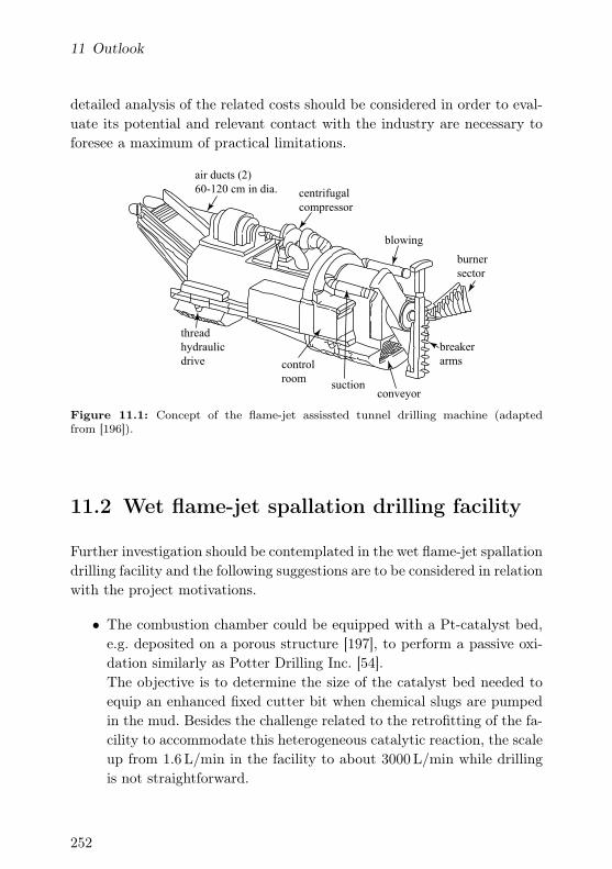
11 Outlook
detailed analysis of the related costs should be considered in order to eval-uate its potential and relevant contact with the industry are necessary toforesee a maximum of practical limitations.
burner
sector
breaker
arms
suctionconveyor
control
room
thread
hydraulic
drive
air ducts (2)
60-120 cm in dia. centrifugal
compressor
blowing
Figure 11.1: Concept of the flame-jet assissted tunnel drilling machine (adaptedfrom [196]).
11.2 Wet flame-jet spallation drilling facility
Further investigation should be contemplated in the wet flame-jet spallationdrilling facility and the following suggestions are to be considered in relationwith the project motivations.
• The combustion chamber could be equipped with a Pt-catalyst bed,e.g. deposited on a porous structure [197], to perform a passive oxi-dation similarly as Potter Drilling Inc. [54].The objective is to determine the size of the catalyst bed needed toequip an enhanced fixed cutter bit when chemical slugs are pumpedin the mud. Besides the challenge related to the retrofitting of the fa-cility to accommodate this heterogeneous catalytic reaction, the scaleup from 1.6L/min in the facility to about 3000L/min while drillingis not straightforward.
252

11.2 Wet flame-jet spallation drilling facility
• Linked to the former point, a common supply line could be envisionedfor the oxidizer and the fuel. This is relevant from a practical pointof view and enables to produce premixed hydrothermal flames.
• As the wall cooled hydrothermal burner 4 was not designed to drillrock samples at the relevant formation conditions, a load cell has beendeveloped and constructed to mimic the impact of the vertical stresson the rock and prevent it to expand.Unfortunately, this limits significantly the volume of the pressure ves-sel filled with water and results in elevated outlet temperatures. Thus,as this can be accepted for a limited number of experiments, it is notrecommended to operate the facility continuously at these unstableconditions. The limited volume of the pressure vessel contributing toaccentuate pressure fluctuations. Hence to proceed with drilling ex-periments, it would be important to consider the construction of alarger vessel. The design should focus on a dedicated solution to al-low reproducible confinement loads by using a hydraulic piston wherethe fluid pressure is monitored [73].
• The exhaust line of the pressure vessel could be equipped with aninline high pressure liquid chromatography system in order to monitorthe concentration of the exhaust. This can be used e.g. to check ifcombustion is complete.
• In case retrofitting takes place, it is important to consider to positionthe gas compressor above the water level, hence preventing any backflow of liquid in the gas line.
• According to the future plans in the WCHB-4, it is important to con-sider to bypass the preheating units, thereby reducing the residencetime of fuel and oxidizer in the facility.
• The ignition process could be automized by controlling the position ofthe solid state relay used to cut the power to the igniter by monitoringthe resistance of the coil.
253

11 Outlook
11.3 Geothermal energy
Considering that the driving motivation of this project is to contributeto the development of geothermal energy, efforts should be dedicated toenhance and test stimulation techniques for the construction of the under-ground heat exchanger. An interesting operation that could be performedby a flame-jet machine mounted on a coil tubing consists in drilling lat-eral slim holes outwards from the main borehole. The result is an increasedprobability to intersect fractures and improved reservoir characteristics.
254

A Appendix
Additional information about the wet flame-jet spallation drilling facilityis presented in A.1. A link to the production drawings of the pilot scaleburner is available in A.2 and finally the numerical code to reproduce theresults presented in Ch. 7 is reported in A.3.
A.1 Wet flame-jet spallation drilling facility
In this appendix, a document edited by Sitec to close the pressure ves-sel (WCHB-4) is presented. Then, some additional temperature measure-ments using different fuel injection nozzles than those reported in Ch. 5are presented and finally instructions to operate the wet flame-jet drillingspallation facility (Ch. 4).
A.1.1 Recommended service torque values
While assembling the pressure vessel following the installation of a rockprobe or a sensor, it is important to follow the instructions edited by Sitecto ensure sealing without damaging the contact surfaces. The documentwith the instructions is available at:
http://www.thierrymeier.ch/documents/740_8029_D.pdf
and should be followed every time the flanges of the pressure vessel areopened.
255

A Appendix
A.1.2 Additional temperature profiles
The data have been acquired following the same procedure as presented inSec. 5.3 and supplement them for two additional fuel injection geometries(Fig. A.1). The large cross sectional area (a, p.159) of both fuel injection
10 x 1.7 mm x 45° 8 x 2 mm x 45°
E F
2α
D
4.1 mm
Figure A.1: Two additional geometries of the fuel injection tip. The numbers belowthe fuel injection tip represent the number of holes (n), the holes diameter (D) and theangle (α).
0 20 40 60 80 100 120 140
downstream of the injector tip, z, [mm]
0
200
400
600
800
1000
1200
tem
per
ature
,T[
C]
0 20 40 60 80 100 120 140
downstream of the injector tip, z, [mm]
0
200
400
600
800
1000
1200
tem
per
ature
,T[
C]
λ = 1.2
λ = 1
λ = 0.8
Figure A.2: Temperature profiles for different oxygen to fuel ratios (λ) and the fuelinjection nozzle E (see Fig. A.1). Left panel: 20 kg/h and measurement positions alongthe combustion chamber indicated with red dots. Right panel: 50 kg/h and labels.
nozzles (E and F) results in limited injection velocity and a rapid temper-ature increase.
In terms of combustion efficiency and flame stability, none of these beat
256
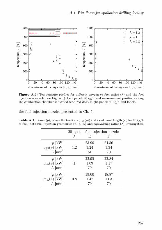
A.1 Wet flame-jet spallation drilling facility
0 20 40 60 80 100 120 140
downstream of the injector tip, z, [mm]
0
200
400
600
800
1000
1200
tem
per
ature
,T[
C]
0 20 40 60 80 100 120 140
downstream of the injector tip, z, [mm]
0
200
400
600
800
1000
1200
tem
per
ature
,T[
C]
λ = 1.2
λ = 1
λ = 0.8
Figure A.3: Temperature profiles for different oxygen to fuel ratios (λ) and the fuelinjection nozzle F (see Fig. A.1). Left panel: 20 kg/h and measurement positions alongthe combustion chamber indicated with red dots. Right panel: 50 kg/h and labels.
the fuel injection nozzles presented in Ch. 5.
Table A.1: Power (p), power fluctuations (σ95(p)) and axial flame length (L) for 20 kg/hof fuel, both fuel injection geometries (n, a, α) and equivalence ratios (λ) investigated.
20 kg/h fuel injection nozzleλ E F
p [kW]1.2
23.90 24.56σ95(p) [kW] 1.24 1.34
L [mm] 61 70
p [kW]1
22.95 22.84σ95(p) [kW] 1.09 1.17
L [mm] 79 70
p [kW]0.8
19.00 18.87σ95(p) [kW] 1.47 1.03
L [mm] 79 70
257

A Appendix
Table A.2: Power (p), power fluctuations (σ95(p)) and axial flame length (L) for 50 kg/hof fuel, both fuel injection geometries (n, a, α) and equivalence ratios (λ) investigated.
50 kg/h fuel injection nozzleλ E F
p [kW]1.2
67.25 74.24σ95(p) [kW] 5.49 3.48
L [mm] 99 99
p [kW]1
66.91 72.29σ95(p) [kW] 2.83 3.57
L [mm] 99 99
p [kW]0.8
62.47 65.74σ95(p) [kW] 2.86 2.86
L [mm] 75 89
A.1.3 Operating procedure
The procedure to operate the wet flame-jet spallation drilling facility(Ch. 4) is reported in the following.
Start-up
During the heat up, if anything goes wrong: close the outlet of the com-pressor (FMIC-1) and then release the pressure at the outlet of the reactor(RV-10).
Plant
(1) Plug in the plant.
(2) Switch on the computer and open internet explorer.
(3) Log in (password: vier) and select hand twice.
(4) In O2, give freigabe to the compressor.
(5) Open the ER3000 program and change the setpoint to 20 bar.
(6) Plug in the electricity for the igniter and Beckhoff.
(7) Open the air for the compressor (black hose).
258

A.1 Wet flame-jet spallation drilling facility
(8) Open the air to drive the valves.
(9) Open the air for the air gun.
(10) Turn the dryer on.
(11) Switch on the compressor.
(a) Open the gas bundle valve.
(b) Turn on the compressor.
(c) Wait until the bottle is filled.
(d) Set the compressors knobs to 300 bar.
(e) Give 4 bar to the compressors.
(12) Provide a gas flow (40NL/min) at 50 bar.
(13) Fill the 2.5m3 buffer tank.
(14) Open the hand valve to feed the water pump (WP-2).
(15) Open the valve to feed the water pump (WP-1).
(16) Open the water to feed the fuel pump (FP-1).
(17) Set the stroke of the fuel pump: 27.
(18) Open V-5.
Computer
Make sure you logged in the touch panel (vier–remove caps lock) and inthe computer.
(1) Open saia.
(a) Click on program file.
(b) Select ignition experiment.
(c) Press f9.
(2) Open er3000.
(a) Check the setpoint of the compressor (50 bar).
(3) Pressurize the water side to around 40 bar:
(a) Check the setpoint of the pressure controller (0 bar).
(b) Check the oxygen gas flow (40NL/min).
259

A Appendix
(c) Turn the small CW 2 pump on (setpoint: 600 kg/h).
(d) Turn the large CW 1,3 pump on.
(e) Turn the fuel pump on (20 kg/h, stroke: 27).
(f) Check the feed of the 2.5m3 water storage tank.
(4) Pressurize the oxygen line in er3000 to 120 bar:
(a) Set the O2 mass flow: 60NL/min.
(b) Increase the pressure in small steps (20 bar) until 120 bar.bar 50 70 90 120
(5) Pressurize the water side to 100 bar:
(a) Switch the controller on.
(b) Change the setpoint: 100 bar.
(6) Pressurize the oxygen line to about 273 bar:
(a) Increase the pressure in small steps (20 bar) until 273 bar.bar 140 160 180 200 220
240 273
(7) Pressurize the water side to 260 bar:
(a) Change the setpoint of the controller: 260 bar.
(8) Optional heat up the fuel line (water):
(a) Set HX-2: 400 C or less.
(9) Optional heat up the O2 line:
(a) Set HX-1: 390 C or less.
Shut Down
The overall idea is to make sure that the mixture does not start to boil(RV-10).
(1) Switch the position of the 3WV-1 to water only.
(2) Wait until the temperature of TIAH-3 reaches 50 C.
(3) Switch off HX-2 (fuel heater).
260

A.1 Wet flame-jet spallation drilling facility
(4) Switch off HX-1 (O2 heater).
(5) Adjust the flow rate of O2 to 60NL/min.
(6) Increase the fuel pump setpoint (max: 80 kg/h, stroke: 28).
(7) Export the data saved on the PLC.
(a) go to trend, load data, save data
(8) Wait until the fuel line reaches 130/140 C (resp. O2 line reaches190/200 C)
(9) Stop the compressor:
(a) Close the bundle.
(b) Open the inlet valve.
(c) Stop the driving air to the compressors.
(10) Start to reduce the pressure in steps of 25 bar.bar 235 210 185 160 135
110 85 60 35 0
Hint: Here the flowrate of the gas can be adjusted. Increase itin steps of 20NL/min until the maximum value of 100NL/min isreached.
(11) Stop the controller of the outlet valve and check the opening is full(0%).
(12) Wait until there is no flow of O2 anymore.
(13) Switch off the large cooling water pump (WP-2).
(14) Purge the system with N2:
(a) Check the setpoint of the compressor: 15 bar.
(b) Feed the gas bottle with 40 bar N2.
(c) Once nothing is flowing anymore, shut down the compressor.
(15) Switch off the small pump.
(16) Switch off the fuel pump.
(17) Make sure the upper positioning device is at its lower position(104.5mm).
(18) Save the data from SAIA: f9 and then ctrl-d.
(19) Close V-5.
261

A Appendix
(20) Close the feed valves (fuel pump, WP-1,2).
(21) Switch off the computer and unplug the plant.
(22) Do not forget to close the fuel tank valves.
A.2 Pilot scale burner
The production drawings of the pilot scale burner utilized for the demon-stration of flame-jet drilling (Ch. 8) can be downloaded at:
http://www.thierrymeier.ch/documents/drillBabydrill_VT5_R4.pdf
A.3 Numerical investigation of thermal
spallation drilling
The results of the numerical investigation presented in Ch.7 can be repro-duced using:
http://www.thierrymeier.ch/documents/FEM_2D_heatConduction.m
http://www.thierrymeier.ch/documents/FEM_2D_thermoelastic.m
The codes have to be run in sequential order starting with the heat conduc-tion. Additionally, the mapping of the temperature field is direct, requiringthe same mesh for both problems. Besides the boundary conditions andinitial conditions, the material properties can be adjusted to investigatefurther details of the thermal process.
262

Bibliography
[1] J. W. Tester et al., “The future of geothermal energy: Impact ofenhanced geothermal systems (EGS) on the United States in the 21st
century,” Massachusetts Institute of Technology, 2006.
[2] J. Nguyen, Le Forage. Éditions Technip, 1993.
[3] I. Bowman, Well-drilling Methods. No. 257, US Government PrintingOffice, 1911.
[4] P. K. Ngugi, “Geothermal well drilling,” short course VIII on Explo-
ration for Geothermal Resources, organized by UNU-GTP, GDC and
KenGen, Lake Bogoria and Lake Naivasha, Kenya, 2013.
[5] M. Z. Lukawski et al., “Cost analysis of oil, gas, and geothermal welldrilling,” Journal of Petroleum Science and Engineering, vol. 118,pp. 1–14, 2014.
[6] J. Finger and D. Blankenship, “Handbook of best practices forgeothermal drilling,” Sandia National Laboratories, Albuquerque,2010.
[7] B. Plemons et al., “New cutter technology for faster drilling inhard/abrasive formations,” in International Oil and Gas Conference
and Exhibition in China, Society of Petroleum Engineers, 2010.
[8] S. Ezzedine et al., “Laser-Enhanced Drilling for Subsurface EGSApplications,” Geothermal Resources Council Transactions, vol. 36,pp. 287–290, 2012.
[9] J. L. Wise et al., “Hard-Rock Field Performance of Drag Bits anda Downhole Diagnostics-While-Drilling (DWD) Tool,” in Proceedings
World Geothermal Congress, 2005.
263
Bibliography
[10] R. Schulz, “The Reason to Expect Prolonged USD 30–60/bbl Oil,”Journal of Petroleum Technology, vol. 10, pp. 42–45, 2016.
[11] Bundesamt für Energie, “Energieperspektiven 2050,” tech. rep., 2013.
[12] A. Oudalov et al., “Utility Scale Applications of Energy Storage,” inIEEE Energy 2030 Conference, pp. 1–7, November 2008.
[13] D. J. Swider, “Compressed Air Energy Storage in an Electricity Sys-tem With Significant Wind Power Generation,” IEEE Transactions
on Energy Conversion, vol. 22, pp. 95–102, March 2007.
[14] B. Steffen, “Prospects for pumped-hydro storage in Germany,” Energy
Policy, vol. 45, pp. 420–429, 2012.
[15] S. Vazquez et al., “Energy Storage Systems for Transport and GridApplications,” IEEE Transactions on Industrial Electronics, vol. 57,pp. 3881–3895, December 2010.
[16] A. Nasiri, “Integrating energy storage with renewable energy sys-tems,” in Industrial Electronics, 2008. IECON 2008. 34th Annual
Conference of IEEE, pp. 17–18, November 2008.
[17] R. M. Rauenzahn, Analysis of Rock Mechanics and Gas Dynamics of
Flame-Jet Thermal Spallation Drilling. PhD thesis, MassachusettsInstitute of Technology, 1986.
[18] R. Rinaldi, “A technical and economic evaluation of thermal spalla-tion drilling technology,” Report prepared for Sandia National Labo-
ratory by Resource Technology, Inc., 1984.
[19] K. Evans, “Geothermal energy.” ETH Lecture, 2015.
[20] The KamLAND Collaboration, “Partial radiogenic heat model forearth revealed by geoneutrino measurements,” Nature Geoscience,vol. 4, no. 9, pp. 647–651, 2011.
[21] D. L. Turcotte and G. Schubert, Geodynamics. Cambridge UniversityPress, 2002.
[22] R. Bertani, “Geothermal power generation in the world 2005–2010update report,” Geothermics, vol. 41, pp. 1–29, 2012.
264

Bibliography
[23] P. Bodmer and L. Rybach, Geothermal Map of Switzerland: Heat
Flow Density. No. 22, Bern: Beiträge zur Geologie der Schweiz. Geo-physik, 1984.
[24] V. Stefansson, “The renewability of geothermal energy,” Proceedings
World Geothermal Congress, pp. 883–887, 2000.
[25] A. J. Mansure et al., “Geothermal Well Cost Analyses 2005,” Geother-
mal Resources Council Transactions, vol. 29, pp. 515–519, 2005.
[26] D. A. Blankenship and A. J. Mansure, “Geothermal Well Cost Update2013,” Geothermal Resources Council Transactions, vol. 37, pp. 629–632, 2013.
[27] Baker Hughes INTEQ, “Drilling engineering workbook,” 1995.
[28] G. Gabolde and J.-P. Nguyen, Drilling Data Handbook. EditionsTechnip, 1999.
[29] S. Ivo, “Electromagnetic MWD/LWD - Where and why?,” Mining,
Geology and Petroleum Codes, vol. 8, pp. 123–128, 1996.
[30] G. Bruton et al., “PDC Bit Technology for the 21st Century,” Oilfield
Review, vol. 26, no. 2, pp. 48–57, 2014.
[31] S. Orazzini et al., “New Roller Cone Bit Technology for Geother-mal Application Significantly Increases On-Bottom Drilling Hours,”Geothermal Resources Council Transactions, vol. 35, pp. 215–224,2011.
[32] Y. Xiang, “Roller cone drill bit structure having improved journalangle and journal offset,” May 13 2003. US Patent 6,561,291.
[33] W. Rickard et al., “KymeraTM
Hybrid Bit Technology ReducesDrilling Cost,” in 39th Workshop on Geothermal Reservoir Engineer-
ing, Stanford University, February 2014.
[34] J. D. Schroder, “Cone retention and tapered bearing preload systemfor roller cone bit,” February 10 2015. US Patent 8,950,515.
[35] J. D. Schroder et al., “Extending Bit Life Through Bearing Innova-tions,” in SPE/IADC Drilling Conference and Exhibition, Society of
265

Bibliography
Petroleum Engineers, 2015.
[36] D. W. Raymond et al., “PDC Bits Outperform Conventional Bitin Geothermal Drilling Project,” in Geothermal Resources Council
Transactions, vol. 36, pp. 307–316, 2012.
[37] R. P. Radtke et al., “Thermally Stable Polycrystalline Diamond Cut-ters for Drill Bits,” in SPE Annual Technical Conference and Exhibi-
tion, no. SPE 90845, Society of Petroleum Engineers, 2004.
[38] R. P. Radtke et al., “New high strength and faster drilling tsp diamondcutters.,” tech. rep., Technology International, Inc., 2006.
[39] J. F. Brett et al., “Bit Whirl: A New Theory of PDC Bit Failure,”in SPE Annual Technical Conference and Exhibition, pp. 275–281,Society of Petroleum Engineers, 1989.
[40] D. W. Raymond et al., “Controllable Damper demonstrates improvedStability for PDC bits Drilling Hard-rock Formations,” in Geothermal
Resources Council Transactions, vol. 29, pp. 521–527, 2005.
[41] C. Augustine et al., “A comparison of geothermal with oil and gaswell drilling costs,” in 31st Workshop on Geothermal Reservoir Engi-
neering, pp. 5–19, Stanford University, February 2006.
[42] K. Denninger et al., “Optimizing Geothermal Drilling: Oil and GasTechnology Transfer,” in Geothermal Resources Council Transac-
tions, vol. 39, pp. 171–180, September 2015.
[43] A. J. Mansure and D. A. Blankenship, “Geothermal Well Cost Anal-yses 2008,” in Geothermal Resources Council Transactions, vol. 32,pp. 43–48, 2008.
[44] A. J. Mansure et al., “Geothermal Well Cost Analyses 2006,” inGeothermal Resources Council Transactions, vol. 30, pp. 271–276,2006.
[45] K. G. Pierce et al., “Advanced Drilling Systems Study.,” Tech. Rep.SAND95-033 1, Sandia National Laboratories, Albuquerque, NM(United States), 1996.
266

Bibliography
[46] J. W. Tester et al., “Prospects for Universal Geothermal Energy fromHeat Mining,” Science & Global Security, vol. 5, no. 1, pp. 99–121,1994.
[47] R. Ford, “Getting ready to roll,” Oilfield Technology, November 2014.Reprinted.
[48] M. Schluter et al., “MIDACO: New global optimization software forMINLP,” 2011.
[49] S. Petty et al., “Synergies and Opportunities Between EGS Develop-ment and Oilfield Drilling Operations and Producers,” in SPE West-
ern Regional Meeting, (San Jose, CA (United States)), Society ofPetroleum Engineers, March 2009.
[50] W. C. Maurer, Advanced Drilling Techniques. Petroleum PublishingCo., 1980.
[51] W. C. Maurer et al., “Deep-Drilling Basic Research Volume 5 – Sys-tem Evaluation,” tech. rep., Maurer Engineering Inc. Universisty ofCalifornia, Berkeley, 1990. Final Report.
[52] W. C. Maurer et al., “Deep-Drilling Basic Research Volume 4 – Sys-tem Description,” tech. rep., Maurer Engineering Inc. Universisty ofCalifornia, Berkeley, 1990. Final Report.
[53] I. Kocis et al., “Utilization of Electrical Plasma for Hard Rock Drillingand Casing Milling,” in SPE/IADC Drilling Conference and Exhibi-
tion, no. SPE/IADC-173016-MS, (London (United Kingdom)), Soci-ety of Petroleum Engineers, March 2015.
[54] R. M. Potter et al., “Laboratory Study and Field Demonstration ofHydrothermal Spallation Drilling,” in Geothermal Resources Council
Transactions, vol. 34, pp. 249–252, 2010.
[55] A. Rødland, “Drilling for Geothermal Energy "where we are andwhere we go..." The EPB Story,” in Photonics for deep geothermal
energy harvesting, Université de Neuchâtel, November 2012.
[56] M. S. Zediker et al., “High Power Laser for Rock Drilling,” in Photon-
ics for deep geothermal energy harvesting, Université de Neuchâtel,
267

Bibliography
November 2012.
[57] V. Wittig et al., “Hydraulic DTH Fluid/Mud Hammers with Recir-culation Capabilities to Improve ROP and Hole Cleaning For Deep,Hard Rock Geothermal Drilling,” in Proceedings World Geothermal
Congress 2015, vol. 6, (Melbourne, (Australia)), April 2015.
[58] M. Voigt and E. Anders, “Electric Impulse Technology – Long RunDrilling in Hard Rocks,” in Internationale Geothermiekonferenz, Of-fenbourg (Germany), February 2016.
[59] H. O. Schiegg et al., “Electro-pulse-boring (EPB): Novel super-deepdrilling technology for low cost electricity,” Journal of Earth Science,vol. 26, pp. 37–46, February 2015.
[60] J. J. Calaman and H. C. Rolseth, “Jet Piercing,” Transactions of
the American Institute of Mining, Metallurgical and Petroleum En-
gineers, pp. 325–337, 1968.
[61] J. Browning et al., “Recent advances in flame-jet working of miner-als,” in 7th Symposium on Rock Mechanics, 1965.
[62] C. R. Augustine, Hydrothermal Spallation Drilling and Advanced En-
ergy Conversion Technologies for Engineered Geothermal Systems.PhD thesis, Massachusetts Institute of Technology, 2009.
[63] H. Warth, “The Quarrying of Granite in India,” Nature, vol. 51,pp. 272–272, Jan 1895.
[64] F. H. Norton, “A general theory of spalling,” 1925.
[65] F. W. Preston, “Theory of spalling*,” Journal of the American Ce-
ramic Society, vol. 16, no. 1-12, pp. 131–133, 1933.
[66] F. W. Preston and H. E. White, “Observations on spalling,” Journal
of the American Ceramic Society, vol. 17, pp. 137–144, Dec 1934.
[67] W. M. Gray, “Surface spalling by thermal stresses in rocks,” inProceedings of the Rock Mechanics Symposium, vol. 15, (Toronto(Canada)), pp. 85–105, Department of Mines and Technical Surveys,January 1965.
268
Bibliography
[68] K. Thirumalai, “Process Of Thermal Spalling Behavior In Rocks –An Exploratory Study,” in 11th US Symposium on Rock Mechanics,1969.
[69] T. N. Dey and R. L. Kranz, “Methods for increasing drilling per-formance of the thermal spallation drilling system,” in Geothermal
Resources Council Transactions, vol. 9, August 1985.
[70] M. S. Paterson and T-f. Wong, Experimental Rock Deformation: The
Brittle Field, 2nd Edition. Springer, 2005.
[71] P. Stathopoulos, Hydrothermal Spallation Drilling Experiments in a
Novel High Pressure Pilot Plant. PhD thesis, ETH Zurich, 2013.
[72] D. Höser, Flame-jet Assisted Drilling Technology. PhD thesis, ETHZurich, 2016.
[73] T. W. Wideman et al., “Methods and apparatus for thermal drilling,”August 7 2012. US Patent 8,235,140 B2.
[74] S. Nemat-Nasser and H. Horii, “Compression-Induced NonplanarCrack Extension With Application to Splitting, Exfoliation, andRockburst,” Journal of Geophysical Research, vol. 87, pp. 6805–6821,August 1982.
[75] L. N. Germanovich, “Thermal spalling of rock,” in Proceedings of
the 9th International Conference of Fracture, vol. 6, (Sydney, (Aus-tralia)), pp. 2771–2782, 1997.
[76] M. J. Schuler, Fundamental Investigations of Supercritical Water
Flows for Hydrothermal Spallation Drilling. PhD thesis, ETH Zurich,2014.
[77] F. J. R. e Silva et al., “Analysis of the Performance of a ThermalSpallation Device for Rock Drilling,” in 11th Brazilian Congress of
Thermal Sciences and Engineering, no. CIT06-0339, Brazil Societyof Mechanical Sciences and Engineering, 2006.
[78] T. E. Diller, “Advances in Heat Flux Measurements,” Advances in
heat transfer, vol. 23, pp. 279–368, 1993.
269

Bibliography
[79] Y. A. Çengel, Heat Transfer : A Practical Approach. Boston:McGraw-Hill, 2nd ed., 2003.
[80] W. J. Minkowycz, Advances in Numerical Heat Transfer. Advancesin Numerical Heat Transfer, Taylor & Francis, 1997.
[81] S. Gordon and B. J. McBride, “Computer Program for Calculationof Complex Chemical Equilibrium Compositions and Applications: I.Analysis,” NASA Reference Publication, vol. 1311, October 1994.
[82] S. Gordon and B. J. McBride, “Computer Program for Calculation ofComplex Chemical Equilibrium Compositions and Applications: II.Users Manual and Program Description,” NASA Reference Publica-
tion, vol. 1311, June 1996.
[83] M. W. Chase Jr et al., “JANAF Thermochemical Tables Third Edi-tion Part I and II, Al-Zr,” American Institute of Physics, pp. 1–1245,1986.
[84] D. R. Lide, CRC Handbook of Chemistry and Physics. CRC Press,Boca Raton, FL, Internet Version 2005.
[85] C. J. Sahle et al., “Microscopic structure of water at elevated pressuresand temperatures,” Proceedings of the National Academy of Sciences,vol. 110, pp. 6301–6306, April 2013.
[86] Y. A. Kozlovsky, “The World’s Deepest Well,” Scientific American,vol. 251, no. 6, pp. 98–104, 1984.
[87] E. W. Lemmon et al., NIST Standard Reference Database 23: Refer-
ence Fluid Thermodynamic and Transport Properties - REFPROP.National Institute of Standards and Technology, Standard ReferenceData Program, Gaithersburg, 8.0 ed., 2007.
[88] W. Wagner and A. Pruß, “The IAPWS formulation 1995 for thethermodynamic properties of ordinary water substance for generaland scientific use,” Journal of Physical and Chemical Reference Data,vol. 31, no. 2, pp. 387–535, 2002.
[89] M. L. Huber et al., “New International Formulation for the Viscosityof H2O,” Journal of Physical and Chemical Reference Data, vol. 38,
270

Bibliography
no. 2, pp. 101–125, 2009.
[90] P. Infelta, Thermodynamique principes et applications. Boca Raton,CA (United States): Brown Walker Press, 2006.
[91] S. M. Shelton and W. H. Swanger, “Thermal conductivity of irons andsteels and some other metals in the temperature range 0 to 600C,”American Society for Steel Treating, vol. 21, pp. 1061–1078, 1933.
[92] B. Sundqvist, “Thermal diffusivity and thermal conductivity ofChromel, Alumel, and Constantan in the range 100–450 K,” Jour-
nal of Applied Physics, vol. 72, no. 2, pp. 539–545, 1992.
[93] Y. S. Touloukian, Thermophysical properties of high temperature solid
materials. Vol. 4, Oxydes and their solutions and mixtures. New York:Macmillan, 1967.
[94] “Standard Specification and Temperature-Electromotive Force(EMF) Tables for Standardized Thermocouples,” 2003.
[95] F. Hofmann, “Design and Construction of a Calibration System forHeavy Duty Heat Flux Sensors,” Master’s thesis, ETH Zurich, 2010.
[96] A. A. Fernandes, “Construction and Calibration of Heat Flux Sen-sors,” Master’s thesis, ETH Zurich, 2014.
[97] T. E. Diller and S. Onishi, “Heat flux gage,” October 25 1988. USPatent 4,779,994.
[98] P. Stathopoulos et al., “Calibration of a Gardon Sensor in a High-Temperature High Heat Flux Stagnation Facility,” Experimental Heat
Transfer, vol. 25, no. 3, pp. 222–237, 2012.
[99] T. Rothenfluh, Heat transfer phenomena of supercritical water jets in
hydrothermal spallation drilling. PhD thesis, ETH Zurich, 2013.
[100] B. Deuchert et al., “Heat Flux Sensor,” 2011.
[101] R. W. Boydston, “Thermo-electric effect in single-crystal bismuth,”Physical Review, vol. 30, p. 911, December 1927.
[102] S. Z. Sapozhnikov et al., “Gradient Heat-Flux Sensors: Possibilities
271

Bibliography
and Prospects of Use,” Thermal Engineering, vol. 53, no. 4, pp. 270–278, 2006.
[103] Th. Zahner et al., “Picosecond thermoelectric response of thinYBa2Cu3O7−δ films,” Physica C: Superconductivity, vol. 313, no. 1,pp. 37–40, 1999.
[104] S. Z. Sapozhnikov et al., “Bismuth-Based Gradient Heat-Flux Sensorsin Thermal Experiment,” High Temperature, vol. 42, no. 4, pp. 629–638, 2004.
[105] V. P. Babin et al., “Anisotropic synthetic thermoelements andtheir maximum capabilities,” Soviet physics Semiconductors, vol. 8,pp. 748–753, April 1974.
[106] C. Reitmaier et al., “Transverse thermoelectric devices,” Applied
Physics A, vol. 99, pp. 717–722, June 2010.
[107] A. V. Mityakov et al., “Gradient heat flux sensors for high temper-ature environments,” Sensors and Actuators A: Physical, vol. 176,pp. 1–9, April 2012.
[108] A. V. Mityakov et al., “Application of the Transverse Seebeck Effectto Measurement of Instantaneous Values of a Heat Flux on a VerticalHeated Surface under Conditions of Free-Convection Heat Transfer,”High Temperature, vol. 40, no. 4, pp. 620–625, 2002.
[109] S. Z. Sapozhnikov et al., “Gradient heat flux sensors based on theartificial anisotropic thermoelements,” Journal of Thermoelectricity,no. 4, 2010.
[110] S. V. Bobashev et al., “Measurements of Convective Heat Fluxes bySensors Based on Anisotropic Thermal Elements in Pulsed Gasdy-namic Processes,” in 50th AIAA Aerospace Sciences Meeting, 2012.
[111] B. S. Mann, “Transverse Thermoelectric Effects for Cooling and HeatFlux Sensing,” Master’s thesis, Virginia Polytechnic Institute andState University, 2006.
[112] H. Knauss et al., “A Novel Sensor for Fast Heat Flux Measurements,”in 25th AIAA, Aerodynamic Measurement Technology and Ground
272

Bibliography
Testing Conference, no. AIAA 2006-3637, (San Francisco, CA (UnitedStates)), pp. 1–32, Institute of Aeronautics and Astronautics, Inc.,June 2006.
[113] Th. Zahner et al., “Transverse thermoelectricity in a tilted metallicmultilayer structure,” International Journal of Infrared and Millime-
ter Waves, vol. 20, no. 6, pp. 1103–1111, 1999.
[114] O. V. Nitsovich, “Two approaches to study of transverse thermoele-ments – approximate theories and computer simulation,” Journal of
Thermoelectricity, no. 3, 2008.
[115] K. Fischer et al., “Anisotropic thermopower in tilted metallic multi-layer structures,” Applied Physics A: Materials Science & Processing,vol. 78, pp. 323–326, February 2004.
[116] H. W. Coleman and W. G. Steele, Experimentation and Uncertainty
Analysis for Engineers. John Wiley & Sons, Inc., 3 ed., 1999.
[117] W. M. Huber et al., “Transverse Seebeck effect in Bi2Sr2CaCu2O8,”Applied Physics A: Materials Science & Processing, vol. 64, no. 5,pp. 487–489, 1997.
[118] M. Fénot et al., “A heat transfer measurement of jet impinge-ment with high injection temperature,” Comptes Rendus Mécanique,vol. 333, pp. 778–782, October 2005.
[119] T. Meier et al., “The Potential of Hydrothermal Flames to InduceSpallation in Gneiss,” in Proceedings World Geothermal Congress
2015, (Melbourne (Australia)), April 2015.
[120] A. R. Gifford et al., “Durable Heat Flux Sensor for Extreme Temper-ature and Heat Flux Environments,” Journal of Thermophysics and
Heat Transfer, vol. 24, pp. 69–76, March 2010.
[121] C. A. Pullins and T. E. Diller, “In situ High Temperature Heat FluxSensor Calibration,” International Journal of Heat and Mass Trans-
fer, vol. 53, no. 17–18, pp. 3429–3438, 2010.
[122] T. E. Diller, “High temperature Heat Flux Sensor - Evaluation Re-sponse.” December 2014.
273

Bibliography
[123] T. E. Diller, “Modeling the High Temperature Heat Flux Sensor.”December 2014.
[124] T. Meier and Ph. Rudolf von Rohr, “Heat flux sensor and system witha heat flux sensor,” June 18 2015. WO2016202971 A1.
[125] A. J. Slifka et al., “Thermal Conductivity of Magnesium Oxide FromAbsolute, Steady-State Measurements,” Journal of Research of the
National Institute of Standards and Technology, vol. 103, no. 4, p. 357,1998.
[126] M. Weber, Apparate einer SCWO-Anlage und deren Leistungs-
fähigkeit. PhD thesis, ETH Zurich, 1997.
[127] ASTM G93-03(2011), “Standard Practice for Cleaning Methods andCleanliness Levels for Material and Equipment Used in Oxygen-Enriched Environments,” ASTM International, April 2011.
[128] T. Meier and Ph. Rudolf von Rohr, “Progression towards the assess-ment of spallation drilling at depth,” tech. rep., ETH Zurich, April2014.
[129] C. Augustine and J. W. Tester, “Hydrothermal flames: From phe-nomenological experimental demonstrations to quantitative under-standing,” The Journal of Supercritical Fluids, vol. 47, no. 3, pp. 415–430, 2009.
[130] E. W. Lemmon et al., NIST Standard Reference Database 23: Refer-
ence Fluid Thermodynamic and Transport Properties - REFPROP.National Institute of Standards and Technology, Standard ReferenceData Program, Gaithersburg, 9.1 ed., 2013.
[131] K. D. Ninck, “Ignition Experiments for Hydrothermal Flames,” Mas-ter’s thesis, ETH Zurich, 2011.
[132] J. W. Buckel and S. Chandra, “Hot wire ignition of hydrogen–oxygenmixtures,” International Journal of Hydrogen Energy, vol. 21, no. 1,pp. 39–44, 1996.
[133] P. Stathopoulos et al., “Heat transfer of supercritical mixtures ofwater, ethanol and nitrogen in a bluff body annular flow,” The Journal
274

Bibliography
of Supercritical Fluids, vol. 70, no. 0, pp. 112–118, 2012.
[134] P. Stathopoulos et al., “Hot-wire ignition of ethanol–oxygen hy-drothermal flames,” Combustion and Flame, vol. 160, no. 11,pp. 2386–2395, 2013.
[135] T. Meier et al., “Hot surface ignition of oxygen–ethanol hydrothermalflames,” The Journal of Supercritical Fluids, vol. 107, pp. 462–468,2016.
[136] L. Michalski et al., Temperature Measurements, ch. ThermoelectricThermometers, pp. 37–84. John Wiley & Sons, Ltd, 2nd ed., 2002.
[137] G. W. Burns and M. G. Scroger, The Calibration of Thermocouples
and Thermocouple Materials, vol. 250. US Department of Commerce,National Institute of Standards and Technology, 1989.
[138] T. G. Kollie et al., “Temperature Measurement Errors with TypeK(Chromel vs Alumel) Thermocouples Due to Short-Ranged Order-ing in Chromel,” Review of Scientific Instruments, vol. 46, no. 11,pp. 1447–1461, 1975.
[139] T. Meier et al., “Numerical investigation of thermal spallation drillingusing an uncoupled quasi-static thermoelastic finite element formu-lation,” Journal of Thermal Stresses, vol. 39, no. 9, pp. 1138–1151,2016.
[140] B. Wellig, Transpiring Wall Reactor for Supercritical Water Oxida-
tion. PhD thesis, ETH Zurich, 2003.
[141] Karol Príkopský, Characterization of Continuous Diffusion Flames
in Supercritical Water. PhD thesis, ETH Zurich, 2007.
[142] C. Augustine et al., “Feasibility of Spallation Drilling in a High Pres-sure, High-Density, Aqueous Environment: Characterization of HeatTransfer from an H2-O2 Flame Jet,” in Geothermal Resources Council
Transactions, vol. 31, pp. 241–245, 2007.
[143] J. U. Steinle and E. U. Franck, “High Pressure Combustion – Igni-tion Temperatures to 1000 bar,” Berichte der Bunsengesellschaft für
physikalische Chemie, vol. 99, no. 1, pp. 66–73, 1995.
275

Bibliography
[144] L-D. Chen and G. M. Faeth, “Initiation and Properties of Decom-position Waves in Liquid Ethylene Oxide,” Combustion and Flame,vol. 40, pp. 13– 28, 1981.
[145] D. R. Hall et al., “Downhole electric power generator,” October 112011. US Patent 8,033,328.
[146] A. Gidner and L. Stenmark, “Supercritical water oxidation of sewagesludge–State of the art,” in IBC’s Conference on Sewage Sludge and
Disposal Options, 2001.
[147] J. W. Griffith and D. H. Raymond, “The first commercial supercriticalwater oxidation sludge processing plant,” Waste Management, vol. 22,no. 4, pp. 453–459, 2002.
[148] D. Xu et al., “Design of the first pilot scale plant of China for su-percritical water oxidation of sewage sludge,” Chemical Engineering
Research and Design, vol. 90, no. 2, pp. 288–297, 2012.
[149] M. J. Cocero et al., “Supercritical Water Oxidation (SCWO) forPoly(ethylene terephthalate) (PET) Industry Effluents,” Industrial
& Engineering Chemistry Research, vol. 39, no. 12, pp. 4652–4657,2000.
[150] M. D. Bermejo and M. J. Cocero, “Supercritical Water Oxidation: ATechnical Review,” AIChE Journal, vol. 52, no. 11, pp. 3933–3951,2006.
[151] M. D. Bermejo and M. J. Cocero, “Destruction of an industrialwastewater by supercritical water oxidation in a transpiring wall re-actor,” Journal of Hazardous Materials, vol. 137, no. 2, pp. 965–971,2006.
[152] M. D. Bermejo et al., “Experimental study of the operational param-eters of a transpiring wall reactor for supercritical water oxidation,”The Journal of Supercritical Fluids, vol. 39, no. 1, pp. 70–79, 2006.
[153] A. A. Abdurashidova et al., “The Thermal Properties of Water-Ethanol System in the Near-Critical and Supercritical States,” High
Temperature, vol. 45, no. 2, pp. 178–186, 2007.
276

Bibliography
[154] ISO 8466-1:1990 (E), “Water quality – Calibration and evaluationof analytical methods and estimation of performance characteristics.Part 1: Statistical evaluation of the linear calibration function,” 1990.
[155] D. B. Hibbert, “The uncertainty of a result from a linear calibration,”Analyst, vol. 131, no. 12, pp. 1273–1278, 2006.
[156] Th. Hirth and E. U. Franck, “Oxidation and Hydrothermolysis ofHydrocarbons in Supercritical Water at High Pressures,” Berichte der
Bunsengesellschaft für physikalische Chemie, vol. 97, no. 9, pp. 1091–1097, 1993.
[157] A. Sobhy et al., “Selected profiles of high-pressure methanol–airflames in supercritical water,” Proceedings of the Combustion Insti-
tute, vol. 31, no. 2, pp. 3369–3376, 2007.
[158] R. R. Steeper et al., “Methane and Methanol Diffusion Flames inSupercritical Water,” The Journal of Supercritical Fluids, vol. 5,pp. 262–268, December 1992.
[159] C-C. Chen et al., “Autoignition Temperature Data for Methanol,Ethanol, Propanol, 2-Butanol, 1-Butanol, and 2-Methyl-2,4-pentanediol,” Journal of Chemical & Engineering Data, vol. 55,no. 11, pp. 5059–5064, 2010.
[160] W. Schilling and E. U. Franck, “Combustion and Diffusion Flamesat High Pressures to 2000 bar,” Berichte der Bunsengesellschaft für
physikalische Chemie, vol. 92, no. 5, pp. 631–636, 1988.
[161] J. Licht et al., “Heat transfer to water at supercritical pressures in acircular and square annular flow geometry,” International Journal of
Heat and Fluid Flow, vol. 29, no. 1, pp. 156–166, 2008.
[162] H. E. Dillon and S. G. Penoncello, “A Fundamental Equation for Cal-culation of the Thermodynamic Properties of Ethanol,” International
Journal of Thermophysics, vol. 25, no. 2, pp. 321–335, 2004.
[163] R. Schmidt and W. Wagner, “A new form of the equation of state forpure substances and its application to oxygen,” Fluid Phase Equilib-
ria, vol. 19, no. 3, pp. 175–200, 1985.
277

Bibliography
[164] P. Strakey et al., “Investigation of the effects of hydrogen addition onlean extinction in a swirl stabilized combustor,” Proceedings of the
Combustion Institute, vol. 31, no. 2, pp. 3173–3180, 2007.
[165] Z-H. Wang et al., “Ethanol oxidation on a nichrome-supported spher-ical platinum microparticle electrocatalyst prepared by electrodepo-sition,” International Journal of Hydrogen Energy, vol. 33, no. 21,pp. 6143–6149, 2008.
[166] ISO 8466-2:1990 (E), “Water Quality- Calibration and evaluation ofanalytical methods and estimation of performance characteristics.Part 2: Calibration strategy for non-linear second-order calibrationfunctions,” 1990.
[167] H. K. Ma et al., “Mixing and Recirculation Characteristics of a Dou-ble Concentric Burner with Bluff-Body,” Journal of Thermal Science,vol. 2, no. 4, pp. 294–303, 1993.
[168] P. Bossart and M. Mazurek, “Structural geology and water flow-pathsin the migration shear-zone,” Tech. Rep. 91-12, NAGRA, November1991.
[169] D. H. Fleming and J. J. Calaman, “Production Jet-Piecing of Blast-holes in Magnetic Taconite,” Mining Engineering, pp. 585–591, July1951.
[170] R. E. Williams et al., “Experiments in Thermal Spallation of VariousRocks,” Journal of Energy Resources Technology, vol. 118, pp. 2–8,March 1996.
[171] J. L. Smith et al., “Fracture Data and Stress-Strain Behavior of Rocksin Triaxial Compression,” Experimental Mechanics, vol. 9, no. 8,pp. 348–355, 1969.
[172] F. Yufang and L. Lianchong, “Study on mechanism of thermal spallingin concrete exposed to elevated temperatures,” Materials and Struc-
tures, vol. 44, no. 1, pp. 361–376, 2011.
[173] P. J. Lauriello and Y. Chen, “Thermal Fracturing of Hard Rock,”Journal of Applied Mechanics, vol. 40, pp. 909–914, December 1973.
278

Bibliography
[174] B. A. Boley and J. H. Weiner, Theory of Thermal Stresses. NewYork: Wiley, 1960.
[175] T. J. R. Hughes, The Finite Element Method: Linear Static and Dy-
namic Finite Element Analysis. Courier Corporation, 2012.
[176] P. J. Roache, “Code verification by the method of manufactured solu-tions,” Journal of Fluids Engineering, vol. 124, no. 1, pp. 4–10, 2002.
[177] G. Prathap and B. P. Naganarayana, “Consistent thermal stress eval-uation in finite elements,” Computers & Structures, vol. 54, no. 3,pp. 415–426, 1995.
[178] J. Pittr and H. Hartl, “Improved stress evaluation under thermalload for simple finite elements,” International Journal for Numerical
Methods in Engineering, vol. 15, no. 10, pp. 1507–1515, 1980.
[179] D. Höser et al., “Influence of uniaxial load on flame jet drilling – anexperimental study,” International Journal of Rock Mechanics and
Mining Sciences, submitted.
[180] D. Zimmermann, “A 10 m deep borehole in the grimsel undergroundlaboratory using a flame-jet drilling machine,” Master’s thesis, ETHZurich, 2016.
[181] M. D. Limaye et al., “Local heat transfer distribution on a flat plateimpinged by a compressible round air jet,” International Journal of
Thermal Sciences, vol. 49, no. 11, pp. 2157–2168, 2010.
[182] E. Muschelknautz, “Die Berechnung von Zyklonabscheidern fürGase,” Chemie Ingenieur Technik, vol. 44, no. 1-2, pp. 63–71, 1972.
[183] J. A. Browning, “Flame jet drilling and chambering to great depthsin crystalline rock.,” Tech. Rep. N00014-82-C-0249, Browning Engi-neering Corporation, 1982.
[184] W. C. Maurer, Novel drilling techniques, vol. 114. Pergamon PressNew York, 1968.
[185] Z. Xu et al., “Laser spallation of rocks for oil well drilling,” in 23rd
International Congress on Applications of Lasers and Electro-Optics,
279

Bibliography
pp. 1–6, 2004.
[186] L. B. Geller, “A new look at thermal rock fracturing,” Transactions
of the Institution of Mining and Metallurgy, vol. 79, pp. A133–A170,1970.
[187] S. D. C. Walsh et al., “Simulation Tools for Modeling Thermal Spal-lation Drilling on Multiple Scales,” Tech. Rep. LLNL-CONF-555171,Lawrence Livermore National Laboratory, Livermore, CA (UnitedStates), 2012.
[188] S. D. C. Walsh et al., “Grain-scale failure in thermal spallationdrilling,” in 37th Workshop on Geothermal Reservoir Engineering,(Standford, CA (United States)), Standford University, 2012.
[189] S. D. C. Walsh and I. N. Lomov, “Micromechanical modeling of ther-mal spallation in granitic rock,” International Journal of Heat and
Mass Transfer, vol. 65, pp. 366–373, 2013.
[190] A. Patru, “Influence of process parameters on flame-jet drilling atambient conditions,” Master’s thesis, ETH Zurich, 2016.
[191] A. Hobé, “Grimsel Granodiorite’s Thermal Spallation Mechanism,”2015.
[192] T. W. Wideman et al., “Hydrothermal Spallation for the Treatment ofHydrothermal and EGS Wells: A Cost-Effective Method for Substan-tially Increasing Reservoir Production and Flow Rates,” Australian
Geothermal Conference, pp. 222–225, 2010.
[193] F. Guinot et al., “A New Age in Well Perforating History-Evolving from Roman to Gothic?,” in Rock Mechanics Conference,no. SPE/ISRM 78195, Society of Petroleum Engineers, 2002.
[194] J. P. Carstens et al., “An Evaluation Of Heat-Weaking Hard RockAs An Assist To Mechanical Tunneling,” in 12th US Symposium on
Rock Mechanics, American Rock Mechanics Association, 1970.
[195] Ph. Rudolf von Rohr et al., “Rock drilling in great depths by thermalfragmentation using highly exothermic reactions evolving in the en-vironment of a water-based drilling fluid,” March 3 2015. US Patent
280

Bibliography
8,967,293 B2.
[196] J. P. Carstens, “Feasibility of Flame-jet Tunneling: Volume 1 - Sum-mary Report,” Tech. Rep. G-910560-10, United Aircraft ResearchLaboratories, May 1968.
[197] C. Hutter, Laser sintered meso sale reactor by design: Charactrizta-
tion of heat and mass transfer. PhD thesis, ETH Zurich, 2010.
281

Awards and publications
Award
(1) Thierry Meier and Philipp Rudolf von Rohr, Top 5 Finalist 2016Spark Award, ETH Zurich
Journal publications
(1) Thierry Meier, Martin Jörg Schuler, Panagiotis Stathopoulos, BrunoKramer and Philipp Rudolf von Rohr, Hot surface ignition and mon-itoring of an internal oxygen-ethanol hydrothermal flame at 260 bar,The Journal of Supercritical Fluids, in-press
(2) Thierry Meier, Dave May and Philipp Rudolf von Rohr, Numeri-cal investigation of thermal spallation drilling using an uncoupledquasi-static thermoelastic finite elements formulation, The Journal of
Thermal Stresses, Vol. 39, Issue 9, pp. 1138-1151, 2016
(3) Thierry Meier, Panagiotis Stathopoulos and Philipp Rudolf vonRohr, Hot surface ignition of oxygen-ethanol hydrothermal flames,The Journal of Supercritical Fluids, Vol. 107, pp. 462-468, January2016
(4) Thierry Meier, Panagiotis Stathopoulos and Philipp Rudolf von Rohr,Design and convective calibration of a transverse heat flux sensor,Experimental Heat Transfer, Vol. 29, Issue 2, pp. 132-150, 2016
(5) Dragana Höser, Thierry Meier, Antoine Patru, Michael Kant andPhilipp Rudolf von Rohr, Influence of uniaxial load on flame-jetdrilling - an experimental study, Journal of Rock Mechanics and
Mining Sciences, under-review
282

(6) Panagiotis Stathopoulos, Thierry Meier and Philipp Rudolf von Rohr,Hydrothermal flame impingement experiments. combustion chamberdesign and impingement temperature profiles, The Journal of Super-
critical Fluids, Vol. 89, pp. 48-57, May 2014
(7) Martin Jörg Schuler, Tobias Rothenfluh, Panagiotis Stathopoulos,Dragana Brkic, Thierry Meier and Philipp Rudolf von Rohr, Sim-ulating Supercritical Water Jets with a Variable Turbulent PrandtlNumber, Chemical Engineering & Technology, Vol. 37, Issue 11, pp.1896-1902, November 2014
Patent
(1) Thierry Meier and Philipp Rudolf von Rohr, Heat flux sensor and sys-tem with a heat flux sensor, WO 2016202971 A1, Patent ApplicationPublication, 2015
Conference contributions
(1) Thierry Meier, Tête de forage à flamme. Forer à grande profondeuravec des temps-morts réduits. Journée romande de la géothermie,Yverdon-les-bains, Switzerland, 2016
(2) Thierry Meier, Frédéric Guinot and Philipp Rudolf von Rohr, Anassessment of flame-jet drilling to access deep underground resources.Celle Drilling 2016, Celle, Germany, 2016.
(3) Thierry Meier, Michael Kant, Dragana Brkic and Philipp Rudolf vonRohr, Flame-Jet Drilling: An Alternative Technique to Access DeepHeat reservoirs. 1st Bochum Drilling Dialogue, Bochum, Germany,2016.
(4) Thierry Meier, Flame-jet drilling - An assessment of the technique ina borehole environement at fluid pressures up to 26MPa and verti-cal stress up to 100MPa. International geothermal conference, Offen-bourg, Germany, 2016.
283

Awards and publications
(5) Thierry Meier, Dragana Brikc, Martin Jörg Schuler, Michael Kantand Philipp Rudolf von Rohr, Hydrothermal Spallation Drilling - De-sign and Experiments for a Novel Drilling Technology World Geother-
mal Congress, Melbourne, Australia, 2015.
(6) Thierry Meier, Panagiotis Stathopoulos and Philipp Rudolf von Rohr,The Potential of Hydrothermal Flames to Induce Spallation in Gran-ite. 4th European Geothermal PhD Day, Szeged, Hungary, 2013.
284

Curiculum vitae
Name: Thierry [email protected]
Date of birth: December 18th, 1988Nationality: Swiss
05/2013 – 12/2016 Doctoral studies at the Institute of Process Engineer-ing, ETH Zurich (Prof. Dr. Ph. Rudolf von Rohr)
05/2012 – 05/2013 Teaching assistant at the Institute of Process Engi-neering, ETH Zurich (Prof. Dr. Ph. Rudolf von Rohr)
09/2010 – 04/2012 Master studies in Process Engineering, ETH Zurich,(adademic degree: MSc ETH PE)
05/2011 – 07/2011 Internship at Micafluid AG, Schlieren09/2007 – 07/2010 Bachelor studies in Chemistry and Chemical En-
gineering, EPF Lausanne, (adademic degree: BScEPF)
08/2004 – 07/2007 Gymnase Cantonale de Nyon, Vaud, Switzerland(Maturité de Type C)
08/2001 – 07/2004 Etude secondaire, Collège de Nyon-Marens, Vaud,Switzerland
09/1995 – 07/2001 Ecole primaire, Collège du Centre-ville et du Rocher,Nyon, Switzerland
Zurich, July 2016
285