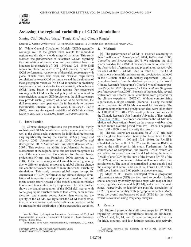
Assessing the regional variability of GCM simulations

Ximing Cai,1 Dingbao Wang,1 Tingju Zhu,2 and Claudia Ringler2

Received 23 October 2008; revised 1 December 2008; accepted 12 December 2008; published 28 January 2009.

[1] While General Circulation Models (GCM) generallyconverge well at the global level, results for individualregions usually show a wide range of variation. This studyassesses the performance of seventeen GCMs regardingtheir simulation of temperature and precipitation based onhindcasts for the periods of 1961–1990 and 1931–1960. Skillscores are plotted on a 2� � 2� grid to present ‘‘zones’’ ofGCM performance. An overlay of these skill score maps withglobal climate zones, land cover, and elevation maps showscorrelations between GCM performance and the distribution ofthese geographic variables. No GCM is superior in predictingtemperature or precipitation for thewhole world, although someGCMs score better in particular regions. For researchersworking with GCM results and policymakers who need tomake decisions based onGCMprojections, the skill score mapsmay provide useful guidance; while for GCM developers, theskill score maps may open areas for further study to improvetheir models. Citation: Cai, X., D. Wang, T. Zhu, and C. Ringler

(2009), Assessing the regional variability of GCM simulations,

Geophys. Res. Lett., 36, L02706, doi:10.1029/2008GL036443.

1. Introduction

[2] Climate change projections are generated by highlysophisticated GCMs.While these models converge relativelywell at the global scale, outcomes for individual regions canvary significantly among the various GCMs [Giorgi andMearns, 2003; Schmittner et al., 2005; Connolley andBracegirdle, 2007; Laurent and Cai, 2007; Whetton et al.,2007]. This regional variability is problematic for impactassessments at the regional level and has been recognized asone of the major sources of uncertainty for climate changeprojections [Giorgi and Francisco; 2000; Murphy et al.,2004]. Differences among model simulations are generallydue to different regional responses to global climate changeand chaotic behaviors embedded in multi-decadal variabilitysimulations. This study presents global maps (except forAntarctica) of GCM performance for climate change simu-lation of temperature and precipitation, based on the rootmean square error (RMSE) of the model simulation relativeto observed temperature and precipitation. The paper furthershows the spatial association of the GCM skill scores withsome geographic variables such as land cover, earth surfaceelevation and climate zones. Rather than evaluating thequality of the GCMs, we argue that the GCM model struc-ture, parameterization and model validation practices mightbe affected by the distribution of these geographic variables.

2. Methods

[3] The performance of GCMs is assessed according totheir ‘‘skill scores’’ [Murphy et al., 2004;Muller et al., 2005;Connolley and Bracegirdle, 2007]. We calculate the skillscores based on the RMSE of the model simulation relative tothe observation of temperature and precipitation, respectively,for each of the 17 GCMs listed in Table S1.1 The GCMsimulations ofmonthly temperature and precipitation includedin the ‘‘Climate of the 20th century experiment’’ (20C3M)were downloaded from the database prepared by the WorldClimate Research Programme’s Coupled Model Intercompar-ison Project (CMIP3) [Program for Climate Model Diagnosisand Intercomparison, 2008]. For each of thesemodels, severalrealizations for different initial conditions were prepared forthe climate experiment (20C3M). Without compromisingsignificance, a single scenario (scenario 1) using the sameinitial condition for all GCMs was used for this study. Theobserved temperature and precipitation data were taken fromthe CRU05 0.5�, 1901–1995 monthly climate time series ofthe Climatic Research Unit from the University of East Anglia[New et al., 2000]. The comparison between the GCMs’ sim-ulation and observation is based on the average variable valuein each month over the period from 1961–1990. The periodfrom 1931–1960 is used to verify the results.[4] The skill scores are calculated for 2� � 2� grid cells

over the global land surface (except for Antarctica). For thegiven periods (1961–1990 and 1931–1960), the RMSE iscalculated for each of the 17 GCMs, and the inverse RMSE isused as the skill score in this study. Furthermore, for theconvenience of comparison, the inverse RMSE values arenormalized to values between 0 and 1 (dividing the inverseRMSE of one GCM by the sum of the inverse RMSE of the17 GCMs), which represent relative skill scores rather thanabsolute ones. The sum of the normalized values equals 1 andthe average skill score is 1/17 � 0.06. Thus a GCM with askill score higher than 0.06 performs above average.[5] Maps of skill scores developed with a geographic

information system (GIS) are then used to conduct furtherspatial analyses by overlaying these maps with maps of landcover, digital elevation models (DEM), and a map of climatezones, respectively, to identify the possible association ofGCM regional variability with geographic variables. More-over, the overall performance of each GCM for the wholeworld is evaluated using frequency analysis.

3. Results

[6] Figure 1 presents the skill score maps for 17 GCMsregarding temperature simulations based on hindcasts.GCMs 1 and, 16, 14, and 13 have the highest skill scoresfor high, medium, and low latitude regions, respectively.

1Auxiliary materials are available in the HTML. doi:10.1029/2008GL036443.

GEOPHYSICAL RESEARCH LETTERS, VOL. 36, L02706, doi:10.1029/2008GL036443, 2009ClickHere

for

FullArticle

1Ven Te Chow Hydrosystems Laboratory, Department of Civil andEnvironmental Engineering, University of Illinois at Urbana-Champaign,Urbana, Illinois, USA.

2International Food Policy Research Institute, Washington, D. C., USA.

Copyright 2009 by the American Geophysical Union.0094-8276/09/2008GL036443$05.00

L02706 1 of 6

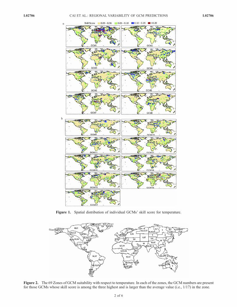
Figure 1. Spatial distribution of individual GCMs’ skill score for temperature.

Figure 2. The 69 Zones of GCM suitability with respect to temperature. In each of the zones, the GCM numbers are presentfor those GCMs whose skill score is among the three highest and is larger than the average value (i.e., 1/17) in the zone.

L02706 CAI ET AL.: REGIONAL VARIABILITY OF GCM PREDICTIONS L02706

2 of 6

Some GCMs score high in specific regions, such as GCM 1for Australia and Europe; GCMs 5 and 9 for Greenland withsnow and ice cover; GCM 13 for the western coastal area ofNorth and South America and Southern Africa; GCMs 16and 17 for the Amazon region and central and easternEurope; GCM 6 for Northern Africa and the eastern sideof the Rocky Mountains in North America; and GCM 14 forthe Queen Elizabeth Islands of Canada. Moreover, GCMs 5,6 and 7 have a similar distribution for North America, theAmazon region, Northern Africa, and the Middle East,probably because these three models are developed by thesame institute (Table S1).

[7] For some regions, such as South Asia, none of theGCMs is strongly preferred according to the skill scoringtechnique used in this study. One plausible explanation is thecomplex climate in this region, such as the monsoons, whichundergo aperiodic and high amplitude variations on intra-seasonal, annual, biennial and interannual timescales. Asillustrated by Webster et al. [1998], the simulation of themean structure of theAsianmonsoon has proven to be elusiveand the observed ENSO-monsoon relationships are difficultto replicate.[8] Starting from the skill score maps (Figure 1), we delin-

eate ‘‘zones of best GCMs’’ for temperature by aggregating

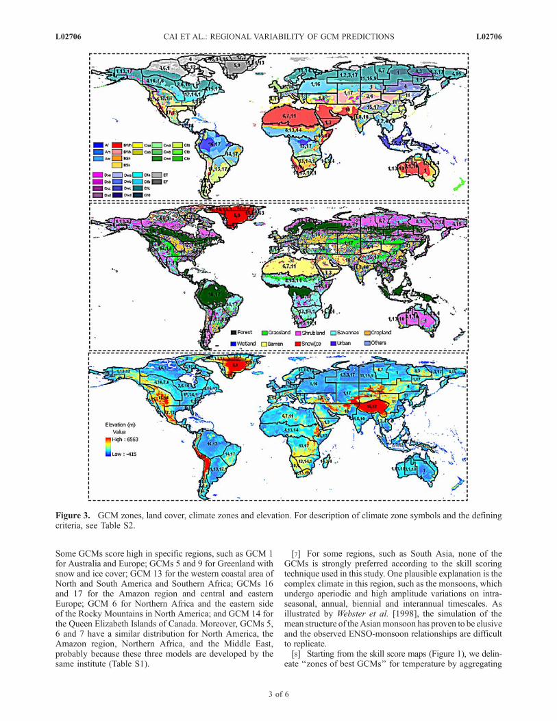
Figure 3. GCM zones, land cover, climate zones and elevation. For description of climate zone symbols and the definingcriteria, see Table S2.

L02706 CAI ET AL.: REGIONAL VARIABILITY OF GCM PREDICTIONS L02706

3 of 6

the pixels in the neighborhood taking into account the highestskill scores for up to three GCMs, as shown in Figure 2. Suchdelineation can be accomplished in GIS by overlaying theseventeen skill score maps of Figure 1 and then generatingpolygons in which one to three GCMs have the highest skillscores. Since the patterns are obvious for most regions fromthe skill score maps, we identify the zones visually bycomparing the skill scores in the various regions. For exam-ple, in Northern Africa GCMs 6, 7 and 11 have the best skillscores. This region is thus labeled with the numbers of theseGCMs (i.e., 6, 7, 11). Zones where only one or two GCMshave high performance scores are labeled accordingly. Sixty-nine zones are identified for the global land surface except forAntarctica.[9] Figures 3a, 3b, and 3c display overlays of these GCM

zones with climate zones, land cover and elevation, respec-tively. As shown in Figure 3a, the GCM zones match wellwith the most recently developed climate zones [Peel et al.,2007]. For example, zones (6, 7, 11) and (1, 3) are locatedin the climate zone of arid hot deserts; zones (2, 6, 10) and(1, 13, 17) are located in the cold climate zone with very coldwinters and without a dry season; zone (2) is located in thetemperate climate region with hot summers and without a dryseason. Climate zones depend on global terrain morphologyand land cover since these variables influence large-scaleatmospheric circulations [Peel et al., 2007]. In Figure 3b,most GCM zones closely match land cover around the world,for example, zone (6, 7, 11) matches well with barren land innorthern Africa; zone (1, 8,10) relates to crop land; zone(16, 17) to forest land; and zone (7, 4, 13) to shrub land. Landcover depends on climate zones but also provides feedbackeffects to climate dynamics.[10] Furthermore, GCMs also seem to be related to eleva-

tion. The relationship is particularly strong in the Pacificregion of America and almost for all of Africa and Asia(Figure 3c). For example, zones (15, 17), (5, 9), among

others, relate to regions with high elevations and zones(1, 16), (11, 15, 9), (5, 13), among others, relate to regionswith low elevations. Thus the GCM zones in terms of tem-perature likely reflect some geo-biophysical patterns.[11] To verify the results, the skill score maps are devel-

oped for another testing period, 1931–1960 (see Figure S1).These maps show results similar to those with the primarytesting period (1961–1990).[12] Compared to temperature, what is the regional vari-

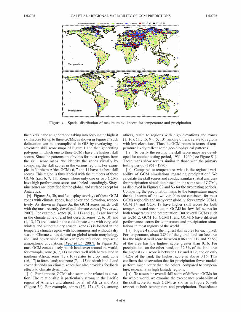
ability of GCM simulations regarding precipitation? Wecalculate the skill scores and conduct similar spatial analysesfor precipitation simulation based on the same set of GCMs,as displayed in Figures S2 and S3 for the two testing periods.Comparing the precipitation maps to the temperature maps,the skill scores of the two variables are consistent for mostGCMs regionally andmany even globally; for exampleGCM1,GCM 14 and GCM 17 have higher skill scores for bothtemperature and precipitation; GCM8 has low skill scores forboth temperature and precipitation. But several GCMs suchas GCM 2, GCM 10, GCM11, and GCM16 have differentperformance scores for temperature and precipitation simu-lations in most regions of the world.[13] Figure 4 shows the highest skill scores for each pixel.

For temperature, about 3.8% of the global land surface areahas the highest skill score between 0.06 and 0.12 and 27.5%of the area has the highest score greater than 0.16. Forprecipitation, on the other hand, on 52.3% of the land areathe highest skill score is between 0.06 and 0.12, and on only14.2% of the land, the highest score is above 0.16. Thisconfirms the observation that for precipitation fewer modelsperform much better than the others, compared to tempera-ture, especially in high latitude regions.[14] To assess the overall skill score of different GCMs for

the whole world, we examine the exceedance probability ofthe skill score for each GCM, as shown in Figure 5, withrespect to both temperature and precipitation. Exceedance

Figure 4. Spatial distribution of maximum skill score for temperature and precipitation.

L02706 CAI ET AL.: REGIONAL VARIABILITY OF GCM PREDICTIONS L02706

4 of 6

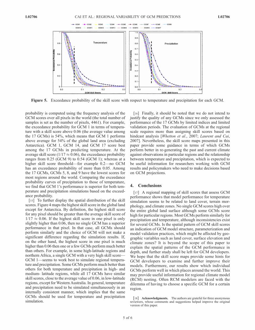
probability is computed using the frequency analysis of theGCM scores over all pixels in the world (the total number ofsamples is set as the number of pixels, 4461). For example,the exceedance probability for GCM 1 in terms of tempera-ture with a skill score above 0.06 (the average value amongthe 17 GCMs) is 54%, which means that GCM 1 performsabove average for 54% of the global land area (excludingAntarctica). GCM 1, GCM 14, and GCM 17 score bestamong the 17 GCMs in predicting temperature. At theaverage skill score (1/17� 0.06), the exceedance probabilityranges from 0.25 (GCM 9) to 0.54 (GCM 1); whereas at ahigher skill score threshold—for example 0.2—no GCMhas an exceedance probability of more than 0.05. Amongthe 17 GCMs, GCMs 5, 8, and 9 have the lowest scores formost regions around the world. Comparing the exceedanceprobability curves of precipitation to those of temperature,we find that GCM 1’s performance is superior for both tem-perature and precipitation simulations based on the exceed-ance probability.[15] To further display the spatial distribution of the skill

scores. Figure 4maps the highest skill score in the global landexcept for Antarctica. By definition, the highest skill scorefor any pixel should be greater than the average skill score of1/17 � 0.06. If the highest skill score in one pixel is onlyslightly higher than 0.06, then no single GCM has a superiorperformance in that pixel. In that case, all GCMs shouldperform similarly and the choice of GCM will not make asignificant difference regarding the simulation results. If,on the other hand, the highest score in one pixel is muchhigher than 0.06 then one or a few GCMs performmuch betterthan others. For example, in some high-latitude regions andnorthern Africa, a single GCM with a very high skill score—GCM 1—seems to work best to simulate regional tempera-ture and precipitation. SomeGCMs performmuch better thanothers for both temperature and precipitation in high- andmedium- latitude regions, while all 17 GCMs have similarskill scores, close to the average value of 0.06, in low-latituderegions, except forWestern Australia. In general, temperatureand precipitation need to be simulated simultaneously in aninternally consistent manner, which implies that the sameGCMs should be used for temperature and precipitationsimulation.

[16] Finally, it should be noted that we do not intend tojustify the quality of any GCMs since we only assessed theperformance of the 17 GCMs by limited indices and limitedvalidation periods. The evaluation of GCMs at the regionalscale requires more than assigning skill scores based onhindcast analysis [Whetton et al., 2007; Laurent and Cai,2007]. Nevertheless, the skill score maps presented in thispaper provide some guidance in terms of which GCMsperform better in re-generating the past and current climateagainst observations in particular regions and the relationshipbetween temperature and precipitation, which is expected tobe useful information for researchers working with GCMresults and policymakers who need to make decisions basedon GCM projections.

4. Conclusions

[17] A regional mapping of skill scores that assess GCMperformance shows that model performance for temperaturesimulation seems to be related to land cover, terrain mor-phology, and climate zones. No single GCM scores high overthe entire global land surface although some GCMs scorehigh for particular regions. Most GCMs perform similarly forprecipitation and temperature, although inconsistencies existfor several GCMs. Is the spatial pattern of GCM skill scoresan indication of GCM model structure, parameterization andmodel validation practices, which might be affected by geo-graphic variables such as land cover, surface elevation andclimate zones? It is beyond the scope of this paper toexplain the spatial patterns of the GCM performance indepth, and further study shall be left for GCM developers.We hope that the skill score maps provide some hints forGCM developers to examine and further improve theirmodels. Furthermore, our results show which individualGCMs perform well in which places around the world. Thismay provide useful information for regional climate model(RCM) nesting. Often RCM modelers are faced with thedilemma of having to choose a specific GCM for a certainregion.

[18] Acknowledgments. The authors are grateful for three anonymousreviewers, whose comments and suggestions helped improve the originalversion of this paper.

Figure 5. Exceedance probability of the skill score with respect to temperature and precipitation for each GCM.

L02706 CAI ET AL.: REGIONAL VARIABILITY OF GCM PREDICTIONS L02706

5 of 6

ReferencesClaussen, M., et al. (2000), Earth system models of intermediate complexity:Closing the gap in the spectrum of climate system models, Clim. Dyn., 18,579–586.

Connolley, W. M., and T. J. Bracegirdle (2007), An Antarctic assessment ofIPCC AR4 coupled models, Geophys. Res. Lett., 34, L22505,doi:10.1029/2007GL031648.

Giorgi, F., and R. Francisco (2000), Evaluating uncertainties in the predictionof regional climate change, Geophys. Res. Lett., 27, 1295–1298.

Giorgi, F., and L. O. Mearns (2003), Probability of regional climate changebased on the Reliability Ensemble Averaging (REA) method, Geophys.Res. Lett., 30(12), 1629, doi:10.1029/2003GL017130.

Grassl, H. (2000), Status and improvements of coupled general circulationmodels, Science, 288, 1991–1997.

Laurent, R., and X. Cai (2007), A maximum entropy method for combiningAOGCMs for regional intra-year climate change assessment, Clim.Change, 82, 411–435.

Muller, W., A. C. Appenzeller, F. J. Doblas-Reyes, and M. A. Liniger(2005), A debiased ranked probability skill score to evaluate probabilisticensemble forecasts with small ensemble sizes, J. Clim., 18, 1513–1523.

Murphy, J. M., D. M. H. Sexton, D. N. Barnett, G. S. Jones, M. J. Webb,M. Collins, and D. A. Stainforth (2004), Quantification of modelinguncertainties in a large ensemble of climate change simulations, Nature,430, 768–772.

New, M., M. Hulme, and P. Jones (2000), Representing twentieth-centuryspace-time climate variability. Part II: Development of 1901–1996monthly grids of terrestrial surface climate, J. Clim., 13, 2217–2238.

Peel, M. C., B. L. Finlayson, and T. A. McMahon (2007), Updated worldmap of the Koppen-Geiger climate classification, Hydrol. Earth Syst. Sci.,11, 1633–1644.

Program for Climate Model Diagnosis and Intercomparison (2008), WorldClimate Research Programme’s Coupled Model Intercomparison Project,http://www-pcmdi.llnl.gov/ipcc/about_ipcc.php, Lawrence LivermoreNatl. Lab., Livermore, Calif., September.

Schmittner, A., M. Latif, and B. Schneider (2005), Model projections of theNorth Atlantic thermohaline circulation for the 21st century assessed byobservations, Geophys. Res. Lett., 32, L23710, doi:10.1029/2005GL024368.

Webster, P. J., V. O. Magana, T. N. Palmer, J. Shukla, R. A. Tomas,M. Yanai, and T. Yasunari (1998), Monsoons: Processes, predictability,and the prospects for prediction, J. Geophys. Res., 103, 14,451–14,510.

Whetton, P., I. Macadam, J. Bathols, and J. O’Grady (2007), Assessment ofthe use of current climate patterns to evaluate regional enhanced green-house response patterns of climate models, Geophys. Res. Lett., 34,L14701, doi:10.1029/2007GL030025.

�����������������������X. Cai and D. Wang, Ven Te Chow Hydrosystems Laboratory, Depart-

ment of Civil and Environmental Engineering, University of Illinois atUrbana-Champaign, Urbana, IL 61801, USA. (xmcai@uiuc.edu)C. Ringler and T. Zhu, International Food Policy Research Institute,

Washington, DC 20006, USA.

L02706 CAI ET AL.: REGIONAL VARIABILITY OF GCM PREDICTIONS L02706

6 of 6