HAL Id: tel-02922887https://tel.archives-ouvertes.fr/tel-02922887

Submitted on 26 Aug 2020

HAL is a multi-disciplinary open accessarchive for the deposit and dissemination of sci-entific research documents, whether they are pub-lished or not. The documents may come fromteaching and research institutions in France orabroad, or from public or private research centers.

L’archive ouverte pluridisciplinaire HAL, estdestinée au dépôt et à la diffusion de documentsscientifiques de niveau recherche, publiés ou non,émanant des établissements d’enseignement et derecherche français ou étrangers, des laboratoirespublics ou privés.

Représentation d’une huile dans des simulationsmésoscopiques pour des applications EOR

David Steinmetz

To cite this version:David Steinmetz. Représentation d’une huile dans des simulations mésoscopiques pour des appli-cations EOR. Theoretical and/or physical chemistry. Sorbonne Université, 2018. English. �NNT :2018SORUS521�. �tel-02922887�

Sorbonne Université

ED 388 - Ecole doctorale de Chimie Physique et de Chimie Analytique de Paris

Centre

Représentation d’une huile dans des simulations

mésoscopiques pour des applications EOR

par

David Steinmetz

Thèse de doctorat de Chimie

Dirigée par Carlos Nieto-Draghi

Présentée et soutenue publiquement le 19/10/2018

Devant un jury composé de :

Prof. Malfreyt Patrice Rapporteur

Prof. Lisal Martin Rapporteur

Prof. Jardat Marie Examinateur

Prof. Carbone Paola Examinateur

Dr. Lemarchand Claire Examinateur

Dr. Nieto-Draghi Carlos Directeur de thèse

Dr. Creton Benoît Examinateur

Sorbonne University

ED 388 - Ecole doctorale de Chimie Physique et de Chimie Analytique de Paris

Centre

Representation of an oil in mesoscopic simulations for

EOR applications

by

David Steinmetz

Chemistry Ph.D. Thesis

Directed by Carlos Nieto-Draghi

Presented and defended publicly on 19 October 2018

In front of jury:

Prof. Malfreyt Patrice Reviewer

Prof. Lisal Martin Reviewer

Prof. Jardat Marie Examiner

Prof. Carbone Paola Examiner

Dr. Lemarchand Claire Examiner

Dr. Nieto-Draghi Carlos Thesis supervisor

Dr. Creton Benoît Examiner

1

Acknowledgement

Firstly, I would like to thank Ms. Ruffier-Meray, head of the Direction Chimie et

Physico-Chimie Appliquées, and Mr. Mougin, head of the Departement Thermodynamique et

Modélisation Moléculaire, for welcoming me at IFP Energies nouvelles and allowing me to

do this work in excellent conditions.

I would like to sincerely thank my thesis supervisor, Carlos Nieto-Draghi, for the

continuous support of my Ph.D study and research. I have been extremely lucky to have a

supervisor who cared so much about my work. I appreciated his great efforts to explain things

clearly and simply.

I would like to express my deep gratitude to my supervisor Benoît Creton. This work

would not have been possible without his guidance, support and encouragement. Under his

guidance, I successfully overcame many difficulties and leaned a lot.

Véronique Lachet gave me invaluable help during my thesis and I am grateful to for

her advices and valuable comments.

I also wish to express my gratitude to Bernard Rousseau for his valuable advice,

constructive criticism and his extensive discussions around my work.

Most of the results described in this thesis would not have been obtained without the

involvement of Jan Verstraete. I would like to thank him for sharing his expertise in

petroleum field.

I am also deeply thankful to Rafael Lugo for fruitful discussions and for allowing me

to understand some aspects of thermodynamics.

A very special thanks goes out to all the Ph.D students and colleagues: Saifuddin,

Germain, Mona, Michel, Anand, Xavier and Sébastien for providing a stimulating and fun

environment and for keeping me motivated throughout my thesis.

I take this opportunity to express my gratitude to all the people of the department for

the warm welcome.

2

Table of contents

ACKNOWLEDGEMENT 1

TABLE OF CONTENTS 2

INTRODUCTION 5

CHAPTER 1. SETTING UP STAGE 8

1.1 INTRODUCTION 8 1.2 CRUDE OIL AND PETROLEUM FRACTIONS 8 1.2.1 FORMATION OF PETROLEUM 8 1.2.2 DESCRIPTION OF PETROLEUM 9 1.2.3 DESCRIPTION OF PETROLEUM FRACTIONS 10 1.3 MOLECULAR COMPOSITION OF CRUDE OIL 12 1.3.1 HYDROCARBONS 12 1.3.2 OTHER CRUDE OIL COMPONENTS 14 1.4 CRUDE OIL EXTRACTION 17 1.4.1 CRUDE OIL EXTRACTION METHODS 17 1.4.2 RECOVERY OF RESIDUAL OIL USING EOR TECHNIQUES 18 1.5 CONCLUSIONS 21

CHAPTER 2. CHARACTERIZATION OF CRUDE OIL 22

2.1 INTRODUCTION 22 2.2 PROPERTIES OF CRUDE OIL: EXPERIMENTAL METHODS 23 2.2.1 ELEMENTAL ANALYSIS 23 2.2.2 DENSITY AND SPECIFIC GRAVITY 24 2.2.3 MOLECULAR WEIGHT 25 2.2.4 BOILING TEMPERATURE AND DISTILLATION CURVES 25 2.2.5 CHEMICAL FAMILIES 27 2.2.6 INTERFACIAL TENSION 28 2.3 STATE OF THE ART FOR THE REPRESENTATION OF CRUDE OIL 30 2.3.1 FRACTIONATION APPROACHES 30 2.3.2 LUMPING METHODS 32 2.3.3 MOLECULAR RECONSTRUCTION 34 2.4 CONCLUSIONS 38

CHAPTER 3. COARSE-GRAINED SIMULATION METHODS 40

3.1 INTRODUCTION 40 3.2 DISSIPATIVE PARTICLES DYNAMICS (DPD) 42 3.2.1 CONSERVATIVE FORCE 42 3.2.2 INTRAMOLECULAR FORCE 43 3.2.3 DISSIPATIVE AND RANDOM FORCES 44 3.2.4 FLUCTUATION-DISSIPATION THEOREM 45

3

3.2.5 TIME INTEGRATION SCHEMES 46 3.3 COARSE-GRAINED-MONTE CARLO SIMULATION (CG-MC) 47 3.3.1 PRINCIPLE AND METROPOLIS ALGORITHM 47 3.3.2 STATISTICAL ENSEMBLES 48 3.3.3 MONTE CARLO MOVES 50 3.4 COARSE-GRAINED SIMULATIONS 53 3.4.1 COARSE-GRAINED MODEL 53 3.4.2 SIMULATIONS BOXES AND BOUNDARY CONDITIONS 54 3.4.3 INTERFACIAL TENSION CALCULATION 55 3.4.4 COARSE-GRAINED UNITS 59 3.5 CONCLUSIONS 60

CHAPTER 4. PARAMETERIZATION OF LIQUID-LIQUID TERNARY MIXTURES 61

4.1 INTRODUCTION 61 4.2 STATE OF THE ART OF PARAMETERIZATION OF COARSE-GRAINED SIMULATIONS 64 4.3 NEW PARAMETERIZATION APPROACH FOR LIQUID-LIQUID EQUILIBRIUM OF TERNARY SYSTEMS: METHODOLOGY

AND COMPOSITIONAL DETAILS 68 4.3.1 PARAMETERIZATION OF INTERACTIONS 68 4.3.2 STATISTICAL ENSEMBLES – METHODOLOGY TO COMPUTE IFT 72 4.3.3 SYSTEMS STUDIED 75 4.4 RESULTS 78 4.4.1 COMPOSITION DEPENDENCE OF THE FLORY-HUGGINS INTERACTION PARAMETERS 78 4.4.2 LIQUID-LIQUID EQUILIBRIUM (LLE) 80 4.4.3 INTERFACE COMPOSITIONS 86 4.4.4 INTERFACIAL TENSION 87 4.5 THERMODYNAMIC MODELS FOR PREDICTION OF LIQUID-LIQUID EQUILIBRIA 93 4.5.1 PREDICTION OF THE COMPOSITION OF LIQUID-LIQUID EQUILIBRIA 93 4.5.2 PREDICTION OF INTERACTION PARAMETERS USING A THERMODYNAMIC MODEL 98 4.5.3 TRANSFERABILITY OF INTERACTION PARAMETERS FOR ALKANES 102 4.6 CONCLUSIONS 104

CHAPTER 5. REPRESENTATION AND COARSE-GRAINED SIMULATIONS OF CRUDE OILS 106

5.1 INTRODUCTION 106 5.2 THEORETICAL BACKGROUND FOR CRUDE OIL MOLECULAR REPRESENTATION 108 5.2.1 REPRESENTATION OF THE LIGHT FRACTION (C20-): THE LUMPED ALGORITHM 108 5.2.2 REPRESENTATION OF HEAVY FRACTIONS (C20+) 109 5.3 RESULTS 118 5.3.1 MOLECULAR MODEL OF CRUDE OIL 118 5.3.2 COARSE-GRAINED MODEL OF CRUDE OIL 126 5.3.3 PARAMETERIZATION OF INTERACTIONS FOR DPD SIMULATIONS 128 5.4 RESULTS OF DPD SIMULATIONS OF CRUDE OIL 131 5.5 CONCLUSIONS 134

GENERAL CONCLUSION 136

BIBLIOGRAPHY 140

4

APPENDICES 150

APPENDICES – CHAPTER 4 150 APPENDICES – CHAPTER 5 182

LIST OF FIGURES 192

LIST OF TABLES 197

5

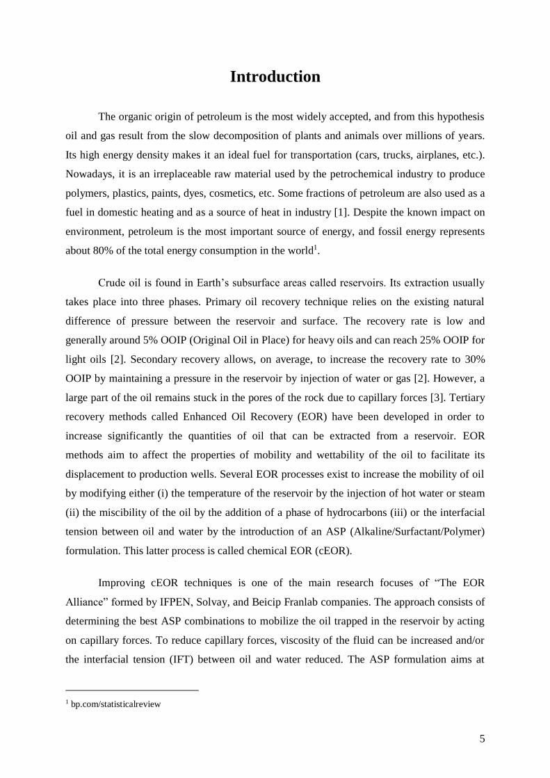
Introduction

The organic origin of petroleum is the most widely accepted, and from this hypothesis

oil and gas result from the slow decomposition of plants and animals over millions of years.

Its high energy density makes it an ideal fuel for transportation (cars, trucks, airplanes, etc.).

Nowadays, it is an irreplaceable raw material used by the petrochemical industry to produce

polymers, plastics, paints, dyes, cosmetics, etc. Some fractions of petroleum are also used as a

fuel in domestic heating and as a source of heat in industry [1]. Despite the known impact on

environment, petroleum is the most important source of energy, and fossil energy represents

about 80% of the total energy consumption in the world1.

Crude oil is found in Earth’s subsurface areas called reservoirs. Its extraction usually

takes place into three phases. Primary oil recovery technique relies on the existing natural

difference of pressure between the reservoir and surface. The recovery rate is low and

generally around 5% OOIP (Original Oil in Place) for heavy oils and can reach 25% OOIP for

light oils [2]. Secondary recovery allows, on average, to increase the recovery rate to 30%

OOIP by maintaining a pressure in the reservoir by injection of water or gas [2]. However, a

large part of the oil remains stuck in the pores of the rock due to capillary forces [3]. Tertiary

recovery methods called Enhanced Oil Recovery (EOR) have been developed in order to

increase significantly the quantities of oil that can be extracted from a reservoir. EOR

methods aim to affect the properties of mobility and wettability of the oil to facilitate its

displacement to production wells. Several EOR processes exist to increase the mobility of oil

by modifying either (i) the temperature of the reservoir by the injection of hot water or steam

(ii) the miscibility of the oil by the addition of a phase of hydrocarbons (iii) or the interfacial

tension between oil and water by the introduction of an ASP (Alkaline/Surfactant/Polymer)

formulation. This latter process is called chemical EOR (cEOR).

Improving cEOR techniques is one of the main research focuses of “The EOR

Alliance” formed by IFPEN, Solvay, and Beicip Franlab companies. The approach consists of

determining the best ASP combinations to mobilize the oil trapped in the reservoir by acting

on capillary forces. To reduce capillary forces, viscosity of the fluid can be increased and/or

the interfacial tension (IFT) between oil and water reduced. The ASP formulation aims at

1 bp.com/statisticalreview

6

reaching an ultralow IFT for the brine/surfactant/crude oil systems. However, the difficulty of

the formulation design stands in the fact that each oil reservoir is unique and they differ from

each other by their composition, salinity, pressure, and temperature condition. A specific

S/SP/ASP formulation for a given reservoir is necessary. Because of complex involved

phenomena, identification and selection of relevant surfactants is challenging, and it requires

a large number of trial-and-error tests. Modelling tools such as molecular simulations are

adapted to improve the efficiency of such a process by providing information about

phenomena occurring at the molecular level and at the interface [4].

Molecular simulation of petroleum requires establishing the molecular representation

of the fluid. However, petroleum is a mixture of molecules so complex that even the most

efficient analytical techniques do not identify molecules one by one. Even now, the molecular

description of the composition of petroleum is not completely resolved. Analytical techniques

commonly used in the oil industry provide only global and average information such as

elemental analysis, average density or distillation curves of petroleum and its fractions [1].

The most recent analytical techniques (chromatography, RMN spectroscopy, mass

spectroscopy, etc.) provide statistical data on the distribution of atoms or groups of atoms in

petroleum fractions [5]. A relation must be established between the available experimental

data and the molecular composition in order to define a simplified representation of crude oil.

The representation in molecular simulations of crude oil and phenomena that occur at

interfaces requires the consideration of large length and time scales. Atomistic methods such

as Molecular Dynamics cannot handle such scales to properly consider such systems with

reasonable computational resources. Mesoscopic simulation techniques such as the

Dissipative Particle Dynamics (DPD) seem to be most suitable to simulate large systems. In

the DPD model, molecular structures are substituted by DPD beads (coarse-grained model) to

simplify the description of systems. Parameterization of interactions between the DPD beads

is essential to correctly model properties of the simulated system. For example, interfacial

tension, which is one of the most important properties for cEOR, results from an imbalance in

intermolecular forces. Therefore, an adequate description of interactions between beads is

required to accurately predict this property using DPD simulations.

The objective of this thesis consists in establishing a methodology to represent a crude

oil in molecular simulations in order to predict phenomena taking place at the interfaces. This

work is the first part of a larger project to develop a predictive tools based on molecular

7

simulation for improvement of cEOR techniques. Further work will be required to take into

account, for example, surfactants contained in the ASP formulation. Three main scientific and

technical challenges must be removed in order to achieve the prediction of crude oil

properties by molecular simulation:

(1) Establish a simplified representation for a crude oil. A methodology must be

elaborate to build a realistic representation of a crude oil using experimental data

available for the crude oil of interest. This representation must be limited to a few

components in order to be introduced in molecular simulation tools.

(2) Parameterize molecular simulations. An accurate method to parameterize

interactions between particles must be developed and validated to reproduce

interfacial properties.

(3) Simulate a crude oil using molecular simulations. Molecular simulations are

performed using the simplified representation of the crude oil and appropriate

parameters to predict the crude oil/water interfacial tension.

The manuscript is divided into five chapters. The Chapter 1 gives general information

about crude oils and their chemical composition. In addition, methods for crude oil extraction

and principle of EOR techniques will be described. Chapter 2 is a short review dealing with

the main crude oil properties that can be measured experimentally. Additionally, a state of the

art on methodologies developed to build a molecular representation a crude oil or crude oil

fractions is proposed in this chapter. Chapter 3 is dedicated to the description of the

simulation methods used in this work. In Chapter 4, different methods to parameterize

interactions between DPD beads are proposed and compared to predict the interfacial tension

of liquid-liquid equilibrium systems. This chapter allows defining the parameterization

method that will be applied to generate parameters to feed simulations of a crude oil system.

In Chapter 5, a molecular representation method of crude oil is proposed. This method is

applied to the sample of a crude oil that has been analyzed at IFPEN and DPD simulations are

performed to predict the crude oil/water interfacial tension. This manuscript ends with a

chapter dedicated to main conclusions and perspectives for this work.

8

Chapter 1. Setting up stage

1.1 Introduction

The first chapter gives general information about petroleum and extraction methods. In

a first part, the nature and chemical composition of crude oil will be presented.

In a second part, extraction methods and the principle of EOR will be explained. This

section will highlight objectives of EOR techniques and to show the properties targeted by

these processes. Interfacial tension between crude oil and water is one of these properties and

its minimization allow to increase the efficiency of petroleum extraction by chemical EOR.

1.2 Crude oil and petroleum fractions

1.2.1 Formation of petroleum

Petroleum results from the slow transformation of organic matter over millions of

years. Organic matter derived from plants and animals such as zooplankton and algae. It is

composed mainly of hydrogen (H), carbon (C), and some heteroatoms such as nitrogen (N),

oxygen (O) and sulfur (S). Transformation of organic matter into petroleum takes place in

three stages:

- This organic matter settles in the sea or lake bottoms where it mixes with sand and

silt. In this oxygen-poor environment, the organic matter is partly preserved from

decomposition by aerobic bacteria. Thus, organic matter can accumulate in

successive layers over tens and even hundreds of meters.

- The second stage is the degradation (called diagenesis) of the organic matter under

mild conditions of temperature and pressure. Organic matter undergoes

transformation under the action of anaerobic bacteria. They extract certain

chemical elements such as sulfur, nitrogen and oxygen, resulting in the formation

of kerogen. Kerogen is composed of macromolecules with a large structure

containing cyclic and aromatic structures [6].

9

- With the gradual burial of kerogen, the increase in temperature (from 100-120°C

[1]) and pressure (from 17 MPa [1]) leads to the second stage of degradation of

organic matter (called catagenesis). The kerogen undergoes a thermal cracking

(pyrolysis). This chemical transformation removes residual nitrogen, and oxygen

to leave water, CO2, hydrocarbons (gas, liquid and solid). The mixture of liquid

hydrocarbons is called crude oil.

The conditions of catagenesis determine the properties of the products. For example,

high temperature and pressure lead to more complete “cracking” of the kerogen and lighter

and smaller hydrocarbons.

1.2.2 Description of petroleum

Petroleum is drawn out from beneath the earth’s surface and comes in form of gases

(natural gas), liquids (crude oil), semisolids (bitumen), or solids (wax or asphaltite) [1]. Crude

oil is a brown to black liquid that contains thousands of different molecules. The molecular

complexity comes from the diversity in size of molecules. Molecules involved can be simple,

such as methane, to more complex structures such as asphaltenes. In the latter case, molar

mass can reach 10 000 g/mol. The diversity in structural assembly and molecules size leads to

wide variety of molecules and isomers. For example, in Table 1, the number of isomers for

paraffin (alkane) family is presented as a function of the number of carbon atoms in a

molecule.

Table 1. Number of isomers as a function of number of carbon atoms for paraffin family.

Extracted from the publication of Beens [7].

Number of carbon atoms Number of isomers Boiling point (n-paraffin) (°C)

5 3 36

8 18 126

10 75 174

15 4347 271

20 3.66 × 105 344

25 3.67 × 107 402

30 4.11 × 109 450

35 4.93 × 1011 490

40 6.24 × 1013 525

45 8.22 × 1015 554

60 2.21 × 1022 620

80 1.06 × 1031 678

100 5.92 × 1039 715

10

1.2.3 Description of petroleum fractions

Crude oil can be broken down into several fractions according to the boiling point of

compounds. For a given chemical family, the boiling point of a hydrocarbon is usually

correlated with the number of carbon atoms. Table 1 shows that, for the n-paraffin family, the

boiling temperature increases from 36 to 715 °C for a molecule composed of 5 to 100 carbon

atoms. Therefore, compounds of a crude oil can be separated as a function of their size in

different fraction by a procedure called fractional distillation. Each fraction is a mixture of a

reduced number of compounds with a specific range of boiling point values. For instance,

Figure 1 represents obtained fractions and associated proportions for a crude oil originating

from Alaska.

Figure 1. Composition of a crude oil originating from Alaska. Data are extracted from the

book by Riazi [1].

11

Distillation of crude oil is performed by means of a column at atmospheric pressure.

Compounds having a boiling point below 350°C are separated in five fractions: light gases,

light gasoline, naphtha, kerosene, and light gas oil. Compounds having a boiling point above

350°C called residuum are removed from the bottom of the atmospheric distillation column

and sent to a vacuum distillation column. Indeed, to avoid breaking of carbon-carbon bonds

and, thus, change the nature of molecules, the residuum fraction separation must be carried

out at low pressure (50-100 mmHg or 6666-13332 Pa).

The boiling point of a hydrocarbon is strongly correlated to its size (i.e. the carbon skeleton

length as shown in Table 1) and to its molecular structure. Figure 2 shows the composition of

crude oils as a function of boiling point and molar mass of compounds. The molar mass is

estimated from the number of carbon and hydrogen atoms for the paraffin family respecting

the chemical formula CnH2n+2. Chemical families are differentiated by their molecular

structure (chains, cycles, saturated or unsaturated compounds). The different chemical

structures present in the crude oil are presented in the next section.

Figure 2. Composition of crude oil as a function of boiling points and molecular weight of

compounds. PAH means Polycyclic Aromatic Hydrocarbons. Extracted from the reference

[8]. Reprinted (adapted) with permission from McKenna, A. M.; Purcell, J. M.; Rodgers, R.

P.; Marshall, A. G., Energy Fuels 2010, 24, 2929–2938. Copyright (2010) American

Chemical Society.

12

1.3 Molecular composition of crude oil

1.3.1 Hydrocarbons

Hydrocarbons are organic compounds consisting exclusively of carbon and hydrogen

atoms. Generally, hydrocarbons are divided into four groups: (1) paraffins, (2) olefins, (3)

naphthenes, and (4) aromatics.

(1) Paraffins, also known as alkanes in organic chemistry, are acyclic saturated

hydrocarbons. General chemical formula of paraffins can be expressed with CnH2n+2

where 𝑛 is an integer. All carbon-carbon bonds are single. Paraffins are divided into

two subgroups: n-paraffins which are straight molecules and iso-paraffins that contain

at least one branched chain. In Table 2, some examples of chemical structures of

paraffins are presented. Since paraffins are fully saturated, these molecules are

chemically stable and hence remain unchanged over long periods of geological time.

Table 2. Examples of chemical structures of paraffins. Molecules presented are isomers of

hexane (C6H14).

Name Closed formula Name Closed formula

n-hexane

2,2-dimethylbutane

2-methylpentane

2,3-dimethylbutane

3-methylpentane

(2) Olefins, also known as alkenes in organic chemistry, are acyclic unsatured

hydrocarbons. These molecules contain at least one carbon-carbon double bond. The

general chemical formula can be expressed with the CnH2(n-a+1) where 𝑎 is the number

of double bonds in the molecule. In Table 3, some examples of olefinic chemical

structures are presented. Olefins are uncommon in crude oils due to their reactivity

with hydrogen that makes them saturated. Similarly, compounds containing triple

13

bonds (alkynes, in organic chemistry) are not found in crude oils because of their

tendency to become saturated.

Table 3. Examples of chemical structures of olefins.

Name Closed formula Name Closed formula

ethylene

1,3-butadiene

1-butene

2-methyl-2-penten

(3) Naphthenes, also known as cycloalkanes in organic chemistry, are statured

hydrocarbons which have one or more rings. General chemical formula can be

expressed with CnH2(n-b+1) where 𝑏 is the number of cycles in the molecule. Naphthene

rings with five and six carbon atoms are the most common due to their thermodynamic

stability. In addition, aliphatic chains can be bonded to rings, leading to a wide variety

of chemical structures. In Table 4, some examples of chemical structure for

naphthenes are presented.

Table 4. Examples of chemical structures of naphthenes.

Name Closed formula Name Closed formula

cyclopentane

decalin

cyclohexane

1-methyldecalin

(4) Aromatics are hydrocarbons which have one or more planar unsaturated carbon rings

and delocalized pi electrons between carbon atoms. This arrangement of electrons

allows compounds that are particularly unreactive and stable. Many structures

containing aromatic rings exist in petroleum. For example, alkyl groups of different

sizes (methyl, ethyl, propyl, etc.) can be attached to an aromatic ring to form

alkybenzene compounds. In addition, several aromatics rings can be fused with each

14

other or with naphthenic ring to form large and complex structures. These polycyclic

aromatic hydrocarbons (PAH) compounds can be found in the heaviest fractions of

petroleum. In Table 5, some examples of chemical structures for aromatic compounds

are presented.

Table 5. Examples of chemical structures of aromatic hydrocarbons.

Name Closed formula Name Closed formula

benzene

toluene

naphthalene

biphenyl

anthracene

tetralin

1.3.2 Other crude oil components

Crude oils contain heteroatoms such as sulfur (S), nitrogen (N), or oxygen (O) and, in

smaller amounts, organometallic compounds. These constituents appear mainly in the heavier

fractions of crude oils [9]. Although nonhydrocarbon compounds are found in small quantities

in crude oils, identification of these compounds and characterization of chemical functions is

essential for the oil and gas industry. For example, presence of organic compounds that

contain a carboxyl group (-COOH) or mercaptan function (-SH) can promote metallic

corrosion which must be taken into account for transport or storage of crude oil. In addition,

presence of metals can affect conversion processes of crude oil into finished products by

poisoning catalysts. For example, metals poison the catalyst used for the cracking process to

convert high-molecular weight hydrocarbons into more valuable products such as gasoline or

olefinic gases. It can be expected that compounds with heteroatoms and chemical functions

exhibit surface-active characteristics and have a role in the interactions between crude oil and

water. For example, chemical functions such as alcohol (-OH) form hydrogen bonds with

water molecules. Therefore, interfacial tension between water and a crude oil may be

influenced by the presence of such chemical functions.

15

The main families of compounds containing (1) sulfur, (2) nitrogen, (3) oxygen and,

(4) metals atoms are listed below.

(1) Sulfur atoms are usually the most abundant among heteroatoms in crude oil and it can

be encountered under three different forms: mercaptanes, sulfides and thiophenes.

Mercaptanes (or thiols) are organosulfur compounds that contain a sulfhydryl group (-

SH) linked to an alkyl chain. Sulfides (or thioethers) are organic compounds with

sulfur atoms bonded by two alkyl groups with the connectivity R-S-R’, where R and

R’ denote the alkyl groups. Two sulfur atoms can be linked to form a disulfide bridge

(R-S-S-R’). Thiophenes are heterocyclic compounds consisting of a planar five-

membered ring composed by four unsaturated carbon atoms and one sulfur atom. The

aromatic character of thiophene contributes to their stability. In Table 6, some

examples of chemical structures containing sulfur atoms are proposed.

Table 6. Examples of chemical structures containing sulfur atoms.

Name Closed formula Name Closed formula

mercaptanes

disulfides

sulfides

thiophene

cyclic sulfides

benzothiophene

(2) Nitrogen compounds may be classified as basic or nonbasic. Pyrroles are neutral

heterocyclic aromatic organic compounds consisting of a five-membered ring with

four carbon atoms and one NH group. The basic nitrogen compounds are composed

mainly of pyridine and its derivatives. Pyridine is a heterocyclic organic compounds

consisting of a six-membered ring with five carbon atoms and a nitrogen atom. In

crude oil, it is also possible to find in very small quantities of amines (primary R-NH2;

secondary R-NH-R’; tertiary (R)3-N) and anilines. In Table 7, some examples of

chemical structures containing nitrogen atoms are presented. Nitrogen compounds

have tendency to exist in the higher boiling fractions and residua.

16

Table 7. Examples of chemical structures containing nitrogen atoms.

Name Closed formula Name Closed formula

pyridine

pyrrole

quinoline

carbazole

tertiary amine

aniline

(3) Oxygen atoms are generally less abundant than other heteroatoms in crude oil.

However, oxygen in organic compounds can occur in a large variety of forms based

on one or more oxygen atoms: alcohols (R-OH and Aro-OH), carboxylic acids (R-

COOH and Aro-COOH), ethers (R-O-R), ketones (R-CO-R), aldehydes (R-CO-H),

esters (R-COO-R), acid anhydrides (R-CO-O-CO-R) and amides (R-C(O)-NR2)

where R and R’ are alkyl groups and Aro stands for an aromatic group. In addition,

heterocyclic organic compound such as furan can be found. Furan compounds consist

of a five-membered aromatic ring with four carbon atoms and one oxygen atom. In

crude oil, the most common compounds are the derivatives of naphthenic acid and

phenol. In Table 8, some examples of chemical structures containing oxygen atoms

are presented.

Table 8. Examples of chemical structures containing oxygen atoms.

Name Closed formula Name Closed formula

naphthenic acid

phenol

acetone

diethyl ether

furan

benzofuran

(4) Metals can be found in the heavier fractions of crude oil. Among metals, nickel (Ni)

and vanadium (V) are the most common in petroleum. These elements are chelated

17

with porphyrins to form organometallic compounds. Porphyrins are derivatives of

porphine that consists of four pyrrole molecules joined by methine (-CH=) bridges.

Figure 3 shows nickel atoms included into porphyrin through chelation.

Figure 3. Nickel chelate of porphine. Extracted from the book of Speight [9].

1.4 Crude oil extraction

1.4.1 Crude oil extraction methods

Crude oil extraction takes place in three stages (Figure 4):

- Primary oil recovery starts once a well has been drilled. This technique relies on

the natural pressure into the reservoir to push the oil up to the surface. Artificial lift

are sometimes used to increase the flow rate above what would flow naturally. It is

a mechanical device such as a pump jacks. The recovery rate of primary recovery

is low and it is generally around 5% OOIP (Original Oil in Place) for heavy oils

and can reach 25% OOIP for light oils [2].

- Secondary recovery methods are used when there is insufficient pressure into the

reservoir. The most common technique is water flooding which consists to inject

water into the reservoir to maintain the pressure and sweep the oil encountered by

water. Another possibility to maintain the pressure is to inject natural gas instead

of water. Secondary recovery allows, on average, to increase the recovery rate to

30% OOIP [2].

18

- Tertiary recovery methods called Enhanced Oil Recovery (EOR) are used when

primary and secondary recovery methods are either exhausted or no longer

economically viable. Several EOR techniques have been developed and aim to

affect the properties of mobility and wettability of the oil to facilitate its

displacement to production wells.

It can be noted that many reservoir production operations are not conducted in the specified

order above. For example, primary and secondary recovery methods are ineffective for the

exploitation of heavy oil wells due to the high viscosity of the fluid. In this case, the bulk of

the production comes from EOR methods.

Figure 4. Summary diagram of crude oil extraction methods. (EOR = Enhanced Oil Recovery,

and IOR = Improved Oil Recovery)

1.4.2 Recovery of residual oil using EOR techniques

In the reservoir, oil is trapped in pores due to capillary forces and a high viscosity of

the fluid [3]. EOR techniques are designed to significantly increase the recovery of residual

oil by influencing two major factors: capillary number (𝑁𝐶) and mobility ratio (𝑀).

The first parameter is the capillary number, 𝑁𝐶, which is defined as the ratio of the

viscous forces and local capillary forces. 𝑁𝐶 can be calculated using equation (1).

19

𝑁𝐶 =𝑣 ∙ 𝜂

𝛾 (1)

where 𝑣 is the interstitial velocity (m/s), 𝜂 is the displacing fluid viscosity (e.g. oil) (Pa.s) and

𝛾 is the interfacial tension (IFT) between the displacing fluid and oil (N/m). A small capillary

number suggests that the motion of the fluid is dominated by capillary forces. A large

capillary number indicates a viscous dominated regime. It has been shown that when the

capillary number increases, the residual oil saturation (𝑆𝑜𝑟) decreases (Figure 5).

Figure 5. Effect of capillary number on residual oil saturation.

An increase in capillary number implies a decrease in residual oil saturation and, thus, an

increase in oil recovery. According to equation (1), there are three ways to increase the

capillary number: increasing injection fluid velocity, increasing displacing fluid viscosity

(e.g. oil) and reducing IFT.

In Figure 5, the critical capillary number, 𝑁𝑐𝑟𝑖, is the point which corresponds to a break in

the desaturation curve (𝑁𝐶 ≈ 10−5). To improve the oil recovery, the capillary number must

be significantly higher than the critical capillary number.

The second parameter to increase recovery of residual oil is the mobility ratio (𝑀)

which is defined as:

𝑀 =𝜆𝑖𝑛𝑔

𝜆𝑒𝑑 (2)

20

where 𝜆𝑖𝑛𝑔 is the mobility of the displacing fluid, 𝜆𝑒𝑑 is the mobility of the displaced fluid

(e.g. oil) and 𝜆 = 𝑘µ⁄ , where 𝑘 is the effective permeability (m²) and µ is the viscosity (Pa.s)

of the fluid concerned.

Recovery of residual oil is favorable when the mobility ratio is less than one (𝑀 < 1). The

mobility of the displaced fluid is improved due to a more efficient sweep by the displacing

fluid. Therefore, the viscosity of the oil must be lowered or that of the displacing fluid must

be increased.

EOR techniques aim at increasing the recovery of residual oil by increasing the

capillary number or/and to decrease the mobility ratio:

- Thermal methods. Heat is introduced into the reservoir by injection of steam to

lower the oil viscosity which decreases the mobility ratio. Thus, oil can flow more

easily through the reservoir. Heat can also lower the water/oil interfacial tension,

which increases the capillary number.

- Gas injection: Miscible gas such as light hydrocarbons or carbon dioxide (CO2) is

injected into the reservoir. The gas can either expand and push the oil through the

reservoir, or dissolve within the oil, decreasing viscosity of oil. The mobility ratio

is lowered in both cases.

- Chemical injection: Chemical floods contain surfactant (S), alkali (A), polymer (P)

or combinations of them (A-, SP- or ASP-formulations) is injected into the

reservoir. By solubilizing in water, polymers are effective in lowering the mobility

ratio. Thus, the viscosity of the injection water increases (water flooding) and can

push more oil. The role of surfactants and alkali is to reduce the water/oil

interfacial tension in order to increase the capillary number. Alkaline chemical

reacts with the acid components of the crude oil and produces in situ surfactants.

21

1.5 Conclusions

Crude oil is a liquid mixture composed mainly of hydrocarbons and some compounds

containing heteroatoms or metals. The complexity of the fluid stands in the diversity in

molecular structures and in molecular sizes. Crude oil contains thousands of different

molecules, and it seems obvious that the detailed analysis of this fluid by experimental

methods is difficult.

The increase in the amount of oil extracted from a reservoir is carried out by EOR

methods. These techniques involve modifying viscosity properties and/or decreasing capillary

forces to enhance the recovery of residual oil. Efficiency of EOR methods depend of two

major factors: the capillary number (𝑁𝐶) which must be increased, and the mobility ratio (𝑀)

which must be lowered.

Chemical EOR aims in particular at increasing the capillary number. One of the most

effective ways of increasing the capillary number is by reducing the IFT, which can be done

by using surfactants. Interfacial tension between oil and water can be easily reduced from 20

to 30 to reach the order of 10-3 mN/m using efficient surfactants [10]. Molecular simulations

could allow identification and selection of relevant combinations of surfactants for a given

reservoir.

22

Chapter 2. Characterization of crude oil

2.1 Introduction

Characterization of crude oil, from a molecular point of view has been the subject of

many works since the 1970s [11–13]. Crude oil and petroleum fractions are composed of

thousands of molecules that cannot be identified one by one. Even today, analytical

techniques are not enough powerful to provide the detailed exact composition of crude oils.

Therefore, experimental analyses are conducted to characterize crude oil in a more global way

and to provide average data of the mixture. To overcome the lack of molecular detail in

petroleum, theoretical approaches have been developed to build representative mixtures of

molecules based on these analytical data.

A complete molecular representation of a crude oil can be very useful to simulate a

crude oil/water system and to predict phenomena taking place at the interfaces. However, the

large number of molecules in petroleum would be difficult to exploit in some numerical tools

such as molecular simulation. The computation cost of such system would be too high.

Therefore, some methodologies have been developed to establish a simplified representation

of a crude oil using a limited number of representative molecules.

In the first part of this chapter, a non-exhaustive list of experimental analyzes for

crude oil is presented. Note that in the oil & gas industry, analytical procedures are

standardized to ensure the replication of experiments. ASTM (American Society for Testing

and Materials) technical standards and IP (International Petroleum) Standard Test Methods

are mainly followed. In the second part of this chapter, a state of the art on methodologies

developed to build a molecular representation of a crude oil or crude oil fractions is presented.

These methodologies are based on average experimental data presented in the first part.

23

2.2 Properties of crude oil: experimental methods

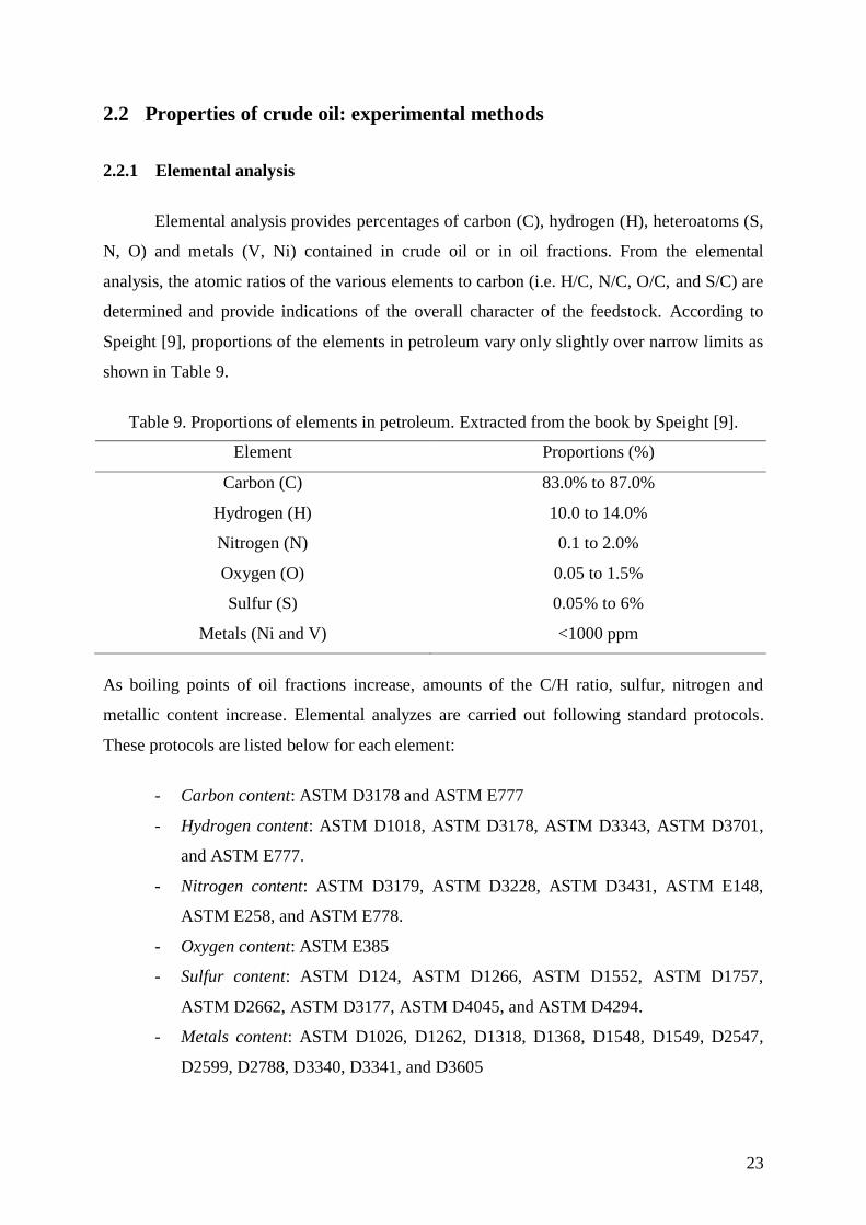
2.2.1 Elemental analysis

Elemental analysis provides percentages of carbon (C), hydrogen (H), heteroatoms (S,

N, O) and metals (V, Ni) contained in crude oil or in oil fractions. From the elemental

analysis, the atomic ratios of the various elements to carbon (i.e. H/C, N/C, O/C, and S/C) are

determined and provide indications of the overall character of the feedstock. According to

Speight [9], proportions of the elements in petroleum vary only slightly over narrow limits as

shown in Table 9.

Table 9. Proportions of elements in petroleum. Extracted from the book by Speight [9].

Element Proportions (%)

Carbon (C) 83.0% to 87.0%

Hydrogen (H) 10.0 to 14.0%

Nitrogen (N) 0.1 to 2.0%

Oxygen (O) 0.05 to 1.5%

Sulfur (S) 0.05% to 6%

Metals (Ni and V) <1000 ppm

As boiling points of oil fractions increase, amounts of the C/H ratio, sulfur, nitrogen and

metallic content increase. Elemental analyzes are carried out following standard protocols.

These protocols are listed below for each element:

- Carbon content: ASTM D3178 and ASTM E777

- Hydrogen content: ASTM D1018, ASTM D3178, ASTM D3343, ASTM D3701,

and ASTM E777.

- Nitrogen content: ASTM D3179, ASTM D3228, ASTM D3431, ASTM E148,

ASTM E258, and ASTM E778.

- Oxygen content: ASTM E385

- Sulfur content: ASTM D124, ASTM D1266, ASTM D1552, ASTM D1757,

ASTM D2662, ASTM D3177, ASTM D4045, and ASTM D4294.

- Metals content: ASTM D1026, D1262, D1318, D1368, D1548, D1549, D2547,

D2599, D2788, D3340, D3341, and D3605

24

2.2.2 Density and specific gravity

Density is defined as the mass of a fluid per unit of volume. It is a highly temperature-

dependent property, but effects of pressure are negligible. When the temperature increases,

the liquid density tends to decrease. By convention in the oil & gas industry, density is more

often expressed with the specific gravity or the API gravity. Specific gravity (SG) is a

dimensionless quantity which is defined as the ratio of density of a liquid to that of water. The

temperature at which specific gravity is reported should be specified as shown in equation (3).

𝑆𝐺(𝑇1 𝑇2⁄ ) =𝑑𝑒𝑛𝑠𝑖𝑡𝑦 𝑜𝑓𝑙𝑖𝑞𝑢𝑖𝑑 𝑎𝑡 𝑡𝑒𝑚𝑝𝑒𝑟𝑎𝑡𝑢𝑟𝑒 𝑇1𝑑𝑒𝑛𝑠𝑖𝑡𝑦 𝑜𝑓 𝑤𝑎𝑡𝑒𝑟 𝑎𝑡 𝑡𝑒𝑚𝑝𝑒𝑟𝑎𝑡𝑢𝑟𝑒 𝑇2

, (3)

where 𝑇1 is the temperature of the fluid studied and 𝑇2 is the temperature of water. The

standard conditions adopted by the petroleum industry are 15.5°C (60°F) and 1 atmosphere

for both fluids. At standard conditions, density of water is 0.999 g/cm3, therefore, the value of

specific gravity is closed to that of the density. In the International System of Units (SI),

temperature of water is set to 4°C which corresponds exactly to 1 g/cm3 and temperature of

hydrocarbon fluid is kept at 15.5°C. Since most of hydrocarbons found in reservoir fluids

have densities less than that of water, specific gravities of hydrocarbons are generally less

than 1. API gravity (degrees API) has been defined by The American Petroleum Institute

(API) following equation (4).

𝐴𝑃𝐼 𝑔𝑟𝑎𝑣𝑖𝑡𝑦 = 141.5

𝑆𝐺 (𝑎𝑡 𝑇1 = 𝑇2 = 15.5°𝐶)− 131.5 (4)

Liquid hydrocarbons with lower specific gravities have higher API gravity. The

specific gravity of petroleum usually ranges from about 0.8 (45.3 API gravity) for the lighter

crude oils to over 1.0 (less than 10 API gravity) for heavy crude oil and bitumen. Density

gives a rough estimation of the nature of petroleum. For example, aromatic oils are denser

than paraffinic oils [1].

Density, specific gravity and API gravity may be measured by means of a hydrometer

(ASTM D287, ASTM D1298, ASTM D1657, IP 160), a pycnometer (ASTM D70, ASTM

D941, ASTM D1217, ASTM D1480, and ASTM D1481) or by the displacement method

(ASTM D712), or by means of a digital density meter (ASTM D4052, IP 365) and a digital

density analyzer (ASTM D5002).

25

2.2.3 Molecular weight

Molecular weight (or mass molar) of a mixture is defined as the average of the molar

mass of each molecule contained in the fluid weighted by their molar fraction as show in

equation (5).

𝑀 =∑𝑥𝑖𝑀𝑖𝑖

(5)

where 𝑀 is the molecular weight of the mixture, and 𝑥𝑖 and 𝑀𝑖 are the mole fraction and

molecular weight of component 𝑖, respectively. For a pure compound, molecular weight is

determined from its chemical formula and the atomic weights of its elements. Since the exact

composition of crude oil and petroleum fractions are generally unknown, equation (5) cannot

be used to calculate the average molecular weight of these mixtures. Experimental methods

have been developed to determine the average molecular weight of mixtures based on

physical properties. The most widely used method is the cryoscopy method. This process

consists of measuring the lowering of the freezing point of a solvent when a known quantity

of sample (here the oil) is added. A second method widely used is the Vapor Pressure method.

It consists on measuring the difference between vapor pressure of sample and that of a known

reference solvent with a vapor pressure greater than that of the sample. This method is

described by the ASTM D2503 and is applicable to oils with an initial boiling point greater

than 220°C. In the case of heavy petroleum and heavy fractions, it is well known that

experimental measurement of molecular weight of the petroleum fluid is unreliable due to the

presence of asphaltene compounds. Asphaltenes tend to form aggregates whose size and

structure is influenced by temperature, solution concentration, and the nature of the solvent. In

this case, the size exclusion chromatography (SEC) described in the ASTM D5296 is more

suitable. A distribution of molecular weights is measured by comparing the elution time of a

sample with that of a reference solution.

2.2.4 Boiling temperature and distillation curves

Distillation techniques consist in separating the different constituents of a mixture

according to their boiling point. The boiling point may be presented by a curve of boiling

temperature versus volume fraction (vol %) or mass fraction (wt %). The boiling point of the

lightest component in a mixture is called Initial Boiling Point (IBP) and the boiling point of

26

the heaviest compound is called the Final Boiling Point (FBP). For crude oil, FBP is above

550°C, however, it can happen that some heavier compounds cannot vaporize. Therefore, the

FBP value measured is not accurate and does not correspond to the boiling of heaviest

compound present in the mixture. There are three main types of distillation curves: the

distillation D86 (ASTM D86), the True Boiling Point (ASTM D2892) and the Simulated

Distillation curve (ASTM D2887).

2.2.4.1 Distillation D86

Distillation D86 (ASTM D86) is one of the oldest and most common methods used to

determine the boiling range characteristics of crude oil. The distillation is conducted with 100

mL of sample and at atmospheric pressure. The temperature is measured for different

percentage of volume vaporized and collected of the sample (0, 5, 10, 20, 30, 40, 50, 60, 70,

80, 90, 95 and 100% volume). However, this method is limited to mixtures with boiling

points below 350°C. Indeed, the heavier molecules can break under effect of heat. In addition,

ASTM D86 distillation data do not represent actual boiling point of components in a

petroleum fraction [1].

2.2.4.2 True Boiling Point (TBP)

The TBP distillation (ASTM D2892) betters reflects the boiling point of compounds.

This technique is based on a column of 15 to 100 theoretical plates with a reflux ratio 5:1.

Distillation can be conducted under atmospheric pressure or under reduced pressure (down to

0.1 mbar). Similarly to the ASTM D86, the maximum operation temperature is around 350°C.

The main drawback of TBP distillation is that there is no standardized method. Distillation

curves are presented in terms of boiling point versus wt% or vol% of mixture vaporized.

2.2.4.3 Simulated Distillation by Gas Chromatography

A distillation curve produced by a Gas chromatography (GC) is called Simulated

Distillation (SD) and the method is described in ASTM D2887 test method. Simulated

Distillation method is known to be simple, consistent, and reproducible. This method is

applicable to petroleum fractions with a FBP up to 538°C (even 700°C) and a boiling range of

greater than 55°C. Samples are analyzed on a non-polar chromatographic column that

separates hydrocarbons according to their boiling points. Each component has a certain

retention time depending on the structure of compound, type of column and stationary phase,

27

flow rate of mobile phase, length, and temperature of column. The retention time is the

amount of time required for a given component to cross the column. More volatile

compounds with lower boiling points have lower retention times. Distillation curves by SD

are presented in terms of boiling point versus wt% of mixture vaporized. Note that SD curves

are very close to actual boiling points shown by TBP curves. But these two types of

distillation data are not identical and conversion methods should be used to convert SD to

TBP curves.

2.2.5 Chemical families

Hydrocarbons can be identified by their molecular type or chemical family. The most

important types of composition are given below:

- PONA (Paraffins, Olefins, Naphthenes, and Aromatics)

- PNA (Paraffins, Naphthenes, and Aromatics)

- PINA (n-Paraffins, iso-Paraffins, Naphthenes, and Aromatics)

- PIONA (n-Paraffins, iso-Paraffins, Olefins, Naphthenes, and Aromatics)

- SARA (Saturates, Aromatics, Resins and Asphaltenes)

PONA, PNA and PIONA analyzes are useful to characterize light fractions. SARA analysis is

more suitable for heavy fractions of petroleum due to high contents of aromatics, resins, and

asphaltenes.

2.2.5.1 Light fractions (PONA, PNA, PIONA)

Due to the low olefin content in crude oils, light fractions are often expressed in terms

of PINA. In addition, n-paraffins and iso-paraffins content can be combined and, thus, its

fraction can be simplified and expressed in terms of PNA composition. Chemical families in

light fractions are generally separated using instruments called PIONA analyzer or

Chrompack Model 940 PIONA analyzer.

2.2.5.2 Heavy fractions (SARA)

SARA analysis is based on a solvent separation approach; it means that components in

crude oil are divided according to their solubility in a particular solvent. Solubility of

compounds in solvents depends on their polarity. When two compounds have the same

28

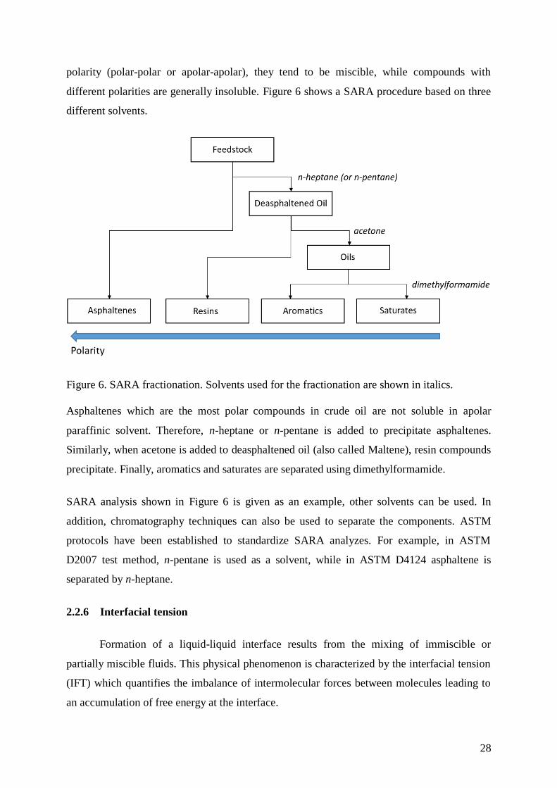
polarity (polar-polar or apolar-apolar), they tend to be miscible, while compounds with

different polarities are generally insoluble. Figure 6 shows a SARA procedure based on three

different solvents.

Figure 6. SARA fractionation. Solvents used for the fractionation are shown in italics.

Asphaltenes which are the most polar compounds in crude oil are not soluble in apolar

paraffinic solvent. Therefore, n-heptane or n-pentane is added to precipitate asphaltenes.

Similarly, when acetone is added to deasphaltened oil (also called Maltene), resin compounds

precipitate. Finally, aromatics and saturates are separated using dimethylformamide.

SARA analysis shown in Figure 6 is given as an example, other solvents can be used. In

addition, chromatography techniques can also be used to separate the components. ASTM

protocols have been established to standardize SARA analyzes. For example, in ASTM

D2007 test method, n-pentane is used as a solvent, while in ASTM D4124 asphaltene is

separated by n-heptane.

2.2.6 Interfacial tension

Formation of a liquid-liquid interface results from the mixing of immiscible or

partially miscible fluids. This physical phenomenon is characterized by the interfacial tension

(IFT) which quantifies the imbalance of intermolecular forces between molecules leading to

an accumulation of free energy at the interface.

29

Figure 7. Schematic representation of forces leading to an interfacial tension.

As shown in Figure 7, intermolecular interactions of molecules near to the interface are not

equal to those in bulk phases, leading to unequal forces acting upon the molecules in two

sides of the interface. IFT is defined as the work, 𝑑𝑊, which must be expended to increase

the size of the interface 𝐴 by 𝑑𝐴:

𝐼𝐹𝑇 =𝑑𝑊

𝑑𝐴 (6)

IFT can be expressed in term of force per unit length, N/m, or in term of energy per surface,

J/m2. Note that in the literature, the term surface tension is sometimes used instead of

interfacial tension. Generally, surface tension is used for a vapor-liquid interface while

interfacial tension is appropriate for a liquid-liquid interface.

Numerous experimental techniques have been developed in order to measure IFT

values. The choice of the method depends on the studied system, phases considered

(liquid/liquid, liquid/gas, solid/liquid, or gas/solid), and on the order of magnitude of the

expected interfacial tension value. To measure low values of IFT (less than 1 mN/m), the

spinning drop and the pendant drop methods are generally chosen while Du Noüy ring,

Wilhelmy plate, and Capillary rise methods are more suitable for higher values of IFT (a few

tens of mN/m).

30

2.3 State of the art for the representation of crude oil

In the literature, three main methodologies of molecular representation of a crude oil

and oil fractions can be distinguished: (1) fractionation approaches, (2) lumping approaches,

and (3) approaches based on the construction of model molecules. These methods are briefly

introduce hereafter.

2.3.1 Fractionation approaches

The principle of fractionation approaches is to divide a complex mixture into several

fractions. Then, a molecular representation of the fluid can be proposed by assigning a model

molecule to each fraction.

2.3.1.1 Fractionation by chemical group

Crude oil can be represented by the four main chemical groups based on polarity and

solubility differences (see section 2.2.5.2). The four fractions are saturates, aromatics, resins

and asphaltenes compounds, commonly denoted as SARA fractions. Then, a model molecule

can be assigned to each group. Model molecules must be selected or constructed on the basis

of experimental data. A special attention is given to the construction of asphaltene models

because it consists in large molecules with a complex molecular structure that may contain

several different structural elements (aromatic rings, naphthenic rings, alkyl chains) and also

heteroatoms (oxygen, nitrogen and sulfur) or metals (nickel or vanadium). Asphaltenes have

an important influence on properties of crude oils such as the oil/water interfacial tension [14–

18]. Different methods have been developed to build molecular structures for asphaltenes

based on a large number of experimental data [12, 13, 19–22]. According to Nguyen et al.

[23], fractional approach by chemical family is time-consuming, expensive and lacking

reproducibility.

2.3.1.2 Fractionation by boiling temperature

A mixture of representative compounds for petroleum fluids can be obtained using a

distillation curve such as a simulated distillation curve (ASTM D2887) or a True Boiling

Point (TBP) curve. As explained in the previous section, distillation curves represent the

temperature measured as a function of the mass or the volume fraction distilled. The

distillation curve is divided into several ranges of boiling points in order to obtain

31

non-overlapping temperature intervals. An example of the decomposition of a TBP distillation

curve into several temperature intervals is given in Figure 8. According to Eckert and

Vaněk [24], it is sufficient to use intervals about 15°C for normal boiling points up to

426.85°C (700 K), about 30°C within 426.85°C and 676.85°C (950 K) and about 50°C for

higher boiling mixtures. Then, a pseudo-component is assigned for each of these temperature

intervals. This procedure is called “breakdown”.

Figure 8. TBP distillation curve representing the boiling temperature (𝑇b) as a function of the

volume fraction (∅). Volume fraction intervals (∅𝑖) and boiling temperature (𝑇bi) for an

interval 𝑖 are determined using the breakdown approach. Extracted from the reference [24]. “Reprinted (adapted) with permission from Eckert, E.; Vaněk, T., Computers & Chemical

Engineering 2005, 30, 343–356. Copyright (2005), with permission from Elsevier”.

Pseudo-components are characterized by boiling temperature (𝑇b𝑖) and a volume fraction

interval (∅𝑖). The boiling temperature can be calculated by the integral mean value of the

fraction of the TBP curve that is covered by the pseudo-component (equation (7)), or by the

arithmetic mean value of the TBP temperature at the lower and upper boundary of the pseudo-

component (equation (8)).

𝑇b𝑖 =1

(𝛷𝑖𝑅 −𝛷𝑖

𝐿)∫ 𝑇b(𝛷)𝑑𝛷,𝛷𝑖𝑅

𝛷𝑖𝐿

𝑖 = 1,… 𝐼 (7)

𝑇b𝑖 =𝑇b(𝛷𝑖

𝑅) + 𝑇b(𝛷𝑖𝐿)

2, 𝑖 = 1, … 𝐼 (8)

32

where (𝛷𝑖𝑅 −𝛷𝑖

𝐿) is the interval of fraction distilled. Properties of each pseudo-component

can be calculated. Density can be obtained using the constant 𝐾𝑈𝑂𝑃 approach developed by

Watson [25]. Pseudo-formula (CxHyOz), molar weight (𝑀𝑤), critical temperature (𝑇𝐶), critical

pressure (𝑃𝐶), critical volume (𝑉𝐶) and an acentric factor (ω) can be calculated using the

equations of Twu [26] and Edmister [27].

A real component can be assigned to each pseudo-component if a suitable database of

hydrocarbon molecules is available. By comparing the properties of each pseudo-component

with those of molecules in the database, a model molecule is assigned. The molecule is

chosen so that the difference between properties of the molecule and those of the pseudo-

component is minimized. This method of representation is not adapted to the heavier fractions

of crude oil. On the one hand, distillation of heavy compounds is difficult because of breaking

effect under heat. On the other hand, there is no reliable database of heavy molecules from

crude oil, especially for asphaltenes whose chemical structure is still under debate.

2.3.2 Lumping methods

Lumping methods consist to grouping compounds or pseudo-components together

according to common or similar properties. Then, a representative compound is assigned to

each group. Lumping methods are intended to simplify the representation of a fluid with a

limited number of compounds. Generally, input data for lumping methods are:

- A database of possible compounds to mimic the fluid under consideration. For

crude oils, the exact composition is available only for the lightest fractions such as

gasoline. The identification of compounds requires accurate analyses of the fluid

using modern and efficient techniques such as chromatography [7, 28], two-

dimensional chromatography [28], spectroscopy [29, 30] or spectrometry [31, 32].

- A list of pseudo-components determined form a distillation curve using the

breakdown approach (see previous section).

The most common Lumping method for characterizing a petroleum mixture is the

MTHS (Molecular-Type Homologous Series) method introduced in 1999 by Peng and Zhang

[33, 34]. This lumping method allows to group molecules according to their chemical family

and their number of carbon atoms (𝑛𝐶). Other more complex methods rely on an algorithm.

For example, Montel and Gouel [35] have developed an algorithm named “Dynamic

33

clustering algorithm” to group components according to their physico-chemical and

thermodynamic properties (for example ω, 𝑀𝑤, 𝑛𝐶 , C/H ratio, 𝑇𝐶, 𝑃𝐶 and 𝑉𝐶). This algorithm

has been used in our work and will be presented in more details in Chapter V.

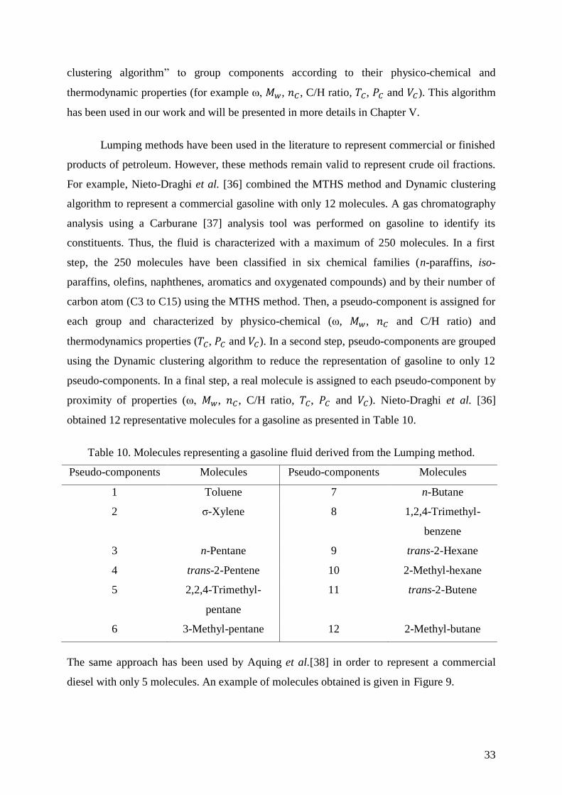
Lumping methods have been used in the literature to represent commercial or finished

products of petroleum. However, these methods remain valid to represent crude oil fractions.

For example, Nieto-Draghi et al. [36] combined the MTHS method and Dynamic clustering

algorithm to represent a commercial gasoline with only 12 molecules. A gas chromatography

analysis using a Carburane [37] analysis tool was performed on gasoline to identify its

constituents. Thus, the fluid is characterized with a maximum of 250 molecules. In a first

step, the 250 molecules have been classified in six chemical families (n-paraffins, iso-

paraffins, olefins, naphthenes, aromatics and oxygenated compounds) and by their number of

carbon atom (C3 to C15) using the MTHS method. Then, a pseudo-component is assigned for

each group and characterized by physico-chemical (ω, 𝑀𝑤, 𝑛𝐶 and C/H ratio) and

thermodynamics properties (𝑇𝐶, 𝑃𝐶 and 𝑉𝐶). In a second step, pseudo-components are grouped

using the Dynamic clustering algorithm to reduce the representation of gasoline to only 12

pseudo-components. In a final step, a real molecule is assigned to each pseudo-component by

proximity of properties (ω, 𝑀𝑤, 𝑛𝐶 , C/H ratio, 𝑇𝐶, 𝑃𝐶 and 𝑉𝐶). Nieto-Draghi et al. [36]

obtained 12 representative molecules for a gasoline as presented in Table 10.

Table 10. Molecules representing a gasoline fluid derived from the Lumping method.

Pseudo-components Molecules Pseudo-components Molecules

1 Toluene 7 n-Butane

2 σ-Xylene 8 1,2,4-Trimethyl-

benzene

3 n-Pentane 9 trans-2-Hexane

4 trans-2-Pentene 10 2-Methyl-hexane

5 2,2,4-Trimethyl-

pentane

11 trans-2-Butene

6 3-Methyl-pentane 12 2-Methyl-butane

The same approach has been used by Aquing et al.[38] in order to represent a commercial

diesel with only 5 molecules. An example of molecules obtained is given in Figure 9.

34

Figure 9. Set of five molecules representing a diesel obtained by a Lumping method.

Extracted from the reference [38]. “Reprinted (adapted) with permission from C.; Pina, A.;

Dartiguelongue, C.; Trusler, J. P. Martin; Vignais, R.; Lugo, R.; Ungerer, P. et al., Energy

Fuels 2012, 26, 2220–2230. Copyright (2012) American Chemical Society”.

The main difficulty for Lumping methods is to identify the most relevant criteria for

grouping the molecules. For example, gasoline is a hydrocarbon mixture with a low

heteroatoms content, it is possible to use thermodynamic properties (𝑇𝐶, 𝑃𝐶, 𝑉𝐶) to groups

compounds. However, for polar fluids with high heteroatom contents, these criteria are no

longer suitable because polarity and hydrogen bonds are not taken into account. Resins and

asphaltenes in heavy fractions are polar molecules; therefore, thermodynamic criteria may not

be the most appropriate.

2.3.3 Molecular reconstruction

Molecular reconstruction methods generate libraries of representative molecules of

crude oil fractions using only average or global data. Experimental data are usually derived

from analyzes commonly performed in the petroleum industry (elemental analyzes,

distillation curves, SARA analysis, etc.). Molecular reconstruction methods are particularly

appropriate to heavy petroleum fractions for which identification and quantification of the

compounds one by one is impossible because of: (i) large diversity of molecular structures

and (ii) the low volatility of these compounds.

Molecular reconstruction methods are based on the assumption that a complex mixture

with a large diversity of compounds can be represented with a limited number of structural

attributes. To our knowledge, the first works based on this hypothesis are those of Khorasheh

and al. [39, 40]. In 1986, they developed a technique called Structural Group Analysis (SGA)

which was applied to characterize the heavy fraction of Alberta heavy gas oils. They

35

established an inventory of all possible structural groups in the fluid and assigned them a

molar fraction.

Following the same principle, Klein and coworker [41–45] have developed, in the

1990s, a molecular reconstruction method for heavy fractions of crude oil including vacuum

residue and asphaltene fractions. This method, called Stochastic Reconstruction, refers to the

work of Boduszynski [13] who has shown that structural properties such as the number of

aromatic rings or the number of carbon atoms per molecule follow statistical distributions.

Thus, probability of finding a structural block in a molecule is a molecular attribute that

follows a distribution function. Then, the structural blocks can be assembled randomly with

each other via a Monte Carlo algorithm to form molecules.

Neurock et al. [41] have published a first Stochastic Reconstruction approach taking

place in several successive stages. This approach was applied to three different petroleum

feedstock fractions: an offshore California asphaltene, a Kern River heavy oil, and heavy gas

oil. To illustrate the method, its application will be explained using the asphaltenic fraction.

1) For each crude oil fraction, a specific structural hierarchy diagram must be

defined. This diagram defines the separation of molecules (for example PIONA or

SARA separation) and the structural attributes required to represent the fraction

considered. Moreover, this diagram serves to establish the assembly order of

structural attributes. An example of a structural hierarchy diagram for describing

an asphaltene fraction, proposed by Savage and Klein [46], is presented in Figure

10. In this model, the asphaltene molecules are of "archipelago" types (i.e. an

oligomer) and are described by six different structural attributes: (1) the number of

monomer units, (2) the number of aromatic rings per unit sheet, (3) the number of

naphthenic rings per monomer unit sheet (4) the degree of substitution of

peripheral aromatic carbons with aliphatic chains, (5) the degree of substitution of

peripheral naphthenic carbons with aliphatic chains and (6) the length of each

aliphatic chain. Each of these attributes is assigned a distribution probability

function that can be of several forms: gaussian, gamma, exponential, chi-square. In

the case of asphaltene, gaussian functions are used.

36

Figure 10. The structural hierarchy of asphaltene as suggested by Savage and Klein [46].

2) The second step is to parameterize the distribution probability functions from a

series of analyzes. For a Gaussian function, it is necessary to determine the

average value and the standard deviation. Asphaltene fraction has been

characterized by Neurock et al. [41] with an elemental analysis (C and H content),

VPO (average molecular weight) and 1H NMR analyzes (identification of each

proton). These data are used to calculate the average values of each structural

attribute by the methods of Speight (SP) [12] or Hirsch and Algekt (HA) [11].

Average values of each structural attribute obtained by Neurock et al. [41]

according to the two methods SP and HA are given in Table 11.

Table 11. Comparison of Speight (SP) and Hirsch-Altgelt (HA) methods for determining

average values of structural attributes for an asphaltene fraction. Extracted from the

reference [41]

Structural attributes SP HA

(1) Number of unit sheets (US) per molecule 2.85 4.60

(2) Number of aromatic rings per US 10.0 3.95

(3) Number of naphthenic rings per US 2.2 2.92

(4) Degree of substitution of peripheral aromatic carbons 7.30 7.30

(5) Degree of substitution of peripheral naphthenic carbons 26.9 26.89

(6) Length of aliphatic chains 13.2 13.17

37

The standard deviation of gaussian functions is determined by setting a minimum

and maximum value for each attribute and establishing that over 98% of each

attribute distribution fall between the minimum and maximum values of that

attribute reported in the literature.

3) The molecular representation of an asphaltene is generated via a Monte Carlo

algorithm. A stochastic sampling of each structural attribute is performed taking

into account its cumulative probability distribution and respecting the assembly

order fixed by structural hierarchy diagram. This step has, for example, been

repeated 10,000 times by Neurock and al. [41] to create a library of 10,000

asphaltene molecules.

Other research groups have used the Stochastic Reconstruction method. Sheremata et

al. [47, 48] have proposed a method to reduce the number of molecules necessary for the

representation of asphaltene fractions by selecting the most representative molecules. They

showed that a sample of only five or six asphaltenes is enough to obtain a representation in

good agreement with the analytical data. Verstraete and coworker have conducted several

works on Stochastic Reconstruction. They have been able to adapt the Stochastic

Reconstruction method for oil fractions from diesel to vacuum residues [49–55]. They also

proposed to combine the Stochastic Reconstruction method with the Reconstruction by

Entropy Maximization (REM), which significantly improved the concordance between data

calculated for a library of molecules with the analytical data of oil fractions. REM has been

used in our work and it will be described in more details in chapter V.

38

2.4 Conclusions

Crude oil and its fractions are complex mixtures composed of thousands of molecules

with a large diversity in molecular structures and in molecular sizes (see Chapter I). This

complexity makes the characterization of petroleum mixtures a difficult or an impossible task.

The detailed compositional data are not accessible except for the lightest fractions. In this

chapter, it has been shown that characterization of oil mixtures can be carried out by two

approaches: a global characterization or a characterization by fractions. The global

characterization consists in determining the average properties of petroleum mixtures such as

the elemental composition, the density or the average molecular weight. The characterization

by fractions allows to fractionate a mixture in different fractions. Fractions are determined

according to physicochemical properties such as the chemical family (PIONA, SARA, etc.) or

the boiling temperature of compounds (TBP, simulated distillation curves, etc.).

Although, the composition of crude oil and its fractions remains unknown, a molecular

representation can be obtained using available experimental data. In the literature, three main

approaches can be distinguished: (1) the fractionation approaches, (2) the lumping method

and (3) the molecular reconstruction. Fractionation approaches rely on fractional analytical

methods to determine the petroleum fractions, and then, to assign a representative molecule to

each fraction. Lumping method are used to provide a simplified representation of a mixture

using a limited number of representative compounds. This approach has been only used for

light fractions because it is based on experimental data that cannot be obtain for heavy

fractions (i.e. the detailed composition) or unreliable (D86 and TBP curves are unreliable for

heavy fractions due to cracking effects). For the heaviest fractions, reconstruction methods

seem to be better adapted. This method consists in building a library of molecules based on a

large number of experimental data.

In this work, we propose to combine existing approaches to establish a simplified

molecular representation of crude oil (see Figure 11). Crude oil is separated according to the

number of carbon atoms into two fractions: C20- and C20+. The light fraction C20-, contains

compounds having less than 20 carbon atoms while the heavy fraction, C20+, contains those

having more than 20 carbon atoms method. The Lumping method is used to represent the

light fraction. This approach has already used in the literature to represent light hydrocarbon

mixtures (gasoline [36] and diesel [38]) and it allows to limit the number of representative

39

compounds. The heavy fraction is built using the Stochastic Reconstruction method. Based on

a large number of experimental data, Stochastic Reconstruction seems to be the most suitable

approach for the representation of the most complex molecules contained in the heavy

fraction.

Figure 11. Proposed methodology to establish a simplified representation of a crude oil.

40

Chapter 3. Coarse-grained simulation methods

3.1 Introduction

Numerical methods allow to mimic experimental data or even to predict them when

they are not available. There are many reasons for using a simulation method to predict a

property instead of measuring it directly. In some cases, the cost and time of an experimental

measurement is too important or the measurement is difficult due to the experimental

conditions (high temperature and pressure for instance). In addition, by modeling a system at

the microscopic scale, simulation methods provide information allowing a better understating

on the phenomena that occurs. For example, in the case of a liquid-liquid system, the

composition or the orientations of the molecules at the interface are not easily accessible

experimentally due to its thickness, but molecular tools can provide these information.

Molecular simulation methods are based on statistical mechanics to estimate

macroscopic properties. At the microscopic level, a chemical system of 𝑁 particles can be

described by a set of microstates (noted Γ). Each microstate corresponds to a configuration

where each particle is characterized by its position (𝑟𝑖) and its momentum (𝑞𝑖). At the

macroscopic level, a system is thermodynamically described by several parameters such as

the pressure (𝑃), the temperature (𝑇) or the volume (𝑉). Statistical mechanics allows relating

the microscopic properties of individual particles to the macroscopic properties of a system.

The value of a macroscopic property (𝐴𝑚𝑎𝑐𝑟𝑜) is obtained by computing the average

value of this property calculated for a large number of microstates Γ. Accessible microstates

depend on the imposed constraints to the simulated system (𝑁,𝑉 and 𝑇 constant for instance)

defining the statistical ensemble. Molecular simulation methods aim at generating a large

number of microstates respecting the statistical ensemble. For dynamic simulations such as

Molecular Dynamic (MD), the time evolution of a system is followed by numerically

integrating the Newton’s equation of motion of its particles with time. The value of the

macroscopic property is the time average 𝐴(𝛤):

𝐴𝑚𝑎𝑐𝑟𝑜 = ⟨𝐴(𝛤)⟩𝑡𝑖𝑚𝑒 = lim𝑡→∞

1

𝑡∫ 𝐴(𝛤(𝑡))𝑑𝑡𝑡

0

(9)

41

Where 𝑡 is the time. In other words, it can be considered that for each time step (𝑑𝑡), a

microstate is generated and value of 𝐴(𝛤) is calculated.

For Monte Carlo simulations (MC), successive of configurations are generated

stochastically by elementary changes to the previous configuration. Then, the value of the

macroscopic property is calculated by averaging the value on microstates weighted by their

Boltzmann probability 𝑃𝑏𝑜𝑙𝑡𝑧(𝛤):

𝐴𝑚𝑎𝑐𝑟𝑜 = ⟨𝐴(𝛤)⟩𝑒𝑛𝑠 =∑𝐴(𝛤) × 𝑃𝑏𝑜𝑙𝑡𝑧(𝛤)𝛤

(10)

The Boltzmann probability can be written according to the following equation:

𝑃𝑏𝑜𝑙𝑡𝑧(𝛤) =𝑤𝑒𝑛𝑠(𝛤)

𝑄𝑒𝑛𝑠 (11)

where 𝑤𝑒𝑛𝑠(𝛤) is probability to observe a microstate and 𝑄𝑒𝑛𝑠 the partition function. MC

method is generally limited to computation of static properties since only the configurational

part of microstates is considered (momentum of particles is not taken into account) and time

is not an explicit variable.

In this work, both methods will be applied to our systems. The time evolution of

systems will be modeled using the Dissipative Particle Dynamics (DPD) technique and it will

be described in part 3.2. The stochastic approach will be used with Coarse-grained Monte

Carlo simulations and it will be presented in section 3.3. These simulation techniques are both

based on a coarse-grained model to represent the chemical system. The methodology to

represent a system with a coarse-grained model will be explained in section 3.4.

42

3.2 Dissipative particles dynamics (DPD)

Dissipative Particle Dynamics (DPD) was introduced for the first time in 1992 by

Hoogerbrugge and Koelman to model the hydrodynamic behavior of complex fluids at the

mesoscopic scale [56, 57]. In the DPD model, a chemical system is represented by spherical

particles of identical volume called “beads”. These beads are chosen and assembled following

a coarse-gained model that will be explained in more details in section 3.4.1. Beads interact

with pairwise, and time evolution is governed by Newton’s laws:

𝑑𝐫𝐢𝑑𝑡

= 𝐯𝐢, (12)

𝑚𝑖

𝑑𝐯𝐢𝑑𝑡

= 𝐟𝐢, (13)

Where 𝐫𝐢, 𝐯𝐢 and 𝐟𝐢 are the position, velocity, and force applied to the bead 𝑖, respectively.

Note that, in the DPD model used in this manuscript, all masses, (𝑚𝑖), are set to unity

(reduced unit) although other choices are possible. This assumption can be done only if one is

not interested in dynamical system properties. The total force exerted on a bead 𝑖 is defined as

the sum of the conservative (𝐅𝐢𝐣𝐂), dissipative (𝐅𝐢𝐣

𝐃) and random (𝐅𝐢𝐣𝐑) forces, as expressed in

equation (14) (Other forces can also be included, such as electrostatics). To simulate a

molecular skeleton, typically present in long hydrocarbons or amphiphilic molecules, an

intramolecular force (𝐅𝐢𝐣𝐢𝐧𝐭𝐫𝐚) is added to bind two neighboring beads:

𝐟𝐢 =∑(𝐅𝐢𝐣𝐂 + 𝐅𝐢𝐣

𝐃 + 𝐅𝐢𝐣𝐑 + 𝐅𝐢𝐣

𝐢𝐧𝐭𝐫𝐚)

𝑗≠𝑖

. (14)

3.2.1 Conservative force

In the DPD model, intermolecular interactions are represented by the conservative

force 𝐅𝐢𝐣𝐂. This force describes by a pairwise soft repulsive interactions:

𝐅𝐢𝐣𝐂 = 𝑎𝑖𝑗 (1 −

𝑟𝑖𝑗

𝑟𝑐) �̂�𝐢𝐣, (15)

where 𝑎𝑖𝑗 is the interaction parameter representing the maximum repulsive magnitude

between beads 𝑖 and 𝑗. 𝑟𝑐 is the cutoff radius and represents the maximum range of

43

interactions. The unit vector �̂�𝐢𝐣 pointing from the bead 𝑗 to the bead 𝑖 is defined by the

following expression �̂�ij = 𝐫𝐢𝐣/|𝒓𝒊𝒋| with 𝐫𝐢𝐣 = 𝒓𝑖 − 𝒓𝑗 and 𝑟𝑖𝑗 = |𝒓𝑖𝑗|.

Unlike Molecular Dynamics methods, interaction forces vary linearly with the distance

between the two beads (Variation of the conservative force, 𝐅𝐢𝐣𝐂, as a function of the distance,

𝑟𝑖𝑗, between beads i and j. 𝑟𝑐 is the cutoff radius and 𝑎𝑖𝑗 is the interaction parameter.. This

simplified description of interactions allows the use of larger time steps, typically of the order

of 5 × 10−12𝑠 [58].

Figure 12. Variation of the conservative force, 𝐅𝐢𝐣𝐂, as a function of the distance, 𝑟𝑖𝑗, between

beads i and j. 𝑟𝑐 is the cutoff radius and 𝑎𝑖𝑗 is the interaction parameter.

3.2.2 Intramolecular force

In order to simulated molecules made of several beads, intramolecular forces (𝐅𝐢𝐣𝐢𝐧𝐭𝐫𝐚)

are needed. To bind two beads together and to describe the variation of the distances between

them, 𝐅𝐢𝐣𝐢𝐧𝐭𝐫𝐚 generally expressed as an ideal spring:

𝐅𝐢𝐣𝐢𝐧𝐭𝐫𝐚 = −𝐾(𝑟𝑖𝑗 − 𝑟0)�̂�ij, (16)

where 𝐾 is the spring constant and 𝑟0 is the equilibrium spring distance. Note that spring

forces are conservatives.

An appropriate description of intramolecular forces is particularly important to simulate some

type of molecules such as surfactants. Indeed, these amphiphilic compounds must be

44

represented by at least two beads: one polar bead for the head and another nonpolar for the

tail. Goicochea et al. [59] and, more recently, Deguillard et al. [60, 61] have shown that

parameters of bond forces (𝐾 and 𝑟0) for surfactants may influence the values of

water/hydrocarbon interfacial tension.

More complex molecules represented by three beads or more may require additional

intramolecular forces to maintain their structural conformation. In this case, an angle potential

(𝑈𝑏𝑒𝑛𝑑) can be added to describe the interaction between three beads (equation (17)) and a

torsion potential (𝑈𝑡𝑜𝑟𝑠) can be used to represent the conformation between four beads

(equation (18)). Two types of torsion potentials are most commonly distinguished: torsional

rotation and improper torsion. The torsional rotation describes dihedral interactions between

four consecutively bonded beads and it can be used, for example, to constrain the rotation

around the central bond. The improper torsion depends on three beads centered around a

fourth atom and it is generally used to maintain planarity in a molecule.

𝑈𝑏𝑒𝑛𝑑 = 𝐾𝜃(𝜃𝑏𝑒𝑛𝑑 − 𝜃𝑏𝑒𝑛𝑑,0)2

(17)

where 𝐾𝜃 is the force constant for the bending, 𝜃𝑏𝑒𝑛𝑑 the bend angle and 𝜃𝑏𝑒𝑛𝑑,0 the

equilibrium angle.

𝑈𝑡𝑜𝑟𝑠 =∑𝑎𝑖(cos(𝜃𝑡𝑜𝑟𝑠))𝑖

𝑚

𝑖=0

(18)

where 𝑎𝑖 are the constants for the torsion potential, 𝜃𝑡𝑜𝑟𝑠 is the torsion angle and 𝑚 the order

of the function (set at 8 in this manuscript).

3.2.3 Dissipative and random forces

The dissipative force, (𝐅𝐢𝐣𝐃), can be interpreted as a frictional force representing

viscosity effects and is defined as:

𝐅𝐢𝐣𝐃 = −𝛾𝑖𝑗𝜔𝐷(𝑟𝑖𝑗)(�̂�𝐢𝐣 ∙ 𝐯𝐢𝐣)�̂�𝐢𝐣, (19)

45

where 𝜔𝐷(𝑟𝑖𝑗) is the dissipative weight function, 𝛾𝑖𝑗 the friction coefficient and 𝐯𝐢𝐣 the

velocity difference between bead 𝑖 and bead 𝑗, defined as follow: (𝐯𝐢𝐣 = 𝐯𝐢 − 𝐯𝐣). It means that

if a bead i moving apart from j, it feels a viscous force towards j. And if it moves towards j

the viscous force is in the opposite direction [62]. In a physical sense, the dissipative force

cools down the system.

To avoid the system freezing and keep the system in thermal motion, energy is injected

through the random force, 𝐅𝐢𝐣𝐑, as follows:

𝐅𝐢𝐣𝐑 = 𝜎𝑖𝑗𝜔𝑅(𝑟𝑖𝑗)𝜃𝑖𝑗�̂�𝐢𝐣, (20)

where 𝜔𝑅(𝑟𝑖𝑗) is the random weight function, 𝜎𝑖𝑗 is the random force amplitude for the beads

𝑖 and bead 𝑗, and 𝜃𝑖𝑗 is a random number with zero mean and unity variance when averaged

over time. The random force can be interpreted as resulting from a thermal energy. It means

that, this force represents the collisions between independent beads, or the vibration between

two bound beads of a molecule. In this manuscript, the random force amplitude (𝜎𝑖𝑗) and the

friction coefficient (𝛾𝑖𝑗) are independent of the type of beads.

3.2.4 Fluctuation-dissipation theorem

Español and Warren [62] have shown that, to ensure that the simulation obeys a

statistical ensemble (NVT), 𝐅𝐢𝐣𝐃 and 𝐅𝐢𝐣

𝐑 forces must be coupled together through a fluctuation-

dissipation relation. Authors derived the Fokker-Plank equation for the DPD model and they

deduced that the friction coefficient (𝛾) and the random force amplitude (𝜎), as well as the

weight functions 𝜔𝐷(𝑟𝑖𝑗) and 𝜔𝑅(𝑟𝑖𝑗) are related by equations (21) and (22).

𝜎2 = 2𝛾𝑘𝐵𝑇, (21)

𝜔𝐷(𝑟𝑖𝑗) = [𝜔𝑅(𝑟𝑖𝑗)]

2 = {(1 −

𝑟𝑖𝑗

𝑟𝑐), 𝑟𝑖𝑗 ≤ 𝑟𝑐

0, 𝑟𝑖𝑗 > 𝑟𝑐

(22)

where 𝑘𝐵 is the Boltzmann constant and 𝑇 the temperature. These conditions make that the

energy taken from the system is equal to the energy injected into the system. Thus, the

dissipative and random forces are dependent on each other and they ensure the temperature

equilibrium of the system (role of thermostat).

46

3.2.5 Time integration schemes

A time integration algorithm must be selected to integrate the equations of motion. In

the DPD model, a finite difference method is used and relies on knowledge of positions,

velocities and accelerations of each particle at a given time. In early works on DPD

simulations, particle positions and velocities were fixed in advance by the Euler algorithm

(equations (23))

{

𝐫i(𝑡 + ∆𝑡) = 𝐫i(𝑡) + ∆𝑡𝐯i(𝑡)

𝐯i(𝑡 + ∆𝑡) = 𝐯i(𝑡) + ∆𝑡𝐟𝐢(𝑡)

𝐟i(𝑡 + ∆𝑡) = 𝐟i(𝐫(𝑡 + ∆𝑡), 𝐯(𝑡 + ∆𝑡)) (23)

where fi is the total force applied to the i molecule. The Euler method is a simple numerical

procedure for solving differential equations, but it is limited to short time steps when position

(ri) and velocity (vi) do not change very much. In order to use higher time steps and to

improve the precision on calculated particle positions and velocities, Groot and Warren [63]

proposed a modified version of the velocity-Verlet algorithm (vV) as presented in the

following system of equations:

{

𝐫i

(𝑡 + ∆𝑡) = 𝐫i(𝑡) + ∆𝑡𝐯i(𝑡) +1

2(∆𝑡)2𝐟i(𝑡) (𝑠𝑡𝑒𝑝 1)

�̃�i(𝑡 + ∆𝑡) = 𝐯i(𝑡) + 𝜆∆𝑡𝐟i(𝑡) (𝑠𝑡𝑒𝑝 2)

𝐟i(𝑡 + ∆𝑡) = 𝐟𝑖(𝐫i(𝑡 + ∆𝑡), �̃�(𝑡 + ∆𝑡)) (𝑠𝑡𝑒𝑝 3)

𝐯i(𝑡 + ∆𝑡) = 𝐯i(𝑡) +1

2∆𝑡(𝐟i(𝑡) + 𝐟i(𝑡 + ∆𝑡)) (𝑠𝑡𝑒𝑝 4)

(24)

In the vV algorithm, an estimated value of the velocity �̃�(𝑡 + ∆𝑡) at the time (𝑡 + ∆𝑡) is used

to calculate the total force 𝐟i(𝑡 + ∆𝑡) at the same time. Then, the value of the velocity is

corrected in the fourth step. The force is altered at each iteration (after the second step). All

physical properties that depend on the position of particles are calculated after the second

step. Temperature is measured after the last step when the velocity is corrected. A factor 𝜆

(step 2) is added to account for additional effects of stochastic interactions [64]. It should be

noted that if the parameter 𝜆 is fixed at 𝜆 = 0.5, the numerical integration scheme is identical

to the original vV algorithm. But since the force is not independent of velocity, 𝜆 must be set

appropriately. Groot and Warren have shown that to obtain a reasonable compromise between

a rapid temperature equilibration, a suitable simulation time and a physically realistic system,

the time step can be fixed at ∆𝑡 = 0.04 in DPD unit, amplitude of the noise at 𝜎 = 3 when

𝜆 = 0.5. By adjusting the lambda value to 𝜆 = 0.65, it is possible to increase the time step to

47

∆𝑡 = 0.06 in DPD unit without a significant loss of temperature control (i.e. 𝑘𝐵𝑇 is constant

and equal to 1).

3.3 Coarse-grained-Monte Carlo simulation (CG-MC)

3.3.1 Principle and Metropolis algorithm

Monte Carlo methods are based on a random sampling of a set of configurations,

noted 𝛤𝑖 , of a molecular system. A large number of representative configurations are

generated in order to calculate the average properties of the system at equilibrium. In the

algorithm introduced by Metropolis et al. [65], sampling is not totally random but bias are

introduced to favor the most likely configurations. The probability of a configuration is

calculated from its Boltzmann probability, 𝑃𝐵𝑜𝑙𝑡𝑧(𝛤), and depends on the statistical ensemble

chosen for the simulations. Statistical ensembles used in this work for CG-MC simulations are

described in greater details in the next sections.

In the Metropolis algorithm, configurations are generated using a Markov chain. A Markov

chain must respect the condition of reversibility of a system. It means that the appearance rate

of a configuration 𝛤 must be equal to the disappearance rate of this configuration. Thus, the

transition rate, Π(𝛤 → 𝛤′), from a configuration 𝛤 to 𝛤′ is equal to the transition rate,

Π(𝛤′ → 𝛤), from a configuration 𝛤′ to 𝛤, as shown in the following expression:

Π(𝛤 → 𝛤′) = Π(𝛤′ → 𝛤) ∀ {𝛤, 𝛤′} (25)

The condition of microscopic reversibility can also be written using probabilities:

𝑃𝐵𝑜𝑙𝑡𝑧(𝛤) ∙ 𝑃𝑔𝑒𝑛(𝛤 → 𝛤′) ∙ 𝑃𝑎𝑐𝑐(𝛤 → 𝛤′) = 𝑃𝐵𝑜𝑙𝑡𝑧(𝛤′) ∙ 𝑃𝑔𝑒𝑛(𝛤′ → 𝛤) ∙ 𝑃𝑎𝑐𝑐(𝛤′ → 𝛤) (26)

where 𝑃𝐵𝑜𝑙𝑡𝑧(𝛤) is the Boltzmann probability to sample a configuration 𝛤, 𝑃𝑔𝑒𝑛(𝛤 → 𝛤′) is

the probability to generate a configuration 𝛤′ from a configuration 𝛤 and 𝑃𝑎𝑐𝑐(𝛤 → 𝛤′) is the

probability of acceptation of the configuration 𝛤′ from 𝛤.

Generation of a configuration 𝛤𝑖+1 depends only on the previous configuration 𝛤𝑖 . Each

transition from a configuration 𝛤𝑖 to the next configuration 𝛤𝑖+1 runs through three steps:

48

1) From a configuration 𝛤𝑖 , a configuration 𝛤 is generated randomly with a

probability 𝑃𝑔𝑒𝑛(𝛤𝑖 → 𝛤).

2) The probability of acceptation 𝑃𝑎𝑐𝑐(𝛤𝑖 → 𝛤) of configuration 𝛤 is calculated

(equation (29)).

3) The configuration is accepted with a probability 𝑃𝑎𝑐𝑐(𝛤𝑖 → 𝛤). When

configuration is accepted, then 𝛤𝑖+1 = 𝛤. Otherwise, the previous configuration

is retained, 𝛤𝑖+1 = 𝛤𝑖.

In the Metropolis algorithm, the probability of acceptation 𝑃𝑎𝑐𝑐(𝛤𝑖 → 𝛤) is expressed as

follow:

𝑃𝑎𝑐𝑐(𝛤𝑖 → 𝛤) = min (1,𝑃𝐵𝑜𝑙𝑡𝑧(𝛤) ∙ 𝑃𝑔𝑒𝑛(𝛤 → 𝛤𝑖)

𝑃𝐵𝑜𝑙𝑡𝑧(𝛤𝑖) ∙ 𝑃𝑔𝑒𝑛(𝛤𝑖 → 𝛤)) (27)

In classical Monte Carlo simulations, the configuration 𝛤𝑖 is generated completely randomly

from 𝛤 :

𝑃𝑔𝑒𝑛(𝛤𝑖 → 𝛤) = 𝑃𝑔𝑒𝑛(𝛤 → 𝛤𝑖) (28)

Thus, probability of acceptation, 𝑃𝑎𝑐𝑐(𝛤𝑖 → 𝛤), is written:

𝑃𝑎𝑐𝑐(𝛤𝑖 → 𝛤) = min (1,𝑃𝐵𝑜𝑙𝑡𝑧(𝛤)

𝑃𝐵𝑜𝑙𝑡𝑧(𝛤𝑖)) (29)

Probability of acceptation of the new configuration 𝑃𝑎𝑐𝑐 depends on the statistical ensemble in

which the simulation is performed. The statistical ensembles used in my thesis work are the

Gibbs ensemble (NVT) and the osmotic ensemble (µPT).

3.3.2 Statistical ensembles

3.3.2.1 Gibbs ensemble

The Gibbs ensemble (NVT) allows simulating two-phase equilibria using two

simulation boxes. There is no interface between the two boxes. In this ensemble, the total

number of beads 𝑁, the total volume 𝑉 of the system (considering the two boxes) and the

temperature 𝑇 are constant. Equality of the chemical potentials of the constituents in the two

phases is ensured by a transfer of molecules between simulation boxes. For a system that is

49

divided into two separate subsystems 𝑎 and 𝑏 with respective volumes 𝑉𝑎 and 𝑉𝑏 and

numbers of beads 𝑁𝑎 and 𝑁𝑏 so that 𝑉 = 𝑉𝑎 + 𝑉𝑏 and 𝑁 = 𝑁𝑎 +𝑁𝑏, the partition function

for the Gibbs ensemble (NVT) is given by:

𝑄𝑁𝑉𝑇𝐺𝑖𝑏𝑏𝑠 =

1

𝑁! ∧3𝑁 𝑉0∑

𝑁!

𝑁𝑎! 𝑁𝑏!∫ 𝑑𝑉𝑎𝑉

0

𝑁

𝑁𝑎=0

×∫ 𝑑𝑟1𝑎…𝑑𝑟𝑁𝑎

𝑎 𝑒−𝛽𝑈𝑎(𝑟1

𝑎,…,𝑟𝑁𝑎𝑎 )

𝑉𝑎∫ 𝑑𝑟1

𝑏…𝑑𝑟𝑁𝑏𝑏 𝑒

−𝛽𝑈𝑏(𝑟1𝑏,…,𝑟

𝑁𝑏𝑏 )

𝑉𝑏

(30)

where 𝛽 = 1𝑘𝐵𝑇⁄ , ∧ is the thermal de Broglie wavelength, 𝑉0 is a basic unit of volume

chosen to render the partition function dimensionless. (𝑟1𝑎, … , 𝑟𝑁𝑎

𝑎 ) and (𝑟1𝑏, … , 𝑟

𝑁𝑏𝑏 ) represent

positions of the N beads in subsystems 𝑎 and 𝑏. 𝑈𝑎 and 𝑈𝑏 are the energy of subsystems 𝑎

and 𝑏, respectively. After introducing the rescaled coordinates Ϛ = 𝑟/𝐿, where 𝐿 is the box

length of the simulated subsystem, the partition function of the total systems can be written

as:

𝑄𝑁𝑉𝑇𝐺𝑖𝑏𝑏𝑠 =

1

𝑁! ∧3𝑁 𝑉0∑

𝑁!

𝑁𝑎! 𝑁𝑏!∫ 𝑑𝑉𝑎(𝑉𝑎)𝑁

𝑎(𝑉𝑏)𝑁

𝑏𝑉

0

𝑁

𝑁𝑎=0

×∫ 𝑑Ϛ1𝑎…𝑑Ϛ𝑁𝑎

𝑎 𝑒−𝛽𝑈𝑎(Ϛ1

𝑎,…,Ϛ𝑁𝑎𝑎 )

𝑉𝑎∫ 𝑑Ϛ1

𝑏…𝑑Ϛ𝑁𝑏𝑏 𝑒

−𝛽𝑈𝑏(Ϛ1𝑏,…,Ϛ

𝑁𝑏𝑏 )

𝑉𝑏

(31)

And the Boltzmann probability in the Gibbs ensemble (NVT) is expressed as follow:

𝑃𝑁𝑉𝑇𝐺𝑖𝑏𝑏𝑠(𝛤) = exp [𝑙𝑛 (

𝑁!

𝑁𝑎! 𝑁𝑏!) + 𝑁𝑎𝑙𝑛𝑉𝑎 + 𝑁𝑏𝑙𝑛𝑉𝑏 − 𝛽𝑈𝑎(Ϛ1

𝑎, … , Ϛ𝑁𝑎𝑎 )

− 𝛽𝑈𝑏(Ϛ1𝑏, … , Ϛ

𝑁𝑏𝑏 )]

(32)

3.3.2.2 Osmotic ensemble

In the osmotic (µ𝑖𝑃𝑇) ensemble, the chemical potential µ𝑖 of the constituent 𝑖, the

pressure and the temperature 𝑇 are constant. This ensemble allows simulating a system with a

variable number of constituents 𝑖 and a variable volume. It can be considered that the system

is coupled with a reservoir of infinite size containing the constituents 𝑖 in which their

chemical potential µ𝑖 is fixed. The partition function in the osmotic ensemble can be written

as:

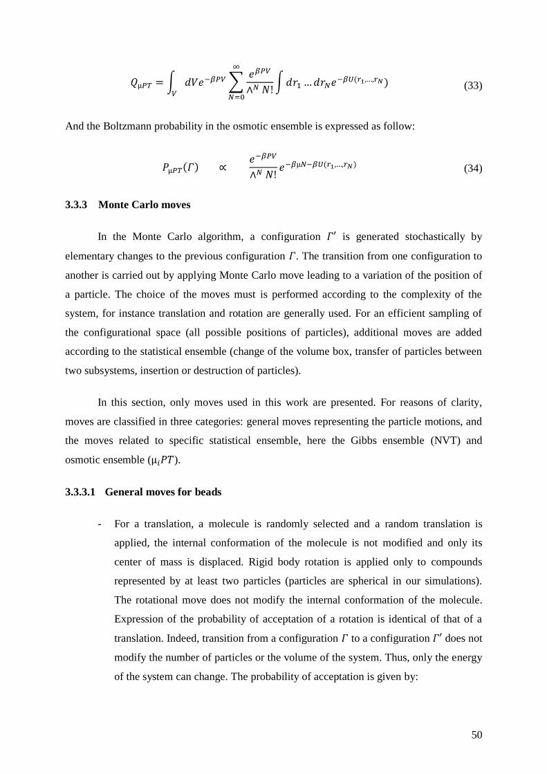
50

𝑄µ𝑃𝑇 = ∫ 𝑑𝑉𝑒−𝛽𝑃𝑉∑𝑒𝛽𝑃𝑉

∧𝑁 𝑁!

∞

𝑁=0𝑉

∫𝑑𝑟1…𝑑𝑟𝑁𝑒−𝛽𝑈(𝑟1,…,𝑟𝑁) (33)

And the Boltzmann probability in the osmotic ensemble is expressed as follow:

𝑃µ𝑃𝑇(𝛤) ∝ 𝑒−𝛽𝑃𝑉

∧𝑁 𝑁!𝑒−𝛽µ𝑁−𝛽𝑈(𝑟1,…,𝑟𝑁) (34)

3.3.3 Monte Carlo moves

In the Monte Carlo algorithm, a configuration 𝛤′ is generated stochastically by

elementary changes to the previous configuration 𝛤. The transition from one configuration to

another is carried out by applying Monte Carlo move leading to a variation of the position of

a particle. The choice of the moves must is performed according to the complexity of the

system, for instance translation and rotation are generally used. For an efficient sampling of

the configurational space (all possible positions of particles), additional moves are added

according to the statistical ensemble (change of the volume box, transfer of particles between

two subsystems, insertion or destruction of particles).

In this section, only moves used in this work are presented. For reasons of clarity,

moves are classified in three categories: general moves representing the particle motions, and

the moves related to specific statistical ensemble, here the Gibbs ensemble (NVT) and

osmotic ensemble (µ𝑖𝑃𝑇).

3.3.3.1 General moves for beads

- For a translation, a molecule is randomly selected and a random translation is

applied, the internal conformation of the molecule is not modified and only its

center of mass is displaced. Rigid body rotation is applied only to compounds

represented by at least two particles (particles are spherical in our simulations).

The rotational move does not modify the internal conformation of the molecule.

Expression of the probability of acceptation of a rotation is identical of that of a

translation. Indeed, transition from a configuration 𝛤 to a configuration 𝛤′ does not

modify the number of particles or the volume of the system. Thus, only the energy

of the system can change. The probability of acceptation is given by:

51

𝑃𝑎𝑐𝑐(𝛤 → 𝛤′) = min [1, exp (𝛽 ∙ exp(𝑈(𝛤) − 𝑈(𝛤′))] (35)

where 𝑈(𝛤) − 𝑈(𝛤′) represents the energy change due to the translation or the

rotation.

- Configurational regrowth: For the molecules represented by several beads linked

together by an intramolecular force, a move is added, reflecting the internal

relaxation of the molecule. This move consists of removing the molecule, and then

rebuilding it into the system. During the rebuilding phase, beads are reinserted one

after the other. The probability of acceptation is given by:

𝑃𝑎𝑐𝑐(𝛤 → 𝛤′) = min [1,𝑊(𝛤′)

𝑊(𝛤)] (36)

With

𝑊(𝛤′) =∏∑exp (−𝛽(𝑈𝑛(𝑞𝑗))

𝑘′

𝑗=1

𝑁

𝑛=1

(37)

where N is the number of beads of the molecule, 𝑘′ the number of positions in

which the bead 𝑛 can be inserted in the system, 𝑞𝑗 are the insertion positions and

𝑈𝑛 is the energy of the bead 𝑛 inserted at the position 𝑞𝑗. And

𝑊(𝛤) =∏[exp(−𝛽𝑈𝑛(𝛤)) + ∑ exp (−𝛽𝑈𝑛(𝑞𝑗′))

𝑘′−1

𝑗=1

]

𝑁

𝑛=1

(38)

where 𝑈𝑛(𝛤) is the energy before the insertion of the bead 𝑛 at the position 𝑞𝑗

(when 𝑛 = 1, 𝑈1(𝛤) is the initial energy of the system), 𝑘′ − 1 corresponds to the

number of positions around the bead 𝑛 − 1. And 𝑞𝑗′ are the positions around the

bead 𝑛 − 1 including the initial position of the bead 𝑛.

It can be noted that this move can be used for simulations in the Gibbs ensemble to

transfer a molecule between two phases.

52

3.3.3.2 Moves specific to the Gibbs ensemble

Two different moves are added specifically for the simulations in the Gibbs ensemble

(NVT):

- Transfer of beads between two boxes: One molecule is randomly selected in one

box and then transferred to the other box. This move is accepted with a

probability:

𝑃𝑎𝑐𝑐(𝛤 → 𝛤′) = min [1, exp (𝑙𝑛 (𝑁𝑖𝑑𝑉𝑎

(𝑁𝑖𝑎 + 1)𝑉𝑑

) − 𝛽(𝑈(𝛤) − 𝑈(𝛤′)))] (39)

where 𝑁𝑖𝑑 and 𝑁𝑖

𝑎 are the number of particles of the selected compound 𝑖 in the

donor (d) and acceptor (a) boxes, respectively, and 𝑉𝑎 and 𝑉𝑑 are volumes of

these two boxes.

- Concerted change of volume of each box at constant total volume: The volume of

box 𝐼 (𝑉𝐼) is increased by ∆𝑉 and the volume of box 𝐼𝐼 (𝑉𝐼𝐼) is decreased by the

same volume. This move is accepted with a probability:

𝑃𝑎𝑐𝑐(𝛤 → 𝛤′) = min [(1,𝑉𝐼 + ∆𝑉

𝑉𝐼×𝑉𝐼𝐼 − ∆𝑉

𝑉𝐼𝐼× exp(−𝛽(𝑈(𝛤) − 𝑈(𝛤′)))] (40)

This equation assumes that box I is the box whose volume increases.

3.3.3.3 Moves specific to the osmotic ensemble

Two different moves are added specifically for the simulations in the osmotic (µ𝑖𝑃𝑇):

- Change of volume: The volume of the simulation box changes from a volume 𝑉 to

𝑉′ = 𝑉 + ∆𝑉, ∆𝑉 is randomly chosen in the range [−∆𝑉𝑚𝑎𝑥, ∆𝑉𝑚𝑎𝑥]. This move is

accepted with a probability:

𝑃𝑎𝑐𝑐(𝛤 → 𝛤′) = min [1, (𝑉′

𝑉)𝑁

× exp(−𝛽(𝑈(𝛤′) − 𝑈(𝛤) + 𝑃(𝑉′ − 𝑉)))] (41)

When this move is used, coordinates of particles are rescaled to the new box

volume. Note that constraints can be added to control the volume change of the

53

box. In this work, simulations in the osmotic ensemble are performed considering

x and y sides of the simulation box fixed, thus, the volume of the box can change

only along the z-axis.

- Insertion/removal: Insertion and removal moves have the same probability of

occurring. These movements are applied to molecules whose chemical potential is

known and their number can vary during the simulation. In the case of insertion

move, a molecule is inserted at a random position in the simulation box. This move

is accepted with a probability:

𝑃𝑎𝑐𝑐(𝛤 → 𝛤′) = min [1,𝑉

Ʌ3(𝑁 + 1)∙ exp (−β(U(𝛤′) − U(𝛤) − µ)) ] (42)

In the case of a removal move, a molecule is chosen randomly in the simulation

box and is removed. This move is accepted with a probability:

𝑃𝑎𝑐𝑐(𝛤 → 𝛤′) = min [1,𝑁Ʌ3

𝑉∙ exp (−β(U(𝛤′) − U(𝛤) + µ)) ] (43)

3.4 Coarse-grained simulations

3.4.1 Coarse-grained model

DPD and CG-MC are both coarse-grained (CG) simulation methods as atoms or

molecules are grouped in a particle called in this document “bead”. By decreasing the number

of degrees of freedom of the system, coarse-grained methods allow to simulate larger systems

as compared to classical “all-atoms” simulations such as Molecular Dynamic or molecular

Monte Carlo methods. An example of a coarse-grained representation is shown in Figure 13.

54

Figure 13. Schematic representation of a coarse-grained model applied to a molecule of

dodecyldimethylamine oxide (DDAO). Bead C (in yellow) and bead N (in red) are connected

to each other by a harmonic spring. Water bead W (in blue) consists of three water molecules.

Extracted from the work of Ryjkina et al. [66]. “Reprinted (adapted) with permission from

Ryjkina, E.; Kuhn, H.; Rehage, H.; Müller, F.; Peggau, J., Angew. Chem. Int. Ed., 2002, 983–

986. Copyright (2002)”.

CG model should reproduce the physical structure of the original molecules as

accurately as possible, and also its physicochemical properties. For example, as proposed in

Figure 13, the polar head and the nonpolar tail of the surfactant (DDAO) are represented with

different beads.

One of the important steps in building a coarse-grained model for a molecular system

is the choice of the degree of coarse-graining, noted 𝑁𝑚. For a system containing water

molecules, the degree of coarse-graining is generally given by the number of water molecules

in a bead. The degree of coarse-graining has a direct impact on the accessible chemical details

and to model precisely the phenomena of interest. A low degree of coarse-graining allows

studying phenomena that occur at small scale while a higher degree of coarse-graining gives

access to simulations over large scales of space and time. In addition, the DPD model used in

this work implies that all beads have the same volume. This means that the number of

molecules or atoms grouped in a bead must be based on a criterion such as the mass or the

molar volume. Generally, it is the molar volume that is chosen as criterion.

3.4.2 Simulations boxes and boundary conditions

DPD and CG-MC simulations are carried out in orthorhombic simulation box for

which boundary conditions are added. Two types of boundary conditions can be imposed:

- The walls of the simulation box are impassable and beads are forced to remain in

the space initially defined.

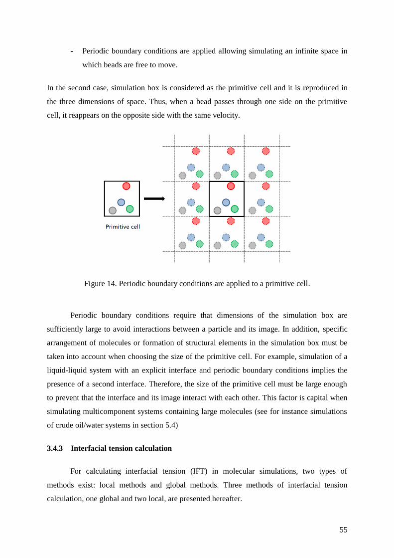
55

- Periodic boundary conditions are applied allowing simulating an infinite space in

which beads are free to move.

In the second case, simulation box is considered as the primitive cell and it is reproduced in

the three dimensions of space. Thus, when a bead passes through one side on the primitive

cell, it reappears on the opposite side with the same velocity.

Figure 14. Periodic boundary conditions are applied to a primitive cell.

Periodic boundary conditions require that dimensions of the simulation box are

sufficiently large to avoid interactions between a particle and its image. In addition, specific

arrangement of molecules or formation of structural elements in the simulation box must be

taken into account when choosing the size of the primitive cell. For example, simulation of a

liquid-liquid system with an explicit interface and periodic boundary conditions implies the

presence of a second interface. Therefore, the size of the primitive cell must be large enough

to prevent that the interface and its image interact with each other. This factor is capital when

simulating multicomponent systems containing large molecules (see for instance simulations

of crude oil/water systems in section 5.4)

3.4.3 Interfacial tension calculation

For calculating interfacial tension (IFT) in molecular simulations, two types of

methods exist: local methods and global methods. Three methods of interfacial tension

calculation, one global and two local, are presented hereafter.

56

3.4.3.1 Global methods

The general expression of the global method developed by Kirkwood-Buff [67] is

given by equation (44).

𝐼𝐹𝑇𝐾𝐵 =1

2⟨𝑃𝑁 − 𝑃𝑇⟩𝐿𝑧 (44)

Where 𝑃𝑁 and 𝑃𝑇 are the normal and tangential pressures in the simulation box and 𝐿𝑧 is the

length of the simulation box in the 𝑧 direction and the factor of 1

2 accounts for two existing

interfaces in the simulation box. 𝑃𝑁 is noted 𝑃𝑧𝑧 and 𝑃𝑇 is given by 1

2(𝑝𝑥𝑥 + 𝑝𝑦𝑦) and they are

expressed using the virial theorem which is the expression of the pressure as a function of the

derivatives of the inter-molecular potential.

𝑝𝛼𝛽 = 𝜌𝑘𝐵𝑇I +1

𝑉⟨ ∑ ∑(𝐫𝑖𝑗)𝛼

𝑁𝑡𝑜𝑡

𝑗>1

𝑁𝑡𝑜𝑡−1

𝑖=1

(Fij)𝛽⟩ (45)

where 𝛼 and 𝛽 are Cartesian coordinates 𝑥, 𝑦 and 𝑧, 𝜌 the density of the system, I the unit

tensor, 𝑉 the volume of the simulation box, 𝑁𝑡𝑜𝑡 is the total number of particles, 𝐫𝑖𝑗 is the

vector between particles of molecules 𝑖 and 𝑗 and Fij the intermolecular force between the

molecules 𝑖 and 𝑗. The latter can be expressed:

Fij =∑∑(𝐟𝑖𝑎𝑗𝑏)

𝑁𝑗

𝑏=1

𝑁𝑖

𝑎=1

= −∑∑r𝑖𝑎𝑗𝑏

𝑟𝑖𝑎𝑗𝑏

𝑛𝑗

𝑏=1

𝑑𝒰(𝑟𝑖𝑎𝑗𝑏)

𝑑𝑟𝑖𝑎𝑗𝑏

𝑛𝑖

𝑎=1

(46)

where 𝐟𝑖𝑎𝑗𝑏 is the interaction force between the particle 𝑎 of the molecule 𝑖 and the particle 𝑏

of the molecule 𝑗, 𝑁𝑖 and 𝑁𝑗 are the number of particles constituting of molecules 𝑖 and 𝑗 and

𝒰(𝑟𝑖𝑎𝑗𝑏) is the conservative potential between the particle 𝑎 of the molecule 𝑖 and the particle

𝑏 of the molecule 𝑗.

57

3.4.3.2 Local methods

For local methods, the value of the IFT is obtained by integrating the difference

between normal, 𝑃𝑁(𝑧), and tangential, 𝑃𝑇(𝑧), pressures across the z-direction as shown in

equation (47).

𝐼𝐹𝑇 =1

2∫ (𝑃𝑁(𝑧) − 𝑃𝑇(𝑧))𝑑𝑧𝐿𝑧

0

, (47)

where 𝐿𝑧 is the length of the simulation box in the 𝑧 direction and the factor of 1

2 accounts for

two existing interfaces in the simulation box. Local methods are based on a division into

layers, in the direction parallel to the interfaces, of the simulation box (see Figure 15).

Considering that interfaces are perpendicular to the z-direction, the simulation box is divided

into 𝑁𝑧 layers each having a thickness of 𝛿𝑧 =𝐿𝑧

𝑁𝑧.

Figure 15. Division of a simulation box in 𝑁𝑧 layers of thickness 𝛿𝑧. Particles 𝑖 and 𝑗, located

in the layers 𝑘𝑖 and 𝑘𝑗 respectively, are represented by blue circles. The path chosen by Irving

and Kirkwood is designated by the term 𝐶𝑖𝑗𝐼𝐾 and the arrow in full line, and that of Harasima

method by the term 𝐶𝑖𝑗𝐻𝐴 and the arrow in dashed line. Extracted and adapted from the

reference [60]

Expression for the local pressure,𝑃𝑁(𝑧) and 𝑃𝑇(𝑧), involves an integral along an arbitrarily

chosen contour [68]. However, different contours lead to different expressions of the pressure

tensor. Irving and Kirkwood [69] have proposed a straight line between particles 𝑖 and 𝑗,

while Harasima [70] used another path which consists of following the direction parallel to

58

the interface from the particle 𝑖 and, then, the direction perpendicular to the interface to the

particle 𝑗. These two paths are shown in Figure 15.

Expression of 𝑃𝑁(𝑧) and 𝑃𝑇(𝑧) according to the Irving and Kirkwood method [69] are

given in equation (48) and (49), respectively.

𝑃𝑁(𝑧𝑘) = ⟨𝑘𝐵𝑇𝜌(𝑧𝑘)⟩

+1

2𝐴( ∑ ∑ ∑∑(𝑟𝑧𝑖𝑗𝑟𝑧𝑖𝑎𝑗𝑏)

1

|𝑧𝑖𝑗|

𝑁𝑗

𝑏=1

𝑁𝑖

𝑎=1

𝑑𝒰(𝑟𝑖𝑎𝑗𝑏)

𝑑𝑟𝑖𝑎𝑗𝑏

𝑁𝑡𝑜𝑡

𝑗=𝑖+1

𝜃 (𝑧𝑘 − 𝑧𝑖𝑧𝑖𝑗

)

𝑁𝑡𝑜𝑡−1

𝑖=1

𝜃 (𝑧𝑗 − 𝑧𝑘

𝑧𝑖𝑗))

(48)

𝑃𝑇(𝑧𝑘) = ⟨𝑘𝐵𝑇𝜌(𝑧𝑘)⟩

+1

4𝐴( ∑ ∑ ∑∑(𝑟𝑥𝑖𝑗𝑟𝑥𝑖𝑎𝑗𝑏 + 𝑟𝑦𝑖𝑗𝑟𝑦𝑖𝑎𝑗𝑏)

1

|𝑧𝑖𝑗|

𝑁𝑗

𝑏=1

𝑁𝑖

𝑎=1

𝑑𝒰(𝑟𝑖𝑎𝑗𝑏)

𝑑𝑟𝑖𝑎𝑗𝑏

𝑁𝑡𝑜𝑡

𝑗=𝑖+1

𝜃 (𝑧𝑘 − 𝑧𝑖𝑧𝑖𝑗

)

𝑁𝑡𝑜𝑡−1

𝑖=1

𝜃 (𝑧𝑗 − 𝑧𝑘

𝑧𝑖𝑗))

(49)

Where 𝑧𝑘 is the average position of each layer of the simulation box along the z-direction,

𝜌(𝑧𝑘) the local particle density of the layer located at 𝑧 = 𝑧𝑘, 𝐴 the interface area (𝐴 =

𝐿𝑥𝐿𝑦), 𝑁𝑡𝑜𝑡 is the total number of particles, 𝑁𝑖 the number of particles constituting the

molecule 𝑖, 𝑁𝑗 the number of particles constituting the molecule 𝑗, 𝑎 is the 𝑎𝑡ℎ particle in the

molecule 𝑖, 𝑏 is the 𝑏𝑡ℎ particle in the molecule 𝑗, and 𝜃(𝑧) the Heaviside step function.

And expression of 𝑃𝑁(𝑧) and 𝑃𝑇(𝑧) according to Harasima method [70] are given in equation

(50) and (51), respectively.

𝑃𝑁(𝑧𝑘) = ⟨𝑘𝐵𝑇𝜌(𝑧𝑘)⟩ +1

2𝐴(∑ ∑ ∑∑(𝑟𝑧𝑖𝑗𝑟𝑧𝑖𝑎𝑗𝑏)

𝑁𝑗

𝑏=1

𝑁𝑖

𝑎=1

1

|𝑧𝑖𝑗|

𝑑𝒰(𝑟𝑖𝑎𝑗𝑏)

𝑑𝑟𝑖𝑎𝑗𝑏

𝑁

𝑗=𝑖+1

𝑁−1

𝑖=1

) (50)

𝑃𝑇(𝑧𝑘) = ⟨𝑘𝐵𝑇𝜌(𝑧𝑘)⟩ +1

4𝐴(∑ ∑ ∑∑(𝑟𝑥𝑖𝑗𝑟𝑥𝑖𝑎𝑗𝑏 + 𝑟𝑦𝑖𝑗𝑟𝑦𝑖𝑎𝑗𝑏)

1

|𝑧𝑖𝑗|

𝑁𝑗

𝑏=1

𝑁𝑖

𝑎=1

𝑑𝒰(𝑟𝑖𝑎𝑗𝑏)

𝑑𝑟𝑖𝑎𝑗𝑏

𝑁

𝑗=𝑖+1

𝑁−1

𝑖=1

) (51)

59

3.4.4 Coarse-grained units

Simulations based on a coarse-grained model are performed using reduced units. The

reference variables are the mass which is fixed at �̅� = 1 for all beads, the cutoff radius which

is equal to �̅�𝑐 = 1 and the energy which is fixed such that 𝑘𝐵𝑇 = 1. In this document, all

variables expressed in reduced units are indicated by an upper bar (�̅�). Then, the other

variables can be converted in the international system (SI) from the references. A table that

summarizes the conversion between the reduced units and the units in the international system

for thermodynamic and physicochemical properties is given in Table 12.

Table 12. Conversion between the reduced units and the units of the international system.

Variable/property Symbol Conversion Comments

Energy 𝐸 �̅� = 𝐸 𝐸𝑟𝑒𝑓⁄ 𝐸𝑟𝑒𝑓 = 𝑘𝐵𝑇 in J

Mass 𝑚 �̅� = 𝑚 𝑀𝑟𝑒𝑓⁄ and �̅� = 1 𝑀𝑟𝑒𝑓 is the base unit

for the mass (in kg)

Distance 𝑅 �̅� = 𝑟 𝑅𝑟𝑒𝑓⁄ and �̅�𝑐 =𝑟𝑐𝑅𝑟𝑒𝑓⁄

𝑅𝑟𝑒𝑓 is the base unit

for the distance (in

m). The cutoff 𝑟𝑐 is

traditionally equal to

𝑅, so �̅�𝑐 = 1

Time 𝑡 𝑡̅ = 𝑡√𝑘𝐵𝑇

𝑀𝑟𝑒𝑓𝑟𝑐2 𝑡 in s

Pressure 𝑃 �̅� = 𝑝 (𝑟𝑐3

𝑘𝐵𝑇) 𝑝 in Pa

Density 𝜌 �̅� = 𝜌𝑟𝑐3 𝜌 in beads/Å3

Interaction parameter 𝑎𝑖𝑗 �̅�𝑖𝑗 = 𝑎𝑖𝑗 (𝑟𝑐𝑘𝐵𝑇

) 𝑎𝑖𝑗 in N

Interfacial tension 𝐼𝐹𝑇 𝐼𝐹𝑇̅̅ ̅̅ ̅ = 𝐼𝐹𝑇 (𝑟𝑐2

𝑘𝐵𝑇) 𝐼𝐹𝑇 in N/m

Hildebrand solubility

parameter 𝛿 𝛿̅ = 𝛿 (

𝑟𝑐3

𝑘𝐵𝑇)

12⁄

𝛿 in (J/cm3)1/2

Isothermal

compressibility 𝜅−1 𝜅−1 =

1

�̅�=1

𝜅𝑇(

1

𝜌 ∙ 𝑘𝐵𝑇) 𝜅𝑇 in Pa-1

60

3.5 Conclusions

In this chapter, two molecular simulation techniques based on a coarse-grained model

were presented: the Dissipative Particle Dynamics (DPD) and Coarse-Grained Monte Carlo

(CG-MC) methods. In the coarse-grained model, the molecular representation is simplified

using beads. These beads are not the atoms but correspond to groups of atoms or molecules.

Therefore, coarse-grained model allows simulating very large systems such as crude oil over

long simulation times.

Both simulation techniques are based on the statistical mechanics. DPD relies on the

temporal evolution of a mesoscopic system while MC is based on a stochastic approach where

mesoscopic states are generated randomly. These two approaches allow, using mesoscopic

states, to compute macroscopic data. The choice of the simulation technique depends on the

data that must be predicted (for example IFT, bulk concentrations or adsorption).

Monte Carlo simulations can be used to simulate systems using statistical ensemble

that are not available for DPD. For example, the Gibbs ensemble (NVT) allows to model

liquid-liquid phase equilibrium without the presence of an interface. These simulations are

very useful for representing the properties or phenomena taking place in the bulk phases. The

osmotic ensemble (µ𝑖𝑃𝑇) allows simulating systems where the chemical potential of

molecules is held constant during the simulation. This ensemble can be used, for example, to

study the adsorption of molecules towards an interface and by maintaining a constant

concentration in bulk phases.

One of the key point to represent realistic systems in a simulation method is to

parameterize the interactions. The behavior of the molecules is governed by the interactions

between the beads. For example, the non-miscibility between water and oil results from

unfavorable interactions between the two fluids. Therefore, interactions must be

parameterized to reproduce properties of the system. In this work, simulations will be

parameterized to reproduce the interfacial tension and the liquid-liquid equilibrium between

two fluids (water and oil).

61

Chapter 4. Parameterization of liquid-liquid ternary

mixtures

4.1 Introduction

In this chapter, liquid-liquid equilibria of ternary systems are simulated using the

Dissipative Particle Dynamics (DPD) and Coarse-grained Monte Carlo (CG-MC) simulations.

This work is carried out in order to determine a parameterization method allowing to predict

quantitative values of interfacial tension and to reproduce compositions of liquid-liquid

equilibria. This methodology will be then used in the next chapter to model more complex

hydrocarbon mixtures such as crude oil.

Interfacial tension (IFT) of water/oil mixtures has already been intensively studied

with atomistic scale simulation methods such as Molecular Dynamics (MD) [71–75] and

Monte Carlo (MC) [76, 77]. Many works have shown that atomistic simulation methods

provide reasonable values of IFT for binary systems when compared to experiments [71, 72,

75]. Furthermore, additional information that is difficult to access experimentally can be

extracted from simulations such as interface thickness, position and orientation of molecules

at interfaces, and molecular compositions. However, calculations of IFT values in agreement

with experimental data required a reliable model of intra- and inter-molecular interactions. A

recent study conducted by Papavasileiou et al. [74] have shown that IFT values calculated

from atomistic simulations are very sensitive to the chosen molecular model. They studied

IFT temperature dependence in the range from 383.15 K to 443.15 K at 1.83 MPa for

water/oil systems using different atomistic force fields that have been primarily developed for

biomolecules. They studied binary mixtures (water/toluene and water/n-dodecane) and a

ternary system (water/toluene/n-dodecane) where the organic phase is described with the

General AMBER Force Field (GAFF) and the Lipid14 force field for toluene and n-dodecane,

respectively. Water molecules were modeled with three force fields: TIP4P/2005, TIP3P and

SPC/E models. They showed that, TIP4P/2005 and SPC/E are responsible for an

overestimation of IFT while TIP3P model leads to slightly underestimated IFT values. In

addition, they also proposed to model water/hydrocarbon interactions with modified Lorentz-

Berthelot combining rules by introducing a correction term, 𝑘𝑖𝑗, fitted on experimental data.

They showed that this correction term improves the accuracy of the IFT predictions using all

62

water models for binary systems. However, they were not able to provide accurate

reproduction of experimental IFT values for the ternary system. Recently, Ghoufi et al. [78]

have presented a review about molecular simulations in which different methodological

factors (size-effects, truncation procedures, long-range corrections, and potential models)

were analyzed to bring out their effects on interfacial systems and IFT values.

Atomistic scale simulation methods have been used many times to represent systems

that are more complex than binary or ternary water/hydrocarbon mixtures, such as crude oil

fractions [36, 38, 79–83]. For example, systems including asphaltene compounds that have

very complex molecular structures have been modeled in order to study the nature of

interactions and to calculate the interaction energies of asphaltene/asphaltene systems [79–

83]. However, representation at the atomistic scale of a liquid-liquid system containing an

explicit interface and bulk phases requires a large length scale and, therefore, a high

computational cost. Furthermore, time scales accessible to atomistic simulations are too short

to observe phenomena that are often studied in liquid-liquid systems, such as the formation of

micelles or micelle reorganization and their diffusion to the interfaces when surfactant

molecules are added [84, 85].

In the case of large and complex systems, the numerical study of interfaces requires

the use of mesoscopic simulation techniques based on a coarse-grained model (CG). CG

model consists of grouping atoms or molecules into particles in order to reduce the number of

degrees of freedom of the system and, therefore, the computational time. Several works in the

literature deal with liquid-liquid interfaces using the MARTINI force field [73, 86]. This force

field is based mainly on a four-to-one mapping, meaning that four heavy atoms plus

associated hydrogen atoms are grouped into a single particle. In the case of water, four water

molecules are grouped into a particle. Alternatively to the MARTINI model, DPD seems to be

a promising molecular simulation method. In DPD simulations, the coarse-grained model can

be easily adapted according to the phenomena studied. For example, the study of interactions

between asphaltenes [87] or the orientation [88] of these molecules at interfaces requires

small coarse-grained levels (i.e. water particle corresponds to three water molecules) while

emulsion phenomena [89, 90] are simulated using large coarse-grained levels (i.e. a water

particle corresponds to at least to 18 water molecules).

Although the CG model decreases the level of details on the molecular structure

compared to the atomistic model, CG simulations have already been used to predict

63

quantitative values of IFT for binary mixtures [73, 86, 91–93]. It has been shown that

MARTINI model allows a prediction of the IFT within ±10 mN/m with respect to

experiments for organic-water systems such as alkanes/water, benzene/water or

chloroform/water[86]. However, additional calibration of the parameters on the basis of

liquid-liquid properties seems necessary for more quantitative results [73]. Using DPD

simulations, Goel et al. [92] have estimated the interfacial tension for a large number of

immiscible and partially miscible systems. The percentage of error obtained on the value of

IFT is usually a few percent (<10%). Following the same methodology, Rezaei and

Modarress [91] have shown that DPD simulations can be used to study the temperature

dependence of IFT of water/hydrocarbon systems in the range from 298.15 to 348.15 K at 0.1

MPa. More complex interfacial systems such as water/surfactant/hydrocarbon systems have

already been modeled using DPD simulations. For example, Rekvig et al. [84, 94] compared

different surfactant structures and their ability to reduce the IFT between oil and water. Shi et

al. [95] studied the properties of the water/benzene/caprolactam system in the absence or

presence of nonionic surfactant. They investigated the surfactant efficiency at different

surfactant tail lengths and at different volume fractions of caprolactam.

However, the representation of multiconstituent systems within molecular simulations

remains a difficult task. Indeed, IFT values calculated with molecular simulations can be

compared with experimental data only if compositions of bulk phases are well reproduced in

the simulation boxes. Typically, when a solute is partially miscible in the two bulk phases of a

liquid-liquid equilibrium, the partition coefficient of this compound must be perfectly

reproduced, thus, the calculated value of IFT can be compared to the experimental value for a

given concentration of solute. Therefore, parameterization of CG simulations for

multiconstituent systems requires that chemical interactions must be precisely described to

model forces governing the IFT and to take into account solubility and miscibility of chemical

species. To the best of our knowledge, a reliable method that fulfills these requirements is not

available in the literature.

The key point of this chapter is to develop a parameterization strategy for DPD

simulations involving multiconstituent systems including partially miscible solutes and

providing quantitative predictions of the interfacial tension. We propose four parameterization

approaches to reproduce ternary liquid-liquid systems. These approaches are compared with

each other feeding DPD simulations to reproduce miscibility, IFT and to investigate

64

interfacial composition. The chapter is organized as follows: in section 4.2, we describe

existing approaches for DPD parameterization and discuss their limits. In section 4.3,

alternative parameterization methods are proposed to take into account the miscibility and

solubility. Methodology and computational details for simulations are also presented is this

section. Then, in section 4.4, the simulation results obtained using different parameterization

approaches are presented for six ternary systems and the ability of these approaches to

reproduce liquid-liquid equilibrium and predict IFT is discussed. In section 4.5,

thermodynamic models are introduced to present an alternative to parameterize simulations

when experimental data are not available. Finally, the last section gives our conclusions and

perspectives.

4.2 State of the art of parameterization of coarse-grained simulations

The most widely used method to determine interaction parameters between two

identical beads (like beads) has been developed in 1997 by Groot and Warren [63]. They

proposed a relationship between the isothermal compressibility and the interaction parameter

between like beads as shown in equations (52) and (53).

𝑎𝑖𝑖 =𝜅−1 − 1

2𝛼�̅�𝑘𝐵𝑇, (52)

with

𝜅−1 =1

𝑛𝑘𝐵𝑇𝜅𝑇, (53)

where 𝜅−1 is the dimensionless isothermal compressibility, �̅� the DPD number density, 𝑛 the

number density of molecules and 𝛼 is a constant equal to 0.101 as proposed by Groot and

Warren. Note that, in the DPD model, interaction parameters are temperature dependent. The

dimensionless isothermal compressibility of water 𝜅𝑤𝑎𝑡𝑒𝑟−1 under ambient conditions with �̅� =

3 is approximately equal to 16 which leads to the value 𝑎𝑖𝑖 = 25𝑘𝐵𝑇 commonly used in the

literature. However, alternative formulations introduced the degree of coarse-graining, 𝑁𝑚,

which is the number of water molecules grouped within a DPD bead, to express the

interaction parameter between like beads:

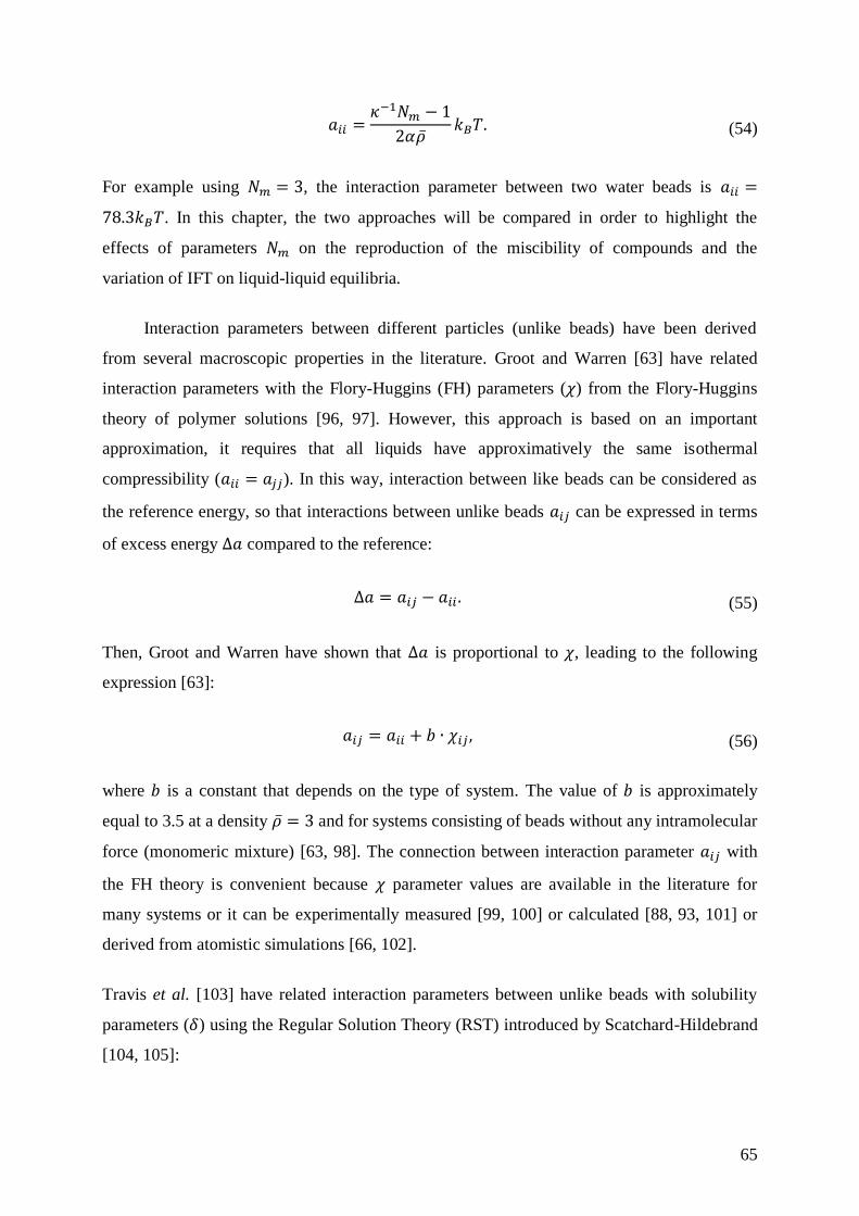
65

𝑎𝑖𝑖 =𝜅−1𝑁𝑚 − 1

2𝛼�̅�𝑘𝐵𝑇. (54)

For example using 𝑁𝑚 = 3, the interaction parameter between two water beads is 𝑎𝑖𝑖 =

78.3𝑘𝐵𝑇. In this chapter, the two approaches will be compared in order to highlight the

effects of parameters 𝑁𝑚 on the reproduction of the miscibility of compounds and the

variation of IFT on liquid-liquid equilibria.

Interaction parameters between different particles (unlike beads) have been derived

from several macroscopic properties in the literature. Groot and Warren [63] have related

interaction parameters with the Flory-Huggins (FH) parameters (𝜒) from the Flory-Huggins

theory of polymer solutions [96, 97]. However, this approach is based on an important

approximation, it requires that all liquids have approximatively the same isothermal

compressibility (𝑎𝑖𝑖 = 𝑎𝑗𝑗). In this way, interaction between like beads can be considered as

the reference energy, so that interactions between unlike beads 𝑎𝑖𝑗 can be expressed in terms

of excess energy ∆𝑎 compared to the reference:

∆𝑎 = 𝑎𝑖𝑗 − 𝑎𝑖𝑖 . (55)

Then, Groot and Warren have shown that ∆𝑎 is proportional to 𝜒, leading to the following

expression [63]:

𝑎𝑖𝑗 = 𝑎𝑖𝑖 + 𝑏 ∙ 𝜒𝑖𝑗 , (56)

where 𝑏 is a constant that depends on the type of system. The value of 𝑏 is approximately

equal to 3.5 at a density �̅� = 3 and for systems consisting of beads without any intramolecular

force (monomeric mixture) [63, 98]. The connection between interaction parameter 𝑎𝑖𝑗 with

the FH theory is convenient because 𝜒 parameter values are available in the literature for

many systems or it can be experimentally measured [99, 100] or calculated [88, 93, 101] or

derived from atomistic simulations [66, 102].

Travis et al. [103] have related interaction parameters between unlike beads with solubility

parameters (𝛿) using the Regular Solution Theory (RST) introduced by Scatchard-Hildebrand

[104, 105]:

66

(𝛿𝑖 − 𝛿𝑗)2 = −𝑟𝑐

4𝛼(𝜌𝑖2𝑎𝑖𝑖 + 𝜌𝑗

2𝑎𝑗𝑗 − 2𝜌𝑖𝜌𝑗𝑎𝑖𝑗), (57)

where 𝛿𝑖 and 𝛿𝑗 are the solubility parameters of the ith and jth beads, respectively. The

dimensionless equation can be expressed as:

(𝛿�̅� − 𝛿�̅�)2 = −�̅�2𝛼(�̅�𝑖𝑖 + �̅�𝑗𝑗 − 2�̅�𝑖𝑗), (58)

where 𝛿�̅� and 𝛿�̅� are the dimensionless solubility parameters of the ith and jth beads,

respectively, and �̅�𝑖𝑖, �̅�𝑗𝑗 and �̅�𝑖𝑗 are the dimensionless interaction parameters (�̅� = 𝑎𝑘𝐵𝑇⁄ ).

This approach has the advantage of removing the assumption of identical repulsions between

like beads.

Recently, Vishnyakov et al. [106] proposed a thermodynamic approach in which

interaction parameters between unlike beads are obtained by fitting infinite dilution activity

coefficients for binary solutions. Note that this approach requires the same approximation

used by Groot and Warren [63], all fluids have the same isothermal compressibility. The

authors obtained quantitative results in agreement with experimental data for the critical

micelle concentration and aggregation number for several typical surfactants of different

chemical structures. Alternatively, Alasiri and Chapman [101] have shown that infinite

dilution activity coefficients can be related to the χ parameters, thus, interaction parameters

are obtained using equation (56). This approach has been validated on interfacial tension for

water/alkane systems.

Anderson et al. [107] proposed a parameterization scheme to determine interaction

parameters based on water-octanol partition coefficients and liquid phase densities.

Interaction parameters between unlike beads are tuned, step by step, using a brute-force

approach, in order to reproduce the experimental partition coefficient. In addition, at each

step, the interaction parameters between like beads and the cutoff radius for each interaction

pair are optimized to fit phase densities. This parameterization method is noteworthy because,

to our knowledge, cut-off radius optimization has never been discussed to parameterize DPD

simulations in order to reproduce experimental data.

Quantitative data of IFT are generally obtained from DPD simulations by

parameterizing interactions between unlike beads using Hildebrand solubility [91–93]. For

example, Rezaei and Modarress [91] have compared the approach of Travis et al. with that of

67

Groot and Warren on IFT reproduction for several water/hydrocarbon systems. In the latter

case, the Flory-Huggins parameters have been calculated using Hildebrand solubility

parameters as shown in equation

𝜒𝑖𝑗 =𝑣𝑏𝑘𝐵𝑇

(𝛿𝑖 − 𝛿𝑗)2, (59)

where 𝑣𝑏 is the mean volume of a bead. Rezaei and Modarress [91] have shown that

parameterization of interactions between unlike particles using Hildebrand solubility

parameters with both approaches leads to quantitative values of IFT, in good agreement with

experimental data. However, Hildebrand solubility parameters are not suitable for interaction

between polar molecules or mixtures involving hydrogen bonds. Consequently, only

immiscible binary systems such as the water/hydrocarbon system can be handled. To examine

more complex systems, alternative approaches exist, using Hansen solubility parameters

[108]. According to Hansen, the solubility parameter can be divided into three components: a

term for dispersion (𝛿𝑑), a term for polarity (𝛿𝑝) and term for hydrogen bonding (𝛿ℎ𝑏). Thus,

the Flory-Huggins parameter can be expressed as:

𝜒𝑖𝑗 = 𝛼𝑣𝑏𝑘𝐵𝑇

[(𝛿𝑖,𝑑 − 𝛿𝑗,𝑑)2+ 0.25(𝛿𝑖,𝑝 − 𝛿𝑗,𝑝)

2+ 0.25(𝛿𝑖,ℎ𝑏 − 𝛿𝑗,ℎ𝑏)

2], (60)

where 𝛼 = 1 as suggested by Hansen. This approach has been used by Shi and al. [95] for the

water/benzene/caprolactam system. However, variation of the IFT calculated with DPD

simulations as a function of the caprolactam concentration differs from experimental data. It

can be possible that differences between simulation and experimental data result from an

insufficient consideration of partial miscibility between compounds. The study of IFT

variation as a function of the solute concentration can be performed only if the phase

composition is well reproduced in the DPD simulations.

68

4.3 New parameterization approach for liquid-liquid equilibrium of

ternary systems: methodology and compositional details

4.3.1 Parameterization of interactions

In this chapter, we propose a new methodology to parameterize interactions between

unlike beads in order to reproduce the liquid-liquid equilibrium of ternary systems. Interaction

parameters for ternary systems labeled solvent 1/solvent 2/solute are obtained as follows:

- Interactions between like particles. The corresponding

interaction parameters are calculated from the isothermal

compressibility of fluid 𝜅𝑇, as proposed by Groot and

Warren.

- Solvent 1/solvent 2 interactions. This interaction is

calculated from the Hildebrand solubility parameters. As

shown previously, this approach provides quantitative

values of IFT in agreement with experimental data for

water/hydrocarbon systems.

- Solute/solvent 1 and solute/solvent 2 interactions. These

parameters must be determined precisely because they

govern the solubility of the solute in bulk phases. In this

chapter, we propose a new parameterization method using

compositional data to determine solute/solvent

interactions.

The parameterization of solute/solvent interactions is based on the assumption that solvents

which constitute the bulk phases are totally immiscible. The solute is considered to be

miscible in both bulk phases. For a solvent 1/solvent 2/solute system, this means that each

bulk phase represents a binary system. The first one consists of solvent 1 and solute molecules

while the second phase is a mixture of solvent 2 and solute molecules (see Figure 16).

69

Figure 16. Representation of a ternary system where bulk phases are immiscible.

Based on the work of Groot and Warren [63], Flory-Huggins (FH) theory can be used

to derive DPD parameters to reproduce the miscibility of compounds. For this purpose, we

propose to use compositional data in the Flory-Huggins equations. In the FH theory, the

Helmholtz free energy of mixing, ∆𝐹𝑚, between two molecules A and B can be written

according to the equation (61).

∆𝐹𝑚 = 𝑛𝑅𝑇 [∅𝐴𝑁𝐴𝑙𝑛∅𝐴 +

∅𝐵𝑁𝐵𝑙𝑛∅𝐵 + 𝜒𝐴,𝐵∅𝐴∅𝐵], (61)

where ∅𝐴 and 𝑁𝐴 are respectively the volume fraction and the number of beads constituting

the molecule 𝐴, and ∅𝐵 and 𝑁𝐵 are the volume fraction and the number of beads constituting

the molecule 𝐵. The chemical potential of compounds 𝐴 and 𝐵 are given by equations (62)

and (63), respectively.

µ𝐴 − µ𝐴° = 𝑅𝑇 [ln(1 − ∅𝐵) + (1 −

1

𝑁𝐴𝑁𝐵)∅𝐵 +𝑁𝐴𝜒𝐴,𝐵∅𝐵

2 ], (62)

µ𝐵 − µ𝐵° = 𝑅𝑇 [ln(1 − ∅𝐴) + (1 −

1

𝑁𝐴𝑁𝐵)∅𝐴 +𝑁𝐵𝜒𝐴,𝐵∅𝐴

2], (63)

where µ𝐴° and µ𝐵

° are pure compound chemical potentials of molecules 𝐴 and 𝐵, respectively.

By applying the FH theory for a liquid-liquid equilibrium on the solvent 1/solvent 2/solute

system shown in Figure 16, equation of the chemical potential of the solute, 𝜇𝑆, can be written

as a function of solvent 1 and solvent 2. At thermodynamic equilibrium, the chemical

potential of the solute is equal in the two liquid phases:

𝜇𝑆𝑠𝑜𝑙𝑣𝑒𝑛𝑡 1 = 𝜇𝑆

𝑠𝑜𝑙𝑣𝑒𝑛𝑡 2 (64)

70

thus, equation (64) can be used to link, 𝜒𝑆,1, the parameter between solute and solvent 1 with,

𝜒𝑆,2, the parameter between solute and solvent 2, as shown in equation (65).

[ln(1 − ∅1) + (1 −1

𝑁1𝑁𝑆)∅1 +𝑁𝑆𝜒𝑆,1∅1

2]

= [ln(1 − ∅2) + (1 −1

𝑁2𝑁𝑆)∅2 + 𝑁𝑆𝜒𝑆,2∅2

2] (65)

where 𝑁1, 𝑁2, and 𝑁𝑆 is the number of beads constituting the solvent 1 molecules, the solvent

2 molecules and the solute molecules, respectively. Finally, the χ parameters are related with

DPD interaction parameters using equation (56). Note that the use of Flory-Huggins

parameters and equation (56) requires that the interactions between like beads are equal. In

this manuscript, we proposed two approaches to determine the 𝜒𝑠𝑜𝑙𝑢𝑡𝑒/𝑠𝑜𝑙𝑣𝑒𝑛𝑡 parameters:

1) The first approach (#1) combines Hildebrand solubility parameters and experimental

data for only one liquid-liquid composition. Thus, one of the two χ parameters is

calculated with solubility parameters, while the second is obtained by solving equation

(65). This approach is valid only if one of the solute/solvent interaction parameters can

be calculated from the Hildebrand solubility parameters.

2) The second approach (#2) consists in using 𝑁 different experimental composition data

of LLE, with 𝑁 ≥ 2. A system of equations is established with 𝑁 equations (65) and

two unknowns: 𝜒𝑆,1 and 𝜒𝑆,2. An optimal solution of this system can be obtained with

the least squares method. The 𝜒𝑆,1 and 𝜒𝑆,2 parameters are obtained by minimizing the

objective function presented in (66).

𝑓(𝜒𝑆,2 ; 𝜒𝑆,1) =∑[𝑌 − (𝜒𝑆,2 × (∅2∅1)2

− 𝜒𝑆,1)]

2

𝑁

(66)

with

𝑌 =ln(1 − ∅1) + (1 −

1𝑁1𝑁𝑆

)∅1 − ln(1 − ∅2) − (1 −1

𝑁2𝑁𝑆) ∅2

𝑁𝑆∅12 (67)

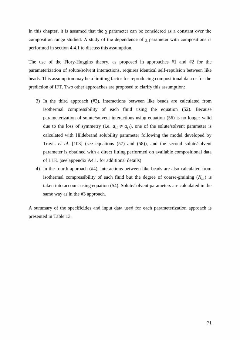
71

In this chapter, it is assumed that the χ parameter can be considered as a constant over the

composition range studied. A study of the dependence of χ parameter with compositions is

performed in section 4.4.1 to discuss this assumption.

The use of the Flory-Huggins theory, as proposed in approaches #1 and #2 for the

parameterization of solute/solvent interactions, requires identical self-repulsion between like

beads. This assumption may be a limiting factor for reproducing compositional data or for the

prediction of IFT. Two other approaches are proposed to clarify this assumption:

3) In the third approach (#3), interactions between like beads are calculated from

isothermal compressibility of each fluid using the equation (52). Because

parameterization of solute/solvent interactions using equation (56) is no longer valid

due to the loss of symmetry (i.e. 𝑎𝑖𝑖 ≠ 𝑎𝑗𝑗), one of the solute/solvent parameter is

calculated with Hildebrand solubility parameter following the model developed by

Travis et al. [103] (see equations (57) and (58)), and the second solute/solvent

parameter is obtained with a direct fitting performed on available compositional data

of LLE. (see appendix A4.1. for additional details)

4) In the fourth approach (#4), interactions between like beads are also calculated from

isothermal compressibility of each fluid but the degree of coarse-graining (𝑁𝑚) is

taken into account using equation (54). Solute/solvent parameters are calculated in the

same way as in the #3 approach.

A summary of the specificities and input data used for each parameterization approach is

presented in Table 13.

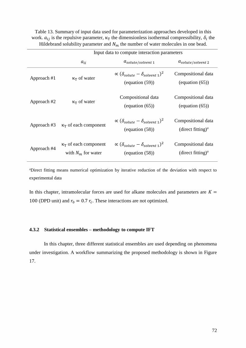
72

Table 13. Summary of input data used for parameterization approaches developed in this

work. 𝑎𝑖𝑗 is the repulsive parameter, κT the dimensionless isothermal compressibility, 𝛿𝑖 the

Hildebrand solubility parameter and 𝑁𝑚 the number of water molecules in one bead.

Input data to compute interaction parameters

𝑎𝑖𝑖 𝑎𝑠𝑜𝑙𝑢𝑡𝑒/𝑠𝑜𝑙𝑣𝑒𝑛𝑡 1 𝑎𝑠𝑜𝑙𝑢𝑡𝑒/𝑠𝑜𝑙𝑣𝑒𝑛𝑡 2

Approach #1 κT of water ∝ (𝛿𝑠𝑜𝑙𝑢𝑡𝑒 − 𝛿𝑠𝑜𝑙𝑣𝑒𝑛𝑡 1)

2

(equation (59))

Compositional data

(equation (65))

Approach #2 κT of water Compositional data

(equation (65))

Compositional data

(equation (65))

Approach #3 κT of each component ∝ (𝛿𝑠𝑜𝑙𝑢𝑡𝑒 − 𝛿𝑠𝑜𝑙𝑣𝑒𝑛𝑡 1)

2

(equation (58))

Compositional data

(direct fitting)a

Approach #4 κT of each component

with 𝑁𝑚 for water

∝ (𝛿𝑠𝑜𝑙𝑢𝑡𝑒 − 𝛿𝑠𝑜𝑙𝑣𝑒𝑛𝑡 1)2

(equation (58))

Compositional data

(direct fitting)a

aDirect fitting means numerical optimization by iterative reduction of the deviation with respect to

experimental data

In this chapter, intramolecular forces are used for alkane molecules and parameters are 𝐾 =

100 (DPD unit) and 𝑟0 = 0.7 𝑟𝑐. These interactions are not optimized.

4.3.2 Statistical ensembles – methodology to compute IFT

In this chapter, three different statistical ensembles are used depending on phenomena

under investigation. A workflow summarizing the proposed methodology is shown in Figure

17.

73

Figure 17. Workflow representing the steps of the methodology used to compute interfacial

tension of ternary mixtures from bulk compositions.

- The DPD model is combined with coarse-grained Monte Carlo (CG-MC)

technique in order to simulate systems in the Gibbs (NVT) ensemble. This

approach has already been used and validated by Wijmans et al. [98] with beads

and soft potentials from DPD models. In the Gibbs ensemble, two separated

simulation boxes that can exchange particles are used with a constant total volume

𝑉. Thus, it is possible to describe equilibrium between two phases without

considering explicitly the interface. Gibbs (NVT) ensemble simulations are used in

our work in order to compute phase diagram and, thus, to check the relevance of

parameterization methods to reproduce composition in bulk phases. Three different

types of Monte Carlo moves are used: (1) translation of beads, (2) transfer of beads

between the two boxes and (3) concerted change of volume of each box. In

addition, for hexane molecules which are represented by two beads, rigid body

rotation and configurational regrowth moves are added. These movements are

described in greater details in the section 3.3.3. During CG-MC simulations in the

74

Gibbs (NVT) ensemble, chemical potential of each species are calculated using

Widom insertion test method [109].

- Some CG-MC simulations are also performed in the osmotic (µsoluteNsolventPzzT)

ensemble in order to describe a system with a constant number of solvent particles

(Nsolvent) and a variable number of solute particles, fixing the chemical potential of

the solute (µsolute). Osmotic ensemble has already been used by Rekvig et al. [84]

to compute the number of surfactants necessary to reach an imposed IFT value

between water and oil phases. CG-MC simulations in osmotic (µsoluteNsolventPzzT)

ensemble with an explicit interface allow to predict the solute concentration at the

interface from known bulk compositions. The imposed chemical potentials are

obtained from previous simulations in the Gibbs (NVT) ensemble. Three different

types of Monte Carlo moves are used: (1) translation of beads, (2) change of

volume along z-axis (perpendicular to the interface) and (3) insertion or removal of

solute beads. For hexane molecules, rigid body rotation and configurational

regrowth moves are added. These movements are described in greater details in the

section 3.3.3.

- Finally, DPD simulations are performed in the NVT ensemble in order to compute

the interfacial tension.

In this chapter, CG-MC in the Gibbs (NVT) ensemble and DPD simulations are

performed at constant density (�̅� = 3). Therefore, the total pressure of the system varies

depending on the composition. This choice was made to simplify the parameterization

procedure. However, it is important to notice that an alternative parameterization of DPD

interactions can be done by working at constant pressure. In this case, calculation of

interaction parameters between like and unlike beads is dependent on the total density of the

system (see equations (52), (56) and (57)). Consequently, additional bulk phase density data

are required to obtain interaction parameters of pure components. Noting that, on this basis,

any phase property should be calculated at constant pressure using a reference value.

CG-MC simulations were carried out with the molecular simulation package GIBBS

[110]. For simulations in the Gibbs (NVT) ensemble, the two subsystems (“boxes”) have each

an initial dimension of 𝐿𝑥 = 𝐿𝑦 = 𝐿𝑧 = 10 (in DPD units). The volume of each boxes can

vary during the simulation but the total volume remains constant. The total number of beads is

6000. For simulations in the osmotic (µsoluteNsolventPzzT) ensemble, box dimensions were set to

75

𝐿𝑧 = 60, 𝐿𝑥 = 𝐿𝑦 = 10 (in DPD units). Two planar water-organic compound interfaces are

created normal to the z-axis. Box length in z-direction is six times larger than in the x and y-

directions in order to avoid interactions between the two interfaces. Initial boxes containing a

total of 18 000 DPD beads are built for different solute/solvent concentrations using the

PACKMOL software package [111, 112]. DPD simulations in the NVT ensemble were

performed using the molecular dynamics simulation package NEWTON [113]. Initial

configurations are derived from simulations in the osmotic (µsoluteNsolventPzzT) ensemble. The

area of the interface is kept constant (𝐿𝑥 = 𝐿𝑦 = 10, in DPD units). A modified version of

the velocity-Verlet algorithm [63] governed the equation of motion, and the time step is fixed

at δt = 0.001 in DPD units. Constants in the dissipative force γ and random force σ were set to

4.5 and 3, respectively, in order to keep the temperature fixed at 𝑘𝐵𝑇 = 1, thus satisfying the

fluctuation-dissipation theorem (see section 3.2.4). In all simulations, periodic boundary

conditions were imposed in all directions.

The IFT values are evaluated using two local methods (Irving and Kirkwood [69] and

Harasima [70]) and one global method (Kirkwood-Buff [67]). More details on these methods

are given in section 3.4.3.

4.3.3 Systems studied

The representation of ternary systems with the coarse-grained model follows the

procedure reported by Goel et al. [92]. Beads are chosen to represent the same molecular

volume. This procedure leads to more accurate results on the interfacial tension [91].

Depending on the coarse grained level, a bead of water represents 4 or 5 water molecules. The

volume of a bead, 𝑣𝑏, is fixed as the arithmetic mean of bead volumes as proposed by Rezaei

and Modarress [91]. Following Maiti and McGrother [93], the cut-off radius is given from the

volume of the DPD particles with 𝑟𝑐 = (�̅� × 𝑣𝑏)1/3. The overall DPD density �̅� is 𝜌𝑟𝑐

3 = 3,

which is a value commonly used in DPD simulations.

Above mentioned methodologies for the parameterization of DPD interactions were

applied on six different ternary systems (Figure 18): water/benzene/1,4-dioxane,

water/chloroform/acetone, water/benzene/acetic acid, water/benzene/2-propanol,

water/hexane/acetone and water/hexane/2-propanol. For each of these systems, experimental

data of bulk phase compositions and corresponding interfacial tension values are available in

the literature [114–116] and are reported in the appendix A4.2. Compositional data are molar

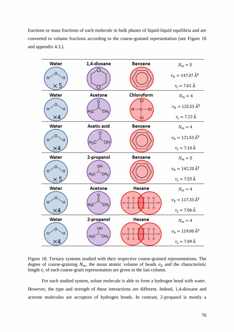
76

fractions or mass fractions of each molecule in bulk phases of liquid-liquid equilibria and are

converted to volume fractions according to the coarse-grained representation (see Figure 18

and appendix 4.3.).

Figure 18. Ternary systems studied with their respective coarse-grained representations. The

degree of coarse-graining 𝑁𝑚, the mean atomic volume of beads 𝑣𝑏 and the characteristic

length 𝑟𝑐 of each coarse-grain representation are given in the last column.

For each studied system, solute molecule is able to form a hydrogen bond with water.

However, the type and strength of these interactions are different. Indeed, 1,4-dioxane and

acetone molecules are acceptors of hydrogen bonds. In contrast, 2-propanol is mostly a

77

hydrogen bonding donor, while acetic acid has the particularity of being both an acceptor and

a donor of hydrogen bonds with water. These solute/water hydrogen bond interactions must

be implicitly represented in the DPD simulation in order to both reproduce the miscibility and

the solubility of molecules. It can be noticed that solutes do not form hydrogen bonds with the

molecules of the organic solvents except for the chloroform with acetone. Therefore, when

parameterization approaches #1, #3 and #4 are followed, it seems more reasonable to

calculate the solute/organic solvent interactions with Hildebrand solubility parameters and

compute solute/water using compositional data.

Coarse-grained representation of these systems and their characteristics are shown in

Figure 18. To construct coarse-grained model and to parameterize DPD simulations,

molecular volume and Hildebrand solubility parameters for each component are required.

Values used in this chapter are given in the Table 14 and were calculated using data extracted

from the DIPPR database [117]. Molecular volumes (𝑣 in Å3) in were obtained from molar

volumes (𝑉𝑚𝑖 in m3/mol), and Hildebrand solubility parameters were calculated using molar

vaporization enthalpies ∆𝐻𝑣𝑎𝑝, according to equation (68).

𝛿𝑖 = √𝐸𝑐𝑜ℎ𝑉𝑚𝑖

= √∆𝐻𝑣𝑎𝑝 − 𝑅𝑇

𝑉𝑚𝑖 (68)

where 𝑉𝑚𝑖 is the molar volume of molecule 𝑖. The right-hand side of equation (68) assumes

that vapor phase can be considered as an ideal gas.

Table 14. Properties of individual components (DIPPR) at 298.15 K and 1 bar.

Molecules 𝑣 (Å3) ΔHvap (kJ/mol) δ (J/cm3)1/2

Water 30.07 43.982 47.9

Benzene 148.58 33.871 18.7

Chloroform 133.68 31.393 19.0

Hexane 218.13 31.549 14.9

1,4-dioxane 142.25 38.595 20.5

Acetone 122.61 31.166 19.7

Acetic acid 95.70 24.313 19.5

2-propanol 127.64 46.081 23.8

78

4.4 Results

4.4.1 Composition dependence of the Flory-Huggins interaction parameters

In our simulations, it is assumed that χ parameters and repulsive interaction parameters

𝑎𝑖𝑗 are constant over the composition range studied. A study of the compositional dependence

of 𝜒𝑠𝑜𝑙𝑢𝑡𝑒/𝑠𝑜𝑙𝑣𝑒𝑛𝑡 Flory-Huggins parameters determined from experimental compositions was

conducted. In this chapter, 𝜒𝑠𝑜𝑙𝑢𝑡𝑒/𝑠𝑜𝑙𝑣𝑒𝑛𝑡 are determined using one (approach #1) or several

(approach #2) compositional data of bulk phases of liquid-liquid equilibria. The dependence

of 𝜒𝑠𝑜𝑙𝑢𝑡𝑒/𝑠𝑜𝑙𝑣𝑒𝑛𝑡 parameters, as a function of composition data obtained using approaches #1

and #2 for the water/benzene/acetic acid system is presented in Figure 19. For other systems

studied in this work, the dependence of the 𝜒𝑠𝑜𝑙𝑢𝑡𝑒/𝑠𝑜𝑙𝑣𝑒𝑛𝑡 parameters according to approaches

#1 and #2 is given in the appendix A4.4.

Figure 19. (a) Variation of 𝜒𝑠𝑜𝑙𝑢𝑡𝑒/𝑠𝑜𝑙𝑣𝑒𝑛𝑡 parameters, as a function of each experimental

composition for the water/benzene/acetic acid system (obtained using approach #1). The

composition is expressed using the molar fraction of solute in the aqueous phase. (b)

Variation of 𝜒𝑠𝑜𝑙𝑢𝑡𝑒/𝑠𝑜𝑙𝑣𝑒𝑛𝑡 parameters as a function of the average solute molar fractions in

the aqueous phase for each pair of compositions for the water/benzene/acetic acid system

(obtained using approach #2).

Figure 19 (a) shows the dependence of 𝜒𝑠𝑜𝑙𝑢𝑡𝑒/𝑠𝑜𝑙𝑣𝑒𝑛𝑡 parameters determined using

approach #1 as a function of the molar fraction of solute in the aqueous phase. The

𝜒𝑎𝑐𝑒𝑡𝑖𝑐 𝑎𝑐𝑖𝑑/𝑏𝑒𝑛𝑧𝑒𝑛𝑒 parameter between acid acetic and benzene beads is constant since it is

calculated using Hildebrand solubility parameters and is not dependent on compositional data.

The second parameter, 𝜒𝑎𝑐𝑒𝑡𝑖𝑐 𝑎𝑐𝑖𝑑/𝑤𝑎𝑡𝑒𝑟, is calculated for each composition. Figure 19 (a)

79

shows that, using approach #1, large variations of the 𝜒𝑎𝑐𝑖𝑑 𝑎𝑐𝑒𝑡𝑖𝑐/𝑤𝑎𝑡𝑒𝑟 parameter can be

observed as a function of the composition used and the values obtained vary from -14.65

to -3.84 (dimensionless) (i.e. �̅�𝑎𝑐𝑒𝑡𝑖𝑐 𝑎𝑐𝑖𝑑/𝑤𝑎𝑡𝑒𝑟 varies from -26.29 to 11.56 (DPD unit),

negative �̅�𝑖𝑗 values cannot be used in the DPD model used in this work). Large variations of

the 𝜒𝑠𝑜𝑙𝑢𝑡𝑒/𝑤𝑎𝑡𝑒𝑟 parameter are also observed for the water/benzene/2-propanol and

water/hexane/2-propanol systems (see in appendix A4.4. Figure 42 and Figure 44). It is clear

that for these systems the assumption of constant parameters over the whole studied

composition range is not valid using approach #1. However, for systems containing acetone

solute, variations of the 𝜒𝑎𝑐𝑒𝑡𝑜𝑛𝑒/𝑤𝑎𝑡𝑒𝑟 parameter seem to be more reasonable and less

dependent on the composition (see in appendix A4.4. Figure 41 and Figure 43). For example,

the 𝜒𝑎𝑐𝑒𝑡𝑜𝑛𝑒/𝑤𝑎𝑡𝑒𝑟 parameter varies between 1.37 and 1.60 for the water/chloroform/acetone

system (i.e. �̅�𝑎𝑐𝑒𝑡𝑜𝑛𝑒/𝑤𝑎𝑡𝑒𝑟 varies from 29.83 to 30.61).

Figure 19 (b) presents the compositional dependence of 𝜒𝑎𝑐𝑒𝑡𝑖𝑐 𝑎𝑐𝑖𝑑/𝑤𝑎𝑡𝑒𝑟 and

𝜒𝑎𝑐𝑒𝑡𝑖𝑐 𝑎𝑐𝑖𝑑/𝑏𝑒𝑛𝑧𝑒𝑛𝑒 parameters obtained using approach #2. In this case, parameters are

calculated using pairs of adjacent compositions (sorted from smallest to highest) and values

obtained are expressed as a function of the average solute molar fractions in the aqueous

phase for each pair of compositions. In addition, dashed lines indicate values of parameters

obtained when all available compositions data are used for the minimization of equation (66)

following approach #2. Figure 19 (b) shows that approach #2 seems to provide less

compositional dependent 𝜒𝑠𝑜𝑙𝑢𝑡𝑒/𝑠𝑜𝑙𝑣𝑒𝑛𝑡 parameters than approach #1 for the

water/benzene/acetic acid system. Indeed, the values of the 𝜒𝑎𝑐𝑒𝑡𝑖𝑐 𝑎𝑐𝑖𝑑/𝑠𝑜𝑙𝑣𝑒𝑛𝑡 parameters

seem to be relatively constant, regardless of the compositions used in the optimization

process. Although, the pair of compositions with the lowest solute concentration provide

slightly lower parameters than the others. The same trend can be observed for the

water/benzene/1,4-dioxane for 𝜒𝑠𝑜𝑙𝑢𝑡𝑒/𝑠𝑜𝑙𝑣𝑒𝑛𝑡 parameters (see in appendix Figure 40). For

systems containing hexane molecules, it can be noted that 𝜒𝑠𝑜𝑙𝑢𝑡𝑒/𝑤𝑎𝑡𝑒𝑟 parameters can vary

according to the pairs of compositions used, but the value of these parameters remain around

an average value (the value of parameters when all compositions are used in approach #2, (see

in appendix Figure 43 and Figure 44).

On one hand, it appears that approach #2 provide less compositional dependent

𝜒𝑠𝑜𝑙𝑢𝑡𝑒/𝑠𝑜𝑙𝑣𝑒𝑛𝑡 parameters than the approach #1 for the water/benzene/1,4-dioxane,

80

water/benzene/acetic acid and water/hexane/2-propanol systems. On the other hand,

approach #1 seems better suited to water/chloroform/acetone and water/hexane/acetone

systems. Therefore, the assumption of constant parameters over the entire composition range

is valid for these systems depending on the approach used. Among all the systems studied in

this chapter, only the water/benzene/2-propanol cannot be parameterized using both

approaches in order to obtain parameters that are weakly dependent on the composition (see

in appendix Figure 42)

4.4.2 Liquid-liquid equilibrium (LLE)

Compositions of bulk phases for liquid-liquid equilibrium are computed using Monte

Carlo coarse-grained simulations in the Gibbs ensemble (NVT). The four parameterization

approaches are compared in detail using the water/benzene/1,4-dioxane system, and results

for other systems are given in the appendix A4.5. For the water/benzene/1,4-dioxane system,

interaction parameters obtained with approaches #1, #3 and #4 were determined from the less

concentrated solute composition. With the approach #2, the four compositions with the lowest

concentrations of 1,4-dioxane were selected; the fifth composition is not taken into account

because of the excessive solubility of water in benzene (see appendix A4.2.). Phase

compositions are visualized using ternary diagrams and corresponding interaction parameters

used to compute LLE are indicated below each diagram (Figure 20). In addition, the

coefficient of regression 𝑅𝑠𝑜𝑙𝑢𝑏𝑖𝑙𝑖𝑡𝑦2 , is used to quantify the accuracy of our parameterization

approaches in the reproduction of the solubility of solutes in the aqueous and organic phases

(Table 15).

81

Table 15. Values of regression functions for the four parameterization approaches to reproduce the experimental data. Phase compositions are

used for parameterization, IFT correspond to predictions.

Number of compositional

data available, 𝑁 Solvent 1 Solvent 2 Solute Parameterization approaches 𝑅𝑠𝑜𝑙𝑢𝑏𝑖𝑙𝑖𝑡𝑦

2 [a] 𝑅𝐼𝐹𝑇

2 [b]

5 water benzene 1,4-dioxane

approach #1 0.994 0.997

approach #2 0.994 0.847

approach #3 0.985 0.899

approach #4 0.988 0.909

5 water chloroform acetone

approach #1 0.971 0.970

approach #2 0.983 0.964

approach #3 0.995 0.871

approach #4 0.989 0.924

5 water benzene acetic acid

approach #1 0.875 0.677

approach #2 0.967 0.893

approach #3 0.759 0.908

approach #4 0.768 0.911

7 water benzene 2-propanol

approach #1 0.900 0.805

approach #2 0.888 0.237

[1] approach #3 0.938 0.814

approach #4 0.954 0.537

11 water hexane

(2 beads) acetone

Transferability[c] 0.758 0.905

approaches [#1- #2] 0.998 0.849

approach #3 0.997 0.812

approach #4 0.998 0.851

11 water hexane

(2 beads) 2-propanol

approach #1 0.514 0.818[d]

approach #2 0.988 0.416

approach #3 0.996 0.557

approach #4 0.997 0.377

82

[a] 𝑅𝑠𝑜𝑙𝑢𝑏𝑖𝑙𝑖𝑡𝑦2 = 1 − [

∑ (𝑥𝑖𝑒𝑥𝑝

−𝑥𝑖𝑐𝑎𝑙𝑐)

22×𝑁𝑖=1

∑ (𝑥𝑖𝑒𝑥𝑝

−�̅�)22×𝑁

𝑖=1

] with �̅� =1

2×𝑁∑ 𝑥𝑖

𝑒𝑥𝑝2×𝑁𝑖=1 where 𝑥𝑖 is the molar fraction of solute in the aqueous phase and in the organic phase for the

ith composition. N is the number of compositions and a factor 2 is added because the molar fraction of the solute is taken into account for both bulk phases.

[b] 𝑅𝐼𝐹𝑇2 = 1 − [

∑ (𝐼𝐹𝑇𝑖𝑒𝑥𝑝

−𝐼𝐹𝑇𝑖𝑐𝑎𝑙𝑐)

2𝑁+1𝑖=1

∑ (𝐼𝐹𝑇𝑖𝑒𝑥𝑝

−𝐼𝐹𝑇̅̅ ̅̅ ̅)2𝑁+1

𝑖=1

] with 𝐼𝐹𝑇̅̅ ̅̅ ̅ =1

𝑁+1∑ 𝐼𝐹𝑇𝑖

𝑒𝑥𝑝𝑁+1𝑖=1 where 𝐼𝐹𝑇𝑖 is the value of the interfacial tension for the ith composition. To calculate

𝑅𝐼𝐹𝑇2 , composition in absence of solute is included.

[c] water/acetone interaction parameter from water/chloroform/acetone system (approach #2) is used for the water/hexane/acetone system.

[d] Due to a phase separation between the 2-propanol and the organic phase, IFT for the five most concentrated compositions in solute cannot be computed.

83

Figure 20. Liquid-liquid equilibrium ternary diagrams for the water/1,4-dioxane/benzene

system at 298.15 K for (a) approach #1, (b) approach #2, (3) approach #3 and (4) approach

#4. Experimental data are plotted in black (solid lines) and the results from the CG-MC

simulations are in red (dashed lines). Dimensionless DPD interaction parameters used to

compute LLE are located below each ternary plot. Numbers in shown red represent the

solute/solvent parameters.

84

Data presented in Figure 20 come from the equilibration of a heterogeneous system

that decants, following the conodal lines (red dashed line), into two phases represented on the

ternary diagram by red squares. Initial compositions are given in appendix A4.6. In approach

#1, with a high concentration of 1,4-dioxane, the molar fraction of solute is well reproduced

in the organic phase but is overestimated in the aqueous phase. In the parameterization

approach #2, conodal lines are better reproduced but an increasing excess of 1,4-dioxane is

observed in the organic phase when the concentration of this solute increases. In approaches

#1 and #2, a deviation can be observed on the molar fractions of water in benzene with a high

solute concentration. Differences can be explained by the main assumption of our

parameterization method: the miscibility between the two solvents is not taken into account

for the calculation of the solvent/solvent interaction parameters. However, with the

approaches #3 and #4, when the compressibility of each fluid is taken into account, the

miscibility between water and benzene appears to be slightly better reproduced. Other

systems also seem to benefit from the use of different interaction parameters between like

beads. The parameterization approach #3 roughly provides the best predicted miscibility

between the aqueous phase and the organic phase.

Performances of CG-MC simulations for the water/chloroform/acetone system are

similar to those obtained for the water/benzene/1,4-dixoane system. LLE diagrams are

consistent with experimental data when using the four parameterization approaches but the

same errors on the calculated compositional data are observed. Molar fractions of acetone in

organic phase are overestimated when the solute concentration increases. In addition, the

solubility of water in the organic phase is not sufficiently well reproduced in our simulations.

It can be noted that with the approach #2, the chloroform/acetone interaction parameter is

lower than 25, this value denotes a strong attraction between the two compounds, it is

important to emphasize that values lower than 25 cannot be obtained using Hildebrand

solubility parameters (see equation (59)).

For the water/benzene/acetic acid system, the LLE diagram parameterized with the

approach #2 is in good agreement with experiments, with some deviations in the organic

phase. However, LLE diagrams calculated using interaction parameters derived from

approaches #1, #3 and #4 are different from those drawn using experimental data. In these

approaches, interaction parameter 𝑎𝑎𝑐𝑒𝑡𝑖𝑐 𝑎𝑐𝑖𝑑/𝑏𝑒𝑛𝑧𝑒𝑛𝑒 is determined from Hildebrand

solubility parameters and is not dependent on compositional data. In addition, as shown in the

85

section 4.4.1, setting interaction parameter between acetic acid and benzene to a constant

value leads to a strong dependence on the composition of the acetic acid/water parameter.

Using approaches #1, #3 and #4, we arbitrarily selected the second less concentrated

composition for the parameterization.

For the water/hexane/acetone system, the parameterization approaches #1 and #2

provide similar solute/solvent interaction parameters and, therefore, results on phase

compositions are also similar (results are grouped and noted [#1-#2] in Table 15). Phase

compositions obtained with the four parameterization approaches are in very good agreement

with the experimental data. The miscibility between the aqueous and organic phases is

particularly well reproduced with the approach #4. For this system, we propose a fifth

parameterization approach based on the principle of transferability of interaction parameters;

this is called Transferability in Table 15. Indeed, the water/acetone parameter with a water

bead containing four water molecules has already been calculated for the

water/chloroform/acetone system. Therefore, the water/acetone interaction parameter

(�̅�𝑤𝑎𝑡𝑒𝑟/𝑎𝑐𝑒𝑡𝑜𝑛𝑒 = 28.20 with the approach #2) from the water/chloroform/acetone system is

used in the Transferability approach and the second solute/solvent parameter

(𝑎ℎ𝑒𝑥𝑎𝑛𝑒/𝑎𝑐𝑒𝑡𝑜𝑛𝑒 ) is directly obtained with equation (65). Results of our simulations show that

this method is valid only for compositions with a low acetone molar fraction in bulk phases

(i.e., 𝑥𝑎𝑐𝑒𝑡𝑜𝑛𝑒 < 0.2 in the aqueous and organic phases).

Systems containing 2-propanol beads are the only cases where LLE diagrams cannot

be reproduced correctly. For the water/benzene/2-propanol system, LLE diagrams calculated

using the four parameterization approaches are very similar although interaction parameters

are different. Some deviations on the calculated compositional data in comparison to

experiments are observable on solubility of solute in the aqueous and organic phases and also

on the miscibility between solvents. For the water/hexane/2-propanol system, solute

concentrations in aqueous and organic phases calculated with CG-MC simulations are in good

agreement with experimental data but the miscibility between the aqueous and organic phases

is not well reproduced. Moreover, it should be noted that LLE diagrams for the

water/hexane/2-propanol system parameterized using approach #1, strongly deviates from

experimental data with the most concentrated compositions in 2-propanol (i.e., 𝑥2−𝑝𝑟𝑜𝑝𝑎𝑛𝑜𝑙 >

0.1 in the aqueous and organic phases). Our DPD simulations carried out with an explicit

86

interface (section 4.4.3 and 4.4.4) have shown that these deviations are due to a phase

separation of the solute and the organic phase.

Overall, the four parameterization approaches allow good reproductions of

experimental LLE diagrams as shown by the analysis of regression functions in Table 15. In

most cases, approach #2 allows a better reproduction of the LLE diagram compared to

approach #1. Approaches #3 and #4 which take into account the isothermal compressibility of

each fluid may, in some cases, slightly improve miscibility between solvents.

Another point to be highlighted is that parameterization approaches #1 and #2 can

provide different solute/solvent interaction parameters. For instance, the solute/solvent

interaction parameters, 𝑎𝑤𝑎𝑡𝑒𝑟/𝑑𝑖𝑜𝑥𝑎𝑛𝑒 and 𝑎𝑏𝑒𝑛𝑧𝑒𝑛𝑒/𝑑𝑖𝑜𝑥𝑎𝑛𝑒, obtained with the approach #1

are lower than those obtained with the approach #2 and are predicted to be very close to 25,

which is the value of the interaction between like beads. However, overall, compositional data

are well reproduced in both cases for the water/benzene/1,4-dioxane system. Therefore, there

are several sets of parameters that allow to reproduce compositional data with CG-MC

simulations. Prediction of interfacial phenomena/properties with DPD simulations thus

represents an additional criterion for identifying the best parameterization approach(es) (see

section 4.4.4).

4.4.3 Interface compositions

Interface compositions are difficult to characterize experimentally and are generally

left unknown. Indeed, interfaces are very thin surfaces at the macroscopic scale, but at the

mesoscopic scale, dimensions of interfaces are large, and consequently, construction of the

simulations boxes with an explicit interface requires knowledge of the composition of this

region. Therefore, CG-MC simulations in the (µsoluteNsolventPzzT) osmotic ensemble have been

conducted in order to impose the precise bulk phase composition and to predict the

composition at the interface. This step allows a perfect comparison between the interfacial

tension values predicted by DPD calculations with experimental data at exactly the same

phase compositions. Chemical potential used in the CG-MC simulations and compositions

resulting from simulations are given in appendices A4.7 and A4.8, respectively.

To determine the interface composition from numerical simulations, the thickness of

the interfacial region should be defined. Following the method used by Rezaei et al. [118], the

87

thickness of the interface is determined with the criterion “90-90” which defines the distance

between two positions where the densities of two phases are 90% of their own bulk densities.

Interfacial concentration and thickness of the interfaces were extracted from CG-MC

simulations and are plotted as a function of the solute bulk concentration (here, the molar

fraction of solute in the aqueous phase). Results for the water/benzene/1,4-dioxane system are

reported in Figure 21 and data for other systems are given in the appendix A4.9.

Figure 21. (a) Variation of the 1,4-dioxane interfacial concentration, as a function of the molar

fraction of 1,4-dioxane in the aqueous phase. (b) Variation of the water/benzene interface

thickness, as a function of the molar fraction of 1,4-dioxane in the aqueous phase.

Figure 21 (a) indicates that the interfacial concentration (𝐶𝑖) increases with solute

molar fraction in the bulk phase. Figure 21 (b) shows that the thickness of the interface

increases by following exactly the same trend as 𝐶𝑖. In addition, inspection of the Figure 21

(b) reveals that the thickness of the interfacial zone can be quite large (1-5 nm). In our

simulations the thickness of each bulk phase are on the order of 15-20 nm approximately (~40

nm for the simulation box in z). It is evident that such length scales are in the limit of what

can be obtained with atomistic simulations. This fact is particularly important to prevent any

possible effect induced by the presence of the two interfaces in the system.

4.4.4 Interfacial tension

DPD simulations in the NVT ensemble were used to quantitatively predict the

variation of IFT with solute concentration. Note that values obtained for the IFT are pure

predictions and were not used to derive any interaction parameters. For all systems, variation

of IFT are presented as a function of the bulk solute concentration in the aqueous and in the

88

organic phases and compared together with experimental data [114–116]. For

water/benzene/1,4-dioxane, water/chloroform/acetone and water/benzene/acetic acid systems,

IFT values are also compared with predictive calculations using the COSMO-RS method

implicit solvent model combined with Density Functional Theory (DFT) calculations,

extracted from the work by Andersson et al. [119]. Authors indicated that their methodology

is fast, reliable and requires no experimental input data. Difference between calculated and

experimental IFT values is given by the relative deviation, RD (%), following the equation

(69).

𝑅𝐷(%) = |𝐼𝐹𝑇𝑒𝑥𝑝 − 𝐼𝐹𝑇𝑐𝑎𝑙𝑐

𝐼𝐹𝑇𝑒𝑥𝑝| × 100 (69)

In addition, criteria, 𝑅𝐼𝐹𝑇2 , were employed to compare calculated variations of IFT values with

experimental data in order to determine the most suitable parameterization approach (Table

15). In a first step, results on IFT are analyzed on systems that do not include intramolecular

forces (Figure 22 to Figure 25).

Figure 22. Experimental and predicted variation of water/benzene IFT as a function of the

1,4-dioxane concentration in (a) the aqueous phase and (b) the organic phase. Uncertainty

regarding the value of the interfacial tension in DPD simulations is ~0.20 mN/m.

89

Figure 23. Experimental and predicted variation of water/chloroform IFT as a function of

acetone concentration in (a) the aqueous phase and (b) the organic phase. Uncertainty

regarding the value of the interfacial tension in DPD simulations is ~0.20 mN/m.

Figure 24. Experimental and predicted variation of water/benzene IFT as a function of acetic

acid concentration in (a) the aqueous phase and (b) the organic phase. Uncertainty regarding

the value of the interfacial tension in DPD simulations is ~0.20 mN/m.

90

Figure 25. Experimental and predicted variation of water/benzene IFT as a function of 2-

propanol concentration in (a) the aqueous phase and (b) the organic phase. Uncertainty on the

value of the interfacial tension in DPD simulations is ~0.20 mN/m.

First of all, it can be noted that local methods (Irving and Kirkwood [69] and Harasima

[70]) and the global method (Kirkwood-Buff [67]) provide identical values of IFT for our

simulations. The IFT values of water/benzene and the water/chloroform interface in absence

of solute are predicted in a good agreement with experimental data. For instance, Figure 22

shows IFT value for the water/benzene/1,4-dioxane system and the relative deviation is lower

than 1.8 % for approaches #1 and #2. The approach #3 underestimates the IFT (𝑅𝐷 = 10.3%)

while the approach #4 overestimates the IFT (𝑅𝐷 = 18.2%). For the

water/chloroform/acetone system presented in Figure 23, water/chloroform IFT in absence of

solute is slightly overestimated with approaches #1 and #2 with a relative deviation of 10.4%.

The approach #3 underestimates the IFT (𝑅𝐷 = 7.6%) while the approach #4 overestimates

the IFT (𝑅𝐷 = 18.8%).

In presence of solute, prediction of variation of IFT presented in Figure 22 for the

water/benzene/1,4-dioxane system is in very good agreement with experimental data using the

parameterization approach #1 with 𝑅𝐼𝐹𝑇2 = 0.997. Other parameterization methods

underestimate the variation of IFT, in comparison to the experimental data. For example, with

the approach #2, predicted IFT values are about two times lower than the experimental data

(𝑅𝐼𝐹𝑇2 = 0.847). Deviations on IFT values obtained with our DPD simulations are of the same

order of magnitude as those obtained with other predictive methods such as COSMO-RS

(Figure 22 (a) and (b)).

91

For the water/chloroform/acetone system (Figure 23), all of the parameterization

approaches provide a trend of the IFT variation with acetone molar fraction in agreement with

experimental data. The best results are obtained with the approaches #1 (𝑅𝐼𝐹𝑇2 = 0.970) and

#2 (𝑅𝐼𝐹𝑇2 = 0.964). In addition, DPD simulations predict more precisely the variation of IFT

as a function of the organic phase composition than the COSMO-RS method as shown in

Figure 23 (b).

In the case of the water/benzene/acetic acid system (Figure 24), IFT are overestimated

by 30% with approaches #2, #3 and #4 (𝑅𝐼𝐹𝑇2 varies from 0.893 to 0.911) and by 40% with the

approach #1 (𝑅𝐼𝐹𝑇2 = 0.677). Note that prediction of IFT values can be compared to the

experimental data only if compositions are reproduced in bulk phases. Although, approach #2

does not provide the best prediction of IFT compared to approaches #3 and #4, bulk phases

compositions are better reproduced. DPD simulations provide better predictions of variation

of IFT than the COSMO-RS method. In Figure 24 (a), COSMO-RS strongly overestimates

the values of IFT while in Figure 24 (b) variation of IFT is not reproduced and IFT values are

largely underestimated.

Our parameterization approaches do not seem adapted to the

water/benzene/2-propanol system (Figure 25). Indeed, values and variations of IFT are not in

agreement with experimental data using the four parameterization approaches. In addition, we

have showed in section 4.4.2 that LLE diagram is not precisely reproduced. We can assume

that these deviations can be attributed to composition dependence of interaction parameters

that is not represented by using constant interaction parameters over the range of

compositions studied. A better reproduction of hydrogen bonds or electrostatics interactions

that are not sufficiently well included in the standard DPD model (including neither attractive

nor electrostatic terms) could improve the results. The work presented by Kacar and de With

[120] seems to be a promising way to take into account hydrogen bonding within alcohol-

water mixtures. They proposed to modify the conventional DPD potential by adding a Morse

potential term to represent hydrogen bonding interaction.

In the coarse-grained model, hexane molecules are represented by two beads bonded

using an intramolecular force. Results on IFT for these two systems are presented in Figure 26

and Figure 27.

92

Figure 26. Experimental and predicted variation of water/hexane IFT as a function of acetone

concentration in (a) the aqueous phase and (b) the organic phase. Uncertainty regarding the

value of the interfacial tension in DPD simulations is ~0.20 mN/m.

Figure 27. Experimental and predicted variation of water/hexane IFT as a function of 2-

propanol concentration in (a) the aqueous phase and (b) the organic phase. Uncertainty

regarding the value of the interfacial tension in DPD simulations is ~0.20 mN/m.

Predicted IFT values of the water/hexane system in absence of solute are not in a good

agreement with experimental data and are largely underestimated. For instance, Figure 26

shows IFT values for the water/hexane/acetone system and the relative deviation is about

20.9% for approaches #1 and #2, and for the transferability approach. The approach #3

underestimates the IFT by 31.1% in absence of solute. The best result is obtained with the

approach #4 with an RD of 8.3%. These deviations are commonly found in the literature for

water/alkane systems [91, 92].

93

In the presence of solute, variation of IFT for water/hexane/acetone and

water/hexane/2-propanol systems is not well reproduced as shown in Figure 26 and Figure 27,

respectively. For the water/hexane/2-propanol system that was parameterized using approach

#2, prediction of the variation of IFT is in a relative good agreement with experimental data

but on a limited range of compositions. A simulated phase separation occurs when the molar

fraction of 2-propanol exceeds 0.1 in the aqueous phase and in the organic phase. Although,

parameterization approaches that we propose based on compositional data allow one to

reproduce the solubility of acetone or 2-propanol in the water/hexane LLE, the variation of

the IFT is not reproduced. We can assume that prediction of interfacial tension for systems

containing hexane molecules seems to require a better parameterization of the intramolecular

forces [121] or a better coarse-grained representation of hexane molecules.

Among systems studied in this chapter, variation of IFT has been predicted

quantitatively for three systems: water/benzene/1,4-dioxane, water/chloroform/acetone and

water/benzene/acetic acid. Based on IFT predictions, comparison of parameterization

approaches does not favor one approach over another. From our point of view, we made

approach #2 our first choice, because this is the best compromise to replicate the LLE

diagram and quantitative IFT values. If compositional data of LLE are limited, the

parameterization method described by approach #1 is perhaps the most convenient approach.

Approaches #3 and #4, which take into account the isothermal compressibility of each fluid,

do not seem to bring sufficient benefit, with regard to reproduction of the LLE diagram and

IFT to justify their use. Indeed, determination of the solute/solvent parameters is more

complex, because equation (65) which is derives from the Flory-Huggins theory cannot be

exploited, therefore, parameters must be calibrated directly on the experimental compositional

data.

4.5 Thermodynamic models for prediction of liquid-liquid equilibria

4.5.1 Prediction of the composition of liquid-liquid equilibria

In previous sections, it has been shown that interaction parameters for CG simulations

can be determined using compositional data of LLE. For obtaining the composition of LLE

when experimental data are not available, thermodynamic based methods exist, such as

activity coefficient models and Equations of State (EoS). These thermodynamic models allow

to calculate thermophysical properties and phase equilibrium for a mixture at a given

94

temperature (𝑇), pressure (𝑃), and composition. An Equation of State is a 𝑃𝑉𝑇 relation, with

𝑉 the volume, that is applicable over wide ranges of temperatures, pressures and

compositions, and it can provide satisfactory results for hydrocarbons, gases, non-polar

compounds and, even polar compounds for some specific EoS. Activity coefficient models

are more reliable for predicting the behavior of non-ideal liquids, especially for polar

mixtures. It can be noted that activity coefficient models are limited to liquid systems while

EoS can be used for liquid and gaseous systems.

During phase equilibrium calculations, the chemical potential µ𝑖 of a molecule 𝑖 is

defined as:

µ𝑖 = µ𝑖𝑟𝑒𝑓(𝑇0,𝑃0) + 𝑅𝑇 × ln (

𝑓𝑖

𝑓𝑖𝑟𝑒𝑓) (70)

where µ𝑖𝑟𝑒𝑓

is the chemical potential of the molecule 𝑖 at the reference state, 𝑓𝑖 the fugacity of

the molecule 𝑖 and 𝑓𝑖𝑟𝑒𝑓

the fugacity of the molecule 𝑖 at the reference state. The reference

state is generally taken either as the pure liquid solvent or as the fluid mixture in the ideal gas

state at the same pressure and temperature. In the first case, the equation (70) becomes:

µ𝑖 = µ𝑖∗(𝑇, 𝑃) + 𝑅𝑇 × ln (𝑥𝑖𝛾𝑖) (71)

where 𝛾𝑖 is the activity coefficient, which can be calculated using a suitable activity

coefficient model. The reference state (indicated by a “*”) is generally taken, for neutral

molecules, at its vapor pressure. The drawback of this approach is that the pressure is not

taken into account since the activity coefficient models are generally pressure independent. In

the second case, equation (70) becomes:

µ𝑖 = µ𝑖#(𝑇, 𝑃, 𝑥) + 𝑅𝑇 × ln (𝜑𝑖) (72)

where 𝜑𝑖 is the fugacity coefficient that can be calculated using an EoS. The reference state

(indicated by “#”) is then the fluid mixture taken as an ideal gas at the same temperature 𝑇

and pressure 𝑃 as the fluid mixture, and 𝑥 compositions. The relationship between the two

approaches can be obtained using the definition of activity coefficients:

95

𝛾 =𝜑𝑖𝜑𝑖∗ (73)

where 𝜑𝑖∗ is the fugacity coefficient of molecule 𝑖 at the reference state.

There are a large number of EoS and activity coefficient models. For example, Peng-

Robinson EoS [122] (PR) and the Soave-Redlich-Kwong [123] (SRK) EoS belong to the

cubic EoS. Other forms of EoS are based on statistical thermodynamic concepts such as the

Statistical Associating Fluid Theory (SAFT) EoS, which was proposed by Chapman et al.

[124, 125] on the basis of Wertheim’s perturbation theory [126, 127]. Among the activity

coefficient models, the most commonly known are Wilson [128], NRTL (Non-random two-

liquid model) [129], UNIQUAC (UNIversal QUAsiChemical) [130] and UNIFAC (UNIversal

Functional Activity Coefficient) [131]. Moreover, many extensions have been developed for

each of these thermodynamic models. Description of all thermodynamic models and their

extensions are out of the scope of this work.

A comparative study has been conducted between several thermodynamic models in

order to predict liquid-liquid compositional data. LLE are calculated for the same

experimental compositions and for the six systems studied in previous sections. Results are

presented for the water/benzene/1,4-dioxane system in Table 16 and in the appendix A4.10.

for the five others systems. Thermodynamic models compared in Table 16 are those available

in the Simulis Thermodynamics software [132].

Table 16. Comparison of thermodynamic models for prediction of liquid-liquid equilibrium

for the water/benzene/1,4-dioxane system.

Thermodynamic models 𝑅𝑠𝑜𝑙𝑢𝑏𝑖𝑙𝑖𝑡𝑦2 [a]

EoS

models

PR No solute distribution between bulk phases

SRK No solute distribution between bulk phases

GC-PPC-SAFT 0.962

Activity

models

NRTL-SAC 0.983

UNIFAC original 0.958

UNIFAC LL 0.961

SRK-MHV2-UNIFAC 0.998

96

[a] 𝑅𝑠𝑜𝑙𝑢𝑏𝑖𝑙𝑖𝑡𝑦2 = 1 − [

∑ (𝑥𝑖𝑒𝑥𝑝

−𝑥𝑖𝑐𝑎𝑙𝑐)

22×𝑁𝑖=1

∑ (𝑥𝑖𝑒𝑥𝑝

−�̅�)22×𝑁

𝑖=1

] with �̅� =1

2×𝑁∑ 𝑥𝑖

𝑒𝑥𝑝2×𝑁𝑖=1 where 𝑥𝑖 is the molar fraction of

solute in the aqueous phase and in the organic phase for the ith composition. N is the number of

compositions and a factor 2 is added because the molar fraction of the solute is taken into account for

both bulk phases.

The criterion for comparing the thermodynamic models is the regression function,

𝑅𝑠𝑜𝑙𝑢𝑏𝑖𝑙𝑖𝑡𝑦2 , which corresponds to the error on the solute distribution between the aqueous and

the organic phases compared to the experimental data. Note that this criterion was used in

section 4.4.2 to compare the parameterization appraoches of CG simulations to reproduce

LLE.

PR and SRK do not reproduce the LLE of the water/benzene/1,4-dioxane system, as

shown in Table 16. These results are not surprising since these cubic EoS are not suitable for

polar molecules. Group-Contribution Polar Perturbed-Chain SAFT (GC-PPC-SAFT) model is

an extension of the SAFT model where a specific term (PPC) is added to deal with polar

systems [133]. This model relies on a group contribution (GC) method to compute equation’s

settings for a large number of chemical families. GC method is a technique to estimate and

predict a property value only knowing the molecular structures of the studied fluids. The

predictive capability of the GC-PPC-SAFT EoS for liquid-liquid equilibria of the

water/benzene/1,4-dioxane system is good considering the agreement between predicted and

experimental data, as shown in Table 16 (𝑅𝑠𝑜𝑙𝑢𝑏𝑖𝑙𝑖𝑡𝑦2 = 0.962). However, for other systems

presented in appendix, LLE are not well reproduced using GC-PPC-SAFT EoS.

Among existing activity coefficient models, we propose to compare NRTL-sac and

UNIFAC model. The NRTL-SAC (SAC = Segment Activity Coefficient) model [134–136] is

based on the original NRTL [129] and polymer NRTL [137], and its particularity stands in the

characterization of molecules in terms of pre-defined conceptual segments. As shown in

Table 16, NRTL-SAC provides LLE for the water/benzene/1,4-dioxane system in good

agreement with experimental data (𝑅𝑠𝑜𝑙𝑢𝑏𝑖𝑙𝑖𝑡𝑦2 = 0.983). The UNIFAC model, which is based

on a GC method, provides also LLE predictions in agreement with experimental data for

water/benzene/1,4-dioxane system (𝑅𝑠𝑜𝑙𝑢𝑏𝑖𝑙𝑖𝑡𝑦2 = 0.958). In addition, UNIFAC LL which is a

specific model for liquid-liquid equilibria [138, 139], improves the accuracy of LLE

reproduction with 𝑅𝑠𝑜𝑙𝑢𝑏𝑖𝑙𝑖𝑡𝑦2 > 0.900 in most cases studied in this chapter.

97

The thermodynamic model that provides the most accurate predictions of LLE for the

six systems studied in this chapter is the SRK-MHV2-UNIFAC model. Developed in 1978 by

Vidal [140, 141], SRK-MHV2-UNIFAC is based on a combination of EoS (SRK) with 𝐺𝐸-

mixing rules (MHV2). This kind of approach allows using cubic EoS for polar compounds

(water, alcohol, etc.). 𝐺𝐸mixing rules obtain the interaction information from excess Gibbs

energy 𝐺𝛾𝐸 models, originally developed for the prediction of liquid activity coefficients. In

the case of SRK-MHV2-UNIFAC, interaction information is given by the UNIFAC model.

Figure 28 presents the prediction of the liquid-liquid equilibrium ternary diagram for the

water/benzene/1,4-dioxane system using the SRK-MHV2-UNIFAC model and the results are

in very good agreement with available experimental data (𝑅𝑠𝑜𝑙𝑢𝑏𝑖𝑙𝑖𝑡𝑦2 = 0.998).

In this section, it has been shown that thermodynamic models can predict

compositional data for LLE in good agreement with experimental data. Therefore, it is

possible to parameterize DPD simulations using the parameterization approaches developed

in previous sections for liquid-liquid equilibria systems when experimental data is missing.

And among the models compared, SRK-MHV2-UNIFAC seems to be the best model to

predict experimental data.

Figure 28. Prediction of liquid-liquid equilibrium ternary diagrams for the

water/benzene/1,4-dioxane system at 298.15K using the SRK-MHV2-UNIFAC model.

98

Experimental data are plotted in black (solid lines for the conodal lines) and the results from

the thermodynamic model are in red (dashed lines for the conodal lines).

4.5.2 Prediction of interaction parameters using a thermodynamic model

This section aims at defining a 5th parametrization approach (#5) where the interaction

parameters are obtained directly from chemical potentials or activity coefficients calculated

using a thermodynamic models. The chemical potential is related to the Flory-Huggins

parameter by the equation (62), and to the interaction parameters by the equation (56). Similar

approaches have been proposed in the literature where activity coefficients at infinite dilution

have been related to the interaction parameters (see section 4.2) [101, 106].

The choice of the thermodynamic model is an important step for predicting activity

coefficient and, therefore, appropriate interaction parameters. Alasiri and Chapman [101]

have proposed to estimate the activity coefficients at infinite dilution using COSMO-RS

model [142]. However, Vishnyakov et al. [106] have shown that calculations of parameters

using COSMO-RS “did not always lead to plausible results”. Indeed, they obtained results

which deviate from reference experimental data for a system where the polar head group of a

surfactant is more soluble in the organic phase than in the aqueous phase. In this section, a

comparative study is carried out in order to determine the best thermodynamic model to

predict activity coefficients and chemical potentials of solute in a solvent. In this chapter, a set

of validated interaction parameters allowing to reproduce the liquid-liquid equilibrium and the

variation of the interfacial tension have been obtained for the water/benzene/1,4-dioxane

(approach #1), water/chloroform/acetone (approach #2) and water/benzene/acid acetic

(approach #2) systems. These parameters are used as a reference to choose the most

appropriate thermodynamic model.

In a first step, the chemical potential of the solute in the aqueous phase and in the

organic phase are calculated with several thermodynamic models and values are reported for

each bulk phases (Figure 29 (a) for the aqueous phase and (b) for the organic phase).

Chemical potentials used in CG simulations were derived from interaction parameters (see

equation (56) and (62)). Interaction parameters feeding CG simulations can be compared to

those obtained from thermodynamic models (Figure 30 (a) for the aqueous phase and (b) for

the organic phase).

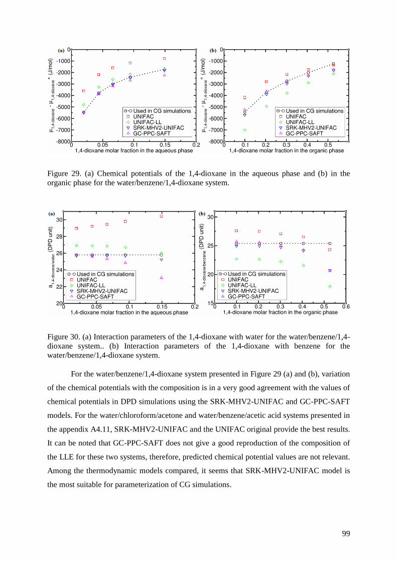
99

Figure 29. (a) Chemical potentials of the 1,4-dioxane in the aqueous phase and (b) in the

organic phase for the water/benzene/1,4-dioxane system.

Figure 30. (a) Interaction parameters of the 1,4-dioxane with water for the water/benzene/1,4-

dioxane system.. (b) Interaction parameters of the 1,4-dioxane with benzene for the

water/benzene/1,4-dioxane system.

For the water/benzene/1,4-dioxane system presented in Figure 29 (a) and (b), variation

of the chemical potentials with the composition is in a very good agreement with the values of

chemical potentials in DPD simulations using the SRK-MHV2-UNIFAC and GC-PPC-SAFT

models. For the water/chloroform/acetone and water/benzene/acetic acid systems presented in

the appendix A4.11, SRK-MHV2-UNIFAC and the UNIFAC original provide the best results.

It can be noted that GC-PPC-SAFT does not give a good reproduction of the composition of

the LLE for these two systems, therefore, predicted chemical potential values are not relevant.

Among the thermodynamic models compared, it seems that SRK-MHV2-UNIFAC model is

the most suitable for parameterization of CG simulations.

100

In Figure 30 (a) and (b), the interaction parameters of 1,4-dioxane with water and with

benzene are plotted as a function of the composition in the aqueous and organic phase,

respectively. Since there is a direct relationship between interaction parameters and chemical

potentials, SRK-MHV2-UNIFAC still provide the best interaction parameters compared to

those used in DPD simulations. However, it can be noticed that interaction parameters

obtained from thermodynamic models are sensitive to the composition. The composition

dependence of interactions parameters has already been studied in section 4.4.1. These results

obtained from the thermodynamic models confirm that the use of constant parameters over

the whole composition range is an important approximation in the DPD simulations

Finally, interaction parameters are calculated using the SRK-MHV2-UNIFAC model

for water/solute and organic compound/solute binary systems and results are presented in

Table 17. Parameters are calculated for a given composition since the equation (62) between

the chemical potential and the Flory-Huggins parameter involves the composition of the

system (volume fractions). The chosen composition corresponds to a relatively diluted system

with 1 mol% of solute and 99 mol% of solvent. This method consists, to a certain extent, in

calculating the activity coefficient at infinite dilution activity with a validated thermodynamic

model.

101

Table 17. Interaction parameters calculated for binary systems using the SRK-MHV2-

UNIFAC thermodynamic model for water/solute and organic compound/solute binary

systems. (Compositions: 1 mol% of solute and 99 mol% of solvent). Parameters are compared

with those obtained in CG simulations with approach #2 except for the

water/benzene/1,4-dioxoane system which is parameterized with approach #1.

Systems

𝑎𝑤𝑎𝑡𝑒𝑟/𝑠𝑜𝑙𝑢𝑡𝑒 𝑎𝑜𝑟𝑔𝑎𝑛𝑖𝑐 𝑐𝑜𝑚𝑝𝑜𝑢𝑛𝑑/𝑠𝑜𝑙𝑢𝑡𝑒

Used in CG

simulations

Calculated

for binary

systems

Used in CG

simulations

Calculated

for binary

systems

water/benzene/1,4-dioxane

(𝑁𝑚 = 5) 25.80 25.74 25.41 25.10

water/chloroform/acetone

(𝑁𝑚 = 4) 28.20 26.91 22.07 20.91

water/benzene/acetic acid

(𝑁𝑚 = 4) 21.38 23.97 31.12 30.45

water/benzene/2-propanol

(𝑁𝑚 = 5) 12.46 27.83 18.96 34.08

water/hexane/acetone

(𝑁𝑚 = 4) 23.58 26.91 27.44 33.83

water/hexane/2-propanol

(𝑁𝑚 = 4) 23.60 28.58 29.01 38.68

Table 17 shows that 𝑎𝑤𝑎𝑡𝑒𝑟/𝑠𝑜𝑙𝑢𝑡𝑒 and 𝑎𝑜𝑟𝑔𝑎𝑛𝑖𝑐 𝑐𝑜𝑚𝑝𝑜𝑢𝑛𝑑/𝑠𝑜𝑙𝑢𝑡𝑒 interaction parameters are in

good agreement with those used in CG simulations for the water/benzene/1,4-dioxane,

water/chloroform/acetone and water/benzene/acetic acid systems. These systems have been

well parameterized to represent liquid-liquid equilibrium and interfacial tension variation in

CG simulations. For water/benzene/2-propanol, water/hexane/acetone and water/hexane/2-

propanol systems, thermodynamic models predict higher interaction parameters than those

obtained with the approach #2. This result does not seem incoherent because higher

𝑎𝑠𝑜𝑙𝑢𝑡𝑒/𝑠𝑜𝑙𝑣𝑒𝑛𝑡 interaction parameters result in stronger repulsion between solute and solvent,

and consequently to/with a greater affinity of the solute to the interface. The IFT should be

reduced as compared to results obtained in DPD simulations shown in previous section 4.4.4.

In our simulations, the interfacial tension was overestimated for these systems. However, high

𝑎𝑠𝑜𝑙𝑢𝑡𝑒/𝑠𝑜𝑙𝑣𝑒𝑛𝑡 interaction parameters can lead to a phase separation between the solute and

102

the solvent as it has been shown for the water/hexane/2-propanol parameterized with the

approach #1.

In this section, thermodynamic models were used to calculate interaction parameters

of a solute in a solvent, and results were compared to those obtained from parametrization

approaches based on experimental data developed previously in this chapter. It has been

shown that SRK-MHV2-UNIFAC model provides interaction parameters of the same order of

magnitude as those used in DPD simulations for water/benzene/1,4-dioxane,

water/chloroform/acetone and water/benzene/acetic acid systems. It can be noted that these

interaction parameters are not precise enough to allow an accurate reproduction of LLE.

However, thermodynamic models allow calculating directly interaction parameters for

solute/solvent binary systems. This approach is therefore faster to calculate interaction

parameters compared to the other approaches based on LLE compositional data because it

does not need to represent a liquid-liquid equilibrium of ternary systems. Complex mixtures

such as crude oil require to estimate a large number of interaction parameters. Therefore, this

approach based on the SRK-MHV2-UNIFAC model will used to evaluate interaction

parameters for crude oil/water systems in the chapter V.

4.5.3 Transferability of interaction parameters for alkanes

In previous sections, parameterization approaches have been applied to

water/solvent/solute ternary systems with solvent belonging to hydrocarbon compounds. A

more complex systems such as a crude oil should result in a higher number of bead types, and

therefore, to a large number of interactions to be parameterized. Transferability of interaction

parameters could simplify the parameterization step. In this section, we present a study

carried out to evaluate the transferability of interaction parameters to representing a linear

alkane with a solute. Due to the chosen coarse-grained level, n-hexane molecule is

represented with two beads, n-nonane molecule with three beads, and n-dodecane molecule

with four beads (see Figure 31). The interactions of a solute (1,4-dioxane, acetone, acetic acid

and 2-propanol) with the three alkanes were calculated using the SRK-MHV2-UNIFAC

thermodynamic model et results are presented in Table 18. The results presented in Table 18

show that variation of the interaction parameters between the solute beads and the alkane

beads as function of the alkane length is low. Therefore, it seems reasonable in the case of

103

simulation of systems containing alkanes of different lengths to use the same solute/alkane

interaction parameters.

Figure 31. Representation of interactions between a solute and linear alkanes such as n-

hexane, n-nonane and n-dodecane.

Table 18. Interaction parameters calculated for n-alkane/solute binary systems using the

thermodynamic model SRK-MHV2-UNIFAC.

(Composition used is 1 mol% in solute and 99 mol% in hydrocarbon).

Systems 𝜒𝑖𝑗 𝑎𝑖𝑗 Systems 𝜒𝑖𝑗 𝑎𝑖𝑗

n-hexane/1,4-dioxane 2.23 32.82 n-hexane/acetone 2.53 33.86

n-nonane/1,4-dioxane 2.39 33.38 n-nonane/acetone 2.66 34.31

n-dodecane/1,4-dioxane 2.34 33.19 n-dodecane/acetone 2.52 33.83

Systems 𝜒𝑖𝑗 𝑎𝑖𝑗 Systems 𝜒𝑖𝑗 𝑎𝑖𝑗

n-hexane/acetic acid 3.10 35.87 n-hexane/2-propanol 3.87 38.54

n-nonane/acetic acid 3.35 36.71 n-nonane/2-propanol 4.09 39.30

n-dodecane/acetic acid 3.32 36.62 n-dodecane/2-propanol 4.01 39.03

104

4.6 Conclusions

A consistent methodology for parameterization of interaction parameters in DPD

taking into account the miscibility of species in a diphasic solution and to predict

quantitatively the interfacial tension is proposed in this chapter. Two parameterization

approaches based on the introduction of compositional data into equations of the Flory-

Huggins theory were applied. The first approach (#1) needs compositional data for only one

LLE and Hildebrand solubility parameter values, while the second approach (#2) is based on

several compositional data of LLE. Both approach are based on the main hypothesis that bulk

phases in LLE are totally immiscible (negligible partial solubility of solvent phases). The

influence of interaction parameters between like DPD particles on IFT and miscibility has

also been studied in the case of a third approach (#3) involving the isothermal compressibility

(𝜅𝑇) of each fluid and in the case of a fourth approach (#4) by adding a term corresponding to

the degree of coarse-graining for water beads. It is important to remark that parameterization

methods proposed in this chapter use phase compositions (or solubility) as input data,

independently of the source type. An additional study was performed to test the possibility to

use a thermodynamic model instead of experimental compositional data. We conclude that the

thermodynamic SRK-MHV2-UNIFAC model is a reliable source for predicting liquid-liquid

compositions when experimental data are not available for the different systems tested in this

manuscript.

Concerning the liquid-liquid equilibrium, CG-MC simulations in the Gibbs (NVT)

ensemble were carried out in order to compute the liquid-liquid equilibrium. This method

allows a precise determination of the phase diagram of considered ternary systems analyzed

in this manuscript (i.e. water/benzene/1,4-dioxane, water/chloroform/acetone and

water/benzene/acid acetic, water/benzene/2-propanol, water/hexane/acetone and

water/hexane/2-propanol). From comparisons drawn in this chapter dealing with different

methods to parameterize DPD simulations, among tested approaches, approach #2 appears as

the most accurate to reproduce LLE. In addition, the use of different parameters between like

beads (𝑎𝑖𝑖 ≠ 𝑎𝑗𝑗) slightly improve the miscibility between bulk phases.

One of the important contributions of this work is the use of CG-MC simulations in

the osmotic (µsoluteNsolventPzzT) ensemble for the preparation of systems with an explicit

interface within DPD simulations. This step allows to work rigorously at experimental

105

concentrations by computing the precise bulk phase compositions. Interface compositions can

then be predicted by means of DPD simulations. It is important to remark that the interface

composition in equilibrium with the bulk phases is a relevant property which is not easily

accessible experimentally. This is a crucial preliminary step to compute the interfacial tension

(by any molecular simulation method).

IFT for the ternary systems were calculated using DPD simulations. Our results show

that the proposed parameterization approaches allow us to reproduce qualitatively the

interfacial tension variation as a function of the solute molar fraction in the aqueous and

organic phases for the water/benzene/1,4-dioxane, water/chloroform/acetone and

water/benzene/acetic acid systems. Furthermore, predictions can be considered as quantitative

since we obtained good agreements between simulated and experimental data (𝑅𝐼𝐹𝑇2 > 0.893).

We observed that results on interfacial tension for systems containing intramolecular forces

are not accurate enough when compared with available experimental data. Noting that the

accuracy of predictions could be improved including an optimization of intermolecular forces

(which was out of the scope of the present work).

Among the parameterization approaches investigated in this chapter, approach #2

seems to be the best compromise for reproducing solute solubility in bulk phases and

quantitatively predicting interfacial tension. This option is the most appropriate if

experimental data is available on fluid composition. If only one experimental data of LLE is

available, approach #1 is perhaps the most convenient. If additional precisions on phase

densities are required, parameterization methods #3 and #4 may provide better results as

compared to approaches #1 and #2 since they account for the isothermal compressibility of

each solvent.

Finally, parametrization approaches presented in this chapter provide interaction

parameters when used within DPD simulations reproduce both liquid-liquid equilibrium and

interfacial tension values. These parameters have been used as a reference for selecting a

thermodynamic model. The chosen model, SRK-MHV2-UNIFAC, represents a fast and a

relatively reliable tool for estimating interaction parameters for much more complex systems.

Crude oils are among the most complex mixtures of chemical compounds, in the next chapter

we propose a novel methodology to predict IFT value for a system containing a crude oil and

water.

106

Chapter 5. Representation and coarse-grained

simulations of crude oils

5.1 Introduction

Representation of a crude oil in mesoscopic simulations is one of the main goals of

this PhD thesis. It has been shown in Chapter 1 that one of the major difficulties in the

representation of a crude oil stands in its molecular complexity. A petroleum mixture is

composed of thousands different molecules with a wide variety in size and molecular

structures. The exact composition of a crude oil remains inaccessible with the current

experimental methods of analysis, only average data can be provided, especially for the

heaviest fractions.

Several strategies have been developed to determine a simplified molecular structure

of crude oil based on the available experimental data. The three main approaches, developed

in chapter 2, are: (1) the fractionation approaches, (2) the lumped method and, (3) the

molecular reconstruction. So far, in most of published works dealing with the molecular

simulation of crude oils, the representative mixtures are based on the fractionation approach.

Using a SARA analysis based on polarity and solubility differences (see section 2.3.1.1 for

details), a crude oil can be represented by the four main fractions: saturates, aromatics, resins

and asphaltenes compounds. In order to obtain a more realistic representation of the molecular

composition of a petroleum fluid in coarse-grained simulations, we proposed a novel

methodology based on two approaches. The crude oil is separated according to the number of

carbon atoms into two fractions: C20- and C20+. The fraction C20- is represented using a method

based on lumping (labeled “Lumped” method) while the fraction C20+ is built using a

reconstruction method. These latter approaches will be explained and applied in more detail in

this chapter.

This crude oil representation will be considered in DPD simulations in order to

simulate crude oil/water systems. DPD model is a mesoscopic simulation method based on a

coarse-grained model where several atoms or molecules are grouped in a bead. By decreasing

the number of degrees of freedom in a system, a coarse-grained model allows to simulate

larger systems than classical “all-atoms” simulations. However, interactions between beads

107

must be parameterized in order to reproduce the targeted properties. In this work, interactions

must be parameterized to reproduce crude oil/water equilibrium and to predict the interfacial

tension. A parametrization method of the interactions between DPD beads has been

developed in Chapter 4. This method has been applied and validated for

water/hydrocarbon/solute ternary systems. In this chapter, the parameterization method will

be applied on the crude oil/water system.

The chapter is organized as follows: in section 2, we describe theoretical aspects about

the representation methods used for the light and heavy fractions, C20- and C20+, respectively.

In section 3, results from experiments and simulations performed on the crude oil

representations (light and heavy) are presented and converted according to the coarse-grained

model. Interaction parameters between DPD beads are calculated. In section 4, DPD

simulations are performed on crude oil/water system and the results are discussed. Finally,

section 5 contains our conclusions and perspectives.

108

5.2 Theoretical background for crude oil molecular representation

5.2.1 Representation of the light fraction (C20-): the Lumped algorithm

“Lumped” methods allow reducing the composition of a fluid to a few representative

compounds. The algorithm used in this work is known as “Dynamic clustering algorithm”. It

was developed by Montel and Gouel [35] in 1984 and was integrated in the IFPEN software

ReFGen (Representative Fuel Generator) [143].

The Lumped algorithm procedure is an iterative process and the steps are as follows:

1) A number 𝑛 of pseudo-components (or classes) is chosen.

2) The properties used for the Lumping procedure must be selected (here, 𝜔, 𝑀𝑤, 𝑛𝑐,

C/H ratio, 𝑇𝐶 and 𝑃𝐶.)

3) The 𝑛 major compounds are chosen to be the center of a class. During the first

iteration, the main compounds are determined randomly.

4) All properties 𝑃𝑟𝑜𝑝𝑁𝑖𝑘 of each class 𝑖 and property 𝑘 are normalized and

calculated using the equation below:

𝑃𝑟𝑜𝑝𝑁𝑖𝑘 =𝑃𝑟𝑜𝑝𝑖𝑘 −𝑀𝑖𝑛(𝑃𝑟𝑜𝑝𝑖𝑘 , 𝑖)

𝑀𝑎𝑥(𝑃𝑟𝑜𝑝𝑖𝑘 , 𝑖) − 𝑀𝑖𝑛(𝑃𝑟𝑜𝑝𝑖𝑘, 𝑖) (74)

Where 𝑀𝑖𝑛(𝑃𝑟𝑜𝑝𝑖𝑘 , 𝑖) and 𝑀𝑎𝑥(𝑃𝑟𝑜𝑝𝑖𝑘, 𝑖) are, respectively, the minimum and maximum

values of the kth property among the properties of the components belonging to the ith pseudo-

component. This calculation modifies all the properties to be in the range 0-1 and ensures that

all properties have the same weight.

5) Each component is allocated to the nearest center. To do so, distances of each

component (𝑖) to all the centres (c) are calculated as follow:

𝑑𝑖𝑐 =∑𝑃𝑘|𝑃𝑟𝑜𝑝𝑁𝑖𝑘2 − 𝑃𝑟𝑜𝑝𝑁𝑐𝑘

2 |

𝑁𝑃

𝑘=1

(75)

where 𝑁𝑃 is the number of properties used for the lumping and 𝑃𝑘 is the weight

associated to the property 𝑘.

109

6) The centres of all the classes can then be calculated by a weight average of the

properties 𝑃𝑟𝑜𝑝𝑁𝑖𝑘, the weight factors being the mole fractions:

𝑃𝑟𝑜𝑝𝑁𝑐𝑘 =∑𝑥𝑖𝑃𝑟𝑜𝑝𝑁𝑖𝑘

∑ 𝑥𝑖𝑖 (76)

7) These centres (c) are considered as new centres of the 𝑛 classes. New distances as

obtained in stage 5) are then calculated and an iterative calculation begins. The

calculation stops when no component changing classes from one stage to the next

one.

This algorithm provides a set of pseudo-components characterized by thermodynamic

and physicochemical properties, but they do not have a well-defined molecular structure. All

methods used to calculate the properties of the pseudo-components resulting from the

Lumping method are given in the appendix A5.2. To ensure that the mixture of pseudo-

components obtained using the Lumped method is consistent with the initial mixture; their

phase envelope (liquid-vapor equilibrium) and their distillation curve are compared.

Prediction of phase envelopes are obtained using the Peng-Robinson EoS [122].

5.2.2 Representation of heavy fractions (C20+)

To represent the heavy fraction, (C20+), two methods are used: the Stochastic

Reconstruction (SR) and the Reconstruction by Entropy Maximization (REM). These

methods were developed by Verstraete and coworkers at IFP Energies nouvelles [50, 55]. SR

is used to build a library of molecules whose properties are in agreement with experimental

data. REM is used to refine the results of SR method by adjusting the molar fraction of the

molecules in order to improve the representativeness of the generated mixture.

5.2.2.1 Stochastic reconstruction

SR is a method for building molecules to form a mixture whose properties are in

agreement with experimental data. Operations of the SR method are summarized on the flow

diagram proposed in Figure 32.

110

Figure 32. Flow diagram of the stochastic reconstruction method. Extracted from the work of

Pereira de Oliveira et al. [53]. “Reprinted with permission from de Oliveira, L. Pereira;

Vazquez, A. T.; Verstraete, J. J.; Kolb, M., Energy Fuels 2013, 27, 3622–3641. Copyright

(2013) American Chemical Society”.

Stochastic reconstruction is based on the assumption that a petroleum fraction can be

entirely characterized by a set of probability distribution functions of molecular structural

attributes. Any molecule in the petroleum feedstock can be considered to be an assembly of

molecular attributes (for example the type of a molecule, the number of aromatic rings in a

molecule, the number of aliphatic chains in a molecule, etc.). The occurrence frequency of the

attributes is given by a distribution probability function. By arranging molecular structures

next to each other, it becomes possible to form a molecule.

The molecular attributes used in stochastic reconstruction depend on the type of crude

oil fraction studied. Indeed, light fractions (for example gasolines or gas oils) do not contain

the same type of molecules as a heavy fraction (for instance vacuum residues). Molecular

attributes must be chosen on the basis of the chemical characteristics of the petroleum fraction

to be represented. Based on the work of Schnongs et al. [55], Oliveira de Pereira [53]

proposed to describe the fraction of vacuum residues with a total of 16 structural attributes.

The list of attributes, their possible values, their type of distribution function and the number

111

of parameters for the distribution functions used are presented in Table 19. These attributes

will be used to represent the heavy fraction of our crude oil in section 5.3.1.2.

Table 19. Definition of the structural attributes used in the stochastic reconstruction. Extracted

from the work of Pereira de Oliveira et al. [53]

Structural attribute Values Distribution Number of

parameters

1 Type of molecule[a] 0, 1, 2 or 3 Histogram 3

2 Number of cores 1 < X < 5 Exponential 1

3 Type of heterocycle[b] 0, 1, 2 or 3 Histogram 3

4 Number of benzene rings per core 1 < X < 5 Exponential 1

5 Total number of rings per core 0.5 < X < 2 Gamma 1

6 Number of thiophenes per core 0, 1 or 2 Histogram 2

7 Number of pyridines per core 0, 1 or 2 Histogram 2

8 Number of pyrroles per core 0, 1 or 2 Histogram 2

9 Number of furans per core 0, 1 or 2 Histogram 2

10 Acceptance probability for a peripheral

carbon 0 or 1 Histogram 1

11 Length of the paraffinic chains 1 < X < 10 Gamma 1

12 Length of an alkyl chain (lateral and

intercore) 1 < X < 10 Exponential 1

13 Probability of sulfur substitution for

aliphatic CH3 or CH2 0 or 1 Histogram 1

14 Substitution probability of a carbon atom

by a heteroatom 0 or 1 Histogram 1

15 Type of heteroatom substitution[c] 0 or 1 Histogram 1

16 Type of oxygen group[d] 0 or 1 Histogram 1

[a]Type of molecule: 0 – paraffin, 1 – naphthene, 2 – aromatic monocore, 3 – aromatic multicore.

[b]Type of heterocycle: 0 – thiophene, 1 – pyridine, 2 – pyrrole, 3 – furan.

[c]Type of heteroatom: 0 – nitrogen, 1 – oxygen.

[d]Type of oxygen group: 0 – ether function, 1 – carbonyl function

As shown in Table 19, molecules built from these attributes consist of carbon,

hydrogen, sulfur, nitrogen and/or oxygen atoms. Metals are not included because of their very

low content even in the heavier fractions. Each molecular attribute is associated with a

112

distribution function that describes the probability of finding each value of the corresponding

attribute. Ideally, this distribution function should represent the actual distribution of each

attribute in the petroleum fraction studied. However, in the case of heavy fractions, these

distributions are unknown because they are difficult to obtain experimentally. Therefore,

Oliveira de Pereira et al. have chosen flexible and configurable distribution functions such as

histogram functions, gamma functions, and exponential functions [49, 53]. The histogram

functions are used when the number of values of the attribute is less than 4 while the gamma

and exponential functions are chosen for attributes having a wide range of possible values.

The exponential function is preferred to the gamma function when low values of the attribute

are preponderant or required [53].

The last column of Table 19 shows the number of parameters for each of the

distribution functions. All these parameters must be determined and optimized (this step will

be discussed later). Optimization is a time consuming step, therefore, the number of

parameters must be limited. In the case of histograms, the number of parameters is equal to

the number of possible values of the structural attribute minus 1. For an exponential

distribution, there is only one parameter. The distributions in the form of a gamma law have

two parameters: a shape parameter α and a scale parameter β. In order to reduce the number

of parameters required for stochastic reconstruction, Oliveira de Pereira et al. [53] has fixed

the parameter β as twice the parameter α. Thus, the functions of gamma distributions are

limited to a single parameter. For the vacuum residue fractions, there are therefore a total of

24 parameters to be determined and optimized.

The construction of one molecule follows a construction diagram indicating the

relationship between molecular attributes and the order of assembly of molecular structures.

This diagram avoids the creation of impossible or improbable molecules. Following this

diagram, the distribution functions of each molecular attribute are sampled to determine the

number of each molecular structure in the molecule. Then, these structures are assembled

together to form a molecule. This process is repeated N times in order to construct an

equimolar mixture of N molecules. The construction diagram is specific to the oil fraction

(light or heavy) and the diagram used for heavy fractions is shown in Figure 33. These

construction diagram will be used to represent the heavy fraction of our crude oil in section

5.3.1.2.

113

Figure 33. Building diagram for residue fractions. Process A constructs a single polycyclic

core with side chains and heteroatoms. Extracted from [53]. “Reprinted with permission from

de Oliveira, L. Pereira; Vazquez, A. T.; Verstraete, J. J.; Kolb, M., Energy Fuels 2013, 27,

3622–3641. Copyright (2013) American Chemical Society”.

Sampling a distribution function means that a value of the attribute is chosen randomly

by following a statistical distribution. The sampling procedure is as follows:

- Discretization then truncation and normalization to 1, if the distribution function is

continuous (gamma and exponential functions).

114

- Creation of cumulative probability distribution from the distribution function

- A number between 0 and 1 is chosen randomly, which corresponds to the

probability of a molecular attribute value.

Figure 34 shows the sampling of the number of aromatic rings in a molecule. The

distribution function in this example is a histogram where four attribute values are possible

(i.e. the molecule may contain between 0 and 3 aromatic rings). The probability of having no

aromatic ring is 40% while the probability of having 1, 2 or 3 aromatic rings is 20% in each

case.

Figure 34. Sampling of a cumulative distribution function to define the number of aromatic

rings constituting a molecule. Extract from reference [144].

The physico-chemical and thermodynamic properties of molecules assembled by the

stochastic reconstruction method are calculated either by direct inspection of the structure of

the molecule (for example the chemical formula and molar mass) or from correlations and

group contribution methods (for example the boiling point and density). The properties of the

mixture formed by the molecules are calculated from the properties of the molecules weighted

by their molar fractions or from assumptions or correlations. All the correlation methods used

to calculate the properties of the molecules and the mixture are given in the Appendix A5.3.

The properties of the mixture are then compared with the experimental data using an

objective function. A minimization algorithm allows to minimize this objective function 𝐹 by

modifying the parameters of the probability distribution functions of the molecular attributes

so that the properties of the mixture are as close as possible to the experimental data. The

expression of the objective function is given in equation (77).

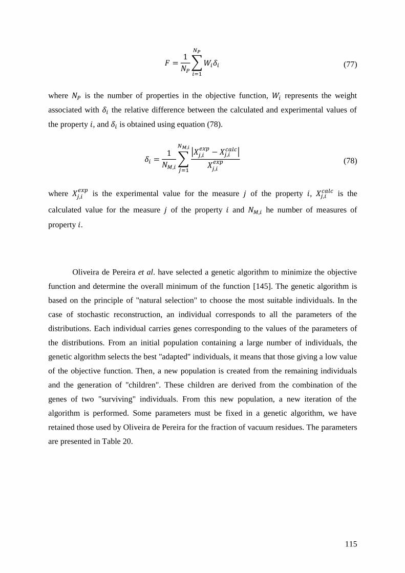
115

𝐹 =1

𝑁𝑃∑𝑊𝑖𝛿𝑖

𝑁𝑃

𝑖=1

(77)

where 𝑁𝑃 is the number of properties in the objective function, 𝑊𝑖 represents the weight

associated with 𝛿𝑖 the relative difference between the calculated and experimental values of

the property 𝑖, and 𝛿𝑖 is obtained using equation (78).

𝛿𝑖 =1

𝑁𝑀,𝑖∑

|𝑋𝑗,𝑖𝑒𝑥𝑝 − 𝑋𝑗,𝑖

𝑐𝑎𝑙𝑐|

𝑋𝑗,𝑖𝑒𝑥𝑝

𝑁𝑀,𝑖

𝑗=1

(78)

where 𝑋𝑗,𝑖𝑒𝑥𝑝

is the experimental value for the measure 𝑗 of the property 𝑖, 𝑋𝑗,𝑖𝑐𝑎𝑙𝑐 is the

calculated value for the measure 𝑗 of the property 𝑖 and 𝑁𝑀,𝑖 he number of measures of

property 𝑖.

Oliveira de Pereira et al. have selected a genetic algorithm to minimize the objective

function and determine the overall minimum of the function [145]. The genetic algorithm is

based on the principle of "natural selection" to choose the most suitable individuals. In the

case of stochastic reconstruction, an individual corresponds to all the parameters of the

distributions. Each individual carries genes corresponding to the values of the parameters of

the distributions. From an initial population containing a large number of individuals, the

genetic algorithm selects the best "adapted" individuals, it means that those giving a low value

of the objective function. Then, a new population is created from the remaining individuals

and the generation of "children". These children are derived from the combination of the

genes of two "surviving" individuals. From this new population, a new iteration of the

algorithm is performed. Some parameters must be fixed in a genetic algorithm, we have

retained those used by Oliveira de Pereira for the fraction of vacuum residues. The parameters

are presented in Table 20.

116

Table 20. Parameters of the genetic algorithm for vacuum residue reconstruction. Extracted

from the reference [53]

Parameters Values

Number of molecules per individual 5000

Number of iterations of the algorithm 100

Initial number of individual 2048

Maximum percentage of refused molecules 50

Average mutation percentage per individual 25

Number of crossover points 1

Population percentage kept for the next generation 50

Minimum number of individuals 128

Reduction rate of the number of individuals 1

Frequency of reevaluation of the parents 1

This parameterization of the genetic algorithm implies that the final mixture will

contain a total of 5000 molecules. It should be noted that stochastic reconstruction will

provide an equimolar mixture of 5000 molecules. But it does not mean that there will be 5000

different molecules. Two molecules may be strictly identical in the mixture, but they will be

treated independently and will each provide a molar fraction equivalent to 1/5000 (common

case with n-paraffins).

5.2.2.2 Reconstruction by Entropy Maximization

The Reconstruction by Entropy Maximization (REM) method was developed at IFP

Energies nouvelles by Hudebine and Verstraete [50, 54] to improve the concordance between

the properties of a mixture of molecules with the analytical data. The molar fractions of a

library of molecules are adjusted based on the entropy criterion. Originally formulated in the

context of Shannon's information theory [146], this entropic criterion could be adapted for the

study of oil composition. The term of entropy S in equation (79) must be maximized in order

to obtain the optimal result:

𝑆 = −∑𝑥𝑖 × ln 𝑥𝑖

𝑁

𝑖=1

(79)

117

with

∑𝑥𝑖 = 1

𝑁

𝑖=1

(80)

where 𝑁 is the total number of molecules in the library and 𝑥𝑖 is the molar fraction of the

molecule 𝑖.

The entropic term measures the homogeneity of the molar fractions of the molecules.

Maximizing this term ensures that the distribution of molecules is as uniform as possible.

However, if the value of the entropic term is maximized without setting any constraints, the

distribution of the molecules will be equimolar (as it is by default by the SR method described

before). Constraints correspond to the analytical data and are added to the entropic term by

means of Lagrange parameters as shown in equation (81):

𝐻 = −∑𝑥𝑖 ∙ ln 𝑥𝑖

𝑁

𝑖=1

+ 𝜇 ∙ (1 −∑𝑥𝑖

𝑁

𝑖=1

) + ∑𝜆𝑗

𝐽

𝑗=1

∙ (𝑓𝑗 −∑𝑥𝑖

𝑁

𝑖

∙ 𝑓𝑖,𝑗) (81)

where 𝐻 represents the information entropy criterion, 𝑓𝑗 is the value of the constraint 𝑗, 𝑓𝑖,𝑗

represents the property or coefficient of molecule 𝑖 for constraint 𝑗, 𝜇 represents the Lagrange

multiplier associated with the mass balance constraint, 𝜆𝑗 represents the Lagrange multiplier

associated with constraint 𝑗, and 𝐽 is the total number of equality constraints.

In the equation (81), the first, second and third terms represent the information entropy, the

mass balance and the constraint associated with the analytical data, respectively. By

maximizing the entropy criterion with exact linear constraints, the number of initial unknowns

(equal to N + J) is reduced to a problem with only J unknowns, these unknowns are then the

Lagrange multipliers λ associated with each constraint.

118

5.3 Results

A sample of a crude oil available at IFP Energies nouvelles was used as a study case.

This crude oil has a API of 32 indicating a light crude oil. The light fraction (C20-)

corresponds to compounds whose boiling point is lower than 344 °C while the heavy fraction

(C20+) contains compounds whose boiling point is higher than 344 °C. The light fraction

represents 46 % by weight (and 73% by mole) and the heavy fraction 54% by weight (and

27% by mole). Experimental data of the two fractions are given in the appendices A5.1.

5.3.1 Molecular model of crude oil

5.3.1.1 Application of the Lumped method to the light fractions (C20-)

For the light fraction, the detailed composition is unknown but a simulated distillation

curve (ASTM D2887) is available. Therefore, a “breakdown” procedure is applied to define a

list of pseudo-components as explained in section 2.3.1.2. It should be noted that the

breakdown procedure can be perform only on TBP distillation curve using the ReFGen

software. To convert the simulated distillation curve into a TBP curve, we chose the

procedures developed by Daubert and presented in the sixth edition of API-TDB [147]. The

simulated distillation curve (ASTM D2887) is converted to an ASTM D86 distillation curve

according to the 3A3.2 procedure. Then, the resulting ASTM D86 curve is converted to a

TBP distillation curve using the procedure 3A1.1. This two-step methodology provides

slightly better results than a direct conversion of a simulated distillation curve to a TBP curve

[147]. Conversion of the experimental simulated distillation curve into an ASTM D86 then a

TBP curve can be found in the Appendix A.5.2.

Then, the TBP distillation curve is divided into 20 equivalent temperature intervals.

For each interval is assigned a pseudo-component whose boiling temperature and volume

fraction are estimated from the distillation curve according to the “breakdown” procedure.

The density is estimated using the Watson approach [25]. Other thermodynamic properties of

the pseudo-components (critical properties and acentric factor) can be obtained using

correlations. The properties and the reference of the correlations used to characterize the

pseudo-components derived from the distillation curve are provided in the Appendix A.5.2.

119

Pseudo-components derived from the distillation curve are used as initial fluid in the Lumped

method. Thus, this representation of 20 pseudo-components is reduced, using the lumping

algorithm, to a final fluid consisting of 5 pseudo-components. To compare the final fluid with

the initial fluid, the phase envelope and the distillation curve of each fluid were plotted and

the results are shown in Figure 35.

Figure 35. Comparison between the initial fluid (20 pseudo-components) and the final fluid

resulting from the Lumped method (5 pseudo-components). The calculated phase envelopes

are shown on the left (a) and the calculated distillation curves on the right (b).

Figure 35 (a) shows a very good agreement between the initial fluid and finalist

representation (final fluid) on the liquid/vapor equilibrium. Deviations between distillation

curves occur for temperatures above 300°C as presented in Figure 35 (b). The physico-

chemical and thermodynamic properties of each of the five pseudo-components of the final

fluid are presented in Table 21. In addition, a representative molecule extracted from a

gasoline database that contains about 250 molecules [37] was assigned to each pseudo-

component. This molecule is chosen so that the difference between the properties of the

molecule and the pseudo-component is minimized. The chemical structure of the

representative molecules (C20- fraction) are given in Table 22. Coarse-grained models for

these molecules are also presented in Table 22 and will be explained in more details in section

5.3.2. The Lumped method seems to be an effective approach to represent the light fraction of

a crude oil. The main advantage of this method is that it provides a very small number of

representative molecules of the oil fraction.

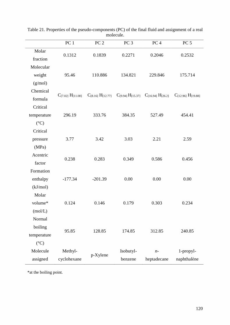
120

Table 21. Properties of the pseudo-components (PC) of the final fluid and assignment of a real

molecule.

PC 1 PC 2 PC 3 PC 4 PC 5

Molar

fraction 0.1312 0.1839 0.2271 0.2046 0.2532

Molecular

weight

(g/mol)

95.46 110.886 134.821 229.846 175.714

Chemical

formula C[7.02] H[11.08] C[8.16] H[12.77] C[9.94] H[15.37] C[16.94] H[26.2] C[12.96] H[19.88]

Critical

temperature

(°C)

296.19 333.76 384.35 527.49 454.41

Critical

pressure

(MPa)

3.77 3.42 3.03 2.21 2.59

Acentric

factor 0.238 0.283 0.349 0.586 0.456

Formation

enthalpy

(kJ/mol)

-177.34 -201.39 0.00 0.00 0.00

Molar

volume*

(mol/L)

0.124 0.146 0.179 0.303 0.234

Normal

boiling

temperature

(°C)

95.85 128.85 174.85 312.85 240.85

Molecule

assigned

Methyl-

cyclohexane p-Xylene

Isobutyl-

benzene

n-

heptadecane

1-propyl-

naphthalène

*at the boiling point.

121

Table 22. Chemical structures and coarse-grained models of the representative molecules of

the light fraction. The degree of coarse-graining is 𝑁𝑚 = 4 (the volume of a bead corresponds

to 4 water molecules).

Light fraction (C20-)

Molecular representation Coarse-grained representation

Methylcyclohexane

Methylcyclohexane

p-Xylene

p-Xylene

Isobutylbenzene

Isobutylbenzene

n-heptadecane

n-heptadecane

1-propyl-naphthalene

1-propyl-naphthalene

5.3.1.2 Molecular reconstruction of the heavy fractions (C20+)

In a first step, the heavy fraction of the crude oil was reconstructed with 5000

molecules using RS method. Then, the RME method is used to adjust the mole fractions. In

the case of our study, the measured experimental data are an elemental analysis (C, H, O, N,

122

S), a SARA analysis and a simulated distillation curve. It is well known that experimental

measurements of the molecular weight are not accurate for the heavy fractions [1, 9] (see

section 2.2.3). Therefore, the molecular weight is calculated according to the Goossens

approach detailed in the reference [148]. The comparison of the properties of the mixture with

the experimental data is presented in Table 23. The parameters of the distribution functions

for the reconstruction of the mixture of 5000 molecules can be found in the Appendix A5.3.

Table 23. Comparison of experimental and calculated properties of mixtures representing the

C20+ fraction (with 5000 or 10 molecules) obtained using the Stochastic Reconstruction (SR)

and the coupling between the SR and the reconstruction by entropy maximization (SR/REM).

5000 molecules 10 molecules

Unity

Experimental

data SR SR/REM SR/REM

Elemental

analysis

Carbon % (w/w) 84.521 84.287 84.520 84.320

Hydrogen % (w/w) 11.433 11.463 11.429 11.582

Sulfur % (w/w) 3.604 3.790 3.610 3.394

Nitrogen % (w/w) 0.191 0.185 0.191 0.191

Oxygen % (w/w) 0.251 0.276 0.251 0.515

Molecular

weight

g/mol 494.87 501.9 494.7 506.0

Simulated

distillation

2 % weight °C 374.1 247.9 364.8 380.6

6 % weight °C 391.4 333.8 391.4 398.9

10 % weight °C 405.0 367.6 404.6 398.9

14 % weight °C 417.2 392.2 417.1 445.1

18 % weight °C 428.6 409.7 428.8 445.1

22 % weight °C 440.1 429.4 440.0 445.1

26 % weight °C 452.1 450.5 452.1 445.1

30 % weight °C 464.5 468.1 464.6 445.1

34 % weight °C 476.5 487.2 476.5 445.1

38 % weight °C 489.4 506.3 489.5 540.1

42 % weight °C 502.6 526.4 502.6 540.1

46 % weight °C 516.2 548.7 516.3 540.1

50 % weight °C 532.4 573.7 532.1 561.6

54 % weight °C 545.4 597.3 545.5 561.6

58 % weight °C 562.7 621.3 563.0 585.6

123

62 % weight °C 577.9 647.4 578.3 585.6

66 % weight °C 595.3 671.6 595.6 585.6

70 % weight °C 614.2 697.5 614.3 585.6

74 % weight °C 634.7 727.7 635.4 585.6

78 % weight °C 658.1 757.5 658.3 585.6

82 % weight °C 686.8 784.4 686.6 916.1

86 % weight °C 714.2 814.8 714.1 916.1

90 % weight °C 740.0 858.3 741 916.1

SARA

Saturates % (w/w) 30.493 31.96 30.49 30.88

Aromatics % (w/w) 45.585 44.22 45.57 46.25

Resins % (w/w) 22.177 21.46 22.18 22.87

Asphaltenes % (w/w) 1.745 2.36 1.75 0.00

In the case of the mixture of 5000 molecules, Table 23 shows relatively large

deviations after the SR method compared to reference experimental data. The largest

differences is obtained for the distillation curve with some differences higher than 100 °C.

However, after the REM step, a very good agreement is obtained between the properties of

the mixture and the experimental data.

Although the stochastic reconstruction method was originally designed to build

libraries of several thousand molecules, this approach can also be used to build a mixture of

only 10 molecules (which is more suitable to perform molecular simulation). Following the

same methodology, RS method has been applied to the heavy fraction to build a mixture of 10

molecules. However, the REM step has reduced the representation to 8 molecules. Indeed, the

molar fraction of two molecules of the mixture tends to zero. Although the final mixture is

reduced, Table 23 shows good agreement between the properties of the mixture of 8

molecules and the experimental data. It can be noted that no asphaltene molecule is

constructed because of its very low concentration in the heavy fraction (less than 1.745 % by

weight). The chemical structure and the coarse-grained model of the representative molecules

(C20+ fraction) are given in Table 24. Construction of the coarse-grained model will be

explained in more details in section 5.3.2.

124

Table 24. Chemical structures and coarse-grained models of the representative molecules of the heavy fraction. For reasons of readability, an

identification number (ID) is given to each molecule. The chemical family according to the SARA separation and the molar percentage of each

molecule is given in the third column. The degree of coarse-graining is 𝑁𝑚 = 4 (the volume of a bead corresponds to 4 water molecules).

Molecular representation Coarse-grained representation (ID) / Chemical family / % mole

(1) / Resin / 5.43 %

(2) / Aromatic / 7.19%

(3) / Saturate / 17.15%

125

(4) / Aromatic / 9.08%

(5) / Resin / 6.89%

(6) / Aromatic / 39.04%

(7) / Saturate C25H52 / 8.80%

(8) / Saturate C21H46 / 6.43%

No coarse-grained model (9) / Saturate / 0.00%

No coarse-grained model (10) / Saturate C22H44 / 0.00%

126

5.3.2 Coarse-grained model of crude oil

To perform CG simulations, molecular representation of light fraction (C20-) and heavy

fraction (C20+) are converted into a coarse-grained model. In this work, the coarse-grained

model is built according to three criteria. The first one is to represent as closest as possible the

same molecular volume in the DPD beads. Indeed, it has been shown that DPD simulations

leads to more accurate results on IFT when the beads represent the same molecular volume

[91, 92]. The second criterion is to preserve the chemical structure and the chemical

properties of the molecules. A particular attention has been given to the chemical functions

containing heteroatoms. These functions generate attractive interactions such as hydrogen

bonds and influence the miscibility of molecules and the value of the interfacial tension.

Finally, the coarse-grained representation must be limited to only a few types of beads. In

doing so, the number of interactions that must be parameterized remains limited.

As the light fraction of the crude oil contains the smallest molecules, the maximum

size of the beads is constrained by the size of the molecules in the light fraction (i. e. beads

should be small enough to represent each molecule of the light fraction). The light fraction is

used to define the building blocks of hydrocarbon molecules. The main building blocks are

the aromatic rings, naphthene rings, n-paraffins consisting of three carbon atoms and

i-paraffins of four carbon atoms as shown in Table 22. At ambient conditions, the molecular

volume of aromatic and naphthene rings is around 150 Å3 (Vbenzene ≈ 148 Å3 and Vcycloalkane ≈

150 Å3) while a linear chain of three carbon atoms is around 109 Å3 (based on half the

molecular volume of hexane). In this work, the bead volume, 𝑣𝑏, is defined as 𝑣𝑏 = 𝑁𝑚 ×

(volume of a water molecule), where 𝑁𝑚 is the degree of coarse-graining. Since the

molecular volume of a water molecule is 30 Å3 at ambient conditions, a degree of coarse-

graining set to 𝑁𝑚 = 4 seems to be the best compromise to meet the first criterion on

molecular volume. Therefore, the bead volume is equal to 𝑣𝑏 = 120 Å3. The cut-off radius is

given from the volume of the beads with 𝑟𝑐 = (�̅� × 𝑣𝑏)1/3. With an overall DPD number

density �̅� set to 3, the cut-off radius is equal to 𝑟𝑐 = 7.11 Å.

In this work, we have selected a set of eleven different chemical structures as building

blocks (DPD beads) for the mesoscopic model as can be seen in Figure 36. In order to

preserve the chemical properties, five building blocks are used to represent the different

chemical functions of heteroatoms: thiol, thiophene, pyridine, phenol and furan.

127

Figure 36. List of beads used to represent the considered crude oil. Water beads contain four

molecules of water (𝑁𝑚 = 4).

For the heavy fraction, it can be noticed that many methyl groups are attached to the

carbon atoms of aromatic rings and naphthene rings (see Table 24). Methyl groups are too

small to be represented by a bead; their molar volume would not be represented. Therefore,

we have decided to distinguish two types of aromatic rings: aromatic rings substituted by one

or more methyl groups, which are represented by a p-xylene bead, while aromatic rings where

no methyl group is attached are represented by a benzene bead. It can be noted that alkyl

groups containing two or three carbon atoms are represented by an n-paraffin bead.

128

5.3.3 Parameterization of interactions for DPD simulations

The parameterization of interactions between DPD beads is carried out in order to

reproduce crude oil/water equilibrium and to predict the interfacial tension. The methodology

proposed here is based on the previous work (presented in Chapter 4) where

water/hydrocarbon/solute ternary systems have been parameterized. Beads used in the coarse-

grained representation of the crude oil can be classified into three categories: water beads that

represent the aqueous phase, hydrocarbon beads that represent the organic phase and

compounds with a heteroatom that represent chemical functions present in some crude oil

molecules. The parameterization of pair interactions between these chemical functions (DPD

beads) is a key point to reproduce the crude oil/water equilibrium. Indeed, the presence of one

or several chemical functions in some molecules in crude oil can promote attractive

interactions with water such as hydrogen bonds. These molecules could migrate to the

interface and influence the value of the interfacial tension. In some way, chemical functions

can be compared to the solute molecules, with the difference that chemical functions are part

of hydrocarbon molecules while solute are independent.

Based on the methodology presented in Chapter 4, interaction parameters for a crude

oil/water system are obtained as follows:

- Interactions between like beads. The corresponding interaction parameters are

calculated from the isothermal compressibility of water as proposed by Groot and

Warren [63]. (here, 𝑎𝑖𝑖 = 𝑎𝑗𝑗 = 25)

- Water/Hydrocarbon interactions. These interactions are calculated from the

Hildebrand solubility parameters. As shown in section 4.2, this approach provides

quantitative values of IFT in agreement with experimental data.

- Functional group/water and functional group/hydrocarbon interactions. It has

been shown in Chapter 4 (see section 4.5.2) that a suitable thermodynamic model

can be used to calculate solute/solvent interaction parameters. This method allows

calculating the interaction of a solute in a solvent environment. We propose to use

the thermodynamic model SRK-MHV2-UNIFAC to determine the functional

group/water and functional group/hydrocarbon interactions (for compositions at

1% mol in functional group and 99% mol in water or hydrocarbon).

- Functional group/functional group interactions. These interaction parameters are

calculated using Hildebrand solubility parameters despite the polarity of the

129

molecules represented and the formation of electrostatic bonds. We assume that

functional group concentration is low, and therefore, the number of functional

group/functional group interactions is too small to influence the result of the

simulations.

Interactions parameters for the crude oil/water system are presented in Table 25.

Hildebrand solubility parameters are extracted from the DIPPR [117] and are given in the

appendix A5.4.

Table 25. Interaction parameters calculated for the crude oil/water system (in DPD unit).

Parameters are obtained from the isothermal compressibility of water , parameters

which are calculated using a thermodynamic model , and parameters which are

calculated using the Hildebrand solubility parameters .

It can be noted that interactions with furan beads could not be calculated using the

thermodynamic model SRK-MHV2-UNIFAC. Furan parameters are not available in our

UNIFAC parameters database [131]. Therefore, Hildebrand solubility parameters were used.

Indeed, In addition, the reference molecule for calculating interactions with n-paraffin and i-

paraffin are n-hexane and 2-butane, respectively.

Table 25 shows, as expected, a strong repulsion between hydrocarbon and water

beads. The i-paraffin exhibits the strongest repulsion with water (𝑎𝑖−𝑝𝑎𝑟/𝑊 = 152.1) while

benzene is the hydrocarbon with the lowest repulsion with water (𝑎𝑏𝑒𝑛𝑧/𝑊 = 111.6). These

strong repulsions demonstrate the poor miscibility between hydrocarbons and water, and

therefore, the formation of an interface.

The repulsion between two hydrocarbon beads is weak with interaction parameter

values between 25.1 and 28.9 (DPD unit). It should be emphasized that these interaction

parameters cannot be less than 25 because we used Hildebrand solubility parameters to feed

130

equation (59). It can be noticed that the repulsion between two hydrocarbons of different

chemical families (saturate/aromatic interactions) tends to be stronger than between two

identical families (saturate/saturate or aromatic/aromatic interactions). For example,

the n-paraffin/methylcyclohexane interaction parameter (𝑎𝑛−𝑝𝑎𝑟/𝑐𝑦𝑐𝑙 = 25.1) is lower than

n-paraffin/benzene interaction parameter (𝑎𝑛−𝑝𝑎𝑟/𝑏𝑒𝑛𝑧 = 26.5). Similarly, the

p-xylene/benzene interaction parameter (𝑎𝑝−𝑥𝑦𝑙/𝑏𝑒𝑛𝑧 = 25.1) is lower than the

n-paraffin/benzene interaction parameter (𝑎𝑛−𝑝𝑎𝑟/𝑏𝑒𝑛𝑧 = 26.0).

Values of interaction parameters between functional groups and water are between

19.3 and 113.0 (DPD unit). The magnitude of the interaction parameter between furan and

water (𝑎𝑓𝑢𝑟/𝑊 = 113.0) can be explained by its lows solubility in water. Experimentally, the

solubility of furan in water is about 0.15 mol/L at 25 °C [149]. On the contrary, interaction

between thiol and water are favorable (𝑎𝑇ℎ𝑙/𝑊 = 19.3). The presence of thiol function in a

molecule should favor its migration towards the interface. It should be noted that, in most

cases, functional groups/hydrocarbons and functional groups/water interactions are of the

same order of magnitude.

In this work, intramolecular forces are added to bind two neighboring beads in a

molecule and to maintain the structural conformation of the molecules. Although

intramolecular parameters can affect the results of simulations, optimization of these forces is

out of the scope of this work. Parameters for bond forces are 𝐾𝑏𝑜𝑛𝑑 = 100 (DPD unit) and

𝑟0 = 0.7 𝑟𝑐. These values are commonly used in the literature for bond forces [84, 94, 150,

151]. Some bond angle bending and torsional rotations are added to represent the rigidity of

fused rings. The parameter for the harmonic bending is 𝐾𝑏𝑒𝑛𝑑 = 6 and parameters for torsion

potentials, presented in Table 26, derived from a fitting a harmonic potential using a constant

of angle 𝐾𝑡𝑜𝑟𝑠 = 6 to the equation (18) (see section 3.2.2).

Table 26. Parameters for torsion potentials (in DPD unit) derived from a fitting on a harmonic

potential using 𝐾𝑡𝑜𝑟𝑠 = 6.

𝑎0 14.8651 𝑎5 23.0215

𝑎1 -18.0499 𝑎6 -37.0607

𝑎2 3.3179 𝑎7 -20.2979

𝑎3 -12.0708 𝑎8 26.3820

𝑎4 19.9738

131

5.4 Results of DPD simulations of crude oil

DPD simulations of crude oil/water systems were performed in the NVT ensemble

using the molecular dynamics simulation package NEWTON [113]. Initial boxes containing a

total of 162 000 beads are built using the PACKMOL software package [111, 112]. Boxes

dimensions were set to 𝐿𝑧 = 60, 𝐿𝑥 = 𝐿𝑦 = 30 (in DPD units). Two planar interfaces are

created normal to the z-axis. A modified version of the velocity-Verlet algorithm governed

the equation of motion, and the time step is fixed at δt = 0.01 in DPD units. Constants in the

dissipative force γ and random force σ were set to 4.5 and 3, respectively; in order to keeps

the temperature fixed at 𝑘𝐵𝑇 = 1, thus satisfying the fluctuation-dissipation theorem. In all

simulations, periodic boundary conditions were imposed in all directions. The molar fraction

of each molecule calculated according to the experimental data and the composition of the

simulations boxes are given in the appendix A5.4. An image of the simulation box is shown in

Figure 37 (a), the same simulation box is also presented (removing hydrocarbon and water

beads) with only the beads corresponding to the functional groups in Figure 37 (b).

Figure 37. (a) Simulation box containing the crude oil/water system. (b) Simulation box

containing the crude oil/water system where only the chemical functions are displayed. Water

beads are in blue, hydrocarbon in silver, furan in green, phenol in red, thiophene in yellow,

thiol in orange and pyridine in purple.

132

Simulations have been carried out using 1 500 000 steps of equilibration and 300 000

steps of production. IFT values are calculated using local method proposed by Irving and

Kirkwood (see section 3.4.3). DPD simulations of the crude oil/water system were performed

using four independent initial configurations. The values of the IFT obtained are between

30.19 and 31.59 mN/m (i.e. 3.71 and 3.88 in DPD units), and the average value and the

standard deviation are given in Table 27. The values of the IFT seem to be in a relatively

narrow range, which shows that the initial configuration does not influence on the results.

Table 27 shows that the value of the calculated interfacial tension for the crude

oil/water system is in very good agreement with the experimental data. The relative deviation

is about 5.04%. It should be noted that the experimental value is given with a salt (mainly

NaCl) concentration of 5g/L (≈ 0.1 mol/L). This concentration seems to be sufficiently low to

be neglected.

Table 27. Average values of the interfacial tension obtained from DPD simulations.

𝐼𝐹𝑇𝑐𝑎𝑙𝑐𝑢𝑙𝑎𝑡𝑒𝑑

𝑎𝑣𝑒𝑟𝑎𝑔𝑒

(in DPD units)

𝐼𝐹𝑇𝑐𝑎𝑙𝑐𝑢𝑙𝑎𝑡𝑒𝑑𝑎𝑣𝑒𝑟𝑎𝑔𝑒

(in mN/m)

𝐼𝐹𝑇𝑒𝑥𝑝𝑒𝑟𝑖𝑚𝑒𝑛𝑡𝑎𝑙

(in mN/m)

Crude oil/water 3.78 ± 0.08 30.78 ± 0.61 29.3 ± 0.2

C20-/water 4.68 ± 0.03 38.05 ± 0.24 Not available

C20+ /water 3.28 ± 0.07 26.70 ± 0.54 Not available

The interfacial tension between the light fraction and water as well as between the

heavy fraction and water were computed using DPD simulations. Results presented in Table

27, show that the light fraction leads to higher values of IFT than the heavy fraction. In

addition, the molecules of the heavy fraction represent only 26.9% in mole of the total

number of molecules in the crude oil. The heavy fraction appears to significantly reduce the

value of the crude oil/water IFT.

The density profile of the crude oil/water system is shown in Figure 38. For reasons of

readability, only the density of the molecules of the heavy fraction and water are displayed.

Molecules are indicated by their ID number (attributed in Table 24).

133

Figure 38. Density profile of the crude oil/water system. Only the molecules of the heavy fraction are given, molecules of the light fraction are

not displayed. For reasons of readability, molecules are indicated by their ID number, the chemical family according to the SARA separation and

the functional groups included in the molecule. Note that the density of water has been halved.

134

Figure 38 shows clearly that two molecules of the heavy fraction have migrated to the

interface: the aromatic molecule (6) with a thiol group in its structure and the resin (5) with a

pyridine group. The migration of these molecules towards the interface can be explained by a

lower functional group/water interaction parameter than functional group/hydrocarbons

interaction parameters (see Table 25). The presence of certain functional groups such as thiol

or pyridine seems to lead some molecules to behave like a “natural surfactant” of the crude

oil.

5.5 Conclusions

A representation of a crude oil with a limited number of compounds has been

developed based on a separation according to the number of carbon atoms: C20-/C20+. This

approach was applied to a crude oil that have been analyzed at IFP Energies nouvelles. A

Lumped method was applied to the light fraction C20- using the RefGen tool. From a

distillation curve and a molecular database of a gasoline, a representation with only 5

representative molecules has been established. The heavy fraction C20+ was reconstructed

using the Stochastic Reconstruction (SR) method and the Reconstruction by Entropy

Maximization method (REM). The SR allows generating mixture of representative

compounds based on a large number of experimental data. Then, the mole fraction of each

compound is optimized by the REM method in order to refine the agreement with the

experimental data. Thus, the heavy fraction has been represented with only 8 molecules. The

methodology proposed in this chapter allows representing the molecular composition of a

crude oil with only 13 molecules.

The molecular representation of the crude oil has been converted into a coarse-grained

model. Criteria were applied to select the DPD beads which are the most representative of the

different molecular structures. A set of only 11 DPD bead types was used to represent the

crude oil and water: 1 type of bead to represent 4 water molecules, 5 types of beads to

represent hydrocarbons and 5 types of beads to represent the different heteroatoms present in

the molecules of the crude oil.

Interaction parameters between the DPD beads were calculated based on the method

described in chapter 4. One of the key points of the parametrization method is to use a

135

thermodynamic model, SRK-MHV2-UNIFAC, which has been validated to represent liquid-

liquid equilibria and to predict the interfacial tension. Results of DPD simulations of crude

oil/water systems show a good agreement on IFT values compare to the experimental data

with a relative deviation about 5.04%. The density profile analysis revealed that among the

molecules in the heavy fraction, two molecules tend to migrate to the interface and to lower

the interfacial tension. The presence of thiol and pyridine functional groups appears to favor

interactions of molecules with the interface.

136

General conclusion

The objective of this work is to represent a crude oil in mesoscopic simulations in

order to predict interfacial phenomena. Representation of a chemical system in molecular

modeling tool consists of (1) establishing a molecular representation and (2) defining the

interactions between the compounds. However, it has been shown, in Chapter 1, that crude oil

is a complex mixture that contains thousands of different molecules. The complexity of the

fluid stands in the diversity in molecular structures and in molecular sizes. Therefore, it is not

currently possible to introduce in any type of molecular modeling tool the total and exact

composition of a crude oil. On the one hand, there is no experimental analysis that can

provide the exact composition of a crude oil, and on the other hand, computational

capabilities for numerical simulations are far from sufficient to deal with such systems.

Experimental analyzes commonly used in the oil and gas industry (presented in

Chapter 2) provide average or global information of crude oils and their fractions. A state of

the art has been conducted on the representation methods of crude oils and it has shown that

three main approaches can be distinguishable: (1) fractionation approaches, (2) lumping

method (suitable for light fractions) and (3) molecular reconstruction (mainly for heavy

fractions). Representation of a crude oil for molecular simulation tools must be constructed

using a limited number of compounds and rely on available experimental data. Fractionation

approaches based on separation of a components of a fluid according to differences in polarity

and solubility (SARA fractions) have already been used to represent a crude or its heavy

fractions in molecular simulations. We have proposed a representation methodology for crude

oils that combines the lumping method and the molecular reconstruction (SR/REM2). A crude

oil is divided into two fractions according to the number of carbon atoms: C20- and C20+. The

lumping method is used on the light fraction while the heavy fraction is built using the

SR/REM methods. This approach allows both to construct a representation based on a large

number of experimental data and to limit the number of representative compounds. By

applying this approach on a light crude oil that has been analyzed at IFPEN, a set of only 13

representative molecules were obtained.

The number and size of the molecules contained in crude oils as well as the thickness

of the interface with water require to simulate large systems over long period time. Atomistic

2 Stochastic Reconstruction and Reconstruction by Entropy Maximization

137

simulations cannot handle such scale, and mesoscopic simulation methods based on a coarse-

grained (CG) model are more suitable. CG model consists to group atoms or molecules in

particles (called “beads) in order to simplify the description of systems. Coarse-Grained

Monte Carlo methods and Dissipative Particle Dynamics simulations have been retained to

carry out this work (Chapter 3).

Interactions between beads have been parameterized in order to reproduce the

miscibility between the compounds, and the transferability of parameters to predict the

targeted properties which is the IFT has been validated. In first step, a parameterization study

has been conducted on liquid-liquid equilibria (LLE) of ternary systems in which a solute is

partially miscible in the bulk phases (Chapter 4). Several parameterization approaches have

been proposed and compared on the basis of compositional data of LLE. It has been shown

that the use of the Helmholtz free energy in the Flory-Huggins theory (called approach #2)

represents the best parameterization approach among the evaluated ones to reproduce

experimental LLE and quantitatively predict the IFT. In a second step, a methodology based

on the osmotic ensemble (µsoluteNsolventPzzT) using CG-MC simulations has been proposed to

preserve the bulk concentration from the migration of solute toward the interface. In a third

step, when experimental data are scared or absent, the use of thermodynamic models to

predict LLE compositional data to parameterize the approach selected in step one has been

investigated. It has been shown that SRK-MHV2-UNIFAC is the best model for LLE

predictions. This latter approach represents a fast method to parameterize systems with a large

number of chemical families.

The simplified model of crude oil containing 13 representatives molecules has been

coarse-grained (i.e. 4 water molecules in a water bead) conserving as much as possible the

molecular structure and the chemical properties of molecules. Interactions between beads

have been parameterized using an approach developed in this manuscript (Chapter 4) and

using the SRK-MHV2-UNIFAC model. DPD simulations have been carried out on crude oil

model, and results on interfacial tension are in very good agreement with the experimental

value. In addition, the density profile have been plotted and it was highlighted that two

functional groups have a strong affinity with the interface.

138

As an extension of this work, we can mention the following perspectives:

- Concerning the representation of crude oil: the methodology developed in this

work must be validated to many other systems, in particular for heavier crude oils

including a large concentration of asphaltenes (the crude oil used in this study can

be considered as a light crude oil (API = 32) with only 1.745% by weight in the

heavy fraction (C20+)). Asphatlenes are known to be the most active molecules at

the interfaces and have a significant influence on the interfacial tension [14–18]. In

addition, the SR method used to represent the heavy fraction is based on a random

generation of molecules. Therefore, it will interesting to generate several other

representations of the heavy fraction based on the same experimental data in order

to explore the variability of the crude oil model composition on the IFT. Moreover,

more complex experimental analyzes such as 1H or 13C RMN data or mass

spectroscopy data can provide more information on the chemical structure of

molecules to enrich the SR method.

- Concerning the parameterization procedure: additional DPD forces can be

included in order to improve the representation of molecules able to form strong

hydrogen bonds such as alcohols. Moreover, optimization of the intramolecular

forces can be explored to better represent the conformation of complex molecules.

- Concerning simulation of crude oil: simulation results on crude oil model have

shown the migration of molecules at the interface. Consequently, Coarse-grained

Monte Carlo simulations in the osmotic ensemble should be carried out to correct

bulk composition in order to analyze the possible modification of interfacial

composition and consequences on the computed IFT.

Finally, the methodology developed during the thesis can be extended to simulate

brine/surfactants/crude oil systems for the chemical EOR. Surfactants are amphiphilic

molecules that are adsorbed at the interface between water and crude oil, which decrease the

IFT. One of their distinctive characteristics is the formation of micelles when the critical

micellar concentration (CMC) is reached. Micelles are a self-organization of surfactants to

form a supramolecular assembly whose size may change depending on the nature of the

surfactants. The simulation of such molecules requires an adapted parameterization of

interactions to reproduce the CMC and the number of aggregate. Some studies can be found

in the literature to parameterize DPD simulations with surfactants [84, 106, 121, 150–152].

139

Indeed, surfactants can be ionic (anionic, cationic or Zwitterionic) and salts can be found in

water or in crude oils. Consequently, explicit electrostatic interactions must be included to the

DPD simulations. Ongoing works dealing with the development of DPD parameterization

methods including electrostatic interactions for surfactants and electrolytes are in progress.

140

Bibliography

1 Riazi M.R. (2005) Characterization and properties of petroleum fractions, ASTM

International, West Conshohocken, PA. ISBN: 1621987167.

2 Thomas S. (2008) Enhanced Oil Recovery - An Overview, Oil & Gas Science and

Technology - Rev. IFP 63, 1, 9–19. DOI: 10.2516/ogst:2007060.

3 Avendano J. (2012) Viscoélasticité et récupération améliorée du pétrole, Université Paris-

Est, Ph.D thesis.

4 Creton B., Nieto-Draghi C., Pannacci N. (2012) Prediction of Surfactants’ Properties

using Multiscale Molecular Modeling Tools: A Review, Oil Gas Sci. Technol. – Rev. IFP

Energies nouvelles 67, 6, 969–982. DOI: 10.2516/ogst/2012040.

5 Hudebine D. (2003) Reconstruction moléculaire de coupes pétrolières, Ecole Normale

Supérieure de Lyon, Ph.D thesis.

6 Vandenbroucke M., Largeau C. (2007) Kerogen origin, evolution and structure, Organic

Geochemistry 38, 5, 719–833. DOI: 10.1016/j.orggeochem.2007.01.001.

7 Beens J. (2000) The role of gas chromatography in compositional analyses in the

petroleum industry, TrAC Trends in Analytical Chemistry 19, 4, 260–275. DOI:

10.1016/S0165-9936(99)00205-8.

8 McKenna A.M., Purcell J.M., Rodgers R.P., Marshall A.G. (2010) Heavy Petroleum

Composition. 1. Exhaustive Compositional Analysis of Athabasca Bitumen HVGO

Distillates by Fourier Transform Ion Cyclotron Resonance Mass Spectrometry: A

Definitive Test of the Boduszynski Model, Energy Fuels 24, 5, 2929–2938. DOI:

10.1021/ef100149n.

9 James G. Speight (2006) The Chemistry and Technology of Petroleum, Fourth Edition,

CRC Press/Taylor & Francis.

10 Sheng J.J. (2015) Status of surfactant EOR technology, Petroleum 1, 2, 97–105. DOI:

10.1016/j.petlm.2015.07.003.

11 Hirsch E., Altgelt K.H. (1970) Integrated structural analysis. Method for the

determination of average structural parameters of petroleum heavy ends, Anal. Chem. 42,

12, 1330–1339. DOI: 10.1021/ac60294a005.

12 Speight J. (1970) A structural investigation of the constituents of Athabasca bitumen by

proton magnetic resonance spectroscopy, Fuel 49, 1, 76–90. DOI: 10.1016/0016-

2361(70)90010-4.

13 Boduszynski M.M. (1988) Composition of heavy petroleums. 2. Molecular

characterization, Energy Fuels 2, 5, 597–613. DOI: 10.1021/ef00011a001.

14 Xia L., Lu S., Cao G. (2004) Stability and demulsification of emulsions stabilized by

asphaltenes or resins, Journal of colloid and interface science 271, 2, 504–506. DOI:

10.1016/j.jcis.2003.11.027.

15 Guzmán-Lucero D., Flores P., Rojo T., Martínez-Palou R. (2010) Ionic Liquids as

Demulsifiers of Water-in-Crude Oil Emulsions: Study of the Microwave Effect, Energy

Fuels 24, 6, 3610–3615. DOI: 10.1021/ef100232f.

16 Kilpatrick P.K. (2012) Water-in-Crude Oil Emulsion Stabilization: Review and

Unanswered Questions, Energy Fuels 26, 7, 4017–4026. DOI: 10.1021/ef3003262.

17 Czarnecki J., Tchoukov P., Dabros T. (2012) Possible Role of Asphaltenes in the

Stabilization of Water-in-Crude Oil Emulsions, Energy Fuels 26, 9, 5782–5786. DOI:

10.1021/ef300904a.

141

18 Tchoukov P., Yang F., Xu Z., Dabros T., Czarnecki J., Sjöblom J. (2014) Role of

Asphaltenes in Stabilizing Thin Liquid Emulsion Films, Langmuir 30, 11, 3024–3033.

DOI: 10.1021/la404825g.

19 Sjöblom J., Simon S., Xu Z. (2015) Model molecules mimicking asphaltenes, Advances

in colloid and interface science 218, 1–16. DOI: 10.1016/j.cis.2015.01.002.

20 GAUTHIER T., Daniafortain P., Merdrignac I., GUIBARD I., QUOINEAUD A. (2008)

Studies on the evolution of asphaltene structure during hydroconversion of petroleum

residues, Catalysis Today 130, 2-4, 429–438. DOI: 10.1016/j.cattod.2007.10.005.

21 Yang F., Tchoukov P., Dettman H., Teklebrhan R.B., Liu L., Dabros T., Czarnecki J.,

Masliyah J., Xu Z. (2015) Asphaltene Subfractions Responsible for Stabilizing Water-in-

Crude Oil Emulsions. Part 2: Molecular Representations and Molecular Dynamics

Simulations, Energy Fuels 29, 8, 4783–4794. DOI: 10.1021/acs.energyfuels.5b00657.

22 Artok L., Su Y., Hirose Y., Hosokawa M., Murata S., Nomura M. (1999) Structure and

Reactivity of Petroleum-Derived Asphaltene, Energy Fuels 13, 2, 287–296. DOI:

10.1021/ef980216a.

23 Nguyen T.-B., Hemptinne J.-C. de, Creton B., Kontogeorgis G.M. (2015)

Characterization Scheme for Property Prediction of Fluid Fractions Originating from

Biomass, Energy Fuels. DOI: 10.1021/acs.energyfuels.5b00782.

24 Eckert E., Vaněk T. (2005) New approach to the characterisation of petroleum mixtures

used in the modelling of separation processes, Computers & Chemical Engineering 30, 2,

343–356. DOI: 10.1016/j.compchemeng.2005.10.005.

25 Wauquier J.-P. (1995) Petroleum Refining 1, Editions TECHNIP, Paris.

26 Twu C.H. (1984) An internally consistent correlation for predicting the critical properties

and molecular weights of petroleum and coal-tar liquids, Fluid Phase Equilibria 16, 2,

137–150. DOI: 10.1016/0378-3812(84)85027-X.

27 Edmister W.C. (1958) Applied hydrocarbon thermodynamics, part 4: Compressibility

Factors and Equations of state, Petroleum Refiner.

28 Blomberg J., Schoenmakers P., Brinkman U. (2002) Gas chromatographic methods for oil

analysis, Journal of Chromatography A 972, 2, 137–173. DOI: 10.1016/S0021-

9673(02)00995-0.

29 Davarpanah L., Vahabzadeh F., Dermanaki A. (2013) Structural Study of Asphaltenes

from Iranian Heavy Crude Oil, Oil Gas Sci. Technol. – Rev. IFP Energies nouvelles. DOI:

10.2516/ogst/2012066.

30 Falla F.S., Larini C., Le Roux G., Quina F.H., Moro L., Nascimento C. (2006)

Characterization of crude petroleum by NIR, Journal of Petroleum Science and

Engineering 51, 1-2, 127–137. DOI: 10.1016/j.petrol.2005.11.014.

31 Briker Y., Ring Z., Iacchelli A., McLean N., Rahimi P.M., Fairbridge C., Malhotra R.,

Coggiola M.A., Young S.E. (2001) Diesel Fuel Analysis by GC−FIMS: Aromatics, n -

Paraffins, and Isoparaffins, Energy Fuels 15, 1, 23–37. DOI: 10.1021/ef000106f.

32 Brodskii E.S., Shelepchikov A.A., Kalinkevich G.A., Mir-Kadyrova E.Y., Zhil’nikov

V.G. (2014) Type analysis of petroleum heavy distillates and residua by gas

chromatography/mass spectrometry, Pet. Chem. 54, 1, 28–36. DOI:

10.1134/S0965544114010022.

33 Zhang Y. (1999) A molecular approach for characterization and property predictions of

petroleum mixtures with applications to refinery modelling, University of Manchester,

Ph.D thesis.

34 Peng B. (1999) Molecular Modelling of Petroleum Processes, University of Manchester,

Ph.D thesis.

142

35 Montel F., Gouel P.L. (1984) A New Lumping Scheme of Analytical Data for

Compositional Studies, 59th annual Technical Conference and Exhibition-Houston,

Society of Petroleum Engineers of AIME (Conference paper).

36 Nieto-Draghi C., Bocahut A., Creton B., Have P., Ghoufi A., Wender A., Boutin A.,

Rousseau B., Normand L. (2008) Optimisation of the dynamical behaviour of the

anisotropic united atom model of branched alkanes: application to the molecular

simulation of fuel gasoline, Molecular Simulation 34, 2, 211–230. DOI:

10.1080/08927020801993370.

37 Durand J.P., Fafet A., Barreau A. (1989) Direct and automatic capillary GC analysis for

molecular weight determination and distribution in crude oils and condensates up to C20,

J. High Resol. Chromatogr. 12, 4, 203. DOI: 10.1002/jhrc.1240120408.

38 Aquing M., Ciotta F., Creton B., Féjean C., Pina A., Dartiguelongue C., Trusler, J. P.

Martin, Vignais R., Lugo R., Ungerer P., Nieto-Draghi C. (2012) Composition Analysis

and Viscosity Prediction of Complex Fuel Mixtures Using a Molecular-Based Approach,

Energy Fuels 26, 4, 2220–2230. DOI: 10.1021/ef300106z.

39 Khorasheh F., Gray M.R., Dalla_Lana I.G. (1986) Structural analysis of Alberta heavy

gas oils, Fuel 66, 4, 505–511. DOI: 10.1016/0016-2361(87.

40 Khorasheh F., Khaledi R., Gray M.R. (1998) Computer generation of representative

molecules for heavy hydrocarbon mixtures, Fuel 77, 4, 247–253. DOI: 10.1016/S0016-

2361(97)00206-8.

41 Neurock M. (1992) A Computational Chemical Reaction Engineering Analysis of

Complex Heavy Hydrocarbon Reactions Systems, University of Delaware, Ph.D thesis.

42 Neurock M., Nigam A., Trauth D., Klein M.T. (1994) Molecular representation of

complex hydrocarbon feedstocks through efficient characterization and stochastic

algorithms, Chemical Engineering Science 49, 24, 4153–4177. DOI: 10.1016/S0009-

2509(05)80013-2.

43 Trauth D.M. (1993) Structure of Complex Mixtures through Characterization, Reaction,

and Modeling, University of Delaware, Ph.D thesis.

44 Trauth D.M., Stark S.M., Petti T.F., Neurock M., Klein M.T. (1994) Representation of the

Molecular Structure of Petroleum Resid through Characterization and Monte Carlo

Modeling, Energy Fuels 8, 3, 576–580. DOI: 10.1021/ef00045a010.

45 Campbell D.M., Klein M.T. (1997) Construction of a molecular representation of a

complex feedstock by Monte Carlo and quadrature methods, Applied Catalysis A:

General 160, 1, 41–54. DOI: 10.1016/S0926-860X(97)00123-3.

46 Savage P.E., Klein M.T. (1989) Asphaltene reaction pathways. Chemical and

mathematical modeling, Chemical Engineering Science 44, 2, 393–404. DOI:

10.1016/0009-2509(89)85076-6.

47 Sheremata J.M., Gray M.R., Dettman H.D., McCaffrey William C. (2004) Quantitative

Molecular Representation and Sequential Optimization of Athabasca Asphaltenes, Energy

Fuels 18, 5, 1377–1384.

48 Boek E.S., Yakovlev D.S., Headen T.F. (2009) Quantitative Molecular Representation of

Asphaltenes and Molecular Dynamics Simulation of Their Aggregation, Energy Fuels 23,

3, 1209–1219. DOI: 10.1021/ef800876b.

49 de Oliveira, Luís Pereira, Verstraete J.J., Kolb M. (2014) Simulating vacuum residue

hydroconversion by means of Monte-Carlo techniques, Catalysis Today 220-222, 208–

220. DOI: 10.1016/j.cattod.2013.08.011.

143

50 Hudebine D., Verstraete J.J. (2011) Reconstruction of Petroleum Feedstocks by Entropy

Maximization. Application to FCC Gasolines, Oil Gas Sci. Technol. – Rev. IFP Energies

nouvelles 66, 3, 437–460. DOI: 10.2516/ogst/2011110.

51 Van Geem, Kevin M., Hudebine D., Reyniers M.F., Wahl F., Verstraete J.J., Marin G.B.

(2007) Molecular reconstruction of naphtha steam cracking feedstocks based on

commercial indices, Computers & Chemical Engineering 31, 9, 1020–1034. DOI:

10.1016/j.compchemeng.2006.09.001.

52 Hudebine D., Verstraete J., Chapus T. (2011) Statistical Reconstruction of Gas Oil Cuts,

Oil Gas Sci. Technol. – Rev. IFP Energies nouvelles 66, 3, 461–477. DOI:

10.2516/ogst/2009047.

53 de Oliveira, L. Pereira, Vazquez A.T., Verstraete J.J., Kolb M. (2013) Molecular

Reconstruction of Petroleum Fractions: Application to Vacuum Residues from Different

Origins, Energy Fuels 27, 7, 3622–3641. DOI: 10.1021/ef300768u.

54 Hudebine D., Verstraete J.J. (2004) Molecular reconstruction of LCO gasoils from overall

petroleum analyses, Chemical Engineering Science 59, 22-23, 4755–4763. DOI:

10.1016/j.ces.2004.09.019.

55 Verstraete J.J., Schnongs P., Dulot H., Hudebine D. (2010) Molecular reconstruction of

heavy petroleum residue fractions, Chemical Engineering Science 65, 1, 304–312. DOI:

10.1016/j.ces.2009.08.033.

56 Hoogerbrugge P.J., Koelman, J. M. V. A (1992) Simulating Microscopic Hydrodynamic

Phenomena with Dissipative Particle Dynamics, Europhys. Lett. 19, 3, 155–160. DOI:

10.1209/0295-5075/19/3/001.

57 Koelman, J. M. V. A, Hoogerbrugge P.J. (1993) Dynamic Simulations of Hard-Sphere

Suspensions Under Steady Shear, Europhys. Lett. 21, 3, 363–368. DOI: 10.1209/0295-

5075/21/3/018.

58 Groot R.D., Rabone K.L. (2001) Mesoscopic Simulation of Cell Membrane Damage,

Morphology Change and Rupture by Nonionic Surfactants, Biophysical Journal 81, 2,

725–736. DOI: 10.1016/S0006-3495(01)75737-2.

59 Goicochea A.G., Romero-Bastida M., López-Rendón R. (2007) Dependence of

thermodynamic properties of model systems on some dissipative particle dynamics

parameters, Molecular Physics 105, 17-18, 2375–2381. DOI:

10.1080/00268970701624679.

60 Deguillard E. (2014) Simulations de Dynamique Particulaire Dissipative pour le calcul de

tension interfaciale dans des systèmes eau/tensioactif/huile, Université Paris-Sud, Ph.D

thesis.

61 Deguillard E., Pannacci N., Creton B., Rousseau B. (2013) Interfacial tension in oil-

water-surfactant systems: on the role of intra-molecular forces on interfacial tension

values using DPD simulations, J. Chem. Phys. 138, 14, 144102. DOI: 10.1063/1.4799888.

62 Español P., Warren P. (1995) Statistical Mechanics of Dissipative Particle Dynamics,

Europhys. Lett. 30, 4, 191–196. DOI: 10.1209/0295-5075/30/4/001.

63 Groot R.D., Warren P.B. (1997) Dissipative particle dynamics: Bridging the gap between

atomistic and mesoscopic simulation, J. Chem. Phys. 107, 11, 4423. DOI:

10.1063/1.474784.

64 Öttinger H.C. (1996) Stochastic processes in polymeric fluids: Tools and examples for

developing simulation algorithms, Springer, Berlin New York. ISBN: 9780387583532.

65 Metropolis N., Rosenbluth A.W., Rosenbluth M.N., Teller A.H., Teller E. (1953)

Equation of State Calculations by Fast Computing Machines, The Journal of Chemical

Physics 21, 6, 1087–1092. DOI: 10.1063/1.1699114.

144

66 Ryjkina E., Kuhn H., Rehage H., Müller F., Peggau J. (2002) Molecular Dynamic

Computer Simulations of Phase Behavior of Non-Ionic Surfactants, Angew. Chem. Int.

Ed. 41, 6, 983–986. DOI: 10.1002/1521-3773(20020315)41:6<983:AID-

ANIE983>3.0.CO;2-Y.

67 Kirkwood J.G., Buff F.P. (1949) The Statistical Mechanical Theory of Surface Tension,

The Journal of Chemical Physics 17, 3, 338–343. DOI: 10.1063/1.1747248.

68 Schofield P., Henderson J.R. (1982) Statistical Mechanics of Inhomogeneous Fluids,

Proceedings of the Royal Society A: Mathematical, Physical and Engineering Sciences

379, 1776, 231–246. DOI: 10.1098/rspa.1982.0015.

69 Irving J.H., Kirkwood J.G. (1950) The Statistical Mechanical Theory of Transport

Processes. IV. The Equations of Hydrodynamics, The Journal of Chemical Physics 18, 6,

817–829. DOI: 10.1063/1.1747782.

70 Harasima A. (1958) Molecular Theory of Surface Tension, Advances in chemical physics

1, 203–237. DOI: 10.1002/9780470143476.ch7.

71 Buhn J.B., Bopp P.A., Hampe M.J. (2004) A molecular dynamics study of a liquid–liquid

interface: Structure and dynamics, Fluid Phase Equilibria 224, 2, 221–230. DOI:

10.1016/j.fluid.2004.02.012.

72 Natália D.S.Cordeiro M. (2010) Interfacial Tension Behaviour of Water/Hydrocarbon

Liquid–Liquid Interfaces: A Molecular Dynamics Simulation, Molecular Simulation 29,

12, 817–827. DOI: 10.1080/0892702031000121905.

73 Neyt J.-C., Wender A., Lachet V., Ghoufi A., Malfreyt P. (2014) Quantitative Predictions

of the Interfacial Tensions of Liquid-Liquid Interfaces through Atomistic and Coarse

Grained Models, Journal of chemical theory and computation 10, 5, 1887–1899. DOI:

10.1021/ct500053c.

74 Papavasileiou K.D., Moultos O.A., Economou I.G. Predictions of water/oil interfacial

tension at elevated temperatures and pressures: A molecular dynamics simulation study

with biomolecular force fields, Fluid Phase Equilibria in press. DOI:

10.1016/j.fluid.2017.05.004.

75 Wang H., Carlson E., Henderson D., Rowley R.L. (2010) Molecular Dynamics

Simulation of the Liquid–liquid Interface for Immiscible and Partially Miscible Mixtures,

Molecular Simulation 29, 12, 777–785. DOI: 10.1080/0892702031000121842.

76 Gao J., Jorgensen W.L. (1988) Theoretical examination of hexanol-water interfaces, J.

Phys. Chem. 92, 20, 5813–5822. DOI: 10.1021/j100331a053.

77 Linse P. (1987) Monte Carlo simulation of liquid–liquid benzene–water interface, The

Journal of Chemical Physics 86, 7, 4177–4187. DOI: 10.1063/1.451877.

78 Ghoufi A., Malfreyt P., Tildesley D.J. (2016) Computer modelling of the surface tension

of the gas-liquid and liquid-liquid interface, Chemical Society reviews 45, 5, 1387–1409.

DOI: 10.1039/c5cs00736d.

79 Costa, J L L F S, Simionesie D., Zhang Z.J., Mulheran P.A. (2016) Aggregation of model

asphaltenes: a molecular dynamics study, Journal of physics. Condensed matter : an

Institute of Physics journal 28, 39, 394002. DOI: 10.1088/0953-8984/28/39/394002.

80 Gao F., Xu Z., Liu G., Yuan S. (2014) Molecular Dynamics Simulation: The Behavior of

Asphaltene in Crude Oil and at the Oil/Water Interface, Energy Fuels 28, 12, 7368–7376.

DOI: 10.1021/ef5020428.

81 Greenfield M.L. (2011) Molecular modelling and simulation of asphaltenes and

bituminous materials, International Journal of Pavement Engineering 12, 4, 325–341.

DOI: 10.1080/10298436.2011.575141.

145

82 Murgich J. (2003) Molecular Simulation and the Aggregation of the Heavy Fractions in

Crude Oils, Molecular Simulation 29, 6-7, 451–461. DOI:

10.1080/0892702031000148762.

83 Sedghi M., Piri M., Goual L. (2016) Atomistic Molecular Dynamics Simulations of Crude

Oil/Brine Displacement in Calcite Mesopores, Langmuir : the ACS journal of surfaces

and colloids 32, 14, 3375–3384. DOI: 10.1021/acs.langmuir.5b04713.

84 Rekvig L., Kranenburg M., Vreede J., Hafskjold B., Smit B. (2003) Investigation of

Surfactant Efficiency Using Dissipative Particle Dynamics, Langmuir 19, 20, 8195–8205.

DOI: 10.1021/la0346346.

85 Marrink S.J., Tieleman D.P., Mark A.E. (2000) Molecular Dynamics Simulation of the

Kinetics of Spontaneous Micelle Formation, J. Phys. Chem. B 104, 51, 12165–12173.

DOI: 10.1021/jp001898h.

86 Ndao M., Devémy J., Ghoufi A., Malfreyt P. (2015) Coarse-Graining the Liquid-Liquid

Interfaces with the MARTINI Force Field: How Is the Interfacial Tension Reproduced?,

Journal of chemical theory and computation 11, 8, 3818–3828. DOI:

10.1021/acs.jctc.5b00149.

87 Zhang S.-F., Sun L., Xu J.-B., Wu H., Wen H. (2010) Aggregate Structure in Heavy

Crude Oil: Using a Dissipative Particle Dynamics Based Mesoscale Platform, Energy

Fuels 24, 8, 4312–4326. DOI: 10.1021/ef1003446.

88 Ruiz-Morales Y., Mullins O.C. (2015) Coarse-Grained Molecular Simulations to

Investigate Asphaltenes at the Oil–Water Interface, Energy Fuels 29, 3, 1597–1609. DOI:

10.1021/ef502766v.

89 Alvarez F., Flores E.A., Castro L.V., Hernández J.G., López A., Vázquez F. (2011)

Dissipative Particle Dynamics (DPD) Study of Crude Oil−Water Emulsions in the

Presence of a Functionalized Co-polymer, Energy Fuels 25, 2, 562–567. DOI:

10.1021/ef1012038.

90 Song X., Shi P., Duan M., Fang S., Ma Y. (2015) Investigation of demulsification

efficiency in water-in-crude oil emulsions using dissipative particle dynamics, RSC Adv 5,

77, 62971–62981. DOI: 10.1039/c5ra06570d.

91 Rezaei H., Modarress H. (2015) Dissipative particle dynamics (DPD) study of

hydrocarbon–water interfacial tension (IFT), Chemical Physics Letters 620, 114–122.

DOI: 10.1016/j.cplett.2014.12.033.

92 Goel H., Chandran P.R., Mitra K., Majumdar S., Ray P. (2014) Estimation of interfacial

tension for immiscible and partially miscible liquid systems by Dissipative Particle

Dynamics, Chemical Physics Letters 600, 62–67. DOI: 10.1016/j.cplett.2014.03.061.

93 Maiti A., McGrother S. (2004) Bead-bead interaction parameters in dissipative particle

dynamics: relation to bead-size, solubility parameter, and surface tension, J. Chem. Phys.

120, 3, 1594–1601. DOI: 10.1063/1.1630294.

94 Rekvig L., Hafskjold B., Smit B. (2004) Simulating the effect of surfactant structure on

bending moduli of monolayers, J. Chem. Phys. 120, 10, 4897–4905. DOI:

10.1063/1.1645509.

95 Shi K., Lian C., Bai Z., Zhao S., Liu H. (2015) Dissipative particle dynamics study of the

water/benzene/caprolactam system in the absence or presence of non-ionic surfactants,

Chemical Engineering Science 122, 185–196. DOI: 10.1016/j.ces.2014.09.030.

96 Huggins M.L. (1941) Solutions of Long Chain Compounds, The Journal of Chemical

Physics 9, 5, 440. DOI: 10.1063/1.1750930.

97 Flory P.J. (1942) Thermodynamics of High Polymer Solutions, The Journal of Chemical

Physics 10, 1, 51–61. DOI: 10.1063/1.1723621.

146

98 Wijmans C.M., Smit B., Groot R.D. (2001) Phase behavior of monomeric mixtures and

polymer solutions with soft interaction potentials, J. Chem. Phys. 114, 17, 7644. DOI:

10.1063/1.1362298.

99 Clarke C.J., Eisenberg A., La Scala J., Rafailovich M.H., Sokolov J., Li Z., Qu S.,

Nguyen D., Schwarz S.A., Strzhemechny Y., Sauer B.B. (1997) Measurements of the

Flory−Huggins Interaction Parameter for Polystyrene−Poly(4-vinylpyridine) Blends,

Macromolecules 30, 14, 4184–4188. DOI: 10.1021/ma961135l.

100 Mumby S.J., Sher P. (1994) Determination of .chi. from liquid-liquid phase data and the

computation of phase diagrams for quasi-binary polymer solutions and blends,

Macromolecules 27, 3, 689–694. DOI: 10.1021/ma00081a011.

101 Alasiri H., Chapman W.G. (2017) Dissipative particle dynamics (DPD) study of the

interfacial tension for alkane/water systems by using COSMO-RS to calculate interaction

parameters, Journal of Molecular Liquids 246, 131–139. DOI:

10.1016/j.molliq.2017.09.056.

102 Sun H. (1998) COMPASS: An ab Initio Force-Field Optimized for Condensed-Phase

ApplicationsOverview with Details on Alkane and Benzene Compounds, J. Phys. Chem.

B 102, 38, 7338–7364. DOI: 10.1021/jp980939v.

103 Travis K.P., Bankhead M., Good K., Owens S.L. (2007) New parametrization method for

dissipative particle dynamics, J. Chem. Phys. 127, 1, 14109. DOI: 10.1063/1.2746325.

104 Scatchard G. (1931) Equilibria in Non-electrolyte Solutions in Relation to the Vapor

Pressures and Densities of the Components, Chem. Rev. 8, 2, 321–333. DOI:

10.1021/cr60030a010.

105 Hildebrand J.H., Wood S.E. (1933) The Derivation of Equations for Regular Solutions,

The Journal of Chemical Physics 1, 12, 817–822. DOI: 10.1063/1.1749250.

106 Vishnyakov A., Lee M.-T., Neimark A.V. (2013) Prediction of the Critical Micelle

Concentration of Nonionic Surfactants by Dissipative Particle Dynamics Simulations, The

journal of physical chemistry letters 4, 5, 797–802. DOI: 10.1021/jz400066k.

107 Anderson R.L., Bray D.J., Ferrante A.S., Noro M.G., Stott I.P., Warren P.B. (2017)

Dissipative particle dynamics: Systematic parametrization using water-octanol partition

coefficients, The Journal of Chemical Physics 147, 9, 94503. DOI: 10.1063/1.4992111.

108 Hansen C.M. (2012) Hansen Solubility Parameters: A User's Handbook, Second Edition,

Taylor and Francis, Hoboken. ISBN: 9780849372483.

109 Widom B. (1963) Some Topics in the Theory of Fluids, The Journal of Chemical Physics

39, 11, 2808–2812. DOI: 10.1063/1.1734110.

110 Ungerer P., Tavitian B., Boutin A. (2005) Applications of molecular simulation in the oil

and gas industry: Monte Carlo methods, Editions TECHNIP, Paris, France. ISBN:

2710808587.

111 Martínez L., Andrade R., Birgin E.G., Martínez J.M. (2009) PACKMOL: a package for

building initial configurations for molecular dynamics simulations, Journal of

computational chemistry 30, 13, 2157–2164. DOI: 10.1002/jcc.21224.

112 Martínez J.M., Martínez L. (2003) Packing optimization for automated generation of

complex system's initial configurations for molecular dynamics and docking, Journal of

computational chemistry 24, 7, 819–825. DOI: 10.1002/jcc.10216.

113 Nguyen T.V.-O., Houriez C., Rousseau B. (2010) Viscosity of the 1-ethyl-3-

methylimidazolium bis(trifluoromethylsulfonyl)imide ionic liquid from equilibrium and

nonequilibrium molecular dynamics, Physical chemistry chemical physics : PCCP 12, 4,

930–936. DOI: 10.1039/b918191a.

147

114 Backes H.M., Jing Jun M., E. B., G. M. (1990) Interfacial tensions in binary and ternary

liquid—liquid systems, Chemical Engineering Science 45, 1, 275–286. DOI:

10.1016/0009-2509(90)87099-E.

115 Paul G.W., De Chazal, L. E. Marc (1967) Interfacial tensions in ternary liquid-liquid

systems, J. Chem. Eng. Data 12, 1, 105–107. DOI: 10.1021/je60032a033.

116 Sada E., Kito S., Yamashita M. (1975) Interfacial tensions of two-phase ternary systems,

J. Chem. Eng. Data 20, 4, 376–377. DOI: 10.1021/je60067a026.

117 Rowley, R. L., Wilding, W. V., Oscarson, J. L., Zundel, N. A. (2014) DIPPR 801, Design

Institute for Physical Property Research/AIChE.

118 Rezaei H., Amjad-Iranagh S., Modarress H. (2016) Self-Accumulation of Uncharged

Polyaromatic Surfactants at Crude Oil–Water Interface: A Mesoscopic DPD Study,

Energy Fuels 30, 8, 6626–6639. DOI: 10.1021/acs.energyfuels.6b00254.

119 Andersson M.P., Bennetzen M.V., Klamt A., Stipp S.L.S. (2014) First-Principles

Prediction of Liquid/Liquid Interfacial Tension, Journal of chemical theory and

computation 10, 8, 3401–3408. DOI: 10.1021/ct500266z.

120 Kacar G., With G. de (2016) Hydrogen bonding in DPD: application to low molecular

weight alcohol-water mixtures, Physical chemistry chemical physics : PCCP 18, 14,

9554–9560. DOI: 10.1039/c6cp00729e.

121 Lee M.-T., Mao R., Vishnyakov A., Neimark A.V. (2016) Parametrization of Chain

Molecules in Dissipative Particle Dynamics, The journal of physical chemistry. B 120, 22,

4980–4991. DOI: 10.1021/acs.jpcb.6b00031.

122 Peng D.-Y., Robinson D.B. (1976) A New Two-Constant Equation of State, Ind. Eng.

Chem. Fund. 15, 1, 59–64. DOI: 10.1021/i160057a011.

123 Soave G. (1972) Equilibrium constants from a modified Redlich-Kwong equation of state,

Chemical Engineering Science 27, 6, 1197–1203. DOI: 10.1016/0009-2509(72)80096-4.

124 Chapman W.G., Gubbins K.E., Jackson G., Radosz M. (1989) SAFT: Equation-of-state

solution model for associating fluids, Fluid Phase Equilibria 52, 31–38. DOI:

10.1016/0378-3812(89)80308-5.

125 Chapman W.G., Gubbins K.E., Jackson G., Radosz M. (1990) New reference equation of

state for associating liquids, Ind. Eng. Chem. Res. 29, 8, 1709–1721. DOI:

10.1021/ie00104a021.

126 Wertheim M.S. (1986) Fluids of dimerizing hard spheres, and fluid mixtures of hard

spheres and dispheres, The Journal of Chemical Physics 85, 5, 2929–2936. DOI:

10.1063/1.451002.

127 Wertheim M.S. (1984) Fluids with highly directional attractive forces. II.

Thermodynamic perturbation theory and integral equations, J Stat Phys 35, 1-2, 35–47.

DOI: 10.1007/BF01017363.

128 Wilson G.M. (1964) Vapor-Liquid Equilibrium. XI. A New Expression for the Excess

Free Energy of Mixing, J. Am. Chem. Soc. 86, 2, 127–130. DOI: 10.1021/ja01056a002.

129 Renon H., Prausnitz J.M. (1968) Local compositions in thermodynamic excess functions

for liquid mixtures, AIChE J. 14, 1, 135–144. DOI: 10.1002/aic.690140124.

130 Abrams D.S., Prausnitz J.M. (1975) Statistical thermodynamics of liquid mixtures: A new

expression for the excess Gibbs energy of partly or completely miscible systems, AIChE

J. 21, 1, 116–128. DOI: 10.1002/aic.690210115.

131 Fredenslund A., Gmehling J., Michelsen M.L., Rasmussen P., Prausnitz J.M. (1977)

Computerized Design of Multicomponent Distillation Columns Using the UNIFAC

Group Contribution Method for Calculation of Activity Coefficients, Ind. Eng. Chem.

Proc. Des. Dev. 16, 4, 450–462. DOI: 10.1021/i260064a004.

148

132 ProSim Simulis Thermodynamics, Version 2.0.16.

133 Nguyen T.-B., Hemptinne J.-C. de, Creton B., Kontogeorgis G.M. (2013) GC-PPC-SAFT

Equation of State for VLE and LLE of Hydrocarbons and Oxygenated Compounds.

Sensitivity Analysis, Ind. Eng. Chem. Res. 52, 21, 7014–7029. DOI: 10.1021/ie3028069.

134 Chen C.-C., Song Y. (2004) Solubility Modeling with a Nonrandom Two-Liquid Segment

Activity Coefficient Model, Ind. Eng. Chem. Res. 43, 26, 8354–8362. DOI:

10.1021/ie049463u.

135 Chen C.-C., Crafts P.A. (2006) Correlation and Prediction of Drug Molecule Solubility in

Mixed Solvent Systems with the Nonrandom Two-Liquid Segment Activity Coefficient

(NRTL−SAC) Model, Ind. Eng. Chem. Res. 45, 13, 4816–4824. DOI:

10.1021/ie051326p.

136 Tung H.-H., Tabora J., Variankaval N., Bakken D., Chen C.-C. (2008) Prediction of

pharmaceutical solubility Via NRTL-SAC and COSMO-SAC, Journal of Pharmaceutical

Sciences 97, 5, 1813–1820. DOI: 10.1002/jps.21032.

137 Chen C.-C. (1993) A segment-based local composition model for the gibbs energy of

polymer solutions, Fluid Phase Equilibria 83, 301–312. DOI: 10.1016/0378-

3812(93)87033-W.

138 Fredenslund A., Jones R.L., Prausnitz J.M. (1975) Group-contribution estimation of

activity coefficients in nonideal liquid mixtures, AIChE J. 21, 6, 1086–1099. DOI:

10.1002/aic.690210607.

139 Magnussen T., Rasmussen P., Fredenslund A. (1981) UNIFAC parameter table for

prediction of liquid-liquid equilibriums, Ind. Eng. Chem. Proc. Des. Dev. 20, 2, 331–339.

DOI: 10.1021/i200013a024.

140 Dahl S., Fredenslund A., Rasmussen P. (1991) The MHV2 model: A UNIFAC-based

equation of state model for prediction of gas solubility and vapor-liquid equilibria at low

and high pressures, Ind. Eng. Chem. Res. 30, 8, 1936–1945. DOI: 10.1021/ie00056a041.

141 Dahl S., Macedo E.A. (1992) The MHV2 model: A UNIFAC-based equation of state

model for vapor-liquid and liquid-liquid equilibria of mixtures with strong electrolytes,

Ind. Eng. Chem. Res. 31, 4, 1195–1201. DOI: 10.1021/ie00004a033.

142 Klamt A., Eckert F. (2000) COSMO-RS: A novel and efficient method for the a priori

prediction of thermophysical data of liquids, Fluid Phase Equilibria 172, 1, 43–72. DOI:

10.1016/S0378-3812(00)00357-5.

143 Lugo R., Ebrahimian V., Lefebvre C., Habchi C., Hemptinne J.-C. de (2010) A

Compositional Representative Fuel Model for Biofuels - Application to Diesel Engine

Modelling, SAE 2010 Powertrains Fuels & Lubricants Meeting, SAE Technical Papers

(Conference paper). DOI: 10.4271/2010-01-2183.

144 Luís Carlos Pereira de Oliveira (2013) Développement d'une méthodologie de

modélisation cinétique de procédés de raffinage traitant des charges lourdes, Université

de Lyon, Ph.D thesis.

145 Pereira de Oliveira, Luís, Verstraete J.J., Kolb M. (2012) A Monte Carlo modeling

methodology for the simulation of hydrotreating processes, Chemical Engineering

Journal 207-208, 94–102. DOI: 10.1016/j.cej.2012.05.039.

146 Shannon C.E. (1948) A Mathematical Theory of Communication: The Bell System

Technical, The Bell System Technical Journal 27, 1, 379–423.

147 Daubert T.E., Danner R.P. (1997) API Technical Data Book - Petroleum Refining,

American Petroleum Institute (API), Washington, DC.

148 Goossens A.G. (1996) Prediction of Molecular Weight of Petroleum Fractions, Ind. Eng.

Chem. Res. 35, 3, 985–988. DOI: 10.1021/ie950484l.

149

149 Zeitsch K.J. (2000) The chemistry and technology of furfural and its many by-products,

Elsevier.

150 Rekvig L., Hafskjold B., Smit B. (2004) Molecular simulations of surface forces and film

rupture in oil/water/surfactant systems, Langmuir : the ACS journal of surfaces and

colloids 20, 26, 11583–11593. DOI: 10.1021/la048071p.

151 Rekvig L., Frenkel D. (2007) Molecular simulations of droplet coalescence in

oil/water/surfactant systems, J. Chem. Phys. 127, 13, 134701. DOI: 10.1063/1.2780865.

152 Lee M.-T., Vishnyakov A., Neimark A.V. (2013) Calculations of critical micelle

concentration by dissipative particle dynamics simulations: the role of chain rigidity, The

journal of physical chemistry. B 117, 35, 10304–10310. DOI: 10.1021/jp4042028.

153 Wiehe I.A. (1994) The Pendant-Core Building Block Model of Petroleum Residua,

Energy Fuels 8, 3, 536–544. DOI: 10.1021/ef00045a003.

154 Wiehe I.A. (2008) Process chemistry of petroleum macromolecules, CRC Press, Boca

Raton. ISBN: 1574447874.

155 Poling, B.E., Prausnitz, J.M., O’Connell, J.P. (2000) The properties of gases and liquids,

McGraw-Hill.

156 Fedors R.F. (1974) A method for estimating both the solubility parameters and molar

volumes of liquids, Polym. Eng. Sci. 14, 2, 147–154. DOI: 10.1002/pen.760140211.

150

Appendices

Appendices – Chapter 4

A4.1. Determination of solute/solvent interaction parameters following the approaches #3 and

#4.

Using the parametrization approaches #3 and #4, one of the solute/solvent parameter

is calculated with Hildebrand solubility parameters following the model developed by Travis

et al. [103] (see equations (57) and (58)), and the second solute/solvent parameter is obtained

with a direct fitting performed on available compositional data in order to respect the

distribution constant of the solute in both bulk phases. Distribution constant can be expressed

according to the following equation:

𝐾𝑒𝑥𝑝 =𝑥𝑠𝑜𝑙𝑢𝑡𝑒𝑜𝑟𝑔.

𝑥𝑠𝑜𝑙𝑢𝑡𝑒𝑎𝑞. ,

where 𝑥𝑠𝑜𝑙𝑢𝑡𝑒𝑜𝑟𝑔.

is the experimental molar fraction of solute in the organic phase and 𝑥𝑠𝑜𝑙𝑢𝑡𝑒𝑎𝑞.

is

the experimental molar fraction of solute in the aqueous phase.

As an example, approach #3 is applied to the water/benzene/1,4-dioxane system. The

interaction parameter between 1,4-dioxane and benzene is calculated using Hildebrand

solubility parameter (𝑎1,4−𝑑𝑖𝑜𝑥𝑎𝑛𝑒/𝑏𝑒𝑛𝑧𝑒𝑛𝑒 = 67.45 𝑘𝐵𝑇). Then, composition of bulk phases is

calculated for different values of parameter 𝑎1,4−𝑑𝑖𝑜𝑥𝑎𝑛𝑒/𝑤𝑎𝑡𝑒𝑟 using several Coarse-grained

Monte Carlo (CG-MC) simulations in the Gibbs (NVT) ensemble. Variation of log (𝐾𝑒𝑥𝑝) as

a function of the 𝑎1,4−𝑑𝑖𝑜𝑥𝑎𝑛𝑒/𝑤𝑎𝑡𝑒𝑟 is presented in Figure 39. Interaction parameter between

1,4-dioxane and water is obtained by reading the Figure 39 (𝑎1,4−𝑑𝑖𝑜𝑥𝑎𝑛𝑒/𝑤𝑎𝑡𝑒𝑟 = 43.1 𝑘𝐵𝑇).

Figure 39. Application of the parametrization approach #3 on the water/benzene/1,4-dioxane

system. Composition used is the less concentrated in 1,4-dioxane: log 𝐾𝑒𝑥𝑝 ≈ 0.70.

151

A4.2 Experimental data from the literature for the studied systems

Table 28. Experimental data for the water/benzene/1,4-dioxane system at 298.15 K extracted

from the work by Backes et al. [114]

Aqueous phase Organic phase

Molar fraction Density Molar fraction Density IFT

𝑥1′

(%) 𝑥2′

(%) 𝑥3′

(%) 𝜌′ (g/cm3)

𝑥1′′

(%)

𝑥2′′

(%)

𝑥3′′

(%) 𝜌′′

(g/cm3)

σ

(mN/m)

98.015 0.025 1.960 1.0042 0.872 89.228 9.900 0.889 18.3

95.586 0.054 4.360 1.0120 1.320 78.280 20.400 0.9061 12.2

93.322 0.058 6.620 1.0178 2.650 67.150 30.200 0.9222 8.7

90.537 0.063 9.400 1.0234 4.410 55.090 40.500 0.9398 5.6

84.990 0.110 14.900 1.0301 10.300 37.100 52.600 0.9660 2.6

Interfacial tension between water and benzene in the absence of solute is 33.8 mN/m at

298.15 K.

Table 29. Experimental data for the water/chloroform/acetone system at 298.15 K extracted

from the work of Backes et al. [114]

Aqueous phase Organic phase

Molar fraction Density Molar fraction Density IFT

𝑥1′

(%) 𝑥2′

(%) 𝑥3′

(%) 𝜌′

(g/cm3) 𝑥1′′

(%) 𝑥2′′

(%) 𝑥3′′

(%) 𝜌′′

(g/cm3)

σ

(mN/m)

99.042 0.140 0.818 0.9939 1.820 84.280 13.900 1.3870 21.0

97.957 0.143 1.900 0.9892 2.830 73.070 24.100 1.3152 16.3

95.222 0.168 4.610 0.9792 5.500 55.400 39.100 1.2024 9.8

91.960 0.180 7.860 0.9682 9.320 41.180 49.500 1.1131 5.7

87.787 0.213 12.000 0.9554 14.60 29.600 55.800 1.0395 3.0

Interfacial tension between water and chloroform in the absence of solute is 30.8 mN/m at

298.15 K.

152

Table 30. Experimental data for the water/benzene/acetic acid system at 298.15 K extracted

from the work of Backes et al. [114]

Aqueous phase Organic phase

Molar fraction Density Molar fraction Density IFT

𝑥1′

(%) 𝑥2′

(%) 𝑥3′

(%) 𝜌′

(g/cm3) 𝑥1′′

(%) 𝑥2′′

(%) 𝑥3′′

(%) 𝜌′′

(g/cm3) σ (mN/m)

94.041 0.079 5.88 1.0198 0.43 97.89 1.68 0.8750 17.3

87.852 0.148 12.0 1.0358 0.852 94.288 4.86 0.8778 11

79.608 0.392 20.0 1.0463 1.05 89.49 9.46 0.8820 7.0

68.77 1.43 29.8 1.0499 1.85 82.15 16.0 0.8889 4.0

56.35 3.75 39.9 1.0784 4.14 69.96 25.9 0.9013 2.0

Interfacial tension between water and benzene in the absence of solute is 33.8 mN/m at

298.15 K.

Table 31. Experimental data for the water/benzene/2-propanol system at 298.15 K extracted

from the work of Sada et al. [116]. Data were converted from mass fractions to molar

fractions.

Aqueous phase Organic phase

Molar fraction Density Molar fraction Density IFT

𝑥1′

(%) 𝑥2′

(%)

𝑥3′

(%) 𝜌′

(g/cm3) 𝑥1′′

(%) 𝑥2′′

(%)

𝑥3′′

(%) 𝜌′′

(g/cm3) σ (mN/m)

98.5 0.1 1.4 0.9869 0.0 98.6 1.4 0.8722 19.99

97.0 0.0 3.0 0.9803 0.0 96.8 3.2 0.8706 13.27

94.2 0.1 5.7 0.9699 0.4 90.0 9.6 0.8647 5.92

93.1 0.1 6.8 0.9656 0.8 84.3 14.8 0.8604 4.42

92.2 0.2 7.6 0.9620 2.4 77.4 20.2 0.8564 2.84

90.3 0.2 9.5 0.9530 12.2 53.8 34.0 0.8474 1.47

89.2 0.3 10.5 0.9481 17.8 43.7 38.5 0.8454 1.05

Interfacial tension between water and benzene in the absence of solute is 33.8 mN/m at

298.15 K.

153

Table 32. Experimental data for the water/hexane/acetone system at 298.15 K extracted from

the work of Paul and Chazal [115]

Aqueous phase Organic phase

Molar fraction Density Molar fraction Density IFT

𝑥1′

(%) 𝑥2′

(%) 𝑥3′

(%) 𝜌′

(g/cm3) 𝑥1′′

(%) 𝑥2′′

(%) 𝑥3′′

(%) 𝜌′′

(g/cm3) σ (mN/m)

99.8 0.0 0.2 0.9950 0.06 99.0 0.9 0.6623 41.6

97.5 0.0 2.5 0.9865 0.06 96.5 3.4 0.6625 20.5

94.9 0.0 5.1 0.9860 0.06 92.4 7.5 0.6641 12.8

89.4 0.0 10.6 0.9584 0.06 86.2 13.7 0.6671 6.3

85.7 0.0 14.3 0.9444 0.06 79.2 20.7 0.6698 4.7

77.8 0.0 22.2 0.9155 1.20 65.1 33.7 0.6790 2.9

73.3 0.1 26.6 0.9040 2.40 58.9 38.7 0.6856 2.2

69.2 0.4 30.4 0.8931 3.70 51.5 44.8 0.6904 1.5

65.2 0.6 34.2 0.8787 4.60 44.9 50.5 0.6991 1.2

60.5 0.9 38.6 0.8674 5.50 39.0 55.5 0.7092 1.0

54.1 1.5 44.4 0.8464 8.50 31.6 59.9 0.7231 0.9

Interfacial tension between water and hexane in the absence of solute is 50.1 mN/m at 298.15

K.

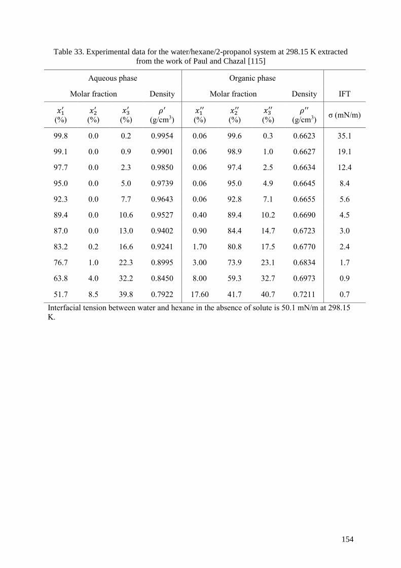
154

Table 33. Experimental data for the water/hexane/2-propanol system at 298.15 K extracted

from the work of Paul and Chazal [115]

Aqueous phase Organic phase

Molar fraction Density Molar fraction Density IFT

𝑥1′

(%) 𝑥2′

(%)

𝑥3′

(%) 𝜌′

(g/cm3) 𝑥1′′

(%) 𝑥2′′

(%)

𝑥3′′

(%) 𝜌′′

(g/cm3) σ (mN/m)

99.8 0.0 0.2 0.9954 0.06 99.6 0.3 0.6623 35.1

99.1 0.0 0.9 0.9901 0.06 98.9 1.0 0.6627 19.1

97.7 0.0 2.3 0.9850 0.06 97.4 2.5 0.6634 12.4

95.0 0.0 5.0 0.9739 0.06 95.0 4.9 0.6645 8.4

92.3 0.0 7.7 0.9643 0.06 92.8 7.1 0.6655 5.6

89.4 0.0 10.6 0.9527 0.40 89.4 10.2 0.6690 4.5

87.0 0.0 13.0 0.9402 0.90 84.4 14.7 0.6723 3.0

83.2 0.2 16.6 0.9241 1.70 80.8 17.5 0.6770 2.4

76.7 1.0 22.3 0.8995 3.00 73.9 23.1 0.6834 1.7

63.8 4.0 32.2 0.8450 8.00 59.3 32.7 0.6973 0.9

51.7 8.5 39.8 0.7922 17.60 41.7 40.7 0.7211 0.7

Interfacial tension between water and hexane in the absence of solute is 50.1 mN/m at 298.15

K.

155

A4.3 Calculation of volume fractions from molar fractions.

Volume fractions are calculated from molar fractions according to the coarse-grained

model. In this manuscript, all beads have the same volume.

𝜃𝑤𝑎𝑡𝑒𝑟 =

𝑥𝑤𝑎𝑡𝑒𝑟𝑁𝑚

𝑥𝑤𝑎𝑡𝑒𝑟𝑁𝑚

+𝑥𝑠𝑜𝑙𝑢𝑡𝑒 and ∅𝑜𝑟𝑔. =

𝑥𝑜𝑟𝑔.×𝑁𝑜𝑟𝑔.

𝑥𝑜𝑟𝑔.×𝑁𝑜𝑟𝑔.+𝑥𝑠𝑜𝑙𝑢𝑡𝑒,

Where 𝑥𝑤𝑎𝑡𝑒𝑟 and 𝜃𝑤𝑎𝑡𝑒𝑟 are the molar and the volume fraction of water representing the

aqueous phase, respectively, while 𝑥𝑜𝑟𝑔. and ∅𝑜𝑟𝑔. are the molar and the volume fraction of

molecules representing the organic phase, respectively. 𝑁𝑚 is the degree of coarse-graining

(i.e. the number of water molecules in a bead of water) and 𝑁𝑜𝑟𝑔. is the number of beads

constituting a molecule of the organic solvent (𝑁𝑜𝑟𝑔. = 1 for benzene and chloroform, and

𝑁𝑜𝑟𝑔. = 2 for hexane). Note that miscibility between solvents is completely neglected.

156

A4.4 Dependence of solute/solvent Flory-Huggins parameters with compositional data.

Figure 40. Variation of 𝝌𝒔𝒐𝒍𝒖𝒕𝒆/𝒔𝒐𝒍𝒗𝒆𝒏𝒕 parameters, as a function of each experimental

composition for the water/benzene/1,4-dioxane system (obtained using approach #1). The

composition is expressed using the molar fraction of solute in the aqueous phase. (b)

Variation of 𝝌𝒔𝒐𝒍𝒖𝒕𝒆/𝒔𝒐𝒍𝒗𝒆𝒏𝒕 parameters as a function of the average solute molar fractions in

the aqueous phase for each pair of compositions for the water/benzene/1,4-dioxane system

(obtained using approach #2).

Figure 41. Variation of 𝝌𝒔𝒐𝒍𝒖𝒕𝒆/𝒔𝒐𝒍𝒗𝒆𝒏𝒕 parameters, as a function of each experimental

composition for the water/chloroform/acetone system (obtained using approach #1). The

composition is expressed using the molar fraction of solute in the aqueous phase. (b)

Variation of 𝝌𝒔𝒐𝒍𝒖𝒕𝒆/𝒔𝒐𝒍𝒗𝒆𝒏𝒕 parameters as a function of the average solute molar fractions in

the aqueous phase for each pair of compositions for the water/chloroform/acetone system

(obtained using approach #2).

157

Figure 42. Variation of 𝝌𝒔𝒐𝒍𝒖𝒕𝒆/𝒔𝒐𝒍𝒗𝒆𝒏𝒕 parameters, as a function of each experimental

composition for the water/benzene/2-propanol system (obtained using approach #1). The

composition is expressed using the molar fraction of solute in the aqueous phase. (b)

Variation of 𝝌𝒔𝒐𝒍𝒖𝒕𝒆/𝒔𝒐𝒍𝒗𝒆𝒏𝒕 parameters as a function of the average solute molar fractions in

the aqueous phase for each pair of compositions for the water/benzene/2-propanol system

(obtained using approach #2).

Figure 43. Variation of 𝝌𝒔𝒐𝒍𝒖𝒕𝒆/𝒔𝒐𝒍𝒗𝒆𝒏𝒕 parameters, as a function of each experimental

composition for the water/hexane/acetone system (obtained using approach #1). The

composition is expressed using the molar fraction of solute in the aqueous phase. (b)

Variation of 𝝌𝒔𝒐𝒍𝒖𝒕𝒆/𝒔𝒐𝒍𝒗𝒆𝒏𝒕 parameters as a function of the average solute molar fractions in

the aqueous phase for each pair of compositions for the water/hexane/acetone system

(obtained using approach #2).

158

Figure 44. Variation of 𝝌𝒔𝒐𝒍𝒖𝒕𝒆/𝒔𝒐𝒍𝒗𝒆𝒏𝒕 parameters, as a function of each experimental

composition for the water/hexane/2-propanol system (obtained using approach #1). The

composition is expressed using the molar fraction of solute in the aqueous phase. (b)

Variation of 𝝌𝒔𝒐𝒍𝒖𝒕𝒆/𝒔𝒐𝒍𝒗𝒆𝒏𝒕 parameters as a function of the average solute molar fractions in

the aqueous phase for each pair of compositions for the water/hexane/2-propanol system

(obtained using approach #2).

159

A4.5. Results of CG-MC simulations in the Gibbs ensemble (NVT).

1) Liquid-liquid equilibrium ternary diagrams for water/chloroform/acetone system at

298.15K

Parametrization approaches #1, #3 and #4 were carried out with the less concentrated acetone

composition. Approach #2 is based on the three compositions less concentrated in acetone.

Figure 45. Liquid-liquid equilibrium ternary diagrams for the water/chloroform/acetone

system at 298.15K for (a) approach #1, (b) approach #2, (3) approach #3 and (4) approach #4.

Experimental data are plotted in black and the results from the CG-MC simulations are in red.

DPD interaction parameters used to compute LLE are located below each ternary plot.

Numbers in red represent the solute/solvent parameters obtained for each approach.

160

2) Liquid-liquid equilibrium ternary diagram for water/benzene/acetic acid system at

298.15K.

Parametrization approaches #1, #3 and #4 were carried out with the second composition the

less concentrated in acetic acid. Approach #2 is based on the five compositions.

Figure 46. Liquid-liquid equilibrium ternary diagrams for the water/benzene/acetic acid

system at 298.15K for (a) approach #1, (b) approach #2, (3) approach #3 and (4) approach #4.

Experimental data are plotted in black and the results from the CG-MC simulations are in red.

DPD interaction parameters used to compute LLE are located below each ternary plot.

Numbers in red represent the solute/solvent parameters obtained for each approach.

161

3) Liquid-liquid equilibrium ternary diagram for water/benzene/2-propanol system at

298.15K.

Parametrization approaches #1, #3 and #4 were carried out with the fourth composition the

less concentrated in 2-propanol. Approach #2 is based on the five compositions less

concentrated in 2-propanol.

Figure 47. Liquid-liquid equilibrium ternary diagrams for the water/benzene/2-propanol

system at 298.15K for (a) approach #1, (b) approach #2, (3) approach #3 and (4) approach #4.

Experimental data are plotted in black and the results from the CG-MC simulations are in red.

DPD interaction parameters used to compute LLE are located below each ternary plot.

Numbers in red represent the solute/solvent parameters obtained for each approach.

162

4) Liquid-liquid equilibrium ternary diagram for water/hexane/acetone system at

298.15K.

Transferability approach and approaches #3 and #4were carried out with the fifth composition

the less concentrated in acetone. Approach #2 is based on the eleven compositions. Note that

approach #1 provides similar interaction parameters than approach #2 regardless of the

composition used.

Figure 48. Liquid-liquid equilibrium ternary diagrams for the water/hexane/acetone system at

298.15K for (a) approach #1, (b) approach #2, (3) approach #3 and (4) approach #4.

Experimental data are plotted in black and the results from the CG-MC simulations are in red.

DPD interaction parameters used to compute LLE are located below each ternary plot.

Numbers in red represent the solute/solvent parameters obtained for each approach.

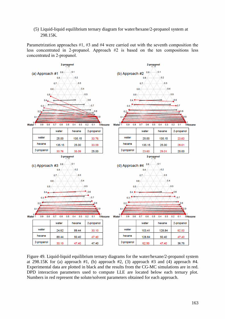
163

(5) Liquid-liquid equilibrium ternary diagram for water/hexane/2-propanol system at

298.15K.

Parametrization approaches #1, #3 and #4 were carried out with the seventh composition the

less concentrated in 2-propanol. Approach #2 is based on the ten compositions less

concentrated in 2-propanol.

Figure 49. Liquid-liquid equilibrium ternary diagrams for the water/hexane/2-propanol system

at 298.15K for (a) approach #1, (b) approach #2, (3) approach #3 and (4) approach #4.

Experimental data are plotted in black and the results from the CG-MC simulations are in red.

DPD interaction parameters used to compute LLE are located below each ternary plot.

Numbers in red represent the solute/solvent parameters obtained for each approach.

164

A4.6. Coarse-grained compositions of the systems studied for the CG-MC simulations in the

Gibbs ensemble (NVT).

These compositions were calculated from experimental compositional data of liquid-liquid

equilibrium and correspond to a heterogeneous system that decants following the conodal

lines. The total number of beads for each system is set at 6000.

Table 34. Compositions used in CG-MC simulations in the Gibbs (NVT) ensemble for the

water/benzene/1,4-dioxane system.

Number of water beads Number of benzene beads Number of 1,4-dioxane beads

2411 3014 575

2141 2677 1182

1898 2372 1730

1632 2041 2327

1242 1553 3205

Table 35. Compositions used in CG-MC simulations in the Gibbs (NVT) ensemble for the

water/chloroform/acetone system.

Number of water beads Number of chloroform beads Number of acetone beads

3236 2284 480

2979 2103 918

2511 1772 1717

2088 1474 2438

1705 1203 3092

165

Table 36. Compositions used in CG-MC simulations in the Gibbs (NVT) ensemble for the

water/benzene/acetic acid system.

Number of water beads Number of benzene beads Number of acetic acid beads

2223 3168 609

1896 2922 1182

1536 2652 1812

1171 2378 2451

845 2133 3022

Table 37. Compositions used in CG-MC simulations in the Gibbs (NVT) ensemble for the

water/benzene/2-propanol system.

Number of water beads Number of benzene beads Number of 2-propanol beads

2564 3204 232

2455 3069 476

2233 2791 976

2116 2645 1239

2011 2513 1476

1700 2125 2175

1551 1938 2511

166

Table 38. Compositions used in CG-MC simulations in the Gibbs (NVT) ensemble for the

water/hexane/acetone system.

Number of water beads Number of hexane beads* Number of acetone beads

1988 3978 34

1912 3824 264

1821 3640 539

1651 3304 1045

1527 3054 1419

1289 2578 2133

1178 2358 2464

1076 2152 2772

978 1958 3064

881 1762 3357

771 1542 3687

* Hexane molecules are represented by two beads

167

Table 39. Compositions used in CG-MC simulations in the Gibbs (NVT) ensemble for the

water/hexane/2-propanol system.

Number of water beads Number of hexane beads Number of 2-propanol beads

1351 4632 17

1338 4590 72

1314 4504 182

1269 4352 379

1226 4204 570

1177 4036 787

1127 3866 1007

1074 3680 1246

985 3376 1639

838 2872 2290

728 2494 2778

* Hexane molecules are represented by two beads

168

A4.7. Chemical potentials of the solute and pressures of the system.

These data are calculated at equilibrium using CG-MC simulation in the Gibbs ensemble

(NVT) following the four parametrization approaches.

Table 40. Chemical potentials of 1,4-dioxane and pressures for the water/benzene/1,4-dioxane

system. P = pressure

#1 approach #2 approach #3 approach #4 approach

µ1,4−𝑑𝑖𝑜𝑥𝑎𝑛𝑒

(DPD unit)

P

(DPD

unit)

µ1,4−𝑑𝑖𝑜𝑥𝑎𝑛𝑒 (DPD unit)

P

(DPD

unit)

µ1,4−𝑑𝑖𝑜𝑥𝑎𝑛𝑒

(DPD unit)

P

(DPD

unit)

µ1,4−𝑑𝑖𝑜𝑥𝑎𝑛𝑒 (DPD unit)

P

(DPD

unit)

11.13 23.74 12.86 24.48 24.18 40.50 37.41 76.85

11.83 23.80 13.37 25.05 25.84 43.04 37.50 75.64

12.22 23.86 13.56 25.39 27.16 45.43 37.46 74.56

12.48 23.91 13.67 25.58 28.45 48.14 37.34 73.44

12.77 24.02 13.73 25.70 30.30 52.36 37.09 71.94

Table 41. Chemical potentials of acetone and pressures for the water/chloroform/acetone

system. P = pressure

#1 approach #2 approach #3 approach #4 approach

µ𝑎𝑐𝑒𝑡𝑜𝑛𝑒 (DPD

unit)

P

(DPD

unit)

µ𝑎𝑐𝑒𝑡𝑜𝑛𝑒 (DPD

unit)

P

(DPD

unit)

µ𝑎𝑐𝑒𝑡𝑜𝑛𝑒 (DPD

unit)

P

(DPD

unit)

µ𝑎𝑐𝑒𝑡𝑜𝑛𝑒 (DPD

unit)

P

(DPD

unit)

11.40 23.79 11.49 23.42 16.26 31.66 26.37 67.15

12.02 23.89 11.19 23.31 16.93 32.02 26.20 64.12

12.59 24.08 11.92 23.27 17.63 32.65 25.32 58.76

12.88 24.25 12.34 23.40 18.03 33.21 24.27 54.18

13.07 24.41 12.62 23.60 18.33 33.73 23.37 50.31

Table 42. Chemical potentials of acetic acid and pressures for the water/benzene/acetic acid

system. P = pressure

#1 approach #2 approach #3 approach #4 approach

µ𝑎𝑐𝑒𝑡𝑖𝑐 𝑎𝑐𝑖𝑑 (DPD

unit)

P

(DPD

unit)

µ𝑎𝑐𝑒𝑡𝑖𝑐 𝑎𝑐𝑖𝑑 (DPD

unit)

P

(DPD

unit)

µ𝑎𝑐𝑒𝑡𝑖𝑐 𝑎𝑐𝑖𝑑 (DPD

unit)

P

(DPD

unit)

µ𝑎𝑐𝑒𝑡𝑖𝑐 𝑎𝑐𝑖𝑑 (DPD

unit)

P

(DPD

unit)

5.73 21.09 10.64 23.22 16.25 37.40 24.07 62.82

7.66 19.65 11.48 23.05 17.65 36.94 24.12 58.06

9.21 19.24 12.07 23.09 18.71 37.13 23.84 53.78

10.34 19.71 12.52 23.35 19.52 37.83 23.37 50.29

11.17 20.63 12.88 23.78 20.14 38.74 22.88 47.69

169

Table 43. Chemical potentials of 2-propanol and pressures for the water/benzene/2-propanol

system. P = pressure

#1 approach #2 approach #3 approach #4 approach

µ2−𝑝𝑟𝑜𝑝𝑎𝑛𝑜𝑙 (DPD unit)

P

(DPD

unit)

µ2−𝑝𝑟𝑜𝑝𝑎𝑛𝑜𝑙 (DPD unit)

P

(DPD

unit)

µ2−𝑝𝑟𝑜𝑝𝑎𝑛𝑜𝑙 (DPD unit)

P

(DPD

unit)

µ2−𝑝𝑟𝑜𝑝𝑎𝑛𝑜𝑙 (DPD unit)

P

(DPD

unit)

10.57 23.74 5.69 22.87 17.29 38.05 27.54 75,78

11.27 23.81 6.62 22.16 17.92 37.92 27.69 73,50

11.97 23.95 7.72 20.99 18.50 37.63 27.19 69,00

12.20 24.02 8.14 20.52 18.65 37.48 26.90 66.72

12.36 24.08 8.47 20.16 18.73 37.33 26.54 64.73

12.70 24.22 9.30 19.46 18.94 36.94 25.39 59.14

12.82 24.29 9.66 19.32 18.95 36.75 24.79 56.60

Table 44. Chemical potentials of acetone and pressures for the water/hexane/acetone system.

P = pressure

Transferability [#1-#2] approach #3 approach #4 approach

µ𝑎𝑐𝑒𝑡𝑜𝑛𝑒 (DPD

unit)

P

(DPD

unit)

µ𝑎𝑐𝑒𝑡𝑜𝑛𝑒 (DPD

unit)

P

(DPD

unit)

µ𝑎𝑐𝑒𝑡𝑜𝑛𝑒 (DPD

unit)

P

(DPD

unit)

µ𝑎𝑐𝑒𝑡𝑜𝑛𝑒 (DPD

unit)

P

(DPD

unit)

9.48 22.67 8.18 22.64 14.03 35.90 20.48 57.59

11.44 22.94 10.17 22.64 16.10 35.66 22.26 56.25

12.06 23.20 10.90 22.67 16.85 35.42 22.69 54.75

12.59 23.58 11.59 22.76 17.55 35.12 22.75 52.22

12.80 23.78 11.91 22.84 17.88 34.96 22.63 50.48

13.04 24.05 12.35 23.02 18.27 34.76 22.20 47.44

13.12 24.13 12.49 23.12 18.40 34.71 21.96 46.14

13.17 24.19 12.61 23.22 18.48 34.67 21.70 44.99

13.22 24.23 12.72 23.31 18.57 34.67 21.51 43.93

13.26 24.27 12.81 23.42 18.65 34.67 21.26 42.99

13.29 24.32 12.90 23.55 18.71 34.72 20.98 41.92

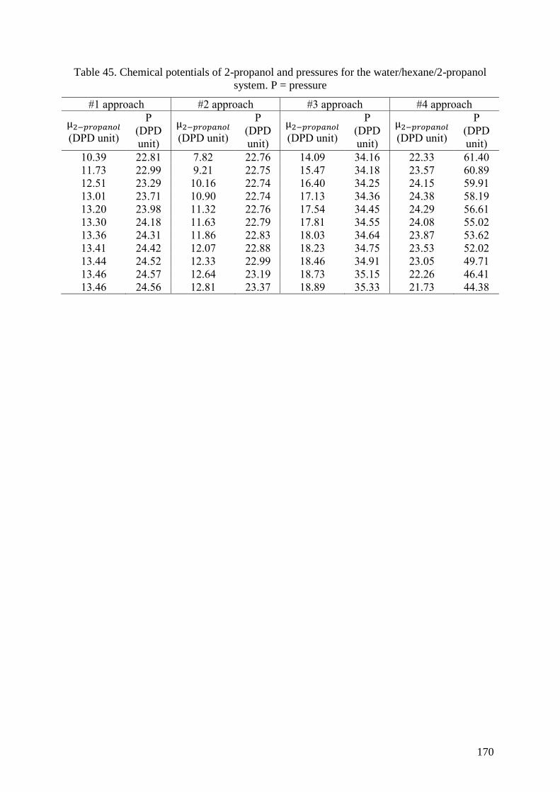
170

Table 45. Chemical potentials of 2-propanol and pressures for the water/hexane/2-propanol

system. P = pressure

#1 approach #2 approach #3 approach #4 approach

µ2−𝑝𝑟𝑜𝑝𝑎𝑛𝑜𝑙 (DPD unit)

P

(DPD

unit)

µ2−𝑝𝑟𝑜𝑝𝑎𝑛𝑜𝑙 (DPD unit)

P

(DPD

unit)

µ2−𝑝𝑟𝑜𝑝𝑎𝑛𝑜𝑙 (DPD unit)

P

(DPD

unit)

µ2−𝑝𝑟𝑜𝑝𝑎𝑛𝑜𝑙 (DPD unit)

P

(DPD

unit)

10.39 22.81 7.82 22.76 14.09 34.16 22.33 61.40

11.73 22.99 9.21 22.75 15.47 34.18 23.57 60.89

12.51 23.29 10.16 22.74 16.40 34.25 24.15 59.91

13.01 23.71 10.90 22.74 17.13 34.36 24.38 58.19

13.20 23.98 11.32 22.76 17.54 34.45 24.29 56.61

13.30 24.18 11.63 22.79 17.81 34.55 24.08 55.02

13.36 24.31 11.86 22.83 18.03 34.64 23.87 53.62

13.41 24.42 12.07 22.88 18.23 34.75 23.53 52.02

13.44 24.52 12.33 22.99 18.46 34.91 23.05 49.71

13.46 24.57 12.64 23.19 18.73 35.15 22.26 46.41

13.46 24.56 12.81 23.37 18.89 35.33 21.73 44.38

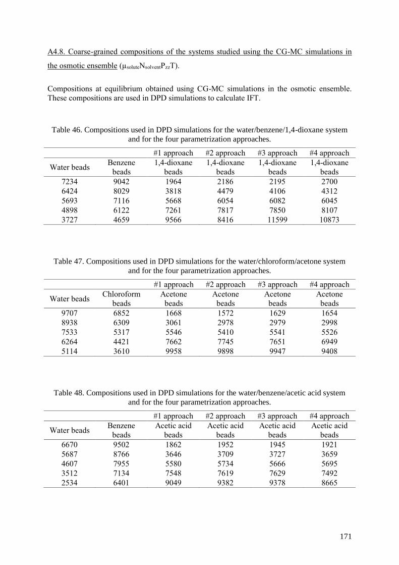
171

A4.8. Coarse-grained compositions of the systems studied using the CG-MC simulations in

the osmotic ensemble (µsoluteNsolventPzzT).

Compositions at equilibrium obtained using CG-MC simulations in the osmotic ensemble.

These compositions are used in DPD simulations to calculate IFT.

Table 46. Compositions used in DPD simulations for the water/benzene/1,4-dioxane system

and for the four parametrization approaches.

#1 approach #2 approach #3 approach #4 approach

Water beads Benzene

beads

1,4-dioxane

beads

1,4-dioxane

beads

1,4-dioxane

beads

1,4-dioxane

beads

7234 9042 1964 2186 2195 2700

6424 8029 3818 4479 4106 4312

5693 7116 5668 6054 6082 6045

4898 6122 7261 7817 7850 8107

3727 4659 9566 8416 11599 10873

Table 47. Compositions used in DPD simulations for the water/chloroform/acetone system

and for the four parametrization approaches.

#1 approach #2 approach #3 approach #4 approach

Water beads Chloroform

beads

Acetone

beads

Acetone

beads

Acetone

beads

Acetone

beads

9707 6852 1668 1572 1629 1654

8938 6309 3061 2978 2979 2998

7533 5317 5546 5410 5541 5526

6264 4421 7662 7745 7651 6949

5114 3610 9958 9898 9947 9408

Table 48. Compositions used in DPD simulations for the water/benzene/acetic acid system

and for the four parametrization approaches.

#1 approach #2 approach #3 approach #4 approach

Water beads Benzene

beads

Acetic acid

beads

Acetic acid

beads

Acetic acid

beads

Acetic acid

beads

6670 9502 1862 1952 1945 1921

5687 8766 3646 3709 3727 3659

4607 7955 5580 5734 5666 5695

3512 7134 7548 7619 7629 7492

2534 6401 9049 9382 9378 8665

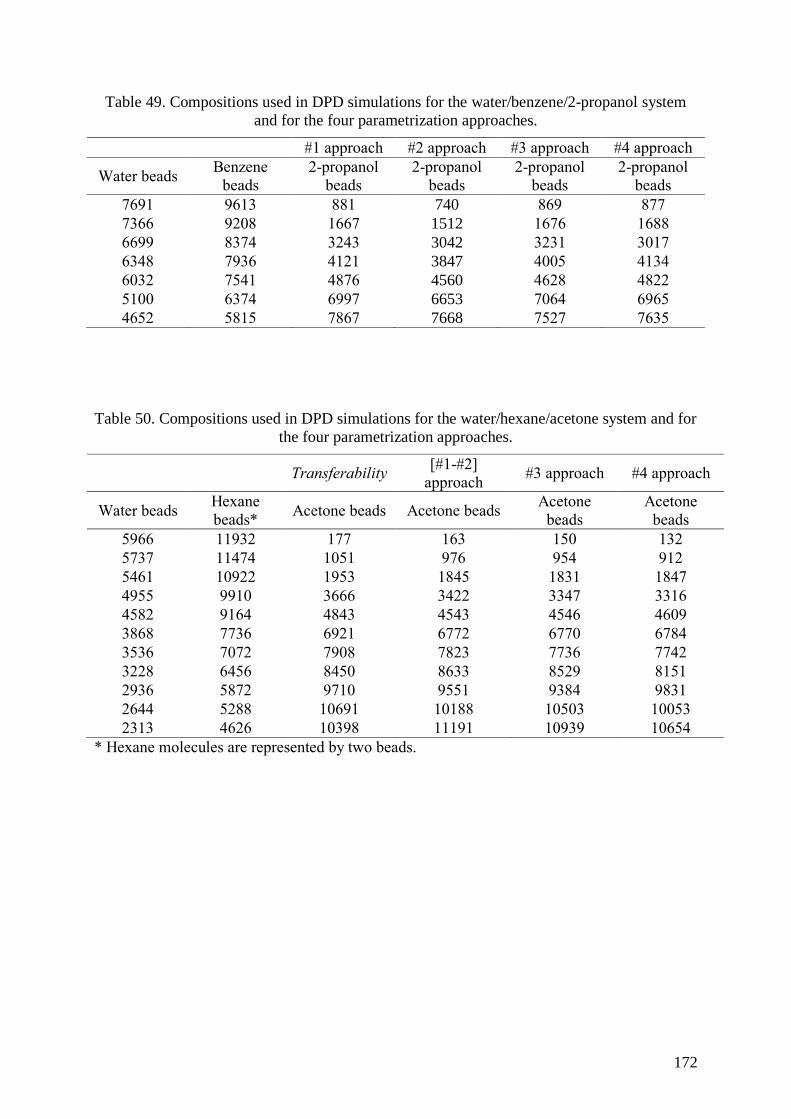
172

Table 49. Compositions used in DPD simulations for the water/benzene/2-propanol system

and for the four parametrization approaches.

#1 approach #2 approach #3 approach #4 approach

Water beads Benzene

beads

2-propanol

beads

2-propanol

beads

2-propanol

beads

2-propanol

beads

7691 9613 881 740 869 877

7366 9208 1667 1512 1676 1688

6699 8374 3243 3042 3231 3017

6348 7936 4121 3847 4005 4134

6032 7541 4876 4560 4628 4822

5100 6374 6997 6653 7064 6965

4652 5815 7867 7668 7527 7635

Table 50. Compositions used in DPD simulations for the water/hexane/acetone system and for

the four parametrization approaches.

Transferability [#1-#2]

approach #3 approach #4 approach

Water beads Hexane

beads* Acetone beads Acetone beads

Acetone

beads

Acetone

beads

5966 11932 177 163 150 132

5737 11474 1051 976 954 912

5461 10922 1953 1845 1831 1847

4955 9910 3666 3422 3347 3316

4582 9164 4843 4543 4546 4609

3868 7736 6921 6772 6770 6784

3536 7072 7908 7823 7736 7742

3228 6456 8450 8633 8529 8151

2936 5872 9710 9551 9384 9831

2644 5288 10691 10188 10503 10053

2313 4626 10398 11191 10939 10654

* Hexane molecules are represented by two beads.

173

Table 51. Compositions used in DPD simulations for the water/hexane/2-propanol system and

for the four parametrization approaches.

#1 approach #2 approach #3 approach #4 approach

Water beads Hexane

beads*

2-propanol

beads

2-propanol

beads

2-propanol

beads

2-propanol

beads

7426 10498 157 112 116 114

7306 10376 555 403 419 417

7069 10136 1243 952 950 954

6646 9704 2349 1836 1824 1897

6253 9304 3614 2683 2707 2757

5841 8884

Phase

separation

3484 3476 3610

5476 8516 4369 4260 4426

5047 8078 5223 5200 4970

4405 7424 6507 6385 6354

3446 6448 8507 8291 8241

2809 5802 9534 9355 9149

* Hexane molecules are represented by two beads.

174

A4.9. Interfacial concentration in solute and thickness of the interface.

Figure 50. Water/chloroform/acetone system at 298.15K (a) Variation of the acetone

interfacial concentration, as a function of the molar fraction of acetone in the aqueous phase.

(b) Variation of the water/chloroform interface thickness, as a function of the molar fraction

of acetone in the aqueous phase.

Figure 51. Water/benzene/acetic acid system at 298.15K (a) Variation of the acetic acid

interfacial concentration, as a function of the molar fraction of acetic acid in the aqueous

phase. (b) Variation of the water/benzene interface thickness, as a function of the molar

fraction of acetic acid in the aqueous phase.

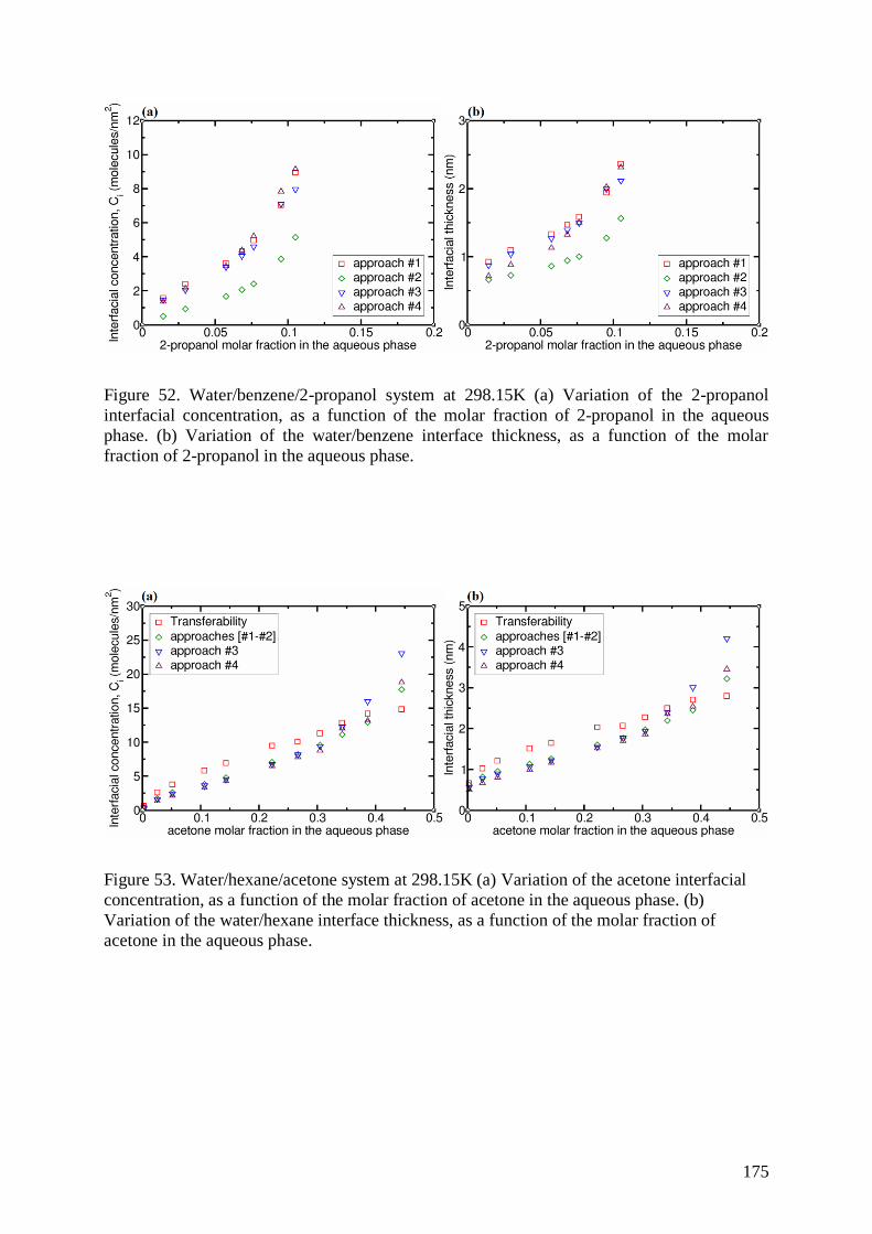
175

Figure 52. Water/benzene/2-propanol system at 298.15K (a) Variation of the 2-propanol

interfacial concentration, as a function of the molar fraction of 2-propanol in the aqueous

phase. (b) Variation of the water/benzene interface thickness, as a function of the molar

fraction of 2-propanol in the aqueous phase.

Figure 53. Water/hexane/acetone system at 298.15K (a) Variation of the acetone interfacial

concentration, as a function of the molar fraction of acetone in the aqueous phase. (b)

Variation of the water/hexane interface thickness, as a function of the molar fraction of

acetone in the aqueous phase.

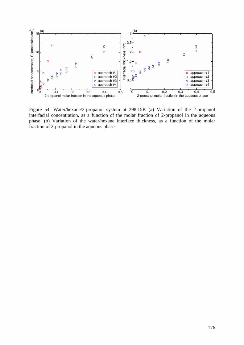
176

Figure 54. Water/hexane/2-propanol system at 298.15K (a) Variation of the 2-propanol

interfacial concentration, as a function of the molar fraction of 2-propanol in the aqueous

phase. (b) Variation of the water/hexane interface thickness, as a function of the molar

fraction of 2-propanol in the aqueous phase.

177

A4.10. Comparison of thermodynamic models to predict liquid-liquid equilibrium

Table 52. Comparison of thermodynamic models for prediction of liquid-liquid equilibrium

for the water/chloroform/acetone system.

Thermodynamic models 𝑅𝑠𝑜𝑙𝑢𝑏𝑖𝑙𝑖𝑡𝑦2

EoS

models

PR No solute distribution between bulk phases

SRK No solute distribution between bulk phases

GC-PPC-SAFT No solute distribution between bulk phases

Activity

models

NRTL-SAC No solute distribution between bulk phases

UNIFAC original 0.985

UNIFAC LL 0.979

SRK-MHV2-UNIFAC 0.995

Table 53. Comparison of thermodynamic models for prediction of liquid-liquid equilibrium

for the water/benzene/acetic acid system.

Thermodynamic models 𝑅𝑠𝑜𝑙𝑢𝑏𝑖𝑙𝑖𝑡𝑦2

EoS

models

PR No solute distribution between bulk phases

SRK No solute distribution between bulk phases

GC-PPC-SAFT 𝑅𝑠𝑜𝑙𝑢𝑏𝑖𝑙𝑖𝑡𝑦2 < 0

Activity

models

NRTL-SAC 0.997

UNIFAC original 0.976

UNIFAC LL No solute distribution between bulk phases

SRK-MHV2-UNIFAC 0.988

178

Table 54. Comparison of thermodynamic models for prediction of liquid-liquid equilibrium

for the water/benzene/2-propanol system.

Thermodynamic models 𝑅𝑠𝑜𝑙𝑢𝑏𝑖𝑙𝑖𝑡𝑦2

EoS

models

PR No solute distribution between bulk phases

SRK No solute distribution between bulk phases

GC-PPC-SAFT 0.957 (but only the four least concentrated

compositions in 2-propanol could be calculated)

Activity

models

NRTL-SAC 0.787

UNIFAC original 0.922

UNIFAC LL 0.962

SRK-MHV2-UNIFAC 0.995

Table 55. Comparison of thermodynamic models for prediction of liquid-liquid equilibrium

for the water/hexane/acetone system. Note that 𝑅𝑠𝑜𝑙𝑢𝑏𝑖𝑙𝑖𝑡𝑦2 are calculated using only the seven

less concentrate compositions in solute.

Thermodynamic models 𝑅𝑠𝑜𝑙𝑢𝑏𝑖𝑙𝑖𝑡𝑦2

EoS

models

PR No solute distribution between bulk phases

SRK No solute distribution between bulk phases

GC-PPC-SAFT 𝑅𝑠𝑜𝑙𝑢𝑏𝑖𝑙𝑖𝑡𝑦2 < 0

Activity

models

NRTL-SAC 0.902

UNIFAC original 0.799

UNIFAC LL 0.970

SRK-MHV2-UNIFAC 0.911

179

Table 56. Comparison of thermodynamic models for prediction of liquid-liquid equilibrium

for the water/hexane/2-propanol system. Note that 𝑅𝑠𝑜𝑙𝑢𝑏𝑖𝑙𝑖𝑡𝑦2 are calculated using only the

seven less concentrate compositions in solute.

Thermodynamic models 𝑅𝑠𝑜𝑙𝑢𝑏𝑖𝑙𝑖𝑡𝑦2

EoS

models

PR No solute distribution between bulk phases

SRK No solute distribution between bulk phases

GC-PPC-SAFT 0.381

Activity

models

NRTL-SAC 𝑅𝑠𝑜𝑙𝑢𝑏𝑖𝑙𝑖𝑡𝑦2 < 0

UNIFAC original 0.618

UNIFAC LL 0.983

SRK-MHV2-UNIFAC 0.973

180

A4.11. Prediction of the chemical potentials and the interaction parameters using a

thermodynamic model.

Figure 55. (a) Chemical potentials of the acetone in the aqueous phase and (b) in the organic

phase for the water/chloroform/acetone system.

Figure 56. (a) Interaction parameters of the acetone with water for the

water/chloroform/acetone system. (b) Interaction parameters of the acetone with chloroform

for the water/chloroform/acetone system.

181

Figure 57. (a) Chemical potentials of the acetic acid in the aqueous phase and (b) in the

organic phase for the water/benzene/acetic acid system.

Figure 58. (a) Interaction parameters of the acetic acid with water for the water/benzene/acetic

acid system. (b) Interaction parameters of the acetic acid with benzene for the

water/benzene/acetic acid system.

182

Appendices – Chapter 5

A5.1. Experimental data of crude oil and its fractions

(1) Experimental data of crude oil

Elemental analysis (% w/w): Volumetric mass density:

Carbon content 83.6 at 15 °C (g/cm3) 0.8745

Hydrogen content 12.47 at 20 °C (g/cm3) 0.871

Nitrogen content 0.14

Oxygen content 0.76

Sulfur content 2.24

(2) Experimental data of the light fraction (𝑇 < 344°𝐶)

Elemental analysis (% w/w): Volumetric mass density:

Carbon content 85.1 at 15 °C (g/cm3) 0.7975

Hydrogen content 13.69 at 20 °C (g/cm3) 0.8012

Nitrogen content 0.09

Oxygen content 0

Sulfur content 0.53

Chemical family (% w/w):

n-Paraffins 13.8

i-Paraffins 10

Naphthenes 7.8

Aromatics 5.4

Saturates C15+ 5.6

Aromatics C15+ 3.6

Unknown C20- 0

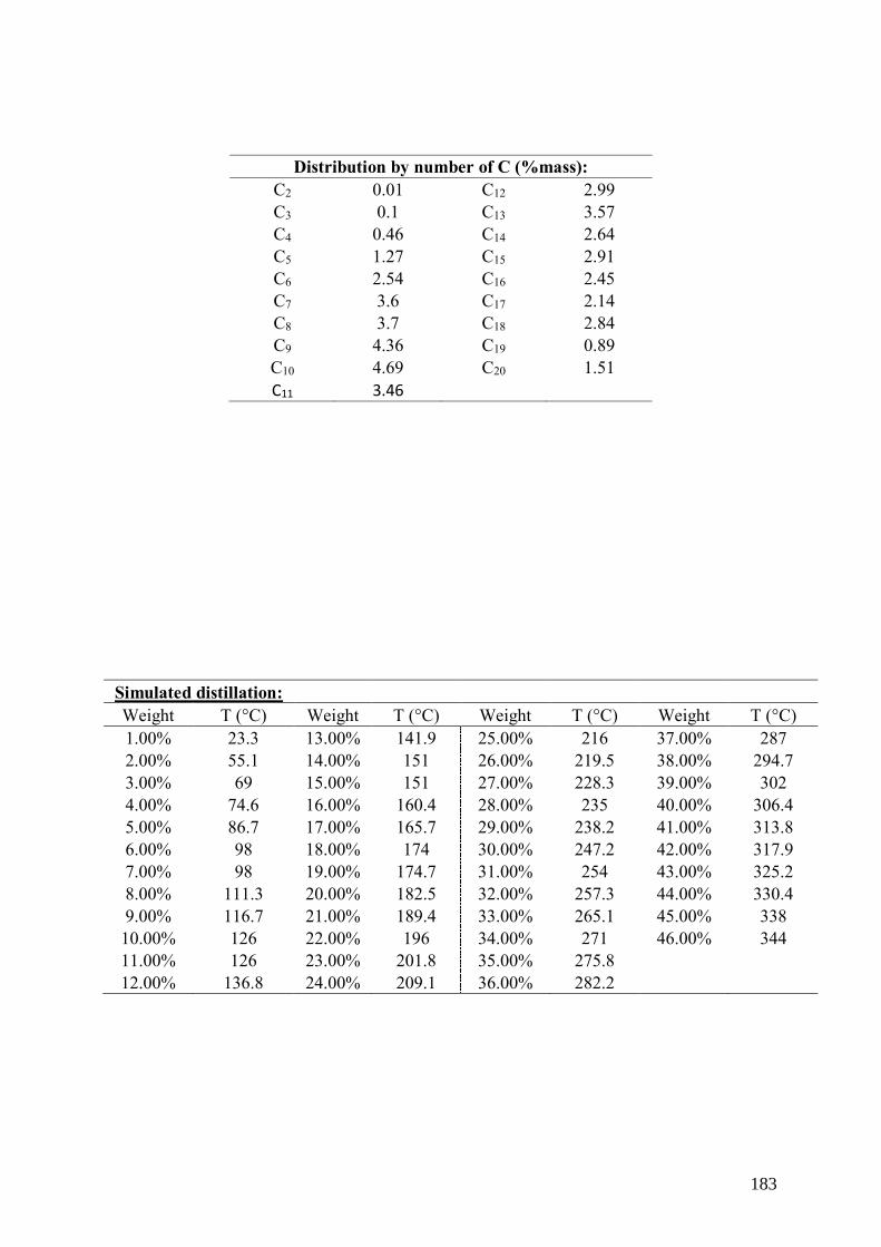
183

Distribution by number of C (%mass):

C2 0.01 C12 2.99

C3 0.1 C13 3.57

C4 0.46 C14 2.64

C5 1.27 C15 2.91

C6 2.54 C16 2.45

C7 3.6 C17 2.14

C8 3.7 C18 2.84

C9 4.36 C19 0.89

C10 4.69 C20 1.51

C11 3.46

Simulated distillation: Weight T (°C) Weight T (°C) Weight T (°C) Weight T (°C)

1.00% 23.3 13.00% 141.9 25.00% 216 37.00% 287

2.00% 55.1 14.00% 151 26.00% 219.5 38.00% 294.7

3.00% 69 15.00% 151 27.00% 228.3 39.00% 302

4.00% 74.6 16.00% 160.4 28.00% 235 40.00% 306.4

5.00% 86.7 17.00% 165.7 29.00% 238.2 41.00% 313.8

6.00% 98 18.00% 174 30.00% 247.2 42.00% 317.9

7.00% 98 19.00% 174.7 31.00% 254 43.00% 325.2

8.00% 111.3 20.00% 182.5 32.00% 257.3 44.00% 330.4

9.00% 116.7 21.00% 189.4 33.00% 265.1 45.00% 338

10.00% 126 22.00% 196 34.00% 271 46.00% 344

11.00% 126 23.00% 201.8 35.00% 275.8

12.00% 136.8 24.00% 209.1 36.00% 282.2

184

(3) Experimental data of the heavy fraction (𝑇 > 344°𝐶)

Elemental analysis (% m/m): Volumetric mass density:

Carbon content 84.2 at 15 °C (g/cm3) 0.9685

Hydrogen content 11.39 at 20 °C (g/cm3) 0.9651

Nitrogen content 0.19 at 70 °C (g/cm3) 0.9308

Oxygen content 0.25

Sulfur content 3.59

SARA analysis:

Saturates (% w/w) 29.7 ± 1.1

Aromatics (% w/w) 44.4 ± 1.1

Resins (% w/w) 21.6 ± 1.1

Asphaltenes (% w/w) 1.7 ± 0.2

Waste 2.5

185

Simulated distillation:

Weight T (°C) Weight T (°C) Weight T (°C) Weight T (°C)

IBP (0.50

%) 357 23.00% 443 46.00% 516.2 69.00% 609.7

1.00% 366.2 24.00% 446.1 47.00% 519.7 70.00% 614.2

2.00% 374.1 25.00% 449.1 48.00% 523.6 71.00% 619

3.00% 379.6 26.00% 452.1 49.00% 527.9 72.00% 624.2

4.00% 384 27.00% 455.2 50.00% 532.4 73.00% 629.6

5.00% 388.1 28.00% 458.1 51.00% 535.9 74.00% 634.7

6.00% 391.4 29.00% 461.3 52.00% 539 75.00% 640.2

7.00% 395.1 30.00% 464.5 53.00% 542.1 76.00% 646.1

8.00% 398.6 31.00% 467.4 54.00% 545.4 77.00% 652.5

9.00% 401.7 32.00% 470.5 55.00% 550 78.00% 658.1

10.00% 405 33.00% 473.4 56.00% 554.7 79.00% 665.3

11.00% 408.2 34.00% 476.5 57.00% 558.8 80.00% 672.4

12.00% 411.4 35.00% 479.6 58.00% 562.7 81.00% 679.5

13.00% 414.2 36.00% 482.7 59.00% 566.6 82.00% 686.8

14.00% 417.2 37.00% 486.1 60.00% 570.1 83.00% 693.5

15.00% 420.1 38.00% 489.4 61.00% 573.7 84.00% 700.7

16.00% 422.7 39.00% 492.9 62.00% 577.9 85.00% 707.2

17.00% 425.6 40.00% 496.2 63.00% 582.3 86.00% 714.2

18.00% 428.6 41.00% 499.5 64.00% 586.6 87.00% 721.2

19.00% 431.3 42.00% 502.6 65.00% 590.8 88.00% 727.4

20.00% 434.4 43.00% 505.9 66.00% 595.3 89.00% 734

21.00% 437.2 44.00% 509.2 67.00% 599.9 90.00% 740

22.00% 440.1 45.00% 512.7 68.00% 604.9 91.00% 749.1

186

A5.2. Lumped method

Table 57. Conversion of the simulated distillation curve to an ASTM D86 curve, and then to a

TBP curve.

Distillation curves

ASTM D86 TBP

% Volume T (°C) T (°C)

10 106.23 83.54

30 151.88 147.62

50 198.01 205.58

70 257.38 270.33

90 308.71 321.83

100 328.88 347.37

Table 58. Calculation of molecule and pseudo-component properties

Properties of pseudo-components derived

from the distillation curve

Properties of pseudo-components derived from

the Lumping method

Molecular weight

(g/mol)

Riazi [1]

(Procedure API

B2B.1 [147])

Molecular weight

(g/mol)

Weighted average value

on initial compounds

Chemical formula

(CxHy) Riazi [1]

Chemical formula

(CxHy) Riazi [1]

Critical temperature

(TC) Twu [26]

Critical temperature

(TC)

Weighted average value

on initial compounds

Critical pressure

(PC) Twu [26] Critical pressure (PC)

Weighted average value

on initial compounds

Acentic factor (ω) Edmister [27] Acentic factor (ω) Weighted average value

on initial compounds

Enthalpy of formation

(kJ/mol)

Lower heating value

[143]

Molar volume (mol/L) Peng et Robinson EoS

[122]

Normal boiling

temperature (K)

Riazi (Procedure API

2B1.1 [147])

187

A5.3. Stochastic Reconstruction

Table 59. Calculation methods for the properties of molecules and mixtures

Properties of molecules Methods

SARA family Wiehe [153, 154]

Boiling temperature Hudebine et Wahl [5]

Density Hudebine et Wahl [5]

Critical temperature Joback [155]

Critical pressure Joback [155]

Critical molar volume Joback [155]

Standard enthalpy of formation Joback [155]

Cohesive energy Fedors [156]

188

Table 60. Additional results for the stochastic reconstruction of the mixture of 5000 molecules

Distribution 1

Type of molecule

Attribute « Paraffins »

Attribute « Naphthenes»

Attribute « Mono-core »

Attribute « Multi-cores »

0.165

0.105

0.598

0.132

Distribution 2

Number of cores Value 1.0 < X < 5.0 1.111

Distribution 3

Type of heterocycle

Attribute « Thiophene »

Attribute « Pyridine »

Attribute « Pyrrole »

Attribute « Furan »

0.719

0.092

0.073

0.116

Distribution 4

Number of benzene rings per core Value 1.0 < X < 5.0 4.754

Distribution 5

Total number of rings per core Value 0.5 < X < 2.0 1.035

Distribution 6

Number of thiophenes per core

Attribute « 0 »

Attribute « 1 »

Attribute « 2 »

0.481

0.240

0.279

Distribution 7

Number of pyridines per core

Attribute « 0 »

Attribute « 1 »

Attribute « 2 »

0.619

0.306

0.076

Distribution 8

Number of pyrroles per core

Attribute « 0 »

Attribute « 1 »

Attribute « 2 »

0.684

0.001

0.315

Distribution 9

Number of furans per core

Attribute « 0 »

Attribute « 1 »

Attribute « 2 »

0.727

0.206

0.067

Distribution 10

Acceptance probability for a peripheral carbon

Attribute « No »

Attribute « Yes »

0.320

0.680

Distribution 11

Length of the paraffinic chains Value 1.0 < X < 10.0 2.217

Distribution 12

Length of an alkyl chain

(lateral and intercore)

Value 1.0 < X < 10.0 2.235

Distribution 13

Probability of sulfur substitution for aliphatic CH3

or CH2

Attribute « No »

Attribute « Yes »

0.984

0.016

Distribution 14

Substitution probability of a carbon atom by a

heteroatom

Attribute « No »

Attribute « Yes »

0.995

0.005

Distribution 15

Type of heteroatom substitution

Attribute « Nitrogen »

Attribute « Oxygen »

0.182

0.818

Distribution 16

Type of oxygen group

Attribute « Ether »

Attribute « Carbonyl »

0.001

0.999

Objective Function 2.154

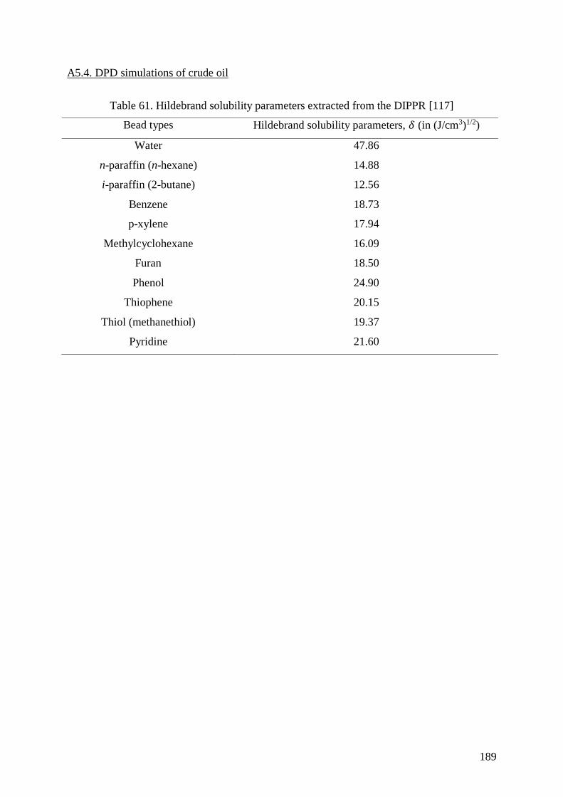
189

A5.4. DPD simulations of crude oil

Table 61. Hildebrand solubility parameters extracted from the DIPPR [117]

Bead types Hildebrand solubility parameters, 𝛿 (in (J/cm3)1/2)

Water 47.86

n-paraffin (n-hexane) 14.88

i-paraffin (2-butane) 12.56

Benzene 18.73

p-xylene 17.94

Methylcyclohexane 16.09

Furan 18.50

Phenol 24.90

Thiophene 20.15

Thiol (methanethiol) 19.37

Pyridine 21.60

190

Table 62. Composition of the simulation box for the crude oil/water system.

Molecule name

or ID

Molar fraction/fraction (%

mol)

Molar

fraction

(% mol)

Number of

molecules

Water 54005

Light fraction

(C20-)

Methylcyclohexane 13.12 9.59 2299

p-xylene 18.39 13.44 3222

Isobutylbenzene 22.71 16.60 3979

n-heptadecane 20.46 14.96 3584

1-propyl-

naphthalene 25.32 18.51 4436

Heavy fraction

(C20+)

(1) Resin 5.43 1.46 350

(2) Aromatic 7.19 1.93 463

(3) Saturate 17.15 4.61 1105

(4) Aromatic 9.08 2.44 585

(5) Resin 6.89 1.85 444

(6) Aromatic 39.03 10.50 2515

(7) Saturate 8.80 2.37 567

(8) Saturate 6.43 1.73 414

Table 63. Composition of the simulation box for the light fraction C20-/water system.

Molecule name

or ID

Molar fraction/fraction

(% mol)

Molar

fraction

(% mol)

Number of

molecules

Water 54003

Light fraction

(C20-)

Methylcyclohexane 13.12 13.12 5140

p-xylene 18.39 18.39 7205

Isobutylbenzene 22.71 22.71 8898

n-heptadecane 20.46 20.46 8016

1-propyl-

naphthalene 25.32 25.32 9920

191

Table 64. Composition of the simulation box for the heavy fraction C20+/water system

Molecule name

or ID

Molar fraction/fraction

(% mol)

Molar

fraction

(% mol)

Number of

molecules

Water 53999

Heavy fraction

(C20+)

(1) Resin 5.43 5.43 21522

(2) Aromatic 7.19 7.19 10894

(3) Saturate 17.15 17.15 19990

(4) Aromatic 9.08 9.08 11638

(5) Resin 6.89 6.89 3212

(6) Aromatic 39.03 39.03 27294

(7) Saturate 8.80 8.80 8208

(8) Saturate 6.43 6.43 5243

192

List of figures

Figure 1. Composition of a crude oil originating from Alaska. Data are extracted from the

book by Riazi [1]. ..................................................................................................................... 10

Figure 2. Composition of crude oil as a function of boiling points and molecular weight of

compounds. PAH means Polycyclic Aromatic Hydrocarbons. Extracted from the reference

[8]. Reprinted (adapted) with permission from McKenna, A. M.; Purcell, J. M.; Rodgers, R.

P.; Marshall, A. G., Energy Fuels 2010, 24, 2929–2938. Copyright (2010) American

Chemical Society. ..................................................................................................................... 11

Figure 3. Nickel chelate of porphine. Extracted from the book of Speight [9]. ....................... 17

Figure 4. Summary diagram of crude oil extraction methods. (EOR = Enhanced Oil Recovery,

and IOR = Improved Oil Recovery) ......................................................................................... 18

Figure 5. Effect of capillary number on residual oil saturation................................................ 19

Figure 6. SARA fractionation. Solvents used for the fractionation are shown in italics. ........ 28

Figure 7. Schematic representation of forces leading to an interfacial tension. ....................... 29

Figure 8. TBP distillation curve representing the boiling temperature (𝑇b) as a function of the

volume fraction (∅). Volume fraction intervals (∅𝑖) and boiling temperature (𝑇bi) for an

interval 𝑖 are determined using the breakdown approach. Extracted from the reference [24].

“Reprinted (adapted) with permission from Eckert, E.; Vaněk, T., Computers & Chemical

Engineering 2005, 30, 343–356. Copyright (2005), with permission from Elsevier”. ............ 31

Figure 9. Set of five molecules representing a diesel obtained by a Lumping method.

Extracted from the reference [38]. “Reprinted (adapted) with permission from C.; Pina, A.;

Dartiguelongue, C.; Trusler, J. P. Martin; Vignais, R.; Lugo, R.; Ungerer, P. et al., Energy

Fuels 2012, 26, 2220–2230. Copyright (2012) American Chemical Society”......................... 34

Figure 10. The structural hierarchy of asphaltene as suggested by Savage and Klein [46]. .... 36

Figure 11. Proposed methodology to establish a simplified representation of a crude oil....... 39

Figure 12. Variation of the conservative force, 𝐅𝐢𝐣𝐂, as a function of the distance, 𝑟𝑖𝑗, between

beads i and j. 𝑟𝑐 is the cutoff radius and 𝑎𝑖𝑗 is the interaction parameter. ............................... 43 Figure 13. Schematic representation of a coarse-grained model applied to a molecule of

dodecyldimethylamine oxide (DDAO). Bead C (in yellow) and bead N (in red) are connected

to each other by a harmonic spring. Water bead W (in blue) consists of three water molecules.

Extracted from the work of Ryjkina et al. [66]. “Reprinted (adapted) with permission from

Ryjkina, E.; Kuhn, H.; Rehage, H.; Müller, F.; Peggau, J., Angew. Chem. Int. Ed., 2002, 983–

986. Copyright (2002)”. ........................................................................................................... 54

Figure 14. Periodic boundary conditions are applied to a primitive cell. ................................ 55

Figure 15. Division of a simulation box in 𝑁𝑧 layers of thickness 𝛿𝑧. Particles 𝑖 and 𝑗, located

in the layers 𝑘𝑖 and 𝑘𝑗 respectively, are represented by blue circles. The path chosen by Irving

and Kirkwood is designated by the term 𝐶𝑖𝑗𝐼𝐾 and the arrow in full line, and that of Harasima

method by the term 𝐶𝑖𝑗𝐻𝐴 and the arrow in dashed line. Extracted and adapted from the

reference [60] ........................................................................................................................... 57

Figure 16. Representation of a ternary system where bulk phases are immiscible. ................ 69

Figure 17. Workflow representing the steps of the methodology used to compute interfacial

tension of ternary mixtures from bulk compositions. .............................................................. 73

Figure 18. Ternary systems studied with their respective coarse-grained representations. The

degree of coarse-graining 𝑁𝑚, the mean atomic volume of beads 𝑣𝑏 and the characteristic

length 𝑟𝑐 of each coarse-grain representation are given in the last column. ............................ 76

Figure 19. (a) Variation of 𝜒𝑠𝑜𝑙𝑢𝑡𝑒/𝑠𝑜𝑙𝑣𝑒𝑛𝑡 parameters, as a function of each experimental

composition for the water/benzene/acetic acid system (obtained using approach #1). The

193

composition is expressed using the molar fraction of solute in the aqueous phase. (b)

Variation of 𝜒𝑠𝑜𝑙𝑢𝑡𝑒/𝑠𝑜𝑙𝑣𝑒𝑛𝑡 parameters as a function of the average solute molar fractions

in the aqueous phase for each pair of compositions for the water/benzene/acetic acid system

(obtained using approach #2). .................................................................................................. 78

Figure 20. Liquid-liquid equilibrium ternary diagrams for the water/1,4-dioxane/benzene

system at 298.15 K for (a) approach #1, (b) approach #2, (3) approach #3 and (4) approach

#4. Experimental data are plotted in black (solid lines) and the results from the CG-MC

simulations are in red (dashed lines). Dimensionless DPD interaction parameters used to

compute LLE are located below each ternary plot. Numbers in shown red represent the

solute/solvent parameters. ........................................................................................................ 83

Figure 21. (a) Variation of the 1,4-dioxane interfacial concentration, as a function of the molar

fraction of 1,4-dioxane in the aqueous phase. (b) Variation of the water/benzene interface

thickness, as a function of the molar fraction of 1,4-dioxane in the aqueous phase. ............... 87

Figure 22. Experimental and predicted variation of water/benzene IFT as a function of the

1,4-dioxane concentration in (a) the aqueous phase and (b) the organic phase. Uncertainty

regarding the value of the interfacial tension in DPD simulations is ~0.20 mN/m. ................ 88

Figure 23. Experimental and predicted variation of water/chloroform IFT as a function of

acetone concentration in (a) the aqueous phase and (b) the organic phase. Uncertainty

regarding the value of the interfacial tension in DPD simulations is ~0.20 mN/m. ................ 89

Figure 24. Experimental and predicted variation of water/benzene IFT as a function of acetic

acid concentration in (a) the aqueous phase and (b) the organic phase. Uncertainty regarding

the value of the interfacial tension in DPD simulations is ~0.20 mN/m. ................................. 89

Figure 25. Experimental and predicted variation of water/benzene IFT as a function of 2-

propanol concentration in (a) the aqueous phase and (b) the organic phase. Uncertainty on the

value of the interfacial tension in DPD simulations is ~0.20 mN/m. ....................................... 90

Figure 26. Experimental and predicted variation of water/hexane IFT as a function of acetone

concentration in (a) the aqueous phase and (b) the organic phase. Uncertainty regarding the

value of the interfacial tension in DPD simulations is ~0.20 mN/m. ....................................... 92

Figure 27. Experimental and predicted variation of water/hexane IFT as a function of 2-

propanol concentration in (a) the aqueous phase and (b) the organic phase. Uncertainty

regarding the value of the interfacial tension in DPD simulations is ~0.20 mN/m. ................ 92

Figure 28. Prediction of liquid-liquid equilibrium ternary diagrams for the

water/benzene/1,4-dioxane system at 298.15K using the SRK-MHV2-UNIFAC model.

Experimental data are plotted in black (solid lines for the conodal lines) and the results from

the thermodynamic model are in red (dashed lines for the conodal lines). .............................. 97

Figure 29. (a) Chemical potentials of the 1,4-dioxane in the aqueous phase and (b) in the

organic phase for the water/benzene/1,4-dioxane system. ....................................................... 99

Figure 30. (a) Interaction parameters of the 1,4-dioxane with water for the water/benzene/1,4-

dioxane system.. (b) Interaction parameters of the 1,4-dioxane with benzene for the

water/benzene/1,4-dioxane system. .......................................................................................... 99

Figure 31. Representation of interactions between a solute and linear alkanes such as n-

hexane, n-nonane and n-dodecane.......................................................................................... 103

Figure 32. Flow diagram of the stochastic reconstruction method. Extracted from the work of

Pereira de Oliveira et al. [53]. “Reprinted with permission from de Oliveira, L. Pereira;

Vazquez, A. T.; Verstraete, J. J.; Kolb, M., Energy Fuels 2013, 27, 3622–3641. Copyright

(2013) American Chemical Society”. .................................................................................... 110

Figure 33. Building diagram for residue fractions. Process A constructs a single polycyclic

core with side chains and heteroatoms. Extracted from [53]. “Reprinted with permission from

de Oliveira, L. Pereira; Vazquez, A. T.; Verstraete, J. J.; Kolb, M., Energy Fuels 2013, 27,

3622–3641. Copyright (2013) American Chemical Society”. ............................................... 113

194

Figure 34. Sampling of a cumulative distribution function to define the number of aromatic

rings constituting a molecule. Extract from reference [144]. ................................................. 114

Figure 35. Comparison between the initial fluid (20 pseudo-components) and the final fluid

resulting from the Lumped method (5 pseudo-components). The calculated phase envelopes

are shown on the left (a) and the calculated distillation curves on the right (b). ................... 119

Figure 36. List of beads used to represent the considered crude oil. Water beads contain four

molecules of water (𝑁𝑚 = 4). ............................................................................................... 127

Figure 37. (a) Simulation box containing the crude oil/water system. (b) Simulation box

containing the crude oil/water system where only the chemical functions are displayed. Water

beads are in blue, hydrocarbon in silver, furan in green, phenol in red, thiophene in yellow,

thiol in orange and pyridine in purple. ................................................................................... 131

Figure 38. Density profile of the crude oil/water system. Only the molecules of the heavy

fraction are given, molecules of the light fraction are not displayed. For reasons of readability,

molecules are indicated by their ID number, the chemical family according to the SARA

separation and the functional groups included in the molecule. Note that the density of water

has been halved. ..................................................................................................................... 133

Figure 39. Application of the parametrization approach #3 on the water/benzene/1,4-dioxane

system. Composition used is the less concentrated in 1,4-dioxane: log𝐾𝑒𝑥𝑝 ≈ 0.70. .......... 150

Figure 40. Variation of 𝝌𝒔𝒐𝒍𝒖𝒕𝒆/𝒔𝒐𝒍𝒗𝒆𝒏𝒕 parameters, as a function of each experimental composition for the water/benzene/1,4-dioxane system (obtained using approach #1). The

composition is expressed using the molar fraction of solute in the aqueous phase. (b)

Variation of 𝝌𝒔𝒐𝒍𝒖𝒕𝒆/𝒔𝒐𝒍𝒗𝒆𝒏𝒕 parameters as a function of the average solute molar

fractions in the aqueous phase for each pair of compositions for the water/benzene/1,4-

dioxane system (obtained using approach #2). ...................................................................... 156

Figure 41. Variation of 𝝌𝒔𝒐𝒍𝒖𝒕𝒆/𝒔𝒐𝒍𝒗𝒆𝒏𝒕 parameters, as a function of each experimental composition for the water/chloroform/acetone system (obtained using approach #1). The

composition is expressed using the molar fraction of solute in the aqueous phase. (b)

Variation of 𝝌𝒔𝒐𝒍𝒖𝒕𝒆/𝒔𝒐𝒍𝒗𝒆𝒏𝒕 parameters as a function of the average solute molar fractions in the aqueous phase for each pair of compositions for the water/chloroform/acetone

system (obtained using approach #2). .................................................................................... 156

Figure 42. Variation of 𝝌𝒔𝒐𝒍𝒖𝒕𝒆/𝒔𝒐𝒍𝒗𝒆𝒏𝒕 parameters, as a function of each experimental

composition for the water/benzene/2-propanol system (obtained using approach #1). The

composition is expressed using the molar fraction of solute in the aqueous phase. (b)

Variation of 𝝌𝒔𝒐𝒍𝒖𝒕𝒆/𝒔𝒐𝒍𝒗𝒆𝒏𝒕 parameters as a function of the average solute molar fractions in the aqueous phase for each pair of compositions for the water/benzene/2-propanol

system (obtained using approach #2). .................................................................................... 157

Figure 43. Variation of 𝝌𝒔𝒐𝒍𝒖𝒕𝒆/𝒔𝒐𝒍𝒗𝒆𝒏𝒕 parameters, as a function of each experimental composition for the water/hexane/acetone system (obtained using approach #1). The

composition is expressed using the molar fraction of solute in the aqueous phase. (b)

Variation of 𝝌𝒔𝒐𝒍𝒖𝒕𝒆/𝒔𝒐𝒍𝒗𝒆𝒏𝒕 parameters as a function of the average solute molar

fractions in the aqueous phase for each pair of compositions for the water/hexane/acetone

system (obtained using approach #2). .................................................................................... 157

Figure 44. Variation of 𝝌𝒔𝒐𝒍𝒖𝒕𝒆/𝒔𝒐𝒍𝒗𝒆𝒏𝒕 parameters, as a function of each experimental composition for the water/hexane/2-propanol system (obtained using approach #1). The

composition is expressed using the molar fraction of solute in the aqueous phase. (b)

Variation of 𝝌𝒔𝒐𝒍𝒖𝒕𝒆/𝒔𝒐𝒍𝒗𝒆𝒏𝒕 parameters as a function of the average solute molar fractions in the aqueous phase for each pair of compositions for the water/hexane/2-propanol

system (obtained using approach #2). .................................................................................... 158

Figure 45. Liquid-liquid equilibrium ternary diagrams for the water/chloroform/acetone

system at 298.15K for (a) approach #1, (b) approach #2, (3) approach #3 and (4) approach #4.

195

Experimental data are plotted in black and the results from the CG-MC simulations are in red.

DPD interaction parameters used to compute LLE are located below each ternary plot.

Numbers in red represent the solute/solvent parameters obtained for each approach. .......... 159

Figure 46. Liquid-liquid equilibrium ternary diagrams for the water/benzene/acetic acid

system at 298.15K for (a) approach #1, (b) approach #2, (3) approach #3 and (4) approach #4.

Experimental data are plotted in black and the results from the CG-MC simulations are in red.

DPD interaction parameters used to compute LLE are located below each ternary plot.

Numbers in red represent the solute/solvent parameters obtained for each approach. .......... 160

Figure 47. Liquid-liquid equilibrium ternary diagrams for the water/benzene/2-propanol

system at 298.15K for (a) approach #1, (b) approach #2, (3) approach #3 and (4) approach #4.

Experimental data are plotted in black and the results from the CG-MC simulations are in red.

DPD interaction parameters used to compute LLE are located below each ternary plot.

Numbers in red represent the solute/solvent parameters obtained for each approach. .......... 161

Figure 48. Liquid-liquid equilibrium ternary diagrams for the water/hexane/acetone system at

298.15K for (a) approach #1, (b) approach #2, (3) approach #3 and (4) approach #4.

Experimental data are plotted in black and the results from the CG-MC simulations are in red.

DPD interaction parameters used to compute LLE are located below each ternary plot.

Numbers in red represent the solute/solvent parameters obtained for each approach. .......... 162

Figure 49. Liquid-liquid equilibrium ternary diagrams for the water/hexane/2-propanol system

at 298.15K for (a) approach #1, (b) approach #2, (3) approach #3 and (4) approach #4.

Experimental data are plotted in black and the results from the CG-MC simulations are in red.

DPD interaction parameters used to compute LLE are located below each ternary plot.

Numbers in red represent the solute/solvent parameters obtained for each approach. .......... 163

Figure 50. Water/chloroform/acetone system at 298.15K (a) Variation of the acetone

interfacial concentration, as a function of the molar fraction of acetone in the aqueous phase.

(b) Variation of the water/chloroform interface thickness, as a function of the molar fraction

of acetone in the aqueous phase. ............................................................................................ 174

Figure 51. Water/benzene/acetic acid system at 298.15K (a) Variation of the acetic acid

interfacial concentration, as a function of the molar fraction of acetic acid in the aqueous

phase. (b) Variation of the water/benzene interface thickness, as a function of the molar

fraction of acetic acid in the aqueous phase. .......................................................................... 174

Figure 52. Water/benzene/2-propanol system at 298.15K (a) Variation of the 2-propanol

interfacial concentration, as a function of the molar fraction of 2-propanol in the aqueous

phase. (b) Variation of the water/benzene interface thickness, as a function of the molar

fraction of 2-propanol in the aqueous phase. ......................................................................... 175

Figure 53. Water/hexane/acetone system at 298.15K (a) Variation of the acetone interfacial

concentration, as a function of the molar fraction of acetone in the aqueous phase. (b)

Variation of the water/hexane interface thickness, as a function of the molar fraction of

acetone in the aqueous phase.................................................................................................. 175

Figure 54. Water/hexane/2-propanol system at 298.15K (a) Variation of the 2-propanol

interfacial concentration, as a function of the molar fraction of 2-propanol in the aqueous

phase. (b) Variation of the water/hexane interface thickness, as a function of the molar

fraction of 2-propanol in the aqueous phase. ......................................................................... 176

Figure 55. (a) Chemical potentials of the acetone in the aqueous phase and (b) in the organic

phase for the water/chloroform/acetone system. .................................................................... 180

Figure 56. (a) Interaction parameters of the acetone with water for the

water/chloroform/acetone system. (b) Interaction parameters of the acetone with chloroform

for the water/chloroform/acetone system. .............................................................................. 180

Figure 57. (a) Chemical potentials of the acetic acid in the aqueous phase and (b) in the

organic phase for the water/benzene/acetic acid system. ....................................................... 181

196

Figure 58. (a) Interaction parameters of the acetic acid with water for the water/benzene/acetic

acid system. (b) Interaction parameters of the acetic acid with benzene for the

water/benzene/acetic acid system. .......................................................................................... 181

197

List of tables

Table 1. Number of isomers as a function of number of carbon atoms for paraffin family.

Extracted from the publication of Beens [7]. ............................................................................. 9

Table 2. Examples of chemical structures of paraffins. Molecules presented are isomers of

hexane (C6H14). ........................................................................................................................ 12

Table 3. Examples of chemical structures of olefins................................................................ 13

Table 4. Examples of chemical structures of naphthenes. ...................................................... 13

Table 5. Examples of chemical structures of aromatic hydrocarbons. ..................................... 14

Table 6. Examples of chemical structures containing sulfur atoms. ........................................ 15

Table 7. Examples of chemical structures containing nitrogen atoms. .................................... 16

Table 8. Examples of chemical structures containing oxygen atoms....................................... 16

Table 9. Proportions of elements in petroleum. Extracted from the book by Speight [9]. ...... 23

Table 10. Molecules representing a gasoline fluid derived from the Lumping method. ......... 33

Table 11. Comparison of Speight (SP) and Hirsch-Altgelt (HA) methods for determining

average values of structural attributes for an asphaltene fraction. Extracted from the

reference [41] ........................................................................................................................... 36

Table 12. Conversion between the reduced units and the units of the international system. ... 59

Table 13. Summary of input data used for parameterization approaches developed in this

work. 𝑎𝑖𝑗 is the repulsive parameter, κT the dimensionless isothermal compressibility, 𝛿𝑖 the

Hildebrand solubility parameter and 𝑁𝑚 the number of water molecules in one bead. .......... 72 Table 14. Properties of individual components (DIPPR) at 298.15 K and 1 bar. .................... 77

Table 15. Values of regression functions for the four parameterization approaches to

reproduce the experimental data. Phase compositions are used for parameterization, IFT

correspond to predictions. ........................................................................................................ 81

Table 16. Comparison of thermodynamic models for prediction of liquid-liquid equilibrium

for the water/benzene/1,4-dioxane system. .............................................................................. 95

Table 17. Interaction parameters calculated for binary systems using the SRK-MHV2-

UNIFAC thermodynamic model for water/solute and organic compound/solute binary

systems. (Compositions: 1 mol% of solute and 99 mol% of solvent). Parameters are compared

with those obtained in CG simulations with approach #2 except for the

water/benzene/1,4-dioxoane system which is parameterized with approach #1. ................... 101

Table 18. Interaction parameters calculated for n-alkane/solute binary systems using the

thermodynamic model SRK-MHV2-UNIFAC. (Composition used is 1 mol% in solute and 99

mol% in hydrocarbon). ........................................................................................................... 103

Table 19. Definition of the structural attributes used in the stochastic reconstruction. Extracted

from the work of Pereira de Oliveira et al. [53] ..................................................................... 111

Table 20. Parameters of the genetic algorithm for vacuum residue reconstruction. Extracted

from the reference [53] ........................................................................................................... 116

Table 21. Properties of the pseudo-components (PC) of the final fluid and assignment of a real

molecule. ................................................................................................................................ 120

Table 22. Chemical structures and coarse-grained models of the representative molecules of

the light fraction. The degree of coarse-graining is 𝑁𝑚 = 4 (the volume of a bead

corresponds to 4 water molecules). ........................................................................................ 121

Table 23. Comparison of experimental and calculated properties of mixtures representing the

C20+ fraction (with 5000 or 10 molecules) obtained using the Stochastic Reconstruction (SR)

and the coupling between the SR and the reconstruction by entropy maximization (SR/REM).

................................................................................................................................................ 122

198

Table 24. Chemical structures and coarse-grained models of the representative molecules of

the heavy fraction. For reasons of readability, an identification number (ID) is given to each

molecule. The chemical family according to the SARA separation and the molar percentage

of each molecule is given in the third column. The degree of coarse-graining is 𝑁𝑚 = 4 (the

volume of a bead corresponds to 4 water molecules). ........................................................... 124

Table 25. Interaction parameters calculated for the crude oil/water system (in DPD unit).

Parameters are obtained from the isothermal compressibility of water , parameters

which are calculated using a thermodynamic model , and parameters which are

calculated using the Hildebrand solubility parameters . ............................................... 129

Table 26. Parameters for torsion potentials (in DPD unit) derived from a fitting on a harmonic

potential using 𝐾𝑡𝑜𝑟𝑠 = 6...................................................................................................... 130 Table 27. Average values of the interfacial tension obtained from DPD simulations. .......... 132

Table 28. Experimental data for the water/benzene/1,4-dioxane system at 298.15 K extracted

from the work by Backes et al. [114] ..................................................................................... 151

Table 29. Experimental data for the water/chloroform/acetone system at 298.15 K extracted

from the work of Backes et al. [114]...................................................................................... 151

Table 30. Experimental data for the water/benzene/acetic acid system at 298.15 K extracted

from the work of Backes et al. [114]...................................................................................... 152

Table 31. Experimental data for the water/benzene/2-propanol system at 298.15 K extracted

from the work of Sada et al. [116]. Data were converted from mass fractions to molar

fractions. ................................................................................................................................. 152

Table 32. Experimental data for the water/hexane/acetone system at 298.15 K extracted from

the work of Paul and Chazal [115] ......................................................................................... 153

Table 33. Experimental data for the water/hexane/2-propanol system at 298.15 K extracted

from the work of Paul and Chazal [115] ................................................................................ 154

Table 34. Compositions used in CG-MC simulations in the Gibbs (NVT) ensemble for the

water/benzene/1,4-dioxane system. ........................................................................................ 164

Table 35. Compositions used in CG-MC simulations in the Gibbs (NVT) ensemble for the

water/chloroform/acetone system........................................................................................... 164

Table 36. Compositions used in CG-MC simulations in the Gibbs (NVT) ensemble for the

water/benzene/acetic acid system. .......................................................................................... 165

Table 37. Compositions used in CG-MC simulations in the Gibbs (NVT) ensemble for the

water/benzene/2-propanol system. ......................................................................................... 165

Table 38. Compositions used in CG-MC simulations in the Gibbs (NVT) ensemble for the

water/hexane/acetone system. ................................................................................................ 166

Table 39. Compositions used in CG-MC simulations in the Gibbs (NVT) ensemble for the

water/hexane/2-propanol system. ........................................................................................... 167

Table 40. Chemical potentials of 1,4-dioxane and pressures for the water/benzene/1,4-dioxane

system. P = pressure ............................................................................................................... 168

Table 41. Chemical potentials of acetone and pressures for the water/chloroform/acetone

system. P = pressure ............................................................................................................... 168

Table 42. Chemical potentials of acetic acid and pressures for the water/benzene/acetic acid

system. P = pressure ............................................................................................................... 168

Table 43. Chemical potentials of 2-propanol and pressures for the water/benzene/2-propanol

system. P = pressure ............................................................................................................... 169

Table 44. Chemical potentials of acetone and pressures for the water/hexane/acetone system.

P = pressure ............................................................................................................................ 169

Table 45. Chemical potentials of 2-propanol and pressures for the water/hexane/2-propanol

system. P = pressure ............................................................................................................... 170

199

Table 46. Compositions used in DPD simulations for the water/benzene/1,4-dioxane system

and for the four parametrization approaches. ......................................................................... 171

Table 47. Compositions used in DPD simulations for the water/chloroform/acetone system

and for the four parametrization approaches. ......................................................................... 171

Table 48. Compositions used in DPD simulations for the water/benzene/acetic acid system

and for the four parametrization approaches. ......................................................................... 171

Table 49. Compositions used in DPD simulations for the water/benzene/2-propanol system

and for the four parametrization approaches. ......................................................................... 172

Table 50. Compositions used in DPD simulations for the water/hexane/acetone system and for

the four parametrization approaches. ..................................................................................... 172

Table 51. Compositions used in DPD simulations for the water/hexane/2-propanol system and

for the four parametrization approaches. ................................................................................ 173

Table 52. Comparison of thermodynamic models for prediction of liquid-liquid equilibrium

for the water/chloroform/acetone system. .............................................................................. 177

Table 53. Comparison of thermodynamic models for prediction of liquid-liquid equilibrium

for the water/benzene/acetic acid system. .............................................................................. 177

Table 54. Comparison of thermodynamic models for prediction of liquid-liquid equilibrium

for the water/benzene/2-propanol system............................................................................... 178

Table 55. Comparison of thermodynamic models for prediction of liquid-liquid equilibrium

for the water/hexane/acetone system. Note that 𝑅𝑠𝑜𝑙𝑢𝑏𝑖𝑙𝑖𝑡𝑦2 are calculated using only the

seven less concentrate compositions in solute. ...................................................................... 178

Table 56. Comparison of thermodynamic models for prediction of liquid-liquid equilibrium

for the water/hexane/2-propanol system. Note that 𝑅𝑠𝑜𝑙𝑢𝑏𝑖𝑙𝑖𝑡𝑦2 are calculated using only the seven less concentrate compositions in solute. ...................................................................... 179

Table 57. Conversion of the simulated distillation curve to an ASTM D86 curve, and then to a

TBP curve. .............................................................................................................................. 186

Table 58. Calculation of molecule and pseudo-component properties .................................. 186

Table 59. Calculation methods for the properties of molecules and mixtures ....................... 187

Table 60. Additional results for the stochastic reconstruction of the mixture of 5000 molecules

................................................................................................................................................ 188

Table 61. Hildebrand solubility parameters extracted from the DIPPR [117] ....................... 189

Table 62. Composition of the simulation box for the crude oil/water system. ...................... 190

Table 63. Composition of the simulation box for the light fraction C20-/water system. ........ 190

Table 64. Composition of the simulation box for the heavy fraction C20+/water system....... 191

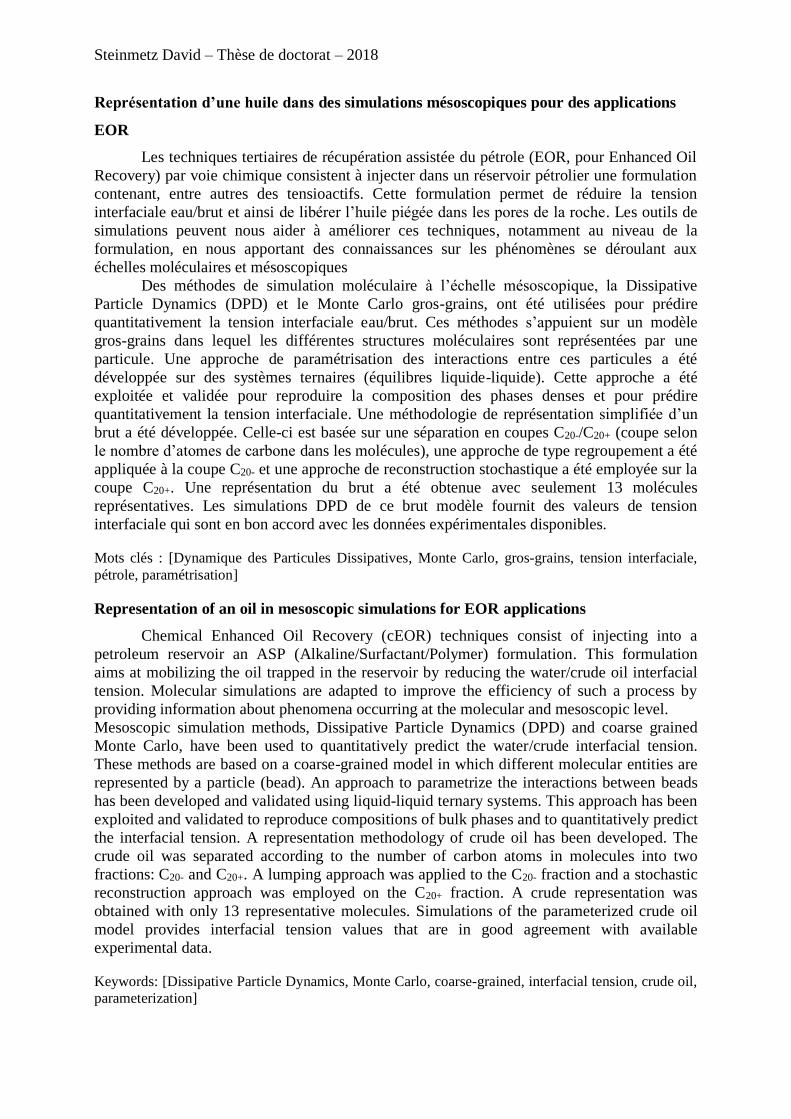
Steinmetz David – Thèse de doctorat – 2018

Représentation d’une huile dans des simulations mésoscopiques pour des applications

EOR

Les techniques tertiaires de récupération assistée du pétrole (EOR, pour Enhanced Oil

Recovery) par voie chimique consistent à injecter dans un réservoir pétrolier une formulation

contenant, entre autres des tensioactifs. Cette formulation permet de réduire la tension

interfaciale eau/brut et ainsi de libérer l’huile piégée dans les pores de la roche. Les outils de

simulations peuvent nous aider à améliorer ces techniques, notamment au niveau de la

formulation, en nous apportant des connaissances sur les phénomènes se déroulant aux

échelles moléculaires et mésoscopiques

Des méthodes de simulation moléculaire à l’échelle mésoscopique, la Dissipative

Particle Dynamics (DPD) et le Monte Carlo gros-grains, ont été utilisées pour prédire

quantitativement la tension interfaciale eau/brut. Ces méthodes s’appuient sur un modèle

gros-grains dans lequel les différentes structures moléculaires sont représentées par une

particule. Une approche de paramétrisation des interactions entre ces particules a été

développée sur des systèmes ternaires (équilibres liquide-liquide). Cette approche a été

exploitée et validée pour reproduire la composition des phases denses et pour prédire

quantitativement la tension interfaciale. Une méthodologie de représentation simplifiée d’un

brut a été développée. Celle-ci est basée sur une séparation en coupes C20-/C20+ (coupe selon

le nombre d’atomes de carbone dans les molécules), une approche de type regroupement a été

appliquée à la coupe C20- et une approche de reconstruction stochastique a été employée sur la

coupe C20+. Une représentation du brut a été obtenue avec seulement 13 molécules

représentatives. Les simulations DPD de ce brut modèle fournit des valeurs de tension

interfaciale qui sont en bon accord avec les données expérimentales disponibles.

Mots clés : [Dynamique des Particules Dissipatives, Monte Carlo, gros-grains, tension interfaciale,

pétrole, paramétrisation]

Representation of an oil in mesoscopic simulations for EOR applications

Chemical Enhanced Oil Recovery (cEOR) techniques consist of injecting into a

petroleum reservoir an ASP (Alkaline/Surfactant/Polymer) formulation. This formulation

aims at mobilizing the oil trapped in the reservoir by reducing the water/crude oil interfacial

tension. Molecular simulations are adapted to improve the efficiency of such a process by

providing information about phenomena occurring at the molecular and mesoscopic level.

Mesoscopic simulation methods, Dissipative Particle Dynamics (DPD) and coarse grained

Monte Carlo, have been used to quantitatively predict the water/crude interfacial tension.

These methods are based on a coarse-grained model in which different molecular entities are

represented by a particle (bead). An approach to parametrize the interactions between beads

has been developed and validated using liquid-liquid ternary systems. This approach has been

exploited and validated to reproduce compositions of bulk phases and to quantitatively predict

the interfacial tension. A representation methodology of crude oil has been developed. The

crude oil was separated according to the number of carbon atoms in molecules into two

fractions: C20- and C20+. A lumping approach was applied to the C20- fraction and a stochastic

reconstruction approach was employed on the C20+ fraction. A crude representation was

obtained with only 13 representative molecules. Simulations of the parameterized crude oil

model provides interfacial tension values that are in good agreement with available

experimental data.

Keywords: [Dissipative Particle Dynamics, Monte Carlo, coarse-grained, interfacial tension, crude oil,

parameterization]