Journal of Machine Learning Research 22 (2021) 1-37 Submitted 2/18; Revised 7/19; Published 4/21

As You Like It: Localization via Paired Comparisons

Andrew K. Massimino massimino@gatech.eduMark A. Davenport mdav@gatech.eduSchool of Electrical and Computer EngineeringGeorgia Institute of Technology777 Atlantic Dr NWAtlanta, GA 30332 USA

Editor: Francis Bach

AbstractSuppose that we wish to estimate a vector x from a set of binary paired comparisons ofthe form “x is closer to p than to q” for various choices of vectors p and q. The problemof estimating x from this type of observation arises in a variety of contexts, includingnonmetric multidimensional scaling, “unfolding,” and ranking problems, often because itprovides a powerful and flexible model of preference. We describe theoretical bounds for howwell we can expect to estimate x under a randomized model for p and q. We also presentresults for the case where the comparisons are noisy and subject to some degree of error.Additionally, we show that under a randomized model for p and q, a suitable number ofbinary paired comparisons yield a stable embedding of the space of target vectors. Finally,we also show that we can achieve significant gains by adaptively changing the distributionused for choosing p and q.Keywords: paired comparisons, ideal point models, recommendation systems, 1-bit sensing,binary embedding

1. Introduction

In this paper we consider the problem of determining the location of a point in Euclideanspace based on distance comparisons to a set of known points, where our observations arenonmetric. In particular, let x ∈ R𝑛 be the true position of the point that we are trying toestimate, and let (p1, q1), . . . , (p𝑚, q𝑚) be pairs of “landmark” points in R𝑛 which we assumeto be known a priori. Rather than directly observing the raw distances from x, i.e., ‖x−p𝑖‖and ‖x− q𝑖‖, we instead obtain only paired comparisons of the form ‖x− p𝑖‖ < ‖x− q𝑖‖.Our goal is to estimate x from a set of such inequalities. Nonmetric observations of thistype arise in numerous applications and have seen considerable interest in recent literaturee.g., (Ailon, 2011; Davenport, 2013; Eriksson, 2013; Shah et al., 2016). These methods areoften applied in situations where we have a collection of items and hypothesize that it ispossible to embed the items in R𝑛 in such a way that the Euclidean distance between pointscorresponds to their “dissimilarity,” with small distances corresponding to similar items.

Here, we focus on the sub-problem of adding a new point to a known (or previouslylearned) configuration of landmark points.

As a motivating example, we consider the problem of estimating a user’s preferences fromlimited response data. This is useful, for instance, in recommender systems, information

c○2021 Andrew K. Massimino and Mark A. Davenport.

License: CC-BY 4.0, see https://creativecommons.org/licenses/by/4.0/. Attribution requirements are providedat http://jmlr.org/papers/v22/18-105.html.

Massimino and Davenport

qi

pi

x

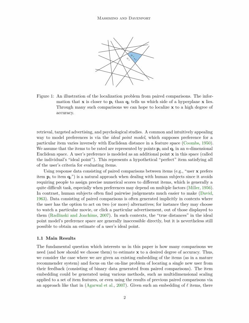
Figure 1: An illustration of the localization problem from paired comparisons. The infor-mation that x is closer to p𝑖 than q𝑖 tells us which side of a hyperplane x lies.Through many such comparisons we can hope to localize x to a high degree ofaccuracy.

retrieval, targeted advertising, and psychological studies. A common and intuitively appealingway to model preferences is via the ideal point model, which supposes preference for aparticular item varies inversely with Euclidean distance in a feature space (Coombs, 1950).We assume that the items to be rated are represented by points p𝑖 and q𝑖 in an 𝑛-dimensionalEuclidean space. A user’s preference is modeled as an additional point x in this space (calledthe individual’s “ideal point”). This represents a hypothetical “perfect” item satisfying allof the user’s criteria for evaluating items.

Using response data consisting of paired comparisons between items (e.g., “user x prefersitem p𝑖 to item q𝑖”) is a natural approach when dealing with human subjects since it avoidsrequiring people to assign precise numerical scores to different items, which is generally aquite difficult task, especially when preferences may depend on multiple factors (Miller, 1956).In contrast, human subjects often find pairwise judgements much easier to make (David,1963). Data consisting of paired comparisons is often generated implicitly in contexts wherethe user has the option to act on two (or more) alternatives; for instance they may chooseto watch a particular movie, or click a particular advertisement, out of those displayed tothem (Radlinski and Joachims, 2007). In such contexts, the “true distances” in the idealpoint model’s preference space are generally inaccessible directly, but it is nevertheless stillpossible to obtain an estimate of a user’s ideal point.

1.1 Main Results

The fundamental question which interests us in this paper is how many comparisons weneed (and how should we choose them) to estimate x to a desired degree of accuracy. Thus,we consider the case where we are given an existing embedding of the items (as in a maturerecommender system) and focus on the on-line problem of locating a single new user fromtheir feedback (consisting of binary data generated from paired comparisons). The itemembedding could be generated using various methods, such as multidimensional scalingapplied to a set of item features, or even using the results of previous paired comparisons viaan approach like that in (Agarwal et al., 2007). Given such an embedding of ℓ items, there

2

Localization via Paired Comparisons

are a total of(ℓ

2)

= Θ(ℓ2) possible paired comparisons. Clearly, in a system with thousands(or more) items, it will be prohibitive to acquire this many comparisons as a typical user willlikely only provide comparisons for a handful of items. Fortunately, in general we can expectthat many, if not most, of the possible comparisons are actually redundant. For example, ofthe comparisons illustrated in Fig. 1, all but four are redundant and—at least in the absenceof noise—add no additional information.

Any precise answer to this question would depend on the underlying geometry of theitem embedding. Each comparison essentially divides R𝑛 in two, indicating on which side ofa hyperplane x lies, and some arrangements of hyperplanes will yield better tessellationsof the preference space than others. Thus, to gain some intuition on this problem withoutreference to the geometry of a particular embedding, we will instead consider a probabilisticmodel where the items are generated at random from a particular distribution. In this casewe show that under certain natural assumptions on the distribution, it is possible to estimatethe location of any x to within an error of 𝜖 using a number of comparisons which, up to logfactors, is proportional to 𝑛/𝜖. This is essentially optimal, so that no set of comparisonscan provide a uniform guarantee with significantly fewer comparisons. We then describeseveral stability and robustness guarantees for various settings in which the comparisonsare subject to noise or errors. Finally, we then describe a simple extension to an adaptivescheme where we adaptively select the comparisons (manifested here in adaptively alteringthe mean and variance of the distribution generating the items) to substantially reduce therequired number of comparisons.

1.2 Related Work

It is important to note that the ideal point model, while similar, is distinct from the low-rankmodel used in matrix completion (Rennie and Srebro, 2005; Candès and Recht, 2009).Although both models suppose user choices are guided by a number of attributes, the idealpoint model leads to preferences that are non-monotonic functions of those attributes. Theideal point model suggests that each feature has an ideal level; too much of a feature can bejust as undesirable as too little. It is not possible to obtain this kind of performance with atraditional low-rank model, though if points are limited to the sphere, then the ideal pointmodel can duplicate the performance of a low-rank factorization. There is also empiricalevidence that the ideal point model captures behavior more accurately than factorizationbased approaches do (Dubois, 1975; Maydeu-Olivares and Böckenholt, 2009).

There is a large body of work that studies the problem of learning to rank items fromvarious sources of data, including paired comparisons of the sort we consider in this paper.See, for example, (Jamieson and Nowak, 2011a,b; Wauthier et al., 2013) and referencestherein. We first note that in most work on rankings, the central focus is on learning a correctrank-ordered list for a particular user, without providing any guarantees on recovering acorrect parameterization for the user’s preferences as we do here. While these two problemsare related, there are natural settings where it might be desirable to guarantee an accuraterecovery of the underlying parameterization (x in our model). For example, one could exploitthese guarantees in the context of an iterative algorithm for nonmetric multidimensionalscaling which aims to refine the underlying embedding by updating each user and item oneat a time (e.g., see O’Shaughnessy and Davenport, 2016), in which case an understanding of

3

Massimino and Davenport

the error in the estimate of x is crucial. Moreover, we believe that our approach provides aninteresting alternative perspective as it yields natural robustness guarantees and suggestssimple adaptive schemes.

Also closely related is the work in (Lu and Negahban, 2015; Park et al., 2015; Oh et al.,2014) which consider paired comparisons and more general ordinal measurements in thesimilar (but as discussed above, subtly different) context of low-rank factorizations. Perhapsmost closely related to our work is that of (Jamieson and Nowak, 2011a), which examinesthe problem of learning a rank ordering using the same ideal point model considered in thispaper. The message in this work is broadly consistent with ours, in that the number ofcomparisons required should scale with the dimension of the preference space (not the totalnumber of items) and can be significantly improved via a clever adaptive scheme. However,this work does not bound the estimation error in terms of the Euclidean distance, which isour central concern. (Jamieson and Nowak, 2011b) also incorporates adaptivity, but seeksto embed a set of points in Euclidean space (as opposed to estimating a single user’s idealpoint) and relies on paired comparisons involving three arbitrarily selected points (ratherthan a user’s ideal point and two items). Our dyadic adaptive strategy is also similar inspirit to a higher-dimensional form of binary search, as in (Nowak, 2009), however herewe consider estimating a continuous ideal point x rather than choosing from a finite set ofpossible hypotheses.

Constructing an embedding of items given comparison measurements is sometimesreferred to as ordinal embedding and is studied in (Kleindessner and Luxburg, 2014), (Jainet al., 2016), and (Arias-Castro et al., 2017). As mentioned, in this work we assume thepresence of an item embedding created by e.g., those methods. Our work could then beused to create a corresponding embedding of users based on response data to perform e.g.,personalization and customer segmentation.

Finally, while seemingly unrelated, we note that our work builds on the growing bodyof literature of 1-bit compressive sensing. In particular, our results are largely inspired bythose in (Knudson et al., 2016; Baraniuk et al., 2017), and borrow techniques from (Jacqueset al., 2013) in the proofs of some of our main results. Our embedding result of Section 4.1is most directly related to the work of (Plan and Vershynin, 2014), which studies a similarproblem to (2) but under a different, non-pairwise model. Because of this distinction, theirresults are not directly applicable. However, due to our particular probabilistic model, ourresults are also in some sense stronger. We will expand further with a direct comparison tothis work during the presentation of our result. The 1-bit sensing problem is also consideredin (Plan and Vershynin, 2013b) and (Plan and Vershynin, 2013a) but these works handleonly queries involving homogeneous hyperplanes, without offset, which is not applicableto our pairwise setting. Ideas similar to 1-bit sensing appear in field of locality sensitivehashing, e.g, (Konoshima and Noma, 2012) which does treat inhomogeneous hyperplanesbut does not provide theory.

Note that in this work we extend preliminary results first presented in (Massimino andDavenport, 2016, 2017).

4

Localization via Paired Comparisons

2. A Randomized Observation Model

For the moment we will consider the “noise-free” setting where each comparison between xand q𝑖 versus p𝑖 results in assigning the point which is truly closest to x with probability1. In this case we can represent the observed comparisons mathematically by letting 𝒜𝑖(x)denote the 𝑖th observation, which consists of comparisons between p𝑖 and q𝑖, and setting

𝒜𝑖(x) := sign(‖x− q𝑖‖2 − ‖x− p𝑖‖2

)={

+1 if x is closer to p𝑖

−1 if x is closer to q𝑖.(1)

We will also use 𝒜(x) := [𝒜1(x), · · · ,𝒜𝑚(x)]𝑇 to denote the vector of all observationsresulting from 𝑚 comparisons. Note that since

‖x− q𝑖‖2 − ‖x− p𝑖‖2 = 2(p𝑖 − q𝑖)𝑇 x + ‖q𝑖‖2 − ‖p𝑖‖2 ,

if we set a𝑖 = (p𝑖 − q𝑖) and 𝜏𝑖 = 12(‖p𝑖‖2 − ‖q𝑖‖2), then we can re-write our observation

model as𝒜𝑖(x) = sign

(2a𝑇

𝑖 x− 2𝜏𝑖

)= sign

(a𝑇

𝑖 x− 𝜏𝑖

). (2)

This is reminiscent of the standard setup in one-bit compressive sensing (with dithers) (Knud-son et al., 2016; Baraniuk et al., 2017) with the important differences that: (i) we have notmade any kind of sparsity or other structural assumption on x and, (ii) the “dithers” 𝜏𝑖,at least in this formulation, are dependent on the a𝑖, which results in difficulty applyingstandard results from this theory to the present setting.

However, many of the techniques from this literature will nevertheless be helpful inanalyzing this problem. To see this, we consider a randomized observation model wherethe pairs (p𝑖, q𝑖) are chosen independently with i.i.d. entries drawn according to a normaldistribution, i.e., p𝑖, q𝑖 ∼ 𝒩 (0, 𝜎2I). In this case, we have that the entries of our sensingvectors are i.i.d. with ��𝑖(𝑗) ∼ 𝒩 (0, 2𝜎2). Moreover, if we define b𝑖 = p𝑖 + q𝑖, then we alsohave that b𝑖 ∼ 𝒩 (0, 2𝜎2I), and

12 a𝑇

𝑖 b𝑖 = 12∑

𝑗

(p𝑖(𝑗)− q𝑖(𝑗))(p𝑖(𝑗) + q𝑖(𝑗))

= 12∑

𝑗

p𝑖(𝑗)2 − q𝑖(𝑗)2 = 12(‖p𝑖‖2 − ‖q𝑖‖2) = 𝜏𝑖.

Note that while 𝜏𝑖 = 12 a𝑇

𝑖 b𝑖 is clearly dependent on a𝑖, we do have that a𝑖 and b𝑖 areindependent.

To simplify, we re-normalize by dividing by ‖a𝑖‖, i.e., setting a𝑖 := a𝑖/ ‖a𝑖‖ and 𝜏𝑖 :=𝜏𝑖/ ‖a𝑖‖, in which case we can write

𝒜𝑖(x) = sign(a𝑇𝑖 x− 𝜏𝑖). (3)

It is easy to see that a𝑖 is distributed uniformly on the sphere S𝑛−1 = {a ∈ R𝑛 : ‖a‖ = 1}.Note that throughout our analysis we will exploit the fact that a𝑖 is uniform on S𝑛−1 andwill let 𝜈 denote the uniform measure on the sphere. Note also that

𝜏𝑖 = 12a𝑇

𝑖 b𝑖.

5

Massimino and Davenport

Since a𝑖 and b𝑖 are independent, a𝑖 and b𝑖 are also independent. Moreover, for any unit-vector a𝑖, if b𝑖 ∼ 𝒩 (0, 2𝜎2I) then a𝑇

𝑖 b𝑖 ∼ 𝒩 (0, 2𝜎2). Thus, we must have 𝜏𝑖 ∼ 𝒩 (0, 𝜎2/2),independent of a𝑖, which is the key insight that enables the analysis below.

3. Guarantees in the Noise-Free Setting

We now state a result concerning localization under the noise-free random model fromSection 2. Extensions to noisy comparisons and efficient estimation in practice are discussedin Sections 4 and 5, respectively. Let B𝑛

𝑅 denote the 𝑛-dimensional, radius 𝑅 Euclidean ball.

Theorem 1 Let 𝜖, 𝜂 > 0 be given. Let 𝒜𝑖(·) be defined as in (1), and suppose that 𝑚 pairs{(p𝑖, q𝑖)}𝑚𝑖=1 are generated by drawing each p𝑖 and q𝑖 independently from 𝒩 (0, 𝜎2𝐼) where𝜎2 = 2𝑅2/𝑛. There exists a constant 𝐶 such that if

𝑚 ≥ 𝐶𝑅

𝜖

(𝑛 log 𝑅

√𝑛

𝜖+ log 1

𝜂

), (4)

then with probability at least 1− 𝜂, for all x, y ∈ B𝑛𝑅 such that 𝒜(x) = 𝒜(y),

‖x− y‖ ≤ 𝜖.

The result follows from applying Lemma 2 below to pairs of points in a covering set of B𝑛𝑅.

The key message of this theorem is that if one chooses the variance 𝜎2 of the distributiongenerating the items appropriately, then it is possible to estimate x to within 𝜖 using anumber of comparisons that is nearly linear in 𝑛/𝜖. As we will show in Theorem 3, thisresult is optimal, ignoring log factors, in terms of the scaling of 𝑚 with 𝑛 and 𝜖. This alsomakes intuitive sense; if all the hyperplanes were all axis-aligned, one would require thenumber of hyperplanes be at least proportional to the number of dimensions, 𝑛, otherwisesome direction would be unconstrained. Theorem 1 is also sensible in terms of the ratio ofthe initial uncertainty 𝑅 to the target uncertainty 𝜖 since 𝑅/𝜖 hyperplanes would be requiredto uniformly localize a point along a single dimension.

A natural question is what would happen with a different choice of 𝜎2. In fact, thisassumption is critical—if 𝜎2 is substantially smaller the bound quickly becomes vacuous, andas 𝜎2 grows much past 𝑅2/𝑛 the bound begins to become steadily worse.1 As we will see inSection 6, this is in fact observed in practice. It should also be somewhat intuitive: if 𝜎2 istoo small, then nearly all the hyperplanes induced by the comparisons will pass very close tothe origin, so that accurate estimation of even ‖x‖ becomes impossible. On the other hand,if 𝜎2 is too large, then an increasing number of these hyperplanes will not even intersect theball of radius 𝑅 in which x is presumed to lie, thus yielding no new information.

Lemma 2 Let w, z ∈ B𝑛𝑅 be distinct and fixed, and let 𝛿 > 0 be given. Define

𝐵𝛿(w) := {u ∈ B𝑛𝑅 : ‖u−w‖ ≤ 𝛿}.

1. We note that it is possible to try to optimize 𝜎2 by setting 𝜎2 = 𝑐𝑅2/𝑛 for some constant 𝑐 and thenselecting 𝑐 so as to minimize the constant 𝐶 in (4). We believe this would yield limited insight since,in order to obtain a result which is valid uniformly for all possible 𝑛, we use certain bounds which forgeneral 𝑛 can be somewhat loose and would skew the resulting 𝑐. We instead simply select 𝑐 = 2 forsimplicity in our analysis (as it results in 𝜏𝑖 ∼ 𝒩 (0, 𝑅2/𝑛)) and because it aligns well with simulations.

6

Localization via Paired Comparisons

Let 𝒜𝑖 be defined as in Theorem 1. Denote by 𝑃sep the probability that 𝐵𝛿(w) and 𝐵𝛿(z) areseparated by hyperplane 𝑖, i.e.,

𝑃sep := P [∀u ∈ 𝐵𝛿(w),∀v ∈ 𝐵𝛿(z) : 𝒜𝑖(u) = 𝒜𝑖(v)] .

For any 𝜖0 ≤ ‖w− z‖ we have

𝑃sep ≥𝜖0 − 𝛿

√2𝑛

22√

𝜋𝑒5/2𝑅.

Proof Let 𝜖 = ‖w− z‖. Here, we denote the normal vector and threshold of hyperplane 𝑖by a and 𝜏 respectively. It is easy to show that 𝑃sep can be expressed as

𝑃sep = P[a𝑇 z + 𝛿 ≤ 𝜏 ≤ a𝑇 w− 𝛿 or a𝑇 w + 𝛿 ≤ 𝜏 ≤ a𝑇 z− 𝛿

]= 2P

[a𝑇 z + 𝛿 ≤ 𝜏 ≤ a𝑇 w− 𝛿

], (5)

where the second equality follows from the symmetry of the distributions of a and 𝜏 .Define 𝐶𝛼 := {a ∈ S𝑛−1 : a𝑇 (w− z) ≥ 𝛼}. Note that the probability in (5) is zero unless

a ∈ 𝐶2𝛿. Thus, recalling that 𝜏𝑖 ∼ 𝒩 (0, 𝜎2/2) we have

𝑃sep = 2∫

𝐶2𝛿

Φ(

a𝑇 w− 𝛿

𝜎/√

2

)− Φ

(a𝑇 z + 𝛿

𝜎/√

2

) 𝜈(da)

≥ 2∫

𝐶′

Φ(

a𝑇 w− 𝛿

𝜎/√

2

)− Φ

(a𝑇 z + 𝛿

𝜎/√

2

) 𝜈(da) (6)

for any 𝐶 ′ ⊆ 𝐶2𝛿. To obtain a lower bound on (6), we will consider a carefully chosen subset𝐶 ′ ⊆ 𝐶2𝛿 and then simply multiply the area of 𝐶 ′ by the minimum value 𝛾 of the integrandover that set, yielding a bound of the form

𝑃sep ≥ 2𝛾𝜈(𝐶 ′).

We construct the set 𝐶 ′ as follows. Let 𝑊 := {a : a𝑇 w ≤ 𝜉/√

𝑛 ‖w‖}, 𝑍 := {a : a𝑇 z ≥−𝜉/√

𝑛 ‖z‖}, and set 𝐶 ′ := 𝐶𝛼 ∩ 𝑊 ∩ 𝑍 for some 𝛼 ≥ 2𝛿. Note that for any a ∈ 𝐶 ′,since a𝑇 (w − z) ≥ 𝛼 ≥ 2𝛿, we have −𝑅𝜉/

√𝑛 ≤ a𝑇 z + 𝛿 ≤ a𝑇 w − 𝛿 ≤ 𝑅𝜉/

√𝑛. Thus, by

Lemma 11,

𝛾 = infa∈𝐶′

Φ(

a𝑇 w− 𝛿

𝜎/√

2

)− Φ

(a𝑇 z + 𝛿

𝜎/√

2

) ≥√

2𝜎

(𝛼− 2𝛿)𝜑(√2𝑅𝜉

𝜎√

𝑛

).

Recall by assumption we have that 𝜎 =√

2𝑅/√

𝑛, thus we obtain by setting 𝜉 =√

5,

𝛾 ≥√

𝑛

𝑅(𝛼− 2𝛿)𝜑(𝜉) =

√𝑛(𝛼− 2𝛿)√2𝜋𝑒5/2𝑅

. (7)

Next note that 𝐶 ′ = 𝐶𝛼 ∩𝑊 ∩𝑍 = 𝐶𝛼 ∖𝑊 𝑐 ∖𝑍𝑐 is a difference of a set of hypersphericalcaps. To obtain a lower bound on 𝜈(𝐶 ′) we use the upper and lower bounds on the measureof hyperspherical caps given in Lemma 2.1 of (Brieden et al., 2001).

7

Massimino and Davenport

Case 𝑛 ≥ 6 Provided that 𝛼/𝜖 <√

2/𝑛 we can bound 𝜈(𝐶 ′) as

𝜈(𝐶 ′) ≥ 𝜈(𝐶𝛼)− 𝜈(𝑊 𝑐)− 𝜈(𝑍𝑐) ≥ 112 − 2 1

2𝜉(1− 𝜉2/𝑛)(𝑛−1)/2 ≥ 1

12 −1√

5𝑒5/2 ,

where the last inequality follows from the fact that (1 − 𝑥/𝑛)𝑛−1 ≤ 𝑒−𝑥 for 𝑛 ≥ 𝑥 ≥ 2.Combining this with lower estimate (7),

𝑃sep ≥ 2𝛾𝜈(𝐶 ′) ≥ 2√

𝑛(𝛼− 2𝛿)√2𝜋𝑒2𝑅

1− 12𝑒−5/2/√

512 .

Setting 𝛼 = 𝛿 + 𝜖/√

2𝑛, since 1− 12𝑒−5/2/√

5 > 5/9, we have that

𝑃sep ≥2√

𝑛(𝜖/√

2𝑛− 𝛿)(1− 12𝑒−5/2/√

5)12√

2𝜋𝑒5/2𝑅≥ 𝜖− 𝛿

√2𝑛

22√

𝜋𝑒5/2𝑅.

Note that this bound holds under the assumption that 𝛼/𝜖 <√

2/𝑛, which for our choiceof 𝛼 is equivalent to the assumption that 𝜖 > 𝛿

√2𝑛. However, this bound also holds trivially

for all 𝜖 ≤ 𝛿√

2𝑛, and thus in fact holds for all 𝜖 ≥ 0.

Case 𝑛 ≤ 5 In this case, note that 𝜉/√

𝑛 ≥ 1, so the sets 𝑊 and 𝑍 are the entire sphere.Hence, 𝜈(𝑊 𝑐) = 𝜈(𝑍𝑐) = 0 and 𝜈(𝐶 ′) = 𝜈(𝐶𝛼) ≥ 1

12 . Thus,

𝑃sep ≥ 2𝛾𝜈(𝐶 ′) ≥ 𝜖− 𝛿√

2𝑛

12√

𝜋𝑒5/2𝑅.

We obtain the stated lemma by noting 𝜖0 ≤ 𝜖.

Proof of Theorem 1 Let 𝑃e denote the probability that there exists some x, y ∈ B𝑛𝑅 with

‖x− y‖ > 𝜖 and 𝒜(x) = 𝒜(y). Our goal is to show that 𝑃e ≤ 𝜂. Towards this end, let 𝑈 bea 𝛿-covering set for B𝑛

𝑅 with |𝑈 | ≤ (3𝑅/𝛿)𝑛. By construction, for any x, y ∈ B𝑛𝑅, there exist

some w, z ∈ 𝑈 satisfying ‖x−w‖ ≤ 𝛿 and ‖y− z‖ ≤ 𝛿. In this case, if ‖x− y‖ > 𝜖 then

‖w− z‖ ≥ ‖x− y‖ − 2𝛿 > 𝜖− 2𝛿.

Our goal is to upper bound the probability that there exists some w, z ∈ 𝑈 with ‖w− z‖ ≥𝜖0 = 𝜖− 2𝛿 and 𝒜(u) = 𝒜(v) for some u ∈ 𝐵𝛿(w) and v ∈ 𝐵𝛿(z). Said differently, we wouldlike to bound the probability that there exists a w, z ∈ 𝑈 with ‖w− z‖ ≥ 𝜖0 for which𝐵𝛿(w) and 𝐵𝛿(z) are not separated by any of the 𝑚 hyperplanes.

Let 𝑃𝑚(w, z) denote the probability that 𝐵𝛿(w) and 𝐵𝛿(z) are not separated by anyof the 𝑚 hyperplanes for a fixed w, z ∈ 𝑈 with ‖w− z‖ ≥ 𝜖0. Lemma 2 controls thisprobability for a single hyperplane, yielding a bound of

1− 𝑃sep ≤ 1− 𝜖0 − 𝛿√

2𝑛

22√

𝜋𝑒5/2𝑅.

Since the (p𝑖, q𝑖) are independent, we obtain

𝑃𝑚(w, z) ≤(

1− 𝜖0 − 𝛿√

2𝑛

22√

𝜋𝑒5/2𝑅

)𝑚

. (8)

8

Localization via Paired Comparisons

Since we are interested in the event that there exists any w, z ∈ 𝑈 with ‖w− z‖ ≥ 𝜖0 forwhich 𝐵𝛿(w) and 𝐵𝛿(z) are separated by none of the 𝑚 hyperplanes, we use the fact thatthere are at most (3𝑅/𝛿)2𝑛 such pairs w, z and combine a union bound with (8) to obtain

𝑃e ≤(3𝑅

𝛿

)2𝑛(

1− 𝜖0 − 𝛿√

2𝑛

22√

𝜋𝑒5/2𝑅

)𝑚

≤ exp

⎛⎝2𝑛 log 3𝑅

𝛿−

(𝜖0 − 𝛿

√2𝑛)

𝑚

22√

𝜋𝑒5/2𝑅

⎞⎠ , (9)

which follows from (1− 𝑥) ≤ 𝑒−𝑥. Bounding the right-hand side of (9) by 𝜂, we obtain

2𝑛 log 3𝑅

𝛿−

(𝜖0 − 𝛿

√2𝑛)

𝑚

22√

𝜋𝑒5/2𝑅≤ log 𝜂. (10)

If we now make the substitutions 𝜖0 = 𝜖 − 2𝛿 and 𝛿 = 𝜖/(4 +√

8𝑛), then we have that𝜖0 − 𝛿

√𝑛 = 𝜖/2 and thus we can reduce (10) to

2𝑛 log 3𝑅(4 +√

8𝑛)𝜖

− 𝜖𝑚

44√

𝜋𝑒5/2𝑅≤ log 𝜂.

By rearranging, we see that this is equivalent to

𝑚 ≥ 44√

𝜋𝑒5/2 𝑅

𝜖

(2𝑛 log 3𝑅(4 +

√8𝑛)

𝜖+ log 1

𝜂

). (11)

One can easily show that (4) implies (11) for an appropriate choice of 𝐶.

We now show that the result in Theorem 1 is optimal in the sense that any set ofcomparisons which can guarantee a uniform recovery of all x ∈ B𝑛

𝑅 to accuracy 𝜖 will requirea number of comparisons on the same order as that required in Theorem 1 (up to log factors).

Theorem 3 For any configuration of 𝑚 (inhomogeneous) hyperplanes in R𝑛 dividing B𝑛𝑅

into cells, if 𝑚 < 2𝑒

𝑅𝜖 𝑛, then there exist two points x, y ∈ B𝑛

𝑅 in the same cell such that‖x− y‖ ≥ 𝜖.

Proof We will use two facts. First, the number of cells (both bounded and unbounded)defined by 𝑚 hyperplanes in R𝑛 in general position2 is given by

𝐹𝑛(𝑚) =𝑛∑

𝑖=0

(𝑚

𝑖

)≤(

𝑒𝑚

𝑛

)𝑛

<

(2𝑅

𝜖

)𝑛

, (12)

where the second inequality follows from the assumption that 𝑚 < 2𝑅𝑛/𝑒𝜖.Second, for any convex set 𝐾 we have the isodiametric inequality (Giaquinta and Modica,

2010): where Diam(𝐾) = sup𝑥,𝑦∈𝐾 ‖𝑥− 𝑦‖,(Diam(𝐾)

2

)𝑛 𝜋𝑛/2

Γ(𝑛/2 + 1) ≥ Vol(𝐾), (13)

2. For non-general position, this is an upper bound (Buck, 1943).

9

Massimino and Davenport

with equality when 𝐾 is a ball. Since the entire volume of B𝑛𝑅, denoted Vol(B𝑛

𝑅), is filled byat most 𝐹𝑛(𝑚) non-overlapping cells, there must exist at least one such cell 𝐾0 with

Vol(𝐾0) ≥ Vol(B𝑛𝑅)

𝐹𝑛(𝑚) = 𝜋𝑛/2

Γ(𝑛/2 + 1)𝑅𝑛

𝐹𝑛(𝑚) . (14)

Combining (13) with (14), we obtain(Diam(𝐾0)2

)𝑛

≥ 𝑅𝑛

𝐹𝑛(𝑚) ,

which, together with (12), implies that

Diam(𝐾0) ≥ 2𝑅𝑛√

𝐹𝑛(𝑚)> 𝜖.

Thus there are vectors x, y ∈ 𝐾0 such that ‖x− y‖ > 𝜖.

4. Stability in Noise

So far, we have only considered the noise-free case. In most practical applications, obser-vations may be corrupted by noise. We consider two scenarios; in the first, we make noassumption on the source of the errors and instead show the paired comparison observationsare stable with respect to Euclidean distance. That is, two signals that have similar signpatterns are also nearby (and vice-versa). One can view this as a strengthening of the resultin Theorem 1. In the second case, Gaussian noise is added prior to the sign(·) function in (3).This is equivalent to the Thurstone model (Thurstone, 1927) with the Probit (normal) link.

The results of this section apply without considering any particular recovery methodor algorithm and relate to the number of paired comparisons which may be flipped due tothe noise, not from reconstruction. We address these concerns by introducing a practicalalgorithm and associated guarantees in Section 5.

Throughout the following, we denote by 𝑑𝐻 the Hamming distance, i.e., 𝑑𝐻 counts thefraction of comparisons which differ between two sets of observations, here denoted 𝒜(x)and 𝒜(y):

𝑑𝐻(𝒜(x),𝒜(y)) := 1𝑚

𝑚∑𝑖=1

12 |𝒜𝑖(x)−𝒜𝑖(y)|. (15)

4.1 Stable Embedding

Here we show that given enough comparisons there is an approximate embedding of thepreference space into {−1, 1}𝑚 via our model. Theorem 4 states that if x and y are sufficientlyclose, then the respective comparison patterns 𝒜(x) and 𝒜(y) closely align. In contrast withTheorem 8, Theorem 4 is a purely geometric statement which makes no assumptions on anyparticular noise model. Note also that Theorem 4 applies uniformly for all x and y.

10

Localization via Paired Comparisons

Theorem 4 Let 𝜂, 𝜁 > 0 be given. Let 𝒜(x) denote the collection of 𝑚 observations definedas in Theorem 1. There exist constants 𝐶1, 𝑐1, 𝐶2, 𝑐2 such that if

𝑚 ≥ 12𝜁2

(2𝑛 log 3

√𝑛

𝜁+ log 2

𝜂

), (16)

then with probability at least 1− 𝜂, for all x, y ∈ B𝑛𝑅 we have

𝐶1‖x− y‖

𝑅− 𝑐1𝜁 ≤ 𝑑𝐻(𝒜(x),𝒜(y)) ≤ 𝐶2

‖x− y‖𝑅

+ 𝑐2𝜁. (17)

This result implies that the fraction of differences in the set of observed comparisonsbetween x and y will be constrained to within a constant factor of the Euclidean distance,plus an additive error approximately proportional to 1/

√𝑚. At first glance, this seems worse

than the result of Theorem 1, which suggests the rate 1/𝑚. However, Theorem 4 comes withmuch greater flexibility in that Theorem 1 only concerns the case where 𝑑𝐻(𝒜(x),𝒜(y)) = 0.As in Theorem 1, this result applies for all x on the same randomly drawn set of items.

This result is very reminiscent of Theorem 1.10 in (Plan and Vershynin, 2014) whichconcerns tessellations under uniform random affine hyperplanes generated according to theHaar measure, rather than the particular Gaussian model we study. Compared to thatwork, our result is much better in terms of the scaling of the lower bound on 𝑚 with respectto distortion 𝜁 (they predict 1/𝜁12 while ours is 1/𝜁2). This is due to both our specificprobabilistic model and because we do not use the technique of “lifting” the problem todimension 𝑛 + 1 in our analysis because it would incur additional distortion. On the otherhand, the result of (Plan and Vershynin, 2014) is applicable to x lying in an arbitrary convexbody whereas our result considers only x within a radius 𝑅 ball.

Unlike in Theorem 1, we are not aware whether the relationship between 𝜁 and 𝑚 givenin Theorem 4 is optimal. This result is related to open questions concerning Dvoretzky’stheorem for embedding ℓ2 into ℓ1. See the discussion of optimality in Section 1.7 of (Planand Vershynin, 2014) and Remark 1.6 of (Plan and Vershynin, 2013b).

In the context of a hypothetical recovery problem, suppose x is a parameter of interestand y is an estimate produced by any algorithm. Then, (17) says that if we want to recoverx to within error 𝜖, the algorithm should look for vectors y which have up to 𝑂(𝜖) incorrectcomparisons. Likewise, if a y can be found having up to 𝑂(𝜖) comparison errors, we havethe same 𝑂(𝜖) guarantee on the Euclidean error of the estimate. In many cases, such aswhen errors are generated randomly, Theorem 1 would be inappropriate because finding a ysuch that 𝑑𝐻(𝒜(x),𝒜(y)) = 0 is likely to be impossible.

To prove Theorem 4 we will require the following Lemmas 5 and 6.

Lemma 5 Let w, z ∈ B𝑛𝑅 be distinct and fixed, and let 𝛿 > 0 be given. Let 𝒜(x) denote the

collection of 𝑚 observations defined as in Theorem 1, and let 𝐵𝛿(·) be defined as in Lemma 2.Denote by 𝑃0 the probability that 𝐵𝛿(w) and 𝐵𝛿(z) are not separated by hyperplane 𝑖, i.e.,

𝑃0 = P [∀u ∈ 𝐵𝛿(w), ∀v ∈ 𝐵𝛿(z) : 𝒜𝑖(u) = 𝒜𝑖(v)] .

Then1− 𝑃0 ≤

√2𝜋

(‖w− z‖

𝑅+ 𝛿√

𝑛

𝑅

).

11

Massimino and Davenport

Proof We need an upper bound on

1− 𝑃0 = P [𝒜𝑖(u) = 𝒜𝑖(v) for some u ∈ 𝐵𝛿(w), v ∈ 𝐵𝛿(z)] .

Suppose for now that a is fixed and without loss of generality that a𝑇 w > a𝑇 z. Then thisprobability is simply

P[a𝑇 v < 𝜏 < a𝑇 u for some u ∈ 𝐵𝛿(w), v ∈ 𝐵𝛿(z)

]= P

[min

v∈𝐵𝛿(z)a𝑇 v < 𝜏 < max

u∈𝐵𝛿(w)a𝑇 u

]≤ P

[a𝑇 z− 𝛿 < 𝜏 < a𝑇 w + 𝛿

],

since by Cauchy–Schwarz we have

minv∈𝐵𝛿(z)

a𝑇 v ≥ a𝑇 z− 𝛿 and maxu∈𝐵𝛿(w)

a𝑇 u ≤ a𝑇 w + 𝛿.

Thus, recalling that 𝜏𝑖 ∼ 𝒩 (0, 𝑅2/𝑛), from Lemma 11 we have

P[a𝑇 z− 𝛿 < 𝜏 < a𝑇 w + 𝛿

]= Φ

(a𝑇 w + 𝛿

𝑅/√

𝑛

)− Φ

(a𝑇 z− 𝛿

𝑅/√

𝑛

)

≤ 1𝑅

√𝑛

2𝜋

(a𝑇 (w− z) + 2𝛿

).

Similarly, for a𝑇 w < a𝑇 z we have

P[a𝑇 w− 𝛿 < 𝜏 < a𝑇 z + 𝛿

]≤ 1

𝑅

√𝑛

2𝜋

(a𝑇 (z−w) + 2𝛿

).

Combining these we have

1− 𝑃0 ≤∫S𝑛−1

1𝑅

√𝑛

2𝜋

(|a𝑇 (w− z)|+ 2𝛿

)𝜈(da)

= 1𝑅

√𝑛

2𝜋

∫S𝑛−1|a𝑇 (w− z)| 𝜈(da) + 2𝛿

𝑅

√𝑛

2𝜋

=√

2𝑛

𝑅𝜋

Γ(𝑛2 )

Γ(𝑛+12 )‖w− z‖+ 𝛿

𝑅

√2𝑛

𝜋,

where the last equality is proven in Lemma 12. The lemma then follows from the facts thatΓ(1/2)Γ(1) =

√𝜋 and Γ( 𝑛

2 )Γ( 𝑛+1

2 ) ≤2√

2𝑛−1 ≤√

𝜋𝑛 for 𝑛 ≥ 2 (Qi, 2010, (2.20)).

Lemma 6 Let w, z ∈ B𝑛𝑅 be distinct and fixed, and let 𝛿, 𝜁 > 0 be given. Let 𝒜(x) denote

the collection of 𝑚 observations defined as in Theorem 1, and let 𝐵𝛿(·) be defined as inLemma 2. Then for all u ∈ 𝐵𝛿(w) and v ∈ 𝐵𝛿(z),

122𝑒5/2√𝜋

(‖w− z‖

𝑅− 𝛿√

2𝑛

𝑅

)− 𝜁 ≤ 𝑑𝐻(𝒜(u),𝒜(v)) ≤

√2𝜋

(‖w− z‖

𝑅+ 𝛿√

𝑛

𝑅

)+ 𝜁,

with probability at least 1− exp(−2𝜁2𝑚).

12

Localization via Paired Comparisons

Proof Fix 𝛿 > 0 and let u ∈ 𝐵𝛿(w), v ∈ 𝐵𝛿(z). Recall that the Hamming distance 𝑑𝐻 isa sum of independent and identically distributed Bernoulli random variables and we maybound it using Hoeffding’s inequality. Since our probabilistic upper and lower bounds musthold for all u, v as described above, we introduce quantities 𝐿0 and 𝐿1 which represent two“extreme cases” of the Bernoulli variables:

𝐿0 := supu∈𝐵𝛿(w),v∈𝐵𝛿(z)

12𝑚

𝑚∑𝑖=1|𝒜𝑖(u)−𝒜𝑖(v)|

𝐿1 := infu∈𝐵𝛿(w),v∈𝐵𝛿(z)

12𝑚

𝑚∑𝑖=1|𝒜𝑖(u)−𝒜𝑖(v)|.

Then we have𝐿1 ≤ 𝑑𝐻(𝒜(u),𝒜(v)) ≤ 𝐿0.

Denote 𝑃0 = 1− E𝐿0 and 𝑃1 = E𝐿1, i.e.,

𝑃0 = P [∀u ∈ 𝐵𝛿(w), ∀v ∈ 𝐵𝛿(z) : 𝒜𝑖(u) = 𝒜𝑖(v)]𝑃1 = P [∀u ∈ 𝐵𝛿(w), ∀v ∈ 𝐵𝛿(z) : 𝒜𝑖(u) = 𝒜𝑖(v)] .

By Hoeffding’s inequality,

P [𝐿0 > (1− 𝑃0) + 𝜁] ≤ exp(−2𝑚𝜁2)P [𝐿1 < 𝑃1 − 𝜁] ≤ exp(−2𝑚𝜁2).

Hence, with probability at least 1− 2 exp(−2𝑚𝜁2),

𝑃1 − 𝜁 ≤ 𝑑𝐻(𝒜(u),𝒜(v)) ≤ (1− 𝑃0) + 𝜁.

The result follows directly from this combined with the facts that from Lemma 2 we have

𝑃1 ≥1

22𝑒5/2√𝜋

(‖w− z‖

𝑅− 𝛿√

2𝑛

𝑅

),

and from Lemma 5 we have

1− 𝑃0 ≤√

2𝜋

(‖w− z‖

𝑅+ 𝛿√

𝑛

𝑅

).

Proof of Theorem 4 By Lemma 6, for any fixed pair w, z ∈ B𝑛𝑅 we have bounds on the

Hamming distance that hold with probability at least 1− 2 exp(−2𝜁2𝑚), for all u ∈ 𝐵𝛿(w)and v ∈ 𝐵𝛿(z). Recall that the radius 𝑅 ball can be covered with a set 𝑈 of radius 𝛿balls with |𝑈 | ≤ (3𝑅/𝛿)𝑛. Thus, by a union bound we have that with probability at least1− 2(3𝑅/𝛿)2𝑛 exp(−2𝜁2𝑚), for any w, z ∈ 𝑈 ,

122𝑒5/2√𝜋

(‖w− z‖

𝑅− 𝛿√

2𝑛

𝑅

)− 𝜁 ≤ 𝑑𝐻(𝒜(u),𝒜(v)) ≤

√2𝜋

(‖w− z‖

𝑅+ 𝛿√

𝑛

𝑅

)+ 𝜁,

13

Massimino and Davenport

for all u ∈ 𝐵𝛿(w) and v ∈ 𝐵𝛿(z). Since ‖x− y‖−2𝛿 ≤ ‖w− z‖ ≤ ‖x− y‖+2𝛿, this impliesthat

122𝑒5/2√𝜋

(‖x− y‖ − 2𝛿

𝑅− 𝛿√

2𝑛

𝑅

)−𝜁 ≤ 𝑑𝐻(𝒜(x),𝒜(y)) ≤

√2𝜋

(‖x− y‖+ 2𝛿

𝑅+ 𝛿√

𝑛

𝑅

)+𝜁,

Letting 𝛿 = 𝜁𝑅/√

𝑛 and setting 𝐶1, 𝑐1, 𝐶2, 𝑐1 appropriately3 this reduces to (17). Lowerbounding the probability by 1− 𝜂, we obtain

2(3√

𝑛/𝜁)2𝑛 exp(−2𝜁2𝑚) ≤ 𝜂.

Rearranging yields (16).

4.2 Gaussian Noise

Here we aim to understand how the paired comparisons change with the introduction of“pre-quantization” Gaussian noise. This will have the effect of causing some comparisons tobe erroneous, where the probability of an error will be largest when x is equidistant from p𝑖

and q𝑖 and will decay as x moves away from this boundary.Towards this end, recall that the observation model in (1) can be reduced to the form

𝒜𝑖(x) = sign(𝑞𝑖) 𝑞𝑖 := a𝑇𝑖 x− 𝜏𝑖. (18)

In the noisy case, we will consider the observations

𝒜𝑖(x) = sign(𝑞𝑖) 𝑞𝑖 := a𝑇𝑖 x− 𝜏𝑖 + 𝑧𝑖 = 𝑞𝑖 + 𝑧𝑖, (19)

where 𝑧𝑖 ∼ 𝒩 (0, 𝜎2𝑧). Note that since ‖a𝑖‖ = 1, this model is equivalent to adding multivariate

Gaussian noise directly to x with covariance 𝜎2𝑧I. For a fixed x, we can then quantify the

probability that 𝑑𝐻(𝒜(x),𝒜(x)) is large via our next two results. We first consider the caseof a single comparison in Lemma 7, then extend this to an arbitrary number of comparisonsin Theorem 8.

Lemma 7 Suppose 𝑛 ≥ 4. Then P[𝒜𝑖(x) = 𝒜𝑖(x)] ≤ 𝜅𝑛(𝜎2𝑧) where 𝜅𝑛 is defined by

𝜅𝑛(𝜎2𝑧) := 1

2

√𝜎2

𝑧

𝜎2𝑧 + 2𝑅2/𝑛 + 4 ‖x‖2 /𝑛

≤ 12

√1

1 + 2𝑅2/(𝑛𝜎2𝑧) . (20)

For clarity, we focus here on the 𝑛 ≥ 4 case. We consider the 𝑛 = 2 and 𝑛 = 3 cases separatelybecause when 𝑛 ≥ 4 the probability distribution function of a𝑇

𝑖 x is well-approximated by aGaussian function but not for 𝑛 < 4. We give alternative expressions for 𝜅𝑛 when 𝑛 = 2 and𝑛 = 3 in Appendix B.

3. We set 𝐶1 = 1/22𝑒5/2√𝜋 and 𝐶2 =

√2/𝜋. We may set 𝑐1 = 1+1/11𝑒5/2√

𝜋+√

2/𝜋 and 𝑐2 = 1+3√

2/𝜋to obtain constants that are valid for all 𝑛—improved values are possible for large 𝑛.

14

Localization via Paired Comparisons

Theorem 8 Suppose 𝑛 ≥ 4 and fix x ∈ B𝑛𝑅. Let 𝒜(x) and 𝒜(x) denote the collection of 𝑚

observations defined as in (18) and (19) respectively, where the {(p𝑖, q𝑖)}𝑚𝑖=1 (and hence the{(a𝑖, 𝜏𝑖)}𝑚𝑖=1) are generated as in Theorem 1. Then,

E 𝑑𝐻(𝒜(x),𝒜(x)) ≤ 𝜅𝑛(𝜎2𝑧) ≤ 1

2

√1

1 + 2𝑅2/(𝑛𝜎2𝑧) . (21)

andP[𝑑𝐻(𝒜(x),𝒜(x)) ≥ 𝜅𝑛(𝜎2

𝑧) + 𝜁]≤ exp(−2𝑚𝜁2). (22)

where 𝜅𝑛 is defined in (20).

Proof By Lemma 7, we have that P[𝒜𝑖(x) = 𝒜𝑖(x)] is bounded by 𝜅𝑛(𝜎2𝑧). Since the

comparisons are independent, the expected number of sign mismatches is just the probabilityof a sign flip just computed, which establishes (21). The tail bound in (22) is a simpleconsequence of Hoeffding’s inequality.

The bound (21) of Theorem 8 behaves as one would expect. If the variance 𝜎2𝑧 of the

added Gaussian noise is small, we predict that the expected fraction of errors is also small.To place this result in context, recall that 𝜏𝑖 ∼ 𝒩 (0, 𝑅2/𝑛). Suppose that 𝜎2

𝑧 = 𝑐0𝑅2/𝑛. Inthis case one can bound 𝜅𝑛(𝜎2

𝑧) in (20) as

12

√𝑐0

𝑐0 + 6 ≤ 𝜅𝑛(𝜎2𝑧) ≤ 1

2

√𝑐0

𝑐0 + 2 .

Intuitively, if 𝑐0 is close to 1, meaning the noise variance is comparable to that of 𝜏𝑖,then we would expect to lose a significant amount of information about x, in which case𝑑𝐻(𝒜(x),𝒜(x)) could potentially be quite large. In contrast, by letting 𝑐0 grow small wecan bound 𝜅𝑛(𝜎2

𝑧) ≤√

𝑐0/8 arbitrarily close to zero.It is instructive to consider Theorem 8 next to Theorem 4, which also predicts the

fraction of sign mismatches up to an additive constant which is proportional to 1/√

𝑚. (21)and (22) provide upper estimates of the level of comparison errors which is unavoidable,regardless of recovery technique. If, in a particular application the noise is expected tobe Gaussian, the bound in (22) can be used in the lower half of (17) to create a recoveryguarantee. Note that since Theorem 4 is a uniform guarantee, better estimates than thiscould be possible in the specific case of Gaussian noise. We explore Gaussian noise furtherin Section 5.1.Proof of Lemma 7 The probability of a sign flip is given by

P [𝑞𝑖𝑞𝑖 < 0] = P [𝑞𝑖 < 0 and 𝑞𝑖 > 0] + P [𝑞𝑖 > 0 and 𝑞𝑖 < 0] .

Note that if we set 𝑟𝑖 := a𝑇𝑖 x/ ‖x‖ ∈ [−1, 1], then we can write 𝑞𝑖 = 𝑟𝑖 ‖x‖ − 𝜏𝑖 and

𝑞𝑖 = 𝑟𝑖 ‖x‖ − 𝜏𝑖 + 𝑧𝑖 where the random variables 𝑟𝑖, 𝜏𝑖, and 𝑧𝑖 are independent. Where 𝑓𝑟(𝑟𝑖)denotes the probability density functions for 𝑟𝑖 and recalling that 𝜏𝑖 ∼ 𝒩 (0, 2𝑅2/𝑛), weshow in Appendix B using standard Gaussian tail bounds that

P[𝑞𝑖𝑞𝑖 < 0] ≤ 1𝑅

√𝑛

𝜋

∫ 1

0

∫ ∞

−∞𝑓𝑟(𝑟𝑖) exp

(−(𝑟𝑖 ‖x‖ − 𝜏𝑖)2

2𝜎2𝑧

− 𝑛𝜏2𝑖

4𝑅2

)d𝜏𝑖 d𝑟𝑖. (23)

15

Massimino and Davenport

The remainder of the proof (given in Appendix B) is obtained by bounding this integral.Note that in general, we have 1

2(𝑟𝑖 + 1) ∼ Beta((𝑛− 1)/2, (𝑛− 1)/2), but 𝑟𝑖 is asymptoticallynormal with variance 1/𝑛 (Spruill, 2007). For 𝑛 ≥ 4, we use the simple upper bound

𝑓𝑟(𝑟𝑖) = 12

[𝐵

(𝑛− 1

2 ,𝑛− 1

2

)]−1(1 + 𝑟𝑖

21− 𝑟𝑖

2

)(𝑛−3)/2

≤ 12

[√2𝜋 𝑛−1

2(𝑛−2)/2 𝑛−1

2(𝑛−2)/2

(𝑛− 1)𝑛−1−1/2

]−1(1− 𝑟2

𝑖

4

)(𝑛−3)/2

= 12

[ √2𝜋

2𝑛−2√𝑛− 1

]−1 12𝑛−3 exp(−(𝑛− 3)𝑟2

𝑖 /2)

=√

𝑛− 14√

2𝜋exp(−(𝑛− 3)𝑟2

𝑖 /2) ≤√

𝑛

4√

2𝜋exp(−𝑛𝑟2

𝑖 /8). (24)

This follows from the standard inequalities 𝐵(𝑥, 𝑦) ≥√

2𝜋𝑥𝑥−1/2𝑦𝑦−1/2/(𝑥 + 𝑦)𝑥+𝑦−1/2 (e.g.,Grenié and Molteni, 2015) and 1− 𝑥 ≤ exp(−𝑥).

5. Estimation Algorithm and Guarantees

In the noise-free setting, given a set of comparisons 𝒜(x), we may produce an estimate xby finding any x ∈ B𝑛

𝑅 satisfying 𝒜(x) = 𝒜(x). A simple approach is the following convexprogram:

x = arg minw

‖w‖2 subject to 𝒜𝑖(x)(a𝑇𝑖 w− 𝜏𝑖) ≥ 0 ∀𝑖 ∈ [𝑚]. (25)

This is relatively easy to solve since the constraints are simple linear inequalities and thefeasible region is convex. Note that (25) is guaranteed to satisfy x ∈ B𝑛

𝑅 since x ∈ B𝑛𝑅 and x

is feasible, so that ‖x‖ ≤ ‖x‖ ≤ 𝑅. In this case we may apply Theorem 1 to argue that if 𝑚obeys the bound in (4), then ‖x− x‖ ≤ 𝜖.

However, in most practical applications, observations are likely to be corrupted by noiseleading to inconsistencies. Any errors in the observations 𝒜(x) would make strictly enforcing𝒜(x) = 𝒜(x) a questionable goal since, among other drawbacks, x itself would becomeinfeasible. In fact, in this case we cannot even necessarily guarantee that (25) has anyfeasible solutions. In the noisy case we instead use a relaxation inspired by the extended𝜈-SVM of (Perez-Cruz et al., 2003), which introduces slack variables 𝜉𝑖 ≥ 0 and is controlledby the parameter 𝜈. Specifically, we denote by 𝒜(x) the collection of (potentially) corruptedmeasurements, and we solve

minimizew∈R𝑛+1,𝜉∈R𝑚,𝜌∈R−𝜈𝜌 + 1

𝑚

𝑚∑𝑖=1

𝜉𝑖

subject to 𝒜𝑖(x)([a𝑇𝑖 ,−𝜏𝑖] w) ≥ 𝜌− 𝜉𝑖, 𝜉𝑖 ≥ 0, ∀𝑖 ∈ [𝑚],

‖ w[1 : 𝑛]‖2 ≤ 2𝑅2

1+𝑅2 , and ‖ w‖2 = 2.

(26)

Finally, we set x = w[1, . . . , 𝑛]/ w[𝑛 + 1]. The additional constraint ‖ w[1 : 𝑛]‖2 ≤ 2𝑅2

1+𝑅2

ensures that ‖x‖ ≤ 𝑅. Note that an important difference between the extended 𝜈-SVM and

16

Localization via Paired Comparisons

(26) is that there is no “offset” parameter to be optimized over. That is, if we interpret[a𝑖,−𝜏𝑖] as “training examples,” then w := [x, 1] ∈ R𝑛+1 corresponds to a homogeneouslinear classifier. Note that in the absence of comparison errors, setting 𝜈 = 0, we would havea feasible solution with 𝜉𝑖 = 0.

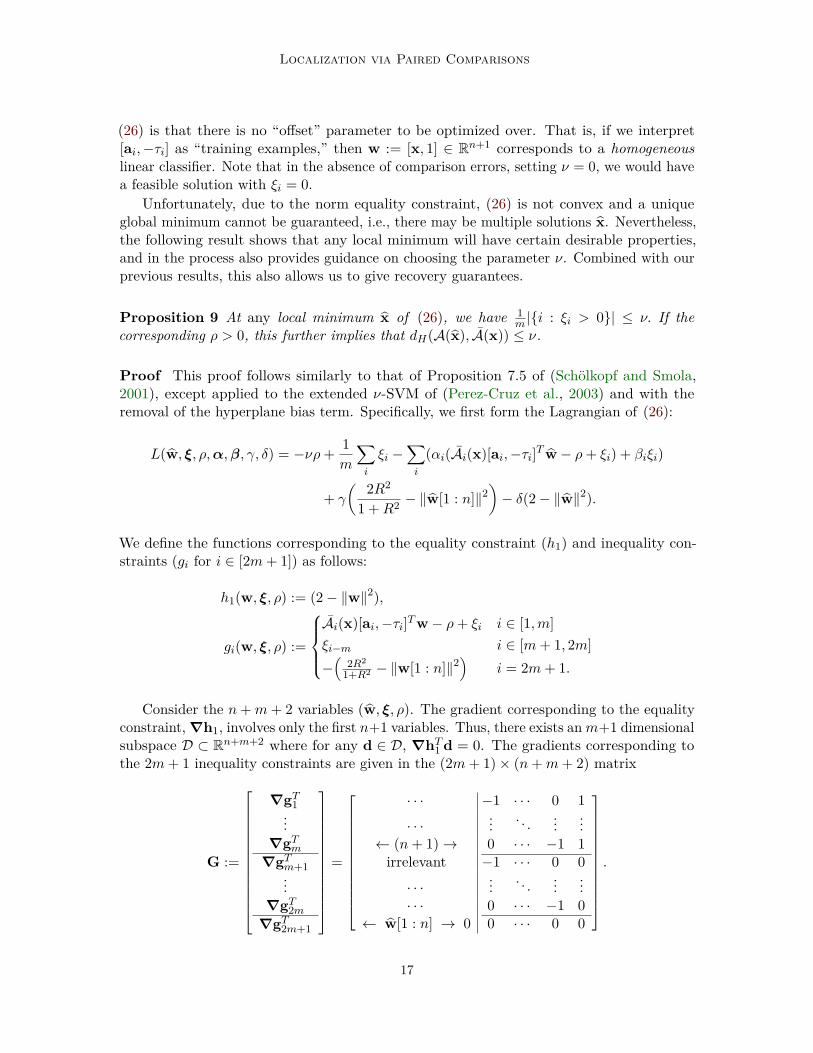
Unfortunately, due to the norm equality constraint, (26) is not convex and a uniqueglobal minimum cannot be guaranteed, i.e., there may be multiple solutions x. Nevertheless,the following result shows that any local minimum will have certain desirable properties,and in the process also provides guidance on choosing the parameter 𝜈. Combined with ourprevious results, this also allows us to give recovery guarantees.

Proposition 9 At any local minimum x of (26), we have 1𝑚 |{𝑖 : 𝜉𝑖 > 0}| ≤ 𝜈. If the

corresponding 𝜌 > 0, this further implies that 𝑑𝐻(𝒜(x),𝒜(x)) ≤ 𝜈.

Proof This proof follows similarly to that of Proposition 7.5 of (Schölkopf and Smola,2001), except applied to the extended 𝜈-SVM of (Perez-Cruz et al., 2003) and with theremoval of the hyperplane bias term. Specifically, we first form the Lagrangian of (26):

𝐿( w, 𝜉, 𝜌, 𝛼, 𝛽, 𝛾, 𝛿) = −𝜈𝜌 + 1𝑚

∑𝑖

𝜉𝑖 −∑

𝑖

(𝛼𝑖(𝒜𝑖(x)[a𝑖,−𝜏𝑖]𝑇 w− 𝜌 + 𝜉𝑖) + 𝛽𝑖𝜉𝑖)

+ 𝛾

( 2𝑅2

1 + 𝑅2 − ‖ w[1 : 𝑛]‖2)− 𝛿(2− ‖ w‖2).

We define the functions corresponding to the equality constraint (ℎ1) and inequality con-straints (𝑔𝑖 for 𝑖 ∈ [2𝑚 + 1]) as follows:

ℎ1(w, 𝜉, 𝜌) := (2− ‖w‖2),

𝑔𝑖(w, 𝜉, 𝜌) :=

⎧⎪⎪⎨⎪⎪⎩𝒜𝑖(x)[a𝑖,−𝜏𝑖]𝑇 w− 𝜌 + 𝜉𝑖 𝑖 ∈ [1, 𝑚]𝜉𝑖−𝑚 𝑖 ∈ [𝑚 + 1, 2𝑚]−(

2𝑅2

1+𝑅2 − ‖w[1 : 𝑛]‖2)

𝑖 = 2𝑚 + 1.

Consider the 𝑛 + 𝑚 + 2 variables ( w, 𝜉, 𝜌). The gradient corresponding to the equalityconstraint, ∇h1, involves only the first 𝑛+1 variables. Thus, there exists an 𝑚+1 dimensionalsubspace 𝒟 ⊂ R𝑛+𝑚+2 where for any d ∈ 𝒟, ∇h𝑇

1 d = 0. The gradients corresponding tothe 2𝑚 + 1 inequality constraints are given in the (2𝑚 + 1)× (𝑛 + 𝑚 + 2) matrix

G :=

⎡⎢⎢⎢⎢⎢⎢⎢⎢⎢⎢⎢⎢⎣

∇g𝑇1

...∇g𝑇

𝑚

∇g𝑇𝑚+1...

∇g𝑇2𝑚

∇g𝑇2𝑚+1

⎤⎥⎥⎥⎥⎥⎥⎥⎥⎥⎥⎥⎥⎦=

⎡⎢⎢⎢⎢⎢⎢⎢⎢⎢⎢⎢⎣

· · · −1 · · · 0 1

· · ·... . . . ...

...← (𝑛 + 1)→ 0 · · · −1 1

irrelevant −1 · · · 0 0

· · ·... . . . ...

...· · · 0 · · · −1 0

← w[1 : 𝑛] → 0 0 · · · 0 0

⎤⎥⎥⎥⎥⎥⎥⎥⎥⎥⎥⎥⎦.

17

Massimino and Davenport

Since there is a d ∈ 𝒟 such that (Gd)[𝑖] < 0 for all 𝑖 (for example, d = [0, . . . , 0|1, . . . , 1,−1]),the Mangasarian–Fromovitz constraint qualifications hold and we have the following first-order necessary conditions for local minima (see e.g., Bertsekas, 1999),

𝜕𝐿

𝜕𝜌= −𝜈 +

∑𝛼𝑖 =⇒

∑𝛼𝑖 = 𝜈

and𝜕𝐿

𝜕𝜉𝑖= 1

𝑚− 𝛼𝑖 − 𝛽𝑖 = 0 =⇒ 𝛼𝑖 + 𝛽𝑖 = 1

𝑚.

Since∑𝑚

𝑖=1 𝛼𝑖 = 𝜈, at most a fraction of 𝜈 can have 𝛼𝑖 = 1/𝑚. Now, any 𝑖 such that 𝜉𝑖 > 0must have 𝛼𝑖 = 1/𝑚 since by complimentary slackness, 𝛽𝑖 = 0. Hence, 𝜈 is an upper boundon the fraction of 𝜉 such that 𝜉𝑖 > 0.

Finally, note that if 𝜌 > 0, then 𝜉𝑖 = 0 implies 𝒜𝑖(x)([a𝑇𝑖 ,−𝜏𝑖] w) ≥ 𝜌− 𝜉𝑖 > 0. Hence,

the fraction of 𝜉 such that 𝜉𝑖 > 0 is an upper bound for 𝑑𝐻(𝒜(x),𝒜(x)).

5.1 Estimation Guarantees

We now show how the results of Theorems 8 and 4 can be combined with Proposition 9to give recovery guarantees on ‖x− x‖ when (26) is used for recovery under realistic noisyobservation models. We consider three basic noise models. In the first, an arbitrary (butsmall) fraction of comparisons are reversed. We then consider the implication of this resultin the context of two other noise models, one where Gaussian noise is added to either theunderlying x or to the comparisons “pre-quantization,” that is, directly to (a𝑇

𝑖 x− 𝜏𝑖), andanother where the observations are generated using an arbitrary (but bounded) perturbationof x. We will ultimately see that largely similar guarantees are possible in all three cases,summarized in Table 1.

Table 1: Summary of our estimation guarantees in this section, where each result holdsseparately with probability at least 1− 𝜂 where 𝜂, 𝑐1, 𝑐2, 𝐶1, 𝐶2 are constants whichmay differ between results.

Noise type Guarantee on ‖x− x‖ /𝑅 Eq.

Adversarial, level 𝜅 ∘ ≤ 2𝐶1

𝜅 + 𝑐1𝐶1

√𝑛 log(18𝑚)+log(2/𝜂)

2𝑚 (30)i.i.d. Gaussian, 𝜎2

𝑧 ∘ ≤√

2𝐶1

√𝑛𝜎2

𝑧𝑅2 + 1

𝐶1

√log(1/𝜂)

2𝑚 + 𝑐1𝐶1

√𝑛 log(18𝑚)+log(2/𝜂)

2𝑚 (31)Perturbations 𝑥 ↦→ 𝑥′ ∘ ≤ 2𝐶2

𝐶1‖x−x′‖

𝑅 + 𝑐1+2𝑐2𝐶1

√𝑛 log(18𝑚)+log(2/𝜂)

2𝑚 (33)

In our analysis of all three settings, we will use the fact that from the lower bound ofTheorem 4 we have

‖x− x‖𝑅

≤ 𝑑𝐻(𝒜(x),𝒜(x)) + 𝑐1𝜁

𝐶1(27)

18

Localization via Paired Comparisons

with probability at least 1− 𝜂 provided that 𝑚 is sufficiently large, e.g., by taking

𝑚 = 12𝜁2

(2𝑛 log 3

√𝑛

𝜁+ log 2

𝜂

). (28)

Note that by setting 𝛽 = 9𝑛𝜁2

(2𝜂

)1/𝑛, we can rearrange (28) to be of the form

18𝑚

(2𝜂

)1/𝑛

= 𝛽 log 𝛽,

which implies that

𝛽 = 18𝑚(2/𝜂)1/𝑛

𝑊(18𝑚(2/𝜂)1/𝑛

) ,where 𝑊 (·) denotes the Lambert 𝑊 function. Using the fact that 𝑊 (𝑥) ≤ log(𝑥) for 𝑥 ≥ 𝑒and substituting back in for 𝛽, we have

𝜁 ≤

√𝑛 log(18𝑚) + log(2/𝜂)

2𝑚

under the mild assumption that 𝑚 ≥ 𝑒18(𝜂

2 )1/𝑛. Substituting this in to (27) yields

‖x− x‖𝑅

≤ 𝑑𝐻(𝒜(x),𝒜(x))𝐶1

+ 𝑐1𝐶1

√𝑛 log(18𝑚) + log(2/𝜂)

2𝑚. (29)

We use this bound repeatedly below.

Noise model 1. In the first noise model, we suppose that an adversary is allowed toarbitrarily flip a fraction 𝜅 of measurements, where we assume 𝜅 is known (or can be bounded).This would seem to be a challenging setting, but in fact a guarantee under this model followsimmediately from the lower bound in Theorem 4. Specifically, suppose that 𝒜(x) representsthe noise-free comparisons, and we receive instead 𝒜(x), where 𝑑𝐻(𝒜(x),𝒜(x)) ≤ 𝜅.

Consider using (26) to produce an x setting 𝜈 = 𝜅. If x is a local minimum for (26) with𝜌 > 0, Proposition 9 implies that 𝑑𝐻(𝒜(x),𝒜(x)) ≤ 𝜅. Thus, by the triangle inequality,

𝑑𝐻(𝒜(x),𝒜(x)) ≤ 𝑑𝐻(𝒜(x),𝒜(x)) + 𝑑𝐻(𝒜(x),𝒜(x)) ≤ 2𝜅.

Plugging this into (29) we have that with probability at least 1− 𝜂

‖x− x‖𝑅

≤ 2𝜅

𝐶1+ 𝑐1

𝐶1

√𝑛 log(18𝑚) + log(2/𝜂)

2𝑚. (30)

We emphasize the power of this result—the adversary may flip not merely a randomfraction of comparisons, but an arbitrary set of comparisons. Moreover, this holds uniformlyfor all x and x simultaneously (with high probability).

19

Massimino and Davenport

Noise model 2. Here we model errors as being generated by adding i.i.d. Gaussian beforethe sign(·) function, as described in Section 4.2, i.e.,

𝒜𝑖(x) = sign(a𝑇𝑖 x− 𝜏𝑖 + 𝑧𝑖),

where 𝑧𝑖 ∼ 𝒩 (0, 𝜎2𝑧). Note that this model is equivalent to the Thurstone model of

comparative judgment (Thurstone, 1927), and causes a predictable probability of errordepending the geometry of the set of items. Specifically, comparisons which are “decisive,”i.e., whose hyperplane lies far from x, are unlikely to be affected by this noise. Conversely,comparisons which are nearly even are quite likely to be affected.

Under the random observation model considered in this paper, by Theorem 8 we havethat, with probability at least 1− 𝜂,

𝑑𝐻(𝒜(x),𝒜(x)) ≤ 𝜅𝑛(𝜎2𝑧) +

√log(1/𝜂)

2𝑚,

where

𝜅𝑛(𝜎2𝑧) =

√𝜎2

𝑧

𝜎2𝑧 + 2𝑅2/𝑛 + 4 ‖x‖2 /𝑛

≤

√𝑛𝜎2

𝑧

2𝑅2 .

We now assume that x is a local minimum of (26) with 𝜈 = 𝜅𝑛(𝜎2𝑧) such that 𝜌 > 0. By the

triangle inequality and Proposition 9,

𝑑𝐻(𝒜(x),𝒜(x)) ≤ 𝑑𝐻(𝒜(x),𝒜(x)) + 𝑑𝐻(𝒜(x),𝒜(x)) ≤ 2

√𝑛𝜎2

𝑧

2𝑅2 +

√log(1/𝜂)

2𝑚.

Combining this with (29), we have that with probability at least 1− 2𝜂,

‖x− x‖𝑅

≤√

2𝐶1

√𝑛𝜎2

𝑧

𝑅2 + 1𝐶1

√log(1/𝜂)

2𝑚+ 𝑐1

𝐶1

√𝑛 log(18𝑚) + log(2/𝜂)

2𝑚. (31)

We next consider an alternative perspective on this model. Specifically, suppose thatour observations are generated via

𝒜𝑖(x) = 𝒜𝑖(x′𝑖) where x′

𝑖 = x + z𝑖,

where z𝑖 ∼ 𝒩 (0, 𝜎2𝑧𝐼). Note that we can write this as

𝒜𝑖(x′𝑖) = a𝑇

𝑖 (x + z𝑖)− 𝜏𝑖 = a𝑇𝑖 x− 𝜏𝑖 + a𝑇

𝑖 z𝑖.

Since ‖a𝑖‖ = 1, a𝑇𝑖 z𝑖 ∼ 𝒩 (0, 𝜎2

𝑧), and thus this is equivalent to the model described above.Thus, we can also interpret the above results as applying when each comparison is generatedusing a “misspecified” version of x which has been perturbed by Gaussian noise. Moreover,note that

Ex− x′

𝑖

2 = E ‖z𝑖‖2 = 𝑛𝜎2𝑧 ,

in which case we can also express the bound in (31) as

‖x− x‖𝑅

≤√

2𝐶1

√E ‖x− x′

𝑖‖2

𝑅2 + 1𝐶1

√log(1/𝜂)

2𝑚+ 𝑐1

𝐶1

√𝑛 log(18𝑚) + log(2/𝜂)

2𝑚. (32)

20

Localization via Paired Comparisons

Thus, a small Gaussian perturbation of x in the comparisons will result in an increasedrecovery error roughly proportional to the (average) size of the perturbation.

Note that in establishing this result we apply Theorem 8, and so in contrast to our firstnoise model, here the result holds with high probability for a fixed x (as opposed to beinguniform over all x for a single choice of 𝒜).

Noise model 3. In the third noise model, we assume the comparisons are generatedaccording to

𝒜(x) = 𝒜(x′),

where x′ represents an arbitrary perturbation of x. Much like in the previous model,comparisons which are “decisive” are not likely to be affected by this kind of noise, whilecomparisons which are nearly even are quite likely to be affected. Unlike the previous model,our results here make no assumption on the distribution of the noise and will instead usethe upper bound in Theorem 4 to establish a uniform guarantee that holds (with highprobability) simultaneously for all choices of x (and x′). Thus, in this model our guaranteesare quite a bit stronger.

Specifically, we use the fact that from the upper bound of Theorem 4, with probabilityat least 1− 𝜂 we simultaneously have (27) and

𝑑𝐻(𝒜(x),𝒜(x)) ≤ 𝐶2‖x− x′‖

𝑅+ 𝑐2𝜁 =: 𝜅.

We again use (26) with 𝜈 = 𝜅 and Proposition 9 to produce an estimate x satisfying𝑑𝐻(𝒜(x),𝒜(x)) ≤ 𝜅. Again using the triangle inequality, we have

𝑑𝐻(𝒜(x),𝒜(x)) ≤ 𝑑𝐻(𝒜(x),𝒜(x)) + 𝑑𝐻(𝒜(x),𝒜(x)) ≤ 2𝜅.

Combining this with (27) we have

‖x− x‖𝑅

≤ 2𝜅 + 𝑐1𝜁

𝐶1= 2𝐶2

𝐶1

‖x− x′‖𝑅

+ 𝑐1 + 2𝑐2𝐶1

𝜁.

Substituting in for 𝜁 as in (29) yields

‖x− x‖𝑅

≤ 2𝐶2𝐶1

‖x− x′‖𝑅

+ 𝑐1 + 2𝑐2𝐶1

√𝑛 log(18𝑚) + log(2/𝜂)

2𝑚. (33)

Contrasting the result in (33) with that in (32), we note that up to constants, the resultsare essentially the same. This is perhaps somewhat surprising since (33) applies to arbitraryperturbations (as opposed to only Gaussian noise), and moreover, (33) is a uniform guarantee.

5.2 Adaptive Estimation

Here we describe a simple extension to our previous (noiseless) theory and show that ifwe modify the mean and variance of the sampling distribution of items over a number ofstages, we can localize adaptively and produce an estimate with many fewer comparisonsthan possible in a non-adaptive strategy. We assume 𝑡 stages (𝑡 = 1 for the non-adaptiveapproach). At each stage ℓ ∈ [𝑡] we will attempt to produce an estimate xℓ such that

21

Massimino and Davenport

‖x − xℓ‖ ≤ 𝜖ℓ where 𝜖ℓ = 𝑅ℓ/2 = 𝑅2−ℓ, then recentering to our previous estimate anddividing the problem radius in half. In stage ℓ, each p𝑖, q𝑖 ∼ 𝒩 (x, 2𝑅2

ℓ /𝑛I). After 𝑡 stageswe will have ‖x− x𝑡‖ ≤ 𝑅2−𝑡 =: 𝑒𝑡 with probability at least 1− 𝑡𝜂.

Proposition 10 Let 𝜖𝑡, 𝜂 > 0 be given. Suppose that x ∈ B𝑛𝑅 and that 𝑚 total comparisons

are obtained following the adaptive scheme where

𝑚 ≥ 2𝐶 log2

(2𝑅

𝜖𝑡

)(𝑛 log 2

√𝑛 + log 1

𝜂

),

where 𝐶 is a constant. Then with probability at least 1− log2(2𝑅/𝜖𝑡)𝜂, for any estimate xsatisfying 𝒜(x) = 𝒜(x),

‖x− x‖ ≤ 𝜖𝑡.

Proof The adaptive scheme uses 𝑡 = ⌈log2(𝑅/𝜖𝑡)⌉ ≤ log2(2𝑅/𝜖𝑡) stages. Assume each stageis allocated 𝑚ℓ comparisons. By Theorem 1, localization at each stage ℓ can be accomplishedwith high probability when

𝑚ℓ ≥ 𝐶𝑅ℓ

𝜖ℓ

(𝑛 log 𝑅ℓ

√𝑛

𝜖ℓ+ log 1

𝜂

)= 2𝐶

(𝑛 log 2

√𝑛 + log 1

𝜂

).

This condition is met by giving an equal number of comparisons to each stage, 𝑚ℓ = ⌊𝑚/𝑡⌋.Each stage fails with probability 𝜂. By a union bound, the target localization fails withprobability at most 𝑡𝜂. Hence, localization succeeds with probability at least 1− 𝑡𝜂.

Proposition 10 implies 𝑚adapt ≍ (𝑛 log 𝑛) log2(𝑅/𝜖𝑡) comparisons suffice to estimate xto within 𝜖𝑡. This represents an exponential improvement in terms of number of totalcomparisons as a function of the target accuracy, 𝜖𝑡, as compared to a lower bound on thenumber of required comparisons, 𝑚lower := 2𝑛𝑅/(𝑒𝜖𝑡) for any non-adaptive strategy (recallTheorem 3).

Note that this result holds in the noise-free setting, but can be generalized to handlenoisy settings via the approaches discussed in Sections 4 and 5. While we cannot hope toachieve the same exponential improvement in the general case, we expect rates better thanthose of passive methods to be possible for certain noise levels.

6. Simulations

In this section we perform a range of synthetic experiments to demonstrate our approach.

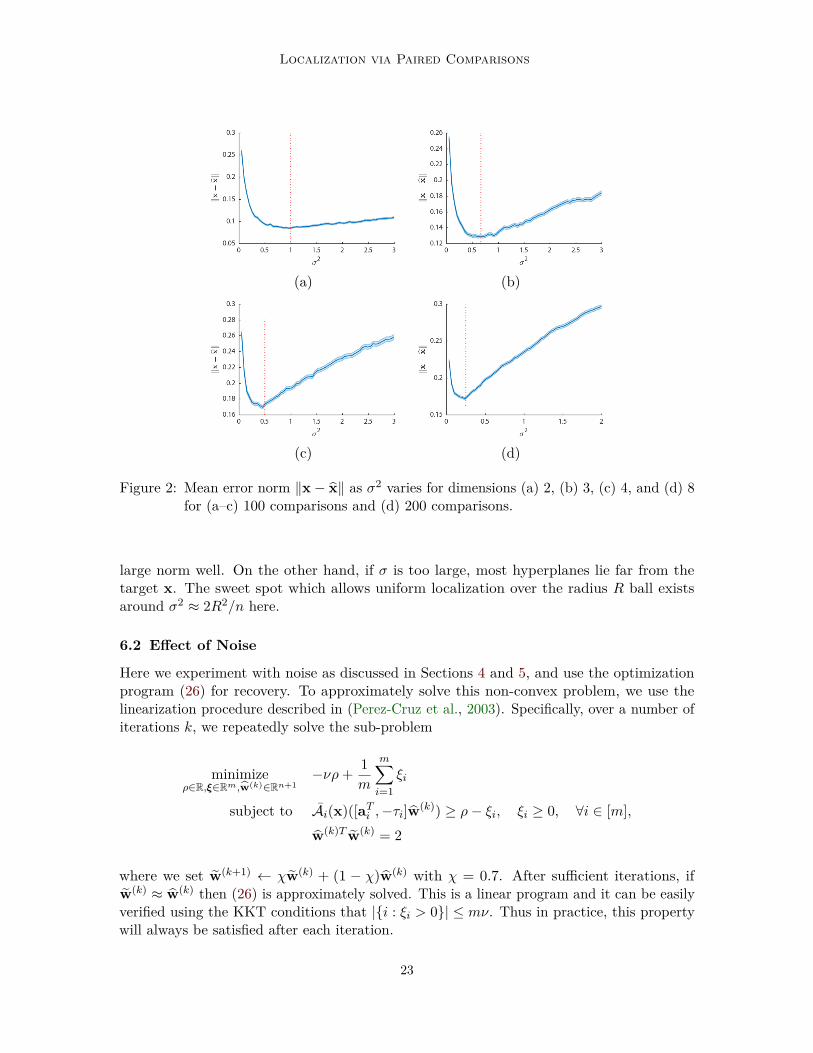
6.1 Effect of Varying 𝜎2

In Fig. 2, we let x ∈ R{2,3,4,8} with ‖x‖ = 𝑅 = 1. We vary 𝜎2 and perform 1500 trials, eachwith 𝑚 = 100 or 𝑚 = 200 pairs of points drawn according to 𝒩 (0, 𝜎2𝐼). To isolate theimpact of 𝜎2, we consider the case where our observations are noise-free, and use (25) torecover x. As predicted by the theory, localization accuracy depends on the parameter 𝜎,which controls the distribution of the hyperplane thresholds. Intuitively, if 𝜎 is too small,the hyperplane boundaries concentrate closer to the origin and do not localize points with

22

Localization via Paired Comparisons

(a) (b)

(c) (d)

Figure 2: Mean error norm ‖x− x‖ as 𝜎2 varies for dimensions (a) 2, (b) 3, (c) 4, and (d) 8for (a–c) 100 comparisons and (d) 200 comparisons.

large norm well. On the other hand, if 𝜎 is too large, most hyperplanes lie far from thetarget x. The sweet spot which allows uniform localization over the radius 𝑅 ball existsaround 𝜎2 ≈ 2𝑅2/𝑛 here.

6.2 Effect of Noise

Here we experiment with noise as discussed in Sections 4 and 5, and use the optimizationprogram (26) for recovery. To approximately solve this non-convex problem, we use thelinearization procedure described in (Perez-Cruz et al., 2003). Specifically, over a number ofiterations 𝑘, we repeatedly solve the sub-problem

minimize𝜌∈R,𝜉∈R𝑚,w(𝑘)∈R𝑛+1

−𝜈𝜌 + 1𝑚

𝑚∑𝑖=1

𝜉𝑖

subject to 𝒜𝑖(x)([a𝑇𝑖 ,−𝜏𝑖] w(𝑘)) ≥ 𝜌− 𝜉𝑖, 𝜉𝑖 ≥ 0, ∀𝑖 ∈ [𝑚],w(𝑘)𝑇 w(𝑘) = 2

where we set w(𝑘+1) ← 𝜒 w(𝑘) + (1 − 𝜒) w(𝑘) with 𝜒 = 0.7. After sufficient iterations, ifw(𝑘) ≈ w(𝑘) then (26) is approximately solved. This is a linear program and it can be easilyverified using the KKT conditions that |{𝑖 : 𝜉𝑖 > 0}| ≤ 𝑚𝜈. Thus in practice, this propertywill always be satisfied after each iteration.

23

Massimino and Davenport

We also emphasize that the error bounds in Section 5 rely on the fact from Proposition 9that 𝑑𝐻(𝒜(x),𝒜(x)) ≤ 𝜈, provided that the solution results in a 𝜌 > 0. Unfortunately, wecannot guarantee that this will always be the case. Empirically, we have observed that givena certain noise level quantified by 𝑑𝐻(𝒜(x),𝒜(x)) = 𝜅, we are more likely to observe 𝜌 ≤ 0when we aggressively set 𝜈 = 𝜅. By increasing 𝜈 somewhat this becomes much less likely.As a rule of thumb, we set 𝜈 = 2𝜅. We note that while in our context this choice is purelyheuristic, it has some theoretical support in the 𝜈-SVM literature (e.g., see Proposition 5 ofChen et al., 2005).

We consider the following noise models; (i) Gaussian, where we add pre-quantizationGaussian noise as in Section 4.2, (ii) logistic, in which pre-quantization logistic noise is added,(iii) random, where a uniform random 𝜈/2 fraction of comparisons are flipped, and (iv)adversarial, where we flip the 𝜈/2 fraction of comparisons whose hyperplanes lie farthest fromthe ideal point. The logistic noise assumption is commonly studied in paired comparisonliterature and is equivalent to the Bradley–Terry model (Bradley and Terry, 1952). Althoughwe do not have theory for this case, we expect the logistic noise case to behave similarlyto the Gaussian case. In both the Gaussian and logistic cases, we sweep the added noisevariance, then for each variance plot against the mean number of errors induced as thex-axis. In each case, we set 𝑛 = 5 and generate 𝑚 = 1000 pairs of points and a random xwith ‖x‖ = 0.7.

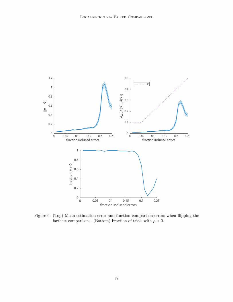
The mean and median recovery error ‖x− x‖ and the fraction of violated comparisons𝑑𝐻(𝒜(x),𝒜(x)) are plotted over 100 independent trials with varying number of comparisonerrors in Figs. 3–6. In the Gaussian noise, logistic noise, and uniform random comparisonflipping cases, the actual fraction of comparison errors of the estimate is on average muchsmaller than our target 𝜈. This is also seen in the adversarial case (Fig. 6) for smallerlevels of error. However, at a high fraction of error (greater than about 17%) the error(both in terms of Euclidean norm and fraction of incorrect comparisons) grows rapidly. Thisillustrates a limitation to the approach of using slack variables as a relaxation to the 0–1 loss.We mention that in this regime, the recovery approach of (26) frequently yields 𝜌 ≤ 0, towhich our theory does not apply. Here, the recovery error counter-intuitively decreases withincreasing comparison flips. This scenario, with a large number of erroneous comparisons,represents a very difficult situation in which any tractable recovery strategy would likelystruggle. A possible direction for future work would be to make (26) more robust to suchlarge outliers.

6.3 Adaptive Comparisons

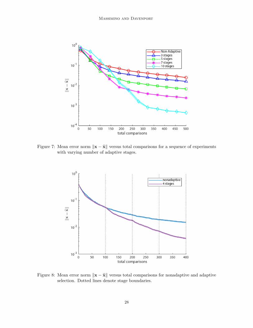
In Fig. 7, we show the effect of varying levels of adaptivity, starting with the completelynon-adaptive approach up to using 10 stages where we progressively re-center and re-scalethe hyperplane offsets. In each case, we generate x ∈ R3 where ‖x‖ = 0.75 and choosing thedirection randomly. The total number of comparisons are held fixed and are split as equallyas possible among the number of stages (preferring earlier stages when rounding). We set𝜎2 = 𝑅 = 1 and plot the average over 700 independent trials. As the number of stagesincreases, performance worsens if the number of comparisons are kept small due to badlocalization in the earlier stages. However, if the number of total comparisons is sufficientlylarge, an exponential improvement over non-adaptivity is possible.

24

Localization via Paired Comparisons

Figure 3: Mean estimation error and average fraction comparison errors when adding pre-quantization Gaussian noise, sweeping the variance and plotting against theaverage number of induced errors for each variance.

Figure 4: Mean estimation error and fraction comparison errors when adding pre-quantization logistic noise, sweeping the variance and plotting against the averagenumber of induced errors for each variance.

25

Massimino and Davenport

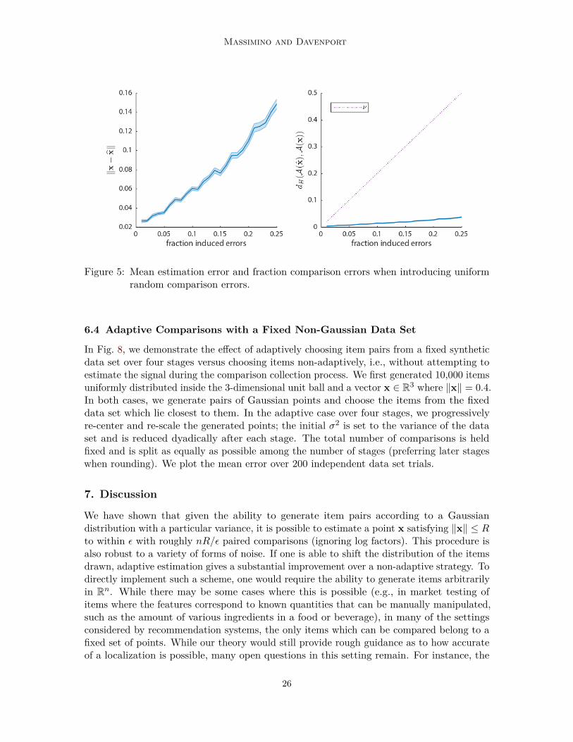
Figure 5: Mean estimation error and fraction comparison errors when introducing uniformrandom comparison errors.

6.4 Adaptive Comparisons with a Fixed Non-Gaussian Data Set

In Fig. 8, we demonstrate the effect of adaptively choosing item pairs from a fixed syntheticdata set over four stages versus choosing items non-adaptively, i.e., without attempting toestimate the signal during the comparison collection process. We first generated 10,000 itemsuniformly distributed inside the 3-dimensional unit ball and a vector x ∈ R3 where ‖x‖ = 0.4.In both cases, we generate pairs of Gaussian points and choose the items from the fixeddata set which lie closest to them. In the adaptive case over four stages, we progressivelyre-center and re-scale the generated points; the initial 𝜎2 is set to the variance of the dataset and is reduced dyadically after each stage. The total number of comparisons is heldfixed and is split as equally as possible among the number of stages (preferring later stageswhen rounding). We plot the mean error over 200 independent data set trials.

7. Discussion

We have shown that given the ability to generate item pairs according to a Gaussiandistribution with a particular variance, it is possible to estimate a point x satisfying ‖x‖ ≤ 𝑅to within 𝜖 with roughly 𝑛𝑅/𝜖 paired comparisons (ignoring log factors). This procedure isalso robust to a variety of forms of noise. If one is able to shift the distribution of the itemsdrawn, adaptive estimation gives a substantial improvement over a non-adaptive strategy. Todirectly implement such a scheme, one would require the ability to generate items arbitrarilyin R𝑛. While there may be some cases where this is possible (e.g., in market testing ofitems where the features correspond to known quantities that can be manually manipulated,such as the amount of various ingredients in a food or beverage), in many of the settingsconsidered by recommendation systems, the only items which can be compared belong to afixed set of points. While our theory would still provide rough guidance as to how accurateof a localization is possible, many open questions in this setting remain. For instance, the

26

Localization via Paired Comparisons

Figure 6: (Top) Mean estimation error and fraction comparison errors when flipping thefarthest comparisons. (Bottom) Fraction of trials with 𝜌 > 0.

27

Massimino and Davenport

Figure 7: Mean error norm ‖x− x‖ versus total comparisons for a sequence of experimentswith varying number of adaptive stages.

Figure 8: Mean error norm ‖x− x‖ versus total comparisons for nonadaptive and adaptiveselection. Dotted lines denote stage boundaries.

28

Localization via Paired Comparisons

algorithm itself needs to be adapted, as done in Section 6.4. Of course, there are manyother ways that the adaptive scheme could be modified to account for this restriction. Forexample, one could use rejection sampling, so that although many candidate pairs wouldneed to be drawn, only a fraction would actually need to be presented to and labeled by theuser. We leave the exploration of such variations for future work.

Acknowledgments

This work was supported by grants AFOSR FA9550-14-1-0342, NSF CCF-1350616, and agift from the Alfred P. Sloan Foundation.

29

Massimino and Davenport

30

Localization via Paired Comparisons

Appendix A. Supporting Lemmas

Lemma 11 Let 𝑏 > 𝑎 and let 𝐿 = min{|𝑎|, |𝑏|} and 𝑈 = max{|𝑎|, |𝑏|}. Then if Φ and 𝜑respectively denote the standard normal cumulative distribution function and probabilitydistribution function, we have the bounds

(𝑏− 𝑎)𝜑(𝑈) ≤ Φ(𝑏)− Φ(𝑎) ≤ (𝑏− 𝑎)𝜑(𝐿) ≤ (𝑏− 𝑎)𝜑(0).

Proof By the mean value theorem, we have for some 𝑎 < 𝑐 < 𝑏, Φ(𝑏)−Φ(𝑎) = (𝑏−𝑎)Φ′(𝑐) =(𝑏− 𝑎)𝜑(𝑐). Since 𝜑(|𝑥|) is monotonic decreasing, it is lower bounded by 𝜑(𝑈) and upperbounded by 𝜑(𝐿) (and also 𝜑(0)).

Lemma 12 Let x, y ∈ R𝑛. Then,∫S𝑛−1|a𝑇 (x− y)| 𝜈(da) = 2√

𝜋

Γ(𝑛2 )

Γ(𝑛+12 )‖x− y‖ .

Proof By spherical symmetry, we may assume Δ = x − y = [𝜖, 0, . . . , 0] for 𝜖 > 0without loss of generality. Then ‖x− y‖ = 𝜖 and |a𝑇 (x − y)| = 𝑎(1)𝜖 = 𝜖|cos 𝜃|, wherecos−1(𝑎(1)) = 𝜃 ∈ [0, 𝜋]. We will use the fact (Gradshteyn and Ryzhik, 2007):∫ 𝜋

2

0cos𝜇−1 𝜃 sin𝜔−1 𝜃 d𝜃 = 1

2𝐵

(𝜇

2 ,𝜔

2

)= 1

2Γ(𝜇/2)Γ(𝜔/2)Γ((𝜇 + 𝜔)/2) .

Integrating |cos 𝜃| in the first spherical coordinate, since the integrand is symmetric about 𝜋2 ,∫ 𝜋

0|cos 𝜃| sin𝑛−2 𝜃 d𝜃 = 2

∫ 𝜋/2

0cos 𝜃 sin𝑛−2 𝜃 d𝜃 =

Γ(1)Γ(𝑛−12 )

Γ(1 + 𝑛−12 )

= 2𝑛− 1 .

Then with the appropriate normalization, we have (using Γ(1/2) =√

𝜋)∫𝑆𝑛−1

|𝑎𝑇 (x− y)| 𝜈(d𝑎) =(∫ 𝜋

0sin𝑛−2 𝜃 d𝜃

)−1 ∫ 𝜋

0𝜖|cos 𝜃| sin𝑛−2 𝜃 d𝜃

= 𝜖

(Γ(1

2)Γ(𝑛−12 )

Γ(12 + 𝑛−1

2 )

)−1 2𝑛− 1 = 2√

𝜋

Γ(𝑛2 )

Γ(𝑛+12 )‖x− y‖ .

Appendix B. Integral Calculations for Lemma 7

Bound (23) Recall that 𝑟𝑖 := a𝑇𝑖 x/ ‖x‖ ∈ [−1, 1], 𝑞𝑖 = 𝑟𝑖 ‖x‖− 𝜏𝑖, and 𝑞𝑖 = 𝑟𝑖 ‖x‖− 𝜏𝑖 + 𝑧𝑖.

Thus, if 𝑓𝑟(𝑟𝑖), 𝑓𝜏 (𝜏𝑖), and 𝑓𝑧(𝑧𝑖) denote the probability density functions for 𝑟𝑖, 𝜏𝑖, and 𝑧𝑖,then since these random variables are independent we can write

P [𝑞𝑖 < 0 and 𝑞𝑖 > 0] = P [𝑟𝑖 ‖x‖ − 𝜏𝑖 < 0 and 𝑟𝑖 ‖x‖ − 𝜏𝑖 + 𝑧𝑖 > 0]

=∫ 1

−1

∫ ∞

𝑟𝑖‖x‖

∫ 𝑟𝑖‖x‖−𝜏𝑖

−∞𝑓𝑟(𝑟𝑖)𝑓𝜏 (𝜏𝑖)𝑓𝑧(𝑧𝑖) d𝑧𝑖 d𝜏𝑖 d𝑟𝑖

=∫ 1

−1

∫ ∞

𝑟𝑖‖x‖𝑓𝑟(𝑟𝑖)𝑓𝜏 (𝜏𝑖)P [𝑧𝑖 > 𝜏𝑖 − 𝑟𝑖 ‖x‖] d𝜏𝑖 d𝑟𝑖

=∫ 1

−1

∫ ∞

𝑟𝑖‖x‖𝑓𝑟(𝑟𝑖)𝑓𝜏 (𝜏𝑖)𝑄

(𝜏𝑖 − 𝑟𝑖 ‖x‖

𝜎𝑧

)d𝜏𝑖 d𝑟𝑖,

31

Massimino and Davenport

where 𝑄(𝑥) = 1√2𝜋

∫∞𝑥 exp(−𝑥2/2) d𝑥, i.e., the tail probability for the standard normal

distribution. Via a similar argument we have

P [𝑞𝑖 > 0 and 𝑞𝑖 < 0] = P [𝑟𝑖 ‖x‖ − 𝜏𝑖 > 0 and 𝑟𝑖 ‖x‖ − 𝜏𝑖 + 𝑧𝑖 < 0]

=∫ 1

−1

∫ 𝑟𝑖‖x‖

−∞

∫ ∞

𝑟𝑖‖x‖−𝜏𝑖

𝑓𝑟(𝑟𝑖)𝑓𝜏 (𝜏𝑖)𝑓𝑧(𝑧𝑖) d𝑧𝑖 d𝜏𝑖 d𝑟𝑖

=∫ 1

−1

∫ 𝑟𝑖‖x‖

−∞𝑓𝑟(𝑟𝑖)𝑓𝜏 (𝜏𝑖)P [𝑧𝑖 < 𝜏𝑖 − 𝑟𝑖 ‖x‖)] d𝜏𝑖 d𝑟𝑖

=∫ 1

−1

∫ 𝑟𝑖‖x‖

−∞𝑓𝑟(𝑟𝑖)𝑓𝜏 (𝜏𝑖)𝑄

(𝑟𝑖 ‖x‖ − 𝜏𝑖

𝜎𝑧

)d𝜏𝑖 d𝑟𝑖.

Combining these we obtain

P[𝑞𝑖𝑞𝑖 < 0] = P [𝑞𝑖 < 0 and 𝑞𝑖 > 0] + P [𝑞𝑖 > 0 and 𝑞𝑖 < 0]

=∫ 1

−1

∫ ∞

−∞𝑓𝑟(𝑟𝑖)𝑓𝜏 (𝜏𝑖)𝑄

( |𝑟𝑖 ‖x‖ − 𝜏𝑖|𝜎𝑧

)d𝜏𝑖 d𝑟𝑖

= 2∫ 1

0

∫ ∞

−∞𝑓𝑟(𝑟𝑖)𝑓𝜏 (𝜏𝑖)𝑄

( |𝑟𝑖 ‖x‖ − 𝜏𝑖|𝜎𝑧

)d𝜏𝑖 d𝑟𝑖,

following from the symmetry of 𝑓𝑟(·). Using the bound 𝑄(𝑥) ≤ 12 exp(−𝑥2/2) (see (13.48) of

Johnson et al., 1994), and recalling that 𝜏𝑖 ∼ 𝒩 (0, 2𝑅2/𝑛), we have that

P[𝑞𝑖𝑞𝑖 < 0] ≤ 1𝑅

√𝑛

𝜋

∫ 1

0

∫ ∞

−∞𝑓𝑟(𝑟𝑖) exp

(−(𝑟𝑖 ‖x‖ − 𝜏𝑖)2

2𝜎2𝑧

− 𝑛𝜏2𝑖

4𝑅2

)d𝜏𝑖 d𝑟𝑖.

B.1 Bounding 𝜅𝑛

First, we give an expression for 𝜅𝑛 for all cases 𝑛 ≥ 2, expanding upon that given inTheorem 8 and Lemma 7. We have

𝜅𝑛(𝜎2𝑧) :=

⎧⎪⎪⎪⎪⎪⎪⎨⎪⎪⎪⎪⎪⎪⎩

12

√𝜎2

𝑧𝜎2

𝑧+𝑅2 𝑛 = 2

min{√

𝜎2𝑧

𝜎2𝑧+2𝑅2/3 ,

√𝜋2

𝜎𝑧‖x‖

}𝑛 = 3√

𝜎2𝑧

𝜎2𝑧+2𝑅2/𝑛+4‖x‖2/𝑛

𝑛 ≥ 4.

Below we derive this expression for the cases 𝑛 = 2, 𝑛 = 3, and 𝑛 ≥ 4.

B.2 Case 𝑛 = 2

For the special case 𝑛 = 2, 𝑑𝑖 = cos 𝜃𝑖 where 𝜃𝑖 ∈ [−𝜋, 𝜋] is distributed uniformly. In thiscase, (23) can be re-written as

P[𝑞𝑖𝑞𝑖 < 0] ≤ 12𝑅

√2𝜋

∫ 𝜋/2

−𝜋/2

∫ ∞

−∞

12𝜋

exp(−(‖x‖ cos 𝜃𝑖 − 𝜏𝑖)2

2𝜎2𝑧

− 𝜏2𝑖

2𝑅2

)d𝜏𝑖 d𝜃𝑖

= 1𝜋𝑅

√1

2𝜋

∫ 𝜋/2

0

∫ ∞

−∞exp

(−(‖x‖ cos 𝜃𝑖 − 𝜏𝑖)2

2𝜎2𝑧

− 𝜏2𝑖

2𝑅2

)d𝜏𝑖 d𝜃𝑖.

32

Localization via Paired Comparisons

Expanding and setting 𝛼, 𝛽, and 𝛾 appropriately,

P[𝑞𝑖𝑞𝑖 < 0] ≤ 1𝜋𝑅

√1

2𝜋

∫ 𝜋/2

0

∫ ∞

−∞exp

(−‖x‖

2 cos2 𝜃𝑖

2𝜎2𝑧

+ 2 ‖x‖ 𝜏𝑖 cos 𝜃𝑖

2𝜎2𝑧

− 𝜏2𝑖

2𝜎2𝑧

− 𝜏2𝑖

2𝑅2

)d𝜏𝑖 d𝜃𝑖

= 1𝜋𝑅

√1

2𝜋

∫ 𝜋/2

0

∫ ∞

−∞exp

(−𝛾 cos2 𝜃𝑖 + 𝛽𝜏𝑖 cos 𝜃𝑖 − 𝛼𝜏2

𝑖

)d𝜏𝑖 d𝜃𝑖.

Completing the square for 𝜏𝑖,

P[𝑞𝑖𝑞𝑖 < 0] = 1𝜋𝑅

√1

2𝜋

∫ 𝜋/2

0

∫ ∞

−∞exp

(−𝛼

(𝜏𝑖 + 𝛽 cos 𝜃𝑖

2𝛼

)2+ (𝛽 cos 𝜃𝑖)2

4𝛼− 𝛾 cos2 𝜃𝑖

)d𝜏𝑖 d𝜃𝑖

= 1𝜋𝑅

√1

2𝜋

∫ 𝜋/2

0

√𝜋

𝛼exp

(−(

𝛾 − 𝛽2

4𝛼

)cos2 𝜃𝑖

)d𝜃𝑖

= 𝜋

2𝜋𝑅

√1

2𝛼exp

(−1

2

(𝛾 − 𝛽2

4𝛼

))𝐼0

(12

(𝛾 − 𝛽2

4𝛼

)),

where 𝐼0(·) denotes the modified Bessel function of the first kind. Since exp(−𝑡)𝐼0(𝑡) < 1,by plugging back in for 𝛼 we obtain

P[𝑞𝑖𝑞𝑖 < 0] ≤ 12𝑅

√1

2𝛼= 1

2√

2𝑅

⎯⎸⎸⎷ 11

2𝜎2𝑧

+ 12𝑅2

= 12

√𝜎2

𝑧

𝜎2𝑧 + 𝑅2 .

We also note that since since exp(−𝑡)𝐼0(𝑡) < 1/√

𝜋𝑡, we can obtain the bound P[𝑞𝑖𝑞𝑖 < 0] ≤1√𝜋

𝜎𝑧‖x‖ , but one can show that the previous bound will dominate this whenever ‖x‖ ≤ 𝑅.

B.3 Case 𝑛 = 3

For the case 𝑛 = 3, 𝑑𝑖 ∼ [−1, 1] is itself distributed uniformly. In this case we have

P[𝑞𝑖𝑞𝑖 < 0] ≤ 12𝑅

√3𝜋

∫ 1

0

∫ ∞

−∞exp

(−(𝑑𝑖 ‖x‖ − 𝜏𝑖)2

2𝜎2𝑧

− 3𝜏2𝑖

4𝑅2

)d𝜏𝑖 d𝑑𝑖.

Expanding and setting 𝛼, 𝛽, and 𝛾 appropriately,

P[𝑞𝑖𝑞𝑖 < 0] ≤ 12𝑅

√3𝜋

∫ 1

0

∫ ∞

−∞exp

(−𝑑2

𝑖 ‖x‖2

2𝜎2𝑧

+ 2𝑑𝑖 ‖x‖ 𝜏𝑖

2𝜎2𝑧

− 𝜏2𝑖

2𝜎2𝑧

− 3𝜏2𝑖

4𝑅2

)d𝜏𝑖 d𝑑𝑖

= 12𝑅

√3𝜋

∫ 1

0

∫ ∞

−∞exp

(−𝛾𝑑2

𝑖 + 𝛽𝑑𝑖𝜏𝑖 − 𝛼𝜏2𝑖

)d𝜏𝑖 d𝑑𝑖.

Completing the square for 𝜏𝑖,

P[𝑞𝑖𝑞𝑖 < 0] = 12𝑅

√3𝜋

∫ 1

0

∫ ∞

−∞exp

(−𝛼

(𝜏𝑖 + 𝑑𝑖𝛽

2𝛼

)2+ (𝑑𝑖𝛽)2

4𝛼− 𝛾𝑑𝑖

)d𝜏𝑖 d𝑑𝑖

= 12𝑅

√3𝜋

∫ 1

0

√𝜋

𝛼exp

(−𝑑2

𝑖

(𝛾 − 𝛽2

4𝛼

))d𝑑𝑖

= 12𝑅

√3𝛼

√𝜋

2erf(√

𝛾 − 𝛽2/4𝛼)

√𝛾 − 𝛽2/4𝛼

.

33

Massimino and Davenport

Since erf(𝑡)/𝑡 ≤ 2/√

𝜋, by plugging back in for 𝛼 we obtain

P[𝑞𝑖𝑞𝑖 < 0] ≤ 12𝑅

⎯⎸⎸⎷ 31

2𝜎2𝑧

+ 34𝑅2

=√

𝜎2𝑧

𝜎2𝑧 + 2𝑅2/3 .

Additionally, since erf(𝑡) ≤ 1,

P[𝑞𝑖𝑞𝑖 < 0] ≤√

3𝜋

4𝑅

(𝛾𝛼− 𝛽2/4

)−1/2

=√

3𝜋

4𝑅

(‖x‖2

2𝜎2𝑧

( 12𝜎2

𝑧

+ 34𝑅2

)− ‖x‖

2

4𝜎4𝑧

)−1/2

=√

3𝜋

4𝑅

(3 ‖x‖2

8𝜎2𝑧𝑅2

)−1/2

=√

𝜋

2𝜎𝑧

‖x‖ ,

which can be tighter when 𝜎𝑧 is small and ‖x‖ is large.

B.4 Case 𝑛 ≥ 4

Combining (23) with our upper bound (24) on 𝑓𝑑(𝑑𝑖), we obtain

P[𝑞𝑖𝑞𝑖 < 0] ≤ 𝑛

4√

2𝜋𝑅

∫ 1

0

∫ ∞

−∞exp

(−(𝑑𝑖 ‖x‖ − 𝜏𝑖)2

2𝜎2𝑧

− 𝑛𝜏2𝑖

4𝑅2 −𝑛𝑑2

𝑖

8

)d𝜏𝑖 d𝑑𝑖.

Expanding and setting 𝛼, 𝛽, and 𝛾 appropriately,

P[𝑞𝑖𝑞𝑖 < 0] ≤ 𝑛

4√

2𝜋𝑅

∫ 1

0

∫ ∞

−∞exp

(−𝑑2

𝑖

(‖x‖2

2𝜎2𝑧

+ 𝑛

8

)+ 2𝑑𝑖 ‖x‖ 𝜏𝑖

2𝜎2𝑧

− 𝜏2𝑖

2𝜎2𝑧

− 𝑛𝜏2𝑖

4𝑅2

)d𝜏𝑖 d𝑑𝑖

= 𝑛

4√

2𝜋𝑅

∫ 1

0

∫ ∞

−∞exp

(−𝛾𝑑2

𝑖 + 𝛽𝑑𝑖𝜏𝑖 − 𝛼𝜏2𝑖

)d𝜏𝑖 d𝑑𝑖.

Completing the square for 𝜏𝑖,

P[𝑞𝑖𝑞𝑖 < 0] = 𝑛

4√

2𝜋𝑅

∫ 1

0

∫ ∞

−∞exp

(−𝛼

(𝜏𝑖 −

𝑑𝑖𝛽

2𝛼

)2+ (𝑑𝑖𝛽)2

4𝛼− 𝛾𝑑2

𝑖

)d𝜏𝑖 d𝑑𝑖

= 𝑛

4√

2𝜋𝑅

∫ 1

0

√𝜋

𝛼exp

(−𝑑2

𝑖

(𝛾 − 𝛽2

4𝛼

))d𝑑𝑖

= 𝑛

4√

2𝜋𝛼𝑅

√𝜋

2erf(√

𝛾 − 𝛽2/4𝛼)

√𝛾 − 𝛽2/4𝛼

.

34

Localization via Paired Comparisons

Since erf(𝑡) ≤ 1, we have

P[𝑞𝑖𝑞𝑖 < 0] ≤ 𝑛

4√

2𝑅

(𝛾𝛼− 𝛽2/4

)−1/2

= 𝑛

4√

2𝑅

((‖x‖2

2𝜎2𝑧

+ 𝑛

8

)( 12𝜎2

𝑧

+ 𝑛

4𝑅2

)− ‖x‖

2

4𝜎4𝑧

)−1/2

= 12

(32𝑅2

𝑛2

(‖x‖2 𝑛

8𝜎2𝑧𝑅2 + 𝑛

16𝜎2𝑧

+ 𝑛2

32𝑅2

))−1/2

= 12

√𝜎2

𝑧

𝜎2𝑧 + 2𝑅2/𝑛 + 4 ‖x‖2 /𝑛

.

We also note that since erf(𝑡)/𝑡 ≤ 2/√

𝜋, it is also possible to obtain the bound

P[𝑞𝑖𝑞𝑖 < 0] ≤ 12

√𝑛

2𝜋

√𝜎2

𝑧

𝜎2𝑧 + 2𝑅2/𝑛

.

However, this bound can only be tighter when ‖x‖ is small and when 𝑛2𝜋 < 1 (i.e., for 𝑛 ≤ 6).

Given this narrow range of applicability, we omit this from the formal statement of theresult.

35

Massimino and Davenport

36

Localization via Paired Comparisons

References

S. Agarwal, J. Wills, L. Cayton, G. Lanckriet, D. Kriegman, and S. Belongie. Generalizednon-metric multidimensional scaling. In Proc. Int. Conf. Art. Intell. Stat. (AISTATS),San Juan, Puerto Rico, Mar. 2007.

N. Ailon. Active learning ranking from pairwise preferences with almost optimal querycomplexity. In Proc. Adv. in Neural Processing Systems (NIPS), Grenada, Spain, Dec.2011.

E. Arias-Castro et al. Some theory for ordinal embedding. Bernoulli, 23(3):1663–1693, 2017.

R. Baraniuk, S. Foucart, D. Needell, Y. Plan, and M. Wootters. Exponential decay ofreconstruction error from binary measurements of sparse signals. IEEE Trans. Inform.Theory, 63(6):3368–3385, 2017.

D. P. Bertsekas. Nonlinear programming. Athena scientific Belmont, 1999.

R. A. Bradley and M. E. Terry. Rank analysis of incomplete block designs: I. the method ofpaired comparisons. Biometrika, 39(3/4):324–345, 1952.

A. Brieden, P. Gritzmann, R. Kannan, V. Klee, L. Lovász, and M. Simonovits. Deterministicand randomized polynomial-time approximation of radii. Mathematika, 48(1-2):63–105,2001.

R. Buck. Partition of space. Amer. Math. Monthly, 50(9):541–544, 1943.

E. Candès and B. Recht. Exact matrix completion via convex optimization. Found. Comput.Math., 9(6):717–772, 2009.

P.-H. Chen, C.-J. Lin, and B. Schölkopf. A tutorial on 𝜈-support vector machines. Appl.Stoch. Models Bus. Ind., 21(2):111–136, 2005.

C. Coombs. Psychological scaling without a unit of measurement. Psych. Rev., 57(3):145–158, 1950.

M. Davenport. Lost without a compass: Nonmetric triangulation and landmark multidimen-sional scaling. In Proc. IEEE Int. Work. Comput. Adv. Multi-Sensor Adaptive Processing(CAMSAP), Saint Martin, Dec. 2013.

H. David. The Method of Paired Comparisons. Charles Griffin & Company Limited, London,UK, 1963.

B. Dubois. Ideal point versus attribute models of brand preference: A comparison ofpredictive validity. Adv. Consumer Research, 2(1):321–333, 1975.

B. Eriksson. Learning to Top-K search using pairwise comparisons. In Proc. Int. Conf. Art.Intell. Stat. (AISTATS), Scottsdale, AZ, Apr. 2013.

M. Giaquinta and G. Modica. Mathematical Analysis: An Introduction to Functions ofSeveral Variables. Birkhäuser, New York, NY, 2010.

37

Massimino and Davenport

I. Gradshteyn and I. Ryzhik. Table of Integrals, Series, and Products. Academic Press,Burlington, MA, 2007.

L. Grenié and G. Molteni. Inequalities for the beta function. Math. Inequal. Appl, 18(4):1427–1442, 2015.

L. Jacques, J. Laska, P. Boufounos, and R. Baraniuk. Robust 1-bit compressive sensing viabinary stable embeddings of sparse vectors. IEEE Trans. Inform. Theory, 59(4):2082–2102,2013.

L. Jain, K. G. Jamieson, and R. Nowak. Finite sample prediction and recovery boundsfor ordinal embedding. In Advances In Neural Information Processing Systems, pages2711–2719, 2016.

K. Jamieson and R. Nowak. Active ranking using pairwise comparisons. In Proc. Adv. inNeural Processing Systems (NIPS), Granada, Spain, Dec. 2011a.

K. Jamieson and R. Nowak. Low-dimensional embedding using adaptively selected ordinaldata. In Proc. Allerton Conf. Communication, Control, and Computing, Monticello, IL,Sept. 2011b.

N. Johnson, S. Kotz, and N. Balakrishnan. Continuous Univariate Distributions, volume 1.Wiley, New York, NY, 1994.

M. Kleindessner and U. Luxburg. Uniqueness of ordinal embedding. In Conference onLearning Theory, pages 40–67, 2014.

K. Knudson, R. Saab, and R. Ward. One-bit compressive sensing with norm estimation.IEEE Trans. Inform. Theory, 62(5):2748–2758, 2016.

M. Konoshima and Y. Noma. Hyperplane arrangements and locality-sensitive hashing withlift. arXiv preprint arXiv:1212.6110, 2012.

Y. Lu and S. Negahban. Individualized rank aggregation using nuclear norm regularization.In Proc. Allerton Conf. Communication, Control, and Computing, Monticello, IL, Sept.2015.

A. Massimino and M. Davenport. Binary stable embedding via paired comparisons. In Proc.IEEE Work. Stat. Signal Processing, Palma de Mallorca, Spain, June 2016.

A. Massimino and M. Davenport. The geometry of random paired comparisons. In Proc.IEEE Int. Conf. Acoust., Speech, and Signal Processing (ICASSP), New Orleans, Louisiana,Mar. 2017.

A. Maydeu-Olivares and U. Böckenholt. Modeling preference data. In R. Millsap andA. Maydeu-Olivares, editors, The SAGE Handbook of Quantitative Methods in Psychology,chapter 12, pages 264–282. SAGE Publications Ltd., London, UK, 2009.

G. Miller. The magical number seven, plus or minus two: Some limits on our capacity forprocessing information. Psych. Rev., 63(2):81, 1956.

38

Localization via Paired Comparisons

R. Nowak. Noisy generalized binary search. In Advances in neural information processingsystems, pages 1366–1374, 2009.

S. Oh, K. Thekumparampil, and J. Xu. Collaboratively learning preferences from ordinaldata. In Proc. Adv. in Neural Processing Systems (NIPS), Montréal, Québec, Dec. 2014.

M. O’Shaughnessy and M. Davenport. Localizing users and items from paired comparisons.In Proc. IEEE Int. Work. Machine Learning for Signal Processing (MLSP), Vietri sulMare, Salerno, Italy, Sept. 2016.

D. Park, J. Neeman, J. Zhang, S. Sanghavi, and I. Dhillon. Preference completion: Large-scale collaborative ranking form pairwise comparisons. In Proc. Int. Conf. MachineLearning (ICML), Lille, France, July 2015.

F. Perez-Cruz, J. Weston, D. Herrmann, and B. Schölkopf. Extension of the 𝜈-SVM rangefor classification. NATO Science Series Sub Series III Computer and Systems Sciences,190:179–196, 2003.

Y. Plan and R. Vershynin. One-bit compressed sensing by linear programming. Communi-cations on Pure and Applied Mathematics, 66(8):1275–1297, 2013a.

Y. Plan and R. Vershynin. Robust 1-bit compressed sensing and sparse logistic regression: Aconvex programming approach. IEEE Transactions on Information Theory, 59(1):482–494,2013b.

Y. Plan and R. Vershynin. Dimension reduction by random hyperplane tessellations. Discrete& Computational Geometry, 51(2):438–461, 2014.

F. Qi. Bounds for the ratio of two gamma functions. J. Inequal. Appl., 2010(1):493058, 2010.

F. Radlinski and T. Joachims. Active exploration for learning rankings from clickthroughdata. In Proc. ACM SIGKDD Int. Conf. on Knowledge, Discovery, and Data Mining(KDD), San Jose, CA, Aug. 2007.

J. Rennie and N. Srebro. Fast maximum margin matrix factorization for collaborativeprediction. In Proc. Int. Conf. Machine Learning (ICML), Bonn, Germany, Aug. 2005.

B. Schölkopf and A. Smola. Learning with Kernels: Support Vector Machines, Regularization,Optimization, and Beyond. MIT Press, Cambridge, MA, 2001.

N. Shah, S. Balakrishnan, J. Bradley, A. Parekh, K. Ramchandran, and M. Wainwright.Estimation from pairwise comparisons: Sharp minimax bounds with topology dependence.J. Machine Learning Research, 17(58):1–47, 2016.

M. Spruill. Asymptotic distribution of coordinates on high dimensional spheres. Elec. Comm.in Prob., 12:234–247, 2007.

L. Thurstone. A law of comparative judgment. Psych. Rev., 34(4):273, 1927.

F. Wauthier, M. Jordan, and N. Jojic. Efficient ranking from pairwise comparisons. In Proc.Int. Conf. Machine Learning (ICML), Atlanta, GA, June 2013.

39