applied sciences

Article

Performance Comparisons of Broadband Power LineCommunication Technologies

Young Mo Chung

Department of Electronics and Information Engineering, Hansung University, Seoul 02876, Korea;ymchung@hansung.ac.kr; Tel.: +82-2-760-4342

Received: 5 April 2020; Accepted: 6 May 2020 ; Published: 9 May 2020�����������������

Abstract: Broadband power line communication (PLC) is used as a communication technique foradvanced metering infrastructure (AMI) in Korea. High-speed (HS) PLC specified in ISO/IEC12139-1and HomePlug Green PHY (HPGP) are deployed for remote metering. Recently, internet of things(IoT) PLC has been proposed for reliable communications on harsh power line channels. In thispaper, the physical layer performance of IoT PLC, HPGP, and HS PLC is evaluated and compared.Three aspects of the performance are evaluated: the bit rate, power spectrum, and bit error rate(BER). An expression for the bit rate for IoT PLC and HPGP is derived while taking the padding bitsand number of tones in use into consideration. The power spectrum is obtained through computersimulations. For the BER performance comparisons, the upper bound of the BER for each PLCstandard is evaluated through computer simulations.

Keywords: advanced metering infrastructure; power line communication; IoT PLC; HPGP;ISO/IEC 12139-1; HS PLC; bit error rate

1. Introduction

In a smart grid, the advanced metering infrastructure (AMI) is responsible for collecting datafrom consumer utilities and giving commands to them. AMI consists of smart meters, communicationnetworks, and data managing systems [1,2]. An important challenge in building an AMI is choosinga cost-effective communication network [2–4]. As a field communication method for AMI, powerline communication (PLC) or wireless communication can be considered. PLC deploys a pre-existenttransmission medium, represented by the wires where the communication nodes are connected,so deployment and operating costs can be low.

PLC technologies can be classified into narrowband and broadband PLC according to the frequencybandwidth used. Narrowband PLC generally provides low data rates due to the narrow bandwidthof 3–500 kHz. To overcome the limitations of low rates and accommodate various service demandsfor utilities, powerline intelligent metering evolution (PRIME) and G3-PLC based on the orthogonalfrequency division multiplexing technology were introduced [5]. These narrowband PLC technologieshave been deployed for communication methods for AMI in European countries [5]. Broadband PLCuses a wide frequency bandwidth of 2–30 MHz. ITU-T G.hn, IEEE 1901, and ISO/IEC12139-1 [2,6] havebeen established as standards for broadband PLC. The HomePlug Powerline Alliance has also developedthe HomePlug Green PHY (HPGP) standard for broadband PLC technology [7].

In Korea, most low-voltage customers are powered by pole-mounted transformers, and, onaverage, dozens of customers are connected to the transformer. The Korea Electric Power Corporation(KEPCO), a Korean power company, uses the ISO/IEC12139-1 standard PLC as an AMI fieldcommunication method in downtown residential areas [2]. The method is also referred to as high-speed(HS) PLC or Korean Industrial Standards (KS) PLC. HPGP is also being used in downtown areas.KEPCO plans to build AMI networks for 22.50 million low-voltage customers by 2020 [2,8].

Appl. Sci. 2020, 10, 3306; doi:10.3390/app10093306 www.mdpi.com/journal/applsci

Appl. Sci. 2020, 10, 3306 2 of 21

In addition, several new services such as load profile (LP) metering and time-of-use (TOU) pricingare planned nationwide using AMI networks. To provide these services properly, more reliablecommunication is required. Recently, a new broadband PLC technology called IoT PLC [9] hasbeen proposed for robust communication on power line channels. IoT PLC has several features forreliable communication. For example, it provides robustness to intersymbol interference (ISI) usingorthogonal frequency division multiplexing (OFDM) with a longer guard interval than other methods,and convolutional turbo code (CTC) is used for forward error correction (FEC). In addition, it has awide selectable range of repetitions from 1 to 15 for the coded bits, providing flexible transmissionmodes depending on the channel conditions. Currently, IoT PLC is being tested for deployment inKorea. One of three PLC technologies will be chosen for AMI through a performance competition: HSPLC, HPGP, or IoT PLC. Therefore, it is important to evaluate and compare the performance of thesePLC technologies.

A PLC signal received through a power line is distorted due to the multipath propagation. Severalbroadband PLC channel models are available in [10,11]. One channel model is based on the transmissionline (TM) theory and is suitable for the specified PLC network topology [12–16]. This model is knownto have a realistic description of in-home power line topology [17]. Another channel model is obtainedby matching the parametric multipath model of the channel frequency response with real data obtainedfrom measurements [18]. This model represents the PLC channel as a finite sum of delayed echoes withdifferent amplitudes [17]. In this paper, a broadband channel model in [18] is used for simulation andperformance comparison. It is readily applied to an outdoor power line environment with obtainedparameters in [18].

In addition, PLC signals are also corrupted by noise added by the power line channel. The noiseis modeled as background noise added by impulsive noise [10,19–22]. The performance of the OFDMtransmission scheme for PLC applications was investigated with the channel model in the presence ofnoise [22,23]. Studies on narrowband PLC standards such as G3-PLC and PRIME were conducted in [24,25]. When it comes to performance comparisons of PLC standards, a few results have been reported.For narrowband PLC technologies, the performances of the physical layers of G3-PLC and PRIMEwere compared on a frequency-selective channel with additive white Gaussian noise (AWGN) [26].In [27], performance comparisons were conducted with different noise environments. Physical layersof narrowband PLC including IEEE1901.2 were compared under AWGN and narrowband interfererin [28]. Recently, Llano et al. [5] compared the performances of the latest versions of the standardsincluding PRIME 1.4 with that of G3-PLC coherent mode. The comparisons were made through thetest metrics defined by the European Telecommunications Standards Institute (ETSI) in the presence ofstandard and controlled noise patterns. Unlike the physical layer of the narrowband PLC standards,studies are not widely conducted on the physical layer of broadband PLC standards. Especially, resultsof performance comparisons of broadband PLC standards such as HPGP and HS PLC have not beenreported yet.

In this paper, studies on the performance evaluation of the IoT PLC as well as HPGP and HSPLC are conducted. The performances are evaluated in three aspects of the physical layer: the bit rate,power spectrum, and bit error rate (BER). The bit rates of the PLC are obtained with mathematicalformulas. The power spectrum is obtained with a PLC signal generated by the computer in MATLABcodes. These two evaluations are relatively easy and simple compared to the BER evaluation. For theBER comparison, we obtain the upper bound of the performance for each standard. The BERperformance depends on the transmitted signal specified in the standard and the receiver architecture.However, the receiver architecture is not specified in the standard. Therefore, it is assumed that eachPLC receiver achieves the best performance possible. The equalizer in each receiver has a one-tap filterand is assumed to have a perfect channel estimation. In this context, impulsive noise is not includedsince our purpose is to obtain the upper performance bound for each PLC. For background noise,colored noise is known to reflect the noise of the PLC environment better. However, AWGN is also

Appl. Sci. 2020, 10, 3306 3 of 21

considered useful when comparing the upper performance bound of the PLC. Through computersimulations, the upper bound of the performance of each PLC standard is evaluated and compared.

2. Structures of PLC

2.1. IoT PLC

The structure of an IoT PLC transmitter is shown in Figure 1 [9]. Two information subblocks Aand B with N bits are provided to the CTC encoder. IoT PLC uses two values for N. For the data frame(DF), which is used for data transmission, N is 1440. The control frame (CF) or Mini DF uses a shorterframe length. For these frames, N is 48.

Figure 1. Block diagram of IoT PLC.

2.1.1. CTC Encoder

Figure 2 shows block diagram of the CTC encoder [9,29]. The CTC consists of two constituentencoders and a CTC interleaver as shown in Figure 2a. A double binary circular recursive systematicconvolutional (RSC) encoder with a constraint length of 4 is used for the constituent encoder. Figure 2bshows the constituent encoder. When blocks A and B are encoded, a parity bit block Y1 is generated.The inputs are then interleaved by the CTC interleaver, and the interleaved bits are encoded again bythe constituent encoder, generating a parity block Y2. Y1 and Y2 each have N bits. The CTC interleavershuffles the bit order in such a way that the bits are spread as evenly as possible. The outputs ofthe CTC encoder are A, B, Y1, and Y2, resulting in 4N output bits. For the initial state of the encoder,the start and end states are set to be the same, which is known as tail biting encoding and can improvethe decoding performance without adding trailing bits at the encoder [30]. The CTC encoder generates4N bits with a 2N bit input, resulting in a code rate of 1/2.

(a) (b)

Figure 2. Block diagram of CTC encoder: (a) CTC encoder; and (b) constituent encoder.

Appl. Sci. 2020, 10, 3306 4 of 21

2.1.2. Interleavers

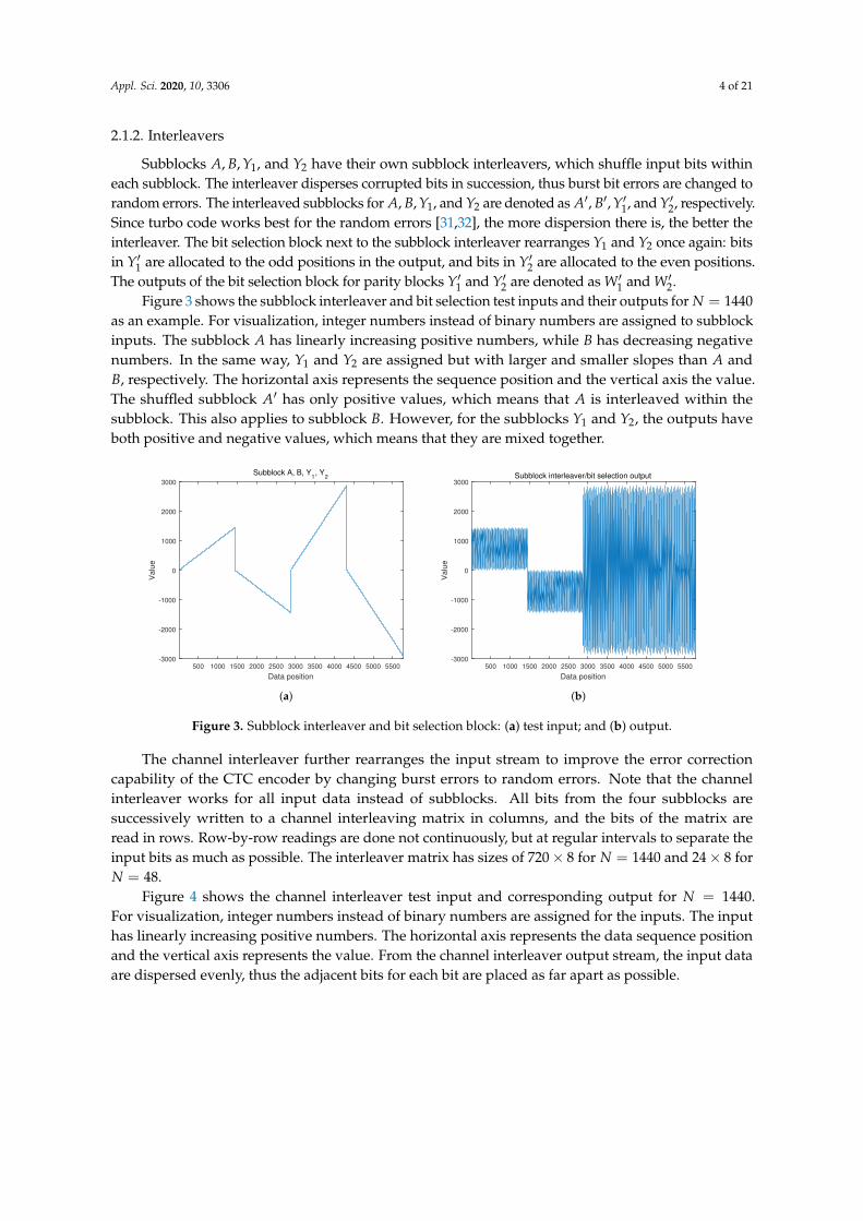
Subblocks A, B, Y1, and Y2 have their own subblock interleavers, which shuffle input bits withineach subblock. The interleaver disperses corrupted bits in succession, thus burst bit errors are changed torandom errors. The interleaved subblocks for A, B, Y1, and Y2 are denoted as A′, B′, Y′1, and Y′2, respectively.Since turbo code works best for the random errors [31,32], the more dispersion there is, the better theinterleaver. The bit selection block next to the subblock interleaver rearranges Y1 and Y2 once again: bitsin Y′1 are allocated to the odd positions in the output, and bits in Y′2 are allocated to the even positions.The outputs of the bit selection block for parity blocks Y′1 and Y′2 are denoted as W′1 and W′2.

Figure 3 shows the subblock interleaver and bit selection test inputs and their outputs for N = 1440as an example. For visualization, integer numbers instead of binary numbers are assigned to subblockinputs. The subblock A has linearly increasing positive numbers, while B has decreasing negativenumbers. In the same way, Y1 and Y2 are assigned but with larger and smaller slopes than A andB, respectively. The horizontal axis represents the sequence position and the vertical axis the value.The shuffled subblock A′ has only positive values, which means that A is interleaved within thesubblock. This also applies to subblock B. However, for the subblocks Y1 and Y2, the outputs haveboth positive and negative values, which means that they are mixed together.

Data position

500 1000 1500 2000 2500 3000 3500 4000 4500 5000 5500

Valu

e

-3000

-2000

-1000

0

1000

2000

3000

Subblock A, B, Y1, Y

2

(a)

Data position

500 1000 1500 2000 2500 3000 3500 4000 4500 5000 5500

Valu

e

-3000

-2000

-1000

0

1000

2000

3000Subblock interleaver/bit selection output

(b)

Figure 3. Subblock interleaver and bit selection block: (a) test input; and (b) output.

The channel interleaver further rearranges the input stream to improve the error correctioncapability of the CTC encoder by changing burst errors to random errors. Note that the channelinterleaver works for all input data instead of subblocks. All bits from the four subblocks aresuccessively written to a channel interleaving matrix in columns, and the bits of the matrix areread in rows. Row-by-row readings are done not continuously, but at regular intervals to separate theinput bits as much as possible. The interleaver matrix has sizes of 720× 8 for N = 1440 and 24× 8 forN = 48.

Figure 4 shows the channel interleaver test input and corresponding output for N = 1440.For visualization, integer numbers instead of binary numbers are assigned for the inputs. The inputhas linearly increasing positive numbers. The horizontal axis represents the data sequence positionand the vertical axis represents the value. From the channel interleaver output stream, the input dataare dispersed evenly, thus the adjacent bits for each bit are placed as far apart as possible.

Appl. Sci. 2020, 10, 3306 5 of 21

Data position

0 1000 2000 3000 4000 5000

Valu

e

0

1000

2000

3000

4000

5000

6000Channel interleaver input

(a)

Data position

0 1000 2000 3000 4000 5000

Valu

e

0

1000

2000

3000

4000

5000

6000Channel interleaver output

(b)

Figure 4. Channel interleaver: (a) test input; and (b) output.

2.1.3. Diversity Mapper

The diversity mapper copies the input bits by a specified number of times. The number of copiesis specified by parameter DVn. Users can set the values of DVn from 1 to 15. OFDM is used in thetransmission technique. The copied bits are placed at different frequencies and times of OFDM symbols.This gives the input bit frequency and time diversity, providing robustness against frequency-selectiveand time-varying distortions in the PLC channel.

An OFDM symbol has a number of usable subcarriers, or tones, denoted as Ntone. Each tonecan transmit Nbpt bits, depending on the modulation scheme used. When quadrature phase shiftkeying (QPSK) is used for modulation, Nbpt = 2. The number of diversity mapper input bits is 4Nand the number of copies is DVn. Then, the number of bits to be transmitted is 4N × DVn bits andan OFDM symbol can carry up to Ntone × Nbpt bits. Note that 4N × DVn is not always an integermultiples of Ntone × Nbpt. The number of tones in use is denoted as N′tone, and extra padding bits areintroduced. The padding bits are added at the end of the diversity mapper input bits and copiedtogether. The padding bits are filled with the preceding bits of the diversity mapper inputs. The numberof padding bits is denoted as Npad, and the number of required OFDM symbols is denoted as Nsym.Then, the following equation should hold for all integer-valued variables.

(4N + Npad)× DVn = (N′tone × Nbpt)× Nsym. (1)

A method is described to find N′tone, Npad, and Nsym when integer values are given forN, DVn, Ntone, and Nbpt [9]. Figure 5a shows Npad and N′tone according to DVn when N = 1440,Ntone = 800, and Nbpt = 2. It is observed that Npad varies from 0 to 640 depending on DVn. However,the variation of N′tone is very small.

Next, it is necessary to place the copied bits far apart in the frequency bands of OFDM symbolsto fully exploit frequency diversity. The detailed frequency mapping algorithm is described in [9].Figure 5b shows the frequency allocation result for the copied bits when DVn = 15 as an example.When DVn = 15, N′tone = 795, Nbpt = 2, and N = 1440, 55 OFDM symbols are required for the entiredata transmission. The horizontal axis represents time, more specifically, the OFDM symbol sequencenumber. The vertical axis represents frequency, i.e., the subcarrier number of the OFDM symbol. It isnoted that 15 copies of a bit are located at different frequencies and times with a considerable distance,providing robustness against distortions in both the frequency and time domain.

Appl. Sci. 2020, 10, 3306 6 of 21

DVn

0 5 10 15

Nu

mb

er

of

pa

dd

ing

bits o

r to

ne

s in

use

0

100

200

300

400

500

600

700

800

Npad

and N'tone

according to DVn

Npad

N'tone

(a)

Symbol number

0 5 10 15 20 25 30 35 40 45 50 55

Su

bca

rrie

r n

um

be

r

0

100

200

300

400

500

600

700

800

DVn =15, N

sym=55, N'

tone =795

(b)

Figure 5. Diversity mapper: (a) number of padding bits and tones in use; and (b) locations of the copied bits.

2.1.4. Modulation, IFFT, CP/CS Insertion, and Windowing

For modulations, both coherent and noncoherent schemes are used. For the coherent scheme,QPSK or 16-ary quadrature amplitude modulation (16QAM) is used. 16QAM has 16 signal spacepoints, thus 4 bits can be conveyed by one 16QAM symbol. For a noncoherent scheme, π/4-differentialphase shift keying (π/4-DQPSK) is used. With the selected modulation technique, the binary valuesfrom the diversity mapper are converted to complex symbols.

OFDM symbols are produced by an inverse fast Fourier transform (IFFT). By modulation,1280 complex symbols and their complex conjugates are converted to a real-valued OFDM symbolthrough a 2560-point IFFT. OFDM symbols have a cyclic prefix (CP) and a cyclic suffix (CS) before andafter each symbol, respectively. The CP and CS make symbols resistant to intersymbol interference(ISI). For the CP and CS, 944 and 336 samples are used, respectively. Figure 6 shows an OFDM symbolstructure.

Figure 6. OFDM symbol.

At both ends of the symbol, samples are shaped to have a good power spectrum, and the intervalis referred to as roll-off interval (RI), as shown in Figure 6. A detailed description of values in Figure 6 isgiven in [9]. For the pulse shaping, raised-cosine windowing is used. For the RI, 320 samples are used.The RI is overlapped and added to the adjacent RIs. The sampling frequency fs is 62.5 MHz. Thereare 3520 samples in an OFDM symbol period Ts, which corresponds to 56.32 µs. Finally, the OFDMsymbols go to the analog interface (I/F) block, and the output signal is transmitted to the receiverthrough the channel.

2.2. HPGP

A detailed description of HPGP is found in [7]. In this section, a brief description for the physicallayer of HPGP is given for the sake of completeness. In Figure 7, a block diagram for the physicallayer of HPGP is shown. The information bits are provided in physical block (PB) units. For payloadsymbols, PB136 and 520 are used, which have 136 and 520 bytes in the block, respectively. For FEC, a

Appl. Sci. 2020, 10, 3306 7 of 21

rate 1/2 turbo convolutional code is used and a double binary RSC encoder with a constraint lengthof 4 is used for the constituent encoder. The turbo convolutional code of HPGP is similar to the CTCof IoT PLC. However, the generator and feedback polynomials of the constituent coder are different.At PB136, there are 1088 input bits. Thus, the size of each input block N is 544. For PB520, N is 2080.

Figure 7. Block diagram of HPGP.

The encoded bits go to the channel interleaver. The channel interleaver uses an interleavermatrix. In HPGP, information blocks and parity blocks are interleaved separately, unlike in IoT PLC.Two 1040 × 4 matrices are used for PB520, while two 272× 4 matrices are used for PB136. The row-wise4-bit output of each matrix is shuffled once more through subblock switching. The robust OFDM(ROBO) interleaver copies the input bits for the output. The function is essentially the same as thediversity mapper of IoT PLC. HPGP has three ROBO modes: standard (STD), high speed (HS), andmini (MINI). The number of copies for the input bits for STD, HS, and MINI modes is 4, 2, and 5,respectively. STD and HS modes use PB520, whereas MINI mode uses PB136.

HPGP uses OFDM for the transmission technique. For modulation, only coherent QPSK is used.The number of IFFT points is 3072. CP is also used to mitigate the effect of ISI. However, CS is not usedin HPGP. There are 372 samples of RI at both ends of the symbol. For the pulse shaping, raised-cosinewindowing is used. The sampling frequency fs is 75 MHz. It is noted that the length of the guardinterval (GI) depends on the ROBO modes. The length of GI is the length of CP minus RI. In STD andHS modes, 417 samples are assigned to the GI, whereas 567 samples are assigned to the MINI mode.The OFDM symbol period is (3072 + GI) samples long, which corresponds to (40.96 + τ) µs. For STDand HS modes, τ = 5.56 µs, whereas τ = 7.56 µs for MINI mode.

2.3. HS PLC

In this section, a brief description for the physical layer of HS PLC [6] is given. In Figure 8, a blockdiagram of the HS PLC physical layer is shown. The binary input is provided to the FEC block. For dataframes, different FEC schemes are used according to three operating modes: NORMAL, diversity (DV),and extended diversity (EDV) mode. For NORMAL mode, a concatenated code with Reed–Solomon(RS) and convolutional code is used. The RS code uses a shortened code of (255, 239). The rate of theconvolutional code is 1/2 or 3/4 and the constraint length is 7. For signal transmission in HS PLC, discretemulti-tone is used, which is essentially the same as OFDM. Thus, in this paper, it is called OFDM insteadof DMT. A symbol block (SB) consists of 16 OFDM symbols. Encoding is performed by each SB unit.Then, the encoded bits of an SB are interleaved with an interleaving matrix of size NBPS× 16, where NBPSrepresents the number of bits in an OFDM symbol. NBPS depends on the modulation method, which isdetermined by the channel conditions. In NORMAL mode, encoded bits bypass the diversity mapper.For modulation, differential phase shift keying (DBPSK), DQPSK, or differential 8 phase shift keying(D8PSK) is used for each subcarrier of OFDM. The selection among the three modulations is made basedon the channel condition. Information on the modulations selected for all the subcarriers is called a tonemap (TM) and is transmitted to the communicating receivers.

Figure 8. Block diagram of HS PLC.

In DV mode, (20, 12) RS code is used. An input block of 96 bits is encoded, and a 160-bit outputblock is generated. These output bits go to the diversity mapper directly, and are transmitted by 16

Appl. Sci. 2020, 10, 3306 8 of 21

OFDM symbols. In an OFDM symbol, 124 subcarriers with DBPSK are used and 10 encoded bitsare transmitted. Thus, each encoded bit is copied at least 12 times. DV mode is the most reliablecommunication mode in HS PLC. In the case of EDV mode, (56, 40) RS code is used. This encodergenerates 448 bits with a 320-bit input block. These output bits go to the diversity mapper directly,and are transmitted by 16 OFDM symbols as in DV mode. In an OFDM symbol, 152 subcarriers withDBPSK are used, and 28 encoded bits are transmitted, resulting in five copies for each encoded bit.

The number of IFFT points for OFDM is 512. In HS PLC, CP is also used as in the other PLCtechnologies and 128 samples are assigned. At both ends of symbols, there are RIs of 16 samples.For the pulse shaping, raised-cosine windowing is used as in the other PLC technologies. The samplingfrequency fs is 50 MHz. The OFDM symbol period is 624 samples long, which corresponds to 12.48 µs.

3. Bit Rate and Power Spectrum Comparisons

The operating modes and data protection methods of the PLC technologies are summarized inTable 1. HPGP and HS PLC each have three operating modes, and each mode has its own diversitynumber. However, IoT PLC has Mini DF and Normal DF, and Normal DF has 15 different diversitynumbers, enabling very flexible operations. In Normal DF mode of IoT PLC, the diversity number isdetermined by the diversity field setting in the physical layer (PHY) header. The diversity numberof 15 of IoT PLC is the largest of the three PLC technologies, and provides powerful error correctingcapabilities.

CTC is known to have very strong error correcting capability against random errors. Thus, it isnecessary to change burst errors that usually occur in the PLC channel into random ones. This is whyIoT PLC and HPGP use interleavers for all modes. HS PLC uses an interleaver in NORMAL modeonly. The size of NBPS depends on the TM determined by the channel conditions. DV and EDV modesdo not use an interleaver.

As mentioned above, IoT PLC and HPGP use a rate 1/2 CTC for FEC. However, their constituentencoders are different. HS PLC uses a concatenated code of RS and convolutional code or RS code alonedepending on the operation mode. Theses codes have relatively weak error correction capabilitiescompared to CTC.

Table 1. Operation modes and data protection schemes.

IoT PLC HPGP HS PLC

Mode Normal DF Mini DF STD HS MINI NORMAL EDV DV

DVn 1–15 16 4 2 5 1 5 12

Interleaver 720× 8 24× 8 two of two of two of NBPS × 16 - -size (1040× 4) (1040× 4) (272× 4)

FEC rate 1/2 rate 1/2 rate 1/2 rate 1/2 rate 1/2 (255,239) RS (56,40) RS (20,12) RSCTC CTC CTC CTC CTC + rate 1/2 CC

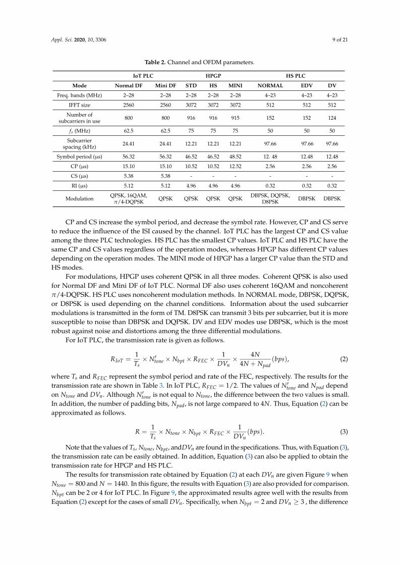
All three PLC technologies use the OFDM technique for transmission. The channel and OFDMparameters are summarized in Table 2. The frequency bands used for IoT PLC and HPGP are 2 to28 MHz. However, HS PLC uses a narrower frequency bands. In these frequency bands, bands usedby other wireless communications and regulated by emission laws can not be used. Therefore, thenumber of usable subcarriers is smaller than half of the IFFT size. The sampling frequency fs and theIFFT size determine the subcarrier spacing. HPGP has the smallest subcarrier spacing, and HS PLChas the largest subcarrier spacing. The small value of the subcarrier spacing makes it easy to controlthe PLC signal spectrum where allowed and forbidden bands are closely located. The signal spectrumshape is also related to the RI value. The large RI value results in low out-of-band spectral components.IoT PLC has the largest RI value and HS PLC has the smallest RI.

Appl. Sci. 2020, 10, 3306 9 of 21

Table 2. Channel and OFDM parameters.

IoT PLC HPGP HS PLC

Mode Normal DF Mini DF STD HS MINI NORMAL EDV DV

Freq. bands (MHz) 2–28 2–28 2–28 2–28 2–28 4–23 4–23 4–23

IFFT size 2560 2560 3072 3072 3072 512 512 512

Number of 800 800 916 916 915 152 152 124subcarriers in use

fs (MHz) 62.5 62.5 75 75 75 50 50 50

Subcarrier 24.41 24.41 12.21 12.21 12.21 97.66 97.66 97.66spacing (kHz)

Symbol period (µs) 56.32 56.32 46.52 46.52 48.52 12. 48 12.48 12.48

CP (µs) 15.10 15.10 10.52 10.52 12.52 2.56 2.56 2.56

CS (µs) 5.38 5.38 - - - - - -

RI (µs) 5.12 5.12 4.96 4.96 4.96 0.32 0.32 0.32

Modulation QPSK, 16QAM, QPSK QPSK QPSK QPSK DBPSK, DQPSK, DBPSK DBPSKπ/4-DQPSK D8PSK

CP and CS increase the symbol period, and decrease the symbol rate. However, CP and CS serveto reduce the influence of the ISI caused by the channel. IoT PLC has the largest CP and CS valueamong the three PLC technologies. HS PLC has the smallest CP values. IoT PLC and HS PLC have thesame CP and CS values regardless of the operation modes, whereas HPGP has different CP valuesdepending on the operation modes. The MINI mode of HPGP has a larger CP value than the STD andHS modes.

For modulations, HPGP uses coherent QPSK in all three modes. Coherent QPSK is also usedfor Normal DF and Mini DF of IoT PLC. Normal DF also uses coherent 16QAM and noncoherentπ/4-DQPSK. HS PLC uses noncoherent modulation methods. In NORMAL mode, DBPSK, DQPSK,or D8PSK is used depending on the channel conditions. Information about the used subcarriermodulations is transmitted in the form of TM. D8PSK can transmit 3 bits per subcarrier, but it is moresusceptible to noise than DBPSK and DQPSK. DV and EDV modes use DBPSK, which is the mostrobust against noise and distortions among the three differential modulations.

For IoT PLC, the transmission rate is given as follows.

RIoT =1Ts× N′tone × Nbpt × RFEC ×

1DVn

× 4N4N + Npad

(bps), (2)

where Ts and RFEC represent the symbol period and rate of the FEC, respectively. The results for thetransmission rate are shown in Table 3. In IoT PLC, RFEC = 1/2. The values of N′tone and Npad dependon Ntone and DVn. Although N′tone is not equal to Ntone, the difference between the two values is small.In addition, the number of padding bits, Npad, is not large compared to 4N. Thus, Equation (2) can beapproximated as follows.

R =1Ts× Ntone × Nbpt × RFEC ×

1DVn

(bps). (3)

Note that the values of Ts, Ntone, Nbpt, andDVn are found in the specifications. Thus, with Equation (3),the transmission rate can be easily obtained. In addition, Equation (3) can also be applied to obtain thetransmission rate for HPGP and HS PLC.

The results for transmission rate obtained by Equation (2) at each DVn are given Figure 9 whenNtone = 800 and N = 1440. In this figure, the results with Equation (3) are also provided for comparison.Nbpt can be 2 or 4 for IoT PLC. In Figure 9, the approximated results agree well with the results fromEquation (2) except for the cases of small DVn. Specifically, when Nbpt = 2 and DVn ≥ 3 , the difference

Appl. Sci. 2020, 10, 3306 10 of 21

due to the approximation is almost negligible. When Nbpt = 4 and DVn ≥ 5, the difference due to theapproximation is also almost negligible.

Table 3. Transmission rate for IoT PLC (Mbps).

DVn 1 2 3 4 5 6 7 8

Rate, Nbpt = 2 12.784 6.392 4.649 3.409 2.841 2.324 1.967 1.763Rate, Nbpt = 4 25.568 12.784 8.523 6.392 5.682 4.649 3.934 3.409

DVn 9 10 11 12 13 14 15 Mini DF

Rate, Nbpt = 2 1.550 1.421 1.278 1.162 1.065 1.003 0.930 0.852Rate, Nbpt = 4 3.008 2.841 2.557 2.324 2.131 1.967 1.826 -

DVn

0 5 10 15

Rate

(M

bps)

0

5

10

15

20

25

30

IoT PLC, Nbpt

= 2

IoT PLC, Nbpt

= 2, approx.

IoT PLC, Nbpt

= 4

IoT PLC, Nbpt

= 4, approx.

HPGP

HPGP, approx.

HS PLC

Figure 9. Transmission rate of IoT PLC according to diversity numbers.

For HPGP, Nbpt = 2 and RFEC = 1/2, regardless of the operating modes. The symbol period Ts

and the number of subcarriers in use Ntone are shown in Table 2. The diversity number is shown inTable 1. Padding bits are also used in HPGP. Using Equation (2), the transmission rates are obtainedand are shown in Table 4. The approximate transmission rates using Equation (3) are also obtainedand shown in parentheses. The results of the transmission rates are shown in Figure 9 for comparison.

Table 4. Transmission rate for HPGP and HS PLC (Mbps).

HPGP HS PLC

Mode STD HS MINI NORMAL EDV DV

Rate 4.707 (4.923) 8.942 (9.845) 3.737 (3.772) ≤25.684 1.603 0.481

In the NORMAL mode of HS PLC, the transmission rate varies according to the TM and therate of the FEC, which can be set by the software or operator. We choose the maximum valueof RFEC for convenience, which is equal to (239/255) × (3/4). In addition, Nbpt changes with themodulation method determined by the TM. Likewise, we choose the maximum value of 3 for Nbpt.Thus, the transmission rate obtained for the NORMAL mode is the maximum that the mode can achieve.

For EDV and DV modes, 40 information bytes and 12 bytes are transmitted by 16 OFDM symbols,respectively. Using the values in Tables 1 and 2, the transmission rates are obtained by Equation (2).The transmission rates for HS PLC are shown in Table 4. The transmission rate for NORMAL mode,25.684 Mbps, is the maximum rate, when assuming that D8PSK is used for each subcarrier, and therate 3/4 CC is employed for the FEC. When the rate 1/2 CC is used for the FEC, the transmission ratedecreases to 17.123 Mbps. For the modes of DV and EDV, the values are the actual transmission ratesof the physical layer. These transmission rates for HS PLC are also shown in Figure 9.

There are several methods to numerically estimate the power spectrum or power spectral density,such as periodograms and Welch’s method. Welch’s method is known to reduce the noise in the

Appl. Sci. 2020, 10, 3306 11 of 21

estimated power spectra which is noticeable in a periodogram [33]. We estimate the power spectrumof the transmitted PLC signals by Welch’s method.

The number of samples used to obtain the spectrum is about 1 million. Figure 10a shows thepower spectrum of the IoT PLC signal. The horizontal axis ranges from 0 to half of the samplingfrequency. The signal is designed to occupy the frequency band of 2–28 MHz. However, in the band,there are forbidden ranges due to the use of wireless communication such as short-wave radio andamateur radio. As in other countries around the world, the radiation levels for each frequency bandare strictly regulated by law in Korea. In Figure 10a, the notches are located in the forbidden bandsand are very deep. The power at band edges is about 70 dB lower.

Figure 10b,c shows the spectrum results for HPGP and HS PLC, respectively. The frequencyrange is from 0 to fs/2, which corresponds to 37.5 and 25 MHz for HPGP and HS PLC, respectively.The frequency bands for HPGP and HS PLC are 2–28 and 4–24 MHz, respectively. In the computerexperiment, the subcarrier masks in the standards [6,7,9] are applied, and the power of the transmittedsignals for the three PLC technologies is made to be equal. Since the bandwidth of HS PLC is narrowerthan the others, the power spectrum level is higher. The spectrum notches in HS PLC is very shallowcompared to those of the others. The notches are only about 20–25 dB deep because the RI value of HSPLC is short. Since the power at the band edges is observed only about 30 dB lower, an additionalanalog filter is needed to control the sidelobe power. In HPGP, the notch depth is about 30–40 dB andthe power at band edges is about 40 dB lower. Thus, HPGP has better power spectrum properties thanHS PLC in terms of the notch depth and out-of-band power. IoT PLC has better spectral propertiesthan HPGP since IoT PLC has deeper notches and lower out-of-band power than HPGP.

Frequency (MHz)

0 5 10 15 20 25 30

Pow

er

spectr

al density (

dB

/Hz)

-120

-110

-100

-90

-80

-70

-60

-50

-40

-30

-20

(a)

Frequency (MHz)

0 5 10 15 20 25 30 35

Po

we

r sp

ectr

al d

en

sity (

dB

/Hz)

-120

-110

-100

-90

-80

-70

-60

-50

-40

-30

-20

(b)

Frequency (MHz)

0 5 10 15 20 25

Po

we

r sp

ectr

al d

en

sity (

dB

/Hz)

-120

-110

-100

-90

-80

-70

-60

-50

-40

-30

-20

(c)

Figure 10. Power spectrum: (a) IoT PLC; (b) HPGP; and (c) HS PLC.

Appl. Sci. 2020, 10, 3306 12 of 21

4. BER Comparisons and Discussion

4.1. Computer Simulation Blocks

The communication reliability for the PLC physical layer is investigated in terms of BER. Figure 11shows the computer simulation block diagram for BER measurement. Randomly generated bits areprocessed at the transmitter, and the output OFDM signal of the transmitter enters the PLC channel.The channel output corrupted by noise is input to the receiver. The receiver specifications for the threePLC technologies are not given in the standards. Thus, the algorithm used for each PLC receiver isdesigned to achieve the best performance possible. In this context, impulsive noise is not included sinceour purpose is to obtain the upper performance bound for each PLC. For background noise, colorednoise is known to reflect the noise of the PLC environment better. However, AWGN is also considereduseful when comparing the upper performance bound of the PLC technologies. Thus, for the noise,AWGN is used in the simulation. The performance comparisons are based on the upper limit of theperformance that each PLC specification can achieve.

The IoT PLC receiver in Figure 11 consists of several functional blocks. In this paper, it is assumedthat symbol and carrier synchronization between the transmitter and the receiver is perfect. That is, thereis no timing error and no carrier frequency error at the receiver. CP and CS are removed from the receivedsignal, which is then converted to the frequency domain by FFT. There are pilot symbols or pilot carriersin the transmitted signal to help channel estimation. Algorithms to estimate the channel response from thepilot tones have been described, and each algorithm has pros and cons [34]. Since our goal is to evaluatethe upper limit of the BER performance, we assume a perfect channel and signal-to-noise ratio (SNR)estimation. The channel response is used to equalize each distorted subcarrier signal by a frequencydomain one-tap equalizer using the minimum mean square error (MMSE) algorithm.

The equalized subcarrier signals are demodulated. The demodulator produces soft decisionvalues since CTC decoding uses soft decision inputs. The demodulated in-phase or quadraturecomponents are combined by the diversity demapper. The combined values are sent to the channeldeinterleaver and subblock deinterleaver, which function as an inverse channel interleaver andsubblock deinterleaver, respectively.

Figure 11. Simulation block diagram for BER measurements.

For CTC decoding, several methods are described in the literature [35–37]. Maximum a posteriori(MAP) or log-MAP, which is the log-domain implementation of the MAP, is the optimal decodingalgorithm. Log-MAP provides less computational burden than MAP, but the complexity is still high.The max-log-MAP algorithm with a correction term has viable complexity and provides equivalentperformance to the log-MAP. Thus, the max-log-MAP with a correction term is used for CTC decoding.

Appl. Sci. 2020, 10, 3306 13 of 21

This algorithm is also used when the performance of HPGP is evaluated. Finally, the decoded bitstream is compared to the input bit stream and the BER is computed.

4.2. Channel Model

The broadband channel model in [18] is described briefly. The frequency response of the channelis as follows.

H( f ) =K

∑k=1

gk · A( f , dk) · e−j2π f (dk/vp), (4)

where gk is a weighting factor and A( f , dk) is an attenuation. The last portion e−j2π f (dk/vp) representsdelay, where dk and vp are the length of the kth path and the propagation speed on the transmissionline, respectively. K represents the number of signal paths between the transmitter and receiver.The attenuation A( f , dk) and the parameters gk and dk are obtained from field measurements.

When a power line has one tap and the number of signal paths is 4, the attenuation andthe parameters are obtained in [18]. The magnitude response of this model with the attenuationand parameters is shown in Figure 12a. This model covers all substantial effects of the transfercharacteristics in the frequency range from 500 kHz to 20 MHz. However, observing that the attenuationdecreases as the frequency increase in the range above 20 MHz, it is believed that this model can beused up to 28 MHz without loss of generality.

For the simulation, the frequency response is cut to the range of half the sampling frequency ofIoT PLC and sampled with the frequency resolution of subcarrier spacing. Then, the discrete impulseresponse obtained from the sampled channel frequency response is convolved with the sampled IoTPLC signal to produce the channel output. This method also applies to HPGP and HS PLC. Since theirsampling frequency and subcarrier spacing are different, each discrete channel impulse response isobtained accordingly. The discrete impulse response for IoT PLC is shown in Figure 12b as an example.

Frequency (MHz)

5 10 15 20 25 30 35

|H(f

)| (

dB

)

-70

-60

-50

-40

-30

-20

-10

0

(a)

Sample number

0 500 1000 1500 2000 2500

Ch

an

ne

l im

pu

se

re

sp

on

se

-0.04

-0.02

0

0.02

0.04

0.06

0.08

0.1

0.12

0.14

(b)

Figure 12. PLC channel: (a) magnitude frequency response of the channel; and (b) channel impulseresponse for IoT PLC.

4.3. Simulation Results and Discussion

The CTC decoder decodes the input block by an iterative algorithm. The CTC decoder has twosoft-input soft-output (SISO) decoders, which compute a posteriori log-likelihood ratio (LLR) forinformation bits. With soft-decision inputs and a priori LLR of information bits, a SISO decoder alsoproduces an extrinsic information. The extrinsic information is provided to the other SISO decoderas an updated a priori LLR. This process is done iteratively. As the iteration continues, a posterioriLLR values become more reliable with the updated a priori LLRs. Detailed descriptions of the iterativedecoding algorithm are given in [35–37]. After each iteration, errors in the decoded bits are reduced.The BER results for IoT PLC with QPSK modulation are shown in Figure 13. The number of information

Appl. Sci. 2020, 10, 3306 14 of 21

bits for subblocks A and B used in the simulation is about 106. The diversity number DVn of IoT PLCis 1–15 . The SNR in dB is defined as 10log10(Sp/Np), where Sp and Np are the signal power and noisepower at the receiver, respectively. In Figure 13, the results for diversity numbers of 3 and 15 are shownas examples. In the figures, the BER value decreases as the number of iterations increases. In thesecond iteration, the BER performance is greatly improved. However, the BER improvement becomessaturated when the iterations are large. The difference between the BER results at Iterations 6 and 8 isvery small. In addition, the BER drops rapidly when SNR≥ −5 dB and DVn = 3. However, when DVn

increases to 15, the rapid fall of the BER begins at a much lower SNR of −13.5 dB. When DVn = 3 and15, the required SNR to obtain 10−3 for the BER is −3.3 dB and −12.8 dB at six iterations, respectively.

SNR (dB)

-7 -6 -5 -4 -3 -2 -1

BE

R

10-5

10-4

10-3

10-2

10-1

100

QPSK, DVn=3

Iteration:1

iteration: 2

iteration: 4

iteration: 6

iteration: 8

(a)

SNR (dB)

-15 -14 -13 -12 -11 -10 -9

BE

R

10-5

10-4

10-3

10-2

10-1

100

QPSK, DVn=15

Iteration:1

iteration: 2

iteration: 4

iteration: 6

iteration: 8

(b)

Figure 13. BER results for IoT PLC with QPSK modulation: (a) DVn = 3; and (b) DVn = 15.

The BER results for IoT PLC with 16QAM modulation are shown in Figure 14. The shape of thisfigure is similar to that of Figure 13. However, the beginning SNR for a rapid BER fall is very large.For example, the BER drops rapidly when SNR ≥ 5 dB and DVn = 3. When DVn = 15, the BER showsrapid fall at SNR ≥ −5.5 dB. In addition, as DVn increases, the slopes of the falling portion of thecurves are steeper, which is also seen in Figure 13.

SNR (dB)

3 4 5 6 7 8 9

BE

R

10-5

10-4

10-3

10-2

10-1

100

16QAM, DVn=3

Iteration:1

iteration: 2

iteration: 4

iteration: 6

iteration: 8

(a)

SNR (dB)

-8 -7 -6 -5 -4 -3 -2

BE

R

10-5

10-4

10-3

10-2

10-1

100

16QAM, DVn=15

Iteration:1

iteration: 2

iteration: 4

iteration: 6

iteration: 8

(b)

Figure 14. BER results for IoT PLC with 16QAM modulation: (a) DVn = 3; and (b) DVn = 15.

The BER results for IoT PLC with π/4-DQPSK modulation are shown in Figure 15.For π/4-DQPSK mode, noncoherent detection is used. The channel equalizer is not applied for thismode. The differential detection is performed with symbols adjacent in time in the same subchannel.On static or slowly changing channels, distortions caused by the channel can be compensated withdifferential detection. When DVn = 3, an irreducible error floor is observed. The subchannel located atthe deep notch of the channel has unrecoverable bit errors. If the diversity number is not large, the bit

Appl. Sci. 2020, 10, 3306 15 of 21

copies are not spread enough to be corrected, which results in error floor. When DVn = 15, the errorfloor is not present and the BER decreases rapidly as the SNR increases owing to the rich diversity.With the channel used in the simulation, the error floor is not observed in the range down to 10−5

when DVn ≥ 4.

SNR (dB)

-2 -1 0 1 2 3 4

BE

R

10-5

10-4

10-3

10-2

10-1

100

π/4-DQPSK, DVn=3

Iteration:1

iteration: 2

iteration: 4

iteration: 6

iteration: 8

(a)

SNR (dB)

-9 -8 -7 -6 -5 -4 -3

BE

R

10-5

10-4

10-3

10-2

10-1

100

π/4-DQPSK, DVn=15

Iteration:1

iteration: 2

iteration: 4

iteration: 6

iteration: 8

(b)

Figure 15. BER results for IoT PLC with π/4-DQPSK modulation: (a) DVn = 3; and (b) DVn = 15.

Next, the BER results for Mini DF are shown in Figure 16. In Mini DF mode, QPSK modulation isused and the block size is N = 48. Since the block size is smaller than that of DF, the BER shows arelatively slow decrease with increasing SNR, which is commonly observed in systems with CTC ofsmall processing blocks. However, for Mini DF mode with many copies of coded bits (16 copies), theBER begins to fall at a low SNR of −14 dB. The required SNR to obtain 10−3 for the BER is −11.7 dB atsix iterations.

SNR (dB)

-16 -15 -14 -13 -12 -11 -10

BE

R

10-5

10-4

10-3

10-2

10-1

100Mini DF

Iteration:1

iteration: 2

iteration: 4

iteration: 6

iteration: 8

Figure 16. BER results for Mini DF.

Next, the performance change according to the diversity number at each modulation isinvestigated. The BER results for the whole values of DVn are shown in Figure 17, where the iterationnumber is set to 6. The BER performance improves as DVn increases. In Figure 17a, to obtain a BER of10−3 in QPSK mode, an SNR of 0.3 dB is required with DVn = 2 and an SNR of −3.3 dB with DVn = 3.Thus, an SNR improvement of 3.6 dB is obtained owing to the diversity number increasing from 2to 3. However, the performance improvement obtained from the diversity becomes small when thediversity number becomes large. For example, when the diversity number increases from 9 to 10, anSNR improvement of 0.4 dB is obtained. The other modulations, 16QAM and π/4-DQPSK, show asimilar trend.

Figure 17b shows the BER results for 16QAM mode. The BER hardly decrease even with a largeSNR when DVn = 1. However, when DVn ≥ 2, the BER decreases rapidly as the SNR increases.Without diversity, a bit may be not recovered even at a high SNR due to a deep notch in the channel,

Appl. Sci. 2020, 10, 3306 16 of 21

but in the presence of diversity, copies of the bit can make the bit correctable. At BER=10−3, an SNRimprovement of 2.95 dB is obtained with a DVn increase from 2 to 3. When DVn increases form 9to 10, an SNR improvement of 0.31 dB is observed at BER=10−3. In Figure 17c, the BER results forπ/4-DQPSK mode are shown. Comparing the BER performance of π/4-DQPSK mode with that of theother modes at every DVn, the BER performance of π/4-DQPSK is better than that of 16QAM but isworse than that of QPSK.

SNR (dB)

-15 -10 -5 0 5 10

BE

R

10-3

10-2

10-1

100QPSK, iteration=6

1 2 3 4 5 6 7 8 9 10 11 12 13 14 15

(a)

SNR (dB)

-6 -4 -2 0 2 4 6 8 10 12 14 16

BE

R

10-3

10-2

10-1

10016QAM, iteration=6

1 2 3 4 5 6 7 8 9 10 11 12 13 14 15

(b)

SNR (dB)

-5 0 5 10 15

BE

R

10-3

10-2

10-1

100π/4-DQPSK, iteration=6

1 2 3 4 5 6 7 8 9 10 11 12 13 14 15

(c)

Figure 17. BER results of IoT PLC for the whole DVn: (a) QPSK mode; (b) 16QAM mode; and(c) π/4-DQPSK mode.

Appl. Sci. 2020, 10, 3306 17 of 21

HPGP uses CTC for the FEC. Thus, iterative decoding is used as in IoT PLC. Figure 18 shows theBER results for HPGP. BER values are given at Interations 2, 4, 6, and 8. As the iterations increase,the BER difference between iterations decreases. The block size for STD and HS modes is 2080, whilethe block size of MINI mode is 544. The falling slope of the BER curve in Figure 18a is less steep thanthose in the other modes, because the block size at the MINI mode is smaller. The STD mode makesfour copies for the coded bits while HS makes two copies. Thus, the STD mode outperforms the HSmode in terms of the BER. At a BER of 10−3, the STD mode requires an SNR of −5.7 dB while the HSmode requires 1.3 dB. The MINI mode has the most copies for the coded bits, but the BER performanceat high SNR is not better than the STD mode because of the small input block size.

SNR (dB)

-9 -8 -7 -6 -5 -4 -3

BE

R

10-5

10-4

10-3

10-2

10-1

100HPGP, MINI mode

iteration: 2

iteration: 4

iteration: 6

iteration: 8

(a)

SNR (dB)

-9 -8 -7 -6 -5 -4 -3

BE

R

10-5

10-4

10-3

10-2

10-1

100HPGP, STD mode

iteration: 2

iteration: 4

iteration: 6

iteration: 8

(b)

SNR (dB)

-2 -1 0 1 2 3 4

BE

R

10-5

10-4

10-3

10-2

10-1

100HPGP, HS mode

iteration: 2

iteration: 4

iteration: 6

iteration: 8

(c)

Figure 18. BER results for HPGP: (a) MINI mode; (b) STD mode; and (c) HS mode.

The BER results for HS PLC are shown in Figure 19. For the performance evaluation of HS PLC,the best and worst modes in terms of the BER are considered. The FEC in HS PLC does not use iterativedecoding. Figure 19a shows the BER results for the NORMAL mode. An error floor is present andthe BER does not fall below 0.02 in the NORMAL mode. There is no diversity in the NORMAL mode.In the DV mode, the BER decreases as the SNR increases due to the high diversity of 12 at the expenseof the transmission rate, but the falling slope of the BER is not as rapid as that of IoT PLC or HPGP,which uses CTC for FEC.

In Figure 20, the BER performance of HS PLC and HPGP are shown for comparison. The STDmode of HPGP has the best performance at BER = 10−3, followed by the MINI mode, the DV mode ofHS PLC, and the HS mode of HPGP. In terms of the BER, the NORMAL mode of HS PLC shows theworst performance. The BER curves of HPGP are steeper than those of HS PLC. Thus, the differencebetween the BER values of the MINI mode of HPGP and the DV mode of HS PLC becomes larger asthe SNR increases.

Appl. Sci. 2020, 10, 3306 18 of 21

SNR (dB)

8 10 12 14 16 18 20 22 24 26 28

BE

R

10-5

10-4

10-3

10-2

10-1

100HS PLC, NORM mode

(a)

SNR(dB)

-9 -8.5 -8 -7.5 -7 -6.5 -6 -5.5 -5 -4.5 -4

BE

R

10-5

10-4

10-3

10-2

10-1

100HS PLC, DV mode

(b)

Figure 19. BER results for HS PLC: (a) NORMAL mode; and (b) DV mode.

SNR (dB)

-8 -6 -4 -2 0 2 4 6 8 10 12 14

BE

R

10-3

10-2

10-1

100HPGP with iteration=6, and HS PLC

HPGP, HS

HPGP, STD

HPGP, MINI

HS PLC, NORM

HS PLC, DV

Figure 20. BER results of HPGP and HS PLC.

Now, performance comparisons of the three PLC technologies are provided. Since there are manymodes of PLC technologies to compare, a plot would be very complex and difficult to read if all theBER curves for all the modes were shown in the same plot. Instead of comparing all the BER curves,the SNR value required to obtain a target BER at each mode of the PLC is compared. In Figure 21,the SNR values required to obtain a BER of 10−3 are shown for all modes of the PLC technologies.The horizontal axis is the diversity number (the number of copies for the coded bits) and the verticalaxis represents the required SNR. Therefore, a lower point means better BER performance. The threedotted lines represent the results for IoT PLC. IoT PLC in QPSK mode has better BER performancethan any other PLC technologies at each diversity number. The QPSK mode of IoT PLC with DVn = 15is the best in terms of the BER performance. The Mini DF of IoT PLC has an SNR value similar to theQPSK mode with DVn = 11, but this SNR value cannot be achieved with the other PLC technologies.

On the other hand, the STD mode of HPGP outperforms the other two modes of HPGP andprovides similar performance to the QPSK mode of IoT PLC with DVn = 4. The HS mode of HPGPhas a slightly worse performance than the QPSK mode of IoT PLC with DVn = 2. The DV mode of HSPLC has worse performance than π/4-DQPSK mode with DVn = 12 and has similar performance toπ/4-DQPSK mode with DVn = 9. The performance of the DV mode of HS PLC is worse than that ofthe STD and MINI mode of HPGP. However, the DV mode of HS PLC has better performance thanthe HS mode of HPGP. The NORMAL mode of HS PLC does not appear in this figure since it cannotachieve a BER of 10−3 on the PLC channel. This also applies to the 16QAM mode of IoT PLC withDVn = 1.

Appl. Sci. 2020, 10, 3306 19 of 21

Diversity number

0 2 4 6 8 10 12 14 16

SN

R (

dB

)

-15

-10

-5

0

5

10

15

20SNR required for BER = 10-3

IoT, QPSK

IoT, π /4-DQPSK

IoT, 16QAM

IoT, Mini DF

HPGP, HS

HPGP, STD

HPGP, MINI

HS PLC, DV

Figure 21. Comparisons of SNR required for BER of 10−3.

5. Conclusions

This study compared the physical layer performance of broadband PLC technologies beingdeployed or tested in Korea. The PLC technologies included IoT PLC, HPGP, and HS PLC. The bitrate, power spectrum, and BER were evaluated. For the transmission rate, an expression for the bitrate for IoT PLC and HPGP was derived while taking the padding bits and the number of tones in useinto consideration. The expression was compared with an approximate formula. IoT PLC provides 31different bit rates ranging from 0.930 to 25.568 Mbps. HPGP and HS PLC each provides three differentbit rates. The power spectrum was obtained through computer simulations. IoT PLC was found tohave good power spectrum properties in terms of the notch depth and out-of-band power. For the BERperformance comparisons, the upper bound of the BER for each PLC standard was evaluated throughcomputer simulations. From the results, the STD mode of HPGP provides similar performance to theQPSK mode of IoT PLC with a diversity number of 4. Finally, we observed that IoT PLC in QPSKmode has better BER performance than any other PLC technologies at each diversity number.

Funding: This research was supported by a grant from the Korea Energy Efficiency Cooperative.

Conflicts of Interest: The authors declare no conflict of interest. The funders had no role in the design of thestudy; in the collection, analyses, or interpretation of data; in the writing of the manuscript, or in the decision topublish the results.

References

1. Mohassel, R.R.; Fung, A.; Mohammadi, F.; Raahemifar, K. A survey on advanced metering infrastructure.Electr. Power Energy Syst. 2014, 63, 473–484. [CrossRef]

2. Kim, D.S.; Chung, B.J.; Chung, Y.M. Statistical learning for service quality estimation in broadband PLCAMI. Energies 2019, 12, 684. [CrossRef]

3. Uribe-Pérez, N.; Angulo, I.; de la Vega, D.; Arzuaga, T.; Fernández, I.; Arrinda, A. Smart grid applicationsfor a practical implementation of IP over narrowband power line communications. Energies 2017, 10, 1782.[CrossRef]

4. Chung, Y.M. Overview and characteristics of IoT PLC physical layer. In Proceedings of the InternationalConference of Electronics, Information, and Communication (ICEIC) 2020, Barcelona, Spain, 19–22 January2020; pp. 99-101.

5. Llano, A.; Angulo, I.; de la Vega, D.; Marron, L. Impact of channel disturbances on current narrowband powerline communications and lessons to be learnt for the future technologies. IEEE Access 2019, 7, 83797–83811.[CrossRef]

6. International Organization for Standardization. Information Technology-Telecommunications and InformationExchange between Systems-Powerline Communication (PLC) Medium Access Control (MAC) and Physical Layer

Appl. Sci. 2020, 10, 3306 20 of 21

(PHY)-Part 1: General Requirements; ISO/IEC 12139-1; International Organization for Standardization: Geneva,Switzerland, 2009.

7. HomePlug Alliance. HomePlug Green PHY Specification Release Version 1.1.1; HomePlug Alliance: Beaverton,OR, USA, 2013.

8. Korea Smart Grid Association (KSGA). Smart Grid Technology Trends Report; KSGA: Seoul, Korea, 2012.9. Korea Electrical Manufacturers Association (KOEMA). General Requirements for Power-Line Communication

(PLC) Media Access Control (MAC) and Physical Layer (PHY) for Internet of Things; SPS-KOEMA 0915-XXXX,submitted for Alliance Standards; Korea Electrical Manufacturers Association (KOEMA): Seoul, Korea, 2018.

10. Gotz, M.; Rapp, M.; Dostert, K. Power line channel characteristics and their effect on communication systemdesign. IEEE Commun. Mag. 2004, 42, 78–86. [CrossRef]

11. Esmailian, T.; Kschischang, F.R.; Gulak P.G. In-building power lines as high-speed communication channels:channel characterization and a test channel ensemble. Int. J. Commun. Syst. 2003, 16, 381–400. [CrossRef]

12. Banwell T.; Galli, S. A novel approach to the modeling of the indoor power line channel part I: Circuitanalysis and companion model. IEEE Trans. Power Deliv. 2005, 20, 655–663. [CrossRef]

13. Galli, S.; Banwell, T. A novel approach to the modeling of the indoor power line channel-part II: Transferfunction and its properties. IEEE Trans. Power Deliv. 2005, 20, 1869-1878. [CrossRef]

14. Canete, F.J.; Cortés, J.A.; Díez, L.; Entrambasaguas, J.T. A channel model proposal for indoor power linecommunications. IEEE Commun. Mag. 2011, 49, 166–174. [CrossRef]

15. Tonello, A.M.; Versolatto, F. Bottom-up statistical PLC channel modeling-part I: random topology model andefficient transfer function computation. IEEE Trans. Power Deliv. 2011, 26, 891–898. [CrossRef]

16. Tonello, A.M.; Versolatto, F. Bottom-up statistical PLC channel modeling-part II: Inferring the statistics.IEEE Trans. Power Deliv. 2010, 25, 2356–2363. [CrossRef]

17. Marrocco, G.; Statovci, D.; Trautmann, S. A PLC broadband channel simulator for indoor communications.In Proceedings of the 2013 IEEE 17th International Symposium on Power Line Communications and ItsApplications, Johannesburg, South Africa, 24–27 March 2013; pp. 321–326.

18. Zimmermann, M.; Dostert, K. A multipath model for the powerline channel. IEEE Trans. Commun. 2002, 50,553–559. [CrossRef]

19. Hirayama, Y.; Okada, H.; Yamazato, T.; Katayama, M. Noise analysis on wide-band PLC with highsampling rate and long observation time. In Proceedings of the 7th International Symposium on Power-LineCommunications and Its Applications, Kyoto, Japan, 26–28 March 2003; pp. 142–147.

20. Andreadou, N.; Pavlidou, F. PLC channel: impulsive noise modelling and its performance evaluation underdifferent array coding schemes. IEEE Trans. Power Deliv. 2009, 24, 585–595. [CrossRef]

21. Meng, H.; Guan, Y.L.; Chen, S. Modeling and analysis of noise effects on broadband power-linecommunications. IEEE Trans. Power Deliv. 2005, 20, 630–637. [CrossRef]

22. Andreadou, N.; Pavlidou, F. Modeling the noise on the OFDM power-line communications system.IEEE Trans. Power Deliv. 2010, 25, 150–157. [CrossRef]

23. Mlynek, P.; Koutny, M.; Misurec, J. Power line modelling for creating PLC communication system. Int. J.Commun. 2010, 4, 13–21.

24. Llano, A.; Angulo, I.; Angueira, P.; Arzuaga, T.; de la Vega, D. Analysis of the channel influence to powerline communications based on ITU-T G.9904 (PRIME). Energies 2016, 9, 39. [CrossRef]

25. Sanz A.; Sancho, D.; Guemes, C.; Cortés, J.A. A physical layer model for G3-PLC networks simulation.In Proceedings of the 2017 IEEE International Symposium on Power Line Communications and itsApplications (ISPLC), Madrid, Spain, 3–5 April 2017; pp. 1–6.

26. Hoch, M. Comparison of PLC G3 and PRIME. In Proceedings of the 2011 IEEE International Symposium onPower Line Communications and Its Applications, Udine, Italy, 3–6 April 2011; pp. 165–169.

27. Matanza, J.; Alexandres, S.; Rodriguez-Morcillo, C. Performance evaluation of two narrowband PLC systems:PRIME and G3. Comput. Stand. Interfaces 2013, 36, 198–208. [CrossRef]

28. Upadhyay, A.; Gupta, A.; Kumar, V. Comparative study of narrow band PLCs physical layer under AWGNand narrowband interferer. In Proceedings of the 2015 Annual IEEE India Conference (INDICON), NewDelhi, India, 17–20 December 2015; pp. 1–4.

29. IEEE Computer Society and the IEEE Microwave Theory and Techniques Society. In IEEE Standardfor WirelessMAN-Advanced Air Interface for Broadband Wireless Access Systems; IEEE Std 802.16.1-2012;IEEE Standard Association: New York, NY, USA, 2012.

Appl. Sci. 2020, 10, 3306 21 of 21

30. Ma, H.; Wolf, J. On tail biting convolutional codes. IEEE Trans. Commun. 1986, 34, 104–111. [CrossRef]31. Kang, J.H.; Stark, W.E.; Hero, A.O. Turbo codes for fading and burst channels. In Proceedings of the

1998 IEEE Globecom, Communications Theory Mini Conference, Sydney, Australia, 8–12 November 1998;pp. 40–45.

32. Hall, E.K.; Wilson, S.G. Design and analysis of turbo codes on Rayleigh fading channels. IEEE J. Sel. AreasCommun. 1998, 16, 160–174. [CrossRef]

33. Welch, P. The use of fast Fourier transform for the estimation of power spectra: A method based on timeaveraging over short, modified periodograms. IEEE Trans. Audio Electroacoust. 1967, 15, 70–73. [CrossRef]

34. Sure, P.; Bhuma, C.M. A survey on OFDM channel estimation techniques based on denoising strategies. Eng.Sci. Technol. Int. J. 2017, 20, 629–636. [CrossRef]

35. Lin, C.-H.; Chen, C.-Y.; Wu, A.-Y.; Tsai, T.-H. Low-power memory-reduced traceback MAP decoding fordouble-binary convolutional turbo decoder. IEEE Trans. Circ. Syst. Regul. Pap. 2009, 56, 1005–1016.

36. Kim, J.H.; Park, I.-C. Double-binary circular turbo decoding based on border metric encoding. IEEE Trans.Circ. Syst.-II Exp. Briefs 2008, 55, 79–83. [CrossRef]

37. Claussen, H.; Karimi, H.R.; Mulgre, B. Improved max-log-MAP turbo decoding by maximization of mutualinformation transfer. EURASIP J. Adv. Signal Process. 2005, 2005, 820–827. [CrossRef]

c© 2020 by the author. Licensee MDPI, Basel, Switzerland. This article is an open accessarticle distributed under the terms and conditions of the Creative Commons Attribution(CC BY) license (http://creativecommons.org/licenses/by/4.0/).