Article Reference Prototype land-cover mapping of the Huascaran Biosphere Reserve (Peru) using DEM,...

Article

Reference

Prototype land-cover mapping of the Huascaran Biosphere Reserve

(Peru) using DEM, NDSI and NDVI indices

SILVERIO TORRES, Walter Claudio, JAQUET, Jean-Michel

Abstract

On the basis of Landsat 7 ETM+ imagery, a prototype land-cover map was prepared for the

Huascarán Biosphere Reserve (Peru). This document should contribute to the sustainable

management of the Huascarán Biosphere Reserve, while making it possible to establish a

regional planning policy and to prepare a natural risks map, which is still lacking in the region.

The influence of the topography on radiometry was attenuated by using NDSI and NDVI

indices, which were segmented using their histogram. A digital elevation model (DEM) was

introduced to define the “highlands” and “lowlands”. In the latter, the slope derived from the

DEM was combined with the NDVI to map the agricultural surfaces. Twenty-one spectral

classes were defined and their correspondence with land-cover themes was checked by field

observations. The land-cover map provides original information on the extent of the glacial

cover, debris-covered glaciers, 881 lakes, vegetation density, agricultural surfaces, urban

zones and mines.

SILVERIO TORRES, Walter Claudio, JAQUET, Jean-Michel. Prototype land-cover mapping of

the Huascaran Biosphere Reserve (Peru) using DEM, NDSI and NDVI indices. Journal of

Applied Remote Sensing, 2009, vol. 3, no. 033516, p. 20

Available at:

http://archive-ouverte.unige.ch/unige:1470

Disclaimer: layout of this document may differ from the published version.

[ Downloaded 17/09/2014 at 07:11:06 ]

1 / 1

http://archive-ouverte.unige.ch/unige:1470

Journal of Applied Remote Sensing, Vol. 3, 033516 (6 March 2009)

1

Prototype land-cover mapping of the Huascarán

Biosphere Reserve (Peru) using DEM, NDSI and

NDVI indices

Walter Silverio,a Jean-Michel Jaquet

b

aRemote Sensing and GIS Unit, Earth Science Section, University of Geneva, 13 rue des

Maraîchers, CH-1205 Geneva, Switzerland.

[email protected] bEarth Observation, UNEP/DEWA-Europe GRID Geneva, 11 Chemin des Anémones, CH-

1219 Geneva, Switzerland.

[email protected]

Abstract. On the basis of Landsat 7 ETM+ imagery, a prototype land-cover map was

prepared for the Huascarán Biosphere Reserve (Peru). This document should contribute to

the sustainable management of the Huascarán Biosphere Reserve, while making it possible to

establish a regional planning policy and to prepare a natural risks map, which is still lacking

in the region. The influence of the topography on radiometry was attenuated by using NDSI

and NDVI indices, which were segmented using their histogram. A digital elevation model

(DEM) was introduced to define the “highlands” and “lowlands”. In the latter, the slope

derived from the DEM was combined with the NDVI to map the agricultural surfaces.

Twenty-one spectral classes were defined and their correspondence with land-cover themes was checked by field observations. The land-cover map provides original information on the

extent of the glacial cover, debris-covered glaciers, 881 lakes, vegetation density, agricultural

surfaces, urban zones and mines.

Keywords: remote sensing, sustainable development, snow and vegetation indices, land-

cover, Andes, DEM, Landsat 7 ETM+.

1 INTRODUCTION

Because of the beauty of its landscapes, the diversity of its flora and fauna and its ecological

characteristics, the Cordillera Blanca, located in the Peruvian State of Ancash, was declared

Huascarán National Park (HNP) in 1975 [1]. The Cordillera Blanca attracts more than one hundred thousand tourists annually. However, this human presence, being added to the direct

and indirect users of the HNP, is not without consequences: pressure on fauna and flora in

sectors with a precarious ecological equilibrium; competition for space; conflicts for the

water resources; and waste production [2]. Hence, an integrated management of the

Huascarán Biosphere Reserve (HBR) is urgently needed. To this end, we have proposed

elsewhere a prototype Geographic Information Systems (GIS) for this protected area [3,4].

The land-cover map is an important part of the Geographic Information System and

constitutes an instrument for the understanding and management of the territory [5].

Moreover, in the context of sustainable development, this type of information is essential for

the management of hydrological reserves in high mountain regions [4]. The socio-economic

context of Peru and the dimensions of Huascarán Biosphere Reserve explain why this

information is not yet available.

In the Ancash region, mining activity has been growing since the launch of the Pierina

(1998) and Antamina (1998) ventures [3]. As a consequence, conflicts over water resources

have arisen with the local population. Furthermore, these mines are located within the


2

Biosphere reserve, thereby inducing significant landscape changes and threats for the

ecosytsem [4]. In this context, a land cover map provides a useful inventory of both the

natural landscape types and impacts upon them caused by mining activities.

In a previous study, we used the Normalized Difference Snow Index to map the glacier

area of the Cordillera Blanca [1] for the years 1987 and 1996, excluding the other land cover

types. We present and discuss here the approach we have taken for the production of the first

complete land-cover map of the Huascarán Biosphere Reserve, based on the 2002 Landsat 7

Enhanced Thematic Mapper Plus (ETM+) satellite imagery [6].

2 STUDY AREA

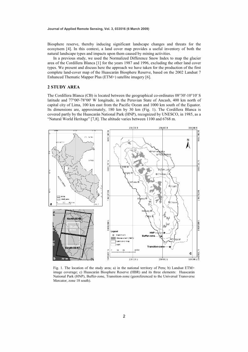
The Cordillera Blanca (CB) is located between the geographical co-ordinates 08°30'-10°10' S

latitude and 77°00'-78°00' W longitude, in the Peruvian State of Ancash, 400 km north of

capital city of Lima, 100 km east from the Pacific Ocean and 1000 km south of the Equator. Its dimensions are, approximately, 180 km by 30 km (Fig. 1). The Cordillera Blanca is

covered partly by the Huascarán National Park (HNP), recognized by UNESCO, in 1985, as a

“Natural World Heritage” [7,8]. The altitude varies between 1100 and 6768 m.

Fig. 1. The location of the study area; a) in the national territory of Peru; b) Landsat ETM+

image coverage; c) Huascarán Biosphere Reserve (HBR) and its three elements: Huascarán

National Park (HNP), Buffer-zone, Transition-zone (georeferenced to the Universal Transverse

Mercator, zone 18 south).


3

The Cordillera Blanca includes 101 mountains higher than 5000 m [9], of which 27 are

higher than 6000 m, such has Huascarán Sur (6768 m), the highest summit in Peru. The

Cordillera Blanca also harbours numerous lakes and glacial valleys [3,10]. According to

Silverio [4], 881 lakes were identified in 2002, flowing either into the Pacific or into the

Atlantic Oceans. The flora is exuberant and the fauna very rich [7]. In this zone, there is also

a great social diversity [4].

According to Kaser et al. [11], the oscillation of the Inter-tropical Convergence Zone

(ITCZ) causes the seasonal distribution of the precipitations. This leads to a succession

between a dry (May–September), and a wet season (October–April) [12,13]. The most intense rains occur between January and March, the wettest month of the year [4].

In 1977, under the UNESCO’s Man and Biosphere Convention, the Cordillera Blanca was

recognized as a Biosphere Reserve [14]. This includes the “core zone” (represented by the

HNP), surrounded by a buffer zone and a transition zone [4]. According to INRENA [15], the

Huascarán Biosphere Reserve covers a surface of 11765 km2, distributed between Huascarán

National Park (3400 km2), the buffer zone (2594 km

2) and the transition zone (5771 km

2).

However, these figures differ from those advanced by UNESCO, respectively, 3400, 1702

and 6456 km2 [14].

According to INRENA [16], the Huascarán National Park is devoted to the biodiversity

and natural environment protection, the buffer zone being an envelope protecting the park and

intended for the development of ecotourism. The transition zone is dedicated to urban

development, commercial activities and tourism infrastructures. According to Silverio [4], the majority of the villages which surround the Cordillera Blanca are located in the buffer zone;

the transition zone includes the valleys of Callejón de Huaylas and Conchucos, where the

principal cities and the chief towns of the districts are concentrated.

3 SATELLITE AND TOPOGRAPHIC DATA

UNEP/GRID-Sioux Falls (USA) provided a mosaic image (Path: 008; Rows: 066-067) from

ETM+ satellite, taken on 17 June 2002. Its pixel resolution is 30 m. It is of good quality (no

visible haze, and cloud cover of only 0.2%). The dimensions of the image are 360 km by 250

km.

The topographic contour lines of the Peruvian National Geographic Institute (IGN) were

provided by Peruvian National Institute of Natural Resources (INRENA). The original

information was georeferenced in Geographic Coordinate System and covered an area of

63775 km2, between 7°56'3''-10°53'10'' S latitude and 76°35'58''-78°45'16'' W longitude. This

area is larger than the Peruvian State of Ancash (35936.5 km2). The topographic contour lines

have a 50 m equidistance, and the minimum and maximum altitudes are 25 m and 6700 m

respectively.

The Digital Elevation Model (DEM) was interpolated from the corrected topographic

contour lines with ARC/INFO® (50 m pixel). This DEM was resampled to a 25 m resolution

using the script “Grid Utilities” for Spatial Analyst of ARCVIEW 3.2® [4]. Resampling was

done to match the DEM resolution with that of the imagery, both of them being combined to

estimate the area of cultivation (see Fig. 2, step 10).

4 METHODOLOGY

The Cordillera Blanca’s complex topography induces a strong relief effect on the images and

hence, on the spectral signatures of land-cover classes [2]. This effect should be ideally corrected by a topographic normalisation using digital elevation models (DEM) [17], which

must have a spatial resolution of at least four times better than the image needing correction

[18]. The DEM interpolated by Silverio [4] using IGN’s contour lines (50 m resolution) does

not meet this condition and the normalisation attempted using the cosine correction available

from the ERDAS software [19] was of poor quality [2,3]. Instead, we used Landsat ETM+


4

band ratios (indices) that enable a certain amount of relief attenuation [1]. Our methodology

is summarised in the flowchart of Fig. 2.

NDVI

(.grid)

Logic operation: AV/Spatial Analyst/Map Calculator

Buffer + vector to raster conversion: AV/Xtools/Edit/Convert to Grid

Logic operation: AV/Spatial Analyst/Map Query

Indice: ERDAS / Operators

Union of themes: AV/Xtools

DEM

Pixel 25 m

Image 2002

Pixel 25 mVectors

Composite

image (7,4,2)Study area

Glacier, debris-

covered glacier, rock

intrusion

Altitude

> 3650 mSlope

Slope

<= 30°

Union of

themes

NDVI

(Mask 1)

Mask 1

Altitude

<= 3650 m

Cultures

Vegetation

<= 3650 m

Vegetation

> 3650 m

NDVI

(.grid)

Urban

Mines

Lakes

Avalanche

Debris flow

Roads

Rivers

1 2

3

4

5

7

8

9

13

11

7

11

1

2

3

4

5

6

7

8

9

10

12

Derive slope: AV/Spatial Analyst/Slope

Logic operation: AV/Spatial Analyst/Map Query

Digitisation: AV

Raster to vector conversion: AV/Spatial Analyst

Edition of themes: AV/Edit

10

Clip: AV/Script

1

Vector to raster conversion: AV/Convert to Grid11

Villages

12

NDSI

(.grid)

NDSI

>= 0.51

6

Cloud

51

11

Mask 2

Final land-cover map

Provisional land-cover map

4

7

14

8

Superposition of themes: AV / Spatial Analyst / Grid Tools13

Clip: AV/Script14

Quality control

Field work

Fig. 2. Flowchart of methodology followed for the prototype land cover map of the

Huascarán Reserve (AV = ArcView).


5

4.1 Image preparation

Bands 1, 2, 3, 4, 5 and 7, respectively (in µm), 0.45-0.52, 0.52-0.60, 0.63-0.69, 0.76-0.90,

1.55-1.75 and 2.0.8-2.35, were stacked and a sub-image (3733 columns by 7000 lines) was

extracted from the 17 June 2002 ETM+ mosaic. Based on the 31 May 1987 baseline image,

which was rectified in our previous study [1], an image-to-image registration was carried out

with 55 ground-control points (GCPs), a first-degree polynomial transformation and a nearest

neighbour resampling (25 m pixel), in UTM coordinate system, zone 18 south. The root-mean-square (RMS) error was 1 pixel. From the resulting image, another extract was taken

using the following coordinates:

Emin; Nmin : 180 000; 8 872 000

Emax; Nmax : 276 000; 9 048 000

The dimension of this image is of 3840 columns by 7040 lines.

No atmospheric correction was carried out on the imagery because a careful visual

inspection revealed no haze over the study area, and no ground data on the atmosphere was

available. This precluded the application of a correction scheme such as advocated by Liang

et al [20]. Moreover, atmospheric corrections do not necessarily yield convincing results [21,

22].

4.2 Calculation of indices

According to Colby [23], indices or spectral band ratios are known for their ability to

eliminate, or at least minimise, illumination differences due to topography. These ratios must

be calculated using little correlated channels (visible and near infra-red) and ideally, after

elimination of additive noise [24]. Since no mist was actually visible on the images, this last

treatment was not deemed necessary [2].

In order to have an optimal representation of the Huascarán Biosphere Reserve high-

altitude land-cover themes for 2002, ranging from pure ice to rock outcrops, and including the vegetation, we have used two indices:

- Normalized Difference Vegetation Index (NDVI); it can be determined using digital

numbers (DN) of ETM+ two bands from the following equation:

NDVI = (Band 4 – Band 3) / (Band 4 + Band 3)

The NDVI is traditionally used for the weekly evaluations of biomass and as support of

the modelling programs of planetary changes [24]. We have used it here to discriminate bare

soils from various vegetation density classes.

- Normalized Difference Snow Index (NDSI) computed from digital numbers (DN) using two

ETM+ bands from the following equation [25]:

NDSI = (Band 2 – Band 5) / (Band 2 + Band 5)

The NDSI makes it possible to distinguish snow from soil, rocks and clouds [26]. The effectiveness of this index was demonstrated for snow and ice mapping in uneven topography

[1,2,27].


6

4.3 Spatial segmentation using NDSI

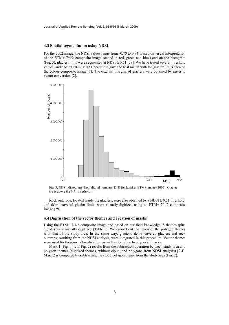
For the 2002 image, the NDSI values range from -0.70 to 0.94. Based on visual interpretation

of the ETM+ 7/4/2 composite image (coded in red, green and blue) and on the histogram

(Fig. 3), glacier limits were segmented at NDSI ≥ 0.51 [28]. We have tested several threshold

values, and chosen NDSI ≥ 0.51 because it gave the best match with the glacier limits seen on

the colour composite image [1]. The external margins of glaciers were obtained by raster to

vector conversion [2].

Fig. 3. NDSI Histogram (from digital numbers: DN) for Landsat ETM+ image (2002). Glacier

ice is above the 0.51 threshold.

Rock outcrops, located inside the glaciers, were also obtained by a NDSI ≥ 0.51 threshold,

and debris-covered glacier limits were visually digitized using an ETM+ 7/4/2 composite

image [29].

4.4 Digitisation of the vector themes and creation of masks

Using the ETM+ 7/4/2 composite image and based on our field knowledge, 8 themes (plus

clouds) were visually digitized (Table 1). We carried out the union of the polygon themes

with that of the study area. In the same way, glaciers, debris-covered glaciers and rock

outcrops, resulting from the NDSI analysis, were integrated in this procedure. Vector themes

were used for their own classification, as well as to define two types of masks.

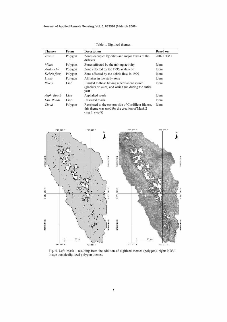
Mask 1 (Fig. 4, left; Fig. 2) results from the subtraction operation between study area and

polygon themes (digitized themes, without cloud, and polygons from NDSI analysis) [2,4].

Mask 2 is computed by subtracting the cloud polygon theme from the study area (Fig. 2).


7

Table 1. Digitized themes.

Themes Form Description Based on

Towns Polygon Zones occupied by cities and major towns of the

districts

2002 ETM+

Mines Polygon Zones affected by the mining activity Idem

Avalanche Polygon Zone affected by the 1995 avalanche Idem

Debris flow Polygon Zone affected by the debris flow in 1999 Idem

Lakes Polygon All lakes in the study zone Idem

Rivers Line Limited to those having a permanent source

(glaciers or lakes) and which run during the entire

year

Idem

Asph. Roads Line Asphalted roads Idem

Uns. Roads Line Unsealed roads Idem

Cloud Polygon Restricted to the eastern side of Cordillera Blanca,

this theme was used for the creation of Mask 2

(Fig 2, step 8)

Idem

Fig. 4. Left: Mask 1 resulting from the addition of digitized themes (polygon); right: NDVI

image outside digitized polygon themes.


8

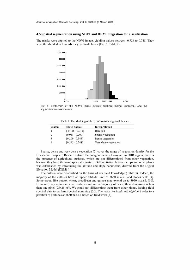
4.5 Spatial segmentation using NDVI and DEM integration for classification

The masks were applied to the NDVI image, yielding values between -0.726 to 0.748. They

were thresholded in four arbitrary, ordinal classes (Fig. 5; Table 2).

Fig. 5. Histogram of the NDVI image outside digitized themes (polygon) and the

segmentation classes values.

Table 2. Thresholding of the NDVI outside digitized themes.

Classes NDVI values Interpretation

1 [-0.726 - 0.011] Bare soil

2 [0.011 - 0.209] Sparse vegetation

3 [0.209 - 0.345] Dense vegetation

4 [0.345 - 0.748] Very dense vegetation

Sparse, dense and very dense vegetation [2] cover the range of vegetation density for the

Huascarán Biosphere Reserve outside the polygon themes. However, in HBR region, there is

the presence of agricultural surfaces, which are not differentiated from other vegetation,

because they have the same spectral signature. Differentiation between crops and other plants

was established by introducing the altitude and slope parameters, derived from the Digital

Elevation Model (DEM) [4].

The criteria were established on the basis of our field knowledge (Table 3). Indeed, the

majority of the cultures have an upper altitude limit of 3650 m.a.s.l. and slopes ≤30° [4]. Some crops, like potato, wheat, broadbean and quinoa may extend up to 3950 m.a.s.l. [10].

However, they represent small surfaces and in the majority of cases, their dimension is less

than one pixel (25x25 m2). We could not differentiate them from other plants, lacking field

spectral data to perform spectral unmixing [30]. The terms lowlands and highlands refer to a

partition of altitudes at 3650 m.a.s.l. based on field work [4].


9

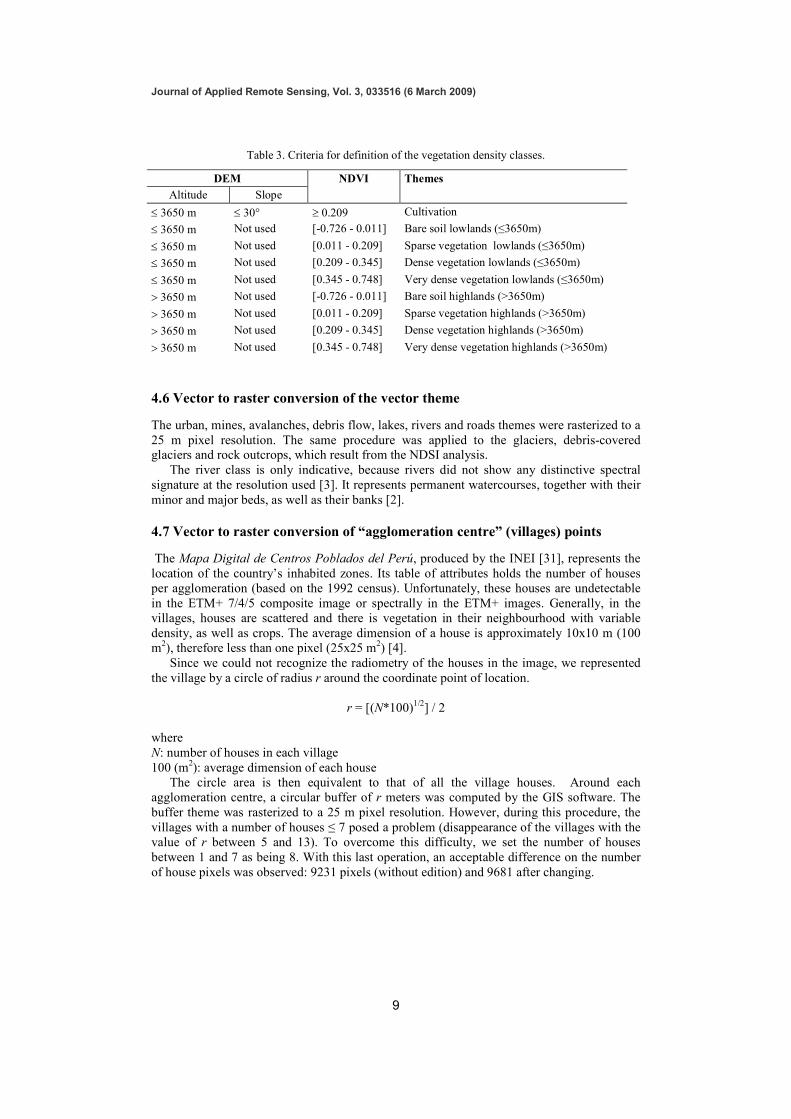
Table 3. Criteria for definition of the vegetation density classes.

DEM NDVI Themes

Altitude Slope

≤ 3650 m ≤ 30° ≥ 0.209 Cultivation

≤ 3650 m Not used [-0.726 - 0.011] Bare soil lowlands (≤3650m)

≤ 3650 m Not used [0.011 - 0.209] Sparse vegetation lowlands (≤3650m)

≤ 3650 m Not used [0.209 - 0.345] Dense vegetation lowlands (≤3650m)

≤ 3650 m Not used [0.345 - 0.748] Very dense vegetation lowlands (≤3650m)

> 3650 m Not used [-0.726 - 0.011] Bare soil highlands (>3650m)

> 3650 m Not used [0.011 - 0.209] Sparse vegetation highlands (>3650m)

> 3650 m Not used [0.209 - 0.345] Dense vegetation highlands (>3650m)

> 3650 m Not used [0.345 - 0.748] Very dense vegetation highlands (>3650m)

4.6 Vector to raster conversion of the vector theme

The urban, mines, avalanches, debris flow, lakes, rivers and roads themes were rasterized to a

25 m pixel resolution. The same procedure was applied to the glaciers, debris-covered glaciers and rock outcrops, which result from the NDSI analysis.

The river class is only indicative, because rivers did not show any distinctive spectral

signature at the resolution used [3]. It represents permanent watercourses, together with their

minor and major beds, as well as their banks [2].

4.7 Vector to raster conversion of “agglomeration centre” (villages) points

The Mapa Digital de Centros Poblados del Perú, produced by the INEI [31], represents the

location of the country’s inhabited zones. Its table of attributes holds the number of houses

per agglomeration (based on the 1992 census). Unfortunately, these houses are undetectable

in the ETM+ 7/4/5 composite image or spectrally in the ETM+ images. Generally, in the

villages, houses are scattered and there is vegetation in their neighbourhood with variable

density, as well as crops. The average dimension of a house is approximately 10x10 m (100

m2), therefore less than one pixel (25x25 m

2) [4].

Since we could not recognize the radiometry of the houses in the image, we represented

the village by a circle of radius r around the coordinate point of location.

r = [(N*100)1/2

] / 2

where

N: number of houses in each village

100 (m2): average dimension of each house

The circle area is then equivalent to that of all the village houses. Around each

agglomeration centre, a circular buffer of r meters was computed by the GIS software. The

buffer theme was rasterized to a 25 m pixel resolution. However, during this procedure, the

villages with a number of houses ≤ 7 posed a problem (disappearance of the villages with the

value of r between 5 and 13). To overcome this difficulty, we set the number of houses

between 1 and 7 as being 8. With this last operation, an acceptable difference on the number

of house pixels was observed: 9231 pixels (without edition) and 9681 after changing.


10

4.8 Field work and quality control

The land cover map quality was evaluated with the help of data collected in the field at 199

control points. Data collection took place in May-June 1999; April-September 2000; June-

August 2001; May-September 2003, and June-September 2004. The land cover type was

evaluated visually according to the 21-term legend (Table 4) within a radius of 50 meters

about the control point, and photographs were taken. Field and classified values were

compared in a contingency matrix using the KappaAnalysis v.2 extension in ArcView 3.2. [32].

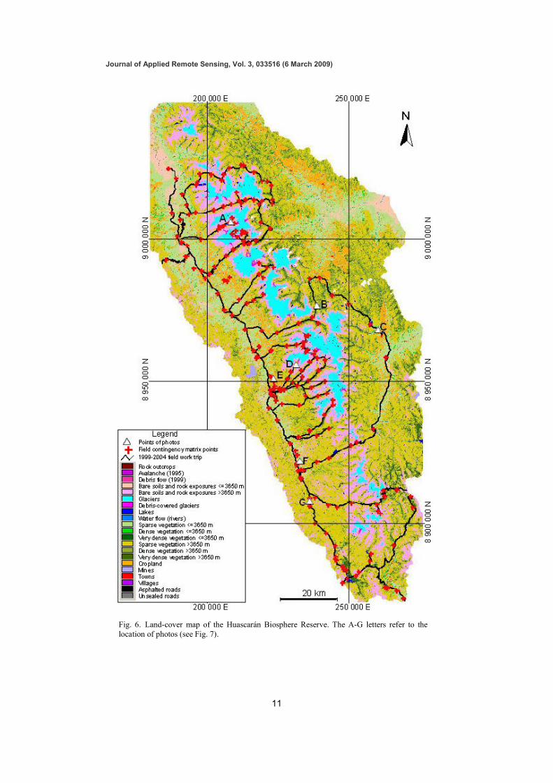
5 RESULTS

The land-cover map of the Huascarán Biosphere Reserve results in the overlay of all the individual maps obtained in the preceding stage (Fig. 2). As a whole, it comprises twenty-one

thematic classes (Table 4; Fig. 6): nine classes were obtained by thresholding of the NDVI

and combined with the DEM; three classes were obtained by thresholding of the NDSI; and

nine other classes were obtained by vector to raster conversion of the vectors themes.

Table 4 presents a first estimate of the areal distribution of the various land cover classes

in the Huascaran Biosphere Reserve. It is representative of the situation at the beginning of the 21

st century, centered on year 2002. Broadly speaking, the land-cover of the Huascarán

Biosphere Reserve is distributed between the vegetation (66% of surface), bare soils and rock

exposures (17%), cultivation (8%) and glaciers (6%).

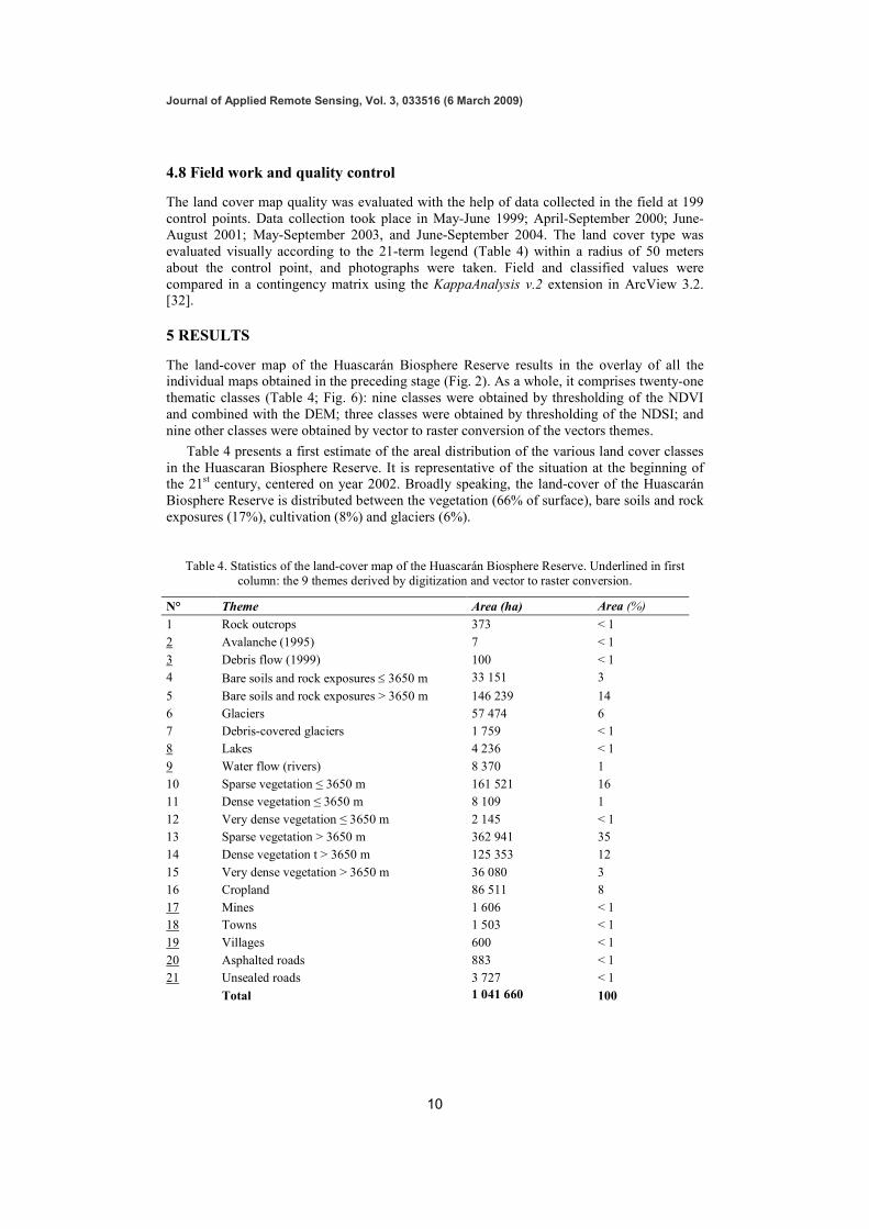
Table 4. Statistics of the land-cover map of the Huascarán Biosphere Reserve. Underlined in first

column: the 9 themes derived by digitization and vector to raster conversion.

N° Theme Area (ha) Area (%)

1 Rock outcrops 373 < 1

2 Avalanche (1995) 7 < 1

3 Debris flow (1999) 100 < 1

4 Bare soils and rock exposures ≤ 3650 m 33 151 3

5 Bare soils and rock exposures > 3650 m 146 239 14

6 Glaciers 57 474 6

7 Debris-covered glaciers 1 759 < 1

8 Lakes 4 236 < 1

9 Water flow (rivers) 8 370 1

10 Sparse vegetation ≤ 3650 m 161 521 16

11 Dense vegetation ≤ 3650 m 8 109 1

12 Very dense vegetation ≤ 3650 m 2 145 < 1

13 Sparse vegetation > 3650 m 362 941 35

14 Dense vegetation t > 3650 m 125 353 12

15 Very dense vegetation > 3650 m 36 080 3

16 Cropland 86 511 8

17 Mines 1 606 < 1

18 Towns 1 503 < 1

19 Villages 600 < 1

20 Asphalted roads 883 < 1

21 Unsealed roads 3 727 < 1

Total 1 041 660 100


11

Fig. 6. Land-cover map of the Huascarán Biosphere Reserve. The A-G letters refer to the

location of photos (see Fig. 7).


12

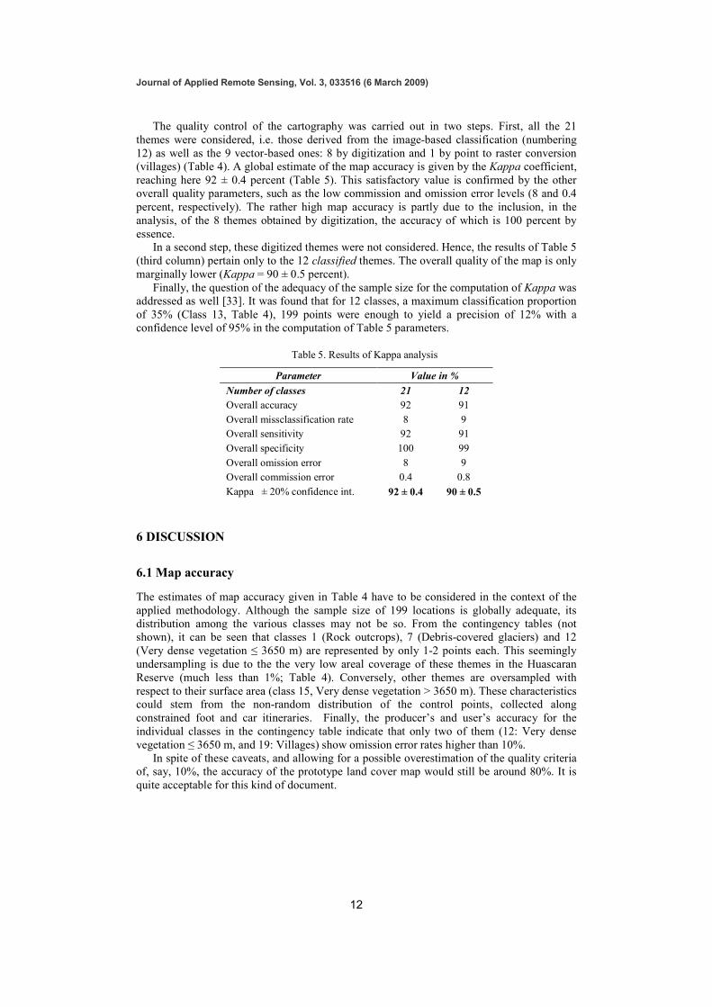
The quality control of the cartography was carried out in two steps. First, all the 21

themes were considered, i.e. those derived from the image-based classification (numbering

12) as well as the 9 vector-based ones: 8 by digitization and 1 by point to raster conversion

(villages) (Table 4). A global estimate of the map accuracy is given by the Kappa coefficient,

reaching here 92 ± 0.4 percent (Table 5). This satisfactory value is confirmed by the other

overall quality parameters, such as the low commission and omission error levels (8 and 0.4

percent, respectively). The rather high map accuracy is partly due to the inclusion, in the

analysis, of the 8 themes obtained by digitization, the accuracy of which is 100 percent by

essence. In a second step, these digitized themes were not considered. Hence, the results of Table 5

(third column) pertain only to the 12 classified themes. The overall quality of the map is only

marginally lower (Kappa = 90 ± 0.5 percent).

Finally, the question of the adequacy of the sample size for the computation of Kappa was

addressed as well [33]. It was found that for 12 classes, a maximum classification proportion

of 35% (Class 13, Table 4), 199 points were enough to yield a precision of 12% with a

confidence level of 95% in the computation of Table 5 parameters.

Table 5. Results of Kappa analysis

Parameter Value in %

Number of classes 21 12

Overall accuracy 92 91

Overall missclassification rate 8 9

Overall sensitivity 92 91

Overall specificity 100 99

Overall omission error 8 9

Overall commission error 0.4 0.8

Kappa ± 20% confidence int. 92 ± 0.4 90 ± 0.5

6 DISCUSSION

6.1 Map accuracy

The estimates of map accuracy given in Table 4 have to be considered in the context of the

applied methodology. Although the sample size of 199 locations is globally adequate, its

distribution among the various classes may not be so. From the contingency tables (not

shown), it can be seen that classes 1 (Rock outcrops), 7 (Debris-covered glaciers) and 12

(Very dense vegetation ≤ 3650 m) are represented by only 1-2 points each. This seemingly

undersampling is due to the the very low areal coverage of these themes in the Huascaran

Reserve (much less than 1%; Table 4). Conversely, other themes are oversampled with

respect to their surface area (class 15, Very dense vegetation > 3650 m). These characteristics could stem from the non-random distribution of the control points, collected along

constrained foot and car itineraries. Finally, the producer’s and user’s accuracy for the

individual classes in the contingency table indicate that only two of them (12: Very dense

vegetation ≤ 3650 m, and 19: Villages) show omission error rates higher than 10%.

In spite of these caveats, and allowing for a possible overestimation of the quality criteria

of, say, 10%, the accuracy of the prototype land cover map would still be around 80%. It is

quite acceptable for this kind of document.


13

6.2 Cartographic reliability

Since the georeference of the satellite images was carried out with topographic maps at

1:100,000 scale (about ±100 m accuracy), we estimate that the land-cover map will be usable

at the same scale order, in spite of the higher pixel resolution of the images (25 m).

Generalization was not carried out, because the operation was irreversible [2].

In the absence of a DEM with a sufficient resolution (approximately 5 m) to carry out

topographic corrections, we estimate that the segmentation of the classes using NDVI represents fairly well the density of the vegetation populations, including the three chosen

classes (i.e. sparse, dense and very dense).

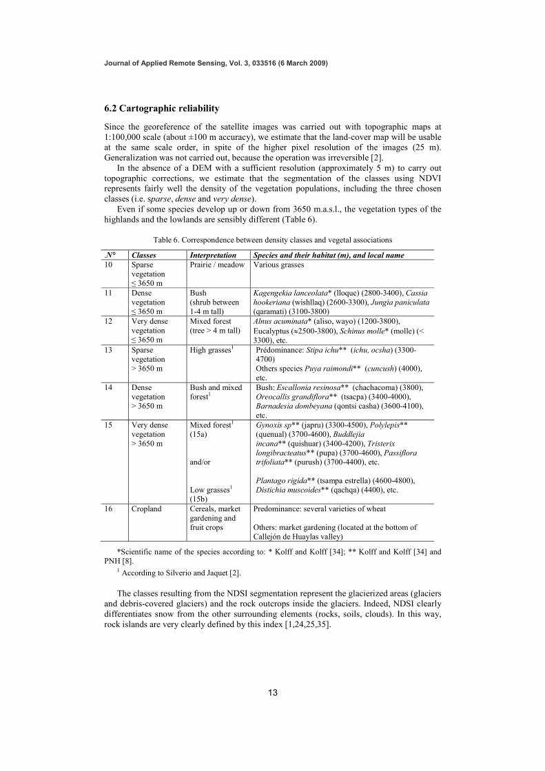
Even if some species develop up or down from 3650 m.a.s.l., the vegetation types of the

highlands and the lowlands are sensibly different (Table 6).

Table 6. Correspondence between density classes and vegetal associations

.N° Classes Interpretation Species and their habitat (m), and local name

10 Sparse

vegetation

≤ 3650 m

Prairie / meadow Various grasses

11 Dense

vegetation

≤ 3650 m

Bush

(shrub between

1-4 m tall)

Kagengekia lanceolata* (lloque) (2800-3400), Cassia

hookeriana (wishllaq) (2600-3300), Jungia paniculata

(qaramati) (3100-3800)

12 Very dense

vegetation

≤ 3650 m

Mixed forest

(tree > 4 m tall)

Alnus acuminata* (aliso, wayo) (1200-3800),

Eucalyptus (≈2500-3800), Schinus molle* (molle) (<

3300), etc.

13 Sparse

vegetation

> 3650 m

High grasses1

Prédominance: Stipa ichu** (ichu, ocsha) (3300-

4700)

Others species Puya raimondi** (cuncush) (4000),

etc.

14 Dense

vegetation

> 3650 m

Bush and mixed

forest1

Bush: Escallonia resinosa** (chachacoma) (3800),

Oreocallis grandiflora** (tsacpa) (3400-4000),

Barnadesia dombeyana (qontsi casha) (3600-4100),

etc.

15 Very dense

vegetation

> 3650 m

Mixed forest1

(15a)

and/or

Low grasses1

(15b)

Gynoxis sp** (japru) (3300-4500), Polylepis**

(quenual) (3700-4600), Buddlejia

incana** (quishuar) (3400-4200), Tristerix

longibracteatus** (pupa) (3700-4600), Passiflora

trifoliata** (purush) (3700-4400), etc.

Plantago rigida** (tsampa estrella) (4600-4800),

Distichia muscoides** (qachqa) (4400), etc.

16 Cropland Cereals, market

gardening and

fruit crops

Predominance: several varieties of wheat

Others: market gardening (located at the bottom of

Callejón de Huaylas valley)

*Scientific name of the species according to: * Kolff and Kolff [34]; ** Kolff and Kolff [34] and

PNH [8]. 1 According to Silverio and Jaquet [2].

The classes resulting from the NDSI segmentation represent the glacierized areas (glaciers

and debris-covered glaciers) and the rock outcrops inside the glaciers. Indeed, NDSI clearly

differentiates snow from the other surrounding elements (rocks, soils, clouds). In this way,

rock islands are very clearly defined by this index [1,24,25,35].


14

6.3 Interpretation

The land-cover map of the Huascarán Biosphere Reserve that we propose here is provisional

and should be improved in the future. In fact, this is the first land-cover map of the eastern

and western slopes of the Cordillera Blanca, going through the Callejón de Huaylas and

Conchucos valleys, up to the eastern slope of the Cordillera Negra.

In a previous study, Silverio and Jaquet [2] validated the radiometric classes, defined by

segmentation of the spectral indices for the highlands inside the Huascarán National Park. For

the rest, including the lowlands, the thematic classes complete the land-cover map established

by Silverio [3] and Silverio and Jaquet [2], and allow a better apprehension of the region [4].

Concerning the glacial cover, we did not distinguish subclasses (ice, snow of different

texture; see [36]). In the same way, inside the debris-covered glaciers, no subcategories were

differentiated [2,3].

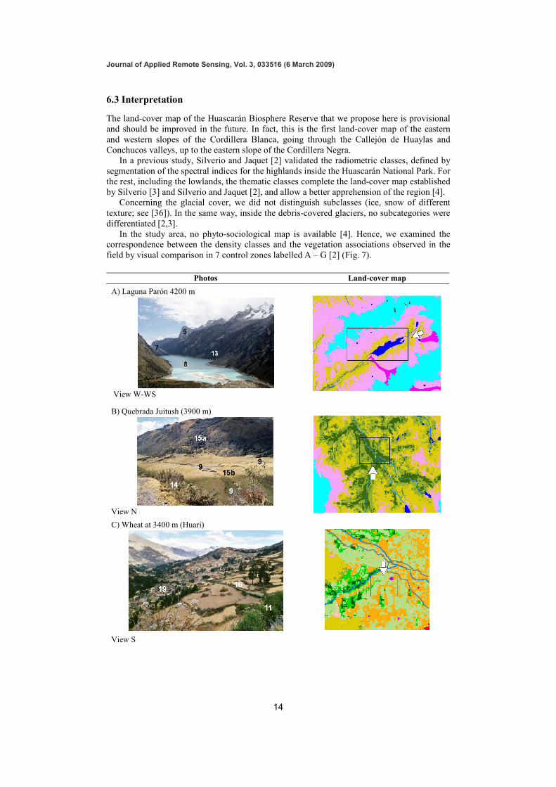
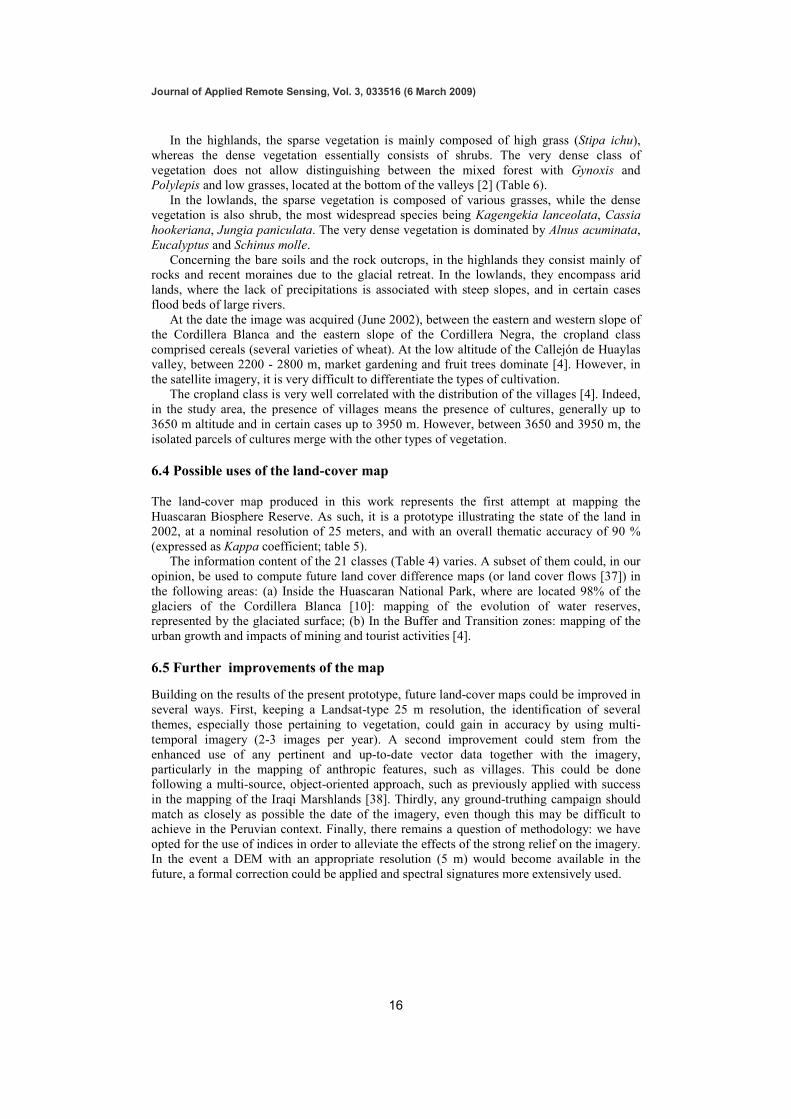
In the study area, no phyto-sociological map is available [4]. Hence, we examined the

correspondence between the density classes and the vegetation associations observed in the

field by visual comparison in 7 control zones labelled A – G [2] (Fig. 7).

Photos Land-cover map

A) Laguna Parón 4200 m

View W-WS

B) Quebrada Juitush (3900 m)

View N

C) Wheat at 3400 m (Huari)

View S


15

D) Q. Llaca: debris-covered glacier at 4600 m

View N-NE

E) City of Huaraz at 3090 m

View SW

F) Waste of mining activity, Ticapampa 3457 m

View SW

G) Andean plateau (> 4000 m) and Nevados Caullaraju

(> 5500 m)

View SE

Fig. 7. Examples of ground truthing areas for land-cover classes. Left: view from the ground,

with class numbers as per table 3. Right: extract of land-cover map. White arrows indicate

direction of photo shots. Photos I. Machguth: A and E (2003). C. Bugniet: B and C (2000).

W. Silverio: D (2001), F (2000), and G (2003).


16

In the highlands, the sparse vegetation is mainly composed of high grass (Stipa ichu),

whereas the dense vegetation essentially consists of shrubs. The very dense class of

vegetation does not allow distinguishing between the mixed forest with Gynoxis and

Polylepis and low grasses, located at the bottom of the valleys [2] (Table 6).

In the lowlands, the sparse vegetation is composed of various grasses, while the dense

vegetation is also shrub, the most widespread species being Kagengekia lanceolata, Cassia

hookeriana, Jungia paniculata. The very dense vegetation is dominated by Alnus acuminata,

Eucalyptus and Schinus molle.

Concerning the bare soils and the rock outcrops, in the highlands they consist mainly of rocks and recent moraines due to the glacial retreat. In the lowlands, they encompass arid

lands, where the lack of precipitations is associated with steep slopes, and in certain cases

flood beds of large rivers.

At the date the image was acquired (June 2002), between the eastern and western slope of

the Cordillera Blanca and the eastern slope of the Cordillera Negra, the cropland class

comprised cereals (several varieties of wheat). At the low altitude of the Callejón de Huaylas

valley, between 2200 - 2800 m, market gardening and fruit trees dominate [4]. However, in

the satellite imagery, it is very difficult to differentiate the types of cultivation.

The cropland class is very well correlated with the distribution of the villages [4]. Indeed,

in the study area, the presence of villages means the presence of cultures, generally up to

3650 m altitude and in certain cases up to 3950 m. However, between 3650 and 3950 m, the

isolated parcels of cultures merge with the other types of vegetation.

6.4 Possible uses of the land-cover map

The land-cover map produced in this work represents the first attempt at mapping the

Huascaran Biosphere Reserve. As such, it is a prototype illustrating the state of the land in

2002, at a nominal resolution of 25 meters, and with an overall thematic accuracy of 90 %

(expressed as Kappa coefficient; table 5).

The information content of the 21 classes (Table 4) varies. A subset of them could, in our

opinion, be used to compute future land cover difference maps (or land cover flows [37]) in

the following areas: (a) Inside the Huascaran National Park, where are located 98% of the

glaciers of the Cordillera Blanca [10]: mapping of the evolution of water reserves, represented by the glaciated surface; (b) In the Buffer and Transition zones: mapping of the

urban growth and impacts of mining and tourist activities [4].

6.5 Further improvements of the map

Building on the results of the present prototype, future land-cover maps could be improved in

several ways. First, keeping a Landsat-type 25 m resolution, the identification of several

themes, especially those pertaining to vegetation, could gain in accuracy by using multi-

temporal imagery (2-3 images per year). A second improvement could stem from the

enhanced use of any pertinent and up-to-date vector data together with the imagery,

particularly in the mapping of anthropic features, such as villages. This could be done

following a multi-source, object-oriented approach, such as previously applied with success

in the mapping of the Iraqi Marshlands [38]. Thirdly, any ground-truthing campaign should

match as closely as possible the date of the imagery, even though this may be difficult to

achieve in the Peruvian context. Finally, there remains a question of methodology: we have

opted for the use of indices in order to alleviate the effects of the strong relief on the imagery.

In the event a DEM with an appropriate resolution (5 m) would become available in the

future, a formal correction could be applied and spectral signatures more extensively used.


17

7 CONCLUSION

The land-cover map presented in this work is the first of the kind established for the

Huascarán Biosphere Reserve. The absence of an adequate digital elevation model did not

allow a formal correction of the strong relief effects on the satellite imagery. We thus had

recourse to the NDSI and NDVI indices within a procedure of segmentation. NDSI was used

to map the glaciated areas, whereas NDVI was combined with the DEM to define the

highlands and lowlands, as well as the various vegetation and cropland themes.

According to the first field checks, the overall map accuracy is fair (Kappa around 90%).

The cartographic representation can be regarded as good for the glaciers, the debris-covered

glaciers, rock outcrops and the lakes, and as satisfactory to poor for the various individual

vegetation classes. This land-cover map represents a basic information layer which could be

incorporated in a Geographical Information System. It would thus help establish a regional

planning policy and the elaboration of a natural risk map, which is missing in the region. It

could also be used as a basis for future diachronic comparisons, particularly in the fields of

the evolution of glacial cover and its related natural hazards, as well as mining activity and

urbanization.

Acknowledgments

We would thank to Mark A. Ernste, former collaborator of UNEP/GRID-Sioux Falls

(DEWA), USGS EROS Dated Center, SD Dakota (USA) for providing 2002 satellite images

and to Pascal Peduzzi, UNEP/GRID/DEWA (Geneva) for his help. The critical comments of

two anonymous reviewers are gratefully acknowledged.

References

[1] W. Silverio and J.-M. Jaquet, “Glacial Cover Mapping (1987 – 1996) of the Cordillera

Blanca (Peru) Using Satellite Imagery,” Remote Sensing of Environment 95, 342-350

(2005).

[2] W. Silverio and J.-M. Jaquet, “Cartographie provisoire de la couverture du sol du Parc

national Huascaran (Perou), à l’aide des images TM de Landasat,” Teledetection, 3(1),

69-83 (2003).

[3] W. Silverio, “Elaboration d’un SIG pour la gestion d’une zone protegee de haute

montagne: application au Parc national Huascaran, Perou,” Validation memoir, post

graduate certificate in Geomatics, University of Geneva (2001).

[4] W. Silverio, “A GIS for the sustainable management of the water resources in Cordillera

Blanca, Peru” (in French), PhD Thesis in Geography, University of Geneva (2007).

[5] USGS (United State Geological Survey) “Global Land Cover Characterization,” (2007).

<http://edcsns17.cr.usgs.gov/glcc/> (20 December 2007)

[6] J. Cihlar, “Land cover mapping of large areas from satellites: status and research

priorities,” International Journal of Remote Sensing 21(6-7), 1093-1114 (2000).

[7] UNESCO, “Huascaran National Park (Peru)” (2006a).

<http://www.unep-wcmc.org/protected_areas/data/sample/0024q.htm>

(20 December 2007)

[8] PNH (Huascaran National Park), Plan Maestro, Generalidades y diagnostico. PHN,

Huaraz, Peru, Internal document (1990).

[9] A. Ames, J. Alean and G. Kaser “Variations des glaciers de la Cordillera Blanca, au

Perou”. Les Alpes, 3e trimestre, 138-152 (1994).

[10] W. Silverio, Atlas del Parque Nacional Huascaran – Cordillera Blanca – Peru, W.

Silverio (ed.), Lima (2003).

[11] G. Kaser, A. Ames and M. Zamora, “Glacier fluctuations and climate in the Cordillera

Blanca, Peru”, Annals of Glaciology 14, 136-140 (1990).


18

[12] G. Kaser, C. Georges and A. Ames, “Modern glacier fluctuations in the Huascarán-

Chopicalqui massif of the Cordillera Blanca, Peru,” Zeitschrift für Gletscherkunde und

Glazialgeologie 32, 91-99 (1996).

[13] G. Kaser and H. Osmaston, Tropical Glaciers, Cambridge University Press and

UNESCO, Cambridge (2002).

[14] UNESCO, “Huascaran Biosphere Reserve (Peru)” (2006b).

<http://www2.unesco.org/mab/br/brdir/directory/biores.asp?code=PER+01&mode=all>

(20 December 2007)

[15] INRENA (Peruvian National Institute of Natural Resources), “Mapa de la Reserva de Biosfera – Parque Nacional Huascaran – Ancash – Perú,” INRENA, Lima, Internal

document (2000).

[16] INRENA (Peruvian National Institute of Natural Resources), “Parque Nacional

Huascaran, Plan Maestro 2003 – 2007,” INRENA, Lima, (2003).

[17] J.R. Dymond and J.D. Shepherd, “Correction of the Topopgraphic Effect in Remote

Sensing,” IEEE Transactions on Geoscience and Remote Sensing 37(5), 2618-2619

(1999).

[18] S. Sandmeier, A Physically-Based Radiometric Correction Model, Correction of

Atmospheric and Illumination Effects in Optical Satellite Data of Rugged Terrain,

Remote Sensing Series vol. 26, Remote Sensing Laboratories, Department of

Geography, University of Zurich (1995).

[19] ERDAS, Field Guide, 5th

ed., Erdas Inc., Atlanta, Georgia (1999). [20] S. Liang, H. Fang, J. T. Morisette, M. Chen, C. J. Shuey, C. L. Walthall, C. S. T.

Daughtry, “Atmospheric correction of Landsat ETM+ land surface imagery. II.

Validation and applications”, IEEE Trans. Geosci. Rem. Sens. 40(12), 2736 - 2746

(2002).

[21] F. Dell’Acqua, “Testing the effect of atmospheric correction on urban hyperspectral data through classifier performance comparison: a case study”. International Archives of

Photogrammetry, Remote Sensing and Spatial Information Sciences 36, part 8/W27

(2005).

<http://www.isprs.org/commission8/workshop_urban/dell'acqua.pdf>

(10 October 2008)

[22] S.H. Kim, J.I. Shin, H.R. Yoo and K.S. Lee, “Effect of atmospheric correction for the

land cover classification using hyperspectral data”. Asian Association of Remote

Sensing proceedings, P-2 (2006).

<http://www.aars-acrs.org/acrs/proceeding/ACRS2006/Papers/P-2_Q50.pdf>

(10 October 2008)

[23] J.D. Colby, “Topographic Normalization in Rugged Terrain”, Photogrametric

Engineering and Remote Sensing 57(5), 531-537 (1991). [24] F. Bonn and G. Rochon, Precis de Teledetection, volume 1: principes et methodes.

Presses de l’Université de Québec et AUPELF, Sainte-Foy, Canada (1993).

[25] D.K. Hall, G.A. Riggs and V.V. Salomonson, “Development of methods for mapping

global snow cover using Moderate Resolution Imaging Spectroradiometer (MODIS)

data,” Remote Sensing of Environment 54,127-140 (1995). [26] J. Dozier, “Spectral signature of Alpine snow cover from Landsat Thematic Mapper,”

Remote Sensing of Environment 28, 9-22 (1989).

[27] R. W. Sidjak and R. D. Wheate, “Glacier mapping of the Illecillewaet Icefield, British

Columbia, Canada, using Landsat TM and digital elevation model data,” International

Journal of Remote Sensing 20(2), 273-284 (1999).

[28] R. Caloz and C. Collet, Precis de Teledetection, volume 3: Traitements numeriques

d’images de teledetection. Presses de l’Université de Quebec et AUPELF, Sainte-Foy,

Canada (2001).

[29] W. Silverio and J.-M. Jaquet, “Modern glacier fluctuation mapping of the tropical

Cordillera Blanca, Peru, using satellite imagery (1987-2002). In review (2008).


19

[30] J.B. Adams, D.E. Sabor, V. Kapos, R. Almeida Filho, D.A. Roberts, M.O. Smith and

A.R. Gillespie, “Classification of multispectral images based on fractions of

endmembers: Application to land-cover change in the Brazilian Amazon”, Remote

Sensing of Environment 52, 137-154 (1995).

[31] INEI (Peruvian National Institute of Statistics and Informatics), “Mapa Digital de

Centros Poblados del Peru,” INEI, Lima (Distribution format Shape) (2002).

[32] J. Jenness and J. J. Wynne, “Cohen's Kappa and classification table metrics 2.0: an

ArcView 3x extension for accuracy assessment of spatially explicit models”. USGS

Series Open-File Report, Number 2005-1363 (2005). <http://www.jennessent.com/arcview/kappa_stats.htm> (09 October 2008)

[33] R.G. Congalton and K. Green, “Assessing the Accuracy of Remotely sensed data.

Principles and Practices”, Lewis Publishers, Boca Raton, Florida (1999).

[34] H. Kolff and K. Kolff., Wildflowers of the Cordillera Blanca. The Mountain Institute

(ed.), Lima (1997).

[35] D.K. Hall, K. Bayr, R.A. Bindschadler and W. Schöner, “Changes in the Pasterze

Glacier, Austria, as Measured from the Ground and Space,” 58th

Eastern Snow

Conference, Ottawa, Ontario, Canada (2001).

<http://www.easternsnow.org/proceedings/2001/Hall_1.pdf > (20 December 2007)

[36] D.K. Hall, A.T.C. Chang and H. Siddalingaiah, “Reflectances of Glaciers as Calculated

Using Landsat-5 Thematic Mapper Data,” Remote Sensing of Environment 25, 311-321

(1988). [37] O. Gomez and F. Páramo, “Environmental Accounting. Methodological guidebook:

Data processing of land cover flows”. LEAC project, European Environment Agency.

< http://www.eea.europa.eu/themes/landuse/land-and-ecosystem-accounting-leac >

(30 October 2008)

[38] J.-M. Jaquet, K. Allenbach, S. Schwarzer, O. Norbeck. and H. Partow, “ Iraqi Marshlands Observation System“, UNEP Technical Report. UNEP PCoB and DEWA

/GRID-Europe, 71 p. (2006).

< http://imos.grid.unep.ch/uploads/imos_techn_report.pdf > (06 November 2008)

Article Reference Prototype land-cover mapping of the Huascaran Biosphere Reserve (Peru) using DEM,...

Documents

Transcript of Article Reference Prototype land-cover mapping of the Huascaran Biosphere Reserve (Peru) using DEM,...