ARE TRAINING PROGRAMS MORE EFFECTIVE WHEN

UNEMPLOYMENT IS HIGH?

Michael Lechner and Conny Wunsch

Swiss Institute for Empirical Economic Research (SEW)

First version: August, 2006

This version: August, 2009

Date this version has been printed: 24 August 2009

Abstract (and nontechnical summary)

We estimate short-run, medium-run, and long-run individual labor market effects of

training programs for the unemployed by following program participation on a monthly basis

over a ten-year period. Since analyzing the effectiveness of training over such a long period

is impossible with experimental data, we use an administrative database compiled for

evaluating German training programs. Based on matching estimation adapted to address the

various issues that arise in this particular context, we find a clear positive relation between

the effectiveness of the programs and the unemployment rate over time.

Addresses for correspondence

Michael Lechner, Conny Wunsch

Swiss Institute for Empirical Economic Research (SEW), University of St. Gallen

Varnbüelstr. 14, CH-9000 St. Gallen, Switzerland

Michael.Lechner@unisg.ch, Conny.Wunsch@unisg.ch, www.sew.unisg.ch/lechner

published in Journal of Labor Economics, 27, 653-692, 2009

Lechner and Wunsch, 2009 1

1 Introduction1

Although the body of knowledge about the effectiveness of training programs for the

unemployed is rapidly growing, there is not much convincing evidence on the relationship

between the effectiveness of the programs and the state of the economy. Such information is,

however, important. If, for example, changes in the effectiveness of the policy or its different

instruments are related to the business cycle at the time when decisions have to be made, then

policymakers can react by adjusting the policy accordingly. Thus, the policymaker should be

interested in knowing under which macroeconomic circumstances the programs are more or

less beneficial. It is the goal of this paper to provide systematic insights on this issue.

The empirical literature on the effects of active labor market policies (ALMPs) suggests

that almost all programs reduce (unsubsidized) employment and earnings in the short-run.

This so-called lock-in effect is well documented in many studies and typically attributed to

reduced search intensity of program participants or fewer job offers by caseworkers while

participating in the program (e.g. van Ours, 2004). This lock-in effect is one of the (indirect)

cost components of ALMPs. If it varies with labor market conditions, this would be an im-

portant argument for varying the composition of programs and program size over time. Our

results show that this is indeed the case.

1 The first author has further affiliations with ZEW, Mannheim, CEPR and PSI, London, IZA, Bonn and IAB, Nuremberg.

Financial support from the Institut für Arbeitsmarkt- und Berufsforschung (IAB), Nuremberg, (project 6-531a) is

gratefully acknowledged. The data originated from a joint effort with Annette Bergemann, Bernd Fitzenberger, Ruth

Miquel, and Stefan Speckesser to make the administrative data accessible for research. The paper has been presented at

workshops at the University of St. Gallen, 2006, at the IRP Summer Research conference in Madison, 2006, the 3rd

Conference on evaluation of labour market programs at the ZEW, Mannheim, 2006, at the COST A23 meeting in Essen,

2007, at the IAB, Nuremberg, 2007, at the Annual Meeting of the Swiss Society of Economics and Statistics in St. Gallen,

2007, at the University of Rome Tor Vergata, 2007, Annual Meeting of the German Economic association in Munich,

2007, as well as the Annual Meeting of the Society of Labor Economists in Chicago, 2007. We thank participants, in

particular John Ham, for helpful comments and suggestions. Additional background material for this paper is available in

an internet appendix on our website www.siaw.unisg.ch/lechner/lw_cycles.

Lechner and Wunsch, 2009 2

With respect to the medium-run to long-run effects, some wage subsidies and training pro-

grams increase employment and earnings (e.g., Couch, 1992; Hotz, Imbens, and Klerman,

2006, Winter-Ebmer, 2006, Jacobson, LaLonde, and Sullivan, 2005, Jespersen, Munch, and

Skipper, 2008, Fitzenberger and Speckesser, 2007, Lechner, Miquel, and Wunsch, 2009).

Most of this particular literature, which is more optimistic about the effectiveness of ALMPs

than most of the older experimental literature, is based on large administrative data sources

with long follow-up periods. Understanding the differences between short-run lock-in effects

and medium-run to long-run effects that may capture more accurately the effects of the human

capital added by the programs was an important step towards understanding how these pro-

grams work.2 In fact, this difference will turn out to be crucial for the interpretation of our

findings in this paper as well. However, none of these studies systematically investigates if

and eventually why the effects of different types of programs change over time.3

The most closely related literature is Raaum, Torp, and Zhang (2002). They analyze how

the effects of labor market training in Norway are related to post-training job opportunities.

They exploit the fact that labor market conditions are different at different points in time after

training was completed. They find a positive correlation. This is in line with the findings of

the related literature on the effect of the state of the economy at labor market entry on the la-

bor market performance of different cohorts (see in particular Raaum and Roed, 2006). How-

ever, these studies focus on labor market conditions after labor market training or secondary

2 The recent increase in evaluation studies is documented for example by the surveys of Heckman, LaLonde,

and Smith (1999), Martin and Grubb (2001), Kluve and Schmidt (2002), and Kluve (2006). For examples of

studies based on a selection on observables strategy, see Gerfin and Lechner (2002), van Ours (2004), or

Sianesi (2004). A recent example of papers using instrumental variable types of assumptions is Frölich and

Lechner (2006). The experimental literature is well documented in the survey by Heckman, LaLonde, and

Smith (1999). Boone and van Ours (2004) provide and survey empirical evidence based on aggregated time

series data.

3 Roed and Raaum (2003, 2006) and Richardson and Van den Berg (2006) include the relevant individual local

or occupational unemployment rate as a determinant in a parametric specification of the training effect on the

transition rate from unemployment to employment.

Lechner and Wunsch, 2009 3

education, which are unobserved at the time when decisions about training assignment or in-

vestment in education have to be made. Thus, the results have little relevance from a policy

perspective. Moreover, they do not take into account time variation in the composition of the

participating cohorts, which can induce a spurious correlation that must be separated from the

time variation in the effectiveness of the programs. Our study takes care of both issues.

There is also some evidence based on analyzing regional data over time. For example, Jo-

hansson (2001) uses variation in Swedish active labor market programs over municipalities.

She shows that the effect of these programs is to prevent the unemployed from leaving the

labor force during a downturn. She concludes that ALMPs are most effective during a down-

turn.4

An alternative to macro studies that come with the usual caveats of aggregation bias and

policy endogeneity is to exploit the fact that different micro studies are conducted under

different economic conditions. Meta-analyses are based on this idea. For example, Kluve

(2006) combines more than 100 studies, and each study (or specification within a study)

constitutes one data point. In a regression type approach he controls for different aspects of

the methods and data used, features of the program, as well as the economic environment.

Although the analysis of the latter is not the main thrust of his study, he finds the program

effects to be somewhat larger when unemployment rates are higher. Thus, his results seem to

be roughly in line with Johansson (2001). Although meta-analyses provide interesting

summaries of the literature, there are problems as well. The different individual studies that

are treated as the data of the meta-analyses are based on heterogeneous programs that are run

in different institutional environments and economic conditions, and with different types of

participants. It is obviously very challenging to control for all these background factors within

4 This pattern of the programs leading to a redirection of the flows from unemployment to out-of-labor-force

towards unemployment and then towards employment appears in the cross-sectional study by Lechner,

Miquel, and Wunsch (2009), as well.

Lechner and Wunsch, 2009 4

a regression framework using only a few control variables and tight functional forms dictated

by the limited degrees of freedom available.

In this paper, we retain the advantage of the classical microeconometric evaluation studies,

like nonparametric identification and heterogeneity of the program effects, but adjust the

standard methodology to learn important lessons about the evolution of the effects over time.

Since there are no experiments running for a sufficiently long period to be interesting for such

an investigation, any such endeavor has to rely on observational data. Survey data, however,

are typically problematic because of insufficient sample sizes, insufficient covariate and pro-

gram information, short time windows to observe outcomes, misreporting, and attrition.

Newly available high-quality administrative data can overcome these problems. Europe,

where experiments are rare because of strong political resistance, has gained a comparative

advantage in providing large and informative administrative databases that allow much richer

analyses than experimental data which are usually used in the U.S.5

We exploit a particularly informative administrative micro data set for Germany that

became available only recently. These data contain reliable information on participants (and

non-participants) in different types of training programs on a monthly basis from 1986 to

1995. Information on labor market outcomes is available monthly from 1980 to 2003. Thus,

the data allow us to investigate whether changes in labor market conditions influence the

lock-in effects in a different way than the medium-run or long-run effects.

5 There are only few observational studies using U.S. data. None of the databases used are sufficiently

informative in terms of covariates and the time horizon covered to study time variation of the effects of

ALMP in sufficient detail (see in particular the survey by Heckman, LaLonde, and Smith, 1999, as well as

Jacobson, LaLonde, and Sullivan, 2004, and Mueser, Troske, and Gorislavsky, 2007, for example). However,

the study by Herbst (2008) investigates the dependence of the effects of welfare policies on the economic

cycle using the US March Population Surveys over 20 years. He finds that social policies are more effective

under good economic conditions. Although, that paper is similar in spirit to our analysis, it is based on less

informative data and less robust, parametric estimation methods.

Lechner and Wunsch, 2009 5

These data have been used recently in classical evaluation studies by Fitzenberger and

Speckesser (2007), and Lechner, Miquel, and Wunsch (2009), among others. These studies

argue that the data are informative enough to control for selective participation and thus allow

identification of program effects by matching methods. Based on this identification strategy,

we analyze the effects of training programs on short-run to long-run labor market outcomes

for unemployed workers entering programs over 10 years on a monthly basis. Another

advantage of using Germany for analyzing potential time variation in the effects of training is

that no major changes occurred within the broad types of training programs considered in this

paper, or in the institutional setup.

Our empirical strategy relies on different matching estimators. We begin by analyzing the

evolution of the effects over time. Thus, in this specification the characteristics of participants

and the use of different program types may vary over time. Any time pattern of the effects

that we might isolate from this step may thus be due to changes in the composition of pro-

grams, of participants, and/or of economic conditions. Next, by modifying the matching esti-

mator, we keep the characteristics of the program participants constant over time. Thus, the

remaining dynamics in the effects reflect changes in program composition and economic con-

ditions only. Then, additionally keeping the shares of the various subprograms and planned

program durations constant allows us to isolate the effects of the economic environment.

Finally, to improve our confidence in a causal interpretation of the strikingly clear pattern we

obtain, the results are subjected to an intensive sensitivity analysis.

In line with the recent literature mentioned above, we consistently find negative lock-in ef-

fects as well as positive medium-run to long-run employment and earnings effects of the

training programs in the 10-year period we consider. However, we detect considerable varia-

tion of those effects over time, even for the case of a fixed population of participants and a

fixed composition of the programs. This variation is clearly related to the unemployment rate

Lechner and Wunsch, 2009 6

prevailing at the start of the program: The negative lock-in effects are smaller and the positive

long-run effects are larger in times of higher unemployment. As argued above, this has im-

portant implications from a policy perceptive as policymakers can exploit this.

The remainder of the paper is organized as follows: Section 2 provides background

information on the economic conditions, the unemployment insurance system, and the use of

active labor market policies in West Germany in the relevant period. In Section 3, the data

and the sample are outlined. Section 4 details the econometric identification and estimation

strategy. In Section 5, we discuss in detail the effects of training over time. In the following

section, we analyze how the changing characteristics of participants or the changing

composition of programs over time may have influenced the effectiveness of training. Section

7 describes the results of our extensive sensitivity analyses. The last section concludes. An

appendix contains further details on the data, on the definition of our sample and the outcome

variables, as well as on the estimation procedure. A second appendix, available in the internet,

contains detailed background material.

2 Economic conditions and institutions in West Germany

2.1 The West German economy between 1984 and 2003

During the economic slowdown following the second oil-price shock, unemployment in

West Germany had risen to a quite persistent 9% in the mid-1980s.6 Economic activity kept

declining until 1988 when a slow recovery started. Directly after unification in 1990, West

Germany experienced a boom with substantial East German spending diverted away from

domestic products to previously unavailable West German goods. Accordingly, production

and labor demand increased in West Germany. GDP grew 5.7% in 1990 and 5% in 1991.

Registered unemployment declined to a rate of 6.3% in 1991 despite a significant growth of

6 All numbers presented in this section are taken from official statistics published by the Federal Employment

Agency, the Institute for Employment Research, and the Federal Statistical Office 1984-2004.

Lechner and Wunsch, 2009 7

the labor force due to migration from East Germany and Eastern Europe. At the same time,

the world economy was experiencing a recession. In 1992, this recession hit West Germany as

well. Economic growth slowed down to 1.7%. One year later, the West German economy was

deep in recession. GDP declined by 2.6% in 1993 and unemployment rose to 8%. With the

recovery of the world economy in the late 1990s, the situation began to improve. GDP growth

increased from 0.6% in 1996 to more than 3% in 2000. However, economic growth

decelerated following the slowdown of the world economy after September 11, 2001, and

registered unemployment returned to a level of more than 9% in 2003.

During the period 1984-2003, economic activity shifted especially from the primary and

secondary sectors to the service sector. The structure of unemployment changed as well. The

fraction of unemployed without any occupational qualification declined constantly from al-

most 50% in 1984 to 41% in 2003. The share of foreigners increased over time by about 4%

to 17% in 2003 with a temporary dip during the post-unification boom. Long-term unem-

ployment (one year or longer) has largely moved with total unemployment varying between

26% and 38% in the period 1984-2003.

As shown by Figure 1, expenditures on ALMPs, in particular on training, varied considera-

bly over the years. However, they are only mildly correlated with GDP growth and unemploy-

ment (note the different scaling used for ALMP expenditures), because political considera-

tions (e.g. upcoming elections in 1986, 1990, and 1998) and changes in the mix of ALMP

instruments (1997, 2003) had strong impacts on ALMP expenditure. The fraction of it spent

on training almost continuously increased from 33% in 1984 to almost 45% in 1998. It

dropped slightly afterwards. In 2003, there was a large decline to 30% resulting from a regime

change in the use of training from longer, more intense programs to short courses with less

substantial adjustment of skills. The changes that occurred after 1995 are of limited interest to

our empirical study, because we analyze programs that start between 1986 and 1995, only.

Lechner and Wunsch, 2009 8

- Figure 1 about here -

2.2 Unemployment insurance in Germany 1986 to 1995

In Germany, unemployment insurance (UI) is compulsory for all employees with more

than minor employment (i.e. earning more than about 315 € per month) as well as apprentices

in vocational training.7 German UI does not cover the self-employed. Persons who have

contributed to the UI for at least 12 months within the three years preceding an unemployment

spell are eligible for unemployment benefits (UB). The minimum UB entitlement is six

months. The maximum claim increases stepwise with the total duration of the contributions in

the seven years before becoming unemployed, and age, up to a maximum of 32 months at age

54 or above (requiring previous contributions of at least 64 months). Participation in govern-

ment-sponsored training counts towards the contribution period for both the acquisition and

the duration of UB claims. Actual payment of UB for eligible unemployed is conditional on

active job search, regular appearances at the public employment service (PES), and participa-

tion in ALMP measures. Since 1994, the replacement rate is 67% of previous average net

earnings from insured employment with dependent children, and 60% without. Before, re-

placement rates were 68% and 63%, respectively.

Until 2005, unemployed workers became eligible for unemployment assistance (UA) after

exhaustion of UB. In contrast to UB, UA was means tested and potentially indefinite. How-

ever, like UB, UA was proportional to previous earnings but with lower replacement rates

than UB.8

7 However, civil servants (Beamte), judges, professional soldiers, clergymen and some other groups of persons

are exempted from contributions. For further details on the German UI and ALMP, see the comprehensive

survey by Wunsch (2005).

8 Before 1994, UA replacement rates were 58% (with children) and 56% (no children). Thereafter, they

decreased to 57% and 53%.

Lechner and Wunsch, 2009 9

Unemployed workers who were ineligible for UB and UA could receive social assistance,

which was a fixed monthly payment unrelated to previous earnings, means tested and admin-

istered by local authorities.

For the following empirical analysis, it is important to note that except for the change in

the UB/UA replacement rate, UI institutions were stable in the period 1986-1995.

2.3 German ALMP 1986 to 1995

ALMP has a long tradition in Germany. Among OECD countries, Germany's expenditure

on ALMP is one of the highest (OECD, 2004). With increasing unemployment in the 1980s,

the main objective of German ALMP shifted from keeping employment high and fostering

economic growth towards reducing unemployment by increasing the employability of

jobseekers. The main instruments traditionally used in German ALMP are counseling and job

placement services, labor market training, subsidized employment, and support of self-

employment.

Training has always been the most important program group in West Germany. It consists

of heterogeneous instruments that differ in the form and intensity of the human capital invest-

ment as well as in their respective duration. Durations range from a few weeks to three years.

Traditionally, German training courses have the aim of assessing, maintaining, or improving

the occupational knowledge and skills of the participant, of adjusting skills to technological

changes, of facilitating a career improvement, or even of awarding a first occupational quali-

fication. So-called 'career improvement measures', for which the employed may also be eligi-

ble, had played a major role before unemployment rose in the 1980s. Since then they have

become negligible as the focus shifted towards removal of the skill deficits and skill mismatch

of the unemployed.

In the period under consideration, there are five types of training. Basic job-search

assistance (JSA) existed only until 1992. So-called practice firms (PF) simulate - under

Lechner and Wunsch, 2009 10

realistic conditions - working in a specific occupation. Short training (ST) with a planned

duration of up to six months, and long training (LT) with a planned duration of more than six

months provide a general update or adjustment of skills. Retraining (RT) leads to an

occupational qualification equivalent to a qualification obtained in the German apprenticeship

system. JSA and PF have always been relatively small programs. ST and LT were by far the

most important programs with LT gaining importance relative to ST. LT more than doubled

its share in the period we consider. RT was relatively small as well, but became more

important from the early 1990s on. However, given its long durations it is the most expensive

program so its share in expenditure is substantially larger than its share among participants.

Overall, the average direct costs of training varied between 2,000 and 4,000 EUR per

participant in the period 1986-1995, with an average of about 3,000 EUR per participant.

Thus, costs are quite large which mainly results from the relatively long durations of many

German programs.

Access to training courses is largely limited to unemployed workers who are eligible for

UB or UA. To underline the character of further job related training rather than primary

occupational training, eligibility also required holding a first occupational qualification

(before 1994, in addition 3 years of work experience) or at least three years of work

experience (before 1994, six years). Usually, participants receive a transfer payment, which is

called the maintenance allowance (MA). Since 1994, MA is of the same amount as UB.

Before, MA had been somewhat higher than UB with a replacement rate of 73% with

dependent children and 65% without. Moreover, the PES bears the direct cost of the program,

and it may cover parts of additional expenses for childcare, transportation, and

accommodation.

Note that with respect to eligibility and MA, replacement rates and training regulations

have been relatively stable. Moreover, our data allow us to control for the few changes that

Lechner and Wunsch, 2009 11

actually occurred, especially with respect to the shifting emphasis on specific types of

programs.

3 Data and sample definition

We use the same administrative data sources as Lechner, Miquel, and Wunsch (2009)

which combine information from social insurance records on employment, data on benefit

receipt during unemployment, and information on participation in training programs. The

original data covers the period 1980-1997, but employment and unemployment records up to

2003 have been added to allow the construction of long-run outcome variables. The database

is unique in several respects. In particular, it is much more informative than observational

data that was previously available (e.g., see Jacobson, LaLonde, and Sullivan, 2005, for the

US). It is the first micro database that allows the analysis of program participation over a

sufficiently long period (10 years) on a monthly basis to capture business cycle movements.

Moreover, it allows the construction of up to 24 years of individual employment histories on a

monthly basis. In total, we have available between 6 and 15 years of pre-program history, as

well as at least 8 years of post-program-start observations for the outcome variables. Detailed

personal, regional, employer and earnings information of good quality allow us to control for

all of the main factors that determine selection into programs (see the discussion in the next

section) and to analyze precisely measured outcome variables of interest (in particular

employment status and earnings). Table 1 provides the relevant details on the administrative

data sources used.

For our analysis, we use a sample of participants in training and eligible non-participants.

We focus on the prime-age part (age 20-55) of the West German labor force covered by social

insurance.9 All of the unemployed who start a program in a particular month in the period

9 In particular, we only use persons who are observed at least once in employment subject to social insurance

before a (potential) program start. We exclude persons who were last employed as home workers, apprentices,

Lechner and Wunsch, 2009 12

1986-1995 (in total 120 months) are considered participants. In contrast, non-participants are

all unemployed workers who do not start a program but receive UB/UA in that month.10 To

ensure that we do not use unemployed workers who completed a program shortly before the

(potential) program start (and so are still in an earlier unemployment-participation-unemploy-

ment spell), we require that nobody participated in a program in the four years before the

(potential) program start we consider. Moreover, to make sure that all persons we consider are

eligible for participation, we require that they received UB/UA in the month before the (po-

tential) program start.

- Table 1 about here -

Defining non-participants as those persons who do not start a program in a particular

month is similar to the approach of Sianesi (2004) as the control group of 'non-participants'

includes some future participants. An important difference, however, is that we do not stratify

the sample by elapsed unemployment duration up to that month (but do match on this

information), and that for non-participants we require that they did not participate in the 11

months following potential program start. The reason is that in contrast to Sianesi (2004) our

parameter of interest is not the effect of starting a program at different points in the unem-

ployment spell, but the effect of training relative to a well-defined and relatively stable non-

treated comparison group, at different points in the business cycle. If we would choose the

Sianesi (2004) approach, the comparison group would change immediately after the starting

month considered depending on the fraction of non-participants who start a program in the

next month(s), and a very different policy parameter would be estimated. Furthermore, the

composition of such a control group would be affected directly by the business cycle as the

probability of receiving a program in the next month clearly varies with the business cycle.

trainees, or part-time workers below half of the full-time equivalent, because we want to focus on the most

common forms of regular employment.

10 Note that as long as they fulfil all sample selection criteria individuals can be participants in one and non-

participants in another month.

Lechner and Wunsch, 2009 13

The price to pay for our approach is the possibility of some bias because we potentially con-

dition on future outcomes (see Fredriksson and Johansson, 2003, 2008).

To obtain a sufficient number of participants we pool participants and non-participants

over a six-month window in the estimation. The effect of starting a program in month t is esti-

mated using all persons who start or do not start a program in one of the months t to t+5.

Thus, we estimate effects for 115=120-5 different program starts in the period 1986-1995.

Since all the choices mentioned in this subsection may affect our estimation results, we per-

form an extensive sensitivity analysis, which is detailed in Section 7.

4. Econometrics

4.1 Effects of interest and identification

We are interested in the mean effects of participating in training in period t ( t ) for some

population of participants ( tP ). Varying the latter in an interesting way will be one of the key

issues in the following empirical sections. Based on the usual notation of the evaluation lit-

erature, we denote by 1

tY the potential outcome of participation in a program, by 0

tY the

potential outcome of not participating in a program, and by tY the observed outcome. Thus,

the mean of the effect of the policy for a member of the population of interest, tP , is given by

( )t tP = 1( | )t tE Y P - 0( | )t tE Y P . tP may or may not change over time.

Since participation and non-participation are not observable for the same individual, the

issue of the identification of the effects arises. Below we argue that given the institutional set-

up, the newly created data are informative enough such that a selection on observed variables

strategy (the conditional independence assumption, CIA) identifies the effects conditional on

treatment status and covariates. In particular, we obtain expressions for the mean potential

Lechner and Wunsch, 2009 14

outcomes conditional on covariates that are functions of participation status, observed

outcomes (Yt), and covariates only:

1( | 0, )t t t tE Y D X x ( | 1, )t t t tE Y D X x ; 0( | 1, )t t t tE Y D X x ( | 0, )t t t tE Y D X x .

This equation must hold for all values of tx that are of interest, i.e. those that affect both

selection into the population of interest and the outcome. Given identification, under the usual

assumptions a matching strategy identifies our parameters of interest, because

( )t tP = |( | 1, ) ( )t tt t t X PE Y D X x f x dx - |( | 0, ) ( )

t tt t t X PE Y D X x f x dx .

| ( )t tX Pf x denotes the distribution of tX in the population Pt. In the next section, we call

| ( )t tX Pf x the target population towards which the distributions of tX for participants and non-

participants are adjusted. An example of such a target population would be the participants in

period t. In this case, we would estimate the classical average treatment effect on the treated

(ATET).

For the identification strategy to be plausible, it is also important that in addition to the

CIA the so-called stable unit value treatment assumption holds (SUTVA, Rubin, 1979). This

assumption rules out so-called feedback or general equilibrium effects.11 Such effects are par-

ticularly likely either when the program under consideration is sufficiently large to alter labor

demand and supply relations, or when the intervention is likely to exhibit substantial dis-

placement effects, as is argued for many public employment and wage subsidy schemes.12

Here, we are concerned with training programs only. Although they are a very costly part of

11 For the relevant literature discussing and 'solving' general equilibrium problems for the evaluation of public

programs, see Calmfors (1994), Heckman, Lochner, and Taber (1998), Coady and Harris (2004), Lise, Seitz,

and Smith (2009), and the references given in those papers. Since we measure outcomes at different points in

time, SUTVA has to hold for the full time-path of the potential outcomes.

12 However, the literature suggests that the displacement effects of such programs are rather small; see e.g.

Davidson and Woodbury (1993), Blundell et al. (2004).

Lechner and Wunsch, 2009 15

the German active labor market policy, in West Germany they appear not to be large enough

to seriously alter demand and supply relations in relevant skill segments of the labor market.

4.2 Is the matching assumption plausible with our data?

In Germany, selection into programs is determined by three main factors: eligibility,

selection by caseworkers and self-selection by potential participants. Eligibility is ensured by

the construction of our sample (see Section 3). Caseworkers select participants based on

individual employment prospects and corresponding skill deficits, chances for successful

completion of a program and conditions in the local labor market. Variables capturing

information about employment prospects and chances for successful completion of a program

comprise age, educational attainment, marital status, presence of children and past

performance in the labor market including information about firm size, earnings, position in

job, specific occupation, and industry. Moreover, our data contain detailed regional

information that allows us to control for local labor market conditions. In Internet Appendix

IF we present various statistics which show that regional variation in economic and labor

market conditions is quite large in West Germany. Moreover, there is a statistically significant

correlation between the industry structure of a region and the regional unemployment rate

(Table IF.1). Thus, it is important to control for these factors.

When constructing regional control variables we have to make sure that we do not

(implicitly) condition on the development of the national labor market over time, because this

would take out some of the effect we want to measure. We avoid dependence of the regional

control variables on the national trend of interest by using deviations from the national mean

at the time of measurement instead of the actual values of the respective regional indicators.

The implicit assumption underlying this approach is that the deviations are unaffected by the

overall time trend. Table IF.2 in Internet Appendix IF shows for the regional unemployment

rates that the dispersion of the deviations increases somewhat with the national

Lechner and Wunsch, 2009 16

unemployment rate. Therefore, to further reduce the impact of the overall time trend we also

include region dummies which are time independent by construction.

From the point of view of the unemployed, his decision whether or not to participate in a

program is guided by considerations very similar to those of the caseworker. In addition,

legislation provides rather strong incentives for individuals to participate. On the one hand,

persons who refuse to participate, risk suspension of their benefits. On the other hand, periods

during which individuals receive transfer payments while participating in a training program

count towards acquisition of unemployment benefit claims. Therefore, we constructed

variables from the (un-)employment histories that indicate the UB claim at the beginning and

at the end of a spell.

Although this is much more information than usually available in studies that rely on the

CIA (e.g. Heckman and Smith, 1999, Brodaty, Crépon, and Fougère, 2001, Larsson, 2003,

Dorsett, 2005), there are some potentially important factors missing. In contrast to Gerfin and

Lechner (2002) or Sianesi (2004), there is no information about the caseworker's direct

assessment of the characteristics and prospects of the unemployed, for example with respect

to motivation and ability. Moreover, we do not observe crime and health histories. For these

variables, we rely on their indirect effects, i.e. on their effects on the employment and

earnings history that materialized in the past. This is a reasonable approach given that our data

allow us to reconstruct between 6 and 15 years of individual pre-program employment

histories on a monthly basis including information on the stability and quality of employment.

To conclude, our data allow us to control - either directly or indirectly - for all of the main

factors that determine selection into Germany's active labor market programs. In fact, since in

most cases considered below we interpret only the changes in the effects over time, any vio-

Lechner and Wunsch, 2009 17

lation of the conditional independence assumption that leads to a bias that does not change

over time would not change the main conclusions in this paper. 13

4.3 Estimation

Having established identification of the effects, the question of the appropriate estimator

arises. All possible parametric, semi- and nonparametric estimators are (implicitly or explic-

itly) built on the principle that for every comparison of two programs and for every participant

in one of those programs we need a comparison observation from the other program with the

same characteristics regarding all factors that jointly influence selection and outcomes.14 Here,

we use propensity score matching estimators to produce such comparisons. An advantage of

these estimators is that they are semi-parametric and that they allow arbitrary individual effect

heterogeneity (see Heckman, LaLonde, and Smith, 1999; Imbens, 2004, provides an excellent

survey of the recent advances in this field).

We use a matching procedure that incorporates the improvements suggested by Lechner,

Miquel, and Wunsch (2009). These improvements aim at two issues: (i) To allow for higher

precision when many 'good' comparison observations are available, they incorporate the idea

of caliper or radius matching (e.g. Dehejia and Wahba, 2002) into the standard (nearest-neigh-

bor) algorithm. (ii) Furthermore, matching quality is increased by exploiting the fact that ap-

propriately weighted regressions that use the sampling weights from matching have the so-

called double robustness property. This property implies that the estimator remains consistent

if either the matching step is based on a correctly specified selection model, or the regression

model is correctly specified (see in particular Scharfstein, Rotnitzky and Robins, 1999, Rob-

ins, 2000, Bang and Robins (2005) as well as Rubin, 1979, and Joffe, Ten, Have, Feldman,

and Kimmel, 2004). Moreover, this procedure should reduce the small sample bias as well as

13 See also Lechner, Miquel, and Wunsch (2009) and Fitzenberger and Speckesser (2007), who justify a

selection-on-observables strategy based on the same data as well.

14 Of course, parametric models may construct such a group artificially outside the support of the data.

Lechner and Wunsch, 2009 18

the asymptotic bias of matching estimators (see Abadie and Imbens, 2006, 2008) and thus

increase the robustness of the estimator. The actual matching protocol is shown in Table B.1

in the appendix, which also contains the technical information about the estimator.

We use the fixed-weight standard error estimator proposed by Lechner, Miquel, and

Wunsch (2009). It is the same as the one suggested by Lechner (2001) and applied in Gerfin

and Lechner (2002) except that heteroscedasticity is allowed for. See the Internet Appendix

IE for the motivation and all the details for this variance estimator, which shows some

resemblance to the estimator suggested by Abadie and Imbens (2009).

5 The program effects over time

According to German legislation, the most important objectives of ALMPs are to increase

reemployment chances and to reduce the probability to remain unemployed. Therefore, we

use outcome variables related to the employment status, in particular registered unemploy-

ment, and employment subject to social insurance.15 We also consider gross earnings as a

crude measure for individual productivity. All effects are measured from the month of the

(potential) program start. Focusing on the beginning instead of the end of the programs ac-

counts for the potential endogeneity of actual program durations and allows the detection of

potential negative lock-in effects of the programs. We consider a program most successful if

everybody would leave for employment immediately after starting participation. Whenever a

person participates in a program, he is considered as registered unemployed (and not em-

ployed).

We estimate the effects for different times after the start of the program for a better under-

standing of their dynamics. We expect the programs to begin with a negative lock-in effect

before the effect reaches its long-run level. The lock-in effect is approximated by the effect

after 6 months. The long-run effect is approximated by the effect after 8 years. We also esti-

15 'Registered unemployment' is defined as receipt of UB or UA or participation in training.

Lechner and Wunsch, 2009 19

mate the effects 3 and 6 years after program start, but the effects appear not to change too

much after 3 years.16

We also consider the cumulated outcomes of training from its beginning to the respective

point of measurement, i.e. we add the monthly outcomes up to this point. This provides

something like a net effect that trades off negative lock-in effects against potential positive

long-run effects, which gives a summary of the overall effect. Due to a lack of reliable cost

information, an exact cost-benefit analysis is not possible with the available data.

Figure 2 shows the short-run and long-run effects of training for each starting month in the

period January 1986 to July 1995. We find that after 6 months, programs increase the unem-

ployment probability by about 25 percentage-points for participants, and, correspondingly,

reduce the employment probability by about 15 percentage-points. In the long run, employ-

ment is increased by about 10 percentage-points, but any effect on unemployment is hard to

spot (if there is any, then unemployment is increased). Thus, the program effect operates by

increasing employment at the expense of the share of individuals leaving the labor force ra-

ther than reducing registered unemployment.17 Considering the effects on earnings (non-

employment is counted as zero), we find similar effects with an average long-run monthly

earnings gain of about 100 EUR. Although all effects show considerable variation over time,

it is hard to spot any relation with the unemployment rate, which is shown in Figure 2 as well

(for clarity, it is presented net of its mean over the 115 months presented in the table).

- Figure 2 about here -

16 Choosing one particular month only may be a noisy measurement of these effects. Therefore, we calculate the

short-run effects as the mean of months 5-7, the medium-run effects as the mean of months 33-39, the long-

run effects after six years as the mean of months 61-72 and the long-run effects after eight years as the mean

of months 85-96.

17 These findings are largely consistent with the studies analyzing the effects of post-1992 training programs

with these data (i.e. Fitzenberger and Speckesser, 2007, Fitzenberger, Osikominu and Völter, 2006, and

Lechner, Miquel, Wunsch, 2005; note the different definitions of participation and non-participation in these

studies).

Lechner and Wunsch, 2009 20

Figure 3 shows the estimates for the mean of the potential outcome variable employment

that underlies the corresponding effect estimates in Figure 2. The short-run outcomes show a

clear seasonal effect (at least for the first 8 years), whereas, not surprisingly, such a relation-

ship does not appear for the long-run effects.

- Figure 3 about here -

Finally, Figure 4 shows the cumulated effects in months of (un-)employment over time.

They imply that the total negative effect in the first 6 months after program start corresponds

to a reduction of about 1.5 months of employment as well as an additional month of unem-

ployment. In the long run, there appears to be a gain of about 4 to 6 months of employment

and an additional 4 to 6 months of unemployment (!), which again suggests that the programs

reduce the share of people leaving the labor force drastically.18 Comparing the cumulated

effects with a particular point-in-time estimate after treatment, we find very similar shapes of

the effects over time, although obviously the magnitudes and sampling uncertainty differs.

- Figure 4 about here -

The next step is to condense the dynamic information about the effects and examine their

correlation with indicators for the state of the economy more thoroughly. In Table 2 we

display the correlation of the effects presented, including earnings, as well as the effects

measured 3 and 6 years after program start, with the quarterly GDP growth rate, the monthly

national unemployment rate, and the monthly number of participants in training programs.

These correlations are obtained from a regression of the respective estimated impact on a

constant term and the macroeconomic variable of interest.19 The internet appendix presents

18 This seems to be mainly an eligibility effect (program participation extends UB eligibility) rather than an

effect for groups with lower labor market participation rates (we find, for example, no significant gender

differences).

19 The significance levels of the correlations are obtained from a bivariate regression of the effects on a constant

and the respective macroeconomic indicator using the Newey-West procedure to correct for the correlation of

Lechner and Wunsch, 2009 21

correlations of the unemployment rate with the estimated means of the potential outcomes as

well. Since we are interested in indicators that can be used by policymakers when decisions

are to be made, we focus on their values at program start (rather than, for example, at outcome

measurement). 20

The results suggest that the programs are more effective when unemployment is higher at

the time when the program starts. This positive dependence of the program effect on the

unemployment rate is somewhat larger for the long-run effects than for the lock-in effects. If

these correlations have a causal interpretation, their magnitudes imply, for example, that on

average the employment effect of the programs increases by about 0.7-1.8 percentage-points

when the national unemployment rate is increased by 1 percentage-point (depending on the

point in time after program start when the outcome is measured). The quarterly GDP figures

appear to be too rough to detect any correlation. Similarly, no systematic correlation can be

detected with indicators of program size, such as the number of participants.

- Table 2 about here -

In the remainder of the paper, we will try to gain more insights on why there is such a

positive correlation between the effectiveness of the programs and labor market conditions as

characterized by the monthly national unemployment rate at program start.

the program effects over time. The significance level presented relates to a two-sided t-test of the null

hypothesis that the coefficient on the unemployment rate is zero.

20 In the original discussion paper version of this paper, we also look at the correlation with the national monthly

unemployment rate at the time after program start when the different outcomes are measured. In line with

Raaum, Torp, and Zhang (2002) we find a strong and significant negative correlation with the employment

and earnings effects of training.

Lechner and Wunsch, 2009 22

6 The changing composition of program participants and programs

6.1 Participants

The key question raised by the relationship between the effects and the state of the labor

market documented in the preceding section is whether these correlations reflect the fact that

the same programs have different effects (different production functions) depending on the

state of the economy or whether the correlations are spurious. A spurious correlation could be

induced by some other background factor moving the effects in a similar direction as the

unemployment rate. Therefore, it is important to 'eliminate' other potentially important factors

that change over time, and affect program effectiveness.

The first such potential factor relates to the dependence of the pool of potential participants

(from which the actual participants are selected) on the state of the economy. In a recession,

there might be excess supply of unemployed who would benefit from the programs. When the

economy recovers fewer of them would be available, but program places still have to be filled

(for example because there is a rigidity in the adjustment of the supply of courses due to long-

run contracts between the PES and suppliers). Figures IA.1 and IA.2 in the internet appendix

show the changes of the composition of participants and non-participants over time for some

selected characteristics. We see that both groups change, and that they change in a similar

fashion. In particular, the share of women, the employment histories and the education levels

fluctuate, whereas the share of foreigners increases more or less continuously.21

The impression that the change in the characteristics of participants over time merely

reflects changes in the supply of unemployed is reinforced as well by looking at the monthly

probit models for program participation that do not show any large difference in the

21 See, e.g., Black, Smith, Plesca, and Plourde (2003) for US evidence on increasing variation in the

characteristics of unemployment insurance claimants as the unemployment rate increases.

Lechner and Wunsch, 2009 23

conditional selection model over time. Almost two thirds of the coefficients have the same

sign in all 115 periods when significant (see also Table IB.1 in the internet appendix).

A key question that remains is whether these changes in the composition of program

participants are also correlated with the situation in the labor market. Table 3 shows that this

is indeed the case. Keeping in mind that current unemployment rates are likely to be

negatively correlated with average unemployment rates in the last six years, the negative

correlation between past unemployment and the positive correlation with past employment is

expected.22 However, the relative participation of women, foreigners, and unemployed

workers with lower education is also lower during times of higher unemployment.

- Table 3 about here -

To the extent that there is effect heterogeneity, a fact that is documented in numerous

evaluation studies (for West Germany, e.g., Lechner, Miquel, and Wunsch, 2009), such

systematic relationships between the state of the labor market and the characteristics of

participants might influence the correlation with the effects as well. Therefore, we re-estimate

the effects of the training programs for a fixed population of participants. Month by month,

we match participants as well as non-participants with respect to that target distribution to

obtain estimates of the potential outcomes of both participation and non-participation for a

population that resembles the chosen target. The average treatment effect on the target

population is then obtained by subtracting these estimated potential outcomes. Since the target

distribution is the same for all periods, characteristics of the participants are held constant in

the estimation of the effects of training.23

22 The higher unemployment was in the past, the more likely it is that cumulated individual unemployment is

high and, at the same time, that the current unemployment rate is low.

23 Note again that in the matching we carefully avoid dependency of the matching variables on time or a

function of it, which would pick up some of the effect of time-varying labor market conditions we are

interested in.

Lechner and Wunsch, 2009 24

- Figure 5 about here -

The target population is defined as having the average characteristics of the intersection of

all common supports between the overall population of participants in the period 1986-1995

and the period-participants over time (based on the estimated propensity scores). That is, more

technically speaking, we define a target population of participants with comparable partici-

pants and non-participants in all months.24 It is important to note that the strict support

criterion is necessary here to ensure that the population for which we estimate the effects

really does not vary over time. Moreover, in our setting this population does not have to fulfill

representativeness because it is only a device to keep participant characteristics constant over

time. It can be chosen arbitrarily (as long as it is of some interest from a policy point of view).

Also note that, when estimating the potential participation outcome for a given period by

matching the participants of that period to the reference population, no participants of that

period are dropped when implementing the common support because they are the comparison

group in this case (they only might get zero weight). We examine the sensitivity of our results

to allowing for less strict support criteria in Section 7.4.

- Table 4 about here -

Albeit somewhat larger, the results in Figure 5 are similar to those for the specification that

allows the characteristics of the participants to vary over time. This is particularly so when we

take into account that sampling uncertainty is somewhat larger due to a reduced sample size

resulting from the far more restrictive common support requirement. Checking the correlation

of the effects that results from this specification with different indicators of the macroeco-

nomic situation, it turns out that, if anything changes, the correlations increase. Table 4 shows

the exact values of those correlations for the unemployment rates and selected outcome vari-

ables. For better comparability, in the second column of Table 4 we show the results of the

24 We exclude observations with a propensity score higher than the maximum in the comparison groups. Out of

9418 participants in the reference population, 2101 (22%) fulfill this criterion.

Lechner and Wunsch, 2009 25

specification with varying participant characteristics when the same strict common support

over time is used for the participants as for the reference population. We obtain similar re-

sults.

6.2 Programs

Figure IA.3 in the internet appendix shows that other import factors that change over time

are the composition of the training policy and average planned durations of the training

courses.25

Long training increases over time, whereas the job search assistance programs were termi-

nated after 1992. The shares of the other program groups fluctuate in an unsystematic matter.

Similarly, the planned program duration of all participants fluctuates considerably. It reaches

its peak of more than 12 months for programs beginning in the second part of 1993, when the

rather long retraining courses were used extensively. The lowest level of about 6 months ap-

pears in 1986, when short training was most important.

As before, the key question is whether these changes are related to labor market conditions

as well. Table 5 shows the correlation of those variables with the unemployment rate at pro-

gram start. These results suggest that this correlation exists, at least for short and long training

(positive) and job search assistance (negative). This finding holds for all participants as well

as those used in the previous section.

- Table 5 about here -

In the next step, the effects of changing program shares and planned durations over time is

eliminated by keeping the characteristics of participants (as in the previous section) as well as

the program shares and planned program durations constant over time. This is implemented

25 This figure is based on the participants used in Section 5. The plot for the target population defined in Section

6.1 is very similar and therefore relegated to the internet appendix. That appendix also shows a plot of the

program type specific planned durations.

Lechner and Wunsch, 2009 26

by adding the type of program as well as its planned duration to the set of control and match-

ing variables when we match the program participants of the particular period to the target

population of program participants. Obviously, nothing changes for non-participants. Figure 6

shows the results. They are based on a population of participants with an average duration of

programs of 9.4 months (standard deviation is 7.5 months). 46% of those participants take

part in short training, 34% in long training, and 20% in retraining. Participants receiving job

search assistance are omitted because the program is terminated after 1992. Since participants

in job search assistance are no longer part of the reference population to which participants

and non-participants are matched, they are removed from the sample and estimates of the ef-

fects for this program do not appear in this figure.

- Figure 6 about here -

- Table 6 about here -

Although the effects seem to be somewhat larger than in the previous specifications, these

changes are within a range that could be attributed to sampling error. Analyzing the

correlations of the effects with the unemployment rate (Table 6), we find that, at least for

employment, the correlations increase further compared to the previous two specifications.

Overall, we conclude that keeping the characteristics of the participants and the training pol-

icy constant reaffirms the findings of the previous section that programs are more effective

when unemployment is high.

7 Sensitivity analyses

7.1 Seasonal patterns

Looking at the effect estimates in the various specifications presented before may suggest

that the correlation with the unemployment rate is merely a reflection of some seasonal

Lechner and Wunsch, 2009 27

variation, instead of a more long-term macroeconomic trend. To understand whether this may

be a valid interpretation, we analyze the seasonal pattern of the effects directly.

- Table 7 about here -

We control for seasonal differences in the effects by including, first, four dummies for the

quarter in the regressions (which we run to obtain autocorrelation-robust standard errors for

the correlations presented in the table), and second, we add interactions of these with a post-

unification dummy.26 The results are displayed in Table 7. This table shows that the correla-

tions remain almost unchanged compared with the baseline estimates presented in Table 6.

Therefore, seasonal correlation does not explain the detected correlation patterns between the

effects and labor market conditions.

7.2 Regional variation

If it is true that the effectiveness of the training programs increases with unemployment,

then one should expect that programs are more effective in regions with higher unemployment

than in regions with lower unemployment. As a first way to investigate this, we repeat the

analysis for high and low unemployment regions. Since splitting the sample increases the

noise in our estimates considerably, we choose an overlapping split (60% of all unemployed

facing the lowest regional unemployment rates in a specific period versus 60% of those

unemployed facing the highest ones).27

The corresponding results are shown by Figures ID.8 and ID.9 in the internet appendix.

Again, it is difficult to spot the difference between the two plots. In other words, our test has

26 In the baseline setup, we only include a constant and the unemployment rate. Here, to capture seasonality

effects, we replace the constant by four dummies for the quarters February-April, May-July, August-October,

and November-January. We do not use dummies for the months, because this would inflate the number of

regressors too much, given that we only have 115 observations.

27 We used a classification in terms of the deviation of the local unemployment rate from the national

unemployment rate in the period under consideration (at program start) to rule out conditioning on the

business cycle.

Lechner and Wunsch, 2009 28

not much power, because splitting the sample led to increased variability of the estimates.

However, when we consider the mean effects over time we find that the long-term effects are

indeed lower in regions with lower unemployment, albeit only by about 1%-point for em-

ployment. Moreover, columns 2 and 3 in Table 8 show that within the two types of regions,

the effects are again positively correlated with the development of unemployment over time.

- Table 8 about here -

Just comparing the effects in regions with low and high unemployment is not very

powerful, because many aspects of the labor market that might influence program effects, like

the industry structure and the characteristics of the participants differ across local labor

market. To overcome this drawback we mimic the strategy applied to examine the correlation

between the effects and labor market conditions over time by estimating regional program

effects and relating them to the average regional unemployment rate. In particular, we

estimate the effects of training separately for 36 regions (without holding participant

characteristics constant)28 as well as the correlation of these effects with the corresponding

average (1986-1995) regional unemployment rate. The results are displayed in the last column

of Table 8. In most cases, in particular for the outcome unemployment, the correlations have

the expected sign that indicates a positive relation between regional unemployment and the

program effects. However, the link is much weaker than for labor market conditions over

time. This is possibly due to the reduced precision (only 36 observations) as well as to the

potential mobility of jobseekers across regions,29 which is of course not possible across time.

28 Since our target population used to hold participant characteristics constant includes individuals from

different regions, we cannot estimate the effects for this population when we are interested in regional effects.

29 However, note that inter-regional mobility in West Germany is relatively low: 3.7% of persons employed in

April 1996 worked more than 50 km away from their home and 4.2% commuted across federal state borders.

The numbers for 2000 and 2004 are very similar. See Statistisches Bundesamt (2005).

Lechner and Wunsch, 2009 29

7.3 Stability of the correlation between the effects and unemployment over time

There may be a concern that the relation between unemployment and program effects is

different before and after German reunification. Therefore, we repeat our correlation analysis

for the first and second half of the ten-year period to see whether the correlations between the

effects of the programs and the labor market conditions remain constant before and after

German reunification.

- Table 9 about here -

When splitting the sample in October 1990, the findings shown in Table 9 confirm again

that short and long-term employment and earnings impacts are positively related to the unem-

ployment rate. However, one of the measures for medium-run outcomes (3 years after pro-

gram start) is large and significant in the first period, whereas the correlation for the other

long-run outcome (8 years after program start) is large and significant in the second period.

We conjecture that this results from the additional sampling uncertainty coming from reduc-

ing the sample by half. When estimating the pre- and post-unification correlation by including

an interaction term of the unemployment rate with a corresponding period-dummy in the

regression, the results are very similar to the baseline case, independent of whether seasonal

dummies (quarters as in Section 7.1) are included or not (see the last four columns of Table

9).

7.4 Further sensitivity checks

This section summarizes further checks to improve the credibility of our key result that the

effects of the training programs are positively correlated with the unemployment rate over

time. For the sake of brevity, all the details are relegated to the internet appendix (Section ID).

Before discussing the different checks, the reader should be aware of the limitations of the

data. Given that we are interested in the dynamic evolution of the effects in relation to the

starting dates of the program, the sample sizes for participants quickly become too small to

Lechner and Wunsch, 2009 30

have enough precision to detect individual heterogeneity. For example, it would be interesting

to investigate the correlations of the effects of the different types of programs with the labor

market conditions. Clearly, there are not enough observations for practice firms, retraining

and job search assistance, but even the estimates for the larger groups of short and long train-

ing courses are too noisy to allow any firm conclusions. In a similar vein, it is not possible to

investigate the issues of participant subgroup heterogeneity much further.30

A crucial issue that comes up in our implementation is how observations are aggregated

over time. For each month, the results above are based on the participants and non-

participants in that month and the next five months. For a sensitivity check that window is,

first, reduced to four months and, second, increased to nine months. The results are detailed in

the internet appendix. Qualitatively, the results do not change, but, again, in the first case

sample size becomes an issue. Thus, in the first case the precision of the estimated

coefficients is reduced whereas in the second case precision increases. With respect to the

correlation of the effects with the unemployment rate over time, we find somewhat smaller

(larger) correlations when the pooling window is reduced (increased) but the overall

conclusions do not change.

Another important issue is how a non-participant is defined. The papers by Fredriksson

and Johansson (2003, 2008) and Sianesi (2004) provide an extensive discussion of the

problems that can arise for different definitions of non-participation. In the results presented

above, nonparticipants are required not to participate for the 12 months following and

including their potential program start. We checked the sensitivity of our results by requiring

six (24) months instead which reduces (increases) potential bias but makes non-participants in

30 We estimated the specification with constant participants and programs separately for men and women. The

correlations are somewhat smaller for women than for men. However, because of small sample sizes the

estimates are too noisy to draw any conclusions.

Lechner and Wunsch, 2009 31

a particular month more (less) similar to participants. In both cases, we find very similar

results to the ones presented above.

A related issue is that future participation rates of non-participants might be related to the

business cycle. We find that future participation rates for both participants and non-

participants are decreasing over the ten-year period we consider and that they are uncorrelated

with the unemployment rate. Thus, the correlation of the program effects with the

unemployment rate we find is not due to differential future program participation of non-

participants over the business cycle.

Furthermore, the fact that we require all persons not to have participated in a program in

the 48 months before (potential) program start might affect our results. For the most important

specification with stable population and program characteristics, this choice does not matter at

all since the common support of the reference population we choose only includes persons

who have never participated in a program before.

The construction of the target population that kept all characteristics constant required a

substantial reduction in the target population in order to ensure that the same type of

participants is observable in all periods. To examine the sensitivity of our results with respect

to that reduction, we use less strict criteria for the common support. In particular, we use

definitions of the 'common' support that allow for specific non-overlap by extending the

bounds of the support by 5%, 10%, and 20% of the standard deviation of the propensity score.

This induces possibly some bias as for some members of the target population there are no

similar treated and controls, which in turns implies that participant characteristics do vary to

some extent over time even if we match all groups to the target population. However, the

results remain very similar.

The estimation of and inference for the correlations may be questioned. Using regression-

based inference based on the Newey-West t-values should take care of any autocorrelation

Lechner and Wunsch, 2009 32

and heteroscedasticity that is inherent in the effects (e.g. by construction of the moving 6-

months defining participation). In addition, the dependent variable in that regression is esti-

mated and thus mismeasured. Since it is consistently estimated, this type of measurement er-

ror in the dependent variable should not induce bias. Nevertheless, as a sensitivity check we

estimated a weighted regression in which the weights are proportional to the precision of the

effects. Again, the results confirm our findings.

It remains to check the sensitivity of the results with respect to some operational

characteristics of the chosen matching estimator, like the bias correction procedure or the

choice of the caliper width. Such checks have been extensively performed and documented by

Lechner, Miquel, and Wunsch (2009) who use an identical estimator, but apply it only at one

point in time. The reader is referred to their results that indicate a low sensitivity of the

estimator with respect to modest changes in these parameters.

8 Conclusions

We analyze the effects of training programs for the unemployed over a ten-year period

based on newly available very informative German administrative data. We generally find

negative lock-in effects as well as positive medium to long-run employment and earnings

effects of the training programs. Moreover, the cumulated effects that add up periods of

employment and earnings over time, thus trading off negative short and positive long-run

effects, suggest that there is a net gain in employment and earnings 8 years after program

start.

We also detect considerable variation in the effects over time. This variation remains even

when we artificially (econometrically) keep the characteristics of participants and the compo-

sition of the programs (both of which show considerable variation) constant over time. We

find that this variation is related to the level of unemployment at the start of the program, in

Lechner and Wunsch, 2009 33

the sense that the negative lock-in effects are larger in times of low unemployment and the

positive long-run effects are larger in times of high unemployment.

At least for the first part of this finding the explanation appears to be obvious. The

negative lock-in effects occur because, while in the program, the unemployed show reduced

job search effort and receive fewer job offers from the caseworkers who want to recoup their

investment in the participants' human capital. However, participants have an incentive to stay

in the program because the net gain of the program is likely to be positive and because of the

possibility to extend their unemployment benefit claim by staying in the program. Therefore,

unemployed not 'locked-in' in a program find jobs faster. When unemployment is high, it

takes longer to find a job. Hence, the cost of reduced job search because of attending a

program is lower. Since this affects the current participants in the program, we expect the

lock-in effect to worsen when the labor market situation improves.

For the long-run effects, it is not so obvious why this correlation between effects and labor

market conditions exists. One possible explanation is that the negative lock-in effects reduce

future job finding probabilities because of worsened employment histories, although this

effect is dominated by the positive effects of the additional human capital received in the pro-

grams. Thus, even if the human capital effect is more or less unrelated to labor market condi-

tions, the correlation of the lock-in effect is sufficient to induce the same correlation in the

medium and long-run effects as found for the lock-in effects. An additional explanation is,

however, that in times of high unemployment non-participants are not only less likely to find

a job match but also more likely to find a worse match than in times of low unemployment,

and that this has a persistent effect on labor market outcomes, e.g. because of shorter job

durations and recurring unemployment. In contrast, program participants avoid unfavorable

job matches because by the time they have completed their program, labor market conditions

have improved relative to the ones faced earlier by non-participants.

Lechner and Wunsch, 2009 34

In conclusion, our results suggest that when the economy picks up and unemployment

falls, one may want to reduce the volume of training programs by more than the proportional

reduction in unemployment would suggest. On the other hand, when labor market conditions

worsen, then the share of unemployed in the programs might be increased.

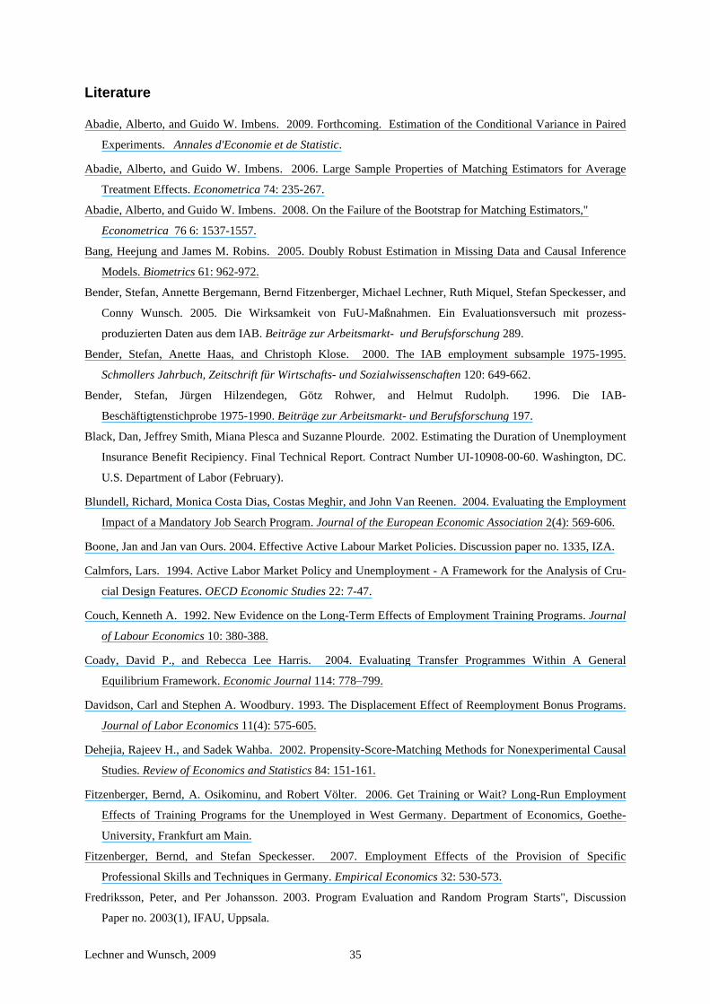
Lechner and Wunsch, 2009 35

Literature

Abadie, Alberto, and Guido W. Imbens. 2009. Forthcoming. Estimation of the Conditional Variance in Paired

Experiments. Annales d'Economie et de Statistic.

Abadie, Alberto, and Guido W. Imbens. 2006. Large Sample Properties of Matching Estimators for Average

Treatment Effects. Econometrica 74: 235-267.

Abadie, Alberto, and Guido W. Imbens. 2008. On the Failure of the Bootstrap for Matching Estimators,"

Econometrica 76 6: 1537-1557.

Bang, Heejung and James M. Robins. 2005. Doubly Robust Estimation in Missing Data and Causal Inference

Models. Biometrics 61: 962-972.

Bender, Stefan, Annette Bergemann, Bernd Fitzenberger, Michael Lechner, Ruth Miquel, Stefan Speckesser, and

Conny Wunsch. 2005. Die Wirksamkeit von FuU-Maßnahmen. Ein Evaluationsversuch mit prozess-

produzierten Daten aus dem IAB. Beiträge zur Arbeitsmarkt- und Berufsforschung 289.

Bender, Stefan, Anette Haas, and Christoph Klose. 2000. The IAB employment subsample 1975-1995.

Schmollers Jahrbuch, Zeitschrift für Wirtschafts- und Sozialwissenschaften 120: 649-662.

Bender, Stefan, Jürgen Hilzendegen, Götz Rohwer, and Helmut Rudolph. 1996. Die IAB-

Beschäftigtenstichprobe 1975-1990. Beiträge zur Arbeitsmarkt- und Berufsforschung 197.

Black, Dan, Jeffrey Smith, Miana Plesca and Suzanne Plourde. 2002. Estimating the Duration of Unemployment

Insurance Benefit Recipiency. Final Technical Report. Contract Number UI-10908-00-60. Washington, DC.

U.S. Department of Labor (February).

Blundell, Richard, Monica Costa Dias, Costas Meghir, and John Van Reenen. 2004. Evaluating the Employment

Impact of a Mandatory Job Search Program. Journal of the European Economic Association 2(4): 569-606.

Boone, Jan and Jan van Ours. 2004. Effective Active Labour Market Policies. Discussion paper no. 1335, IZA.

Calmfors, Lars. 1994. Active Labor Market Policy and Unemployment - A Framework for the Analysis of Cru-

cial Design Features. OECD Economic Studies 22: 7-47.

Couch, Kenneth A. 1992. New Evidence on the Long-Term Effects of Employment Training Programs. Journal

of Labour Economics 10: 380-388.

Coady, David P., and Rebecca Lee Harris. 2004. Evaluating Transfer Programmes Within A General

Equilibrium Framework. Economic Journal 114: 778–799.

Davidson, Carl and Stephen A. Woodbury. 1993. The Displacement Effect of Reemployment Bonus Programs.

Journal of Labor Economics 11(4): 575-605.

Dehejia, Rajeev H., and Sadek Wahba. 2002. Propensity-Score-Matching Methods for Nonexperimental Causal

Studies. Review of Economics and Statistics 84: 151-161.

Fitzenberger, Bernd, A. Osikominu, and Robert Völter. 2006. Get Training or Wait? Long-Run Employment

Effects of Training Programs for the Unemployed in West Germany. Department of Economics, Goethe-

University, Frankfurt am Main.

Fitzenberger, Bernd, and Stefan Speckesser. 2007. Employment Effects of the Provision of Specific

Professional Skills and Techniques in Germany. Empirical Economics 32: 530-573.

Fredriksson, Peter, and Per Johansson. 2003. Program Evaluation and Random Program Starts", Discussion

Paper no. 2003(1), IFAU, Uppsala.

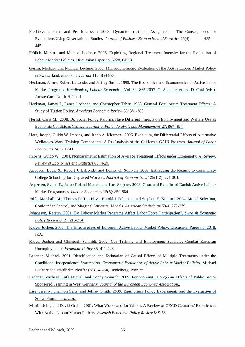
Lechner and Wunsch, 2009 36

Fredriksson, Peter, and Per Johansson. 2008. Dynamic Treatment Assignment - The Consequences for

Evaluations Using Observational Studies. Journal of Business Economics and Statistics 26(4): 435-

445.

Frölich, Markus, and Michael Lechner. 2006. Exploiting Regional Treatment Intensity for the Evaluation of

Labour Market Policies. Discussion Paper no. 5728, CEPR.

Gerfin, Michael, and Michael Lechner. 2002. Microeconometric Evaluation of the Active Labour Market Policy

in Switzerland. Economic Journal 112: 854-893.

Heckman, James, Robert LaLonde, and Jeffrey Smith. 1999. The Economics and Econometrics of Active Labor

Market Programs. Handbook of Labour Economics, Vol. 3: 1865-2097, O. Ashenfelter and D. Card (eds.),

Amsterdam: North-Holland.

Heckman, James J., Lance Lochner, and Christopher Taber. 1998. General Equilibrium Treatment Effects: A

Study of Tuition Policy. American Economic Review 88: 381-386.

Herbst, Chris M. 2008. Do Social Policy Reforms Have Different Impacts on Employment and Welfare Use as

Economic Conditions Change. Journal of Policy Analysis and Management 27: 867–894.

Hotz, Joseph, Guido W. Imbens, and Jacob A. Klerman. 2006. Evaluating the Differential Effects of Alternative

Welfare-to-Work Training Components: A Re-Analysis of the California GAIN Program. Journal of Labor

Economics 24: 521-566.

Imbens, Guido W. 2004. Nonparametric Estimation of Average Treatment Effects under Exogeneity: A Review.

Review of Economics and Statistics 86: 4-29.

Jacobson, Louis S., Robert J. LaLonde, and Daniel G. Sullivan. 2005. Estimating the Returns to Community

College Schooling for Displaced Workers. Journal of Econometrics 125(1-2): 271-304.

Jespersen, Svend T., Jakob Roland Munch, and Lars Skipper. 2008. Costs and Benefits of Danish Active Labour

Market Programmes. Labour Economics 15(5): 859-884.

Joffe, Marshall. M., Thomas R. Ten Have, Harold I. Feldman, and Stephen E. Kimmel. 2004. Model Selection,

Confounder Control, and Marginal Structural Models. American Statistician 58-4: 272-279.

Johansson, Kerstin. 2001. Do Labour Market Programs Affect Labor Force Participation?. Swedish Economic

Policy Review 8 (2): 215-234.

Kluve, Jochen. 2006. The Effectiveness of European Active Labour Market Policy. Discussion Paper no. 2018,

IZA.

Kluve, Jochen and Christoph Schmidt. 2002. Can Training and Employment Subsidies Combat European

Unemployment?. Economic Policy 35: 411-448.

Lechner, Michael. 2001. Identification and Estimation of Causal Effects of Multiple Treatments under the

Conditional Independence Assumption. Econometric Evaluation of Active Labour Market Policies, Michael

Lechner and Friedhelm Pfeiffer (eds.) 43-58, Heidelberg: Physica.

Lechner, Michael, Ruth Miquel, and Conny Wunsch. 2009. Forthcoming . Long-Run Effects of Public Sector

Sponsored Training in West Germany. Journal of the European Economic Association,.

Lise, Jeremy, Shannon Seitz, and Jeffrey Smith. 2009. Equilibrium Policy Experiments and the Evaluation of

Social Programs. mimeo.

Martin, John, and David Grubb. 2001. What Works and for Whom: A Review of OECD Countries' Experiences

With Active Labour Market Policies. Swedish Economic Policy Review 8: 9-56.

Lechner and Wunsch, 2009 37

Miquel, Ruth, Conny Wunsch and Michael Lechner. 2002. Die FuU-Teilnehmer-Datei 1976-1997. Graues

Papier des Instituts für Arbeitsmarkt- und Berufsforschung, Nuremberg.

Mueser, Peter R., Kenneth Troske, and Alexey Gorislavsky. 2007. Using Administrative Data to Measure

Program Performance. Review of Economics and Statistics 89: 761–783.

OECD (2004). Employment Outlook, Paris.

Raaum, Oddbjørn, and Knut Roed. 2006. Do Business Cycle Conditions at the Time of Labor Market Entry

Affect Future Employment Prospects?. Review of Economics and Statistics 88: 193-210.

Raaum, Oddbjørn, Hege Torp, and Tao Zhang. 2002. Business Cycles and the Impact of Labour Market

Programmes. Memorandum 14/2002, Department of Economics, University of Oslo.

Richardson, Katarina and Gerard J. van den Berg. 2006. Swedish Labor Market Training and the Duration of

Unemployment. Discussion Paper no. 2314, IZA.

Robins, James M. 2000. Robust Estimation in Sequentially Ignorable Missing Data and Causal Inference

Models. Proceedings of the American Statistical Association Section on Bayesian Statistical Science 6-10.

Roed, Knut and Oddbjørn Raaum. 2003. The Effect of Programme Participation on the Transition Rate from

Unemployment to Employment. Memorandum 13/2003, Department of Economics, University of Oslo.

Roed, Knut and Oddbjørn Raaum. 2006. Do Labour Market Programmes Speed up the Return to Work?. Oxford

Bulletin of Economics and Statistics 68: 541–68.

Rubin, Daniel B. 1979. Using Multivariate Matched Sampling and Regression Adjustment to Control Bias in

Observational Studies. Journal of the American Statistical Association 74: 318-328.

Scharfstein, Daniel O., Andrea Rotnitzky and James M. Robins. 1999. Adjusting for Nonignorable Drop-out

Using Semiparametric Nonresponse Models. Journal of the American Statistical Association 94: 1096-1120

(with rejoinder 1135-1146).

Sianesi, Barbara. 2004. An Evaluation of the Swedish System of Active Labour Market Programmes in the

1990s. Review of Economics and Statistics 86: 133-155.

Statistisches Bundesamt. 2005. Leben und Arbeiten in Deutschland - Ergebnisse des Mikrozensus 2004.

Wiesbaden.

Van Ours, Jan. 2004. The Locking-in Effect of Subsidized Jobs. Journal of Comparative Economics 32: 37-52.

Winter-Ebmer, Rudolf. 2006. Coping with a Structural Crisis: Evaluating an Innovative Redundancy-Retraining

Project. International Journal of Manpower 27(8): 700-721.

Wunsch, Conny. 2005. Labour Market Policy in Germany. Institutions, Instruments and Reforms since Unifica-

tion. Discussion Paper no. 2005-06, Department of Economics, University of St. Gallen.

Lechner and Wunsch, 2009 38

Appendix A: Further details on the data

A.1 Sample sizes of participants

Sample sizes decrease when keeping first the characteristics of participants and then the

composition of programs constant over time due to enforcing common support with our

reference population (see A.5 for details). The minimum is about 200 participants pooled over

6 months. The average is about 400 participants. While these numbers are sufficient for many

interesting analyses, it is clear that insights from further disaggregation of the data are limited.

- Figure A.1 about here -

A.2 Characteristics of the target population

The following table provides descriptive statistics for selected characteristics of the target

population we use to keep the composition of participants and programs constant over time.

As target population, we chose the pool of all training participants in our sample in the period

1986-1995, reduced to the intersection of the common support in all starting months.

- Table A.1 about here -

Appendix B: Technical details of the matching estimator used

- Table B.1 about here -

The parameter used to define the radius for the distance-weighted radius matching (R) is

set to 90%. This value refers to the distance of the worst match in a one-to-one matching

based on the propensity score. Different values for R are checked in the sensitivity analysis in

Lechner, Miquel, and Wunsch (2009). The results were robust as long as R did not become

'too large'.

Figures

Figure 1: Selected indicators for business cycle movements in West Germany

-2

0

2

4

6

8

10

12

1984 1985 1986 1987 1988 1989 1990 1991 1992 1993 1994 1995 1996 1997 1998 1999 2000 2001 2002 2003

GDP growth Unemployment rate Employment rate / 10

0

1000

2000

3000

4000

5000

6000

7000

1984 1985 1986 1987 1988 1989 1990 1991 1992 1993 1994 1995 1996 1997 1998 1999 2000 2001 2002 2003

Employment / 10000 Unemployment / 1000 Expenditure on training in Mio. €

Expenditure on ALMP in 10 Mio. € Exp. on ALMP per unemployed in €

Sources: Official statistics published by the Federal Employment Agency, the Institute for Employment Research and the

Federal Statistical Office.

Note: The employment rate is calculated as employment plus unemployment as a percentage of the labor force (potential

employment). Expenditure on active labor market policies (ALMP) and training are at 1995 prices.

Figure 2: Effect of training on the employment and unemployment probabilities of participants

-0.2

-0.1

0

0.1

0.2

0.3

0.4

1/86 7/86 1/87 7/87 1/88 7/88 1/89 7/89 1/90 7/90 1/91 7/91 1/92 7/92 1/93 7/93 1/94 7/94 1/95

U6TH significant U96TH significant E6TH significantE96TH significant U6TH U96THE9TH E96TH Detrended unemployment rate

Note: The outcome variables are named as follows: U: unemployment, E: employment, 6 or 96: month after program

start, TH: theta (average treatment effect on the treated). For each outcome variable, symbols appear if the effect

is significant at the 5% level in a particular month. The unemployment rate is presented net of its mean 1986-1995.

All effects are smoothed using three-month moving averages. 300-730 observations per period (pooled).

Figure 3: Mean employment rates given participation and non-participation for participants

-0.3

-0.2

-0.1

0

0.1

0.2

0.3

0.4

0.5

0.6

0.7

1/86 7/86 1/87 7/87 1/88 7/88 1/89 7/89 1/90 7/90 1/91 7/91 1/92 7/92 1/93 7/93 1/94 7/94 1/95

E60M E960M E61M E961M Detrended unemployment rate / 10

Note: The outcome variables are named as follows: E: employment, 6 or 96: month after program start, 0: non-participa-

tion, 1: participation, M: mean level. 300-730 observations per period (pooled). See also note below Figure 2.

Figure 4: Cumulated effects of training on the employment and unemployment probabilities of par-

ticipants (in months)

-2

-1

0

1

2

3

4

5

6

7

8

9

1/86 7/86 1/87 7/87 1/88 7/88 1/89 7/89 1/90 7/90 1/91 7/91 1/92 7/92 1/93 7/93 1/94 7/94 1/95

CU6TH significant CU96TH significant CE6TH significant

CE96TH significant CU6TH CU96TH

CE6TH CE96TH Detrended unemp. rate Note: The outcome variables are named as follows: CU: cumulated unemployment, CE: cumulated employment, 6 or 96:

month after program start, TH: theta (average treatment effect on the treated). 300-730 observations per period

(pooled). See also note below Figure 2.

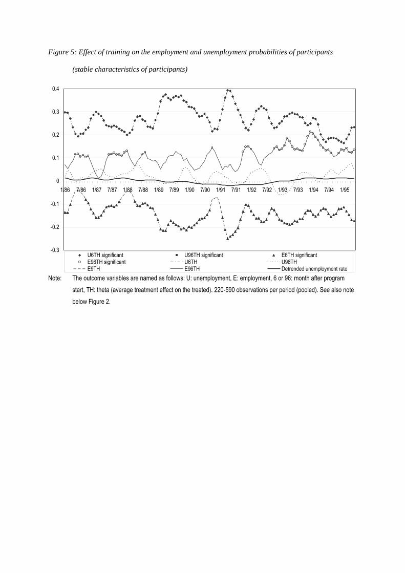
Figure 5: Effect of training on the employment and unemployment probabilities of participants

(stable characteristics of participants)

-0.3

-0.2

-0.1

0

0.1

0.2

0.3

0.4

1/86 7/86 1/87 7/87 1/88 7/88 1/89 7/89 1/90 7/90 1/91 7/91 1/92 7/92 1/93 7/93 1/94 7/94 1/95

U6TH significant U96TH significant E6TH significantE96TH significant U6TH U96THE9TH E96TH Detrended unemployment rate

Note: The outcome variables are named as follows: U: unemployment, E: employment, 6 or 96: month after program

start, TH: theta (average treatment effect on the treated). 220-590 observations per period (pooled). See also note

below Figure 2.

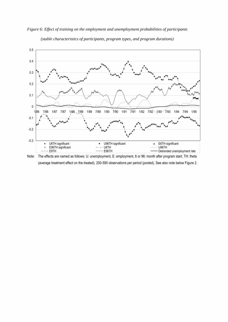
Figure 6: Effect of training on the employment and unemployment probabilities of participants

(stable characteristics of participants, program types, and program durations)

-0.3

-0.2

-0.1

0

0.1

0.2

0.3

0.4

0.5

1/86 7/86 1/87 7/87 1/88 7/88 1/89 7/89 1/90 7/90 1/91 7/91 1/92 7/92 1/93 7/93 1/94 7/94 1/95

U6TH significant U96TH significant E6TH significantE96TH significant U6TH U96THE9TH E96TH Detrended unemployment rate

Note: The effects are named as follows: U: unemployment, E: employment, 6 or 96: month after program start, TH: theta

(average treatment effect on the treated). 200-590 observations per period (pooled). See also note below Figure 2.

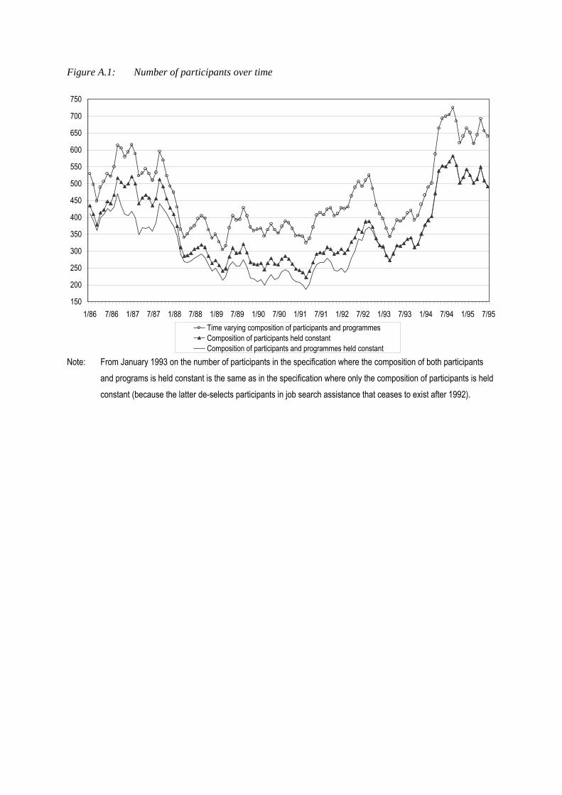
Figure A.1: Number of participants over time

150

200

250

300

350

400

450

500

550

600

650

700

750

1/86 7/86 1/87 7/87 1/88 7/88 1/89 7/89 1/90 7/90 1/91 7/91 1/92 7/92 1/93 7/93 1/94 7/94 1/95 7/95

Time varying composition of participants and programmes

Composition of participants held constant

Composition of participants and programmes held constant

Note: From January 1993 on the number of participants in the specification where the composition of both participants

and programs is held constant is the same as in the specification where only the composition of participants is held

constant (because the latter de-selects participants in job search assistance that ceases to exist after 1992).

Tables

Table 1: Combined administrative data sources used

IAB Employment Subsample (ES)

Benefit Payment Register (BPR)

Training Participant Data (TPD)

Source Employer supplied mandatory social insurance entries.

Benefit payment register of the PES.

Questionnaires filled in by PES staff for statistical pur-

poses.

Period 1980-2003 1980-2003 1980-1997

Population 1% random sample of all persons covered by social insurance for at

least one day 1975-1997. Self-employed, civil servants and uni-versity students are not included.

Recipients of benefit pay-ments from the PES.

Participants in further train-ing, retraining, short training, German language courses and temporary wage subsi-

dies 1980-1997.

Available information

Start and end date of employ-ment, gender, age, nationality, education, profession, occupa-tional status, industry, firm size, earnings, regional information.

Start and end date of benefit receipt, marital status, num-

ber of children, type and amount of benefits received,

regional information.

Start and end date, type, planned and actual duration of the program, type of in-come support paid during

participation, regional infor-mation.

Note: The merged data is based on monthly information. For detailed information on the merging and recoding proce-

dures, see Bender et al. (2005). The construction of this database is a result of a three-year joint project of re-

search groups at the Universities of Mannheim (Bergemann, Fitzenberger, Speckesser) and St. Gallen (Lechner,

Miquel, Wunsch) as well as the Institute for Employment Research of the FEA (Bender). A detailed description of

the ES is provided by Bender, Hilzedegen, Rohwer, and Rudolph (1996), and Bender, Haas, and Klose (2000). For

the TPD see Miquel, Wunsch, and Lechner (2002).

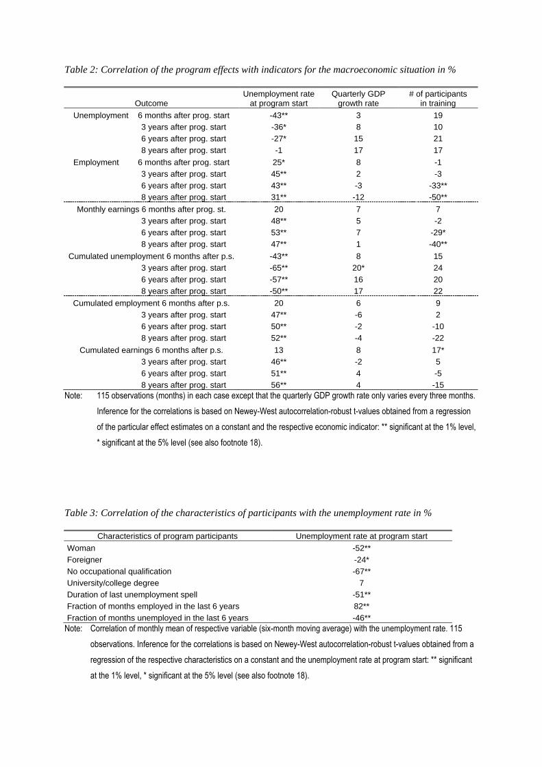
Table 2: Correlation of the program effects with indicators for the macroeconomic situation in %

Outcome Unemployment rate

at program start Quarterly GDP

growth rate # of participants

in training

Unemployment 6 months after prog. start -43** 3 19

3 years after prog. start -36* 8 10

6 years after prog. start -27* 15 21

8 years after prog. start -1 17 17

Employment 6 months after prog. start 25* 8 -1

3 years after prog. start 45** 2 -3

6 years after prog. start 43** -3 -33**

8 years after prog. start 31** -12 -50**

Monthly earnings 6 months after prog. st. 20 7 7

3 years after prog. start 48** 5 -2

6 years after prog. start 53** 7 -29*

8 years after prog. start 47** 1 -40**

Cumulated unemployment 6 months after p.s. -43** 8 15

3 years after prog. start -65** 20* 24

6 years after prog. start -57** 16 20

8 years after prog. start -50** 17 22

Cumulated employment 6 months after p.s. 20 6 9

3 years after prog. start 47** -6 2

6 years after prog. start 50** -2 -10

8 years after prog. start 52** -4 -22

Cumulated earnings 6 months after p.s. 13 8 17*

3 years after prog. start 46** -2 5

6 years after prog. start 51** 4 -5

8 years after prog. start 56** 4 -15

Note: 115 observations (months) in each case except that the quarterly GDP growth rate only varies every three months.

Inference for the correlations is based on Newey-West autocorrelation-robust t-values obtained from a regression

of the particular effect estimates on a constant and the respective economic indicator: ** significant at the 1% level,

* significant at the 5% level (see also footnote 18).

Table 3: Correlation of the characteristics of participants with the unemployment rate in %

Characteristics of program participants Unemployment rate at program start

Woman -52**

Foreigner -24*

No occupational qualification -67**

University/college degree 7

Duration of last unemployment spell -51**

Fraction of months employed in the last 6 years 82**

Fraction of months unemployed in the last 6 years -46**

Note: Correlation of monthly mean of respective variable (six-month moving average) with the unemployment rate. 115

observations. Inference for the correlations is based on Newey-West autocorrelation-robust t-values obtained from a

regression of the respective characteristics on a constant and the unemployment rate at program start: ** significant

at the 1% level, * significant at the 5% level (see also footnote 18).

Table 4: Correlation of the program effects with the unemployment rate at program start in %

(stable characteristics of participants)

Outcome Participants

constant

Previous specification: participants change

Strict joint support+ Original sample

Unemployment 6 months after program start -49** -14 -43**

3 years after program start -48** -39** -36*

8 years after program start 19 12 -1

Employment 6 months after program start 36** 33** 25*

3 years after program start 45** 54** 45**

8 years after program start 31* 29** 31**

Monthly earnings 6 months after program start 40** 27* 20

3 years after program start 44** 45** 48**

8 years after program start 53** 37** 47**

Note: 115 observations. Inference for the correlations is based on Newey-West autocorrelation-robust t-values obtained

from a regression of the particular effect estimates on a constant and the respective economic indicator: ** significant

at the 1% level, * significant at the 5% level (see also footnote 18). +To make the results more comparable, partici-

pants are reduced to the same joint support over time as in the reference population. Note that the number of treated

observations is rather small in some months.

Table 5: Correlation of the characteristics of the training policy with the unemployment rate at pro-

gram start in %

Characteristics of programs Participants Stable participants

Fraction of participants in practice firms 5 -4

Fraction of participants in short training 28** 26**

Fraction of participants in long training 34** 25**

Fraction of participants in retraining -1 6

Fraction of participants in job search assistance -42** -27*

Planned program duration 6 1

Planned duration of practice firms -34** 20

Planned duration of short training -20* 27**

Planned duration of long training -13 6

Planned duration of retraining -21* -54**

Planned duration of job search assistance 34** 46**

Note: Correlation of monthly mean of respective variable (six-month moving average) with the unemployment rate. Partici-

pants are those participants used in Section 5, whereas stable participants are those used in Section 6.1.

115 observations. Inference for the correlations is based on Newey-West autocorrelation-robust t-values obtained

from a regression of the respective characteristics on a constant and the unemployment rate at program start: ** sig-

nificant at the 1% level, * significant at the 5% level (see also footnote 18).

Table 6: Correlation of the program effects with the unemployment rate in %

(stable characteristics of participants, program types, and program durations)

Previous specifications

Outcome Participants and

programs constant Participants

constant Participants

change

Unemployment 6 months after prog. start -58** -49** -43**

3 years after prog. start -39** -48** -36*

8 years after prog. start 3 19 -1

Employment 6 months after prog. start 46** 36** 25*

3 years after prog. start 31* 45** 45**

8 years after prog. start 40** 31* 31**

Monthly earnings 6 months after prog. start 52** 40** 20

3 years after prog. start 37* 44** 48**

8 years after prog. start 55** 53** 47**

Note: 115 observations. Inference for the correlations is based on Newey-West autocorrelation-robust t-values obtained

from a regression of the respective effect estimates on a constant and the unemployment rate at program start: **

significant at the 1% level, * significant at the 5% level (see also footnote 18).

Table 7: Correlation of the program effects with the unemployment rate at program start in %

(participants and program composition do not change over time)

Outcome

Monthly unemployment rate 1986 - 1995

Quarter dummies only Interacted with post-unification dummy

Unemployment 6 months after prog. start -58** -66**

3 years after prog. start -31* -28*

8 years after prog. start 6 5

Employment 6 months after prog. start 49** 50**

3 years after prog. start 25 19

8 years after prog. start 38** 47**

Monthly earnings 6 months after prog. start 53** 54**

3 years after prog. start 29* 21*

8 years after prog. start 53** 58**

Note: 115 observations for each cell. Inference for the correlations is based on Newey-West autocorrelation-robust t-

values: ** significant at the 1% level, * significant at the 5% level.

Table 8: Correlation of the program effects with the unemployment rate %

(stable characteristics of participants, program types, and planned durations)

Outcome

Correlation of the effects with national unemployment rate over time

Correlation of re-gional effects with average regional

unemployment rate b

Regional unem-ployment low

a

Regional unem-ployment high

a

Unemployment 6 months after prog. start -56** -37** -21**

3 years after prog. start -47** -37** -18**

8 years after prog. start -13 -14 -14**

Employment 6 months after prog. start 38** 15 9

3 years after prog. start 40* 36* 7

8 years after prog. start 49** 46** -8

Monthly earnings 6 months after prog. start 48** 27 11*

3 years after prog. start 44** 39** 9

8 years after prog. start 59** 60** -4

Note: Low / high unemployment regions are those where 60% of the unemployed facing the lowest / highest regional un-

employment rate in a specific period live. a 115 observations for each cell. b 36 observations for each cell. Inference

for the correlations is based on Newey-West autocorrelation-robust t-values: ** significant at the 1% level, * signifi-

cant at the 5% level.

Table 9: Correlation of the program effects with the unemployment rate in %

(stable characteristics of participants, program types, and durations)

Outcome

Separate estimation Interaction terms c

With seasonal dummies

c

pre

10/1990 a

post

10/1990 b

pre

10/1990

post

10/1990

pre

10/1990

post

10/1990

Unemployment 6 months after prog. start -38* -75** -57** -64** -58** -66**

3 years after prog. start -70** -20 -31* -25* -31* -24*

8 years after prog. start 2 6 6 7 6 8

Employment 6 months after prog. start 33* 55** 48** 45** 49** 46**

3 years after prog. start 62** 4 26* 13 26* 12

8 years after prog. start 23 56** 39** 46** 38** 46**

Monthly earnings 6 months after prog. start 41** 62** 52** 49** 53** 50**

3 years after prog. start 55** 19 29** 14 29* 15

8 years after prog. start 29 68** 51** 54** 53** 56**

Note: a 57 observations for each cell. b 58 observations for each cell. c 115 observations for each cell. Inference for the

correlations is based on Newey-West autocorrelation-robust t-values: ** significant at the 1% level, * significant at the

5% level.

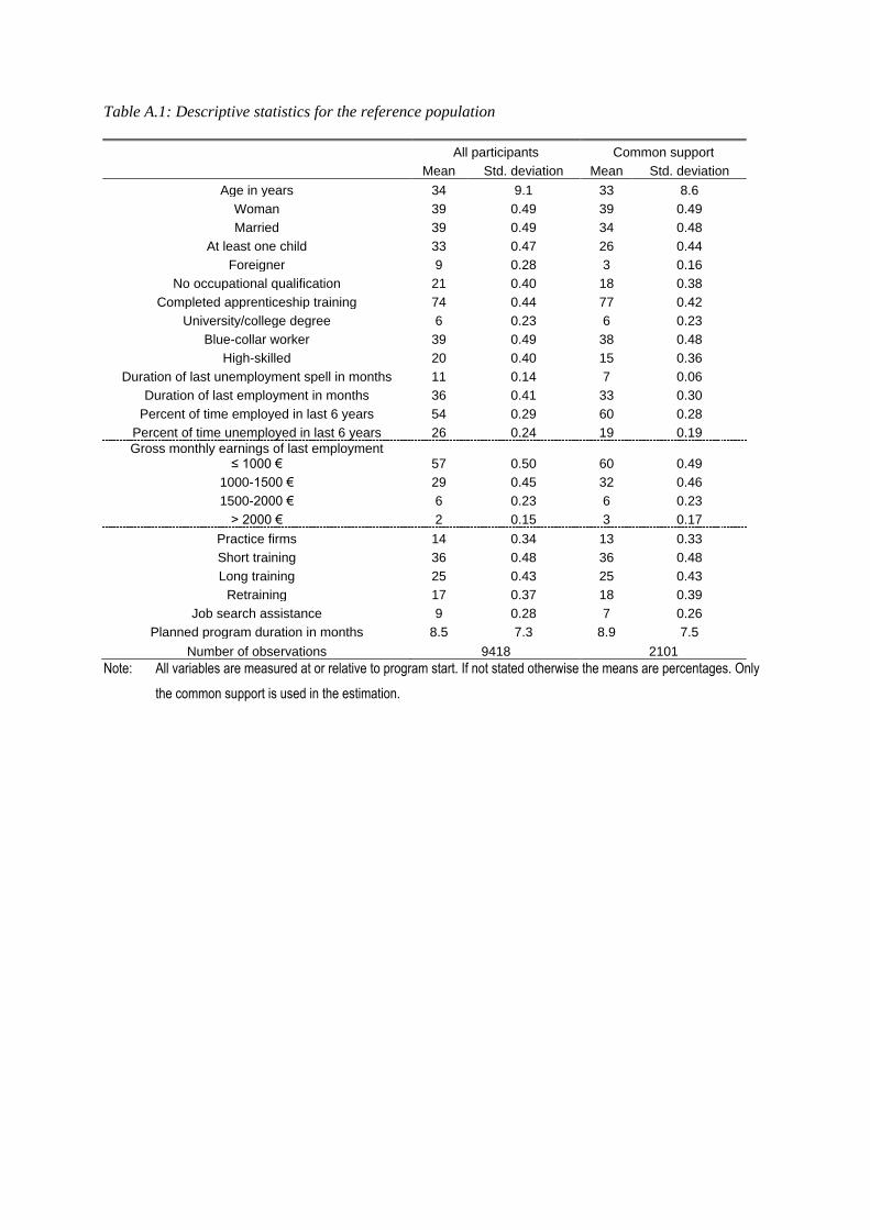
Table A.1: Descriptive statistics for the reference population

All participants Common support

Mean Std. deviation Mean Std. deviation

Age in years 34 9.1 33 8.6

Woman 39 0.49 39 0.49

Married 39 0.49 34 0.48

At least one child 33 0.47 26 0.44

Foreigner 9 0.28 3 0.16

No occupational qualification 21 0.40 18 0.38

Completed apprenticeship training 74 0.44 77 0.42

University/college degree 6 0.23 6 0.23

Blue-collar worker 39 0.49 38 0.48

High-skilled 20 0.40 15 0.36

Duration of last unemployment spell in months 11 0.14 7 0.06

Duration of last employment in months 36 0.41 33 0.30

Percent of time employed in last 6 years 54 0.29 60 0.28

Percent of time unemployed in last 6 years 26 0.24 19 0.19

Gross monthly earnings of last employment ≤ 1000 € 57 0.50 60 0.49

1000-1500 € 29 0.45 32 0.46

1500-2000 € 6 0.23 6 0.23

> 2000 € 2 0.15 3 0.17

Practice firms 14 0.34 13 0.33

Short training 36 0.48 36 0.48

Long training 25 0.43 25 0.43

Retraining 17 0.37 18 0.39

Job search assistance 9 0.28 7 0.26

Planned program duration in months 8.5 7.3 8.9 7.5

Number of observations 9418 2101

Note: All variables are measured at or relative to program start. If not stated otherwise the means are percentages. Only

the common support is used in the estimation.

Table B.1: A matching protocol for the estimation of a counterfactual outcome and the effects

Step 1 Specify a reference distribution defined by X.

Step 2 Pool the observations forming the reference distribution and the participants in the respective period. Code an

indicator variable W, which is 1 if the observation belongs to the reference distribution. All indices, 0 or 1, used

below relate to the actual or potential values of W.

Step 3 Specify and estimate a binary probit for ( ) : ( 1| )p x P W X x

Step 4 Restrict sample to common support: Delete all observations with probabilities larger than the smallest maximum

and smaller than the largest minimum of all subsamples defined by W.

Step 4 Estimate the respective (counterfactual) expectations of the outcome variables.

Standard propensity score matching step (multiple treatments)

a-1) Choose one observation in the subsample defined by W=1 and delete it from that pool.

b-1) Find an observation in the subsample defined by W=0 that is as close as possible to the one chosen in step a-1) in terms of ( ),p x x . 'Closeness' is based on the Mahalanobis distance. Do not remove that ob-

servation, so that it can be used again.

c-1) Repeat a-1) and b-1) until no observation with W=1 is left.

Exploit thick support of X to increase efficiency (radius matching step)

d-1) Compute the maximum distance (d) obtained for any comparison between a member of the reference distri-

bution and matched comparison observations.

a-2) Repeat a-1).

b-2) Repeat b-1). If possible, find other observations in the subsample of W=0 that are at least as close as R * d

to the one chosen in step a-2) (to gain efficiency). Do not remove these observations, so that they can

be used again. Compute weights for all chosen comparisons observations that are proportional to their

distance (triangular kernel). Normalise the weights such that they add to one.

c-2) Repeat a-2) and b-2) until no participant in W=1 is left.

d-2) For any potential comparison observation, add the weights obtained in a-2) and b-2).

Exploit double robustness properties to adjust small mismatches by regression

e) Using the weights ( )iw x obtained in d-2), run a weighted linear regression of the outcome variable on the

variables used to define the distance (and an intercept).

f-1) Predict the potential outcome 0 ( )iy x of every observation using the coefficients of this regression: 0ˆ ( )iy x .

f-2) Estimate the bias of the matching estimator for 0( | 1)E Y W as: 00

11

1 01

ˆˆ 1( 0) ( )1( 1) ( )Ni

i

W w y xW y x

N N.

g) Using the weights obtained by weighted matching in d-2), compute a weighted mean of the outcome variables

in W=0. Subtract the bias from this estimate to get 0( | 1)E Y W .

Step 5 Repeat Steps 2 to 4 with the non-participants playing the role of participants before. This gives the desired esti-

mate of the counterfactual non-participation outcome.

Step 6 The difference of the potential outcomes gives the desired estimate of the effect with respect to the reference

distribution specified in Step 1.

Note: x includes gender, elapsed unemployment duration until program start, and whether a person is employed in

month 12 or month 24 before program start. In some specifications, we also match on education. In the specifica-

tion where program composition is held constant, we also match on the type of program and planned program du-

ration. x is included to ensure a high match quality with respect to these critical variables.