APSIM Rice Modeling Asia 1- Europeaan J. Agronomy

(This is a sample cover image for this issue. The actual cover is not yet available at this time.)

This article appeared in a journal published by Elsevier. The attachedcopy is furnished to the author for internal non-commercial researchand education use, including for instruction at the authors institution

and sharing with colleagues.

Other uses, including reproduction and distribution, or selling orlicensing copies, or posting to personal, institutional or third party

websites are prohibited.

In most cases authors are permitted to post their version of thearticle (e.g. in Word or Tex form) to their personal website orinstitutional repository. Authors requiring further information

regarding Elsevier’s archiving and manuscript policies areencouraged to visit:

http://www.elsevier.com/copyright

http://www.elsevier.com/copyright

Author's personal copy

Europ. J. Agronomy 39 (2012) 9– 24

Contents lists available at SciVerse ScienceDirect

European Journal of Agronomy

jo u r n al hom epage: www.elsev ier .com/ locate /e ja

Rice in cropping systems—Modelling transitions between flooded andnon-flooded soil environments

D.S. Gaydona,f,∗, M.E. Proberta, R.J. Bureshb, H. Meinkec,f, A. Suriadid, A. Dobermannb,B. Boumanb, J. Timsinae

a CSIRO Ecosystem Sciences, 41 Boggo Rd, Dutton Park, Brisbane 4102, Australiab International Rice Research Institute (IRRI), Los Banos, Philippinesc University of Tasmania, Tasmanian Institute of Agriculture, Hobart TAS 7001, Australiad Balai Pengkajian Technology Pertanian Nusa Tengarra Barat (BPTPNTB), Nusa Tenggara Barat, Indonesiae International Rice Research Institute (IRRI), Dhaka, Bangladeshf Wageningen University, Centre for Crop Systems Analysis, PO Box 430, 6700 AK Wageningen, The Netherlands

a r t i c l e i n f o

Article history:Received 12 September 2011Received in revised form30 December 2011Accepted 10 January 2012

Keywords:APSIMORYZA2000RiceCropping systemsSoil nutrient dynamics

a b s t r a c t

Water shortages in many rice-growing regions, combined with growing global imperatives to increasefood production, are driving research into increased water use efficiency and modified agricultural prac-tices in rice-based cropping systems. Well-tested cropping systems models that capture interactionsbetween soil water and nutrient dynamics, crop growth, climate and management can assist in the eval-uation of new agricultural practices. The APSIM model was designed to simulate diverse crop sequences,residue/tillage practices and specification of field management options. It was previously unable tosimulate processes associated with the long-term flooded or saturated soil conditions encountered inrice-based systems, due to its heritage in dryland cropping applications. To address this shortcoming,the rice crop components of the ORYZA2000 rice model were incorporated and modifications weremade to the APSIM soil water and nutrient modules to include descriptions of soil carbon and nitrogendynamics under anaerobic conditions. We established a process for simulating the two-way transitionbetween anaerobic and aerobic soil conditions occurring in crop sequences of flooded rice and other non-flooded crops, pastures and fallows. These transitions are dynamically simulated and driven by modelledhydraulic variables (soil water and floodwater depth). Descriptions of floodwater biological and chemicalprocesses were also added. Our assumptions included a simplified approach to modelling O2 transportprocesses in saturated soils. The improved APSIM model was tested against diverse, replicated experimen-tal datasets for rice-based cropping systems, representing a spectrum of geographical locations (Australia,Indonesia and Philippines), soil types, management practices, crop species, varieties and sequences.The model performed equally well in simulating rice grain yield during multi-season crop sequencesas the original validation testing reported for the stand-alone ORYZA2000 model simulating single crops(n = 121, R2 = 0.81 with low bias (slope, ˛ = 1.02, intercept, ˇ = −323 kg ha−1), RMSE = 1061 kg ha−1 (cf.SD of measured data = 2160 kg ha−1)). This suggests robustness in APSIM’s simulation of the rice-growingenvironment and provides evidence on the usefulness of our modifications and practicality of our assump-tions. Aspects of particular strength were identified (crop rotations; response to applied fertilizers; theperformance of bare fallows), together with areas for further development work (simulation of retainedcrop stubble during fallows, greenhouse gas emissions). APSIM is now suitable to investigate productionresponses of potential agronomic and management changes in rice-based cropping systems, particularlyin response to future imperatives linked to resource availability, climate change, and food security. Fur-ther testing is required to evaluate the impact of our simplified assumptions on the model’s simulationof greenhouse gas emissions in rice-based cropping systems.

Crown Copyright © 2012 Published by Elsevier B.V. All rights reserved.

∗ Corresponding author at: CSIRO Ecosystem Sciences, 41 Boggo Rd, Dutton Park,Brisbane 4102, Australia. Tel.: +61 738335705; fax: +61 746881193.

E-mail address: [email protected] (D.S. Gaydon).

1. Introduction

Water shortages in agriculture present an increasing problemglobally (Rijsberman, 2006). Rice-based cropping systems, bothirrigated and rainfed, represent the most important croppingsystem in South Asia (Devendra and Thomas, 2002), and an

1161-0301/$ – see front matter. Crown Copyright © 2012 Published by Elsevier B.V. All rights reserved.doi:10.1016/j.eja.2012.01.003


10 D.S. Gaydon et al. / Europ. J. Agronomy 39 (2012) 9– 24

important system throughout Southeast and East Asia. Varioussectors with increasing water demand (urban, industrial, envi-ronmental) competing for this limited resource are likely toexacerbate the impact of climate change effects on water supplyto rice-growing areas globally (Bouman et al., 2007).

The forthcoming global challenge of producing more food andfibre with limited or reduced future irrigation water has been iden-tified by numerous authors (Keating et al., 2010; Ali and Talukder,2008; Bouman, 2007; Tuong et al., 2005). Consequently, there isa desire to investigate new practices in rice-growing regions withthe aim of enhancing water productivity (WP) (Bouman, 2007), andcropping intensity (Dobermann and Witt, 2000). Suggested path-ways include the incorporation of non-flooded crops and pasturesinto traditional rice rotations (Zeng et al., 2007; Singh et al., 2005;Cho et al., 2003), changed agronomic and/or irrigation practices(Yadav et al., 2011a; Belder et al., 2007; Bouman and Tuong, 2001),reduction of non-productive water loses (Humphreys et al., 2010),and genetic improvement (Bennett, 2003; Sheehy et al., 2000; Penget al., 1999).

Well-tested simulation models are useful tools to exploreopportunities for increasing WP. The APSIM cropping systemsmodel (Keating et al., 2003) has a proven track record in modellingthe performance of diverse cropping systems, rotations, fallowing,crop and environmental dynamics (Whitbread et al., 2010; Carberryet al., 2002; Robertson et al., 2002; Verburg and Bond, 2003; Turpinet al., 1998). The major barrier to modelling rice-based croppingsystems in APSIM has been the lack of suitable descriptions for soilprocesses under long-term anaerobic conditions – a consequence ofthe model’s heritage in dryland cropping systems. The ORYZA2000rice model (Bouman and van Laar, 2006) was incorporated into theAPSIM framework and validated in several studies (Zhang et al.,2006; Gaydon et al., 2006). All soil and water components fromthe original ORYZA2000 model were removed during this process,retaining only the crop growth routines which now received theirwater and nutrient supply directly from the APSIM soil and watermodules. In each of these studies, soil nitrogen (N) was eitherassumed to be non-limiting, or calculated for a rice monocultureusing a simple N accounting component within ORYZA2000. Theinability of APSIM to simulate the complex dynamics of carbon (C)and N in alternately flooded and non-flooded soil environmentswas identified in these studies as a major future constraint to mod-elling complex rice-based cropping system scenarios (Zhang et al.,2006).

Jing et al. (2007, 2010) addressed this issue of transitionalsoil environments for rice-wheat rotations in the RIWER model,demonstrating good modelling performance in that specific sys-tem. However the flexibility for simulating more varied croppingsystems options (other crop species, different sequences, andassorted irrigation and tillage practices) was not present. A rangeof other published models (such as DNDC (Li et al., 1994); WOFOST(Van Keulen and Wolf, 1986); WARM (Confalonieri et al., 2006);CropSyst (Stöckle et al., 2003); C-Farm (Kemanian and Stöckle,2010); Chowdary et al., 2004; Jamu and Piedrahita, 2002) are sim-ilarly limited when considering flexibility for future adaptationstudies in diverse cropping systems.

Another vital element missing in existing models was the abil-ity to simulate additions of C and N to rice-based cropping systemsfrom biological nitrogen fixation (BNF – by cyanobacteria) andgrowth of other non-N-fixing photosynthetic algal biomass (PAB).These are now considered to be critical for sustaining soil organicC and soil N supplying capacity (Pampolino et al., 2008; Roger andLadha, 1992). Pampolino et al. (2008) found that soil organic C andtotal soil N were maintained during 15 years of continuous ricecropping with ample water supply for near continuous soil sub-mergence in four experiments in the Philippines. Soil organic C andanaerobic N mineralization were maintained even with three rice

crops per year, zero fertilizer inputs, and complete removal of allabove-ground rice biomass at maturity. The ability to simulate thisphenomenon is essential for models aiming to examine long-termtrends in rice-based cropping systems.

Prior to our work, no existing cropping system model simu-lated these additions. The impacts of algal activity on floodwaterpH and partial pressure of ammonia (and consequently on ammo-nia volatilization) are well simulated in the CERES-Rice model(Godwin and Singh, 1991), however the associated additions of Cfrom PAB and additions of N through BNF are not simulated. Thishas not restricted the ability of CERES-Rice to simulate N losses andavailability during single rice crops, but has limited its capacity tosimulate long-term crop sequences and soil organic C dynamicssuccessfully. Timsina and Humphreys (2006) presented evidencethat CERES-Rice did not simulate soil organic C dynamics well.

We concentrated our efforts on improving the existing APSIMframework, with a view to addressing this range of limiting issuesand developing a model capable of simulating diverse future adap-tation scenarios in rice-based cropping systems. APSIM alreadypossessed the required flexibility and inherent design for specifyingan infinite range of different management practices. Enhance-ments were necessary to achieve realistic simulation of soil C andN dynamics through cycles of aerobic and anaerobic soil condi-tions. Modelling of PAB influence on nutrient dynamics was alsorequired. We used algorithms and constants from both CERES-Riceand RIWER, whilst introducing some new concepts relating to sys-tem C and N contributions from PAB. Up until now, simulation ofcrop production in diverse rice-based systems has not been possi-ble. Here we report on incorporation of this functionality into theAPSIM model and subsequent performance evaluation against keydatasets.

2. Materials and methods

2.1. Overview of the APSIM model

APSIM is a dynamic daily time-step model that combines bio-physical and management modules within a central engine tosimulate cropping systems. The model is capable of simulatingsoil water, C, N and P dynamics and their interaction withincrop/management systems, driven by daily climate data (solarradiation, maximum and minimum temperatures, rainfall). Dailypotential production for a range of crop species is calculated usingstage-related RUE constrained by climate and available leaf area.The potential production is then limited to actual production ona daily basis by soil water, nitrogen and (for some crop modules)phosphorus availability (Keating et al., 2003). The SOILWAT mod-ule uses a multi-layer, cascading approach for the soil water balancefollowing CERES (Jones and Kiniry, 1986). The SURFACEOM mod-ule simulates the fate of the above-ground crop residues that canbe removed from the system, incorporated into the soil or leftto decompose on the soil surface. The SOILN2 module simulatesthe transformations of C and N in the soil. These include freshorganic matter decomposition, N immobilization, urea hydroly-sis, ammonification, nitrification and denitrification. Crop residuestilled into the soil, together with roots from the previous crop,constitute the soil fresh organic matter (FOM) pool. This pool candecompose to form the BIOM (microbial biomass), HUM (humus),and mineral N (NO3 and NH4) pools. The BIOM pool notionallyrepresents the more labile soil microbial biomass and microbialproducts, whilst the more resistant HUM pool represents the restof the SOM (Probert et al., 1998). APSIM crop modules seek infor-mation regarding water and N availability directly from SOILWATand SOILN modules, for limitation of crop growth on a dailybasis.


D.S. Gaydon et al. / Europ. J. Agronomy 39 (2012) 9– 24 11

Fig. 1. Key processes for system simulation in a flooded rice environment.

2.2. Enhancements required to APSIM

2.2.1. The flooded environmentFig. 1 illustrates the broad nutrient and biological processes rel-

evant to simulation of a flooded soil environment. All but one ofthese processes (denitrification) was originally absent from APSIM.The following is a brief description of the new system elementsrequired:

• Pond C and N loss and gain mechanisms: Floodwater introduces arange of C and N loss and gain mechanisms not present in aero-bic soil environments. These include significant volatilization ofammonia arising from diurnal elevations in floodwater pH asso-ciated with growth of PAB (largely algae, a proportion of whichmay be N-fixing) (Fillery and Vlek, 1983; Buresh et al., 1980;Roger and Ladha, 1992). They also include separating nitrifica-tion into a small volume of the surface soil, overlying floodwater,and crop rhizosphere, together with denitrification into the largerunderlying anaerobic soil layer (Buresh et al., 2008).

• Fertilizer applied into pond: In rice-based systems, N fertilizer isoften broadcast as urea directly into the floodwater. This ureaN is then subject to hydrolysis, N loss via ammonia volatilizationand nitrification–denitrification, movement into the soil, and ulti-mately uptake by the rice plant. Previously in APSIM, all appliedfertilizer was conceptualized as being applied directly into thesoil layers.

• Surface organic matter decomposition in pond: Surface organicmatter decomposition is comprehensively modelled in APSIM(Probert et al., 1998) for aerobic conditions, however decomposi-tion of organic material in the floodwater is governed by differentrate constants reflecting a slower potential rate of decomposition(Acharya, 1935a,b,c; Villegas-Pangga et al., 2000)

• Reduced potential rates of soil organic matter (SOM) decompositionand cycling: In an anaerobic soil profile saturated for extendedperiods, reduced potential rates of organic matter decompositionand cycling are likely to be a significant factor in modelling systembehaviour (Jing et al., 2007, 2010).

2.2.2. Transitional abilityChanging the aeration status of the soil has significant con-

sequences for nutrient dynamics, movement, and availability toplants. Nitrogen behaves differently in flooded (anaerobic) soilenvironments compared with non-flooded (aerobic) soil envi-ronments (Buresh et al., 2008). In flooded conditions, ammoniavolatilization from the floodwater is a major source of N loss (Filleryand Vlek, 1983), hence movement of urea, ammonium and nitrate

between the floodwater and the soil, where it is available for plantuptake and protected from atmospheric volatilization, becomes animportant process for simulation. Ammonium (NH4), the majorsource of mineral N for rice crops, is rapidly nitrified to nitrate (NO3)when the soil is drained. Nitrate is the major form in which mineralN exists in aerobic soil environments and is used by non-floodedcrops such as wheat. When aerobic soil is re-flooded, nitrate presentin the system is promptly lost by denitrification to the atmo-sphere. These cycles of nitrification and denitrification, togetherwith ammonia volatilization during the flood phase, are major lossmechanisms for N loss in cropping systems which include floodedrice phases (Buresh and De Datta, 1991; Buresh et al., 2008; Shibuet al., 2006; Kirk, 2004; Kirk and Olk, 2000).

The key challenge for incorporating new process descriptionsinto APSIM was to establish smooth transitions between floodedand non-flooded soil environments within a simulation, capturingthe effect of the changed nutrient dynamics on crop growth. It wasa design criteria that this transition be contingent on continuoushydraulically-modelled variables (floodwater depth and soil mois-ture status), rather than an arbitrary switch when one phase hadfinished and the next begun.

2.3. Enhancements implemented

2.3.1. Layering of the systemWhen a soil is flooded, surface water limits oxygen transfer

from the atmosphere to the soil. The imbalance between the highrespiration rate of soil organisms and the slow rate of oxygen dif-fusion through the floodwater (10,000 times less than air (Bureshet al., 2008)) quickly results in the soil layers becoming anaerobic,reduced, or depleted of oxygen (Buresh et al., 2008; Kirk and Olk,2000). Anaerobic organisms then dominate nutrient and organicmatter cycling within the reduced soil. Three distinct layers in thesystem can be conceptualized: (1) the oxygenated floodwater; (2)a thin (a few millimeters) oxidized layer at the surface of the soiland around rice crop roots; and (3) the vast bulk of the soil masswhich is reduced when flooded. CERES-Rice models N transforma-tions within each of these zones (Godwin et al., 1990), the modeltherefore consisting of a three-layer system with flows calculatedbetween each. Nitrification following urea hydrolysis or ammoni-fication of organic matter can occur in both the floodwater andoxidized soil layer, however any NO3 subsequently moving intothe reduced subsoil is subject to denitrification.

We have used a two layer system (floodwater and soil) onthe assumption that the thin oxidized layer at the soil surface isrelatively insignificant when modelling larger-scale nutrient pro-cesses, as is the oxygenated rhizosphere around rice crop roots.Buresh and De Datta (1990) explained the relative unimportanceof nitrification–denitrification in continuously flooded soil. In ourmodifications, the chemistry of the floodwater is modelled by anew module (APSIM-Pond), and the chemistry of the soil layers byAPSIM-SoilN. These two modules communicate with each other ona daily basis to transfer nutrients via a central engine according tostandard APSIM protocols (Keating et al., 2003). We assume thatN is only available for uptake by the rice crop once it is in the soillayers (i.e. crop uptake from the SoilN module). Fig. 2 shows ourconceptualization of nutrient flows within APSIM for both floodedand non-flooded soil environments.

2.3.2. New module: APSIM-PondThe APSIM-Pond module is a transient module in the simulation.

It becomes active whenever the APSIM soil water balance moduledetermines that water is ponding on the soil surface. A resettableinput parameter for surface water storage capacity (max pond inmm) can be specified to represent the maximum bund height inrice systems. Runoff only occurs once the surface storage capacity



De-nit

(N2 and N2O)

CROP

SOIL WAT SOILN

SurfaceO M FERTILISER

Lea ching

a) Aero bic system (Tradition al APSIM)

runoff

CO2

CROP

SOIL WAT SOILN


Lea ching

POND

PAB

Algae

decomp

runoff

Ammonia (NH3)

Volatilisation

Nitrification

stop s

b) Ana erobi c system (Flooded environment)

Methan e

(CH4)N up take

leaf loss

roo t sloughing

Decomp/ tillage

harvest

harvest

leaf loss

De-nit

(N2 and N2O)

De-nit

(N2 and N2O)

CROP

SOIL WAT SOILN


Lea ching


runoff

CO2

CROP

SOIL WAT SOILN


Lea ching

POND

PAB

Algae

decomp

runoff

Ammonia (NH3)

Volatilisation

Nitrification

stop s


Methan e

(CH4)N up take

leaf loss

roo t sloughing

Decomp/ tillage

harvest

harvest

leaf loss

De-nit

(N2 and N2O)

De-nit

(N2 and N2O)

CROP

SOIL WAT SOILN


Lea ching


runoff

CO2

CROP

SOIL WAT SOILN


Lea ching

POND

PAB

Algae

decomp

runoff

Ammonia (NH3)

Volatilisation

Nitrification

stop s


Methan e

(CH4)N up take

leaf loss

roo t sloughing

Decomp/ tillage

harvest

harvest

leaf loss

De-nit

(N2 and N2O)

Fig. 2. Conceptual structure of APSIM module communications and C&N loss (red) and gain (blue) mechanisms in: (a) traditional aerobic systems; and (b) flooded systems.The black dotted line represents the soil surface. (For interpretation of the references to colour in this figure legend, the reader is referred to the web version of the article.)

has been exceeded. Daily irrigation or rainfall in excess of infiltra-tion rate can be stored on the surface as floodwater if max pondis greater than zero. The APSIM-Pond module is only concernedwith floodwater chemical and biological processes – the soil waterbalance module simulates the water balance of floodwater andsoil alike, as a continuum. When rainfall and/or irrigation cease,the floodwater depth will decrease by infiltration into the soil andevaporation until there is no floodwater remaining. APSIM-Pondchecks with the soil water balance module on a daily basis to seewhether it should be ‘active’ or not, as well as obtaining informationon evaporation and its current depth. The module simulates ‘algalactivity’ in the pond using the approach of CERES-Rice (Godwinand Singh, 1991). Additionally, a new innovation of APSIM-Pondis the extension of ‘algal activity’ (via the concept of a potentialdaily algal growth rate) to simulation of actual algal growth andbiomass accumulation, including N uptake and fixation, leading tosignificant additions of C and N to rice system processes (Gaydonet al., 2012). The simulated ‘algal activity’ is a function of availablelight (solar radiation, reduced by canopy cover), floodwater tem-perature, phosphorus, and mineral N availability, and is used tomaintain a dynamic pH balance within the floodwater. This enablespartial pressure of ammonia to be calculated and ultimately dailyammonia volatilization – the major avenue for loss of applied fer-tilizer N in flooded rice systems (Buresh et al., 2008). We apply afactor, NH4 loss fact, to the calculated partial pressure of ammo-nia for determination of volatilization. In CERES-Rice (Godwin andSingh, 1991) an empirical factor called wind was used, recogniz-ing that wind at a site is a key mechanism by which ammoniais transported away from the floodwater surface, thereby limitingvolatilization. Since wind-speed is rarely measured in weather dataas input for simulations, APSIM-Pond instead applies NH4 loss facttogether with pan evaporation (either measured or calculated fromdaily maximum and minimum temperature) as a direct surrogatefor wind-speed, modifying the algorithm used in CERES-Rice (Eq.(1)).

amlos = 0.036 ∗ fnh3p + (NH4 loss fact ∗ evap)

× (0.0082 + 0.000036 ∗ fnh3p2 ∗ pond depth) (1)

where amlos is the daily ammonia loss (kg ha−1); fnh3p is thepartial pressure of ammonia; evap is pan evaporation (mm); andpond depth is the depth of the floodwater (mm). The base valueof NH4 loss fact is varied within the APSIM-Pond module on anintra-daily time-step and as a function of rice crop LAI. This rec-ognizes that wind-speed at pond level is indirectly proportional tocrop development and varies during the day (convection effects).

NH4 loss fact is a calibrated constant within APSIM (see Section2.4.3). The APSIM-Pond module may effectively be conceptualizedas a filter of nutrients – not allowing all applied N to reach the crop(due to volatilization losses and algal uptake), and simulating lossand gain mechanisms for both C and N. When the floodwater hasdrained down, the APSIM-Pond module becomes inactive and thenutrient filter is removed. When the floodwater is hydraulicallyre-established (as determined by the soil water balance module),APSIM-Pond becomes active and once again begins its role filteringN and potentially producing new C and N in the system throughalgal growth (if conditions are appropriate). A detailed descriptionof pond module processes is provided in Gaydon et al. (2012).

2.3.3. Changes to APSIM soil carbon and nitrogen module (SoilN)Under anaerobic conditions, organic matter cycling takes place

in the absence of oxygen at a decreased potential rate (Buresh et al.,2008). We assumed different governing rate constants (Table 1)on the basis of various reports in the literature (Jing et al., 2007,2010; Kirk and Olk 2000). We assumed that anaerobic soil con-ditions develop rapidly after flooding and there is no lag whilstthe micro-organisms adapt to the changed conditions. Each organicmatter decomposition rate constant (input parameters to APSIM-SoilN module) now has two values instead of one; a value foraerobic conditions and one for anaerobic conditions. Fig. 3 illus-trates the logic diagram for the new APSIM-SoilN code structureenabling seamless switching between aerobic and anaerobic soilconditions during a simulation, as a function of soil water contentand the presence of floodwater on the surface. If the answer at eachof the decision points in Fig. 3b is ‘no’ then aerobic conditions pre-vail and the APSIM-SoilN module operates in aerobic mode, as pernormal for any non-flooded crop. If floodwater arises and a subse-quent soil layer is saturated (answer ‘yes’ in Fig. 3b) then the dailyorganic matter cycling within that soil layer starts to be governedby the anaerobic rate constants (Table 1). If the floodwater sub-sequently disappears at some point (dries down or is drained), thesystem can seamlessly move back to aerobic organic matter cyclingas the decision points now answer ‘no’. In this way, seamless tran-sition between aerobic and anaerobic conditions is achieved – aswitching process solely governed by the hydraulically-modelledpresence (or absence) of floodwater and saturated soil.

2.3.4. Changes to APSIM surface organic matter module(SurfaceOM)

The decomposition of surface residues in APSIM is governedby a potential decomposition rate (specific to residue type),



Table 1Constants governing organic matter cycling in APSIM-SoilN, showing values for both aerobic and anaerobic conditions.

Soil N2 constant Description Aerobic value Anaerobic value

opt temp Soil temperature above which there is no further effect onmineralization and nitrification (◦C)

32 32

rd biom Potential rate of soil biomass mineralization (per day) 0.0081 0.004rd hum Potential rate of humus mineralization (per day) 0.00015 0.00007rd carb Potential rate for decomposition of FPool1 – carbohydrate (per day) 0.2 0.1rd cell Potential rate for decomposition of FPool2 – cellulose (per day) 0.05 0.025rd lign Potential rate for decomposition of FPool3 – lignin (per day) 0.0095 0.003

Jing et al. (2007, 2010), Kirk and Olk (2000).

modified on a daily basis by several 0-1 limiting factors: a tempera-ture factor, a moisture factor, a C:N ratio factor, and a contact factor(Probert et al., 1998; Thorburn et al., 2001). When the residue is sub-merged (as in floodwater) we have assumed a constant moisturefactor of 0.5. This recognizes a slower potential decomposition rateunder submerged conditions, compared with moist, air-exposedconditions (moisture factor = 1.0). We assume the restricted move-ment of oxygen through floodwater contributes to slower potentialdecomposition of surface residues. Depending on soil moistureconditions of course, actual decomposition rates under submergedconditions may be higher than under non-submerged conditionswith moisture limiting. Any immobilization demand from sub-merged residues is met from mineral-N pools in APSIM-Pond.Decomposition of surface residues in standing water may thereforebe limited by available mineral-N in the floodwater.

2.3.5. Flux of solutes between floodwater and soilAn important component of our modifications to APSIM is the

description of transport processes for nutrients between floodwa-ter and soil. The rates of these processes are major determinants ofN-use efficiency in rice-based systems (Buresh et al., 2008). APSIM-Pond pools of urea, NH4

+ and NO3− are transferred to/from the soil

(APSIM-SoilN module) on a daily basis via the processes of massflow and diffusion. For diffusion calculations, the concentration ofeach solute in the floodwater is compared with that in soil solution.When the concentrations are different in the two compartments, adiffusion process is invoked to determine the flux. This is a simple

process for the highly soluble NO3 and urea components, as bothfloodwater and soil pools are assumed to be freely diffusible. Theflux of NH4 between floodwater and soil is more complex, andrequires determination of the diffusible component of soil NH4 (inother words NH4 that is not adsorbed onto clay particles in the soil).A Langmuir isotherm is used to calculate this freely diffusible NH4proportion as a function of the surface soil cation exchange capacity(CEC), in accordance with the methodology of Godwin and Singh(1991). A concentration gradient is then determined, and a positiveor negative flux is calculated for the NH4 in solution, for NO3 andfor the urea components. CEC is a new required APSIM-SoilN inputparameter. Further details of our conceptualization and implemen-tation of these process descriptions is reported in Gaydon et al.(2012).

2.4. Model evaluation

Model evaluation was performed in two stages; an initialadjustment of empirical parameters through iteratively compar-ing simulated and observed data for specific experimental datasets(calibration), followed by testing of the calibrated model againstan additional range of independent datasets, designed to evaluatethe model’s performance across a range of environments, practices,and seasons (validation). The primary focus of this developmentexercise was to produce a model capable of simulating croppingsystem performance. Hence the bulk of validation datasets werechosen to provide an insight into system behaviour during crop

Is there a

pond?

NY

PROCESS

Get soil water profile

Calculate or get soil temp (la yer )

Layer lo op: is th is

layer sat ura ted and

a pond is pres ent?

Y N

Hydrolyse Urea

Denitrification

Anaerob ic rate

constant s used

Hydr olyse Urea

Denitrific ation

Nitrif icat ionNo Nit rif icat ion

Miner alise Hum,

Biom, FOM Poolssoil

layer

loop

‘Old’ APS IM

Aerob ic rate

constants used

Miner alise Hu m,

Biom, FOM Pools

Minera lise re sidues

in pond

Mineralise re sid ues

in atmosphere

PROCESS

Get soil water profile (from SoilWat)

Calculate or get soil tempera ture (layer)


Hydr olyse Urea

Denitrification

Mineralise Humic, Bio m

and FOM poo ls

Nitrific ation

soil

layer

lo

op

Is there a

pond?

NY

PROCESS





a pond is pres ent?

Y N

Hydrolyse Urea

Denitrification

Anaerob ic rate

constant s used

Hydr olyse Urea

Denitrific ation


Miner alise Hum,

Biom, FOM Poolssoil

layer

loop

‘Old’ APS IM

Aerob ic rate

constants used

Miner alise Hu m,

Biom, FOM Pools


in pond


in atmosphereIs there a

pond?

NY

PROCESS





a pond is pres ent?

Y N

Hydrolyse Urea

Denitrification

Anaerob ic rate

constant s used

Hydr olyse Urea

Denitrific ation


Miner alise Hum,

Biom, FOM Poolssoil

layer

loop

‘Old’ APS IM

Aerob ic rate

constants used

Miner alise Hu m,

Biom, FOM Pools


in pond


in atmosphere

PROCESS




Hydr olyse Urea

Denitrification


and FOM poo ls

Nitrific ation

soil

layer

lo

op

PROCESS




Hydr olyse Urea

Denitrification


and FOM poo ls

Nitrific ation

soil

layer

lo

op

)b)a

Is there a

pond?

NY

PROCESS





a pond is pres ent?

Y N

Hydrolyse Urea

Denitrification

Anaerob ic rate

constant s used

Hydr olyse Urea

Denitrific ation


Miner alise Hum,

Biom, FOM Poolssoil

layer

loop

‘Old’ APS IM

Aerob ic rate

constants used

Miner alise Hu m,

Biom, FOM Pools


in pond


in atmosphere

PROCESS




Hydr olyse Urea

Denitrification


and FOM poo ls

Nitrific ation

soil

layer

lo

op

Is there a

pond?

NY

PROCESS





a pond is pres ent?

Y N

Hydrolyse Urea

Denitrification

Anaerob ic rate

constant s used

Hydr olyse Urea

Denitrific ation


Miner alise Hum,

Biom, FOM Poolssoil

layer

loop

‘Old’ APS IM

Aerob ic rate

constants used

Miner alise Hu m,

Biom, FOM Pools


in pond


in atmosphereIs there a

pond?

NY

PROCESS





a pond is pres ent?

Y N

Hydrolyse Urea

Denitrification

Anaerob ic rate

constant s used

Hydr olyse Urea

Denitrific ation


Miner alise Hum,

Biom, FOM Poolssoil

layer

loop

‘Old’ APS IM

Aerob ic rate

constants used

Miner alise Hu m,

Biom, FOM Pools


in pond


in atmosphere

PROCESS




Hydr olyse Urea

Denitrification


and FOM poo ls

Nitrific ation

soil

layer

lo

op

PROCESS




Hydr olyse Urea

Denitrification


and FOM poo ls

Nitrific ation

soil

layer

lo

op

)b)a

Fig. 3. Logic of daily process simulation within APSIM-SoilN illustrating: (a) old; and (b) new structures. Note that if there is no ‘pond’, the ‘new’ is exactly the same as the‘old’ process path.



sequences (rather than individual crops). These calibration and val-idation datasets included fallow periods, a range of crop types, andvarying management practices (Table 2).

2.4.1. Datasets used2.4.1.1. Calibration. Calibration of empirical parameters whicheffect slowly-changing system characteristics (such as soil organiccarbon) are impossible from single-crop datasets, however suchshort-term datasets can be useful in assessing more dynamiccharacteristics such as ammonia volatilization, provided key driv-ing variables are available in the dataset. We used dataset RB85(Table 2) to calibrate the APSIM-Pond constant NH4 loss fact. RB85was particularly suited for this calibration – detailed measurementsof pond chemistry were available for floodwater pH, temperature,and ammoniacal-N (ammonium plus ammonia) for the 10 daysfollowing each fertilizer application, crop N uptake, crop biomass,and final grain yield. The experiment included a treatment withurea broadcast onto irrigated rice in the Philippines on two occa-sions at five different total rates of fertilizer N. (0, 30, 60, 90 and120 kgN ha−1 crop−1). The fertilizer splits were 2/3 of total amountat 18 days after transplanting, and 1/3 5 days after panicle initiation(PI).

2.4.1.2. Validation. The calibrated model was subsequently vali-dated against a number of independent datasets (Table 2). A singledataset was used to validate pond-soil chemistry and N-balanceperformance (SKD88). Four subsequent datasets were used to testthe model performance in simulation of crop grain yields. Thesedatasets comprised experiments featuring crop sequences (mul-tiple rice crops and other species, separated by fallow periodsof varying length and management), a range of biophysical envi-ronments (tropical to temperate climates, highly permeable toheavy impermeable soils, influence of shallow water-tables), arange of in-crop management treatments (different irrigation andfertiliser regimes), and of course a spread of variable climatic sea-sons. Datasets with extensive measurements of soil water, N andC, together with algal activity/biomass/senescence were not avail-able to directly test the key new drivers implemented in our APSIMscience modifications. Hence we have focused on indirect valida-tion of our changes through examination of more widely availablymeasures of cropping system performance, namely crop yields.The assumption is that successful simulation of crop yields withina multi-crop sequence confirms sensible simulation of soil waterand N dynamics. Bellocchi et al. (2010) and Sinclair and Seligman(2000) suggest it is desirable for several different output vari-ables to be validated in unison to confirm crop model robustness.They gave the example of using not only crop yields, but also LAI,biomass partitioning between plant components, crop N-uptakeetc., to thoroughly demonstrated robust simulation of crops. How-ever we have chosen to focus on crop yields alone in this validationof APSIM, since the simulation of those additional crop componentsin the ORYZA2000 routines has already been thoroughly developedand tested by Bouman and van Laar (2006). A few specific notes onthe individual datasets used in this validation of APSIM follows:

• SKD88: This experiment was conducted over a two year periodat Munoz, Philippines to determine the N-use efficiency of threeurea application practices in both puddled transplanted rice (PTR)and broadcast-seeded flooded rice (BFR). The treatments imposedconsisted of different application methods, timings and splits forfertilizer N. For the BFR, treatments simulated for this validationwere a researchers’ split (T3) applied 2/3 urea basally, and 1/3 at5–7 days before PI; a triple split (T5) applied 1/3 urea basally, 1/3at 20 days after seeding, and 1/3 at 5–7 days before PI; and afarmers’ split (T6) applied 1/2 urea at 15 days after seeding, and1/2 at 10 days after PI. For the PTR, a researchers’ split (T12) and Ta

ble

2D

etai

ls

of

fiel

d

exp

erim

ents

use

d

in

the

cali

brat

ion

and

vali

dat

ion

of

the

APS

IM

mod

el.

Dat

aset

abbr

evia

tion

Ref

eren

ceLo

cati

onY

ears

Trea

tmen

tsC

rop

s/va

riet

ies

Mea

sure

men

t

det

ails

Calib

rati

onR

B85

Bu

resh

et

al. (

1988

)

Pila

, Ph

ilip

pin

es

1985

0,

30, 6

0,

90, 1

20

kgN

ha−1

PTR

/IR

58

Pon

d

chem

istr

y,

N-u

pta

ke,

and

rice

pro

du

ctio

nV

alid

atio

nPo

nd

–soi

l ch

emis

try

SKD

88

De

Dat

ta

et

al. (

1988

)

Mu

noz

, Ph

ilip

pin

es

1985

Thre

e

(3)

N

pla

cem

ent

met

hod

s/ti

min

g

PTR

, BFR

/IR

60

Pon

d

chem

istr

y,

com

ple

teN

-bal

ance

(up

take

, in

situ

soil

, an

d

loss

)

and

rice

pro

du

ctio

nC

rop

sequ

ence

AS0

9

Suri

adi e

t

al. (

2009

)

Lom

bok,

Ind

ones

ia

2007

–200

9

R–R

–S–R

–R

rota

tion

;

two

(2)

wat

ertr

eatm

ents

(CS,

AW

D).

Thre

e

(3)

Ntr

eatm

ents

:-

0,

69, 1

38

kgN

ha−1

crop

−1

PTR

/cig

euli

s;

soyb

ean

/wil

is

Prod

uct

ion

, wat

er

use

,p

ond

and

soil

chem

istr

y

AB

04B

olin

g

et

al. (

2004

)

Jake

nan

, Jav

a,In

don

esia

1997

–200

0 Si

x

(6)

con

secu

tive

rice

crop

s;

thre

e

(3)

Ntr

eatm

ents

:

0,

120,

144

kgN

ha−1

crop

−1;

two

(2)

wat

er

trea

tmen

ts

(I, R

F)

PTR

(dry

seas

on)

and

DSR

(wet

seas

on)/

IR64

Infl

uen

ce

of

wat

er

tabl

e,ri

ce

pro

du

ctio

n

SB01

Bu

cher

(200

1)IR

RI,

Los

Ban

os,

Phil

ipp

ines

1996

–200

0

Seve

n

(7)

con

secu

tive

rice

crop

s;

±str

aw,

earl

y/la

te

resi

du

e

inco

rpor

atio

nPT

R/I

R72

Prod

uct

ion

, soi

l ch

emis

try

GB

06B

eech

er

et

al. (

2006

)C

olea

mba

lly,

NSW

,A

ust

rali

a20

02–2

006

Seve

n

(7)

crop

sequ

ence

s

(com

bin

atio

ns

of

R,

W, B

, S, F

);

thre

e

(3)

irri

gati

on

layo

uts

(flat

,be

ds,

dri

pp

ers)

;

fou

r

(4)

N

trea

tmen

ts

(0, 6

0,12

0,

180

kgN

ha−1

for

rice

)

DSR

/Am

aroo

, Qu

est

Prod

uct

ion

, wat

er

use

, soi

lw

ater

and

min

eral

NW

hea

t/C

har

aB

arle

y/G

aird

ner

Soyb

ean

/Dja

kal

PTR

, pu

dd

led

tran

spla

nte

d

rice

;

BFR

, bro

adca

st

floo

ded

rice

;

DSR

, dir

ect-

seed

ed

rice

;

R, r

ice;

S,

soyb

ean

;

W, w

hea

t;

B, b

arle

y;

F,

fall

ow;

CS,

con

tin

ual

ly

pon

ded

;

AW

D, a

lter

nat

e

wet

and

dry

;

I,

irri

gate

d;

RF,

rain

fed

.



a farmers’ split (T14) were also imposed according to the sameschedule, with ‘transplanting date’ substituted for ‘seeding date’.A complete N balance for all treatments was conducted using 15N,making this dataset particularly valuable for validation testing ofAPSIM performance in simulating N loss via volatilization. In thisexperiment N loss was calculated by deduction; the total N recov-ered at the end of the experiment (in soil, grain, stover, roots) wassubtracted from the total N applied (as fertilizer, and in irrigationwater) and existing in the soil at the beginning of the experimentto determine the unrecovered N, or N loss. Losses were assumedto have predominantly occurred via ammonia volatilization andto some degree denitrification.

• AS09: This experiment was conducted over a 3 year period inLombok, Indonesia, and featured an irrigated PTR-soybean rota-tion on a highly-permeable soil. Crop residues were cut andremoved from the field between crops, as per local practice. Akey focus of the experiment was evaluating potential gains inwater productivity (WP) from alternate wet-and-dry (AWD) irri-gation management, compared with continuous flooding. ThreeN fertilizer regimes were included in sub-plots.

• AB04: This experiment was also conducted in Indonesia (Jakenan,Java) over a 3 year period, but on a heavier soil influenced by ashallow water-table. Six seasons of continuous rice were planted,a mixture of PTR (dry season) and DSR (direct-seeded rice) (wetseason). Imposed treatments were two irrigation (irrigated andrainfed), and three effective N fertilizer treatments.

• SB01: This experiment was conducted over a four year periodat IRRI, Los Banõs, Philippines, with seven consecutive PTR ricecrops on a heavy clay soil. The primary focus was on manage-ment of intercrop fallow periods, with treatments including (i)residues removed at harvest; (ii) residues incorporated 10 daysafter harvest; and (iii) residues retained throughout fallow periodand incorporated during land preparation for next crop. Twofertilizer treatments were overlaid – plus and minus N – withdry season crops receiving 210 kgN ha−1 as urea, and wet-seasoncrops receiving 140 kgN ha−1 in the plus N treatments. All cropswere fully irrigated and flooded. A factorial of plus/minus N andplus/minus residue treatments was used in the validation.

• GB06: This experiment was conducted over a 4 year period in thetemperate rice-growing district of Australia (Coleambally, NSW),and compared a range of crops sequences (including rice, wheat,barley and soybeans) on different layouts (e.g. beds vs flat) underdifferent irrigation practices and fertilizer regimes.

2.4.2. Statistical evaluation methods usedA linear regression across all crop sequence datasets was used

to compare measured and simulated grain yield, for both rice andother crops. We determined the slope (˛), intercept (ˇ), and coeffi-cient of correlation (R2) of the linear regression between simulatedand measured values. We also evaluated model performance usingthe Student’s t-test of means assuming unequal variance P(t), andthe absolute square root of the mean squared error, RMSE (Eq. (2)).

RMSE =

√∑i=1,n

(Si − Oi)2

n(2)

Where Si and Oi are simulated and observed values, respectively,and n is the number of pairs. A model reproduces experimental databest when is 1, is 0, R2 is 1, P(t) is larger than 0.05 (indicatingobserved and simulated data are the same at the 95% confidencelevel), and the absolute RMSE is similar to standard deviation ofexperimental measurements. We also calculated the modelling

efficiency, EF (Willmott, 1981; Krause et al., 2005) as another rec-ognized measure of fit. The modelling efficiency is defined as:

EF = 1 −

∑i=1,n

(Oi − Si)2

∑i=1,n

(Oi − Oi)2

(3)

where O is the mean of the observed values. A value of EF = 1 indi-cates a perfect model (MSE = 0) and a value of 0 indicates a modelfor which MSE is equal to the original variability in the measureddata. Negative values suggest that the average of the measured val-ues is a better predictor than the model in all cases. The term ‘modelrobustness’ refers to the model’s reliability under a range of exper-imental conditions (Bellocchi et al., 2010; Confalonieri et al., 2010).Given the broad spread of geographical locations and conditionsexamined in this model evaluation, we calculated the robustnessindicator, IR, (Confalonieri et al., 2010) as a measure of the transfer-ability of APSIM’s performance across varied conditions (Eq. (4)).

IR = �EF

�SAM(4)

where �EF is the standard deviation of the modelling efficiencies,and �SAM is the standard deviation of the values of a SAM (SyntheticAgroMeteorological indicator; Confalonieri et al., 2010). IR has beendemonstrated as fairly independent of more traditional statisticalmetrics and model accuracy measures (such as correlation-basedmethods detailed earlier), hence we have used it to provide an addi-tional perspective to further appraise model performance. IR rangesbetween 0 and +∞, with optimum = 0.

The method outlined by Kobayashi and Salam (2000) was usedfor a deeper examination of revealed error, via decomposition of themean squared deviation (MSD) components. This method breaksthe MSD (=RMSE2) into the numeric sum of three parts (Eq. (5)); thesquared bias (SB), the squared difference between standard devia-tions (SDSD), and the lack of correlation weighted by the standarddeviations (LCS). Kobayashi and Salam (2000) demonstrate that:

MSD = SB + SDSD + LCS (5)

The relative sizes of these three components allow attributionof the relative sources of error. A small value for the SDSD indi-cates that simulated data exhibits a similar sensitivity to changesin conditions as the observed data – a large value indicates differ-ing sensitivities play a large role in observed error; the LCS reflectsthe contribution of general correlation to the error; and the relativesize of SB is a measure of the bias in the simulated data comparedwith the observed.

2.4.3. Parameterization and calibrationAPSIM was parameterized for each experimental site using

reported values for the datasets (Table 2). The model requires dailyvalues of rainfall, maximum and minimum temperature and solarradiation. Also required were soil physical parameters includinglayer-based bulk density, saturated water content, soil, and waterat field capacity and wilting point. Two parameters, U and CONA,which determine first and second stage soil evaporation (Ritchie,1972) are also required. The latter parameters were set at 6 mmand 3.5 mm day−1, respectively, values accepted for tropical con-ditions such as those described here (Probert et al., 1998; Keatinget al., 2003). The proportion of water in excess of field capacity thatdrains to the next layer within a day was specified via a coefficient,SWCON, which varies depending on soil texture. Poorly drainingclay soils will characteristically have values <0.5 whilst sandy soilsthat have high water conductivity can have values >0.8 (Probertet al., 1998). The values for saturated percolation rate (Ks in APSIM,mm day−1) were readily available from the published experimental



0

20

40

60

80

100

120

Po

nd

Ure

a (

kg

/ha

)

120 kgN/ha as urea

b.

0

2

4

6

8

Po

nd

NH

4 (

kg

/ha

)

d.

0

2

4

6

8

10

12

14

20 40 60 80 100 120 140

Day of Year (19 85)

Bio

ma

ss

(M

g/h

a)

f.biomas s

yield

0

20

40

60

80

100

120

Po

nd

Ure

a (

kg

/ha

)

30 kgN/ha as urea

a.

0

2

4

6

8

Po

nd

NH

4 (

kg

/ha

)

c.

0

2

4

6

8

10

12

14

20 40 60 80 10 0 120 140

Day of Yea r (1985 )

Bio

ma

ss

(M

g/h

a)

e.biomass

yield

Fig. 4. Simulated vs measured data for 30 and 120 kgN ha−1 treatments in RB85. Amounts are total N applied, split 2/3 and 1/3. Simulated data is shown as continuous lines,measured data as discrete points with associated error bars representing 1× standard deviation either side of the mean. Graphs a, c, and e are for the 30 kgN ha−1 treatment;graphs b, d, and f for the 120 kgN ha−1 treatment. The spikes in pond NH4 coincide with applications of fertilizer (urea) to the experiments.

papers. Soil chemical parameters required by APSIM included soilpH, organic C, the fraction of SOM-C inert and initial BIOM-C, andmineral N. The maximum daily algal growth rate was estimated andassumed to be constant between sites (Gaydon et al., 2012). Sev-eral new constants (Table 1) were employed without calibration,straight from the literature, due to lack of experimental data onwhich to calibrate. Other parameters required iterative calibrationand are described in the following sections.

2.4.3.1. Ammonia volatilization. APSIM was configured to simulatethe soil, crop, and imposed management this experiment (RB85)and the value of NH4 loss fact was incrementally varied until con-centrations of urea and ammonium in the pond, together withrice biomass accumulation and final yield, were all simulated well(Fig. 4) with R2 values of greater than 90% for both rice biomassand grain yields (Fig. 5). A value for NH4 loss fact of 0.4 was foundto apply, and was used for all subsequent validation simulations atall sites.

2.4.3.2. SOM mineralization. Because SOM mineralization capacityvaries between locations as a function of soil biota ecology and theproportion of SOM in the resistant or lignin pool (inert fraction),the values of the APSIM parameters Fbiom and Finert (Probertet al., 1998) were calibrated for each experiment using data fromzero-N treatments. A certain amount of plant-available mineralN was assumed to come from rainfall and/or irrigation water,and the remainder from mineralization of organic matter for the

simulation of these treatments. The values of Fbiom and Finert wereincrementally varied within reasonable bounds (Probert et al.,1998) until the simulated indigenous N supply in the zero-Ntreatments allowed close simulation of the measured crop yields.

2.4.3.3. Crop phenology. In simulation of each experiment, rice cropvarieties were calibrated by varying the ORYZA2000 crop phe-nology parameters until the modelled phenology dates matchedthe observed dates. The same process was followed with APSIMcrops like wheat, barley, and soybean. The primary dates of focus

R2 = 0.996

R2 = 0.98

0

2

4

6

8

10

12

14

0 2 4 6 8 10 12 14

Mea sured Produ ction (Mg/ha)

Sim

ula

ted

Pro

du

cti

on

(Mg

/ha

)

yield

biomass1:1

y = 0.87 x + 2.1

y = 0.8x + 0.4

Fig. 5. Simulated vs measured production for calibration experiment RB 85; broad-cast urea applications rates of 0, 30, 60, 90 and 120 kgN ha−1 crop−1.



were those associated with sowing, transplanting, panicle initia-tion, flowering, and physiological maturity.

3. Results

3.1. Validation of floodwater chemistry performance

The model was able to simulate the pattern and magnitude ofN-loss characteristics for the various treatments in SKD88 (Fig. 6),thereby providing an independent validation for model floodwa-ter chemistry performance resulting from the calibration processdetailed in Section 2.4.3. N-loss in APSIM was determined bysumming the daily simulated ammonia volatilization and deni-trification. The comparison between simulated and measured Nloss percentages across all treatments gave an r2 of 0.98 (n = 5treatments), with an RMSE of 2.98, compared with the averagemeasured standard deviation within treatments of 3.65. This indi-cates satisfactory model performance, with error of predictionswithin the bounds of experimental variability. The simulated vsmeasured grain yields for the same treatments (data not shown)gave an overall RMSE of 453 kg ha−1, compared with a rangeof standard deviations amongst the experimental treatments of255–577 kg ha−1.

3.2. Validation of crop sequence performance

Fig. 7 shows simulated versus measured data for two treat-ments of AS09; zero N and non-limited N. The fallow periods wereshort (less than 14 days) and four rice crops were separated bya single soybean crop in each treatment. This dataset was chosento test the performance of the model across fertilizer treatmentsin a highly permeable soil, for a mix of rice and non-rice crops.Fig. 7 demonstrates a good model response to applied fertilizerin the continuously flooded treatments. Model performance fordifferent treatments is illustrated in Fig. 8. The model performsbest in the continuously submerged treatments (a), with marginalover-prediction of rice yields in the AWD treatments (b). Acrossindividual fertiliser treatments (c), the model performed best forthe mid-range fertilizations (69 kgN ha−1), with excessive systemsensitivity for zero-N treatments (illustrated by trend-line tend-ing to vertical), and insufficient system sensitivity at the high(138 kg ha−1) N rates. The overall correlation for all treatments

0

5

10

15

20

25

30

35

40

45

t3 t5 t6 t12 t14

Fertili zer Applica tion Treatment

Nit

rog

en

Lo

ss

(%

ap

plie

d N

)

Simulated

Mea sured

Fig. 6. Validation of the calibrated APSIM model in simulating loss of applied Nfertilizer for five (5) different N application methods and timings (SKD8). Resultsfor year 1985 are shown. Treatments 3–6 are in broadcast – seeded flooded rice;treatments 12 and 14 are in puddled transplanted rice.

(around a 1:1 line through the origin) was R2 = 0.82, indicating goodmodel performance for a 3 year crop-sequence dataset, consistingof 5 crops with no model resets.

SB01 was included to test APSIM’s ability to simulate the effectof different fallow residue management practices (Figs. 9 and 10).This experiment was conducted over 4 years at IRRI, Los Banõs,Philippines, comprising 7 consecutive rice crops and a particularlywide variety of season types (Bucher, 2001). The fallow periodshad either crop residues retained or removed; combined factori-ally with ±N. Figs. 9 and 10 illustrate the performance of the APSIMmodel in predicting aboveground biomass and grain yield. Overthe period of four (4) years and seven (7) consecutive rice cropsfor SB01, the comparison between simulated and measured grainyields for the minus-N treatments showed no decreasing trend inaccuracy with time. The plus-N treatment yield dynamics are wellsimulated; indicating our calibration of NH4 loss fact is perform-ing well. Fig. 10 illustrates measured vs simulated 1:1 plots foreach treatment category, as well as all treatments combined. A ten-dency to underestimate grain yields is evident overall (Fig. 10e), andparticularly marked in the Residue Retained treatments (Fig. 10c),in which total above-ground biomass was also under-predicted.This may indicate APSIM is immobilizing too much N duringresidue decomposition. Overall the correlation figures are remark-ably good for crop production in this experiment, given a diversityof treatments over seven (7) consecutive crops with markedlydifferent season types, employing no model resets of any kindwhatsoever.

The final validation dataset (GB06) was included specifically totest the performance of the APSIM model in simulating severaldiverse crop sequences. This experiment also provided testing in acontrasting environment (temperate climate – southern Australia),and included measurements of nitrogen and moisture in the top90 cm of soil. For this reason we have used GB06 to illustrate the fullsystem simulation capabilities of APSIM. Fig. 11 shows simulatedcrop production, together with the dynamics of crop residues, soilNO3 and NH4, soil moisture, and ponding depth; presented againstmeasured data where available. Within the bounds of experimentalvariability and standard uncertainties around model input param-eters, APSIM captured the system dynamics well over the fouryears of the experiment, regardless of the management treatmentsimposed (Four treatments were simulated, but only one (Treatment4) is illustrated). No system variable resets were used, suggest-ing the dynamics of nitrogen, water, crop production and residuedecomposition are being sensibly simulated.

Scatter plots (1:1) were produced comparing observed and sim-ulated grain yields across all validation datasets, for both rice andnon-rice crops (Fig. 12). Table 3 gives associated statistics. We con-sider that the overall R2 value of 0.81, with low bias ( = 1.018,

= −323 kg ha−1) provides strong evidence that our APSIM mod-ifications are facilitating sensible system simulation over the widevariety of environments, managements, and seasons representedin our validation datasets. The overall RMSE of 1061 kg ha−1 isof the same magnitude, but considerably less than the overallstandard deviation within the measured data (2160 kg ha−1), sug-gesting acceptable model performance. The Student’s paired t-test(assuming non-equal variances) gave a significance of P(t) = 0.43,indicating that there is no statistical difference between measuredand simulated data at the 95% confidence level, whilst the highoverall EF of 0.79 indicates the model is performing acceptably.

The diversity of calculated values of the SAM indicates the broadenvironmental variability of the validation datasets used (Table 4).The values range from positive in the Philippines (0.23 for RB85)indicating less cumulative reference evapotranspiration thanrainfall over the March to October reference period, to stronglynegative in Australia (−0.564 for GB06) indicating much drierconditions (greater evapotranspiration than rainfall). Simulations



0

2

4

6

8

10

12

14

16

18

Bio

ma

ss

(M

g/h

a)

Rice Rice

Rice

Rice

Soybean

300 kg /ha Urea pe r rice crop

b.

0

2

4

6

8

10

12

14

16

18

Bio

ma

ss

(M

g/h

a)

Rice Rice

Rice

RiceSoybe an

0 kg/ha Urea per rice crop

a.

2008 2009 2010

Date

138 kgN/ha per rice crop

0 kgN/ha per rice cr op

0

2

4

6

8

10

12

14

16

18

Bio

ma

ss

(M

g/h

a)

Rice Rice

Rice

Rice

Soybean

300 kg /ha Urea pe r rice crop

b.

0

2

4

6

8

10

12

14

16

18

Bio

ma

ss

(M

g/h

a)

Rice Rice

Rice

RiceSoybe an

0 kg/ha Urea per rice crop

a.

2008 2009 2010

Date

138 kgN/ha per rice crop

0 kgN/ha per rice cr op

Fig. 7. Performance of APSIM in simulating a rice-rice-soybean-rice-rice crop sequence (AS09) in Lombok, Indonesia, on a highly permeable soil. Simulated data is shown assolid lines, measured data as discrete points with associated error bars (1× standard deviation either side of the mean). Graph (a) shows the biomass and yield for a 0 kgN ha−1

application per rice crop; and (b) a 138 kgN ha−1 input, for continuously submerged rice production with partial stubble removal during fallows.

gave acceptably high modelling efficiencies (EF) for grain yieldacross the range, leading to a model robustness (IR) of 0.27. Thiscompares well with published figures for several modern ricecrop models (0.1632–0.3719; WARM, CropSyst, and WOFOST,Confalonieri et al., 2010) reporting above-ground rice biomass.

It is particularly relevant that we have compared observedand simulated grain yields for crops in sequence, not individualcrops with initialized system variables at the commencementof each growing season. For the equivalent validation testingof the original stand-alone ORYZA2000 model, Bouman and van

R2 = 0.850 1

0

2

4

6

8

10

RICE

SOYBEAN

R2 = 0.826 4RICE

SOYBEAN

R2 = 0.4755

R2 = 0.72 36

R2 = 0.22 02

0

2

4

6

8

10

0 2 4 6 8 10 12

300 N

150 N

0 N

RICE

R2 = 0.824

0 2 4 6 8 10 12

RICE

SOYBEAN

a)

Continu ously

submerge d rice

trea tments

b)

AWD ri ce

trea tments

c)

Fertiliser

treatments

d)

ALL trea tmen ts

Measured Grain Yields (M g/ha)

Sim

ula

ted

Gra

in Y

ield

s (

Mg

/ha

)

69 kgN /ha

138 kgN /ha

0 kgN/ha

R2 = 0.850 1

0

2

4

6

8

10

RICE

SOYBEAN

R2 = 0.826 4RICE

SOYBEAN

R2 = 0.4755

R2 = 0.72 36

R2 = 0.22 02

0

2

4

6

8

10

0 2 4 6 8 10 12

300 N

150 N

0 N

RICE

R2 = 0.824

0 2 4 6 8 10 12

RICE

SOYBEAN

a)

Continu ously

submerge d rice

trea tments

b)

AWD ri ce

trea tments

c)

Fertiliser

treatments

d)

ALL trea tmen ts

Measured Grain Yields (M g/ha)

Sim

ula

ted

Gra

in Y

ield

s (

Mg

/ha

)

69 kgN /ha

138 kgN /ha

0 kgN/ha

Fig. 8. Performance of APSIM in simulating rice and soybean yields during a rice-rice-soybean-rice-rice crop sequence (AS09) in Lombok, Indonesia, on a highly permeablesoil. Graphs (a) and (b) show APSIM performance in simulating the two (2) water treatments across a range of fertilizer treatments; Graph c) shows the three (3) fertilizertreatments across water treatments; whilst d) shows APSIM performance across all treatments.



0

4

8

12

16

01-Dec-96 19 -Jun -97 05-Jan-98 24-Jul-98 09-Feb -99 28 -Aug-99 15-Mar-00

Date

Bio

ma

ss (

Mg

/ha

)

early till age ; plus straw; minus Ne.

0

4

8

12

16

Bio

ma

ss (

Mg

/ha

) a. late till age ; minus straw; plus N

b.

0

4

8

12

16

01-Dec-96 19 -Jun -97 05-Jan-98 24-Jul-98 09-Feb -99 28 -Aug-99 15-Mar-00

Date

Bio

ma

ss (

Mg

/ha

)

early till age ; plus straw; minus Ne.

0

4

8

12

16

Bio

ma

ss (

Mg

/ha

) a. late till age ; minus straw; plus N

b.

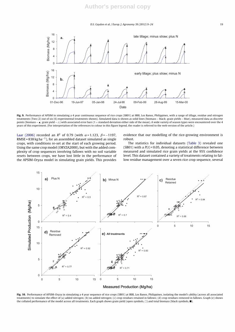
Fig. 9. Performance of APSIM in simulating a 4 year continuous sequence of rice crops (SB01) at IRRI, Los Banos, Philippines, with a range of tillage, residue and nitrogentreatments (Two (2) out of six (6) experimental treatments shown). Simulated data is shown as solid lines (biomass – black; grain yields – blue), measured data as discretepoints (biomass – �; grain yield – �) with associated error bars (1 × standard deviation either side of the mean). A wide variety of season types were encountered over the 4years of this experiment. (For interpretation of the references to colour in this figure legend, the reader is referred to the web version of the article.)

Laar (2006) recorded an R2 of 0.79 (with = 1.123, = −1197,RMSE = 838 kg ha−1), for an assembled dataset simulated as singlecrops, with conditions re-set at the start of each growing period.Using the same crop model (ORYZA2000), but with the added com-plexity of crop sequences involving fallows with no soil variableresets between crops, we have lost little in the performance ofthe APSIM-Oryza model in simulating grain yields. This provides

evidence that our modelling of the rice-growing environment isrobust.

The statistics for individual datasets (Table 3) revealed one(SB01) with a P(t) < 0.05, denoting a statistical difference betweenmeasured and simulated rice grain yields at the 95% confidencelevel. This dataset contained a variety of treatments relating to fal-low residue management over a seven rice crop sequence, several

R2 = 0.683 4

R2 = 0.84 04

0

5

10

15

0 5 10 15

Residue

Retained

R2 = 0.7064

R2 = 0.870 6

0

5

10

15

0 5 10 15

Minus N

R2 = 0.406 4

R2 = 0.500 7

0

5

10

15

0 5 10 15

Plus N

Sim

ula

ted

Pro

du

ction

(M

g/h

a)

Mea sured Product ion (Mg/ha )

a) b) c)

R2 = 0.712 9

R2 = 0.832 9

0

5

10

15

0 5 10 15

All treatmentsd)

R2 = 0.775 1

R2 = 0.9237

0

5

10

15

0 5 10 15

Residue

Removedd) e)

R2 = 0.683 4

R2 = 0.84 04

0

5

10

15

0 5 10 15

Residue

Retained

R2 = 0.7064

R2 = 0.870 6

0

5

10

15

0 5 10 15

Minus N

R2 = 0.406 4

R2 = 0.500 7

0

5

10

15

0 5 10 15

Plus N

Sim

ula

ted

Pro

du

ction

(M

g/h

a)

Mea sured Product ion (Mg/ha )

a) b) c)

R2 = 0.712 9

R2 = 0.832 9

0

5

10

15

0 5 10 15

All treatmentsd)

R2 = 0.775 1

R2 = 0.9237

0

5

10

15

0 5 10 15

Residue

Removedd) e)

Fig. 10. Performance of APSIM-Oryza in simulating a 4 year sequence of rice crops (SB01) at IRRI, Los Banos, Philippines, isolating the model’s ability (across all associatedtreatments) to simulate the effect of (a) added nitrogen; (b) no added nitrogen; (c) crop residues retained in fallows; (d) crop residues removed in fallows. Graph (e) showsthe collated performance of the model across all treatments. Each graph shows grain yield (open symbols, �) and total biomass (black symbols, �).



0

5

10

15

20

25

30

24-May-02 10-Dec-0 2 28- Jun- 03 14- Jan -04 01-Aug-04 17- Feb-05 05- Sep-05 24- Mar-0 6 10- Oct-06 28 -Apr-0 7

Pro

du

cti

on

(t/h

a)

Rice

Barley

Soybea n

Barley

Soybea n

Rice

0

100

200

300

400

25-May-0 2 11-De c-02 29-Jun-0 3 15-Jan-0 4 02-Aug-0 4 18- Feb-05 06-Sep-0 5 25- Mar-0 6 11- Oct-06 29-Apr-0 7

Date

So

il W

ate

r (m

m)

0

50

100

150

200

250

Flo

od

de

pth

Flood water

Dep th

0

4

8

12

16

Cro

p R

es

idu

es

(t/h

a)

stubb le burnt stubb le left on

surface

0

20

40

60

80

100

120

So

il N

(k

g/h

a)

measured NH 4

measured NO3NH4 NO3

Fig. 11. Simulated vs measured system data for GB06, Treatment 4: a rice–barley–soybean experimental rotation on a transitional red brown earth soil at Coleambally,NSW, Australia. Simulated production (t ha−1), crop residues (t ha−1), soil NH4, NO3 (kg ha−1) and soil water (mm) in top 90 cm soil, and floodwater depth (mm) are shown(Reference: Beecher et al., 2006). Ponded depths are less in Treatment 4 of this experiment (cf. treatments 1 and 2) due to the presence of beds in the rice bays.

R2 = 0.81

0

2

4

6

8

10

12

14

0 2 4 6 8 10 12 14

Measured

Sim

ula

ted

Rice crops

R2 = 0.91

0

2

4

6

8

10

0 2 4 6 8 10

Mea sure d

Sim

ula

ted

Other crops in rotation

with Ri ce

Soybe an

Wheat/ Barley R

2 = 0.81

0

2

4

6

8

10

12

14

0 2 4 6 8 10 12 14

Measured

Sim

ula

ted

Rice crops

R2 = 0.91

0

2

4

6

8

10

0 2 4 6 8 10

Mea sure d

Sim

ula

ted

Other crops in rotation

with Ri ce

Soybe an

Wheat/ Barley

Fig. 12. Comparison between measured and simulated grain yields (t ha−1) for all validation crop sequence experiments, for (a) rice crops; and (b) non-rice crops in rotationwith rice.



Table 3Statistics for measured vs simulated rice yield across the datasets.

Dataset abbreviation N Xmeas (SD) (kg ha−1) Xsim (SD) (kg ha−1) P(t) (kg ha−1) R2 RMSE (kg ha−1) EF

AB04 31 4135 (1562) 4227 (2224) 0.85 1.20 −751 0.71 1214 0.38AS09 24 5319 (1366) 5708 (1798) 0.4 1.19 −644 0.82 874 0.57SB01 56 4496 (1462) 3885 (1571) 0.04 0.91 −196 0.71 1043 0.48RB85 5 5599 (1129) 4855 (901) 0.28 0.80 395 0.99 773 0.41GB06 5 12204 (1487) 11733 (2240) 0.71 1.23 −3317 0.67 1281 0.37Overall (combined) 121 4931 (2160) 4699 (2423) 0.43 1.02 −323.23 0.82 1061 0.79

N, number of data pairs; Xmeas, mean of measured values; Xsim, mean of simulated values; SD, standard deviation; P(t), significance of Student’s paired t-test assumingnon-equal variances; ˛, slope of linear regression between simulated and measured values; ˇ, y-intercept of linear regression between simulated and measured values; R2,square of linear correlation coefficient between simulated and measured values; RMSE, absolute root mean squared error; EF, the modelling efficiency.

Table 4Calculation of Model Robustness index, IR, using standard deviations of the syntheticagro-meteorological indicator, SAM, and the modelling efficiency, EF (Eq. (4)). Ricegrain yield was the variable of focus.

Dataset Av. SAM EF

AS09 −0.228 0.573AB04 −0.225 0.376SB01 0.093 0.481RB85 0.244 0.414GB06 −0.564 0.37Standard deviation �SAM = 0.315 �EF = 0.085

IR = �SAM/�EF = 0.27

treatments of which were simulated extremely well (Figs. 9 and 10).For this reason, we sought to examine the sources of the revealederror more closely using the methods outlined by Kobayashi andSalam (2000).

We calculated these three components of MSD for observedversus simulated comparisons in each factorial treatment in SB01and presented them as a segmented summation of the MSD(Fig. 13). This analysis yielded a clear picture of the treatmentswhich exerted the greatest influence over the revealed error, andit also provided an insight into the nature of that error.

Fig. 13 shows that the Minus Residue treatments were simu-lated well, with no statistical difference between observed andsimulated grain yields for both the ±N factorials at the 95% con-fidence level (P(t) > 0.05). The dominant source of error lay in thePlus Residue treatments, particularly in the +N factorial. An exam-ination of the components of the MSD tell us that the SDSD wasa small component of the error, indicating the modelled grainyields demonstrated similar sensitivity to changes in conditionsas the observed grain yields. The largest source of error was the

0

5

10

15

20

25

Minus Residue -

Minus N

Minus Re sidue -

Plus N

Plus Residue -

Minus N

Plus Res idue -

Plus N

Mea

n S

qu

are

d D

evia

tio

n (

MS

D x

10

^5

)

LCS

SDSD

SB

P(t) = 0.17

P(t) = 0.69P(t) = 0.52

P(t) = 0.03

R = 0.782

R = 0.762

R = 0.642

R = 0.322

0

5

10

15

20

25

Minus Residue -

Minus N

Minus Re sidue -

Plus N

Plus Residue -

Minus N

Plus Res idue -

Plus N

Mea

n S

qu

are

d D

evia

tio

n (

MS

D x

10

^5

)

LCS

SDSD

SB

P(t) = 0.17

P(t) = 0.69P(t) = 0.52

P(t) = 0.03

R = 0.782

R = 0.762

R = 0.642

R = 0.322

Fig. 13. Breakup of the mean squared deviation (MSD) between simulated and mea-sured rice yield data for four (4) treatment categories in SB01. MSD is the sum ofthe squared bias (SB), the squared difference between standard deviations (SDSD),and the lack of correlation weighted by the standard deviations (LCS) (Kobayashiand Salam 20); P(t) is the significance of Student’s paired t-test assuming non-equalvariances.

LCS, indicating a general lack of correlation between simulated andmeasured yields when residue was retained in the fallows, an errorwhich was increased by the addition of N fertilizer. Anecdotal evi-dence from this experiment indicates that the fallows were oftenvery wet during this four year experiment. This suggests that thesimulation of N immobilization by residues during saturated fal-lows is a current weak point for APSIM, providing at least onedirection for further work on improving this modelling framework.

4. Discussion

The ability to simulate the performance of a single crop doesnot necessarily confirm accurate description of whole-of-systemprocesses in a model. Most models have many empirical inputparameters to adjust, and it is possible to achieve the “right resultsfor the wrong reasons”, particularly when simulating a single crop(Bellocchi et al., 2010; Sinclair and Seligman, 2000). Howeversuccessful simulation of cropping sequences (including several con-secutive crops, fallows, season types, residue treatments and othermanagement impositions), such as demonstrated in this paper,provides much greater confidence that the model is realisticallycapturing key system processes in both soil and crop arenas.

The soil environment is a complex ecosystem with numer-ous interacting physical, chemical and biological processes. Thiscomplexity is exemplified by transitions between flooded and non-flooded conditions. Some system elements are complex to modeland the relevant variables even more complex to measure, makingit difficult to directly confirm correct simulation. In our enhance-ments to APSIM we have chosen to ignore some well-known systemprocesses (which other models have described at length) on theassumption they do not significantly impact on the key systemvariables we wish to simulate (crop yields, water-use and N-useefficiency etc.). Examples include the thin oxidized layer whichdevelops at the surface of a submerged soil, and the aerobic rhizo-sphere which develops within millimeters of the crop roots. Both ofthese zones have been well studied, exhibiting N-transformationalprocesses such as ammonification, nitrification, and denitrification,however we have assumed the scale of these processes does notwarrant inclusion for a cropping systems model focused primarilyon simulation of crop production. N transformations within thesezones are implicitly captured within other calibrated parametersand constants, and are not modelled independently in our develop-ments. We have also assumed that reduced soil conditions developinstantly following ponding of water on the soil surface, despiteknowing in reality there is a lag period. Arah (2000) suggested that acomprehensive treatment of soil organic matter (SOM) transforma-tion in flooded rice requires at least the following: (1) an account ofbelow-ground O2 transport, occurring primarily through the roots,and (2) an account of the direct influence of O2 availability onSOM decomposition. Our model development philosophy has beento start with simple process descriptions of what we believe arethe key processes driving system performance, only adding furtherprocess descriptions (or enhancing detail of existing descriptions)



when simulations are not capable of capturing the dynamics of themeasured data of interest. Whereas the assertions of Arah (2000)are not questioned, our aim with APSIM is ultimately to model agri-cultural production, not detailed SOM dynamics. APSIM does notmodel O2 transport within the soil. Our simplified assumptions donot represent an alternative understanding of the key drivers ofSOM dynamics, rather a basic attempt to simplify description ofthe system for simulation of crop production.

In this paper we have tested our assumptions and new modelmodifications against a diverse range of collated experimental rice-based cropping datasets. In the absence of widely available soil Ndata to directly test our model improvements, we used crop grainyields as an indirect surrogate measure of model performance. Sim-ulations were performed over several years without any variableresets, simulating continuous dynamics of crops, water and soil.The particular focus for the testing has been crop sequences whichexhibit alternate anaerobic and aerobic soil conditions, representedby flooded and non-flooded phases in rice-based rotations. Thenon-flooded phases in our data-sets have consisted of dry fal-lows between rice crops, in addition to non-rice crops. We haveused published, replicated experimental datasets from Indonesia,Philippines, and Australia, capturing varying management imposi-tions, and have used robust statistical methods to help understandthe model’s strengths and current weaknesses.

The results of comparisons between simulated and observedvariables for these datasets have illustrated the strength of APSIM’snew capacity to simulate the rice-growing environment for the pur-poses of modelling crop yields, and therefore the practicality of ourmodifications. Revealed error between our observed and simulatedrice yields (APSIM-Oryza) showed little difference compared withthose reported for the stand-alone ORYZA2000 (Bouman and vanLaar, 2006), which were obtained through testing against singlecrop data sets. This was despite our simulations including sequencesof crops and fallows over several years with no soil variable resetsbetween crops. This indicates APSIM was able to simulate the start-ing and finishing soil conditions for each crop as least as well onaverage as the ORYZA2000 researchers were able to initialize soilvariables in each of their single-crop simulations.

The APSIM model showed particular strength in simulatingvaried crop sequences, response to applied fertilizers and the per-formance of bare fallows. Continuously submerged rice crops weresimulated better than those with periods of mild water stress, how-ever recent developments in ORYZA2000 science have addressedsome of these shortcomings (Yadav et al., 2011b; Tao Li, personalcommunication) and these will soon be implemented within thenow outdated APSIM-Oryza code. The model was able to simulatethe performance of both PTR and DSR on several soil types andin several different environments. The simulation of retained cropstubble during fallows was identified as an area for improvement,with immobilization N dynamics likely to be a driving feature. Fur-ther testing of the model against observed data from AWD andaerobic systems would assist in addressing revealed shortcomingsand better position the APSIM framework for future adaptationstudies in which these management systems are likely to play asignificant role. Further testing is also desirable in the simulationof new/future cropping systems, including newly emerging man-agement options such as no-till direct-seeded rice/conservationagriculture, or a range of potential future nutrient managementoptions. Specifically, datasets with detailed measurements of soilN and water, residues, and crop dynamics would be helpful infine-tuning APSIM performance in such systems. APSIM is alreadycapable of simulating total gaseous emissions of C and N (Probertet al., 1998), however further development work to segregategreenhouse gas (GHG) emissions into specific pools (N2, NO2, N2O,CO2, CH4) would be desirable for adding an additional perspectiveto future simulation studies on management options in rice-based

cropping systems. Further assessment is required on whether oursimplifying model assumptions (for example, ignoring the thinoxidized soil layer and oxidized root zone) remain valid when GHGemissions are the output variable of focus.

5. Conclusions

Any simulation model aiming to assist in evaluating futureadaptation strategies in rice-based cropping systems must be welltested in a range of possible configurations – different geograph-ical locations, soil types, crop mixes and sequences, agronomicmanagements (fertilizer, sowing criteria, crop establishment andtillage practices), irrigation practices and variation in incident cli-matic variables such as temperatures and CO2. In this paper wehave described the initial efforts in improving the APSIM modelfor rice-based systems, and presented evaluation against a rangeof experimental datasets for cropping sequences involving rice.We have demonstrated the robustness of APSIM’s new capacityto simulate the rice-growing environment (as affects crop pro-duction), and therefore the practicality of a number of simplifyingassumptions and modifications. The validation testing has allowedidentification of conditions under which the model is performingwell (crop rotations; response to applied fertilizers; the perfor-mance of bare fallows) and areas in which to concentrate furtherwork (simulation of N immobilization in retained crop stubbleduring fallows, greenhouse gas emissions). We will continue toseek datasets which allow further evaluation and enhancementof APSIM’s capacity to simulate new and innovative practices,as well as a greater diversity of environmental conditions. TheAPSIM framework is now a useful tool to investigate the productionimpacts of future climate and resource scenarios in rice-based crop-ping systems, as well as potential adaptation options in response tochanges. Further testing is required to evaluate the impact of oursimplified assumptions on APSIM’s simulation of greenhouse gasemissions in rice-based cropping systems.

Acknowledgments

The authors would like to thank the DSSAT group for access toCERES-Rice source code, and also the Ricegrowers Association ofAustralia (RGA), the Australian Department of Agriculture, Fisheriesand Forestry (DAFF), and the Australian Centre for InternationalAgricultural Research (ACIAR) for jointly funding this developmentwork. We also express our appreciation to Susanna Bucher (viaAchim Dobermann), Annie Boling (via Bas Bouman), Geoff Beecher,and Brian Dunn, for provision of datasets for model testing.

References

Acharya, C.N., 1935a. Studies on the anaerobic decomposition of plant materials.I. The anaerobic decomposition of rice straw (Oryza sativa). Biochem. J. 29,528–541.

Acharya, C.N., 1935b. Studies on the anaerobic decomposition of plant materials.II. Some factors influencing the anaerobic decomposition of rice straw (Oryzasativa). Biochem. J. 29, 953–960.

Acharya, C.N., 1935c. Studies on the anaerobic decomposition of plant materials.III. Comparison of the course of decomposition of rice straw under anaerobic,aerobic, and partially aerobic conditions. Biochem. J. 29, 1116–1120.

Ali, M.H., Talukder, M.S.U., 2008. Increasing water productivity in crop production– a synthesis. Agric. Water Manag. 95 (11), 1201–1213.

Arah, J.R.M., 2000. Modeling SOM cycling in rice-based production systems. In: G.J.D.Kirk, D.C. Olk (Eds.) Carbon and nitrogen dynamics in flooded soils. InternationalRice Research Institute, Makati City (Philippines), pp. 163–179.

Beecher, H.G., Dunn, B.W., Thompson, J.A., Humphreys, E., Mathews, S.K., Tim-sina, J., 2006. Effect of raised beds, irrigation and nitrogen management ongrowth, water use and yield of rice in south-eastern Australia. J. Exp. Agric. 46,1363–1372.

Belder, P., Bouman, B.A.M., Spiertz, J.H.J., Lu, G., 2007. Comparing options for watersavings in lowland rice using a modeling approach. Agric. Syst. 92, 91–114.



Bellocchi, G., Rivington, M., Donatelli, M., Matthews, K., 2010. Validation of bio-physical models: issues and methodologies. A review. Agron. Sustain. Dev. 30,109–130.

Bennett, J., 2003. Status of breeding for tolerance of water deficit and prospects forusing molecular techniques. In: J.W. Kijne, R., Baker, D. Molden, (Eds.), WaterProductivity in Agriculture: Limits and Opportunities for Improvement, CABI,Publishing, Wallingford, UK, pp. 103–126.

Boling, A., Tuong, T.P., Jatmiko, S.Y., Burac, M.A., 2004. Yield constraints of rainfedlowland rice in Central Java, Indonesia. Field Crops Res. 90, 351–360.

Bouman, B.A.M., Tuong, T.P., 2001. Field water management to save water andincrease its productivity in irrigated lowland rice. Agric. Water Manag. 49 (1),11–30.

Bouman, B.A.M., van Laar, H.H., 2006. Description and evaluation of the ricegrowth model ORYZA2000 under nitrogen-limited conditions. Agric. Syst. 87,249–273.

Bouman, B.A.M., 2007. A conceptual framework for the improvement of crop waterproductivity at different spatial scales, Agricultural Systems 93 (1–3), 43–60.

Bouman, B.A.M., Lampayan, R., Tuong, T., 2007. Water Management in Irrigated Rice– coping with water scarcity. International Rice Research Institute publication,Los Banos, Philippines.

Bucher, S., 2001. Nitrogen and phosphorus availability in irrigated rice as influencedby soil drying during the fallow period, straw incorporation, and tillage. PhDdissertation submitted to the Swiss Federal Institute of Technology Zurich, Diss.ETH No. 14017.

Buresh, R.J., Reddy, K.R., van Kessel, C., 2008. Nitrogen transformations in submergedsoils. In: Schepers, J.S., Raun, W.R. (Eds.), Nitrogen in Agricultural Systems.Agronomy Monograph 49. ASA, CSSA, and SSSA, Madison, WI, USA, pp. 401–436.

Buresh, R.J., De Datta, S.K., 1991. Nitrogen dynamics and management inrice–legume cropping systems. Adv. Agron. 45, 1–59.

Buresh, R.J., De Datta, S.K., 1990. Denitrification losses from puddled rice soils in thetropics. Biol. Fert. Soils 9, 1–13.

Buresh, R.J., De Datta, S.K., Padilla, J.L., Samson, M.I., 1988. Effect of two ureaseinhibitors on floodwater ammonia following urea application to lowland rice.Soil Sci. Am. Soc. J. 52, 856–861.

Buresh, R.J., Casselman, M.E., Patrick Jr., W.H., 1980. Nitrogen fixation in flooded soilsystems, a review. Adv. Agron. 33, 149–192.

Carberry, P.S., Probert, M.E., Dimes, J.P., Keating, B.A., McCown, R.L., 2002. Role ofmodelling in improving nutrient efficiency in cropping systems. Plant Soil 245,193–203.

Cho, Y.S., Hidaka, K., Mineta, T., 2003. Evaluation of white clover and rye grown inrotation with no-tilled rice. Field Crops Res. 83 (3), 237–250.

Chowdary, V.M., Rao, N.H., Sarma, P.B.S., 2004. A coupled soil water and nitrogenbalance model for flooded rice fields in India. Agric. Ecosyst. Environ. 103 (3),425–441.

Confalonieri, R., Acutis, M., Bellocchi, G., Cerrani, I., Tarantola, S., Donatelli, M.,Genovese, G., 2006. Exploratory sensitivity analysis of CropSyst WARM andWOFOST: a case-study with rice biomass simulations. Ital. J. Agrometeorol. 11,17–25.

Confalonieri, R., Bregaglio, S., Acutisa, M., 2010. A proposal of an indicator for quan-tifying model robustness based on the relationship between variability of errorsand of explored conditions. Ecol. Modell. 221, 960–964.

De Datta, Buresh, S.K., Samson, R.J., Wang Kai-Rong., M.I., 1988. Nitrogen use effi-ciency and N-15 balances in broadcast-seeded flooded and transplanted rice.Soil Sci. Soc. Am. J. 52, 849–855.

Devendra, C., Thomas, D., 2002. Smallholder farming systems in Asia. Agric. Syst. 71(1-2), 17–25.

Dobermann, A., Witt, C., 2000. The potential impact of crop intensification on carbonand nitrogen cycling in intensive rice systems. In: G.J.D. Kirk, D.C. Olk (Eds.),Carbon and Nitrogen Dynamics in Flooded Rice: Proceedings of the Workshopon Carbon and Nitrogen Dynamics in Flooded Soils, IRRI, Los Banõs, Laguna,Philippines, 19–22 April 2000, p. 188.

Fillery, I.R.P., Vlek, P.L.G., 1983. Reappraisal of the significance of ammoniavolatilization as an N loss mechanism in flooded rice fields. In: Nitrogen econ-omy of flooded rice soils, Washington DC, USA, Dordrecht: Martinus Nijhoff,Netherlands.

Gaydon, D.S., Probert, M.E., Buresh, R.J., Meinke, H., Timsina, J., 2012. Capturingthe role of algae in rice crop production and soil organic carbon maintenance,submitted to European Journal of Agronomy.

Gaydon D.S., Lisson S.N., Xevi E., 2006. Application of APSIM ‘multi-paddock’ toestimate whole-of-farm water-use efficiency, system water balance and cropproduction for a rice-based operation in the Coleambally Irrigation District,NSW, Proceedings of the 13th Australian Society of Agronomy Conference,10–14 September 2006, Perth, Western Australia.

Godwin, D.C., Singh, U., Buresh, R.J., De Datta, S.K., 1990. Modeling of nitrogendynamics in relation to rice growth and yield. Transactions 14th InternationalCongress of Soil Science, Kyoto, Japan. Volume IV, pp. 320–325.

Godwin, D.C., Singh, U., 1991. Modelling nitrogen dynamics in rice croppingsystems. In: Deturek and Ponnamperuma (Eds), Rice Production on AcidSoils of the Tropics, Institute of Fundamental Studies, Kandy, Sri Lanka,pp. 287–294.

Humphreys, E., Kukal, S.S., Christen, E.W., Hira, G.S., Singh, B., Yadav, S., Sharma,R.K., 2010. Halting the groundwater decline in north-west India – which croptechnologies will be winners? Adv. Agron. 109, 155–217.

Jamu, D.M., Piedrahita, R.H., 2002. An organic matter and nitrogen dynamics modelfor the ecological analysis of integrated aquaculture/agriculture systems: I.model development and calibration. Environ. Model. Software 17 (6), 571–582.

Jing, Q., van Keulen, H., Hengsdijk, H., 2010. Modeling biomass, nitrogen and waterdynamics in rice–wheat rotations. Agric. Syst. 103, 433–443.

Jing, Q., Hengsdijk, H., van Keulen, H., 2007. Modeling nitrogen and water dynam-ics in rice-wheat rotations. Proceedings Third IASTED International ConferenceEnvironmental Modelling and Simulation, Honolulu, Hawaii, USA, pp. 121–126.ISBN CD 978-0-88986-682-9.

Jones, C.A., Kiniry, J.R., 1986. CERES-Maize: A Simulation Model of Maize Growthand Development. Texas A&M University Press, College Station, Texas.

Keating, B.A., Carberry, P.S., Bindraban, P.S., Asseng, S., Meinke, H., Dixon, J. (2010).Eco-efficient Agriculture: Concepts, Challenges, and Opportunities, Crop Science50 (suppl. 1), S109–S119.

Keating, B.A., Carberry, P.S., Hammer, G.L., Probert, M.E., Robertson, M.J., Holzworth,D., Huth, N.I., Hargreaves, J.N.G., Meinke, H., Hochman, Z., McLean, G., Verburg,K., Snow, V., Dimes, J.P., Silburn, M., Wang, E., Brown, S., Bristow, K.L., Asseng,S., Chapman, S., McCown, R.L., Freebairn, D.M., Smith, C.J., 2003. An overviewof APSIM, a model designed for farming systems simulation. Eur. J. Agron. 18,267–288.

Kemanian, A.R., Stöckle, C.O., 2010. C-Farm: a simple model to evaluate the carbonbalance of soil profiles. Eur. J. Agron. 32 (1), 22–29.

Kirk, G.J.D., 2004. The Biogeochemistry of Submerged Soils. John Wiley & Sons, WestSussex, England.

Kirk, G.J.D., Olk, D.C., 2000. Carbon and Nitrogen Dynamics in Flooded Soils. IRRI, LosBanos, Philippines, p. 250.

Kobayashi, K., Salam, M.U., 2000. Comparing simulated and measured val-ues using mean squared deviation and its components. Agron. J. 92,345–352.

Krause, P., Boyle, D.P., Bäse, F., 2005. Comparison of different efficiency criteria forhydrological model assessment. Adv. Geosci. 5, 89–97.

Li, C., Frolking, S., Harriss, R.C., 1994. Modelling carbon biogeochemistry in agricul-tural soils. Glob. Biogeochem. Cycle 8, 237–254.

Pampolino, M.F., Laureles, E.V., Gines, H.C., Buresh, R.J., 2008. Soil carbon and nitro-gen changes in long-term continuous lowland rice cropping. Soil Sci. Soc. Am. J.72 (3), 798–807.

Peng, S., Cassman, K.G., Virmani, S.S., Sheehy, J., Khush, G.S., 1999. Yield potentialtrends of tropical rice since the release of IR8 and the challenge of increasingrice yield potential. Crop Sci. 39, 1552–1559.

Probert, M.E.P., Dimes, J.P., Keating, B.A., Dalal, R.C., Strong, W.M., 1998. APSIM’swater and nitrogen modules and simulation of the dynamics of water and nitro-gen in fallow systems. Agric. Syst. 56 (1), 1–28.

Rijsberman, F.R., 2006. Water scarcity: fact or fiction? Agric. Water Manag. 80, 5–22.Ritchie, J.T., 1972. Model for predicting evaporation from a row crop with incomplete

cover. Water Resour. Res. 8 (5), 1204–1213.Robertson, M.J., Carberry, P.S., Huth, N.I., Turpin, J.E., Probert, M.E., Poulton, P.L.,

Bell, M., Wright, G.C., Yeates, S.J., Brinsmead, B.R., 2002. Simulation of growthand development of diverse legume species in APSIM. Aust. J. Agric. Res. 53 (4),429–446.

Roger, P.A., Ladha, J.K., 1992. Biological nitrogen fixation in wetland rice fields:estimation and contribution to nitrogen balance. Plant Soil 141, 41–55.

Sinclair, T.R., Seligman, N., 2000. Criteria for publishing papers on crop modelling.Field Crops Res. 68, 165–172.

Singh, V.K., Dwivedia, B.S., Shuklaa, A.K., Chauhan, Y.S., Yadav, R.L., 2005. Diversi-fication of rice with pigeon pea in a rice–wheat cropping system on a TypicUstochrept: effect on soil fertility yield and nutrient use efficiency. Field CropsRes. 92 (1), 85–105.

Sheehy, J.E., Mitchell, P.L., Hardy, B. (Eds.), 2000. Redesigning Rice Pho-tosynthesis to Increase Yield, Elsevier Science, Amsterdam, Netherlands,p. 293.

Shibu, M.E., Leffelaar, P.A., van Keulen, H., Aggarwal, P.K., 2006. Quantitative descrip-tion of soil organic matter dynamics – a review of approaches with reference torice-based cropping systems. Geoderma 137 (1-2), 1–18.

Stöckle, C.O., Donatelli, M., Nelson, R., 2003. CropSyst, a cropping systems simulationmodel. Eur. J. Agron. 18, 289–307.

Sudhir-Yadav, Humphreys, E., Kukal, S.S., Gill, G., Rangarajan, R., 2011a. Effect ofwater management on dry seeded and puddled transplanted rice: Part 2: waterbalance and water productivity. Field Crops Res. 120 (1), 123–132.

Sudhir-Yadav, Li, T., Humphreys, E., Gill, G., Kukal, S.S., 2011b. Evaluation and appli-cation of ORYZA2000 for irrigation scheduling of puddled transplanted rice inNorth West India. Field Crops Res. 122 (2), 104–117.

Suriadi, A., Misra, R., Gaydon, D.S., Abawi, G.Y., 2009. Performance of rice on a coarsesandy loam soil in response to water-saving irrigation practices in lowland east-ern Indonesia. In: Proceedings of Farming Systems Design 2009 – InternationalSymposium on Methodologies for Integrated Analysis of Farm Production Sys-tems, Monterey, California, USA, 23–26 August.

Thorburn, P.J., Probert, M.E., Robertson, F.A., 2001. Modelling decomposition ofsugar cane surface residues with APSIM-residue. Field Crops Res. 70 (3),223–232.

Timsina, J., Humphreys, E., 2006. Performance of CERES-rice and CERES-wheat mod-els in rice-wheat systems: a review. Agric. Syst. 90 (1-3), 5–31.

Tuong, T.P., Bouman, B.A.M., Mortimer, M., 2005. More rice, less water – integratedapproaches for increasing water productivity in irrigated rice based systems inAsia. Plant Prod. Sci. 8 (3), 229–239.

Turpin, J.E., Carberry, P.S., McCown, R.L., Probert, M.E., 1998. Simula-tion of legume-cereal systems using APSIM. Aust. J. Agric. Res. 49 (3),317–328.

Van Keulen, H., Wolf, J., 1986. Modelling of Agricultural Production: Weather Soilsand Crops. Simulation Monographs, Pudoc, Wageningen.



Verburg, K., Bond, W.J., 2003. Use of APSIM to simulate water balances of drylandfarming systems in south eastern Australia, CSIRO Land and Water, Canberra,Technical Report 50/03.

Villegas-Pangga, G., Blair, G., Lefroy, R., 2000. Measurement of decomposition andassociated nutrient release from straw (Oryza sativa L.) of different rice varietiesusing perfusion system. Plant Soil 223, 1–11.

Whitbread, A.M., Robertson, M.J., Carberry, P.S., Dimes, J.P., 2010. How farmingsystems simulation can aid the development of more sustainable smallholderfarming systems in southern Africa. Eur. J. Agron. 32 (1), 52–58.

Willmott, C.J., 1981. On the validation of models. Phys. Geogr. 2, 184–194.Zeng, X., Sun, N., Gao, J., Wang, B., Li, L., 2007. Effects of cropping system change

for paddy field with double harvest rice on the crops growth and soil nutrient.Agric. Sci. Chin. 6 (9), 1115–1123.

Zhang, X., Jae-Hong Lee, Abawi, Y., Young-ho Kim, Hee-Dong Kim, 2006. Testingthe simulation capability of APSIM-ORYZA under different levels of nitrogenfertiliser and transplanting time regimes in Korea. Aust. J. Exp. Agric. 47 (12),1446–1454.

APSIM Rice Modeling Asia 1- Europeaan J. Agronomy

Documents

Transcript of APSIM Rice Modeling Asia 1- Europeaan J. Agronomy