Approximation by quantization of the filter process and

applications to optimal stopping problems under partial

observation

Huyen PHAM

Laboratoire de Probabilites et

Modeles Aleatoires

CNRS, UMR 7599

Universite Paris 7

pham@math.jussieu.fr

and CREST

Wolfgang RUNGGALDIER

Dipartimenta di Matematica

Pura ed Applicata

Universita degli studi di Padova

runggal@math.unipd.it

Afef SELLAMI

Laboratoire de Probabilites et

Modeles Aleatoires

CNRS, UMR 7599

Universite Paris 7

sellami@math.jussieu.fr

Abstract

We present an approximation method for discrete time nonlinear filtering in view ofsolving dynamic optimization problems under partial information. The method is basedon quantization of the Markov pair process filter-observation (Π, Y ) and is such that, ateach time step k and for a given size Nk of the quantization grid in period k, this grid ischosen to minimize a suitable quantization error. The algorithm is based on a stochasticgradient descent combined with Monte-Carlo simulations of (Π, Y ). Convergence resultsare given and applications to optimal stopping under partial observation are discussed.Numerical results are presented for a particular stopping problem : American optionpricing with unobservable volatility.

Key words: Nonlinear filtering, Markov chain, quantization, stochastic gradient descent,Monte-Carlo simulations, partial observation, optimal stopping.

MSC Classification (2000): 60G35, 65C20, 65N50, 62L20, 60G40.

1

1 Introduction

We consider a discrete time, partially observable process (X, Y ) where X represents thestate or signal process that may not be observable, while Y is the observation. The signalprocess {Xk, k ∈ N} is valued in a measurable space (E, E) and is a Markov chain withprobability transition (Pk) (i.e. the transition from time k−1 to time k), and initial law µ.The observation sequence (Yk) is valued in Rd and such that the pair (Xk, Yk) is a Markovchain and

(H) The law of Yk conditional on (Xk−1, Yk−1, Xk), k ≥ 1, denoted qk(Xk−1, Yk−1, Xk, dy′),admits a bounded density

y′ 7−→ gk(Xk−1, Yk−1, Xk, y′).

For simplicity, we assume that Y0 is a known deterministic constant equal to y0. No-tice that the probability transition of the Markov chain (Xk, Yk)k∈N is then given byPk(x, dx′)gk(x, y, x′, y′)dy′ with initial law µ(dx)δy0(dy).

We denote by (FYk ) the filtration generated by the observation process (Yk) and by Πk

the filter conditional law of Xk given FYk :

Πk(dx) = P[Xk ∈ dx| FY

k

], k ∈ N.

The filter process (Πk)k allows one to transform problems related to the partially ob-served process (X, Y ) into equivalent problems under complete observation related to thepair (Π, Y ) and this latter pair turns out to be Markov with respect to the observationfiltration (FY

k ). An important class of problems related to partially observable processesare stochastic control and stopping problems that are dynamic stochastic optimizationproblems where the partial observation concerns the state/signal process. We shall, in par-ticular, consider optimal stopping under partial information and, in this context, a financialapplication concerning the pricing of American options in a partially observed stochasticvolatility model.

We shall assume that the state space E of the state/signal process (Xk) consists of afinite number m of points. Problems with a more general state space can be approximatedby problems with a finite state space (see e.g. [8]). With Xk taking the m values xi (i =1, · · · ,m), the filter process is characterized by an m−vector with components Πi

k = P[Xk =xi|FY

k ] and takes thus values in the m−simplex Km in Rm. While the filter process allowsthus to transform a problem under partial observation into one under full observation, ithas the drawback that a finite-valued state space becomes infinite. This leads to difficultieswhen trying to solve dynamic optimization problems also in discrete time. For actualcomputation one has thus to discretize the process (Πk), approximating it with a processthat takes a finite number of values in the simplex Km. Approaches to this effect haveappeared in the literature; they are based on discretizing the observations process (Yk) andthen approximating Πk by a filter of Xk, given the discretized observations path (see e.g.[5], [3], [15], [10] and references therein). Such an approach has the drawback that thenumber of possible values for the approximating filter grows exponentially fast with thetime step.

2

In this paper, we propose a new approach by exploiting the Markov property of (Π, Y )k

with respect to the observation filtration (FYk ) : the conditional law of Xk+1 given FY

k

is summarized by the sufficient statistics (Πk, Yk) valued in Km × Rd. This suggests toapproximate the couple process (Π, Y ) with (Π, Y ) that in the generic time step k takes anumber of values Nk that can be assigned arbitrarily. Following standard usage, we shallcall this quantization and the problem then arises to find an optimal quantization, namelysuch that it minimizes for each time period k the L2−approximation error induced by thequantization. This error is related to what e.g. in information theory is called distorsion.The implementation of the minimizing algorithm itself is based on a stochastic gradientdescent method combined with Monte-Carlo simulations of (Π, Y ). As a byproduct, weobtain an approximation of the probability transition matrices of the Markov chain (Π, Y ).These companion parameters provide in turn an approximation algorithm , via the dynamicprogramming principle, for computing optimal values associated to dynamic optimizationproblems under partial observation.

Optimal quantization methods have been developed recently in numerical probabilityand various problems of optimal stopping, control or nonlinear filtering, see [11], [1], [2],[13], [14], [12]. In our context, we obtain error bounds and rate of convergence for theapproximation of the pair filter-observation process (Π, Y ). We then give an applicationto the approximation of optimal stopping problem under partial observation and studyassociated convergence results. Finally, we present a numerical illustration for the Americanoption pricing problem with unobservable volatility.

The rest of the paper is organized as follows. In Section 2, we recall some preliminarieson nonlinear filtering. Section 3 is the heart of the paper. We first present the quantizationapproximation method for the filter-observation Markov chain, and then analyze the in-duced error. The rate of convergence and the practical implementation of the algorithm forthe optimal quantization are discussed. In Section 4, we apply our quantization method tothe approximation of an optimal stopping problem under partial observation. Convergenceresults for the associated optimal value functions are provided. The last Section 5 presentsnumerical tests for the American option pricing with unobservable volatility.

2 Preliminaries

We denote byM(E) the set of finite nonnegative measures on (E, E) and by P(E) the subsetof probability measures on (E, E). It is known that M(E) is a Polish space equipped withthe weak topology, hence a measurable space endowed with the Borel σ-field. We recallthat from Bayes formula, Πk is given in inductive form by :

Π0 = µ

Πk = Gk(Πk−1, Yk−1, Yk), k ≥ 1, (2.1)

where Gk is the continuous function from M(E)× Rd × Rd into M(E) defined by :

Gk(π, y, y′)(dx′) =∫

Egk(x, y, x′, y′)Pk(x, dx′)π(dx),

3

and Gk is the normalized continuous function valued in P(E) :

Gk(π, y, y′) =Gk(π, y, y′)∫

E Gk(π, y, y′)(dx′).

Denoting by (Fk) the filtration generated by (Xk, Yk), and using the law of iterated condi-tional expectations, we have for any k and bounded Borelian function ϕ on P(E)× Rd :

E[ϕ(Πk+1, Yk+1)| FY

k

]= E

[E[ϕ(Gk+1(Πk, Yk, Yk+1), Yk+1)|Fk]

∣∣FYk

]= E

[∫ϕ(Gk+1(Πk, Yk, y

′), y′)Pk+1(Xk, dx′)qk+1(Xk, Yk, x′, dy′)

∣∣∣∣FYk

]=

∫ϕ(Gk+1(Πk, Yk, y

′), y′)Pk+1(x, dx′)qk+1(x, Yk, x′, dy′)Πk(dx). (2.2)

This proves that the pair (Πk, Yk)k is a (P, (FYk )k) Markov chain in P(E)×Rd, with initial

value (µ, y0). Moreover, under (H), this also shows that the (unnormalized) law of Yk

conditional on (Πk−1, Yk−1), denoted Qk(Πk−1, Yk−1, dy′) admits a density given by :

y′ 7−→∫

Gk(Πk−1, Yk−1, y′)(dx′) =

∫gk(x, Yk−1, x

′, y′)Pk(x, dx′)Πk−1(dx). (2.3)

Notice that the probability transition Rk (from time k − 1 to k) of the Markov chain(Πk, Yk)k is not explicit in general. Actually, from (2.2), we can write :

Rkϕ(π, y) =∫

ϕ(Gk(π, y, y′), y′)Qk(π, y, dy′), ∀(π, y) ∈ P(E)× Rd. (2.4)

In the sequel, we denote by |.|2 the Euclidian norm and by |.|1 the l1 norm on Rl. Forany Rl-valued random variable U , we denote :

‖U‖2

=(E|U |2

2

) 12 and ‖U‖

1= E|U |1 .

3 An optimal quantization approach for the approximation

of the filter process

3.1 The approximation method

We assume here that the state space E of the signal process (Xk) is finite consisting of m

points : E = {x1, . . . , xm}. The initial discrete law µ = (µi) and the probability transitionmatrix Pk are defined by :

µi = P[X0 = xi], i = 1, . . . ,m,

P ijk = P[Xk = xj |Xk−1 = xi], i, j = 1, . . . ,m.

The random filter Πk is characterized by its random weights :

Πik = P[Xk = xi|FY

k ], i = 1, . . . ,m,

4

and may then be identified with a random vector valued in the m-simplex Km in Rm ofdimension m− 1 :

Km =

{π = (πi) ∈ Rm : πi ≥ 0, 1 ≤ i ≤ m, |π|1 =

m∑i=1

πi = 1

}.

By (2.1), it is expressed in the recursive form :

Π0 = µ

Πk = Gk(Πk−1, Yk−1, Yk) =GPk(Yk−1, Yk)>Πk−1

|GPk(Yk−1, Yk)>Πk−1|1, (3.1)

where GPk(Yk−1, Yk) is a m×m random matrix given by :

GPk(Yk−1, Yk)ij = gk(xik−1, Yk−1, x

jk, Yk)P ij

k , 1 ≤ i, j ≤ m. (3.2)

Here M> denotes the transpose of a matrix M .A first approach for approximating the filter process (Πk) consists in discretizing the

observation process (Yk) by replacing it by a process (Yk) taking a finite number N ofvalues, and then approximate for each k the random filter Πk by a random filter of Xk

given Y1, . . . , Yk. So at each time step k, given Yk and Πk, the random variable Πk+1 maytake N values. Thus, at time n, the random filter Πn is identified with a random vectortaking Nn possible values. All these values are precomputed and stored in a “look-up table”but this could be very heavy, typically when n is large. Such an approach was introducedin [5] and [3], and investigated further in [15],[10] and [16].

We propose here a new approach. This starts from the key remark that the pair process(Πk, Yk) is Markov with respect to the observation filtration (FY

k ). In other words, theconditional law of Xk+1 given FY

k may be summarized by the sufficient statistic (Πk, Yk).Therefore, since the Markov chain (Πk, Yk) is completely characterized by its probabilitytransitions, the idea is to approximate these probability transitions by suitable probabilitytransition matrices.

In a first step, we discretize for each k the couple (Πk, Yk) by approximating it by(Πk, Yk) taking a finite number of values. The space discretization (or quantization) of therandom vector Zk = (Πk, Yk) in Km × Rd is constructed as follows. At initial time k = 0,recall that Z0 is a known deterministic vector equal to z0 = (µ, y0), so we start from thegrid with one point in Km × Rd :

Γ0 = {z0 = (µ, y0)} .

At time k ≥ 1, we are given a grid Γk of Nk points in Km × Rd :

Γk ={

z1k = (πk(1), y1

k), . . . , zNkk = (πk(Nk), yNk

k )}

,

and we denote by Ci(Γk), i = 1, . . . , Nk, the associated Voronoi tesselations :

Ci(Γk) ={

z ∈ Km × Rd : ProjΓk(z) = zi

k

}, i = 1, . . . , Nk.

5

Here ProjΓkis a closest neighbor projection for the Euclidian norm :∣∣z − ProjΓk

(z)∣∣2

= mini=1,...,Nk

|z − zik|2 , ∀ z ∈ Km × Rd.

Notice that by definition of the Euclidian norm, we clearly have :

ProjΓk=(

ProjΓΠk, ProjΓY

k

), Ci(Γk) = Ci(ΓΠ

k )× Ci(ΓYk ),

where :

ΓΠk = {πk(1), . . . , πk(Nk)}

ΓYk =

{y1

k, . . . , yNkk

}.

We then approximate the pair Zk = (Πk, Yk) by Zk = (Πk, Yk) valued in Γk and definedby :

Zk = ProjΓk(Zk) =

(ProjΓΠ

k(Πk), ProjΓY

k(Yk)

).

In a second step, we approximate the probability transitions of the Markov chain (Zk) :

Rk(z, dz′) = P[Zk ∈ dz′|Zk−1 = z

], k ≥ 1, z ∈ Km × Rd,

by the following probability transition matrix :

rijk = P

[Zk = zj

k

∣∣∣ Zk−1 = zik−1

]=

P [Zk ∈ Cj(Γk), Zk−1 ∈ Ci(Γk−1)]P [Zk−1 ∈ Ci(Γk−1)]

=:βij

k

pik−1

,

for all k ≥ 1, i = 1, . . . , Nk−1, j = 1, . . . , Nk. We shall see later how the grids Γk andthe number of points Nk are optimally chosen and implemented, and how the associatedprobability transition matrix rk can be estimated.

Example : Computation of predictor conditional expectation.

Suppose we are interested in the computation for any k = 0, . . . , n, and for arbitrarymeasurable function ϕk+1 on Km × Rd, of the filter predictor :

Uk = E[ϕk+1(Xk+1, Yk+1)| FY

k

].

A precise application where such FYk -measurable random variables appear is presented in

Section 4. Then, by introducing the function :

ϕk+1(π, y) =m∑

i=1

ϕk+1(xi, y)πi, ∀ π = (πi)i ∈ Km, ∀y ∈ Rd,

and using the law of iterated conditional expectation, we can rewrite Uk as :

Uk = E[ϕk+1(Πk+1, Yk+1)| FY

k

]= E

[ϕk+1(Zk+1)| FY

k

].

We thus approximate the sequence of FYk -measurable random variables Uk by Uk = vk(Zk)

where the functions vk, k = 0, . . . , n, are defined on Γk by :

vk(zik) = E

[ϕk+1(Zk+1)

∣∣∣ Zk = zik

]=

Nk+1∑j=1

rijk+1ϕk+1(zj

k+1), ∀ zik ∈ Γk.

6

3.2 The error analysis

The quality of the approximation described in the previous paragraph is measured as fol-lows. We denote for any subset D in Rl :

BL1(D) = {ϕ Borelian from D into R :

‖ϕ‖sup := supx∈D

|ϕ(x)| ≤ 1, [ϕ]lip

:= supx,y∈D,x 6=y

|ϕ(x)− ϕ(y)||x− y|1

≤ 1

}.

We make the following assumption.

(H1) There exists a constant Lg such that for all k ≥ 1 :

m∑i,j=1

P ijk

∫ ∣∣gk(xi, y, xj , y′)− gk(xi, y, xj , y′)∣∣ dy′ ≤ Lg|y − y|1 , ∀y, y ∈ Rd.

Proposition 3.1 Under (H1), we have for any n and ϕ1, . . ., ϕn ∈ BL1(Km × Rd) :∣∣∣∣∫ ϕ1(z1) . . . ϕn(zn) (R1(z0, dz1) . . . Rn(zn−1, dzn) − r1(z0, dz1) . . . rn(zn−1, dzn))∣∣∣∣

≤n∑

k=1

3√

m + d

2Lg − 1

[(2Lg)n−k+1 − 1

] ∥∥∥Zk − Zk

∥∥∥2

, (3.3)

where Lg = max(Lg, 1).

We first state a preliminary result on the Lipschitz property of the transition of theMarkov chain (Zk)k = (Πk, Yk)k.

Lemma 3.1 Under (H1), we have for all k ≥ 1 and Borelian function ϕ on Km × Rd :

|Rkϕ(z)−Rkϕ(z)| ≤(2[ϕ]

lip+ ‖ϕ‖sup

)Lg |z − z|1 , ∀z, z ∈ Km × Rd.

Proof. Recall from (2.3) that the conditional law Qk(π, y, dy′) of Yk given (Πk−1, Yk−1) =(π, y) admits a density given by :

y′ 7−→ fk(π, y, y′) =m∑

i,j=1

gk(xi, y, xj , y′)P ijk πi.

This conditional density satisfies the Lipschitz property : for all (π, y) and (π, y) ∈Km×Rd,∫ ∣∣fk(π, y, y′)− fk(π, y, y′)∣∣ dy′ ≤

m∑i,j=1

P ijk

∫ ∣∣gk(xi, y, xj , y′)− gk(xi, y, xj , y′)∣∣ dy′

+m∑i

|πi − πi|, (3.4)

7

where we used the fact that∑

j P ijk

∫gk(xi, y, xj , y′)dy′ = 1. From (2.4), we then have for

any z = (π, y) and z = (π, y) ∈ Km × Rd :

|Rkϕ(z)−Rkϕ(z)| ≤∫ ∣∣ϕ(Gk(π, y, y′), y′)− ϕ(Gk(π, y, y′), y′)

∣∣Qk(π, y, dy′)

+∣∣∣∣∫ ϕ(Gk(π, y, y′), y′)

(Qk(π, y, dy′)−Qk(π, y, dy′)

)∣∣∣∣≤ [ϕ]

lip

∫ ∣∣Gk(π, y, y′)− Gk(π, y, y′)∣∣1fk(π, y, y′)dy′

+ ‖ϕ‖sup

∫ ∣∣fk(π, y, , y′)− fk(π, y, y′)∣∣ dy′

≤ [ϕ]lip

∫ ∣∣Gk(π, y, y′)− Gk(π, y, y′)∣∣1fk(π, y, y′)dy′

+ ‖ϕ‖sup

m∑i,j=1

P ijk

∫ ∣∣gk(xi, y, xj , y′)− gk(xi, y, xj , y′)∣∣ dy′

+ ‖ϕ‖sup

m∑i

|πi − πi|. (3.5)

Now, from (3.2), we have :∫ ∣∣Gk(π, y, y′)− Gk(π, y, y′)∣∣1fk(π, y, y′)dy′

≤m∑

j=1

∫ ∣∣∣Gjk(π, y, y′)− Gj

k(π, y, y′)∣∣∣ fk(π, y, y′)dy′

=m∑

i,j=1

∫ ∣∣∣∣∣gk(xi, y, xj , y′)P ijk πi

fk(π, y, y′)−

gk(xi, y, xj , y′)P ijk πi

fk(π, y, y′)

∣∣∣∣∣ fk(π, y, y′)dy′

≤m∑

i,j=1

P ijk πi

∫ ∣∣gk(xi, y, xj , y′)fk(π, y, y′)− gk(xi, y, xj , y′)fk(π, y, y′)∣∣

fk(π, y, y′)dy′

+m∑

i=1

|πi − πi|

≤m∑

i,j=1

P ijk

∫ ∣∣gk(xi, y, xj , y′)− gk(xi, y, xj , y′)∣∣ dy′

+∫ ∣∣fk(π, y, y′)− fk(π, y, y′)

∣∣ dy′ +m∑

i=1

|πi − πi|

≤ 2m∑

i,j=1

P ijk

∫ ∣∣gk(xi, y, xj , y′)− gk(xi, y, xj , y′)∣∣ dy′ + 2

m∑i=1

|πi − πi|,

where we used again (3.4). Plugging into (3.5) and using (H1) yield :

|Rkϕ(z)−Rkϕ(z)|

≤(2[ϕ]

lip+ ‖ϕ‖sup

) m∑i,j=1

P ijk

∫ ∣∣gk(xi, y, xj , y′)− gk(xi, y, xj , y′)∣∣ dy′ +

m∑i=1

|πi − πi|

8

≤(2[ϕ]

lip+ ‖ϕ‖sup

)(Lg|y − y|1 + |π − π|1) , (3.6)

and then the required result. 2

Remark 3.1 In the case where the law of Yk conditional on (Xk−1, Yk−1, Xk) does notdepend on Yk−1, i.e. its density gk depends only Xk−1, Xk, the condition (H1) is empty,or in other words is trivially satisfied wth Lg = 0. Then, inequality (3.6) shows that for allz = (π, y), z = (π, y) ∈ Km × Rd,

|Rkϕ(z)−Rkϕ(z)| ≤(2[ϕ]

lip+ ‖ϕ‖sup

)|π − π|1 . (3.7)

Proof of Proposition 3.1. For k = 1, . . . , n, we define the measurable functions onKm × Rd, resp. on Γk :

vk(z) = ϕk(z)∫

ϕk+1(zk+1) . . . ϕn(zn)Rk+1(z, dzk+1) . . . Rn(zn−1, dzn),

vk(z) = ϕk(z)∫

ϕk+1(zk+1) . . . ϕn(zn)rk+1(z, dzk+1) . . . rn(zn−1, dzn),

with the convention that for k = n, vn = vn = ϕn, we then have the backward inductionformulas :

vk(z) = ϕk(z)Rk+1vk+1(z) := ϕk(z)E[vk+1(Zk+1)|Zk = z] (3.8)

vk(z) = ϕk(z)rk+1vk+1(z) := ϕk(z)E[vk+1(Zk+1)|Zk = z], (3.9)

for all k = 1, . . . , n− 1.

Step 1. We clearly have ‖vk‖sup ≤ 1. Moreover, from (3.8) and using Lemma 3.1, wehave :

[vk]lip

≤ [ϕk]lip

+ [Rk+1vk+1]lip

≤ 1 + Lg + 2Lg[vk+1]lip

.

Since [vn]lip≤ 1, a standard backward induction yields :

[vk]lip

≤32 (2Lg)n−k+1 − 1− Lg

2Lg − 1, (3.10)

for all k = 0, . . . , n.

Step 2. From (3.8)-(3.9), we may write :∥∥∥vk(Zk)− vk(Zk)∥∥∥

1

≤∥∥∥vk(Zk)− E[vk(Zk)|Zk]

∥∥∥1

+∥∥∥E [(ϕk(Zk)− ϕk(Zk)

)Rk+1vk+1(Zk)

∣∣∣ Zk

]∥∥∥1

+∥∥∥E [ϕ(Zk)

(Rk+1vk+1(Zk)− rk+1vk+1(Zk)

)∣∣∣ Zk

]∥∥∥1

= I1 + I2 + I3. (3.11)

9

By the law of iterated conditional expectation, we have :

I1 ≤∥∥∥vk(Zk)− vk(Zk)

∥∥∥1

+∥∥∥E[vk(Zk)|Zk]− E[vk(Zk)|Zk]

∥∥∥1

≤ 2∥∥∥vk(Zk)− vk(Zk)

∥∥∥1

≤ 2[vk]lip

∥∥∥Zk − Zk

∥∥∥1

.

Since conditional expectation (here with respect to Zk) is a L1-contraction, and vk+1 isbounded by 1, we have :

I2 ≤∥∥∥ϕk(Zk)− ϕk(Zk)

∥∥∥1

≤∥∥∥Zk − Zk

∥∥∥1

,

recalling that ϕk is in BL1(Km × Rd). Since Zk is σ(Zk)-measurable, and recalling alsothat ϕk is bounded by 1, we have :

I3 ≤∥∥∥vk+1(Zk+1)− vk+1(Zk+1)

∥∥∥1

.

Plugging these estimates of I1, I2 and I3 into (3.11), we get∥∥∥vk(Zk)− vk(Zk)∥∥∥

1

≤(1 + 2[vk]

lip

) ∥∥∥Zk − Zk

∥∥∥1

+∥∥∥vk+1(Zk+1)− vk+1(Zk+1)

∥∥∥1

.

Since∥∥∥vn(Zn)− vn(Zn)

∥∥∥1

≤∥∥∥Zn − Zn

∥∥∥1

, a direct backward induction yields :

∥∥∥vk(Zk)− vk(Zk)∥∥∥

1

≤n∑

j=k

(1 + 2[vj ]lip

) ∥∥∥Zj − Zj

∥∥∥1

.

The required result is proved by taking k = 0, substituting the estimate (3.10) and usingCauchy-Schwarz inequality :

∥∥∥Zj − Zj

∥∥∥1

≤√

m + d∥∥∥Zj − Zj

∥∥∥2

. 2

3.3 Optimal quantization and rate of convergence

The estimation error (3.3) in Proposition 3.1 shows that to obtain the best approximationof the sequence of probability transitions (Rk) of the Markov chain (Zk)k = (Πk, Yk)k bythis quantization approach, one has to minimize at each time k ≥ 1 the L2 quantizationerror ‖Zk − Zk‖2. By identifying a grid Γk = {z1, . . . , zNk} of size |Γk| = Nk points inKm×Rd, with the Nk-tuple (z1, . . . , zNk) ∈ (Km×Rd)Nk , the objective is then to minimizethe symmetric function :

DZkNk

(z1, . . . , zNk) =∥∥Zk − ProjΓk

(Zk)∥∥2

2

= E[

min1≤i≤Nk

∣∣Zk − zi∣∣22

], ∀Γk = (z1, . . . , zNk) ∈ (Km × Rd)Nk ,(3.12)

which is the square of the L2 quantization error and is usually called distorsion. The optimalquantization consists, for each k ≥ 1 and given a number of points Nk, to find a grid Γk ofsize Nk that reaches the minimum of the distorsion function DZk

Nk. This question has been

tackled for a long time as part of quantization for information theory and signal processing,and more recently in probability for both numerical and theoretical purpose (see [7] or [11]).

10

We recall these results and apply them in our context in the next paragraph. Now, we focuson the behaviour of the minimum of this function, i.e. the minimal L2 quantization error,when the number of points Nk goes to infinity. For this, we first recall the so-called Zadortheorem, see e.g. [7].

Theorem 3.1 Let X be a Rl-valued random variable with distribution PX , s.t. E|X|2+δ2

<

∞ for some δ > 0. Then

limN

(N

2l min|Γ|≤N

‖X − ProjΓ(X)‖22

)= J2,l

(∫Rl

|f |l

l+2 (x) dx

) l+2l

(3.13)

where PX (dx) = f(x) λl(dx) + ν(dx) is the Lebesgue decomposition of PX with respect tothe Lebesgue measure λl on Rl. The constant J2,l corresponds to the case where X is theuniform distribution on [0, 1]l.

Remark 3.2 In dimension l = 1 and 2, the values of J2,l are known : J2,1 = 1/6 and J2,2

= 518√

3. In higher dimension, the true value of J2,l is unknown but we have an equivalent

J2,l ∼ l2πe as l goes to infinity.

Here, we cannot apply directly this theorem to Zk since the distribution PZkof (Πk, Yk)

is not known in general, and in particular its decomposition with respect to the Lebesguemeasure. However, one can prove the following error bound for the minimal distorsion errorof Zk.

Proposition 3.2 For k ≥ 1, assume that there exists some ε > 0 s.t. :∫|yk|2+ε

2

k∏l=1

gl(xl−1, yl−1, xl, yl)dyl < ∞, ∀ x0, . . . , xk ∈ E. (3.14)

Then, we have :

lim supNk→∞

N2

m−1+d

k min|Γk|≤Nk

‖Zk − ProjΓk(Zk)‖2

2≤ C(m, d, fk),

where

C(m, d, fk) =m(d + m− 1)

(md)d

d+m−1

(J2,d)d

d+m−1

(∫Rd

|fk|d

d+2 (y) dy

) d+2d+m−1

,

and fk is the marginal density of Yk given by :

fk(y) =∫

gk(xk−1, yk−1, xk, y)Pk(xk−1, dxk)k−1∏l=1

gl(xl−1, yl−1, xl, yl)Pl(xl−1, dxl)dylµ(dx0).

11

Remark 3.3 In the case where the law of Yk conditional on (Xk−1, Yk−1, Xk) does notdepend on Yk−1, i.e. the function gk does not depend on Yk−1, the expression fk of themarginal density of Yk simplifies into :

fk(y) = E[gk(Xk−1, Xk, y)], y ∈ Rd, (3.15)

and condition (3.14) is written as :∫|yk|2+δ

2gk(xk−1, xk, yk)dyk < ∞, ∀ xk−1, xk ∈ E,

for some δ > 0.

Proof of Proposition 3.2. For any grids

ΓΠ = {π(1), . . . , π(M)} of size |ΓΠ| = M points in Km,

ΓY ={y1, . . . , yL

}of size |ΓY | = L points in Rd,

we denote

ΓΠ ⊗ ΓY ={

(π(i), yj) : 1 ≤ i ≤ M, 1 ≤ j ≤ L}

of size ML points in Km × Rd.

We then have by definition of the norm ‖.‖2 and of the projection :∥∥Zk − ProjΓΠ⊗ΓY (Zk)∥∥2

2= ‖Πk − ProjΓΠ(Πk)‖2

2+ ‖Yk − ProjΓY (Yk)‖2

2,

and so

min|Γk|≤Nk

‖Zk − ProjΓk(Zk)‖2

2

≤ minM,L :ML≤Nk

(min

|ΓΠ|≤M‖Πk − ProjΓΠ(Πk)‖2

2+ min|ΓY |≤L

‖Yk − ProjΓY (Yk)‖22

)(3.16)

For M0 in N\{0}, consider the grid ΓΠ of size M = Mm−10 points in Km :

ΓΠ =

{(i1M0

, . . . ,im−1

M0, 1−

m−1∑l=1

ilM0

): i1, . . . , im−1 = 1, . . . ,M0,

m−1∑l=1

il ≤ M0

},

Denoting for all a ∈ R, [a] the smallest integer smaller than a, we have for all π = (πi)1≤i≤m

∈ Km :

|π − ProjΓΠ(π)|22

= mini1, . . . , im−1 = 1, . . . , M0

i1 + . . . + im−1 ≤ M0

m−1∑l=1

∣∣∣∣πl − ilM0

∣∣∣∣2 +

∣∣∣∣∣m−1∑l=1

(πl − il

M0

)∣∣∣∣∣2

≤ m mini1, . . . , im−1 = 1, . . . , M0

i1 + . . . + im−1 ≤ M0

m−1∑l=1

∣∣∣∣πl − ilM0

∣∣∣∣2

≤ m

m−1∑l=1

∣∣∣∣πl − [πlM0]M0

∣∣∣∣2≤ m(m− 1)

M20

.

12

This shows that :

min|ΓΠ|≤M

‖Πk − ProjΓΠ(Πk)‖22≤ m(m− 1)

M2

m−1

. (3.17)

On the other hand, notice that condition (3.14) ensures that E|Yk|2+ε2

< ∞. Thus, fromTheorem 3.1 applied to Yk, we have for all δ > 0 and L large enough,

min|ΓY |≤L

‖Yk − ProjΓY (Yk)‖22≤

(J2,d‖fk‖ d

d+2

+ δ

)L

2d

, (3.18)

where we set :

‖fk‖ dd+2

=(∫

Rd

|fk|d

d+2 (y) dy

) d+2d

.

Substituting (3.17) and (3.18) into (3.16) yields :

min|Γk|≤Nk

‖Zk − ProjΓk(Zk)‖2

2

≤ minM,L :ML≤Nk

m(m− 1)

M2

m−1

+

(J2,d‖fk‖ d

d+2

+ δ

)L

2d

.

We conclude with the elementary result that for all a, b > 0 :

minM,L :ML≤N

[a

M2l

+b

L2d

]= (d + l)

(a

l

) ld+l

(b

d

) dd+l 1

N2

d+l

.

2

3.4 Practical implementation of the optimal approximating filter process

We now come back to the numerical implementation of an algorithm that computes foreach k :

• an optimal grid Γk which minimizes the distorsion :

DZkNk

(Γk) = ‖Zk − ProjΓk(Zk)‖2

2

as well as an estimation of this error,

• the weights of the Voronoi tesselations :

pik = P

[Zk ∈ Ci(Γk)

], i = 1, . . . , Nk,

βijk+1 = P

[Zk+1 ∈ Cj(Γk+1), Zk ∈ Ci(Γk)

], i = 1, . . . , Nk, j = 1, . . . , Nk+1,

and so the probability transition matrix rijk+1 = βij

k+1/pik.

13

This program is based on the following key property of the distorsion : The functionDZk

Nkis continuously differentiable at any Nk-tuple Γk = (z1, . . . , zNk) ∈ (Km×Rd)Nk having

pairwise distinct components and its gradient is obtained by formal differentiation insidethe expectation operator in (3.12) (see [11]) :

∇DZkNk

(Γk) = 2 E[H(Γk, Zk)], (3.19)

where the (Km × Rd)Nk -vector valued function H is given by :

H(Γk, z) =((zi − z)1z∈Ci(Γk)

)1≤i≤Nk

, Γk = (z1, . . . , zNk) ∈ (Km × Rd)Nk , z ∈ Km × Rd.

This above integral representation for ∇DZkNk

suggests to implement a stochastic gradientdescent, whenever one is able to simulate easily independent copies of Zk. We will comeback below on the simulation of Zk. The stochastic gradient procedure is recursively definedby

Γs+1k = Γs

k − δs+1 H(Γsk, ξ

s+1k ) (3.20)

where the initial grid Γ0k has Nk pairwise distinct components, (ξs

k)s≥1 is an i.i.d. sequenceof PZk

-distributed random vectors, and (δs)s≥1 is a sequence of step parameters satisfyingthe usual conditions : ∑

s

δs = ∞ and∑

s

δ2s < ∞.

In an abstract framework (see e.g. [6] or [9]), under some appropriate assumptions, astochastic gradient descent associated to the integral representation of a so-called poten-tial function (DZk

Nkin our problem) converges a.s., when s goes to infinity, toward a local

minimum Γk of this potential function :

∇DZkNk

(Γk) = 0.

Although these assumptions are not fulfilled by DZkNk

, the encountered theoretical problemscan be partially overcome (see [11]) Practical implementation does provide satisfactoryresults (a commonly encountered situation with gradient descents). Moreover, computationof the weights of the tesselations and of the distorsion can be implemented as by-product ofthe procedure. We now describe this algorithm, known as the Competitive Learning VectorQuantization algorithm.

Simulation of the Markov chain (Zk)k :

We notice that from (2.4), we are able to simulate the probability transition Rk of the(P,FY

k ) Markov chain (Zk)k = (Πk, Yk)k. For k = 0, recall that Z0 is a known deterministicvector equal to z0 = (µ, y0). For k ≥ 1, starting from (Πk−1, Yk−1),

• we simulate Xk−1 with probability law Πk−1, and then Xk according to the probabilitytransition Pk.

• we simulate Yk according to the probability transition qk(Xk−1, Yk−1, Xk, dy′).

14

• we compute Πk by the formula (3.1) :

Πk =GP (Yk−1, Yk)>Πk−1

|GP (Yk−1, Yk)>Πk−1|1.

Subsequently, we stock S independent copies of the Markov chain (Z0, . . . , Zn), that wedenote ξs = (ξs

0, . . . , ξsn), s = 1, . . . , S. The algorithm reads as follows :

Initialisation phase :

• Initialize the n grids Γ0k = (z0,1

k , . . . , z0,Nkk ) ∈ (Km × Rd)Nk for k = 0, . . . , n, with Γ0

0

= z0 reduced to N0 = 1 point for k = 0.

• Initialize the weights vectors : p0,ik = 1/Nk, β0,ij

k+1 = 0, i = 1, . . . , Nk, j = 1, . . . , Nk+1,and the distorsion D0

Nk= 0, for k = 0, . . . , n.

Updating s → s + 1 : At step s, the n grids Γsk = (zs,1

k , . . . , zs,Nkk ), the weights vectors

ps,ik , βs,ij

k+1, i = 1, . . . , Nk, j = 1, . . . , Nk+1, the distorsion DsNk

have been obtained and weuse the sample ξs+1 of (Z0, . . . , Zn) to update them as follows : for all k = 0, . . . , n,

• Competitive phase : select ik(s + 1) ∈ {1, . . . , Nk} such that

ξs+1 ∈ Cik(s+1)(Γsk), i.e. ik(s + 1) ∈ argmin1≤i≤Nk

|zs,ik − ξs+1|2 .

• Learning phase :

? Updating of the grid :

zs+1,ik = zs,i

k − δs+1 1i=ik(s+1)

(zs,ik − ξs+1

), i = 1, . . . , Nk

? Updating of the weights vectors and of the probability transition

ps+1,ik = ps,i

k − δs+1

(ps,i

k − 1i=ik(s+1)

),

βs+1,ijk+1 = βs,ij

k+1 − δs+1

(βs,ij

k+1 − 1i=ik(s+1),j=ik+1(s+1)

),

rs+1,ijk+1 =

βs+1,ijk+1

ps+1,ik

,

for all i = 1, . . . , Nk, j = 1, . . . , Nk+1.

? Updating of the distorsion

Ds+1Nk

= DsNk− δs+1

(Ds

Nk−∣∣∣zs,ik(s+1)

k − ξs+1∣∣∣22

),

It is shown in [11] that on the event {Γsk → Γk}, set of trajectories of (Γs

k)s that convergeto Γk local minimum of the distorsion, we have :

ps,ik −→ pi

k = P[Zk ∈ Ci(Γk)

], a.s.

βs,ijk+1 −→ βij

k+1 = P[Zk+1 ∈ Cj(Γk+1), Zk ∈ Ci(Γk

], a.s.

DsNk

−→ DZkNk

(Γk), a.s.

for all k = 0, . . . , n, i = 1, . . . , Nk, j = 1, . . . , Nk+1, as s goes to infinity.

15

4 Application : optimal stopping under partial observation

We consider the framework of Section 3. We denote by T Yn the set of stopping times

adapted with respect to the observation filtration (FYk ) and valued in {0, . . . , n}. Given

two measurable functions f and h on E × Rd, we consider the following optimal stoppingproblem under partial observation :

u0 = supτ∈T Y

n

E

[τ∑

k=0

f(Xk, Yk) + h(Xτ , Yτ )

]. (4.1)

We shall transform this problem into an optimal stopping problem under complete obser-vation. We denote

J(τ) = E

[τ∑

k=0

f(Xk, Yk) + h(Xτ , Yτ )

], τ ∈ T Y

n ,

the expected gain function associated to (4.1). We shall also introduce the functions :

f(π, y) =m∑

i=1

f(xi, y)πi, ∀ π = (πi)i ∈ Km, ∀y ∈ Rd,

h(π, y) =m∑

i=1

h(xi, y)πi, ∀ π = (πi)i ∈ Km, ∀y ∈ Rd.

Then, by using the law of iterated conditional expectations and the definition of the filter(Πk), we have for all τ ∈ T Y

n :

J(τ) = E

n∑j=0

1τ=j

(j∑

k=0

f(Xk, Yk) + h(Xj , Yj)

)= E

n∑j=0

1τ=j

(j∑

k=0

E[f(Xk, Yk)| FY

k

]+ E

[h(Xj , Yj)| FY

j

])= E

n∑j=0

1τ=j

(j∑

k=0

f(Πk, Yk) + h(Πj , Yj)

)= E

[τ∑

k=0

f(Zk) + h(Zτ )

].

Therefore, problem (4.1) may be rewritten as :

u0 = supτ∈T Y

n

E

[τ∑

k=0

f(Zk) + h(Zτ )

]. (4.2)

Since the process (Zk)k = (Πk, Yk)k is a (P, (FYk )) Markov chain, problem (4.2) is then an

optimal stopping problem under complete observation.

16

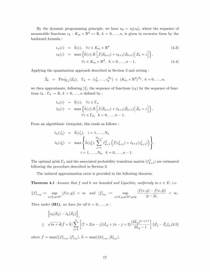
By the dynamic programming principle, we have u0 = v0(z0), where the sequence ofmeasurable functions vk : Km × Rd 7→ R, k = 0, . . . , n, is given in recursive form by thebackward formula :

vn(z) = h(z), ∀z ∈ Km × Rd (4.3)

vk(z) = max{

h(z); E[f(Zk+1) + vk+1(Zk+1)

∣∣∣Zk = z]}

,

∀z ∈ Km × Rd, k = 0, . . . , n− 1. (4.4)

Applying the quantization approach described in Section 3 and setting :

Zk = ProjΓk(Zk), Γk = (z1

k, . . . , zNkk ) ∈ (Km × Rd)Nk , k = 0, . . . , n,

we then approximate, following [1], the sequence of functions (vk) by the sequence of func-tions vk : Γk → R, k = 0, . . . , n defined by :

vn(z) = h(z), ∀z ∈ Γn

vk(z) = max{

h(z); E[f(Zk+1) + vk+1(Zk+1)

∣∣∣ Zk = z]}

,

∀z ∈ Γk, k = 0, . . . , n− 1.

From an algorithmic viewpoint, this reads as follows :

vn(zin) = h(zi

n), i = 1, . . . , Nn

vk(zik) = max

h(zik);

Nk+1∑j=1

rijk+1

(f(zj

k+1) + vk+1(zjk+1)

) ,

i = 1, . . . , Nk, k = 0, . . . , n− 1.

The optimal grids Γk and the associated probability transition matrix (rijk+1) are estimated

following the procedure described in Section 3.

The induced approximation error is provided in the following theorem.

Theorem 4.1 Assume that f and h are bounded and Lipschitz, uniformly in x ∈ E, i.e.

‖f‖sup := supx∈E,y∈Rd

|f(x, y)| < ∞ and [f ]lip

:= supx∈E,y,y∈Rd,y 6=y

|f(x, y)− f(x, y)||y − y|1

< ∞.

Then under (H1), we have for all k = 0, . . . , n :∥∥∥vk(Zk)− vk(Zk)∥∥∥

1

≤√

m + d(f + h)n∑

j=k

[(7 + 2(n− j))Lg + (n− j + 2)

(2Lg)n−j+1

2Lg − 1

]‖Zj − Zj‖2 ,(4.5)

where f = max(‖f‖sup , [f ]lip

), h = max(‖h‖sup , [h]lip

).

17

Remark 4.1 In view of Proposition 3.2, the estimation (4.5) provides a rate of convergencefor the approximation of v0(Z0) of order

n(2Lg)n

N1

m−1+d

,

when Nk = N is the number of points at each grid Γk used for the optimal quantization ofZk, k = 0, . . . , n. The term (2Lg)n is important when n is large, but this is consistent withthe rate of convergence obtained in approximation of nonlinear filtering by quantization,see [12] or by Monte-Carlo particle methods, see [4].

Lemma 4.1 Under the assumptions of Theorem 4.1, the functions vk, k = 0, . . . , n, definedin (4.4), are bounded and Lipschitz with :

‖ vk ‖sup ≤ (n− k + 1)(f + h), (4.6)

[vk]lip

≤ n− k + 32

(f + h)2Lg − 1

(2Lg)n−k+1. (4.7)

Proof. From (4.4), we have ‖ vk ‖sup ≤ ‖h‖sup + ‖f‖sup + ‖ vk+1 ‖sup . Since ‖ vn ‖sup

= ‖h‖sup , ‖f‖sup ≤ ‖f‖sup , ‖h‖sup ≤ ‖h‖sup , we obtain immediately the inequality (4.6) byinduction.

On the other hand, relation (4.4) and Lemma 3.1 also show

[vk]lip

≤ [h]lip

+ [Rk+1(f + vk+1)]lip

≤ [h]lip

+ Lg

(‖f‖sup + 2[f ]

lip+ ‖vk+1‖sup + 2[vk+1]

lip

). (4.8)

By definition of f , we clearly have for all z = (π, y) and z′ = (π′, y′) in Km × Rd,

|f(z)− f(z′)| ≤ ‖f‖sup |π − π′|1 + [f ]lip|y − y′|1

≤ f |z − z′|1 ,

A similar inequality holds for [h]lip

i.e. [h]lip≤ h. Plugging into (4.8) and using (4.6) yields

[vk]lip

≤ h + Lg

(3f + (n− k)(f + h)

)+ 2Lg[vk+1]

lip. (4.9)

Since [vn]lip

= [h]lip

, a straightforward induction gives (4.7). 2

Proof of Theorem 4.1.We set Φk(z) = E[f(Zk+1)+vk+1(Zk+1)|Zk = z] and Φk(z) = E[f(Zk+1)+ vk+1(Zk+1)|Zk =z]. Then, for k = 0, . . . , n− 1,∥∥∥vk(Zk)− vk(Zk)

∥∥∥1

≤∥∥∥h(Zk)− h(Zk)

∥∥∥1

+∥∥∥Φk(Zk)− Φk(Zk)

∥∥∥1

≤ [h]lip‖Zk − Zk‖1 +

∥∥∥Φk(Zk)− Φk(Zk)∥∥∥

1

(4.10)

+∥∥∥E[Φk(Zk)|Zk]− E[Φk(Zk)|Zk]

∥∥∥1

+∥∥∥E[Φk(Zk)|Zk]− Φk(Zk)

∥∥∥1

≤ [h]lip‖Zk − Zk‖1 + 2

∥∥∥Φk(Zk)− Φk(Zk)∥∥∥

1

+∥∥∥E[Φk(Zk)|Zk]− Φk(Zk)

∥∥∥1

, (4.11)

18

by the law of iterated conditional expectation. Since Zk is σ(Zk)-measurable, we have∥∥∥E[Φk(Zk)|Zk]− Φk(Zk)∥∥∥

1

=∥∥∥E[f(Zk+1) + vk+1(Zk+1)|Zk] − E[f(Zk+1) + vk+1(Zk+1)|Zk]

∥∥∥1

≤ [f ]lip

∥∥∥Zk+1 − Zk+1

∥∥∥1

+∥∥∥vk+1(Zk+1)− vk+1(Zk+1)

∥∥∥1

.

Plugging into (4.11) yields :∥∥∥vk(Zk)− vk(Zk)∥∥∥

1

≤(

[h]lip

+ 2[Φk]lip

)‖Zk − Zk‖1 + [f ]

lip

∥∥∥Zk+1 − Zk+1

∥∥∥1

+∥∥∥vk+1(Zk+1)− vk+1(Zk+1)

∥∥∥1

.

Since∥∥∥vn(Zn)− vn(Zn)

∥∥∥1

≤ [h]lip‖Zn − Zn‖1 , a direct induction gives :

∥∥∥vk(Zk)− vk(Zk)∥∥∥

1

≤n∑

j=k

aj‖Zj − Zj‖1 (4.12)

where

aj =

[h]

lip+ 2[Φk]

lip, j = k

[h]lip

+ 2[Φj ]lip + [f ]lip

, j = k + 1, ...n− 1[h]

lip+ [f ]

lip, j = n

(4.13)

Now, by Lemmata 3.1 and 4.1, we have

[Φk]lip

= [Rk+1(f + vk+1)]lip

≤ Lg

(‖f‖sup + 2[f ]

lip+ ‖vk+1‖sup + 2[vk+1]

lip

)≤ Lg[3f + (n− k)(f + h)]

+ (f + h)(n− k

2+ 1)

(2Lg)n−k+1

2Lg − 1.

Substituting into (4.13) and (4.12) provides the required result by using also Cauchy-Schwarz inequality.

5 Numerical illustration : Bermudean options in a partially

observed stochastic volatility model

We consider an observable risky asset price (Sk) with dynamics given by :

Sk+1 = Sk exp[(

r − 12X2

k

)δ + Xk

√δεk+1

], S0 = s0 > 0,

where (εk) is a sequence of Gaussian white noise, and (Xk) is the unobservable volatilityprocess. δ > 0 may represent some discretization time step. Equivalently, we observe the

19

process (Yk) = (ln Sk), and we notice that the conditional law of Yk+1 given (Xk, Yk) has adensity given by :

g(Xk, Yk, y′) =

1√2πX2

kδexp

[−(y′ − Yk − (r − 1

2X2k)δ)2

2X2kδ

], y′ ∈ R.

We model here the dynamics of (X, S) under some risk neutral martingale measure P, r

representing in this case the riskless interest rate.We assume that (Xk) is an homogeneous Markov chain taking three possible values xb

< xm < xh in R+\{0}. Its probability transition matrix is given by :

Pk =

1− (pbm + pbh)δ pbmδ pbhδ

pmbδ 1− (pmb + pmh)δ pmhδ

phbδ phmδ 1− (phb + phm)δ

. (5.1)

In this context of a partially observed stochastic volatility model, we consider a Bermudeanput option with payoff :

h(y) = (κ− ey)+, y ∈ R,

and we want to compute its price given by :

u0 = supτ∈T Y

n

E[e−rτδh(Yτ )

]. (5.2)

We consider a model where the volatility (Xk) is a Markov-chain approximation a laKushner (see [8]) of a mean-reverting process :

dXt = λ(x0 −Xt)dt + ηdWt.

Denoting by ∆ > 0 the spatial step, this corresponds to a probability transition matrix ofthe form (5.1) with :

xb = x0 −∆, xm = x0, xh = x0 + ∆,

and

pbm = λ +η2

2∆2, pbh = 0

pmb =η2

2∆2, pmh =

η2

2∆2

phb = 0, phm = λ +η2

2∆2.

In order to ensure that Pk is indeed a probability transition matrix, we have the consistencyconditions :

1−(

λ +η2

2∆2

)δ ≥ 0 and 1− η2

∆2δ ≥ 0

We perform numerical tests with

20

- Price and put option parameters : r = 0.05, S0 = 110, κ = 100,- Volatility parameters : λ = 1, η = 0, 1, X0 = 0.15,- Spatial step : ∆ = 0, 05.- Quantization : Grids are of same size N fixed for each time period with step δ = 1

n .

We first compare in Table 1 the filter expectation at the final date computed with atime step size δ = 1/5 and by using the optimal quantization method with increasing gridsize N , and with 106 Monte Carlo iterations.

E[Π1n] E[Π2

n] E[Π3n] Relative error (%)

Monte Carlo 0.287608 0.422833 0.289558Quant. with N = 300 0.301651 0.421725 0.276624 0.898Quant. with N = 600 0.301604 0.421458 0.276938 0.886Quant. with N = 900 0.301598 0.421316 0.277086 0.881Quant. with N = 1200 0.301618 0.42122 0.277162 0.879Quant. with N = 1500 0.301605 0.421205 0.27719 0.878

Table 1: Comparison of quantized filter value to its Monte Carlo estimation

We observe that besides the very low error level, the absolute error (plotted in Figure1) and the relative error are decreasing as the grid size grows.

Secondly, in order to illustrate the effect of the time step, we compute the Americanoption price under partial observation when the time step δ decreases to zero (i.e. n

increases) and compare it with the American option price with complete observation of(Xk, Yk). Indeed, in the limit for δ → 0 we fully observe the volatility, and so the partialobservation price should converge to the complete observation price.

Moreover, when we have more and more observations, the difference between the twoprices should decrease and converge to zero. This is shown in figure 2, where we performedoption pricing over grids of size NΠ,Y = 1500 in case of partial observation. The totalobservation price is given by the same pricing algorithm carried out on NX,Y = 45 pointsfor the product grid of (Xk, Yk). We have seen in Remark 4.1 that for fixed n, the rateof convergence for the approximation of the value function under partial observation is oforder N1/(m−1+d)

Π,Ywhere NΠ,Y is the number of points used at each time k for the grid of

(Πk, Yk) valued in Km×Rd. From results of [1], we also know that the rate of convergencefor the approximation of the value function under full observation is of order m×NY whereNX,Y = m×NY is the number of points at each time k, used for the grid of (Xk, Yk) valuedin E × Rd. This explains why, in order to have comparable results, and with m = 3 and d

= 1, we have chosen NY ∼ N1/3Π,Y

.In addition, it is possible to observe the effect of information enrichment as the time

step decreases. In fact, if we consider multiples of n as the time step parameter, we noticethat the American option price increases for both total and partial observation models (seetables 2 and 3).

21

200 400 600 800 1000 1200 1400 16001.315

1.32

1.325

1.33

1.335

1.34

1.345

1.35

1.355x 10

−3

Figure 1: Filter error convergence as N grows

n 4 8 16Tot. Obs. (NX,Y = 30) 1.45863 1.75689 1.77642

Part. Obs. (NΠ,Y = 1000) 0.921729 1.13898 1.47089Variation 0.53 0.61 0.30

Table 2: American option price for embedded filtrations - First Example

n 5 10 20Tot. Obs. (NX,Y = 45) 1.57506 1.72595 1.91208

Part. Obs. (NΠ,Y = 1500) 0.988531 1.30616 1.59632Variation 0.58 0.42 0.31

Table 3: American option price for embedded filtrations - Second Example

22

0 5 10 15 20 25 30 350

0.5

1

1.5

2

2.5

Tot Obs Option Price (45 pts)Part Obs Option Price (1500pts)

Figure 2: Partial and total observation option prices as δ → 0

23

References

[1] V. Bally, G. Pages (2003): A quantization algorithm for solving discrete time multi-dimensionaloptimal stopping problems, Bernoulli, 9, 1003-1049.

[2] Bally V., Pages G., Printems J. (2001) : A stochastic quantization method for non linearproblems, Monte Carlo Methods and Applications, 7, n01-2, pp.21-34.

[3] A. Bensoussan and W. Runggaldier (1987) : An approximation method for stochastic controlproblems with partial observation of the state : a method for constructing ε-optimal controls,Acta Appli. Math., 10, 145-170.

[4] P. Del Moral, J. Jacod, P. Protter (2001) : The Monte-Carlo method for filtering with discrete-time observations, Prob. Theory Rel. Fields, 120, 346-368.

[5] Di Masi G.B., Runggaldier W.J. (1987) : An Approach to Discrete-Time Stochastic ControlProblems under Partial Observation, SIAM J. Control & Optimiz. 25, pp. 38 - 48.

[6] Duflo, M. (1997): Random Iterative Models, Coll. Applications of Mathematics, 34, Springer-Verlag, Berlin, 1997, 385p.

[7] Graf S., Luschgy H. (2000): Foundations of quantization for random vectors, Lecture Notes inMathematics n01730, Springer, Berlin, 230 pp.

[8] Kushner H.J., Dupuis P.G. (1992) : Numerical Methods for Stochastic Control Problems inContinuous Time, Springer, New York.

[9] Kushner H.J., Yin G.G. (1997): Stochastic Approximation Algorithms and Applications,Springer, New York.

[10] N. Newton (2001) : Approximations for nonlinear filters based on quantization, Monte CarloMethods and Appl, 7, 311-320.

[11] Pages G. (1997): A space vector quantization method for numerical integration, Journal ofComputational and Applied Mathematics, 89, pp.1-38.

[12] G. Pages, H. Pham (2002): Optimal quantization methods for nonlinear filtering with discrete-time observations, Preprint, Laboratoire de Probabilites et modeles aleatoires, Universites Paris6 & 7 (France).

[13] G. Pages, H. Pham, J. Printems (2003): An optimal Markovian quantization algorithm formultidimensional stochastic control problems, to appear in Stochastics and Dynamics.

[14] G. Pages, H. Pham, J. Printems (2003): Optimal quantization methods and applications tonumerical problems in finance, to appear in Handbook of numerical methods in finance, ed. Z.Rachev, Birkhauser.

[15] Runggaldier W.J., Stettner L. (1991) : On the Construction of Nearly Optimal Strategies for aGeneral Problem of Control of Partially Observed Diffusions, Stochastics and Stochastics Reports,37 , pp.15-47.

[16] A. Sellami (2004) : Nonlinear filtering with observation quantization, Preprint, Laboratoire deProbabilites et modeles aleatoires, Universites Paris 6 & 7 (France).

24