Approximation and numerical realization of 3D

quasistatic contact problems with Coulomb friction.

J. Haslingera,∗, R. Kucerab, O. Vlachc, C. C. Baniotopoulosd

aDepartment of Numerical Mathematics, Faculty of Mathematics and Physics, CharlesUniversity, Sokolovska 83, 186 75 Praha 8, Czech Republic

bDepartment of Mathematics, VSB–TU Ostrava, Tr. 17. listopadu 15, 708 33Ostrava–Poruba, Czech Republic

cDepartment of Applied Mathematics, VSB–TU Ostrava, Tr. 17. listopadu 15, 708 33Ostrava–Poruba, Czech Republic

dDepartment of Civil Engineering, Aristotle University, Thessaloniki, Greece

Abstract

This paper deals with the full discretization of quasistatic 3D Signorini prob-lems with local Coulomb friction and a coefficient of friction which may de-pend on the solution. After a time discretization we obtain a system of staticcontact problems with Coulomb friction. Each of these problems is solved bythe T-FETI domain decomposition method used in auxiliary contact prob-lems with Tresca friction. Numerical experiments show the efficiency of theproposed method.

Key words: contact problems, Coulomb friction, domain decompositionmethods

1. Introduction

Contact problems represent a special branch of mechanics of solids whichanalyzes the behavior of loaded, deformable bodies being in a mutual contact.Due to non-penetration and friction conditions, the resulting problems arehighly non-linear. Both, unilateral and friction phenomena depend on time.Therefore contact problems with friction should be defined as a dynamical

∗Corresponding authorEmail addresses: Jaroslav.Haslinger@mff.cuni.cz (J. Haslinger),

radek.kucera@vsb.cz (R. Kucera), oldrich.vlach2@vsb.cz (O. Vlach),ccb@civil.auth.gr (C. C. Baniotopoulos)

Preprint submitted to Elsevier September 20, 2010

process. If however applied forces vary slowly in time, inertia of the sys-tem can be neglected and one can use a quasistatic approximation. This,together with a dependence of friction coefficients on the solution, typicallyarises in geomechanics (modelling of a movement of tectonic plates, predic-tion of earthquakes). Applied forces are functions of time, the Coulomb lawof friction uses the velocity of the tangential contact displacements and thecoefficient of Coulomb friction itself may depend on the modulus of the pre-viously mentioned velocities (see [6]). This paper extends results of [14] fromtwo (2D) to three (3D) space dimensions. Let us note that this extension isnot straightforward since the friction conditions are more involved in 3D.

Using a three–step finite–difference approximation of the time derivativewe arrive at a sequence of static contact problems with (local) Coulomb fric-tion whose solutions are defined by using a fixed point approach. Thus themethod of successive approximations turns out to be a natural tool for thenumerical solution. Each iterative step is represented by an auxiliary con-tact problem with a given slip bound (Tresca model of friction). Since itsmathematical formulation is given by a variational inequality of the secondkind (see [8, 11]), we obtain (after a finite element discretization) a con-vex, but non-smooth constrained minimization problem for a discrete totalpotential energy function. Using the method of Lagrange multipliers, thenon-penetration conditions are released and the non-smooth frictional termis transformed into a smooth one. Eliminating the displacement field fromthis formulation we obtain a new formulation solely in terms of Lagrange mul-tipliers which represent the discrete contact stresses. In this way we arrive ata minimization problem for a quadratic function subject to separated simpleand quadratic inequality constraints. The numerical minimization may beperformed by the algorithm proposed in [15] and analyzed in [16]. To in-crease the efficiency of the whole computational process we use a variant ofthe FETI domain decomposition method ([7]) which introduces (additionallyto the original setting) also new Lagrange multipliers by means of which thesolutions on the individual sub-domains are glued together. The resultingminimization problem is solved by the augmented Lagrangian method ([4])in which the algorithm from [16] is used repeatedly. To solve static contactproblems with Coulomb friction, the augmented Lagrangian method is com-bined together with the method of successive approximations in one inexactiterative loop.

Let us mention main benefits of the variant ([2]) of the FETI calledthe total FETI (T–FETI). Unlike to the original FETI the satisfaction of

2

the Dirichlet boundary conditions is enforced also by Lagrange multipliers.Therefore all subdomains can be treated as floating bodies with six rigidbody modes. Thus the kernel spaces of the stiffness matrices may be iden-tified directly without any computation and, moreover, the Moore-Penroseinverse is easily available. Since the global stiffness matrix exhibits the blockdiagonal structure, one can handle it in parallel. Finally, under additionalassumptions on the used finite element partitions, the spectrum of all blocksand, consequently of the whole stiffness matrix, lies within an interval inR

1+ which does not depend on the mesh norms ([12]). It is well–known that

convergence of conjugate gradient type methods depends on the spectrumof the Hessian ([5, 9, 16]). Therefore the number of iterations needed to geta solution with a given accuracy can be independent of the mesh norms, aswell. This property is known as the scalability of the method. See [1, 3, 4]for more details on scalable algorithms.

The paper is organized as follows: Section 2 deals with the formulationof quasistatic contact problems with Coulomb friction and introduces theirthree–step time discretization. Next two sections present main ideas of theused methods in the continuous setting: Section 3 describes the fixed–pointapproach for static contact problems with Coulomb friction while Section 4gives the T–FETI domain decomposition formulation of contact problemswith a given slip bound. In Section 5 we analyze an algebraic representa-tion of the discrete problems and mention optimization algorithms used incomputations. Finally Section 6 shows results of numerical experiments.

2. Formulation of the problem

Let us consider an elastic body represented by a domain Ω ⊂ R3 whose

Lipschitz boundary ∂Ω is decomposed as follows: ∂Ω = Γu ∪ Γp ∪ Γc , wheredifferent boundary conditions will be prescribed. The body is subject tovolume forces of density F := (Fi)

3i=1 and surface tractions of density P :=

(Pi)3i=1 on Γp both acting in an interval [0, T0], T0 > 0 given. On Γu the body

is fixed, while along Γc is supported by a rigid foundation S. For the sake ofsimplicity of our presentation we shall suppose that S is represented by thehalf–space and there is no gap between Γc and S. On Γc the non–penetrationand friction conditions will be prescribed. Friction will be involved intothe mathematical model by using the local Coulomb law with a coefficientof friction depending on the solution. Our aim is to find an equilibriumstate of Ω.

3

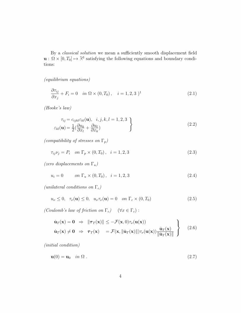
By a classical solution we mean a sufficiently smooth displacement fieldu : Ω× [0, T0] 7→ R

3 satisfying the following equations and boundary condi-tions:

(equilibrium equations)

∂τij∂xj

+ Fi = 0 in Ω× (0, T0) , i = 1, 2, 3 )1 (2.1)

(Hooke’s law)

τij = cijklεkl(u), i, j, k, l = 1, 2, 3

εkl(u) = 12(∂uk∂xl

+ ∂ul∂xk

)

(2.2)

(compatibility of stresses on Γp)

τijνj = Pi on Γp × (0, T0) , i = 1, 2, 3 (2.3)

(zero displacements on Γu)

ui = 0 on Γu × (0, T0) , i = 1, 2, 3 (2.4)

(unilateral conditions on Γc)

uν ≤ 0, τν(u) ≤ 0, uντν(u) = 0 on Γc × (0, T0) (2.5)

(Coulomb’s law of friction on Γc) (∀x ∈ Γc) :

uT (x) = 0 ⇒ ‖τ T (x)‖ ≤ −F(x, 0)τν(u(x))

uT (x) 6= 0 ⇒ τ T (x) = F(x, ‖uT (x)‖)τν(u(x))uT (x)‖uT (x)‖

(2.6)

(initial condition)

u(0) = u0 in Ω . (2.7)

4

We use classical notation of the linear elasticity: τ = (τij)3i,j=1 is a stress

tensor, ε(u) = (εij(u))3i,j=1 a linearized strain tensor corresponding to a dis-

placement vector u, cijkl ∈ L∞(Ω), i, j, k, l = 1, 2, 3 are coefficients of a linearHooke’s law (2.2). We shall suppose that they satisfy the following symmetryand ellipticity conditions:

cijkl = cjikl = cklij a.e. in Ω , i, j, k, l = 1, 2, 3

∃α > 0 : cijklξijξkl ≥ αξijξij a.e. in Ω ∀ξij = ξji ∈ R1 .

(2.8)

Further, ν = (νi)3i=1 is the unit normal vector to ∂Ω, uν := uiνi , uT :=

u−uνν is the normal and tangential component of a displacement vector u.Analogously, τν := τijνiνj , τ T := τijνj − τνν is the normal and tangentialcomponent of a stress vector (τijνj)

3i=1 on ∂Ω. Finally, the symbol F in (2.6)

stands for the coefficient of friction which depends on the spatial variablex ∈ Γc and on the euclidean norm ‖uT‖ of the velocity uT := ∂

∂tuT on Γc.

To define the weak solution we introduce the following sets of functions:

V = v ∈ H1(Ω) | v = 0 on Γu , V = V × V × VK = v ∈ V | vν ≤ 0 a.e. on Γc

H1/2(Γc) = V |Γc (space of traces on Γc of functions from V )

H−1/2(Γc) = (H1/2(Γc))′ (the dual of H1/2(Γc))

H−1/2

− (Γc) (cone of all non− positive elements of H−1/2(Γc)).

Next we shall suppose that Γc is sufficiently smooth so that vν ∈ H1/2(Γc) forevery v ∈ V.

By the weak formulation of the quasistatic contact problem with localCoulomb law of friction and the coefficient of friction F which depends onthe solution we mean the following problem formulated in terms of the dis-placement vector u and the normal contact stress λν :

Find u ∈ W 1,2(0, T0,V), λν ∈ W 1,2(0, T0, H−1/2(Γc)) such that

u(t) ∈ K for a.a. t ∈ [0, T0], u(0) = u0 in Ω

a(u(t),v − u(t)) + j(λν(t),v)− j(λν(t), u(t)) ≥ L(t)(v − u(t))+

+〈λν(t), vν − uν(t)〉 ∀v ∈ V and a.a. t ∈ [0, T0]

〈λν(t), zν − uν(t)〉 ≥ 0 ∀z ∈ K and a.a. t ∈ [0, T0] ,

(P)

1here and in what follows the summation convention is used.

5

where

a(u,v) :=

∫Ω

cijklεij(u)εkl(v) dx ,

L(t)(v) :=

∫Ω

Fi(t)vi dx +

∫Γp

Pi(t)vi ds

j(λν ,v) :=− 〈F(‖uT‖)λν , ‖vT‖〉

and 〈 , 〉 is the duality pairing between H−1/2(Γc) and H1/2(Γc). Using Green’sformula with an appropriate choice of the test functions v one can show thatthe classical and weak formulations are formally equivalent. In addition, λνis equal to the normal contact stress on Γc.

We shall suppose that F ∈ W 1,2(0, T0, (L2(Ω))3), P ∈ W 1,2(0, T0, (L

2(Γp))3)

and the initial displacement u0 ∈ K satisfies the compability condition

a(u0,v − u0) + j(λ0ν ,v − u0) ≥ L(0)(v − u0) ∀v ∈ K ,

where λ0ν = τν(u0)|Γc . The mathematical analysis of (P) in the case whenF := F(x) depends only on the spatial variable x has been already donein [17]. The more general case of F := F(x, ‖uT‖) is analyzed in [6].

Now we replace problem (P) by a sequence of static problems arisingfrom its time discretization. Let ∆t = T0/n, n ∈ N, be a time step, ti =i∆t, i = 0, . . . , n and denote ui := u(ti), Fi := F(ti), etc. Assume that(ui+1, λi+1

ν ) ∈ K×H−1/2(Γc) is a solution of (P) at t = ti+1 :

a(ui+1,v − ui+1)− 〈F(‖ui+1T ‖)λi+1

ν , ‖vT‖〉+ 〈F(‖ui+1T ‖)λi+1

ν , ‖ui+1T ‖〉

≥ Li+1(v − ui+1) + 〈λi+1ν , vν − ui+1

ν 〉 ∀v ∈ V〈λi+1

ν , zν − ui+1ν 〉 ≥ 0 ∀z ∈ K ,

(P)i+1

where ui+1 := ∂∂t

u|t=ti+1using also the definition of the frictional term j.

Next we replace ui+1 by a three–step finite difference:

ui+1 ≈ ∆i+1u

∆t, (2.9)

where

∆i+1u := αui+1 + βui + γui−1 , α, β, γ ∈ R1 , α > 0 .

6

Inserting (2.9) into the first inequality in (P)i+1 we get (∀v ∈ V):

a(ui+1,v − αui+1 + βui + γui−1

∆t )− 〈F(‖∆i+1uT‖

∆t )λi+1ν , ‖vT‖〉

+〈F(‖∆i+1uT‖

∆t )λi+1ν ,‖αui+1

T + βuiT + γui−1T ‖

∆t 〉

≥ Li+1(v − αui+1 + βui + γui−1

∆t ) + 〈λi+1ν , vν − αui+1

ν + βuiν + γui−1ν

∆t 〉 .

Multiplying this inequality by ∆t and dividing by α we obtain:

a(ui+1, ∆tα v − ui+1 − β

αui − γαui−1)− 〈F(

‖∆i+1uT‖∆t )λi+1

ν , ∆tα ‖vT‖〉

+〈F(‖∆i+1uT‖

∆t )λi+1ν , ‖ui+1

T +βαuiT +

γαui−1

T ‖〉≥ Li+1(∆t

α v − ui+1 − βαui − γ

αui−1)

+〈λi+1ν , ∆t

α vν − ui+1ν − β

αuiν − γ

αui−1ν 〉 ∀v ∈ V .

Setting w := ∆tα v − β

αui − γαui−1 ∈ V we arrive at

a(ui+1,w − ui+1)− 〈F(‖∆i+1uT‖

∆t )λi+1ν , ‖wT +

βαuiT +

γαui−1

T ‖〉

+〈F(‖∆i+1uT‖

∆t )λi+1ν , ‖ui+1

T +βαuiT +

γαui−1

T ‖〉≥ Li+1(w − ui+1) + 〈λi+1

ν , wν − ui+1ν 〉 ∀w ∈ V .

(2.10)

If we restrict ourselves to test functions w ∈ K in (2.10), the last termon the right of (2.10) is non–negative since λi+1

ν ∈ H−1/2

− (Γc) in virtue of thesecond inequality in (P)i+1 . Thus ui+1 ∈ K solves the following implicitvariational inequality:

a(ui+1,w − ui+1)−〈F(‖∆i+1uT‖

∆t )λi+1ν , ‖wT +

βαuiT +

γαui−1

T ‖〉

+〈F(‖∆i+1uT‖

∆t )λi+1ν , ‖ui+1

T +βαuiT +

γαui−1

T ‖〉≥ Li+1(w − ui+1) ∀w ∈ K ,

(Q)i+1

which is the weak form of the state contact problem with Coulomb frictionand the coefficient of friction F depending on the solution at the time t = ti+1.

7

In particular, the friction conditions hidden in (Q)i+1 read for all x ∈ Γc asfollows:

∆i+1uT (x) = 0 ⇒ ‖τ i+1T (x)‖ ≤ −F(x, 0)τ i+1

ν (u(x))

∆i+1uT (x) 6= 0 ⇒ τ i+1T (x) =

F(x,‖∆i+1uT‖

∆t )τ i+1ν (u(x)) ∆i+1uT

‖∆i+1uT‖(x)

(2.11)

To make numerical relization of (Q)i+1 easier we replace the unknown func-tion ‖∆i+1uT‖ in the argument of F by the known value ‖∆iuT‖ and denoteF i := F(‖∆uiT‖/∆t). The resulting problem involves the Coulomb frictionlaw with the coefficient which does not depend on the solution on the currenttime level t = ti+1.

The coefficients defining the finite diference (2.9) used in computationsare α = 3/2, β = −2 and γ = 1/2.

With such a choice of α, β and γ the final form of the problem we shallsolve at each time level reads as follows:

Find ui+1 ∈ K such that ∀w ∈ Ka(ui+1,w − ui+1)− 〈F iλi+1

ν , ‖wT − 43uiT + 1

3ui−1T ‖〉

+〈F iλi+1ν , ‖ui+1

T − 43uiT + 1

3ui−1T ‖〉 ≥ Li+1(w − ui+1) ,

(Q)i+1

where λi+1ν = τ i+1

ν (u)|Γc .

3. Static contact problems with local Coulomb friction

In this section we shall describe how static contact problems (Q)i+1 willbe solved. To simplify our notation the index i denoting the time level willbe skipped and we set z := 4

3ui − 1

3ui−1. The problem we have to solve now

reads as follows:

Find u ∈ K such thata(u,w − u) + j(λν ,w − z)− j(λν ,u− z) ≥ L(w − u) ∀w ∈ K ,

(Q)

where λν = τν(u)|Γc and

j(λν ,v) = −〈Fλν , ‖vT‖〉 . (3.12)

Recall that due to our approach, the coefficient of friction F in (Q) nowdoes not depend on the solution u from actual timestep, but only on the

8

known solution from the previous ones. The unilateral constraint u ∈ K

can be released by means of Lagrange multipliers. We obtain the followingequivalent formulation of (Q):

Find u ∈ V and λν ∈ H−1/2

− (Γc) such that

a(u,w − u) + j(λν ,w − z)− j(λν ,u− z) ≥L(w − u) + 〈λν , wν − uν〉 ∀w ∈ V

〈µν − λν , uν〉 ≥ 0 ∀µν ∈ H−1/2

− (Γc)

(3.13)

Problem (3.13) has an alternative formulation based on a fixed–point ap-proach which turned out to be efficient from the numerical point of view.For given g ∈ H−1/2

− (Γc) defining the slip bound we consider the variationalinequality:

Find u := u(g) ∈ V and λν := λν(g) ∈ H−1/2

− (Γc) such that

a(u,w − u) + j(g,w − z)− j(g,u− z) ≥L(w − u) + 〈λν , wν − uν〉 ∀w ∈ V

〈µν − λν , uν〉 ≥ 0 ∀µν ∈ H−1/2

− (Γc)

(3.14)

This problem has a unique solution (u, λν) for any g ∈ H−1/2

− (Γc) . Thefirst component u(g) solves the contact problem with the Tresca model offriction in which the slip bound −Fg is given a–priori and λν = τν(u(g))|Γcis the normal contact stress. This makes it possible to define a mappingΦ : H−1/2

− (Γc) 7→ H−1/2

− (Γc) by

Φ(g) = λν(g) ∀g ∈ H−1/2

− (Γc) , (3.15)

where λν(g) is the second component of the solution to (3.14). If we compare(3.13) with (3.14) we see that (u, λν) solves (3.13) if and only if λν ∈ H−1/2

− (Γc)is a fixed–point of Φ, i.e.

Φ(λν) = λν (3.16)

A natural idea how to find λν satisfying (3.15) is to use the method of suc-cessive approximations :

λ(0)ν ∈ H−1/2

− (Γc) given;

if λ(k)ν ∈ H−1/2

− (Γc) is known

solve (3.14) with g := λ(k)ν and

set λ(k+1)ν := λν(λ

(k)ν ) , k := k + 1

repeat until stopping criterion .

(3.17)

9

It is worth noting that convergence of this method in the continuous set-ting of the static problem is not guaranteed since Φ is not a contractivemapping. The situation is rather different in the discrete case. After a suit-able discretization of V and H−1/2

− (Γc) one can define a discrete version Φh of Φwhose fixed–points are solutions of discrete contact problems with Coulombfriction. It is known that Φh is already contractive provided that the coeffi-cient of friction F is small enough but this property is mesh-dependent ([10]).In our computations we use the method of successive approximations (3.17).Since the efficiency of (3.17) depends mainly on how each iterative step canbe realized we focus on this subject in the next section.

4. T–FETI for contact problems with given friction

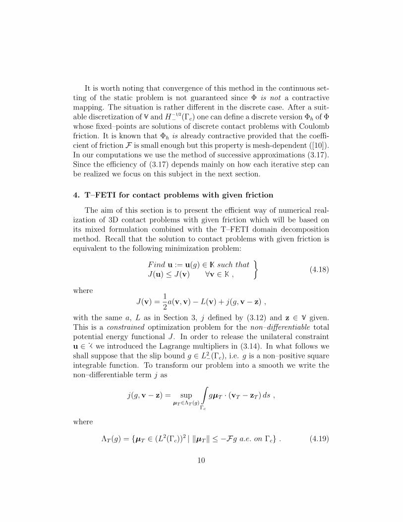
The aim of this section is to present the efficient way of numerical real-ization of 3D contact problems with given friction which will be based onits mixed formulation combined with the T–FETI domain decompositionmethod. Recall that the solution to contact problems with given friction isequivalent to the following minimization problem:

Find u := u(g) ∈ K such thatJ(u) ≤ J(v) ∀v ∈ K ,

(4.18)

where

J(v) =1

2a(v,v)− L(v) + j(g,v − z) ,

with the same a, L as in Section 3, j defined by (3.12) and z ∈ V given.This is a constrained optimization problem for the non–differentiable totalpotential energy functional J . In order to release the unilateral constraintu ∈ K we introduced the Lagrange multipliers in (3.14). In what follows weshall suppose that the slip bound g ∈ L2

−(Γc), i.e. g is a non–positive squareintegrable function. To transform our problem into a smooth we write thenon–differentiable term j as

j(g,v − z) = supµT∈ΛT (g)

∫Γc

gµT · (vT − zT ) ds ,

where

ΛT (g) = µT ∈ (L2(Γc))2 | ‖µT‖ ≤ −Fg a.e. on Γc . (4.19)

10

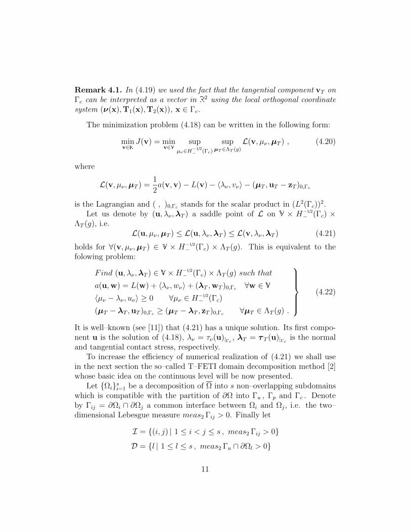
Remark 4.1. In (4.19) we used the fact that the tangential component vT onΓc can be interpreted as a vector in R

2 using the local orthogonal coordinatesystem (ν(x),T1(x),T2(x)), x ∈ Γc.

The minimization problem (4.18) can be written in the following form:

minv∈K

J(v) = minv∈V

supµν∈H−1/2

− (Γc)

supµT∈ΛT (g)

L(v, µν ,µT ) , (4.20)

where

L(v, µν ,µT ) =1

2a(v,v)− L(v)− 〈λν , vν〉 − (µT ,uT − zT )0,Γc

is the Lagrangian and ( , )0,Γc stands for the scalar product in (L2(Γc))2.

Let us denote by (u, λν ,λT ) a saddle point of L on V × H−1/2

− (Γc) ×ΛT (g), i.e.

L(u, µν ,µT ) ≤ L(u, λν ,λT ) ≤ L(v, λν ,λT ) (4.21)

holds for ∀(v, µν ,µT ) ∈ V × H−1/2

− (Γc) × ΛT (g). This is equivalent to thefolowing problem:

Find (u, λν ,λT ) ∈ V×H−1/2

− (Γc)× ΛT (g) such that

a(u,w) = L(w) + 〈λν , wν〉+ (λT ,wT )0,Γc ∀w ∈ V〈µν − λν , uν〉 ≥ 0 ∀µν ∈ H−1/2

− (Γc)

(µT − λT ,uT )0,Γc ≥ (µT − λT , zT )0,Γc ∀µT ∈ ΛT (g) .

(4.22)

It is well–known (see [11]) that (4.21) has a unique solution. Its first compo-nent u is the solution of (4.18), λν = τν(u)|Γc , λT = τ T (u)|Γc is the normaland tangential contact stress, respectively.

To increase the efficiency of numerical realization of (4.21) we shall usein the next section the so–called T–FETI domain decomposition method [2]whose basic idea on the continuous level will be now presented.

Let Ωisi=1 be a decomposition of Ω into s non–overlapping subdomainswhich is compatible with the partition of ∂Ω into Γu , Γp and Γc . Denoteby Γij = ∂Ωi ∩ ∂Ωj a common interface between Ωi and Ωj, i.e. the two–dimensional Lebesgue measure meas2 Γij > 0. Finally let

I = (i, j) | 1 ≤ i < j ≤ s , meas2 Γij > 0D = l | 1 ≤ l ≤ s , meas2 Γu ∩ ∂Ωl > 0

11

be the sets identifying the common interfaces and parts of ∂Ωl contained inΓu. On Ωisi=1 we introduce the space

W = v ∈ (L2(Ω))3 |vi := v|Ωi ∈ (H1(Ωi))3, i = 1, . . . , s .

It is easy to see that

v ∈ V iff v ∈ W ∧ [v]ij= 0 ∀(i, j) ∈ I ∧ vl|Γul= 0 ∀l ∈ D , (4.23)

where [v]ij := (vi −vj)|Γij , (i, j) ∈ I, Γul := Γu ∩ ∂Ωl, l ∈ D. To release the

conditions on (4.23) we introduce the following sets of Lagrange multipliers:

Yij := (H1(Ωi))3|Γij , (i, j) ∈ I, Zl := (H1(Ωl))

3|Γul , l ∈ D ,

whose duals are denoted by Y′ij, and Z′l, respectively. Then

v ∈ V iff v ∈ W ∧ 〈µij, [v]ij〉 = 0 ∀µij ∈ Y′ij ∀(i, j) ∈ I∧ 〈µl,vl〉 = 0 ∀µl ∈ Z′l ∀l ∈ D ,

where 〈 , 〉 denotes the duality pairings between Y

′ij and Yij, Z

′l and Zl.

Further let Y′ =∏

(i,j)∈I Y′ij, Z

′ =∏

l∈D Z′l be the cartesian products of Y′ij

and Z′l, respectively and define:

〈µint, [v]〉 :=∑

(i,j)∈I

〈µij, [v]ij〉 , µij ∈ Y′ij

〈µDir,v〉 :=∑l∈D

〈µl,vl〉 , µl ∈ Z′l .

Finally let H1/2(Γc) := W|Γc be the trace space on Γc of functions from W,

H−1/2(Γc) the dual ofH1/2(Γc) andH−1/2

− (Γc) the cone of non–positive elementsof H−1/2(Γc). The respective duality pairing will be denoted again by 〈 , 〉.The T–FETI domain decomposition formulation of (4.21) reads as follows:

Find (u, λν ,λT ,λint,λDir) ∈ W×H−1/2

− (Γc)× ΛT (g)× Y′ × Z′ s.t.a(u,w) = L(w) + 〈λν , wν〉+ (λT ,wT )0,Γc + 〈λint, [w]〉

+〈λDir,w〉 ∀w ∈ W ,

〈µν − λν , uν〉+ (µT − λT ,uT )0,Γc ≥ (µT − λT , zT )0,Γc

∀µν ∈ H−1/2

− (Γc) ∀µT ∈ ΛT (g)

〈µint, [u]〉+ 〈µDir,u〉 = 0 ∀(µint,µDir) ∈ Y′ × Z′ .

(4.24)

The elimination of u from (4.24) leads to the new formulation in terms ofthe Lagrange multipliers λν , λT , λint and λDir. This approach will be usedin the next section for numerical realization of (4.24).

12

5. Algebraic T-FETI and algorithm

Let us suppose that the domains Ωi, i = 1, . . . , s are polygonal and denoteby Ti a partition of Ωi into tetrahedrons. Next we suppose that Ti|Γij = Tj |Γijfor any (i, j) ∈ I, i.e. the nodes Ti and Tj on the common interface Γijcoincide. Then T = Tisi=1 defines the partition of Ω. With any Ti weassociate the finite dimensional space Xi, where

Xi = v ∈ (C(Ωi))3 | v|T ∈ P1(T ) ∀T ∈ Ti

and denote

X =s∏i=1

Xi .

The space X consists of all piecewise linear functions on T which are discon-tinuous on Γij, (i, j) ∈ I.

The spaces of the Lagrange multipliers used in (4.24) will be approximatedby Dirac functions concentrated at some specific nodes of T . To this enddenote by

xijq dijq=1 . . . nodes of Ti on Γij \ Γu , (i, j)∈ I

ylqdlq=1 . . . nodes of Tl on Γul , l∈ Dzkqdkq=1 . . . nodes of Tk on Γck \ Γu , k ∈ C ,

(5.25)

where Γck := Γc ∩ ∂Ωk, dij, dl, dk denote appropriate dimensions, and

C = k | 1 ≤ k ≤ s , meas2 Γck > 0 .

Dirac functions at xijq dijq=1, ylqdlq=1 and zkqdkq=1 will ensure the continuity

across Γij, the zero boundary condition on Γu and the satisfaction of the non–penetration and friction conditions on Γc, respectively. Let us concentratenow on the Dirac functions at zkqdkq=1, k ∈ C. To simplify our notationdenote by w one of theese nodes. Then the Lagrange multipliers acting at ware of the form ν(w)δw, T1(w)δw and T2(w)δw, where T1 and T2 are thesame as in Remark 4.1. If v ∈ X then

[ν(w)δw,v] := [δw,v · ν] = vν(w)

[T1(w)δw + T2(w)δw,v] := [δw,vT ] = vT (w) .

13

The spaces H−1/2

− (Γc) and ΛT (g) in (4.24) are now discretized by

ν= µν |µν =∑k∈C

dk∑q=1

µkqν(zkq)δzkq , µkq ≤ 0

T (g)=µT |µT =∑k∈C

dk∑q=1

(µkq1T1(zkq)+µkq2T2(zkq))δzkq ,

||(µkq1, µkq2)||2 ≤ (−Fg)(zkq) ∀zkq ,

where || ||2 stands for the Euclidean norm of vectors. If µν ∈ ν , µT ∈ T (g)and v ∈ X are given then

[µν ,v] :=∑k∈C

dk∑q=1

µkqvν(zkq)

[µT ,vT ] :=∑k∈C

dk∑q=1

µkq · vT (zkq) , µkq = (µkq1, µkq2) ∈ R2 .

Denote by ei, i = 1, 2, 3 the canonical basis of R3. The spaces Y′ and Z′ willbe now discretized as follows :

int = µint | µint =∑

(i,j)∈I

dij∑q=1

3∑p=1

µijqpep(δxijq − δxjiq ) , µijqp ∈ R1

Dir = µDir | µDir =∑l∈D

dl∑q=1

3∑p=1

µlqpepδylq , µlqp ∈ R1 ,

respectively. If µint ∈ int and v ∈ X then

[µint,v] :=∑

(i,j)∈I

dij∑q=1

3∑p=1

µijqp[vp(xijq )]

where [vp(xijq )] denotes the jump of the p-th component of v at xijq . Similarily

[µDir,v] :=∑l∈D

dl∑q=1

3∑p=1

µlqpvp(ylq) .

14

In order to obtain the algebraic formulation of the T–FETI domain de-composition method we shall identify the used sets with the respective Eu-clidean spaces or their subsets. Thus X ∼ R

p, ν ∼ Rmν− , int ∼ R

mint ,Dir ∼ RmDir and T (g) with ΛT (~g), where

ΛT (~g) = (~µ>a , ~µ>b )> ∈ R2mν | ||(µai, µbi)||2 ≤ −Figi ∀i = 1, . . . ,mν

and ~g = gimνi=1. The duality pairings introduced above can be expressed inthe matrix form as follows:

[µν ,v] = (~µν ,N~v) [µT ,v] = (~µT ,T~v)

[µint,v] = (~µint,Bint~v) [µDir,v] = (~µDir,BDir~v) ,

where ~v is the vector of all nodal values of v ∈ X and N ∈ Rmν×p, T ∈

R2mν×p, Bint ∈ R

mint×p, and BDir ∈ RmDir×p are the matrices representing

the corresponding linear mappings.The algebraic form of (4.24) reads as follows:

Find (~u, ~λ) ∈ Rp ×Λ(~g) such that

K~u = ~f + B>~λ

(~µ− ~λ)>B~u ≥ (~µ− ~λ)>B~z ∀~µ ∈ Λ(~g) ,

(M(~g))

where K ∈ Rp×p is the stiffness matrix, ~f ∈ Rp is the load vector,

Λ(~g) = Rmν− ×ΛT (~g)× Rmint × RmDir ,

and

~µ =

~µn~µT~µint~µDir

, B =

NTBint

BDir

, ~z =

~0~zT~0~0

.

Eliminating the linearly dependent rows from B one obtains the matrix offull row rank which will be denoted by the same symbol. From this we obtainthe existence and uniqueness of the solution to (M(~g)).

From the first equation in (M(~g)) one can express ~u. This equation issatisfied iff

~f + B>~λ ∈ Im K (5.26)

15

and~u = K†(~f + B>~λ) + R~α (5.27)

for an appropriate ~α ∈ RdimKerK, where K† ∈ Rp×p is a generalized inverse ofK and R ∈ Rp×dimKerK is a matrix whose columns span Ker K. Let us notethat the Moore-Penrose inverse is easily available in the T-FETI domaindecomposition method [12]. Moreover ~α can be computed solely from ~λ

provided that ~λ is known [13].Since Ker K is the orthogonal complement of Im K in R

n, one can write(5.26) equivalently as

R>(~f + B>~λ) = ~0. (5.28)

Eliminating ~u from (M(~g)) by using (5.27) and adding the constraint (5.28)

to the definition of the feasible set we arrive at the following problem for ~λ:

Find ~λ ∈ Λ#(~g) such that

S(~λ) ≤ S(~µ) ∀~µ ∈ Λ#(~g) ,

(D(~g))

where

S(~µ) =1

2~µ>BK†B>~µ− ~µ>B(~z−K†~f),

Λ#(~g) = ~µ ∈ Λ(~g) | R>B>~µ = −R>~f.

To simplify the next presentation we denote:

F = BK†B>, G = R>B>, ~e = −R>~f .

Then the solution ~λ to (D(~g)) satisfies (see (5.28))

G~λ = ~e.

Since ~λ can be uniquely split into ~λIm ∈ Im G> and ~λKer ∈ Ker G as

~λ = ~λIm + ~λKer (5.29)

and ~λIm is easily computable by

~λIm = G>(GG>)−1~e,

16

it remains to show how to get ~λKer. Inserting (5.29) into (D(~g)) we obtain

the new minimization problem for ~λKer:

Find ~λKer ∈ Λ#Ker(~g) such that

SKer(~λKer) ≤ SKer(~µ) ∀~µ ∈ Λ#Ker(~g),

(D′(~g))

where

SKer(~µ) = 12~µ>F~µ− ~µ>~h, ~h = B(~z−K†~f)− F~λIm,

Λ#Ker(~g) = ~µ ∈ R3mν+mint+mDir : ~µ+ ~λIm ∈ Λ(~g),G~µ = ~0.

Finally we introduce the orthogonal projectors Q and P on Im G> andKer G:

Q = G>(GG>)−1G and P = I−Q,

respectively. It is easy to verify that (D′(~g)) is equivalent to:

Find ~λKer ∈ Λ#Ker(~g) such that

SProjKer (~λKer) ≤ SProj

Ker (~µ) ∀~µ ∈ Λ#Ker(~g),

(D′′(~g))

where

SProjKer (~µ) =

1

2~µ>(PFP + ρQ)~µ− ~µ>P~h, ρ > 0.

Remark 5.1. It can be shown that the eigenvalues of the Hessian PFP +ρQ of the quadratic form SProj

Ker belong to an interval in R1+ whose bounds

are independent of the mesh norms provided that the ratio H/h between thedomain decomposition norm H and the finite element norm h is bounded (see[3, 7]).

In the rest of this section we present the SMALSE algorithm of Dostal [4](in a sense optimal) for solving (D′′(~g)), which is based on the augmentedLagrangian method. To this end we introduce the Lagrange multiplier vector~β ∈ RdimKerK releasing the equality constraint in Λ#

Ker(~g) and the augmentedLagrangian to the problem (D′′(~g)) by:

Lρ(~µ, ~β) =1

2~µ>(PFP + ρQ)~µ− ~µ>Ph + ~β

>G~µ.

The algorithm generates two sequences ~µ(k) and ~β(k) which approximate~λKer and ~β, respectively. Each ~µ(k) is computed by

minimize Lρ(~µ, ~β(k)) subject to ~µ+ ~λIm ∈ Λ(~g) (5.30)

17

for ~β(k) being fixed. In order to recognize a sufficiently accurate approxi-mation of the minima, we need a suitable optimality criterion. To this endwe use the so–called K-gradient gK = gK(~µ, ~β(k)) represented by the vectorof the KKT-optimality conditions to the problem (5.30) (see [4] for moredetails).

Algorithm 4.1. Given ~β(0) ∈ RdimKerK, ε > 0, ρ > 0, M0 > 0, η > 0, andβ > 1. Set k := 0 and ε1 = ε‖Ph‖.

(Step 1.) Find ~µ(k) such that ~µ(k) + ~λIm ∈ Λ(~g) and

‖~gK(~µ, ~β(k))‖ ≤ minMk‖G~µ(k)‖, η.

(Step 2.) If ‖~gK(~µ, ~β(k))‖ ≤ ε1 and ‖G~µ(k)‖ ≤ ε1M0‖~µ(k)‖ then return~λKer := ~µ(k), else go to Step 3.

(Step 3.) Compute ~β(k+1) = ~β(k) + ρG~µ(k).

(Step 4.) Update the precision control Mk as follows: if k > 0 and

Lρ(~µ(k), ~β(k)) < Lρ(~µ

(k−1), ~β(k−1)) +ρ

2‖G~µ(k)‖2

then Mk+1 = Mk/β, else Mk+1 = Mk.

(Step 5.) Set k := k + 1 and go to Step 1.

Step 1 can be performed by the K-optimal KPRGP algorithm of Kucera [4]for solving (5.30), i.e., the algorithm that guarantees convergence of the K-gradient ~gK to zero. As (5.30) is a minimization problem for the strictlyconvex quadratic function with the separable convex constraints, we applythe algorithm based on the ideas proposed of [15]. The analysis in [16](originally developed in [5] for simple bound constraints) shows that its con-vergence rate can be expressed in terms of the spectral condition numberof the Hessian of the objective function. This result is the key for provingthat Algorithm 4.1 computes the solution in O(1) iterations provided thatthe eigenvalues of the Hessian PFP + ρQ belong to an interval in R1

+ whosebounds are independent of the size of the problem [4]. Under the conditionof Remark 5.1 we conclude that Algorithm 4.1 is scalable, i.e., it finds thesolution of (D′′(~g)) in a number of iterations independent of the mesh norms.

18

Γu

Γc

Γ1p

Γ2p

Γ3p

P

S

Figure 6.1: Geometry of a model example

0 0.05 0.1 0.15 0.2 0.25

0.21

0.22

0.23

0.24

0.25

0.26

0.27

0.28

0.29

0.3

t

F

Figure 6.2: Coefficient of friction F(t)

0 0.2 0.4 0.6 0.8 10

0.2

0.4

0.6

0.8

1

1.2

1.4

t

φa(t)φb(t)φc(t)

Figure 6.3: Functions describing the loading history

6. Numerical examples

We shall consider an elastic body represented by a brick Ω = (0, 3) ×(0, 1)×(0, 1) (in meters) made of a homogenous and isotropic material whichis characterized by Young’s modulus E = 211.9e9[Pa] and Poisson’s ratioσ = 0.277. The partition of ∂Ω into Γu, Γp = Γ1

p ∪ Γ2p ∪ Γ3

p and Γc isdepicted on Fig. 6.1. The rigid foundation is represented by the halfspaceS = (x1, x2, x3) ∈ R

3| x3 ≥ −0.1, i.e. the initial gap between the bodyand S is 0.1 [m]. The part Γp is subject to surface tractions of density P ,where P (t) = (0, 0, 30)φa(t) on Γ1

p, P (t) = (9, 0, 15)φx(t) on Γ2p and P (t) =

(0, 0, 0) on Γ3p. The functions φa, φx : [0, 1] 7→ R

1 characterize the historyof the loading process. Since friction is a non–conservative phenomenon,the equilibrium state of Ω at the end of loading depends also on its history,

19

i.e. on a particular choice of φa and φx. We shall consider monotone loadingφx := φb and nonmonotone loading φx := φc (see Fig. 6.3 for the graphs). Letus note that both loading processes start and end with the same loads. Thefunction describing the coefficient of friction F(||uT ||) is shown on Fig. 6.2.

0 0.5 1 1.5 2 2.5 3 3.50

0.5

1

0

0.2

0.4

0.6

0.8

1

xy

z

Figure 6.4: total deformation (φb)

0 0.5 1 1.5 2 2.5 3 3.50

0.5

1

0

0.2

0.4

0.6

0.8

1

xyz

Figure 6.5: total deformation (φc)

0 0.5 1 1.5 2 2.5 300.5

1

0

5

10

15

x 109

0 0.5 1 1.5 2 2.5 300.5

1

0

0.05

0.1

0.15

0.2

||λT||

xy

||uT||

Figure 6.6: Distrib. of ||λT || and ||uT || (φb)

0 0.5 1 1.5 2 2.5 300.5

1

0

5

10

15

x 109

0 0.5 1 1.5 2 2.5 300.5

1

0

0.05

0.1

0.15

0.2

||λT||

xy

||uT||

Figure 6.7: Distrib. of ||λT || and ||uT || (φc)

The domain Ω is divided into 3n × n × n cubic subdomains Ωi for n =1, 2, 3, 4 and 5. Each subdomain Ωi is divided into 5×5×5 cubes. Each cubeis finally divided into 5 tetrahedra. Thus we obtain four different partitionsTh of Ω with the total number of the primal variables np = 1944, 15552,52488, 124416 and 243000. The time step was chosen ∆t = 0.05 representing50 time–steps. The initial state was u0 = 0.

To find a solution to the corresponding contact problem with Coulombfriction at each time level we use the method of successive approximations

20

presented in the previous sections. Each iterative step which leads to a con-tact problem with given friction was realized in its dual form by usingthe modified version of the quadratic programming algorithm MPGRP (forthe detailed description we refer to [16]). The stopping criterion for fixed–point iterations (Coulomb’s loop) was chosen the same at all time levels:

‖λ(k+1)ν −λ(k)

ν ‖/‖λ(k)ν ‖ < 10−6, where λ

(k)ν is the k–th iteration of the normal

contact stress and ‖ ‖ stands for the Euclidean norm of a vector.In Table 6.1 the following characteristics are summarized: ns = 3n×n×n

denotes the number of subdomains; np and nd is the total number of theprimal and dual variables, respectively; it and nm stand for the total numberof the fixed–point iterations in Coulomb’s loop and for the total numberof multiplications by the dual matrix (at all time levels). The respectivenumbers in the last three columns of Table 6.1 pertains to φb and φc. Thecomputations were performed by Matlab code on AMD Opteron 2210 HE,8GB DDR2.

n ns np nd it nm time [s]1 3 1944 612 563/908 17798/18194 2.2e2/2.1e22 24 15552 5685 639/1101 23612/35279 2.0e3/2.9e33 81 52488 20136 743/1342 29763/33444 9.7e3/1.2e44 192 124416 48879 835/1627 29252/33950 2.1e4/2.4e45 375 243000 96828 913/1876 29741/39369 4.7e4/6.1e4

Table 6.1: the number of iterations and the solution times

Numerical results at time t = 1 are depicted in Figs. 6.4-6.7. The totaldeformation of Ω is shown in Figs. 6.4 and 6.5. As we have already mentioned,the final state of Ω depends also on the loading history, characterized bythe functions φb, φc. This is clearly seen from Figs. 6.6 and 6.7 which showthe distribution of the norm of the friction force ||λT || and the norm of thetangential velocity ||uT || on Γc.

7. Conclusions and comments

The present paper deals with the full discretization of 3D quasistaticcontact problems with Coulomb friction and a solution dependent coeffi-cient of friction. Such type of problems typically arises in geomechanicswhen modelling the movement of tectonic plates. The time discretization

21

is done by a three–step finite difference. The explicit form of the staticcontact problem with Coulomb friction solved at each time level is derived.Its numerical treatment is based on the method of successive approxima-tions in which each iterative step is represented by a contact problem withTresca friction. The finite element approximation of the Tresca problemsis based on the T-FETI domain decomposition method [2] that results inminimizing a quadratic function subject to separable quadratic inequalityand linear equality constraints. The total computational complexity of theoverall method is determined by the scalable behavior of the augmented La-grangian based algorithm [1, 3, 4] that we use for the minimization. Thenumerical experiments show that the relative efficiency (i.e., the number ofmatrix multiplications per the fixed-point iteration) is lower for finer dis-cretizations. In addition, the benefit from applying the T-FETI consists ina simple identification of the kernel-spaces to the sub-body stiffness matricesand in a simple parallelization of computations.

Acknowledgement: This research was supported by MSM 0021620839and by the project 201/07/0294 of the Grant Agency of the Czech Republic.A part of this research was also done in the frame of the bilateral co-operationbetween Charles University, Prague and Aristotle University in Thessaloniki(the first and fourth author)

References

[1] Z. Dostal, Optimal Quadratic Programming Algorithms: With Applica-tions to Variational Inequalities, Springer Publishing Company, Incor-porated, 2009.

[2] Z. Dostal, D. Horak, R. Kucera, Total FETI - an easier implementablevariant of the FETI method for numerical solution of elliptic PDE, Com-mun. Numer. Methods in Engrg. 22 (2006) 1155–1162.

[3] Z. Dostal, T. Kozubek, A. Markopoulos, T. Brzobohaty, V. Vondrak,P. Horyl, Theoretically supported scalable TFETI algorithm for the so-lution of multibody 3D contact problems with friction, submitted toComput. Methods Appl. Mech. Engrg. (2010).

[4] Z. Dostal, R. Kucera, An optimal algorithm for minimization ofquadratic functions with bounded spectrum subject to separable con-

22

vex inequality and linear equality constraints, acceptted in SIAM J.Optimization (2010).

[5] Z. Dostal, J. Schoberl, Minimizing quadratic functions over non-negativecone with the rate of convergence and finite termination, Comput. Op-tim. and Appl. 20 (2005) 23–44.

[6] C. Eck, J. Jarusek, M. Krbec, Unilateral contact problems: Variationalmethods and existence theorems, Taylor and Francis, 2005.

[7] C. Farhat, J. Mandel, F. Roux, Optimal convergence properties of theFETI domain decomposition method, Comput. Methods Appl. Mech.Engrg. 115 (1994) 365–385.

[8] R. Glowinski, Numerical Methods for Nonlinear Variational Problems,Springer–Verlag Berlin Heidelberg, 1984.

[9] G. Golub, C. Van Loan, Matrix computations, Johns Hopkins UniversityPress, 1996.

[10] J. Haslinger, Approximation of the signorini problem with friction obey-ing coulomb’s law, Math. Methods in Appl. Sci. 5 (1983) 422–437.

[11] J. Haslinger, I. Hlavacek, J. Necas, Numerical methods for unilat-eral problems in solid mechanics, Handbook of Numerical Analysis,ed. P.G. Ciarlet and J.L. Lions 4 (1996) 313–485.

[12] J. Haslinger, R. Kucera, Scalable T-FETI based algorithm for 3D con-tact problems with orthotropic friction, accepted in Springer Book SeriesLecture Notes in Applied and Computational Mechanics (2009).

[13] J. Haslinger, R. Kucera, T. Kozubek, Discretization and numerical real-ization of contact problems with orthotropic coulomb friction, submittedto SIAM J. Scientific Computing (2009).

[14] J. Haslinger, O. Vlach, Z. Dostal, C. Banitopoulos, The FETI-DPdomain decomposition method for quasistatic contact problems withcoulomb friction, Variational Formulations in Mechanics: Theory andApplications CIMNE Barcelona (2007) 125–141.

[15] R. Kucera, Minimizing quadratic functions with separable quadraticconstraints, Optim. Meth. Software 22 (2007) 453–467.

23

[16] R. Kucera, Convergence rate of an optimization algorithm for minimiz-ing quadratic functions with separable convex constraints, SIAM J. Op-tim. 19 (2008) 846–862.

[17] R. Rocca, M. Coccu, Numerical analysis of quasistatic unilateral contactproblems with local friction, SIAM J. Numer. Anal. 39 (2001) 1324–1342.

24