Approche comportementale de la dispersion larvaire en milieu ...

1 / 219

Université Pierre et Marie CurieEcole Doctorale des Sciences de l’Environnement d’Ile de FranceInstitut de Recherche pour le Développement

Combinaisonde lamodélisationbiophysiqueet de marquages isotopiquespour estimer la connectivité démographiquedes populations marines

Application à Dascyllus aruanusdans le lagon sud-ouest de Nouvelle-Calédonie

Par Marion CUIF

Thèse pour l’obtention du grade de docteur en océanographie biologique

Dirigée par :

Christophe LETT, IRD, UMI 209 UPMC UMMISCODavid KAPLAN, IRD, UMR 212 EME & Virginia Institute of Marine ScienceLaurentVIGLIOLA, IRD, Laboratoire d’Excellence LABEXCorail, UR 227COREUS

Présentée et soutenue publiquement le 15 décembre 2014

Devant un jury composé de (par ordre alphabétique) :

Pascale CHABANET Directeur de recherches, IRD ExaminateurMireille HARMELIN-VIVIEN Directeur de recherches, CNRS RapporteurDavid KAPLAN Chargé de recherches, IRD Co-directeurChristophe LETT Chargé de recherches, IRD DirecteurJacques PANFILI Directeur de recherches, IRD RapporteurEric THIEBAUT Maître de conférences, UPMC PrésidentLaurent VIGLIOLA Chargé de recherches, IRD Co-directeur

2 / 219

3 / 219

Résumé

Comprendre la dynamique des populations marines est essentiel à une gestion efficaceet requiert des connaissances sur la dispersion et la connectivité entre populationsqui sont encore très lacunaires. Beaucoup d’organismes marins ont un cycle de viebipartite avec une phase larvaire pélagique qui représente souvent la seule possibilitéde dispersion. De nouvelles techniques de mesure de la dispersion larvaire, parmarquage ou modélisation, ont été développées durant ces quinze dernières années.Cependant, les résultats de ces deux types d’approches ont rarement été comparésau sein d’un même système marin, limitant l’utilisation des modèles de dispersiondans les modèles de métapopulation. Dans cette thèse, nous utilisons ces deux typesd’approches pour étudier la connectivité larvaire d’un poisson de récif corallien,Dascyllus aruanus, dans le lagon sud-ouest de Nouvelle-Calédonie. Notre modèle dedispersion montre que la rétention larvaire présente une variabilité temporelle élevéeà l’échelle lagonaire et à l’échelle d’un patch de récif, et atteint périodiquement desvaleurs élevées malgré des temps moyens de résidence courts. Le marquage artificieltransgénérationnel des otolithes montre des taux d’auto-recrutement relativementbas à l’échelle de la saison reproductive, suggérant une ouverture importante despopulations, et une variabilité temporelle considérable de l’auto-recrutement. Enfin,les grandes différences entre les résultats du modèle et ceux des marquages appuientle besoin de mieux comprendre les processus qui facilitent la rétention larvaire commeles comportements de homing et la circulation des courants à très petite échelle.

Mots clefs

Dispersion larvaire, connectivité démographique, auto-recrutement, rétention locale,modélisation biophysique, marquage transgénérationnel, otolithe, Dascyllus aruanus,Nouvelle-Calédonie, récif corallien

4 / 219

5 / 219

Abstract

Understanding marine populations dynamics is critical to their effective management,and requires information on patterns of dispersal and connectivity that are still poorlyknown. Many marine organisms have a bipartite life history with a pelagic larvalstage that often represents the only opportunity for dispersal. In the last decade,new empirical and simulation approaches to measuring larval dispersal have beendeveloped, but results from these two different approaches have rarely been comparedin the context of a single marine system, impeding the use of larval dispersal modelsin metapopulation models supporting decision making. In this doctoral research, weused both approaches to investigate larval connectivity for a coral reef fish, Dascyllusaruanus, in the South-West Lagoon of New Caledonia. Our biophysical dispersalmodel shows that larval retention exhibits considerable temporal variability at bothlagoon and patch reef scales and periodically reaches large values despite low averagewater residence time. Artificial transgenerational marking of embryonic otoliths inthe wild also showed relatively low self-recruitment rates indicating high populationopenness at the reproductive season scale, with considerable monthly variability ofself-recruitment. Large quantitative discrepancies between simulations and empiricalresults emphasize the need to better understand processes that facilitate local retention,such as homing behavior and very small scale circulation patterns.

Key words

Larval dispersal, demographic connectivity, self-recruitement, local retention, biophys-ical modelling, transgenerational marking, otolith, Dascyllus aruanus, New Caledonia,coral reef

6 / 219

7 / 219

Table des matières

Table des matières vii

Liste des figures xi

Liste des tableaux xv

1 Introduction 1

2 Dascyllus aruanus as a biological model for studying larval dispersal 132.1 Introduction . . . . . . . . . . . . . . . . . . . . . . . . . . . . . . . . . 152.2 Benthic adult life . . . . . . . . . . . . . . . . . . . . . . . . . . . . . . . 16

2.2.1 Habitat and home range . . . . . . . . . . . . . . . . . . . . . . 162.2.2 Feeding behavior and growth . . . . . . . . . . . . . . . . . . . 172.2.3 Reproduction . . . . . . . . . . . . . . . . . . . . . . . . . . . . 17

2.3 Pelagic larval life . . . . . . . . . . . . . . . . . . . . . . . . . . . . . . . 302.3.1 Hatching . . . . . . . . . . . . . . . . . . . . . . . . . . . . . . . 312.3.2 Planktonic larval duration . . . . . . . . . . . . . . . . . . . . . 312.3.3 Swimming capabilities of planktonic larvae . . . . . . . . . . . 332.3.4 Sensory mechanisms at settlement . . . . . . . . . . . . . . . . 352.3.5 Habitat and behavior at settlement . . . . . . . . . . . . . . . . 37

2.4 Conclusion . . . . . . . . . . . . . . . . . . . . . . . . . . . . . . . . . . 38

3 Wind-induced variability in larval retention in a coral reef system 413.1 Introduction . . . . . . . . . . . . . . . . . . . . . . . . . . . . . . . . . 443.2 Material and methods . . . . . . . . . . . . . . . . . . . . . . . . . . . . 46

3.2.1 Study area . . . . . . . . . . . . . . . . . . . . . . . . . . . . . . 46

vii

8 / 219

viii Table des matières

3.2.2 Local meteo-oceanography in summertime . . . . . . . . . . . 463.2.3 Study species . . . . . . . . . . . . . . . . . . . . . . . . . . . . 483.2.4 Biophysical model . . . . . . . . . . . . . . . . . . . . . . . . . 493.2.5 Simulations . . . . . . . . . . . . . . . . . . . . . . . . . . . . . 493.2.6 Lagoon vs. reef retention . . . . . . . . . . . . . . . . . . . . . . 503.2.7 Cross-correlations . . . . . . . . . . . . . . . . . . . . . . . . . . 513.2.8 Larval settlement maps . . . . . . . . . . . . . . . . . . . . . . . 51

3.3 Results . . . . . . . . . . . . . . . . . . . . . . . . . . . . . . . . . . . . 523.3.1 Time series . . . . . . . . . . . . . . . . . . . . . . . . . . . . . . 523.3.2 Cross-correlations . . . . . . . . . . . . . . . . . . . . . . . . . . 533.3.3 Settlement maps . . . . . . . . . . . . . . . . . . . . . . . . . . 543.3.4 Sensitivity to release depth . . . . . . . . . . . . . . . . . . . . 54

3.4 Discussion . . . . . . . . . . . . . . . . . . . . . . . . . . . . . . . . . . 553.5 Acknowledgments . . . . . . . . . . . . . . . . . . . . . . . . . . . . . . 583.6 Appendix A . . . . . . . . . . . . . . . . . . . . . . . . . . . . . . . . . 643.7 Appendix B . . . . . . . . . . . . . . . . . . . . . . . . . . . . . . . . . 653.8 Appendix C . . . . . . . . . . . . . . . . . . . . . . . . . . . . . . . . . 66

4 Evaluation of transgenerational isotope labeling of embryonic otoliths 694.1 Introduction . . . . . . . . . . . . . . . . . . . . . . . . . . . . . . . . . 724.2 Methods . . . . . . . . . . . . . . . . . . . . . . . . . . . . . . . . . . . 74

4.2.1 Study species . . . . . . . . . . . . . . . . . . . . . . . . . . . . 744.2.2 Fish sampling and handling . . . . . . . . . . . . . . . . . . . . 744.2.3 Enriched 137Ba solution preparation . . . . . . . . . . . . . . . 754.2.4 Enriched 137Ba injections . . . . . . . . . . . . . . . . . . . . . . 754.2.5 Spawning success and larval rearing . . . . . . . . . . . . . . . 784.2.6 Otolith preparation and analysis . . . . . . . . . . . . . . . . . 784.2.7 Eggs and larvae measurements . . . . . . . . . . . . . . . . . . 794.2.8 Statistical analysis . . . . . . . . . . . . . . . . . . . . . . . . . . 80

4.3 Results . . . . . . . . . . . . . . . . . . . . . . . . . . . . . . . . . . . . 814.3.1 Validation of Barium isotope markers . . . . . . . . . . . . . . 814.3.2 Spawning success . . . . . . . . . . . . . . . . . . . . . . . . . . 824.3.3 Size of 1-day eggs and 2-day larvae . . . . . . . . . . . . . . . . 82

4.4 Discussion . . . . . . . . . . . . . . . . . . . . . . . . . . . . . . . . . . 874.4.1 Success of maternal transmission . . . . . . . . . . . . . . . . . 874.4.2 Longevity in maternal transmission and repeated injections . . 874.4.3 Impacts of marking on spawning success and condition of off-

spring . . . . . . . . . . . . . . . . . . . . . . . . . . . . . . . . 884.4.4 Applications and implications for future studies . . . . . . . . 89

4.5 Acknowledgments . . . . . . . . . . . . . . . . . . . . . . . . . . . . . . 904.6 Supplementary material . . . . . . . . . . . . . . . . . . . . . . . . . . 91

9 / 219

TABLE DES MATIÈRES ix

5 Monthly variability of self-recruitment for a coral reef damselfish 995.1 Introduction . . . . . . . . . . . . . . . . . . . . . . . . . . . . . . . . . 1025.2 Methods . . . . . . . . . . . . . . . . . . . . . . . . . . . . . . . . . . . 103

5.2.1 Study species and area . . . . . . . . . . . . . . . . . . . . . . . 1035.2.2 Transgenerational marking . . . . . . . . . . . . . . . . . . . . 1045.2.3 Settlers and juveniles sampling . . . . . . . . . . . . . . . . . . 1055.2.4 Otoliths analysis . . . . . . . . . . . . . . . . . . . . . . . . . . 106

5.3 Results . . . . . . . . . . . . . . . . . . . . . . . . . . . . . . . . . . . . 1105.3.1 Self-recruitment and connectivity . . . . . . . . . . . . . . . . . 1105.3.2 Settlement intensity and PLD . . . . . . . . . . . . . . . . . . . 112

5.4 Discussion . . . . . . . . . . . . . . . . . . . . . . . . . . . . . . . . . . 1125.5 Acknowledgments . . . . . . . . . . . . . . . . . . . . . . . . . . . . . . 1165.6 Supplementary material . . . . . . . . . . . . . . . . . . . . . . . . . . 118

6 Comparison between a larval dispersal model and field observations 1236.1 Introduction . . . . . . . . . . . . . . . . . . . . . . . . . . . . . . . . . 1256.2 Methods . . . . . . . . . . . . . . . . . . . . . . . . . . . . . . . . . . . 126

6.2.1 Biophysical model . . . . . . . . . . . . . . . . . . . . . . . . . 1266.2.2 Comparison between years . . . . . . . . . . . . . . . . . . . . 1266.2.3 Self-recruitment, total recruitment and connectivity . . . . . . 130

6.3 Results . . . . . . . . . . . . . . . . . . . . . . . . . . . . . . . . . . . . 1326.3.1 Comparison between MARS3D versions . . . . . . . . . . . . . 1326.3.2 Comparison between reproductive seasons . . . . . . . . . . . 1336.3.3 Self-recruitment and total recruitment at the focal reef, and

connectivity to the other reefs . . . . . . . . . . . . . . . . . . . 1366.4 Discussion . . . . . . . . . . . . . . . . . . . . . . . . . . . . . . . . . . 1426.5 Appendix A . . . . . . . . . . . . . . . . . . . . . . . . . . . . . . . . . 1466.6 Appendix B . . . . . . . . . . . . . . . . . . . . . . . . . . . . . . . . . 1476.7 Appendix C . . . . . . . . . . . . . . . . . . . . . . . . . . . . . . . . . 1486.8 Appendix D . . . . . . . . . . . . . . . . . . . . . . . . . . . . . . . . . 1496.9 Appendix E . . . . . . . . . . . . . . . . . . . . . . . . . . . . . . . . . 150

7 Conclusion 1537.1 Principaux résultats . . . . . . . . . . . . . . . . . . . . . . . . . . . . . 1567.2 Perspectives . . . . . . . . . . . . . . . . . . . . . . . . . . . . . . . . . 160

Bibliographie 163

Communications 185

Contributions 191

10 / 219

x Table des matières

Remerciements 195

11 / 219

Liste des figures

1.1 Représentation schématique du concept de métapopulation. . . . . . . . . 31.2 Schéma d’un otolithe. . . . . . . . . . . . . . . . . . . . . . . . . . . . . . . 81.3 Localisation du lagon sud-ouest de Nouvelle-Calédonie. . . . . . . . . . . 101.4 Adulte Dascyllus aruanus dans une colonie de corail branchu. . . . . . . . 11

2.1 Distribution map of Dascyllus aruanus. . . . . . . . . . . . . . . . . . . . . 152.2 Dascyllus aruanus life cycle. . . . . . . . . . . . . . . . . . . . . . . . . . . . 162.3 Adults Dascyllus aruanus on their branching coral colony . . . . . . . . . . 172.4 Sampling area : the South-West Lagoon of New Caledonia (SWL). . . . . . 192.5 Sex-change for Dascyllus aruanus. . . . . . . . . . . . . . . . . . . . . . . . 202.6 Histological sections of Dascyllus aruanus gonads. . . . . . . . . . . . . . . 222.7 Weight-length relationship for Dascyllus aruanus. . . . . . . . . . . . . . . 242.8 Mean gonadosomatic index (GSI) measured for Dascyllus aruanus. . . . . 252.9 Mean number of Dascyllus aruanus settlers per colony. . . . . . . . . . . . 252.10 First sexual maturity curve of Dascyllus aruanus. . . . . . . . . . . . . . . . 262.11 Oocytes size frequency distribution for ten selected activeDascyllus aruanus

females. . . . . . . . . . . . . . . . . . . . . . . . . . . . . . . . . . . . . . . 282.12 Dascyllus aruanus clutch. . . . . . . . . . . . . . . . . . . . . . . . . . . . . 282.13 Gonad weight-female length relationship for Dascyllus aruanus. . . . . . . 302.14 Otolith increment profile. . . . . . . . . . . . . . . . . . . . . . . . . . . . . 322.15 Estimated PLD for different settlement months for individuals collected

on the central patch reef. . . . . . . . . . . . . . . . . . . . . . . . . . . . . 332.16 Estimated PLD for individuals collected on eight reefs surrounding the

central patch reef. . . . . . . . . . . . . . . . . . . . . . . . . . . . . . . . . 34

xi

12 / 219

xii Liste des figures

3.1 Study area : the South-West Lagoon of New Caledonia. . . . . . . . . . . . 473.2 Simulated retention rate time series, WRF wind speed and direction and

probability of occurrence of weather regimes. . . . . . . . . . . . . . . . . 593.3 Cross-correlations between retention time series and along-shore wind

component. . . . . . . . . . . . . . . . . . . . . . . . . . . . . . . . . . . . . 603.4 Cross-correlations between retention time series and weather regimes. . . 613.5 Maps of settlement using an 11-day precompetency period over the whole

simulated period. . . . . . . . . . . . . . . . . . . . . . . . . . . . . . . . . 623.6 Maps of settlement using an 11-day precompetency period for simulations

corresponding to hatching events followed by a precompetency perioddominated at 75% by weather regime 1 or at 75% by weather regime 4. . . 62

3.7 Mean retention over the austral summer 2003-2004 at natal reef scale andat lagoon scale for different release depths . . . . . . . . . . . . . . . . . . 63

3.8 Maps of settlement using a 21-day precompetency period. . . . . . . . . . 653.9 Location of the focal reef and the four reefs used to evaluate the impact of

the focal reef choice on the results. . . . . . . . . . . . . . . . . . . . . . . . 66

4.1 Aquarium experiment pictures. . . . . . . . . . . . . . . . . . . . . . . . . 754.2 138Ba/137Ba ratios in otoliths of larvae produced by D. aruanus females

injected once with 137BaCl2. . . . . . . . . . . . . . . . . . . . . . . . . . . 844.3 138Ba/137Ba ratios in otoliths of larvae produced by D. aruanus females

injected monthly with 137BaCl2. . . . . . . . . . . . . . . . . . . . . . . . . 854.4 1-day egg diameter and 2-day larval standard length for clutches produced

at various times since the beginning of the experiment. . . . . . . . . . . . 94

5.1 Study area. . . . . . . . . . . . . . . . . . . . . . . . . . . . . . . . . . . . . 1045.2 Frequency histogram of Barium ratio measured in Dascyllus aruanus oto-

liths cores. . . . . . . . . . . . . . . . . . . . . . . . . . . . . . . . . . . . . 1125.3 PLD of Dascyllus aruanus settlers, number of settlers per colony, and self-

recruitment rate for each settlement month on the focal reef. . . . . . . . . 1135.4 Time elapsed between settlement and collect in function of size at capture. 1185.5 Profiles of 138Ba/137Ba ratio and 55Mn/43Ca ratio in otoliths of a Dascyllus

aruanus control and a marked settler. . . . . . . . . . . . . . . . . . . . . . 119

6.1 Study area : the South-West Lagoon of New Caledonia. . . . . . . . . . . . 1276.2 Retention time series. . . . . . . . . . . . . . . . . . . . . . . . . . . . . . . 1356.3 Cross-correlations between retention time series and wind components. . 1356.4 Average simulated value of self-recruitment at the focal reef obtained for

increasing values of X. . . . . . . . . . . . . . . . . . . . . . . . . . . . . . 1386.5 Average simulated value of self-recruitment at the focal reef obtained for

increasing values of P. . . . . . . . . . . . . . . . . . . . . . . . . . . . . . . 138

13 / 219

Liste des figures xiii

6.6 Combinations of parameters X and P. . . . . . . . . . . . . . . . . . . . . . 1396.7 Simulated time series of self-recruitment and total recruitment at the focal

reef. . . . . . . . . . . . . . . . . . . . . . . . . . . . . . . . . . . . . . . . . 1416.8 Habitat selection map for Dascyllus aruanus in the biophysical model. . . . 1466.9 Simulated self-recruitment obtained for different release depth intervals. . 1476.10 Number of focal reef’s recruits that were released in each grid cell. . . . . 1486.11 Mean gonadosomatic index measured for Dascyllus aruanus from February

2012 to January 2013. . . . . . . . . . . . . . . . . . . . . . . . . . . . . . . 1506.12 Simulated total recruitment time series on the focal reef without and with

GSI correction. . . . . . . . . . . . . . . . . . . . . . . . . . . . . . . . . . . 151

7.1 Trois types de populations structurées spatialement. . . . . . . . . . . . . 159

14 / 219

15 / 219

Liste des tableaux

2.1 Weight-length relationship for adults Dascyllus aruanus in New Caledonia. 182.2 Sampling dates of the Dascyllus aruanus colonies from which the length of

the reproductive period was estimated. . . . . . . . . . . . . . . . . . . . . 192.3 Sex-ratio and functional sex-ratio for each collected Dascyllus aruanus colony. 212.4 Reproductive strategies of marine species. . . . . . . . . . . . . . . . . . . 272.5 Number of spawning events, spawning lag and batch frequency observed

for each Dascyllus aruanus colony. . . . . . . . . . . . . . . . . . . . . . . . 312.6 Review of studies that estimated PLD for Dascyllus aruanus. . . . . . . . . 322.7 P.values of t.tests performed between PLDs of different months estimated

on the central patch reef. . . . . . . . . . . . . . . . . . . . . . . . . . . . . 332.8 P.values of t.tests between mean PLDs estimated on the eight surrounding

reefs. . . . . . . . . . . . . . . . . . . . . . . . . . . . . . . . . . . . . . . . 34

3.1 Description of the four weather regimes. . . . . . . . . . . . . . . . . . . . 483.2 Statistical comparison between WRF model predicted values and observa-

tions at Amédée Lighthouse weather station. . . . . . . . . . . . . . . . . . 64

4.1 Treatments used to evaluate mark success and effect of injections on spaw-ning success and 1-day eggs and 2-day larvae size. . . . . . . . . . . . . . 77

4.2 Operating conditions of the New Wave Research 213 nm UV laser andAgilent 7500cs inductively coupled plasma mass spectrometer. . . . . . . 79

4.3 Nonlinear models of enriched 137Ba mark transmission success for D.aruanus females injected with single injections. . . . . . . . . . . . . . . . . 83

4.4 Generalized linear mixed-effects model of spawning success of D. aruanusfemales injected with single or repeated injections. . . . . . . . . . . . . . 83

xv

16 / 219

xvi Liste des tableaux

4.5 Number of spawning events, spawning lag and spawning periodicity ob-served for each colony. . . . . . . . . . . . . . . . . . . . . . . . . . . . . . 85

4.6 Linear mixed-effects models of 1-day eggs diameter and 2-day larval stan-dard length produced by D. aruanus females injected with single or repea-ted injections. . . . . . . . . . . . . . . . . . . . . . . . . . . . . . . . . . . 86

4.7 Fish weight, corresponding fork length and total length for Dascyllus arua-nus, total length categories and injected volume of BaCl2 diluted solution(ml) for each length category. . . . . . . . . . . . . . . . . . . . . . . . . . . 93

4.8 Review of studies investigating transgenerational isotope labeling usinginjections of enriched 137Ba. . . . . . . . . . . . . . . . . . . . . . . . . . . 95

5.1 Injections dates of Dascyllus aruanus colonies on the focal reef, numberof colonies injected each month and corresponding percentage of focalpopulation marked. Settlement dates intervals and assigned settlementmonths. . . . . . . . . . . . . . . . . . . . . . . . . . . . . . . . . . . . . . . 105

5.2 Number of Dascyllus aruanusmarked settlers found on the focal reef andon the ten neighboring reefs in function of threshold value. . . . . . . . . 109

5.3 Number of Dascyllus aruanus settlers collected on the focal reef and onthe 10 neighboring reefs that were analyzed with LA-ICP-MS for eachsettlement month and presented a clear 55Mn peak in otolith core, numberof marked settlers with the default threshold of 5.76, fraction of settlers onreef j that originated from the focal reef and 95% confidence interval. . . 111

5.4 Settlement estimation dates of Dascyllus aruanus on the focal reef, numberof colonies sampled, number of settlers per colony and estimated totalnumber of settlers for each sampling month on the focal reef. . . . . . . . 118

5.5 Operating conditions of the New Wave Research 213 nm UV laser andAgilent 7500cs inductively coupled plasma mass spectrometer. . . . . . . 120

5.6 Details of the 13 Dascyllus aruanus settlers identified as marked. . . . . . . 1205.7 P.values of t.tests between mean Dascyllus aruanus PLDs. . . . . . . . . . . 1215.8 Number and percent of Dascyllus aruanus individuals measured each

month on the injected colonies per size classes of total length. . . . . . . . 121

6.1 Details of the dispersal model runs. . . . . . . . . . . . . . . . . . . . . . . 1296.2 Comparison of retention values and dispersal distances between “old” and

“new” versions of MARS3D. . . . . . . . . . . . . . . . . . . . . . . . . . . 1336.3 Comparison of retention values and dispersal distances between reproduc-

tive seasons. . . . . . . . . . . . . . . . . . . . . . . . . . . . . . . . . . . . 1346.4 Simulated percentage of larvae exported from the focal reef to each settle-

ment reef i. . . . . . . . . . . . . . . . . . . . . . . . . . . . . . . . . . . . . 1376.5 Same as table 6.4 for three different combinations of parameters X and P. . 140

17 / 219

Liste des tableaux xvii

6.6 Mean number of recruits estimated on the field and simulated with themodel. . . . . . . . . . . . . . . . . . . . . . . . . . . . . . . . . . . . . . . 142

6.7 Habitat selection for Dascyllus aruanus in the biophysical model. . . . . . . 1466.8 Simulated percentage of larvae exported from the focal reef to each settle-

ment reef i. . . . . . . . . . . . . . . . . . . . . . . . . . . . . . . . . . . . . 1496.9 Mean number of recruits at the focal reef estimated on the field and simu-

lated with the model. . . . . . . . . . . . . . . . . . . . . . . . . . . . . . . 151

18 / 219

19 / 219

Chapitre 1

Introduction

1

20 / 219

21 / 219

3

La biosphère fait face à de multiples changements se produisant à une vitesse sansprécédent : surexploitation, destruction d’habitats, invasions d’espèces, changementclimatique. Ces changements ont souvent lieu à des échelles de temps trop courteset/oudes échelles spatiales trop grandes pour permettre aux organismes de s’adapter àleur nouvel environnement par des mécanismes évolutifs (Clobert et al. 2012). Dans cecontexte, la persistance des populations d’êtres vivants est fortement remise en cause etdépend entre autres choses de notre capacité àmettre en oeuvre desmesures de gestionet de conservation efficaces permettant d’augmenter la résilience des écosystèmesi.e., leur aptitude à se rétablir suite à des perturbations (Nystrom et al. 2000). Cettecapacité repose essentiellement sur notre compréhension de l’écologie des espèces et,en particulier, de leur dynamique en relation avec leur environnement.

Au sens écologique, une population désigne un ensemble d’individus de la mêmeespèce vivant en interaction à un endroit particulier et à un temps donné. L’habitat estun endroit qui rassemble toutes les conditions permettant à cette espèce d’y effectuerune partie ou l’ensemble de son cycle de vie. En milieux terrestre et marin, l’habitatest très souvent discontinu. Ces discontinuités peuvent être dues à la nature même del’habitat (e.g., patchs de récifs coralliens, sources hydrothermales, herbiers marins)ou résultent de perturbations naturelles (e.g., cyclone) ou anthropiques (e.g., défores-tation, routes, barrages) (Fahrig 2003). La fragmentation de l’habitat se traduit parune séparation géographique des populations sur chaque fragment (ou patch) dis-tinct d’habitat. Ces populations spatialement discrètes sont plus ou moins connectéesentre elles par des échanges d’individus, formant des réseaux de populations appelésmétapopulations (Hanski 1999, Sale et al. 2006, Cowen et al. 2007) (fig. 1.1). Le degréde connectivité entre sous-populations ou populations locales, et ses échelles spatialeet temporelle, sont au coeur du fonctionnement des métapopulations.

Figure 1.1 Représentation schématique du concept de métapopulation.

Les échanges d’individus entre populations locales peuvent intervenir à plusieursmoments du cycle de vie par dispersion de larves, mouvements de juvéniles oud’adultes (Clobert et al. 2001). Il est important de faire la distinction entre deux types

22 / 219

4 Introduction

de connectivité suivant l’échelle temporelle considérée. A l’échelle évolutive on parlede connectivité génétique, i.e., de flux de gènes entre populations qui ont lieu sur de nom-breuses générations successives. Le degré de connectivité génétique entre populationsdétermine leur degré de différentiation génétique, et influence donc les phénomènesde spéciation et l’aire de répartition géographique des espèces (Sale et al. 2010). Ilsuffit de quelques individus échangés en moyenne par génération entre populationspour qu’elles soient génétiquement homogènes et donc génétiquement connectées. Al’échelle écologique on parle de connectivité démographique, i.e., d’échanges d’individussuffisamment importants pour influencer les paramètres démographiques des popu-lations concernées (Sale et al. 2010). Les niveaux d’échanges requis pour influencer lespopulations sur le plan démographique sont bien supérieurs à ceux nécessaires pourmaintenir l’homogénéité génétique entre populations (Planes et al. 2002, Cowen et al.2007, Hedgecock et al. 2007). Le degré de connectivité démographique entre popula-tions a un effet important sur leur dynamique et leur persistance à la fois à l’échellelocale et à l’échelle de la métapopulation (Hanski 2002, Hastings and Botsford 2006).La persistance d’une population est permise par le remplacement de ses individus :chaque adulte doit en moyenne être remplacé au cours de sa vie par un descendant lui-même capable de se reproduire. Dans le cas d’une métapopulation, la persistance duréseau de populations est possible si le niveau de connectivité démographique entrepopulations est tel que chaque adulte est remplacé par un nouvel individu capablede se reproduire, même si aucune de ces populations n’est auto-persistante (Burgesset al. 2014). Dans le cadre de mon travail de thèse je m’intéresse à la connectivitédémographique des populations.

Dand le milieu marin, la grande majorité des organismes dispersent pendant leurspremiers stades de développement (Thorson 1950, Sale 1993). La dispersion des oeufset des larves constitue même chez certains de ces organismes la seule occasion dedéplacement au cours de leur cycle de vie (Armsworth et al. 2001, Kinlan and Gaines2003). C’est le cas pour de nombreuses espèces démersales dont les stades de vie adultesont relativement sédentaires, plus ou moins associés à un substrat benthique, et dontla phase larvaire s’effectue dans le milieu pélagique. Chez ces espèces la dispersionlarvaire définit l’échelle spatiale de la connectivité (Cowen and Sponaugle 2009). Lestade larvaire correspond a un stade immature, de petite taille (généralement inférieurà 1 cm), très distinct du juvénile et de l’adulte d’un point de vue morphologique,physiologique et écologique (habitat, régime alimentaire), adapté à la vie pélagique(Kendall et al. 1984, Sale 1993) et soumis à des taux de mortalité très élevé (Leis 2006).Au cours de sa vie pélagique, la larve devient compétente en acquérant les capacitéslui permettant de s’installer sur un habitat favorable (Jackson and Strathmann 1981)et de se métamorphoser en juvénile.

23 / 219

5

La dispersion larvaire peut être décomposée en trois étapes : le départ du site deponte (sous forme de larve déjà éclose ou d’oeuf), le déplacement en pleine eau, etl’installation sur l’habitat juvénile ou adulte (Pineda et al. 2007). Plusieurs scénariisont possibles après le départ de la larve du site de ponte : 1) la larve meurt pendantson déplacement (prédation, famine) ou à la fin de sa vie pélagique car elle ne trouvepas d’habitat favorable, 2) la larve revient à sa population natale (auto-recrue), 3) lalarve s’installe sur une population distante (allo-recrue), et enfin 4) la larve s’installesur un nouvel habitat (colonisation). La dispersion larvaire peut être influencée pardivers facteurs. Le départ du site de ponte est dépendant de la reproduction : la saison,l’âge et la condition des adultes reproducteurs, le succès de fertilisation (Pinedaet al. 2007). Le déplacement dans le milieu pélagique dépend d’une part de l’actiondes courants, qui soumettent les larves à des processus d’advection et de diffusion(Scheltema 1986), mais également de la durée de vie larvaire (quelques heures àquelques mois suivant les espèces, Shanks et al. (2003)), des capacités natatoireset comportementales des larves (Leis 2010), et de leur probabilité de survie qui estfonction de la disponibilité en nourriture et de la prédation. La combinaison de tous cesfacteurs rend le déplacement dans le milieu pélagique extrêmement difficile à mesurer(Pineda et al. 2007). Enfin, l’installation des larves sur leur site d’arrivée dépend de ladistribution et de la disponibilité de l’habitat ainsi que de leur comportement (Pinedaet al. 2007).

Les populations marines ont longtemps été considérées comme des populations ou-vertes, i.e., très connectées sur de grandes échelles spatiales (Caley et al. 1996, Roberts1997). Cette représentation s’appuyait sur le paradigme selon lequel les larves dis-persent de façon passive au gré des courants marins, à l’instar des graines de végétauxdispersées passivement par le vent en milieu terrestre (Clobert et al. 2012), pendantde longues périodes. L’observation de flux de gènes abondants entre populations etl’absence de liens entre la production locale de larves et l’installation à un site donnéconfortait cette théorie (Dixon et al. 1999). Le concept de métapopulations, utilisé enécologie terrestre depuis la fin des années 1960 (Levins 1969), était alors jugé inadaptéaux problématiques marines (Sale et al. 2006). Cependant, depuis une quinzaine d’an-nées, des études suggèrent une dispersion larvaire à plus petite échelle (1-100 km) etun retour des larves dans leur population natale plus fréquent que ce qui était admisjusqu’alors. Ainsi, Cowen et al. (2000) montrent à travers des simulations numériquesbasées sur les courants et le comportement larvaire que la rétention larvaire à petiteéchelle est possible. Ce résultat a été relayé par des mesures de terrain montrant unauto-recrutement très élevé (Jones et al. 1999, 2005, Almany et al. 2007, Planes et al.2009) et une dispersion restreinte à quelques kilomètres seulement (Saenz-Agudeloet al. 2012). Parallèlement à ces études, la mise en évidence des capacités natatoires etsensorielles des larves a remis en cause le paradigme selon lequel la phase larvaire est

24 / 219

6 Introduction

passive (Leis et al. 2011). Il est maintenant admis que les populations marines sontplus ou moins interconnectées au sein de métapopulations, et l’enjeu actuel est doncd’identifier la position des populations locales sur le continuum entre états ouvertset fermés (Bertness et al. 2001, Johnson 2005, Leis 2006, Jones et al. 2009). Quantifierl’échelle spatiale de la connectivité et identifier les facteurs la régulant (Leis 2006)est donc devenu un enjeu crucial pour pouvoir mettre en place des politiques deconservation et de gestion des populations marines adaptées à leur écologie (Kritzerand Sale 2004, Sale et al. 2005, Pineda et al. 2007, Jones et al. 2009, Leis et al. 2011).Par exemple, les connaissances sur la connectivité démographique sont un pré-requisessentiel à l’élaboration de réseaux d’aires marines protégées (AMPs) cohérents. LesAMPs sont principalement des outils de conservation de la biodiversité et de gestiondes ressources halieutiques (Kritzer and Sale 2004, Leis 2006). Du point de vue dela conservation, le but des AMPs est d’assurer la persistance des populations en yrégulant, voire en y interdisant, les activités humaines, à l’instar des réserves naturellesen milieu terrestre. D’un point de vue halieutique, l’objectif principal des AMPs estd’exporter, via la dispersion, des individus, issus de populations protégées et doncplus larges et plus fécondes, vers les populations exploitées. La capacité des AMPs àatteindre ces deux objectifs dépend de l’échelle de la dispersion et de la connectivitédémographique entre populations (Palumbi 2003, Kritzer and Sale 2004, Almanyet al. 2009, Botsford et al. 2009, White et al. 2014, Burgess et al. 2014). Cependant, lesconnaissances sur la connectivité démographique sont encore très lacunaires à causede la difficulté à mesurer la connectivité, par dispersion larvaire notamment.

Pour quantifier la connectivité démographique par dispersion larvaire entre deuxpopulations A et B, il faut être capable d’identifier les larves parties de A qui se sontinstallées sur B. Les techniques classiques de suivi du déplacement des individusen milieu marin par marquage physique interne ou externe (e.g., marqueurs élec-troniques, Nielsen et al. (2009)) s’avèrent très difficiles voire impossibles à mettre enoeuvre lorsque les individus observés sont extrêmement nombreux et de très petitetaille (Thorrold et al. 2002, Levin 2006). Pour surmonter les difficultés liées à la pe-titesse et l’abondance des larves, diverses méthodes ont été développées durant lesquinze dernières années (Jones et al. 2009, Leis et al. 2011). Ces méthodes peuvent êtreregroupées en deux grandes catégories (Kool et al. 2013) : les méthodes utilisant desmarqueurs génétiques ou chimiques, et les méthodes de modélisation numérique dela dispersion larvaire.

Les outils classiques de génétique des populations permettent une estimationindirecte du nombre de migrants à partir de la variabilité des fréquences alléliquesentre populations. Lorsque les différences génétiques entre populations sont faibles,cette approche n’est pas assez sensible pour estimer la connectivité démographique

25 / 219

7

(Sale et al. 2010). D’autres approches ont donc été développées, basées sur l’assignationd’individus à leur population d’origine ou à leurs parents et mettant en oeuvre desmarqueurs génétiques ou chimiques.

Les méthodes génétiques permettant une évaluation de la connectivité démogra-phique par assignation d’individus à leur population d’origine (tests d’assignationgénétique) ou à leurs parents (analyses de parenté) mettent en jeu des marqueursgénétiques très polymorphes et spécifiques à l’espèce étudiée (e.g., les marqueursmicrosatellites, Manel et al. (2005)). Les tests d’assignation génétique permettent d’af-fecter un individu à sa population d’origine en se basant sur la fréquence attenduede son génotype à plusieurs loci. Les deux principales limites de cette approche sontque : (1) toutes les populations d’origine potentielles doivent être échantillonnéeset, (2) ces populations doivent être suffisamment différentiées génétiquement (leurconnectivité démographique doit être faible) (Saenz-Agudelo et al. 2009). La plupartdes populations marines ne remplissent pas ce dernier critère (Hedgecock et al. 2007).Les analyses de parenté permettent quant à elle d’assigner un individu à un de cesparents ou à un couple en sélectionnant le parent le plus probable parmi un groupede parents potentiels. Les deux principales limites de cette approche sont que : (1) lalocalisation des parents aumoment de la reproduction doit être connue si l’on souhaiteconnaitre la population locale d’origine (donc cette approche n’est pas adaptée pourdes espèces mobiles au stade adulte) et, (2) la plupart des parents potentiels doiventêtre échantillonnés pour assurer une puissance de test statistique suffisante (Sale et al.2010).

Les méthodes chimiques sont basées sur la propriété qu’ont certains tissus calcifiéscomme les écailles, les coquilles, les otolithes ou les statolithes à incorporer et archiverquotidiennement les éléments chimiques de l’eau environnante au cours de la crois-sance des individus. Ces structures calcifiées sont métaboliquement inertes, si bienqu’une fois intégrés, les éléments sont retenus de façon permanente (Campana andNeilson 1985). L’analyse de la composition chimique naturelle des pièces calcifiéespermet donc de mesurer la connectivité entre habitats suffisamment différenciés sur leplan chimique. Cette approche est utilisée fréquemment chez les poissons téléostéenscar ceux-ci possèdent des otolithes (fig. 1.2), un tissu calcifié inerte de l’oreille internequi enregistre l’âge, la croissance, et l’environnement chimique des individus (Cam-pana 1999). Lorsque la chimie naturelle n’est pas assez discriminante, les techniquesde marquage artificiel des pièces calcifiées peuvent être employées. Un marqueurchimique artificiel est incorporé dans les pièces calcifiées en modifiant l’environne-ment chimique des individus pendant la phase embryonnaire. Le marquage peutêtre réalisé par immersion des embryons dans une solution contenant le marqueur(e.g., marqueur fluorescent, Jones et al. (1999, 2005)). Cependant, ces techniques par

26 / 219

8 Introduction

immersion nécessitent de manipuler les embryons ex situ et de pouvoir les collecterdans le milieu naturel ce qui s’avère très compliqué pour les espèces qui pondent enpleine eau et pas sur un substrat. Pour pallier ces difficultés, Thorrold et al. (2006) ontdéveloppé une méthode de marquage de masse, dit transgénérationnel, permettant unmarquage in situ des embryons. Cette méthode repose sur la modification de l’environ-nement chimique des embryons par injection du marqueur dans la cavité abdominaledes femelles pendant leur période de reproduction. Thorrold et al. (2006) utilisentune solution enrichie en un isotope stable du baryum, le 137Ba. Les ions de baryumayant approximativement le même rayon que le calcium, leur incorporation dans lamatrice calcaire de l’otolithe est rendue possible par substitution avec les ions calcium(Campana 1999). La marque est détectée par ablation laser du noyau de l’otolithe etpar analyse au spectromètre de masse du rapport isotopique 138Ba/137Ba, qui est plusfaible que le rapport isotopique naturel pour les individus marqués (Thorrold et al.2006).

Figure 1.2 A gauche : Les trois paires d’otolithes d’un juvénile de Dascyllus aruanus. S : sagitta,L : lapillus, A : astericus. Barre d’échelle = 200µm. A droite : Section à travers un sagitta montrantles trois plans d’orientation typiques et indiquant des marques de croissance et la localisation dunoyau (modifié d’après Panfili et al. (2002)).

Les techniques de marquage fournissent un aperçu localisé et instantané de laconnectivité larvaire. Même si des études récentes tentent d’estimer la variabilitéspatiale et temporelle de cette connectivité (Saenz-Agudelo et al. 2012, Hogan et al.2012), ces approches restent coûteuses et lourdes à mettre en oeuvre. Les modèles nu-mériques de dispersion larvaire permettent de quantifier la connectivité en simulantla dispersion larvaire à différentes échelles spatiales et temporelles. Ils s’appuient surdes champs de courants issus de modèles hydrodynamiques en trois dimensions etpeuvent prendre en compte la biologie et le comportement larvaire en incluant desprocessus tels que la migration verticale (Paris et al. 2007), la nage orientée (Staatermanet al. 2012), la mortalité (Cowen et al. 2000) et/ou la croissance des individus (Koneet al. 2013). La plupart de ces modèles biophysiques sont individu-centrés. Ils reposent

27 / 219

9

sur des algorithmes lagrangiens permettant le suivi de trajectoires individuelles de par-ticules larvaires dans le domaine d’étude. A partir du moment où l’hydrodynamismede la zone d’étude et les paramètres biologiques et comportementaux de l’espèce d’in-térêt sont connus, les modèles biophysiques permettent de quantifier la connectivitélarvaire, d’inférer la présence ou le rôle d’un mécanisme particulier et de générerdes hypothèses (Miller 2007). Ils peuvent également être utilisés pour effectuer desprojections dans le temps et évaluer par exemple les effets du changement climatiquesur la connectivité larvaire simulée (Aiken et al. 2011, Brochier et al. 2013, Andrelloet al. 2014). Comparativement aux approches empiriques de marquage, l’approche parmodélisation est relativement peu coûteuse. L’augmentation des puissances de calcul apermis de faire des progrès considérables dans la modélisation des courants marins enpermettant d’affiner la résolution spatiale des modèles hydrodynamiques. Si la partiephysique des modèles biophysiques est relativement générique, la partie biologiqueest spécifique et donc difficilement généralisable. Les modèles biophysiques sont doncprincipalement limités par le manque de connaissances approfondies des processusbiologiques (e.g., la croissance, la mortalité) et comportementaux (e.g., les distancesde détection de l’habitat d’installation, Wright et al. (2011)) disponibles sur les larves.Ces modèles sont également très peu confrontés aux données de terrain issues desapproches empiriques de connectivité, ce qui est pourtant indispensable pour pouvoirutiliser les résultats issus de ces modèles en appui aux décisions de gestion (Bowlerand Benton 2005, Pineda et al. 2007, Leis et al. 2011).

Dans ce contexte, l’objectif demon travail de thèse est de confronter deux approchescomplémentaires : une approche par modélisation biophysique de la dispersion lar-vaire et une approche par marquage isotopique transgénérationnel, pour étudier laconnectivité démographique des populations de poissons dans le lagon sud-ouest deNouvelle-Calédonie, en m’appuyant sur un poisson demoiselle, Dascyllus aruanus.

La Nouvelle-Calédonie est un archipel du Pacifique Sud constituant un des troissystèmes récifaux les plus vastes du monde (Andréfouët et al. 2009). Les deux tiersdes lagons néo-calédoniens ont été inscrits au patrimoine mondial de l’UNESCO en2008. La proximité de l’archipel indo-malais, considéré comme un point chaud debiodiversité, fait de la Nouvelle-Calédonie une des régions les plus riches en espècesmarines. Mon travail de thèse se focalise sur le lagon sud-ouest de Nouvelle-Calédonie(fig. 1.3). La proximité de la ville de Nouméa et les fortes pressions anthropiques quien résultent ont entraîné la mise en place progressive d’un réseau d’AMPs depuis ledébut des années 1980, et font du lagon sud-ouest une des zones lagonaires les plusétudiées de Nouvelle-Calédonie. La nature et la structure spatiale de la mosaïqued’habitat récifal y sont très bien documentées (Andréfouët and Torres-Pulliza 2004). Lacirculation océanique à l’intérieur du lagon a fait l’objet de nombreuses études basées

28 / 219

10 Introduction

sur des modèles hydrodynamiques (Douillet 1998, Jouon et al. 2006, Ouillon et al. 2010,Fuchs et al. 2012). Tous ces paramètres font du lagon sud-ouest de Nouvelle-Calédonieun système idéal pour l’étude de la connectivité des populations par dispersionlarvaire. Quelques études existent sur les flux de gènes (Planes et al. 1998) et sur lesdéplacements ontogéniques (Mellin et al. 2007, Paillon et al. 2014) de certaines espècesdans les lagons néo-calédoniens, et un modèle de dispersion larvaire passive a été misen place à l’extérieur du lagon à l’échelle de la zone économique exclusive de Nouvelle-Calédonie pour le thon germon (Andres Vega pers. com.). Par contre, aucune étudene s’est encore focalisée sur la connectivité démographique par dispersion larvaire àl’intérieur des lagons néo-calédoniens, et en particulier dans le lagon sud-ouest.

Figure 1.3 Localisation du lagon sud-ouest de Nouvelle-Calédonie. Le lagon s’étend sur unesurface de 2000 km2 environ et est séparé de la mer de corail par un récif barrière entrecoupéde passes. Un réseau d’Aires Marines Protégées a été mis en place, représenté ici en pointillésrouges.

Dans le chapitre 2 je présente mon espèce d’étude : la demoiselle à queue blanche,Dascyllus aruanus (fig. 1.4). Ce chapitre est une synthèse bibliographique des connais-sances actuelles sur la biologie et l’écologie de cette espèce, complétée par des connais-sances acquises au cours de stages que j’ai co-encadré pendant ma thèse, notammentsur la reproduction de l’espèce et son stade larvaire.

Les trois chapitres suivants (3 à 5) sont présentés sous forme d’articles scientifiques.

Dans le chapitre 3, j’utilise un modèle biophysique pour simuler la dispersionlarvaire de D. aruanus dans le lagon sud-ouest de Nouvelle-Calédonie. Je tente derépondre aux questions suivantes. La rétention larvaire est-elle possible à l’échelle

29 / 219

11

Figure 1.4 Adulte Dascyllus aruanus dans une colonie de corail branchu. Photo : A. Renaud.

du lagon et à la l’échelle d’un patch de récif malgré des temps de résidence courtsdes eaux lagonaires ? Quelle est l’influence de la date et de la profondeur de ponte,de la durée de la phase de pré-compétence, et d’un comportement de “homing” surla rétention larvaire ? Des régimes de vent définis à l’échelle synoptique peuvent-ilsexpliquer en partie la variabilité de la rétention simulée à l’intérieur du lagon ? Dansce chapitre, le modèle biophysique s’appuie sur un forçage hydrodynamique réalistecorrespondant à une saison de reproduction (octobre 2003 à mars 2004) coïncidantavec une période neutre en termes d’épisodes El Niño et La Niña.

Le chapitre 4 a pour objectif de valider la méthode de marquage trangénérationneldes larves de D. aruanus via injection des femelles avec une solution enrichie en 137Baen répondant aux questions suivantes. Quelles sont les doses de 137Ba efficaces pourmarquer les larves de D. aruanus par transmission maternelle ? Pendant combiende temps après l’injection la marque reste-t-elle transmise par les femelles à leursembryons selon la dose ? Le succès reproducteur, la taille des oeufs et des larves sont-ils impactés par les différentes doses et par une répétition mensuelle des injections ?Pour répondre à ces questions, une expérience a été menée à l’Aquarium des Lagons deNouméa sur la durée d’une saison de reproduction et une méthode inédite d’analysemicrochimique des otolithes a été élaborée pour des larves âgées de 2 jours.

Le chapitre 5 applique en milieu naturel la méthode de marquage validée dans lechapitre précédent pour répondre aux questions suivantes. Quelle est l’intensité et lavariabilité temporelle de l’auto-recrutement pour une population locale de D. aruanusdans le lagon sud-ouest ? Quelles sont les distances de dispersion des larves et qu’elle

30 / 219

12 Introduction

est la connectivité entre les populations locales du lagon sud-ouest ? Pour répondreà ces questions, des marquages ont été réalisés mensuellement sur deux périodesde reproduction d’une population focale située au centre du lagon sud-ouest, et descohortes de recrues potentiellement marquées ont été collectées sur le récif focal etdix récifs alentours.

Le chapitre 6 a pour but de comparer les résultats obtenus en milieu naturel et pré-sentés dans le chapitre 5, aux résultats du modèle biophysique de dispersion présentédans le chapitre 3, mais en simulant cette fois la dispersion larvaire pour l’année deterrain 2012. Il tente d’apporter des éléments permettant de comprendre les différencesconstatées entre les résultats des marquages et ceux du modèle biophysique.

Le chapitre 7 synthétise et met en perspective les principaux résultats de ce travailde thèse.

31 / 219

Chapitre 2

Dascyllus aruanus as a biological modelfor studying larval dispersal

13

32 / 219

33 / 219

Introduction 15

2.1 Introduction

Dascyllus aruanus (Linnaeus 1758) belongs to Pomacentridae (Perciformes) whichcontains over 200 tropical damselfish species (Allen 1991). Pomacentridae is one ofthe most intensively studied coral reef fish family and has contributed largely togeneral understanding of the biology and ecology of coral reef fish species (Leis 2006,Leis et al. 2011). Among damselfishes, the biology and ecology of D. aruanus havebeen particularly investigated for a number of reasons. First, this species is broadlydistributed throughout the Indo-Pacific region from French Polynesia to Mozambique(fig. 2.1) and its strong dependence on corals and reef habitats make it an indicator ofbiodiversity and overall reef health (Chabanet et al. 2010, Pratchett et al. 2012). Thisspecies is very easy to identify, catch, and manipulate in the wild, and it adapts wellto captivity which is of special interest for the ornamental industry (Wabnitz et al.2003, Gopakumar et al. 2013, Rhyne et al. 2014). As most marine organisms,D. aruanuspresents a bipartite life cycle, with a pelagic larval stage and a benthic adult stage(fig. 2.2). This species is very sedentary and territorial as an adult and is therefore agood model species to study marine population connectivity through larval dispersal.

Figure 2.1 Distribution map of Dascyllus aruanus (plotted from relative probabilities of occur-rence available in Kaschner et al. (2013)).

In this chapter I give an overview of biological and ecological knowledge of D.aruanus available in the literature, together with complementary information acquiredthroughout this thesis with a focus on reproduction, pelagic larval phase and settle-ment in the South-West Lagoon of New Caledonia (SWL). I first present informationon the adult benthic life and follow with the pelagic larval life.

34 / 219

16 Dascyllus aruanus as a biological model for studying larval dispersal

Figure 2.2 Dascyllus aruanus life cycle.

2.2 Benthic adult life

2.2.1 Habitat and home range

D. aruanus has a benthic sedentary and territorial adult stage. This species livesamong live branching coral colonies (Coker et al. 2014) in spatially discrete groupswith up to 80 individuals but typically less than 10 (Holbrook et al. 2000) (fig. 2.3).Live corals provide shelter to fish and fish enhance coral growth through defense fromcoral predators, aeration of coral tissue and nutrient provisioning (Chase et al. 2014).D. aruanus associates with over 20 coral species (Coker et al. 2014) and is more likelyto occupy larger coral colonies than smaller ones (Nadler et al. 2013). Fish group sizeincreases significantly with coral colony volume and with larger branch spacing (Sale1972b, Holbrook et al. 2000). The association of D. aruanuswith other fish species iscommon especially when branching density is low and coral size high (Nadler et al.2013) (fig. 2.3).

The home range of D. aruanus is very limited usually centered on a single coralcolony as fish restrict their activities to the water immediately around it (Sale 1971).Individuals have low potential to join a new group due to targeted and cooperativeaggression by conspecific resident group members (Jordan et al. 2010, Coker et al.2014). This aggressive behavior limits migration between colonies and has the effectof stabilizing group membership over time (Forrester 1991). Stable social groups are

35 / 219

Benthic adult life 17

organized into dominance hierarchies based on size whereby the largest individual inthe colony is dominant to all other colony members (Forrester 1991, Jordan et al. 2010).

Holbrook et al. (2000) showed that, in the South Pacific, the availability of suitablehabitatwas generally an excellent predictor ofD. aruanusdensity.However, Sale (1972b)indicated through observations on Heron reef on the Great Barrier Reef (Australia)that available suitable habitat might not be always fully used.

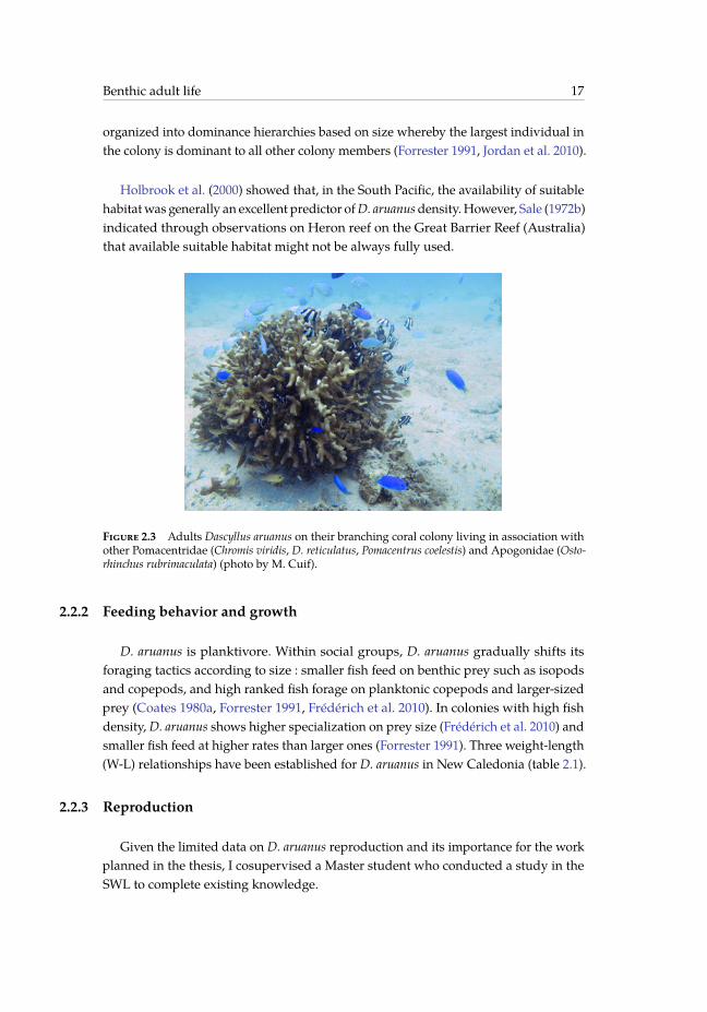
Figure 2.3 Adults Dascyllus aruanus on their branching coral colony living in association withother Pomacentridae (Chromis viridis, D. reticulatus, Pomacentrus coelestis) and Apogonidae (Osto-rhinchus rubrimaculata) (photo by M. Cuif).

2.2.2 Feeding behavior and growth

D. aruanus is planktivore. Within social groups, D. aruanus gradually shifts itsforaging tactics according to size : smaller fish feed on benthic prey such as isopodsand copepods, and high ranked fish forage on planktonic copepods and larger-sizedprey (Coates 1980a, Forrester 1991, Frédérich et al. 2010). In colonies with high fishdensity,D. aruanus shows higher specialization on prey size (Frédérich et al. 2010) andsmaller fish feed at higher rates than larger ones (Forrester 1991). Three weight-length(W-L) relationships have been established for D. aruanus in New Caledonia (table 2.1).

2.2.3 Reproduction

Given the limited data on D. aruanus reproduction and its importance for the workplanned in the thesis, I cosupervised a Master student who conducted a study in theSWL to complete existing knowledge.

36 / 219


Table 2.1 Weight-length relationship (Weight = a * FLb) established for adultsDascyllus aruanusin New Caledonia. FL = fork length.

a b FL min (cm) FL max (cm) N fish Reference0.0716 2.635 2.4 6.5 105 Letourneur et al. (1998)0.0415 2.989 2.4 6.5 112 Kulbicki et al. (2005)0.0486 2.755 2.4 6.8 111 Paillon (2014)

Data collection in the SWL

Field survey

A first survey was conducted in February 2012 when thirteen reproductive coloniesofD. aruanus comprising two to 89 fish were collected by scuba divers on the same dayon a patch reef in the SWL (reef 8, fig. 2.4). Fish took refuge in their host coral whendivers approached. For each colony, the branching coral was surrounded with a largeplastic bag and fish were anesthetized with clove oil (20 to 40 ml at 5%), collected byhand, placed in a separate plastic bag tomaintain colony integrity, and put immediatelyon ice after the dive. Back in the lab, every fish were measured to the nearest 0.1 mmtotal length (TL) using an electronic calliper. Gonads were extracted and placed inBouin’s fixative (71% of picric acid in distilled water solution ; 25% of formaldehyde ;4% of glacial acetic acid) for every fish of the smallest colonies (6 colonies of less than10 individuals and one colony of 20 individuals) and for a stratified random sampleof fish for the biggest colonies (15 to 20 individuals per colony, respecting the sizestructure of the colony). A total of 103 gonads were extracted. After fixation, the 103gonads were taken through a dehydration series, embedded in paraffin, and sectionedtransversally using a microtome. Three to six sections (5µm) were performed persample. Sections were mounted on microscope slides, stained with hematoxylin andeosin, and viewed with an optical microscope to sex individuals and determine themost advanced gonad cells of each fish in order to classify them according to Cole(2002).

A second sampling was carried out over one year from February 2012 to January2013 to determine the length of the reproductive period. One colony of approximately10 mature individuals was collected monthly on a patch reef in the SWL (fig. 2.4,table 2.2). Colony collection, fish length measurements and gonads extractions wereconducted as described in the previous paragraph. A total of 10 colonies was collectedrepresenting 130 fish. Gonads of each individual were also weighted to the nearest0.1mg with a precision balance.

Measurements in aquarium

37 / 219


Figure 2.4 Sampling area : the South-West Lagoon of New Caledonia (SWL). Localization ofthe reefs (numbered from 0 to 10) and sampling stations (orange stars) where Dascyllus aruanussamplings were performed during the thesis. Land is depicted in black, barrier reef in dark greyand shallow reefs in light grey. Blue polygons localize Marine Protected Areas.

Table 2.2 Sampling dates of the 10 Dascyllus aruanus colonies from which the length of thereproductive period was estimated.

Colony Sampling date Reef n°1 23/02/2012 82 06/04/2012 103 07/06/2012 04 26/07/2012 45 23/08/2012 76 21/09/2012 47 09/11/2012 48 22/11/2012 09 19/12/2012 410 17/01/2013 0

Another experiment was conducted in the aquarium facilities of the Aquariumdes Lagons in Nouméa, New Caledonia, to measure parameters regarding D. aruanusreproduction. Twelve discrete colonies of D. aruanuswere collected with their bran-ching coral in the SWL in November 2011 (reef 8, fig. 2.4). The branching coral wassurrounded with a large plastic bag, detached from the substrate, carried up to the

38 / 219


boat and placed in a seawater tub. The colonies were then transported to the aquariumfacilities and the bigger individuals were selected so that each colony comprised ap-proximately eight mature fish. Each colony was then transferred to 80 liters aquariumwith its own branching coral. Spawning events were monitored daily.

Settlement survey

Settlement (mean number of settlers per colony) was estimated on reef 0 in theSWL (fig. 2.4) each month by counting the number of young settlers (< 1.5 cm TL) ona random sample of colonies (∼ 100 colonies each month) from October 2011 to May2014.

Sex ratio

D. aruanus is a protogynous hermaphrodite (Coates 1982). Cole (2002) distingui-shed several types of individuals. Juveniles (Juv) with undifferentiated gonads becomeimmature females (Fi), i.e., females with primary-growth stage oocytes only (inactiveovary) (fig. 2.5, fig. 2.6). Immature females become either active females (Fa, presenceof oogenic ovary) that are able to spawn, or hermaphrodites (fig. 2.5, fig. 2.6). Her-maphrodites are either as inactive males (Hi, developing spermatogenic tissue anddegenerating immature ovarian tissue), or as active males (Hma, spermatogenic testisand degenerating immature ovarian tissue), thus, being a stage of transition fromfemale to male (Cole (2002), Asoh (2003), fig. 2.5, fig. 2.6). All individuals who becomeactive males (Ma, presence of spermatogenic testis) pass through a female stage, buthave never laid eggs (i.e., Fi to Hi transition) , although a sex-change from activefemales (Fa to Hi) cannot be totally excluded (Cole (2002), fig. 2.5, fig. 2.6).

Figure 2.5 Sex-change forDascyllus aruanus. Juv = Juvenile, Fi = immature female, Hi = inactivehermaphrodite, Fa = active female, Hma = active hermaphrodite male, Ma = active male. 1 :Developing ovarian tissue. 2 : Degeneration of immature ovarian tissue and development ofspermatogenic tissue. 3 : Spermatogenesis. 4 : Development of vitellogenic oocytes. Adaptedfrom Saulnier (2013).

39 / 219


Fricke and Holzberg (1974) showed that the sexual composition of D. aruanuscolonies may change with the number of individuals. The sex ratio was female-biasedfor colonies of less than 6 individuals (a single-male and several females) and changedto unity as group size increased (Fricke and Holzberg 1974, Fricke 1977).

In the SWL, the sex ratio and functional sex ratio (i.e., based on active individualsonly) were estimated for nine colonies collected in February 2012 (table 2.3) as :

Sex ratio =Hi + Hma + Ma

Fi + Fa (2.1)

Functional sex ratio =Hma + Ma

Fa (2.2)

The 3 smallest colonies of less than 6 fish contained one male only, in accordance withFricke and Holzberg (1974) results. The number of males increased for bigger colonies,however the proportion of females (Fi + Fa) was always superior to the proportionof males (Ma + Hma) unless only active individuals were considered (e.g., colony 6).The sex ratio and the functional sex ratio were very similar (but see colony 6) becausethere were very few immature individuals.

Table 2.3 Sex-ratio and functional sex-ratio for each collected Dascyllus aruanus colony. N is thetotal number of individuals per colony. Numbers in brackets indicate the number of individualsfor which maturity stage was estimated.

Colony N Fi Hi Fa Ma + Hma Sex ratio Functional sex ratio1 3 0 0 2 1 0.33 / 0.67 0.33 / 0.679 5 0 1 3 1 0.40 / 0.60 0.25 / 0.752 6 0 0 5 1 0.17 / 0.83 0.17 / 0.834 7 (5) 1 0 3 1 0.20 / 0.80 0.25 / 0.757 7 (6) 2 0 2 2 0.33 / 0.67 0.50 / 0.503 20 1 0 11 7 0.37 / 0.63 0.39 / 0.615 23 (14) 1 0 7 6 0.43 / 0.57 0.46 / 0.5412 36 (12) 2 0 7 3 0.25 / 0.75 0.30 / 0.706 36 (19) 8 0 3 7 0.39 / 0.61 0.70 / 0.30

Reproductive seasonality

As for many species, spawning ofD. aruanus is directly linked to water temperature.Therefore spawning seasonality varies significantly according to geographical positionbut the spawning peak takes place during the warm season. In Minicoy (India) forexample, spawning events were observed all year long with a peak from April toJanuary (Pillai et al. 1985). In Okinawa (Japan), spawning peaks between June andSeptember (Mizushima et al. 2000).

40 / 219


Figure 2.6 Histological sections of Dascyllus aruanus gonads. Fi : immature female (2.9 cm TL)with primary-growth stage oocytes (PG), po = ovarian wall. Fa : active female (4.8 cm TL) withprimary-growth stage oocytes (PG), cortical alveolar phase oocytes (CA) and vitellogenic phaseoocytes (Vtg). Ma : active male (4.5 cm TL) with spermatozoa (Sz), Ls = testis lobules walls. Hi :inactive hermaphrodite (4.6 cm TL) with primary-growth stage oocytes (PG) and spermatocytes(Sc). Hma 1 : active male hermaphrodite (4.6 cm TL) with primary-growth stage oocytes (PG),spermatocytes (Sc) and spermatozoa (Sz). Hma 2 : active male hermaphrodite (5.4 cm TL). Photosby E. Saulnier.

41 / 219


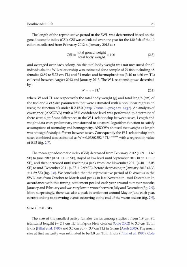
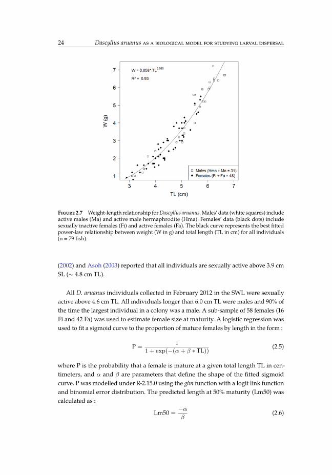
The length of the reproductive period in the SWL was determined based on thegonadosomatic index (GSI). GSI was calculated over one year for the 130 fish of the 10colonies collected from February 2012 to January 2013 as :

GSI =total gonad weighttotal body weight ∗ 100 (2.3)

and averaged over each colony. As the total body weight was not measured for allindividuals, the W-L relationship was estimated for a sample of 79 fish including 48females (2.89 to 5.73 cm TL) and 31 males and hermaphrodites (3.10 to 6.66 cm TL)collected between August 2012 and January 2013. The W-L relationship was describedby :

W = a ∗ TLb (2.4)

where W and TL are respectively the total body weight (g) and total length (cm) ofthe fish and a et b are parameters that were estimated with a non linear regressionusing the function nls under R-2.15.0 (http://www.R-project.org/). An analysis ofcovariance (ANCOVA) with a 95% confidence level was performed to determine ifthere were significant differences in the W-L relationship between sexes. Length andweight data were preliminary transformed to a natural logarithm function to satisfyassumptions of normality and homogeneity. ANCOVA showed that weight-at-lengthwas not significantly different between sexes. Consequently the W-L relationship bothsexes combined was estimated as W = 0.05802352 * TL2.56508 with a regression valueof 0.93 (fig. 2.7).

The mean gonadosomatic index (GSI) decreased from February 2012 (1.89 ± 1.69SE) to June 2012 (0.34 ± 0.16 SE), stayed at low level until September 2012 (0.55 ± 0.19SE), and then increased until reaching a peak from late November 2011 (4.40 ± 2.08SE) to mid-December 2011 (4.37 ± 2.99 SE), before decreasing in January 2013 (3.33± 1.59 SE) (fig. 2.8). We concluded that the reproductive period of D. aruanus in theSWL lasts from October to March and peaks in late November - mid December. Inaccordance with this timing, settlement peaked each year around summer monthsJanuary and February andwas very low inwinter between July andDecember (fig. 2.9).More surprisingly, there was also a peak in settlement around May or June each year,corresponding to spawning events occurring at the end of the warm season (fig. 2.9).

Size at maturity

The size of the smallest active females varies among studies : from 1.9 cm SL(standard length) (∼ 2.3 cm TL) in Papua New Guinea (Cole 2002) to 3.0 cm TL inIndia (Pillai et al. 1985) and 3.0 cm SL (∼ 3.7 cm TL) in Guam (Asoh 2003). The meansize at first maturity was estimated to be 3.8 cm TL in India (Pillai et al. 1985). Cole

http://www.R-project.org/

42 / 219


Figure 2.7 Weight-length relationship forDascyllus aruanus. Males’ data (white squares) includeactive males (Ma) and active male hermaphrodite (Hma). Females’ data (black dots) includesexually inactive females (Fi) and active females (Fa). The black curve represents the best fittedpower-law relationship between weight (W in g) and total length (TL in cm) for all individuals(n = 79 fish).

(2002) and Asoh (2003) reported that all individuals are sexually active above 3.9 cmSL (∼ 4.8 cm TL).

All D. aruanus individuals collected in February 2012 in the SWL were sexuallyactive above 4.6 cm TL. All individuals longer than 6.0 cm TL were males and 90% ofthe time the largest individual in a colony was a male. A sub-sample of 58 females (16Fi and 42 Fa) was used to estimate female size at maturity. A logistic regression wasused to fit a sigmoid curve to the proportion of mature females by length in the form :

P =1

1 + exp(−(α+ β ∗ TL))(2.5)

where P is the probability that a female is mature at a given total length TL in cen-timeters, and α and β are parameters that define the shape of the fitted sigmoidcurve. P was modelled under R-2.15.0 using the glm function with a logit link functionand binomial error distribution. The predicted length at 50% maturity (Lm50) wascalculated as :

Lm50 =−αβ

(2.6)

43 / 219


Figure 2.8 Mean gonadosomatic index (GSI) measured for Dascyllus aruanus from February2012 to January 2013 (n = 130 fish). Error bars represents standard error.

Figure 2.9 Mean number of Dascyllus aruanus settlers per colony estimated from October 2011to May 2014. error bars represent standard error. Numbers above bars indicate the number ofcolonies examined to estimate settlement.

A confidence interval at 95% for Lm50 has been estimated by bootstrap. The estimatedLm50 of females was 3.75 cm TL [3.39 ; 4.07] (fig. 2.10). The smaller active femalemeasured 3.10 cm TL.

44 / 219


Figure 2.10 First sexual maturity curve of Dascyllus aruanus adjusted to the logistic model.

Fecundity

Gopakumar et al. (2009) observed spawning events of D. aruanus that occurred incaptivity and found that the number of eggs laid by a single female ranged between12,000 to 15,000. Pillai et al. (1985) counted the number of eggs present in an ovary ata time and found from 2,125 to 7,157 eggs per ovary (n = 5 females). Finally, Wonget al. (2012) collected egg clutches from 13 colonies in the wild (mean group size =9.8 ± 1.65 SE) and counted the number of eggs under a dissecting microscope. Totalclutch size ranged from 38 to 5,617 eggs (mean = 2,393 ± 475 eggs).

In order to estimate D. aruanus fecundity in the SWL, we had first to determine thespecies reproductive strategy (Murua et al. 2003) (table 2.4). As D. aruanus is iteropa-rous and a batch spawner species, its ovary development may be group-synchronous(oocytes of all stages are present in the ovary without dominant populations) orasynchronous (at least two cohorts of oocytes can be distinguished in the maturingovary) (Murua et al. 2003). The usual method to determine if ovary development issynchronous or not is to estimate the oocyte size frequency distribution (an asynchro-nous ovary development leads to a continuous distribution of oocytes size frequencyand a gap in this distribution is characteristic of a group-synchronous development,Murua et al. (2003)). When the ovary development is group-synchronous, fecundity

45 / 219


is determinate (the standing stock of yolked oocytes prior to the onset of spawningis considered to be equivalent to the potential annual fecundity, Murua et al. (2003)),otherwise fecundity may be determinate or indeterminate (potential annual fecundityis not fixed before the onset of spawning and unyolked oocytes continue to be maturedand spawned during the spawning season, Murua et al. (2003)).

Table 2.4 Reproductive strategies of marine species.

Ovary development Fecundity Type of spawning type

SemelparitySynchronous

DeterminateTotal

Asynchronous Batch

Iteroparity

Group-synchronous Determinate

TotalBatch

AsynchronousDeterminate

BatchIndeterminate

When the fecundity is determinate it is possible to estimate the annual fecundity(i.e., the total number of eggs released per female in a year) by counting, at thebeginning of the spawning season, the number of oocytes destined to be spawned(Murua et al. 2003). Otherwise, annual fecundity may be estimated from other means,for example by using the mean number of eggs per spawning batch, the frequency ofspawning events, the duration of the spawning season and the proportion of spawningfemales across the season (a function of GSI).

The oocyte size frequency of D. aruanus in the SWL was estimated from gonadsections of 10 active females (fig. 2.11). Pictures of ovary sections were taken withan optical microscope (LEICA DM 2000) and a Scion corporation for each femalewith a magnification of 40. Diameters of oocytes were measured on a randomlychosen picture for each female using the ObjectJ plug-in (http://simon.bio.uva.nl/objectj/2-Tutorial.html) of the ImageJ software (http://rsbweb.nih.gov/ij/).Only the entire and undamaged oocytes were measured totalizing 1,219 oocytes.The oocyte diameter was calculated as the average of the maximal and the minimaldiameter.

The oocyte size frequency distribution was continuous with a peak around 35µm(fig. 2.11), indicating an asynchronous ovary development. To determine if fecundity isdeterminate or indeterminate measuring other parameters such as the evolution of thenumber of advanced yolked oocytes or the incidence of atresia during the spawningseason would have been necessary (Murua et al. 2003) but not achievable in the courseof this work.

http://simon.bio.uva.nl/objectj/2-Tutorial.html


http://rsbweb.nih.gov/ij/

46 / 219


Figure 2.11 Oocytes size frequency distribution for ten selected activeDascyllus aruanus females.

Instead, we chose to estimate the annual fecundity through the batch fecundity(Murua et al. 2003) from the aquarium experiment. A total of 16 clutches correspondingto 16 distinct spawning events produced by nine colonies were pictured twice with acamera with a waterproof housing. The first picture covered the entire clutch and thesecond picture was zoomed and taken with macro mode (fig. 2.12).

Figure 2.12 Left : Dascyllus aruanus clutch attached to a side of an aquarium. Right : Zoom ona clutch and 300 mm2 squares used to count the eggs.

Pictures were analyzed using the ImageJ software. Total clutch area was measuredon the first picture and egg density on the second picture using the ObjectJ plug-in andtwo to six randomly selected 300 mm2 squares within which eggs were manually poin-ted and automatically counted. The total number of eggs per clutch was extrapolated

47 / 219


as :

Number of eggs in the clutch =N1 + ...+Nn

n ∗ 300∗Area (2.7)

whereNi is the number of eggs in the randomly selected square i, n is the total numberof randomly selected squares in the clutch, and Area is the total area of the clutch (inmm2).

This method resulted in a number of eggs per clutch varying from 5,829 to 46,217.As each clutch may correspond to several females we took into account the numberof females per aquarium to finally estimate that D. aruanus in the SWL may spawnbetween 2,000 and 15,000 eggs per batch.

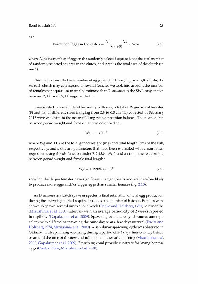
To estimate the variability of fecundity with size, a total of 29 gonads of females(Fi and Fa) of different sizes (ranging from 2.9 to 6.0 cm TL) collected in February2012 were weighted to the nearest 0.1 mg with a precision balance. The relationshipbetween gonad weight and female size was described as :

Wg = a ∗ TLb (2.8)

where Wg and TL are the total gonad weight (mg) and total length (cm) of the fish,respectively, and a et b are parameters that have been estimated with a non linearregression using the nls function under R-2.15.0. We found an isometric relationshipbetween gonad weight and female total length :

Wg = 1.099253 ∗ TL3 (2.9)

showing that larger females have significantly larger gonads and are therefore likelyto produce more eggs and/or bigger eggs than smaller females (fig. 2.13).

As D. aruanus is a batch spawner species, a final estimation of total egg productionduring the spawning period required to assess the number of batches. Females wereshown to spawn several times at one week (Fricke and Holzberg 1974) to 2 months(Mizushima et al. 2000) intervals with an average periodicity of 2 weeks reportedin captivity (Gopakumar et al. 2009). Spawning events are synchronous among acolony with all females spawning the same day or at a few days interval (Fricke andHolzberg 1974, Mizushima et al. 2000). A semilunar spawning cycle was observed inOkinawa with spawning occurring during a period of 2-4 days immediately beforeor around the time of the new and full moon, in the early morning (Mizushima et al.2000, Gopakumar et al. 2009). Branching coral provide substrate for laying benthiceggs (Coates 1980a, Mizushima et al. 2000).

48 / 219


Figure 2.13 Gonad weight-female length relationship for Dascyllus aruanus. The black curverepresents the best fitted relationship between gonad weight (Wg in mg) and female total length(TL in cm) for all individuals (n = 29).

In the SWL, we estimated batch frequency based on the aquarium experiment.Females of the same colony spawned synchronously and attached their eggs to sidesof the tank making monitoring easy. Daily recording of spawning events started afterone year of acclimation from October 2012 to January 2013 (for the 12 colonies) andlasted until April 2013 for the 2 colonies that were kept as control (i.e., not injected)in the transgenerational marking experiments (chapter 4). The batch frequency wascalculated for each colony as the ratio of the total number of spawning events to theduration of the spawning period (table 2.5).

The mean batch frequency of the 12 colonies was 0.09 d-1 (standard deviation (SD)± 0.03), i.e., a female produced one batch every 11 days on average (SD ± 3 days).Batch frequency may be over-estimated as we assumed that all females in one colonyparticipated to all spawning events, which might not always be so.

2.3 Pelagic larval life

After the benthic adult life I now review the most relevant information on thepelagic larval life of D. aruanus from hatching to settlement.

49 / 219

Pelagic larval life 31

Table 2.5 Number of spawning events, spawning lag (in days) and batch frequency observedfor each Dascyllus aruanus colony.

Colony Nb of spawning events Total duration of spawning period (days) Batch frequency (d-1)1 16 158 0.102 15 132 0.113 4 50 0.084 9 80 0.115 7 67 0.106 6 109 0.067 6 55 0.118 10 67 0.159 5 77 0.0610 5 65 0.0811 6 78 0.0812 7 76 0.09

2.3.1 Hatching

D. aruanus eggs hatch three days after spawning just after sunset (Danilowicz andBrown 1992, Mizushima et al. 2000, Gopakumar et al. 2009). The average length ofnewly hatched larvae is 2.4 mm (Gopakumar et al. 2009). The larvae are altricial typewith no mouth opening at the time of hatching (Gopakumar et al. 2009). Gopakumaret al. (2009) observed mouth opening on the second day after hatching and a mouthgape of approximately 160µm. Larvae start feeding from the third day after hatching(Gopakumar et al. 2009).

2.3.2 Planktonic larval duration

D. aruanus planktonic larval duration (PLD) has been estimated in several studiesto last on average 3 weeks with a range extending from 2 to 4 weeks (table 2.6).

I estimated PLD for 579 D. aruanus individuals collected in the SWL including 466individuals collected on a central patch reef (reef 0, fig. 2.4) over two reproductive sea-sons, and 113 individuals collected in March 2012 on eight surrounding reefs (fig. 2.4).I assumed that one increment corresponded to one day and that the first incrementclosest to the core of the otolith was formed at the time of hatching (Campana andNeilson 1985, Wellington and Victor 1989). PLD was determined for each fish as theage at which increment width abruptly fell (Wilson and McCormick 1999) (fig. 2.14).Settlement date of each fishwas calculated as capture date minus number of days sincesettlement. Mean PLD were compared by pairs using t-tests with a 95% confidencelevel.

50 / 219


Table 2.6 Review of studies that estimated PLD for Dascyllus aruanus. SD is standard deviationand SE is standard error. N is the number of fish used for the estimate. GBR means Great BarrierReef.

MeanPLD(days)

Error (SDor SE)

Range N Site Reference

24.4 1.6 (SE) 20 - 28 5 One Tree Island (GBR) Brothers et al. (1983)20 2.4 (SD) 16 - 24 12 Palau Wellington and Victor (1989)22.4 NA 20 - 26 5 Lizard Island (GBR) Thresher et al. (1989)23.8 NA 23 - 25 4 Tuamotu (French Polynesia) Lo-Yat (2002) in Juncker et al. (2007)18.1 0.2 (SE) 14 - 23 122 Wallis island Juncker et al. (2007)26.3 1.7 24 - 29 10 Ryukyu Islands (Japan) Soeparno et al. (2012)

Figure 2.14 Otolith increment profile from longest axis plotted chronologically from otolithcore for aDascyllus aruanus individual collected in February 2013 (1.2 cm TL). Red vertical dottedline indicates PLD.

I found a mean PLD of 23.0 days (± 3.4 SD, range = 14 to 32 days, n = 466) on thecentral patch reef and there were significant differences in mean PLD between somemonths (fig. 2.15, table 2.7) with shorter PLD during months with warmer sea surfacetemperatures. Juncker et al. (2007) found similar seasonal variability of PLD for D.aruanus in Wallis island.

The 113 individuals collected in March 2012 on eight reefs were estimated to haveall settled in February 2012. There seems to be a spatial pattern in PLD with shorter

51 / 219


Figure 2.15 Estimated PLD for different settlement months for individuals collected on thecentral patch reef (reef 0, n = 466). Error bars represent standard error. The vertical dotted lineseparates the two reproductive seasons.

Table 2.7 P.values of t.tests performed between mean PLDs of different months estimated onthe central patch reef (n = 466). Significant p.values (< 0.05) are indicated in bold.

Dec11 Jan12 Feb12 Mar12 Dec12 Jan13 Feb13Dec11 1 - - - - - -Jan12 0.0751 1 - - - - -Feb12 0.0029 0.0080 1 - - - -Mar12 8.44E-05 2.40E-10 3.80E-03 1 - - -Dec12 1.17E-03 1.81E-09 2.72E-12 5.90E-14 1 - -Jan13 0.6839 0.1088 0.0146 1.42E-03 4.72E-02 1 -Feb13 0.0124 0.0670 0.1497 5.90E-09 1.46E-10 0.0372 1Mar13 0.0063 0.0269 0.5316 8.86E-05 1.53E-11 0.0237 0.4163

PLDs for individuals settling North of the Dumbea Pass and longer PLD South of thepass (fig. 2.4, fig. 2.16, table 2.8). For example, average PLD of individuals collected onreef 3 and on reef 5 are significantly longer than PLD of individuals collected on thereefs 1, 2 and 10 that are located more in the North (fig. 2.4, fig. 2.16, table 2.8).

2.3.3 Swimming capabilities of planktonic larvae

In a review, Fisher (2005) showed that late-stage larvae (just before settlement) ofa range of coral reef fish families were able to swim at speeds higher than the meancurrent speeds reported aroundmost reefs. Leis and Carson-Ewart (1997) showed that,although in situ swimming speeds of Pomacentrids varied widely among species (7 to35 cm s-1), D. aruanus late-stage larvae were effective swimmers with a mean speed of19.7 cm s-1 ± 1.9 SE (range = 9.1 to 30.1 cm s-1) higher than the average current speeds

52 / 219


Figure 2.16 Estimated PLD for individuals collected on eight reefs (n = 113) surrounding thecentral patch reef (reef 0, n = 74) in March 2012. Error bars represent standard error. Reefs areplotted according to their localization from the North (reef 6) to the South (Reef 3) of the SWL(fig. 2.4).

Table 2.8 P.values of t.tests between mean PLDs estimated on the eight surrounding reefs (n =113). Significant p.values (< 0.05) are indicated in bold.

Reef 1 Reef 2 Reef 3 Reef 4 Reef 5 Reef 6 Reef 7 Reef 10Reef 1 1 - - - - - - -Reef 2 0.8586 1 - - - - - -Reef 3 0.0274 0.0096 1 - - - - -Reef 4 0.1615 0.0667 0.3093 1 - - - -Reef 5 0.0347 0.0038 0.5452 0.5463 1 - - -Reef 6 0.6464 0.4772 0.0718 0.3540 0.1107 1 - -Reef 7 0.5848 0.3994 0.0679 0.3565 0.1006 0.9524 1 -Reef 10 0.7456 0.8371 0.0132 0.0827 0.0139 0.4335 0.3727 1Reef 0 0.1029 0.0087 0.1819 0.8959 0.2929 0.2973 0.2869 0.0423

in their study area (10 to 15 cm s-1). Fisher et al. (2005) alsomeasured critical swimmingspeeds in captivity, by placing late-stage larvae in a swimming flume and increasingthe current speed incrementally over time until the larva could no longer maintain itsposition for the full time interval (2 min in this study). The highest speed maintainedis termed critical speed. Fisher et al. (2005) found an average critical swimming speedof 24 cm s-1 ± 0.8 SE, (range = 19.7 to 27.1 cm s-1) for D. aruanus late-stage larvae(mean TL = 0.94 ± 0.02 cm SE), which is intermediate compared to other coral reeffish species (Leis 2006).

To determine the time larvae could maintain such an active swimming behavior,Stobutzki (1998) run an experiment in a swimming flume where fish were swum untilthey were fatigued, i.e., they could no longer maintain position against the current.

53 / 219


The time until they became fatigued was recorded and from this the travelled distancewas calculated. They showed a significant correlation between sustained swimmingability and total length of individuals. They found that D. aruanus late-stage larvae(mean TL = 1.17 cm) were able to travel a distance of 21.37 km against a water speedof 13.5 cm s-1. This suggests that speeds as high as 50% of critical swimming speedare sustainable by late-stage D. aruanus larvae for considerable time periods (over 24h) (Fisher and Wilson 2004).

Fisher and Bellwood (2003) showed that the proportion of time larvae spent swim-ming at night increased rapidly towards the end of the larval phase for five coral reefspecies, including a Pomacentrid. In addition, they showed that the swimming speedsof larvae were significantly higher at night than during the day. Patterns of nocturnalactivity appear to relate to the nocturnal settlement behavior of larvae.

All the above cited studies concentrated solely on the late pelagic phase. Fisher et al.(2000) suggested that some species have the potential to actively modify their dispersalpatterns from an early age. Fisher (2005) suggested that the development of swimmingability can be described adequately as a linear increase from zero at hatching to aspecies-specific maximum at settlement. Calculations based on this developmentalpattern suggest that most reef fish families could substantially influence their dispersalpatterns relative to ocean currents for over 50% of their larval phase Fisher (2005). Leis(2006) underlined the fact that swimming abilities might develop sooner as expected,but suggested that it might not actually come into play until competency to settle isattained, or particular cues from settlement habitats are detected.

Active swimming behavior allows larvae to exert some control over their depth(Huebert 2012). Huebert and Sponaugle (2009) suggested that pressure is their primaryproximate cue for vertical navigation. The depth at which larval fishes swim duringtheir pelagic phase depends on the species and time of day (Leis et al. 2011), butthe larvae of many species, including damselfish, are found at relatively shallowdepths (Leis 1991, Hendriks et al. 2001). Irisson and Lecchini (2008) showed thatPomacentridae postflexion larvae tend to have a shallower depth distribution thanflexion and preflexion larvae.

2.3.4 Sensory mechanisms at settlement

The potential influence of swimming capabilities on survival depends on the abilityof larvae to orient in the open ocean (Paris et al. 2008, Leis et al. 2014) particularlytowards their settlement habitat. Fishes larvae may use a range of sensory mechanismseffective over different spatial scales to detect and actively choose settlement sites,

54 / 219


including sound, smell and sight (Montgomery et al. 2001, Lecchini 2004, Lecchiniet al. 2005).

Sound

The use of sound is the best understood mechanism (Leis et al. 2011). Sound travelswell underwater with little attenuation, and is current-independent but location-dependent (Leis et al. 2011). Larvae of many coral reef fishes, and especially Poma-centridae, can hear as soon as otoliths are formed, i.e., during much of their pelagiclarval phase and possibly before they hatch (Simpson et al. 2005). Settlement-stagelarvae can distinguish among sounds (Leis et al. 2002, Radford et al. 2011) and areattracted to settlement habitats sounds (Simpson et al. 2004). Simpson et al. (2008)showed that coral reef fish larvae prefer the higher-frequency invertebrate-generatedaudible component of reef noise.

Distances over which larvae can detect a given sound vary among species andlargely increase with ontogeny (Leis et al. 2011, Wright et al. 2011). Mann et al. (2007)suggested that larval fishes could not detect settlement habitat sound at distancessuperior to 1 km. But recent studies suggest otherwise (Leis et al. 2011, Wright et al.2011) and that large reefs should be detectable from larger distances than small ones(Leis et al. 2011).

Smell

Olfactory cues are both current- and location-dependent (Leis et al. 2011). Larvaeare able to detect odors during most of their pelagic phase and even during theirembryonic stage (Arvedlund and Nielsen 1996, Atema et al. 2002, Kavanagh andAlford 2003, Dixson et al. 2014). Arvedlund and Nielsen (1996) showed that small post-settlement D. aruanus larvae had relatively high olfactory ability compared to otherdamselfish, suggesting good olfactory ability during younger stages. Pre-settlementlarvae can detect odors associated to predators, conspecifics (Sweatman 1988), orwater to which they were acclimated (Atema et al. 2002, Gerlach et al. 2007). The lattersuggests that, once their settlement stage is reached, larvae may be able to return totheir natal reef by actively swimming within the reef-odor plume. Little is knownabout the ontogeny of olfactory ability or the range over which larvae can localize odorsources (Leis et al. 2011). Lecchini et al. (2014) suggested that fish larvae could detectchemical cues emitted by coral reefs until 1 km. Paris et al. (2013) showed that pelagicreef fish larvae discriminated reef odor and responded by changing their swimmingspeed and direction. They concluded that reef fish larvae could smell the presence of

55 / 219


coral reefs from several kilometers offshore and that odor was a primary componentof their navigational system by activating other directional sensory cues.

Sight

Celestial cues are current- and location-independent and can therefore apply overbroader scales than other sensory abilities like sound and olfaction (Leis et al. 2011).Hawryshyn et al. (2003) reported that juveniles of damselfishes possessed the mostcomplex polarization sensitivity recorded for any vertebrate. Mouritsen et al. (2013)showed that solar compass may be used for orientation in coral reef fish larvae. Al-though polarized light will not assist larvae to locate a particular reef, it can enablethemmaintain a general position, or to orient in a particular direction which is helpfulin counteracting a prevailing current (Leis et al. 2011). Leis et al. (2011) suggested thatcelestial visual cues might be used early in development.

Other cues

To our knowledge, the use of magnetic fields for orientation has not been shown inmarine fish larvae (Leis et al. 2011). Tide and wind have been suggested to be cues fororientation of pre-settlement spiny lobster larvae (Kough et al. 2014).

2.3.5 Habitat and behavior at settlement

D. aruanus larvae settle on branching coral colonies at varying depths (Leis et al.2002). Jones (1997) showed that D. aruanus larvae settled preferentially to deepersites (4 - 8 m depth). A growing number of studies show that coral reef fish larvaeare able to recognize their natal reef through imprinting on chemical cues duringembryonic stage, which could help explaining strong site attachment and high valuesof self-recruitment observed for many species (Atema et al. 2002, Gerlach et al. 2007,Dixson et al. 2008, 2014).

Settlement occurs at night for a range of coral reef fish families (Kingsford 2001).Accordingly, Sweatman (1985b) observed that a large proportion of D. aruanus larvaesettled in darkness, when light levels were low and adults were hidden in the coral,suggesting that vision is unlikely to be important in habitat selection. Schmitt andHolbrook (1999) showed that settlement of D. aruanus in French Polynesia was follo-wing a semilunar cycle with settlement peaks lasting 3-5 days around the two quartermoon phases.

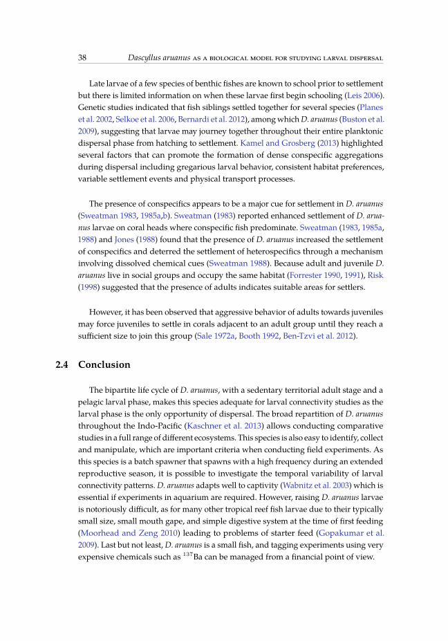
56 / 219


Late larvae of a few species of benthic fishes are known to school prior to settlementbut there is limited information on when these larvae first begin schooling (Leis 2006).Genetic studies indicated that fish siblings settled together for several species (Planeset al. 2002, Selkoe et al. 2006, Bernardi et al. 2012), amongwhichD. aruanus (Buston et al.2009), suggesting that larvae may journey together throughout their entire planktonicdispersal phase from hatching to settlement. Kamel and Grosberg (2013) highlightedseveral factors that can promote the formation of dense conspecific aggregationsduring dispersal including gregarious larval behavior, consistent habitat preferences,variable settlement events and physical transport processes.

The presence of conspecifics appears to be a major cue for settlement in D. aruanus(Sweatman 1983, 1985a,b). Sweatman (1983) reported enhanced settlement of D. arua-nus larvae on coral heads where conspecific fish predominate. Sweatman (1983, 1985a,1988) and Jones (1988) found that the presence of D. aruanus increased the settlementof conspecifics and deterred the settlement of heterospecifics through a mechanisminvolving dissolved chemical cues (Sweatman 1988). Because adult and juvenile D.aruanus live in social groups and occupy the same habitat (Forrester 1990, 1991), Risk(1998) suggested that the presence of adults indicates suitable areas for settlers.

However, it has been observed that aggressive behavior of adults towards juvenilesmay force juveniles to settle in corals adjacent to an adult group until they reach asufficient size to join this group (Sale 1972a, Booth 1992, Ben-Tzvi et al. 2012).

2.4 Conclusion

The bipartite life cycle of D. aruanus, with a sedentary territorial adult stage and apelagic larval phase, makes this species adequate for larval connectivity studies as thelarval phase is the only opportunity of dispersal. The broad repartition of D. aruanusthroughout the Indo-Pacific (Kaschner et al. 2013) allows conducting comparativestudies in a full range of different ecosystems. This species is also easy to identify, collectand manipulate, which are important criteria when conducting field experiments. Asthis species is a batch spawner that spawns with a high frequency during an extendedreproductive season, it is possible to investigate the temporal variability of larvalconnectivity patterns.D. aruanus adapts well to captivity (Wabnitz et al. 2003) which isessential if experiments in aquarium are required. However, raising D. aruanus larvaeis notoriously difficult, as for many other tropical reef fish larvae due to their typicallysmall size, small mouth gape, and simple digestive system at the time of first feeding(Moorhead and Zeng 2010) leading to problems of starter feed (Gopakumar et al.2009). Last but not least,D. aruanus is a small fish, and tagging experiments using veryexpensive chemicals such as 137Ba can be managed from a financial point of view.

57 / 219

Conclusion 39

D. aruanus has a very limited home range like more than half of coral reef fishspecies in New Caledonia (Guillemot et al. 2011). Its reproductive strategy is broadlyreflective of many families associated with coral reefs : its reproductive season extendsover the whole warm season, and as many other reef fishes it changes sex and presentsa protogynous hermaphrodism that is the normal pattern of reproductive ontogeny(Warner 1984). With a PLD of 3-4 weeks, D. aruanus spend approximately the sameamount of time to disperse in the plankton than the majority of other teleost fish(Wellington and Victor 1989, Luiz et al. 2013). However, its PLD is longer than that ofspecies usually used in connectivity studies (e.g., Planes et al. (2009), Saenz-Agudeloet al. (2012). D. aruanus larvae are also intermediate in terms of swimming capacities(Fisher 2005, Leis 2006).

All these criteria makeD. aruanus potentially reflective of a broad range of demersalcoral reef fishes, and a species particularly easy to survey for larval connectivitystudies.

58 / 219

59 / 219

Chapitre 3

Wind-induced variability in larvalretention in a coral reef system :A biophysical modelling study in theSouth-West Lagoon of New Caledonia

41

60 / 219

61 / 219

43

M. Cuifa,b,c,d, D. M. Kaplanc, J. Lefèvree, V. M. Fauref,g , M. Caillaudh, P. Verleyi,L. Vigliolab, C. Letta

Progress in Oceanography 122, 105 - 115 (2014)

a IRD, UMI 209 UPMC UMMISCO, Sète, Franceb IRD, Laboratoire d’Excellence LABEX Corail, UR 227 COREUS, Nouméa, New Caledoniac IRD, UMR 212 EME, Sète, Franced AgroParisTech, Paris, Francee IRD, LEGOS/MIO, Nouméa, New Caledoniaf Aix-Marseille Université, MIO, Marseille, Franceg Université du Sud Toulon-Var, CNRS-INSU/IRD UM 110, La Garde, Franceh DYNECO/PHYSED IFREMER, Centre de Bretagne Technopôle de Brest-Iroise, Plouzané, Francei IRD, UMR 212 EME, Marine Research Institute and Oceanography Department, Cape Town, South Africa

Abstract

In the present work, a biophysical dispersal model is used to understand the roleof the physical environment in determining reef fish larval dispersal patterns in theSouth-West Lagoon of New Caledonia. We focus on a reef fish species, the humbugdamselfish Dascyllus aruanus, to investigate seasonal variability of simulated larvalretention at the scale of a reef patch and at the scale of the lagoon, and to explorelinks between larval retention and wind variability. The model shows that retentionexhibits considerable temporal variability and periodically reaches values much largerthan anticipated. Non-zero larval settlement occurs over a large part of the lagoon.Nevertheless, settlement values decrease quickly away from the natal reef and meandispersal distances are of order 25 - 35 km. Cross-correlation analyses indicate thatweather conditions characterized by strong south east tradewinds lead to low retentionrates at both local (reef) and regional (lagoon) scales. By contrast, subtropical weatherconditions characterized by weak winds result in high retention rates. These resultssuggest that large-scale weather regimes can be used as proxies for larval retention ofthe humbug damselfish in the South-West Lagoon of New Caledonia. Nevertheless,relatively small mean dispersal distances suggest that metapopulation dynamics occuron relatively small spatial scales.

Keywords : Biophysical model, Larval dispersal, Wind-driven transport, Dascyllusaruanus, Precompetency, Homing, New Caledonia

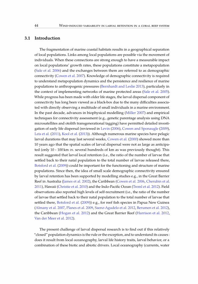
62 / 219

44 Wind-induced variability in larval retention in a coral reef system

3.1 Introduction

The fragmentation of marine coastal habitats results in a geographical separationof local populations. Links among local populations are possible via the movement ofindividuals. When these connections are strong enough to have a measurable impacton local populations’ growth rates, these populations constitute a metapopulation(Sale et al. 2006) and the exchanges between them are referred to as demographicconnectivity (Cowen et al. 2007). Knowledge of demographic connectivity is requiredto understand metapopulation dynamics and the persistence and resilience of marinepopulations to anthropogenic pressures (Bernhardt and Leslie 2013), particularly inthe context of implementing networks of marine protected areas (Sale et al. 2005).While progress has been made with older life stages, the larval dispersal component ofconnectivity has long been viewed as a black-box due to the many difficulties associa-ted with directly observing a multitude of small individuals in a marine environment.In the past decade, advances in biophysical modelling (Miller 2007) and empiricaltechniques for connectivity assessment (e.g., genetic parentage analysis using DNAmicrosatellites and otolith transgenerational tagging) have permitted detailed investi-gation of early life dispersal (reviewed in Levin (2006), Cowen and Sponaugle (2009),Leis et al. (2011), Kool et al. (2013)). Although numerous marine species have pelagiclarval durations that may last several weeks, Cowen et al. (2000) showed more than10 years ago that the spatial scales of larval dispersal were not as large as anticipa-ted (only 10 - 100 km vs. several hundreds of km as was previously thought). Thisresult suggested that larval local retention (i.e., the ratio of the number of larvae thatsettled back to their natal population to the total number of larvae released there,Botsford et al. (2009)) could be important for the functioning and structure of marinepopulations. Since then, the idea of small scale demographic connectivity ensuredby larval retention has been supported by modelling studies e.g., in the Great BarrierReef in Australia (James et al. 2002), the Caribbean (Cowen et al. 2006, Cherubin et al.2011), Hawaii (Christie et al. 2010) and the Indo-Pacific Ocean (Treml et al. 2012). Fieldobservations also reported high levels of self-recruitment (i.e., the ratio of the numberof larvae that settled back to their natal population to the total number of larvae thatsettled there, Botsford et al. (2009)) e.g., for reef fish species in Papua New Guinea(Almany et al. 2007, Planes et al. 2009, Saenz-Agudelo et al. 2012, Berumen et al. 2012),the Caribbean (Hogan et al. 2012) and the Great Barrier Reef (Harrison et al. 2012,Van der Meer et al. 2012).

The present challenge of larval dispersal research is to find out if this relatively“closed” population dynamics is the rule or the exception, and to understand its causes :does it result from local oceanography, larval life history traits, larval behavior, or acombination of these biotic and abiotic drivers. Local oceanography (currents, water

63 / 219

Introduction 45

residence time) has been shown to be of great importance for explaining relativelyclosed population dynamics (Paris and Cowen 2004, Treml et al. 2012). Among lifehistory traits, the length of the larval precompetency period, i.e., the period of timein which larvae may not settle (Jackson and Strathmann 1981), has been shown tobe a key driver for local retention within the natal population (Black and Moran1991, Paris and Cowen 2004, Treml et al. 2012). Whereas the precompetency periodof reef-building coral larvae is relatively short (between 2 and 5 days, Heyward andNegri (2010)), it can reach several weeks for other reef species (Staaterman et al.2012, Butler et al. 2011, Soria et al. 2012). Concerning larval behavior, several studiesdemonstrate that fish larvae have sensory capabilities coupled with strong swimmingcapabilities (Leis 2010) that facilitate local retention through homing. For instance,larvae are capable of olfactory discrimination and prefer the odor of their home reef(Gerlach et al. 2007). Acoustic (e.g., Radford et al. (2011)) and sun compassmechanisms(Mouritsen et al. 2013) have also been suggested to allow pelagic larvae to locate theirnatal reef. Modelling studies show that early active larval movement associated withorientation behavior is a mechanism for self-recruitment (James et al. 2002, Paris et al.2005, Staaterman et al. 2012).

In this study we investigate the roles of local meteo-oceanography, precompetencyperiod and homing behavior in determining reef fish larval retention in the South-WestLagoon of New Caledonia (SWL). The oceanography of the SWL has been particularlywell studied over the last 40 years through in situ measurements and numericalmodels that provide insights on sediment transport and biogeochemical dynamicsin the lagoon (Jarrige et al. 1975, Douillet 1998, Faure et al. 2010, Ouillon et al. 2010,Fuchs et al. 2012). Previous studies using Lagrangian tracers show that the SWL iswell mixed by the joined action of tide currents, winds and swell which results ina rather low average water residence time (defined as the time needed for a waterparticle to leave the lagoon) of 11 days (Jouon et al. 2006, Ouillon et al. 2010). If weassume, as a first approximation, that larvae of marine species are passive entitiesduring their precompetency period, and are therefore advected like water parcels, theshort water residence time found in the SWL has enormous consequences for larvalretention : species with a larval precompetency period longer than 11 days will bemostly flushed out of the lagoon.

In this study we focus on a coral reef damselfish, Dascyllus aruanus, a species thathas precisely a precompetency period of ∼ 11 days (see section 3.2.3). We use a three-dimensional biophysical model to investigate larval retention of D. aruanus and itsseasonal variability inside the SWL. We first describe the study species and regionfocusing on the oceanographic context. The biophysical model is then described andused to assess larval retention at two different spatial scales : SWL scale (“natal lagoon

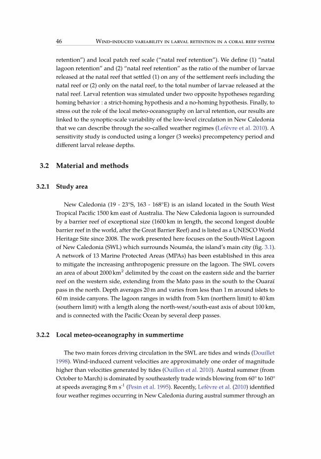
64 / 219


retention”) and local patch reef scale (“natal reef retention”). We define (1) “natallagoon retention” and (2) “natal reef retention” as the ratio of the number of larvaereleased at the natal reef that settled (1) on any of the settlement reefs including thenatal reef or (2) only on the natal reef, to the total number of larvae released at thenatal reef. Larval retention was simulated under two opposite hypotheses regardinghoming behavior : a strict-homing hypothesis and a no-homing hypothesis. Finally, tostress out the role of the local meteo-oceanography on larval retention, our results arelinked to the synoptic-scale variability of the low-level circulation in New Caledoniathat we can describe through the so-called weather regimes (Lefèvre et al. 2010). Asensitivity study is conducted using a longer (3 weeks) precompetency period anddifferent larval release depths.

3.2 Material and methods

3.2.1 Study area

New Caledonia (19 - 23°S, 163 - 168°E) is an island located in the South WestTropical Pacific 1500 km east of Australia. The New Caledonia lagoon is surroundedby a barrier reef of exceptional size (1600 km in length, the second longest doublebarrier reef in the world, after the Great Barrier Reef) and is listed as a UNESCOWorldHeritage Site since 2008. The work presented here focuses on the South-West Lagoonof New Caledonia (SWL) which surrounds Nouméa, the island’s main city (fig. 3.1).A network of 13 Marine Protected Areas (MPAs) has been established in this areato mitigate the increasing anthropogenic pressure on the lagoon. The SWL coversan area of about 2000 km2 delimited by the coast on the eastern side and the barrierreef on the western side, extending from the Mato pass in the south to the Ouaraïpass in the north. Depth averages 20m and varies from less than 1m around islets to60m inside canyons. The lagoon ranges in width from 5km (northern limit) to 40 km(southern limit) with a length along the north-west/south-east axis of about 100 km,and is connected with the Pacific Ocean by several deep passes.

3.2.2 Local meteo-oceanography in summertime

The two main forces driving circulation in the SWL are tides and winds (Douillet1998). Wind-induced current velocities are approximately one order of magnitudehigher than velocities generated by tides (Ouillon et al. 2010). Austral summer (fromOctober to March) is dominated by southeasterly trade winds blowing from 60° to 160°at speeds averaging 8m s-1 (Pesin et al. 1995). Recently, Lefèvre et al. (2010) identifiedfour weather regimes occurring in New Caledonia during austral summer through an

65 / 219

Material and methods 47

Figure 3.1 Study area : the South-West Lagoon ofNewCaledonia (SWL in light blue). Settlementreefs (in dark grey) are buffered by a 1-km sensory zone (in light grey).

objective classification applied to remote sensed winds for nine summer seasons from1999 to 2008 (table 3.1). Three of these weather regimes (regimes 1, 3 and 4) exhibitlow-level circulation dominated by SE trade winds. Regime 1 captures a strong, nearsteady and alongshore trade wind flow, averaging 8m s-1 and is referred to here as“Strong SE Trade-wind”. This regime is the most frequent, accounting for slightly lessthan a third of the austral summer days. Long spells of regime 1 are more favorableto the flushing of the lagoon by driving a general north-west drift. The SWL is thusmainly fed with oceanic waters at its southern end, through the different passes of thebarrier reef as described in Jouon et al. (2006). This regime promotes the formationof upwelling events along the barrier reef (Marchesiello et al. 2010) and local windacceleration in SWL due to flow splitting by the mountainous island (Lefèvre et al.2010). The regional circulation in regime 4, called “Subtropical SE wind”, also showsa near steady alongshore SE direction, but with weaker winds (5.2m s-1 in average)associated with strong subtropical westerlies south of the island. Occurring for 27% ofthe days in Lefèvre et al. (2010) analysis, this regime is more frequent in early summer(November - December). Regime 3, called “Tropical SE wind”, accounts for 22% ofthe days, occurs more frequently during the warm and wet period from January toMarch, and produces average winds of 5.2m s-1. The fourth regime, regime 2, called“Weak Easterly Circulation”, exhibits a weak easterly airflow circulation (below 2ms-1) and the largest variability in wind direction. It is also the most transient and leastrobust regime, accounting for less than 8% of the days.

66 / 219


Table 3.1 Description of the four weather regimes defined in Lefèvre et al. (2010). Statisticsof wind speed and direction were computed from remote sensed surface winds for the period1999-2008 (adapted from Lefèvre et al. (2010)). SD = standard deviation.

Name % of occurence Wind speed (m s-1) Wind direction (°N)Mean SD Mean SD

Regime 1 Strong SE Trade-wind 30 8 2.2 122.5 21.6Regime 2 Weak Easterly Circulation 7.4 1.4 2.3 120.6 94.8Regime 3 Tropical SE wind 22.6 5.2 2.8 122.9 60.5Regime 4 Subtropical SE wind 27.3 5.2 2.2 118.9 45.6

3.2.3 Study species

This study is part of a larger program focusing on the population connectivityof the Humbug damselfish (Pomacentridae), Dascyllus aruanus, in the SWL of NewCaledonia. Here, we therefore use the larval life history traits of this species as thebasis for our exploration of larval dispersal patterns in the SWL. D. aruanus is anobligate coral-dwelling Pomacentridae, found exclusively in lagoon habitats (Allen1991), where it lives in well-mixed waters among branching coral colonies in spatiallydiscrete groups of 2 - 80 individuals (Sale 1972a, Holbrook et al. 2000, Cole 2002).Coral colonies provide protection from predators and substrate for laying benthiceggs Coates (1980b), Mizushima et al. (2000). D. aruanus adults are sedentary benthicspawners that breed on a lunar cycle throughout the year (Pillai et al. 1985). Spawningpeaks in summer, during which each female can spawn several times at 1 week(personal observation) to 2 months (Mizushima et al. 2000) intervals. Eggs remain inbenthic nests for 3 days after which hatchlings are released into the plankton wherethey disperse on average 3 weeks (mean planktonic larval duration -PLD- Thresheret al. (1989), Juncker et al. (2007), Soeparno et al. (2012) prior to settling on adult reefhabitats. Newly hatched larvae have well developed sensorial abilities (Leis 2010) andpomacentrids larvae are able to swim actively against currents during the second halfof their pelagic larval phase (Fisher 2005). Furthermore, field evidence indicates thatlate-stage larvae of coral reef fish can detect the presence of a reef at a range of atleast 1 km (Leis et al. 1996). Thus the sensorial and swimming abilities which allowthe orientation of competent larvae to suitable recruitment habitat (Sweatman 1983,Holbrook et al. 2000) may be present in D. aruanus larvae as early as the age of 11 days(i.e., half of mean PLD).

67 / 219


3.2.4 Biophysical model

Larval dispersal was simulated with a biophysical model using version 3.0 ofthe Lagrangian tool Ichthyop (Lett et al. 2008). Ichthyop is a three-dimensional (3D)particle-tracking model designed to study the effects of physical and biological factorson the transport and settlement of ichthyoplankton. The biophysical model is basedon an offline forcing of an individual-based model (IBM) by a 3D hydrodynamicmodel. The hydrodynamic model used here is the high-resolution 3D Model forApplications at Regional Scales (MARS3D, Lazure and Dumas (2008)). MARS3Dprovides 3D dynamic fields of current velocities which result from the combinedactions of wind and tidal forcing. Several configurations of this model have beendeveloped and validated in the SWL (Douillet 1998, Douillet et al. 2001, Ouillon et al.2010). The configuration of MARS3D used in this study covers the SWL from 22.06°to 22.52°S and from 165.98° to 166.79°E. The model grid has a horizontal resolutionof 500m and 30 terrain following generalized sigma levels in the vertical dimension.This configuration is forced by realistic hourly winds at 4 km resolution obtained fromthe mesoscale Weather Research and Forecasting (WRF) model (Lefèvre et al. 2010).Simulated surface wind speeds and directions are very close to observations (Indiceof Agreement IOA of 0.9 and RMSE < standard deviation of observations for bothspeed and direction, section 3.6, table 3.2). Realistic wind forcing corresponds to theyears 2003-2004. This period is neutral regarding ENSO phases. Tides are included inMARS3D through a lateral forcing using the Oregon State University TPXO.6 tidessolution (Egbert et al. 1994) for 8 tidal constituents. The TPXO tides solution is refinedfurther within ADCIRC (ADvanced CIRCulation model, Luettich et al. (1992)), byusing an unstructured and very fine resolution mesh (from 500 to 25m in the SWL,Lefèvre, pers. comm.).

Our larval transport IBM uses MARS3D model results covering the reproductiveperiod of D. aruanus in New Caledonia i.e., from mid - September to late March.Outputs ofMARS3D simulationswere stored every 12min as this time step is sufficientto account for the effects of tides. In the IBM, larvae are characterized by their latitude(°S), longitude (°E) and depth (m). Locations of individuals are updated every 5minin three dimensions using the velocity fields stored from MARS3D interpolated inspace and time via a forward-Euler integration scheme.

3.2.5 Simulations

In order to study the effect of wind regime on larval retention, we examineddispersal from a ∼ 500m diameter patch reef located at the center of the SWL (callednatal reef hereafter) where water residence time is close to the average of 11 days

68 / 219


(Ouillon et al. 2010). Location and extent of the natal reef and settlement areas in theSWL were defined as polygons based on GIS habitat maps provided by the atlas ofcoral reefs in New Caledonia (Andréfouët and Torres-Pulliza 2004). Since D. aruanusis ubiquitous in the SWL all reefs shallower than 20m were considered as potentialsettlement habitats in the model. Hatching events (representing a release of 500 virtuallarvae each) were simulated over the natal reef every 3 h over austral summer frommid-September 2003 to late March 2004 (i.e., 1320 simulations). For each releaseon the natal reef, larvae were randomly distributed throughout the water columnfrom 0 to 20m depth. Larvae from each hatching event were followed for up to 30days (the largest value of PLD reported for D. aruanus (Soeparno et al. 2012)). Weconsidered that larvae were initially transported passively by ocean currents duringan 11-day precompetency period and that they became active afterwards with sensoryand swimming capabilities that allowed them to detect and approach a settlementarea. To do so, a non-explicit swimming behavior during the competency period wasincluded by assuming that larvae could actively settle once at a given distance from asettlement reef. This distance was defined as 1 km (Leis et al. 1996). Any virtual larvalocated less than 1 km away from a settlement reef at any time between the end of theprecompetency period and 30 days was then considered to have successfully settled.

Simulations were run under two alternative hypotheses about natal homing. Underthe first hypothesis, settlement was supposed to be driven by strict natal homing :settlement was only allowed on the natal reef, i.e., competent larvae were only ableto settle on the natal reef. We will refer to this hypothesis as the “strict hominghypothesis”. Under the second hypothesis, settlement of competent larvaewas allowedon the natal reef and in any other part of the SWLwhere suitable habitat forD. aruanuswas available. We will refer to this hypothesis as the “no-homing hypothesis”. Alonger precompetency period of 3 weeks (21 days) was also tested. A sensitivityanalysis to the larval release depth was also conducted using simulations run for aprecompetency period of 11 days for both hypotheses regarding natal homing. Aslarvae are characterized by their latitude (°S), longitude (°E) and depth (m) at eachtime step, it is possible to know the release depth of each recruited larvae at theend of the simulation. Five release depth intervals were tested from 0 to 20m. Allpost-processing computations were done using R-2.15.0.

3.2.6 Lagoon vs. reef retention

Simulation outputs were used to calculate larval retention at two different spatialscales. Larval retention was first computed for each simulation at the SWL scale. Thisretention, hereafter called “natal lagoon retention” (NLR), is defined as the ratio ofthe number of larvae released at the natal reef that settled on any of the settlement

69 / 219


reefs to the total number of larvae released at the natal reef. Larval retention wasalso computed for each hatching event at the natal reef scale. This local retention,hereafter referred to as “natal reef retention” (NRR), is defined as the ratio of thenumber of larvae released at the natal reef that settled back to that site to the totalnumber of larvae released at the natal reef. Three retention time series extending frommid-September 2003 to early March 2004 were obtained : NLR under the no-hominghypothesis ; NRR under the no-homing hypothesis ; NRR under the strict-hominghypothesis. Note that under the strict-homing hypothesis NLR equals NRR.

3.2.7 Cross-correlations

To study the link between wind conditions and simulated D. aruanus larval reten-tion, we calculated cross-correlations between wind and retention time series with amaximum lag of 30 days. We extracted hourly meridional and zonal wind componentsfrom the WRF model at the closest grid point to the natal reef and converted theminto an along-shelf (V-component) and cross-shelf (U-component) coordinate system,rotated 60° anti-clockwise from true north, with V positive towards the north-west(300°) and U positive onshore towards 30°. Time series of daily probability of occur-rence of the four weather regimes defined by Lefèvre et al. (2010) were also used in across-correlation analysis with simulated retention time series. We used the Spearmanrank-order correlation coefficient (hereafter Spear-R) because the simulated retentionvalues were not normally distributed. Given that autocorrelation of time series in-creases the risk to consider that correlations between series are significant when theyare not, we accounted for autocorrelation of all time series explicitly in judging thesignificance of correlations by adjusting the degrees of freedom following Pyper andPeterman (1998) and Botsford and Paulsen (2000). Auto-correlation timescales of order2-8 days, depending on the simulation and time series examined, were identified andthe effective degrees of freedom were corrected accordingly. This correction reducedthe effective degrees of freedom and consequently substantially increased the valueof correlation required for a significant result. All reported correlation coefficients aresignificantly different from zero at the 95% confidence level.

3.2.8 Larval settlement maps

Larval settlementmapswere plotted at the SWL scale from the simulations with theno-homing hypothesis. For each hatching event, the spatial distribution of settlers wascomputed for square grid cells of 0.01° spatial resolution. The proportional number ofsettlers (relative to the total number of released larvae = 500) in each grid cell was thenaveraged over all hatching events, as well as over two extreme decompositions of thesimulation period : (1) hatching events whose precompetency period consisted of at

70 / 219


least 75% weather regime 1 (Strong SE Trade-wind, table 3.1) and (2) hatching eventswhose precompetency period consisted of at least 75% weather regime 4 (SubtropicalSE wind, table 3.1). The centers of mass of settlement maps were then calculated as theweighted (by settlement) spatial average over grid cells. To enhance visibility, someresults were converted to a logarithmic scale by calculating log10(Ni + 1) where Ni isthe total number of larvae, over all simulations, settling in grid cell i.

3.3 Results

3.3.1 Time series

The retention time series exhibit considerable temporal variability for both precom-petency periods (fig. 3.2a and b). For an 11-day precompetency period, natal lagoonretention (NLR) ranges from 0% to 100% with a mean of 56.7% (± 26.4% SD). NatalReef Retention (NRR) ranges from 0% to 42.6%with a mean of 6.7% (± 8.2% SD) underthe strict-homing hypothesis. Under the no-homing hypothesis, NRR is considera-bly smaller, ranging from 0% to 23.0% with a mean of 1.4% (± 2.3% SD). The threesimulated retention time series are highly positively correlated (Spear-R 0.63, 0.82,and 0.73, for the NLR and NRR when no homing, NLR and NRR when strict homing,and NRR when no homing and NRR when strict homing time series, respectively). Atboth spatial scales (natal reef and natal lagoon) and under both hypotheses (strict andno homing), mean retention decreases as the precompetency period increases. For a21-day precompetency period, NLR ranges from 0% to 86.4% with a mean of 32.9%(± 20.9% SD). NRR ranges from 0% to 18.8% with a mean of 1.9% (± 3.0% SD) underthe strict-homing hypothesis. Under the no-homing hypothesis, it ranges from 0% to4.0% with a mean of 0.3% (± 0.5% SD).

Wind conditions simulated by WRF model over austral summer 2003-2004 showtwo predominant states (fig. 3.2c) representing each about a third of the time series.Periods corresponding to trade winds with wind speed> 8 m s-1 and steady direction(mean = 110°N ± 23 SD) alternate with periods with weak wind speed (< 5 m s-1)and variable direction (mean = 160°N ± 88 SD). During trade wind episodes thealong-shore wind component (V) is high towards North-West (mean = 8.6 m s-1 ± 2.0SD) and the cross-shelf wind component (U) is oriented offshore (mean = -1.5 m s-1

± 2.4 SD), whereas weak and variable wind episodes are characterized by a lower V(mean = 1.2 m s-1 ± 2.3 SD) and U component towards the coast (mean = 0.1 m s-1 ±2.3 SD) (fig. 3.2c and d). Consistent with these conditions, wind regimes 1 (Strong SETrade-wind) and 4 (Subtropical SE wind) are predominant during the study period(fig. 3.2e), occurring 35% and 43% of the study period, respectively. Regimes 2 (weak

71 / 219

Results 53

easterly circulation) and 3 (tropical SE wind) winds represent 8% and 13% of the studyperiod, respectively.

3.3.2 Cross-correlations

Natal lagoon retention (NLR)

For an 11-day precompetency period, the time series of NLR shows significantnegative cross-correlations with the along-shore component of wind (fig. 3.3a) bet-ween days 2 and 9 after release, with an absolute maximum correlation coefficient of0.3 occurring at a lag of 5 days. For a 21-day precompetency period, correlations areconsistently negative at about -0.2 for lags of 3-20 days, albeit only marginally signifi-cant at lags of 12-13 days and 18-19 days (correlation coefficient of ∼ -0.3) (fig. 3.3b).Cross-correlationswith the cross-shelf component are not significant. For both precom-petency period lengths, NLR is negatively correlated with the probability of weatherregime 1 (fig. 3.4a and b) between days 2 and 5 after release with absolute maximumcorrelation coefficients of 0.4. NLR is not significantly correlated to regime 4, butcorrelation coefficients are generally positive (fig. 3.4c and d) for both precompetencyperiod lengths. Cross-correlations with regimes 2 and 3 are not significant.

Natal reef retention (NRR)

Time series of NRR under the strict-homing hypothesis show significant negativecross-correlations with the along-shore component of wind for both precompetencyperiod lengths (fig. 3.3a and b). Significant correlations occur between days 3 and 10and between days 5 and 13 after release for precompetency period lengths of 11 and21 days respectively, with absolute maximum correlation coefficients of 0.3 for bothprecompetency period lengths (fig. 3.3a and b). Under the no-homing hypothesis NRRis not significantly correlated to along-shore winds for a precompetency of 11 days, butcorrelation coefficients are generally negative at the beginning of the precompetencyperiod (fig. 3.3a). For a precompetency of 21 days, the time series of NRR underthe no-homing hypothesis shows significant negative cross-correlations with along-shore winds between 5 and 7 days (fig. 3.3b), with an absolute maximum correlationcoefficient of 0.2. Cross-correlations with cross-shelf winds are not significant.

For an 11-day precompetency period, NRR under the strict homing hypothesis issignificantly and negatively correlated to regime 1 at day 4 with an absolute maximumcorrelation coefficient of 0.4 (fig. 3.4a) and NRR under the no-homing hypothesis is notsignificantly correlated to weather regime 1 at the beginning of the PLD, but the cor-relation coefficients are consistently negative (fig. 3.4a). For an 11-day precompetency

72 / 219


period, NRR is significantly and positively correlated with regime 1 between days 16and 24 (no-homing hypothesis) and between days 17 and 19 (strict-homing hypothesis)with maximum correlation coefficients of 0.4 (fig. 3.4a). For a 21-day precompetencyperiod with the no-homing hypothesis, NRR is significantly and negatively correlatedwith regime 1 between days 3 and 6, with an absolute maximum correlation coefficientof 0.4 (fig. 3.4b). For a 21-day precompetency period with the strict-homing hypothesis,NRR is significantly and positively correlated with regime 1 between days 21 and 24,with a maximum correlation coefficient of 0.4 (fig. 3.4b).

For an 11-day precompetency period, NRR under the strict-homing hypothesisis significantly and positively correlated to regime 4 between days 1 and 5 afterrelease with a maximum correlation coefficient of 0.5 (fig. 3.4c). Under the no-hominghypothesis NRR is not significantly correlated to regime 4, but correlation coefficientsare generally positive (fig. 3.4c). For a 21-day precompetency period and under bothhoming hypotheses, NRR is significantly and positively correlated with regime 4between days 4 and 5 after release with maximum correlation coefficients of 0.5(fig. 3.4d).Cross-correlations with regimes 2 and 3 are not significant.

3.3.3 Settlement maps

For an 11-day precompetency period, the average settlement map over the 1320hatching events covering austral summer has non-zero settlement in nearly everysuitable habitat, north and south of the natal reef (fig. 3.5). Nevertheless, settlement isinhomogeneous over space, decreasing rapidly with distance from the natal reef andreaching very low values in the north and the south of the SWL (fig. 3.5). The meandispersal distance is 25 km (35 km for a 21 day precompetency period) and the centerof mass is located slightly north of the natal reef.

When hatching is followed by a precompetency period dominated at 75% by wea-ther regime 1, the vast majority of larvae settled north of the natal reef (fig. 3.6a). Bycontrast, when the precompetency period is dominated at 75% by regime 4, larvaesettle almost everywhere in the lagoon (fig. 3.6b). Settlement maps are very similarfor a 21-day precompetency period (section 3.7, fig. 3.8).

3.3.4 Sensitivity to release depth

At both spatial scales (natal reef and natal lagoon) and under both hypotheses(strict and no homing), time series of retention corresponding to different depth ofrelease are positively correlated. For instance, NLR of larvae released in the upper layer

73 / 219

Discussion 55

(between 0 and 4m depth) and NLR of larvae released in the bottom layer (between 16and 20m depth) are correlated with a Spear-R of 0.4. The extremely high variability insimulated larval retention is equally true for all release depth levels. Nevertheless timeseries show different magnitude depending on the depth of release. Larvae releasedin upper layers had significantly less chance to settle than larvae released in bottomlayers (fig. 3.7). For example, NRR under the strict-homing hypothesis averaged 8.1%(± 0.4 Standard Error) when larvae were released between 16 and 20m depth, butonly 4.8% (± 0.2 Standard Error) when they were released between 0 and 4m depth.These two values are significantly different (Student test p value <0.05).

3.4 Discussion

Results from our larval dispersal modelling study show that larval retention ishighly temporally variable over a reproductive season in the South-West Lagoon ofNew Caledonia (SWL) at both lagoon and natal reef scales (fig. 3.2). Occasionally, weobtained much larger larval retention rates than suggested by short average waterresidence timescales reported by previous hydrodynamic studies in the SWL (Jouonet al. (2006), Ouillon et al. (2010), see section 3.1). These modelling studies assumedperiodic tides and constant, uniform winds over the SWL corresponding to strongtrade winds (SE, 8m s-1), the most frequent and long-lasting wind regime on NewCaledonia (similar to Lefèvre et al. (2010) weather regime 1). Using realistic windforcing, our results indicate that during periods of weaker (regime 4) winds, larvae canstay within the SWL for their entire precompetency period. Correspondingly, larvalretention rates during these periods can be as high as 100% for natal lagoon retention(NLR), and 43%/23% for natal reef retention (NRR)with/without homing respectively,for a precompetency period of 11 days. High retention rates occurred occasionallyeven for larvae released in the upper part of the water column and/or having a longerprecompetency period, although average retention levels were smaller than for larvaereleased at greater depth (fig. 3.7) and/or having a shorter precompetency period(fig. 3.2). Homing behavior significantly increased retention at the reef scale (fig. 3.2),but it is not strictly necessary and all model configurations and simulations had atleast some time periods with high levels of local retention.

High retention rates do not imply that populations are “closed” at the scale ofindividual reefs. In our study, NRR and NLR are highly positively correlated (Spear-R0.63 and 0.82, for NLR and NRR when no homing or strict homing, respectively),and non-zero settlement occurs over a large part of the SWL (fig. 3.5). Nevertheless,settlement rates are low far from the natal reef (fig. 3.5), suggesting that while there isnon-zero exchange of genetic material over the entire SWL, population dynamics isdominated by processes occurring at smaller spatial scales. For example, protected

74 / 219


areas of order 10’s of km in size should have significant local retention of larvae andtherefore a non-negligible chance of achieving self-persistence (Burgess et al. 2014).

Natal reef retention (NRR) is generally called “local retention” (Botsford et al. 2009),i.e., the ratio of the number of larvae that settled back to their natal population to thetotal number of larvae released there. Local retention is clearly an important variableto consider in population dynamics studies. Indeed, an isolated population can persistif each individual produces enough offspring to replace itself in the next generation(Botsford et al. 2009, Burgess et al. 2014) and this number increases with local retention.However, local retention is in practice difficult to measure as the reproductive output(number of larvae released) of a particular population must be assessed. This problemcan be partially avoided by measuring local retention as defined by Hogan et al. (2012),i.e., the ratio of the number of larvae that settled back to their natal population to thetotal number of larvae released there that settled anywhere. This variable has beenestimated in the field by Hogan et al. (2012) for a damselfish in the Caribbean, a specieswith life history traits very similar to ours. They found a mean value of 21% (±12%SD) on the 7 sites sampled over a 3-years study period. Hogan et al. (2012) definitionof local retention corresponds exactly to NRR divided by NLR in our study. Valuesof NRR/NLR we obtain in our simulations are 2.0% (±2.8 SD) for a precompetencyperiod of 11 days and 0.8% (±1.0 SD) for a precompetency period of 21 days, i.e.,respectively ten and twenty times smaller than the values assessed by Hogan et al.(2012). These differences are potentially due to differences in the sizes of natal vs. allsettlement reefs. In our case, the natal reef represents only 0.01% of all settlementreefs in the SWL (fig. 3.1), whereas if the 7 sites considered by Hogan et al. (2012)have similar sizes, each site represents ∼ 1/7 = 14% of the total habitat considered.In both our study and Hogan et al. (2012), the fraction of larvae retained locally issuperior to the fraction of habitat that the focal site represents, indicating that localretention is superior to what would be expected for a uniformly mixed larval pool,despite numerical retention rates being quite different between the two studies. Thishighlights the importance of taking habitat area into account when assessing localretention rates.

In order to understand the extremely high variability in simulated retention at bothlagoon and reef scales, we calculated cross-correlations of retention time series withwind and weather regime time series. We found significant negative cross-correlationsbetween all simulated retention time series and along-shore winds (approximatelywinds from the south-east) during the precompetency period (fig. 3.3), except for NRRunder the no-homing hypothesis with an 11-day precompetency period. These resultsshow that larval retention variability in the SWL is partly explained by wind forcing.Strong along-shore winds represent unfavorable conditions for larval retention in

75 / 219

Discussion 57

the SWL because resulting ocean circulation flushes larvae out of the lagoon beforethey have time to settle (Jouon et al. 2006, Ouillon et al. 2010). This overall pattern isreflected in the relationship between settlement and the wind regimes identified inLefèvre et al. (2010). The strong SE trade wind regime (regime 1) is unfavorable tolarval retention during the larval precompetency period (fig. 3.4a and b). By contrast,the subtropical regime (regime 4) is positively correlated to retention values duringthe first days of pelagic larval life for both precompetency period lengths studied(fig. 3.4c and d). This regime is characterized by weaker SE winds with more variabledirection than regime 1, including the majority of cross-shelf winds observed du-ring our study period. Both these features reduce mean wind forcing and increaseretention. Surprisingly, regime 1 had a slight but significant favorable effect on natalreef retention if occurring during the competency period (at a lag of approximately 3weeks whatever the precompetency stage duration, fig. 3.4a and b). This suggests thatoptimal settlement conditions result from a combination of weak, regime-4 windsduring the early part of the precompetency period, followed by strong, regime-1 windsclose to the time of settlement (e.g., January 15th - 21st 2004 ; fig. 3.2a and e). Whenlarvae disperse towards the south of the lagoon during the precompetency period as aresult of regime-4 winds, regime-1 winds are needed for these to return to their natalreef (located in the center of the study area). This relationship breaks down whennatal lagoon retention is considered because in this case larvae can settle in manydifferent places within the SWL and therefore do not have to be transported back tothe central natal site.

As shown in Lefèvre et al. (2010), the low-level circulation in New Caledoniavaries significantly in connection with large scale forcing mechanisms, such as theEl Niño/Southern Oscillation (ENSO) or the Madden Julian Oscillation (MJO). Forexample, Lefèvre et al. (2010) show that high regime 1 winds are more prevalentduring El Niño events, the opposite being true during La Niña events. Since dynamicsand residence time in shallow lagoons are tied to low-level winds, this implies thatthe large scale forcing may modulate larval retention in a similar way. Our results the-refore suggest that El Niño (La Niña) years will lead to lower (higher) larval retentionthan average years. Given the strong correlation between retention rates and windconditions, weather regimes and their connection with large scale oscillations (ENSO,MJO) may be a useful predictor of settlement success. To confirm the applicability ofthese proxies for settlement in the entire SWL, we compared retention time series fromthe focal reef with those from four other reefs located throughout the SWL, and foundsignificant quantitative agreement in all but the most coastal reef (section 3.8), sugges-ting that weather regimes are likely a good predictor of settlement at intraseasonaland interannual scales over the majority of the SWL.

76 / 219


Real larval dispersal and settlement is considerably more complex than what isrepresented in our model, and we have consciously chosen not to explicitly representa number of processes, such as larval mortality and vertical migration, because verylittle is known about them in general and particularly for our study species. Othermodelling studies have demonstrated potentially significant effects of such processeson larval dispersal and connectivity (Paris et al. 2007, Brochier et al. 2008, Yannicelliet al. 2012). At this stage, our modelling work focused on investigating the effect ofmeteo-oceanography on larval retention and we believe that most of our qualitativeconclusions on favorable and unfavorable wind conditions for retention remain largelyunchanged if larval mortality or vertical migration were added in the model. Suppor-ting this belief, including homing in our model did not lead to significant qualitativechanges in our results (figs. 3.3 and 3.4), though absolute retention rates were affected(fig. 3.2).

3.5 Acknowledgments

This work was supported by the COMPO project (Connectivity Of Marine POpula-tions, www.compo.ird.fr) through a grant from the French National Research Agency(ANR), grant n° 2010 JCJC 1701 01.

www.compo.ird.fr

77 / 219

Acknowledgments 59

Figure 3.2 (a and b) Simulated retention rate time series : natal lagoon retention (NLR) underthe no-homing hypothesis (black), natal reef retention (NRR) under the no-homing hypothesis(red) and NRR under the strict-homing hypothesis (blue) for two values of precompetencyperiod (PC) : (a) PC = 11 days ; (b) PC = 21 days. Each time series provides larval retention ratecorresponding to 1320 hatching events from mid-September 2003 to early March 2004 : retentionrates are plotted for each corresponding release date. (c) WRF wind speed and direction ; (d)WRF U and V wind components ; (e) probability of occurrence of weather regimes defined byLefèvre et al. (2010) from early November 2003 to early March 2004.

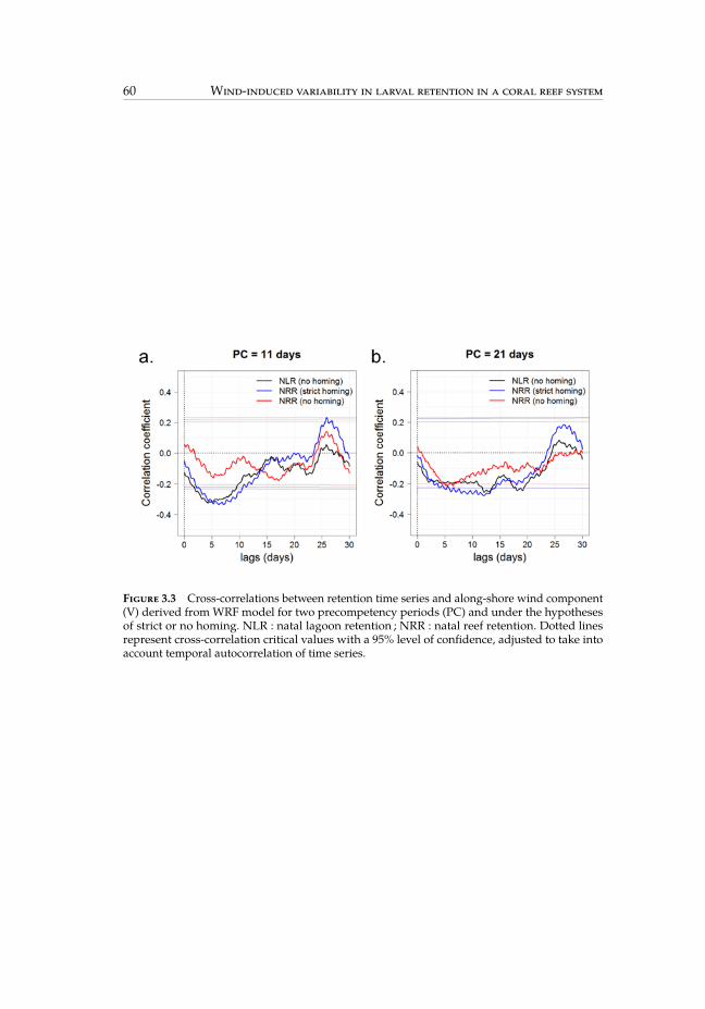
78 / 219


Figure 3.3 Cross-correlations between retention time series and along-shore wind component(V) derived fromWRF model for two precompetency periods (PC) and under the hypothesesof strict or no homing. NLR : natal lagoon retention ; NRR : natal reef retention. Dotted linesrepresent cross-correlation critical values with a 95% level of confidence, adjusted to take intoaccount temporal autocorrelation of time series.

79 / 219

Acknowledgments 61

Figure 3.4 Cross-correlations between retention time series and weather regimes 1 and 4 fortwo precompetency periods (PC) and under the hypotheses of strict or no homing. NLR : natallagoon retention ; NRR : natal reef retention. Dotted lines represent cross-correlation criticalvalues with a 95% level of confidence, adjusted to take into account temporal autocorrelation oftime series.

80 / 219


Figure 3.5 Maps of settlement using an 11-day precompetency period. For each simulation,the number of settlers was computed in square grid cells of 0.01° in size. For each grid cell,the number of settlers was (a) averaged over the whole simulated period (1320 simulations)and presented as a percentage of the total number of larvae released and (b) calculated on alogarithmic scale as log10(Ni + 1) whereNi is the number of larvae settling in grid cell i.

Figure 3.6 Maps of settlement using an 11-day precompetency period. The number of settlerswas computed in square grid cells of 0.01° in size for simulations corresponding to hatching eventsfollowed by (a) a precompetency period dominated at 75% by weather regime 1 (42 simulations)and (b) a precompetency period dominated at 75% by weather regime 4 (34 simulations). Foreach grid cell, the number of settlers was calculated on a logarithmic scale as log10(Ni + 1) whereNi is the number of larvae settling in grid cell i.

81 / 219

Acknowledgments 63

Figure 3.7 Mean retention over the austral summer 2003-2004 at natal reef scale (NRR) underno-homing or strict-homing hypotheses, and at lagoon scale (NLR) under no-homing hypothesisfor different release depths for an 11-day precompetency period. Error bars represent standarderrors.

82 / 219


3.6 Appendix A

Wind conditions predicted by the WRF model during austral summer 2003-2004were compared to in situ data obtained from Amédée Lighthouse Météo-France wea-ther station. This station is located along the barrier reef on a patch of reef close tothe Boulari pass approximately 20 km offshore in front of Nouméa (fig. 3.1) and isrepresentative of marine weather conditions in the SWL (Lefèvre et al. 2010). Thestation provides hourly wind speed (m s-1) and direction (°N) with an accuracy of1m s-1 for wind speed and 10° for direction. The WRF predicted wind variables areextracted at the closest grid point to Amédée Lighthouse station and 6-hourly averagesare computed for wind vector of both model and observations. Observations markedwith low wind data (speed < 3m s-1) are removed prior to the statistical computationof wind direction. Validation of predicted wind with observation was done throughstatistical performance measures including the root mean square error (RMSE) andindex of agreement (IOA) according to Lefèvre et al. (2010). The IOA is a measureof model skills in predicting variations about the observed mean ; a value above 0.5is considered to be good, 1 means a perfect match (see Lefèvre et al. (2010) for moredetails about this index) (see table 3.2).

Table 3.2 Statistical comparison between WRF model predicted values and observations atAmédée Lighthouse weather station. SD = standard deviation.

Wind speed (m s-1) Wind direction (°N)Amédée Lighthouse observations(Number of data = 3908)Mean 7.1 118.5SD 2.9 60.3Model - observations differenceBias -0.8 9.4RMSE 1.9 21.4IOA 0.9 0.9

83 / 219

Appendix B 65

3.7

App

endixB

Figu

re3.8

Map

sofs

ettle

men

tusing

a21

-day

precom

petenc

ype

riod.

Fore

achsimulation,

thenu

mbe

rofs

ettle

rswas

compu

tedin

squa

regrid

cells

of0.01

°insize.F

oreach

grid

cell,

thenu

mbe

rofs

ettle

rswas

calculated

onaloga

rithm

icscaleas

log 1

0(Ni+1)

whe

reNiisthenu

mbe

roflarva

esettlingin

grid

celliov

er(a)the

who

lesimulated

perio

d(132

0simulations

)and

fors

imulations

correspo

ndingto

hatching

even

tsfollo

wed

by(b)a

precom

petenc

ype

rioddo

minated

at75%

byweather

regime1

(42simulations

)and

by(c)a

precom

petenc

ype

rioddo

minated

at75%

byweather

regime4

(34simulations

).

84 / 219


3.8 Appendix C

Figure 3.9 Location of the focal reef and the four reefs used to evaluate the impact of the focalreef choice on the results.

We based our study on larval releases from a patch reef located at the centerof the SWL where water residence time is close to the average of 11 days (Ouillonet al. 2010). In order to evaluate the impact of this natal reef choice in the results,we simulated larval retention for 4 other natal reefs. We chose a reef located 25 kmfurther south of the focal reef (reef 2) and a reef 20 km further north (reef 4) in areaswhere water residence time is also close to the average of 11 days (Ouillon et al. 2010),and 2 others reefs located on the barrier reef (reef 3) and close to the coast (reef 1)where water residence times are around 5 and 20 days respectively (Ouillon et al.2010) (fig. 3.9). We simulated NRR under the stricthoming hypothesis and NLR underthe no-homing hypothesis for an 11-day precompetency period and we calculatedSpearman rank-order correlation coefficient (Spear-R) between the retention timeseries for the focal reef and the four other reefs. Average retention values ranged from1.6% (± 2.1% SD, reef 3) to 7.3% (± 7.8% SD, reef 4) and from 48.9% (± 20.7% SD,reef 3) to 73.6% (± 18.1% SD, reef 2) for NRR and NLR, respectively. For NRR wefound significant positive correlations of varying intensities between focal reef and

85 / 219

Appendix C 67

the reefs 1, 2, 3, and 4 (Spear-R 0.1, 0.2, 0.5 and 0.7 respectively). For NLR we foundsignificant positive correlations between focal reef and reefs 3 and 4 (Spear-R 0.3 and0.7), a not significant positive correlation between focal reef and reef 2 (Spear-R 0.1),but a significant negative correlation between focal reef and reef 1 (Spear-R -0.2). Werelate the singularity of reef 1 to its position in a coastal area where gyres are generatedby trade winds (Douillet et al. 2001). However in these gyres areas (North of OuenIsland in the southeast part of the SWL and in bays, fig. 3.9) the habitat of our studyspecies is scarce. For these reasons we strongly believe that the conclusions of ourstudy based on the focal reef remain meaningful for a large part of the SWL whereour study species is present (patch reefs and barrier reefs).

86 / 219

87 / 219

Chapitre 4

Evaluation of transgenerational isotopelabeling of embryonic otoliths in a coralreef damselfish with single and repeatedinjections of enriched 137Barium

69

88 / 219

89 / 219

71

M. Cuifa,b,c,d, F. Kellere, O. Chateaue, D. M. Kaplanc, M. Labonnef ,C. Letta, L. Vigliolab

Journal of Experimental Marine Biology and Ecology 459, 151 - 159 (2014)

a IRD, UMI 209 UPMC UMMISCO, Sète, Franceb IRD, Laboratoire d’Excellence LABEX Corail, UR 227 COREUS, Nouméa, New Caledoniac IRD, UMR 212 EME, Sète, Franced AgroParisTech, Paris, Francee Laboratory of marine biology and ecology, Aquarium des Lagons, Noumea, New Caledoniaf IRD, UMR 6539 LEMAR, Institut Universitaire Européen de la Mer, Plouzané, France

Abstract

Quantifying the larval dispersal component of population connectivity is extremelychallenging due to the many difficulties associated with directly observing larvae intheir marine environment. Transgenerational isotope labeling is a recent empiricaltechnique that addresses this challenge. It relies on the transmission of an artificiallyenriched stable isotope (e.g., 137Ba) from gravid females to the embryonic otoliths oftheir offspring, allowing for mass permanent marking of larvae. Before implemen-ting transgenerational isotope labeling in the wild, it is essential to investigate thetransmission longevity of the mark from females to larvae and to assess the potentialnegative effects on females and their offspring. We injected females of the Humbugdamselfish,Dascyllus aruanus, with an enriched 137Ba solution and reared the resultingprogeny to test the marking success and the transmission longevity of the mark, aswell as determine potential effects of transgenerational isotope labeling on spawningfrequency and size of 1-day eggs and 2-day larvae. Three different single-injection do-sages (0.5, 1 and 5 µg of 137Ba g-1 fish weight) were tested, as well as monthly repeatedinjections of the lowest dosage over a whole reproductive season. We implemented anew method that allows extracting otoliths of newly hatched larvae and analyzingthem using laser ablation coupled plasma mass spectrometry (ICP-MS). We showedthat forD. aruanus, injection with a low dose (0.5 µg of 137Ba g-1 fish weight) producedconsistently significantly marked larvae with a half-life for successful enriched Bamark transmission of approximately 1 month, and that monthly repeated injections ofthis dose did not negatively impact spawning success or condition of eggs and larvae.Monthly repeated injections of enriched Ba isotope injections at 0.5 µg of 137Ba g-1 fishweight will therefore present an effective means of mass marking D. aruanus larvaethroughout an entire reproductive season.Keywords : Barium isotopes, Connectivity, Dascyllus aruanus, LA-ICP-MS, Otolithmicrochemistry, Transgenerational marking

90 / 219

72 Evaluation of transgenerational isotope labeling of embryonic otoliths

4.1 Introduction

Knowledge of marine metapopulation dynamics is essential to better understandpopulation persistence and effectively manage and conserve marine resources andbiodiversity. For this reason, quantifying demographic connectivity, i.e., the exchangeof individuals among discrete populations (Cowen et al. 2007), has been identifiedas a priority area for research (Hixon 2011, Sale et al. 2005). While progress has beenachievedwith older life stages, the larval dispersal component of connectivity has longbeen viewed as a black-box (Sale et al. 2010) and its quantification remains challengingdue to the many difficulties associated with directly observing a multitude of smallindividuals subject to high mortality rates in a marine environment (Thorrold et al.2001).

Several empirical techniques have been developed and successfully applied duringthe last decade to address this knowledge gap (Leis et al. 2011) : analyses of traceelements in calcified structures (Carson et al. 2010), genetic approaches focusing onthe assignment of individuals to populations of origin (assignment methods) (Hoganet al. 2012) or to specific parents (parentage analyses) (Saenz-Agudelo et al. 2011,2012), and artificial chemical marking of calcified structures (Almany et al. 2007, Joneset al. 2005). Analyses of trace elements in calcified structures or assignment methodsare potentially of limited value at small spatial scales due to homogeneity of geneticand microchemical signatures. By contrast, parentage analyses and artificial chemicalmarking are not constrained by the lack of difference among populations because theyrely on unequivocal markers that uniquely assign individuals to their populations oforigin. Artificial chemical marking of calcified structures has been accomplished byimmersing embryos in solutions of fluorescent compound (Jones et al. 1999, 2005) orlarvae in solutions of enriched stable isotope solutions (Munro et al. 2008, Woodcocket al. 2011). The major limitation of applying an immersion method in the wild is thatit requires collecting and handling eggs.

An alternative artificial chemical marking method, called transgenerational iso-tope labeling, overcomes this limitation by marking individuals in situ before birth(Thorrold et al. 2006). This method relies on the transmission of an enriched stableisotope (e.g., 137Ba) from gravid females to the embryonic otoliths of their offspring.The injection of a single female is sufficient to mark thousands of larvae that femalewill produce within the weeks following injection. Otoliths are then collected from-larvae or juveniles, and marked individuals are identified by measuring Barium (Ba)isotope ratios in otolith cores using laser ablation inductively coupled plasma massspectrometry (LA-ICP-MS). Thorrold et al. (2006) successfully applied transgeneratio-nal isotope labeling to both a benthic and a pelagic spawning species (respectively

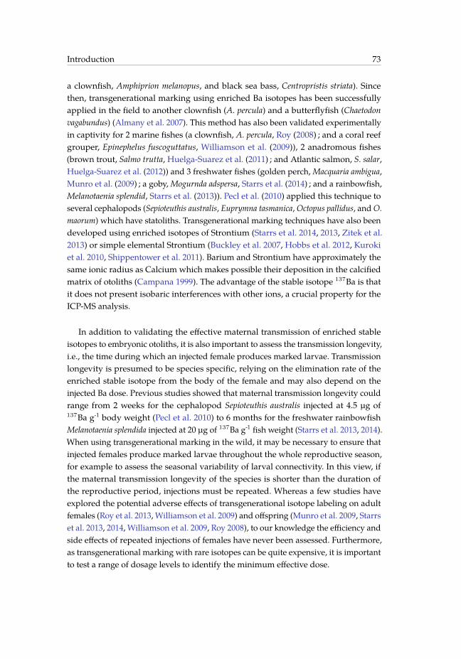
91 / 219

Introduction 73

a clownfish, Amphiprion melanopus, and black sea bass, Centropristis striata). Sincethen, transgenerational marking using enriched Ba isotopes has been successfullyapplied in the field to another clownfish (A. percula) and a butterflyfish (Chaetodonvagabundus) (Almany et al. 2007). This method has also been validated experimentallyin captivity for 2 marine fishes (a clownfish, A. percula, Roy (2008) ; and a coral reefgrouper, Epinephelus fuscoguttatus, Williamson et al. (2009)), 2 anadromous fishes(brown trout, Salmo trutta, Huelga-Suarez et al. (2011) ; and Atlantic salmon, S. salar,Huelga-Suarez et al. (2012)) and 3 freshwater fishes (golden perch, Macquaria ambigua,Munro et al. (2009) ; a goby, Mogurnda adspersa, Starrs et al. (2014) ; and a rainbowfish,Melanotaenia splendid, Starrs et al. (2013)). Pecl et al. (2010) applied this technique toseveral cephalopods (Sepioteuthis australis, Euprymna tasmanica,Octopus pallidus, andO.maorum) which have statoliths. Transgenerational marking techniques have also beendeveloped using enriched isotopes of Strontium (Starrs et al. 2014, 2013, Zitek et al.2013) or simple elemental Strontium (Buckley et al. 2007, Hobbs et al. 2012, Kurokiet al. 2010, Shippentower et al. 2011). Barium and Strontium have approximately thesame ionic radius as Calcium which makes possible their deposition in the calcifiedmatrix of otoliths (Campana 1999). The advantage of the stable isotope 137Ba is thatit does not present isobaric interferences with other ions, a crucial property for theICP-MS analysis.

In addition to validating the effective maternal transmission of enriched stableisotopes to embryonic otoliths, it is also important to assess the transmission longevity,i.e., the time during which an injected female produces marked larvae. Transmissionlongevity is presumed to be species specific, relying on the elimination rate of theenriched stable isotope from the body of the female and may also depend on theinjected Ba dose. Previous studies showed that maternal transmission longevity couldrange from 2 weeks for the cephalopod Sepioteuthis australis injected at 4.5 µg of137Ba g-1 body weight (Pecl et al. 2010) to 6 months for the freshwater rainbowfishMelanotaenia splendida injected at 20 µg of 137Ba g-1 fish weight (Starrs et al. 2013, 2014).When using transgenerational marking in the wild, it may be necessary to ensure thatinjected females produce marked larvae throughout the whole reproductive season,for example to assess the seasonal variability of larval connectivity. In this view, ifthe maternal transmission longevity of the species is shorter than the duration ofthe reproductive period, injections must be repeated. Whereas a few studies haveexplored the potential adverse effects of transgenerational isotope labeling on adultfemales (Roy et al. 2013, Williamson et al. 2009) and offspring (Munro et al. 2009, Starrset al. 2013, 2014, Williamson et al. 2009, Roy 2008), to our knowledge the efficiency andside effects of repeated injections of females have never been assessed. Furthermore,as transgenerational marking with rare isotopes can be quite expensive, it is importantto test a range of dosage levels to identify the minimum effective dose.

92 / 219


In this context, the objective of this study is to test the efficacy of transgenerational137Ba isotope labeling for the coral reef damselfish Dascyllus aruanus and to identifyan optimal dose for this species taking into account potential side effects of singleand repeated injections on spawning success, eggs and larvae size. Furthermore, wedescribe a new method to extract and analyze otoliths from newly hatched larvae.

4.2 Methods

4.2.1 Study species

The Humbug damselfish, D. aruanus (fig. 4.1a) is a protogynous hermaphroditePomacentridae (Coates 1982) found exclusively in lagoon habitats throughout theIndo-Pacific region (Allen 1991). This sedentary fish lives among branching coral inspatially discrete groups with up to 80 individuals but typically less than 10 (Holbrooket al. 2000). Sex ratio is female-biased for colonies of less than 10 individuals (single-male polygynous group) and change to unity as group size increases (Fricke 1977,Fricke and Holzberg 1974). Branching coral provide protection from predators andsubstrate for laying benthic eggs (Coates 1980b, Mizushima et al. 2000). Spawningpeaks in summer (October to March in New Caledonia), during which time eachfemale can spawn several times at one week (Fricke and Holzberg 1974) to 2 months(Mizushima et al. 2000) intervals. After spawning, males guard the eggs for 3 daysuntil they hatch.

4.2.2 Fish sampling and handling

Twelve discrete colonies of D. aruanus were collected with their branching coralin the South-West Lagoon of New Caledonia (SWL) in November 2011. To collecta colony, two divers approached the coral so that the fish hid among the branches.The branching coral was then covered with a large plastic bag, detached from thesubstrate, carried up to the boat and placed in a seawater tub. The colonies were thentransported to the lab and the biggest individuals (> 45 mm total length) were selectedso that each colony comprised 5 to 7 mature fish. Each colony was then transferred toan 80 l aquarium with its own branching coral. The twelve aquaria were connectedto a flow-through seawater system and exposed to ambient temperatures (26 - 29 °C)and salinity. Fish were fed twice daily a diet consisting of frozen Artemia and a mix ofcut frozen tuna, squid and mussel. A programmed light system provided a naturalphotoperiod to all aquaria. All experimental fish were subject to an acclimation periodof 11 months before beginning experimental trials in October 2012.

93 / 219

Methods 75

Figure 4.1 a) Adult D. aruanus on its branching coral colony, b) injection of an adult D. aruanuswith enriched 137Ba solution, c) clutch attached to a side of an aquarium, d) eggs sampled froma clutch and colored for measurement in the software program ImageJ, e) 2-day larvae sampledfrom a clutch, f) otoliths extracted from 2-day larvae originating from the same clutch ready forLA-ICP-MS analyses.

4.2.3 Enriched 137Ba solution preparation

A Barium carbonate (BaCO3) highly enriched in stable 137Ba isotope (81.9%) anddepleted in 138Ba (17.4%) as compared to natural Ba isotope (11.32% 137Ba and 71.66%138Ba), was purchased from Oak Ridge National Laboratory (Tennessee, USA). Toobtain a solution in chloride form, 179.6 mg of BaCO3 powder was dissolved in asmall amount of ultrapure water with 1 ml of HCl (36%). Then, ultrapure water wasadded to obtain 25 ml of a BaCl2 stock solution at 5 mg Ba ml-1. The stock solutionwas then diluted to the desired concentrations with ultrapure water and neutralizedwith a solution of NaHCO3 at 54 mg ml-1 (see section 5.6).

4.2.4 Enriched 137Ba injections

Fish were anesthetized by adding 20 ml of alcoholic clove-oil solution (5%) inthe aquarium, and captured using hand nets. All fish of a colony were transferredto a seawater tub. As D. aruanus does not present any sexual dimorphism, all fishof the colony were measured to the nearest mm total length and injected with theappropriate volume of 137Ba solution (see section 5.6). Injections were performed witha 0.3 ml insulin syringe through the bodywall into the abdominal cavity (fig. 4.1b).Five different treatments were given to two replicate colonies each (table 4.1) : singleinjections of 0.5, 1 and 5 µg of 137Ba g-1 fish weight (treatments T0.5, T1 and T5,

94 / 219


respectively) andmonthly repeated injections of 0.5µg of 137Ba g-1 fishweight and 0.9%sodium chloride (NaCl) (treatments T0.5rep and TNaClrep, respectively). Injections ofNaCl were used to distinguish between the effect of Barium accumulation over timeand the potential effect of repeated manipulations (anesthesia and injection). Twocontrol colonies were not manipulated at all. From the beginning of the spawningperiod in October 2012, we waited for at least 3 spawning events per colony beforestarting the injections. Injections began a few days before the full moon betweenmid-January 2013 and mid-February 2013 depending on the colony (table 4.1), afterwhich time fish were monitored for a period of 4 months.

95 / 219

Methods 77

Tabl

e4.1

Treatm

entsus

edto

evalua

temarksu

ccessa

ndeff

ecto

finjectio

nson

spaw

ning

successa

nd1-da

yeg

gsan

d2-da

ylarvae

size.F

W=fis

hweigh

t.

Totaln

umbe

rofc

lutche

scollected

toassess

:Treatm

ent

Barium

dosage

(µgof

137Ba

g-1

FW)

Num

bero

finjec-

tion(s)

Date

ofinjec-

tion(s)

Num

berof

colo-

nies

Marksu

ccess

Effects

on1-deg

gsEff

ects

on2-dlar-

vae

Con

trol

00

-2

110

9T0

.50.5

111/0

1/2013

212

1319

T11

113/0

2/2013

26

1211

T55

129/0

1/2013

28

1814

T0.5rep

0.5

411/0

1/2013

218

2528

13/0

2/2013

13/0

3/2013

12/0

4/2013

TNaC

lrep

04

13/0

1/2013

2-

2319

13/0

2/2013

13/0

3/2013

12/0

4/2013

Total

1245

101

100

96 / 219


4.2.5 Spawning success and larval rearing

Spawning success was monitored daily in each colony over a period of 195 daysfrom the first observed spawning event (the 25th of October 2012 in colonies 4 and9) to the last one (the 7th of May 2013 in colony 1). Spawning events were generallysynchronous among females of the same colony, though occasionally individualswere observed to spawn 1 - 2 days before or after the main spawning event. Theperiodicity of spawning in each colony was calculated as the ratio of the number ofdays between the first and the last spawning events observed in that colony to thenumber of spawning events observed in the same period. Females attached their eggsto the side glasses of aquaria (fig. 4.1c). Around 10% of each clutch was collected onthe morning after spawning using a scraper and a pipette, and was stored in 80%Ethanol for 1-day egg measurements (fig. 4.1d). The remaining clutch was collectedon the 3rd day after spawning and transferred to 2 l larval-rearing aquaria containingseawater having the same physicochemical characteristics as the parental aquarium.Hatching took place the night after transfer. Larvae were not fed until collection twodays later (fig. 4.1e). Two-day larvae were stored in 80% Ethanol for otolith extractionand standard length (SL) measurements. As several females were present in eachaquarium and spawning events were synchronous, it was not possible to separate theeggs produced by different females of the same colony. Thus, all eggs produced in anaquarium during one spawning event were pooled.

4.2.6 Otolith preparation and analysis

A total of 45 clutches, including a control clutch, were analyzed to assess markingsuccess as a function of dosage and experimental protocol (table 4.1). Otoliths of 2-daylarvae were extracted by dissolving organic tissue of larvae in commercial bleach(NaClO at 2.6%). Around 0.5 ml of larvae was put in a 1.5 ml Eppendorf Tubewith 1mlof bleach. The tube was shaken with a vortex and then centrifuged. The supernatantwas removed and the operation (bleaching, shaking, centrifugating) was repeatedtwice more, so that the larvae were totally dissolved. After the third centrifugationthe supernatant was removed and the operation repeated three times with ultrapurewater, so that the otoliths were well rinsed. Then, the tube was shaken and poured in aglass Petri dish with the help of a wash bottle to ensure that all otoliths were removedfrom the tube. The Petri dishwas placed under a binocular microscope and a clockwiserotary movement was applied until the otoliths gathered in the middle of the Petridish. It is worthwhile noting that this does not work with a plastic Petri dish. Waterin excess was removed using a pipette and then evaporated by placing the Petri dishabove a hot plate to speed up the process. Aggregated otoliths were then collectedall together using a piece of tape that was later mounted on a clean petrographic

97 / 219

Methods 79

slide with double-sided tape and then covered with a thin layer of cyanoacrylic glueto prevent them from being dislodged (fig. 4.1f). Each otolith aggregation sampleobtained this way corresponded to one spawning event from one colony. Ba isotoperatios were measured in aggregated larval otoliths with a New Wave Research 213nm UV laser ablation system connected to an Agilent 7500cs inductively coupledplasma mass spectrometer (ICPMS) located at Charles Darwin University (Darwin,Australia). Each analysis lasted 60 s including 10 s of background and 50 s of ablation(laser activated). A reference standard (NIST 612, National Institute of Standards andTechnology) was analyzed at the beginning and end of each session to account formass bias and machine drift throughout the analyses. Operating conditions of thelaser and ICP-MS are provided in table 4.2. Between 3 and 5 ablations were randomlyperformed through each otolith aggregation sample so that around 10 otoliths wereablated per clutch. Each sample was analyzed for 43Ca, 137Ba and 138Ba.

Table 4.2 Operating conditions of the NewWave Research 213 nm UV laser and Agilent 7500csinductively coupled plasma mass spectrometer (ICP-MS) used for the otoliths analysis.

Laser parametersWavelength 213 nmMode Q-switchedFrequency 5 HzLaser power 90%Beam density 9 - 11 J cm-2

Carrier gas Ar 1.01 l min-1

Ablation mode SpotBeam diameter 55 µmICP-MS parametersOptional gas He (140)Dwell times 137Ba & 138Ba (300 ms) ; 43Ca (30 ms)Cone Nickel sampler cone and nickel skimmer coneDetection modes Pulse and analog

4.2.7 Eggs and larvae measurements

One-day eggs

A total of 101 clutches were analyzed to assess the effect of injections on 1-dayegg size (table 4.1). Measurements were performed using the plug-in ObjectJ (http://simon.bio.uva.nl/objectj/2-Tutorial.html) for the software program ImageJ(http://rsbweb.nih.gov/ij/, Schneider et al., 2012). Eggs were colored with Tolui-dine blue dye, separated using tweezers under a binocular microscope and photogra-phed with a Scion CFW 1308C digital camera at X20 magnification. Images (fig. 4.1f)were calibrated in ObjectJ and the software automatically marked each egg with the




98 / 219


best fitting ellipse and recalculated the corresponding diameter for a perfect spherewith the same silhouette area (called “egg diameter” hereafter). A minimum of onehundred 1-day eggs were measured per clutch, except for 13 clutches for which only46 to 87 eggs were measured. A total of 10,804 eggs were measured to the nearest µm.

Two-day larvae

A total of 100 clutches were analyzed to assess the effect of injections on 2-daylarvae size (table 4.1). Photos of each sample of larvae (fig. 4.1e) were taken using thesame microscope and camera than for eggs. Measurements of SL were performedusing the segmented line tool of ImageJ. A minimum of one hundred 2-day larvaewere measured per clutch, except for 15 clutches for which only 50 to 88 larvae weremeasured. A total of 9,771 larvae were measured to the nearest 0.01 mm.

4.2.8 Statistical analysis

All statistical analyses were conducted using the R-2.15.0 statistical environment.Mixed-effects models were computed with packages nlme (Pinheiro et al. 2011) andMASS (Venables and Ripley 2002). Percentages of variance explained by randomfactors were calculated by extracting standard deviations of random effects frommodels summaries, squaring them to get the variances, and then expressing them aspercentages of total original variances (Pinheiro and Bates 2000). All statistical testswere considered significant at the 5% level.

Marking success

Isotope abundancesmeasured in otoliths by LA-ICP-MSwere first blank-subtracted.Ba ratios were then computed and corrected for mass bias and machine drift using thereference standard. The ratio 138Ba/137Ba in the reference standard was assumed to bethe same as the relative natural abundance (i.e., 6.38) based on the International Unionof Pure and Applied Chemistry values of isotopes abundance (Berglund and Wieser2011). Following Munro et al. (2008), data were smoothed using a six-point runningmean to decrease noise. Ba ratio measurements corresponding to 43Ca values lessthan 1500 counts per second were excluded from analyses to remove measurementsperformed in the glue, leaving only those Ba ratios resulting from laser ablation of theotoliths, which are principally composed of CaCO3. Mean Ba ratios from the treatmentsampleswere then compared against ratios in the control sample usingMann-Whitney-Wilcoxon (MWW) tests to determine if mark transmission was successful. Mean Baratios (y), resulting from single injection treatments, were modeled as an exponentialdecay function of number of days post-injection (t) using a nonlinear mixed-effects

99 / 219

Results 81

model fitted by maximizing the restricted log-likelihood with treatment (3 levels :T0.5, T1 and T5) as fixed effect and colony (numbered from 1 to 6) as random effect :

y = yc − α · exp−β·t (4.1)

with yc the control mean Ba ratio.

The half-life (t1/2) for successful enriched Ba mark transmission was calculated asfollows :

t1/2 =ln(2)

β(4.2)

Effect on spawning success

To assess the potential effect of injection on spawning success, a generalized linearmixed model using penalized quasi-likelihood was fitted with a binomial distributionfor daily spawning success (0 = no spawning event, 1 = spawning event). Treatment (6levels : Control, T0.5, T1, T5, TNaClrep, T0.5rep) and time (days numbered from 1 to195) were specified as fixed factors. The effect of colony (numbered from 1 to 12) wasspecified as random.

Effect on eggs and larvae

In order to detect potential effects of treatment on 1-day egg diameter and 2-daylarval SL, we modeled these response variables using two mixed-effects models withpolynomial terms fitted by maximizing the restricted log-likelihood. Treatment (6levels : Control, T0.5, T1, T5, TNaClrep, T0.5rep) was specified as a fixed linear factor.The effect of time (number of days elapsed from the beginning of the experiment tothe date that the clutch is produced) was also specified as fixed and modeled with acubic function to represent temporal variability observed in the response variables.The effect of colony (numbered from 1 to 12) was specified as a random linear effect.

4.3 Results

4.3.1 Validation of Barium isotope markers

The mean Ba isotope ratio in otoliths of control larvae was 6.2 (± 0.1 standard error(SE)). For all treatments, Ba isotope ratios in larval otoliths of the first spawned clutchdiffered considerably from the ratio in otoliths of control larvae (MWW tests p.values< 0.0005) even if variability among clutches within treatment was strong, ranging

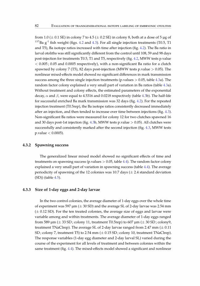
100 / 219


from 1.0 (± 0.1 SE) in colony 7 to 4.5 (± 0.2 SE) in colony 8, both at a dose of 5 µg of137Ba g-1 fish weight (figs. 4.2 and 4.3). For all single injection treatments (T0.5, T1and T5), Ba isotope ratios increased with time after injection (fig. 4.2). The Ba ratio inlarval otoliths was still significantly different from the control until 108, 59 and 98 dayspost-injection for treatments T0.5, T1 and T5, respectively (fig. 4.2, MWW tests p.value< 0.005 ; 0.05 and 0.0005 respectively), with a non-significant Ba ratio for a clutchspawned by colony 7 (T5), 82 days post-injection (MWW tests p.value > 0.05). Thenonlinear mixed-effects model showed no significant differences in mark transmissionsuccess among the three single injection treatments (p.values > 0.05, table 4.3a). Therandom factor colony explained a very small part of variation in Ba ratios (table 4.3a).Without treatment and colony effects, the estimated parameters of the exponentialdecay, α and β, were equal to 4.5316 and 0.0218 respectively (table 4.3b). The half-lifefor successful enriched Ba mark transmission was 32 days (fig. 4.2). For the repeatedinjection treatment (T0.5rep), the Ba isotope ratios consistently decreased immediatelyafter an injection, and then tended to increase over time between injections (fig. 4.3).Non-significant Ba ratios were measured for colony 12 for two clutches spawned 16and 30 days post-1st injection (fig. 4.3b, MWW tests p.value > 0.05). All clutches weresuccessfully and consistently marked after the second injection (fig. 4.3, MWW testsp.value < 0.0005).

4.3.2 Spawning success

The generalized linear mixed model showed no significant effects of time andtreatments on spawning success (p.values> 0.05, table 4.4). The random factor colonyexplained a very small part of variation in spawning success (table 4.4). The averageperiodicity of spawning of the 12 colonies was 10.7 days (± 2.4 standard deviation(SD)) (table 4.5).

4.3.3 Size of 1-day eggs and 2-day larvae

In the two control colonies, the average diameter of 1-day eggs over the whole timeof experiment was 597 µm (± 30 SD) and the average SL of 2-day larvae was 2.54 mm(± 0.12 SD). For the ten treated colonies, the average size of eggs and larvae werevariable among and within treatments. The average diameter of 1-day eggs rangedfrom 589 µm (± 33 SD ; colony 11, treatment T0.5rep) to 607 µm (± 30 SD ; colony9,treatment TNaClrep). The average SL of 2-day larvae ranged from 2.47 mm (± 0.11SD ; colony 7, treatment T5) to 2.54 mm (± 0.15 SD ; colony 10, treatment TNaClrep).The response variables (1-day egg diameter and 2-day larval SL) varied during thecourse of the experiment for all levels of treatment and between colonies within thesame treatment (fig. 4.4). The mixed-effects model showed a significant and nonlinear

101 / 219

Results 83

Table 4.3 Nonlinearmodels of enriched 137Bamark transmission success forD. aruanus femalesinjected with single injections of 0.5, 1 or 5 µg 137Ba g-1 fish weight (treatment T0.5, T1 and T5respectively). a) Results of the nonlinear mixed-effects model with treatment as fixed effect andcolony as random effect. b) Results of the nonlinear model without treatment and colony effects.SE = standard error.

a)Random effetcs Varianceα Colony 8.1956E-10β Colony 5.5797E-14Residual 0.6847Fixed effects Estimate SE p-valueα T0.5(Intercept) 4.9523 0.6697 0.0000α T1 0.7127 1.8004 0.6978α T5 -1.2339 1.0188 0.2446β T0.5(Intercept) 0.0215 0.0054 0.0012β T1 0.0098 0.0151 0.5263β T5 -0.0020 0.0105 0.8549Number of Observations 26Number of Groups 6

b)Parameters Estimate SE p-valueα 4.5316 0.4649 8.0700E-10β 0.0218 0.0044 4.7400E-05Residual Std. Error 0.9224

Table 4.4 Generalized linear mixed-effects model of spawning success of D. aruanus femalesinjected with single injections of 0.5, 1 or 5 µg 137Ba g-1 fish weight (treatment T0.5, T1 andT5 respectively) or with monthly repeated injections of 0.5 µg 137Ba g-1 fish weight (treatmentT0.5rep) or NaCl (treatment TNaClrep). SE = standard error.

Random effetcs VarianceColony 2.2677E-08Residual 0.9999Fixed effects Estimate SE p-valueControl (Intercept) -2.5039 0.2342 0.0000Time 0.0002 0.0014 0.8890TNaClrep 0.2877 0.2545 0.3015T0.5 -0.1137 0.2759 0.6947T0.5rep 0.1681 0.2602 0.5420T1 -0.2850 0.2873 0.3596T5 -0.1961 0.2812 0.5117Number of Observations 2,340Number of Groups 12

102 / 219


Figure 4.2 Mean (± standard error (SE)) 138Ba/137Ba ratios in otoliths of larvae produced byD. aruanus females injected once with 137BaCl2 at dosage rates of 0.5 µg of 137Ba g-1 fish weight(T0.5, black solid squares), 1 µg of 137Ba g-1 fish weight (T1, green solid circles), 5 µg of 137Bag-1 fish weight (T5, magenta solid triangles), as a function of spawning time (days post-injection).The thick gray horizontal line represents mean (± SE) 138Ba/137Ba ratios in control otoliths.Numbers noted beside data points refer to the colony. Data points with error bars that overlapwith thick gray bar are not significantly different from controls. Arrow indicates date of injection.Red curve represents best fit exponential decay relationship between time and Ba ratio for allsingle injection treatments. Red dash line indicates half-life for successful enriched Ba marktransmission.

effect of time on 1-day egg diameter and on 2-day larval SL (table 4.6). No significanteffects of the different treatments were detected on 1-day egg diameter and on 2-daylarval SL (table 4.6). The random factor colony explained 24% and 5% of variation in1-day egg diameter and 2-day larval SL, respectively (table 4.6).

103 / 219

Results 85

Figure 4.3 Mean (± standard error (SE)) 138Ba/137Ba ratios in otoliths of larvae produced byD. aruanus females from colonies 11 (a) and 12 (b) injectedmonthly with 137BaCl2 at a dosage rateof 0.5 µg of 137Ba g-1 fish weight (T0.5rep) as a function of spawning time (days post-injection).Black solid squares indicate samples analyzed using the standard beam diameter, whereas opensquares are used for a few samples that were analyzed with a beam diameter of 25 µm. The thickgray horizontal line represents mean (± SE) 138Ba/137Ba ratios in control otoliths. Data pointswith error bars that overlap with thick gray bar are not significantly different from controls.Arrows indicate dates of injections.

Table 4.5 Number of spawning events, spawning lag (number of days between the first and thelast observed spawning events in a colony) and spawning periodicity observed for each colonyfrom the 25th of October 2012 to the 7th of May 2013. SD = standard deviation.

Number of Spawning SpawningTreatment Colony spawning lag periodicity

events (days) (days)Control 1 16 158 9.9

2 14 132 9.4T0.5 3 11 158 14.4

4 16 186 11.6T1 5 12 168 14.0

6 11 117 10.6T5 7 11 148 13.5

8 14 91 6.5TNaClrep 9 24 186 7.8

10 15 158 10.5T0.5rep 11 17 167 9.8

12 18 189 10.5Mean 10.7SD 2.4

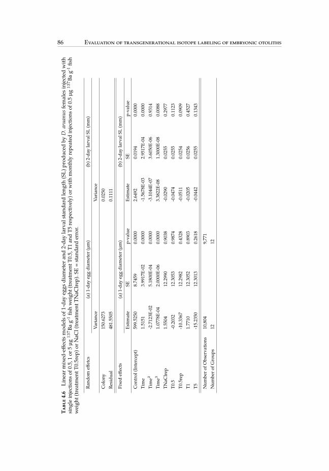
104 / 219


Tabl

e4.6

Line

armixed

-effe

ctsm

odelso

f1-day

eggs

diam

eter

and2-da

ylarval

stan

dard

leng

th(SL)

prod

uced

byD.aruan

usfemales

injected

with

sing

leinjections

of0.5,1or

5µg

137Ba

g-1fis

hweigh

t(treatm

entT

0.5,T1

andT5

resp

ectiv

ely)

orwith

mon

thly

repe

ated

injections

of0.5

µg137Ba

g-1fis

hweigh

t(treatm

entT

0.5rep

)orN

aCl(treatm

entT

NaC

lrep).S

E=stan

dard

error.

Rand

omeff

etcs

(a)1

-day

eggdiam

eter

(µm)

(b)2

-day

larval

SL(m

m)

Varia

nce

Varia

nce

Colon

y150.6273

0.0250

Residu

al481.5505

0.1111

Fixedeff

ects

(a)1

-day

eggdiam

eter

(µm)

(b)2

-day

larval

SL(m

m)

Estim

ate

SEp-va

lue

Estim

ate

SEp-va

lue

Con

trol

(Intercep

t)599.5250

8.7459

0.0000

2.6492

0.0194

0.0000

Time

1.5151

3.9917E-02

0.0000

-1.5678E

-03

2.9517E-04

0.0000

Time2

-2.7123E

-02

5.1800E-04

0.0000

-3.1044E

-07

3.6050E-06

0.9314

Time3

1.0778E-04

2.0000E-06

0.0000

3.3822E-08

1.3000E-08

0.0088

TNaC

lrep

1.5504

12.2990

0.9038

-0.0290

0.0255

0.2977

T0.5

-0.2032

12.3053

0.9874

-0.0474

0.0255

0.1123

T0.5rep

-10.3367

12.2982

0.4328

-0.0511

0.0254

0.0909

T11.7710

12.3052

0.8903

-0.0205

0.0256

0.4527

T5-15.2350

12.3013

0.2618

-0.0442

0.0255

0.1343

Num

bero

fObserva

tions

10,804

9,771

Num

bero

fGroup

s12

12

105 / 219

Discussion 87

4.4 Discussion

4.4.1 Success of maternal transmission

Transgenerational isotope labeling ofD. aruanus embryonic otoliths was experimen-tally tested for 44 spawning events ranging from 2 to 108 days post-injection of 0.5 to 5µg 137Ba g-1 fish weight, resulting in 41 clutches (or 93%) successfully marked (figs. 4.2and 4.3). Irrespective of dosage, 100% of first spawning events after injection of femalesproduced larvae with otoliths having significantly lower 138Ba/137Ba ratios (figs. 4.2and 4.3). Mark transmission failure in 3 clutches spawned after the first spawningevent may have resulted for a variety of reasons. Laser ablation may hit calcareousdetritus instead of otoliths, and therefore fail to indicate marked individuals. Amongthe three clutches for which wewere unable to detect anymark, two clutches displayedsmall calcareous detritus in the preparation (colony 12 at 16 days postinjection, andcolony 7 at 82 days), suggesting possible failure due to contamination during otolithextraction as opposed to real negative marking. If this was the case, then the true marksuccess rate would increase from 93 to 98% (41 out of 42 correctly analyzed clutches).Alternatively, injected Barium solution in some females may have been leached viathe dermal puncture wound or excreted via the intestinal tract (Roy et al. 2013). Asfemales in an aquarium occasionally spawn asynchronously, this can lead to markfailure if a given clutch only represents a small number of individuals. This couldexplain the two failed mark transmission events in colony 12 after the initial injection.Finally, there may be individual differences in Barium metabolism among spawningfemales (Pecl et al. 2010), for example distinct Barium uptake in bone tissue (Royet al. 2013). Such differences are supported by the occasional considerable variationin 138Ba/137Ba ratio between colonies that received the same treatment (e.g., firstspawning of colonies 7 and 8, and colonies 5 and 6 ; fig. 4.2).

4.4.2 Longevity in maternal transmission and repeated injections

Besides validating the effective maternal transmission of enriched stable isotopesto embryonic otoliths, we assessed the time during which injected females producedmarked larvae. Results indicate that isotope ratios remained clearly distinguishable inlarval otoliths from those of control individuals for at least two months after initialinjection for the intermediate and highest dosage (1 and 5 µg 137Ba g-1 fish weight) anduntil 3.5months for the lowest dosage tested (0.5 µg 137Ba g-1 fishweight) (fig. 4.2). Thisis consistent with the results of Thorrold et al. (2006),who found 3-month longevity inmaternal transmission for another Pomacentridae (Amphiprion melanopus) with a doseof 2.3 µg 137Ba g-1 fish weight (section 4.6). Enriched Ba mark transmission follows an

106 / 219


exponential decaywith a half-life of 32 days with no difference among tested doses,suggesting that successful marking may be achieved for D. aruanus at a dose evenlower than 0.5 µg 137Ba g-1 fish weight.

One colony in the repeated injection treatment spawned four times during themonth following the first injection and produced larvae whose otoliths were foundto be significantly marked for the 1st and 3rd spawning events, but not for the 2nd

and 4th events (colony 12 in fig. 4.3b). These results indicate that monthly repeatedinjections may be required to assure mark transmission and limit the impact of failedsingle injections when the aim of the study is to mark larvae over several months. Ourrepeated injection treatment indeed showed that each injection resulted in a decreasein 138Ba/137Ba ratios (fig. 4.3), generating persistent detection of the mark in all casesafter the 2nd injection.

4.4.3 Impacts of marking on spawning success and condition of offspring

Before implementing transgenerational marking in the wild, it is imperative toinvestigate potential negative effects of the Barium injection on adult females andtheir offspring. Our results showed that neither single injections of any of the threeBa doses nor repeated injections of the lowest Ba dose had an effect on spawningsuccess. This is consistent with the few other studies that have assessed the impactof transgenerational isotope labeling on adult females, indicating no negative effecton physiological stress (Roy et al. 2013, Williamson et al. 2009) or spawning success(Munro et al. 2009) (section 4.6). Regarding the effects on offspring, some studiesassessing the effects of transgenerational marking using enriched Ba isotopes foundpositive (Starrs et al. 2013) or negative (Williamson et al. 2009) effects on newly hat-ched larvae depending on species and Ba doses (section 4.6). Size at hatching partlydetermines post-settlement survivorship (Vigliola and Meekan 2002, Vigliola et al.2007) which is crucial in connectivity studies. Our results showed that the differenttreatments did not significantly affect 1-day egg diameter and 2-day larval standardlength. Investigating impacts on growth throughout the larval period would also beworthwhile as negative effects have been detected for 3-week old larvae for a Poma-centridae (Roy (2008), section 4.6). However, this requires rearing larvae of D. aruanus,which is notoriously difficult (Danilowicz and Brown 1992, Gopakumar et al. 2009),as it is for most tropical reef fish larvae because of their small mouth gape (Moorheadand Zeng 2010).

107 / 219

Discussion 89

4.4.4 Applications and implications for future studies

We developed a new method for extraction, laser ablation and analysis of otolithsof very young larvae (2-day old). Compared to previous studies that analyzed thecore of single otoliths of juveniles that had reached the age of settlement (Huelga-Suarez et al. 2011, 2012, Munro et al. 2008, 2009, Thorrold et al. 2006, Williamson et al.2009), the advantages of our method are (1) that the rearing of 2-day larvae requiresreduced aquarium facilities and time, and (2) that rapid and simultaneous extractionand laser ablation of hundreds of otoliths is possible. In this study, we measured anaverage isotope ratio per clutch by ablating multiple otoliths at once, and thus wecannot state with certainty that all individuals originating fromthe same clutch aresuccessfully marked. Nevertheless, we worked at the clutch level as we consider itto be very unlikely that the mark success rate of individual larvae originating fromthe same clutch differs significantly from 100% provided an effective dosage is used.Other studies investigating success of transgenerational marking found that maternalinjections of effective dosages resulted in 100% mark success for juveniles originatingfromthe same clutch (e.g., Williamson et al. (2009), Starrs et al. (2014)).

Nevertheless, it is worthwhile and feasible to evaluate the risk of miss-identifyingmarked fish by investigating the mark success rate at the individual level in futurestudies. A slightly modified version of our protocol could be used to analyze singleotoliths of very young larvae, though such analyses may be technically more challen-ging. The bleaching dissolution technique may be used to extract individual otolithsby placing a single larva in a Petri dish, putting a few drops of bleach on it and waitinguntil the organic matter totally dissolves. In this case, the centrifugation and shakingprocesses that are necessary when dissolving multiple larvae would be unnecessary.Another possibility to allow for individual ablation of larval otoliths originating fromthe same clutch is to carefully separate aggregated otoliths with tweezers before theglue dries, creating sufficient space around otoliths so that each can be individuallyanalyzed. In this study we used a laser beam diameter that was large enough to ablateseveral otoliths simultaneously to ensure that enough material was sent to the ICP-MSfor the enriched 137Ba to be detected. A smaller laser beam diameter that fits the sizeof a 2-day larva otolith ( 25 µm)must be used for laser ablation of an individual otolithand parameters like beam power and pulse rate must be adjusted to ensure that otolithmaterial is correctly ablated. With these modifications, our method could therefore beused to determine a maternal transmission probability among individuals in a singleclutch.

Based on our results, future studies investigating population connectivity of D.aruanus throughout an entire reproductive season should use monthly repeated in-

108 / 219


jections of 0.5 µg 137Ba g-1 fish weight. We have shown that such treatments produceconsistently significantly marked larvae over the reproductive season without negati-vely impacting spawning success or condition of eggs and larvae. Higher dosages areequally effective and show no signs of negative impacts on larval health, but will bemore costly than the lower dosage.

Since the seminal study of Thorrold et al. (2006), transgenerational isotope labelinghas proved to be a promising empiricalmethod for tracking larvae for a range ofmarineand freshwater species. Differential marking by combining several different enrichedisotopes (e.g., Huelga-Suarez et al. (2011, 2012), Starrs et al. (2014)) allows offspringto be clearly identified in connectivity studies investigating more than one sourcepopulation. Even if the results of transgenerational marking are limited to snapshotsin time and space and require significant field work, this method provides invaluabledata to evaluate the performance of larval dispersal models and to contribute to theassessment of marine population connectivity and persistence (Almany et al. (2007),Burgess et al. (2014), Lett et al., under review).

4.5 Acknowledgments

We thank the staff of Aquarium des Lagons (Nouméa) for assistance with fishsampling and handling, Léocadie Jamet for preparation of enriched Barium isotopesolution, Françoise Foti and the RIEL team of Charles Darwin University for assistancewith LA-ICP-MS. Funding was provided by the COMPO project (Connectivity OfMarine POpulations, www.compo.ird.fr) through a grant from the French NationalResearch Agency (ANR) n° 2010 JCJC 1701 01. Ethics and sampling approvalswereprovided by the Direction du Service de l’Environnement de la Province Sud deNouvelle-Calédonie, arrêté n° 3117-2011/ARR/DENV.

www.compo.ird.fr

109 / 219

Supplementary material 91

4.6 Supplementary material

Preparation of 25 ml of BaCl2 stock solution at 5 mg Ba ml-1 :

• Weight 179.6 mg of BaCO3 in a weighing scoop with a precision balance

• Place the BaCO3 in a 25 ml graduated flask

• Add 9 ml ultrapure water

• Add 1 ml HCl at 36%

• Complete with ultrapure water until 25 ml mark

Preparation of 50 ml of NaHCO3 solution at 54 mg ml-1 :

• Weight 2700 mg of NaCO3 in a weighing scoop with a precision balance

• Place the NaCO3 in a 50 ml graduated flask


Preparation of 50 ml of diluted solution at 50 µg Ba ml-1 for injection at 0.5 µg137Ba g-1 fish weight :

• Place 10 ml ultrapure water in a 50 ml graduated flask

• Add 0.5 ml of stock solution at 5 mg Ba ml-1 with a micropipette

• Add 1.5 ml of NaHCO3 solution at 54 mg ml-1 with a micropipette


Preparation of 50 ml of diluted solution at 100 µg Ba ml-1 for injection at 1 µg137Ba g-1 fish weight :


• Add 1 ml of stock solution at 5 mg Ba ml-1 with a micropipette

• Add 3 ml of NaHCO3 solution at 54 mg ml-1 with a micropipette


110 / 219


Preparation of 50 ml of diluted solution at 500 µg Ba ml-1 for injection at 1 µg137Ba g-1 fish weight :


• Add 5 ml of stock solution at 5 mg Ba ml-1 with a micropipette

• Add 15 ml of NaHCO3 solution at 54 mg ml-1 with a micropipette


Injections :

Note that a volume of 0.05 ml g-1 of fish weight was defined as a limit volume ofinjected liquid that a fish could tolerate.

• Fish of 5 g : injection of 0.05 ml of diluted solution at 50, 100 or 500 µg Ba ml-1 toobtain Ba dosage of 0.5, 1 or 5 µg 137Ba g-1 fish weight

• Fish of 10 g : injection of 0.1 ml of diluted solution at 50, 100 or 500 µg Ba ml-1 toobtain Ba dosage of 0.5, 1 or 5 µg 137Ba g-1 fish weight

• Fish of 15 g : injection of 0.15 ml of diluted solution at 50, 100 or 500 µg Ba ml-1

to obtain Ba dosage of 0.5, 1 or 5 µg 137Ba g-1 fish weight

Definition of three length categories and corresponding injected volume :

The end of our experimental tests on transgenerational isotope labeling was tofinally apply this technique to wild populations of Dascyllus aruanus. Hence, themanipulation must be as simple as possible to implement on SCUBA. As it is easier tomeasure fish length instead of fish weight when working underwater, we focused onfish total length to determine which volume of solution had to be injected in order toobtain the desired Ba dosage. We then fixed three categories of injected volume basedon fish total length (table 4.7).

111 / 219


Table 4.7 Fish weight (W, g), corresponding fork length (FL, cm) and total length (TL, cm) forDascyllus aruanus, TL categories and injected volume of BaCl2 diluted solution (ml) for eachlength category. FL was calculated from W using an allometric length-weight relationship (W =0.0716 * FL2.635 ; Letourneur et al. (1998)). TL was calculated from FL using a linear length-lengthrelationship (TL = 1.075 * FL ; www.fishbase.org).

Injected volume ofW(g) FL (cm) TL (cm) TL categories BaCl2 diluted

solution (ml)1 2.7 2.92 3.5 3.8 Category I 0.053 4.1 4.4 (TL≤ 5.4 cm)4 4.6 4.95 5 5.46 5.4 5.87 5.7 6.1 Category II 0.18 6 6.4 (5.4< TL≤ 7 cm)9 6.3 6.710 6.5 711 6.8 7.312 7 7.5 Category III 0.1513 7.2 7.7 (TL> 7 cm)14 7.4 815 7.6 8.2

112 / 219


Figure 4.4 1-day egg diameter (A) and 2-day larval standard length (SL) (B) for clutchesproduced at various times since the beginning of the experiment, for the 12 colonies within 6treatments. Arrows indicate dates of injections.

113 / 219


T abl

e4.8

Review

ofstud

iesinv

estig

atingtran

sgen

erationa

lisotope

labe

lingus

inginjections

ofen

riche

d137Ba

.FW

=fis

hweigh

t.*ind

icates

mixture

of135an

d137Ba

Dosag

erate

Long

evity

inAssessm

ento

feffe

cts

Referenc

esSp

ecies

(µg

137Ba

materna

lMeasu

redva

riables

Sign

ificant

g-1FW

)tran

smission

Adu

ltfemales

Eggs

Larvae

effects

Thorrold

etal.

(2006)

Fire

clow

nfish

(Amphiprio

nmela

nopu

s)

0.45

≥60

days

2.3

≥90

days

4.5

≥30

days

--

Hatch

ingtim

eNo

23≥

60da

ysDiameter

of

Black

seab

ass(C

en-

tropris

tisstria

ta)

0.8

-larval

otolith

s

Roy(200

8)Orang

eclow

nfish

(Amphiprio

npercula)

0.5

∼40

days

-Clutchsize

Clutch

area

Leng

thof

1-,1

4-&

21-d

larvae

Neg

ativeeff

ecto

fthehigh

estd

ose

on21-d

larval

leng

th1;

2.5

≥80

days

Weigh

tof2

1-dlar-

vae

Mun

roet

al.

(2009)

Golde

npe

rch(M

ac-

quiriaam

bigu

a)20

;40

-Sp

awning

success

Fertilizatio

nrate

Hatch

ingrate

No

Con

tinue

don

next

page

114 / 219


Tabl

e4.8–continue

dfrom

prev

ious

page

Dosag

erate

Long

evity

inAssessm

ento

feffe

cts

Referenc

esSp

ecies

(µg

137Ba

materna

lMeasu

redva

riables

Sign

ificant

g-1FW

)tran

smission

Adu

ltfemales

Eggs

Larvae

effects

Williamson

etal.(2009)

Coral-reef

grou

per

(Epinephelu

sfuscogu

t-tatus)

0.5;

2-

Timing

ofsp

aw-

ning

Eggdiam

eter

Egg

area

1-,2

-&3-dlarvae

:SL

;Head

depth;

Yolk

sacarea

;Oil

glob

ulearea

;Eye

diam

eter

Neg

ativeeff

ectof

the

high

estdo

seon

2-d

larval

SLan

doil

glob

ule

area

and

on1-d

larval

yolk

sac

area

;Neg

ative

effect

ofbo

thdo

seso

n2-dlarval

head

depth

Williamson

etal.(2009)

Coral-reef

grou

per

(Plec

tropom

usleo

par-

dus)

2;4

-W

hole

bloo

dva

riab

les;

Plasma

conc

entrations

ofsteroidho

rmon

es

--

No

Peclet

al.(2010)So

uthe

rncala-

mary

(Sepioteuthis

australis)

2.3;

4.5;

23

∼15

days

--

--

Southe

rndu

mpling

squid(Eup

rymna

tas-

manica

)

∼35

days

Paleoctopu

sOctopus

pallidu

s)0

Con

tinue

don

next

page

115 / 219

Supplementary material 97Ta

ble4.8–continue

dfrom

prev

ious

page

Dosag

erate

Long

evity

inAssessm

ento

feffe

cts

Referenc

esSp

ecies

(µg

137Ba

materna

lMeasu

redva

riables

Sign

ificant

g-1FW

)tran

smission

Adu

ltfemales

Eggs

Larvae

effects

Mao

rioctopu

sOcto-

pusm

aorum)

0

Hue

lga-

Suarez

etal.

(2011)

Brow

ntrou

t(Salmo

trutta)

0.3*

≥7mon

ths

--

--

Hue

lga-

Suarez

etal.

(2012)

Atla

ntic

salm

on(Salmosalar)

0.3*

--

--

-

Starrs

etal.

(2013)

Easternrainbo

wfis

h(M

elanotaenia

splen

-dida)

20;4

0≥

6mon

ths

--

1-da

ylarvae

:Hatch

ing

time;

SL;Bo

dyde

pth;

Eyeb

alld

iameter

Positiv

eeff

ectof

the

lowest

dose

onlarval

SL,b

ody

depth,

andeyeb

all

diam

eter

Starrs

etal.

(2014)

Purp

le-spo

ttedgu

d-ge

on(M

ogurnd

aad-

spersa)

20-

--

1-&

12-d

larvae

:SL

;Bo

dyde

pth;

Eyeb

alldiam

eter

;31-d

larvae

:TL

Neg

ativeeff

ecto

nlarval

body

depth

Roy

etal.

(2013)

Fire

clow

nfish

(Am-

phiprio

nmela

nopu

s)2;

456

days

infe-

maleg

onad

Plasma

cortisol

conc

entration

--

No

116 / 219

117 / 219

Chapitre 5

Monthly variability of self-recruitmentfor a coral reef damselfish

99

118 / 219

119 / 219

101

M. Cuifa,b,c,d, D. M. Kaplanc,e, C. Letta, L. Vigliolab

Coral Reefs (under review)

a IRD, UMI 209 UPMC UMMISCO, Sète, Franceb IRD, Laboratoire d’Excellence LABEX Corail, UR 227 COREUS, Nouméa, New Caledoniac IRD, UMR 212 EME, Sète, Franced AgroParisTech, Paris, Francee Virginia Institute of Marine Science, Virginia, USA

Abstract

Understanding the dynamics of marine populations is critical to manage marinesystems effectively, and requires information on patterns and scales of population dis-persal and connectivity that are still poorly known.We used artificial transgenerationalmarking of embryonic otoliths to study larval dispersal of the Humbug damselfish,Dascyllus aruanus, in the patchy reefs seascape of the South-West Lagoon of New Cale-donia (SWL), South-West Tropical Pacific. The adult population of a patch reef locatedin the central part of the SWL was injected repeatedly with an enriched 137Ba solutionto ensure mass production of marked larvae over two successive reproductive seasons.Multiple cohorts of newly settled larvae were sampled and their otolith core analyzedby laser-ICPMS to assess the seasonal and interannual variability of self-recruitmentat the central reef. Connectivity between this reef and ten neighboring reefs was alsoestimated. Analysis of 1,200 settlers indicates that self-recruitment varies significantlybetween months (ranging from 0% to 68%) and years (21% in 2011 and 0% in 2012).However, variable self-recruitment did not always correspond to variable numbers ofself-recruits. Therefore, whereas self-recruitment is undoubtedly a good indication ofpopulation openness, it may not elucidate local population persistence. Finally, beingthe first self-recruitment study to include such a large number of settlers, our workreveals that the threshold used to determine marked individuals significantly affectsperceived self-recruitment and connectivity rates, and, therefore, must be carefullychosen.

Keywords : Dascyllus aruanus, Transgenerational marking, Otolith, Self-recruitment,Larval dispersal, Connectivity

120 / 219

102 Monthly variability of self-recruitment for a coral reef damselfish

5.1 Introduction

Most coastal marine species begin their life cycle with a planktonic larval stage (Leiset al. 2013). During this stage, larvae may be dispersed to distant populations, retainedwithin their natal population or lost in the marine realm (Jones et al. 2009). Knowledgeof larval connectivity/retention within spatially-distributed marine populations iscrucial for understanding population dynamics, persistence, and resilience, and toimplement effective management measures such as Marine Protected Areas (Sale et al.2005, Botsford et al. 2009, Burgess et al. 2014). However, the quantification of larvalconnectivity and retention is a very difficult task given the complexity of directlyobserving a multitude of tiny larvae subject to high mortality rates in the immensity ofthe ocean (Thorrold et al. 2001). Moreover, larval dispersal may be influenced by manyfactors including oceanic currents, pelagic larval duration (PLD), larval behavior andthe distribution of suitable habitat (Sponaugle et al. 2002, Gerlach et al. 2007, Pinskyet al. 2012).

It was historically assumed that large scale dispersal of larvaewas the rule inmarinesystems (Caley et al. 1996). This paradigm has been challenged over the past 15 years,with studies suggesting shorter dispersal distances (100m to 100 km) than originallysuspected and consequently higher self-recruitment for some species (e.g., Jones et al.(1999), Cowen et al. (2000), Almany et al. (2007)). Among the empirical techniquesfor estimating larval connectivity, transgenerational marking of calcified structures(Thorrold et al. 2006, Hobbs et al. 2012) has proved effective when the environment ischemically too homogenous to use natural chemical signatures (Almany et al. 2007).This mass marking technique relies on the transmission of a permanent and artificialchemical mark (e.g., via injection of water enriched in a particular stable isotope)from gravid females to their offspring. Larvae or juveniles are later captured and theoriginal populations of marked individuals are identified by analyzing the chemicalcomposition of calcified structures (e.g., otoliths for fish). To our knowledge, despitevalidation in captivity for a range of fish species (e.g., Thorrold et al. (2006), Munroet al. (2009), Starrs et al. (2014), Cuif et al. (2014)), this method has been applied onlyonce in the field (Almany et al. 2007).

Empirical studies of self-recruitment and connectivity are limited in number andoften restricted to single dispersal events (Jones et al. 1999, Almany et al. 2007, D’Aloiaet al. 2013, Schunter et al. 2014). However, investigating the temporal variability of dis-persal patterns at several seasonal and interannual scales is essential for understandingthe degree of openness of marine populations and thus inferring sizing and spacingof marine protected area networks (Selkoe et al. 2006, Pusack et al. 2014). Amongthe few studies investigating such temporal variability, most focused on interannual

121 / 219

Methods 103

variability, via sampling realized over 2 to 6 years (Jones et al. 2005, Carreras-Carbonellet al. 2007, Carson et al. 2010, Hogan et al. 2012, Saenz-Agudelo et al. 2012). Only alimited number of studies provide an assessment of intra-seasonal variability (Planeset al. 2009, Carson et al. 2010, Madduppa et al. 2014). At both temporal scales, studiesshowed either remarkable stability of self-recruitment and/or connectivity over time(Carreras-Carbonell et al. 2007, Planes et al. 2009), or a significant temporal variability(Hogan et al. 2012). To our knowledge, the only studies estimating self-recruitment andconnectivity variability at amonthly scale also revealed significant variability (Chittaroand Hogan 2013, Cook et al. 2014). Recent biophysical modelling work also suggestslarge temporal variability in larval dispersal patterns (Cuif et al. 2014) emphasizingthe need for empirical data to corroborate these results.

The objective of this study is to quantify inter-annual and monthly variabilityin larval dispersal of the Humbug damselfish Dascyllus aruanus (Linnaeus 1758) inthe patchy reefs seascape of the South-West Lagoon of New Caledonia (SWL) usingtransgenerational marking with enriched stable isotope of 137Ba. D. aruanus providesan excellent model for studying variability in larval dispersal patterns because of itshigh density in the SWL, its strong territoriality after settlement that limits dispersal ofadults among local populations and its significant potential for larval transport due toits 3 week Pelagic Larval Duration (PLD ; Wellington and Victor (1989)). Furthermore,the SWL, located in the South-West Tropical Pacific 1500 km east of Australia, isregularly flushed by strong trade winds (Douillet 1998), potentially producing largetemporal variability in larval dispersal and recruitment (Cuif et al. 2014). Our resultsprovide the first direct estimates of spatio-temporal variability in self-recruitment andconnectivity in the SWL. These estimates are critical for the validation of simulation-based predictions of larval dispersal patterns ultimately supporting marine resourcesmanagement.

5.2 Methods

5.2.1 Study species and area

The Humbug damselfish D. aruanus (Linnaeus 1758) is a batch spawner (Frickeand Holzberg 1974) that lives among branching coral in spatially discrete groups(Holbrook et al. 2000). To study larval transport of this species, a focal reef was chosenfor its central position in the SWL (22.2951 °S - 166.3322 °E) and the reasonable size oftheD. aruanus population living there (fig. 5.1a, b).D. aruanus branching coral colonieswere found on the reef flat (∼ 3m depth), the fore reef (from ∼ 3 to 10m depth) andon the surrounding sandy bottom (from∼ 10 to 12m depth) with the exception of the

122 / 219


north-east quarter of the reef where sea grass beds dominated (fig. 5.1b). The focalreef was surveyed in totality by scuba divers from late October to early November2011 to count all D. aruanus colonies (508 in total, fig. 5.1b). Every colony was labeledwith a number carved on a squared piece of plastic attached to the coral with aColson strip (fig. 5.1c). To facilitate field work, the reef was then subdivided into 10zones comprising approximately 50 colonies each. A subsample of 100 colonies wasgenerated by randomly selecting 10 colonies in each zone (fig. 5.1b). Ten reefs locatedat various distances (range 3 - 20 km) and directions from the focal reef were selectedin order to estimate larval connectivity between the focal reef and surrounding areas(fig. 5.1a).

Figure 5.1 Study area. a) The South-West Lagoon of New Caledonia (SWL) : localization of thefocal reef and the 10 neighboring reefs (numbered from 1 to 10). Land is depicted in black, barrierreef in dark grey and shallow reefs in light grey. Orange stars indicate juveniles sampling stationson the 10 neighboring reefs. Blue polygons localize Marine Protected Areas. b) Focal reef dividedinto 10 subareas containing ∼ 50 colonies each. Pink and yellow points indicate approximatelocalization of the 508 focal reef Dascyllus aruanus colonies and localization of the 100 coloniesrandomly selected for injections. c) Adults D. aruanus on their branching coral colony and zoomon a colony numbered tag.

5.2.2 Transgenerational marking

The transgenerational marking procedure used in this study is fully described inCuif et al. (2014) where it was shown to be an effective means of mass marking D.aruanus larvae without any adverse effects on females, eggs and hatchlings. Bariumcarbonate (BaCO3) highly enriched in stable 137Ba isotope (81.9%) and depleted in

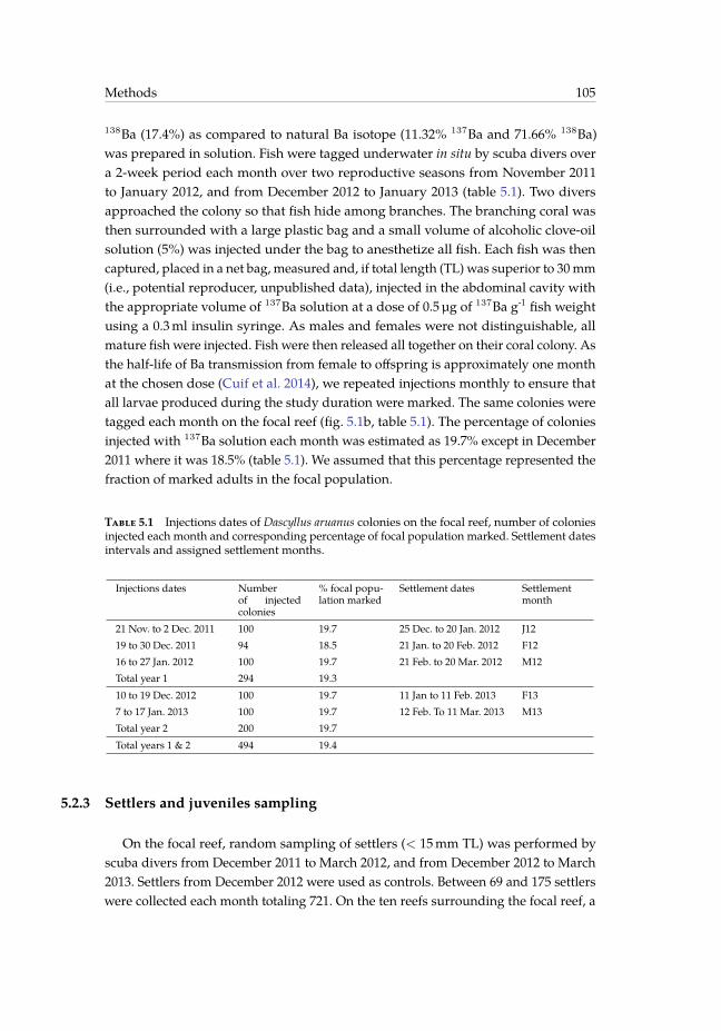
123 / 219

Methods 105

138Ba (17.4%) as compared to natural Ba isotope (11.32% 137Ba and 71.66% 138Ba)was prepared in solution. Fish were tagged underwater in situ by scuba divers overa 2-week period each month over two reproductive seasons from November 2011to January 2012, and from December 2012 to January 2013 (table 5.1). Two diversapproached the colony so that fish hide among branches. The branching coral wasthen surrounded with a large plastic bag and a small volume of alcoholic clove-oilsolution (5%) was injected under the bag to anesthetize all fish. Each fish was thencaptured, placed in a net bag, measured and, if total length (TL) was superior to 30mm(i.e., potential reproducer, unpublished data), injected in the abdominal cavity withthe appropriate volume of 137Ba solution at a dose of 0.5µg of 137Ba g-1 fish weightusing a 0.3ml insulin syringe. As males and females were not distinguishable, allmature fish were injected. Fish were then released all together on their coral colony. Asthe half-life of Ba transmission from female to offspring is approximately one monthat the chosen dose (Cuif et al. 2014), we repeated injections monthly to ensure thatall larvae produced during the study duration were marked. The same colonies weretagged each month on the focal reef (fig. 5.1b, table 5.1). The percentage of coloniesinjected with 137Ba solution each month was estimated as 19.7% except in December2011 where it was 18.5% (table 5.1). We assumed that this percentage represented thefraction of marked adults in the focal population.

Table 5.1 Injections dates of Dascyllus aruanus colonies on the focal reef, number of coloniesinjected each month and corresponding percentage of focal population marked. Settlement datesintervals and assigned settlement months.

Injections dates Numberof injectedcolonies

% focal popu-lation marked

Settlement dates Settlementmonth

21 Nov. to 2 Dec. 2011 100 19.7 25 Dec. to 20 Jan. 2012 J1219 to 30 Dec. 2011 94 18.5 21 Jan. to 20 Feb. 2012 F1216 to 27 Jan. 2012 100 19.7 21 Feb. to 20 Mar. 2012 M12Total year 1 294 19.310 to 19 Dec. 2012 100 19.7 11 Jan to 11 Feb. 2013 F137 to 17 Jan. 2013 100 19.7 12 Feb. To 11 Mar. 2013 M13Total year 2 200 19.7Total years 1 & 2 494 19.4

5.2.3 Settlers and juveniles sampling

On the focal reef, random sampling of settlers (< 15mm TL) was performed byscuba divers from December 2011 to March 2012, and from December 2012 to March2013. Settlers from December 2012 were used as controls. Between 69 and 175 settlerswere collected each month totaling 721. On the ten reefs surrounding the focal reef, a

124 / 219


total of 941 juveniles (< 20mm TL) covering 3 larval cohorts from January to March2012 were also collected in March 2012, with approximately 100 juveniles at each reef.Except for barrier reef stations where only one site was sampled, all reefs were sampledon both leeward and windward sides, with approximately 50 juveniles collected oneach side (fig. 5.1a). Sampling was performed at approximately 10 meters depth oneach reef. Settlers (or juveniles) were anesthetized using a spray of alcoholic clove-oilsolution (5%), captured with hand nets, transported to the surface in plastic bags andkilled by cold shock. Upon return to the laboratory, samples were immediately placedin a freezer.Settlement on the focal reef (number of settlers per colony) was estimated each monthby counting the number of settlers on a random sample of colonies (table 5.4).

5.2.4 Otoliths analysis

Preparation

The total length of each individual was measured with electronic calipers to thenearest 0.1mm before otolith extraction. Both sagittal otoliths were extracted undera binocular microscope by dissecting the dorsal section of the skull using scalpeland tweezers. Otoliths were cleaned in ultra pure water to remove adhering tissue,dried in a laminar flow hood for 24 h and stored in a 0.5ml microcentrifuge tube.One sagittal otolith per individual was then mounted rostrum up in thermoplasticglue (Crystalbond 509) on a piece of microscope slide (7.5mm x 5mm) affixed ona standard microscope slide with thermoplastic glue. The otolith rostrum was firstgrounded and polished and the otolith was then turned over, grounded to the mid-plane and polished with P1200 sandpaper and 9, 3 and 1µm lapping film. A distanceof approximately 20µm was left between the polished surface and the core of theotolith to ensure that the entire core was ablated during ICP analysis. The piece ofmicroscope slide containing the otolith section was unglued from the standard slide,rinsed in ultrapure water, dried in a laminar flow hood for 24 h and stored individuallyin 1.5ml microcentrifuge tubes.

Age reading and PLD determination

Age at capture and PLD (in days)was estimated for a subsample of 502 settlers of thefocal reef collected fromDecember 2011 toMarch 2013. The number of daily incrementswas counted along the longest axis of the otolith from the core to the edge usingthe multipoint tool of the software program ImageJ (http://rsbweb.nih.gov/ij/).Wilson andMcCormick (1999) showed that settlementmark for Pomacentridae consistsof an abrupt decrease in increment width. PLD was hence determined for each fish as


125 / 219

Methods 107

the age at which increment width fell. Settlement date of each fish was calculated ascapture date minus number of days since settlement.

In order to assign a settlement month to the focal reef’s settlers for which age andPLD were not available, we adjusted a linear regression between size at capture andthe number of days elapsed between settlement and capture for the 502 settlers whoseage was known (fig. 5.4). It was then possible, from the size at capture and date ofcapture of a settler, to estimate its settlement date. For each reproductive season, weconsidered only settlers that settled in a time interval ranging from the date of thelast injection performed at the beginning of the reproductive season plus the meanPLD and the date of the last injection performed at the end of the reproductive seasonplus the mean PLD, to ensure that all settlers collected were potentially issued frommarked females. Then this time interval was divided into approximately month-longperiods (table 5.1).

ICP-MS analysis

A NewWave Research 213 nm UV laser ablation system connected to an Agilent7500cs inductively coupled plasma mass spectrometer (ICP-MS) located at the CharlesDarwin University (Darwin, Australia) was used for the otolith elemental analysis.Otoliths were fixed per group of approximately 15 using double-sided tape on petro-graphic slides to be placed in the ablation chamber. A reference standard (NIST612,National Institute of Standards and Technology) was analyzed at the beginning andend of each ∼ 1-hour session to account for mass bias and machine drift throughoutthe analyses. Otoliths were vertical-depth profiled by laser ablation with a laser beamdiameter of 30µm and energy density of 7 to 11 J cm-2 pulsed at 5Hz. Each analysislasted 60 s including 10 s of background and 50 s of ablation (laser activated). If theotolith core was partly altered during grounding, a horizontally laser line scan (1µms-1) was preferably undertaken across the otolith core. Each otolith core was analyzedfor 43Ca, 55Mn, 137Ba and 138Ba (table 5.5).

Statistical analysis

All statistical analyses were conducted using R-2.15.0. ICP-MS data in the blankwere first cleaned of outliers, defined as any value greater than 1.5 times the inter-quartile distance (Tukey 1977). Isotope abundances of 43Ca, 55Mn, 137Ba and 138Bameasured in each otolith were then blank-subtracted. We used the peak of 55Mn as anindicator of the otolith core (Brophy et al. 2004, Macdonald et al. 2008, Munro et al.2009, Starrs et al. 2014). To do this, counts of 43Ca and 55Mn were smoothed usinga 5-point running mean to remove noise (Sinclair et al. 1998), after which the ratio

126 / 219


55Mn/43Ca was computed. A peak of Mn was identified when the 55Mn/43Ca valuerose above the modal value (calculated for each ablation) by a factor of 2 or more andstayed at this elevated level for a period of at least 2.5 s (corresponding to 3.5 datapoints, adapted from Brophy et al. (2004)). The mean core diameter of D. aruanus isapproximately 15µm (first increment width = 7.5µm ± 1.2 standard deviation (SD),n = 502 fish) which corresponds to 21 data points in each ablation profile. These21 data points centered on the 55Mn peak were considered as measurements in theotolith core. 137Ba and 138Ba data in this core were cleaned of outliers and the mean138Ba/137Ba ratio was then computed and corrected for mass bias using the referencestandard in which the 138Ba/137Ba ratio was assumed to be the same as the relativenatural abundance (i.e., 6.38) based on the International Union of Pure and AppliedChemistry values of isotopes abundance (Berglund and Wieser 2011). Controls wereassayed throughout the ICP-MS runs.

A threshold on the mean 138Ba/137Ba ratio value inside the otolith core was deter-mined below which an individual was considered marked. This threshold was equalto the mean 138Ba/137Ba ratio of the controls minus q * SD with q the quantile of thenormal distribution corresponding to an adjusted p-value. An overall significancelevel (α) of 0.01 was chosen for statistical tests, which was then adjusted using themethod of Benjamini and Yekutieli (2001) to control for the false discovery rate due torepeated statistical tests. The mean 138Ba/137Ba ratio in the control otoliths was 6.46with a SD of 0.15 (n = 64). The final adjusted p-value was 1e-06, corresponding to q =4.70 and therefore a 138Ba/137Ba threshold of 5.76 (table 5.2).

To test the sensitivity of our results to this particular threshold value, we alsoestimated the number of marked individuals for three other threshold values rangingfrom 5.65 to 6.16 (table 5.2). Two of these threshold values were based on the controls’mean ratio minus 2 or 3 times the controls ratios’ SD (e.g., Almany et al. (2007),Munro et al. (2009)), corresponding approximately to α equal to 0.05 or 0.01 withoutadjustment and producing 138Ba/137Ba thresholds of 6.16 and 6.02 (table 5.2). Themost conservative threshold value tested was calculated based on the difference in138Ba/137Ba ratio between themean of the controls and themaximum ratio observed inall recruits (7.27). This difference was then subtracted from the mean ratio, producinga 138Ba/137Ba threshold of 5.65 (“inverse max” threshold in table 5.2).

Connectivity between focal reef and reef j is here defined as the fraction of settlerson reef j that originated from the focal reef as :

Cj =mj/sjpm (5.1)

127 / 219

Methods 109

Table 5.2 Number of Dascyllus aruanus marked settlers found on the focal reef and on the tenneighboring reefs (Reefs 1 to 10) in function of threshold value. SD = standard deviation.

Threshold6.16 6.02 5.76 5.65

Settlementmonth

(2*SD) (3*SD) (α = 0.01,corrected,default)

(inversemax)

Focal reef J12 8 1 0 0F12 10 3 2 2M12 30 21 11 9F13 11 1 0 0M13 9 4 0 0Total 68 30 13 11

Reef 1 J12 to M12 1 0 0 0Reef 2 J12 to M12 1 0 0 0Reef 3 J12 to M12 1 0 0 0Reef 4 J12 to M12 5 2 0 0Reef 5 J12 to M12 0 0 0 0Reef 6 J12 to M12 1 0 0 0Reef 7 J12 to M12 2 0 0 0Reef 8 J12 to M12 1 0 0 0Reef 9 J12 to M12 1 0 0 0Reef 10 J12 to M12 0 0 0 0

Total 13 2 0 0

with mj the number of marked settlers on reef j, sj the total number of settlers on reefj that were analyzed and pm the fraction of marked adult population on the focal reef.Self-recruitment on the focal reef was calculated similarly with j being the focal reef.

Self-recruitment and connectivity estimates are subject to uncertainty due to smallsample size and the random nature of collecting marked versus unmarked indivi-duals. 95% confidence intervals for self-recruitment and connectivity estimates weredetermined using a bootstrap approach assuming collection of marked settlers is theresult of two random binomial processes : first, a collected recruit must be from thefocal site ; second, collected recruits from the focal site must come from eggs that weremarked. The probability of the first process is given by the fraction of all recruits thatoriginated at the focal site, i.e., the self-recruitment or connectivity values that we wishto estimate. The probability that an egg produced at the focal site is marked (i.e., thesecond process) is assumed to be the same as the fraction of the total adult populationinjected with barium (table 5.1). Confidence intervals were calculated by randomlygenerating a large number of simulated recruitment samples and determining thelikelihood that a potential self-recruitment or connectivity value will result in a sample

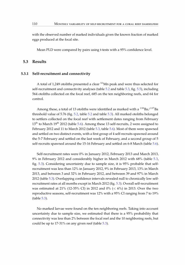
128 / 219


with the observed number of marked individuals given the known fraction of markedeggs produced at the focal site.

Mean PLD were compared by pairs using t-tests with a 95% confidence level.

5.3 Results

5.3.1 Self-recruitment and connectivity

A total of 1,249 otoliths presented a clear 55Mn peak and were thus selected forself-recruitment and connectivity analyses (table 5.2 and table 5.3, fig. 5.5), including564 otoliths collected on the focal reef, 685 on the ten neighboring reefs, and 64 forcontrol.

Among these, a total of 13 otoliths were identified as marked with a 138Ba/137Bathreshold value of 5.76 (fig. 5.2, table 5.2 and table 5.3). All marked otoliths belongedto settlers collected on the focal reef with settlement dates ranging from February13th to March 19th 2012 (table 5.6). Among these 13 self-recruits, 2 were assigned toFebruary 2012 and 11 to March 2012 (table 5.3, table 5.6). Most of them were spawnedand settled on two distinct events, with a first group of 4 self-recruits spawned aroundthe 5-7 February and settled on the last week of February, and a second group of 5self-recruits spawned around the 15-16 February and settled on 6-8 March (table 5.6).

Self-recruitment rates were 0% in January 2012, February 2013 and March 2013,9% in February 2012 and considerably higher in March 2012 with 68% (table 5.3,fig. 5.3). Considering uncertainty due to sample size, it is 95% probable that self-recruitment was less than 12% in January 2012, 9% in February 2013, 13% in March2013, and between 3 and 32% in February 2012, and between 39 and 97% in March2012 (table 5.3). Overlapping confidence intervals revealed null to chronically low self-recruitment rates at all months except in March 2012 (fig. 5.3). Overall self-recruitmentwas estimated at 21% (12-35% CI) in 2012 and 0% (< 6%) in 2013. Over the tworeproductive seasons, self-recruitment was 12% with a 95% CI ranging from 7 to 19%(table 5.3).

No marked larvae were found on the ten neighboring reefs. Taking into accountuncertainty due to sample size, we estimated that there is a 95% probability thatconnectivity was less than 2% between the focal reef and the 10 neighboring reefs, butcould be up to 17-31% on any given reef (table 5.3).

129 / 219

Results 111

Table 5.3 Number of Dascyllus aruanus settlers collected on the focal reef and on the 10 neigh-boring reefs (Reefs 1 to 10) that were analyzed with LA-ICP-MS for each settlement month andpresented a clear 55Mn peak in otolith core, number of marked settlers with the default thresholdof 5.76, fraction of settlers on reef j that originated from the focal reef (Cj ) and 95% confidenceinterval (CI).

Reef j Settlementmonths

Numberof otolithswith a55Mn peak

Numbermarked

Cj (%) 95% CI

Focal reef J12 121 0 0 <12%F12 115 2 9% [3% ; 32%]M12 82 11 68% [39% ; 97%]Total year 1 318 13 21% [12% ; 35%]F13 155 0 0 <9%M13 91 0 0 <16%Total year 2 246 0 0 <6%Total years 1 & 2 564 13 12% [7% ; 19%]

Reef 1 J12 to M12 81 0 0 <18%Reef 2 J12 to M12 51 0 0 <28%Reef 3 J12 to M12 75 0 0 <19%Reef 4 J12 to M12 84 0 0 <17%Reef 5 J12 to M12 76 0 0 <18%Reef 6 J12 to M12 70 0 0 <21%Reef 7 J12 to M12 80 0 0 <18%Reef 8 J12 to M12 77 0 0 <20%Reef 9 J12 to M12 46 0 0 <31%Reef 10 J12 to M12 45 0 0 <31%

Total year 1 685 0 0 <2%

These results changed significantly when we changed the threshold for defining anindividual as marked (table 5.2). For example, with the least conservative threshold(2*SD threshold), 68 individuals were identified as marked on the focal reef (insteadof 13) over 2 reproductive seasons with a maximum of 30 marked individuals (insteadof 11) in March 2012 and a minimum of 8 (instead of 0) in January 2012 (table 5.2,fig. 5.3).With this threshold, 13 marked individuals (instead of 0) originating fromthe focal reef were found to have settled on the neighboring reefs, especially on reef4 located in the south-east. On the contrary, with the most conservative threshold(“inverse max” threshold) we obtained 11 marked individuals on the focal reef andzero on the neighboring reefs.

130 / 219


Figure 5.2 Frequency histogram of mean Barium ratio measured in Dascyllus aruanus otolithscores (n = 1249). Values on the Y axis between 190 and 330 were omitted to reduce the gap in therange of values represented as bar heights. Vertical dotted lines indicate threshold values of 6.16(2*SD, in cyan), 6.02 (3*SD, in orange), 5.76 (alpha = 0.01, corrected (default), in red) and 5.65(inverse max, in dark red).

5.3.2 Settlement intensity and PLD

The mean number of settlers per colony on the focal reef ranged from 0.4 (±1.0 SD) in March 2012, to 6.8 (± 6.9 SD) in February 2012 (fig. 5.3). These numberscorresponded to a total number of recruits to the focal reef population ranging from305 in March 2012 to 3,454 the month before (table 5.4). Collected settlers had a meanage at capture of 36.4 days (± 7.2 SD, n=502) and a mean PLD of 23.0 days (± 3.4SD). Mean PLD of settlers ranged from 20.7 days ± 2.1 SD (n = 64) in March 2012 to23.6 days ± 2.9 SD (n = 76) in January 2012 (fig. 5.3). Mean PLD in March 2012 wassignificantly lower than the mean PLD of settled larvae the other months (fig. 5.3,table 5.7).

5.4 Discussion

A critical aspect of empirical methods assigning individuals to their populationof origin is to identify with certainty as many truly marked individuals as possible,while minimizing false assignments (Christie et al. 2013, Harrison et al. 2013b,a). Intransgenerational marking studies, it is common to use a threshold below which anindividual is considered marked based on the 138Ba/137Ba ratio measured in the

131 / 219

Discussion 113

Figure 5.3 Mean PLD (in days) ± standard error (SE) of Dascyllus aruanus settlers for whichotolith was read, mean number of D. aruanus settlers per colony on the focal reef ± SE, and D.aruanus self-recruitment rate (SR) ± 95% confidence interval for each settlement month on thefocal reef. Numbers of settlers (s) and numbers of colonies (c) used to estimate each value areindicated above each bar.

core of control samples (e.g., Thorrold et al. (2006), Almany et al. (2007)). Our studydemonstrates the importance of carefully choosing this threshold as results may be

132 / 219


quite sensitive to this value (fig. 5.2, table 5.2). Threshold values commonly used inthe literature based on the controls’ mean ratio minus 2 or 3 times the controls ratios’SD (e.g., Almany et al. (2007), Munro et al. (2009)) appear not be strict enough in ourcase, leading to false positives and subsequent overestimation of self-recruitment andconnectivity among reefs. Plotting the distribution of mean Ba ratios for 1200 fishotolith cores, one finds that values of 6.16 (2*SD) or 6.02 (3*SD) are not unusual, lyingwell within a continuous distribution of sample values approximately normally distri-buted above and below the natural isotope ratio (fig. 5.2). To avoid misidentification ofmarked settlers, we used a statistical test that explicitly corrects for repeated measures(Benjamini and Yekutieli 2001). The resulting threshold value (5.76) thus accounts forpotential overlapping of marked and unmarked individuals and avoids significantovercounting of marked individuals. Moreover, among the 13 individuals identifiedthis way, most individuals (11) were considerably further from the natural mean thanthe maximum value is from that mean, which increases our confidence in our results(fig. 5.2, table 5.2). Overall, one needs to find an acceptable trade-off between false po-sitives and negatives by testing sensitivity of results to several marking thresholds. Inorder to avoid false positives and inflate artificially self-recruitment and connectivityestimates, we recommend (1) to analyze as many control samples as possible becausethe threshold will be based on these, (2) to use a strong statistical power, (3) to adjustthe significance level to control for the false discovery rate due to repeated statisticaltests, and (4) to do a close examination of otolith profiles (e.g., fig. 5.5) to validate theassignment tests.

Our study revealed that self-recruitment of D. aruanus could occur in the SWLof New Caledonia on a small central patch of reef despite average water residencetimes (11 days, Jouon et al. (2006), Ouillon et al. (2010)) well below the PLD (23 days)of our study species. This PLD is typical of many tropical marine fishes (Victor andWellington 2000, Lester and Ruttenberg 2005), and intermediate compared to otherspecies investigated in similar larval connectivity studies (e.g., Saenz-Agudelo et al.(2012), Harrison et al. (2012)). We found an average self-recruitment of 12% over 2reproductive seasons. This value is intermediate compared to results of other fine-scale studies using direct methods (transgenerational marking and genetic parentageanalysis) with self-recruitment ranging from 0% (Saenz-Agudelo et al. 2012) to 65%(Berumen et al. 2012). Our intermediate value could be due to the intermediate PLD ofour study species as high (low) self-recruitment rates have been reported for specieswith relatively short (long) PLDs (e.g., Planes et al. (2009), D’Aloia et al. (2013) ; but seeSaenz-Agudelo et al. (2012), Berumen et al. (2012)). Besides PLD, habitat patchiness alsoinfluences the level of self-recruitment (Pinsky et al. 2012) with low self-recruitmentestimated in continuous seascapes (distances between sites inferior to 2 km, D’Aloiaet al. (2013), Schunter et al. (2014)) and high self-recruitment on isolated islands

133 / 219

Discussion 115

(nearest reef at more than 10 km, Almany et al. (2007), Planes et al. (2009), Berumenet al. (2012)). In that context, the intermediate patchiness of the habitat in the SWL,where the closest reefs to our focal reef are approximately 3 km away, could alsoexplain the intermediate value of self-recruitment that we found.

The significant interannual (21% in 2012, 0% in 2013) and intermonth (0% to 68%)variability of self-recruitment may be due to many factors, including wind-drivencirculation in the SWL, cohesive larval dispersal and/or maternal age effects. Watercirculation in the SWL is determined by strong and steady trade winds much of theyear (Douillet 1998). In a larval dispersal modeling study in the SWL, Cuif et al. (2014)showed that this weather regimewas unfavorable to larval retention at lagoon and reefscales by flushing larvae in the open ocean through passes, but that certain episodicweather conditions (weaker winds that are more variable in direction) create favorablehydrodynamic conditions that allowed larvae to settle back to their natal reef. Cohesivedispersal, i.e., larvae originating from the same spawning event spending their entirepelagic larval life together and settling collectively, may also play a role in observedrecruitment variability. Buston et al. (2009) suggested cohesive dispersal forD. aruanuslarvae. We did not analyze kinship among the self-recruits found in March 2012, butbirth and settlement dates for all self-recruits were estimated and two groups of settlersthat were potentially born the same day and settled together were identified (table 5.6),suggesting that large peaks in self-recruitmentmayhave been due to cohesive dispersal.Maternal size effects on phenotypic traits of larvae have been suggested to influencelarval dispersal pattern with larger females contributing disproportionally to self-recruitment through larger body size at hatching or faster growth and/or earliercompetency, allowing larvae to come back to their natal reef (Beldade et al. 2012).In our study, small females injected at the beginning of the reproductive season inNovember 2011 likely grew to become larger females in February 2012 (Table S5)potentially producing larvae best able to settle back to their natal reef in March 2012than at the beginning of the reproductive season. We did not find differences inhatching size (otolith growth back-calculation, results not shown), but the mean PLDof larvae that settled in March 2012 was significantly shorter than the PLD of larvaeof the other monthly cohorts. However, the difference in PLD between March 2012and the other months remains small (between 2 to 3 days), so that it is unlikely that aslightly shortened PLD alone can explain the higher self-recruitment rate observedin March 2012. Favorable hydrodynamic events (Cuif et al. 2014), associated withcohesive dispersal (Buston et al. 2009), larval preference for natal habitat (Gerlachet al. 2007) coupled to strong oriented swimming capabilities (Leis et al. 2011), andmaternal effects on larval life traits enhancing the capacity of larvae to come back totheir natal reef (Beldade et al. 2012) may have all facilitated self-recruitment in March2012.

134 / 219


Self-recruitment informs population openness (Hixon et al. 2002). Demographicallyopen populations are dependent upon larval connectivity as opposed to closed popu-lations that are replenished by self-recruitment (Pinsky et al. 2012). Most coral reef fishpopulations exist in a continuum between open and closed states (Jones et al. 2009).In this study, relatively low self-recruitment rates indicate that D. aruanus populationopenness in the SWL of New Caledonia is high at the reproductive season scale. Giventhat D. aruanus life history traits are closer to the majority of coral reef fishes, webelieve that our results are relevant for other similar species in the SWL and in othercomparable systems. Furthermore we showed through sampling of multiple cohortsthat population openness is highly variable on a monthly scale. The relationship bet-ween openness and self-recruitment is clear (Pinsky et al. 2012) but the relationshipbetween these metrics and population persistence is not. As underlined by Burgesset al. (2014), the total number of self-recruits is more directly related to self-persistenceof local populations than self-recruitment is. In our study, differences in estimatedself-recruitment between February and March 2012 (resp. 9% and 68%) were in factcompensated by differences in overall recruitment between these two months (resp.3,454 and 305 recruits) resulting in a similar total number of self-recruits (resp. 310and 207). Recruitment variability can result in strong variability in self-recruitmentand small or undetectable self-recruitment does not mean that there are not manyself-recruiting larvae arriving on their natal reef. Because recruitment is notoriouslyhighly variable in both space and time, self-recruitment is also expected to be highlyvariable simply due to a “dilution” effect. This dilution effect must necessarily besmaller in isolated areas which are far away from other sources of larvae. Conse-quently, it is potentially not surprising to observe strong and steady self-recruitmentin remote places (Planes et al. 2009) as opposed to variable and lower self-recruitmentin continuous seascapes (Hogan et al. 2012). Our observations of strong variability inself-recruitment rates are consistent with local reef fish populations in a continentalisland such as New Caledonia being very open, receiving many self-recruits eachmonth that are diluted in many more allo-recruits coming from neighboring reefs.This has important implications for management as open local populations with smallor undetectable self-recruitment may still receive a sufficient number of self-recruitsto benefit from local protection measures and ensure their persistence.

5.5 Acknowledgments

We thank G. Mou-Tham, J. Tiavouane, C. Fauvelot, D. Grulois, the staff of thescuba diving service and boat drivers of IRD for assistance with field work, J. Baly, E.Dabas, M. Labonne, G. Lecroizier, J.M. Munaron, and M. Vannereau for assistancewith otoliths preparation, L. Jamet for assistance with preparation of enriched Bariumisotope solution, F. Foti and the RIEL team of Charles Darwin University for assistance

135 / 219

Acknowledgments 117

with LA-ICP-MS. Funding was provided by the COMPO project (Connectivity OfMarine POpulations, www.compo.ird.fr) through a grant from the French NationalResearch Agency (ANR) n° 2010 JCJC 1701 01. Ethics and sampling approvals wereprovided by the Direction du Service de l’Environnement de la Province Sud deNouvelle-Calédonie, arrêté n° 3117-2011/ARR/DENV.

www.compo.ird.fr

136 / 219


5.6 Supplementary material

Figure 5.4 Time elapsed between settlement and collect (in days) in function of size at capture(Lcapt in mm) for 502 Dascyllus aruanus fish collected on the focal reef for which settlement datewas estimated through otolith reading. Blue line represents best fit linear model.

Table 5.4 Settlement estimation dates of Dascyllus aruanus on the focal reef, number of coloniessampled, number of settlers per colony and estimated total number of settlers for each samplingmonth on the focal reef.

Month Settlement estima-tion dates

Numberof coloniessampled

Mean nb ofsettlers (<15mm TL)per colony (±SD)

Estimated numberof settlers in thefocal population[95% confidenceinterval]

Year 1 January 2012 19 to 27 Jan. 2012 198 1.1 (± 1.9) 559 [424-693]February 2012 13 to 21 Feb. 2012 259 6.8 (± 6.9) 3,454 [3,028-3,881]March 2012 12 & 22 Mar. 2012 191 0.6 (± 1.0) 305 [233-377]

Year 2 February 2013 6 & 8 Feb. 2013 112 3.3 (± 3.8) 1,676 [1,319-2,034]March 2013 22 Mar. 2013 132 1.7 (± 2.4) 864 [656-1,072]

137 / 219


Figure 5.5 Profiles of 138Ba/137Ba ratio (black solid line) and 55Mn/43Ca ratio (grey solidline) in otoliths of aDascyllus aruanus control settler (a) and a marked settler (b). X-axis representstime (seconds) elapsed since the beginning of otolith laser ablation. Grey vertical dashed linesindicate limits of otolith core. The red horizontal dashed line indicates the threshold value of5.76. Shaded box indicates mean ± SD of the 138Ba/137Ba ratio in the control otoliths (n = 64).

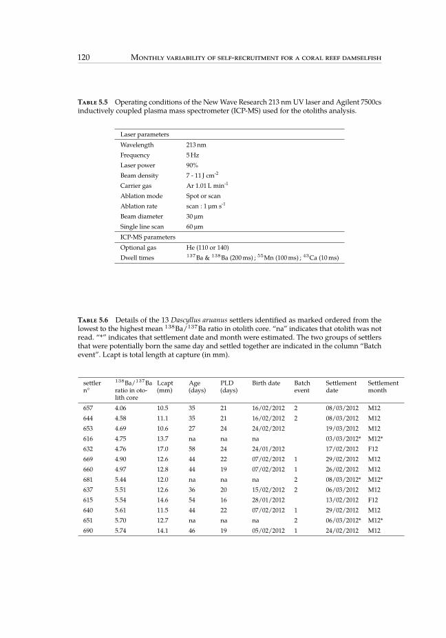
138 / 219


Table 5.5 Operating conditions of the NewWave Research 213 nm UV laser and Agilent 7500csinductively coupled plasma mass spectrometer (ICP-MS) used for the otoliths analysis.

Laser parametersWavelength 213 nmFrequency 5HzLaser power 90%Beam density 7 - 11 J cm-2

Carrier gas Ar 1.01 L min-1

Ablation mode Spot or scanAblation rate scan : 1µm s-1

Beam diameter 30µmSingle line scan 60µmICP-MS parametersOptional gas He (110 or 140)Dwell times 137Ba & 138Ba (200ms) ; 55Mn (100ms) ; 43Ca (10ms)

Table 5.6 Details of the 13 Dascyllus aruanus settlers identified as marked ordered from thelowest to the highest mean 138Ba/137Ba ratio in otolith core. “na” indicates that otolith was notread. “*” indicates that settlement date and month were estimated. The two groups of settlersthat were potentially born the same day and settled together are indicated in the column “Batchevent”. Lcapt is total length at capture (in mm).

settlern°

138Ba/137Baratio in oto-lith core

Lcapt(mm)

Age(days)

PLD(days)

Birth date Batchevent

Settlementdate

Settlementmonth

657 4.06 10.5 35 21 16/02/2012 2 08/03/2012 M12644 4.58 11.1 35 21 16/02/2012 2 08/03/2012 M12653 4.69 10.6 27 24 24/02/2012 19/03/2012 M12616 4.75 13.7 na na na 03/03/2012* M12*632 4.76 17.0 58 24 24/01/2012 17/02/2012 F12669 4.90 12.6 44 22 07/02/2012 1 29/02/2012 M12660 4.97 12.8 44 19 07/02/2012 1 26/02/2012 M12681 5.44 12.0 na na na 2 08/03/2012* M12*637 5.51 12.6 36 20 15/02/2012 2 06/03/2012 M12615 5.54 14.6 54 16 28/01/2012 13/02/2012 F12640 5.61 11.5 44 22 07/02/2012 1 29/02/2012 M12651 5.70 12.7 na na na 2 06/03/2012* M12*690 5.74 14.1 46 19 05/02/2012 1 24/02/2012 M12

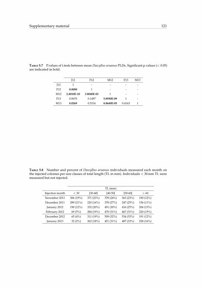
139 / 219


Table 5.7 P.values of t.tests between mean Dascyllus aruanus PLDs. Significant p.values (< 0.05)are indicated in bold.

J12 F12 M12 F13 M13J12 1 - - - -F12 0.0080 1 - - -M12 2.4010E-10 3.8040E-03 1 - -F13 0.0670 0.1497 5.8950E-09 1 -M13 0.0269 0.5316 8.8640E-05 0.4163 1

Table 5.8 Number and percent of Dascyllus aruanus individuals measured each month onthe injected colonies per size classes of total length (TL in mm). Individuals < 30mm TL weremeasured but not injected.

TL (mm)Injection month < 30 [30-40[ [40-50[ [50-60[ > 60November 2011 306 (19%) 371 (23%) 378 (24%) 363 (23%) 190 (12%)December 2011 289 (21%) 220 (16%) 378 (27%) 347 (25%) 156 (11%)January 2012 190 (12%) 332 (20%) 491 (30%) 416 (25%) 206 (13%)February 2012 69 (5%) 284 (19%) 470 (31%) 467 (31%) 220 (15%)December 2012 65 (4%) 311 (19%) 509 (32%) 534 (33%) 191 (12%)January 2013 32 (2%) 262 (18%) 451 (31%) 487 (33%) 228 (16%)

140 / 219

141 / 219

Chapitre 6

Comparison between self-recruitment andconnectivity estimates from a larvaldispersal model and field observations

123

142 / 219

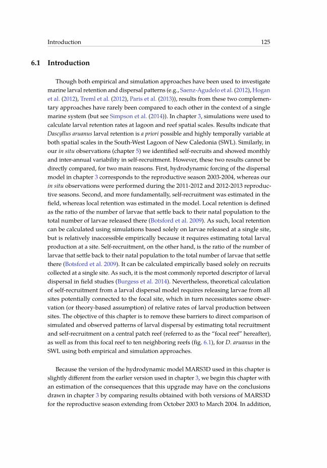
143 / 219

Introduction 125

6.1 Introduction

Though both empirical and simulation approaches have been used to investigatemarine larval retention and dispersal patterns (e.g., Saenz-Agudelo et al. (2012), Hoganet al. (2012), Treml et al. (2012), Paris et al. (2013)), results from these two complemen-tary approaches have rarely been compared to each other in the context of a singlemarine system (but see Simpson et al. (2014)). In chapter 3, simulations were used tocalculate larval retention rates at lagoon and reef spatial scales. Results indicate thatDascyllus aruanus larval retention is a priori possible and highly temporally variable atboth spatial scales in the South-West Lagoon of New Caledonia (SWL). Similarly, inour in situ observations (chapter 5) we identified self-recruits and showed monthlyand inter-annual variability in self-recruitment. However, these two results cannot bedirectly compared, for two main reasons. First, hydrodynamic forcing of the dispersalmodel in chapter 3 corresponds to the reproductive season 2003-2004, whereas ourin situ observations were performed during the 2011-2012 and 2012-2013 reproduc-tive seasons. Second, and more fundamentally, self-recruitment was estimated in thefield, whereas local retention was estimated in the model. Local retention is definedas the ratio of the number of larvae that settle back to their natal population to thetotal number of larvae released there (Botsford et al. 2009). As such, local retentioncan be calculated using simulations based solely on larvae released at a single site,but is relatively inaccessible empirically because it requires estimating total larvalproduction at a site. Self-recruitment, on the other hand, is the ratio of the number oflarvae that settle back to their natal population to the total number of larvae that settlethere (Botsford et al. 2009). It can be calculated empirically based solely on recruitscollected at a single site. As such, it is the most commonly reported descriptor of larvaldispersal in field studies (Burgess et al. 2014). Nevertheless, theoretical calculationof self-recruitment from a larval dispersal model requires releasing larvae from allsites potentially connected to the focal site, which in turn necessitates some obser-vation (or theory-based assumption) of relative rates of larval production betweensites. The objective of this chapter is to remove these barriers to direct comparison ofsimulated and observed patterns of larval dispersal by estimating total recruitmentand self-recruitment on a central patch reef (referred to as the “focal reef” hereafter),as well as from this focal reef to ten neighboring reefs (fig. 6.1), for D. aruanus in theSWL using both empirical and simulation approaches.

Because the version of the hydrodynamic model MARS3D used in this chapter isslightly different from the earlier version used in chapter 3, we begin this chapter withan estimation of the consequences that this upgrade may have on the conclusionsdrawn in chapter 3 by comparing results obtained with both versions of MARS3Dfor the reproductive season extending from October 2003 to March 2004. In addition,

144 / 219

126 Comparison between a larval dispersal model and field observations

as the results of chapter 3 suggested El Niño (La Niña) years could lead to lower(higher) larval retention than neutral years, we attempt to verify this statement bymodelling larval retention for an El Niño (October 2009 to March 2010) and a LaNiña (October 2011 to March 2012) austral summer. Finally, we compare simulatedand observed total recruitment and self-recruitment estimates on the focal reef, andthe contribution of this reef to ten neighboring reefs in the SWL, for the 2011-2012reproductive season. We try to bring together simulated and observed estimates byfocusing first on average values of self-recruitment and connectivity and then ontemporal variability of self-recruitment and total recruitment on the focal reef overthe reproductive season.

6.2 Methods

6.2.1 Biophysical model

The larval dispersal model used here is very similar to the one used in chapter 3.The main difference with chapter 3 is that the hydrodynamic forcing of the individual-based model comes from an enhanced version of MARS3D (v8.19) with an improvedconfiguration on the SWLa. Furthermore, we added a reef (Ilôt Sable) located ap-proximately 8 km North of the focal reef in the habitat layer (fig. 6.1). This reef wasmissing in the atlas of Andréfouët and Torres-Pulliza (2004) on which we based thehabitat selection in chapter 3. Horizontal and vertical resolution, MARS3D outputsrecord frequency, and Ichthyop calculation time step remained unchanged (report tochapter 3 for further details on these parameters).

6.2.2 Comparison between years

For comparison with chapter 3 and between reproductive seasons, we ran exactlythe same simulations but with realistic hydrodynamic forcing corresponding to aus-tral summers 2003-2004, (same as chapter 3), 2009-2010 (El Niño) and 2011-2012 (LaNiña). Year selection was based on the Oceanic Niño Index published by the ClimatePrediction Center of the National Oceanic and Atmospheric Administration (NOAA)National Weather Service. Release zone, settlement habitat, hatching events frequency,planktonic larval duration (PLD), settlement habitat detection distance and hypo-theses about natal homing were kept the same to allow for direct comparison andare summarized in table 6.1. Precompetency duration (PC) was set at 11 days for thiscomparison between years. Natal lagoon retention (NLR) and natal reef retention

aMajor changes are : (1) Delimitation of study area : slightly increased behind the barrier reef towardsopen ocean, (2) Open Boundary Conditions : BRAN version changed, (3) Boundary Conditions of Atmosphericforcing : WRF was forced with NCEP data instead of AMIP data, (4) Better resolution of sigma levels.

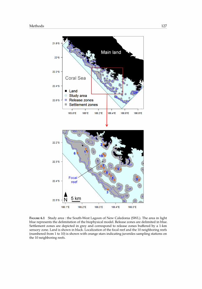
145 / 219

Methods 127

Figure 6.1 Study area : the South-West Lagoon of New Caledonia (SWL). The area in lightblue represents the delimitation of the biophysical model. Release zones are delimited in blue.Settlement zones are depicted in grey and correspond to release zones buffered by a 1-kmsensory zone. Land is shown in black. Localization of the focal reef and the 10 neighboring reefs(numbered from 1 to 10) is shown with orange stars indicating juveniles sampling stations onthe 10 neighboring reefs.

146 / 219


(NRR) were calculated as the fraction of larvae released at the focal site that recruitto the lagoon and to the focal reef under both homing hypotheses, as in chapter 3.Cross-correlations between wind along-shelf and cross-shelf component and retentiontime series were performed as in chapter 3. Mean dispersal distances from focal reefwere also calculated over each austral summer.

147 / 219

Methods 129

Tabl

e6.1

Detailsof

thedisp

ersalm

odel

runs

used

inthisch

apter.PC

=precom

petenc

ype

riod.

PLD

=plan

kton

iclarval

duratio

n.

RunMARS

3Dve

rsion

Windforcingpe

riod

Nbre-

leases

Nb

larvae

perre-

lease

Release

zone

Settle

zone

(s)

Hom

ing

hypo

the-

sis

PCdu

-ratio

nDetectio

ndis-

tanc

e

Simulation

dura-

tion

(PLD

)1

old

1Oct.2003to

1Mar.2

004

1,217

500

Focalreef

Allha

bitat

Noho

ming

11da

ys1km

30da

ys2

old

1Oct.2003to

1Mar.2

004

1,217

500

Focalreef

Allha

bitat

Stric

thom

ing

11da

ys1km

30da

ys3

new

1Oct.2003to

1Mar.2

004

1,217

500

Focalreef

Allha

bitat

Noho

ming

11da

ys1km

30da

ys4

new

1Oct.2003to

1Mar.2

004

1,217

500

Focalreef

Focalreef

Stric

thom

ing

11da

ys1km

30da

ys5

new

1Oct.2009to

1Mar.2

010

1,209

500

Focalreef

Allha

bitat

Noho

ming

11da

ys1km

30da

ys6

new

1Oct.2009to

1Mar.2

010

1,209

500

Focalreef

Focalreef

Stric

thom

ing

11da

ys1km

30da

ys7

new

1Oct.2011to

1Mar.2

012

1,217

500

Focalreef

Allha

bitat

Noho

ming

11da

ys1km

30da

ys8

new

1Oct.2011to

30Jun.

2012

2,192

500

Focalreef

Focalreef

Stric

thom

ing

11da

ys1km

30da

ys9

new

1Oct.2011to

30Jun.

2012

2,192

10,000

Allha

bitat

Allha

bitat

Noho

ming

11da

ys1km

30da

ys10

new

1Oct.2011to

30Jun.

2012

2,192

500

Focalreef

Allha

bitat

Noho

ming

21da

ys1km

30da

ys11

new

1Oct.2011to

30Jun.

2012

2,192

10,000

Allha

bitat

Allha

bitat

Noho

ming

21da

ys1km

30da

ys

148 / 219


6.2.3 Self-recruitment, total recruitment and connectivity

Simulations

To simulate self-recruitment on the focal reef over the 2011-2012 reproductiveseason, larvae were released uniformly over all suitable habitat (240 release zones intotal, including the focal reef) every 3 hour from 1 October 2011 to 30 June 2012 (forPC = 11 and PC = 21 days, runs 9 and 11, respectively ; table 6.1 ; fig. 6.1). This releasestrategy implicitly assumes that all suitable habitat has equal reproductive output.Released larvae were randomly distributed throughout the water column from 0 to20 m depth. As in chapter 3, we supposed that larvae became active after a givenprecompetency period with sensory and swimming capabilities that allowed themto detect and approach a settlement area. This non-explicit swimming behavior wasincluded by assuming that competent larvae could actively settle once at a distanceof 1 km from a settlement reef. Recruitment zones were thus defined in the model asrelease zones with a buffer of 1 km that lead to the definition of 27 recruitment zonesincluding the focal reef (fig. 6.1).

Limited storage space and run time constrained us to release 10,000 larvae at eachrelease event. As the focal reef only represents a small percentage (∼ 0.03%) of thetotal habitat area, the number of larvae released in the focal reef was thus very small(∼ 3 on average), leading to inaccurate estimates of self-recruitment. Therefore, resultsfrom both focal-reef-only and all-habitat runs were combined (i.e., runs 7 and 9 forPC = 11 days, and runs 10 and 11 for PC = 21 days) when estimating self-recruitmenton the focal reef (SR) and the percentage of recruitment to other reefs (indexed i) thatoriginated at the focal reef (Ci,FR) for each release event.

Calculations

After adjusting for the inhomogeneous number of larvae released at the focal reefin the two combined runs (i.e., ∼ 3 for run 9 vs. 500 for run 7), Ci,FR was calculatedas the ratio between recruits produced at the focal reef that recruited on reef i (Ri,FR)and recruits from all sites (Ri,tot). Numerically, this is :

Ci,FR =Ri,FRRi,tot

∗ 100 (6.1)

Note that SR is equal to Ci,FR with i being the focal reef. These calculations wererepeated for each spawning event along the simulated reproductive season.

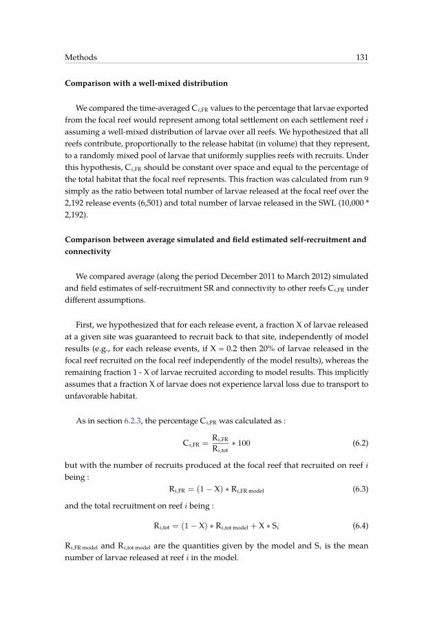
149 / 219

Methods 131

Comparison with a well-mixed distribution

We compared the time-averaged Ci,FR values to the percentage that larvae exportedfrom the focal reef would represent among total settlement on each settlement reef iassuming a well-mixed distribution of larvae over all reefs. We hypothesized that allreefs contribute, proportionally to the release habitat (in volume) that they represent,to a randomly mixed pool of larvae that uniformly supplies reefs with recruits. Underthis hypothesis, Ci,FR should be constant over space and equal to the percentage ofthe total habitat that the focal reef represents. This fraction was calculated from run 9simply as the ratio between total number of larvae released at the focal reef over the2,192 release events (6,501) and total number of larvae released in the SWL (10,000 *2,192).

Comparison between average simulated and field estimated self-recruitment andconnectivity

We compared average (along the period December 2011 to March 2012) simulatedand field estimates of self-recruitment SR and connectivity to other reefs Ci,FR underdifferent assumptions.

First, we hypothesized that for each release event, a fraction X of larvae releasedat a given site was guaranteed to recruit back to that site, independently of modelresults (e.g., for each release events, if X = 0.2 then 20% of larvae released in thefocal reef recruited on the focal reef independently of the model results), whereas theremaining fraction 1 - X of larvae recruited according to model results. This implicitlyassumes that a fraction X of larvae does not experience larval loss due to transport tounfavorable habitat.

As in section 6.2.3, the percentage Ci,FR was calculated as :

Ci,FR =Ri,FRRi,tot

∗ 100 (6.2)

but with the number of recruits produced at the focal reef that recruited on reef ibeing :

Ri,FR = (1 − X) ∗ Ri,FR model (6.3)

and the total recruitment on reef i being :

Ri,tot = (1 − X) ∗ Ri,tot model + X ∗ Si (6.4)

Ri,FR model and Ri,tot model are the quantities given by the model and Si is the meannumber of larvae released at reef i in the model.

150 / 219


As before, SR is equal do Ci,FR with i being the focal reef : in that case, RFR, thenumber of self-recruits on the focal reef, is equal to :

RFR = (1 − X) ∗ RFR model + X ∗ SFR (6.5)

WhenX= 0, SR andC are as given by themodel.WhenX= 1, all recruits are self-recruitson all sites, and none are allo-recruits.

Secondly, we assumed that the production on the focal reef was larger than in theother reefs by multiplying the number of larvae produced by this reef by P > 1. Thiseffect was simply included by multiplying the number of recruits originated from thefocal reef by P :

Ri,FR = P ∗ Ri,FR model (6.6)

Ri,tot = Ri,tot model + (P− 1) ∗ Ri,FR model (6.7)

Note that these quantities, and therefore SR and C, are as given by the model when P= 1.

Finally, we combined the effects represented by X and P.

Comparison between simulated and observed time series of self-recruitment andtotal recruitment

Putative birth dates of self-recruits estimated from the field were positioned alongthe simulated time series of self-recruitment for the 3-month period extending fromDecember 2011 to February 2012. Monthly total recruitment values estimated from thefield at the focal reef were also compared to simulated time series of total recruitmentfor the same period.

6.3 Results

6.3.1 Comparison between MARS3D versions

The slightly different versions ofMARS3D used in this chapter and chapter 3 lead tosimilar results, with slightly smaller average dispersal distances and retention valueswith the new version (table 6.2).

With the new version of MARS3D, time series of NRR under both homing hypo-theses show significant negative cross-correlations with the along-shore component of

151 / 219

Results 133

Table 6.2 Comparison of retention values and dispersal distances between “old” (chapter 3)and “new” (this chapter) versions of MARS3D. NRR = natal reef retention ; NLR = natal lagoonretention ; SD = standard deviation ; SE = standard error. Run number refers to table 6.1.

No homing Strict homingMARS3Dversion

Dispersal distance(km)

NRR (%) NLR (%) NRR (%)

Old run : 1 1 1 2mean : 25.2 1.4 56.7 6.7SD : 18.1 2.3 26.4 8.2SE : 0.52 0.07 0.76 0.24range : [0.02 ; 89.0] [0 ; 23] [0 ; 100] [0 ; 42.6]

New run : 3 3 3 4mean : 19.7 1.1 47.0 6.1SD : 14.7 1.6 20.9 6.0SE : 0.42 0.05 0.60 0.17range : [0.04 ; 89.8] [0 ; 14] [7.6 ; 99.4] [0 ; 31]

wind, as with the old version. Significant correlations occur between days 3 and 6 andbetween days 0 and 11 for no-homing and strict-homing hypotheses, respectively, withabsolute maximum correlation coefficient of 0.3 and 0.4 occurring at a lag of 4 and5 days, respectively (not shown). The time series of NLR shows significant negativecross-correlations with the along-shore component of wind between days 1 and 9after release, with an absolute maximum correlation coefficient of 0.4 (not shown).These results are very similar to results of chapter 3.

With the new version of MARS3D, time series of NRR under both homing hy-potheses and time series of NLR also showed significant positive cross-correlationswith the cross-shore component of wind with maximum correlation coefficient of 0.2between days 7 and 16 (NRR no homing), days 6 and 17 (NRR strict homing) and days8 and 20 (NLR) after release.

6.3.2 Comparison between reproductive seasons

Using the new version of MARS3D, we found similar average dispersal distancesand retention values across years (table 6.3). The lowest average retention is obtai-ned for the El Niño reproductive season under both homing hypotheses (table 6.3).Regarding simulated time series, retention values are highly variable within each re-productive season for all years, without apparent synchronicity among years (fig. 6.2).

152 / 219


Table 6.3 Same as table 6.2 but using MAR3D new version for different reproductive seasons.

No homing Strict homingReproductiveseason

Dispersal distance(km)

NRR (%) NLR (%) NRR (%)

2003-2004 run : 3 3 3 4(Neutral) mean : 19.7 1.1 47.0 6.1

SD : 14.7 1.6 20.9 6.0SE : 0.42 0.05 0.60 0.17range : [0.04 ; 89.8] [0 ; 14] [7.6 ; 99.4] [0 ; 31]

2009-2010 run : 5 5 5 6(El Niño) mean : 20.0 0.6 38.1 3.4

SD : 15.1 1.0 18.0 4.5SE : 0.43 0.03 0.52 0.13range : [0.09 ; 89.7] [0 ; 6.6] [4.4 ; 97.6] [0 ; 26.8]

2011-2012 run : 7 7 7 8(La Niña) mean : 20.3 0.7 44.0 5.3

SD : 14.4 1.1 24.9 5.9SE : 0.41 0.03 0.71 0.17range : [0.02 ; 89.8] [0 ; 7.2] [2.6 ; 100] [0 ; 27.4]

For reproductive season 2011-2012, corresponding to the field season, time series ofNRR under both homing hypotheses show significant negative cross-correlations withthe along-shore component of wind (fig. 6.3a). Significant correlations occur betweendays 6 and 11 and between days 5 and 11 for no-homing and strict-homing hypotheses,respectively, with absolute maximum correlation coefficient of 0.4 occurring at a lagof 9 days. The time series of NLR shows significant negative cross-correlations withthe along-shore component of wind between days 1 and 10 after release, with anabsolute maximum correlation coefficient of 0.5. These results are very similar toresults obtained for the reproductive season 2003-2004 with the new and old versionsof MARS3D. Time series of NLR also showed significant cross-correlations with thecross-shore component of wind with maximum correlation coefficient of 0.2 betweendays 6 and 8 (fig. 6.3b).

153 / 219

Results 135

Figure 6.2 Retention time series for release dates comprised between 1st of October and 1st ofMarch and 3 different reproductive seasons. NRR = natal reef retention ; NLR = natal lagoonretention.

Figure 6.3 Cross-correlations between 2011-2012 retention time series and along-shore (a) andcross-shore (b) wind components derived fromWRF model for a precompetency period of 11days and under the hypotheses of strict or no homing. NLR = natal lagoon retention ; NRR =natal reef retention. Dotted lines represent cross-correlation critical values with a 95% level ofconfidence, adjusted to take into account temporal autocorrelation of time series.

154 / 219


6.3.3 Self-recruitment and total recruitment at the focal reef, and connectivityto the other reefs

Comparison between model estimates and a well-mixed distribution

Assuming a well-mixed distribution of larvae over all reefs, the percentage thatlarvae export from the focal reef would represent among total settlement on anysettlement reef is equal to 0.03%. Simulated self-recruitment and connectivity estimatesare only slightly superior to this value (table 6.4), suggesting that distribution of larvaeis close to being well-mixed in the model.

Comparison between average simulated and field estimates

The average simulated value of self-recruitment SR for larvae released at the focalreef between December 2011 and February 2012 is 0.1% ± 0.1 (range = [0 ; 1.2%]). Theaverage value of connectivity Ci,FR from the focal reef to the ten neighboring reefs forthe same period is 0.09% (table 6.4) with little variability among reefs. Table 6.4 showsthe result obtained for a precompetency period (PC) of 21 days, but a similar result isobtained for PC = 11 (section 6.8).

From chapter 5, I remind the following relevant results for comparison. The averagepercentage of self-recruitment measured in the field at the focal reef between Januaryand March 2012 is 21% (with a 95% confidence interval ranging from 12 to 35%).The export of larvae from the focal reef to the ten neighboring reefs during thisperiod is estimated to be 0% (< 2% with a 95% probability). Individuals that settledbetween January and March 2012 were born between December 2011 and February2012 (table 6.9).

Therefore, the average simulated self-recruitment value of larvae released at thefocal reef between December 2011 and February 2012 is more than two orders ofmagnitude lower than the percentage measured on the field. The average value ofconnectivity to the ten neighboring reefs is within the confidence interval of the fieldestimate.

A way to reconcile the average simulated and observed values of self-recruitmentis to assume that the fraction of released larvae self-recruiting independently of modelresults is X ∼ 0.35 (fig. 6.4). As a consequence, the simulated connectivity valuesbetween the focal reef and the surrounding reefs (Ci,FR) decrease slightly (table 6.5)but remain consistent with the confidence interval found in the field.

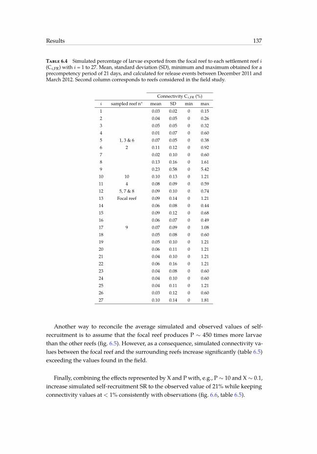
155 / 219

Results 137

Table 6.4 Simulated percentage of larvae exported from the focal reef to each settlement reef i(Ci,FR) with i = 1 to 27. Mean, standard deviation (SD), minimum and maximum obtained for aprecompetency period of 21 days, and calculated for release events between December 2011 andMarch 2012. Second column corresponds to reefs considered in the field study.

Connectivity Ci,FR (%)i sampled reef n° mean SD min max1 0.03 0.02 0 0.152 0.04 0.05 0 0.263 0.05 0.05 0 0.324 0.01 0.07 0 0.605 1, 3 & 6 0.07 0.05 0 0.386 2 0.11 0.12 0 0.927 0.02 0.10 0 0.608 0.13 0.16 0 1.619 0.23 0.58 0 5.4210 10 0.10 0.13 0 1.2111 4 0.08 0.09 0 0.5912 5, 7 & 8 0.09 0.10 0 0.7413 Focal reef 0.09 0.14 0 1.2114 0.06 0.08 0 0.4415 0.09 0.12 0 0.6816 0.06 0.07 0 0.4917 9 0.07 0.09 0 1.0818 0.05 0.08 0 0.6019 0.05 0.10 0 1.2120 0.06 0.11 0 1.2121 0.04 0.10 0 1.2122 0.06 0.16 0 1.2123 0.04 0.08 0 0.6024 0.04 0.10 0 0.6025 0.04 0.11 0 1.2126 0.03 0.12 0 0.6027 0.10 0.14 0 1.81

Another way to reconcile the average simulated and observed values of self-recruitment is to assume that the focal reef produces P ∼ 450 times more larvaethan the other reefs (fig. 6.5). However, as a consequence, simulated connectivity va-lues between the focal reef and the surrounding reefs increase significantly (table 6.5)exceeding the values found in the field.

Finally, combining the effects represented by X and P with, e.g., P∼ 10 and X∼ 0.1,increase simulated self-recruitment SR to the observed value of 21% while keepingconnectivity values at < 1% consistently with observations (fig. 6.6, table 6.5).

156 / 219


Figure 6.4 Average simulated value of self-recruitment at the focal reef (SR) obtained forincreasing values of X. Red dotted line indicates SR measured on the field.

Figure 6.5 Same as fig. 6.4 for increasing values of P (and X = 0).

157 / 219

Results 139

Figure 6.6 Combinations of parameters X and P that result in average simulated SR ∼ 21%.

158 / 219


Tabl

e6.5

Sameas

table6.4forthree

diffe

rent

combina

tions

ofpa

rametersX

andP.

Con

nectivity

Ci,FR(%

)

X=0.35

;P=1

X=0;

P=450

X=0.1;

P=10

isampled

reef

n°mean

SDmin

max

mean

SDmin

max

mean

SDmin

max

51,

3&

66E

-03

5E-03

0E+0

00.03

22.46

12.41

0.00

63.41

0.21

0.18

00.94

62

0.07

0.06

00.44

27.20

17.84

080.76

0.92

0.88

07.03

1010

0.06

0.06

00.37

23.67

20.92

084.59

0.81

0.94

05.91

114

0.04

0.04

00.21

22.13

17.21

072.79

0.63

0.67

04.00

125,7&

80.02

0.02

00.13

22.97

18.89

076.92

0.44

0.51

03.68

179

0.01

0.02

00.11

18.06

18.20

083.15

0.37

0.45

03.74

159 / 219

Results 141

Comparison between simulated and observed time series of self-recruitment andtotal recruitment at the focal reef

With X = 0.1 and P = 10, fig. 6.7 shows time series of self-recruitment and totalrecruitment simulated at the focal reef. Simulated self-recruitment is different fromzero at estimated birth dates of self-recruits collected in the field (fig. 6.7). Nevertheless,the model suggests a peak of self-recruitment for larvae released in mid-January 2012although we did not find self-recruits born at this period in the field.

Field measurement of total recruitment at the focal reef showed a peak in mid-February 2012 at 6.8 recruits per colony, corresponding to larval hatching dates bet-ween late December 2011 and late January 2012 (table 6.6), as opposed to lowerrecruitment ( 1 recruit per colony) assessed in late January 2012 and mid-March 2012,corresponding to larvae released during December 2011 and between mid-Januaryand mid-February 2012, respectively (table 6.6). The simulation of total recruitment atthe focal reef suggests an opposite temporal pattern (table 6.6).

Figure 6.7 Simulated time series of self-recruitment (SR) and total recruitment (RFR,tot) at thefocal reef for larvae released between December 2011 and March 2012. Vertical red dotted linesindicate the estimated birth date of the 10 self-recruits identified in chapter 5 for which otolithwas read (table 5.6, chapter 5).

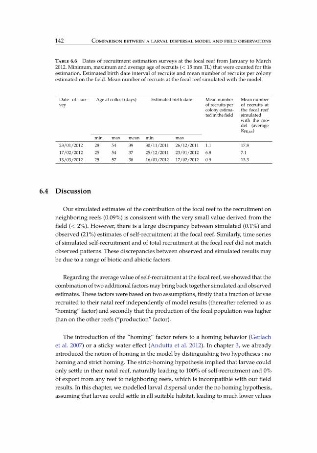
160 / 219


Table 6.6 Dates of recruitment estimation surveys at the focal reef from January to March2012. Minimum, maximum and average age of recruits (< 15 mm TL) that were counted for thisestimation. Estimated birth date interval of recruits and mean number of recruits per colonyestimated on the field. Mean number of recruits at the focal reef simulated with the model.

Date of sur-vey

Age at collect (days) Estimated birth date Mean numberof recruits percolony estima-ted in the field

Mean numberof recruits atthe focal reefsimulatedwith the mo-del (averageRFR,tot)

min max mean min max23/01/2012 28 54 39 30/11/2011 26/12/2011 1.1 17.817/02/2012 25 54 37 25/12/2011 23/01/2012 6.8 7.113/03/2012 25 57 38 16/01/2012 17/02/2012 0.9 13.3

6.4 Discussion

Our simulated estimates of the contribution of the focal reef to the recruitment onneighboring reefs (0.09%) is consistent with the very small value derived from thefield (< 2%). However, there is a large discrepancy between simulated (0.1%) andobserved (21%) estimates of self-recruitment at the focal reef. Similarly, time seriesof simulated self-recruitment and of total recruitment at the focal reef did not matchobserved patterns. These discrepancies between observed and simulated results maybe due to a range of biotic and abiotic factors.

Regarding the average value of self-recruitment at the focal reef, we showed that thecombination of two additional factorsmay bring back together simulated and observedestimates. These factors were based on two assumptions, firstly that a fraction of larvaerecruited to their natal reef independently of model results (thereafter referred to as“homing” factor) and secondly that the production of the focal population was higherthan on the other reefs (“production” factor).

The introduction of the “homing” factor refers to a homing behavior (Gerlachet al. 2007) or a sticky water effect (Andutta et al. 2012). In chapter 3, we alreadyintroduced the notion of homing in the model by distinguishing two hypotheses : nohoming and strict homing. The strict-homing hypothesis implied that larvae couldonly settle in their natal reef, naturally leading to 100% of self-recruitment and 0%of export from any reef to neighboring reefs, which is incompatible with our fieldresults. In this chapter, we modelled larval dispersal under the no homing hypothesis,assuming that larvae could settle in all suitable habitat, leading to much lower values

161 / 219

Discussion 143

of self-recruitment. This, again, results in simulated values of self-recruitment thatare incompatible with our results. The “homing” factor used in this chapter allowsmodulating results according to a fraction of released larvae that are “guaranteed”to recruit to their natal reef. This factor may also be interpreted as a local circulationeffect. Even if the resolution of our biophysical model is fine (horizontal resolution of500 m and 30 terrain following generalized sigma levels in the vertical dimension), itmay still not be enough to represent currents at the very small spatial scale of patchreefs and thus miss to model processes like sticky water and Stokes drift that couldcontribute to retention of larvae (Andutta et al. 2012, Fujimura et al. 2014).

The “production” factor allows for considering heterogeneous production over allsuitable habitat used in the model. The uniform release of larvae over all suitable ha-bitat in the Ichthyop tool indeed implicitly assumes that adult density is homogenousover all suitable habitats. But production is likely to be heterogeneous in the wild. Forexample, we found that D. aruanus adult density may vary by one order of magnitudeamong sampled reefs (e.g., 0.17 adults per m2 on reef 8 vs. 1.23 adults per m2 on reef 7).The “production” factor can also be interpreted as a differential mortality in favor ofself-recruits (Vigliola and Meekan 2002, Meekan et al. 2006, Nanninga 2013). Selectivemortality occurring in favor of larvae originating from the focal reef during dispersalor settlement may indeed influence self-recruitment significantly by increasing theproportion of self-recruits.

When used separately, these factors must be included at such high values (e.g., aproduction 450 times higher at the focal reef) that they are likely not compatible withthe reality. When used in combination, however, the values are much lower (e.g., aproduction 10 times higher at the focal reef with 10% of larvae recruiting to their natalreef), although these can only be confirmed via additional field research.

Beside the “homing” and “production” factors, other factors were considered asbeing potentially responsible for the differences between observed and simulatedresults. For example,D. aruanus habitat was defined in the model as all reefs shallowerthan 20 m (Allen 1991) based on GIS habitat maps provided by the atlas of coral reefsin New Caledonia (Andréfouët and Torres-Pulliza 2004) and supported by knowledgegathered from field work (section 6.5). But habitat might be more restricted. Forexample, we observed that most D. aruanus colonies were localized between 8 and 12meters on patch reefs in the SWL and we showed in chapter 3 that release depth mayinfluence larval retention, with better retention when release depth was deeper. In oursimulations, estimates of self-recruitment generally did increase with release depth(section 6.6) but the values obtained for the 8 to 12 m depth levels were only slightlyhigher than the average.We also identified amajor source zone, localized on the barrier

162 / 219


reef North-West of the focal reef, that represents 30% of the total released larvae in theSWL that recruits on the focal reef (section 6.7). This zone is principally composed ofshallow terrace (section 6.5), which is not the preferred habitat ofD. aruanus. However,excluding this zone lead to a 30% increase in self-recruitment.The age of competencemight also influence dispersal patterns by increasing/decreasing the passive dispersalphase and thus decreasing/increasing larval retention at both reef and lagoon scale(chapter 3). However, for a shorter precompetency period of 11 days we found veryclose estimates as with a precompetency of 21 days (section 6.8). Furthermore, settingthe precompetency duration at 21 days in the model gives settlement ages that arecloser to the mean PLD of 3 weeks estimated for D. aruanus in the SWL (chapter 2).These results suggest that these different factors are unlikely to play a major rolein increasing the simulated self-recruitment value to the level required to matchobservations.

The comparison between temporal variability of simulated and observed self-recruitment and total recruitment at the focal reef also showed differences. Whena constant “homing” factor is included, the variability in the simulated number ofself-recruits is much reduced. Consequently, the temporal variability of the percentageof self-recruitment is mostly driven by, and the inverse of, the temporal variability oftotal recruitment in the model. But the model failed to reproduce the variability oftotal recruitment properly. It suggested a peak of recruitment for larvae released inDecember 2011 that was not observed in the field and weak recruitment for larvaereleased in January 2012 while observed recruitment peaked. We thought that thesecontrasting results could be due to our model assumption that egg production isconstant during the reproductive season. As shown in chapter 2, this productionmight actually be variable according to the gonadosomatic index (GSI). We used GSIas a correction factor of total recruitment but this proved insufficient to change thesimulated temporal variability of total recruitment significantly (section 6.9). Theplanktonic larval duration (PLD), and therefore the duration of the precompetencyperiod, might also change during the reproductive season according to water tempe-rature with longer PLD at the beginning of the reproductive season leading to weakerrecruitment. Including this effect in the model might help to inverse the tendency inthe simulated recruitment peaks. Finally, it may well be that the temporal variabilityassociated to the processes represented by our factors X and P might also govern thetemporal variability of observed self-recruitment and total recruitment.

Comparing simulated and observed data of larval dispersal is a complicated task asdiscrepancies might arise from a range of reasons that are often difficult to disentanglewithout additional research. Nevertheless, one of the interests of this work is to drawattention to the most plausible explanations of these differences and prioritize future

163 / 219

Discussion 145

work directions. Here we showed that the habitat of D. aruanus, because it drives thenumber of larvae released, must be better known as it is likely not as homogenous,and maybe more restricted, than previously assumed. Then we showed that futurework should focus on possible biotic or abiotic processes (e.g., homing behavior, localcirculation patterns) that allow larvae to recruit back to their natal population muchmore than when these processes are not considered.

164 / 219


6.5 Appendix A

Table 6.7 Habitat selection for Dascyllus aruanus in the biophysical model : selected gridcodesand corresponding attributes in (Andréfouët and Torres-Pulliza 2004).

Gridcode L2 attrib L3 attrib L4 attrib658

Continental patchcomplex

Intra-lagoonpatch-reefcomplex

Shallow terrace665 Forereef666 Reef flat829

Continental outershelf barrier

Outer barrier reefcomplex

Shallow terrace830 Shallow terrace with constructions834 Deep terrace with constructions929

Continentalfringing

Lagoon exposedfringing

Forereef930 Reef flat934 Shallow terrace937 Diffuse fringing Diffuse fringing

Figure 6.8 Habitat selection map for Dascyllus aruanus in the biophysical model. Barrier reefhabitat is depicted in blue, patch reef habitat is in red and fringing reef habitat is in green. Codescorrespond to selected gridcodes in Andréfouët and Torres-Pulliza (2004).

165 / 219

Appendix B 147

6.6 Appendix B

The influence of release depth on the rate of simulated self-recruitment at the focalreef was estimated. To do so, we used the same equation as insection 6.2.3 for differentrelease depth intervals. Release depth intervals were grouped into 2m bins beginningat 0m and going to 18m (no habitat is available at the focal reef between 18-20m depth).Except for the release depth interval [−18m, −16m] for which very few larvae werereleased from the focal reef (12 larvae per release on average), the percentage of self-recruitment increasedwith increasing release depthwith amaximumof 0.18% reachedfor the release depth interval [−16m, −14m]. As most of D. aruanus colonies wereobserved between 8 and 12 meters depth on patch reefs in the SWL, considering theserelease depths would only multiplied simulated self-recruitment by approximately1.5 which is too low to reach the value of self-recruitment observed on the field.

Figure 6.9 Simulated SR obtained for different release depth intervals and averaged for spaw-ning events that occurred between December 2011 and March 2012. Red dotted line indicatesaveraged simulated SR for the release depth interval [-20 m, 0 m].

166 / 219


6.7 Appendix C

We mapped the departure localization of larvae that recruited on the focal reef toidentify potential major source zones in the model, by plotting the number of larvaereleased in each square grid cell of 0.01° spatial resolution from December 2011 toMarch 2012.

Figure 6.10 Number of focal reef’s recruits that were released in each grid cell of 0.01° insize from December 2011 to March 2012 for both precompetency periods (PC), calculated on alogarithmic scale as log10(Ni + 1) whereNi is the number of larvae release in grid cell i.

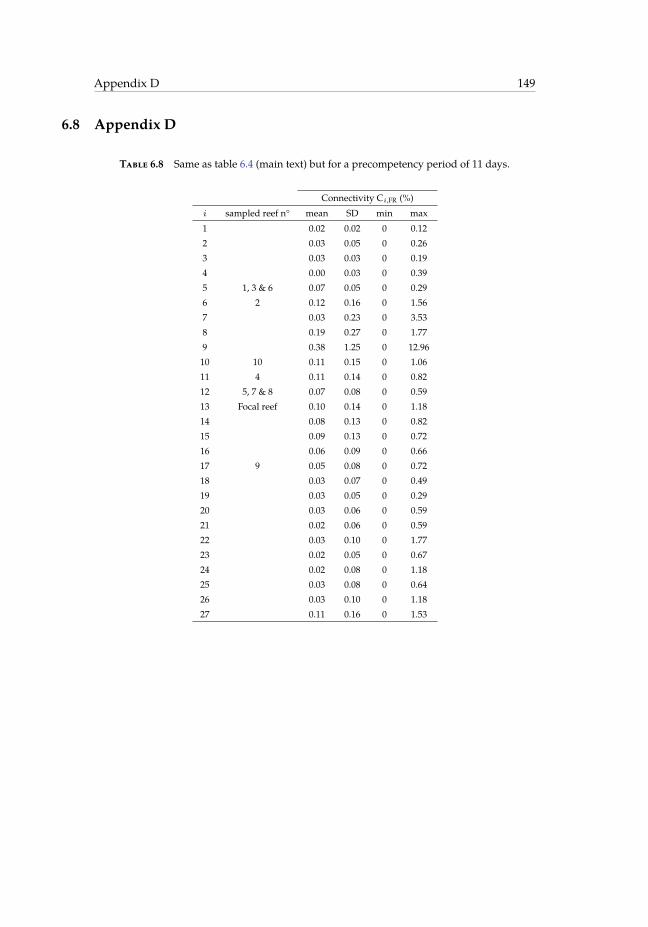
167 / 219

Appendix D 149

6.8 Appendix D

Table 6.8 Same as table 6.4 (main text) but for a precompetency period of 11 days.

Connectivity Ci,FR (%)i sampled reef n° mean SD min max1 0.02 0.02 0 0.122 0.03 0.05 0 0.263 0.03 0.03 0 0.194 0.00 0.03 0 0.395 1, 3 & 6 0.07 0.05 0 0.296 2 0.12 0.16 0 1.567 0.03 0.23 0 3.538 0.19 0.27 0 1.779 0.38 1.25 0 12.9610 10 0.11 0.15 0 1.0611 4 0.11 0.14 0 0.8212 5, 7 & 8 0.07 0.08 0 0.5913 Focal reef 0.10 0.14 0 1.1814 0.08 0.13 0 0.8215 0.09 0.13 0 0.7216 0.06 0.09 0 0.6617 9 0.05 0.08 0 0.7218 0.03 0.07 0 0.4919 0.03 0.05 0 0.2920 0.03 0.06 0 0.5921 0.02 0.06 0 0.5922 0.03 0.10 0 1.7723 0.02 0.05 0 0.6724 0.02 0.08 0 1.1825 0.03 0.08 0 0.6426 0.03 0.10 0 1.1827 0.11 0.16 0 1.53

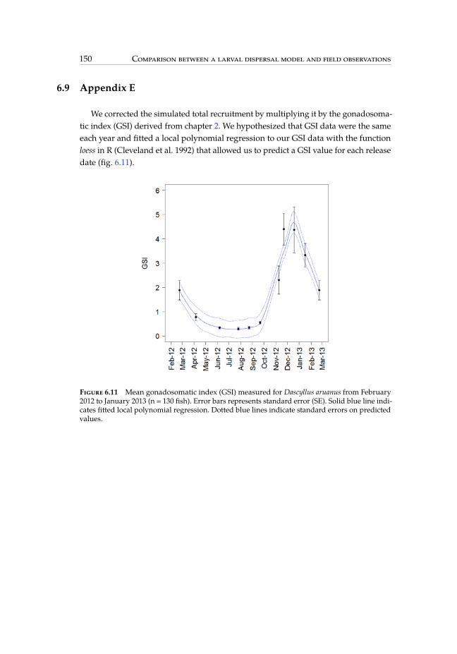
168 / 219


6.9 Appendix E

We corrected the simulated total recruitment by multiplying it by the gonadosoma-tic index (GSI) derived from chapter 2. We hypothesized that GSI data were the sameeach year and fitted a local polynomial regression to our GSI data with the functionloess in R (Cleveland et al. 1992) that allowed us to predict a GSI value for each releasedate (fig. 6.11).

Figure 6.11 Mean gonadosomatic index (GSI) measured for Dascyllus aruanus from February2012 to January 2013 (n = 130 fish). Error bars represents standard error (SE). Solid blue line indi-cates fitted local polynomial regression. Dotted blue lines indicate standard errors on predictedvalues.

169 / 219

Appendix E 151

Figure 6.12 Simulated total recruitment time series on the focal reef (RFR,tot) without and withGSI correction.

Table 6.9 Estimated birth date interval of recruits (< 15 mm TL) that were counted for theestimation of total recruitment on the focal reef in the field and mean number of recruits percolony estimated on the field. Mean number of recruits at the focal reef simulated with the model,without and with GSI correction.

Estimated birth date Mean number ofrecruits per colonyestimated in thefield

Average RFR,tot wi-thout GSI

Average RFR,totwith GSI

min max30/11/2011 26/12/2011 1.1 17.8 79.425/12/2011 23/01/2012 6.8 7.1 28.916/01/2012 17/02/2012 0.9 13.3 36.3

170 / 219

171 / 219

Chapitre 7

Conclusion

153

172 / 219

173 / 219

155

Cette thèse s’inscrit dans un contexte de demande croissante en connaissances surla dispersion larvaire des espèces marines, connaissances qui sont indispensables àune meilleure compréhension de la structure et de la dynamique des populationset à une gestion avisée des ressources marines (Botsford et al. 2009, Berglund et al.2012, Sale 2013). La dispersion larvaire a longtemps été considérée comme une boitenoire en écologie marine due à la difficulté d’observer des individus extrêmementpetits et nombreux dans l’immensité de l’océan (Sale et al. 2005). Des progrès ontété faits ces 15 dernières années avec le développement de différentes approches,par modélisation numérique ou marquages génétiques et chimiques, pour étudier ladispersion larvaire à l’échelle démographique (Jones et al. 2009, Leis et al. 2011, Koolet al. 2013). Ces techniques ont été développées de façon plus ou moins indépendantespar des communautés de chercheurs différentes et le défi actuel réside dans uneconfrontation de ces approches complémentaires (Jones et al. 2009, Leis et al. 2011, Koolet al. 2013). La plupart des études comparant les résultats de modèles de dispersionlarvaire avec des mesures in situ concernent la connectivité génétique et s’appuientsur des mesures indirectes des flux de gènes entre populations (e.g., Gilg and Hilbish(2003), Galindo et al. (2006), Foster et al. (2012)). Or il existe un réel besoin de confronterles modèles de dispersion larvaire à la réalité, à une échelle démographique, afinde pouvoir les utiliser de façon opérationnelle dans des modèles de dynamique depopulations (Selkoe et al. 2008, Cowen and Sponaugle 2009, Jones et al. 2009, Burgesset al. 2014).

Ce travail de comparaison entre les résultats d’un modèle de dispersion larvaireet des mesures in situ de l’auto-recrutement et de la connectivité démographiqueobtenues par marquages, est extrêmement rare. Cette rareté s’explique tout d’abordpar la nouveauté et la difficulté de mettre en oeuvre des études de mesures in situde la connectivité démographique, qui sont par conséquent souvent limitées à unépisode de dispersion unique (Jones et al. 1999, Almany et al. 2007, D’Aloia et al. 2013,Schunter et al. 2014), ou répliquées à l’échelle de quelques années (Jones et al. 2005,Carreras-Carbonell et al. 2007, Carson et al. 2010, Hogan et al. 2012, Saenz-Agudeloet al. 2012) mais très rarement répliquées à plus haute fréquence (Chittaro and Hogan2013, Cook et al. 2014). Or une comparaison robuste avec des résultats de modèlenécessite d’avoir une série temporelle consistante de mesures in situ. D’autre part,la résolution des modèles biophysiques doit être adaptée à l’échelle d’étude de laconnectivité démographique, souvent de l’ordre de quelques centaines de mètres àplusieurs dizaines de km (Jones et al. 1999, Cowen et al. 2000, Jones et al. 2005, Almanyet al. 2007, Planes et al. 2009, Saenz-Agudelo et al. 2012) ce qui requiert une résolutionfine des processus hydrodynamiques. Enfin la comparaison entre modèle et donnéesnécessitent de choisir des métriques comparables. Par exemple, une des métriques lesplus communément mesurée in situ pour mesurer le taux de retour des larves à leur

174 / 219

156 Conclusion

population d’origine est l’auto-recrutement (mesurée par rapport au nombre totalde recrues dans cette population) alors que les modèles biophysiques fournissent laplupart du temps une mesure de la rétention locale (calculée par rapport au nombretotal de larves produites par la population d’origine).

Dans ce contexte, l’objectif de ce travail de thèse était d’étudier la dispersion lar-vaire à une échelle de temps écologique en utilisant la modélisation biophysique etles marquages chimiques, au sein d’un même écosystème marin où aucune étuden’avait encore été menée sur la dispersion larvaire, le lagon sud-ouest de Nouvelle-Calédonie (SWL), et en s’appuyant sur un poisson de récif, la demoiselle à queueblanche (Dascyllus aruanus).

7.1 Principaux résultats

La synthèse bibliographique sur la biologie et l’écologie de Dascyllus aruanus réa-lisée dans le chapitre 2, et complétée par les connaissances acquises au cours de lathèse sur sa reproduction et son stade larvaire, permet de conclure que D. aruanus estune espèce modèle adéquate pour étudier la connectivité par dispersion larvaire ausens où elle est représentative de nombreuses autres espèces de poissons démersaux,notamment en termes de stratégie de reproduction, de durée de vie larvaire, et dedomaine vital (Wellington and Victor 1989, Guillemot et al. 2011). Comme beaucoupd’espèces de poissons démersaux, cette espèce possède en effet un domaine vitalextrêmement limité au stade adulte et les échanges d’individus entre populationslocales ne peuvent se faire que pendant le stade larvaire pélagique. Cette espèce estfacile à identifier, collecter et manipuler, et elle s’adapte bien à la captivité, ce quifacilite son étude. De plus, D. aruanus se reproduit avec une fréquence élevée sur unelongue période de reproduction ; il est donc possible d’étudier la variabilité temporellede la connectivité. Enfin,D. aruanus possède une aire de répartition très vaste à traversl’Indo-Pacifique rendant possible la mise en place d’études comparatives dans denombreux écosystèmes.

La circulation des masses d’eau dans le SWL est soumise à des vents d’alizéspendant une majeure partie de l’année (Douillet 1998). Ce forçage atmosphériqueentraîne des temps de résidence relativement courts des eaux à l’intérieur du lagon(Jouon et al. 2006, Ouillon et al. 2010), et peut donc se révéler extrêmement défavorableà la rétention des larves et donc aux connexions entre populations locales lagonairespour des espèces dont la durée de vie larvaire excède ces temps de résidence. Lemodèle biophysique de dispersion larvaire mis en place dans le chapitre 3 se basesur des champs de courants issus d’un modèle hydrodynamique forcé par des ventsréalistes et prend en compte l’habitat de D. aruanus, sa saison de reproduction, sa

175 / 219

Principaux résultats 157

durée de vie larvaire et de pré-compétence. Cemodèle montre que la rétention larvaireest possible à l’échelle d’une population locale et à l’échelle du lagon, atteignantpériodiquement des valeurs beaucoup plus grandes que prévues, et qu’elle présenteune grande variabilité temporelle. Les résultats de corrélations croisées entre sériestemporelles de rétention et de régimes de vent suggèrent que la rétention larvaire deD. aruanus au sein du lagon peut être prédite par des conditions climatiques à largeéchelle. Des conditions climatiques caractérisées par de forts alizés conduisent à unerétention larvaire très faible aux deux échelles spatiales considérées. En revanche,des taux de rétention élevés sont permis par des conditions climatiques caractériséespar des vents plus faibles en intensité et de direction plus variable. Les distances dedispersion sont relativement courtes, de l’ordre de 25 à 35 km selon l’hypothèse faitesur la durée de la pré-compétence, ce qui suggèrent une connectivité entre populationslocales à l’intérieur du lagon.

Afin de confronter ces résultats de modèle à la réalité, une expérience de marquagechimique des larves a été menée dans le SWL (chapitre 4). Le marquage transgéné-rationnel est une technique récente permettant un marquage de masse in situ partransmission maternelle d’une marque chimique artificielle aux pièces calcifiées desembryons (Thorrold et al. 2006). L’efficacité de cette méthode a été prouvée pourplusieurs espèces de poissons et de céphalopodes (e.g., Munro et al. (2009), Pecl et al.(2010), Starrs et al. (2014)). Cependant, elle n’a été utilisée qu’une fois en milieu naturelpour estimer l’auto-recrutement (Almany et al. 2007). Avant d’utiliser cette méthodedans le milieu naturel il est primordial de tester son efficacité et ses impacts potentielssur les adultes et les larves. C’était l’objet de l’expérience menée dans le chapitre 3dont les résultats montrent (1) l’efficacité de la plus petite dose testée (0.5µg de 137Bapar gramme de femelle) pour marquer des larves pendant au moins 1 mois, et (2)l’absence d’effet négatif d’injections uniques ou répétées tous les mois sur le succèsreproducteur, la taille des oeufs un jour après la ponte et la taille des larves âgées dedeux jours. En conclusion, des injections mensuelles de solution enrichie en 137Ba à0.5µg de 137Ba par gramme de femelle permettent donc de marquer sans danger deslarves deD. aruanus sur la durée d’une saison de reproduction. Ce chapitre développeégalement une nouvelle méthode d’analyse chimique des otolithes de larves âgéesde deux jours par analyse au spectromètre de masse à ablation laser permettant devalider le succès de marquage tout en réduisant la durée, et donc les coûts, de l’élevagelarvaire.

L’application de cette technique de marquage à une population de D. aruanussituée au centre du SWL fait l’objet du chapitre 5. Cette population a été marquéemensuellement sur deux saisons de reproduction (étés austraux 2011-2012 et 2012-2013) afin d’estimer la variabilité temporelle de l’auto-recrutement et la contribution

176 / 219

158 Conclusion

de cette population au recrutement des populations de récifs voisins. L’analyse deplusieurs cohortes de jeunes recrues a permis de mettre en évidence une variabilitéintra-saisonnière, mensuelle (de 0% à 68%), et une variabilité inter-annuelle (21% en2012 et 0% en 2013) de l’auto-recrutement. L’analyse spatiale montre quant à elle unecontribution nulle, ou du moins extrêmement réduite (< 2%), de la population focaleau recrutement des récifs voisins. Ces résultats confirment les résultats obtenus avecle modèle du chapitre 3 en montrant que le retour de larves à leur population nataleest possible dans le lagon sud-ouest, suggérant l’existence de conditions climatiqueset/ou de comportements larvaires favorables à la rétention. Avec une valeur moyenned’auto-recrutement de 12% sur deux saisons de reproduction, cette population deD. aruanus est intermédiaire en termes d’ouverture comparée aux études conduitesdans d’autres écosystèmes pour des espèces similaires (e.g., Berumen et al. (2012),Saenz-Agudelo et al. (2012)). Ce travail souligne enfin l’influence du choix du seuilutilisé pour déterminer si un individu est marqué ou non sur les valeurs estimées del’auto-recrutement et de la connectivité.

La confrontation entre modèle et données s’appuie sur trois métriques : (1) le pour-centage d’auto-recrutement dans la population locale, mesuré par les marquages duchapitre 4 et modélisé dans le chapitre 6, plutôt que la rétention locale, utilisée dansle chapitre 3 qui informe également sur le retour des larves à leur population natalemais est beaucoup plus difficile à estimer dans le milieu naturel ; (2) la contributionde cette population locale au recrutement de 10 récifs voisins situés dans un rayon de20 km ; (3) la variabilité temporelle du recrutement total dans cette population focaleen s’appuyant sur l’été austral 2011-2012. Au niveau qualitatif, modèle et données serejoignent sur l’importance de la variabilité temporelle de l’auto-recrutement et durecrutement total dans la population locale. Du point de vue quantitatif, modèle etdonnées se rejoignent également sur la contribution extrêmement faible de la popula-tion focale au recrutement des récifs voisins. Le principal point de désaccord entremodèle et donnée réside dans la quantification du pourcentage d’auto-recrutement,avec un écart de plus de deux ordres de grandeur : 0.1% estimé par le modèle et 21%mesuré sur le terrain en moyenne sur la même saison de reproduction. Le chapitre 6montre que la prise en compte de certains éléments permet une meilleure adéquationentre modèle et données, mais elle repose sur des hypothèses très fortes sur la capacitédes larves à revenir à leur population natale et/ou sur l’importance de la productionde la population natale par rapport aux autres populations locales lagonaires, dont lacorroboration nécessitera des études qui dépassent le cadre de ce travail.

Les résultats de ce travail permettent néanmoins de conclure qu’à l’échelle du SWL(i.e., quelques dizaines de kilomètres), les populations de D. aruanus sont intercon-nectées, avec un pourcentage d’auto-recrutement très fluctuant mais pouvant être

177 / 219

Principaux résultats 159

Figure 7.1 Adaptée de Kritzer and Sale (2004). Trois types de populations structurées spa-tialement. Les petits disques représentent des populations locales discrètes à l’intérieur d’unerégion plus large représentée par un ovale. Les lignes épaisses définissent l’échelle spatiale àlaquelle se situe la dynamique de population. Pour chaque type de structures sont représentéesles courbes de dispersion schématique de chaque population locale. (A) Populations localesfermées avec des dynamiques indépendantes sans échange d’individus à l’échelle démogra-phique ; les distances de dispersion sont très courtes par rapport aux distances séparant lespopulations. (B) Métapopulation ; les distances de dispersion sont courtes mais suffisantes pourpermettre l’échange de larves entre populations à l’échelle démographique. (C) Ensemble degroupes discrets composant une seule et même population fermée ; la dispersion se produit àsuffisamment longue distance pour que les groupes soient très connectées. NB : D’autres typesde structures de populations existent (voir par exemple Freckleton andWatkinson (2002), Grimmet al. (2003)

ponctuellement élevé. Cela suggère que parmi les trois grands types de structure depopulation proposés par Kritzer and Sale (2004) (fig. 7.1), les populations deD. aruanusdans le SWL constitueraient bien unemétapopulation (fig. 7.1B) plutôt qu’un ensemblede populations fermées aux dynamiques indépendantes (fig. 7.1A) ou qu’une seule etmême population fragmentée mais composée de groupes très connectés (fig. 7.1C).L’efficacité de mesures de protection sur la persistance de cette métapopulation dansle SWL va donc fortement dépendre du choix des populations locales à protéger, choixqui devra prendre en compte la démographie de ces populations locales et les échanges

178 / 219

160 Conclusion

d’individus avec les autres populations. Une caractéristique qui distingue les méta-populations des populations composées de groupes discrets mais très connectés estune possible asynchronie dans la dynamique des sous-populations qui la composent(Sale et al. 2006), propriété qu’il conviendra d’étudier pour la demoiselle dans le SWLavant d’en évaluer les conséquences potentielles en termes de gestion. L’importancede la variabilité temporelle de l’auto-recrutement et du recrutement suggère unevariabilité de la connectivité entre populations au sein du SWL. Les conséquencesde ces fluctuations sur le fonctionnement des métapopulations et leur persistancesont encore peu connues et font l’objet de recherches très récentes (Watson et al. 2012,Williams and Hastings 2013, Snyder et al. 2014)). Watson et al. (2012) démontrent queces fluctuations peuvent faire diminuer les taux de croissance au sein de la métapopu-lation en comparaison à des conditions non variables, en particulier pour des espècesà longue vie larvaire et qui ne se reproduisent qu’une fois pas an. Snyder et al. (2014)montrent que pour une espèce se reproduisant plusieurs fois par an (Stegastes partitus),dont l’écologie est proche de D. aruanus, ces fluctuations de connectivité ont très peud’effet sur les taux de croissance de la métapopulation.

7.2 Perspectives

Une autre technique de marquage, couramment utilisée pour répondre aux ques-tions de connectivité démographique à des échelles spatiales comparables à ce travail,est l’analyse génétique de parenté. L’avantage de cette autre technique est qu’ellepermet d’identifier les parents des recrues collectées et donc de faire le lien entre ladispersion et les conditions parentales. Le marquage chimique transgénérationnelpourrait techniquement permettre d’identifier les parents de chaque individu maiscela nécessiterait d’injecter chaque adulte avec une marque différente (Huelga-Suarezet al. 2012) ce qui se révélerait coûteux et compliqué à mettre en oeuvre. Néanmoinsles analyses de parenté nécessite d’échantillonner la population adulte de façon ex-haustive afin de réaliser les tests statistiques de parenté (Sale et al. (2010) ; mais voirChristie et al. (2013)) alors que dans le cas du marquage transgénérationnel, la marquetransmise par les femelles à leurs descendants est univoque (Thorrold et al. 2006).Ceci représente un avantage lorsque les populations à échantillonner sont grandes, cequi est le cas des populations de D. aruanus, car il est alors possible de ne marquerqu’une fraction de la population adulte. De plus l’otolithe peut fournir de nombreusesinformations complémentaires aux informations de marquage, telles que l’âge dupoisson, sa croissance, sa durée de vie larvaire et même éventuellement sa trajectoirependant la dispersion sous réserve de pouvoir utiliser la chimie naturelle. Les analysesde parenté peuvent quant à elles permettre d’étudier les relations de fraternité entreles individus (Beldade et al. 2012). Une utilisation en parallèle des deux techniques, si

179 / 219

Perspectives 161

elle est possible, permet d’une part la validation croisée de leurs résultats et d’autrepart l’apport de connaissances complémentaires.

La résolution spatiale dumodèle biophysique utilisé dans ce travail est relativementfine (maille carrée de 500 m de côté en horizontal et 30 niveaux verticaux). Néanmoinsles différences entre modèle et données concernant les estimations d’auto-recrutementlaissent penser que cette résolution pourrait ne pas être suffisamment précise autourdes patchs de récifs pour prendre en compte les effets de circulation à très petite échelle,qui sont peut-être déterminants pour la rétention au niveau d’un récif. La mise enplace d’un modèle à grille non structurée permettrait de faire varier la résolutionspatiale, e.g., très fine autour des récifs et plus large dans des zones de pleine eau,sans augmenter le temps de simulation et le volume de stockage (Thomas et al. 2014).De plus notre modèle dans sa version actuelle ne prend pas en compte plusieursparamètres tels que la migration verticale des larves, leur mortalité différentielle enfonction de leur population natale, ou encore la croissance des larves en lien parexemple avec la température et la disponibilité en nourriture qui sont des facteurs quipeuvent influencer significativement les valeurs de connectivité et d’auto-recrutementsimulées par un modèle (Paris and Cowen 2004, Leis 2006).

Cette étude était limitée géographiquement au lagon sud-ouest de Nouvelle-Calédonie. L’inversion des courants due à la marée dans le canal de la Havannah rendles échanges larvaires entre cette partie du lagon et le lagon est très peu probables. Lesrésultats de Planes et al. (1998) vont d’ailleurs dans ce sens en montrant une différen-tiation génétique entre les populations du SWL et celles du lagon est pour deux autresespèces de poissons récifaux (Stegastes nigricans et Acanthurus triostegus). Par contre,des connexions sont possibles à l’échelle démographique entre le SWL et le lagon sud,puisque le SWL est essentiellement alimenté par les eaux qui entrent par le sud. Il seraitdonc intéressant dans les études futures d’élargir la zone d’étude au lagon sud. Deséchanges possibles avec des populations hors lagon (e.g., îles Chesterfields) semblentpeu probables à l’échelle démographique au vu des distances considérables entre cespopulations et le SWL. Il serait cependant intéressant d’étudier les connexions pardispersion larvaire en intégrant l’échelle intra-lagonaire à l’échelle plus globale dela Mer de Corail, notamment dans le contexte actuel de création d’un parc naturelmarin de la Mer de Corail initié par le gouvernement français.

Enfin, dans ce travail la dispersion a été étudiée du départ des larves à leur instal-lation. On parle de connectivité potentielle (Pineda et al. 2007, Burgess et al. 2012).Or toutes les larves qui s’installent dans une population adulte à l’issue de leur viepélagique ne survivront pas jusqu’à la reproduction. Pour pouvoir mesurer l’impact dela dispersion sur la démographie il est donc nécessaire de prendre en considération les

180 / 219

162 Conclusion

taux de survie post-installation dans l’estimation de la connectivité dite alors réalisée(Pineda et al. 2007). Cette survie peut elle aussi dépendre de multiples facteurs, ycompris d’effets parentaux liés à la population natale (Nanninga 2013), et donc différerentre auto- et allo-recrues. Cette étape sera indispensable à l’intégration des résultatsde cette étude dans une approche de dynamique de population plus complète.

181 / 219

Bibliographie

Aiken, C. M., S. A. Navarrete, and J. L. Pelegrí (2011). Potential changes in larvaldispersal and alongshore connectivity on the central Chilean coast due to an alteredwind climate. Journal of Geophysical Research : Biogeosciences 116(G4), 77–88.

Allen, G. R. (1991). Damselfishes of the world. Mergus. 271 pp.

Almany, G. R., M. L. Berumen, S. R. Thorrold, S. Planes, and G. P. Jones (2007). Localreplenishment of coral reef fish populations in a marine reserve. Science 316(5825),742–744.

Almany, G. R., S. R. Connolly, D. D. Heath, J. D. Hogan, G. P. Jones, L. J. McCook,M. Mills, R. L. Pressey, and D. H. Williamson (2009). Connectivity, biodiversityconservation and the design of marine reserve networks for coral reefs. CoralReefs 28(2), 339–351.

Andréfouët, S., G. Cabioch, B. Flamand, and B. Pelletier (2009). A reappraisal ofthe diversity of geomorphological and genetic processes of New Caledonian coralreefs : a synthesis from optical remote sensing, coring and acoustic multibeamobservations. Coral Reefs 28(3), 691–707.

Andréfouët, S. and D. Torres-Pulliza (2004). Atlas des récifs coralliens de Nouvelle-Calédonie. Technical report, IRD, IFRECOR Nouvelle-Calédonie. 26 pp. + 22 pp.

Andrello, M., D. Mouillot, S. Somot, W. Thuiller, and S. Manel (2014). Additive effectsof climate change on connectivity between marine protected areas and larval supplyto fished areas. Diversity and Distributions. DOI : 10.1111/ddi.12250.

163

182 / 219

164 Bibliographie

Andutta, F. P., M. J. Kingsford, and E. Wolanski (2012). ‘Sticky water’ enables theretention of larvae in a reef mosaic. Estuarine, Coastal and Shelf Science 101, 54–63.

Armsworth, P. R., M. K. James, and L. Bode (2001). When to press on or turn back :dispersal strategies for reef fish larvae. The American Naturalist 157(4), 434–450.

Arvedlund, M. and L. E. Nielsen (1996). Do the anemonefish Amphiprion ocellaris(Pisces : Pomacentridae) imprint themselves to their host sea anemone Heteractismagnifica (Anthozoa : Actinidae) ? Ethology 102(2), 197–211.

Asoh, K. (2003). Reproductive parameters of female Hawaiian damselfish Dascyllusalbisella with comparison to other tropical and subtropical damselfishes. MarineBiology 143(4), 803–810.

Atema, J., M. J. Kingsford, and G. Gerlach (2002). Larval reef fish could use odourfor detection, retention and orientation to reefs. Marine Ecology Progress Series 241,151–160.

Beldade, R., S. J. Holbrook, R. J. Schmitt, S. Planes, D. Malone, and G. Bernardi (2012).Larger female fish contribute disproportionately more to self-replenishment. Pro-ceedings of the Royal Society B : Biological Sciences 279(1736), 2116–2121.

Ben-Tzvi, O., A. Abelson, S. D. Gaines, G. Bernardi, R. Beldade, M. S. Sheehy, G. L.Paradis, and M. Kiflawi (2012). Evidence for Cohesive Dispersal in the Sea. PLoSONE 7(9), e42672.

Benjamini, Y. and D. Yekutieli (2001). The control of the false discovery rate in multipletesting under dependency. Annals of statistics 29(4), 1165–1188.

Berglund, M., M. Nilsson Jacobi, and P. R. Jonsson (2012). Optimal selection of marineprotected areas based on connectivity and habitat quality. Ecological Modelling 240,105–112.

Berglund, M. and M. E. Wieser (2011). Isotopic compositions of the elements 2009(IUPAC Technical Report). Pure and Applied Chemistry 83(2), 397–410.

Bernardi, G., R. Beldade, S. J. Holbrook, and R. J. Schmitt (2012). Full-Sibs in Cohortsof Newly Settled Coral Reef Fishes. PLoS ONE 7(9), e44953.

Bernhardt, J. R. and H. M. Leslie (2013). Resilience to Climate Change in CoastalMarine Ecosystems. Marine Science 5, 371–392.

Bertness, M. D., S. D. Gaines, and M. E. Hay (2001). Marine community ecology, Volume550. Sinauer Associates Sunderland. 550 pp.

Berumen, M. L., G. R. Almany, S. Planes, G. P. Jones, P. Saenz-Agudelo, and S. R.Thorrold (2012). Persistence of self-recruitment and patterns of larval connectivityin a marine protected area network. Ecology and evolution 2(2), 444–452.

183 / 219

BIBLIOGRAPHIE 165

Black, K. and P. Moran (1991). Influence of Hydrodynamics on the Passive Dispersaland Initial Recruitment of Larvae of Acanthaster planci (echinodermata, Asteroidea).Marine Ecology-Progress Series 69(1-2), 55–65.

Booth, D. J. (1992). Larval settlement patterns and preferences by domino damselfishDascyllus albisella Gill. Journal of Experimental Marine Biology and Ecology 155(1),85–104.

Botsford, L. W. and C. M. Paulsen (2000). Assessing covariability among populationsin the presence of intraseries correlation : Columbia River spring-summer chinooksalmon (Oncorhynchus tshawytscha) stocks. Canadian Journal of Fisheries and AquaticSciences 57(3), 616–627.

Botsford, L. W., J. White, M. Coffroth, C. B. Paris, S. Planes, T. Shearer, S. Thorrold, andG. Jones (2009). Connectivity and resilience of coral reef metapopulations in marineprotected areas : matching empirical efforts to predictive needs. Coral Reefs 28(2),327–337.

Bowler, D. E. andT.G. Benton (2005). Causes and consequences of animal dispersal stra-tegies : relating individual behaviour to spatial dynamics. Biological Reviews 80(02),205–225.

Brochier, T., V. Echevin, J. Tam, A. Chaigneau, K. Goubanova, and A. Bertrand (2013).Climate change scenarios experiments predict a future reduction in small pelagicfish recruitment in the Humboldt Current system. Global change biology 19(6), 1841–1853.

Brochier, T., C. Lett, J. Tam, P. Fréon, F. Colas, and P. Ayón (2008). An individual-basedmodel study of anchovy early life history in the northern Humboldt Current system.Progress in Oceanography 79(2-4), 313–325.

Brophy, D., T. E. Jeffries, and B. S. Danilowicz (2004). Elevated manganese concen-trations at the cores of clupeid otoliths : possible environmental, physiological, orstructural origins. Marine Biology 144(4), 779–786.

Brothers, E. B., D. M.Williams, and P. F. Sale (1983). Length of larval life in twelve fami-lies of fishes at One Tree Lagoon, Great Barrier Reef, Australia. Marine Biology 76(3),319–324.

Buckley, R., L. LeClair, E. Volk, and S. Schroder (2007). Preliminary results of trans-generational marking of larval marine fish otoliths. In North Pacific Rockfishes, pp.87–98. Alaska Sea Grant, University of Alaska Fairbanks.

Burgess, S. C., K. J. Nickols, C. D. Griesemer, L. A. Barnett, A. G. Dedrick, E. V. Satter-thwaite, L. Yamane, S. G. Morgan, J. W. White, and L. W. Botsford (2014). Beyondconnectivity : how empirical methods can quantify population persistence to im-prove marine protected-area design. Ecological Applications 24(2), 257–270.

184 / 219

166 Bibliographie

Burgess, S. C., E. A. Treml, andD. J.Marshall (2012). Howdodispersal costs and habitatselection influence realized population connectivity ? Ecology 93(6), 1378–1387.

Buston, P. M., C. Fauvelot, M. Y. Wong, and S. Planes (2009). Genetic relatedness ingroups of the humbug damselfish Dascyllus aruanus : small, similar-sized indivi-duals may be close kin. Molecular ecology 18(22), 4707–4715.

Butler, M. J., C. B. Paris, J. S. Goldstein, H. Matsuda, and R. K. Cowen (2011). Behaviorconstrains the dispersal of long-lived spiny lobster larvae. Marine Ecology ProgressSeries 422, 223–237.

Caley, M. J., M. H. Carr, M. A. Hixon, T. P. Hughes, G. P. Jones, and B. A. Menge (1996).Recruitment and the local dynamics of open marine populations. Annual Review ofEcology and Systematics 27, 477–500.

Campana, S. E. (1999). Chemistry and composition of fish otoliths : pathways, mecha-nisms and applications. Marine Ecology Progress Series 188, 263–297.

Campana, S. E. and J. D. Neilson (1985). Microstructure of fish otoliths. CanadianJournal of Fisheries and Aquatic Sciences 42(5), 1014–1032.

Carreras-Carbonell, J., E. Macpherson, and M. Pascual (2007). High self-recruitmentlevels in a Mediterranean littoral fish population revealed by microsatellite markers.Marine Biology 151(2), 719–727.

Carson, H. S., P. C. Lopez-Duarte, L. Rasmussen, D. Wang, and L. A. Levin (2010).Reproductive timing alters population connectivity in marine metapopulations.Current Biology 20(21), 1926–1931.

Chabanet, P., N. Guillemot, M. Kulbicki, L. Vigliola, and S. Sarramegna (2010). Baselinestudy of the spatio-temporal patterns of reef fish assemblages prior to amajorminingproject in New Caledonia (South Pacific). Marine Pollution Bulletin 61(7–12), 598–611.

Chase, T. J., M. S. Pratchett, S. P. W.Walker, andM. O. Hoogenboom (2014). Small-scaleenvironmental variation influences whether coral-dwelling fish promote or impedecoral growth. Oecologia, 1–14.

Cherubin, L. M., R. S. Nemeth, and N. Idrisi (2011). Flow and transport characteris-tics at an Epinephelus guttatus (red hind grouper) spawning aggregation site in St.Thomas (US Virgin Islands). Ecological Modelling 222(17), 3132–3148.

Chittaro, P. M. and J. D. Hogan (2013). Patterns of connectivity among populations ofa coral reef fish. Coral reefs 32(2), 341–354.

Christie, M. R., J. A. Tennessen, and M. S. Blouin (2013). Bayesian parentage analysiswith systematic accountability of genotyping error, missing data and false matching.Bioinformatics 29(6), 725–732.

185 / 219

BIBLIOGRAPHIE 167

Christie, M. R., B. N. Tissot, M. A. Albins, J. P. Beets, Y. Jia, D. M. Ortiz, S. E. Thompson,and M. A. Hixon (2010). Larval Connectivity in an Effective Network of MarineProtected Areas. PLoS ONE 5(12), e15715.

Clobert, J., M. Baguette, T. G. Benton, J. M. Bullock, and S. Ducatez (2012). Dispersalecology and evolution. Oxford University Press. 496 pp.

Clobert, J., E. Danchin, A. A. Dhondt, and J. D. Nichols (2001). Dispersal. OxfordUniversity Press. 452 pp.

Coates, D. (1980a). Prey-Size Intake in Humbug Damselfish, Dascyllus aruanus (Pisces,Pomacentridae) Living Within Social Groups. Journal of Animal Ecology 49(1), 335–340.

Coates, D. (1980b). The discrimination of and reactions towards predatory and non-predatory species of fish by humbug damselfish, Dascyllus aruanus (Pisces, Poma-centridae). Zeitschrift für Tierpsychologie 52(4), 347–354.

Coates, D. (1982). Some Observations on the Sexuality of Humbug Damselfish,Dascyl-lus aruanus (Pisces, Pomacentridae) in the Field. Zeitschrift für Tierpsychologie 59(1),7–18.

Coker, D. J., S. K. Wilson, and M. S. Pratchett (2014). Importance of live coral habitatfor reef fishes. Reviews in Fish Biology and Fisheries 24(1), 89–126.

Cole, K. (2002). Gonad morphology, sexual development, and colony compositionin the obligate coral-dwelling damselfish Dascyllus aruanus. Marine Biology 140(1),151–163.

Cook, G. S., P. E. Parnell, and L. A. Levin (2014). Population Connectivity Shifts at HighFrequency within an Open-Coast Marine Protected Area Network. PLoS ONE 9(7),e103654.

Cowen, R. K., G. G. Gawarkiewicz, J. Pineda, S. R. Thorrold, and F. E. Werner (2007).Population connectivity in marine systems : an overview. Oceanography 20(3), 14–21.

Cowen, R. K., K. M. M. Lwiza, S. Sponaugle, C. B. Paris, and D. B. Olson (2000).Connectivity of Marine Populations : Open or Closed ? Science 287(5454), 857 –859.

Cowen, R. K., C. B. Paris, and A. Srinivasan (2006). Scaling of Connectivity in MarinePopulations. Science 311(5760), 522 –527.

Cowen, R. K. and S. Sponaugle (2009). Larval dispersal and marine populationconnectivity. Annual Review of Marine Science 1, 443–466.

Cuif, M., D. M. Kaplan, J. Lefèvre, V. M. Faure, M. Caillaud, P. Verley, L. Vigliola, andC. Lett (2014). Wind-induced variability in larval retention in a coral reef system : a

186 / 219

168 Bibliographie

biophysical modelling study in the South-West Lagoon of New Caledonia. Progressin Oceanography 122, 105–115.

Cuif, M., F. Keller, O. Chateau, D. M. Kaplan, M. Labonne, C. Lett, and L. Vigliola(2014). Evaluation of transgenerational isotope labeling of embryonic otoliths ina coral reef damselfish with single and repeated injections of enriched 137Barium.Journal of Experimental Marine Biology and Ecology 459, 151–159.

D’Aloia, C. C., S. M. Bogdanowicz, J. E. Majoris, R. G. Harrison, and P.M. Buston (2013).Self-recruitment in a Caribbean reef fish : a method for approximating dispersalkernels accounting for seascape. Molecular Ecology 22(9), 2563–2572.

Danilowicz, B. S. and C. L. Brown (1992). Rearing methods for two damselfish species :Dascyllus albisella (Gill) and D. aruanus (L.). Aquaculture 106(2), 141–149.

Dixon, P. A., M. J. Milicich, and G. Sugihara (1999). Episodic fluctuations in larvalsupply. Science 283(5407), 1528–1530.

Dixson, D. L., G. P. Jones, P. L. Munday, S. Planes, M. S. Pratchett, M. Srinivasan,C. Syms, and S. R. Thorrold (2008). Coral reef fish smell leaves to find island homes.Proceedings of the Royal Society B : Biological Sciences 275(1653), 2831–2839.

Dixson, D. L., G. P. Jones, P. L. Munday, S. Planes, M. S. Pratchett, and S. R. Thorrold(2014). Experimental evaluation of imprinting and the role innate preference playsin habitat selection in a coral reef fish. Oecologia 174(1), 99–107.

Douillet, P. (1998). Tidal dynamics of the south-west lagoon of New Caledonia. Ocea-nologica Acta 21(1), 69–79.

Douillet, P., S. Ouillon, and E. Cordier (2001). A numerical model for fine suspendedsediment transport in the southwest lagoon of New Caledonia. Coral Reefs 20(4),361–372.

Egbert, G. D., A. F. Bennett, and M. G. Foreman (1994). TOPEX/POSEIDON tidesestimated using a global inverse model. Journal of Geophysical Research : Oceans(1978-2012) 99(C12), 24821–24852.

Fahrig, L. (2003). Effects of habitat fragmentation on biodiversity. Annual review ofecology, evolution, and systematics 34, 487–515.

Faure, V., C. Pinazo, J.-P. Torréton, and P. Douillet (2010). Modelling the spatial andtemporal variability of the SW lagoon of New Caledonia II : Realistic 3D simulationscompared with in situ data. Marine Pollution Bulletin 61(7-12), 480–502.

Fisher, R. (2005). Swimming speeds of larval coral reef fishes : impacts on self-recruitment and dispersal. Marine Ecology Progress Series 285, 223–232.

187 / 219

BIBLIOGRAPHIE 169

Fisher, R. and D. R. Bellwood (2003). Undisturbed swimming behaviour and nocturnalactivity of coral reef fish larvae. Marine Ecology Progress Series 263, 177–188.

Fisher, R., D. R. Bellwood, and S. D. Job (2000). Development of swimming abilities inreef fish larvae. Marine Ecology Progress Series 202, 163–173.

Fisher, R., J. M. Leis, D. L. Clark, and S. K. Wilson (2005). Critical swimming speedsof late-stage coral reef fish larvae : variation within species, among species andbetween locations. Marine Biology 147(5), 1201–1212.

Fisher, R. and S. K. Wilson (2004). Maximum sustainable swimming speeds of late-stage larvae of nine species of reef fishes. Journal of Experimental Marine Biology andEcology 312(1), 171–186.

Forrester, G. E. (1990). Factors Influencing the Juvenile Demography of a Coral ReefFish. Ecology 71(5), 1666–1681.

Forrester, G. E. (1991). Social rank, individual size and group composition as deter-minants of food consumption by humbug damselfish, Dascyllus aruanus. AnimalBehaviour 42(5), 701–711.

Foster, N. L., C. B. Paris, J. T. Kool, I. B. Baums, J. R. Stevens, J. A. Sanchez, C. Bastidas,C. Agudelo, P. Bush, O. Day, R. Ferrari, P. Gonzalez, S. Gore, R. Guppy, M. A. Mc-Cartney, C. McCoy, J. Mendes, A. Srinivasan, S. Steiner, M. J. A. Vermeij, E. Weil, andP. J. Mumby (2012). Connectivity of Caribbean coral populations : complementaryinsights from empirical and modelled gene flow. Molecular Ecology 21(5), 1143–1157.

Freckleton, R. P. and A. R. Watkinson (2002). Large-scale spatial dynamics of plants :metapopulations, regional ensembles and patchy populations. Journal of Eco-logy 90(3), 419–434.

Frédérich, B., O. Lehanse, P. Vandewalle, and G. Lepoint (2010). Trophic niche width,shift, and specialization of Dascyllus aruanus in Toliara lagoon, Madagascar. Co-peia 2010(2), 218–226.

Fricke, H. W. (1977). Community structure, social organization and ecological requi-rements of coral reef fish (Pomacentridae). Helgoländer wissenschaftliche Meeresunter-suchungen 30(1-4), 412–426.

Fricke, H. W. and S. Holzberg (1974). Social units and hermaphroditism in a poma-centrid fish. Die Naturwissenschaften 61(8), 367–368.

Fuchs, R., C. Dupouy, P. Douillet, M. Caillaud, A. Mangin, and C. Pinazo (2012).Modelling the impact of a La Niña event on a South West Pacific Lagoon. Marinepollution bulletin 64(8), 1596–1613.

188 / 219

170 Bibliographie

Fujimura, A. G., A. Reniers, C. B. Paris, A. L. Shanks, J. H. MacMahan, and S. G.Morgan (2014). Numerical simulations of larval transport into a rip-channeled surfzone. Limnololy and Oceanography 59, 1434–1447.

Galindo, H. M., D. B. Olson, and S. R. Palumbi (2006). Seascape Genetics : A CoupledOceanographic-Genetic Model Predicts Population Structure of Caribbean Corals.Current Biology 16(16), 1622–1626.

Gerlach, G., J. Atema, M. J. Kingsford, K. P. Black, and V. Miller-Sims (2007). Smellinghome can prevent dispersal of reef fish larvae. Proceedings of the National Academy ofSciences 104(3), 858 –863.

Gilg, M. R. and T. J. Hilbish (2003). The geography of marine larval dispersal : couplinggenetics with fine-scale physical oceanography. Ecology 84(11), 2989–2998.

Gopakumar, G., B. Ignatius, I. Santhosi, and N. Ramamoorthy (2009). ControlledBreeding and Larval Rearing Techniques of Marine Ornamental Fishes. AsianFisheries Science 22(2), 797–804.

Gopakumar, G., K. Madhu, R. Madhu, B. Ignatius, L. Krishnan, and G. Mathew (2009).Broodstock development, breeding and seed production of selected marine foodfishes and ornamental fishes. Marine Fisheries Information Service 201, 1–9.

Gopakumar, G., A. A. Nazar, and R. Jayakumar (2013). Seed production and cultureof marine ornamental fishes. Teaching Resource. 7 pp.

Grimm, V., K. Reise, and M. Strasser (2003). Marine metapopulations : a usefulconcept ? Helgoland Marine Research 56(4), 222–228.

Guillemot, N., M. Kulbicki, P. Chabanet, and L. Vigliola (2011). Functional redundancypatterns reveal non-random assembly rules in a species-rich marine assemblage.PLoS ONE 6(10), e26735.

Hanski, I. (1999). Habitat connectivity, habitat continuity, and metapopulations indynamic landscapes. Oikos 87(2), 209–219.

Hanski, I. (2002). Metapopulation ecology. New York, USA : Oxford University Press.328 pp.

Harrison, H. B., P. Saenz-Agudelo, S. Planes, G. P. Jones, and M. L. Berumen (2013a).On minimizing assignment errors and the trade-off between false positives andnegatives in parentage analysis. Molecular ecology 22(23), 5738–5742.

Harrison, H. B., P. Saenz-Agudelo, S. Planes, G. P. Jones, and M. L. Berumen (2013b).Relative accuracy of three common methods of parentage analysis in natural popu-lations. Molecular ecology 22(4), 1158–1170.

189 / 219

BIBLIOGRAPHIE 171

Harrison, H. B., D. H. Williamson, R. D. Evans, G. R. Almany, S. R. Thorrold, G. R.Russ, K. A. Feldheim, L. Van Herwerden, S. Planes, andM. Srinivasan (2012). Larvalexport from marine reserves and the recruitment benefit for fish and fisheries.Current biology 22(11), 1023–1028.

Hastings, A. and L. W. Botsford (2006). Persistence of spatial populations depends onreturning home. Proceedings of the National Academy of Sciences 103(15), 6067–6072.

Hawryshyn, C. W., H. D. Moyer, W. T. Allison, T. J. Haimberger, and W. N. McFar-land (2003). Multidimensional polarization sensitivity in damselfishes. Journal ofComparative Physiology A 189(3), 213–220.

Hedgecock, D., P. H. Barber, and S. Edmands (2007). Genetic approaches to measuringconnectivity. Oceanography 20(3), 70–79.

Hendriks, I., D. Wilson, and M. Meekan (2001). Vertical distributions of late stagelarval fishes in the nearshore waters of the San Blas Archipelago, Caribbean Panama.Coral Reefs 20(1), 77–84.

Heyward, A. J. and A. P. Negri (2010). Plasticity of larval pre-competency in responseto temperature : observations on multiple broadcast spawning coral species. CoralReefs 29(3), 631–636.

Hixon, M. A. (2011). 60 Years of Coral Reef Fish Ecology : Past, Present, Future. Bulletinof Marine Science 87(4), 727–765.

Hixon, M. A., S. W. Pacala, and S. A. Sandin (2002). Population Regulation : HistoricalContext and Contemporary Challenges of Open vs. Closed Systems. Ecology 83(6),1490–1508.

Hobbs, J. A., G. Castillo, G. Tigan, J. Lindberg, N. Ikemiyagi, and G. Ramos (2012).Tagging the next generation : validation of transgenerational chemical tagging foran endangered fish. Environmental Biology of Fishes 95(4), 463–468.

Hogan, J., R. Thiessen, P. Sale, and D. Heath (2012). Local retention, dispersal andfluctuating connectivity among populations of a coral reef fish. Oecologia 168(1),61–71.

Holbrook, S. J., G. E. Forrester, and R. J. Schmitt (2000). Spatial patterns in abundanceof a damselfish reflect availability of suitable habitat. Oecologia 122(1), 109–120.

Huebert, K. B. (2012). Connecting recent studies on fish vertical navigation. Journal offish biology 80(4), 739–740.

Huebert, K. B. and S. Sponaugle (2009). Observed and simulated swimming trajectoriesof late-stage coral reef fish larvae off the Florida Keys. Aquatic Biology 7, 207–216.

190 / 219

172 Bibliographie

Huelga-Suarez, G., B. Fernández, M. Moldovan, and J. Alonso (2012). Detectionof transgenerational barium dual-isotope marks in salmon otoliths by means ofLA-ICP-MS. Analytical and Bioanalytical Chemistry 405(9), 1–9.

Huelga-Suarez, G., M. Moldovan, A. Garcia-Valiente, E. Garcia-Vazquez, and J. I. G.Alonso (2011). Individual-specific transgenerational marking of fish populationsbased on a barium dual-isotope procedure. Analytical chemistry 84(1), 127–133.

Irisson, J. and D. Lecchini (2008). Observation of settlement behaviour in larvae ofcoral reef fishes at night. Journal of Fish Biology 72(10), 2707–2713.

Jackson, G. A. and R. R. Strathmann (1981). Larval mortality from offshore mixingas a link between precompetent and competent periods of development. AmericanNaturalist 118(1), 16–26.

James, M. K., P. R. Armsworth, L. B. Mason, and L. Bode (2002). The structure of reeffishmetapopulations : modelling larval dispersal and retention patterns. Proceedingsof the Royal Society of London. Series B : Biological Sciences 269(1505), 2079–2086.

Jarrige, F., R. Radok, G. Krause, and P. Rual (1975). Courants dans le lagon de Nouméa(Nouvelle-Calédonie). Rapp. ORSTOM (Noumea) et H. Lamb. Inst. of Oceanogr.,Flinders Univ. S. Australia., 6 p.

Johnson, M. P. (2005). Is there confusion over what is meant by open population ?Hydrobiologia 544(1), 333–338.

Jones, G. (1997). Relationships between recruitment and postrecruitment processes inlagoonal populations of two coral reef fishes. Journal of Experimental Marine Biologyand Ecology 213(2), 231–246.

Jones, G. P. (1988). Some interactions between residents and recruits in two coral reeffishes. Journal of Experimental Marine Biology and Ecology 114(2), 169–182.

Jones, G. P., G. R. Almany, G. R. Russ, P. F. Sale, R. S. Steneck, M. J. H. Oppen, and B. L.Willis (2009). Larval retention and connectivity among populations of corals andreef fishes : history, advances and challenges. Coral Reefs 28(2), 307–325.

Jones, G. P., M. J. Milicich, M. J. Emslie, and C. Lunow (1999). Self-recruitment in acoral reef fish population. Nature 402(6763), 802–804.

Jones, G. P., S. Planes, and S. R. Thorrold (2005). Coral reef fish larvae settle close tohome. Current Biology 15(14), 1314–1318.

Jordan, L. A., C. Avolio, J. E. Herbert-Read, J. Krause, D. I. Rubenstein, and A. J. Ward(2010). Group structure in a restricted entry system is mediated by both residentand joiner preferences. Behavioral Ecology and Sociobiology 64(7), 1099–1106.

191 / 219

BIBLIOGRAPHIE 173

Jouon, A., P. Douillet, S. Ouillon, and P. Fraunié (2006). Calculations of hydrodynamictime parameters in a semi-opened coastal zone using a 3D hydrodynamic model.Continental Shelf Research 26(12-13), 1395–1415.

Juncker, M., L. Wantiez, and D. Ponton (2007). Flexibility in size and age at settlementof coral reef fish : spatial and temporal variations in Wallis Islands (South CentralPacific). Aquatic Living Resources 19(4), 339–348.

Kamel, S. J. and R. K. Grosberg (2013). Kinship and the evolution of social behavioursin the sea. Biology letters 9(6), 20130454.

Kaschner, K., J. Rius-Barile, K. Kesner-Reyes, C. Garilao, S. Kullander, T. Rees, andR. Froese (2013). AquaMaps. Predicted range maps for aquatic species World WideWeb electronic publication, Version 08/2013.

Kavanagh, K. D. and R. A. Alford (2003). Sensory and skeletal development andgrowth in relation to the duration of the embryonic and larval stages in damselfishes(Pomacentridae). Biological Journal of the Linnean Society 80(2), 187–206.

Kendall, J. A., E. Ahlstrom, and H. Moser (1984). Early life history stages of fishes andtheir characters. American Society of Ichthyologists and Herpetologists 1, 11–22.

Kingsford, M. J. (2001). Diel patterns of abundance of presettlement reef fishes andpelagic larvae on a coral reef. Marine Biology 138(4), 853–867.

Kinlan, B. P. and S. D. Gaines (2003). Propagule Dispersal in Marine and TerrestrialEnvironments : A Community Perspective. Ecology 84(8), 2007–2020.

Kone, V., C. Lett, and P. Freon (2013). Modelling the effect of food availability onrecruitment success of Cape anchovy ichthyoplankton in the southern Benguelaupwelling system. African Journal of Marine Science 35(2), 151–161.

Kool, J. T., A. Moilanen, and E. A. Treml (2013). Population connectivity : recentadvances and new perspectives. Landscape Ecology 28(2), 165–185.

Kough, A. S., C. B. Paris, and E. Staaterman (2014). In situ swimming and orientationbehavior of spiny lobster (Panulirus argus) postlarvae. Marine Ecology ProgressSeries 504, 207–219.

Kritzer, J. P. and P. F. Sale (2004). Metapopulation ecology in the sea : from Levins’model to marine ecology and fisheries science. Fish and Fisheries 5(2), 131–140.

Kulbicki, M., N. Guillemot, and M. Amand (2005). A general approach to length-weight relationships for New Caledonian lagoon fishes. Cybium 29(3), 235–252.

Kuroki, M., R. M. Buckley, L. L. LeClair, and L. Hauser (2010). Validation and efficacyof transgenerational mass marking of otoliths in viviparous fish larvae. Journal ofFish Biology 77(1), 292–298.

192 / 219

174 Bibliographie

Lazure, P. and F. Dumas (2008). An external-internal mode coupling for a 3D hy-drodynamical model for applications at regional scale (MARS). Advances in WaterResources 31(2), 233–250.

Lecchini, D. (2004). Étude expérimentale sur les capacités sensorielles des larves depoissons coralliens dans la détection de leur lieu d’installation. Comptes RendusBiologies 327(2), 159–171.

Lecchini, D., T. Miura, G. Lecellier, B. Banaigs, and Y. Nakamura (2014). Transmis-sion distance of chemical cues from coral habitats : implications for marine larvalsettlement in context of reef degradation. Marine Biology, 1–10.

Lecchini, D., J. Shima, B. Banaigs, and R. Galzin (2005). Larval sensory abilities andme-chanisms of habitat selection of a coral reef fish during settlement. Oecologia 143(2),326–334.

Lefèvre, J., P. Marchesiello, N. C. Jourdain, C. Menkes, and A. Leroy (2010). Wea-ther regimes and orographic circulation around New Caledonia. Marine pollutionbulletin 61(7), 413–431.

Leis, J., H. Sweatman, and S. Reader (1996). What the Pelagic Stages of Coral Reef FishesAre Doing out in Blue Water : Daytime Field Observations of Larval BehaviouralCapabilities. Marine and Freshwater Research 47(2), 401–411.

Leis, J. M. (1991). Vertical distribution of fish larvae in the Great Barrier Reef Lagoon,Australia. Marine Biology 109(1), 157–166.

Leis, J. M. (2006). Are larvae of demersal fishes plankton or nekton ? Advances inmarine biology 51, 57–141.

Leis, J. M. (2010). Ontogeny of behaviour in larvae of marine demersal fishes. Ichthyo-logical Research 57(4), 325–342.

Leis, J. M. and B. M. Carson-Ewart (1997). In situ swimming speeds of the late pelagiclarvae of some Indo-Pacific coral-reef fishes. Marine Ecology Progress Series 159,165–174.

Leis, J. M., B. M. Carson-Ewart, and D. H. Cato (2002). Sound detection in situ by thelarvae of a coral-reef damselfish (Pomacentridae). Marine Ecology Progress Series 232,259–268.

Leis, J. M., J. E. Caselle, I. R. Bradbury, T. Kristiansen, J. K. Llopiz, M. J. Miller, M. I.O’Connor, C. B. Paris, A. L. Shanks, S. M. Sogard, and others (2013). Does fish larvaldispersal differ between high and low latitudes ? Proceedings of the Royal Society B :Biological Sciences 280(1759), 20130327.

193 / 219

BIBLIOGRAPHIE 175

Leis, J. M., C. B. Paris, J.-O. Irisson, M. N. Yerman, and U. E. Siebeck (2014). Orientationof fish larvae in situ is consistent among locations, years and methods, but varieswith time of day. Marine Ecology Progress Series 505, 193–208.

Leis, J. M., U. Siebeck, and D. L. Dixson (2011). How Nemo finds home : the neu-roecology of dispersal and of population connectivity in larvae of marine fishes.Integrative and comparative biology. DOI : 10.1093/icb/icr004.

Leis, J. M., L. Van Herwerden, and H. M. Patterson (2011). Estimating Connectivityin Marine Fish Populations : What Works Best ? In R. N. Gibson, R. J. A. Atkinson,and J. D. M. Gordon (Eds.), Oceanography and Marine Biology : An Annual Review,Volume 49 of Oceanography and Marine Biology, pp. 193–234. Gibson, RN ; Atkinson,RJA ; Gordon, JDM.

Lester, S. E. and B. I. Ruttenberg (2005). The relationship between pelagic larvalduration and range size in tropical reef fishes : a synthetic analysis. Proceedings ofthe Royal Society B : Biological Sciences 272(1563), 585–591.

Letourneur, Y., M. Kulbicki, and P. Labrosse (1998). Length-weight relationship offishes from coral reefs and lagoons of New Caledonia-an update. Naga 21(4), 39–46.

Lett, C., P. Verley, C. Mullon, C. Parada, T. Brochier, P. Penven, and B. Blanke (2008). ALagrangian tool for modelling ichthyoplankton dynamics. Environmental Modelling& Software 23(9), 1210–1214.

Levin, L. A. (2006). Recent progress in understanding larval dispersal : new directionsand digressions. Integrative and Comparative Biology 46(3), 282–297.

Levins, R. (1969). Some demographic and genetic consequences of environmentalheterogeneity for biological control. Bulletin of the ESA 15(3), 237–240.

Luettich, R. A., J. J. Westerink, and N. W. Scheffner (1992). An Advanced Three-Dimensional Circulation Model for Shelves, Coasts, and Estuaries (ADCIRC) :Theory and Methodology of ADCIRC-2DDI and ADCIRC-3DL. Technical Report 1,DTIC Document. 143 pp.

Luiz, O. J., A. P. Allen, D. R. Robertson, S. R. Floeter,M. Kulbicki, L. Vigliola, R. Becheler,and J. S. Madin (2013). Adult and larval traits as determinants of geographic rangesize among tropical reef fishes. Proceedings of the National Academy of Sciences 110(41),16498–16502.

Macdonald, J. I., J. M. G. Shelley, and D. A. Crook (2008). A method for improvingthe estimation of natal chemical signatures in otoliths. Transactions of the AmericanFisheries Society 137(6), 1674–1682.

Madduppa,H.H., J. Timm, andM.Kochzius (2014). Interspecific, Spatial and TemporalVariability of Self-Recruitment in Anemonefishes. PLoS ONE 9(2), e90648.

194 / 219

176 Bibliographie

Manel, S., O. E. Gaggiotti, and R. S. Waples (2005). Assignment methods : matchingbiological questions with appropriate techniques. Trends in Ecology & Evolution 20(3),136–142.

Mann, D. A., B. M. Casper, K. S. Boyle, and T. C. Tricas (2007). On the attraction oflarval fishes to reef sounds. Marine Ecology-Progress Series 338, 307–310.

Marchesiello, P., J. Lefèvre, A. Vega, X. Couvelard, and C. Menkes (2010). Coastalupwelling, circulation and heat balance aroundNewCaledonia’s barrier reef.Marinepollution bulletin 61(7), 432–448.

Meekan, M. G., L. Vigliola, A. Hansen, P. J. Doherty, A. Halford, J. H. Carleton, andothers (2006). Bigger is better : size-selective mortality throughout the life historyof a fast-growing clupeid, Spratelloides gracilis. Marine Ecology Progress Series 317,237–244.

Mellin, C., S. Andréfouët, and D. Ponton (2007). Spatial predictability of juvenilefish species richness and abundance in a coral reef environment. Coral Reefs 26(4),895–907.

Miller, T. (2007). Contribution of individual-based coupled physical-biological modelsto understanding recruitment in marine fish populations. Marine Ecology ProgressSeries 347, 127–138.

Mizushima, N., Y. Nakashima, and T. Kuwamura (2000). Semilunar spawning cycle ofthe humbug damselfish Dascyllus aruanus. Journal of Ethology 18(2), 105–108.

Montgomery, J. C., N. Tolimieri, and O. S. Haine (2001). Active habitat selection bypre-settlement reef fishes. Fish and Fisheries 2(3), 261–277.

Moorhead, J. A. and C. Zeng (2010). Development of captive breeding techniques formarine ornamental fish : a review. Reviews in Fisheries Science 18(4), 315–343.

Mouritsen, H., J. Atema, M. J. Kingsford, and G. Gerlach (2013). Sun compass orienta-tion helps coral reef fish larvae return to their natal reef. PLoS ONE 8(6), e66039.

Munro, A. R., B. M. Gillanders, T. S. Elsdon, D. A. Crook, and A. C. Sanger (2008). En-riched stable isotope marking of juvenile golden perch (Macquaria ambigua) otoliths.Canadian Journal of Fisheries and Aquatic Sciences 65(2), 276–285.

Munro, A. R., B. M. Gillanders, S. Thurstan, D. A. Crook, and A. C. Sanger (2009).Transgenerational marking of freshwater fishes with enriched stable isotopes : atool for fisheries management and research. Journal of Fish Biology 75(3), 668–684.

Murua, H., G. Kraus, F. Saborido-Rey, P. R. Witthames, A. Thorsen, S. Junquera, andothers (2003). Procedures to estimate fecundity of marine fish species in relation totheir reproductive strategy. Journal of Northwest Atlantic fishery science 33, 33–54.

195 / 219

BIBLIOGRAPHIE 177

Murua, H., F. Saborido-Rey, and others (2003). Female reproductive strategies of ma-rine fish species of the North Atlantic. Journal of Northwest Atlantic fishery science 33,23–31.

Nadler, L. E., D. C. McNeill, M. A. Alwany, and D. M. Bailey (2013). Effect of habitatcharacteristics on the distribution and abundance of damselfish within a Red Seareef. Environmental Biology of Fishes, 1–13.

Nanninga, G. B. (2013). Merging Approaches to Explore Connectivity in the Anemonefish,Amphiprion bicinctus, along the Saudi Arabian Coast of the Red Sea. Ph. D. thesis, KingAbdullah University of Science and Technology. 186 pp.

Nielsen, J. L., H. Arrizabalaga, N. Fragoso, A. Hobday, M. Lutcavage, and J. Sibert(2009). Tagging and Tracking of Marine Animals with Electronic Devices, Volume 9. 451pp.

Nystrom, M., C. Folke, and F. Moberg (2000). Coral reef disturbance and resilience ina human-dominated environment. Trends in Ecology & Evolution 15(10), 413–417.

Ouillon, S., P. Douillet, J. P. Lefebvre, R. Le Gendre, A. Jouon, P. Bonneton, J. M.Fernandez, C. Chevillon, et al. (2010). Circulation and suspended sediment transportin a coral reef lagoon : The south-west lagoon of New Caledonia. Marine pollutionbulletin 61, 269–296.

Paillon, C. (2014). Etude de la connectivité entre les communautés de poissons de différentshabitats du lagon de Nouvelle-Calédonie par microchimie des otolithes et de l’environnement.Ph. d. thesis, Université de Nouvelle-Calédonie. 233 pp.

Paillon, C., L. Wantiez, M. Kulbicki, M. Labonne, and L. Vigliola (2014). Extent ofMangrove Nursery Habitats Determines the Geographic Distribution of a CoralReef Fish in a South-Pacific Archipelago. PLoS ONE 9(8), e105158.

Palumbi, S. R. (2003). Population Genetics, Demographic Connectivity, and the Designof Marine Reserves. Ecological Applications 13(1), S146–S158.

Panfili, J., H. de Pontual, H. Troadec, and P.-J. Wright (2002). Manuel de sclérochronologiedes poissons. Editions Quae. 467 pp.

Paris, C. B., J. Atema, J.-O. Irisson, M. Kingsford, G. Gerlach, and C. M. Guigand (2013).Reef Odor : A Wake Up Call for Navigation in Reef Fish Larvae. PLoS ONE 8(8),e72808.

Paris, C. B., L. M. Chérubin, A. Srinivasan, and R. K. Cowen (2007). Surfing, spinning,or diving from reef to reef : how does it change population connectivity ? MarineEcology Progress Series 347, 285–300.

196 / 219

178 Bibliographie

Paris, C. B. and R. K. Cowen (2004). Direct evidence of a biophysical retention mecha-nism for coral reef fish larvae. Limnology and Oceanography 49(6), 1964–1979.

Paris, C. B., R. K. Cowen, R. Claro, and K. C. Lindeman (2005). Larval transport path-ways fromCuban snapper (Lutjanidae) spawning aggregations based on biophysicalmodeling. Marine Ecology Progress Series 296, 93–106.

Paris, C. B., C.M. Guigand, J. Irisson, R. Fisher, and E. D’Alessandro (2008). Orientationwith no frame of reference (OWNFOR) : a novel system to observe and quantifyorientation in reef fish larvae. NMSP-08-07, Silver Spring, MD, 52–62.

Pecl, G. T., Z. A. Doubleday, L. Danyushevsky, S. Gilbert, and N. A. Moltschaniwskyj(2010). Transgenerational marking of cephalopods with an enriched barium isotope :a promising tool for empirically estimating post-hatchingmovement and populationconnectivity. ICES Journal of Marine Science : Journal du Conseil 67(7), 1372–1380.

Pesin, E., S. Blaize, and D. Lacoste (1995). Atlas climatique de la Nouvelle Calédonie.Nouméa, New Caledonia : Météo France. 104 pp.

Pillai, C. S. G., M. Mohan, and K. K. Kunhikoya (1985). Ecology and biology of thewhite-tailed Humbug Dascyllus aruanus (Pomacentriade, Pisces) fromMinicoy Atoll.Journal of the Marine Biological Association of India 27(1-2), 113–123.

Pineda, J., J. A. Hare, and S. Sponaungle (2007). Larval transport and dispersal in thecoastal ocean and consequences for population connectivity. Oceanography 20(3),22–39.

Pinheiro, J., D. Bates, S. DebRoy, D. Sarkar, and the R Development Core Team (2011).Linear and Nonlinear Mixed Effects Models. nlme R package.

Pinheiro, J. C. and D. M. Bates (2000). Mixed-effects models in S and S-PLUS. Springer.530 pp.

Pinsky, M. L., S. R. Palumbi, S. Andréfouët, and S. J. Purkis (2012). Open and closedseascapes : Where does habitat patchiness create populations with high fractions ofself-recruitment ? Ecological Applications 22(4), 1257–1267.

Planes, S., G. P. Jones, and S. R. Thorrold (2009). Larval dispersal connects fishpopulations in a network of marine protected areas. Proceedings of the NationalAcademy of Sciences 106(14), 5693 –5697.

Planes, S., G. Lecaillon, P. Lenfant, and M. Meekan (2002). Genetic and demographicvariation in new recruits of Naso unicornis. Journal of Fish Biology 61(4), 1033–1049.

Planes, S., M. Parroni, and C. Chauvet (1998). Evidence of limited gene flow in threespecies of coral reef fishes in the lagoon of New Caledonia. Marine Biology 130(3),361–368.

197 / 219

BIBLIOGRAPHIE 179

Pratchett, M. S., D. J. Coker, G. P. Jones, and P. L. Munday (2012). Specialization inhabitat use by coral reef damselfishes and their susceptibility to habitat loss. Ecologyand evolution 2(9), 2168–2180.

Pusack, T. J., M. R. Christie, D. W. Johnson, C. D. Stallings, and M. A. Hixon (2014).Spatial and temporal patterns of larval dispersal in a coral-reef fish metapopulation :evidence of variable reproductive success. Molecular ecology 23(14), 3396–3408.

Pyper, B. J. and R. M. Peterman (1998). Comparison of methods to account for au-tocorrelation in correlation analyses of fish data. Canadian Journal of Fisheries andAquatic Sciences 55(9), 2127–2140.

Radford, C. A., J. A. Stanley, S. D. Simpson, and A. G. Jeffs (2011). Juvenile coral reeffish use sound to locate habitats. Coral Reefs 30(2), 295–305.

Rhyne, A. L., M. F. Tlusty, and L. Kaufman (2014). Is sustainable exploitation of coralreefs possible ? A view from the standpoint of the marine aquarium trade. CurrentOpinion in Environmental Sustainability 7, 101–107.

Risk, A. (1998). The effects of interactions with reef residents on the settlement.Environmental Biology of Fishes 51(4), 377–389.

Roberts, C. M. (1997). Connectivity and Management of Caribbean Coral Reefs.Science 278(5342), 1454–1457.

Roy, A.-S. (2008). Transgenerational marking of clownfish larvae viamaternal transmis-sion of stable isotopes. M.sc. thesis, James Cook University, Townsville, Australia.62 pp.

Roy, A.-S., A. J. Frisch, C. Syms, S. R. Thorrold, and G. P. Jones (2013). Retention of atransgenerational marker (137Barium) in tissues of adult female anemonefish andassessment of physiological stress. Environmental Biology of Fishes 96(4), 459–466.

Saenz-Agudelo, P., G. P. Jones, S. R. Thorrold, and S. Planes (2009). Estimating connec-tivity in marine populations : an empirical evaluation of assignment tests andparentage analysis under different gene flow scenarios. Molecular Ecology 18(8),1765–1776.

Saenz-Agudelo, P., G. P. Jones, S. R. Thorrold, and S. Planes (2011). Connectivitydominates larval replenishment in a coastal reef fish metapopulation. Proceedings ofthe Royal Society B : Biological Sciences 278(1720), 2954–2961.

Saenz-Agudelo, P., G. P. Jones, S. R. Thorrold, and S. Planes (2012). Patterns andpersistence of larval retention and connectivity in a marine fish metapopulation.Molecular Ecology 21(19), 4695–4705.

198 / 219

180 Bibliographie

Sale, P. F. (1971). Extremely Limited Home Range in a Coral Reef Fish, Dascyllusaruanus (Pisces ; Pomacentridae). Copeia 1971(2), 324–327.

Sale, P. F. (1972a). Effect of Cover on Agonistic Behavior of a Reef Fish : A PossibleSpacing Mechanism. Ecology 53(4), 753–758.

Sale, P. F. (1972b). Influence of Corals in the Dispersion of the Pomacentrid Fish,Dascyllus Aruanus. Ecology 53(4), 741–744.

Sale, P. F. (1993). The ecology of fishes on coral reefs. Gulf Professional Publishing. 754pp.

Sale, P. F. (2013). Animal behaviour : Older but less wise. Nature 493(7431), 167–168.

Sale, P. F., R. K. Cowen, B. S. Danilowicz, G. P. Jones, J. P. Kritzer, K. C. Lindeman,S. Planes, N. V. C. Polunin, G. R. Ruse, Y. J. Sadovy, and R. S. Steneck (2005). Criticalscience gaps impede use of no-take fishery reserves. Trends in Ecology & Evolu-tion 20(2), 74–80.

Sale, P. F., I. Hanski, and J. P. Kritzer (2006). Chapter 1 - TheMerging ofMetapopulationTheory and Marine Ecology : Establishing the Historical Context. In J. P. K. F. Sale(Ed.), Marine Metapopulations, pp. 3–28. Burlington : Academic Press.

Sale, P. F., H. Van Lavieren, M. A. Lagman, J. Atema,M. Butler, C. Fauvelot, J. D. Hogan,G. P. Jones, K. C. Lindeman, and C. B. Paris (2010). Preserving reef connectivity :A handbook for marine protected area managers. Connectivity Working Group,Coral Reef Targeted Research & Capacity Building for Management Program, UNU-INWEH. 80 pp.

Saulnier, E. (2013). Evaluation de la capacité reproductrice d’une population deDascyllus aruanus du lagon sud de Nouvelle-Calédonie. Rapport de stage de m1.,Agrocampus Ouest. 49 pp.

Scheltema, R. S. (1986). Long-distance dispersal by planktonic larvae of shoal-waterbenthic invertebrates among central Pacific islands. Bulletin of Marine Science 39(2),241–256.

Schmitt, R. J. and S. J. Holbrook (1999). Temporal patterns of settlement of threespecies of damselfish of the genus Dascyllus (Pomacentridae) in the coral reefs ofFrench Polynesia. In Proceedings of the 5th Indo-Pacific Fish Conference, Noumea. Sociétéfrançaise d’ichtyologie, Paris, pp. 537–551.

Schunter, C., M. Pascual, J. C. Garza, N. Raventos, and E. Macpherson (2014). Kinshipanalyses identify fish dispersal events on a temperate coastline. Proceedings of theRoyal Society B : Biological Sciences 281, 20140556.

199 / 219

BIBLIOGRAPHIE 181

Selkoe, K. A., S. D. Gaines, J. E. Caselle, and R. R. Warner (2006). Current shifts and kinaggregation explain genetic patchiness in fish recruits. Ecology 87(12), 3082–3094.

Selkoe, K. A., C. M. Henzler, and S. D. Gaines (2008). Seascape genetics and the spatialecology of marine populations. Fish and Fisheries 9(4), 363–377.

Shanks, A. L., B. A. Grantham, and M. H. Carr (2003). Propagule dispersal distanceand the size and spacing of marine reserves. Ecological applications 13(sp1), 159–169.

Shippentower, G. E., C. B. Schreck, and S. A. Heppell (2011). Who’s your momma?Recognizing maternal origin of juvenile steelhead using injections of strontiumchloride to create transgenerational marks. Transactions of the American FisheriesSociety 140(5), 1330–1339.

Simpson, S. D., H. B. Harrison, M. R. Claereboudt, and S. Planes (2014). Long-DistanceDispersal via Ocean Currents Connects Omani Clownfish Populations throughoutEntire Species Range. PLoS ONE 9(9), e107610.

Simpson, S. D., M. G. Meekan, A. Jeffs, J. C. Montgomery, and R. D. McCauley (2008).Settlement-stage coral reef fish prefer the higher-frequency invertebrate-generatedaudible component of reef noise. Animal Behaviour 75(6), 1861–1868.

Simpson, S. D., M. G. Meekan, R. D. McCauley, A. Jeffs, and others (2004). Attraction ofsettlement-stage coral reef fishes to reef noise. Marine Ecology Progress Series 276(1),263–268.

Simpson, S. D., H. Y. Yan, M. L. Wittenrich, M. G. Meekan, and others (2005). Responseof embryonic coral reef fishes(Pomacentridae : Amphiprion spp.) to noise. MarineEcology Progress Series 287, 201–208.

Sinclair, D. J., L. P. J. Kinsley, and M. T. McCulloch (1998). High resolution analysisof trace elements in corals by laser ablation ICP-MS. Geochimica et CosmochimicaActa 62(11), 1889–1901.

Snyder, R. E., C. B. Paris, and A. C. Vaz (2014). How Much Do Marine ConnectivityFluctuations Matter ? The American Naturalist 184(4), 523–530.

Soeparno, Y. Nakamura, T. Shibuno, and K. Yamaoka (2012). Relationship betweenpelagic larval duration and abundance of tropical fishes on temperate coasts ofJapan. Journal of Fish Biology 80(2), 346–357.

Soria, G., A. Munguía-Vega, S. G. Marinone, M. Moreno-Báez, I. Martínez-Tovar, andR. Cudney-Bueno (2012). Linking bio-oceanography and population genetics toassess larval connectivity. Marine Ecology Progress Series 463, 159–175.

Sponaugle, S., R. K. Cowen, A. Shanks, S. G. Morgan, J. M. Leis, J. Pineda, G. W.Boehlert, M. J. Kingsford, K. C. Lindeman, C. Grimes, and others (2002). Predicting

200 / 219

182 Bibliographie

self-recruitment in marine populations : biophysical correlates and mechanisms.Bulletin of Marine Science 70(Supplement 1), 341–375.

Staaterman, E., C. B. Paris, and J. Helgers (2012). Orientation behavior in fish larvae : Amissing piece to Hjort’s critical period hypothesis. Journal of theoretical biology 304(7),188–196.

Starrs, D., J. T. Davis, J. Schlaefer, B. C. Ebner, S. M. Eggins, and C. J. Fulton (2014).Maternally-transmitted isotopes and their effects on larval fish : a validation ofdual isotopic marks within a meta-analysis context. Canadian Journal of Fisheries andAquatic Sciences 71(3), 387–397.

Starrs, D., B. C. Ebner, S.M. Eggins, andC. J. Fulton (2013). Longevity inmaternal trans-mission of isotopic marks in a tropical freshwater rainbowfish and the implicationsfor offspring morphology. Marine and Freshwater Research 65(5), 400–408.

Stobutzki, I. C. (1998). Interspecific variation in sustained swimming ability of latepelagic stage reef fish from two families (Pomacentridae and Chaetodontidae). CoralReefs 17(2), 111–119.

Sweatman, H. P. A. (1983). Influence of conspecifics on choice of settlement sites bylarvae of two pomacentrid fishes (Dascyllus aruanus andD. reticulatus) on coral reefs.Marine Biology 75(2-3), 225–229.

Sweatman, H. P. A. (1985a). The Influence of Adults of Some Coral Reef Fishes onLarval Recruitment. Ecological Monographs 55(4), 469–485.

Sweatman, H. P. A. (1985b). The timing of settlement by larval Dascyllus aruanus :some consequences for larval habitat selection. In Proc. 5th int. coral Reef Congr,Volume 5, pp. 367–371.

Sweatman, H. P. A. (1988). Field evidence that settling coral reef fish larvae detectresident fishes using dissolved chemical cues. Journal of Experimental Marine Biologyand Ecology 124(3), 163–174.

Thomas, C. J., J. Lambrechts, E. Wolanski, V. A. Traag, V. D. Blondel, E. Deleersnij-der, and E. Hanert (2014). Numerical modelling and graph theory tools to studyecological connectivity in the Great Barrier Reef. Ecological Modelling 272, 160–174.

Thorrold, S. R., G. P. Jones, M. E. Hellberg, R. S. Burton, S. E. Swearer, J. E. Neigel,S. G. Morgan, and R. R. Warner (2002). Quantifying larval retention and connecti-vity in marine populations with artificial and natural markers. Bulletin of MarineScience 70(Supplement 1), 291–308.

Thorrold, S. R., G. P. Jones, S. Planes, and J. A. Hare (2006). Transgenerational markingof embryonic otoliths inmarine fishes using barium stable isotopes. Canadian Journalof Fisheries and Aquatic Sciences 63(6), 1193–1197.

201 / 219

BIBLIOGRAPHIE 183

Thorrold, S. R., C. Latkoczy, P. K. Swart, and C. M. Jones (2001). Natal homing in amarine fish metapopulation. Science 291(5502), 297–299.

Thorson, G. (1950). Reproductive and larval ecology of marine bottom invertebrates.Biological Reviews 25(1), 1–45.

Thresher, R. E., P. L. Colin, and L. J. Bell (1989). Planktonic Duration, Distribution andPopulation Structure of Western and Central Pacific Damselfishes (Pomacentridae).Copeia 1989(2), 420–434.

Treml, E. A., J. J. Roberts, Y. Chao, P. N. Halpin, H. P. Possingham, and C. Riginos(2012). Reproductive Output and Duration of the Pelagic Larval Stage DetermineSeascape-Wide Connectivity of Marine Populations. Integrative and ComparativeBiology 52(4), 525–537.

Tukey, J. W. (1977). Exploratory data analysis. Addison - Wesley. 688 pp.

Van der Meer, M. H., J.-P. A. Hobbs, G. P. Jones, and L. van Herwerden (2012). Ge-netic Connectivity among and Self-Replenishment within Island Populations of aRestricted Range Subtropical Reef Fish. PLoS ONE 7(11), e49660.

Venables, W. N. and B. D. Ripley (2002). Modern applied statistics with S. Springer. 498pp.

Victor, B. C. and G. M.Wellington (2000). Endemism and the pelagic larval duration ofreef fishes in the eastern Pacific Ocean. Marine Ecology Progress Series 205, 241–248.

Vigliola, L., P. J. Doherty, M. G. Meekan, D. M. Drown, M. E. Jones, and P. H. Barber(2007). Genetic identity detemrines risk of post-settlement mortality of a marinefish. Ecology 88(5), 1263–1277.

Vigliola, L. and M. G. Meekan (2002). Size at hatching and planktonic growth deter-mine post-settlement survivorship of a coral reef fish. Oecologia 131(1), 89–93.

Wabnitz, C., M. Taylor, E. Green, and T. Rasak (2003). From ocean to aquarium. Num-ber 17. UNEP-WCMC, Cambridge, UK. 66 pp.

Warner, R. R. (1984). Deferred reproduction as a response to sexual selection in a coralreef fish : a test of the life historical consequences. Evolution 38(1), 148–162.

Watson, J. R., B. E. Kendall, D. A. Siegel, and S. Mitarai (2012). Changing seascapes,stochastic connectivity, and marine metapopulation dynamics. The American Natu-ralist 180(1), 99–112.

Wellington, G. M. and B. C. Victor (1989). Planktonic larval duration of one hundredspecies of Pacific and Atlantic damselfishes (Pomacentridae). Marine Biology 101(4),557–567.

202 / 219

184 Bibliographie

White, J. W., J. Schroeger, P. T. Drake, and C. A. Edwards (2014). The value of lar-val connectivity information in the static optimization of marine reserve design.Conservation Letters. DOI : 10.1111/conl.12097.

Williams, P. D. and A. Hastings (2013). Stochastic dispersal and population persistencein marine organisms. The American Naturalist 182(2), 271–282.

Williamson, D. H., G. P. Jones, and S. R. Thorrold (2009). An experimental evaluationof transgenerational isotope labelling in a coral reef grouper. Marine biology 156(12),2517–2525.

Williamson, D. H., G. P. Jones, S. R. Thorrold, and A. J. Frisch (2009). Transgenerationalmarking of marine fish larvae : stable-isotope retention, physiological effects andhealth issues. Journal of Fish Biology 74(4), 891–905.

Wilson, D. T. and M. I. McCormick (1999). Microstructure of settlement-marks in theotoliths of tropical reef fishes. Marine Biology 134(1), 29–41.

Wong,M. Y. L., C. Fauvelot, S. Planes, and P.M. Buston (2012). Discrete and continuousreproductive tactics in a hermaphroditic society. Animal Behaviour 84(4), 897–906.

Woodcock, S. H., B. M. Gillanders, A. R. Munro, F. McGovern, D. A. Crook, and A. C.Sanger (2011). Using enriched stable isotopes of barium and magnesium to batchmark otoliths of larval golden perch (Macquaria ambigua, Richardson). Ecology ofFreshwater Fish 20(1), 157–165.

Wright, K. J., D. M. Higgs, and J. M. Leis (2011). Ontogenetic and interspecific variationin hearing ability in marine fish larvae. Marine Ecology Progress Series 424, 1–13.

Yannicelli, B., L. Castro, C. Parada, W. Schneider, F. Colas, and D. Donoso (2012).Distribution of Pleuroncodes monodon larvae over the continental shelf of south-central Chile : Field and modeling evidence for partial local retention and transport.Progress in Oceanography 92-95, 206–227.

Zitek, A., J. Irrgeher, M. Kletzl, T.Weismann, and T. Prohaska (2013). Transgenerationalmarking of brown trout Salmo trutta ff, using an 84Sr spike. Fisheries Management andEcology 20(4), 354–361.

203 / 219

Communications

185

204 / 219

205 / 219

187

Articles scientifiques

Cuif M., D. M. Kaplan, J. Lefèvre, V. M. Faure, M. Caillaud, P. Verley, L. Vigliola, C.Lett. (2014) Wind-induced variability in larval retention in a coral reef system : A biophysicalmodelling study in the South-West Lagoon of New Caledonia. Progress in Oceanography122, 105 - 115

Cuif M., F. Keller, O. Chateau, D. M. Kaplan, M. Labonne, C. Lett, L. Vigliola. (2014)Evaluation of transgenerational isotope labeling of embryonic otoliths in a coral reef damselfishwith single and repeated injections of enriched 137Barium. Journal of Experimental MarineBiology and Ecology 459, 151 - 159

Cuif M., D. M. Kaplan, C. Lett, L. Vigliola. (under review)Monthly variability of self-recruitment for a coral reef damselfish. Coral Reefs.

Lett C., T. Nguyen-Huu, M. Cuif, P. Saenz-Agudelo, D. M. Kaplan. (under review)Linking local retention, self-recruitment and persistence in marine metapopulations. Ecology.

Verley P., G. Andres, S. Bonhommeau,M.Cuif, L. Garavelli, B. Malauene, A.E. Nieblas,N. Putman, D. Kaplan, C. Lett, (submitted) Ichthyop, a customizable tool for modelingichthyoplankton dynamics. Environmental Modelling & Software.

Congrès international

12th International Coral Reef Symposium. 9-13 Juillet 2012. Cairns, Queensland, Aus-tralia.Cuif Marion, David Kaplan, Maylis Labonne, Christophe Lett, Laurent Vigliola. Lar-val connectivity assessed with biophysical modelling and otolith transgenerational marking.Theme : Larval ecology, recruitment & connectivitiy. Mini-symposium : The ecologicalimportance of larval dispersal. Talk of 15 minutes.

Séminaires

RIEL seminar. 7 novembre 2013. Charles Darwin University, Darwin, Australia.Cuif Marion, David Kaplan, Christophe Lett, Laurent Vigliola. Larval connectivityassessed with biophysical modelling and otolith transgenerational marking.

Jeudis d’EME. 6 février 2014. IRD, Sète, France.Cuif Marion, David Kaplan, Christophe Lett, Laurent Vigliola. Connectivité des popu-

206 / 219

188 Communications

lations marines par dispersion larvaire. Approche par modélisation biophysique et marquagesisotopiques.

Séminaire annuel d’UMMISCO. 11 mars 2014. IRD, Bondy, France.Cuif Marion, David Kaplan, Christophe Lett, Laurent Vigliola. Connectivité des popu-lations marines par dispersion larvaire. Approche par modélisation biophysique et marquagesisotopiques.

Réunions de projet

1ère réunion du projet ANR COMPO. 24 octobre 2011. IRD, Nouméa, Nouvelle-Calédonie.Cuif Marion, David Kaplan, Christophe Lett. Modélisation de la dispersion des larves deDemoiselle (Dascyllus aruanus) dans le lagon Sud-Ouest de Nouvelle-Calédonie.

1ère réunion du GDRMarCo. 7-10 novembre 2011. SMEL, Sète, France.Kaplan David, Marion Cuif, Cécile Fauvelot, Pascal Dumas, Christophe Lett, TriNguyen-Huu, Josina Tiavouane, Laurent Vigliola. Projet ANR COMPO : étude de laconnectivité larvaire dans l’écosystème corallien de Nouvelle-Calédonie.

2ème réunion du projet ANR COMPO. 3 septembre 2012. IRD, Sète, France.Cuif Marion, David Kaplan, Christophe Lett, Laurent Vigliola. Bilan de la 1ère annéede thèse.

2ème réunion du GDRMarCo. 8-11 octobre 2012. IFREMER, Roscoff, France.Cuif Marion & Fauvelot Cécile, Pascal Dumas, David Kaplan, Christophe Lett, TriNguyen-Huu, Josina Tiavouane, Laurent Vigliola. Projet ANR COMPO : étude de laconnectivité larvaire dans l’écosystème corallien de Nouvelle-Calédonie.

3ème réunion du projet ANR COMPO. 17 octobre 2013. IRD, Sète & Montpellier,France.Cuif Marion, David Kaplan, Christophe Lett, Laurent Vigliola. Bilan de la 2ème annéede thèse.

4ème réunion du GDRMarCo et du projet ANR COMPO. 2-6 juin 2014. IRD, Sète &Montpellier, France :

Cuif Marion, Christophe Lett, David Kaplan, Laurent Vigliola. Marquage isotopiquetransgénérationnel des otolithes : expériences en aquarium et estimation de l’auto-recrutement

207 / 219

189

d’une population de demoiselles (Dascyllus aruanus) dans le lagon sud-ouest de Nouvelle-Calédonie.

Saulnier Erwan,Marion Cuif, Christophe Lett, Laurent Vigliola. Etude de la capacitéreproductrice d’une population de demoiselles (Dascyllus aruanus) dans le lagon sud-ouest deNouvelle-Calédonie.

Doctoriales

Doctoriales 2011 de l’Université de Nouvelle-Calédonie. 13-14 octobre 2011. UNC,Nouméa, Nouvelle-Calédonie.Cuif Marion, Christophe Lett, David Kaplan, Laurent Vigliola. Connectivité des popu-lations marines et implication pour la mise en place des réseaux d’aires marines protégées :application au Lagon sud-ouest de Nouvelle-Calédonie.

Doctoriales 2012 de l’Université de Nouvelle-Calédonie. 8-9 octobre 2012. UNC,Nouméa, Nouvelle-Calédonie.Cuif Marion, Christophe Lett, David Kaplan, Laurent Vigliola. Connectivité des popu-lations marines et implication pour la mise en place des réseaux d’aires marines protégées :application au Lagon sud-ouest de Nouvelle-Calédonie.

Journée des formations doctorales IPEF. 30 janvier 2014. ENGREF, Paris, France.Cuif Marion, Christophe Lett, David Kaplan, Laurent Vigliola. Connectivité des popu-lations marines par dispersion larvaire. Approche par modélisation biophysique et marquagesisotopiques.

Journée des doctorants et post-doctorants de la future UMRMARBEC. 19 juin 2014.IRD, Sète, France.Cuif Marion & Tournois Jennifer. Connectivité écologique des populations marines, étudespar microchimie des otolithes.

Enseignement & encadrement

Modules d’enseignements EME, IRD, Sète, France :

• Approche Ecosystémique des RessourcesMarines Exploitées (AERME). 3 dé-cembre 2013.Cuif Marion, David Kaplan, Christophe Lett, Laurent Vigliola. Connectivité lar-vaire des populations marines : Modélisation biophysique et marquages isotopiques desotolithes.

208 / 219

190 Communications

• Quantitative Ecosystem Approach to Fisheries (Q-EAF). 18 avril 2014.Cuif Marion, David Kaplan, Christophe Lett, Laurent Vigliola. Larval connecti-vity assessed with biophysical modelling and otolith transgenerational marking.

Encadrement de stages de Master 1 :

• Erwan Saulnier, Agrocampus Ouest. Septembre 2012 - Février 2013.Evaluation de la capacité reproductrice d’une population de Dascyllus aruanus du lagonsud de Nouvelle Calédonie.

• Mathis Vannereau, Université de La Rochelle. Avril - Août 2013.Traits de vie du poisson demoiselle Dascyllus aruanus en Nouvelle-Calédonie par analyseoptique des otolithes.

Médias

Canal IRD - Vidéo en ligne. Septembre 2013.Cuif Marion. Réalisation : Jean-Michel Boré. Conseiller scientifique : Laurent Vigliola.Connectivité des populations de poissons en Nouvelle-Calédonie.

Sciences au Sud. Juillet/Août 2014. Les larves de poisson au bénéfice des vents.

Investissement dans la vie étudiante

Mise en place et animation des petits déjeuners étudiants à l’IRDdeNouméa. 2011,2012 & 2013.

Représentante des étudiants d’EME. 2013 & 2014 :

• Représentation des étudiants aux conseils d’unité.• Organisation des mercredis étudiants.• Préparation de l’évaluation AERES 2014.• Organisation de la Journée des Doctorants et Post-Doctorants de la future UMR

MARBEC du 19 juin 2014.

Membre actif de l’organisation du 10ème colloque étudiants “Ecology and Beha-viour”. 12-16 mai 2014. Montpellier, France. Recherche de financement & définitiondes thématiques de sessions.

209 / 219

Contributions

191

210 / 219

211 / 219

193

J’ai eu la chance de bénéficier au cours de ma thèse de l’aide technique de nom-breuses personnes. Le tableau suivant a pour but de clarifier mon implication person-nelle dans les diverses tâches techniques qu’ont nécessité l’expérience en aquarium,les marquages sur le terrain, les suivis biologiques et la modélisation biophysique. Jedonne ici pour chaque tâche une estimation de ma contribution personnelle et le typede collaboration dont j’ai bénéficié pour leur réalisation.

Tâche technique Contributionpersonnelle

Type de collaboration

Marquages : aquariumCapture colonies 100% Aquarium des Lagons de NouméaMaintenance poissons 0% Aquarium des Lagons de NouméaInjections 100% Aquarium des Lagons de NouméaSuivi journalier pontes 20% Aquarium des Lagons de NouméaElevage larves 20% Aquarium des Lagons de NouméaMesures oeufs et larves 100%Extraction et préparation otolithes 100%Analyse LA-ICP-MS 100% LEMAR Brest, Charles Darwin UniversityMarquages : terrainInjections et collectes en plongée 100% Plongeurs COREUSExtraction otolithes 85% Techniciens COREUSPréparation otolithes 70% LEMAR Brest, techniciens COREUSAnalyse LA-ICP-MS 100% Charles Darwin UniversitySuivi du recrutement 50% Plongeurs COREUSEtude ReproductionEncadrement stage 50% Laurent Vigliola, Yves LetourneurCollecte gonades en plongée 100%Extraction gonades 100%Préparation, analyses gonades 5% Stagiaire M2Etude PLDEncadrement stage 50% Laurent Vigliola, Maylis LabonnePréparation otolithes 50% Stagiaire M1Lectures 70% Stagiaire M1Modèle biophysiquePréparations sorties MASR3D 0% IFREMERCréation logiciel Ichthyop 0% Ingénieur EMESimulations et post processing 100%

212 / 219

213 / 219

Remerciements

195

214 / 219

215 / 219

197

Et voilà trois années intenses qui se terminent. Entre Sète et Nouméa, avec quelquespassages à Brest et Darwin, ces trois années furent riches en rencontres et je voudraisremercier toutes les personnes qui m’ont entourée.

Tout d’abord, un immense merci à mes trois directeurs de thèse : Christophe, Davidet Laurent pour m’avoir proposé ce sujet de thèse et pour m’avoir encadrée pendantces trois années. Merci Christophe pour la confiance que tu m’as accordée et pour tonhumanité. Merci Laurent pour ton enthousiasme et ton optimisme sans limites. MerciDavid pour ta disponibilité et ta bienveillance. C’était un réel plaisir de travailler avecvous trois. Votre complémentarité de personnalités et de savoirs ont rendu ces troisannées extrêmement riches.

Je remercie Philippe Cury et Claude Payri pour m’avoir accueillie dans leurs unitésrespectives de l’IRD : EME à Sète et Coréus à Nouméa. Merci à Léocadie Jamet pourm’avoir permise d’utiliser son laboratoire de chimie à l’IRDdeNouméa.Merci àMaylisLabonne de m’avoir accueillie dans son équipe au LEMAR à Brest pour les analysesLA-ICP-MS et d’avoir mis à ma disposition son laboratoire pour la préparation desotolithes.Merci à l’équipe du Research Insitute for the Environnement and Livelihoodsde la Charles Darwin University de m’avoir accueillie pour les analyses LA-ICP-MS.

Je remercie tous les membres de mon comité de thèse : Cyril Kao, Jean-OlivierIrisson, Dominique Ponton et Marie-Hélène Tusseau-Vuillemin pour avoir suivi cetravail et pour l’avoir enrichi de leurs commentaires et conseils. Merci aux membresdu jury : Pascale Chabanet, Mireille Harmelin-Vivien, Jacques Panfili, Eric Thiébaut,d’avoir accepté de juger ce travail.

Merci au reste de la COMPO team : Cécile Fauvelot, Josina Tiavouane, Tri Nnguyen-Huu et Pascal Dumas pour les riches discussions autour de la connectivité et les bonsmoments passés ensemble sur le terrain et lors des réunions de projet.

Un grand merci aux physiciens océanographes de l’IRD et de l’IFREMER. Merci àPascal Douillet, Vincent Faure, Mathieu Caillaud et Rosalie Fuchs pour avoir produitles sorties MARS3D. Merci à Jérôme Lefèvre et Andres Vega pour les discussionsautour de la circulation océanique en Nouvelle-Calédonie.

Je remercie Philippe Verley pour m’avoir initiée au logiciel Ichthyop. Merci de t’êtretoujours rendu disponible pour répondre à mes questions malgré la distance, mercipour ta gentillesse, tes encouragements et ta générosité.

216 / 219

198 Remerciements

Je remercie Richard Farman pour m’avoir permis de réaliser mon expérience ausein des locaux de l’Aquarium des Lagons de Nouméa. Un grand merci à OlivierChateau et Florent Keller pour leur investissement scientifique et technique dans cetteexpérience, ainsi qu’à tout le personnel de l’aquarium (Yann Guillot, Phillipe Leblancet tous les autres) pour avoir assuré la maintenance des colonies, le suivi des ponteset l’élevage larvaire.

Six heures de plongée par jour, dix jours par mois pendant deux étés austraux,dans des conditions climatiques pas toujours dignes d’une carte postale : un immensemerci aux plongeurs et aux pilotes de l’IRD de Nouméa qui m’ont assistée lors desmarquages sur le terrain.Je tiens tout d’abord à remercier très chaleureusement Gérard Mou-Tham qui m’aaccompagnée dans la plupart de mes sorties terrain : merci GG pour ta ponctualité,ton endurance et ta bonne humeur ainsi que pour les pauses fruitées, les saladestahitiennes et les histoires de plongeurs dont tu m’as régalée ! Un grand merci àDaphné Grulois sans qui je n’aurais pas pu mener la réplication des marquages endeuxième année.Merci Daphné pour ta constance et tamotivation,merci aussi pour lesheures passées à m’aider à ranger les échantillons et extraire les otolithes. Je remercieégalement Armelle Renaud et Christophe Peignon pour leur aide ponctuelle sur leterrain, ainsi que le reste de l’équipe du service plongée : Eric et Bertrand pour leurgentillesse et leur disponibilité.Un immense merci aux pilotes : Philippe Naudin, Samuel Tereua et Miguel Clarquepour m’avoir conduite sur les sites de plongée en toute sécurité et pour avoir eu lapatience de m’attendre des heures durant en surface. Merci Philippe pour ta fiabilité,ton efficacité et tes histoires de marin. Merci Sam pour les séances de “méditation”,ta jovialité sans faille et tes encouragements parce que “y’en a ça fait longtempsy z’auraient jeter l’éponge”. Merci Miguel, peu de sorties ensemble mais pas desmoindres, je n’oublierai jamais l’expérience de l’alerte au tsunami !

Un très grand merci à Françoise Foti pour son accueil à Darwin. Tu as tout faitpour que tout se passe au mieux pour moi en me formant à l’utilisation du laserICP-MS, en me permettant ainsi de l’utiliser de façon autonome, en veillant à ce quel’approvisionnement en gaz soit constant, en étant toujours disponible pour pareraux vicissitudes de cette machine capricieuse, en réfléchissant avec moi à la meilleurecombinaison de paramètres possible pour analyser les échantillons. Merci pour tout.

Un grand merci à toutes les personnes qui m’ont aidé à préparer les otolithes :à Brest (Eric Dabas, Gaël Le Croizier, Mathis Vannereau, Jean-Marie Munaron) et àNouméa (Joseph Bali). Merci également à Erwan Saulnier pour son aide lors de sonstage de master 1.

217 / 219

199

Un grand merci à tous les thésards et post-docs de Sète et Nouméa : Christelle,Laury, Josina, Jean-Baptiste, Magali, Agathe, Simon, Charles, William, Christophe,Lysel, Manu, Laure, Alex, Elisabeth, Laurianne, Pablo, Rob, Jen, JD, Fabien, Mariana,Rocio, Daniel, Fany, Andréa, Ainhoa, Justin, etc. J’ai eu la chance malgré plusieursaller-retours aux antipodes de vous trouver toujours présents pour partager les pausesréconfortantes, les petits déjeuners ou mardis étudiants, les sorties plongée, apnée ourollers, merci à vous tous de m’avoir si bien entourée ! Un immense merci à Victoriapour sa présence durant cette dernière année, merci à toi pour ton soutien indéfectible,ton franc-parler et ta générosité.

Un immense merci aux amis. Merci Céline pour ton écoute et ton soutien tout aulong de la thèse, de Brest à Montpellier en passant par le fin fond du Queensland :c’est ton tour maintenant, j’essaierai d’être à la hauteur ! Merci aux amis de l’Engref,de Nouméa et d’ailleurs pour les bons weekends de lâcher prise. Merci à la coloc deBrest pour son accueil et les bonnes soirées remontantes.

Je remercie très fort ma famille et en particulier mes parents qui m’ont toujourslaissée libre et soutenue dans mes choix, merci pour votre ouverture d’esprit et votreamour.

Enfin, Guillaume, merci pour ta présence et pour toute la force que tu m’as donnéeau cours de la dernière ligne droite.

218 / 219

219 / 219

Document typeset by LATEX — 16th November 2014

Approche comportementale de la dispersion larvaire en milieu ...

Documents

Transcript of Approche comportementale de la dispersion larvaire en milieu ...