
Une approche intégrée du risque avalanche
226
THÈSE Pour obtenir le grade de DOCTEUR DE L’UNIVERSITÉ DE GRENOBLE Spécialité : Sciences de la Terre, Univers et Environnement Arrêté ministériel : 7 août 2006 Présentée par Philomène Favier Thèse dirigée par Mohamed Naaim et co-encadrée par David Bertrand et Nicolas Eckert préparée au sein de l’IRSTEA Grenoble et de l’INSA Lyon et de l’école doctorale « Terre - Univers - Environnement » Une approche intégrée du risque avalanche : quantification de la vulnérabilité physique et humaine et optimisation des structures de protection. Thèse soutenue publiquement le 13 octobre 2014, devant le jury composé de : Mme Clémentine Prieur HDR, Professeur Université de Grenoble, Examinatrice M. Bruno Sudret HDR, Professeur ETHZ, Rapporteur M. Thierry Verdel HDR, Professeur École des Mines de Nancy, Rapporteur M. Éric Parent HDR, ICPEF, Professeur AgroParisTech, Président M. Alberto Pasanisi HDR, Chef de Projet EDF R&D, Examinateur M. Mohamed Naaim HDR, Directeur de recherche, IRSTEA Grenoble, Directeur de thèse M. David Bertrand Dr., Maître de conférences, INSA Lyon, Co-Encadrant de thèse M. Nicolas Eckert Dr., ICPEF, IRSTEA Grenoble, Co-Encadrant de thèse
-
Upload
khangminh22 -
Category
Documents
-
view
1 -
download
0
Transcript of Une approche intégrée du risque avalanche

THÈSE
Pour obtenir le grade de
DOCTEUR DE L’UNIVERSITÉ DE GRENOBLESpécialité : Sciences de la Terre, Univers et Environnement
Arrêté ministériel : 7 août 2006
Présentée par
Philomène Favier
Thèse dirigée par Mohamed Naaimet co-encadrée par David Bertrand et Nicolas Eckert
préparée au sein de l’IRSTEA Grenoble et de l’INSA Lyonet de l’école doctorale « Terre - Univers - Environnement »
Une approche intégrée du risqueavalanche : quantification de lavulnérabilité physique et humaineet optimisation des structures deprotection.
Thèse soutenue publiquement le 13 octobre 2014,devant le jury composé de :
Mme Clémentine PrieurHDR, Professeur Université de Grenoble, Examinatrice
M. Bruno SudretHDR, Professeur ETHZ, Rapporteur
M. Thierry VerdelHDR, Professeur École des Mines de Nancy, Rapporteur
M. Éric ParentHDR, ICPEF, Professeur AgroParisTech, Président
M. Alberto PasanisiHDR, Chef de Projet EDF R&D, Examinateur
M. Mohamed NaaimHDR, Directeur de recherche, IRSTEA Grenoble, Directeur de thèse
M. David BertrandDr., Maître de conférences, INSA Lyon, Co-Encadrant de thèse
M. Nicolas EckertDr., ICPEF, IRSTEA Grenoble, Co-Encadrant de thèse


Abstract
Long term avalanche risk quantification for mapping and the design of defense structures is done in most
countries on the basis of high magnitude events. Such return period/level approaches, purely hazard-
oriented, do not consider elements at risk (buildings, people inside, etc.) explicitly, and neglect possible
budgetary constraints. To overcome these limitations, risk based zoning methods and cost-benefit analyses
have emerged recently. They combine the hazard distribution and vulnerability relations for the elements
at risk. Hence, the systematic vulnerability assessment of buildings can lead to better quantify the risk
in avalanche paths. However, in practice, available vulnerability relations remain mostly limited to scarce
empirical estimates derived from the analysis of a few catastrophic events. Besides, existing risk-based
methods remain computationally intensive, and based on discussable assumptions regarding hazard mod-
elling (choice of few scenarios, little consideration of extreme values, etc.). In this thesis, we tackle these
problems by building reliability-based fragility relations to snow avalanches for several building types and
people inside them, and incorporating these relations in a risk quantification and defense structure optimal
design framework. So, we enrich the avalanche vulnerability and risk toolboxes with approaches of various
complexity, usable in practice in different conditions, depending on the case study and on the time available
to conduct the study. The developments made are detailed in four papers/chapters.
In paper one, we derive fragility curves associated to different limit states for various reinforced concrete
(RC) buildings loaded by an avalanche-like uniform pressure. Numerical methods to describe the RC
behaviour consist in civil engineering abacus and a yield line theory model, to make the computations as
fast as possible. Different uncertainty propagation techniques enable to quantify fragility relations linking
pressure to failure probabilities, study the weight of the different parameters and the different assumptions
regarding the probabilistic modelling of the joint input distribution. In paper two, the approach is extended
to more complex numerical building models, namely a mass-spring and a finite elements one. Hence, much
more realistic descriptions of RC walls are obtained, which are useful for complex case studies for which
detailed investigations are required. However, the idea is still to derive fragility curves with the simpler,
faster to run, but well validated mass-spring model, in a “physically-based meta-modelling” spirit. In
paper three, we have various fragility relations for RC buildings at hand, thus we propose new relations
relating death probability of people inside them to avalanche load. Second, these two sets of fragility
curves for buildings and human are exploited in a comprehensive risk sensitivity analysis. By this way,
we highlight the gap that can exist between return period based zoning methods and acceptable risk
thresholds. We also show the higher robustness to vulnerability relations of optimal design approaches on
a typical dam design case. In paper four, we propose simplified analytical risk formulas based on extreme
value statistics to quantify risk and perform the optimal design of an avalanche dam in an efficient way. A
sensitivity study is conducted to assess the influence of the chosen statistical distributions and flow-obstacle
interaction law, highlighting the need for precise risk evaluations to well characterise the tail behaviour of
extreme runouts and the predominant patterns in avalanche - structure interactions.
iii

iv
Remerciements
J’ai vécu milles choses pendant ma thèse, de la surprise, de l’incompréhension, des questionnements, des
réussites, des échecs, des réponses, des doutes, des résultats et je serais encore perdue dans ces ater-
moiements sans le concours précieux de plusieurs personnes. Mes premières pensées vont d’abord vers
mes encadrants. Je souhaite remercier Mohamed Naaim, Mo, mon directeur de thèse pour son optimisme
et sa bienveillance sur mes travaux. Il me semble avoir sollicité mes encadrants Nicolas Eckert et David
Bertrand plus que de raison ! Merci Nico pour ton exigence scientifique, tes corrections qui m’ont donné du
fil à retorde mais qui étaient tellement nécessaires pour m’améliorer. Merci pour ta sympathie, ta présence
et prévenance en toute épreuve. Merci David pour m’avoir initié au génie civil et plus concrètement au
comportement du béton armé, pour ton enthousiasme envers mon travail, ta disponibilité sans faille et la
sympathie que tu m’as accordée.
Merci à mon jury de thèse qui a consacré un temps précieux à la lecture de mon manuscrit et à
ma soutenance. Merci à Eric Parent d’avoir présidé mon jury: c’était un honneur pour moi. Merci à
messieurs Bruno Sudret et Thierry Verdel d’avoir relu ma thèse, pour les interrogations qu’ils ont relevé
sur le manuscrit et l’intérêt qu’ils ont manifesté pour mon travail. Merci à Clémentine Prieur et Alberto
Pasinisi d’avoir été examinateurs de ma thèse et pour leurs questions lors de ma soutenance.
Merci à mon école doctorale d’avoir suivi mon travail et à Christine pour l’appui administratif et
les encouragements ! Je souhaite remercier toutes les personnes qui ont participé aux bon déroulement
administratif de ma thèse : le personnel à Irstea (Corinne, Martine, Alexandra, Thomas, Élodie, Séverine,
Valérie ...) et les chefs d’équipe, j’ai apprécié effectuer ma thèse avec Didier en chef d’unité (tes qualités
humaines m’ont aidé et merci pour la bière à mon nom) et Florence en chef d’équipe. Les réunions
scientifiques avec mon comité et les chercheurs du projet MOPERA ont toujours été enrichissantes et
m’ont toujours données un élan, de nouvelles idées, de nouvelles questions: merci donc à Lilliane Bel,
Delphine Granger, Ophélie Guin, Mickaël Brun, Vincent Jomelli, Chris Keylock, Frédéric Leone, Philippe
Naveau, Eric Parent et mes encadrants.
Je n’oublie pas les doctorants avec qui j’ai partagé de chouettes moments, coups à boire, “geekeries”
en tout genre, conférences ou sessions escalade, jardin...: il y a les “vieux doctorants of the dark corridor”
(Adeline, Joshua, Paolo, Nejib, Johan), mes contemporains de thèse (Nico, Sandrine, Mathieu, Popo,
Amandine, Antoine) et les petits jeunes (Coraline, Pascal, Gaëtan, Raphaël). Merci Isa pour avoir partagé
ton bureau avec moi, pour nos discussions qui permettaient de faire avancer la réflexion sur nos sujets de
thèse bien proches, pour ta gentillesse et disponibilité envers moi ! Merci en général aux collègues pour
m’avoir appris plein de choses techniques, ludiques et scientifiques (Merci Hervé de m’avoir fait découvrir
l’instrumentation d’un couloir avalancheux ou la métrologie du Col du Lac Blanc pour étudier la neige
soufflée, Xav pour le déclenchement et le ski de rando). Merci aux collègues du labo Fred et Christian.
Faire partie de l’association Aski a été une chouette expérience. Je garde tout particulièrement en mémoire
les ateliers chocolat de Nicolle et ses minis Paris-Brest lors de ma thèse ; merci Nicolle pour ta générosité
et sympathie. Merci à Stéphane, Renaud, Sophie, Dédé, Gillou, Evgeny et tous ceux avec qui j’ai pu
v

partagé le quotidien à l’Irstea avec le sourire. Je vous souhaite plein de réussites tant professionnelles que
personnelles, j’ai beaucoup apprécié le cadeau et vos aides le jour de ma soutenance. Le bouquin photo
avec vos touchants messages est simplement génial.
Enfin, je pense à tous mes amis qui m’ont supporté pendant ces années, avec qui j’ai fait de superbes
sorties montagnes et/ou de longues et joyeuses soirées, toute cette période a été plus colorée grâce à
vous ! Merci à ma famille et belle-famille pour leur soutien, leur bienveillance et leur aide pour le super
pot ! Je pense bien fort à Marie, Charlo et Mamoune. Enfin une montagne de merci à toi Flo pour tes
encouragements, ton infinie patience, l’équilibre et la joie que tu m’apportes quotidiennement.
Je dédie cette thèse à mamy Suzy, qui se disait paysanne et qui me surestimait affectueusement.
vi

vii

viii

Contents
Abstract iii
remerciements v
1 Introduction 1
1.1 Casualties due to snow avalanches . . . . . . . . . . . . . . . . . . . . . . . 2
1.2 Avalanche risk management . . . . . . . . . . . . . . . . . . . . . . . . . . . 3
1.2.1 Short term risk versus long term risk . . . . . . . . . . . . . . . . . . 3
1.2.2 From long term risk mapping to risk zoning . . . . . . . . . . . . . . 3
1.2.3 Snow avalanche protection . . . . . . . . . . . . . . . . . . . . . . . . 6
1.3 Sub-models for risk calculation . . . . . . . . . . . . . . . . . . . . . . . . . 6
1.3.1 Vulnerability assessment and vulnerability/fragility distinction . . . 7
1.3.2 Avalanche models . . . . . . . . . . . . . . . . . . . . . . . . . . . . . 8
1.4 Aim of this work and lecture grid . . . . . . . . . . . . . . . . . . . . . . . . 11
1.4.1 Overview of the work . . . . . . . . . . . . . . . . . . . . . . . . . . 11
1.4.2 Chapters content . . . . . . . . . . . . . . . . . . . . . . . . . . . . . 11
2 A reliability assessment of physical vulnerability of reinforced concrete
walls loaded by snow avalanches 13
Abstract . . . . . . . . . . . . . . . . . . . . . . . . . . . . . . . . . . . . . . . . . 14
2.1 Introduction . . . . . . . . . . . . . . . . . . . . . . . . . . . . . . . . . . . . 14
2.2 Methods . . . . . . . . . . . . . . . . . . . . . . . . . . . . . . . . . . . . . . 16
2.2.1 RC wall description . . . . . . . . . . . . . . . . . . . . . . . . . . . 17
2.2.2 Mechanical approaches . . . . . . . . . . . . . . . . . . . . . . . . . . 21
2.2.3 Reliability framework . . . . . . . . . . . . . . . . . . . . . . . . . . 26
2.2.4 Vulnerability assessment . . . . . . . . . . . . . . . . . . . . . . . . . 28
2.3 Results . . . . . . . . . . . . . . . . . . . . . . . . . . . . . . . . . . . . . . . 32
2.3.1 Fragility curves with uncorrelated normally distributed inputs . . . . 32
2.3.2 Parametric study . . . . . . . . . . . . . . . . . . . . . . . . . . . . . 35
2.3.3 Sensitivity to input distributions choice . . . . . . . . . . . . . . . . 36
ix

2.4 Conclusion . . . . . . . . . . . . . . . . . . . . . . . . . . . . . . . . . . . . 39
2.5 Acknowledgements . . . . . . . . . . . . . . . . . . . . . . . . . . . . . . . . 40
2.6 Appendix: Nomenclature . . . . . . . . . . . . . . . . . . . . . . . . . . . . 40
3 Reliability-based physical vulnerability assessment of a RC wall im-
pacted by snow avalanches using a nonlinear SDOF model 43
Abstract . . . . . . . . . . . . . . . . . . . . . . . . . . . . . . . . . . . . . . . . . 44
3.1 Introduction . . . . . . . . . . . . . . . . . . . . . . . . . . . . . . . . . . . . 44
3.2 Deterministic SDOF model . . . . . . . . . . . . . . . . . . . . . . . . . . . 46
3.2.1 RC wall description . . . . . . . . . . . . . . . . . . . . . . . . . . . 46
3.2.2 SDOF model . . . . . . . . . . . . . . . . . . . . . . . . . . . . . . . 48
3.2.3 Validation . . . . . . . . . . . . . . . . . . . . . . . . . . . . . . . . . 52
3.3 Vulnerability assessment . . . . . . . . . . . . . . . . . . . . . . . . . . . . . 55
3.3.1 Failure probability . . . . . . . . . . . . . . . . . . . . . . . . . . . . 55
3.3.2 Inputs statistical distributions . . . . . . . . . . . . . . . . . . . . . 56
3.3.3 Reliability methods . . . . . . . . . . . . . . . . . . . . . . . . . . . . 59
3.3.4 Fragility curves derivation . . . . . . . . . . . . . . . . . . . . . . . . 61
3.4 Results . . . . . . . . . . . . . . . . . . . . . . . . . . . . . . . . . . . . . . . 62
3.4.1 Reliability methods comparisons . . . . . . . . . . . . . . . . . . . . 62
3.4.2 Fragility curve sensitivity to inputs . . . . . . . . . . . . . . . . . . . 64
3.4.3 Effect of physical parameters . . . . . . . . . . . . . . . . . . . . . . 66
3.4.4 Comparison to Favier et al. (2014a)’s fragility curves . . . . . . . . . 70
3.4.5 CDF Tails . . . . . . . . . . . . . . . . . . . . . . . . . . . . . . . . . 71
3.5 Conclusions . . . . . . . . . . . . . . . . . . . . . . . . . . . . . . . . . . . . 73
4 Sensitivity of avalanche risk to vulnerability relations 75
Abstract . . . . . . . . . . . . . . . . . . . . . . . . . . . . . . . . . . . . . . . . . 76
4.1 Introduction . . . . . . . . . . . . . . . . . . . . . . . . . . . . . . . . . . . . 76
4.2 From building vulnerability to human fragility . . . . . . . . . . . . . . . . 80
4.2.1 Review of vulnerability and fragility relations for snow avalanches . 80
4.2.2 How can one relate building vulnerability/fragility to lethality rates? 85
4.2.3 Four sets of reliability-based fragility curves for humans inside build-
ings . . . . . . . . . . . . . . . . . . . . . . . . . . . . . . . . . . . . 88
4.3 Evaluating risk sensitivity to vulnerability/fragility relations . . . . . . . . . 88
4.3.1 Formal risk framework . . . . . . . . . . . . . . . . . . . . . . . . . . 88
4.3.2 Hazard distribution . . . . . . . . . . . . . . . . . . . . . . . . . . . 91
4.3.3 Quantifying sensitivity to vulnerability/fragility: bounds and indexes 93
4.3.4 Numerical risk computations . . . . . . . . . . . . . . . . . . . . . . 94
x

4.4 Application of risk sensitivity analysis to a case study . . . . . . . . . . . . 95
4.4.1 Case study presentation . . . . . . . . . . . . . . . . . . . . . . . . . 95
4.4.2 Individual risk range for buildings . . . . . . . . . . . . . . . . . . . 97
4.4.3 Individual risk range for humans inside buildings . . . . . . . . . . . 99
4.4.4 Optimal design range . . . . . . . . . . . . . . . . . . . . . . . . . . 101
4.5 Discussion . . . . . . . . . . . . . . . . . . . . . . . . . . . . . . . . . . . . . 103
4.5.1 Reliability-based fragility relations versus empirical vulnerability re-
lations . . . . . . . . . . . . . . . . . . . . . . . . . . . . . . . . . . . 103
4.5.2 Risk sensitivity to vulnerability/fragility (mis)specification . . . . . 106
4.5.3 Comparison with acceptable levels and high return period design
events . . . . . . . . . . . . . . . . . . . . . . . . . . . . . . . . . . . 108
4.5.4 Optimal design sensitivity versus risk sensitivity . . . . . . . . . . . 109
4.6 Conclusion and outlooks . . . . . . . . . . . . . . . . . . . . . . . . . . . . . 110
4.7 Acknowledgements . . . . . . . . . . . . . . . . . . . . . . . . . . . . . . . . 111
5 Avalanche risk evaluation and protective dam optimal design using ex-
treme value statistics: simple analytical formulae and sensitivity study
to hazard modeling assumptions 113
Abstract . . . . . . . . . . . . . . . . . . . . . . . . . . . . . . . . . . . . . . . . . 114
5.1 Introduction . . . . . . . . . . . . . . . . . . . . . . . . . . . . . . . . . . . . 114
5.2 Methods . . . . . . . . . . . . . . . . . . . . . . . . . . . . . . . . . . . . . . 119
5.2.1 Runout models based on extreme value statistics . . . . . . . . . . . 119
5.2.2 Avalanche-dam interaction laws . . . . . . . . . . . . . . . . . . . . . 122
5.2.3 Individual risk and optimal design based on its minimisation . . . . 126
5.2.4 Quantifying uncertainty and sensitivity: intervals, bounds and indexes130
5.3 Application and results . . . . . . . . . . . . . . . . . . . . . . . . . . . . . 132
5.3.1 Case study . . . . . . . . . . . . . . . . . . . . . . . . . . . . . . . . 132
5.3.2 Fitted runout distance - return period relationships . . . . . . . . . 133
5.3.3 Residual risk estimates . . . . . . . . . . . . . . . . . . . . . . . . . 139
5.3.4 Optimal dam heights . . . . . . . . . . . . . . . . . . . . . . . . . . 143
5.4 Discussion and conclusion . . . . . . . . . . . . . . . . . . . . . . . . . . . . 153
5.4.1 Summary of the work done . . . . . . . . . . . . . . . . . . . . . . . 153
5.4.2 Main findings of the sensitivity analysis . . . . . . . . . . . . . . . . 155
5.4.3 Modelling variability and uncertainty in risk and optimal design
procedures . . . . . . . . . . . . . . . . . . . . . . . . . . . . . . . . 157
5.4.4 Other outlooks for further work . . . . . . . . . . . . . . . . . . . . . 159
5.5 Acknowledgements . . . . . . . . . . . . . . . . . . . . . . . . . . . . . . . . 160
5.6 Appendices . . . . . . . . . . . . . . . . . . . . . . . . . . . . . . . . . . . . 161
xi
5.6.1 Existence of optimal heights with the volume catch interaction law 161
5.6.2 Confidence intervals for return levels with profile likelihood GPD
estimates . . . . . . . . . . . . . . . . . . . . . . . . . . . . . . . . . 162
5.6.3 A Bayesian outlook of the problem . . . . . . . . . . . . . . . . . . 164
5.6.4 Is it possible to further compare the two flow-dam interaction laws? 167
6 Conclusion 169
6.1 Civil engineering approaches . . . . . . . . . . . . . . . . . . . . . . . . . . . 169
6.2 Risk and decisional analysis . . . . . . . . . . . . . . . . . . . . . . . . . . . 171
6.3 Main perspectives . . . . . . . . . . . . . . . . . . . . . . . . . . . . . . . . 172
Bibliography 188
A Résumé étendu 189
B Article de review 195
xii

CHAPTER 1
Introduction
1

1. Introduction
1.1 Casualties due to snow avalanches
Snow avalanches threaten mountain communities and are, at fine spatio-temporal scales,
fairly unpredictable. Several winters of the last decades remain in the collective memory
as having been very lethal or destructive in mountain valleys. For instance, the Val d’Isère
avalanche in February 1970, which has initiated in France a real policy of recognition of
avalanche risk at the state level, killed 39 people. Similarly, February 1999 was a black
month in Alpine countries: 12 people died in dwellings in Evolène (Switzerland), 38 people
were buried in Galtür and Valzür ski resorts (Austria) and 12 people passed away in chalets
due to the Péclerey avalanche in Montroc (France) (Ancey et al., 2000).
More recently, a remarkable avalanche cycle occurred in December 2008 in the Southern
French Alps (Queyras and Mercantour, France). Several people were buried without any
death, but few buildings were partially destroyed and ski resorts isolations, ski lifts and
forests damages were reported (Eckert et al., 2010b). Extreme avalanches exceeding the
limits of the official avalanche map were also observed in the Piedmont Region in Italy
(Maggioni et al., 2009). Also, casualties are recorded every year among back country skiers
(Jarry, 2011). All in all, in France, avalanches kill an average of 30 people per year.
Not only do avalanches injure and kill people but they also cost to population and local
authorities. As shown in catastrophic events causing materials damages, the decision to
protect and at which extent is a difficult question. Decision makers have to determine
the protective measures that conjugate safety and economy for populations. Decisions can
affect various elements at risk such as ski resorts, buildings and communication axes. For
instance, ski resorts can be partially closed due to avalanche risk or avalanche damages. For
example, the recent impressive avalanche in Saint-François-Longchamp ski resort nearly
destroyed a ski chairlift and the decision was taken to protect the ski tracks with stabi-
lization devices (260ke). These were assessed as being less expensive than the damages
due to a new potential avalanche (360ke) (Roudnitska, 2013).
However, cost-benefit approaches are not as simple to apply to complex systems as to
single elements at risk. The example of road closure is relevant. For instance, the access
road to the Mont-Blanc tunnel is an important international axe and its closure can cost a
lot to French and Italian companies and, more widely, to different actors. At a more local
scale, some ski resorts, such as for instance Isola 2000 whose access road often suffers from
cut offs, are regularly isolated, inducing consequences difficult to evaluate as a whole. For
buildings, economic losses are calculated according to insurance payments due to damages,
and to the costs of rescuing and rebuilding (Johannesson and Arnalds, 2001; Fuchs and
Bründl, 2005). For the 1998-99 winter, the SLF institute in Davos estimated the material
damages in the whole Alpine area to about 1 billion Euros.
2

1.2 Avalanche risk management
1.2 Avalanche risk management
1.2.1 Short term risk versus long term risk
Short-term risk quantification deals with the estimation of avalanche activity at a short
temporal horizon (1-5 days). Mainly used by mountain practitioners, short-term risk
quantification consists in providing a 1 to 5 index revealing the daily risk of avalanche
triggering. Short-term risk quantification is deduced according to meteorological and
physical observations and modelling of the snow. Short term risk quantification is not in
the scope of this work. In contrast, long term risk quantification aims at providing tools to
decision makers in order to manage land use planning and optimize permanent mitigation
measures such as defense structures construction. This is what we deal with in this thesis.
1.2.2 From long term risk mapping to risk zoning
Local authorities in charge of population safety are in front of an intricate situation. To
manage this natural threat and ensure the most adequate decision making for stake holders,
risk to people exposed to snow avalanches must be well quantified. Beyond this human
aspect, economical, environmental and cultural issues must also be taken into account.
Buildings (hotels, industries, shopping centres, schools, hospitals, places of worship ...)
have to be preserved to ensure a socio-economic activity in mountain valleys. On the other
hand, land use spread due to increasing area devoted to urbanisation, see for instance the
time evolution of urban sprawl in Bessans (Savoie, France) (Fig. 1.1), encourages the
development of more accurate risk quantification tools.
Figure 1.1 – Cumulative evolution of urban sprawl (•), that is to say urbanised area(whatever its use: residential, economic, transport infrastructure), and built surfaces (•)from 1945 to 2010 in Bessans township. Source by: http://www.observatoire.savoie.
equipement-agriculture.gouv.fr
3
1. Introduction
Current approaches are using the estimation of return periods to delineate land use
planning zones. The decision maker needs to define three zones: the red zone corresponds
to an interdiction of new constructions, the blue zone corresponds to zones with regulated
new constructions subjected to requirements and recommendations (e.g. structures resist-
ing to a 30 kPa pressure, no opening in the wall facing the flow, etc.) and the white zone
is defined as the zone with no restriction (Givry and Perfettini, 2004). To do so, generally,
only high magnitude events are used, defined on the basis of typical return period cal-
culations. A search for normalisation and equal exposition against risk at the European
scale has been attempted, but a large diversity of legal thresholds between countries is still
observed: 100-year in France, 30- and 300-year in Switzerland, 30- to 100-year depending
on regions in Italy (Maggioni et al., 2006), 150-year in Austria and 1000-year in Norway.
Arnalds et al. (2004) underlined the original individual risk approach adopted in Iceland
in 2000 as a new regulation tool for avalanche hazard zoning, using the estimation of
avalanche frequency, runout distribution but also vulnerability of people inside buildings.
In France, in practice, hazard maps are first proposed by avalanche expert (Fig.
1.2(a)) ; then, on this basis, a PPR (Risk Prevention Plan) zoning defining potential
interdictions and prescriptions is defined (Fig. 1.2(b)). Hazard assessment to determine
potential pressures and runouts includes various steps like analysis of historical data,
terrain analysis, analysis of aerial photos, modelling, expert judgement, etc. but no of-
ficial methodological guide actually exists to systematize the calculation of references
avalanches. Besides, in existing methods, no standardised way to take consistently the
elements at risk into account, for example by performing cost benefit analyses, is yet
available (except in some ways in the Icelandic example).
4

1.2 Avalanche risk management
(a) Example of hazard maps.
215X215X215X215X215X215X215X215X215X
Les FLes FLes FLes FLes FLes FLes FLes FLes F
Le BiollayLe BiollayLe BiollayLe BiollayLe BiollayLe BiollayLe BiollayLe BiollayLe Biollay
VauVauVauVauVauVauVauVauVau
La Coria La Coria La Coria La Coria La Coria La Coria La Coria La Coria La Coria
BlaitièreBlaitièreBlaitièreBlaitièreBlaitièreBlaitièreBlaitièreBlaitièreBlaitière
La CodreLa CodreLa CodreLa CodreLa CodreLa CodreLa CodreLa CodreLa Codre
Les EgoléronsLes EgoléronsLes EgoléronsLes EgoléronsLes EgoléronsLes EgoléronsLes EgoléronsLes EgoléronsLes Egolérons
Les Egolérons sudLes Egolérons sudLes Egolérons sudLes Egolérons sudLes Egolérons sudLes Egolérons sudLes Egolérons sudLes Egolérons sudLes Egolérons sudLe CryLe CryLe CryLe CryLe CryLe CryLe CryLe CryLe Cry
Le Lays Le Lays Le Lays Le Lays Le Lays Le Lays Le Lays Le Lays Le Lays
Les CluzLes CluzLes CluzLes CluzLes CluzLes CluzLes CluzLes CluzLes Cluz
Les PlansLes PlansLes PlansLes PlansLes PlansLes Plans
Nant Favre Nant Favre Nant Favre Nant Favre Nant Favre Nant Favre Nant Favre Nant Favre Nant Favre
Nant PcheuNant PcheuNant PcheuNant PcheuNant PcheuNant PcheuNant PcheuNant PcheuNant Pcheu
Le BréventLe BréventLe BréventLe BréventLe BréventLe BréventLe BréventLe BréventLe Brévent
Le PylôneLe PylôneLe PylôneLe PylôneLe PylôneLe PylôneLe PylôneLe PylôneLe Pylône
la Côtela Côtela Côtela Côtela Côtela Côtela Côtela Côtela Côte
Les Journées Les Journées Les Journées Les Journées Les Journées Les Journées Les Journées Les Journées Les Journées
Les PlatsLes PlatsLes PlatsLes PlatsLes PlatsLes PlatsLes PlatsLes PlatsLes Plats
Les Journées-Nord Les Journées-Nord Les Journées-Nord Les Journées-Nord Les Journées-Nord Les Journées-Nord Les Journées-Nord Les Journées-Nord Les Journées-Nord
Le MontLe MontLe MontLe MontLe MontLe MontLe MontLe MontLe Mont
La Montagne de TaconnazLa Montagne de TaconnazLa Montagne de TaconnazLa Montagne de TaconnazLa Montagne de TaconnazLa Montagne de TaconnazLa Montagne de TaconnazLa Montagne de TaconnazLa Montagne de Taconnaz
TaconnazTaconnazTaconnazTaconnazTaconnazTaconnazTaconnazTaconnazTaconnaz
Glacier desGlacier desGlacier desGlacier desGlacier desGlacier desGlacier desGlacier desGlacier des
Bossons Bossons Bossons Bossons Bossons Bossons Bossons Bossons Bossons
La Creuzette La Creuzette La Creuzette La Creuzette La Creuzette La Creuzette La Creuzette La Creuzette La Creuzette Les Glaciers Les Glaciers Les Glaciers Les Glaciers Les Glaciers Les Glaciers Les Glaciers Les Glaciers Les Glaciers
Le DardLe DardLe DardLe DardLe DardLe DardLe DardLe DardLe Dard
Vouillours Vouillours Vouillours Vouillours Vouillours Vouillours Vouillours Vouillours Vouillours
Rive DroiteRive DroiteRive DroiteRive DroiteRive DroiteRive DroiteRive DroiteRive DroiteRive Droite
EntremèneEntremèneEntremèneEntremèneEntremèneEntremèneEntremèneEntremèneEntremène
Les Vouillours Les Vouillours Les Vouillours Les Vouillours Les Vouillours Les Vouillours Les Vouillours Les Vouillours Les Vouillours
Les Songenaz Les Songenaz Les Songenaz Les Songenaz Les Songenaz Les Songenaz Les Songenaz Les Songenaz Les Songenaz
l'Etrangleurl'Etrangleurl'Etrangleurl'Etrangleurl'Etrangleurl'Etrangleurl'Etrangleurl'Etrangleurl'Etrangleur
Le BourgeatLe BourgeatLe BourgeatLe BourgeatLe BourgeatLe BourgeatLe BourgeatLe BourgeatLe Bourgeat
TaconnazTaconnazTaconnazTaconnazTaconnazTaconnazTaconnazTaconnazTaconnaz
LappazLappazLappazLappazLappazLappazLappazLappazLappaz
LappazLappazLappazLappazLappazLappazLappazLappazLappaz
Affêtement-EpinetteAffêtement-EpinetteAffêtement-EpinetteAffêtement-EpinetteAffêtement-EpinetteAffêtement-EpinetteAffêtement-EpinetteAffêtement-EpinetteAffêtement-Epinette
AffêtamoinsAffêtamoinsAffêtamoinsAffêtamoinsAffêtamoinsAffêtamoinsAffêtamoinsAffêtamoinsAffêtamoins
199A199A199A199A199A199A199A199A199A
196X196X196X196X196X196X196X196X196X
198X198X198X198X198X198X198X198X198X
200AB200AB200AB200AB200AB200AB200AB200AB200AB
202X202X202X202X202X202X202X202X202X
205V205V205V205V205V205V205V205V205V
203A'203A'203A'203A'203A'203A'203A'203A'203A'
204AB204AB204AB204AB204AB204AB204AB204AB204AB
208A'208A'208A'208A'208A'208A'208A'208A'208A'
212X212X212X212X212X212X212X212X212X
211A211A211A211A211A211A211A211A211A
206V206V206V206V206V206V206V206V206V207X207X207X207X207X207X207X207X207X
206V206V206V206V206V206V206V206V206V
209AB209AB209AB209AB209AB209AB209AB209AB209AB
210X210X210X210X210X210X210X210X210X
213A213A213A213A213A213A213A213A213A
217V217V217V217V217V217V217V217V217V
214V214V214V214V214V214V214V214V214V
217V217V217V217V217V217V217V217V217V
216A216A216A216A216A216A216A216A216A
44X44X44X44X44X44X44X44X44X
42X42X42X42X42X42X42X42X42X
40X40X40X40X40X40X40X40X40X
43A43A43A43A43A43A43A43A43A
45A'45A'45A'45A'45A'45A'45A'45A'45A'
46A46A46A46A46A46A46A46A46A
46A46A46A46A46A46A46A46A46A
36A36A36A36A36A36A36A36A36A
37X37X37X37X37X37X37X37X37X39A39A39A39A39A39A39A39A39A
41A41A41A41A41A41A41A41A41A
220V220V220V220V220V220V220V220V220V
27A'27A'27A'27A'27A'27A'27A'27A'27A' 30A30A30A30A30A30A30A30A30A
28AB28AB28AB28AB28AB28AB28AB28AB28AB
31V31V31V31V31V31V31V31V31V 33X33X33X33X33X33X33X33X33X
34A34A34A34A34A34A34A34A34A
35X35X35X35X35X35X35X35X35X
32V32V32V32V32V32V32V32V32V
32V32V32V32V32V32V32V32V32V
32V32V32V32V32V32V32V32V32V
32V32V32V32V32V32V32V32V32V
47V47V47V47V47V47V47V47V47V
27A'27A'27A'27A'27A'27A'27A'27A'27A'
19A'19A'19A'19A'19A'19A'19A'19A'19A'
26X26X26X26X26X26X26X26X26X
27A'27A'27A'27A'27A'27A'27A'27A'27A'
29B29B29B29B29B29B29B29B29B
218X218X218X218X218X218X218X218X218X
219AB219AB219AB219AB219AB219AB219AB219AB219AB
221V221V221V221V221V221V221V221V221V
222X222X222X222X222X222X222X222X222X
223X223X223X223X223X223X223X223X223X
18X18X18X18X18X18X18X18X18X
20AB20AB20AB20AB20AB20AB20AB20AB20AB
23X23X23X23X23X23X23X23X23X
24A'24A'24A'24A'24A'24A'24A'24A'24A'
25A25A25A25A25A25A25A25A25A28AB28AB28AB28AB28AB28AB28AB28AB28AB
225X225X225X225X225X225X225X225X225X
224X224X224X224X224X224X224X224X224X
226V226V226V226V226V226V226V226V226V
17V17V17V17V17V17V17V17V17V
21V21V21V21V21V21V21V21V21V 22V22V22V22V22V22V22V22V22V
19A'19A'19A'19A'19A'19A'19A'19A'19A'
12X12X12X12X12X12X12X12X12X
13AB13AB13AB13AB13AB13AB13AB13AB13AB
14V14V14V14V14V14V14V14V14V 15X15X15X15X15X15X15X15X15X
16AB16AB16AB16AB16AB16AB16AB16AB16AB
230B230B230B230B230B230B230B230B230B
227X227X227X227X227X227X227X227X227X
228A'228A'228A'228A'228A'228A'228A'228A'228A'
228A'228A'228A'228A'228A'228A'228A'228A'228A'
229AB229AB229AB229AB229AB229AB229AB229AB229AB
222222222 ABABABABABABABABAB
3B3B3B3B3B3B3B3B3B
1X1X1X1X1X1X1X1X1X
4V4V4V4V4V4V4V4V4V5X5X5X5X5X5X5X5X5X
6V6V6V6V6V6V6V6V6V
7X7X7X7X7X7X7X7X7X
10AB10AB10AB10AB10AB10AB10AB10AB10AB
11V11V11V11V11V11V11V11V11V
8V8V8V8V8V8V8V8V8V 9X9X9X9X9X9X9X9X9X
������������������������������������������������������������������������������������������
������������������������������������������������������
���������������������������������������������������������������������������������
���� ���������������� ���������������� ���������������� ���������������� ���������������� ���������������� ���������������� ���������������� ������������
������������������������������������
���������������������������������������������������������������������������������������������������������������������������������������������������������������������������������������������
������� ������� ������� ������� ������� ������� ������� ������� �������
������� ������������� ������������� ������������� ������������� ������������� ������������� ������������� ������������� ������
���������������������������������������������������������������������������������
���������������������������������������������������������������������������������������������������������������������������������������
������������ ������������� ������������� ������������� ������������� ������������� ������������� ������������� ������������� �������� ������������� ������������� ������������� ������������� ������������� ������������� ������������� ������������� ������
������������������������������������������������������������������������������������������
������������������������������������������������������������������������������������������������������������
������������������������������������������������������������������������
���������������������������������������������������������������������������������������������������������������������������������������������������������
������������������������������������������������������������������������������������������������������������������������������������������������
������������������������������������������������������������������������������������������
������������������������������������������������������������������������������������������
���� ���������� ���������� ���������� ���������� ���������� ���������� ���������� ���������� ������
���� ��������� ��������� ��������� ��������� ��������� ��������� ��������� ��������� �����
������������������������������������������������������������������������������������������
���������������������������������������������������������������������������������������������������
��� ������� ������� ������� ������� ������� ������� ������� ������� ����
���������������������������������������������������������������������������������������������������
���������������������������������������������������������������������������������������������������������������������������������������������������������
���������������������������������������������������������������
������������������������������������������������������������������������������������������������������������
������������������������������������������������������
������������������� ������������������� ������������������� ������������������� ������������������� ������������������� ������������������� ������������������� �������������������
���������������������������������������������������������������������������������������������������������������������������������������������������������������������������������������������
�������������� ����������������� ����������������� ����������������� ����������������� ����������������� ����������������� ����������������� ����������������� ���
������������������������������������������������������
������������������������������������������������������������������������������������������������������������
������������������������������������������������������������������������������������������
������������������ ������������������ ������������������ ������������������ ������������������ ������������������ ������������������ ������������������ ������������������
������������� ��������������� ��������������� ��������������� ��������������� ��������������� ��������������� ��������������� ��������������� ��
���������������������������������������������������������������������������������������������������
���������������������������������������������������������������������������������������������������
���������������� ���������������� ���������������� ���������������� ���������������� ���������������� ���������������� ���������������� ����������������
�������������������� �������������������� �������������������� �������������������� �������������������� �������������������� �������������������� �������������������� ��������������������
����������������� ����������������� ����������������� ����������������� ����������������� ����������������� ����������������� ����������������� �����������������
���������������������������������������������������������������������������������
���������������������������������������������
������������������������������������������������������������������������������������������
��� ������� ������� ������� ������� ������� ������� ������� ������� ����
������� ������� ������� ������� ������� ������� ������� ������� �������
��� ����������������� ����������������� ����������������� ����������������� ����������������� ����������������� ����������������� ����������������� ��������������
������������ ������������ ������������ ������������ ������������ ������������ ������������ ������������ ������������
���������������������������������������������������������������������������������������������������
���������������������������������������������������������������������������������������������������������������������������������������������������������������������������������������������������������������
������������������������������������������������������������������������
���������������������������������������������������������������������������������������������������������������������������������������
������������������������������������������������������������������������������������������
��� ���������� ���������� ���������� ���������� ���������� ���������� ���������� ���������� �������
������������������������������������������������������
��������� ������������ ������������ ������������ ������������ ������������ ������������ ������������ ������������ ���
�������� ����������� ����������� ����������� ����������� ����������� ����������� ����������� ����������� ������������������������������������������������������������������������������������������������������������������������
���������������������������������������������������������������������������������
������������������������������������������������������
���������������������������������������������������������������
������������������������������������������������������������������������������������������������������������������������������������������������
���������������������������������������������������������������������������������������������������������������������������������������������������������
���������������������������������������������������������������������������������������������������������������������������������������������������������
���������������������������������������������������������������
������������������������������������������������������������������������������������������������������������������������������������������������������������������������������������������������������
������������������������������������������������������������������������������������������������������������������������������������������������������������������
�������������������� �������������������� �������������������� �������������������� �������������������� �������������������� �������������������� �������������������� ��������������������
��� ������� ������� ������� ������� ������� ������� ������� ������� ����
������������������������������������������������������������������������������������������������������������������������������������������������������������������
������������������������������������������������������������������������������������������������������������������������������
������������������������������������������������������������������������
���������������������������������������������������������������
������������������������������������������������������������������������������������������
������������������������������������������������������������������������������������������
���������������������������������������������������������������������������������������������������������������������������������������������������������������������������
���������������������������������������������������������������������������������������������������������������������������������������������������������������������������������������������
������������������������������������������������������������������������������������������������������������������������������������������������������������������������������������������������������������������������
������������������������������������������������������������������������������������������������������������������������������������������������������������������
���� ��������� ��������� ��������� ��������� ��������� ��������� ��������� ��������� �����
������������������ ������������������ ������������������ ������������������ ������������������ ������������������ ������������������ ������������������ ������������������
��������������� ������������������ ������������������ ������������������ ������������������ ������������������ ������������������ ������������������ ������������������ ���
������������������������������������������������������������������������������������������������������������������������������������������������������������������
������������������� ���������������������� ���������������������� ���������������������� ���������������������� ���������������������� ���������������������� ���������������������� ���������������������� ���
��������������� ����������������� ����������������� ����������������� ����������������� ����������������� ����������������� ����������������� ����������������� ��
������������������������������������������������������
������������������������������������������������������������������������������������������������������������
���������������������������������������������������������������������������������������������������
������������������������������������������������������������������������������������������������������������������������������
���������������������������������������������������������������
������ ��������� ��������� ��������� ��������� ��������� ��������� ��������� ��������� ���
���������������������������������������������������������������������������������
����������� ������������� ������������� ������������� ������������� ������������� ������������� ������������� ������������� ��
������������������������������������������������������������������������
������������� ����������������� ����������������� ����������������� ����������������� ����������������� ����������������� ����������������� ����������������� ����
���������������������������������������������������������������������������������
��� ��� ��� ��� ��� ��� ��� ��� ���
���������������������������������������������������������������
��������� ����������� ����������� ����������� ����������� ����������� ����������� ����������� ����������� ��
��� �������� �������� �������� �������� �������� �������� �������� �������� �����
���������������������������������������������������������������
���������������������������������������������������������������������������������������������������������������������������������������������������������������������������
���������������������������������������������������������������������������������������������������������������������������������������������������������������������������������������������������������������������������������
������������������������������������������������������������������������������������������������������������������������������������������������
���������������������������������������������������������������������������������������������������������������������������������������
������������������������������������������������������������������������������������������
������ �������� �������� �������� �������� �������� �������� �������� �������� ��
��� ������� ������� ������� ������� ������� ������� ������� ������� ����
������������������������������������������������������������������������������������������������������������
��� �������������� �������������� �������������� �������������� �������������� �������������� �������������� �������������� �����������
������������� ���������������� ���������������� ���������������� ���������������� ���������������� ���������������� ���������������� ���������������� ���
���������������������������������������������������������������������������������
������������������������������������������������������������������������������������������������������������������������������������������������������������������������������������������������������
��� ������ ������ ������ ������ ������ ������ ������ ������ ���
���������������������������������������������������������������
���������������������������������������������������������������������������������������������������������������������������������������������������������
������������������������������������������������������������������������������������������������������������������������������
���������������������������������������������������������������������������������
���������������������������������������������������������������������������������������������������
�������� ���������� ���������� ���������� ���������� ���������� ���������� ���������� ���������� ��
����������������� ����������������� ����������������� ����������������� ����������������� ����������������� ����������������� ����������������� �����������������
������������������������������������������������������������������������������������������������������������
������������������������������������������������������������������������������������������
���� �������������� �������������� �������������� �������������� �������������� �������������� �������������� �������������� ����������
���������������������������������������������������������������������������������������������������������������������������������������������������������������������������
��� ������ ������ ������ ������ ������ ������ ������ ������ ���
������������������������������������������������������������������������������������������
��� ������������������ ������������������ ������������������ ������������������ ������������������ ������������������ ������������������ ������������������ ���������������
������������������������������������������������������������������������������������������������������������������������������������������������
���������������������������������������������������������������������������������������������������
��� �������� �������� �������� �������� �������� �������� �������� �������� �����
����� ��������� ��������� ��������� ��������� ��������� ��������� ��������� ��������� ����
������������������������������������������������������������������������������������������������������������
���������������������������������������������
���������������������������������������������������������������������������������
��� ����������� ����������� ����������� ����������� ����������� ����������� ����������� ����������� ��������
��� ������ ������ ������ ������ ������ ������ ������ ������ ���
��� ������� ������� ������� ������� ������� ������� ������� ������� ����
���������������������������������������������������������������������������������������������������
���������������������������������������������������������������������������������������������������
������������������������������������������������������������������������������������������������������������
������������������������������������������������������������������������������������������������������������������������������������������������������������������������������������
���������������������������������������������������������������������������������������������������
����������������� ����������������� ����������������� ����������������� ����������������� ����������������� ����������������� ����������������� �����������������
���������������������������������������������������������������������������������������������������������������������������������������������������������������������������
���������������������������������������������������������������������������������������������������
������������������������������������������������������������������������������������������������������������
��� ��������� ��������� ��������� ��������� ��������� ��������� ��������� ��������� ������
���������������������������������������������������������������������������������������������������������������������������������������
���������������������������������������������������������������
��� ��������� ��������� ��������� ��������� ��������� ��������� ��������� ��������� ������
���������������������������������������������������������������
������������������������������������������������������������������������������������������������������������������������������������������������
���������������������������������������������������������������������������������
������������������������������������������������������������������������
������������������������������������������������������������������������������������������
��� ������ ������ ������ ������ ������ ������ ������ ������ ���
�������� ��������������� ��������������� ��������������� ��������������� ��������������� ��������������� ��������������� ��������������� �������
���������������������������������������������������������������������������������������������������������������������������������������������������������
���������������������������������������������������������������
��� ����� ����� ����� ����� ����� ����� ����� ����� ��
������������������������������������������������������������������������
������������� ������������������� ������������������� ������������������� ������������������� ������������������� ������������������� ������������������� ������������������� ������
17 mars 2010
Plan de Prévention des Risques d'Avalanches
Office National des Forêts
Préfecture de la Haute-Savoie Direction Départementale des Territoires
Réglementation des zones
Zone rouge, interdiction d'urbaniser.
Règlements applicables
Numéro de zone
218X218X218X218X218X218X218X218X218X218X218X218X218X218X218X218X218X218X218X218X218X218X218X218X218X
Service de Restauration des Terrains en Montagne
CHAMONIX-MONT-BLANC
Carte Réglementaire
BréventBréventBréventBréventBréventBréventBréventBréventBréventBréventBréventBréventBréventBréventBréventBréventBréventBréventBréventBréventBréventBréventBréventBréventBréventBréventBréventBréventBréventBréventBréventBréventBréventBréventBréventBréventBréventBréventBréventBréventBréventBréventBréventBréventBréventBréventBréventBréventBrévent
CARTE N°1/4
Zone bleue urbanisable moyenant la prise en compte
de contraintes dues à une avalanche coulante
avec ou sans aérosol.Zone urbanisable moyenant la prise en compte
de contraintes dues aux seuls effets d'un aérosol.
Nom du couloir
Identification des zones
ème
Forêts à Fonction de Protection
Zone bleue "dure", entretien et protection
de l'urbanisme existant.
Limite périmètre réglementaire
Echelle : 1/5000
(b) Example of PPR.
Figure 1.2 – Maps concerning the Chamonix valley, Haute-Savoie,France. Source by: www.haute-savoie.gouv.fr/Politiques-publiques/
Environnement-risques-naturels-et-technologiques/Prevention-des-risques-naturels
5

1. Introduction
1.2.3 Snow avalanche protection
Avalanche protections can be sorted into different types, depending on their action. When
the protection prevents the avalanche from triggering in the release area, it is called active
protection ; in contrast, when the protection slows down or stops the avalanche once it is
triggered, it is called a passive protection. Such protections devices can be temporarily or
permanently installed (Tab. 1.1).
Table 1.1 – Usual classification of countermeasures protection against snow avalanches.
Temporary Permanent
Passive warning, closure (road avalanche de-
tector), evacuation plans
deflecting dams, breaking mounds,
catching dams, buildings reinforce-
ment, hazard zoning
Active artificial release (explosive or gas),
snow grooming
snow sheds (galleries or tunnels),
steel snow bridges, snow nets, ter-
races, silvicultural measures
Permanent passive structures are under interest for long term land use planning in
avalanche prone areas. Historically made according to empirical observations or according
to expert knowledge, defence structures design is now gaining interest in the scientific
community. The influence of their size and shape on the flow intensity reduction was
studied in small scale laboratory experiments and on full-scale experimental sites (Faug
et al., 2008; Caccamo, 2012). To better understand their behaviour and improve future de-
sign, some researches aim at well determining their dynamical response against avalanches
(Berthet-Rambaud et al., 2008; Ousset et al., 2014). Beyond these mechanical questions,
optimal design approaches were developed based on a cost-benefit analyse taking into ac-
count uncertainty sources within a Bayesian framework (Eckert et al., 2008a, 2009). This
approach allows performing the design within the risk evaluation using decision theory.
1.3 Sub-models for risk calculation
As previously explained, current risk approaches rely, for most of them, on incomplete
calculations of risk by only considering hazard description. In this section, we will see how
to treat elements at risk via vulnerability/fragility curves. Second, monovariate (runouts)
and multivariate (runout/pressure) snow avalanche models are briefly exposed. Risk quan-
tification as an expected damage will not be introduced here since it is described in the
6

1.3 Sub-models for risk calculation
chapters of the thesis where risk calculation is needed. Furthermore, a detailed presenta-
tion of the framework can be found in the review from Eckert et al. (2012) presented in
appendix B of the thesis and to which I collaborated at the beginning of my PhD.
1.3.1 Vulnerability assessment and vulnerability/fragility distinction
The need for assessing the vulnerability of elements at risk against avalanches was recently
highlighted and is now kept under close research interests. For example, the Irasmos (In-
tegral Risk Management of Extremely Rapid Mass Movements) project was interested in
rock avalanches, debris flows, and snow avalanches. Review and development of vulnera-
bility relations was one of the outcome of the project. In that context, Naaim et al. (2008a)
made efforts to express available vulnerability curves in a single pressure intensity unit
(Fig. 1.3(a)). More recently, Bertrand et al. (2010) obtained some vulnerability relations
for reinforced concrete structures impacted by snow avalanches using a displacement-based
damage index and a parametric study to investigate the damage domain of a reinforced
structure (Fig. 1.3(b)).
(a) (b)
Figure 1.3 – Example of vulnerability relations: (a) vulnerability curves reviewed in the
Irasmos project (Naaim et al., 2008a), (b) vulnerability function according to a displace-
ment damage index obtained for several values of maximum compressive strength of con-
crete (Bertrand et al., 2010).
Fragility curves are increasing curves providing a [0, 1] failure probability according to
a solicitation magnitude of the studied natural hazard. Vulnerability and fragility curves
have different definitions. A vulnerability curve provides a damage index conditionally
to an intensity value: for instance, Bertrand et al. (2010) expressed a displacement ratio,
that is to say, the ratio between the displacement at a given pressure and the ultimate
7

1. Introduction
displacement the structure can tolerate ; others expressed the damage index as the ratio
between a reparation cost and the cost of the building (Fuchs et al., 2007a). Fragility
curves express a failure probability, i.e. a structural limit state exceedence probability, for
a given applied pressure.
Today, vulnerability curves exist in several natural hazard engineering domains, but few
were obtained with reliability approaches. Examples can be found for rockfalls impacts
(Mavrouli and Corominas, 2010a), landslides or debris-flows (Papathoma-Köhle et al.,
2012). Seismic engineering vulnerability research figures as exception, since structural
reliability studies have been numerous in this field (Ellingwood, 2001; Li and Ellingwood,
2007; Lagaros, 2008; Sudret et al., 2014).
Structural reliability studies of complex structures consist in covering a range of steps
from the civil engineering model choice to the statistical treatment of the system. First, the
whole complex system is simplified to a single structural element which failure behaviour
represents the failure of the whole system. Second, a numerical method to simulate the
structure is chosen (analytical approach, Finite Element Analysis, etc.). Third, a failure
criterion needs to be established in order to define a damage or a limit state for the
structure. Fourth, uncertainties on the inputs of the numerical model have to be considered
and modelled by PDF distributions. Finally, two ways for assessing fragility curve can be
followed: i) for each hazard intensity, the failure probability is calculated and the fragility
curve is discretely built, ii) the resistance (or capacity) of the system is known as the
numerical output and the fragility curve is the CDF distribution of the capacity of the
studied element. To carry out uncertainty propagation and evaluate the failure probability,
Lemaire (2005) gives an overview of current commonly used reliability methods.
In avalanche engineering, such methods have been seldomly used and mostly for the
detailed study of reinforced concrete structures, but not to build fragility curves (Kyung
and Rosowsky, 2006; Daudon et al., 2013). Note by the way that reinforced concrete is
one of the most common construction materials that can be found in moutanious areas ;
others are masonries, steel structures or framed buildings. Reinforced concrete is widely
used for snow avalanche protection measures (Berthet-Rambaud et al., 2007; Nicot, 2010).
1.3.2 Avalanche models
To better understand avalanche extension, runout distance distribution models have long
attracted widespread attention. However, to build risk maps, other quantities are required,
mainly pressure fields. Whereas runouts and flow depths can be obtained as direct outputs
of avalanche model runs, the derivation of pressure fields requires an additional step.
8

1.3 Sub-models for risk calculation
Three classes of avalanche models
Some statistical approaches, namely the alpha-beta and runout ratio methods use topo-
graphical considerations (the typical local slope characteristics) to predetermine avalanche
runout positions (Lied and Bakkehoi, 1980; McClung and Lied, 1987), sometimes with ex-
plicit references to extreme value theory (Keylock, 2005). Research is still active at a more
regional scale (Lavigne, 2013) or in a cross validation perspective (Schläppy et al., 2014).
Statistical approaches have long been opposed to fully deterministic hydraulic-based
models. The latters are based on the resolution of hydraulic equations in the framework of
continuum mechanics (Savage and Hutter, 1989). The snow avalanche can be considered
and modelled as a multilayer flow (Issler, 1997; Naaim, 1998), but, for practical needs,
only the dense layer is generally taken into account when modelling (Bartelt et al., 1999).
Nowadays, in practice, for deterministic flow modelling, two approaches prevail (Ancey,
2006): the snow avalanche can be considered as a sliding block subjected to a basal friction
or can be treated with Saint-Venant equations. Both remain dependant on the choice of
rheological friction laws.
To take advantage of numerical hydraulic models developments, statistical-mechanical
models are gaining popularity among the avalanche scientists community (Bozhinskiy
et al., 2001; Barbolini and Keylock, 2002). This consists in picking up the inputs of
deterministic models in statistical distributions. The joint distribution of outputs under
interests such as the velocity of the flow or its depth is then obtained. In such studies,
Monte Carlo simulations are the predominant method. Last improvements used Bayesian
framework to better assess uncertainties in input distributions (Eckert et al., 2007a, 2010c).
Pressure derivation
For the design of defense structures, the dense part of the flow is more crucial as it
represents the greatest threat in terms of potential damage due to its high density (ρ ≈200−500 kg.m−3). The medium velocity of a dense avalanche is around 40 m.s−1. Typical
dense avalanche deposits can be observed in figure 1.4 threatening back country skiers
(a) and exposed buildings (c). Snow avalanche velocities are direct output quantities of
avalanche dynamical models. Meanwhile, mechanical structural models need pressure-like
inputs expressed in Pascal to determine a wall failure. This paragraph is devoted to the
question of pressure derivation.
Several field (Gauer et al., 2007; Sovilla et al., 2008b) or laboratory (Caccamo et al.,
2012) experiments have been conducted to assess the avalanche pressure on an obstacle.
The col du Lautaret site (Fig. 1.4(b)) and the instrumented mounds in the Taconnaz
avalanches path (Ravanat et al., 2012; Bellot et al., 2013) enabled to obtain relevant field
data (Thibert et al., 2008; Baroudi and Thibert, 2009). A spatio-temporal variation of the
9

1. Introduction
(a) (b) (c)
Figure 1.4 – Dense avalanches: (a) near a back country skier in the Briançonnais, Écrins,
Hautes-alpes, (b) deposit of a dense avalanche in the Irstea experimental site of col du
Lautaret, (c) avalanche that occurred after a warming period in january 1980, the Eymen-
dras chalet was destroyed in Le Sappey-en-Chartreuse, Isère (Valla, F.).
avalanche pressure signal is observed (Schaer and Issler, 2001) but, for convenience, it is
often assumed that the pressure is uniformly loading the structure and that the maximum
pressure over all the loading time is the main relevant feature of the avalanche intensity.
Apart from on-the-field data, numerical models provide velocities. As already ex-
plained, avalanche impact pressure is an important data to know when considering obsta-
cle/flow interactions. We want here to know what are the possible relations linking the
velocity to the applied pressure on an obstacle. The dynamic pressure in a free surface
flow is defined as ρV 2. For a free surface flow, the impact pressure can be expressed as:
Pr = Cx12ρv2 , (1.1)
where Cx is the total drag coefficient, ρ is the fluid density and v is the flow velocity.
The drag coefficient expresses the size and shape of the impacted obstacle considered.
For obstacles small enough, the drag coefficient is equal to 2. This calculation is the
most common engineering approach but it is admitted that the dynamical pressure is
then under-estimated. Thus, the drag coefficient Cx can be expressed according to the
empirical formulation of Sovilla et al. (2008a) or the semi-empirical formulation of Naaim
et al. (2008b) considering the Reynolds number, the Froude number, the lateral dimension
of the obstacle and the flow height of the snow avalanche as additional control parameters.
10

1.4 Aim of this work and lecture grid
1.4 Aim of this work and lecture grid
1.4.1 Overview of the work
Grounding on this overview of methods and models potentially usable in snow avalanche
risk quantification, we aim in this thesis at addressing the long term risk assessment prob-
lem by combining reliability-based fragility curves together with integrated risk assess-
ment. The work done is fully numerical and consists in mixing civil engineering models
together within statistical and combined statistical-numerical avalanche models with a
common framework. The thesis core is made of 4 chapters, each chapter is intended to be
a self-containing journal published article. For instance, the first chapter has been pub-
lished in Natural Hazard and Earth System Sciences, the third is accepted in Cold Regions
Science and Technology. The two others are not yet submitted but will be soon. The
thesis addresses two aspects of the risk analysis: the vulnerability which is treated in the
chapters 2-3 and the risk quantification and sensitivity which is tackled in the chapters 4-5.
Chapter 6 is a brief general conclusion. My contribution to the four articles consists in all
technical developments, and the major part of the writing. As usual, my co-authors/PhD
supervisors had a close look on the work and helped me organise and smooth the ideas
and the writing.
1.4.2 Chapters content
In Chapter 2, we derive systematic fragility curves associated to different limit states for
various reinforced concrete (RC) buildings loaded by an avalanche-like uniform pressure.
The work aimed at building fragility curves according to different technologies depending
on their boundary conditions. Four limit states were taken into account. Thanks to simple
mechanical resolution via basic civil engineering abacus and a yield line theory model, we
succeed in obtaining a spectrum of forty fragility relations using Monte Carlo simulations.
We took advantage of various inputs distributions (normal, log-normal, correlated or not,
etc.) to weight the effects of different choices on the fragility curves determination (Sobol
indices and a quantitative comparison).
In Chapter 3, we focus on more refined mechanical models for the behaviour of RC
walls. We developed a mass-spring model validated according to a finite element model and
to limit analysis. The mass-spring model can be seen as a meta-model of the more complex
model based on finite element theory. The non-linearities of the materials can well be taken
into account and mechanical justifications ensure to stay close to physical reality. One wall
was tested, and fragility curves were obtained considering various statistical distributions
as inputs. Due to important computation times, we choose methods alternative to the
standard Monte Carlo sampling picked up in the reliability toolbox to evaluate fragility
11

1. Introduction
curves.
In Chapter 4, to take advantage of the vulnerability curves set of chapter 2, human
fragility curves are proposed, based on the state of the building. Risk was then calculated
considering successively human and buildings fragility curves. For various abscissas in
the path, risk values obtained are compared to acceptable risk thresholds showing the
limits of classical return period based zoning method. A sensitivity index is calculated
to understand the influence of the fragility curves on the risk quantification. An optimal
design calculation is done on a simple case.
In Chapter 5, an analytical expression of the risk is proposed based on extreme value
statistics. More particularly, a generalized Pareto distribution (GPD) is used. The an-
alytical expression guarantees a fast calculation for the risk and the optimal design of a
dam. The goal was first to assess the influence of the statistical distributions. Then, two
flow-obstacle interaction laws were tested to quantify how the patterns occurring when the
avalanche hits an obstacle affect the risk calculation. A sensitivity index is built and shows
that the GPD input distribution choice is more influential on the risk than the interaction
law choice.
In Chapter 6, we remind the main results and conclusions of the thesis, and we propose
perspectives to pursue this work.
12

CHAPTER 2
A reliability assessment of physical vulnerability of reinforced
concrete walls loaded by snow avalanches
Le contenu de ce chapitre a été publié dans Natural Hazard and Earth System Sciences, la
citation est : Favier, P., Bertrand, D., Eckert, N., and Naaim, M. (2014). A reliability as-
sessment of physical vulnerability of reinforced concrete walls loaded by snow avalanches.
Nat. Hazards Earth Syst. Sci., 14:689–704.
Les auteurs souhaitent alerter le lecteur sur le fait que les courbes de fragilité développées
dans ce chapitre ne doivent pas être utilisées pour tout type de bâtiments en béton armé
mais pour ceux répondant aux même caractéristiques structurelles que celles énoncées
et se trouvant dans la gamme des paramètres matériaux et géométriques balayée par les
distributions statistiques choisies dans ce chapitre.
13

2. A reliability assessment of physical vulnerability of reinforced concrete walls loaded by snowavalanches
Abstract
Snow avalanches are a threat to many kinds of elements (human beings, communication axes, structures,
etc.) in mountain regions. For risk evaluation, the vulnerability assessment of civil engineering structures
such as buildings and dwellings exposed to avalanches still needs to be improved. This paper presents an
approach to determine the fragility curves associated with reinforced concrete (RC) structures loaded by
typical avalanche pressures and provides quantitative results for different geometrical configurations. First,
several mechanical limit states of the RC wall are defined using classical engineering approaches (Eurocode
2), and the pressure of structure collapse is calculated from the usual yield line theory. Next, the fragility
curve is evaluated as a function of avalanche loading using a Monte Carlo approach, and sensitivity studies
(Sobol indices) are conducted to estimate the respective weight of the RC wall model inputs. Finally,
fragility curves and relevant indicators such a their mean and fragility range are proposed for the different
structure boundary conditions analyzed. The influence of the input distributions on the fragility curves
is investigated. This shows the wider fragility range and/or the slight shift in the median that has to be
considered when a possible slight change in mean/standard deviation/inter-variable correlation and/or the
non-Gaussian nature of the input distributions is accounted for.
2.1 Introduction
The increasing urban development in mountainous areas means that issues associated with
rockfalls, landslides and avalanches need to be addressed (Naaim et al., 2010). Prospective
human casualties and physical civil engineering structures damages are of concern for snow
avalanche risk management. Depending on the external loading applied to the structure,
that is to say the natural hazard considered (rockfall, landslide, earthquake, etc.), the
physical vulnerability of civil engineering structures is usually assessed differently depend-
ing on the nature of the failure modes involved. If a relevant failure criterion is defined
that represents the overall damage level of the structure, the potential failure of the system
can be assessed and even its failure probability if the calculations are performed within a
stochastic framework.
Avalanche risk mapping is often carried out by combining probabilistic avalanche haz-
ard quantification (e.g., Keylock, 2005; Eckert et al., 2010c) and vulnerability (determinis-
tic framework) or fragility (probabilistic framework) relations to assess individual risk for
people (Arnalds et al., 2004) and buildings (Cappabianca et al., 2008). For instance, the
Bayesian framework (Eckert et al., 2009, 2008a; Pasanisi et al., 2012) makes it possible to
take into account uncertainties in the statistical modeling assumptions and data availabil-
ity. On the other hand, a better definition of vulnerability or fragility relations remains
a challenge for the improvement of the integrated framework of avalanche risk assessment
(Eckert et al., 2012).
14

2.2 Introduction
A review of vulnerability approaches for alpine hazards (Papathoma-Köhle et al., 2011)
mentioned various studies conducted to derive vulnerability relations. Several definitions
have been proposed. One point of view is to define the vulnerability of a structure by
its economic cost and not its physical damage (Fuchs et al., 2007a), which necessitates
an expression for the recovery cost (Mavrouli and Corominas, 2010a). Another point of
view suggests that human survival probability inside a building is commonly related to the
vulnerability of the building itself by empirical relations (Jónasson et al., 1999; Barbolini
et al., 2004a). For instance, Wilhelm (1998) introduced thresholds to build vulnerability
relations for five different construction types impacted by snow avalanches, and Keylock
and Barbolini (2001) proposed relating the vulnerability of buildings with their position in
the avalanche path. More recently, Bertrand et al. (2010) suggested using a deterministic
numerical simulation to assess the structural failure susceptibility of reinforced concrete
(RC) structures.
To describe the failure probability of civil engineering structures exposed to snow
avalanches and thus derive fragility curves, reliability approaches can be considered. For
instance, in earthquake engineering (Ellingwood, 2001; Li and Ellingwood, 2007; Lagaros,
2008) or for RC structures subjected to blast loading (Low and Hao, 2001), the latter tech-
nique is often used. In hydraulic risk research, some studies focus on assessing dam safety
using reliability methods (Peyras et al., 2012). Direct simulations (such as Monte Carlo
methods) give robust results but can be time-consuming. As an alternative, simulation-
based or surface approximation methods are used to avoid the direct calculation of the
failure probability (Lemaire, 2005), but convergence of the algorithm can be cumbersome.
In the snow avalanche context, vulnerability relations are often derived from back-
analyzed in situ data, which are often very scarce. These relations give the fraction of
destroyed buildings as a function of the avalanche loading. A reliability assessment of
vulnerability relations (fragility curve derivation) is therefore a useful complementary tool
for examining the interaction between the avalanche and the structures at different scales
(avalanche path, urban area, individual house, etc.). This paper attempts to improve risk
evaluations by proposing an innovative way to derive refined fragility curves that can be
used in snow avalanche engineering.
As RC is the most usual material used to build structures exposed to potential
avalanche loadings, herein we focus on this technology. First of all, the RC structure
is described. Secondly, the mechanical model of the RC wall and the snow avalanche load-
ing description are exposed. Then, the damage level definitions opted for in the structure
limit state description are presented. The next part deals with statistical distributions
of the inputs of the deterministic mechanical model. Finally, fragility curves are derived
and their sensitivity to input parameters, modeling assumptions and failure criterion are
discussed.
15

2. A reliability assessment of physical vulnerability of reinforced concrete walls loaded by snowavalanches
y
z
x
(b) (c)
y
z
steel bar
concrete
matrix
(a)
u
v
xl
yl
h
q
Avalanche Flow
Figure 2.1 – Dwelling house impacted by a snow avalanche: loading applied onto the
structure (a); RC wall geometry and orthogonally distributed reinforcement (b–c).
2.2 Methods
To protect people against snow avalanches, French legal hazard zoning defines three re-
gions, which correspond to several levels of danger. The white zone corresponds to the
geographic zone where the consequences of an avalanche in terms of structural damage
have been estimated negligible. Hence, no specific recommendations related to the ability
of the structure to resist to an avalanche are needed. In the red zone, the avalanche return
period has been estimated less than 100 yr and thus no construction is allowed. In the last
zone (blue zone), civil engineering structures, such as buildings or houses, can be built only
within certain restrictions. For the wall facing the avalanche, no opening is allowed and
the wall has to resist at least a pressure of 30 kPa. Several technologies are available. As
mentioned by Givry and Perfettini (2004), the most common are wooden, masonry, RC or
mixed structures. RC technology appears to provide the best value for money. Moreover,
RC is usually the most frequently encountered material for such structures and in partic-
ular for dwelling houses. The most vulnerable part of a structure built in an avalanche
path is the wall facing the flow (Fig. 2.1). Thus, the damage of the entire structure can be
assessed from the wall’s resistance capacity. Indeed, the pressure applied by the avalanche
flow on the structure is balanced almost solely by the wall facing the avalanche. Thus, as
a first approximation, the damage of the entire structure is reduced to the damage of the
structural elements directly exposed to the load, i.e., a flat vertical RC wall.
16

2.2 Methods
2.2.1 RC wall description
First, the features of the wall considered are presented (geometry, mechanical properties
of reinforced concrete, boundary conditions). Then, the out-of-plane mechanical response
of an RC wall is described. The nature of the damage and the different damage stages
the structure undergoes are presented as a function of the loading magnitude. From the
physical vulnerability assessment point of view, relevant performance functions dedicated
to quantifying the damage level of the RC wall can be proposed. Finally, the wall loading
due to a snow avalanche is presented and discussed.
RC wall features
The RC wall is composed of concrete and steel bars. The bars are distributed homoge-
neously along the horizontal and vertical directions in the region of the wall where tensile
stresses can develop (Fig. 2.1b–c). The number of steel bars is calculated from the steel
density (ρs) needed to ensure the resistance of the RC wall. The usual sizes of dwelling
houses situated in mountainous regions have been considered. Depending on the con-
struction solution chosen, the RC wall boundary conditions can vary from one dwelling
to another. The modeling of such various technologies of construction is considered in
the boundary conditions of the wall. Three kinds of boundary conditions are usually en-
countered. Each edge of the wall can be considered either simply supported or clamped
or free (e.g., can move without any constraint). From a mechanical point of view, con-
crete strength differs from compressive to tensile regimes. The characteristic compressive
strength (fc28) is generally 10 times greater than the tensile strength (ft). The compres-
sive strength allowable for calculation is defined as fbc by the Eurocode 2 (Committee,
2004), as a function of the loading time parameter, i.e., the creep consideration, θ and the
safety factor γb described below:
fbc =0.85fc28
θγb. (2.1)
Steel’s behavior exhibits two typical limits. First, the yield strength (fy) exceeding
corresponds to the development of permanent strain inside steel; secondly, the ultimate
tensile strain (ǫuk) highlights the ability of steel to undergo more or less substantial yield
strain before failure. The RC behavior is a combination of the two materials. Figure 2.2
depicts the typical evolution of an RC member subjected to a monotonic loading. Four
stages can be identified. The first stage represents the elastic response of the RC wall. The
second stage corresponds to crack appearance and growth in the tensile zone of concrete.
Once the crack distribution is fully developed (beginning of stage 3), the opening of the
cracks continues. For higher loading and for low reinforced concrete, the capacity of the
RC wall is only controlled by the resistance of the steel bars. When a steel bar starts
17

2. A reliability assessment of physical vulnerability of reinforced concrete walls loaded by snowavalanches
collapse
yielding of the steel
stabilized cracking pattern
tensile crack growth
elastic phase
load
deformation
uq
Figure 2.2 – Typical mechanical response of RC members subjected to a pushover test
(monotonic loading until the collapse of the system), derived from (Favre et al., 1990,
p. 343).
to undergo plastic strain, it is the beginning of the fourth stage. The end of the stage 4
corresponds to the collapse of the RC wall, where strains are concentrated through yield
lines that can be described as macro-cracks. At the scale of the RC member, this last
stage ends when a typical fracture line pattern develops over the entire RC structure.
This failure mechanism induces the structure’s loss of equilibrium, leading to its collapse.
Limit state definitions
The structural failure is assumed to be due to excessive bending of the wall. The RC wall
collapses under a bending failure mode. The first damage level is defined as when the RC
wall is no longer elastic. See for instance the European standard dedicated to the design
of RC members: the Eurocode 2 provides mechanical design recommendations for several
types of loadings. In this paper, the mechanical states used to describe the damage level
of the structure are inspired from the Eurocode 2. The second and third damage levels
are defined from Eurocode 2 (Mosley et al., 2007), where typical safety coefficients are
proposed. Finally, the collapse of the RC wall is modeled by yield line theory (Johansen,
1962). It allows for calculating the ultimate pressure that the structure can support before
18

2.2 Methods
Table 2.1 – Safety coefficients on steel and concrete strength for ULS and ALS calculations
(Committee, 2004).
ULS safety coefficient ALS safety coefficient
Steel γs = 1.15 γs = 1
Concrete γb = 1.5 γb = 1.15
collapse. The first three stages are defined from the local mechanical balance of the cross
section where the highest bending moment arises, whereas stage 4 considers the whole
failure pattern of the wall.
Elastic limit state
The first crack in the concrete defines the upper limit of stage 1. Beyond the first stage
upper limit, the RC wall is no longer elastic. This limit is defined as when the tensile
strength inside the concrete is reached.
Ultimate limit state (ULS)
This mechanical state is defined in the Eurocode 2 regulation and concerns the safety
of people inside buildings and that of the building itself. In this paper, the Eurocode 2
terminology is used, but it can be a bit confusing. Indeed, the ULS does not correspond
to the “real” ultimate resistance of the RC wall, which is here assessed by the yield line
theory (see Sect. 2.2.1). From the Eurocode 2, the ULS is related to potential loadings
that can arise during the “normal” life of the RC wall. The loadings are either permanent
or transitory but not exceptional. Thus, the safety factors associated to the ULS loading
are calculated based on “normal” life of the structure. Under bending, the ultimate limit
state is obtained when either the concrete reaches its ultimate compressive strain or the
steel its ultimate tensile strain.
Accidental limit state (ALS)
When dimensioning, the ALS differs from the ULS only in the loading description. Load-
ings are assumed exceptional (i.e., accidental) and not usual or “normal” as for the ULS.
The probability of occurrence of such loadings is often low and explains why the safety
factors are lower than in the ULS case and thus the margin to support the loading is lower
(Table 2.1). Using ALS as a structural limit state the structure could reach consists in
applying a different multiplicative safety coefficients on the strength of the two materials
comparing to those applied in the ULS approach.
19

2. A reliability assessment of physical vulnerability of reinforced concrete walls loaded by snowavalanches
Collapse
Finally, the collapse of the structure is characterized by its failure pattern. Under bending,
yield lines develop through the RC member, leading to the structure’s collapse. In order
to obtain the ultimate load, the yield line theory is used, which is based on limit analysis
theory (see for instance Nielsen and Hoang, 2011). In the literature, some theoretical
and experimental studies have been compared. These studies proposed collapse failure
patterns as a function of boundary conditions (Sawczuk and Jaeger, 1963). Favre et al.
(1990) provide theoretical solutions for RC slabs under various geometrical configurations.
Snow avalanche loading
Different types of avalanche flows can be observed in the Alps, inducing various loadings
on the impacted structures. Spatial and temporal changes in snow avalanche loadings
were experimentally observed and measured. For instance, small-scale experiments were
conducted to reproduce the granular behavior of snow and study its interaction with
obstacles (Faug et al., 2010). Moreover, real-scale experiments have been conducted to
measure the pressure magnitudes reached by dense avalanche flows (Thibert et al., 2008)
and powder avalanches (Sovilla et al., 2008a).
An open question concerning the physical vulnerability assessment of civil engineering
structures is whether the problem should be considered with a dynamical approach or
a quasi-static approach. Various studies (Daudon et al., 2013) have considered that the
dynamic effect has to be taken into account, whereas others have obtained vulnerability
results assuming quasi-static approaches (Bertrand et al., 2010). In addition, in some cases
(powder avalanches for instance) negative pressures can arise during the loading and thus
can modify the failure mode of the structure considered. However, as already suggested,
the type of avalanche controls the type of loading (quasi-static or dynamic), and here the
avalanche type is considered as dense, which cannot generate negative pressures.
To determine whether a dynamic or a quasi-static approach has to be considered, a
modal analysis has to be performed to compare avalanche loading and structural natural
periods. In this paper, it is assumed that the duration of the accidental loadings is not
creating dynamical effects. Thus, the pressure of the avalanche is supposed to be quasi-
static, as proposed by Bertrand et al. (2010). Moreover, a uniform pressure distribution
is applied to the wall even if vertical variations are observed (Baroudi et al., 2011). The
pressure is uniformly distributed on the entire facing wall, along x and y axes. Due
to the quasi-static assumption, the response of the RC wall is calculated considering the
maximal pressure reached over time. The time variation is not considered because only the
peak pressure for a quasi-static approach is relevant. The assumption of uniform pressure
distribution is conservative, since the maximum is applied over the entire vertical, whereas
20

2.2 Methods
collapse
yielding of the steel
stabilized cracking pattern
tensile crack growth
elastic phase
q
Elas
ULS
ALS
YLT
d
YLTq
ALSq
ULSq
Elasq
Figure 2.3 – Transitions between each damage level (Elas: elastic limit; ULS: ultimate
limit state; ALS: accidental limit state; YLT: yield line theory).
in reality it decreases with the vertical coordinate.
2.2.2 Mechanical approaches
Figure 2.3 depicts the transitions between each damage level (Elas: elastic limit; ULS:
ultimate limit state; ALS: accidental limit state; YLT: yield line theory). For each point,
a loading pressure (qElas, qULS, qALS, qYLT) can be calculated. For the first three cases, the
load is obtained from the mechanical balance of the cross section, which is subjected to
the maximal bending moment inside the RC wall (Fig. 2.4). For the collapse load, yield
line theory is used.
RC wall design under bending
Bending moment expression
First, the loss of RC elasticity is related to crack appearance when the tensile strength of
concrete is exceeded. At this stage, the steel contribution in the overall behavior can be
ignored. The bending moment can thus be expressed as
MElas =ftlxh
2
6. (2.2)
21

2. A reliability assessment of physical vulnerability of reinforced concrete walls loaded by snowavalanches
Start
RC wall
geometry
Concrete and steel
mechanical characteristics
Bending moment
determination
ALS Moment, 1s
ABACUS (Bares, 1969)
0005,3
bcf
00010
s
fe
00010
s
fe
0005,3
tf
bcf
First Crack Moment 15,1sULS Moment,
),,( ElasyxElas Mllfq ),,( ALSyxALS Mllfq ),,( ULSyxULS Mllfq
Figure 2.4 – Flowchart to calculate loading pressure related to each moment based on
damage levels (Elas/ULS/ALS): first levels include geometry, mechanical characteristics
and moment calculation; then, by inverting the Bares abacus (Bares, 1969), the corre-
sponding loads are deduced.
The second (third) damage limit is attained when the bending moment defined by the
ULS (ALS) is reached. In this case, the following assumptions are made:
• Sections remain planar during loading.
• No slip can occur between concrete and steel.
• The strain is linear along the thickness.
• Concrete’s tensile strength is ignored (ft = 0).
• The ultimate compressive strain of the concrete (ǫbc) and the ultimate tensile strain
of the steel (ǫuk) are limited to 3.5 ‰ and 10 ‰, respectively.
22

2.2 Methods
m�jI�
w�
m��¼w
¼
��
�
¼�
��
¼
�
�
��
F�����������
������ � �������
���������� �
�������
���j��
w�
m���
w@
�
�
��
��
W�
@�����
j
��
���
���
Figure 2.5 – Strain–stress calculation diagrams of the steel: perfect elasto-plastic grey
diagram for the ALS and YLT calculations, black dotted line for the ULS calculation
diagram where the steel yield strength is modified by the safety coefficient γs (a), and
strain–stress calculation diagram of the concrete (b).
As functions of the ULS and the ALS, concrete and steel strengths change with the
safety coefficients (γb and γs). As a consequence, the corresponding maximal bending
moments also change. Figure 2.5 depicts assumed behaviors of the concrete and the steel.
The RC wall design consists in attaining the maximum strengths in concrete and in the
steel at the same time. The compressive strength of concrete fbc (Eq. 2.1) is estimated: no
creep effect is taken into account (θ = 0.85), and the safety coefficient γb = 1.15. According
to assumptions previously made, the Eurocode 2 supplies the coefficient µAB = 0.186.
Thus, knowing the effective depth of the RC cross section d, the corresponding moment
per linear meter developed in the section can be calculated:
MAB = µABd2fbc. (2.3)
Next, by knowing the lever arm z ≈ 0.9d, the amount of steel (i.e., the percentage of steel
inside concrete if normalized by the section area) needs to ensure that the balance of the
bending moment is equal to
As =MAB
zfy
γs
, (2.4)
where γs = 1.15 for ULS. The ULS and ALS bending moments differ in the value taken
23

2. A reliability assessment of physical vulnerability of reinforced concrete walls loaded by snowavalanches
by the safety coefficient γs. Finally, the ULS and ALS (γs = 1.0) bending moments are
expressed as
MULS = MAB, (2.5)
MALS = Aszfy
γs. (2.6)
Boundary conditions
When the RC wall is subjected to a uniform pressure, the spatial distribution of bending
moments depends on the boundary conditions of each wall edge. Many combinations can
be considered (free edge, clamped edge or simply supported edge). Bares (1969) proposed
a useful abacus that gives the maximal bending moments developed in elastic rectangular
plates for numerous configurations of boundary conditions.
In this paper, the derivation of vulnerability relations is carried out within a relia-
bility framework. Thus, to calculate the failure probability of the RC wall, many runs
are needed. By using the abacus to assess the RC wall’s resistance capacity, the compu-
tational time to perform a single run is very low, which makes it possible to use robust
but computationally intensive reliability methods such as Monte Carlo simulations. Ten
boundary conditions were implemented (1 to 10, cf. Table 2.2). A linear spline is fitted
to extrapolate coefficients from available coefficients (βx and βy) provided by the abacus.
Knowing the limit bending moment for each damage stage, the corresponding pressure is
deduced for each direction x and y:
qx =M
βxl2x, (2.7)
qy =M
βyl2y. (2.8)
RC wall collapse (yield line theory)
The ultimate resistance of RC slabs under uniformly distributed pressure can be derived
from the classical yield line theory (Johansen, 1962). This theory provides the collapse
mechanism of the RC wall. Under an external loading, cracks will develop to form a
pattern of “yield lines” until a mechanism is formed. A yield line corresponds to a nearly
straight line along which a plastic hinge has developed. To perform the yield line theory
algorithm, the bending moment along yield lines needs to be calculated. The bending
moment per unit length along those lines remained constant and equal to the moment
calculated in Eq. (2.6). Indeed, as we are considering a uniform and equal reinforcement
along the horizontal and vertical directions, the steadiness is verified. Then the energy
24

2.2 Methods
Table 2.2 – Maximum bending moment coefficients (βx, βy) for a rectangular plate sub-
jected to an uniform load. The Poisson’s ratio ν = 0.15 and lxly
= 0.5.
Boundary conditions βx βy
(1) four simply supported edges 0.0991 0.0079
(2) simply supported on the two large edges 0.0835 0.0088
clamped on the two small edges
(3) simply supported on one large edge 0.0550 0.0045
clamped on the three other edges
(4) one free large edge −ν × βy 0.0268
clamped on the three other edges
(5) one free large edge −ν × βy 0.0575
simply supported on the three other edges
(6) clamped on one small edge 0.0908 0.0084
simply supported on the three other edges
(7) simply supported side by side 0.0570 0.0040
clamped on the two other edges
(8) four clamped edges 0.0405 0.0024
(9) one free large edge/one clamped large edge −ν × βy 0.0288
simply supported on the two small edges
(10) one free large edge/one simply supported large edge −ν × βy 0.0361
clamped on the two small edges
balance between external and internal forces is calculated. According to the assumed yield
line pattern, each adjacent plate can rotate. The plates rotate around axes defined by the
edges of the slab and the yield lines. During the rotation, energy is dissipated inside the
material by yielding. The dissipated energy is calculated as M ipθiLi, where M i
p is the
plastic moment of the yield line considered i, θi the magnitude of the angle of rotation,
and Li the length of the yield line. The ultimate load is calculated from the equality
between the external energy (Wext) and the internal energy (Wint). In order to find the
most likely collapse pattern, the kinematic theorem is used. It consists in determining the
failure pattern minimizing the collapse load. Thus, the following equations are derived:
{
Wint =∑nL
i=1~M i
p.~θi.Li
Wext = q∫∫
δ(x, y)dxdy, (2.9)
25

2. A reliability assessment of physical vulnerability of reinforced concrete walls loaded by snowavalanches
Boundary Conditions Possible Collapse Schemes
(1) 4 simply supported edges
(2) simply supported on the 2 large edges
and clamped on the 2 small edges
(3) simply supported on one large edge
and clamped on the 3 other edges
(4) one free large edge / clamped on the 3
other edges
(5) one free large edge / simply supported
on the 3 other edges
(6) clamped on one small edge / simply
supported on the 3 other edges
(7) simply supported side by side /
clamped on the 2 other edges
(8) 4 clamped edges
(9) one free large edge / one clamped large
edge / simply supported on the 2
small edges
(10) one free large edge / one simply
supported large edge / clamped on the 2
small edges
α1 α2
clamped
simply
supported
Figure 2.6 – Failure patterns according to several boundary conditions when considering
yield line theory.
where nL is the number of yield lines, δ(x, y) is the displacement field of the slab and q is
the uniform load applied on the slab. Various failure patterns were considered as functions
of the boundary conditions (Fig. 2.6). For each boundary condition, two failure patterns
are mainly observed (Fig. 2.6, col. 2 and 3). Each pattern depends on an angle α1 or α2
calculated in order to minimize the energy.
2.2.3 Reliability framework
The structure’s safety cannot be assessed from a deterministic point of view because
several properties of the system are uncertain. Thus, the study is performed in a reliability
framework.
26

2.2 Methods
Failure probability definition
The failure probability Pf is defined as the probability for the resistance of the structure
r to be less than or equal to an event size s:
Pf = P [r ≤ s] =∫ s
−∞fR(r)dr. (2.10)
To solve Eq. (2.10), the probability density function of the resistance fR(r) needs to beknown. The Monte Carlo algorithm is used to generate data samples. Depending on whatit is calculated with, it is a robust but time-consuming method. By randomly generatingN variables from the input probability distributions, N mechanical runs can be performed.Thus, the probability density function of the response can be approximated by the MonteCarlo integral: Pf . The central limit theorem provides a (1 − α) asymptotic confidenceinterval reflecting a significance level of α:
Pf
(
1 − z1−α/2
√
Pf (1 − Pf )√N
)
≤ Pf ≤ Pf
(
1 + z1−α/2
√
Pf (1 − Pf )√N
)
,
where z1−α/2 is the α quantile of the normal distribution.
Sobol’s index
Sobol’s index provides the contribution of inputs to model outputs. It consists in quanti-
fying the contribution of each input variable to the entire system’s variability. It is based
on a variance sensitivity analysis (Sobol, 2001). Saltelli et al. (2010) provide different
numerical estimates and a comparison between their efficiency. For independent input
variables, Sobol’s first-order sensitivity coefficient Si is equal to the total effect index STi.
Considering Y as the model output and X as the vector of inputs, Sobol’s indices are
defined as
Si =VXi(EX∼i(Y |Xi))
V (Y ), (2.11)
ST i = 1 − VX∼i(EXi(Y |X∼i))V (Y )
, (2.12)
where V is the variance and more particularly VXi is the variance of the argument taken
over Xi, VXi(EX∼i(Y |Xi)) is the expected reduction in variance that would be obtained if
Xi could be fixed.
According to Saltelli et al. (2010), Jansen (1999) provides the most efficient estimator
of Eq. (2.12) through the approximation
ST i =1
2N
N∑
j=1
(f(A)j − f(A(i)B )j)2, (2.13)
where Y = f(X1, X2, . . . , Xk), A and B are an N × k matrix of input factors and A(i)B is
a matrix where column i comes from matrix B and all other k − 1 columns from matrix
A.
27
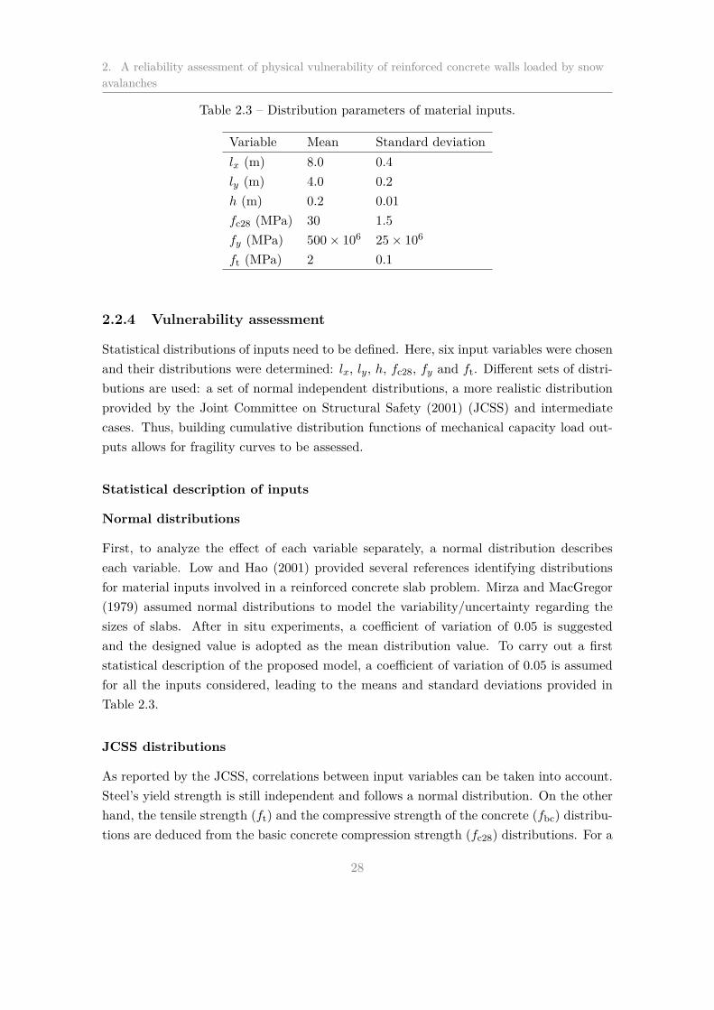
2. A reliability assessment of physical vulnerability of reinforced concrete walls loaded by snowavalanches
Table 2.3 – Distribution parameters of material inputs.
Variable Mean Standard deviation
lx (m) 8.0 0.4
ly (m) 4.0 0.2
h (m) 0.2 0.01
fc28 (MPa) 30 1.5
fy (MPa) 500 × 106 25 × 106
ft (MPa) 2 0.1
2.2.4 Vulnerability assessment
Statistical distributions of inputs need to be defined. Here, six input variables were chosen
and their distributions were determined: lx, ly, h, fc28, fy and ft. Different sets of distri-
butions are used: a set of normal independent distributions, a more realistic distribution
provided by the Joint Committee on Structural Safety (2001) (JCSS) and intermediate
cases. Thus, building cumulative distribution functions of mechanical capacity load out-
puts allows for fragility curves to be assessed.
Statistical description of inputs
Normal distributions
First, to analyze the effect of each variable separately, a normal distribution describes
each variable. Low and Hao (2001) provided several references identifying distributions
for material inputs involved in a reinforced concrete slab problem. Mirza and MacGregor
(1979) assumed normal distributions to model the variability/uncertainty regarding the
sizes of slabs. After in situ experiments, a coefficient of variation of 0.05 is suggested
and the designed value is adopted as the mean distribution value. To carry out a first
statistical description of the proposed model, a coefficient of variation of 0.05 is assumed
for all the inputs considered, leading to the means and standard deviations provided in
Table 2.3.
JCSS distributions
As reported by the JCSS, correlations between input variables can be taken into account.
Steel’s yield strength is still independent and follows a normal distribution. On the other
hand, the tensile strength (ft) and the compressive strength of the concrete (fbc) distribu-
tions are deduced from the basic concrete compression strength (fc28) distributions. For a
28

2.2 Methods
Table 2.4 – Table presenting the marginal distributions of independent material inputs for
the JCSS distribution case. Other inputs are computed according to Eqs. (2.14), (2.15)
and (2.16) of Sect. 2.2.4.
Variable Mean Standard deviation
lx (m) 8.0 0.4
ly (m) 4.0 0.2
h (m) 0.2 0.01
fy (MPa) 560 × 106 30 × 106
ready-mixed concrete type with a C25 concrete grade, based on the given parameters, the
values of m, v, s, n are m = 3.65, v = 3, s = 0.12 and n = 10, and tv is a random variable
from a Student distribution for v degrees of freedom:
fc28 = exp(m+ tvs(1 +1n
)0.5). (2.14)
Then, ft and fbc are calculated with λ, Y1 and, Y2. λ is a factor taking into account
the systematic variation of in situ compressive strength and the strength from standard
tests. Finally, (Yi)i=1,2 are lognormal variables representing additional variations due to
special placing, curing, and hardening of the concrete. In our case, αc is considered equal
to 0.85θγb
:
fbc = αcfλc28Y1, (2.15)
ft = 0.3f2/3bc Y2. (2.16)
For all parameters, the marginal mean and standard deviation were set according to the
JCSS recommendation (Table 2.4). Difference with the previous case (Table 2.3) concerns
(fc28) for which they are higher in this case.
Intermediate distributions
To bridge the gap between the realistic JCSS distributions case and the normal indepen-
dent choice, seven intermediate distributions were considered, differing from each other in
terms of distribution type and/or covariance matrix:
• A lognormal distribution for three multiplicative variables: the tensile strength and
the compressive strength of concrete, and the steel yield strength with parameters
of Table 2.5. Means and standard deviations are the same as for the normal case.
• A lognormal distribution for the tensile strength and the compressive strength of
concrete, and the steel yield strength with parameters of Table 2.6. Means and
standard deviations are the same as for the JCSS case.
29

2. A reliability assessment of physical vulnerability of reinforced concrete walls loaded by snowavalanches
Table 2.5 – Table presenting the marginal lognormal distributions used for the tensile
strength and the compressive strength of concrete, as well as the steel yield strength.
Means and standard deviations are the same as in Table 2.3. The parameters µLN and
σLN are the resulting parameters of the lognormal distributions.
Variable Mean Standard µLN σLN
deviation
ft (MPa) 2 0.1 0.69 0.05
fc28 (MPa) 30 1.5 3.40 0.05
fy (MPa) 500 × 106 25 × 106 20.03 0.05
Table 2.6 – Marginal JCSS-based lognormal distributions used for the tensile strength
and the compressive strength of concrete, as well as the steel yield strength.
Variable Mean Standard µLN σLN
deviation
ft (MPa) 2.38 0.76 0.82 0.31
fc28 (MPa) 38.9 6.11 3.65 0.16
fy (MPa) 560 × 106 30 × 106 20.14 0.053
• A lognormal distribution for the tensile strength and the compressive strength of con-
crete, and the steel yield strength. According to the Table 2.6, standard deviations
are multiplied by 2 to emphasize lognormal distributions asymmetry.
• A normal joint distributions for all the variables with variance–covariance matrix
deduced from the JCSS distributions and the means from Table 2.3.
• A normal joint distribution for the six parameters lx, ly, h, fc28, fy and ft using mean
and standard deviation from Table 2.3 and correlation coefficients (covariance) of the
JCSS case. The main correlation is the relation between fc28 and ft: ρ(fc28, ft) =
0.31; others are lower than 0:01, i.e., close to independence.
• A normal joint distribution for the six parameters lx, ly, h, fc28, fy and ft using
mean, standard deviation and correlation coefficients (covariance) of the JCSS case.
• Uncorrelated JCSS distributions: to assess the effect of correlation on the JCSS case,
each modeled variable was selected independently to break down dependencies.
30

2.3 Methods
40 60 800
100
200
300
400
500
600
700
800(a)
x (kPa)
f(x)
40 50 60 700
0.2
0.4
0.6
0.8
1
x (kPa)F
(x)
(b)
Figure 2.7 – Output histogram of the ULS case for a rectangular wall with one free
edge and three clamped edges with normal independent inputs (a), and the cumulative
distribution function associated (b).
Fragility curves derivation
A fragility curve F (x) is a monotonic curve providing a failure probability as a function
of the magnitude of a loading, here a pressure applied, hence the cumulative distribution
function F (x) of the failure probability for the load x. The usual way to compute fragility
curves is to set a pressure and vary the inputs from their statistical distributions. Thus,
for each pressure a failure probability is obtained to build the fragility curve. In this
paper, the approach is somewhat original because failure probabilities are derived from
an inverse resolution. First, the structure capacity of resistance is found; then, by abacus
inversion, a load distribution is assessed. Finally, the cumulative distribution function of
the latter distribution makes it possible to link a failure probability to a pressure. As an
example, Fig. 2.7 depicts an output histogram of the ULS case for a rectangular wall with
one free edge and three clamped edges with normal independent inputs and the fragility
curve associated through its cumulative distribution function.
31

2. A reliability assessment of physical vulnerability of reinforced concrete walls loaded by snowavalanches
0 50 100 150 200 2500
0.5
1
x (kPa)
F(x
)
100
101
102
0
0.5
1
x (kPa)
F(x
)
ULS
ALS
Elas
YLT
(b)
(a)
Figure 2.8 – Fragility curves according to boundary conditions sorted by failure criterion:
(a) linear frame and (b) semi-log frame.
2.3 Results
2.3.1 Fragility curves with uncorrelated normally distributed inputs
Overview of all configurations
Using 10 000 runs per curve, smooth fragility curves are obtained. Figure 2.8 depicts
fragility curves according to explored boundary conditions. They are sorted by the four
failure criteria. Two visual groups are formed. First, all the curves representing the elastic
limit state are gathered at low pressure loads. By considering the minimum 2.5 % quantile
and their maximum 97.5 % quantile, their fragility range is [2.8, 27.2] (kPa). They do
not interfere with fragility curves of the other failure criteria. On the other hand, the
ULS, ALS and YLT fragility curves are defined on a range from 22.7 kPa to 218.6 kPa.
It is interesting to note that the ALS fragility curves are scaled from the ULS curves by
the safety factor 1.15. This is easily explained by the definition itself of the ALS failure
criterion.
Another point of view can be taken by plotting the same data according to the de-
scription of their boundary conditions (Fig. 2.9). Sets of fragility curves can be deduced.
The four weakest structures present free edges. Rectangular walls with one free edge are
32

2.3 Results
0 50 100 150 200 2500
0.5
1
x (kPa)
F(x
)
100
101
102
0
0.5
1
F(x
)
x (kPa)
4 supported
2 supported2 clamped
1 supported3 clamped
1 free 3 supported
1 free 3 clamped
1 clamped 3 supported
2 supported 2 clamped s. by s.
4 clamped
1 clamped 2 supp./1 free
1 supp./2 clamped1 free
(a)
(b)
Figure 2.9 – Fragility curves according to boundary conditions sorted by boundary con-
ditions: (a) linear frame and (b) semi-log frame.
sorted from the weakest by their boundary conditions as below: (1) one free edge and
three supported edges; (2) one supported edge, two clamped edges and one free; (3) one
clamped edge, two supported edges and one free*; and (4) one free edge and three clamped
edges (*exception for the YLT limit state where 3 and 4 are exchanged). Then the sec-
ond set of curves gathers the rectangular wall with supported edges ((5) four supported
edges, (6) one clamped edge and three supported ones, (7) two supported edges and two
clamped ones, (8) two supported edges and two clamped edges side by side, and (9) one
supported edge and three clamped ones). Finally, the less vulnerable rectangular wall has
four clamped edges.
Equation (2.17) provides the p quantile of each vulnerability curve:
F (x) = Pr(X ≤ x) = p. (2.17)
The previous equation allows considering a more quantitative approach. Table 2.7
sums up the 50 % quantiles and similar conclusions as described above are set up. The
fragility range is defined as an interval: the lower bound is the 2.5 % quantile and the
upper bound is the 97.5 % quantile of the fragility curve, which could be considered as
very useful quantitative thresholds for engineering applications.
33

2. A reliability assessment of physical vulnerability of reinforced concrete walls loaded by snowavalanches
Table 2.7 – The 50 % quantile of the CDF fragility curves according to boundary conditions
and failure criterion, and (2.5 %, 97.5 %) quantile defining a fragility range (kPa).
Boundary conditions Elas ULS ALS YLT
(1) four simply supported
edges
8.4 60.2 69.3 97.0
(6.5, 10.9) (52.3, 69.1) (60.2, 79.5) (85.5, 109.5)
(2) simply supported on the
two large edges
10.0 71.6 82.4 121.0
clamped on the two small
edges
(7.7, 13.0) (59.4, 87.6) (68.3, 100.7) (104.8, 139.1)
(3) simply supported on one
large edge
15.2 108.6 124.9 158.5
clamped on the three other
edges
(11.6, 19.7) (95.0, 124.2) (109.3, 142.8) (138.8, 180.2)
(4) one free large edge 7.8 56.0 64.4 80.5
clamped on the three other
edges
(6.0, 10.3) (49.9, 63.7) (57.4, 73.2) (66.6, 96.7)
(5) one free large edge 3.6 26.0 29.9 38.1
simply supported on the three
other edges
(2.8, 4.7) (22.7, 29.6) (26.1, 34.1) (30.9, 46.7)
(6) clamped on one small edge 9.2 65.8 75.7 109.5
simply supported on the three
other edges
(7.1, 11.9) (56.0, 77.6) (64.4, 89.2) (95.6, 124.7)
(7) simply supported side by
side
14.6 104.7 120.4 145.5
clamped on the two other
edges
(11.2, 19.2) (93.1, 117.6) (107.1, 135.3) (128.3, 164.4)
(8) four clamped edges 20.7 147.9 170.0 194.0
(15.6, 27.5) (133.3, 163.4) (153.3, 187.9) (171.1, 219.2)
(9) one free large edge / one
clamped large edge
7.2 51.9 59.7 55.9
simply supported on the two
small edges
(5.3, 10.3) (43.2, 58.9) (53.2, 67.8) (47.2, 65.8)
(10) one free large edge / one
simply supported large edge
5.8 41.4 47.6 60.9
clamped on the two small
edges
(4.4, 7.5) (33.5, 50.8) (38.5, 58.5) (48.9, 74.1)
34

2.3 Results
Table 2.8 – Quantiles of fragility curves illustrated in Fig. 2.13.
Approach Q2.5 % Q50 % Q97.5 % Q97.5 %–Q2.5 %
Deterministic 55.5 0
JCSS 44.9 62.4 86.8 41.9
JCSS independent 45.3 62.6 86.8 41.6
Normal independent 50.2 56.3 64.3 14.1
Correlated normal 50.3 56.3 64.0 13.6
Normal, correlation and variance from
JCSS case
33.7 56.6 79.4 45.7
Lognormal, mean and variance from nor-
mal case
51.3 56.2 63.6 12.3
Normal, correlation, variance and mean
from JCSS case
42.8 63.3 84.5 41.7
Lognormal, mean and variance from JCSS
case
45.2 62.4 86.2 41.0
Lognormal, mean and variance (×4) from
JCSS case
32.0 60.3 114.6 82.6
An example: one free edge and three clamped edges
To investigate Monte Carlo confidence interval quantification, a focus on a particular case
was required. The selected case is the rectangular wall with one free edge and three
clamped edges (Fig. 2.10). The four limit state fragility curves can be distinguished to-
gether with Monte Carlo confidence intervals. As mechanical runs are not time-consuming,
the number of calls N can be high enough to make numerical uncertainty negligible. Thus
10 000 runs induce thin confidence intervals near the curve, giving confidence in all the
numerical results provided.
2.3.2 Parametric study
This section is devoted to the analysis of total Sobol indices. As each of the input variables
is independent, their sum is equal to 1. Sensitivity pie charts of outputs according to the
input distribution can be plotted (Fig. 2.11). Four input parameters influence the fragility
assessment based on the elastic failure criterion: ft, lx, ly and h. The variable h is the
predominant variable affecting the elastic-based failure probability. The ULS and ALS
have the same sensitivity pie charts. Three input parameters are involved in the variability
of ULS- and ALS-based failure probabilities: lx, ly and fc28. fc28 seems to be the variable
influenced the most by these outputs. This indicates which variables should be considered
35

2. A reliability assessment of physical vulnerability of reinforced concrete walls loaded by snowavalanches
Figure 2.10 – Vulnerability curves and their 95 % confidence intervals from Monte Carlo
simulations of a slab with one free edge and three clamped edges.
with the greatest care while designing a structure in practice, depending on the chosen
failure criterion.
2.3.3 Sensitivity to input distributions choice
Fragility curves are highly dependent on the input distributions used. Outcomes were
obtained from the two first distributions previously described (Fig. 2.12). As a general
overview, more elaborated distributions induce greater spread in fragility curves. Their
fragility ranges have a higher amplitude than the range derived from independent nor-
mal approaches. One explanation is that taking into account correlations makes certain
“extreme” combinations of inputs more likely than in the independent case. Another ex-
planation lies in the number of variables considered: the more numerous they are, the
more uncertainties are taken into account, and also the larger the fragility range of the
fragility curves is.
To ascertain and detail this conclusion, Fig. 2.13 focuses on the ULS example for the
same boundary conditions. It appears clearly that, from the deterministic point of view (a
simple 0–1 response if the fragility limit is attained or is not attained) to the JCSS-based
approach, fragility curves have wider fragility ranges. Quantiles at 2.5 %, 50 % and 97.5 %
36

2.3 Results
Figure 2.11 – Sensitivity pie charts for the elastic, ULS (ALS) and YLT failure criteria.
37

2. A reliability assessment of physical vulnerability of reinforced concrete walls loaded by snowavalanches
0 50 100 1500
0.5
1
x (kPa)
F(x
)
0 50 100 150 2000
0.5
1
x (kPa)
F(x
)
Elastic
ULS
ALS
YLT
95% confidenceinterval upper bound
95% confidenceinterval lower bound
(a)
(b)
Figure 2.12 – Comparison of fragility curves from different input distributions of a slab
with one free edge and three clamped edges: (a) normal independent distributions, (b)
JCSS distribution.
support these results (Table 2.8). Note, however, that the more complex case (i.e., the
JCSS case), despite its wider spread, shows higher (and thus “safer”) modal values, and
therefore simpler approaches (normal or lognormal inputs) can be used in practice, at least
as first approximations.
The 50 % quantile depends nearly only on the means of the three material parameters
fy, fc28 and ft. Indeed, the 50 % quantile remains fully constant to ∼ 56 kPa regardless of
the covariance matrix for Gaussian inputs with fy, fc28 and ft centered on their nominal
values 500 × 106, 30 and 2 MPa, respectively. Switching to the JCSS leads to a higher
50% quantile ∼ 62 kPa independent of the correlation structure. In addition, the 50 %
quantile remains nearly unchanged with independent lognormally distributed inputs with
the same mean even if these, by definition, introduce non-symmetry into the problem.
This asymmetry effect is, however, visible when the standard deviation is multiplied by 2.
By the way, the fragility range is logically also increased (Table 2.8).
All in all, the fragility range and fragility curves shape changes mainly according to
the marginal variances, much higher in the different JCSS cases, with covariance between
the different inputs and marginal distribution types having less influence.
38
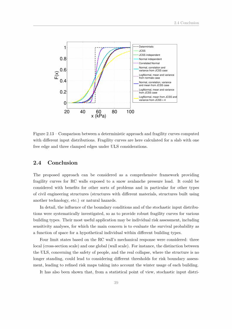
2.4 Conclusion
20 40 60 80 100
0
0.2
0.4
0.6
0.8
1
x (kPa)
F(x
)
Deterministic
JCSS
JCSS independent
Normal independent
Correlated Normal
Normal, correlation andvariance from JCSS case
LogNormal, mean and variancefrom normale case
Normal, correlation, varianceand mean from JCSS case
LogNormal, mean and variancefrom JCSS case
LogNormal, mean from JCSS and
variance from JCSS × 4
Figure 2.13 – Comparison between a deterministic approach and fragility curves computed
with different input distributions. Fragility curves are here calculated for a slab with one
free edge and three clamped edges under ULS considerations.
2.4 Conclusion
The proposed approach can be considered as a comprehensive framework providing
fragility curves for RC walls exposed to a snow avalanche pressure load. It could be
considered with benefits for other sorts of problems and in particular for other types
of civil engineering structures (structures with different materials, structures built using
another technology, etc.) or natural hazards.
In detail, the influence of the boundary conditions and of the stochastic input distribu-
tions were systematically investigated, so as to provide robust fragility curves for various
building types. Their most useful application may be individual risk assessment, including
sensitivity analyses, for which the main concern is to evaluate the survival probability as
a function of space for a hypothetical individual within different building types.
Four limit states based on the RC wall’s mechanical response were considered: three
local (cross-section scale) and one global (wall scale). For instance, the distinction between
the ULS, concerning the safety of people, and the real collapse, where the structure is no
longer standing, could lead to considering different thresholds for risk boundary assess-
ment, leading to refined risk maps taking into account the winter usage of each building.
It has also been shown that, from a statistical point of view, stochastic input distri-
39
2. A reliability assessment of physical vulnerability of reinforced concrete walls loaded by snowavalanches
butions strongly influence the shape of the fragility curves. Hence, mean and standard
deviation of each variable, independent or correlated variables as well as the number of
variables considered, constitute important factors in the variability of fragility curves.
This sensitivity to the input parameter distributions highlights that it seems important to
consider and describe precisely the uncertainty sources for each application.
The deterministic simulations were carried out through simplified and effective me-
chanical models in terms of CPU time. This allowed using the Monte Carlo method,
which gave robust results for the failure probability assessment. Probabilistic input dis-
tributions are provided by the literature, but no statistical inference has been performed.
Future work should therefore take real data into consideration and a Bayesian approach
could then be appropriate to update the information conveyed by numerical simulations
(Eckert et al., 2009).
Finally, it should be noted that more sophisticated mechanical models for civil engi-
neering structures exist, based on the finite-element (FE) method, which can simulate the
structure in greater detail and in particular describe how the damage field evolves when
material nonlinearities develop inside the concrete and the steel reinforcement. However,
these FE models are often more complex (i.e., in term of convergence) and time-consuming.
Hence, they may be less well adapted to a generic individual risk base approach, but more
useful for studies deriving refined fragility curves for specific structures included in precise
engineering projects.
2.5 Acknowledgements
The authors thank the ANR research program MOPERA (Modélisation probabiliste pour
l’Etude du Risque d’Avalanche – avalanches.irstea.fr/mopera-projet/) and the MAP3 AL-
COTRA INTERREG program for financially supporting this work. The authors are also
grateful to Regis Monnard for fruitful discussions. We also thank Dr. Lasaponara (han-
dling editor) and the two anonymous referees for their constructive comments used to
improve the paper. Edited by: R. Lasaponara Reviewed by: three anonymous referees
2.6 Appendix: Nomenclature
40

2.6 Appendix: Nomenclature
Table 2.9 – Nomenclature.
ρs density of steel
lx length of the slab
ly height of the slab
h thickness of the slab
fc28 cylinder characteristic compressive strength of concrete (age, 28 days)
fbc compressive strength of concrete
ft tensile strength of concrete
fy steel yield strength
ǫuk ultimate tensile strain of the steel
γb, γs safety coefficients on concrete and steel strength
qULS, qALS, qElas, qYLT characteristic loading at the ultimate limit state, at the accidental limit state, at
the first cracks of the concrete in the tensile zone and at the collapse
ǫbc ultimate compressive strain of the concrete
θ loading time parameter
MAB rational dimensioning moment
µAB ULS rational dimensioning coefficient
d effective depth of the RC cross section
z lever arm in the section
βy, βx Bares coefficient
ν Poisson coefficient
Wint internal virtual work
Wext external virtual work
nL number of yield lines
M ip unitary plastic moment along the ith line
Li length of the ith line
θi rotation angle of the ith element
δ(x, y) displacement matrix
q uniform load
α1, α2 angles of YLT patterns
Pf failure probability
r resistance of the structure
s solicitation
α significance level of confidence interval
fR(r) probability density function of the resistance
Si first-order Sobol sensitivity coefficient
STi total Sobol sensitivity coefficient
αc coefficient from the JCSS distribution
41

2. A reliability assessment of physical vulnerability of reinforced concrete walls loaded by snowavalanches
42

CHAPTER 3
Reliability-based physical vulnerability assessment of a RC
wall impacted by snow avalanches using a nonlinear SDOF
model
Le contenu de ce chapitre a vocation à être soumis après travail à Reliability Engineering
and System Safety, les auteurs sont : Favier, P., Bertrand, D., Eckert, N., Ousset, I. and
Naaim, M..
43

3. Reliability-based physical vulnerability assessment of a RC wall impacted by snow avalanchesusing a nonlinear SDOF model
Abstract
As often in reliability engineering, the CPU time required to obtain accurate and robust results is the main
issue. Here, the objective is to propose a simplified modelling of the RC structure keeping the involved
physics and especially the dynamic nature of the structure’s mechanical response. This paper presents
the assessment of the physical vulnerability of a Reinforced Concrete (RC) wall subjected to an avalanche
loading within a reliability framework. A Single Degree-Of-Freedom (SDOF) model is used to describe the
dynamical response of the RC member. The non-linear behaviour of the material is taken into account by
a Moment-Curvature approach which allows describing the overall bending response of the RC wall until
the collapse. The deterministic SDOF model is validated by Finite Element Analysis (FEA) and by limit
analysis.
A reliability analysis is conducted in order to derive fragility curves providing the limit state reach
as function of avalanche pressure. A performance analysis is carried out which underlines the necessity
to use efficient numerical models in terms of computation time. For our case of snow avalanche loadings,
a SDOF model seems to be an interesting option to derived rapidly fragility curves keeping a sufficient
accuracy. Several reliability methods (Monte-Carlo, Kernel smoothing, Taylor expansion) are used and
compared suggesting that non parametric methods (not based on parametrized families of probability
distributions) have a good potential to approach fragility curves. Finally, the sensitivity to strength
parameters (material tensile and compressive strengths, reinforcement ratio) and to loading parameters
are proposed. It highlights that both have influences on the fragility curve derivation; the loading rate has
also a significant influence on both the shape and the mode of the fragility curve. Discussion is proposed
with regards to the seldom fragility curves available in this field.
Keywords: Vulnerability Relations; Fragility Curves; RC Wall; Reliability; Natural Hazard; Snow
Avalanche; Risk; SDOF model; Finite Element Analysis.
3.1 Introduction
Nowadays, risk analysis is more and more used in order to help decision makers. In safety
domains, such as natural hazards prevention and mitigation engineering, the construction
of hazard models together with vulnerability relations are needed. Vulnerability relations
are used to represent a degree of damage of the considered system, or fragility curves which
express the probability to reach a given limit state. Vulnerability curves are deterministic
in opposition to fragility curves which are probabilistic.
In the context of avalanche risk mitigation, technical prescriptions for buildings lying
in dangerous runout zones impose that the part of the structure facing the snow flow has
to resist to pressures up to 30kPa. Several kind of construction technologies can be used
to achieve this resistance (masonry, wood or metallic structures, etc.). In a first step, only
reinforced concrete is considered in this paper. Indeed, most of usual constructions which
can be found in the Alps are built with this composite material. Thus, this paper deals
with the definition of the fragility curves for RC walls impacted by a snow avalanche. For
a given magnitude of avalanche loading, a fragility curve provides the probability that the
44

3.1 Introduction
RC wall would reach a given damage level.
Until now, very few fragility curves established within the context of snow avalanche
risk are available. Indeed, most studies dedicated to the assessment of physical vulnerabil-
ity to snow avalanches are dealing only with vulnerability curves and not fragility curves
(Papathoma-Köhle et al., 2011). Vulnerability relations are often empirically assessed,
based on historical observations (Keylock and Barbolini, 2001; Barbolini et al., 2004a;
Cappabianca et al., 2008). Because these relations were deduced from scarce data which
can be site dependent, the accuracy and the generalization of such relations is question-
able. Recently, in order to propose an alternative way to derive vulnerability curves, Finite
Element Analysis (FEA) was used to described the damage level of typical RC structures
subjected to an avalanche pressure field (Bertrand et al., 2010). The main advantage of
numerical approaches is to define and control accurately the studied structure (geometry,
resistance, reproducibility, etc.).
Second, fragility curves are non homogeneously used with natural or anthropic hazards.
For instance, the failure probability quantification of structures within an industrial con-
text is currently undertaken (explosions (Low and Hao, 2001; Nassr et al., 2012), geotech-
nical works (Mollon et al., 2013), etc.). Besides, for multistorey buildings exposed to
earthquake loadings, the probability to overpass a drift limit according to the peak ground
acceleration is very often described via reliability-based fragility curves (Ellingwood, 2001;
Kyung and Rosowsky, 2006; Li and Ellingwood, 2007; Lagaros, 2008). However, for rock-
falls (Mavrouli and Corominas, 2010a,b), landslides or debris flows (Papathoma-Köhle
et al., 2012), tephra falls (Spence et al., 2005), fragility curves are seldom used and vul-
nerability relations are preferred.
The failure probability assessment is based on the well-established framework of relia-
bility analysis (Lemaire (2005)). Once the deterministic model and the failure criterion of
the system are chosen, the uncertainties related to the random variables are propagated
through the mechanical model to calculate the failure probability. Usually, simulation
methods are used. These methods are more or less based on the Monte-Carlo approach
and give robust results. However, they can be time consuming depending on the rapidity
of the deterministic model. In some cases, if too many runs are needed to get a good
accuracy of the failure probability or if the deterministic model is not effective enough in
terms of CPU time, approximation methods can be alternatively used in order to lower the
number of simulation calls. However, the convergence is not always ensured, depending,
inter alia, on the non linearity of the deterministic model and on the number of random
variables involved.
Alternative models to highly time-consuming models are preferred in reliability anal-
ysis. Reducing the calculation time can be made by performing simplifying assumptions
on the mechanical model together with keeping the involved physics. Reinforced concrete
45

3. Reliability-based physical vulnerability assessment of a RC wall impacted by snow avalanchesusing a nonlinear SDOF model
structures are broadly studied and various numerical models exist to describe the me-
chanical response of the structure and possibly its failure. For snow avalanche loadings,
FEA have already been used in order to better understand the interaction between the
avalanche and the RC structure. For instance, a FEA has been performed on deflective
RC walls of the protection system of Taconnaz (Berthet-Rambaud, 2004; Ousset et al.,
2013). Besides, typical structure geometries have been considered for residential buildings,
i.e. three vertical walls with a U-like shape (Bertrand et al., 2010). Within a stochastic
framework, the main drawback of these approaches is the CPU time needed to performed
a single simulation. As an alternative, the mechanical capacity of a RC structure can be
estimated using classical civil engineering abacuses allowing the use of reliability analysis.
Thus, for a wide range of boundary conditions, the failure probability calculation of RC
slabs impacted by snow avalanches has been proposed by Favier et al. (2014a). The main
assumption consists in supposing that the response of the structure is quasi-static. Nev-
ertheless, this approach does not account for potential inertial effects or strain rate effects
due to the dynamical nature of the loading.
In order to find a compromise between simplified time effective models and refined mod-
els but time consuming, RC structures can be described using Single-Degree-of-Freedom
(SDOF) approaches (Biggs, 1964). The structure is modeled by an equivalent mass and an
equivalent spring. This approach has been largely used and validated in the field of struc-
tures subjected to blast loads (Ngo et al., 2007; Jones et al., 2009; Carta and Stochino,
2013). In this paper, a simply supported RC wall is considered and modeled by a SDOF
approach. The model is able to describe the ultimate state of the RC wall, i.e. its collapse
which corresponds to the ultimate bending moment which can be undergone. A FEA and
limit analysis are used to validate the ultimate mechanical state predicted by the SDOF
model. Then, several inputs of the SDOF model are randomized and a reliability anal-
ysis is performed in order to established fragility curves according to various simulation
and approximation methods. A comparison of the relevance and efficacy of the reliability
methods is proposed. Finally, a parametric study is presented which underlines the rela-
tion between random input variables and, particularly, the effect of variable correlations
and the coefficients of variation of each variable.
3.2 Deterministic SDOF model
3.2.1 RC wall description
Geometry and loading
The considered RC wall is rectangular with a length L of 8m, a width b of 1m and a
thickness h of 20cm (Figure 3.1a). The RC wall is simply supported along the two smaller
46

3.2 Deterministic SDOF model
Figure 3.1 – Simply supported RC wall (a) and time evolution of the pressure (b).
)0(c
)0(c
cf
cy cu
CEA concrete
t
tf
(a) Concrete.
mS
m�
��
m�� m��
(b) Steel.
Figure 3.2 – Stress-strain relations for concrete (a) and steel (b).
edges. This boundary condition allows considering the system as a 2D problem and thus
the RC wall can be assimilated to a simply supported beam.
The snow avalanche applies an uniform pressure p(t) along the y axis which evolves
through time from 0s to tend up to the maximal pressure Pmax which is reached for tend/2.
This time evolution is shown in figure 3.1b. The loading rate (pmax
tend) is fixed at 0.3 kPa.s−1.
Steel and concrete
Many stress-strain relations for concrete and steel are available in the literature (Bazant
and Oh (1983); Mazars (1986); De Borst and Guitiérrez (1999); Wang and Hsu (2001);
CEB-FIP (2010), etc.). As a function of the problem assumptions (cyclic loading, 3D
formulation, etc.), the evolutions of the stress-strain relations can be more or less complex.
47

3. Reliability-based physical vulnerability assessment of a RC wall impacted by snow avalanchesusing a nonlinear SDOF model
In this paper, the concrete and steel behaviour laws are piecewise linear relations describing
the evolution of stress (σxx) as a function of strain (ǫxx) along the longitudinal axis x of
the slab (Figure 3.2a).
The behaviour laws proposed by Leprêtre et al. (1988) have been used. The elastic
part of the behaviours laws is described by the Young modulus of steel (Es) and concrete
(Ec). For concrete, compressive and tensile responses have been distinguished (Figure
3.2a). Under compression regime, the stress (σc) increases as a function of the strain (ǫc)
up to the compressive strength of concrete (fc) which corresponds to a strain of ǫcy. Then
a negative hardening compressive behaviour develops. When the ultimate compressive
strain (ǫcu) is reached, σc = 0. Under tensile regime, the same behaviour is qualitatively
used. The tensile strength of concrete (ft) and the ultimate tensile strain of concrete (ǫt)
are involved. The strain associated to ft equals ǫty = ft/Ec. For steel, the behaviour law
is supposed elastic perfectly plastic (Figure 3.2b). fy is the yielding stress associated to
the yield strain ǫsy and ǫsu is the ultimate strain of steel.
Reinforced concrete is a composite material for which the quantity of steel included
within concrete plays a major role. The steel reinforcement ratio (ρr) is defined as the
ratio between the steel area (As) on the cross-section surface (h × b) and equals 0.4%.
Figure 3.3a depicts a cross sectional view of the RC wall.
3.2.2 SDOF model
The pressure is applied out-of-plan of the RC wall and thus bending and shearing efforts
exist through cross-sections. Because the loading is uniformly applied and the time of
loading is quite higher than the fundamental frequency of the structure (5Hz, thus an
oscillation period of 0.2s), it can be assumed that the failure mode occurs by excessive
bending at midspan (Figure 3.4c). Thus, it justifies to use SDOF modelling to represent
the RC wall mechanical response.
The proposed SDOF model corresponds to a mass-spring system loaded by a uniform
pressure (Figure 3.4a-b). An equivalent concentrated mass (Meq) is maintained by a
spring of stiffness Keq. The expressions of Meq and Keq are deduced respectively from the
deformed shape (Biggs, 1964) and from the Moment-Curvature relationship presented in
the section 3.2.2. Finally, no viscous damping has been considered because, if the structure
collapses, the failure criteria will be necessarily achieved during the loading phase and thus
it is not necessary to account for the post peak oscillation regime.
Elasto-plastic overall response
The elasto-plastic behaviour of the SDOF model can be represented by a bilinear Load-
Displacement curve which is derived from the Moment-Curvature (M − χ) relationship
48

3.2 Deterministic SDOF model
b
h sA d
s
)( yc
s
)(yc
(a) (b) (c)
yxC
OM
PR
ES
SIO
N
TE
NS
ION
m ax,c
x
y
h/2
Neutral axis Concrete
Steel
Figure 3.3 – Cross-section of the RC beam (a), stress diagram (b), strain diagram (c).
L/2
0
L
xy
Plastic hinge
(c)
0v
Figure 3.4 – Simply supported beam (a), mass-spring system (b) and failure mode of the
RC wall (c).
49

3. Reliability-based physical vulnerability assessment of a RC wall impacted by snow avalanchesusing a nonlinear SDOF model
uM
M
yM
y u
K
elK
plKyP
uP
P
vuvyv
(a)
(b)
Figure 3.5 – Bending moment - Curvature relation (a) and load-displacement relation of
the SDOF model (b).
50

3.2 Deterministic SDOF model
deduced at the cross-section scale (cf. paragraph 3.2.2). The bending moment My cor-
responds to the beginning of either steel yielding or concrete crushing depending on the
reinforcement ratio. The ultimate bending moment Mu corresponds to the achievement
of the ultimate strain value either within concrete or steel. Related curvatures are χy and
χu.
The first part of the Load-Displacement bilinear curve represents the elastic response
and the second part is the plastic response of the RC wall. Two forces are respectively
expressed such as Py = 8My
L and Pu = 8MuL which can be transformed into a uniform
pressure as p = P/L (Figure 3.4a). Then, the expression of the midspan displacement
corresponding to the transition from elastic to plastic is
vy =5PyL
3
384K, (3.1)
where K = My
χywhich is the bending stiffness of the RC wall. The ultimate midspan
displacement is deduced from
vu = vy +14
(χu − χy)L lp , (3.2)
where lp is the plastic hinge length (Figure 3.3c) which can be estimated by the relation
lp = d+ 0.05L (Mattock, 1967) where d is the effective depth of the cross-section (Figure
3.3a). Finally, the Load-Displacement curve (Figure 3.5b) has two stiffnesses which are
defined such as
Kel =Py
vy, (3.3)
Kpl =Pu − Py
vu − vy. (3.4)
Moment-Curvature relationship
The curvature, defined as χ = ∂2vo∂x2 where vo is the midspan displacement, is obtained
assuming that the strain distribution along the y axis follows classical Euler-Bernoulli
assumptions which means that sections remain plane and orthogonal to the neutral axis
during the loading of the RC wall (Figure 3.3b). Thus, the curvature can be calculated by
χ =ǫc(y = −h
2 )xy
=ǫs(y = d− h
2 )d− xy
, (3.5)
51

3. Reliability-based physical vulnerability assessment of a RC wall impacted by snow avalanchesusing a nonlinear SDOF model
where xy is the neutral axis depth. xy is deduced from the translational mechanical balance
along x of the cross-section which can be expressed by the equation
b
∫ xy
0σcdy = σsAs + b
∫ h
xy
σcdy . (3.6)
The Moment-Curvature relationship is constructed step by step by calculating the position
of the neutral axis for a given strain distribution, i.e. a given curvature χ, which fulfil the
condition of equation 3.6. Then, the bending moment is calculated from
M(χ) = b
∫ xy
0σc(d− y)dy . (3.7)
At the end of the process, My, Mu, χy and χu are identified on the M −χ curve and used
to derive the Load-Displacement curve of the SDOF model.
Equations of motion
By applying the fundamental principle of dynamics, the mechanical balance of the SDOF
leads to the following differential equations. For the elastic phase (0 < vo < vy), it comes:
Meld2vo(t)dt2
+Kelvo(t) = P (t) , (3.8)
and, for the plastic phase (vy < vo < vu):
Mpld2vo(t)dt2
+Kplvo(t) + (Kel −Kpl)vy = P (t) , (3.9)
where P (t) is the time evolution of the external force deduced from the uniform pressure
p(t) applied to the RC wall. In order to solve through time equations 3.8 and 3.9, usual
Newmark’s algorithm technics have been used (Newmark, 1959).
3.2.3 Validation
Finite Element Analysis
In order to validated the SDOF model, a Finite Element simulation of the RC wall re-
sponse to avalanche loading has been undertaken with the computational software Cast3M
(Millard, 1993). The analysis is carried out in 2D (plane stress). Concrete (resp. steel) is
meshed using eight node quadrilateral (resp. two node segment) finite elements (Figure
3.6a). 100 finite elements are placed along the x axis and 10 along the y axis. A per-
fect adhesion between concrete and steel is supposed and thus no slip can occurs. The
same behaviour laws previously described are adopted but formulated here in plane stress
conditions.
52

3.2 Deterministic SDOF model
0
y
x
2L
(a)
(b)
MPa102.6)max( 6xx
MPa106.2)min( 7xx
Figure 3.6 – Mesh of the FEA in black and deformed shape in red (a) and stress field
(σxx) at the collapse pressure (b).
A uniform pressure is applied. As for a pushover test, the loading increases linearly
up to reach either the ultimate strain within steel or concrete. Thus, the midspan dis-
placement can be expressed as a function of the pressure applied. The stress field at the
collapse is depicted in figure 3.6b.
Furthermore, a modal analysis has been carried out. The first (resp. the second) mode
of vibration has a frequency of 4.92Hz (resp. 19.64Hz) which match the theoretical values
4.91Hz (resp. 19.63Hz).
Limit analysis
The ultimate resistance of RC slabs under uniformly distributed pressure can be derived
from the classical yield line theory (Johansen, 1962) which also provides the collapse
mechanism of the RC member. Under an external loading, macrocracks will develop to
form a pattern of ”yield lines” until a mechanism is formed and leads to the collapse.
A yield line corresponds to a nearly straight line along which a plastic hinge develops
where the bending moment becomes constant and equals the plastic bending moment.
The ultimate pressure is deducted from the energy balance between external and internal
energies. The external energy coming from the loading and the internal energy is due to
energy dissipation within the yield lines.
For a one-way simply supported slab, the only collapse mechanism that can arise is
53

3. Reliability-based physical vulnerability assessment of a RC wall impacted by snow avalanchesusing a nonlinear SDOF model
0 0.02 0.04 0.06 0.08 0.1 0.12 0.140
2
4
6
8
10
Displacement (m)
Forc
e (
kP
a)
Finite element response
SDOF response
Elastic response
Limit analysis
Figure 3.7 – Load-displacement curve obtained with FEA and SDOF model. The green
curve represents the elastic response of a beam loaded by a uniform pressure.
depicted in figure 3.4c. Under an uniform pressure, a single yield line would develop
at mispan and thus, for a given arbitrary midspan rotation θ, the internal work (2θMp)
equals the external work (2∫
L2
0 θ x qdx = θ qL2
4 ) and finally leads to the ultimate pressure
qY LT = 8Mp
L2 where Mp is the plastic bending moment of the RC member. Mp can be
obtained by (Favre et al., 1990):
Mp = As fy 0.9 d , (3.10)
which leads to Mp = 57.5 kN.m and finally qY LT = 7.2 kN.m2.
Results comparison
Table 3.1 summarizes inputs of FE and SDOF models and Table 3.2 gives a comparison of
ultimate displacement, ultimate pressure and computation time. Results are compared in
figure 3.7 which demonstrates that Load-displacement curves of both models are in good
agreement. The elastic regime is accurately reproduced by the SDOF model. Moreover,
the ultimate pressure is also well predicted. The limit analysis gives the same result. A
slight difference can be noticed concerning the ultimate displacement which is higher in the
case of the FEA. It can be explained by the formulation of the behaviours laws. Indeed,
in the case of FEA, the plane stress assumption leads to enable stress redistribution which
54

3.3 Vulnerability assessment
Parameters Symbol Value
Length L 8 m
Width b 1 m
Thickness h 20 cm
Concrete cover eexc 4 cm
Mass density (S) ρs 7500 kg.m−3
Mass density (C) ρc 2500 kg.m−3
Young modulus (S) Es 200 GPa
Young modulus (C) Ec 30 GPa
Poisson ratio (S)∗ νs 0.3
Poisson ratio (C)∗ νc 0.2
Ult. tensile strain (S) ǫsu 0.01
Ult. compressive strain (C) ǫcu −0.0035
Ult. tensile strain (C) ǫt 3ft/Ec = 4.10−4
Ult. tensile strength (C) ft 4 MPa
Ult. compressive strength (C) fc 30 MPa
Reinforcement ratio ρr 0.4%
Yield strength (S) fy 500 MPa
Ult. bi-compressive strength (C)∗ fbic 1.15fc
Table 3.1 – Parameter values for models comparison (∗ only needed in the FEM model due
to plane stress formulation). The following notations are adopted : Ult. means Ultimate,
S (resp. C) means Steel (resp. Concrete).
cannot be accounted for by the SDOF approach and leads to a the stiffer response of the
SDOF. Within a reliability context, those observations ensure the SDOF model to provide
conservative and hence safe results for ultimate state prediction of the RC wall.
Finally, the computational time of each approach is compared (Table 3.2). With the
same computer, a computation time of 40 minutes is needed for the FE analysis whereas
the SDOF model runs and finish calculations in less than half a minute. Limit analysis
can be time effective but only provides the ultimate pressure.
3.3 Vulnerability assessment
3.3.1 Failure probability
In a reliability framework, model inputs (x) allows defining the Probability Density Func-
tion (PDF) fR(r) which represents the structure resistance (or structure capacity) and
55

3. Reliability-based physical vulnerability assessment of a RC wall impacted by snow avalanchesusing a nonlinear SDOF model
Models Ult. pressure Ult. displacement Comp. time
SDOF 7.58 kPa 0.0923 m ∼ 35 s
FEA 7.65 kPa 0.1283 m ∼ 40 min
Limit Analysis 7.56 kPa − ∼ 0.2 s
Table 3.2 – Ultimate displacement, ultimate pressure and CPU time provided by the three
approaches.
where r is the capacity of the structure for a given input vector x. For a solicitation s,
the failure probability is obtained by (Lemaire, 2005)
Pf (s) = P (r ≤ s) =∫ s
−∞fR(r) dr (3.11)
The capacity r of the RC wall is defined by the ultimate pressure pu. The fragility
curve is the Cumulative Density Function (CDF) of the structure capacity according to the
ultimate pressure limit state and gives the failure probability as a function of the pressure
magnitude applied to the structure (p). In the following, PDF inputs distributions are
presented. Then, the different methods to derive fragility curves are exposed.
3.3.2 Inputs statistical distributions
Two classes of inputs are considered as random variables: geometrical (L, b and h) and
strength (ft, fc, fy and ρr) parameters. The mean value of the input vector refers to the
deterministic case (Table 3.1). The inputs variables are supposed either independent or
correlated.
First, input distributions are normal PDF and no correlation is supposed between
random variables. Values of Coefficients Of Variation (COV) are considered through three
typical cases. First, 5% is often used when no specific COV values are available (Tab. 3.3,
sets (1.α.a)). Second, values can be proposed from literature justifications (sets (2.β.b)).
The last set (sets (3.γ.c)) corresponds to the deterministic point of view (COV=0).
Then, random variable correlation is assumed between strength parameters (ft, fc and
fy). The variable correlation is taken into account following the Joint Comity of Structural
Safety recommendations (Joint Committee on Structural Safety, 2001).
Marginal PDF distributions
To describe geometrical uncertainties, normal distributions are largely assumed (Lu et al.,
1994; Val et al., 1997; Low and Hao, 2002; Kassem et al., 2013). COV are usually taken in
a range from 0.01 to 0.07. Three sets (1, 2, 3) of COV are tested using normal distributions
(Table 3.3).
56

3.3 Vulnerability assessment
Inputs Mean COV
set 1 set 2 set 3
L 8m 0.05 0.03 determ.
b 4m 0.05 0.03 determ.
h 20cm 0.05 0.03 determ.
set α set β set γ
ρr 0.4% 0.05 0.03 determ.
set a set b set c
ft 4MPa 0.05 0.18 determ.
fc 30MPa 0.05 0.18 determ.
fy 500MPa 0.05 0.08 determ.
Table 3.3 – Marginal distributions of inputs parameters. “determ.” means deterministic
which corresponds to a COV equals to zero. In the case of independent variables, normal
distributions are used.
Concerning strength parameters, in a first approximation, normal distributions with
a COV of 0.05 are considered (set a). In a second step, more realistic COV are used (set
b). For the compressive strength of concrete fc the normal distribution is an usual choice
(Mirza et al., 1979; Val et al., 1997; Low and Hao, 2001, 2002) and COV ranging between
0.11 and 0.18 are generally used. Here, a COV of 0.18 is used. For the tensile strength of
the concrete, a normal distribution with a COV of 0.18 can also be assumed (MacGregor
et al., 1983). Finally, for fy, normal, lognormal or beta distributions are often proposed
(MacGregor et al., 1983) and the COV varies from 0.08 to 0.11 (Val et al., 1997). In the
paper, a normal distribution is adopted and the COV equals 0.08. All these choices are
summarized in Table 3.3.
Eventually, no datum is already available about the reinforcement ratio’s COV. Be-
cause ρr is defined from geometrical parameters, a normal PDF is assumed and COV is
supposed equal to 0.03 or 0.05, depending on the set considered (Table 3.3).
Strength parameters correlation
The case of strength parameter correlation is also considered. The JCSS (Joint Com-
mittee on Structural Safety, 2001) proposed more realistic distribution descriptions by
accounting for their potential dependencies.
The concrete tensile strength (ft) is expressed according to the compressive strength
of the concrete fc. The distribution of fc is deduced from the basic concrete compression
strength fc28 distribution. For a ready-mixed concrete type with a C25 concrete grade, it
57

3. Reliability-based physical vulnerability assessment of a RC wall impacted by snow avalanchesusing a nonlinear SDOF model
0 10 20 30 40 50 600
0.05
0.1
0.15
0.2
0.25
fc (MPa)
PD
F
JCSS in situ compressive strengthNormal with COV=0.05Normal with COV=0.18
(a) Concrete compressive strength parameter
fc.
0 2 4 6 8 10 120
0.5
1
1.5
2
ft (MPa)
PD
F
JCSS tensile strengthNormal with COV=0.05Normal with COV=0.18
(b) Concrete tensile strength parameter ft.
300 400 500 600 7000
0.005
0.01
0.015
0.02
fy (MPa)
PD
F
JCSS yield strengthNormal with COV = 0.05Normal with COV = 0.08
(c) Steel yield strength parameter fy.
Figure 3.8 – Statistical distributions for fc, ft and fy according to Tab. 3.3, and compar-
ison with JCSS distributions.
58

3.3 Vulnerability assessment
yields:
fc28 = exp(m+ tvs(1 +1n
)0.5), (3.12)
where the values of the parameters m, v, s, n are: m = 3.65, v = 3.0, s = 0.12, n = 10
and, tv is a random variable from a Student distribution with v degrees of freedom. Then,
ft and fc are calculated with λ, Y1 and, Y2. The parameter λ is taken equal to 0.96 and
is a factor taking into account the systematic variation of in situ compressive strength
and the strength from standard tests. The coefficient αc equals 0.92. Finally, (Yi)i=1,2 are
log-normal variables representing additional variations due to special placing, curing, and
hardening of the concrete:
fc = αcfλc28Y1, (3.13)
ft = 0.3f2/3c Y2, (3.14)
where Y1 and Y2 means are 1 and their respective coefficients of variation are 0.06 and
0.3. For all other parameters, the marginal mean and standard deviation were also set
according to the JCSS recommendation.
For the yield strength of steel (fy) and based on JCSS assumptions, a normal distri-
bution can be adopted with a mean of 560 MPa and a COV of 0.054. Figure 3.8 depicts
strength parameter distributions used in this paper and underlines observed differences
related to fy and ft PDF definitions.
3.3.3 Reliability methods
From inputs PDF distributions (x) and by propagating uncertainties through the deter-
ministic model (M), output PDF distribution (fR(r)) can be obtained ((Saltelli et al.,
2004; Faivre et al., 2013)). As the capacity r of the RC wall is defined by the ultimate
pressure pu, the output PDF distribution can be noted (fpu(pu)). Two approaches are
considered. Either the output is described through the direct approximation of its PDF or
by the estimation of the output’s moments (mean and variance). In order to perform these
calculations, effective methods exist such as Kernel Smoothing (KS) or Taylor Expansion
(TE) (Lemaire, 2005).
Kernel Smoothing
Direct MC simulations of input variables can provide a discrete PDF distribution of
model’s outputs. However, the resulting curve is a piecewise linear function. KS al-
lows approximating the output PDF distribution considering a normal kernel function K
59

3. Reliability-based physical vulnerability assessment of a RC wall impacted by snow avalanchesusing a nonlinear SDOF model
such as
ˆfpu(pu) =1
nhK
n∑
i=1
K
(
pu − p(i)u
hK
)
, (3.15)
where p(i)u is the ith component of the output sample of ultimate pressure of size n and
the kernel function is expressed as
K(x) =1√2πe− 1
2x2, (3.16)
and hK is the optimal bandwidth which is evaluated with Silverman rule (Wand and
Jones, 1995).
Taylor Expansion
Mean and variance of the output vector of a model M can be calculated directly from
MC simulations but this can be time consuming. TE allows approximating the output
moments of the model more quickly. The moment approximations suppose that the mean
of the output (µpu) can be well estimated by model TE around the input mean (µx). The
mean (µpu) and variance (σ2pu
) of the output pu are approximated though the following
expressions:
µpu = M(µx) +12
m∑
i,k=1
∂2M
∂xi∂xk(µx)Cik , (3.17)
σ2pu
=m∑
i,k=1
∂M
∂xi(µx)
∂M
∂xk(µx)Cik , (3.18)
wherem is the number of input variables, µx is the mean of the input vector x and Cik is the
ik component of the variance-covariance matrix of x. The non linearity of the deterministic
model should not be too strong in order to ensure a satisfactory approximation of the
second partial derivatives of the model and, hence, of the results µpu and σ2pu
provided by
this method. If no covariances is considered (Cik = 0 if i 6= k), preceding equations can
be rewritten more simply as
µpu = M(µx) +12
m∑
i=1
∂2M
∂x2i
(µx)Cii , (3.19)
σ2pu
=m∑
i=1
(
∂M
∂xi(µx)
)2
Cii . (3.20)
60
3.3 Vulnerability assessment
3.3.4 Fragility curves derivation
Four methods are proposed to derive fragility curves. First, non-parametric approaches
are exposed (crude MC simulations and MC simulations combined with Kernel Smoothing
(KS)) and then parametric estimation methods are presented (TE-based method and
Maximum Likelihood Estimation (MLE) method). Non parametric approaches consist
in a direct estimation deriving the fragility curve without performing any assumptions
regarding the form of the output function. Parametric approaches consist in assuming the
shape of the output PDF distribution and approximating its constitutive parameters. The
OpenTURNS software is dedicated to the treatment of the uncertainty, risk and statistics,
its extensive reliability methods library was used to build fragility curves.
Empirical CDF via crude MC simulations (ECDF)
Fragility curves can be assessed directly by crude MC simulations such as
Pf (pu) =1n
n∑
i=1
I(
(p(i)u ≤ pu
)
, (3.21)
where p is the external pressure applied to the RC wall, p(i)u corresponds to the ultimate
pressure of the ith simulated RC wall, and n is the number of simulations. The indicator
function I(pu ≥ p(i)u ) equals 1 if the structure collapses and 0 otherwise. Because of
CPU time limitations, the resulting Empirical CDF (ECDF) is often a rough but robust
approximation. Another limitation is that the ECDF is non differentiable and non strictly
monotonous.
MC using KS approximation (MCKS)
By contrary to crude MC approaches, smoothing methods allows obtaining strictly
monotonous and bijective curves. An approximation of the fragility curve can be ex-
pressed integrating out equation (3.15), which gives the following expression
Pf (pu) =∫ pu
−∞ˆfpu(q) dq . (3.22)
TE using log-normal and normal CDF (TECDF)
If the shape of the fragility curve is postulated (normal or lognormal CDF), the CDF
distribution can be deduced from its first (µpu) and second (σpu) central moments approx-
imation based on TE (Equations (3.17) and (3.18)). For an assumed normal CDF FN , the
following expression comes
Pf (pu) = FN (pu|µpu , σpu) = φ
(
pu − µpu
σpu
)
, (3.23)
61

3. Reliability-based physical vulnerability assessment of a RC wall impacted by snow avalanchesusing a nonlinear SDOF model
where φ(x) =∫ x
−∞1√2πe
−u2
2 du is the CDF of the standard normal distribution.
For an assumed log-normal CDF, the estimators ( ˆµLN , ˆσLN ) are deduced from the
following relations:
ˆµLN = log
µ2pu
√
σ2pu
+ µ2pu
and ˆσLN =
√
√
√
√log
(
σ2pu
µ2pu
)
+ 1 . (3.24)
A random variable has a log-normal CDF distribution ( ˆµLN and ˆσLN ) if its logarithm
has a normal PDF with mean ˆµLN and standard deviation ˆσLN . Then, the fragility curve
can be approximated by the log-normal CDF FLN
Pf (pu) = FLN (pu| ˆµLN , ˆσLN ) = φ
(
log(pu) − ˆµLN
ˆσLN
)
. (3.25)
MLE using log-normal and normal CDF (MLECDF)
From the MC sampling, the output CDF can be also fitted assuming the fragility curve
shape. MLE allows calculating estimators µjMLE and σMLE
j for the normal or the log
normal CDF. µjMLE and σMLE
j aim at maximizing the probability of having obtained the
sample actually at hand (Fisher, 1922). Fragility curves are expressed as:
Pf (pu) = Fj(pu|µjMLE , σMLE
j ) , (3.26)
where µjMLE and σMLE
j are, respectively, the mean and variance MLE estimate of the
output PDF; j equals N (resp. LN) in the case of a normal (resp. log-normal) CDF.
3.4 Results
3.4.1 Reliability methods comparisons
The comparison between each methods is carried out using the input PDF defined by the
set (1.α.a) where all COVs are fixed to 0.05. For the reliability methods using MC simula-
tions (ECDF, MLECDF and MCKS), the number of simulations is set to respectively 30,
300 and 1, 000. The ECDF method is the most robust and its accuracy increases with the
MC sample size. Thus, the reference fragility curve is derived by the 1, 000 simulations
ECDF sample (Figure 3.9a).
Depending on the expected fragility range (the pressure range on which the CDF
increases from ≈ 0 to ≈ 1), a large number of simulations can be needed to obtain
smooth fragility curves. Since the MCKS method by definition smooths the CDF curve
approximation, fewer simulations than with ECDF method are required to obtain a valid
62
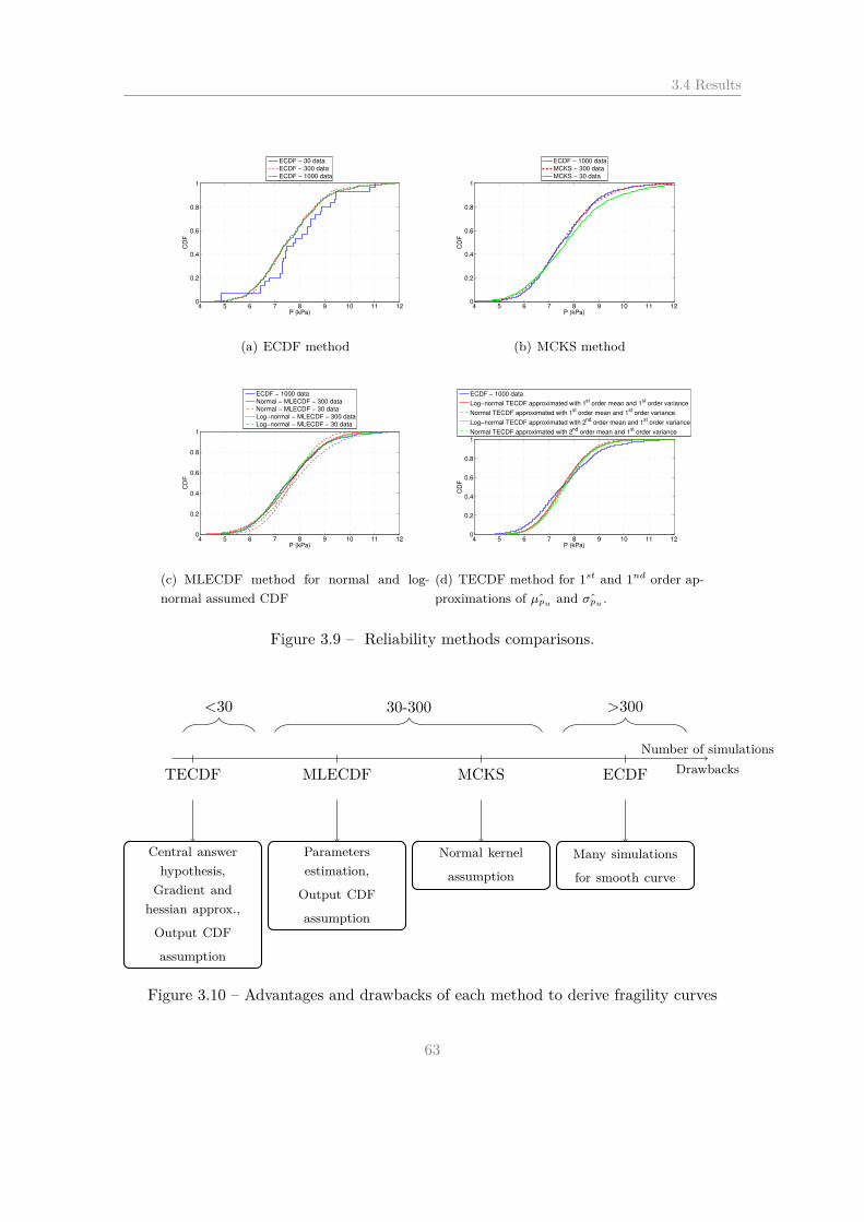
3.4 Results
4 5 6 7 8 9 10 11 120
0.2
0.4
0.6
0.8
1
P (kPa)
CD
F
ECDF − 30 dataECDF − 300 dataECDF − 1000 data
(a) ECDF method
4 5 6 7 8 9 10 11 120
0.2
0.4
0.6
0.8
1
P (kPa)
CD
F
ECDF − 1000 dataMCKS − 300 dataMCKS − 30 data
(b) MCKS method
4 5 6 7 8 9 10 11 120
0.2
0.4
0.6
0.8
1
P (kPa)
CD
F
ECDF − 1000 dataNormal − MLECDF − 300 dataNormal − MLECDF − 30 dataLog−normal − MLECDF − 300 dataLog−normal − MLECDF − 30 data
(c) MLECDF method for normal and log-
normal assumed CDF
4 5 6 7 8 9 10 11 120
0.2
0.4
0.6
0.8
1
P (kPa)
CD
F
ECDF − 1000 data
Log−normal TECDF approximated with 1st
order mean and 1st
order variance
Normal TECDF approximated with 1st
order mean and 1st
order variance
Log−normal TECDF approximated with 2nd
order mean and 1st
order variance
Normal TECDF approximated with 2nd
order mean and 1st
order variance
(d) TECDF method for 1st and 1nd order ap-
proximations of ˆµpuand ˆσpu
.
Figure 3.9 – Reliability methods comparisons.
Number of simulations
DrawbacksTECDF MLECDF MCKS ECDF
Central answer
hypothesis,
Gradient and
hessian approx.,
Output CDF
assumption
Parameters
estimation,
Output CDF
assumption
Normal kernel
assumption
Many simulations
for smooth curve
<30 30-300 >300
Figure 3.10 – Advantages and drawbacks of each method to derive fragility curves
63

3. Reliability-based physical vulnerability assessment of a RC wall impacted by snow avalanchesusing a nonlinear SDOF model
curve (Figure 3.9b). The same conclusion can be drawn in the case of MLECDF method,
which by definition always lead to smooth curves. A significant effect of the assumed
output CDF can be noticed for low simulation numbers but it disappeared when 300
simulations are performed (Figure 3.9c).
In the case of the TECDF method, the approximation of the first and the second cen-
tred moments combined with normal or log-normal CDF needs only 15 simulations at the
1st order. One simulation allows approximating the mean at the 1st order and 14 simula-
tions allow approximating the variance at the 1st order. The 2nd order mean estimation
needs 113 simulations. For TECDF method, the approximation of fragility curve exhibits
slight differences compared to the ECDF fragility curve whatever the assumed output
CDF (Figure 3.9d). This method is based on the assumption that a good estimator of
the output mean of the model can be calculated with the mean of input variables (central
answer). This assumption is fully valid when the deterministic model is linear. Thus, the
observed differences can be due to the non-linearity of the SDOF model. Nevertheless,
if non linearities of the deterministic model are not too significant, few simulations are
needed which allows deriving quickly fragility curves. The efficiency and drawbacks of each
methods are summed up in the scheme of figure 3.10. To conduct the sensibility analy-
sis of fragility curves, the kernel smoothing method is a good compromise. It allows to
take into account possible non-linearities of the deterministic model and to obtain smooth
curves without too much MC simulations and without any assumption on the shape of
the fragility curve.
3.4.2 Fragility curve sensitivity to inputs
Input PDF effect
Four cases are considered. First, all COVs are set to 0.05 (set 1.α.a). Second, COVs are set
to their maximal value deduced from the literature (set 1.α.b). Intermediate COV values
(set 2.β.b) are used for the third case. These latter combinations involve independent
random variables. The last case used JCSS PDF distributions (set 2.β.J , J refering to
section 3.3.2) where correlation between strength parameters is accounted for. The derived
fragility curves are depicted in figure 3.11.
Independent input PDFs give similar fragility curves when they are centered around
the same nominal values. For the three independent cases, the 50% quantile is similar and
the fragility range, defined as the interval between the 2.5% and 97.5% quantile, varies
slightly (Table 3.4). The more the COV have important values, the more the fragility
curve is spread. Finally, correlations between strength parameters induce a shift of the
fragility curve toward higher pressures.
64

3.4 Results
4 5 6 7 8 9 10 11 12 130
0.1
0.2
0.3
0.4
0.5
0.6
0.7
0.8
0.9
1
P (kPa)
CD
F
(1.α.a) set
(1.α.b) set
(2.β.b) set
(2.β.J) set
Figure 3.11 – Vulnerability depending on types of statistical inputs PDF based on MCKS
method.
Input PDF set 2.5% 50% 97.5%
set (1.α.a) 5.6 7.5 9.9
set (1.α.b) 5.4 7.4 10.1
set (2.β.b) 6.0 7.6 9.2
set (2.β.J) 6.9 8.3 9.9
set (3.α.a) 6.7 7.57 8.4
set (3.γ.a) 6.9 7.59 8.2
set (3.γ.c) (-) 7.56 (-)
Table 3.4 – The 2.5%, 50% and 97.5% quantiles (in kPa) of the fragility curves according
to the input PDF reference set. J refers to section 3.3.2.
65

3. Reliability-based physical vulnerability assessment of a RC wall impacted by snow avalanchesusing a nonlinear SDOF model
4 6 8 10 12 140
0.2
0.4
0.6
0.8
1
P (kPa)
CD
F
MCKS (Normal kernel − 300 data)
ECDF
MLECDF (Lognormal CDF −parameters from empirical estimate − MLE)
set (3.α.a)
set (3.γ.a)
set (3.γ.c)
set (1.α.a)
Figure 3.12 – Effect on fragility curves of the number and the class of input parameters.
The black curve corresponds to the determinist case. Red (resp. blue and black dashed)
curves are derived from MCKS (resp. ECDF and MLECDF) method.
Number and class of random variables
Three combinations of input PDFs are considered. First, the deterministic case (set 3.γ.c)
is taken as the reference fragility curve. Second, only geometrical inputs are supposed
deterministic (set 3.α.a). Third, only the material strength parameters are described as
random variables (set 3.γ.a). Finally, all the input variables are considered as random
variables (set 1.α.a). Results are presented in figure 3.12.
The number of inputs random parameters controls the fragility curve spreading (Tab.
3.4). If the geometrical uncertainties are not considered, the fragility range drops from
[5.6 − 9.9] kPa to [6.7 − 8.4] kPa. Assuming the reinforcement ratio as deterministic, the
fragility range drops from [6.7 − 8.4] kPa to [6.9 − 8.2] kPa. The more random input
variables are considered, the more wide is the fragility range. Finally, one can notice
the asymmetry of the fragility range even if inputs distributions are symmetric (normal
PDFs).
3.4.3 Effect of physical parameters
Length effect
The ultimate pressure value (pu) is significantly influenced by the nominal length of the
RC wall (Figure 3.13a). The longer the RC wall is, the lower the ultimate pressure is
(Pu = 8MuL ). The 2.5%, 50% and 97.5% quantiles underline the fragility curve spreading
(Table 3.5). In a semi log-scale, the fragility range is almost the same for each fragility
66
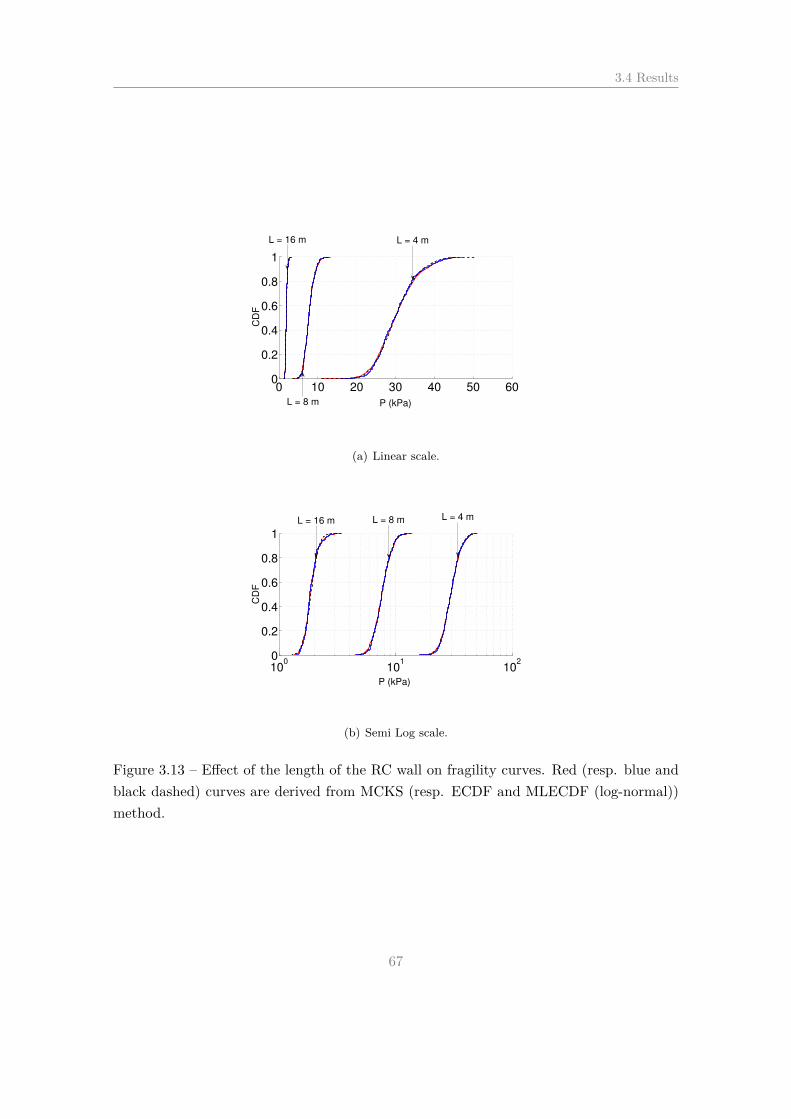
3.4 Results
0 10 20 30 40 50 600
0.2
0.4
0.6
0.8
1
P (kPa)
CD
F
L = 4 m
L = 8 m
L = 16 m
(a) Linear scale.
100
101
102
0
0.2
0.4
0.6
0.8
1
P (kPa)
CD
F
L = 4 mL = 8 mL = 16 m
(b) Semi Log scale.
Figure 3.13 – Effect of the length of the RC wall on fragility curves. Red (resp. blue and
black dashed) curves are derived from MCKS (resp. ECDF and MLECDF (log-normal))
method.
67

3. Reliability-based physical vulnerability assessment of a RC wall impacted by snow avalanchesusing a nonlinear SDOF model
RC wall length (L) 2.5% 50% 97.5%
4 m 22.4 29.79 40.3
8 m 5.6 7.45 9.9
16 m 1.5 1.85 2.4
Reinforcement Ratio (ρr)
0.3% 5.2 5.8 6.2
0.4% 6.9 7.6 8.2
0.5% 8.6 9.3 9.9
1.8% 17.4 18.8 20.4
Table 3.5 – The 2.5%, 50% and 97.5% quantiles (in kPa) of the fragility curves according
to the length and reinforcement ratio.
curve (Figure 3.13b). If the fragility range spreading is normalized by the 50% quantile
((Q97.5% −Q2.5%)/Q50%) it leads to 0.48, 0.58 and 0.60 for respectively 16m, 8m and 4m.
Reinforcement ratio
The influence of reinforcement ratio is explored for several typical values. Lower the
reinforcement ratio is, lower the ultimate pressure is (Figure 3.14). The values of the 50%
quantile are presented in Table 3.5. In a semi-log scale (Figure 3.14b), fragility range
spreading is almost the same for each fragility curves respectively to the 50%-quantile.
Because, the reinforcement ratio plays an important role in the failure mode of the
structure, high density reinforcement ratio is tested (1.8%). For a low reinforcement
ratio (< 1%), the failure of the RC member occurs by reaching the ultimate stain within
steel. On the contrary, for a high reinforcement ratio, the concrete reaches its ultimate
strain first. This aspect is implicitly taken into account by the Bending moment-Curvature
relationship. Nevertheless, for highly reinforced RC members, the failure mode can change
depending on the magnitude of traversal shearing forces (along y axis) and, thus, a bending
failure mode can be questionable when the length of the RC wall becomes small.
Loading rate effect
Depending on the structure mechanical features and the snow avalanche loading, inertial
effects can develop and modify the structural response through time. For all the previous
results, a loading rate of 0.3 kPa.s−1 has been used. In order to assess the SDOF model
sensibility to loading rate, higher values were tested: 6 and 10 kPa.s−1. Resulting fragility
curves are depicted in figure 3.15. For higher loading rates, inertial effects are more
predominant, which leads to an artificial increase of the structure strength. However, this
68

3.4 Results
4 6 8 10 12 14 16 18 20 22 240
0.2
0.4
0.6
0.8
1
P (kPa)
CD
F
ρr = 0.3%
ρr = 0.4%
ρr = 0.5% ρ
r = 1.8%
(a) Linear scale.
101
0
0.2
0.4
0.6
0.8
1
P (kPa)
CD
F
ρr = 0.3% ρ
r = 0.5% ρ
r = 1.8%
ρr = 0.4%
(b) Semi Log scale.
Figure 3.14 – Effect of the reinforcement ratio on fragility curves. Red (resp. blue and
black dashed) curves are derived from MCKS (resp. ECDF and MLECDF (log-normal))
method.
69

3. Reliability-based physical vulnerability assessment of a RC wall impacted by snow avalanchesusing a nonlinear SDOF model
6 6.5 7 7.5 8 8.5 9 9.50
0.2
0.4
0.6
0.8
1
P (kPa)
CD
F
0.3 kPa.s−1 10 kPa.s
−1
6 kPa.s−1
Figure 3.15 – Loading rate effect on the fragility curve. Red (resp. blue and black dashed)
curves are derived from MCKS (resp. ECDF and MLECDF (log-normal)) method.
result should be used with caution. In this paper, a triangular shape describes the time
evolution of the loading. Thus, for high loading rates, the duration of the applied pressure
becomes shorter. The limit case is the Dirac loading signal which induces an impulsive
response of the structure. The energy transferred to the structure is low and the collapse
of the structure can occur only for higher pressures than in the static case. Obviously, in
the case of higher loading duration, for instance using a trapezoidal loading signal, the
fragility curves would be significantly affected.
3.4.4 Comparison to Favier et al. (2014a)’s fragility curves
Based on classical design engineering approach, (Favier et al., 2014a) proposed to obtain
ultimate pressures related to typical limit states of the RC structure. Four limit states
have been defined (Elast, ULS, ALS and YLT). The limit state “Elast” is related to the
reaching of the elastic limit within the RC member. “ULS” (resp. “ALS”) is based on
the classical definition of the ultimate (resp. accidental) limit state given in the Eurocode
2, which allows calculating the ultimate pressure considering safety coefficients related to
strength parameters of the RC member. The last limit state allows obtaining the collapse
70

3.4 Results
100
101
102
0
0.5
1
P (kPa)
CD
F
YLT
MCKS method
Figure 3.16 – Fragility curves comparison with Favier et al. (2014a)’s study.
pressure deduced from the classical yield line theory (“YLT”). Several boundary conditions
were investigated (clamped, supported, free and combination of these latter).
The comparison with our results is presented in figure 3.16. The same input PDFs have
been considered in both studies where COVs equal to 0.05 for all random variables (set
1.α.a). The derived fragility curve shows that the structure collapses for lower pressure
values compared to Favier et al. (2014a) which is mainly due to boundary conditions.
Indeed, one-way slab configuration lead to lower structural capacity compared to those
considered by Favier et al. (2014a).
3.4.5 CDF Tails
Methods presented in this study allows defining accurately the central response of the
fragility range. An important aspect, for instance in structure design, is the estimation
of the extremal quantile of the fragility curve. For instance, in a risk analysis framework,
it is important to determine accurately very low quantiles of the fragility curve which
correspond to the lowest loadings for which collapse cannot be excluded. To improve the
estimation of these low quantiles and symetrically of the high quantiles, in the studied case,
71
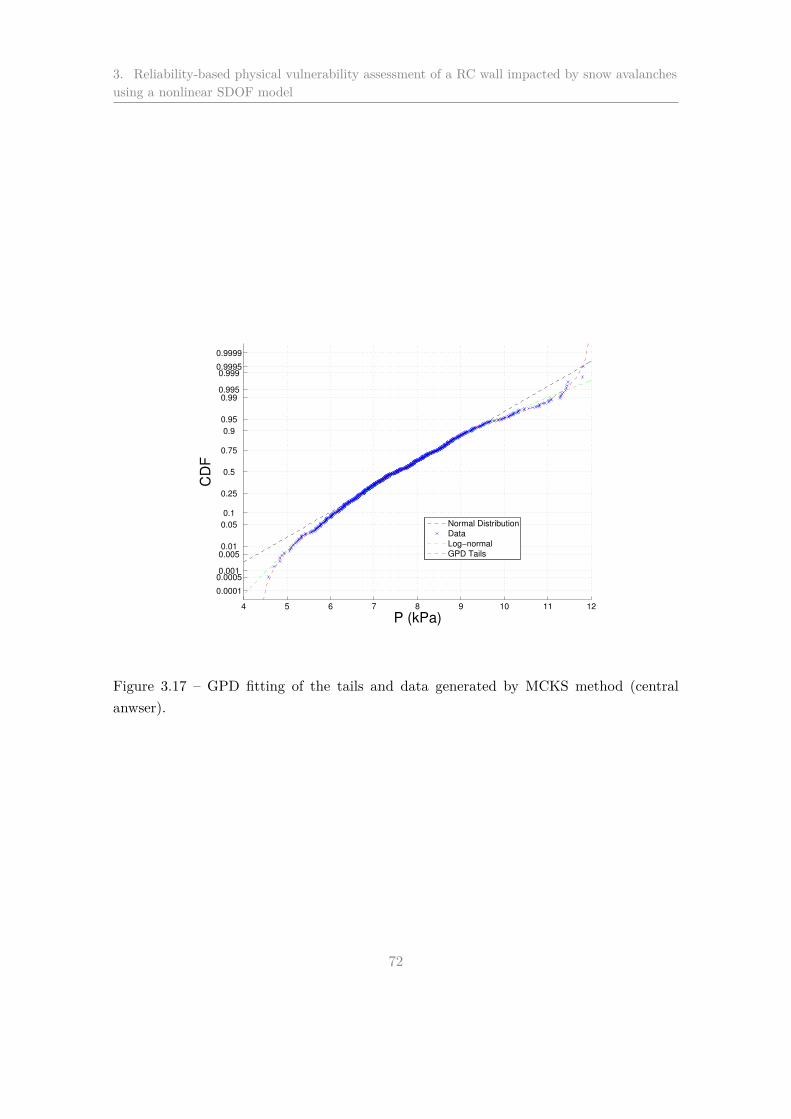
3. Reliability-based physical vulnerability assessment of a RC wall impacted by snow avalanchesusing a nonlinear SDOF model
4 5 6 7 8 9 10 11 12
0.0001
0.00050.001
0.005 0.01
0.05
0.1
0.25
0.5
0.75
0.9
0.95
0.99 0.995
0.999 0.9995
0.9999
P (kPa)
CD
F
Normal Distribution
Data
Log−normal
GPD Tails
Figure 3.17 – GPD fitting of the tails and data generated by MCKS method (central
anwser).
72

3.5 Conclusions
the two tails of the sample are assumed to follow a Generalized Pareto Distribution (GPD)
statistical distribution (Coles, 2001) which is the suitable distribution for exceedances of
high thresholds (Pickands, 1975). For the middle of the sample (90% of the data), the
MCKS method is used to fit data. The figure 3.17 depicts the results of this approach
(MCKS + GPD tail) to full parametric approaches (normal and log-normal). It underlines
that even if the full parametric approaches will be relevant to estimate the central part of
the fragility curve, they may lead to wrongly estimate very high / low quantiles. If these
are really important, extrapolation beyond the empirical sample should be performed
rather with specific approaches as the GPD extreme value based one.
3.5 Conclusions
This paper presents solutions to derive fragility curves to snow avalanches within a reliabil-
ity framework. A one-way simply supported RC wall exposed to snow avalanche loadings
has been considered. A deterministic model based on mass-spring system equivalence has
been used. The ability of the SDOF model to predict the RC wall mechanical response
has been validated by FEA and limit analysis comparisons. Using a SDOF approach al-
lows reducing significantly the CPU time (70 times faster than FEM simulations) needed
to perform a single simulation and allows accounting for the physics involved up to the
collapse of the structure during the interaction between the wall and the avalanche.
Four methods have been proposed to derive fragility curves. ECDF and MCKS are
mainly based on MC simulations. For TECDF and MLECDF methods, the shape of the
fragilty curve is the main assumption. The fragility curves are obtained following two steps:
(1) postulate CDF functions (lognormal or normal CDF) and (2) calculate parameters of
the CDF by maximum likelihood estimation or by Taylor expansion approximation. All
methods give similar results whatever the configuration considered at least for the core of
the distribution. If very low / high quantiles are needed, our preliminary GPD application
approaches should be accounted, focusing on specific techniques from EVT. This could be
considered for structural engineering when very low failure probability are of interest.
The advantages and drawbacks of each methods have been identified. This framework
could be used for a large range of reliability-based engineering applications. The simplified
mechanical model allows to reduce computation time. The choice of well adapted relia-
bility methods is crucial. It will mainly depend on the available calculation time and the
expected accuracy of the fragility curve (good definition of the central behaviour, better
description of the tails...). From our specific engineering field, systematic fragility curves
have been derived. They supplement the seldom curves already available.
Parametric studies have underlined that fragility curves are very sensitive to physical
73
3. Reliability-based physical vulnerability assessment of a RC wall impacted by snow avalanchesusing a nonlinear SDOF model
parameters such as the RC wall’s geometry, its reinforcement ratio or the loading features.
In particular, the fragility range spreading can strongly vary. From a relative point of view,
if the fragility range is normalized by the 50% quantile, the relative fragility spreading
remains almost the same.
By definition, snow avalanche is a dynamic loading which can involve inertial effects
during the mechanical response of the structure. As a function of the structure’s me-
chanical features (stiffness and mass distribution) and the loading characteristic time, the
loading rate can influence significantly the fragility curve, especially for flexible civil en-
gineering structures which might develop fundamental periods close to the typical time
variation of the pressure applied. If the fundamental period of the structure is lower than
typical loading time, the structure mechanical response can be supposed quasi-static and
thus classical engineering methods of design can be used. Otherwise, dynamic effects have
to be accounted by the deterministic model.
As a perspective, the main difficulty concerns the modelling of the avalanche pressure
which can vary significantly as a function of meteorological conditions and specially in
terms of pressure magnitude and typical time of variation. Pressure magnitude is im-
plicitly taken into account by the fragility curves but the time of variation can have a
significant influence on the structure mechanics. The structure mechanical features are
generally better known than the avalanche loading time evolution. Thus, further researches
accounting for several typical time evolutions of the pressure might be of specific interest
to highlight the influence of avalanche loadings.
Then, the application of this approach to other types of structures is forecasted. Dif-
ferent technologies (masonry, timber, metallic, etc) with more complex geometries might
be investigated using these approaches. The challenge will remain to propose simplified
mechanical models able to account the main involved phenomenon with a reduce CPU
time.
Acknowledgment
The authors are very grateful to the ANR research program MOPERA (Modélisation
probabiliste pour l’Etude du Risque d’Avalanche - avalanches.irstea.fr/mopera-projet/)
and the MAP3 ALCOTRA INTERREG program for financially supporting this work.
74
CHAPTER 4
Sensitivity of avalanche risk to vulnerability relations
Le contenu de ce chapitre a été soumis après révision pour publication dans Cold Regions
Science and Technology, les auteurs sont : Favier, P., Eckert, N., Bertrand, D., and Naaim,
M..
75

4. Sensitivity of avalanche risk to vulnerability relations
Abstract
Long-term avalanche risk assessment is of major importance in mountainous areas. Individual risk methods
used for zoning and defense structure design are now gaining popularity in the effort to overcome the major
drawbacks of approaches based on high return period events only. They require, for instance, precise
vulnerability relations, whereas available knowledge mostly consists in coarse curves inferred from a few
catastrophic events. In this paper, we first considerably expand the vulnerability curve sets in use today
for reinforced concrete buildings and humans inside them. To do so, we take advantage of the results of
a comprehensive reliability analysis of various building types subjected to avalanche loads, and we adapt
them to humans inside buildings using different link functions. The fragility curves obtained propose
refined destruction (building) / death (people) rates as a function of avalanche pressure that can be used
in the risk context exactly like deterministic vulnerability curves.
Second, since land use planning should be done for a reasonably large class of buildings rather than
for a very precise single building type, this study shows how a comprehensive risk sensitivity to vul-
nerability/fragility relation analysis can be conducted. Specifically, we propose bounds and indexes for
individual risk estimates and optimally designed defense structures of both theoretical (quantifying uncer-
tainty/variability that cannot be simply expressed in a probabilistic way) and practical (minimal/maximal
plausible values) aspects. This is implemented on a typical case study from the French Alps. The re-
sults show that individual risk estimates are extremely sensitive to the choice of the vulnerability/fragility
relation, whereas optimal design procedures may well be more robust, in accordance with mathematical
decision theory. These two outcomes are of crucial importance in practice. For example, the individual
risk for buildings and people at various positions in the runout zone spreads over several orders of magni-
tude. For risk zoning, this suggests that the usual (tri)centennial choice may be seen as optimistic since
only abscissas above the 1000-year return period are below standard risk acceptance levels with certainty
according to plausible variations of human fragility. On the other hand, the optimal height of a protective
dam can be more precisely determined, promoting the use of cost-benefit analyses in avalanche engineering.
Keywords: snow avalanche; building vulnerability and fragility; human fragility; risk bounds; risk
sensitivity; optimal design sensitivity; acceptable risk.
4.1 Introduction
Snow avalanches are a serious threat to mountain communities. For their inhabitants, land
use planning and zoning are crucial steps that define where it is “reasonably” safe to build.
Standard engineering procedures generally consider high return periods as reference design
events, e.g. the commonly used 30-, 100- and 300-year return period events. For planners,
zoning then results from the combination of these with additional social and political
considerations. However, this is a simplified means of handling the multivariate danger
resulting from impact pressure, flow depth or deposit volume within a single avalanche
event, that is to say, all the tangible quantities that describe hazard intensity. Furthermore,
high return period-based zoning methods do not explicitly take into account the elements
76

4.1 Introduction
at risk and/or possible budgetary constraints, which does not guarantee that unacceptable
exposure levels cannot be reached and/or that the mitigation choices made are optimal.
To overcome these limitations, an integrated quantitative risk evaluation is an appeal-
ing additional instrument. This approach is based on a solid formalism (Eckert et al.,
2012), for individual or collective risk mapping. Individual risk mapping consists in eval-
uating the expected damage for a typical element at risk at any position in an avalanche
path (Keylock et al., 1999). In contrast, collective risk mapping implies considering a two-
to three-dimensional hazard description together with all elements potentially impacted.
In both cases, zoning then includes both hazard and elements at risk. Another possible
outcome of a quantitative risk approach is the optimal design of mitigation measures based
on risk minimisation, that is to say, a cost-benefit assessment performed throughout the
hazard distribution and, if possible, over a continuous space of potential decisions to be
taken. Mitigation measures of maximal economic efficiency can then be chosen (Eckert
et al., 2008a, 2009; Rheinberger et al., 2009). As a consequence of these advantages over
purely hazard-oriented approaches (high return periods), integral risk management is now
gaining popularity among stakeholders, and has increasing importance in practice (Bründl
et al., 2009).
Specifically, risk quantification requires combining the model describing avalanche haz-
ard with a quantitative assessment of consequences for one or several elements at risk. The
avalanche hazard model consists in the distributions of the characteristics of avalanches
that can occur in the site studied. These distributions are (at least partially) site-specific
and have to be estimated with historical events as much as possible. Two main approaches
exist for workable distributions. “Direct” statistical inference can be used to fit explicit
distributions on relevant avalanche data, mainly runout distances (Lied and Bakkehoi,
1980; McClung and Lied, 1987; Keylock, 2005; Eckert et al., 2007b; Gauer et al., 2010).
As an alternative, richer but more computationally intensive, statistical-dynamical ap-
proaches include hydrodynamical modelling within the probabilistic framework (Barbolini
and Keylock, 2002; Ancey et al., 2004; Eckert et al., 2008b), which can be seen as an ex-
tension of Salm’s method (Salm et al., 1990) to multivariate random inputs. They ensure
the joint distribution of all variables of interest, including the spatio-temporal pressure
field variable (Eckert et al., 2010c). These accurate intensity distributions can then be
combined with the damage susceptibility of elements at risk i.e. the vulnerability relation.
Vulnerability curves are increasing curves with values within the range [0, 1], expressed
as functions of hazard intensity. When studying avalanche-prone areas, the diversity
of elements (people, buildings, infrastructures, etc.) exposed implies the use of several
curves to represent the overall damage potential. For alpine hazards, existing vulnerability
relations mainly focus on buildings. Most of them have been assessed according to field
data (Papathoma-Köhle et al., 2010; Schwendtner et al., 2013; Cappabianca et al., 2008).
77

4. Sensitivity of avalanche risk to vulnerability relations
These empirical curves have drawbacks in that they are based on scarce underlying data
(interpolated with statistical regressions, adding potential approximation errors) and to
be somewhat site-dependent (because of different technology choices in different countries,
for example). More generally, they sometimes fail to provide trustworthy and unique
quantitative damage levels in relation to hazard intensity.
As a consequence, in the specific case of snow avalanches, numerical approaches have
recently emerged to evaluate the vulnerability of buildings more systematically (Bertrand
et al., 2010). Indeed, numerical approaches have the major advantage of being imple-
mentable whenever needed for as many building types/configurations as necessary, pro-
viding a set of vulnerability relations that can be used for risk evaluation. Among existing
numerical approaches, the one detailed in Favier et al. (2014a) made it possible to obtain
fragility curves according to typical limit states of different building types. Limit states are
defined according to relevant ultimate mechanical characteristics for the building studied,
e.g. a maximum allowed displacement or an ultimate strength for a composite material.
The limit state definition remains, however, a difficult task, depending on the interaction
between the hazard and the building (dynamical or quasi-static solicitation) and on the
failure scale chosen (local, semi- local, or global).
The distinction between fragility curves and vulnerability curves is important. For
a given hazard intensity, fragility curves provide a probability of exceeding a limit state
(crudely speaking, a destruction probability), whereas a vulnerability curve provides a
deterministic damage index or rate. As stated above, Favier et al. (2014a) studied the
collapse behaviour of a building within a reliability framework, providing fragility relations
quantifying the probability that the entire building would be completely destroyed. On
the other hand, in the literature, vulnerability curves are often easier to interpret in terms
of a ratio of a building that fails. It is noteworthy that a fragility estimate can be seen as a
conditional expectancy, averaging over the influence of certain factors possibly included in
the “full”, multidimensional, deterministic vulnerability relation (Eckert et al., 2012). As a
consequence, from a mathematical point of view, vulnerability and fragility curves can be
treated and used similarly in the risk framework. However, their intrinsic difference may
induce different interpretations in practice that should be kept in mind while comparing
risk estimates obtained with the two approaches.
Decision-makers typically need to link the vulnerability of buildings to the vulnerabil-
ity of the people inside them. By definition, human vulnerability is always expressed as a
fragility, i.e. as a probability of an individual death as a function of snow avalanche inten-
sity. To do that, some studies have suggested multiplying building vulnerability/fragility
(the distinction is not always clearly made) by a particular coefficient (Wilhelm, 1998).
However, usually, human fragility has been for the most part assessed using past events
(Jónasson et al., 1999; Arnalds et al., 2004; Keylock and Barbolini, 2001; Barbolini et al.,
78

4.2 Introduction
2004a), so that existing curves mainly consist in empirical lethality rates brought together
by smoothing approximations. Section 4.2.1 provides a comprehensive review of existing
relations. Their scarcity shows how necessary it is to transpose recent advances in building
physical vulnerability/fragility assessment to human fragility assessment.
According to these observations, the first objective of this paper is to provide an
updated review of available vulnerability/fragility relations for reinforced concrete (RC)
buildings and humans inside them (Sect. 4.2). Indeed, RC is a commonly used material in
areas endangered by snow avalanches, which ensures reasonable safety in areas with high
exposure to avalanche pressure, i.e. in areas where up to 30 kPa snow avalanche impact
pressures are expected. From this RC vulnerability/fragility curve set, and, specifically,
from the fragility curves of Favier et al. (2014a), we then deduce a large set of human
fragility curves. Linking fragility relations for buildings to human death rates has rarely
been done, and we propose four quantitative methods to achieve this goal.
Another major problem in many individual and total risk assessments for land use
planning is that the exact technology of existing buildings and/or potential new buildings
to be built in the future is unknown or, at least, intrinsically variable. As a consequence,
it may not be easy to choose the relevant vulnerability/fragility relation among those in
existence today, even though this choice may have a considerable influence on the final
risk estimates. The second objective of the paper is therefore to study and quantify
risk sensitivity to the choice of the vulnerability/fragility relation, which has never been
attempted to date to our knowledge. The study was conducted on individual risk for
mapping/zoning purposes and within a decisional procedure aiming at minimising risk
with a defense structure construction.
In Sect. 4.3, we detail how bounds for risk or optimal solutions to the risk minimisation
problem taking into account the variability or (mis)specification of vulnerability/fragility
relations can be defined and derived from our systematic building and human fragility
curve sets. In Sect. 4.4, we apply this methodology to a case study from the French Alps,
illustrating how vulnerability/fragility sensitivity logically provides high risk bounds for
buildings and humans inside them as well as for optimal protection design. This range of
plausible values should be preferred to single values with low robustness for zoning and
the design of defense structures. Section 4.5 discusses the major outcomes of the study,
specifically those highly relevant for practice, including comparison with acceptable levels
and with the results of standard engineering approaches using 30-, 100-, 300- year, etc.
return periods as design events. Section 4.6 summarises and concludes.
79

4. Sensitivity of avalanche risk to vulnerability relations
4.2 From building vulnerability to human fragility
4.2.1 Review of vulnerability and fragility relations for snow avalanches
Physical vulnerability and fragility relations for buildings
Wilhelm (1998) assessed the damage susceptibility of five types of buildings to dense
avalanche flows: light construction, mixed construction (“chalets”), masonry, concrete
buildings with reinforcement and reinforced concrete buildings. To build damage suscep-
tibility curves, his study assumed that four typical pressures needed to be known: pu,
corresponding to the general damage threshold, i.e. valid for every building type, pui, cor-
responding to the specific damage threshold of the building considered, pai, corresponding
to the specific demolition limit and poi, corresponding to the specific destruction limit.
Barbolini et al. (2004a) proposed relations for buildings impacted by mixed snow
avalanches (i.e. snow avalanches composed of two layers, a dense bottom layer and a
powder upper layer). These result from linear fits on two well-documented events in Ty-
rol, Austria and are provided as functions of avalanche impact pressure and flow depth.
Buildings considered are “partly reinforced”. Vulnerability relations are derived by intro-
ducing a specific loss function in addition to the degree of damage evaluated by expert
assessment. The specific loss Vb(P ) corresponds to the vulnerability of the building b
function of the impact pressure P :
Vb(P ) =
{
0.0297P if P ≤ 34 kPa
1 if P > 34 kPa .(4.1)
Fuchs et al. (2007b) implemented a monetary-based method to assess the vulnerability
of buildings and humans, providing expected damage expressed in CHF, the Swiss cur-
rency unit, for several avalanche scenarios. Finally, a numerical approach was adopted by
Bertrand et al. (2010). The method consists first in defining a damage index. Exceedence
of a typical value on this index leads to the failure of the building. By scanning possible
input values of the numerical building model, vulnerability curves are obtained. Updating
the review by Cappabianca et al. (2008), Table 4.1 sums up all these vulnerability relations
available for buildings. The approach chosen by each author is specified (e.g. empirical or
numerical modelling).
In an attempt to systematize and increase this limited set, Favier et al. (2014a) related
uniform pressure on a reinforced or partially reinforced concrete wall to failure probabil-
ities. The goal of the study was to obtain fragility curves for buildings impacted by a
uniform dense avalanche using a reliability approach. A reliability approach consists in
considering probabilistic inputs of a deterministic model to study the occurrence of the
80

4.2 From building vulnerability to human fragility
output studied. Four typical engineering limit states of RC were considered. By assuming
the material behaviour as imperfectly known (at a certain reasonable level of uncertainty),
the probability for reaching one of the four limit states was assessed. The wall was assumed
to collapse due to flexural failure. The four limit states considered were:
• the elastic limit state (Elas) which defines the step between the reversibility and
the irreversibility of building damage. In the case of the RC under flexural strain
and low reinforcement, it is quantified by the appearance of the first cracks in the
concrete under tensile stresses.
• the ultimate limit state (ULS) defined as the onset of plastic yield within steel.
This limit state is Eurocode 2-based and is characterized by the calculation of the
maximum plastic moment developed in the section combined with safety coefficients
applied on the material parameters’ behaviour.
• the accidental limit state (ALS) corresponds to the calculation of the maximum
plastic moment developed in the section combined with lower safety coefficients than
those used in the ULS, i.e., it is a “less safe” limit state.
• the collapse is described by the yield line theory (YLT) (Johansen, 1962): this is
assumed to occur when a complete failure pattern composed of yield lines develops
throughout the wall and leads to the collapse of the RC building.
A wall was modelled, considering ten different boundary condition configurations rep-
resenting construction technology choices. The four edges of the wall were successively
assumed to be clamped, simply supported or free. Hence, the ten configurations are: four
supported; two supported and two clamped; one supported and three clamped; one free
and three supported; one free and three clamped; one clamped and three supported; two
supported and two clamped side by side; four clamped; one clamped, two supported and
one free; one supported, two clamped and one free. As already assumed in Favier et al.
(2014a), these ten configurations can be associated with ten building types. Thus, 40
fragility relations were computed (Figure 4.1(a)). Figure 4.1(b) compares them to empir-
ical and numerical literature-based vulnerability relations (see Sect. 4.5.1 for discussion).
Human fragility relations (lethality rates)
It should be remembered that, by definition, human vulnerability is always expressed
as a fragility, i.e. an individual probability of death (lethality rate) as a function of
snow avalanche intensity. For instance, if the pressure is considered as representing snow
avalanche intensity, human fragility is Vp(P ), where Vp is the probability of death for
people and P is the pressure considered.
81

4. Sensitivity of avalanche risk to vulnerability relations
100
101
102
0
0.2
0.4
0.6
0.8
1
pressure (kPa)
bu
ildin
g v
uln
era
bili
ty,
Vb
ElasULSALSYLT
(a) Vulnerability relations from reliability analysis as a function of the
limit state choice for different building types (Favier et al., 2014a). One
wall with ten boundary conditions is considered together with four different
limit states: Elas is the elastic limit state, ULS is the ultimate limit state,
ALS is the accidental limit state and YLT is the collapse of the building.
10−1
100
101
102
0
0.2
0.4
0.6
0.8
1
pressure (kPa)
bu
ildin
g v
uln
era
bili
ty,
Vb
(Wilhelm, 1998): part. reinforced,dense avalanche (1)
(Wilhelm, 1998): part. reinforced,dense avalanche (2)
(Wilhelm, 1998): RC, denseavalanche (1)
(Wilhelm, 1998): RC, denseavalanche (2)
(Barbolini et al., 2004): partlyreinforced, mixed avalanche
(b) Comparison with other relations from literature (see text for details).
Figure 4.1 – Vulnerability relations for buildings comparing historical/reliability-based
relations (semi-log frame). Vb(P ) is either a probability (reliability point of view) or a
damage level (deterministic point of view). Interpretation of Wilhelm (1998)’s work: (1):
vulnerability is 1 for pressure above pai; (2): vulnerability linearly rises from pai to the
specific destruction limit pressure poi where it reaches 1.
82

4.2 From building vulnerability to human fragility
Table 4.1 – Summary of considered vulnerability approaches (RC is Reinforced Concrete).
element at risk approach(data) max. vuln. avalanche type ref.
building (Figure 4.1)
partly reinforced and
RC
empirical (Swiss data) 1.0 dense Wilhelm (1998)
partly reinforced empirical (Austrian data) 1.0 mixed Barbolini et al. (2004a)
RC numerical - deterministic 1.0 dense Bertrand et al. (2010)
RC numerical - reliability 1.0 dense Favier et al. (2014a)
human inside building
(Figure 4.2)
partly reinforced and
RC
empirical (Swiss data) 0.46 dense Wilhelm (1998)
weak timber or
concrete
empirical (Icelandic data) 1.0 dense Keylock and Barbolini (2001)
partly reinforced empirical (Austrian data) 0.27 mixed Barbolini et al. (2004a)
weak timber or
concrete
empirical (Icelandic data) 0.95 dense Arnalds et al. (2004)
Fragility of people inside buildings was assessed in Barbolini et al. (2004a) by fitting
linear least square regressions on data from two well-documented events in Tyrol, Austria.
The resulting probability of being killed by a mixed avalanche inside a building as a
function of impact pressure is:
Vp(P ) =
0 if P ≤ 5 kPa
0.0094P − 0.0508 if 5 < P ≤ 34 kPa
0.27 if P > 34 kPa .
(4.2)
For each building hit by the avalanche, the authors summarised: the degree of damage
to the building, the impact pressure applied to it, the number of people inside it and the
number of victims. The degrees of damage levels correspond to: 1: no visible damage to
structural elements, damage to frames, windows, etc.; 2: failed chimneys, attics, or gable
walls; damage or collapse of roof; 3: heavy damage to structural elements; 4: partial or
complete failure of the building.
Two other well-documented events in Súðavik and Flateyri, Iceland, were used by
Jónasson et al. (1999) to assess empirical human fragility relations. Considering the same
data, Arnalds et al. (2004) provided a continuously differentiable probability of being killed
by an avalanche Vp(v) as a function of avalanche speed v:
Vp(v) =
{
kv2 if v < v1
c+ av−b if v ≥ v1 ,
(4.3)
where, k = 0.0013, c = 0.95, a = 1.151, b = 18.61 and v1 = 23.0 m.s−1.
83

4. Sensitivity of avalanche risk to vulnerability relations
0 100 200 300 400 5000
0.2
0.4
0.6
0.8
1
pressure (kPa)
hu
ma
n v
uln
era
bili
ty
(Barbolini et al., 2004): mixed avalanche
(Wilhelm, 1998): partially reinforced,dense avalanche(1)
(Wilhelm, 1998): partially reinforced,dense avalanche (2)
(Wilhelm, 1998): RC, dense avalanche (1)
(Wilhelm, 1998): RC, dense avalanche (2)
(Keylock and Barbolini, 2001): data from
(Jonasson et al., 1999), 1st
parameters pair
(Keylock and Barbolini, 2001): data from
(Jonasson et al., 1999), 2nd
parameters pair
(Keylock and Barbolini, 2001): data from
(Jonasson et al., 1999), 3rd
parameters pair
(Arnalds et al., 2004): data from(Jonasson et al., 1999)
Figure 4.2 – Vulnerability relations from the literature for people inside reinforced or
partially reinforced buildings. Arnalds et al. (2004) is added assuming P = ρv2 with ρ =
300kg.m−1. Keylock and Barbolini (2001) parameter pairs in Eq. (4.4): 1st, (C1, C2) =
(0, 79.2); 2nd, (C1, C2) = (2.5, 73.5); 3rd, (C1, C2) = (5, 68.3) (kPa).
Jónasson et al. (1999) specified that most of the houses in the Icelandic villages threat-
ened by avalanches are fairly weak timber or concrete structures with relatively large win-
dows facing the mountainside. This means that this relation is valid for people inside any
such constructions, but may not be easy to apply in other European countries where RC
is more common.
Based on this study, Keylock and Barbolini (2001) proposed fragility relations for
people inside similar buildings with pressure as an index variable instead of velocity:
Vp(P ) =
0 if P ≤ C1
P −C1C2−C1
if C1 < P ≤ C2
1 if P > C2 .
(4.4)
C2 is calculated as a function of C1 so that the average fragility remains equal to 0.29.
Three parameter pairs are proposed: (C1;C2) = {(0; 79.2), (2.5; 73.5), (5; 68.3)} (kPa).
As mentioned by Keylock and Barbolini (2001), for pressures lower than C1, the avalanche
is insufficiently powerful to cause substantial damage and it is assumed that no fatalities
would occur within the building; otherwise, for sufficiently high pressures (higher than
C2), the avalanche is expected to cause 100% fatalities.
Finally, as the only formulation not based on past events, Cappabianca et al. (2008)
84

4.2 From building vulnerability to human fragility
took into consideration Wilhelm (1998), i.e. they used a 0.46 factor to relate the fragility
of a person in a building to the building vulnerability/fragility.
Figure 4.2 and Table 4.1 summarise these relations from the literature for people inside
buildings, showing how rare these relations are. This also highlights the differences in terms
of the methods that were used to derive these relations, and in terms of data quality and
the country and avalanche events on which the calculations were based. For instance, the
building technology variability among and within countries, on which inhabitant fragility
is largely dependent, makes direct comparisons between the different curves difficult. The
extension of the reliability-based approach of Favier et al. (2014a) presented below is an
attempt to fill the gaps by focusing on people within RC buildings.
4.2.2 How can one relate building vulnerability/fragility to lethality
rates?
To take advantage of the systematic curves shown in Figure 4.1, we suggest herein four
ways to derive additional fragility relations for people, connecting the structural fragility
of the building to the lethality rates of humans inside buildings. Four methods are pro-
posed, sorted into three categories. The two empirically based connection methods aim
at providing a coefficient deduced from historical data which can link the two fragility
relations. The ULS-based approach suggests directly using the building fragility relations
obtained with a human safety-based definition of building failure. A more exploratory
method takes advantage of knowing four different probabilities of reaching different limit
states for each building under study. We call this semi-empirical, or the degree-damage
approach.
Empirically
• As indicated above, Wilhelm (1998) and Cappabianca et al. (2008) suggested choos-
ing a 0.46 reduction coefficient linking building vulnerability/fragility to human
fragility. Figure 4.4(b) applies this approach to the set of building fragility curves
at our hand.
• According to Arnalds et al. (2004), this reduction coefficient can be evaluated as a
function of avalanche pressure (Figure 4.3(a)):
Vp(P ) = α(P ) × Vb(P ), (4.5)
where Vp is the human fragility inside a building, Vb is the vulnerability/fragility of
the building and (P ) is the pressure value considered. The coefficient α(P ) resulting
85

4. Sensitivity of avalanche risk to vulnerability relations
from this approach may be valid under certain assumptions only, according to the
validity of Arnalds et al. (2004)’ relations. Nevertheless, we assume here that α(P )
remains a good link between the probability of building failure and the probability
of death inside the building for all structures considered in the reliability study of
Favier et al. (2014a). To be as close as possible to the conditions of Arnalds et al.
(2004), we assessed α(P ) from the weakest configuration considered in Favier et al.
(2014a), the RC wall with one free edge and three supported edges. The resulting
human fragility curves are plotted in Figure 4.4(a).
Using ULS considerations
By definition, the Eurocode limit state, if not exceeded, ensures the safety of people
in Eurocode-based design buildings. By calculating the probability for the building to
reach the ULS, we obtain a maximum probability for the people inside the building to be
killed, resulting in the human fragility curves of Figure 4.4(d). Note that this approach
corresponds to the previous approach with a constant α(P ) = 1, but a different building
fragility relation based on the ULS criterion instead of building collapse.
Semi-empirically
Let us consider the four degrees of damage defined by Barbolini et al. (2004a), to obtain
vulnerability curves in relation to buildings’ degree of damage. A linear regression is used
to link the building’s degree of damage to the vulnerability of the people inside it:
Vp(DD) =
{
0.0297 if DD ≤ 1.34
0.0851DD − 0.1140 if DD > 1.34 .(4.6)
Here, we assume that the four damage degrees defined in this study correspond to the
four structural limit states as the referred to above elastic limit state, ultimate limit state,
accidental limit state and collapse in the reliability-based approach of Favier et al. (2014a).
The fragility for the people inside buildings is simply:
Vp(P ) =4∑
i=1
V ib (P ) × Vp(DDi) , (4.7)
where V ib (P ) is the probability for the building b under the pressure P to overpass the
limit state i, i.e. the ith degree of damage DDi, and Vp(DDi) is the probability of death
in a building at the ith degree of damage DDi according to the fit of Eq. (4.6) depicted
in Figure 4.3(b). The resulting human fragility curves are plotted in Figure 4.4(c).
86

4.2 From building vulnerability to human fragility
0 200 400 6000
0.2
0.4
0.6
0.8
1
pressure (kPa)
vu
lne
rab
ility
building with1 free and 3supported edgespeople insidebuilding
0 250 500
100
102
102
α (
Pr)
(a) Empirical link function: coefficient α(P ) depending on avalanche pressure (kP a).
α(P ) is Arnalds et al. (2004)’s ratio linking people fragility to Favier et al. (2014a)
fragility relation for a RC building with one free edge and three supported edges.
1 1.5 2 2.5 3 3.5 40
0.05
0.1
0.15
0.2
0.25
degree of damage
hu
ma
n v
uln
era
bili
ty
(b) Semi-empirical link function for people inside buildings according to the degree of
damage: (1): no visible damage to structural elements, damage to frames, windows,
etc.; (2): failed chimneys, attics, or gable walls; damage or collapse of roof; (3): heavy
damage to structural elements; (4): partial or complete failure of the building. Data
from Barbolini et al. (2004a)
Figure 4.3 – Link functions between building vulnerability/fragility and human fragility.87

4. Sensitivity of avalanche risk to vulnerability relations
4.2.3 Four sets of reliability-based fragility curves for humans inside
buildings
The resulting four sets of human fragility curves are monotonous and differentiable (Figure
4.4). They differ from each other mainly in their maximum probability of death, ranging
from ≃ 0.41 (degree-damage approach) to 1 (ULS approach). In addition, two types of
shape can be distinguished. The human fragility curves obtained with Wilhelm’s and
the ULS approaches have a classical sigmoidal shape, increasing from 0 to their maximum
value within a pressure range depending on the building configuration considered. In other
words, these two curve sets look quite similar to the building fragility curves from which
they were derived, except that, with Wilhelm’s approach, human fragility is bounded at
0.46. The two other sets obtained with the degree-damage and Arnalds’s approaches show
more original shapes, variable from one building configuration to another, illustrating the
more complex way they were evaluated. Nevertheless, the pressure range on which they
rise from 0 to their maximum value remains similar to the pressure ranges of the two
other sets, simply showing the underlying fragility curves for buildings from which they
all derive.
4.3 Evaluating risk sensitivity to vulnerability/fragility re-
lations
4.3.1 Formal risk framework
In the following, risk is first quantified in a “static” perspective, which consists in calculat-
ing expected damage in order to obtain annual destruction rates for buildings and annual
death rates for the people inside them. Second, a “dynamic” decisional framework is set
by taking into account a potential countermeasure, a dam in the runout zone. Monetary
costs for the building value and dam construction are necessary together with the dam
effect on the hazard intensity distribution, so as to evaluate the remaining residual risk as
a function of the dam height, and to determine the dam height that minimises this risk.
All static and dynamic computations are made in an individual risk perspective, focusing
on a single element at risk (building or person). However, whereas static computations
are made at the annual time scale, dynamic computations are made over the long term
using an actualisation term that accounts for the dam amortisation period.
“Static” risk without countermeasures
Risk is broadly defined in natural hazards as the expected damage, in accordance with
mathematical theory (e.g., Merz et al. (2010) for floods, Mavrouli and Corominas (2010b)
88

4.3 Evaluating risk sensitivity to vulnerability/fragility relations
0 100 2000
0.2
0.4
0.6
0.8
pressure (kPa)
hu
ma
n v
uln
era
bili
ty
4 supported
2 supported2 clamped
1 supported3 clamped
1 free 3 supported
1 free 3 clamped
1 clamped 3 supported
2 supported 2 clamped s. by s.
4 clamped
1 clamped 2 supp./1 free
1 supp./2 clamped1 free
(a) Using Arnalds et al. (2004) ap-
proach: a multiplicative coefficient de-
pending on the pressure is applied on
building fragility.
0 50 100 150 200 2500
0.1
0.2
0.3
0.4
0.5
pressure (kPa)
hu
ma
n v
uln
era
bili
ty
(b) Using Wilhelm (1998) approach: a
constant coefficient is applied on building
fragility.
0 50 100 150 200 2500
0.1
0.2
0.3
0.4
0.5
pressure (kPa)
hu
ma
n v
uln
era
bili
ty
(c) Using the degree damage approach
based on Barbolini et al. (2004a) (Eq.
(4.7)).
0 50 100 150 200 2500
0.2
0.4
0.6
0.8
1
pressure (kPa)
hu
ma
n v
uln
era
bili
ty
(d) Using the ULS approach: α(P r) = 1,
and Vb(P r) is given by the ULS fragility
curves.
Figure 4.4 – Human fragility relations derived from the building fragility curve set. The
legend refers to the ten building types of the reliability-based approach which differ from
each other in the boundary conditions of their four edges: four supported; two supported
and two clamped; one supported and three clamped; one free and three supported; one free
and three clamped; one clamped and three supported; two supported and two clamped
side by side; four clamped; one clamped, two supported and one free; one supported, two
clamped and one free.
89

4. Sensitivity of avalanche risk to vulnerability relations
for rockfall, Jordaan (2005) in engineering, etc.). Following the notations of Eckert et al.
(2012), the specific risk rz for an element at risk z is:
rz = λ
∫
p(y)Vz(y) dy , (4.8)
where λ is the annual avalanche rate, that is to say, the annual frequency occurrence of an
avalanche, p(y) is the (potentially multivariate) avalanche intensity distribution (runout,
flow depth, etc.) and Vz(y) is the vulnerability-fragility of the element z towards the
avalanche intensity y. By definition, the specific risk is expressed in year−1.
Classically, in a two-dimensional cartesian framework, avalanche intensity is defined
by the joint distribution p(P, xstop) of pressure fields P and runout distances xstop. The
specific risk rz(xb) for the element z at the xb abscissa is then:
rz(xb) = λ
∫
p(P |xb ≤ xstop)p(xb ≤ xstop) × Vz(P ) dP . (4.9)
This holds since p(P, xstop) = p(P |xb ≤ xstop)p(xb ≤ xstop), where p(P |xb ≤ xstop) is the
pressure distribution at abscissa xb knowing that xb has been reached by an avalanche and
p(xb ≤ xstop) is the probability for the element at xb to be reached by an avalanche.
According to our approach, the vulnerability of a building is simply the fragility of its
wall facing the avalanche, defined by one of the relations illustrated in Figure 4.1(a). The
resulting annual probability of the building at the abscissa xb reaching its limit state (one
of the four defined above, and used in the specific Vb(P ) relationship considered) is:
rb(xb) = λ
∫
p(P |xb ≤ xstop)p(xb ≤ xstop) × Vb(P ) dP , (4.10)
and the annual probability of death for somebody inside a building at abscissa xb is:
rp(xb) = λ
∫
p(P |xb ≤ xstop)p(xb ≤ xstop) × Vp(P ) dP , (4.11)
with Vp(P ) one of the human fragility relations in Figure 4.4.
Decisional framework: minimising residual risk
To study the sensitivity of decisional procedures to vulnerability relations, the classical
example of the optimal design of a dam height (Eckert et al., 2008a) is reconsidered,
with the fragility curve set from Figure 4.1. The approach minimises the long-term costs
obtained by summing up the construction costs and the expected damage at the building
abscissa xb. This is analogous to the precursor work of Van Danzig (1956) for maritime
dykes in Holland, and it is based on an extensive mathematical theory (Von Neumann and
Morgenstern, 1953; Raiffa, 1968). Hence, the residual risk at the abscissa xb and with a
protective dam hd is:
Rb(xb, hd) = C0hd + C1Aλ
∫
p(P |xb ≤ xstop, hd) × p(xb ≤ xstop, hd) × Vb(P ) dP , (4.12)
90

4.3 Evaluating risk sensitivity to vulnerability/fragility relations
where C0 and C1 are, respectively, the value of the dam per metre height in e·m−1 unit
and the value of the entire threatened building situated at abscissa xb in e(the monetary
currency used herein). The notation “.|hd” denotes that runout and pressure distributions
are now modified in the runout zone, conditional to the dam height hd. A =∑+∞
t=11
(1+it)t
is the actualisation factor to pass from annual to long-term costs, with it the interest rate
for the year t. So the unit for Rb(xb, hd) we consider is e.
Note that the residual risk Rb(xb, hd) is no more than C0hd + C1Arb(xb, hd), with
rb(xb, hd) the specific risk for the building at the abscissa xb with the dam height hd,
highlighting that the approach remains based on individual risk (a single building at
abscissa xb is considered at risk). A similar computation or formalism could easily be
proposed and implemented with humans inside buildings as elements at risk, but this
would imply monetising human life, and we prefer to avoid this ethically contestable issue
at this stage.
4.3.2 Hazard distribution
Outputs of a statistical-dynamical model
In Eqs. (4.9-4.12), avalanche hazard is expressed by the joint distribution of runout dis-
tances and pressure fields. To calculate this, we use the statistical-dynamical model devel-
oped by Eckert et al. (2010c) to easily sample from p(P, xstop). In this model, the avalanche
is (rather classically) modelled by a shallow-water approximation of the mass and momen-
tum conservation equations supplemented by a Voellmy friction law (Naaim et al., 2004) .
Additionally, a statistical model considers the depth and the length of the release area, the
abscissa of release and the friction coefficients as random input variables, so as to provide
the joint distribution of runout distance and velocity spatio-temporal fields as outputs.
Independently, the frequency parameter (mean annual avalanche rate) λ is defined within
a Poisson model of occurrences, a rather usual assumption (e.g. McClung (2003); Eckert
et al. (2007a); Lavigne et al. (2012)). It has recently been proven on case studies using
independent validation data from tree-ring sampling that this statistical-dynamical model
can provide good approximations of the magnitude-frequency relationship in the runout
zone (Schläppy et al., 2014).
Pressure evaluation
To feed the vulnerability relations with the statistical-dynamical simulations, velocities
must be converted into pressures. For a free surface flow, the impact pressure can be
expressed as:
P = Cx12ρv2 , (4.13)
91

4. Sensitivity of avalanche risk to vulnerability relations
where Cx is the drag coefficient, ρ is the fluid density and v is the flow velocity. For snow
avalanches, the drag coefficient Cx can now be expressed in rather realistic ways according,
e.g., to the empirical formulation of Sovilla et al. (2008a) or the semi-empirical formulation
of Naaim et al. (2008c). These depend on the Froude number of the flow, highlighting the
potentially high impact pressures exerted by flows close to rest. Here, to greater simplicity,
we instead use a constant drag coefficient of 2. The dynamic pressure on the impacted
wall considered is then ρV 2, a common approximation in engineering. Note, however, that
our approach can easily be employed with other drag coefficient assumptions than ours,
as soon as Cx can be readily evaluated for each simulation in the statistical-dynamical
set-up, as demonstrated in Eckert et al. (2010c).
Optimal design computations: obstacle / flow interaction and delta propaga-
tion
For the decisional risk calculations, one must also compute the residual risk for each dam
height, which requires the quantification of the dam effects on the flow. According to Faug
et al. (2008), semi-empirical relations can be used to account for the effect of a vertical
dam on snow avalanche flows. Typically, it has been found that the normalised velocity
at the dam abscissa and the normalised flow height are linked through:
v2hd
(xd)
v20(xd)
= 1 − αhd
2h, (4.14)
where vhd(xd) is the velocity at the dam abscissa with a dam height hd, v0(xd) is the
velocity at the dam abscissa without the dam, h is the flow height at the dam abscissa
and α = 0.14 is the energy dissipation coefficient determined by Faug et al. (2008) on the
basis of small and real-scale flow experiments and energy budget considerations.
Once the modified velocity at the dam abscissa is known, one must propagate the
effect of the dam on the avalanche characteristics along the entire runout zone. A simple
method consists in assuming a delta propagation. This approach suggests that the velocity
decrease is propagated homogeneously throughout the velocity profile after the dam. First,
the difference of velocities δvelocity at the dam abscissa is calculated. Then this delta is
subtracted from the rest of the velocity profile:
δvelocity = v0(xd) − vhd(xd) (4.15)
Hence, for any abscissa x in the path, the velocity vhd(x) of the avalanche with the
dam height hd is:
vhd(x) =
{
max ((v0(x) − δvelocity), 0) if x ≥ xd
v0(x) else ,(4.16)
92
4.3 Evaluating risk sensitivity to vulnerability/fragility relations
whith v0(x) the velocity of the avalanche at the x abscissa with no dam.
Finally, the optimal dam height hopt is found by minimising the residual risk expressed
in Eq. (4.12):
hopt = argminhd
(Rb(xb, hd)) , (4.17)
where the function argmin gives the height hd at which Rb is minimal for a building
abscissa position xb.
4.3.3 Quantifying sensitivity to vulnerability/fragility: bounds and in-
dexes
Since the objective of the paper is to study how risk estimates and optimal design values
vary across vulnerability formulations, we now propose quantitative sensitivity indicators
that may illustrate some theoretical (general) and practical (local, for case studies) aspects.
Fragility-based risk bounds for buildings
As detailed in Sect. 4.2, in Favier et al. (2014a), four limit states were used to calculate
probabilities for buildings to reach different limit states, and, hence, as surrogates of de-
struction probabilities as a function of the pressure load. This was done for 10 building
configurations differing in their boundary conditions, providing as many as 40 fragility
relations. By evaluating Eq. (4.10) with these 40 relations throughout the runout zone, a
set of 40 individual risk curves rb(xb) representing different evaluations of annual destruc-
tion rates is obtained. The main advantage of doing this is to build plausible intervals for
risk taking into account a certain variability in the response of the RC building considered
to the avalanche load. Hence, as an outline for operational applications aiming at assess-
ing the risk of a building being destroyed, relevant intervals can be determined, taking
into account imperfect knowledge of the most relevant failure state and/or the variability
within a reasonably large building class.
Specifically, a useful but very large interval can be delimited by, as the upper bound,
the risk for the “weakest” building (in terms of geometry / boundary conditions) to reach
the elastic state, and, as the lower bound, the risk for the “strongest” building to reach
the collapse state. Another relevant risk interval, less wide and which enables to remain
consistent among limit states use is defined by: as the lower bound, the risk of the strongest
building collapsing, and, as the upper bound, the risk of the weakest building collapsing,
and, similarly, with the three other limit states considered, providing four specific limit
state intervals whose union corresponds to the overall interval defined above.
93

4. Sensitivity of avalanche risk to vulnerability relations
Fragility-based risk bounds for humans
By developing new human fragility relations in Sect. 4.2, we have increased the number
of available relations relating avalanche hazard to a probability of death for people inside
buildings. As for buildings, evaluating Eq. (4.11) with these curves makes it possible to
obtain various individual risk curves for people inside buildings in the runout zone.
This panel of human risk curves reflects the same uncertainty/variability sources as
for building fragility, but taking into account the additional uncertainty resulting from the
choice of the link function between human and building fragility. This implies that the
assumptions made above to set a link function have to be kept in mind when interpreting
human risk results. However, with this approach, sensitivity towards fragility relations
of human risk estimates can at least be quantified, a crucial point in practice. As for
buildings, this can be done with upper/lower bounds, either with all the human fragility
curves illustrated in Figure 4.4 together or distinguishing the four sets, corresponding to
Figure 4.4 a-d, depending on the link function: empirically based - Arnalds’s, empirically-
based - Wilhelm, ULS or degree-damage.
Sensitivity indexes in risk minimisation (optimal design)
Finally, to assess the sensitivity to building fragility relations of optimal dam heights, we
evaluate the spread of the solutions based on Eq.(4.17) towards the 10 relations corre-
sponding to the 10 building configurations through:
δhopt =hopt,max − hopt,min
hopt, (4.18)
where hopt,max = maxi=1,...10
hopt,i (resp. min), with hopt,i the optimal value minimising the
residual risk obtained in Eq.(4.17), when considering the ith fragility curve for modelling
the fragility of building b. We compute this index for the four limit states separately, and
for different positions xb in the runout zone.
We compare δhopt to the risk spread that is similarly quantified with the indicator δR
calculated for the 10 fragility relations, for each limit state, as:
δR =max(R(xb, 0)) −min(R(xb, 0))
R(xb, 0). (4.19)
The notation R(xb, 0) indicates that the risk spread over fragility relations is evaluated at
the abscissa xb without any countermeasure (hd = 0).
4.3.4 Numerical risk computations
Classically, Eqs. (4.10) and (4.11) are discretely solved for the element z under study (the
building or people inside the building) by the Monte Carlo integral:
94
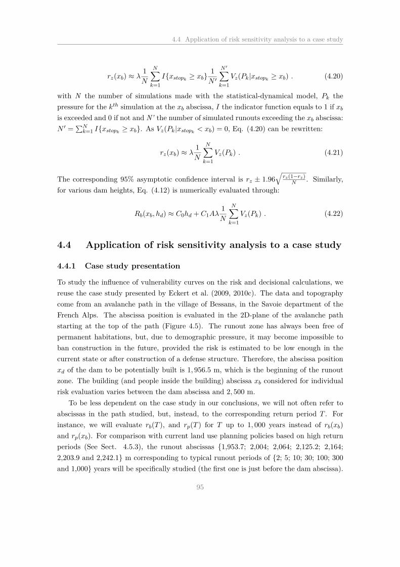
4.4 Application of risk sensitivity analysis to a case study
rz(xb) ≈ λ1N
N∑
k=1
I{xstopk≥ xb}
1N ′
N ′
∑
k=1
Vz(Pk|xstopk≥ xb) . (4.20)
with N the number of simulations made with the statistical-dynamical model, Pk the
pressure for the kth simulation at the xb abscissa, I the indicator function equals to 1 if xb
is exceeded and 0 if not and N’ the number of simulated runouts exceeding the xb abscissa:
N ′ =∑N
k=1 I{xstopk≥ xb}. As Vz(Pk|xstopk
< xb) = 0, Eq. (4.20) can be rewritten:
rz(xb) ≈ λ1N
N∑
k=1
Vz(Pk) . (4.21)
The corresponding 95% asymptotic confidence interval is rz ± 1.96√
rz(1−rz)N . Similarly,
for various dam heights, Eq. (4.12) is numerically evaluated through:
Rb(xb, hd) ≈ C0hd + C1Aλ1N
N∑
k=1
Vz(Pk) . (4.22)
4.4 Application of risk sensitivity analysis to a case study
4.4.1 Case study presentation
To study the influence of vulnerability curves on the risk and decisional calculations, we
reuse the case study presented by Eckert et al. (2009, 2010c). The data and topography
come from an avalanche path in the village of Bessans, in the Savoie department of the
French Alps. The abscissa position is evaluated in the 2D-plane of the avalanche path
starting at the top of the path (Figure 4.5). The runout zone has always been free of
permanent habitations, but, due to demographic pressure, it may become impossible to
ban construction in the future, provided the risk is estimated to be low enough in the
current state or after construction of a defense structure. Therefore, the abscissa position
xd of the dam to be potentially built is 1, 956.5 m, which is the beginning of the runout
zone. The building (and people inside the building) abscissa xb considered for individual
risk evaluation varies between the dam abscissa and 2, 500 m.
To be less dependent on the case study in our conclusions, we will not often refer to
abscissas in the path studied, but, instead, to the corresponding return period T . For
instance, we will evaluate rb(T ), and rp(T ) for T up to 1, 000 years instead of rb(xb)
and rp(xb). For comparison with current land use planning policies based on high return
periods (See Sect. 4.5.3), the runout abscissas {1,953.7; 2,004; 2,064; 2,125.2; 2,164;
2,203.9 and 2,242.1} m corresponding to typical runout periods of {2; 5; 10; 30; 100; 300
and 1,000} years will be specifically studied (the first one is just before the dam abscissa).
95

4. Sensitivity of avalanche risk to vulnerability relations
Figure 4.5 – 2D topography of the path studied (Bessans township, French Alps). xd is
the abscissa where dam construction is envisaged, and xb is the abscissa of the building
at risk. The facing wall is highlighted in red as its failure is assumed to be representative
of the failure of the whole building.
The one-to-one mapping between runout distance and return period results from Eq.
(4.23):
T =1
λ(1 − F (xstop)), (4.23)
where λ is the avalanche rate estimator and F (xstop) is the estimated cumulative distribu-
tion function of the runout distance, approximated by the runout outputs from statistical-
dynamical model simulations conditional to model parameter estimates. These estimates
(best guesses, traditionally denoted by a “hat”) have been obtained using Bayesian in-
ference as detailed in Eckert et al. (2010c). For numerical evaluations (Sect. 4.3.4),
N = 20, 000 predictive simulations conditional to these estimates were used.
For the decisional computations, the construction cost for the dam and the building
value (single element at risk) were set to, respectively, 5, 530 e · m−1 and 3 · 106 e. A
is fixed to 25, which is obtained with a constant interest rate it = 4%. Eight abscissa
positions xb in the path were studied for possible building positions: {1, 966.5; 1, 971.5;
1, 976.5; 1, 981.5; 1, 986.5; 1, 991.5; 1, 996.5 and 2, 001.5 m} (resp. corresponding to a
runout period of {2.3; 2.5; 2.8; 3.1; 3.5; 3.9; 4.3 and 4.8 years}). These relatively low values
were chosen so that the dam would have a greater chance to demonstrate its effectiveness.
Indeed, for buildings situated at positions very rarely reached by avalanches, it is very
unlikely that a large defense structure will be economically sound.
96
4.4 Application of risk sensitivity analysis to a case study
4.4.2 Individual risk range for buildings
Figure 4.6 depicts the building risk curves obtained as functions of the runout return period
abscissa for a wall with one free edge and three clamped edges, our weakest configuration.
Given that a very large number of simulations is used for numerical risk evaluations (N =
20, 000), confidence intervals are (very) small for low return periods. On the other hand,
they become very large for high return periods because the runout exceedence probability
is very small, so that only very few events among the simulated set provide non-zero
values. For instance, the lower bounds drop to zero as soon as it becomes possible that no
simulation reaches the corresponding abscissa with pressure sufficient to provide a non-
zero destruction probability for the building considered (it should be remembered that the
probability of reaching the limit state is, somewhat abusively, considered the same as the
destruction probability). However, these confidence intervals are numerical artefacts which
do not reflect epistemic uncertainty regarding the concrete behaviour and/or variability
among different elements at risk. They could be reduced even further if necessary (e.g.
for practice) with more simulations and/or with more efficient approximation methods, so
that they would not be considered in the following.
Globally, risk decreases with the runout return period, a trivial result. Also, for a
given runout return period, the risk is higher when the elastic limit state is considered
than when the ULS is considered, etc. for the two other limit states. This is simply
a natural consequence of the definition of the four limit states along the pushover test
curve (see Favier et al. (2014a)). Specifically, in the log-scale in Figure 4.6, the four
risk curves quasi-linearly decrease with T for return periods up to 500 years, and then
decrease faster and drop to zero, except the elastic limit state-based risk curve for which
the linear decrease goes on even for T longer than 1, 000 years. The linear shape in the
log scale signifies a quasi-exponential decay of runout exceedence probabilities for the case
study, whereas the risk drops to zero as soon as there are close to zero avalanches with
impact pressures strong enough to be associated with significantly non-zero probabilities
of reaching the limit state considered. With the elastic limit state, these probabilities
remain high for the few avalanches that reach very high return periods.
When all building configurations are considered together (Figure 4.7), most of these
conclusions remain true. For instance, even if the variability of building configurations
considered adds “noise”, in general, we still have Elas-based risk > ULS based risk > ALS
based risk > YLT based risk. Nevertheless, for a given return period, risk estimates are
lower than in Figure 4.6 because the nine additional building configurations considered
are stronger, inducing lower probabilities of reaching each limit state. Hence, the pattern
of decay in risk is generally, with regards to Figure 4.6, shifted to the left. For instance,
the annual probability of reaching YLT or even ULS is extremely small for T > 300 years
97

4. Sensitivity of avalanche risk to vulnerability relations
30 100 300 100010
−10
10−5
100
runout return period (year)
ind
ivid
ua
l risk
Elas
ULS
ALS
YLT
Figure 4.6 – Risk (annual limit states reach probability, solid lines) and associated 95%
confidence interval (dotted lines) for a wall with one free edge and three clamped edges.
The four limit states defined in the text are considered (semi-log frame). On the x-axis,
the runout return period is considered instead of the abscissa position in the path. In the
runout zone, the lower bound confidence intervals quickly drop to zero.
with the strongest buildings considered herein.
The resulting risk bounds are therefore very large, showing an overall high sensitivity
to the limit state considered, and, for a given limit state, to the building configuration. In
other words, risk estimates are highly sensitive to the choice of fragility relations, so that
global bounds over the four limit states may be excessively large to be useful in practice.
Hence, Figure 4.8 displays risk intervals as a function of the limit state choice, and Table
4.2 resumes the thus-obtained bounds for classical high return period abscissas.
For example, for T = 100 years, the risk estimates range from 4.5·10−3 (very high, with
the weakest building and the Elas limit state) to 5.5 · 10−7 (very small, with the strongest
building and the YLT limit state), indeed an interval that is too large to be meaningful.
Restricting ourselves to the ULS and ALS, more realistic and useful intervals are obtained,
but still very wide: [1.3 · 10−5 − 1.5 · 10−3] and [5 · 10−6 − 1.2 · 10−3], respectively.
For T = 1, 000 years, the lower bound for risk estimates is non-zero only with the Elas
limit state. The upper bound is ≃ 3 · 10−4 with the Elas limit states and ≃ [3 − 5 · 10−5]
with the other limit states.
98

4.4 Application of risk sensitivity analysis to a case study
30 100 300 100010
−10
10−5
100
runout return period (year)
ind
ivid
ua
l risk
ElasULSALSYLT
Figure 4.7 – Risk (annual probability of reaching the limit state considered) in the runout
zone for the ten building types and the four limit states defined in the text (semi-log
frame).
Table 4.2 – Minimal and maximal individual risk values (annual destruction rate bounds)
for a building at typical return period abscissas Tz where z is the corresponding return
period (in years). These bounds are derived from the reliability curve sets and are given
as function of the four limit states considered.
T2 T5 T10 T30 T100 T300 T1000
Elastic min 0.12 0.058 0.028 0.0041 0.0017 6.7 · 10−4 8.0 · 10−5
max 0.28 0.14 0.074 0.011 0.0045 0.0017 3.1 · 10−4
ULS min 0.0048 0.0016 5.3 · 10−4 4.8 · 10−5 1.3 · 10−5 1.1 · 10−6 0
max 0.10 0.047 0.022 0.0033 0.0015 5.1 · 10−4 4.9 · 10−5
ALS min 0.0029 8.9 · 10−4 2.9 · 10−4 2.7 · 10−5 5.0 · 10−6 2.6 · 10−9 0
max 0.091 0.040 0.019 0.0028 0.0012 4.1 · 10−4 3.8 · 10−5
YLT min 0.0017 4.6 · 10−4 1.4 · 10−4 1.3 · 10−5 5.5 · 10−7 0 0
max 0.071 0.031 0.014 0.0020 8.9 · 10−4 3.0 · 10−4 2.8 · 10−5
4.4.3 Individual risk range for humans inside buildings
Similarly, our human vulnerability relations allow obtaining a range of human risk curves
that translates the same uncertainty/variability sources as for building fragility, but taking
into account the additional uncertainty resulting from the choice of the link function
99

4. Sensitivity of avalanche risk to vulnerability relations
Figure 4.8 – Risk bound definition, i.e. annual destruction probability bound definition:
delimited by the risk for the weakest building and the risk for the strongest building of
reaching each of the four limit states (linear frame).
between human and building fragility (Figure 4.9). Again, the substantial width of the
resulting risk intervals/bounds highlights the strong variability of human risk estimates
depending on the choice of the fragility curve, and more particularly on the choice of the
type of building (boundary conditions, materials properties, etc.) and the human-building
link function (Figure 4.10).
Globally, one has an exponential-like pattern of decay of human risk curves similar
to that of building risk curves, with very low values reached for (nearly) all building
configurations / link functions for T > 1, 000 years only (see Sect. 4.5.3 for discussion).
For a given human-building link function, human risk estimates differ from each other as
a function of the building configuration, exactly like the risk for building estimates. From
one link function to another, human risk curves are less separated than, for buildings,
from one limit state to another. Nevertheless, globally, human risk estimates obtained with
Wilhelm’s approach are the lowest (the most “optimistic” due to the small maximum value
of human fragility it postulates). On the other hand, the ULS approach generally provides
the highest estimates, whereas the Arnalds and degree-damage approaches provide less
separated values spread in between. However, these are only general rules because, due to
the strong influence of building configuration, there are many exceptions (Figure 4.9).
For example, for T = 100 years, the Wilhelm, degree-damage and Arnalds approaches
100
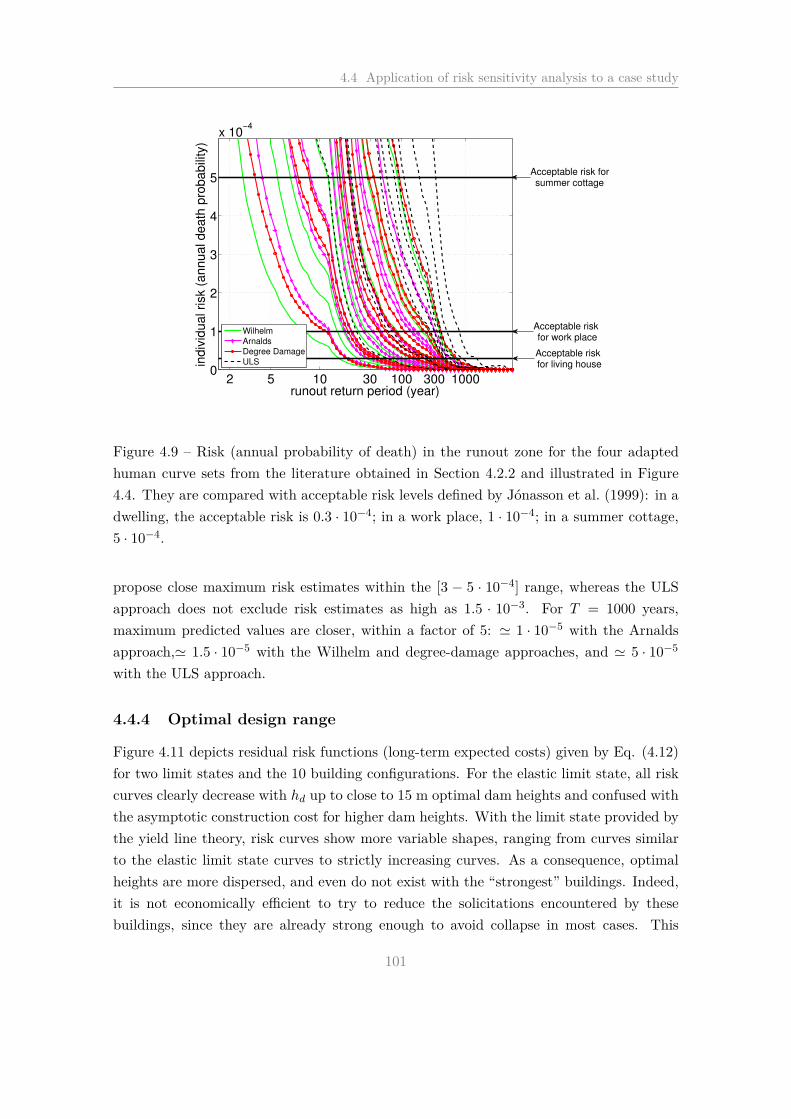
4.4 Application of risk sensitivity analysis to a case study
2 5 10 30 100 300 10000
1
2
3
4
5
x 10−4
runout return period (year)
indiv
idual risk (
annual death
pro
babili
ty)
Wilhelm
Arnalds
Degree Damage
ULS
Acceptable risk for work place
Acceptable risk for living house
Acceptable risk forsummer cottage
Figure 4.9 – Risk (annual probability of death) in the runout zone for the four adapted
human curve sets from the literature obtained in Section 4.2.2 and illustrated in Figure
4.4. They are compared with acceptable risk levels defined by Jónasson et al. (1999): in a
dwelling, the acceptable risk is 0.3 · 10−4; in a work place, 1 · 10−4; in a summer cottage,
5 · 10−4.
propose close maximum risk estimates within the [3 − 5 · 10−4] range, whereas the ULS
approach does not exclude risk estimates as high as 1.5 · 10−3. For T = 1000 years,
maximum predicted values are closer, within a factor of 5: ≃ 1 · 10−5 with the Arnalds
approach,≃ 1.5 · 10−5 with the Wilhelm and degree-damage approaches, and ≃ 5 · 10−5
with the ULS approach.
4.4.4 Optimal design range
Figure 4.11 depicts residual risk functions (long-term expected costs) given by Eq. (4.12)
for two limit states and the 10 building configurations. For the elastic limit state, all risk
curves clearly decrease with hd up to close to 15 m optimal dam heights and confused with
the asymptotic construction cost for higher dam heights. With the limit state provided by
the yield line theory, risk curves show more variable shapes, ranging from curves similar
to the elastic limit state curves to strictly increasing curves. As a consequence, optimal
heights are more dispersed, and even do not exist with the “strongest” buildings. Indeed,
it is not economically efficient to try to reduce the solicitations encountered by these
buildings, since they are already strong enough to avoid collapse in most cases. This
101

4. Sensitivity of avalanche risk to vulnerability relations
Figure 4.10 – Risk bound definition (annual death probability bound definition): for each
of the four human vulnerability curve sets obtained in Section 4.2.2 and illustrated in
Figure 4.4. The risk bounds are delimited, for a given return period abscissa, by the
lowest risk value (strongest building) and the highest risk value (weakest building).
Table 4.3 – Minimal and maximal individual risk values (annual death rate bounds) for a
human inside a building at typical return period abscissas Tz where z is the corresponding
return period (in year). Results of three upon four of the adapted human vulnerability
approaches detailed in Section 4.2.2 are provided. The ULS interval is provided in Table
4.2 (same as for the building).
T2 T5 T10 T30 T100 T300 T1000
Wilhelm min 8.2 · 10−4 2.3 · 10−4 7.2 · 10−5 6.6 · 10−6 2.7 · 10−7 0 0
max 0.035 0.015 0.0068 0.0010 4.4 · 10−4 1.5 · 10−4 1.4 · 10−5
Arnalds min 0.0015 4.0 · 10−4 1.3 · 10−4 1.1 · 10−5 4.4 · 10−7 0 0
max 0.027 0.011 0.0051 7.4 · 10−4 3.0 · 10−4 1.0 · 10−4 8.3 · 10−6
Degree Damage min 0.0011 3.4 · 10−4 1.1 · 10−4 1.0 · 10−5 1.6 · 10−6 6.7 · 10−8 0
max 0.037 0.016 0.0073 0.0011 4.7 · 10−4 1.6 · 10−4 1.5 · 10−5
shows that a full decisional treatment of the problem is not always possible, depending on
when the building failure is assumed to occur and on the building configuration chosen.
Figure 4.12 depicts the risk sensitivity index δR function of the decisional sensitivity
δhopt for the four limit states and for eight different (close) building positions in the runout
zone. Each point represents the normalised spread over the 10 building types investigated
102

4.5 Discussion
(a) Elastic limit state (Elas) (b) Collapse (YLT)
Figure 4.11 – Residual risk (expected loss over the long-term in e) curves as a function
of the dam height provided by Eq. (4.12) for two reliability-based fragility curves sets: a)
Elastic limit state, b) Yield line theory. For each curve, a red circle (◦) denotes optimum
(minimum risk). Abscissa position considered for the building is 1,966.5 m, corresponding
to a return period of 2.3 years (just beyond the dam).
for a specific building position in the runout zone. Substantially, δhopt is always around ten
times lower than δR, a point that argues in favour of much higher robustness of optimal
design approaches with regards to “static” risk evaluations (see Sect. 4.5.4 for discussion).
In greater detail, two scatter-plot groups are observed: an elastic limit state scatter-plot
around δR ≃ 1 and another limit state scatter-plot around δR ≃ 3, confirming that the
risk spread is lower with the elastic limit state than with the other limit states, as already
suggested by Figure 4.11. Note also that, for the close building positions investigated,
significant variations of δhopt compared to the variations of δR occur, since, for a given
limit state, δR is nearly constant, whereas the optimal design sensitivity index varies from
0 to 0.5.
4.5 Discussion
4.5.1 Reliability-based fragility relations versus empirical vulnerability
relations
Building vulnerability relations from the literature rise from 0 to 1 over the [0 − 50] kPa
range (Figure 4.1(b)), whereas some of the reliability-based fragility relations of (Favier
et al., 2014a) reach 1 above 250kPa only (Figure 4.1(a)). Thus, it seems at first glance
that buildings damaged by avalanches that were reported in the literature were more vul-
103

4. Sensitivity of avalanche risk to vulnerability relations
Figure 4.12 – Sensitivity of optimal height to building fragility relations for the four limit
states considered (Eq. (4.18)) versus sensitivity of risk (Eq. (4.19)). Eight abscissa
positions in the path were considered for the exposed building, corresponding to runout
return periods between 2.3 and 4.8 years.
nerable than those considered in (Favier et al., 2014a) and in the present study. This
statement remains questionable, however, since buildings reported in the literature and
the numerically designed buildings in Favier et al. (2014a) are not essentially similar, in
addition to the already discussed variability in technology choices between and within
countries that affects empirical relations. For instance, differences in concrete grade, in
percentages of reinforcement or in the size of the buildings considered could explain dif-
ferences between empirical vulnerability and reliability- based fragility to a given pressure
load.
Another explanation could be a methodological bias: the vulnerability curves reported
in the literature provide damage levels as a function of impact pressures retrieved by
expertise and back-analyses of real events, whereas numerical fragility curves result from
limit states based on mechanical theory whose exceedence probabilities are considered
identical to destruction probabilities. Hence, even if exactly the same building could be
studied with the two approaches, it is presumable that the same vulnerability/fragility
curve would not be obtained. Note also that the failure mode in Favier et al. (2014a)
study was assumed to be the flexural mode, making fragility curves conditional to this
assumption. Other failure definitions could have provided different fragility estimates.
104

4.5 Discussion
Comparing empirical vulnerability relations and Favier et al. (2014a) fragility relations
in the risk calculation results in Figure 4.13. For a given runout abscissa/return period,
risk estimates based on literature vulnerability relations are high. They correspond to
those obtained, with the fragility approach, with the “strongest” building configurations
and the elastic limit state definition (the most pessimistic and conservative of the four
limit states considered) or with weaker building configurations and the elastic ULS/ALS
limit state definition (more “optimistic”). For example, literature-based risk estimates
are ≃ [8 · 10−4 − 3 · 10−3] at the centennial abscissa and still ≃ [2 · 10−5 − 2 · 10−4] at
the millennial abscissa (Table 4.4). Again, this shows that the characteristics of the
vulnerability/fragility relation used (modal value, spread, pressure range within which it
rises from 0 to 1, etc.) are directly propagated on risk estimates, making those highly
sensitive to the choice of the vulnerability/fragility relation.
However, the general shape of the risk curves with the literature vulnerability relations
is essentially similar to the shape of the risk curves with the reliability-based fragility curves
(exponential decay with the runout return period abscissa, Figure 4.13). This suggests
that the fragility relations can be used to supplement the empirical vulnerability curves,
for instance within the risk framework. Indeed, their intrinsic differences in terms of inter-
pretation (deterministic damage index for the empirical vulnerability curves - destruction
probability for the fragility relations) is then totally smoothed in the integral calculation
(Eckert et al., 2012), as illustrated by the different estimates we have obtained for the case
study.
Table 4.4 – Individual risk values (annual destruction rate) for a building at typical return
period abscissas Tz where z is the corresponding return period (in year) with the five
considered vulnerability curves from the literature.
T2 T5 T10 T30 T100 T300 T1000
Barbolini et al. (2004a) 0.17 0.080 0.041 0.0062 0.0025 0.0010 1.5 · 10−4
Wilhelm (1998), part. RC (1) 0.071 0.031 0.014 0.0021 9.0 · 10−4 3.1 · 10−4 3.1 · 10−5
Wilhelm (1998), part. RC (2) 0.063 0.027 0.012 0.0018 7.6 · 10−4 2.6 · 10−4 2.4 · 10−5
Wilhelm (1998), RC (1) 0.11 0.051 0.024 0.0036 0.0015 5.7 · 10−4 5.8 · 10−5
Wilhelm (1998), RC (2) 0.096 0.043 0.020 0.0030 0.0013 4.7 · 10−4 4.8 · 10−5
Regarding human vulnerability of mountain community inhabitants, quantitatively
linking it to the structural vulnerability/fragility of housing buildings is a very important
issue in avalanche engineering practice. As for the buildings themselves (and even more
rarely), human fragility relations have been, in the past, mainly empirically assessed on the
basis of well-documented catastrophic events, leading to survival/death rates as a function
of impact pressure. An appealing alternative has been presented herein to simply derive
105

4. Sensitivity of avalanche risk to vulnerability relations
30 100 300 100010
−10
10−5
100
runout return period (year)
ind
ivid
ua
l risk
Elas
ULS
ALS
YLT
Barbolini et al., 2004
Wilhelm 1998: RC,dense av. (1)
Wilhelm 1998: RC,dense av., (2)
Wilhelm 1998: part. RC,dense av. (1)
Wilhelm 1998: part. RC,dense av., (2)
Figure 4.13 – Risk (annual destruction probability) for a building in the runout zone with
the literature curves, versus risk with reliability-based fragility curves: YLT, ALS, ULS
and Elas curves from Favier et al. (2014a)).
human fragility relations from building fragility curves in a systematic way, assuming var-
ious (three or four) simple deterministic link functions based on existing work. Therefore
a large set of human fragility curves, a function of the link function and the building
configuration, were obtained.
The strong assumptions made to evaluate these curves must be kept in mind while
using and interpreting them. Specifically, the rather simple link functions used herein
are arguably oversimplified preliminary proposals that could be reconsidered in future
studies. However, as for buildings, these have been sufficient to obtain fragility curves
that have shapes similar to the shapes of the empirical literature curves (although highly
dependent on the building configuration and link function), which promotes their use as
an advantageous supplement to the scarce relations available to date. Furthermore, our
human fragility curves were clearly essential to conduct our risk to vulnerability sensitivity
study on a typical case study.
4.5.2 Risk sensitivity to vulnerability/fragility (mis)specification
Vulnerability/fragility relations are one of the key ingredients of a quantitative risk as-
sessment, directly controlling buildings and individual risk estimates for humans inside
buildings, which are the crucial outputs required for avalanche risk zoning in practice.
106

4.5 Discussion
Our application has abundantly illustrated how highly sensitive to the choice of vulnera-
bility/fragility relation these are, whereas existing RC buildings are never perfectly known.
Indeed, existing RC buildings are composed of two materials (concrete and steel) whose
behaviours may be described somewhat inaccurately. Besides, the proportion of steel to-
gether with its arrangement within the concrete matrix can add other uncertainties to the
building description (the same building will never be exactly reproduced).
Furthermore, from a more predictive point of view, risk zoning for land use planning
should not only focus on existing buildings, but should also anticipate the possible con-
struction of a reasonably large class of new construction and still account for the same
uncertainties. From land use planners’ perspective, it is also difficult to know the exact,
most suitable building configuration to choose, as well at the best limit state to concen-
trate on to ensure the safety of building inhabitants together with reasonable architectural
recommendations. This all makes the application of one single curve among the existing
curve set a tricky, if not impossible, task.
How then should this uncertainty/variability and the related high sensitivity of risk
estimates be handled in practice? If this variability/uncertainty could be expressed in a
probabilistic way, the risk framework would easily account for it as an additional source
of randomness to average over. This is illustrated with different examples by Eckert et al.
(2012). For instance, if φ is the additional source of “noise” to be considered (e.g. a
parameter of the hazard or vulnerability model), then, one simply needs to evaluate the
Bayesian-like risk:
r′z(xb) =
∫
rz(xb, φ).p(φ)d(φ), (4.24)
where rz(xb, φ) is, for example, the risk estimates provided by Eq. ((4.9)) with the pa-
rameter value φ and p(φ) its probability distribution . However, in the case of the choice
of a vulnerability/fragility relation, this probabilistic response is presumably not possible.
This is the reason why we chose a “bound approach” instead: ten boundary conditions
were considered, providing ten vulnerability relations for each limit state. Propagating
these curves through the risk calculation allowed us to propose risk bounds, i.e. risk es-
timate ranges that are valid for different boundary conditions and/or different thresholds
above which the building is assumed to fail (limit state).
The width of these intervals precisely quantifies the strong variability of building and
human risk estimates according to the choice of the fragility curve, and more particularly,
to the choice of the type of building (boundary conditions, material properties, etc.).
Bounds are large even for positions in the path only reached by rare avalanches (e.g.
Figure 4.10 for humans), and even higher if the results provided by empirical curves are
considered together with the fragility curves (Tables 4.3 and 4.4).
107

4. Sensitivity of avalanche risk to vulnerability relations
In detail, risk bounds can be refined focusing on one type of variability/uncertainty
only. For buildings, the overall interval mixing all limit states and configurations may
be too large (Figure 4.8), requiring additional assumptions to provide usable values in
practice, such as fixing the considered limit state. For humans inside buildings, the four
link functions provide partially imbricated intervals (Figure 4.10), so that, instead of
setting the link function, making additional reasonable assumptions regarding the building
configuration considered may more efficiently reduce the width of risk bounds.
4.5.3 Comparison with acceptable levels and high return period design
events
To go even further in terms of the practical outcomes of the study, the high return period
abscissas currently used as legal risk assessment limits were compared to the abscissas
where risk estimates provided by our approach are acceptable according to Jónasson et al.
(1999). Acceptable risk values from Jónasson et al. (1999) are: in a dwelling: 0.3 · 10−4;
in a work place: 1 · 10−4; in a summer cottage: 5 · 10−4 (Figure 4.9).
Table 4.5 displays abscissa intervals in the path where these conditions are fulfilled. The
interval spread corresponds to the evaluation of risk estimates with our different human
fragility relations. This shows that acceptable risks for dwellings can be observed for houses
situated above 2, 086.5 m in the avalanche path for the most “optimistic” human fragility
relation, but only above 2, 255.5 m for the most “pessimistic”. This corresponds to runout
return periods of [11.9 − 1, 955] years. Similarly, abscissa intervals of [2, 043.6 − 2, 235.1]
m and [1, 969.6 − 2, 205.5] m (respectively corresponding to runout period of [8 − 693.7]
years and [2.4 − 336] years), depending on the choice of the fragility relation, correspond
to acceptable risk thresholds for, respectively, a work place and a summer cottage.
Again, in addition to dramatically highlighting the sensitivity of risk estimates to the
choice of the vulnerability/fragility relation, this clearly illustrates the limit of return
period-based approaches for human risk zoning. Depending on the vulnerability/fragility
relation, traditional return period-based zoning thresholds can overestimate the risk as
well as underestimate the risk, an obviously critical problem. For instance, the acceptable
risk threshold of 0.3 · 10−4 (in a residential house or building) is reached for 13 out of
40 fragility-based risk curves before attaining the reference centennial abscissa, but only
abscissa positions above the 1, 000-year return period are associated with risk estimates
lower than 0.3 · 10−4 with all fragility relations. Hence, only these can be considered as
fully safe for our typical case study if one takes into account all the possible range of
variability of human fragility relations that this study has suggested.
108
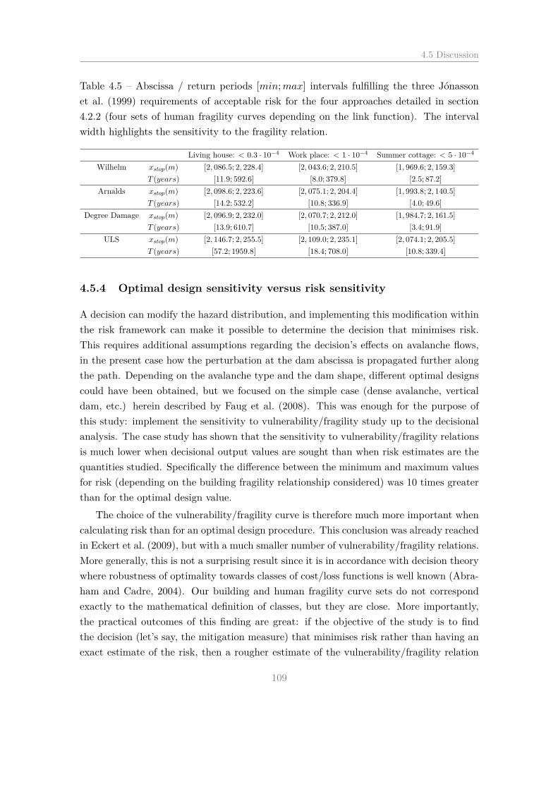
4.5 Discussion
Table 4.5 – Abscissa / return periods [min;max] intervals fulfilling the three Jónasson
et al. (1999) requirements of acceptable risk for the four approaches detailed in section
4.2.2 (four sets of human fragility curves depending on the link function). The interval
width highlights the sensitivity to the fragility relation.
Living house: < 0.3 · 10−4 Work place: < 1 · 10−4 Summer cottage: < 5 · 10−4
Wilhelm xstop(m) [2, 086.5; 2, 228.4] [2, 043.6; 2, 210.5] [1, 969.6; 2, 159.3]
T (years) [11.9; 592.6] [8.0; 379.8] [2.5; 87.2]
Arnalds xstop(m) [2, 098.6; 2, 223.6] [2, 075.1; 2, 204.4] [1, 993.8; 2, 140.5]
T (years) [14.2; 532.2] [10.8; 336.9] [4.0; 49.6]
Degree Damage xstop(m) [2, 096.9; 2, 232.0] [2, 070.7; 2, 212.0] [1, 984.7; 2, 161.5]
T (years) [13.9; 610.7] [10.5; 387.0] [3.4; 91.9]
ULS xstop(m) [2, 146.7; 2, 255.5] [2, 109.0; 2, 235.1] [2, 074.1; 2, 205.5]
T (years) [57.2; 1959.8] [18.4; 708.0] [10.8; 339.4]
4.5.4 Optimal design sensitivity versus risk sensitivity
A decision can modify the hazard distribution, and implementing this modification within
the risk framework can make it possible to determine the decision that minimises risk.
This requires additional assumptions regarding the decision’s effects on avalanche flows,
in the present case how the perturbation at the dam abscissa is propagated further along
the path. Depending on the avalanche type and the dam shape, different optimal designs
could have been obtained, but we focused on the simple case (dense avalanche, vertical
dam, etc.) herein described by Faug et al. (2008). This was enough for the purpose of
this study: implement the sensitivity to vulnerability/fragility study up to the decisional
analysis. The case study has shown that the sensitivity to vulnerability/fragility relations
is much lower when decisional output values are sought than when risk estimates are the
quantities studied. Specifically the difference between the minimum and maximum values
for risk (depending on the building fragility relationship considered) was 10 times greater
than for the optimal design value.
The choice of the vulnerability/fragility curve is therefore much more important when
calculating risk than for an optimal design procedure. This conclusion was already reached
in Eckert et al. (2009), but with a much smaller number of vulnerability/fragility relations.
More generally, this is not a surprising result since it is in accordance with decision theory
where robustness of optimality towards classes of cost/loss functions is well known (Abra-
ham and Cadre, 2004). Our building and human fragility curve sets do not correspond
exactly to the mathematical definition of classes, but they are close. More importantly,
the practical outcomes of this finding are great: if the objective of the study is to find
the decision (let’s say, the mitigation measure) that minimises risk rather than having an
exact estimate of the risk, then a rougher estimate of the vulnerability/fragility relation
109

4. Sensitivity of avalanche risk to vulnerability relations
may be sufficient. This is another point arguing in favour of the use of the systematic but
presumably oversimplified fragility relation set, and also for the promotion of cost benefit
analyses / optimal design approaches in avalanche engineering.
4.6 Conclusion and outlooks
In a nutshell, few relations reflecting vulnerability/fragility to snow avalanches currently
exist for buildings, and even fewer for humans inside buildings. Furthermore, these rela-
tions were mainly derived from catastrophic historical events whose characteristics do not
often correspond to paths where refined risk estimates are needed. In this study, system-
atic reliability analyses of buildings impacted by avalanche loads were used to deduce large
sets of building and human fragility relations according to avalanche pressure. By com-
parison to empirical back analyses, this approach is powerful and infinitely reproducible,
allowing the existing knowledge to be supplemented as needed.
Second, this new large set of curves was used to produce a comprehensive sensitivity
to vulnerability/fragility relation analysis up to the design of a defence structure. To do
so, we promoted the ability of the risk framework to accommodate differences between
vulnerability/fragility, and proposed bounds and indexes of both theoretical (quantifying
uncertainty/variability that cannot be simply expressed in a probabilistic way) and prac-
tical (minimum/maximum plausible values) aspects. In a typical case study, we clearly
showed how highly risk estimates are sensitive to the choice of the vulnerability/fragility
relation, whereas optimal design procedures may be more robust. Even if a certain case-
study dependence may exist, requiring more studies for wider generalisation, these results
enhance our overall understanding of avalanche risk and may therefore well be worth con-
sidering by avalanche engineers. For instance, they clearly show that current runout return
period-based zoning policies can be far from the quantification of true risk. Specifically,
comparisons with acceptable risk levels has highlighted the variability of abscissas in the
path where the acceptable risk threshold is exceeded. For example, for the case study,
only abscissas above the 1, 000 year return period may be considered as fully safe.
The generally high sensitivity to vulnerability/fragility relations that has been high-
lighted emphasizes the need for reliable relations, that is to say accurate and systematically
available relations for a large variety of building types, provided e.g., by fully numerical
approaches. The application presented in this paper was undertaken for a relatively large
class of RC buildings, but using a rather simple numerical engineering approach. Hence,
the results are subjected to all the inherent approximations and assumptions. For example,
the fragility relations were assessed under the assumption of quasi-static pressure loads
only, which is questionable in some typical situations. In the future, a more complex me-
chanical building model could be developed to study a particular geometry and carefully
110

4.7 Acknowledgements
propagate confidence intervals up to risk quantification, taking into account additional
epistemic uncertainties and/or variability sources within the various processes involved.
Similarly, we worked with hazard distributions calibrated on a typical case study, but
in a simple (x,z) geometry (no lateral spread), and with only one building or human taken
into account in an individual risk perspective. For real risk mapping and optimal design
of mitigation measures in already urbanised areas, this is not enough, and expanding the
approach to a 2D to 3D avalanche hazard model is still required. Combining its outputs
with more advanced mechanical models accurately describing the existing buildings, as
discussed above, would definitely help refine the quantification of risk to humans and
buildings, and, therefore, be very useful for managing risk in the most delicate case studies.
4.7 Acknowledgements
The authors thank the ANR research program MOPERA (Modélisation probabiliste pour
l’Étude du Risque d’Avalanche - www.avalanches.fr/mopera-projet/) and the MAP3 Al-
cotra Interreg program for funding this work. The authors are also grateful to P. Gauer
and two anonymous referees whose constructive comments helped to improve the paper.
111

4. Sensitivity of avalanche risk to vulnerability relations
112

CHAPTER 5
Avalanche risk evaluation and protective dam optimal design
using extreme value statistics: simple analytical formulae and
sensitivity study to hazard modeling assumptions
Le contenu de ce chapitre a vocation à être soumis après travail à Journal of Glaciology,
les auteurs en sont : Favier, P., Eckert, N., Bertrand, D., Faug, T. and Naaim, M..
113

5. Avalanche risk evaluation and protective dam optimal design using extreme value statistics:simple analytical formulae and sensitivity study to hazard modeling assumptions
Abstract
In snow avalanche long term forecasting, existing risk-based methods remain difficult to use in a real
engineering context. Yet, they make use of debatable assumptions for hazard modelling. In this work,
we address these limitations by expanding a quasi analytical decisional model so as to obtain simple risk
formulae to quantify risk and perform the optimal design of an avalanche dam in a quick and efficient
way. These may be usable in a variety of situations, as soon as a very generic additive cost model with
a constant damage susceptibility is found suitable. Specifically, the exponential runout model is replaced
by the generalised Pareto distribution (GPD) that has theoretical justifications that promotes its use for
modelling the different possible runout tail behaviours. Regarding the defence structure - flow interaction,
a simple law based on kinetic energy dissipation is confronted to a law based on the volume stored upstream
of the dam whose flexibility make it able to cope for various types of snow. We finally show how a detailed
sensitivity study can be conducted, leading intervals and bounds for risk estimates and optimal design
values.
Application on a typical case study from the French Alps demonstrates that it is often not easy to fit a
robust runout tail distribution on the basis of the data only, making the forecasted high return levels badly
constrained. A profile likelihood approach can tackle this difficulty, but residual risk estimates and optimal
dam heights remain highly variable towards possible runout tail types. Similarly, a very high sensitivity
to the avalanche-dam interaction law exists: the energy dissipation one generally postulates a higher risk
reduction, but the flexility of the volume catch one makes the case of high deposit shape angles due to wet
snow flows an exception to this rule. Also, with this law, the higher complexity of the dependency to the
dam height makes that no solution to the optimal design problem exists over a large range of abscissas in
the runout zone. The highest sensitivity to the runout tail type and interaction law is fond at abscissas of
legal importance for hazard zoning ( return periods of 10 − 1, 000 years), a crucial result for practice. This
all suggests that the tail behaviour of extreme runouts, as well as the energy dissipation and deposition
patterns occurring when an avalanche hits an obstacle should be reinvestigated to reduce uncertainty levels
in operational contexts.
Keywords: Snow Avalanche; Individual Risk; Defense Structure; Risk Minimisation; Extreme Value
Statistics; Runout return period; Interaction Law; Uncertainty Quantification and Propagation.
5.1 Introduction
Snow avalanche long term forecasting for risk mapping and the design of defense structures
is generally done on the basis of high magnitude events defined by their return period
e.g. Salm et al. (1990). Such purely hazard-oriented approaches do not explicitly consider
elements at risk (buildings, people inside, etc.), and neglect possible budgetary constraints.
Therefore, they do not guarantee that unacceptable exposition levels and/or unacceptable
costs cannot be reached. This is well demonstrated in Favier et al. (2014b) by confronting
standard hazard zone limits with acceptable risk levels as defined in Jónasson et al. (1999).
To overcome these limitations, risk based zoning methods (Keylock et al., 1999; Arnalds
114

5.1 Introduction
et al., 2004) and cost-benefit analyses (Fuchs et al., 2007a) have emerged recently in this
field, allowing socioeconomic considerations to be included into the analysis (Bründl et al.,
2009) in a proper mathematical framework (Eckert et al., 2012).
Risk quantification requires combining the model for avalanche hazard with a quan-
titative assessment of consequences for the elements at risk. The hazard distribution is
(at least partially) site-specific, and two main approaches exist to determine it. “Direct”
statistical inference can be used to fit explicit probability distributions on avalanche data,
mainly runout distances (Lied and Bakkehoi, 1980; Eckert et al., 2007b; Gauer et al.,
2010). As an alternative, richer but more computationally intensive, statistical-dynamical
approaches include hydrodynamical modelling within the probabilistic framework (Bar-
bolini and Keylock, 2002; Meunier and Ancey, 2004; Eckert et al., 2008a). They lead the
joint distribution of all variables of interest, including the one of spatio-temporal pressure
fields (Eckert et al., 2010c).
Consequences for elements at risk are estimated using vulnerability relations, i.e. in-
creasing curves with values in [0 − 1] quantifying, for various types of elements at risk
(people, buildings, infrastructures ...), the expected damage as function of avalanche in-
tensity. The latter is generally expressed in terms of impact pressure, but sometimes also
of flow depth or velocity (Barbolini et al., 2004a). Existing vulnerability to snow avalanche
relations have been historically assessed empirically, by back-analysis of well documented
events (Keylock and Barbolini, 2001; Papathoma-Köhle et al., 2010), but numerical ap-
proaches have emerged recently to evaluate more systematically the vulnerability of build-
ings, deterministically (Bertrand et al., 2010), or within a reliability framework (Favier
et al., 2014a).
To conduct a cost benefit analysis between various mitigation solutions and, for in-
stance, minimize the residual risk after the construction of a defense structure, effects
of such structures on avalanche flows must also be quantified. This is complex because
fundamental physical processes are involved (propagating jumps, dead zones and airborne
jets), which are still not fully understood. This makes the full modelling of the interaction
between avalanches and various defense structure types such as dams currently impossible
with state of the art depth-averaged models for avalanche propagation (Bartelt et al., 1999;
Naaim et al., 2004). However, for this purpose, semi-empirical analytic equations could
be developed to describe the runout shortening caused by dam-like obstacles. These laws
were established for walls spanning the whole width of the incoming flow with the help
of simple theoretical arguments combined with small-scale laboratory tests on granular
avalanches. For high Froude number incoming flows (fast dry snow avalanche), a simple
linear relation between the runout shortening and the dam height relative to the incident
flow was evidenced (Hakonardottir, 2000; Faug et al., 2003) and partly verified on avail-
able full-scale observations (Faug et al. (2008)). For low Froude number flows (very slow
115

5. Avalanche risk evaluation and protective dam optimal design using extreme value statistics:simple analytical formulae and sensitivity study to hazard modeling assumptions
avalanche), the runout shortening was found to be a function of the volume stored up-
stream of the dam relative to the total avalanche volume (Faug et al. (2004a)). These two
existing interaction laws correspond to idealized situations for which the runout shortening
is caused by either the local dissipations of kinetic energy (purely inertial regime) or the
volume reduction due to storage of the snow upstream of the dam (purely gravitational
regime). In real world, however, both process may coexist, and other semi-empirical, more
complex laws for the runout shortening may be used (Faug et al., 2003; Faug, 2004).
A specific difficulty remains poorly addressed in the avalanche community. Long term
forecasting deals with high magnitude events, by definition rare, whereas available data
series are short and lacunar, when they exist. Hence, robust methods to extrapolate be-
yond the observational records should, in principle, be used. For this, statistical models
based on extreme value theory (EVT) are ideal candidates because of their strong mathe-
matical justifications (Leadbetter et al., 1983; Embrechts et al., 1997; Coles, 2001). They
are therefore commonly used, e.g., in hydraulic engineering to evaluate high return period
discharges, e.g. Katz et al. (2002). Specifically, for univariate random numbers, block
maxima (see, e.g., Coles (2001) for a synthesis of the original work of Fisher, Tippett
and Gnedenko) and exceedences above high thresholds (Pickands, 1975) converge, under
rather mild regularity conditions, to well known distributions of three types: heavy tailed
(Fréchet type), light tailed (Gumbel type) and bounded (Weibull type). These can be
summarised into one unique class of limit models, namely Generalized Extreme Value
(GEV) distributions for block maxima, and Poisson - Generalized Pareto Distributions
(GPD) for Peak Over Threshold (POT) exceedences. Both approaches are asymptotically
equivalent, leading to the same prediction of high return levels.
For multivariate random numbers, the class of limit models is not unique, but analogous
convergence results exist, providing properties to be satisfied by multivariate extremes,
e.g., Resnick (1987). These include asymptotic dependance/independence measures indi-
cating how two marginal tails of distributions are related (Coles et al., 1999; Schlather and
Tawn, 2003). The approach can be generalised to the infinite dimension case of spatial
processes (De Haan, 1984; Naveau et al., 2009).
The univariate EVT framework is more or less behind most of the statistical approaches
to high return period avalanche evaluation, even if it not always explicitly advocated. For
instance, Ancey (2012) has discussed the behaviour of extreme avalanches with regards
to outliers’ theory. Also, the runout ratio approach of McClung and Lied (1987) where
normalized runouts of extremes avalanches collected over a sample of paths are fitted by
a Gumbel distribution may be seen as a specific application of the block-maxima GEV
approach. More recently, available runout samples have been studied in search for some
systematic behaviour of the tail of their distribution, which could give valuable insights
for practice. Indeed, results showed a Weibull type more often than not (Keylock, 2005).
116

5.1 Introduction
Critically, however, the strong dependency of runouts on local topography makes that
exceptions arise, precluding from general conclusions, and making extrapolations beyond
the highest recorded value speculative as soon as the paths topography is irregular. This
is well shown in Eckert et al. (2009) with long range simulations highlighting strong dis-
continuities in the runout distribution tail linked to very local changes in path’s concavity.
Finally, the use of univariate EVT is emerging for characterizing avalanche cycles (clusters
of events, generally during a winter storm), but with specific difficulties due to the discrete
nature of the data (Eckert et al., 2010b, 2011).
The framework of multivariate EVT has not been, up to now, used for snow avalanches,
except in a simplified way for a few engineering studies, (Naaim et al., 2010), and, from a
slightly different perspective, to evaluate in a spatial context extreme snowfall (Blanchet
and Davison, 2011; Gaume et al., 2013) and subsequent avalanche release depths (Gaume
et al., 2012), taking into account dependence between close measurement stations to re-
fine predictions. Hence, evaluation of the joint distribution of rare avalanche flow depths,
velocities, runouts, etc. generally rely on the statistical-dynamical models previously in-
troduced. In them, the inter-variable dependence is strongly constrained by the physical
equations used (mass and momentum conservation, flow rheology, etc.) within the numer-
ical model (Bartelt et al., 1999; Naaim et al., 2004). This has some evident advantages,
but also the limitation of being not necessarily consistent with the limit results of EVT,
making the most extreme events predicted questionable, whereas their validation on the
basis of observations remains a challenging task (Schläppy et al., 2014).
More generally, existing risk-based methods available for engineers in the snow
avalanche field suffer from strong limitations. On the one hand, standard cost-benefit
analyses generally consider a limited value of potential actions/decisions, and, even more
critically, reduce the hazard distribution to one or a few scenarios. The retained choice
may therefore be far from optimal, and even be inappropriate in case of a strong sensitiv-
ity to the retained hazard scenarios. Application exist mostly in the domains of defense
structure efficiency assessment, (Wilhelm, 1997; Fuchs and Bründl, 2005; Margreth and
Romang, 2010), and risk to traffic roads minimization (Margreth et al., 2003; Hendrikx
and Owens, 2008). Existing risk based methods that well consider the full hazard dis-
tribution mainly address the question of zoning for land use planning purposes (Keylock
et al., 1999; Barbolini et al., 2004b). However, as for the statistical-dynamical models on
which they rely, they do not benefit from the theoretical justifications of extreme value
statistical models. Furthermore, they remain so computationally intensive that strong
simplifying assumptions are generally made to reduce the numerical burden, e.g. a linear
relation between avalanche release depth and impact pressure in the runout zone in Cap-
pabianca et al. (2008). And even so, they remain little used by practitioners because of
their inherent complexity, difficult to conciliate with operational constraints.
117

5. Avalanche risk evaluation and protective dam optimal design using extreme value statistics:simple analytical formulae and sensitivity study to hazard modeling assumptions
Up to now, at our knowledge, only two exceptions consistently combine all the elemen-
tary bricks of the risk framework within a single decisional perspective more or less based
on EVT. In Rheinberger et al. (2009), a quantitative comparison of organisational (tem-
porary) and structural (permanent) risk to traffic road reduction options is performed. In
Eckert et al. (2008a) the size of the avalanche dam that maximizes the economical ben-
efit of its construction in a land use planning application is searched. These approaches
work at more than reasonable computational costs since they are nearly fully analytical.
Yet, some drawbacks can be found. In Rheinberger et al. (2009), the different competing
decisions are too different from each others to allow a sound representation of the risk as
function of decision. In Eckert et al. (2008a), the decision space is continuous and simpler
and, hence, better accounted for, but this arises because only the case of a dam interact-
ing with fast dry snow avalanches (Faug et al., 2008) is considered. Furthermore, in both
papers, only the relatively simple case of light runout tails is considered: Gumbel block
maxima in Rheinberger et al. (2009), and Poisson Exponential exceedences of the dam
position in Eckert et al. (2008a). And even if a Bayesian analysis is made in Eckert et al.
(2008a) to take data quantity into account in the decisional procedure, little attention in
given in both papers to the question of model uncertainty and sensitivity of risk estimates
and related minimisation rules to its choice.
On this basis, the first objective of this paper is to expand the pre-existing dam deci-
sional procedure of Eckert et al. (2008a) to make it workable under much less restrictive
assumptions regarding hazard distribution and interaction law, but keeping the idea to
develop fully analytical risk equations easily usable in practice. Specifically, to address the
question of well describing runout tails within the EVT framework, we consider the full
class of Poisson-GPD models of which the exponential case used previously is only a very
particular case. Similarly, regarding the interaction laws for runout shortening, we will
confront the simple formulation based on energy dissipation used before to the one based
on the retained volume developed in Faug et al. (2004a). This latter is suitable for slow
flows and more flexible thanks to an additional free parameter representing the deposit
shape angle from the horizontal. This framework leads different analytical formulae based
on extreme value statistics to quantify risk and perform the optimal design of an avalanche
dam in a quick and efficient way. These may be usable in a variety of situations faced
in the engineering practice as soon as a very generic additive cost model is adopted to
express losses to elements at risk and construction costs in the same monetary currency.
All computations are made in an individual risk perspective, focusing on a single element
at risk (say a building) and over the long range using an econometric actualisation term
that accounts for the dam amortizing duration.
The second objective of the paper is to implement these formulae on a real case study
(a path from the French Alps), where, as usual for real applications, available data is
118

5.2 Methods
seldom and presumably imperfect. This makes strong uncertainties regarding estimates
of the runout model and, more generally, regarding the different modelling assumptions
unavoidable, e.g. which flow regime should be considered in priority for the dam design.
Hence, we show how results can be provided in terms of intervals/bounds usable by the
engineers to fairly quantify and represent the impact of different uncertainty sources on
risk zoning and defense structure design values, in the spirit of the work made by Favier
et al. (2014b) for vulnerability relations, but, as said before, at much lower computational
costs (analytical evaluation here, versus numerical in (Favier et al., 2014b)). These in-
tervals/bounds result from different techniques of uncertainty propagation/quantification
suitable for different types of uncertainty/variability, depending, for instance, if these are
expressible in a quantitative probabilistic way or not. In fine, from a wider perspective,
we use our case study to discuss the sensitivity of risk quantification and minimisation
procedures to avalanche hazard modelling choices.
In what follows, Sect. 5.2 presents the elementary bricks of the work. Sect. 5.3 details
the application of our approach on the chosen case study. Sect. 5.4 discusses the outcomes
of the work, potential outlooks and concludes.
5.2 Methods
5.2.1 Runout models based on extreme value statistics
In this subsection, we present the extreme value statistical model class we are working
with, and how its parameters can be fitted on the data. For practitioners willing not
to worry with the technical difficulties, most of the computations can be performed with
existing routines in open-source statistical softwares like R.
POT modelling
The Poisson GPD Peak Over Threshold (POT) approach is now commonly used in hy-
drology to estimate high quantiles (Parent and Bernier, 2003a; Naveau et al., 2014), and
has gained recent interest for analysing related processes such as debris flows (Nolde and
Joe, 2013). The reason is that Pickands (1975) has shown that the Poisson GPD class
of models includes all limit models for independent exceedences of asymptotically high
thresholds. In practice, this “only” means choosing a sufficiently high threshold and, if
necessary, decluster possibly dependent exceedences (Coles, 2001) before fitting the model
parameters. Specifically, it writes as follows.
The number at of threshold exceedences on a winter period follows a Poisson distribu-
119

5. Avalanche risk evaluation and protective dam optimal design using extreme value statistics:simple analytical formulae and sensitivity study to hazard modeling assumptions
tion with parameter λ:
f(at|λ) =λat
at!exp(−λ). (5.1)
The intensity of exceedences follows a Generalized Pareto Distribution (GPD). In our
case, the avalanche runout abscissa xstop0 is the intensity variable of interest. The 0 index
refers to the fact that no protective measure is considered (natural activity of the avalanche
phenomenon). Hence, the probability density function of avalanche runouts exceeding the
xd dam abscissa (the “d” index denotes that the the chosen threshold corresponds here to
the position where a dam construction is envisaged, but other choices are straightforward)
is:
f (xstop0 − xd|ρ, β, xstop0 > xd) =
{
ρ (1 − β (xstop0 − xd))ρβ
−1 if β 6= 0
ρ exp(−ρ(xstop0 − xd)) if β = 0. (5.2)
In practice, two different GPD parametrization are used, with the correspondence
ξ = −β
ρand σ =
1
ρ. The (σ, ξ) couple is more interpretable in terms of physics (σ is
a scale parameter and ξ a dimensionless shape parameter), whereas the (ρ, β) couple is
computationally more convenient (Parent and Bernier, 2003b). As a consequence, we will
deal with the latter for inference only, and, with the former, in the rest of the analysis.
Notably, the ξ parameter fully characterises the shape of the GPD tail. A heavy tail
associated to the Fréchet domain corresponds to (ξ > 0). The light (exponential) tail
(Gumbel domain) is the (ξ = 0) limit case, and (ξ < 0) characterizes the bounded tail of
the Weibull domain.
The one-to-one mapping between runout distance beyond xd and return period T
results, for λT > 1, from equation:
T =1
λ (1 − F (xstop0)), (5.3)
where λ is the avalanche exceedence rate of the abscissa xd (mathematical expectancy
of the Poisson distribution), and F (xstop0) the cumulative distribution function of unper-
turbed (without dam) runout distances beyond the abscissa xd.
Replacing F (xstop0) by its expression given by the integral of Eq. (5.2) leads the
(1 − 1/λT ) quantile (also denoted return level) corresponding to the return period T fully
analytically, an enormous advantage for practice:
xT |(xT > xd) =
xd +σ
ξ((λT )ξ − 1) if ξ 6= 0
xd + σ ln(λT ) if ξ = 0. (5.4)
This expression shows well the crucial role of the sign of the ξ parameter: positive values
lead to “explosive” increments of the return level with T , faster than in the exponential
120

5.2 Methods
case (ξ = 0), for which this increase is log-linear with T . On the contrary, in the Weibull
case (ξ < 0), the quantile tends, for high values of T , to the limit return level xd + σ/ξ.
Likelihood maximisation
To get estimates λ and F (xstop0) = F (ρ, β) (best guesses, traditionally denoted by a “hat”)
for λ and F (xstop0), respectively, the standard procedure is to use likelihood maximisation,
i.e. to determine the parameter values that maximise the probability of having observed
the data actually at hand. For the Poisson distribution, λ is simply the mean exceedence
rate, i.e. λ =m
Tobswhere m =
∑Tobst=1 at is the number of recorded exceedences of the xd
abscissa during the Tobs winters of observation.
The Generalized Pareto log-likelihood l(ρ, β), the logarithm of the probability density
function seen as function of model parameter, is, for β 6= 0:
l(ρ, β) = n log ρ+(
ρ
β− 1
) n∑
i=1
log(
1 − β(
xstop0i− xd
))
, (5.5)
where xstop0i, i in [1, n], is an independant and identically distributed (iid) sample of the
distribution f(xstop0).
The partial derivative according to ρ is:
∂l
∂ρ=n
ρ+
1β
n∑
i=1
log(
1 − β(
xstop0i− xd
))
. (5.6)
It follows that the maximum log-likelihood estimate for ρ is: ρ =n
Sn(xstop0 , β), where
Sn(xstop0 , β) = − 1β
∑ni=1 log
(
1 − β(
xstop0i− xd
))
. The estimate β of β is obtained nu-
merically, knowing ρ = ρ, leading the log-likelihood maximum: β = maxβ
l(ρ, β).
Classical theory of statistical estimation relies on asymptotic properties resulting from
suites of experiments. It provides standard errors for the maximum likelihood estimates
trough:
var(θ) = [−E[H(l|θ)]]−1 (5.7)
where E denotes the mathematical expectation and H(l|θ) is the so-called Hessian matrix
of the log-likelihood l indexed by the parameters θ (traditional generic notation).
Specifically, the expression of the (negative) Hessian of the GPD is (see, e.g., Coles
(2001)):
−H(l|θ) =
nρ2
1β
∑ni=1
(xstop0i−xd)
(
1−β(xstop0i−xd)
) − Sn(xstop0 , β)
sym. − 2ρβ2
∑ni=1
(xstop0i−xd)
(
1−β(xstop0i−xd)
) + Sn(xstop0 , β)
+(
ρβ − 1
)
∑ni=1
(xstop0i−xd)2
(
1−β(xstop0i−xd)
)2
, (5.8)
121
5. Avalanche risk evaluation and protective dam optimal design using extreme value statistics:simple analytical formulae and sensitivity study to hazard modeling assumptions
where sym denotes that the matrix is symmetrical. Since maximum likelihood esti-
mates are asymptotically Gaussian, these standard errors allow constructing asymptotic
confidence intervals for the estimated parameters easily, so as to fairly represent the un-
certainty resulting from the limited data sample available.
Model selection and profile likelihood maximisation
The Poisson - Exponential model is a very specific (limit) case of the Poisson - GPD one
(ξ = 0), with a different writing of the likelihood according to Eq. (5.2). This implies
that two different likelihood minimisations must be carried out and that, then, a model
selection tool must be employed to discriminate between the best fitted exponential and
GPD (Fréchet or Weibull) models. An usual way to do that is to implement a likelihood
ratio test based on the D deviance statistics, i.e. two times the logarithm of the ratio
of the two maximized likelihoods. Specifically, if ℓ1(M1) is the maximised log-likelihood
corresponding to the exponential distribution (β = 0) and ℓ0(M0) the maximised log-
likelihood corresponding to the GPD distribution (β 6= 0):
D = 2 {ℓ1(M1) − ℓ0(M0)} = 2{
n log(
∑ni=1
(
xstop0i− xd
))
− n log(
Sn
(
xstop0 , β))
+ βSn
(
xstop0 , β)}
. (5.9)
The model choice is then made according to the value of D. Its asymptotic distribution
is the one degree of freedom χ2 law. The null hypothesis is the choice of the exponential
model, whereas the alternative hypothesis is the GPD model with ξ 6= 0 (Fréchet or
Weibull). The null hypothesis is rejected at the α% significance level if D > cαχ2 where
cαχ2 is the 1 −α% quantile of the one degree of freedom χ2. Specifically, the 95%-quantile
of the one degree of freedom χ2 law is 3.841.
Yet, this may not be enough for choosing a model among the GPD class. Indeed,
the shape parameter ξ (or β) is often difficult to estimate on real data whereas σ and
the estimates ξ are linked. As a consequence, the likelihood is often very flat around the
optimum (σ, ξ) provided by the maximisation of Eq. (5.5), so that different couples (σ, ξ)
may well fit the data rather similarly. To explore the practical implication of that, and,
hence, go on with the uncertainty/sensitivity analysis to hazard model choice, we hereafter
test different couples obtained by solving the profile likelihood maximisation for various
possible values ξ0 as:
σ(ξ0) = argminσ
(
−n∑
i=1
logf (σ | xi, ξ0)
)
. (5.10)
5.2.2 Avalanche-dam interaction laws
This sub-section deals with the semi-empirical analytic laws governing the influence of a
dam on avalanche-flows, with a specific focus on runout shortening.
122

5.2 Methods
It is rarely possible (for economical and/or environmental reasons) to design a catching
dam that could stop all avalanches at all times. Some avalanches might overflow the
dam and flow downstream. One way of quantifying the residual risk related to overflow
is to estimate the avalanche runout shortening, xxtop(hd) − xstop0, caused by the dam,
where xxtop(hd) and xstop0are the maximum runout distances with dam and without
dam, respectively, and hd is the dam height. Depending on the flow regime of the incoming
avalanche and the size of the dam, the physical processes involved in the dam-avalanche
interaction are expected to vary. Studying the details of the involved mechanics in this
interaction is beyond the scope of this paper. In what follows, we shortly present two
semi-empirical analytic equations that were previously developed and tested on small-
scale laboratory experiments about granular avalanches (Faug et al., 2003; Faug, 2004),
and which will be used in the present work.
Runout shortening by energy dissipation
A first interaction law was established to relate the maximum runout distance downstream
of a dam, xstop(hd) relative to the maximum runout distance without dam, xstop0, to the
dam height hd relative to the thickness of the incident avalanche-flow h0 as:
xstop(hd) − xd
xstop0 − xd= 1 − α
hd
h0. (5.11)
α is the energy dissipation coefficient quantifying the dam efficiency. It is assumed to be
constant and equal to 0.14 in the present study.
This interaction law was initially developed by Faug et al. (2003), further justified and
verified by Faug et al. (2008), and previously used for risk and optimal design computations
by Eckert et al. (2008a, 2009, 2012). It is expected to be valid when local dissipations
of kinetic energy prevail, which is generally verified under two conditions: (i) fast dry
snow avalanches (inertial regime) characterized by relatively high Froude numbers (around
5 − 10) and (ii) a dam height not too high in order to prevent the formation of shocks
upstream of the dam. If the dam height is too high, typically hd/h0 around 5 − 11 for
Froude numbers in the range 5 − 10, propagating waves are likely to be formed upstream
of the dam which may lead to important volumes of snow retained upstream of the dam.
A positivity constraint exists with this interaction law, i.e. hd <h0α . For higher dams,
all avalanches are stopped. For instance, for an incident avalanche flow h0 = 1m, hd varies
with Eq. (5.11) in the [0 m, 7.14 m] interval. As stated previously, another critical upper
value for the dam height that avoids the formation of shocks upstream of the dam can
also be determined according to the Froude number of the flow. In theory, this critical
value can be lower or greater than h0α , the upper bound due to the positivity constraint in
Eq. (5.11). In this paper, however, we consider that we investigate only Froude number
123

5. Avalanche risk evaluation and protective dam optimal design using extreme value statistics:simple analytical formulae and sensitivity study to hazard modeling assumptions
ranges for which the minimal height for shock formation is higher than h0α , so that we
avoid the problem of determining it precisely, and only consider the positivity constraint
directly linked to Eq. (5.11).
Runout shortening by volume catch
We propose to test also another interaction law, initially developed by Faug et al. (2004a)
as well. As Eq. (5.11), this interaction law relates the maximum runout distance down-
stream of the dam, xstop(hd) relative to the runout distance without dam, xstop0, to the
dam height. However, it is somewhat different because it is based on the idea that the
runout shortening is mainly driven by the volume reduction. Hence, the runout shortening
can be related to the difference between the total volume of the avalanche flow V and the
volume retained upstream of the dam Vs. As a natural deposit, caused by friction with
the bottom, is likely to occur with or without the presence of the obstacle (Faug, 2004),
the volume retained upstream of the dam is the sum of this natural volume due to friction,
Vstop, and the volume retained by the obstacle only, Vobs(hd), which depends on the dam
height (Figure 5.1).
Specifically, under the assumption of a very slow avalanche (Froude number less than
or around 1), the following equation was proposed by Faug et al. (2004a):
xstop(hd) − xd
xstop0 − xd=
(
1 − Vobs(hd)V − Vstop
)n
(5.12)
where n can be either 1/2 or 1/3 ,depending on the characteristics of the upstream storage
zone (confined or not). For a confined storage zone, n = 1/2 is more suitable. Furthermore,
the reasonable assumption that Vstop is much smaller that Vobs yields:
xstop(hd) − xd
xstop0 − xd=(
1 − Vobs(hd)V
)1/2
. (5.13)
Finally, by assuming that the volume Vobs(hd) stored upstream of the dam roughly
has a triangular shape forming a line inclined at constant slope φ with the horizontal,
one can explicitly relate the retained volume to the dam height hd when the deposit zone
upstream of the dam is confined and of constant width ℓfz. However, the shape of the
deposit Vobs might depend on the snow type: dry snow (fast flow - Eq. (5.14) (a)) versus
more humid and, hence, heavier snow (slower flow - Eq. (5.14) (b)), so that one may
expect two situations to occur, described by the following equation:
Vobs(hd) =ℓfz × h2
d
2 tan(αs)with αs = ψfz − φ
{
φ < 0 (Table 5.1a)
φ ≥ 0 (Table 5.1b), (5.14)
since the length L of the deposit upstream the dam is simply L = hdtan(αs) .
124

5.2 Methods
Figure 5.1 – Definition of deposited volumes without (1) and with (2) obstacle (dam of
height hd at the abscissa xd), inspired by Faug et al. (2004a).
These two cases are considered because, for heavy humid snow (very slow flows), the
friction coefficient, classically denoted as µ in the avalanche literature, should be high
(e.g. Naaim et al. (2013)), resulting in larger deposits with a deposit line above the
horizontal plane. In contrast, dry cold snow should flow faster and give a lower friction
coefficient, resulting in shorter deposits with a deposit line below the horizontal plane. All
assumptions and notations regarding runout shortening by volume catch are outlined in
Table 5.1 where the angle of snow deposit φ is the angle with the horizontal measured in
the inverse trigonometric wise.
In practice, the volume stored upstream of the dam is smaller or equal to the incident
avalanche volume leading the constraint hd <(
V ×2 tan(αs)ℓfz
)1/2. Furthermore, in a given
path, and knowing the dam width, we can write: Aa = V/ℓfz. The positivity constraint
associated to Eq. (5.13) then becomes: h2dℓfz < 2V × tanαs, which is equivalent to
hd < (2Aa tanαs)1/2. For example, for an incident volume V = 50, 000 m3, φ = 0◦,
ψfz = 10◦ and ℓfz = 100 m, hd may vary in the [0 − 18.7]m interval.
Finally, all these considerations highlight that the runout shortening according to
volume catch relation is much more flexible than the one regarding energy dissipation.
Indeed, whereas in Eq. (5.11) and Eqs. (5.12), (5.13), (5.14) an avalanche scenario is a
flow depth / volume, respectively, with the volume catch relation, one has, in addition,
the deposit angle φ (value and sign) to choose/specify, according to the snow type one
considers.
125
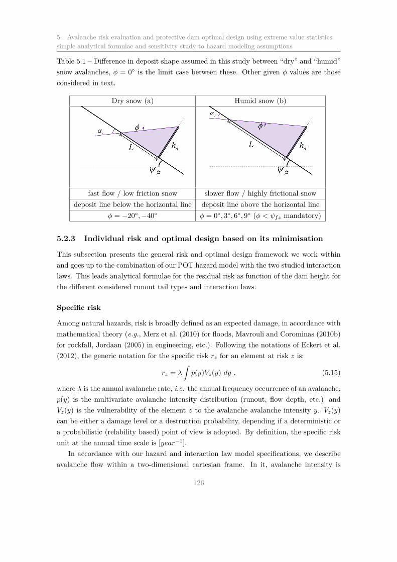
5. Avalanche risk evaluation and protective dam optimal design using extreme value statistics:simple analytical formulae and sensitivity study to hazard modeling assumptions
Table 5.1 – Difference in deposit shape assumed in this study between “dry” and “humid”
snow avalanches, φ = 0◦ is the limit case between these. Other given φ values are those
considered in text.
Dry snow (a) Humid snow (b)
fast flow / low friction snow slower flow / highly frictional snow
deposit line below the horizontal line deposit line above the horizontal line
φ = −20◦,−40◦ φ = 0◦, 3◦, 6◦, 9◦ (φ < ψfz mandatory)
5.2.3 Individual risk and optimal design based on its minimisation
This subsection presents the general risk and optimal design framework we work within
and goes up to the combination of our POT hazard model with the two studied interaction
laws. This leads analytical formulae for the residual risk as function of the dam height for
the different considered runout tail types and interaction laws.
Specific risk
Among natural hazards, risk is broadly defined as an expected damage, in accordance with
mathematical theory (e.g., Merz et al. (2010) for floods, Mavrouli and Corominas (2010b)
for rockfall, Jordaan (2005) in engineering, etc.). Following the notations of Eckert et al.
(2012), the generic notation for the specific risk rz for an element at risk z is:
rz = λ
∫
p(y)Vz(y) dy , (5.15)
where λ is the annual avalanche rate, i.e. the annual frequency occurrence of an avalanche,
p(y) is the multivariate avalanche intensity distribution (runout, flow depth, etc.) and
Vz(y) is the vulnerability of the element z to the avalanche avalanche intensity y. Vz(y)
can be either a damage level or a destruction probability, depending if a deterministic or
a probabilistic (relability based) point of view is adopted. By definition, the specific risk
unit at the annual time scale is [year−1].
In accordance with our hazard and interaction law model specifications, we describe
avalanche flow within a two-dimensional cartesian frame. In it, avalanche intensity is
126

5.2 Methods
classically defined by the joint distribution p(y) = p(P, xstop0) of spatio-temporal pressure
fields P and runout distances xstop0 . The specific risk rb(xb) for the element b at the xb
abscissa is then:
rb(xb) = λ
∫
p(P |xb ≤ xstop)p(xb ≤ xstop) × Vb(P ) dP , (5.16)
where the notation “.|.” classically denotes a conditional probability. Notations xb, Vb,
and rb (indice b) indicate that the typical element at risk we consider is a building, see
Sects. 5.3 for details (numerical values) and 5.4 for discussion.
We consider only building abscissas such as xb > xd, a natural choice in practice (one
would’nt build higher in the path for evident safety reasons) which makes the link with
our POT approach. Hence, the λ avalanche rate in Eq. (5.16) can be assimilated to the
occurrence rate in Eq. (5.1). Also, the over threshold xb > xd condition should appear in
all risk equations (Eq. (5.16) and the following), but it is dropped, for simplicity.
Finally, note that Eq. (5.16) holds since the pressure distribution p(P |xb > xstop0) =
δ(0), so that p(P, xstop0) = p(P |xb ≤ xstop0)p(xb ≤ xstop0), with p(P |xb > xstop0) the
pressure distribution at abscissa xb knowing that the abscissa xb is not reached, δ(0)
the Dirac distribution in zero, p(P |xb ≤ xstop0) the pressure distribution at abscissa xb
knowing that the abscissa xb has been reached by an avalanche and p(xb ≤ xstop0) is the
probability for xb to be reached by an avalanche.
Residual risk and optimal design
The dam optimal design approach we consider minimizes the long term costs obtained by
summing up the construction costs and the expected damages for the building at abscissa
xb. In has been proposed in avalanche engineering by Eckert et al. (2008a, 2009), in analogy
to the precursor work made by Van Danzig (1956) for maritime dykes in Holland and by
Bernier (2003) for river dams. All this work ground itself on an extensive mathematical
theory (Von Neumann and Morgenstern, 1953; Raiffa, 1968). Hence, the long term costs
with a protective dam hd are:
R(xb, hd) =C0hd + C1Aλ
∫
p(Pr|hd, xb ≤ xstop)
× p(xb ≤ xstop|hd) × Vz(Pr) dPr ,
(5.17)
where C1 and C0 are, respectively, the value of the building at risk at abscissa xb in e, the
monetary currency we work with, and the value of the dam per meter height in e.m−1.
A =∑+∞
t=1
1
(1 + it)tis the actualisation factor to pass from annual to long term risk with
it is the interest rate for the year t. The unit of the long term costs R(xb, hd) is therefore
[e].
127

5. Avalanche risk evaluation and protective dam optimal design using extreme value statistics:simple analytical formulae and sensitivity study to hazard modeling assumptions
The notation “.|hd” in Eq. (5.17) denotes that runout and pressure distributions are
now modified in the runout zone, conditional to the dam height hd. As a consequence,
for a fixed hd value, the long term costs correspond to the residual risk after the dam
construction.
By the way, Rb(xb, hd) is nothing more than C0hd +C1Arb(xb, hd), with rb(xb, hd) the
specific residual risk at the annual time scale for the building at the abscissa xb with the
dam height hd. This highlights that the approach remains individual risk based, with
one single element at risk at abscissa position xb. Note also that the damages caused
to the dam by successive avalanches and the consecutive reparation costs do not appear
explicitly in (5.17). In fact, they are included in the C0 evaluation through the definition of
a suitable amortizing period, a straightforward econometrical computation. Yet, a strong
underlying assumption is made: in case an avalanche severely damages or even destroys
the dam, the dam still reduces the hazard for this specific avalanche event according to
Eqs. (5.11) or (5.13), and is repaired immediately after.
Strong simplifications occur if the additional assumption of a constant “step” vulnera-
bility function is made. The worst-case scenario is that the damage is maximal as soon as
the element at risk is attained, whereas the considered element at risk remains obviously
undamaged if the avalanche does not reach its abscissa. The integral in Eq. (5.17) is then
reduced to P ((xstop − xd) > xb − xd|hd), the probability of exceeding the abscissa xb with
a protective dam height hd, so that:
R(xb, hd) = C0hd + λC1A (1 − F (xb − xd|hd)) , (5.18)
where F (xb − xd|hd) is the cumulative distribution function of runouts in xb with a pro-
tective dam height hd. This is the key assumption to keep a fully analytical decisional
model with our POT approach, see below.
Eq. (5.18) can first be regarded as a residual risk function that, for a fixed value of
hd, varies according to the xb position. It is then a linear function of the non exceedence
probability F (xb − xd|hd) showing the decrease of the residual risk in the runout zone as
one goes further and further away downstream. This directly represents/illustrates the
coupling of the interaction law with the probabilistic POT hazard model.
Second, Eq. (5.18) can be regarded as total costs depending on the dam height hd at a
fixed xb position, for instance a specific position of the runout zone which has some legal
meaning (such as the limit of a hazard zone), or a position where a real element at risk
/ building is situated. The optimal dam height from a stake holder’s perspective is then
simply:
hopt = argminhd
(Rb(xb, hd)) , (5.19)
where the function argmin gives, for a given xb, the height hd at which Rb is minimal.
128

5.2 Methods
Explicit risk formulae with the energy dissipation interaction law
According to Eq. (5.11), under the constraint hd <h0α , one has P (xstop−xd > xb−xd|hd) =
P
xstop0 −xd
1−αhd
h0
> xb − xd
. In other words, the random variable xstop −xd|hd remains GPD
distributed, with the same shape parameter ξ than xstop0 −xd, but with the reduced scale
parameter σ(1 −αhdh0
). The expression of the residual risk for the Poisson - GPD model is
straightforward:
R(xb, hd) =
C0hd + λC1A
1 +ξ(xb − xd)
σ(1 − αhdh0
)
−1ξ
if ξ 6= 0
C0hd + λC1A exp
− (xb − xd)
σ(1 − αhdh0
)
if ξ = 0
. (5.20)
Explicit risk formulae with the volume catch interaction law
According to Eq. (5.13), under the constraint hd < (2Aa tanαs)1/2, one has this time
P (xstop − xd > xb − xd|hd) = P
xstop0 −xd(
1−h2
d2Aatanαs
)1/2 > xb − xd
. Hence, xstop − xd|hd
is once again still GPD distributed, but with this time the reduced scale parameter
σ
(
1 − h2d
2Aa tan αs
)1/2
. This time, the residual risk writes:
R(xb, hd) =
C0hd + λC1A
1 +ξ(xb − xd)
σ
(
1 − h2d
2Aa tan αs
)1/2
−1ξ
if ξ 6= 0
C0(hd) +AλC1
exp
− (xb − xd)
σ
(
1 − h2d
2Aa tan αs
)1/2
if ξ = 0
, (5.21)
where tan(αs) = tan(ψfz − φ) and φ is arbitrary negative for dry cold snow avalanches
and positive for humid snow avalanches, with the standard limit case φ = 0 (Table 5.1).
Solutions to the risk minimisation problem
Sadly, none of these risk equations provide analytical solutions to Eq. (5.19). As a conse-
quence, this is the only place of the work where a numerical search is required, spanning,
129

5. Avalanche risk evaluation and protective dam optimal design using extreme value statistics:simple analytical formulae and sensitivity study to hazard modeling assumptions
for a fixed xb position, the possible values of hd according to the positivity constraints of
each interaction law. With the energy dissipation law, as already demonstrated in (Eckert
et al., 2008a) in the Poisson-Exponential case, this is easy because of the (rather) nice
shape of the residual risk function over a relatively large range of building positions and
model parameter values. The residual risk decreases with increasing dam heights for dam
heights below a single (rather) clear optimum, and increases with increasing dam heights
above the optimum. Only exception is when one considers building positions too far down
in the path. The dam is then useless making the optimal choice to be hd = 0m
For the volume catch interaction law, however, things are not that simple because of
the higher complexity of the dependency of R(xb, hd) to hd. Therefore, different typi-
cal cases can be encountered for plausible parameter values: no optimum, one “pseudo”
optimum due to the positivity constraint, and the “good” case of a minimum residual
risk arising as an optimal compromise between losses and construction costs. Yet, in the
latter case, relative maximum residual risks can also be observed. These different cases
are detailed/examplified in Appendix 5.6.1. For our application, we identified which of
them occurred in all configurations we tested, and only dam heights truly minimising
the risk were kept. These correspond to optimal compromises between construction costs
and losses, but also to the pseudo optimums, i.e. dam heights just sufficient to stop all
avalanches before the considered building position.
5.2.4 Quantifying uncertainty and sensitivity: intervals, bounds and in-
dexes
Since one objective of the paper is to quantify how risk estimates and optimal design values
vary across runout tail distribution types and avalanche-dam interaction laws, we propose
in this subsection different intervals, bounds and indexes suitable for taking into account
different types of uncertainty/variability. These intervals, bounds and indexes may be
usable by engineers in risk zoning and defense structure design to represent sensitivity
to available data resulting from parameter estimates standard errors, and/or sensitivity
to non probabilistic model uncertainty. They have also wider interest, being somewhat
interpretable in terms of respective weight of the different ingredients of the decisional
analysis.
In the core of the paper, and with regards to the difference to be made between model
parameters and their estimates on the basis of the available data, all risk computations
are performed under the classical paradigm of statistical inference. This means that we
plug the maximum full/profile likelihood estimates (λ, ξ, σ) or (λ, σ(ξ0)) in the Poisson -
GPDs/Exponential distribution functions, and we evaluate return levels and risk functions
accordingly, considering R(hd, λ, ξ, σ) or R(hd, λ, σ(ξ0)). Here, and in all what follows, the
130

5.2 Methods
notation ξ0 indicates that the GPD shape parameter is chosen and that the profile likeli-
hood is maximised conditionally to its choice. Discussion with regards to the alternative
Bayesian paradigm is provided in Sect. 5.4 and Appendix 5.6.3.
Propagating uncertainty on parameter estimates
To quantify the uncertainty resulting from the limited data sample available, the usual
approach is to propagate parameter standard errors (Eq. (5.7)) up to the quantities of
interest. Starting from the MLE estimates for the Poisson - GPD model and the associated
asymptotic variance-covariance matrix, different methods exist in the literature to evaluate
confidence intervals for high return levels. Appendix 5.6.2 presents how the arguably two
most common of them can be adapted to our profile likelihood case, where the shape
parameter value ξ0 results from a more or less arbitrary modelling choice rather than from
inference.
Bounds and sensitivity indexes to the runout tail shape
From a different perspective, to evaluate the influence of the runout tail shape, we evaluate
Eqs. (5.20) and (5.21) according to the range of ξ0 values provided by the profile likelihood
maximisation procedures. We do that without dam, and also for a given dam height and
interaction law. From these set of values (one for each ξ0 ), retaining the maximum and
minimum risk value at each abscissa leads risk bounds function of the abscissa, interaction
law and dam height. They constitute plausible upper/lower bounds for the risk taking
into account the variability of risk estimates towards runout distribution tail types. To
summarise the spread at the abscissa xb, the sensitivity index δR(xb,hd) is evaluated:
δR(xb,hd) =max
ξ0
(R(xb, hd)) − minξ0
(R(xb, hd))
R(xb, hd)(5.22)
with R(xb, hd) the mean value evaluated at the abscissa xb with the dam height hd. Note
that with the different interaction laws at our hand (energy dissipation and volume catch
with varying deposit shape angles), different values of δR(xb,hd) can de obtained.
To do a similar evaluation for the optimal design procedure, we also search, for a given
position xb and interaction law, the solution h∗d of (5.19) for each possible value ξ0. The
solution spread towards runout tail shapes is quantified from the minimum, maximum and
mean optimal height at the abscissa xb, denoted h∗d(xb) as:
δxb,h∗
d=
maxξ0
(h∗d(xb)) − min
ξ0
(h∗d(xb))
h∗d(xb)
. (5.23)
131

5. Avalanche risk evaluation and protective dam optimal design using extreme value statistics:simple analytical formulae and sensitivity study to hazard modeling assumptions
Finally, to confront risk and optimal design sensitivity to the ξ0 choice, we evaluate
the same sensitivity index function of abscissa and interaction law as:
δxb,R(h∗
d) =
maxξ0
(R(h∗d(xb))) − min
ξ0
(R(h∗d(xb)))
R(h∗d(xb))
, (5.24)
where R(h∗d(xb)) denotes the minimum residual risk at the abscissa xb given hd = h∗
d(xb).
Note that the latter index is somewhat different to the one provided by eq. (5.22) where hd
was fixed once for all. This time, for each value ξ0, the dam height considered to evaluate
the risk is different, as it is the one that locally minimises the residual risk.
Bounds and sensitivity index to the avalanche/dam interaction law
Similarly, to evaluate the sensitivity to the choice on one interaction law instead of another,
we evaluate, for a given runout tail (ξ0 is fixed), abscissa xb, and dam height hd, the spread
between the possible risk estimates as:
δ′
R(xb,hd) =max
IL(R(xb, hd)) − min
IL(R(xb, hd))
R(xb, hd), (5.25)
where IL is the short-name for the interaction laws considered: the volume catch interac-
tion law with various deposit angles, plus, potentially, the energy dissipation interaction
law.
5.3 Application and results
5.3.1 Case study
The case study selected is the same as in Eckert et al. (2008a), a real path from the French
avalanche database situated in the township of Bessans, in the Savoie department. It has
a vertical drop of 1, 175 m from its top to the Arc river, is only very slightly channelled
and the average slope is steep. The runout zone that consists in the gentle slope preceding
the Arc River (x = 1, 763 m in the (x, z) 2D-plane starting at the top of the path) is
rather regular, making the use of a simple stochastic model for runout distances such as
the POT-GPD possible.
The most extreme runout distance recorded corresponds to the Arc River, but, beyond
it, the terrain remains rather flat, making it potentially possible for extreme avalanches to
reach higher abscissas. This runout zone is, up to now, free from permanent habitations.
However, due to demographic pressure, it may become urbanizable in the future, provided
risk is estimated to be low enough in the current state or after a permanent defense
structure construction. Hence, we study the potential risk reduction by a dam at the
132
5.3 Application and results
abscissa which corresponds to the beginning of the runout zone according to a classical
slope criterion. In the whole work, xd = 1, 550 m and ψfz = 10◦ are therefore fixed.
During the 1973-2003 time period, 28 avalanches exceeding xd were recorded by the local
forestry service.
The risk evaluation and sensitivity analysis is performed all over the runout zone.
However, for being less case-study dependant in our conclusions, specific positions of legal
importance are studied, corresponding to return periods of 10 - 1000 years. These are
evaluated with Eq. (5.4) conditionally to “reasonable” GPD shape parameter values ξ0
(see below).
The construction cost for the dam and the building value (the single element at risk we
consider) were set to, respectively, 5, 530 e.m−1 and 300, 000 e. A is fixed to 25, which is
obtained with a constant interest rate it = 4%. In all risk minimisation calculations, the
xb building position is fixed, but a range of positions is investigated. The bounds of this
range correspond to the shortest decennial runout and to the longest centennial runout we
evaluate according to data and choices made regarding possible GPD shape parameters.
5.3.2 Fitted runout distance - return period relationships
Without dam
The maximum likelihood method supplies estimates for the Poisson (λ = 0.904) and the
GPD parameters (Table 5.2). The likelihood ratio test rejects the exponential distribution
to the benefit of the GPD distribution at the 5% significance level. The negativity of the
MLE estimate β, or, identically, the positivity of ξ, indicates that the best fitted GPD
distribution belongs to the Fréchet domain and has therefore a heavy tail. However, the
MLE estimate ξMLE is close to 1.1, suggesting a tail so heavy that it is presumably un-
trustful since ξ values above 0.5 are known to be extremely rare in environmental systems.
Furthermore, the associated standard error is very high (Table 5.2). As a consequence,
the high return levels predicted on the basis of the MLE estimates are presumably unre-
alistic and, anyhow, the associated confidence intervals provided by the two uncertainty
propagation methods we have implemented are so large that they are practically useless
(Tables 5.4 and 5.5). These results highlight that it is presumably not possible to fit a
reliable runout tail for this case study on the basis of the data only.
Our profile likelihood approach introduces extra-data information into the analysis
through the choice of a ξ0 value, somewhat arbitrary, but at least in a realistic range.
Figure 5.2(a) shows the negative profile log-likelihood curves corresponding to the different
values tested. It confirms that the likelihood of the data sample under the GPD model
is very flat around the MLE couple, so that a wide range of other couples may be nearly
as suitable in terms of data fitting (Table 5.3). This is even clearer when the different
133

5. Avalanche risk evaluation and protective dam optimal design using extreme value statistics:simple analytical formulae and sensitivity study to hazard modeling assumptions
fitted models are confronted to the data (Figure 5.2(b)). We may just note that the
minimum negative log-likelihood increases with decreasing values of ξ0, suggesting a little
more confidence in a heavy tail (positive shape parameter) than in other runout types
(null or negative shape parameter, Table 5.3).
The ξ0 choice, however, considerably impacts the estimated runout distance - return
period relationship, for instance the high return levels of interest for hazard mapping
(Figure 5.2(c)). ξ0 values lower than 0.5 provide ˆx100 - ˆx1000 return levels arguably plausible
from the perspective on an expert analysis of the path. On the contrary, these are clearly
too high for ξ0 > 0.5, as expected with regards to the poor confidence we may have in
ξ0 values above 0.5. As a consequence, in the following, we concentrate our analysis on
ξ0 = {−0.3; −0.1; 0; 0.1; 0.3; 0.5}, i.e. on a range of plausible values containing the three
different runout tail types, but with more weight on the heavy tail Fréchet type, according
to the information the data seem to contain. Furthermore, in the same spirit, when a
single value is required, we focus on ξ0 = 0.3.
In more details, one may note that the concave/convex shape of return level plots with
positive/negative ξ0 values, respectively, makes return levels higher in the Weibull domain
(ξ0 < 0) for low return periods, but much higher in the Fréchet domain (ξ0 > 0) for high
return periods. For the same shape parameter absolute value |ξ0|, the Frechet/Weibull
return level plots cross on the straight line corresponding to the exponential case (ξ0 = 0,
leading to a linear behavior in log scale). For our case study, this crossing is obtained for
return periods of 50 − 500 years, depending on |ξ0|.Regarding return levels confidence intervals due to parameter uncertainty, Tables 5.4
and 5.5 illustrate how the two methods detailed in Appendix 5.6.2 perform in our case for
x10 and ˆx100. Both approaches show well that the uncertainty becomes higher and higher
for increasing return periods, a classical and intuitive result. Also, for high return periods,
the uncertainty literally explodes for very high ξ0 values, in accordance with what was
already observed for the MLE. More interestingly, the delta approach does not provide
return level confidence intervals for negative shape parameters, and leads unrealistically
large return level confidence intervals for slightly positive shape parameters (the zero
case seems trustful since the computation is performed with the exponential likelihood
rather than with the GPD one). These problems related to the variance covariance matrix
approximation do not show with the deviance based approach, for which plausible return
level confidence intervals are evaluated for all the ξ0 values tested. In addition, even for
very high ξ0 values, the high return level confidence intervals provided by the deviance
approach are much narrower than with the delta approach. These advantages are partly
attributable to the fact that the deviance approach does not impose symmetry for return
level confidence intervals. Hence, all in all, the deviance based method seems to perform
much better than the delta method in our profile likelihood context.
134

5.3 Application and results
In Tables 5.4 and 5.5, the ˆξMLE column provides return level confidence intervals
with ξ0 set to the MLE in the profile likelihood maximisation. If ξ is not set, with
both approaches, the confidence interval is much larger, which illustrates well the ad-
ditional uncertainty resulting from having one more free parameter to estimate (or, in
contrast, the uncertainty reduction by the “arbitrary” choice of ξ0). For example, with
the deviance approach (in that case, a more classical full likelihood uncertainty propaga-
tion), the confidence intervals for x10 (resp. ˆx100) is CI ˆx10 = [1, 586 − 1, 707.8] m (resp.
CI ˆx100 = [1, 762.6 − 3, 714.6] m) when the uncertainty on ˆξMLE is taken into account, i.e.
intervals much larger than those displayed in Table 5.5.
With a fixed dam height
Figure 5.3 shows the impact on the return level plots of the two interaction laws (and of
the deposit shape angle for the volume catch interaction law) for different dam heights and
GPD parameterisations, the latter being provided by the profile likelihood maximisation
with different ξ0 choices. Logically, for both interaction laws, return levels decrease for
increasing value of the dam height hd, which simply illustrates the ability of the dam in
reducing the hazard in the runout zone.
Furthermore, for a fixed GPD parametrisation and dam height, the energy dissipation
law generally evaluates a higher return period for a given path abscissa than the volume
catch interaction law. This first suggests that the dam is more efficient in protecting
potential elements at risk under the assumption of a dam-avalanche interaction governed
by energy dissipation rather than by volume catch. An exception to this rule is, however,
observed for the “extreme” deposit angle shape φ = 9◦ (just below the 10◦ local slope,
which is its maximal possible value), that is to say, the case catching the highest volume
of snow behind the dam. For instance, in case where hd = 6 m, ℓfz = 100 m and φ = 9◦
(Figure 5.3(b)), all avalanches are stopped by the dam, whereas, with a similar dam height,
a few exceedences are still observed with the energy dissipation law. This highlights well
the higher flexibility of the volume catch interaction law due to the additional parameter
φ.
Regarding the influence of ξ0, Figure 5.3, shows well that, for all dam heights and
interaction laws, the similar features discussed before as function of the sign of ξ0 without
dam remain true. Simply, the crossing of the different return level plots on the exponential
straight line for the same |ξ0| values occurs for return levels that slightly decrease with
the dam height. This traduces that all interaction laws and dam heights impacts the
scale of the runout distance distribution only: xstop − xd > xb − xd|hd remain always
GPD distributed with ξ0 shape parameter whatever the dam height and interaction law
considered.
135

5. Avalanche risk evaluation and protective dam optimal design using extreme value statistics:simple analytical formulae and sensitivity study to hazard modeling assumptions
Table 5.2 – Maximum likelihood estimates and respective standard errors for the GPD
parameters with the two possible parametrisations
Maximum-likelihood estimates Standard errors
ρ 0.1165 0.0223
β -0.1284 0.0079
ξ 1.1018 0.3372
σ 8.5826 2.7957
Table 5.3 – Full and profile likelihood estimates. nll is the minimum negative log-likelihood
in each case. ∗ is the exponential case (ξ0 = 0).
ξ0 σ(ξ0) −2 nll
-0.3 86.86 280.9
-0.1 56.63 272.0
0 ∗ 43.1679 (ρMLE = 0.0232) 266.8
0.1 31.72 261.3
0.3 17.58 250.9
0.5 12.29 243.9
0.7 10.21 240.2
0.9 9.18 238.5
ξMLE = 1.1018 σMLE =8.5826 238.1
1.3 8.20 238.4
136

5.3 Application and results
0 20 40 60 80 100110
115
120
125
130
135
140
145
150
155
160
σ
Ne
ga
tive
Lo
g−
like
liho
od
ξ0 = −0.3
ξ0 = −0.1
ξ0 = 0.1
ξ0 = 0.3
ξ0 = 0.5
ξ0 = 0.7
ξ0 = 0.9
ξ0 = 1.1
ξ0 = 1.3
ξMLE
Exp.
σMLE
(a) Profile negative log-likelihoods: green square markers de-
note the minimum of each curve.
1550 1600 1650 1700 1750 18000
0.005
0.01
0.015
0.02
0.025
0.03
0.035
0.04
0.045
0.05
xstop
0
(m)
Pro
ba
bili
ty D
en
sity f
un
ctio
n
ξ0 = −0.3
ξ0 = −0.1
ξ0 = 0.1
ξ0 = 0.3
ξ0 = 0.5
ξ0 = 0.7
ξ0 = 0.9
ξ0 = 1.1
ξ0 = 1.3
Exp.
(b) Density functions provided by the profile likelihood minimi-
sation method versus histogram of original data.
100
101
102
103
1600
1650
1700
1750
1800
1850
1900
1950
2000
Re
turn
le
ve
l, X
T (
m)
Return period, T (year)
ξ0 = −0.3
ξ0 = −0.1
ξ0 = 0.1
ξ0 = 0.3
ξ0 = 0.5
ξ0 = 0.7
ξ0 = 0.9
ξ0 = 1.1
ξ0 = 1.3
ξMLE
Exp.
(c) Return level plots provided by the profile likelihood min-
imisation method versus original data in red circles (◦).
Figure 5.2 – Model fit and checking: negative log-likelihood curves, density plots and
return level plots. Exp is the exponential case (ξ0 = 0).
137

5. Avalanche risk evaluation and protective dam optimal design using extreme value statistics:simple analytical formulae and sensitivity study to hazard modeling assumptions
101
102
103
1550
1600
1650
1700
1750
1800
1850
1900
1950
Return period, T (years)
Re
turn
le
ve
l, X
T (
m)
hd=0 m
hd=3 m
hd=6 m
(a) With the energy dissipation interaction law. h0 = 1 m, α = 0.14.
101
102
103
1550
1600
1650
1700
1750
1800
1850
1900
1950
2000
2050
Return period, T (years)
Re
turn
le
ve
l, X
T (
m)
101
102
103
1550
1600
1650
1700
1750
1800
1850
1900
1950
2000
2050
Return period, T (years)
hd=0 m
hd=3 m
hd=6 m
ii)i)
(b) With the volume catch interaction law, V = 50, 000 m3, ℓfz = 100 m: (i) “intermediate”
case: φ = 0◦ (standard volume storage), and (ii) “optimistic” case: φ = 9◦ (maximal volume
storage and, hence, runout shortening with “humid” snow). In that case, for hd = 6 m, all
avalanches are stopped by the dam.
Figure 5.3 – Runout distance - return period relationships for different dam heights, the
two interaction laws and three possible GPD parameterisations provided by the profile
likelihood maximisation. Solid line: ξ0 = −0.3, dashed line: ξ0 = 0, dotted line: ξ0 = 0.3).
138

5.3 Application and results
Table 5.4 – Return levels and corresponding 95% confidence intervals from the delta
method; * same calculation with the specific exponential formulae (ξ0 = 0); N nega-
tive diagonal terms in the approximate variance-covariance matrix VxT (ξ0), see Appendix
5.6.2.
ξ0 -0.3N -0.1N 0 * 0.1 0.3 0.5 0.7 0.9 ˆξMLE 1.3
x10 ±zα
2
√
VxT (ξ0)
(m)
1, 690.6
/
1, 662.6
/
1, 645.6±38.65
1, 628.8±843.30
1, 605.5±50.12
1, 600.0±36.74
1, 604.2±38.68
1, 614.4±47.29
1, 630.9±62.54
1, 654.7±85.88
ˆx100 ±zα
2
√
VxT (ξ0)
(m)
1, 765.2
/
1, 756.0
/
1, 744.8±73.76
1, 731.2±1, 948.4
1, 718.4±150.54
1, 759.7±150.93
1, 877.3±227.98
2, 127.8±414.60
2, 655.68±838.6
3, 744.5±1775.2
Table 5.5 – Return levels and corresponding 95% confidence intervals ([CI], [lower bound−upper bound]) from the deviance method (Appendix 5.6.2); * same calculation with the
specific exponential formulae (ξ0 = 0).
ξ0 -0.3 -0.1 0 * 0.1 0.3 0.5 0.7 0.9 ˆξMLE 1.3
x10 (m)
[CI] (m)
1, 690.6
[1, 668 −1, 731]
1, 662.6
[1, 636 −1, 707]
1, 645.6
[1, 617 −1, 693]
1, 628.8
[1, 601 −1, 675]
1, 605.5
[1, 583 −1, 648]
1, 600
[1, 579 −1, 641]
1, 604.2
[1, 581 −1, 649]
1, 614.4
[1, 586 −1, 669]
1, 630.9
[1, 594 −1, 701]
1, 654.7
[1, 606 −1, 747]
ˆx100 (m)
[CI] (m)
1, 765.2
[1, 732 −1, 827]
1, 756
[1, 707 −1, 838]
1, 744.8
[1, 687 −1, 840]
1, 731.2
[1, 668 −1, 837]
1, 718.4
[1, 649 −1, 848]
1, 759.7
[1, 671 −1, 932]
1, 877.3
[1, 736 −2, 152]
2, 127.8
[1, 877 −2, 622]
2, 655.7
[2, 165 −3, 624]
3, 744.5
[2, 735 −5, 723]
5.3.3 Residual risk estimates
Influence of the GPD ξ0 shape parameter
According to Eq. (5.18), residual risk is a linear function of exceedence probability, so
that most noticeable features in residual risk plots directly derive from what is observable
on return level plots. For instance, Figure 5.4 shows the influence of the dam height hd
on the risk reduction with a fixed ξ0 shape parameter whereas Figure 5.5 illustrates, with
a constant dam height, the influence of the GPD parametrisation, with the ξ0 parameter
taken in the [−0.3 − 0.5] interval.
In Figure 5.4, with both interaction laws, the residual risk reduction as function of
the dam height increase is clear, e.g. from 74, 993e with no dam to 57, 201e with hd =
1m, 35, 124e with hd = 3m and 33, 676e with hd = 5m for a building situated at a
position corresponding to the centennial runout without dam (xb = 1, 718.4) and the
energy dissipation law. Here, ξ0 is fixed to 0.3, which is, as said before, a potentially
139
5. Avalanche risk evaluation and protective dam optimal design using extreme value statistics:simple analytical formulae and sensitivity study to hazard modeling assumptions
sensible choice since it is positive but not too high.
In Figure 5.5(a), the GPD shape parameter influence is also clear: the Fréchet-type
values tested (ξ0 > 0) provide the lowest residual risk estimates for buildings situated just
above the dam abscissa but lead by far the highest risk estimates further down in the
path, and vice versa for the Weibull-type values (ξ0 < 0). The exponential case where
ξ0 = 0 provides intermediate residual risk estimates, and, for one given |ξ0|, all estimates
are the same only for the abscissa position at which the Fréchet and Weibull-type return
level plots cross the exponential straight line.
Figure 5.5(b) summarises, for the same constant dam height and the two interaction
laws, the variability of risk estimates towards runout distribution tail types, i.e. on the
plausible ξ0 range [−0.3 − 0.5], slightly positive on average. The resulting lower and
upper risk bounds may be very valuable insights for practice. For example, for hd =
6m and the energy dissipation law, the residual risk is estimated to be in the interval
[33, 180 − 37, 389]efor a building situated at a position corresponding to the centennial
runout without dam (and ξ0 = 0.3). The width of the inter-bounds interval depends on
the position in the path: it is minimal for “intermediate” abscissas where the different risk
curves lead similar estimates, and is much larger when Fréchet/Weibull-type risk estimates
strongly diverge.
The δR(xb,hd) sensitivity index (Eq. (5.22)) more quantitatively ascertains the spread
of risk bounds towards ξ0 values. Figure 5.5(c) shows that it varies as function of the
considered building position and interaction law, but that, with the two interaction laws,
the relative difference between risk estimates can be as high as 200%. This indicates that
considerable errors can be made if the ξ0 value for which the risk is minimal is chosen
instead of the one maximizing the risk at the considered abscissa, and vice versa. For
each interaction law, δR(xb,hd) has two modes as function of xb. The first (closer to xd)
corresponds to the position where Weibull type estimates are the highest with regards to
Fréchet type ones, and the second mode, further down in the path, to the opposite case.
For very high abscissas, all estimates drop to zero, eventually reducing the sensitivity to
the runout tail shape. The local minimum between the two modes in δR(xb,hd) corresponds
to the region in the path previously discussed where all risk estimates are similar.
Influence of the the interaction law and of the φ deposit shape angle
Regarding the respective efficiency of the two interaction laws in reducing risk, conclusions
made with return level plots remain obviously true here. For all dam heights, the energy
dissipation interaction law predicts a strong risk reduction with regards to the no-dam
case, residual risk drops sharply for abscissas just above the dam and this effect is all
the more marked that the dam is high. With a standard deposit shape angle φ = 0◦,
140

5.3 Application and results
Figure 5.4 – Residual risk functions with ξ0 = 0.3 for various dam heights hd with the
energy dissipation interaction law (solid line, h0 = 1 m, α = 0.14) and the volume catch
interaction law (dashed line with circles, V = 50 000 m3, ℓfz = 100 m), (i) intermediate
case φ = 0◦, and (ii) “optimistic case” φ = 9◦.
the volume catch interaction law predicts a much weaker risk reduction for a given dam
height, with residual risk estimates dropping at much lower pace as one goes further down
in the path (Figure5.4 (i)).
As already stated in the previous 5.3.2 subsection, the only exception to the higher
efficiency of the energy dissipation interaction law with regards to the volume catch one
occurs for “extremal” volume storages, e.g. with φ = 9◦ in Figure 5.4 (ii). In that case,
with moderate dam heights (1 − 3m), the two interaction laws lead rather similar risk
estimates, and, for hd = 6 m, the volume catch interaction law predicts even a higher
risk reductions since all avalanches are stopped before or at the dam abscissa. As a
consequence, for a given abscissa in the path, low and high risk bounds obtained towards
possible runout tails are much higher for a given dam height with the energy dissipation law
than with the volume catch one (Figure 5.5(b)). Also the pattern in resulting sensitivity
index is shifted to the right with the volume catch interaction law, with higher values
further down in the path (Figure 5.5(c)) .
To further quantify the effect of φ on the risk estimation, Figure 5.6 systematically
investigates the hd = 5.5 m case, and ℓfz = 50 m, which stays within the validity range
of the two interaction laws for all φ values (for the volume catch interaction law, the
141

5. Avalanche risk evaluation and protective dam optimal design using extreme value statistics:simple analytical formulae and sensitivity study to hazard modeling assumptions
(a) Residual risk functions for various ξ0 values with the energy dissipation interaction law (solid line) and
the volume catch interaction law (dashed line with circles).
(b) Residual risk bounds constructed according to the ξ0 = {−0.3; −0.1; 0; 0.1; 0.3; 0.5} sample with the
two interaction laws.
(c) Sensitivity index δR(xb,hd) (Eq. (5.22)) to the runout tail shape as function of the building position xb
for the two interaction laws, ξ0 = {−0.3; −0.1; 0; 0.1; 0.3; 0.5}.
Figure 5.5 – Residual risk sensitivity to the GPD parametrisation. h0 = 1 m, α = 0.14,
V = 50, 000 m3, ℓfz = 100 m, φ = 0◦ and hd = 6 m.
142

5.3 Application and results
limit height is 5.9 m with V = 50, 000 m3, φ = 9◦ and ℓfz = 50 m). As expected, the
residual risk increases when the deposit shape angle becomes increasingly negative, and,
hence, the dam, under the volume catch interaction law, less efficient. For this 5.5 m dam
height, for which none of the interaction laws is able to stop all avalanches, the energy
dissipation interaction law remains the most optimistic regarding the beneficial action of
the dam. Risk estimates provided by the volume catch interaction law become close to
the energy dissipation ones only with the maximal φ = 9◦ value, and much higher with
“less optimistic” lower deposit shape angles (Figure 5.6(a)).
From the set of risk curves of Figure 5.6(a), for each position in the path, two risk
bound couples can be built: the first one considers the minimum and maximum risk
estimates with the volume catch interaction law according to the variability on φ only
(Figure 5.6(b) (i)). The second one takes into account, in addition, the minimal risk value
provided by the energy dissipation interaction law (Figure 5.6(b) (ii)). In other words,
due to the higher efficiency postulated by the energy dissipation law, upper risk bounds
are the same in the two cases, whereas lower bounds differ sightly. For example, without
considering the energy dissipation law, the residual risk is estimated to be in the interval
[35, 172 − 104, 233] efor a building situated at a position corresponding to the centennial
runout without dam (with ξ0 = 0.3). And with the inclusion of the energy dissipation law
in the bounds definition, it is in the interval [31, 808 − 104, 233] e.
The resulting sensitivity to the interaction law index δ′
R(xb,hd) (Eq. (5.25)) evaluated
all over the runout zone ascertains that a maximal error of 130% (including the energy
dissipation law) / 105% (with the volume catch interaction law only) can be made on the
risk quantification if the interaction law chosen is wrong in terms of postulated mechanism
and/or deposit shape angle. As for the sensitivity to the GPD parametrisation, the width
between these risk bounds and hence the δ′
R(xb,hd) sensitivity index are small for buildings
very close to the dam (highly exposed), as well as very far down in the path (positions
reached by the most extreme avalanches only). Sensitivity to interaction law is therefore
maximal for buildings situated at “intermediate” abscissa positions (Figure 5.6(c)).
5.3.4 Optimal dam heights
With the GPD versus the Exponential runout model
For now, we consider the various residual risk functions at hour hand as functions
of the dam height, searching the height that minimizes the residual risk according to
Eq. (5.19). Optimal design sensitivity to GPD parametrisation is still evaluated on
the ξ0 = [−0.3 − 0.5] range. Since the building position in the risk minimisation is
fixed, four positions are chosen: the minimal and the maximal decennial and centen-
nial abscissas provided by these possible parameterisations without dam, that is to say
143

5. Avalanche risk evaluation and protective dam optimal design using extreme value statistics:simple analytical formulae and sensitivity study to hazard modeling assumptions
(a) Residual risk function according to various deposit shape angles φ (volume catch interaction law).
For comparison, the residual risk with the energy dissipation interaction law is plotted in solid line with
squares. The dam construction cost C0hd appears in black.
(b) Residual risk bounds constructed according to the φ = {−40◦; −20◦; 0◦; 3◦; 6◦; 9◦} sample (volume
catch interaction law), without (i) or with (ii) the energy dissipation interaction law. The dam construction
cost C0hd appears in black.
(c) Sensitivity index to the interaction law δ′
R(xb,hd) (Eq. (5.25)) as function of the building position xb
without or with the energy dissipation interaction law, φ = {−40◦; −20◦; 0◦; 3◦; 6◦; 9◦}.
Figure 5.6 – Residual risk sensitivity to the interaction law, with focus on the φ deposit
shape angle: h0 = 1 m, α = 0.14, V = 50, 000 m3, ℓfz = 50 m, ξ0 = 0.3 and hd = 5.5 m.
144

5.3 Application and results
[1, 600 m; 1, 690.6 m; 1, 718.4 m; 1, 765.2 m].
Figures 5.7 shows, for these four positions and the different tested ξ0 values, the ob-
tained residual risk curves, as functions of the dam height hd, with the energy dissipation
law. For each curve, the optimal height minimising the risk is highlighted. It is more or
less clear, depending on the abscissa position xb and the ξ0 value considered, but, as a
general rule, a minimum can well be found on the range of hd values allowed by the pos-
itivity constraint. As intuitively expected, optimal dam heights are higher for buildings
situated closer to the dam than for buildings located further down in the path, since it is
economically more sound to protect more exposed elements at risk. Also, for very high
dam heights, the risk converge to the construction cost C0hd. This occurs as soon as the
dam is high enough to stop all avalanches before the considered building abscissa, making
the additional construction effort unnecessary.
The same evaluation can be done considering the volume catch interaction law instead
of the energy dissipation one. At this stage, we consider φ = 9◦, lfz = 100 m and
V = 50, 000 m3, i.e. parameter values for which the dam is “efficient” so that it is easier
to determine optimal heights minimizing the residual risk. This is not always the case
with this interaction law, see Sect 5.3.4.
Table 5.6 summarizes optimal dam heights and associated risk estimates R(xb, h∗d) for
the two interaction laws. As first glance it appears that Fréchet like positive ξ0 values
lead higher optimal heights and higher corresponding minimum estimates whith regards
to the ones lead by Weibull or Gumbell like ξ0 values. This conclusion reflects the fact
that heavy tailed GPD distributions forecast more extreme avalanches than the two other
tail types considered. This makes higher constructions economically advantageous, but
the remaining risk after dam construction still higher. Note that the increase with ξ0 is
very clear with the energy dissipation interaction law, and somewhat less clear with the
volume catch interaction law. This is attributable to the fact that with the advantageous
volume catch parameters used here, low dam heights are quite efficient. For instance, the
4.18 m limit height is sufficient to stop all avalanches, and it is economically sound to
construct uo to this height for many of the ξ0 and xb values tested.
To confirm this shape parameter effect, previous calculations were generalized, with
the energy dissipation law, to a large range of building positions (Figure 5.8) and to a
quasi continuous sample of ξ0 values (Figure 5.9), retaining in each case h∗d and R(xb, h
∗d).
Overall, results illustrate very clearly that, for a given building position, the higher ξ0, the
higher the optimal dam height and corresponding minimum risk. However, it also appears
that the differences in optimal dam heights and corresponding residual risks obtained with
different ξ0 values strongly increase with increasingly high xb positions up to very high xb
values. For example, Figure 5.8(a) illustrates the results of the optimisation procedure all
along the path with a typical Fréchet-type choice (ξ0 = 0.3), the symmetrical Weibull-type
145

5. Avalanche risk evaluation and protective dam optimal design using extreme value statistics:simple analytical formulae and sensitivity study to hazard modeling assumptions
choice (ξ0 = −0.3), and the intermediate Gumbel-type case (ξ0 = 0). Fréchet-type optimal
heights and corresponding risks estimates are systematically higher than Gumbel-type
ones, themselves systematically higher that the Weibull-type ones, and these differences
increase with xb. Same conclusions still hold with the volume catch interaction law, even
if the decreasing pattern is weaker (Figure 5.8(b)). These results simply traduce again the
fact that difference in tail types especially affects the most extreme return levels, and, as
a consequence, the design choices controlled by these. Note, however, that for b values so
high that they are “never” reached by avalanches, the optimal height and the associated
residual risk logically drop to zero. This occurs for xb abscissas all the more small than ξ0
is low (Figure 5.9(a)).
In terms of optimal design sensitivity indexes δxb,R(h∗
d) and δxb,h∗
dreflecting the sensi-
tivity of the risk minimisation procedure to the GPD parametrisation, values a bit lower
than for the risk sensitivity indexes δR(xb,hd) and δ′
R(xb,hd) are obtained. Still, they remain
quite high, up to 120% with the energy dissipation law and 40% with the volume catch
interaction law, depending on the xb position (Figure 5.8(c)). Hence, optimal dam heights
and associated minimum risk estimates can well be misvalued by a factor two if a wrong
ξ0 value is considered, for instance at high (obviously, not too high to be unattainable)
abscissas in the path, where, as discussed before, the sensitivity to the tail behaviour is
the highest. Finally, the scatter plot of the two indexes (Figure 5.8(c)) shows that the ξ0
choice is slightly more influential on the optimal design than on the corresponding risk
estimate, but this effect is not very marked.
Table 5.6 – Optimal dam height h∗d and corresponding minimum risk R(xb, h
∗d) with the
two interaction laws at the four abscissas xb = [1, 600 m; 1, 690.6 m; 1, 718.4 m; 1, 765.2 m].
These correspond to [minξ0
(xT 10),maxξ0
(xT 10),minξ0
(xT 100),maxξ0
(xT 100)], respectively, for ξ0 ∈{−0.3; −0.1; 0; 0.1; 0.3; 0.5}. The used parameter set is C0 = 5, 530 e.m−1, C1 = 300, 000
e, α = 0.14, h0 = 1 m, V = 50, 000 m3, ℓfz = 100 m, and φ = 9◦. With these, the maximal
dam height is 7.14 m with the energy dissipation law and 4.18 m with the volume catch
one. .
ξ0 Energy dissipation: h∗d (m), R(xb, h
∗d) (ke) Volume catch: h∗
d (m), R(xb, h∗d) (ke)
−0.3 [6.0; 3.6; 2.8; 1.5] [33.3; 20.2; 16.1; 9.2] [4.1; 3.6; 3.3; 2.6] [22.8; 20.1; 18.6; 14.8]
−0.1 [6.3; 4.2; 3.5; 2.3] [35.1; 24.3; 20.9; 14.9] [4.18; 3.9; 3.7; 3.2] [23.0; 21.6; 20.7; 18.7]
0 (Exp) [6.4; 4.4; 3.7; 2.5] [36.0; 26.3; 23.0; 17.4] [4.18; 4.0; 3.8; 3.5] [23.0; 22.2; 21.6; 20.1]
0.1 [6.5; 4.6; 3.9; 2.6] [36.8; 28.1; 25.0; 19.5] [4.18; 4.1; 4.0; 3.7] [23.1; 22.6; 22.3; 21.3]
0.3 [6.9; 5.2; 4.6; 3.3] [38.6; 32.7; 30.3; 25.8] [4.18; 4.18; 4.18; 4.1] [23.1; 23.1; 23.1; 23.0]
0.5 [7.14; 6.6; 6.2; 5.5] [40.0; 38.2; 37.3; 35.4] [4.18; 4.18; 4.18; 4.18] [23.1; 23.1; 23.1; 23.1]
146

5.3 Application and results
Figure 5.7 – Optimal design with the energy dissipation law for different GPD parametri-
sations and at diffent building abscissas xb: (i) 1, 600 m, (ii) 1, 690.6 m, (iii) 1, 718.4 m,
(iv) 1, 765.2 m. Red circles denote the minimum of each residual risk curve. The dashed
black line is the asymptotic dam construction cost C0hd. Decisional model parameters are
C0 = 5, 530 e.m−1, C1 = 300, 000 e, α = 0.14, and h0 = 1 m, which imposes hd ≤ 7.14 m
147

5. Avalanche risk evaluation and protective dam optimal design using extreme value statistics:simple analytical formulae and sensitivity study to hazard modeling assumptions
(a) Optimal height hd = h∗
d (dashed line) and cor-
responding minimum residual risk R(xb, h∗
d) (solid
line) as functions of the building position xb with
the energy dissipation interaction law.
(b) Optimal height hd = h∗
d (dashed line) and cor-
responding minimum residual risk R(xb, h∗
d) (solid
line) as functions of the building position xb with
the volume catch interaction law.
0 25 50 75 100 125 1500
20
40
60
80
100
120
140
160
180
200
δx
b, h
d
* (%)
δ R(x
b,h
d*) (
%)
Energy dissipation interaction law
Volume catch interaction law
First bisector
(c) Risk sensitivity index δR(xb,h∗
d) (Eq. (5.24)) as function of the optimal design sensitivity index δxb,h∗
d
(Eq. (5.23)) for the two interactions laws. Each point of the plot corresponds to a different building
abscissa xb. Black dashed line is the first bisector of the scatter plot.
Figure 5.8 – Optimal design sensitivity to the runout tail shape. C0 = 5, 530 e.m−1,
C1 = 300, 000 e, α = 0.14, h0 = 1 m, V = 50, 000 m3, ℓfz = 100 m, φ = 9◦.
148

5.3 Application and results
(a) Optimal dam height. (b) Risk value at the optimal dam height.
Figure 5.9 – Optimal dam height and corresponding minimum risk estimate as continuous
functions of the GPD shape parameter ξ0 and building position xb, energy dissipation law.
C0 = 5, 530 e.m−1, C1 = 300, 000 e, α = 0.14, and h0 = 1 m.
With the volume catch versus the energy dissipation interaction laws
Figure 5.10 shows the residual risk curves as function of the dam height hd for various
deposit shape angles at the same abscissas studied in Figure 5.7, and with a constant
ξ0 = 0.3 value. Whereas things were rather simple with the energy dissipation law, here,
as a result of the higher complexity of the volume catch interaction law, many cases are
likely to occur. First, green squares (�) are optimal heights resulting from the positivity
constraint in the interaction law. Second, from the second abscissa studied until the last
one, it is observed that, for the lowest deposit shape angles tested, the risk curves never
stop increasing: the cost of the dam is then always high enough to dominate the total
cost. Such curve shapes induce an optimal height equal to zero (black star ∗), which
never occured for the same abscissas with the energy dissipation law (Figure 5.7). Third,
red circles (•) denote “true” optimal heights resulting from the residual risk minimization
on a dam height range where the risk derivative exists. As said before, Appendix 5.6.2
details these three different cases. Finally, for highly negative deposit shape angles and low
abscissas in the path (−40◦ and −20◦ in (i)), the risk decreases over a very large hd range
and the the maximal value allowed by the positivity constraint is very high. In that cases,
we have stopped the analysis at 30 m, assuming that higher dams would’t be allowed for
environmental or engineering reasons even if they would apparently be sound from the
purely economical perspective of our computational framework. Such limits, rather than
truly optimal dam heights, are all equal to 30 m. They appear as black triangles (N).
As for the GPD parametrisation, to fully quantify the sensitivity of the optimal design
and corresponding minimum risk estimate to the interaction law, Figure 5.11 was drawn.
It spans a large set of building positions and deposit shape angles with the deposit volume
149
5. Avalanche risk evaluation and protective dam optimal design using extreme value statistics:simple analytical formulae and sensitivity study to hazard modeling assumptions
interaction law, and the energy dissipation law is also considered. Figure 5.11(a) shows
that with the deposit volume interaction law and with regards to the energy dissipation
law, atypical patterns are observed in the h∗d and R(xb, h
∗d) curves as functions of xb: for
each deposit shape angle φ, an abscissa xb in the path can be found where the optimal
dam height drops brutally from a more or less high h∗d value to zero, whereas the residual
risk switches to the baseline risk without dam. This behaviour comes from the fact that,
with the deposit volume interaction law, for high abscissas in the avalanche path, strictly
increasing risk curves where the dam construction cost dominates the risk reduction due
to the dam protective effect are always obtained, as illustrated in Figure 5.10 (ii-iv). The
path position at which this optimal height drop to zero is observed decreases with φ, since
a lower value of φ implies a less efficient dam.
More generally, Figure 5.11(a) suggests that, for a given GPD parametrisation, when
the optimal dam height exists, except for the highest φ value tested, it is higher with
the volume catch interaction law than with the energy dissipation law, and that the
corresponding remaining risk is higher as well. These effects are due to the generally
lower risk reduction for a given dam height with the volume catch interaction law, except
when φ is close to its maximal possible value, as discussed in Sect. 5.3.3. This is all
the more true than φ is low, making the dam less and less efficient. For example, at
the centennial abscissa xb = 1, 718.4m (ξ0 = 0.3), optimal heights and corresponding
minimum risk are 0 m (no optimum) and 75, 800e (baseline risk) with φ = −40◦, 10.6 m
and 59, 500e, respectively, and 4.6 m and 30, 300e with the energy dissipation law. On the
contrary, for φ = 9◦, optimal height (4.18 m) and corresponding risk (23, 100e) are lower
than with the energy dissipation law, since the limit height that stops all avalanches is
reached.
Finally, Figure 5.11(b) shows the spread of the optimal dam height, when it exists, as
a continuous function of the deposit shape angle and the building position, with, as said
before, a maximal dam height set to 30 m. For low deposit shape angles, say φ < −15◦, this
maximal value is easily attained, but as the dam is weakly useful, it is rapidly (i.e. when
one goes down in the path) observed that no protection is economically more advantageous
than a huge dam. This in black no-optimum domain where the best economical choice is
hd = 0 begins at abscissa 1625 m, for φ = −40◦, at abscissa 1662 m, for φ = −20◦ and
at abscissa 1677 m, for φ = −10◦. For higher deposit shape angles, the no optimum area
becomes narrower and narrower, and the maximal optimal height decreases. As a limit
case, for φ = 9◦, the optimal height exists all over the investigated xb range, but it is very
small ((4.18 m, and, as said before, even smaller than the optimal height provided by the
energy dissipation law at the same abscissa. This lastly illustrates the higher complexity
of the volume catch interaction law. With the energy dissipation law, high optimal dam
heights are found for abscissa positions close to the dam and, the higher the dam, the
150

5.4 Application and results
higher its efficiency in reducing the risk, so that h∗d tends to zero with xb rather smoothly.
On the contrary, with the volume catch interaction law, h∗d is controlled primarily by
φ rather than by xb. Low values close or equal to the limit value sue to the positivity
constraint correspond to the highest φ value and the risk reduction is important, whereas
very high h∗d values can be obtained over a large range of positions in the path for low φ.
The dam is then rather inefficient in reducing risk, but still economically sound, before
brutally dropping to zero when the construction is no longer justified.
Figure 5.10 – Optimal design with the volume catch interaction law for different deposit
shape angles and at different building abscissas xb: (i) 1, 600.0 m, (ii) 1, 690.6 m, (iii)
1, 718.4 m, (iv) 1, 765.2 m. The dashed black line is the asymptotic dam construction
cost C0hd. Decisional model parameters are C0 = 5, 530 e.m−1, C1 = 300, 000 e, V =
50, 000 m3, ℓfz = 100 m, ξ0 = 0.3. The positivity constraint depends on the considered
deposit shape angle φ, but is not very restrictive for low deposit shape angles, e.g, hd ≤34.5 m for φ = −40◦, hd ≤ 13.3 m for φ = 0◦, and hd ≤ 4.18 m for φ = 9◦. When the
maximal dam height allowed by the interaction law is above 30 m, the numerical minimum
search is restricted to the [0 − 30 m] interval. Symbology regarding the different residual
risk minima refers to the different optimum types pointed out in Appendix 5.6.1 and is
detailed in text (Sect. 5.3.4).
151

5. Avalanche risk evaluation and protective dam optimal design using extreme value statistics:simple analytical formulae and sensitivity study to hazard modeling assumptions
(a) Optimal height hd = h∗
d (dashed line) and corresponding minimum resid-
ual risk R(xb, h∗
d) (solid line) as functions of the building position xb with
different interaction laws: energy dissipation and volume catch with various
deposit shape angles.
b
(b) Optimal dam height as continuous function of the abscissa xb and of the
deposit shape angle φ. The black area is the region where no optimal design
exists.
Figure 5.11 – Optimal design sensitivity to interaction law, C0 = 5, 530 e.m−1, C1 =
300, 000 e, α = 0.14, h0 = 1 m, V = 50, 000 m3, ℓfz = 100 m, ξ0 = 0.3.
152

5.4 Discussion and conclusion
5.4 Discussion and conclusion
5.4.1 Summary of the work done
In snow avalanche long term forecasting, existing risk and optimal design methods are
computationally intensive and, therefore, rarely used in a real engineering context. In
addition, they ground on discussible assumptions for hazard modelling, for instance, re-
garding the distribution of extreme runouts, and their interaction with defense structures.
In this work, we addressed these limitations by expanding a pre-existing quasi analyt-
ical decisional model (Eckert et al., 2008a) to make it usable with a much wider class
of avalanche runout models based on extreme value statistics and of avalanche - defense
structure interaction laws.
Specifically, we replaced the classical exponential runout model by the more general
Generalised Pareto one. This latter has, coupled with a Poisson model for occurrences,
theoretical justifications that promotes its use for modelling “all” possible tails of distri-
butions. This is a huge advantage that should make it sufficient for determining high
return period events and perform the risk and optimal design computations on most of
the avalanche paths. Indeed, whereas the exponential distribution may fit runout data
on runout zones having a rather regular topography compatible with a light tail behavior
only, the GPD distribution may cope also for bounded or heavy tailed runout distance dis-
tributions controlled by more complex/irregular topographies. However, when the runout
zone topography is really extravagant, even the GPD may fail, and a statistical-numerical
approach should be proffered, see Sect.5.4.4.
Regarding the defense structure, a simple flow-dam law based on local dissipation of
kinetic energy was confronted to a more flexible law based on the volume stored upstream
of the dam. The energy dissipation interaction law provides a formula linking the runout
distance in the path without a dam to the runout with a dam of height hd, depending
on only the height of the flow h0. The volume catch interaction law provides the same
output, but depending on the deposit volume upstream the dam Vobs(hd) and on the total
volume of the avalanche V . Intricately, the value of Vobs(hd) not only depends on the dam
height but also on the dam width and on the shape angle of the deposit upstream the
dam. It is admitted that, as reported in the Table 5.1, the deposit shape angle can be
related either to the humidity rate of the snow, the velocity of the avalanche and/or the
µ frictional effect. As a consequence, the volume catch interaction law is more flexible,
allowing a more insightful inclusion of the avalanche hazard model one considers into the
analysis.
Hence, combining these elementary bricks, we have obtained simple risk formulae to
quantify risk and perform the optimal design of an avalanche dam in a quick and efficient
153

5. Avalanche risk evaluation and protective dam optimal design using extreme value statistics:simple analytical formulae and sensitivity study to hazard modeling assumptions
way that cover a variety of situations corresponding to different paths topographies (tail
type) and/or types of snow (deposit shape angle). From these, we showed how a detailed
uncertainty propagation and sensitivity study (data quantity, stochastic avalanche mod-
elling and flow-obstacle interaction assumptions) can be conducted, leading intervals and
bounds for risk estimates and optimal design choices. Practical implementation has been
made on a typical case study from the French Alps, illustrating the approach and allowing
to more broadly discuss and evaluate the sensitivity of risk quantification and minimisa-
tion procedures to avalanche hazard modelling choices (see Sect. 5.4.2 for a summary of
main findings).
A somewhat criticizable point of the approach is that we used an extremely rough
quantification of the costs. The reason was to be able to obtain analytical equations
function of the dam height and the stochastic hazard model. In fact, such analytical
solutions exist as soon as the residual risk can be written as:
Rb(xb, hd) = C0(hd) + kp × p(xstop > xb|hd), (5.26)
where kp is a proportionality to the exceedence probability p(xstop) coefficient. Hence,
the approach works as soon as the damage is supposed not to vary with avalanche intensity
(pressure, flow depth, etc.). In Eq. (5.18), we considered the worst-case: kp = C1Aλ, i.e.
a total C1 loss as soon as the building of value C1 at the abscissa xb is attained. This is
compatible with an economical point of view saying that a building loses all of its value
as soon as it has been hit one time by an avalanche because nobody will be ready to buy
it afterwards.
However, implementing other choices more compatible with data regarding damages
by avalanches to various types of constructions is straightforward, e.g. kp = AλC1Vi,
with Vi =∫
p(y)Vb(y) dy the average vulnerability towards the whole range of avalanche
intensities that can be derived from the vulnerability curves of, e.g. Favier et al. (2014a). In
practice, Vi may be roughly in the [0.05−0.5] interval, depending on the considered building
technology and local hazard distribution, leading to residual risk estimates systematically
lower than those provided by our worst case approach. Also, the A actualisation factor was
used to obtain finite total risk estimates on the long range, but there is nothing against
working at the annual time scale instead, as often done in risk assessment methods in the
snow avalanche field, e.g. (Keylock et al., 1999). This only requires transforming the total
construction cost C0(hd) into an annual construction cost C′
0(hd) = C0(hd)/A. This shows
that the actualisation factor is interpretable, with our simple risk/costs expression, as an
amortizing period for our dam.
Eventually, Eq. (5.26) highlights well the that the approach, even if originally de-
signed as individual-risk based (Arnalds et al., 2004), should rather be seen as “local-risk”
154

5.4 Discussion and conclusion
based: risk is evaluated and minimised with regards to the abscissa xb, without consid-
ering elements at risk possibly located at other positions in the path, but with possible
consideration of many elements at risk together at the abscissa xb as soon as they can
be combined into a single C1 value. For instance, here, only damages to a building were
studied, but similar computations could easily be performed with, e.g., furniture or even
humans inside the considered building as elements at risk. For the latter, recent develop-
ments relating lethality rates to avalanche impacts could be used (Favier et al., 2014b).
However, this would also imply monetizing human life, and we prefer avoid this ethically
contestable issue at this stage. Finally, note that, according to Eq. (5.26), the construc-
tion cost C0(hd) does not need to be linear with the dam height, a choice we made for
simplicity. The approach works with any other explicit function of hd, since, anyhow,the
risk minimum search (Eq.(5.19) ) is done numerically.
5.4.2 Main findings of the sensitivity analysis
Despite the theoretical interest of the GPD distribution with regards to simpler distri-
butions (modelling “all” possible tails of extreme avalanche runouts), the case study has
well shown the high difficulty to practically fit it on real runout data. Specifically, it was
impossible to obtain a realistic shape parameter estimate by simply maximizing the likeli-
hood of the data sample at our hand. We strongly believe that this may occur more often
that not for avalanche runout data, by definition scarce and recorded with a high level of
uncertainty. Since the shape parameter is specifically the one that fully determines the
tail behavior type (Fréchet, Gumbel or Weibull), this may cause huge miss-specification
of high return levels, and, therefore, induce a bad assessment of the related risk. Here,
we have proposed a practical way to tackle the difficulty: implement a profile likelihood
maximisation method given a reasonable set of possible shape parameters containing the
different tail types (for our case study, [−0.3 − 0.5], with a preferred value ξ0 = 0.3), and
consider the whole range of return level plots this set leads within a sensitivity analysis in
(residual) risk estimation and optimal design of a defense structure.
Also, for the defense structure effect, it is in practice not easy to make a single choice
between the two we considered, and, for the deposit volume one, which deposit shape
angle / snow type should be preferred. Furthermore, it can even be reasonably argued
that risk mapping /defense structure design should be efficient according to all possible
interaction processes/laws, so that taking land use planning decisions on the basis of one
single scenario may be contested. We therefore addressed this question as well within the
sensitivity analysis, with the goal of having a comprehensive picture of the sensitivity to
the different assumptions made in hazard modelling (the way the flow interacts with the
structure is for us included in the hazard modelling).
155

5. Avalanche risk evaluation and protective dam optimal design using extreme value statistics:simple analytical formulae and sensitivity study to hazard modeling assumptions
In summary, the risk sensitivity to the GPD shape parameter was assessed as being
a bit more influential with regards to the interaction law choice: up to 200% relative
error according to Eq.(5.22)), versus up to 130% relative error according to (Eq. (5.25).
However, these sensitivity indexes are both very high, and on the same order of magnitude.
Hence, the analyses done in Sect. 5.3.3 lead to conclude that the statistical distribution
of runouts (and, for instance, the tail type), as well as the interaction law are both crucial
if one wants to properly estimate the residual risk in the runout zone according to a given
dam height.
In addition, the two sensitivity indexes δR(xb,hd) (Eq.(5.22)) and δ′
R(xb,hd) (Eq. (5.25))
showed more (the former) or less (the latter) complex behaviours according to the abscissa
position in the path, but both of them took their highest values for abscissas positions
of interest for hazard mapping/zoning procedures. Indeed, modelling assumptions, for
instance the tail behavior, most strongly affects high magnitude events, but become in-
significant at abscissa (nearly) never reached by avalanches. As a consequence, the very
high sensitivity to hazard modelling assumptions we have highlighted may well be criti-
cal in practice for engineers and stake-holders concerned by land-use planning decisions.
This is a good argument to recommend the bounds approach we have proposed instead of
dealing with safety considerations on the basis of a single estimate that may be far from
the true risk.
In 5.3.4 the sensitivity study was conducted for the decisional procedure. Here also,
sensitivity to the ξ0 GPD shape parameter choice has been shown to be quite high whatever
the considered interaction law. For instance, the higher ξ0, the higher the optimal height,
and the higher the remaining residual risk after the dam construction. Furthermore, we
highlighted that the sensitivity to ξ0 measured by the decisional sensitivity indexes δxb,h∗
d
(Eq.(5.23)) and δxb,R(h∗
d) (Eq.(5.24)) is also especially high (up to 120%) for buildings
situated far down in the path, but still sometimes reached by avalanches. This is consistent
with results obtained for residual risk estimates, and is more generally related to the
extreme sensitivity of high return levels to the tail behavior.
Regarding the sensitivity of the optimal design procedure to the interaction law choice,
it was first shown that the volume catch interaction law has a less stable behaviour than
the energy dissipation one, because of its higher number of parameters and more complex
dependency to hd. Hence, the higher flexibility of the volume catch law and, especially,
its ability to better reflect the variability of the nature of the flowing snow has a practical
drawback: the optimal design procedure is more difficult to carry out, with the different
cases discussed in Appendix 5.6.1 needing to be carefully identified and accounted for.
Meanwhile, it was possible to show that the lower the deposit shape angle φ, the higher
the optimal dam height, when it exists, but the higher the residual risk after the dam
construction. This simply comes from the fact that the lower the deposit shape angle one
156

5.4 Discussion and conclusion
considers, the less efficient the dam is in reducing the risk. Because of this effect, for nearly
all possible φ values, h∗d is a strongly discontinuous function of xb. The position in the
path beyond which an optimal height no longer exists increases with the deposit shape
angle, until disappearing (on the range of reasonable building positions xb considered)
for the maximal possible value φ = 9◦. For the latter, the dam is the most efficient,
making its construction nearly always rewarded by a cost reduction up to, e.g. 4.18 m
for ℓfz = 100 m, the limit value that stops everything. It is the only deposit volume
interaction law parametrisation for which a given dam height is more efficient in reducing
the risk than with the energy dissipation law. Therefore, it is the only case for which the
optimal height and the remaining risk are lower, for a given xb position, with the volume
catch law than with the energy dissipation law. For all other φ values tested, and whatever
the position in the path, the optimal height (when it exists) and the remaining risk are
higher with the volume catch law.
All in all, risk and optimal design sensitivity to hazard modelling assumptions regarding
the behaviour of extreme runout and the perturbation of the flow by a permanent defense
structures seem to be both very strong. Even if some more case studies may be needed
to be fully affirmative, this may well be true for a large variety of avalanche paths, and
even for a range of defense structures and flow/structures interaction processes much
wider than those considered in this study. It is a very important outcome for practice
which somewhat differs from what is observed regarding sensitivity to vulnerability /
costs. Indeed, according to theoretical (Abraham and Cadre, 2004) and practical (Favier
et al., 2014b) evidences, rough vulnerability/cost estimates may be sufficient to determine
the defense structure that minimizes the risk even if the true risk is then (rather) badly
estimated. Here, on the contrary, we have shown that both risk and optimal design
evaluations will fail in producing sensible results if hazard modelling assumptions are even
slightly fallacious.
5.4.3 Modelling variability and uncertainty in risk and optimal design
procedures
The sensitivity /uncertainty analysis has been carried out through various ways. First,
a rather classical uncertainty propagation approach has been implemented to derive con-
fidence intervals for high return levels from the Poisson-GPD point estimates and the
related standard errors. To do so, we have adapted two approaches to our profile likeli-
hood context (Appendix 5.6.2), and shown that, for it, the deviance-based one may be the
most robust, providing apparently coherent results all over the different Fréchet, Gumbel
and Weibull runout tail domains. Such confidence interval fairly represent the uncertainty
resulting from the limited size of the data sample available.
157

5. Avalanche risk evaluation and protective dam optimal design using extreme value statistics:simple analytical formulae and sensitivity study to hazard modeling assumptions
In a second time, we considered a reduced range of ξ0 values, and, conditional to
these, plugged the point estimates for the other Poisson-GPD model parameters provided
by the profile likelihood maximisation in the residual risk functions. At this stage, we
forgot the data quantity related uncertainty (parameters standard errors), focusing on the
sensitivity to ξ0 in risk and optimal design approaches through the indexes δR(xb,hd), δxb,h∗
d,
and δR(xb,h∗
d). Our approach was driven by both practical considerations (the impossibility
to fit a reliable ξ0 value with the full likelihood maximisation on our data set) and more
theoretical ons (getting some broader insights about the sensitivity of risk estimates and
optimal dam heights to the runout tail shape).
Yet, such a two-step approach is somewhat contestable since it would be conceptu-
ally more satisfactory to take the parameter uncertainty into account into the sensitivity
analysis. A possible way to achieve this would be to switch to a Bayesian approach of
the problem, averaging the residual risk functions over the posterior distribution of model
parameters and evaluating the optimal dam heights and sensitivity indexes accordingly.
Conditionally to ξ0, the approach can still be partly implemented analytically thanks to
so called conjugation properties. However, residual risk functions are then presumably no
longer fully explicit, which is the main reason we preferred working under the classical
paradigm in this paper. Further details about such a possible extension of our work is
provided in Appendix 5.6.3.
Furthermore, the limitation of working conditionally to ξ0 thus remains. As a conse-
quence, the real added value of a Bayesian consideration of the problem would probably
be to work with informative priors on all GPD parameters, for instance ξ. To construct
them, one could use the results reported in the literature regarding the tail behavior of
avalanche runouts in other areas/paths (with care since the result of a presumable Fréchet-
type tail behavior obtained for our case study contradicts the evidences of a Weibull type
behaviour obtained on larger samples, Keylock (2005); Ancey (2012)). This extra-data
information would be of great help in practice, avoiding the ξ0 choice we had to make
because of our limited data set and, presumably reducing the width of high return level
confidence intervals. However, in that case, there would be clearly be no full analytical
solution of the problem, since no conjugate distribution exists for ξ (Parent and Bernier,
2003a,b).
Regarding the interaction law choice, we proceeded as for ξ0 (sensitivity index
δ′
R(xb,hd)), but things are a little bit different. Clearly, here, one deals not with uncer-
tainty related to a limited data sample, but with a real modelling assumption regarding
the type of dam /flow interaction and consecutive deposit shape angle. Hence, what
should be done in practice with the high sensitivity highlighted remains a difficult ques-
tion: e.g. to chose always the energy dissipation one, no matter the rheological behaviour
it hides, because it is the most stable numerically? Or to take a mean or a maximum
158

5.4 Discussion and conclusion
value provided by each of the interactions laws so as to maximize the safety with the final
decision? If some expert information about the most probable amount and type of snow
and, hence, deposit shape angle, is available, the volume catch interaction law is probably
a good option. However, this is clearly not often the case. To help the engineer to make a
sensible choice, Appendix refappendix4 pushes forward the comparison between the two
interaction laws we used.
All in all, lots of work remains to be done to find appropriate ways to better quantify
and represent the different uncertainty sources that combines while trying to estimate
avalanche risk and design the most appropriate defense structure in the context of limited
funds. However, we believe that, from a practical perspective, our approach is already a
nice refinement with regards to earlier attempts, showing how, on a practical case, bounds
and sensitivity indexes to runout tail types or to possible interaction processes can be
(rather) easily computed to add information into the decision making, and, hopefully,
make the stake holder’s choice more appropriate
5.4.4 Other outlooks for further work
Even if extreme value statistics are used, for example, in the different variations of the
runout ratio approach, e.g. McClung (2000, 2001), our feeling is that, for snow avalanche
problems, their use could probably be more intense that it is currently the case. By
replacing the exponential distribution by the much more general GPD one, our work may
contribute to the diffusion of important extreme value concepts such as the tail behaviour
in this specific community. However, much work on this question remains to be done, for
instance, to more deeply analyse extreme runouts on data sample as large and clean as
possible within this framework. Symmetrically, in the extreme value community, optimal
design approaches in which a real effort on costs and decision modelling is made remain, at
our knowledge, seldom (e.g. Rietsch et al. (2013)), and our work main encourage further
developments in this promising direction.
Second, the bridge remains to be done with similar risk and optimal design approaches
involving an avalanche numerical propagation model (Barbolini et al., 2004a; Cappabianca
et al., 2008; Eckert et al., 2009; Favier et al., 2014b). Since the expected damage can eas-
ily be computed according to existing vulnerability curves and the multivariate avalanche
model outputs, these have the advantage to avoid the assumptions we have made regard-
ing a constant loss whatever the avalanche impact on a considered element at risk. Also,
they are able to deal with the most complex path topographies on which runout extrap-
olation beyond the further recorded value will fail, even with a GPD tail. On the other
hand, if such statistical-numerical approaches have desirable extreme value properties (tail
behaviour, etc.), which could be crucial for well evaluating the most damageable events,
159

5. Avalanche risk evaluation and protective dam optimal design using extreme value statistics:simple analytical formulae and sensitivity study to hazard modeling assumptions
remains a critical and rather open question. Also, clearly, their inherent computation cost
will remain an obstacle to their use in engineering practice, which justifies the development
of simpler alternatives such as ours.
Finally, avalanches - defense structures interaction remains a research field of high
practical relevance, very active, but also where lots of work remains to be done to better
understand the complex physics it involves. However, it would already be clearly useful
to expand our work to other types of defence structures and avalanche flow interaction
laws already available. For instance, it must be remembered that the two we considered
correspond to idealised cases only (typical but limited Froude number ranges). Hence,
first ideal candidates to enlarge the applicability of our approach would be interaction
laws combining runout shortening by energy dissipation and volume catch. Such laws
account for both the storage effects and the local dissipation of kinetic energy and are
therefore able to work at intermediate Froude numbers (Faug et al., 2004a). Potentially,
they could be implemented within the same framework, making the results of the risk and
optimal design computations less specific to one type of flow obstacle interaction (and/or
to one given snow type), which would, in turn, facilitate the engineer’s choice. However,
if the convenience of having analytical risk equations at hand would still be true remains
to be investigated.
5.5 Acknowledgements
The authors thank the ANR research program MOPERA (Modélisation probabiliste pour
l’Étude du Risque d’Avalanche - www.avalanches.fr/mopera-projet/) and the MAP3 Al-
cotra Interreg program for financially supporting this work.
160

5.6 Appendices
5.6 Appendices
5.6.1 Existence of optimal heights with the volume catch interaction law
For the general GPD case, when ξ 6= 0, the derivative of Eq. (5.21) with regards to the
dam height is:
∂R(xb, hd)∂hd
= C0 + λC1A∂
∂hd
1 +ξ(xb − xd)
σ
(
1 − h2d
2Aa tan αs
)1/2
−1ξ
= C0 + λC1A−1ξ
1 +ξ(xb − xd)
σ
(
1 − h2d
2Aa tan αs
)1/2
−1−ξξ
∂
∂hd
1 +ξ(xb − xd)
σ
(
1 − h2d
2Aa tan αs
)1/2
= C0 + λC1A−1ξ
1 +ξ(xb − xd)
σ
(
1 − h2d
2Aa tan αs
)1/2
−1−ξξ
ξ(xb − xd)
σ
∂
∂hd
(
1 − h2d
2Aa tanαs
)−1/2
= C0 −λC1Ahd
2σAa tanαs(xb − xd)
1 +ξ(xb − xd)
σ
(
1 − h2d
2Aa tan αs
)1/2
−1−ξξ(
1 − h2d
2Aa tanαs
)−3/2
. (5.27)
This expression allows better understanding of the different cases likely to occur. Figure
5.12 a-b shows the no optimum case, where the risk derivative is positive all over the range
of possible hd values, and, hence, the residual risk is a strictly increasing function of hd.
This is typically observed for buildings situated at large abscissas in the path and/or for
low values of the deposit shape angle φ. According to the volume catch interaction law,
the dam has then a very small protective effect, so that the loss reduction with increasing
hd values is always lower than the concomitant construction cost increase.
Figure 5.12 c-d shows the case of a pseudo-optimum due to the positivity constraint in
Eq. (5.13). The risk derivative is always negative over the range of possible hd values, so
that the minimum risk obtained corresponds to the maximal investigated hd value. This is
typically observed for buildings situated just beyond the dam abscissa in the path and/or
for high values of the deposit shape angle φ. The dam has then a very high protective
efficiency, making the additional construction effort rewarded all over the possible hd
range. Noteworthy, the maximal investigated height is, in this case, hd =(
V ×2 tan(αs)ℓfz
)1/2,
the limit value just sufficient to stop all avalanches before the considered element at risk.
From a practical point of view, this height can be considered an optimal choice.
Finally, Figure 5.12 e-f shows the case of a real optimum occurring on the investigated
hd range. In fact, the residual risk derivative has even two zeros in this case, but only
the one corresponding to the local minimum of the residual risk function is of interest. It
161

5. Avalanche risk evaluation and protective dam optimal design using extreme value statistics:simple analytical formulae and sensitivity study to hazard modeling assumptions
highlights the dam height above which the additional protective effect no longer compen-
sates the additional construction costs. This is typically observed for reasonable building
positions / deposit shape angles, intermediate between the two extreme cases previously
discussed.
5.6.2 Confidence intervals for return levels with profile likelihood GPD
estimates
With the delta method
According to Eq. (5.4), the σ, ξ and λ derivatives of the return level xT (the indices “stop”
and “0” are dropped in the return level, for simplicity, and so is the xT > xd condition),
are, respectively:∂xT
∂σ=
1ξ
((λT )ξ − 1), (5.28)
∂xT
∂ξ= − σ
ξ2((λT )ξ − 1) +
σ
ξ(λT )ξ ln(λT )), (5.29)
∂xT
∂λ= σT ξ(λ)ξ−1. (5.30)
In our profile-likelihood approach, we set the ξ0 value, and determine σ(ξ0), which yields:
xT (ξ0) = xT (ξ0, σ(ξ0), λ) = xd +σ(ξ0)
ξ0((λT )ξ0 − 1). (5.31)
The delta method considers xT to be asymptotically normally distributed (theorem 2.4 of
Coles (2001)). In our case, this writes:
xT (ξ0) ∼ N(xT (ξ0, σ(ξ0), λ), VxT (ξ0)), (5.32)
where VxT (ξ0) = ∇xTT (ξ0)Vσ(ξ0),λ∇xT (ξ0). Vσ(ξ0),λ is the approximate variance-covariance
matrix of the profile likelihood estimates and ∇xT (ξ0) =
(
∂xT (ξ0)∂σ
∂xT (ξ0)∂λ
)
is evaluated at
(σ(ξ0), λ). It follows that an approximate (1 − α) confidence interval for xT (ξ0) is:
xT (ξ0) ± zα2
√
VxT (ξ0), (5.33)
where zα2
is the (1 − α2 ) quantile of the standard normal distribution.
On the basis of the deviance statistics
The deviance statistics defined in Sect. 5.2 in the context of the GPD - Exponential model
choice allows obtaining another confidence interval for high return levels. In our case, one
needs to evaluate the profile deviance at the ξ0 value. To do so, according to Eq. (5.4),
162

5.6 Appendices
0 5 10 15 20 25 302000
2500
3000
3500
4000
4500
5000
5500
6000
hd (m)
∂ R
(xb, h
d)
/ ∂
hd
(a) Derivative plot. (b) Risk plot.
0 1 2 3 4 5−6
−5
−4
−3
−2
−1
0
1x 10
5
hd (m)
∂ R
(xb,h
d)
/ ∂
hd
(c) Derivative plot. (d) Risk plot.
0 1 2 3 4 5 6 7 8 9−8000
−6000
−4000
−2000
0
2000
4000
6000
hd (m)
∂ R
(xb,h
d)
/ ∂
hd
(e) Derivative plot. (f) Risk plot.
Figure 5.12 – Existence of optimal heights with the volume catch interaction law, C0 =
5, 530 e.m−1, C1 = 300, 000 e, V = 50, 000 m3, and ξ0 = 0.3. (a)-(b) No optimum case:
The used parameter set is: φ = −40◦, ℓfz = 50 m and xb = 1, 690.7 m; (c)-(d) Pseudo-
optimum case induced by the positivity constraint in the volume catch interaction law.
The damage to the building costs are zero for hd values exceeding the positivity constraint
hd = 5.9 m in this case. For higher dams, all avalanches are stopped below or at the
dam abscissa and the risk derivative does not exist. The used parameter set is: φ = 9◦,
ℓfz = 50 m, and xb = 1, 589.7 m; (e)-(f) Real optimum case corresponding to residual risk
minimization. The used parameter set is: φ = 3◦, ℓfz = 150 m, xb = 1, 718.7 m.
163

5. Avalanche risk evaluation and protective dam optimal design using extreme value statistics:simple analytical formulae and sensitivity study to hazard modeling assumptions
2000 2500 3000 3500 4000119
119.5
120
120.5
121
121.5
122
122.5
123
123.5
x100
Negative L
og−
likelih
ood
negative log−likelihood
min
delimitation of CI
Figure 5.13 – Deviance based 95% confidence interval (CI) for the 100 years return level,
ξ0 = 0.3. The green square denotes the minimum of the negative log-likelihood curve.
The red straight line is the Chi-squared based 95% threshold. Its intersection with the
negative log likelihood curve delimitates the 95% confidence interval for the centennial
runout distance.
for ξ0 6= 0, we can write σ(ξ0) = (ξ0(xT (ξ0)−xd)
((λT )(ξ0)−1. Replacing all the occurrence of σ in the
log-likelihood function by this expression leads the searched profile deviance as function of
ξ0, λ and xT (ξ0). According to the theorem 2.5 of Coles (2001), its asymptotic distribution
is, again, the one degree of freedom χ2 distribution, which provides easily the searched
(1 −α) confidence interval for the true value of xT (ξ0), with α the considered significance
level.
Figure 5.13 applies this result to the evaluation of the 95% confidence interval for the
centennial runout. The best guess ˆx100 is at the minimum of the profile log-likelihood. The
cut-off straight line corresponds to 12 χ2
1(0.05) = 1.921. Its intersection with the profile
log–likelihood corresponds to the bounds of the searched interval 95%. Note that these are
non symmetric around the best guess ˆx100, an important difference with the delta method,
where the asymptotic normality assumption imposes symmetry of confidence intervals on
return levels.
5.6.3 A Bayesian outlook of the problem
The Bayesian framework proposes an alternative paradigm for inference. Statistical esti-
mates are considered as random variables whose joint posterior distribution given the data
is evaluated (Parent and Bernier, 2007). This framework has been recently popularised in
the avalanche literature because of its ability to treat various problems, for instance, cali-
bration of flow codes (Ancey, 2005; Straub and Gret-Regamey, 2006; Eckert et al., 2010c)
or spatio-temporal assessment of climate change impacts (Eckert et al., 2010d,a), but also
because there is a strong link between the Bayesian paradigm and statistical theory of
164

5.6 Appendices
decision under uncertainty (Raiffa, 1968; Berger, 1985).
Posterior distribution of the POT model conditional to ξ0
Let us first recall that, with the dam height hd and our two interaction laws, the distribu-
tion of runout distances exceeding the dam abscissa xb (the xb > xd condition is dropped)
is:
xstop(hd) ∼ GPD(σhd, ξ) (5.34)
with σhd= 1
σ(1−αhdh0
)under the energy dissipation law and σhd
= 1
σ
√
1−h2
d2Aa tan αs
under the
volume catch interaction law.
Conditionally to a fixed ξ0 value, applying Bayes’ theorem to our sample xstop(hd) =
xstopi(hd), i in [1, n] of runouts shortened by the dam hd leads the posterior distribution:
p(σhd|xstop(hd), ξ0) ∝ π(σhd
)l(xstop(hd)|σhd, ξ0) (5.35)
where π(σhd) is the prior probability distribution of the modified scale parameter σhd
and
l(xstop(hd)|σhd, ξ0) the profile GPD likelihood of the available modified sample with the
dam height hd and the chosen shape parameter ξ0.
To benefit more easily of so-called conjugation properties, it is easier to work again
with the inverse scale parameter ρhd= 1/σhd
. Then, under the convenience choice of:
π(ρhd) ∼ Gamma(aρ(hd), bρ(hd)), (5.36)
it should be possible to proof that the posterior distribution is:
p(ρhd|xstop(hd), ξ0) ∼ Gamma(a
′
ρ(hd), b′
ρ(hd)) (5.37)
with a′
ρ(hd) = aρ(hd)+Sn(hd) and b′
ρ(hd) = bρ(hd)+n, where Sn(hd) =∑n
i=1(xstopi(hd)−xd) is the sum of exceedences in the available sample or runout distances shortened by
one of the two interaction laws.
The annual probability of reaching the dam abscissa xd is not modified whatever the
dam height, which writes λ(hd) = λ. Furthermore, with the POT approach, magnitude
and frequency of threshold exceedences are independent. As a consequence, it is straight-
forward that the full joint posterior of the POT model writes:
p(λ, ρhd|xstop(hd), ξ0) = p(λ|xstop)p(ρhd
|xstop(hd), ξ0). (5.38)
Finally, under the assumption of the conjugate π(λ) ∼ Gamma(aλ, bλ) distribution for
λ:
p(λ|xstop) ∼ Gamma(a′
λ, b′
λ), (5.39)
with a′
λ = aλ + Tobs and b′
λ = bλ + n. Tobs is simply the length of the observation period
on which the runout sample has been recorded.
165

5. Avalanche risk evaluation and protective dam optimal design using extreme value statistics:simple analytical formulae and sensitivity study to hazard modeling assumptions
Bayesian risk, optimal design and sensitivity indexes
As a generic expression, the Bayesian (exposant B) residual risk function writes:
RB(xb, hd) =∫
R(xb, hd, θ(hd))p(θ(hd)|xstop(hd))dθ(hd), (5.40)
where R(xb, hd, θ(hd)) is the residual risk function provided by, Eq. (5.17) conditional to
the model parameters θ(hd) and p(θ(hd)|xstop(hd)) the joint posterior distribution of the
parameters of the stochastic hazard model given the available shortened sample.
With our POT model, still conditionally to ξ0, this writes
RB(xb, hd|ξ0) = C0hd+C1A
∫ ∫
λP (xstop(hd) > xd|ρ(hd), ξ0)p(λ, ρhd|xstop(hd), ξ0)dλdρ(hd).
(5.41)
Because of the magnitude-frequency independence, this simplifies into:
RB(xb, hd|ξ0) = C0hd + C1Ab
′
λ
a′
λ
∫
P (xstop(hd) > xd|ρ(hd), ξ0)p(ρhd|xstop(hd), ξ0)dρ(hd),
(5.42)
since the integral over λ is simply the posterior expectancy, close to the empirical obser-
vation rate if the prior parameters (aλ, bλ) are chosen so that π(λ) is poorly informative.
Hence, only the integral over the posterior distribution of the modified scale parameter
ρhdremains, and P (xstop(hd) > xd|ρ(hd), ξ0) = (1+ρ(hd)ξ0(xb −xd)−1/ξ0 , ξ0 6= 0 is simply
the exceedence probability under the GPD model. At this stage, even if Eq. (5.37) truly
holds, if the full analytical computation is possible or not remains to be investigated in
more details.
However, in any case, an standard numerical computation should lead RB(xb, hd|ξ0)
as function of hd, which can easily be minimised exactly as it is done for R(xb, hd, θ) in
Eq.(5.19) for the classical risk evaluated conditional to point estimates (plug-in approach).
The big difference is that the λ and σ / ρ parameters are then no longer fixed, so that
uncertainty concerning them resulting from the limited data sample available is explicitly
taken into account in the risk assessment, and in the optimal design procedure. This
could be very useful for, in the future, evaluating for example the sensitivity to interaction
processes, but taking into account parameter uncertainty in addition to possible variability
among interaction laws and deposit shape angles. For this, the Bayesian sensitivity index
analogous to Eq. (5.25) is simply:
δ′BR(xb,hd) =
∫
δ′
R(xb,hd,ρhd|ξ0)p(ρhd
|xstop(hd), ξ0)dρ(hd). (5.43)
166

5.6 Appendices
5.6.4 Is it possible to further compare the two flow-dam interaction
laws?
It is tempting to push forward the direct comparison between the two flow-dam interaction
laws used in the present paper. By considering n = 1/2 (confined zone upstream of the
dam) and by making use of Taylor expansion, the volume’s catch interaction (see Eq.
(5.12)) law yields:xstop(hd) − xd
xstop0 − xd≈ 1 − 1
2Vobs
V. (5.44)
The avalanche volume and the volume stored upstream of the dam can be expressed,
respectively, as: V = h0L0lfz = k0h20ℓfz and Vobs = ksLℓfzhd, under the assumption of a
rough proportionality for the avalanche length L0 = k0h0, L the deposit length and ks a
coefficient representing deposit’s shape. This leads:
xstop(hd) − xd)xstop0 − xd
≈ 1 − 12ksLhd
k0h20
. (5.45)
By making use of ks = 1 and L = hd/(2 tan(αs)) (triangular-shaped deposit upstream of
the dam), it yields:
xstop(hd) − xd)xstop0 − xd
= 1 −(
14k0 tan(αs)
(hd
h0)2)
. (5.46)
This above equation is equivalent to the linear model (see equation (5.11)) only if:
α =1
4k0 tan(αs)hd
h0. (5.47)
For this latter equation to be true, either the righthandside term must be kept constant
or α must be a function of hd/h0. The first option leads to a somewhat non-physical
result: the length of the deposit and the volume stored upstream of the dam are constant
whatever the dam height. The second option can give more physical results, but only with
small values of α, ten times smaller than the typical value of 0.14 that was used in this
study. This factor 10 explains why the volume’s catch law generally evaluates a residual
risk higher than the one obtained with the energy dissipation law, as discussed in the
present paper.
More generally, this second option also shows that the two interaction laws are defi-
nitely different models, difficult to directly compare. For instance, the run-out shortening
derived from the Taylor’s expansion of the volume’s catch law is no longer a linear function
of hd/h0). However, better understanding the similarities and differences between the two
interaction laws we considered may make it possible in the future to better describe flows
characterised by intermediate Froude numbers, in link with the more general formulations
previously advocated that combines the two shortening processes (Faug et al., 2004b).
This may be important since the 1 − 5 Froude range, to which none of our two interaction
laws is perfectly adapted, is typical for snow avalanche flows in many paths.
167

5. Avalanche risk evaluation and protective dam optimal design using extreme value statistics:simple analytical formulae and sensitivity study to hazard modeling assumptions
168

CHAPTER 6
Conclusion
In this thesis, a framework for the evaluation of the vulnerability of elements at risk
towards snow avalanches and its consideration in risk assessment and optimal design pro-
cedures was proposed. First, fragility curves for ten reinforced concrete structures were
obtained considering four limit states. Then the efforts were concentrated on improving
the mechanical model, but keeping a good effectiveness/computation time ratio for the
fragility curve assessment. Third, the risk sensitivity to fragility relations was assessed on
a simple case. Finally, analytical risk formula were obtained to make practitioners benefit
from extreme value theory. The flow/structure interaction law influence in the decisional
framework was also investigated on a case study. What follows sums up the main outcomes
of the work and points out further outlooks.
6.1 Civil engineering approaches
Classical RC design approaches
The method we worked on consisted in finding good approximations of the distribution of
the ultimate uniform avalanche-like pressure on a RC wall. We assumed that the bending
failure is the dominant failure mode when a RC wall is loaded by an avalanche. We
considered four limit states based on four specific bending moments the wall can undergo.
The four limit states were defined as the moments where (1) the elastic limit within
concrete is reached, (2) the steel yielding occurs weighted by a coefficient of safety, (3) the
steel yielding occurs (no safety coefficient is considered) and (4) the wall collapses. These
were evaluated at low computational costs via abacus.
169

6. Conclusion
Fragility assessment with the classical RC design approaches
The mechanical model was based on abacus relations that enable to calculate the maximal
bending moment which develops within the RC wall for a given applied pressure. A Monte
Carlo sampling was used to build the CDF of the ultimate pressure of the RC wall which
corresponds to the fragility relation of the structure. Because a very low CPU time
was needed to perform the ultimate pressure calculation, massive sets of fragility curves
were derived. Ten walls were considered, differing from each others by their boundary
conditions. Thus, forty fragility curves were obtained ranging from 2.8 kPa to 218.6 kPa
(the range is defined by the minimum 2.5% quantile and the maximum 97.5% quantile
among all the fragility curves). The sensitivity of the approach was analysed by two
different ways. First, various statistical inputs distributions for the mechanical model
were tested to underline the effect of this choice on the fragility relation. The marginal
variances had the strongest effect in our case. Then the Sobol indices were calculated for
independent inputs to understand the role of the inputs for each limit states calculation.
Fragility assessment with the SDOF non linear model
In a second time, the approach was enlarged to less stringent mechanical assumptions.
Finite elements methods provide good approximations of the behaviour of a RC wall
structure, but the time needed for calculations remains too high for establishing fragility
relations. The idea was to perform a meta-modelling based on physical considerations.
A meta-model based on statistical assumption (polynomial approximation, regression ...)
could have fit our problem, but the interest of our approach is that, with our choice, the
main physics is kept. The choice was made of a single-degree-of-freedom (SDOF) model.
We showed that it gives satisfactory results when modelling the ultimate behaviour of the
RC structure. Indeed, the comparison with limit analysis and Finite Element Analysis
showed that the SDOF model well reproduces the load-displacement behaviour.
With the SDOF model, four reliability methods were investigated to highlight their
pros and cons for evaluating a fragility curve. An accuracy analysis was conducted to
find out which of the four fragility assessment methods provides the best computation
time-accuracy compromise. The non parametric Kernel smoothing one appeared as a
good choice, making no strong assumptions regarding the shape of the fragility curve but
allowing smooth approximations to be obtained.
170

6.3 Risk and decisional analysis
6.2 Risk and decisional analysis
Sensitivity to the fragility relations for various buildings
We took advantage of having at hand a large set of vulnerability curves to improve our
risk understanding. A case study was used to calculate the annual risk of reaching a given
limit state and to evaluate dam heights that minimise the risk. We obtained minimal and
maximal values using all the fragility relations. We showed that the difference between
the minimal and maximal values for risk was ten times higher than for the optimal design
value. We choose not to integrate on all the fragility relations we had but to use the
available set to build risk bounds. Thus, the risk is not any more presented as a single
estimate but as an interval that takes into account various building technologies, showing
the high sensitivity to the fragility relations choice.
Human fragility relations derivation for risk quantification
This conclusion was consolidated by the use of human vulnerability relations in the risk
study. We assumed that a numerical link exists between fragility relations for buildings
and human death probability for people inside these buildings. A set of lethality rates
as function of avalanche loading for people inside buildings was thus obtained. It has
been pointed out how human risk quantification is highly dependent on the vulnerability
curve choice. As an evidence, we showed that acceptable risk levels may be reached with
certainty further down in the path than predicted by return period based zoning policies.
Sensitivity to hazard modelling assumptions
The risk sensitivity to the hazard distribution was also assessed: (1) by using analytical
expression for modeling avalanche runout distribution and (2) by considering two avalanche
- defense structure interaction laws. Avalanche runout models were analytically modelled
using the generalized Pareto distribution (GPD) from extreme value statistics. Thus, we
obtained simple analytical risk formulae to quantify risk and perform the optimal design
of an avalanche dam in a quick and efficient way. A simple avalanche - defense structure
interaction law based on kinetic energy dissipation was confronted to a law based on the
volume stored upstream of the dam whose flexibility make it able to cope for various
types of snow. We showed that the energy dissipation one generally postulates a higher
risk reduction, but the flexibility of the volume catch one makes the case of high deposit
shape angles due to wet snow flows an exception to this rule. Eventually, here also,
we demonstrated how a detailed uncertainty propagation and sensitivity study can be
conducted, leading intervals and bounds for risk estimates and optimal design values.
171

6. Conclusion
6.3 Main perspectives
Improve the mechanical model
Ultimate bending moments were used to describe a damage level of the RC structure.
However, as function of the complexity of the structure and the loading features, RC
structures can develop several failure modes (direct shear, punching, etc.) which should
be better accounted for by the structure model than we did. For this, it is important
to mention that experimental work has already been achieved to better understand the
behaviour of a RC structure loaded by a snow avalanche, and that some studies are
under progress to better assess possible quasi-static, dynamic or impulsive responses of
the structure. Consequently, as shown in Chap. 3, inertial effects could have an influence
and our curves could be revisiting according to this result.
Fragility assessment via other reliability methods
We also used simple reliability methods to assess fragility relations, i.e. Monte Carlo sam-
pling, kernel smoothing and parametric approaches based on fixed shapes of the fragility
curve. If more complex mechanical are put in use in the future, efforts should be made to
well choose more efficient reliability methods suitable for time consuming models. Several
choices may be possible such as improved MC methods or adapted meta-models.
We also suggest that the tail behaviour of the fragility curve may be important in
various relaibility problems. Indeed, for risk quantification, for instance, it can be of high
interest to know precisely very low quantiles of the fragility curve indicating loadings for
which the structure failure becomes possible. Including this aspect into the analysis, for
instance using a GPD tail such as illustrated in Chap. 3 would be interesting, making the
link with the extreme value framework used in Chap. 5.
Use the Bayesian approach to integrate the parameters uncertainties
In this work, we did not use Bayesian approaches but “played” with uncertainty to obtain
risk bounds. For example, in Chap. 4, we did not integrate all over the fragility curves
set. Also in Chap 5, in order to keep analytical risk formulas, we did not take parame-
ter uncertainty into account in these. Considering these choices in the future would be
worthily.
172

6.3 Main perspectives
Using other flow/structure interaction laws and perform a “global” sen-
sitivity study
Another perspective may be to test other flow/structure interaction relations within the
same framework. Indeed, even if the two interaction laws we considered take into account
two types of avalanche flows, some underlying assumptions remain strong and could lead
to wrongly evaluate risk and optimal design decisions.
Also, from a wider perspective, the risk sensitivity analysis has been conducted for
each of the sub-models but not in a global way, checking how the uncertainty/variability
regarding the different sub-models may interact in the final outputs. In the future, it
would be interesting from an operationnal perspective to confront all the inputs of the
model in the same sensitivity study, giving access to more general bounds for risk suitable
for all the tested configurations.
173

174

Bibliography
Abraham, C. and Cadre, B. (2004). Asymptotic global robustness in bayesian decision
theory. The annals of Statistics, 32:1341–1366.
Ancey, C. (2005). Monte Carlo calibration of avalanches described as Coulomb fluid
flows. Philosophical Transactions of the Royal Society A: Mathematical, Physical and
Engineering Sciences, 363(1832):1529–1550.
Ancey, C. (2006). Dynamique des avalanches. Presses polytechnique et universitaires
romandes.
Ancey, C. (2012). Are there "dragon-kings" events (i.e. genuine outliers) among extreme
avalanches? European Physical Journal: Special Topics, 205(1):117–129.
Ancey, C., Gervasoni, C., and Meunier, M. (2004). Computing extreme avalanches. Cold
Regions Science and Technology, 39(2-3):161 – 180. Snow And Avalanches: Papers
Presented At The European Geophysical Union Conference, Nice, April 2003. Dedicated
To The Avalanche Dynamics Pioneer Dr. B. Salm.
Ancey, C., Rapin, F., Martin, E., Coleou, C., Naaim, M., and Brunot, G. (2000).
L’avalanche de péclerey du 9 février 1999. La Houille Blanche, 5:45–53.
Arnalds, D., Jonasson, K., and Sigurdsson, S. (2004). Avalanche hazard zoning in iceland
based on individual risk. Annals of Glaciology, 38:285–290. International Symposium
on Snow and Avalanches, Davos, Switzerland.
Barbolini, M., Cappabianca, F., and Sailer, R. (2004a). Empirical estimate of vulnerability
relations for use in snow avalanche risk assessment. In Risk Analysis IV, volume 9, pages
533–542.
Barbolini, M., Cappabianca, F., and Savi, F. (2004b). Risk assessment in avalanche-prone
areas. In Annals of Glaciology, volume 38, pages 115–122.
Barbolini, M. and Keylock, C. (2002). A new method for avalanche hazard map-
ping using a combination of statistical and deterministic models. Natural Haz-
ards and Earth System Sciences, 2:239–245.
175

Bibliography
Bares, R. (1969). Tables pour le calcul des dalles et des parois. Dunod, Paris (French).
Baroudi, D., Sovilla, B., and Thibert, E. (2011). Effects of flow regime and sensor geometry
on snow avalanche impact-pressure measurements. Journal of Glaciology, 57(202):277–
288.
Baroudi, D. and Thibert, E. (2009). An instrumented structure to measure avalanche
impact pressure: Error analysis from monte carlo simulations. Cold Regions Science
and Technology, 59:242–250.
Bartelt, P., Salm, B., and Gruber, U. (1999). Calculating dense-
snow avalanche runout using a Voellmy-fluid model with active/passive lon-
gitudinal straining. Journal of Glaciology, 45:242–254.
Bazant, Z. P. and Oh, B. H. (1983). Deformation of cracked net-reinforced concrete walls.
Journal of Structural Engineering, 109(1):93–108.
Bellot, H., Naaim Bouvet, F., Naaim, M., Caccamo, P., Faug, T., and Ousset, F. (2013).
Taconnaz avalanche path: pressure and velocity. In International Snow Science Work-
shop (ISSW 2013), Grenoble Chamonix-Mont-Blanc, France, October 7-11, 2013 : a
merging of theory and practice, p. 1378-1383.
Berger, J. O. (1985). Statistical Decision Theory and Bayesian Analysis.
Bernier, J. (2003). Decisions and attitude of decision makers facing hydrological risk.
Hydrological Sciences Journal, 48(3):301–316.
Berthet-Rambaud, P. (2004). Structures rigides soumises aux avalanches et chutes de
blocs : modélisation du comportement mécanique et caractérisation de l’interaction
phénomène-ouvrage. PhD thesis, Université Grenoble 1 - Joseph Fourier.
Berthet-Rambaud, P., Limam, A., Baroudi, D., Thibert, E., and Taillandier, J. (2008).
Characterisation of avalanche loading on impacted structures: a new approach based
on inverse analysis. Journal of Glaciology, 54:525–541.
Berthet-Rambaud, P., Limam, A., Roenelle, P., Rapin, F., Tacnet, J., and Mazars, J.
(2007). Back-analysis of the collapse of taconnaz reinforced concrete deflective walls by
february 11th 1999 avalanche. Cold Reg Sci Technol, 47:16–31.
Bertrand, D., Naaim, M., and Brun, M. (2010). Physical vulnerability of reinforced con-
crete buildings impacted by snow avalanches. Natural Hazard and Earth System Sci-
ences, 10(7):1531–1545.
176

Bibliography
Biggs, J. (1964). Introduction to structural dynamics. New York: McGraw-Hill Book
Company.
Blanchet, J. and Davison, A. (2011). Spatial modeling of extreme snow depth. Annals of
Applied Statistics, 5(3):1699–1725.
Bozhinskiy, A., Nazarov, A., and Chernouss, P. (2001). Avalanches : a probabilistic
approach to modelling. Annals of Glaciology, 32:255–258.
Bründl, M., Romang, H., Bishof, N., and Rheinberger, C. (2009). The risk concept and
its application in natural hazard risk management in swotzerland. Natural Hazard and
Earth System Sciences, 9:801–813.
Caccamo, P., a. C. B., Faug, T., Bellot, H., and Naaim-Bouvet, F. (2012). Small-scale
tests to investigate the dynamics of finite-sized dry granular avalanches and forces on a
wall-like obstacle. Granular Matter, 14:577–587.
Caccamo, P. (2012). Experimental study of the ifluence of protection structures on
avalanches and impact pressures. PhD thesis, Université de Grenoble, spécialité : Sci-
ence de la Terre, de l’Univers et de l’Environnement.
Cappabianca, F., Barbolini, M., and Natale, L. (2008). Snow avalanche risk assessment
and mapping: A new method based on a combination of statistical analysis, avalanche
dynamics simulation and empirically-based vulnerability relations integrated in a GIS
platform. Cold Regions Science and Technology, 54:193–205.
Carta, G. and Stochino, F. (2013). Theoretical models to predict the flexural failure of
reinforced concrete beams under blast loads. Engineering structures, 49:306–315.
CEB-FIP (2010). Model code 2010, first complete draft, volume 1: fib, bulletin 55. Tech-
nical report, Federal Institute of Technology, Lausanne (Switzerland).
Coles, S. (2001). An Introduction to Statistical Modeling of Extreme Values. Springer.
Coles, S., Heffernan, J., and Tawn, J. (1999). Dependence measures for extreme value
analyses. Extremes, 2:4:339–365.
Committee, C. T. (2004). Eurocode 2: Design of concrete structures - Part:1-1 - general
rules and rules for buildings (EN 1992-1-1:2004).
Daudon, D., Baroth, J., Ma, Y., Perrotin, P., and Mommessin, M. (2013). Sensitivity of
a reinforced concrete protective gallery under a snow avalanche load. Structural Safety,
41:47–56.
177

Bibliography
De Borst, R. and Guitiérrez, M. A. (1999). A unified framework for concrete damage and
fracture models including size effects. International Journal of Fracture, 95:261–277.
De Haan, L. (1984). A spectral representation for max-stable processes. The Annals of
Probability, 12:1194–1204.
Eckert, N., Baya, H., and Deschâtres, M. (2010a). Assessing the response of snow avalanche
runout altitudes to climate fluctuations using hierarchical modeling: application to 61
winters of data in France. Journal of Climate, 23(12):3157–3180.
Eckert, N., Coleou, C., Castebrunet, H., Deschatres, M., Giraud, G., and Gaume, J.
(2010b). Cross-comparison of meteorological and avalanche data for characterising
avalanche cycles: The example of december 2008 in the eastern part of the french alps.
Cold Regions Science and Technology, 64(2):119–136.
Eckert, N., Deschâtres, M., Bonnefoy, M., and Rapin, F. (2009). La crue avalancheuse de
décembre 2008 dans les alpes françaises : Quelques éclairages fournis par l’epa et autres
dispositifs gérés par le cemagref. Technical report, Cemagref, TR RIVAGE.
Eckert, N., Gaume, J., and Castebrunet, H. (2011). Using spatial and spatial-extreme
statistics to characterize snow avalanche cycles. In Procedia Environmental Sciences,
volume 7, pages 224–229.
Eckert, N., Keylock, C., Bertrand, D., Parent, E., Faug, T., Favier, P., and Naaim, M.
(2012). Quantitative risk and optimal design approaches in the snow avalanche field:
Review and extensions. Cold Regions Science and Technology, 79-80:1–19.
Eckert, N., Naaim, M., and Parent, E. (2010c). Long-term avalanche hazard assessment
with bayesian depth-averaged propagation model. Journal of Glaciology, 56:563–583.
Eckert, N., Parent, E., and Belanger, L. (2007a). Hierarchical modelling for spatial anal-
ysis of the number of avalanche occurrences at the scale of the township.
Cold Regions Science and Technology, 50:97–112.
Eckert, N., Parent, E., Faug, T., and Naaim, M. (2008a). Optimal design under uncer-
tainty of a passive defense structure against snow avalanches: from a general Bayesian
framework to a simple analytical model. Natural Hazard and Earth System Sciences,
8(5):1067–1081.
Eckert, N., Parent, E., Kies, R., and Baya, H. (2010d). A spatio-temporal modelling
framework for assessing the fluctuations of avalanche occurrence resulting from climate
change: application to 60 years of data in the northern French Alps. Climatic change,
101(3-4):515–553.
178

Bibliography
Eckert, N., Parent, E., Naaim, M., and Richard, D. (2008b). Bayesian stochastic modelling
for avalanche predetermination: from a general system framework to return period
computations. Stochastic Environmental Research and Risk Assessment, 22:185–206.
Eckert, N., Parent, E., and Richard, D. (2007b). Revisiting statistical-topographical meth-
ods for avalanche predetermination: Bayesian modelling for runout distance predictive
distribution. Cold Regions Science and Technology, 49:88–107.
Ellingwood, B. R. (2001). Earthquake risk assessment of building structures. Reliability
Engineering and System Safety, 74:251–262.
Embrechts, P., Klüppelberg, C., and Mikosch, T. (1997). Modelling extremal events for
insurance and finance. Springer Verlag.
Faivre, R., Iooss, B., Mahévas, S., Makowski, D., and Monod, H. (2013). Analyse
de sensibilité et exploration de modéles. Application aux sciences de la nature et de
l’environnement.
Faug, T. (2004). Simulation sur modèle réduit de l’influence d’un obstacle sur un écoule-
ment à surface libre Application aux ouvrages de protection contre les avalanches de
neige. PhD thesis, Université Joseph Fourier.
Faug, T., Chanut, B., Beguin, R., Naaim, M., Thibert, E., and Baroudi., D. (2010). A
simple analytical model for pressure on obstacles induced by snow avalanches. Ann.
Glaciol., 51(54):1–8.
Faug, T., Gauer, P., Lied, K., and Naaim, M. (2008). Overrun length of avalanches
overtopping catching dams: Cross-comparison of small-scale laboratory experiments
and observations from full-scale avalanches. Journal of Geophysical Research F: Earth
Surface, 113(3).
Faug, T., Naaim, M., Bertrand, D., Lachamp, P., and Naaim-Bouvet, F. (2003). Varying
dam height to shorten the run-out of dense avalanche flows: developing a scaling law
from laboratory experiments. Surveys in Geophysics, 24(5/6):555–568.
Faug, T., Naaim, M., and Naaim-Bouvet, F. (2004a). An equation for spreading length,
centre of mass and maximum run-outs shortenings of avalanche flows by obstacle. Cold
Regions Science and Technology, 39(2/3):141–151.
Faug, T., Naaim, M., and Naaim-Bouvet, F. (2004b). Experimental and numerical study
of granular flow and fence interaction. Annals of Glaciology, 38:135–138.
179

Bibliography
Favier, P., Bertrand, D., Eckert, N., and Naaim, M. (2014a). A reliability assessment of
physical vulnerability of reinforced concrete walls loaded by snow avalanches. Natural
Hazards and Earth System Sciences, 14:689–704.
Favier, P., Eckert, N., Bertrand, D., and Naaim, M. (2014b). Sensitivity of avalanche risk
to vulnerability relations. Cold Regions Science and Technology, Accepted.
Favre, R., Jaccoud, J., Burdet, O., and Charif, H. (1990). Dimensionnement des structure
en béton - Aptitude au service et éléments de structures. Presses Polytech. et Univ.
Romandes.
Fisher, R. A. (1922). On the mathematical foundations of theoretical statistics. Philo-
sophical Transactions of the Royal Society of London. Series A, Containing Papers of
a Mathematical or Physical Character, 222:309–368.
Fuchs, S. and Bründl, M. (2005). Damage potential and losses result-
ing from snow avalanches in settlements in the canton of grisons, switzerland.
Natural Hazards, 34:53–69.
Fuchs, S., Thoeni, M., McAlpin, M. C., Gruber, U., and Bruendl, M. (2007a). Avalanche
hazard mitigation strategies assessed by cost effectiveness analyses and cost benefit
analyses - evidence from Davos, Switzerland. Nat Hazards, 41(1):113–129.
Fuchs, S., Thoeni, M., McAlpin, M. C., Gruber, U., and Bruendl, M. (2007b). Avalanche
hazard mitigation strategies assessed by cost effectiveness analyses and cost benefit
analyses - evidence from Davos, Switzerland. Nat Hazards, 41(1):113–129.
Gauer, P., Issler, D., Lied, K., Kristensen, K., Iwe, H., Lied, E., Rammer, L., and
Schreiber, H. (2007). On full-scale avalanche measurements at the ryggfonn test site.
Cold Reg Sci Technol, 49:39–53.
Gauer, P., Kronholm, K., Lied, K., Kristensen, K., and Bakkehøi, S. (2010). Can we learn
more from the data underlying the statistical α-β model with respect to the dynamical
behavior of avalanches? Cold Regions Science and Technology, 62:42–54.
Gaume, J., Chambon, G., Eckert, N., and Naaim, M. (2012). Relative influence of mechan-
ical and meteorological factors on avalanche release depth distributions: An application
to french alps. Geophysical Research Letters, 39(12).
Gaume, J., Eckert, N., Chambon, G., Naaim, M., and Bel, L. (2013). Mapping extreme
snowfalls in the french alps using max-stable processes. Water Resources Research,
49(2):1079–1098.
180
Bibliography
Givry, M. and Perfettini, P. (2004). Construire en montagne : la prise en compte du risque
d’avalanche (french). Technical report, Ministère de l’écologie et du développement
durable.
Hakonardottir, K. M. (2000). Retarding effects of braking mounds: Granular flows. Mas-
ter’s thesis, School of Mathematics, University of Bristol.
Hendrikx, J. and Owens, I. (2008). Modified avalanche risk equations to account for waiting
traffic on avalanche prone roads. Cold Regions Science and Technology, 51(2-3):214–218.
Issler, D. (1997). Modelling of snow entrainment and deposition in pow-
der snow avalanches. Annals of glaciology, 26:253–258.
Jansen, M. (1999). Analysis of variance designs for model output. Computer Physics
Communications, 117:35–43.
Jarry, F. (2011). 40 ans d’accidents d’avalanches... 40 ans de prévention. Neige et
Avalanches, 135:18–22.
Johannesson, T. and Arnalds, D. (2001). Accidents and economic damage due to snow
avalanches and landslides in iceland. Jökull, 50:81–94.
Johansen, K. (1962). Yield Line Theory. Cement and Concrete Association, London, UK.
Joint Committee on Structural Safety, J. (2001). Probabilistic model code, part i-iii.
Jones, J., Wu, C., Oehlers, D., A.S. Whittaker, a. W. S., Marks, S., and Coppola, R.
(2009). Finite difference analysis of simply supported rc slabs for blast loadings. Engi-
neering Structures, Volume 31, Issue 12:2825–2832.
Jordaan, I. (2005). Decisions under Uncertainty. Probabilistic Analysis for Engineering
Decisions. Cambridge University Press.
Jónasson, K., Sigurðsson, S. T., and Arnalds, D. (1999). Estimation of avalanche risk.
Report No. R99001-URO, Reykjavík, Veðurstofu Íslands.
Kassem, F., Bertrand, D., Brun, M., and Limam, A. (June 16-20, 2013). Reliability anal-
ysis of reinforced concrete slab subjected to low velocity impact accounting of material
damage. 11th International Conference on Structural Safety & Reliability - Columbia
University - New York, NY.
Katz, R., Parlange, M., and Naveau, P. (2002). Statistics of extremes in hydrology. Ad-
vances in Water Resources, 25(8-12):1287–1304.
181

Bibliography
Keylock, C. (2005). An alternative form for the statistical distribution of extreme
avalanche runout distances. Cold Regions Science and Technology, 42(3):185–193.
Keylock, C. and Barbolini, M. (2001). Snow avalanche impact pressure - vulnerability
relations for use in risk assessment. Canadian Geotechnical Journal, 38(2):227–238.
Keylock, C., McClung, D., and Magnusson, M. (1999). Avalanche risk mapping by simu-
lation. Journal of Glaciology, 45 (150):303–314.
Kyung, H. L. and Rosowsky, D. V. (2006). Fragility analysis of woodframe buildings
considering combined snow and earthquake loading. Structural safety, 28:289–303.
Lagaros, N. D. (2008). Probabilistic fragility analysis: A tool for assessing design rules of
rc buildings. Earthquake engineering and engineering vibration, 7:45–56.
Lavigne, A. (2013). Modélisation statistique régionale de l’activité avalancheuse. PhD
thesis, AgroParisTech.
Lavigne, A., Bel, L., Parent, E., and Eckert, N. (2012). A model for spatio-temporal
clustering using multinomial probit regression: application to avalanche counts. Envi-
ronmetrics, 23:522 – 534.
Leadbetter, M., Lindgren, G., and Rootzén, H. (1983). Extremes and related properties of
random sequences and processes.
Lemaire, M. (2005). Fiabilité des structures - Couplage mécano-fiabiliste statique.
Leprêtre, C., Millar, A., Combescure, A., and Janet, P. (1988). Report demt 88/330.
Technical report, Atomic Energy Comission, Saclay, France.
Li, Y. and Ellingwood, B. R. (2007). Reliability of woodframe residential construction
subjected to earthquakes. Structural Safety, 29(4):294 – 307. Probabilistic Concepts in
the Design of Timber Structures.
Lied, K. and Bakkehoi, S. (1980). Empirical calculations of snow-avalanche run-out dis-
tances based on topographic parameters. Journal of Glaciology, 26 (94):165–176.
Low, H. Y. and Hao, H. (2001). Reliability analysis of reinforced concrete slabs under
explosive loading. Structural Safety, 23:157 – 178.
Low, H. Y. and Hao, H. (2002). Reliability analysis of direct shear and flexural failure
modes of rc slabs under explosive loading. Engineering Structures, 24:189–198.
Lu, R., Luo, Y., and Conte, J. (1994). Reliability evaluation of reinforced concrete beams.
Structural Safety, 14:277–298.
182

Bibliography
MacGregor, J. G., Mirza, S. A., and Ellingwood, B. (1983). Statistical analysis of resistance
of reinforced and prestressed concrete members. ACI Journal, 80:167–176.
Maggioni, M., Caimi, A., Godone, D., Freppaz, M., Bertea, A., Cordola, M., Prola, M.,
Bertoglio, V., and Frigo, B. (2009). The avalanche events of december 2008 in ceresole
reale (piedmont western italian alps). In International Snow Science Workshop, Davos
2009, Proceedings.
Maggioni, M., Gruber, U., Purves, R., and Freppaz, M. (2006). Potential release areas
and return period of avalanches: is there a relation ? In International Snow Science
Workshop, 2006, Proceedings.
Margreth, S. and Romang, H. (2010). Effectiveness of mitigation measures against natural
hazards. Cold Regions Science and Technology, 64(2):199–207.
Margreth, S., Stoffel, L., and Wilhelm, C. (2003). Winter opening of high alpine pass roads-
analysis and case studies from the swiss alps. Cold Regions Science and Technology,
37(3):467–482.
Mattock, A. H. (1967). Discussion of rotational capacity of reinforced concrete beams. J.
Struct. Div., 93(ST2):519–522.
Mavrouli, O. and Corominas, J. (2010a). Rockfall vulnerability assessment for reinforced
concrete buildings. Natural Hazards and Earth System Science, 10(10):2055–2066.
Mavrouli, O. and Corominas, J. (2010b). Vulnerability of simple reinforced concrete build-
ings to damage by rockfalls. Landslides, 7(2):169–180.
Mazars, J. (1986). A description of micro- and macroscale damage of concrete structures.
Engineering Fracture Mechanics, 25(5–6):729 – 737.
McClung, D. (2000). Extreme avalanche runout in space and time. Canadian Geotechnical
Journal, 37(1):161–170.
McClung, D. (2001). Extreme avalanche runout: a comparison of empirical models.
CANADIAN GEOTECHNICAL JOURNAL, 38:1254–1265.
McClung, D. (2003). Time arrival of slab avalanche masses. Journal of Geophysical
Research B: Solid Earth, 108 (10):ETG 3–1 – ETG 3–11.
McClung, D. and Lied, K. (1987). Statistical and geometrical definition of snow avalanche
runout. Cold Regions Science and Technology, 13(2):107–119.
183
Bibliography
Merz, B., Kreibich, H., Schwarze, R., and Thieken, A. (2010). Review article "assessment
of economic flood damage". Natural Hazards and Earth System Science, 10(8):1697–
1724.
Meunier, M. and Ancey, C. (2004). Towards a conceptual approach to predetermining
long-return-period avalanche run-out distances. Journal of Glaciology, 50(169):268–278.
Millard, A. (1993). CASTEM 2000, Manuel d’utilisation, Rapport no CEA-LAMBS
93/007. Commissariat à l’Energie Atomique, www-cast3m.cea.fr., Saclay.
Mirza, S., Hatzinikolas, M., and J.G., M. (1979). Statistical descriptions of strength of
concrete. Journal of the Structural Division, ASCE, 105(6):1021–1037.
Mirza, S. A. and MacGregor, J. G. (1979). Variations in dimensions of reinforced concrete
members. ASCE J Struct Div, 105(4):751–766.
Mollon, G., Dias, D., and Soubra, A.-H. (2013). Probabilistic analyses of tunneling-induced
ground movements. Acta Geotechnica, 8(2):181–199.
Mosley, B., Bungey, J., and Hulse, R. (2007). Reinforced Concrete Design: to Eurocode 2.
Palgrave Macmillan (6th ed.).
Naaim, M. (1998). Contribution to snow drift and avalanches flows modelling. Habilita-
tion thesis, University Joseph Fourier, Grenoble, France.
Naaim, M., Bertrand, D., Faug, T., Fuchs, S., Cappabianca, F., and Bründl, M. (2008a).
Vulnerability to rapid mass movements. Technical report, Irasmos - WP4 Project no.
018412.
Naaim, M., Durand, Y., Eckert, N., and Chambon, G. (2013). Dense avalanche friction
coefficients : influence of physical properties of snow. Journal of Glaciology, 59:771–782.
Naaim, M., Faug, T., Eckert, N., Chambon, G., Naaim, F., and Bellot, H. (2008b). Snow
avalanche pressure on obstacles. In International Snow Science Workshop, Whistler
2008, Proceedings.
Naaim, M., Faug, T., N, E., Chambon, G., and Naaim, F. (2008c). A macroscopic formu-
lation of the total drag coefficient of rapid shallow mass flows. J. Geophys. Res.
Naaim, M., Faug, T., Naaim, F., and Eckert, N. (2010). Return period calculation and
passive structure design at the taconnaz avalanche path, france. Annals of Glaciology,
51(54):89–97.
184
Bibliography
Naaim, M., Naaim-Bouvet, F., Faug, T., and Bouchet, A. (2004). Dense snow avalanche
modeling: flow, erosion, deposition and obstacle effects. Cold regions science and tech-
nology, 39(2):193–204.
Nassr, A., Razaqpur, A., Tait, M., Campidelli, M., and Foo, S. (2012). Single and multi
degree of freedom analysis of steel beams under blast loading. Nucl Eng Des, 242:63–77.
Naveau, P., Guillou, A., Cooley, D., and Diebolt, J. (2009). Modelling pairwise dependence
of maxima in space. Biometrika, 96(1):1–17.
Naveau, P., Toreti, A., Smith, I., and Xoplaki, E. (2014). A fast nonparametric spatio-
temporal regression scheme for generalized pareto distributed heavy precipitation. Water
Resources Research, 50(5):4011–4017.
Newmark, N. (1959). A method of computation for structural dynamics. ASCE Journal
of Engineering Mechanics Division, 85:67–94.
Ngo, T., Mendis, P., Gupta, A., and Ramsay, J. (2007). Blast loading and blast effects on
structures - an overview. Electronic Journal of Structural Engineering, 7:76–91.
Nicot, F. (2010). Neige, paravalanches et constructions.
Nielsen, M. and Hoang, L. (2011). Limit Analysis and Concrete Plasticity. CRC Press,
Boca Raton, FL, USA.
Nolde, N. and Joe, H. (2013). A bayesian extreme value analysis of debris flows. Water
Resources Research, 49(10):7009–7022.
Ousset, I., Bertrand, D., Brun, M., Limam, A., and Naaïm, M. (2013). Vulnerability of
a reinforced concrete wall loaded by a snow avalanche: experimental testing and fem
analysis. International Snow Science Workshop Grenoble, Chamonix Mont-Blanc - 2013.
Ousset, I., Bertrand, D., Carjaval, C., Limam, A., and Naaim, M. (2014). Etude fiabiliste
d’une dent déflectrice en béton armé sollicitée par une avalanche de neige dense. In
8èmes Journées Fiabilité des Matériaux et des Structures.
Papathoma-Köhle, M., Kappes, M., Keiler, M., and Glade, T. (2010). Physical vulnera-
bility assessment for alpine hazards: state of the art and future needs. Natural Hazards,
pages 1–36.
Papathoma-Köhle, M., Kappes, M., Keiler, M., and Glade, T. (2011). Physical vulnera-
bility assessment for alpine hazards: state of the art and future needs. Natural Hazards,
58(2):645–680. 10.1007/s11069-010-9632-4.
185

Bibliography
Papathoma-Köhle, M., Keiler, M., Totshing, R., and Glade, T. (2012). Improvement of
vulnerability curves using data from extreme events: debris flow event in south tyrol.
Natural Hazards, 64 (3):2083–2105.
Parent, E. and Bernier, J. (2003a). Encoding prior experts judgments to improve risk
analysis of extreme hydrological events via pot modeling. Journal of Hydrology, 283(1-
4):1–18.
Parent, E. and Bernier, J. (2003b). Encoding prior experts judgments to improve risk
analysis of extreme hydrological events via pot modeling. Journal of Hydrology, 283(1-
4):1–18.
Parent, E. and Bernier, J. (2007). Le raisonnement bayésien: modélisation et inférence.
Springer.
Pasanisi, A., Keller, M., and Parent, E. (2012). Estimation of a quantity of interest in
uncertainty analysis: Some help from bayesian decision theory. Reliability Eng. System
Safety, 100:93–101.
Peyras, L., Carvajal, C., Felix, H., Bacconnet, C., Royet, P., Becue, J.-P., and Boissier,
D. (2012). Probability-based assessment of dam safety using combined risk analysis
and reliability methods-application to hazards studies,. Euro. J. Environ. Civil Eng.,
16:795–817.
Pickands, J. (1975). Statistical inference using extreme order statistics. The Annals of
Statistics, 3(1):pp. 119–131.
Raiffa, H. (1968). Decision Analysis: Introductory Lectures on Choices Under Uncertainty.
Addison-Wesley.
Ravanat, X., Bellot, H., Ousset, F., Thibert, E., and Naaim, M. (2012). Lautaret avalanche
test site: outcomes from the 11th april 2012 event. In Proceedings, 2012 International
Snow Science Workshop, Anchorage, Alaska, p. 622-627.
Resnick, S. (1987). Extreme Values, Point Processes and Regular Variation. Springer
Verlag.
Rheinberger, C., Bründl, M., and Rhyner, J. (2009). Dealing with the white death:
Avalanche risk management for traffic routes. Risk Analysis, 29(1):76–94.
Rietsch, T., Naveau, P., Gilardi, N., and Guillou, A. (2013). Network design for heavy rain-
fall analysis. Journal of Geophysical Research D: Atmospheres, 118(23):13075–13086.
186

Bibliography
Roudnitska, S. (2013). Retour sur l’avalanche de saint-françois-longchamp, un an après.
Neige et Avalanches, 141:12–15.
Salm, B., Burkard, A., and Gubler, H. (1990). Berechnung von fliesslawinen, eine anleitung
für praktiker mit beispielen. Tech. Rep. No. 47, Eidgenössisches Institut für Schnee -und
Lawinenforschung, Davos.
Saltelli, A., Annoni, P., Azzini, I., Campolongo, F., Ratto, M., and Tarantola, S. (2010).
Variance based sensitivity analysis of model output. design and estimator for the total
sensitivity index. Computer Physics Communications, 181:259–270.
Saltelli, A., Tarantola, S., Campolongo, F., and Ratto, M. (2004). Sensitivity analysis in
practice: A guide to assessing scientific models.
Savage, S. and Hutter, K. (1989). The motion of a finite mass of granular mate-
rial down a rough incline. Journal of Fluid Mechanics, 199:177–215.
Sawczuk, A. and Jaeger, T. (1963). Grenztragfdhigkeits-Theorie der Flatten. Springer-
Verlag.
Schaer, M. and Issler, D. (2001). Particle densities, velocities and size distributions in
large avalanches from impact-sensor measurements. Ann. Glaciol., 32:321–327.
Schlather, M. and Tawn, J. (2003). A dependence measure for multivariate and spatial
extreme values: Properties and inference. Biometrika, 90(1):139–156.
Schläppy, R., Eckert, N., Jomelli, V., Stoffel, M., Grancher, D., Brunstein, D., Naaim, M.,
and Deschatres, M. (2014). Validation of extreme snow avalanches and related return
periods derived from a statistical-dynamical model using tree-ring techniques. Cold
Regions Science and Technology, 99:12–26.
Schwendtner, B., Papathoma-Köhle, M., and Glade, T. (2013). Risk evolution: How can
changes in the built environment influence the potential loss of natural hazards. Natural
Hazards and Earth System Sciences, 13:2195–2207.
Sobol, I. (2001). Global sensitivity indices for nonlinear mathematical models and their
monte carlo estimates. Mathematics and Computers in Simulation, 55:271–280.
Sovilla, B., Schaer, M., Kern, M., and Bartelt, P. (2008a). Impact pressures and flow
regimes in dense snow avalanches observed at the vallée de la sionne test site. J. Geophys.
Res., 113.
187

Bibliography
Sovilla, B., Shaer, M., and Rammer, L. (2008b). Measurements and analysis of full-scale
avalanche impact pressure at vallée de la sionne test site. Cold Reg Sci Technol, 51(2-
3):122–137.
Spence, R. J., Kelman, I., Baxter, P. J., Zuccaro, G., and Petrazzuoli, S. (2005). Resi-
dential building and occupant vulnerability to tephra fall. Natural Hazards and Earth
System Sciences, 5:477–494.
Straub, D. and Gret-Regamey, A. (2006). A Bayesian probabilistic framework for
avalanche modelling based on observations. Cold Reg. Sci. Tech., 46(3):192–203.
Sudret, B., Mai, C., and Konakli, K. (2014). Computing seismic fragility curves unsing
non-parametric representations. Earthquake engineering and structural dynamics.
Thibert, E., Baroudi, D., Limam, A., and Berthet-Rambaud, P. (2008). Avalanche impact
pressure on an instrumented structure. Cold Regions Science and Technology, 54:206–
215.
Val, D., Bljuger, F., and Yankelevsky, D. (1997). Reliability evaluation in nonlinear
analysis of reinforced concrete structures. Structural Safety, 19(2):203–217.
Van Danzig, D. (1956). Economic decision problems for flood prevention. Econometrica,
24:276–287.
Von Neumann, J. and Morgenstern, O. (1953). Theory of Games and Economic Behaviour.
Princeton University Press.
Wand, M. and Jones, M. (1995). Kernel smoothing.
Wang, T. and Hsu, T. T. (2001). Nonlinear finite element analysis of concrete structures
using new constitutive models. Computers & Structures, 79(32):2781 – 2791.
Wilhelm, C. (1997). Wirtschaftlichkeit im lawinenschutz. methodik und erhebungen zur
beurteilung von schutzmassnahmen mittels quantitativer risikoanalyse und ökonomis-
cher bewertung. Mitt.Eidgenöss. Inst. Schnee- Lawinenforsch, 203:288–293.
Wilhelm, C. (1998). Quantitative risk analysis for evaluation of avalanche protection
projects. In Norwegian Geotechnical Institute, Norway.
188

APPENDIX A
Résumé étendu
Contexte
Les avalanches de neige sont une menace pour les populations de montagne. En particulier,
tous les ans, on dénombre des victimes parmi les pratiquants de sports d’hiver. Lors des
hivers rigoureux des années 1970, 1999 et 2008 en France, des victimes et des dommages
matériels importants sont également à déplorer. Ces dommages sont observés jusqu’en fond
de vallée, lá où se trouvent les principaux enjeux exposés. Pour ces avalanches extrêmes
arrivant en fond de vallée différentes stratégies de protection peuvent être employées.
On peut citer comme exemples, la prévention à court terme via la mise en alerte de la
population, ou alors la gestion de la crise via l’évacuation de la population ou encore
le déclenchement préventif de l’aléa. Cependant, l’imprévisibilité et la brutalité d’une
avalanche rendent cette option difficile en pratique. La gestion du développement du
territoire passe avant tout par la vision à long terme : par exemple étendre l’urbanisation
dans les zones où le risque est acceptable pour la population ou encore choisir et optimiser
les mesures de protection à mettre en place (digues, tas freineurs, etc.). Cette étape de
zonage et d’élaboration de mesures de protection se basent sur la quantification du risque
à long terme.
Actuellement, celle-ci est généralement restreinte à l’étude de l’aléa de référence. En
France, c’est l’estimation de l’avalanche centennale qui prime. En Europe, d’autres seuils
sont employés. Aucune méthode systématisée ou normalisée d’estimation de ces événe-
ments de période de retour donnée, i.e. l’avalanche atteignant l’abscisse centennale pour la
France, n’est prédominante. En pratique, les cartes des plans de prévention des risques na-
turels utilisées comme délimitation des zones à risque sont faites par le croisement de don-
nées historiques, d’analyses de terrain, de photos aériennes, de modélisations numériques
et/ou statistiques, de jugements d’experts, etc. Un pays européen fait figure d’exception :
l’Islande a opté pour une approche intégrée du risque, prenant en compte non seulement
189

A. Résumé étendu
l’étude de l’aléa (fréquence, intensité) mais aussi la vulnérabilité des personnes à l’intérieur
de bâtiments potentiellement exposés.
La recherche appliquée en ingénierie paravalancheuse pour l’estimation du risque à long
terme se focalise sur deux problématiques majeures : comment améliorer l’estimation des
avalanches de période de retour élevée, et quels sont les méthodes qui pourraient améliorer
le zonage afin d’augmenter la sécurité des personnes et pallier aux défauts découlant de
l’utilisation de méthodes purement “aléa-centrées”. Cette thèse tente de répondre à la
deuxième problématique. Nous proposons de nouvelles approches pour tout d’abord con-
struire des courbes de fragilité caractérisant la vulnérabilité de l’enjeu considéré via sa
probabilité de défaillance, et ensuite effectuer des calculs de risque dans un cadre intégré
utilisant les courbes de fragilité déduites à l’échelle de l’ enjeu. Enfin, nous avons essayer
de répondre au probléme de l’optimisation des moyens de protections à partir d’outils issus
de la théorie décisionnelle.
Les objectifs de cette thèse sont multiples et sont présentés en détails dans la suite de
cette partie introductive. Par la suite, chacun des chapitres sera détaillé dans une section
dédiée. Les deux premiers chapitres s’intéressent à la mise en place de courbes de fragilité
avec différents modèles mécaniques et différentes méthodes fiabilistes. Les deux derniers
chapitres cherchent à quantifier la sensibilité du risque intégré. La sensibilité est d’abord
étudiée par rapport aux courbes de vulnérabilité précédemment développées, puis par
rapport au modèle d’aléa (distribution des distances d’arrêt basée sur la théorie statistique
des valeurs extrêmes et deux lois d’interactions fluide/structure). Une conclusion est
proposée afin de clore ce résumé étendu du travail effectué.
Chaque chapitre peut être lu indépendamment des autres ; le premier est publié dans le
journal international Natural Hazards and Earth System Sciences, le troisième est en cours
de finalisation pour publication dans le journal international Cold Regions Science and
Technology et les deux autres ont vocation à être soumis prochainement pour publication.
Objectifs
Transposer et assembler
Autant pour les risques anthropiques que pour les risques naturels, des méthodes ont été
développées de manière rigoureuse et validées sur de nombreux cas. Un des objectifs a
été d’adapter ces approches au cadre risque avalanche dans lequel s’insère ce travail de
recherche. Ce dernier s’intéresse à l’étude des “briques élémentaires” permettant le calcul
de risque. Des améliorations notables ont été proposées d’une part pour la description
de vulnérabilité des enjeux et d’autres part pour la description de l’aléa avalancheux. En
outre, un autre objectif est l’utilisation de ces nouveaux outils de calcul de risque dans le
190

A.0
cadre de la théorie de la décision afin de rechercher les structures de protection optimales.
Mettre à profit les techniques de génie civil
Le domaine du génie civil fournit des modèles mécaniques plus ou moins raffinés perme-
ttant de décrire les dommages occasionnés par un champ de pression sur une structure.
Des structures en béton armé ont été étudiées. Le champ d’étude de la fiabilité permet de
calculer la fragilité des structures fournissant la probabilité de survenue de ces dommages
en fonction d’une sollicitation donnée. Ce cadre nous permet de pallier aux limites des
approches actuelles de mise en place de courbe de vulnérabilité aux avalanches. Celles-ci
restent essentiellement basées sur des approches empiriques. Ces approches reposent sur
des données rares et imparfaites issues de cas réels bien documentés. En particulier, nous
avons chercher à proposer une alternative à ce type de courbes de vulnérabilité en pro-
posant des jeux systématisés de courbes de fragilité de structures en béton armé chargées
par une avalanche pour une très large gamme de type de structures définies par leurs
conditions aux limites.
Mieux évaluer le risque pour les personnes et les biens
Les courbes de fragilité sont déjà largement utilisées en génie parasismique. Leur utilisation
commence pour les aléas gravitaires, notamment les éboulements rocheux. Nous avons
cherché à mettre en place des courbes de fragilité aux avalanches de structures en BA
pouvant permettre de mieux évaluer les risques matériels et humains. Il est ainsi possible de
connaître dans quelle mesure le développement de plusieurs courbes de fragilité fournissant
la probabilité d’atteinte d’un état limite donné peut améliorer le calcul de risque. D’autre
part, la vulnérabilité des habitants est directement liée à la vulnérabilité des structures
dans lesquelles ils se trouvent. La recherche de liens quantitatifs reliant la vulnérabilité
structurelle à la vulnérabilité humaine est de ce fait un champ d’étude pertinent. L’objectif
suivant est donc de quantifier les intérêts liés au développement de plusieurs courbes de
fragilité. Le risque et des bornes pour le risque peuvent être calculés, d’abord pour une
structure (risque de destruction ou d’atteinte d’un état donné) puis pour la vie humaine
(risque de mort). L’apport de tels outils est particulièrement important pour le praticien
en charge de la prise de décision.
Améliorer la modélisation de l’aléa via la statistique des extrêmes
L’un des sous-modèles influents du calcul de risque est le modèle d’aléa, et en particulier
son comportement au niveau des queues de distribution qui vont induire des dommages sur
les éléments à risque étudiés. Dans cette thèse nous avons utilisé des modèles de valeurs
191

A. Résumé étendu
extrêmes appliqués aux données d’avalanches. Par rapport aux modèles d’ingénierie clas-
sique, cela évite de restreindre le modèle d’aléa à l’étude de quelques scénarios rares et
donc de disposer d’une distribution plus complète et réaliste. Par rapport aux méthodes de
calcul de risque utilisant un modèle numérique de propagation, un effort a été fait ici pour
utiliser ces modèles de manière analytique, de manière à disposer de relations simples et
rapides à mettre en œuvre. L’objectif était de voir le potentiel d’application de tels outils
tout en analysant leur limite d’utilisation (difficulté d’inférence, réalisme des périodes de
retour prédites, etc.). En pratique, il est important de connaître le bénéfice à utiliser de
tels modèles statistiques pour le calcul de risque et à l’intérieur du modèle décisionnel en
découlant.
Améliorer l’interaction fluide/structure dans le calcul décisionnel
Enfin, le dernier objectif était d’exploiter les développements récents semi-empiriques
de relations d’interactions fluides/structures. Ces relations permettent de prendre en
compte l’effet de la structure de protection sur la distribution de l’aléa. Dans la littéra-
ture, plusieurs lois d’interactions ont été établies, notamment en fonction de la nature de
l’avalanche dévalant la pente (vitesse, taux d’humidité, etc.). De ce fait, le risque peut être
calculé en utilisant la distribution originale d’aléa ou celle modifiée par la prise en compte
de l’effet de la structure sur l’intensité de l’aléa. En faisant directement intervenir les
paramètres structurels dans le calcul de risque, nous avons la possibilité de poursuivre le
calcul jusqu’à la recherche de la structure minimisant les pertes matérielles et humaines.
Nous cherchons à comprendre comment, dans ce cadre, le choix d’une loi d’interaction
plutôt qu’une autre influence la sortie décisionnelle.
Chapitre 2 : Obtention de courbes de fragilité de structures en béton
armé via une approche fiabiliste couplée avec des modéles mécaniques
classiques de l’ingénierie civil
Des modèles utilisés classiquement en bureau d’études basés sur la théorie des plaques
et sur la théorie des lignes de ruptures sont utilisés. Ils ont l’avantage de fournir une
bonne approximation de la réponse mécanique de la structure en des temps de calculs
très courts. L’obtention des courbes de fragilité est effectuée à partir de la caractérisation
de différents états de dommages de la structure. Ces derniers permettent de définir les
critères de défaillance pour le calcul de la probabilité de défaillance qui, compte tenu des
temps de calcul du modèle déterministe, est effectué avec la méthode de Monte Carlo.
Différentes techniques de propagation des incertitudes permettent de quantifier le poids
des différents paramètres ainsi que l’influence des différentes hypothèses concernant la
modélisation probabiliste de la distribution des variables d’entrée. Les indices de Sobol
192

A.0
ont été utilisés dans le cas de variables d’entrées indépendantes.
Chapitre 3 : Obtention de courbes de fragilité via des approches fiabilistes
couplées à des modèles enrichit de type masse-ressort ou éléments finis
L’objectif de cette partie est la mise en place d’un modèle restant simple mais gardant une
bonne représentation de la physique et l’optimisation des méthodes d’approximation de la
fragilité. Ainsi, l’approche précédente est étendue à la construction de modèles numériques
plus sophistiqués et permettant de tenir compte d’un plus grands nombre de processus
physiques comme le développement de potentiels effets dynamiques. Les deux modèles
mécaniques sont basés respectivement sur une approche masse-ressort et une approche
éléments finis. Des comportements mécaniques plus réalistes de la structure chargée par
une avalanche peuvent être ainsi obtenus tout en gardant un temps de calcul raisonnable.
Quant bien même ces temps de calculs restent faibles, leur implémentation dans un cadre
fiabiliste nécessite d’avoir recours a des méthodes de calcul de la probabilité de défail-
lance qui réduisent le nombre d’appels au code déterministe. Ainsi, quatre méthodes sont
proposées et comparées.
Chapitre 4 : Sensibilité du calcul de risque aux relations de fragilité
Dans la troisième partie, nous saisissons l’opportunité d’avoir à disposition un large éven-
tail de relations de fragilité pour des bâtiments en BA pour proposer de nouvelles rela-
tions de probabilité de mort de personnes à l’intérieur de ces bâtiments chargés par une
avalanche. Les courbes de fragilité de bâtiments correspondent à quatre états limites ;
les courbes de vulnérabilité des personnes sont issues de quatre méthodes quantitatives
différentes. Ces deux séries de courbes de fragilité, pour les bâtiments et les humains, sont
exploitées dans une analyse complète de sensibilité du risque au modèle de dommage. De
cette manière, nous mettons en évidence l’écart qui peut exister entre le zonage basé sur
l’estimation de la période de retour d’avalanches rares ou extrêmes et les seuils de risques
acceptables. Nous montrons aussi combien les approches décisionnelles sont robustes à la
vulnérabilité sur un cas de conception de digue paravalanche typique. Ces résultats sont
particulièrement intéressants pour la pratique en ingénierie paravalanche.
Chapitre 5 : Sensibilité du calcul de risque aux distributions de l’aléa
d’entrée: utilisation de la statistique des extrêmes et de deux lois
d’interaction écoulement/ouvrage
En quatrième partie, nous proposons des formules de risque analytiques simplifiées basées
sur la statistiques des valeurs extrêmes. Ainsi, nous effectuons la recherche du design op-
timal d’une digue paravalanche par un moyen rapide et efficace. Deux lois d’interactions
193

A. Résumé étendu
fluides/structures sont testées, l’une issue du calcul de dissipation d’énergie par une digue
de hauteur donnée, l’autre basée sur des critères géométriques de retenue du volume
de neige en amont de la digue. Une étude de sensibilité détaillée est effectuée pour
évaluer l’influence des distributions statistiques choisies et les lois d’interaction écoule-
ment/obstacle. L’importance d’une évaluation précise de la queue de distribution des
dépôts d’avalanches ainsi que de la relation régissant l’interaction fluides/structures est
montrée au travers de la recherche des erreurs relatives induites par l’étendue possible des
modèles d’aléas considérés, notamment en terme de domaine d’attraction.
Conclusion et perspectives
Ce travail de thèse apporte de nouvelles connaissances concernant les possibilités et les
limites de modélisation des “briques élémentaires” impliquées dans le calcul de risque, ainsi
que leur effet sur des calculs effectués dans un cadre décisionnel. La caractérisation de la
vulnérabilité des structures en béton armé impactées par des avalanches de neige a été pro-
posée via l’obtention de courbes de fragilité déduites à partir de plusieurs approches. Tout
d’abord, la fragilité de onze structures en béton armé, différenciées par leurs conditions
aux limites, a été éstimée à partir d’approches issues de l’ingénierie civil particulièrement
économes en temps de calcul. Ensuite, le raffinement des modéles déterministes a permis
une meilleure description des phénomènes physiques mais engendrant des coût de calculs
plus importants. Ainsi des méthodes fiabilistes alternatives ont été proposées dont les
résultats sont pleinement satisfaisants. Le besoin de modèles déterministes rapides en
terme de temps CPU pour le calcul de fiabilité et l’actuelle méconnaissance de la réponse
mécanique des structures face à des avalanches de neige ouvrent des perspectives sur de
futures études dédiées à la proposition de nouveaux modèles mécaniques. Par exemple,
ces derniers permettraient de prendre en compte plusieurs modes de ruine en fonction de
la structure considérée.
D’autre part, l’étude de la sensibilité du risque aux données d’entrée est, pour la pra-
tique, intéressante et plaide pour une intensification des efforts à mieux caractériser la
vulnérabilité des structures et des personnes à l’intérieur. Nous avons montré la faib-
lesse des approches actuelles. Les risques acceptables sont dépassés pour les abscisses
légalement admises, i.e. centennales. L’étude analytique d’une distribution extrême de
Pareto généralisée permet d’obtenir des résultats probants sur l’influence des paramètres
du modèle statistique sur le risque. Une approche bayésienne pourrait prendre en compte
l’incertitude de leur estimation. Cependant, l’accent sur cette thèse a été mis sur la val-
orisation de l’incertitude des hypothèses du problème comme un outil d’aide à la décision.
Les plages de risques et le calcul d’erreurs relatifs en fonction de la décision de protection
optimales révèlent l’étendue et combien une unique valeur peut être difficile à interpréter.
194

APPENDIX B
Article de review
195

Quantitative risk and optimal design approaches in the snow avalanche field:Review and extensions
N. Eckert a,⁎, C.J. Keylock b, D. Bertrand c, E. Parent d, T. Faug a, P. Favier a,c, M. Naaim a
a IRSTEA, UR ETGR, 38 402 Saint Martin d' Hères, Franceb Department of Civil and Structural Engineering, Mappin Street, University of Sheffield, S1 3JD, UKc INSA de Lyon, L.G.C.I.E., Laboratoire de Génie Civil en Ingénierie Environnementale, 69100, Villeurbanne cedex, Franced Equipe MORSE, UMR 518 INRA-AgroParisTech, 16 rue C Bernard, 75005, Paris, France
a b s t r a c ta r t i c l e i n f o
Article history:
Received 20 May 2011
Accepted 8 March 2012
Keywords:
Snow avalanche risk analysis
Vulnerability
Formal risk framework
Risk zoning
Decision theory
Optimal design
Uncertainty
Standard engineering procedures, such as adopting high return periods as reference events, are a simplified
means of handling the complex and multivariate nature of snow avalanches. Furthermore, such methods do
not explicitly take into account the elements at risk and/or possible budgetary constraints. In recent years,
many authors from a variety of fields have tried to overcome these limitations with quantitative risk evalu-
ations including cost–benefit analyses. Their proposals are based on different modelling assumptions, and
often on different definitions for certain important concepts including scenarios, vulnerability relations and
time effects. The first goal of this paper is to propose a state of the art, and to discuss the common points, ad-
vantages and drawbacks of the various proposals within a unified formal framework based on decision the-
ory. Most of the applications already in use concern long term risk assessment in land use planning and traffic
road regulation, but some potential also exists for short term problems including risk assessment to back-
country skiing. In a second time, new extensions of a simple decisional model for the optimal design of an
avalanche dam are proposed to illustrate the key point of the place of uncertainty in risk analyses. Finally,
to stimulate further research efforts, other important outlooks including computational issues, multivariate
optimal design and measures of risk alternative to the standard expected loss minimisation are discussed.
© 2012 Elsevier B.V. All rights reserved.
1. Introduction
Long term avalanche hazard assessment is generally based on high
return period reference events. For the design of a passive defence
structure, several variables such as impact pressure, flow depth and
snow volume must be considered whereas only univariate random
variables show a one-to-one correspondence between a return period
and an exceedence probability (Ancey et al., 2004; Eckert et al.,
2007a). This difficulty can be somewhat overcome by considering dif-
ferent combinations of variables corresponding to the same return
period, see Naaim et al. (2010) for an example of the design of a com-
plex avalanche defence structure using a bivariate analysis of volumes
and Froude numbers. However, such an approach, common in struc-
tural engineering, remains hard to implement in practice when the
variables to be considered are numerous. Furthermore, for hazard
zoning, return-period-based approaches are even more problematic.
Indeed, two return periods derived from runout distances and impact
pressures are generally retained (Salm et al., 1990), but the return pe-
riod of the reference event considered is then somewhat undefined
from the perspective of the runout-pressure joint distribution. This
all indicates that the multivariate nature of snow avalanche hazard
creates difficulties when trying to use legal thresholds such as the
100 year return period in practice.
Similarly, in avalanche forecasting, a high danger can have several
origins: a generalised high probability of release of small natural av-
alanches, a more localised high probability of release of major natural
avalanches, a high probability of human triggers due to a weak layer
with a large spatial extent…, etc. The raw avalanche danger, general-
ly expressed on a 1–5 scale, is therefore always completed by a more
detailed bulletin that makes precise the exact nature of the threat.
This clearly implies that, in short term hazard assessment also, haz-
ard is too complex to be reduced to a single quantity that can be
used for taking decisions such as closing ski tracks without
interpretation.
Cappabianca et al. (2008) list other important reasons that make
hazard-oriented approaches somewhat insufficient to quantify ava-
lanche risk. First, they do not consider the elements at risk, which
makes it impossible to compare the level of exposure of different
mountain communities to avalanche hazard, and of a given moun-
tain community to different natural hazards such as debris flows,
Cold Regions Science and Technology 79-80 (2012) 1–19
⁎ Corresponding author. Tel.: +33 476762822.
E-mail address: [email protected] (N. Eckert).
0165-232X/$ – see front matter © 2012 Elsevier B.V. All rights reserved.
doi:10.1016/j.coldregions.2012.03.003
Contents lists available at SciVerse ScienceDirect
Cold Regions Science and Technology
j ourna l homepage: www.e lsev ie r .com/ locate /co ldreg ions

and rock falls. Second, hazard-oriented approaches do not allow
comparison between different mitigation strategies such as land
use planning policies, temporary evacuations or construction of
permanent defence structures. This is clearly not adapted to
the current context of limited public funds which requires cost–
benefit analyses of different competing solutions and a search for
optimality.
Taking inspiration from other related fields such as hydrology and
flood mitigation (e.g. Bernier, 2003), several authors have, over the
last years, proposed formal (i.e. quantitative and model based) ava-
lanche risk quantification procedures to overcome these limitations.
The principle is to combine the model describing avalanche hazard
with a quantitative assessment of its consequences for one or several
elements at risk, mainly people, buildings and traffic roads. These
methods are now gaining popularity among stakeholders, and take
increasing importance in practice (Bründl et al., 2009). However, the
definitions used and modelling assumptions made remain different
from one proposal to another. Furthermore, confusion regarding cer-
tain key concepts such as scenario/decision, uncertainty/variability or
stationarity/time effects remains frequent so that it may be difficult
for avalanche engineers and practitioners willing to use the different
proposals to understand their differences and to compare them to
each other on the cases studies of interest. Finally, even when an inte-
grated risk approach is claimed, often only one aspect of the problem
is addressed, e.g. randomness in snow stability simulations (Chernouss
and Fedorenko, 2001), evaluation of damage potential with respect to
one or several scenarios (e.g. Fuchs and Bründl, 2005), or communica-
tion and management of organisational measures during intense ava-
lanche cycles (Bründl et al., 2004).
The first goal of this work is therefore to propose a state of the
art of the existing quantitative risk (Section 2) and optimal design
(Section 3) approaches in the snow avalanche field, and to discuss
their common points, advantages and drawbacks within the uni-
fied and clarified formal framework of decision theory. This might
make them more accessible for Cold Regions scientists and engi-
neers. Because the majority of recent work has been focussed to-
wards long term risk assessment in land-use planning, and to
civil engineering structures such as buildings as elements at risk,
these applications provide the primary focus of this paper. Howev-
er, short term and traffic road risk assessment are also considered,
and potential for risk evaluation to back-country skiing and for in-
cluding less material elements at risk into the analysis are dis-
cussed. Second, starting from this basis, the key point of the place
of uncertainty in risk analyses is illustrated with respect to some
new extensions of a simple decisional model for the optimal design
of an avalanche dam (Section 4). Finally, to stimulate research ef-
forts, possible additional developments that have great potential
for developing innovative mitigation strategies are pointed out
(Section 5).
2. A formal framework for quantifying avalanche risk
2.1. Formal risk framework
2.1.1. Risk as an expected damage
In the field of natural hazards, risk is generally defined by the
product of hazard and vulnerability, i.e. a combination of the
damageable phenomenon and its consequences. For instance, as
pointed out by Barbolini et al. (2004a), this is widely adopted in
the landslide community (IUGS, 1997). Also, in the avalanche field,
the existence of different components to risk was already recog-
nised and analysed by Burkard (1992). However, such a definition
remains insufficiently precise for a quantitative risk assessment. Fol-
lowing Wald (1950)'s seminal work in statistical decision, (for a
modern exposition accessible to engineers and scientists interested
in applications of probability and risk, see Jordaan, 2005), the risk Rw
affecting the system at riskw can be expressed as the expected dam-
age:
Rw ¼ Ey ∑z∈w
q zwð ÞzwV z; yð Þ� �
¼ ∑z∈w
q zwð Þzw∫p yð ÞV z; yð Þdy: ð1Þ
Eq. (1) says that Rw is the expectation (or mathematical average),
Ey, of the consequences of avalanche activity for the whole system at
risk w. p(y) is the local probability distribution of avalanches y. w is a
set of any element or combination of elements, zw, that may be at risk
including physical factors such as persons, traffic roads, a full moun-
tain village…, etc., and less tangible aspects such as the spirit of the
inhabitants of the village or the image and aesthetics of the village.
The consequences for any element zw included in w of any avalanche
y are measured by the product zwV(z,y). zw refers to the nature and
value of the considered, specific element ofw. V(z,y) is the vulnerabil-
ity of the general type of element z to the hazard y, i.e. the damage
susceptibility for any element from type z affected by the hazard y.
The term q(zw) is simply a weighting factor representing the expo-
sure of zw, generally a fraction of time that corresponds to the proba-
bility of the element zw to be exposed at the time of the avalanche
event.
The major advantage with respect to simpler formulations of this
approach is that it permits separation of what depends on the case
study, i.e. identifying the different elements at risk zw included in
the studied system w, quantifying their exposures q(zw) and evaluat-
ing the local distribution of avalanche hazard p(y), from what can be
used for any case study involving one or several elements at risk from
the type z, namely the vulnerability relation V(z,y). As an example,
w can be an avalanche prone area including two elements at risk, a
building and a car, which have their own socio-economic value and
exposure depending on local characteristics, but much more general
damage susceptibilities that would be the same if they were placed
in another runout area.
Eq. (1) uses the linearity of integration to take the summation out-
side the integral. This emphasises the dimensionless quantity
rz ¼ ∫p yð ÞV z; yð Þdy, sometimes denoted the specific risk for the ele-
ment z (e.g. Cappabianca et al., 2008), which depends on its damage
susceptibility and on the local avalanche distribution only. Individual
risk Rz=zrz which is used in risk mapping applications, see
Section 2.5.1, is obtained by multiplying the specific risk by the
value of the considered element. It is also obtained by posing
ð∑z∈w
zw¼zÞ in Eq. (1). If a unitary element at risk is considered, the
only difference with the specific risk is that the individual risk is no
longer dimensionless. Finally, the total risk for the full system w is
simply the sum of individual risks for each of the different elements
zw of w weighted by their exposure, i.e.:
Rw ¼ ∑z∈w
q zwð ÞRz ¼ ∑z∈w
q zwð Þzwrz: ð2Þ
2.1.2. Computations in practice
This sum of integrals Rw can rarely be computed analytically. As
early shown by Keylock et al. (1999), it can however be approximated
by the sum of Monte Carlo integrals Rw≈∑z∈w
zwq zwð Þ 1N
P
N
k¼1
V z; ykð Þwhere the yk, k∈ [1,N] is a large enough sample of p(y).
Summation in Eqs. (1)–(2) implies that one is able to express all of
the elements zw of the system w by the same unit. For instance, a crit-
ical point is how to take human lives into account, and compare them
to pieces of equipment. Similarly, difficulties also arise if one wants to
consider the less tangible elements at risk and compare them to ma-
terial values. Mathematical convenience is to follow insurance tech-
niques and to express everything in the same monetary currency.
The risk is then the total expected loss for the system at risk. Alterna-
tively, all the computations can be carried out by considering only one
2 N. Eckert et al. / Cold Regions Science and Technology 79-80 (2012) 1–19

kind of element at risk, for instance human lives or buildings, leading
to a risk that has to be interpreted as an expected number of deaths or
destroyed buildings, see Section 2.5.1.
2.1.3. Link with other well-known definitions
As noted by McClung (2005), risk definitions vary among disci-
plines, and none will be universally accepted. However, clear con-
nections between the different fields can be found. For instance, in
the field of statistical decision theory, risk is not considered indepen-
dently from the probability model p(y) or from a set of potential de-
cisions d (for example, various levels of protection) whose socio-
economical consequences on the system at risk are made explicit
by writing Rw(d,p(y)). The function Rw(d,p(y)) is termed as the
expected disutility of decision d under the model p(y), and the defi-
nition of risk requires the additional concept of decision rule (Wald,
1950), which takes into account that only a sample, denoted yobs, of
past observations is available at the time of decision. Decision rules
are mappings δ() between the samples of observations and the ele-
ments of the decision set such that d=δ(yobs). This framework per-
mits the mappings that have optimal properties (admissible rules)
to be determined given that the probability model p(y) might be im-
perfectly known because of the limited sample yobs available. The
statistical risk Rw(δ,p(y)) is then obtained by integrating out all pos-
sible samples that can be generated by the statistical model p(y) such
thatRw δ;p yð Þð Þ ¼ ∫yobs
Rw δ yobsð Þ;p yð Þð Þ � p yobsð Þdyobs . For now, these re-
finements are however unfruitful, since no action on the system at
risk is considered, and uncertainty regarding the hazard model p(y)
is neglected, so that the correspondence between a limited sample
and what works to design is not yet investigated. Both points are
reconsidered in Sections 3 and 4, respectively.
In avalanche engineering, a simpler risk definition is often
adopted. The distribution of avalanche hazards is assumed to be re-
ducible to a single scenario yk, leading to:
Rw ykð Þ ¼ ∑z∈w
q zwð ÞzwV z; ykð Þ; ð3Þ
which corresponds to the total damage to be expected if the yk event
occurs. Note that Eqs. (1) and (2) are equivalent if a Dirac distribution
is postulated for y, i.e. the discrete probability p(y=yk)=1. However,
neglecting any possible randomness of the damageable phenomenon
is of course a strongly questionable simplification that should be
avoided. The reason is that the risk/total loss may be highly sensitive
to the hazard magnitude, i.e. may greatly increase with a small in-
crease in avalanche runout. For example, it is shown by Fuchs and
McAlpin (2005) on a case study in Switzerland, with yk taken as the
300 year return period avalanche. The important risk increase arises
from an undesirable consequence of a land use planning policy that
has been based on a single reference event, so that many buildings
have been constructed very close to the limit of the hazard zones.
Similarly, according to Wastl et al. (2011) for a case study in Iceland,
the risk to traffic on roads is directly proportional to the total length
of threatened road sections, i.e. to the sum of the widths of the
retained avalanche scenarios that cross the threatened road. These
two examples show well that if no randomness around the possible
reference scenario is considered, the obtained risk estimate cannot
be robust.
Finally, in the field of human geography, a scenario approach is
generally retained, but the risk equation is written with additional
terms C and M representing local capacity for protective actions in
time of crisis and larger mitigation measures, respectively (e.g.
Wisner et al., 2004). For us, C can be included in the q(zw) and zwterms of Eqs. (1)–(3), since, if protective actions in times of crisis
are taken, they indeed contribute to restrict the number/value/
exposure of the elements at risk. Furthermore, M corresponds to a
particular case of the decisional setting discussed in Section 3.1.
2.2. The different bricks of the risk framework in detail
2.2.1. Stochastic avalanche modelling
The stochastic avalanche model p(y) describes the variability of
snow avalanches affecting the considered system. Obtaining reliable
models for p(y) in long term and short term hazard assessments is
one of the most frequently addressed problems in the avalanche com-
munity. In short term avalanche hazard assessment, probabilistic
models generally aim at evaluating the release probability or at least
the avalanche danger level as a function of a set of snow and weather
covariates. Classical approaches include nearest neighbours (e.g.
Gassner and Brabec, 2002) and discriminant analyses (e.g. McClung
and Tweedy, 1994). Spatial scale is generally a discrete grid of mas-
sifs/elevations/aspects (e.g. Durand et al., 1999;McCollister et al., 2003).
In long term avalanche hazard assessment, the proposed models
are generally working at the path scale, and aim at determining the
magnitude–frequency relationship in the runout zone. The dichoto-
my between statistical relations (Keylock, 2005; Lied and Bakkehoi,
1980; McClung and Lied, 1987) and deterministic propagation
models (e.g. Bartelt et al., 1999; Naaim et al., 2004) associated with
extreme value analyses of snow depths (e.g. Blanchet and Lehning,
2010) has produced controversy for some time. However, in the last
few years, statistical–dynamical models have been proposed
(Barbolini and Keylock, 2002; Bozhinskiy et al., 2001; Meunier and
Ancey, 2004). A joint probability distribution p(x) is chosen for the
random vector of input variables x of the deterministic propagation
model G, and fictitious avalanches are generated to reconstruct the
probability distribution p(y)=G(p(x)). An up-to-date example de-
rived from Eckert et al. (2010a) is given in Fig. 1. The statistical–
dynamical model calibrated on the local data provides the one-to-one
relation between runout distance and return period. Furthermore, for
each runout distance/return period (here 10 years), the joint
distribution of all other variables is evaluated conditional to its
exceedence.
2.2.2. The elements at risk
The definition and analysis of the system at risk,w, is more of a so-
cial science/geography problem. It includes identifying the system, w,
carefully counting the different elements at risk, determining their
nature (e.g., for a building, the fabrication methods: masonry, rein-
forced concrete, steel structure, wood frames…, etc.) and evaluating
their value zw as well as their exposure q(zw). Note that Eq. (1) is im-
plicitly written for independent elements. Formally, it should always
be possible to define the set w such that it includes only independent
elements by considering possible correlations as additional elements.
Nevertheless, in practice, identifying and evaluating these depen-
dences may be far from easy, except for simple cases, e.g. longer
stays in exposed buildings because of a road closure.
Detailed studies of elements at risk can be found in the risk litera-
ture for different countries. For example, Fuchs et al. (2004, 2005)
have studied in details the region of Davos, Switzerland, and Keiler
(2004), the region of Galtür, Austria. In these approaches, the system
at risk is delimited by considering the avalanche prone areas corre-
sponding to the current legal hazard maps. Counting the number
and type of buildings within these areas and their inhabitants leads
to the total loss associated with the reference scenario, which is also
called the probable maximal loss, a common insurance concept. It is
obtained by setting V(y,z)=1∀z,y>0 in Eq. (1), i.e. under the as-
sumption of total destruction of the different elements at risk as
soon as they are attained by the flow. In Keiler et al. (2005), the ap-
proach is expanded to mobile values such as cars. Over a larger spatial
scale, Johannesson and Arnalds (2001) review avalanche accidents
3N. Eckert et al. / Cold Regions Science and Technology 79-80 (2012) 1–19

and economic damage in Iceland, showing the high exposure of the
country to avalanche danger since its settlement.
2.2.3. Vulnerability relations
In the classical definition, where risk is a product of hazard and
vulnerability, one would call vulnerability of the system w the full
term ∑z∈w
q zwð ÞzwV z; ykð Þ, which is in fact nothing more than the loss
associated with the scenario yk, i.e. the risk in a scenario approach.
The chosen definition of vulnerability as a damage susceptibility for
a given type of element z is much more restrictive but, again, has
the advantage of being independent of the considered system at
risk, so that it can be determined once for all. A generic representation
of V(z,y) for a given type of element at risk z is a non-strictly mono-
tonically increasing function of y limited by [0,1] (Fig. 2).
Precursor formulations for material elements at risk were pro-
posed by Wilhelm (1998) linking the damage potential for five build-
ing classes to avalanche pressure. For humans, Jonasson et al. (1999)
first proposed relations between avalanche velocity and probability of
surviving inside buildings obtained by back calculation of a few well
documented catastrophic avalanches. A first review of available vul-
nerability relations for standalone people, buildings of different
types, people inside buildings of different types, and cars has been
made by Barbolini et al. (2004b). Since then, the work has been ex-
tended to different rapid mass movements (Bertrand et al., 2008;
Papathoma-Köhle et al., 2011). Nevertheless, the compiled data re-
main rather scarce and imprecise. Furthermore, for the less tangible
elements at risk, damage susceptibility has been very rarely even
quantified, and only hard to validate formulations provided by social
science or economical analyses are available (Fuchs, 2009).
Particular points that remain discussed and/or vary from one type
of element at risk to another are indicated in Fig. 2: the existence and
values of thresholds ym and YM for which the damage is minimal/
maximal respectively, the damage corresponding to these thresholds
(i.e. Vm=V(ym)≥0 and Vm≤VM=V(YM)≤1), and the shape of the
curve between ym and YM. For example, it is generally admitted that
VM=1 for standalone people because the survival probability is
close to zero for somebody caught by a very large and/or intense av-
alanches, whereas VMb1 (and equals 0.27 according to Barbolini et al.,
2004b) for people inside reinforced houses. It must also be noted that,
even if vulnerability is dimensionless, there may be a significant differ-
ence for a given hazard value between the damage level to a physical el-
ement and the economical damage level. For instance, a building can
lose all (or nearly all) its value if it is reached by an avalanche
even if it is only damaged slightly. Indeed, potential buyers may re-
nounce the purchase because of fear of even greater avalanches, or
Fig. 1. Multivariate statistical–dynamical avalanche model. Avalanche model and case study from Eckert et al. (2010a): a) local runout distance distribution. b) one-to-one relation
between runout distance and return period. For a runout distance corresponding to a 10 year return period, the conditional distribution of c) maximal velocity, d) maximal flow
depth, and e) impact pressure computed following Naaim et al. (2008), taking the rheology of snow into account.
Fig. 2. Schematic representation of a vulnerability relation. “?” indicates the main un-
certainty sources: the threshold values ym and YM for which the damage is minimal/
maximal respectively, the damage Vm and VM corresponding to these thresholds, and
the shape of the curve between ym and YM.
4 N. Eckert et al. / Cold Regions Science and Technology 79-80 (2012) 1–19

it may cost more to fully repair the building than to build a new
one. This somewhat justifies using a probable maximal loss ap-
proach (V(z,y)=1∀ y>0) rather than employing more complex
vulnerability curves when risk is measured in an economic
currency.
Another great concern is the choice of the variable y. In the case of
material elements at risk and/or human lives, impact pressure is most
commonly used (e.g. Keylock and Barbolini, 2001). However, during
the interaction of an avalanche flow with, e.g., a building, pressure
evolutes in space and time, and the respective contributions of max-
imal pressure, total loading duration, pressure fluctuations…, etc., to
the overall damage state is imperfectly understood. Second, the link
between impact pressure and flow properties remains unclear
(Naaim et al., 2008; Sovilla et al., 2008). Third, one variable such as
pressure, is presumably not enough to estimate the damage level
that may also depend on the avalanche duration, its depth…, etc. In-
teractions between flow and structures using full-scale measure-
ments on real test sites (e.g. Thibert et al., 2008), small scale
numerical simulations (e.g. Chanut et al., 2010; Faug et al., 2009),
and laboratory tests (Caccamo et al., 2010) have provided some in-
sights on the relation between impact forces and properties of the in-
coming flow. However, much work is still to be done to reach a fair
and precise quantification of the basic response of an element at
risk to the different space and time dependent avalanche variables.
Recently, an interesting way of progressing has been proposed:
the numerical modelling of full-scale simplified civil engineering
structures subjected to avalanche loading. The avalanche loading is
described by a pressure field applied on the wall exposed to the ava-
lanche, and appropriate numerical methods have been used for
modelling the building technology. For instance, reinforced masonry
walls have been modelled by the discrete element method (Bonnevie
et al., 2003). Moreover, Bertrand et al. (2010) have used the finite
element method to explore the dynamic response of reinforced con-
crete walls. For a given impact pressure, the damage level is formulated
as the ratio between themaximumdisplacement over themaximumal-
lowable displacement. Fig. 3 shows how the damage level evolves with
avalanche loading for several structure configurations differing in terms
of geometrical and internal mechanical parameters, leading to the cor-
responding vulnerability relations.
2.3. Randomness in damages and link with structural reliability
An important characteristic of the chosen formalism is that the re-
lation V(z,y) is purely deterministic, and free from any randomness or
uncertainty. However, existing formulations and many papers intro-
duce some doubt regarding the way V(z,y) should be interpreted: as
a fraction of the considered element z destroyed (“deterministic”
point of view); or, as a probability for the entire element to be fully
destroyed (“probabilistic” point of view)? This is the difference be-
tween vulnerably curves in the strict sense of the term, and fragility
curves. The distinction is commonly made in the community of earth-
quake engineering (e.g. Ellingwood, 2001; Kyung and Rosowsky,
2006; Lagaros, 2008), but generally not in the avalanche community.
The “deterministic” point of view is appealing, because, at the
scale of interactions between avalanches and elements at risk, there
is presumably no “true” randomness. It is compatible with numerical
evaluations of vulnerability curves, since, for a given type of element
at risk, one gets a unique relation between the damage level and av-
alanche magnitude. However, this point of view means that, for risk
computations, a realistic V(z,y) relation must be determined for
each very precise type of element at risk z, which is nearly impossible
in practice. This is clearly shown in Fig. 3, with different vulnerability
curves for slight changes in configuration and/or mechanical
Fig. 3. Physical vulnerability defined as a damage level for reinforced a concrete civil engineering structure derived from Bertrand et al. (2010). For a given loading pressure, the
damage level is the ratio between the maximum displacement and the ultimate displacement. a) Finite Element Model (FEM) of the u-shape reinforced concrete structure
where shell DKT elements have been used. b) Vulnerability as a function of structure's mechanical properties: reinforcement's density (steel density) from 0.2% to 0.8% and ultimate
concrete strength from 20 to 45 MPa. c) Vulnerability as a function of structure's dimensions: L (form 2m to 4.8m) and wall thickness (from 10 cm to 30 cm).
5N. Eckert et al. / Cold Regions Science and Technology 79-80 (2012) 1–19

parameters of an already somewhat oversimplified civil engineering
structure.
Themain objective of structural reliability is to estimate the failure
probability of a given system with regard to the variability of certain
inputs/parameters taken as random (see, e.g., Lemaire, 2009). For in-
stance, for civil engineering structures, many physical parameters
(stability, resistance, fatigue, maximal deformation…, etc.) can be used
to define the limit state separating the safe state from the failure state
under a given external load, for example a damageable phenomenon.
In details, under the loading y and for random inputs/parameters u, the
failure probability is:
P f yð Þ > f lð Þ ¼ ∫umaxumin
p uð Þ � I f y;uð Þ>f lf gdu; ð4Þ
where f is the response of the considered structure to the loading y
under the input/parameter u, p(u) the joint probability distribution of
the inputs/parameters, f1 the limit state of the structure, and I{f(y,u)> fl}
the 1–0 indicator function indicating if the limit state is attained or
not (other notations are of more common use in the physical reliability
community, see e.g. Papadrakis et al., 1996).
Considering themore general case of the element at risk z, and posing
in Eq. (4) v(z,y,u)= I{f(y,u)> fl} the “elementary” deterministic 0–1 vul-
nerability relation indicating if the element z is viable under the (y,u)
conditions or not leads to the conditional expectancy Eu[v(z,y,u)|y],
which is also the probability for z to be destroyed for the loading y, taking
into account the effect of the additional variability p(u). Noting this con-
ditional expectancyV(z,y) clearly shows that the “probabilistic” interpre-
tation of vulnerability curves is compatible with the one of structural
reliability.
Reliability analysis has been widely used to assess the vulnerabil-
ity of buildings of specific technology: reinforced concrete beams (e.g.
Frangopol et al., 1996; Lu et al., 1994) or slabs (e.g. Low and Hoa,
2001), masonry infilled walls (Park et al., 2009)…, etc. Moreover, dif-
ferent kinds of hazards have been considered (e.g. Rizzano and
Tolone, 2009; Ruiz-Garcia andMiranda, 2010), as well as combination
of different hazards (Asprone et al., 2010; Lee and Mosalam, 2004).
Taking inspiration from these approaches, systematic reliability anal-
yses could be performed in the snow avalanche field for different
types of elements at risk. This could complete the seldom data collect-
ed after real events, and reduce the number of configurations to be
explored with regard to very precise but computationally intensive
deterministic numerical approaches such as the one of Bertrand
et al. (2010).
It is important to state that evaluating Eq. (1) using a “probabilistic”
vulnerability curve V(z,y) instead of the elementary deterministic vul-
nerability relation v(z,y,u) defined earlier is consistent from a mathe-
matical point of view because the specific risk rz=Eu,y[v(z,y,u)]
coincides with ∫p yð ÞV z; yð Þdy ¼ Ey Eu v z; y;uð Þ yj �½ �½ , a consequence of
the rather intuitive Theorem of Iterated Expectation. This shows that
the difference between vulnerability and fragility curves is not that
important when they are used within a risk framework. Distinction
will therefore not be made in the rest of the paper. This also indicates
that, by averaging over the influence of certain factors prior to risk
evaluation, “probabilistic” vulnerability relations are very useful,
not only because they are valid over a larger range of situations
than “deterministic” ones, but also because they reduce computa-
tions by lowering the number of factors over which integration has
to be made for each case study.
However, one last point remains to be discussed: where does the
randomness p(u) comes from? From slightly different elements at
risk subject to the same avalanche hazard y and/or from the same el-
ement associated with slightly different avalanche hazard values? For
example, the probability of a building to be destroyed for a given
maximal pressure may be linked to spatio-temporally different pres-
sure signals with same maximal peak and/or to buildings apparently
similar, but that differ in terms of spatial variability of their
mechanical parameters. Similarly, the probability of surviving an ava-
lanche may depend to a certain extent on avalanche characteristics
which are not accounted for in the V(z,y) relation, e.g. flow depth
for a vulnerability relation that depends on velocity only), but also
on survival chances as a function of the age/sex/fitness of the people
caught.
Presumably, these two cases are not distinguished in the available
data concerning catastrophic avalanches. However, even if they lead
to the same risk evaluation for a given case-study, it is important to
interpret them differently. Variability related to the element at risk
may be taken into account into probabilistic vulnerability relations
derived from a reliability analysis, with the advantages previously
listed in terms of complexity and computation time reductions. On
the other hand, as soon as avalanche variables are also considered,
the result should be interpreted as a partial (in the sense that integra-
tion is not “finished”) specific risk rather than as a vulnerability, be-
cause the assumption of a V(z,y) relation independent from the
system at risk and usable for any case study is then no longer fulfilled.
Hence, reliability analyses devoted to evaluating vulnerability rela-
tions should concentrate on the variability of the considered elements
at risk rather than on hazard variables.
2.4. Time effects
As discussed in Keiler et al. (2006), temporal changes in risk can
result from changes in hazard and/or in the system at risk. In contrast,
with the chosen formalism, time effects do not affect vulnerability
curves, since they are defined as independent of the system at risk.
Changes in hazard can be either natural (e.g. under climate change)
or under human influence (e.g. because of the construction of active
defence structures such as fans that reduce the release probability).
Changes in the system at risk often result from changes in land use:
e.g. new buildings, or reinforcement of existing ones. The construc-
tion of passive defence structures (e.g. deflecting dams) that prevent
the elements at risk from being hit without affecting the release prob-
ability can affect both the hazard (because the magnitude–frequency
relation is modified at certain locations of the runout zone) and the
system at risk (because the number of exposed buildings may be re-
duced because of a smaller “maximal” runout area). Finally, the oppo-
site case of an ageing and therefore less efficient defence structure
can increase the hazard for certain elements at risk, and/or the size
of the system at risk.
Practically, the question of temporal changes in the system at risk
can be investigated by considering different time windows, counting
the different elements included in the system at risk for each time
window, associating them with their vulnerability and adding/sub-
tracting the terms changing from one time window to another in
Eq. (1). This is difficult, since it involves finding reliable data regard-
ing the evolution of land use, but technically it is similar to evaluating
the elements at risk in a stationary case. For example, in Fuchs et al.
(2004), it is demonstrated that avalanche risk has substantially de-
creased around Davos, Switzerland, between 1950 and 2000, presum-
ably because of enhanced active defence structures in the release
zones. On the contrary, according to Keiler et al. (2006), no clear
risk trend is visible in Galtür, Austria, over the same period, because
the construction of new countermeasures has been compensated by
the increase of the number and value of the elements at risk.
Things are more complicated for changes in hazard. Eq. (1) is writ-
ten under stationarity, i.e. under the assumption that, for any time in-
crement δt,
p y tj Þ ¼ p y t þ δtj Þ:ðð ð5Þ
However, for existing risk approaches computing risk values at
shorter time scales (generally days), the avalanche model is possibly
different for each time window. The important thing to note is that
6 N. Eckert et al. / Cold Regions Science and Technology 79-80 (2012) 1–19

the damage expectation remains nevertheless computed over the full
avalanche distribution as expressed in Eq. (1) for each time window.
For example, in Zischg et al. (2005a), the hazard model is taken as the
daily binomial variable indicating if an avalanche occurs on the consid-
ered day or not, depending on the daily snow and weather conditions.
This permits estimation of the temporal variability of risk to traffic
roads and, comparing it to the long termmean risk, shows the existence
of sharp and short risk peaks resulting from high snow instabilities and/
or intense traffic. In Zischg et al. (2005b), similar work is done for wet
snow avalanches with a fuzzy logic release model.
On the other hand, the assumption of stationarity of the hazard
model is always made in existing long term avalanche risk analy-
ses. An actualisation is then needed for obtaining converging esti-
mates (e.g. finite total or annual risk values), which is essentially
similar to considering a depreciation period for the elements at
risk, see Section 3. Hence, work remains to be done to perform
long term risk computations taking into account the growing evi-
dences of recent structured changes in avalanche activity (Eckert
et al., 2010b, 2010c; Keylock, 2003), and/or expected changes
(Lazar and Williams, 2008; Martin et al., 2001) due to snowpack
modifications under predicted climate warming (López-Moreno
et al., 2009; Räisänen, 2008). The problem is that under nonstatio-
narity, quantities of interest such as the expected mean time be-
tween two extreme avalanches of given magnitude/return period
is time dependent and must be conditioned on the initial system
state. The modelling task is therefore not easy, and further develop-
ments of the formal framework of Eq. (1) are required before this
appealing goal can be reached.
2.5. Specific applications
2.5.1. Risk zoning
Long term risk zoning was one of the early applications of formal
risk computations in the avalanche field. First methodological devel-
opments and applications were proposed in Iceland (Jonasson et al.,
1999; Keylock and Barbolini, 2001; Keylock et al., 1999), with rapid
introduction in the legislation and engineering practice, both in Ice-
land (Arnalds et al., 2004) and Italy (Barbolini et al., 2004a). Risk zon-
ing is an individual risk approach for a person inside a building or a
standalone building. The considered element zw is generally taken
as fully exposed, which implies q(zw)=1.
Proposed methods use the semi-empirical vulnerability curves re-
lating damage susceptibility for buildings or people to pressure or ve-
locity described in Section 2.2.3 and avalanche probability models
ranging from explicit statistical models to coupled statistical–dynam-
ical simulations. Implementation is generally performed along 1D to-
pographical profiles, but lateral spread is sometimes taken into
account, so as to evaluate the risk in the whole runout zone rather
than only along the main flow path. In all cases, the results of the
computations, which are generally made on an annual basis, is a
long-term death rate as a function of space for people, and a long-
term destruction rate for a building.
In the early work of Keylock et al., 1999 illustrated in Fig. 4, the
risk computations are based on the runout ratio (McClung and Lied,
1987) statistical model for runout distance expanded to the ava-
lanche width. Statistical distributions are formulated for different
size classes of avalanches, and vulnerability is evaluated as a death
Fig. 4. Precursor risk model and case-study from Keylock et al. (1999). Flateyri, Iceland: risk contours versus outline of the 1995 avalanche. Figure reprinted from the Journal of
Glaciology with permission of the International Glaciological Society. The risk for people inside buildings is expressed as an annual probability of death.
7N. Eckert et al. / Cold Regions Science and Technology 79-80 (2012) 1–19

probability function of avalanche size for people inside buildings. In
Arnalds et al. (2004), the PCM (Perla et al., 1980) sliding block ava-
lanche propagation model is used instead. The probability distribu-
tion of runouts in each path is evaluated by transfer onto a model
path on which comparison with a large data set of extreme events
is possible (Sigurdsson et al., 1998). In Barbolini et al. (2004a), a
depth-averaged propagation model is coupled with statistical simula-
tions of release depths, and a deterministic relation between the re-
lease depth and the friction parameters is used. In Cappabianca
et al. (2008) a relatively similar approach is proposed, but in a 2D
framework. The risk evaluation is approximated by showing and using
a deterministic relation between release depth and impact pressure at
a given location of the path, so as to reduce computation times.
The main problem for switching from risk mapping to risk zoning
is the definition of acceptable risk limits for allowing urbanisation
and/or deciding that countermeasures are unavoidable. As discussed
in Cappabianca et al. (2008), proposed methods to evaluate accept-
able risk levels include considering the other types of risks faced in
everyday life such as domestic fatalities, and confronting them to av-
alanche risk. For example, protection goals in Switzerland are
reported in Ammann (2006).
Remarkably, as extensively discussed by McClung (2005), hazard
zoning procedures using return periods may be seen as worst case
risk zoning methods with an accepted risk equal to the chosen re-
turn period, a dimensionless unitary element at risk z at position
xo and V(z,y)=1∀z,y(xo)>0, i.e. total destruction of the element
at risk as soon as it is attained. For example, in the French practice
that generally retains the centennial avalanche as the reference
event, the equivalent accepted risk is then 10−2 per year.
2.5.2. Risk assessment to traffic roads
Risk assessment to traffic road is another important application of
formal risk computations in the avalanche field. Precursor work was
made by Wilhelm (1997) in Switzerland, and then transposed in sev-
eral other countries (Europe, North America, New-Zealand…, etc.) by
various authors. Individual and collective risks are estimated for a sin-
gle path, or for a system at risk constituted of a road section threat-
ened by several paths. Total risk is then the sum of the risks
corresponding to each path according to the summation of Eq. (1),
but with possibly different avalanche hazard levels for each path. Wil-
helm's approach was made in a scenario perspective, i.e. by assuming
that the avalanche corresponding to a given return period was
known, thus avoiding integration over hazard variability. Similarly,
Hendrikx and Owens (2008) use Schearer (1989)'s avalanche hazard
index to represent avalanche magnitude in each threatened road sec-
tion. However, extension to an α/β-like statistical framework (e.g.
Wastl et al., 2011), or even to a stochastic avalanche model including
dynamical simulations (Zischg et al., 2005b) is straightforward.
The main contributions of Wilhelm (1997)'s work are a way to
evaluate the exposure rate of cars travelling on a road affected by av-
alanches and a usable value for the death rate λd of people in a vehicle
hit by an avalanche. The proposed formula is a semi-empirical func-
tion of the daily traffic volume, the mean number of passengers in
cars, the speed of the vehicle and the length of the exposed road sec-
tion. It has been extended to account for waiting traffic (Hendrikx and
Owens, 2008). The proposed death rate λd was obtained by analyses
of past accidents, leading to the value 0.2. Variations around this
value have been discussed, with regard to the type of vehicle or ava-
lanche path. For instance, Kristensen et al. (2003) propose the value
0.4 for Norwegian paths, to take into account longer rescue times
in remote regions that increase the probability of death after an
accident.
With regard to the discussion of Section 2.3, it must be noted that if
λd is supposed to vary with the type of vehicle z only, it can be seen as
the vulnerability V(z,y)=λd∀y>0. On the contrary, if it depends on
local topographic and/or climatologic constraints, it is rather the specific
risk for an individual crossing the considered path within its car since
integration over the local avalanche activity is implicitly performed,
making the value no longer usable, without care, for another path.
Because of the low loss that represents the destruction of a car
with regard to one or several human fatalities, Wilhelm chose to mea-
sure risk to traffic roads in terms of long term death rate, i.e. to ne-
glect all other kind of losses. This is enough to compare the risk on
different roads to each other and to acceptable thresholds, as well
as for a rough analysis of the benefit of different mitigation strategies.
For instance, in Margreth et al. (2003), winter opening of three Alpine
passes is studied, and it is stated that death number reduction is too
low to justify full protection using permanent countermeasures.
However, considering human lives only becomes insufficient as
soon as detailed cost–benefit analyses are undertaken because the
reduction of fatalities must then be compared to investment costs
using the same units. Therefore, Rheinberger et al. (2009) have pro-
posed within a risk perspective (i.e. with a Gumbel stochastic model
of runout distances instead of scenarios “only”) a monetary exten-
sion of Wilhelm's framework to express all losses in the same eco-
nomic currency, see Section 3.
2.5.3. Risk for mountaineers/back-country skiers
Existing methods to assess risk for mountaineers/back-country
skiers consist in the detailed analysis of the respective weight of the
different factors leading to accidents. The factors considered are ei-
ther only natural (e.g. Grímsdóttir and McClung, 2006), or both natu-
ral and human. In the latter case, precursor work was done by Munter
(1992), followed by several authors (e.g. McCammon and Hägeli,
2007). For instance, Pfeifer (2009) has proposed logit/zero inflated
models to evaluate the probability of an accident as a function of dif-
ferent covariates, providing a quantitative decision support for going/
not going on a ski slope a given day.
However, although obviously very useful, these approaches can-
not totally be viewed within the formal framework of Eq. (1) because
they do not consider the damage susceptibility component of risk.
Hence, there is surely potential for future developments of formal
risk analyses for mountaineers/back-country skiers combining long
or short term avalanche release probability maps, vulnerability curves
for standalone people, such as those proposed in Barbolini et al.
(2004b), and statistics concerning the frequency of visits to estimate
exposure. This would give more support to decisions that restrict in
ski resorts access to certain areas (or at least advise against visiting
them) in the long term, or during specific situations (a function of
snow pack depth and meteorological conditions).
3. Decision and optimisation
3.1. The decisional setting
Risk can be modified by a decision/action d such as the construc-
tion of a defence structure, a road closure, artificial avalanche re-
leases…, etc., in fact nothing more than a particular case of time
effects discussed in Section 2.4. Decision can influence the hazard
model p(y|d) and the exposure q(zw|d), the notation indicating that
hazard and exposition are now conditioned by the decision d, but
not the vulnerability relations that characterise the different types
of elements at risk. Decision can also influence the system at risk, by
modifying the number of elements at risk, their nature and/or value,
the latter because better protected elements at risk may be valued
more highly. The total risk is therefore a function of the (possibly
multidimensional) decisional variable d. Since the work of Van
Dantzig (1956) applied to flood prevention in Holland, an additive
form is generally chosen:
Rw dð Þ ¼ Co dð Þ þ ∑z∈w
ðzw dj Þqðzw dj Þ∫p y dj ÞV z; yð Þdy;ð ð6Þ
8 N. Eckert et al. / Cold Regions Science and Technology 79-80 (2012) 1–19
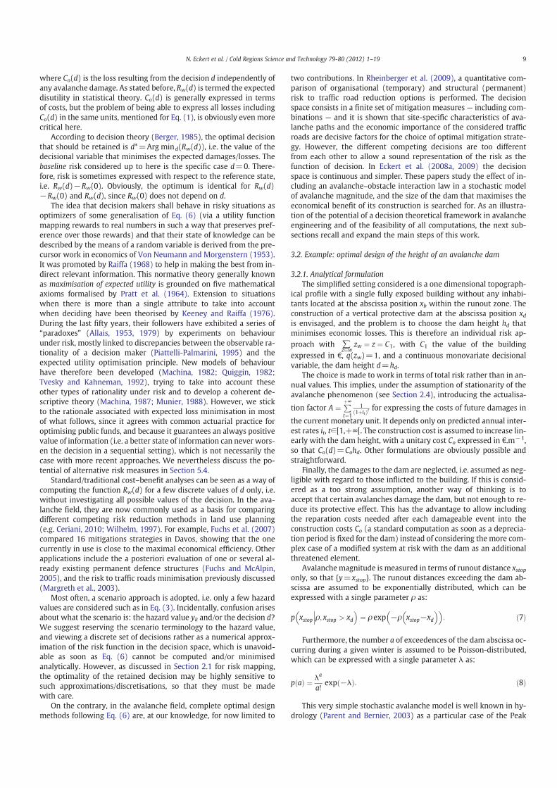
where Co(d) is the loss resulting from the decision d independently of
any avalanche damage. As stated before, Rw(d) is termed the expected
disutility in statistical theory. Co(d) is generally expressed in terms
of costs, but the problem of being able to express all losses including
Co(d) in the same units, mentioned for Eq. (1), is obviously even more
critical here.
According to decision theory (Berger, 1985), the optimal decision
that should be retained is d*=Arg mind(Rw(d)), i.e. the value of the
decisional variable that minimises the expected damages/losses. The
baseline risk considered up to here is the specific case d=0. There-
fore, risk is sometimes expressed with respect to the reference state,
i.e. Rw(d)−Rw(0). Obviously, the optimum is identical for Rw(d)
−Rw(0) and Rw(d), since Rw(0) does not depend on d.
The idea that decision makers shall behave in risky situations as
optimizers of some generalisation of Eq. (6) (via a utility function
mapping rewards to real numbers in such a way that preserves pref-
erence over those rewards) and that their state of knowledge can be
described by the means of a random variable is derived from the pre-
cursor work in economics of Von Neumann and Morgenstern (1953).
It was promoted by Raiffa (1968) to help in making the best from in-
direct relevant information. This normative theory generally known
as maximisation of expected utility is grounded on five mathematical
axioms formalised by Pratt et al. (1964). Extension to situations
when there is more than a single attribute to take into account
when deciding have been theorised by Keeney and Raiffa (1976).
During the last fifty years, their followers have exhibited a series of
“paradoxes” (Allais, 1953, 1979) by experiments on behaviour
under risk, mostly linked to discrepancies between the observable ra-
tionality of a decision maker (Piattelli-Palmarini, 1995) and the
expected utility optimisation principle. New models of behaviour
have therefore been developed (Machina, 1982; Quiggin, 1982;
Tvesky and Kahneman, 1992), trying to take into account these
other types of rationality under risk and to develop a coherent de-
scriptive theory (Machina, 1987; Munier, 1988). However, we stick
to the rationale associated with expected loss minimisation in most
of what follows, since it agrees with common actuarial practice for
optimising public funds, and because it guarantees an always positive
value of information (i.e. a better state of information can never wors-
en the decision in a sequential setting), which is not necessarily the
case with more recent approaches. We nevertheless discuss the po-
tential of alternative risk measures in Section 5.4.
Standard/traditional cost–benefit analyses can be seen as a way of
computing the function Rw(d) for a few discrete values of d only, i.e.
without investigating all possible values of the decision. In the ava-
lanche field, they are now commonly used as a basis for comparing
different competing risk reduction methods in land use planning
(e.g. Ceriani, 2010; Wilhelm, 1997). For example, Fuchs et al. (2007)
compared 16 mitigations strategies in Davos, showing that the one
currently in use is close to the maximal economical efficiency. Other
applications include the a posteriori evaluation of one or several al-
ready existing permanent defence structures (Fuchs and McAlpin,
2005), and the risk to traffic roads minimisation previously discussed
(Margreth et al., 2003).
Most often, a scenario approach is adopted, i.e. only a few hazard
values are considered such as in Eq. (3). Incidentally, confusion arises
about what the scenario is: the hazard value yk and/or the decision d?
We suggest reserving the scenario terminology to the hazard value,
and viewing a discrete set of decisions rather as a numerical approx-
imation of the risk function in the decision space, which is unavoid-
able as soon as Eq. (6) cannot be computed and/or minimised
analytically. However, as discussed in Section 2.1 for risk mapping,
the optimality of the retained decision may be highly sensitive to
such approximations/discretisations, so that they must be made
with care.
On the contrary, in the avalanche field, complete optimal design
methods following Eq. (6) are, at our knowledge, for now limited to
two contributions. In Rheinberger et al. (2009), a quantitative com-
parison of organisational (temporary) and structural (permanent)
risk to traffic road reduction options is performed. The decision
space consists in a finite set of mitigation measures — including com-
binations — and it is shown that site-specific characteristics of ava-
lanche paths and the economic importance of the considered traffic
roads are decisive factors for the choice of optimal mitigation strate-
gy. However, the different competing decisions are too different
from each other to allow a sound representation of the risk as the
function of decision. In Eckert et al. (2008a, 2009) the decision
space is continuous and simpler. These papers study the effect of in-
cluding an avalanche–obstacle interaction law in a stochastic model
of avalanche magnitude, and the size of the dam that maximises the
economical benefit of its construction is searched for. As an illustra-
tion of the potential of a decision theoretical framework in avalanche
engineering and of the feasibility of all computations, the next sub-
sections recall and expand the main steps of this work.
3.2. Example: optimal design of the height of an avalanche dam
3.2.1. Analytical formulation
The simplified setting considered is a one dimensional topograph-
ical profile with a single fully exposed building without any inhabi-
tants located at the abscissa position xb within the runout zone. The
construction of a vertical protective dam at the abscissa position xdis envisaged, and the problem is to choose the dam height hd that
minimises economic losses. This is therefore an individual risk ap-
proach with ∑z∈w
zw ¼ z ¼ C1, with C1 the value of the building
expressed in €, q(zw)=1, and a continuous monovariate decisional
variable, the dam height d=hd.
The choice is made to work in terms of total risk rather than in an-
nual values. This implies, under the assumption of stationarity of the
avalanche phenomenon (see Section 2.4), introducing the actualisa-
tion factor A ¼ P
þ∞
t¼1
11þitð Þt for expressing the costs of future damages in
the current monetary unit. It depends only on predicted annual inter-
est rates it, t∈[1,+∞[. The construction cost is assumed to increase lin-
early with the dam height, with a unitary cost Co expressed in €.m−1,
so that Co(d)=Cohd. Other formulations are obviously possible and
straightforward.
Finally, the damages to the dam are neglected, i.e. assumed as neg-
ligible with regard to those inflicted to the building. If this is consid-
ered as a too strong assumption, another way of thinking is to
accept that certain avalanches damage the dam, but not enough to re-
duce its protective effect. This has the advantage to allow including
the reparation costs needed after each damageable event into the
construction costs Co (a standard computation as soon as a deprecia-
tion period is fixed for the dam) instead of considering the more com-
plex case of a modified system at risk with the dam as an additional
threatened element.
Avalanchemagnitude is measured in terms of runout distance xstoponly, so that {y=xstop}. The runout distances exceeding the dam ab-
scissa are assumed to be exponentially distributed, which can be
expressed with a single parameter ρ as:
p xstop ρ; xstop > xd
�
�
�
�
¼ ρ exp −ρ xstop−xd
� �� �
:�
ð7Þ
Furthermore, the number a of exceedences of the dam abscissa oc-
curring during a given winter is assumed to be Poisson-distributed,
which can be expressed with a single parameter λ as:
p að Þ ¼ λa
a!exp −λð Þ: ð8Þ
This very simple stochastic avalanche model is well known in hy-
drology (Parent and Bernier, 2003) as a particular case of the Peak
9N. Eckert et al. / Cold Regions Science and Technology 79-80 (2012) 1–19

Over Threshold (POT) model family (Coles, 2001) which models the
exceedences of any stationary process as soon as the threshold is
high enough (Pickands, 1975).
Following Faug et al. (2008), the influence of the dam on relatively
rapid avalanche flows is expressed as a linear relation between the
runout distance reduction and the ratio, hd/ho, between the dam
height, hd, and the depth of the flow without the dam, ho. The runout
distance without the dam, xstopo, is therefore reduced to xstop(hd), the
runout distance of the same avalanche with a dam height hd, with a
proportionality coefficient α quantifying the first-order effect of the
dam:
xstop hdð Þ−xdxstopo−xd
¼ 1−αhdho
: ð9Þ
For simplicity, in the rest of the paper, we will consider the ficti-
tious case corresponding to the known and fixed value ho=1m. How-
ever, all the proposed developments and results can be understood
and interpreted more realistically as functions of the scaled variable
hd/ho.
With this avalanche–dam interaction law, the cumulated probability
of exceeding the building abscissa P(xstop≥xb)=exp(−ρ(xb−xd)) is
reduced, leading to the residual probability for the building of being
hit with the dam:
P xstop≥xb hdj Þ ¼ exp−ρ xb−xdð Þ1−α hd=hoð Þ
� �
:
�
ð10Þ
This shows that (1−α(hd/ho))/ρ is the scale parameter for the ex-
ponential distribution of runouts with the dam hd, leading to the an-
nual quantile:
xstopT hdð Þ ¼ 1−α hd=hoð Þρ
� �
ln λTð Þ þ xd; ð11Þ
i.e. to the runout distance xstopT(hd) corresponding to the return peri-
od T with the dam height hd. It represents the residual hazard after
the dam construction. It is represented in Fig. 5a for different dam
heights, including the baseline case hd=0.
Finally, the very rough worst case vulnerability relationship is as-
sumed: maximal damage as soon as the building is attained, whereas
it remains obviously undamaged if the avalanche does not reach its
abscissa:
V z; yð Þ ¼ V C1; xstop
� �
¼ I xstop≥xbf g: ð12Þ
All these modelling assumptions can be seen as very strong. Their
limits and implications, as well as detailed results for a case study are
extensively discussed in the original paper (Eckert et al., 2008a).
Their advantage is that they permit easy computation of Eq. (6) ana-
lytically, leading to:
R hdð Þ ¼ Cohd þ AλC1 ∫þ∞
xb−xd1−α hd=hoð Þ
ρ exp −ρ xstop−xd
� �� �
dxstop
¼ Cohd þ AλC1 exp−ρ xb−xdð Þ1−α hd=hoð Þ
� �
; ð13Þ
which nicely illustrates the contribution of the different terms to the
total expected losses. The construction cost, Cohd, depends on the size
of the obstacle only. Avalanche hazard is involved through the expec-
tation of the annual distribution of avalanche numbers reaching the
dam abscissa, i.e. the annual exceedence rate λ, and through the re-
duced probability of hitting the building P(xstop≥xb|hd). The actualisa-
tion factor A corresponds to the equivalent number of years that has
to be considered for the annual risk computation to coincide with
the total damage starting from the date of the dam construction. An-
other way to see it is as an equivalent number of buildings that
weights the annual risk for a single building.
R(hd) is plotted as functions of xb in Fig. 5b. The baseline risk is
R0=R(0)=AλC1 exp(−ρ(xb−xd)). For all other dam heights, R(hd)
is the residual risk in the runout zone. This family of curves illustrates
the reduction of expected losses with the increase of the dam height
for “small” values of xb, as well as the convergence to the constant
Cohd (different for each dam height) for “large” values of xb because
the building is then constructed at a safe position.
Finally, the difference in expected losses if the dam hd is con-
structed instead of no dam built:
R hdð Þ−R0 ¼ Cohd
þ AλC1 exp−ρ xb−xdð Þ1−α hd=hoð Þ
� �
− exp −ρ xb−xdð Þð Þ� �
; ð14Þ
is simply the opposite of the benefit expected from the dam
construction.
Seen rather as functions of hd, Eqs. (13)–(14) can be minimised for
each building position, xb, which can be used to maximise the benefit
from the dam construction. Fig. 6 shows the risk functions obtained
for buildings situated at annual quantile positions xstopT(0) ranging
Fig. 5. Residual hazard and residual risk. Analytical model and case study from Eckert et
al. (2008a). a) Residual hazard is the annual quantile xstopT from Eq. (11) for different
dam heights hd. b) Residual risk represents the total expected loss as a function of
the abscissa position of a single building xb for different dam heights. ho=1m is fixed.
10 N. Eckert et al. / Cold Regions Science and Technology 79-80 (2012) 1–19
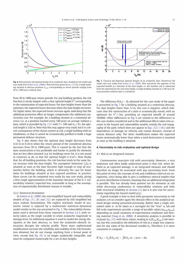
from 30 to 1000 year return periods. For any building position, the risk
function is nicely shaped, with a clear optimal height h⁎ corresponding
to the minimisation of expected losses. For dam heights lower than the
optimum, the expected losses decrease when the dam height increases.
For higher dams, the expected losses increase again, indicating that the
additional protective effect no longer compensates the additional con-
struction cost. For example, for a building situated at a centennial ab-
scissa (i.e. at a position reached every 100 years on average without a
dam, which is provided by Eq. (11) with T=100 and hd=0), the opti-
mal height is 3.02 m. Note that this may appear very small, but it is a di-
rect consequence of the chosen system at risk, a single building with no
inhabitants, so that it cannot be economically justified to build a huge
permanent defence structure.
Fig. 6 also shows that the optimal dam height decreases from
4.32 m to 0.34 m when the return period of the considered abscissa
increases from 30 to 1000 years. This is caused by the fact that the
dam construction is less profitable and harder to justify for elements
that are less often attained (e.g. for buildings never hit, it is not sound
to construct at all, so that the optimal height is 0 m!). Note finally
that, for all building positions, the risk function tends to the same lin-
ear increase with the dam height. The asymptotic behaviour Cohd is
attained as soon as the dam becomes high enough to stop all ava-
lanches before the building, which is obviously the case for lower
dams for buildings situated at less exposed positions. In practice,
these curves can be computed very easily for any case study, giving
a first rough approximation of the maximal (because of the 0–1 vul-
nerability relation) expected loss, reasonable as long as the assump-
tion of exponentially distributed runouts is tenable.
3.2.2. Numerical formulation
In Eckert et al. (2009) the oversimplified hazard and vulnerability
models of Eqs. (7), (8) and (12) are replaced by still simplified but
more realistic formulations. The explicit stochastic model of ava-
lanche runout is replaced by a multivariate statistical–dynamical
model similar to the one presented in Fig. 1. The vulnerability formu-
lation used is derived from those reported in Section 2.2.3, with ve-
locity taken as the single variable to relate avalanche magnitude to
damage level. An additional equation is used to model the energy dis-
sipation at the dam abscissa, i.e. how the avalanche–obstacle in-
teraction disrupts the velocity profile. These more sophisticated
modifications increase the reliability and usability of the risk formula-
tion obtained, but do not change anything from a formal point of
view, except that Eq. (6) is no longer analytically integrable, and
must be computed numerically for a set of dam heights.
The difference R(hd)−R0 obtained for the case study of the paper
is presented in Fig. 7 for a building situated at a centennial abscissa.
For dam heights lower than 12 m, this cost is negative, which indi-
cates that the construction of a dam is economically sound, with an
optimum for h⁎=5m, providing an expected benefit of around
30000€. Other differences to Fig. 6 are related to the differences in
the case studies considered and in the additional effects taken into ac-
count in the hazard and vulnerability models, mainly the real topog-
raphy of the path (which does not appear in Eqs. (12)–(14)) and the
dependence of damage on velocity and runout distance, instead of
runout distance only. The latter modification makes the expected
losses systematically lower than when a total destruction is assumed
as soon as the building is attained.
4. Uncertainty in risk evaluation and optimal design
4.1. Risk as an integrated measure
Commonsense associates risk with uncertainty. However, a very
important and often badly understood point is that risk, when de-
fined as an expected damage, is an integrated measure and should
therefore no longer be associated with any uncertainty level. From
this point of view, the concepts of risk and confidence interval are an-
tagonistic, since being able to give a confidence interval implies that
an error distribution is known, meaning that an additional integration
is possible. This has already been pointed out for elements at risk
while discussing randomness in vulnerability relations and links
with structural reliability in Section 2.3, but it is also true for uncer-
tainty regarding the hazard model p(y).
A good example is how to deal with parameter uncertainty in risk
analyses. Let us consider again the obstacle effect in the analytical op-
timal design setting presented previously. Rather than a single esti-
mated value α to be taken as a surrogate for the “true” α, lab and
full scale experiments provide a range of possible values [αmin,αmax],
depending on small variations of experimental conditions and flow-
ing material (Faug et al., 2008). A sensitivity analysis is possible to
evaluate Eq. (13) with these values, leading to a [Rmin,Rmax] risk inter-
val, but this contradicts the definition of risk as a single loss expecta-
tion for any value of the decisional variable hd. Therefore, it is more
consistent to compute:
R0hdð Þ ¼ Eα R hd;αð Þ½ � ¼ ∫R hd;αð Þ � p αð Þ � dα; ð15Þ
Fig. 6. Risk function and optimal design of an avalanche dam. Analytical risk model and
case study from Eckert et al. (2008a). Risk functions given by Eq. (13) for a single build-
ing situated at abscissa positions xstopT corresponding to return periods ranging from
30 to 1000 years without dam.
Fig. 7. Classical and Bayesian optimal designs of an avalanche dam. Numerical risk
model and case study from Eckert et al. (2009). Risk represents the opposite of the
expected benefit as a function of the dam height, i.e. the baseline risk is subtracted
from the expected loss for each dam height. A single building situated at a 100-year ab-
scissa position without dam is considered.
11N. Eckert et al. / Cold Regions Science and Technology 79-80 (2012) 1–19

where R(hd,α) is the risk with a fixed value of α given by Eq. (13), and
p(α) a probability distribution quantifying the possible values of the
parameter and their respective credibilities, i.e. a probabilistic judge-
ment ascertaining a degree of belief. If one is willing to assume the
uncertainty on α to be represented by the uniform distribution
p αð Þ ¼ 1αmax−αmin
on ]αmin,αmax[, R ' (hd) is then:
R0hdð Þ ¼ Cohd þ
AλC1
αmax−αmin∫
αmax
αmin
exp−ρ xb−xdð Þ ho=hdð Þ
ho=hdð Þ−α
� �
dα: ð16Þ
Integration is still analytically feasible, leading to:
R0hdð Þ ¼ Cohd þ
AλC1
αmax−αmin
αmax− ho=hdð Þð Þ exp −ρ xb−xdð Þ ho=hdð Þho=hdð Þ−αmax
� �
− αmin− ho=hdð Þð Þ exp −ρ xb−xdð Þ ho=hdð Þho=hdð Þ−αmin
� �
þρ xb−xdð Þ ho=hdð Þ expint ρ xb−xdð Þ ho=hdð Þho=hdð Þ−αmax
� �
−ρ xb−xdð Þ ho=hdð Þ expint ρ xb−xdð Þ ho=hdð Þho=hdð Þ−αmin
� �
2
6
6
6
6
6
6
6
6
6
6
6
6
6
6
6
4
3
7
7
7
7
7
7
7
7
7
7
7
7
7
7
7
5
;
ð17Þ
where exp int xð Þ ¼ ∫x
−∞1t exp −tð Þdt is the exponential integral func-
tion which is tabulated by most computational software. By compar-
ison to Eq. (13), the risk R ' depends on the bounds (αmin,αmax) rather
than on a single value of α.
Logically, Eq. (17) converges to the risk function givenby Eq. (13) for
very sharp distributions of α. Uniform “flat” distributions for the credi-
bility about α have large variances, meaning that when little is known
about α except bounds, probabilistic bets can be scattered on a large
range of possible values. Hence, the optimal height and expected losses
tend to increase with the variance of the credibility regarding α, and
convergence to the asymptote Cohd is slower when α is poorly known
(Fig. 8). This is all attributable to the explicit incorporation of an addi-
tional uncertainty source into the decisional process. It makes the
expected losses higher for a given damheight, and requires amore cau-
tious design when α is not known perfectly, which is logical.
Finally, it is noteworthy that optimality is more conservative than
risk., i.e. that the optimal height increases more slowly with the uncer-
tainty level regarding α than the expected losses at the optimum, i.e. of
around 8% versus of around 17% on the investigated uncertainty range
(Table 1).
4.2. Variability and uncertainty in the risk framework
Another point which needs clarification is the difference between
uncertainty and variability (O'Hagan and Oakley, 2004). The former re-
sults from a lack of knowledge (for example, about critical parameters)
and is called uncertainty by ignorance or epistemic uncertainty by some
authors, whereas the second (sometimes called uncertainty by essence
or rather confusingly random uncertainty) is related to natural varia-
tions of the studied phenomenon, here snow avalanches, driven by var-
iable snow and weather conditions. Therefore, uncertainty and
variability imply totally different modelling assumptions since, in reali-
ty, there is only a fixed single value for every uncertain unknown but
many different outcomes can occur from the same variablemechanism.
However, itmust be emphasised that both are treated in a similarway
with the mathematical toolbox of probabilities in the risk framework. As
an example of this non-distinction, onemay consider the case, important
in practice, of a risk evaluation with a scenario approach, but taking into
account a given uncertainty level around the chosen reference value.
This is the basis of the analysis of Fuchs and McAlpin (2005) discussed
earlier to highlight the sensitivity of risk evaluation to a reference hazard
value. In the decisional context, the risk function associated to the scenar-
io y is the total loss expected if the y event occurs:
Rw d; yð Þ ¼ Co dð Þ þ ∑z∈w
zw dj Þq zw dj ÞV z; yð Þ:ðð ð18Þ
A classical representation for the uncertainty around the reference
scenario is the Gaussian distribution y~N(yk,σyk2), i.e. centred on the
chosen reference scenario yk, with a variance σyk2 modelling the asso-
ciated distribution of uncertainty. In other words yk is the best guess,
but one believes to make a winning bet with odds 95 against 5 that
the scenario y lies between yk−1.96σyk and yk+1.96σyk. This leads
to the integrated risk function:
R0
w hdð Þ ¼ ∫ 1
σyk
ffiffiffiffiffiffi
2πp exp
y−ykð Þ2
2σ2yk
!
Rw hd; yð Þdy: ð19Þ
This function Rw' is the result of epistemic uncertainty concerning
the reference scenario yk. However, the same function is obtained by
evaluating Eq. (6) with p(y)~N(yk,σyk2), i.e. under the assumption
that the variability of snow avalanches in the considered system at
risk can be modelled by a perfectly known Gaussian probability
model.
Application to the chosen optimal design illustrative example leads to
evaluating Eq. (13) with the normal distribution p(xstop)~N(xstopk,σxstopk2)
instead of an exponential one. For homogeneitywith Eq. (13), a total cost
Fig. 8. Sensitivity of the optimal design to the uncertainty regarding the avalanche–obstacle
interaction law. Case study from Eckert et al. (2008a). Risk functions are evaluated using Eq.
(17). They represent the total expected loss as a function of the dam height for different un-
certainty levels regarding theαparameter. A single building situated at a30-year abscissa po-
sition without dam is considered.
Table 1
Effect of the uncertainty regarding the avalanche–obstacle interaction law on the optimal
height and associated risk. Risk model and case study from Eckert et al. (2008a). The ele-
ment at risk is a single building at an abscissa position corresponding to a 30 year return
period.Δh� represents the difference in optimal height h* between α ¼ α and the consid-
ered uncertainty range. ΔR h�ð Þ is the corresponding difference in expected loss.
α ¼ α ¼ 0:1376 α � 0:01 α � 0:03 α � 0:05
h* (m) 4.32 4.33 4.45 4.7
Δh� (m) / 0.01 0.13 0.38
Δh� (%) / 0.2 2.9 8.1
R(h*) (€) 25 873 26 057 27 500 30 193
ΔR h�ð Þ (€) / 184 1627 4320
ΔR h�ð Þ (%) / 0.7 6.3 16.7
12 N. Eckert et al. / Cold Regions Science and Technology 79-80 (2012) 1–19

approach is kept, adding the A and λ factors to weight the loss expected
from a single event, which gives:
R0hdð Þ ¼ Cohd
þAλC1 ∫þ∞
xb−xd1−α hd=hoð Þ
1
σ xstopk
ffiffiffiffiffiffi
2πp exp
xstop−xstopk
� �2
2σ2xstopk
0
B
@
1
C
Adxstop
¼ Cohd þ AλC1 1−ϕxb−xd
1−α hd=hoð Þ
� �� �
;
ð20Þ
whereϕ xb−xd1−α hd=hoð Þ
� �
represents the normal cumulative distribution func-
tion of mean xstopk and standard deviation σxstopk2 evaluated in xb−xd
1−α hd=hoð Þ.
Hence, R '(hd) represents the total losses to be expected from the succes-
sive occurrences of the xstopk reference event on the long term, but taking
into account the associated uncertainty. The alternative interpretation as
a result of the variability of snowavalanches on the considered case study
is mathematically plausible, but practically highly unlikely because the
assumption of normally distributed runout distances is never fulfilled.
Intuitively, without uncertainty about xstopk, the dam construction
is unsound if xstopkbxb because the building is then constructed at a
safe position, On the contrary, if xstopk>xb, the building is exposed
without the dam, and the height h� ¼ hoα
1− xb−xdxstopk−xd
� �
just sufficient
to stop the reference event at the building abscissa should be advised.
For uncertainty levels represented by σxstopk>0, the building is not
fully safe even for xstopkbxb, and Eq. (20) can be evaluated for any
dam height and minimised, leading to results very useful in an oper-
ational context to test the economical efficiency of a hazard zoning
map based on a reference event and its modification by a dam.
For example, Fig. 9 shows the risk functions obtained with differ-
ent building positions xb, different uncertainty levels, σxstopk, and the
reference event xstopktaken as the centennial quantile from Eq. (11)
without a dam, a classical hazard zoning limit. The three curves in
Fig. 9a represent a building within the extension of the considered
reference event (blue), just at the limit of the extension of the refer-
ence event (black), and beyond its extension (red), respectively.
They are nicely shaped, with, in all cases, first a rapid decrease of
expected losses with the dam height, then a clear optimal height,
and finally a rapid convergence to the asymptotic behaviour Cohd for
higher dams. This is even true in the case of the building situated out-
side the extension of the reference event because its probability of
being hit is significant for low dam heights with the considered un-
certainty level. Differences with the case of exponentially distributed
runouts of Fig. 6 are, for a given building position, a lower optimal
height, lower expected losses and a sharper shape before and after
the optimum. They are related to the greater dispersion and asymme-
try of an exponential tail with regard to the bell-shaped Gaussian
case. Fig. 9b corresponds to the case of a building situated just at
the extension limit of the reference event (black line in 9a), but
with different uncertainty levels, σxstopk. The different curves show
the increase in optimal height and expect losses with the uncertainty
level, because, with high uncertainty levels, the probability of hitting
the building remains high even for relatively high dams.
4.3. Calibration, parameter uncertainty and Bayesian risk
Another particular case of the variability/uncertainty distinction is
the one related to the calibration of the stochastic avalanche model
and the related estimation error. Indeed, avalanche models are still
far from perfect, so that they need local calibration to give reliable re-
sults. Classical notation for the avalanche model is p(y|θ), where θ is
the vector of unknown parameters. For example, θ={λ,ρ} in the
POT model of Eqs. (7)–(8), and includes the friction coefficients of
the propagation model as additional component of θ when a statisti-
cal–dynamical model such as the one of Fig. 1 is used.
The typical calibration challenge is to get a point estimate, θˆ, using
the available data in order to use p y θˆ�
�
�
��
for risk computations or,
more classically, quantifying reference hazards. Beyond the possible
technical difficulty of the calibration task, such an approach has the
drawback that it neglects the estimation error around θˆ, which is unre-
alistic with regard to the generally poor local information available. Fur-
thermore, this may bias the decision in an undesirable way, because
calibration is generally performed byminimisation of a variance criteri-
on (e.g. mean square error minimisation), which is a symmetrical qua-
dratic function, whereas, in the context of natural hazards, the penalty
to be applied for the decision is clearly asymmetrical. As an obvious ex-
ample, the total costs increase muchmore strongly if an avalanche dam
height is overestimated by a given value than if it is underestimated by
the same amount. These problems are fairly addressed within the
Fig. 9. Risk functions and optimal design for Gaussian uncertainty around reference
scenarios. Case study from Eckert et al. (2008a). Risk functions evaluated using Eq.
(20): a) for various building positions xb with xstopk=xstop100
and σxstopk=30m, b) for
various uncertainty levels σxstopk with xstopk=xb=xstop100
.
13N. Eckert et al. / Cold Regions Science and Technology 79-80 (2012) 1–19

Bayesian framework by first computing the posterior distribution of the
parameters given the available data sample yobs such as:
p θ yobsj Þ∝p θð Þ � p yobs θj Þ;ðð ð21Þ
where p(yobs|θ) is the probability of the data under the assumption that
they are (generally independent) realisations of p(y|θ), and p(θ), a (pos-
sibly non or poorly informative) prior distribution representing extra-
data information (Berger, 1985). In this framework, the Bayesian
definition of probability quantifies directly the degree of uncertainty
of a scientific judgement, the probability of an event being the price at
which one would buy or sell a bet that rewards one currency unit if it
happens, and nothing if it fails (Kadane, 2011). Accordingly, the posteri-
or distribution expresses mathematically the uncertainty source stem-
ming from partial knowledge of θ in the risk equation, in turn leading
to the Bayesian risk by integrating over parameter uncertainty:
RBw d; yobsð Þ ¼ ∫p θ yobsj Þ � Rw d; θð Þdθ;ð ð22Þ
where Rw(d,θ) is the risk function for the system, w, provided by
Eq. (6) with the model parameter value θ. From a practical point of
view RBw(d,yobs) is, a function of d only instead of being a function
of model parameters also, making the search of the optimal decision
dB*=Arg min d(RBw(d,yobs)) thatminimises the expected losses easier.
From the more theoretical point of view of statistical decision the-
ory, it can be shown that choosing dB* instead of other decisions has
suitable properties with regard to the statistical risk defined in
Section 2.1.3. First, dB* minimises the averaged opportunity loss
Λ Rw− ¼ ∫ Rw d�; θ
�
−Rw d; θð Þ �
� p θ yobsj Þdθð , i.e. the loss to be expected
because of an imperfect knowledge of the hazard model if the deci-
sion d is taken instead of the optimal one d*. Second, when considered
as a function of data, dB* is the decision rule dB*=δ(yobs), which be-
longs to the set of so-called Bayes' rules obtained by varying the
prior distribution. Such rules are known to dominate other decision
rules under low restrictive regularity conditions (Wald, 1950). An ex-
ample of a comparison of Bayes' rule to other intuitive rules including
safety factors can be found in Parent et al. (2010) in the related case of
the optimal design of a dam protecting against river floods.
Applications of Bayesian methods to various forms of avalanche
models can be found in McClung and Tweedy (1994), Harbitz et al.
(2001), Ancey (2005), and Eckert et al. (2007b, 2008b). For example,
Bayesian risk computations have been applied to avalanche risk map-
ping over large areas in a GIS environment (Grêt-Regamey and
Straub, 2006). This leads to a risk value as a function of space as de-
tailed in Section 2.5.1, but taking into account the imperfect local in-
formation. On the other hand, no decisional variable is considered in
this particular study, and only a finite set of possible friction parame-
ters values for the statistical–dynamical hazard model is used.
Application of Bayesian optimal design procedures and compari-
son with classical ones can be found in the previously mentioned pa-
pers (Eckert et al., 2008a, 2009). In the case of the analytical
illustrative example, integration of Eq. (13) leads to:
RB hd; yobsð Þ ¼ Cohd þ AC1∫∞
λ¼0 ∫∞
ρ¼0
λ exp−ρ xb−xdð Þ1−α hd=hoð Þ
� �
p λ;ρ yobsj Þdρdλ:ð
ð23Þ
Analytical computation remains possible, if so called conjugate
Gamma priors are chosen for {λ,ρ}:
p ρ aρ; bρÞ ¼aρ
bρ
Γ bρ
� �ρbρ−1
exp −aρρ� �
; and
�
�
�
�
�
�
0
@ ð24Þ
p λ aλ; bλÞ ¼ aλbλ
Γ bλð Þλbλ−1
exp −aλρð Þ:�
�
�
�
�
ð25Þ
(aρ,bρ) and (aλ,bλ) are two pairs of parameters to be specified repre-
senting the knowledge about avalanche magnitude and frequency on
the studied site prior to local data analysis, and possibly resulting from
expert knowledge concerning their regional behaviour (Kadane and
Wolfson, 1998). Posterior distributions for λ and ρ are then still
Gamma distributed, with the parameter pairs (aρ' ,bρ
' ) and (aλ' ,bλ
' )
combining the prior knowledge and the information conveyed by
the data. More precisely, with a data set yobs of n avalanches exceed-
ing the threshold xd in m years and S(n) the sum of these excee-
dences, aλ' =aλ+m, bλ
' =bλ+n, aρ' =aρ+S(n) and bρ
' =bρ+n,
which indicates that, when n and m are large enough, the prior
knowledge does not play much of a role. Computations detailed in
Eckert et al. (2008a) lead to:
RB hd; yobsð Þ ¼ Cohd þ AC1
b0
λ
a0
λ
a0
ρ
a0ρ þ xb−xd
1−α hd=hoð Þ
!b0ρ
; ð26Þ
i.e. to a risk function similar to Eq. (13) since bλ' /aλ
' is the posterior ex-
pectancy of λ (i.e. themost probable exceedence rate given the data),
anda0ρ
a0ρþxb−xd
� �b0ρ
the posterior probability of exceeding the distance xb
without dam, which is reduced by the avalanche–obstacle interac-
tion law.
Results obtained for different building positions are summarised
in Table 2. For all dam heights, the Bayesian optimum is higher than
the classical one leading to a more cautious recommendation, due
to imperfect knowledge. This result is coherent with those obtained
regarding the influence of the α parameter in Section 4.1, and σxstopk
in Section 4.2: the additional uncertainty source, here parameter un-
certainty resulting from the lack of local information, calls for a more
cautious optimal design hB* and higher expected losses. Note that, in
fact, Eq. (17) can be seen as a Bayesian risk if the chosen uniform dis-
tribution p(α) is interpreted as a posterior distribution derived from
observations.
Moreover, the systematic difference between the Bayesian and
classical optimal heights increases from 5% to 250% for return periods
of the building abscissa ranging from 10 to 1000 years. Taking estima-
tion error into account therefore affects, in particular, the optimal de-
sign of a defence structure protecting buildings threatened only by
the most extreme events. This is another intuitive result given that
estimation error affects the evaluation of the highest quantiles of
the hazard distribution more strongly, making extreme runout dis-
tances more probable than if perfect knowledge is assumed.
Going back to the numerical model of Fig. 7 yields similar results,
with the Bayesian optimal height 20% higher (6 m versus 5 m) than
the classical one, and the benefit expected from the construction of
the optimal dam higher when the Bayesian computation is used
(41465 €) than when the classical computation is used (28863 €),
with a relative difference of 54%. The absolute difference RB(hB*)
−R(h*)=14602 € can be interpreted as the expected opportunity
loss ΛR for the Bayesian decision rule against the minimisation of
expected losses under the classical paradigm. It is attributable to the
limited sample of avalanche runouts on the case study. In other words
Table 2
Classical and Bayesian optimal heights for buildings situated at abscissa positions cor-
responding to different return periods. Risk model and case study from Eckert et al.
(2008a). Δh� ¼ h�B−h� represents the difference between the Bayesian hB* and classical
h* optimal heights.
T10 T30 T100 T300 T1000
h* (m) 5.42 4.32 3.02 1.77 0.34
hB* (m) 5.69 4.73 3.58 2.47 1.19
Δh� (m) 0.27 0.41 0.56 0.7 0.85
Δh� (%) 5 9.5 18.5 39.6 250
14 N. Eckert et al. / Cold Regions Science and Technology 79-80 (2012) 1–19

this is the value of information, i.e. the value quantifying what the deci-
sion maker should be ready to pay to obtain perfect information θ ¼ θˆ
with full confidence, i.e. to fund an exhaustive data collection protocol.
Optimal properties of Bayes' decision rules grant that other decisional
procedures would yield a lower expected profit for the decision maker.
4.4. Decisional sensitivity analyses
Even if the risk concept is designed to integrate as many variability/
uncertainty sources as possible, it cannot take into account those for
which it is unsound to consider them as being expressible in terms of
probability distributions. For instance, this concerns quantities such as
the position of the elements at risk. The risk function itself can never-
theless be computed for different values, so as to investigate their influ-
ence on the risk function and on the optimal solution, thus leading to
(classical or Bayesian) decisional sensitivity analyses. Previous develop-
ments have already illustrated decisional sensitivity analyses, with e.g.
the evolution of the total risk and of the optimal dam height with the
position of the building in Fig. 6. Much more detailed results regarding
the effects of the different parameters on risk functions can be found
in Eckert et al., 2008a. A particularly important case is the one related
to the vulnerability relation. Keylock and Barbolini (2001) postulated
simple hypothetical functions for the vulnerability relation and showed
that risk zoning is relatively robust to the vulnerability formulation
used. This finding has been confirmed in Eckert et al. (2009) where
the risk functions obtainedwere quite similarwith a set of different vul-
nerability relations. Furthermore, the optimal damheightwas shown to
be even less sensitive to the choice of the damage formulation, in a sim-
ilar way that the uncertainty regarding α affected the optimal decision
less than the total losses corresponding to the optimal decision in the
example of Section 4.1.
These results can be explained by the fact that, for a disastrous
phenomenon such as a snow avalanche, the “first order effect” is
whether or not the element at risk is attained by the flow or not. It
is therefore understandable that results remain mainly unchanged
for damage formulations that only differ in the precise way in
which the dependency between damage and flow velocity or pres-
sure is accounted for. More generally, these results are also compati-
ble with theoretical work showing the robustness of optimal
decisions with regard to a relatively large class of loss functions
(Abraham and Cadre, 2004). All this suggests that the main results
from risk analyses can already be used with reasonable confidence
for avalanche engineering projects, even if important efforts remain
to be done to improve our knowledge about vulnerability relations.
5. Open questions and directions for further work
5.1. Improvements to the different sub-models
Risk analyses combine different sub-models for avalanche hazard
and vulnerability. The influence of decisions must also be modelled
in cases of an optimal design approach, e.g. the effect of an obstacle
(such as a dam) on the flow dynamics as a function of its size and
shape. Nevertheless, according to our review, existing applications,
even if they give interesting preliminary results such as the maximal
expected loss in the case of the proposed illustrative analytical com-
putations, often rely on simplified sub-models instead of the most
up-to-date ones. For example, simple statistical models of avalanche
runout are generally used as hazard models rather than fully multivar-
iate statistical–dynamical modelswith avalanche flows described in the
framework of continuum mechanics. Similarly, semi-empirical, sim-
plified vulnerability curves are generally put in use rather than the
most recent results of systematic numerical investigations. There-
fore, improving the reliability of risk estimations involves putting
more effort into adapting state-of-the-art sub-models to the risk set-
ting. To do so, one major difficulty is the possible incompatibilities of
the input/outputs of the different sub-models. For example, as
shown with the illustrative analytical model, existing simplified for-
mulations for the effect of an obstacle on avalanche flows consider a
unique flow depth value (the maximum avalanche flow depth),
which is difficult to reconcile with, e.g., flow depths that vary at
each time step of the simulation.
Even if a certain robustness to the choice of the vulnerability rela-
tion exists (Section 4.4), priority should be given to improvements in
their formulation for both the tangible and less tangible elements at
risk. For civil engineering structures, numerical approaches, such as
those developed by Bertrand et al. (2010) but coupled with the struc-
tural reliability approach detailed in Section 2.3 seem promising for
estimating the probability of destruction for classes of elements at
risk large enough to be used in practice. In the short term, this should
help improve the methods currently in use for the design of perma-
nent defence structures, thus allowing a more optimal use of limited
public funds.
Another important point is that it should be possible to improve
existing methods for describing systems at risk, i.e. for identifying,
counting and evaluating the elements at risk, especially the less tan-
gible aspects of risk, whose value is certainly underestimated in exist-
ing approaches. This may require involving more people with social
science backgrounds into quantitative risk analyses.
Finally, the avalanche hazard models themselves may require
some degree of re-thinking tomove away from the old-fashioned con-
flict between deterministic and statistical schools ofmodelling. For ex-
ample, statistical avalanche models often neglect the existence of
different types of avalanche flows, different phases in the flow…,
etc., and we do not know if the distributions they provide for extreme
avalanches under various forcing inputs are always consistent with
Extreme Value Theory (Coles, 2001). Similarly, when a more physical
description of the flow is used, crucial questions such as the depen-
dency of impact pressure on hydrodynamic conditions (flow depth
and velocity), rheological properties (friction parameters on topogra-
phy and snow quality) and/or geometrical conditions (shape of the
impacted element) remain at least partially unclear. Therefore, much
work remains to be done for a better physical representation of the
flow, including an assessment of the stochasticity of the avalanche
phenomenon, e.g. of the variable properties of all possible avalanches
on a given site under study and of avalanches with the same starting
mass but varying dynamics due to variablemass entrainment, density,
or mass partitioning between powder and dense components.
5.2. Multivariate decisional approaches
Decision analyses performed within a risk framework can better ac-
count for the multivariate nature of avalanche hazard than standard
return-period based approaches. However, the seldom existing deci-
sional models reviewed in this work mostly consider a univariate deci-
sion variable such as a mitigation strategy chosen from a small number
of alternatives, or the choice of a dam height. This is a limitation that
does not really describe situations faced by stakeholders that have to
make several choices simultaneously, e.g. the extension of an area to
be evacuated during an avalanche cycle and the duration of the evacu-
ation. Existing decisionmodels can therefore arguably be seen rather as
toy-models or mathematical exercises than as useful tools in operation-
al contexts. This pleads in favour of expanding the existing decision
models towards amultivariate decisional framework. For instance, use-
ful improvements would be the joint optimisation of the different di-
mensions (height, width, length) of a defence structure, or of the time
and duration of a road closure for traffic regulation.
5.3. Computational issues in risk evaluation
Computational limitations are closely related to the necessity of
using themost up to date sub-models and of working in amultivariate
15N. Eckert et al. / Cold Regions Science and Technology 79-80 (2012) 1–19

decisional framework. Indeed, with advanced sub-models based on a
set of differential equations requiring a long time of computer occupa-
tion to be solved and/or complex decisional variables, the thousand
runs with different avalanche combinations of avalanche hazard and
decision necessary to evaluate Eqs. (1)–(6) by standard Monte Carlo
procedures cannot be launched (remember the typical statistical con-
vergence rate, i.e. 1=ffiffiffi
np
where n is the number of simulations). This is
especially true for short term problems such as road closures when it
is not possible to wait several days (or weeks!) to take decisions.
Therefore, existing methods for approximating Monte Carlo inte-
grals more rapidly than random searches should be adapted to the av-
alanche field, so as to significantly reduce the number of simulations
necessary for obtaining robust approximated solutions for the prob-
lem of risk minimisation. This could be done by putting in use the nu-
merous methods that have been developed in structural reliability for
approximating small probabilities in an efficient manner (Lemaire,
2009), with (e.g. First or Second Order Reliability Method — FORM/
SORM) or without (e.g. directional or stratified Monte Carlo searches)
approximations regarding the shape of the response surface, or even
with emulation of the entire model using stochastic processes as in
Sacks et al. (1989) or Kennedy and O'Hagan (2001).
5.4. Several measures of risk
A major characteristic of the decisional setting of Eq. (6) is that it
offers a unique optimal solution to a given problem. In most cases,
this is a positive attribute, but it can also have undesirable effects.
First, statistical decision theory is a “personal” theory in the sense
that it minimises losses according to the stakeholder's valuation of
the considered system at risk. On the contrary, in an operational con-
text, there are many different concerned protagonists to discuss and
negotiate different trade-offs between protection and costs (exposed
people may prefer a higher protection even if it is not fully “sound”
from the economical point of view). Second, the five behaviour prin-
ciples of Pratt et al. (1964) define a very strict rationale whereas
stakeholders may act rationally, but have their own definition of ra-
tionality, depending on their personality or psychology, for instance
on their risk perception. Third, from an even more theoretical point
of view, choosing to define optimality as the minimisation of
expected losses may be a dangerous strategy for a small mountain
community because of very limited funds available for recovering
after a major catastrophic event. Indeed, in the standard loss expecta-
tion, nothing is said about the time necessary to reach the expected
loss, and to the maximal loss that may be feared during this time.
This is well known in finance as a major cause of bankruptcies, espe-
cially in the context of extreme damageable phenomena, because the
amount of money available to compensate very high losses is not in-
finite (Embrechts et al., 1997).
These different problems could be overcome by using measures of
risk alternative to the simple loss expectation. This would restore
possibilities for negotiations, and leave to the stakeholders the final
decision, depending on their personality and on their political, social
and/or budgetary constraints. For instance, as discussed in Bernier
(2003) for hydrological problems, the behaviour of stakeholders fac-
ing risk can be taken into account by distorting the costs in the risk
equation via a coefficient representing a careful, neutral or risk-
prone personality. Even if it is not easy to quantify the marginal atti-
tude towards risk as a distortion of perceived potential incomes
(Munier, 1988), distorting costs into utility functions presents the ad-
vantage of staying under the mathematical framework grounded by
the axioms of Pratt et al. (1964), which introduces only little changes
to the general decisional framework of Eq. (6).
More radically, financial and insurance techniques have developed
a large range of risk measures. Optimal decision is then based on the
full distribution of random losses rather than on the maximised
expected utility only. The most usual of these alternative measures
is the Value at Risk (VaR), nothing more than a quantile of the distri-
bution of random losses that is not exceeded at a certain confidence
level. Many others exist, with mathematical properties and practical
advantages/limits that remain discussed (e.g. Landsman and Sherris,
2001). The most validated ones could be used in avalanche engineer-
ing, leading, for a given case study, to different optimal solutions (one
for each measure of risk), but corresponding to different behaviours
against risk and/or strategies of loss minimisation, e.g. at long term
only, or both at short and long terms by granting that a certain
amount of losses is not exceeded on a given time window.
6. Conclusion
Risk analyses and optimal design approaches are appealing, since
they combine different methods and sub-models that were devel-
oped separately, leading to real knowledge integration, both from se-
mantic and mathematical (Eqs. (1) and (6)) points of views. With the
ambition of breaking the walls between disciplines, this work has
provided an up-to-date review of existing developments in the
snow avalanche field. Special emphasis has been given to the clarifi-
cation of key points such as time effects, links with structural reli-
ability, and the difference between a scenario and a decision.
Furthermore, the quantitative examples given in Section 4 have dem-
onstrated how additional uncertainty sources can be processed and
incorporated into decision making, generally leading to more cau-
tious decisions, especially through a fully Bayesian approach of the
decisional problem, from model calibration to risk minimisation.
Our hope is that this work will stimulate further interdisciplinary re-
search, not only at the stage of risk evaluation, but also at the early
stage of the construction of the different sub-models, because we
firmly believe that only by working together can physicists, engineers
and statisticians better represent the different sources of variability/
uncertainty that exist in avalanche flows, from one element at risk
to another, and across the mechanical parameters of one given ele-
ment at risk.
It is also important to note that the framework discussed herein,
although developed from a science and engineering perspective, is
able to integrate information provided by multidisciplinary and
social-science oriented approaches as soon as the effort (not neces-
sarily trouble-free) is made to express them in a quantitative way.
This is especially true for taking the less tangible elements at risk
into account. Furthermore, as shown by pre-existing applications,
this is relevant not only for long term risk assessment in land use
planning, but also for short term and traffic road risk assessment,
and potentially for back-country skiing.
However, fully usable decision models remain for the moment sel-
dom applied, computationally intensive, and oversimplified in terms
of modelling assumptions. This latter point is especially critical be-
cause, once the optimal solution is provided, there is no more space
for uncertainty since it is hidden in the modelling assumptions them-
selves. As discussed in Section 5, there is therefore much room for fur-
ther development to bridge the gap between theory and practice, and
adapts this framework to the various situations for which it is theo-
retically suited. This involves expanding the already existing deci-
sional models for risk zoning, traffic road regulation and optimal
design of defence structures, developing new ones, checking more
deeply their sensitivity by using a variety of case studies, attempting
to reduce computation times to permit greater use of such methods
in real time and proposing measures of risk alternative to the stan-
dard loss expectation that can more readily accommodate complex,
multivariate processes and budgetary or political constraints.
Finally it is noteworthy that all the developments presented here
for snow avalanches are, in essence, usable for a wide range of natural
hazards including all other rapid mass movements. For instance, sim-
ilar developments have been recently proposed for rock falls, includ-
ing modelling different variability and uncertainty sources (Bourrier
16 N. Eckert et al. / Cold Regions Science and Technology 79-80 (2012) 1–19

et al., 2009), quantifying physical vulnerability of structures/buildings
using numerical simulation campaigns (Mavrouli and Corominas,
2010a; 2010b) and integrating the different sub-models in a formal
risk framework (Agliardi et al., 2009). Even the hydrological commu-
nity, from which inspiration has been taken at the beginning of risk
implementations in the avalanche field, could benefit in turn from
the experience acquired. This is particularly the case for statistical–
dynamical simulations including rainfall-runoff models that try to mi-
metic the variability of damageable floods with reasonable physical
realism (e.g. Kuczera and Parent, 1998). Hence, idea exchange/transfer
between the different communities could be initiated/pursued with
mutual benefit.
Acknowledgements
This work was mainly achieved in the framework of the MOPERA
project funded by the French National Research Agency (ANR-09-
RISK-007-01). For the French/British exchanges, it has benefited
from the support of the British Council and the French Ministère des
Affaires Etrangères et Européennes. Our statistical considerations have
been sharpened by many personal communications from Jacques
Bernier, retired research engineer from Electricité de France. Finally,
the authors are grateful to the International Glaciological Society for
allowing the reprint of Fig. 4, and to the anonymous referee that
helped in improving the paper.
References
O' Hagan, A., Oakley, J., 2004. Probability is perfect, but we can't elicit it perfectly. Reli-ability Engineering and System Safety 85, 239–248.
Abraham, C., Cadre, B., 2004. Asymptotic global robustness in Bayesian decision theory.The Annals of Statistics 32, 1341–1366.
Agliardi, F., Crosta, G.B., Frattini, P., 2009. Integrating rockfall risk assessment and coun-termeasure design by 3D modelling techniques. Natural Hazards and Earth SystemSciences 9, 1059–1073.
Allais, M., 1953. Le comportement de l'homme rationnel devant le risque : critique despostulats et axiomes de l'école américaine. Econometrica 21 (4), 503–546.
Allais, M., 1979. The so-called Allais paradox and rational decisions under uncertainty.In: Allais, M., Hagen, O. (Eds.), Expected Utility Hypotheses and the Allais Paradox.Reidel publishing, pp. 437–681.
Ammann, W.J., 2006. Risk concept, integral risk management and risk governance. In:Ammann, W.J., Dannenmann, S., Vuilliet, L. (Eds.), RISK 21— Coping with Risks dueto Natural Hazards in the 21st Century. Balkema Press, Rotterdam, pp. 3–23.
Ancey, C., 2005. Monte Carlo calibration of avalanches described as Coulomb fluidflows. Philosophical Transactions of the Royal Society of London, Series A 363,1529–1550.
Ancey, C., Gervasoni, C., Meunier, M., 2004. Computing extreme avalanches. Cold Re-gions Science and Technology 39, 161–184.
Arnalds, P., Jonasson, K., Sigurdson, S.T., 2004. Avalanche hazard zoning in Icelandbased on individual risk. Annals of Glaciology 38, 285–290.
Asprone, D., Jalayer, F., Prota, A., Manfredi, G., 2010. Proposal of a probabilistic modelfor multi-hazard risk assessment of structures in seismic zones subjected to blastfor the limit state of collapse. Structural Safety 32, 25–34.
Barbolini, M., Keylock, C.J., 2002. A new method for avalanche hazard mapping using acombination of statistical and deterministic models. Natural Hazards and EarthSystem Sciences 2, 239–245.
Barbolini, M., Cappabianca, F., Savi, S., 2004a. Risk assessment in avalanche-proneareas. Annals of Glaciology 38, 115–122.
Barbolini, M., Cappabianca, F., Sailer, R., 2004b. Empirical estimate of vulnerability re-lations for use in snow avalanche risk assessment. In: Brebbia, C.A. (Ed.), Atti delConvegno Risk Analysis 2004, pp. 533–542. 27–29 Settembre, Rodi, Grecia.
Bartelt, P., Salm, B., Gruber, U., 1999. Calculating dense-snow avalanche runout using aVoellmy-fluid model with active/passive longitudinal straining. Journal of Glaciol-ogy 45, 242–254.
Berger, J.O., 1985. Statistical Decision Theory and Bayesian Analysis, Second edition.Springer-Verlag. 617 pp.
Bernier, J., 2003. Décisions et comportements des décideurs face au risque. Journal desSciences Hydrologiques 48 (3), 301–316.
Bertrand, D., Bründl, M., Cappabianca, F., Chambon, G., Eckert, N., Faug, T., Fuchs, S.,Naaim, F., 2008. Vulnerability to rapid mass movements. In: Naaim, M. (Ed.), Inte-gral Risk Management of Extremely Rapid Mass Movements-IRASMOS, Delivrable4. Sixth Framework Programme (2002–2006). 112 pp. available at: http://irasmos.slf.ch/results_wp4.htm.
Bertrand, D., Naaim, M., Brun, M., 2010. Physical vulnerability of reinforced concretebuildings impacted by snow avalanches. Natural Hazards and Earth System Science10 (7), 1531–1545.
Blanchet, J., Lehning, M., 2010. Mapping snow depth return levels: smooth spatialmodeling versus station interpolation. Hydrology and Earth System Sciences 7,6129–6177.
Bonnevie, C., Berthet Rambaud, P., Nicot, F., 2003. Assessment of the vulnerability ofmasonry buildings subjected to avalanche loadings. Ingénieries-EAT. Numéro spé-cial Risques naturels et aménagement du territoire, pp. 137–150.
Bourrier, F., Eckert, N., Nicot, F., Darve, F., 2009. Bayesian stochastic modeling of aspherical rock bouncing on a coarse soil. Natural Hazards and Earth SystemSciences 9, 831–846.
Bozhinskiy, A.N., Nazarov, A.N., Chernouss, P.A., 2001. Avalanches: a probabilisticapproach to modelling. Annals of Glaciology 32, 255–258.
Bründl, M., Etter, H.-J., Steiniger, M., Klingler, C., Rhyner, J., Ammann, W.J., 2004. IFKIS—a basis for managing avalanche risk in settlements and on roads in Switzerland.Natural Hazards and Earth System Sciences 4, 257–262.
Bründl, M., Romang, H.E., Bischof, N., Rheinberger, C.M., 2009. The risk concept and itsapplication in natural hazard risk management in Switzerland. Natural Hazardsand Earth System Sciences 9, 801–813.
Burkard, A., 1992. Composition of the avalanche risk. Université européenne d'été surles risques naturels : neige et avalanches, Chamonix, 14–25 Septembre 1992:Cemagref publication, 1995, pp. 213–216.
Caccamo, P., Chanut, B., Faug, T., Bellot, H., Naaim-Bouvet, F., 2010. Small-scale laboratorytests on granular avalanches overflowing a flat obstacle: flow regimes, dead zone andinduced forces. Proceedings of the EPFL Doctoral Conference in Mechanics.
Cappabianca, F., Barbolini, M., Natale, L., 2008. Snow avalanche risk assessment andmapping: a new method based on a combination of statistical analysis, avalanchedynamics simulation and empirically-based vulnerability relations integrated in aGIS platform. Cold Regions Science and Technology 54, 193–205.
Ceriani, E., 2010. La mitigazione del rischio in relazione al rapporto Costi/Benefici e allavalutazione di impatto ambientale. Université d' Eté des Risques Naturels. Module10.1. 13–17 Septembre 2010. Les Deux Alpes, France. 13 pp. Availaible at http://www.obs.ujf-grenoble.fr/risknat/pages/universites/session2010.html.
Chanut, B., Faug, T., Naaim, M., 2010. Time varying force from dense granular ava-lanches on a wall. Physical Review E 82, 041302. doi:10.1103/PhysRevE.82.041302.
Chernouss, P.A., Fedorenko, Y., 2001. Application of statistical simulation for avalancherisk evaluation. Annals of Glaciology 32, 182–186.
Coles, S., 2001. An introduction to statistical modelling of extreme values. Springer Ed.208 pp.
Durand, Y., Giraud, G., Brun, E., Merindol, L., Martin, E., 1999. A computer based systemsimulating snowpack structures as a tool for regional avalanche forecasting.Journal of Glaciology 45 (151), 469–484.
Eckert, N., Parent, E., Richard, D., 2007a. Revisiting statistical–topographical methodsfor avalanche predetermination: Bayesian modelling for runout distance predictivedistribution. Cold Regions Science and Technology 49, 88–107.
Eckert, N., Parent, E., Belanger, L., Garcia, S., 2007b. Hierarchical modelling for spatialanalysis of the number of avalanche occurrences at the scale of the township.Cold Regions Science and Technology 50, 97–112.
Eckert, N., Parent, E., Naaim, M., Richard, D., 2008a. Bayesian stochastic modelling foravalanche predetermination: from a general system framework to return periodcomputations. Stochastic Environmental Research and Risk Assessment 22,185–206.
Eckert, N., Parent, E., Faug, T., Naaim, M., 2008b. Optimal design under uncertainty of apassive defense structure against snow avalanches: from a general Bayesianframework to a simple analytical model. Natural Hazards and Earth System Sci-ences 8, 1067–1081.
Eckert, N., Parent, E., Faug, T., Naaim, M., 2009. Bayesian optimal design of an avalanchedam using a multivariate numerical avalanche model. Stochastic EnvironmentalResearch and Risk Assessment 23, 1123–1141.
Eckert, N., Naaim, M., Parent, E., 2010a. Long-term avalanche hazard assessment with aBayesian depth-averaged propagation model. Journal of Glaciology 56 (198), 563–586.
Eckert, N., Parent, E., Kies, R., Baya, H., 2010b. A spatio-temporal modelling frameworkfor assessing the fluctuations of avalanche occurrence resulting from climatechange: application to 60 years of data in the northern French Alps. ClimaticChange 101 (3–4), 515–553.
Eckert, N., Baya, H., Deschâtres, M., 2010c. Assessing the response of snow avalancherunout altitudes to climate fluctuations using hierarchical modeling: applicationto 61 winters of data in France. Journal of Climate 23, 3157–3180.
Ellingwood, B., 2001. Earthquake risk assessment of building structures. ReliabilityEngineering and System Safety 74, 251–262.
Embrechts, P., Kluppelberg, C., Mikosch, T., 1997. Modelling Extremal Events: for Insur-ance and Finance. Springer Ed. 648 pp.
Faug, T., Gauer, P., Lied, K., Naaim, M., 2008. Overrun length of avalanches overtoppingcatching dams: cross-comparison of small-scale laboratory experiments and ob-servations from full-scale avalanches. Journal of Geophysical Research 113,F03009. doi:10.1029/2007JF000854.
Faug, T., Beguin, R., Chanut, B., 2009. Mean steady granular force on a wall overflowedby free-surface gravity-driven dense flows. Physical Review E 80, 021305.doi:10.1103/PhysRevE.80.021305.
Frangopol, D., Ide, Y., Spacone, E., Iwaki, I., 1996. A new look at reliability of reinforcedconcrete columns. Structural Safety 18, 123–150.
Fuchs, S., 2009. Susceptibility versus resilience to mountain hazards in Austria— paradigmsof vulnerability revisited. Natural Hazards and Earth System Sciences 9, 337–352.
Fuchs, S., Bründl, M., 2005. Damage potential and losses resulting from snow avalanchesin settlements in the Canton of Grisons, Switzerland. Natural Hazards 34, 53–69.
Fuchs, S., McAlpin, M.C., 2005. The net benefit of public expenditures on avalanche de-fense structures in the municipality of Davos, Switzerland. Natural Hazards andEarth System Sciences 5, 319–330.
17N. Eckert et al. / Cold Regions Science and Technology 79-80 (2012) 1–19

Fuchs, S., Bründl, M., Stötter, J., 2004. Development of avalanche risk between 1950 and2000 in the municipality of Davos, Switzerland. Natural Hazards and Earth SystemSciences 4, 263–275.
Fuchs, S., Keiler, M., Zischg, A., Bründl, M., 2005. The long-term development of avalancherisk in settlements considering the temporal variability of damage potential. NaturalHazards and Earth System Sciences 5, 893–901.
Fuchs, S., Thöni, M., McAlpin, M.C., Gruber, U., Bründl, M., 2007. Avalanche hazard mitiga-tion strategies assessed by cost effectiveness analyses and cost benefit analyses —
evidence from Davos, Switzerland. Natural Hazards 41 (1), 113–129.Gassner, M., Brabec, B., 2002. Nearest neighbour models for local and regional ava-
lanche forecasting. Natural Hazards and Earth System Sciences 2, 247–253.Grêt-Regamey, A., Straub, D., 2006. Spatially explicit avalanche risk assessment linking
Bayesian networks to a GIS. Natural Hazards and Earth System Sciences 6,911–926.
Grímsdóttir, H., McClung, D., 2006. Avalanche risk during backcountry skiing — ananalysis of risk factors. Natural Hazards 39, 127–153.
Harbitz, C., Harbitz, A., Farrokh, N., 2001. On probability analysis in snow avalanchehazard zoning. Annals of Glaciology 32, 290–298.
Hendrikx, J., Owens, I., 2008. Modified avalanche risk equations to account for waitingtraffic on avalanche prone roads. Cold Regions Science and Technology 51,214–218.
IUGS, 1997. Quantitative risk assessment for slopes and landslides — the state of theart. In: Cruden, D.M., Fell, R., Balkema, A.A. (Eds.), Landslide Risk Assessment, Pro-ceedings of the International Workshop on Landslide Risk Assessment, 19–21 Feb.1997, Honolulu, Hawaii, pp. 3–12. Rotterdam, The Netherlands.
Johannesson, T., Arnalds, T., 2001. Accidents and economic damage due to snow ava-lanches and landslides in Iceland. Jokull 50, 81–94.
Jonasson, K., Sigurdson, S.T., Arnalds, P., 1999. Estimation of avalanche risk. VedurstofuIslands. Reykjavik. VI-R99001-UR01. 44 pp.
Jordaan, I., 2005. Decisions Under Uncertainty: Probabilistic Analysis for EngineeringDecisions. Cambridge University Press. 672 pp.
Kadane, J., 2011. Principles of uncertainty. Texts in Statistical Science. Chapman & Hall.475 pp.
Kadane, J.B., Wolfson, D.B., 1998. Experiences in elicitation. The Statistician 47, 1–20.Keeney, R.L., Raiffa, H., 1976. Decisions with Multiple Objectives: Preferences and Value
Tradeoffs. J. Wiley, New York. 569 pp.Keiler, M., 2004. Development of the damage potential resulting from avalanche risk in
the period 1950–2000, case study Galtür. Natural Hazards and Earth System Sci-ences 4, 249–256.
Keiler, M., Zischg, A., Fuchs, S., Hama, M., Stötter, J., 2005. Avalanche related damagepotential— changes of persons andmobile values since the mid-twentieth century,case study Galtür. Natural Hazards and Earth System Sciences 5, 49–58.
Keiler, M., Sailer, R., Jörg, P., Weber, C., Fuchs, S., Zischg, A., Sauermoser, S., 2006. Ava-lanche risk assessment — a multi-temporal approach, results from Galtür, Austria.Natural Hazards and Earth System Sciences 6, 637–651.
Kennedy, M.C., O'Hagan, A., 2001. Bayesian calibration of computer models. Journal ofthe Royal Statistical Society. Series B. Methodological 63, 425–464.
Keylock, C.J., 2003. The North Atlantic Oscillation and snow avalanching in Iceland.Geophysical Research Letters 30 (5), 1254. doi:10.1029/2002GL016272.
Keylock, C.J., 2005. An alternative form for the statistical distribution of extreme ava-lanche runout distances. Cold Regions Science and Technology 42, 185–193.
Keylock, C.J., Barbolini, M., 2001. Snow avalanche impact pressure — vulnerability rela-tions for use in risk assessment. Canadian Geotechnical Journal 38, 227–238.
Keylock, C.J., McClung, D., Magnusson, M., 1999. Avalanche risk mapping by simulation.Journal of Glaciology 45 (150), 303–314.
Kristensen, K., Harbitz, C.B., Harbitz, A., 2003. Road traffic and avalanches — methodsfor risk evaluation and risk management. Surveys in Geophysics 24 (5–6),603–616.
Kuczera, G., Parent, E., 1998. Monte Carlo assessment of parameter uncertainty in con-ceptual catchment models: the Metropolis algorithm. Journal of Hydrology 211(1–4), 69–85.
Kyung, H., Rosowsky, D., 2006. Fragility analysis of woodframe buildings consideringcombined snow and earthquake loading. Structural Safety 28, 289–303.
Lagaros, N., 2008. Probabilistic fragility analysis: a tool for assessing design rules of RCbuildings. Earthquake Engineering and Engineering Vibration 7, 45–56.
Landsman, Z., Sherris, M., 2001. Risk measures and insurance premium principles. In-surance: Mathematics and Economics 29, 103–115.
Lazar, B., Williams, M., 2008. Climate change in western ski areas: potential changes inthe timing of wet avalanches and snow quality for the Aspen ski area in the years2030 and 2100. Cold Regions Science and Technology 51 (2–3), 219–228.
Lee, T., Mosalam, M., 2004. Probabilistic fiber element modeling of reinforced concretestructure. Computers and Structures 82, 2285–2299.
Lemaire, M., 2009. Structural Reliability. ISTE/Wiley ed. 488 pp.Lied, K., Bakkehoi, S., 1980. Empirical calculations of snow-avalanche run-out distances
based on topographic parameters. Journal of Glaciology 26 (94), 165–176.López-Moreno, J.I., Goyette, S., Beniston, M., 2009. Impact of climate change on snow-
pack in the Pyrenees: horizontal spatial variability and vertical gradients. Journalof Hydrology 374 (3–4), 384–396.
Low, H., Hoa, H., 2001. Reliability analysis of reinforced concrete slabs under explosiveloadings. Structural Safety 23, 157–178.
Lu, R., Luo, Y., Conte, J., 1994. Reliability evaluation of reinforced concrete beams. Struc-tural Safety 14, 277–298.
Machina, M.J., 1982. Expected utility without the independence axiom. Econometrica50, 277–323.
Machina, M.J., 1987. Choice under uncertainty: problems solved and unsolved. TheJournal of Economic Perspectives 1 (1), 121–154.
Margreth, S., Stoffel, L., Wilhelm, C., 2003. Winter opening of high alpine pass roads —analysis and case studies from the Swiss Alps. Cold Regions Science and Technolo-gy. 37 (3), 467–482.
Martin, E., Giraud, G., Lejeune, Y., Boudart, G., 2001. Impact of climate change on ava-lanche hazard. Annals of Glaciology 32, 163–167.
Mavrouli, O., Corominas, J., 2010a. Vulnerability of simple reinforced concrete buildingsto damage by rockfalls. Landslides 7, 169–180.
Mavrouli, O., Corominas, J., 2010b. Rockfall vulnerability assessment for reinforced con-crete buildings. Natural Hazards and Earth System Sciences 10, 2055–2066.
McCammon, I., Hägeli, P., 2007. An evaluation of rule-based decision tools for travel inavalanche terrain. Cold Regions Science and Technology 47 (1–2), 193–206.
McClung, D., 2005. Risk-based definition of zones for land-use planning in snow ava-lanche terrain. Canadian Geotechnical Journal 42, 1030–1038.
McClung, D., Lied, K., 1987. Statistical and geometrical definition of snow-avalancherunout. Cold Regions Science and Technology 13, 107–119.
McClung, D., Tweedy, J., 1994. Numerical avalanche prediction: Kootenay Pass, BritishColumbia, Canada. Journal of Glaciology 40 (135), 350–358.
McCollister, C., Birkeland, K., Hansen, K., Aspinall, R., Comey, R., 2003. Exploring multi-scale spatial patterns in historical avalanche data, Jackson Hole Mountain Resort,Wyoming. Cold Regions Science and Technology 37, 299–313.
Meunier, M., Ancey, C., 2004. Towards a conceptual approach to predetermining high-return-period avalanche run-out distances. Journal of Glaciology 50 (169), 268–278.
Munier, B., 1988. Risk, Decision and Rationality. Reidel Publishing Company, Dordrecht.707 pp.
Munter, W., 1992. Neue Lawinenkunde: Ein Leitfaden für die Praxis. Verlag des SAC,Bern, Switzerland.
Naaim, M., Naaim-Bouvet, F., Faug, T., Bouchet, A., 2004. Dense snow avalanche model-ling: flow, erosion, deposition and obstacle effects. Cold Regions Science and Tech-nology 39, 193–204.
Naaim, M., Faug, T., Thibert, E., Eckert, N., Chambon, G., Naaim, F., 2008. Snow ava-lanche pressure on obstacles. Proceedings of the International Snow Science Work-shop. Whistler. Canada. September 21st–28th 2008.
Naaim, M., Faug, T., Naaim, F., Eckert, N., 2010. Return period calculation and passivestructure design at Taconnaz avalanche path, France. Annals of Glaciology 51(54), 89–97.
Papadrakis, M., Papadopoulos, V., Lagaros, D., 1996. Structural reliability analysis ofelastic–plastic structures using neural networks and Monte Carlo simulation. Com-puter Methods In Applied Mechanics and Engineering 136, 145–163.
Papathoma-Köhle, M., Kappes, M., Keiler, M., Glade, T., 2011. Physical vulnerability as-sessment for alpine hazards: state of the art and future needs. Natural Hazards 58,645–680.
Parent, E., Bernier, J., 2003. Bayesian P.O.T. modelling for historical data. Journal of Hy-drology 274, 95–108.
Parent, E., Pasanisi, A., Keller, M., Bousquet, N., Bernier, J., 2010. Considérations déci-sionnelles pour la construction d'un ouvrage de protection contre les crues.Luminy, France. 37 pp.
Park, J., Towashiraporn, P., Craig, J., Goodno, B., 2009. Seismic fragility analysis of low-rise unreinforced masonry structures. Engineering Structures 31, 125–137.
Perla, R., Cheng, T., Mc Clung, D., 1980. A two-parameter model of snow-avalanche mo-tion. Journal of Glaciology 26, 197–207.
Pfeifer, C., 2009. On probabilities of avalanches triggered by alpine skiers. An empirical-ly driven decision strategy for backcountry skiers based on these probabilities. Nat-ural Hazards 48 (3), 425–438.
Piattelli-Palmarini, M., 1995. La réforme du jugement: ou comment ne plus se tromper,Odile Jacob ed. . 273 pp.
Pickands, J., 1975. Statistical inference using extreme order statistics. The Annals of Sta-tistics 3, 11–130.
Pratt, J.W., Raiffa, H., Schlaifer, R., 1964. The foundations of decision under uncertainty:an elementary exposition. Journal of the American Statistical Association 59 (306),353–375.
Quiggin, J., 1982. A theory of anticipated utility. Journal Of Economic Behavior and Or-ganization 3, 323–343.
Raiffa, H., 1968. Decision Analysis— Introductory Lectures on Choices under Uncertain-ty. Addison Wesley, Reading, MA. 309 pp.
Räisänen, J., 2008. Warmer climate: less or more snow? Climate Dynamics 30, 307–319.Rheinberger, C., Bründl, M., Rhyner, J., 2009. Dealing with the White Death: avalanche
risk management for traffic routes. Risk Analysis 29 (1), 76–94.Rizzano, G., Tolone, I., 2009. Seismic assessment of existing RC frames: probabilistic ap-
proach. Journal of Structural Engineering 135 (7), 836–852.Ruiz-Garcia, J., Miranda, E., 2010. Probabilistic estimation of residual drift demands for
seismic assessment of multi-story framed buildings. Engineering Structures 32,11–20.
Sacks, J., Welch, W.J., Mitchell, T.J., Wynn, H.P., 1989. Design and analysis of computerexperiments. Statistical Science 4, 409–423.
Salm, B., Burkard, A., Gubler, H.U., 1990. Berechnung von Fliesslawinen : eine Anleitungfür Praktiker mit Beispilen. SLF Davos technical report 47.
Schaerer, P., 1989. The avalanche hazard index. Annals of Glaciology 13, 241–247.Sigurdsson, S., Jonasson, K., Arnalds, K., 1998. Transferring avalanches between paths.
Proceedings of the anniversary conference 25 years of snow avalanche research,Voss, 12–16 May. Norwegian Geotechnical Institute Publication, 203, pp. 259–263.
Sovilla, B., Schaer, M., Kern, M., Bartelt, P., 2008. Impact pressures and flow regimes indense snow avalanches observed at the Vallée de la Sionne test site. Journal of Geo-physical Research 113, F01010. doi:10.1029/2006JF000688.
Thibert, E., Baroudi, D., Limam, A., Berthet-Rambaud, P., 2008. Avalanche impact pres-sure on an instrumented structure. Cold Regions Science and Technology 54 (3),206–215.
18 N. Eckert et al. / Cold Regions Science and Technology 79-80 (2012) 1–19

Tvesky, A., Kahneman, D., 1992. Advances in prospect theory: cumulative representa-tion of uncertainty. Journal of Risk and Uncertainty 5, 297–321.
Van Dantzig, D., 1956. Economic decision problems for flood prevention. Econometrica24 (3), 276–287.
Von Neumann, J., Morgenstern, O., 1953. Theory of Games and Economic Behaviour.Princeton University Press, New Jersey, USA.
Wald, A., 1950. Statistical Decision Functions. Wiley ed. 179 pp.Wastl, M., Stötter, J., Kleindienst, H., 2011. Avalanche risk assessment for mountain
roads: a case study from Iceland. Natural Hazards 56, 465–480.Wilhelm, C., 1997. Wirtschaftlichkeit im Lawinenschutz. Methodik und Erhebungen zur
Beurteilung von Schutzmassnahmen mittels quantitativer Risikoanalyse und ökono-mischer Bewertung: Mitt. Eidgenöss. Inst. Schnee- Lawinenforsch, 54, pp. 1–309.
Wilhelm, C., 1998. Quantitative risk analysis for evaluation of avalanche protectionprojects. Proc. of 25 Years of Snow Avalanche Research, Voss, Norway, 12–16May 1998: Norwegian Geotechnical Institute Publications, 203, pp. 288–293.
Wisner, B., Blaikie, P., Cannon, T., Davis, I., 2004. At Risk: Natural Hazards, People's Vul-nerability and Disasters, 2nd ed. Routledge, London. 124 pp.
Zischg, A., Fuchs, S., Keiler, M., Stötter, J., 2005a. Temporal variability of damage poten-tial on roads as a conceptual contribution towards a short-term avalanche risk sim-ulation. Natural Hazards and Earth System Sciences 5, 235–242.
Zischg, A., Fuchs, S., Keiler, M., Meißl, G., 2005b. Modelling the system behaviour of wetsnow avalanches using an expert system approach for risk management on highalpine traffic road. Natural Hazards and Earth System Sciences 5, 821–832.
19N. Eckert et al. / Cold Regions Science and Technology 79-80 (2012) 1–19