SPH modelling of hydrodynamic lubrication: laminar fluid flow-structure interaction with no-slip conditions for slider bearings

Marco Paggi1,*, Andrea Amicarelli2,1, Pietro Lenarda,1

1IMT School for Advanced Studies Lucca, Piazza San Francesco, 19, 55100 Lucca, Italy 2Ricerca sul Sistema Energetico - RSE SpA, Department SFE, via Rubattino, 54, 20134 Milan, Italy

*Corresponding author

marco.paggi@imtlucca.it

andrea.amicarelli@rse-web.it

pietro.lenarda@imtlucca.it

Abstract

The FOSS CFD-SPH code SPHERA v.9.0.0 (RSE SpA) is empowered to deal with “fluid - solid

body” interactions under no-slip conditions and laminar regimes for the simulation of

hydrodynamic lubrication. The code is herein validated in relation to a uniform slider bearing (i.e.,

for a constant lubricant film depth) and a linear slider bearing (i.e., for a film depth with a linear

profile variation along the main flow direction). Validations refer to comparisons with analytical

solutions, herein generalized to consider any Dirichlet boundary condition. Further, this study

allows a first code validation of the “fluid-fixed frontier” interactions under no-slip conditions. With

respect to the most state-of-the-art models (2D codes based on Reynolds’ equation for fluid films),

the following distinctive features are highlighted: (i) 3D formulation on all the terms of the Navier-

Stokes equations for incompressible fluids with uniform viscosity; (ii) validations on both local and

global quantities (pressure and velocity profiles; load-bearing capacity); (iii) possibility to simulate

any 3D topology. This study also shows the advantages of using a CFD-SPH code in simulating the

inertia and 3D effects close to the slider edges, and it opens new research directions overcoming the

limitations of the codes for hydrodynamic lubrication based on the Reynolds’ equation for fluid

films. This study finally allows SPHERA to deal with hydrodynamic lubrication and empowers the

code for other relevant application fields involving fluid-structure interactions (e.g., transport of

solid bodies by floods and earth landslides; rock landslides). SPHERA is developed and distributed

on a GitHub public repository.

Keywords

SPH; FOSS; bearings; SPHERA; hydrodynamic lubrication; fluid-structure interactions; boundary

treatment methods; linear sliders; no-slip conditions.

2

1. Introduction

In tribology, the science and technology of interacting solid surfaces under relative motion, three

lubrication regimes are defined: the full-film lubrication regime (i.e. the solid surfaces are

completely separated by the fluid), the boundary lubrication regime (i.e. the solid surfaces are in

direct contact by means of their asperities and possible additives) and the mixed lubrication regime

(i.e. an intermediate regime). In particular, under the full-film lubrication regime, hydrodynamic

lubrication is a simplification of the elasto-hydrodynamic lubrication, in case elasticity effects are

negligible. Slider bearings and roller bearings are typical examples of applications related to

hydrodynamic lubrication and elasto-hydrodynamic lubrication, respectively. Bearings are largely

employed in several domains: electric machines, turbomachinery, internal combustion engines,

electric vehicles, hydraulic systems, medicine, automation, etc. Hereafter follows a brief

introduction to numerical modelling of bearings for hydrodynamic lubrication.

Williams & Symmons [1] developed a 1D CFD (Computational Fluid Dynamics) - FD (Finite

Difference) model to numerically reproduce the pressure longitudinal profiles within the thin fluid

film of a linear slider (or linear sliding bearing).Dobrica & Fillon [2] developed a 2D CFD-FVM

(Finite Volume Method) code, alternatively using Navier-Stokes equations and Reynolds’ equation

for fluid films, and validated it in relation to the Rayleigh step bearings. They also highlighted the

importance of modelling the advective/inertia terms, neglected by Reynolds’ equation for fluid

films. Similarly, Vakilian et al. [3] found that the assumption of no advection/inertia terms is

responsible for up-stream under-estimations (around the leading edge) and down-stream over-

predictions (around the trailing edge) in the pressure field for step bearings.

Almqvist et al. [4] provided inter-comparisons between a FD (Finite Difference) model based on

Reynolds’ equation for fluid films and a commercial CFD-FVM code based on Navier-Stokes

equations.In a series of follow-up articles, Almqvist et al. [5,6] reported analytical solutions on

pressure longitudinal profiles, velocity vertical profiles, friction force and load-bearing capacity (the

frictional coefficient is the ratio between these two forces) for both a linear slider and the Rayleigh

3

step slider, with null Dirichlet boundary conditions for pressure. They also derived the optimum

geometric configuration for a linear slider to maximize the load-bearing capacity (k=1.189, where k

is the distance increase of the surface gap per unit length). Further, they analysed the effects of

surface roughness by means of a homogenization technique.

Rahmani et al. [7] presented an analytical approach based on Reynolds’ equation for asymmetric

partially textured slider bearings with surface discontinuities, to optimize the choice of the textures

parameters with respect to the load-bearing capacity and the friction force. Papadopoulos et al. [8]

use a 2D CFD-FVM code to optimize micro-thrust bearings with surface texturing by means of

numerical inter-comparisons.Fouflias et al. [9] used a commercial CFD-FVM code to simulate

bearings with pockets/dimples and surface texturing, providing model inter-comparisons on steady-

loads for different designs.

Regarding modelling of complex surface topologies, Paggi and He [10] investigated the effect of

roughness on the evolution of the channel network influencing the fluid flow in the mixed

lubrication regime.

Gropper et al. [11] proposed a detailed review on hydrodynamic lubrication of textured surfaces,

included (multi-scale) roughness effects and cavitation. Hajishaflee et al. [12] adopted a 2D CFD-

FVM model to reproduce elasto-hydrodynamic lubrication problems for rolling element bearings,

including cavitation effects. Snyder and Braun [13] provided analytical solutions and 2D CFD -

FVM (Finite Volume Method) results to quantify the squeezing effects on a sliding bearing load in

terms of dynamic coefficients (dimensionless stiffness and damping). They also used a PRE

(Perturbed Reynolds Equation) - FD model, which is based on the representation of perturbed

quantities (film thickness and pressure) within Reynolds’ equation, and provided three separated

differential equations for static pressure, dynamic pressure associated with stiffness, and dynamic

pressure associated with damping.

With respect to the state-of-the-art on CFD modelling for bearings, mostly based on 2D codes or

Reynolds’ simplified equation, the present study adopts a 3D CFD discretization of all the terms of

4

the Navier-Stokes equations for incompressible fluids with uniform viscosity. It also provides

validations on local quantities (pressure and velocity profiles) and it is able to take into account any

3D surface in input. In particular, the present study empowers, validates and applies the FOSS

(Free/Libre and Open Source Software) CFD-SPH (Smoothed Particle Hydrodynamics) code

SPHERA [14] to “fluid - solid body” interactions under no-slip conditions, simulating uniform and

linear sliders. Validations are provided by comparisons with analytical solutions, here generalized

to deal with non-null Dirichlet boundary conditions for pressure. Validations refer to pressure

longitudinal profiles, velocity vertical profiles and load-bearing capacity. Furthermore, a

demonstrative test case is simulated to represent a linear slider moving over a complex 3D surface,

to show its applicability to any 3D surface input data. Beyond the new numerical developments,

other code features are herein first validated, in particular the “fluid - fixed frontier” interactions

under no-slip conditions. This study represents one the first applications of the SPH method to

bearings. The basic features of this numerical method are briefly recalled hereafter.

Smoothed Particle Hydrodynamics (SPH) is a mesh-less CFD method, whose computational nodes

are represented by numerical fluid particles. In the continuum, the functions and derivatives in the

fluid dynamics balance equations are approximated by convolution integrals, which are weighted by

interpolating (or smoothing functions), called kernel functions.

The integral SPH approximation (<>I) of a generic function (f) is defined as:

=

hV

xIfWdxf 3

,0

(1)

where W (m-3) is the kernel function [15], x0 (m) the position of a generic computational point and

Vh (m3) the integration volume, which is called kernel support. This is represented by a sphere of

radius 2hSPH (m), possibly truncated by the frontiers of the fluid domain.

Any first derivative of a generic function, calculated along i-axis, can be computed as in (1), after

replacing f with the targeted derivative. After integration by parts, one obtains:

5

−=

hh V iA

i

xIi

dxx

WfdxfWn

x

f 32

,0

(2)

The integration also involves the surface Ah (m2) of the kernel support. The associated surface

integral is non-zero in case of a truncated kernel support. The representation of this term noticeably

differentiates SPH codes among each other [16-20].

Far from boundaries, the SPH particle approximation of (2) reads:

b

bb i

b

xi x

Wf

x

f

−=

0

(3)

where a summation on particle volumes (m) replaces the volume integral. The subscripts “0” and

“b” refer to the computational particle and its “neighbouring particles” (fluid particles within the

kernel support of the computational particle), respectively.

Usually, the approximation (3) is replaced by more complicated and accurate formulas. Further, the

SPH method can also approximate a generic n-th derivative, analogously to (3).

Among the various numerical methods, Smoothed Particle Hydrodynamics (SPH) has several

advantages: a direct estimation of free surface and phase/fluid interfaces; effective simulations of

multiple moving bodies and particulate matter within fluid flows; direct estimation of Lagrangian

derivatives (absence of non-linear advective terms in the balance equations); effective numerical

simulations of fast transient phenomena; no meshing; simple non-iterative algorithms (in case the

“Weakly Compressible” approach is adopted). On the other hand, SPH models are affected by the

following drawbacks, if compared with mesh-based CFD tools: computational costs are slightly

higher due to a larger stencil (around each computational particle), which causes a high number of

interacting elements (neighbouring particles) at a fixed time step (nonetheless SPH codes are more

suitable to parallelization); local refining of spatial resolution represents a current issue and is only

addressed by few, advanced and complex SPH algorithms; accuracy is relatively low for classical

CFD applications where mesh-based methods are well established (e.g., confined mono-phase

flows). Detailed reviews on SPH assets and drawbacks are reported in [21-24]. Nevertheless, SPH

6

models are effective in several, but peculiar, application fields. Some of them are here briefly

recalled: flood propagation (e.g., [25, 26]); sloshing tanks (e.g., [20]); gravitational surface waves

(e.g. [27]); hydraulic turbines (e.g., [28]); liquid jets (e.g., [28]); astrophysics and magneto-

hydrodynamics (e.g., [29]; body dynamics in free surface flows (e.g., [30]); multi-phase and multi-

fluid flows; sediment removal from water reservoirs (e.g., [31]); landslides (e.g., [32, 33]).

The paper is organized as follows. Sec. 2 reports the state-of-the-art mathematical models and

analytical solutions relevant for this study. Sec. 3 derives a generalization of the analytical solutions

for the linear slider to take into account non-null Dirichlet boundary conditions for pressure. Sec. 4

reports those basic features of the reference CFD-SPH code relevant for this study, whereas Sec. 5

introduces the new numerical developments of the code. Validations refer to a uniform slider (Sec.

6) and a linear slider (Sec. 7). A demonstrative test case for a linear slider with a 3D complex

surface is briefly outlined in Sec. 8. The overall conclusions are synthesized in Sec. 9.

2. Benchmark analytical solutions

One considers a linearization of Navier-Stokes’ equations for incompressible Newtonian fluids,

with a fluid film flowing between two solid plates:

−

−=

=

z

u

z

u

zx

p

x

ui

ii

ij

j

3,0 (4)

where p is pressure, u is the velocity vector, is the dynamic viscosity, ij is Kronecker’s delta and

x represents a generic position. Advective and gravity terms are herein neglected, and the viscous

shear stress terms only affect the horizontal projection of momentum. Combining the above

expressions, defining the fluid depth h (x,y,t) and assuming the following hypotheses (h0 represents

the minimum value of h and L the upper plate length):

0,;1 20 → − pL

h (5)

one obtains Reynolds’ equation for fluid films:

7

( ) ( )Lx

t

h

y

hvv

x

huu

y

ph

yx

ph

x

ssss

+

++

+=

+

0,

221212

2121

33

(6)

where the subscripts “s1” and “s2” denote the upper and lower plate, respectively. The last formula

represents a 2D time-dependent equation to describe the dynamics of fluid films between two solid

plates.

In case of stationary regime and uniformity along the y-axis, the above equation reduces to 1D

Reynolds’ equation for fluid films:

( )Lx

x

huu

x

ph

x

ss

+=

0,

212

21

3

(7)

In case of uniform viscosity, one obtains:

( ) Lxx

huu

x

p

x

hh

x

ph ss

+=

+

0,3

6

121

2

2

23

(8)

Under these assumptions, the analytical solution of any velocity profile for generic plate geometries

assumes the following form:

( )( ) 221

2sss u

h

zuu

x

phzzu +−+

−=

(9)

where velocity is proportional to the pressure derivative along x-axis and the mass flow rate is

uniform [6]. The analytical solutions in [6] for both the uniform slider and the linear slider are

reported in Sec. 2.1Errore. L'origine riferimento non è stata trovata. and Sec. 2.2, respectively.

2.1 Uniform slider

The uniform slider is featured by a uniform value for the fluid depth h. This geometrical

configuration implies a 1D Laplace equation for pressure, which assumes a linear horizontal profile:

( ) ( )( )( )0

0002

2

0xx

xxpppxp

x

pBh

L

L−

−−+==

=

(10)

where the subscripts “L” and “0” denote the plate edges.

Considering Eq. (9), the analytical solution for the velocity profiles within a uniform slider is:

8

( ) ( )( ) 221

0

2sss

L uh

zuu

L

pphzzu +−+

−−=

(11)

The load-bearing capacity lc represents the hydrodynamic thrust exerted on the plate. On the

uniform slider, the analytical solution for the load-bearing capacity (per unit width) reads:

Lpp

l Lc

2

0 +=

(12)

The following non-dimensional quantities are defined for pressure, velocity magnitude and time:

( )2*

2

1U

pC p

, 2,1,

*

ss uuU + , 0

*2

h

tUT

(13)

with Cp denoting the pressure coefficient.

The non-dimensional load-bearing capacity LC is defined as follows:

( ) LU

lL c

C2*

2

1

(14)

For a uniform slider, the analytical solution for LC is equal to the average of the pressure coefficient

values provided as boundary conditions:

2

,0, Lpp

C

CCL

+

(15)

2.2 Linear slider

Within a linear slider, the depth rate of change of the lubricant along the x-axis is constant:

( )

−+

L

xkkhxh 10

(16)

Almqvist [6] assumed null pressure at the edges of the linear slider and provided analytical

solutions for the longitudinal profile of pressure (which is uniform along the vertical direction), the

vertical profiles of the horizontal velocity, and the load-bearing capacity:

9

( )( ) ( )

( ) ( )

+−

+

+

−+

−

−+

+=

kk

k

L

xkk

L

xkk

kh

Luuxp ss

2

1

2

1

1

1

1

1622

0

2,1,

( )( )( )

( ) ( ) ( ) 2,2,1,22,1,0 3

2

121, sssss u

h

zuu

h

hzzuu

k

k

h

hzxu +−+

−

+

+

+−=

( )( )

( )

+−+

+=

kkk

kh

Luul

ss

c2

21ln

1622

0

2

2,1,

3. Generalized analytical solutions for a linear slider

(17)

Assuming a vanishing pressure at the edges of a linear slider is a theoretical simplification, which

does not take into account the over-pressure and the under-pressure zones determined by the

interaction between the fluid flow and the solid plate at its leading and trailing edges, respectively.

The analytical solutions of Almqvist et al. [6] are herein generalized to impose non-null Dirichlet’s

boundary conditions for pressure at the edges of a linear slider, to cope with more general and

practical configurations. No matter about the particular value of pressure at the edges of the plate,

the longitudinal pressure profile reads [6]:

( ) 22

1

00 26 C

h

C

kh

L

hkh

ULxp ++=

(18)

where C1 and C2 are integration constants.

The velocity scale U is the x-component of the vector summation of the velocities of the solid

plates:

2,1, sss uuU +

(19)

One imposes generic now non-null Dirichlet’s boundary conditions for pressure at the slider edges:

( )( ) ( )

02123

0

2

0 12160 pCC

kkh

L

kkh

LUp s =+

++

+=

(20a)

10

( ) Ls pCC

kh

L

kh

LULp =++= 213

0

2

0 26

(20b)

Solving the first formula of (20) for C2 and replacing this expression in the second formula of (20),

one obtains the following expression for the integration constant C1:

𝐶1 = −2ℎ0(1+𝑘)

(2+𝑘)[6𝜇𝑈𝑠 +

(𝑝0−𝑝𝐿)ℎ02

𝐿(1 + 𝑘)]

(21)

Replacing C1 into the second expression of (20), one obtains the integration constant C2:

𝐶2 = −𝐿

ℎ02𝑘(𝑘+2)

[6𝜇𝑈𝑠 +(𝑝𝐿−𝑝0)ℎ0

2

𝐿(1 + 𝑘)2] + 𝑝𝐿 (22)

Replacing the expressions for the integration constants (21)-(22) and the fluid depth (16) into Eq.

(18), the pressure profile assumes the following form:

( )( ) ( )

( )( ) ( )

( ) +

+

−++

+

+−+

+= k

L

hppuu

k

kh

hkh

L

hkh

Luuxp L

ss

ss16

2

12

2

6 2

002,1,02

00

2,1,

( )( ) ( )

( ) LL

ss pkL

hppuu

kkh

L+

+

−++

+−

22

002,1,2

162

(23)

After minor arrangements, one obtains the following analytical solution for the longitudinal profile

of pressure within a linear slider under generic non-null Dirichlet boundary conditions:

( )( ) ( )

( ) ( )+

+−

+

+

−+

−

−+

+=

kk

k

L

xkk

L

xkk

kh

Luuxp

ss

2

1

2

1

1

1

1

1622

0

2,1,

( )( )( ) LL p

L

xkk

kk

kpp +

−

−+

+

+−− 1

1

1

2

12

2

0

(24)

It is remarkable to note that the first term of the Right Hand Side (RHS) of Eq. (24) represents the

solution in the theoretical case of null pressure at the edges of the linear slider, Eq. (17). This is

directly proportional to the viscosity, the velocity scale, the slider length, and it is inversely

proportional to the square of the minimum fluid depth. The expression within brackets only depends

11

upon the geometric parameter k and the normalized distance from a slider edge, x/L. The second

term on the RHS of Eq. (24) is directly proportional to the difference between the edge pressure

values and depends on k and x/L. The third term on the RHS of Eq. (24) is represented by the

pressure value at the slider edge, the most distant one from the origin of the reference system.

Under normal conditions (pressure at the leading edge “0” is higher than pressure at the trailing edge

“L”), the second and third terms of the RHS of Eq. (24) raise pressure levels. The second term also

shifts the pressure peak towards the body edge with higher pressure.

The integration over the plate length of the analytical solution for pressure (Eq. (24)) provides the

expression for the load-bearing capacity:

( )( )

( )( )

+

+−+

+== kk

kkh

Luudxxpl

ss

L

c2

21ln

1622

0

2

2,1,

0

( )( )( )

Lpdx

L

xkk

kk

kpp L

L

L +

−

−+

+

+−−

0

2

2

0 1

1

1

2

1

(25)

The second to last term in Eq. (25) assumes the following expression:

( )( )( )

=

−

−+

+

+−−

− LL

L dxdxL

xkk

kk

kpp

00

22

0 12

1

( )( )( ) ( )

( )( )( )k

kLpp

kk

k

kk

kLpp LL

+

+−=

++

+−=

2

1

12

10

22

0

(26)

And, once it is introduced back into Eq. (25), the load-bearing capacity reads:

( )( )

( )( )

( )( )

Lpk

kLpp

kkk

kh

Luul LL

ss

c ++

+−+

+−+

+=

2

1

2

21ln

16022

0

2

2,1,

(27)

and its non-dimensional formulation renders:

( )

( )( )

( )( )

( )( )( ) ( )

++

+

+

+

−+

+−+

+

+=

2

2,1,

2

2,1,

0

22

0

2

2,1,

2,1,

2

1

2

21ln

162

ss

L

ss

L

ss

ss

C

uu

p

k

k

uu

pp

kkk

khuu

LuuL

(28)

12

A generic analytical form for the 2D field of the x-component of velocity (u) is expressed by

Almqvist et al. [14]:

( )( )

( ) 2213

1

2

6

2, uuu

h

z

h

C

h

Uhzzzxu s +−+

+

−=

(29)

Considering the integration constant C1 as provided by Eq. (21), the generalized analytical solution

for the 2D velocity field assumes the following expression:

𝑢(𝑥, 𝑧) = {[1 −2ℎ0ℎ

(1 + 𝑘)

(2 + 𝑘)] 3𝑈𝑠 −

(1 + 𝑘)2

(2 + 𝑘)

(𝑝0 − 𝑝𝐿)ℎ03

𝐿𝜇ℎ}𝑧(𝑧 − ℎ)

ℎ2 + (𝑢1 − 𝑢2)

𝑧

ℎ+ 𝑢2 (30)

The configuration of the linear slider used to validate the code SPHERA (Sec. 6.1) is featured by h

dependent both on x and t (Figure 1, right panel). This configuration needs to be related to the

configuration associated with the above analytical solution (Figure 1, left panel), by comparing to

an intermediate configuration (Figure 1, centre panel) and considering the variable changes for the

horizontal components of position, velocity and pressure gradient, and for the fluid depth:

tuxLtuxLxtuxLtuxtuxx sssss

**

1,

**

1,

****

1,

***

1,

***

1,

* 2; −−=−−=+−=+−=

( ) ( ) 2,

*

1,

**

ss uxutuxu −=+ ; ( ) ( ) ( ) 2,

*

1,

****

1,

****

sss uxutuxutuxu +−=+−=+

( ) ( ) xtuxtuxx

p

x

p

x

p

ss

−=

−=

++ *1,

***1,

**

*

*

**

**

−+=

+−+=

−+=

L

tuxkh

L

tuxkh

L

xkhh

ss

**

1,

**

0

*

1,

*

00 11111

(31)

Figure 1. Linear slider. Left panel: basic configuration associated with the analytical solutions. Centre panel:

intermediate configuration (“*”). Right panel: configuration associated with the code validation (“**”).

13

4. Description of the SPH computational framework

The reference code SPHERA used in this study [14] has been applied to floods (with transport of

solid bodies, bed-load transport and a domain spatial coverage up to some hundredths of squared

kilometres), fast landslides and wave motion, sediment removal from water reservoirs, sloshing

tanks. SPHERA is featured by: a scheme for dense granular flows [34]; a scheme for the transport

of solid bodies in free surface flows [30]; a scheme for a boundary treatment (“DB-SPH”) based on

discrete surface and volume elements, and on a 1D Linearized Partial Riemann Solver coupled with

a MUSCL (Monotonic Upstream-Centered Scheme for Conservation Laws) spatial reconstruction

scheme [20]; a scheme for a 2D erosion criterion [31]; a scheme for a boundary treatment (“semi-

analytic approach or SA-SPH” for simplicity of notation) based on volume integrals, numerically

computed outside of the fluid domain [35].

This section only reports the basic features of the code relevant for this study: the balance equations

for fluid (Sec.4.1) and body (Sec.4.2) dynamics, the semi-analytic approach for treating fixed

boundaries (Sec.4.1) and the 2-way interaction terms related to the fluid-body interactions (Sec.4.3).

4.1 SPH approximation of the balance equations for fluid dynamics and the boundary

treatment scheme called “semi-analytic approach”

The numerical scheme for the main flow is a Weakly-Compressible (WC) SPH model, which takes

benefit from a boundary treatment for fixed boundaries based on the semi-analytic approach of Vila

[36], as developed by Di Monaco et al. [35].

One considers Navier-Stokes’ momentum and continuity equations for incompressible fluids with

uniform viscosity:

3,2,1,1

2

2

3 =

+−

−= i

x

ug

x

p

dt

du

j

ii

i

i

udt

d−=

(32)

14

One needs to compute Eq. (32) at each fluid particle position by using the SPH formalism and

taking into account the boundary terms (fluid-frontier and fluid-body interactions), as described in

the following.

One considers the discretization of Eq. (32), as provided by the SPH approximation of the first

derivative of a generic function (f), according to the semi-analytic approach [36] (“SA”):

( ) ( )

−−

−−=

'

3

00

0, hV ib

b

i

bb

SAi

dxx

Wff

x

Wff

x

f

(33)

The inner fluid domain here involved is filled with numerical particles. At boundaries, the kernel

support is (formally) not truncated because it can partially lie outside the fluid domain. In other

words, the summation in Eq. (33) is performed over all the fluid particles “b” (neighbouring

particles with volume ) in the kernel support of the computational fluid particle (“0”). At the same

time, the volume integral in Eq. (33) represents the boundary term, which is a convolution integral

on the truncated portion of the kernel support. In this fictitious and outer volume Vh’ (m3), one

needs to define the generic function f (pressure, velocity or density alternatively).

The semi-analytic approach (“SA”) (as developed in [35]) introduces the following linearization and

assumptions to compute f in Vh’:

( ) ( )

−

−

−

−−=

''

3

0

3

0

hh V iSAiV i

SA

b

b

i

bb

SAi

dxx

Wxx

x

fdx

x

Wf

x

Wff

x

f

(34)

The peculiar “SA” values of the functions and derivatives within Vh’ are assigned to represent a null

normal gradient of reduced pressure at the frontier interface (while considering uniform density):

;, 30 gx

ppp i

SAi

SA −=

=

0,0 =

=

SAi

SAx

(35)

At the same time, the model sets free-slip conditions when estimating velocity at boundaries. The

velocity vector is taken as uniform in the outer part of the kernel support. Here uSA is decomposed in

the sum of a vector normal to boundary ( )nSAu , and a tangential vector ( )TSAu ,

. The first is

represented as a linear extrapolation from the computational fluid particle velocity. The latter is

15

equal to its analogous vector of the same computational fluid particle (the subscript “w” refers to a

generic frontier), in case of no-slip conditions:

( ) ( ) wwwTTwTwTTwTSA ttuuuuuuuu −=−=−−= 0,0,,,0,, 22

( ) ( ) wwwnnwnwnnwnSA nnuuuuuuuu −=−=−−= 0,0,,,0,, 22 (36)

The velocity field within the truncated portion of the kernel support assumes is defined as follows:

( ) ( ) 000,, 22ˆˆ2 uuttuunnuuuuu wwwwwwwTSAnSASA −=−+−=+=

0=

SAi

i

x

u

(37)

where n is the normal vector of the wall surface, according to its local orientation.

At this point, one can write the continuity equation for a Weakly Compressible SPH model

(Einstein’s notation works for the subscript “j”), using the semi-analytic approach for the boundary

integral term (second term on the Right Hand Side):

( ) ( ) s

V j

jw

b

b

bj

jjbb Cdxx

Wnnuu

x

Wuu

dt

d

h

+

−+

−=

'

3

00,0,

0

2

(38)

where Cs (kg×m-3×s-1) represents a “fluid-body” interaction term.

On the other hand, one can analogously derive the approximation of the momentum equation (the

notation “ ” indicates the SPH particle -discrete- approximation):

++−=

b

b

bib

bi

i mx

Wppg

dt

du2

0

0

23

0

+

'

3

0

02

hV i

dxx

Wp

( ) ( ) +

−−−

bib

bb

b

bM

x

Wxxuu

r

m002

00

( ) ( ) s

V biw

wM adxx

Wxx

ruu

h

+

−−−

'

3

02

0

0

12

( )+

+

++−

b

b

rbb

bbi

bb

bb rrr

Wu

m 2

,0

2,

2

,0,0

0,

00

04

( )

−+

'

3

00

12

hVb

w dxr

W

ruu

(39)

where as (m×s-2) is a the acceleration term due to the fluid-body interactions, M (m2×s-1) is the

artificial viscosity [15], m (kg) the particle mass and r (m) the relative distance between the

neighbouring and the computational particle.

16

The last two terms of the RHS of Eq. (39) represent the inner and boundary components of the

shear stress gradient term. They are presented in [35] but had never been validated on a test case

where their role was non-negligible. This study allowed fixing several bugs in the 3D

implementation of these terms which could not be used with the release SPHERA v.8.0 [14].

Finally, a barotropic equation of state (EOS) is linearized as follows:

( )refrefcp − 2

(40)

The artificial sound speed c (m/s, “ref” stands for a reference state) is usually 10 times higher than

the maximum fluid velocity (WC approach) to obtain a density relative error within 1%. However,

Monaghan [15] demonstrated this statement by assuming that the maximum pressure coefficient is

2. Each test case of this study considers an external force continuously applied to the fluid so that

the maximum value of Cp is noticeably higher than 2. A generalization for the definition of the

sound speed value is here obtained assuming that c is 5Cp,max times higher than the maximum fluid

velocity.

The reader is referred to [30] and in [35] for more details.

4.2 SPH balance equations for rigid body transport

Body dynamics is ruled by Euler-Newton equations, whose discretization takes advantage from the

SPH formalism and the coupling terms derived in the following sections:

CMCM

B

TOTCM udt

xd

m

F

dt

ud== ,

( ) BBCBTOTC

B

dt

dIMI

dt

d

=−= − ,1

(41)

Here the subscript “B” refers to a generic computational body and “CM” to its centre of mass.

The first two formulae of Eq. (41) represent the balance equations for the momentum and the time

law for the position of the body barycentre. FTOT (kg×m×s-2) is the global/resultant force exerted on

the solid. The last two formulae of Eq. (41) express the balance equation of the angular momentum

17

- (rad×s-1) denotes the angular velocity of the generic body- and the time evolution of the solid

orientation - (rad) is the vector of Euler angles lying between the body axes and the global

reference system axes-. MTOT (kg×m2×s-2) represents the associated torque acting on the body and

CI (kg×m2) is the matrix of the moments of inertia of the computational body (Einstein’s notation

applies to the subscript “l”):

( )( )

( )

−

=+

=−=

jidVrr

inkjidVrr

dVrrrI

B

B

B

V

ji

V

nk

V

jiijlijc

,

,;,22

2

,

(42)

In this sub-section, r implicitly represents the relative distance from the body centre of mass.

In order to solve the system (41), we need to model the global force and torque, as described in the

following.

The resultant force is composed of several terms:

0, +++++= SFSSFFTOT TTTPTPGF (43)

where G (kg×m×s-2) represents the gravity force, whereas PF (kg×m×s-2) and TF (kg×m×s-2) the

vector sums of the pressure and shear forces provided by the fluid. Analogously, PS (kg×m×s-2) and

TS (kg×m×s-2) are the vector sums of the normal and the shear forces provided by other bodies or

boundaries (solid-solid interactions). In case of inertial and quasi-inertial fluid flows, turbulence

schemes and tangential stresses are not mandatory (simplifying hypothesis).

The fluid-solid interaction is expressed by the hydrodynamic thrust:

=s

sssF nApP

(44)

The computational body is numerically represented by solid volume elements, here called (solid)

“body particles” (“s”). Some of them describe the body surface and are referred to as “surface body

particles”. These particular elements are also characterized by an area and a vector n of norm 1, is

18

perpendicular to the body face of the particle (it belongs to) and pointing outward the fluid domain

(inward the solid body). The pressure of a body particle is computed as described in Sec.4.3.

The torque in (41) is discretized as the summation of each vector product between the relative

position rs, of a surface body particle with respect to the body centre of mass, and the corresponding

total particle force:

=s

ssTOT FrM

(45)

Time integration of (41) is performed using a Leapfrog scheme synchronized with the fluid

dynamics balance equations. This means that the body particle pressure is computed simultaneously

to the fluid pressure, so that this parameter is staggered of around dt/2 with respect to all the other

body particle parameters.

After time integration, the model provides the velocity of a body particle as the vector sum of the

velocity of the corresponding body barycentre and the relative velocity:

sBCMs ruu +=

(46)

Finally, the model updates the body particle normal vectors and absolute positions, according to the

following kinematics formulas - d (rad) is the vector increment in Euler’s angles during the current

time step and Rij is the body rotation matrix-:

( ) ( ) ( ) ( ) ( )trRdttxdttxtnRdttn sBCMssBs ++=+=+ ,

dtdRRRRBBzyxB

== ,

( ) ( )

( ) ( )

−=

xx

xxx

dd

ddR

cossin0

sincos0

001

,

( ) ( )

( ) ( )

−

=

yy

yy

y

dd

dd

R

cos0sin

010

sin0cos

,

( ) ( )

( ) ( )

−

=

100

0cossin

0sincos

zz

zz

zdd

dd

R

(47)

More details are available in Amicarelli et al. [30].

4.3 Fluid-body interaction terms

The fluid-body interaction terms rely on the boundary technique introduced by Adami et al. [16], as

implemented and adapted for free-slip conditions by Amicarelli et al. [30]. If the boundary is fixed,

19

then this method can be interpreted as a discretization of the semi-analytic approach used to treat

fluid-boundary interactions (Sec.4.1). The outer domain of () is herein represented by all the body

particles inside the kernel support of the computational fluid particle. Further, Adami et al. [16]

introduced a new term, related to the acceleration of the fluid-solid interface, which influences the

estimation of body particle pressure.

The fluid-body interaction term in the momentum equation (39) assumes the form:

+=

s

ss

s

s mWpp

a '

2

0

0

(48)

More details are available in Amicarelli et al. [30]. The new formulation for the pressure of a

generic body particle under no-slip conditions is presented in Sec.5.1.

4.4 Time integration schemes

Time integration is ruled by a second-order Leapfrog scheme (stability analysis and time integration

schemes in SPH modelling are discussed in [37], as described in [35] and [30]:

3,2,1,2/

=+=++

idtuxxdtti

ti

dtti

3,2,1,2/2/

=+=−+

idtdt

duuu

t

i

dttidtti

dtdt

d

dtt

tdtt

2/+

++=

(49)

Time integration is constrained by the following stability criteria [34]:

+=

uc

hCFL

hCdt

2;

2min

2

0

(50)

where CFL is the Courant-Friedrichs-Lewy number. Following [16], the viscous term stability

parameter is set to C=0.05.

20

5. New developments for the mathematical and the numerical models: shear stress gradient

term and no-slip conditions for fluid-body interactions

This section describes the new numerical developments implemented into the code SPHERA [14]

by RSE SpA to describe the shear stress gradient term and no-slip conditions at the interface

between the liquid domain and a mobile solid body (i.e. fluid-body interactions). The new coupling

terms are introduced in the momentum (Sec. 5.1) and the continuity (Sec. 5.2) equations.

5.1 Fluid-body coupling terms for the momentum equation

Modelling the shear stress gradient term in the Navier-Stokes equation requires the introduction of

an additional fluid-body coupling term in the RHS of the momentum equation. The discretization of

this coupling term, which takes into account the shear stress exchanged at the fluid-body interface,

needs to be coherent with the SPH particle approximation in the inner domain and assumes the

following form:

( )

−

s

s

ss

s

r

W

r

uu

0

0002

(51)

where the subscript “s0” denotes a generic solid-fluid inter-particle interaction and the solid particle

volume is computed as follows:

D

s

ref

s

s

dx

dx

m

=

=

0

0

0

(52)

The inter-particle velocity us0 represents the field of the fluid velocity virtually reconstructed within

the portion of the kernel support, which is truncated by the solid body.

The component of the inter-particle velocity, which is normal to the interface, guarantees no mass

penetration (symmetric conditions) at the interface:

21

( ) ( ) 000,0,00 222 uuttuunnuuuuu sssssssTsnss −=−+−=+=

(53)

Under no-slip conditions, the component of the inter-particle velocity, which is tangential (subscript

“T”) to the interface guarantees a uniform velocity gradient around the interface (if its position is

assumed to be the average of the positions of the interacting particles):

( ) ( ) sssTTsTsTTsTs ttuuuuuuuu −=−=−−= 0,0,,,0,,0 22

(54)

where the unit vector t is tangential to the interface.

Under no-slip conditions, the difference between the inter-particle velocity and the fluid particle

velocity in Eq. (51) is expressed as follows:

( )00 2 uuuu wSA −=− (55)

No-slip conditions also affect the formulation of the pressure gradient coupling term. The pressure

value of the generic neighbouring surface body particle “s” in Eq. (48) depends on the particular

computational fluid particle “0” we are considering, so that we can refer to the interaction subscript

“s,0”.

The pressure value of the generic neighbouring surface body particle “s” is derived as follows.

Consider a generic point at a generic fluid-body interface. In case of free-slip conditions, the normal

projection of the acceleration on the fluid side (“f”) and on the solid side (“w”) are equal (in-built

motion in the direction normal to the interface):

wwwf

f

w

fnangpn

dt

ud=

+−=

1

(56)

The “wall” acceleration at the position of a generic body particle can then be derived by linearizing

Eq. (56). This depends on the particular computational fluid particle “0” we are considering, so that

we can refer to the interaction subscript “s,0”:

( ) ( ) ( ) wswss

s

nww

s

nwf

f

nxxnagppdlngadlnp −−+−=

− 0'000

00

1

(57)

22

where dln is a vectorial length element along the centreline of the two particles, projected along the

wall element normal:

( ) ( ) ( ) 0'000

00

1xxagppdlgadlp sss

s

nw

s

nf

f

−−+−=

−

(58)

One applies a SPH interpolation over all the pressure values estimated according to [16] to derive a

unique pressure value for a body particle. In case of no-slip conditions, Eq. (58) assumes the

following form [16]:

( )

−+

=

=

0 0

00

0 0

00000

0 0

00

0 0

000

mW

mWragp

mW

mWp

p

s

sss

s

ss

s

(59)

5.2 Fluid-body coupling term for the continuity equation

Modelling the shear stress gradient term in the Navier-Stokes equation requires the introduction of

an additional fluid-body coupling term in the RHS of the continuity equation. The discretization of

this term, which is coherent with the definition of the inter-particle velocity under no-slip conditions

(Sec.5.1), assumes the following form:

( ) −=s

ssss WuuC 0002

(60)

6 Validation: uniform slider

Barkley and Tuckerman [38] defined the Reynolds’ number (Re) for the configuration of a slider

bearing according to the following expression:

( )2

Re2,1, ss uuh +

= (61)

As h is the gap between the upper “s,1” and the lower “s,2” solid plates of the bearing, then the length

scale in the Reynolds’ number is half the fluid depth. According to [38], the 1D infinitive linear

slider shows a laminar regime for Re≤290. As the current validation refers to a finite slider, a lower

23

value (Re=100) is used here to guarantee a laminar regime along the 95% of the slider length (far

enough from the leading and the trailing edges of the mobile plate).

The initial fluid velocity is the average velocity of the solid plates (uf,0=us,1/2). The reference

velocity is U*=50m/s. A high viscosity liquid allows representing a motor oil and makes the

presence of the artificial viscosity (Sec.4.1) irrelevant.

Omitting gravity is equivalent and alternative to replacing pressure with the reduced pressure,

which is defined as the difference between pressure and its hydrostatic component. Under the

hypotheses of Reynolds’ equation for fluid films, the film depth h should tend to zero (or practically

be negligible with respect to the bearing length L).

The domain length and width are Ldom=8.48×10-4m and Wdom=4.2×10-5m, respectively. The slider

length is L=4.24×10-4m. The initial position of the plate barycentre is represented by the horizontal

coordinates xCM,0=0.35×Ldom=2.968×10-4m, yCM,0=Wdom/2=2.1×10-5m. The dynamic viscosity is

=319×10-3Pa×s, representative of the motor oil “SAE 40” at ambient conditions; the oil density is

=900kg/m3, the oil depth is h=0.021mm. The upstream and downstream fluid frontiers are

represented by open boundaries. Monitors are located along the domain centreline (y=Wdom/2).

The spatial resolution is defined by dx=2.1×10-6m, hSPH/dx=1.3 and dx/dxs=2. Since the spatial

discretization of the numerical pressure profile is uniform, the numerical non-dimensional load

bearing capacity is estimated as the average of the pressure coefficient values over the mobile plate

bottom:

( ) ( )==

==Ni

isp

Ni

iis

c

C CN

dxpLULU

lL

,1

,,

,1

,2*2*

12

2

1

(62)

where N represents the number of surface body particles along the centreline of the mobile plate

bottom.

The stationary regime for this uniform slider is obtained at ca. tf=2.4x10-6 s and a laminar regime is

detected in the fluid volume within the bearing. At this time, turbulence only affects the leading and

the trailing edge regions. For further times, turbulence might progressively interest a bigger fluid

volume within the plates due to the propagation of the fluid-structure interactions at the plate edges.

24

Results are reported in terms of non-dimensional quantities. Figure 2 (top panel) shows a lateral

view of the 3D field of the x-component of the normalized velocity. No-slip conditions are well

reproduced both along the fixed frontier and along the plate bottom. The homogeneity along the x-

axis is perturbed around both the leading and the trailing edges of the moving plate. Figure 22

(centre panel) shows a lateral view of the 3D field of the pressure coefficient. One notices that the

presence of a leading and a trailing edge is not coherent with imposing null pressure values at the

inlet and outlet section of a linear slider under stationary regime: the leading/trailing edge is locally

featured by an over/under-pressure region. In particular, in the presence of a free surface flow, the

liquid lifts up at the leading edge and the upstream liquid is slower than the fluid film below the

plate. The simulation shows a local turbulent regime at the plate edges and highlights a drawback of

Reynolds’ equation for fluid films at both the inlet and outlet sections of the slider. Figure 22

(bottom panel) shows a 3D view of the field of the x-component of the normalized velocity.

Although the configuration of this uniform slider is 2D, the model is able to represent an equivalent

3D configuration, with a proper representation of the fluid volume, the solid volume, the fixed

bottom and the symmetry planes. This feature is relevant for its applicability to complex topological

configurations, see Sec. 8.

Figure 3 (left and centre panel) reports the code validations for the uniform slider on the pressure

coefficient longitudinal profile. Four numerical plots are reported: the reference one is monitored

along the surface body particles representing the fluid-body interface. The other plots are monitored

within the fluid domain at different non-dimensional heights (Z=z/h): Z1=1, Z2=0.5, Z3=0. Results

are plotted far from the slider edges so that the effective slider length is Leff=0.95L. The SPH code

can closely reproduce the linear Cp longitudinal profile of the analytical solution (Sec. 3). Close to

the plate leading edge, where some minor differences appear, the hypotheses of Reynolds’

equations for fluid films are not fully respected, as also observed by Vakilian et al. [3] and Dobrica

and Fillon [2]. Contrarily to the analytical solution, the code can simulate the z-dependent pressure

field, the velocity vertical component and the inertial effects due to the fluid-structure interactions

25

at the leading and the trailing edges. Further, the inter-comparisons between the SPH profiles at

different heights show the accuracy of the code in reproducing the uniformity of the pressure field

along z-axis, far enough from the plate edges (Fig. 3, centre panel).

Figure 3 (right panel) reports the code validations for the uniform slider on the vertical profiles of

the x-component of the normalized velocity. The numerical probes are located at X1=0.26, X2=0.5

and X3=0.74, where X is the non-dimensional distance from the trailing edge (x-x0)/L. The

agreement between the numerical model and the analytical solution is very good. The boundary

treatment related to moving solid bodies (Sec. 4.3, domain top) seems more accurate than the

method related to fixed boundaries (Sec. 4.1, domain bottom).

Table1 (second row) reports the estimation (LC,SPH=0.445) for the non-dimensional load capacity

and its analytical solution (LC,an=0.452). The SPH relative error on this quantity is 1.74%.

Figure 2. Uniform slider. Top panel: 3D field (lateral view) of the x-component of the normalized velocity. Centre

panel: 3D field (lateral view) of the pressure coefficient (at the leading and trailing edges the values go beyond the

legend estrems). Bottom panel: 3D field (3D view) of the x-component of the normalized velocity.

26

Figure 3. Validations for the uniform slider: pressure coefficient longitudinal profile (comparison with measures -left

panel-; proof of vertical homogeneity -centre-) and vertical profiles of the x-component of the normalized velocity.

Bearing type

LC (SPH) LC (analytical)

Relative error (%)

Uniform slider 0.445 0.452 1.74

Linear slider 2.77 2.69

2.97

Table1. Non-dimensional load capacity: SPH estimations, analytical solutions and relative errors for the uniform slider

and the linear slider.

7 Validation: linear slider

Figure 4 shows an example of the velocity field for the linear slider under dynamic stationary

conditions for both the fluid and the solid sub-domains. The fluid depth shows a uniform rate of

change for the water depth along x-axis. The velocity gradient grows with the distance from the

leading edge.

With respect to the uniform slider discussed in Sec. 6, the following input data have to be modified

to simulate a linear slider. The maximum and minimum values of the fluid depth are hmax=2.10×10-

5m and h0=1.68×10-5m, respectively (k=hmax/h0-1=0.25, with a slope angle of 0.568°, which is

relevant as h<<L). The height of the plate barycentre is lowered of the quantity kh0/2=2.1×10-6m

during the rotation of the plate around the bottom side of the leading edge: this occurs during the

first 5% of the simulated time, while the plate is translating along x-axis. Stationary conditions are

dynamically achieved at tf=6.0×10-6s (Tf=17.9).

The following features (see Fig. 4 where an example of the velocity field for the linear slider under

stationary conditions achieved at the end of the dynamic simulations is shown, for both the fluid

and the solid sub-domains) are analogous to the uniform slider: no-slip conditions are well

reproduced at both the fixed frontier and the plate bottom; the homogeneity of the pressure field

27

along the x-axis is perturbed only close to the leading and the trailing edges of the mobile plate; the

model is able to represent an equivalent 3D configuration of the 2D analytical slider.

Figure5 (left panel) reports the code validation on the linear slider bearing in terms of pressure

coefficient (Cp) longitudinal profile. Profiles are plotted far from the slider edges so that the

Figure 4. Linear slider. 3D fields. Top panel: non-dimensional velocity (lateral view). Centre panel: pressure coefficient

(lateral view). Bottom panel: non-dimensional velocity (3D view).

Figure 5. Validations for the linear slider: pressure coefficient longitudinal profile. Comparison with measures (left

panel) and proof of vertical homogeneity (right panel).

Figure 6. Validations for the linear slider: vertical profiles of the x-component of the non-dimensional velocity.

effective slider length is Leff=0.95L. The SPH profile fairly matches the herein analytically derived

solution. The maximum value of the pressure coefficient is higher than unity because an external

28

force continuously applies to the fluid domain. Figure (right panel) demonstrates a good

representation of the vertical homogeneity of the pressure field, by means of comparison between

the probes within the fluid domain at the different non-dimensional heights Z1=1, Z2=0.5 and Z3=0.

Figure 66 shows the code validations on the linear slider bearing in terms of velocity vertical

profiles. The numerical SPH profiles fairly agree with the non-linear analytical solutions at the three

monitoring probes X1=0.39, X2=0.64 and X3=0.88. Contrarily to the uniform slider, the vertical

profile of the horizontal velocity is quadratic in z and depends on x. The SPH code is able to

represent an upward concavity (towards the leading edge, X=X3, right panel) and a downward

concavity towards the trailing edge (X=X1, left panel). Analogously to the uniform slider, the

boundary treatment for the solid bodies (top region of the profiles) seems slightly more accurate

than the semi-analytical approach (bottom region of the profiles).

Table 1 (second row) reports the SPH estimation (LC,SPH=2.77) for the non-dimensional load

capacity and its analytical solution (LC,an=2.69), with a relative error of the code equal to 2.97%.

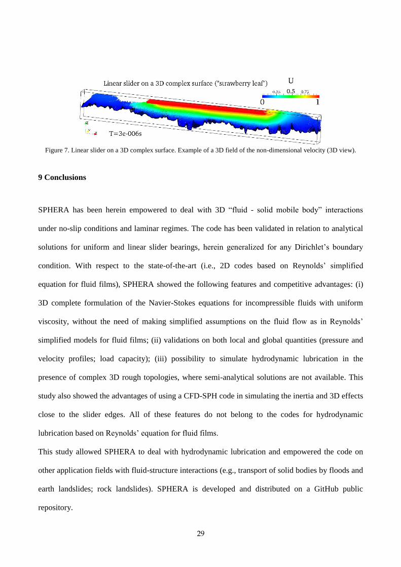
8 Applicability of the computational framework to complex rough surfaces

The linear slider bearing of Sec. 7 is herein modified by imposing a complex 3D surface as the

bottom fixed frontier, to demonstrate the versatility of the approach to take into account complex

rough surfaces as input data. Its shape is taken from a real natural geometry of a strawberry leaf that

was acquired using the Leica DCM 3D confocal profilometer in the MUSAM-Lab of the IMT

School for Advanced Studies Lucca. The spatial resolution needs be finer than the previous test

cases due to roughness, with dx=1.66×10-6m.

Figure 7 shows an example of the velocity field and highlights the capabilities of the code in

simulating complex fluid-structure interactions in the field of hydrodynamic lubrication. Further

investigation on the effect of roughness on the velocity and pressure fields is left for further

investigation in a dedicated follow-up article.

29

Figure 7. Linear slider on a 3D complex surface. Example of a 3D field of the non-dimensional velocity (3D view).

9 Conclusions

SPHERA has been herein empowered to deal with 3D “fluid - solid mobile body” interactions

under no-slip conditions and laminar regimes. The code has been validated in relation to analytical

solutions for uniform and linear slider bearings, herein generalized for any Dirichlet’s boundary

condition. With respect to the state-of-the-art (i.e., 2D codes based on Reynolds’ simplified

equation for fluid films), SPHERA showed the following features and competitive advantages: (i)

3D complete formulation of the Navier-Stokes equations for incompressible fluids with uniform

viscosity, without the need of making simplified assumptions on the fluid flow as in Reynolds’

simplified models for fluid films; (ii) validations on both local and global quantities (pressure and

velocity profiles; load capacity); (iii) possibility to simulate hydrodynamic lubrication in the

presence of complex 3D rough topologies, where semi-analytical solutions are not available. This

study also showed the advantages of using a CFD-SPH code in simulating the inertia and 3D effects

close to the slider edges. All of these features do not belong to the codes for hydrodynamic

lubrication based on Reynolds’ equation for fluid films.

This study allowed SPHERA to deal with hydrodynamic lubrication and empowered the code on

other application fields with fluid-structure interactions (e.g., transport of solid bodies by floods and

earth landslides; rock landslides). SPHERA is developed and distributed on a GitHub public

repository.

30

Acknowledgements

We acknowledge the CINECA award under the ISCRA initiative, for the availability of High

Performance Computing resources and support.” In fact, SPHERA simulations have been financed

by means of the following instrumental funding HPC project: HSPHCS9; HSPHER9b.

The contribution of the author of RSE SpA has been financed by the Research Fund for the Italian

Electrical System (for “Ricerca di Sistema -RdS-”), in compliance with the Decree of Minister of

Economic Development April 16, 2018.

SPHERA v.9.0.0 is realised by RSE SpA thanks to the funding “Fondo di Ricerca per il Sistema

Elettrico” within the frame of a Program Agreement between RSE SpA and the Italian Ministry of

Economic Development (Ministero dello Sviluppo Economico).

References

[1] Williams P.D., G.R. Symmons; 1987; Analysis of hydrodynamic slider thrust bearings lubricated

with non-Newtonian fluids; Wear (117):91-102.

[2] Dobrica M., M. Fillon; 2005; Reynolds’ Model Suitability in Simulating Rayleigh Step Bearing Thermohydrodynamic Problems; Tribol. Trans. (48):522-530.

[3] Vakilian M., S.A. Gandjalikhan Nassab, Z. Kheirandish; 2014; CFD-Based Thermohydrodynamic Analysis of Rayleigh Step Bearings Considering an Inertia Effect; Tribol. Trans. (57):123-133.

[4] Almqvist T., A. Almqvist, R. Larsson; 2004; A comparison between computational fluid

dynamic and Reynolds approaches for simulating transient EHL line contacts; Tribology

International (37):61-69.

[5] Almqvist A., E.K. Essel, L.-E. Persson, P. Wall; 2007; Homogenization of the unstationary incompressible Reynolds equation; Tribology International (40):1344-1350.

[6] Almqvist A.; 2006; On the Effects of Surface Roughness in Lubrication; Ph.D. thesis; Lulea University of Technology (Finland); ISSN: 1402-1544.

[7] Rahmani R., I. Mirzaee, A.Shirvani, H.Shirvani; 2010; An analytical approach for analysis and optimisation of slider bearings with infinite width parallel textures; Tribology International (43):1551-1565.

[8] Papadopoulos C.I., P.G. Nikolakopoulos, L. Kaiktsis; 2011; Evolutionary Optimization of Micro-Thrust Bearings With Periodic Partial Trapezoidal Surface Texturing; Journal of Engineering for Gas Turbines and Power, 133(012301):1-10.

[9] Fouflias D.G., A.G: Charitopoulos, C.I. Papadopoulos, L. Kaiktsis, M. Fillon; 2015; Performance comparison between textured, pocket, and tapered-land sector-pad thrust bearings using computational fluid dynamics thermohydrodynamic analysis; J. Eng. Tribol. (229):376-397.

[10] Paggi M., Q.-C. He; 2015; Evolution of the free volume between rough surfaces in contact, Wear (336–337):86-95.

31

[11] Gropper D., L. Wang, T.J. Harvey; 2016; Hydrodynamic lubrication of textured surfaces: a review of modeling techniques and key findings; Tribology International, 94:509-529.

[12] Hajishafiee A., A. Kadiric, S. Ioannides, D. Dini; 2017; A coupled finite-volume CFD solver for two-dimensional elastohydrodynamic lubrication problems with particular application to rolling element bearings; Tribology International, 109:258–273.

[13] Snyder T., M. Braun; 2018; Comparison of Perturbed Reynolds Equation and CFD Models for the Prediction of Dynamic Coefficients of Sliding Bearings; Lubricants(6,5)

[14] SPHERA (RSE SpA), https://github.com/AndreaAmicarelliRSE/SPHERA

[15] Monaghan JJ.; 2005; Smoothed particle hydrodynamics; Rep. Prog. Phys., 68:1703-1759.

[16] Adami S., X.Y. Hu, N.A. Adams; 2012; A generalized wall boundary condition for smoothed particle hydrodynamics; Journal of Computational Physics, 231:7057–7075.

[17] Hashemi M.R., R. Fatehi, M.T. Manzari; 2012; A modified SPH method for simulating motion of rigid bodies in Newtonian fluid flows; International Journal of Non-Linear Mechanics, 47:626–638.

[18] Macia F., L.M. Gonzalez, J.L. Cercos-Pita; A. Souto-Iglesias; 2012; A Boundary Integral SPH Formulation - Consistency and Applications to ISPH and WCSPH-; Progress of Theoretical Physics, 128-3, 439-462.

[19] Ferrand M., D.R. Laurence, B.D. Rogers, D. Violeau, C. Kassiotis; 2013; Unified semi-analytical wall boundary conditions for inviscid laminar or turbulent flows in the meshless SPH method: International Journal for Numerical Methods in Fluids, 71(4):446-472.

[20] Amicarelli A., G. Agate, R. Guandalini; 2013; A 3D Fully Lagrangian Smoothed Particle Hydrodynamics model with both volume and surface discrete elements; International Journal for Numerical Methods in Engineering, 95: 419–450.

[21] Gomez-Gesteira M., B.D. Rogers, R.A. Dalrymple, A.J.C. Crespo; 2010; State-of-the-art of classical SPH for free-surface flows; Journal of Hydraulic Research, 48(Extra Issue):6-27.

[22] Le Touzé D., A. Colagrossi, G. Colicchio, M. Greco; 2013; A critical investigation of smoothed particle hydrodynamics applied to problems with free-surfaces; Int. J. Numer. Meth. Fluids, 73:660-691.

[23] Shadloo M.S., G. Oger, D. Le Touzé; 2016; Smoothed particle hydrodynamics method for fluid flows, towards industrial applications: Motivations, Current state, And challenges; Computers and Fluids, 136:11-34.

[24] Violeau D., B.D. Rogers; 2016; Smoothed particle hydrodynamics (SPH) for free-surface flows: past, present and future; Journal of Hydraulic Research, 54(1):1-26.

[25] Gu S., X. Zheng, L. Ren, H. Xie, Y. Huang, J. Wei, S. Shao; 2017; SWE-SPHysics simulation of dam break flows at South-Gate Gorges Reservoir; Water (Switzerland), 9(6), art. no. 387.

[26] Vacondio R., Rogers B.D., Stansby P., Mignosa P.; 2012; SPH Modeling of Shallow Flow with Open Boundaries for Practical Flood Simulation; J. Hydraul. Eng., 138(6):530-541.

[27] Colagrossi A., A. Souto-Iglesias, M. Antuono, S. Marrone; 2013; Smoothed-particle hydrodynamics modeling of dissipation mechanisms in gravity waves; Physical Review E - Statistical, Nonlinear, and Soft Matter Physics, 87(2), art. no. 023302.

[28] Marongiu J.C.; F. Leboeuf, J. Caro, E. Parkinson; 2010; Free surface flows simulations in Pelton turbines using an hybrid SPH-ALE method; J. Hydraul. Res., 47:40-49.

32

[29] Price, D.J.; 2012; Smoothed Particle Hydrodynamics and Magnetohydrodynamics; J. Comp.

Phys., 231(3): 759-794.

[30] Amicarelli A., R. Albano, D. Mirauda, G. Agate, A. Sole, R. Guandalini; 2015; A Smoothed

Particle Hydrodynamics model for 3D solid body transport in free surface flows; Computers &

Fluids, 116:205–228.

[31] Manenti S., S. Sibilla, M. Gallati, G. Agate, R. Guandalini; 2012; SPH Simulation of Sediment

Flushing Induced by a Rapid Water Flow; Journal of Hydraulic Engineering ASCE 138(3): 227-311.

[32] Abdelrazek A.M., I. Kimura, Y. Shimizu; 2016; Simulation of three-dimensional rapid free-

surface granular flow past different types of obstructions using the SPH method; Journal of

Glaciology, 62(232):335-347.

[33] Bui Ha H., R. Fukagawa, K. Sako, S. Ohno; 2008; Lagrangian meshfree particles method (SPH)

for large deformation and failure flows of geomaterial using elastic–plastic soil constitutive model;

Int. J. Numer. Anal. Meth. Geomech., 32:1537–1570.

[34] Amicarelli A., B. Kocak, S. Sibilla, J. Grabe; 2017; A 3D Smoothed Particle Hydrodynamics

model for erosional dam-break floods; International Journal of Computational Fluid Dynamics,

31(10):413-434.

[35] Di Monaco A., S. Manenti, M. Gallati, S. Sibilla, G. Agate, R. Guandalini; 2011; SPH modeling

of solid boundaries through a semi-analytic approach. Engineering Applications of Computational

Fluid Mechanics, 5(1):1-15.

[36] Vila J.P.; 1999; On particle weighted methods and Smooth Particle Hydrodynamics;

Mathematical Models and Methods in Applied Sciences, 9(2):161-209.

[37] Violeau D.; A. Leroy; 2014; On the maximum time step in weakly compressible SPH; Journal

of Computational Physics, 256: 388-415.Barkley D., L.S. Tuckerman: 2005; Turbulent-laminar

patterns in plane Couette flow, IUTAM Symposium on Laminar Turbulent Transition and Finite

Amplitude Solutions, T. Mullin and R. Kerswell (eds), Springer, Dordrecht, pp.107-127.

[38] Barkley D., L.S. Tuckerman; 2007; Mean flow of turbulent–laminar patterns in plane Couette

flow; J. Fluid Mech. (576):109-137.