Application of Stochastic Theory to Parameter Estimation:Modeling Saturated Groundwater Flow and

Transport of Radioactive Isotopesat a Humid Site

by

Margaret Evans Talbott

B.S.E., Civil EngineeringPrinceton University, 1990

Submitted to theDepartment of Civil and Environmental Engineering in Partial Fulfillment of the

Requirements for the Degree of

MASTER OF SCIENCEin Civil and Environmental Engineering

at the

MASSACHUSETTS INSTITUTE OF TECHNOLOGY

February, 1994

© 1994 Margaret Evans Talbott. All rights reserved

The author hereby grants to MIT permission to reproduce and to distribute publicly paperand electronic copies of this thesis document in whole and in part.

Signature of the author. .......p Depntof'Civil and Environmental Engineeing

January, 1994

Certified by .

... "................................................................

Lynn W. GelharProfessor of Civil and Environmental Engineeringf. Thesis Supervisor

.-

Accepted by..... -o.. . . .......... ..........

Joseph M. Sussman, ChairmanCommittee on Graduate Studies

-· - - -----·----·-·· ·-- · ·-- ·- · ----- ·

APPLICATION OF STOCHASTIC THEORY TO PARAMETER ESTIMATION:

MODELING SATURATED GROUNDWATER FLOW AND

TRANSPORT OF RADIOACTIVE ISOTOPES AT A HUMID SITE

by

Margaret Evans Talbott

Submitted to the Department of Civil and Environmental EngineeringFebruary, 1994

in Partial Fulfillment of the Requirements for the Degree ofMaster of Science in Civil and Environmental Engineering

ABSTRACT

Stochastic subsurface hydrologic theory is applied to data for a hypothetical low-level radioactive waste site to demonstrate the features of the hydraulic parameterestimation process, as developed by Gelhar and others. Effective values of hydraulicconductivity, macrodispersivity, and macrodispersivity enhancement are estimated fromthe data in this manner. A two-dimensional saturated flow and transport finite-elementcomputer code is used to model the site. Four different isotope inputs and two types ofinput configurations contribute to an evaluation of model sensitivities. These sensitivitiesof the mean concentrations and the uncertainties around the mean are explored using ananalytical model as an example. Results indicate that the spatial heterogeneity of isotopesorption, through its contribution to longitudinal dispersivity enhancement, has a largeeffect on the magnitude of concentration predictions, especially for isotopes with shorthalf-lives in comparison to their retarded mean travel times. This observation emphasizesthe need for accurate site data measurements that compliment the parameter estimationprocess. A comparison of simplified analytical screening models with the numericalmodel predictions shows that the analytical models tend to underestimate concentrationlevels at low times, potentially as a result of oversimplifcation of the flow field. Futuremodels could address aspects that are neglected in this report, such as three-dimensionality or unsaturated flow and transport.

Thesis Supervisor: Dr. Lynn W. Gelhar

Title: Professor of Civil and Environmental Engineering

Acknowledgements

The research described in this thesis is part of a continuing study of contaminanttransport supported by the U.S. Nuclear Regulatory Commission (USNRC) through theresearch project entitled, "Improved Methods for Predicting Field-Scale ContaminantTransport" (Contract No. NRC-04-88-074). Additional support for this research wasprovided by a Ralph M. Parsons Fellowship and by a departmental TeachingAssistantship.

I would like to thank my advisor, Lynn Gelhar, for his guidance and patience withmy work over the past year and a half. It has been a great opportunity to work withsomeone who is at the forefront of his field. I have been lucky to spend some timebenefiting from his scholarship and understanding of groundwater hydrology.

The USNRC contributed to the direction and guidance of this work and wasresponsible for supplying important data and documents. Specifically, ThomasNicholson coordinated the research efforts of the USNRC and MIT and provided me withthe opportunity to meet with the research team at the USNRC. Also at USNRC, AndrewCampbell and Ralph Cady were very helpful in supplying me with documents and resultsof their research. Ralph Cady's calculations are the basis for the input concentrationvalues in this thesis, and Andrew Campbell's work on sorption is relied upon heavily inthis document.

Additionally, I especially want to express my gratitude to Vivek Kapoor forgiving me so much of his valuable time during the last semester of his doctoral programat MIT. Without his help, I would still be puzzling over the hydrologic theory andreading the software manual.

At Geraghty and Miller, Inc., Greg and Linda Ruskauff provided much-neededcomputer support and advice. They were also extremely prompt in sending me updatedversions of the software.

I would like to acknowledge several people at MIT. To Pat Dixon and RaphaelBras in the department headquarters, I owe enormous thanks for arranging financialsupport for my last semester. Somehow they were magically able to find a way for me toreceive funding and still finish everything on time. Without the capable coordinationassistance of Karen Joss at the Parsons Lab, I would never have been able to survive the3000-mile sabbatical separation between me and my advisor. She was always there togrant my requests for her help with sending documents, or for the use of her computer.

I also owe thanks to my parents for their understanding and recognition thatvacations and graduate study are not always compatible. I especially appreciate theircontinual desire to follow the technical aspects of my research, without having had thebenefit of my education in this field.

And to Peter, how can I even begin to show my appreciation. Through thick andthin you have always been there to cheer me on, thank you so much.

5

6

Table of Contents

page

A bstract .............................................................................................................. 3........

Acknowledgements ......................................................................................................... 5

List of Figures .................................................................................................................9

List of Tables ...................................................... 13

A bbreviations ...................................................... 15

Chapter 1: Introduction ................................................................................................... 17

Chapter 2: Site Characteristics ........................................................................................ 212.1 General Description ..................................................................................... 212.2 Site Geology and Hydrology ........................................................................ 21

Chapter 3: Parameter Estimation .................................................................................... 253.1 Sources of D ata ...................................................... 253.2 Saturated Zone ............................................................................................. 26

3.2.1 Correlation Scales ...................................................... 263.2.2 Hydraulic Conductivity ...................................................... 283.2.3 Macrodispersivity .......................................................................... 313.2.4 Longitudinal Macrodispersivity Enhancement throughSorption V ariability ...................................................... 34

3.3 U nsaturated Zone ...................................................... 37

Chapter 4: Isotope Characteristics ...................................................... 414.1 Screening Process ........................................................................................ 41

4.1.1 Step Input ...................................................................................... 424.1.2 Pulse Input ...................................................... 45

4.2 Sorption Dependence and Evaluation .......................................................... 484.2.1 Strontium-90: Sorption Dependence on pH .................................. 484.2.2 Technetium-99: Sorption Dependence on Clay Content .............. 524.2.3 Uranium-238: Macrodispersivity Enhancement ........................... 55

4.3 D iscussion ...................................................... 55

Chapter 5: Numerical Models ......................................................................................... 595.1 Rectangular M odel ...................................................... 59

5.1.1 Model Configuration ..................................................................... 605.1.2 Results ......... .. ..... ...................................... 625.1.3 Discussion and Sensitivity Analysis ............................................. 74

7

Table of Contents (continued)

page5.2 Radial Model ............................................. 76

5.2.1 Model Configuration ..................................................................... 765.2.2 Results ............................................. 805.2.3 Discussion ............................................. 83

5.3 Predictions and Uncertainty ......................................................................... 845.3.1 Analytical Predictions of Numerical Results ................................ 845.3.2 Uncertainties in Model Predictions ............................................. 88

Chapter 6: Conclusions and Recommendations ............................................. 956.1 Conclusions ............................................. 956.2 Recommendations ............................................. 96

References ........................................ ..... 99Appendix A: One-Dimensional Step Input Solution .. ................... 101

Appendix B: Two-Dimensional Pulse Input Solution .. .................... 103

Appendix C: Sample Computer Input File ..................................................................... 107

8

List of Figures

pageFigure 2-1 Map of hypothetical LLW site showing water table contours, relativescale, and proximity to spring and city ........................................................................... 23

Figure 3-1 Collected values of hydraulic conductivity versus depth ............................ 27

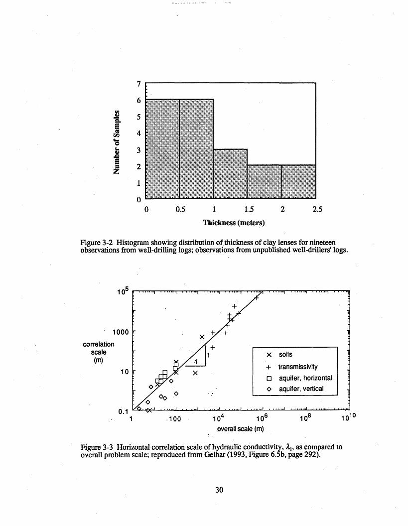
Figure 3-2 Histogram showing distribution of thickness of clay lenses fornineteen observations from well-drilling logs .......................................................... 30

Figure 3-3 Horizontal correlation scale of hydraulic conductivity, l, as comparedto overall problem scale.................................................................................................. 30

Figure 3-4 Standard deviation of hydraulic conductivity, uk, as compared tooverall problem scale for a collection of site examples .................................................. 32

Figure 3-5 Graph showing relationship of KG and a, for each zone tocompilation of hydraulic conductivity data .................................................................... 33

Figure 3-6 Graph showing relationship of K1, and K33 for each zone tocompilation of hydraulic conductivity data .......................................................... 33

Figure 3-7 Longitudinal macrodispersivity versus overall problem scale with dataclassified by reliability ................................................................................................... 36

Figure 3-8 Relationship between R and lnK showing correlation factor, C, andresidual, n........................................................................................................................ 36

Figure 3-9 Idealized representation of the unsaturated zone in cross-section at thehypothetical site, showing distance from bottom of trench to water table .................... 40

Figure 4-1 Collected values of pH versus depth. .......................................................... 49

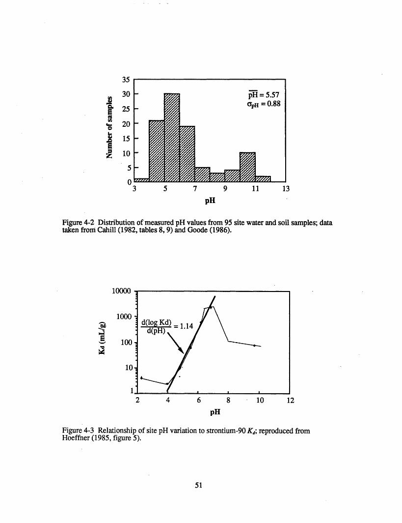
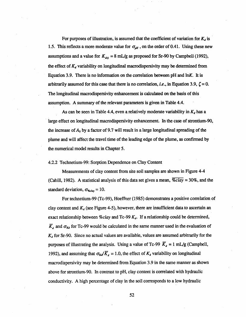
Figure 4-2 Distribution of measured pH values from 95 site water and soilsam ples ........................................................................................................................... 51

Figure 4-3 Relationship of site pH variation to strontium-90 Kd ................................... 51

Figure 4-4 Distribution of measured values of clay content from 14 site soilsam ples ........................................................................................................................... 54

Figure 4-5 Relationship of site clay content variation to technetium-99 Kd .................. 54

Figure 5-1 Cross-section of 2D rectangular model showing relative thickness ofzones. ............................................................................................................................... 61

9

List of Figures (continued)

pageFigure 5-2 Mesh and no-flow and fixed-head boundary conditions used in 2Drectangular finite element model .......................................................... 63

Figure 5-3 Lines of constant head for equal head drops for the 2D anisotropicrectangular model .......................................................... 64

Figure 5-4 Flow pattern for 2D rectangular model with velocity vectors at centerof elements .......................................................... 64

Figure 5-5 Comparison of concentration breakthrough curves for H-3 at springand at property boundary well ........................................................................................ 66

Figure 5-6 Concentration contours of tritium at a) 50 and b) 150 years ........................ 67

Figure 5-7 Comparison of concentration breakthrough curves for U-238 at springand at property boundary well ........................................................................................ 68

Figure 5-8 Concentration contours of uranium-238 at a) 11300 and b) 14000years .............................................. ............ 69

Figure 5-9 Comparison of concentration breakthrough curves for Sr-90 at springand at property boundary well ...................................................................................... 70

Figure 5-10 Concentration contours of strontium-90 at a) 50 and b) 315 years ........... 71

Figure 5-11 Comparison of concentration breakthrough curves for Tc-99 atspring and at property boundary well.......................................................... 72

Figure 5-12 Concentration contours of technetium-99 at a) 20 and b) 300 years ........ 73

Figure 5-13 Comparison of Sr-90 concentration at the spring for numericalsimulations of the 2D rectangular model with A 1l = 242 m and with A 1 = 25 m ........... 75

Figure 5-14 Cross-section of the 2D radial model, showing relative thickness ofzones and locations of river, pumping well, and property boundary well ...................... 78

Figure 5-15 Breakthrough concentration curve for tritium at the propertyboundary well using the 2D radial model ....................................................................... 81

Figure 5-16 Breakthrough concentration curves for tritium at the river and at thepumping well using the 2D radial model .......................................................... 81

Figure 5-17 Concentration contours of tritium in the 2D radial model cross-section at 605 years .......................................................... 82

Figure 5-18 Comparison of H-3 concentration breakthrough curves at the springfor the 1D step model prediction and for the 2D rectangular numericalsimulation ..... 85

10

List of Figures (continued)

pageFigure 5-19 Comparison of U-238 concentration breakthrough curves at thespring for the ID step model prediction and for the 2D rectangular numericalsim ulation........................................................................................................................ 85

Figure 5-20 Comparison of Sr-90 concentration breakthrough curves at the springfor the 2D pulse model prediction and for the 2D rectangular numericalsim ulation ........................................................................................................................ 87

Figure 5-21 Comparison of Tc-99 concentration breakthrough curves at thespring for the 2D pulse model prediction and for the 2D rectangular numericalsim ulation ........................................................................................................................ 87

Figure 5-22 Sensitivity of the 2D pulse screening model for strontium-90 tochanges in input parameters ........................................................................................... 90

Figure 5-23 Mean concentration and plus two standard deviations forstrontium-90 at the spring, using the 2D pulse screening model .................................... 93

11

12

List of Tables

page

Table 3-1 Summary of hydraulic parameters ................................................ 32

Table 4.1 Isotopes of potential interest in modeling. ................................................ 43

Table 4.2 Summary of parameters for step input screening model ............................... 47

Table 4.3 Summary of parameters for pulse input screening model ............................ 47

Table 4.4 Parameters used to calculate effect of Strontium-90 Kd variability ............ 53

Table 4.5 Parameters used to calculate effect of Technetium-99 Kd variability ........... 53

Table 4.6 Summary of isotope parameters that are used in the numerical model ......... 56

13

14

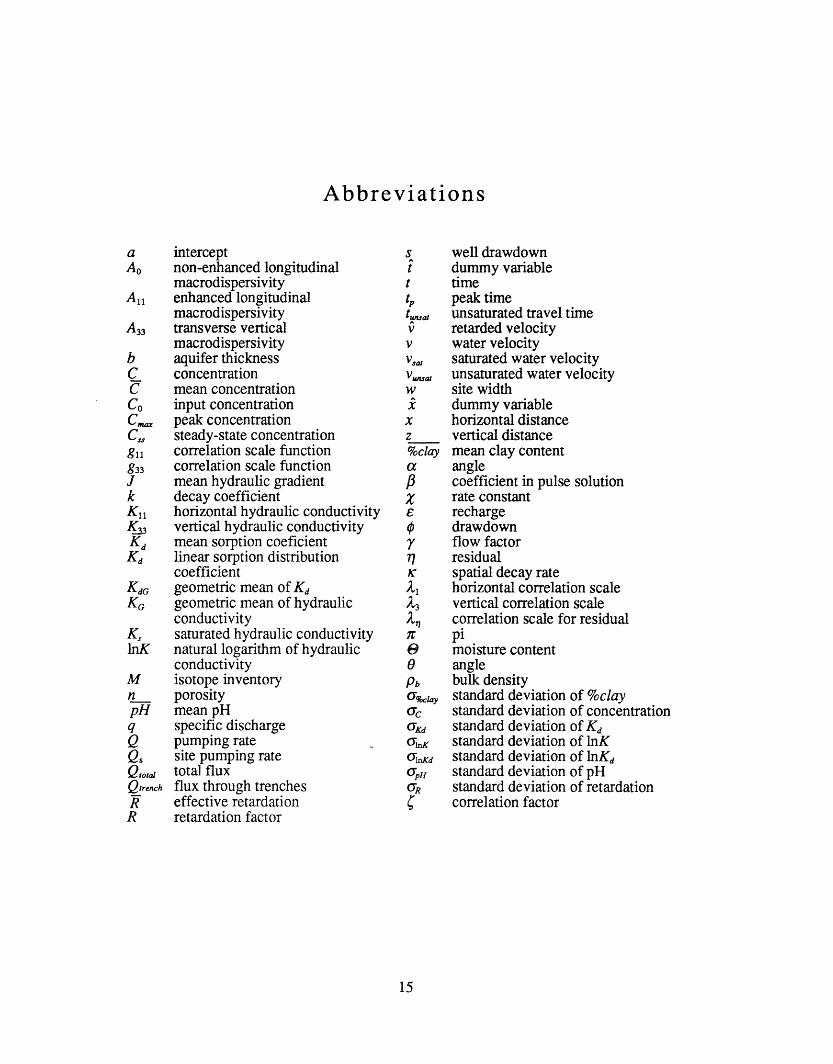
Abbreviations

a interceptAo non-enhanced longitudinal

macrodispersivityAll enhanced longitudinal

macrodispersivityA33 transverse vertical

macrodispersivityb aquifer thicknessC concentrationC mean concentrationCo input concentrationC,,, peak concentrationCss steady-state concentrationg11 correlation scale functiong33 correlation scale functionJ mean hydraulic gradientk decay coefficientK 1 horizontal hydraulic conductivityK,3 vertical hydraulic conductivityKd mean sorption coeficientKd linear sorption distribution

coefficientKdG geometric mean of KdKG geometric mean of hydraulic

conductivityK, saturated hydraulic conductivityInK natural logarithm of hydraulic

conductivityM isotope inventoryn porositypH mean pHq specific dischargeQ pumping rateQs site pumping rateQo,a total fluxQtrench flux through trenchesk effective retardationR retardation factor

sittt^

V

V,Vsat

W

X

XZ

%claya

XE

K

7l

Pb

7cOCoKd

OlnK

C'nKdUpH

(TR

well drawdowndummy variabletimepeak timeunsaturated travel timeretarded velocitywater velocitysaturated water velocityunsaturated water velocitysite widthdummy variablehorizontal distancevertical distancemean clay contentanglecoefficient in pulse solutionrate constantrechargedrawdownflow factorresidualspatial decay ratehorizontal correlation scalevertical correlation scalecorrelation scale for residualpimoisture contentanglebulk densitystandard deviation of %claystandard deviation of concentrationstandard deviation of Kdstandard deviation of InKstandard deviation of lnKdstandard deviation of pHstandard deviation of retardationcorrelation factor

15

16

Chapter 1Introduction

As progress is made in the fields of nuclear power, medicine, cell biology, and

other areas of scientific research, an increasing amount of low-level nuclear waste is

generated. Disposal of this waste is a concern throughout the United States. The United

States Nuclear Regulatory Commission (USNRC) acts as a supervisor and a monitor of

the permitted low-level waste (LLW) storage facilities designed to manage and store low-

level nuclear waste. At any given facility site, the potential for radioactive contamination

of the air, water, and soil is studied by the USNRC through LLW facility performance

assessments. These assessments include hydrologic models appropriate to the various

sites. Because waste facilities typically store waste below ground, groundwater models

are important parts of the overall assessment at every site. This thesis presents a

methodology for the systematic determination of hydraulic input parameters to a

groundwater model of a hypothetical LLW facility. This methodology is appropriate to

groundwater modeling of any site.

Analysis of subsurface contaminant transport is considerably more complex than

it is for surface water bodies. The high degree of natural spatial heterogeneity in soils,

the difficulty in obtaining measurements of large-scale behavior, and the long time scales

over which this behavior occurs all contribute to a complication of the analysis (Polmann

et al., 1988, p. 1-1). Additionally, a true discrete description of the subsurface conditions

is infeasible, both because of cost limitations in data gathering, and because the drilling

of numerous wells for gathering adequate data would itself affect the hydraulic properties

of the aquifer. For these reasons, a statistical or stochastic approach to the quantification

of hydraulic properties seems ideally suited for subsurface conditions. Data collected

17

from several locations may be collectively analyzed to determine the mean and variance

of the data set. These statistical quantities describe the characteristics of the measured

hydraulic property at every location. This stochastic theory is well-developed in the field

of subsurface hydrology and is described in detail in Gelhar (1993).

The most difficult aspect of groundwater modeling is the determination of

appropriate hydraulic input parameters. Traditionally, a rough estimate or an average of a

few measurements is often the basis for the selection of a particular parameter value. As

is shown in this paper, however, commonly available site data sources can be combined

with the application of stochastic theory to result in a more systematic approach to

hydraulic parameter estimation.

In order to demonstrate this process, a hypothetical LLW facility is created.

Situated in a coastal plain environment in a humid climate, the hypothetical site is used as

an example for modeling. Data on measured soil properties, typical of the types of

measurements available at other sites, are assigned to the hypothetical site for the

purposes of illustrating the analysis. These data are analyzed using the saturated

stochastic flow and transport theory presented in Gelhar and Axness (1983).

The application of the theory to the site data results in estimates for several

effective hydraulic parameters, including hydraulic conductivity, macrodispersivity, and

macrodispersivity enhancement. These parameters are used as inputs to a two-

dimensional numerical flow and transport computer code. This simulation is typical of

the types of models commonly employed in the evaluation of groundwater flow and

transport problems. The use of the numerical model shows how the stochastic parameter

estimation may be combined with a traditional numerical modeling approach.

In this paper, several illustrative input examples are modeled using various

isotope contaminants and model configurations. The sensitivity of the numerical model

to variations in input parameters is explored. Additionally, the numerical model

concentration predictions are compared to those of simplified analytical screening

18

calculations to show the importance of accurately representing the spatially-varying flow

field at the site. It is emphasized that results of the parameter estimation and modeling

processes are subject to uncertainties. These uncertainties result from sensitivities of the

mean concentration solutions to input parameters and from stochastic variation around

the mean solution. Although these uncertainties are evaluated to an extent in this paper,

future work should include a more rigorous analysis of some of the other causes of

uncertainty. Some of these include unsaturated flow effects, a larger model extent, and

an inclusion of different isotope inputs.

A major conclusion of this thesis is that the magnitudes of the hydraulic input

parameters have a severe effect on the model results. This observation underscores the

need for a systematic approach to hydraulic parameter estimation, and for a diligence in

obtaining relevant site data measurements that compliment the parameter estimation

process.

19

20

Chapter 2Site Characteristics

As stated in the introduction, the purpose of this report is to apply modeling

techniques to a hypothetical low-level nuclear waste (LLW) storage facility. Some

hypothetical characteristics of the site and its hydrology and geology are defined in this

chapter as background for the later discussion of the analysis. This hypothetical site was

created for use in this report, and will subsequently be referred to in the present tense.

2.1 General Description

The hypothetical site is approximately one kilometer square in size and is located

in a humid climate. Average annual precipitation is about 1.2 meters per year and is

distributed evenly throughout the year. Sixty to seventy percent of the precipitation is

lost to evapotranspiration, yielding a net recharge to the groundwater system of 0.40

meters per year (Cahill, 1982). As a LLW facility, the site receives about 75 percent of

its waste from non-fuel aspects of the nuclear power industry, with the remaining 25

percent from industrial, medical, and academic sources. The waste is buried in standard

210-liter Department of Transportation steel drums that are placed in trenches and

covered with sand and a clay cap. These burial trenches are 15-30 meters wide, 150-300

meters long, and 7 meters deep. On average, there are 50 trenches at the site, spaced 3

meters apart (Cahill, 1982). The minimum distance between the bottom of the trenches

and the water table is 1.2 meters.

2.2 Site Geology and Hydrology

The geology of the site is that of coastal plain sediments. It is characterized by

thick, expansive horizontal layers of sediments with lateral extents of hundreds of

21

kilometers. Sediments are relatively homogeneous within layers and consist primarily of

sands, silts, and some clay lenses and confining beds. Three identifiable hydrologic

zones make up the water table aquifer. These zones are 10-50 meters thick and exhibit

distinct hydrologic properties. A confining bed of clay that is 20 meters thick forms the

horizontal base of the phreatic aquifer at a depth of around 100 meters. The three zones

are labeled Zone 1, Zone 2, and Zone 3, in order of increasing depth. In general,

permeability increases with depth, such that Zone 3 is more permeable than Zone 2, and

Zone 2 is more permeable than Zone 1 (Cahill, 1982).

At this humid site, the water table is close to the ground surface. The unsaturated

zone is relatively thin, extending only 8-14 meters below the surface. Because the trench

depth places the waste 1-2 meters above the water table, it is expected that the

unsaturated zone plays a minimal role in the overall travel of the waste through the

groundwater system. This will be discussed in greater detail in Chapter 3.

The mean horizontal gradient is fairly uniform across the site. Therefore, flow at

any point in the site would be expected to be roughly in the same direction. The mean

horizontal gradient is taken to be 0.01, in the direction of a nearby spring (Cahill, 1982),

as shown in Figure 2-1.

22

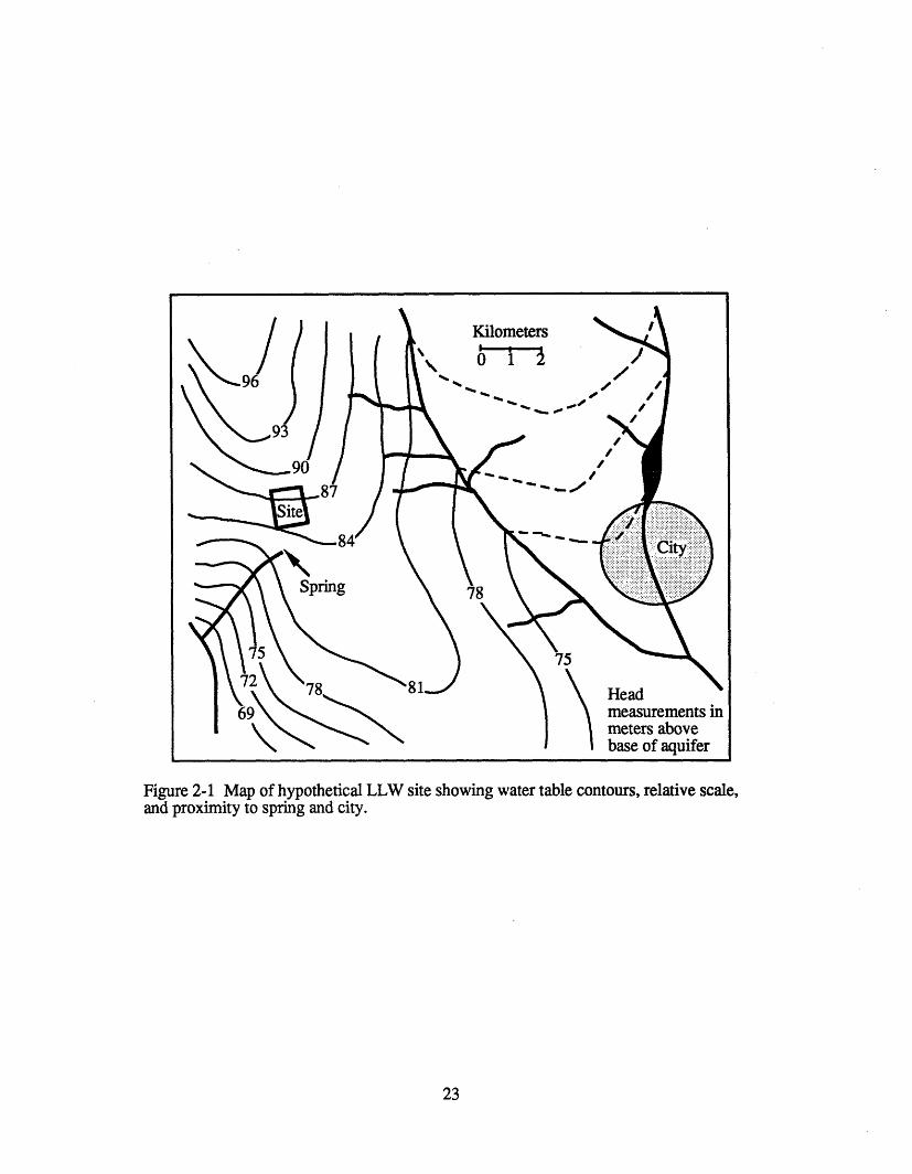
Figure 2-1 Map

of hypothetical

LLW site

showing

water table

contours,

relative

scale,

Figure 2-1 Map of hypothetical LLW site showing water table contours, relative scale,and proximity to spring and city.

23

24

Chapter 3Parameter Estimation

Hydraulic parameters can be estimated through the application of stochastic

theory to groundwater characteristics of the site, gathered from traditional data sources.

This chapter describes the data sources, outlines the theory, and provides a step-by-step

methodology of the parameter estimation process as applied to representative site data.

3.1 Sources of Data

The data used in this hypothetical model are drawn from several available

sources. The sources used are representative of those available for other, actual sites.

Specifically, the quantitative information provided by Cahill (1982) serves as

representative data for the hypothetical site. This section provides a description of the

sources and a compilation of the data that are used in deriving the traditional input

parameters for a discrete numerical groundwater flow and transport model.

Precipitation and recharge measurements from the U.S. National Weather Service

at specific locations are averaged over the last 50 years to obtain estimates of the flow

input to a model. Hydraulic gradients, water table shape, and head distributions are

calculated on the basis of recorded water levels from on-site and local wells.

Data on hydraulic conductivity, K, are compiled from several different sources.

As taken from Cahill (1982), they comprise a collection of values obtained from

laboratory tests on core samples and measurements from in-situ aquifer testing.

Specifically, results of hydraulic conductivity tests on core samples taken at various

depths from seven different wells are combined with measurements of K from on-site

slug tests, an aquifer test in the upper 60 meters of sediments, and the specific capacity of

25

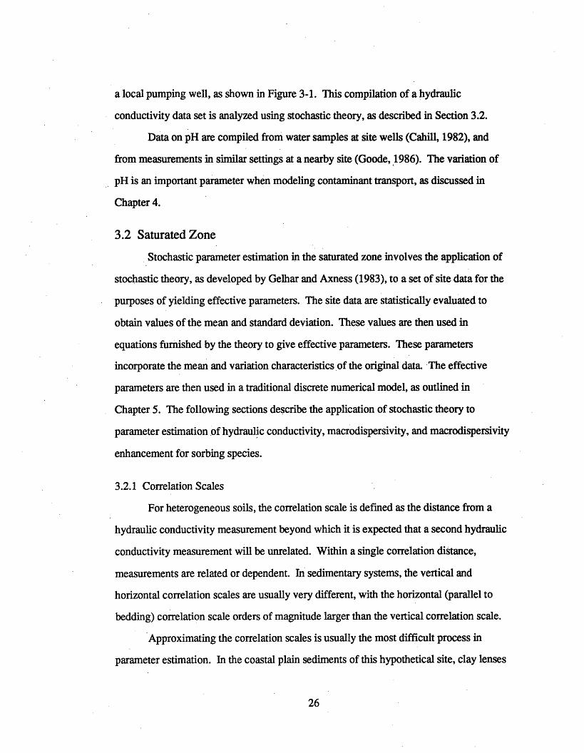
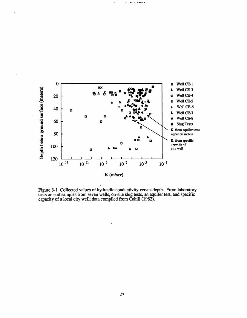
a local pumping well, as shown in Figure 3-1. This compilation of a hydraulic

conductivity data set is analyzed using stochastic theory, as described in Section 3.2.

Data on pH are compiled from water samples at site wells (Cahill, 1982), and

from measurements in similar settings at a nearby site (Goode, 1986). The variation of

pH is an important parameter when modeling contaminant transport, as discussed in

Chapter 4.

3.2 Saturated Zone

Stochastic parameter estimation in the saturated zone involves the application of

stochastic theory, as developed by Gelhar and Axness (1983), to a set of site data for the

purposes of yielding effective parameters. The site data are statistically evaluated to

obtain values of the mean and standard deviation. These values are then used in

equations furnished by the theory to give effective parameters. These parameters

incorporate the mean and variation characteristics of the original data. The effective

parameters are then used in a traditional discrete numerical model, as outlined in

Chapter 5. The following sections describe the application of stochastic theory to

parameter estimation of hydraulic conductivity, macrodispersivity, and macrodispersivity

enhancement for sorbing species.

3.2.1 Correlation Scales

For heterogeneous soils, the correlation scale is defined as the distance from a

hydraulic conductivity measurement beyond which it is expected that a second hydraulic

conductivity measurement will be unrelated. Within a single correlation distance,

measurements are related or dependent. In sedimentary systems, the vertical and

horizontal correlation scales are usually very different, with the horizontal (parallel to

bedding) correlation scale orders of magnitude larger than the vertical correlation scale.

Approximating the correlation scales is usually the most difficult process in

parameter estimation. In the coastal plain sediments of this hypothetical site, clay lenses

26

a Well CE-1

A Well CE-3

o Well CE-4

x Well CE-5

+ Well CE-6

A Well CE-7* Well CE-8

o Slug TestsK from aquifer testsupper 60 meters

K from specificcapacity ofcity well

U

b~V 20

40U 40

la 60

0

h 80

'~ 100

az 1,A

10-13 10-1 10-9 10-7 10- 5 10 - 3

K (m/sec)

Figure 3-1 Collected values of hydraulic conductivity versus depth. From laboratorytests on soil samples from seven wells, on-site slug tests, an aquifer test, and specificcapacity of a local city well; data compiled from Cahill (1982).

27

xx a

1A 0 $BoI8 _ ·

0 00Qb D.o o

a

I I I I I I I I

are common features. A measurement of the average vertical thickness of the clay lenses

serves as a proxy for the correlation scale in the vertical direction, 13, since two

measurements in the vertical direction that are further apart than this thickness will not

encounter the same lens. On the site, clay lens thicknesses are observed and recorded in

well-drillers' logs. A compilation of these measurements is given in the histogram in

Figure 3-2. An evaluation of the distribution of clay lens thicknesses in Figure 3-2

produces an average thickness of approximately 1 meter. On the basis of this

observation, the vertical correlation scale is taken to be 1 meter.

Gelhar (1993) has shown that, for many different sites, the horizontal correlation

scale is related to the overall problem scale. In Figure 3-3, Gelhar (1993) demonstrates a

one-to one relationship between the log of the horizontal correlation scale and the log of

the overall scale, such that the correlation scale is on average one order of magnitude

smaller than the overall scale. For the hypothetical site in this report, the downgradient

distance from the site to the spring is the primary path of concern (see the map in

Figure 2-1), This distance is approximately 1300 meters, and it defines the overall

problem scale for the two-dimensional rectangular model discussed in Chapter 5. From

Figure 3-3, for an overall problem scale of 1000 meters, there is a corresponding

horizontal correlation scale, &, of 100 meters. Therefore, for this site, using a model on

the order of 1000 meters in length, the correlation scales are , = 1 meter, Al = 100

meters, and X/23 = 100. Because little information is available that would indicate a

difference in correlation scales for the three hydraulic zones, the same values for the

correlation scales are used in all three zones.

3.2.2 Hydraulic Conductivity

The principal components of hydraulic conductivity for the three dimensional

(3D) anisotropic system at the site with isotropy in the plane of bedding (A, = 2 >>3)

may be defined in the horizontal direction, KI1 , and in the vertical direction, K33. Using

theory outlined in Gelhar and Axness (1983), in a system with mean flow parallel to

28

bedding, expressions of K,1 and K33 may be written as a function of the correlation scales

and of the statistics of the hydraulic conductivity data.

K11 = KG exp[K ,,(0.5- g)]; g1 = f(A,X / , 3) (3.1)

K3 = KG exp[GTK (o.5-g 3 3)] g33 = f 3(A I3) (3.2)

where KGis the geometric mean of the hydraulic conductivity data set such that

InKG =E[InK], with InK indicating the natural logarithm of K. 2 K is the variance of InK,

and gI1 and g33 are functions of X/A, given by Gelhar and Axness (1983, p. 167). These

functions have values less than one, with gl<< g33 when i, >> A3. This description

assumes a lognormal distribution of K, as is commonly seen in field examples.

The parameters KG and 2, K for each zone are estimated through a statistical

analysis of the values of K in that zone, based on the data in Figure 3-1. It is found,

however, that while calculated values of KG appear to be of a reasonable magnitude,

calculated values of aclK for the hypothetical site data set are noticeably larger than those

expected on the basis of comparison with other sites. All three zones exhibit this

behavior, with Zone 1 having the largest value of 2 K, and Zone 3 the smallest value.

The extremely large values of CarK reflect the strong influence of a small number of very

low conductivity values shown in Figure 3-1. Such low values are expected to have a

minimal effect on transport because the water is practically immobile in regions with

conductivities several orders of magnitude below the geometric mean. Gelhar (1993)

presents a comparison of the standard deviation of InK, crj , with overall problem scale,

as shown in Figure 3-4. This figure represents a compilation of data from many sites, and

indicates that values of aow < 2.5 would be reasonable estimates. Maintaining the same

relative magnitudes of aK for the three zones, estimates of c ,Kare selected on the basis

of the relationship in Figure 3-4. These values are displayed with the data in Figure 3-5.

The computed values of KG, and the selected values of C, are input into

Equations 3.1 and 3.2 to give results for K,1 and K33. This analysis is performed for each

29

7

6

02laco

ME,05z

5

4

3

2

1

00 0.5 1 1.5 2 2.5

Thickness (meters)

Figure 3-2 Histogram showing distribution of thickness of clay lenses for nineteenobservations from well-drilling logs; observations from unpublished well-drillers' logs.

105

1000

correlationscale

(m)

10

0.1.. I 1 .100 104 106 108

overall scale (m)

Figure 3-3 Horizontal correlation scale of hydraulic conductivity, &, as compared tooverall problem scale; reproduced from Gelhar (1993, Figure 6.5b, page 292).

30

1010

-- -------- -~::-·::~~:: ·~::

r~~i8:::8::~~83i:::~:`::~ ~W:::::~~::~:: i~~~~~:~~:....................

:··L:;····· :·:::::~ ~ ~ ~ ~ ~~~~~~~~..............':~~:~:3#::~:~~::k::::::i::i~~aS:::: :··:·:·:·:·:·:·:·~......................

:;:·:r;:·:·:;:·s;:;:;".'.:.:.:.':.:.:·: :i:~::::::S:.:::.......................;:·:·:·:·:·:·:·:·:·s::::::':'r·: ~ ~ ~ ~ ~ ~ ~ ~ ~ ~ .................~~asn:~sff~:·::iS~~i:::~~~i~i:~i~i ::~~:~:~~:~:ra~~.....................·L;·:·5·L······::::::i··::·:·::j::::~..............~~az~~~:::~"'""~~~i:~8 :::::'·::::::j:::::"" ·: ~ ~ ~ ~ .....................·:·:·:·s·:~~:~~d~~~::::~:~::::::::: :·:·:·:·:·:·~·:·~·:r·:..................':::;~~~8#8~:I::::::::j::::::::::::::::: :~:~:y::~:~::::.................... ...· ·.~. · ··:··.·:.·:··:··:·::·:··:·;·: ·;~;...................::, , ii

.:~~~~.... ;~,~: ···;. :~:~:~:... . . . ............ .........:~~~:~~8~~:~~~~,,,,.,~~~, ..·,,,·,,,·.·.,,·.·................·...,·. ·. ·. ·.·. 1.;..;·;·;2.·.·.~ ~ ~ ~ ~ ~ ~~~...............1':5~::·:·:·:·:.8#::.::::::j:::::::::::: .'O, X·:. . . . ......................

zone and for the aquifer evaluated as a whole (disregarding the various zones). These

values of K11 and K33 are then entered into the 2D rectangular finite-element model

described in Chapter 5, and adjusted upward slightly in the calibration of the model with

recharge. A comparison of K11 and K33 with the entire data set appears in Figure 3-6. A

summary of the final parameters is shown in Table 3-1.

3.2.3 Macrodispersivity

While correlation scales and hydraulic conductivity parameter estimation are

sufficient as a description of a flow system, for modeling transport it is necessary to

describe the spreading of the contaminant plume as well. A description of the spreading

in the direction of flow is given by the longitudinal macrodispersivity, Ao, and in the

vertical direction perpendicular to the flow by the transverse vertical macrodispersivity,

A33. The theory supplied by Gelhar and Axness (1983) provides an expression for

longitudinal macrodispersivity:

Ao = °ln (3.3)

where cr K is the variance of InK, and X, is the horizontal correlation scale. The flow

factor, y, is defined by the following:

Y (3.4)KG J

where q is the specific discharge and J is the mean hydraulic gradient. Gelhar and

Axness (1983) show that ymay be expressed as a function of aK, g11, g33, and the angle,

0, between the mean flow direction and the bedding plane, as given in the following:

exp[CInK(O.5 - 3(35)

sin2 0 + {exp[arK(gl - g,3 )]}cos20

31

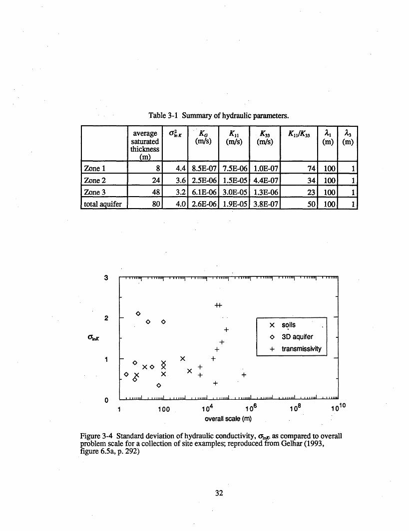
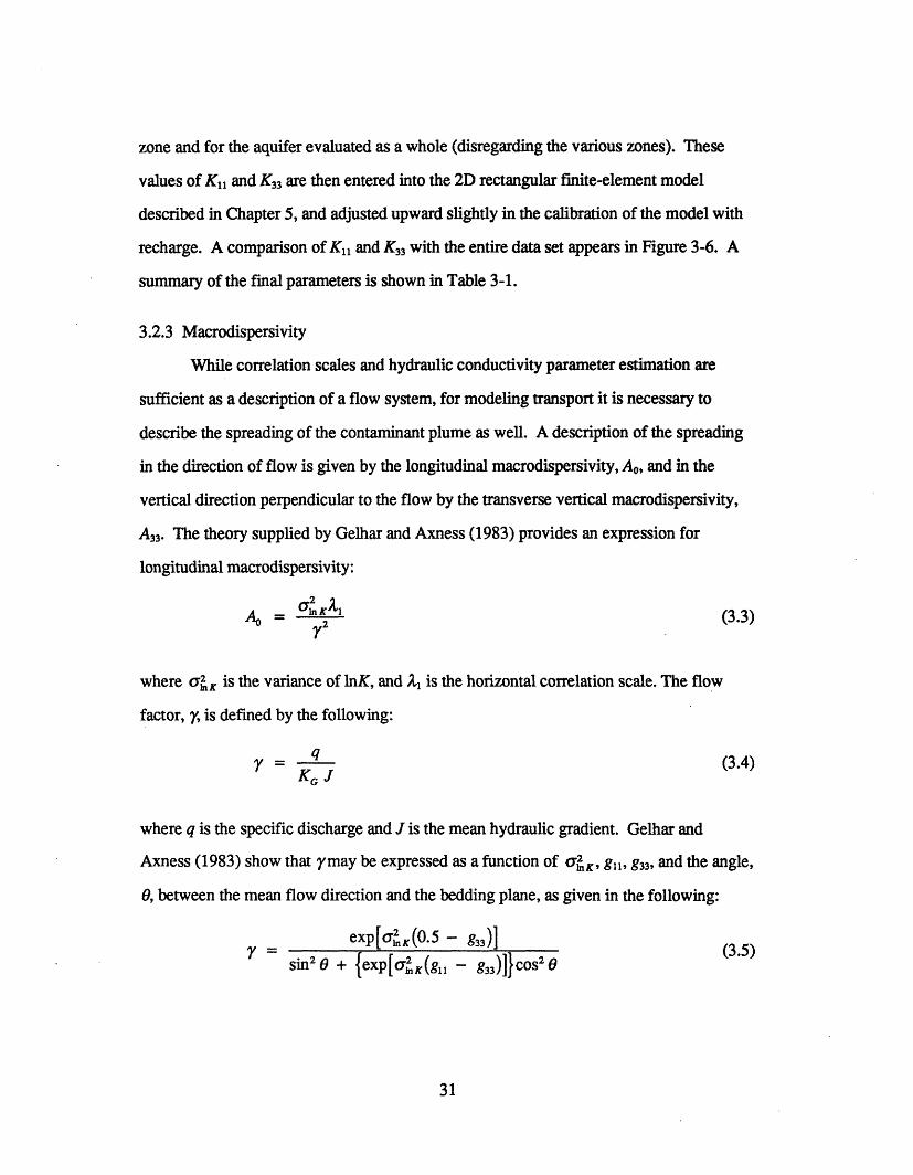
Table 3-1 Summary of hydraulic parameters.

average cyK K KG K K33 11/K33 )i _saturated (m/s) (m/s) (m/s) (m) (m)thickness

Zone 1 8 4.4 8.5E-07 7.5E-06 1.OE-07 74 100 1

Zone 2 24 3.6 2.5E-06 1.5E-05 4.4E-07 34 100 1

Zone 3 48 3.2 6.1E-06 3.OE-05 1.3E-06 23 100 1

total aquifer 80 4.0 2.6E-06 1.9E-05 3.8E-07 50 100 1

3

2

CinK

1

01 100 104 106 1010

overall scale (m)

Figure 3-4 Standard deviation of hydraulic conductivity, a, . as compared to overallproblem scale for a collection of site examples; reproduced from Gelhar (1993,figure 6.5a, p. 292)

32

00 0 X soils

0 3D aquifer

+ + transmissivity

x +

0 X + +

0 +,....... .,1 , .. 1..I ,,,.,1 .1...,1 ,, .. 1. ,, ,,,,,1 , ....... I ....... I , ,,,,,1,,, .,.,1 ,

108

0

20

40

60

80

100

12010-13 101 109 10-7

a

ox

k

04-

III

Well CE-1

Well CE-3

Well CE-4

Well CE-5

Well CE-6

Well CE-7Well CE-8

Slug Tests

KG

+/- 2

10-3

K (m/sec)

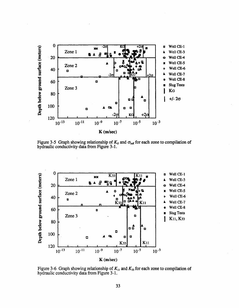
Figure 3-5 Graph showing relationship of KG and q,, for each zone to compilation ofhydraulic conductivity data from Figure 3-1.

0

20

40

60

80

100

12010-' 3 10-11 10-9 10-7 10-5

a

k

0x

0

a

I

Well CE-1

Well CE-3

Well CE-4

Well CE-5

Well CE-6

Well CE-7Well CE-8

Slug Tests

Kll, K33

10- 3

K (m/sec)

Figure 3-6 Graph showing relationship of KI, and K33 for each zone to compilation ofhydraulic conductivity data from Figure 3-1.

33

.,

uco

i,0

I,S.'

E

ug

oI-

c.10AZ~

AJ

xx K33 K I [Zone 1 lK

0 XO iZone2 % A

K3 io Ki

Zone 3 - o

o a e~ o0 0

K33 K In n & ·I

For the particular attributes selected for the hypothetical LLW site, water will

flow vertically under the site when it enters as recharge beneath the trenches, and when it

discharges to the spring. At those locations, 0 will be 90 degrees from the horizontal

bedding. However, for the most part, along the 1300 meter distance between the site and

the spring, the flow is horizontal (parallel to the bedding), and 0 is zero. Ideally, 0 would

be calculated at every point in the flow path and used to describe a spatially-varying

longitudinal macrodispersivity at different points in the flow field. In practice, however,

computer codes, such as the one used here, are not configured to make these calculations.

Therefore, a mean 0 is used to compute a mean yand, subsequently, a mean A0.

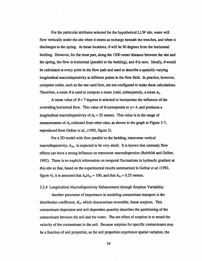
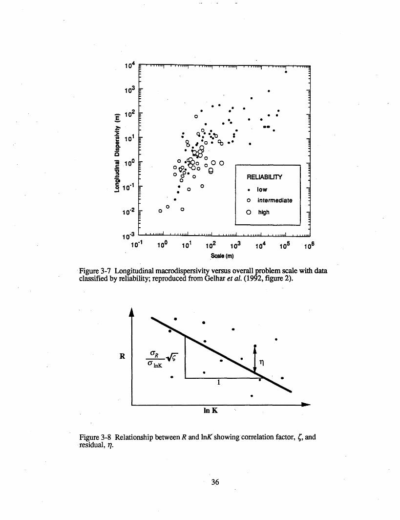
A mean value of 0 = 7 degrees is selected to incorporate the influence of the

overriding horizontal flow. This value of 0 corresponds to y= 4, and produces a

longitudinal macrodispersivity of Ao = 25 meters. This value is in the range of

measurements of Ao collected from other sites, as shown in the graph in Figure 3-7,

reproduced from Gelhar et al., (1992, figure 2).

For a 3D model with flow parallel to the bedding, transverse vertical

macrodispersivity, A33, is expected to be very small. It is known that unsteady flow

effects can have a strong influence on transverse macrodispersion (Rehfeldt and Gelhar,

1992). There is no explicit information on temporal fluctuations in hydraulic gradient at

this site so that, based on the experimental results summarized in Gelhar et al. (1992,

figure 4), it is assumed that Ao/A33 = 100, and that A33 = 0.25 meters.

3.2.4 Longitudinal Macrodispersivity Enhancement through Sorption Variability

Another parameter of importance in modeling contaminant transport is the

distribution coefficient, Kd, which characterizes reversible, linear sorption. This

contaminant-dependent and soil-dependent quantity describes the partitioning of the

contaminant between the soil and the water. The net effect of sorption is to retard the

velocity of the contaminant in the soil. Because sorption for specific contaminants may

be a function of soil properties, as the soil properties experience spatial variation, the

34

sorption also varies. This variation directly affects the velocity of the contaminant,

which, in turn, enhances the spreading of the plume. The enhanced spreading is defined

by a larger reactive longitudinal macrodispersivity, Al,, as distinguished from AO, the non-

reactive longitudinal macrodispersivity. The increased plume spreading, over that which

would be the result for no sorption, is defined as the macrodispersivity enhancement,

A,/Ao. It is important to note that the theory indicates this effect of macrodispersivity

enhancement only occurs in the longitudinal direction. The transverse macrodispersivity

is unaffected by sorption variability, as discussed in Garabedian et al. (1988).

In order to understand clearly the importance of spatially variable sorption, a

number of parameters must be defined. The variable Kd may be described by a mean

(Kd) and a standard deviation (aKd). Further, the retardation factor, R, is related to Kd by

the following:

R = 1 + Pb Kd (3.6)n

where Pb is the bulk density (= mass of solid/bulk volume), and n is the soil porosity. R

may be described statistically by an effective retardation, R = E[R], and by a standard

deviation:

aR n AK (3.7)

By analyzing the mean and variation of a sample data set of a measured soil property, and

by showing a relationship between the soil property and R, R and CYR may be calculated

as a function of the statistics of the soil property data set.

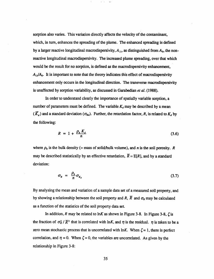
In addition, R may be related to InK as shown in Figure 3-8. In Figure 3-8, cis

the fraction of a / 2 that is correlated with InK, and r is the residual. is taken to be a

zero mean stochastic process that is uncorrelated with InK. When C = 1, there is perfect

correlation, and = 0. When '= 0, the variables are uncorrelated. As given by the

relationship in Figure 3-8:

35

' - llnlr ww1* lr r'rr * .. rIrl , 1.1 ..

a

.

.

0.

0

0 0

° -.b % ..b

o 2 " ° o c

0

O o0O O00·

0

0

S0

* S

so

.

10 '1 100 101 102 103 104 105 106

Scale (m)

Figure 3-7 Longitudinal macrodispersivity versus overall problem scale with dataclassified by reliability; reproduced from Gelhar et al. (1992, figure 2).

0

C

.

S

.

In K

Figure 3-8 Relationship between R andresidual, 7.

lnK showing correlation factor, , and

36

104

103

102

101

100

10.1

A

E

t-

oCO.0

C9

-ij

RELIABILITY

* low

o intermediate

O high10'2

R

- .- - . . . . . .... I . I . . . . . I . . .11 ... I . . ....

, * , , , , 1 ., ..111

R = a a)I nK + (3.8)

where a is the intercept.

The net result of the variation in the retardation and the relationship between

retardation and InK is to increase the longitudinal macrodispersivity of the sorbed species

according to the following equation given by Gelhar (1993, p. 256):

A1= + (1__ _2 ; 4 , (3.9)

where Ao is the non-reactive longitudinal macrodispersivity, AI is the horizontal

correlation scale, , = A1, and ris as defined in Subsection 3.2.3. The result of the

longitudinal macrodispersivity enhancement is to extend significantly the leading edge of

the plume. The effect of enhancement on transport becomes particularly important for

contaminants that exhibit a first order decay and possess a half-life that is on the same

order of magnitude as the peak travel time (see Chapter 4). As will be seen in Chapter 5,

in this case the enhanced macrodispersivity results in much larger concentrations at early

time.

3.3 Unsaturated Zone

The characteristics selected for the hypothetical LLW site result in an unsaturated

zone thickness that is small in comparison to the saturated thickness. To determine if the

unsaturated zone may be neglected in a 2D vertical cross-sectional site model, some

rough calculations are performed. If the expected travel time in the unsaturated zone is

much shorter than the expected saturated travel time from the site to the spring, then it is

assumed to be reasonable to neglect the unsaturated zone in the model.

Using a saturated vertical hydraulic conductivity, K, = 1.0 E-7 m/s (see

Table 3-1); an average moisture content, 9 = 0.28 (Dennehy and McMahon, 1987); and a

37

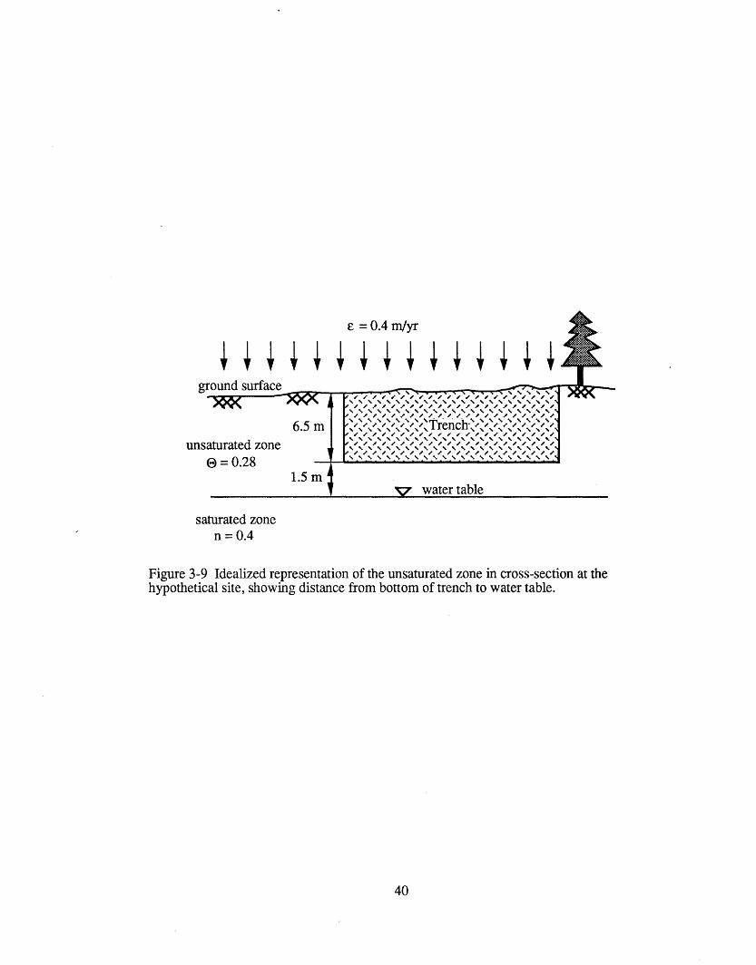
steady recharge, e = 0.4 m/year (Cahill, 1982), the vertical velocity of the water in the

unsaturated zone is given by:

£v- = 7 = 1.4 m/yr (3.10)

The value of recharge represents a worst-case scenario, assuming that all the recharge that

enters the soil will enter the trenches and will subsequently percolate through the bottom

of the trenches to the water table. For a distance from the bottom of the trench to the

water table, z = 1.5 meters (see Figure 3-9), the unsaturated travel time is then:

t,, = 1.1 years (3.11)Vnsat

Even considering longitudinal dispersivity in the unsaturated zone, the travel time is still

on the order of 100 years, a relatively short time for a hydrological system.

In the saturated zone, using a porosity, n = 0.4; a mean hydraulic gradient,

J = 0.011; a horizontal hydraulic conductivity of the total aquifer, K, = 1.9 E-5 m/s (see

Table 3-1); and assuming predominantly horizontal flow, the velocity in the saturated

zone is calculated as:

va = K J = 17.3 m/yr (3.12)n

For a horizontal distance from the site to the spring, x = 1300 meters, the saturated travel

time is given by

t, = x = 75 years (3.13)Vlat

On the basis of these calculations, since t, << t, for the particular site configuration of

this hypothetical LLW problem, the unsaturated zone flow and transport is neglected

from further analysis. Neglecting the unsaturated zone is not a good assumption for all

sites, however. At other humid sites there may be other considerations, such as unsteady

38

recharge or volatile contaminants, where the unsaturated zone plays a more important

role. Likewise, at arid sites where the unsaturated zone is very thick, modeling the

unsaturated zone is essential to the problem.

If the unsaturated zone is to be modeled for a particular site, the effective

unsaturated hydraulic conductivity and moisture retention curve may be derived using

stochastic theory much in the same way as are the saturated parameters. Although this

theory is not expanded upon in depth in this paper, other authors devote their attention to

this subject in great detail. Yeh et al. (1985) outline this theory for steady flow and

present a derivation based on first principles. In two related papers, Mantoglou and

Gelhar (1987a, 1987b) explore the application of the theory to parameter estimation of

hydraulic conductivity and moisture content for transient unsaturated flow in stratified

soils. Polmann (1990) extends the analysis to soil with more complicated and realistic

hydraulic characteristic curves, including solute transport as well as flow for large-scale

systems. Polmann et al. (1988, 1991) use the results of the stochastic analysis in transient

numerical simulations. Additionally, Gelhar (1993) presents a comprehensive synopsis

of the theory, including several examples of its application.

39

£ = 0.4 m/yr

I I ; 4;v;;W groluna surace _ . .-

>QQo< ev 1

6.5 munsaturated zone

e = 0.281.5 m

% % % %%% . % % % % %% \ N rnch~ ~ ° ~ ~ ~l~/)/ (/ ~~

%%%%%%%%% %%%%%%%%%~//

V water table

saturated zonen = 0.4

Figure 3-9 Idealized representation of the unsaturated zone in cross-section at thehypothetical site, showing distance from bottom of trench to water table.

40

- .---- - - - -

__, m �� I I __ 1 I I- I I . . . II I I I I .1 I I I I I .1 I .1 I I I I , ' , , , _5 W

Chapter 4Isotope Characteristics

Low-level nuclear waste is a combination of waste from many sources and

therefore contains many different radionuclides, all of which are potentially a source of

contamination. This report provides examples of some transport phenomena, but does

not attempt to cover all scenarios. Four isotopes with a variety of characteristics are

selected, using a screening process, from a subset of those that potentially compose the

waste. The sorption dependence of these isotopes on aquifer characteristics, and the

corresponding longitudinal macrodispersivity enhancement is evaluated for use in the

2D numerical model in Chapter 5.

4.1 Screening Process

Isotopes are categorized by solubility and trench inventory as one of two types

and are evaluated using two separate screening models. The first screening model is a

step input for isotopes that have high trench inventory in comparison to their solubility.

The second screening model is a pulse input for isotopes that have high solubility in

comparison to their trench inventory. Two isotopes are selected for evaluation using the

step input screening model, and two are selected using the pulse input screening model.

Of the isotopes that are typically found in low-level waste, eight are identified as

isotopes of interest for modeling at the hypothetical site (see Table 4.1). Assumptions are

made regarding the isotope total inventories, expressed in Curies (Ci), and solubilities,

expressed in Curies per cubic meter (Ci/m3 ) (Campbell, 1992), as displayed in Table 4.1.

The time over which an isotope would be completely released from the waste trenches

may be defined as the input duration. This definition assumes that a steady recharge rate

41

of water is received by the trenches, and that the solubility of the isotope completely

controls the amount of isotope dissolution in the water. The recharge is assumed to be

equal to the total recharge received by the site of 0.4 m/year, as defined in Section 2.1.

This representation is a worst-case scenario of complete trench failure where the waste is

easily available for dissolution in and percolation downward with the water. The input

duration is calculated as follows:

Inputduration(years) =inventory() (4.1)trench area(m2 ) x recharge(m / yr) x solubility(Ci / m3)

where units are displayed in parentheses, and trench area is the plan area of the trenches

that contain the isotope. Input durations for the eight isotopes are calculated using

Equation 4.1 and are presented in Table 4.1.

As shown in Table 4.1, for all isotopes other than tritium (H-3) and uranium

(U-238), the input duration is much smaller than one year. From the perspective of the

time scale of a saturated transport problem (see Section 3.3) these isotopes may be treated

as having an instantaneous pulse release. That is, as soon as the trenches are breached,

immediately all the isotope contamination will be transported by the water. For tritium

and uranium-238, however, the input duration is much greater than the expected saturated

transport time scale. From the perspective of this time scale, tritium and uranium-238

may be modeled as step inputs with large inventories. At the time the trenches are

breached, a steady rate of isotope contamination will begin to be transported by the water.

This rate will continue throughout the duration of the simulation, eventually reaching a

steady state concentration level at every point in the aquifer.

4.1.1 Step Input

The step input screening model uses an analytical solution to the 1D transport

equation to approximate the steady state concentration (C,,) at some distance (x) from the

42

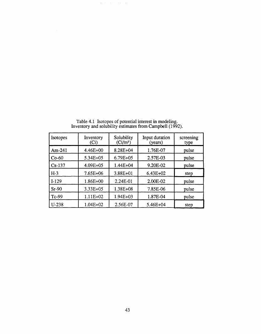
Table 4.1 Isotopes of potential interest in modeling.Inventory and solubility estimates from Campbell (1992).

Isotopes Inventory Solubility Input duration screening(Ci) (Ci/m3 ) (years) type

Am-241 4.46E+00 8.28E+04 1.76E-07 pulse

Co-60 5.34E+05 6.79E+05 2.57E-03 pulse

Cs-137 4.09E+05 1.44E+04 9.20E-02 pulse

H-3 7.65E+06 3.88E+01 6.43E+02 step

I-129 1.86E+00 2.24E-01 2.00E-02 pulse

Sr-90 3.33E+05 1.38E+08 7.85E-06 pulse

Tc-99 1.1 E+02 1.94E+03 1.87E-04 pulse

U-238 1.04E+02 2.56E-07 5.46E+04 step

43

point of concentration input. A complete derivation of this solution is given in

Appendix A. The 1D analytic solution is of the form

C,,(x) = C e (4.2)

where Co is the input concentration and Kc is a spatial decay rate, which is a function of the

decay coefficient (k), the enhanced dispersivity (A,1), and the retarded velocity (0) (see

Appendix A). The retarded velocity is a measure of the velocity of the contaminant as

compared to v, the velocity of the water:

Vv - (4.3)

R

where R is the isotoperetardation factor (see Subsection 3.2.4). A related variable, the

contaminant travel time, is defined as the distance traveled divided by the retarded

velocity. The magnitude of the input concentration, represented as an average over the

gross area, is given by

C (Ci/m3) = solubility (Ci/ m3) x Q..ch (m3 /time step)°Q~o (m 3 / timestep)

where units are displayed in parentheses, and Qt,.,,,is the flux through the trenches such

that

Q ,,.h(m3/timestep) = areaof trenches(m2) x recharge(m / timestep) (4.5)

Qto,a is the total flux through the part of the site where waste is buried. It is equal to the

flux through the trenches and the flux through the areas between the trenches. For this

site it is assumed to have the relationship

Qoa = Qnch + 0.70 (4.6)

where 0.70 represents the fraction of the waste disposal area that is comprised of

trenches.

44

For any contaminant, the U.S. Environmental Protection Agency (EPA) sets limits

for maximum contamination levels allowable in drinking water. These drinking water

limits are used as a reference standard against which steady state isotope concentrations

are compared. For H-3 and U-238, Co is calculated and used to compute C,, at the spring

(x = 1000 meters). C,, is then compared to the drinking water limit for each isotope. A

summary of these results appears in Table 4.2.

The results in Table 4.2 show that concentrations of both H-3 and U-238 are

potentially of concern at the spring. For H-3, the 1D analytical model predicts a steady

state concentration at the spring to be much greater than the drinking water limit. For

U-238, the concentration is close to the drinking water limit and is equal to Co since

uranium-238 has a long half life. This observation indicates that a small increase in

solubility of U-238 would result in a potential steady state concentration at the spring that

is above the drinking water limit. Solubility may be affected by temperature, pH, and

other factors. Not only does U-238 have a long half life, but it also has a high retardation

factor, making the isotope travel time to the spring on the order of 104 years. This

observation may make U-238 less of a concern at the spring, but at distances closer to the

site contamination may reach significant levels at shorter times. This initial screening

model indicates that both H-3 and U-238 are candidates for further investigation in the

2D numerical model in Chapter 5.

4.1.2 Pulse Input

The pulse input model uses a 2D analytical solution to the advection-dispersion

equation for an instantaneous pulse input with longitudinal and transverse dispersivity in

a uniform flow field. A detailed discussion of this solution is given in Appendix B. The

solution is of the form

(X) = max t tA - ( 4.7)

45

where C,. is the peak concentration in Ci/m3, t is the time, tp is the peak time, k is the

decay coefficient, v is the retarded velocity, x is the distance, and /3 is a function of v and

other factors (see Appendix B). M is the total isotope inventory in the waste trenches in

Curies. An expression for the peak time is:

-1 + 1 + 4k+Atp = (4.8)

2 k+ 4 J4Al ,

Using Equations 4.7 and 4.8, for a given distance, C and the time to the peak, t, may

be determined. These variables are evaluated with x =1000 meters and assumed values

for All and A33, for the isotopes identified above as a pulse input isotopes. The

assumptions and results are summarized and compared to the drinking water limits in

Table 4.3.

The results in Table 4.3 show that while no isotopes have predicted peak

concentration levels above the drinking water limits, three isotopes, 1-129, Sr-90, and

Tc-99 have concentrations within three orders of magnitude of the limits. Strontium-90

(Sr-90) is of particular interest because of its short half-life. Not only is Sr-90

concentration reduced by dispersion and dilution, during its transport from the site to the

spring, it is further reduced by radioactive decay. As a result, points between the site and

the spring may have concentrations that are several orders of magnitude higher than those

predicted at the spring. The 2D numerical model provides the opportunity to evaluate

this spatial distribution of Sr-90 over time. I-129 and Tc-99 are both within an order of

magnitude of the drinking water limit, according to the results in Table 4.3. Both

isotopes have extremely long half lives and do not experience significant decay over their

travel to the spring. Technetium-99 (Tc-99) has a peak time at the spring of 216 years, as

compared to 988 years for 1-129. Additionally, Tc-99 exhibits clay-content dependency

of Kd, an aspect that is interesting to model (see Section 4.2). For these reasons, the two

46

Table 4.2 Summary of parameters for step input screening model.

isotope k isotope C C watedrinking(1/year) travel time (l/m) (Ci/m 3) (Ci/m 3) (Ci/m)(years) ( i

H-3 5.64E-02 58 3.03E-03 1.08E+00 5.22E-02 1.OOE-03

U-238 1.55E-10 9241 1.43E-09 1.72E-07 1.72E-07 3.00E-07

Table 4.3 Summary of parameters for pulse input screening model.

isotope k R A,, A33 tp C. drinking(1/year) (m) (m) (years) (Ci/m3) water limit

(Ci/m 3)

Am-241 1.60E-03 6361 100 0.25 23566 8.23E-41 2.00E-08

Co-60 1.32E-01 40.8 100 0.25 207 1.60E-24 3.00E-06

Cs-137 2.30E-02 1988 200 0.25 2479 1.46E-52 1.OOE-06

I-129 4.33E-08 20.9 100 0.25 988 1.30E-08 2.00E-07

Sr-90 2.41E-02 58.2 242 0.25 358 3.57E-10 5.00E-07

Tc-99 3.24E-06 5.0 145.5 0.25 216 3.08E-06 6.00E-05

47

isotopes selected for modeling as pulse inputs in the 2D numerical model of Chapter 5 are

strontium-90 and technetium-99.

The screening models are a method of selecting contaminants for further

evaluation using simple analytical methods. The limitations of these screening models

and a comparison of their predictions with the results of the 2D numerical model is

discussed in Chapter 5.

4.2 Sorption Dependence and Evaluation

Isotope sorption as characterized by the distribution coefficient, Kd, has been

found to vary with any of a number of different soil parameters, depending on the specific

isotope. For the isotopes of concern in this analysis, the governing soil parameters are pH

and clay content. Strontium-90 Kd has been shown to vary with pH, while technetium-99

Kd is dependent on clay content (Hoeffner, 1985). Although little is known about the

dependence of uranium-238 Kd in site soils, the isotope is assumed to exhibit some

increased spreading as a result of sorption variability. Tritium is not sorbed, and

therefore is not treated in this analysis.

4.2.1 Strontium-90: Sorption Dependence on pH

Measurements of pH from soil and water samples at the hypothetical site and at

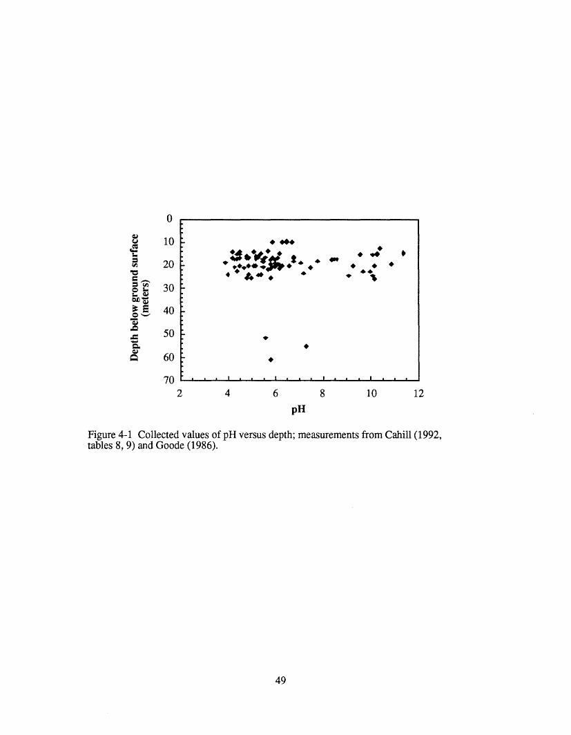
another site with similar soils have been compiled from several different sources (Goode,

1986; Cahill, 1982), and are shown in Figure 4-1 as a function of sample depth. Since

this figure shows an equal scattering of the data for different depths, the sample set is

assumed to be representative of the entire aquifer. The pH data set presented in

Figure 4-1 is shown in a histogram in Figure 4-2. The high values of pH are probably

due to contamination of the samples by dissolution of grout around well bores, and

therefore are assumed not to reflect accurately in situ pH. A statistical analysis of the pH

data gives a mean pH (pH) of 5.57, and a standard deviation of pH ( 0pH ) to be 0.88.

Samples with a pH greater than 8.5 are not included in the statistical calculations.

48

U;KA-:*w4~~* 4

4 6

* *.4*

8 10

pH

Figure 4-1 Collected values of pH versus depth; measurements from Cahill (1992,tables 8, 9) and Goode (1986).

49

0

Cu

o

e,s:

(U,

10

20

30

40

50

60

e,

702 12

- - - - - - - - --I I I I I

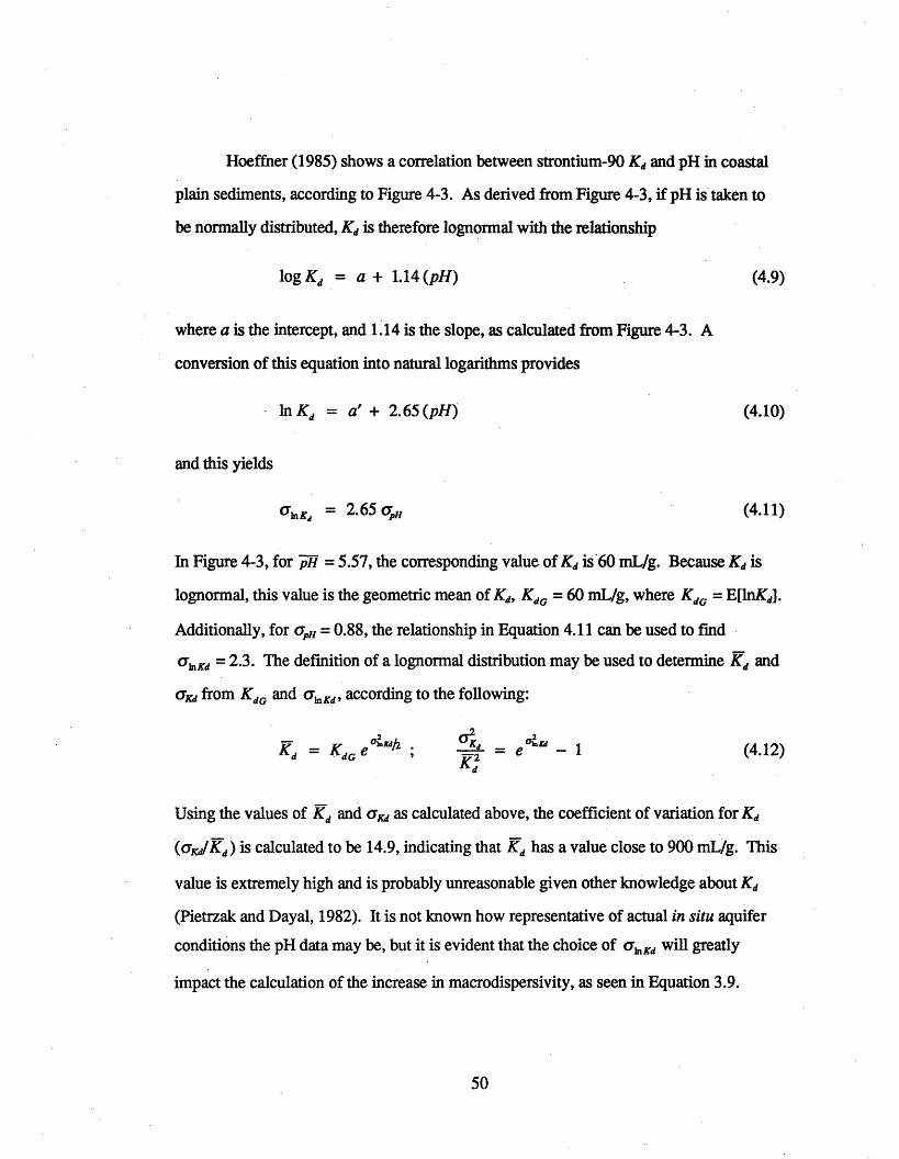
Hoeffner (1985) shows a correlation between strontium-90 Kd and pH in coastal

plain sediments, according to Figure 4-3. As derived from Figure 4-3, if pH is taken to

be normally distributed, Kd is therefore lognormal with the relationship

log K d = a + 1.14(pH) (4.9)

where a is the intercept, and 1.14 is the slope, as calculated from Figure 4-3. A

conversion of this equation into natural logarithms provides

InK d = a' + 2.65(pH) (4.10)

and this yields

hl K, = 2.65 oH (4.11)

In Figure 4-3, for pH = 5.57, the corresponding value of Kd is'60 mL/g. Because Kd is

lognormal, this value is the geometric mean of Kd, KdG = 60 mL/g, where KdG = E[lnKd].

Additionally, for apH = 0.88, the relationship in Equation 4.11 can be used to find

OarlKd = 2.3. The definition of a lognormal distribution may be used to determine Kd and

aKd from KdG and a~Kd, according to the following:

K( = KdG e 2/2 ° K = e -1 (4.12)Kd

Using the values of Kd and aKd as calculated above, the coefficient of variation for Kd

(ad/Kd) is calculated to be 14.9, indicating that Kd has a value close to 900 mL/g. This

value is extremely high and is probably unreasonable given other knowledge about Kd

(Pietrzak and Dayal, 1982). It is not known how representative of actual in situ aquifer

conditions the pH data may be, but it is evident that the choice of a,,Kd will greatly

impact the calculation of the increase in macrodispersivity, as seen in Equation 3.9.

50

03 5 7

pH9

35

g 30

' 25Cu

%o 20

. 15

z 10

5F i u e 4 2 D s r b ti n o e s r d au s fr m 9

Figure 4-2 Distribution of measured pH values from 95taken from Cahill (1982, tables 8, 9) and Goode (1986).

1/vAfzvu~I .AuU

1000

bOC

10(

11 13

site water and soil samples; data

2 4 6 8 10 12

pH

Figure 4-3 Relationship ofHoeffner (1985, figure 5).

site pH variation to strontium-90 Kd; reproduced from

51

pH = 5.57opH = 0.88

ELYO sirr� rle~ l~~J ,,.,_t4fJ~~J~J~~ JJ~~JaE~J~---J

-- - --

--

�Im

For purposes of illustration, is assumed that the coefficient of variation for Kd is

1.5. This reflects a more moderate value for ap,, on the order of 0.41. Using these new

assumptions and a value for KdG = 8 mL/g as proposed for Sr-90 by Campbell (1992),

the effect of Kd variability on longitudinal macrodispersivity may be determined from

Equation 3.9. There is no information on the correlation between pH and InK. It is

arbitrarily assumed for this case that there is no correlation, i.e., in Equation 3.9, = 0.

The longitudinal macrodispersivity enhancement is calculated on the basis of this

assumption. A summary of the relevant parameters is given in Table 4.4.

As can be seen in Table 4.4, even a relatively moderate variability in Kd has a

large effect on longitudinal macrodispersivity enhancement. In the case of strontium-90,

the increase of Ao by a factor of 9.7 will result in a large longitudinal spreading of the

plume and will affect the travel time of the leading edge of the plume, as confirmed by

the numerical model results in Chapter 5.

4.2.2 Technetium-99: Sorption Dependence on Clay Content

Measurements of clay content from site soil samples are shown in Figure 4-4

(Cahill, 1982). A statistical analysis of this data set gives a mean, %clay = 30%, and the

standard deviation, crcay = 10.

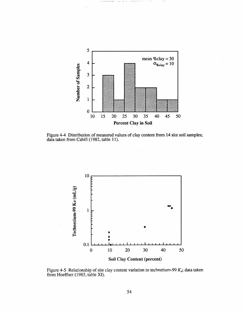
For technetium-99 (Tc-99), Hoeffner (1985) demonstrates a positive correlation of

clay content and Kd (see Figure 4-5), however, there are insufficient data to ascertain an

exact relationship between %clay and Tc-99 Kd. If a relationship could be determined,

Kd and Kdfor Tc-99 would be calculated in the same manner used in the evaluation of

Kd for Sr-90. Since no actual values are available, values are assumed arbitrarily for the

purposes of illustrating the analysis. Using a value of Tc-99 Kd = 1 mL/g (Campbell,

1992), and assuming that aJKd = 1.0, the effect of Kd variability on longitudinal

macrodispersivity may be determined from Equation 3.9 in the same manner as shown

above for strontium-90. In contrast to pH, clay content is correlated with hydraulic

conductivity. A high percentage of clay in the soil corresponds to a low hydraulic

52

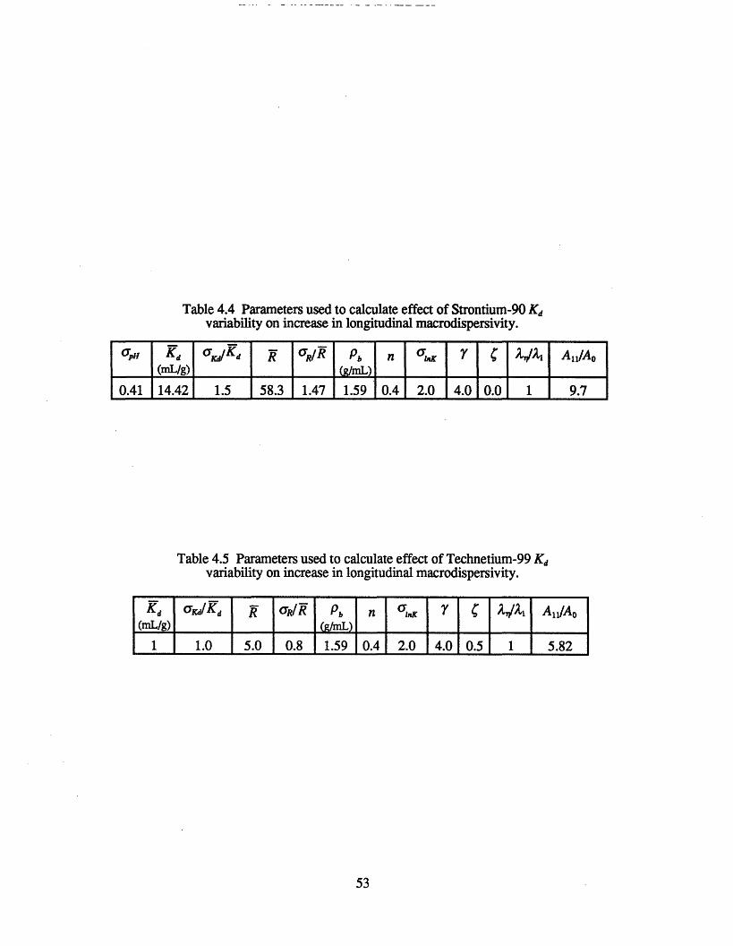
Table 4.4 Parameters used to calculate effect of Strontium-90 Kdvariability on increase in longitudinal macrodispersivity.

Table 4.5 Parameters used to calculate effect of Technetium-99 Kdvariability on increase in longitudinal macrodispersivity.

Kd UKdIKd R kR/ R Pb n ,r Y _ j A 11/AO(mL/g) (g/L)

1 1.0 5.0 0.8 1.59 0.4 2.0 4.0 0.5 1 5.82

53

5

4

E

&M

4

3

2

1

0o

oclay = 1U

mean %clay = 30

p

AU

Y/l///10 15 20 25 30 35 40 45 50

Percent Clay in Soil

Figure 4-4 Distribution of measured values of clay content from 14 site soil samples;data taken from Cahill (1982, table 11).

10

1

0.1

0 10 20 30 40 50

Soil Clay Content (percent)

IrA

Figure 4-5 Relationship of site,from Hoeffner (1985, table XI).

clay content variation to technetium-99 Kd; data taken

54

, . I 1 I I I 1 , I I I . . .

Y///S/f Ss'/// ~Y///Z /////// H//,/,,/////.

�

//F///

conductivity. For this reason, the correlation fraction, C, in Equation 3.9 is assumed to

be 0.5. The relevant parameters are summarized in Table 4.5.

4.2.3 Uranium-238: Macrodispersivity Enhancement

At the hypothetical site, the dependency of uranium-238 (U-238) Kd on soil

properties is not known. However, it is assumed that U-238 does exhibit some

longitudinal macrodispersivity enhancement due to sorption variation. Using a value of

U-238 Kd to be 40 mLIg, as given by Campbell (1992), and assuming acrKd = 0.7 and

= 0, the macrodispersivity enhancement is calculated from Equation 3.9. Following

the procedure for Sr-90 and Tc-99, this calculation gives All/Ao = 2.96 for U-238 in site

soils.

A final summary of the important properties of all four isotopes is provided in

Table 4.6.

4.3 Discussion

The assumptions and the uncertainties in the above analysis emphasize the need

for a more comprehensive method of data collection and evaluation. An important

conclusion of this analysis is that while it is possible to develop crude estimates of Kd

variation from a derived relationship with a soil parameter, it would be more meaningful

to measure Kd variations directly. If laboratory tests for Kd for each isotope are conducted

on the same samples as are tests for K, not only would it result in a quantification of Kd

variability, it would also determine the correlation between Kd and K for each isotope of

concern. Each sample would then be a single data point in Figure 3-8, and a precise

value for C could be derived for each isotope.

The calculated values of macrodispersivity enhancement in this chapter are

tentative, at best. They are not meant to give precise levels of enhancement, but are

calculated to illustrate the process of macrodispersivity enhancement parameter

estimation discussed in Subsection 3.2.3, and to serve as input parameters to the 2D

55

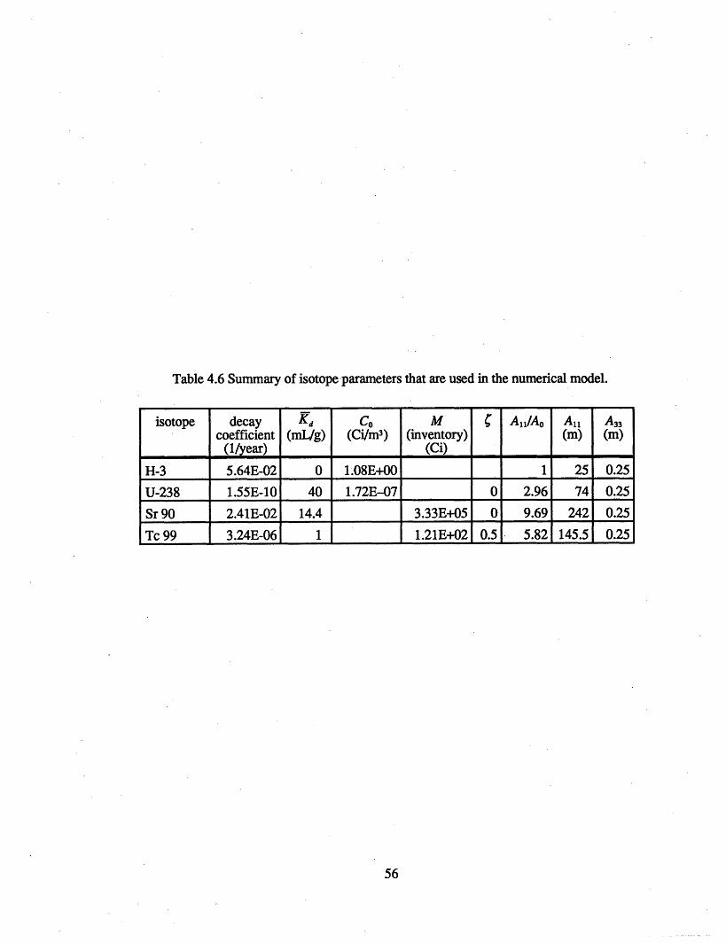
Table 4.6 Summary of isotope parameters that are used in the numerical model.

isotope decay Kd Co M ¢ A11/Ao All A33coefficient (mL/g) (Ci/m3) (inventory) (m) (m)

(1/year) (Ci)

H-3 5.64E-02 0 1.08E+00 1 25 0.25

U-238 1.55E-10 40 1.72E-07 0 2.96 74 0.25

Sr 90 2.41E-02 14.4 3.33E+05 0 9.69 242 0.25

Tc 99 3.24E-06 1 1.21E+02 0.5 5.82 145.5 0.25

56

numerical model in Chapter 5. It is hoped that modelers who traditionally use an

unenhanced value of longitudinal macrodispersivity will recognize the magnitude of the

effect of enhancement on model results, and that this approach will serve as the basis for

future model input parameters.

57

58

Chapter 5Numerical Models

The hydraulic parameters determined from the theory in Chapter 3 and the isotope

parameters from Chapter 4 are entered into traditional numerical models based upon the

hypothetical site characteristics in Chapter 2. These models illustrate the effects of

stochastic parameter estimation on isotope transport simulation.

The models are created and analyzed using a commercially available finite

element flow and transport computer code, SUTRA Mac, Version 1.3 (Geraghty &

Miller, Inc., Reston, VA; see Voss, 1984). The program allows for 2D anisotropic

transient flow and transport modeling with sorption and decay. Although the unsaturated

zone is not included in the models in this report, the program does contain the capability

to include unsaturated flow as well.

Using this program, two models are configured to simulate two separate transport

scenarios. The first model is a 2D rectangular vertical cross-section representing

downgradient flow from the hypothetical waste site to the spring (see Figure 2-1). The

second model is a 2D radial wedge representing the contribution of flow from the site in

the direction of a hypothetical municipal pumping well located near the city in

Figure 2-1.

5.1 Rectangular Model

The hypothetical waste site is located upgradient from the spring, with an

indication that most of the water entering the site as recharge will flow downgradient to

the spring. The 2D rectangular model from the site to the spring is typical of a LLW site

local groundwater model. Analysis using this model includes an evaluation of

59

contaminant transport to the spring and to a hypothetical observation well at the property

boundary for all four isotopes identified in Chapter 4.

5.1.1 Model Configuration

The 2D rectangular model is a one meter-wide vertical slice across the center of

the waste site and along the 1300-meter downgradient path to the spring (see Figure 5-1).

The 2D model represents a conservative estimate of the actual 3D problem, since it does

not account for concentration dilution due to horizontal transverse dispersion. However,

because the width of the waste site (about 400 meters) is significant in comparison to the

overall problem scale (1300 meters), it is expected that even in a 3D model, horizontal

transverse dispersion would play a minimal role in reducing concentrations at the center

of the site. The gradients in Zones 1, 2, and 3 are all in the direction of the spring, so that

the transverse advective flux neglected in a 2D representation of a 3D system will also be

minimal (see Figure 5-1).

As shown in Section 3.3, the unsaturated zone is expected to play a minimal role

in the transport problem. The 2D rectangular model neglects the unsaturated zone and

uses the water table as the upper fixed-head boundary. The lower boundary is provided

by the thick clay aquitard mentioned in Chapter 2. Water table heights are measured

relative to the lower boundary. Figure 5-1 shows an idealized cross-section for the

2D rectangular model.

Because the waste site is located near a groundwater divide, the upstream

boundary of the model is a no-flow boundary. Likewise, the spring is a local flow divide

since it receives influx from the groundwater on either side. For this reason, the

downstream boundary at the spring is also a no-flow boundary. This configuration

assumes that all the water that enters the model as recharge will be discharged at the

spring. The validity of this assumption is dependent on the extent to which Zone 3

receives local recharge and contributes to discharge at the spring. If Zone 3 does not

have a true groundwater divide at the site, some of the flow in Zone 3 may be upstream

60

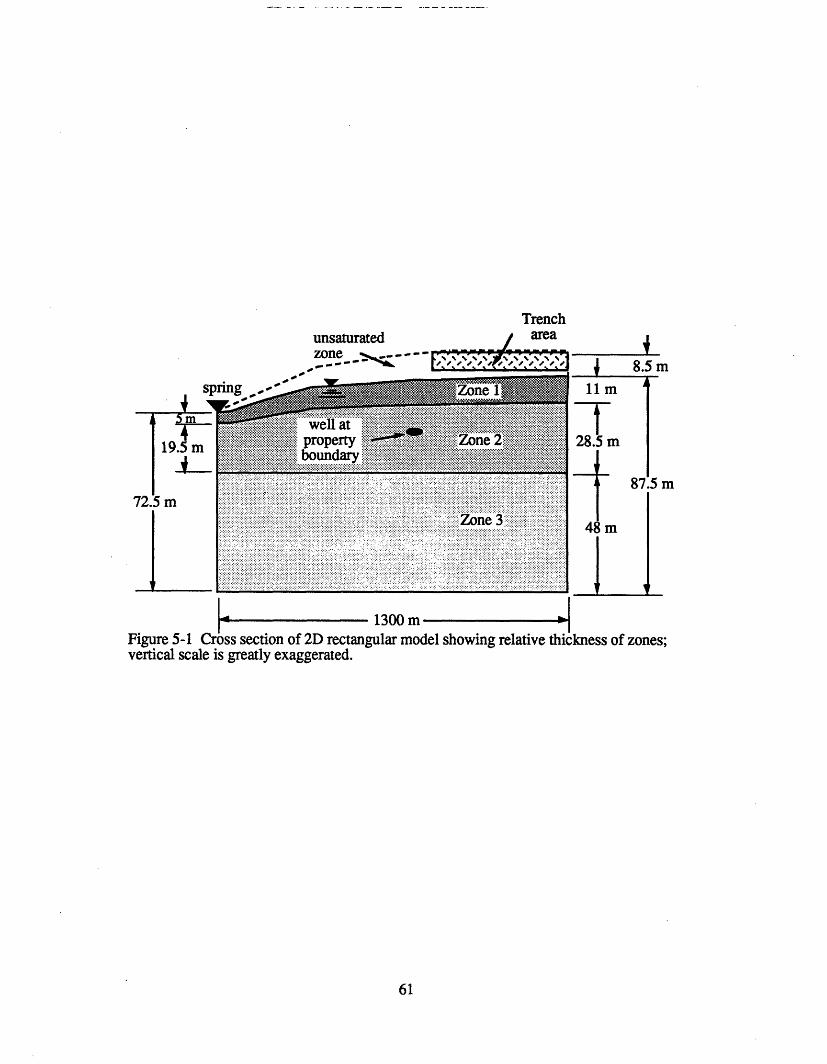
Trench

1 t rn "

1

a fJv , All - _ _ _ _ _ _ _ _ _

_- --- ^J s1 - I . -1 1 . - .. _ . ·

rigure 5-1 ross secuon or zIu rectangular moael snowing relatve tnlcKness or zones;vertical scale is greatly exaggerated.

61

I

-- --- -- - I . .% --

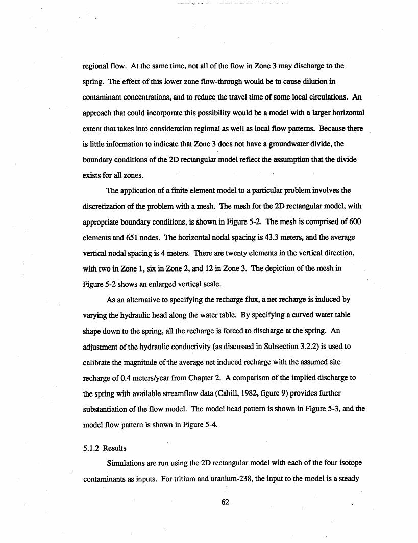
regional flow. At the same time, not all of the flow in Zone 3 may discharge to the

spring. The effect of this lower zone flow-through would be to cause dilution in

contaminant concentrations, and to reduce the travel time of some local circulations. An

approach that could incorporate this possibility would be a model with a larger horizontal

extent that takes into consideration regional as well as local flow patterns. Because there

is little information to indicate that Zone 3 does not have a groundwater divide, the

boundary conditions of the 2D rectangular model reflect the assumption that the divide

exists for all zones.

The application of a finite element model to a particular problem involves the

discretization of the problem with a mesh. The mesh for the 2D rectangular model, with

appropriate boundary conditions, is shown in Figure 5-2. The mesh is comprised of 600

elements and 651 nodes. The horizontal nodal spacing is 43.3 meters, and the average

vertical nodal spacing is 4 meters. There are twenty elements in the vertical direction,

with two in Zone 1, six in Zone 2, and 12 in Zone 3. The depiction of the mesh in

Figure 5-2 shows an enlarged vertical scale.

As an alternative to specifying the recharge flux, a net recharge is induced by

varying the hydraulic head along the water table. By specifying a curved water table

shape down to the spring, all the recharge is forced to discharge at the spring. An

adjustment of the hydraulic conductivity (as discussed in Subsection 3.2.2) is used to

calibrate the magnitude of the average net induced recharge with the assumed site

recharge of 0.4 meters/year from Chapter 2. A comparison of the implied discharge to

the spring with available streamflow data (Cahill, 1982, figure 9) provides further

substantiation of the flow model. The model head pattern is shown in Figure 5-3, and the

model flow pattern is shown in Figure 5-4.

5.1.2 Results

Simulations are run using the 2D rectangular model with each of the four isotope

contaminants as inputs. For tritium and uranium-238, the input to the model is a steady

62

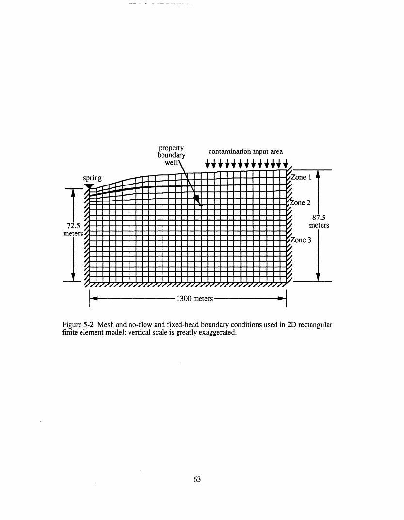
contamination input area

' m - V -V V

,Zone 1

Zone 24-

/-4/-4

1I�

4-1�

4-//

01 I'87.5

'1 metersF

Zone 3PP01PP01

1300 meters

Figure 5-2 Mesh and no-flow and fixed-head boundary conditions used in 2D rectangularfinite element model; vertical scale is greatly exaggerated.

63

propertyboundary

well\

spring I

I72.5meters

1Z4- - -I-

1

7-

e e se e to e e , e

CII

m N l i i l I a, i

m - m m I m- e _...

- - I I - - - - - i

- - I I I -- - - - - - r

irl-·I

�

I,

III

I1.

I--

IIIII--

I

I

IIIIIIIIII

1.

II

�

III

7

I

1.I-Ir�

1.

II1.

r_

7

i

ir-

11

III

7-

IE IIII

I�III

�

I1.I

I

I

II

I-

II

I

7-

IIIIII

II1.I

I

II

III

r-

7Ir

c,CI-CLI 'I�C·i " rr I C-r le -r 4 -- r I irr C ·- r -r C I,

l w _I

--1

:m

_

-

J/,t-, . ..

JIr ,fJ f J r r J J J J

J J J,, 7 A I I l l # l f f I Jr,l j . f. J ~ I I I-I --------e e } e e e e e ,j f J r J J , w J

J r r - - --- 1 - - -

+0+00400/~$-

.mm

j

_ _ imm

I -

l

I

i

m

m

I

m

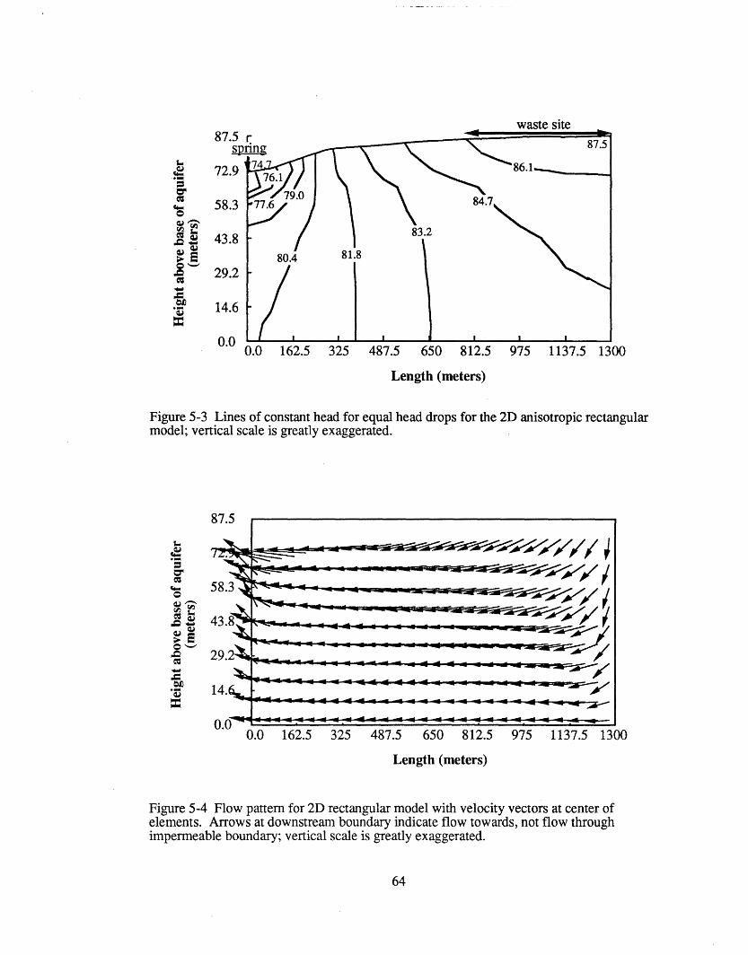
waste site87.

ct.

c>E,I C.OD01

.4

*.aULCW

72.

58.

43.

29.

14.

nA0.0 162.5 325 487.5 650 812.5 975 1137.5 1300

Length (meters)

Figure 5-3 Lines of constant head for equal head drops for the 2D anisotropic rectangularmodel; vertical scale is greatly exaggerated.

A- I

0.cc

CT

4.

o-.0W -V)&

CZ

*-aQ,

0.0 162.5 325 487.5 650 812.5 975 1137.5 1300

Length (meters)

Figure 5-4 Flow pattern for 2D rectangular model with velocity vectors at center ofelements. Arrows at downstream boundary indicate flow towards, not flow throughimpermeable boundary; vertical scale is greatly exaggerated.

64

state concentration flux into the portion of the model that bisects the trench area (see

Figure 5-2). For strontium-90 and technetium-99, the input to the model is a short pulse

of concentration at the trench area, followed by a continuous inflow of uncontaminated

water.

An observation well is placed at the site property boundary at a depth of about 30

meters below the ground surface (see Figures 5-1 and 5-2). This well is characteristic of

local private water supply wells that could be located close to the waste site property.

The observation well is used to monitor the magnitude and travel time of contaminants

that reach the property boundary.

Concentration curves at the property boundary well and at the spring are provided

for each isotope. Additionally, concentration contours in the model cross-section are

shown for the time of peak or steady state concentration at both the property boundary

well and at the spring. These contours demonstrate the spatial extent of concentration at

the given time. The results are displayed by isotope in Figures 5-5 to 5-12.

The minimum contour levels shown in the contour plots for H-3 (Figure 3-6) and

for Sr-90 (Figure 3-10) are the drinking water limits, as discussed in Subsection 4.1.1.

All concentration levels displayed in these figures are above the drinking water limits.

Since neither the concentrations of Tc-99 or U-238 are ever above the drinking water

limits, the concentration contours in Figure 5-8 and Figure 5-12 represent the upper range

of concentration present for each isotope.

65

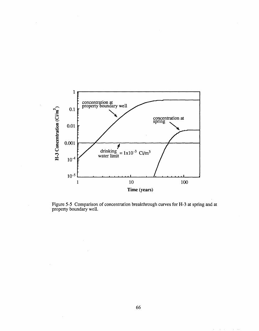
1

enS- 0.1

-e

8 0.001

Q

n lo-4

10-5

1 10 100

Time (years)

Figure 5-5 Comparison of concentration breakthrough curves for H-3 at spring and atproperty boundary well.

66

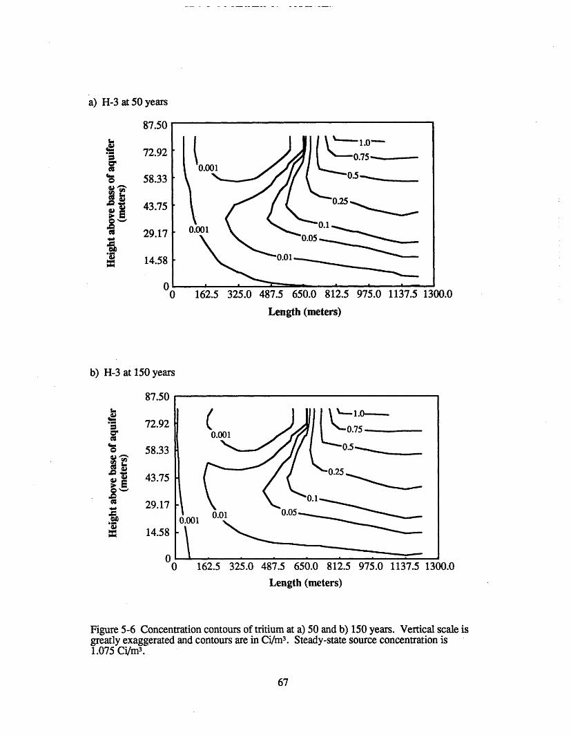
a) H-3 at 50 years

0 162.5 325.0 487.5 650.0 812.

Length (meters)

.5 975.0 1137.5 1300.0

b) H-3 at 150 years

0 162.5 325.0 487.5 650.0 812.5 975.0 1137.5 1300.0

Length (meters)

Figure 5-6 Concentration contours of tritium at a) 50 and b) 150 years. Vertical scale isgreatly exaggerated and contours are in Ci/m3. Steady-state source concentration is1.075 Ci/m3.

67

87.50

s qjCu0

Cr

cnvP.I.9

de

72.92

58.33

43.75

29.17

14.58

0

87.50

S.

oIcd.b1

-C

IaIs

72.92

58.33

43.75

29.17

14.58

0.01 u.uj

Ian%

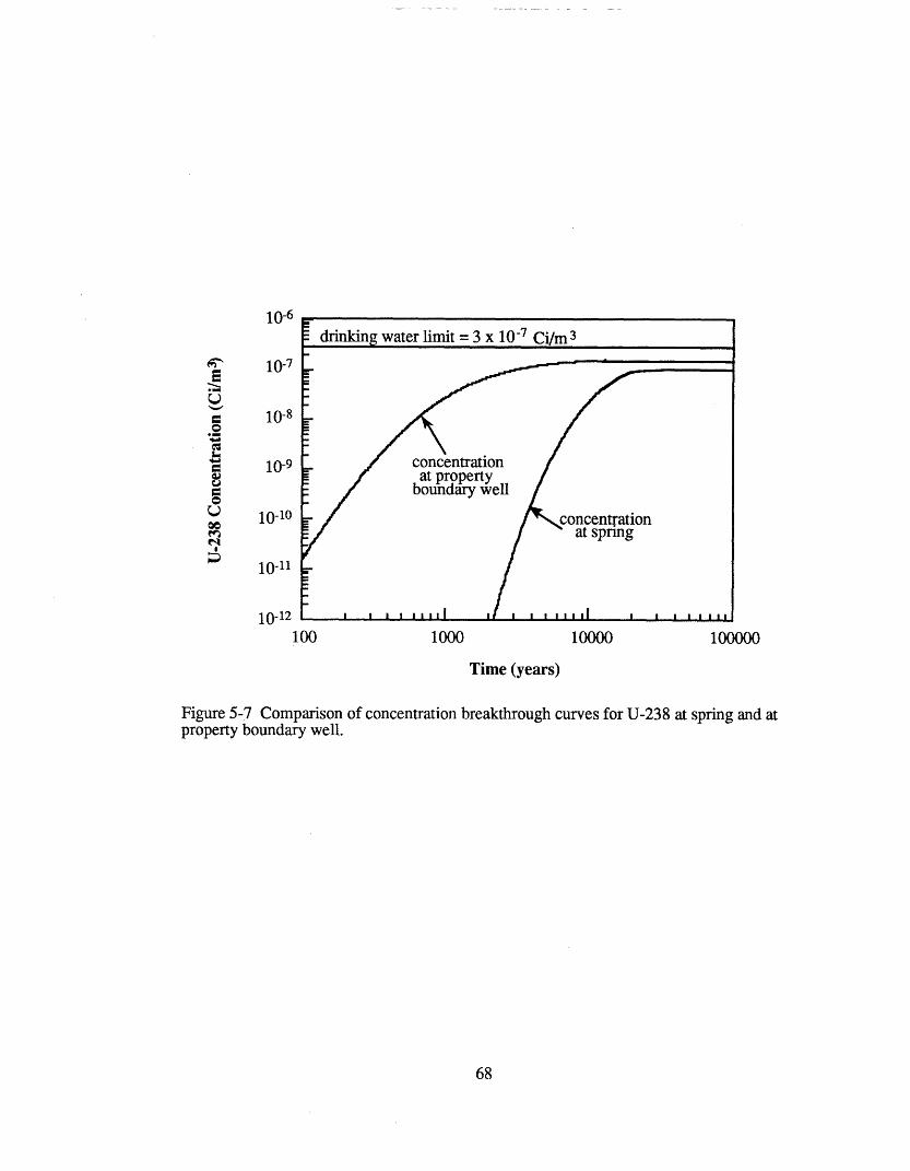
1000 10000

Time (years)

Figure 5-7 Comparisonproperty boundary well.

of concentration breakthrough curves for U-238 at spring and at

68

10-6

mveQ

e.

v0Mo

10-7

10-8

10-9

10-10

10-11

10-12

100 100000

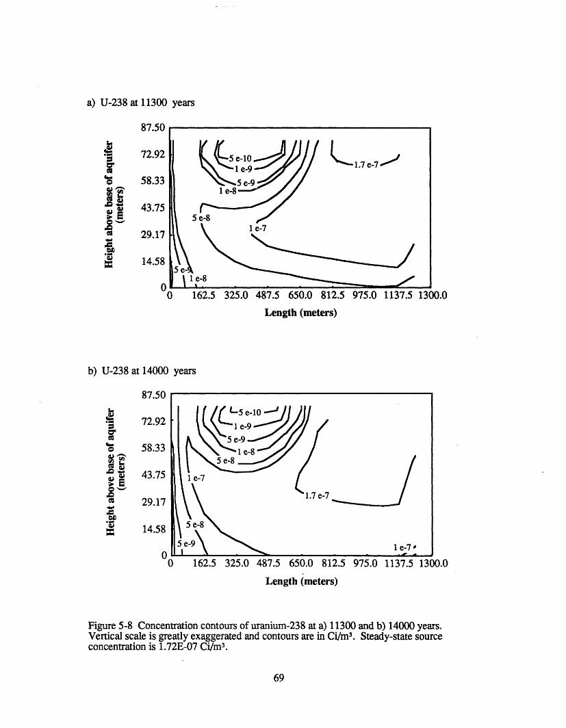
a) U-238 at 11300 years

0 162.5 325.0 487.5 650.0 812.

Length (meters)

.5 975.0 1137.5 1300.0

b) U-238 at 14000 years

0 162.5 325.0 487.5 650.0 812.5 975.0 1137.5 1300.0

Length (meters)

Figure 5-8 Concentration contours of uranium-238 at a) 11300 and b) 14000 years.Vertical scale is greatly exaggerated and contours are in Ci/m3 . Steady-state sourceconcentration is 1.72E-07 Ci/m3.

69

87.50

o

v!tu

-0Ns4mgo

72.92

58.33

43.75

29.17

14.58

0

87.50

.. '

o

c,

cs0CW

.v

I Mo*-

72.92

58.33

43.75

29.17

14.58

0

v

i

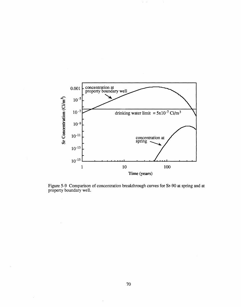
0.00

10

10

10

10-

i0-1

in-I

1 10 100

Time (years)

Figure 5-9 Comparison of concentrationproperty boundary well.

breakthrough curves for Sr-90 at spring and at

70

-U0eo

o

1V

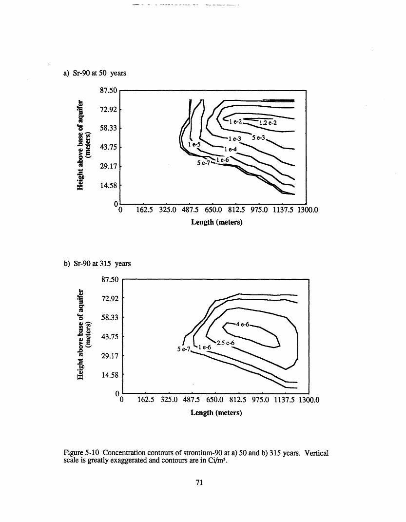
a) Sr-90 at 50 years

87.50

72.92

58.33

43.75

29.17

14.58

nC 162.5 325.0 487.5 650.0 812.5 975.0 1137.5 1300.0

Length (meters)

b) Sr-90 at 315 years

,~ r Il '6 /.3u

IU

LU

0Cra

;>Ev.0...L

:f-UJ

72.92

58.33

43.75

29.17

14.58

A0 162.5 325.0 487.5 650.0 812.5 975.0 1137.5 1300.0

Length (meters)

Figure 5-10 Concentration contours of strontium-90 at a) 50 and b) 315 years. Verticalscale is greatly exaggerated and contours are in Ci/m3.

71

fi42

041Is

ww

LPj

LU

5

· · I I

I

D

L

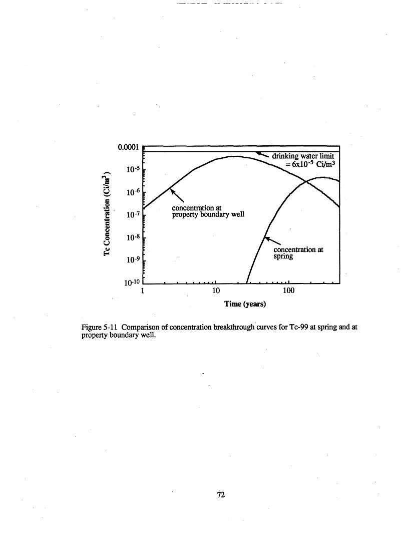
0.0001

10-5

V 10-6

e0._

e 10-7

o 10-8

10-9

1n-10

1 10 100

Time (years)

Figure 5-11 Comparison of concentration breakthrough curves for Tc-99 at spring and atproperty boundary well.

72

_____ ·

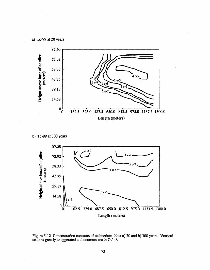
a) Tc-99 at 20 years

87.50

72.92

58.33

43.75

29.17

14.58

00 162.5 325.0 487.5 650.0 812.5 975.0

Length (meters)

1137.5 1300.0

b) Tc-99 at 300 years

0 162.5 325.0 487.5 650.0 812.5 975.0 1137.5 1300.0

Length (meters)

Figure 5-12 Concentration contours of technetium-99 at a) 20 and b) 300 years. Verticalscale is greatly exaggerated and contours are in Ci/m3.

73

I"5.,

Ei.

yCCu

.IV

"oCu0Cr

Co.0*C

C_

X co

A'Y Al.b I.3U

72.92

58.33

43.75

29.17

14.58

A

-

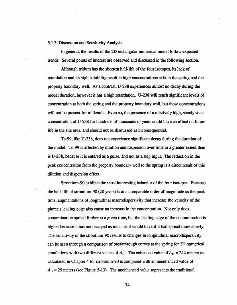
5.1.3 Discussion and Sensitivity Analysis

In general, the results of the 2D rectangular numerical model follow expected

trends. Several points of interest are observed and discussed in the following section.

Although tritium has the shortest half-life of the four isotopes, its lack of

retardation and its high solubility result in high concentrations at both the spring and the

property boundary well. As a contrast, U-238 experiences almost no decay during the

model duration, however it has a high retardation. U-238 will reach significant levels of

concentration at both the spring and the property boundary well, but these concentrations

will not be present for millennia. Even so, the presence of a relatively high, steady state

concentration of U-238 for hundreds of thousands of years could have an effect on future

life in the site area, and should not be dismissed as inconsequential.

Tc-99, like U-238, does not experience significant decay during the duration of

the model. Tc-99 is affected by dilution and dispersion over time to a greater extent than

is U-238, because it is entered as a pulse, and not as a step input. The reduction in the

peak concentration from the property boundary well to the spring is a direct result of this

dilution and dispersion effect.

Strontium-90 exhibits the most interesting behavior of the four isotopes. Because

the half-life of strontium-90 (28 years) is at a comparable order of magnitude as the peak

time, augmentations of longitudinal macrodispersivity that increase the velocity of the

plume's leading edge also cause an increase in the concentration. Not only does

contamination spread further at a given time, but the leading edge of the contamination is

higher because it has not decayed as much as it would have if it had spread more slowly.

The sensitivity of the strontium-90 results to changes in longitudinal macrodispersivity

can be seen through a comparison of breakthrough curves at the spring for 2D numerical

simulations with two different values of All. The enhanced value of All = 242 meters as

calculated in Chapter 4 for strontium-90 is compared with an unenhanced value of

All =25 meters (see Figure 5-13). The unenhanced value represents the traditional

74

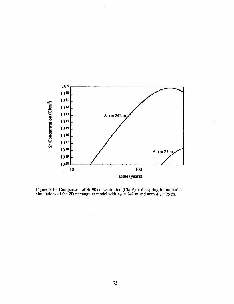
I A-O1V-

1010

$,*S- 10-11

- 10-12

U 1013

· 1014.* 1015

o 10 1 6

_) 10-17

1018

1019

10-2o

10 100

Time (years)

Figure 5-13 Comparison of Sr-90 concentration (Ci/m3) at the spring for numericalsimulations of the 2D rectangular model with All = 242 m and with Al, = 25 m.

75

modeling approach, which would not take into consideration the effects of sorption

variability on macrodispersivity. The transverse dispersivity, A33, is the same for both

cases. Figure 5-13 shows the effects of the different macrodispersivity values. At early

time, the undecayed concentration spreading with the higher dispersivity results in a

concentration increase of up to ten orders of magnitude. The time at which the peak

occurs is almost twice as long for the low dispersivity as it is for the high dispersivity.

Due to the significance of dispersivity changes on strontium-90 concentrations, any

uncertainties in the determination of All will greatly affect results. An approach to the

evaluation of these uncertainties, and a discussion of their effect is presented in

Section 5.3.

5.2 Radial Model

Although the head contours in Figure 2-1 indicate that the mean gradient at the

hypothetical waste site is in the direction of the spring, for the purposes of analysis, a

second situation is proposed. A large municipal well (or well field) is assumed to be

located near the city in the map of Figure 2-1. A second numerical model is designed to

evaluate the possible movement of contamination from the site in the direction of this

pumping well.

5.2.1 Model Configuration

Because the model is concerned with the flow to a well, it is appropriate to use a

radial coordinate system for the configuration. The flow field is represented by a wedge-

shaped mesh, with the well at the center. The wedge extends outward 8400 meters from

the well to the site. The maximum width of the wedge is the width of the site. This

width represents 15 degrees of the entire circular contribution to the flow at the well.

As described for the rectangular model, the upper boundary of the radial model is

the water table, and the lower no-flow boundary is the aquitard. The outer boundary at

the site is a no-flow boundary, implying a groundwater divide at the site. The inner

76

boundary at the well is a fixed head boundary over the well screen and a no-flow

boundary above the well screen (see Figure 5-14). In moving from the city to the site in

Figure 2-1, a river is crossed. Discharge to this river is considered in the radial model.

The relative location of this river to the rest of the model is displayed in Figure 5-14. The

model configuration assumes that all flow is radial as a result of the pumping well. In

reality, local hydraulic circulation may produce non-radial flow that is unaccounted for

by this 2D model.

The pumping well is large enough to be a municipal water supply. It is assumed

to have a total pumping rate of Q = 0.0241 m3/s (550,000 gallons/day), and to have a

radius of 30 meters, representative of a well field. The component of Q that is from the

site, Q,, is given by Q, = Q x 15/360 = 0.001 m3/s. This is a result of the site flow

contribution to the well of 15 degrees. The bottom of the well screen is located 63 meters

below the unadjusted water table, with a well screen of 12 meters.

Before the water table height is specified as the fixed head boundary in the radial

model, an evaluation is made of the effect of the pumping well on drawdown at the water

table. Phillips and Gelhar (1978) provide an expression for drawdown of the water table

(4) at any point due to the effects of a short-screened (point source) pumping well. This

expression is a function of the pumping rate (Q), the horizontal hydraulic conductivity

(K1 l), the depth of the well (z), and the angle (x) from the vertical at the well to a point on

the water table:

= Q cosa (5.1)4 irK z

Using a value of K11 = 1.90E-05 m/s for the entire aquifer (see Table 3.1), 0 is calculated

for various locations on the water table. These results for 0 range from 1.6 meters at the

water table above the well, to 0.08 meters of drawdown at the site. The water table

heights used in the numerical model reflect the drawdown adjustment as applied to the

head measurements from the contours in Figure 2-1.

77

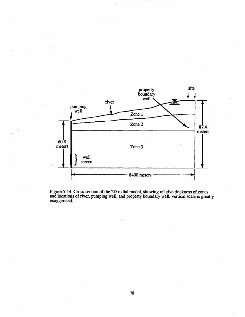
property siteboundary 4s

60.8meters

I

87.4meters

|~4 .~- - -8400 meters -|

Figure 5-14 Cross-section of the 2D radial model, showing relative thickness of zonesand locations of river, pumping well, and property boundary well; vertical scale is greatlyexaggerated.

78

I F

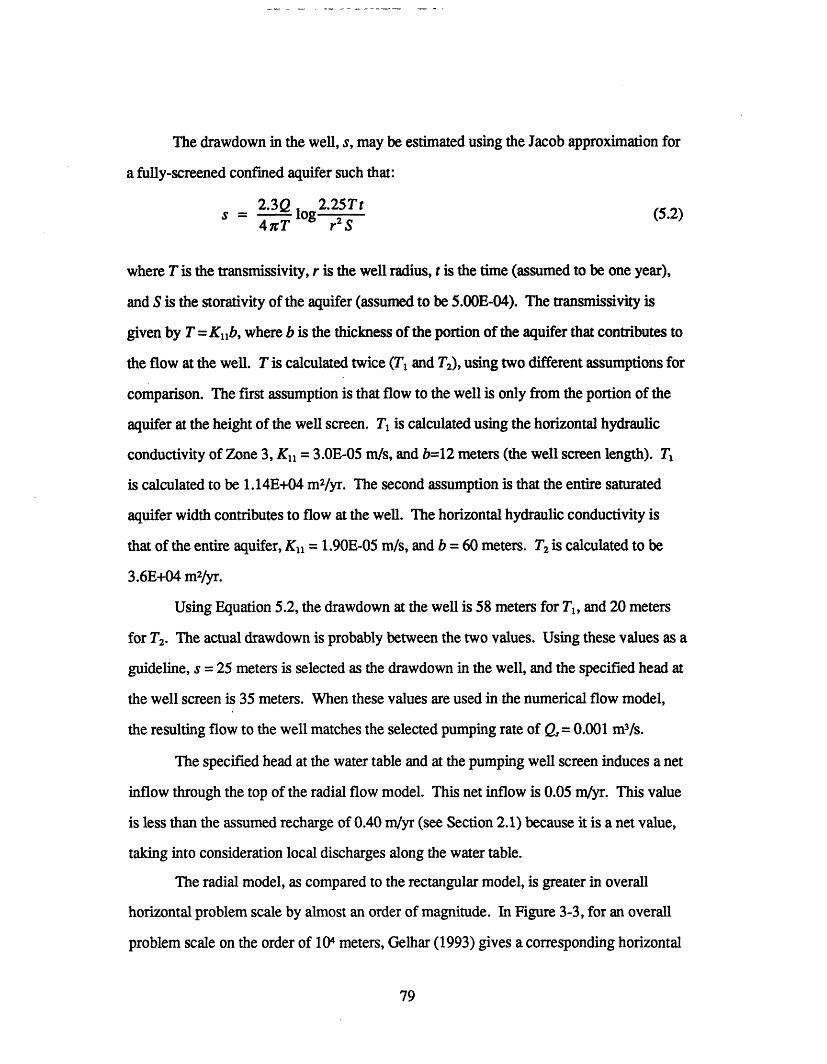
The drawdown in the well, s, may be estimated using the Jacob approximation for

a fully-screened confined aquifer such that:

s = 4 l og 225 (5.2)4xtT br2 S

where T is the transmissivity, r is the well radius, t is the time (assumed to be one year),

and S is the storativity of the aquifer (assumed to be 5.00E-04). The transmissivity is

given by T = Kllb, where b is the thickness of the portion of the aquifer that contributes to

the flow at the well. T is calculated twice (T1 and T2), using two different assumptions for

comparison. The first assumption is that flow to the well is only from the portion of the

aquifer at the height of the well screen. T is calculated using the horizontal hydraulic

conductivity of Zone 3, Kll = 3.OE-05 m/s, and b=12 meters (the well screen length). T,

is calculated to be 1.14E+04 m2/yr. The second assumption is that the entire saturated

aquifer width contributes to flow at the well. The horizontal hydraulic conductivity is

that of the entire aquifer, Kll = 1.90E-05 m/s, and b = 60 meters. T2 is calculated to be

3.6E+04 m2/yr.

Using Equation 5.2, the drawdown at the well is 58 meters for T1, and 20 meters

for T2. The actual drawdown is probably between the two values. Using these values as a

guideline, s = 25 meters is selected as the drawdown in the well, and the specified head at

the well screen is 35 meters. When these values are used in the numerical flow model,

the resulting flow to the well matches the selected pumping rate of Q,= 0.001 m3/s.

The specified head at the water table and at the pumping well screen induces a net

inflow through the top of the radial flow model. This net inflow is 0.05 m/yr. This value

is less than the assumed recharge of 0.40 m/yr (see Section 2.1) because it is a net value,

taking into consideration local discharges along the water table.

The radial model, as compared to the rectangular model, is greater in overall

horizontal problem scale by almost an order of magnitude. In Figure 3-3, for an overall

problem scale on the order of 104 meters, Gelhar (1993) gives a corresponding horizontal

79

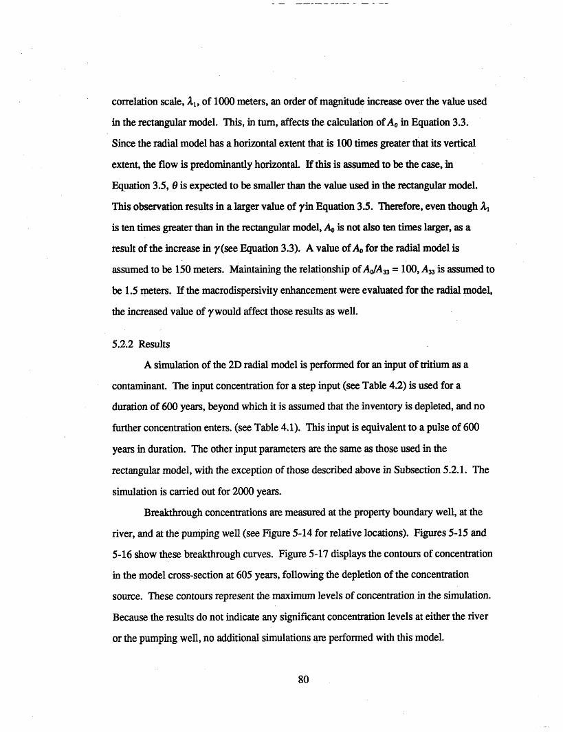
correlation scale, AI, of 1000 meters, an order of magnitude increase over the value used

in the rectangular model. This, in turn, affects the calculation of Ao in Equation 3.3.

Since the radial model has a horizontal extent that is 100 times greater that its vertical

extent, the flow is predominantly horizontal. If this is assumed to be the case, in

Equation 3.5, 0 is expected to be smaller than the value used in the rectangular model.

This observation results in a larger value of yin Equation 3.5. Therefore, even though A,1

is ten times greater than in the rectangular model, Ao is not also ten times larger, as a

result of the increase in y(see Equation 3.3). A value of Ao for the radial model is

assumed to be 150 meters. Maintaining the relationship of AoA33 = 100, A33 is assumed to

be 1.5 meters. If the macrodispersivity enhancement were evaluated for the radial model,

the increased value of rwould affect those results as well.

5.2.2 Results

A simulation of the 2D radial model is performed for an input of tritium as a

contaminant. The input concentration for a step input (see Table 4.2) is used for a

duration of 600 years, beyond which it is assumed that the inventory is depleted, and no

further concentration enters. (see Table 4.1). This input is equivalent to a pulse of 600

years in duration. The other input parameters are the same as those used in the

rectangular model, with the exception of those described above in Subsection 5.2.1. The

simulation is carried out for 2000 years.

Breakthrough concentrations are measured at the property boundary well, at the

river, and at the pumping well (see Figure 5-14 for relative locations). Figures 5-15 and

5-16 show these breakthrough curves. Figure 5-17 displays the contours of concentration

in the model cross-section at 605 years, following the depletion of the concentration

source. These contours represent the maximum levels of concentration in the simulation.

Because the results do not indicate any significant concentration levels at either the river

or the pumping well, no additional simulations are performed with this model.

80

1

0.1

0.01

0.001

10-4

10-5

10 1000100

Time (years)

Figure 5-15 Breakthrough concentration curve for tritium at the property boundary wellusing the 2D radial model.

10-10

eS

U

0I=

coCu

0UMe

10-12

10-14

10-16

10-18

10-20

100 1000

Time (years)

Figure 5-16 Breakthrough concentration curves for tritium at the river and at thepumping well using the 2D radial model.

81

rnEo00

elam

o8UM

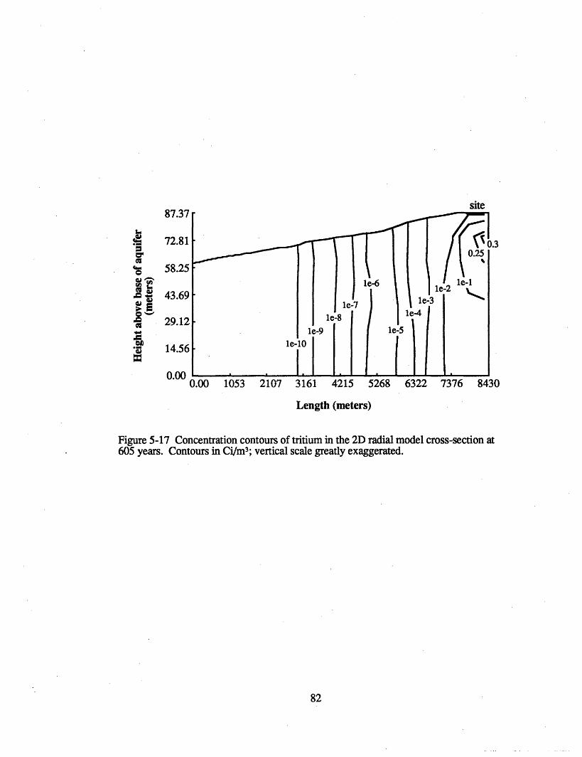
87.37

!a 72.81'U

WO 58.25

4. 43.69

c0s -29.12

· 14.56

nnn

site

0.00 1053 2107 3161 4215 5268 6322 7376 843(

Length (meters)

Figure 5-17 Concentration contours of tritium in the 2D radial model cross-section at605 years. Contours in Ci/m3; vertical scale greatly exaggerated.

)

82

A_ At

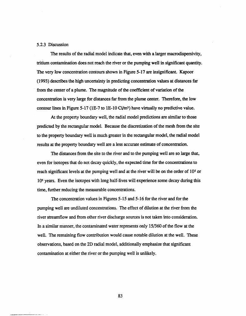
5.2.3 Discussion

The results of the radial model indicate that, even with a larger macrodispersivity,

tritium contamination does not reach the river or the pumping well in significant quantity.

The very low concentration contours shown in Figure 5-17 are insignificant. Kapoor

(1993) describes the high uncertainty in predicting concentration values at distances far

from the center of a plume. The magnitude of the coefficient of variation of the

concentration is very large for distances far from the plume center. Therefore, the low

contour lines in Figure 5-17 (1E-7 to 1E-10 Ci/m3) have virtually no predictive value.

At the property boundary well, the radial model predictions are similar to those

predicted by the rectangular model. Because the discretization of the mesh from the site

to the property boundary well is much greater in the rectangular model, the radial model

results at the property boundary well are a less accurate estimate of concentration.

The distances from the site to the river and to the pumping well are so large that,

even for isotopes that do not decay quickly, the expected time for the concentrations to

reach significant levels at the pumping well and at the river will be on the order of 105 or

106 years. Even the isotopes with long half-lives will experience some decay during this

time, further reducing the measurable concentrations.

The concentration values in Figures 5-15 and 5-16 for the river and for the

pumping well are undiluted concentrations. The effect of dilution at the river from the

river streamflow and from other river discharge sources is not taken into consideration.

In a similar manner, the contaminated water represents only 15/360 of the flow at the

well. The remaining flow contribution would cause notable dilution at the well. These

observations, based on the 2D radial model, additionally emphasize that significant

contamination at either the river or the pumping well is unlikely.

83

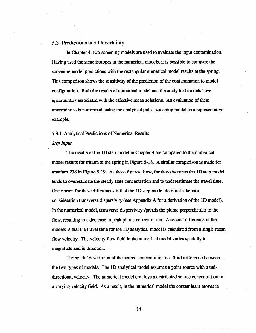
5.3 Predictions and Uncertainty

In Chapter 4, two screening models are used to evaluate the input contamination.

Having used the same isotopes in the numerical models, it is possible to compare the

screening model predictions with the rectangular numerical model results at the spring.

This comparison shows the sensitivity of the prediction of the contamination to model

configuration. Both the results of numerical model and the analytical models have

uncertainties associated with the effective mean solutions. An evaluation of these

uncertainties is performed, using the analytical pulse screening model as a representative

example.

5.3.1 Analytical Predictions of Numerical Results

Step Input

The results of the ID step model in Chapter 4 are compared to the numerical

model results for tritium at the spring in Figure 5-18. A similar comparison is made for

uranium-238 in Figure 5-19. As these figures show, for these isotopes the ID step model

tends to overestimate the steady state concentration and to underestimate the travel time.

One reason for these differences is that the ID step model does not take into

consideration transverse dispersivity (see Appendix A for a derivation of the ID model).

In the numerical model, transverse dispersivity spreads the plume perpendicular to the

flow, resulting in a decrease in peak plume concentration. A second difference in the

models is that the travel time for the ID analytical model is calculated from a single mean

flow velocity. The velocity flow field in the numerical model varies spatially in

magnitude and in direction.

The spatial description of the source concentration is a third difference between

the two types of models. The 1D analytical model assumes a point source with a uni-

directional velocity. The numerical model employs a distributed source concentration in

a varying velocity field. As a result, in the numerical model the contaminant moves in

84

0.1

2

0U3C"0

UM,

0.01

0.001

10- 4

10 -5

10-6

10 100Time (years)

Figure 5-18 Comparison of H-3 concentration breakthrough curves at the spring for theID step model prediction and for the 2D rectangular numerical simulation.

A-1

4E

-Ua0Q.MmO:I

I

0

0

U

cc,

etI

10

10

101000 10000

Time (years)

100000

Figure 5-19 Comparison of U-238 concentration breakthrough curves at the spring forthe 1D step model prediction and for the 2D rectangular numerical simulation.

85

1(-7

1£

V(

V(

V(

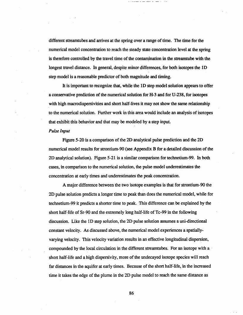
different streamtubes and arrives at the spring over a range of time. The time for the

numerical model concentration to reach the steady state concentration level at the spring

is therefore controlled by the travel time of the contamination in the streamtube with the

longest travel distance. In general, despite minor differences, for both isotopes the ID

step model is a reasonable predictor of both magnitude and timing.

It is important to recognize that, while the D step model solution appears to offer

a conservative prediction of the numerical solution for H-3 and for U-238, for isotopes

with high macrodispersivities and short half-lives it may not show the same relationship

to the numerical solution. Further work in this area would include an analysis of isotopes

that exhibit this behavior and that may be modeled by a step input.

Pulse Input

Figure 5-20 is a comparison of the 2D analytical pulse prediction and the 2D

numerical model results for strontium-90 (see Appendix B for a detailed discussion of the

2D analytical solution). Figure 5-21 is a similar comparison for technetium-99. In both

cases, in comparison to the numerical solution, the pulse model underestimates the

concentration at early times and underestimates the peak concentration.

A major difference between the two isotope examples is that for strontium-90 the

2D pulse solution predicts a longer time to peak than does the numerical model, while for

technetium-99 it predicts a shorter time to peak. This difference can be explained by the

short half-life of Sr-90 and the extremely long half-life of Tc-99 in the following

discussion. Like the D step solution, the 2D pulse solution assumes a uni-directional

constant velocity. As discussed above, the numerical model experiences a spatially-

varying velocity. This velocity variation results in an effective longitudinal dispersion,

compounded by the local circulation in the different streamtubes. For an isotope with a

short half-life and a high dispersivity, more of the undecayed isotope species will reach

far distances in the aquifer at early times. Because of the short half-life, in the increased

time it takes the edge of the plume in the 2D pulse model to reach the same distance as

86

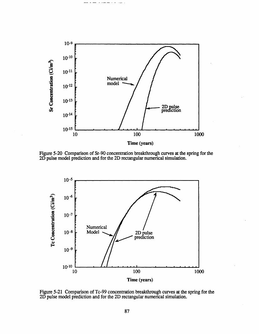
10-9

t

U

CoI-SO**W

a

10-10

1012

10-14

10 100 1000

Time (years)

Figure 5-20 Comparison of Sr-90 concentration breakthrough curves at the spring for the2D pulse model prediction and for the 2D rectangular numerical simulation.

10-5

m-)M

v

E0U.

C0UUS

10-6

10-7

10-8

10-9

10-1010 100 1000

Time (years)

Figure 5-21 Comparison of Tc-99 concentration breakthrough curves at the spring for the2D pulse model prediction and for the 2D rectangular numerical simulation.

87

that of the numerical model, the isotope will experience significant decay. Therefore at

early times, the difference between the uniform velocity 2D pulse model and the

numerical model will be great.

This non-uniform flow is also the reason why, for strontium-90, the time to the

peak measured concentration in the numerical model is shorter than the time to the peak

for the 2D pulse model. It is not that the peaks arrive at different times, it is that the

measurements of undecayed concentration in advance of the center of the plume have the

effect of "moving" the numerical plume peak higher in magnitude and forward in time.

When the peaks pass, the two solutions converge as the diluted concentrations decrease,

and the decay continues.

Because the half-life of technetium-99 is very long, it represents the case of a non-

decaying contaminant. The non-uniform velocity is still the cause of an increased

spreading of the numerical model plume, but the lack of decay results in a solution of the

analytical model that is much closer to that of the numerical model at early time.

Because the isotope does not decay, the spreading of contaminant in advance of the peak

will not affect the measured location of the peak. Other issues, such as model

configuration as described above for the step solution, may provide an explanation for the

differences in peak magnitude and timing between the two models of Tc-99. In general,

however, the pulse model offers a reasonable prediction of the concentration

breakthrough curves.

5.3.2 Uncertainties in Model Predictions

The discussion in Subsection 5.3.1 illustrates the sensitivity of the concentration

predictions to analytical and numerical model assumptions. Regardless of the model

configuration, the concentration predictions in all the models are mean, or effective,

solutions. The sensitivity of the predictions to various parameters highlights the potential

sources of uncertainty in the mean solution. Model configuration, as discussed in

Subsection 5.3.1, is one source of uncertainty. The mean solutions are based on effective

88

flow and transport input parameters that are derived in the manner discussed in Chapter 3.

Inadequate estimates of these effective parameters are another source of uncertainty in the

mean solution. Another aspect of uncertainty concerns the variations of concentration

around the mean solution as a result of heterogeneity. Some theoretical approaches to

predicting these variations of concentration around the mean are discussed in Gelhar

(1993, section 5.3).

Uncertainties in the mean solution

The sensitivity of the model predictions to uncertainties in the effective

parameters is demonstrated using the pulse screening model from Section 4.1 for

strontium-90 at the spring. Figure 5-22 contrasts the behavior of the pulse model with an

enhanced longitudinal macrodispersivity (All = 242m) with that of an unenhanced

macrodispersivity (All = 25m). The first case corresponds to heterogeneous sorption, and

the second case corresponds to a non-sorbing solute. In modeling groundwater transport,

it is common practice to arbitrarily assume the same unenhanced dispersivity for all

transported species. The results in Figure 5-22 show that this assumption can yield

extreme underestimates of peak concentration (by 10 orders of magnitude). This same

extreme difference in magnitude of the peak concentration is found using the numerical

model (see Figure 5-13).

The sensitivity of the screening model is further illustrated in Figure 5-22 by

considering the influence of a 25 percent increase in the longitudinal dispersivity and a 25

percent decrease in the retardation factor. This modest change in these key input

parameters produces an increase in the peak concentration of two orders of magnitude.

Overall, these sensitivity results emphasize the importance of reliable dispersivity

estimates, especially in cases of radionuclides with small half-lives (28.8 years for

strontium-90) compared to the retarded mean travel time (3400 years for strontium-90)

(see also Section 5.3.1).

89

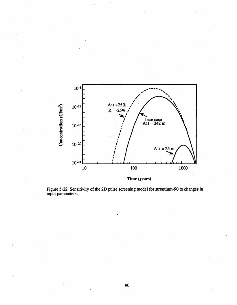
10-8

10-12

010-16

L-0

0 10-20

10-2410 100 1000

Time (years)

Figure 5-22 Sensitivity of the 2D pulse screening model for strontium-90 to changes ininput parameters.

90

Uncertainties around the mean solution

The variations in concentration around the mean concentration can be

characterized through a stochastic evaluation of the concentration variance. The

stochastic theory has been developed for the case of saturated transport of non-sorbing

solutes by Vomvoris and Gelhar (1990) and Kapoor (1993). For purposes of qualitative

illustration, it will be assumed that the developed theory for a non-sorbing solute is

applicable to the case with spatially variable sorption, provided that the enhanced

macrodispersivity is used for the sorbing species. Kapoor (1993, equation 3.28) shows

that after relatively large plume displacement the concentration variance along the

centerline of the plume can be approximated by

2 = 2 @ d (5.3)

where C is the mean concentration, x is the longitudinal distance, AlI is the longitudinal

macrodispersivity, is the retarded velocity, and X is a rate constant for variance decay

that depends on the microscale of the velocity variations. Equation 5-3 is a local variance

relationship indicating that the concentration variance is proportional to the square of the

mean concentration gradient. This equation is applicable everywhere along the centerline

of the plume, except very near the point of maximum mean concentration where the

gradient is zero. At that location a modified form, as developed by Kapoor (1993), is

applicable.

The coefficient of variation of concentration can be expressed from Equation 5.3

as

= Ltn C Lx-itI (5.4)C dx 2Av t

where L is given by

91

L = (2 V (5.5)

Equation 5.4 is found by differentiating the expression for the two-dimensional pulse

solution (Equation 4.7) evaluated on the centerline of the plume (z = O). The parameter L

is evaluated using the results in Kapoor (1993, appendix IV), assuming that the

microscales of InK are one tenth of the correlation scales, and that the local longitudinal

and transverse dispersivities are 0.005 m and 0.0005 m, respectively. Using the resulting

value of L = 409 m, the expected variation of concentration is evaluated for the

strontium-90 breakthrough at the spring as shown in Figure 5.23. The mean

concentration is the solid line, and the mean plus two standard deviations is the dashed

line in Figure 5-23. This calculation indicates that the variation of concentration around

the mean can be very large. Concentration fluctuations reflecting the effect of aquifer

hydraulic and chemical heterogeneity can produce concentrations as much as two orders

of magnitude larger than the mean predicted by a traditional deterministic analytical or

numerical solution. Because the currently available theory does not explicitly consider

the effects of heterogeneous sorption, this theoretical evaluation of the concentration

variance should be regarded as tentative.

In summary, the concentration predictions are subject to uncertainties in the mean

solution and to uncertainties around the mean solution. Consequently, the results of the

transport simulations should be regarded as crude order of magnitude estimates. The

results are particularly sensitive to the magnitude of the dispersivity for the sorbing

solutes. Major improvements in the reliability of the predictions could be attained if

systematic data on the variation of sorption characteristics and their correlation with

hydraulic conductivity were obtained.

92

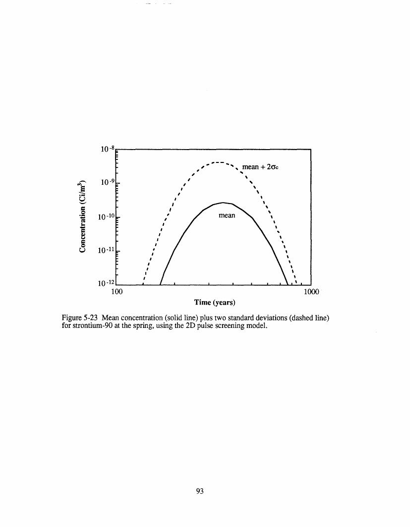
U

.

L

100 1000

Time (years)

Figure 5-23 Mean concentration (solid line) plus two standard deviations (dashed line)for strontium-90 at the spring, using the 2D pulse screening model.

93

94

Chapter 6Conclusions and Recommendations

6.1 Conclusions

This thesis demonstrates the application of stochastic parameter estimation to a

hypothetical LLW site. Drawing upon commonly available site data sources, stochastic

theory is used to systematically derive input parameters for a traditional flow and

transport numerical model. A unique feature of this paper is that it uses standard data

sources and a commercially-available numerical model, but it defines a new methodology

of parameter derivation based on stochastic principles. The step-by-step application of

this methodology in the preceding chapters confirms the viability of this approach to

modeling LLW sites.

The results of the stochastic parameterization process are mean or effective

hydraulic parameters that are sensitive to site variables. The effective parameters are

used in numerical and analytical algorithms to determine mean concentration predictions.

Sensitivities to effective input parameters and to model configurations contribute to

uncertainty in the mean predictions. Additionally, since the effective concentration

predictions represent a mean solution, fluctuations about this mean are another source of

uncertainty. These uncertainties are also present in traditional parameter estimation

methods, where they are often unnoticed and incalculable. The effect of the uncertainty

in the concentration predictions is that they represent a band of estimates over a range of

at least an order of magnitude. Any conclusions drawn from the predictions must take

into consideration their approximate nature.

An outcome of the stochastic parameter estimation process is the use of species-

dependent enhanced longitudinal macrodispersivities in the numerical and analytical

95

models. It is common practice in traditional models to use the same macrodispersivity

for all species. The analysis in this paper shows the importance of varying

macrodispersivity by contaminant species on the basis of sorption heterogeneity and

correlation with hydraulic conductivity. An enhancement of macrodispersivity is shown

to have enormous effects on the expected concentration predictions for both numerical

and analytical models. This is seen as particularly important for isotopes that have a

short half-life relative to their retarded mean travel time.

Concentration and peak time predictions of one-dimensional (ID) and two-

dimensional (2D) analytical models are compared to the numerical model results and are

found to give reasonable peak estimates. However, the overall shapes of the analytical

breakthrough curves tend to underestimate numerical concentration results, especially for

early times. On the basis of these findings, it is concluded that while they are useful for

screening the input isotopes, the ID and 2D analytical uniform flow models can not

adequately treat the complicated flow system as represented by the 2D cross-section in

the numerical model.

6.2 Recommendations

Because the magnitude of the macrodispersivity enhancement has significant

effects on concentration output, it is important to be able to make accurate estimates of

this input parameter. Macrodispersivity enhancement, as a function of sorption

variability and correlation with hydraulic conductivity, needs to be quantified for each

contaminant species. It is therefore important to emphasize the recommendation that, in

the data collection process, measurements of the sorption distribution coefficient (Kd) for

each species should be made on the same soil samples as are measurements of hydraulic

conductivity (K). From these measurements, a direct correlation of K and Kd may be

derived for each species. Because it is not yet common practice to perform stochastic

parameter estimation, this correlation is normally not developed explicitly. As this

96

approach becomes more widely used, the necessity of measuring K and Kd correlation

will be recognized.

An analysis of unsaturated zone flow and transport was not included in this paper.

The effect of excluding the unsaturated zone at humid sites is a subject for future

analysis. Additionally, it is recommended that this modeling approach be applied to arid

sites, with the inclusion of unsaturated zone stochastic theory for the estimation of

unsaturated parameters. As explored for the saturated zone in this research, analytical

and numerical model predictions and sensitivities could be compared for the unsaturated

zone.

Based on the findings of substantial differences between the D analytical and 2D

numerical solutions, it may be worthwhile to evaluate a 3D model in a future project.

Similarly, other 2D model configurations could be explored. A 2D model with a larger

spatial extent, or one that incorporates temporal or spatial variations in the contamination

source are important options for future consideration.

The uncertainties in the analytical and numerical model results are investigated to

an extent in this paper, but a more comprehensive evaluation of the different aspects

needs to be made. This analysis would include a development of the stochastic theory of

concentration variance around the mean concentration solution for solutes with spatially-

variable sorption. Additionally, in applying these modeling techniques to an actual site,

the concentration predictions would be validated through a comparison with field

concentration measurements. This point further emphasizes the need for better

cooperation between the groundwater modeling goals and the plans for measuring field

data at the site. Even if it is not achieved to a full extent, any improvement in this

cooperation will greatly increase the effectiveness of the stochastic parameter estimation

process.

97

98

References

Cahill, J.M., Hydrology of the low-level radioactive solid-waste burial site and vicinitynear Barnwell, South Carolina, U.S. Geological Survey Open File Report 82-863, 1982.

Campbell, A. C., Geochemistry of soils and waters at LLW disposal site, U.S. NuclearRegulatory Commission Staff Report, 1992.

Dennehy, K.F. and P.B. McMahon, Water movement in the unsaturated zone at a low-level radioactive waste burial site near Barnwell, South Carolina, U.S. GeologicalSurvey Open File Report 87-46, 1987.

Garabedian, S.P., L.W. Gelhar, and M.A. Celia, Large-scale dispersive transport inaquifers:field experiments and reactive transport theory, R.M. Parsons Lab Tech. ReportNo. 315, Massachusetts Institute of Technology, Cambridge, MA, 1988.

Gelhar, L.W. and C.L. Axness, Three-dimensional stochastic analysis of macrodispersionin Aquifers, Water Resources Research, 19(1), 161-180, 1983.

Gelhar, L.W., C. Welty, and K.R. Rehfeldt, a critical review of data on field-scaledispersion in aquifers, Water Resources Research, 28(7), 1955-1974, 1992.

Gelhar, L.W., Stochastic Subsurface Hydrology, Prentice Hall, New York, 1993.

Gelhar, L.W., Stochastic subsurface hydrology from theory to applications, WaterResources Research, 22(9), 135s-145s, 1986.

Goode, D.J., Nonradiological groundwater quality at low-level radioactive wastedisposal sites, Technical Report No. NUREG-1 183, U.S. Nuclear RegulatoryCommission, 1986.

Hoeffner, S.L., Radioactive sorption on Savannah River Plant burial ground soil - Asummary and interpretation of laboratory data, DP-1702, E.I. du Pont de Nemours &Co., Savannah River Laboratory, Aiken, SC, 1985.

Kapoor, V., Macrodispersion and concentration fluctuations in three-dimensionallyheterogeneous aquifers, ScD dissertation, Massachusetts Institute of Technology,Cambridge, MA, 1993.

Mantoglou, A. and L.W. Gelhar, Effective hydraulic conductivities of transientunsaturated flow in stratified soils, Water Resources Research, 23(1), 57-67, 1987a.

Mantoglou, A. and L.W. Gelhar, Stochastic modeling of large-scale transient unsaturatedflow systems, Water Resources Research, 23(1), 37-46, 1987b.

Phillips, K.J., and L.W. Gelhar, Contaminant transport to deep wells, Journal of theHydraulics Division, ASCE, 104(HY6), 807-819, 1978.

99

Pietrzak, R.F. and R. Dayal, Evaluation of isotope migration-land burial. Waterchemistry at commercially operated low-level radioactive waste disposal sites. QuarterlyProgress Report. October-December 1981, Report No. NUREG/CR-2192, I1(3-4),Brookhaven Nat'l Lab, 1982.

Polmann, D. J., D. McLaughlin, S. Luis, L.W. Gelhar, and R. Ababou, Stochasticmodeling of large-scale flow in heterogeneous unsaturated soils, Water ResourcesResearch, 27(7), 1447-1458, 1991.

Polmann, D.J., Application of stochastic methods to transientflow and transport inheterogeneous unsaturated soils, PhD dissertation, Massachusetts Institute ofTechnology, Cambridge, MA, 1990.

Polmann, D.J., E.G. Vomvoris, D. McLaughlin, E.M. Hammick, and L.W. Gelhar,Application of stochastic methods to the simulation of large-scale unsaturated flow andtransport, Report No. NUREG/CR-5094, U.S. Nuclear Regulatory Commission, 1988.

Rehfeldt, K.R., and L.W. Gelhar, Stochastic analysis of dispersion in unsteady flow inheterogeneous aquifers, Water Resources Research, 28(8), 2085-2099, 1992.

Vomvoris, E.G., and L.W. Gelhar, Stochastic analysis of the concentration variability in athree-dimensional, heterogeneous aquifer, Water Resources Research, 26(10), 2591-2602, 1990.

Voss, C.I., A finite-element simulation modelfor saturated-unsaturated, fluid-density-dependent groundwater flow with energy transport or chemically-reactive single-speciessolute transport, U.S. Geological Survey Water Resources Investigations Report84-4369, 1984.

Yeh, T.-C., L.W. Gelhar, and A.L. Gutjahr, Stochastic analysis of unsaturated flow inheterogeneous soils, 1., Statistically isotropic media, Water Resources Research, 21(4),447-456, 1985.

100

Appendix AOne-Dimensional Step Input Solution

The following is a derivation of the D step input solution as used in Subsection

4.1.1. It is analagous to a 1D column experiment with a steady-state concentration

release at the top of the column.

The D form of the advection-dispersion equation with decay and retardation is

given by:

dC aC a2CR + v -- A v- + RCk = 0 (A.1)at ax ax2

where x is the horizontal distance, k is the decay coefficient, R is the retardation factor,

C is the steady-state concentration, v is the fluid velocity, and AI, is the longitudinal

macrodispersivity. Let v - vlR, and assuming steady state, dCl/t = O. Then:

.a -All + 0~ = (A.2)A d2C Ck

Multiplying through by (/k, and letting = (xk)/v and a = dx(k/v) gives:

dC_ kAI C + C = 0 (A.3)d Ox d 2

if B is defined as B = (kA 1)/N, then Equation A.3 may be written as:

d2C dC-Ba + i +C= O (A.4)d 2 dx

Equation A.4 is a second-order homogeneous differential equation. Substituting

C = exp(m x) gives the characteristic form of the equation to be:

101

-Bm2 + m + 1 = 0 (A.5)

where m is a root of Equation A.5, and C = exp(m i) is a solution of Equation A.3.

Solving the quadratic in Equation A.5 for m, and satisfying the initial conditions, at x = 0,

C(x) = Co, the solution is given by:

C(x) = C exp(+mx) (A.6)

where Co is the initial source concentration. Substituting back in for m and for x, and

rearranging:

CLCo ( F2AI xT (A.7)

Let

-1+ d1 + 4B = (A.8)2AnI

then

C(x) = C e- 'x (A.9)

which corresponds to Equation 4.2. C(x) is the steady-state concentration.

The 1D step input solution is applicable to those isotopes that have a relatively

low solubility in comparison to their site inventory. H-3 and U-238 are evaluated using

this method in Subsection 4.1.1.

102

Appendix BTwo-Dimensional Pulse Input Solution

The following is a derivation of the 2D pulse input solution as used in

Subsection 4.1.2.

The 2D form of the advection-dispersion equation with uniform horizontal

velocity, first-order decay, and retardation is:

CC dC d2C . 2CR-+ V - A33 + RCk = (B.1)dt dr dX2 V z2

where x is the horizontal direction, z is the vertical distance as measured from the center

of the plume, t is the time after the pulse is released, k is the decay coefficient, R is the

retardation factor, C is the steady-state concentration, v is the fluid velocity, A33 is the

vertical transverse macrodispersivity, and All is the longitudinal macrodispersivity. Let

v - v / R, then:

1 dC C d2C C Ck1 a+ _AllaC_ 3 z + A33 = O(B.2)d 0t + x2Az2 +

Equation B.2 is a second-order homogeneous partial differential equation that may be

solved for C(x, z, t). For a pulse input of mass, M, over a width, w, in the unidirectional

velocity field, the solution is given by:

M exp -[(Xt + 4A 3 t + kt]C(x,z,t) =n w 4 vt A 11A33 (B.3)

where n is the porosity. The maximum value of C at a particular downstream distance x

for any time will be at the center of the plume, where z = 0. Letting / = Rnw4n v the

103

maximum value of C is given by:

C(x,t) = [ L1X J tM exp + ktpt(X' fA74 t) ~(B.4)

At any location x, the maximum value of C(x,t) will occur at some peak time, t.

Me -k (XVt)C.(x) = max, M' [exp 4CtA(x t) (B.5)t fiA I pA33 4P'tAj

Equation B.5 corresponds to Equation 4.7 in Subsection 4.1.2.

The peak time, t, is found by taking the natural logarithm of Equation B.5, by

differentiating it with respect to time, and by setting it equal to zero. Let t = (t) / x,

N = (kx) / , and P = (4A ) / x. Taking the natural logarithm of Equation B.5:

In(C.) = In / J -M In - N t- () (B.6)

Differentiating with respect to t:

1 2(1-f) (l-_i)2o= - - N+ (- + p (B.7)t Pt P?2

multiplying through by pt 2 gives:

0 = - Pi - NP?2 + 2 i(1-?) + (1-t)2 (B.8)

Expanding and collecting like terms gives a quadratic

= 2(1+ NP) + t(P)- 1 (B.9)

The expression in Equation B.9 may be solved using the quadratic formula. Solving and

rearranging gives:

104

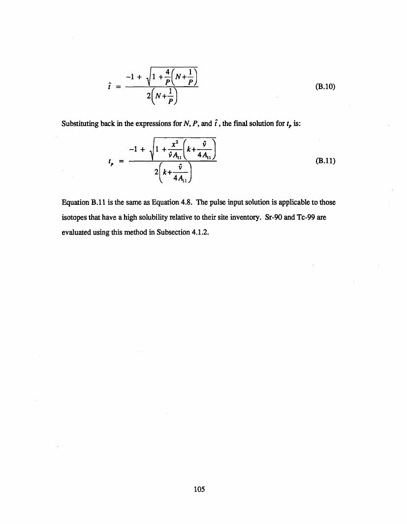
-1+ 1 +4 N+I)- 11 (B.10)2 N+ p1

Substituting back in the expressions for N, P, and t, the final solution for t is:

-1 + 1 (

= (B.11)2 k+4A

4AI 1

Equation B.11 is the same as Equation 4.8. The pulse input solution is applicable to those

isotopes that have a high solubility relative to their site inventory. Sr-90 and Tc-99 are

evaluated using this method in Subsection 4.1.2.

105

106

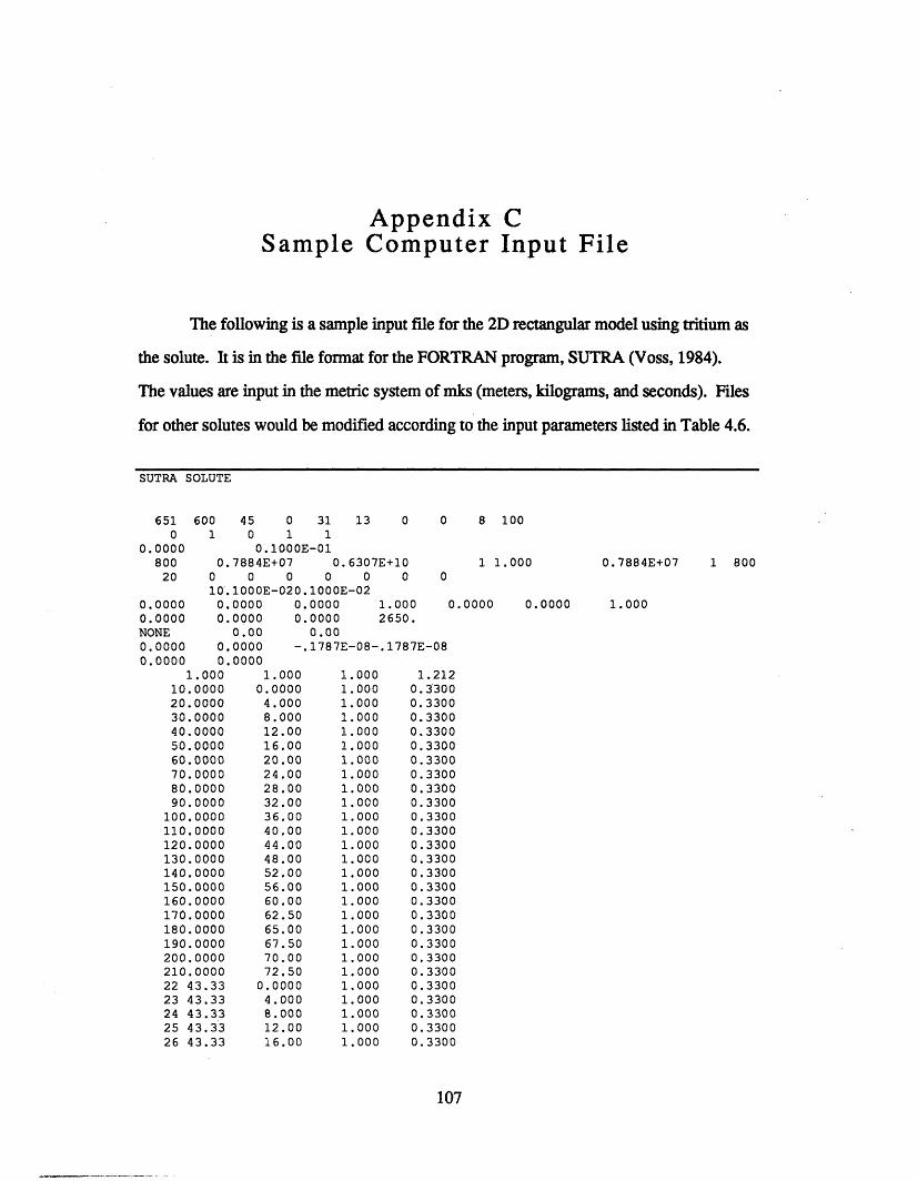
Appendix CSample Computer Input File

The following is a sample input file for the 2D rectangular model using tritium as

the solute. It is in the file format for the FORTRAN program, SUTRA (Voss, 1984).

The values are input in the metric system of mks (meters, kilograms, and seconds). Files

for other solutes would be modified according to the input parameters listed in Table 4.6.

SUTRA SOLUTE

6510

0.0000800

20

0.00000.0000NONE0.0000

6000 45 0 31 13 0 01 0 1 1

0.1000E-010.7884E+07 0.6307E+10

0 0 0 0 0 O 010.1000E-020.1000E-020.0000 0.0000 1.0000.0000 0.0000 2650.

0.00 0.000.0000 -.1787E-08-.1787E-08

0.0000 0.00001.000 1.000

10.0000 0.000020.0000 4.00030.0000 8.00040.0000 12.0050.0000 16.0060.0000 20.0070.0000 24.0080.0000 28.0090.0000 32.00

100.0000 36.00110.0000 40.00120.0000 44.00130.0000 48.00140.0000 52.00150.0000 56.00160.0000 60.00170.0000 62.50180.0000 65.00190.0000 67.50200.0000 70.00210.0000 72.5022 43.33 0.000023 43.33 4.00024 43.33 8.00025 43.33 12.0026 43.33 16.00

1.0001.0001.0001.0001.0001.0001.0001.0001.0001.0001.0001.0001.0001.0001.0001.0001.0001.0001.0001.0001.0001.0001.0001.0001.0001.0001.000

8 100

1 1.000

0.0000 0.0000

1.2120.33000.33000.33000.33000.33000. 33000.33000.33000.33000. 33000. 33000.33000.33000.33000. 33000.33000. 33000.33000.33000. 33000.33000.33000.33000. 33000.33000. 3300

107

0.7884E+07 1 800

1.000

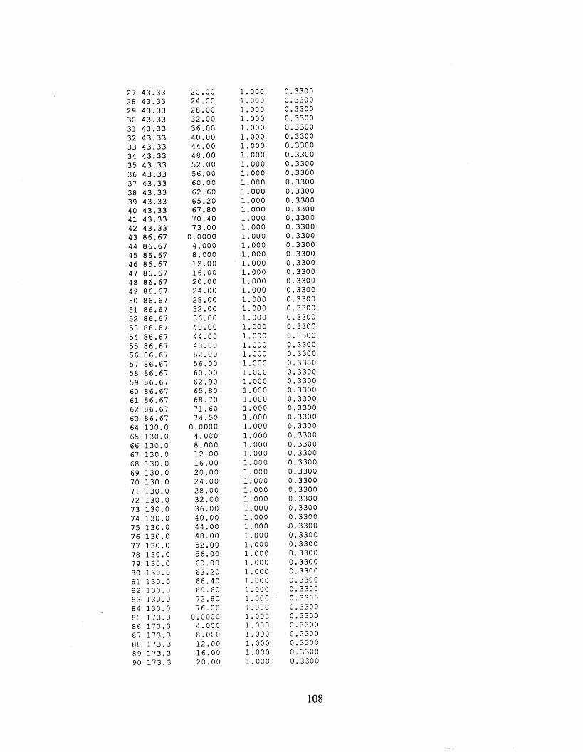
27 43.33 20.00 1.000 0.330028 43.33 24.00 1.000 0.330029 43.33 28.00 1.000 0.330030 43.33 32.00 1.000 0.330031 43.33 36.00 1.000 0.330032 43.33 40.00 1.000 0.330033 43.33 44.00 1.000 0.330034 43.33 48.00 1.000 0.330035 43.33 52.00 1.000 0.330036 43.33 56.00 1.000 0.330037 43.33 60.00 1.000 0.330038 43.33 62.60 1.000 0.330039 43.33 65.20 1.000 0.330040 43.33 67.80 1.000 0.330041 43.33 70.40 1.000 0.330042 43.33 73.00 1.000 0.330043 86.67 0.0000 1.000 0.330044 86.67 4.000 1.000 0.330045 86.67 8.000 1.000 0.330046 86.67 12.00 1.000 0.330047 86.67 16.00 1.000 0.330048 86.67 20.00 1.000 0.330049 86.67 24.00 1.000 0.330050 86.67 28.00 1.000 0.330051 86.67 32.00 1.000 0.330052 86.67 36.00 1.000 0.330053 86.67 40.00 1.000 0.330054 86.67 44.00 1.000 0.330055 86.67 48.00 1.000 0.330056 86.67 52.00 1.000 0.330057 86.67 56.00 1.000 0.330058 86.67 60.00 1.000 0.330059 86.67 62.90 1.000 0.330060 86.67 65.80 1.000 0.330061 86.67 68.70 1.000 0.330062 86.67 71.60 1.000 0.330063 86.67 74.50 1.000 0.330064 130.0 0.0000 1.000 0.330065 130.0 4.000 1.000 0.330066 130.0 8.000 1.000 0.330067 130.0 12.00 1.000 0.330068 130.0 16.00 1.000 0.330069 130.0 20.00 1.000 0.330070 130.0 24.00 1.000 0.330071 130.0 28.00 1.000 0.330072 130.0 32.00 1.000 0.330073 130.0 36.00 1.000 0.330074 130.0 40.00 1.000 0.330075 130.0 44.00 1.000 0.330076 130.0 48.00 1.000 0.330077 130.0 52.00 1.000 0.330078 130.0 56.00 1.000 0.330079 130.0 60.00 1.000 0.330080 130.0 63.20 1.000 0.330081 130.0 66.40 1.000 0.330082 130.0 69.60 1.000 0.330083 130.0 72.80 1.000 0.330084 130.0 76.00 1.000 0.330085 173.3 0.0000 1.000 0.330086 173.3 4.000 1.000 0.330087 173.3 8.000 1.000 0.330088 173.3 12.00 1.000 0.330089 173.3 16.00 1.000 0.330090 173.3 20.00 1.000 0.3300

108

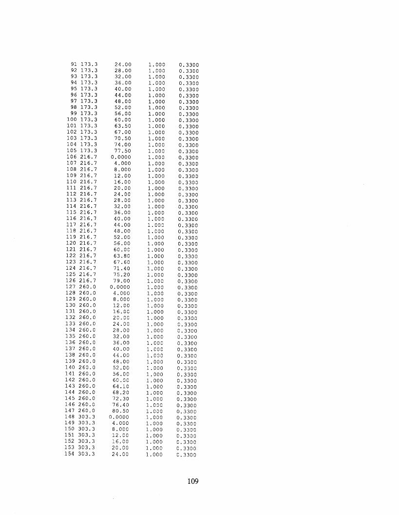
91 173.392 173.393 173.394 173.395 173.396 173.397 173.398 173.399 173.3

100 173.3101 173.3102 173.3103 173.3104 173.3105 173.3106 216.7107 216.7108 216.7109 216.7110 216.7111 216.7112 216.7113 216.7114 216.7115 216.7116 216.7117 216.7118 216.7119 216.7120 216.7121 216.7122 216.7123 216.7124 216.7125 216.7126 216.7127 260.0128 260.0129 260.0130 260.0131 260.0132 260.0133 260.0134 260.0135 260.0136 260.0137 260.0138 260.0139 260.0140 260.0141 260.0142 260.0143 260.0144 260.0145 260.0146 260.0147 260.0148 303.3149 303.3150 303.3151 303.3152 303.3153 303.3154 303.3

24.0028.0032.0036.0040.0044.0048.0052.0056.0060.0063.5067.0070.5074.0077.50

0. 00004.0008.00012.0016.0020.0024.0028.0032.0036.0040.0044.0048.0052.0056.0060.0063.8067.6071.4075.2079.00

0.00004.0008.00012.0016.0020.0024.0028.0032.0036.0040.0044.0048.0052 .0056.0060.0064.1068.2072.3076.4080.50

0.00004.0008.00012.0016.0020.0024.00

1.0001.0001.0001.0001.0001.0001.0001.0001.0001. 0001.0001.0001.0001.0001.0001.0001.0001.0001.0001.0001.0001.0001.0001.0001.0001.0001.0001.0001.0001. 0001.0001.0001.0001. 0001.0001.0001.0001.0001.0001.0001.0001.0001.0001.0001.0001.0001.0001.0001. 0001.0001.0001. 0001. 0001.0001. 0001.0001. 0001.0001.0001.0001 .0001. 0001.0001.000

0.33000.33000.33000.33000.33000.33000.33000. 33000.33000.33000. 33000.33000.33000. 33000.33000.33000. 33000.33000.33000.33000. 33000. 33000.33000. 33000.33000.33000.33000.33000. 33000. 33000.33000.33000. 33000.33000.33000. 33000.33000. 33000. 33000.33000. 33000.33000.33000. 33000.33000. 33000. 33000.33000. 33000.33000.33000.33000.33000.33000.33000.33000.33000.33000. 33000.33000.33000.33000.33000.3300

109

155 303.3 28.00 1.000 0.3300156 303.3 32.00 1.000 0.3300157 303.3 36.00 1.000 0.3300158 303.3 40.00 1.000 0.3300159 303.3 44.00 1.000 0.3300160 303.3 48.00 1.000 0.3300161 303.3 52.00 1.000 0.3300162 303.3 56.00 1.000 0.3300163 303.3 60.00 1.000 0.3300164 303.3 64.30 1.000 0.3300165 303.3 68.60 1.000 0.3300166 303.3 72.90 1.000 0.3300167 303.3 77.20 1.000 0.3300168 303.3 81.50 1.000 0.3300169 346.7 0.0000 1.000 0.3300170 346.7 4.000 1.000 0.3300171 346.7 8.000 1.000 0.3300172 346.7 12.00 1.000 0.3300173 346.7 16.00 1.000 0.3300174 346.7 20.00 1.000 0.3300175 346.7 24.00 1.000 0.3300176 346.7 28.00 1.000 0.3300177 346.7 32.00 1.000 0.3300178 346.7 36.00 1.000 0.3300179 346.7 40.00 1.000 0.3300180 346.7 44.00 1.000 0.3300181 346.7 48.00 1.000 0.3300182 346.7 52.00 1.000 0.3300183 346.7 56.00 1.000 0.3300184 346.7 60.00 1.000 0.3300185 346.7 64.50 1.000 0.3300186 346.7 69.00 1.000 0.3300187 346.7 73.50 1.000 0.3300188 346.7 78.00 1.000 0.3300189 346.7 82.50 1.000 0.3300190 390.0 0.0000 1.000 0.3300191 390.0 4.000 1.000 0.3300192 390.0 8.000 1.000 0.3300193 390.0 12.00 1.000 0.3300194 390.0 16.00 1.000 0.3300195 390.0 20.00 1.000 0.3300196 390.0 24.00 1.000 0.3300197 390.0 28.00 1.000 0.3300198 390.0 32.00 1.000 0.3300199 390.0 36.00 1.000 0.3300200 390.0 40.00 1.000 0.3300201 390.0 44.00 1.000 0.3300202 390.0 48.00 1.000 0.3300203 390.0 52.00 1.000 0.3300204 390.0 56.00 1.000 0.3300205 390.0 60.00 1.000 0.3300206 390.0 64.60 1.000 0.3300207 390.0 69.20 1.000 0.3300208 390.0 73.70 1.000 0.3300209 390.0 78.30 1.000 0.3300210 390.0 82.90 1.000 0.3300211 433.3 0.0000 1.000 0.3300212 433.3 4.000 1.000 0.3300213 433.3 8.000 1.000 0.3300214 433.3 12.00 1.000 0.3300215 433.3 16.00 1.000 0.3300216 433.3 20.00 1.000 0.3300217 433.3 24.00 1.000 0.3300218 433.3 28.00 1.000 0.3300

110

219220221222223224225226227228229230231232233234235236237238239240241242243244245246247248249250251252253254255256257258259260261262263264265266267268269270271272273274275276277278279280281282

433.3433.3433.3433.3433.3433.3433.3433.3433.3433.3433.3433.3433.3476.7476.7476.7476.7476.7476.7476.7476.7476.7476.7476.7476.7476.7476.7476.7476.7476.7476.7476.7476.7476.7520.0520.0520.0520.0520.0520.0520.0520.0520.0520.0520.0520.0520.0520.0520.0520.0520.0520.0520.0520.0520. 0563.3563.3563.3563.3563.3563.3563.3563.3563.3

32.0036.0040.0044.0048.0052.0056.0060.0064.7069.3074.0078.6083.30

0.00004.0008.00012.0016.0020.0024.0028.0032.0036.0040.0044.0048.0052.0056.0060.0064.7069.5074.2079.0083.70

0 .00004.0008.00012.0016.0020.0024.0028.0032.0036.0040.0044.0048.0052 .0056.0060.0064.8069.6074.5079.3084.10

0.00004.0008.00012.0016.0020.0024.0028.0032.00

1.0001.0001.0001.0001. 0001.0001.0001.0001.0001.0001.0001.0001.0001.0001.0001.0001.0001.0001.0001.0001.0001.0001.0001.0001.0001.0001.0001. 0001.0001.0001.0001.0001.0001.0001.0001.0001.0001.0001.0001. 0001.0001.0001.0001.0001. 0001.0001.0001.0001.0001.0001.0001.0001.0001.0001.0001. 0001.0001.0001. 0001.0001. 0001.0001.0001.000

0.33000.33000.33000.33000.33000.33000.33000.33000.33000.33000. 33000.33000.33000.33000.33000.33000.33000.33000.33000.33000. 33000.33000.33000.33000.33000.33000.33000.33000.33000. 33000. 33000.33000. 33000.33000.33000.33000.33000.33000.33000. 33000. 33000. 33000. 33000.33000.33000.33000. 33000.33000. 33000.33000.33000.33000.33000.33000.33000.33000. 33000.33000. 33000. 33000. 33000.33000. 33000.3300

111

283 563.3284 563.3285 563.3286 563.3287 563.3288 563.3289 563.3290 563.3291 563.3292 563.3293 563.3294 563.3295 606.7296 606.7297 606.7298 606.7299 606.7300 606.7301 606.7302 606.7303 606.7304 606.7305 606.7306 606.7307 606.7308 606.7309 606.7310 606.7311 606.7312 606.7313 606.7314 606.7315 606.7316 650.0317 650.0318 650.0319 650.0320 650.0321 650.0322 650.0323 650.0324 650.0325 650.0326 650.0327 650.0328 650.0329 650.0330 650.0331 650.0332 650.0333 650.0334 650.0335 650.0336 650.0337 693.3338 693.3339 693.3340 693.3341 693.3342 693.3343 693.3344 693.3345 693.3346 693.3

36.0040.0044.0048.0052.0056.0060.0064.9069.8074.6079.5084.40

0.00004.0008.00012.0016.0020.0024.0028.0032.0036.0040.0044.0048.0052.0056.0060.0064.9069.9074.8079.8084.70

0.00004.0008.00012.0016.0020.0024.0028.0032.0036.0040.0044.0048.0052.0056.0060.0065.0070.0075.0080.0085.00

0 .000004.0008.00012.0016.0020.0024.0028.0032.0036.00

1.0001.0001.0001.0001.0001.0001.0001.0001.0001.0001.0001.0001.0001.0001.0001.0001.0001.0001.0001.0001.0001.0001.0001.0001.0001.0001.0001.0001.0001.0001.0001.0001.0001.0001.0001.0001 .0001.0001 .0001 .0001 .0001.0001 .0001.0001 .0001.0001.0001.0001.0001. 0001. 0001 .0001.0001 .0001.0001.0001 .0001 .0001. 0001.0001. 0001 .0001 .0001.000

0. 33000.33000.33000. 33000. 33000.33000.33000.33000. 33000.33000.33000.33000.33000. 33000.33000.33000. 33000.33000.33000.33000. 33000. 33000. 33000.33000.33000.33000.33000.33000.33000.33000.33000.33000.33000.33000.33000.33000.33000.33000. 33000.33000.33000. 33000.33000.33000. 33000. 33000. 33000. 33000.33000.33000.33000. 33000.33000.33000.33000.33000.33000. 33000. 33000. 33000. 33000. 33000.33000.3300

112

347 693.3348 693.3349 693.3350 693.3351 693.3352 693.3353 693.3354 693.3355 693.3356 693.3357 693.3358 736.7359 736.7360 736.7361 736.7362 736.7363 736.7364 736.7365 736.7366 736.7367 736.7368 736.7369 736.7370 736.7371 736.7372 736.7373 736.7374 736.7375 736.7376 736.7377 736.7378 736.7379 780.0380 780.0381 780.0382 780.0383 780.0384 780.0385 780.0386 780.0387 780.0388 780.0389 780.0390 780.0391 780.0392 780.0393 780.0394 780.0395 780.0396 780.0397 780.0398 780.0399 780.0400 823.3401 823.3402 823.3403 823.3404 823.3405 823.3406 823.3407 823.3408 823.3409 823.3410 823.3

40.0044.0048.0052.0056.0060.0065.0070.1075.1080.2085.20

0.00004.0008.00012.0016.0020.0024.0028.0032 .0036.0040.0044.0048.0052.0056.0060.0065.1070.2075.2080.3085.40

0.00004.0008.00012.0016.0020.0024.0028.0032.0036.0040.0044.0048.0052.0056.0060.0065.1070.2075.4080.5085.60

0.00004.0008.00012.0016.0020.0024.0028.0032.0036.0040.00

1.0001.0001.0001.0001. 0001.0001.0001.0001.0001.0001.0001.0001.0001.0001. 0001.0001.0001.0001.0001.0001.0001.0001. 0001.0001. 0001.0001.0001.0001.0001.0001.0001.0001.0001.0001.0001.0001.0001.0001.0001.0001.0001.0001.0001.0001. 0001.0001.0001.0001. 0001.0001. 0001.0001. 0001.0001. 0001.0001 0001 .0001 .0001.0001.0001.0001. 0001. 000

0.33000. 33000.33000.33000.33000. 33000.33000.33000.33000.33000. 33000.33000.33000.33000.33000.33000.33000.33000. 33000. 33000. 33000.33000.33000. 33000.33000. 33000.33000.33000.33000.33000. 33000.33000.33000.33000.33000.33000.33000.33000. 33000.33000. 33000.33000. 33000.33000.33000. 33000.33000.33000. 33000.33000.33000. 33000. 33000. 33000. 33000.33000.33000.33000.33000.33000.33000.33000.33000. 3300

113

411 823.3412 823.3413 823.3414 823.3415 823.3416 823.3417 823.3418 823.3419 823.3420 823.3421 866.7422 866.7423 866.7424 866.7425 866.7426 866.7427 866.7428 866.7429 866.7430 866.7431 866.7432 866.7433 866.7434 866.7435 866.7436 866.7437 866.7438 866.7439 866.7440 866.7441 866.7442 910.0443 910.0444 910.0445 910.0446 910.0447 910.0448 910.0449 910.0450 910.0451 910.0452 910.0453 910.0454 910.0455 910.0456 910.0457 910.0458 910.0459 910.0460 910.0461 910.0462 910.0463 953.3464 953.3465 953.3466 953.3467 953.3468 953.3469 953.3470 953.3471 953.3472 953.3473 953.3474 953.3

44.0048.0052.0056.0060.0065.2070.3075.5080.6085.80

0.00004.0008.00012.0016.0020.0024.0028.0032.0036.0040.0044.0048.0052.0056.0060.0065.2070.4075.6080.8086.00

0.00004.0008.00012.0016.0020.0024.0028.0032.0036.0040.0044.0048.0052.0056.0060.0065.2070.5075.7081.0086.20

0.00004.0008.00012.0016.0020.0024.0028.0032.0036.0040.0044.00

1.0001.0001.0001.0001.0001.0001.0001.0001.0001.0001.0001.0001.0001.0001.0001.0001.0001.0001.0001.0001.0001.0001.0001.0001.0001.0001.0001.0001.0001.0001.0001.0001.0001.0001.0001.0001.0001.0001.0001.0001.0001.0001.0001.0001.0001.0001.0001.0001.0001.0001.0001.0001.0001.0001.0001.0001.0001.0001.0001.0001.0001.0001. 0001.000

0.33000. 33000.33000. 33000.33000.33000.33000. 33000.33000.33000.33000.33000.33000.33000.33000.33000.33000.33000.33000.33000. 33000.33000.33000. 33000.33000.33000.33000. 33000.33000. 33000. 33000.33000.33000.33000.33000.33000.33000.33000.33000.33000.33000.33000.33000. 33000.33000.33000.33000.3300-0.33000.33000. 33000. 33000.33000. 33000. 33000.33000. 33000. 33000.33000. 33000.33000. 33000. 33000.3300

114

475 953.3476 953.3477 953.3478 953.3479 953.3480 953.3481 953.3482 953.3483 953.3484 996.7485 996.7486 996.7487 996.7488 996.7489 996.7490 996.7491 996.7492 996.7493 996.7494 996.7495 996.7496 996.7497 996.7498 996.7499 996.7500 996.7501 996.7502 996.7503 996.7504 996.7505 1040.506 1040.507 1040.508 1 040.509 1040.510 1040.511 1040.512 1040.513 1040.514 1040.515 1040.516 1.040.517 1040.518 1040.519 1040.520 1040.521 1040.522 1040.523 1040.524 1040.525 1040.526 1083.527 1083.528 1083.529 1083.530 1083.531 1083.532 1083.533 1083.534 1083.535 1083.536 1083.537 1083.538 1083.

48.0052.0056.0060.0065.3070.6075.8081.1086.40

0.00004.0008.00012.0016.0020.0024.0028.0032.0036.0040.0044.0048.0052.0056.0060.0065.3070.6076.0081.3086.60

0. 00004.0008.00012.0016.0020.0024.0028.0032.0036.0040.0044.0048.0052.0056.0060.0065.4070.7076.1081.4086.80

0.00004.0008.00012.0016.0020.0024.0028.0032.0036.0040.0044.0048.00

1.0001.0001.0001.0001. 0001.0001.0001.0001.0001.0001.0001.0001.0001.0001.0001.0001.0001.0001.0001.0001.0001. 0001.0001.0001.0001. 0001.0001.0001.0001. 0001.0001.0001.0001.0001.0001.0001.0001. 0001. 0001.0001.0001.0001.0001.0001.0001.0001.0001.0001.0001.0001.0001.0001.0001.0001.0001.0001.0001.0001. 0001 0001.0001.0001.0001. 000

0.33000. 33000.33000.33000.33000. 33000.33000.33000. 33000.33000. 33000.33000.33000. 33000.33000.33000.33000.33000. 33000.33000.33000.33000.33000. 33000.33000. 33000.33000. 33000.33000.33000. 33000.33000. 33000. 33000.33000. 33000. 33000.33000.33000. 33000. 33000.33000. 33000.33000.33000.33000.33000.33000. 33000.33000.33000. 33000. 33000. 33000. 33000.33000. 33000.33000.33000.33000. 33000. 33000.33000.3300

115

539 1083.540 1083.541 1083.542 1083.543 1083.544 1083.545 1083.546 1083.547 1127.548 1127.549 1127.550 1127.551 1127.552 1127.553 1127.554 1127.555 1127.556 1127.557 1127.558 1127.559 1127.560 1127.561 1127.562 1127.563 1127.564 1127.565 1127.566 1127.567 1127.568 1170.569 1170.570 1170.571 1170.572 1170.573 1170.574 1170.575 1170.576 1170.577 1170.578 1170.579 1170.580 1170.581 1170.582 1170.583 1170.584 1170.585 1170.586 1170.587 1170.588 1170.589 1213.590 1213.591 1213.592 1213.593 1213.594 1213.595 1213.596 1213.597 1213.598 1213.599 1213.600 1213.601 1213.602 1213.

52.0056.0060.0065.4070.8076.2081.6087.00

0.00004.0008.00012.0016.0020.0024.0028.0032.0036.0040.0044.0048.0052.0056.0060.0065.4070.8076.3081.7087.10

0.00004.0008.00012.0016.0020.0024.0028.0032.0036.0040.0044.0048.0052.0056.0060.0065.4070.9076.3081.8087.20

0.00004.0008.00012.0016.0020.0024.0028.0032.0036.0040.0044.0048.0052.00

1.0001.0001.0001.0001.0001.0001.0001.0001.0001.0001.0001.0001.0001.0001.0001.0001.0001.0001.0001.0001.0001.0001.0001.0001.0001.0001.0001.0001.0001.0001.0001.0001.0001.0001.0001.0001.0001.0001.0001.0001.0001.0001.0001.0001.0001.0001.0001.0001.0001.0001.0001.0001.0001.0001.0001.0001.0001.0001.0001.0001.0001.0001.0001.000

0.33000.33000.33000.33000.33000.33000.33000.33000.33000.33000.33000.33000.33000.33000.33000.33000.33000.33000.33000.33000.33000.33000.33000.33000.33000.33000.33000.33000.33000.33000.33000.33000.33000.33000.33000.33000.33000.33000.33000.33000.33000.33000.33000.33000.33000.33000.33000.33000.33000.33000.33000.33000.33000.33000.33000.33000.33000.33000.33000.33000.33000.33000.33000.3300

116

603 1213. 56.00 1.000 0.3300604 1213. 60.00 1.000 0.3300605 1213. 65.50 1.000 0.3300606 1213. 70.90 1.000 0.3300607 1213. 76.40 1.000 0.3300608 1213. 81.80 1.000 0.3300609 1213. 87.30 1.000 0.3300610 1257. 0.0000 1.000 0.3300611 1257. 4.000 1.000 0.3300612 1257. 8.000 1.000 0.3300613 1257. 12.00 1.000 0.3300614 1257. 16.00 1.000 0.3300615 1257. 20.00 1.000 0.3300616 1257. 24.00 1.000 0.3300617 1257. 28.00 1.000 0.3300618 1257. 32.00 1.000 0.3300619 1257. 36.00 1.000 0.3300620 1257. 40.00 1.000 0.3300621 1257. 44.00 1.000 0.3300622 1257. 48.00 1.000 0.3300623 1257. 52.00 1.000 0.3300624 1257. 56.00 1.000 0.3300625 1257. 60.00 1.000 0.3300626 1257. 65.50 1.000 0.3300627 1257. 71.00 1.000 0.3300628 1257. 76.40 1.000 0.3300629 1257. 81.90 1.000 0.3300630 1257. 87.40 1.000 0.3300631 1300. 0.0000 1.000 0.3300632 1300. 4.000 1.000 0.3300633 1300. 8.000 1.000 0.3300634 1300. 12.00 1.000 0.3300635 1300. 16.00 1.000 0.3300636 1300. 20.00 1.000 0.3300637 1300. 24.00 1.000 0.3300638 1300. 28.00 1.000 0.3300639 1300. 32.00 1.000 0.3300640 1300. 36.00 1.000 0.3300641 1300. 40.00 1.000 0.3300642 1300. 44.00 1.000 0.3300643 1300. 48.00 1.000 0.3300644 1300. 52.00 1.000 0.3300645 1300. 56.00 1.000 0.3300646 1300. 60.00 1.000 0.3300647 1300. 65.50 1.000 0.3300648 1300. 71.00 1.000 0.3300649 1300. 76.50 1.000 0.3300650 1300. 82.00 1.000 0.3300651 1300. 87.50 1.000 0.3300

0.1000E-040.1000E-060.0000 25.00 25.00 0.25001 3.000 13.00 0.0000 1.000 1.000 1.0002 3.000 13.00 0.0000 1.000 1.000 1.0003 3.000 13.00 0.0000 1.000 1.000 1.0004 3.000 13.00 0.0000 1.000 1.000 1.0005 3.000 13.00 0.0000 1.000 1.000 1.0006 3.000 13.00 0.0000 1.000 1.000 1.0007 3.000 13.00 0.0000 1.000 1.000 1.0008 3.000 13.00 0.0000 1.000 1.000 1.0009 3.000 13.00 0.0000 1.000 1.000 1.000

10 3.000 13.00 0.0000 1.000 1.000 1.00011 3.000 13.00 0.0000 1.000 1.000 1.00012 3.000 13.00 0.0000 1.000 1.000 1.00013 1.500 4.400 0.0000 1.000 1.000 1.00014 1.500 4.400 0.0000 1.000 1.000 1.000

117

15 1.50016 1.50017 1.50018 1.500190.7500200.750021 3.00022 3.00023 3.00024 3.00025 3.00026 3.00027 3.00028 3.00029 3.00030 3.00031 3.00032 3.00033 1.50034 1.50035 1.50036 1.50037 1.50038 1.500390.7500400.750041 3.00042 3.00043 3.00044 3.00045 3.00046 3.00047 3.00048 3.00049 3.00050. 3.00051 3.00052 3.00053 1.50054 1.50055 1.50056 1.50057 1.50058 1.500590.7500600.750061 3.00062 3.00063 3.00064 3.00065 3.00066 3.00067 3.00068 3.00069 3.00070 3.00071 3.00072 3.00073 1.50074 1.50075 1.50076 1.50077 1.50078 1.500

4.4004.4004.4004.4001.0101.01013.0013.0013.0013.0013.0013.0013.0013.0013.0013.0013.0013.004.4004.4004.4004.4004.4004.4001.0101.01013.0013.0013.0013.0013.0013.0013.0013.0013.0013.0013.0013.004.4004.4004.4004.4004.4004.4001.0101.01013.0013.0013.0013.0013.0013.0013.0013.0013.0013.0013.0013.004 .4004.4004.4004.4004.4004.400

0.00000.00000.00000.00000.00000.00000.00000.00000.00000.00000.00000.00000.00000.00000.00000. 00000.00000.00000.00000.00000.00000.00000.00000.00000.00000.00000. 00000.00000.00000.00000.00000.00000.00000.00000.00000.00000.00000.00000.00000.00000.00000.00000.00000.00000.00000.00000.00000.00000.00000.00000.00000. 00000.00000. 000000.00000.00000. 00000.00000.00000.00000.00000.00000.00000.0000

1.0001.0001.0001.0001.0001.0001.0001.0001.0001.0001.0001.0001.0001.000C1.0001.0001.0001.0001.0001.0001.0001.0001.0001.0001.0001.0001.0001.0001.0001.0001.0001.0001.0001.0001.0001.0001.0001.0001.0001.0001.0001.0001.0001.0001.0001.0001.0001.0001.0001. 0001.0001. 0001 .0001. 0001 .0001. 0001.0001 .0001.0001. 0001. 0001.0001.0001. 000

1.0001.0001.0001.0001.0001.0001.0001.0001.0001.0001.0001.0001.0001.0001.0001.0001.0001.0001.0001.0001.0001.0001.0001.0001.0001.0001.0001.0001.0001.0001.0001.0001.0001.0001.0001.0001.0001.0001.0001.0001.0001.0001.0001.0001.0001.0001.0001.0001.0001 .0001 .0001 .0001 .0001.0001 .0001.0001.0001. 0001.0001.0001.0001.0001.0001.000

1.0001. 0001.0001.0001.0001.0001.0001.0001.0001.0001.0001.0001.0001.0001.0001.0001.0001. 0001.0001.0001.0001.0001.0001.0001.0001.0001.0001.0001.0001.0001.0001.0001.0001.0001.0001.0001.0001. 0001.0001. 0001.0001.0001.0001.0001.0001.0001.0001.0001.0001.0001.0001.0001.0001.0001.0001.0001.0001.0001.0001.0001.0001.0001.0001.000

118

790.7500800.750081 3.00082 3.00083 3.00084 3.00085 3.00086 3.00087 3.00088 3.00089 3.00090 3.00091 3.00092 3.00093 1.50094 1.50095 1.50096 1.50097 1.50098 1.500990.7500

1000.7500101 3.000102 3.000103 3.000104 3.000105 3.000106 3.000107 3.000108 3.000109 3.000110 3.000111 3.000112 3.000113 1.500114 1.500115 1.500116 1.500117 1.500118 1.5001190.75001200.7500121 3.000122 3.000123 3.000124 3.000125 3.000126 3.000127 3.000128 3.000129 3.000130 3.000131 3.000132 3.000133 1.500134 1.500135 1.500136 1.500137 1.500138 1.5001390.75001400.7500141 3.000142 3.000

1.0101.01013.0013.0013.0013.0013.0013.0013.0013.0013.0013.0013.0013.004.4004.4004.4004.4004.4004.4001.0101.01013.0013.0013.0013.0013.0013.0013.0013.0013.0013.0013.0013.004.4004.4004.4004.4004.4004 .4001.0101.01013.0013.0013.0013.0013.0013.0013.0013.0013.0013.0013.0013.004.4004.4004.4004.4004.4004.4001.0101.01013.0013.00

0.00000.00000.00000.00000.00000.00000. 00000.00000.00000.00000. 00000.00000.00000. 00000. 00000.00000. 00000.00000.00000. 00000. 00000.00000.00000.00000.00000. 00000.00000.00000.00000. 00000 .00000. 00000.00000. 00000. 00000 00000 00000 00000 00000. 00000. 00000. 00000 .00000. 00000. 00000 . 00000. 00000 .00000. 00000.00000.00000. 00000. 000

.0 00000.00000 .00000.00000. 00000 .00000. 00000.00000.00000.00000.0000

1.0001.0001.0001. 0001.0001.0001.0001.0001.0001.0001.0001.0001.0001.0001.0001.0001.0001.0001.0001.0001.0001.0001.0001.0001.0001.0001.0001.0001.0001.0001.0001.0001.0001.0001. 0001.0001.0001.0001.0001 .0001.0001.0001.0001.0001.0001.0001.0001 0001.0001 0001. 0001 0001 0001 0001 0001.0001.0001.0001.0001.0001.0001.0001.0001.000

1.0001.0001. 0001.0001. 0001.0001.0001.0001.0001.0001. 0001.0001.0001.0001.0001.0001.0001.0001.0001.0001.0001.0001.0001. 0001.0001.0001.0001.0001.0001.0001.0001.0001.0001.0001.0001.0001.0001.0001.0001.0001 .0001.0001. 0001 .0001.0001 .0001.0001 .0001. 0001 .0001 .0001. 0001 .0001.0001.0001 .0001 .0001. 0001.0001 0001. 0001 0001.0001.000

1.0001.0001. 0001.0001. 0001.0001.0001.0001.0001.0001.0001.0001.0001.0001.0001.0001.0001.0001.0001. 0001.0001.0001. 0001. 0001. 0001.0001.0001.0001.0001.0001.0001.0001.0001. 0001.0001.0001.0001.0001.0001.0001.0001.0001.0001.0001.0001.0001.0001. 0001.0001.0001.0001. 0001. 0001. 0001. 0001 0001. 0001 0001.0001. 0001.0001. 0001.0001 .000

119

143 3.000144 3.000145 3.000146 3.000147 3.000148 3.000149 3.000150 3.000151 3.000152 3.000153 1.500154 1.500155 1.500156 1.500157 1.500158 1.5001590.75001600.7500161 3.000162 3.000163 3.000164 3.000165 3.000166 3.000167 3.000168 3.000169 3.000170 3.000171 3.000172 3.000173 1.500174 1.500175 1.500176 1.500177 1.500178 1.5001790.75001800.7500181 3.000182 3.000183 3.000184 3.000185 3.000186 3.000187 3.000188 3.000189 3.000190 3.000191 3.000192 3.000193 1.500194 1.500195 1.500196 1.500197 1.500198 1.5001990.75002000.7500201 3.000202 3.000203 3.000204 3.000205 3.000206 3.000

13.0013.0013.0013.0013.0013.0013.0013.0013.0013.004 . 4004. 4004.4004 .4004.4004 .4001.0101 . 01013.0013.0013.0013.0013.0013.0013.0013.0013.0013.0013.0013.004 .4004.4004.4004.4004.4004.4001.0101.01013.0013.0013.0013.0013.0013.0013.0013.0013.0013.0013.0013.004.4004.4004.4004.4004.4004.4001.0101.01013.0013.0013.0013.0013.0013.00

0. 00000. 00000. 00000. 00000. 00000. 00000..00000. 00000. 00000. 00000. 00000. 00000. 00000. 00000. 00000. 00000. 00000. 00000. 0000O.00000. 00000. 00000. 00000. 00000.00000. 00000. 00000.00000. 00000. 00000. 00000.00000.00000.00000. 00000. 00000.00000.00000. 00000.00000.00000.00000.00000.00000.00000.00000.00000.00000. 00000. 00000.00000. 00000. 00000. 00000. 00000.00000. 00000.00000.00000.00000. 00000.00000. 00000.0000

1.0001.0001.0001.0001.0001.0001. 0001.0001.0001.0001.0001.0001.0001.0001.0001.0001.0001. 0001.0001.0001.0001. 0001.0001.0001.0001.0001.0001.0001 . 0001 .0001 .0001.0001 .0001. 0001. 0001.0001. 0001 . 0001.0001 .0001.0001.0001.0001 . 0001.0001.0001.0001. 0001.0001.0001 . 0001 . 0001 .0001 . 0001. 0001 .0001 . 0001 .0001 . 0001 . 0001..0001.0001. 0001.000

1.0001.0001.0001.0001 .0001.0001.0001.0001. 0001.0001.0001.0001.0001.0001.0001.0001.0001.0001.0001.0001.0001.0001.0001.0001.0001.0001.0001.0001.0001.0001.0001.0001.0001.0001.0001.0001.0001.0001.0001.0001.0001.0001.0001.0001.0001.0001.0001.0001.0001.0001.0001.0001.0001.0001. 0001.0001.0001.0001.0001.0001.0001.0001.0001.000

1.0001.0001.0001.0001.0001.0001.0001.0001.0001.0001.0001.0001.0001.0001.0001.0001.0001.0001.0001.0001.0001.0001.0001.0001.0001.0001.0001.0001.0001.0001 .0001.0001.0001. 0001.0001.0001.0001.0001.0001 . 0001.0001.0001.0001 . 0001.0001.0001.0001.0001.0001.0001.0001.0001.0001.0001.0001.0001.0001.0001.0001 .0001.0001.0001 . 0001 . 000

120

207 3.000208 3.000209 3.000210 3. 000211 3. 000212 3. 000213 1. 500214 1. 500215 1.500216 1. 500217 1.500218 1. 5002190. 75002200.7500221 3.000222 3.000223 3.000224 3.000225 3.000226 3.000227 3.000228 3.000229 3.000230 3.000231 3. 000232 3.000233 1.500234 1.500235 1.500236 1.500237 1.500238 1.5002390.75002400.7500241 3. 000242 3.000243 3.000244 3.000245 3.000246 3.000247 3.000248 3.000249 3.000250 3.000251 3 000252 3.000253 1.500254 1.500255 1.500256 1.500257 1 500258 1.5002590.75002600.7500261 3.000262 3.000263 3.000264 3.000265 3.000266 3.000267 3.000268 3.000269 3.000270 3.000

13.0013.0013.0013.0013.0013.004.4004 .4004. 4004.4004 .4004.4001.0101.01013.0013.0013.0013.0013.0013.0013.0013.0013.0013.0013.0013.004.4004.4004.4004.4004.4004.4001.0101.01013.0013.0013.0013. 0013. 0013. 0013. 0013. 0013 0013.0013.0013.004.4004.4004.4004.4004.4004.4001.0101.01013.0013.0013.0013.0013.0013.0013.0013.0013.0013.00

0.00000.00000. 00000.00000. 00000. 00000. 00000. 00000.00000. 00000.00000.00000. 00000. 00000. 00000. 00000.00000.00000. 00000.00000. 00000. 00000. 00000. 00000. 00000. 00000.00000.00000.00000. 00000.00000.00000.00000. 00000. 00000.00000.00000.00000.00000.00000.00000. 00000. 00000.00000.00000. 00000.00000. 00000. 00000.00000. 00000. 00000. 00000.00000.00000.00000. 00000. 00000 000

0 00000 0000 000

0. 00000 000

1 .0001 .0001. 0001.0001. 0001 . 0001. 0001 .0001 .0001. 0001.0001 .0001. 0001 .0001 .0001. 0001 .0001.0001. 0001. 0001 . 0001. 0001.0001 .0001 .0001. 0001.0001.0001 .0001.0001.0001.0001 0001 0001 0001 0001 0001 0001 0001.0001 0001 0001 0001 0001 0001 0001 0001 0001 0001 .0001 .0001.0001. 0001. 0001 0001 0001 0001 0001 000I 0001 0001 000i 0001 . 000

1. 0001.0001. 0001 .0001.0001.0001. 0001.0001 .0001 .0001 .0001 .0001. 0001.0001.0001.0001 .0001. 0001. 0001.0001 .0001 .0001 .0001. 0001. 0001. 0001.0001 .0001.0001.0001.0001. 0001.0001. 0001.0001. 0001.0001.0001 .0001 .0001 .0001 .0001 0001. 0001. 0001 0001 0001 0001.0001 .0001.0001 .0001 0001 0001 0001 0001 0001 0001 0001 0001 0001 0001. 0001 . 000

1 .0001. 0001. 0001.0001 .0001 .0001 .0001 .0001 .0001. 0001 . 0001.0001 . 0001.0001.0001.0001 .0001.0001 .0001. 0001. 0001 .0001 .0001 .0001. 0001.0001.0001.0001 .0001 .0001.0001.0001.0001 .0001 .0001 .0001 .0001.0001.0001 .0001. 0001 .0001 .0001. 0001 .0001 .0001 .0001 .0001 .0001 .0001. 0001.0001 .0001.0001.0001 .0001.0001 .0001.0001.0001 .0001.0001. 0001 .000

121

271 3.000 13.00 0.0000 1.000 1.000 1.000272 3.000 13.00 0.0000 1.000 1.000 1.000273 1.500 4.400 0.0000 1.000 1.000 1.000274 1.500 4.400 0.0000 1.000 1.000 1.000275 1.500 4.400 0.0000 1.000 1.000 1.000276 1.500 4.400 0.0000 1.000 1.000 1.000277 1.500 4.400 0.0000 1.000 1.000 1.000278 1.500 4.400 0.0000 1.000 1.000 1.0002790.7500 1.010 0.0000 1.000 1.000 1.0002800.7500 1.010 0.0000 1.000 1.000 1.000281 3.000 13.00 0.0000 1.000 1.000 1.000282 3.000 13.00 0.0000 1.000 1.000 1.000283 3.000 13.00 0.0000 1.000 1.000 1.000284 3.000 13.00 0.0000 1.000 1.000 1.000285 3.000 13.00 0.0000 1.000 1.000 1.000286 3.000 13.00 0.0000 1.000 1.000 1.000287 3.000 13.00 0.0000 1.000 1.000 1.000288 3.000 13.00 0,0000 1.000 1.000 1.000289 3.000 13.00 0.0000 1.000 1.000 1.000290 3.000 13.00 0.0000 1.000 1.000 1.000291 3.000 13.00 0.0000 1.000 1.000 1.000292 3.000 13.00 0.0000 1.000 1.000 1.000293 1.500 4.400 0.0000 1.000 1.000 1.000294 1.500 4.400 0.0000 1.000 1.000 1.000295 1.500 4.400 0.0000 1.000 1.000 1.000296 1.500 4.400 0.0000 1.000 1.000 1.000297 1.500 4.400 0.0000 1.000 1.000 1.000298 1.500 4.400 0.0000 1.000 1.000 1.0002990.7500 1.010 0.0000 1.000 1.000 1.0003000.7500 1.010 0.0000 1.000 1.000 1.000301 3.000 13.00 0.0000 1.000 1.000 1.000302 3.000 13.00 0.0000 1.000 1.000 1.000303 3.000 13.00 0.0000 1.000 1.000 1.000304 3.000 13.00 0.0000 1.000 1.000 1.000305 3.000 13.00 0.0000 1.000 1.000 1.000306 3.000 13.00 0,0000 1.000 1.000 1.000307 3.000 13.00 0.0000 1.000 1.000 1.000308 3.000 13.00 0.0000 1.000 1.000 1.000309 3.000 13.00 0.0000 1.000 1.000 1-.000310 3.000 13.00 0.0000 1.000 1.000 1.000311 3.000 13.00 0.0000 1.000 1.000 1.000312 3.000 13.00 0.0000 1.000 1.000 1.000313 1.500 4.400 0.0000 1.000 1.000 1.000314 1.500 4.400 0.0000 1.000 1.000 1.000315 1.500 4.400 0.0000 1.000 1.000 1.000316 1.500 4.400 0.0000 1.000 1.000 1.000317 1.500 4.400 0.0000 1.000 1.000 1.000318 1.500 4.400 0.0000 1.000 1.000 1.0003190.7500 1.010 0.0000 1.000 1.000 1.0003200.7500 1.010 0.0000 1.000 1.000 1.000321 3.000 13.00 0.0000 1.000 1.000 1.000322 3.000 13.00 0.0000 1.000 1.000 1.000323 3.000 13.00 0.0000 1.000 1.000 1.000324 3.000 13.00 0.0000 1.000 1.000 1.000325 3.000 13.00 0.0000 1.000 1.000 1.000326 3.000 13.00 0.0000 1.000 1.000 1.000327 3.000 13.00 0.0000 1.000 1.000 1.000328 3.000 13.00 0.0000 1.000 1.000 1.000329 3.000 13.00 0.0000 1.000 1.000 1.000330 3.000 13.00 0.0000 1.000 1.000 1.000331 3.000 13.00 0.0000 1.000 1.000 1.000332 3.000 13.00 0.0000 1.000 1.000 1.000333 1.500 4.400 0.0000 1.000 1.000 1.000334 1.500 4.400 0.0000 1.000 1.000 1.000

122

335 1.500336 1.500337 1.500338 1.5003390.75003400.7500341 3.000342 3.000343 3.000344 3.000345 3.000346 3.000347 3.000348 3.000349 3.000350 3.000351 3.000352 3.000353 1.500354 1.500355 1.500356 1.500357 1.500358 1.5003590.75003600.7500361 3.000362 3.000363 3.000364 3.000365 3.000366 3.000367 3.000368 3.000369 3.000370 3.000371 3.000372 3.000373 1.500374 1.500375 1.500376 1.500377 1.500378 1.5003790.75003800.7500381 3.000382 3.000383 3.000384 3.000385 3.000386 3.000387 3.000388 3.000389 3.000390 3.000391 3.000392 3.000393 1.500394 1.500395 1.500396 1.500397 1.500398 1.500

4.4004.4004.4004.4001.0101.01013.0013.0013.0013.0013.0013.0013.0013.0013.0013.0013.0013.004.4004.4004.4004.4004.4004.4001.0101.01013.0013.0013.0013.0013.0013.0013.0013.0013.0013.0013.0013.004.4004. 4004 4004.4004 .4004 4001.0101.01013.0013.0013.0013.0013.0013.0013.0013.0013.0013.0013.0013.004.4004.4004.4004.4004.4004.400

0.00000.00000.00000.00000.00000.00000.00000.00000.00000.00000.00000.00000.00000.00000.00000.00000.00000.00000.00000.00000.00000.00000.00000.00000.00000.00000.00000.00000.00000.00000.00000.00000.00000.00000.00000.00000.0000.00000.00000.00000.00000.00000.00000 . 00000.00000.00000. 00000.00000.00000.00000.0000.00000.00000.00000.00000.00000. 00000.00000.00000. 00000.00000.00000.00000 000

1.0001.0001.0001.0001.0001.0001.0001.0001.0001.0001.0001.0001.0001.0001.0001.0001.0001.0001.0001.0001.0001.0001.0001.0001.0001.0001.0001.0001.0001.0001.0001.0001.0001.0001.0001.0001.0001.0001.0001.0001.0001.0001.0001.0001.0001.0001.0001.0001.0001.0001.0001.0001.0001.0001.0001.0001.0001.0001.0001.0001.0001.0001 .0001.000

1.0001.0001.0001.0001.0001.0001.0001.0001.0001.0001.0001.0001.0001.0001.0001.0001.0001.0001.0001.0001.0001.0001.0001.0001.0001.0001.0001.0001.0001.0001.0001.0001 .0001.0001.0001.0001.0001.0001.0001.0001.0001.0001.0001.0001.0001.0001.0001.0001.0001.0001.0001.0001.0001 0001 0001 0001. 0001.0001 0001.0001.0001 0001.0001 000

1.0001.0001.0001.0001.0001.0001.0001.0001.0001.0001.0001.0001.0001.0001.0001.0001.0001.0001.0001.0001.0001.0001.0001.0001.0001.0001.0001.0001.0001.0001.0001.0001.0001.0001.0001.0001.0001.0001.0001.0001.0001.0001.0001.0001.0001.0001.0001.0001.0001.0001.0001.0001.0001.0001.0001.0001.0001.0001.0001.0001.0001.0001.0001.000

123

3990.75004000.7500401 3.000402 3.000403 3.000404 3.000405 3.000406 3.000407 3.000408 3.000409 3.000410 3.000411 3.000412 3.000413 1.500414 1.500415 1.500416 1.500417 1.500418 1.5004190.75004200.7500421 3.000422 3.000423 3.000424 3.000425 3.000426 3.000427 3.000428 3.000429 3.000430 3.000431 3.000432 3.000433 1.500434 1.500435 1.500436 1.500437 1.500438 1.5004390.75004400.7500441 3.000442 3.000443 3.000444 3.000445 3.000446 3.000447 3.000448 3.000449 3.000450 3.000451 3.000452 3.000453 1.500454 1.500455 1.500456 1.500457 1.500458 1.5004590.75004600.7500461 3.000462 3.000

1.0101.01013.0013.0013.0013.0013.0013.0013.0013.0013.0013.0013.0013.004.4004.4004.4004.4004.4004.4001.0101.01013.0013.0013.0013.0013.0013.0013.0013.0013.0013.0013.0013.004.4004.4004.4004.4004.4004 .4001.0101.01013.0013.0013.0013.0013.0013.0013.0013.0013.0013.0013.0013.004.4004.4004.4004.4004.4004.4001.0101.01013.0013.00

0.00000.00000. 0000.00000.00000.00000. 00000.00000. 00000. 00000.00000. 00000. 00000. 00000. 0000. 00000. 00000.00000. 0000o0.00000. 00000.00000.00000. 0000.00000. 00000. 00000.00000. 0000.00000. 00000.00000.00000.00000.00000.00000.00000.00000. 0000.00000 00000. 00000 00000 00000 00000 . 00000 00000 00000. 00000 . 00000 00000 00000. 00000. 00000 .00000. 00000 00000 00000. 00000 00000 00000 00000 . 00000 . 0000

1.0001.0001.0001.0001.0001.0001.0001.0001.0001.0001.0001.0001.0001.0001.0001.0001.0001.0001.0001.0001.0001.0001.0001.0001.0001.0001.0001.0001.0001.0001.0001.0001.0001.0001.0001.0001.0001.0001.0001 0001 0001 0001.0001.0001 0001.0001.0001.0001.0001.0001.0001.0001.0001.0001.0001. 0001 0001 0001. 0001.0001 0001. 0001 0001. 000

1.0001.0001.0001.0001. 0001.0001.0001.0001.0001.0001.0001.0001.0001.0001.0001.0001.0001.0001.0001.0001.0001.0001.0001.0001.0001.0001.0001.0001.0001.0001. 0001.0001.0001.0001.0001.0001.0001.0001.0001.0001.0001. 0001 0001.0001 0001 0001 0001 0001 0001.0001.0001.0001.0001.0001.0001 0001 0001. 0001.0001 0001 0001 0001. 0001. 000

1.0001.0001.0001. 0001.0001.0001.0001.0001.0001.0001.0001.0001.0001.0001.0001.0001.0001.0001.0001.0001.0001.0001.0001.0001.0001.0001.0001.0001.0001.0001.0001.0001.0001.0001. 0001.0001.0001.0001.0001.0001.0001.0001. 0001.0001.0001. 0001.0001.0001. 0001.0001.0001.0001.0001.0001.0001.0001.0001. 0001.0001. 0001.0001.0001.0001.000

124

463 3.000 13.00 0.0000 1.000 1.000 1.000464 3.000 13.00 0.0000 1.000 1.000 1.000465 3.000 13.00 0.0000 1.000 1.000 1.000466 3.000 13.00 0.0000 1.000 1.000 1.000467 3.000 13.00 0.0000 1.000 1.000 1.000468 3.000 13.00 0.0000 1.000 1.000 1.000469 3.000 13.00 0.0000 1.000 1.000 1.000470 3.000 13.00 0.0000 1.000 1.000 1.000471 3.000 13.00 0.0000 1.000 1.000 1.000472 3.000 13.00 0.0000 1.000 1.000 1.000473 1.500 4.400 0.0000 1.000 1.000 1.000474 1.500 4.400 0.0000 1.000 1.000 1.000475 1.500 4.400 0.0000 1.000 1.000 1.000476 1.500 4.400 0.0000 1.000 1.000 1.000477 1.500 4.400 0.0000 1.000 1.000 1.000478 1.500 4.400 0.0000 1.000 1.000 1.0004790.7500 1.010 0.0000 1.000 1.000 1.0004800.7500 1.010 0.0000 1.000 1.000 1.000481 3.000 13.00 0.0000 1.000 1.000 1.000482 3.000 13.00 0.0000 1.000 1.000 1.000483 3.000 13.00 0.0000 1.000 1.000 1.000484 3.000 13.00 0.0000 1.000 1.000 1.000485 3.000 13.00 0.0000 1.000 1.000 1.000486 3.000 13.00 0.0000 1.000 1.000 1.000487 3.000 13.00 0.0000 1.000 1.000 1.000488 3.000 13.00 0.0000 1.000 1.000 1.000489 3.000 13.00 0.0000 1.000 1.000 1.000490 3.000 13.00 0.0000 1.000 1.000 1.000491 3.000 13.00 0.0000 1.000 1.000 1.000492 3.000 13.00 0.0000 1.000 1.000 1.000493 1.500 4.400 0.0000 1.000 1.000 1.000494 1.500 4.400 0.0000 1.000 1.000 1.000495 1.500 4.400 0.0000 1.000 1.000 1.000496 1.500 4.400 0.0000 1.000 1.000 1.000497 1.500 4.400 0.0000 1.000 1.000 1.000498 1.500 4.400 0.0000 1.000 1.000 1.0004990.7500 1.010 0.0000 1.000 1.000 1.0005000.7500 1.010 0.0000 1.000 1.000 1.000501 3.000 13.00 0.0000 1.000 1.000 1.000502 3.000 13.00 0.0000 1.000 1.000 1.000503 3.000 13.00 0.0000 1.000 1.000 1.000504 3.000 13.00 0.0000 1.000 1.000 1.000505 3.000 13.00 0.0000 1.000 1.000 1.000506 3.000 13.00 0.0000 1.000 1.000 1.000507 3.000 13.00 0.0000 1.000 1.000 1.000508 3.000 13.00 0.0000 1.000 1.000 1.000509 3.000 13.00 0.0000 1.000 1.000 1.000510 3.000 13.00 0.0000 1.000 1.000 1.000511 3.000 13.00 0.0000 1.000 1.000 1.000512 3.000 13.00 0.0000 1.000 1.000 1.000513 1.500 4.400 0.0000 1.000 1.000 1.000514 1.500 4.400 0.0000 1.000 1.000 1.000515 1.500 4.400 0.0000 1.000 1.000 1.000516 1.500 4.400 0.0000 1.000 1.000 1.000517 1.500 4.400 0.0000 1.000 1.000 1.000518 1.500 4.400 0.0000 1.000 1.000 1.0005190.7500 1.010 0.0000 1.000 1.000 1.0005200.7500 1.010 0.0000 1.000 1.000 1.000521 3.000 13.00 0.0000 1.000 1.000 1.000522 3.000 13.00 0.0000 1.000 1.000 1.000523 3.000 13.00 0.0000 1.000 1.000 1.000524 3.000 13.00 0.0000 1.000 1.000 1.000525 3.000 13.00 0.0000 1.000 1.000 1.000526 3.000 13.00 0.0000 1.000 1.000 1.000

125

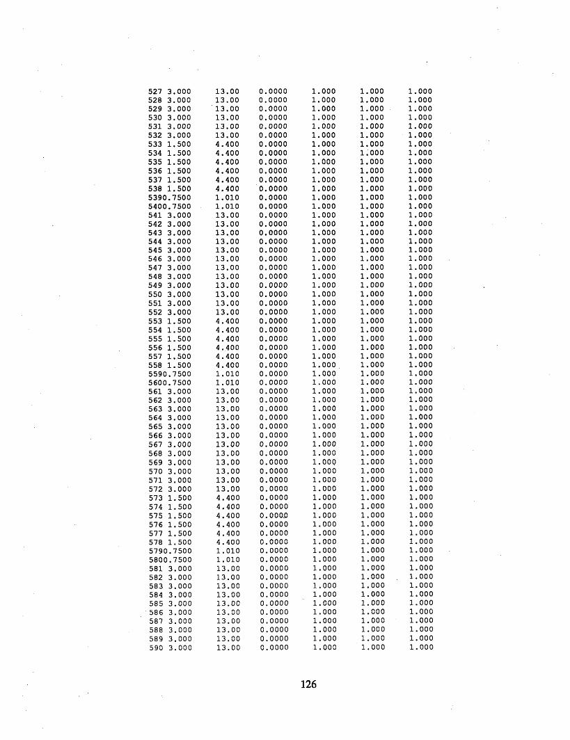
527 3.000 13.00 0.0000 1.000 1.000 1.000528 3.000 13.00 0.0000 1.000 1.000 1.000529 3.000 13.00 0.0000 1.000 1.000 1.000530 3.000 13.00 0.0000 1.000 1.000 1.000531 3.000 13.00 0.0000 1.000 1.000 1.000532 3.000 13.00 0.0000 1.000 1.000 1.000533 1.500 4.400 0.0000 1.000 1.000 1.000534 1.500 4.400 0.0000 1.000 1.000 1.000535 1.500 4.400 0.0000 1.000 1.000 1.000536 1.500 4.400 0.0000 1.000 1.000 1.000537 1.500 4.400 0.0000 1.000 1.000 1.000538 i.500 4.400 0.0000 1.000 1.000 1.0005390.7500 1.010 0.0000 1.000 1.000 1.0005400.7500 1.010 0.0000 1.000 1.000 1.000541 3.000 13.00 0.0000 1.000 1.000 1.000542 3.000 13.00 0.0000 1.000 1.000 1.000543 3.000 13.00 0.0000 1.000 1.000 1.000544 3.000 13.00 0.0000 1.000 1.000 1.000545 3.000 13.00 0.0000 1.000 1.000 1.000546 3.000 13.00 0.0000 1.000 1.000 1.000547 3.000 13.00 0.0000 1.000 1.000 1.000548 3.000 13.00 0.0000 1.000 1.000 1.000549 3.000 13.00 0.0000 1.000 1.000 1.000550 3.000 13.00 0.0000 1.000 1.000 1.000551 3.000 13.00 0.0000 1.000 1.000 1.000552 3.000 13.00 0.0000 1.000 1.000 1.000553 1.500 4.400 0.0000 1.000 1.000 1.000554 1.500 4.400 0.0000 1.000 1.000 1.000555 1.500 4.400 0.0000 1.000 1.000 1.000556 1.500 4.400 0.0000 1.000 1.000 1.000557 1.500 4.400 0.0000 1.000 1.000 1.000558 1.500 4.400 0.0000 1.000 1.000 1.0005590.7500 1.010 0.0000 1.000 1.000 1.0005600.7500 1.010 0.0000 1.000 1.000 1.000561 3.000 13.00 0.0000 1.000 1.000 1.000562 3.000 13.00 0.0000 1.000 1.000 1.000563 3.000 13.00 0.0000 1.000 1.000 1.000564 3.0.00 13.00 0.0000 1.000 1.000 1.000565 3.000 13.00 0.0000 1.000 1.000 1.000566 3.000 13.00 0.0000 1.000 1.000 1.000567 3.000 13.00 0.0000 1.000 1.000 1.000568 3.000 13.00 0.0000 1.000 1.000 1.000569 3.000 13.00 0.0000 1.000 1.000 1.000570 3.000 13.00 0.0000 1.000 1.000 1.000571 3.000 13.00 0.0000 1.000 1.000 1.000572 3.000 13.00 0.0000 1.000 1.000 1.000573 1.500 4.400 0.0000 1.000 1.000 1.000574 1.500 4.400 0.0000 1.000 1.000 1.000575 1.500 4.400 O.000 D 1.000 1.000 1.000576 1.500 4.400 0.0000 1.000 1.000 1.000577 1.500 4.400 0.0000 1.000 1.000 1.000578 1.500 4.400 0.0000 1.000 1.000 1.0005790.7500 1.010 0.0000 1.000 1.000 1.0005800.7500 1.010 0.0000 1.000 1.000 1.000581 3.000 13.00 0.0000 1.000 1.000 1.000582 3.000 13.00 0.0000 1.000 1.000 1.000583 3.000 13.00 0.0000 1.000 1.000 1.000584 3.000 13.00 0.0000 1.000 1.000 1.000585 3.000 13.00 0.0000 1.000 1.000 1.000586 3.000 13.00 0.0000 1.000 1.000 1.000587 3.000 13.00 0.0000 1.000 1.000 1.000588 3.000 13.00 0.0000 1.000 1.000 1.000589 3.000 13.00 0.0000 1.000 1.000 1.000590 3.000 13.00 0.0000 1.000 1.000 1.000

126

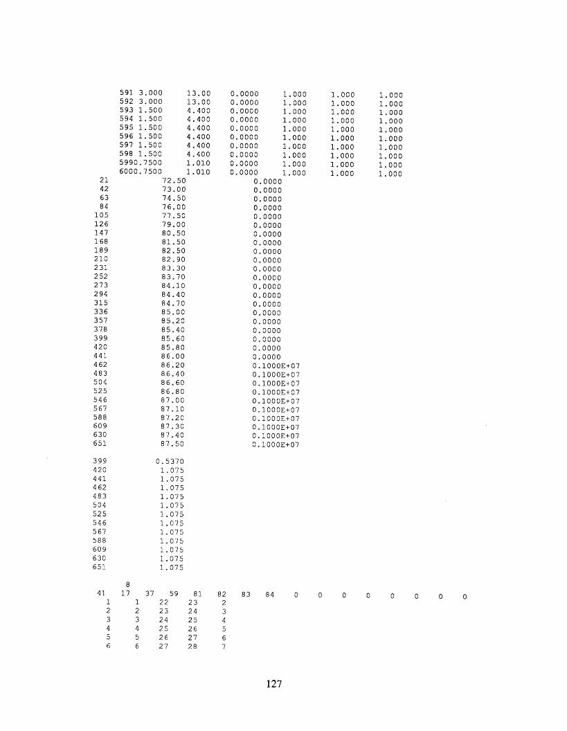
13.0013.004.4004.4004.4004.4004.4004.4001.0101. 010

0.00000. 00000.00000 .00000. 00000. 00000. 00000.00000.00000.0000

1 . 0001. 0001.0001.0001.0001.0001.0001.0001.0001 . 000

0.00000. 00000.00000. 00000. 00000.00000. 00000. 00000.00000.00000.00000.00000. 00000.00000.00000.00000.00000. 00000.0000.00000. 00000.1000E+070. 1000E+070.1000E+070. 1000E+070.1000E+070. 1000E+070. 1000E+070.1000E+070.1000E+070.1000E+07

81 82 83 8423 224 325 426 527 628 7

1. 0001.0001.0001.0001.0001.0001.0001.0001.0001.000

1. 0001.0001. 0001.0001.0001.0001.0001.0001.0001.000

0 0 0 0 0 0 0 0

127

591 3.000592 3.000593 1.500594 1.500595 1.500596 1.500597 1.500598 1.5005990.75006000.7500

72.5073.0074.5076.0077.5079.0080.5081.5082.5082.9083.3083.7084.1084.4084.7085.0085.2085.4085.6085.8086.0086.2086.4086.6086.8087.0087.1087.2087.3087.4087.50

21426384

105126147168189210231252273294315336357378399420441462483504525546567588609630651

399420441462483504525546567588609630651

41123456

0.53701.0751.0751.0751.0751.0751.0751.0751.0751.0751.0751.0751 .075

817 37 59

1 222 233 244 255 266 27

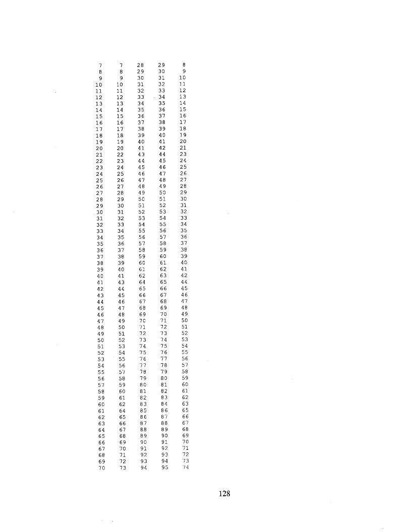
7 7 28 29 88 8 29 30 99 9 30 31 10

10 10 31 32 1111 11 32 33 1212 12 33 34 1313 13 34 35 1414 14 35 36 1515 15 36 37 1616 16 37 38 1717 17 38 39 1818 18 39 40 1919 19 40 41 2020 20 41 42 2121 22 43 44 2322 23 44 45 2423 24 45 46 2524 25 46 47 2625 26 47 48 2726 27 48 49 2827 28 49 50 2928 29 50 51 3029 30 51 52 3130 31 52 53 3231 32 53 54 3332 33 54 55 3433 34 55 56 3534 35 56 57 3635 36 57 58 3736 37 58 59 3837 38 59 60 3938 39 60 61 4039 40 61 62 4140 41 62 63 4241 43 64 65 4442 44 65 66 4543 45 66 67 4644 46 67 68 4745 47 68 69 4846 48 69 70 4947 49 70 71 5048 50 71 72 5149 51 72 73 5250 52 73 74 5351 53 74 75 5452 54 75 76 5553 55 76 77 5654 56 77 78 5755 57 78 79 5856 58 79 80 5957 59 80 81 6058 60 81 82 6159 61 82 83 6260 62 83 84 6361 64 85 86 6562 65 86 87 6663 66 87 88 6764 67 8.8 89 6865 68 89 90 6966 69 90 91 7067 70 91 92 7168 71 92 93 7269 72 93 94 7370 73 94 95 74

128

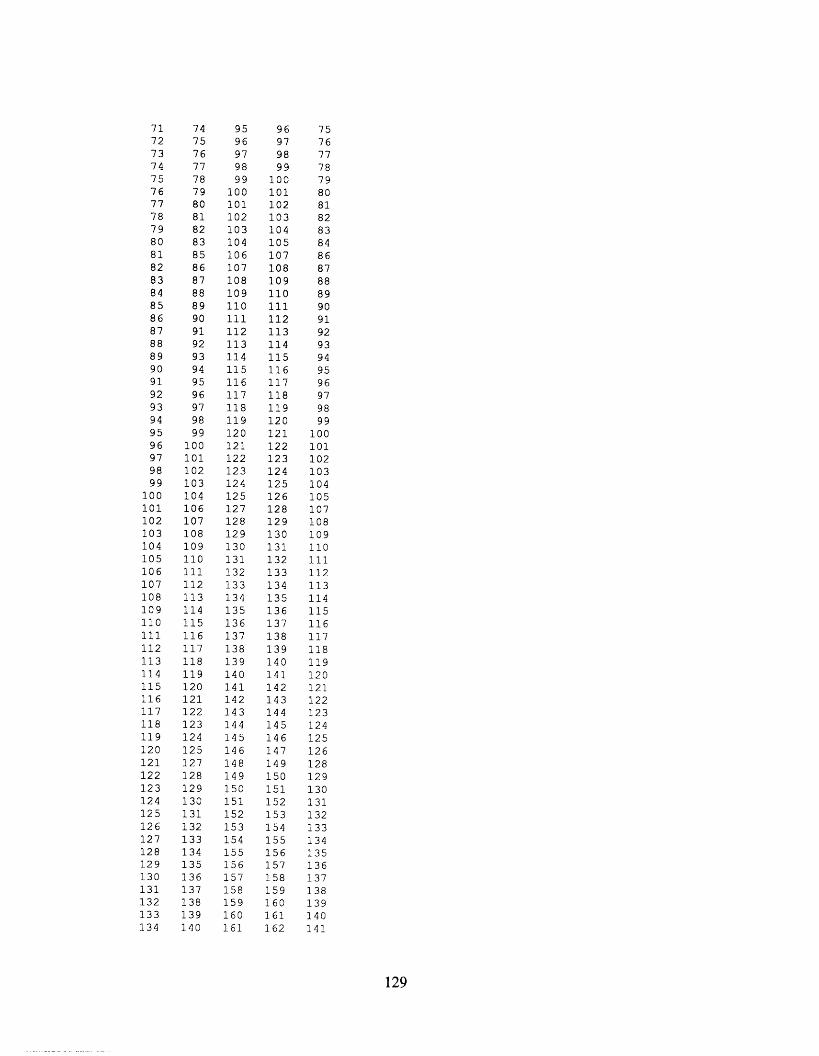
7172737475767778798081828384858687888990919293949596979899

100101102103104105106107108109110111112113114115116117118119120121122123124125126127128129130131132133134

74757677787980818283858687888990919293949596979899

100101102103104106107108109110111112113114115116117118119120121122123124125127128129130131132133134135136137138139140

9596979899

100101102103104106107108109110111112113114115116117118119120121122123124125127128129130131132133134135136137138139140141142143144145146148149150151152153154155156157158159160161

96979899

100101102103104105107108109110

11112113114115116117118119120121122123124125126128129130131132133134135136137138139140141142143144145146147149150151152153154155156157158159160161162

757677787980818283848687888990919293949596979899

100101102103104105107108109110111112113114115116117118119120121122123124125126128129130131132133134135136137138139140141

129

135136137138139140141142143144145146147148149150151152153154155156157158159160161162163164165166167168169170171172173174175176177178179180181182183184185186187188189190191192193194195196197198

141142143144145146148149150151152153154155156157158159160161162163164165166167169170171172173174175176177178179180181182183184185186187188190191192193194195196197198199200201202203204205206207

162163164165166167169170171172173174175176177178179180181182183184185186187188190191192193194195196197198199200201202203204205206207208209211212213214215216217218219220221222223224225226227228

163164165166167168170171172173174175176177178179180181182183184185186187188189191192193194195196197198199200201202203204205206207208209210212213214215216217218219220221222223224225226227228229

142143144145146147149150151152153154155156157158159160161162163164165166167168170171172173174175176177178179180181182183184185186187188189191192193194195196197198199200201202203204205206207208

130

199 208200 209201 211202 212203 213204 214205 215206 216207 217208 218209 219210 220211 221212 222213 223214 224215 225216 226217 227218 228219 229220 230221 232222 233223 234224 235225 236226 237227 238228 239229 240230 241231 242232 243233 244234 245235 246236 247237 248238 249239 250240 251241 253242 254243 255244 256245 257246 258247 259248 260249 261250 262251 263252 264253 265254 266255 267256 268257 269258 270259 271260 272261 274262 275

229 230 209230 231 210232 233 212233 234 213234 235 214235 236 215236 237 216237 238 217238 239 218239 240 219240 241 220241 242 221242 243 222243 244 223244 245 224245 246 225246 247 226247 248 227248 249 228249 250 229250 251 230251 252 231253 254 233254 255 234255 256 235256 257 236257 258 237258 259 238259 260 239260 261 240261 262 241262 263 242263 264 243264 265 244265 266 245266 267 246267 268 247268 269 248269 270 249270 271 250271 272 251272 273 252274 275 254275 276 255276 277 256277 278 257278 279 258279 280 259280 281 260281 282 261282 283 262283 284 263284 285 264285 286 265286 287 266287 288 267288 289 268289 290 269290 291 270291 292 271292 293 272293 294 273295 296 275296 297 276

131

263 276 297 298 277264 277 298 299 278265 278 299 300 279266 279 300 301 280267 280 301 302 281268 281 302 303 282269 282 303 304 283270 283 304 305 284271 284 305 306 285272 285 306 307 286273 286 307 308 287274 287 308 309 288275 288 309 310 289276 289 310 311 290277 290 311 312 291278 291 312 313 292279 292 313 314 293280 293 314 315 294281 295 316 317 296282 296 317 318 297283 297 318 319 298284 298 319 320 299285 299 320 321 300286 300 321 322 301287 301 322 323 302288 302 323 324 303289 303 324 325 304290 304 325 326 305291 305 326 327 306292 306 327 328 307293 307 328 329 308294 308 329 330 309295 309 330 331 310296 310 331 332 311297 311 332 333 312298 312 333 334 313299 313 334 335 314300 314 335 336 315301 316 337 338 317302 317 338 339 318303 318 339 340 319304 319 340 341 320305 320 341 342 321306 321 342 343 322307 322 343 344 323308 323 344 345 324309 324 345 346 325310 325 346 347 326311 326 347 348 327312 327 348 349 328313 328 349 350 329314 329 350 351 330315 330 351 352 331316 331 352 353 332317 332 353 354 333318 333 354 355 334319 334 355 356 335320 335 356 357 336321 337 358 359 338322 338 359 360 339323 339 360 361 340324 340 361 362 341325 341 362 363 342326 342 363 364 343

132

327328329330331332333334335336337338339340341342343344345346347348349350351352353354355356357358359360361362363364365366367368369370371372373374375376377378379380381382383384385386387388389390

343344345346347348349350351352353354355356358359360361362363364365366367368369370371372373374375376377379380381382383384385386387388389390391392393394395396397398400401402403404405406407408409

364365366367368369370371372373374375376377379380381382383384385386387388389390391392393394395396397398400401402403404405406407408409410411412413414415416417418419421422423424425426427428429430

365366367368369370371372373374375376377378380381382383384385386387388389390391392393394395396397398399401402403404405406407408409410411412413414415416417418419420422423424425426427428429430431

344345346347348349350351352353354355356357359360361362363364365366367368369370371372373374375376377378380381382383384385386387388389390391392393394395396397398399401402403404405406407408409410

133

391392393394395396397398399400401402403404405406407408409410411412413414415416417418419420421422423424425426427428429430431432433434435436437438439440441442443444445446447448449450451452453454

410411412413414415416417418419421422423424425426427428429430431432433434435436437438439440442443444445446447448449450451452453454455456457458459460461463464465466467468469470471472473474475476

431432433434435436437438439440442443444445446447448449450451452453454455456457458459460461463464465466467468469470471472473474475476477478479480481482484485486487488489490491492493494495496497

432433434435436437438439440441443444445446447448449450451452453454455456457458459460461462464465466467468469470471472473474475476477478479480481482483485486487488489490491492493494495496497498

411412413414415416417418419420422423424425426427428429430431432433434435436437438439440441443444445446447448449450451452453454455456457458459460461462464465466467468469470471472473474475476477

134

455456457458459460461462463464465466467468469470471472473474475476477478479480481482483484485486487488489490491492493494495496497498499500501502503504505506507508509510511512513514515516517518

477478479480481482484485486487488489490491492493494495496497498499500501502503505506507508509510511512513514515516517518519520521522523524526527528529530531532533534535536537538539540541542543

498499500501502503505506507508509510511512513514515516517518519520521522523524526527528529530531532533534535536537538539540541542543544545547548549550551552553554555556557558559560561562563564

499500501502503504506507508509510511512513514515516517518519520521522523524525527528529530531532533534535536537538539540541542543544545546548549550551552553554555556557558559560561562563564565

478479480481482483485486487488489490491492493494495496497498499500501502503504506507508509510511512513514515516517518519520521522523524525527528529530531532533534535536537538539540541542543544

135

519520521522523524525526527528529530531532533534535536537538539540541542543544545546547548549550551552553554555556557558559560561562563564565566567568569570571572573574575576577578579580581582

544545547548549550551552553554555556557558559560561562563564565566568569570571572573574575576577578579580581582583584585586587589590591592593594595596597598599600601602603604605606607608610611

565566568569570571572573574575576577578579580581582583584585586587589590591592593594595596597598599600601602603604605606607608610611612613614615616617618619620621622623624625626627628629631632

566567569570571572573574575576577578579580581582583584585586587588590591592593594595596597598599600601602603604605606607608609611612613614615616617618619620621622623624625626627628629630632633

545546548549550551552553554

55556557558559560561562563564565566567569570571572573574575576577578579580581582583584585586587588590591592593594595596597598599600601602603604605606607608609611612

136

583 612 633 634 613584 613 634 635 614585 614 635 636 615586 615 636 637 616587 616 637 638 617588 617 638 639 618589 618 639 640 619590 619 640 641 620591 620 641 642 621592 621 642 643 622593 622 643 644 623594 623 644 645 624595 624 645 646 625596 625 646 647 626597 626 647 648 627598 627 648 649 628599 628 649 650 629600 629 650 651 630

137

---- L - -

138 -_ i n