Application of Pattern Recognition and Adaptive DSP Methods for Spatio-temporal Analysis of

Satellite Based Hydrological Datasets

Anish Chand Turlapaty

DISSERTATION.COM

Boca Raton

Application of Pattern Recognition and Adaptive DSP Methods for Spatio-temporal Analysis of Satellite Based Hydrological Datasets

Copyright © 2010 Anish Chand Turlapaty

All rights reserved. No part of this book may be reproduced or transmitted in any form or by any means, electronic or mechanical, including photocopying, recording, or by any information storage and

retrieval system, without written permission from the publisher.

Dissertation.com Boca Raton, Florida

USA • 2010

ISBN-10: 1-59942-336-7 ISBN-13: 978-1-59942-336-4

Name: Anish Chand Turlapaty

Date of Degree: May 1, 2010

Institution: Mississippi State University

Major Field: Electrical Engineering

Major Professor: Dr. Nicolas H. Younan

Title of Study: APPLICATION OF PATTERN RECOGNITION AND ADAPTIVE DSP METHODS FOR SPATIO-TEMPORAL ANALYSIS OF SATELLITE BASED HYDROLOGICAL DATASETS

Pages in Study: 131

Candidate for Degree of Doctor of Philosophy

Data assimilation of satellite-based observations of hydrological variables with

full numerical physics models can be used to downscale these observations from coarse

to high resolution to improve microwave sensor-based soil moisture observations.

Moreover, assimilation can also be used to predict related hydrological variables, e.g.,

precipitation products can be assimilated in a land information system to estimate soil

moisture. High quality spatio-temporal observations of these processes are vital for a

successful assimilation which in turn needs a detailed analysis and improvement. In this

research, pattern recognition and adaptive signal processing methods are developed for

the spatio-temporal analysis and enhancement of soil moisture and precipitation datasets.

These methods are applied to accomplish the following tasks: (i) a consistency analysis

of level-3 soil moisture data from the Advanced Microwave Scanning Radiometer – EOS

(AMSR-E) against in-situ soil moisture measurements from the USDA Soil Climate

Analysis Network (SCAN). This method performs a consistency assessment of the entire

time series in relation to others and provides a spatial distribution of consistency levels.

The methodology is based on a combination of wavelet-based feature extraction and one-

class support vector machines (SVM) classifier. Spatial distribution of consistency levels

are presented as consistency maps for a region, including the states of Mississippi,

Arkansas, and Louisiana. These results are well correlated with the spatial distributions of

average soil moisture, and the cumulative counts of dense vegetation; (ii) a modified

singular spectral analysis based interpolation scheme is developed and validated on a few

geophysical data products including GODAE’s high resolution sea surface temperature

(GHRSST). This method is later employed to fill the systematic gaps in level-3 AMSR-E

soil moisture dataset; (iii) a combination of artificial neural networks and vector space

transformation function is used to fuse several high resolution precipitation products

(HRPP). The final merged product is statistically superior to any of the individual

datasets over a seasonal period. The results have been tested against ground based

measurements of rainfall over our study area and average accuracies obtained are 85% in

the summer and 55% in the winter 2007.

 

 

ii  

DEDICATION

I would like to dedicate this dissertation to my parents Saiprasad and Vijaya

 

iii  

ACKNOWLEDGEMENTS

I would like to express gratitude to my advisor Dr. Nicolas H. Younan for

facilitating this opportunity and also for his technical guidance throughout this research. I

am also grateful to my supervisor Dr. Valentine Anantharaj for his excellent scientific

guidance and support. I would also like to thank my committee members Dr. Lori M.

Bruce, Dr. James Fowler, and Dr. Qian Du for serving on my committee and providing

valuable feedback and advice. I would also like to extend my sincere thanks to Dr. F.

Joseph Turk of the Naval Research Laboratory for providing us research data and

insightful discussions. I also appreciate the suggestions provided by Dr. Christa Peters

Lidard from NASA, Goddard Space Flight Center. Finally, I would like to acknowledge

both NASA and NOAA for providing financial support throughout the research.

 

iv  

TABLE OF CONTENTS

DEDICATION .................................................................................................................... ii

ACKNOWLEDGEMENTS ............................................................................................... iii

LIST OF TABLES ............................................................................................................ vii

LIST OF FIGURES ......................................................................................................... viii

CHAPTER

I. INTRODUCTION. ............................................................................................1

1.1 Background .................................................................................................1 1.2 Motivation ...................................................................................................5

1.2.1 Consistency analysis of soil moisture data ......................................5 1.2.2 Interpolation of geophysical datasets .............................................10 1.2.3 Rainfall measurements and fusion ..................................................12

1.3 Contributions ............................................................................................16 1.3.1 Consistency analysis of AMSR-E soil moisture data .....................16 1.3.2 Interpolation of gaps in AMSR-E soil moisture product using modified SSA .................................................................................17 13.3 Precipitation data fusion ..................................................................17

II. LITERATURE REVIEW ................................................................................19

2.1 Soil moisture measurements and consistency analysis .............................19 2.1.1 In-situ measurements ......................................................................19 2.1.2 Remotely-sensed estimates .............................................................20 2.1.3 Value-added soil moisture products from land data assimilation systems ...........................................................................................24 2.1.4 Review of consistency analysis ......................................................25

2.2 Importance of interpolation techniques for geophysical datasets .............28 2.2.1 Spectral analysis of geophysical variables .....................................28 2.2.2 Data gap filling methods ................................................................29

 

v  

2.3 Multi-sensor data fusion techniques .........................................................31

III. METHODOLOGY ..........................................................................................36

3.1 Pattern recognition-based consistency analysis ........................................36 3.1.1 Foundation ......................................................................................36 3.1.2 Step one: feature extraction ............................................................39

3.1.2.1 Features from the discrete wavelet transform (DWT) .......41 3.1.2.2 Features from the redundant discrete wavelet transform (RDWT) .............................................................................42

3.1.3 Step two: classification with one-class support vector machines ...43 3.1.4 Step three: consistency assessment technique ................................44

3.2 Modified SSA-based interpolation ...........................................................48 3.2.1 Foundation ......................................................................................48 3.2.2 Method description .........................................................................51

3.3 Data fusion: a two-step process ................................................................55 3.3.1 Pattern recognition-based fusion ....................................................55

3.3.1.1 Vector space transformation ..............................................58 3.3.1.2 Artificial neural networks ..................................................59 3.3.1.3 Stage one learning ..............................................................62 3.3.1.4 Stage two learning..............................................................62

3.3.2 Cross-validation ..............................................................................65

IV. RESULTS AND DISCUSSION ......................................................................66

4.1 Implementation of pattern recognition based consistency analysis ..........66 4.1.1 Time series generation ....................................................................66

4.1.1.1 Soil moisture data from SCAN ..........................................66 4.1.1.2 AMSR-E soil moisture data ...............................................67

4.1.2 Implementation ...............................................................................69 4.1.3 Method validation ...........................................................................70

4.1.3.1 Sensitivity studies ..............................................................72 4.1.3.2 Interpretation and possible applications of consistency maps ...................................................................................74 4.1.3.3 Performance comparison and seasonal variation ...............74

4.1.4 Discussion .......................................................................................76 4.2 Implementation of the modified SSA interpolation ..................................79

4.2.1 Validation with sample sets ............................................................79 4.2.1.1 Synthetic spatio-temporal dataset ......................................79 4.2.1.2 Sea surface temperature .....................................................80 4.2.1.3 Normalized difference vegetation index ............................84 4.2.1.4 Land surface temperature ...................................................86

4.2.2 Interpolation of incomplete AMSR-E soil moisture data ...............87 4.2.3 Discussion .......................................................................................92

 

vi  

4.3 Fusion of HRPPs case study .....................................................................92 4.3.1 Fusion process for rainfall data ......................................................92

4.3.1.1 Input data description .........................................................93 4.3.1.2 Reference data ....................................................................95 4.3.1.3 Training ..............................................................................95 4.3.1.4 Evaluation ..........................................................................97

4.3.2 Results ............................................................................................99 4.3.2.1 Cross-validation results ......................................................99 4.3.2.2 Performance of the merged data against the ABRFC reference data ...................................................................100

4.3.3 HSS difference maps ....................................................................105 4.3.3.1 Comparison with CMORPH ............................................106 4.3.3.2 Comparison with GOES AE ............................................108 4.3.3.3 Comparison with GOES HE ............................................109 4.3.3.4 Comparison with NRL BLEND and SCAMPR ...............110

4.3.4 Additional discussion ...................................................................111

V. CONCLUSION AND FUTURE WORK ......................................................114

REFERENCES ................................................................................................................117

 

 

vii  

LIST OF TABLES

1. List of SCAN Sites.........................................................................................................9

2. Consistency analysis method .......................................................................................46

3. Parameter list for the feed forward artificial neural network .......................................61

4. Performance comparisons ............................................................................................74

5. Success rates from the cross-validation experiments ...................................................99

6. HSS skill quartile percentages of the area in the study region ..................................105

7. Skill difference quartile percentages of the area in the study region .........................108

 

viii  

LIST OF FIGURES

1. Concept of a Land Data Assimilation System (LDAS) illustrating the partitioning of the energy and moisture fluxes, including response of the surface soil moisture to external forcings (precipitation, temperature and radiation) and the vegetation and soil parameters. Figure Courtesy: Paul Houser, George Mason University. .........................................................................................................6

2. Map of Land cover for the study region. Scan sites are marked with Arabic numerals and site names are given in Table 1 ..............................................................8

3. Soil texture map for a part of our study region. Scan sites are marked with Arabic numerals (Figure Courtesy: Mostovoy and Anantharaj [17]) ...........................9

4. Feature space for consistency assessment of samples with two features ...................38

5. Feature extraction process applied to soil moisture time series from a SCAN site ....40

6. A block diagram of consistency analysis methodology .............................................47

7. An illustration of spatial grid with missing values and determination of the optimal subset size ......................................................................................................49

8. A block diagram of the modified SSA interpolation scheme .....................................51

9. A block diagram of the fusion process .......................................................................57

10. A two layer artificial neural network architecture with vector transformation function .......................................................................................................................60

11. Scan sites and consistency maps .................................................................................70

12. Sensitivity plot: average SVM distance measure versus SCAN site dropped ...........72

13. Consistency maps with SCAN sites dropped .............................................................73

14. Consistency maps comparison ....................................................................................75

 

ix  

15. Consistency maps of AMSR-E soil moisture data for various seasons ......................76

16. Performance of the interpolation algorithm on a synthetic dataset with two

multivariate signals .....................................................................................................80

17. Algorithm performance vs. spatial block size ............................................................82

18. SST from GHRSST-PP for a 25o x 25o region centered at (27.5oN, 67.5oW) ............83

19. MSE comparison between the actual SST versus interpolated SST, on a daily basis, computed from different interpolation algorithms ...........................................84

20. Performance of the modified SSA algorithm, on MODIS NDVI dataset, based on different spatial block sizes ...................................................................................85

21. MODIS LST for a 5o x 5o region centered at (40oN, 109oW) ..................................87

22. AMSR-E Soil moisture maps before and after interpolation comparisons ................90

23. Performance comparison of interpolated data on AMSR-E data: modified SSA vs. SSA .......................................................................................................................91

24. Convergence of neural network training ....................................................................97

25. Improvement in success rate due to vector space transformation ............................100

26. Heidke skill score maps and skill score distributions of the merged data compared with the ABRFC data for four seasons ....................................................101

27. Algorithm performance for different sections of the study region (Spring 2008) ...103

28. Maps and distributions of the difference in Heidke skill score between the merged data and the seasonal CMORPH data for four seasons ...............................107

29. Maps and distributions of the difference in Heidke skill score between the merged data and the auto estimator data for four seasons ........................................109

30. Maps and distributions of difference in Heidke skill score between the merged data and the hydro estimator data for four seasons ...................................................110

31. Maps and distributions of the difference in Heidke skill score between the merged data and the NRL-BLEND data for different seasons .................................111

 

x  

32. Comparison between the success rates of the merged data and those of the individual datasets ....................................................................................................112

33. Comparison between the success rates and the minimum error used for early

stopping of network training .....................................................................................112  

 

 

1  

CHAPTER I

INTRODUCTION

1.1 Background

Satellite-based sensors are used to obtain information with large coverage

pertaining to applications such as land classification, ocean surface properties, and

climate processes. For instance, climate phenomena, such as precipitation, soil moisture,

and temperature, are remotely sensed and spatio-temporal data of their approximate states

are obtained. The advancement of the remote sensing technology has improved the

spatial and temporal resolutions of these datasets. Spatio-temporal analysis techniques

include analytical model-based methods, exploratory analysis of geo-spatial patterns in

epidemics, and data mining methods for knowledge extraction from large scale

geophysical data [1]. Spatio-temporal analysis methods have been successfully used in

understanding phenomena such as wildfire events in Florida [2], and land cover/ land use

change in the yellow river delta in China [3]. Spatio-temporal analyses of geophysical

data include i) recognition of hidden structures in data, ii) anomaly detection in large

datasets, and iii) regression to discover temporal trends. These techniques were originally

developed for temporal data and are recently extended to study spatio-temporal aspect of

data [4].

2  

Pattern recognition and signal processing are emerging tools for spatio-temporal

analysis of geophysical data obtained from satellites observations. Broad arrays of

methods are available for these applications. Pattern recognition can be defined as an

application of machine learning to engineering problems. Some examples of these

engineering problems include anomaly detection, data fusion, object tracking and

identification, and land surface classification, just to mention a few. In this area, the main

objective is to learn hidden structures or processes from a large set of examples and apply

that knowledge to analyze new unseen observations. In the context of remote sensing,

pattern recognition is mainly used in applications such as image and data classification.

Supervised and unsupervised classification of land surface images is a popular

application of pattern recognition in remote sensing. For example, a satellite image of an

urban area can be classified into different classes based on land use by using a simple

classification algorithm.

Two major signal processing tools used for spatio-temporal data analysis are

digital spectral analysis and digital filters. Traditionally, spectral analysis tools, such as

the discrete Fourier transform (DFT) and short-time Fourier transform (STFT), were

developed only for one-dimensional data. These methods have fixed basis functions, for

instance, complex exponential for DFT. Later, more sophisticated spectral analysis tools

with adaptive basis functions were developed. Some examples include the discrete

wavelet transform (DWT), singular value decomposition (SVD) analysis, and Huang

Hilbert transform (HHT). An interesting application of wavelets for satellite images is

image fusion. In image fusion, several images with varying spatial resolutions are merged

3  

together into a final image which inherits superior qualities of all its contributors

[5]. Recently, tools, such as multivariate spectral analysis, have been developed for

spatio-temporal signal detection. An example of multivariate spectral analysis is the

inquiry of interactions between several climate processes. Most well known global

signals include the El-Niño Southern oscillation and North Atlantic oscillation. The

ensemble Kalman filter-based methods are most widely used in data assimilation. L-band

microwave soil moisture observations from the southern Great Plains hydrology

experiment were assimilated into a soil-vegetation-atmosphere model. An optimal

ensemble size for robust assimilation performance has been determined for the

experiment [6].

The area of focus in this research is spatio-temporal analysis of two key

hydrological variables surface soil moisture and precipitation. Soil moisture is one of the

most important environmental variables in regional weather and global climate systems.

In particular, it plays an important role in modulating the energy and water cycles of the

Earth’s system [7]. It is also directly related to other bio- and geophysical variables, such

as precipitation, vegetation characteristics, temperature, evaporation, and transpiration. It

has been characterized as an “environmental descriptor that integrates much of the land

surface hydrology and is a key variable linking the earth surface and the atmosphere” [8].

The soil moisture near the surface determines the partitioning of latent and sensible heat

fluxes, evaporation and surface runoff. Moreover, soil moisture in deeper layers also

regulates how the ecosystems respond based on available water content in the soils [9].

Hence, the monitoring, analysis, and prediction of soil moisture is critical for weather and

4  

climate studies of routine forecasting of weather events, including flooding; and for

planting, irrigation and drought prediction, and management strategies for agriculture.

The other hydrological phenomenon, precipitation, is also an important component of the

global energy and water cycle; it is one of the main variables predicted in weather

forecast models. Moreover, it is a key process in short-term meteorological and long-term

climatological studies. Precipitation events are a driving force behind the hydrological

phenomenon, such as floods and storms [10, 11]. These two variables are highly

interdependent, for instance, spatio-temporal structure of soil moisture is dependent on

long-term variability in precipitation [12 -14]. Based on this fact, the soil moisture

observations can be used to estimate errors in precipitation retrievals, and those errors can

be corrected by using assimilation with physics based water-balance models [15] . Before

this type of assimilation, it is necessary to analyze and improve the consistency and

accuracy of respective satellite based retrievals.

In this research, we propose spatio-temporal analysis methods to accomplish the

following tasks: (i) consistency analysis of satellite-based soil moisture data, (ii)

interpolation of missing data in soil moisture datasets, and (iii) merging of satellite-based

precipitation observations. Novel pattern recognition approaches are developed in the

first and the third tasks. Existing signal processing methodologies are used and modified

in the second task. This dissertation is structured as follows: (i) motivation behind each

individual task, (ii) contribution for each application, (iii) discussion of related work in

respective fields, (iv) methodologies to achieve the objectives, and (v) implementation,

results, and discussion.

5  

1.2 Motivation

1.2.1 Consistency analysis of soil moisture data

The soil moisture dynamics at the surface layer (Figure 1) is highly inter-related

to hydrometeorological forcing fields (precipitation, air temperature, incident shortwave

and longwave radiation) and other bio- and geophysical parameters, such as vegetation

(type, fraction, leaf and stem area indices), topography and soil parameters (type, texture

and hydraulic properties). Soil moisture budget can be modeled as a difference between

accumulated precipitation and various forms of water distribution such as evaporation,

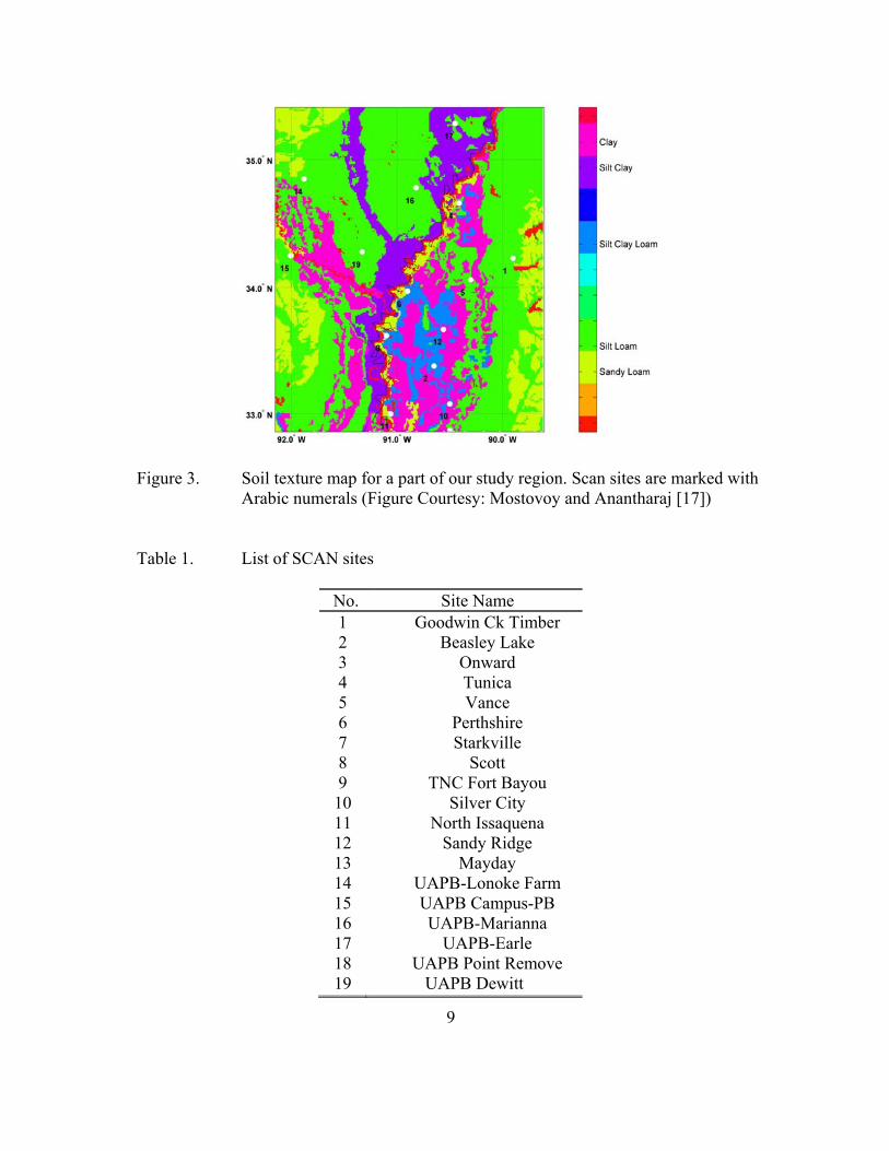
transpiration, runoff and groundwater losses Huang et al. [16]. The spatial scale of the

soil moisture is also characterized by the spatial heterogeneity of the vegetation and soil

parameters (Figures 2 and 3). The response of the soil moisture is a complex physical

process that is determined by both the external hydrometeorological processes as well as

the soil hydraulic properties. In the Lower Mississippi River Valley (aka. The Mississippi

Delta), the soil moisture depends primarily on the soil texture which is used to determine

the soil hydraulic properties [17]. Further, evapotranspiration also exerts a controlling

influence on the variability of the soil moisture in this region during most of the year,

except during the summer [18], (Anantharaj, V., 2010 – personal communication).

Hence, sophisticated signal processing and pattern recognition techniques are necessary

to extract and analyze the information content from soil moisture fields at multiple and

spatial scales.

6  

Figure 1. Concept of a Land Data Assimilation System (LDAS) illustrating the

partitioning of the energy and moisture fluxes, including response of the surface soil moisture to external forcings (precipitation, temperature and radiation) and the vegetation and soil parameters.

Figure Courtesy: Paul Houser, George Mason University.

7  

A comparative time series analysis of soil moisture data with these land surface

processes would provide insight into the above mentioned relationship. Traditional time

series analysis tools such as windowed Fourier transform has many limitations such as

aliasing for high-low frequencies and determination of optimal window length that make

the process of time-frequency localization inefficient. Wavelet analysis is a very popular

alternative for such analysis of geophysical time series data. An important objective of

wavelet analysis is to understand localized variations of frequency components in the

data. Thus, wavelet analysis decomposes the soil moisture time series into sequences at

multiple temporal resolutions. These separate sequences in the wavelet decomposition

should show the significant signals and their variations with correspondence to the

contributions from the individual physical components in the soil moisture model. Parent

et al, [19] studied the temporal variability (using wavelet analysis) in soil moisture time

series at very short time scales from 1h to 2 weeks. It was found that for scales less than

48h soil moisture is directly related to precipitation events, but for longer scales upto

1week it depends on frequency of precipitation and for even larger scales 1 to 2 weeks it

is linked to dry spells. An easy to follow wavelet analysis toolbox for analysis of

meteorological time series was developed by Torrence and Compo [20]. A similar

wavelet analysis between the soil moisture data and other related land surface processes

would provide a better understanding of such physical significance of these wavelet

based features. Thus, energy and entropy features constructed from wavelet analysis

would be very useful for analyzing the statistical agreement (consistency) between

ground based and remotely sensed soil moisture data.

8  

Moreover, soil moisture for a given grid cell is basically an average for a

heterogeneous area with different possible land classes. For in-situ measurements, soil

moisture budget also depends on the specific soil type (affects ground water loss and

evaporation) and land cover (affects transpiration and runoff) (Figure 1). A wavelet

analysis of spatio-temporal soil moisture data would address the relation between the soil

moisture variations and the corresponding land classes.

  

Water Barren or sparsely vegetated Snow and ice Cropland/natural vegetation Urban and built-up Croplands Permanent wetlands Grasslands Savannas Woody savannas Open shrubland Closed shrublands Mixed forests Deciduous broadleaf forest Deciduous needleleaf forest Evergreen broadleaf forest Evergreen needleleaf forest Water  

Figure 2. Map of Land cover for the study region. Scan sites are marked with

Arabic numerals and site names are given in Table 1.

9  

Figure 3. Soil texture map for a part of our study region. Scan sites are marked with Arabic numerals (Figure Courtesy: Mostovoy and Anantharaj [17])

Table 1. List of SCAN sites

No. Site Name 1 2 3 4 5 6 7 8 9 10 11 12 13 14 15 16 17 18 19

Goodwin Ck Timber Beasley Lake

Onward Tunica Vance

Perthshire Starkville

Scott TNC Fort Bayou

Silver City North Issaquena

Sandy Ridge Mayday

UAPB-Lonoke Farm UAPB Campus-PB UAPB-Marianna

UAPB-Earle UAPB Point Remove

UAPB Dewitt

10  

Despite the diverse critical application needs, accurate measurement and routine

monitoring of soil moisture at global scales remains a great challenge. There is general

consensus that most immediate requirement of a routine global soil moisture product at

50 km resolution could be feasible using a combination of both in-situ measurements and

remotely sensed estimates, assimilated into land surface models [8]. An approach to deal

with this problem is the use of the Noah land surface model of NASA Land Information

System (LIS) [21]. The idea is to downscale the data to higher temporal and spatial

resolutions. Before assimilation of soil moisture data into the LIS, the validity of the data

has to be verified. In this context, consistency analysis can be defined as an attempt to

understand the spatio-temporal quality of satellite-based data with respect to in-situ data

obtained at certain stations within the study region for the same temporal duration.

1.2.2 Interpolation of geophysical datasets

The time scales of interactions of the Earth’s subsystems are usually in the order

of years or longer. These complex interactions result in quasi-periodic and low frequency

fluctuations in the climate. A couple of advantages for studying these interactions are a

better understanding of the climate and a possible improvement in the forecast of future

climate. The complex nature of climatic interactions does not support any single

methodology. Periodic components can be best understood using frequency domain

methods. However, episodic events, such as volcanic eruptions, can be best studied using

time domain methods. There are some phenomena in climate structure which exhibit both

oscillatory and episodic behavior, for instance, the El-Niño southern oscillation.

11  

Mann and Park [22] developed the multi-taper multivariate singular value

decomposition (MTM-SVD) method, an improvement over the existing spectral analysis

techniques, to study couplings between various climatic processes. In a study on a

synthetic data set, the MTM-SVD method has detected a spatio-temporal signal that is

statistically significant over the underlying noise in the data. Los et al. [23] employed the

MTM-SVD method on the datasets such as adjusted NDVI from the Advanced Very

High Resolution Radiometer (AVHRR), precipitation and land surface temperature from

the National Oceanic and Atmospheric Administration’s (NOAA) and the National

Climate Data Center (NCDC), and sea surface temperature from the National Center for

Atmospheric Research (NCAR). A principal mode, strong in sea surface temperature,

was found corresponding to a 2.6 year period and related to the El-Niño southern

oscillation index. Wu et al., [13] applied a SVD-based method to analyze the spatio-

temporal relationship between spring soil moisture and summer precipitation in the

United States. The NCAR community climate model coupled with multilayer land model

(CLM) was analyzed while simulating the US land-atmospheric system. The first SVD

mode accounted for 27% of the covariance between soil moisture and precipitation, while

the second mode has accounted for 16% of the variance. In a recent work, Kim and Wang

[24] studied the influence of soil moisture on precipitation in North America and found

that there was a considerable time lag for the soil moisture impact on precipitation.

Overall, the SVD analysis has been a successful method for the analysis of the

interactions between different phenomena and their overall influence on global climate.