Vol. 117 (2010) ACTA PHYSICA POLONICA A No. 6

Application of Bayesian Reasoning and the MaximumEntropy Method to Some Reconstruction Problems

K.W. Fornalskia, G. Parzycha, M. Pylaka, D. Satułab

and L. Dobrzyńskia,b,∗aThe Andrzej Sołtan Institute for Nuclear Studies, 05-400 Otwock-Świerk, PolandbFaculty of Physics, University of Białystok, Lipowa 41, 15-424 Białystok, Poland

(Received January 29, 2010; in final form March 9, 2010)

The so-called Bayesian reasoning is applied whenever uncertainty has to be considered as serious factor ininterpretation of results. The paper presents analysis of the impact of inaccurate data on the straight line andquadratic relation fittings. This type of analysis is particularly important when one tries to decide on the type ofdependence. The paper also shows examples of the Maximum Entropy Methods applied to the reconstruction ofthe hyperfine parameters distribution from the measured Mössbauer spectra of GaFeO3 and the electron–positronmomentum distribution from the positron annihilation data of Gd.

PACS numbers: 29.85.−c, 78.70.Bj, 76.80.+y

1. Introduction

Experimental data always bear uncertainties. The re-searcher needs usually either to fit certain function tothe measured points or to reconstruct certain distri-bution which is hidden in the experiment. This hap-pens e.g. when one measures a spectrum which usu-ally has smeared details due to the finite resolution ofthe spectrometer. In the conventional analysis, least--square method is most commonly used. Description ofthe method can be found in every academic textbooks ondata analysis. Moreover, method of curve fitting, is sus-ceptible to ‘outliers’ — the points that accidentally arehaving values significantly different from other measuredpoints. When such points appear in a single spectrum,it is not particularly difficult to qualify them as outliersand eventually neglect them in the analysis. Much moredifficult case is when one collects the data obtained in dif-ferent laboratories or measured by different techniques.When the scatter of points is substantially larger thantheir claimed accuracies would allow, the parameters ofa curve fitted to the measured points may have very lowcredibility. In the more difficult case of a reconstructionof a distribution observed through a spectrum smeared byresolution function of measuring instrument, one meetsin fact two problems: one is the most accurate decon-volution of the spectrum, the other — carrying out non--parametric model-free reconstruction of the distribution.This is typical inverse problem which is generally difficultto solve. The Maximum Entropy Method is often veryuseful in solving such problems. In both cases, excel-

∗ corresponding author; e-mail: ludwik@ipj.gov.pl

lent introduction to the Bayesian and Maximum Entropymethods can be found in [1]. Their bases would only bebriefly described in the next sections where it would benecessary.

2. “Outliers” and curve fitting

A good example of the problem was considered by For-nalski and Dobrzyński [2] who analyzed the epidemiolog-ical data obtained for the cancer deaths of the nuclearindustry workers. The scatter of points presented in orig-inal papers [3], that were intended to show that the risk ofcancer death increases with the dose absorbed by work-ers, by far exceeded declared experimental uncertainties.These points exhibited also uneven distribution of pointsalong abscissa axis. In such situation one could imme-diately say that conventional least-square fitting mustlead to the parameters of the fit that may not be reli-able. It could be suspected that the conclusions reachedin papers [3] were due to a few “outliers” in the data. Infact, in the data considered one cannot directly say whichpoints should be treated as outliers just because of thescatter of the data. Therefore, instead of removing sus-pected points, the authors of [2] used the method [1], ofcarrying out the fit under assumption that the values ofuncertainties are declared for the points lowest estimateof the true ones.

In accordance to [1], for given uncertainty σ0, one as-sumes that this value is showing rather the lowest esti-mate, and a probability density that the “true” uncer-tainty σ is given by so-called Jeffrey’s prior:

p(σ) =1

ln(σmax/σmin)1σ

, (2.1)

where σmin can be set to σ0, and σmax is chosen arbitrar-

(892)

Application of Bayesian Reasoning and the Maximum Entropy Method . . . 893

ily, or by simpler formula:

p(σ) =σ0

σ2, (2.2)

where σ lies in the limits [σ0,∞).The Bayes theorem for conditional probability of an

event X given Y and some general information I, whichwe could have about the studied object or distribution:

p (X|Y, I) =p (Y |X, I) p (X| I)

p (Y | I), (2.3)

where the probability p(X|I) should be understood asshowing the state of knowledge (“degree-of-belief”) aboutX in light of the information I. The expression in thenominator is a product of likelihood function (how wellthe data Y reflect correctness of hypothesis X) and theprior (what do we know about X expressed in terms ofa probability value between 0 and 1). The former can becalculated within usual theory of likelihood.

For the case we are interested in, the conditional prob-ability density of having experimental datum E, given itsuncertainty σ and expected theoretical value T , is givenby:

P (E|σ) =1√2πσ

exp[−(T − E)2/(2σ2)

]p(σ) , (2.4)

where the information I was dropped for better clarityof the formula. The probability (for all N experimentalpoints) should be maximized for a number of parameters{αn, n = 1, 2, . . . ,M} of expected function (T ), whichdescribes the data. In order to find the maximum of:

P =N∏

i=1

Pi =N∏

i=1

∫1√

2πσi

× exp(−(Ti − Ei)2/(2σ2

i ))p(σi)dσi , (2.5)

it is convenient to maximize the logarithm L =∑Ni=1 ln Pi with respect to any of the of parameter fit αn:

dL

dαn=

N∑

i=1

−(Ti − Ei)dTi

dαn

1Pi

×∫

1√2πσ3

i

exp(−(Ti−Ei)2/(2σ2

i ))p(σi)dσi ,(2.6)

which can be written in shorter form:dL

dαn=

N∑

i=1

gi

(Ti − Ei

) dTi

dαn, (2.7)

where N is the number of all analyzed data points, andthe derivative (2.7) should thus be set to zero. The in-tegral’s range in (2.5) and (2.6) for the prior (2.1) is[σmin, σmax] and for (2.2) — [σ0,∞). For example, withthe prior (2.2), after integrating (2.4) in the above lim-its, the following expression is obtained for the probabil-ity Pi:

Pi =σ0i

(Ti − Ei)2√

2π

×[1− exp

(− (Ti − Ei)2/(2σ20i)

)]. (2.8)

The set of as many equations of the form (2.7) as thenumber M of parameters αn has to be solved numerically.

From purely technical point of view, this corresponds tochanging the weights 1/σ2

ι of any i-th point in classicalleast-square routine to a new value gi:

gi =1

(Ti − Ei)2

×(

2− (Ti − Ei)2

σ20i

1exp

((Ti − Ei)2/2σ2

0i

)− 1

).(2.9)

Let’s note that the weights gi contain the parameters ofinterest which appear in theoretical functions Ti.

In the case of straight line fitting one deals with n = 2parameters, so Ti = aDi+b, where Di denotes the exper-imental datum. This problem was considered in the text-book by Sivia and Skilling [1]. It was shown there thata few ‘outliers’ are effectively not influencing parametersof searched dependence while direct least-square fittingresults in producing serious errors of these parameters.It was shown in the paper [2], that such a comfortablesituation is encountered only when the number of “out-liers” is not too large and not deviating from the properline (trend) in one direction only as may happen e.g. inmeasurements of low count rates.

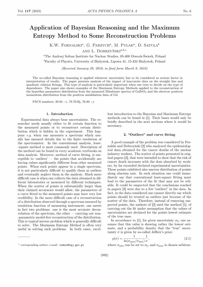
Fig. 1. Four examples of classical χ2 fitting (dottedlines) and the Bayesian one (solid lines). All pointsare simulated. The main trend was assumed to bey = 0.6x + 4.76.

An example of the straight line fitting is shown inFig. 1. In four parts of the figure one can see simulatedexperimental points scattered around assumed originaltrend yi = 0.6xi + 4.76, plus a number of points thatintentionally deviate markedly from the assumed trend.While the dotted lines present results of the classicalleast-squares fitting, the solid lines are obtained by meansof the Bayesian approach. To show the quality of agree-ment with the original trend, it is convenient to calculatethe value of the following parameter SA:

894 K.W. Fornalski et al.

SA =n∑

i=1

∣∣yd,i − yt,i

∣∣ , (2.10)

where yd,i denotes the value of the i-th point which follow

from the parameters of the fit, and yt,i its “ideal” value(here yt,i = 0.6xi +4.76). It is obvious that better recon-struction of the trend must have lower parameter SA.

TABLE IFitted parameters and parameters SA for both cases presented in Figs. 1 and 2.The least squares (χ2) and Bayesian methods were used.

CaseLinear (Fig. 1) Quadratic (Fig. 2)

χ2 method Bayes χ2 method Bayes

f(x)a = 0.29± 0.11

b = 9.94± 1.2

SA = 42.6

a = 0.59± 0.07

b = 5.04± 1.1

SA = 4.1

a = 0.17± 0.05

b = −1.79± 0.62

c = 14.77± 1.6

SA = 28.5

a = 0.19± 0.03

b = −2.19± 0.52

c = 15.21± 1.3

SA = 10.7

g(x)a = 0.39± 0.15

b = 12.11± 1.7

SA = 103.1

a = 0.58± 0.12

b = 4.73± 1.2

SA = 4.0

a = 0.14± 0.02

b = −1.06± 0.13

c = 12.66± 2.1

SA = 57.1

a = 0.16± 0.01

b = −1.44± 0.09

c = 10.87± 1.4

SA = 20.2

h(x)a = 0.48± 0.15

b = 11.57± 1.7

SA = 111.6

a = 0.35± 0.15

b = 18.68± 1.4

SA = 225.9

a = 0.07± 0.02

b = −0.18± 0.34

c = 13.24± 1.3

SA = 89.6

a = 0.05± 0.02

b = 0.66± 0.27

c = 10.60± 1.1

SA = 124.2

j(x)a = 0.36± 0.2

b = 9.62± 2.4

SA = 47.2

a = 0.58± 0.14

b = 4.47± 1.4

SA = 9.2

a = 0.12± 0.01

b = −1.12± 0.24

c = 14.74± 1.7

SA = 56.3

a = 0.16± 0.01

b = −1.52± 0.14

c = 10.75± 0.96

SA = 23.9

The first function (see Fig. 1) f(x) shows the resultsof fitting when only three apparent outliers are present.It is a common example of typical experimental eventwith some outliers. In such a case it would be justifiedto reject those three points and concentrate on remain-ing points only. It is shown that the Bayesian approachneeds not make such rejection in order to arrive at properresult, what is in good agreement with the results pre-sented in [1]. The g(x) and remaining functions containmuch more outliers (such data could come e.g. from dif-ferent laboratories). It is seen that in the first two casesthe Bayesian approach results in the fitted line which isvery close to the “true” one. In the third example h(x)the number of points which are away from the expectedtrend is larger than the number of “correct” points. Inthis particular case one can hardly differentiate between“correct” points and “outliers”. This is also seen in the re-sult of the Bayesian analysis, see parameter SA in Table I,which favors “outliers”. However, one can also see that insuch case the parameters SA obtained within the maxi-mum likelihood approach and the Bayesian one are notas different as in the other cases. In the last case j(x)although the number of “outliers” is high, they lie belowand above the trend. One can see, that from many op-tions of drawing single line, the Bayesian analysis selects

the points that most likely lie on a straight line or areclosest to such line. The last three cases are very seldomin practice. In fact, such data with large scatter appearin reality. The authors met such situation when theyanalyzed epidemiological data on the cancer mortalityamong nuclear workers [2].

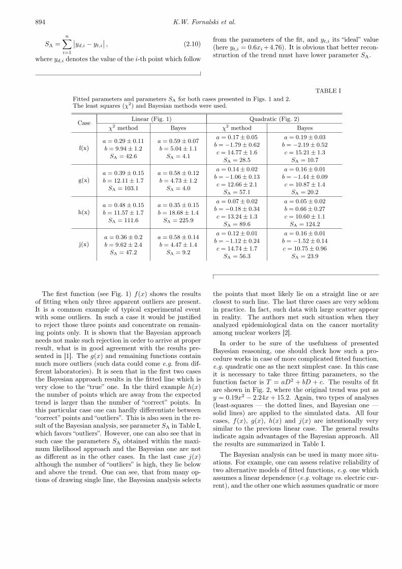
In order to be sure of the usefulness of presentedBayesian reasoning, one should check how such a pro-cedure works in case of more complicated fitted function,e.g. quadratic one as the next simplest case. In this caseit is necessary to take three fitting parameters, so thefunction factor is T = aD2 + bD + c. The results of fitare shown in Fig. 2, where the original trend was put asy = 0.19x2 − 2.24x + 15.2. Again, two types of analyses(least-squares — the dotted lines, and Bayesian one —solid lines) are applied to the simulated data. All fourcases, f(x), g(x), h(x) and j(x) are intentionally verysimilar to the previous linear case. The general resultsindicate again advantages of the Bayesian approach. Allthe results are summarized in Table I.

The Bayesian analysis can be used in many more situ-ations. For example, one can assess relative reliability oftwo alternative models of fitted functions, e.g. one whichassumes a linear dependence (e.g. voltage vs. electric cur-rent), and the other one which assumes quadratic or more

Application of Bayesian Reasoning and the Maximum Entropy Method . . . 895

Fig. 2. Four examples of classical χ2 fitting (dottedlines) and the Bayesian one (solid lines). All points aresimulated ones. They should reflect quadratic functiony = 0.19x2 − 2.24x + 15.2.

complicated dependences. Generally speaking, it is nec-essary to find the posterior (confidence) ratio for bothmodels and multiply it by so called “Ockham’s factor”,which prevent using of over-complicated model. As it wasshown in [1] and [2], if one model A has no parameter tofit, while a model B contains one parameter λ than theirrelative value can be calculated as follows. If λ turnedout to appear with the uncertainty δλ, while prior to thefitting we knew only that it must be contained within the(λmin, λmax) limits, the relative superiority of one modelA with respect to B is:

Wm =P (A|D, I)P (B|D, I)

=P (A|I)P (B|I)

P (D|A, I)P (D|λ0, B, I)

× λmax − λmin

δλ√

2π, (2.11)

where the first term describes our evaluation of the rel-ative importance of the models before doing the experi-ment, the second term is a ratio of likelihood functions,and the last term describes the “Ockham’s factor”.

3. Maximum Entropy Method: application tothe results of Mössbauer spectroscopy and 2DAngular Correlation of Annihilation Radiation

(ACAR)

The Maximum Entropy Method is used to constructthe prior in the form of exp(αS), where α is a parame-ter, and S is information entropy which is used often inthe form of cross-entropy, i.e.:

S = −∑

i

pi log(pi/mi) , (3.1)

where pi and mi describe searched and prior distribu-tions, respectively. In the simplest case one can use un-

informative (uniform) prior, i.e. mi = constant. This,however, is known to cause some unwanted features as itis presented e.g. in the case of charge-, spin- or electronmomentum-density distributions in solids [4].

The Mössbauer spectrum is described by many hy-perfine parameters (magnetic hyperfine field B, isomershift (IS), quadrupole splitting (QS)) that can have theirown distributions. In addition, the relative intensities ofspectroscopic lines may be determined by possible sam-ple texture and sample thickness effects. When theselast two effects are neglected one can use so-called thin--absorber approximation. In the simplest case one getssix Lorentzian lines in the measured spectra appearingat the source velocities:

v1 = B∗(3g3/2 − g1/2)/2 + QS + IS ,

v2 = B∗(g3/2 − g1/2)/2−QS + IS ,

v3 = B∗(−g3/2 − g1/2)/2−QS + IS ,

v4 = B∗(g3/2 + g1/2)/2−QS + IS ,

v5 = B∗(−g3/2+g1/2)/2−QS + IS ,

v6 = B∗(−3g3/2 + g1/2)/2 + QS + IS , (3.2)where the gyromagnetic factors for 57Fe nucleusare: g3/2 = −0.067897 mm/s/T, and g1/2 =0.118821 mm/s/T. The intensities of the lines are shownin Table II.

TABLE IILine intensities in Zeeman sextets in the case of unpolarizedas well as circularly polarized photons.

Line number Unpolarized radiation∗ Circularly polarizedradiation∗

1 I1 = 3(1 + c2)/16 I1 = 3(1 + c2 + 2c1)/16

2 I2 = (1− c2)/4 I2 = (1− c2)/4

3 I3 = (1 + c2)/16 = I1/3 I3 = (1 + c2 − 2c1)/16

4 I4 = I3 I4 = I1/3

5 I5 = I2 I5 = I2

6 I6 = I1 I6 = 3I3

∗ — where c1 = 〈cosΘ〉 and c2 = 〈cos2 Θ〉 with Θ being anangle between the direction of a photon and direction of themagnetization of the sample (the averaging runs over all possiblegrains and domains in the sample [5]).

A given i-th line contributes to the j-th channel in thevelocity spectrum the intensity proportional to:

Jj =Ii

(V (j)− vi)2 + (Γ/2)2, (3.3)

where Γ denotes the natural width of the line from Möss-bauer source. When the hyperfine parameters B, IS andQS have distributions described by a probability densityP(B, IS,QS) the Eq. (3.3) modifies to:

Jj =∫ ∫ ∫

P (B, IS, QS)

× Ii(V (j)− vi

)2 + (Γ/2)2dB dIS dQS , (3.4)

896 K.W. Fornalski et al.

where the range of integrals may always be reasonablychosen. In practice, the integral (3.4) is changed to asum: the whole 3D space is divided into pixels and one iscarrying out summation over the pixels seeking for valuesof Pi, where i denotes a linear parameter of a pixel. Fromthe form of (3.4) it is seen that such a reconstruction isformidable task.

The measured spectra are usually composed of 256points only, so any kind of least square method can besuccessfully applied only when the number of pixels isvery low, and when one deals with the one dimensionaldistribution or one can assume certain dependencies be-tween the hyperfine parameters, e.g. that the field Blinearly depends on isomer shift and quadrupole split-ting. In this situation Maximum Entropy Method is themethod of choice. The Maximum Entropy Method canbe effectively used for reconstruction of the hyperfineparameters distribution from the Mössbauer spectrum.This was shown in Refs. [6–8] on mimicked spectra. TheMEM analysis of experimental case of the experimentalspectrum measured for amorphous Fe-B alloy was firstpresented in the paper [9]. On the example of recentlyobtained data for GaFeO3 it is shown in the present paperthat three dimensional MEM analysis of the probabilitydistributions of hyperfine parameters can be carried outand the results are shown in Figs. 3–6. The spectrumitself [10] exhibits quite broadened lines. The broaden-ing can be due to the overlapping spectra arising fromdifferent lattice sites and possible different environmentof the sites. This broadening does not allow to determineuniquely hyperfine field parameters that can character-ize each of the sites occupied by iron. The reconstruc-tion by MEM (see Figs. 3–6) shows how much the realdistribution is collapsed when one wants to get infor-mation about hyperfine magnetic field (B), isomer shifts(IS), and quadrupole splitting (QS) connected with givencrystallographic site. Nevertheless, knowing that MEMproduces as much diffuse maps as possible. Obtainedreconstruction gives certain limits for hyperfine field val-ues and may still be used as a starting point to the de-scription of the measured spectra as a sum of spectraconnected with given crystallographic sites. In this case,however, it is not possible to avoid a number of assump-tions that may turn out to be invalid. The distributionsobtained by MEM are directly making full use of the ex-perimental data and show what we really know withoutmaking reference to any model.

It can be noticed that in spite of certain noise presentin the figures (that appears mainly at the borders ofthe analyzed region of hyperfine parameters), they im-ply that one can hardly speak about linear dependenciesbetween hyperfine parameters. Such correlations are typ-ically assumed in the conventional analysis of the Möss-bauer spectra with hyperfine fields distributions. Thedistributions show that the spectra are most generallyinterpreted in terms of the hyperfine parameters distri-butions that can be correlated, but the way they are cor-related is not described by a simple linear function. The

Fig. 3. The distribution of probabilities of hyperfineparameters in GaFeO3 in B-IS plane from the measure-ments at 14 K as obtained by MEM. P(B, IS) denotesthe probability distribution obtained as a sum of thedistributions for all quadrupole splittings.

Fig. 4. Similar in B-QS plane at 14 K. The distributionis a sum of the distributions for all IS.

spectrum itself can also be analyzed by fitting four or fiveindividual spectra to the measured spectrum, but, as itfollows from the figures, the parameters fitted in this waycan be put to doubts. However, if one wishes to do that,the MEM results offer at least the limits of the fit pa-

Fig. 5. Reconstruction (by MEM) of the distributionat T = 14 K in B-IS plane shown in the 2D contourplot.

Application of Bayesian Reasoning and the Maximum Entropy Method . . . 897

Fig. 6. Reconstruction (by MEM) of the distributionat T = 100 K in B-IS plane.

rameters. In the particular case of GaFeO3 the spectrumquite rapidly broadens with increase of the temperature.The differences of the P(B, IS) distributions at T = 14 Kand T = 100 K are shown in 2D contour plots in the nexttwo figures. Apparent broadening of the spectra at hightemperature is clearly seen.

Another novel example of application of MEM to re-construction of the electron–positron momentum distri-bution is given below. In the experiment are injectedpositrons into the material of interest. The positrons arethermalized in the matter and could annihilate with elec-trons producing two annihilation quanta. If the positron--electron pair had zero momentum, the quanta would beemitted at 180◦ with respect to each other. Because thereis always certain momentum distribution ρ(p) of suchpair, one observes distribution of angles through whichthe annihilation quanta appear. The 2D ACAR data aredescribed by:

N(px, py) =∫

ρ(p)dpz , (3.5)

where p is momentum of annihilating positron-electronpair. The data are measured for various values of pz alongmany directions in (px, py)-plane. Therefore, one can re-construct the momentum distribution ρ(px, py; pz) in theplane perpendicular to pz. The MEM analysis was car-ried out on the data for Gd, measured by R.L. Waspe andR.N. West [11], and deconvoluted (also by MEM [12]) byFretwell et al. [13].

Maximization of entropy should be carried out undercertain constraints Φk(ρ), which, added to Eq. (3.5), re-sult in Lagrangian:

L = −∑

i

ρi log(ρi/ρ0

i

)−∑

k

λkΦk(ρ) , (3.6)

where k runs over the number of constraints and λk

are Lagrange multipliers. The reconstructed densitymust also be normalized to certain value A, so Φ0(ρ) =∑

i ρi − A. The constraints may be chosen so to ensure

that every experimental value Ek differs from the recon-structed one:

Tk =∑

j

rkjρj , (3.7)

(rkj — transformation matrix elements), by not morethan the uncertainty σk assigned to the experimentalpoint: (Tk − Ek)2 ≤ σ2

k. However, instead of usingmany Lagrange multipliers one uses mainly only singleconstraint, namely, that a misfit function:

χ2 =∑

k

(Tk − Ek)2 /σ2 ≤ const , (3.8)

where const is chosen close to the number of experimen-tal points. Finally, the following equation for density isobtained:

ρi = Aρ0

i exp(− 1

2α∂χ2

∂ρi

)

∑i ρ0

i exp(− 1

2α∂χ2

∂ρi

) , (3.9)

where α denotes Langrange multiplier appearing in theprior exp(αS).

Fig. 7. Electron–positron momentum distribution inGd for pz = 0. The experimental data used were cor-rected for resolution [10]. The first Brillouin zone ismarked by white dashed line.

Figure 7 shows the reconstruction of the positron--electron momentum distribution from 16 directions mea-sured in pz = 0 plane [12]. The first Brillouin zone (BZ)was also depicted (white line). Again, one notices veryclear shape of this distribution and low level of noise.Moreover, one can observe an increase of density of iso-lines at the borders of BZ.

Good reconstruction of the electron–positron momen-tum density turns out to be obtained with much smallernumber of directions. Figure 8 shows comparison of theresults obtained on the grounds of experimental datafrom 6 projections (6 different directions from ΓM toΓK) and 16 projections with 6-projection reconstructiontreated as a prior. Only little difference between bothpanels can be observed for medium momentum range.General shape and character of acquired distribution

898 K.W. Fornalski et al.

Fig. 8. Electron–positron momentum distribution inGd for pz = 0. Comparison of reconstructions from 6(left panel) and 16 projections (right panel).

stayed untouched. Also position of the steepest slope atthe BZ is not changed. The difference between these den-sities, relative to the result obtained from 16-projectionis presented in Fig. 9. Only one bigger cusp can be ob-served, however, its position corresponds to rather lowlevel of density and could not be noticed in Fig. 8, wherethis area is presented as a background.

Fig. 9. Relative difference between 6- and 16--projection electron–positron momentum distributionin Gd for pz = 0.

Above situation reveals how useful and powerful is theMaximum Entropy Method technique. Even incompleteset of experimental data (less than half of available pro-jections) is sufficient for correct reconstruction. Natu-rally, too modest data may lead to improper results andsome important details may be lost during reconstruc-tion.

This kind of reconstructions can be used for determi-nation of the shape of Fermi surfaces without the need offitting a number of parameters when the distribution isrepresented as a series in symmetry-adapted harmonics,see [14–16].

4. Conclusions

The paper present a few novel applications of theBayesian reasoning and the Maximum Entropy Methodto true experimental problems. In all cases it is shownthe powerfulness of these techniques, even in such dif-ficult cases like 3D reconstruction of the hyperfine fieldparameters from a 1D Mössbauer spectrum.

Acknowledgments

We are very grateful to Prof. R.N. West for makingavailable his experimental 2D ACAR spectra for Gd, toDr A. Alam and Dr S. Dugdale for their deconvoluteddata. We wish to express our gratitude to professorsH. Fuess and K. Szymański for their agreement to pub-lish the results of preliminary analysis of the data onGaFeO3, and to Prof. G. Kontrym-Sznajd for very stim-ulating discussion of the case of Gd.

References

[1] D.S. Sivia, J. Skilling, Data Analysis. A BayesianTutorial, Oxford University Press, 2006.

[2] K.W. Fornalski, L. Dobrzyński, Int. J. Low Rad. 6,57 (2009).

[3] M. Vrijheid, E. Cardis, M. Blettner, E. Gilbert,M. Hakama, C. Hill, G. Howe, J. Kaldor, C.R. Muir-head, M. Schubauer-Berigan, T. Yoshimura,Y.O. Ahn, P. Ashmore, A. Auvinen, J.M. Bae,H. Engels, G. Gulis, R.R. Habib, Y. Hosoda,J. Kurtinaitis, H. Malker, M. Moser, F. Rodriguez--Artalejo, A. Rogel, H. Tardy, M. Telle-Lamberton,I. Turai, M. Usel, K. Veress, Radiat. Res. 167,361 (2007); I. Thierry-Chef, M. Marshall, J.J. Fix,F. Bermann, E.S. Gilbert, C. Hacker, B. Heinmiller,W. Murray, M.S. Pearce, D. Utterback, K. Bernar,P. Deboodt, M. Eklof, B. Griciene, K. Holan,H. Hyvonen, A. Kerekes, M.C. Lee, M. Moser,F. Pernicka, E. Cardis, ibid., p. 380; E. Cardis,M. Vrijheid, M. Blettner, E. Gilbert, M. Hakama,C. Hill, G. Howe, J. Kaldor, C.R. Muirhead,M. Schubauer-Berigan, T. Yoshimura, F. Bermann,G. Cowper, J. Fix, C. Hacker, B. Heinmiller, M. Mar-shall, I. Thierry-Chef, D. Utterback, Y.O. Ahn,E. Amoros, P. Ashmore, A. Auvinen, J.M. Bae,J. Bernar, A. Biau, E. Combalot, P. Deboodt,A. Diez Sacristan, M. Eklöf, H. Engels, G. Engholm,G. Gulis, R.R. Habib, K. Holan, H. Hyvonen,A. Kerekes, J. Kurtinaitis, H. Malker, M. Martuzzi,A. Mastauskas, A. Monnet, M. Moser, M.S. Pearce,D.B. Richardson, F. Rodriguez-Artalejo, A. Rogel,H. Tardy, M. Telle-Lamberton, I. Turai, M. Usel,K. Veress, ibid., p. 396.

[4] L. Dobrzyński, in X-ray Compton Scattering, Eds.M.J. Cooper, P.E. Mijnarends, N. Shiotani, N. Sakai,A. Bansil, Oxford University Press 2004, p. 188.

Application of Bayesian Reasoning and the Maximum Entropy Method . . . 899

[5] K. Szymański, L. Dobrzyński, D. Satuła, B. Kalska--Szostko, in: Material Reseach in Atomic Scaleby Mössbauer Spectroscopy, Eds. by M. Mashlan,M. Miglierini, P. Schaaf, Vol. 94, Kluwer AcademicPublishers, Dordrecht 2003, p. 317.

[6] R.A. Brand, G. Le, Caer, Nucl. Instr. Methods Phys.Res. 34, 272 (1988).

[7] L. Dobrzyński, K. Szymański, D. Satuła, Nukleonika49 Suppl. 3, S89 (2004).

[8] L. Dobrzyński, A. Holas, D. Satuła, K. Szymański,in Proc. 26th International Workshop on BayesianInference and Maximum Entropy Methods in Sci-ence and Engineering, Ed. A. Mohamad-Djafari, AIPConf. Proc. 872, 511 (2006).

[9] P.M. Bentley, S.H. Kilcoyne, J. Phys.; Condens. Mat-ter 18, 7751 (2006).

[10] M. Bakr, A. Senyshyn, H. Wang, G. Parzych,L. Dobrzyński, K. Szymański, H. Fuess, poster pre-sented during XX International School on Physicsand Chemistry of Condensed Master, July 4–11,Białowieża, Poland (2009).

[11] R.L. Waspe, R.N. West, Positron Annihilation, Eds.P.G. Coleman, S.C. Sharma, L.M. Diana, North--Holland Publishing Company, 1982 p. 328.

[12] S.B. Dugdale, Ph.D. Thesis, University of Bristol,1996 (unpublished).

[13] H.M. Fretwell, S.B. Dugdale, M.A. Alam, M. Biasini,L. Hoffmann, A.A. Manuel, Europhys. Lett. 32, 771(1995).

[14] A. Alam, R.L. Waspe, R.N. West, Positron Annihila-tion, Ed. L. Dorikens-Vanpraet, World-Scientific, Sin-gapore 1988, p. 242.

[15] G. Kontrym-Sznajd, M. Samsel-Czekała, Appl.Phys. A 70, 89 (2000).

[16] G. Kontrym-Sznajd, Fizika Nizkikh Temperatur 35,765 (2009); G. Kontrym-Sznajd Low Temp. Phys. 35,599 (2009).