Application and comparison of wind speed sampling methods for wind generation in reliability studies...

EUROPEAN TRANSACTIONS ON ELECTRICAL POWEREuro. Trans. Electr. Power 2009; 19:1002–1015Published online 25 July 2008 in Wiley InterScience
(www.interscience.wiley.com) DOI: 10.1002/etep.278
*CyE-

Co

Application and comparison of wind speed sampling methods for wind generationin reliability studies using non-sequential Monte Carlo simulations

F. Vallee*,y, J. Lobry and O. Deblecker

Faculte Polytechnique de Mons, Department of Electrical Engineering Bvd. Dolez, 31 B-7000 MONS, Belgium

SUMMARY

Given the actual context of increased dispersed generation and highly loaded lines, probabilistic methods are more and more required to take intoaccount the stochastic behavior of electrical network components (possible spate of outages by use of the electrical network near its physical limits)in reliability studies. To implement those probabilistic methods, numerical Monte Carlo simulations are typically used and can be divided in twocategories: sequential and non-sequential techniques.

This paper deals with two wind speed sampling methods adapted for non-sequential Monte Carlo simulations, among which an originalapproach based on the combination of a mean statistical law (for a large geographical area like a country) and Normal distributions (to characterizesmaller wind speed zones inside the country). Both proposed techniques are then applied on a self-developed non-sequential Monte Carlosimulation only taking into account generation units outages and load changes (hierarchical level HL-I). Finally, the collected simulation resultsallow, not only, to evaluate the impact of sampling methods on the collected reliability indices but also to decide which proposed technique will leadto the most interesting situations (larger wind power fluctuations from one state to the other) for the electrical network operation management. Notethat our simulations are applied to the Belgian production park. Copyright # 2008 John Wiley & Sons, Ltd.

key words: Weibull distributions; wind energy; reliability; adequacy evaluation; Monte Carlo simulation

1. INTRODUCTION

The major characteristic of a Monte Carlo method is to simulate the random behavior of the considered electrical system. Typically,

two kinds of Monte Carlo simulations can be found in the literature, based on the stochastic dependence between consecutive states.

In that context, the introduction of wind models in an electrical network reliability study will have to be imagined in agreement with

the chosen Monte Carlo method. In case of a non-sequential approach (consecutive states totally independent), a random wind speed

drawing is to be implemented to model wind generation in the proposed reliability study.

In this paper, two wind speed sampling methods well adapted for non-sequential Monte Carlo simulations are applied in a

reliability study limited to hierarchical level I (HL-I) [1].

Here, the focus is more particularly axed on an original sampling method based on the combination of a single mean distribution

for the considered country and of normal noises N(m,s) to particularize smaller wind regions inside the country. This new method is

then compared with a classical one funded on the inversion of Weibull Cumulative Distribution Functions.

The paper will thus be organized as follows. After a brief description of the existing sampling method, advantages and drawbacks

to be associated with this solution are listed tending to demonstrate the interest (especially when the geographical correlation level

between wind parks is to be taken into account) of defining a new sampling method. This last one is based on the computation of a

global statistical distribution and on the characterization of each considered wind region with a particular normal noise. Finally, both

wind speed sampling methods are introduced in an HL-I reliability study and, in that way, applied to the Belgian wind park that was

orrespondence to: F. Vallee, Faculte Polytechnique de Mons, Department of Electrical Engineering Bvd. Dolez, 31 B-7000 MONS, Belgium.mail: [email protected]

pyright # 2008 John Wiley & Sons, Ltd.

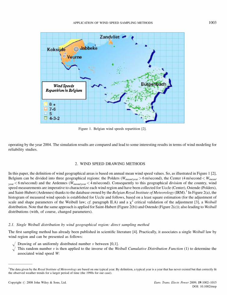
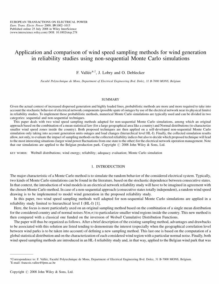
Figure 1. Belgian wind speeds repartition [2].

APPLICATION OF WIND SPEED SAMPLING METHODS 1003

operating by the year 2004. The simulation results are compared and lead to some interesting results in terms of wind modeling for

reliability studies.

2. WIND SPEED DRAWING METHODS

In this paper, the definition of wind geographical areas is based on annual mean wind speed values. So, as illustrated in Figure 1 [2],

Belgium can be divided into three geographical regions: the Polders (Wmean/year> 6 m/second), the Center (4 m/second<Wmean/

year< 6 m/second) and the Ardennes (Wmean/year< 4 m/second). Consequently to this geographical division of the country, wind

speed measurements are imperative to characterize each wind region and have been collected for Uccle (Center), Ostende (Polders),

and Saint-Hubert (Ardennes) thanks to the database owned by the Belgian Royal Institute of Meteorology (IRM).1 In Figure 2(a), the

histogram of measured wind speeds is established for Uccle and follows, based on a least square estimation (for the adjustment of

scale and shape parameters of the Weibull law; cf. paragraph II.A) and a x2 critical validation of the adjustment [3], a Weibull

distribution. Note that the same approach is applied for Saint-Hubert (Figure 2(b)) and Ostende (Figure 2(c)); also leading to Weibull

distributions (with, of course, changed parameters).

2.1. Single Weibull distribution by wind geographical region: direct sampling method

The first sampling method has already been published in scientific literature [4]. Practically, it associates a single Weibull law by

wind region and can be presented as follows:

1Tthe

Co

H D

he dob

pyri

rawing of an uniformly distributed number n between [0,1].

H T
his random number n is then applied to the inverse of the Weibull Cumulative Distribution Function (1) to determine the
associated wind speed W:

ata given by the Royal Institute of Meteorology are based on one typical year. By definition, a typical year is a year that has never existed but that correctly fitserved weather trends for a larger period of time (the 1990s for our case).

ght # 2008 John Wiley & Sons, Ltd. Euro. Trans. Electr. Power 2009; 19:1002–1015

DOI: 10.1002/etep

0 2 4 6 8 10 12 14 16 18 200

0.02

0.04

0.06

0.08

0.1

0.12

0.14Density of probability histogram for Ostende (based on IRM data)

Wind speed (m/s)

Den

sity

of p

roba

bilit

y

Density of probability histogram

(c)

0 2 4 6 8 10 12 14 16 18 200

0.02

0.04

0.06

0.08

0.1

0.12

0.14

0.16Density of probability histogram for Uccle (based on IRM data)

Wind speed (m/s)

Den

sity

of p

roba

bilit

y

Density of probability historgram

0 2 4 6 8 10 12 14 16 18 200

0.05

0.1

0.15

0.2

0.25

Wind speed (m/s)

Den

sity

of p

roba

bilit

y

Density of probability histogram for Saint-hubert (based on IRM data)

Density of probability histogram

(a) (b)

Figure 2. Probability density histogram (based on IRM data) established for Uccle (a), Saint-Hubert (b), and Ostende (c).

Copyri

1004 F. VALLEE, J. LOBRY AND O. DEBLECKER

W ¼ A ð�ln ð1 � vÞÞ1B

h i(1)

with, A the scale parameter and B the shape parameter.

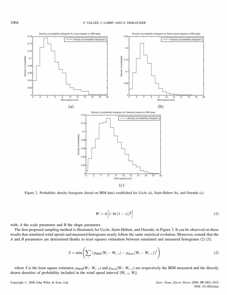
The first proposed sampling method is illustrated, for Uccle, Saint-Hubert, and Ostende, in Figure 3. It can be observed on these

results that simulated wind speeds and measured histograms nearly follow the same statistical evolution. Moreover, remark that the

A and B parameters are determined thanks to least squares estimation between simulated and measured histograms (2) [3].

S ¼ minXi

ð pIRMðWi �Wi�1Þ � pdrawðWi �Wi�1ÞÞ2

!(2)

where S is the least square estimator, pIRM(Wi�Wi�1) and pdraw(Wi�Wi�1) are respectively the IRM measured and the directly

drawn densities of probability included in the wind speed interval [Wi�1, Wi].


DOI: 10.1002/etep

0 2 4 6 8 10 12 14 16 18 200

0.02

0.04

0.06

0.08

0.1

0.12

0.14

0.16

Wind Speed (m/s)

Den

sity

of

prob

abili

ty

Validation of the direct drawing method with Uccle optimal parameters

IRM density of probability histogramSimulated density of probability histogramWeibull density of probability : A = 6.1 et B = 1.8

0 2 4 6 8 10 12 14 16 18 200

0.05

0.1

0.15

0.2

0.25Weibull direct drawing method with optimal parameters for St Hubert : Validation

Wind Speed (m/s)

Den

sity

of

prob

abili

ty

IRM measured histogramSimulated histogramWeibull density of probability : A = 4.85 et B = 2.3

(a) (b)

0 2 4 6 8 10 12 14 16 18 200

0.02

0.04

0.06

0.08

0.1

0.12

0.14Weibull direct drawing method with optimal parameters for Ostende : Validation

Wind Speed (m/s)

Den

sity

of

prob

abili

ty

IRM histogramSimulated histogramWeibull density of probability : A = 7.6 et B = 2.25

(c)

Figure 3. Direct drawing method for Uccle (a), Saint-Hubert (b), and Ostende (c).


Also note that this first proposed drawing method is classically justified by a property of Cumulative Distribution Functions that

implies to find back the initial statistical law by a uniform drawing on the distribution function if this last one is well adjusted. In that

way, our least squares adjustment has been critically validated by use of a x2 statistical test [3].

However, even if justified and validated, this classical sampling method presents some drawbacks:

Co

H I

pyri

ndeed, the correlation level to be associated between each wind park of the same region must be discussed. If we refer to the

worst case, a complete dependence between wind parks (a single wind speed drawn for each region) must be considered, as it

will lead to greater wind power fluctuations from one simulated hour to the other [4]. Nevertheless, by definition of the direct

sampling method and, as a different Weibull distribution is associated to each wind region (inside the same country), there will

always be an independency level between wind regions related to the use of the direct sampling method.

H M
oreover, each geographical region is here based on an identical annual mean wind speed value. Given the narrowness of
Belgium, the choice of a single Weibull distribution for each of these regions can be justified as the distribution of hourly wind

speeds around the annual mean wind speed will be approximately the same all over each considered region. On the opposite, in


DOI: 10.1002/etep

Copyri


case of a larger country (and, thus, possible larger wind regions inside this country), the association of a single Weibull law for

each wind region (being still based on an identical annual mean wind speed) could lead to errors as, for possibly larger wind

speed regions inside the considered country, the distribution of hourly wind speeds can change from one site to the other in the

same wind region (even if the same annual mean wind speed is still calculated all over the wind region) and, thus, a single

Weibull law associated to each defined wind region is no more sufficient in this last case.

2.2. Combination of a mean distribution and of a normal noise N(m,s) characteristic of each wind region

To introduce a dependency level between wind regions inside the country, the idea is to introduce a mean distribution for the entire

country and to particularize this last one by adding, for each wind region (inside the considered country), a normal noise (the normal

noise parameters being different for each wind region) to the single drawn mean wind speed. This mean distribution is, here,

obtained by calculating, for each hour, the arithmetical mean wind speed between the IRM data for the three considered sites (Uccle,

Ostende, and Saint-Hubert). We, so, compute 8760 (IRM data are given, on hourly basis for a single typical year) hourly mean wind

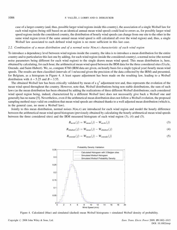
speeds. The results are then classified (intervals of 1 m/second given the precision of the data collected by the IRM) and presented,

for Belgium, as a histogram in Figure 4. A least square adjustment has been made on the resulting law, leading to a Weibull

distribution with A¼ 5.25 and B¼ 3.55.

The obtained Weibull law has been critically validated by mean of a x2 adjustment test and, thus represents the evolution of the

mean wind speed throughout the country. However, note that, Weibull distributions being non stable distributions, the sum of such

laws (as the mean distribution has been obtained by adding the realizations of three different Weibull distributions; each considered

wind speed region being, indeed, characterized by a different Weibull law) does not necessarily give back a Weibull one and

generally has no name [5]. Nevertheless, even if the arithmetical mean distribution does not follow a Weibull evolution, the proposed

sampling method stays valid on condition that mean wind speeds are obtained thanks to a well adjusted mean distribution (which is,

in the general case, no more a Weibull law).

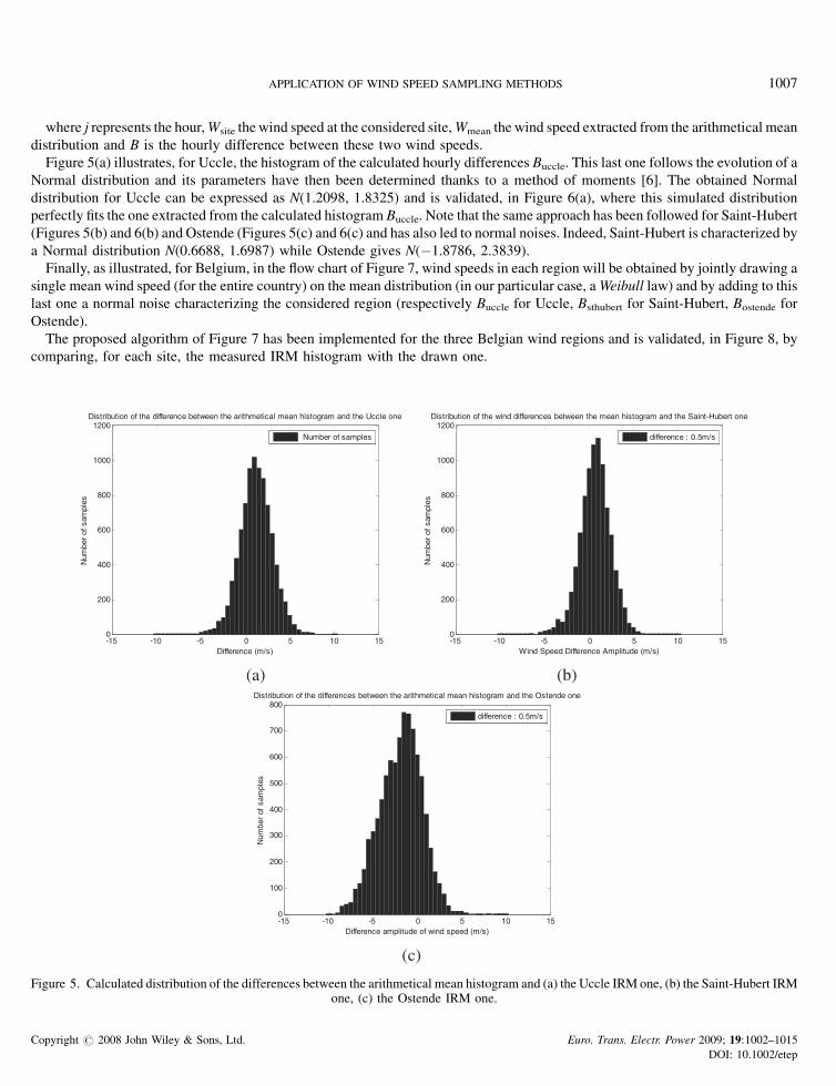
Jointly to this mean distribution, normal noises N(m,s) are introduced for each wind region and model the hourly difference

between the arithmetical mean wind speed histogram (previously obtained by calculating the hourly arithmetical mean wind speeds

between the three considered sites) and the IRM measured histogram of each wind region (3), (4) and (5).

Buccleð jÞ ¼ Wmeanð jÞ �Wuccleð jÞ (3)

Bsthubertð jÞ ¼ Wmeanð jÞ �Wsthubertð jÞ (4)

Bostendeð jÞ ¼ Wmeanð jÞ �Wostendeð jÞ (5)

0 2 4 6 8 10 12 14 16 18 200

0.05

0.1

0.15

0.2

0.25

0.3

0.35

Wind Speed (m/s)

Probability Density Validation

Calculated Histogram with 3 Belgian sites

Simulated Weibull Histogram

Simulated Weibull Probability Density

Figure 4. Calculated (blue) and simulated (dashed) mean Weibull histogramsþ simulated Weibull density of probability.


DOI: 10.1002/etep


where j represents the hour, Wsite the wind speed at the considered site, Wmean the wind speed extracted from the arithmetical mean

distribution and B is the hourly difference between these two wind speeds.

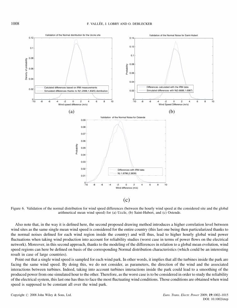
Figure 5(a) illustrates, for Uccle, the histogram of the calculated hourly differences Buccle. This last one follows the evolution of a

Normal distribution and its parameters have then been determined thanks to a method of moments [6]. The obtained Normal

distribution for Uccle can be expressed as N(1.2098, 1.8325) and is validated, in Figure 6(a), where this simulated distribution

perfectly fits the one extracted from the calculated histogram Buccle. Note that the same approach has been followed for Saint-Hubert

(Figures 5(b) and 6(b) and Ostende (Figures 5(c) and 6(c) and has also led to normal noises. Indeed, Saint-Hubert is characterized by

a Normal distribution N(0.6688, 1.6987) while Ostende gives N(�1.8786, 2.3839).

Finally, as illustrated, for Belgium, in the flow chart of Figure 7, wind speeds in each region will be obtained by jointly drawing a

single mean wind speed (for the entire country) on the mean distribution (in our particular case, a Weibull law) and by adding to this

last one a normal noise characterizing the considered region (respectively Buccle for Uccle, Bsthubert for Saint-Hubert, Bostende for

Ostende).

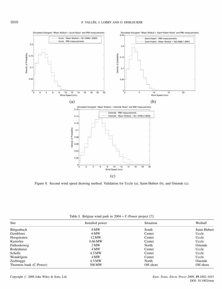
The proposed algorithm of Figure 7 has been implemented for the three Belgian wind regions and is validated, in Figure 8, by

comparing, for each site, the measured IRM histogram with the drawn one.

-15 -10 -5 0 5 10 150

200

400

600

800

1000

1200Distribution of the difference between the arithmetical mean histogram and the Uccle one

Difference (m/s)

Num

ber

of s

ampl

es

Number of samples

-15 -10 -5 0 5 10 150

200

400

600

800

1000

1200Distribution of the wind differences between the mean histogram and the Saint-Hubert one

Wind Speed Difference Amplitude (m/s)

Num

ber

of s

ampl

esdifference : 0.5m/s

(a) (b)

-15 -10 -5 0 5 10 150

100

200

300

400

500

600

700

800Distribution of the differences between the arithmetical mean histogram and the Ostende one

Difference amplitude of wind speed (m/s)

Num

ber

of s

ampl

es

difference : 0.5m/s

(c)

Figure 5. Calculated distribution of the differences between the arithmetical mean histogram and (a) the Uccle IRM one, (b) the Saint-Hubert IRMone, (c) the Ostende IRM one.

Copyright # 2008 John Wiley & Sons, Ltd. Euro. Trans. Electr. Power 2009; 19:1002–1015

DOI: 10.1002/etep

-10 -8 -6 -4 -2 0 2 4 6 8 100

0.02

0.04

0.06

0.08

0.1

0.12Validation of the Normal distribution for the Uccle site

Wind speed difference (m/s)

Den

sity

of

prob

abili

ty

Calulated differences based on IRM measurements

Simulated differences thanks to N(1.2098,1.8325) distribution

-10 -8 -6 -4 -2 0 2 4 6 8 100

0.02

0.04

0.06

0.08

0.1

0.12

0.14Validation of the Normal Noise for Saint-Hubert

Wind Speed Difference (m/s)

Pro

babi

lity

Differences calculated with the IRM data

Simulated differences with N(0.6688,1.6987)

(a) (b)

(c)

-10 -8 -6 -4 -2 0 2 4 6 8 100

0.01

0.02

0.03

0.04

0.05

0.06

0.07

0.08

0.09Validation of the Normal Noise for Ostende

Wind difference (m/s)

Pro

babi

lity

Differences with IRM data

N(-1.8786,2.3839)

Figure 6. Validation of the normal distribution for wind speed differences (between the hourly wind speed at the considered site and the globalarithmetical mean wind speed) for (a) Uccle, (b) Saint-Hubert, and (c) Ostende.


Also note that, in the way it is defined here, the second proposed drawing method introduces a higher correlation level between

wind sites as the same single mean wind speed is considered for the entire country (this last one being then particularized thanks to

the normal noises defined for each wind region inside the country) and will thus, lead to higher hourly global wind power

fluctuations when taking wind production into account for reliability studies (worst case in terms of power flows on the electrical

network). Moreover, in this second approach, thanks to the modeling of the differences in relation to a global mean evolution, wind

speed regions can here be defined on basis of the corresponding Normal distribution characteristics (which could be an interesting

result in case of large countries).

Point out that a single wind speed is sampled for each wind park. In other words, it implies that all the turbines inside the park are

facing the same wind speed. By doing this, we do not consider, as parameters, the direction of the wind and the associated

interactions between turbines. Indeed, taking into account turbines interactions inside the park could lead to a smoothing of the

produced power from one simulated hour to the other. Therefore, as the worst case is to be considered in order to study the reliability

of the electrical system, this last one has thus to face the most fluctuating wind conditions. Those conditions are obtained when wind

speed is supposed to be constant all over the wind park.


DOI: 10.1002/etep

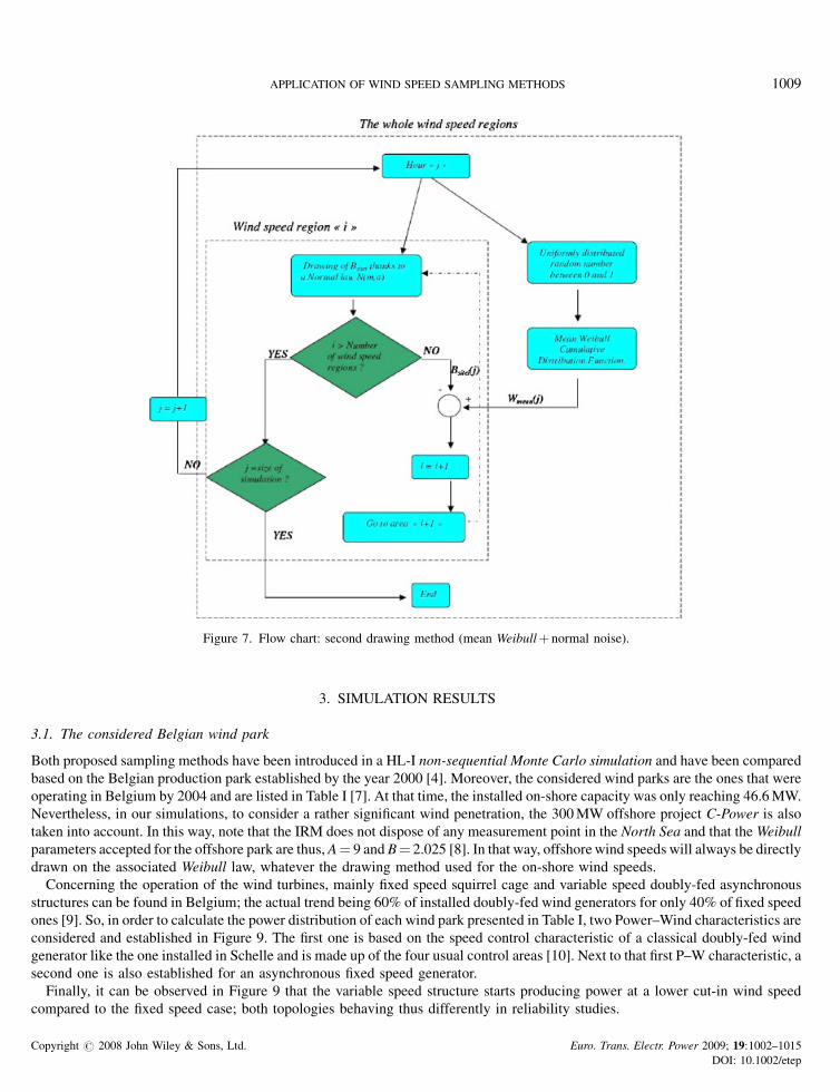
Figure 7. Flow chart: second drawing method (mean Weibullþ normal noise).


3. SIMULATION RESULTS

3.1. The considered Belgian wind park

Both proposed sampling methods have been introduced in a HL-I non-sequential Monte Carlo simulation and have been compared

based on the Belgian production park established by the year 2000 [4]. Moreover, the considered wind parks are the ones that were

operating in Belgium by 2004 and are listed in Table I [7]. At that time, the installed on-shore capacity was only reaching 46.6 MW.

Nevertheless, in our simulations, to consider a rather significant wind penetration, the 300 MW offshore project C-Power is also

taken into account. In this way, note that the IRM does not dispose of any measurement point in the North Sea and that the Weibull

parameters accepted for the offshore park are thus, A¼ 9 and B¼ 2.025 [8]. In that way, offshore wind speeds will always be directly

drawn on the associated Weibull law, whatever the drawing method used for the on-shore wind speeds.

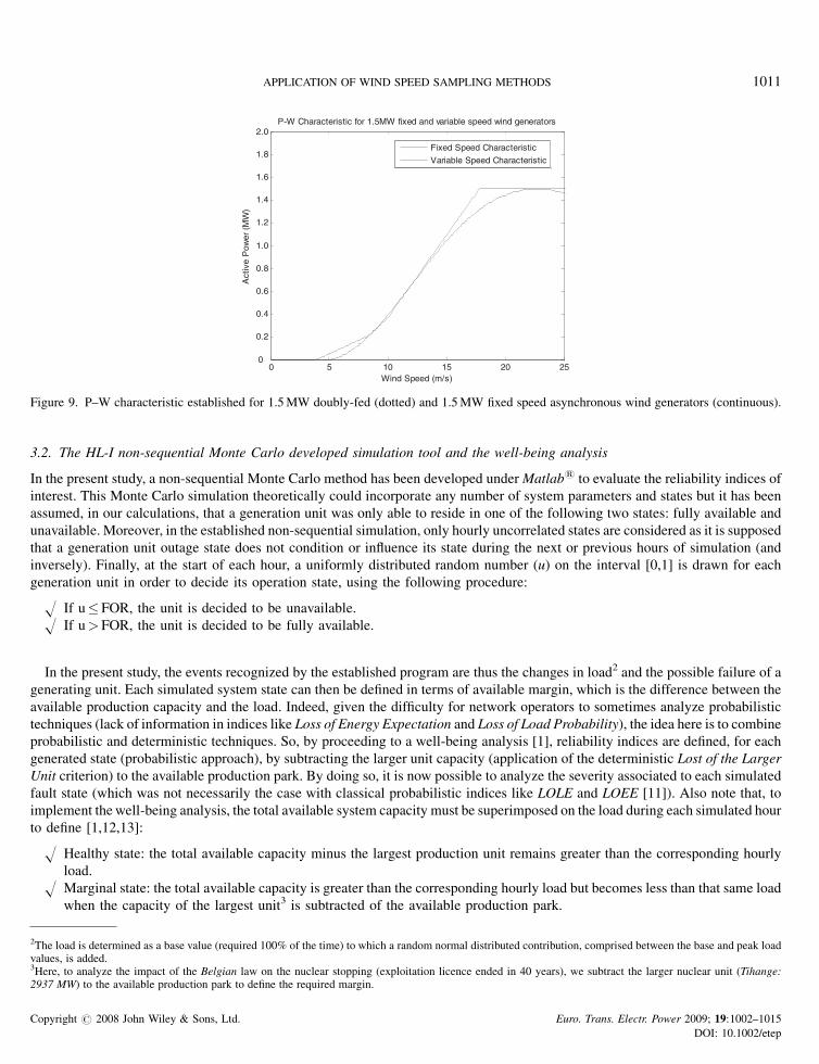
Concerning the operation of the wind turbines, mainly fixed speed squirrel cage and variable speed doubly-fed asynchronous

structures can be found in Belgium; the actual trend being 60% of installed doubly-fed wind generators for only 40% of fixed speed

ones [9]. So, in order to calculate the power distribution of each wind park presented in Table I, two Power–Wind characteristics are

considered and established in Figure 9. The first one is based on the speed control characteristic of a classical doubly-fed wind

generator like the one installed in Schelle and is made up of the four usual control areas [10]. Next to that first P–W characteristic, a

second one is also established for an asynchronous fixed speed generator.

Finally, it can be observed in Figure 9 that the variable speed structure starts producing power at a lower cut-in wind speed

compared to the fixed speed case; both topologies behaving thus differently in reliability studies.


DOI: 10.1002/etep

0 2 4 6 8 10 12 14 16 18 20 220

0.05

0.1

0.15

0.2

Wind Speed (m/s)

Den

sity

of

Pro

babi

lity

Simulated histogram "Mean Weibull + Uccle Noise" and IRM measurements

Uccle : Mean Weibull + N(1.2098,1.8325)

Uccle : IRM measurements

0 5 10 15 200

0.05

0.1

0.15

0.2

0.25

Den

sity

of

prob

abili

ty

Wind Speed (m/s)

Simulated histogram "Mean Weibull + Saint-Hubert Noise" and IRM measurements

Saint-Hubert : IRM measurements

Saint-Hubert : Mean Weibull + N(0.6688,1.6981)

(a) (b)

0 2 4 6 8 10 12 14 16 18 200

0.02

0.04

0.06

0.08

0.1

0.12

0.14

0.16Simulated histogram "Mean Weibull + Ostende Noise" and IRM measurements

Wind Speed (m/s)

Den

sity

of

Pro

babi

lity

Ostende : IRM measurements

Ostende : Mean Weibull + N(-1.8786,2.3839)

(c)

Figure 8. Second wind speed drawing method. Validation for Uccle (a), Saint-Hubert (b), and Ostende (c).

Table I. Belgian wind park in 2004þC-Power project [7].

Site Installed power Situation Weibull

Butgenbach 8 MW South Saint-HubertGembloux 6 MW Center UccleHoogstraten 12 MW Center UccleKasterlee 0.66 MW Center UcclePathoekeweg 3 MW North OstendeRodenhuize 4 MW Center UccleSchelle 4.5 MW Center UccleWondelgem 4 MW Center UccleZeebrugge 4.5 MW North OstendeThornton bank (C-Power) 300 MW Off-shore Off-shore


DOI: 10.1002/etep


0 5 10 15 20 250

0.2

0.4

0.6

0.8

1.0

1.2

1.4

1.6

1.8

2.0P-W Characteristic for 1.5MW fixed and variable speed wind generators

Wind Speed (m/s)

Act

ive

Pow

er (

MW

)

Fixed Speed Characteristic

Variable Speed Characteristic

Figure 9. P–W characteristic established for 1.5 MW doubly-fed (dotted) and 1.5 MW fixed speed asynchronous wind generators (continuous).


3.2. The HL-I non-sequential Monte Carlo developed simulation tool and the well-being analysis

In the present study, a non-sequential Monte Carlo method has been developed under Matlab1 to evaluate the reliability indices of

interest. This Monte Carlo simulation theoretically could incorporate any number of system parameters and states but it has been

assumed, in our calculations, that a generation unit was only able to reside in one of the following two states: fully available and

unavailable. Moreover, in the established non-sequential simulation, only hourly uncorrelated states are considered as it is supposed

that a generation unit outage state does not condition or influence its state during the next or previous hours of simulation (and

inversely). Finally, at the start of each hour, a uniformly distributed random number (u) on the interval [0,1] is drawn for each

generation unit in order to decide its operation state, using the following procedure:

2Tva3H29

Co

H I

he loluesere,37 M

pyri

f u� FOR, the unit is decided to be unavailable.

H I
f u> FOR, the unit is decided to be fully available.
In the present study, the events recognized by the established program are thus the changes in load2 and the possible failure of a

generating unit. Each simulated system state can then be defined in terms of available margin, which is the difference between the

available production capacity and the load. Indeed, given the difficulty for network operators to sometimes analyze probabilistic

techniques (lack of information in indices like Loss of Energy Expectation and Loss of Load Probability), the idea here is to combine

probabilistic and deterministic techniques. So, by proceeding to a well-being analysis [1], reliability indices are defined, for each

generated state (probabilistic approach), by subtracting the larger unit capacity (application of the deterministic Lost of the Larger

Unit criterion) to the available production park. By doing so, it is now possible to analyze the severity associated to each simulated

fault state (which was not necessarily the case with classical probabilistic indices like LOLE and LOEE [11]). Also note that, to

implement the well-being analysis, the total available system capacity must be superimposed on the load during each simulated hour

to define [1,12,13]:

H H
ealthy state: the total available capacity minus the largest production unit remains greater than the corresponding hourly
load.

H M
arginal state: the total available capacity is greater than the corresponding hourly load but becomes less than that same load
when the capacity of the largest unit3 is subtracted of the available production park.

ad is determined as a base value (required 100% of the time) to which a random normal distributed contribution, comprised between the base and peak load, is added.to analyze the impact of the Belgian law on the nuclear stopping (exploitation licence ended in 40 years), we subtract the larger nuclear unit (Tihange:W) to the available production park to define the required margin.


DOI: 10.1002/etep

Co


H A

pyri

t risk state: the total available capacity is directly less than the corresponding hourly load value.

Three well-being indices are then defined as [2]

Probability of health ¼ PðHÞ ¼ nðHÞN � 8760

(6)

Probability of margin ¼ PðMÞ ¼ nðMÞN � 8760

(7)

Probability of risk ðLOLPÞ ¼ PðRÞ ¼ nðRÞN � 8760

(8)

where n(H), n(M), and n(R) are respectively the total number of hourly healthy, marginal and risky simulated states;N being the total

amount of simulated years.

3.3. Impact of wind production on the HL-I reliability

To quantify the impact of wind generation on the HL-I reliability of the Belgian electrical network, two case studies are investigated

and compared. So, in the first step, the developed Monte Carlo tool is launched with the entirely defined wind park (see Table I).

Then, to have a comparison point (in terms of ‘‘reliable’’ behavior) between wind production and classical units, a second approach

consists to replace each considered wind production park (cf. Table I) by a thermal unit (with the Forced Outage Rate of a thermal

unit equal to 0.025 [14]). The nominal power of each introduced thermal unit equals the installed capacity of the wind park that the

thermal unit replaces.

Also note that, when taking the entire wind production park into account, both proposed wind speed sampling methods are

applied. In our case, given the narrowness of Belgium, and to be in the worst case of highly fluctuating global wind energy, all the

wind parks of the same wind region are supposed to be entirely correlated. Consequently, this hypothesis implies that only one single

wind speed is drawn for each wind region and, thus, that:

H D
uring the considered hour, one different single random number is drawn, for each wind region (a single random number per
region), in case of Weibull direct sampling method.

H D
uring the considered hour, each of the three established different normal noises is applied to its corresponding wind region, in
case of ‘‘Mean WeibullþNormal Noise’’ sampling method.

The collected results are presented, for each considered case, in Table II. Several observations can be made on the basis of the

calculated ‘‘Well-being’’ indices:

H T
he introduction of an additional production unit (wind or thermal unit) reduces the risk of meeting critical situations of load
non-recovering. This observed fall of the LOLP values when adding an additional unit is quite logical as the installed capacity

is, in each case, increased while the load characteristics stay unchanged.

H T
he ‘‘Well-being’’ indices calculated with wind production are nearly equal, whatever sampling method be used. This result is
not surprising, here, in the way that both sampling techniques have been implemented to simulate the same experimental

histograms of wind densities of probability. However, note that the ‘‘MeanWeibullþNormal Noise’’ sampling method implies

a larger correlation level between wind regions and, thus, an increased ‘‘all or nothing’’ behavior for wind production.

Therefore, it is not surprising to observe, in this last case, slightly worsened LOLP and P(M) values. Indeed, with the ‘‘Mean

WeibullþNormal Noise’’ method, the drawing of a reduced mean wind speed will quasi immediately lead to a limited wind

production level all over the country, while the independency between wind regions involved by the direct drawing method

will, de facto, imply a smooth evolution for the global hourly wind production (and, thus, a better behavior from reliability

point of view).

H F
rom a reliability point of view, the fluctuating behavior of wind power makes this last one (LOLP¼ 0.0046) less efficient than
thermal production with an identical installed capacity (LOLP¼ 0.0038). Indeed, as illustrated in Figure 10, the simulated


DOI: 10.1002/etep

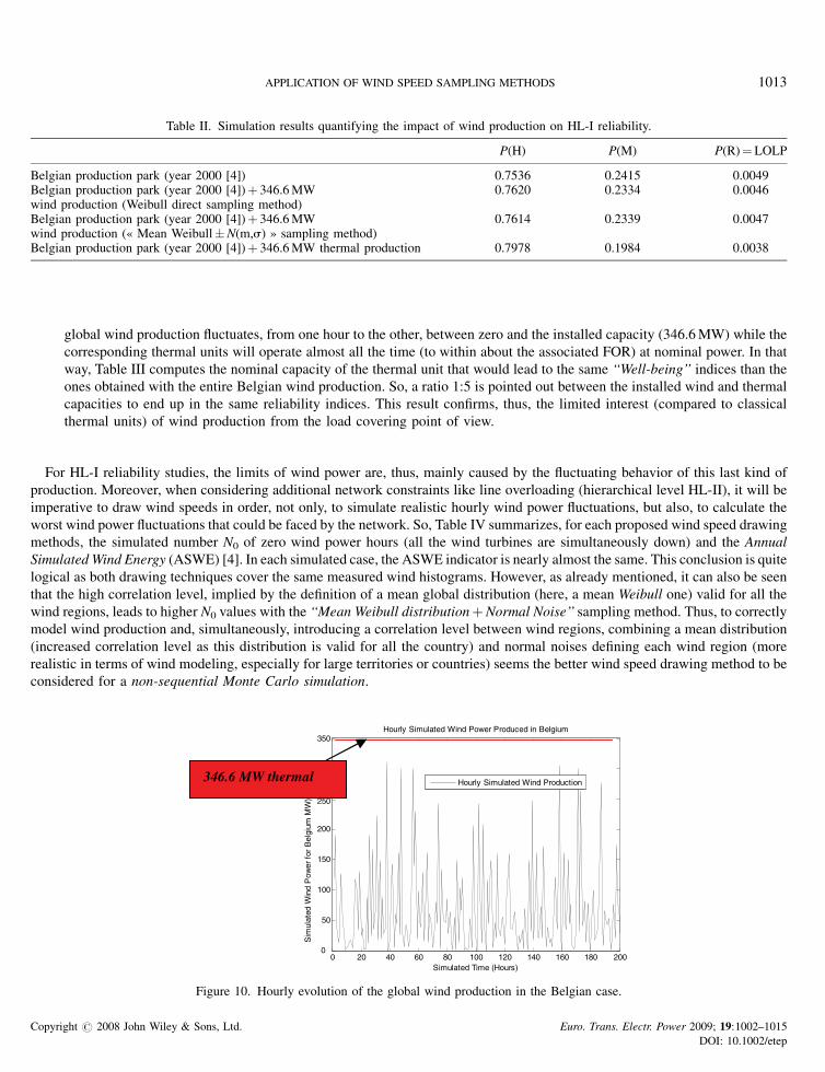
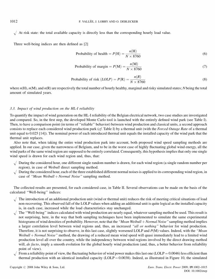
Table II. Simulation results quantifying the impact of wind production on HL-I reliability.

P(H) P(M) P(R)¼LOLP

Belgian production park (year 2000 [4]) 0.7536 0.2415 0.0049Belgian production park (year 2000 [4])þ 346.6 MWwind production (Weibull direct sampling method)

0.7620 0.2334 0.0046

Belgian production park (year 2000 [4])þ 346.6 MWwind production (« Mean Weibull�N(m,s) » sampling method)

0.7614 0.2339 0.0047

Belgian production park (year 2000 [4])þ 346.6 MW thermal production 0.7978 0.1984 0.0038

Copyri


global wind production fluctuates, from one hour to the other, between zero and the installed capacity (346.6 MW) while the

corresponding thermal units will operate almost all the time (to within about the associated FOR) at nominal power. In that

way, Table III computes the nominal capacity of the thermal unit that would lead to the same ‘‘Well-being’’ indices than the

ones obtained with the entire Belgian wind production. So, a ratio 1:5 is pointed out between the installed wind and thermal

capacities to end up in the same reliability indices. This result confirms, thus, the limited interest (compared to classical

thermal units) of wind production from the load covering point of view.

For HL-I reliability studies, the limits of wind power are, thus, mainly caused by the fluctuating behavior of this last kind of

production. Moreover, when considering additional network constraints like line overloading (hierarchical level HL-II), it will be

imperative to draw wind speeds in order, not only, to simulate realistic hourly wind power fluctuations, but also, to calculate the

worst wind power fluctuations that could be faced by the network. So, Table IV summarizes, for each proposed wind speed drawing

methods, the simulated number N0 of zero wind power hours (all the wind turbines are simultaneously down) and the Annual

Simulated Wind Energy (ASWE) [4]. In each simulated case, the ASWE indicator is nearly almost the same. This conclusion is quite

logical as both drawing techniques cover the same measured wind histograms. However, as already mentioned, it can also be seen

that the high correlation level, implied by the definition of a mean global distribution (here, a mean Weibull one) valid for all the

wind regions, leads to higher N0 values with the ‘‘Mean Weibull distributionþNormal Noise’’ sampling method. Thus, to correctly

model wind production and, simultaneously, introducing a correlation level between wind regions, combining a mean distribution

(increased correlation level as this distribution is valid for all the country) and normal noises defining each wind region (more

realistic in terms of wind modeling, especially for large territories or countries) seems the better wind speed drawing method to be

considered for a non-sequential Monte Carlo simulation.

0 20 40 60 80 100 120 140 160 180 2000

50

100

150

200

250

300

350

Simulated Time (Hours)

Sim

ulat

ed W

ind

Pow

er f

or B

elgi

um M

W)

Hourly Simulated Wind Power Produced in Belgium

Hourly Simulated Wind Production346.6 MW thermal

Figure 10. Hourly evolution of the global wind production in the Belgian case.


DOI: 10.1002/etep

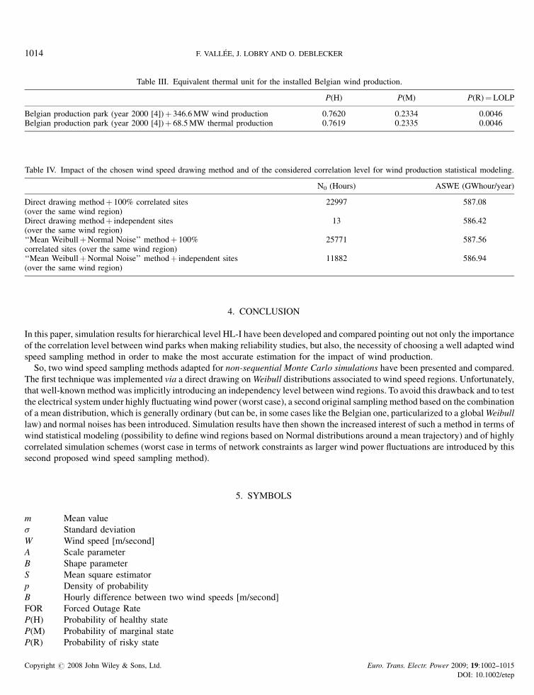
Table III. Equivalent thermal unit for the installed Belgian wind production.

P(H) P(M) P(R)¼LOLP

Belgian production park (year 2000 [4])þ 346.6 MW wind production 0.7620 0.2334 0.0046Belgian production park (year 2000 [4])þ 68.5 MW thermal production 0.7619 0.2335 0.0046

Table IV. Impact of the chosen wind speed drawing method and of the considered correlation level for wind production statistical modeling.

N0 (Hours) ASWE (GWhour/year)

Direct drawing methodþ 100% correlated sites(over the same wind region)

22997 587.08

Direct drawing methodþ independent sites(over the same wind region)

13 586.42

‘‘Mean WeibullþNormal Noise’’ methodþ 100%correlated sites (over the same wind region)

25771 587.56

‘‘Mean WeibullþNormal Noise’’ methodþ independent sites(over the same wind region)

11882 586.94


4. CONCLUSION

In this paper, simulation results for hierarchical level HL-I have been developed and compared pointing out not only the importance

of the correlation level between wind parks when making reliability studies, but also, the necessity of choosing a well adapted wind

speed sampling method in order to make the most accurate estimation for the impact of wind production.

So, two wind speed sampling methods adapted for non-sequential Monte Carlo simulations have been presented and compared.

The first technique was implemented via a direct drawing on Weibull distributions associated to wind speed regions. Unfortunately,

that well-known method was implicitly introducing an independency level between wind regions. To avoid this drawback and to test

the electrical system under highly fluctuating wind power (worst case), a second original sampling method based on the combination

of a mean distribution, which is generally ordinary (but can be, in some cases like the Belgian one, particularized to a global Weibull

law) and normal noises has been introduced. Simulation results have then shown the increased interest of such a method in terms of

wind statistical modeling (possibility to define wind regions based on Normal distributions around a mean trajectory) and of highly

correlated simulation schemes (worst case in terms of network constraints as larger wind power fluctuations are introduced by this

second proposed wind speed sampling method).

5. SYMBOLS

m M

Copyright #

ean value

s S
tandard deviation
W W
ind speed [m/second]
A S
cale parameter
B S
hape parameter
S M
ean square estimator
p D
ensity of probability
B H
ourly difference between two wind speeds [m/second]
FOR F
orced Outage Rate
P(H) P
robability of healthy state
P(M) P
robability of marginal state
P(R) P
robability of risky state
2008 John Wiley & Sons, Ltd. Euro. Trans. Electr. Power 2009; 19:1002–1015

DOI: 10.1002/etep


N T

Copyright #

otal number of simulated years

n(H) T
otal number of healthy state hours (hour)
n(M) T
otal number of marginal state hours (hour)
n(R) T
otal number of risky state hours (hour)
LOLP L
oss of Load Probability
ASWE A
nnual Simulated Wind Energy [GWhour/year]
N0 N
umber of zero wind power hours (hour)
ACKNOWLEDGEMENTS

The authors thank M. Stubbe, K. Karoui, and S. Rapoport from Tractebel Engineering (Suez) for their comments, suggestions, and support given tothis work.

REFERENCES

1. Karki R, Billinton R. Cost-effective wind energy utilization for reliable power supply. IEEE Transactions on Energy Conversion 2004; 19(2):435–440.2. Buyse H. Electrical Energy Production. Electrabel Documentation,UCL, 2004.3. Lawson CL, Hanson RJ. Solving least squares problems. Classics in Applied Mathematics 1974; Chap. 2, 15:30–45.4. Vallee F, Lobry J, Deblecker O. Impact of the wind geographical correlation level for reliability studies. IEEE Transactions on Power Systems 2007; 22(4):2232–

2239.5. Samorodnitsky G, Taqqu MS. Stable Non-Gaussian Random Processes; Stochastic Modeling, Chap. 1, CRC Press: New York, USA, 1994; 2–10.6. Hall AR. Generalized Method of Moments. Oxford University Press: Warwick, England, 2005; Chap. 1, pp 1–31.7. Electrabel. Belgian wind parks in MW (End 2004), Documentation Electrabel, 2005.8. Belgian Public Planning Service Science Policy. Optimal Offshore Wind Development in Belgium, 2003; Part 1, CP-21, pp 19–20.9. Robyns B. Vers une meilleure integration de l’eolien dans le reseau electrique grace a l’electronique de puissance, GREPES study day, March 2006.

10. Al Aimani S. Modelisation de differentes technologies d’eoliennes integrees a un reseau de distribution moyenne tension. These de l’Ecole Centrale de Lille2004; chap. 2, pp 24–25.

11. Patel J. Reliability/Cost Evaluation of a Wind Power Delivery System. Master of Science Thesis, Department of Electrical Engineering, University ofSaskatchewan, March 2006.

12. Barberis Negra N, Holmstrm O, Bak-Jensen B, Sorensen P. Aspects of relevance in offshore wind farm reliability assessment. IEEE Transactions on EnergyConversion 2007; 22(1):159–166.

13. Da Silva AML, De Resende LC, Da Fonseca Manso LA, Billinton R. Well-being analysis for composite generation and transmission systems. IEEE Transactionson Power Systems 2004; 19(4):1763–1770.

14. Raison B, Crappe M, Trecat J. Effets de la production decentralisee dans les reseaux electriques, Projet « Connaissance des emissions de CO2 », Sous-projet 5,Faculte Polytechnique de Mons, 2001.

2008 John Wiley & Sons, Ltd. Euro. Trans. Electr. Power 2009; 19:1002–1015

DOI: 10.1002/etep

Application and comparison of wind speed sampling methods for wind generation in reliability studies...

Documents

Transcript of Application and comparison of wind speed sampling methods for wind generation in reliability studies...