APPENDIX B STAFF PAPERS - DEVELOPMENT ...

EGYPT WATER USE AND MANAGEMENT PROJECT

MID-PROJECT REPORT

VOLUME I11

APPENDIX B STAFF PAPERS Section 3 of 4

by Egyptian and American Team

Cairo, ARE Ft. Collins, Colorado USA September 1980

Mid Project Report Volume 111

Appendix B S t a f f Papers

Section 3 of 4

Prepared under support o f United S t a t e s Agency f o r In te rna t iona l Development

Contract AID/NE-C-1351 A l l reported opinions, conclusions o r

recommendations a re those of the w r i t e ~ s and not those o f the funding

agency o f the United S t a t e s Government

Egyptian and American Team Members

Egypt Water Use and Management Projec t

Engineering Research Center Colorado S t a t e University Fort Col l ins , Colorado 80523 USA

22 E l Galaa S t ~ e e t Bulak, Cairo, ARE September 1980

Tablc o f Contents Volumc 111

S e c t i o n 1 of 4

STA l:l: I'Al'I~lt 1 1 . Sum~nary of Egypt Water Use and Management P r o j e c t wi th i ts

Accoml)lisl~ments by R . t i . Brooks and 11. Wahby, February 13, 1980

STAFI; PAl'l:R 11 2 A I '~ .c l . ie inary Comparison o f Two Cropping Scl~cmcs a t Abueha, Bliuyn Govcrnoratc Brondbeans - I:cr~ugrcck - Cotton vs Berseem - Cot ton 11)' Tllin S o r i n l and Gcne Q~rcncn~ocn, March 1980

s'rl4I;l~ l'Al'l:l< .3 ( 'P I -1) I I I S ~ C ~ S I>y Elwy A t a l l n , Flay 1980

S T I : m R 14 R i c c i n s e c t s by Elwy A t a l l a , May 1980

S'l'Al:l: l'Al'El< 11 5 blnjor F i c ld Crop I n s e c t s and Thc i r Control by Elwy A t a l l a , May I !)SO

STAFi; I'!\l3ER 11 6 ( h ~ t t h r o a t Flume Metr ic Equat ions by M. i l e l a l , May 1980

STAFF P,4l'l:R 11 7 Progrcss Report o f Rice P l a n t i n g T r i a l s a t Abou Raia , Kafr E l Sl)cikl~ C;ovcri~orate 1979 by M . Samire Abdel Azia, Ragy Darwish nntl Ccnc Qucncmoen, June 1980

STA1;F PAl'ltR !'8 Cnlculati.otr o f Machincry Costs f o r Egyptian Condit ions by blollalecd I lc ln l , Bayoumi Ahmed, Gilmal Ayad, , J i m L o f t i s , M . E, Qucncmoc~l and R , J . FfcConnen, December 1979

STAFF I 'API;I< n9 llol~cy Production a t Kafr E l Sheikh Governorate by Yusef Yusef

STAI:l; l'API:I< If 1 O An Ecoi~omic Evaluat ion o f Corn T r i a l s a t Abueha by E l i a S o r i a l , Apri l 1980

srrAw I~IPI :R I! I I I;cono~nic Costs o f Watcr Shortngcs Along Branch Canals hy S l~ innnwi , Mclvin D. Skold and Nohamcd Loutfy Nasr, June 1980

STAFI: I'AI'ER 11 1 2 Cost o f Production o f I r r i g a t e d Soybeans and Comparison with Cotton i n Egypt by M . E . Quenemoen, R . J . FlcConnen and Gamal Ayad, Scptemher 1979

Table o f Contcnts Volume I11 - Continucd

STAFF PAI'EII f1 1.3 Soc io log ica l Survey f o r Beni Clagdoul Area by Farouk Abdel A1

STAFF PlII'ER 114 l lntcr Budget f o r Beni Magdoul Area i n 1979 by Wadie Fahim

STAFF 1'Ar'I':R f1 15 Arl l i co~~o~~ i i c . Analysis f o r Squnsll T r i a l a t E l Hammami by M , Lotfy N n z r

S'I'A1:l: I'AI'I~II 11 I 0 I \ ~ ~ l icn~~o~iiic. Analysis f o r 'To~nnto Tri n l n t lln~n~nnmi by b l . ' 1,otfy N:I 5 1-

STA1:I.' I'AI'I~R !' I 7 'lllc [if fcct of So i l and Pes t blanngcmcnt on Farm Product ion, 1 . Sq11ash bv b1. Semaika and Harold Golus

Sl'A l:l: I'b 1'1: It 11 1 8 I t n t a t i o n Sys tcm o r Cont inuous Flow System f o r I r r i g a t i o n Canals i r i ligypt h y blona El Kady, John IVolfc, and D r . Hassan Wahhy

Sl'Al:l: 1'AI'l:R 11 1 !I An lit-ononiic Ar~nlys i s of Cahbagc T r i a l a t E l llammami f o r One 1:ctltlnn hy Blohamcd Lotfy Nasr and Carnal Fawzy

S'rAFl' Pll l ' l iR 11 20 1\11 liconor~i c Analysis f o r Wheat T r i a l a t Beni Magdoul by Mohamed 1.0 t. f y N:i s r

Table o f Cor~ tcn t s Volume I 1 1

Scct ion 2 o f 4

STAI:I: PAPER 1121 Itv;l t c.1- I,i f t ing hy Snkia: Tlic Iticrcmcntal Cost o f Cow Power, At1~1is t l ! ) R O

s*rAl;l: I'AI'I:II 11 2 2 SIII-vcy of Pcst s I n f c c t i ng Matisouri n Vcgctnbl c s and c rops (I3cni Mngtloul G E l llammami Arcns) Fl Thc i r Control by Elwy A t a l l a

STAI'I: PAPI:R 1\23 A Proccdurc f o r Eva lua t ing t h e Cost o f L i f t i n g Watcr f o r I r r i g a t i o n i l l 1:gypt I)y flnssan Wahby, Gene Quenemoen and Mohamed I l e l a l , June l?80

Table o f Contclits Volume I 1 1 - Colrtinucd

STAFF I'APEIt H24 Effcc t ivc. Extension f o r ~ ~ ~ p t i n n Ilural I)evclopment : Parmcrs and O f f i c i a l s 1 Views on A l t c m a t i v e S t r a t e g i e s by M, S . Sallam, E . C . Kliop and S . A . Knop

S7'AI:I: I'AI'I: R 25 l'optrlntion Growtll and Devclopmcnt i n Egypt : Farmcrs ' and Rural I~cvcloparc~it O f f i c i a l s Perspec t ives by C . C. Knop, M. S . Sallam ; I I I ~ S. A . Knop

STAFF PAPER 1126 I:;11-rn Rccortl Su~nmnry and A n n lys i s f o r Stucly Cnscs a t Ahu-Rnia and \ ln l i so~~r i a S-i tcs by Farouk Ahdcl A1 and Clclvin D . Skold, .July 19SO

S'I'AIyF PAPER f f 2 7 'Thc Bcrii blagdoul Watcr Budget Jariuary 1980 t o April 1980 by William 0 . Rce, Dan Sunada, Jim Ruff , June 1980

Tablc o f Contents Volumc IT1

Sect ion 3 of 4

STAFF PAPER 126 It011 c r Bcdshnper f o r Basin-Furrow I r r i g a t i o n by N , I l l s l e y and A . Chcema

STA1:F PAPEII 1129 lco~lornjc F e a s i b i l i t y of Concrete Lining f o r the B e n i Magdoul Canal a n d Branch Canal by Gamal Ayad, G . Nasr Far id , and Gcnc Qucncmocn , April 1978

STAFF PAPER H30 Programs f o r Ca lcu la to r s tip-67 and 11P-97 by Gamal A, Ayad !

STAI'T: P,\I'ER # 31 01i-l:arnl IVatcr Flanagcment Tnvcstig:tt ions i n Clansourin D i s t r i c t , 1 '.)7!)- 80 l)y .John Wolfc , Scptcml)er 1980

STAFI: I'Al'llR 32 Socjologicnl Data of thc P ro jcc t S i t c s : Somc C r i t e r i a f o r ~l~i t lcrs tnt id ing the Implementat ion Process by the Sociology 'I'c;lm, S c l ~ t c d ~ c r 1980

STAI~I: rAl'l:ll 11 33 Arlnlysis o f So i l Water Data Collcctecl from Winter Crops i n l i l Clill)la 1979-80 by Agronomy Discipl ille o f El Ffinya and Main Of f i ce Cairo Abdel S a t t a r , A . Taher 4 R . T ins ley

Tnble o f Contents Volume 111 - Continl~cd

STA1:I: PAl'Elt /I -34 llsc of C:llcn~ical F c r t i l i z c r s i n Mansouria Location by M . Zana t i , CI. 1,otfy f, G. Ayad, J u l y 1980

s+rAl:l: rvi71:ll 11 35 A p - i cul tur . ;~ 1 Pcs t s and T h e i r Control General Concepts by Llr. I:. A. 11. AtaI l a

S[',ll'l,' I'Al'l~Il l .36 (:c~rivc:!,:i~icc I,osscs i n Canals Ily I:nrouk Sllnhi n , F1. S a i f I s s n , l;i~:;li:li~~ I:s!::Ic :i~ld \li~di.c Faliim

STAI:I: l'i\l'IilZ 1; :Z 7 A S!.stcniatic Framework f o r I)cvelopmcnt o f So lu t ions by Flax K . I,owdcrmi l k , Apri 1 1980

SI'AFI' P!\I'I:R 4 35 I ~ c ! ; ~ ~ o ~ i s c o f Ricc, Illlent and Flax t o Zinc Appl ica t ions on t h e S o i l s c?f t lw N i l c Ilclta I)y A . I), Dotzcnko, F1, Z a n a t i , Abdel-tlnfez, A . Kclcg, A . 'I'. Floustnfa, A . Scr ry

S'I'AI:I: I'APIII1 II 3! ) I'vn l r l n t i o r~ o f Furrow I r r i g a t i o n Systems by Thomas IV. Ley and

c C I !. ma

STA1:l; I'Al'I~lt 114 0 1iv;iluation o f Cradcd Border I r r i g a t i o n Systems by Thomas W . I,cy ;ilid Itlnyne Clyma

Table o f Contents \~olume J I I

Scc t ion 4 o f 4

STAFF PAI'IiR 114 I 'I'llc Cost. of Dclivery o f I r r i g a t i o n Wntcr by Raymond L . A~lderson

S'l'Al:l: I 'AI ' I~IZ 114 2 Agi-omctcorol og i ca l S t a t i o n s f o r Crop Water Requirements by Richard Cilcnca, .January 1980

S.~AI;I: 1'Al)r:ll [I 3 S o i l Fcr t i l i t v Survcy o f Kafr E l Sheikh I , Phosphrus by Parviz Sol tanpour , January 1980

STAFT: I'AI'ER 6 4 4 So i l nntl l,nnd C l a s s i f i c a t i o n 1)). R . D . Ilcil, January 1979

T a b l e o f Contents Volumc 111 - Continued

STAFF PAPER # 4 5 0l)t imal Ilcsign o f Border I r r i g a t i o n Systems by J . Mollan Reddy and Wayne Clymo

STAFF I'APlill 1140A l r r i p a t i o n Systcm Improvement by S i m u l a t i o n and O p t i m i z a t i o n : 1 , 'Tlicory by .J. Ftohan Reddy and Wayne Clyma

STAFF PAI'I'R 1140B l r r i g n t i o ~ i Systcm Irnprovemcnt hy S i m u l a t i o n and O p t i m i z a t i o n : 3 , App1ic;ltion by J . Flohan Rcddy and Wayllc Clyma

STAFF I'AI'ER 114 7 S t a t u s Rcport on t h e Water blanagement A l t e r n a t i v e s Study by Robert P . King

S t a f f P a p e r #28

ROLLER BEDSHAPER FOR BASIN-FURROW IRREGATTON

N . I l l s l ey and A , C h e e m a

Good irrigation water management implies getting enough water to the root zone to satisfy the evapotranspiration needs of the crop. At the same time, a minimal amount of water should be allowed to penetrate below the root zone to maintain a proper salt balance in the soil. This requires a uniform application of water over the surface of the field. With surface or flood irrigation, this uniformity is par- tially dependent on how precisely the field has been leveled. The degree of precision felt necessary and yet practicable for Pakistani fields ( 2 ha) is + 2 . 5 cm from the average - elevation.

To achieve this degree of precision, accurate surveying and staking are required, followed by tractor-drawn scrapers and land planes to transport and level the soil. This is expensive and time consuming. Due to the size of the machinery used, it becomes less practical to level the smaller fields, with two acres being about the minimum size.

A possible alternative to precision land leveling is the cultivation of crops on beds, with irrigation water applied through small (15 cm deep by 2 5 cm wide) furrows between the beds. Assuming the beds to be 5 0 to 100 cm wide with furrows about 15 cm deep, the levelness of the field can vary + 7 cm, as compared with + 2.5 cm for flood irrigation, andstill deliver water to tEe root zone of all the crop without flooding any portion of the beds. !Sater will always reach to within less than a half-bed \\-idt!~ of t!?c plants. There will still be portions of the f i e l d t:hic!l ;lrc! either over or underirrigated, but because the ret!!od of water movement through the soil from the furro:,;s to thc rcot zone is capillary, at the end of an irrigation period, the only excess water will be that standing in the furrows. This is about one quarter the amount that vrould be standing in the same field if it were not bedded.

l~gricultural Engineers, Water llanagement Research Project, Colorado State University.

ADVANTAGES O F BASIN-FURROW I R R I G A T I O N

Depending o n l o c a l c o n d i t i o n s a d v a n t a g e s o f t h i s method over l eve l b a s i n f l o o d i n g i n c l u d e :

1. Energy consumpt ion i n l a n d p r e p a r a t i o n i s lower .

2. G r e a t e r f i e l d unevenness c a n be t o l e r a t e d w i t - h o u t o v e r or u n d c r i r r i g a t i n g p o r t i o n s o f t h e c r o p .

3. Smal l f i e l d s i z e d o e s n o t l i r n i t u s e of t h i s method.

4 . L o w e r water d e l i v e r y r a t e s may bc u s e d .

5. C r u s t i n g i s minimized and a p o r o u s mulch scedbcd i s e a s i e r t o m a i n t a i n .

6 . The f u r r o w s c a n ac t a s g u i d e s f o r c o n t r o l l i n g c u l t i v a t i o n implements .

7 . Beds c a n be walked o n s o o n e r a f t e r i r r i g a t i o n .

8 . T h i s method c a n b e used i n more s a l i n e c o n d i t i o n s .

9 . Deep p e r c o l a t i o n l o s s e s a r e r e d u c e d .

10 . T h e r e i s less r i s k o f c r o p s b c i n q drowned by heavy r a i n s .

11. F e r t i l i z e r c a n b e a p p l i e d d u r i n q b e d s h a p i n q .

Energy Consumption

Because of the nature of the operation, p r e c i s i o n l a n d l e v e l i n g f o r f l o o d i r r i g a t i o n r e q u i r e s s c r a p e r s and ].and p l a n e s . These implements a r e b e s t o p e r a t e d w i t h medium s i z e d t r a c t o r s i n t h e 40 t o 60 IIP r a n g e (depend ing on t h e t y p e o f s o i l . b e i n g moved) . L e s s p o w e r f u l t r a c t o r s have d i f f i c u l t y l o a d i n g and u n l o a d i n g t h e s c r a p e r b u c k e t . A b e d s h a p e r making two b e d s and two f u r r o w s can be p u l l e d w i t h a 35 HP t r a c t o r .

P r e c i s i o n l a n d l e v e l i n g r e q u i r e s l a r g e amounts of s o i l t o b e moved from t h e h i g h a r e a s t o t h e low a r e a s . Fo r example , i f a o n e a c r e f i e l d h a s , h a l f o f i t s s u r f a c c aver- a g i n g 7.5 c m h i g h e r t h a n t h e g e s i r e d f i n a l f i e l d e l a v a t i o n , it would i n v o l v e moving 303 m o f s o i l from t h e h i q h a r e a s t o t h e l o w a r e a s w i t h a n a v e r a g e t r a v e l d i s t a n c e of hi i l f the l e n g t h o f 11 c m p r o d u c i n g 4 c m ~ f f i l l t o form t h e bed. T h i s amounts t o a b o u t 93 meters o f s o i l dug p e r a c r e .

Once dug, t h e s o i l would be moved an average o f about 25 c m t o form t h e bed. A bedded f . i e l d having 15 c m deep furrows should be a b l e t o have undu la t ions of as much as + 6 cm without t h e i r caus ing e i t h e r d r y areas o r f looded - areas. Typ ica l ly , t h e bedshaper l e a v e s t h e t e x t u r e and s u r f a c e of t h e f i e l d i n an i d e a l c o n d i t i o n f o r p l a n t i n g . Once t h e t r a n s p o r t i n g wi th s c r a p e r s i s done, t h e f i e l d must s t i l l be f i n i s h e d wi th a l and p l ane , r e q u i r i n g a t l e a s t t h r e e p a s s e s ove r t h e f i e l d f o r adequa te l e v e l n e s s . F i n a l l y , a f t e r l e v e l i n g , t h e seedbed must be prepared by plowing, d i s c i n g and/or harrowing.

On l a n d s t h a t have a g e n t l e s l o p e i n one d i r e c t i o n , beds can be e s t a b l i s h e d on t h e contour . This w i l l reduce o r even e l i m i n a t e t h e need f o r e a r t h moving. I f a f i e l d i s t o o uneven, it can be l e v e l e d i n one d i r e c t i o n t o w i t h i n t o l e r - ances accep tab le f o r bed c u l t i v a t i o n . I n t h e second d i r e c - t i o n , t h a t i s , a c r o s s t h e beds , a s l o p e does no t i n t e r f e r e because t h e water does n o t flow i n t h a t d i r e c t i o n .

Therefore , p r e p a r a t i o n o f f i e l d s f o r bedded i r r i g a t i o n should r e q u i r e f a r less energy than l e v e l i n g t h e same f i e l d s f o r l e v e l b a s i n i r r i g a t i o n .

F i e l d Unevenness

With beds u s ing furrows t h a t a r e a t l e a s t 15 cm deep, a t o l e r a n c e i n e l e v a t i o n o f + 5 c m w i l l s t i l l l e a v e 1/2 cm f o r water dep th and f r eeboa rd r n t h e furrows. Water w i l l be w i t h i n a few c e n t i m e t e r s l a t e r a l l y o f a l l t h e p l a n t s . Although ove r and u n d e r i r r i g a t i o n w i l l s t i l l e x i s t , it w i l l be less s e v e r e t h a n wi th f l ood ing . Even i f t h e furrow i s t o o sha l low a t t h e h igh a r e a s of t h e f i e l d , it i s ve ry e a s y t o d i g t h e s e s e c t i o n s deeper by hand by walking a long on t h e bed which remains unsa tu ra t ed .

With a 6 c m average dep th o f w a t e r i n t h e fur rows , t h e lowes t e l e v a t i o n p o r t i o n s o f t h e furrows would have 12 cm of s t and ing water when i r r i g a t i o n i s f i n i s h e d . With a 60 c m bed wid th , S h i s would r e s u l t i n an o v e r i r r i g a t i o n of about 9.6 l i t e r / m of bedded a r e a . I f 2 t h e f i e l d was f l ood irriga t ed , t h e r e would be 60 l i t e r / m ove r t h e same a r e a .

F i e l d S i z e

Sc rape r s and land p l anes a r e t y p i c a l l y l a r g e implements t h a t are n o t s u i t e d f o r u se on small f i e l d s , w i t h about two acres being t h e minimum f e a s i b l e s i z e . Sc rape r s could conce ivab ly be s c a l e d down i n s i z e t o work wi th animal power

i n smaller f i e l d s , b u t l a n d p l a n e s must be o f s u f f i c i e n t l e n g t h t o accompl ish t h e i r p l a n i n g a c t i o n . On t h e o t h e r hand, a bedshaper mounted on a t h r e e - p o i n t h i t c h i s a s maneuverable a s t h e t r a c t o r it i s mounted on and can even be backed i n t o c o r n e r s o f f i e l d s . The bedshaper , l i k e any o t h e r p i e c e o f equipment, l o s e s e f f i c i e n c y when used i n s m a l l f i e l d s due t o t h e p r o p o r t i o n of t i m e s p e n t i n t u r n i n g around. But it is n o t a s c o s t l y a problem as w i t h t r a i l i n q implements such a s s c r a p e r s . The bedshaper i s a machine t h a t can be s c a l e d down. The l i m i t a t i o n s are t h e s i z e of fur row r e q u i r e d f o r t h e i r r i g a t i o n wa t e r and t h e energy i n p u t r e q u i r e d t o o p e r a t e it. ' A s m a l l model t h a t made a s i n g l e furrow 12 c m deep w i t h 20 c m of bed on e i t h e r s i d e was u sed expe r imen t a l l y w i t h a team of two b u l l o c k s .

Water De l i ve rv Rate

Flood i r r i g a t i o n r e q u i r e s a l a r g e enough s t r e am flow i n t o t h e f i e l d s o t h a t t h e i n f i l t r a t i o n r a t e of t h e wa t e r i n t o t h e ground is i n s i g n i f i c a n t compared t o t h e r a t e a t which t h e wa t e r i s p r o g r e s s i n g a c r o s s t h e f i e l d . With fu r rows , uni form i r r i g a t i o n can be accomplished w i t h much s m a l l e r f low r a t e s f o r two r e a s o n s ; f i r s t , t h e i r r i g a t o r ha s t h e cho i ce o f how many fu r rows he w i s h e s t o t u r n t h e wa te r i n t o a t any one t i m e , t h u s r e g u l a t i n g t h e r a t e of f low of wa t e r i n t o t h e f i e l d and u s u a l l y t h e i r r i g a t i o n wa te r advances much more r a p i d l y i n a furrow t h a n i t does o v e r a f l a t f i e l d . T h i s r educes t h e t i m e l a g between when t h e head o f t h e furrow and t h e t a i l of t h e fu r row a r e we t t ed . There- f o r e , t h e w a t e r p e n e t r a t i o n i s more uni form o v e r t h e l e n g t h o f t h e f i e l d .

A l s o , t h e compacting e f fec t of t h e bedshaper roller r educes t h e i n f i l t r a t i o n r a t e of t h e bottom of t h e furrow a l l owing t h e u s e o f s m a l l e r s t r e am f lows i n t h e fu r rows .

C r u s t i n g and Mulch

C r u s t i n g o f t h e s o i l s u r f a c e can become a s e r i o u s problem, e s p e c i a l l y w i t h f i n e s o i l s t h a t a r e a l k a l i n e . C r u s t forms e i t h e r a f t e r f l o o d i r r i g a t i o n o r heavy r a i n s . C r u s t can s e r i o u s l y impa i r t h e emergence of d e l i c a t e seed- l i n g s and t h u s reduce t h e c r o p s t a n d . A c r u s t w i l l a l s o have a h i g h e r s o i l m o i s t u r e e v a p o r a t i o n r a t e t h a n a c o a r s e t e x t u r e d so i l s u r f a c e . The problem o f c r u s t i n g from i r r i g a - t i o n i s e l i m i n a t e d w i t h bed i r r i g a t i o n , and c r u s t i n g caused by r a i n i s reduced because t h e furrows p r o v i d e f i e l d s t o r a q e f o r r a i n so t h a t t h e r e i s less chance of wa te r s t a n d i n q on

t h e s u r f a c e of t h e bed where t h e c rop is grown. I n addi - t i o n , s t and ing water i n t h e furrows a f t e r r a i n f a l l would move l a t e r a l l y i n t o t h e beds , w i th t h e s o i l mois ture then r i s i n g v e r t i c a l l y by c a p i l l a r i t y , which would s o f t e n any c r u s t t h a t might have formed around t h e p l a n t .

Guiding Machinery

Furrows provide a permanent guide i n t h e f i e l d f o r o t h e r equipment. T r a c t o r wheels and implement wheels can fo l low t h e furrows f o r p r e c i s e ' p o s i t i o n i n g of equipment w i t h r e s p e c t t o t h e crop. The furrow openers of t h e bedshaper can be used a lone t o c l e a n o u t t h e furrows, and c u l t i v a t o r sweeps can be a t t a c h e d f o r p r e c i s i o n weeding a t t h e s a m e t i m e . The r o l l e r p o r t i o n of t h e bedshaper i s an e f f e c t i v e c r u s t b reake r and h a s been s u c c e s s f u l l y used t o break up c r u s t s when heavy r a i n f e l l b e f o r e t h e c rop had sp rou ted . I t can a l s o be used a f t e r s p r o u t i n g s o long a s t h e p l a n t s a r e t e n d e r enough n o t t o be damaged by being bent t o t h e ground.

Walking on Beds

The c e n t e r of t h e bed w i l l r e c e i v e t h e l e a s t wa te r and w i l l d r y o u t t h e soones t a f t e r i r r i g a t i o n . Th i s w i l l a l low walking through t h e f i e l d sooner a f t e r i r r i g a t i o n f o r weed- i n g o r o t h e r c u l t u r a l p r a c t i c e s , than if t h e e n t i r e f i e l d had been flooded.

S a l i n i t y Tolerance

S a l t s move through t h e s o i l w i th t h e s o i l mois ture . Th i s i s why s a l i n e s o i l s w i th a h igh water t a b l e f r e q u e n t l y d i s p l a y t h e wh i t e concen t r a t ed s a l t on t h e s u r f a c e . With furrows and beds t h e mois ture i s moving h o r i z o n t a l l y from t h e furrow toward t h e c e n t e r of t h e bed. T h i s movement w i l l concen t r a t e t h e s a l t a t t h e c e n t e r of t h e bed which i s beyond t h e r o o t zone of t h e c rop growing a t t h e edge of t h e furrow.

Minimize Deep P e r c o l a t i o n

By us ing t h e r o l l e r t o compact t h e bottom of t h e f u r - rows, t h e mois ture c r o s s s e c t i o n p r o f i l e w i l l be sha l lower and broader t han wi th a s imple furrow. Th i s w i l l reduce t h e p ropor t ion of water l o s t t o deep p e r c o l a t i o n . The degree of spread i s dependent on both t h e s o i l and p r e s s u r e e x e r t e d by

the roller. The moisture cross secfions should resemble those drawn in Figure 1. The compacted furrows allow for more rapid advance of the furrow stream, which allows smaller depths of appLication for a single irrigation, which in turn will result in less deep percolation loss.

Crop Drowninq

The usual problem from heavy rains is the actual drown- ing of a crop from excessive water standing on the surface of the ground for extended periods of time. Again, the water storage capacity of the furrows will alleviate this problem. This was well demonstrated at the Cotton Research Center at Multan during the heavy rains of 1978. Level fields containing cotton plants 15 to 20 cm high were completely destroyed, while adjoining fields planted on beds maintained a reasonable stand.

Fertilizing

Fertilizer can be placed in the bed at the original ground level. This can be done by dropping the fertilizer just ahead of the bedshaper so that the fertilizer is covered by the soil from the furrow when it is spread by the roller. This would place the fertilizer at about the 5 cm depth with the heaviest concentration at the edge of the furrow.

Hand broadcasting is the typical method of fertilizing now. The fertilizer is not uniformly distributed. It is mixed into the upper 25 cm of soil by plowing prior to seeding. This results in only part of the fertiliz,er reaching the potential root zone of the crop.

DEVELOPMENT OF BEDSHAPER

The bedshapers designed and made in Pakistan were developed to test the concept of bed cultivation under local conditions and to test the concept of a roller to shape the bed. It was also of interest to see if a suitable machine could be fabricated locally. The machines fabricated to date, although successful, are not the ultimate design, and no doubt could be improved. Further, time did not permit the development of the attachments such as planters and cultivators which would be desirable additions to the basic bedshaper.

Figure 1. Moisture and salt movement in compacted and loose furrows.

Purpose

Bed c u l t i v a t i o n i s n o t a new i d e a and i s commonly used f o r a v a r i e t y of r e a sons . The o v e r r i d i n g r ea son t o t r y beds i n P a k i s t a n i s t o h e l p manage t h e u s e o f i r r i g a t i o n wa te r on t h e f i e l d s . Water i s i n s h o r t supp ly and t o o much i s heinq wasted. I t was expec ted t h a t w i t h a g iven q u a n t i t y of wa t e r more l a n d cou ld be i r r i g a t e d producinq more c r o p s , w i t h less wate r l o s t t o deep p e r c o l a t i o n , which c o n t r i b u t e s t o t h e r i s i n g wa t e r t a b l e problem.

C r i t e r i a

When deve lop ing an implement t o perform a c e r t a i n t a s k , many f a c t o r s must be cons ide r ed bo th a s t o t h e f u n c t i o n i n g of t h e machine and t h e c o n d i t i o n s under which it i s t o be made. Do n o t u se a s l e d g e hammer t o d r i v e a t a c k , nor u s e a t a c k t o hang a s l e d g e hammer.

When t h e p rope r s i z e and s o p h i s t i c a t i o n of machine i s dec ided , c o n s i d e r a t i o n must a l s o be g iven t o what equipment , m a t e r i a l s , and s k i l l s a r e a v a i l a b l e f o r f a b r i c a t i n g t h e machine.

With t h i s i n mind, t h e fo l l owing c r i t e r i a w e r e cons ide r ed i n d e s i g n i n g t h e bedshaper .

1. The implement must be a b l e t o shape beds of t h e v a r i o u s w id th s t y p i c a l l y used and make fu r rows adequa te f o r good i r r i g a t i o n p r a c t i c e s .

2 . Only l o c a l l y a v a i l a b l e m a t e r i a l s and l o c a l shop s k i l l s and f a c i l i t i e s shou ld be used f o r i t s f a b r i c a t i o n .

3 . The c o s t of t h e implement shou ld n o t be beyond t h e r e a c h o f t h e average t r a c t o r owner.

4 . The bedshaper shou ld r e q u i r e a s l i t t l e energy a s p r a c t i c a l t o o p e r a t e .

5. The implement shou ld be bo th s imple and rugged s o t h a t r e p a i r s a r e bo th i n f r e q u e n t and e a s i l y made.

6 . The bedshaper shou ld be compat ib le w i th o t h e r f i e l d equipment bo th p r e s e n t l y i n use and a n t i c i - pa t ed i n t h e n e a r f u t u r e .

Existing Bedshapers

Two versions of bedshapers have been introduced in Pakistan. The first is a design brought in by USAID. It consists of a flat steel plate about two meters wide by one meter long. Two adjustable furrow packers that are shaped like a small boat hull are mounted underneath the plate. The whole assembly is built on a three-point hitch for mounting on a tractor. Its weight, of about 300 kilos, is necessary in order to pack the beds smoothly. This bed shaper does not actually dig its own furrows, but rather must follow another implement such as a lister which digs the furrows; then, the bedshaper smooths and shapes the beds. Thus far, the one unit that has been built was only used on a few demonstration plots.

The second bedshaper was imported from Australia by the Cotton Research Center at Multan. This machine has proven very successful at the Cotton Research Center, but there has been no effort to introduce it into the mainstream of Pakistani agriculture. It remains a tool for research on cotton and is both larger and more costly than the CSU machine.

Roller Bedshaper Design

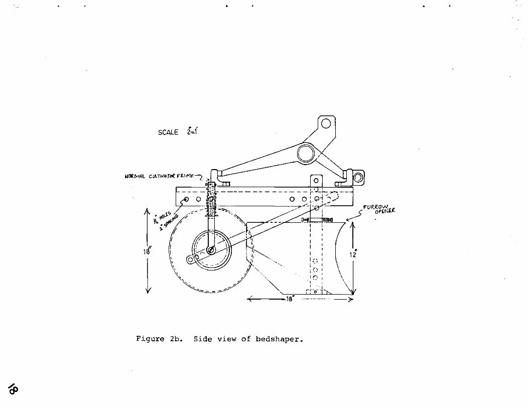
This machine consists of a furrow opener followed by a roller system (Fig. 2). The furrow opener lifts and wind- rows the soil, and the roller system spreads the soil, crushes the clods and smooths the top of the bed, compacting both the bed surfaces and furrow surfaces. The roller thus controls the shape of the bed and the furrows.

The bed shaper is a bolt-on attachment to the cultivator frames commonly used in Pakistan. Although made by many manufacturers, these frames are virtually identical because they have been copied from just a few original imports. The frame consists of two parallel 2.5 m pieces of 5 cm angle iron, spaced 50 cm apart on a three-point hitch. The angle iron is drilled at 2.5 cm spacings so that attachments can be bolted onto the frame at any desired spacing.

The furrow opener is made of sheet metal abouto2 mm thick (Fig. 3). It is a "V" shaped plow, with a 30 included angle. The wings are 45 cm high by 50 cm long. The sides of the opener are bent inwards diagonally so thst the bgttom is 12 cm wide, and the sides rise to give a 30 or 45 slope to the furrow banks (both slopes were tried). The front edge of the opener curves forward at the bottom, and the bottom is arched concave to improve penetration (Fig. 3) .

BESTAV&LABLE COPY

SCALE f=f

Figure 2b. S ide view of bedshaper.

s i d e Opener

I -4 3-,

f r o n t

s i d e Ro l l e r f r o n t

Figure 3 . E s s e n t i a l s of bedshaper components.

The opener i s suppor ted on a v e r t i c a l shank t h a t i s pinned t o t h e i n s i d e s o l e about 20 cm back from t h e t i p . The shank passes through an a d j u s t i n g s l o t on t h e t o p of t h e opener. The a d j u s t i n g s l o t a l l ows p r e c i s e a d j u s t n e n t o f t h e tilt o f t h e opener i n o r d e r t o c o n t r o l p e n e t r a t i o n . To a t t a c h t h e opener t o t h e frame, two p i e c e s of angle i r o n a r e b o l t e d between t h e f r o n t and r e a r frame b a r s i n such a way t h a t t h e y form a s l o t f o r t h e shank t o pas s through and be he ld w i t h a b o l t on to t h e ang le i r o n b races . Mul t ip l e h o l e s i n bo th t h e shank and t h e ang le i r o n s provide a d j u s t n e n t of t h e opener p o s i t i o n .

The shank of t h e opener absorbs t h e v e r t i c a l l o a d s . The l a t e r a l and l o n g i t u d i n a l l oads a r e taken up by b races t h a t run from t h e bottom o f t h e shank up d i agona l t o t h e rear frame member. Th i s method of mounting a l lows any number of openers t o be used on t h e frame, and any d e s i r e d bed width can be made.

The r o l l e r assembly i s e s s e n t i a l l y one long p i e c e of p i p e wi th furrow cones f a s t e n e d on it a t t h e d e s i r e d spac- i ngs . The p i p e i s t h i n w a l l s teel , 2.4 m long and 13 cm i n d iameter . The ends of t h e p i p e , 5 mm s teel , a r e capped wi th d i s c s and 25 mm s t u b a x l e s , 5 cm long , a r e welded on t h e caps. The cones a r e made of 1 .5 mm s h e e t steel an2 he13 t o t h e r o l l e r s e i t h e r by set screws o r band type clamps.

The r o l l e r i s a t t a c h e d t o t h e frame by two arms a t each end. One arm i s v e r t i c a l and s p r i n g mounted t o keep c o n s t a n t downward p r e s s u r e on t h e r o l l e r . The second arm i s a d r a f t arm, running d i agona l ly up t o t h e forward frame member. 130th arms a r e mounted on a s h o r t p i e c e of p i p e t h a t a c t s a s a bea r ing on t h e s t u b a x l e of t h e r o l l e r . The p i p e i s welded t o t h e v e r t i c a l arm and t h e d i agona l arm i s d r i l l e d t o s l i p over t h e pipe. There is no need f o r d iagonal b rac- i n g f o r t h e r o l l e r because t h e cones must fo l low i n t h e furrows l e f t by t h e openers .

A unique f e a t u r e of t h e r o l l e r i s t h a t it r o t a t e s a t less than ground speed. The cones t h a t shape t h e furrows a r e t h r e e t i m e s t h e d iameter of t h e p i p e t h a t r o l l s t h e bed. These cones a r e wedged i n t h e furrow where t h e r e i s g r e a t e r t r a c t i o n than on t h e bed, and t h e cones , w i th t h e i r g r e a t e r r a d i u s , have a mechanical advantage over t h e p i p e i n d e t e r - mining t h e speed a t which t h e r o l l e r r o t a t e s . The r e s u l t of t h i s lower speed of t h e p i p e i s t h a t it has a bu l ldoz ing a c t i o n on t h e windrow of s o i l and sp reads t h e s o i l more evenly a c r o s s t h e bed b e f o r e it is a c t u a l l y r o l l e d . As on ly one p o i n t on t h e r a d i u s o f t h e cone w i l l be t u r n i n g a t a c t u a l ground speed, a l l t h e rest of t h e cone and r o l l e r

assembly will be having a troweling effect on the soil surface. At the bottom of the furrow, this qives some compaction which should facilitate even water distribution across the field.

Results and Discussion

Using a 35 HP tractor, this bedshaper will pull two 20 cm deep furrows and smooth the equivalent of two beds (one full bed between the furrows and two half beds on the outside of the two furrows). If the implement is not pene- trating deeply enough, the furrows will still be properly shaped, but the center of the bed will not be finished due to insufficient soil in the windrow for spreading. If the penetration is too deep, the draft increases and the wind- rows tend to spill over the top of the opener and the inside corners of the roller, leaving this loose spill in the furrow. Regardless of the depth adjustment, the edges of the bed are well shaped and firm. This is the critical area where the crop is normally planted.

Although this machine was developed to work as a unit for making complete beds, it was found that either the openers alone or the roller alone could be used for certain field conditions. In one instance, heavy rain had fallen after planting and before emergence. The resulting crust was effectively broken by using the roller alone on the beds. Although it was not tried, the furrow openers should be able to work independently for reconditioning the furrows, or for acting as guides which follow the furrows and control the position of other equipment such as seeders or cultivators.

A seeder attachment should be developed to follow the bedshaper, and a precision cultivator could replace the rollers, using the furrow openers to guide the implement along the established furrows.

A bedshaper was developed during the summer of 1978. Since then, five tractor-drawn units have been manufactured for government departments, and two additional units have been sold to private farmers. The shop making these units is keeping one bedshaper for display.

A small bullock-drawn model was made using a single furrow opener and two bed rollers of 75 mrn PVC pipe. The implement made suitable small beds and could be pulled by an average pair of bullocks. However, the implement rocked sideways on the opener, making it difficult to hold level because it was only making one furrow. A team of bullocks

does not have enough strength to pull two furrows. Further- more, it is difficult to drive bullocks in a line straight enough that the resulting beds will be of uniform width.

The initial machines were demonstrated to both farmers and government officials at the Mona Research Center on private farmers' fields; at Niaz Begh on the On-Farm Water Management Research fields; at Chichiwatni, Khaniwahl, and near Multan on farmers' fields; and at the Agricultural University, Faisalabad, where the engineers are working with the firm that has been making the bedshapers.

Hopefully, the advantages of bed cultivation will become sufficiently obvious that the machine will gain general acceptance by the farmers.

S t a f f Paper #29

ECONOMIC FEASIBILITY OF CONCRETE LINING FOR THE BEN1 MAGDWL CANAL AND BRANCH CANAL

Gamal Ayad, G. Nasr Farid, and Gene Quenemoen

Apr i l , 1978

The Beni Magdoul Canal, supplied from the Mansouria Main Canal i n

the Giza I r r i g a t i o n D i s t r i c t , i s 2.92 ki lometers i n length and serves 860

feddans. A l a t e r a l branch of t h i s canal is 0.84 ki lometers i n length and

serves 140 feddans within the 860 feddan area . The Beni Magdoul Canal

was l ined with concre te i n 1977 and t h e l a t e r a l branch was l ined i n 1978.

This r epor t d iscusses the economic f e a s i b i l i t y of l i n i n g these

canals . ' Economists from the Egyptian Water Use Management P ro jec t (EWUP)

inves t iga ted t h i s matter , obtained re levant da ta from t h e Giza I r r i g a t i o n

Department and from EWUP personnel, and prepared t h i s r e p o r t . I t w i l l

be obvious t o the reader t h a t the r epor t i s incomplete. The EWUP

economists were unable t o obta in , i n the shor t time a v a i l a b l e , s u f f i c i e n t

r e l i a b l e d a t a t o make a s c i e n t i f i c a l l y defens ib le ana lys i s . However

even though a complete and thorough ana lys i s i s not poss ib le given

l i m i t a t i o n s on time and research resources, it was decided t o r epor t our

explora tory e f f o r t s i n t h i s s t a f f paper.

Methodology

The economic f e a s i b i l i t y o f an investment which g ives r i s e t o a

flow of annual b e n e f i t s and annual cos t s can be evaluated through a

discounted cash flow ana lys i s , The general form o f benef i t -cos t flow

ana lys i s is shown i n the following equation:

'This ana lys i s involves not only t h e l i n i n g o f t h i s p a r t i c u l a r canal but a l s o o t h e r changes i n t h e i r r i g a t i o n system i t s e l f such as reduced number of o u t l e t s , reduced l e v e l o f water i n the canal and a s h i f t from a r o t a t i o n system t o constant low.

Where: DV i s t he amount o f t h e i n i t i a l investment,

a i s t h e amount of n e t annual b e n e f i t s f o r any given year ,

r i s t h e r a t e o f r e t u r n ,

n i s t h e number o f yea r s f o r payoff o r t h e " l i f e " of t h e ) f2

pro j e c t , &:

In our a n a l y s i s we s h a l l attempt t o determine t h e r a t e o f r e t u r n ( r ) ,

given the i n i t i a l cos t (PV) , t h e n e t annual b e n e f i t s (a) and t h e number

o f years of l i f e o f t.he d i t c h l i n i n g p r o j e c t (n) . I n i t i a l Investment

The cos t o f l i n i n g and a d j u s t i n g o u t l e t s on t h e main canal was LE

4 0 , 7 5 5 . ~ Although t h e c o s t s a r e not completely t abu la t ed f o r t h e l a t e r a l 2

branch canal it i s es t imated t h a t they w i l l be about LE 6,000 . These amounts do not inc lude t h e cos t o f planning, design and

cons t ruc t ion supervis ion which was provided by t h e Water Research

I n s t i t u t e . One can make a case f o r no t inc luding these c o s t s s i n c e they

were provided a s p a r t o f t he on-going work of a government agency with

s o c i a l r e s p o n s i b i l i t i e s . I f they a r e included i t has been es t imated

t h a t they should be approximately seven percent o f cons t ruc t ion c o s t s 3

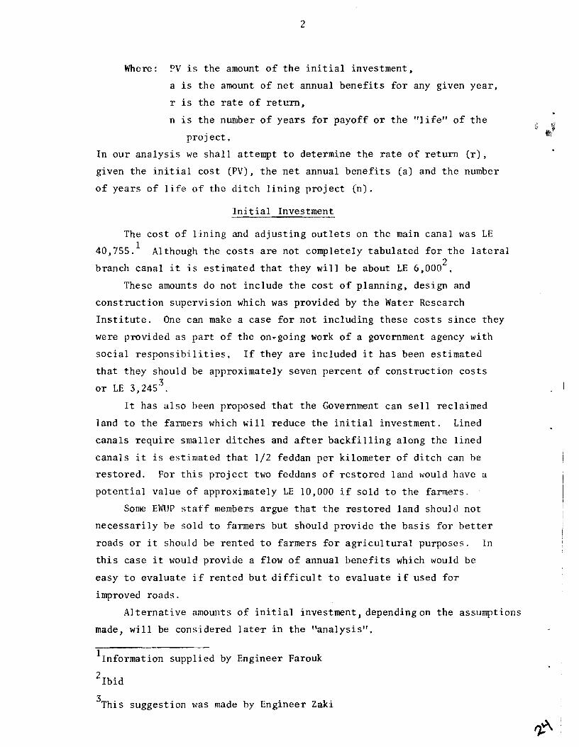
o r LE 3,245 . I t has a l s o been proposed t h a t t h e Government can s e l l reclaimed

land t o t h e farmers which w i l l reduce t h e i n i t i a l investment. Lined

canals r equ i re smal le r d i t ches and a f t e r b a c k f i l l i n g along the l i n e d

cana l s it i s es t imated t h a t 1/2 feddan p e r ki lometer o f d i t c h can be

r e s to red . For t h i s p r o j e c t two feddans o f r e s t o r e d land would have a

p o t e n t i a l va lue of approximately LE 10,000 i f so ld t o t h e farmers.

Some EWUP s t a f f members argue t h a t t h e r e s to red land should not

n e c e s s a r i l y be so ld t o farmers but should provide t h e b a s i s f o r b e t t e r

roads o r it should be ren ted t o farmers f o r a g r i c u l t u r a l purposes. In

t h i s case i t would provide a flow o f annual b e n e f i t s which would be

easy t o eva lua te i f ren ted b u t d i f f i c u l t t o eva lua te i f used f o r

improved roads.

A l t e rna t ive amoullts of i n i t i a l investment, dependingon the assumptions

made, w i l l be considered late^ i n t h e "analysis" ,

l ~ n f o r m a t i o n supplied by Engineer Farouk

'1bid

3 ~ h i s suggest ion was made by Engineer Zaki

Annual Benef i t s - Costs

The i n i t i a l c a p i t a l investment i n l i n i n g canals i s expected t o

cause a flow o f b e n e f i t s and c o s t through t ime. I t i s d e s i r a b l e f o r

economic f e a s i b i l i t y a n a l y s i s , t o quan t i fy these b e n e f i t s and c o s t s .

In some cases t h i s i s r e l a t i v e l y easy, i n some cases it can be done with

c a r e f u l l y designed and sometimes lengthy research e f f o r t s and i n some

cases it i s p r a c t i c a l l y impossible , The fol lowing d iscuss ion s t a r t s

with t h e easy and moves toward t h e d i f f i c u l t . In a l l cases we w i l l

a t tempt t o de r ive ''net1' b e n e f i t s o r c o s t s which i s t h e d i f f e r e n c e i n

before and a f t e r s i t u a t i o n s .

Annual Cleaning and Maintenance

The c o s t o f removing sediment from unl ined canals i s c u r r e n t l y about

LE 0.235 p e r cubic meter. This i s based on d a t a from t h e Giza I r r i g a t i o n

D i s t r i c t regard ing t h e 1978 c o s t s of c leaning t h e E l Shimi Canal. Also

according t o t h e Giza I r r i g a t i o n D i s t r i c t records t h e Beni Magdoul Canal

was cleaned each s i x years f o r t h e pas t e ighteen yea r s . The average

c o s t , us ing cu r ren t c leaning p r i c e s , was LE 66 p e r year .

Data on c leaning l i n e d cana l s were n o t a v a i l a b l e . Based on t h e

g rad ien t o f t h e Beni Magdoul Canal and i t s l i n e d branch, EWUP engineers

es t imated it would c o s t LE 60 t o LE 100 p e r year , I t was a l s o es t imated

t h a t t h e annual cos t of r e p a i r i n g t h e l i n e d canals would be LE 300.

The d i f f e r e n c e between c leaning and maintenance c o s t s f o r t h e l i n e d

and unl ined canals appears t o be i n f avor o f t h e unl ined. This can be

considered a s an annual "cost" a s soc ia t ed with l i n i n g o r a negat ive

"bene f i t . I t

Water Saved

H i s t o r i c records a r e a v a i l a b l e f o r water r e l e a s e d from the Mansouria

Main Canal i n t o t h e Beni Magdoul Canal. Since l i n i n g t h e canals t h e

amount o f water now being r e l eased from t h e Mansouria Main Canal i s 1

reduced more than 25 percent .

l ~ s t i m a t e d by Engineer Farouk

This means a saving o f more than 4,000 cubic meters p e r feddan f o r a l l

t h e land served by t h e Beni Magdoul Canal,

The value of t h i s water i s d i f f i c u l t t o determine, Technica l ly i t s

va lue i s determiend by i t s "use value" f o r some o t h e r a l t e r n a t i v e . I f

it i s simply r e l eased i n t o t h e Ni le t o flow i n t o t h e s e a i t s value may

be n e g l i g i b l e , perhaps only a s an a i d t o naviga t ion . ~ f , however, i.t

i s used f o r higlily p r o f i t a b l e a g r i c u l t u r a l o r i n d u s t r i a l purposes i ts

value may be s u b s t a n t i a l . I t has been pointed out t h a t "water saved"

has d i f f e r e n t values depending on loca t ion , Free flowing waste water

on the upper reaches o f t h e Nile may be r e l eased back i n t o the r i v e r f o r

use downstream. I f t h e q u a l i t y o f t h e Teleased waste water i s no t

impaired', then ''saving" it may have l i t t l e value o r meaning. Perhaps

a t t h i s t ime t h e value of water saved must be a r b i t ~ a r i l y determined by

po l i cy makers. The t o t a l value of water saved f o r t h e 860 feddans

under d i f f e ~ e n t p r i c e assumptions follows!

LE 0.001 pe r cubic meter LE 3,440

LE 0.003 per cubic meter LE 10,320

LE 0.005 pe r cubic meter LE 17,20Q

Land Res tora t ion

A s p revious ly mentioned l i n e d d i t c h e s r e q u i r e l e s s land a r e a ,

When o l d d i t ches a r e l i n e d t h e back f i l l provides more land f o r roads

and/or a g r i c u l t u r a l production. In both cases t h e r e is a b e n e f i t . The

amount of land r e s to red i n t h i s process v a r i e s depending on the

condit ion o f t h e o l d d i t c h . I t i s es t imated t h a t 1/2 feddan w i l l be

r e s to red f o r each ki lometer of d i t ch o r approximately two feddans on 1

t h e p ro jec t . The cash r e n t f o r t h e land i n t h i s a r e a i s about LE 70 2

p e r feddan . A t t h i s r a t e t h e l i n i n g should genera te about LE 140

annual b e n e f i t s i f t h e land can be leased t o f a ~ m e r s .

Increased Agr i cu l tu ra l Production

Lined canals provide flow of water r a p i d l y t o f i n a l po in t s of

d e s t i n a t i o n with minimum seepage l o s s . Often l i n i n g makes it poss ib l e

t o provide continuous flow de l ive ry which permits farmers t o i r r i g a t e

' ~ s t i m a t e d By Engineer Farouk

2 ~ n f o r m a t i o n provided by Economist Lotfy

whm they need water r a t h e r than fo l lowing t h e t r a d i t i o n a l water

r o t a t i o n system. The more e f f i c i e n t handl ing o f water can l ead t o

lowering t h e water t a b l e and more t imely a p p l i c a t i o n o f water which should

i n c r e a s e p ~ o d u c t i o n . However t h i s increased product ion may c o s t more

than product ion under t h e o l d system because o f l i f t i n g t h e water h i g h e r

from t h e deeper l i n e d d i t c h e s , u s ing more f e r t i l i z e r and o t h e r c o s t s

a s s o c i a t e d with more i n t e n s i v e cropping. Carefu l s t u d i e s a r e needed t o

measure t h e va lue o f increased product ion which may become p o s s i b l e a s

a r e s u l t of cana l l i n i n g . We have not been a b l e t o ob ta in d a t a from

such s t u d i e s a p p l i c a b l e t o t h e Beni Magdoul Canal. An es t ima te was

made by t h e F ie ld Team Leader f o r t h e Mansouria Study S i t e t h a t t h e

va lue o f n e t increased product ion would be LE 4,300 but t h i s i s admi t ted ly

only a guess and not based on empir ica l d a t a , Also i f t h i s b e n e f i t

i s t o go t o t h e i n v e s t o r (presumably t h e government) it must be taxed

away from t h e fa rmers ,

Other Benefi ts

Numerous o t h e r b e n e f i t s a r e o f t e n mentioned f o r l i n i n g c a n a l s , Most

o f them a r e extremely d i f f i c u l t t o eva lua t e and quan t i fy . A p a r t i a l

l ist fol lows :

1. Health - reduct ion i n breeding a r e a s f o r s n a i l s and mosquitoes.

2 . Reduction i n s i z e and concent ra t ion of f i e l d dra inage f a c i l i t i e s .

This assumes t h a t l i n e d cana l s make i t p o s s i b l e t o accomplish

b e t t e r on- farm water management.

3, Reduction i n c o s t s o f pumping from t h e d r a i n s i n t he Lower Del ta .

Analvsis

I t i s c l e a r t h a t s eve ra l equat ions can be cons t ruc t ed t o eva lua t e

t h e b e n e f i t s and c o s t s of l i n i n g t h e Reni Magdoul Canals , The va lues

one pu t s i n to t h e s c equations depends upon t h c assumptions onc makcs

and t h e degree of d a t a r e l i a b i l i t y one r e q u i r e s . Several a l t e r n a t i v e s

fo l low;

This equation assumes no c o s t is assigned t o planning, des ign and

cons t ruc t ion supervis ion , canal c leaning c o s t s a r e LE 44 more a f t e r

l i n i n g , water saved has a va lue o f LE 0.001 pe r cubic meter and

r e s to red land i s r en ted t o fanners a t LE 140. Rates of r e t u r n a r e :

n = 10 then r = -2.73 percent

n = 20 then r = 0.13 percent

n = 30 then r = 7,86 percent

This equation assumes a charge f o r planning design and cons t ruc t ion

supervis ion , sel l ; -ng r e s t o r e d land t o farmers, canal c leaning c o s t s

and maintenance a r e LE 294 more a f t e r l i n i n g , a value o f LE 4,300 i s

placed on increased product ion, and t h e value o f water saved i s LE

0 ,003 per cubic meter. Rates of r e t u r n a r e :

n = 10 then T = 34.38 percent



Conclusion

A t t h e present time EWUP does not have adequate da ta t o provide a

scientifically de fens ib l e economic a n a l y s i s of canal l i n i n g a t Beni

Magdoul. Since l i n i n g canals i s one means f o r improving on-farm water

management inEgypt it w i l l be given cons idera t ion along with o t h e r

means, fo r f u r t h e r i nves t iga t ion a t t h e conclusion o f t he problem

i d e n t i f i c a t i o n phase o f EWUP, scheduled f o r J u l y 1 , 1978, f o r t he

Mansouria Study S i t e ,

I t is recommended t h a t any dec i s ions t o make s u b s t a n t i a l i n v e s t -

ments i n canal l i n i n g f o r Egypt should await adequate economic

f e a s i b i l i t y a n a l y s i s , To do otherwise involves a high r i s k o f mis-

a l l o c a t i n g sca rce na t iona l resources. EWUP may genera te valuable d a t a

f o r such an a n a l y s i s depending on dec is ions regard ing research plans

which w i l l be made a t the conclusion o f t h e problem i d e n t i f i c a t i o n

phase.

S t a f f Paper #30

PROGRAMS FOR CALCULATORS HP-67 AND HP-97

Gamal A. Ayad

February, 1979

AREA OF A POLYGON PROGRAM

FOR CALCULA'TORS IIP-25, 111'-67 AND 11P-97

I f

j ( s ide) ( dj (angle) a j s i d e length - - .. - - - -- - --

430

360

420

54 0

!

PROGRAha42 FOR THE POCKET CALCULATOil HP-25

Phis programme c a l c u l a t e s t h e area of polygon of n s i d e s , de f ined by:

where i s t h e a n ~ l e ( i n decrees) t h e s i d e j forms with North measured i n clockwise j d i r e c t i o n , and ai i s t h e len($h of t h i s s i d e .

Let 3 X . z a Sin n J J J

and l e t X . = 2 J 'xj j= 1

''he a rea of the polycon ( A ) , :uld tfrr cl osure e r r o r ( d i s t n n c c bctwc;c.ti t h r c t n r t i n c N I ~

end1r.g po in t ) expressed ac percent of' t h e per imeter (c), w i l l r e spec - t i ve ly be:

1 he a r e a c a l c u l a t e d r e p r e s e n t s t h e area of a c losed polygon ob ta ined by shift in^ t h e ' e r t i c e s or' t h e given polygon alonf: t h e l i n e s g a r a l l e l t o t h e l i n e pas s in& t h r o u a t h e

s t a r t i n g a d endin? p o i n t . The v e r t e x i i s s h i f t e d by t h e i / n f r a c t i o n of t h e d i s t a n c e between s t a r t i n e and ending po in t .

BEST AVAILABLE COPY

I

1 4 3 3 f E C

2 4 0 3 RCL3

74 R/S

23 51 oo s'r + o 14 09 f -4 R

25 2' + R 1

' Z Y

R b

f LASTx

RCL 4

SF0 + i X

X Z Y

rfcl, 7

S'1'0 + 1

X - - CTO 0 3

CLX '

2

Regintern 1 -.

Ro v a i

1 ,vx. 1 '.

R* 2 ' Y i

3 n

R 4 'i

R 5

USED

'6 USED

.'i -

Diopley

Line Cod0

REfdARK: T h i s p r o g r m e is made t o calculate area i n heatares for input i n metree. Should different un i t e be used, the converoion factor 10 000 given i n 1ine.n 35-39 should be changed:

Key entry

25 14 21 f F 26 24 02 RCL 2 .

27 61 X 28 24 04 RCL 4

29 24 03 RCL 3

30 71 4

31 2 4 0 1 RCL 1

32 61 X

33 41 - 34 51 +

35 ' 01 1

36 00 0

37 00 0

38 00 0

39 . 00 0

40 71 f

4 1 42 2 4 0 4 IiCL4

43 24 07 RCL 7 1 44 1 5 0 9 g - + P I

4,5 24 00 RCL 0

fi6 71 i

47 33

45 02 2

49 61 X

Convereion factror

1.000

43 560 1:0oo

4200.8335

4046.856

EEX 4 EEX 6

miles259ENT EEX6x i

Input

Net r e s

Feet - Feet

Metres

Metres

Metrcs . Metres

Metres

. Output

Sq.met res'

Acree

S q . feet

Feddans

Acres

llectars sq. kms.

sq.

A = 17.16 ha.

Inst~wctions

j ( s ide)

1

2

3

4

- o (angle : degrees)

15

64 168

25 3

a . (length r metres) . J

4 30

360 .

420

540 .

Out put'

-

0.03

A

I 4

Keys

U U O O

loj p-1

m n n n m o n o . [CTO] 11 ' '1 [)I

E K I n ~

Input

a J

a J

s tep

1

2

3

4

5-

6

lnst ruct ion

&t er programme

I n i t i a l i z e

Perform 3 for

j - 1, 2, ..., n

Calculate area

Calculate o i o ~ u r e error

For a new case go t o 2

Area o f a Polygon Program f o r t h e C a l c u l a t o r s

HP-67 and HP-97

Same example:

I n s t r u c t i o n s :

j ( s i d e )

1

2

3

4

Thi s program i s designed t o c a l c u l a t e a r e a i n square metres f o r i n p u t s i n metres. Should d i f f e r e n t u n i t s be used, t h e fol lowing s t e p s should

d j (ang1e)

15

64

168

253

be added a f t e r s t e p # 73 of t h e program s t e p s .

- -- - - --- a j s i d e l eng th

430

360

420

540

Keys

ENTERS

El ENTER^

El ENTER?

El ENTER t El

El El

Input

Angle 1 (15')

S i d e 1 (430)

Angle 2 (64')

S i d e 2 (360)

Angle 3 (168')

S i d e 3 (420)

Angle 4 (253')

S i d e 4 (540)

S t e p

1

2

3

4

Output

0 .00

15.00

1 .00

64.00

2 .00

168.00

3.00

253.00

4 .00

172068.89

0 .42

I n s t r u c t i o n

Load program

En te r ang le s and

S i d e l eng ths

C a l c u l a t e a r e a

Ca lcu l a t e e r r o r

Exercises -

Inputs

Metres

Metres

Metres

Metres

Metres

Fee t

S ide

1

2

3

Ang 1 e 0

150

1 Feet 1 s q . f e e t b n e I N0.e ' I --

Outputs

Feddans

Acres

l lec tars

Sq. K m s .

Sq. Miles

Acres

S ide length i n meters

250

250

250

Solu t ion should be: (Area = 27063.29 m 2 , e r r o r = 0.00%)

Adding

4200.8335 I

4046.856 i

B 4 i

m 6 1

259 1-rn 6xr

4356 I

Side Angle S ide length i n metres

1 270 2 5

2 0 o r 360 2 5

3 9 0 25

4 180 2 5

- No. of adding

s t e p s

10

9

3

3

8

Solu t ion should be: (Area = 625.00 m 2 , e r r o r = 0.00%).

Use t h e example's d a t a assuming t h a t t h e s i d e lengthes should b e i n metres and t h e a r e a i n feddans.

So lu t ion should be: (Area = 40 .96 feddans, e r r o r = 0.42%)-

PROGRAM STEPS FOR CALCULATORS H P - 6 7 -- AND H P - 9 7 --

LAND LEVEL1 NG PROGRAM

FOR CALCULATORS HP-67 AND HP-97

Prepared by :

LAND LEVELING PROGRAM For HP-67 and HL-97 C a l c u l a t o r s

- -

Prepared by Econ. Gamal M . Ayad March 5 , 1979

This program c a l c u l a t e s t h e dep ths of c u t s and f i l l s ( C & F ) , t h e volume of each and t h e C/F r a t i o f o r l e v e l i n g i n one o r two d i r e c t i o n s .

Before running t h e program t h e fo l lowing d a t a must be s t o r e d i n t h e s t o r a g e r e g i s t e r s .

ST0 A = Number of s t a t i o n s i n one s t r i p i n t h e d i r e c t i o n o f t h e f i r s t s l o p e .

ST0 B = Slope i n meters p e r g r i d spac ing f o r t h e d i r e c t i o n of t h e f i r s t s l o p e .

ST0 C = Number of s t a t i o n s i n one s t r i p i n t h e d i r e c t i o n of t h e second s l o p e .

ST0 D = Slope i n me te r s pe r g r i d spacing f o r t h e d i r e c t i o n of t h e second s l o p e .

ST0 E = Grid spac ing i n meters. ST0 2 = The mean of a l l o r i g i n a l l and e l e v a t i o n s . (The mean

w i l l be c a l c u l a t e d and a u t o m a t i c a l l y s t o r e d i n ST0 2, o r any d e s i r e d mean va lue may be s t o r e d manually ( e n t e r e d ) i n s t e p 3 of t h e i n s t ruc t ions ) .

- I f t h e program i s used f o r on ly one -d i r ec t ion s l o p e , n e g l e c t s t o r a g e r e g i s t e r s C and D.

- I f t h e program i s used f o r dead - l eve l , n e g l e c t t h e s t o r a g e r e g i s t e r s A , B , C and D. ( i f HP-97 i s used, s t o r e d a t a i n s t o r a g e r e g i s t e r "A". The d e p t h s of c u t s and f i l l s w i l l t hen be grouped on t h e p r i n t ~ o u t . )

- Eleva t ion r e a d i n g s a r e p r e f e r e d . Rod r e a d i n g s w i l l g i v e r e v e r s e meaning f o r c u t s and f i l l s .

- Other u n i t s may be used a s w e l l a s meters.

S t e p s (what)

1 1 Load program .

2 -

Store d a t a i n s t o r a g e r e g i s t e r s A through E .

3 S t o r e e l e v . mean i n s t o r a g e r e g i - s t e r "2" (procedure) "a" o r

4

I n s t r u c t i o n s f o r Using t h e Program

C a l c u l a t e t h e depths o f c u t s and f i l l s .

5 C a l c u l a t e t h e volumes o f c u t s and f i l l s and t h e C/F r a t i o . *

I n s e r t prerecorded magnetic ca rd o r e n t e r keys t rokes of program

Procedure (how t o do i t )

s t e p s manual ly . 1 ) I I

i n p u t Da ta /un i t s Keys

a . Automatic : Enter each o r i g i n a l land e leva t ion ( i n any sequence) , each fol lowed by p r e s s i n g key "E". b . Manual : ' ~ n t e r d e s i r e d va lue o f t h e mean followed by p r e s s i n g keys a.

each s t r i p i n o rde r . I I

F i r s t e l e v a t i o n . Second e l eva t ion . I I n !I e l eva t ion .

Desired mean.

S t a r t i n g a t t h e h ighes t d e s i g - nated e l e v a t i o n l e v e l , and pro- ceding a long one s t r i p i n t h e d i r e c t i o n o f t h e f i r s t s l o p e , e n t e r t h e o r i g i n a l land e l eva - t i o n read ing o f each s t a t i o n f o l - lowed by p r e s s i n g key "A". En t e r

P re s s '.key "C" .

IE

F i r s t e l e v a t i o n .

Second e l e v a t i o n

I I ~ I I e l e v a t i o n .

ou tpu t s Data/Units

0.000

F i r s t e l e v a t i o n . Second e l e v a t i o n . I I ~ I I e l e v a t i o n .

Desired mean

- - - c u t o r + = f i l l - - - c u t o r + = f i l l - - - c u t o r + = f i l l

volume o f c u t s ( - volume o f f i l l s ( + C/F r a t i o . 0.000000000 0.000

* Remember, wi th t h e HP-67, t h e f l a s h i n g decimal p o i n t i n d i c a t e s t h a t t h e cu t o r f i l l va lue w i l l d i s appea r a f t e r few seconds and t h e l a s t e l e v a t i o n keyed i n w i l l appear . The d isappeared va lues can be r e t r i e v e d by p r e s s i n g k e y s m

a ** The C/F r a t i o can be changed by e n t e r i n g d i f f e r e n t mean i ~ n s t e p 3 , procedure"b:

rl

***Immediately a f t e r 0.000000000 appears , a l l s t o r a g e r e g i s t e r s a r e c l e a r e d (e rased) and t h e program i s ready f o r ano the r run.

1) Program s t e p s on page 8.

STRIP STRIP

'I n 2 EXAMPLE

STRIP STRIP

S'TRTP A

STRIP (3 1 I

STRIP D

+-

STRIP E

t---

i f we want t o l eve l t h e land i n t h i s example i n one d i r e c t i o n s lope f o r 0.05% ( the h ighes t l eve l a t s t r i p ( I ) and t h e lowest leve l a t s t r i p (4)).

1. Load program,

4. 12.55 - 0.233

12.50 0 - 0.188 1 This i s t h e f i r s t s t r i p # A

12.48 0 - 0.173 ( a l l c u t s )

1 2 . 4 4 0 - 0 . 1 3 8

12.49 0 - 0.173 Second s t r i p # B . and so on t ill the end of t h e f i e l d ( t h e l a s t e l eva t ion w i l l be 12.14).

5 . Press a - 123.600 (volume o f c u t s i n cubic metres). 123.600 '(volume of f i l l s i n cubic metres) . 1.000 C/F r a t i o

P r in t -ou t s l i p

S t r i p A - 0.233 - 0.188 - 0.173 - 0.138

S t r i p B - 0.173 - 0,238 - 0.093

0.002

S t r i p C 0.067 0.092 0.107 0.152

S t r i p D t 0.047 0.032 0.127 0.132

S t r i p E 0.087 0.072 0.157 0.162

After t h i s run i f you want t o change t h e mean e l e v a t i o n from 12.3095 t o 12.29, r epea t t h e same s t e p s except s t o r i n g t h e new mean manually (procedure 'lb").

1. Program i s a l r e a d y loaded .

t i l l t h e end of e l e v a t i o n s .

5. Press 0 P r i n t - o u t slip

S t r i p A - 0.253

- 0.208

- 0.193

- 0.358

S t r i p B - 0.193

- 0.258

- 0.313

- 0.038

S t r i p C

S t r i p 1)

S t r i p E

When

P r e s s C

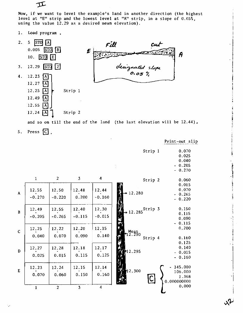
Now, i f we want t o l e v e l t h e example's l and i n another d i r e c t i o n ( t h e h ighes t l e v e l a t "Et1 s t r i p and t h e lowest l e v e l a t "A" s t r i p , i n a s lope o f 0 .05%, u s ing t h e va lue 12.29 a s a d e s i r e d mean e l e v a t i o n ) .

Load program . 5

0.005 a / . :,- s:.;?$,$ 2: ~2 .. ..#

10. tmJ - B I? 12.29 0 s&

12.23 0

1 *,os % I

12.27 I

12.25 0 S t r i p 1

12.49

12.55 0 1 2 . 2 4 0 1 S t r i p 2

and s o on t i ll t h e end o f t h e land ( t h e l a s t e l e v a t i o n w i l l be 12 .44) .

P r e s s a , Pr in t -ou t slip

S t r i p 1 0.070 0.025 0.040

- 0.205 - 0.270

. - - 5

.280

S t r i p .285

an 290

S t r i p

295

300

i f you want t o l e v e l t h e l and i n t he same example i n tow d i r e c t i o n s slopes. One o f t he s lopes i s 0.05%, highest l e v e l a t s t r i p ( 1 ) t h e lowest a t s t r i p (4 ) . The second s lope i s 0.10%, the h ighes t l e v e l a t s t r i p (A) and the lowest a t s t r i p ( E ) , us ing 12.29 as a mean e l e v a t i o n .

1. Load Program P r i ntsd-out s l ip_

2. 4 ma 4. 12.55 0 S t r i p A - 0.233

0.005 ma 12.50 0 - 0.188

5 12.48 a - 0.173

0.01 m] 12.44 0 - 0.138

10 ST0 t i l l the end o f the f i e l d

3. 12.29 S t r i p B - 0.183

- 0.246

Outupts

5. Press - 127.000 ( v o l u ~ i ~ e ~ ~ o f c u t s ) S t r i p C 0.048 In In In r- N I. 88.000 (volume o f f i l l s ) 0.073 41 41 4 1 0 3 N N N N ,P 1.443 C/F r a t i o . N N N N % d d d d fi.

S t r i p D

S t r i p E

When press .2.28

-

Program S teps

MAR. 5 - 1979

Step No.

001

002

003

004

005

006

007

008

009

010 . 011

012

013

014

015

016

017

918

019

020

Key Entry

LBL E

S T 0 1

ST+8

1

ST+9

RcL8

RcL9 -

ST02

R C L I

RTN

LBLA

DSp 3

SToS

1

STt7

RcLA

RcL7

XpY?

GTOB

q Step No.

021

022

023

024

025

026

02 7

028

029

030

031

032

033

0 34

035

036

037

038

039

04 0

Key Entry

LBL d

RCL A

2 -

5

+

RCL 7

- RcLB

X

SToO

RCLC

2 -

S

+

RCL 1

1

Step No.

04 1

04 2

043

04 4

045

04 6

047

04 8

049

050

051

052

053

054

055

056

057

058

059

060

Key Entry

+ -

RCLD

X

RcLO

+

RcL2

+

RcL5

- PRT X

X<O?

ST+6

X>O?

ST+4

RcL5

RTN

LBLB

SPC

1

- Key Entry

X<O?

CHS

PRTX

CLX

DSp9

PRTX

DSp2

CLRG

CLX

ENT+

ENT+

ENT+

RTN

Step No.

081

082

083

084

085

086

087

088

089

090

091

092

093

I

1

6 t e p No.

061

062

063

064

065

066

067

068

069

070

07 1

072

073

074

075

076

077

078

079

080

!

t

Key Entry

ST+l

1

S T 0 7

GTO d

RTN

LBLC

Spc

RcLE

x2 RcL6

X

PRTX

RcLE

x * RcL4

X

PRTX

RcL6

RcL4 -

T

I

Prepared by :

INTERNAL RATE OF RETURN PROGRAM

FOR HP-67 AND HP-97

For a f l o w o f costs and r e t u r n s t h r o u g h t i m e t h e program

s o l v e s f o r t h e i n t e r n a l r a t e o f r e t u r n f o r a maximum o f 35

y e a r s . Add t h e costs and r e t u r n s e a c h y e a r , costs n e g a t i v e

.3nd r e t u r n s p o s i t i v e .

For example l e t u s s u p p o s e you make a n i n v e s t m e n t t o d a y

o f $2000 and a t t h e end o f t h e f i r s t y e a r it y i e l d s r e t u r n s o f

$250, t h e s e c o n d y e a r $260, t h e - t h i r d y e a r $273, t h e f o u r t h

$280 and t h e n $300 e a c h y e a r t h e r e a f t e r . The i n i t i a l i n v e s t -

ment i s t h e o n l y " c o s t " . Thus t h e n e t f l o w c a n b e d e p i c t e d

as :

Year Amount Year Amount

The program s o l v e s t h e f o l l o w i n g e q u a t i o n f o r t h e v a l u e

7- "n" n o t more t h a n 17 (17 y e a r s p e r i o d ) -

2 1 ~ t o r e d a t a i n o r d e r . * I a 0

Input Data/Uni t s

S t e p

1

Always when you u s e

t o s t o r e o v e r 9 v a l -

I n s t r u c t i o n s

Load p r o g r a m . S i d e #1 S i d e # 2

u 1 u e s you s h o u l d u s e - <S a g a i n a f t e r IW you f i n -

1 i s h s t o r i n g ( i m p o r t a n t

1 n o t t o f o r g e t ) . I 1 * I f you h a v e z e r o w i t h i n I I t h e d a t a se t , s t o r e a I I s m a l l number e .g .0.000011

I i n s t e a d of z e r o t o k e e p I I t h e y e a r s i n o r d e r . I I as example i f a 2 i n t h e I I above d a t a i s 0 , you I I have t o s t o r e 0.00001 ( I a n d n o t 0 . I

1 s t o p e a c h t i m e r e a c h e s t h e I 3

1 e q u a t i o n v a l u e and " r " I

I f you want t h e program t o

v a l u e a p r e s s @ ( t h i s i s a n

o p t i o n a l s t e p ) , when t h e

program s t o p s , p r e s s R/S u t o c o n t i n u e c a l c u l a t i o n s .

I I f you d o n o t u s e t h i s I I s t e p , t h e v a l u e s w i l l I 1 p o u s e f o r 2 s e c o n d s and I c o n t i n u e c a l c u l a t i o n s till

t h e end .

Keys

I f you want t o s t a r t w i th

r = 0, p r e s s a **

I f you want' t o s t a r t w i th

r # 0, s t o r e " r " f i r s t

( a s f r a c t i o n e .g . 15 %

s t o r e d a s 0.15) t hen @ ** The c a l c u l a t e r w i l l

c a l c u l a t e t h e v a l u e of

t h e l e f t s i d e of t h e

e q u a t i o n , d i s p l a y s it

f o r two seconds, t h e n

d i s p l a y s t h e "r1I v a l -

ue. If s t e p # 3 i s

used t h e program w i l l

s t o p a f t e r d i s p l a y i n g

each v a l u e i n s t e a d of

j u s t pquse it f o r 2

seconds. The " r l ' va l -

ue w i l l b e i nc reased

by 1 percen t ,and t h e

p roces s w i l l r e p e a t

till reaches t h e f i r s t

nega t ive v a l u e f o r t h e

equa t ion , t h e n " r " va l -

ue w i l l b e decreased by

0 .1 p e r c e n t , The program

s t o p s a s soon a s t h e

f i r s t p o s i t i v e v a l u e f o r

t h e equa t ion is reached)

and d i s p l a y s t h e equa t ion

va lue ( i f HP-97 i s used 7 t h e v a l u e w i l l be p r i n t e g

t o d i s p l a y t h e ' appro-

p r i a t e " r " v a l u e press(a/q

i f s t e p

# 3 was

used

i f s t e p

# 3 was

used

i f s t e p

# 3 was

used

i f s t e p

# 3 was

used

i f s t e p

# 3 was

used

i f s t e p

# 3 was

used

i f s t e p

# 3 was

used or

not

same a s

s t e p #5

eq . v a l u e (+I r%

2q. v a l u e (+)

r + 2 %

2 q . va lue (+)

r + 3%

2q. v a l u e (-1 ( r + n ) %

:q. v a l u e (-1 ( r + n ) - 0 . 1 %

:q. va lue (+I

vanted " r "

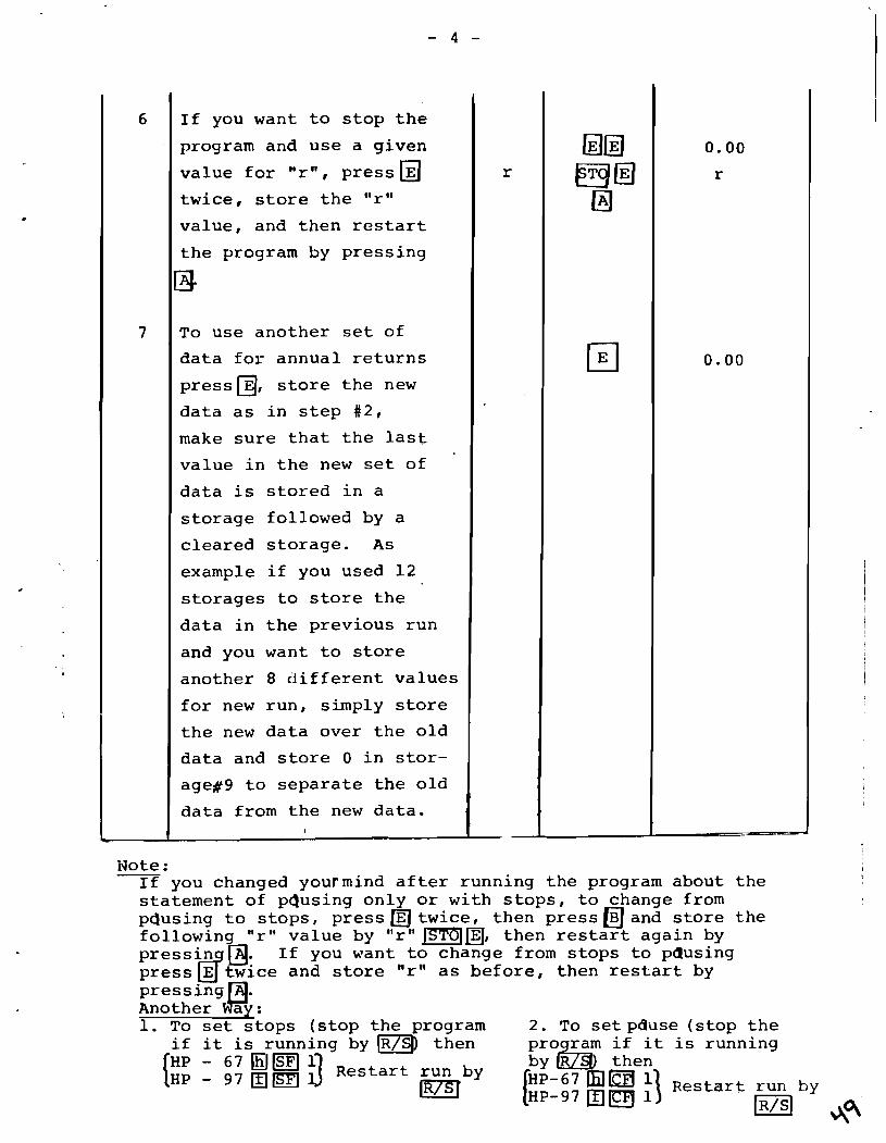
I f you want t o s t o p t h e

1 program and u s e a g iven

v a l u e f o r "r", p r e s s @

t w i c e , store t h e "r"

v a l u e , and t h e n r e s t a r t

1 t h e program by p r e s s i n g

I To u s e a n o t h e r se t of

d a t a f o r a n n u a l r e t u r n s

p re s s@, s t o r e t h e new

d a t a a s i n s t e p # 2 ,

make s u r e t h a t t h e l a s t

v a l u e i n t h e new set of

d a t a is s t o r e d i n a

s t o r a g e fo l lowed by a

c l e a r e d s t o r a g e . A s

example i f you used 1 2

s t o r a g e s t o s t o r e t h e

I d a t a i n t h e p r e v i o u s r u n

and you want t o store

a n o t h e r 8 d i f f e r e n t v a l u e s

f o r new r u n , s imply s t o r e

t h e new d a t a ove r t h e o l d

d a t a and s t o r e 0 i n stor-

age#9 t o s e p a r a t e t h e o l d

I d a t a from t h e new d a t a .

Note : I

I f you changed yourmind a f t e r running t h e program about t h e s t a t e m e n t of pQusing o n l y or w i t h s t o p s , t o change from paus ing t o s t o p s , p r e s s a t w i c e , t hen p r e s s m a n d s t o r e t h e ~ ; ~ ~ ~ ; g b ~ r I* v a l u e by "rl' mg, then r e s t a r t a g a i n by

I f you w a n t t o change from s t o p s t o pausing p r e s s E t w i c e and s t o r e "r" a s b e f o r e , t h e n r e s t a r t by p r e s s i n g g . : Another Y 1. To set s t o p s ( s t o p t h e program 2 . To s e t p d o s e ( s t o p t h e

i f it is running by (R/SD t h e n p r o ram i f it i s running

I g: BH 3 R e s t a r t r u n by then

m

I f y o u s t a r t e d w i t h r = 0 , t h e p r o g r a m w i l l t a k e 1 5 m i n u t e s t o f i n i s h t h i s c a l c u l a t i o n . I f y o u h a v e more y e a r s , t h e t i m e o f c a l c u l a t i o n w i l l i n c r e a s e , it c o u l d b e more t h a n h a l f a n h o u r . THAT IS WHY IT IS DEFINITELY RECOMMENDED TO START WITH r = l o % , IF YOU FOUND EQ. V. STILL HIGH NUMBER, TRY 2 0 % 1 IF YOU GET NEGATIVE VALUE REDUCE "rw,AND SO ON TILL YOU REACH A REASONABLE POSITIVE VALUE FOR THE EQUATION THEN LET THE CALCULATOR COMPLETE THE REST OF THE CALCULATIONS.

3 ( O p t i o n a l ) i f y o u w a n t

s t o p s . El

4

[?inifE u s e d

wq i f E u s e d

i f p u s e d

i f u s e d

[fi7SI i f , u s e d

p 7 i - f u s e d

i f u s e d

IR/sl i iE u s e d

IR/sl i f u s e d

liT7S] i f E u s e d

IR/sl i f a u s e d Or

n o t

If y o u w a n t t o s t a r t

w i t h r = 0 .

End o f c a l c u l a t i o n s

r = 2 1 . 6 %

2 9 0 . 0 0

0 . 0 0

2 6 7 . 0 4

1 . 0 0

2 4 5 . 4 8

2 . 0 0

2 2 5 . 2 2

3 . 0 0

1 4 . 7 7

21 .00

- 2 . 3 6

22 .00

- 2 . 3 6

2 2 . 0 0

- 1 . 6 6

2 1 . 9 0

-0 .96

2 1 . 8 0

- 0 . 2 5

2 1 . 7 0

0 . 4 5

2 1 . 6 0

I

- 7 -

To solve the same example by the recommended method.

By this method the whole process takes only 5 minutes to finish the calculations.

Example 2

Year Amount -- $

-1500

-500

-250

300

500

500

500

500

Year Amount -- --

$

500

500

Output DataIUnits

Crd

0.00

-1500.00

-500.00

-250.00

300.00

500.00

500.00

500.00

500.00

1

Step

1

Instructions

Load program

Side #1

Side #2

Input DataIUnit s

Keys

S t o p s s t a t e m e n t

S t a r t w i t h r = 1 0 % .

Run p r o s ram ,

Change " r " t o 15% . Change s t o p s t o pause .

S t a r t w i t h 1 4 % .

Run -

T h i s p a r t w i l l be done

a u t o m a t i c a l l y

End o f c a l c u l a t i o n , t h e

b e s t " r " v a l u e = 13.3%

Example 3:

L e t u s c a l c u l a t e lor: v a l u e f o r a p e r i o d o f 30 y e a r s f o r t h e f o l l o w i n g d a t a :

Year Amount Year Amount Year -- -- Amount

$ $ $

F o r t h e f i r s t 1 7 y e a r s f o l l o w t h e s a m e i n s t r u c t i o n s as

i n example 2 , R e s u l t s w i l l be:

r v a l u e eq . v a l u e

3.50

- 87.82

-192.85

-288.76

Then s tore t h e d a t a f o r y e a r s 1 8 + 30, f o l l o w t h e s a m e

i n s t r u c t i o n s as i n example 2 e x c e p t u s i n g o n l y t h e above

t h r e e v a l u e s o f "r" and u s e t o s t a r t i n s t e a d o f m. R e m e m b e r : A f t e r you s tore 300 f o r t h e y e a r 30 i n s t o r a g e

4 store 0 i n 5 t o separate t h e rest o f t h e o l d

d a t a from t h e new d a t a , as m e n t b n e d b e f o r e .

r v a l u e -- eq. v a l u e

229.97

188.94

155.65

Add t h e n e g a t i v e e q u a t i o n v a l u e s o b t a i n e d f r o m t h e

f i r s t 1 7 y e a r s t o t h e p o s i t i v e v a l u e s o b t a i n e d from t h e

y e a r s 1 8 .+ 30, t h e v a l u e n e a r e s t t o z e r o w i l l i n d i c a t e t h e

most a p p r o p r i a t e "r" v a l u e .

"r" v a l u e E q u a t i o n v a l u e E q u a t i o n v a l u e A l g e b r a i c --- sum

0 -, 1 7 1 8 -t 30

1 3 % - 87.82 229.97 142 .15

14% -192.85 188.94 - 3 .91

1 5 % -288.76 155.65 -133.11

I t i s clear t h a t 1 4 % i s v e r y n e a r t h e t r u e i n t e r n a l

rate o f r e t u r n (r) which s a t i f i e s e q u a t i o n v a l u e = 0 .

- , L.? - LV .

INTERNAL KATE OF RETURN PROGWV.1 STEPS FOR CALCULATORS HP-67 8 111'- 97

KEY ENTR

'L5LA

1

ST+0

RCLB

1 0

X = Y ?

G T O l

'LBL0

RCL0

S T 0 l 2

8 X=Y?

GT06

R C L i

X=0?

GT06

STOA

2 3

S T 0 l 1

ST+ i RCLi

RCLE

1 +

S T 0 9

R 4

1 ,

RCLB

X:Y

YX

RC LA XZY

I

2 2

S T 0 1

x = u

ST+ i GTOA

'LBL6

0

S T 0 0

STOD

RCLC

PSE

F l ?

R/S

RCLE

1 0

0

X

PSE

F 1 ?

R/S

RCLC

X=0?

GT03

X 4 ? GTO4

CLX

STOC

2

4

S T 0 I

RCL i

8 1

ST+ i F0?

GTOC

Gf OA

'LBL3

KEY ENTRY +-----

PRTX

R/S RCLE

1 0

0

X RTN

'LBL1

1

1 S T 0 0

GT00

'LBL2

1 ST+@

RCLB

1 0

X=Y?

G T O ~

' L B L c

RCL0

S T 0 l 2

8

X=Y?

GT04

RCL i X=0?

GT04

STOA

2

3 S T 0 l

1

ST+ j RCL i RCLE

1

STOB

R+

1

- RCLB

x= Y

y x

R C I A x= Y

t

2 2

S T 0 l X:-Y

ST+ i GT02

'LB L 4

8

S T 0 0

STOD

RCLC

PSE

F l ? R/S

RCLE

1 8

0. X

PSE

F l ?

R/S

RCLC

X=0?

GT03 X > 0 ?

GTO3

CLX

I X K -

A PROGRAM FOR CALCULATORS HP-67 AND HP-97

ADDING FEDDANS - KERATS - SAHMS, CONVERTING TO DECIMAL SYSTEM, HEC- TARES, ACRES, SQUARE METERS AND REVERSELY,

Prepared by:

I. ADDING FEDDANS - KERATS - SAHMS

Based on 1 feddan = 24 kera ts = 576 sahms which a r e the a g r i c u l t u r a l land

u n i t s area. The program adds the areas and shows the t o t a l i n t h e same

system, fed.-ket-sms.

Example: add t h e f o l l o w i n g areas:

Feddan Kera t Sa hm

Area 1 2

Area 2 7

Area 3 13

Area 4 9

Area 5 - - Area 6 6

Cont.

The r e s u l t shows t h a t t h e t o t a l i s 39 feddans, 2 k e r a t s and 5 sahms.

Note: I f you keyed i n a wrong number, e.g. i f you keyed i n t h e t h i r d

area as 13.20 i n s t e a d o f 13.02 and you d i d n o t y e t p ress B, s imp ly press ICLX] then key i n t h e r i g h t number 13.02,then press

. Bu t if you d iscovered t h e mis take a f t e r p r e s s i n g a, s u b s t r a c t i t by p ress ing m, then press , and key i n t h e

c o r r e c t number.

e.g. Press .- D i s p l a y

t h e t h i r d area

Oops! you made a

mis take.

-13.2000

The c o r r e c t area

ar Use be fo re when you want t o s u b s t r a c t an area.

If you want a s u b t o t a l w i t h i n t h e da ta se t , s imp l y press

whenever a s u b t o t a l i s needed, then press a n d key i n t h e

n e x t area.

Press -- D i s p l a y

The f i r s t area

The second area

7.0003 0 7.0003

Subto ta l i s needed

El 9.2018

El 9.2018

The t h i r d area


The f o u r t h area

9.1722 0 9.1722

The f i f t h area


The s i x t h area

6.002

TOTAL

El

11. CHANGING FEDDAN-KERATS-SAHMS TO DECIMAL SYSTEM (+0.00)

fed. ket. shm. I f you want t o change t h e t o t a l i n t he l a s t example f r om 39. 02 05 t o decimal system, press m, e.g. 39.0205 a d i s p l a y 39.09 ( i f t h e

conver ted area i s n o t d i sp layed on t h e screan, key i t i n f i r s t , then pres: a). I I I. CHANGING FEDDANS AREA FROM DECIMAL SYSTEM TO FED. KKSS SYSTEM (+ f. kkss)

Reverse o f u s i n g a. Press a e.g. 22.14 d i s p l a y 22.0309

1V. -- CONVERTING DDANS* TO SQUARE METERS ( f + m7) ------- -

Press

e.g. 14.36 D d isp lays 60323.97

(feddans) = (square meters)

Ifl Based on 1 feddan = 4,200.8335 sq. meter

V. - CONVERTING -- SQ. METERS TO - FEDDANS (m2 + f )

Reverse o f us ing D. press 0 0 e.g. 56142.54 00 d isp lays 13.36

(sq. meters) - - ( feddan)

68 Based on 1 feddan = 4,200.8335 sq. meters

V I . CONVERTING FEDDANS* TO ACRES ( f + AC. )

Press IT10 e.g. 13.36 a m d s i p l a y 13.87

(feddans) = (acres)

Based on 1 feddan = 1.03805 acres

V I I . CONVERTING ACRES TO FEDDANS (AC. + -- f. )

Reverse o f us ing m. Press 0 0 e.g. 22.54 00 d i s p l a y 21.71

(acres) - - ( feddans )

BI Based on 1 ac re = 0.96335 feddan

Reverse of us ing a a. Press a e.g. 56.23 d i sp lays 23.62

Ei Based on 1 feddan = 0.42038 hectares.

* Feddans must be keyed i n i n decimal system .

I X . CONVERTING HECTARES TO FEDDANS (HEC. -h f )

Reverse o f using El m. Press lfl e.g. 63.45 ID(disp7ays 151.04

(hectares ) - - ( feddans)

B) Based on 1 hectare = 2.38048 feddan

Staff Paper #31

On-Farm Water Management Investigations In Mansouria District, 1979-80

John Wol fe

September, 1980

Observations and measurements of water management practices in the Mansouria Irrigation District have been reported in considerable detail (Mona Mostafa El Kady, 1979; M. El KAdy, W. Clyma, and M. Abu Zeid, 1979; EWLJP, 1979). The purpose of this paper is to examine more recently obtained data from two selected farms, one in sandy soil on the El Hamami Branch Canal and the other in clay soil on the Beni Magdoul Branch Canal. The data include irrigation frequencies and amounts of water applied to most of the dominant crops grown in the region. For selected fields and crops it includes moisture-tension data obtained from mercury tensiometers. The depth to water table was measured at frequent intervals in a number of observation wells on these farms. Before irrigation and after irrigation soil moisture samples were taken to a depth of 30 cm at selected field sites.

The data from these two farms was examined and analyzed to help answer the following questions:

1. Is there over irrigation? If so, how much?

2. What frequencies and amounts of irrigation water are currently being applied to fields planted to each of the major and minor crops?

3. Can soil moisture samples, taken to the depth of the root zone, estimated at 30 cm, be used to estimate the total stored moisture available to plants?

4. What is the relative importance of over irrigation, as compared with seepage from canals and private ditches, as a factor affecting the position of the high, fluctuating water table?

5. Do crops ever suffer from drouth when the supply in the canal is adequate?

6 . Can a relationship between tensiometer readings and the depth to water table be established that would be useful to predict when it is time to irrigate?

To help answer the first three questions, a very simple water budget was calculated for each crop measured on the two farms. The results appear in tables 1 through 8.

Table 1 shows the data taken from a corn field in Beni Magdoul. The first two columns are self explanatory. The irrigation amounts shown in column 3 were obtained from cutthroat flume measurements, with readings being taken about every 15 minutes. A linear variation between readings was assumed. The total application for the season was 91 cm. Column 4 shows :he interval between irrigations, averaging 11 days, and the total growth period of 112 days. The average application was 9 cm per irrigation.

Column 5 in Table 1 shows the estimated evapotranspiration for the period since the last irrigation. It'was calculated by the Blaney-Criddla method using coefficients developed in Arizona. The estimated total for the season is 53 cm, or about 58% of the total water applied.

Column'6 figures were obtained by subtracting tile flgures in column 5 from corresponding figures in column 3. The difference is presumed to be available to raise the water table and eventually to reach the drains. The total is about 39 cm, or nearly 43% of the water applied. The calculated leaching requirement to remove the salts carried in with the irrigation water is only about lo%, but it is difficult to irrigate with less than 20% loss to deep percolation. With this allowance, there is still about 25 cm excess application, if the measurements and estimates are sufficiently accurate. These data may or may not be typical, but this farmer is considered to be a good irrigator, so perhaps his excess application is less than average.

Column 7 figures in Table 1 represent the soil moisture depletion in the top 30 cm of the soil profile. The column is labeled."re~ised'~ soil moisture depletion because the figures have been augmented to account for the depletion that occurred from evapotranspiration during the period between the irrigation and the after-irrigation sampling, usually three days. The rate of depletion was calculated at the rate measured during the period following, before the next irrigation. Note that in all but one interval, the soil moisture depletion was less than the calculated evapotranspiration, and the total depletion was only half of the total ET. Although both sets of values are subject to some error, the very large differences between them are sufficient evidence to conclude that not all the moisture used by the plants came from that stored in the top 30 cm of soil. Apparently about half of the total used came up from below, causing the water table to recede. For the sake of future investigations, one can also conclude that soil moisture sampling to a depth of only 30 cm at this site or similar site cannot be expected to yield any useful estimate of the total quantity of moisture exchanged between the soil and the plants.

Tables 2, 3, and 4 were similarly prepared for berseem clover. Since Table 2 has the most complete data, it is chosen for discussion. Again, the Arizona coefficients were used for estimating consumptive use, but this time the coefficients fur alfalfa were chosen, since berseem data was not available. Further, the monthly coefficients were shifted somewhat in an attempt to adjust for the fall planting. There is likely more error in these estimates than those for corn.

The records summarized in Table 2 show no irrigation at planting, so it was hssumed that a pre-irrigation filled the rootzone. If so, the heavy irrigations September 17 and 26 went mostly to the water table. There was another excessively heavy irrigation Nov. 3, but on Dec. 31 the water applied was less than the calculated consumptive use during the 27 day interval since the last irrigation. The next irrigation didn't catch up any, so there are two zeros in the excess application column. In the calculations, it was assumed that a soil moisture deficit continued until sxbsequent irrigations accumulated enough excesses to refill the soil to field capacity. The tote1 excess application tabulated was 74 cm, or 47% of the water applied. The farmer demonstrated he could apply irrigationsof only three, four or five centimeters at a time, so . ~ f he had good advice on how much to apply, he could avoid contributing so much to the water table.

Table 1. ON-FARM WATER BLIDGET Corn field, Farm 5, Beni Magdoul

Date of planting April 24, 1979 Date of harvest August 14, 1979

* Dummy values, calculated from averages

Estimated ET for interval

cm

3.93

4.22

3.43

4.11

3.82

4.94

6.67

7.89

5.50

8.58

5 3

Irrig . No.

1

2

3

4

5

6

7

8

9

10

Harvest

Irrg. amount

cm

7.49

6.62

12.41

4.96

10.22

7.71

10.32

11.57

8.86

10.59

9 1

9.1

Date of irrigation

day-mo . - year

24-4-79

13-5-79

31-5-79

11-6-79

21-6-79

29-6-79

7- 7- 79

17-7-79

27-7-79

3-8-79

14-8-79

Totals

Means

Excess application cm

2.69

8.19

1.53

6.11

3.89

5.38

4.90

0.97

5.09

39 (43%)

I

Time since last irrig.

days

19

18

11

10

8

8

10

10

7

11

112

11

I

- Revised Soil moisture depletion cm

1.94

3.13

5.05

1.17

1.27

1.88*

4.07

2.35*

2.72

2.59*

26

Table 2. ON-FARM WATER BUDGET Berseem clover field, Farm 5, Beni Magdoul

Date of planting 2 Sept. 1979 Date of last harvest 1, April, 1980

* Dummy values, calculated from averages.

6%

Table 3. ON-FARM WATER BUDGET Berseem Clover F i e l d , Farm 1, E l Hammami, 1978-79

Date o f P l a n t i n g Nov. 2 , 1978 Date of Last Harves t May 25, 1979

Es t imated from t h e number o f hou r s t h e s a k i a presumably r a n .

I r r i g . No.

1

2

3

4

5

6

7

8

9

10

11

12

12

14

Last ha r - v e s t .

Date o f i r r i g a - t i o n

mo.-day-yr

11-2-78

11-13-78

12-8-78

12-19-78

12-29-78

2-7-79

2- 14- 79

2-25-79

3- 10-79

3-22-79

4-4-79

4-15-79

4-28-79

5-9-79

5-25-79

t o t a1 s

means

I r r i g . amount

cm

14.62

5 .5*

3 .0*

5 . 6

7 .95

13.19

9 . 7

13.79

11.71

17.88

12.17

8.37

9 .02

12.76

145

10.4

Time s i n c e last i r r i g .

days

11

2 5

11

10

4 0

7

11

1 3

12

1 3

11

1 3

11

16

204

14

Revised s o i l

mo i s tu r e dep l e - t i o n

c m

d e f i c i t = 10 c m

2 .15

2 .43

3 .68

3 . 1 3

1 .71

1 .89

I .I

Est imatedET f o r i n t e r v a l

cm

1 . 3 1

6 .05

3 .91

4 .19

16.69

3 .45

5 . 7 3

7 .36

7.57

8 .65

7.26

8 .78

7.44

10.90

9 9

Excess a p p l i c r t

t i o n

cm

Assume 4.62

4 .19

- - - -

- - - -

2.40

- - - -

2.75

8 .06

4.35

10.31

3.52

1.11

0.24

5.32

4 7

Table 4 . ON-FARM WATER BUDGET Berseem f i e l d , Farm 5 , Beni Magdoul

Date o f p l a n t i n g S e p t . 2 , 1978 Date of harves t

Excess a p p l i c a - t i o n

cm

* Assumed v a l u e a s t h e mean of o t h e r a p p l i c a t i o n s .

Assumed adequate I

t h e t o t a l excess a p p l i c a t i o n , according t o t h e f i g u r e s i n t h i s t a b l e . T.IL second i r r i g a t i 0 . n seven days l a t e r was a l s o excess ive . A l l t h e i r r i g a t i u ~ which followed ranged from about 2.6 t o only about 5.5 cm. I r r i g a t i o n i n t hese amounts cannot be c r i t i c i s e d seve re ly f o r being too l a r g e , even though t h e r e was probably some s u r p l u s each time. . There could be a problem though i f those small amounts were n o t d i s t r i b u t e d with s u f f i c i e n t uni formi ty . The t o t a l excess a p p l i c a t i o n f a r exceeds t h e c a l c u l a t e d leaching requirement ( l e s s than 10 cm) and t h e r e f o r e should no t b e necessary t o maintain s o i l s a l i n i t y a t i t s p resen t l e v e l .

The ET es t ima tes i n Table 5 were adapted from measured va lues f o r cau l i f lower i n Arizona. I t was assumed t h a t t h e peak use r a t e f o r tomatoes would be s l i g h t l y h igher and would reach about 5 .3 mm p e r day maximum i n October. The t o t a l es t imated ET was 59 cm dur ing t h e 172-day growing per iod . I t i s i n t e r e s t i n g t o observe t h a t , dur ing t h e long pe r iods between i r r i g a t i o n s i n November and December, t h e e s t ima ted ET f a r exceeded t h e water a p p l i e d , y e t t h e farmer was apparent ly s a t i s f i e d t h a t h i s i r r i g a t i o n s were adequate. The ET es t ima tes could be i n e r r o r , bu t l i k e l y not t h a t much. I t is more l i k e l y t h a t t h e upward flow from t h e water t a b l e was nea r ly a b l e t o keep up wi th ET dur ing t h i s cool per iod . The small a p p l i c a t i o n s were probably adequate under t h e s e circumstances.

The squash c rop r epor t ed i n Table 6 grew f o r only 60 days. Since no ET coeff icient f o r squash were a v a i l a b l e , t hose f o r l a t e cabbage were used ins t ead . I f t h e ET e s t i m a t e s a r e reasonably c l o s e , they suggest a 4-cm t o t a l excess a p p l i c a t i o n , which is only about 7% of t h e water app l i ed . In a d d i t i o n much of t h e f i r s t i r r i g a t i o n had t o b e s u r p l u s s i n c e we have a l r e a d y observed t h a t t h e d e f i c i t probably d id no t exceed 4 cm. The 10-cm i n i t i a l d e f i c i t assumed i n most o f t h e s e t a b l e s was a generous e s t ima te t h a t could only occur i f t h e top 60 cm of s o i l were n e a r t h e w i l t i n g po in t . Apparently t h e s n a l l a p p l i c a t i o n s (about 3 cm) were p o s s i b l e because of t h e wide furrow spacing. The l i g h t i r r i g a t i o n s combined wi th s h o r t i r r i g a t i o n i n t e r v a l s demonstrafe good i r r i g a t i o n p r a c t i c e f o r t h i s s o i l , assuming t h a t t h e young p l a n t s were no t s t r e s s e d t o o much be fo re t h e i r r o o t s were well e s t a b l i s h e d .

The pepper c rop descr ibed i n Table 7 is i n t e r e s t i n g i n t h a t it continued f o r 286 days t o the l a s t ha rves t Then t h e p l a n t s were allowed t o remain i n t h e f i e l d when t h e next c rop , corn f o r f eed , was grown. The ET es t ima tes were made f o r b r a c c o l i , s i n c e pepper c o e f f i c i e n t s were no t a v a i l a b l e . However, s i n c e b r a c c o l i doesn ' t grow t h a t long, it was a r b i t r a r i l y assumed t h a t t h e Blaney-Criddle K- va lues reduced l i n e a r i l y from 1.05 i n February t o 0 .65 i n June, a f t e r t h e p l a n t s passed t h e i r a c t i v e growth per iod .

A s happened i n o t h e r c rops , t h e p l a n t i n g i r r i g a t i o n was very heavy. But then t h e next 10 i r r i g a t i o n s ranged only from 2 t o 6 cm, a very good i r r i g a - t i o n p r a c t i c e . However, t h e l a s t 9 i r r i g a t i o n s a l l exceeded 6 cm and a l l exceeded t h e es t imated ET. A f t e r a good s t a r t f o r t h e season, it was estima.ted t h a t about one t h i r d o f a l l t h e water app l i ed reached t h e ground water t a b l e . The average i r r i g a t i o n i n t e r v a l was 15 days, but except f o r t he win te r months. t h e schedule followed t h e 12 day r o t a t i o n per iod f a i r l y c lose ly . I t appears from t a b l e 7 a s thougk 4 cm each 12 days may no t have been q u i t e enough. I f so , t h e i d e a l s o l u t i o n would have been more f requent i r r i g a t i o n s , not heav ie r i r r i g a t i o n s . Tensiometers i n t h i s f i e l d showed no excess ive mois ture s t r e s s .

TAe s o i l mois ture dep le t i on column i n Table 2 is interest ing i n t h a t t h e measured va lues compare favorab ly wi th e s t ima ted ET whenever t h e i r r i g a t i o n i n t e r v a l i s 11 days o r l e s s . Even t h e 17-day i n t e r v a l showed a reasonably good comparison, a l though t h e 14-day i n t e r v a l f i g u r e s 2 i d n o t . However, f o r t h e long i n t e r \ . a l L j (20, 27, 28 days) t h e measured mc i s tu re dep le t i on was c o n s i s t e n t l y much l e s s than t h e e s t ima ted ET. The l o g i c a l conclusion from t h i s obse rva t ion is t h a t , i n t h i s c a s e , t h e upward flow from t h e water t a b l e was slow a t f i r s t . , then increased sha rp ly . However, t h e r eco rds f o r o t h e r c rops do not c o n s i s t e n t l y suppor t t h i s conc lus ion , s o perhaps t h i s apparent r e l a t i o n s h i p was due t o chance. The t o t a l r ev i sed s o i l mois ture d e p l e t i o n was on ly 61% of t h e t o t a l e s t ima ted ET. These r e s u l t s support t h e f i g u r e s i n Table 1 f o r co rn , inasmuch a s they show t h a t no t n e a r l y a l l t h e water used by t h e p l a n t s i s ob ta ined from t h e t o p 30 cm o f s o i l .

The r eco rds from a berseem f i e l d i n E l tlammami a r e summarized i n Table 3. Again it appears t h a t some i r r i g a t i o n s a r e unneces sa r i l y l a r g e , e s p e c i a l l y du r ing February and March. With t h e r e s i d u a l wa te r t a b l e a t about 75 cm depth i n t h i s sandy s o i l , and r i s i n g h igh enough t o con f ine t h e r o o t s t o t h e t o p 40 cm o f s o i l , o r even l e s s , it is u s u a l l y n o t p r a c t i c a l t o apply more than 5 cm a t one i r r i g a t i o n . Except ions t o t h i s r u l e could occur when t h e leaching o f r e s i d u a l s a l t s i s r equ i r ed f o r l and rec lamat ion , o r when t h e f i e l d i r r i g a t i o n system i s not capable of sp read ing t h i s small amount uniformly o v e r t h e f i e l d . S o i l mois ture sampling of t h e t o p 30 cm of s o i l shows an average of 5 .39 cm o f water i n t h e p r o f i l e t h r e e days a f t e r i r r i g a - t i o n . The average 15-atmospheremoisture con ten t o f E l Hammami s o i l a s measured i n t h e l abo ra to ry i s 0.45 cm o f water i n t h e t o p 30 cm of s o i l , based on a measured mean bulk d e n s i t y o f 1 .67. This leaves about 4.94 cm a s t h e t o t a l a v a i l a b l e i n t h i s zone. A c rop should no t be expected t o ex- t r a c t more t han 4 cm o f t h i s amount between i r r i g a t i o n s . In f a c t t h e maximum measured d e p l e t i o n shown i n Table 3 i s 3.68 cm, even a f t e r a 40-day per iod . Thus it appears t h a t a 5-cm i r r i g a t i o n w i l l always be i n excess of t h e amount needed. Even smal le r a p p l i c a t i o n s would be d e s i r a b l e i f t hey could be spread with s u f f i c i e n t un i fo rmi ty .

The berseem f i e l d descr ibed i n Table 4 appears t o have been i r r i g a t e d w i t h ve ry l i t t l e c o n t r i b u t i o n t o t h e water t a b l e . I n f a c t , t h e f i g u r e s suggest an i nc reas ing mois ture d e f i c i t i n t h e s o i l a f t e r November 12. N o t e n s i o m t e r s were i n s t a l l e d i n t h i s f i e l d t o t e l l t h e exac t s t o r y , b u t t h e b e f o r e - i r r i g a - t i o n mois ture samples do show a s t eady d e c l i n e from 11 .8 cm p r i o r t o t h e 6 t h i r r i g a t i o n t o 9 . 3 cm p r i o r t o t h e 9 t h i r r i g a t i o n . However, t h e a f t e r - i r x g a t i o n samples showed a s teady i n c r e a s e f r o m 12.8 cm t o 14.6 cm dur ing t h e same p e r i o d . T h u s t h i s s e t o f d a t a a p p e a r s t o b e anotherexample o f t h e d e f i c i t be ing supp l i ed from the water t a b l e . I t i s a l s o q u i t e p o s s i b l e t h a t t h e ET e s t i m a t e s a r e somewhat h igh , s i n c e they were based on a l f a l f a d a t a from Arizona . The i r r i g a t i o n a p p l i c a t i o n t o s e l e c t e d vege t ab l e c rops i s shown i n Tables 5, 6 , 7 , and 8. All. were i n sandy s o i l i n El Hammami. Tomatoes shown i n Table 5 r ece ived 14 i r r i g a t i o n s , b u t t h e f irst i r r i g a t i o n continued f o r f o u r days. Su re ly t h e hope of the3e heavy i r r i g a t i o n s a t p l an t ing was t o l each ou t s a l t . The t o t a l water app l i ed t hose 4 days was 47.7 cm, whi le t h e s o i l m o i s t u r e d e f i c i t could n o t pos s ib ly have exceeded 10 cm, leaving an e s t ima ted . su rp1us o f about 38 cm. f o r l e ach ing . This is about 63% of

Table 5. ON-FARM WATER BUDGE?' Tomato field, Farm 1, El Hammami, 1979

Date of planting Aug. 1, 1979 Date of harvest Jan. 20, 1980

, . * Not counting the first irrigation, which lasted 4 days q3

Irrig. No.

Estimated ET for interval

cm

Time since last irrig.

days

Date of Irrig.

--

Excess applica- t ion cm

3.91

0.06

0.06

0.06

0.45

0.73

1.73.

1.74

2.43

3.11

2.98

3.79

1.90

4.19

8.53

5.33

8.28

9.78

59.44

1

1

1

7

7

11

8

12

8

7

8

4

8

17 '

12

22

3 8

172

12

Irrig. amount

cm -- - (assuming deficit is 10 cm) 15.61

12.91

5.06

6.86

3.81

0.85

2.59

2.26

0.44

0.17

0.78

2.98

1.35

-

- -

-

59.58

13.91

15.67

12.97

5.12

7.31

4.54

2.58

4.33

4.69

3.55

3.15

4.57

4.88

5.54

4.89

3.4

4.98

Harv . 106.08

7.6

4.5

August 1

2

1

2

3

4

5

6

7

8

9

10.

11

12

13

14

3 . 4

August 11

18

29

Sept. 6

18

26

Oct. 3

11

15

2 3

Nov. 9

2 1

Dec. 13

Jan. 20

totals

means

mean*

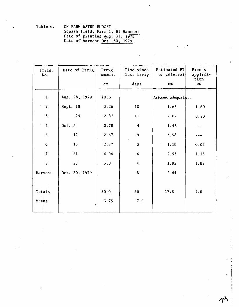
Table 6 . ON-FARM WATER BUDGET Squash f i e l d , Farm 1 , E l Hammami Date of planting Aug. 31, 1979 Date o f harvest Oct . 30 . 1979

T a b l e 7 . ON-FARM WATER BUDGET . .. Pepper f i e l d , Farm 1 , E l Hammami

Date o f vlantinn Seut. 7 . 1979

Table 8. ON-FARM WATER BUDGET Cabbage f i e l d , Farm 1, E l Hammami

D&tc o f p l a n t i n g Dec. 5 , 1978 Date o f ha rves t May 23, 1979

* Missing va lues es t imated from o t h e r d a t a .

I r r i g . amount

cm

13.38

2.47

2.42

4.61

4.44*

7 .0

2.52

1 . 5

2.47

6.86

3.25

6.85

57 .8

4.82

I'ime s i n c e l a s t i r r i g .

days

24

37

10

11

11

9

8

2

5

14

13

24

168

13.1

I r r i g . No.

1

2

3

4

5

6

7

8

9

10

11

12

Harvest

T o t a l s

Means

D a t e o f I r r i g .

Dec. 6 , 1978

Dec. 30

Feb. 5 , 1979

Feb. 15

Feb. 26

Mar. 9

Mar. 18

Mar. 26

Mar. 28

Apr. 2

Apr. 16

Apr. 29

May 23

Es t imated ET f o r i n t e r v a l

cm

2.52

12.04

4.74

5 .32

5.77

4.29

4.00

1.00

2.56

7.40

6.42

12.29

68.35

Excess a p p l i c a - t i o n

c m

Assume d e f i - c i t i s 10 cm

3.38

- - -

- - -

- - -

- - -

- - -

- - -

- - -

- - -

- - -

- - - 1 - - -

3 . 3 8

Table 9 . TENSIOMETER READINGS AND WATER TABLE DEPTHS Corn F i e l d , Farm 5 , Beni Magdoul, 1979

Date o f planting April 2 4 , 1979 Date Of harvest August 14, 1979

The l a s t t a b l e i n t h i s group r e p o r t s t h e i r r i g a t i o n s on cabbage. Agaif t h e f i r s t i r r i g a t i o n was heavy, b u t only t h r e e o f t h e subsequent e leven i r r i g a t i o n s exceeded 5 cm. The ET e s t i m a t e s , when compared with t h e i r r i g a t i o n amounts, suggest some d e f i c i t s accumulated, but then a l a r g e r i r r i g a t i o n tended t o reduce o r e l i m i n a t e t h e d e f i c i t . These ET e s t i m a t e s fromArizonacould be somewhat high f o r Cairo. Also, t h e supply i n t h e water t a b l e comes t o t h e r e scue , s o l i k e l y t h i s c rop d id not s u f f e r excess ive moisture s t r e s s . Note t h a t some i r r i g a t i o n i n t e r v a l s a r e l e s s than 9 days, which sugges ts i r r i g a t i o n dur ing t h e o f f -pe r iod .

Questions 4 , 5 , and 6 cannot be p r e c i s e l y and f i rmly answered from t h e d a t a c o l l e c t e d i n Mansouria. However some i n s i g h t can be obta ined from t h e records of water t a b l e l e v e l s and tens iometer readings . Questions 4 and 5 a r e very important f o r good water management. For ques t ion 6 , it i s important t h a t a method be found t o h e l p t h e farmer decide when it 3s time t o i r r i g a t e , bu t it i s no t e s s e n t i a l t h a t t h e p o s i t i o n of t h e water t a b l e be found t o be a r e l i a b l e guide f o r t h i s dec i s ion . I n t h e following paragraphs, t h e recorded d a t a on water t a b l e p o s i t i o n and t h e readings o f tens iometers w i l l be examined, s e p a r a t e l y and t o g e t h e r , t o ob ta in a t l e a s t some p a r t i a l answers.

I n Table 9, t h e water t a b l e depths shown were measured on t h e same day a s t h e s e l e c t e d tens iometer r ead ings . The measurements s e l e c t e d f o r t h i s t a b l e were made e i t h e r j u s t b e f o r e i r r i g a t i o n o r about t h r e e days a f t e r . The cup of one tensiometer was p l aced 30 cm below ground su r face and t h e o t h e r 60 cm. The one a t 90 cm was not included because i t showed very l i t t l e change i n reading throughout t h e season. A l l t h r e e were t h e mecury-column type , and were p l aced between p l a n t s r i g h t i n t h e corn row.

Looking f i r s t t o ques t ion 5, it appears from t h e tens iometer readings t h a t t h e r e was not excess ive mois ture s t r e s s except poss ib ly be fo re t h e May 13 i r r i g a t i o n , 19 days a f t e r p l a n t i n g . A t ens ion of 458 m i l l i b a r s (mb) i s not excess ive , except t h a t i n t h i s c a s e t h e r o o t s were mostly above t h e 30 cm l e v e l , where t h e t e n s i o n was s u r e l y h igher . A t t h i s s t a g e o f growth t h e c e n t e r of t h e r o o t mass may have been a t 12 o r 15 cm depth. I r r i g a t i o n i s recommended when t h e t ens ion i n t h e c e n t e r of t h e roo t mass reaches about 400 mb. Usually no s e r i o u s damage is done a t 500, o r even a b i t h ighe r . A m i l l i b a r i s about 1/1000 atmosphere, o r equiva lent t o t h e p res su re of one cen t ime te r depth of water . I t appears from t h e reading a t 30 cm t h a t t h e l a s t t h r e e i r r i g a t i o n s were each sooner than needed. However t h e 60 cm readings i n d i c a t e cons iderable r o o t a c t i v i t y t h e r e a l s o , sugges t ing t h a t t h e r e was a t t h a t t ime adequate capac i ty t o s t o r e a l i g h t i r r i g a t i o n . The d a t a from Table 1 shows t h a t t h i s was t r u e , bu t t h a t t h e 11.57 cm and t h e 10.59 cm a p p l i c a t i o n s were much too l a r g e . One can conclude t h a t except poss ib ly f o r t h e f i r s t i rr i- ga t ion , t h e t iming o f t h e s e i r r i g a t i o n s was q u i t e good, even though some o f t h e amounts appl ied werc, excess ive .

Table 10 sugges ts t h a t t h e peppers i n t h e sandy E l Hanunarny s o i l were not s t r e s s e d a s much as t h e corn i n Beni Magdoul, and t h a t perhaps t h e irri- g a t i o n s could have been l e s s f r e q u e n t . However, f o r produce harvested i n a moist o r wet cond i t ion , l i k e peppers , f requent i r r i g a t i o n s usua l ly tend t o i n c r e a s e product ion, provid ing t h e amounts appl ied a r e not exces- s i v e , and s o i l a e r a t i o n i s not jmpaired. A t t h e f i r s t o f t h e season t h e amounts appl ied were q u i t e reasonable , bu t l a t e r they were excess ive .

Table 10. TENSIOMETER READINGS AND WATER TABLE DEPTHS Pepper Fie ld , Farm 1, E l Hammami

Date of p lant ing Sept 7, 1979 Date of l a s t harves t J u n e ' l 9 , 1980

Date o f I r r i g a t i o n

Sept . 7, 79

Sept . 18

Sept . 30

Oct. 15

Oct. 27

Nov. 9

Nov. 21

Dec. 12

Jan. 1, 80

Feb. 3

Mar. 3

Mar. . I5

Mar. 30

Apr. 4

Apr. 20

Apr. 30

May 12

May 23

June 7

June 17

Means

Water Appl i ed

cm

27.82

5.14

5.79

4.08

4.25

4.89

2.29

3.67

3.14

4 .5

3.5

6.41

8.04

9.58

10.14

11.62

9.88

9.90

6.67

6.99

7.41

Tensiometer r a t 15 cm dept Before i r r i g .

ladings . , mb

After i r r i g

50

6 0

64

6 0

7 2

7 0

8 9

65

5 0

8 3

4 5

44

4 6

5 0

67

30

6 0

6 0

7 0

7 5

60.5

Mean depth t - Before i r r i g

66

7 6

7 3

55

7 5

5 5

I 49

75

7 3

5 1

6 3

I 7 1

6 0

7 1

5 2

66

62

58

6 8

75

6 5

-

water -

After i r r i g

38

3 7

54

5 7

5 6

5 4

6 5

4 6

57

55

3 9

4 6

60

4 1

5 2

4 7

39

5 U

77

5 2

5 1

The conclusion is that, after theroot system was well established, c& interval between irrigations could have been increased somewhat. h w - ever, if the yield was limited by irrigation practice, it was not bewU5e the irrigations were too frequent, but because the amounts applied at each irrigation were too great. It is of course possible thatthetensio- meters were not reading quite all the tension that the roots were subjected to. One possible cause could be an energy barrier between the cup and the soil, in case the pores in the sand are much, much larger than those in the tensiometer cup.

Tab1.e 9 also shows t!le depths to water table just before irrigation and froni one to three days after irrigation. The average rise and fall is about one-third meter, between 71 and 104 cm below ground surface. The well locations are generally around the edges of the farm, and are not immediately adjacent to the tensiometer locations, so a mean of all five wells is shown in the table. From the table it appeared that a correlation exists between tensiometer reading and water table depth, so an attempt was made to fit a curve to the set of data points. The graph of the best fit curve is shown in Figure 1. The R2 value is not high enough to give a useful method of predicting when it is time to irrigate by measuring the depth to water. One would like to irrigate when the sum of the tensiometer values reaches about 500, or at least in the range from 400 to 600. But in that range the fluctuation of corresponding depths to water table is too great to be used as an index. This set of data thus gives a negative answer to question 6.

A similar attempt was made to correlate the tensiometer readings in El Hammami with water table depth, and the result was equally unsatis- factory as a method of predicting when to irrigate. Figures 2, 3, and 4 show the results. Only the tensiometer at 15 cm depth was used because the others showed little drying below field capacity. Figure 2 shows a scatter similar to that in Figure 1. The R2 value is much too low to be useful. Only the best fit curve is shown. Figure 3 shows a much more uniformly placed set of points and a much higher ~2 value for the month of September. However, the tensiometer readings were all below 100. Figure 4 for the month of June illu- strates the scatter problems when the tensiometer readings go to 200 mb. The linear curve gave as good a fit as any, but the correlation is too low to be useful. Thus we can conclude that the depth to water table is not a sufficiently accurate indicator of the need to irrigate.

From Figure 5 one can obtain a partial answer to question 4, as far as El Hammami is concerned. Three of the four wells plotted are located in the pepper field, and the other in an adjacent field. The fluctuating lines show the water levels in each of the four wells, respectively. The time and amount of each irrigation is shown by the scaled arrows pointing up from the bottom line of the graph. Amounts are in cm of water. The following features can be observed from this plot:

' 1. The water levels in all wells seem to fluctuate together on about a 12 day cycle, corresponding to the on-periods of the El Hammami Canal.

2 . Thc longest rcccssion was during the January closure period. 'The lowest lcvcl was about 10 cm below the usual low. A

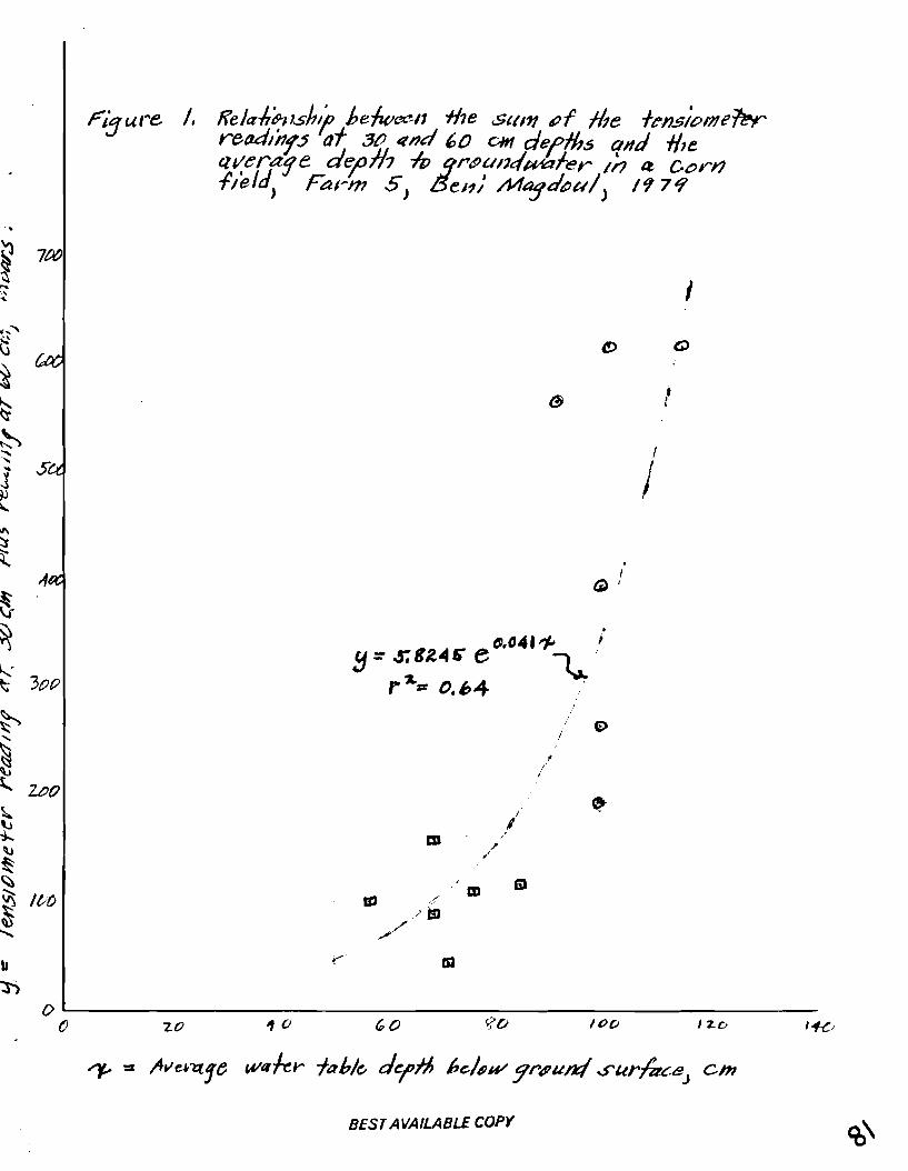
BEST AVAILABLE COPY

' f i i r r c 4 ~ e n s i ~1 fm- readhgs 5 , wafer .16bje deptR %&ing June, , 9 8 0 i n LZ pepper Fie jd , Form / / H t l ~ m ~ * n ;

mathematical p ro jec t ion o f t h i s recess ion curve predic ted a l eve l o f 16 .71.on Jan. 31, o r about another 8 cm lower. The recess ion equat ion was Elev = 16 + 1 . l l e -0.0145t, where I 1 t l l

is time i n days.

3. The water t a b l e r i s e s during each on-period, even i f t h e r e i s no i r r i g a t i o n on t h i s f i e l d ( i . e . Dec. 1, Dec. 23, Feb. 1 8 ) . However, t h e very heavy i r r i g a t i o n Sept . 7 may have been p a r t l y responsib le f o r t h e high r i s e recorded on t h e 9 t h . Likely , however t h e r e was another g r e a t e r influence which a l s o caused t h e high peaks one e i t h e r s i d e .

4 . During t h e r e l a t i v e l y steady flow period o f October and November, t h e h i g h ' s peaked about 17.5 and t h e lows about 16.9, f o r a range o f 25 cm. However, during March, Apr i l , May, and p a r t of June t h e h ighs peaked about 17.8 and t h e lows about 16.94, o r about 3 o r 4 cm higher than i n October and November. Late i n June and dur ing J u l y , both t h e highs and t h e lows dropped near ly 10 cm. The l o g i c a l explanation f o r these changes i s t h a t t h e weeds increased i n t h e spr ing i n both t h e Hammami and Shimi branches, backing water t o a higher l e v e l i n t h e main Hammami Canal nea r Farm 1. Then t h e cleaning opera t ion s t a r t e d i n t h e Shimi and Hammami branches, permi t t ing a lowering o f t h e l e v e l i n t h e canal (and i n t h e groundwater l e v e l ) a t Farm 1.

The conclusions t o be drawn from these observations i s t h a t t h e base level ( the low p o i n t s i n t h e hydrograph) o f t h e water t a b l e is d e t e r - mined by t h e l e v e l of water i n t h e E l Hammami Canal, i t s branches, and i ts meskas. Apparently t h i s l e v e l is maintained mostly by seepage from t h e water courses . Even t h e high peaks, usua l ly about 25 cm higher , a r e governed more by t h e water l e v e l s i n t h e water courses than by t h e amount of i r r i g a t i o n a p p l i c a t i o n . Perhaps t h e same r e l a t i o n s h i p e x i s t s i n Beni Magdoul t o a l e s s e r degree, but because t h e r e is no r o t a t i o n the re , t h e hydrographs don ' t reveal it so c l e a r l y . Thus it appears t h a t t h e water t a b l e i n E l Hammami cannot be lowered a g rea t amount by t h e s i n g l e e f f o r t o f inc reas ing a p p l i c a t i o n e f f i c i ency , although c e r t a i n l y t h i s would he lp . What would he lp much more would be t o decrease t h e conveyance l o s s i n t h e E l Hammami Canal and a l l d i t ches leading from it .

One could specu la te t h a t , i f t h e proposed E l Hammami p ipe l ine could be i n s t a l l e d with t i g h t j o i n t s and l i t t l e seepage, and i f t h e meskas could . l ikewise be replaced by p i p e l i n e s , t h e water t a b l e would su re ly drop a t l e a s t 20 cm a t any farm s i t u a t e d l i k e Farm 1. A g r e a t e r than 20 cm drop might be expected on land c l o s e l y a f f e c t e d by main d ra ins .

There was one c a l c u l a t i o n made from t h e s o i l moisture d a t a t h a t couldprove useful t o t h e water budget c a l c u l a t i o n s . Spec i f i c y i e l d was c a l c u l a t e d f o r t h e top 30 cm of s o i l i n Farm 1 i n E l Hammami and Farm 5 i n Beni Magdoul. The average moisture content measured about 3 days a f t e r irri- gat ion was assumed t o be f i e l d capac i ty . Bulk dens i ty was assumed t o be t h e average measured f o r t h e s e r e spec t ive a reas , 1.68 f o r Farm 1, E l Hammami and 1.217 f o r Farm 5 , Beni Magdoul. F ie ld capaci ty was 5.39 cm and 13.89 cm r e s p e c t i v e l y . P a r t i c l e dens i ty was assumed t o be 2.65. From these values , s p e c i f i c y i e l d was estimated a s about 19% f o r E l Hammami and about 5% f o r Beni Magdoul.

BEST AVAILABLE COPY

Another set of interesting data recorded was the 1979-80 yield of berseem in Beni Magdoul (refer to Table 2) in terns of Egyptian pounds paid for the harvested crop. The first cutting from 6 kerat brought L.E. 42. The second and third cuttings were fed to the owner's animals. The fourth cutting sold for L.E. 30. The last cutting was primarily to clear the land for tomato cultj.vation, and brought only L.E. 5.

\

Conclusions

The following conclusions are based on the six questions adressed by this study.

There is over irrigation in both El Hammami and Beni Magdoul, sometimes in substantial amounts. In general, the amount is more than is needed to leach the salt contained in the irrigation water. However, not all fields measured received excessive total amounts, when you consider that some loss is inevitable. Most of the over irrigation results from too much water applied at a particular irrigation. In some crop seasons, most of the irrigations were excessive. In others there may have been one or no excessive irrigations. But usually there were several excessive and several not excessive. The planting irrigation was usually the heaviest, perhaps in part for leaching purposes.

2 . The following average frequencies and amounts of irrigation were recorded:

Soil moisture samples taken to a depth of only 30 cm before and after irrigation do not give an accurate estimate of the quantity of water extracted from the soil between irrigations. They gave a closer estimate of this quantity for short intervals, say 5 days, than for long intervals, say 21 days. The reason is believed due to the upward moisture gradient in the root zone. During the winter when ET is low, the moisture supplied from the water table apparently is almost enough to satisfy the entire ET requirement without irrigation.

4 . In Farm 5, Beni Magdoul, t h e water t a b l e r i s e s and f a l l s with i r r i g a t i o n s on t h a t farm. The d a t a contained i n t h i s r epor t does not r evea l t h e r e l a t i v e inf luence of conveyance l o s s on t h e pos i t ion of t h e water t a b l e . However, i n t h e sandy s o i l i n E l Hammami, t h e water t a b l e i n Farm 1 seems t o depend almost e n t i r e l y on t h e r i s e and f a l l o f water i n t h e E l Hammami Canal, during t h e r o t a t i o n , r ega rd less of t h e water applied t o t h e farm. Therefore seepage from t h e water courses i s t h e major f a c t o r .

5. The da ta i n t h i s r epor t o f f e r s l i t t l e evidence t h a t e i t h e r of t h e crops monitored with tensiometers suffered from water s t r e s s . Perhaps t h e f i r s t i r r i g a t i o n a f t e r p lan t ing on the corn f i e l d was delayed too long.

6 . The measured depth t o water t a b l e does not serve a s an adequate index f o r deciding when it i s time t o i r r i g a t e .

References

1. El Kady, Mona Moustafa. On-Farm Water Management in Egypt. Ph.D. Thesis, Ain Shams University, 1979.

2. El Kady, M., W. Clyma, and M. Abu-Zeid. On-Farm Irrigation Practices in Mansouria District, Egypt. Paper No. 79-2566, presented at the 1979 Winter Meeting of the American Society of Agricultural Engineers, Hyatt Regency Hotel, New Orleans, La., Dec. 11-14, 1979.

3. Egypt Water Use Project. Problem Identification Report for Mansouria Study Area. Technical Report No. 1, October 1977 to October 1978, Cairo, ARE, March, 1979.

S t a f f Paper # 3 2

SOCIOLOGICAL DATA OF THE PROJECT SITES: SOME CRITERIA FOR UNDERSTANDING THE

IMPLEMENTATION PROCESS

The Sociology Team

Thc fol lowing r e p o r t c o n s i s t s of a s e t o f d a t a which h a s hccn co~npilctl

f o r t h c purpose of ( I ) supplementing the two major soc io1o~ ; i ca l r e p o r t s

d i scuss ing t h e p r o j e c t a r eas and ( 2 ) providing a means i n which c n i c i a l

ques t ions focusing on the implementation process have emerged. A general

d e s c r i p t i o n of t h e a reas have been presented i n t h e fol lowing two repor t s :

- "Social Dimensions of Egyptian I r r i g a t i o n P;itterns1I; and

- " E f f c c t i v e Extension f o r Egyptian Rur;ll llcvcl c)l)mcnt: Fanners ' and O f f i c i a l s ' Views on Al t e rna t ive S t r a t e g i e s " .

l a a t w i l l be presented here is more d e t a i l e d d a t a descr ib ing each pro-

j e c t s i t e with regard t o c e r t a i n c r u c i a l v a r i a b l e s f o r t h e i r r e l a t i o n s h i p

t o an implementation program. The s e t of v a r i a b l e s used a r e organized undcr

four ca t egor i e s : (1) demographic c h a r a c t e r i s t i c s , ( 2 ) i r r i g a t i o n pract ice: ,

(3) t h e fa rmers ' l eve l of i n t e g r a t i o n with each o t h e r and ( 4 ) t h e farmers '

r e c e p t i v i t y toward change. These ca t egor i e s were chosen f o r t h e i r s a l i ence

toward t h e implementation phase of t h e p r o j e c t . A few demographic charac-

t e r i s t i c s were chosen i n o rde r t o provide some d a t a of t h e farmers i n t h e a r e a s

and a l s o t o be used a s a means t o f u r t h e r examine some s p e c i f i c i r r i g a t i o n

p r a c t i c e s . An a n a l y s i s of a few i r r i g a t i o n p r a c t i c e s pcrformcd by t h e

f a r z t r ::ill hcl; d e l i n e a t e saze a c t i v i t i e s and percept ions which w i l l s v r v e

a s an informat ional bas i s f o r c r e a t i n g s p e c i f i c change s t r a t e g i e s and

t a c t i c s . The l a s t two ca t egor i e s provide some measures t o dep ic t t h e envi-

ronment o f t h e farmers with regard t o how change i n genera l may be f a c i l i -

t a t e d o r hindered. Again, t h e focus of t h i s information w i l l c e n t e r on

p o s s i b l e po in t s which w i l l s e rve a s parameters f o r t h e work i n t h e implc-

mentation phase o f t h e p r o j e c t .

The format of t h e r epor t c o n s i s t s mostly o f t a b l e s with some introductory

~ m m e n t s . Tables were used a s t h e mcans by which d a t a i s presented i n order

4\

to allow for the different disciplines involved in the project to make

distinct judgements as to the meaning of the information. Such tables

are supplemented with some general comments which delineate a few major

questions which have to be considered in any examination of the proposed

implementation programs. Iiopefully through a thorough examination of

the tables and comments by the different disciplines in concert with each

other, some effective and nicaningful procedures for imp1 ementati on may

evolve. What will now follow is the presentation of data divided into

the four major categories of demographic characteristics, irrigation

practices, farmers' integration, and farmers' receptivity to change.

DEMOGRAPHIC CHARACTER1 STICS

The variables of concern in this category include the following:

- Family size

- Full time/part time operator

- Farm size

- Division of farm plots on the meska and in the villages

Such information which may evolve from these variables include a delinea-

tion of the labor force available in the area, the degree of time and

commitment exhibited by the farmer concerning his operation, the degree

of wealth of the farmers, and operation procedures of the farms. All of L 1- ,..: abovc informatic2 has been viewed as indicators to explain :?.:

adoption of different innovations.

Table 1: Total Size of the Farmers' Household

Project Site

I\';;;bcr

in

Family

N (Col. %)

1-5

6-10

11 +

Total

Mansouria

12 (52)

7 (30)

4 (17)

23 ( 1 00)

Kafr El Sheikh

5(25)

. 13(65)

2(10)

20 (100)

Minya

11 (35)

17 (55)

3 (10)

31 (100)

Table 2: Fu l l Time/Part Time Operator

P r o j e c t S i t e

Table 3: Tota l Feddans Farmed


M i nya --

27 (84)

5(16)

- -

3 2 (1 01))

Kafr E l Sheikh

20 (1 00)

o(0)

- - - - -

20 (1 00)

- N (Col. %)

Ful l Time

Operator Pa r t Time

Tota l

Mansouria

16(70)

7 (30)

23 ( 1 00)

N (Col. %) Kafr E l Sheikh I Minva I Mansouria

< 1.9 Number -

0 f 2.0-3.9

Feddans 4.0-9.9

lo?

Tota l

N (Col. %)

Owns A l l

Owns Most, Rents Some

Ownership Rents Most, Owns Some

Rents A l l

Uses Family Owned Land

Tota l

12 (52)

5(22)

6 (26)

O(0)

23 (1 00)

Table 4: Ownership P a t t e r n s


Mansouria Kafr E l Sheikh

15 (65) 16(80)

4 (17)

Minya

27 (84)

0 (0)

Table 5: Div is ion of Farming P l o t s


Table 6: P l o t s Farmed i n Other V i l l ages


N (Col. %)

Divis ion Contiguous

of

P l o t s Divided

Tota l

Other

V i l l age

P l o t s

Mansouria

7 (30)

16 (70)

23 (100)

IRRTGATION PRACTTCES/PERCEPTIONS

N (Col. %)

None

Some

Total

A number of ques t ionswereasked which measured s p e c i f i c a s p e c t s of I

t h e fa rmers1 i r r i g a t i o n a c t i v i t i e s and t h e i r i deas p e r t a i n i n g t o some o f

t h e condi t ions involved i n t hose a c t i v i t i e s . The s p e c i f i c a r eas of con- I I

cern inc lude who i r r i g a t e s , when t h e farmer i r r i g a t e s , and t h e fa rmers '

percept ion a s t o how s a t i s f a c t o r y t h e i r r i g a t i o n system i s i n s e rv ing

them. What i s t o follow i s a gene ra l summation of t h e f ind ings and t h e

p r e s e n t a t i o n of some ques t ions which need t o be addressed i n des iga ing

an implementation p r o j e c t .

Kafr EL Sheikh

4 (20)

16 (80)

20 (1 00)

Concerning who i r r i g a t e s , f o r both Mansouria and Kafr E l Sheikh many 1 members of t h e f ami l i e s p a r t i c i p a t e i n t h e i r r i g a t i o n of t h e f i e l d s (Tab le 7 ) .- '

Minya. i s d i f f e r e n t i n t h a t t h e ma jo r i t y of t h e i r r i g a t i o n w o r k i s p ~ r f o r n ~ c d

only by t h e farmer himself (60%). When c o n t r o l l i n g f o r t h e s j z e of f i l ~ m s . ,

Minya

5 (16)

27 (84)

32 (100)

Mansouria

12(52)

11 (48)

23 (100)

Kafr E l Sheikh

13 (65)

7 (35)

20 (100)

Minya

28 (87)

4 (12)

32 (1 00)

i n Minya, from l e s s than o n e f e d d a n t o t e n feddans, t h e farmers show no

s i g n i f i c a n t change i n t h i s p a t t e r n of work (Table 8). Thus t h e r e i s no

focus of farmer workers concen t r a t ing t o t a l l y on t h e smal l farm p l o t s .

The survey has shown a number of i n t e r e s t i n g f i n d i n g s p e r t a i n i n g t o

t h e t ime of i r r i g a t i o n s . For t h e most p a r t , t h e farmers i n t h e t h r e e

a r e a s b e l i e v e t h a t t h e most important i r r i g a t i o n s a r e dur ing t h e p l a n t i n g

and germination s t a g e s o f t h e p l a n t ' s l i f e cyc l e . In Kafr E l Sheikh t h i s

percept ion is l e s s s i n g u l a r i n na tu re with answers being d i s t r i b u t e d from

p r e - i r r i g a t i o n t o i r r g a t i o n a t h a r v e s t t ime (Table 9) . When c o n t r o l l i n g

f o r t h e d i f f e r e n t crops i n t h e a r eas , t h e pe rcep t ions of t h e farmers about

t h e most important i r r i g a t i o n s do change (Tables 10-12). Two i r r i g a t i o n s

were examined i n more d e t a i l i n t h e survey: p r e - i r r i g a t i o n and t h e i r r i g a -

t i o n a t p l an t ing . The m a j o r i t y o f farmers d i d not perform a p r e - i r r i g a t i o n ,

bu t i n Mansouria t h e percentage o f t h o s e who d i d i s g r e a t e r than i n Kafr E l -

Sheikh o r Minya (Table 13) . Again, when c o n t r o l l i n g f o r crops t h e p r a c t i c e s

were d i f f e r e n t f o r each crop (Tables 14-15). For vege tab le s t h e farmers who

d i d have a p r e - i r r i g a t i o n were almost a s many a s those who d i d not while f c r

berseem, a v a s t m a j o r i t y o f farmers (75% i n both Mansouria and Kafr El Sheikh)

d id not perform a p r e - i r r i g a t i o n . When t h e size of t h e ope ra t ion was c o n t r o l -

l ed f o r (Tables 18-19), t h e r e may b e a i n v e r s e r e l a t i o n s h i p p r e s e n t ; i . e . t h e

l a r g e r t h e farm, t h e g r e a t e r t h e p r o b a b i l i t y of not having a p r e - i r r i g a t i o n .

The small N leaves such an i n f e r e n c e h i g h l y ques t ionable , b u t it i s something

which may be pursued.

Ccrrce~nAng t h e p r ~ c t i c e of irrigltlrrg a t t h e t i ~ o 3f p l a n t i n g , t h e

ma jo r i t y of farmers s a y they do no t i r r i g a t e (Table 20). However, Msnsouria

aga in shows t h e l a r g e s t percentage o f people who do i r r i g a t e . When c o n t r o l -

l i n g f o r crops (Tables 21-22) and s i z e o f ho ld ings (Tables 25-26), t n e

tendency of t h e r e l a t i o n s h i p s a r e s i m i l a r t o t h e ones f o r t h e farmers who

have a p r e - i r r i a t i o n f o r t h e i r f i e l d s . One a d d i t i o n a l q u e s t i o ~ concerning

t h e time of i r r i g a t i o n refers t o whether or not t h e farmers i r r i g a t e a t

n igh t (Tables 27-35). A m a j o r i t y of the farmers i n i ia f r E l SLeikh (90%)

say they do, while a major i ty of t h e farmers a r e p r e t t y well d iv ided i n . ha l f of those who do and those who do not . In looking a t some p o s s i b l e

explanations f o r t h e s e r e l a t i o n s h i p s , it was found t h a t t h e p o s i t i o n on

t h e meska i n Minya made l i t t l e d i f f e rence a s t o who does i r r i g a t e , and

who does not . Other poss ib le explanations f o r n ight i r r i g a t i o n may be

t h e farmer 's p o s i t i o n o f having p l o t s i n o the r v i l l a g e s and t h e s i z e of

t h e household ( the g r e a t e r t h e number t h e g r e a t e r t h e p robab i l i ty i n irri-

gat ing a t n ight ) . Again, these r e l a t i o n s h i p s w i l l have t o be more f u l l y

analyzed i n order t o allow f o r any concre te inferences t o be made. There

does not seem t o be any s i g n i f i c a n t r e l a t i o n s h i p between s i z e , o f holdings

and the p rac t i ce of n igh t i r r i g a t i o n . The major reason f o r n igh t i r r i g a -

t i o n i s the lack of s u f f i c i e n t water during t h e day (Table 35). The

farmers were a l s o asked how many times they i r r i g a t e t h e i r crops (Tables

36-39) and how they decide when t o begin and s t o p t h e i r r i g a t i o n of t h e i r

f i e l d s (Tables 40-41).

When asked i f they be l i eve t h a t they rece ive an adequate amount of

water f o r i r r i g a t i o n , t h e farmers on t h e whole s t a t e d t h a t they d id

(Table 42). Kafr E l Sheikh was t h e s i t e which showed a more even d i s t r i -

bution between those farmers who s a i d they d id r ece ive an adequate amount

and those who s a i d they d id not . When con t ro l l ing f o r t h e loca t ion of

t h e farmer's land on t h e meska, t h e t a i l end farmers i n Kafr E l Sheikh

e i t h e r s a i d they always received enough (62%) o r never received enough

(38%). A t t he head, t h e major i ty of farmers s t a t e d t h a t t h e water was

genera l ly not adequate i n t h e summer (58%). (Table 43) Minya shows

l i t t l e d i f ference between head, miaaie, and r a i i . A s t o t h e crops

planted, farmers were not cons i s t en t i n t h e i r b e l i e f about adequatewater

ifi any o f the areas . Farmers ~ l s n t i c g t h e s z i e crop; C O t t G i . Kafr E l -

Sheikh, sugarcane i n Minya, and wheat i n Mansouria; have difr'e-rent idea:;

about receiving adequate water (Tables 44, 47, 49). Control l ing f o r t h e

size of .farms (Tables 45, 48, 50) i n t h e t h r e e a reas shows t h a t t h e r e

might be a r e l a t i o n s h i p i n Kafr E l Sheikh ( the smal ler t h e s i z e , t h e

g rea te r t h e p r o b a b i l i t y of having adequate water) bu t not i n t h e o the r

areas .

The farmers were then quer ied a s t o t h e i r b e l i e f s about dra inage ,

maintenance of d i t c h e s and t h e l e v e l of t h e i r land. Only i n Mansouria

did t h e fanners s t a t e t h e i r dra inage was usua l ly bad (Table 52) . Regard-

ing t h e maintenance of d i t c h e s and d ra ins , t h e farmers i n Minya and Kafr

E l Sheikh did not b e l i e v e t h e p r i v a t e d ra ins and d i t ches were maintained

while i n Minya t h e farmers a l s o d i d not think t h e government d i t c h e s and

d ra ins were maintained (Tables 55 and 57). F i n a l l y , t he farmers i n a l l

t h e areas gene ra l ly thought t h a t t h e i r f i e l d s were a s l e v e l a s they need

be f o r i r r i g a t i o n purposes (Table 56).

One of t h e outputs o f t h e s e genera l f indings a r e the many ques t ions

which must be addressed when developing an implementation program; f o r

- t he d i f f e r e n t s t r a t e g i e s which may be developed i n t h e program w i l l depend

on t h e circumstances permeating t h e a r e a chosen t o be t h e s i t e of t h e

p r o j e c t . The fol lowing l is t i s an i n i t i a l s e t of quest ions evolving from

t h e da ta which should be taken i n t o cons idera t ion .

To whom i s t h e - Who performs t h e ac tua l i r r i g a t i o n of t h e f i e l d s ?

program t o be - What is t h e a v a i l a b i l i t y of labor i n t h e a rea? d i r ec ted?

Upon which base - What is t h e l e v e l of knowledge o f t h e farmer concern-

w i l l extension i n g t h e var ious p r a c t i c e s i n which he engages?

programs evolve? - What is t h e d i f f e r e n c e of knowledge l e v e l s of t h e

f~--?? rhynrlnhn!!? t h e 2-e:7 2,

What a r e t h e r e a l - What a r e t h e circumstances govern;ng G i expia in ing

c o n s t r a i n t s t h e p a r t i c u l a r a c t i v i t i e s of t h e farmer?

toward changing

behavior?

What must be - What are t h e percept ions of fanners a s t o t h e i r

addressed before circumstances?

programs a r e

i n i t i a t e d ?

Table 7: Individuals Who I r r i g a t e t h e F ie lds

Projec t S i t e

Kafr E l Sheikh

Farmer Ilimself

Table 8: Tota l Feddans Farmed and t h e Persons I r r i g a t i n g t h e Fie ld -

Minya

I r r i g a t o r Farmer with Others (family,

e t c . )

Hired Help

Total

Number of Feddans

12(52)

4(17)

23(100)

17 (85)

0 (0)

20 (1 00)

Tota l

18(60)

7(23)

5(17)

7 (23)

5(17) - 30 (100)

10 +

O(0)

3(60)

2(40)

4.0-9.9

3 (60)

0 (0)

1 (40) --

4(100) 1 5 (100)

2.0-3.9

lO(71)

3(21)

1(7)

N (Col. %)

Fanner Himself

I r r i g a t o r Farmer with Others

Hired Help

14 (100)

< 1.9

S(71)

1(14)

l (14)

Tota l 7 (100)

Table 9 : Farmers1 Perception of t h e Most Important I r r i g a t i o n

Plant ing I

Projec t S i t e

Germination I

N (Col . %)

E: 0 -4

Between Germ & 9 a Flowering cd E M .d

b Flowering k k H Beginning o f

Seed

Mansouria Kafr El Sheikh

Later Seed & F r u i t Dev .

I

Tota l 1 23(100) 1 20(100) 1

Table 10: Cropping Pa t t e rn and Farmers1 Perception of the Most

Important l r r i g a t i o n - Mansouria

Crop

Vegetables

8 (73) 12 (55)

Table 11: Cropping Pa t t e rn and Farmers' Perception o f t h e Most

Important I r r i g a t i o n - Kafr E l Sheikh

Crop

Wheat

0 (0)

3(75)

l(25)

4 (100)

N (Col. %)

Plant ing

Germination

Other

Total

N ( ~ 0 1 . t) 1) co t ton II

I

E: 0 .d

P 1 an t ing cr a (d 6 Germination M .d .A

k k

Flowering W Seed

... AuT31

Rice

O(0)

0 (0)

OjOj

4(100)

4 (100)

5 (56)

1111)

3 (33)

0 (0)

9(100)

Tota l

6 (40)

2(13)

3 jZu j

4 (27)

15 (100)

\ h e a t

l(50)

l(50)

0 (0)

O(0)

2 (100)

I

Table 12: Cropping Pattern and Farmers' Perception of the Most - --

Important Irrigation - Minya

N (Col. %)

Planting c 0 -4 Germinat ion w Q)

. Latter Seed k

14 Harvest H

Total

Cotton

9 (69)

2(15)

2 (15)

O(0)

Crop

Maize

7 (100)

Sugarcane -- -- 7 (100)

0 (0)

0 (0)

0 (0)

7 (100)

Total -- -la 23(77)

2 (7)

Table 13: Pre-Irrigation Applied Before Plowing

Project Site

Table 14: Cropping Pattern and Pre-Irrigation Before Plowing - - 1 Plansouria I

Minya

32 (100)

0 (0)

32 (100)

Crop I

Kafr El Sheikh

16 (80)

4 (20)

20 (100)

N (Col . - %)I

N o Pre-Irrigation Yes

N o:. %I 1 ;;; i ~;;;;;m ve:;;;;les li 1 Pre-Irrigation 3(75) . 2(18) 3(43) 8 (36)

Total I! 4(100) 1 ll(100) 1 7(100) 1 1 22(100) 1

Mansouria

15 (65)

8 (35)

Table 15: Cropping Pattern and Pre-Irrigation Before Plowing -

Kafr El Sheikh

Total 1 23(100)

Crop

Cotton Rice Berseem Total

Pre-Irrigation

Total

Table 16: Size of Household and Pre-Irrigation Before Planting - Mansouria

Size of Household

Table 17: Size of Household and Pre-Irrigation Before Planting -

N (Col. %)

Pre-Irrigation No

Yes

Total

Kafr El Sheikh

Size of Household

Total -.

15(65)

8 (35) - 23 (100)

Table 18: Total Feddans Farmed and Pre-Irrigation Before Planting, -

11 +

2(50)

2(50) ~.--

4 (100)

1-5

9 (75)

3 (25)

12 (100)

Number of Feddans

6- 10

4(57)

3(43)

7 (100)

N (Col. %)

Pre-Irrigation No

Yes

Total

6- 10

ll(85)

2(15)

13(100)

1 - 5 3(60)

2 (40)

5 (100)

able 19: Total Feddans Farmed and Pre-Irrigation Before Plantinl: -

Kafr El Sheikh

N (Col. %)

No Pre-Irrigation

Yes

Total

Number of Feddans

11 +

2(100)

O(0)

2(100)

N (ill. %) ll < 1.9

l(100) Pre- Irrigation Yes 0 (0)

Total

16(80)

4 (20)

20(100)

< 1.9 ,

7 (58)

5 (42)

12 (100)

10 +

0 (0)

0 (0)

O(0)

Total

Total I 15(65)

8(35)

23(100)

2.0-3.9

4 (80)

l(20)

5 (100)

l(100)

4.0-9.9

4 (67)

2 (33)

6(100)

Total

16(80)

4(20)

20 (100)

10 +

2(67)

l(33)

3 (100)

2.0-3.9

4 (57)

3 (43)

7 (100)

4.0-9.9

9(100)

0 (0)

9 (100)

Table 21: - Cropping P a t t e r n and I r r i g a t i o n a t Time o f P l a n t i n g - I

Mansouria

C ~ O D

Table 20: - F i e l d s I r r i g a t e d a t Time o f P l a n t i n g


N (Col. %) --

I r r i g a t i o n N o

Yes - T o t a l

* Note (Kafr E l Sheikh - A l l Rice)

Table 22: Cropping P a t t e r n and I r r i g a t i o n a t ~ l m e o f P l a n t i n g - M inya

N (Col. %)

No I r r i g a t i o n

Yes

T o t a l

Crop

Minya

24 (75)

S(25) ---

32 (100)

Mansouria

14 (61)

9 (39)

23 (100)

Berseem

lO(91)

1(9)

l l ( 1 0 0 )

Wheat

2(50)

2 (50)

4(100) '

Kafr E l Sheikh

17 (85)

. 3(15)

20 (100)

Table 23: S i z e of Household and I r r i g a t i o n a t Time of P l a n t i n g - - Mansouria

S i z e of Household

Vegetables

l ( 1 4 )

6 (86)

7 (100)

T o t a l

13 (59)

9(41)

22 (100)

N (Col. %)

No I r r i g a t i o n

Yes

T o t a l

Maize

8 (100)

O(0)

8 (100)

Cotton

11 (79)

3(21)

14 (100)

T o t a l

14(61)

9 (39)

73(100)

N (Col. %)

lu'o I r r i g a t i o n

Yes

T o t a l

Sugarcane

3 (43)

4 (57)

7 (100)

1-5

7(58)

S(42)

Other

2(67)

l ( 3 3 )

3 (100)

To ta l

24(75) I 8 (25)

32 (100) I

6-10

S(71)

2(29)

11 +

2(50)

2(50)

12(100) 1 7(100) :(loo)

Table 24: S i z e o f Household and I r r i g a t i o n a t Time o f P l an t ing -

Minya

S i z e o f Housel~old

N o 8(73) 13(76) 3(100) 24(77) I r r i g a t i o n

Yes 11 3(27) I 4(24i / o ( o ) I 7(231 1 Tota l j j l l ( loo) j 1 7 ( l ~ o ~ ~ ~ t

Table 25: T o t a l Feddans and I r r i g a t i o n a t Time o f P l a n t i n g - Mansouria

Number o f Feddans

Table 26: T o t a l Feddans Farmed and I r r i g a t i o n a t Time of P l an t ing -

Minya

Number o f Feddans

N (Col. %) c 1 . 9 2.0-3.9

S(42) 5(100)

7(58) O(0)

T o t a l 12(100) S(100)

4 .0-9 .9

4 (67)

2 (33) ---

6(100) &

N (Col. %)

I r r i g a t i o n No

Yes

T o t a l

R e l a t i v e Frequency R e l a t i v e Frequency R e l a t i v e Frequency from 10-50% . from 14-83% from 9-83%

10 + T o t a l

O(0) 23(100)

Table 27: Farmers I r r i g a t e a t Night


c 1 . 9

5(71)

2(29)

7 (100)

N (Col. %)

I r r i g a t e a t Night Yes

T o t a l

2.0-3.9

9(64)

S(36)

14 (100)

Mansouria

17 (74)

6 (26)

23 (1 00)

Kafr E l Sheikh

2 (1 0)

18 (90)

20 (1 00)

Minya

18 (56)

14 (44)

32 (1 00)

4.0-9.9

5 (83)

l ( 1 7 )

6 (1 00)

1 0 + 5 (1 00)

o(0)

5 (100)

T o t a l

24 (75)

8 (25) -

32(100)

Table 28: Farmer Meska l o c a t i o n and Night I r r i g a t i o n - Minya

Locat ion on Meska

Table 29: Farmer's P l o t s i n Other V i l l a g e s and Night I r r i g a t i o n -

Minya

P l o t s i n Other V i l l a g e s

N (Col. %) ( 1 None 1 Some ( 1 T o t a l I I I I I

N (Col. %)

I r r i g a t e No

a t Night Yes

T o t a l

Middle

8(100)

o(0)

8(100)

Head

4(44)

5(56)

9 (100)

T o t a l 11 28(100) 14(100) 11 32(100) 1

I r r i g a t e No a t Night

Table 30: S i z e o f Household and Night I r r i g a t i o n - Minya

S i z e . o f Household

Ta i 1

6(40)

9(60)

15 (1 00)

T o t a l

18(56)

14(44)

32(100)

18(64)

10 (36)

T o t a l ( 1 l l ( 100 ) 117(100) 1 3(100)11 31(100) 1

Table 31: T o t a l Feddans Farmed and Night . I r r i g a t i o n - Minya

O(0)

4 (100)

Feddans Farmed ! 1

18 (56)

14 (44)

11 +

l ( 33 )

2(67)

6-10

9(53)

8(47) .

N (Col. %)

I r r i g a t e No

a t Night Yes

T o t a l

17(55)

14(45)

1-5

7(64)

4(36)

I4 (Col. %)

I r r i g a t e No

a t Night Yes

T o t a l

! c 1 . 9

4 (57)

3 (43)

7(100)

2.0-5.9

8 (57)

6 (43)

14 (100)

4 .0-9.9

4 (67)

2 (33)

6(100)

10+

2(40)

3(60)

5 (100)

To ta l

18(56)

14(44) --

32(100)

I

I 1 I

I ! I

Table 32: Farmer's P l o t s i n Other V i l l a g e s and Night I r r i g a t i o n - Mansouri a

P l o t s i n Other V i l l a g e s

N (Col. %) I None ( Some (1 T o t a l II I I I I

I r r i g a t e No

a t Night Yes I I I

Total 1 12(100) 1 l l ( 1 0 0 ) 11 23(100) 1

Table 33: S i z e of Household and Night I r r i g a t i o n - Mansouria

S i z e of Household

N (Col. %)

I r r i g a t e No

a t Night Yes

To ta l

Table 35: Circumstances When Night I r r i g a t i o n i s Performed

Table 34: To ta l Feddans Farmed and Night I r r i g a t i o n - Mansouria

Feddans Farmed


1 - 5

9(75)

3(25)

12(100)

N (Col. %)

I r r i g a t e No

a t Night Yes

Tota l

Water no t s u f f i c i e n t dur ing

6-10

5(71)

2(29)

7 (100)

. < 1 . 9

9(75)

3 (25)

12 (100)

0 2 Busy dur ing day 1(12)

Tota l 1 8 ( 1 0 0 ) 1

11 +

3(75)

l (25 )

4(100)

2.0-3.9

4 (80)

1(20)

5 (1 00)

';: ",with o t h e r a c t i v i t i e s W 1

.,-I 0 -2 B e t t e r f o r c rop c-c U

Neighbors i r r i g a t e a t n igh t

Kafr E l 95eikh !

T o t a l

17(74)

6(26)

23(100)

1 (12)

1 (1 2)

Yinya

14(100)

4 .0-9.9

4(67)

2(33)

6(100)

10+

O(0)

O(0)

O(0)

To ta l

17(74)

6 ( 2 6 ) --

23(100) -I

Table 36: Number of Times Crops W i l l be Irrigated

Project Site

I I I

Total 22(100) 16(100) 32(100) 1 Table 37: Cropping Pattern and Number of Times Crop is to be

Irrigated - Mansouria

Minya

6(19)

14 144)

9 (28)

3 (9)

4-8 Number of- 9-11

Irriga- 12-15 t ions

14 +

Table 38: Cropping Pattern and Number of Times Crop is to be

Irrigated - Kafr E l Sheikh

Mansouria

219)

8 (36)

5(23)

7 (32)

Crop

Kafr El Sheikh

12 (75)

4 (25)

O(0)

0 (0)

Crop

Vegetables

O(0)

o(0)

l (17)

5(83)

6(100)

Berseem

O(0)

7 (64)

3(27)

1(9)

11 (100)

N (Col. %)

4-8 Number o f 9-11

Irriga- 12-13 t ions

14 +

Total

Total

l ( 5 )

8 (38)

5 (24)

7 (33)

21 (100)

Wheat

l (25 )

1(25)

1 (25)

1(25)

4 (100)

Wheat

4 (100)

0 (0)

o(0)

o(0)

4 (100)

Berseem

o(0)

l (100)

0 (0)

0 (0)

l (100)

N (Col. %)

4 -8 Number of 9-11

Irriga- 12-13 tions 14 +

Total

Total

12 (75)

4 (25)

o(0)

0 (0)

16(100)

Cotton

8(73)

3(27)

o(0)

o(0)

11 (1 00)

Table 39: Cropping Pattern and Number of Times Crop is to be

Irrigated - Minya Crop

4-8

of Irriga- 12-13 6 (4 3) t ions 14 +

Total 1 1 14(100)

Maize Sugarcane -- . -. - - 0 (0)

l(14)

3 (43)

3 (4 3)

Table 40: Farmer's Deicision on When to Begin an Irrigation

Other

3(100)

o(0)

O(0)

O(0)

3(100)

Project Site

Total --

6(19)

14 (44)

9(28)

3(9) -

32(100)

Time interval since last irrigation

Top soil appearance.

a Subsoil 0 s moisture C,

2 inspection

Plant -4 Appearance 24

2 water Availability in Ditch

.A . . C) o Access to a Lifting

Equip.

Hardness of Soil

Total I

Mansouria 1 Kafr El Sheikh I Mi nya

29 (7 3)

Table 41: Farmer's Decision on When to Stop an Irrigation

N (Col. %)

The total a ground is 0 r covered w

Water reaches M a certain F: .A point in field A

Depth of water in field

.A m . After a 0 a specified a time period

Total

Mansour ia

Project Site

Kafr El Sheikh Minya

32 (84)

Table 42: Farmer's Perception on Receiving Adequate Amount of

Water

Project Site

Total 1 23(100) 1 ZO(l00) 1 32(100) 1

N (Col. %)

Never V) a o w Usually not > cd .rl 3 k in summer a 0-a u a w a a cd Usually

5: always

Table 43: Farmer Meska Location and Adequacy of Irrigation Water - -.-----

Kafr El Sheikh

Location on Meska

Mansouria

4 (17)

l(5)

18 (78)

, I I I

Total 1 12(100) 1 8(100) 11 20(100) I

Kafr El Sheikh

3(15)

7 (35)

lO(50)

Minya

3 (9)

4 (13)

25 (78)

N (Col. %)

m Q) Never Q) w > cd 3 k Usually not 8 % $ in summer a - 2 - Usually always

Head

0 (0)

7(58)

5(42)

Tai 1

3 (38)

0 (0)

5(62)

Total

3(15)

7 (35)

lO(50)

Table 45: Total Feddans Farmed and Adequacy of Irrigation Water - Kafr El Sheikh

Feddans Farmed

Table - 44: Cropping Pattern and Adequacy of Irrigation Water -

Kafr El Sheikh

Crop

Table 46: Farmer Meska Location and Adequacy of Irrigation Water -

Minya

Location on Meska

Total ,

2(11)

7 (36)

lO(53)

19(100)

N (Col . %)

Never 0

Usually not .z Zj in summer o u.l-4

Usually cc 4 always

Total

10 +

2(67)

O(0)

l ( 3 3 )

3(100)

N (Col. %)

Never m o

IJsually not e l - 4 3 k in summer o u o u o c , o u cd Usua'lly c c q z always

Total

Wheat

0 (0)

l ( 25 )

3(75)

4(100)

Cotton

2 (18)

6(54)

3(28)

11 (100)

2 .0-3.9

l ( 1 4 )

2(29)

4(57)

7 (100)

Total

3(15)

7(35)

lO(50)

20(100)

< 1 . 9

0 (0)

O(0)

l (100)

l (100)

N (Col. %)

n o Never o c, .s 9 k Usually not in o d o , u o c, summer o u ,cd

Usually always

Total

Rice

0 (0)

0 (0)

4(100)

4(100)

4 .0-9.9

o (0)

5 (56)

4 (44)

9(100)

Middle

O(0)

l ( 1 2 )

7(88)

8(100)

Head

O(0)

2(22)

7 (78)

9(100)

Tail

3 (20)

l ( 7 )

11 (73)

15(100)

Total - 3 (9)

4(13)

25 (78) ----i 32(100)

Table 47: Cropping Pattern and Adequacy of Irrigation Water -

Mi nya

N (Col. %)

Never In Q) o t ~ Usually not > rd -d 3 k in summer 8 UQ) U G + J Q) a rd Usually IZ " always

Total

Sugarcane

l(14)

3 (43)

3 (43)

Cotton

l(7)

l(7)

12 (86)

14 (100)

Other

O(0)

O(0)

3 (100)

-

3 (100)

A

Maize

l(12)

0 (0)

7 (88)

8 (100)

b

1

Total

25 (78)

32(100)

Table 48: Total Feddans Farmed and Adequacy of Irrigation Water -

Minya

Feddans Farmed

Table 49: Cropping Pattern and Adequacy of Irrigation Water -

N (Col . %)

Never In Q)

Usually not > Cd .r( 3 k in summer Q) UQ)

$ $ 2 Usually IZ " always

Total I

Mansouria

Crop N (Col . %)

Never

Usually not in summer

Usual 1 y always

Total

<1.9

0 (0)

0 (0)

7(100)

7(100)

Wheat

l(25)

l(25)

2 (50)

4 (100)

2.0-3.9

3(21)

2(14)

9(65)

14(100)

Berseem

2(18)

0 (0)

9(82)

11 (100)

4.0-9.9

o(0)

l(17)

5(83)

6(100)

Vegetables

l(14)

O(0)

6 ( 8 6 )

7 (100)

I

' 10 +

o(0)

l(20)

4 (80)

5(100)

Total

4(18)

l(4)

17 (78)

22(100)

Total --

3(9)

4(13)

25(78)

-4 . 32(100)

Table SO: Total Feddans Farmed and Adequacy of Irrigation Water - Mansouria

Feddans Farmed

v) a) P) C, > d -d I k P) UP) u a C , Q Q rb E d =

Total

4(17) l(4)

18(79)

,23(100)

Table 51: Farmer's Perception on Adequate Timing of Water Delivery

Project Site

Estimate of Estimate of Estimiite of Water Table: Water Table: Water Table: 60-300 an 20-200 cm 50-500 cm

10 +

o(0)

O(0)

O(0)

O(0)

Table 52: Farmer's Perception of Adequate Drainage

Project Site

4.0-9.9

3(50)

l(17)

2(33)

6(100)

N (Col. %)

Never

Usually not in summer Usually always

Total

Minya

O(0)

2(6)

30 (94)

32 (100)

Kafr El Sheikh

2(10)

2(10)

16 (80)

20(100]

N (Col. %)

P) Not adequate C,

Adequate in winter only

$ .5 d Usually adequate

Total

Minya

8(25)

3 (9)

21 (66)

32(100)

< 1.9

1(8)

0 (0)

11 (92)

12(100)

Mansouria

3(13)

7.(30)

13(57)

23 (100)

Kafr El Sheikh

o(0)

6(30)

14 (70)

20(100)

N (Col. %)

Usually bad

Drainage Sometimes bad

Not bad

Total

2.0-3.9

o(0)

0 (0)

S(100)

S(100)

Mansouria

14 (61)

2 (9)

7 (30)

23 (1 00)

Table 53: ~armer Meska Location and Perception of Adequate

Drainage - Kafr El Sheikh Location on Meska

N(Col.%) 1 1 fly;; 1 Tai 1

Usually bad 0 (0)

Drainage Sometimes bad 1 ) 6(50) 1 o(0)

Not bad 8(100) - . - - - - - Total

Total

O(0)

6(30)

14 (70) - -- --- I 20(100)

Table 54: Farmer Meska Location and Perception of Adequate

Drainage

Drainage - Minya Location on Meska

Table 55: Farmers1 Perception: Adequacy of Maintenance of

N (Col. %)

Usually bad

Sometimes bad

Not bad

Total

Private Ditches and Drains

Project Site

Head

l(11)

2(22)

6(67)

9(100)

Ditches Adequately Maintained NO 14 (70) 31 (97)

- - -- -- -- Total 20 (100) 32 (100)

Middle

3(38)

l(12)

4(50)

8(100)

Table 56: Farmers1 Perception: Fields Are as Level as They Should Be for Good Irriyation

Project Site

Tai 1

4(26)

o(0)

11 (74)

15(l00)

Field Adequate No

Total

Total

8(25)

3(9)

21 (66)

32(100)

N (Col. %) 1 Mansouria Kafr El Sheikh

20(100) Level of Yes

5(22)

23 (100)

Minya

18 (56) 18 (78)

o(0)

20 (100)

14 (44)

32(100)

Total 1 23(100) 1 20(100) 1 32(100) 1

Table 57: Farmerst Perception: Adequacy of Maintenance of Government Ditches and Drains

Project Site

INTEGRATION OF FARMERS AMONG THEMSELVES

AND THEIR RECEPTIVITY TO CHANGE

N (Col. %)

Ditches Adequately Maintained No

One of the major components of the pilot programs is that of the

organization of farmers for some collective action pertaining to the irri-

gation of their fields. Questions were asked of the farmers to initally

see if any type of cooperation existed and how they viewed change. Know-

ledge of both conditions is necessary to develop strategies pertaining to

the changing of a particular type of behavior, especially when that behavior

will require a collective change. The results of survey show that there

is a distinct predisposition for collective action and change in the areas

of study. How this predisposition can be positively exploited will need

to be examined as the pilot programs develop. Tables 58-70 present some

of the findings pertaining to farmer cooperation and receptively to change.

Table 58: Number of Families (Related) Visited by Respondent

Project Site

Mansouria

16(70)

7 (30)

Mansouria

Number of 4 -6

Kafr El Sheikh

19(95)

1(5)

Families 7-15

Minya

o(0)

32(100)

-- -

Total 1 23(100)

Kafr El Sheikh

4 (20)

8(40)

7 (35)

l(5)

20 (100)

Mi nya

11 (34)

5(141

8 (25)

8(25)

32 (100)

Table 59: Number of Families (Not Related) Visited by Respondent

Project Site

Table 60: Number of Families (Related) Which the Respondent

N (Col. %)

0 -'3 Number of 4-6

Families 7-15

16 +

Total

Exchanged Animals, Tools, etc.

Project Site

Mansouria

11 (48)

6(26)

4 (17)

2(9)

23(100)

Kafr ,El - Sheikh

8 (40)

6(30)

2(10)

4 (20)

20 (100)

N (Col . %)

None Number of Families 4-9

10 +

Total

Table 61: Number of Families (Not Related) Which the Respondent

~xchan~ed Animals, Tools, etc.

Mansouria

3 (1 2)

10 (44)

5 (22)

5(22)

23 (100)

Kafr El Sheikh

1(5)

5 (25)

12 (60)

2(10) .

20 (1 00)

Project Site I

Minya

9 (28)

12 (38)

7 (22)

4(12)

32 (100)

Minya I 13(41)

9 (28)

7 (22)

3 (9)

32(100)

Number of Families

.,

N (Col. %)

None

1 - 3 4-9

10 +

Total

Mansouria

lO(44)

4 (17)

6(26)

3(13)

23 (1 00)

Kafr El Sheikh

4 (20)

10 (50)

3(15)

3(15)

20(100)

Minya

11 (34)

12 (38)

6(19)

3(9)

32(100)

Table 62: Number of Families (Related) Which the Responaent Exchanged

Work

Project Site

Table 64: Respondents1 Answers to the Statement: "On Important

Kafr El Sheikh

4 (20)

3 (15)

5 (25) 8 (40)

20(100)

N (Col. %)

None

Number 1-2 0 f 3-4 Families

5 +

Total

Table 63: Number of Families (Not Related) Which the Respondent

Exchanged Work

Project Site

Things, People Line Up on Opposite Sides"

Mansouria

16 (69)

3(13)

2 (9) 2 (9)

23(100)

N (Col. %)

None Number of

1 - 2 Families 3-4

5 +

Mansouria

16 (69)

2(9)

2(9)

3(13)

Project Site N (Col. %> -

+J

5 Agree a a,

R ~ o t sure

pq a, Disagree EL

Total

32(100)

Kafr El Sheikh

6 (30)

4 (20)

6(30)

4(20)

Total

Minya

11 (34)

7(22)

8(25)

6(19)

23(100) 1 20(100)

Mansouria

5(22) .

O(0)

18 (78)

23(100)

Kafr El Sheikh

5(25)

, O(0)

15 (75)

ZO(100)

Minya

0 (0)

7 (22)

25 (78)

32(1001

Table 66: Respondents' Answers t o t h e Statement: "People Often

Change S ides o f an I s s u e a s it Develops"

Table 65: Respondents' Answers t o t h e Statement: "Even \\%en

Something Seems Like a Good Idea , People W i l l Plot Move"


v, N (Col. %) - +J

5 k Agree a a,

~ o t s u r e a E

Disagree a:

Tota l

Table 67: Respondentst Answers t o t h e Statement: "The E f f e c t

P r o j e c t S i t e In

Required t o Change Things is Often Greater than t h e

Mansouria

5(22)

0 (0)

18 (78)

23 (100)

Benefit"

Minya

29 (91)

3 (9)

32(100)


Kafr E l Shsikh --

5(25)

O(0)

15(75)

20 (100)

Kafr E l Sheikh

19 (95)

l ( 5 )

20 (100)

; N (Col. %) s I4 a cu d f Agree 0 In

2s Disagree a, a:

Total

Minya

6(19)

3 (9)

23 (7 2)

32(100)

Mansouria

23(100)

0 (0)

23(100)

v, N(Co1. %) - w C

k Agree

2 E Not s u r e a r 2 Disagree a:

Tota l

Kafr E l Sheikh

1 (5 )

O(0)

19 (95)

20 (100)

Mansouria

2 (9)

0 (0)

21 (91)

23 (100)

Minya

4(12)

2(6)

26(81)

32(100)

Table 68: Respondents' Answers to the Statement: "There is More

Prof it in Farming by Following the Newest ~ecommendat ions"

Project Site

Table 69: Respondents' Answers to the Statement: "Accept Life

Around Us as God's Will - Do Not Try to Change It" Project Site

Minya

32 (100)

0 (0)

O(0)

32 (100)

N(Col.%) - Agree g P4 Not sure

0 vl 25 Disagree al a:

Total

Table 70: Respondents' Answers to the Statement: "Old Ways are

Generally the Best Ways"

,"1 N (Col. %) c,

g , P4 Agree C Q,

O,z Not sure vr E: $ 4 Disagree

Total

Project Site

Mansouria

23 (100)

O(0)

0 (0)

23(100)

Kafr El Sheikh

20 (100)

O(0)

O(0)

20(100)

Mansouria

6(26)

o(0)

17 (74)

23(100)

The previous set of data is to serve as an initial picture of the

social situation of the farmer in the sites where the pilot programs are

to be established. There-are other types of information which have to

be collected in order to complete the picture; yet the data in this staff

paper, supplementing the two major papers previously addressed, presents

to the sociological team a set of parameters which can be uscd in helring

to design the pilot programs.

Kafr El Shiekh

2(10)

1(5)

17(85)

ZO(100)

.? N(Col.%) c,

Agree -0 P4

Not sure 0 3 n m 3 Disagree 0:

Total

Minya

4(12) 10 (31)

18 (56)

32(100)

Kafr El Sheikh

3(15)

O(0)

17 (85)

20 (lGuj

Mansouria

3(13)

O(0)

20 (87)

23(100)

Minya

0 (0)

0 (0)

32(100)

32 (100)

staff Paper #33

ANALYSIS OF SOIL WATER DATA COLLECTED FROM WINTER CROPS 1N EL MINYA 1979-80

Agronomy Discipline of El Minya and Main Office Cairo

Abdel Satta~, A, Taher E R, Tinsley

This report presents 20 tables reviewing the soil water data collected in El Minya during winter season 1979-80 for four crops. The report is submitted t o illustrate what soil water data is currently being collected, how it is being analyzed, and some interpretations of the analysis. This report also serves as a'first approximation for developing a standard procedure of.soil water analysis,most of which could be done at the site location. For this reason we solicit any comments on how helpful these tables are and what additional tables and interpretations would be more useful for each discipline.

The first set of tables (Table 1-4) is a record for each crop of the irrigations starting with planting as 1st and continuing to harvest. the tables show the volume of soil watcr to30 cm depth in the soil one day before and three days after each irrigation. The three days after irrigation represent the usual time allowed for a wetting front to become distributed through the soil profile. The tables continue to show the volume of water applied, the volume of water stored after three days for each irrigation and then a calculation of irrigation application efficiency. This is based on the water stored after three days and the water applied. It does not account for the water used during the four days between samplings. Thus the actual efficiency is somewhat greater than shown. The irrigation application efficiency ~hows~rnore variation than would be desirable. They also are substantially nigher than expected even going over 100% on a couple occasions. This contrast with the usual surface irrigation application efficiency which will range around 60%. The high values are not completely impossible. There are several possible sources of reasonable error that can have a multiplicative compounding effect. Some of this will be discussed later.

The final portion of the main body of Tables 1-4 relates to soil water depletion between irrigations. This value is calculated as a difference between soil water after one irrigation and before the next irrigation. The value should represent the ttconsumptive use" of plants plus any continual deep percolation. This is finally expressed as daily soil water depletion value. The numerical value of the daily soil water

, depletion appears reasonable close to expected "consumptive usett. This would indicate that the deep percolation after three days was relatively small. However, the values are considerably less than the Blanney-Criddle values used for calmlaTed consumptive use at other project locations, with less evaporation energy than in Minya.

At the bottom of the tables are some summary information on the total water depletion which is the sum .of the soil depletion.values plus a correction to account for the unaccounted four days between sampling. This is then used to calculate a water production index that shows the production per unit of water lost. .

Table 5 is a brief summary of the daily soil watcr depletion for all crops studied. The values are mostly taken fron Tables 1-4 assigned to the month that most nearly corresponds to the irrigation interval involved. The maximum value obtained for any crop is shown at the left along with a letter indicating which crop. This value may be useful in water budget determinations, as the value to use that will accommodate all crop requirements. Likewise they may be useful in an initial estimate of the total water needed in a given month, and coupled with the amount of water released into the canal, provide the first crude approximation of excessive water use. This could than become an realistic initial target for improvement.

Tables 6 to 9, are a closer look at soil water depletion values for each crop. These tables show how muah of the water depletion is coming from the upper 30 cm of the soil. This is the area with the highest concentration of roots and from which most of the water is extracted by the plants. As expected this shows that most of the water loss is coming from this zone. The range is from slightly under 50% all the way to the upper 80 or 90 percent. Most values were between 50 and 75% of total water loss. All the water depleted was not consumptive use as the value of 111% indicates (Table 7). In 'this case some water continued to per- colate from the upper horizons and accumulated in the lower horizons during the inter-irrigation period. These tables illustrate the need to concentrate on the upper 30 cm, but not to the exclusion of the lower horizons.

I

Table 10 and 11 show the changes in soil water from irrigation to irrigation. The tables illustrate a general but not conclusive trend toward wetter conditions as the seasan progresses. This could indicate a certain degree of over irrigation. It is interesting to observe that the soil water in the 60-90 cm depth does not change appreciably after the first irrigation, and is not affected by irrigation during the crop season. Also the average moisture of the 30-60 cm depth is usually higher than the soil water in the 60-90 cm depth. This could be attributed to the tendency of increasing alkalinity and bulk density with depth. Table 10 shows the data in terms of percent dry weight while Table 11 has this converted to % by volume and summed for the 90 cm of soil to give cm H20/90 cm soil. This table also shows only a general non-conclusive trend for wetter soil profiles both before and after the different irrigations.

Table 12 and Fig. 1 show the soil water characteristics of soils in El Minya as measured with pressure plates. The values represent an average of 6 representive profiles. The determinations were made using disturbed samples. This would effect the values obtained from the lower tensions. The samples were originally taken at 30 cm intervals, but the similarity in values for the lower three justified the lumping

together into a 0-30 cm and 30-120 cm fractions. From the data it is observed that there is only a slight decrease in soil moisture content by increasing suction from 0.33 to 1 bar i.e., from field capacity to maximum irrometer reading. .

Table 12 is really to be used in connection with Tables 13 to 16 to illustrate the moisture tension range over which the systems were operating. This shows that irrigation was usually applied when the . soil in the upper 15 cm was between 3 and 15 atmosphere, and after irrigation the soil was between 0.1 and 0.33 atmosphere which is above "field capacity". Lower horizons were generally wetter usually staying wetter than 0.33 to 1 atmosphere tension even just prior to irrigation. This is generally wetter than may be desired and indicates a need to consider longer intervals between irrigation. Unless thepincreasing alkalinity and bulk density prablems hinder water uptake.

The generally wet conditions raise the question of possible aeration problems. Tables 13 to 16 attempt to show this by looking at the percent of the soil which is mineral adding the percent water by volume and sub- stracting from 100. This showed the possibility of saturated condition frequently occuring even in the 15-30 cm depth, and almost continuous saturation below this. This is surprising because the water table is supposed to be 1.5 to 2.0 m below ground level. If this is the case the data indicates either a very large capillary fringe or a perched water table within the first meter, that is not being picked up by the 3 m observation wells. These possible saturated conditions in the sub-soil 1 meter above the water table could be associated with the dispersion

, and compaction of the alkaline clay. If ti:c s ils are indeed saturated below 30 cm there could be a severe aerati~~ prob1:ms. This should be

I examined with some root samples for each crop, and observing influence of irrigation on the water table.

One problem with the aeration data is that frequently the sum of mineral plus water would exceed 100% to even reach almost 120%. This would indicate a systematic error. The most likely place would be in bulk density determinations. The bulk density values particularly at lower depths were actually higher than expected with values of 1.20 at the top and 1.47 at the bottom. Errors under these conditions may be due to either sampling procedure or problems in getting a constant weight in drying these hydrated clays. Also, determination of bulk density could change depending on soil moisture content at sampling time.

Table 17 is a puttering around table looking for some consistency upon which long range project strategy could be developed. None of the parameters examined showed any real promise. It would be very convenient if there was some consistency in the water applied. However, this may improve in other areas where lift irrigation is required. 'The farmers may then either run their animals or pumps for a relatively stable time period and in the process apply water in uniform increments. The other value of real potential for planning is the intervals between irrigations. But consistency here was also lacking. The other parameters really have little practical potential for use. -

.The last three tables are intended to review some of the problems in s%il water measurements and analysis. Tables 18 and 19 review the reliability of soil moisture measurements. This is an outgrowth of the concern for irrigation application efficiency data and the contribution. soil moisture measurements would have. To look at this, nine replicates of soil moisture were taken from two recently planted cotton fields both before and after irrigation. The results were averaged, along with the standard deviation and coefficient of variation. Table 18 shows this with the soil moisture expressed on a dry weight basis. The data looks about as reliable as you can expect from a biological or natural physical setting. Most of the standard deviation are in the order of 2 percentage points with an overall C.V. of 5 percent. However, there can be some compounding effect by which a small error when summed through the entire profile could still contribute to substantial error in application efficiency. Thus Table 19 was made to show the water on a volumetric bases and the effect on the entire profile was examined. As expected there was some within profile compensation between different levels, so that the C.V. for the total volume of water in the profile was usually considerable less than the different depths taken separately. The C.V. were thus in the order of 2 to 3% and the S.D. in order to 1 to 1.25 cm. However, when the applied water is.of the order of 10 cm this could cause an error of 10 to 12 percent.

Other sources of error in measuring water application efficiency could be in use of flumes. This is particularly a problem when flumes are temporary and reinstalled for each irrigation. Bill Ree re1,iewed this problem and developed an HP 67 program to determining the flow error for different errors in hb. This indicated, that for a flume with 20 cm throat, and 10 cm ha near submergence the error of + cm in hb, as would occur in reasonable misalignment of a temporary flume due to set- tling after placement, would be 10 or 20% depending on which way the error was. This added to the 10% error in soil water could bring the error to the 20-30% range.

The last table shows.some of the inconsistency in using tensiometers for measuring soil water. This simply shows that tensiometers are not a vigerous research tool, and never were intended to be such. They are subject to good deal of systematic error, particularly in a hydrated clay soil that cracks and heaves with wstting and'drying. Also as indicated in Table 12 for the El Minya soils the full range of the tensiometer remains in neighborhood of "field capacity". This data is not intended to indicate tensiometers should not be used, but only the appropriate amount of skepticism that is required when relying on them.

This concludes the report. There are no conclusions to be drawn at this time other than the commentary presented. Again it is requested that any comments or ideas for improvement be forwarded to us. This will assist us in formalizing a standard procedure for soil water evaluation.

Table 1. Irrigation and Soil Water Depletion Summary for Wheat in El Minya Winter 1979-1980

Irrigation Sample date . Soil water Water Irrigation Soil water Days .Soil water before/ change applied application depletion between Depletion after efficiency between readings per day

Irrigations

4th - Before : Feb . 28, 1980 After:Mar. 2, 1980

5th Before:Mar . .l9, 1980 45.16 - After:Mar. 23, 1980 52.23 7.07 13.58 52.1

2.97 12 0.25

6th - Before: April 4, 1980 49.26 After:April 9, 1980 53.42 4.16 9.55 43.5

10.30 33 0.31

Harvest May 12, 1980 43.04

Total water loss 38.51 = 7.1U = 45.61 - - - - - - - -

To account for water used during irrigation period calculated by taking daily soil depletion for previous period x 4 for days between before and after irrigation measurement. I ... :.,.

' . <,

Total growing season 161 days Total water loss 45.62 cm = 1915.6 m3/f

Yield: 13.26 + 2.03 Ardab/F. grain C.V. 15% plus 5.8 + 0.61 T/F straw C.V. 10%

Water production index = 13.26 + 5 0 8 = .069 Ardebs grain + 3.0 kg s t r a ~ / m ~ ~ ~ 0 . ,

/ Water loss 1915.6

6

Table 2 . I r r i g a t i o n and S o i l Water Deplet ion f o r Broadbeans i n E l Minya Winter 1979-80

I r r i g a t i o n Sample d a t e S o i l water Water . I r r i g a t i o n S o i l water Days S o i l water Before/ change app l i ed a p p l i c a t i o n d e p l e t i o n between Deplet ion a f t e r e f f i c i e n c y between readings p e r day

I r r i g a t i o n s

Harvest Apr. 18, 1980 4 4 . 7 3

To ta l s o i l wate: d e p l e t i o n 21.85 = 2.60 L/ - -

lJ To account f o r water u s e dur ing i r r i g a t i o n per iod cr~;-,:lnti.:? b:: t zk ing t h e d a i l y s o i l dep le t ion of t h e previous per iod x 4 f o r t h e days between b e f o r e and a f t e r i r r i g a t i o n sampling.

To ta l growing per iod 151 days 3

Tota l water l o s s 24.45 cm = 1027 m / F .c

Yield: 9 .68 5 0.76 Ardabs/F seed C . V . 7 .9% 3.56 t 0.07 T/F s t r a n C . V . 1 . 9 %

Yield - Water product ion index = ,___ 9.68 + 3.56 = 0,0094 Ardabs seed + 3.5 kg strawlm

3 w a L c A A V 3 3 i n37 .. ".. >

Table 3. Irrigation and Soil Water Depletion Summary for Onions in El Minya - Winter 1979-80

Irrigation Sample date Soil water Water Irrigation Soil water Days Soil water Before/ change applied application depletion between Depletion after efficiency between readings per day

Irrigations

1st - Before:Sov. 25, 1979 46.43 After :Xov. 29, i979 53.78 7.35 9.71 76

4.26 3 7 0.12

2nd - ,Before: Jan. 2, 1980 49.52 After:Jan. 5, 1980 58.33 8.81 10.86 8 1

7.95 3 3 0.24

Harvest Apr. 15, 1980 45.69

Total soil water depletion 25.70 + 3.4gU = 29.1;

1/ To account for water used during irrigation period calculated by taking the daily soil depletion of previous period x 4 for days between before and after irrigation sampling.

Total growing period 142 days 3

Total water loss 29.18 = 1226 m /F

Yield: 13.04 t 0.77 T/F C.V. 5.89 n = 4 10% Discount for channels = 12.06 T/F

Water production index = Yield - - 12'060 = 9.84 kg onions/m 3

Water loss 1 7 7 6 H2°

T a b l e 4 . I r r i g a t j o n . and Water Loss Summary f o r Broad bean/Sugarcane i n E l blinya Ninger 1979-80

: r r i g a t i o n Sample d a t e S o i l wate r Water I r r i g a t i o n S o i l wate r Days S o i l wate r Before/ change a p p l i e d app . l i c a t i on d e p l e t i o n between Deple t ion a f t e r e f f i c i e n c y between r e a d i n g s p e r day

I r r i g a t i o n s

2nd - 9efore:Nov. 17 , -1979 44.07 After: Nov. 23, 1979 49.14 5 .07 9 .0 5 7

6.21

5 t h - Before :3lar. 13 , 1980 44.55 After:Mclr. 18, 1980 5 0 . 7 6 5 , k ) l 1 4 . 0

Ha rves t Apr. 15, 1980 4 1 . 8 6

m . 'lot;ll s o i l depletion 32.69 + 4.761i = 37.45

To account f o r wate r u s e du r ing i r r i g a t i o n p e r i o d , c a l c u l a t e d by t a k i n g t h e d a i l y s o i l d e p l e t i o n of t h e p r ev ious pe r iod x 4 f o r t h e days between t h e be fo re and a f t e r i r r i g a t i o n sampling. .c

T o t a l growing pe r iod f o r broad bean 171 days 3

T o t a l water l o s s 37.45 cm = 1572.0 m / f

Y ie ld : 7 .11 t o 0.72 Ardabs/F seed C.V. 10% + 2.64 + 0.45 T/F s t r aw C . V . 17O0

Water p roduc t ion index = Yield - "11 2 ' 6 4 sugar = 0.0045 hrdlbs seed + 1 .7 kg s t raw +. sugarcane/rn 3 H,O wate r l o s s 1572 L

Table 5. Daily S o i l Water Deplet ion f o r Winter Crops i n E l Minya 1979-1980

Approx . Sugarcane/ Wheat Broadbean Onions Max months Broadbean

January 0.12 0.15 0.06 0.24 0.24 0

February 0.29 0.35 - - 0.31 0.35 1V

March 0.32 0.37* 0.21 0.20 0.37 1V

Apr i 1

Gross Ave . 0.24 0.29 0.16 0.22

* Weighted average o f water d e p l e t i o n between 4 t h - and 6 t h - i r r i g a t i o n

Table 6. E l ~ i n ~ a S o i l Water ~ e ~ l e i i o n from Upper 30 cm - Wheat During Winter 1979-80

So i l Volume of So i l Water Water Depletion % of Tota l • Depth After Before Specif ic Total

previous Current Horizon P r o f i l e (90cm) .

From 1st - t o 2nd I r r i g a t i o n - 0-15 8.86 4.97 3.89 5.16 7 5

15-30 7.95 6.79 1.16 2 2

Total 5.05 9 7

From 2nd - t o 3rd I r r i g a t i o n - 8 ..54 6.15 2.39 4.88

8.76 7.08 1.68

Total 4.07

From 3rd - t o 4 th - I r r i g a t i o n

9.24 8.18 1.06

Tota l 4.76

From 4th - t o 5 th I r r i g a t i o n - I

0- 15 8.96 6.18 2.78 7.78

15-30 8.91 8.02 0.89

Total 3.67, 47

From 5 th - t o 6 th - I r r i g a t i o n ,

0- 15 8.80 6.66 2.14 2.97

Total 2.60

. From 6th I r r i ga t i on t o Harvest

0-15 8.99 4.94 4.05 10.38

15-30 8.60 , 6.50 2.10

Total 6.15

* Table 7. E l Minya S o i l Water Depletion from Upper 30 cm - Broad Beaqs During

Winter 1979-80

- S o i l Volume of S o i l Water Water Depletion % of To ta l Wepth Af te r Before S p e c i f i c To ta l

previous Current Horizon Prof i 1 e' (90cm)

From 1st - t o 2nd I r r i g a t i o n - 6.44 2.33 7.67

7.08 0.86

Tota l 3.19

From 2nd - t o 3rd I r r i g a t i o n - 6.44 2.02 2.65

7.40 0.91

To ta l 2.93

From 3rd t o 4 th I r r i g a t i o n - -

Total 4.61

From 4th I r r i g a t i o n t o Harvest - 6.17 2.70 5.11

6.20 1.03

Total 3.73

Table 8. Minya Soil Water Depletion from Upper 30 cm - Onions During Winter 1980

.. . L 1 . ,

, Z .*" b*.. - ,: *

Soil Volunie of Soil Water later Depletion.' - % of Total p:J6%% a Depth . After Before Specific Total

previous current ' ~orizon Profile (90 cm)

4 ......................... cm -------------- cm

From 1st - to 2nd - Irrigation 0-15 8.27 6.55 1.72 4.26 40 15-30 9.04 8.03 1.01 2 4 -

Total 2.73 64

From 2nd to 3rd Irrigation 7 -

8.87 0.80 Total 4.12

From 3rd - to 4th Irrigation -

8.05 1.32 Total 4.05

From 4th Irrigation to Harvest - 0-15 9.33 5.10 4.23 8.92 47 15- 30 8.98 6.98 2.00 -

Total 6.23

Table 9. Minya S o i l Water Depletion f& Upper 30 cm - ~ r o a d b e a * + s u ~ a r c a n e . Intercropped During Winter 1979-9180

. S o i l Volume of S o i l Water Water Depletion % of Tota l Depth After Before S p e c i f i c Tota l

- previous cu r ren t ~ o r i zon Prof i 1 e (90 cm)

cm -----------------------. - cm

From Plant ing t o 1st - I r r i g a t i o n

0-15 7.88 6.73 . . - 1.15 i . 4 . 9 3 23 15-30 7.99 7.14 0.85 17 -

Tota l 2.00 40

From 1st - t o 2nd I r r i g a t i o n - 0- 15 8.16 4.84 3.32 6.22 53 15-30 8.14 6.85 1.29 2 1 -

Tota l 4.61 7 4

From 2nd t o 3rd I r r i g a t i o n - 0-15 8.58 6.13 2.45 4.86 5 0 15-30 8.44 6.80 1.64 - 34

Tota l 4.09 84

From 3rd - t o 4th I r r i g a t i o n - 0-15 8.72 5.99 2.73 7.78 35

7.41 . 1.51 Tota l 42.4

From 4th - I r r i g a t i o n t o Harvest

0-15 8.76 5.04 3.72 8.90 4 2 15-30 8.50 7.23 - 1.27 - 14

Tota l 4.99 5 6

Table 10. Trend Toward Progressively Wetter S o i l s a s Winter Season Advanced i n E l Minya 1979-1980

Soi 1 Day Before I r r i g a t i o n Harvest Three-~fter irrigation Depth 1 2 3 4 5 6 1 2 3 4 5 6 -

cm - - - - - - - - - - - - - - - - - - - - - - - - - - - - - - - - - - - - - - - - - - - - - a - % dry w t . . . . . . . . . . . . . . . . . . . . . . . . . . . . . . . . . . . . . . . . . . . . . . . . . . . . . . . . . . . Wheat

0-15 23.65 27.16 33.61 33.97 33.68 36.40 26.98 48.42 46.68 54.18 48.97 48.12 49.11 15-30 25.15 34.31 35.80 41.34 40.52 38.98 32.82 40.17 44.25 46.66 45.05 41.29 43.43 30- 60 30.16 32.25 38.43 38.99 36.45 46.34 35.76 32.59 40.49 40.86 41.73 41.09 41.56 60-90 34.67 35.21 39.28 , 34.79 34.04 39.11 36.14 35.11 39.13 38.72 38.17 39.22 40.00

3roadbsan 0-15 22.48 33.34 33.34 31.12 32.93 46.79 45.11 47.45 47.32 15-30 34.07 J: .34 36.21 >:..I1 10.69 42.62 34.10

- - 36.38 - -

- - 10.68 30-60 30.96 31.57 3s. 27 35.57 3 v . -3 .iS.33 37.03 40.07 37.73 7 -

60-90 31.59 3J.Jl 35.32 37. S3 . 38.92 35.S5 37.34 35.71 - - Orllons

0-15 34.05 33.85 33.78 35.31 26-23 42.75 51.05 39.33 49.25 - - 15-30 32.52 37.99 41.94 38.11 33.U1 42.79 45.75 44.35 42.47 30-60 36.13 40.29 38.28 41.00 37.13 42.77 42.09 40.48 41.91 60-90 37.51 38.46 40.48 38.89 38.55 39.47 45.27 40.54 39.90

Broadbean/Sugarcane . 0-15 18.93 37.07 26.66 33.78 33.01 27.76 43.40 44.96 47.28 48.03 48.31 15-30 26.19 36.07 34.59 c w.33 37.44 36.50 40.34 41.11 42.65 45.22 42.94 30-60 28.28 40.39 37.64 38.32 37.65 35.49 40.58 39.64 41.11 43.75 40.92 60-90 29.20 32.40 37.55 40.61 38.04 35.71 39.20 39.41 39.68 40.43 39.76

BEST AVAILABLE COPY ,

Tab le 11. Changes i n T o t a l S o i l 1Vater Content WithSutsequent I r r i g a t i o n f o r Winter Crops i n El Minya, 1979-1980

1 Day Before I r r i g a t i o n -3 Days A f t e r I r r i g a t i o n 1 2 3 4 5 6 Harvest 1 2 3 4 5 6

, - - - - - - - - - - - - - - - - - - - - - - - - - - - - cm H20/90 cm s o i l . . . . . . . . . . . . . . . . . . . . . . . . . . . . . . . . . . . . . . . . . . . . . . . . . . . . . . , .

, 37.85 41.44 47.40 46.76 45.16 49.26 43.03 46.60 52.28 54.11 52.94 52.23 53.42

Broadbean 37.e 43.31 45.59 44.53 44.73 50.98 48.24 50.95 49.84

Onions 46.43 49.52 50.39 50.32 45.69 53.78 5'8.33 54.90 54.61

Broadbean/ 32.51 44.07 42.93 45.73 44.85 41.86 49.01 49.14 50.59 52.63 50.76 Sugaxcane

Table 12. Soil Moisture Characteristics of Soil in-El Minya

Depth Moisture Content at specific Atmosphere Tens.

...................... % volume ........................

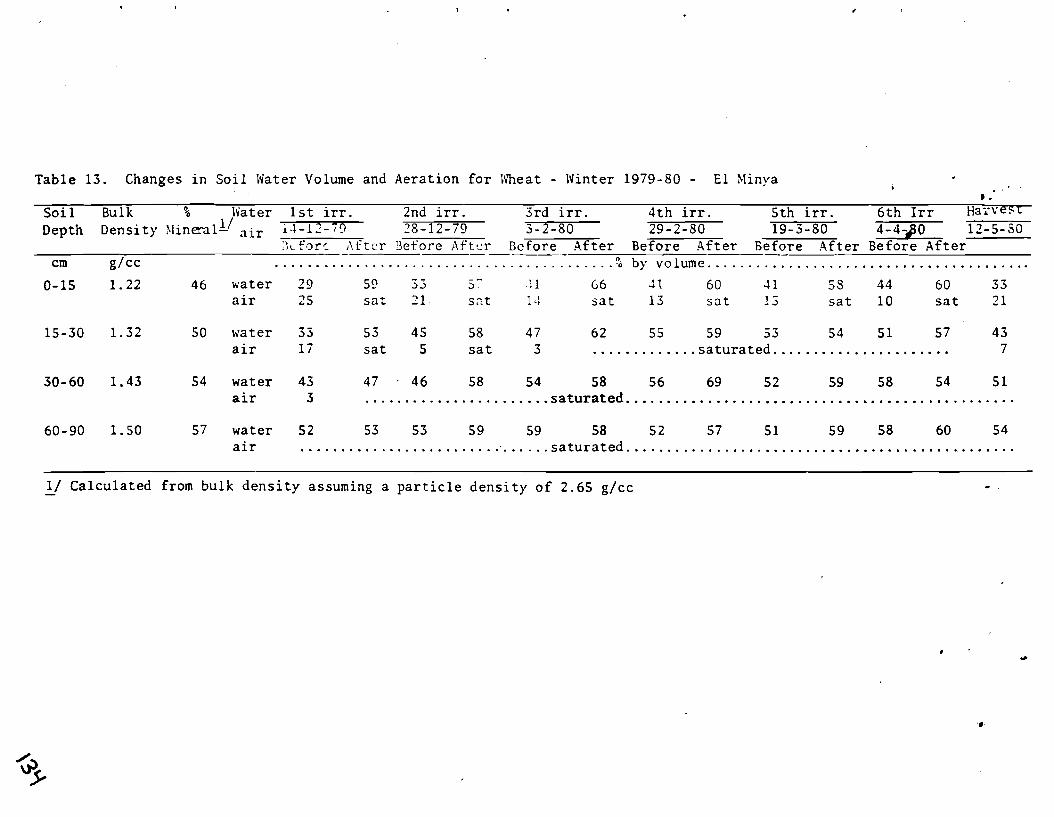
Table 13. Changes i n S o i l Water Volume and Aerat ion f o r \%eat - Winter 1979-80 - E l blinya t

8 .

S o i l Bulk % Water 1st irr. 2nd i r r . 3rd irr. 4 th i r r . 5 th irr . 6 t h Irr Hai-vest I / . Depth Densi ty 3 l inml - air - i-1-12-72) 28-12-79 3-2-80 29-2-80 19-3-80 4-4-90 12-5-80

' L C Afccr 3efo-t.e A f t c r Before Af te r Before Af te r Refore .4f ter Before Af te r -- - . . . . . . . . . . . . . . . . . . . . . . . . . . . . . . . . . . . . . . . . cm g/cc . . . . . . . . . . . . . . . . . . . . . . . . . . . . . . . . . . . . . . . . . by volume - - - -

0- 15 1.22 46 water 29 53 3 3 3 .! 1 66 3 I 60 J 1 5s 44 60 3 3 a i r 2 5 sat 31 s a t 1 ': s a t 13 s a t 13 s a t 10 s a t 2 1

15-30 1.32 50 water 33 53 45 5 8 4 7 6 2 5 5 5 9 5 3 54 5 1 57 4 3 a i r 17 s a t 5 s a t 3 ............. s a t u r a t e d ...................... 7

30-60 1.43 54 water 43 47 . 46 5 8 54 5 8 56 69 5 2 5 9 58 5 4 5 1 ................................................ ....................... air 3 s a t u r a t e d

60-90 1.50 57 water 52 53 53 5 9 5 9 5 8 5 2 57 5 1 59 58 60 54 a i r ................................................ ............................... s a t u r a t e d

1/ Calcula ted from bulk d e n s i t y assuming a p a r t i c l e d e n s i t y o f 2.65 g/cc -

b l e 14 . Changes i n S o i l Water Volume and Aerat ion f o r BroadbeansWmter 1979-80

S o i l Bulk 'Lo - Water 1st irr. 2nd irr 3rd irr . 4 th irr Harvest 1/ - Depth Densi ty Mineral- a i r 9-11-79 29-12-79 15-2-50 20- 3-80 18-4-80 Before Af ter Before A f t e r Before Af te r Before Af te r

cm . . . . . . . . . . . . . . . . . . . . . . . . . . . . . . . . . . . . % by volume ............................................. glee 0-15 1 . 2 5 47 water 2 8 4 8 4 3 5 6 43 59 39 60 4 1

a i r 2 5 5 10 s a t 10 s a t 14 s a t 12 15-30 1.30 49 water 4 4 5 2 47 5 5 4 9 5 7 47 5 3 46

a i r 7 s a t 4 sat 2 s a t 4 s a t 5 30-60 1 .40 5 3 water 43 5 4 4 8 5 2 53 56 5 0 53 5 1

a i r 4 ............................. s a t u r a t e d .................................... 60-90 1.48 56 water 47 5 0 5 1 53 5 2 55 5 6 5 7 56

........................................... ...................................... a i r s a t u r a t e d

1/ Ca lcu la t ed from bulk d e n s i t y assuming a p r a c t i c l e d e n s i t y of 2.65 g /cc . -

T a b l e 15. Changes i n Soil Water Volume and A e r a t i o n f o r Onions - Winter 1979-80 - El blinya

Soil * Bulk b 1/ --- \\later Plantj1:g 75-11-79 - - 1st Trr. 2-1-80 2nd Irr. 3 r d Irr. H a r v e s t Depth D e n s i t y hlincl.31- air 7-2-80 -- 27-2-80 15-4-80

Geforc ! - ' ;cfore .\t'ccr Gcfore V t c r Bcforc A f t e r

0- 15 1.29 49 w a t e r 4 4 55 44 66 44 64 4 6 6 2 3 4

a i r 7 s a t 7 s a t 7 sat 5 sat 17

15-30 1.41 5 3 w a t e r 4 6 60 54 64 59 63 5 4 6 0 47

.......................................... .......... a i r 1 s a t u r a t e d

30-60 1.45 5 5 w a t e r 5 2 62 58 6 1 56 59 59 6 1 5 4

................................... ............................. a i r s a t u r a t e d

60-90 1.51 5 7 w a t e r 5 7 5 9 58 6 8 61 61 5 9 60 - .. 5 8 - ................................... ............................. ai r s a t u r a t e d

1/ C a l c u l a t e d from bu lk d. s i t y assuming a p a r t i c l e d e n s i t y o f 2.65 g / c c . -

BEST AVAILABLE COPY

Table 16. Changes i n s o i l Water Volume and Aeration f o r Borad Bean/sugarcane - Winter 1979-80 - E l Minya

S o i l Bulk Water 1st I r r i . 2nd irr. 3rd irr. 4th irr 5th irr Harvest % 4-12-79 Depth d e n s i t y M i n e r a l 19-11-79 1-1-80 12-2-80 13-3-80 15-4-80

Before Af ter Before a f t e r Before a f t e r Before a f t e r Before Af ter cm g/cc

0-15 1.21 46 water 23 5 3 4 5 54 3 2 57 41 58 40 58 3 4 a i r 3 1 1 9 s a t 2 2 s a t 13 s a t 14 s a t 2 0

15-30 1.32 5 0 water 34 5 3 4 8 5 4 46 5 6 4 5 60 49 5 7 48 a i r 16 s a t 2 s a t 4 s a t 5 s a t 1 s a t 2

30-60 1.37 5 2 water 3 9 5 6 5 5 5 4 5 2 56 5 2 60 52 5 6 4 9 a i r 13 . . . . . . . . . . . . . . . . . . . . s a t u r a t e d .........................................

60-90 1.40 5 3 water 41 5 5 4 5 5 5 53 5 6 5 6 5 7 53 56 50 - a i r 6 s a t 2 ............ : . . . . . . . . . . s a t u r a t e d . . . . . . . . . . . . . . . . . . . . . . .

1/ Calculated from bulk dens i ty assuming a p a r t i c l e d e n s i t y of 2.65 g /cc -

Table 17. Var ia t ion i n Poss ib le I r r i g a t i o n Planning Parameters From Hinya During Winter 1979-80 , --

Ifheat Broadbean Broadbean/sugarcane Onions

Water Water Days P r o f i l e Water Water . Days P r o f i l e Water lfater Days P r o f i l e Water Water Days Pro I r r i g . appl ied s to red between s o i l appl ied s to red between s o i l app l i ed s to red betwan s o i l app l i ed s to red b e t . f i l

i r r i g . moisture i r r i g . mois ture i r r i g . nuisture irr. s o i l

1 P r i o r va lues were c a l c u l a t e d omit t ing the 1st i r r i g a t i o n a t p l an t ing which tended t o be unusual ly heavy 1

BESTAVAILABLE COPY

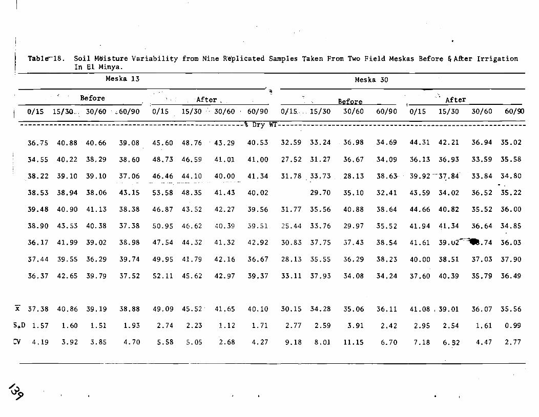
j T a b l c l 8 . S o i l MUisture Variabi l i ty from Nine Replicated Samples Taken From Two Fie ld Meskas Before &After Irrigation In E l Minya.

Meska 13 Meska 30

- Before After . -

Before After I

I

0/15 15/30. . 30/60 -60/90 0/15 15/30 . 3 0 / 6 0 * 60/90 0/15, 15/30 30/60 60/90 0/15 15/30 30/60 60/90

...................................................... % Dry w------------------------------------------------------------

' . fable 19. Soil Moisture Variability by Volume For Nine Replitated Samples Taken Before and After Irrigation in El Minya- '

Mcska 13 Mesla 30

Before After Before After 0115 15/30 30/60 60/90 1 0/15 15/30 30/60 60/90 Z 0/15 15/30 30/60 60/90 1 0/15 15/30 30/60 60/90 8

-------- % volume---------- cm H20 - - - - - - - - % volme----------cm H20 ---------- % volume--------- cm H20 ----------- 8 voI~me-----~m km I

45.57 54.78 57.33 57.45 49.49 56.54 65.34 61.04 59.58 54.47 40.44 49.54 52.14 50.99 44.44 54.94 56.56 52.08 51.48 47.

I 42.84 53.83 53.99 56.74 47.72 60.43 62.43 57.82 60.27 53.86 34.12 41.90 51.70 50.11 41.95 44.80 49.49 47.36 52.30 44 47.39 52.39 55.13 54.48 47.85 57.61 59.09 56.40 60.77 52.66 34.41 45.20 39.66 56.79 41.63 49.50 50.71 47.71 51.16 44. 47.78 52.18 53.60 63.43 50.10 66.44 64.79 58.41 58.83 54.86 39.80 49.49 47.64 40.72 54.05 45.59 51.49 51.77 45. 48.96 54.81 57.99 56.42 49.89 58.12 58.32 59.83 58.15 52.85 34.39 47.65 57.64 56.80 47.39 55.38 54.70 50.68 52.92 47. 48.24 58.33 56.94 54.95 49.55 63.18 62.47 56.95 58.C8' 53.36 31.55 45.24 42.26 52.21 39.86 52.01 55.40 51.66 51.23 46. 44.85 56.27 55.02 57.30 48.86 58.95 59.39 58.26 63.09 54.16 38.23 50.58 52.78 56.65 46.15 51.60 52.29 54.62 52.96 47. 46.43 53.00 51.17 58.42 47.79 61.94 56.00 59.45 53.90 51.70 34.88 47.64 51.17 56.20 44.59 44.60 51.60 52.21 55.71 46. 45.10 57.15 56.10 55.15 48.71 64.62 61.13 60.59 57.87 54.40 41.06 50.83 48.65 50.33 43.48 46.62 54.12 50.46 53.64 46. !

BEST AVAILABLE COPY

Table 20. Inconsistant Tensiometer Reading i n E l Minya

e Date 30 cm 60 cm 90 cm 1 2 3 1 2 3 1 2

I I

3 ! * <

Jan. 23 - - 3 0 33 58 . 38 64 - - 20 48 1 1

2 6 - - 3 0 33 5 8 3 8 64 - - 20 48

3 1 12 38 58 6 1 48 64 - - 20 52

Feb. 2 59 3 8 6 3 6 0 5 2 64 - - 26 5 2 1

Irrigated Feb. 3, 1980 I -------------- - - - - - - - - m e - - - - - - - - - - - - - - - - - - - - - - - - - - - - - - - - - - - - -

1

Feb. 10 4 0 16 2 6 2 4 20 - - 29 20 ,

0 K ) 2 0 3 0 4 0 5 0 6 0 7 0 8 0 9 0 100

Surface = 53.5 - 31.5 = 2290%

t

Fig ( I ) Soil Moisture Chorocteristit Curves For Menia Soils 0

Staff Paper #34

USE OF CHEMICAL FERTILIZERS I N MANSOURIA LOCATION

M, Zanati, M, Lotfy, G G , Ayad

July 1980

Chemical fertilizers is one of the important factors in crop production.

Its kind, rate and time of application should be based on the soil character-

istics, plant varieties and water application. Recommendations for Egyptian

farmers are based on the results obtained from experimental stations located

throughout the country.

The EWUP policy is to identify the problems facing crop produc.tion j.11

three pilot areas in order to look for reasonable solutions to be implernclltcd.

In this concern, the agronomists are dealing with fertilizer situation as ;I~I

effective factor in crop production.

Mansouria area is one of the three selected pilot areas where ~ i o fixed

rotation is followed. Farmers in this area decide by themselves how to make

use of their land. Moreover, the farmers get their fertilizers frcm the coop-

erative and also from theblackmarket in order to meet the crop requirements. I

The EWUP economists are keeping eye on recording all the items of crop produc-

tion. For instance, twelve farms from both Beni Magdoul and El Hammami were

taken into consideration. Every farm has different strips where every strip

was subjected to be grown with different crops for a period of one agricul-

tural year. This gave us an opportunity to have 72 study cases in these two

locations. The amount of nitrogen and phosphorus applied were recorded as

shown in the following tables in kgs of pure nutrientslfed.

The data collected could be discussed under:the following subheadings:

I . Fertilizers applied to different crops

a. Berseem

b. Maize for seed production

c. Maize for forage production

d. Cabbage

e. Wheat

2. Total amount of fertifizers applied to every strip during one year. - 1

I

It is worthy to mention that the two locations under study (Beni Magdoul

and amm ma mi) differ greatly in their texture, where Hauunami location could be

considered as sandy loam for the depth of 0-30 cm then, the rest of profile

till 150 cm is completely sandy. Moreover, the clay concent of the surface

layer is around 10Z while it is 4% in the subsurface layers.

In case of Beni Magdoul, the surface layers contain higher amounts of clay

up till 40% in some areas. The subsurface layers contain less clay as this

location is considered as an interference zone between the desert and the valley.

. The difference in clay content goes in harmony with leaching losses of

applied nutrients.

1 . Fertilizers applied to different crops

a. Berseem

Berseem is considered as the main forage crop in Egypt during the period

of November till May. According to its capability for fixing atmospheric

nitorgen to meet its needs, the rate of recommended nitrogen is so low and is

applied only as a start to encourage the plant at its early stages of growth.

This rate is 7.5 kgs N/fed, where phosphorus is recommended to be applied at a

rate of 15.5 kgs P205/fed. The following table indicates that the farmers in

the studied locations usually apply excessive amounts of phosphorus. Often

twice or three times the recommended rate was used. The average rate of appli-

cation in Beni Magdoul area is approximately twice the recommended rate and

none of these farmers applied less than the recommended rate. In the case of

El Hammami area, the variation in rates of application ranges between 8.84 and

100 kgs P 0 /fed. with an average of 28.35. 2 5

Those aforementioned rates of application increased the amounts of avail-

able phosphorus in the two areas. Data obtained through the soil fertility

survey revealed that the soil contained ample amounts of available P 0 2 5

even in case of the sandy soils at El Hammami. Accordingly, phosphorus defi- - ciency was not considered as a problem.

Table I: Rate of phosph+ ~p~lication inKgs P 0 Ifed. to Berseem in Case 2. 5

- of Beni Magdoul and El am ma mi Areas

- - x = 32.70 Kgs P 0 /fed

2 5 x =.38.42 Kgs P 0 /fed

2 5

b. Maize for seed production

Beni Magdoul

Maize is grown in Mansouria area generally as a grain crop. It does how-

ever supply both grain for human consumption and green forage for feeding

cattle during summer season.

Hammami

It is known that nitrogen is a key element in maize production. Volumin-

ous studies have been conducted in Egypt where N rate, time, kind and method

of application were considered. According to the wide use of high yielding

corn varieties instead of the local varieties, it is recommended to apply

... I.. .

28.50

26.66

.28.83

15.50

15.50

28.37

18.60

36.89

40.76

40.76

40.76

40.76

30.54

31.00

34.72

17.36

BEST AVAILABLE COPY

9.30

100.00

43.40

60.00

60.40

8.84

41.23

41.23

44.49

39.99

36.89

47.12

35.34

31.00

35.34

36.89

36.89

19.84

19.84

80.14

16.90

16.90

23.56

68.80

68.80

31.00

45.50

31.00

9.30

15.50

14.42

10.00

high doses of nitrogen to meet the plant requirements. In this concern, 60 Kgs .,

of N plus 7 . 5 Kgs of P 0 /fed were recommended to be applied to corn grown in , 2 5

delta governorates. In case of Upper Egypt, the recommended rate is increased 2

to 7 0 Kgs of N plus 7 . 5 Kgs P2O5/fed..

Data tabulated in the following table reveal that there is a great differ- .* ence in nitrogen rates applied to corn. Moreover, the average rate of appli-

cation in case of Beni Magdoul area was 105.74 Kgs N/fed., whereas some far- I

mers apply nitrogen up to 165 Kgs. I

Mostly, berseem is followed by corn in those areas. In this case, nitro-

gen rates should be decreased as a result of berseem effect on increasing the 1

soil nitrogen content. Most of the case studies indicate that the previous I I

crop was berseem and at the same time twice or three folds of the recommended 1

1

nitrogen rate was applied to corn.

Tabel 2: Rate of Nitrogen Rate Application in Kgs/Fed to Corn at Beni

Magdoul and El Hammami Areas

Beni Magdoul

95.37

149.17

5 3 . 4 8

33 .00

125.00

165.00 ;

El Hammami

133.74

104.88

9 2 . 0 0

158 .24

158.24

99 - 0 0

3 6 . 8 9

8 5 . 1 0

9 5 . 3 3

194 .58

. 8 9 . 0 0

6 7 . 3 0

c. Maize for forage production

Table 3: Rate of Nitrogen Application in Kgs N/Fed. toMaize (Forage Crop)

in Case of Beni Magdoul and El Hamami Areas

Farmers usually grow maize for forage produbtion ir, Su!:mner. It is known

that the suitable date of planting extends from late in April till September

'and it is recommended not to use the.same land to produce twomaize crops in the

same year to minimize the soil exhaustion resulting from the high seed

rate. Ten Kgs of pure Nlfeddan is recommended to be applied to maize before

the second irrigation. Usually, it could be used for feeding cattle starting

from 45 days after planting. In case of Beni Magdoul area, it is noticed that

the farmers used to apply more nitrogen than recommended. In some cases, the

applied nitrogen exceeds that recommended for maize seed production, where

four cases out of ten did not receive any nitrogen.

Beni Magdoul

In case ofsEl Hammami area, ample amounts of nitrogen were used for forage

production with a range of 23.43 up to 310.94 kgs Nlfed. with an average of

84.80.

... I.. .

43.56

0.00

0.00

132.00

4.65

116.16

El Hanmiami

0.00

68.36

0.00

16.50

0.00

0.00

73.14

310.96

66.00

31 .OO

23.43

65.01

139.36

' 54.25

59.40

44.22

66.00

0.00

r. i - 6 - 3 d. Cabbage 6

'.*. 1 Four cases every area lndicate a high inconsistency in nitrogen i - 3 applications. For instance, those rates range between 109.48 to 375.54

Kgs N/Fed in case of Beni Magdoul with an average of 212.57. Those rates i i . ;

range between 56.12 to 250 Kgs Nlfed in case of El Hammami area with an aver- I

age of 123.95. Leaching losses are great in the coarse textured soils pre-

vailing this area. Thus rates of N application should be higher if compared

with the clay soils of Beni Magdoul area.

Table 4: Rate of Nitrogen Application in Kgs Nlfed to Cabbage in Case

of Beni Magdoul and El H a m m i Areas

e. Wheat

Beni Magdoul

135.24

375.54

109.48

230.00

Wheat is not widespread in the Mansouria area where berseem and vegetables I

! i

are the major winter crops. 1

The data of eleven cases in the two areas reveal that a great variation

El Hanunami

250.00

104.60

85.10

56.12

in rates of nitrogen application exists within farms. But, it is obvious that

.

-

the rates used incase of Beni Magdoul area are not largely different than - . the recommended rate, where the average rate of application is 61.79 Kgs N/fed. t

1

On the other hand, the variation in nitrogen rates is greater in case of El

Hammami, ranging from 19.78 upto 115.50 Kgs Nlfed. with an average of 67.51. I

... I.. .

Table 5: Rate of Nitrogen Application in Kgs N/fed. to Wheat in Case of

Beni Magdoul and.El Hamami Areas

I,

2 . Total amount of fertilizers applied to every strip of land during

one year.

'

Dzta shown in table 6 indicate that the application of fertilizer varies

within the studied strips. The variation in amounts could be attributed to

the cropping pattern itself, but if we consider this contribution to a cer-

tain extent, we will still have a distinct variation in the applied amounts.

In other words, let us assume that those strips are subjected to an intensive

cropping system/yearwhereapproximately 150kgs N/fedis needed. Then we'll find

about 45% of the strips in Beni Magdoul are still subjected to nitrogen over-

fertilization, while this percentage goes up to 68% in-case of El Hamami

area. In addition to the previous findings, there is no relationship between

phosphorus and nitrogen, in other words, the ratio between those two nutrients

varies greatly within strips.

Beni Magdoul

60.72 .

54.74

69.92

The following figure 1 indicates that the average amount of nitrogen

application is 173.79 Kgs fed., where 29% of the strips receive an amount

of nitrogen more than 183 Kgs up to 1085.70. Moreover, 13% of them receive

nitrogen starting from none up to 45.83 Kgs N/fed. It is worthy to mention

that the strip receiving no nitrogen produced berseem followed by maize for

forage. The farmer'did not apply nitrogen for either berseem or maize.

. . ./. . .

El Hauunami

102.30

115.50

100.28

19.78

69.00

39.60

66 .00

27.60

In case of El Hammami area, the situation is quite different (Fig. 2).

The data reveal that the average amount of application is 249.66 Kgs N/fed.

Ten percent of all stujied cases receive an amount of nitrogen ranging from

30 to 74.38 Kgs N/fed, where about 50% of those cases receive more than the

average.

Pn addition to the previous findings, it is obvious from the data that

there is no relationship between the total amounts of both nitrogen and phos-

phorus. In other words, the ratio between those nutrients differ greatly

within the studied cases. It could be said that phosphorus was added in con-

junction with nitrogen for nearly all the studied cases in Reni Magdoul area.

On the contrary, nitrogen was added without any phosphorus application in

case of about 45% of the studied cases at El Hamami. The ratio between the

nitrogen and phosphorus amounts of application differs within areas, i , e. 3.59

and 13.50 for Beni Magdoul and El Hamami areas, respectively.

Discussions

The farm records from the study cases in Beni Magdoul and El Hammami

areas describe the situation of fertilizers usedin those areas. There is no

doubt that what was kept in those farm records is valuable andcan help a lot

in describing the existing system or at least give us an idea about the far-

mers ways of handling the chemical fertilizers.

The data presented in the previous tables and histograms clearly indicate

that a severe variation in rates of fertilizers application exists. In this

concern, the values of c.v are large and it exceeds more than 90% in most of

the cases. Generally, it could be said that the majority apply more fertil-

izers thin needed. For instance, 43 farmers out of 48 farmers in the two

areas applied more phosphorus to berseem than recommended. The same situation

.. ./...

was clear in case of nitrogen,where83X, 76% and 73% of the farmers applied

more nitrogen than recommended in case of corn for seed production, corn for

forage and wheat, respectively. At the same time, the cultivated land in those

areas received ample amounts of chemical fertilizer per year with different

salt indexes whichcreate salinity problems afterwards. The present situation

could be considered as an identified problem which should be tackled by all

disciplines, but we have to throw some light on the reasons which lead to this

situation. First of all, lack of extension services in those areas is well

known andit should be considered. All of us feel that with minimum guidance of

those farmers can increase the crop production. For eg. what was accomplished with L

insect control is a good example for solving a problem by extension services.

At the same time we have to ask the farmers why they do apply less or

more fertilizers. In other words we have to show them that every crop has a

nutrient-yield relationship and the yields obtained as a result of different

rates of application follow the lawaf'diminishing returns. So, why does the

farmer add more than recommended? Does he get more yield? Secondly, is this

situation due to farmers way of living? They are considered as part-time

farmers. In this case they do not devote all their time of farming. Thirdly,

is it due to the availability of fertilizers in Mansouria area? A lot of.

orchards are located there and their owners receive large amounts of subsi-

dized fertilizers. 0

Table (6): Shows t h e r a t e of n i t r o g e n and phosphorus a p p l i c a t i o n s i n kgs/fed t o every farm ( s e l e c t e d t o r e p r e s e n t Beni Magdoul and Hammami Locat ion) dur ing one a g r i c u l t u r a l y e a r Oct. 1978 - Oct. 1979.

Case No.

1

2

3

4

5

6

7

8

9

10

11

12

1 3

14

15

16

17

18

1 9

~ a s e ( 5 0 , I N N P7O5 N

kgs/ f ed .

1

Case.

No.

Locat ion

-

21

22

23

24

25

26

27

28

29

30

31

32

33

34

35

36

37

38

39

40

41

No.

20

21

22

23

24

25

26

27

28

29

30

31

i

81.52

40.76

70.52

61.23

71.30

31.00

34.72

17-36

73.78

36.89

19.84

99.98

50.70

47.12

59.50

82.15

15.50

-

22.79

I Beni Magdsul

138.93

-

135.24

70.95

30.36

132.00

153.82

34 .SO

274.89

164.22

53.48

53.48

124.66

50.16

259.20

56.76

99.00

1085.70

- 323.79

( -

doca t ion

46.50

18.60

73.78

31 .OO

41.23

41.23

44.49

39.99

55.49

9 4 . 2 4

35.34

62.00

P2Q5 N

5.12

38.50

23.57

22.79

- - - - -

- - - - -

- - -

-

-

-

-

kgs / fed

Eamrnami

1095.14

524.10

158.24

158.24

300.16

373.36

229.00

66.00

116.49

396.00

132.00

684 -00

539.33

259.41

180.41

95.09

33.97

244 .OO

255.30

kgs/fed

E l

kgs/fed

~-

184.00

70.75

305.36 j

429.00

109.48

39.27

196.00

108.50

64.15

230.00

175.72

188.94

154.38

174.80

334.96

57 .50

252.52

126.00

284.25

232.27

194.58

261.00

308.22

199.90

138.50

169.41

116.70

138.63

312.44

198.00

247.50

143.51

I

1

2

3

4

5

6

7

8

9

10

11

12.40

- - - - -

- 31.00

45.50

15.50

31.00

- - -

- 18.60

9.30

24.80

14.42

12

13

14

15

16

17

18

19

20

276.00 .

.

'l

Figure (1): Frequency distribution of total nitorgen applied/feddan in Beni Magdoul Area.

Kgs N/Feddan

(1978-1979 Agricul tur'al Year)

Figure (2): Frequency distribution of total nitrogen applied/feddan in EI Hammami Area.

Kgs N/Feddan

(3978-1979 Agricultural Year) -. - . - -. - - - - . ..... ..... . . . . a * . .... . - - - - a

S t a f f Paper #35

AGRICULTURAL PESTS AND THEIR CONTROL GENERAL CONCEPTS

D r . E . A. R. Ata l la

INTRODUCTION

Insects were present and well e s t ab l i shed on e a r t h long before man

es tabl i shed himself . By t h e time he s t a r t e d t o p r a c t i c e a g r i c u l t u r e ,

he was - and s t i l l i s -faced with t h e problem of p ro tec t ing h i s crops

from pes t a t t a c k s . The b a s i s f o r man's problem i s t h a t both he and

i n s e c t s a re competing f o r t h e same resources needed f o r food, c l o t h i n g ,

s h e l t e r , and o t h e r requirements. P e s t s reduce t h e y i e l d , lower t h e

q u a l i t y , increase t h e c o s t of production and requ i re cash ou t l ays f o r

mater ia l and equipment f o r con t ro l measures. Besides, chemical pes t -

i c i d e s used f o r t h e i r con t ro l a r e blamed f o r a good pa r t of environmental

pol lu t ion .

Different genera l es t imat ions of t h e economic l o s s caused by p e s t s

have been suggested. General ly, it is estimated t h a t world a g r i c u l t u r e

s u f f e r s a loss caused by p e s t s amounting t o about 10% i n f i e l d cqops,

20-40% i n f r u i t s c rops , 20% i n vegetable crops, and about 20% i n g r a i n

and o the r s tored products. In Egypt it i s estimated t h a t the annual

l o s s caused by i n s e c t s and p l a n t d i seases t o major crops amounts t o more

than L.E . 60 mi l l ion . With a l l t he con t ro l measures taken, co t ton y i e l d

i n Egypt su f fe r s a reduct ion o f about 7-10% as a r e s u l t of i n f e s t a t i o n

by cotton bollworms alone,. Several cases a r e known i n the world where

cotton production was terminated i n whole countr ies o r regions because

of t h e f a c t t h a t c o s t s of p e s t con t ro l made it impossible t o continue

producing the crop economically.

Furthermore, with t h e explosive inc rease of the human populat ion

t h e the socia l and economic progress of man, h i s requirements increased

both i n quant i ty and i n q u a l i t y . On t h e o the r hand, t h e i n t e n s i v e

andeXten6iveagr icul ture he is p r a c t i c i n g and the continuous a l t e r a t i o n

of t h e environment with more favoured conditfons f o r inc rease of i n s e c t s

and r e l a t e d groups and pathogens a r e leading t o a gradual ly increas ing

grave c r i t i c a l s i t u a t i o n i n t h e c o n f r o n t a t i o n between man and p e s t s .

Man is continuously fac ing an increase i n the abundence and d i s t r i b u t i o n

of p e s t s and t h e f i g h t is growing more and more in tense .

With a l l t h e above-mentioned a c t u a l and p o t e n t i a l hazards and losses ,

it is becoming obvious t h a t i f man is t o continue h i s c i v i l i z a t i o n and

soc ia l progress , i f not even h i s mere existence, he has t o win h i s f i g h t

agains t p e s t s and t o use t h e least in ju r ious and most enl ightened methods

of cont ro l i n t h a t f i g h t .

PESTS AND THEIR TYPES

A p e s t i s a species of organisms t h a t has increased i n numbers t o

exceed t h e economic in ju ry l eve l . This means t h a t a spec ies cannot be

always condemned t o be a p e s t everywhere i n the world s i n c e it can be

an in ju r ious p e s t i n one a r e a and an ex i s t ing organism with no s i g n i f i c a n t

economic consequences i n another area depending on i t s population d e n s i t i e s .

This i s a l s o an important f a c t o r t h a t should be considered i n p e s t cont ro l

programmes s i n c e genera l ly controlmeasures, e spec ia l ly app l i ca t ion of

chemical p e s t i c i d e s , should not be used unless t h e numbers a t t a i n the

economic threshold .

In general p e s t in ju r ious t o p lan t crops may be d iv ided i n t o the

following ca tegor ies :

I. Pests belonging t o t h e p lan t kingdom:

1. Weeds: These a r e higher p lan t s which grow where they a r e not

dksired and, among other i n j u r i e s , o f t e n compete

with economic crops.

2. P a r a s i t i c p l a n t s : These a r e a l s o h ighe r p l a n t s which l i v e

t o t a l l y o r p r a t i a l l y a s p a r a s i t e s on economic

crops .

i, 3 . Some spec ie s o f a lgae ..

4 . P a r a s i t i c fungi .

5. Bacter ia

Pes ts Belonging t o t h e Animal Kingdom:

1. Ver tebra tes : Such as r o d e n t s , b a t s , i n j u r i o u s b i r d s and c e r t a i n - .

o t h e r animals .

2 . I nve r t eb ra t e s : The main group of i -nver tebra tes which is of i m -

mense economic importance a s p l a n t p e s t s a r e

the Asthropoda which inc lude i n s e c t s , t i c k s

and mi tes . I n s e c t s have the h ighes t number

o f s p e c i e s wi th in t h e animal kingdom with an

es t imated over 5 m i l l i o n spec ie s , ou t o f which

only about one m i l l i o n spec ie s a l ready known

and i d e n t i f i e d . A t l e a s t about 10,000 s p e c i e s

o f i n s e c t s a r e known t o be i n j u r i o u s a s p e s t s

t o a g r i c u l t u r e i n d i f f e r e n t a r e a s of t h e world.

Within t h i s ca tegory t h e groups with more important

economic s i g n i f i c a n c e a r e i n s e c t s and mi tes .

3 . Nematodes

4 . P a r a s i t i c protozoa.

111 Viruses:

In t h e present paper, however, we s h a l l be more r e s t r i c t e d t o

problems of p e s t s belonging t o c l a s s i n s e c t s and o t h e r r e l a t e d c l a s s e s .

Before trying to control any pest, a thorough study of the factors

creating favourable conditions for an explosive increase in its numbers I

should be conducted. Such a study should include the biology and life

history of the pest, its behaviour, seasonal history, reaction to dif-

ferent eilvirormental factors, ar:d certain otller zspects. The knowledge

gained from such studies is essential for formulating the most efficient

control programme with the least short and long term hazards. Further-

more, such knowledge helps in forecasting with a reasonable accuracy

the time and degree of future infestationsso that adequate control

measures may be appropriately prepared beforehand.

An important point to be considered is the fact that most present

major agricultural pests in the world are of foreign origin which gained

entry either before the establishment of plant quarantine services or

accidentally after that establishment. This is true in Egypt where

almost all pests and diseases of crop plants have gained entry from

abroad. This fact emphasises the importance of plant quarantine

reguJ.ations in plant protection systems. The economic basis for

quarantine is that it is better :to undergo considerable inconvenience

and initial expense in an effort to exclude, or at least delay, a pest

rather than to submit to its damages and control expenses for an

indefinite period if it gained entry. Nevertheless, it has to be

realized that the increasing volume of foreign exchange of agricultural

commodities, the more and more rapid transport and the growing need for

imports make it almost impossible to totally and permanently prohibit

the introduction of foreign pests and diseases. All that is hoped by

enforcing strict plant quarantine regulation-. is to reduce the number

and rate of foreign pest introductions to a niinimm.

Several methods of pest control are being practiced. Among the

most important of these methods are the following:

I Cultural Control

This is a cheaper, less demanding, method of control. Some

of its practices are the following:

1) Early production of crops: In many cases this procedure helps

in reducing the rate of infestation, even to the point of i-

totally escaping infestation in some cases. It also helps in

preventing the late generations from finding adequate and

appropriate food supplies, which leads to a sharp decrease of

the numbers of the hibernating individuals and consequently

to weak generations in the new season.

Early production can be achieved by general planting, using

early producing varieties and practicing certain agricultural

processes that accelerate ripening. In general early production

helps to reduce infestation in several cases such as the leaf-

worms and bollworms in cotton, corn borers in maize, late season

infestations by aphids and spider mites in several crops, and

many other cases.

2) Following an appropriate crop rotation to stop the increase of

the population densities of pests which occur due to the con-

tinuous availability of their host plants. Such ,rotations help

to control several well known pests such as the corn borers,

sugar-cane mealybug, several vegetable insects and many others.

Generally a good rotation should include, whenever possible,

occasional following.

3) Crop arrangement: Crops should be arranged in such a way that

common hosts of important pests should be separated as much as

possible. An example of the problem is the high infestation

by the Med-bly, Ceratitis capitata, in orchards with mixed host

trees. It is more advisable that different hosts of the Med-fly

should not be gpown together in the same orchard.

4) Growing of certain plants to serve as traps to protect the main

crops. The idea is to grow some less important and more

attractive plants to take the infestation out of the main crop,

these trap plants should be destroyed before they serve as

breeding grounds to spread the infestation to other plants.

For example, growing few corn plants in sugar-cane fields

reduce the infestation of the canes with borers. Few ratoon

cotton plants in a cotton field help reducing the infestation

by bollworms in the main crop.

5) Development of more tolerant or less susceptible varieties

of plants: This procedure can be worked out with the help

of plant breeders and through hybridization and selection.

This procedure is more applied in case of plant diseases,

but there are several successful examples in the world in

case of plant pests such as corn borers, bollworms, alfalfa

aphids and oth,ers .

6) Soil management: Different procedures of soil management

have important effects on pest control. Some examples are:

a. Deep ploughing and hoeing result in killing many soil

inhabiting insect larvae and pupae, either by deeply

burying them, exposing them to natural enemies or exposing

them to unfavourable physicad factors. It was proved in

Egypt that larvae and pupae of the cotton leafworm,

Spodoptera littoralis, are reduced drastically in clover

fields after ploughing than before it.

b. Infestation by Thrips tabaci in cotton can be reduced by

hoeing and weeding, and by repeated irrigation of the

infested cotton field at short intervals.

c. Irlfestation of the potato tuber-moth, Phthorimaea

opercubella, is reduced by burying the sown tubers at

.about 12-15 cm. deep. On hoeing, exposed tubers should

be covered and cracks should be filled so that tubers

may not be exposed to infestation.

d. With the woolly apple aphid, Eriosoma lanigela, surrounding

the apple trees with a layer of sand about 8 cm. deep and

filling the soil cracks reduce the infestation by preventing

the aphids from crawling into the subterranean parts of

the tree for infestation or hibernation.

7) Water management: Irrigation and water management affect both

plant and pest. Excessive irrigation more than needed may

encourage the vegetative growth and accordingly increase

infestation by certain pests, especially leaf feeding insects.

In Egypt it is observed that heavily irrigated cotton leafworm

moths and accordingly infestation is increased. Many farmers

refrain from irrigating their cotton fields during the peak of

moth abundance and in this way successfully reduce egg deposit-

ing in their fields. Irrigation of clover fields is prohibited

after the first week of May in an attempt that low humidity and

high temperature reduce percentage of emerging cotton leafworm

moths. Repeated irrigation of cotton fields infested with

cotton thrips is said to reduce infestation or even control it.

In case of infestation by the bean fly, Agromyza phaseoli, the

first hoeing should be manipulated as early as possible.

Irrigation helps forming more side roots to replace the main

root when affected by the infestation.

8) Sanitation: Removal of weeds and crop residuals, especially

in the pest hibernation period, helps reducing the infestation.

Examples are cleaning stores to reduce infestations by stored

product insects, removal of maize stalks for corn borers,

removal of wheat residues for saw-fly, burning the cotton-

bolls for bollworms, burying or burning infested and fallen

fruits flies. Removing post-season growths of host ,plants

prevents the occurance of an appropriate host plants prevents

the occurance of an appropriate host early in the season for

an overbridging generation.

9) Manures and fertilizers: All of the fertilizing elements must . be use9 with caution and in proper balance. Applications of

nitrogen beyond the amount normally needed on s particular soil

type will result in vegetative growth that is attractive to

some insect pests. Nitrogen in particular must be used in

proper balance to have a plant less attractive to many pests

such as boll weevil, plant bugs, bollworms, and other pests in

case of cotton plants. In general, it is shown that pest dam-

age increases when excessive nitrogenous fertilizers are

applied. On the other hand, several studies have shown that

phosphorous and potash fertilizers may help in resisting

infestation by several insects.

In Egypt, it is known that nitrogen fertilizers in excess in

cotton fields are positively correlated with infestations of

leafworms, bollworms, and possibly other pests. On the other

hand, strengthening the fruit trees by fertilizers helps con-

trolling infestations by shoot borers and bark bettles.

10) Host free period: In some cases, especially if the pest is

more or less monophagous, an establishment of a host free

period may help reducing the infestation.

Closely related to this point is the separation of different

types of host required by an insect to complete its annual

life-history. For instance, the peach aphid, Myzus persicae,

spends part of its annual genrations mainly on potatoes and

another part mainly on peaches and related fruits. Separation

of these different seasonal hosts helps in reducing the

infestation.

I1 Mechanical Control

These methods of control include the mechanical killing of

insects at different stages, preventing them from reaching appro-

priate host plant or appropriate part of the host, mechanical

trapping, mechanical removal of the pest, and several other procedures.

-9-

Some examples of this control method are:

1) Hand picking of the egg-masses of the cotton leafworm,

Spodoptera littoralis, in Egypt. If properly carried

out, cotton crop can be economically saved the ravages

of this pest.

2) Preventing ditches filled with water and dusted on both

sides with lime, calcium oxide, prevent cotton leafworm

from migrating from one field to invade another field.

3) Desert locusts are swept into ditches and destroyed by

buying or burning.

4) Pomegranate butterfly is controlled by screening the

fruits on the trees with paper, cloth or plastic bags,

so preventing the females fromoviposting on such fruits.

5) Tin or wooden traps set around the apiaries, next to

bee-hives, or as upper or side compartments of the hives,

help control the oriental hornet, Vespa orientalis.

6 ) Different kinds of traps could be set in fields to catch

a certain proportion of concerned insects and consequently

reduce their numbers in the fields.

7) Certain other mechanical means are used in several cases,

including plant quarantine stations, for de-infestation

of commodities. Among these methods are grinding, sieving,

mechanical removal by brushing or air pressure and several

others.

Physical Control:

These methods include the application of physical factors,

mainly temperature, in controlling pests. Main measures include

heating of plants or their parts up to degrees affecting the

insects. Examples of such methods of control are:

1 For controlling the pink bollwcrm, Pectinophora - gossypiella, picked cotton is required by law to be ginned before spring

and the produceA seeds should be heated at 55-58O for five

minutes to kill any hibernating larvae without affecting

the viability of the seeds.

2 . Cold storage for several days, down to O'C, of appropriate

fruits may kill eggs and young larvae of fruit flies within

those fruits.

3 . Tests have indicated that covering of land by tarpaulin during

summer time for some days causes a considerable increase in

the soil temperature leading to higher mortality of certain

insects, such as the cotton leafworm in the larval and pupal

stages, and to destruction of some fungus spores.

4 . It was previously mentioned that irrigation of clover fields

is prohibited in Egypt after the first week of May. This is

based on the results obtained that this procedure leads to

an increase in temperature accompanied by a decrease in

humidity leading to higher mortality of the pupae of the

cotton leafworm or to malformation and failure to emergence

of moths.

5. In plant quarantine stations, heating and boiling of commodities

are frequently used for disinfection.

IV. Biological Control:

Biological control is the action of parasites, predators and

pathogens on a host or a prey population which produces a general

lower equilibrium that would prevail in the absence of these agents.

Sometimes biological control is used alone, or at least

without the application of pesticides. However, as will be

discussed later, this method of control is now used in a com-

patible manner with chemical control. Several successful cases

of application of parasites and predators are recorded in the ,

world. Among the recorded cases in Egypt of successful biolog-

ical control caused by imported natural enemies are the

following :

a) Control of the fluted mealybug, Icerya purchasi, by the

coeinellid ladybird bettle Rodolia cardinalis.

b) Control of lebek and hibiscus mealybugs by encyrtid

parasites.

c) Control of the woolly apple aphid, Eriosoma lanigera, by the

aphelinid parasite, Aphelinus mali.

Microbial pesticides, containing pathogens and their toxins

as active ingredients, are now commercially produced and on sale.

They are used either alone or in combination with chemical

pesticides.

Chemical Control

This method refers to the application of poisonous chemicals

(pesticides) for control of pest and disease populations. It is

still the only method available in our hands to be used when

populations exceed the economic injury level and accordingly

economic loss is inevitable. However, this method of control

should be kept as a last resort for controlling a destructive

pest because its application leads to the interference of main

in established ecosystems and in the natural balance and con-

sequently to the creation of incalculable problems. These will

be discussed in more detail later in this paper.

New Approaches.in.Pest Control

There are s-a1 recent non-conventionql approaches for

pest control that are being worked out, mostly still on compara-

tively small scale levels. hong these meth~ds are applications

of the following:

Attractants (including sexual attractants), repellents,

antifeedants, chemosterilants, sterilization by irradiation,

hormones (such as juvenile hormones), including a lethal or

inferior mutations, and several others.

The enthusiasm towards experimenting with such methods

reflects the feeling that fight between man and pests requires

all his ingenuity to win, though it is still very doubtful that

he can exclusively win such a war.

INTEGRATED CONTROL :

Towards the end of the last world war, a new era in pest control

started with the discovery and application of synthetic organic

insecticides. Within a short period, these chemicals were in wide use

in pest control programmes. It is to be admitted that the rapid and

widespread adoption of organic pesticides has brought incalculable

benefits to mankind. However, through their general and mostly

indiscriminate use, the components and complicated interrelations of

the agrecosystems have been drastically changed and accordingly a

number of problems have resulted. Among these problem are the

following :

1) There are many recorded cases of resistance to insecticides,

leading to their reduced effect on pests. In many cases

resistance is already drastic enough to have eliminated cer-

tain insecticides from important pest control programmes.

BEST AVAILABLE COPY

. . . t

2) The resurgence of treated species necessitating repeated

pesticide applications. Such repeated outbreaks occur fr

individuals surviving treatment or migrating into the treated .A

area where they can reproduce unregulated because of the ,+ elimination of their natural enemies.

3) Outbreaks of non-target arthropods. Among other reasons,

these outbreaks usually result from destruction of the

natural enemies which otherwise hold the populations of

these arthropods in check. The more common examples are

the increase of mites, aphids, white flies and others in

fields treated with certain pesticides.

4) Environmental disruption outside the pesticide treated area

resulting in the build-up of pest problems on adjacent crops

or the creation of a pest problem where none existed before.

5) Hazards to pesticide handlers and to persons, livestock and

wildlife subjected to contamination by drift.

6 ) Toxic pesticide residues on food and forage crops and

accumulation of harmful pesticide residues within most

elements of the environment including man, domestic animals,

wildlife, plants, soil, water and others.

With all these problems caused by chemical control, it is more

and more appreciated now that chemical control is not, and cannot be,

the only and final means of control of all pests. On the contrary,

it is more realized now that we need an integrated approach, utilizing

all possible means of control in a harmonial way in what is called

the "integrated control" concept.

7 Integrated control is defined as &a pest management system that,

in the context of the associated environment and the population

dynamics of the pest species, utilizes all suitable techniques and

BEST AVAILABLE COPY

methods in as compatible a manner as possible to maintain the pest

',population at levels below those causing economic injury.

. . .: ' . b,'.

. To practl ce the iiteqratad control. stem t!icrough and deep b

rzsearch work on pests and other related elkments of the environment

should be conducted. These studies should aim at obtained as many

information as possible of the biology, ecology, phenology of the

pest and of its population dynamics and the biotic and abiotic

natural factors affecting its distribution and abundance. A fore-

casting system of the outbreak numbers of the pests should be

developed and economic injury levels of each pest at different condi-

tions should be determined. In general "protective treatments" should

not be used and whenever possible ''selective pesticides" should have

more consideration to be applied.

The effect of pesticides on beneficial forms and on other elements

of the environment should always be considered. Accordingly, chemical

pesticides are to be used only when nothing else can be done, and in

this case the most appropriate pesticide at the lowest possible dose

and at a minimum number of applications should be used. A proper

timing and place of pesticidal application can also be of benefit.

Disease pathogens, used as microbial pesticides, should also be con-

sidered for application either alone or combined with a lower dosage

of chemical pesticide than normal.

In general it should always be kept in mind that the ideal

chemical pesticide is not one that kills the highest proportion of

pest numbers regardless of what happens to the natural enemies, but

is one that helps reducing the pest numbers so that the balance is

shifted back in favour of the natural enemies and hence the pest

numbers could be favol~rable regulated again.

INTEGRATED CONTROL OF COTTON PESTS I N EGYPT:

To illustrate an ongoing programqre of integrated pest control

in action, control progrnmme of cottor. pests in Egypt is summarized

here.

The main cotton pests occurrign in Egypt are the following:

Mole crickets, Gryllotalpa spp.; cotton thrips, Thrips tabaci;

cotton aphid, Aphis gossypii; cutworm, Agrotis ipsilon; cotton leafworm,

Spodoptera littoralis, lesser cotton leafworm, - S. exigua; pink bollworm, Pectinophora gossypiella; spiny bollworm, Earias insulana; and mites,

Tetranychus spp.

Two of the above mentioned pests; the cotton leafworm and the

pink bollworm, are considered as key pests of cotton in this country.

An integrated control programme is devised with the aim of attaining

an acceptable economic control of cotton pests while restricting as

much as possible the use of pesticides and maintaining the natural

balance. The main control procedures of cotton pests currently applied

in Egypt are summerized here:

1) The cotton leafworm is active all the year round and attacks

mainly cotton, maize, clover and many vegetable crops. It

overwinters almost exclusively in clover fields. More than

90% of the moths ovipositing in cotton fields for the first

brood in May and June emerge from pupae in the soil of

adjacent clover fields. In order to minimize infestation

in neighboring cotton fields, it is required of law that

the last irrigation of clover fields should not exceed 1-10

May. The resulting high soil temperature and low humidity

reduces moth emergence and consequently reduces the initial

population of the pest in cotton fields, apparently with no

harmful effects on natural enemies.

2) In late spring, if clover still harbours heavy cotton leafworm

infestations, solar oil (a derivative of crude petroleum oil)

rather than persistent pesticides, is applied with irrigation

water at the rate of 30 It. per acre. This measure helps

reduce the population of the pest with no harmful effects

on beneficial insects. Pesticidal treatments are limited to

fields where infestation actually warrauts cor~trol and no

general spray is applied as used to be the case.

3) No general protective spray is used against thrips infestation

early in the season. An economic injury level (8-12 indivduals

per seedling) was determined and it is generally used for

determining t.reatments of fields reducing the acreage of treated

fields from about one million acres in the early sixties to

about 100,000 acres in recent years. Chemical treatment early

in the season has a drastic effect on natural enemies.

4) For control of cotton leafworm in cotton fields, hand picking

of egg masses still proves to be an efficient control measure.

Up to about 85% of the egg masses could be picked and destroyed

leading o effective control. The current general recommendation

for control comprises concentration on hand picking of epg masses

for as long a period as possible. If chemical control has to be

applied, usually it comes after the predator peak of abundance

in cotton fields which normally takes place in early July.

Hence, through proper timing of chemical treatment, integration

of mechanical, biological and chemical methods of control is

accomplished.

5) An economic injury level has been established for infestation

of the cotton bolls by bollworms, at 10% infestation of green

bolls in fields close to the villages. Since early July each

season, trained teams of the Ministry of Agriculture periodi-

cally inspect cotton fields for level of bollworms infestation.

Chemical control is not allowed in any village unless the

economic injury level is attained. This procedure has helped

minimizing unduly spraying, delaying unnecessary earlier spray-

ing, and in general reducing the total cotton acreage treated

with pesticides.

A t l e a s t p a r t i a l l y due t o t h e p r a c t i c e of t h e above mentioned

procedures, severa l encouraging phenomena i n cot ton agro-

ecosystem i n Egypt have been observed i n the l a s t few years.

Among these phenomena a r e t h e following:

(1) Cotton leafworm i n f e s t a t i o n s a r e becoming more and more

under con t ro l .

(2) Early season i n f e s t a t i o n s have been i n most cases gradual ly

decl in ing wi th in t h e l a s t few years .

(3) Loss of co t ton y i e l d caused by bollworm i n f e s t a t i o n s

declined from about 20% i n t h e f i f t i e s t o about 5-8% only

s ince t h e l a t e s i x t i e s .

(4) The average y i e l d per a c r e is f luc tua t ing but genera l ly

following a h igher l e v e l . I t has reached a record y i e l d

of 334 kg. of baled cot ton pe r a c r e i n 1969.

Finally it should be emphasized t h a t t h e in tegra ted method o f

control has worked s o s a t i s f a c t o r y i n many s i t u a t i o n s and i n many a r e a s

o f t h e world t h a t t h e r e i s no doubt a s t o i t s advantages and potent-

i a l i t i e s i n many o the r cases i n t h e fu tu re . Necessary information,

through research work, should be obtained and whenever poss ib le t h e

method should be t r i e d and s h o r t and long term r e s u l t s evaluated.

In a l l cases i t must be well understood t h a t appl ica t ion of

chemical pes t ic ides i n a g r i c u l t u r e i s here t o s t a y , s t i l l we should

a l s o understand t h a t what i s a c t u a l l y needed i s the "wise" a p p l i c a t i o n

o f pes t ic ides r a t h e r than t h e I'wide" app l i ca t ion of pes t i c ide .

Staff Paper #56

CONVEYANCE LOSSES IN CANALS

Farouk Shahin, M. Sai f Issa , Bushara Essac and Wadie Fahim

1 . INTRODUCTION

I

I n a w o r l d \:irere w a t e r is s u c h a p r e c i o u s r e s o u r c e , w h e r e , w a t e r w a s t e d

or l o s t ~l!f . : :nt : l o ss of a n o t h e r m a n ' s or l a n d ' s n e e d . E f f i c i e n t u s e

o f i r r i r , z t . i c . n w a t e r i s t h e a i m a n d h o p e o f t h e i r r i g a t i o n e n g i n e e r .

T h e e:ij.; j 1 s1 i r r i g a t i o n e f f i c i e n c y c o n c e p t f o r e v a l u a t i n g w a t e r l o s s e s

was wa t c . . c o n v e y a n c e ef 1 i c i e n c y . L o s s e s w h i c h o c c u r e d w f i i l e c o n v e y i n g

w a t e r . e h r c . o f t e n e x c e s s i v e .

I n Egypt :>. t iere p r e c i p i t a t i o n is scarce w i t h i n c r e a s i n g p o p u l a t i o n ; a n

o p t i m j s t ic a g r i c u l t u r a l d e v e l o p m e n t p l a n is l a i d . E a c h d r o p o f t h e

R i v e r I;!!,: w a t e r w i l l te n e e d e d t o a d d new c u l t i v a t e d l a t i d s .

T h e hug!c c . n n a l s u p t o J O O O m3/sec w i t h v e r y l o n g p a t h e s a r e t h e

symptrm: :! t h e i r r i g a t iori s y s t e m i n E g y p t " w h e r e t h e R i v e r N i l e is

t h e n :-i I bc.,urce o f i r r i g a t i o n " .

I n t h c ; y s t e m d e s i g n p r a c t i c a l w a t e r d u t i e s w e r e u s e d f o r maximum a n d

minim^:! : - ec lu i r emen t s a n d c a l c u l a t e d a c c o r d i n g t o t h e c r o p p i n g p a t t e r n ,

t h e c l j : . i> t e h n d t h e s o i l s t o i n s u r e a d e q u a c y o f i r r i g a t i o n w a t e r t o

t h e p l ~ ~ ~ ~ s . T h e a d e c ~ u a c y o f t h e i r r i g a t i o n w a t e r d e l i v e r y s y s t e m

d o e s n ' ~ I c ' pend o n l y upon t h e s y s t e m c a p a c i t y b u t , a l s o upon t h e

s y s t e m , . r i ' j c i e n c y t h a t e v a l u a t e d w h e t h e r i t is a s u c c e s s f u l o n e o r n o t .

* T h ~ s \ w r k h a s b e e n c a r r i e d o u t w i t h i n t h e a c t i v i t i e s o f t h e " E g y p t On r a r m Management P r o j e c t t t u n d e r t h e g u i d a n c e o f D r . M . Abu-Zeid t h e Pri~.lect D i r e c t o r .

B P s r AVAILABLE COPY

w{ter t h a t Is l o s t flhrough d e l l v e r y t o f i e l d s may become q n i i k i l a b l e

t o t h e f a r m . However , p a r t o f s e e p a g e w a t e r may e v e n t u a l 1 , y r e t u r n t o

t11,e g r o u n d w a t e r a q d b e c o n e h a r n 6 f u l b y r a i s l r l g t h e w a t ~ : r t q k l e a n d

c o n s e q u e n t l y c a u s e s w a t e r l o g g i n g a n d s a l i n i t y p r o b l e m s . .Some w a t e r

may a l s o f i n d I ts way t h r o u g h t h e o u t l e t s a n d i n t a k e s t h a t s u p p o s e d

t o b e c l o s e d a n d d o e s n ' t f i n d i ts way t o t h e a p p o i n t e d r e a c h e s . I f

s u c h c o n d i t i o n s h a p p e n s y s t e m . o p e r a t i o n p r o b l e m s a n d low ? m i g a t i o n

e f f i c i e n c i e s w i l l t a k e p l a c e .

3. GENERAL SURVEY

Cqnveyance l o s s e s a r e s t i l l unknown f i e l d b e c a u s e o f t h e complex

v ? r i a b l e s t h a t r u l e s i t . T h e s e l o s s e s w e r e c o n s i t i e r e d a s , a p r o b l e m

s i n c e t h e p e r e n n i a l i r r i g a t i o n was f i r s t p r a c t i c e d i n E g y p t . Many

e n g i n e e r s a n d a u t h o r s w r o t e a b o u t t h e d i r e c t f e e d i n g t o t h e g r o u n d

w a t e r f rom t h e s y s t e m . W i l l c o c k s i n 1 5 1 3 s a i d , "When t h e w a t e r l e v e l s

o f t h e c a n a l s t h r o u g h o u t w i n t e r a n d suri!rner is m a i n t a i n e d a b o v e t h e

s u r f a c e o f t h e g r o u n d , t h e s p r i n g l e v c ? is h i g h and a 1 1 b u t t h e h i g h

l a n d s a l t e d a t t h e s u r f a c e , when I n c a n t r a r y t h e u a t e r l e y e l o f t h e

c a n a l s t h r o u g h o u t w i n t e r and summer m a i n t a i n e d be lo \{ t h e s u r f a c e o f

t h e g r o u n d , t h e s o i l i s ~ i o t s a l t e d . To p r e s e n t t h e w a t e r l o g g i n g o f

t h e s o i l a n d t o k e e p t h e s p r i n g l e v c l w e l l be low t h c l e v e Q o f t h e

c o u n t r y , i t h a s b e e n f o u n d c o n v e n i e n t i n c e r t a i n l o c a l i t i e s t o r u n t h c

c a n a l s i n a l t e r n a t e w e e k s . . . " . Many e n g i n e e r s s i n c e t h a t t i m e r e l a t e i i

t h e h i g h w a t e r t a b l e d i r e c t l y t o t h e h i g h w a t e r l e v e l s i n t h e c a n a l

s y s t e m d u e t o t h e s e e p a g e l o s s e s a l o n g i ts c o u r s e .

T h e r e f o r e , f o r t h e s y s t e m d e s i g n som i m p e r i c a l v a l u e s f o r t h e con-

v e y a n c e l o s s e s i n c a n a l s s p e c i f i c v d l u e s a r e e s t i m a t e d f o r e a c h c a s e .

"or main a n d secondc l ry ck i - i z l s t h e f o l l o w i n g f i g u r e s had bee11 recom-

mended :

. 10% o f t h e d e s i g n a t e d f l o w on Nov., Dec. a n d J a n .

. 15% I ' I ' I I " " F e b . , M a r . , A p r . , S e p . , a n d O c t .

. 20% ' " I I !I " May, J u n e , J u l y , a n d Aug.

Many i n d i v i d ~ a l s t u d i e s w e r e ~ o m p l e t e d f o r some cannls f o r s p e c i f i c

p r o b l e m e v a l u a t i o n . A s t u d y was c a r r i e d o u t f o r t h ~ I s m a i l i a C a n a l .

The c o n v e y a n c e lcsses t h r t L e s t i m a t e d f o r t h e p r o p o s t d c :nlarge showed

e x c e s s i v e l o s s e s b e t w e e n 10-302 . O t t i e r s t u d i e s f o r i n d i v i d u a l c a n a l s

showed l o s s e s t h a t r a n g e be tween 10% a n d 40% o f i t s f l o w d i e c h a r g e s .

@EST AVA KA8Lh €OPY

3. THE FIELD OF STUDY

The system losses and efficiencies are one of Egypt's Water Use and

Management Project fields of interest which are under study in the project areas.

3.1 TYPES OF WATER LOSSES FROM CANALS

The types of losses from canals are: I .

1. Seepage losses

2. Evaporation from the water surface

3. Transpiration of the acquatic weeds

4 . Outlets and intakes' leaks

3.1.1 Seepage Losses

The factors affecting the quantity of the seepage loyses from canals

and ditches are:

a. Deds

b. Uater levels

c. Ground water table and boundary conditions

3.1.2 Evaporation From the Water Surface

Evaporation from canals depends on the following factors:

a . Canal cross section

b. ."eteorologic~l factors

c. kiater depth

3.1.3 E\ zpotranspirat ion from Acquatic Weeds

6;-aputranspiration from acquatic weeds.depends on the following

factors:

a Intensity of weeds

L. Kind 01 iveeds

c. Adequacy of water

d. Agrometeorological conditions

General lay out of Mansoria District

, , ,, Uutlsts and Intakes' Leaks he water lost from the leaking and uncontrolled intakes and outlets 3 : depend up&: .

: ,ti. . Number and size of the leaky points

. 5 :c ; : I b. Hydraplic head

. The downstream conditions

he convkyance losses as the sum of the prementioned items make a

complex interrelations that can't be easily seperated. ? ,

AS the peds change with depth and distance along the canals, the

boundary conditions change randomnly in space and t h e with the*

irrigators. Evaporation and evapotranspiration change with time and

also between day and night and at last the leaks change with npber

and size of outlets and its tightness, effective hydraulic heahs .

beside its downstream conditions.

In thps study, the conveyance losses are studied as a whole without

identifying each kind of loss seperately.

GENERAL DESCRIPTION

The study area (see map) is fed by Mansouria Main Canal 37 kms long

and, serves 24000 f eddans and of about 650,000 m daily discharge.

The canal works as a carrier in its first reach of 12.46 ki;ometers.

The canal inlet is a 2 vent sluice gate 3.0 m wide each. It is also

supplied by three regulators, first at kilometer 16.274, second at

kilometer 28,545 and the last at kilometer 37. A three x.otationa1

system j s mainly applied with 4 days on and 8 days off. 1

1 Mansouria Canal supplies 24 secondary canals of an average length of

3.00 kilometers besides 121 direct on farm intakes. The secondary

canals' intakes are of one vent intakes, that are controlled by timber

blocks or relatively leaky sluice metalic gates. The direct intakes

are r r ~ u s ~ l y supplied with old unmaintained gates that are open all the

tine.

3.3 SITES 01 I:EASUREMENTS

3.3.1 Sites of !.:cr.c urements in Mansouria Canal

The study was accomplished in the canal at three reaches. The reaches

art.! :

1st lteitc)?: Between site (1) krn 0.200 and site (2) km 4.700

2nd ktt2itr;h: Between site (2) km 4.700 and site (4) km 11,980 -----

3rd h::ach: Between site ( 5 ) km 24.700 and site (6) km 27.400 -.-

' B W ~ V A I L A B L L W P Y

3 . 3 . 2 S i t e s o f Measurements i n K a f f r e t N a s s a r Cana l

K a f f r e t N a s s a r s e c o n d a r y c a n a l was c h o s e n t o r e p r e s e n t c a n a l s w i t h

c l a y b e d s . The r e a c h o f t h e S t u d y was be tween s i te (1) a t krn 0 . 0 5 0 -

a n d s i t e ( 2 ) a t km 1.180. The r o t a t i o n i n t h i s c a n a l is 4 d a y s on

a n d 8 d a y s o f f .

3 . 3 . 3 S i t e s o f Measurements i n E l Hammami C a n a l

h he measu remen t s were c a r r i e d o u t be tween s i te (1) km 0 . 0 8 5 and s i t e

(?) a t km 0 . 6 0 0 .

3 . 3 . 4 Meska No. 6 i n Ben i Magdoul Area J

T h i s meska was c h o s e n as a model f o r t h e s t u d y o f losses from meskas .

1ks i n t a k e is a t t h e l e f t s i d e o f Ben i Magdoul c a n a l a t km 1 . 4 2 8 .

The t y p e o f s o i l . i n t h i s meska is c l a y . The meska is a b o u t 500 m i n

l e n g t h . L o s s e s were m e a s u r e d i n a r e a c h o f a b o u t 100 m .

N o t e : D u r i n g t h e d i s c h a r g e measu remen t s t h e i r r i g a t i o n y i t h i n e a c h

r e a c h u n d e r c o n s i d e r a t i o n \';its s t o p p e d . The e n g i n e e r s w e r e a s s u r i n g

t h a t n o one is i r r i g a t i n t : jrom t h e r e a c h .

4 . FIELD MEASUREMENTS OF COLVEYANCE LOSSES

4 . 1 INFLOW OUTFII0K METHOD

T h i s method : ; a s u s e d on l a r g e w a t e r c o u r s e s . The measu r fn l cn t s were

c a r r i e d o u t 3s f o l l o w s :

1. The r e a c h of m e a s u r e m e n t s is chosen be tween two s u i t a b l e s i t e s .

2 . C r o s s s e c ~ i o n s be tween t h e two s i t es i n t h e c h o s e n r e s c h h a v e

b e e n t r a c e d t o o b t a i n t h e mean c r o s s s e c t i o n f o r t h e r e a c h . The

w e t t e d pe r i yne t e r was a l s o e s t i m a t e d .

3. T h e disr!ls~.[:e- were m e a s u r e d i n t h e same t i m e a t t h e c h ~ ~ s e n s i t e s .

a t t h e L::ginning and a t t h e e n d of t h e r e a c h . D i f i r r . c : ! ; ~ d i s -

c h a r g e s r.ercb made a t d i f f e r e n t lev6?ls.

4 . The s o i l was c l a . s s i f l e d v i s ~ ~ l l y Lor d i f f e r e n t reac:lif .- .

T h i s methcd :.+as a p p l i e d i n t h r e e c h o s e n r e a c h e s i n man.;.^:: j a c a n a l ,

t h e c h o s e n r e x h i n K a f f r e t N a s s a r and 111 Hammami bran \ . i l :n:tls.

On K a f f r e t N a s s a r a n d E l Hammami c a n a l ? : , i t warr n o t a l : ' , \ l i . f u r itlc

f a r m e r s t o I r r i g a t e d u r i n g meaeurementr . . The t e c h n i c l r l , c.1.c t a h l I I

c a r e f o r L.!:c!pi ny t h e f a r m e r s n o t i r r l ( ; a t l n g i n t h e t i 1 1 1 t . ' .~ic~usurc,-

ments.

BESr AVAILABLE COPY

f IG .2 ) RELATION SHI@ , 3 E V € c t ~ LnSSES F R O M D I T C H 8 FIG.3) GFIlN AND LOSSES IN MANSURIA

DIFERENCE IN HEAD BETWEEN THE DITCH 8 M. C.

BET. SITES 1 4 2 WATER TABLE

- I Y +

70 .d I

* 6 0 t 0

W ,r s o c' u m

2 4 0

' 3 0 W U z W

2 0

5 0

1 0

0 5 10 15 2 0 ?S 30 3 5 LO

LOSSES m rn/day

8 --- - - .- -

1

m

I 1

I

L

4 . 3 POND AREA METHOD

T h e Pond area method was made f o r small d i t c h e s . T h e s e s t e p & were f o l l o w e d f o r t h e m e a s u r e m e n t s o f t h e losses o n Meska N o . 6 l e f t s i d e

o f Ben1 Magdoul C a n a l .

1. T h e mean c r o s s s e c t i o n o f t h e meslca a n d w e t t e d p e r i m e t e r were

o b t a i n e d .

2 . E a r t h dams were e r e c t e d a t two sites. The d i s t a n c e b e t w e e n t h e

two e a r t h dams was c h o s e n b e t w e e n 100 m a n d 7 0 m, a c c o r d i n g t o

t h e c a s e o f i r r i g a t i o n on t h e m e s k a .

3. ' F o u r o b s e r v a t i o n w e l l s were d r i l l e d a t mid s i t e o f t h e d i t c h ,

a t 3 , 1 0 rn f rom t h e meska a x i s .

4 . The w a t e r l e v e l s were c o n t r o l l e d a t e a c h t i m e o f measunement

by l i f t i n g u p - s t r e a m t h e f i r s t e a r t h dam. I

5 . ' The t i m e o f m e a 5 u r j n g was r a n g e d b e t w e e n 5 h o u r s t o 24 h o u r s .

6 . The d r o p i n t h r ~ ~ ~ l i e r l e v e l i n t h e pond w a s r e c o r d e d jlst a f t e r

t o t a l l y c l o s e t ! l h ~ r e a d a t its e n d , by t h e e a r t h dams. The hook-

g a u g e in s t i l 1 1 1 . b w e l l was u s e d f o r r e c o r d i n g t h e d r o p i n t h e

\ tVhte r l e v e l s .

7. Tlle g r o u n d wale] . t a b l e a n d t h e w a t e r l e v e l i n t h e c i i t c h , t h e

w i d t h oi' t h e v : ~ t c.r s u r f a c e were r e c o r d e d .

5 . ANALYSIS AND RESULTS

5. 1 LOSSES I.'IiOhl MESKAS

From t a b l e - 1 ) a n d f i g ( 2 ) , i t i s n o t i c e d t h a t t h e t o t a l l o s s e s w e r e

a f f e c t e d by t h e e v a p o r a t i o n r a t e a n d t h e g r o u n d water t a b l e , i t

inc rc t : s e s a.Lso w i t h t h e , d i f f e r e n c e i n h e a d b e t w e e n ttie d i t c h writer

l e v i l and t ! le g r o u n d w a t e r t a b l e and v i s e v e r s a .

T a b l e ( 1 ) : R a t e o f d r o p i n t h e w a t c l l e v e l i n d i t c h No. 6 B e n i Magdoul C c n a l (mm/day)

--

T o t a l d r o p b I e A s . Rate o f d r o p 1% Grou-d GI-.>und S e r . D a t e i n the w a t e r Time i n t h e w a t e r 1 Watcr ter N o . l e v e l l e v e l i n l d a y 1: r , t c h t a l ~ l ~ ! c t e n -

mm h r s . m m / d a ~ ( : . ) r 131

5 . 2 M A I N h1ANSOURIA CANAL

I n t h e f i r s t r e a c b b e t w e e n S i tes (1) a n d (2). ( f i g 3) t h e r e was m o s t l y

g a i n w i t h s l i g h t losses a t t h e h i g h e r d i s c h a r g e s . T h e g a i n i n c r e a s e s

w i t h a d e c r e a s e o f c a n a l f l o w . I t ' a p p e a r s t o b e g i n at z e r o a t a - - - -

f l o w o f a b o u t 6m3 /sec a n d i n c r e a s e s t o a b o u t 6% a t a f l o w o f 3 . 5 m 3 / s e e .

T h a t g a i n is a l m o s t c e r t a i n l y d u e t o s e e p a g e f r o m t h e s u r r o u n d i n g s .

- I n t h e rest o f t h e f i r s t r e a c h , losses w e r e d o m i n a n t . Between

si tes 2 & 4 , ( f i g 4 ) a t o t a l l e n g t h o f 7 . 2 8 0 km, t h e l o s s e s i n c r e a s e d

w i t h a n i n c r e a s e i n f l o w , a n d r a n g e d , b e t w e e n 5% a n d 13%, w i t h a n ____^.C. - .

a v e r a g e o f 9.73%,. o f t h e e n t e r i n g d i s c h a r g e a t s i t e 2 . - T h i s l o s s h..

r e p r e s e n t s a l o s s o f 1 . 3 4 % p e r e a c h km l e n g t h . T h e s e r e s u l t s may b e

r e p r e s e n t a t i v e o f a l l losses i n t h a t f i r s t r e a c h . 1

i - T h e s e c o n d r e a c h is n e a r t h e H a m a m i area. I t may bte r e p r e s e n t a -

t i v e o f t h e m i d d l e r e a c h o f t h e c a n a l w h e r e t h e c a n a l b e d is o f coarse t e x t u r e a n d s o i l s . I t is b e t w e e n s i t e s 5 a n d 6 ( f i g 5 ) . T h e m e a s u r e d

d i s c h a r g e s show a h i g h e r r a t e o f l o s s t h a n a p p e a r e d i n t h e f i r s t r e a c h .

They a l s o show a n i n c r e a s e i n w a t e r losses w i t h a n i n c r e a s e i n f l o w .

From t h e l i m i t e d number o f r e a d i n g s it a p p e a r s t h a t t h e l o s s r a n g e s

b e t w e e n 7.E:, a t a f l o w o f a b o u t 4 . 2 m 3 / s e c a n d 1 2 . 9 % atl 4 . 4 1 m 3 / s e c , - w i t h an a v e r h g c o f a b o u t 1 0 . 1 % . T h a t r e p r e s e n t s a - l o s s o f a b o u t

3.93% f o r e a c h km. \

7-

5.3 RAFFRET NASSAR CANAL

I n t h e r e a c h f rom t h e i n t a k e a n d km 1.180 t h e r e w e r e m o s t l y l o s s e s

t h a t i n c r e a s e a p p r e c i a b l y w i t h t h e i n c r e a s e d f l o w , w h i l e d e c r e a s e s

w i t h f l o w a n d t e n d s t o z e r o a t low f l o w s o f a b o u t 9 0 l i t ' / s e c , s l i g h t

g a i n may happen a t f l o w s l o w e r t h a n 90 l i t / s e c . I n t h i s c a n j l i r r i-

g a t i o n is m o s t l y by g r a v i t y w h e r e w a t e r l e v e l s a r e h i g h e r t h a n t h e

g r o u n d . ( f i g 6 )

5 . 4 I:14fF.!AMI CANAL

I n t h i s c a n a l i t was a v a i l a b l e t o m e a s u r e o i l l y t h e l o s s e s aL ~ ! l e f i r s t

8 5 0 m w h e r e n o o u t l e t s e x i s t . . I t st i l l sho \ r s l o s s e s t h a t i ! : : l e a s e w i t h

t h e i n c r e a s e o f f l o w a n d c a n a l w a t e r 1 e v e l s . t h e l o s s e s a r e a b o u t 20%

i n t h a t r e a c h w h e r e t h e b e d is s a n d y and t h , w a t e r l e v e l s a r e s l i g h t l y

b e l o w g r o u n d s u r f a c e ( f i g 7 ) .

L

F i g . 7 LOSSES FROM ELHAMAMI CANAL Fig. 6 LOSSES FROM KA FERET NASSAR

BETWEEN K M . 0 . 0 8 5 8 ~ ~ : b : 8 5 0 CANAL BE.TTWEEN INTAKE AND

K.M. 1.160

0 10 2 0 30 40- 50 60 70 4 0 80 120 160 2 0 0 2 4 0 2 0 0

- LOSSES L ITBEC TOTAL LOSSES (LIT./SEQ

- - L

6 . THE CONCLUSION - -.

The c o l l e c t e d i n f o r m a t i o n and a n a l y s i s i n d i c a t e o r s u g g e s t t h e o c c u r -

e n c e 06 a p p r e c i a b l e l o s s e s i n Mansouria Canal and i t s b r a n c h e s more

t h a n e k p e c t e d .

- The l o s s e s i n c r e a s e a p p r e c i a b l y w i t h t h e i n c r e a s e of water e l e v a -

t j o n i n t h e w a t e r c o u r s e s , and d e c r e a s e s and may demin i sh a s t h e

w a t e r l e v e l s go more below t h e ground s u r f a c e .

- An a p p r e c i a b l e p a r t of t h o s e l o s s e s is due t o t h e e x c e s s i v e uncon-

t r o l l e d d i r e c t i n t a k e s b e s i d e s t h e l e a k y i n t a k e s of t h e b r a n c h e s .

1 RECOMMENDATIONS i

- The a p p l i c a t i o n sys tem i s needed t o b e b e t t e r managed and c o n t r o l l e d .

- D i r e c t u n c o n t r o l l e d i n t a k e s t o be minimized o r even p r o h i b i t e d .

- More c o n l - r o l l e d and less l eaky g a t e d i n t a k e s have t o b e d e v e l o p e d .

- To lqwer t h e des rgn water l e v e l s i n t h e c a n a l s a s p o s s i b l e t o

minitrdize t h e conveyance l o s s e s .

- A n a t i o n a l program is needed f o r measur ing t h e conveyance l o s s e s i n

r e p r e s e n t a t i v e wa te r c o u r s e s and h o p e f u l l y w i t h t h e h e l p of t h e

u n i v e r s i t i e s .

REFERENCES

1 S i r W . Wi l l cocks and J . I . C r i a g , Egyp t i an I r r i g s t i o n , E . & F . N . Spon, L t d . , Z.nndon, N e w York, 1913.

2 H y d r a u l i c R r s t s r c h S t a t i o n , "Car.a.1 L i n i n g a n d Cnc?.] Seepage" Wal l ing Ford O x f o r d s h i r e , Encland, 1975.

3 Ahmed A l i Ilama! and Abdel S a l ' a m Hashim, "Water C o n t r o l and d i s t r i b u t i o n 111 Egyp t t ' , M i n i s r r y r.f I r r i g a t i o n , Egypt , 1966.

4 Egypt Water Use and Management.I'rc:ject, "Problem I d e n t i f i c a t i o n Repor t " , Egyp t , 1979.

A SYSTEMATIC FRAMEWORK FOR DEVELOPMENT OF SOLUTIONS

Max K. Lowdermilk

Apr i l , 1980

There i s no one way t o so lve p r i o r i t y problems o r t o develop - s o l u t i o n s f o r those problems. There a r e , however, s e v e r a l f l e x i b l e

approaches which can be used within t h e context o f a team opera t ion

which w i l l save time and o t h e r resources . The sys temat ic framework

presented he re has been developed by an economist, a s o c i o l o g i s t ,

an agronomist, and two engineers who have w r i t t e n a development o f

s o l u t i o n s manual under t h e Pakis tan Water Management P r o j e c t .

The purpose o f t h i s paper is t o present a framework f o r develop-

ment o f s o l u t i o n s and t o ask each of you t o improve it by u t i l i z i n g

your own knowledge and experience. This paper w i l l focus on seve ra l

key a spec t s o f t h e process and u t i l i z e a few examples.

While reading , keep i n mind t h e key concepts and major emphasis

which guide t h e Research-Development process . A s shown i n Figure 1 we

s t i l l have an on-farm approach which i s management o r i e n t e d and r e q u i r e s

a systems pe r spec t ive us ing a - team o f workers from re l evan t d i s c i p l i n e s .

We s t i l l s t r e s s t h e importance o f knowing and making e x p l i c i t your bas i c

assumptions o r va lua t ions . Also, t r a i n i n g i s important f o r host country

personnel . Communication among team members and between team members,

and farmers i s a s important f o r DOS a s a t any s t a g e o f t h e process.

S e t t i n g ob jec t ives t o know where we a r e going and bui ld ing i n a continuous

monitoring and evalua t ion process is a l s o v i t a l t o DOS. Addi t ional ly ,

a b a s i c emphasis is t h a t t he team which i d e n t i f i e s t h e fa rmer ' s p r i o r i t y

problems must be t h e same team which develops t h e a l t e r n a t i v e so lu t ions

f o r t h e f i n a l s t a g e o f t h e process , p r o j e c t implementation.

The remainder o f t h i s paper w i l l be organized i n t h e fol lowing manner:

I . A Systematic Framework f o r DOS and Key Concepts

A. I d e n t i f i c a t i o n and ranking o f p o t e n t i a l so lu t ions

+ REVIEW PRIORITY PROB1,EMS CAUSES

(1) PROGRAM OBJECTIVES PROGRAM CONSTRAINTS

CENEPATE IDEAS FOR

POTENT I AL IsoLuTI~S T... IDEAS ,

SCREEN OUT IMPLAUSIBLE

AND ALLOCATE TEAM RESOURCES I

4 GOALS, DESIGN TESTS,

SPECIFY DEADLINES, SET - -- - UP FEEDBACK MECHANISMS

+ B TESTING AND ADAPTATION OF SOLUTIONS

(7) HOZD DEMONSTRATIONS, FIELD DAYS, ETC. I

FROM CLIENTS A. FARMERS I

B. AGENCIES

PHASED WITHDRAWAL OF TEAM/

- -- c

NO Y e:j

REFINEMEXT AND SCALING-UP OF e

SOLUTION PACK- S

- Figure 1. Systematic Framework for Development of Solutions

Source : Development of Sc lutions Manual by Sparlin~, Luwdermllk, Skogerboe, -- - Steward, Kt t imore . Pa1.j < call Wazer Managzil~ent Fro j act, CSU Furt Col lins 1980

B. Tes t ing and adap ta t i on o f s o l u t i o n s

C . Assessment, re f inement , and sca l ing-up o f s o l u t i o n

packages

11. A n o t e on the importance o f performance o b j e c t i v e s a s t o o l s i n

developing s o l u t i o n s

111. A method f o r p roduct ive team output i n d e c i s i o n s about performance

o b j e c t i v e s : Brainstorming

I . Sys temat ic Framework f o r DOS and Key Concepts

Time w i l l permit on ly a b r i e f d e s c r i p t i o n o f t h e framework. This

is shown i n F igure 1 and d iscussed below.

A. I d e n t i f i c a t i o n and Ranking o f P o t e n t i a l So lu t ions

The input f o r DOS is t h e exper ience , knowledge, and t h e d a t a from - 01. Remember t h a t i n PI you f i rs t develop hypotheses a f t e r t h e

Reconnaissance, then test t h e hypotheses with q u a n t i t a t i v e and q u a l i t a t i v e

da t a , and f i n a l l y a r e a b l e t o i d e n t i f y some o f t h e major causes i n c o n t r a s t

t o t h e symptoms o f t h e s e problems. A s a team, you e s t a b l i s h e d c r i t e r i a

f o r ranking these problems. These c r i t e r i a could have been inc reased

c rop product ion , income d i s t r i b u t i o n , and r e sou rce maintenance.

U t i l i z i n g t h e input from PI you w i l l need t o review t h e causes of

t h e high p r i o r i t y problems. Experience shows t h a t you should stress a

few key problems r a t h e r than many. Also, a s A( l ) i n F igure 1 i n d i c a t e s , a s - a team you need - -- t o be s u r e o f where you a r e going. Therefore , you should

c a r e f u l l y look a t your o b j e c t i v e s . Some w i l l be provided by Government

p o l i c y and some t h e team may evolve , Again, depending on t h e p a r t i c u l a r

p o l i c y of a Government, t h e o b j e c t i v e s may be i nc reased a g r i c u l t u r a l

p roduct ion , improved income d i s t r i b u t i o n , r e sou rce maintenance o r o t h e r s .

Table 1 provides a long l i s t o f p o s s i b l e ways t o meet t h e s e t h r e e

o b j e c t i v e s , b u t it is by no means complete. Use t h i s t a b l e on ly f o r i d e a s

TABLE 1. PROGRAM OBJECTIVES

Increasing Crop Production optimizing-use of Plant Environment

Identification of best crops and varieties for environment Breeding new varieties Improving practices

Complementing Plant Environment Reduce costs of agri-chemicals Add organic Tatter to soil Add tillable .!-reage by modifyi. g terrain

O?t imi zing Labor U ,c Change cropping patterns to reduce labor bottlenecks Education of farmers Improved nutrition Improved health

Complementing Labor Use Introduction of labor-saving machines Facilitate mo:)ility of seasonal laborers

0:ltirnizing Use of Current Water Supply and Removal System Land leveling Bunding Maintenance of delivery and removal systems Improved application efficiency Improvement of scheduling

Complementing Water Supply and Removal System Modification of supply and removal systems Addition of storage capacity Addition of wells

Optimizing Use of Current Organizational, Institutional and Legal Infra- structure

Rationalization of prices with national priorities Rationalization of organizational incentive structures Develop incentives for Water User Associations Education and training of agency staff

Changing Existing Infrastructure Add new organizations to service farmers Development of marketing services for inputs and outputs Develop new organization to manage interregional water allocation Change laws to allocate water rights to individuals Land consolidation Land reform Organize cooperatives or Water User Associations

Income Distribution Increase ~roductivii~ of Resources Belonging to Poorer Farmers and Laborers :

Labor: education, extension, nutrition, health, machinery, c:iemical inputs, new varieties with shorter duration , Land: consolidation, leveling, increased water supply, complementing nutrients, higher y ie ld ing varle~ies Water: increase application efficiency, increase delivery efficiency, introduce crop varieties better adapted to water

Increase Access to Productive Resources Land: reform, consolidation and cooperative use Water: redistribution and enforcement of water rights Capital: credit, collective ownership of indivisible capital equipment (tubewells, tractors, etc.) Information: Extension, education, mass media

Direct Redistribution of Income Tax relief Subsidies Food programs Free medical care Direct transfer payments (social security, welfare, etc.]

Increase Demand for Farm Products Transportation, storage, and other marketing systems Development of overseas mafkets Development of domestic processing industries

Reduce Uncertainty for Smaller Farmers Disease and pest control Regulation of water supply Regulation of prices Crop insurance Organize credit cooperatives Establish dependable marketing for inputs and outputs

Increase Access of Small Farmers to Government Agencies Organize small farmers into politically-effective groups Furnish small farmers with advocates to plead cases with agencies

Resource Conservation Water

Maintenance of quality of water supplies Maintenance of sustainable yield from water supplies Increasing sustainable yields through storage

Soi 1 Maintenance of "optimal" levels of erosion Reclamation of degraded soils Maintenance of acceptable levels of soil salinity

Air Maintain safe quality Maintain aesthetic quality

Forests Maintenance of sustainable yields from forests Extend acreage of forests to increase sustainable yields Introduce substitutes for wood as fuel and construction materials

Fisheries Maintenance of quality of water Maintenance of sustainable yields or Increasing sustainable yields

Rtlrlgel. and Maintain sustainahl e yield Increase nutritional value of yield Increase efficiency of animals

Source: Development of Solutions Manual by Sparling, Lowdermilk, Skogerboe, and Stewart. Pakistan Water Management Project, Colorado State University, Fort Collins, Colorado, 1980

The specific context of your team work in DOS will likely provide other

ways of meeting objectives. A(l) in Figu-:e 1 also indicates that you,

93 a team, need to carefully consider constraints which limit r~hat can

be done in D O S . In the real world you will have many constraints. If

you assume that there are none, you will run into conflicts between

"the idea" and "the real" situations. For example, Table 2 provides

a checklist of Program Resources which can pose constraints to D O S .

These include personnel available, budget, equipment, access to agencies

and authorities, and available information. Remember Murphy's Law that

"if anything can go wrong, it will," and Lowdermilk's modified collary

that "you can't win completely," "you often can't break even," and "you

certainly can't quit the game of D O S . "

Another consideration under A(l) in Figure 1, is that the team

should look at strategic considerations. Again return to the objectives.

If your objectives are increased agricultural production, improved

income distribution with a focus on small farmers and tenants, plus

resource conservation, then these are criteria which guide and delimit

your work with D O S .

Figures 2 and 3 provide a matrix approach which also helps to focus

the DOS process. Note jn Figure 2 the constraints of program priorities,

program constraints, time requirements, and resource requirements. The

target interest groups also need to be identified, Elite farmers,

?oliticians can be a real constraint, There are many potential

uncertainties as well as complementarities. You may want to reduce -

uncertainties -- by particular solutions and maximize complementary solutions

* See Adams, Jones L . Conceptual Blockbusting, A Guide to Better Ideas,

'd. M. Freeman and Company, San Francisco, 1974

TABLE 2 . PROGRAM RESOURCES CHECKLIST

Project Personnel Agronomists Engineers

Civi l Agricultural

Hydrologists Economists Sociologists Lawyers Managers

Research and Development Budget Transportation Clerical Computational Laboratory Equipment Field Equipment Field Assistants

Equipment Lab equipment Field t e s t i n g equipment Tractors Earthmovers Levelers, e t c ,

Access t o Aeencies Resources Personnel

Access t o Authority I r r iga t ion Department

- ~ a t i o n a l - Regional Local

Agricultural Ministry National Regional Loca 1

Transportation Ministry National Regional Local

Ministry of Finance National Regional Loca 1

Information (Local/Regional (National/International)

Agronomists, e tc . Fac i l i t i e s

Laboratories Experiment Station Field Equipment, e tc .

Source: Development of Solutions Manual, 1960

Climatic Data Soi l Data Water Supply Data Hydrologic Data Plant va r i e t i e s and properties Data on plant disease and pests Economic Data Sociological Data Informat ion regarding in t e r e s t groups

X .?I k C,

2 a .,-I k P) U .#-I k 0 \

2 0 .r( U 5 4 0 w U VI k -4 La.

Program priorities) 1 I 1 Program constraints)

Time rcquirements

Interest groups affected ---

i 'Uncertainties

Complementarities I -

Resource reauirements

Potential soluticns : candidates f Solution 1 1 Solution 2 1 Solution 3

1 I

(See tables 11-1 and 11-2

r development - - - iSolut ion

Figure 2. First Solutions/Criteria Matrix

Figure 3, Final Solutions/Criteria llatrix

Source: Development of Solutions Manual, 1980

which w i l l f i t we1 1 with o t h e r p o t e n t i a l s o l u t i o n s , Figure 3 a l s o

suggests t h a t t h e matrix e x i s t s t o "zero-in" on four major dimensions

which can be de ta i l ed . This i s important a s t h e team brainstorms and

begins t o reach some l eve l o f concensus on s t r a t e g i c cons idera t ions .

Under A(2) i n Figure 1, t h e team us ing t h e matrix approach and

ob jec t ives generates p o t e n t i a l ideas f o r so lu t ions . The ob jec t ives ,

c o n s t r a i n t s , and t h e s t r a t e g i c c o n s i d e r a t i o ~ s help t o s e t limits on t h e

process. Under A(3) you u t i l i z e these l i m i t i n g fac to r s f o r screening-

out implausible ideas about so lu t ions . Each so lu t ion suggested should

be examined i n r e l a t ionsh ip t o t h e matrix t h e team develops (see ~ i ~ u r e

2). For example, a cen te r p ivot i r r i g a t i o n system may be an "ideal

so lu t ion" f o r the problem o f poor app l i ca t ion r a t e s due t o unlevel

topography and s o i l s with high i n f i l t r a t i o n r a t e s , but t h i s i r r i g a t i o n

system may not be p laus ib le f o r small farmers i n a developing na t ion .

U t i l i z e Figures 2 and 3 f o r ranking a l l p o t e n t i a l so lu t ions and

a l l o c a t e the p o t e n t i a l p laus ib le so lu t ions i n r e l a t i o n s h i p t o t h e

scarce resources under your command. Be r e a l i s t i c , a s t h e r e a r e always

c o n s t r a i n t s o f scarce resources a s suggested i n Figure 3.

We w i l l next have t o s e t a c t i v i t i e s under B i n Figure 1 f o r

t e s t i n g and adapta t ions of so lu t ions . Remember t h a t t h e r e a r e o f t e n

d i r e c t so lu t ions t o p r i o r i t y problems where t h e so lu t ion passes t h e t e s t s

o r c r i t e r i a e s t ab l i shed . There a r e some d i r e c t so lu t ions such a s revised

water revenue r a t e s , changes i n o the r p o l i c i e s such a s water a l l o c a t i o n

procedures, incent ives and se rv ices f o r farmers, e t c . For these so lu t ions ,

however, it would be d i f f i c u l t t o design t e s t s , demonstrations, o r

experiments f o r monitoring and evaluat ion. Therefore, such solu t ions

can only be evaluated i n an expost f ac to manner, In some places , however,

t hese s o l u t i o n s can be eva lua ted i n r e l a t i o n s h i p t o bench mark d a t a

about t he change before it occurred.

Tes t ing and Adaptation of Solu t ions

A t s t a g e B(5) i n Figure 1, t h e team should s e t goa ls c a r e f u l l y ,

design t e s t s t o b e conducted, s p e c i f y dead l ines , and e s t a b l i s h feedback

mechanisms t o ensure good communication between farmers and r e sea rche r s ,

and between those p a r t i e s and government o f f i c i a l s . Too o f t e n l i t t l e

a t t e n t i o n i s given t o communication. Without t h i s communication,

c r e d i t a b i l i t y with farmers, between team members, and with r e l evan t

agencies i s hard t o develop, In terms o f goals which seldom can be

measured, you need t o move t o more s p e c i f i c o b j e c t i v e s which descr ibe

what you in tend t o do, These ob jec t ives should a l s o desc r ibe t h e

observable a c t i o n s t o be measured and t h e s t anda rds o r c r i t e r i a which

w i l l h e l p you e s t a b l i s h t h e degree o f success achieved. You can th ink

i n terms o f Figure 4 below:

Under (1) i n Figure 4 you can develop your c r i t e r i a of success on

t h e b a s i s o f quan t i ty , q u a l i t y , t ime o r o t h e r s t anda rds which must be

met. An example of such a c r i t e r i o n would be t o reduce water l o s s e s i n

conveyance channels by 75% i n one month i n such a way t h a t t h i s l e v e l

o f performance i s maintained by farmers. Note t h a t each c r i t e r i o n added

makes t h e a c t i v i t y o r s o l u t i o n more d i f f i c u l t t o measure i n terms o f

e s t ab l i shed c r i t e r i a .

Under (2) i n Figure 4 t h e team must dec ide on t h e processes used t o

achieve t h e c r i t e r i a and under (3) the s p e c i f i c measurements t o be

made. I f t h e measurements show t h a t you have not achieved t h e l eve l of

performance shown i n your e s t a b l i s h e d c r i t e r i a , go back and check t h e

process t o s e e what went wrong.

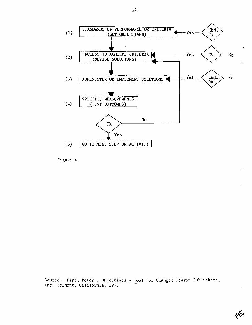
STANDARDS OF PERFORMANCE OR CRITERIA (1) (SET OBJECTIVES) *yes - \ OK

(3 ) 1 ADMINISTER OR IMPLEMENT SOLUTIONS i

(5) 1 GO TO NEXT STEP OR ACTIVITY 1

Figure 4.

Source: Pipe, Peter , Objectives - Tool For Change; Fearon Publishers, Inc . Belmont , California, 1975

Under B(6) i n Figure 1, perform the t e s t s you have es t ab l i shed and

with t h e farmer evaluate t h e r e s u l t s . I f the s o l u t i o n proves useful t o

farmers, then work with t h e farmers t o set-up demonstrations o r f i e l d

days where t h e farmers, not t h e team members, a r e on cen te r s t age . Let - it he t h e i r f i e l d day and s e e t h a t re levant government o f f i c i a l s a r e

t h e r e t o i n t e r f a c e with (not dominate) farmers. I f t h e so lu t ion i s useful

t o farmers, they can l l se l l ' l it t o o the r farmers and o f f i c i a l s b e t t e r

than t h e researcher can, Remember, "if t h e farmer can ' t s e l l i t , we won't

t r y . " A t B(8) work hard t o get feedback from farmers, o f f i c i a l s , and

ind iv idua l s who work both d i r e c t l y and i n d i r e c t l y with farmers (examples:

extension, f e r t i l i z e r , agents , c r e d i t o r banking people) .

A t t h i s point t h e feedback w i l l he lp t h e team t o r e f i n e t h e

so lu t ions (B[9]). This refinement process is c r i t i c a l f o r t h e adoption

of t h e so lu t ions by various c l a s s e s o f farmers who may not have t h e

same condit ions ( s o i l s , crops, e t c . ) a s t h e o r i g i n a l locat ion where t h e

s o l u t i o n was f i r s t developed. A key concept is adaptive research where

f indings developed under one s e t o f condit ions a r e modified f o r o t h e r

condi t ions o r areas .

In B(9) phased withdrawal o f team and f inanc ia l support i s important.

For too prevalent i s t h e problem of "throwing too many resources' ' a t a

problem and then expecting t h a t farmers can adapt . This is a major

reason why farmers do not p lace much c r e d i t a b i l i t y on research s t a t i o n

r e s u l t s , model farm r e s u l t s , and even extension demonstration r e s u l t s .

They simply can never expect t o command a s many resources. This is why

we s t r e s s "on-farm", farm and farmer condi t ions . My experience suggests

t h a t farmers use a discount f a c t o r when they observe r e s u l t s from

experiment s t a t i o n s and p r o j e c t s because they know t h a t they cannot

command a l l those resources o f s c i e n t i f i c manpower and c a p i t a l .

In Pakis tan we of ten made t h i s mistake and gave t h e mistaken impression

t h a t over t ime, farmers could adopt s u c c e s s f u l l y c e r t a i n improvement

so lu t ionsdeveloped by our team. A t some p o i n t t h e team members must "move

back," "Take hands o f f , " and observe s y s t e m a t i c a l l y whether o r no t t h e

s o l u t i o n s w i l l s u rv ive under fa rmer ' s cond i t i ons , e s p e c i a l l y cons ide r ing

t h e l e v e l of support t h e government can provide . Remember t h a t t h e

t r a n s f e r o f technology i n low income na t ions r epea t ed ly f a i l s because i t

i s not app ropr i a t e t o t h e r e a l world cond i t i ons .

C. Assessment, Refinement, and Scaling-Up o f Solu t ion Packages

Under C i n Figure 1, Assessments, Refinements, and Scaling-Up

o f So lu t ion Packages i s t h e next s e t o f a c t i v i t i e s . There a r e many

types o f assessments which inc lude t echn ica l f e a s i b i l i t y , economic

f e a s i b i l i t y , s o c i a l impact and o rgan iza t iona l f e a s i b i l i t y , management

f e a s i b i l i t y , f i n a n c i a l f e a s i b i l i t y , and even p o l i t i c a l f e a s i b i l i t y . Some

o f t h e methods o f doing t h i s w i l l be d iscussed i n t h e seminar. This i s

a new f i e l d which s t i l l needs more a t t e n t i o n then it r e c e i v e s . Always

t h e assessment i s conducted i n r e l a t i o n s h i p t o s p e c i f i c c r i t e r i a and

o b j e c t i v e s which a r e both given t o and de r ived by t h e team. This s e rves

a s a guidance mechanism f o r t h e DOS process and a way f o r d e l i m i t i n g

and measuring t h e worth o f t h e s o l u t i o n s evolved.

The concept o f scal ing-up i n (C) Figure 1, r e f e r s t o t h e assessment

and refinement o f s o l u t i o n s f o r a n a t i o n a l program. Scal ing-up means

an examination o f the resources needed f o r a p r o j e c t . The p r o j e c t could

range from a p i l o t p r o j e c t t o a f u l l hational proj,?ct.

A t t h i s s t a g e , C(12), i f moreinformati 'onis needed f o r refinement

of t h e s o l u t i o n s packages, then as Figure 1 i n d i c a t e s , you go back and

l o c a t e t h e type needed. The assessment process o f t e n w i l l provide t h e

types o f information needed. A t any r a t e , t h e team may need t o r ecyc le

some a c t i v i t i e s , I f t h e object ives change, a s is sometimes the case due

t o p o l i t i c a l forces , then each so lu t ion must be re-examined with the new

c r i t e r i a i n mind. A t C(11), i f more information i s needed you may need

t o conduct more t e s t s ( l l a ) o r move back t o check the designs t o t h e

t e s t s a l ready conducted a t B ( 5 ) .

I f so lu t ions have not been combined e a r l i e r in a complementary

r e l a t i o n s h i p , then such a synthes is w i l l have t o t ake p lace a t C(13).

For l a rge improvement p ro jec t s r a r e l y w i l l t h e r e be only s i n g l e

a l t e r n a t i v e solut ions . The concept of complementarity i s important

here. For example, i n t h e Pakistan p r o j e c t , water course r e h a b i l i t a t i o n ,

precis ion land level ing, and on-farm water management advisory services

were chosen. Because a combination of these t h r e e so lu t ions promised

a reduction i n conveyance losses , improved f i e l d appl ica t ion o f water

due t o level ing f i e l d s , and improved water management and crop p rac t i ces .

A l l these f a c t o r s assured increased crop production f o r small farmers.

The technological and soc ia l so lut ions involved were t e s ted i n t h e Develop-

ment o f Solutions Phase, Further physical , s o c i a l , economic, and o t h e r

assessment r e s u l t s showed t h a t these t h r e e components could be

supported adequately within t h e context o f Pakis tan ' s resource c o n s t r a i n t s .

F inal ly , a t C(14), r epor t s a r e prepared and submitted f o r severa l

audiences. F i r s t , a d e t a i l e d technical r epor t i s made ava i l ab le f o r

personnel who must develop proposals f o r local and foreign funding

agencies. Secondly, a b r i e f non-technical r epor t i s prepared f o r pol icy

decision makers such a s t h e Planning Commission. Third, a b r i e f

non-technical executive summary i s needed f o r top o f f i c i a l s such a s

busy minis ters and t h e i r duputies.

There is a l a s t caveat (warning) t o remember, Once t h e a l t e r n a t i v e

so lu t ions have been made ava i l ab le through t h e DOS process, the decisions

t o be made a r e usua l ly both t echn ica l and p o l i t i c a l , a s a d i f f e r e n t

process emerged f o r po l i cy dec i s ions on z ?rojo:t,

1 1 . A Note on t h e Role o f Objec t ives a s Tools i n Developing So lu t ions

Throughout t h i s b r i e f overview o f a sys temat ic approach f o r DOS,

stress has been given t o t h e r o l e o f c l e a r performance o b j e c t i v e s . To

sum up t h e use o f ob jec t ives , we remind t h e r eade r t h a t ob jec t ives

1. Describe t h e i n t e n t o f what you expect t o do.

2 . Describe t h e condi t ions under which t h e a c t i o n ( t r i a l ,

experiment, demonstration) is t o be perfcrmed.

3 . Includes an ind ica t ion o f t h e resources which a r e t o be made

a v a i l a b l e o r withheld.

4 . Es t ab l i sh t h e c r i t e r i a i n terms o f q u a n t i t y , q u a l i t y , t ime

l imits , o r o t h e r s tandards which must be met t o judge success o r

f a i l u r e .

An example o f a performance o b j e c t i v e r e l a t e d t o improving

d e l i v e r y e f f i c i e n c i e s is as fol lows:

Observable Action: Reduction o f conveyance e f f i e n c i e s on farm d e l i v e r y

systems

Conditions : Earthen improved systems a t farm l eve l

C r i t e r i a : Cost e f f e c t i v e improvements over a

wi th d e l i v e r y e f f i c i e n c i e s o f

70 pe rcen t .

I f performance i t se l f is i m p o ~ t a n t , then it should be s p e c i f i e d i n

t h e o b j e c t i v e s . Therefore, i n t h e -.- c r i t e r i a , - i d e n t i f y t h e minimum

requirements which can be accepted fo r successfu l perforrfiance, Take

heed, however, and remember r e a l world condi t ions a t t h e farm l e v e l .

Pipe, Pe te r , Object ives - Tool For Change, Fearon Publ i shers , Inc. Belmont, C a l i f o r n i a , 1975

Often individuals who do not have adequate experience i n t h e r e a l world

s e t u n r e a l i s t i c c r i t e r i a which a r e impossible t o meet. You need a

r a t i o n a l e f o r e s tab l i sh ing c r i t e r i a r e l a t e d t o time, q u a l i t y , quant i ty ,

o r o the r ind ica t ions which w i l l a sce r t a in degree o f success. Also,

i n s e t t i n g ob jec t ives , i s o l a t e the des i red ac t ion c a r e f u l l y and i d e n t i f y

the condi t ions . This w i l l force on6 t o be s p e c i f i c . Remember t h a t

performance ob jec t ive can be measured while a good is usual ly a desc r ip t ion

o f an i n t e n t s t a t e d i n terms which a r e not measurable. An ob jec t ive ,

then, is a desc r ip t ion of an i n t e n t s t a t e d i n measurable terms. A

performance object ive is one t h a t descr ibes t h a t i n t e n t of terms of

observable performance. There a r e t h e types o f ob jec t ives which would

guide the DOS process and he lp t o make it a systematic r a t h e r than a

random process. I t is a sad f a c t o f l i f e t h a t much development research

i s character ized too o f ten by "dr i f t " r a t h e r than "direct ion", and

"fuzziness" r a t h e r than tlfocusM. The DOS process must have both focus

and d i r e c t i o n i f it is t o produce an u l t ima te r e s u l t .

One conceptual method o f a t t a i n i n g a useful u l t ima te product i s t o

th ink i n terms of process and product. Table 3 shows how t h i s can be

done. Assume t h a t t h e general sood is "the improvement of on-farm

water management," and t h e performance ob jec t ive i s t o "reduce conveyance

losses by 75 percent."

Such an approach o f separa t ing t h e process from the product helps

i n developing c l a r i t y .

111. Rules f o r Brainstorming i n S e t t i n g Performance Objectives Within t h e Ream Context

As is evident from t h e discussion on developing object ives and

reaching concensus i n t h e WS process, it i s important t o develop r u l e s

f o r brainstorming and decision making. A s suggested i n o t h e r mater ia ls

TABLE 3 ,

COAL: Improvement o f OFWM

OBJECTIVE: Reduce Conveyance Losses by 75 percent

PROCESS I PRODUCT

B. Divide p lans f o r DOS

A. Use Output o f P . I . and examine causes vs . symptoms

C. Implement a l t e r n a t i v e s o l u t i o n

A. Causes o f problems documented

B. C lea r p e r f ~ r m a n c e o b j e c t i v e s

D. Tes t a l t e r n a t i v e s o l u t i o n s

C. Receive d a t a from monitoring and eva lua t ion

D. Conveyance l o s s reduced by 75 percent

presented i n t h i s seminary, team work is not easy and team bu i ld ing i s

an unending process . Several bas i c r u l e s e x i t s f o r ga in ing maximum

team output from team ses s ions o f brainstorming. A ca rd ina l p r i n c i p l e

is t h a t no one c r i t i c i z e s anothers idea o r uses any means o f i n t imida t ion .

Such e f f o r t s s t i f f l e c r e a t i v e th inking , s i d e t r a c k s the c r e a t i v e process *

and causes ind iv idua l s t o remain s i l e n t . One product ive approach is

as fo l lows:

1. Write o u t t h e goal o f DOS c l e a r l y s o t h a t it i s v i s i b l e t o a l l .

2 . Each team member i s requested t o work a lone and answer the

ques t ion "how w i l l I know success when I s e e i t ? "

3 . Working a lone , each team member draws up a l i s t of performance

ob jec t ives which, when combined, w i l l mean t h a t t he goal is

reached.

4 . A t t h e end of 20-30 minutes each team member a lone is asked t o

r e f i n e h i s o r h e r performance o b j e c t i v e s . (Be s u r e t h a t t h e

c r i t e r i a f o r success can be measured by observable peformance).

5. Each team member a lone i d e n t i f i e s h i s o r h e r t op t e n i n d i c a t o r s

which a r e t h e b e s t p r e d i c t o r s o f success.

6 . The team l e a d e r then asks each member i n t u r n t o s t a t e t h e top

p r i o r i t y o f h i s o r h e r performance o b j e c t i v e s which i s w r i t t e n

on a blackboard o r f l i p c h a r t . Af t e r each team member has

provided h i s o r h e r t o p o b j e c t i v e s , then t h e l e a d e r goes

around t h e group f o r t h e second b e s t o b j e c t i v e and so on u n t i l

a l l 10 ob jec t ives o f each member a r e recorded.

7 . When t h e l i s t i s complete, it i s r ev i sed i n group d iscuss ion

and r e f ined . Each member o f t h e team can defend h i s o r h e r

performance o b j e c t i v e with r a t i o n a l e .

Adopted from Pipe, Pe te r , Object ives - Tool For Change, Fearon Publ i shers , Inc. Belmont, Ca l i fo rn ia , 1975

Conclusion

I have described the skeleton framework for a systematic DOS

process and stressed the importance of several key concepts. More

detailed information on procedures is available. The emphasis on

performance objectives is to stress thht all important conccpt:

FOCUS.

As you read this, I would appreciate your comments and suggestions.

We, as a team, must search for systematic DOS approaches which will

provide useful results to small farmers around the world,

Staff Paper # 33

RESPONSE OF RICE, WHEAT AND FLAX TO ZINC APPLICATIONS ON THE SOILS

OF THE NILE DELTA

A. D. Dotzenko, M. Zanati, S. Abdel-Hafez A. Keleg, A. T. Moustafa, A. Serry

I NTRODUCTI ON

The Egypt Water Use and Management Pro.iect ob jec t i ves a re p r i m a r i l y

concerned w i t h improving the soc ia l and economic we l fa re o f t h e small

Egyptian farmer by t h e a p p l i c a t i o n o f v i a b l e on-farm management a1 t e r n a t i ves

t h a t would r e s u l t i n crop y i e l d increases. There are fou r bas ic components

i n p r o j e c t a c t i v i t i e s i n order t o formulate and demonstrate on-farm

management a l t e r n a t i v e s : 1. problem i d e n t i f i c a t i o n , 2. search f o r so lu t i ons ,

3. t e s t i n g o f so lu t i ons t o the problems i d e n t i f i e d and, 4. t he d i f f u s i o n

o f in format ion .

Ear ly i n the problem i d e n t i f i c a t i o n phase m ic ronu t r i en t de f ic ienc ies

were observed i n many of t he crops growing on the f i e l d s i t e s t h a t were

se lec ted as common study areas. A review o f recent Egyptian l i t e r a t u r e

indicated, t h a t under experimental cond i t ions , a marked increase i n crop

y i e l d s occured when micro-nut r ien ts ( z i n c i n p a r t i c u l a r ) were added t o the

r e g u l a r f e r t i l i z e r program. This in fomia t ion was the basis f o r t he f i e l d

t r i a l s t h a t were used as a s o l u t i o n t e s t i n g program t o t h e problems t h a t

were i d e n t i f i e d .

The greater m a j o r i t y o f the a l l u v i a l s o i l s o f t he N i l e Val l e y and De l ta

owe t h e i r ex is tence t o the depos i t ion of t he suspended mat te r c a r r i e d by

the r i v e r from i t s source i n the Eth iop ian and V i c t o r i a n plateaus and t h i s

parent mater ia l has a major i n f l uence on s o i l c h a r a c t e r i s t i c s ( 9 ) . Before

cons t ruc t i on o f the High Dam a t o t a l o f as much as 25 n i i l l i o n tons were

est imated t o pass by Cairo dur ing the month o f September and even tua l l y

reaching a minimum o f 0,5 m i l 1 i o n tons i n May and June (9 ) . The suspended

mat ter contained from 55 t o 65 percent c l a y w i t h a s i l t content ranging from

25 t o 30 percent and organic mat ter on the order t o 2.3 t o 4.5 percent. The

-2-

composit ion o f t he suspended ma te r ia l of the N i l e water has changed and t h e

amount o f sediment c a r r i e d decreased markedly a f t e r cons t ruc t i on o f t he High

Dam. This change i n composit ion could i n p a r t be one reason why many

Egypt ian s o i l s a re now d e f i c i e n t i n m ic ronu t r i en ts a t the present t ime.

Another f a c t o r r e l a t e d t o m ic ronu t r i en t de f i c i enc ies i s the present

a1 l o c a t i o n o f f e r t i l i z e r s t o Egypt ian farmers. The p r a c t i c e o f f e r t i l i z a t i o n

i s main ly d i r e c t e d towards the add i t io r : of n i t r o g e r and phosphorus and

1 i t t l e account i s taken o f the v a r i a b i l i t y i n s o i l s , cropping pa t te rns and

micronut r ien ts . This system works f a i r l y w e l l b u t i s s e r i o u s l y d e f i c i e n t

when i t comes t o maximizing y i e l d s . The present p r o d u c t i v i t y o f

Egypt iap s o i l s as determined by the y i e l d o f crops shows t h a t the y i e l d

of t h e major crops are r e l a t i v e l y high. Y ie lds r e l a t e d t o the wor ld average,

as 100 percent, ranged from 208 percent f o r co t ton t o 232 f o r r i c e (9 ) .

These a re broad based averages i n d i c a t i n g t h a t crop product ion p rac t i ces

are r e l a t i v e l y good b u t they can a l so be misleading. Recognizing t h a t

Egypt has f e r t i l e a l l u v i a l s o i l s coupled w i t h adequate water o f good q u a l i t y ,

ample sun l i gh t , weather t h a t permi ts year-round c u l t i v a t i o n o f the land

and h i g h l y s k i l l e d farmers makes f o r an i dea l corr~binat ion f o r h igh l e v e l s

o f crop p r o d u c t i v i t y .

Despite these unique favorab le fac tors the re remain several ser ious

cons t ra in t s t o maximized crop product ion. A h igh water tab1 e, poor drainage,

non-uniform water d i s t r i b u t i o n on land, smal l land hold ings, pest c o n t r o l , and

minor s o i l element de f i c i enc ies are some of t he major cons t ra in t s t o maximized

crop product ion. Yie lds on farm f i e l d s a r e approximately 50 percent of the

y i e l d s obta ined on experimental s t a t i o n s i n Egypt (9).

The purpose of t h i s paper i s t o focus on the m ic ronu t r i en ts c o n s t r a i n t I

and present i n fo rma t ion obta ined from f i e l d t r i a l s r e l a t i v e t o the increase i n

p r o d u c t i v i t y o f var ious crops where . ~ b f c r o n u t r i e n t s were added as p a r t o f t he

r e g u l a r f e r t i l i z e r program. In fo rma t ion of t h i s t y p e w i l l a l s o be a bas is

f o r t h e development of a s o i l t e s t i n g program t h a t w i l l recommend t h e

a p p l i c a t i o n o f f e r t i l i z e r by s p e c i f i c s o i l cond i t ions r a t h e r than by area

wide cond i t ions .

REVIEW OF LITERATURE

The lack o f m ic ronu t r i en ts i n many Egypt ian s o i l s i s a r a t h e r recen t

and unexpected c o n s t r a i n t t o maximized a g r i c u l t u r a l product ion. Def ic ienc ies

i n these minor elements a re no t genera l l y v i s i b l e t o the eye b u t they

do e x e r t s i g n i f i c a n t e f f e c t s p a r t i c u l a r l y i n the l ack o f good response t o

t h e macro-nutr ients such as n i t r o g e n and phosphorus (6) . These d e f i c i e n c i e s

can be a t t r i b u t e d i n p a r t t o each of t he f o l l o w i n g f a c t o r s : 1. The i n t r o -

duc t i on o f new h lgh y i e l d i n g c rop v a r i e t i e s which genera l l y have h i g h e r

requirements f o r these mic ronut r ien ts , 2. The use o f h i g h ana lys i s f e r t -

i l i z e r s which con ta in no i m p u r i t i e s as t h e o l d e r fo rmula t ions had a s i g n i f -

i c a n t amount of t r a c e elements and 3. P r i o r t o t h e b u i l d i n g of t h e High

Dam some minor elements were supp l ied t o t h e s o i l i n t he form o f sediment

c a r r i e d i n t he i r r i g a t i o n water from the N i l e . This y e a r l y replenishment

no longer occurs due t o the depos i t ion o f sediments i n Lake Nasser.

To meet these changed condi t ions, expanded f a c i l i t i e s f o r area s o i l

t e s t i n g and p l a n t t i s s u e ana lys is w i l l be requ i red as w e l l as expanded

demonstrations on farmers f i e l d s as a means of remedying t r a c e element

de f i c i enc ies . A good share of t he agronomic work being c a r r l e d on i n

Mansouria and Ka f r El Sheikh i s i nvo l ved w i t h t h e use o f z i n c su lphate and

f o l i a r f e r t i l i z e r s con ta in ing bo th macro and m ic ronu t r i en ts app l i ed t o t h e

major crops grown i n bo th areas. I n o rde r t o f a c i l i t a t e t h e d iscuss ion on

l i t e r a t u r e t h i s paper will deal w i t h only 4 t race elements namely, zinc,

manganese, copper and iron. 'The reader i s referred t o the following

reference i f more deta i l i s required on other t race elements; Micronutrients

i n Agriculture, 1972. Edited by J . J . Mortvedt, P . M . Giordano and W . L .

Lindsay, edi tors . Soi 1 Sci . Soc. of America Monograph.

Zinc :

Of the s i x micronutrients tha t a r e of importance to crop production,

zinc i s among those found to have low concentration levels i~ s o i l s (12).

Krauskopf ( 1 2 ) points out tha t Z n , Mn, Cu and Fe a re generally more abundant

i n basal ts than i n granites. Concentration i n s o i l s show wide variat ions

since the raw material and the so i l form,ins processes a r e so dift'ererrt

from one climate t o another. Kadi -- e t a1 (7) in evaluating the zinc

s ta tus i n s o i l s of Egypt showed tha t the t o t a l zinc content ranged from

18 t o 156 ppm. They noted tha t the highest levels were found i n heavy a l l u -

via l s o i l s while moderate levels were noted i n calcareous s o i l s with sandy

s o i l s having the lowest levels of zinc. El Damaty e t a1 ( 4 ) i n evaluating 50

s o i l s noted t ha t the to ta l zinc levels ranged from 3 t o 195 ppm. They a l so noted ,

t h a t zinc generally increased w i t h an increase in the s i l t and clay content.

Positive s ign i f ican t correlations were found between Zn i n plant and the

amount extracted from s o i l s . Soils from the Nile Delta, along the Med-

iterranean coast , Wadi el Natrun and Kharga oasis and treated with zinc,

increased dry matter production of tomatoes by an average of 15%. The

increase i n production was exceptionally h i g h on plants growing on

Wadi e l Natrun soi 1s as an increase of 30% was obtained (21 ) . This large

increase was a t t r ibuted to the inherent low level of zinc in these s o i l s .

El Sherif -- e t a1 (8 ) measured the movement of zinc i n some Egyptian so i l s

having high pH values and noted t ha t most of the applied zinc was retained

in the surface 1-2 cm depth except fo r sandy s o i l s from Wadi e l Natrun where there

was no r e s t r i c t i o n t o movement. This f i x a t i o n was, i n par t , a t t r i b u t e d

t o the t rans format ion from a p o s i t i v e l y charged z inc i o n t o a nega t i ve l y

charaged z inca te i o n i n a l k a l i n e s o i l s . The presence o f t he z inca te

complex i n a l k a l i n e systems has been confirmed by Jur inak and Thorne (1 1 ) .

Z inc def ic iency of wetland r i c e has rece ived more a t t e n t i o n than any

o t h e r n u t r i t i o n a l problem i n recent years. Z inc def ic iency i n r i c e was

f i r s t repor ted as a f i e l d problem by Nene ( I ? ) and subsequently has been

repor ted i n Pakistan, Ind ia , Ph i l ipp ines , Japan, U.S., Chad, N iger ia , and

Egypt. Next t o n i t rogen and phosphorus, l ack of z inc i s the most l i m i t i n g

f a c t o r i n t h e product ion o f wetland r i c e . Castro (1) i n a comprehensive

review on z inc de f i c iency i n r i c e noted t h a t t f l i s c o n d i t i o n i n s o i l s

was brought about by h igh pH, continuous waterlogging, low inhe ren t z inc

content o f the s o i l , h igh organic mat ter content and h igh l e v e l s o f f e r t -

i l i z e r s . He concluded t h a t de f ic iency can be cor rec ted by d r a i n i n g f i e l d s ,

d ipp ing seed1 ings i n a 2% suspension o f z inc ox ide i n water before t rans-

p l a n t i n g o r by app ly ing z inc sulphate t o the r i c e nursery o r f i e l d .

Manganese

The chemistry o f manganese i n s o i l s shows t h a t t h i s m ic ronu t r i en t e x i s t s

i n d i f f e r e n t forms having w ide ly d ivergent s o l u b i l i t i e s . A1 though p o s i t i v e

responses o f crops t o the a p p l i c a t i o n o f manganese have been reported, manganese

def ic iency i n most crops has no t been recognized i n the f i e l d . However,

it cannot be r u l e d out as i t could occur on sandy s o i l s , sodic s o i l s and

calcareous s o i l s low i n organic mat ter . These types o f s o i l are c h a r a c t e r i s t i c

o f many of the s o i l s found i n the p r o j e c t work s i t e s and p a r t i c u l a r l y i n the

Abu Rayah and E l Hammami areas.

El Damaty -- e t a1 ( 2 ) i n examining the manganese s ta tus o f seventy-four

samples o f s o i l , which as f a r as possib le, represents most o f t h e s o i l s i n

Egypt, noted t h a t t he water so lub le manganese form was completely absent i n

a l l s o i l s . A l l u v i a l s o i l s were found t o con ta in f a i r l y h igh amounts

o f chemical ly a v a i l a b l e manganese which was s u f f i c i e n t t o support normal

growth. They a l s o found t h a t these a l l u v i a l s o i l s were r i c h i n t o t a l

manganese and a t t r i b u t e d t h i s t o t h e annual sedimentat ion o f t h e s o l i d

mat te r t ranspor ted by t h e N i l e . However, s-ince t h e h i g h dam now stops

t h i s sedimentat ion from occur ing i n the v a l l e y and de l ta , poss ib le

d e f i c i e n c i e s could occl l r p a r t i c u l a r l y i n sandy and calcareous s o i l s as they

a re i n h e r e n t l y low i n manganese t o begin w i th . I n add i t i on , water logging,

as i n t h e case o f paddy r i c e product ion, causes an increase i n concent ra t ion

of water s o l u b l e manganese due t o the reduct ion o f the l ess a v a i l a b l e forms.

The water so lub le forms which were absent be fo re water logging occured,

reached 4 ppm i n many s o i l s . Dry mat te r y i e l d s of r i c e grown on cont inu-

ous l y f looded s o i l s was found t o be h i g h e r than on unsubmerged s o i l s . I n tttt

add i t i on , t he reduc t i on of MN oxides a lso releases copper and z inc

absorbed on them (10).

Copper :

A study (3 ) on t h e s ta tus of copper and i t s r e l a t i o n s h i p w i t h pH,

% CaC03, % o rgan ic mat te r and t h e s o i l p a r t i c l e cons t i t uen ts was c a r r i e d

ou t on 75 samples t h a t represented t h e main types o f t h e s o i l s o f Egypt.

The study revealed t h a t a l l u v i a l s o i l s contained h igh l e v e l s o f chemical ly

a v a i l a b l e copper compared w i t h l e v e l s i n ca7~careous s o i l s . I n add i t i on ,

a sample taken from the N i l e R iver suspended mat te r i nd i ca ted t h a t an

average o f 3.6 ppm o f water -so lub le copper was found i n t h e suspended

matter. Water so lub le copper ranged from 0.6 ppm t o 3.1 ppm w h i l e r e a d i l y

a v a i l a b l e copper f luc tua tes from 7,4 ppm t o 19.7 ppm i n the N i l e mud.

I n reduced environments such as r i c e paddies, copper may be present

as Cu20, Cu, CuS, o r Cu2S and absorbed on s o i l minera ls (10). The

concent ra t ion o f water-soluble copper i n a s o i l decreases on f l ood ing desp i te

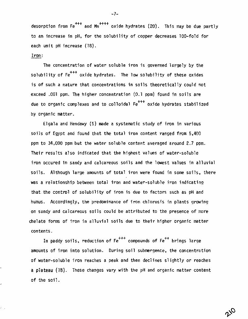
+++ desorpt ion from Fe and ~ n ~ + + oxide hydrates (20). This may be due p a r t l y

t o an increase i n pHy f o r the s o l u b i l i t y o f copper decreases 100-fo ld f o r

each u n i t pH increase (18).

I r o n : - The concentrat ion o f water so lub le i r o n i s governed l a r g e l y by the

s o l u b i l i t y o f ~e'" ox ide hydrates. The low s o l u b i l i t y o f these oxides

i s o f such a nature t h a t concentrat ions i n s o i l s t h e o r e t i c a l l y could no t

exceed .001 ppm. Thb h igher concentrat ion (0.1 ppm) found i n s o i l s are

due t o organic complexes and t o c o l l o i d a l ~e+++ oxide hydrates s t a b i l i zed

by organic mat ter .

E lga la and Hendawy ( 5 ) made a systematic s tudy o f i r o n i n various

s o i l s o f Egypt and found t h a t t he t o t a l i r o n content ranged from 5,400

ppm t o 34,000 ppm b u t the water so lub le content averaged around 2.7 ppm.

The i r r e s u l t s a1 so i nd i ca ted t h a t the h ighest values o f water-soluble

i r o n occured i n sandy and calcareous s o i l s and the lowest values i n a l l u v i a l

s o i l s . Although la rge amounts o f t o t a l i r o n were found i n some s o i l s , there

was a r e l a t i o n s h i p between t o t a l i r o n and water-sol ub le i r o n i n d i c a t i n g

t h a t t he c o n t r o l o f s o l u b i l i t y of i r o n i s due t o fac to rs such as pH and

humus. Accordingly, t he predominance o f i r o n ch lo ros i s i n p lan ts growing

on sandy and calcareous s o i l s could be a t t r i b u t e d t o the presence o f more

chelate forms o f i r o n i n a l l u v i a l s o i l s due t o t h e i r h igher organic mat ter

contents,

I n paddy s o i l s , reduct ion o f ~e"+ compounds o f ~ e + + br ings l a r g e

amounts o f i r o n i n t o so lu t i on . During s o i 1 submergence, the concentrat ion

o f water-soluble i r o n reaches a peak and then decl ines s l i g h t l y o r reaches

a plateau (18) . These changes vary w i t h the pH and organic mat ter content

of t he so i 1.

The p r a c t i c e o f f e r t i l i z a t i o n o f crops i n Egypt which p r i m a r i l y

deals w i t h t he a p p l i c a t i o n o f h igh ana lys is ni t rogenous and phosphat ic

f e r t i l i z e r s coupled w i t h the i n t r o d u c t i o n o f new h igh y i e l d i n g crop

v a r i e t i e s t h a t have h ighe r requirements f o r m ic ronu t r i en ts and the

s topp ing o f t h e annual depos i t i on o f N i l e suspended ma t te r w i l l cont inue

t o cause d e f i c i e n c i e s i n m ic ronu t r i en ts . Therefore, i t becomes impera t ive

t h a t t h e m i c r o n u t r i e n t s ta tus o f Egypt ian s o i l s be assessed e i t h e r by

s o i l f e r t i l i t y ana l ys i s o r by f i e l d demonstrat ion t r i a l s o r by both methods.

-9-

METHODS AND MATERIALS

Informat ion descr ib ing p l a n t responses t o env i ronrnental f a c t o r s

must be i d e n t i f i e d i n order t o c h a r t a path o f a c t i o n t o improve crop

y i e l d s . A ser ious environmental c o n s t r a i n t t o improve crop y i e l d s

was r e c e n t l y discovered as numerous Egypt ian researchers (,2,4,5,13 and

21) po in ted out t h a t many Egypt ian s o i l s were d e f i c i e n t i n m ic ronu t r i en ts .

I n order t o assess the n u t r i e n t s ta tus of t he s o i l s i n the p r o j e c t

work s i t e s a s o i l f e r t i l i t y survey was conducted i n Mansouria and Kaf r

E l Sheikh. The Mansouria area was d i v ided by l o c a t i o n s where 12 samples

were c o l l e c t e d from E l Hamami and 7 samples from Beni Magdoul. I n a d d i t i o n

t o c o l l e c t i n g z inc and i r o n data, i n fo rma t ion was a l s o c o l l e c t e d on pH,

e l e c t r i c a l conduc t i v i t y , organic mat te r content, NO3-N content , phosphorus

l e v e l s , potassium l e v e l s and est imated l ime l e v e l s . One hundred sur face s o i l

samples (0-20 cm depth) were taken from Abu Rayah and 9 o the r surrounding

v i l l a g e s . Ava i l ab le phosphorus, potassium, z inc , copper, i r o n and manganese

1 eve1 s were determined along w i t h pH, e l e c t r i c a l conduc t i v i t y , anion and

c a t i o n content of t he s o i l s a t u r a t i o n e x t r a c t (19 and 22).

F i e l d t r i a l s were conducted i n the Ka f r e l Sheikh (Abu Rayah) p r o j e c t

work s i t e s where 18 farm f i e l d s were se lec ted t o represent t h e average

s o i l and environmental cond i t ions o f the whole area. Three f i e l d crops

were i nvo l ved and these crops are r i c e , wheat and f l a x . The response of

r i c e t o z i n c was evaluated by us ing th ree treatments: 1 ) a c o n t r o l where

normal management p rac t i ces were used, 2) a p r a c t i c e where z i n c sulphate

a t t he r a t e o f 10 kgs. per feddan was added t o the f i e l d and 3) a treatment

of where z i n c sulphate a t t he r a t e o f 20 kgs. per feddan was added t o the

nursery. The t r e a t e d and unt rea ted f i e 1 ds rece ived approximate1 y t he same

l e v e l s o f n i t r o g e n and phosphorus w i t h the on l y d i f f e rence be ing t h e

a d d i t i o n of z i n c su lpha te t o t h e t r e a t e d f i e l d s . Rice seed l ings p r i o r

t o t r a n s p l a n t i n g were weighed and a t ha rves t t ime t he he igh t , t h e number

o f t i l l e r s , t h e n u h e r o f e f f e c t i v e t i l l e r s , g r a i n and s t r aw y i e l d s were

obta ined.

I n t h e wheat demonstrat ion study, 10 kg. of z i n c su lpha te pe r feddan

was added du r i ng seedbed p repa ra t i on s tage t o one -ha l f o f f o u r farm f i e l d s .

Phosphorus and n i t r o g e n were a p p l i e d a t a cons tan t reconlmended r a t e o f

7.5 kg. of P205 and 45 kg. o f n i t r ogen . T o t a l p l a n t , g r a i n and s t raw y i e l d s

were ob ta i ned a t harves t .

I n t h e case o f f l a x , e i g h t f i e l d s were s e l e c t e d where z i n c su lpha te

a t the r a t e o f 10 kg. pe r feddan was added t o one-ha1 f o f each f i e l d .

N i t r ogen a t t h e r a t e o f 45 kg. p e r feddan was a l s o a p p l i e d t o each f i e l d .

A t harves t , whole p l a n t , seed and s t raw y i e l d s were obta ined. I n a d d i t i o n ,

weights of 50 f l a x seed capsules, number of seed i n 50 capsules and t h e

we igh t o f 1,000 seed was a l s o determined t o see how t h e z i n c su l phate

t rea tments a f f e c t e d these components o f y i e l d .

The da ta ob ta i ned was t r e a t e d s t a t i s t i c a l l y by us ing a one way a n a l y s i s

o f va r i ance t o determine if s i g n i f i c a n t d i f fe rences e x i s t e d between

t reatments .

RESULTS AND DISCUSSION

'The s o i l s o f t h e p r o j e c t work s i t e s a t Abu Rayah and t h e sur round ing

areas have been c l ass i f i e d as c l ay s o i 1 s hav ing c l ay percentages r a n g i ng

f rom 45 t o 60. With c l a y con ten t on t h i s o rde r of magnitude c a t i o n exchange

capac i t y (CEC) i s h i g h hav ing mode values of 39.34 meq. p e r 100 g. o f s o i l .

Table (1) The pH, e l e c t r i c a l conduct iv i ty , SAR and ca lcu la ted CEC values a t 10 v i l l a g e s i t e s loca ted i n the Kafr El Sheikh Governorate.

Mode values o f pH, ECe, SAR and CEC f o r a1 1 v i l l a g e s i t e s

pH = 7.96 SAR = 5.47

= 1.88 = 39.34

Locat ion

El-Thabel Coop

E l -Bar ie Coop

El-Riyadh Coop

El-Ragam Coop

El-Wezaria Coop

El-Ethad Coop

El-Halafy Coop

Om-Sen Coop

Dokmera Coop

Abu-Rayah Coop

PH ECe Range

7 . 7 - 8 . 1

7.9 - 8.0

7.8 - 7.9

7.8 - 8.0

7.7 - 8.1

7.6 - 8.0

7.5 - 7.9

7.5 - 8.1

7.7 - 8.0

7.6 - 8.0

Ran*

1.7 - 2.7

1.8 - 3.4

1 . 5 - 2 . 8

1.6 - 2.4

1 . 1 - 5 . 0

1.2 - 4.2

0 . 8 - 3.7

0 . 8 - 4 . 4

1 . 2 - 7 . 1

1.4 - 4.6

Avg .

7.9

7.9

7.9

7.9

7.8

7.7

7.9

7.9

7.8

7.9

Avg .

2.3

2.4

2.1

2.1

2.3

2.2

1.8

2.3

3.4

3.0

SAR

Range

4.4 - 8.0

4.9 - 7.7

3.8 - 8.1

3 . 5 - 6 . 9

3.2 - 7.6

4.6 - 9.2

3.5 - 7.8

2.1 -14.5

4.8 - 9.5

2.3 14.2

Cal cu la ted CEC meq per 100 G.

Avg .

5.9

6.3

2.1

2.1

2.3

6.7

5.0

5.5

6.8

7.5

Ranqe

33.0 - 43.8

34.3 - 38.2

33.4 - 41.2

31.7 - 43.8

28.7 - 39.5

33.9 - 43.8

29.6 - 37.7

30.9 - 45.5

28.3 - 39.5

35.0 - 41.3

Avg .

37.7

36.4

38.1

37.4

34.2

37.2

34.2

37.8

33.9

38.9

Table (2) Phosphorus, Potassium and ava i 1 ab le mi c r o n u t r i e n t s values o f t h e s tud ied s o i l samples

Loca t ion

A- El -'rhabel

cool?

B- El -Bar ie -

Coop

C- E l Riyadh

Coop

b- El -Ragama

Coop

P

5.0

5.3

5.5

5.5

5.0

5.5

7.0

5.7

8.5

5.5

5.5

4.0

4.0

7.0

4.0

9.5 5.0

6.0

9.0

Z n

1.5

1.5

1.3

1.6

1 .O

1.3

1 .I

0.6

0.9

0.7

1.9

0.3

0.9

1 . O

1 .O

0.1

0.5

0.4

1 .O

P PM K

354.0

349.6

385.0

367.3

433.8

433.6

349.6

385.0

367.3

433.6

500.0

411.5

385.0

524.6

340.7

500.0 500.0

385.0

442.5

Cu

7.6

6.7

8.6

7.5

8.4

7.8

9.3

6.9

8.8

7.6

9.0

8.2

6.9

9.3

8.8

- - 8.7

8.2

9.2

M i c r o n u t r i e n t s Mn

37.6

37.6

49.5

38.9

40.2

44.8

49.5

27.7

27.0

37.6

31 .O

36.3

36.9

50.1

25.7

- - 42.9

58.0

51.4

( i n PPM) Fe

4.1

6.1

10.3

6.1

9.6

9.6

12.7

8.6

12.0

7.5

9.6

10.3

5.1

12.0

9.6

- - 8.6

8.6

10.3

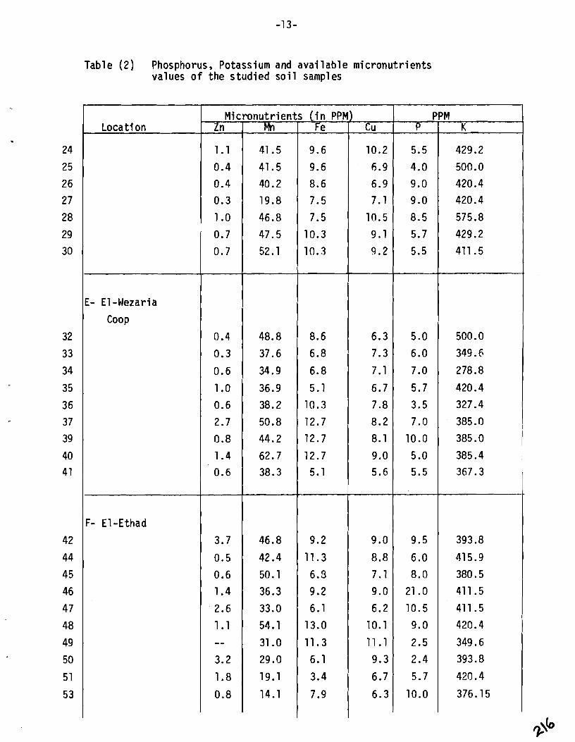
Table (2 ) Phosphorus, Potassium and a v a i l a b l e m ic ronu t r i en ts values o f the s tud ied s o i l samples

I

Loca t i on

E- E l -Wezari a

Coop

P

5.5

4.0

9.0

9.0

8.5

5.7

5.5

5.0

6.0

7.0

5.7

3.5

7.0

F- El-Ethad

PPM K

429.2

500.0

420.4

420.4

575.8

429.2

411.5

500.0

349.6

278.8

420.4

327.4

385.0

Zn

1.1

0.4

0.4

0.3

1 .O

0.7

0.7

0.4

0.3

0.6

1 .O

0.6

2.7

10.0

5.0

5.5

9.5

6.0

8.0

21.0

10.5

9.0

2.5

2.4

5.7

10.0

385.0

385.4 I

367.3

393.8

415.9

380.5

411.5

411.5

420.4

349.6

393.8

420.4

376.15

0.8

1.4

0.6

3.7

0.5

0.6

1.4

2.6

1.1 - - 3.2

1.8

0.8

M ic ronu t r i en ts Mn

41.5

41.5

40.2

19.8

46.8

47.5

52.1

48.8

37.6

34.9

36.9

38.2

50.8

44.2

62.7

38.3

46.8

42.4

50.1

36.3

33.0

54.1

31.0

29.0

19.1

14.1

( i n PPM) Fe

9.6

9.6

8.6

7.5

7.5

10.3

10.3

8.6

6.8

6.8

5.1

10.3

12.7

Cu

10.2

6.9

6.9

7.1

lr1.5

9.1

9.2

6.3

7.3

7.1

6.7

7.8

8.2

12.7

12.7

5.1

9.2

11.3

6.3

9.2

6.1

13.0

11.3

6.1

3.4

7.9

8.1

9.0

5.6

9.0

8.8

7.1

9.0

6.2

10.1

11.1

9.3

6.7

6.3

Table ( 2 ) Phosphorus, Potassium and a v a i l a b l e m ic ronu t r i en ts values o f the s tud ied s o i l samples

54

5 5

5 6

57

59

6 0

61

6 2

63

6 6

67

69

7 1

7 2

73

75

7 5

7 6

7 7

78

79

80

81

8 2

84

85

86

, Locat ion

G- E l -Ha la fy

Coop

H- Om-Sen

Coop

Zn

1.0

1.2

0.5

0.9

0.5

0.9

0.9

0.8

0.7

1 .O

0.7

0.4

0.5

0.7

0.5

0.9

1.1

1.3

0.4

0.9

1.7

0.3

0.3

0.3

0.4

0.6

0.8

P

16.0

5.5

8.0

5.0

6.0

8.0

8.0

6.0

8.5

7.0

5.5

12.0

18.0

17.0

9.5

11.5

7.0

7.0

7.0

19.0

9.5

18.0

9.5

13.5

12.0

13.5

11.0

M ic ronu t r i en ts Mn

22.4

23.1

16.5

33.6

17.8

18.8

31 .O - - 39.6

44.2

40.9

60.7

42.2

42.9

34.9

31.6

28.3

38.9

41.5

41.5

30.3

29.7

19.8

28.3

35.6

47.5

51.4

( i n PPM) PPM K

380.5

316.1

376.1

340.8

320.1

354.0

362.8

385.0

287.6

393.8

331.9

584.7

844.2

868.3

596.9

904.5

402.7

518.6

795.9

808.0

904.5

5b4.8

358.0

1097.4

856.2

795.9

506.5

Fe

10.3

6.8

5.8

Cu

7.5

6.9

6.3

7.5 1 7.5

3.4

6.8

5.1

8.6

7.9

6.8

8.6

11.3

8.6

7.9

6.8

19.2

5.1

8.6

6.1

6.1

4.4

12.0

5.1

5.8

8.5

8.5

8.6

5.6

7.2

7.1

9.0

9.0

7.8

9.2

8.6

9.3

10.5

9.2

7.5

8.8

8.4

7.5

6.7

8.2

6.0

7.1

8.6

7.5

9.3

Table ( 2 ) Phosphorus, Potass i urn and a v a i l a b l e micronutr ients values of t h e s tud ied s o i l samples

1

L

Location

I- Dokmera

Coop

PPM P

8.0

16.0

20.5

5.5

4.0

9.0

4.0

7.5

9.5

4.0

10.0

- K

560.8

856.2

468.0

585.0

536.2

462.1

438.7

438.7

356.8

391.9

567.4

I

Micronut Zn

2.3

1.5

1.5

1.4

4.0

1 .3

2.3

5.0

1.7

1.1

2.3

( i n PPM) Fe

9.6

4.4

6.1

7.9

6.8

6.1

5.1

7.9 - - -- - -

rients Mn

36.3

10.8

31.6

32.3

27.0

31.6

19.8

32.3 - - - - - -

C u

9.0

9 . 3

6.7

9.7

10.5

8.6

7.5

8.1 - - -- --

The m a j o r i t y of t h e s o i l s sampled were found t o be non-sa l ine. There

were except ions as o u t of 120 s i t e s sampled, t h r e e s i t e s had e l e c t r i c a l

c o n d u c t i v i t y read ings of 7.1, 5.4 and 5.1 mnhos cm which p u t them i n t o a

moderate ly s s l i n e c a t e ~ o r y . Data from t a b l e 1 i n d i c a t e s t h a t t h e sodium

abso rp t i on r a t i o s (SAR) vary g r e a t l y w i t h s o i l s and ranges f rom a low o f

2.1 t o a h i g h o f 14.6. From t h i s a n a l y s i s i t i s e v i d e n t t h a t none o f

t h e s o i l s sampled a r e sod i c i n nature.

The amount o f a v a i l a b l e potassium found i n these s o i l s i n d i c a t e s

t h a t t h i s n u t r i e n t i s no t cons idered as a c o n s t r a i n t t o c rop p roduc t ion .

Due t o t he h i g h c l a y con ten t of t h e s o i l s i n t h i s area t he mode va lue o f

t h e a v a i l a b l e potassium i s 394 ppm.

A v a i l a b l e phosphorus l e v e l s however a r e s i g n i f i c a n t l y lower than those

o f potassium and i n many cases cou ld be cons idered as a c o n s t r a i n t t o c rop

p roduc t i on as l e v e l s ranged from 2.5 t o 21.0 ppm. Approx imate ly 55 pe rcen t

o f t he sampled s o i l s can be cons idered t o be i n low and medium ranqe o f

phosphorus a v a i l a b i l i t - v . These r e s u l t s p o i n t o u t t he need f o r t he develop-

ment of a s o i l t e s t i n g program based on i n d i v i d u a l s o i l sampl ing r a t h e r

than on an area wide recommendation as now p r e s e n t l y e x i s t s .

The m i c r o n u t r i e n t s t a t u s as i n d i c a t e d i n t a b l e 2 shows t h a t adequate

amounts o f most m i c r o n u t r i e n t s a re present i n these s o i l s . According t o

Sol tanpour and Schwab (22), Zn, Mn, Fe, and Cu l e v e l s i n s o i l s should n o t

be l e s s than 1.5, 1.8, 4.0 and 0.5 ppm, r e s p e c t i v e l y . Zn l e v e l s a re low

w i t h t h e excep t ion of a few samples i n most l o c a t i o n s .

I n t h e Mansouria area an examinat ion o f Table 3 r e v e a l s t h a t most

s o i l s i n t h e E l Hammami area a re non-sal ine. Only one s o i l sample had

an e l e c t r i c a l c o n d u c t i v i t y r ead ing o f 6.5 mhos/cm which p u t i t i n t o

t h e moderate ly s a l i n e category. I n t he Beni Magdoul area, approx imate ly

30 percen t o f t h e s o i l s sampled e x h i b i t e d s t r o n g l y sa l i ne c h a r a c t e r i s t i cs.

Phosphorus va lues ranged from 3 t o 17 ppm i n bo th s i t e s and approx imate ly +\

Sable 3 . S o i l F e r t i l i t y R e p o r t f o r E l H a m m a m i a n d B e n i H a g d o u l 1978

.- I

PH

S a m p l e No. S a t .

C o n d .

mmhos/ crn 1 p:m I-'%-, -- pi; EST. F e e l P a s t e

0 . m .

Q /O

PPm I PPm PPr.6 , I

I

Water e x . 1 NAHC03 I

N 0 3 N

I I E l Hammami

- NH4-AC 0; P R L i m e T e x t u r e I

I

I

I 1 7 . 9 ; 6 . 5 , 6

1

2 8 . 3 i 1 . 8 1 0 . 2 / 12 ' 3 I I

I I

I

1 87 1 0 . 6

I

88 1 0 . 5

I med I s a n d

med s a n d

6 ' 1

6 .D 1 I 3 7 . 9 1 3 . 6 ' 0 . 5 1 90 1 13 I 91 0 . 7 6 . 6 1 H i g h 1 L . s a n d

I ' H i g h ; L . s a n d 9 . 2 , I I

7 . 5 H i g h 1 L . s a n d

6 . 1 ~ i ~ h L . s a n d

6 . 8 1 H i g h 8 L . s a n d

I i 8 . 2 1 3 . 1 1 0 . 8 I 12 ' 12

I I I - 3 8 . 5 , 3 . 9 1 0 . 2 1 4 i

I 6 . 8 I H i g h

7 . 1 I , H i g h

L . s a n d

L . s a n d

306 1 . 3 I 80 0 . 6

114 , 0 . 7 I

I 85 1 0 . 6

I 68 0 . 5

1 . 3

t3 8 . 0 1 3 . 6 9

I 8 . 0 ; 3 . 2

8 8 . 3 1 0 . 9

9 8 . 4 I 1 . 9

10 8 . 5 1 1 . 0 I

126

110

269

228

312

0 . 2 40 I 3

I

0 . 2 13 I ' 3

7 . 1

6 . 8

7 . 5

1 1 . 9

1 1 . 5

1 0 . 5

11 , 8 . 5

12 8 . 4

! I B e n i U a g d o u l ,

1 8 . 0 I

2 I 7 . 9 I

0 . 8

0 .6

0 . 9

0 . 7

0 . 8

0 . 4

0 . 7

0 . 3

0 . 2 , 0 . 2

I I I

i I I I

0 . 9

1.1

1 . 2

1 . 2

I

3 i 7 . 9 1 1 . 8

~ i g h 1 L . s a n d I

H i g h 1 s a n d

H i g h / S a n d

1 9

H i g h

H i g h

H i g h

1

1

1

1

I

1 . 3 1 i 1 . 5 2

3

SCL

CL

CL

6

4

5

4 .

5

4

5

Cont . 10.0

12.1

10.3

7.9

6

17

4

6

16

6

33

7 3

1.4

1.4

0.8

1.5

High 1 CL I I

322

494

220

500

1.5

34.9

3.0

75.5

4

5

6

7

High

High

0.8

0.9

0.8

1.3

7.9

7.7

8.0

7.4

C L

SCL

High I C

I

42 percent o f the s o i l s cou ld be considered a t dangerously law l e v e l s

from t h e standpoint o f adequately supply ing the needs o f most crop p lan ts .

Potassium l e v e l s a t both l oca t ions are more than adequate f o r good p l a n t

growth w i t h the l e v e l s a t Beni Magdoul almost tw ice as h igh as i n E l

Hamnami and t h i s i s p r i m a r i l y due t o t h e h igher c lay content i n the

s o i l s o f Beni Magdoul . The m ic ronu t r i en t l e v e l s i n d i c a t e t h a t i r o n

contents are adequate f o r a l l crop p lan ts bu t z inc l e v e l s a re low i n

most samples. Zinc l e v e l s tend t o be lower i n t h e E l H a m m i area than

i n Beni Magdoul and t h i s may be poss ib ly due t o t h e h igher organic mat ter

and c lay content o f t he Beni Magdoul s o i l s . This i s i n agreement w i t h

the r e s u l t s obt ianed by E l Damaty e t a l . (4) and Kadi e t a l . (7)

as they found t h a t z inc genera l ly increased w i t h an increase i n the

s i l t , c l ay and organic mat ter content. Pre l im inary r e s u l t s from

demonstration p l o t s i n d i c a t e t h a t a p o s i t i v e response from z inc appl i-

cat ions appears i n c e r t a i n crops.

Fie1 d Demonstration Studies

Rice - Rice i s the second most important export crop o f Egypt and as a

summer crop i t immediately fol lows w in te r crops i n the cropping r o t a t i o n .

Due t o i t s specia l i r r i g a t i o n regime, the r i c e growing area i s r e s t r i c t e d

t o the nor thern h a l f o f t he N i l e Delta. I n general, t h e so i 1s o f t h i s

area a re low t o medium i n f e r t i l i t y and i n vary ing stages o f reclamation.

Abu Rayah i s i n t h e Ka f r E l Sheikh governorate which together w i t h the

governorates o f Dakahl i a , Beheria and Sharkia account f o r 83 percent o f

t he r i c e growing area.

Next t o n i t rogen and phosphorus def ic ienc ies , z i n c def ic iency i s

the most important n u t r i t i o n a l fac tor l i m i t i n g the growth o f wetland r i c e

i n the r i c e growing areas o f t h e wor ld (1) . A study was undertaken

dur ing the e a r l y summer o f 1978 i n the Abu Rayah s i t e t o see the response

o f r i c e app l i ca t i ons o f z inc sulphate. Since r i c e i s genera l ly

Treatment

No Zinc

Table 4 .

Ef Pcct of Zinc S u l l ) t i a l - c or) L l ~ c . W ~ . i c j l ) ~ of 1,000 Itice S e e d l i n g s C g l l e c t e d from N u r s e r i e s i n '\bu Hayah,'978

Zinc a p p l i e d i n Nursery

b

Grccn W C ~ i c j l I t Dry Weight Green W c i g l i t l ) j 1 fcr c ~ l c c , Dry Weight Dif l , : r c n c e - ----- .

- Grams - - Grams - B - Grams - - Gra~ns - %

Table :$.

The Effect of Zinc Sulphate Applications on the Plant Height,

Number of Tillers, Number of Effective Tillers and the yield

of Grain of Rice Grown at Abu Rayah, 1978.

Factor Zn Added in

Control Zn Added in Field Nursery --

Plant Height, cm. 93.9 105.2* 111.4*

Number of Tillers 31.6 31.7 38.2*

Number of Effective Tillers 29.0 29.4

Grain Yield, Tonslhectare 5.4 7.5* 9.0*

* Significant at 5% Level

Plant height, number of tillers, number of effective tillers are the means of 18 counts. Yield of grain means of 9 counts.

t ransplanted, i~ order t o save land and have b e t t e r weed c o n t r o l , nurser ies

are es tab l ished i n l a t e A p r i l and Mav and young seedl ings a r e t ransp lan ted

i n t o the f i e l d about 1 month l a t e r . One feddan o f nursery supp l ies enough

:-ice t ransp lan ts for 6 t o 8 feddans. This arrangement al lowed f o r the

a p p l i c a t i o n of z inc t o nurser ies as w e l l as t o t h e f i e l d thus p e r m i t t i n g

an eva lua t i on of the two methods of a p p l i c a t i o n i n comparison w i t h a no

z i n c a p p l i c a t i o n .

The f i r s t eva lua t ion t o be made was a t the seed l ing s t a ~ e when the

p lan ts were ready f o r t ransp lan t ing . Table 4 shows t h e e f f e c t of z i n c

sulphate app l ied a t t he r a t e o f 20 kgs per feddan on t h e weight o f

1,000 r i c e seedl ings. There was a 18.1% increase i n the d r y weight of

seedl ings due t o the a p p l i c a t i o n o f z inc . These nurser ies were ~ l a n t e d

a t t h e same t ime using the same v a r i e t y and i r r i g a t e d and f looded equa l l y .

V isual observat ions of the seedl ings showed no d i f f e r e n c e i n he igh t o r

th ickness o r stems y e t a s i g n i f i c a n t weight increase was found. Based

on t h i s , one can assume t h a t the z inc t r e a t e d r i c e seedl ings were i n a m r e

advanced stage of growth and probably took t h e shock of t ransp lan t i na

b e t t e r than the c o n t r o l p lan ts .

Table 5 summarizes the major f i nd ings o f the study. The components

o f y i e l d , p l a n t he igh t , number of t i l l e r s and the number o f e f f e c t i v e

t i 1 l e r s showed s i g n i f i c a n t increases due t o z inc appl i c a t i o n i n the nursery.

A r a t h e r unexpected r e s u l t occured i n t h a t t he re was no d i f f e r e n c e

between the f i e l d a p p l i c a t i o n and the c o n t r o l i n t h e number o f t i l l e r s and

t h e number o f e f f e c t i v e t i l l e r s . This may be due, i n p a r t , t h a t t h e z inc

taken up by p l a n t s i n t h e f i e l d may have occured too l a t e t o cause an

increase i n t i l l e r numbers. However, the z i n c t r e a t e d f i e l d d i d g i v e

an increase i n g r a i n y i e l d over t he c o n t r o l . The z inc treatment i n t he

nursery gave the h ighes t p r a i n y i e l d i n comparison t o the o the r two

treatments.

Control

Zinc in f i e l d

Zinc i n Nursery 4 7 . 6 4 kg ZI S04 /H tc t .

GRAIN YIELD. L . S . D . -

4

9.0

STRAW YIELD. TOTAL YIELD 36-7

Fig .k. G r a i n , s t r a w and t o t a l yields of r i c e in tons/hectare as af fected by different methods of z inc

' ' sulphate application ( mean of 9 counts ) .

Figure 1 r e f l e c t s no t on ly the g ra in y i e l d increase due t o z i n c

app l i ca t i ons b u t a1 LO dep ic ts t h e increase i n s t raw y i e l d s . Appror imate ly

10 more tons o f straw i s produced by the z i n c nursery treatment w h i l e 6

tons more st raw i s produced by the z inc f i e l d t reatment i n comparison

t o the c o n t r o l . The z i n c a p p l i c a t i o n t o the nursery i s by f a r t he

cheapest and the bes t method of a p p l i c a t i o n based on g r a i n and st raw

product ion.

Analyses of t he p l a n t and s o i l together w i t h demonstrations on farm

f i e l d s a re the major t o o l s i n the d iagnosis o f a z i n c de f i c i ency problem.

The l e v e l o f a v a i l a b l e s o i l z i n c below which de f i c i ency might occur i s

1.00 ppm. I n a c r i t i c a l examinat ion o f t h e data from t a b l e 2 and 3 i t

becomes very ev ident t h a t z inc concentrat ions general l y fa1 1 below

1 .OO ppm. I n the E l Hammami and Beni Magdoul areas approximately

83-86% o f t h e s o i l s sampled had l e v e l s o f z i n c below which a d e f i c i e n c y

could occur. The i nco rpo ra t i on o f organic mat te r and t h e use o f h iah

l e v e l s o f f e r t i l i z e r s can aggravate z inc de f i c i ency i n z i n c d e f i c i e n t

s o i l s . Z inc a v a i l a b i l i t y i n t h e Abu Rayah s o i l s Table 2 shows t h a t about

52% o f these s o i l s have l ess than 1.0 ppm. However, Castro ( 1 ) po in ted

out t h a t i n wet land r i c e product ion f l ood ing can decrease the concent ra t ion

of water-soluble z inc t o values as low as 0.03 ppm. I n calcareous and

sod ic s o i l s , t he decrease cou ld be due t o the p r e c i p i t a t i o n o f z inc

su lph ide as s o l u b i l i t y data suqqests the presence of i n s o l u b l e z inc

compounds i n f 1 ooded s o i 1s. For r i c e product ion, several a1 t e r n a t i ves

a r e a v a i l a b l e f o r combatt ing z i n c def ic iency. The f i e l d s can be dra ined

and a l lowed t o dry, o r t he seedl ings dipped i n a 2% z i n c ox ide s o l u t i o n

be fore t r a n s p l a n t i n g o r z i n c can be app l i ed i n the sulphate form t o the

f i e l d o r nursery. Z inc app l i ca t i ons t o r i c e f i e l d s and nurser ies seem

t o enhance the e f f e c t o f n i t rogen and phosphorus as the y i e l d increases

obta ined cannot be a t t r i b u t e d t o z inc alone.

Table 6. The effect of zinc sulphate applications on wheat yields,

1978-1979

Component

Total pJ a11L y i ~1 l d , I.o11:;/ I tad

Seed yield, tons/fed

Stl-aw y i e l d , t u n s / l i ~ d

- - - - ~- -- ... . . ~

* Significant at 5% l e v e l

Con t rol Zinc appl j ed - -r2- - - - ---

t i . 2 Cj . 7

Dif f e r e n c t ~

0.:) N.S.

0.3*

0 . 2 N.S.

N . S . Not s j g11 i J' j (:a11 L

Wheat:

Wheat i s the main w i n t e r crop and i s grown throuahout most o f the

country. I t i s usua l l y p lan ted i n Novenber and harvested l a t e i n May.

This cereal i s the major food crop o f Egypt and s ince product ion i n -

country does no t meet domestic needs, considerable amounts have t o be

imported. I n add i t ion , the straw i s o f g reat importance as a l i v e s t o c k

feed a t t imes when forages f o r animals i s almost non-existent . From

these fac ts , t he importance o f increas ing y i e l d s o f wheat i s se l f -ev iden t .

Table 6 summarizes the r e s u l t s obta ined a t Abu Ravah dur ing t h e

wheat growing season of 1978-79 eva luat ing the e f f e c t of z inc sulphate

app l i ca t i ons . Tota l p l a n t y i e l d s and straw ,y ie lds d i d no t e x h i b i t any

s i g n i f i c a n t d i f f e rence due t o the a p p l i c a t i o n of z inc. Grain y i e l d s

on the o the r hand showed a s i g n i f i c a n t small increase as an add i t i ona l

0.3 tons o f g r a i n per feddan was produced on z inc t r e a t e d f i e l d s . 1

Flax:

F lax i s grown as a dual-purpose crop f o r f i b e r and o i l and i s the

main source o f an i n d u s t r i a l o i l f o r the p a i n t i ndus t ry . F lax i s an

important w i n t e r crop i n the Abu Rayah area and considerable acreaae i s

invo lved i n i t s product ion.

Table 7 summarizes the various components o f y i e l d as we l l as the

g r a i n and st raw y i e l d r e l a t i v e t o the a p p l i c a t i o n o f z inc sulphate. The

weight o f 50 seed capsules, the number o f seeds i n 50 capsules and the weight

of 1,000 f l a x seeds showed a s i g n i f i c a n t response t o z inc . Since these

are the basic components i n y i e l d , one would expect t h e f l a x seed t o

respond by showing an increase i n y i e l d . Flax seed d i d respond as there was

an increase o f 151 k g / f due t o the a p p l i c a t i o n o f z inc . Since f l a x i s a dual

purpose crop i t w o i ~ l d have been i d e a l i f the product ion o f f l a x straw

increased b u t z inc had no e f f e c t on t h i s component. However, a 23.3% increase i n

Table 7 . The e f f e c t of z i n c s u l p h a t e a p p l i c a t i o n s o n f l a x y i e l d s

i n Abu Rayah, 1978-1979

Component - C o l ~ t r o l -- Z i n c appl i e d D i f f e r e n c e ---

W t . o f 50 s e c d c a p s u l e s , g . 3 . 2 4 . 4 1 . 2 *

No . o f flax s e e d i n 50 caps. 313 394 81*

Wt. of 1 , 0 0 0 f l a x s c * c d , g . 1 0 . 2 1 1 . I 0 . 9

T c t a l p l a n t y i e l d , t o n s l i e d 3 . 4 3 . 7 0 . 3 N . S .

I I A K y i e l d , k g / i e d 6 4 8 799 151*

F lax straw y i e l d , t o n s l l ' e d 2 . 7 2 . 9 0 . 2 N . S .

* Significant at 5% level

N . S . N o t s i g n i f i c a n t

seed y i e ld even though there was no change i n straw y ie ld warrants t h e

use of zinc f ~ r f l ax production.

Practical Implications

The occurrence of deficiencies of minor elements in Egyptian soi l s

i s l ikely to increase in the future because of:

1 . Increased removal of nutrients due to the increase i n the use of

modern yield yielding varieties.

2. Depletion of micronutrients due t o intensive cropping systems.

3 . Increased use of concentrated and more pure forms of nitrogen

and phosphorus f e r t i 1 i zers . 4 . Agricultural f e r t i l i z e r policy a t the present time i s mainly

concerned with nitrogen and phosphorus fe r t i l i ze r s and not with

micronutrients .

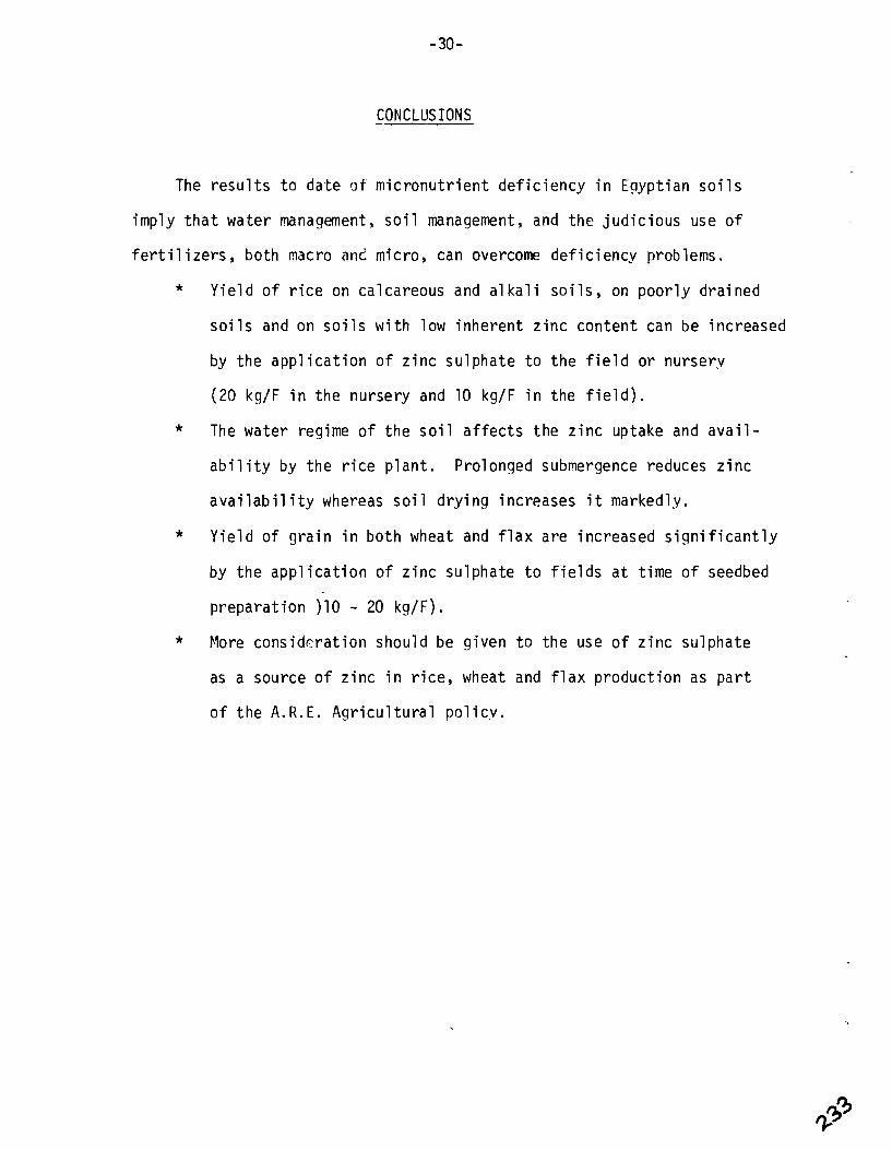
CONCLUSIONS -

The r e s u l t s t o da te of ' m i c r o n u t r i e n t d e f i c i e n c y i n Egypt ian s o i l s

imp l y t h a t wa te r management, s o i l management, and t h e j u d i c i o u s use o f

f e r t i l i z e r s , both macro and micro, can ove rcom d e f i c i e n c y problems.

* Y i e l d o f r i c e on ca lcareous and a1 k a l i s o i l s , on p o o r l y d ra i ned

s o i 1s and on s o i l s w i t h low i nhe ren t z i n c con ten t can be increased

by t h e a p p l i c a t i o n o f z i n c su lpha te t o t h e f i e l d o r nursery

(20 kg/F i n t h e nursery and 10 kg/F i n the f i e l d ) .

* The wate r regime o f t h e s o i l a f f e c t s t h e z i n c uptake and a v a i l -

a b i l i t y by t h e r i c e p l a n t . Prolonged submergence reduces z i n c

a v a i l a b i l i t y whereas s o i 1 d r y i n g inc reases i t markedly.

* Y i e l d o f g r a i n i n b o t h wheat and f l a x a re inc reased s i g n i f i c a n t l y

by t h e a p p l i c a t i o n o f z i n c su lpha te t o f i e l d s a t t ime o f seedbed

p repa ra t i on )10 - 20 kg/F).

* More cons ide ra t i on should be g iven t o t h e use o f z i n c su lpha te

as a source o f z i n c i n r i c e , wheat and f l a x p roduc t i on as p a r t

o f t h e A.R.E. A g r i c u l t u r a l p o l i c y .

LITERATURE CITED

1. Castro, R.U. 1977. Zinc Deficiency i n Rice: A Review of Research a t the IRRI. IRRI Res. Paper No. 9, 18 pgs.

2. El-Damaty, A.H., Hamdi , H. and A. A. Orabi. 1971. Factors affecting the manganese status i n the so i l s of the U.A.R. U.A.R.J. Soil Sci. 11: 7- 26.

3. El-Damaty, A. H . , Hamdi, H:, Serry, A. H. and A. Abdel Razek Sayed. 1973. Copper s tatus i n some selected so i l s of Egypt. Egypt J. Soil Sci. 13:55-64.

4. El- Damaty , A. H. , Hamdi, H. Rasheed, A. and A l i Abdel Fattah A l i . 1973. A preliminary study on zinc i n some selected alluvial Nile Delta so i l s . Egypt J. Soil Sci. 13:109-120.

5. Elgala, A. H. and S. Hendawy. 1972. Studies on iron avai labi l i ty and behavior i n some so i l s on Egypt. Egypt J. Soil Sci. 12:21-30.

6. Egypt: Major constraints t o increasing agricultural productivity. 1976. U.S.A.I.D. and Egyptian Ministry of Agr. Foreign Agr. Econo. Report No. 120.

7. E l Kadi, M. A . , Abdel Salam, M. A., Sabet, S.A., E l Sherif, S. and H. I-Iamdi. 1972. Available zinc status i n the so i l s of Egypt as evaluated by chemical and biological methods. Eavpt J. Soil Sci. 12:123-132.

8. El-Sherif, S., E l Kadi, M. A. Sabet, S. A. andM. A. Abdel Salam. 1973. A st;* of zinc mobility i n so& s o i l s of Egypt using radio- active 6 5 ( ~ n ) , Egypt J. Soil Sci. 13:17-21.

9. El-Tobgy, W.A. 1976. Contemporary Egyptian Agriculture. Published by the Ford Foundation, Garden City, Cairo Egypt.

10. Jenne, E. A. 1968. Controls on h, Fe, Co, N1, Ca, and Zn concentrations in so i l s and water. The significant role as hydrous Mn and Fe oxides. In Trace Inorganics i n Water. Adv. i n Chemistry 73. Am. Chem. Soc. Washington D.C.

11. Jurinak, J . I . and D. W. Thorne. 1955. Zinc solubil i ty under alkaline conditions i n a zinc bentonite system. Soil Sci. Soc. Am. Proc. 19:446.

1 2 . Krauskopf, K.B. 1972. Geochemistry of Micronutrients . In Jhcronutrient s i n Agriculture, Eds , Mortvedt , Giordano and Lindsay. Soil Sci . Soc. America.

13. Mawardi, A., Serry, A , , Azizi, A. Ghaly, S. and S. Maximus. 1974. Effect of micronutrients on paddy production i n Egypt. 2nd Rice Conference, Cairo Egypt Dec . 19 74.

14 . Mawardi, A. , Ghaly, A. S. and A. Serry. 1977, Zinc practices to nursery for e f f ic ien t paddy crop production. Agr. Res. Rev. Cairo. 55:

15. Monged, N.O. and Eid, E.T. and A. Mawardi. 1976. Effect of d i f fe ren t levels of zinc on some r i c e var ie t ies . A q . Res. Rev. Cairo. 54:

16. frlon~ed, N. 0 . Eid, E.T. and A. Mawardi. 1978. Effect o f s o i l application of zinc and manganese on some mineral contents and y ie ld of cotton plants. Agr. Res. Review, Cairo.

17. Nene, Y.L. 1966. Symptoms, cause and control of Khaira disease of paddy. Bul. Ind. Phytopathology Sco. No. 3:97-101.

18. Norwell, W. A. and W. L. Lindsay. 1969. Reactions of EDTA complexes of Fe, Zn, Mn and Cu with s o i l s . Soi l Soc. Am. Roc. 33:86-91.

19. Olsen, S. R.? C. V. Cole, F. S. Watanabe and L. A. Dean. 1954. Estimation of available phosphorus i n s o i l s by extraction with sodium bicarbonate. U. S. D. A. Agr . Circ . 939.

20. Ponnamperuma, M. 1977. Behavior of minor elements i n paddy s o i l s . IRRI Res . Rev. Paper Series No. 8 , 15 pages.

21 . Sabet, S. A , , E l Kadi,'M."A. Shei r i f , S. and M. A. Abdel Salam. 1972. Plant available zinc as an index t o zinc f e r t i l i z a t i o n . Egypt

22, Soltanpour, P.N. and A. P. Schwab. 1977. A new s o i l t e s t fo r sirmltaneous extraction of macro and micro-nutrients i n a lkal ine s o i l s . Soi l Sci. and Plant Analysis 8: (3) 1.95- 207.

S t a f f Paper #39

EVALUATION OF FURROW IRRIGATION SYSTEMS

Thomas W , Ley and Wayne Clyma

INTRODUCTION

E v a l u a t i o n o f t h e performance of furrow i r r i g a t i o n systems r e q u i r e s

t h e c o l l e c t i o n and a n a l y s i s o f d a t a r e l a t i n g t o b o t h t h e o p e r a t i o n and

management o f t h e w a t e r a p p l i c a t i o n subsystem. The p rocedures s u g g e s t e d

f o r t h e c o l l e c t i o n and a n a l y s e s of d a t a which f o l l o w can be used a t two

l e v e l s depending on t h e amount o f d e t a i l d e s i r e d . The l e s s d e t a i l e d

approach p r o v i d e s s a t i s f a c t o r y e v a l u a t i o n o f sys tem performance u t i l i z i n g

a s u g g e s t e d minimum number o f a n a l y s e s . The more d e t a i l e d approach adds

i n f o r m a t i o n on t h e o p e r a t i n g a s p e c t s o f t h e h y d r a u l i c s o f t h e sys tem.

Most o f t e n , t h e more d e t a i l e d measurements a r e d e s i r e d f o r a n e v a l u a t i o n

of some a s p e c t of sys tem d e s i g n h y d r a u l i c s . The l e s s d e t a i l e d approach

p r o v i d e s f u l l y t h e b e n e f i t s of an e v a l u a t i o n o f farmer p r a c t i c e . D i s -

c u s s i o n of t h e p rocedures f o r c o l l e c t i n g and ar ia lyzing t h e more d e t a i l e d

t y p e s o f d a t a is prov ided i n a l a t e r s e c t i o n . An equipment l i s t and

s u g g e s t e d d a t a forms a r e p rov ided l a t e r . The f o l l o w i n g s u b s e c t i o n s

d i s c u s s t h e d a t a t o be c o l l e c t e d , t h e c h r o n o l o g i c a l e v a l u a t i o n p rocedure

and s u g g e s t e d a n a l y s e s of t h e d a t a f o r t h e e v a l u a t i o n of fa rmer p r a c t i c e s .

REQUIRED DATA

P r e l i m i n a r y Data

There is a l a r g e amount of p r e l i m i n a r y s i t e d a t a which shou ld be

c o l l e c t e d and analyzed b e f o r e t h e e v a l u a t i o n of an i r r i g a t i o n o c c u r s .

1 -'prepared under t h e s u p p o r t of t h e U . 6 . Agency f o r I n t e r n a t i o n a l Development, C o n t r a c t s AID/NE-C-1351 and AID/DSAN-C-0058. A l l r e p o r t e d o p i n i o n s , c o n c l u s i o n s o r recommendations a r e t h o s e of t h e a u t h o r s and n o t t h o s e of t h e funding agency o f t h e U.S. Government.

2 ' ~ e s e a r c h A s s o c i a t e and A s s o c i a t e P r o f e s s o r , r e s p e c t i v e l y , Dept. o f A g r i c u l t u r a l and Chemical E n g i n e e r i n g , Colorado S t a t e U n i v e r s i t y , F o r t C o l l i n s , Colorado.

These data include physical information of the site and information from

the farmer concerning his irrigation system and its operation. A list

of suggested questions to direct to the farmer in order to obtain infor-

mation in each of the following categories is included in Appenaix A.

Other more site ~pecific questions should arise from the 'acmer's answers

to these general questions.

1 . Farmer operation and management.--Understanding why cr how 3

farmer does certain things in managing and operating the irrigation

system is vital. Often this aspect of evaluating irrigation performance

may be overlooked and incomplete knowledge of the irrigation system

state results. Farmer management may be constraining the level of

performance which can be attained. The general level of knowledge of

the farmer concerning irrigation principles and practices is evaluated.

Other information discussed later will aid in determining if system

management can be improved.

2. Water supply.--The farmer will know the available water supply,

source, delivery, frequency, etc. He may have only a general knowledge

of the flow rate and quality. These should be measured during the

course of an evaluation. On-farm conveyance losses may be a big problem.

The farmer may or may not know. Measure the losses if necessary.

3 . Crop characteristics.--The crops grown and the planting dates

of each must be known. Available data in the literature on crop seasonal

water requirements, rates and stages of growth, maximum potential rooting

depths, time from planting to effective cover, etc. This information

along with climate daLa i s used to estimate crop water use through the

irrigation season. 'The crop root zone should be measured at each

irrigation for crops with expanding root systems. The measured root

zone f o r a pe renn ia l crop (such a s a l f a l f a ) can o f t e n be assumed v a l i d

f o r t h e e n t i r e season un le s s a h igh ly f l u c t u a t i n g water t a b l e is encoun-

t e r e d . The crop r o o t zone a t each i r r i g a t i o n determines t h e a v a i l a b l e

s o i l water r e s e r v o i r a t t h a t t ime and is necessary t o determine t h e s o i l

water de f i c i ency , t h e s t r e s s a t t h e t ime of i r r i g a t i o n and performance

parameters such a s water a p p l i c a t i o n and water requirement e f f i c i e n c i e s .

4. Phys ica l charac te r i s t ics . - -Measure and record t h e f i e l d

dimensions. S takes should be d r iven i n t o t h e ground a t 25-m i n t e r v a l s

a long t h e l eng th ( a d j u s t f o r s i z e of f i e l d a s necessary) . Measure and

record s u r f a c e e l e v a t i o n a t each s t a k e ( s t a t i o n ) us ing a f i e l d rod and

l e v e l . P l o t t h e s u r f a c e p r o f i l e ( e l eva t ion v s . l e n g t h ) . Measure and

record furrow spacings a t s e v e r a l l o c a t i o n s i n t h e f i e l d . Determine i f

t h e downstream boundary cond i t i on i s ponded o r f r e e outf low. Determine

where and how t o measure furrow inf low and runoff .

5 . S o i l survey.--If a v a i l a b l e , o b t a i n # information on s o i l s i n t h e

a r e a (on t h e farm), such a s maps and c l a s s i f i c a t i o n s from a l o c a l o r

r eg iona l o f f i c e ( e . g . , USDA S o i l Conservation Se rv i ce o r s i m i l a r govern-

ment agency). Such informat ion i s very u s e f u l and a i d s t h e des ign of

d a t a c o l l e c t i o n procedures . S o i l types and t e x t u r e s a r e known and maps

usua l ly d e p i c t t h e v a r i a t i o n of s u r f a c e t e x t u r e s i n a f i e l d . I f t h i s

in format ion is no t a v a i l a b l e , a s o i l survey i s necessary t o determine

t h e s o i l types and uni formi ty i n t h e f i e l d be ing s t u d i e d . S o i l samples

should be c o l l e c t e d i n a minimum of t e n l o c a t i o n s i n t h e f i e l d ( i . e . , a t

f i v e l o c a t i o n s a long t h e l eng th and two along t h e width). Samples

should be taken from a minimum of fou r depths w i th in t h e expected r o o t

zone, i. e . , every 30 cm i n an expected 1 .2 m r o o t zone ( a d j u s t a s

neces sa ry ) . These samples should be analyzed t o determine s o i l types .

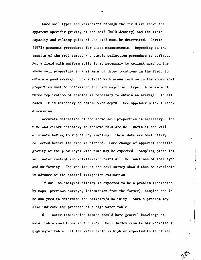
Once s o i l types and v a r i a t i o n s through t h e f i e l d a r e known t h e

apparent s p e c i f i c g r a v i t y of t h e s o i l (bulk d e n s i t y ) and t h e f i e l d

capac i ty and w i l t i n g po in t of t h e s o i l must be determined. Garcia

(1978) p re sen t s procedures f o r t h e s e measurements. Depending on t h e

r e s u l t s of t h e s o i l survey t 4 e sample c o l l e c t i o n procedure is def ined .

For a f i e l d with uniform s o i l s i r i s necessary t o c o l l e c t dara o r t h z

above s o i l p r o p e r t i e s i n a minimum of t h r e e l o c a t i o n s i n t h e f i e l d t o

ob ta in a good average. For a f i e l d w i th nonuniform s o i l s t h e above s o i l

p r o p e r t i e s must be determined f o r each major s o i l type . A minimum o f

t h r e e r e p l i c a t i o n of samples is necessary t o ob ta in an average. I n a l l

c a ses , it i s necessary t o sample wi th depth . See Appendix B f o r f u r t h e r

d i scuss ion .

Accurate d e f i n i t i o n of t h e above s o i l p r o p e r t i e s i s necessary . The

time and e f f o r t necessary t o achieve t h i s a r e well worth it and w i l l

e l imina te having t o repea t any sampling. These da t a a r e most e a s i l y

c o l l e c t e d be fo re t h e c rop is p l an ted . Some change of apparent s p e c i f i c I g r a v i t y of t h e plow l a y e r with t ime may be expected. Sampling p l ans f o r - 1 s o i l water conten t and i n f i l t r a t i o n t e s t s w i l l be func t ions of s o i l type

and uni formi ty . The r e s u l t s of t h e s o i l survey should thus be a v a i l a b l e :

i n advance of t h e i n i t i a l i r r i g a t i o n eva lua t ion .

I f s o i l s a l i n i t y / a l k a l i n i t y i s expected t o be a problem ( ind ica t ed

by maps, previous surveys , information from t h e fa rmer) , samples should

be analyzed t o determine t h e s a l i n i t y / a l k a l i n i t y . Such a problem may

a l s o i n d i c a t e t h e presence of a high water t a b l e .

6 . Water table.--The farmer should have genera l knowledge of

water t a b l e condi t ions i n t h e a r e a . S o i l survey r e s u l t s may i n d i c a t e a I

high water t a b l e . I f t h e water t a b l e is high o r expected t o f l u c t u a t e I

considerably ( i . e . , wi th in t h e maximum p o t e n t i a l roo t zone), it i s

d e s i r a b l e t o monitor t h e ground water l e v e l through t h e i r r i g a t i o n

season. This can be done with a s e r i e s of g r i d of observa t ion wells

(EWUP, Vol. 11, 1979).

A high water t a b l e can l i m i t crop growth through water-logging.

The groundwater q u a l i t y can a l s o s e r i o u s l y a f f e c t crop growth and should

be measured.

Crop water use from t h e c a p i l l a r y f r i n g e o r t h e water t a b l e i s

poss ib l e . Est imates of crop consumptive use by evapo t ransp i r a t ion

modeling techniques w i l l no t correspond wi th measured s o i l water

d e f i c i t s (by s o i l water content sampling) when t h e crop is using ground-

water , assuming e i t h e r method i s y ie ld ing accura t e r e s u l t s . This i s

s i g n i f i c a n t i f t h e water t a b l e r i s e s during t h e season due t o e a r l y

ove r r iga t ion . Water t a b l e f l u c t u a t i o n s due t o o v e r r i r i g a t i o n may a l s o

c o n t r i b u t e t o crop consumptive use and can a f f e c t r o o t zone expansion.

i r r i g a t e d run. Samples should be taken from a minimum of f i v e d i f f e r e n t

depths wi th in t h e r o o t zone. Samples can be c o l l e c t e d us ing a s o i l

auger and should be p laced i n a p a r t i t i o n e d box such t h a t changes i n

s o i l t e x t u r e and composition a r e immediately v i s i b l e . Analysis of a l l

t h e samples taken , f o r type and t e x t u r e , i s d e s i r a b l e . S o i l t e x t u r a l

change throughout t h e f i e l d i s important information. S o i l bulk dens i ty

(apparent s p e c i f i c g r a v i t y ) should be determined making a t l e a s t t h r e e

r e p l i c a t i o n s i n one l o c a t i o n ( a t d i f f e r e n t depths wi th in t h e r o o t zone)

and i n each area where s o i l t e x t u r e was observed t o be d i f f e r e n t .

Garcia (1978) p resen t s da t a c o l l e c t i o n and a n a l y s i s procedures f o r

determining s o i l bulk dens i ty . Representa t ive s o i l sample8 should a l s o

be c o l l e c t e d so t h a t t h e f i e l d capac i ty and w i l t i n g p o i n t of t h e s o i l

( o r s o i l s ) can be determined ( see Garcia , 1978).

On the Day Before I r r i g a t i o n

I n f i l t r a t i o n Data.--Blocked furrow i n f i l t r a t i o n t e s t s should be

conducted i n a t l e a s t fou r l o c a t i o n s along t h e i r r i g a t e d run when t h e

f i e l d has a uniform s o i l . When non-uniform s o i l s a r e p r e s e n t , a minimum

of t h r e e r e p l i c a t i o n s of a t e s t should be conducted on ea:h s o i l type .

There should be enough l abo r a v a i l a b l e s o t h a t each i n f i l t r o m e t e r (F ig .

1) i s manned throughout t h e t e s t . The tests should l a s t no t less than

seven t o e i g h t hours , and i n some cases , a s long a s t h e du ra t ion of

i r r i g a t i o n . Garcia (1978) p r e s a t s procedures f o r t n e assenibly and

ope ra t ion of t h e i n f i l t r o m e t e r s . I n f i l t r a t i o n t e s t s should be conducted

i n furrows o t h e r than those i n which advance and recess ion d a t a w i l l be

c o l l e c t e d , bu t must be i n furrows which w i l l be i r r i g a t e d . Fu r the r

d i scuss ion of cons ide ra t ions of where t o sample and how o f t e n is included

i n Appendix B.

P r e i r r i g a t i o n S o i l Water Content Data.--Garcia (1978) p re sen t s

procedures f o r t h e c o l l e c t i o n and a n a l y s i s of s o i l samples f o r d e t e r -

minat ion of s o i l water conten t by the g rav ime t r i c method. In furrow

i r r i g a t i o n , it is d i f f i c u l t t o determine average water con ten t s i n t h e

s o i l p r o f i l e s i n c e t h e e n t i r e s o i l s u r f a c e i s not covered with water

dur ing i r r i g a t i o n and t h e r e may be s i g n i f i c a n t l a t e r a l movement of water

i n t h e s o i l . I n a l l i n s t ances , samples should be taken from each of

s e v e r a l l a y e r s of t h e measured o r expected maximum roo t ing depth of t h e

crop ( i . e . , f o r a 1 .2 m roo t zone, sample each 30-cm l a y e r , and i n t h e

t o p 30-cm l a y e r , c o l l e c t samples from each 15-cm increment) . I f t h e

water t a b l e is h igher o r near t h e expected maximum roo t ing depth , samples

should be c o l l e c t e d t o near t h e water t a b l e . Each ind iv idua l sample

should be 150 grams o r more. A problem a r i s e s i n determining where t o

Supply ,Reservoir

Plastic Hose

Figure 1. Blocked furrow infiltrometer.

sample a t each l o c a t i o n . When every furrow i s i r r i g a t e d , it i s suggested

t h a t samples be taken from t h e bottom of t h e wet furrow and t h e middle

of t h e furrow r idge ( p l a n t row) between furrows t o g e t a r e p r e s e n t a t i v e

average (Fig. 2a ) . When every o t h e r furrow i s i r r i g a t e d , it i s suggested

t o t a k e samples from t h e bottom of t h e i r r i g a t e d furrow, t h e middle of

t h e furrow r idge ( p l a n t row), and from t h e bottom of t h e non- i r r iga t ed

furrow, i n o rde r t o g e t a r e p r e s e n t a t i v e average of t h e water conten t

below t h e ground s u r f a c e and between wet furrows (Fig. 2b) . For t h i s

ca se , an average water conten t f o r each l a y e r sampled could be def ined

a s :

where P = average water conten t f o r t h e l a y e r , w 9 avg

P = water con ten t f o r t h e l a y e r i n a r ea 1 ( see F ig . 2b) , w , l

P = water con ten t f o r t h e l a y e r i n a r ea 2 ( s ee F ig . 2b ) , w,2

P = water conten t f o r t h e l a y e r i n a r ea 3 ( see F ig . 2b) . w,3

I t i s poin ted ou t t h a t a r e a 2 (Fig. 2b) rece ives twice the weight of t h e

o t h e r s i n computing t h e average, s i n c e t h i s a r ea does i n f a c t occur

twice i n t h e s o i l volume being represented .

S o i l sampling l o c a t i o n s i n t h e f i e l d a r e determined by t h e r e s u l t s

of t h e s o i l survey. I f s o i l s i n t h e f i e l d a r e found t o be uniform a

minimum of t h r e e sampling l o c a t i o n s i n d i f f e r e n t p a r t s of t h e f i e l d

(along t h e furrow) should be s e l e c t e d t o o b t a i n an average f o r t h e

f i e l d . I f s o i l s a r e non-uniform o r i f non-uniform water app l i ca t ions

a r e expected, a minimum of t h r e e r e p l i c a t i o n s of samples i n each repre-

s e n t a t i v e a r ea a r e necessary f o r computing an average. For i n s t ance ,

t h e d i s t r i b u t i o n of app l i ed water i n many f i e l d s i s non-uniform. A

I Soil Volume Represented

nn

a ) Suggested Sample Holes when Every Furrow is I r r iga ted

Soil Volume Represented

b) Suggested Sample Holes when Everyother Furrow is I rr igated

Figure 2 . Suggested s o i l water sampling locations across an irrigated furrow spacing.

sampling scheme to delineate the differences along the length might be

three replications of samples at the head, middle and tail ends of a

field. See Appendix B for further discussion of the considerations of

sampling plans, numbers of samples to collect, etc.

It is recommended that evaluation data (inflow/runoff,

advance/recession, etc.) be collected on a minimum of three furrows.

Flumes or other flow measuring devices should be installed at the head

and tail ends of each furrow to be evaluated. Care must be taken to

ensure that the flumes (if used) are level, have no leaks around them,

and that the furrow sides are built up in the approach to the flume to

prevent overtopping. Since the flume, being a critical depth flow

measurement device requiring a loss of head, water in the approach

section of the furrow will back up. This effect is mcre pronounced on

smaller slopes than steeper ones. Flow measuring devices should be

installed on the day before irrigation.

On the Day of Irrigation

The following data are taken on a minimum of three furrows as the

irrigation progresses. The clock time when water is introduced to each

furrow being studied should be recorded.

Advance Data.--Record the clock time at which the water arrives at

each station (i.e., every 25 m) as the waterfront moves down the furrow.

Inflow Data.-Periodically - record the clock time or elapsed time

from the beginning of irrigation and reading for each inflow rate

measuring device.

Runoff Data.--Record the clock time when water reaches the point

(usually near end of field) where the runoff rate measuring devices are

located. It is suggested that runoff data be collected at 30 sec, 1 min,

2 min, 4 min, 8 min, 15 min, 30 min and then every 112-hour from t h e

time when runoff begins.

Recession Data.--Towards t h e end of i r r i g a t i o n , remove t h e flow

measuring devices from t h e furrows. Record t h e clock time when water i s

shu t o f f . Record t h e clock time a t which water recedes from each s t a t i o n .

The receding water edge i s hard t o def ine . Recession a t a p a r t i c u l a r

p o i n t is assumed t o have occurred when approximately two-thirds of t h e

furrow wetted perimeter i s f r e e of water . Very shal low flow condi t ions

e x i s t dur ing recess ion . Small puddles and r i p p l e s i n t h e furrow bottom

f u r t h e r compound t h e problem. Consistency i s of prime importance when

t ak ing r ecess ion da ta .

A l l flow measuring devices should be check dur ing t h e i r r i g a t i o n

f o r l eaks and proper opera t ing condi t ions . During t h e course of t h e

eva lua t ion any unusual f a c t o r s o r condi t ions should be noted. For

in s t ance , cracks i n t h e s o i l s i g n i f i c a n t l y a f f e c t advance r a t e . Any

e ros ion and sedimentat ion should be noted. Crop condi t ions ( i . e . , r e l a t i v e s i z e , c o l o r , s t and , w i l t i n g , e t c . ) throughout t h e s e c t i o n of

t h e f i e l d being i r r i g a t e d should be noted. S tunted growth may i n d i c a t e

s a l i n i t y problems, poor i n f i l t r a t i o n r a t e s ( i . e . , change i n s o i l t e x t u r e

o r plow pan l a y e r which reduces i n f i l t r a t i o n ) o r o t h e r problems.

Af t e r I r r i g a t i o n

P o s t i r r i g a t i o n s o i l water content samples should be c o l l e c t e d

anywhere from 1-112 days t o 3 days a f t e r i r r i g a t i o n . This depends on

t h e s o i l type and t h e time requi red f o r t h e s o i l t o d r a i n t o f i e l d

capaci ty . Garcia (1978) preueritu a f i e l d procedure f o r es t imat ing when

( a f t e r wet t ing) a s o i l has drained t o f i e l d capac i ty . The same co l l ec -

t i o n procedures a s previous ly discussed apply.

Discussion and Recornendations

I t is important t o convey t o t h e farmer what w i l l be done du r ing

t h e eva lua t ion . Crop damage and s o i l d i s tu rbance should be minimized.

Cooperation of t h e farmer i n a l l a s p e c t s of t h e eva lua t ion i s a neces-

s i t y . I t i s important t h a t nothing t h e i n v e s t i g a t o r s do be fo re o r

dur ing t h e e v a l u a t i o n cause t h e farmer t o d e v i a t e from h i s normal

i r r i g a t i o n p r a c t i c e s .

I t i s important t h a t p re l iminary da t a c o l l e c t e d e a r l y i n t h e season

be good d a t a . A c a r e f u l , coord ina ted , determined e f f o r t he re w i l l save

much time and e l i m i n a t e problems and headaches l a t e r i n t h e season. For

i n s t a n c e , t h e s o i l water con ten t of a f i e l d be fo re t h e i n i t i a l i r r i g a -

t i o n of t h e season may g e n e r a l l y be assumed a s uniform. Huch e f f o r t i n

c a r e f u l s o i l sampling and i n c o l l e c t i o n of more samples ( t o i n c r e a s e t h e * i r -

prec is i .on w i th which t h e mear, s o i l water con ten t i s e s t ima ted ) i s recom-

mended. The e s t ab l i shmen t of t h i s i n i t i a l cond i t i on s e rves an impor tan t

purpose. I t i s t h e s t a r t i n g p o i n t f o r a r o o t zone s o i l water budget .

Prom t h i s i n i t i a l c o n d i o n , water added t o t h e r o o t zone of t h e

crop by p r e c i p i t a t i o n (measured by r a i n gages s e t up i n s e v e r a l loca-

t i o n s a t t h e s i te ) and by i r r i g a t i o n (measured by i r r i g a t i o n evalua-

t i o n s ) is known. Crop use i s es t imated us ing c l ima te d a t a and crop

s t a g e and growth da t a i n an a c c u r a t e , c a l i b r a t e d evapo t r ansp i r a t i on

model. A root-zone s o i l water budget can t h u s be c a l c u l a t e d through t h e

season. S o i l water conten t d a t a c o l l e c t e d a t succeeding i r r i g a t i o n s of

t h e season a r e used a s a check on the p r e d i c t e d s o i l water s t a t u s when

c a l i b r a t i o n of t h e ET model i s necessary .

If t h e r e i s a h igh water t a b l e i n t h e a r e a , crop use from t h e

c a p i l l a r y f r i n g e o r t h e water t a b l e i t s e l f can be es t imated . The

difference between the calculated crop use and the measured soil water

deficit (by sampling) during an irrigation interval is an estimate of

the crop use from the water table during that interval. If there is no

reason to believe that the crop is using water from a water table, then

the computed difference indicates the accuracy of each method and possibly

needed action to improve sampling or predictive techniques.

In some instances, collection of advance/recession data may not be

necessary at each irrigation. For instance, a uniform application of

water may be expected on a field with shorter lengths of run on a heavier

soil. In this case, the distribution is assumed uniform and all that is

required is the water on and water off to determine the water added to

the soil. While this case may occur, it is advisable to collect advance

and recession data when any non-uniformity f water application is 1 e

suspected due to poor irrigation practices, non-uniform soils, non-uniform

field slopes, etc. in order to know the distribution of applied water.

During the course of an actual irridation evaluation, it is

reconmended that a partial evaluation ofkhe data being collected be

conducted. This is accomplished best by processing the data as it is

collected in the field and interpreting the results. For instance, it

is easy to evaluate inflow and runoff data and an obvious error is

determined if the runoff is greater than the inflow. This check on data

provides the investigator a means of eliminating wasted time and effort

in the collection of erroneous data.

FIELD DATA ANALYSIS

Field data analysis provides a basis for understanding the

performance of the irrigation system and how the system is being operated.

The data may be analyzed through a number of prbcedures. Those presented

here represent the minimum of analyses required to formulate an

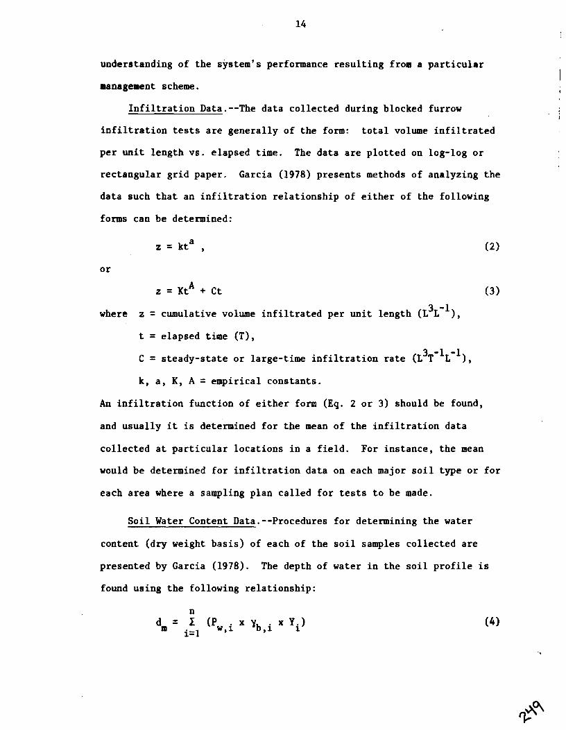
understanding of t h e system's performance r e s u l t i n g from a p a r t i c u l a r

management scheme.

I n f i l t r a t i o n Data.--The da ta c o l l e c t e d during blocked furrow

i n f i l t r a t i o n t e s t s a r e gene ra l ly of t h e form: t o t a l volume i n f i l t r a t e d

p e r u n i t l eng th vs . e lapsed time. The da ta a r e p l o t t e d on log-log o r

r ec t angu la r g r i d paper . Garcia (1978) p resen t s methods of analyzing t h e

da ta such t h a t an i n f i l t r a t i o n r e l a t i o n s h i p of e i t h e r of the fol lowing

forms can be determined:

o r

A z = K t + C t (3 )

3 -1 where z = cumulative volume i n f i l t r a t e d p e r u n i t length (L L ),

t = elapsed time (T),

3 -1 -1 C = s t eady- s t a t e o r large-t ime i n f i l t r a t i o n r a t e (L T L 1,

k, a , K , A = empir ica l cons tants .

An i n f i l t r a t i o n func t ion of e i t h e r form (Eq. 2 o r 3) should be found,

and usua l ly it is determined f o r t h e mean of t h e i n f i l t r a t i o n da ta

c o l l e c t e d a t p a r t i c u l a r l oca t ions i n a f i e l d . For in s t ance , t h e mean

would be determined f o r i n f i l t r a t i o n da ta on each major s o i l type o r f o r

each a rea where a sampling p l an c a l l e d f o r t e s t s t o be made.

S o i l Water Content Data.--Procedures f o r determining t h e water

content (dry weight b a s i s ) of each of t h e s o i l samples co l l ec t ed a r e

presented by Garcia (1978). The depth of water i n t h e s o i l p r o f i l e i s

found us ing t h e fol lowing r e l a t ionsh ip :

where dm = water depth i n the s o i l p r o f i l e (L) , P = water content (dry weight b a s i s ) of t h e i t h l a y e r of t h e w , i

p r o f i l e (w-'),

'b,i = s o i l bulk dens i ty i n t h e i t h l a y e r of t h e p r o f i l e

-3 -1 [ML-~(KL I ,

Yi = th ickness of t h e i t h l aye r (L).

n = number of roo t zone l aye r s sampled.

The p r e i r r i g a t i o n water depths a t each sampling loca t ion ( i . e . , p o s i t i o n

i n t h e f i e l d ) a r e averaged and compared t o t h e water depth when t h e s o i l

i s a t f i e l d capaci ty . This g ives an es t imate of the amount of water

which needs t o be appl ied during i r r i g a t i o n t o b r ing the roo t zone t o

f i e l d capaci ty. This method f o r determining t h e s o i l water d e f i c i t a t

i r r i g a t i o n time i s s u b j e c t t o t h e l a r g e degree of v a r i a b i l i t y observed

i n s o i l water content sampling s t u d i e s , and may g ive u n r e l i a b l e r e s u l t s .

When r e l i a b l e crop da ta and, c l imate da ta a r e a v a i l a b l e , another

es t imate of t h e s o i l water d e f i c i t can be obtained through t h e use of an

evapot ranspi ra t ion modeling procedure and s o i l water budgeting a s

d iscussed e a r l i e r .

Pre- and p o s t i r r i g a t i o n water depths can be compared t o ob ta in an

e s t ima te of the depth of water i n f i l t r a t e d (assuming t h e r e is no deep

pe rco la t ion of water p a s t t h e lowest sampling depth) a t each of the

sampling loca t ions . This i s , of course, s u b j e c t t o t h e c o m e n t made

previous ly concerning t h e r e l i a b i l i t y of s o i l sampling t o determine

water contents . The temporal and s p a t i a l v a r i a b i l i t y i n s o i l p r o p e r t i e s

can be magnitudes and even orders of magnitude i n j u s t a small a rea of a

f i e l d . Thus, t h e l i m i t a t i o n on t h e r e l i a b i l i t y of r e s u l t s is imposed.

AdvancejRecession Data.--Normally, t hese da ta a r e p l o t t e d on a

rec tangular g r i d with time a s t h e o rd ina te and d i s t ance along t h e furrow

as the abscissa (Fig. 3). The difference in tine between the two curves

is the infiltration opportunity time. The infiltration opportunity time

at each station along the field should be determined. Often, the surface

elevations are also plotted on the same sheet. Non-uniformity of slope

along the run will usually show up in the advance and recession curves.

A plot of the surface profile may often be very useful in helping to

explain variations in advance and recession rates.

Inflow/Runoff Data.--The inflow and runoff data shou1.d be plotted

vs. time (with inflow and runoff rates as the ordinates and time as the

abscissa) on the same rectangular grid. These are the inflow and runoff

hydrographs. The inflow hydrograph is plotted up to the time of shut-

off. Graphical integration of the area mder this curve represents the

3 volume .)f water applied, Wa (L ). The cunoff hydrograph is also plotted

up to the time of shutoff. After shutoff, the runoff rate is assumed to

decrease linearly from the runoff rate at the time of shutoff to zero at

the end of recession. Graphical integration of the entire area under

3 this curve represents the total runoff volume, Wu (L ). The difference

between the volume of applied water and volume of runoff, as determined

by this method, is the volume of water remaining in the field, or the

total volume infiltrated during the irrigation, i.e.,

W. = W - W u 1 a

3 where Wi total volume infiltrated (L ).

The inflow-runoff method is assumed to be the most accurate for

determining the total volume of infiltration. This is because it gives

the average infiltration for the entire furrow length (as opposed to

"point" type measurements from infiltration tests or soil water data),

and because flow rates can usually be measured more accurately than

infiltration or soil water content.

Recession Phase

t Depletion -Phase

Cutoff Storage

,, Phase

mfi I ?ration Oppori~ni t y Time

C - Advance 4)

E .- I-

L Distance Down Field, x

Figure 3. Simplified representation of advance and recession curves and phases of irrigation.

Subsurface D i s t r i b u t i o n of Applied Water.--The subsur face d i s t r i -

bu t ion of app l i ed water i n furrow i r r i g a t i o n can be determined when t h e

fol lowing information i s known.

1. A r e p r e s e n t a t i v e i n f i l t r a t i o n f u n c t i o n ( s ) a s determined above.

2 . I n f i l t r a t i o n oppor tun i ty t imes along t h e i r r i g a t e d run, i . e . ,

advance and r eces s ion t imes a t p o i n t s a long t h e run.

Upon cons t ruc t ion of t h e subsur face p r o f i l e , i t i s p o s s i b l e t o charac-

t e r i z e t h e performance of a p a r t i c u l a r i r r i g a t i o n . However, be fo re

i r r i g a t i o n performance parameters a r e def ined i t i s necessary t o d e f i n e

s e v e r a l r e l a t e d q u a n t i t i e s upon which they depend.

F igu re 4 r e p r e s e n t s an i d e a l i z e d p r o f i l e of i n f i l t r a t e d water a s a

r e s u l t of a furrow i r r i g a t i o n . The d i s t a n c e Ab i s the f i e l d l e n g t h , and \

t h e l i n e DFG i s t h e boundary of t h e i n f i l t r a t e d water . I f t h e down-

s t ream boundary cond i t i on i s one of f r e e o u t f a l l , then runoff water from

t h e f i e l d can be assumed t o extend t o t h e imaginary f i e l d l eng th C , and

t o i n f i l t r a t e according t o t h e p r o f i l e CD. The water requirement depth

a t t h e t ime of i r r i g a t i o n i s assumed uniform a long t h e f i e l d l eng th and

i s r ep re sen t ed by l i n e EFH. With t h e s e concepts i n mind t h e fo l lowing

q u a n t i t i e s wi th app rop r i a t e u n i t s shown i n F igure 4 a r e def ined .

1. T o t a l volume of app l i ed water , Wa ( a r ea ACDGA). This i s t h e

t o t a l volume of water introduced per furrow.

2 . T o t a l volume of water requi red i n t h e r o o t zone t o reach f i e l d

capac i ty , Wr ( a rea ABEHA). This i s t h e vo lumet r ic s o i l water d e f i c i t .

3. T o t a l volume of water s t o r e d i n t h e roo t zone, 'rz

( a r ea

ABDFHA). This volume of water i e t l~penden t upon t h e f i e l d capac i ty of

t h e s o i l and t h e a v a i l a b l e s to rage a t the t ime of i r r i g a t i o n . The t o t a l

volume of water a v a i l a b l e f o r p l a n t use a f t e r t h e i r r i g a t i o n and

dra inage per iod equa ls t h e d i f f e r e n c e between t h e f i e l d capac i ty (FC)

~is tance Along Irrigated Run ( x 1

AB length of furrow (L)

ACDGA 3

t o t a l volume of applied water per furrow, Wa(L )

ABEHA 3

t o t a l volume of requirement per furrow, Wr(L )

3 ABDFHA t o t a l volume of a c t u a l root zone s to rage per furrow, WrZ(L )

FGHF 3

t o t a l volume of deep percola t ion per furrow, Wp(L )

BCDB 3

t o t a l volume of runoff water per furrow, WU(L )

DEFD t o t a l volume of root zone d e f i c i t a f t e r i r r i g a t i o n per 3

furrow, Wdf (L )

Figure 4. Ideal ized subsurface p r o f i l e of appl ied water i n furrow i r r i g a t i o n .

and the permanent wilting point (PWP) of the soil, assuming the root

zone is completely filled from the permanent wilting point to field

capacity during irrigation [i.e., the total available water expressed as

a depth, TAW = (FC - PWP) x (bulk density of the soil) x (rooting

depth) ] .

4. Total volume of deep percolation, W (area FGHI;). The volume P

of water which infiltrates past the lower boundary of the root zone. W P

may equal zerc in some cases.

5 . Total volume of tailwater or runoff, Wu (area BCDB). The

volume of water which runs off the end of the field if free outfall

conditions exist.

6 . Total volume of root zone deficit after irrigation, Wdf (area

DEFD). Wdf equals zero if the root zone is completely filled.

The infiltration relationship(s) as determined from infiltration

tests and the infiltration opportunity ti-mes from advance/recession data

are used to plot the subsurface distribution. The total infiltrated

volume as predicted by the infiltration function(s) should be determined

from this plot. Comparison of this value with that determined by the

inflow/runoff hydrograph analysis is a check on the adequacy of the

infiltration function(s) in predicting the total infiltrated volume. If

there is significant deviation, the multiplicative constants of the

infiltration function(s) should be adjusted by a trial and error volume

balance procedure until the two values coincide. Once this is finished,

the subsurface distribution, as predicted by the "adjusted" infiltration

function(s), is plotted. The soil water deficit as estimated through

soil water content analyses or evapotranspiration studies is a l s o

plotted on the same sheet.

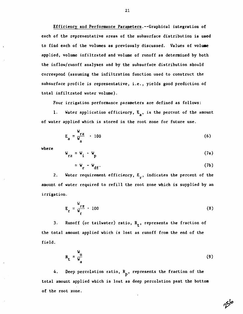
Efficiency and Performance Parameters.--Graphical integration of

each of the representative areas of the subsurface distribution is used

to find each of the volumes as previously discussed. Values of volume

applied, volume infiltrated and volume of runoff as determined by both

the inflow/runoff analyses and by the subsurface distribution should

correspond (assuming the infiltration function used to construct the

subsurface profile is representative, i.e., yields good prediction of

total infiltrated water volume).

Four irrigation performance parameters are defined as follows:

1. Water application efficiency, Ea, is the percent of the amount

of water applied which is stored in the root zone for future use.

where

2. Water requirement efficiency, Er, indicates the percent of the

amount of water required to refill the root zone which is supplied by an

irrigation.

3 . Runoff (or tailwater) ratio, Rt, represents the fraction of

the total amount applied which is lost as runoff from the end of the

field.

4. Deep percolation ratio, R represents the fraction of the P '

total amount applied which is lost as deep percolation past the bottom

of the root zone.

The sum of t h e deep p e r c o l a t i o n r a t i o , t h e runof f r a t i o and t h e

wate r a p p l i c a t i o n e f f i c i e n c y (expressed a s a f r a c t i o n ) i s u n i t y . Each

of t h e above volumes can be t r e a t e d a s average dep th s when d iv ided by

t h e p roduc t of furrow l e n g t h and i r r i g a t e d furrow spac ing .

EXAMPLE SYSTEM EVALUATION

The fo l l owing d i s c u s s i o n p r e s e n t s t h e r e s u l t s of an e v a l u a t i o n of a

furrowed i r r i g a t i o n system us ing t h e p rocedures j u s t d i s c u s s e d . A

des ign of t h i s f i e l d was fo rmula ted u s ing t h e SCS furrow i r r i g a t i o n

de s ign procedure (USDA, 1978 d r a f t ) . The r e s u l t s o f t h i s de s ign a r e

p r e sen t ed i n a s e p a r a t e a n a l y s i s o f t h e d e s i g n procedure ( . Thus,

it i s p o s s i b l e t o compare t h e c u r r e n t system o p e r a t i o n and performance

w i th t h e sugges ted d e s i g n o p e r a t i o n and performance. U l t i m a t e l y , t h i s

a l l ows f o r de t e rmina t i on of p o s s i b l e system r edes ign and management

changes such t h a t improved system performance r e s u l t s . Recommended

d e s i g n paramete rs a r e r epea t ed h e r e f o r t h e r e a d e r ' s convenience.

Q = 0.57 - 0.76 2ps / fu r row (9-12 gpm/furrow)

T1 = 720 min

i r r i g a t e d furrow spac ing = 1 .12 m (3 .67 f t )

d e s i g n dep th = 6 1 mm ( 2 . 4 i n . )

The c rop i r r i g a t e d was suga r b e e t s p l a n t e d on a 0 .56 m (1 .84 f t )

row spac ing . Pre- and p o s t i r r i g a t i o n s o i l wa t e r c o n t e n t samples were

c o l l e c t e d , however, a n a l y s i s has proven them t o h e i nadequa t e . A t any

r a t e , a n average e v a p o t r a n s p i r a t i o n r a t e f o r sugar b e e t s was determined

t o be n e a r 6 mmlday (0 .24 i n . / d a y ) i n t h e gene ra l a r e a . The e l a p s e d

t ime from t h e p rev ious i r r i g a t i o n (when t h e roo t zone was l a s t complete ly

f i l l e d ) t o t h e t ime of t h e i r r i g a t i o n being eva lua ted was 12 days. The

s o i l water d e f i c i t was thus es t imated t o be approximately 72 mm (2 .8 i n . ) .

The farmer was i r r i g a t i n g t h e furrows from a concre te - l ined head

d i t c h us ing 1 1/4- in . siphon tubes . Every o t h e r furrow was being

i r r i g a t e d s o t h e i r r i g a t e d furrow spacing was 1.12 m. The average

furrow grade i s 0.0098 m/m. The furrow l eng th i s 365 m. Inflow and

runoff measurements were taken a t t h e head of t h e furrow and a t

x = 350 m , r e spec t ive ly . S o i l s were found t o be uniform a r e a l l y ,

a l though t h e r e was some v a r i a t i o n i n t e x t u r e with depth .

F ive blocked furrow i n f i l t r a t i o n t e s t s were conducted t h e day

be fo re i r r i g a t i o n a t f i v e l o c a t i o n s along t h e l eng th of run. The d a t a ,

reduced t o t h e form of volume i n f i l t r a t e d p e r u n i t l e n g t h vs . t ime, a r e

p l o t t e d i n F igure 5 . The mean i n f i l t r a t e d volume p e r u n i t l eng th v s .

t ime was found and i s a l s o p l o t t e d i n F igure 5 . A l e a s t squares

r eg re s s ion procedure, o u t l i n e d i n Garcia (1978), was used t o determine

an empi r i ca l i n f i l t r a t i o n func t ion of t h e form of Eq. ( 3 ) f o r t h e mean:

z = 2369.4 t 0.37 + 70 t (11)

3 where z = cumulative volume i n f i l t r a t e d (cm / m ) ,

t = t ime (min).

This func t ion i s a l s o p l o t t e d i n F igure 5 .

Advance and r eces s ion d a t a and s u r f a c e e l e v a t i o n d a t a a r e p l o t t e d

i n F igure 6 . I n f i l t r a t i o n oppor tuni ty t imes a t s t a t i o n s along t h e

furrow a r e included. The time of advance t o t h e runoff measuring device

(x = 350 m) was 180 min. The p l o t of t h e su r f ace p r o f i l e s lope (Fig. 6 )

i n d i c a t e s t h e uni formi ty of s lope i s accep tab le .

Normally, t h e farmer ope ra t e s us ing a 12-hr inf low o r s e t time.

For t h i s p a r t i c u l a r i r r i g a t i o n , however, a power f a i l u r e caused pump

T i m e , minutes

Figure 5. Blocked furrow infiltration test data.

500 Recession A n h - - 0 n

w V V

* rr * L - -__ _ ___--_----------- ---- - - ---- - 1 I l n f i i t r o t i o n I Time of Cutoff

Time, I OPPOrfUnitY I

Oistonce along Furrow, m

Figure 6 . Advancelrecession curves, surface p r o f i l e s lope and i n f i l t r a t i o n opportunity times.

shutdown and iqterrupted the irrigation. The inflow time over which

measurements were taken was 7.5 hr. Inflow and runoff data for this

time duration are plotted in Figure 7. Graphical integration of the

area enclosed by each of these curves resulted in the following volumes:

Total volume applied, Wa = 22.86 m 3

Total runoff volume, WU = 6.68 m 3

Total infiltrated volume, Wi = W a - Wu

= 16.18 m 3

An average infiltrated depth can be found by dividing by the furrow

length and irrigated furrow spacing. In this case, a furrow length of

350 is used since this is the distance over which infiltration

occurred. The average infiltrated depth is:

Infiltration opportunity times (from Fig. 7) are used in Equation (11)

to plot the subsurface distribution (see Fig. 8). The ordinate in

Figure 8 is actually an average infiltration depth in cm which is

3 obtained by converting values obtained in Equation (11) from cm /m to

3 m /m, then by dividing by the irrigated furrow spacing (m) and muitiply-

ing by 100 to obtain cm. Graphical integration of the area enclosed by

this curve results in an estimate of total vol~ume infiltrated per unit

width as predicted by the blocked furrow infiltration function (Eq. 11).

This estimate is:

'i ' lpred. = 15.19 m3/m of width

where Wi ' )pred = estimated total volume infiltrated per unit width

Advance Time = 180 minutes Cutoff Time = 450 minutes

I0 -

I 500

Time, minutes

Figure 7 . Inflow and runoff hydrographs.

Distance along Furrow, m

Estimated Soil Water Def ic i t = 72 mm 1

---------------- -------- --I

Figu re 8. Subsur face d i s t r i b u t i o n of a p p l i e d wate r e s t ima t ed f rm 0.37 +

blocked furrow i n f i l t r a t i o n f u n c t i o n , z = 2369.4t 3

70 .0 t (2-cm /m, t -min).

Multiplying by the furrow spacing (1.12 m) yields an estimate of the

total volume infiltrated. Hence,

where WiIpred. 3 = estimate of total infiltrated volume (L ).

An estimate of the average infiltrated depth as predicted by the blocked

furrow infiltration function is:

Comparison of the prediction of total infiltrated volume as obtained

using the blocked furrow infiltration function with the value obtained

by inflow/runoff hydrograph analysis shows the following deviation:

. This deviation is acceptable, considering the accuracy with which data

can be collected in the field. Had the deviation been unacceptable

(i.e., greater than 10 - 15 percent), then adjustment of the multi-

plicative constants in the infiltration function would have been neces-

sary (by a volume baliince trial and error procedure or graphical proce-

dure, see example border irrigation evaluation by Ley and Clyma, 1980)

until the deviation was within an acceptable range.

Results.--Each of the volumes associated with performance

parameters can be determined with the results of the inflow/runoff

hydrograph analysis and the subsurface distribution plot. For this

case, the inflow/runoff hydrograph results are used. The volumes are as

follows :

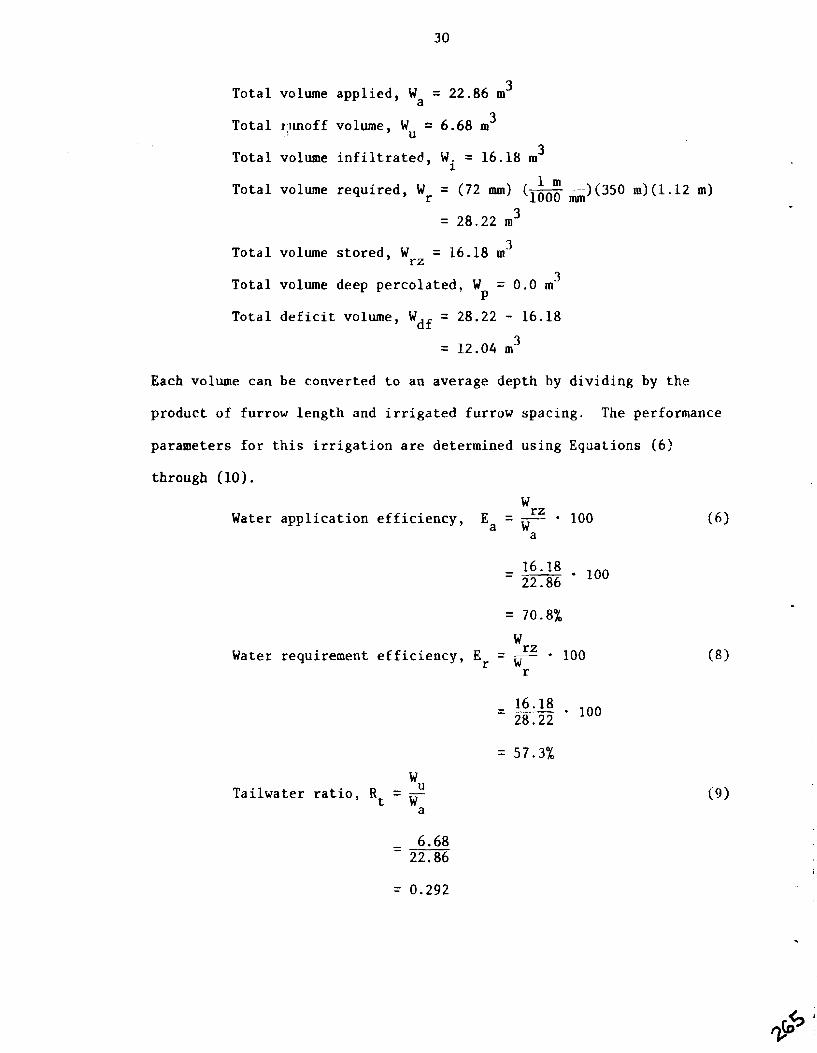
Tota l volume a p p l i e d , Wa = 22.86 m.'

T o t a l ~ : imof f volume, W = 6.68 m 3 U

T o t a l volume i n f i l t r a t e d , W = 16.18 m 3 i

1 m T o t a l volume r equ i r ed , Wr = (72 mm) (- - ) ( 3 5 0 ml(1.12 m) 1000 mm

= 28.22 m 3

T o t a l volume s t o r e d , W = 16.18 m3 r z

T o t a l volume deep p e r c o l a t e d , W = 0 .0 m 3

P T o t a l d e f i c i t volume, Wdf = 28.22 - 16.18

= 12.04 m 3

Each volume can be converted t o an average dep th by d i v i d i n g by t h e

produc t of furrow l e n g t h and i r r i g a t e d furrow spac ing . The performance

parameters f o r t h i s i r r i g a t i o n a r e determined u s ing Equat ions (6)

through (10).

- " r z Water a p p l i c a t i o n e f f i c i e n c y , E a - c 100

- W r z Water requirement e f f i c i e n c y , E r - q * 100

= 57.3%

Ta i lwa te r r a t i o ,

W Deep pe rco la t ion r a t i o , R = 2

'a

S ince t h e i r r i g a t i o n was i n t e r r u p t e d by a power f a i l u r e , it i s not

poss ib l e t o compare t h e design wi th t h e r e s u l t s of t h i s eva lua t ion .

However, it i s known t h a t t he farmer normally uses a 12-hr s e t t ime and

t h a t he makes no adjustment t o t h e furrow inflow r a t e once t h e siphon

tubes a r e s e t . Hence, r e f e r r i n g aga in t o F igure 7, it is p o s s i b l e t o

e s t ima te what t h e volumes f o r a 12-hr inf low time would have been. This

i s done by e x t r a p o l a t i n g both t h e inf low and runoff curves o u t t o 720

minutes a t a d ischarge r a t e equal t o t h e i r averages f o r t h e l a s t h a l f of

t h e 450 minute i r r i g a t i o n . Changes w i l l occur i n W a , WU, Wi, WrZ and

poss ib ly W . Estimates of what t h e volumes and performance parameters P

f o r t h e 12-hr s e t might have been a r e a s follows:

W = 36.40 m 3 a

Wu 13.32 m 3

Wi = 23.08 m 3

WrZ = 23.08 m 3

Table 1 provides a summary of the eva lua t ion and a comparison with

t h e design.

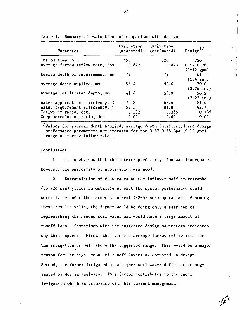
Table 1. Summary of evaluation and comparison with design.

Parameter Evaluation Evaluation

1 1 (measured) (estimatrd) Design-

Inflow time, min Average furrow inflow rate, Rps

Design depth or requirement, mm

Average depth applied, mm

Average infiltrated depth, mm

Water application efficiency, % Water requirement efficiency, % Tailwater ratio, dec. Deep percolation ratio, dec.

720 0.57-0.76 (9-12 gpmj

6 1 (2.4 in.)

70.0 (2.76 in.)

56.5 (2.22 in.)

81.4 92.7

0.186 0.00

L'~alues for average depth applied, average depth infiltrated and design performance parameters are averages for the 0.57-0.76 Rps (9-12 gpm) range of furrow inflow rates.

Conclusions

1. It is obvious that the interrrupted irrigation was inadequate.

However, the uniformity of application was good.

2. Extrapolation of flow rates on the inflow/runoff hydrographs

(to 720 min) yields an estimate of what the system performance would

normally be under the farmer's current (12-hr set) operation. Assuming

these results valid, the farmer would be doing only a fair job of

replenishing the needed soil water and would have a large amount of

runoff loss. Comparison with the suggested design parameters indicates

why this happens. First, the farmer's average furrow inflow rate for

the irrigation is well above the suggested range. This wou1.d be a major

reason for the high amount of runoff losses as compared to design.

Second, the farmer irrigated at a higher soil water deficit than sug-

gested by design analyses. This factor contributes to the under-

irrigation which is occurring with his current management.

3 . The initial design for this field was formulated for a design

depth of 72 mm (2.8 in.), the approximate operating soil water deficit

for the farmer. Only marginally acceptable levels of design performance

could be obtained for these design conditions. Iterations of the design

procedure for smaller design depths were carried out and a feasible

design determined for a design depth of 61 IMI (2.4 in.). The farmer

could significantly improve system performance by altering his system

management to apply a smaller amount (61 IMI) on a more frequent basis.

i.e., reducing the design depth from 72 IMI (2.8 in.) to 61 IMI (2.4 in.)

shortens the irrigation interval by 1 to 2 days.

Reconnuendations

1. The farmer should consider altering his system management to

the smaller design application depth as discussed. Given the range of

furrow inflow rates suggested from the design, 0.57 to 0.76 Ips (9 to 12

gpm), acceptable levels of system performance can be achieved.

2 . Further evaluations of the irrigation system are necessary.

If the farmer accepts the above design parameters then an evaluation of

the new design and management is desired. Also, seasonal changes in

factors and conditions which affect the system performance must be

evaluated so that an efficient operation can be implemented throughout

the season. The example presented has only illustrated the many factors

and conditions to be considered for one irrigation of the season.

COLLECTION AND ANALYSIS OF MORE DETAILED DATA

Data Collection

When it is desirable to obtain more detailed information on the

physical operating aspects of the irrigation system, the following

measurements should be made in sequence with the prpcedures described

previously.

Furrow Cross-section Data.--An estimate of the furrow cross-

sectional area can be obtained through the use of the device shown in

Figure 9. The furrow profilometer is placed in the furrow with the

sliding rods just resting on the furrow bottom. An identification I

- I marker of the location is placed next to the profilometer and a photo of

I

them is taken. This should be done in several (at least three) pre-

selected points along each of the furrows in which other measurements

are made (i.e., advance/recession, inflow/runoff, etc.). Furrow cross-

section data should be collected both before and after the irrigation;

it is suggested that these data be collected at the same time soil water

content samples are collected. Care and good judgement should be

exercised in the placement of the profilometer, making sure to place it

in a representative section of the furrow without disturbing the soil.

I I

Sliding Rods

Figure 9. Furrow profilometer.

Flow Depth and Top Width Data.--The flow depth and top width are 1

measured in each of the furrows in which inflow/runoff and advance/

recession data are taken. Measurements should be made at several points

along these furrows several times during the irrigation. These

measurements should be taken at approximately the same location each

time. When these data are collected, it is desirable to make the

measurements as often as possible during the advance, and may be spaced

out at 30 to 60-minute intervals during the rest of the irrigation.

Furrow Infiltration Data.--Another method for determining

infiltration during furrow irrigation is the inflow-outflow method

presented by Criddle, et al. (1956). Small flumes or other flow mea-

suring devices are placed in the furrow at some spacing, i.e., anywhere

from 25 m to 75 m. The inflow and outflow rates vs. time are recorded

for each section. Flow depth and top width measurements are also taken

in these sections. A volume balance procedure (discussed shortly) is

used to determine an infiltration relationship. When these data are

collected the measurements should be made in furrows other than those in

which advance and recession data are collected.

Data Analyses

Furrow Profiles and Surface Storage.--Once the furrow

cross-section photos are ready, the data is transcribed to the appro-

priate data form. These data can then be analyzed, and in general, an

empirical power relationship between center depth and cross-sectional

area found:

where 2 Af = furrow cross-sectional area (I ),

y = center depth (L),

AR, BR = empirical constants.

The constants AR and BR can be found using a least squares

technique. Usually a mean relationship for the entire furrow length is

determined as follows :

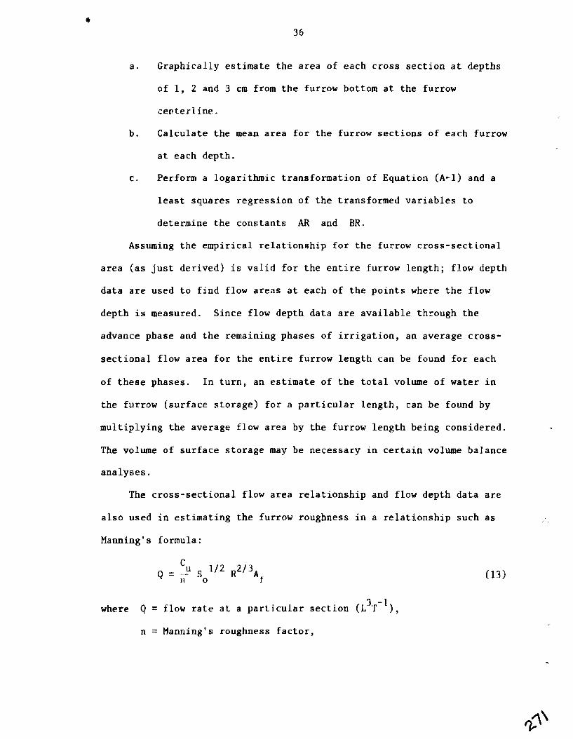
a. Graphically estimate the area of each cross section at depths

of 1, 2 and 3 cm from the furrow bottom at the furrow

centerline.

b. Calculate the mean area for the furrow sections of each furrow

at each depth.

c . Perform a logarithmic transformation of Equation (A-1) and a

least squares regression of the transformed variables to

determine the constants AR and BR.

Assuming the empirical relationship for the furrow cross-sectional

area (as just derived) is valid for the entire furrow length; flow depth

data are used to find flow areas at each of the points where the flow

depth is measured. Since flow depth data are available through the

advance phase and the remaining phases of irrigation, an average cross-

sectional flow area for the entire furrow length can be found for each

of these phases. In turn, an estimate of the total volume of water in

the furrow (surface storage) for a particular length, can be found by

multiplying the average flow area by the furrow length being considered.

The volume of surface storage may be necessary in certain volume balance

analyses.

The cross-sectional flow area relationship and flow depth data are

also used in estimating the furrow roughness in a relationship such as ,. ,

Manning's formula:

3. -1 where Q = flow rate at a particular sect.ion (L- ) ,

n = Manning's roughness factor,

So = bed slope (I, L-~),

R = hydraulic radius (L), 2 Af = cross-sectional flow area (L ),

CU = constant dependent on units (1.0 for metric, 1.486 for English).

For such an analysis steady uniform flow in a prismatic channel of

uniform slope is assumed. This allows usage of Manning's formula with

the energy gradient equal to the furrow bed slope. The condition of

steady uniform flow in furrow irrigation is approximated at the time

when the soil has reached its basic intake rate. Thus, flow depth data

only for about the last half of the irrigation should be used. The flow

rate at any particular section along a furrow is assumed to decrease

linearly from the inflow rate to the runoff rate when the soil is at its

basic intake rate. Hence, Equation (A-2) can be solved for Manning's n

since the other variables can be estimated (i.e., R and Af are found

from the furrow cross-section relation and flow depth data). Point

estimates of n will result, which are averaged to find the mean furrow

roughness.

Furrow Infiltration by Inflow-Outflow.--Griddle, et al. (1956)

present a complete method for analyzing data collected in the inflow-

outflow procedure. It involves a volume balance procedure using the

inflow-outflow rate measurements to determine the furrow infiltration

vs. time. Since flow depth data are available for the sections of

furrow being evaluated, the volume of surface storage for those sections

can be found as described previously. These estimates of surface

storage volume are time distributed as are the inflow rate and outflow

rate measurements. A volume balance as follows results in a time distri-

bution of the volume infiltrated.

where

3 VINF(t) = total volume infiltrated at time t, (L ),

VIN(t) = total volume of inflow to furrow section at time t,

VOUT(t) = total volume of outflow from furrow section at time

3 VSS(t) = volume of water in surface storage at time t, (L ) .

In general, a functional relationship for infiltration can be determined

for the data: volume infiltrated vs. time. More complete discussion of

the method is found in Criddle, et al. (1956).

EQUIPMENT LIST AND SUGGESTED DATA FORMS

Equipment

The following list of equipment necessary for the evaluation of

three furrows is suggested.

1. Six flow measurement devices (i-e., small cutthroat flumes

with 1-in. throats).

2. Engineer's level, field rod, chain or tape, orange flagging.

3. Wood stakes and lathe for station markers, crayon for marking

and hatchet for driving them into ground.

4. Soil sampling equipment:

a. soil auger or tube sampler

b. soil sample cans with tight fitting lids (up to 200,

2-in. diameter cans)

c . box for carrying cans

5. Small carpenter's levels for leveling flumes, etc.

6. Blocked furrow infiltration equipment (up to 10 sets, see

Figure 1) plus plastic sheeting.

7 . 50 small wire stakes with orange flagging.

8. Bulk density equipment.

9. Instruments for measuring time (stop watch, wrist watch with

second hand).

10. Buckets for hauling water.

11. Shovels, sledge hammers.

12. Soil uniformity box (partitioned box).

13. Pencils, clipboards and data forms.

For the more detailed measurements include:

14. Device for measuring flow depth and top width.

15. Furrow profilometer (see Figure Al).

16. Camera, film and identification marker.

17. Small flow measurement devices for furrow infiltration by

inflow-outflow method.

Data Forms

Data forms for the following data sets are provided:

Soil Water Content Data

Bulk Density Data

Blocked Furrow Infiltration Data

Water Advance/Recession Data

Flow Rate Data

Farm and Field Data

Flow Depth and Top Width Data

Furrow Cross-sectional Area Data

Furrow Infiltration Data (Inflow-Outflow Method).

Each form includes a special code for identification of the

evaluation site:

Ident (%, FA, FI, 1, Fu), where the data are identified by the letters in parenthesis.

%--Region

FA--Specific Farm

FI--Field Number on Farm

I--Irrigation Number (starting from the first irrigation at

that location)

FU--Furrow Number

Acknowledgements

Substantial support for the formulation of this paper was provided

by the Egypt Water Use and Management Project, Agency for International

Development Contract No. AID/NE-C-1351.

FLOW RATE DATA

IDENTIFICATION OBSERVER DATE CROP LENGTH INFLOW or RUNOFF

mTRROW/BORDER NO. FURROW SPACING/BORDER WIDTH

HEASURING DEVICE START TIHE STOP TIME

COMMENTS :

1 Elapsed Flow Average Volume Volume

Clock* Time AT Reading Rate Flow Rate ( ) ( Time bin) (mid ( 1 ( ( > (6) x (3) 1 (7)

( 1 ) (2 ) (3) ( 4 ) ( 5 ) (6) (7) (8)

*All clock times are on 24-hour basis.

FARM AND FIELD DATA

IDENTIFICATION 3BSERVER DATE -

FARliER ADDRESS -

(Sketch the farm and on-farm water delivery system noting pertinent roads, boundaries, field boundaries, locations of pumps, open drains, etc.)

FLOW DEPTH AND TOP WIDTH DATA

Ident (%,FA,FI,I,Fu) : Length: Observer: Date:

Crop :

Remarks :

Furrow Spacing (m):

d - Flow depth (cm) w - Top width of flow (cm)

S tar t End S tar t End S tar t End S t a r t End

S ta t ion d/w

Star t End S tar t End S t a r t End S tar t End Time

S ta t ion d/w

APPENDIX A RECONNAISSANCE QUESTIONNAIRE

1. Farmer o ~ e r a t i o n and mananement

How does t h e farmer dec ide when t o i r r i g a t e ? What i s h i s i r r i g a t i o n frequency? How does it change dur ing

t h e season? How does he dec ide how t o i r r i g a t e ? How does he dec ide how much water t o apply? Does t h e farmer know t h e t o t a l flow r a t e a v a i l a h l a t o him? What a r e t h e f a rmer ' s ope ra t ing hours? Does he i r r i g a t e a t n igh t? How does he dec ide how long t o i r r i g a t e a f i e l d ? How long does he i r r i g a t e a f i e l d ? Does t h e farmer have any problems wi th t h e system? What a r e h i s c u l t i v a t i o n and t i l l a g e p r a c t i c e s ? Does he i r r i g a t e every furrow o r a l t e r n a t e furrows? How many furrows does he i r r i g a t e i n one s e t ? How many s e t s does it t a k e t o i r r i g a t e t h e f i e l d ? Does he t r y t o compact t h e furrows equa l ly?

Water supply

What a r e t h e sources of a v a i l a b l e water? Is t h e d e l i v e r y s t a t i o n (po in t of d ive r s ion t o farm) a problem,

i . e . , high l o s s e s , e t c . ? Is t h e on-farm d i s t r i b u t i o n system a problem ( i . e . , t oo many

i n - f i e l d channels , high l o s s e s , e t c . ) ? What i s t h e flow r a t e of each source of water? When i s each source a v a i l a b l e and f o r how long? Is t h e frequency of del. ivery and a v a i l a b l e head a problem? What i s t h e water q u a l i t y ? How i s t h e water de l ive red t o each f i e l d ?

3. Crop c h a r a c t e r i s t i c s

What a r e t h e crops being grown? What a r e t h e r e spec t ive p l a n t i n g da te s? What cropping p a t t e r n s , i f any, have been followed? Does t h e farmer have any major problems i n crop production? What a r e t h e major inputs? P o t e n t i a l y i e l d ? What i s h i s expected y i e l d ? Average y i e l d i n a rea? Any obvious phys ica l symptoms of problems?

4. Phvs ica l c h a r a c t e r i s t i c s

Does t h e farmer know t h e f i e l d dimensions? Does he know t h e s lope and cross-slope ( i f any)? Has t h e f i e l d been leve led t o a uniform slope? I f yes , when? If no, why not? What p rov i s ions , i f any, a r e made f o r su r face runoff? Does runoff leave t h e farm o r i s it used again somewhere on t h e

farm? What i s t h e border spacing and how d i d t h e farmer decide on t h a t

spacing? What i s t h e furrow spacing? What i s t h e method of d i v e r t i n g water i n t o each furrow?

5. S o i l survev

Does t h e farmer know t h e s c i l s on h i s farm? Does h:? know of any t r o ~ b l e s p o t s ( i . e . , ve ry 1; gl t o r h. ivy s o i l s

o r s a l i n i t y problems)?

6. Water t a b l e

Does t h e farmer know t h e groundwater l e v e l ? Does he f e e l it i s a problem? Is su r f ace / subsu r f ace dra inage provided? I f s o , where?

BIBLIOGRAPHY

Black, C. A., D. D. Evans, J. L.. White, L. E. Ensminger, and F. E. Clark, editors. 1965. Methods of Soil Analysis, Part 1, tlonograph Series No. 9, American Society of Agronomy, Inc., Madison, Wisconsin.

Egypt Water Use and Management Project. 1979. Problem Identification Training Manual for On-Farm Irrigation Systems, Volume 11. Egypt Water Use and Management Project, Colorado State University, Fort Collins, Colorado.

Garcia, I. 1978. Soil-Water Engineering Laboratory Manual. Department of Agricultural and Chemical Engineering, Colorado State University, Fort Collins, Colorado.

Hagan, R. M., H. R. Haise, and T. W. Edminister, editors. 1967. Irrigation of Agricultural Lands. Monograph Series No. 11, American Society of Agronomy, Inc., Madison, Wisconsin.

Hart, W. E. 1961. Overhead Irrigation Pattern Parameters. Agricultural Engineering, 42(7):354-355.

Hart, W. E. 1975. Irrigation System Design. Department of Agricultural and Chemical Engineering, Colorado State University, Fort Collins, Colorado.

Hewlett, J. D. and J. E. Douglass. 1961. A Method for Calculating Error of Soil Moisture Volumes in Gravimetric Sampling. Forest Science 7(3):265-272.

Merriam, J. L. and J. Keller. 1978. Farm Irrigation System Evaluation: A Guide for Management. Agricultural and Irrigation Engineering Department, Utah State University, Logan, Utah.

Ley, T. and W. Clyma. 1979. Furrow Irrigation Design. Notes for AE535. Department of Agricultural and Chemical Engineering. Colorado State University, Fort Collins, Colorado.

Ley, T. and W. Clyma. 1979. Graded Border Irrigation Design. Notes for AE535. Department of Agricultural and Chemical Engineering, Colorado State University, Fort Collins, Colorado.

Reuss, J. O., S. A. Qureshi, and N. M. Chaudhry. 1975. Evaluation of Errors in Gravimetric Determination of Soil Water, Appendix 1. Annual Technical Report, Water Management Research Project, Colorado State University, Fort Collins, Colorado.

Staple, W. Y. and J. J. Lehane. 1962. Variability in Soil Moisture Sampling. Canadian Journal of Soil Science, Vol. 42, February, pp. 157-164.

USDA. 1974. Border Irrigaton. National Engineering Handbook, Section 15 , Chap. 4 , S o i l Conservation Service, U . S . Department of Agriculture.

USDA. 1978. Draft of Furrow Irr igat ion. National Engineering Handbook, Section 15, Chap. 5 , S o i l Conservation Service, U . S . Department of Agriculture.

S t a f f Paper #40

EVALUATION OF GRADED BORDER IRRTGATTON SYSTEMS

Thomas W , Ley and Wayne Clyma

INTRODUCTION

Data c o l l e c t i o n and a n a l y s i s procedures f o r eva lua t ing t h e

performance of graded border i r r i g a t i o n systems a r e presented . Informa-

t i o n i s co l l ec t ed on both t h e phys ica l and managerial aspec ts of opera-

t i o n a l systems. Basic da ta reduct ion procedures de f ine t h e s t a t e of t he

i r r i g a t i o n system. A l i s t of suggested equipment and da ta forms a r e

included.

REQUIRED DATA

Prel iminary Data

The eva lua t ion of any i r r i g a t i o n system necessa r i ly r equ i re s t h e

c o l l e c t i o n and a n a l y s i s of a l a r g e amount of da t a . Not the l e a s t of

which a r e b a s i c pre l iminary s i t e da ta which can be obtained through

interviews with the farmer and by performing s e v e r a l b a s i c phys ica l

measurements. Basic s i t e information must be known before the evalua-

t i o n of an i r r i g a t i o n occurs . I t i s a l s o d e s i r a b l e t o ob ta in a s much

information a s poss ib l e from t h e farmer concerning h i s opera t ion and

management of t h e i r r i g a t i o n system before an i r r i g a t i o n is evalua ted .

A l i s t of suggested ques t ions i s found i n Appendix A f o r each of t h e

fol lowing ca t egor i e s of information. The l i s t , i s by no means exhaus-

t i v e , and o f t e n t h e farmers answers t o some of t h e ques t ions w i l l l ead

t h e t r a ined person t o o the r more s i t e s p e c i f i c ques t ions .

''prepared under support of United S t a t e s Agency f o r I n t e r n a t i o n a l Development, Contracts AIDINE-C-1351 and AIDIDSAN-C-0058. A l l reported opinions, conclusions o r recommendations a r e those of t h e au thors and not those of t he funding agency of t he United S t a t e s Government.

Z l ~ e s e a r c h a s s o c i a t e and a s s o c i a t e p ro fes so r , r e spec t ive ly , Agr i cu l tu ra l and Chemical Engineering ~ e ~ a r t m e n t , Colorado ~ t a t e Univers i ty , F o r t C o l l i n s , Colorado.

1. Farmer - -- o p e r a t i o n - and - management.--Understanding - - why o r how a

fiirrr,er docs c e r t a i n t h i n g s i l l managir,g and o p e r a t i n g t h e i r r i g a t i o n

system i s v i t a l . Of ten t h i s a s p e c t of e v a l u a t i n g i r r i g a t i o n performance

may be over looked and incomplete knowledge of t h e i r r i g a t i o n system

s t a t e r e s u l t s . Farmer management may be c o n s t r a i n i n g t h e l e v e l of

performance which can be a t t a i n e d . The g e n e r a l l e v e l o f knowledge of

t h e fa rmer concern ing i r r i g a t i o n p r i n c i p l e s and p r a c t i c e s i s e v a l u a t e d .

Other i n fo rma t ion d i s c u s s e d l a t e r w i l l a i d i n de t e rmin ing i f system

management can be improved.

2. Water supply . --The farmer w i ' l l know t h e a v a i l a b l e wate r

supp ly , s o u r c e , d e l i v e r y , f requency , e t c . He may have o n l y a g e n e r a l

knowledge of t h e flow r a t e and q u a l i t y . These should be measured d u r i n g

t h e course of an e v a l u a t i o n . On-farm conveyance l o s s e s may be a b i g

problem. The farmer may o r may n o t know. Measure t h e l o s s e s i f

nece s sa ry .

3 . Crop c h a r a c t e r i s t i c s . - - T h e c rops grown a n d - t h e p l a n t i n g d a t e s

of each must be known. Ava i l ab l e d a t a i n t h e l i t e r a t u r e a r e needed on

crop s ea sona l wate r requ i rements , r a t e s and s t a g e s of growth, maximum

p o t e n t i a l r o o t i n g d e p t h s , t ime from p l a n t i n g t o e f f e c t i v e cove r , e t c .

Th is i n fo rma t ion a long w i th c l i m a t i c d a t a i s used t o e s t i m a t e c rqp wate r

use th rough t h e i r r i g a t i o n s ea son . The c rop r o o t zone should be measured

a t each i r r i g a t i o n f o r c rops w i th expanding r o o t systems. The measured

r o o t zone f o r a p e r e n n i a l c rop ( such a s a l f a l f a ) can o f t e n be assumed

v a l i d f o r t h e e n t i r e season u n l e s s a f l u c t u a t i n g wate r t a b l e i s encount-

e r e d . The c rop r o o t zone a t each i r r i g a t i o n de te rmines t h e a v a i l a b l e

s o i l wz te r r e s e r v o i r a t t h a t t ime and is nece s sa ry t o de te rmine t h e s o i l 3

wate r d e f i c i e n c y , t h e s t r e s s a t t h e t ime of i r r i g a t i o n and performance

paramete rs such a s wa t e r a p p l i c a t i o n and wa t e r requirement e f f i c i e n c i e s .

4 . Physical characteristics.--Measure and record the field

dimensions. Stakes should be driven into the ground at 25-• intervals

along the length (adjust for size of field as necessary). Measure and

record surface elevations at each stake (station) using a field rod and

level. Plot the surface profile (elevation vs. length). Measure and

record the cross-slope and border spacing at each station. Determine if

a ponded or free outflow boundary condition exists at the downstream

end. Determine where and how to measure border inflow and runoff.

5. Soil survey.--If available, obtain information on soils in the

area (on the farm), such as maps and classifications from a local or

regional off ice (e.g. , USDA Soil Conservation Service or similar govern-

ment agency). Such information is very useful and aids the design of

data collection procedures. Soil types and textures are known and maps

usually depict the variation of surface textures in a field. If this

information is not available a soil survey is necessary to determine the

soil types and uniformity in the field being studied. Soil samples

should be collected in a minimum of ten locations in the field (i.e., at

five locations along the length and two along the width). Samples

should be taken from a minimum of four depths within the expected root

zone, i.e., every 30 cm in an expected 1.2 m root zone (adjust as

necessary). These samples should be analyzed to determine soil types.

Once soil types and variations through the field are known the

apparent specific gravity of the soil (bulk density), the field capacity

and wilting point of the soil must be determined. Garcia (1978) pre-

sents procedures for these measurements. Depending on the results of

the soil survey the sample collection procedure is defined. For a field

with uniform soils it is necessary to collect data on the above soil

p r o p e r t i e s i n a minimum of t h r e e l o c a t i o n s i n t h e f i e l d t o o b t a i n a good

average . I t i s n e c e s s a r y t o sample w i t h d e p t h . For a f i e l d w i t h non-

uniform s o i l s t h e above s o i l p r o p e r t i e s must be determined f o r each

major s o i l t y p e . A minimum of t h r e e r e p l i c a t i o n s o f samples i s

n e c e s s a r y t o o b t a i n an average . Sampling w i t h dep th i s r e q u i r e d . See

Appendix B f o r f u r t h e r d i s c u s s i o n .

Accura te d e f i n i t i o n of t h e above s o i l p r o p e r t i e s i s n e c e s s a r y . The

time and e f f o r t n e c e s s a r y t o a c h i e v e a c c u r a t e d a t a w i l l e l i m i n a t e having

t o r e p e a t any sampling. These d a t a a r e most e a s i l y c o l l e c t e d b e f o r e t h e

c r o p i s p l a n t e d . Some change of a p p a r e n t s p e c i f i c g r a v i t y of t h e plow

l a y e r w i t h t ime may be expec ted . Sampling p l a n s f o r s o i l wa te r c o n t e n t

and i n f i l t r a t i o n tests w i l l be f u n c t i o n s of s o i l t y p e and u n i f o r m i t y .

The r e s u l t s of t h e s o i l su rvey shou ld t h u s be a v a i l a b l e i n advance of

t h e i n i t i a l i r r i g a t i o n e v a l u a t i o n .

I f s o i l s a l i n i t y / a l k a l i n i t y i s expec ted t o be a problem ( i n d i c a t e d

by maps, p r e v i o u s s u r v e y s , i n f o r m a t i o n from t h e f a r m e r s ) , samples shou ld

be ana lyzed t o de te rmine t h e s a l i n i t y f a l k a l i n i t y . Such a problem may

a l s o i n d i c a t e t h e p r e s e n c e of a h i g h w a t e r t a b l e .

6 . Water t a b l e . - - T h e farmer shou ld have g e n e r a l knowledge of

wa te r t a b l e c o n d i t i o n s i n t h e a r e a . S o i l su rvey r e s u l t s may i n d i c a t e a

h igh wate r t a b l e . I f t h e wa te r t a b l e i s h i g h o r expec led t o f l u c t u a t e

c o n s i d e r a b l y ( i . e . , w i t h i n t h e maximum p o t e n t i a l r o o t z o n e ) , it i s

d e s i r a b l e t o w o n i t o r t h e ground wate r l e v e l through t h e i r r i g a t i o n

season . T h i s can b e done w i t h a s e r i e s o r g r i d of o b s e r v a t i o n w e l l s

,EWl.JP, Vol. XI, 1979).

A h i g h wate r t a b l e can l i m i t c r o p growth th rough wate r - logg ing .

The groundwater q u a l i t y can a l s o s e r i o u s l y a f f e c t c r o p growth and should

be measured.

Crop water use from t h e c a p i l l a r y f r i n g e o r t h e water t a b l e i s

p o s s i b l e . Es t imates of crop consumptive use by e v a p o t r a n s p i r a t i o n

modeling techniques w i l l no t correspond wi th measured s o i l water

d e f i c i t s (by s o i l water con ten t sampling) when t h e crop i s us ing ground-

water , assuming each method i s y i e l d i n g a c c u r a t e r e s u l t s . This i s

s i g n i f i c a n t i f t h e water t a b l e rises du r ing t h e season due t o e a r l y

o v e r i r r i g a t i o n . Water t a b l e f l u c t u a t i o n s due t o o v e r i r r i g a t i o n may a l s o

c o n t r i b u t e t o crop consumptive use and can a f f e c t r o o t zone expansion.

On t h e Day be fo re I r r i g a t i o n

P r e i r r i g a t i o n S o i l Water Content Data.--Garcia (1978) p r e s e n t s

procedures f o r t h e c o l l e c t i o n and a n a l y s i s of s o i l samples f o r d e t e r -

mining water con ten t by t h e g rav ime t r i c method. Depending on t h e r e -

s u l t s of t h e s o i l survey (which should be a v a i l a b l e by t h i s p o i n t i n

t ime) , t h e sampling p l a n i s devised . I f t h e s o i l survey r e s u l t s show

t h e s o i l s t o be uniform, a minimum of t h r e e l o c a t i o n s i n d i f f e r e n t p a r t s

of t h e f i e l d a r e s e l e c t e d f o r sampling t o o b t a i n an average f o r t h e

f i e l d . However, i f c e r t a i n v a r i a t i o n s a r e expected (non-uniform water

a p p l i c a t i o n s , e t c . ) o r i f s o i l s a r e non-uniform a minimum of t h r e e

r e p l i c a t i o n s of samples should be c o l l e c t e d where t h e non-uni formi t ies

a r e o r where v a r i a t i o n s a r e expected. For i n s t a n c e , non-uniform water

a p p l i c a t i o n s a long t h e l e n g t h of run i s common and c o l l e c t i o n of a

minimum of t h r e e r e p l i c a t i o n s of samples a t a minimum of t h r e e r ep re -

s e n t a t i v e l o c a t i o n s along t h e l eng th i s suggested. See Appendix B f o r

f u r t h e r d i s c u s s i o n on sampling and how o f t e n t o sample.

I n a l l c a se s , samples should be c o l l e c t e d from each of s e v e r a l

l a y e r s o f t h e measured o r expected maximum r o o t i n g depth of t h e crop

( i . e . , f o r a 1 . 2 m r o o t zone, sample each 30-cm l a y e r , and i n t h e t o p

3-ccm l a y e r c o l l e c t samples from e a c q l 5 - c m increment ) , I f t h e w a t . r

t a b l e is h ighe r t han t h e expected maximum r o o t i n g d e p t h , samples should

be c o l l e c t e d t o t h e wate r t a b l e . Each i n d i v i d u a l sample should be 150

grams o r more.

Other p r e p a r a t i o n s f o r t h e e v a l u a t i o n should be made on t h e day

be fo r e i r r i g a t i o n such a s i n s t a l l a t i o n of f low measuring dev i ce s and

c y l i n d e r i n f i l t r a m e t e r s . Contact t h e farmer and f i n d o u t t h e t ime he

e x p e c t s t o s t a r t i r r i g a t i n g . P lan t o a r r i v e i n s u f f i c i e n t t ime t o

complete a l l p r e p a r a t i o n s f o r t h e e v a l u a t i o n ( s ) such a s p r e p a r a t i o n o f

d a t a forms and assignment of d u t i e s .

On t h e Day of I r r i g a t i o n

I n f i l t r a t i o n Data.--For uniform s o i l s a t l e a s t t h r e e and p r e f e r a b l y

a t o t a l of s i x c y l i n d e r i n f i l t r a t i o n t e s t s should be conducted i n t h r e e

l o c a t i o n s a long t h e l e n g t h . For non-uniform s o i l s t h r e e r e p l i c a t i o n s of

t e s t s should be made i n each a r e a where a d i f f e r e n t s o i l t e x t u r e e x i s t s .

I f non-uniformity i n d i s t r i b u t i o n a long t h e l e n g t h of run i s a n t i c i -

p a t e d , t h e n t h r e e r e p l i c a t i o n s f o r each r e p r e s e n t a t i v e l e n g t h of t h e

f i e l d i s nece s sa ry t o d e l i n e a t e t h e s e d i f f e r e n c e s . During t h e season

d i f f e r e n c e s i n s o i l water con t en t w i l l a c cen tua t e t h e d i f f e r e n c e s i n

i n f i l t r a t i o n and t h e d i s t r i b u t i o n of wate r . See Appendix B f o r f ~ l r t h e r

d i s c u s s i o n of c o n s i d e r a t i o n s of where t o sample and how o f t e n .

The i n f j - l t r o m e t e r measurements should be s t a r t e d a s t h e wate r

a r r i v e s a t each i n f i l t r o m e t e r and t h e ponded dep th main ta ined t h e same

a s t h e dep th of f low of t h e i r r i g a t i o n wa t e r . I f t h e t e s t s cannot be

conducted du r ing i r r i g a t i o n , they should be conducted on t h e day be fo r e

i r r i g a t i o n and a b u f f e r r i n g should be used . Garcia (1975) p r e sen t ed

procedures f o r i n s t a l l i n g t h e i n f i l t r o m e t e r s and conduc t ing t h e t e s t s .

Inflow/Runoff Data.--Flow measurement devices t o determine inf low

t o and runoff from t h e border should be p rope r ly i n s t a l l e d be fo re t h e

1 / i r r i g a t i o n . The c lock time- a t which water is f i r s t introduced t o t h e

border should be recorded. A measurement of t h e i n i t i a l inf low r a t e

should be taken . P e r i o d i c a l l y dur ing t h e i r r i g a t i o n , r e c o r d t h e inf low

r a t e and clock time of t h e obse rva t ion . When t h e water reaches t h e

runoff measurement device begin making runoff r a t e v s . t ime measure-

ments. A suggested p a t t e r n f o r t ak ing runoff da t a from t h e t ime runoff

s t a r t s i s t o t a k e a read ing a t 30 sec/min, 2 min, 4 min, 8 min, 15 min,

30 min, and then every 112 hour. Record t h e clock time when water

e n t e r i n g t h e border is te rmina ted .

Advance/Recession Data.--The r a t e of wa te r f ron t advance should be

observed and recorded. When t h e moving s t ream f r o n t i s i r r e g u l a r ,

record t h e t ime when an "average" f r o n t reaches each s t a t i o n ( s ee F i g .

1 ) . A f t e r t h e inf low i s te rmina ted , record t h e r a t e of r eces s ion .

I d e a l l y , t h i s would be t h e t ime when water d i s appea r s from each s t a t i o n .

I t i s d i f f i c u l t t o determine t h e l o c a t i o n of t h e receding water edge.

When water has disappeared from 50 pe rcen t of t h e g r i d s u r f a c e a r e a

represen ted by each s t a t i o n , r eces s ion i s assumed t o have occurred a t

t h a t s t a t i o n . Consis tency i s of primary importance i n t ak ing r eces s ion

d a t a .

A f t e r I r r i g a t i o n

P o s t i r r i g a t i o n s o i l water con ten t samples should be c o l l e c t e d

anywhere from 1-112 days t o 3 days a f t e r i r r i g a t i o n . This depends on

t h e s o i l type and t h e t ime r equ i r ed f o r t h e s o i l t o d r a i n t o f i e l d

i / ~ l o c k t imes should be on a 24-hour b a s i s ( m i l i t a r y t ime) .

Figure 1. Illustration of irregular waterfront advance and location of 1 f average" waterfront .

capac i ty . Garcia (1978) p re sen t s a f i e l d procedure f o r e s t ima t ing when

( a f t e r wet t ing) a s o i l has dra ined t o f i e l d capaci ty . The same

c o l l e c t i o n procedures a s previous ly discussed apply.

Discussion and Recommendations

To ensure cooperat ion of t h e farmer during t h e eva lua t ion , desc r ibe

exac t ly what w i l l be done. Minimize crop damage and s o i l d i s turbance .

Be s u r e the farmer w i l l opera te h i s system a s he usua l ly does. Avoid

remarks which may in f luence h i s management dec i s ions . The purpose of

t h e eva lua t ion i s t o determine t h e system performance and eva lua te t h e

system opera t ion a s t h e farmer c u r r e n t l y manages i t .

I t i s important t h a t pre l iminary da ta c o l l e c t e d e a r l y i n t h e season

be good d a t a . A c a r e f u l , coordinated, determined e f f o r t here w i l l save

much time and e l imina te problems and headaches l a t e r i n t h e season. For

in s t ance , t he s o i l water content of a f i e l d before t h e i n i t i a l i r r i g a -

t i o n of t h e season may gene ra l ly be assumed a s uniform. Much e f f o r t i n

c a r e f u l s o i l sampling and i n c o l l e c t i o n of more samples ( t o inc rease t h e

p r e c i s i o n with which t h e mean s o i l water content is es t imated) is recom-

mended. The es tab l i shment of t h i s i n i t i a l condi t ion serves an important

purpose. I t i s t he s t a r t i n g po in t f o r a roo t zone s o i l water budget.

From t h i s i n i t i a l condi t ion , water added t o t h e roo t zone of t h e

crop by p r e c i p i t a t i o n (measured by r a i n gages s e t up i n seve ra l loca-

t i o n s a t t h e s i t e ) , and by i r r i g a t i o n (measured by i r r i g a t i o n evalua-

t i o n s ) is known. Crop use i s est imated us ing c l imate da ta and crop

s t age and growth d a t a i n an accura t e , c a l i b r a t e d evapo t ransp i r a t ion

model. A roo t zone s o i l water budget can thus be ca l cu la t ed through t h e

season. S o i l water content da t a c o l l e c t e d a t succeeding i r r i g a t i o n s of

t h e season a r e used a s a check on t h e p red ic t ed s o i l water s t a t u s when

c a l i b r a t i o n of t h e ET model i s necessary.

If t h e r e is a h,gh water t a b l e i i ~ t h e are;, crop use frcnl t h e v

c a p i l l a r y f r i n g e o r t h e water t a b l e i t s e l f can be e s t ima ted . The

d i f f e r e n c e between t h e c a l c u l a t e d c rop use and t h e measured s o i l water

d e f i c i t (by sampling) dur ing an i r r i g a t i o n i n t e r v a l i s an e s t i m a t e of

t h e crop use from t h e water t a b l e dur ing t h a t i n t e r v a l . I f t h e r e i s no

reason t o b e l i e v e t h a t t h e c rop i s u s ing water from a water t a b l e , then

t h e computed d i f f e r e n c e i n d i c a t e s t h e accuracy of each method and pos-,

s i b l y needed a c t i o n t o improve sampling o r p r e d i c t i v e techniques .

I n some i n s t a n c e s , c o l l e c t i o n of advance/recession d a t a may not be

necessary a t each i r r i g a t i o n . For i n s t a n c e , a uniform a p p l i c a t i o n of

water may be expected on a f i e l d wi th s h o r t e r l eng ths of run on a

heavier s o i l . I n t h i s ca se , t h e d i s t r i b u t i o n i s assumed uniform and a l l

t h a t i s requi red i s t h e water on and water o f f t o determine t h e water

added t o t h e s o i l . While t h i s case may occur , it i s adv i sab l e t o co l -

l e c t advance and r eces s ion d a t a when any non-uniformity of water a p ~ l i -

c a t i o n i s sus2ected due t o poor i r r i g a t i o n p r a c t i c e s , non-uniform s o i l s ,

non-uniform f i e l d s l o p e s , e t c . i n order t o know t h e d i s t r i . b u t i o n of

app l i ed water .

During t h e course of an a c t u a l i r r i g a t i o n e v a l u a t i o n , it i s

recommended t h a t a p a r t i a l eva lua t ion of t h e d a t a being c o l l e c t e d be

conducted. This i s accomplished b e s t by p roces s ing t h e da t a a s it i s

c o l l e c t e d i n t h e f i e l d and i n t e r p r e t i n g t h e r e s u l t s . For i n s t ance , it

is easy t o e v a l u a t e inf low and runoff d a t a . An obvious e r r o r i s d e t e r -

mined i f t h e runoff i s g r e a t e r than t h e in f low. This check on da ta

provides t h e i n v e s t i g a t o r a neans of e l i m i n a t i n g wasted t ime and e f f o r t

i n t h e c o l l e c t i o n of erroneous d a t a .

FIELD DATA ANALYSIS

F i e l d d a t a a n a l y s i s provides a b a s i s f o r understanding t h e per -

formance of t h e i r r i g a t i o n system and how t h e system i s being operated.

The d a t a may be analyzed through a number of procedures. Those

presented here r ep resen t t h e minimum of ana lyses requi red t o formulate

an understanding of t h e system's performance r e s u l t i n g from a p a r t i c u l a r

management scheme.

S o i l Water

The s o i l water content may be es t imated by two methods: 1 ) gravi -

met r ic method, and 2) f e e l method. The s o i l water content expressed a s

a depth of water pe r u n i t depth of r o o t zone can be es t imated using t h e

r e s u l t s of t h e gravimetr ic s o i l water ana lyses i n t h e fol lowing

equat ion :

where d = t h e s o i l water content expressed a s a depth (L) f o r t h e m

e n t i r e depth inves t iga t ed ,

'w, i = dry weight s o i l water content f o r t h e i t h l a y e r of t h e

roo t zone (MM-') , -3 -1

Yb, i = s o i l bu lk d e n s i t y i n t h e i t h l a y e r [(M-~)(M'L ) 1,

Y i = th ickness of t h e i t h s o i l l a y e r (L),

n = number of l a y e r s i n t h e roo t zone which were sampled.

The p r e - i r r i g a t i o n s o i l water content da ta a r e checked wi th t h e

s o i l f i e l d capac i ty t o e s t ima te t h e s o i l water d e f i c i t [ ava i l ab le roo t

zone s to rage ) a t t h e time of i r r i g a t i o n . A s p revious ly d iscussed , crop

water use and roo t zone s o i l water budgeting a l s o provides a check on

t h e s o i l water d e f i c i t a t i r r i g a t i o n time. The pre- and p o s t - i r r i g a t i o n

s o i l wa te r da ta can a l s o be u s e f u l i n ana lyz ing dep ths i n f i l t r a t e d and

adequacy o f - i r r i g a t i o n a long he border assuming t h e r e i s na deep :& b P C

p e r c o l a t i o n of wate r belew tlie lowes t dep ths inves t iga ted< , -

The f e e l method f o r e s t i m a t i n g s o i l wa te r c o n t e n t i s l a r g e l y

s u b j e c t i v e s i n c e it i s dependent upon v i s u a l i n s p e c t i o n o f c e r t a i n

c h a r a c t e r i s t i c s of t h e s o i l sample. The method should be used o n l y when

t h e i n v e s t i g a t o r h,ts a l a r g e amount of exper ience and even t hen on ly f c r

a rough e s t i m a t e of s o i l wa te r c o n t e n t . Tab le 1 d e s c r i b e s t h e r c l a -

t i o n s h i p between s o i l p h y s i c a l appearance and s o i l wa te r c o n t e n t f o r

va ry ing s o i l types .

Advance and Recession

The advance and r e c e s s i o n d a t a a r e p l o t t e d on c o o r d i n a t e paper a s

shown i n F igu re 2 . The advance curve i s a p l o t of t h e t ime t h e wate r -

f r o n t advances a long t h e bo rde r v s . t h e l e n g t h o f t h e bo rde r . The

r e c e s s i o n curve i s a p l o t of t h e t ime t h e w a t e r f r o n t recedes from t h e

s u r f a c e v s . t h e bo rde r l e n g t h . The i n t a k e opportuni. ty t ime is t h e

d i f f e r e n c e between t h e advance and r e c e s s i o n t ime a s shown i n F i g u r e 2 .

I n t a k e o p p o r t u n i t y t imes r e p r e s e n t t h e amount of t ime wate r has t h e

oppo r tun i t y t o i n f i l t r a t e a t p o i n t s a long t h e bo rde r . Su r f ace e l e v a t i o n

d a t a a r e o f t e n p l o t t e d on t h e same graph a s an a i d i n e x p l a i n i n g va r i a - ,

t i o n s i n advance and r e c e s s i o n r a t e s , and r e s u l t a n t ~ f f e c t s on i .nFil-

t r a t i o n appo r tun i t y t ime .

I n f i l t r a t i o n R e l a t i o n s h i p

The d a t a from c y l i n d e r i n f i l t r a t i o n rests a r e reduced "o t h e form

of cumulative dep th of i n f i l t r a t i o n v s . t ime . The reduced d a t a a r e t hen

p l o t t e d on log- log paper (Garc ia , 1978). I n g e n e r a l , t h e d a t a p l o t a s

s t r a i g h t l i n e s , b u t may s l i g h t l y curve and o f t e n w i l l "dogleg." Some

Distance Down Field ( x )

4

Figure 2 . Typical advance and recession curves for border irr igat ion.

Intake Opportunity Time

C

C u

t .- C ---------------- Time of Cutoff - - - -_________

Tab le . 1 . S o i l mo i s tu r e d e f i c i e n c y and appearance r e l a t i o n s h i p c h a r t ( a f r e r Merriam and K e l l e r , 1978;. (This c h a r t i n d i c a t e s approximate r e l a t i o n s h i p o f s o i l m o i s t u r e d e f i c i e n c y between f i e l d c ~ 2 a c i t y and w i l t i n g p o i n t . For more a c c u r a t e i n fo rma t ion t h e s o i l must be checked by d r y i n g samples . )

Mois tu re -

Def i c i encv Coarse S o i l Texu t r e C l a s s i f i c a t i o n

Sandv Medium Woisture

F ine Def ic iencv ( i n . / f t i (loamy sand) (sandy loam) (loam) ( c l a y loam) ( i n . / f t ) '

0 .0 Leaves wet o u t l i n e on hand when squeezed

0 .2 A p p e a ~ s mo i s t makes s weak

0 . 4 b a l l

Appear s l i g h t l y 0 . 6 mo i s t s t i c k s

t o g e t h e r

9.8 C;;; lo:;;.-, f lows t h r u f i n g e r s . ( w i l t i n g p c i n t )

1 . 0

Appears v e r y d a r k , l e aves wet o u t l i n e on hand, makes a s h o r t r i bbon

Qui te d a r k c o l o r , makes a hard b a l l

F a i r l y dark c o l o r , makes a good b a l l

S l i g h t l y d a r k c o l o r , makes a weak b a l l

Appears v e r y d a r k , l e a v e s wet o u t l i n e on h a n d , w i l l r i b - bon o u t about one i n c h

Dark c o l o r , forms a p l s t i c b a l l , s l i c k s when rubbed

Q u i t e d a r k , forms a hard b a l l

F a i r l y d a r k , forms a good b a l l

Appears very d a r k , G . 0 l e a v e s s l i g h t mois- t u r e , on hand when squeezzd, w i l l r i b - 0 .2 Son o a t about two i nches

: 0.4 Uark c o l o r , w i l l s l i c k and r ibbons e a s i l y C.6

Qui te da rk , w i i l a.8 make t h i c k r i bbon , may s l i c k when rublred 1 .0

L i g h t l y co lo r ed F a i r l y da rk , makes by mo i s tu r e , w i l l S l i g h t l y d a r k , a good b a l l 1 . 2 n o t b a l l forms weak b a l l

Very s l i g h t c o l o r W i l l b a l l , sma l l due t o mo i s tu r e L i g h t l y c o l o r e d , c l ods w i l l f l a t t e n ( w i l t i n g p o i n t ) sma l l c l o d s crum- o u t r a t h e r t han

b l e f a i r l y e a s i l y crumble

S l i g h t c o l o r due Scme darkness due t o m o i s t u r e , sma l l t o unava i l a b l e ! . 3 c l o d s a r e hard mo i s tu r e , c l ods a r e ( w i l t i n g p o i n t ) ha rd , cracked

{ w i i i i n g p o i n t ) 2.0 ~ . -..~ . .~ - . . - .. . .. . . - - . .- . - - -. -~ .~~ .

. - ' r . . . - .. .- - - - - -.

Fielri ?!ethod 9f p ~ r o x i r n a t i , ; g Sol l ~ ~ o i s c s r e ! Eeetrriency,; !or i r r i g a t i c n ; Traiis.:ctions o i t h e ?meric;rn. G r i e t y ,..2iz, ? u l g t e c h n i c . - .are o f Agr ic . l l tu ra1 . Eng inee r s : '.lol. 3 : No. 1: i960; ;ohn L . :!eri.i.?rn, P r o f e s s o r , C . 3 i i C - . - : -

U n i v e r s i t y , 1 9 1.5, San Luis Gbispo, C a l i f s r c i a .

BEST AVAILABLE COPY

curves s teepen a f t e r a few minutes e i t h e r because of r e l e a s e of t rapped

a i r (u sua l ly i n sand ie r s o i l s ) o r because t h e cy l inde r s were not d r iven

deeply enough. S o i l s which have cracks , i n t o which water d isappears

quickly , o f t e n e x h i b i t curves which a r e i n i t i a l l y s t e e p and then

f l a t t e n . Plow pans may cause a s i m i l a r , bu t u s u a l l y delayed e f f e c t .

The average i n f i l t r a t e d depth v s . t ime should be computed us ing t h e d a t a

from each a rea where s o i l p r o p e r t i e s were found t o be uniform (Herriam

and K e l l e r , 1978). The average i n f i l t r a t e d depth vs . time should then

a l s o be p l o t t e d on t h e same log-log graph a s t h e ind iv idua l da t a s e t s

f o r t hese a reas . A l e a s t squares r eg res s ion technique ( see Garcia ,

1978) i s o f t e n used t o f i n d an i n f i l t r a t i o n funct ion of t h e fol lowing

form f o r t h e average i n f i l t r a t e d depth vs . t ime:

z = kta

where z = cumulative depth i n f i l t r a t e d ( L ) ,

t = time (T)

k , a = empir ica l cons tants .

This type of i n f i l t r a t i o n func t ion i s usua l ly considered r e p r e s e n t a t i v e

i n border i r r i g a t i o n . In most cases , t h e i n f i l t r a t i o n r e l a t i o n s h i p

r e s u l t i n g from r i n g i n f i l t r a t i o n t e s t s i s inadequate i n p r e d i c t i n g t h e

a c t u a l i n f i l t r a t i o n which occurs dur ing t h e i r r i g a t i o n . The a c t u a l

average i n f i l t r a t e d depth can be found using inf low and runoff da ta

(discussed l a t e r ) f o r t h e i r r i g a t i o n . The fol lowing procedure i s used

t o f i n d t h e p red ic t ed average i n f i l t r a t e d depth ( a s predic ted by t h e

i n f i l t r a t i o n r e l a t i o n s h i p ) .

1. Using in t ake oppor tuni ty times (from advance/recession d a t a )

f o r s t a t i o n s along t h e border and t h e i n f i l t r a t i o n r e l a t i o n -

s h i p , f i nd t h e p red ic t ed i n f i l t r a t e d depth a t each s t a t i o n .

2 - Det.ermine t h e average i n f i l t r a t e d d e p t h f o r e a c h reach ( d i s -

t a n c e between s t a t i o n s ) by a v e r a g i n g t h e p r e d i c t e d i n f i l t r a t e d

d e p t h s o f s u c c e s s i v e s t t i o n s . 4 I 7

3 . Determine t h e p red icLec average i n f i l t r a t e d d e p t h f o r t h e

e n t i r e border by summing t h e reach averages (found i n 2 ) alld

d i v i d i n g by t h e number of r e a c h e s . Keep i n mind t h a t t h i s

v a l u e i s an e s t i m a t t d o r p r e d i c t e d v a l u e r e s u l t i n g from t h b

use of t l e e m p i r i c a l i n f i l t r a t i o n f u n c t i o n .

In f low and Runoff

In f low and runoff d a t a p r o v i d e a s imple means of de te rmin ing the

a c t u a l average i n f i l t r a t e d dep th . The i n f l o w and runof f hydrographs a re

c o n s t r u c t e d on t h e same r e c t a n g u l a r g r i d by p l o t t i n g i n f l o w and runof f

r a t e s vs. time. An e s t i m a t e of t h e t o t a l volume of w a t e r a p p l i e d ,

3 Wa(L ) is found by g r a p h i c a l l y i n t e g r a t i n g t h e a r e a under t h e inf lo!r

3 hydrograph. An e s t i m a t e of t h e t o t a l runof f volume, Wu(L ), i s found

by g r a p h i c a l l y i n t e g r a t i n g t h e a r e a under t h e runof f hydrograph. An

3 e s t i m a t e of t h e t o t a l i n f i l t r a t e d volume, Wi(L ) is found by t a k i n g t h e

d i f f e r e n c e a s f o l l o w s :

The a c t u a l average i 11 i i l c r a t e d d e p t h car, t h e n be determined by d i v i d j ng --

Wi by t h e p r o d u c t o f tht? bo l -der widLh and l e n g t h .

Adequacy of I n f i l t r a t i o n R e l a t i o n s h i p

Once b o t h t h e average i n f i l t r a t e d d e p t h and the --. a c l ~ j s l - - .

average - i n f i l t r a t e d d e p t h have been found t h e y a r e compared. T h i s i s a

check on t h e adequacy of t h e e m p i r i c a l i n f i l t r a t i o n f u n c t i o n i n p r e d i c t -

i n g t h e average i n f i l t r a t e d d e p t h . I f thf two v a l u e s a r e not approxi-

mate ly e q u a l ( i . e . , Less t h a n 5 t o 1 0 p e r c e n t d i f f e r e n c e ) , t h e n t h e

infiltration relationship should be adjusted accordingly until the

predicted value is approximately equal to the actual value. The adjust-

ment procedure is done either graphically or numerically and involves

finding a new value for the multiplicative constant in Equation (2 ) ,

while the value of the exponent remains the same (Merriam and Keller,

1978). On the log-log plot, this implies the slope of the curve remains

constant and the curve is either shifted upwards or downwards. Both the

graphical and numerical procedures are much more fully and easily

explained in the example evaluation presented later. ,

Runoff Data Not Available.--When runoff data are not available,

then the adequacy of the infiltration function must be checked using a

different method (Merriam and Keller, 1978). In this case, the check-

point is the actual average applied depth rather than the actual average

infiltrated depth. The method requires the extrapolation of the advance I

and recession curves to their intersection. This provides an estimate

of how far the water would have spread if the downstream boundary condi-

tion at end of the border was an imaginary extended border length, and

is a means of accounting for all of the water applied. The predicted

average applied depth is found by utilizing intake opportunity times in

the infiltration relationship as previously discussed. Now, however,

the opportunity times for the imaginary extended length must be included

in the anaylsis. The actual average gplied depth is found by dividing

the total applied volume by the imaginary wetted area (i.e., the product

of border width and total imaginary extended length). Comparison of the

predicted average and actual average applied depths indicates if adjust-

ment of the infiltration relationship is necessary. This procedure is

obviously not as accurate as that used when runoff data are available

due t o t h e e r r o r s i n t r o d u c e d i n e x t r a p o l a t i o n o f t h e advance and

r e c e s s i o n c u r v e s .

Subsur face T i s c u i b i ~ t i o n 'I

The s u b s ~ i r f a c e d i s t r i b u t i o n of a p p l i e d w a t e r i n b o r d e r i r r i g a t i o n

can be determined when t h e f o l l o w i n g i n f o r m a t i o n is known.

1. A r e p r e s e n t a t i v e i n f i l t r a t i o n f u n c t i o n ( a s determined above) .

2 . I n f i l t r a t i o n o p p o r t u n i t y t imes a l o n g t h e i r r i g a t e d r u n , i . e . ,

advance ~ n d r e c e s s i o n t imes a t p o i n t s a l o n g t h e run

Upon c o n s t r u c t i o n o f t h e s u b s u r f a c e p r o f i l e , it i s p o s s i b l e t o c h a r -

a c t e r i z e t h e performance of a p a r t i c u l a r i r r i g a t i o n . However, b e f o r e

i r r i g a t i o n performance paramete rs a r e d e f i n e d it i s n e c e s s a r y t o d e f i n e

s e v e r a l r e l a t e d q u a n t i t i e s upon which t h e y depend.

F i g u r e 3 r e p r e s e n t s an i d e a l i z e d p r o f i l e o f i n f i l t r a t e d w a t e r a s a

r e s u l t o f b o r d e r i r r i g a t i o n . The d i s t a n c e AB i s t h e b o r d e r l e n g t h , and

t h e l i n e DFG i s t h e boundary o f t h e i n f i l t r a t e d w a t e r . I f t h e down-

s t r e a m boundary c o n d i t i o n i s one o f f r e e o u t f a l l , t h e n r u n o f f water f1:om

t h e f i e l d can be assumed t o ex tend t o t h e imaginary f i e l d l e n g t h C , and

t o i n f i l t r a t e a c c o r d i n g t o t h e p r o f i l e CD. The w a t e r requirement dep th

a t t h e t i m e of i r r i g a t i o n i s assumed uniform a l o n g t h e b o r d e r Length a n d

i s r e p r e s e n t e d by l i n e EFH. With t h e s e concep t s i n mind t h e f o l l o w i n g

q u a n t i t i e s w i t h a p p r o p r i a t e u n i t s a r e d e f i n e d i n F i g u r e 3.

1. T o t a l volume o f a p p l i e d w a t e r , Wa ( a r e a ACDGA). T h i s i s t.he

t o t a l .rolume of wa te r i n t r o d u c e d p e r u n i t wid th o f borde- .

2. T o t a l vol~lme of w a t e r r e q u i r e d i n t h e r o o t zone t o recicb f i n l l l

c a . > ~ c i : y , b t a r e 3 AHEIIA). T h i s i s t h e v o l u m e t r i c r o i l w a t e r i; r

d e f i c i e n c y .

Distance Along Irrigated Run ( % I

AB l eng th of 'border (L)

ACDGA 3 -1 t o t a l volune of app l i ed water p e r u n i t f i e l d width, Wa(L L )

ABEHA 3 - 1 t o t a l volume of requirement p e r u n i t f i e l d width, Wr(L L )

ABDFHA t o t a l volume of a c t u a l roo t zone s to rage p e r u n i t f i e l d wid th , 3 -1

Wrz(L L 1

FGHF t o t a l volume of deep p e r c o l a t i o n p e r u n i t f i e l d width, 3 - 1

Wr(L L 1

BCDB 3 -1 t o t a l volume of runoff water p e r u n i t f i e l d width, WU(L L

DEFD t o t a l volume of roo t zone d e f i c i t a f t e r i r r i g a t i o n p e r u n i t 3 -1 f i e l d wid th , Wdf(L L )

Figure 3. I d e a l i z e d subsur face p r o f i l e of a p p l i e d water i n border i r r i g a t i o n .

3 . Total volume of water s tored i n t h e root zone, WrZ (area

ABDFHA). This volume of water is dependent upon t h e f i e l d

capacity of the s o i l and t h e ava i l ab le s to rage a t t h e time of

i r r i g a t i o n . The t o t a l volume of water ava i l ab le f o r p l a n t use

a f t e r the i r r i g a t i o n and drainage period equals the d i f ference

between the f i e l d capacity (FC) and the permanent w i l t i n g

po in t (PUP) of the s o i l , i f t he root zone i s completely f i l l e d

during i r r i g a t i o n [ i . e . , t he t o t a l ava i l ab le water expressed

a s a depth, TAW = (FC - PWP) x (bulk dens i ty of t h e s o i l ) x

( root ing depth) ] . 4. Total volume of deep percola t ion , W (area FGHF). The volume

P of water which i n f i l t r a t e s p a s t the lower boundary of t h e roo t

zone. W may equal zero i n some cases. P

5 . Tota l volume of t a i l w a t e r o r runoff , WU (a rea BCDB). The

volume of water which runs o f f t h e end of ' t h e f i e l d i f f r e e

o u t f a l l condit ions e x i s t .

6 . Tota l volume of root zone d e f i c i t a f t e r i r r i g a t i o n , Wdf (area

DEFD). Wdf equals zero i f t h e root zone i s completely f i l l e d .

The t o t a l volume of water applied and t h e t o t a l volume of runoff an

be cross-checked with the hydrograph analyses discussed e a r l i e r , when

such data a r e ava i l ab le . Volumes can be converted t o average depths by

d iv id ing by the product of border width and border length.

I r r i g a t i o n Performance Parameters

Four i r r i g a t i o n performance parameters a r e discussed and may be

defined using e i t h e r volumes o r depths.

1. Water app l i ca t ion e f f i c i ency , Ea, i s the percent of t h e

amount of water applied which i s s to red i n t h e root zone f o r

future use. It is a measure of the effectiveness of the

irrigation in storing water.

where WrZ and Wa are as defined previously, and DaU and Da are

the corresponding average depths (L) associated with these

volumes, respectively.

2. Water requirement efficiency, Er, indicates the percent of the

amount of water required to refill the root zone, which is

supplied by an irrigation. It is a measure of the effectiveness

of the irrigation in meeting the crop requirement.

where WrZ and W are as defined previously, and DaU and DU are r

the corresponding average depths (I,) associated with these

volumes, respectively.

3 . Tailwater ratio, Rt, represents the fraction of the total

amount applied which is lost as tailwater or runoff from the

end of the border.

a 3 where WU and Wa are volumes (I ) as previously defined.

4. Deep percolation ratio, R represents the fraction of the P '

total amount applied which is lost as deep percolation past

the bottom of the root zone.

where W is as previously defined. P

It is pointed out that the sum of the water application efficiency

(expressed as a fraction), the tailwater ratio, and the deep percolation

ratio is unity.

Another performance parameter often used describes the uniformity

of water application. It may be unnecessary, however, when a plot of

the subsurface distribution of applied water (as discussed earlier) is

available. This parameter is a measure of the uniformity of the spatial

distribution. Several techniques for characterizing the spatial dist.ri-

bution of infiltrated water have been developed. One of the more comnlon

and more easily calculated parameters is UCH, the Hawaiian Sugar

Planter's Association uniformity coefficient (Hart, 1961):

S UCH = 1 - f i - 5 1-0.798 - - X X

- where x = the mean infiltrated depth (determined from several

observations),

s = the standard deviation of the observations.

EXAMPLE SYSTEM EVALUATION

The following discussian presents the results of an evaluation of a

graded border irrigation system as the farmer was currently operating

it. The original data are taken from Merriam and Keller (1978). The

value of being able to describe system operation and performance through

an evaluation, and then comparing the results to an appropriate design

is illustrated. A design for the field was formulated using the SCS

border irrigbtion design procedure (USDA, 1974). The results of this

design are presented in a seperate analysis of the design procedure

( ) Changes in system operation and management for improved water

application are more easily recognized when compared to the design.

Unfor tuna te ly , f o r t h i s p a r t i c u l a r eva lua t ion , runoff d a t a and

' p o s t i r r i g a t i o n s o i l water conten t da t a a r e no t a v a i l a b l e . The p r e i r r i -

g a t i o n s o i l water s t a t u s was eva lua ted us ing t h e f e e l method p rev ious ly

d iscussed . Recommended des ign parameters a r e repeated he re f o r t h e

r e a d e r ' s convenience.

Qu = 4.31 Q / s - m (0.0464 c f s / , f t )

T = 1 1 8 m i n a

s t r i p width = 7.9 m (26 f t )

design depth = 114 nun (4 .5 i n . )

The farmer was ope ra t ing t h e system us ing t h e f u l l a v a i l a b l e s t ream

of 34 Qps (1.2 c f s ) on a border s t r i p width of only 7 m (23 f t ) and

border l eng th of 210 m (700 c f s ) . This g ives a u n i t width s t ream of

4.83 !J/s-m (0.052 c f s / f t ) (which i s l a r g e r than t h e design va lue due t o

sma l l e r border wid th) . Due t o ha rves t ope ra t ions , t h e farmer scheduled

a more f requent water a p p l i c a t i o n . The a p p l i c a t i o n time was 88 minutes

and t h e s o i l water d e f i c i t a t t h e t ime of i r r i g a t i o n was es t imated t o be

74 mm (2 .9 i n . ) .

Four cy l inde r i n f i l t r a t i o n t e s t s were conducted during t h e

eva lua t ion i n four l o c a t i o n s along t h e l eng th s i n c e t h e s o i l was found

t o be f a i r l y uniform. These d a t a , i n t h e form of cumulative depth

i n f i l t r a t e d versus t ime, a r e p l o t t e d i n F igure 4. A wide range of

i n i t i a l i n t a k e r a t e s i s observed. However, a f t e r approximately 30

minutes, t h e da t a curves have nea r ly t h e same s lope . The average

cumulative i n t a k e vs . t ime was determined from t h e fou r s e t s of da t a and

i s a l s o p l o t t e d i n F igure 4 ( a s t h e curve l abe l ed "average"). A s can be

seen , t h e r e i s a s i g n i f i c a n t dogleg i n t h i s curve (Merriam and K e l l e r ,

1978). Since a l l of t h e d a t a p l o t s e x h i b i t nea r ly t h e same s lope a f t e r

Cylinder Infiltration Test D a t ~

A Average

I 5 10 50 a00 500 Time, minutes

F i g u r e 4 . Cylinder intake d a t a .

30 minutes, it was decided a s t r a i g h t l i n e t y p i c a l o f t h i s cond i t i on b u t

a l s o t y p i c a l of t h e wide range of i n i t i a l r a t e s was most r e p r e s e n t a t i v e .

The curve l abe l ed " typica l" i s t h e r e s u l t . I t is f e l t t h a t t h e

" typ ica l " curve provides adequate r ep re sen ta t ion of t h e i n t a k e d a t a , and

is e a s i e r t o desc r ibe f u n c t i o n a l l y . The i n f i l t r a t i o n func t ion de f in ing

t h e " typ ica l " curve is:

z = 4.27 t 0.64 9

where z = depth i n f i l t r a t e d (m)

t = i n t a k e oppor tuni ty time (min) . Equation (9) was a l s o used t o develop t h e i n i t i a l des ign r e s u l t s

presented e a r l i e r .

Advance and r eces s ion da t a were c o l l e c t e d a t 30-m s t a t i o n s along

t h e i r r i g a t e d run. These da t a along wi th i n f i l t r a t i o n oppor tuni ty times

and t h e su r f ace p r o f i l e s lope a r e presented i n F igure 5. Since runoff

da t a a r e n o t a v a i l a b l e , t h e advance and r eces s ion curves were extrapo-

l a t e d t o t h e i r i n t e r s e c t i o n i n F igure 5. The imaginary extended l eng th

i s seen t o be about 260 m. In t ake oppor tuni ty times f o r t h e imaginary

extended l eng th a r e included. An e s t ima te of t h e a c t u a l average app l i ed

depth can now be determined. The inf low r a t e of 34 2ps (1.2 c f s ) was

cons t an t f o r t h e e n t i r e 88-min. du ra t ion . Therefore:

This va lue can be used a s a checkpoint f o r t e s t i n g t h e adequacy of t h e

i n f i l t r a t i o n func t ion previous ly determined i n p r e d i c t i n g t h e average

150

100 Time of Cutoff

50

0

9 9 L Average Surface Profile Slope= 0.5%

0

Distance along Border, rn

.- C

0 > 98 8

Figure 5 . .+3dvance/reression, stlrface p r o f i l e curves and .nfiltration o p p o r t u n i t y times.

b U * A h U k

8 U -

appl ied depth. The procedure i s i l l u s t r a t e d i n Table 2. Equation (9)

and i n f i l t r a t i o n oppor tuni ty times from Figure 6 a r e used t o f i n d i n f i l -

t r a t e d depths a t s t a t i o n s along t h e run ( a c t u a l p lus extended l e n g t h ) .

The average depth f o r each 30-m reach i s found. The l a s t reach was only

15 m , thus t h e average depth t h e r e was determined p ropor t iona te ly t o i t s

length . The average appl ied depth f o r t h e e n t i r e wetted l eng th a s

p red ic t ed by Equation (9) i s ca l cu la t ed a s 76.9 mm. This does not

correspond with t h e a c t u a l average depth appl ied of 99 mm, a s found

e a r l i e r .

Adjustment of t h e i n f i l t r a t i o n funct ion i s necessary. The

procedure f o r doing t h i s i s i l l u s t r a t e d g raph ica l ly i n Figure 6. The

" typ ica l " curve represented by Equation (9) i s s h i f t e d upwards i n F igure

6 keeping t h e s lope of t h e curve cons tan t . The "adjusted" curve should

have a s lope equal t o t h e " typ ica l t t curve and should pass through t h e

p o i n t , where t h e depth equals 99 mm and t h e time equals t h e time a t

which the " typ ica l t t curve has a depth of 76.9 mm i n f i l t r a t e d . This t ime

(us ing Equation ( 9 ) ) i s approximately 92 minutes. The i n t e r c e p t a t u n i t

time f o r t h e ad jus ted curve i s approximately 5.48 mm. A numerical proce-

dure f o r determining t h e func t iona l r e l a t i o n s h i p of t he "adjusted" curve

involves f ind ing a new value f o r k i n Equation ( 2 ) , such t h a t wi th a =

0.64 and t = 92 min, z w i l l equal 99 mm:

Thus, t h e "adjusted" i n f i l t r a t i o n curve i s represented by:

z = 5.48 t 0.64

Table 2. Check on i n f i l t r a t e d depths and t o t a l appl ied depth predicted by "typica l" i n f i l t r a t i o n funct ion and "adjusted" i n f i l t r a t i o n funct ion ( a f t e r Merriam and K e l l e r , 1978).

S t a t i o n (m) 0 30 60 90 120 150 180 2 10 240 260

Opportunity T i m e (min) 9 6 118 126 123 112 99 84 6 6 38 0

I n f i l t r a t i o n Depths (using Equation (9))

Depth (mm) 79.3 90.5 94.3 92.9 87.5 80.8 72.8 62.4 43.8 0.0

Average Depth (mm) 84.9 92.4 93.6 90.2 84.2 76.8 67.6 53.1 0.5(21.9)

Average Depth on 260 m = 653.718.5 = 76.9 mm

I n f i l t r a t i o n Depths (us ing Equation (11)) h) OD

Depth (mm) 101.7 116.1 121.1 119.2 112.3 103.7 93.4 80.0 56.2 0.0

Average Depth (mm) 108.9 118.6 120.2 115.8 108.0 98.6 86.7 68.1 0.5(28.1)

Average Depth on 260 m = 838.818.5 = 98.7 mm

~OOo - I I I I I I l l 1 I I I I I l l r l I I I I r I I I J - - - - - - - - - - -

E E

C - L

I - - - z = 76.9 mm -

Q) - ."

- 4) > - - - C

0

@ I C

- - 2 I .S I

- - - - - - - I 1

,I - 1 - I - I - I I

I I I I I I I l l I 1 . 1 I 1 1 1 1 1 I I I I I I I I I

I .o I .o I0 100 1000

Time, minutes

Figure 6. Illustration of adjustment of infiltration function.

where z = cumulative infiltrated depth (mn)

t = time (min).

A check on the adequacy of the "adjusted" curve is provided in the lower

section of Table 2 using the same procedure as before. It is seen that

Equation (11) adequately predicts the total average applied depth. 1

* Results

The subsurface distribution of applied water as predicted by

Equation (11) is plotted in Figure 7.

Each of the volumes associated with Figure 7 (as previously

discussed) call be found by graphical integration of related areas of

Figure 7. On a unit width basis (for border width of 7 m ) , they are as

follows :

Volume applied, Wa = 25.6 m3/m

3 Volume runoff, Wu = 2.7 m /m

3 Volume infiltrated, 22.9 m /m

3 Volume required, W = 15.7 m /m r

3 Volume stored, WrZ = 15.7 m /m

Voltrme deep percolated, W = 7.2 m3/m P

3 Volume deficit, W = 0 . 0 m /m d f

Each of these volumes can be converted to an average depth by dividing

by the border length of 240 m. Utilizing the above volumes, the perfor-

mance parameters for this irrigation are determined using Equations (4)

through (7).

Water application efficiency, Ea = Wrz 100 a

Distance along Border, m

Figure 7. Subsurface distribution of applied water.

20 E

3 0 - .. u

40 C

E S 50 .- C C - 60 C

70 - w 0

- I I I I

- I I

- I I I - I I

Actual Soil Water D e f i c i t z 7 4 m m ------------------------ I -i

a 80 - -

- Water requirement e f f i c i e n c y , Er - Wrz 100 r

Tai lwater r a t i o ,

Deep p e r c o l a t i o n r a t i o ,

= 0 . 2 8

The uni formi ty of water a p p l i c a t i o n is i l l u s t r a t e d i n F igure 8.

Table 3 p r e s e n t s a comparison of t h e suggested des ign wi th t h e

system a s it was opera ted f o r t h i s i r r i g a t i o n . The expected runoff and

deep p e r c o l a t i o n f o r t h e des ign a r e no t a v a i l a b l e .

Table 3. Comparison of des ign and c u r r e n t ope ra t i on .

Parameter Curren t

Design Operation

Unit width s t ream, Q / s - m Time of a p p l i c a t i o n , min Border s t r i p width, m Design depth o r requirement , m Average depth a p p l i e d , nnn Water a p p l i c a t i o n e f f i c i e n c y , % Water requirement e f f i c i e n c y , % Tai lwater r a t i o , dec . Deep percolat . ion r a t i o , dec.

4 . 3 1 (0 .0464 c f s / f t ) 118.0

7.9 ( 2 6 . 0 f t ) 114.0 ( 4 . 5 i n . ) 142.5 ( 5 . 6 1 i n . )

80.0 - -

Conclusions

As a result of the evaluation, and comparison of the results to the

suggested design, the following conclusions are made:

1. Obviously, the farmer irrigated too soon, i.e., at a smaller

requirement than suggested. Although he was aware of this and was

trying to apply a lighter amount, he still overirrigated the entire

field.

2. Using the entire available flow on a smaller strip width, the

farmer was using a larger unit width stream. The smaller application

time used must be an attempt at reducing the amount applied. At 80%

design efficiency and a requirement of 74 mm (2.9 in. ), design equations

yield an application time of ap:proximately 68 minutes for this larger

unit width stream. For the given field length this may be too short,

since the distance of advance for this time if about 150 m (Figure 5).

Poor distribution and underirrigation of the lower end would probably

result.

3 . The anticipated advance curve for the design should be only

slightly steeper than in Figure 5 due to the offsetting effects of

greater application time, but higher initial intake rate of the drier

soil. The anticipated recession curve should be slightly steeper at the

lower end and shifted upwards by an amount equal to the increase of

application time, compared to Figure 5. Thus, the expected result if

the system were operated according to design would be a more uniform

application of water, with the upper end being slightly overirrigated

and the lower end being slightly underirrigated.

4 . For the border strip width currently in use, the farmer could

use the larger unit width stream and decrease the application time to

around 106 minutes and expect a value of Ea near 80%. The r e s u l t i n g

i r r i g a t i o n would most l i k e l y be l e s s uniform, however.

5. The nonuniformity i n s lope f o r t h e f i r s t 90 m probably causes

t h e recess ion curve t o be s t e e p e r i n t h a t s ec t ion . The f i r s t 30 m ,

being much s t e e p e r , would cause a s h o r t l a g t ime; and then t h e nex t ,

f l a t t e r 60-m s e c t i o n would cause t h e r ecess ion t o slow down. The advance

i s a l s o slowed down i n the 30-m s t a t i o n t o 90-m s t a t i o n s e c t i o n ( r e f e r

t o Figure 5 ) . I f t h i s s e c t i o n were graded t o t h e s lope of t h e remainder

of t h e f i e l d ) t h e advance and recess ion curves should be more " p a r a l l e l "

and t h e amount of o v e r i r r i g a t i o n i n t h a t s e c t i o n reduced.

6 . The l a r g e amount of deep percola t . ion is a r e s u l t of i r r i g a t i n g

too soon. Tt.e amount of runoff i s about r i g h t , however, i n d i c a t i n g t h e

fanner had about t h e c o r r e c t inflow time. An e f f i c i e n t i r r i g a t i o n would

most l i k e l y be impossible f o r t h e 210 m border , t he given s o i l water

d e f i c i t and t h e a v a i l a b l e stream. E i t h e r a very nonuniform i r r i g a t i o n

would r e s u l t , with t h e requirement a t t h e upper end j u s t being met; o r

t h e r e would be a lar.2e amount of runoff on what have t o be very narrow

borders ( so t h a t t h e u n i t width stream would be l a r g e enough f o r t he

des i r ed advance t ime) .

Recommendat ions

1. The farmer should at tempt t o adhere t o an i r r i g a t i o n schedule

i n which t h e design depth of 114 mm (4.5 i n . ) i s appl ied a t each i r r i g a -

t i o n . Obviously, however, seasonal changes i n crop requirement and

i n f i l t r a t i o n r a t e would have t o be taken i n t o account.

2. Land l eve l ing t o ob ta in a more uniform grade i n the d i r e c t i o n

of i r r i g a t i o n would inc rease the uniformity of t h e water a p p l i c a t i o n . In

p a r t i c u l a r , t he o v e r i r r i g a t i o n occurr ing a t t h e upper end of t h e border

would be reduced.

3. The combined e f f e c t s of t h e f i r s t two recomendations would

y i e l d high values f o r Ea and E . Also, it i s pointed ou t , t h a t

runoff losses from t h e border could be e f f e c t i v e l y reduced through t h e

use of a t a i l w a t e r reuse system.

4. The farmer should not devia te from an i r r i g a t i o n schedule i n

which he appl ies 114 nm (4.5 i n . ) a t each i r r i g a t i o n . The implicat ion

of operat ing a t lower values of design depth f o r t h e given ava i l ab le

flow r a t e and border dimensions is t h a t t h e e f f i c iency and uniformity of

water app l i ca t ion would be reduced. Otherwise, increased f l e x i b i l i t y i n

t h e timing and r a t e of water del ivery i s necessary t o ob ta in a s p e c i f i c

u n i t width stream f o r a p a r t i c u l a r design depth, design e f f i c iency and

app l i ca t ion time.

5 . Using t h e 7-m (23-ft) width borders r a t h e r than t h e design

reconmended 7.9-m (26-ft) width r e s u l t s i n a l a rge r u n i t width stream

when t h e f u l l ava i l ab le flow i s u t i l i z e d . Assuming t h e o the r design

parameters had been used with t h i s u n i t width stream, a reduction i n

e f f i c iency from the design e f f i c iency is expected. The farmer could use

a s l i g h t l y smaller app l i ca t ion time than t h e design and s t i l l achieve

good r e s u l t s s ince the devia t ion i n border widths was small.

EQUIPHENT LIST AND SUGGESTED DATA FORMS

Equipment

The equipment needed f o r a de ta i l ed evaluation of a border i r r i g a t i o n

system is :

1. Engineer's l e v e l and rod f o r reading ground surface e levat ions .

2. A measuring tape f o r locat ing s t a t i o n s and measuring border

dimensions.

3. Laths o r s t akes , hatchet and crayon f o r marking s t a t i o n s .

4. Instrument f o r measuring time (wris twatch wi th a second hand).

5 . Equipment f o r c o l l e c t i n g s o i l samples t o determine water

conten t .

a . S o i l auger o r probe t o t ake s o i l samples.

b. S o i l cans wi th t i g h t - f i t t i n g l i d s .

6 . Equipment f o r determining bulk dens i ty .

7. Cyl inder i n f i l t r o m e t e r s (up t o 6 s e t s ) .

8 . Device f o r measuring t h e water l e v e l i n c y l i n d e r such a s a

hook o r s t a f f gauge.

9 . Equipment f o r i ~ s t a l l i n g cy l inde r s .

a . Metal p l a t e o r a heavy t imber .

b . Sledge hammer.

10. 3-mil p l a s t i c shee t ing o r o t h e r waterproof membrane.

11. Buckets f o r haul ing water .

12. Shovels .

13. Devices f o r measuring flow such a s P a r s h a l l o r c u t t h r o a t

flumes, c a l i b r a t e d s iphons , wei rs o r flow meters .

14. P e n c i l s , c l ipboards and da t a forms.

Data Forms

Data forms f o r t h e fol lowing da t a s e t s a r e provided:

S o i l Water Content Data

Bulk Density Data

Cylinder I n f i l t r o m e t e r Data

Watrr Advance/Recession Data

Flow Rate Data

Farm and F i e l d Data

FLOW RATE DATA

IDENTIFICATION OBSERVER DATE

CROP LENGTH INFLOW or RUNOFF

FURROW/BORDER NO. FURROW SPACING/BORDER WIDTH

HEASURING DEVICE START TIME STOP TIME

COHMENTS : - - -

1 Elapsed Flow Average Volume Volume

Clock* Time AT Reading Rate Flow Rate ( ) ( ) Time bin) (mi4 ( 1 ( 1 ( 1 (6>x(3) z ( 7 )

( 1 1 (21 (3) (4) ( 5 ) (6 1 (7 1 (8)

*All clock times are on 24-hour basis.

FARM AND FIELD DATA

IDENTIFICATION OBSERVER DATE

FARMER ADDRESS /

(Sketch t h e farm and on-farm water d e l i v e r y system n o t i n g p e r t i n e n t roads, boundaries, f i e l d boundaries, l o c a t i o n s o f pumps, open d r a i n s , e t c . )

APPENDIX A

RECONNAISSANCE QUESTIONNAIRE

1. Farmer opera t ion and management

How does t h e farmer decide when t o i r r i g a t e ? What i s h i s i r r i g a t i o n frequency? How does it change dur ing

t h e season? How does he decide how t o i r r i g a t e ? How does he decide how much water t o apply? Does t h e farmer know t h e t o t a l flow r a t e a v a i l a b l e t o him? What a r e the fa rmer ' s opera t ing hours? Does he i r r i g a t e a t n ight? How does he decide how long t o i r r i g a t e a f i e l d ? How long does he i r r i g a t e a f i e l d ? Does the farmer have any problems with t h e system? What a r e h i s c u l t i v a t i o n and t i l l a g e p r a c t i c e s ? Does he i r r i g a t e more than one border s t r i p a t once?

2. Water supply

What a r e t h e sources of a v a i l a b l e water? Is t h e d e l i v e r y s t a t i o n (po in t of d ive r s ion t o farm) a problem,

i . e . , high l o s s e s , e t c . ? Is t h e on-farm d i s t r i b u t i o n system a problem ( i . e . , too many

i n - f i e l d channels , high l o s s e s , e t c . ) ? What i s t h e flow r a t e of each source of water? When i s each source a v a i l a b l e and f o r how long? Is t h e frequency of de l ive ry and a v a i l a b l e head a problem? What is t h e water qua l i ty? How is the water de l ive red t o each f i e l d ?

3. -. Crop c h a r a c t e r i s t i c s

What a r e t h e crops being grown? What a r e t h e r e spec t ive p l a n t i n g da te s? What cropping p a t t e r n s , i f any, have been followed? Does t h e farmer have any major problems i n crop production? What a r e the major inputs? P o t e n t i a l y i e ld? What i s h i s expected y i e ld? Average y i e l d i n a rea? Any obvious phys ica l symptoms of problems?

4. Phys ica l c h a r a c t e r i s t i c s ----.

Does t h e farmer know the f i e l d dimensions? Does he know t h e s lope and cross-slope ( i f any)? Has t h e f i e l d been leve led t o a uniform s lope? I f yes , when? I f no, why not? What p rov i s ions , i.f any, a r e made f o r su r face runoff? Does runoff leave t h e farm o r i s it used again somewhere on t h e

farm? What i s t h e border spacing and how d id t h e fanner decide on t h a t

spacing? What i s t h e method of d i v e r t i n g water i n t o each border?

5 . S o i l survey

Does the farmer know the s o i l s on h i s farm? Does he know of any trouble spots ( i . e . , very l i g h t or heavy s o i l s

or s a l i n i t y problems)?

6 . Water tab le

Does the farmer know the groundwater l e v e l ? Does he f e e l it i s a problem? Is surface/subsurface drainage provided? I f s o , where?

APPENDIX B

SOIL MOISTURE MEASUREMENT CONSIDERATIONS

Basic gu ide l ines t o a i d t h e eva lua to r i n e s t a b l i s h i n g procedures

f o r sampling (where t o samples, how many samples, e t c . ) a r e d iscussed .

Plans w i l l be needed t o determine when, where and how much t o sample f o r

s o i l parameters such a s f i e l d capac i ty , w i l t i n g p o i n t , bulk d e n s i t y ,

water content and i n f i l t r a t i o n a s discussed i n the t e x t . I t i s r eca l l ed

t h a t a minimum of t h r e e repl i .cat ions of sam?les i s c a l l e d f o r i n a l l

cases t o ob ta in a simple average. The fol lowing d i scuss ion i s intended

t o provide a means of determining when more samples should be c o l l e c t e d

(and how many more) t o inc rease t h e p r e c i s i o n of t he r e s u l t s and a l s o t o

i l l u s t r a t e simple t e s t s which can be used t o i n t e r p r e t t h e r e s u l t s .

Garcia (Appendix A , 1978) has presented a b a s i c t reatment of t h e s t a t i s -

t i c a l analyses of measurements. These inc lude measures of c e n t r a l

tendency, such a s the mean; measures of v a r i a b i l i t y , such a s t h e s tandald

dev ia t ion ; and simple s t a t i s t i c a l inference based on these popula t ion

parameters such t h a t f o r a given l e v e l of p r o b a b i l i t y an i n t e r v a l of

va lues which encloses t h e t r u e va lue of a parameter i s es t imated .

Several s t u d i e s have focused on determining the v a r i a b i l i t y of s o i l

sampling f o r water content (Black e t a l . , 1965; Reuss e t a l . , 1975;

S tap le and Lehane, 1962; Hewlett and Douglass, 1961). Each of t hese

s t u d i e s p re sen t s r e s u l t s of s i t e s t u d i e s inc luding means and s tandard

dev ia t ions of sampling and ex t r apo la t ion of t hese r e s u l t s t o methods of

e s t ima t ing numbers of samples required f o r given l e v e l s of p r e c i s i o n .

The problems with such approaches is t h a t it i s necessary t o know before-

hand the v a r i a b i l i t y of water contents t o be expected i n a f i e l d such

that the number of samples or replicated samples to collect to obtain a

confidence interval for the mean at a given precision (level of probabil-

ity) can be determined. It is difficult to estimate the combined effects

of sampling errors, possible sampling bias, and the variation of soil

properties in a field (let alone the individual effects). At any rate,

generalizations are made such as: requiring 30 or more samples per

treatment to provide fair assurance that the least significant difference

between the means of two treatments be less than 0.5 inch of water

(Staple and Lehane, 1961). It should be obvious that given a certain

level of variability in a given sampling plan, the precision with which

a true value is estimated will increase as the number of samples taken

increases. However, this is even further magnified where one is trying

to estimate the difference between two true values. For instance, Reuss

et al. (1975) presented results which showed that 95% confidence intervals

for before and after irrigation water contents in a profile could be

estimated as 9.50 k 0.37 inches and 12.00 + 0.61 inches, respectively. These were quite acceptable for the number of cores taken: five.

However, for the difference of 2.5 inches the precision is k0.71 inches

or approximately '28% of the value which was being estimated. Thls was

unacceptable, and to increase the precision with which the difference is

estimated the number of samples to collect both before and after irriga-

tion is more than 60. This assumes the variability or error variance of

sampling is a constant.

Two useful tools for analyzing sets of samples for significant

differences are one-way and two-way analysis of variance tests. For

instance, if a soil survey shows nonuniform soils in the field being

studied, but significant differences in infiltration rates through the

field are not suspected, a one-way analysis of variance of several sets

of replicated tests would statistically determine if significant differ- -

ences between locations are present. Similarly, a two-way analysis of

variance can be used to check on differences between replications at a

sampling location and on differences between sampling locations.

In all instances, it should be remembered that replications (minimum

of three) are required to establish an average. If soils are uniform,

three cores in the entire field may be all that are necessary, however,

more may be desired to increase precision. When soils are nonuniform,

replications (minimum of three) in each major soil type are necessary to

establish the mean for that soil type. More samples will increase the

precision. A one-way analysis of variance will determine if significant

differences between the estimated means exist. Tradeoffs in precision

and costs (time and effort of the evaluator) occur. In general, the

best design to use is the one that provides the maximum precision at a

given cost (effort) or that provides a specified precision (error) at

the least cost (Black et al., Chap. 5, 1965).

BIBLIOGRAPHY

Black, C . A , , D. D. Evans, J. L. White, L. E. Ensminger, and F. E. Clark , e d i t o r s . 1965. Methods of S o i l Analysis , P a r t 1, Monograph S e r i e s No. 9 , American Soc ie ty of Agronomy, I n c . , Madison, Wisconsin.

Egypt Water Use and Management P ro jec t . 1979. Problem I d e n t i f i c a t i o n Tra in ing Manual f o r On-Farm I r r i g a t i o n Systems, Volume 11. Egypt Water Use and Management P r o j e c t , Colorado S t a t e Univers i ty , F o r t Co l l in s , Colorado.

Hagan, R . M . , H . R . Haise, and T. W . Edminister , e d i t o r s . 1967. I r r i g a t i o n of Agr i cu l tu ra l Lands. Monograph S e r i e s No. 11, American Socie ty of Agronomy, Inc . , Madison, Wisconsin.

Har t , W. E . 1961. Overhead I r r i g a t i o n P a t t e r n Parameters. Agr i cu l tu ra l Engineering, 42(7):354-355.

Har t , W . E. 1975. I r r i g a t i o n System Design. Department of Agr i cu l tu ra l and Chemical Engineering, Colorado S t a t e Un ive r s i ty , F o r t C o l l i n s , Colorado.

Hewlett , J. D. and J. E. Douglass. 1961. A Method f o r Calcula t ing E r r o r of S o i l Moisture Volumes i n Gravimetric Sampling. Fores t Science 7(3):265-272.

Garcia , I . 1978. Soil-Water Engineering Laboratory Manual. Department of Agr i cu l tu ra l and Chemical Engineering, Colorado S t a t e Univers i ty , F o r t Co l l in s , Colorado.

Merriam, J. L. and J. Ke l l e r . 1978. Farm I r r i g a t i o n System Evaluat ion: A Guide f o r Management. Agr i cu l tu ra l and I r r i g a t i o n Engineering Department, Utah S t a t e Univers i ty , Logan, Utah.

Ley, T. and W. Clyma. 1979. Furrow I r r i g a t i o n Design. Notes f o r AE535. Department of Agr i cu l tu ra l and Chemical Engineering. Colorado S t a t e Univers i ty , F o r t Co l l in s , Colorado.

Ley, T. and W . Clyma. 1979. Graded Border I r r i g a t i o n Design. Notes f o r AE535. Department of Agr i cu l tu ra l and Chemical Engineering, Colorado S t a t e Univers i ty , F o r t Co l l in s , Colorado.

Reuss, J. O . , S. A. Qureshi, and N . M. Chaudhry. 1975. Evaluat ion of E r ro r s i n Gravimetric Determination of S o i l Water, Appendix 1. Annual Technical Report, Water Management Research P r o j e c t , Colorado S t a t e Univers i ty , F o r t C o l l i n s , Colorado.

S t a p l e , W . Y . and J. J. Lehane. 1962. V a r i a b i l i t y i n S o i l Moisture Sampling. Canadian Journal of S o i l Science, Vol. 42, February, pp. 157-164.

USDA . 1974. Border Irrigaton. National Engineering Handbook, Section 15, Chap. 4, Soil Conservation Service, U . S . Department of Agriculture.

USDA. 1978. Draft of Furrow Irrigation. National Engineering Handbook, Section 15, Chap. 5, Soil Conservation Service, U.S. Department of 1 Agriculture.

1

APPENDIX B STAFF PAPERS - DEVELOPMENT ...

Documents

Transcript of APPENDIX B STAFF PAPERS - DEVELOPMENT ...