
AP PHYSICS LAB PORTFOLIO - Personal.psu.edu
74
AP PHYSICS LAB PORTFOLIO Daniel McDermott Springfield High School AP Physics 1: 2015-2016 AP Physics C: Mechanics: 2016-2017
-
Upload
khangminh22 -
Category
Documents
-
view
1 -
download
0
Transcript of AP PHYSICS LAB PORTFOLIO - Personal.psu.edu
AP PHYSICS LAB PORTFOLIO
Daniel McDermott
Springfield High School
AP Physics 1: 2015-2016
AP Physics C: Mechanics: 2016-2017

Page 2
TABLE OF CONTENTS
Calculus Car Lab Page 4
Range of a Marble Lab Page 8
Static and Kinetic Friction Lab Page 15
Work and Energy Lab Page 21
Video Lab (abstract only) Page 26
Rotational Inertia Lab Page 27
Simple Harmonic Motion Lab (AP Physics C) Page 30
Pendulum Lab Page 37
Modern Galileo Lab Page 44
Bullseye Lab Page 48
Newton’s Second Law Lab Page 50
Cut Short Lab Page 55

Page 3
Impulse Momentum Lab Page 57
Rotational Inertia Lab Page 62
Simple Harmonic Motion Lab (AP Physics 1) Page 66
Ohm’s Law Lab Page 71

Page 4
CALCULUS CAR LAB
Daniel McDermott
Abstract: In this lab a car was driven for a time of ten minutes and the distance travelled in miles was recorded. It
was then driven for another ten minute interval and the speed at the beginning of each interval in miles per hour was
recorded. Sources of error include rounding the speed to the nearest mile per hour and the odometer only measuring
the distance travelled to the nearest mile. The percent error of this lab was 13.3%.

Page 5
Daniel McDermott
Calculus Car Lab
Time (minutes) Distance Travelled (miles)
0 0
1 1
2 1
3 1
4 1
5 2
6 2
7 3
8 3
9 4
10 4 This is a chart of the time travelled in minutes and the corresponding distance travelled in miles. The time was
measured using a stopwatch and the distance was measured using the car’s odometer.
Time (minutes) Speed (miles per hour)
1 35
2 0
3 27.5
4 30
5 14
6 15
7 30
8 30
9 15
10 15 This is a chart of the time travelled in minutes and the speed at that time in miles per hour. The time was measured
using a stopwatch and the speed was measured using the car’s speed gauge. The odometer measured that during this
10 minute period, the car travelled 3 miles.
Time (hours) Speed (miles per hour)
0.000 0
0.017 35
0.033 0
0.050 27.5
0.067 30
0.083 14
0.100 15
0.117 30
0.133 30
0.150 15
0.167 15

Page 6
This chart contains the same information as the previous graph, but the time has been converted into hours. The
stopwatch used could only measure down to one hundredth of a second, which is why the time has been rounded to
the nearest thousandth.
This is a graph of the car’s speed in miles per hour versus time travelled in hours. The graph’s integral from 0 to
.167 is 3.399, meaning that the car travelled 3.399 miles in that span of ten minutes. The integral was found by
taking the shape of each indicated section of the graph, finding its area using the appropriate equation, and adding
the areas together.
0
0,5
1
1,5
2
2,5
3
3,5
4
4,5
0 2 4 6 8 10 12
Dis
tan
ce (
mil
es)
Time (minutes)
Distance vs Time
1 mile per minute
0 miles per minute
1 mile per minute

Page 7
This is a graph of the car’s speed in miles per hour versus time travelled in hours. The graph’s integral from 0 to
.167 is 3.399, meaning that the car travelled 3.399 miles in that span of ten minutes. The integral was found by
taking the shape of each indicated section of the graph, finding its area using the appropriate equation, and adding
the areas together. The percent error for the distance travelled was 13.3%.
Equations
Slope: = ∆∆
Area of a trapezoid: 𝐴 = + ∗ ℎ
Area of a triangle: 𝐴 = ∗ ∗ ℎ
Area of a rectangle: 𝐴 = ∗ ℎ
Percent error: 𝑃 = |𝐶 𝑉 − 𝑉 | 𝑉 ∗
0
5
10
15
20
25
30
35
40
0 0,01 0,02 0,03 0,04 0,05 0,06 0,07 0,08 0,09 0,1 0,11 0,12 0,13 0,14 0,15 0,16 0,17
Sp
ee
d (
mp
h)
Time (hours)
Speed vs Time

Page 8
Range of a Marble Lab
Daniel McDermott
Matthew Sousa, Michael Welsh
Abstract: In this lab a marble was launched at various angles and both the time it took to hit the ground and the
distance to the position of first impact were recorded. The data from the graph were then linearized by taking the
sine of the angle. The sources of error were inconsistency in the launcher, human error in recording the distance,
time and angle of launch, and air resistance. Human error in determining where the ball initially hit the ground
could account for an inconsistency of at most .02 meter in either direction. Human error in measuring time can be
attributed to reaction time and would most likely have an average impact of .2 second. The error in measuring the
angle of launch would have been less than .3° and would not have had a major effect on distance or time. The
remaining inconsistencies in the data can be ascribed to launcher inconsistency as air resistance would have been
negligible. The data indicated that the projectile’s time in the air and its distance travelled were related to the angle
and followed a sinusoidal equation.

Page 9
Daniel McDermott
Matthew Sousa, Michael Welsh
AP Physics C: Mechanics
26 September, 2016
Marble Launch Lab
Purpose: The primary purpose of this lab was to determine if projectiles launched at angles have the time the
projectile was in the air and the range the projectile travelled while in the air follow sinusoidal motion. Secondary
purposes were to increase competency in linearizing data and data analysis.
Abstract: In this lab a marble was launched at various angles and both the time it took to hit the ground and the
distance to the position of first impact were recorded. The data from the graph were then linearized by taking the
sine of the angle. The sources of error were inconsistency in the launcher, human error in recording the distance,
time and angle of launch, and air resistance. Human error in determining where the ball initially hit the ground
could account for an inconsistency of at most .02 meter in either direction. Human error in measuring time can be
attributed to reaction time and would most likely have an average impact of .2 second. The error in measuring the
angle of launch would have been less than .3° and would not have had a major effect on distance or time. The
remaining inconsistencies in the data can be ascribed to launcher inconsistency as air resistance would have been
negligible. The data indicated that the projectile’s time in the air and its distance travelled were related to the angle
and followed a sinusoidal equation.
Background: The kinematics equations are used to model the motion of objects when their rate of acceleration is
constant. One of these equations is Δ = + when Δx is the displacement, V0 is the initial velocity, a is the
acceleration, and t is the time. The problem with these equations is that they can only be used if the acceleration is
constant; substituting in an equation for acceleration will yield an incorrect answer. So while a car experiencing a
constant acceleration of 5 m/s/s and an initial velocity of 10 m/s will have travelled 52.5 meters.
Vector values such as velocity or acceleration consist of components. Each component is simply the value
of a one dimensional vector that, when added to the other components, is equal to the original vector. In two
dimensional vectors, there are only two components; one for the x axis and one for the y axis. These are referred to
as the x and y components respectively. Because the vector and its components will always form a right triangle,
the trigonometric sine and cosine functions can be used to determine the x and y components when given the degree
of the vector over or under the x axis and the value of the vector. The x component will be equal to the value of the
vector multiplied by the cosine of the angle and the y component will be equal to the value of the vector multiplied
by the sine of the angle. The angle above the x axis is traditionally denoted using the Greek letter theta.
When air resistance is not a factor, all objects experience uniform acceleration due to gravity. Near Earth’s
surface, the rate of acceleration due to gravity is shown using the letter g and is approximately 9.8 m/s/s. This
means that the motion of objects in freefall can be modelled using the kinematics equations with a set equal to –g.
The kinematics equation for an object in freefall would be Δ = + − . when Δy is the displacement, V0 is
the initial velocity, and t is the time. When solved for time, the quadratic formula would have to be used and it
would look like = −𝑉 ±√𝑉 − . Δ− . . Any negative values obtained from this equation can reasonably be ignored.
A real-world example of this would be someone dropping a hammer off of a 60 meter tall building and it taking
about 3.5 seconds to hit the ground.

Page 10
An object in freefall is called a projectile and can have an x component to its velocity. The kinematics
equations can be used to describe the motion of the projectile after the values of each of the vector’s components are
found. The time spent in the air can be found through the equation = −𝑉 sin θ ±√ 𝑉 sin 𝜃 − . Δ− . and the
projectile’s displacement along the x axis can be found using the kinematics equation which, after t is substituted
and all values equal to zero are removed, would look like Δ = cos 𝜃 ∗ −𝑉 sin θ ±√ 𝑉 sin 𝜃 − . Δ− . . The fact
that the quadratic formula is used in creating an equation to describe the motion of a projectile leads many to assume
that the projectile’s motion can be modelled through a quadratic equation. While this holds true for values of θ
between zero and ninety degrees, it does not hold true beyond that. If a ball were thrown 120° above the x axis, a
quadratic equation would yield an incorrect answer while a sinusoidal equation would give the correct answer.
The type of equation that can be best used for a given situation can be determined through linearizing data
gathered in an experiment. When graphing the relation between two sets of data, x and y, set x is run through an
expression and then that data set, z, is graphed against set y. If the graph of set z versus set y creates a straight line,
then the type of expression that set x was run through is what should be used to model the data. For example, if a
graph of y versus the natural logarithm of x forms a straight line, then it can reasonably be inferred that y is
logarithmically proportional to x.
Materials:
Marble launcher
Marble that can fit in launcher
Tape measure
Stopwatch
Protractor (may be built in to marble launcher)
Procedure: The marble launcher was placed on a flat, non-inclined floor. The tape measure was set up so that the
zero was at the point of launch and it ran parallel to the expected path of the marble. The marble was launched at an
angle and both the time it took the marble to hit the ground and the distance travelled by the marble were recorded,
as was the angle of launch above the horizontal. This was repeated twice for each angle and was repeated for eight
different angles. For each trial and angle the initial velocity was to remain the same. The data were then graphed so
that there was a graph of the time versus the angle and a graph of the range versus the angle. The data for the angles
were then converted into radians. The data were then linearized and were graphed so that a graph of the time versus
the sine of the angle in radians and a graph of the range versus the sine of twice the value of the angle in radians
were created. The linearized graphs were then analyzed to find the lines of best fit.
Data:
Angle
(degrees)
Distance
(meters)
Time
(seconds)
Angle
(Radians)
Sine of 2θ Sine of θ
90 0.00 1.35 1.571 0.000 1.000
90 0.00 1.38 1.571 0.000 1.000
0 1.50 0.30 0.000 0.000 0.000
0 1.45 0.48 0.000 0.000 0.000
45 5.32 0.88 0.785 1.000 0.707
45 4.94 0.93 0.785 1.000 0.707
30 4.63 0.66 0.524 0.866 0.500
30 4.66 0.60 0.524 0.866 0.500

Page 11
60 4.28 1.00 1.047 0.866 0.866
60 4.11 1.06 1.047 0.866 0.866
20 3.12 0.36 0.349 0.643 0.342
20 3.57 0.38 0.349 0.643 0.342
80 1.57 1.28 1.396 0.342 0.985
80 1.72 1.25 1.396 0.342 0.985
70 2.95 1.25 1.222 0.643 0.940
70 3.20 1.25 1.222 0.643 0.940 Average difference in time measurement for same angle is .054 second
Average difference in distance measurement for same angle is .185 meter
This is a graph of the range in meters versus the angle in degrees. As can be seen, the data seem to follow a
sinusoidal function.

Page 12
This is a graph of the time in seconds versus the angle in degrees. While it seems that the data follow a linear trend,
they actually can best be modelled using a sinusoidal function as range and time are related, and range can best be
modelled using a sinusoidal function

Page 13
This is a graph of the range in meters versus the sine of twice the value of the angle when measured in radians. As
can be seen, the data are most appropriately modelled using a linear function. The equation for that function is = . + . and the r value is .9613.

Page 14
This is a graph of the time in seconds versus the sine of the angle when measured in radians. Just like the previous
graph, this one should be modelled using a linear function. The function for this is = . + . and the r
value is .9456.
Equations:
Conversion between degrees and radians
𝑖 = ∗
Conclusion: The data gathered from this lab indicate that both the range of a projectile and the time it spends in the
air are proportional to the sine of the angle it is launched from. Because the line of best fit for both the range and the
time in relation to the angle have such a high correlation coefficient, it can reasonably be inferred that both the time
in the air and the distance travelled while in the air are directly proportional to the sine of the angle. The major
sources of error were human error in recording measurements and the launcher having an inconsistent launch
velocity. Human error can account for a variation of up to .02 meter higher or lower in range, up to.2 second higher
in time, and no more than .3° in the angle measure above or below the recorded value. Since the error in the angle
measure was so low, its effect on the data can be ignored; air resistance was also negligible and any possible slope in
the floor was so minor that over the distance the marble travelled that there would not be a noticeable effect in the
data, which means that the effect the slope had on the data can be ignored. Since the only remaining source of error
is launcher inconsistency, any remaining error can be ascribed to that.

Page 15
Static and Kinetic Friction Lab
Daniel McDermott
Matthew Sousa, Michael Welsh
Abstract: In this lab a block of wood with sandpaper and weights of various masses on it was dragged across a
board of wood at a constant velocity. Sources of error were the wood not having a perfectly consistent coefficient of
friction, the string not being pulled exactly perpendicular to the surface, and human error in applying constant force.
Human error in the application of force would probably account for a magnitude deviation averaging .25 newton.
Inconsistency in the surface could be ignored as the board was smooth and had no knots along the length that the
experiment was being performed, and the angle of the string would probably vary by at most 5° and would tend to
be above the horizontal rather than below it.

Page 16
Daniel McDermott
Matthew Sousa, Michael Welsh
AP Physics C: Mechanics
26 September, 2016
Static Versus Kinetic Friction Lab
Purpose: The purpose of this lab was to experimentally determine that the force of friction is directly proportional
to the mass of the object. A secondary objective was to demonstrate the difference between static and kinetic
friction. Tertiary objectives were the development of graphical analysis skills and determining the coefficient of
static and kinetic friction between sandpaper and wood.
Abstract: In this lab a block of wood with sandpaper and weights of various masses on it was dragged across a
board of wood at a constant velocity. Sources of error were the wood not having a perfectly consistent coefficient of
friction, the string not being pulled exactly perpendicular to the surface, and human error in applying constant force.
Human error in the application of force would probably account for a magnitude deviation averaging .25 newton.
Inconsistency in the surface could be ignored as the board was smooth and had no knots along the length that the
experiment was being performed, and the angle of the string would probably vary by at most 5° and would tend to
be above the horizontal rather than below it.
Background: Friction is the force of two objects rubbing against each other. The equation used to determine the
frictional force is = 𝜇 Equation 1
, where Ff is the frictional force, n is the normal force, and µ is the coefficient of friction between the object and the
surface it is moving across. The coefficient of friction does not have a unit because both friction and the normal
force are already in newtons and typically is between zero and two; it can be greater than two, but there are no real
scenarios in which the coefficient of friction will be equal to or less than zero because that would mean that there is
no friction. As equation 1 states, a rise in the coefficient of friction will be met by a rise in the frictional force unless
there is a change in the normal force. And each object-surface interaction actually has two coefficients of friction.
The reason for this is that there are two types of friction, and each one has its own coefficient of friction for
a given scenario. The first of these two types is static friction; friction between a nonmoving object and the surface
it is on. The second type of friction is kinetic friction, which is friction between a sliding object and the surface it is
sliding on. The coefficients of friction for static and kinetic friction are µ s and µk respectively. The coefficient of
static friction tends to be larger than the coefficient of kinetic friction, leading to a greater force needing to be
applied to start an object’s motion than to continue it. This is not always true, however, because there are instances
in which the two coefficients are equal.
The second force in equation 1 is the normal force. This is simply the force exerted on an object by the
surface it is on. On a flat surface with nothing pushing up or down on it, the normal force is equal to the
gravitational force. The normal force is the reason why objects can remain on tables or shelfs; if there was no force
acting in the opposite direction of gravity with equal magnitude, the objects would accelerate. This is described in
Newton’s Second Law, which states = Σ Equation 2

Page 17
, when a is the acceleration of the object, ΣF is the net force, and m is the mass of the object. As can be seen, if
there is no net force, there is no acceleration. Consequently, if there is no acceleration, it can be presumed that there
is no net force, which makes it possible to determine the frictional force on an object. The way this would be done
is by having an object be pulled so that it has a constant velocity. In that scenario, there is no acceleration and
therefore must be no net force, meaning that the horizontal forces would have to cancel out. Since the only
horizontal forces would be the applied force and the frictional force, the two must be equal. From that, equation 1
can be used to determine the coefficient of kinetic friction for that situation.
Materials:
String
Force meter
Logger Pro or other graphing software
Block of wood with sandpaper on one side
Weights of varying masses
Board of wood
Procedure: The force meter was connected to the block using the string. Weights were then placed on the block so
that the side with sandpaper was facing downwards, touching the board. The block was then subjected to a
gradually increasing force until it moved and was then pulled at a constant velocity. The peak static friction was
then determined by finding the peak value before the drop in the force measured. The average kinetic friction was
then determined by finding the average value of the friction after the drop in the force measured. This was done
twice for every mass and for five different masses. A graph of the average peak static friction versus the normal
force was then made, and the slope was entered into the percent error equation and run against the coefficient of
friction determined using the equation for the force of friction. The same was then done for the average kinetic
friction versus the normal force.
Data:
Peak Static Friction Kinetic Friction
Total Mass
(kg)
Normal Force
(N) Trial 1
(N) Trial 2
(N) Average
(N) Trial 1
(N) Trial 2
(N) Average
(N)
0.43 4.214 1.914 1.974 1.9440 1.496 1.512 1.5040
0.58 5.684 3.067 2.392 2.7295 2.065 2.088 2.0765
1.18 11.564 6.387 5.790 6.0885 5.680 4.889 5.2845
1.43 14.014 7.786 7.371 7.5785 6.252 6.591 6.4215
1.58 15.484 8.443 8.801 8.6220 6.924 7.100 7.0120

Page 18
This is a sample force versus time graph. As can be seen, the force increases until it comes to a peak and then
reduces to an approximation of a straight line. The block was at rest until the force reached its maximum value and
then when the force levelled off the block moved at a constant velocity.
This is the graph of the average kinetic friction versus the normal force. As can be seen, the two are linearly related
with an R value of .9991. The slope would be the coefficient of kinetic friction, which the data give as .5027

Page 19
This is the graph of the average peak static friction versus the normal force. This graph is also suggests that the two
sets of data are linearly related with an R value of .9995. The data indicate that the coefficient of static friction is
.5870.
Analysis:
6. The graph for the static friction versus the normal force should pass through the origin. That it does not
indicates that there was some form of error, most likely in the values of the peak static friction as the slope
has such a strong correlation. The value of µ s derived from the graph is .5870.
7. The graph of the kinetic friction versus the normal force should also pass through the origin. Since it does
not, there must have been some error made. The value of µk derived from the graph is .5027
8.
FA
Ff
mg
N

Page 20
10. The coefficient of friction does not depend on speed. The blocks were run at a constant speed, but not
necessarily all the same speed, and the coefficients determined were constant for kinetic or static.
11. The force of friction does depend on the weight of the block. The weight of the block affects the normal
force, which is one of the deciding factors for the value of the frictional force.
12. Mass does not affect the coeeficient of friction. The data gathered indicate that the coefficient of friction
will remain constant regardless of the mass of the object
Equations:
Coefficient of Friction
𝜇 = ΔΔ
Frictional Force
= − cos 𝜃
Normal Force
= ( + 𝑖 ℎ ) sin 𝜃
Conclusion: The data gathered support the validity of equation 1. When the coefficient of friction was constant, an
increase in the normal force resulted in an increase in the force needed not only to start the block’s motion, but also
to maintain a constant velocity. This means that the frictional force increased proportionally to the mass of the
block-weight system. Since equation 1 is supported by the data, it is reasonable to conclude that the slopes of
graphs 2 and 3 in the data section are the kinetic and static coefficients of friction respectively. The major source of
error was human error in applying a constant force in opposition to the kinetic motion, resulting in the force at a
given time being at most .25 N above or below the listed trial value. Another source of error was having the string
be pulled at most 5° above the horizontal, which would decrease the normal force of the block-weight system, which
would not be a problem if the angle from which the block was pulled was constant. Since it was most likely not, the
trial values would deviate slightly from what is expected of them. Any remaining error can be attributed to
inconsistency in the surface.

Page 21
Work and Energy Lab
Daniel McDermott
Matthew Sousa, Michael Welsh
Abstract: In this lab a weight was pulled upwards with a constant velocity, and then the same weight was attached
to a spring and pulled horizontally with a constant velocity. Sources of error were human error in applying a
constant force to the weight, human error in marking off where the motion stopped and ended, the mass of the spring
not being accounted for, and the spring not being pulled exactly horizontal. The standard deviation of force when
the weight was being pulled upwards was .03779 newton, with a maximum deviation of .149 newton; when the
block was being pulled horizontally there was a standard deviation in force applied of .about .1 newton. The weight
would have been pulled upwards during the second part no more than .05 meter, resulting in a possible angle above
the horizontal of about 5.7° and a possible error in the total change in potential energy of about .098 joule. Human
error in marking the start and end of motion in both sections had a possible error of at most .1 second. The error
from not accounting for the mass of the spring is not known as the mass of the spring was not measured.

Page 22
22 November, 2016
Daniel McDermott
Matthew Sousa, Michael Welsh
AP Physics C: Mechanics
Work and Energy Lab
Abstract: In this lab a weight was pulled upwards with a constant velocity, and then the same weight was attached
to a spring and pulled horizontally with a constant velocity. Sources of error were human error in applying a
constant force to the weight, human error in marking off where the motion stopped and ended, the mass of the spring
not being accounted for, and the spring not being pulled exactly horizontal. The standard deviation of force when
the weight was being pulled upwards was .03779 newton, with a maximum deviation of .149 newton; when the
block was being pulled horizontally there was a standard deviation in force applied of .about .1 newton. The weight
would have been pulled upwards during the second part no more than .05 meter, resulting in a possible angle above
the horizontal of about 5.7° and a possible error in the total change in potential energy of about .098 joule. Human
error in marking the start and end of motion in both sections had a possible error of at most .1 second. The error
from not accounting for the mass of the spring is not known as the mass of the spring was not measured.
Purpose: The purpose of this lab was to experimentally verify that work was the integral of force with respect ot
position. Secondary objectives were to confirm that the equations used to determine gravitational potential energy
and elastic potential energy are correct. Tertiary objectives were to further develop skills at analyzing data and
determining a spring’s spring constant.
Background: Work is a force exerted over a distance and is measured in joules. It is calculated by taking the scalar
product of the force and displacement vectors. As an equation it would look like = ⃗ ∙ ⃗ Equation 1
where ⃗ is the force, W is the work, and ⃗ is the displacement. It is also commonly written as = cos 𝜃 Equation 2
where F is the magnitude of the force, d is the magnitude of the displacement, and θ is the angle between the
direction of the force and the direction of the displacement. Work can also be found by taking the integral of force
with respect to displacement (x), which would look like = ∫ Equation 3
. Because work is found using displacement, it will be the same regardless of the path it takes; if three cars were to
go up a hill taking three different lengths, they would output the same amount of work. And then if they were to
return to their initial starting positions, they would have done no work.
Energy is the ability to do work and is also measured in joules. There are two types of energy that relate to
this lab: kinetic energy (KE) and potential energy (PE). Kinetic energy is the measure of how much work is
required to give an object a certain momentum assuming all other forms of energy remain constant, and can be
found through either 𝐾 = ∫ Equation 4

Page 23
where p is momentum or 𝐾 = Equation 5
. Potential energy is takes more forms than kinetic does; for the purposes of this lab only gravitational and elastic
potential are important. Gravitational potential energy is the amount of energy from gravity and can eb found using
the equation 𝑃 = ℎ Equation 6
where m is mass and h is the height above an arbitrarily assigned point. Where the point is placed does not matter
as long as it is consistent throughout the scenario. Elasitc potential energy is the measure of how much work a
spring will do, and is found by taking the integral of the spring’s force with respect to how much it has been
stretched beyond equilibrium. Because the force of the spring can be found through Hooke’s Law, = − Equation 7
where x is the distance from equilibrium and k is the spring constant, the equation for elastic energy would look like 𝑃 𝑖 = ∫ − Equation 8
which can be simplified to 𝑃 𝑖 = Equation 9
.
An interesting property of energy is that there will be no net change in a system unless work is put into it;
this is called the Law of Conservation of Energy, and takes the form + 𝐾 + 𝑃 = 𝐾 + 𝑃 Equation
. This is why if a ball is launched from a cannon it will have the same speed at a given height, regardless of if it is
rising or falling; there was no change in potential energy, and the work done by air resistance is negligible so the
kinetic energy must be the same. Another example would be someone rolling a boulder up a hill at a constant
velocity; because there is a change in potential but not kinetic energy the work done by the person would be equal to
the change in potential energy. However, if both change, then the value of one must be
Materials:
One weight of known mass
One spring
Force meter
Motion tracker
LoggerPro

Page 24
Procedure: The motion tracker was placed on the floor and the force meter was attached to the weight. The weight
was pulled upwards with a constant velocity while three graphs were made. The graphs were Force versus time,
Force versus Position, and Position versus Time. The Position versus Time graph was marked to show when the
motion began and ended. The positions and times for each were recorded. The integral of the Force versus Position
graph over that interval was recorded. The average force from the Force versus Time graph was recorded. The
work done was calculated by multiplying the average force and the displacement and was recorded. The change in
potential energy was calculated using equation 6 and was recorded.
The weight was then attached to the spring and the motion sensor was placed a certain distance away. The force
meter was still attached to the weight. The weight was pulled horizontally with a constant velocity towards the
motion tracker so that the spring was stretched. Graphs of the Position versus Time, Force versus Time, and Force
versus Position were created. The time and respective distance of when the weight started and stopped moving were
marked and recorded. The integral of the Force versus Position graph at .1 meter, .2 meter, and the maximum
stretch were recorded. The changes in potential energy at these points were determined using equation 9 and were
recorded. The spring constant was determined by taking the slope of the graph and was recorded.
Data:
Mass of weight: .2 kg
Part 1
Time (s) Distance (m)
Start Moving 1.26 .1826
Stop Moving 8.94 .8041
Average Force (N) 1.803
Work Done (J) 1.1205
Integral during lift: Force vs Time (N·m) 1.287
ΔPE (J) 1.2181
Part 2
Spring constant: 8.809 N/m
Time (s) Distance (m)
Start Pulling 0.06 0.6354
Stop Pulling 9.14 0.1813
Stretch
.1 m .2 m Maximum
Integral during pull
(N·m)
-0.3818 -0.6890 -1.1220
ΔPE (J) 0.04404 0.17618 1.10112
Analysis:

Page 25
1. The change in potential energy using equation 6 from the background is 1.21814 joules. This is 0.06886
joule less than the value of the integral of the force versus position graph from part 1. The two values are
close, with a percent error of 5.3504%, indicating that the data is fairly accurate and indicates that the two
values do correspond to each other, which they should.
2. The spring constant should be the slope of the force versus position graph from part two, which is about -
7.8899. The spring does seem to follow Hooke’s Law because it would be expected that force would be
linearly proportional to distance stretched, which is the case with the spring used in the experiment.
Hooke’s Law does not specify a maximum distance so in theory the force exerted on the spring should
continue to follow it no matter how far it is stretched, but the spring would break after a certain distance
because it can only take so much force. Due to the way the experiment was set up the slope is negative, but
if the distance from equilibrium were to be measured, the slope would be positive because springs always
exert a restorative force; they always act towards equilibrium.
3. Using equation 9 from the background, the potential elastic energy at .1 meter, .2 meter, and .5 meter are
.0394495 joule, .157798 joule, and .9862375 joule respectively. These values are close to the measured
work for their respective positions. This makes sense because there was no significant change in kinetic
energy, so all the work should go into potential.
Equations:
Work
= ∫
Potential Gravitational Energy
𝑃 = ℎ
Potential Elastic Energy
𝑃 𝑖 =
Spring Constant
=
Conclusion: The data gathered support the idea that work is the integral of force with respect to position. They also
support the accuracy of both the gravitational and elastic potential energy equations. The major source of error was
human error in applying the force to the weight and that had a standard deviation of 0.038 newton during the first
part of the lab and about .1 newton during the second part. Secondary sources of error were the block not being
pulled perfectly horizontally in section two, which would have had at most a .05 meter change in height, and human
error in marking the start and stop of motion which would have been about .2 second at the most. Remaining error
can be attributed to the spring not being an ideal spring.

Page 26
Video Lab
Daniel McDermott
Matthew Sousa
Abstract: In this lab two carts of equal mass collided and had their positions measured, and the position of the
center of mass of their system measured. The same was then done with two different carts, one with twice the mass
of the other. The major source of error was in measuring the distance between the two carts. This error would
account for a difference of .1 centimeter in either direction.
Page 27
Rotational Inertia Lab
Daniel McDermott
Matthew Sousa, Michael Welsh
Abstract: In this lab a ball of known mass was was rolled down a ramp of known height and it’s the time it took to
reach the end recorded. Sources of error were that two balls had to be used, assuming the ball always rolled without
slipping, and human error in timing. Timing error would have been no more than .2 second and the error from the
use of two balls would account for a mass difference of no more than .1 kg below the estimated mass (the ball used
to measure mass had a hook on it and the one used to measure time did not). Air resistance was negligible.

Page 28
Daniel McDermott, Matthew Sousa, Michael Welsh
AP Physics C
9 February 2017
Procedure
First a track of known length was set to a known height. Then the ball’s circumference was measured and
the result was used to find the radius. The ball had its mass measured and was then rolled down the ramp. The ball
was rolled down six times and the time of each trial were recorded. The time was then averaged and the average
velocity at the end of the ramp was calculated along with the radius. The data were then input into moment of
inertia equation.
Background
Inertia is a measure of an object’s resistance to change in motion. According to Newton’s first law, an
object at rest will remain at rest and an object in motion will remain in motion unless acted on by an unbalanced
force. Therefore, inertia is an object's resistance to acceleration. The goal of this lab was to find the rotational
inertia of the given object (the object’s resistance to angular acceleration). Rotational inertia is called the “moment
of inertia”, which is denoted as “I”. The following equation is utilized to determine an object’s rotational inertia:
I = mr2
“m” stands for mass, and “r” stands for the distance between the object and the axis of rotation. Essentially,
rotational inertia is the sum of the moments of inertia of its component subsystems (all taken about the same
axis). According to the equation, an object that has more of its mass concentrated further away will have a higher
moment of inertia, which makes sense. A higher moment of inertia means an object is harder to rotate compared to
an object with a lower moment of inertia. For example, with a thin hollow cylinder and a cylinder with the same
mass spread equally throughout, the hollow cylinder spins more slowly because its mass is concentrated further
away from the axis of rotation. The moment of inertia plays a role in determining rotational kinetic energy (where
omega, "", is the angular velocity):
KEr=12I2
With this, the law of conservation of energy can be used to easily find the moment of inertia of any object that will
easily roll down an incline:
Ug=KEr+KEt
In this lab, the moment of inertia of a round object was found using the law of conservation of energy.
Data
Quantity Being Measured Measurement
Radius 0.05252 m
Mass 1.4 kg
Average Time of Travel 1.557 s
Length of Ramp 1.112 m
Height of Ramp 0.229 m
Moment of Inertia (Calculated by group) 0.004630 kgm^2
Moment of Inertia (Actual) 0.0015 kgm^2
Calculations
L = length of track
h = height of starting point
C = circumference of ball

Page 29
Translational Velocity
v = at
Translational Acceleration
a = ghL
Radius
r = C2
Moment of Inertia
I =2(mgh - 1/2mv2)v2/r2
Conclusion
Although the percent error was 62.5%, the purpose of this lab, finding the moment of inertia of a given
object, was met. The biggest source of error for this lab was the calculated speed of the bocce ball did not take into
account that the part of the potential energy also turned into rotational kinetic energy. To fix this the actual speed of
the ball, which can be found by measuring the distance from the table that the ball landed. This would give a correct
value for v. Another source of error can be contributed to the usage of two different bocce balls. The radius of one
bocce ball was measured, while the mass of a second was used because it was the only one which could be
massed. If these balls were not exactly the same, there would have been discrepancy in the calculations. A second
source of error what not paying attention to the initial release of the ball. The assumption that the bocce ball would
begin rolling immediately after being released was made. However, if the ball slid first, the average time would be
less and the final speed would be greater. These would skew the moment of inertia. A third contributing error was
human. The time it took the ball to reach the bottom of the ramp was measured by phone timer. To lessen the
impact of human delay, the average of ten trials were taken. However, if start and stop reaction time were x
milliseconds off, the average time would still be x milliseconds from the actual, which would could either increase
or decrease the estimated moment of inertia.

Page 30
Simple Harmonic Motion Lab
(AP Physics C)
Daniel McDermott
Matthew Sousa, Michael Welsh
Abstract: In this lab a pendulum with varying masses, constant length and constant amplitude was run through a
photogate. It was then run with constant length and mass and varying amplitude and was run a third time with
constant mass and amplitude and varying length. The primary source of error was human error in measuring the
length and angle, and in synchronizing the data recording with the pendulum being released. The error in measuring
the angle would be no more than one degree in either direction, the error in length measurement would have a
maximum of .2 centimeter and the time error would most likely be around .1 second. Air resistance and the mass of
the string had a negligible effect of the period of the pendulum.

Page 31
Daniel McDermott
Matthew Sousa, Michael Welsh
AP Physics C: Mechanics
24 March, 2017
Pendulum Lab
Abstract: In this lab a pendulum with varying masses, constant length and constant amplitude was run through a
photogate. It was then run with constant length and mass and varying amplitude and was run a third time with
constant mass and amplitude and varying length. The primary source of error was human error in measuring the
length and angle, and in synchronizing the data recording with the pendulum being released. The error in measuring
the angle would be no more than one degree in either direction, the error in length measurement would have a
maximum of .2 centimeter and the time error would most likely be around .1 second. Air resistance and the mass of
the string had a negligible effect of the period of the pendulum.
Purpose: The purpose of this lab was to determine what variables affect the period of a simple pendulum. The first
variable tested was the length of the pendulum. The second variable tested was the mass of the pendulum’s bob.
The third variable tested was the amplitude of the pendulum. Other objectives were to develop greater analytical
skills and approximate a value of g.
Materials:
1 meter stick
1 pendulum mount with built in protractor
9 washers
1 photogate
Graphing software
String
1 paperclip
Background: Simple harmonic motion happens when an object receives a restorative force that is directly
proportional to the object’s distance from equilibrium. The constant by which an object’s distance from the
equilibrium position can be multiplied to get the acceleration is the square of the object’s angular frequency (ω). As
an equation this would look like = 𝜔 Equation 1
. This could then be converted into the differential equation = 𝜔 Equation 2
which could be solved for velocity with respect to time = −𝜔𝐴 𝑖 𝜔 + 𝜙 Equation 3

Page 32
or distance from equilibrium with respect to time = 𝐴 𝜔 + 𝜙 Equation 4
. Either one of these could be integrated to get the acceleration with respect to time = −𝜔 𝐴 𝜔 + 𝜙 Equation 5
. An example of simple harmonic motion would be any spring that follows Hooke’s Law = − Equation 6
because springs exert a restorative force and if it follows Hooke’s Law it would exert a force directly proportional to
the displacement from equilibrium. The relation between an object’s angular frequency and its period is found
through the equation T = 𝜔 Equation 7
Torque (τ) is equal to the product of an object’s moment of inertia (I) and its angular acceleration (α); as an
equation is looks like 𝜏 = 𝐼𝛼 Equation 8
. It can also be found through the equation 𝜏 = 𝑖 𝜃 Equation 9
where θ is the angular displacement, F is the force, and d is the distance from the center of rotation. These two
equations could be combined and solved for the angular acceleration to look like 𝐼𝛼 = 𝑖 𝜃 Equation 10
Simple pendulums experience a tangential force equal to mgsinθ where m is the mass of the weight on the
end and θ is the angular displacement. This means that the angular acceleration of a pendulum can be found through
the equation 𝛼 = 𝐼 𝑖 𝜃 Equation 11
. The moment of inertia of the pendulum can be found through the equation 𝐼 = Equation 12
because all the mass is focused on one point at the pendulum’s end. This means that the pendulum’s angular
acceleration can be simplified into 𝛼 = 𝑖 𝜃 Equation 13
. And because the sine of a small angle is equal to that angle the equation for angular acceleration at small angles
can be simplified to

Page 33
𝛼 = 𝜃 Equation 14
. This means that simple pendulums with low angular displacement experience simple harmonic motion with an
angular frequency of √ . Because of this the period of a pendulum should be able to be determined through the
equation
𝑇 = 𝜋√ Equation 15
. From this it should be possible to determine the value of g by plugging in values derived from an experiment and
solving for g.
Procedure: First the pendulum was set to a known length and mass and the photogate was placed so that the
pendulum would pass through it. Then the pendulum was run at a known angle and had the average of five periods
be recorded. This was done for five different masses. Then the pendulum was run from a known angle with the
same mass and length and had the average of five periods be recorded. This was done for five angles below 20°.
The pendulum was then run with the same mass at a known length and had the average of five periods be recorded.
This was done for five lengths all at the same angle. The data from the experiments were then graphed and analyzed
in order to determine any relation between mass, amplitude, and length and period. The period results from the
length experiment were then squared and a period2 versus length graph was made. The graph was then run through
linear regression and the slope was solved for a value of g.
Data:
Mass (washers) Period (seconds)
1 1.735
3 1.734
5 1.735
7 1.735
9 1.734
Amplitude (degrees) Period (seconds)
4 1.737
8 1.740
12 1.740
16 1.741
20 1.742
Length (meters) Period (seconds) Period2 (seconds
2)
0.420 1.371 1.879641
0.450 1.404 1.971216
0.475 1.435 2.059225
0.700 1.722 2.965284
0.730 1.754 3.076516

Page 34
This is a graph of the Period of the pendulum in seconds versus its mass in washers. As can be seen, changing the
mass had no effect on the period
This is a graph of the period in seconds versus the amplitude in degrees. When the data are run through linear
regression the result is a line of the equation 𝑇 = . 𝜃 + . . The slope is close enough to zero to indicate
that there is no relationship between amplitude and period within the range of amplitudes tested. The y-intercept
does not indicate error because there is no relation between amplitude and period.

Page 35
This is a graph of the period of the pendulum in seconds versus the length of the string in meters. When the data are
run through linear regression the resulting equation is 𝑇 = . + . . The fact that there is a nonzero slope
indicates that there is some form of relationship between the two and the presence of a y-intercept shows that there
is some error.
This is a graph of the square of the period in seconds versus the length of the string in meters. The data form a line
of the equation 𝑇 = . + . . As with the graph of period versus length, the y-intercept indicate there is
some error.

Page 36
Equations:
Period
𝑇 = 𝜋√
Percent Error
= 𝑇ℎ 𝑖 − 𝑖𝑇ℎ 𝑖 ∗
Conclusion: The data support the notion that only length affects the period of a pendulum with a small angle. When
the mass was variable and length and amplitude constant the period was constant, and similar results were found
with when the amplitude was variable and the mass and length were constant. However the period was found to be
proportional to the length of the pendulum and when the period was squared and solved for g the result was g =
9.692 m/s2. This is a percent error of 1.102%, indicating that the results are accurate and that the period of the
pendulum does follow equation 15. As mentioned earlier, the error in measuring the angle was no more than one
degree in either direction, the error in length measurement had a maximum of .2 centimeter and the time error was
most likely be around .1 second. Air resistance and the mass of the string were negligible

Page 37
Pendulum Lab
Daniel McDermott
Paul Quatrani, Jacinth Chikkala
Abstract: In this lab a pendulum was created by tying one end of a string to a paperclip and the other end to a hook
on the ceiling and then swung with various masses, lengths, and amplitudes. The period of the pendulum was
recorded for each different mass, length, and amplitude in order to determine how they each affected the period of
the pendulum. It was found that only length affected the period of the pendulum, and it followed the equation 𝑇 = . + . . Some sources of error were the reaction time from when the pendulum was released and when the
timer started, being a few centimeters off in length, and having the amplitude slightly off.

Page 38
Daniel McDermott
Lab Partners: Paul Quatrani, Jacinth Chikkala
Date: June 25th
, 2015
Pendulum Lab
Purpose: The purpose of the lab was to determine what factors affected the period of a pendulum in a controlled
environment. The factors which were controlled are the presence of wind, any obstacles that would be in the way of
the pendulum, and all factors not actively being tested. The factors that were individually tested were length of the
pendulum, mass of the counterweight, and the amplitude.
Materials: The following materials were used during the experiment
A stopwatch
Graph paper (plotting period of pendulum as function of independent variable)
String
Paperclip
Pendulum clamp
5 washers (all of the same size and mass)
Meter stick
Protractor
Preliminary questions: Using only naked eye observation it appears that the greater the length of the pendulum, the
longer the period. However using only naked eye observation it also seems that the amplitude makes the period
shorter as it increases and the mass makes the period shorter as it increases as well.
Procedure: The experiment was conducted by first assembling the pendulum. The pendulum consisted of the
paperclip tied to one end of the string and the other end tied to a hook. The pendulum was swung 10 times at a
length of 80 centimeters with a mass of 1 washer and amplitude of 10 degrees from a vertical line. The time it took
to complete all swings was noted and the time was divided by ten. The pendulum was swung 10 times with a
constant length of 80 centimeters and a constant mass of one washer at various angles from a vertical line ranging
from 0 to 15. The time it took to complete 10 swings was divided by ten and recorded for each amplitude. The
pendulum was swung with a constant mass of 2 washers and a constant amplitude of 20 degrees with lengths starting
at 80 centimeters and decreasing by 10 centimeters every ten swings. The time it took to complete ten swings was
divided by ten and recorded for each length. The pendulum was swung ten times with a constant length of 80
centimeters and a constant amplitude of 20 degrees at various masses ranging from one washer to five washers. The
time it took for the pendulum to complete ten swings with each mass was divided by ten and recorded.
Data:
Amplitude in degrees Period in seconds
10 1.835
5 1.824
15 1.840
7 1.820
12 1.866

Page 39
Length in centimeters Period in seconds
80 1.781
70 1.662
60 1.527
50 1.459
40 1.293
30 1.148
Mass in washers Period in seconds
1 1.861
2 1.827
3 1.806
4 1.861
5 1.865
Analysis:
1. Why were you told to time 10 back and forth swings of the pendulum and then divide by 10? Why not just
one complete swing
a. The reason that the pendulum swung ten times was so that a more accurate reading of the average
period could be made. If there was just one swing then there would be a much smaller sample size
to work with meaning that if the pendulum had either an abnormally long or short swing, it would
have a greater impact on the accuracy of the data.
2. Using a computer program, plot a graph of pendulum period vs amplitude in degrees. Scale each axis from
the origin. Does the period depend on amplitude? explain

Page 40
a. The period of the pendulum does not seem to depend on its amplitude. This is shown in the data
not accurately fitting an equation with fewer than four terms.
This is a graph of the period in seconds vs the amplitude in degrees. There is no clear correlation between the two.
3. Using a computer program, plot a graph of pendulum period vs length in degrees. Scale each axis from the
origin. Does the period depend on length?
1,81
1,82
1,83
1,84
1,85
1,86
1,87
0 2 4 6 8 10 12 14 16
Period
(seconds)
Amplitude
(degrees)
Period vs Amplitude

Page 41
a. The length of the pendulum does seem to affect its period. This is shown in the graph forming an
almost perfect line in which as the length increases, so does the period.
This is a graph of the period of the pendulum as a function of the length of the pendulum. The data show strong
positive correlation following the equation 𝑖 = . + . when l is the length in centimeters and the
period is measured in seconds.
4. Using a computer program, plot a graph of pendulum period vs mass in degrees. Scale each axis from the
origin. Does the period depend on mass? Do you have enough data to answer conclusively?
𝑖 = . + .
0
0,2
0,4
0,6
0,8
1
1,2
1,4
1,6
1,8
2
0 10 20 30 40 50 60 70 80 90
Period
(seconds)
Length
(centimeters)
Period vs Length

Page 42
a. The mass of the pendulum does not seem to affect the period of the pendulum. This is shown in
the similarity between the periods of the pendulum with 1 washer and with 4 washers. The five
trials have provided enough data to give a conclusive answer
This is a graph of the period in seconds vs the mass in washers. There is no correlation between the two.
The data were then run through the regression functions of a TI-83 plus calculator in order to get the approximate
equations for the relationships. All equations with an r value of at least .8 were recorded, along with the r value and
anything worth considering about the equations. The equations are as follows (x denotes independent variable):
Amplitude
o
R2=.942
The difference between the theoretical and experimental results of this equation were so
great that it is considered useless
1,8
1,81
1,82
1,83
1,84
1,85
1,86
1,87
0 1 2 3 4 5 6
Period
(seconds)
Mass
(washers)
Mass

Page 43
o
R2= 1
The accuracy of this equation quickly degenerates so that by 15 degrees there is a
difference of 1.242 seconds. It is not useful
Length
o Since the graph of the length is clearly a line, only linear regression functions were used
o
R= .995
This equation had a minimum difference of .008 seconds
Mass
o
R2= .812
This equation has shown that it is consistently off by a minimum of .003 seconds and as
the number of washers increases so does the gap
o
R2= 1
Comparison of equation and experiment results show that this equation loses accuracy as
the number of washers increases with 5 washers yielding an experimental result of 1.865
seconds and a theoretical result of 1.845 seconds
Conclusion: There is a clear relation between the length of the pendulum and its period which seems to follow the
equation 𝑖 = . + . . Mass does not seem to have a relation with the period of the pendulum, nor does
amplitude. This was determined by comparing the results from the equations to the results from the experiment.

Page 44
Modern Galileo Lab
Daniel McDermott
Paul Quatrani, Joseph Mea, Kyle Ryan, Michael Feng
Abstract: In this lab a ball was run down an inclined plane and a hovercraft was run over a smooth surface with no
incline. A motion detector was configured to record the distance from the motion detector in meters every .2
seconds. Some sources of error include a slight gap between starting the data collection and releasing the hovercraft
or ball and the hovercraft going at a slight angle from the motion detector. The data supported Galileo’s finding that
objects experience uniform acceleration due to gravity.

Page 45
25 September 2015
Daniel McDermott
Lab Partners: Paul Quatrani, Joseph Mea, Kyle Ryan, Michael Feng
Modern Galileo Lab
Purpose: The purpose of this lab was to determine whether or not Galileo’s belief that objects experience uniform
acceleration was correct. The factors that were controlled were the slope of the plane that the ball rolled down, the
wind speed in the area of testing, and all non-tested factors that could be controlled. The tested factors were the
acceleration of both the ball on the plane and the hovercraft on the flat surface.
Background: Galileo once claimed that a ball going down a ramp experience uniform acceleration, which means
that balls on ramps get faster at a constant rate. It is important to know that Galileo calculated the acceleration of the
ball using time measurements he took with his heartbeat, which is not a reliable method of timekeeping by modern
standards, and a mechanical system that would ring a bell every time the ball went a certain distance. He then used
these recordings to determine the velocity of the ball for each interval, or how long it took to go a certain distance in
a certain direction using the equation = Δ − Δ . In that equation Δx means the change in displacement for each
interval and Δt means the change in time for each interval. He also noted the changes in velocity for each time period and recorded that as the acceleration. The equation that would be used to determine the acceleration would
be = Δ /Δ . Galileo concluded that his original claim was correct, however due to inaccurate time
measurements his experiment cannot be used to support or disprove his claim.
Despite Galileo’s experiment not being considered accurate by modern standards, it is worth noting that his
experiment was, and still is, very important. Galileo was among the first to propose that objects all experience
constant downward acceleration, prior to this it was believed that objects experience acceleration based on their
mass. Another important thing that can be learned from his experiment is the difference between constant
acceleration and constant velocity. The graph of position vs time for an object experiencing constant velocity would
have a slope with the value of the velocity while the graph of position vs time for an object with constant
acceleration would look like an exponential or logarithmic equation, with the slope either increasing or decreasing.
The reason for this is that the former is covering the same distance every second while the latter, assuming positive
acceleration and positive velocity, is increasing the distance covered per second by a set amount each second.
Materials: These are the materials used for this lab
Logger Pro graphing software
A motion detector compatible with the graphing software
A standard pool ball
A straight metal beam with a straight trough for the ball to roll down
A thick book (approximately 3.55 centimeters thick)
A computer
Procedure: The lab was started by piecing together the inclined plane that the pool ball was to roll down. This was
done by placing the metal beam in on the book in such a way that the trough was facing upwards and the two lower
corners not supported by the book were both on the ground. The motion detector was then plugged into the
computer and was set to record the distance at time intervals of .2 seconds and to stop recording at 3.0 seconds. The
motion detector was then placed at the top of the metal beam so that the angle of the motion detector was the same
as that of the metal beam. The Logger Pro software was then told to begin data collection and at the same time the
pool ball was released at the top of the metal beam.

Page 46
Data:
Time Position Split Distance Interval Speed
.2 0.1840195 0.1840195 0.9200975
.4 0.176645 -0.0073745 -0.0368725
.6 0.176302 -0.000343 -0.0017150
.8 0.1764735 0.0001715 0.0008575
1 0.2076865 0.031213 0.1560650
1.2 0.252105 0.0444185 0.2220925
1.4 0.306642 0.054537 0.2726850
1.6 0.374899 0.068257 0.3412850
1.8 0.4474435 0.0725445 0.3627225
2 0.529592 0.0821485 0.4107425
2.2 0.6244315 0.0948395 0.4741975
2.4 0.729561 0.1051295 0.5256475
2.6 0.847896 0.118335 0.5916750
2.8 0.9585135 0.1106175 0.5530875
3 1.091769 0.1332555 0.6662775
This graph shows the relationship between Distance in meters (d) and Time in seconds (t). It appears that the data
follow a quadratic equation of the form d = .1383t2+-.1118t+.1944

Page 47
This graph shows the relation between the objects Speed in meters per second (s) and Time in seconds (t). The data
seem to follow a linear relation of the equation s=.2730t - .1399. In order to attain this equation however, the first
data point (.2, .9200975) had to be ignored as it was clearly an outlier.
Analysis: There seems to be a relation between the amount of time the ball has been rolling and its speed. The
relation in this instance seems to follow the equation = . − . .
Conclusion: Galileo seems to have been correct in his statement that balls experience uniform acceleration when on
an inclined plane. The data show a strong correlation between the time the ball was rolling and the speed of the ball
(with the exception of one outlier) that matches what a Velocity vs Time graph would look like for constant positive
acceleration. There is also a strong correlation between the time the ball was rolling and its distance that matches
what one would expect to expect a Position vs Time graph with constant acceleration to look like.

Page 48
Bullseye Lab
Daniel McDermott
Paul Quatrani, Joseph Mea, Michael Feng, Kyle Ryan
Abstract: In this lab a ball was rolled off of a ramp onto a table, and then off the table in order to test the accuracy
of the kinematics equations. A stopwatch was used to determine how long it took the ball to cover a known
distance. Some sources of error were reaction time in timing and that the ball did not run in a perfectly straight line.
When this is accounted for, the data did support the kinematics equations

Page 49
Daniel McDermott
Lab partners: Paul Quatrani, Joseph Mea, Michael Feng, Kyle Ryan
Date: 10/5/15
Background: A vector is any measurement that contains both magnitude, or size, and direction. All two
dimensional vectors can be described by breaking them into two smaller vectors called the vector’s components.
The components are perpendicular to one another and form a right triangle with the original vector being described.
The components must also align themselves with the X and Y axis, which leads to the component aligned with the X
axis being called the X component and the component aligned with the Y axis called the Y component. As shown in
the diagram, the value of vector components can always be found using the sine and cosine of the angle of the
triangle formed.
One of the most commonly used vectors is velocity (V). In one dimension velocity is calculated by using
the equation = ∆ 𝑖 /∆ where Δx is the displacement along the axis and Δt is the change in time. In two dimensions velocity is calculated using the pythagorean theorem with the velocities for the two component vectors
taking the places of a and b, and the velocity of th vector that interacts with both dimensions taking the place of c,
making the equation look like = √ + .
Another common vector is acceleration (a). Acceleration is the change in velocity (ΔV) over time (t) and is
commonly calculated using the equation = ∆ / . The SI unit for acceleration is meters per second per second
(m/s/s), also called meters per second squared (m/s2).
An object moving in two dimensions can be described using the kinematics equations, which are ∆ 𝑖 =∗ + ∗ ∗ , = + ∗ , and = + ∗ ∗ ∆ 𝑖 . It is worth noting that these equations are
only practical assuming that air resistance is negligible, otherwise these equations will not yield meaningful results
and will be useless. On Earth the value of a on the Y axis due to gravity is equal to -9.8 m/s2. This applies to all
objects regardless of mass or volume, meaning that a larger object should accelerate at the same rate as a smaller
one. Gravity also affects objects regardless of their velocity, so a ball thrown horizontally at 25 m/s will hit the
ground at the same time as one dropped simultaneously. Furthermore an object moving in two dimensions on Earth,
assuming no outside forces other than gravity, will experience no acceleration on the X axis, only downwards
acceleration on the Y axis
Using the information provided, it is possible to calculate the displacement on the X axis of a ball that
rolled off an edge, assuming that both the displacement on the Y axis and the initial velocity of the ball is known.
This would be done by manipulating the kinematics equations to find the time it took the ball to fall, and then
determine the X axis displacement at the time the ball hit the ground.
Vx = V*cosθ
Vy = V*sinθ
V
θ

Page 50
Newton’s Second Law Lab
Daniel McDermott
Paul Quatrani, Joseph Mea, Michael Feng, Kyle Ryan
Abstract: In this lab a cart was run with varying masses and a constant force accelerating it on a smooth surface
with no incline. It was then run on the same surface with a constant total mass in the system it was part of and a
variable force. The primary source of error was friction as that was not accounted for when determining the
theoretical equations and did apply when the cart was being run.

Page 51
23 October 2015
Daniel McDermott
Lab Partners: Michael Feng, Kyle Ryan, Paul Quatrani, Joseph Mea
Newton’s Second Law Lab
Purpose: The purpose of this lab is to observe the acceleration of an object in a system under certain conditions.
The first of these conditions was with a constant force but varying total mass of the system. The second condition
was with a varying force applied to the system when the overall mass is constant. Other purposes were the
comparison of measured and theoretical data for the scenarios, and development of analytical skills as relating to
data.
Materials:
PASCO car
Track for car
Vernier LABPRO
Smart pulley
Mass set
Background: Isaac Newton is well known for his three laws of motion. These laws relate the motion of an
object to the forces acting on it through three statements and one equation. These laws are valid for all inertial
frames of reference, or all constant velocities. In other words, provided the speed and direction of the object and
observer do not change they will follow Newton’s laws of motion.
The first law of motion states that objects will maintain their velocity unless acted on by a net force. This
means that, unless someone or something is pushing or pulling on it, an object will continue going in straight line at
the same speed it was at before. If it was not moving to start with, it will not begin to move without someone or
something pushing or pulling it. This law is also known as the law of inertia as it deals with an objects tendency to
continue in the direction it was going, or its inertia.
The second law of motion deals the relation between
mass, force, and acceleration. In order to properly understand this law, it must first be noted that the mass of an
object is not the same as its weight. Mass is the measure of an object’s inertia in kilograms (kg) and is constant
regardless of where the object is. Weight is the measure of the force of gravity on an object in newtons (N) is
calculated by taking the absolute value of an objects mass multiplied by the acceleration due to gravity (mass cannot
be negative, but depending on which direction is considered positive gravity may have a negative value), in the form
of an equation this would be 𝑁 = | ∗ | where N is weight, m is mass and g is gravity. It must also be
understood that the word force is referring to any push or pull being applied to the object in question and is
measured in newtons. With that background knowledge supplied, the second law states that an object’s acceleration
is directly proportional to its net force but inversely proportional to its mass. This takes the form of the equation = Σ where a is acceleration in meters per second squared (m/s
2), ΣF is net force in newtons, and m is mass in kilograms. This law can be used to predict the rate of acceleration for an object or system, such as the system in this
experiment.
Procedure:
The smart pulley was attached to the car track. The car was then placed on the track and had a .05 kg mass attached
to the string that pulls it. Two .25 kg masses were then added onto the car. The car was then run while the smart
pulley was collecting data. The rate of acceleration was then determined using the slope of the velocity versus time
graph. The rate was recorded along with the mass on the car. The car was run four more times with a decreasing
amount of mass put on the car each time. The .05 kg mass was then removed from the string and all masses were
removed from on top of the car. A .02 kg mass was then added onto the string. A .2 kg, .1 kg, and .5 kg were then
all placed on top of the car. The car was then run with this set up and and the acceleration wsa recorded using the
smart pulley. The .02 kg mass and .05 kg mass switched places and the cart was run again with the acceleration
recorded. The .05 kg mass and .1 kg mass then switched and the cart was run again with the acceleration recorded.
The .1 kg mass and .2 kg mass then switched and the cart was run again with the acceleration recorded. For all runs
the force was calculated using the equation Σ = ∗ . . For all accelerations the theoretical acceleration was

Page 52
calculated using the equation = Σ . The percent error was then calculated using the equation % = | 𝑖 − ℎ 𝑖 𝑖 |ℎ 𝑖 𝑖 ∗ .
Data:
Trial #
Force Applied
Mas
s on
Cart
Measured Acceleration
Mass
of
Cart
Total
Mass
of
System
Theoretical Acceleration
%
Error
1 0.49 N 0.5 kg 0.5248 m/s2
0.25 kg 0.8 kg 0.6125 m/s2 14.3183%
2 0.49 N 0.45 kg 0.5592 m/s2 0.25 kg 0.75 kg 0.6533 m/s
2 14.4081%
3 0.49 N 0.35 kg 0.6538 m/s2 0.25 kg 0.65 kg 0.7538 m/s
2 13.2714%
4 0.49 N 0.25 kg 0.7815 m/s2 0.25 kg 0.55 kg 0.8909 m/s
2 12.2806%
5 0.49 N 0.15 kg 0.9703 m/s2 0.25 kg 0.45 kg 1.0888 m/s
2 10.8908%
This is a graph of acceleration in meters per second squared (a) versus mass in kilograms (m). It appears to follow a
quadratic equation of the form = . + − . + .
Trial #
Force Applied
Mass on Cart
Measured Acceleration
Mass
of Cart
Total
Mass
of
System
Theoretical Acceleration
% Error

Page 53
1 0.196 N 0.35 kg 0.2432 m/s2 0.25 kg 0.62 kg 0.3161 m/s
2 23.0693%
2 0.49 N 0.32 kg 0.6855 m/s2 0.25 kg 0.62 kg 0.7903 m/s
2 13.2632%
3 0.98 N 0.27 kg 1.412 m/s2 0.25 kg 0.62 kg 1.5806 m/s
2 10.6693%
4 1.96 N 0.17 kg 2.911 m/s2 0.25 kg 0.62 kg 3.1612 m/s
2 7.9173%
This is a graph of acceleration in meters per second squared (a) versus force in newtons (f). it appears to follow a
line of the equation = . + −. .
Equations: 𝑖 = 𝑖 ∗ . / / = 𝑖 + + ℎ 𝑖 𝑖 = 𝑖 % = | 𝑖 − ℎ 𝑖 𝑖 |ℎ 𝑖 𝑖 ∗
Analysis:
1. What was the shape of the Distance vs. Time graphs for your trials? Is this what you
would expect?
They tend to be quadratic in shape. This is to be expected because the object is undergoing acceleration.
2. What was the shape of the Velocity vs. Time graphs for your trials? Is this what you would
expect?
The shape was a line sloping upwards. This is what would be expected because the object was
experiencing constant acceleration in the direction of motion.
3. Are your measured accelerations larger or smaller than the theoretical accelerations?
Provide an explanation for this.

Page 54
With one exception the measured accelerations are smaller than the theoretical accelerations. The reason
for this is that while the force of friction is small in this scenario, it nevertheless has a presence that was not
accounted for in the theoretical accelerations.
4. Do the percent error measurements vary significantly from one run to another? If so,
provide an explanation.
There is a significant variation between the average percent error and that of the first trial for Part B
(approximately 2.3215 standard deviations from the mean). There is simply more variation in the percent error for
Part B however, making it seem more likely that there was a mistake in measuring. Part A is relatively consistent,
however with each run for both parts the percent error gradually decreases.
5. Is there significant variation in any of the above from Part A to Part B of this experiment?
If so, explain.
The average percent error for Part A and Part B are about the same and the graphs for each run tended to be
the same shape.
6. What sources of error exist in this experiment? What could you have done to minimize
them?
Friction was the major source of error in the experiment as it was not accounted for in the equations and
would result in the object moving slightly slower than the equations predicted. While the effect was not major, it
could have been reduced by using a hovercraft instead of a cart as they (hovercrafts) experience very little friction.
Although it had almost no influence on the cart, air resistance was another source of error that would have resulted
in the cart moving slightly slower than the equations predicted. The only way that this source of error could be
removed is by running the experiment in a vacuum, which is impractical considering how small an effect air
resistance had on the cart.
Conclusion: Newton’s second law of motion holds true in the scenarios given by the experiment. The data
gathered show that when force is variable and mass is constant the object shall accelerate at a greater rate as the
amount of force applied is increased. They also show that when the force is constant and the mass is variable the
object will accelerate at a greater rate as the amount of mass in the system is decreased These support the claim that
acceleration is both directly proportional to the net force applied and inversely proportional to the mass of the object.
The primary source of error in the experiment was the force of friction acting on the car while moving, which
resulted in the car accelerating at a slower rate than the equations predicted. This source of error could have been
accounted for by using a hovercraft instead of a car as hovercraft experience almost no friction.

Page 55
Cut Short Lab
Daniel McDermott
Paul Quatrani, Joseph Mea, Michael Feng, Kyle Ryan
Abstract: In this lab a ball was swung from a string and released at the bottom of the swing in order to determine
whether or not the gravitational potential energy and the kinetic energy equations were accurate. The mass of the
ball and the height from which it was swung were both known. Sources of error were the height of the ball not
being perfectly measured, the ball not beign swung in a perfectly straight line. The data did support the energy
equations

Page 56
Daniel McDermott
Partners: Joseph Mea, Paul Quatrani, Kyle Ryan, Michael Feng
Date: 11 December 2015
Conservation of Energy Bullseye Lab
Background: The law of conservation of energy states that in the absence of non-conservative forces the sum of
the intial potential energy and kinetic energy is equivalent ot the sum of the final potential and kinetic energy. As an
equation the law takes this form + 𝑃 𝑖 + 𝐾 𝑖 = 𝑃 + 𝐾 in which Wnc is the sum of the
work generated by all nonconservative forces, PE is potential energy, and KE is kinetic energy. Potential energy
generated by gravity can calculated through the formula 𝑃 = ℎ and kinetic energy can be calculated
through the formula = .
The equation ∆ = + is used to determine the distance covered by an object when the
acceleration (a), initial velocity ( ), and time (t) are all known.
If an object is attached to a string that starts at height h0 and has the string detach at height hf at the bottom
of the circle the object swings in, the object will enter freefall with a horizontal velocity determined by the equation = √ ℎ − ℎ and no vertical velocity. The time it takes for the object to then hit the ground can be
determined by the equation = √− ℎ in which g is equal to -9.8 m/s
2. The values of the horizontal velocity
and the time can then be used to find the horizontal displacement. Since there is no horizontal acceleration, this
equation would take the form of ∆ = √ ℎ − ℎ ∗ √− ℎ .

Page 57
Impulse Momentum Lab
Daniel McDermott
Paul Quatrani, Joseph Mea, Michael Feng, Kyle Ryan
Abstract: In this lab a cart was run with varying masses on a smooth surface with no incline at a constant speed and
then had a force applied to it in order to determine the force needed over a certain amount of time to cause a certain
change in momentum. Sources of error include friction and human error in determining the specific points on each
graph where the velocity started to change. The former had a negligible effect on the cart, while the latter was the
primary source of error. The data did support the impulse momentum theorem.

Page 58
8 January 2016
Daniel McDermott
Lab Partners: Michael Feng, Kyle Ryan, Paul Quatrani, Joseph Mea
Impulse-Momentum Lab
Purpose: The purpose of this lab is to experimentally verify of refute the impulse momentum theorem under
controlled circumstances. These circumstances were varying mass of objects, forces applied to the objects, and how
long the force was applied to the object. Secondary purposes were to develop analytical skills as relating to data and
to develop skills in comparing experimental data.
Background: Momentum (P) is a vector quantity used to measure how difficult it is to stop something. It is
calculated using the equation 𝑃 = where m is mass and v is velocity. The SI unit for momentum is newton-
seconds (N·s). Change in momentum is called impulse (Δp) and if the object’s mass does not change can be
calculated by the equation ∆ = − 𝑖 . The amount of force over a time needed to cause an impulse is shown
through the impulse momentum theorem, which when there is no change in the mass of the system takes the
equation ̅∆ = − 𝑖 where ̅ is the average force, t is time, m is mass, and v is velocity. The impulse is also
equal to the integral of force and time, or ∫ = ∆𝑃. Using this knowledge it is possible to experimentally verify
the whether the change in momentum is equal to the product of the force on the object and the duration of the force.
An example of the impulse-momentum theorem would be if a person were falling from a plane and had to land. If
the person were to use a parachute, he or she would significantly slow his or her change in velocity on impact,
thereby reducing the force of the impact. Furthermore, if the person was less massive and crumpled up while hitting
the ground to increase the duration of impact, the force would be less.
Materials:
PASCO cart
Track for cart
Vernier LABPRO
Motion detector
Digital force scale
String
Two rubber bands of different strengths
Weights for cart
Procedure: The string was attached to the cart on one end and the rubber band on the other. The force scale was
then clamped to one end of the track, with the motion detector on the other end. The rubber band was then attached
to the force scale. The cart was run down the track and the data were collected. The final and initial velocity,
impulse, and duration of impulse were all recorded, and then the change in velocity and the force were calculated.
The force was calculated by taking the integral of the force vs time graph during the spike in force on the cart. The
percent difference between the impulse (FΔt) and the change in momentum was then calculated. This process was
repeated for the cart with weights, then for the cart without weights and with the second rubber band, then for the
cart with both weights and the second rubber band.
Data:
Trial
Final Velocity vf
Initial Velocity vi
Change of Velocity
v
Average Force F
Duration of Impulse
t
Impulse Mass of cart
Elastic 1 (m/s) (m/s) (m/s) (N) (s) (Ns) (kg)
1 .2955 -.4583 .75 1.9 .1 .1942 0.250

Page 59
2 .3503 -.6922 1.04 5.47 .157 .8207 0.750
Elastic 2
1 .4707 -.5671 1.04 2.59 .30 .7764 0.250
2 .4644 -.5917 1.06 1.16 .23 .2657 0.750
Trial Impulse
Ft Change in momentum
% difference between Impulse and Change in momentum
Elastic 1 (Ns) (kgm /s) or (Ns) (Ns)
1 .1942 .18884 2.98%
2 .8207 .7819 4.84%
Elastic 2
1 .7764 .7784 .257%
2 .2657 .2640 .642%
This is a Force versus Time graph of the experiment. The first peak in the graph is when the string reached its
fullest length and the rubber band began to pull back. For all of the trials the integral of the first peak was taken and
used as the impulse and the length of the peak was used as the duration of the impulse.
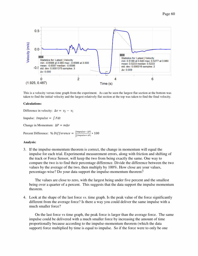
Page 60
This is a velocity versus time graph from the experiment. As can be seen the largest flat section at the bottom was
taken to find the initial velocity and the largest relatively flat section at the top was taken to find the final velocity.
Calculations:
Difference in velocity: ∆ = − 𝑖 Impulse: 𝐼 = ∫
Change in Momentum: ∆𝑃 = ∆
Percent Difference: % 𝑖 = |𝐼 − ∆𝑃|𝐼 𝑢 𝑠 + ∆𝑃 ∗
Analysis:
3. If the impulse-momentum theorem is correct, the change in momentum will equal the
impulse for each trial. Experimental measurement errors, along with friction and shifting of
the track or Force Sensor, will keep the two from being exactly the same. One way to
compare the two is to find their percentage difference. Divide the difference between the two
values by the average of the two, then multiply by 100%. How close are your values,
percentage-wise? Do your data support the impulse-momentum theorem?
The values are close to zero, with the largest being under five percent and the smallest
being over a quarter of a percent. This suggests that the data support the impulse momentum
theorem.
4. Look at the shape of the last force vs. time graph. Is the peak value of the force significantly
different from the average force? Is there a way you could deliver the same impulse with a
much smaller force?
On the last force vs time graph, the peak force is larger than the average force. The same
impulse could be delivered with a much smaller force by increasing the amount of time
proportionally because according to the impulse-momentum theorem (which the data
support) force multiplied by time is equal to impulse. So if the force were to only be one

Page 61
tenth of its original value, in order to have the same impulse it would have to have been
present for ten times as long.
6. When you use different elastic materials, what changes occurred in the shapes of the graphs?
Is there a correlation between the type of material and the shape?
When the rubber band had a lower spring coefficient it made the graph not as tall and
wider. There does seem to be a correlation between the material used and the shape of the
graph
7. When you used a stiffer or tighter elastic material, what effect did this have on the duration
of the impulse? What affect did this have on the maximum size of the force? Can you
develop a general rule from these observations?
The stiffer materials increased the maximum force, but decreased the time the force was
present. In other words, it made the graph taller and skinnier. The graph seems the follow
the rule that the stiffer the material, the taller and skinnier the graph.
Conclusion: The data gathered during this experiment seem to support the impulse-momentum theorem. They
show that the average force multiplied by the amount of time the force was present is almost equal to the mass of the
cart multiplied by the change in velocity. The differences are small enough to be ascribed to human error in
determining the values. The primary source of error was human error in determining the precise moments in which
the velocity began to change and when the force was applied to the cart. The reason for this is that, as shown in the
pictures on page 3, neither the force nor the change in velocity are long in duration. A second source of error was
friction, however its effect on the experiment was negligible because the cart had very little mass, and as shown in
the velocity versus time graph, the cart did not experience much deceleration outside of the time in which the force
of the rubber band was acting on it.

Page 62
Rotational Inertia Lab
Daniel McDermott
Paul Quatrani, Joseph Mea, Michael Feng, Kyle Ryan
Abstract: In this lab, objects of varying shapes, sizes, and masses were rolled down a flat ramp at a constant length
in order to determine the difference in acceleration between the varying objects and the effect that rotational inertia
has on it. The primary source of error was human error in timing and placing the object. The data did support that
rotational inertia is affected by mass, radius, and shape.

Page 63
22 February 2016
Daniel McDermott
Lab Partners: Michael Feng, Kyle Ryan, Paul Quatrani, Joseph Mea
Rotational Inertia Lab
Purpose: The purpose of this lab is to experimentally verify or refute the concept that rotational inertia is affected
by an object’s shape, mass and radius. The shapes used were hoops, disks, and spheres. The height from which the
objects were released was controlled. Secondary objectives include development of analytical skills relating to
finding meaningful patterns in data.
Background: If an object is rolling down an inclined plane, then it has two kinds of kinetic energy: rotational and
translational. The translational energy is determined by the velocity (v) of the object and its mass (m) through the
equation 𝐾 𝑖 = . The rotational energy of the object is determined by the object’s rotational
inertia, also called its moment of inertia, (I) and rotational velocity (ω). The moment of inertia determines how resistant to changes in its angular velocity an object is and can be found by the equation = ∑ , however there
are shape specific equations that are easier to use, and the rotational velocity when there is no slipping can be found
through the equation 𝜔 = . The equation for the rotational kinetic energy can be found through the equation 𝐾 𝑖 = 𝐼𝜔 .
As mentioned previously, there are shape specific equations for determining the moment of inertia of an
object. For a sphere with uniform mass distribution of mass m and radius r, the equation is 𝐼 = and the
equation for a uniform hoop of the same measurements with its axis running through the center and parallel to the
edges is 𝐼 = . For a solid disk the equation is 𝐼 = . This means that a hoop has a greater moment of
inertia than a solid disk, which in turn has a greater moment of inertia than a sphere. When an object has a greater
moment of inertia, it will have more of its kinetic energy put into the rotational aspect instead of the translational
aspect, and therefore have a lower velocity. This means that if a sphere, hoop, and disk were all rolled down the
same hill from the same height, the sphere would reach the bottom first, followed by the disk, and then the hoop.
Since the objects are all rolling, without slipping, from the same height, the average acceleration of any
give object can be determined by solving the conservation of energy equation for velocity and dividing that value by
the time it took to reach the bottom of the slope. The ratio of the acceleration of certain objects can then be found.
In the ratios, the number 1 will be used to denote that the variable relates to a hoop, the number 2 to a sphere, and
the number 3 to a disk. The ratio of the acceleration of a hoop to a sphere should be √ 7 , the ratio of a hoop to a
disk should be √ , and the ratio of a sphere to a disk should be √ 7√ . The ratio of the acceleration of a sphere to
a hoop should be the reciprocal of the ratio of acceleration of a hoop to a sphere and so forth.
Materials:
Solid Metal Ball (two of different masses and sizes)
Hollow Plastic Cylinder
Hollow Plastic Ball

Page 64
Hollow Metal Cylinder
Solid Wooden Cylinder
Stopwatch
Flat Board
Procedure: The board was inclined to a certain angle and a known distance from one end of the board was marked.
The object that was to be rolled was measured to determine its mass and radius, both of which were recorded. The
object to be rolled down was then rolled down the inclined plane starting from the marked distance with the time it
took the object to reach the end of the inclined plane being measured and recorded. This was done twice for each
object. The times of each object were then averaged. The average time of each object was then run through the
equation = ∆ to determine the average acceleration of the object while it was going down the ramp. The
accelerations were then compared to determine whether the data supported the notion that spheres should have the
fastest acceleration, followed by the solid disk, followed by the hoops. The moment of inertia was also calculated
and compared to the accelerations in order to determine whether or not there was a correlation between moment of
inertia and acceleration.
Data:
All objects were run from a distance of 80 centimeters
Object
Radius
(Centimeters)
Mass
(Grams)
Trial 1 Time
(Seconds)
Trial 2 Time
(Seconds)
Average
Time
(Seconds)
Acceleration
(m/s/s)
Solid Metal
Ball 2.45 482.5 1.52 1.69 1.605 0.621
Hollow
Plastic Ball 2.25 23.6 1.64 1.56 1.600 0.625
Hollow
Plastic Hoop 4.45 81.5 1.62 1.84 1.730 0.534
Hollow
Metal Hoop 7.50 589.5 1.72 1.93 1.825 0.480
Solid Wood
Disk 7.50 459.7 1.55 1.59 1.570 0.649
Solid Metal
Ball 0.95 29.1 1.68 1.72 1.700 0.553
Object Radius
(meters)
Mass
(kilograms)
Moment of Inertia
(kg*m2)
Solid Metal Ball 0.0245 0.4825 0.00012
Hollow Plastic Ball 0.0225 0.0236 0.00000
Hollow Plastic Hoop 0.0445 0.0815 0.00016
Hollow Metal Hoop 0.0750 0.5895 0.00332

Page 65
Solid Wood Disk 0.0750 0.4597 0.00129
Solid Metal Ball 0.0095 0.0291 0.00000
Calculations:
Acceleration: = ∆
Moment of Inertia:
Sphere: 𝐼 =
Disk: 𝐼 =
Hoop: 𝐼 =
Analysis:
1. Look at the pairs of objects. Do you notice what quantities affect an object’s rotational inertia? How so?
a. The shape of the object affected the objects rotational inertia by changing how its mass is
distributed. An object with most or all of its mass spread evenly should have less rotational inertia
than an object that has all of its mass spread at its edge. This will in turn mean that it will require
less force to cause greater acceleration in the object.
2. Choose any two different shaped objects and, using your measurements, calculate the objects’ moments of
inertia.
a. The moment of inertia for the wooden cylinder was .00129 kg*m2. This was found through the
equation 𝐼 = . The moment of inertia for the solid metal ball was approximately zero.
While the equation 𝐼 = resulted in 1.05051*10-6
kg*m2, unless significant figures are being
ignored, the result is 0.00000 kg*m2.
Conclusion: The data support the idea that as an object’s moment of inertia increases, its rate of acceleration will
decrease. They show that when the measurements from the first table are run through the equation listed for each
objects respective shape, the objects with higher accelerations tend to have lower rotational inertia. They also
support the idea that when the objects have comparable masses and radii, a sphere will accelerate faster than a disk,
which will accelerate faster than a hoop. The primary source of error in this lab was human error in timing the
objects, leading to the time measurements being slightly larger or smaller than they should have been. Another
source of error was that the objects may have been a few millimeters off of the starting point on the ramp. This
would lead to the object taking slightly more or less time to reach the bottom depending on whether it was higher or
lower than it should have been.
Page 66
Simple Harmonic Motion Lab
(AP Physics 1)
Daniel McDermott
Paul Quatrani, Michael Feng, Kyle Ryan
Abstract: In this lab, weights of varying masses were hung from a spring and pulled at various distances. The
spring remained constant. The period of the system was recorded and from this the spring constant was determined.
Some sources of error are being slightly off in the height and amplitude measurements and being slightly off in the
period measurements. The data supported the simple harmonic equation for springs

Page 67
9 March 2016
Daniel McDermott
Lab Partners: Michael Feng, Paul Quatrani, Kyle Ryan
Simple Harmonic Motion Lab
Data:
Mass
(g)
Initial height
(cm)
Amplitude
(cm)
Period
(s)
Frequency
(Hz)
.200 .709 .05 1.222 0.8183
.200 .709 .10 1.230 0.8130
.200 .709 .15 1.124 0.8896
.200 .709 .20 1.182 0.8460
.200 .709 .25 1.198 0.8347
.500 .315 .05 1.693 0.5906
.100 .829 .05 0.942 1.0615
.050 .914 .05 0.831 1.2033
This is a sample Position versus Time graph from the experiment. As can be seen the object’s movement
fits a negative cosine wave, which indicates that the object is acting in simple harmonic motion. The
highlighted area covers the period of the wave.

Page 68
This is a sample Velocity versus Time graph from the experiment. The object’s velocity roughly fits a
sine wave. The highlighted area covers the period of the graph, showing that it had no velocity at its
peaks.
This is a graph of the Period versus the Mass of the object. As can be seen, a linear equation would not
correctly model this scenario, but one utilizing the square root of the mass would.

Page 69
This is a graph of the objects Period Squared versus the objects Mass. As can be seen, the data can be
modelled using a linear equation with a nonzero slope, which suggests that the period of an object is
proportional to the square root of its mass.
This is a graph of the objects Period versus Amplitude. As can be seen, the data can be modelled using a
linear equation with slope zero, suggesting that the amplitude does not affect the period in this scenario.
Calculating the Spring Constant:

Page 70
The Spring Constant was calculated by solving the equation 𝑇 = 𝜋√ for K, the spring constant. This
resulted in the equation 𝐾 = 𝑇 , which when the various times and masses were plugged in resulted in
the table below. The problem with the data generated from this is that it does not factor in the mass of the
spring, which was not measured in the experiment. Because of this, there are vast differences in the
spring constants generated, ranging from 2.8584 to 6.8867. However, there is only one instance out of all
the trials that has a result lower than four or greater than six, indicating that the constant is most likely
between those two numbers. In order to determine a better approximation, the arithmetic mean of all the
results from the equation was calculated, resulting in 5.2628. So the spring constant is about 5.2628
Newtons per meter.
Mass (kg) Period (s) Spring Constant (N/m)
0.200 1.222 5.2874
0.200 1.230 5.2189
0.200 1.124 6.2496
0.200 1.182 5.6513
0.200 1.198 5.5014
0.500 1.693 6.8867
0.100 0.942 4.4489
0.050 0.831 2.8584

Page 71
Ohm’s Law Lab
Daniel McDermott
Paul Quatrani, Michael Feng, Kyle Ryan
Abstract: In this lab a constant voltage was run through two resistors connected to a voltmeter and an ammeter in
order to determine the resistance of one of the resistors. The main source of error was in not accounting for the
wire’s resistance. The data supported Ohm’s Law with a percent error of 2.36%.

Page 72
20 April 2016
Daniel McDermott
Lab Partners: Michael Feng, Kyle Ryan, Paul Quatrani
Ohm’s Law Lab
Purpose: The purpose of this lab was to verify or refute Ohm’s Law in a controlled environment. The variables that
were controlled were the voltage, one of the two resistors, and the general circuit design. Secondary purposes were
to develop a greater understanding of circuit design and development in analytic skills relating to data.
Background: An object’s resistance (R) is a measure of how difficult it is for electricity to pass through that object
and is measured in Ohms (Ω). It is directly proportional to the voltage (V), or electric potential measured in volts
(V), going through that object. Voltage is measured using a voltmeter. Resistance is also inversely proportional to
the current (I), or speed at which charge moves through an object in amperes (A), going through the object. Current
is measured using an ammeter. This is called Ohm’s Law and in the form of an equation, it would look like 𝑅 = 𝑉𝐼 .
The resistance of a wire can be calculated using the equation 𝑅 = 𝐴 , where L is the length of the path, A is the cross
sectional area of the wire, and ρ is the wire’s resistivity. Resistivity is a property that a material simply has; metals
tend to have lower resistivity values.
A circuit is any low resistance, closed conducting path that goes from a point of high electric potential to low
electric potential and has some device that requires power or offers resistance. There are two main types of circuits:
series and parallel. A series circuit has only one possible path and all objects in it have the same current, but not
necessarily the same voltage. In a series circuit, the sum of each object’s voltage will equal the voltage of the source
or difference. The equivalent resistance of a series circuit is simply the sum of the resistance of each of its resistors
or devices. The other type of circuit is a parallel circuit, which has multiple paths from high to low potential. In a
parallel circuit, each path starts out with the same voltage and the sum of the voltage of every object in any given
path must equal the voltage of the source of difference. The equivalent resistance (Req) can be found through the
equation 𝑅 = 𝑅 + 𝑅 + 𝑅 + . . . . The different paths in series circuits do not necessarily have the same current.
There are circuits that have some elements in series and some in parallel, these are called combination circuits. The
source of difference is denoted using four parallel lines of alternating length, resistors are shown through jagged
squiggles, ammeters are shown by a circle containing a capital a, and voltmeters are shown through a circle
containing a capital v. The conducting path is shown through the straight lines. Ammeters must be in series with
the portion of the circuit being measured and voltmeters must be in parallel.
Assuming Ohm’s Law is correct, it is possible to predict the resistance of an object. This can be done by creating a
circuit that matches the design below. The second resistor (the one that is in parallel with the voltmeter) will be
swapped out with ones of varying resistances while the first resistor shall remain constant. Since the sum of each
object’s voltage must equal the source of difference’s voltage, the voltage of the first resistor must be the source of
difference’s voltage minus the second resistor’s voltage. Because the two are in what is effectively a series circuit
they both have the same current. The constant resistor’s resistance should be equal to the reciprocal of the slope of a
line of best fit for a Current vs Voltage graph of the data.
A
V

Page 73
Materials:
5 Volt power source
Copper wiring
1 390 Ω resistor 6 resistors of different resistances
1 ammeter
1 voltmeter
Vernier LABPRO
Procedure: A circuit was assembled following the design in the background section with a 390 Ω resistor for the first resistor and a 5 V power source. The voltage and amperage was recorded for each variable resistor and their
resistance was determined using the equation 𝑅 = 𝑉𝐼 . The voltage of the 390 Ω resistor (Vc) was determined using
the equation = − . The data were then entered into a current versus voltage graph. The line of best fit for the
data were then determined. The reciprocal of the line’s slope was then found. The percent error between this value
and 390 was then determined.
Data:
Trial Current
(A)
Voltage
(V)
Resistance
Ω
1 0.0030 3.790 1263.3333
2 0.0070 2.280 325.7142
3 0.0040 3.390 847.5000
4 0.0045 3.180 706.6666
5 0.0105 0.862 82.0952
6 0.0110 0.533 48.4545
This is the Amperage versus Time graph of the experiment with the line of best fit. Each data point is a different
resistor and the line of best fit has a slope of .002505.

Page 74
Calculations:
Resistance
𝑅 = 𝐼
Percent error % = | 𝑖 − 𝑖 𝑖 |𝑖 𝑖 ∗
Conclusion: The data support Ohm’s Law. Using the measurements from the experiment, the resistance of the first
resistor was found to be 399.2015 Ω. The percent error between this value and the given value of 390 Ω is 2.36%, which indicates that the results are accurate. The primary source of this error was most likely not accounting for the
resistance in the wires themselves. This is because while copper has a low resistivity, it still has some and this
would increase the found resistance of the first resistor. There is no way to eliminate this source of error outright,
and the difference made by using a material with a lower resistivity would be very slight.