LLSSFF RReesseeaarrcchh WWoorrkkiinngg PPaappeerr SSeerriieess

NN°°.. 1177--1122

*Corresponding Author’s Address:

Tel: +352 46 66 44 69 41 Fax : +352 46 66 44 6835 E-mail address: thorsten.lehnert@uni.lu

The opinions and results mentioned in this paper do not reflect the position of the Institution. The LSF Research Working Paper Series is available online: http://wwwen.uni.lu/recherche/fdef/luxembourg_school_of_ finance_research_in_finance/working_papers For editorial correspondence, please contact: sophie.lux@uni.lu

University of Luxembourg Faculty of Law, Economics and

Finance Luxembourg School of Finance

4 Rue Albert Borschette L-1246 Luxembourg

Date: December 2017

Title: Large Portfolio Risk Management and Optimal Portfolio Allocation

with Dynamic Elliptical Copulas

Author(s)*: Xisong Jin, Thorsten Lehnert Abstract : Previous research focuses on the importance of modeling the multivariate distribution for optimal portfolio allocation and active risk management. However, available dynamic models are not easily applied for large-dimensional problems due to the curse of dimensionality. In this paper, we extend the framework of the Dynamic Conditional Correlation/Equicorrelation and an extreme value approach into a series of Dynamic Conditional Elliptical Copulas. We investigate risk measures like Value at Risk (VaR) and Expected Shortfall (ES) for passive portfolios and dynamic optimal portfolios through Mean-Variance and ES criteria for a sample of US stocks over a period of 10 years. Our results suggest that (1) Modeling the marginal distribution is important for the dynamic high-dimensional multivariate models. (2) Neglecting the dynamic dependence in the copula causes over-aggressive risk management. (3) The DCC/DECO Gaussian copula and t-copula work very well for both VaR and ES. (4) Grouped t-copula and t-copula with dynamic degrees of freedom further match the fat tail. (5) Correctly modeling dependence structure makes an improvement in portfolio optimization against the tail risk. (6) Models driven by multivariate t innovations with exogenously given degrees of freedom provide a flexible and applicable alternative for optimal portfolio risk management.

JEL Classification: G12 Keywords: risk management, assets allocation, VaR, ES, dynamic conditional correlation

(DCC), dynamic equicorrelation (DECO), dynamic copula.

Large Portfolio Risk Management and Optimal Portfolio

Allocation with Dynamic Elliptical Copulas

Xisong Jin∗

Central Bank of Luxembourg

Thorsten Lehnert

Luxembourg School of Finance, University of Luxembourg

This version: December, 2017

Abstract

Previous research focuses on the importance of modeling the multivariate distribution foroptimal portfolio allocation and active risk management. However, available dynamic modelsare not easily applied for large-dimensional problems due to the curse of dimensionality. Inthis paper, we extend the framework of the Dynamic Conditional Correlation/Equicorrelationand an extreme value approach into a series of Dynamic Conditional Elliptical Copulas. Weinvestigate risk measures like Value at Risk (VaR) and Expected Shortfall (ES) for passiveportfolios and dynamic optimal portfolios through Mean-Variance and ES criteria for a sam-ple of US stocks over a period of 10 years. Our results suggest that (1) Modeling the marginaldistribution is important for the dynamic high-dimensional multivariate models. (2) Neglect-ing the dynamic dependence in the copula causes over-aggressive risk management. (3) TheDCC/DECO Gaussian copula and t-copula work very well for both VaR and ES. (4) Groupedt-copula and t-copula with dynamic degrees of freedom further match the fat tail. (5) Cor-rectly modeling dependence structure makes an improvement in portfolio optimization againstthe tail risk. (6) Models driven by multivariate t innovations with exogenously given degreesof freedom provide a flexible and applicable alternative for optimal portfolio risk management.

JEL Classification: G12

Keywords: risk management, assets allocation, VaR, ES, dynamic conditional correlation(DCC), dynamic equicorrelation (DECO), dynamic copula.

∗This paper should not be reported as representing the views of the Banque centrale du Luxembourg (BCL)or the Eurosystem. The views expressed are those of the authors and may not be shared by other research staffor policymakers in the BCL or the Eurosystem. Correspondence can be sent to: Xisong Jin, Banque centrale duLuxembourg, 2, boulevard Royal L-2983 Luxembourg, Tel: (352) 4774-4462; E-mail: xisong.jin@bcl.lu.

1

1 Introduction

Modeling dynamic multivariate distribution is of crucial importance in finance. The cross-sectional

information in dynamic multivariate models is extremely useful for active risk management such as

computing the marginal risk contributions of each position, evaluating the effects of hedges, and

constructing an optimal portfolio. The copula theory is a fundamental tool for modeling multivariate

distributions. It allows the definition of the joint distribution through the marginal distributions

and the dependence between the variables. Correlation, which usually refers to linear correlation,

depends on both the marginal distributions and the copula, and is not a robust measure, as a

single observation can have an arbitrarily strong impact. The copula provides a robust method of

consistent estimation for dependence, and is much more flexible.

The copula theory has been extended to the conditional case, allowing the use of copulas to

model dynamic structures, as in Dias and Embrechts (2004), Patton (2004, 2006a&b) and Jondeau

and Rockinger (2003, 2006). Compared with traditional methods of Value at Risk (VaR) estimation,

conditional copula theory can be a very powerful tool in estimating the VaR, as shown by Fantazzini

(2008) and Palaro and Hotta (2006). However, modelling large-dimensional distributions is not an

easy task and only a few models are potentially useful for constructing flexible distribution models

in large dimensions. Lee and Long (2009) decompose the dependence into linear and nonlinear

component, and use copula-based models for the nonlinear component. Nevertheless, their approach

is computationally infeasible in high dimensions as discussed by Oh and Patton (2016). Latent

factor copula models, see Creal and Tsay (2015) and Oh and Patton (2017) for example, are

particularly attractive for relatively large dimensional applications to the factor structure, but

factor copula models do not generally have a closed-form likelihood, making maximum likelihood

estimation diffi cult. Vine copulas are constructed by sequentially applying bivariate copulas to build

up a larger-dimension copula, see, e.g., Almeida, Czado, and Manner (2012) and Brechmann and

Czado (2013). However, as shown by Acar, Genest, and Neslehova (2012), vine copulas are almost

invariably based on an assumption that is hard to interpret and to test. Extreme-value copulas

such as Archimedean copulas provide appropriate models for the dependence structure between

rare events, e.g., Patton (2004), but usually have one or two free parameters regardless of number

of asset, which is clearly very restrictive in large dimensions.

Multivariate GARCH techniques applied in the dynamic correlation multivariate models are

called Dynamic Conditional Correlation Multivariate GARCH (DCC). It has proven to be diffi cult

to estimate multivariate GARCH models for a large number of underlying securities owning to the

curse of dimensionality; the estimates are usually seriously biased. However, recently several es-

timation methods been developed to treat this large-dimensional problem: the MacGyver method

(Engle (2009)), Dynamic Conditional Equicorrelation (DECO) (Engle and Kelly (2012)), and the

Composite Likelihood method (Engle, Shephard, and Sheppard (2008)). The DCC or DECO ap-

2

proach puts a dynamic multivariate distribution on top of the dynamic marginal distributions and

therefore can be viewed as a simple kind of dynamic copula approach without modeling marginal

distributions specifically. Christoffersen et al. (2012) allow the DCC structure in a skew t copula

for their dependence study of 33 developed and emerging equity market indices, and Christoffersen

et al. (2017) used the same model to study 233 equity returns and credit default swap spreads.

In the light of the recent development of multivariate GARCH techniques for a large number of

underlying securities, in this paper, we extend the DCC/DECO framework to more general Dynamic

Conditional Elliptical Copulas, the Gaussian- and t-copula. Two good candidates that are especially

tractable for large dimensions. The class of elliptical distributions provides very useful examples of

multivariate distributions because they share many of the tractable properties of the multivariate

normal distribution. Furthermore, they allow modeling of multivariate extreme events and forms

of non-normal dependencies. They play an important role in finance. Elliptical copulas are simply

the copulas of elliptical distributions. We limit the choices of copula within the class of elliptical

copulas because (1) elliptical copulas allow us to specify a variance-covariance structure which in

some senses provides the linear dependence between the random variables; (2) except for the normal

copula which gives zero tail dependence, elliptical copulas also allow for non-zero tail dependence;

(3) in addition, elliptical copulas provide the flexibility of simple simulation procedures. Therefore

the class of elliptical copulas is a good candidate for the large-dimensional problem.

In this study, we adopt a semi-parametric form of the marginal distributions and new estimation

methods for multivariate GARCH models. We propose a series of dynamic copulas to examine VaR

and ES accordingly not only for passive large portfolios but also for dynamic optimal large portfolios

by both Mean-Variance and ES criteria. Assuming equal correlation or dependence across assets is

very convenient and widely used by the financial industry: for instance, in the CDO market, the

standard one-factor Gaussian copula also assumes equal dependence. Elton, Gruber, and Green

(2007) find that, despite all the advances in modeling, the assumption that all correlations are

identical to each other still serves about as well as any other forecasting technique for portfolio

optimization. Therefore we further explore if equal correlation or dependence performs about as

well as full dependence structure for active risk management.

In our empirical study, we consider a large sample of US stocks during the period 1995-2005,

which consists of 89 North American investment grade companies included in the CDX.NA.IG,

a credit default swap index. This sample period which includes an apparent change of depen-

dence is perfectly suitable for highlighting the importance of the copula-based dependence approach

compared with the traditional correlation analysis. We construct equally-weighted portfolios and

value-weighted portfolios which are updated annually. The out-of-sample performances in terms of

VaR and ES show that (1) Modeling the marginal distributions well is very important. In DCC

or DECO, simulation directly from multi-normal distribution or multi-t distribution does not in-

duce enough tail fatness. The assumption that the portfolio returns are from univariate conditional

3

t-distribution, with portfolio variance computed from conditional covariance matrix from DCC or

DECO, indeed recovers tail fatness further, but at the sacrifice of the upper quantiles. (2) Ne-

glecting dynamic dependence alone in the copula can cause over-aggressive risk management. The

proportion of excessive losses can be seriously underestimated when real dependence is moving up

and down, for example, in the post high-tech bubble period. (3) DECO and DCC Gaussian copulas

and t-copulas work very well in both VaR and ES. The DCC copula does a better job, especially

for the value-weighted portfolio, by taking care of the widely dispersed dependence structures. For

the equally-weighted portfolio, the DECO copula still performs about as well as the DCC copula.

(4) Grouped t-copula and full dynamic t-copula, in which the degree of freedom is also modeled

dynamically, match the fat tail even further, with an improvement especially at the lower quantiles.

The optimal portfolios are constructed empirically by the Markowitz (1952) portfolio selection

method. When asset returns are far from being normally distributed, the traditional mean-variance

framework may produce misleading results. We therefore minimize the portfolio’s ES also by the

scenario-based copula models as Rockafellar and Uryasev (2000) and Andersson et al. (2000). We

find that (1) Even though the assumption of all correlations identical to each other is convenient,

correctly modeling dependence dispersion can still make a marginal improvement in portfolio op-

timization, which should not be neglected. The optimal portfolio by ES does a better job against

the tail risk compared to the optimal portfolio by mean-variance in both DECO and DCC copulas.

So the Markowitz (1952) portfolio selection is not effi cient if we consider the tail risk. (2) Because

optimizers actually act as statistical error maximizers, the ex ante VaR and ES by simulation in

the framework of the copula underestimate the loss even under short-selling restrictions. Instead,

models driven by multivariate t innovations with exogenously given degrees of freedom actually

works very well for optimal portfolio risk management.

The rest of the paper proceeds as follows. In Section 2, we provide a brief review of elliptical cop-

ulas and several scalar measures of dependence, explain how to model the marginal dynamics, and

introduce a series of dynamic copulas by extending the multivariate GARCH models (DCC/DECO)

into the framework of the Gaussian copula and t-copula. Section 3 shows the empirical applications

and the backtesting results. Finally, conclusions are drawn and future works discussed in Section

4.

2 Dynamic Elliptical Copula Models

Patton (2006b) defined a “conditional copula” as an n-dimensional multivariate distribution of

variables Xt = [X1t, X2t, ..., Xnt]′conditional on some information set Ft−1 = σ(Xt−j; j ≥ 1) for

i = 1, 2, ..., n and t ∈ {1, ..., T}. We adopt the usual convention of denoting random variables in

upper case, and realizations of random variables in lower case. Based on this definition, we can

4

extend Sklar’s theorem to the time series case:

F (x|Ft−1) = C(F1(x1|Ft−1), F2(x2|Ft−1), ..., Fn(xn|Ft−1)|Ft−1),∀x ∈ Rn

where Xt|Ft−1 ∼ F (·|Ft−1) , Xit|Ft−1 ∼ Fi(·|Ft−1) which is independent and identically distributedwith mean zero and variance one by construction, and C is the conditional copula of Xt given Ft−1.The Sklar’s theorem for conditional distributions implies that the conditioning set, Ft−1, must bethe same for all marginal distributions and the copula. It is often the case in financial applications,

however, that some of the information contained in Ft−1 is not relevant for all variables. We mightdefine Fi,t−1 as the smallest subset of Ft−1 such that Xit|Fi,t−1

D= Xit|Ft−1. With this it is possible

to construct each marginal distribution model using only Fi,t−1, which will probably differ acrossmargins, and then use Ft−1 for the copula, to obtain a valid conditional joint distribution.We present two copulas belonging to the elliptical family, which will be used later in the empirical

applications, namely the Gaussian copula and the t-copula. For the Gaussian copula, its dependence

features are characterized by the basic scalar dependence parameter for two variables X and Y :

ρGR = Corr[Φ−1(F (x)),Φ−1(F (y))] = Corr[Φ−1(u),Φ−1(v))

where u = F (x) and v = F (y). ρGR is the correlation between the variables Φ−1(u), and Φ−1(v),

which are both marginally standard Gaussian and admit the same copula as X, Y . As other

rank correlations such as the so-called Spearman’s rho and Kendall’s Tau, it can detect nonlinear

association that Pearson’s linear correlation cannot see. It coincides with the linear correlation if

the basic variables are jointly Gaussian. As for the t-copula, the scalar measure of dependence is

ρTR = Corr[t−1v (u), t−1v (v)). These basic scalar dependence measures are usefull to interpret the

parameters or to construct dependent update forms for parametric dynamic copula families.

The choice of the best distribution for the margins is also crucial. Misspecification of marginals

can lead to dangerous biases in dependence measure estimation, see, for instance, Fantazzini (2009).

Hence, we need a procedure that avoids marginal model risk as much as possible and also does not

mask the dependence structure too much. The proposal is known as the canonical maximum

likelihood method (CML). The CML estimation procedure consists of two stages. In the first one

we fit univariate ARMA(p1, q1) − GARCH (p2, q2) models (for other candidate GARCH, please

see Bollerslev (2008)) to each of the marginal series Xit with innovations εit assumed to come from

iid(0, 1). We can assume εit comes from a t distribution, Hansen’s skewed t distribution or other

distributions with heavy-tailedness as in Jondeau and Rockinger (2006), and estimate univariate

ARMA − GARCH models by Maximum Likelihood. However fitting a parametric distribution

to data sometimes results in a model that agrees well with the data in high-density regions, but

poorly in areas of low density. Instead, we do not specify the marginal distribution but adopt a

5

semi-parametric form of the marginal distributions. We estimate the ARMA − GARCH model

directly by Quasi-Maximum Likelihood by assuming εit ∼ iid(0, 1), and select the best model by

some automatic model selection criteria. Given the standardized i.i.d residuals from the previous

step, we estimate the empirical cumulative distribution function (cdf) of each time series data,

smoothe the cdf estimates with a Gaussian kernel, and then fit the amount by which those extreme

residuals in each tail fall beyond a threshold, e.g. 10% to a parametric GP by maximum likelihood.

This approach is often referred to as the distribution of exceedances or peaks-over-threshold method

(see, for instance, McNeil (1999), McNeil and Frey (2000) or Nystrom and Skoglund (2002a&b)).

In the second step a parametric family of copulas is fitted. The parameters of the copula are

estimated as:

θc = arg maxT∑t=1

log[c(F1(x1t|F1,t−1), F2(x2t|F2,t−1), ..., Fn(xnt|Fn,t−1)|Ft−1; θc)]

where c is the conditional copula density function of Xt given Ft−1, and we assume εit or equivalentin general, Xit|Fi,t−1

D= Xit|Ft−1 ∼ iid(0, 1). In Genest, Ghoudi and Rivest (1995), and Chen and

Fan (2006), it is shown that the estimator θc for the dependence parameter resulting from CML is

consistent and has asymptotically normal distribution under regularity conditions similar to those

of maximum likelihood theory. Moreover, the asymptotic variance-covariance matrix of T 1/2θc is

B−1ΣB−1, where B is the information matrix associated with the copula and Σ is the variance-

covariance matrix of the n-dimensional random vector. The estimation of the variance-covariance

matrix is given in Section 3-4 of Genest, Ghoudi and Rivest (1995).

In the next section, we extend the multivariate GARCH techniques (DCC/DECO) into elliptical

copulas to investigate the conditional dynamic dependence.

2.1 Dynamic Gaussian Copula

The Gaussian copula is the copula of the multivariate normal distribution. In fact, the random

vector Xt|Ft−1 = (ε1t, ..., εnt) is multivariate normal if the univariate margins F1, ..., Fn are Gaus-

sians. Let Rt be a symmetric, positive definite matrix with diagonal of Rt equals to 1, and ΦRt

standardized multivariate normal distribution with correlation matrix Rt at time t. The dynamic

multivariate Gaussian copula is then defined as follows:

C(η1, η2, ..., ηn;Rt) = ΦRt(Φ−1(η1),Φ

−1(η2), ...,Φ−1(ηn))

where ηi = Fi(εi) for i = 1, 2, ..., n. εit ∼ iid(0, 1) innovations from the marginal dynamics intro-

duced in the previous section. Rt can be assumed to be constant or a dynamic process through

time.

6

2.1.1 DCC Gaussian Copula

Engle (2002) proposes a class of models - the Dynamic Conditional Correlation (DCC) - that both

preserves the ease of estimation of Bollerslev (1990)’s constant correlation model and allows the

correlations to change over time. These kinds of dynamic processes can also be extended into

Gaussian copulas. The simplest rank correlation dynamics we consider empirically is the symmetric

scalar model where the entire rank correlation matrix is driven by two parameters.

Qt = (1− α− β)Q+ α(ε∗t−1ε∗′t−1) + βQt−1

where α ≥ 0, β ≥ 0, α + β < 1, ε∗i = Φ−1(ηi = Fi(εi)), Qt = |qij,t| is the auxiliary matrixdriving the rank correlation dynamics, the nuisance parameters Q = E [ε∗t ε

∗′t ] with sample analog

T−1∑T

t=1 ε∗t ε∗′t , so that Rt is a matrix of rank correlations ρi,j,t with ones on the diagonal.

ρi,j,t =qij,t√

qii,t√qjj,t

Cappiello, Engle and Sheppard (2006) extend the DCC model to allow for asymmetric dynamics

in the correlation in addition to the asymmetric response in variances. We can also extend the basic

scalar model to allow for asymmetry by adding a single parameter, ξ.

Qt = (1− α− β)Q− ξN + α(ε∗t−1ε∗′t−1) + βQt−1 + ξ(nt−1n

′t−1)

where nt = I [ε∗t < 0]◦ε∗t is the asymmetric innovation. N = E [ntn′t] with sample analog T

−1∑Tt=1 ntn

′t.

The updated form can also be constructed on the standardized residuals εt as in Jondeau and

Rockinger (2006), and both ways give very similar empirical results in our applications. We prefer

the second method because it makes the Gaussian rank correlation ρGR based on ηn directly. Then

the conditional covariance of ε∗t+1 variables is no longer equal to conditional linear correlation of

the raw returns because variance of ε∗t could be far from one. These “biases” in the sense of

linear correlation are not a problem in the framework of the copula which emphasizes the rank

correlation. ε∗t−1ε∗′t−1 can be interpreted more appropriately as updated information or news shocks,

and normalization of the qij,t variables still insures that the Gaussian rank correlation always falls

in the interval from minus one to plus one. Typically these models are usually completed by

setting Q1 = Q = T−1∑T

t=1 ε∗t ε∗′t . Another good candidate is the non-target scalar models: Qt =

hQ− ξN +α(ε∗t−1ε∗′t−1) +βQt−1 + ξ(nt−1n

′t−1), which converges quickly although the initial Q or Q1

is not well defined.

We could compute the quasi-likelihood function for these models, but in large dimensions, con-

vergence is not guaranteed and sometimes it fails or is sensitive to the starting values. This incidental

parameter problem causes quasi-likelihood based inference to have economically important biases

7

in the estimated dynamic parameters, α especially has a serious downward bias. Engle, Shephard

and Sheppard (2008) suggest an approach to construct a type of composite likelihood, which is then

maximized to deliver the preferred estimator.

CL(ψ) =

T∑t=1

1

M

M∑j=1

log f(yjt;ψ)

where yjt is a pair of data, ψ is a set of parameters, M is the number of all unique pairs, and t =

1, 2, ..., T . The composite likelihood is based on summing up the quasi-likelihood of subsets of assets.

Each subset yields a valid quasi-likelihood, but this quasi-likelihood is only mildly informative

about the parameters. By summing up many subsets we can produce an estimator which has

the advantage that we do not have to invert large dimensional covariance matrices. Further, and

vitally, it is not affected by the incidental parameter problem. It can also be very fast, and does

not have the biases intrinsic in the usual quasi-likelihood when the cross-section is large. We

estimate this DCC Gaussian copula by maximizing m-profile subset composite likelihood (MSCL)

using contiguous pairs, which is attractive from statistical and computational viewpoints for large

dimensional problems compared with the m-profile composite likelihood (MCLE) using all the pairs.

Needless to say, the scalar model is restrictive in forcing the correlation dynamics to be identical

across all pairs of assets. We can therefore extend the model to allow for different rank correlation

dynamics across several blocks of assets as in Billio, Caporin and Gobbo (2006), Vargas (2006) and

Billio and Caporin (2009). These asset blocks can correspond to industries or ratings. We can also

estimate it by the Composite Likelihood method, in which different pairs in different blocks should

be led by different parameters.

2.1.2 DECO Gaussian Copula

The dynamic equicorrelation (DECO) model in Engle and Kelly (2012) is essentially an extreme

case of a DCC model in which the correlations are equal across all pairs of companies but where this

common equicorrelation is changing over time. The resulting dynamic correlation can be thought

of as an average dynamic correlation between the companies included in the analysis.

We also extend the concept of Dynamic Equicorrelation (DECO) to copula-based models to

investigate the residual dependence. Following Engle and Kelly (2012), we parameterize the dynamic

rank equicorrelation matrix as

Rt = (1− ρt)In + ρtJn×n

where In denotes the n-dimensional identity matrix and Jn×n is an n×n matrix of ones. The inverse

8

and determinants of the rank equicorrelation matrix, Rt, are given by

R−1t =1

(1− ρt)[In −

ρt1 + (n− 1)ρt

Jn×n] and

det(Rt) = (1− ρt)n−1[1 + (n− 1)ρt]

Note that R−1t exists if and only if ρt 6= 1 and ρt 6= −1n−1 , and Rt is positive definite if and only if

ρt ∈( −1n−1 , 1

). The time-varying rank equicorrelation parameter, ρt is assumed to follow the simple

dynamic linear form:

ρt+1 = ω + αut + βρt + γ′yt

where yt is a vector of exogenous variables, ut represents the rank equicorrelation update. In our

empirical application, we only consider the following updating rule:

ut =

∑i 6=j ε

∗i,tε∗j,t

(n− 1)∑

i ε∗2i,t

=

(∑i ε∗i,t

)2 −∑i ε∗2i,t

(n− 1)∑

i ε∗2i,t

Note that ut lies within the positive definite range( −1n−1 , 1

), and ε∗t = Φ−1(ηn = Fn(εn)).

The correlation matrices Rt are guaranteed to be positive definite if the parameters satisfy

ω/(1−α−β) ∈ (−1/(n− 1), 1), ut ∈ (−1/(n− 1), 1), and α+β < 1, α > 0, β > 0. The fitted rank

equicorrelation process could obeys the bounds( −1n−1 , 1

)without imposing α + β < 1. The ut form

above will be the least sensitive to residual volatility dynamics and extreme realizations, owning to

the use of a normalization that uses the mean cross-sectional variance.

We can also consider the nonlinear forms similar to those of Dias and Embrechts (2004), such

as ρt+1 = Λ(ω + αut + βΛ−1(ρt) + γ′yt) or similar to those of Patton (2006 a&b), such as ρt+1 =

Λ(ω + αut + βρt + γ′yt) where Λ(·) is the modified logistic function: Λ(x) = 1−exp(−x)

1+exp(−x) . The DECO

Gaussian copula is estimated by maximizing likelihood functions directly.

2.2 Dynamic t-Copula

The copula of the multivariate standardized t distribution is the t-copula and the dynamic t-copula

is defined as follows:

C(η1, η2, ..., ηn;Rt, vt) = TRt,vt(t−1vt (η1), t

−1vt (η2), ..., t

−1vt (ηn))

where ηi = Fi(εi) for i = 1, 2, ..., n. εit ∼ iid(0, 1), the innovations from the marginal dynamics

introduced in the previous section. Rt is the correlation matrix, and vt is the degrees of freedom.

ε∗i = t−1vt (ηi = Fi(εi)), t−1vt (ηi) denotes the inverse of the t cumulative distribution function. Rt and

vt can be assumed to be constant or a dynamic process through time.

9

The t-copula generalizes the normal copula by allowing for non-zero dependence in the extreme

tails. Since it is a symmetric copula, “upper tail dependence”, τU , between the variables during

extreme appreciations is restricted to be the same as “lower tail dependence”, τL, during extreme

depreciations, and is given by:

τUt = τLt = 2− 2Tvt+1(√vt + 1

√1− ρt1 + ρt

)

The normal copula imposes that this probability is zero. The two parameters of the t-copula,

ρt and vt, jointly determine the amount of dependence between the variables in the extremes. The

coeffi cient of tail dependence seems to provide a useful measure of the extreme dependence between

two random variables. In our multivariate case, we can assume any pairwise tail dependence is

determined by the common or average time-varying rank correlations and the degrees of freedom.

For the time-varying rank correlations, the tail dependence exhibits time variation even at constant

degrees of freedom.

2.2.1 DCC t-Copula

The dynamic processes are assumed to be the same as those defined in the DCC Gaussian copula.

We only consider constant degrees of freedom in the DCC t-copula. Since the correlation between

Gaussian rank correlation ρGR and the rank correlation ρTR = Corr[t−1v (u), t−1v (v)) for t-copula is

almost equal to one, and ρTR can be well approximated by ρGR.

We can maximize an objective function that approximates the profile log-likelihood for the

degrees of freedom parameter as in Bouye et al. (2000) with the following algorithm:

(1) Let R0t be the composite likelihood estimate of Rt for the dynamic Gaussian copula.

(2) Rm+1t is obtained using the following equation

Rm+1t =

1

T

(vt +N

vt

) T∑t=1

[t−1vt (η)]ᵀ[t−1vt (η)]

1 + 1vt

[t−1vt (η)]ᵀRmt [t−1vt (η)]

(3) Repeat the second step until convergence: Rm+1t ≈ Rm

t .

This method can be significantly faster than maximum likelihood especially for large samples.

In our empirical application, we only adopt a two-step algorithm for convenience, which means

we first estimate Rt from dynamic Gaussian copula, and then recover the degrees of freedom from

t-copula with Rt fixed from the first step.

10

2.2.2 DECO t-Copula

For the DECO t-copula, dynamic rank equicorrelation parameters are assumed to be the same as

those in the DECO Gaussian copula. For the linear form, the update forms for ut are constructed

on the inverse cdf of the standard normal distribution: Φ−1(ηn = Fn(εn)), and for the nonlinear

form on inverse cdf of the t distribution: t−1v (ηn = Fn(εn)) as in Patton (2006b). Another linear

form might be considered, such as:

Λ−1(ρ) = ω + αΛ−1(ut) + βΛ−1(ρt) + γ′Λ−1(yt)

where Λ−1(x) is the inverse function of Λ(x) = 1−exp(−x)1+exp(−x) , and the update forms for ut are constructed

on the inverse cdf of the t distribution: t−1v (ηn = Fn(εn)) directly.

For the dynamic degrees of freedom, Jondeau and Rockinger (2003, 2006) model a dynamic

univariate skewed t distribution. We can extend their framework into a dynamic multivariate t-

copula:

vt+1 = a1 +n∑i=1

b+1iε∗+it +

n∑i=1

b−2iε∗−it + c1vt + γ

′yt

vt = g[Lv ,Uv ](vt)

where vt is the degrees of freedom, ε∗+it = max(ε∗it, 0) and ε−it = max(−ε∗it, 0), yt is a vector of

exogenous variables. This dynamic is mapped into the authorized domain [Lv, Uv] with the logistic

function g(vt) = Lv +(Uv−Lv)/(1+exp(−vt)). There are at least 2n+2 parameters in this model.

To solve this drawback, we can assume that the parameters are the same within the same group,

or the same parameters for all.

We consider another class of update forms for the degrees of freedom (DF) based on the log-

likelihood function of cross-sectional multivariate t distribution at time t as follows:

log(L(vt)) = log(Γ(vt+n

2

Γ(vt2

))− n log(

Γ(vt+12

Γ(vt2

))−

1

2log |Rt| −

vt + n

2log(1 +

ε∗′t R−1t ε∗tvt

) +vt + 1

2

n∑n=1

log(1 +ε∗2ntvt

)

Maximizing with respect to the degrees of freedom vt:

DFt = arg max log(L(vt))

Update forms for ut constructed on Φ−1(ηn = Fn(εn)) are assumed as the instant rank correlation

11

Rt at time t. The time-varying degree of freedom vt is assumed to follow:

vt+1 = ω + αDFt + βvt + γ′yt

vt = g[Lv ,Uv ](vt)

where yt is a vector of exogenous variables. This dynamic is mapped into the authorized domain

[Lv, Uv] with the same logistic function. SinceDFt can be regarded as the instant degrees of freedom

at time t, we can keep a linear form directly as:

vt+1 = ω + αDF truncatedt + βvt + γ

′yt

where DF truncatedt is the DFt truncated at min(DFt, UDF ), UDF is the upper boundary to avoid α =

0 for suffi ciently large data of DFt. For v = 50, the t-distribution is almost the same as the normal

distribution, we restrict the authorized domain [Lv, Uv] as [2, 50], and ω/(1−α−β) > 2, α+β < 1,

α > 0, β > 0. In our empirical studies, we only consider the linear form ρt+1 = ω + αut + βρt with

constant degrees of freedom and the linear form of time-varying degrees of freedom.

2.3 Dynamic Grouped t-Copula

In risk management, the tail dependence is very important. At the standard t-copula, the assump-

tion of one global degree of freedom parameter may be over-simplistic and too restrictive for a large

portfolio. Empirically we also find that, with more assets, the estimated degrees of freedom could

easily become a big number. As in a block correlation dynamic model, we would like to assume

different degrees of freedom for different groups corresponding to, for example, industries or ratings.

Consider now the following model. Let Zt ∼ Nn(0, Rt), whereRt is an arbitrary linear correlation

matrix, be independent of U , a random variable uniformly distributed on (0, 1). Furthermore, let

Gv denote the distribution function of√v/χ2v. Partition {1, ..., n} into m subsets of sizes s1, ..., sm.

Let Rkt = G−1vk (U) for k = 1, ...,m. If

Y = (R1tZ1,...,R1tZs1 , R

2tZs1+1,...,R

2tZs1+s2 , ..., R

mt Zn)

′,

then the random vector (Y1, ..., Ys1) has an s1-dimensional t-distribution with v1 degrees of freedom

and, for k = 1, ...,m − 1, (Ys1+...+sk+1, ..., Ys1+...+sk+1)′has an sk+1-dimensional t-distribution with

vk+1 degrees of freedom. The grouped t-copula is described in more details in Daul et al. (2003).

For calibration of and simulation from the grouped t-copula, there is no need for an explicit

copula expression. The calibration of this model is identical to that of the t distribution except

that the ML-estimation of the m degrees of freedom parameters has to be performed separately

on each of the m risk factor subgroups. In our dynamic copula application, we adopt a two-step

12

algorithm for convenience, which means we first estimate Rt from the dynamic Gaussian copula,

and then recover vk degrees of freedom for each group from the t-copula with Rkt fixed from the

first step. The dynamic degrees of freedom can also be built into these grouped t-copulas in the

second step, for instance, at group k, the update form for degrees of freedom can be constructed

by assuming dynamic rank equicorrelation, then the time-varying degree of freedom vk,t can be

estimated by ML-estimation for group k. In our empirical studies, we only consider the constant

degrees of freedom for the grouped t-copula.

3 Risk Management Application

Value at Risk (VaR) is probably the most popular risk measure, having a central role in risk

management. Although the VaR may be interesting from a practical point of view, however, it has

a serious drawback: it does not necessarily satisfy the property of subadditivity, which means that

one can find examples where the VaR of a portfolio as a whole is higher than that of the sum of the

VaR of its mutually exclusive sub-portfolios. An alternative practically viable risk measurement

method that satisfies the subadditivity property and other desirable properties is the expected

shortfall (ES).

If a single portfolio is considered, it makes more sense to fit a univariate model to the corre-

sponding return series and base any VaR or ES calculations on this model. On the other hand, if

a number of different portfolios based on the same universe of N assets are considered, it is pre-

ferred practice to base the individual VaR or ES calculations on a conditional joint multivariate

distribution of all N assets. This also allows computing of the marginal risk contributions of each

position and evaluation of the effects of hedges. Hence, multivariate distribution is very useful for

risk management applications.

When we deal with a large portfolio of assets, however, both VaR and ES estimation can become

very diffi cult owning to the complexity of joint multivariate modeling. Some approaches have been

proposed (see Giot and Laurent (2003) for a review), but most of them are rather complicated

to implement and can give similar results to simpler methods. Alternatively, simulations play an

important role in finance. They are used to replicate the effi cient frontiers, to price options, to

estimate joint risks, and so on. Using conditional dynamic copulas, it is relatively easy to construct

and simulate from multivariate distributions built on marginals and dependence structure. The

GARCH-like dynamics in both variance and dependence offer us one-step-ahead predictions of

portfolio losses.

We illustrate the following steps for the one-step-ahead simulation:

1. Draw independently ε∗i1t+1, ..., ε∗imt+1 for each asset from the n-dimensional normal or t distribution

with zero mean, forecast correlation matrix Rt+1, or degrees of freedom vt+1, and obtain

13

µi1t+1, ..., µimt+1 by setting µ

ikt+1 = Φ(ε∗ikt+1) or tvt+1(ε

∗ikt+1),where k = 1, ...,m, the total paths of

simulation, i = 1, ..., n, the number of assets;

2. Obtain εi1t+1, ..., εimt+1 by setting ε

ikt+1 = F−1i (uikt+1),where Fi is empirical marginal dynamics

distribution for asset i;

3. Obtain zi1t+1, ..., zimt+1 by setting ε

ikt+1 ∗ σit+1,where σit+1 is the forecast standard deviation by

GARCH model for asset i;

4. Obtain X i1t+1, ..., X

imt+1 by setting X

ikt+1 = λit+1+zikt+1,where λ

it+1 is the forecast mean by ARMA

model for asset i;

5. Finally obtain the portfolio return r1t+1, ..., rmt+1 by setting r

k = [Xkt+1]

ᵀ[Wt+1], where Wt+1 is

the portfolio weights at t+ 1.

The VaR and ES can be obtained by these simulated r1t+1, ..., rmt+1 portfolio returns. The multi-

day ahead VaR and ES can also be obtained by simulating multi-day forward in a similar way.

In our empirical study, we compare the effects of these copulas on risk measures VaR and ES by

backtesting. For the unconditional coverage testing, VaR performance is acessed by Kupiec’s (1995)

LR test, LRuc and a simple mean test, MT =√T π−p∗√

V ar(It)∼ N(0, 1) where It is “hit sequence”,

equal to one when loss returns in excess of VaR and zero otherwise. As for the independence

testing, it is done by Ljung-Box test, LB, and Christoffersen’s (1998) LR test, LRCC . We evaluate

ES performance by ES bootstrap test of McNeil and Frey (2000).

3.1 Data

The conditional dynamic copulas presented are applied to a portfolio composed by all companies

listed on CDX.NA.IG (a credit default swap index which contains 125 North American investment

grade companies). The database contains 2500 daily returns over the period from Jan 03, 1995

until Dec 03, 2004 taken from the CRSP database. This set includes 125 companies although 36

have one or more periods of non-trading, for example prior to IPO or subsequent to an acquisition.

Selecting only the companies that have returns throughout the sample reduces this set of 89. The

firms selected are reported in Table 11. The data set covers the high-tech bubble period, including

the post high-tech bubble period, but just before the housing bubble. From the return dispersion,

we find dispersion shrinks a little around the end of 1998, and there is a clear dispersion pattern

change within 2001 to 2005, the post high-tech bubble period. Thus, this sample is perfectly

suitable for highlighting the importance of the copula-based dependence approach compared with

the traditional correlation analysis.

14

3.2 Empirical Results

In this section we first use the full sample to show all model differences. The marginal dynamics

is selected, and the dynamic dependence is tested. Results of the estimation of the copula models

described in the previous section are presented in several figures and tables. We then compare the

out-of-sample performances in the post high-tech bubble period not only for passive large portfolios

but also for dynamic optimal large portfolios by both Mean-Variance and ES criteria.

3.3 In-Sample Analysis

For the marginal dynamics, we simply fit a first-order autoregressive model to the conditional

mean of the returns of each equity ri,t = Ci + Φiri,t−1 + zi,t−1, and a symmetric GARCH model to

the conditional variance σi,t = Ki + αiz2i,t−1 + βσi,t−1, the standardized returns εi = zi,t/σi,t. We

estimate this AR(1)−GARCH(1, 1) by the Quasi-Maximum Likelihood. We also try ARMA(p, q)−GARCGH(1, 1) for each return, and let AICC select the best model. The results are as robust as

those obtained by fitting AR(1) − GARCH(1, 1) to all returns. After the conditional mean and

volatility clustering have been filtered out, as shown by Figure 1, these standardized residuals

look like iid(0, 1) but with a non-normal distribution. Largely the kurtosises are quite high and

skewnesses are still different from zero. Apparently the Pearson’s linear correlation is not a good

measure of dependence even for these standardized residuals.

We further test the dynamic dependence with the BQ test (Busetti and Harvey (2011)). These

tests do not require a model for the copula but can be regarded as stationarity tests for time-varying

bivariate quantiles. Consider a bivariate series, y1t and y2t, t = 1, ..., T , by converting to ranks we can

obtain the sample quantiles and the empirical copula. The empirical copula yields the proportion

of cases in which both observations in a pair are less than, or equal to, particular τ − th quantiles:ξ1(τ) and ξ2(τ). This proportion will be denoted as C(τ , τ). The value of C(τ , τ) indicates the

strength of dependence at τ . There are six test statistics here: four single bi-quantic tests (BB,

AA, BA, and AB), a combined bi-quantic test, and a quadrant association test. BB is constructed

from the proportion of cases (y1t ≤ ξ1(τ), y2t ≤ ξ2(τ)), AA from (y1t ≥ ξ1(τ), y2t ≥ ξ2(τ)), BA

from (y1t ≤ ξ1(τ), y2t ≥ ξ2(τ)), and AB from (y1t ≥ ξ1(τ), y2t ≤ ξ2(τ)). A combined test is based

on any three proportions from above, whereas the quadrant association test is based on the sum

of the proportion of cases (y1t ≤ ξ1(τ), y2t ≤ ξ2(τ)) and (y1t ≥ ξ1(τ), y2t ≥ ξ2(τ)). Under the

null hypothesis of serially independent observations with a constant copula C(τ , τ) over time, the

asymptotic distribution of these stationarity test statistics is Cramer von Mises. The 1%, 5% and

10% critical values are 0.743, 0.461 and 0. 347 respectively, except for the combined test (at three-

degree freedom) where they are 1.359, 1.000 for 1%, 5%. The 10% critical value for the combined

test is not available. Table 1 reports rejection ratios by BQ test statistics on those 3916 pairwise

standardized returns. The rejection ratio is the ratio of the number of pairwise over critical value to

15

the total number of pairwise. Tests associated with different quantiles point to changes in different

parts of the copula. We can see that these copulas are not constant through time on average, and

even at these lower critical values, the rejection ratios are still high.

In Figure 2, we plot the dynamic dependences for DCC Gaussian copulas from January 03, 1995

through to December 03, 2004. The rank correlation dispersion from the DCCGaussian copula looks

very dynamic in the range of [-0.3 0.8]. Figure 3 plots the average correlation from DECO/DCC, and

the average rank correlation ρGR from DCC/DECO Gaussian copulas. The equicorrelations from

DECO actually are very similar to the average pairwise correlations from DCC, whereas the average

pairwise rank correlations from the DCC copula are a little lower than the rank equicorrelations

from the DECO copula, which might be caused by assumption of Q1 = Q = T−1∑T

t=1 ε∗t ε∗′t . The

non-target scalar models could do a better job here. The correlations from DECO/DCC are a little

lower, about 0.04 on average, than rank correlations ρGR from their counterpart copula models. As

we know, linear correlation depends on both marginal distributions and copulas, if true distributions

have fat tail dependence; for example, in the t-copula, the derived rank correlation could be higher

than linear correlation. Therefore this additional 0.04 could be from the marginal distributions and

tail dependence which the DECO/DCC model neglects. As shown by Figure 4, the equidependence

from the DECO t-copula with constant degrees of freedom (DF) looks a little more smooth than

that from the DECO t-copula with dynamic DF, but still similar. The likelihood ratio test rejects

the null hypothesis of constant DF. The DF is negative correlated with rank correlations at −62.5%,

which means the dynamic process of DF could recover more information about fat tails; for example,

at the end of 2002, the rank correlation is high, whereas the DF is still heading down. The tail

dependence is high around 2002-3, which reveals that the high-tech bubble crush has more systemic

risk effects.

The estimators are reported in Table 2. For the t-copula with a single DF parameter, the DF

are all similar around 36, and the dynamic DF fits the t-copula better than the constant DF by the

log-likelihood. For grouped t-copula by industries, we find a lot of discrepancies of DF among these

eight industry sections. The average DF at DCC grouped t-copula is down to 25.534 with lowest

DF at 13.906 in utility section, whereas for DECO grouped t-copula, these numbers become 15.234

and 4.511. Therefore the assumption of one global DF parameter could be over-simplistic and too

restrictive for a large portfolio. For our DECO grouped t-copula, we assume equidependence as

one group instead for each industry section, so the resulting DF at each section will be affected by

this assumption. We expect a DECO grouped t-copula in which both DF and equidependence are

grouped would work better.

16

3.4 Passive Portfolios and Risks (Out-Sample Tests)

In our tests, we consider both an equally-weighted portfolio and a value-weighted portfolio. For

the value-weighted portfolio, the weights are updated annually by their market capitalizations. The

upper plot of Figure 5 shows the average value-weights over our sample testing period from Dec

08, 2000 through to Dec 04, 2004. As we see, the value-weights are not well-balanced. General

Electric Co. alone weights up to 13.4%, which would affect the portfolio forecasting considerably.

The equally-weighted portfolios and value-weighted portfolios typically represent two kinds of port-

folios: well-balanced and not well-balanced portfolios, suitable for testing the proposed copulas.

Furthermore the value-weighted portfolio is not static but still updated annually.

In this example, we initially estimate the parameters of models using data from t1 to t1500, the

first 1500 data from Jan 03, 1995 to Dec 07, 2000, and backtesting starts from Dec 08, 2000 through

to Dec 04, 2004 which covers the post high-tech bubble period for a total of 1000 out-of-sample

observations. We simply simulate 2000 values of the innovations for each asset, which, as we have

observed, provides a rough approximation to the observed distribution of model residuals, then

evaluate the VaR and ES value at lower quantiles as α = 0.005, 0.01, 0.05 and 0.1 at equal weights

and value weights by given wt+1. For the next 49 observations we use this same estimated model,

but the marginal distributions are updated daily. That means we use the same copula simulation

for each 50 observations, but at each new observation we update the VaR and ES estimates. We re-

estimate the model and repeat the whole process until all days have been included in the estimation

sample from t1501 to t2500 for a total of 1000 out-of-sample observations. The realized portfolio

returns at the wt+1 are recorded for evaluation.

In order to better show the performance of the dynamic copula, we start from two typical non-

copula methods and constant copula subsequently. Meanwhile, we also examine if equal correlation

or dependence performs about as well as full dependence structure in each model.

3.4.1 Non-Copula

First, we compute the one-day-ahead VaR and ES from DCC/DECO by assuming the standardized

residuals from multi-normal distribution and multi-t distribution. The resulting VaR and ES are

based on simulations directly from multi-normal or multi-t distribution. Table 3 reports p-values

for unconditional coverage tests, independence tests, and ES bootstrap tests on these two weighted

portfolios. Compared with DECO, DCC does a rather better job especially for the value-weighted

portfolio by recovering more dispersed correlation structure. For not well-balanced portfolios, as-

suming equal correlation apparently is too restrictive, especially in our case, General Electric Co.

alone weighs up to 13.4%. The results improve a little from multi-normal distribution to multi-t

distribution with degrees of freedom at 72 for DECO and 62 for DCC. The hitting ratios, however,

are still too high. Clearly, simulation directly from multi-normal distribution or multi-t distribution

17

with such high degrees of freedom would not induce enough fat tail.

In order to better fit the tails of the return distributions and to match the theoretical VaR

levels, we can also obtain the one-day-ahead VaR and ES by assuming the portfolio returns are

from univariate conditional t-distribution, but use the estimated conditional covariance matrix

from DCC and DECO to compute variance of portfolio returns. To be more specific, the estimated

conditional variance of the portfolio at time t is given by hw,t = w′Htw, where w is the vector of

weights, and Ht is estimated covariance from DCC or DECO. At time t − 1, conditioning on the

past portfolio returns and their corresponding estimated conditional variances, we can choose the

number of degrees of freedom, v∗, that maximizes the likelihood

t−1∏s=1

Γ(v+12

)√π(v − 2)hw,sΓ(v/2)

(1 +(w′xs)

2

(v − 2)hw,s)−(v+1)/2

over v, where Γ(·) denotes the gamma function. Note that the standard formula for the t-distributionhas been modified by the scale factor hw,s(v − 2)/v, where the degrees of freedom adjustment is

designed so that hw,s is exactly equal to the conditional variance of w′xs. v∗ having been thus found,

the α quantile VaR at time t is finally computed as tv∗,α√hw,t(v∗ − 2)/v∗, where tv∗,α denotes the

α quantile of the t-distribution with v∗ degrees of freedom. To compare with other models, we

compute VaR and ES from simulation instead of by theoretical formula.

As before, shown by the bottom section of Table 3, compared with DECO, DCC does a rather

better job especially for the value-weighted portfolio by taking care of more dispersed correlation

structure. ES bootstrap tests and independence tests are all doing very well. The univariate t-

distribution indeed recovers more fat tail, but sacrifices the upper quantiles, and, as we see, the

hitting ratios at α = 0.05, 0.1 are still too high. By DECO or DCC, in multivariate or univariate

distribution, the main information lost is the marginal distribution. So the marginal distribution

is very important for VaR and ES, and making the marginal distribution endogenous requires a

copula.

3.4.2 Constant Copula

Next, we consider Constant-Conditional-Correlation (CCC). Bollerslev (1990) suggested a multi-

variate GARCH (1,1) model where the conditional correlations are constant over time. In the

framework of the copula, we assume Rt = R, the full constant dependence matrix, and ρt = ρ

which is the average of all pairwise rank correlations of R. A problem with this model is the as-

sumption of a constant conditional rank correlation, which conceivably will not always hold. In

our sample testing period from Dec 08, 2000 through to Dec 04, 2004, there is a sharp y −shapeddependence pattern change from around 12% in early 2001 up to 40% at the end of 2002, and down

18

back to 25% in late of 2004. Table 4 gives us the ex ante VaR and ES with equal dependence and

full dependence matrix from the constant Gaussian copula and the t-copula respectively. Overall,

the hitting ratios are too high. It seems that neglecting dynamic dependence alone would cause

serious problems in risk management.

3.4.3 Dynamic Copula

Last, we explore in detail conditional dynamic copulas. Our VaR and ES are only based on 2000

simulated values of the innovations. In order to fix the sample bias, we also apply extreme value

theory to those simulated portfolio returns. We estimate the empirical cdf of these forecast portfolio

returns with a Gaussian kernel, and a parametric generalized pareto distribution to those returns

that fall in each tail at upper and lower thresholds of 10%. Then We compute VaR and ES on the

empirical cdf of these forecasted portfolio returns. The method can recover more fat tail information,

especially at lower quantiles α = 0.005, 0.01.

Table 5 reports p-values for unconditional coverage tests, independence tests and ES bootstrap

tests from DECO/DCC Gaussian copula respectively. These models are working very well in both

VaR and ES. The DCC Gaussian copula does a rather better job especially for the value-weighted

portfolio by taking care of more dispersed rank correlation structure. The semi-parametric form of

these forecast portfolio returns distributions further adjusts VaR and ES as well.

Table 6 reports the testing results from DECO and DCC t-copulas respectively. The results

are very similar to those from the Gaussian copula, partly because in our two-step estimation, the

correlation matrix Rt is actually given by the Gaussian copula at the first step, but the degrees

of freedom recovered at the second step are on average still quite high at 40. As shown by Table

7, the grouped t-copulas give us a marginal improvement at the lower quantiles α = 0.005, 0.01,

for example from DCC t-copula at 0.17 (equally-weighted) to DCC grouped t-copula at 0.16 when

α = 0.01, and from 0.01 to 0.007 when α = 0.005. We only have 1000 out-of-sample observations,

which might not be enough to reveal fully the benefit of this grouped t-copula.

We could also estimate the degrees of freedom by a rolling window. For example, take a half year

or one year recent window. As before, we could fix the correlation matrix Rt estimated from the

Gaussian copula at the first step. Usually in this way, at least in our sample, the degrees of freedom

are much lower than those estimated by a full window. There are some problems, however, with this

rolling method: the selection of width of window is very subjective; the degrees of freedom usually

rely on extreme events which do not happen often, and excluding these outliers by a rolling window

might not be helpful to recover the fat tails, and the loss could be underestimated accordingly.

It seems that fully modeling the dynamic of degrees of freedom is a better method than simple

rolling. The only model we consider empirically in this paper is a DECO t-copula with dynamic

DF. As shown in the full sample, the DF is negative correlated with rank correlation at −62.5%,

19

which means the dynamic process of DF, by offering another dimension of freedom, could recover

more information about fat tails. The bottom section in Table 6 reports the test results from the

DECO t-copula with dynamic DF. Compared with the DECO t-copula at a constant DF, there is

a marginal improvement at the lower quantiles α = 0.005, 0.01. We can also build the dynamic

DF into DCC/DECO grouped t-copulas, which are not explored empirically here: intuitively these

DCC/DECO t-copulas with grouped dynamic DF will match the fat tails further.

Table 8 reports the out-of-sample log likelihoods and the p-values of the pair-wise Q test under

the null hypothesis of equal predictive accuracy of two alternative copula specifications. We define

the empirical copula vector Ut+1 associated with the forecast errors εt+1|t . Let dt+1 = log cA,t(Ut+1)−log cB,t(Ut+1) denote the difference in log scores for the two competing copulas A and B, and assume

that N out-of-sample observations are available. According to Diks, anchenko and Dijk (2010), the

test for equal log scores is obtained as

Q =√NdNσN

where dN is the sample mean of the log score difference dt+1, and σN is an autocovariance and

heteroskedasticity consistent (HAC) estimate of the asymptotic standard deviation of√NdN . Un-

der null hypothesis that equal predictive accuracy of two alternative copula specifications, Q is

asymptotically standard normally distributed. We find that the t-copula is favored over Gaussian,

and grouped t-copula is favored over t-copula for both DECO and DCC copulas.

3.5 Portfolio Optimization and Risks (Out-Sample Tests)

An equally important application of the conditional dynamic elliptical copula is portfolio optimiza-

tion. When asset returns are far from being normally distributed, the traditional mean-variance

framework may produce misleading results. In this section we first minimize the portfolio’s ES by

the scenario-based copula models and compare its performance against tail risk with that by the

traditional mean-variance framework, and then explore the risk management for optimal portfolios

accordingly.

3.5.1 Portfolio Optimization

The conditional covariance matrix from elliptical copula can be an input to the Markowitz (1952)

portfolio selection method and, as we discussed in previous sections, the rank correlation from an

elliptical copula could be more robust than linear correlation. Hence, we examine the gains from

diversification obtained by taking into account the time-changing nature of the rank covariance

matrix. The classical optimization problem of a portfolio manager is the following one:

σ2p+t+1 = minwt+1

w′t+1Σt+1wt+1

20

s.t. : w′t+11 = 1

w′t+1µt+1 = g

where g is the portfolio target return; wt+1is the optimal vector of weights at time t + 1; Σt+1 is

the forecast variance-covariance matrix of asset returns at time t+ 1; µt+1 is the vector of expected

returns at time t+ 1.

In order to avoid having to specify the vector of conditional expected returns, which is more

a task for the portfolio manager than a statistical problem, we focus on constructing the global

minimum variance portfolio by minimizing w′t+1Σt+1wt+1 s.t. w′t+11 = 1. It is well known that op-

timizers actually act as statistical “error maximizers”. There are a lot of approaches like shrinkage

estimation, portfolio constraints, Bayesian decision, and robust statistics which effectively reduce

or eliminate the influences of outliers in the data, and get more balanced estimated expected re-

turn and covariance. Here, we simply do not allow shorting. Jagannathan and Ma (2003) show

that constraining portfolio weights to be non-negative is equivalent to shrinkage by reducing the

extreme portfolio weights that are associated with estimation error. Empirically we also find this

non-negative constrained portfolio works better than unconstrained portfolio by global minimum

variance.

When asset returns are far from normally distributed, the traditional mean-variance framework

may produce misleading results. In fact, it has been demonstrated that portfolios effi cient with

respect to the traditional measure of risk, such as the variance, are not effi cient with respect to the

tail risk measures. To monitor and control the tail risk measure, we also minimize the portfolio’s

ES by the scenario-based model proposed by Rockafellar and Uryasev (2000), and Andersson et al.

(2000):

Fβ(wt+1,k) = k +1

(1− β)N

N∑i=1

(−ri,t+1wt+1 − k)+

where ri,t+1 is the return in percentage for scenario i = 1, ..., N , k is the threshold value at quantile

of β. We can reduce this optimization problem to the linear programming problem as:

minw,z,k

k +1

(1− β)N

N∑i=1

zi

s.t. : zi > −ri,t+1wi+1 − k, zi > 0, w′t+11 = 1, w′t+1µt+1 = g

where zi = (−ri,t+1wi+1 − k)+. In order to compare with the global minimum variance portfolio

directly, we assume the conditional expected returns are zeros instead of AR(1).

The simulation algorithm is the same as that in the previous section except the next optimal

weight wt+1 is estimated by minimizing variance-covariance matrix Σt+1 directly, or ES based on

those 2000 simulated values. Table 9 reports the statistics for the four realized weighted portfolio:

21

optimal portfolio by Mean-Variance and ES criteria from December 08, 2000 through to December

03, 2004. As we expect, the optimal portfolio by DCC copula gives us lower portfolio variance, VaR

and ES at 10% quantile than the DECO copula. Although Elton, Gruber, and Green (2007) find

that, despite all the advances in modeling, the assumption that all correlations are identical to each

other still performs about as well as any other forecasting technique for portfolio optimization, here

we find that the modeling dependence dispersion correctly can still make a marginal improvement in

portfolio optimization, which should not be neglected casually. For ES at quantile 10%, the optimal

portfolio by ES does a better job in both DECO and DCC copulas, whereas for standard deviation,

the optimal portfolio by Mean-Variance does a slightly better job only in the DCC copula. So the

Markowitz (1952) portfolio selection is not effi cient if we consider the tail risk. We also tried AR(1)

expected returns, however, the ES at quantile 10% from the scenario-based model could not beat

those from global minimum variance portfolio. The discrepancies could come from the expected

returns. Chopra and Ziemba (1993) argued that correctly estimating expected returns is ten times

more important than getting the variances right, and correlations are even less important. So the

estimation errors on expected returns are critical to the optimal portfolio by ES.

In Figure 5, we can find the average optimal weight differences among DECO/DCC Gaussian

copulas and t-copulas. ES is also affected by the overall risks. The weight patterns (selected vs.

non-selected) are similar, but the magnitudes for some firms are greatly affected by the models,

and at any time t the weights can also be very different. To evaluate the performances of all these

models rigorously, we have to control the expected returns, and try more non-normal financial asset

data.

3.5.2 Optimal Portfolio Risk Management

Because optimizers actually act as statistical “error maximizers”, even not allowing short-selling, the

ex ante VaR and ES for optimal portfolios are still too low for DCC copula, however, for the DECO

copula, the results are not too bad as shown at Table 10. It seems that assuming equicorrelation

can help to get more balanced estimated covariance matrix. Another way to deal with this optimal

portfolio is to treat DF as an exogenously given variable, which is also mentioned in Nystrom and

Skoglund (2002a & b). We might adjust this VaR without simulation as

V aRp,t+1 = w′

t+1µt+1 + t∗v,α(w′

t+1Σt+1wt+1)1/2

where Σt+1 is the covariance matrix derived from the DECO/DCC Gaussian copula, t∗v,α is the

α% quantile of a standardized t distribution with ν degrees of freedom, and t∗v,α is exogenously

given. It is clear that this approach does not emphasize the marginal distributions, and t∗v,α can be

adjusted flexibly enough to cover the misspecification of conditional expected return. We can also

construct the global minimum variance portfolio by DCC/DECO without specifying the marginal

22

distributions. Since the comovement of correlations from DCC/DECO is very similar to those

from DCC/DECO Gaussian copulas, the resulting optimal portfolio weights are also very similar,

only with different t∗v,α to adjust the levels. Correlation constructed by DCC/DECO, however,

is Pearson’s linear correlation, as we discussed in the previous sections, and linear correlation

depends on both the marginal distributions and the copula. It is not a robust measure, and a

single observation can have an arbitrarily high influence on it. It seems that rank correlation from a

Gaussian copula would be more stable. Tables 10 report p-values for unconditional coverage tests,

independence tests and ES bootstrap tests on our optimal weighted portfolio. We chose DF = 15

for the DECO copula and DF = 7 for the DCC copula. This method is simple and actually works

well, especially at lower quantiles 1% and 0.5%. VaR violations still cluster, however, at the upper

quantiles of 10% and 5%, partly because we neglect the marginal distributions in this approach.

We fix t∗v,α through time, which means we adjust the level instead of comovement. It seems that

there is not much “comovement”misspecification compared with “level”misspecification in our

dynamic copula models, otherwise, the hitting ratios at certain quantiles would go wildly adrift

whatever exogenous degrees of freedom we tried. Modeling the expected returns well could make

our simulation in the copula framework work better.

4 Conclusion

The aim of this paper has been to introduce a family of more general Dynamic Conditional Ellip-

tical Copulas for large-dimensional optimal portfolio allocation and risk management. These sug-

gested copulas combine some recently developed techniques in the areas of Multivariate GARCH

(DCC/DECO), the Composite Likelihood method, and Extreme Value Theory.

We propose a series of dynamic copulas to examine VaR and ES empirically not only for passive

large portfolios but also for dynamic optimal large portfolios by both Mean-Variance and ES criteria.

On the basis of empirical studies on portfolios made up of 89 stocks from CDX-listed firms between

1995 and 2005, we find: (1) Modeling the marginal distribution well is very important. DCC or

DECO does not specify the marginal, and the fat tail recovered by DCC/DECO is limited. (2)

Neglecting dynamic dependence alone in the copula can cause over-aggressive risk management,

and the proportion of excessive losses can be seriously underestimated especially when there is a

big dependence pattern change. (3) The DECO/DCC Gaussian copula and t-copula work very

well in both VaR and ES. The DCC copula is necessary for the highly unbalanced portfolio. For

well-balanced portfolios, like the equally-weighted portfolio, the DECO copula still performs about

as well as the DCC copula. (4) Grouped t-copula and full dynamic t-copula in which the degrees

of freedom are also modeled dynamically can match the fat tail further with an improvement

especially at the lower quantiles. (5) Modeling dependence dispersion structure correctly can still

23

make a marginal improvement in portfolio optimization, which should not be neglected. The optimal

portfolio by ES does a better job than the optimal portfolio by mean-variance in both DECO

and DCC copulas; the Markowitz (1952) portfolio selection is not effi cient if we consider the tail

risk. (6) Portfolio optimization can induce statistical error maximization. Assuming multivariate

t innovations with an exogenously given degree of freedom is a flexible and applicable method for

optimal portfolio risk management.

The results also suggest a number of extensions. We present a series of copula models which are

not fully explored in our empirical studies, such as other dynamic update processes for both copula

dependence and degrees of freedom, and their block counterparts. Except for the semi-parametric

form of the marginal distribution which allows asymmetry distribution, both theARMA−GARCH(1, 1)

and elliptical copulas considered empirically are very simple symmetric parametric models. Fur-

thermore, minimizing the portfolio’s ES depends on simulation; if allowing short-selling, symmetric

copula would easily induce over-conservative VaR and ES estimates. As we know, the upper tail

dependence is usually different from the low tail dependence (see, for example, Ang, Chen and Xing

(2006)), and asymmetric models could be critical in optimal portfolio allocation and active risk

management. We would like to consider the conditional asymmetric dynamic process in variance

and dependence, plus a skew t-copula to explore further various types of financial risks. Since the

DECO elliptical copula has a single parameter describing overall dependence, other copulas in the

Archimedean class, e.g. the Clayton n-copula, and a mixed-copula approach will be considered for

later comparative studies.

24

References

[1] Acar, E.F., Genest, C., and J. Neslehova (2012), Beyond Simplified Pair-Copula Constructions,

Journal of Multivariate Analysis, 110, 74—90.

[2] Almeida, C., Czado, C., and H. Manner (2012), Modeling High Dimensional Time-Varying De-

pendence Using D-vine SCAR Models, Working Paper, http://arxiv.org/pdf/1202.2008v1.pdf.

[3] Andersson, F., Mausser, H., Rosen, D., and S. Uryasev (2001), Credit Risk Optimization with

Conditional Value-At-Risk Criterion, Mathematical Programming, 89, 273-291.

[4] Ang, A., Chen, J., and Y. Xing (2006), Downside Risk, Review of Financial Studies, 19, 1191-

1239.

[5] Bams, D., Lehnert, T. and C. Wolff (2005), An Evaluation Framework for Alternative VaR

Models, Journal of International Money and Finance, 24, 944-958.

[6] Bams, D., Lehnert, T. and C. Wolff (2009), Loss Functions in Option Valuation: A Framework

for Selection. Management Science, 55, 853-862.

[7] Berkowitz, J., Christoffersen, P., and D. Pelletier (2009), Evaluating Value-at-Risk Models with

Desk-Level Data, Management Science, 57 (12), 2213-2227.

[8] Billio, M., and M. Caporin (2009), A Generalised Dynamic Conditional Correlation Model for

Portfolio Risk Evaluation, Mathematics and Computers in Simulation, 79, 2566-2578.

[9] Billio, M., Caporin, M., and M. Gobbo (2006), Flexible Dynamic Conditional Correlation

Multivariate GARCH for Asset Allocation, Applied Financial Economics Letters, 2, 123-130.

[10] Bollerslev, T. (1990), Modelling the Coherence in Short-run Nominal Exchange rates: A Mul-

tivariate Generalized ARCH Approach, Review of Economics and Statistics, 72, 498-505.

[11] Bollerslev, T. (2008), Glossary to ARCH (GARCH), CREATES Research Paper,49.

[12] Bouye, E., Durrleman, V., Nikeghbali, A., Riboulet, G., and T. Roncalli (2000), Copulas for

Finance: A Reading Guide and Some Applications, Working Paper, Credit Lyonnais.

[13] Brechmann, E.C., and C. Czado (2013), Risk management with high-dimensional vine copulas:

An analysis of the Euro Stoxx 50, Statistics & Risk Modeling, 30(4), 307-342.

[14] Busetti, F., and A. Harvey (2011), When is a Copula Constant? A Test for Changing Rela-

tionships, Journal of Financial Econometrics, 9 (1), 106-131.

25

[15] Cappiello, L., Engle, R, and K. Sheppard (2006), Asymmetric Dynamics in the Correlations of

Global Equity and Bond Returns, Journal of Financial Econometrics, 4, 537-572.

[16] Creal, D., and R. Tsay (2015), High-dimensional dynamic stochastic copula models, Journal

of Econometrics, 189(2), 335-345.

[17] Chen, X. and Y. Fan (2006), Estimation and Model Selection of Semiparametric Copula-based

Multivariate Dynamic Models under Copula Misspecification, Journal of Econometrics, 135,

125—154.

[18] Chopra, V., and W. Ziemba (1993), The Effect of Error in Means, Variances and Covariances

on Optimal Portfolio Choice, Journal of Portfolio Management, 19, 6-11.

[19] Christoffersen, P. F. (1998), Evaluating Interval Forecasts, International Economic Review, 39,

841-862.

[20] Christoffersen, P.F. (2008), Backtesting, Prepared for the Encyclopedia of Quantitative Fi-

nance, R. Cont (ed), John Wiley and Sons.

[21] Christoffersen, P., Errunza, V., Jacobs, K., and H. Langlois (2012), Is the Potential for In-

ternational Diversification Disappearing? A Dynamic Copula Approach, Review of Financial

Studies, 25, 3711—3751.

[22] Christoffersen, P., Jacobs, K., Jin, X., and H. Langlois (2017), Dynamic Dependence in Cor-

porate Credit, Review of Finance, rfx034, https://doi.org/10.1093/rof/rfx034

[23] Daul, S., DeGiorgi, E., Lindskog, F. and A.J. McNeil (2003), The Grouped t-copula with an

Application to Credit Risk, Journal of Risk, 16, 73-76.

[24] Dias, A., and P. Embrechts (2004), Dynamic Copula Models for Multivariate High Frequency

Data in Finance, Working Paper, ETH Zurich: Department of Mathematics.

[25] Diks, C., Panchenko, V., and D.V. Dijk (2010), Out-of-sample Comparison of Copula Spec-

ifications in Multivariate Density Forecasts, Journal of Economic Dynamics and Control, 34

(9),1596-1609.

[26] Elton, E.J., Gruber, M.J., and T.C. Green (2007). The Impact of Mutual Fund Family Mem-

bership on Investor Risk, Journal of Financial and Quantitative Analysis, 42, 257-278.

[27] Engle, R. (2002), Dynamic Conditional Correlation: A Simple Class of Multivariate GARCH

Models, Journal of Business and Economic Statistics, 20, 339-350.

26

[28] Engle, R. (2009), High Dimension Dynamic Correlations, The Methodology and Practice of

Econometrics: A Festschrift in Honour of David F. Hendry, eds. Jennifer L. Castle and Neil

Shephard (Oxford University Press), chapter 5.

[29] Engle, R., and B. Kelly (2012), Dynamic Equicorrelation, Journal of Business and Economic

Statistics, 30, 212—228.

[30] Engle, R., Shephard, N., and K. Sheppard (2008), Fitting Vast Dimensional Time-varying

Covariance Models, Technical Report, Stern Business School.

[31] Fantazzini, D. (2008), Dynamic Copula Modelling for Value at Risk, Frontiers in Finance and

Economics, 5 (2), 72-108.

[32] Fantazzini, D. (2009), The effects of misspecified marginals and copulas on computing the value

at risk: A Monte Carlo study, Computational Statistics & Data Analysis 53(6), 2168-2188.

[33] Genest, C, Ghoudi, K., and L.-P. Rivest (1995), A semiparametric estimation procedure of

dependence parameters in multivariate families of distributions. Biometrika, 82, 543-552.

[34] Giot P., and S. Laurent (2003), Value-at-Risk for Long and Short Positions, Journal of Applied

Econometrics, 18, 641-663.

[35] Jagannathan, R., and T. Ma (2003), Risk Reduction in Large Portfolios: Why Imposing the

Wrong Constraints Helps, Journal of Finance, 58, 1651-1684.

[36] Jondeau, E., and M. Rockinger (2003). Conditional Volatility, Skewness, and Kurtosis: Exis-

tence, Persistence, and Comovements. Journal of Economic Dynamics and Control 27, 1699-

1739.

[37] Jondeau, E., and M. Rockinger (2006), The Copula-GARCH Model of Conditional Dependen-

cies: An International Stock Market Application, Journal of International Money and Finance

25, 827-853.

[38] Kupiec P. (1995), Techniques for Verifying the Accuracy of Risk Measurement Models, Journal

of Derivatives, 2, 173-184.

[39] Ledoit, O., Santa-Clara, P., and M. Wolf (2003), Flexible Multivariate Garch Modeling with an

Application to International Stock Markets, Review of Economics and Statistics, 85, 735-747.

[40] Markowitz, H.M. (1952), Portfolio Selection, Journal of Finance, 7, 77-91.

[41] McNeil, A.J., (1999), Extreme Value Theory for Risk Managers, Internal Modeling CAD II,

Risk Books, 93—113.

27

[42] McNeil, A.J., and R. Frey (2000), Estimation of Tail-related Risk Measures for Heteroscedastic

Financial Time Series: an Extreme Value Approach, Journal of Empirical Finance, 7, 271—300.

[43] Nystrom, K., and J. Skoglund (2002a), Univariate Extreme Value Theory, GARCH and Mea-

sures of Risk, Preprint, Swedbank.

[44] Nystrom, K., and J. Skoglund (2002b), A Framework for Scenario-Based Risk Management,

Preprint, Swedbank.

[45] Oh D.H., and Patton, A. (2016), High-dimensional copula-based distributions with mixed

frequency data, Journal of Econometrics, 193, 349—366.

[46] Oh D.H., and Patton, A. (2017), Modeling Dependence in High Dimensions With Factor

Copulas, Journal of Business & Economic Statistics, 35, 139-154.

[47] Patton, A. (2004), On the Out-of-Sample Importance of Skewness and Asymmetric Dependence

for Asset Allocation, Journal of Financial Econometrics, 2, 130-168.

[48] Patton, J. (2006a), Estimation of Multivariate Models for Time Series of Possibly Different

Lengths, Journal of Applied Econometrics, 21, 147-173.

[49] Patton, J. (2006b), Modelling Asymmetric Exchange Rate Dependence, 2006, International

Economic Review, 47, 527-556.

[50] Palaro H.P., and L.K. Hotta (2006), Using Conditional Copulas to Estimate Value at Risk,

Journal of Data Science 4, 93-115.

[51] Rockafellar, R.T., and S. Uryasev (2000), Optimization of Conditional Value-at-Risk, Journal

of Risk 2, 21—41.

[52] Vargas, G.A. (2006), An Asymmetric Block Dynamic Conditional Correlation Multivariate

GARCH Model, The Philippine Statistician, 55, 83-102.

28

Figure 1: Descriptive Statistics for Returns and Standardized ARIMA-GARCH Residuals

0 0.5 1 1.5 2

x 10­3

01020

Mean

retu

rns

0.01 0.02 0.03 0.04 0.050

1020

Standard Dev

retu

rns

­4 ­2 0 2 40

2040

Skewness

retu

rns

0 50 1000

50Kurtosis

retu

rns

­0.2 ­0.1 0 0.1 0.20

1020

AutoCorr

retu

rns

0 0.5 10

50LB(20) PValue

retu

rns

­40 ­20 0 20 400

50100

LB(20) P­Val on abs­returns

retu

rns

­0.1 ­0.05 0 0.05 0.10

1020

Mean

resi

dual

s

0.95 1 1.05 1.10

50100

Standard Dev

resi

dual

s

­4 ­2 0 20

2040

Skewness

resi

dual

s

0 20 40 600

2040

Kurtosisre

sidu

als

­0.05 0 0.05 0.1 0.150

1020

AutoCorr

resi

dual

s

0 0.5 105

10LB(20) PValue

resi

dual

s

0 0.5 10

2040

LB(20) PValue on abs­residuals

resi

dual

s

Notes to Figure: We report histograms of the first four sample moments and first-order autocorre-

lations of the returns and standardized ARIMA-GARCH residuals of the 89 CDX companies. We

also report the p-values from a Ljung-Box test where the first 20 autocorrelations are zero for the

residuals and absolute residuals. The sample period is from Jan 03, 1995 to Dec 03, 2004.

29

Figure 2: Rank Correlation Dispersions from DCC Gaussian Copula

1995 1997 1999 2001 2003 2005­0.4

­0.2

0

0.2

0.4

0.6

0.8

1Rank Correlat ion Dispersions: [Max 90% Median 10% Min]

Notes to Figure: We report the rank correlation dispersions from a DCC Gaussian copula (the

symmetric scalar model) for the 89 CDX companies from January 03, 1995 to December 03, 2004.

At each time t, the correlation dispersion is constructed by Max, quantiles (90%, Median, 10%)

and Min of 3916 pairwise equity returns. The DCC Gaussian copula is estimated by maximizing

m-profile subset composite likelihood (MSCL, contiguous pairs).

30

Figure 3: Average Dynamic Conditional Dependences

1995 1997 1999 2001 2003 20050.1

0.15

0.2

0.25

0.3

0.35

0.4DECO Correlat ion

1995 1997 1999 2001 2003 20050.1

0.15

0.2

0.25

0.3

0.35

0.4Average DCC Correlat ion

1995 1997 1999 2001 2003 20050.1

0.15

0.2

0.25

0.3

0.35

0.4DECO Rank Correlat ion

1995 1997 1999 2001 2003 20050.1

0.15

0.2

0.25

0.3

0.35

0.4Average DCC Rank Correlat ion

Notes to Figure: We report average correlations from DCC/DECO, and average rank correlations

from DCC/DECO Gaussian copulas for the 89 CDX companies from January 03, 1995 to December

03, 2004.

31

Figure 4: Dependences from DECO t-Copulas, January 03, 1995 to December 03, 2004

1995 1997 1999 2001 2003 20050.1

0.2

0.3

0.4

0.5Rank Correlat ion, Constant  DoF

1995 1997 1999 2001 2003 20050.1

0.2

0.3

0.4

0.5Rank Correlat ion, Dynamic DoF

1995 1997 1999 2001 2003 200530

35

40

45Degrees of Freedom

1995 1997 1999 2001 2003 200530

35

40

45Degrees of Freedom

1995 1997 1999 2001 2003 20050

0.5

1

x 10­3 T ail Dependence

1995 1997 1999 2001 2003 20050

0.5

1

x 10­3 T ail Dependence

Notes to Figure: We report the rank equicorrelations, degrees of freedom, and tail dependences

from DECO t-copulas for the 89 CDX companies from January 03, 1995 to December 03, 2004.

32

Figure 5: Average Portfolio Weights

0 10 20 30 40 50 60 70 80 900

0.05

0.1

0.15

0.2Stat ic Weights

Value WeightedEqually Weighted

0 10 20 30 40 50 60 70 80 900

0.05

0.1

0.15

0.2Optimal Weights by DECO Copula

MinVar Weighted (Gaussian)MinES Weighted (Gaussian)MinES Weighted (Student 's t )

0 10 20 30 40 50 60 70 80 900

0.05

0.1

0.15

0.2Optimal Weights by DCC Copula

MinVar Weighted (Gaussian)MinES Weighted (Gaussian)MinES Weighted (Student 's t )

Notes to Figure: We report the average static and optimal weights for the 89 CDX companies

from December 08, 2000 to December 04, 2004. The value-weights are updated by the market

capitalizations annually, and the optimal weights are derived by DECO/DCC copulas.

33

Quantiles 0.05 0.10 0.25 0.50 0.75 0.90 0.95

Single bi-quantic testBB 0.12 0.32 0.55 0.34 0.38 0.47 0.45AA 0.41 0.53 0.49 0.53 0.42 0.27 0.14BA 0.25 0.29 0.34 0.48 0.44 0.38 0.33AB 0.26 0.34 0.38 0.50 0.44 0.38 0.31Combined bi-quantic test*Quadrant association test 0.40 0.48 0.53 0.70 0.57 0.52 0.47

Single bi-quantic testBB 0.06 0.21 0.43 0.24 0.27 0.34 0.32AA 0.28 0.38 0.33 0.42 0.33 0.19 0.07BA 0.17 0.19 0.23 0.38 0.34 0.28 0.23AB 0.18 0.23 0.28 0.40 0.33 0.27 0.20Combined bi-quantic test 0.25 0.40 0.57 0.61 0.53 0.42 0.27Quadrant association test 0.27 0.32 0.39 0.62 0.47 0.39 0.35

Single bi-quantic testBB 0.01 0.08 0.23 0.11 0.11 0.14 0.13AA 0.12 0.16 0.12 0.24 0.18 0.07 0.01BA 0.07 0.06 0.09 0.22 0.17 0.14 0.10AB 0.10 0.09 0.14 0.24 0.16 0.10 0.07Combined bi-quantic test 0.11 0.19 0.34 0.44 0.35 0.21 0.12Quadrant association test 0.11 0.12 0.21 0.45 0.30 0.19 0.14

Notes to Table: We report rejection ratios by BQ test statistics on 3916 pairwise standardized returns for the 89 CDX companies from January 03, 1995 to December 03, 2004. The rejection ratio is the ratio of number of pairwise over critical value to the total number of pairwise. There are six test statistics here: four single bi-quantic tests (BB, AA, BA, and AB), combined bi-quantic test, and quadrant association test. The asymptotic distribution of these stationarity test statistics under the null hypothes that the C (quantile; quantile) is constant over time is Cramér von Mises.* (10% critical value for the combined test is not avalaible).

Table 1: Rejection Ratios by BQ Test Statistics, January 03, 1995 to December 03, 2004

At 5% Critical Value

At 1% Critical Value

At 10% Critical Value

34

DECO ω α βEstimate 0.001 0.013 0.986

Asymp. Std. Error 0.001 0.003 0.005Log Likelihood 21606.883

DCC α βEstimate 0.009 0.986

Asymp. Std. Error 0.003 0.006Log Likelihood 25400.770

DECO Gaussian Copula ω α βEstimate 0.002 0.019 0.979

Asymp. Std. Error 0.001 0.004 0.009Log Likelihood 23498.474

DCC Gaussian Copula α βEstimate 0.009 0.987

Asymp. Std. Error 0.004 0.008Log Likelihood 24425.679

DECO t Copula Constant DF ω α β DFEstimate 0.001 0.010 0.989 37.848

Asymp. Std. Error 0.003 0.008 0.006 0.006Log Likelihood 25394.209

DCC t Copula Constant DF α β DoFEstimate 0.009 0.987 35.882

Asymp. Std. Error 0.004 0.008 0.936Log Likelihood 27903.931

DECO t Copula Dynamic DF ω_corr α_corr β_corr ω_dof α_dof β_dof mean DFEstimate 0.003 0.028 0.969 0.970 0.023 0.955 37.628

Asymp. Std. Error 0.001 0.001 0.002 0.003 0.004 0.000Log Likelihood 25419.824

LR Test P-value against Constant DF 0.000

DFAsymp.

Std. ErrorLog

Likelihood DFAsymp.

Std. ErrorLog

LikelihoodIndustrial 18.842 1.004 4139.542 25.550 1.640 5098.564Materials 7.612 0.396 2073.229 16.055 1.464 3156.086Consumer Cyclical 25.234 1.281 6401.924 34.026 2.082 7401.211Consumer Stable 26.869 2.143 2438.961 31.860 2.711 2897.557Utilities 4.511 0.199 2069.089 13.906 1.451 2737.221Energy 6.980 0.455 1550.100 16.039 1.873 2147.462Communications and Technology 16.750 1.414 1591.035 20.884 2.018 1896.023Financial 15.078 0.941 2986.970 21.948 1.679 3949.562

DECO Grouped t Copula DCC Grouped t Copula

Notes to Table: We report parameter estimates for DECO/DCC and DECO/DCC copulas for the 89 CDX companies. The sample period for equity returns is from January 03, 1995 to December 03, 2004. The DCC and DCC copulas are estimated by maximizing m-profile subset composite likelihood (MSCL, contiguous pairs).

Table 2: Parameter Estimates for Dynamic Copulas, January 03, 1995 to December 03, 2004

35

Hitting MT LRuc LB LRcc ES Bootstrap Hitting MT LRuc LB LRcc ES BootstrapWeight VaR Ratio P-value P-value P-value P-value P-value Ratio P-value P-value P-value P-value P-value

EW 0.121 0.021 0.032 0.027 0.033 0.023 0.121 0.021 0.032 0.022 0.061 0.004VW 0.134 0.001 0.001 0.146 0.332 0.000 0.116 0.057 0.099 0.035 0.601 0.030EW 0.069 0.009 0.009 0.000 0.020 0.036 0.071 0.005 0.004 0.000 0.030 0.031VW 0.083 0.000 0.000 0.216 0.197 0.000 0.062 0.058 0.093 0.004 0.041 0.009EW 0.018 0.029 0.022 0.197 0.320 0.015 0.021 0.008 0.002 0.120 0.442 0.129VW 0.030 0.000 0.000 0.009 0.011 0.029 0.019 0.019 0.011 0.073 0.048 0.152EW 0.016 0.003 0.000 0.048 0.247 0.282 0.013 0.013 0.003 0.024 0.544 0.177VW 0.015 0.005 0.000 0.009 0.485 0.014 0.009 0.090 0.107 0.995 0.670 0.041

EW 0.117 0.047 0.080 0.006 0.030 0.017 0.117 0.047 0.080 0.015 0.057 0.006VW 0.135 0.001 0.000 0.072 0.363 0.000 0.116 0.057 0.099 0.018 0.601 0.069EW 0.066 0.021 0.027 0.000 0.031 0.039 0.070 0.007 0.006 0.000 0.025 0.045VW 0.081 0.000 0.000 0.126 0.152 0.002 0.062 0.058 0.093 0.005 0.041 0.032EW 0.017 0.043 0.043 0.106 0.282 0.086 0.021 0.008 0.002 0.120 0.442 0.190VW 0.026 0.001 0.000 0.011 0.029 0.038 0.017 0.043 0.043 0.475 0.282 0.162EW 0.013 0.013 0.003 0.004 0.544 0.315 0.013 0.013 0.003 0.024 0.544 0.266VW 0.015 0.005 0.000 0.594 0.485 0.057 0.009 0.090 0.107 0.995 0.670 0.066

EW 0.128 0.004 0.004 0.043 0.062 0.957 0.132 0.001 0.001 0.060 0.115 0.817VW 0.148 0.000 0.000 0.316 0.250 0.187 0.129 0.003 0.003 0.358 0.519 0.616EW 0.060 0.092 0.159 0.003 0.028 0.957 0.064 0.035 0.051 0.002 0.059 0.870VW 0.084 0.000 0.000 0.480 0.222 0.343 0.061 0.073 0.122 0.001 0.034 0.417EW 0.011 0.381 0.754 0.001 0.605 0.981 0.012 0.281 0.538 0.007 0.574 0.979VW 0.018 0.029 0.022 0.042 0.038 0.486 0.009 0.369 0.746 0.995 0.670 0.402EW 0.002 0.017 0.126 1.000 0.913 0.516 0.002 0.017 0.126 1.000 0.913 0.459VW 0.006 0.341 0.664 0.999 0.771 0.202 0.003 0.124 0.333 1.000 0.877 0.193

1%

0.5%

DCCDECO

0.5%

10%

5%

10%

Assuming Standardized Returns from Multi-Normal Distribution

Table 3: Back-Testing Analysis for Dynamic Conditional Correlation, December 08, 2000 to December 03, 2004

Notes to Table: We report p-values for unconditional coverage tests, independence tests, and ES bootstrap tests. Hitting Ratio is the proportion of the realized loss returns in excess of VaR. MT is the simple means test. LRuc is the unconditional coverage likelihood ratio test. LB is the Ljung-Box autocorrelation test. LRcc is the independence likelihood ratio test. ES Bootstrap Test is based on the exceedance residuals which are the realized returns minus ES whenever violation occurs. The ex ante VaR and ES are from DCC and DECO for both equally-weighted portfolios and value-weighted portfolios updated annually from December 08, 2000 to December 03, 2004.

Assuming Portfolio Returns from Univariate Student's t Distribution

1%

0.5%

Assuming Standardized Returns from Multi-Student's t Distribution

10%

5%

1%

5%

36

Hitting MT LRuc LB LRcc ES Bootstrap Hitting MT LRuc LB LRcc ES BootstrapWeight VaR Ratio P-value P-value P-value P-value P-value Ratio P-value P-value P-value P-value P-value

EW 0.128 0.004 0.004 0.081 0.171 0.000 0.126 0.007 0.008 0.060 0.131 0.000VW 0.149 0.000 0.000 0.086 0.374 0.000 0.120 0.026 0.040 0.105 0.602 0.023EW 0.077 0.001 0.000 0.000 0.085 0.002 0.078 0.000 0.000 0.000 0.044 0.005VW 0.097 0.000 0.000 0.049 0.313 0.001 0.069 0.009 0.009 0.044 0.054 0.078EW 0.022 0.005 0.001 0.200 0.485 0.002 0.022 0.005 0.001 0.200 0.485 0.013VW 0.031 0.000 0.000 0.154 0.078 0.005 0.020 0.012 0.005 0.678 0.400 0.412EW 0.017 0.002 0.000 0.182 0.282 0.092 0.014 0.008 0.001 0.017 0.183 0.090VW 0.021 0.000 0.000 0.718 0.442 0.073 0.005 0.500 1.000 1.000 0.806 0.000

EW 0.126 0.007 0.008 0.060 0.131 0.000 0.124 0.011 0.014 0.056 0.099 0.000VW 0.151 0.000 0.000 0.117 0.435 0.000 0.121 0.021 0.032 0.144 0.586 0.038EW 0.078 0.000 0.000 0.000 0.044 0.001 0.078 0.000 0.000 0.000 0.044 0.002VW 0.094 0.000 0.000 0.028 0.227 0.001 0.070 0.007 0.006 0.065 0.064 0.119EW 0.022 0.005 0.001 0.200 0.485 0.000 0.022 0.005 0.001 0.200 0.485 0.000VW 0.033 0.000 0.000 0.035 0.110 0.001 0.022 0.005 0.001 0.214 0.088 0.381EW 0.019 0.001 0.000 0.405 0.359 0.005 0.016 0.003 0.000 0.100 0.247 0.049VW 0.022 0.000 0.000 0.729 0.485 0.009 0.008 0.144 0.216 0.997 0.703 0.140

Table 4: Back-Testing Analysis for Constant Copula, December 08, 2000 to December 03, 2004

Average Equal Dependence Dependence Matrix

Gaussian Copula

Student's T Copula

10%

10%

5%

1%

0.5%

Notes to Table: We report p-values for unconditional coverage tests, independence tests, and ES bootstrap tests. Hitting Ratio is the proportion of the realized loss returns in excess of VaR. MT is the simple means test. LRuc is the unconditional coverage likelihood ratio test. LB is the Ljung-Box autocorrelation test. LRcc is the independence likelihood ratio test. ES Bootstrap Test is based on the exceedance residuals which are the realized returns minus ES whenever violation occurs. The ex ante VaR and ES are from constant copulas for both equally-weighted portfolios and value-weighted portfolios updated annually from December 08, 2000 to December 03, 2004.

5%

1%

0.5%

37

Hitting MT LRuc LB LRcc ES Bootstrap Hitting MT LRuc LB LRcc ES BootstrapWeight VaR Ratio P-value P-value P-value P-value P-value Ratio P-value P-value P-value P-value P-valueEW 0.100 0.500 1.000 0.002 0.009 0.428 0.107 0.237 0.465 0.002 0.017 0.049VW 0.114 0.082 0.148 0.034 0.562 0.036 0.111 0.134 0.254 0.028 0.596 0.257EW 0.051 0.443 0.885 0.004 0.014 0.433 0.060 0.092 0.159 0.000 0.009 0.166VW 0.064 0.035 0.051 0.003 0.021 0.043 0.055 0.244 0.475 0.003 0.010 0.081EW 0.008 0.239 0.510 0.000 0.703 0.337 0.013 0.201 0.362 0.024 0.544 0.320VW 0.014 0.141 0.231 0.518 0.514 0.120 0.014 0.141 0.231 0.518 0.514 0.343EW 0.002 0.017 0.126 1.000 0.913 0.134 0.005 0.500 1.000 0.000 0.806 0.217VW 0.010 0.056 0.049 0.121 0.637 0.311 0.006 0.341 0.664 0.999 0.771 0.211

EW 0.092 0.191 0.393 0.019 0.179 0.450 0.102 0.417 0.834 0.003 0.013 0.072VW 0.111 0.134 0.254 0.259 0.475 0.074 0.103 0.378 0.753 0.104 0.628 0.237EW 0.045 0.223 0.461 0.014 0.058 0.418 0.058 0.140 0.257 0.000 0.019 0.225VW 0.057 0.170 0.320 0.002 0.004 0.012 0.050 0.500 1.000 0.002 0.003 0.063EW 0.008 0.239 0.510 0.000 0.703 0.324 0.013 0.201 0.362 0.024 0.544 0.289VW 0.014 0.141 0.231 0.518 0.514 0.164 0.012 0.281 0.538 0.980 0.574 0.220EW 0.002 0.017 0.126 1.000 0.913 0.156 0.005 0.500 1.000 0.000 0.806 0.180VW 0.007 0.224 0.398 0.998 0.737 0.202 0.004 0.308 0.642 1.000 0.841 0.046

Table 5: Back-Testing Analysis for Dynamic Gaussian Copula, December 08, 2000 to December 03, 2004

DECO Gaussian Copula DCC Gaussian Copula

1%

5%

Apply EVT to Simulated Portfolio Returns that Fall in Each 10% Tail.

0.5%

10%

1%

10%

5%

0.5%

Notes to Table: We report p-values for unconditional coverage tests, independence tests, and ES bootstrap tests. Hitting Ratio is the proportion of the realized loss returns in excess of VaR. MT is the simple means test. LRuc is the unconditional coverage likelihood ratio test. LB is the Ljung-Box autocorrelation test. LRcc is the independence likelihood ratio test. ES Bootstrap Test is based on the exceedance residuals which are the realized returns minus ES whenever violation occurs. The ex ante VaR and ES are from DCC/DECO Gaussian copulas for both equally-weighted portfolio and value-weighted portfolios updated annually from December 08, 2000 to December 03, 2004.

38

Hitting MT LRuc LB LRcc ES Bootstrap Hitting MT LRuc LB LRcc ES BootstrapWeight VaR Ratio P-value P-value P-value P-value P-value Ratio P-value P-value P-value P-value P-value

EW 0.101 0.458 0.916 0.002 0.011 0.301 0.093 0.223 0.456 0.005 0.110 0.313VW 0.117 0.047 0.080 0.072 0.526 0.042 0.111 0.134 0.254 0.259 0.475 0.069EW 0.052 0.388 0.773 0.004 0.018 0.304 0.045 0.223 0.461 0.014 0.058 0.216VW 0.061 0.073 0.122 0.002 0.011 0.012 0.057 0.170 0.320 0.002 0.004 0.011EW 0.012 0.281 0.538 0.007 0.574 0.366 0.011 0.381 0.754 0.001 0.605 0.326VW 0.014 0.141 0.231 0.518 0.514 0.038 0.014 0.141 0.231 0.518 0.514 0.126EW 0.003 0.124 0.333 0.000 0.877 0.123 0.003 0.124 0.333 0.000 0.877 0.136VW 0.010 0.056 0.049 0.121 0.637 0.159 0.008 0.144 0.216 0.997 0.703 0.176

EW 0.107 0.237 0.465 0.001 0.017 0.020 0.102 0.417 0.834 0.003 0.013 0.021VW 0.108 0.208 0.405 0.117 0.521 0.131 0.103 0.378 0.753 0.104 0.628 0.149EW 0.064 0.035 0.051 0.000 0.021 0.128 0.060 0.092 0.159 0.000 0.028 0.128VW 0.057 0.170 0.320 0.001 0.015 0.117 0.052 0.388 0.773 0.003 0.004 0.068EW 0.017 0.043 0.043 0.106 0.282 0.326 0.016 0.065 0.079 0.048 0.247 0.307VW 0.014 0.141 0.231 0.518 0.514 0.279 0.011 0.381 0.754 0.987 0.605 0.183EW 0.010 0.056 0.049 0.000 0.637 0.416 0.007 0.224 0.398 0.002 0.737 0.255VW 0.006 0.341 0.664 0.999 0.771 0.128 0.006 0.341 0.664 0.999 0.771 0.187

EW 0.101 0.458 0.916 0.002 0.011 0.296 0.093 0.223 0.456 0.005 0.110 0.307VW 0.117 0.047 0.080 0.072 0.526 0.042 0.111 0.134 0.254 0.259 0.475 0.069EW 0.052 0.388 0.773 0.004 0.018 0.300 0.045 0.223 0.461 0.014 0.058 0.221VW 0.060 0.092 0.159 0.003 0.009 0.007 0.057 0.170 0.320 0.002 0.004 0.011EW 0.012 0.281 0.538 0.007 0.574 0.368 0.011 0.381 0.754 0.001 0.605 0.320VW 0.016 0.065 0.079 0.009 0.247 0.104 0.014 0.141 0.231 0.518 0.514 0.125EW 0.003 0.124 0.333 0.000 0.877 0.111 0.003 0.124 0.333 0.000 0.877 0.117VW 0.009 0.090 0.107 0.052 0.670 0.119 0.008 0.144 0.216 0.997 0.703 0.181

1%

0.5%

Notes to Table: We report p-values for unconditional coverage tests, independence tests, and ES bootstrap tests. Hitting Ratio is the proportion of the realized loss returns in excess of VaR. MT is the simple means test. LRuc is the unconditional coverage likelihood ratio test. LB is the Ljung-Box autocorrelation test. LRcc is the independence likelihood ratio test. ES Bootstrap Test is based on the exceedance residuals which are the realized returns minus ES whenever violation occurs. The ex ante VaR and ES are from DCC/DECO t-copula for both equally-weighted portfolios and value-weighted portfolios updated annually from December 08, 2000 to December 03, 2004.

10%

5%

5%

DECO t Copula with Dynamic DF

Table 6: VaR Back-Testing Analysis for Dynamic t-Copula, December 08, 2000 to December 03, 2004

DECO t Copula

10%

0.5%

1%

0.5%

10%

DCC t Copula

Apply EVT to Simulated Portfolio Returns that Fall in Each 10% Tail

5%

1%

39

Hitting MT LRuc LB LRcc ES Bootstrap Hitting MT LRuc LB LRcc ES BootstrapWeight VaR Ratio P-value P-value P-value P-value P-value Ratio P-value P-value P-value P-value P-valueEW 0.102 0.417 0.834 0.003 0.013 0.286 0.109 0.181 0.349 0.001 0.012 0.041VW 0.117 0.047 0.080 0.072 0.526 0.032 0.111 0.134 0.254 0.028 0.596 0.190EW 0.056 0.205 0.393 0.005 0.040 0.504 0.064 0.035 0.051 0.000 0.021 0.193VW 0.066 0.021 0.027 0.010 0.031 0.041 0.056 0.205 0.393 0.005 0.012 0.076EW 0.009 0.369 0.746 0.000 0.670 0.343 0.016 0.065 0.079 0.048 0.247 0.339VW 0.013 0.201 0.362 0.427 0.544 0.072 0.014 0.141 0.231 0.518 0.514 0.275EW 0.002 0.017 0.126 1.000 0.913 0.112 0.007 0.224 0.398 0.002 0.737 0.275VW 0.009 0.090 0.107 0.995 0.670 0.181 0.006 0.341 0.664 0.999 0.771 0.125

EW 0.095 0.295 0.595 0.006 0.037 0.358 0.104 0.339 0.675 0.001 0.009 0.062VW 0.113 0.097 0.179 0.069 0.535 0.070 0.104 0.339 0.675 0.103 0.541 0.239EW 0.047 0.327 0.660 0.028 0.081 0.345 0.058 0.140 0.257 0.000 0.019 0.143VW 0.057 0.170 0.320 0.002 0.004 0.006 0.051 0.443 0.885 0.001 0.003 0.067EW 0.009 0.369 0.746 0.000 0.670 0.359 0.015 0.097 0.139 0.017 0.214 0.324VW 0.015 0.097 0.139 0.009 0.485 0.178 0.009 0.369 0.746 0.995 0.670 0.038EW 0.002 0.017 0.126 1.000 0.913 0.128 0.005 0.500 1.000 0.000 0.806 0.154VW 0.009 0.090 0.107 0.995 0.670 0.200 0.006 0.341 0.664 0.999 0.771 0.147

DCC Grouped t Copula

Table 7: VaR Back-Testing Analysis for Grouped t-Copula, December 08, 2000 to December 03, 2004

Notes to Table: We report p-values for unconditional coverage tests, independence tests, and ES bootstrap tests. Hitting Ratio is the proportion of the realized loss returns in excess of VaR. MT is the simple means test. LRuc is the unconditional coverage likelihood ratio test. LB is the Ljung-Box autocorrelation test. LRcc is the independence likelihood ratio test. ES Bootstrap Test is based on the exceedance residuals which are the realized returns minus ES whenever violation occurs. The ex ante VaR and ES are from DCC/DECO grouped t-copula for both equally-weighted portfolios and value-weighted portfolios updated annually from December 08, 2000 to December 03, 2004.

10%

5%

1%

0.5%

Apply EVT to Simulated Portfolio Returns that Fall in Each 10% Tail.

10%

5%

1%

0.5%

DECO Grouped t Copula

40

DECO DECO DECO DCC DCCGaussian t Dynamic t Gaussian t

Log likelihood 13030.69 14244.36 14246.39 17973.20 18694.58

DECO t 0.00DECO Dynamic t 0.00 0.41DCC Gaussian 0.00 0.00 0.00DCC t 0.00 0.00 0.00 0.00

Q Test Q TestDECO DECO DECO DCC DCC DCC

Grouped t t P-Value Grouped t t P-ValueIndustrial 2434.94 2379.98 0.02 3203.82 3173.90 0.10Materials 1203.43 1082.56 0.00 1900.20 1867.26 0.00Consumer Cyclical 3807.15 3775.63 0.01 4613.03 4599.08 0.01Consumer Stable 1307.67 1296.28 0.04 1519.11 1514.47 0.11Utilities 899.91 844.00 0.13 1171.75 1161.69 0.22Energy 879.41 804.37 0.00 1187.12 1167.27 0.03Communications and Technology 974.95 947.97 0.01 1172.48 1155.05 0.01Financial 1646.76 1601.15 0.01 2068.59 2046.89 0.01Total 13154.21 12731.94 0.00 16836.10 16685.61 0.00

DECO t Copula MinVar Weighted MinES Weighted MinES Weighted

Mean 3.8552E-04 4.2280E-04 3.7531E-04STD 7.3910E-03 7.2514E-03 7.3122E-03Skewness -0.0452 -0.0727 -0.1039Kurtosis 5.2997 5.4297 5.3313Autocorr 0.1002 0.0798 0.0835Lbqtest pValue 0.0261 0.0391 0.1009Sharpe Ratio 0.0522 0.0583 0.0513VaR (10%) 8.0483E-03 8.1133E-03 8.1726E-03ES (10%) 1.3263E-02 1.2896E-02 1.3058E-02

DCC t Copula MinVar Weighted MinES Weighted MinES Weighted

Mean 4.5498E-04 4.4826E-04 4.1925E-04STD 6.8353E-03 6.8483E-03 6.9053E-03Skewness -0.3149 -0.2843 -0.3196Kurtosis 5.5860 5.3284 5.4421Autocorr 0.1412 0.1307 0.1283Lbqtest pValue 0.0001 0.0001 0.0006Sharpe Ratio 0.0666 0.0655 0.0607VaR (10%) 7.7227E-03 7.7030E-03 7.9233E-03ES (10%) 1.2457E-02 1.2315E-02 1.2450E-02

Table 8: Pair-wise Tests for Out-of-sample Performance of Copulas, December 08, 2000 to December 03, 2004

Notes to Table: We report the P-values of the Q test statistic of the null hypothesis of equal predictive accuracy of two alternative copula specifications. P-values indicate better performance of copula with the larger log likelihood. The number of observations in the out-of-sample period is 1000 from December 08, 2000 to December 03, 2004.

Table 9: Statistics of Realized Optimal Portfolio Returns, December 08, 2000 to December 03, 2004

Notes to Table: We report the statistics for the realized optimal portfolios by both Mean-Variance and ES criteria under no-shorting from December 08, 2000 to December 03, 2004.

DECO Gaussian Copula

DCC Gaussian Copula

Q Test P-Value

Log likelihood Log likelihood

41

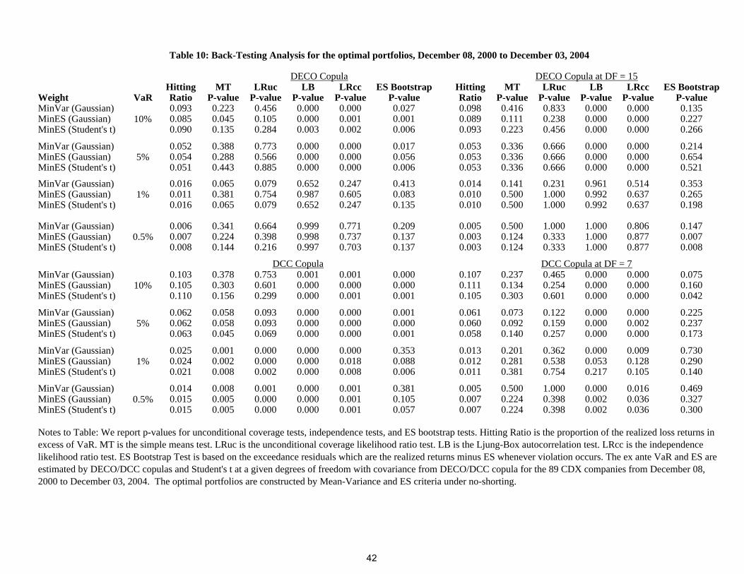
Hitting MT LRuc LB LRcc ES Bootstrap Hitting MT LRuc LB LRcc ES BootstrapWeight VaR Ratio P-value P-value P-value P-value P-value Ratio P-value P-value P-value P-value P-valueMinVar (Gaussian) 0.093 0.223 0.456 0.000 0.000 0.027 0.098 0.416 0.833 0.000 0.000 0.135MinES (Gaussian) 0.085 0.045 0.105 0.000 0.001 0.001 0.089 0.111 0.238 0.000 0.000 0.227MinES (Student's t) 0.090 0.135 0.284 0.003 0.002 0.006 0.093 0.223 0.456 0.000 0.000 0.266

MinVar (Gaussian) 0.052 0.388 0.773 0.000 0.000 0.017 0.053 0.336 0.666 0.000 0.000 0.214MinES (Gaussian) 0.054 0.288 0.566 0.000 0.000 0.056 0.053 0.336 0.666 0.000 0.000 0.654MinES (Student's t) 0.051 0.443 0.885 0.000 0.000 0.006 0.053 0.336 0.666 0.000 0.000 0.521

MinVar (Gaussian) 0.016 0.065 0.079 0.652 0.247 0.413 0.014 0.141 0.231 0.961 0.514 0.353MinES (Gaussian) 0.011 0.381 0.754 0.987 0.605 0.083 0.010 0.500 1.000 0.992 0.637 0.265MinES (Student's t) 0.016 0.065 0.079 0.652 0.247 0.135 0.010 0.500 1.000 0.992 0.637 0.198

MinVar (Gaussian) 0.006 0.341 0.664 0.999 0.771 0.209 0.005 0.500 1.000 1.000 0.806 0.147MinES (Gaussian) 0.007 0.224 0.398 0.998 0.737 0.137 0.003 0.124 0.333 1.000 0.877 0.007MinES (Student's t) 0.008 0.144 0.216 0.997 0.703 0.137 0.003 0.124 0.333 1.000 0.877 0.008

MinVar (Gaussian) 0.103 0.378 0.753 0.001 0.001 0.000 0.107 0.237 0.465 0.000 0.000 0.075MinES (Gaussian) 0.105 0.303 0.601 0.000 0.000 0.000 0.111 0.134 0.254 0.000 0.000 0.160MinES (Student's t) 0.110 0.156 0.299 0.000 0.001 0.001 0.105 0.303 0.601 0.000 0.000 0.042

MinVar (Gaussian) 0.062 0.058 0.093 0.000 0.000 0.001 0.061 0.073 0.122 0.000 0.000 0.225MinES (Gaussian) 0.062 0.058 0.093 0.000 0.000 0.000 0.060 0.092 0.159 0.000 0.002 0.237MinES (Student's t) 0.063 0.045 0.069 0.000 0.000 0.001 0.058 0.140 0.257 0.000 0.000 0.173

MinVar (Gaussian) 0.025 0.001 0.000 0.000 0.000 0.353 0.013 0.201 0.362 0.000 0.009 0.730MinES (Gaussian) 0.024 0.002 0.000 0.000 0.018 0.088 0.012 0.281 0.538 0.053 0.128 0.290MinES (Student's t) 0.021 0.008 0.002 0.000 0.008 0.006 0.011 0.381 0.754 0.217 0.105 0.140

MinVar (Gaussian) 0.014 0.008 0.001 0.000 0.001 0.381 0.005 0.500 1.000 0.000 0.016 0.469MinES (Gaussian) 0.015 0.005 0.000 0.000 0.001 0.105 0.007 0.224 0.398 0.002 0.036 0.327MinES (Student's t) 0.015 0.005 0.000 0.000 0.001 0.057 0.007 0.224 0.398 0.002 0.036 0.300

Table 10: Back-Testing Analysis for the optimal portfolios, December 08, 2000 to December 03, 2004

10%

5%

1%

0.5%

0.5%

1%

Notes to Table: We report p-values for unconditional coverage tests, independence tests, and ES bootstrap tests. Hitting Ratio is the proportion of the realized loss returns in excess of VaR. MT is the simple means test. LRuc is the unconditional coverage likelihood ratio test. LB is the Ljung-Box autocorrelation test. LRcc is the independence likelihood ratio test. ES Bootstrap Test is based on the exceedance residuals which are the realized returns minus ES whenever violation occurs. The ex ante VaR and ES are estimated by DECO/DCC copulas and Student's t at a given degrees of freedom with covariance from DECO/DCC copula for the 89 CDX companies from December 08, 2000 to December 03, 2004. The optimal portfolios are constructed by Mean-Variance and ES criteria under no-shorting.

DCC Copula at DF = 7DCC Copula

DECO Copula at DF = 15DECO Copula

10%

5%

42

Company Name Sector Average Rating Company Name Sector Average RatingHoneywell International Inc Industrial A Sherwin Williams Co Consumer Cyclical AFortune Brands Inc Consumer Stable BBB Weyerhaeuser Co Materials BBBDu Pont E I De Nemours & Co Materials A Computer Sciences Corp Communications and Technology BBBGeneral Electric Co Financial AAA Mcdonalds Corp Consumer Cyclical AGoodrich Corp Industrial BBB Marsh & Mclennan Cos Inc Financial BBBIngersoll Rand Co Ltd Industrial A New York Times Co Communications and Technology BBInternational Business Machs Cor Communications and Technology A Gannett Inc Communications and Technology BBBAltria Group Inc Consumer Stable BBB Union Pacific Corp Industrial BBBConocophillips Energy A Target Corp Consumer Cyclical AAmgen Inc Consumer Stable A Wal Mart Stores Inc Consumer Cyclical AAWyeth Consumer Stable A Conagra Inc Consumer Cyclical BBBKroger Company Consumer Stable BBB Nordstrom Inc Consumer Cyclical AC V S Caremark Corp Consumer Cyclical BBB Southwest Airlines Co Consumer Cyclical BBBGeneral Mills Inc Consumer Stable BBB American Express Co Financial APenney J C Co Inc Consumer Cyclical BBB Chubb Corp Financial ACaterpillar Inc Consumer Cyclical A Centurytel Inc Communications and Technology BBBDeere & Co Consumer Cyclical A Newell Rubbermaid Inc Industrial BBBBristol Myers Squibb Co Consumer Stable A C S X Corp Industrial BBBBoeing Co Financial A C I G N A Corp Financial BBBBlack & Decker Corp Industrial BBB Limited Brands Inc Consumer Cyclical BBDow Chemical Co Materials BBB Norfolk Southern Corp Industrial BBBLockheed Martin Corp Industrial A Dominion Resources Inc Va New Utilities BBBCardinal Health Inc Consumer Cyclical BBB A T & T Inc Communications and Technology AInternational Paper Co Materials BBB Home Depot Inc Consumer Cyclical BBBMotorola Inc Industrial BBB M D C Holdings Inc Consumer Cyclical BBBSara Lee Corp Consumer Stable BBB American International Group Inc Financial AFirstenergy Corp Utilities BBB Toll Brothers Inc Consumer Cyclical BBBProgress Energy Inc Utilities BBB Anadarko Petroleum Corp Energy BBBHalliburton Company Energy BBB Barrick Gold Corp Materials BBBAmerican Electric Power Co Inc Utilities BBB Carnival Corp Industrial AConstellation Energy Group Inc Utilities BBB Staples Inc Consumer Cyclical BBBAlcoa Inc Materials BBB Istar Financial Inc Financial BBBNorthrop Grumman Corp Industrial BBB Safeway Inc Consumer Stable BBBRaytheon Co Industrial A Autozone Inc Consumer Cyclical BBBCampbell Soup Co Consumer Stable A Macys Inc Consumer Cyclical BBBWhirlpool Corp Consumer Cyclical BBB Mohawk Industries Inc Consumer Stable BBBDisney Walt Co Consumer Cyclical A Kohls Corp Consumer Cyclical BBBLoews Corp Consumer Stable A Ace Ltd Financial ARyder Systems Inc Industrial A X T O Energy Inc Energy BBBHewlett Packard Co Communications and Technology A Transocean Inc New Energy BBBBaxter International Inc Consumer Stable A Allstate Corp Financial AXerox Corp Consumer Cyclical BBB Universal Health Services Inc Consumer Stable BBBArrow Electronics Inc Industrial BBB Eastman Chemical Co Materials BBBOmnicom Group Inc Communications and Technology A Simon Property Group Inc New Financial AMasco Corp Industrial BBB

Table 11: The List of 89 CDX Firms

43