Correlation Neglect in Portfolio Choice: Lab Evidence

Correlation Neglect in Portfolio Choice: Lab Evidence

Erik Eyster and Georg Weizsacker∗

October 28, 2016

Abstract

Optimal portfolio theory depends upon a sophisticated understanding of the correlation

among financial assets. In this paper, we examine people’s understanding of correla-

tion using portfolio-allocation problems and find it to be strongly imperfect. Our

experiment uses pairs of problems having the same span of assets—identical sets of

attainable returns—but different correlations between assets. While expected-utility

theory makes the same prediction across paired problems, subjects behave very dif-

ferently within pairs. We find evidence for correlation neglect—treating correlated

variables as uncorrelated—as well as for the “1/n heuristic”—investing half of wealth

each of the two available assets. (JEL B49)

Keywords: portfolio choice, correlation neglect, 1/n heuristic, biases in beliefs

∗Eyster: Department of Economics, London School of Economics (email: [email protected]); School of

Economics and Business, Humboldt Universitat zu Berlin & DIW Berlin (email: [email protected]).

An earlier version of this paper circulated under the title “Correlation Neglect in Financial Decision-Making”.

We thank Xavier Gabaix, Jacob Kes, Matthew Rabin, Sven Rady, Tobias Schmidt, Paul Viefers and nu-

merous seminar audiences for their comments, as well as Jacob Kes, Ameya Muley and Wei Min Wang for

superb research assistance. We thank the STICERD research centre at LSE, the ELSE Centre at UCL, the

Schweizerische Nationalbank (via ESSET 2008), the NIH, and the ERC (Starting Grant 263412) for funding,

and the Technical University Berlin for access to the decision laboratory.

1

1 Introduction

Financial decision-makers face a panoply of correlations across different asset returns. Yet

people have limited attention and find it cognitively challenging to work with joint distribu-

tions of multiple random variables. Even if the typical investor could in principle adequately

analyse financial variables’ co-movement, she still might fail to account for correlation prop-

erly at the moment of allocating her financial portfolio. As a consequence, investors may

hold portfolios that contain undesirable and avoidable risks. Many household investors invest

disproportionately in stock of their own employers (Benartzi 2001) or hold only a handful of

positively-correlated assets (Polkovnichenko 2005). Discussing the recent financial-markets

crisis, numerous commentators have asked whether both households and institutional in-

vestors relied on deficient risk modelling.1

In this paper, we explore people’s tendency to ignore correlation. Although such “correla-

tion neglect” may play an important role in numerous economic settings, we focus entirely on

its consequences for financial decision-making. The investment behaviours described above

are broadly consistent with correlation neglect—but also with a multitude of other forces.

To eliminate such confounds, we design and run a series of controlled experiments that

test people’s attention to correlation. Our experiment studies the standard textbook model

of portfolio choice with state-dependent returns and employs a novel framing variation in

which each participant faces two versions of the same portfolio-choice problem. Across the

two framing variations, we switch asset correlation on and off. Under the null hypothesis

that people correctly perceive the covariance structure, the framing variation does not affect

their behaviour. Nevertheless, we find that behaviour changes strongly, and our data analysis

supports two alternative hypotheses, both irresponsive to correlation. First, people tend to

ignore correlation and treat correlated assets as independent. Second, people tend to follow

a simple “1/n heuristic” that prescribes investing equal shares of a financial portfolio into

1Brunnermeier (2009) and Hellwig (2009) discuss erroneous perceptions of systemic risks during the crisis.

2

all available assets (as in Benartzi and Thaler (2001)). Our experimental data support these

theories despite the fact that, through an understanding test, we ensure that the participants

understand the payoff structure, including the co-movement of the asset returns. Consistent

with limited attention, participants appear to omit these considerations when choosing their

portfolios.

A small set of previous experiments examining people’s responses to correlation uncovers

evidence consistent with neglect. Kroll, Levy and Rapoport (1988) and Kallir and Sonsino

(2009) find that changing the correlation structure of a portfolio-choice problem leads to little

or no change in participants’ decision-making, even when many expected-utility preferences

common in the economics and finance literatures predict significant change. Correlation

neglect predicts no change in participants’ behaviour, consistent with the data.2 Our design

reverses the previous ones: whereas Kroll et al. (1988) and Kallir and Sonsino (2009) vary the

decision problems and find behaviour unchanged, we keep the decision problems economically

unchanged and find that behaviour changes. These two approaches complement each other

and together paint a consistent picture of correlation neglect.3

Our experimental design sharpens the findings of this past work because it allows us

to test the null hypothesis that people correctly appreciate correlation without making any

ancillary assumptions about subjects’ utility functions. Chiefly, we need not assume that

subjects are risk averse to test the null hypothesis that they correctly appreciate correlation.

In our paired-problems design, any fully rational agent will choose the same distribution

2Kroll et al. (1988) also report evidence that choices respond remarkably little to feedback on realized

returns. Kallir and Sonsino (2009) shed additional light on the cognitive nature of the bias that is consistent

with the interpretation of correlation neglect as deriving from limited attention: when asked to predict one

asset’s return conditional upon the other’s return, subjects demonstrate that they do perceive correlation

correctly despite making investment choices that do not incorporate this understanding.3Further closely related evidence is provided by Gubaydullina and Spiwoks (2009), whose participants fail

to minimize portfolio variance in a problem with correlated assets, but not in a different problem without

correlation.

3

of earnings in both investment problems because the set of available portfolios is identical

between them. This isomorphy arises because the assets in the correlated frame are linear

combinations of those in the uncorrelated frame and therefore span exactly the same set of

earnings distributions.4 Section 2 presents the main experiment, which involves four such

pairs of problems. In two of the problems, the correlated frame uses positive correlation

across assets, and in the other two it uses negative correlation. The set of problems with

correlated assets thus offers a nontrivial range of hedging opportunities, which may or may

not be appreciated by the participants.5

Section 3 describes the theoretical predictions for these choice problems. We begin by

describing the rational benchmark of expected utility maximisation under correct beliefs

about the correlation between asset payoffs. Such decision makers would choose identical

portfolios (namely, ones with the same terminal distribution over wealth) no matter which

of the two correlation frames she faced, regardless of risk preferences. Moreover, simply

assuming that the decision maker is risk averse—without imposing any restriction on the

degree of risk aversion— suffices to make a unique prediction in the three of our four pairs of

problems that have a unique portfolio that second-order stochastically dominates all others.

For the remaining pair, we utilise a quadratic approximation of the Bernoulli utility-of-wealth

function to make a unique prediction.

To model correlation neglect, we begin with both assets’ marginal distribution over pay-

offs and construct their product distribution over payoffs; someone who neglects correlation

misperceives payoffs as deriving from this product distribution—where, by construction, the

assets’ payoffs are uncorrelated—rather than from the true, correlated joint distribution.

4This statement is modulo a qualifier about necessary short-sales constraints, which we clarify in Section

2.5Our design is minimal in these sense that switching correlation between non-degenerate random variables

on and off requires at least as many assets (two), states of nature (four), and distinct monetary prizes (three)

as we employ.

4

Section 3 also introduces the third behavioural model that we consider, a decision-maker

who simply invests equal proportions of her wealth in each available asset, the “1/n heuris-

tic”. We also present a model of both covariance neglect and “variance neglect”—ignoring

differences in asset variances—that nests all three behavioural theories. As described below,

the 1/n heuristic may be viewed as an extreme version of variance neglect.

The data summary of Section 4 shows that very few participants choose equivalent port-

folios in paired choice problems. Only one out of 146 participants in the main experiment

behaves fully consistently, choosing four pairs of equivalent portfolios in the four pairs of

choices. Of the remaining participants, a majority (60%) does not choose even a single iso-

morphic pair of portfolios in any of the four pairs of choices. A surprising result appears

regarding the relative predictive value of the three basic models (rational, perceived inde-

pendence, 1/n). In linear regressions, the rational model adds no explanatory power to the

other two: regressing participants’ choices on the predictions of the first two or all three

models, the rational model attracts a point estimate with the wrong sign.

Section 5 further examines the patterns in subjects’ deviations from rationality. By

allowing people to underestimate both the covariance and variance of asset returns, we

build an estimable model that includes all three behavioural models described above in

addition to combinations of the three. First, participants’ perceptions of correlation may be

biased towards zero. Second, they may under-attend to variance; in particular, they may

underestimate the magnitude of differences between the entries of the variance-covariance

matrix. We model this through a concave transformation of variance. We classify subjects

into types according to two parameters, one measuring correlation neglect and the other

variance neglect. The single type that best fits the entire subject pool is one that entirely

neglects correlation and exponentiates variance to the power 0.43. In a mixture model with

type heterogeneity, the two types that best fit the subject pool are: a type covering ninety-one

percent of subjects that essentially coincides with the best-fitting single type just described

and a second, rational type best fitting the remaining nine percent of subjects. Adding

5

additional types does not significantly improve the statistical fit. Under the simplifying

assumption that all participants either correctly appreciate the covariance structure or show

one of the two extreme biases, we estimate that ten percent of the participants correctly

appreciate covariance.

Our study also includes a few more experimental demonstrations of correlation neglect,

which we present in Section 6. In one, we offer the participants two portfolios, the first riskier

than the second, with the property that if one mistakenly ignores the correlation between

the underlying assets the first portfolio appears to first-order stochastically dominate the

second portfolio. Indeed, almost all subjects choose the apparently dominant option. But in

a control treatment, where the the same two portfolios are offered but their true distributions

are explicitly shown to the subjects, about half of the subjects choose the second option.

Our final evidence for correlation neglect comes in a demonstration that participants

sometimes violate arbitrage freeness. In a separate task we present the participants with

three assets, where one asset is state-wise dominated by certain combinations of the other

two. Any investment in the dominated asset constitutes an arbitrage loss: spreading that

investment appropriately across the other two assets would yield more money in every state

of the world. More than three quarters of our subjects fall prey to this arbitrage. Section 7

concludes.

2 Experimental Design and Procedure

The following excerpt from the instructions shows one of the decision problems, labelled

Choice 3.

3. Invest each of your 60 points in either Asset E or Asset F, as given below.

6

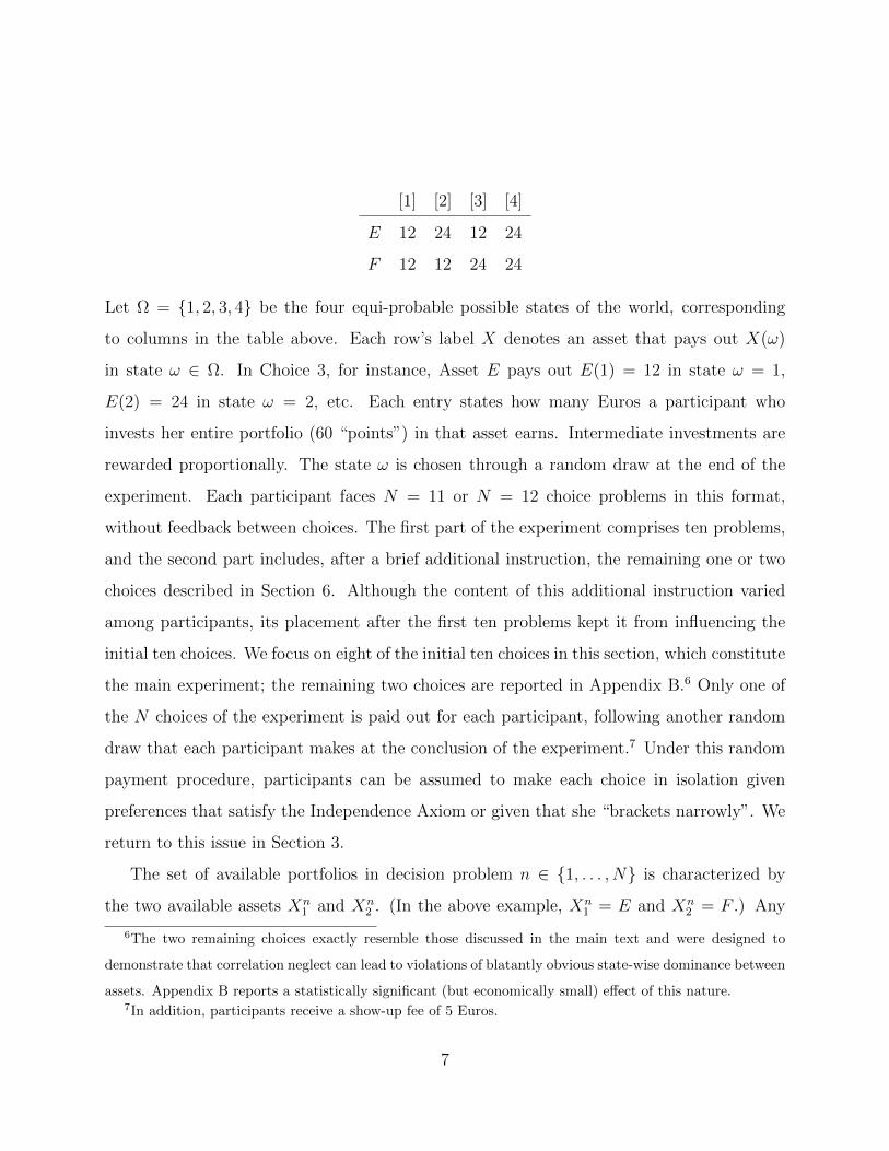
[1] [2] [3] [4]

E 12 24 12 24

F 12 12 24 24

Let Ω = 1, 2, 3, 4 be the four equi-probable possible states of the world, corresponding

to columns in the table above. Each row’s label X denotes an asset that pays out X(ω)

in state ω ∈ Ω. In Choice 3, for instance, Asset E pays out E(1) = 12 in state ω = 1,

E(2) = 24 in state ω = 2, etc. Each entry states how many Euros a participant who

invests her entire portfolio (60 “points”) in that asset earns. Intermediate investments are

rewarded proportionally. The state ω is chosen through a random draw at the end of the

experiment. Each participant faces N = 11 or N = 12 choice problems in this format,

without feedback between choices. The first part of the experiment comprises ten problems,

and the second part includes, after a brief additional instruction, the remaining one or two

choices described in Section 6. Although the content of this additional instruction varied

among participants, its placement after the first ten problems kept it from influencing the

initial ten choices. We focus on eight of the initial ten choices in this section, which constitute

the main experiment; the remaining two choices are reported in Appendix B.6 Only one of

the N choices of the experiment is paid out for each participant, following another random

draw that each participant makes at the conclusion of the experiment.7 Under this random

payment procedure, participants can be assumed to make each choice in isolation given

preferences that satisfy the Independence Axiom or given that she “brackets narrowly”. We

return to this issue in Section 3.

The set of available portfolios in decision problem n ∈ 1, . . . , N is characterized by

the two available assets Xn1 and Xn

2 . (In the above example, Xn1 = E and Xn

2 = F .) Any

6The two remaining choices exactly resemble those discussed in the main text and were designed to

demonstrate that correlation neglect can lead to violations of blatantly obvious state-wise dominance between

assets. Appendix B reports a statistically significant (but economically small) effect of this nature.7In addition, participants receive a show-up fee of 5 Euros.

7

portfolio is a lottery that assigns wealth W (ω) to state ω: a decision maker who invests the

fraction αn1 of her wealth (60 · αn1 “points”) into asset Xn1 and the remaining fraction 1− αn1

into asset Xn2 ends with wealth W (ω) = αn1X

n1 (ω) + (1 − αn1 )Xn

2 (ω) in state ω.8 We also

require that αn1 lie in some constraint set, Cn ⊂ R, which precludes short sales of either asset,

0 ≤ αn1 ≤ 1; in some cases it also includes more stringent constraints. The following table

shows our main eight choice problems by reproducing the eight specifications of (Xn1 , X

n2 ; Cn)

for n = 1, . . . , 8. The experiment presents the problems in two distinct sequences, attaches

abstract labels to states, and varies the order of presentation of states.

n Xn1 (1), Xn

1 (2), Xn1 (3), Xn

1 (4)Xn2 (1), Xn

2 (2), Xn2 (3), Xn

2 (4) Cn

1 15, 21, 15, 2112, 12, 24, 24 0 ≤ α11 ≤ 1

2 18, 30, 6, 1812, 12, 24, 24 0 ≤ α21 ≤ 1

2

3 12, 24, 12, 2412, 12, 24, 24 0 ≤ α31 ≤ 1

4 12, 24, 12, 2412, 18, 18, 24 0 ≤ α41 ≤ 1

5 14, 21, 14, 2114, 14, 21, 21 0 ≤ α51 ≤ 1

6 14, 21, 14, 2114, 0, 35, 21 23≤ α6

1 ≤ 1

7 12, 30, 12, 3012, 12, 30, 30 0 ≤ α71 ≤ 1

8 12, 30, 12, 3012, 18, 24, 30 0 ≤ α81 ≤ 1

Table 1: 8 portfolio-choice problems.

An important feature of the eight problems is that half—those with odd-numbered n—

involve only pairs of uncorrelated assets, whereas the other half involve non-zero correlations.

In Section 3, we explain how each even-numbered decision problem is isomorphic to its

immediate predecessor in the table.

The participants for the eight decision problems described above were 148 students of

Technical University Berlin, mostly undergraduate. Of these, two participants violated one

8Although the participants had to choose integer point allocations, placing αn1 onto a grid, for simplicity

we ignore this complication.

8

of the contraints Cn and their data were excluded from the analysis, leaving 146 complete

observations. The eight experimental sessions were conducted in a paper-and-pencil format

(with a translation of the German instructions in Online Appendix A) following a fixed

protocol and with the same experimenters present. Each session lasted about 90 minutes,

including all payments. Before the main part of the experiment, the participants underwent

an understanding test asking three questions about the payment rule, all of which the par-

ticipants needed to answer correctly before proceeding. About ten percent of participants

needed help from the experimenters to pass the understanding test.9 Controlled variations

of the eight decision problems were also used in four further sessions with 96 additional

participants (see Section 6).

3 Predictions

In this section, we develop predictions in our experiments that derive from different as-

sumptions about the decision maker’s choice behaviour. (A previous version of this paper,

Eyster and Weizsacker (2011), shows how weaker assumptions suffice for many of the pre-

dictions. See Ellis and Piccione (2015) for a related axiomatic treatment.) We first consider

an expected-utility maximiser with Bernoulli utility-of-wealth function u(w) who correctly

perceives correlation. In problem n, with choice set Cn, she chooses

αn ∈ arg maxα∈Cn

∑ω∈Ω

u (αXn1 (ω) + (1− α)Xn

2 ) p(ω),

where p(ω) is the probability of state ω. We assume that the decision maker has a unique

preference-maximising portfolio in each choice set included in the experiment. This implies

that whenever two portfolio-allocation problems have the same asset span, the decision maker

must make the same choice in each. In particular, a participant confronted with only a single

9When aiding participants, the experimenters did not produce the correct answer to ensure that each

participant find it independently.

9

choice problem in the experiment would make a choice that depended only upon the span of

assets in that problem. This observation holds not only for expected-utility preferences but

for all rational preference relations, regardless of whether they are continuous or satisfy the

Independence Axiom.

In our experiment, twinned problems are constructed to have identical asset spans. For

example, in Choices 3 (described in the last section) and Choice 4 (below), Asset G is

identical to Asset E, and Asset H equals 12E + 1

2F .

4. Invest each of your 60 points in either Asset G or Asset H, as given below.

[1] [2] [3] [4]

G 12 24 12 24

H 12 18 18 24

Someone who invests α ≥ 12

in Asset E of Choice 3 can achieve the same portfolio with

α = 2α−1 in Asset G of Choice 4. This holds because the remaining 1− α = 1− (2α− 1) =

2 (1− α) invested in Asset H, itself comprised of 12E+ 1

2F , gives 1

22 (1− α) = (1− α) invested

in Asset F, just like in Choice 3. Hence, any portfolio produced using α ≥ 12

in Choice 3

can be reproduced through a suitably constructed portfolio in Choice 4, and vice versa.

Although this argument breaks down for α < 12, the symmetry of Choice 3 across assets and

states suggests that anyone who wishes to invest less than one-half of her portfolio in Asset

E, essentially betting on State 3 over the symmetric State 2, should be equally willing to

invest more than one-half of her portfolio in Asset F. Indeed, any probability distribution

over wealth that is obtained by allocating α < 12

in E can also be obtained by investing

1 − α > 12

in E, and hence by an appropriate investment in the equivalent Choice 4. The

other three pairs of twinned problems have been constructed similarly so that every feasible

portfolio in the uncorrelated problem can be replicated in the correlated problem, and vice

versa.

If each subject in our experiment were to make only a single portfolio-allocation choice,

10

then a decision maker who correctly perceived correlations would take the same position (as

measured by the resulting state-contingent wealth lottery) in whichever of the two twinned

problems she faced. However, in our experiment each participant does not make a single

choice but instead a sequence of choices, with only one of these randomly chosen to be

paid out. Expected-utility preferences (in particular, the Independence Axiom) imply that a

decision maker who correctly perceives correlation chooses the same portfolio across twinned

problems.10

A standard assumption about preferences under uncertainty is that people dislike risk.

In three out of four pairs of twinned problems (Choices 3-8), knowing that the decision

maker is risk averse and correctly perceives correlations suffices to make unique predictions

about choices. For instance, consider Choice 3 and Choice 4. In both of them, any portfolio

leads to a payoff of 12 in state 1 and 24 in state 4. In Choice 3, investing αE in Asset

E and 1 − αE in Asset F gives payoffs 24αE + 12(1 − αE) = 12 + 12αE in state 2 and

s12αE + 24(1 − αE) = 24 − 12αE in state 3. Since states 2 and 3 occur with the same

probability, any risk averter prefers to receive the expected value of her money payoff across

the two states, 18, in each state to any available lottery. This can be achieved by choosing

αE = 12. Each of Choices 3 through 8 has the feature that in two states the decision maker

can do nothing to hedge her risk while in the remaining two she can perfectly hedge her risk

just as in this case.

In Choices 1 and 2, risk aversion alone does not suffice to identify subjects’ optimal

choice. For this case, we use a quadratic approximation of u. Since all feasible choices

10Yet Tversky and Kahneman (1981) and Rabin and Weizsacker (2009), among others, demonstrate that

participants in experiments often do not make choices on individual problems that take into account the

entire set of problems they have to solve—even when explicitly told to do so—but instead make each choice

in isolation, neglecting all remaining problems. Such narrow bracketing, as formally defined by Rabin and

Weizsacker (2009), provides another reason to think that subjects who correctly perceive correlations should

choose the same portfolio across twinned problems.

11

have the same mean, a decision maker with quadratic preferences chooses the portfolio that

minimises variance. Its value is indicated in the analysis in Section 4.

An alternative hypothesis to rationality is that the decision maker neglects the correlation

in assets’ returns, treating each asset as independent. Someone who neglects correlation acts

as if the state which governs Xn1 (ω) is independent of that which governs Xn

2 (ω). She then

chooses

αn ∈ arg maxα∈Cn

∑ω1∈Ω

∑ω2∈Ω

u (αXn1 (ω1) + (1− α)Xn

2 (ω2)) p(ω1)p(ω2).

Correlation neglect, together with expected utility, risk aversion, and quadratic utility makes

the unique prediction in every problem that the investor allocates her portfolio to minimise

her perceived portfolio variance. The resulting portfolios are also detailed in Section 4.

When X1 is positively correlated with X2, a correlation neglector underestimates the

variance in her portfolio, as stated in the following proposition where σ12 is the covariance

between X1 and X2. (See Appendix A for the proposition’s proof).

Proposition 1. When σ12 > 0 (respectively, σ12 ≤ 0), correlation neglect gives a weakly

more equal (unequal) split of wealth across assets than rationality.

When assets are positively correlated, a correlation neglector overestimates diversification

benefit of moving his her portfolio from a low-variance asset to a high variance one, which

leads her to take a more highly diversified portfolio than a rational decision maker, a form

of false diversification effect. When assets are negatively correlated, a correlation neglector

underestimates the diversification benefit of moving her portfolio from a low-variance asset

to a high variance one, which leads her to take a less diversified portfolio than a rational

decision maker, a form of hedging neglect.

We now consider our third behavioural theory, the 1/n heuristic. Benartzi and Thaler

(2001) have suggested that investors facing a menu of N different mutual funds often use

the simple heuristic of investing a fraction 1/n of wealth in each fund. In the context of our

12

experiment, investing half the portfolio in each of the two choices would lead an investor to

make different portfolios in paired problems.

We close this section by introducing a parametric model that combines the three be-

havioural models (given quadratic utility) through a transformation of the covariance ma-

trix. While much research has demonstrated people’s aversion to risk—even at its smallest

scale—that does not imply that people’s dislike for risk increases linearly, as the Indepen-

dence Axiom implies in this context. Like Fechner and Weber famously demonstrated with a

broad range of physical stimuli, people’s perception of or distaste for risk may increase slower

than linearly with variance. We capture this possibility by positing that people maximise

mean-variance preferences using the following transformed covariance matrix:

V (k, l) =

(σ21)l

k · sgn(σ12)|σ12|l

k · sgn(σ12)|σ12|l (σ22)l

.

The parameter k ∈ [0, 1] appears in the off-diagonal elements and captures people’s respon-

siveness to covariance. The lower is k, the less people attend to covariance. The parameter

l ≥ 0 captures how people’s dislike for risk depends upon its level. The lower is l, the

more people’s marginal dislike for risk diminishes with its level. This transformed covariance

matrix allows us to nest our several hypotheses about behaviour.

Rat: Subjects maximise expected utility under correct perceptions of correlated payoffs

across assets.

CorrNeg: Subjects maximise expected utility with k = 0, i.e. under the incorrect

perception of facing independent payoff across assets.

1/n: Subjects use the 1/n heuristic, i.e., l = 0.11

11Since V (k, 0) =

1 k

k 1

, someone with l = 0 perceives no difference between the two assets and

therefore invests half of her portfolio in each.

13

Finally, when k = 0 and l < 1, behaviour conforms to a correlation neglector who also

exhibits diminishing sensitivity to variance. We return to this parametric model in Section

5 but first turn to the main experimental result.

4 Raw Data and Analysis of Means

This section shows the raw data of the experiment and tests whether the participants take

on the same risks within the pairs of twinned decision problems, as is predicted by a correct

perception of the correlation. Overall, the data provides evidence consistent with both

directions of correlation neglect (CorrNeg and 1/n).

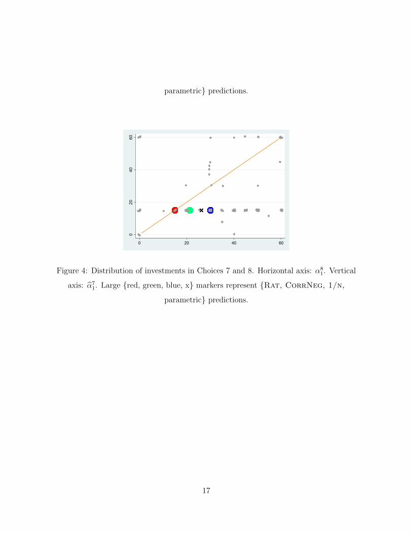
Figures 1 to 4 depict all choices by the participants. Each figure has the 146 participants’

choices in two paired problems, n − 1, n for n even, indicated by the small markers.

(The large markers are the predictions of the different behavioural assumptions, explained

below.) The horizontal axis in each figure measures investment in the first asset, αn1 , in the

even-numbered choice problem—the one with correlated assets. The vertical axis measures

investment in the first asset in the twinned odd-numbered problem n − 1 expressed in the

action space of problem n: αn−11 is the share that must be invested in problem n to achieve

the same distribution of earnings as αn−11 from problem n−1. By construction of the twinned-

problem design, this share is uniquely determined for each feasible investment in problem

n − 1 . Letting W n(ω) denote the earnings in problem n in state ω, for each αn−11 ∈ Cn−1

there exists a unique αn−11 ∈ Cn such that

∀x ∈ R,Pr[W n−1(ω) = x|αn−1

1

]= Pr

[W n(ω) = x|αn−1

1

]and thus each portfolio that the investor might choose in choice problem n− 1 corresponds

to a unique portfolio in problem n. The null hypothesis that participants correctly perceive

covariance gives a simple prediction for the figure: under the assumptions stated in Section

3, the two shares αn−11 and αn1 are identical, meaning that the data lie on the 45-degree line.

14

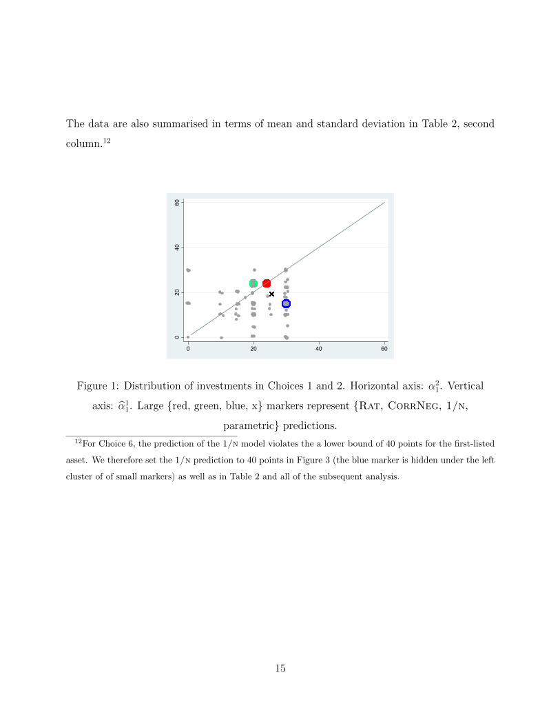
The data are also summarised in terms of mean and standard deviation in Table 2, second

column.12

020

40

60

0 20 40 60

Figure 1: Distribution of investments in Choices 1 and 2. Horizontal axis: α21. Vertical

axis: α11. Large red, green, blue, x markers represent Rat, CorrNeg, 1/n,

parametric predictions.

12For Choice 6, the prediction of the 1/n model violates the a lower bound of 40 points for the first-listed

asset. We therefore set the 1/n prediction to 40 points in Figure 3 (the blue marker is hidden under the left

cluster of of small markers) as well as in Table 2 and all of the subsequent analysis.

15

020

40

60

0 20 40 60




40

45

50

55

60

40 45 50 55 60



16


020

40

60

0 20 40 60




17

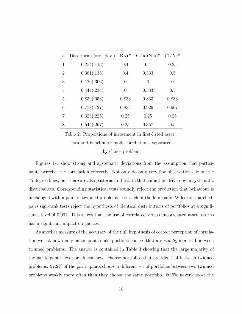
n Data mean (std. dev.) Ratn CorrNegn (1/N)n

1 0.254(.113) 0.4 0.4 0.25

2 0.381(.138) 0.4 0.333 0.5

3 0.126(.306) 0 0 0

4 0.444(.234) 0 0.333 0.5

5 0.839(.053) 0.833 0.833 0.833

6 0.778(.127) 0.833 0.929 0.667

7 0.328(.225) 0.25 0.25 0.25

8 0.545(.267) 0.25 0.357 0.5

Table 2: Proportions of investment in first-listed asset.

Data and benchmark model predictions, separated

by choice problem

Figures 1-4 show strong and systematic deviations from the assumption that partici-

pants perceive the correlation correctly. Not only do only very few observations lie on the

45-degree lines, but there are also patterns in the data that cannot be driven by unsystematic

disturbances. Corresponding statistical tests soundly reject the prediction that behaviour is

unchanged within pairs of twinned problems. For each of the four pairs, Wilcoxon matched-

pairs sign-rank tests reject the hypothesis of identical distributions of portfolios at a signifi-

cance level of 0.001. This shows that the use of correlated versus uncorrelated asset returns

has a significant impact on choices.

As another measure of the accuracy of the null hypothesis of correct perception of correla-

tion we ask how many participants make portfolio choices that are exactly identical between

twinned problems. The answer is contained in Table 3 showing that the large majority of

the participants never or almost never choose portfolios that are identical between twinned

problems. 97.2% of the participants choose a different set of portfolios between two twinned

problems weakly more often than they choose the same portfolio. 60.9% never choose the

18

same portfolio twice.

# Freq. % Cum. %

0 89 60.9 60.9

1 37 25.3 86.2

2 16 11.0 97.2

3 3 2.1 99.3

4 1 0.7 100.0

Total 146 100.0

Table 3: Frequencies of choosing identical portfolios in twinned

choice problems (out of 4)

Of course, the deviations may be influenced by different sources and we must to be careful

not to interpret random deviations from the 45-degree line as evidence of correlation neglect.

We therefore turn to statistical estimations that allow us to conclude that the deviations from

the prediction of Assumptions A and B are indeed systematic in the way that we hypothesise.

The first such estimation is an OLS regression that summarises the statistical connection

between the data and extreme predictions CorrNeg and (1/n). These predictions are

indicated in the figures—the green and blue marker, respectively—as well as in Columns

4 and 5 of Table 2. As a benchmark prediction, the figures and Table 2 also contain the

“rational” prediction Rat (red marker) of a risk averter who understands the correlation

structure.The dependent variable in the regression is the vertical distance of the data points

from the 45-degree line in the figure. The explanatory variables are, analogously, the vertical

distances of the two predictions from the 45-degree line, CorrNegn−1−CorrNegn and

1/nn−1−(1/n)n, respectively.13

13The estimated model is

αn−1,i1 − αn,i

1 = β2( CorrNegn−1,i

−CorrNegn,i) + β3(1/nn−1,i

− (1/n)n,i) + νn,i

19

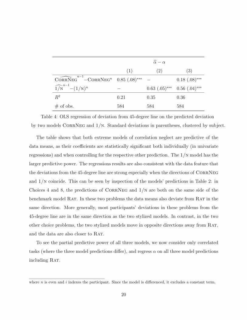
α− α

(1) (2) (3)

CorrNegn−1−CorrNegn 0.85 (.08)∗∗∗ − 0.18 (.08)∗∗∗

1/nn−1−(1/n)n − 0.63 (.05)∗∗∗ 0.56 (.04)∗∗∗

R2 0.21 0.35 0.36

# of obs. 584 584 584

Table 4: OLS regression of deviation from 45-degree line on the predicted deviation

by two models CorrNeg and 1/n. Standard deviations in parentheses, clustered by subject.

The table shows that both extreme models of correlation neglect are predictive of the

data means, as their coefficients are statistically significant both individually (in univariate

regressions) and when controlling for the respective other prediction. The 1/n model has the

larger predictive power. The regressions results are also consistent with the data feature that

the deviations from the 45-degree line are strong especially when the directions of CorrNeg

and 1/n coincide. This can be seen by inspection of the models’ predictions in Table 2: in

Choices 4 and 8, the predictions of CorrNeg and 1/n are both on the same side of the

benchmark model Rat. In these two problems the data means also deviate from Rat in the

same direction. More generally, most participants’ deviations in these problems from the

45-degree line are in the same direction as the two stylized models. In contrast, in the two

other choice problems, the two stylized models move in opposite directions away from Rat,

and the data are also closer to Rat.

To see the partial predictive power of all three models, we now consider only correlated

tasks (where the three model predictions differ), and regress α on all three model predictions

including Rat.

where n is even and i indexes the participant. Since the model is differenced, it excludes a constant term.

20

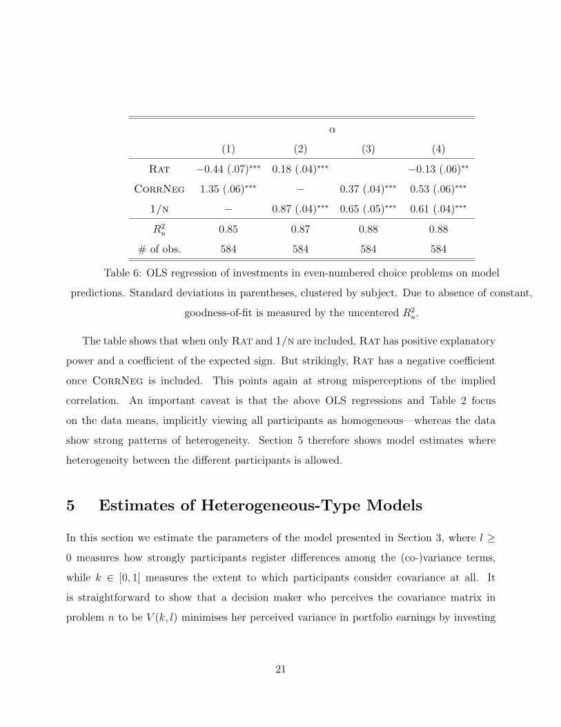
α

(1) (2) (3) (4)

Rat −0.44 (.07)∗∗∗ 0.18 (.04)∗∗∗ −0.13 (.06)∗∗

CorrNeg 1.35 (.06)∗∗∗ − 0.37 (.04)∗∗∗ 0.53 (.06)∗∗∗

1/n − 0.87 (.04)∗∗∗ 0.65 (.05)∗∗∗ 0.61 (.04)∗∗∗

R2u 0.85 0.87 0.88 0.88

# of obs. 584 584 584 584

Table 6: OLS regression of investments in even-numbered choice problems on model

predictions. Standard deviations in parentheses, clustered by subject. Due to absence of constant,

goodness-of-fit is measured by the uncentered R2u.

The table shows that when only Rat and 1/n are included, Rat has positive explanatory

power and a coefficient of the expected sign. But strikingly, Rat has a negative coefficient

once CorrNeg is included. This points again at strong misperceptions of the implied

correlation. An important caveat is that the above OLS regressions and Table 2 focus

on the data means, implicitly viewing all participants as homogeneous—whereas the data

show strong patterns of heterogeneity. Section 5 therefore shows model estimates where

heterogeneity between the different participants is allowed.

5 Estimates of Heterogeneous-Type Models

In this section we estimate the parameters of the model presented in Section 3, where l ≥

0 measures how strongly participants register differences among the (co-)variance terms,

while k ∈ [0, 1] measures the extent to which participants consider covariance at all. It

is straightforward to show that a decision maker who perceives the covariance matrix in

problem n to be V (k, l) minimises her perceived variance in portfolio earnings by investing

21

the fraction αn1 (k, l) =(σ2

2)l−k|σ12|l·sgn(σ12)

(σ21)l+(σ2

2)l−2k|σ12|l·sgn(σ12)of wealth in the first asset.14 We begin by

estimating separate maximum-likelihood values of (k, l) for each individual separately, using

her four decisions that involve correlated assets.15

For the estimation, we assume that participant i when making her choice αn,i1 has her

own individual-specific parameter vector (ki, li) and follows the prediction αn,i1 = αn1 (ki, li)

except insofar as she is subject to the disturbance term εni ): she chooses the investment level

60 · (αn1 (ki, li) + εni , rounded to the nearest integer value. We assume that the distribution of

εni is logistic and i.i.d. across i and n. The likelihood of observing the participant’s quadruple

αi1 = (α2,i1 , α

4,i1 , α

6,i1 , α

8,i1 ) is therefore given by

L(αi1|ki, li) =∏

n=2,4,6,8

Pr[αn1 (ki, li) + εni = αn,i1

]Maximizing this likelihood separately for each individual gives the distribution of estimates

depicted in Figure 5, where the estimate of li appears on the horizontal axis and ki on the

vertical axis.

14The proof of Proposition 1 in Appendix A contains this derivation for the case where l = 1; the extension

to general l is immediate.15All estimations in this section include only Choices 2, 4, 6 and 8 because in most odd-numbered tasks

the predictions coincide for all values of k and l.

22

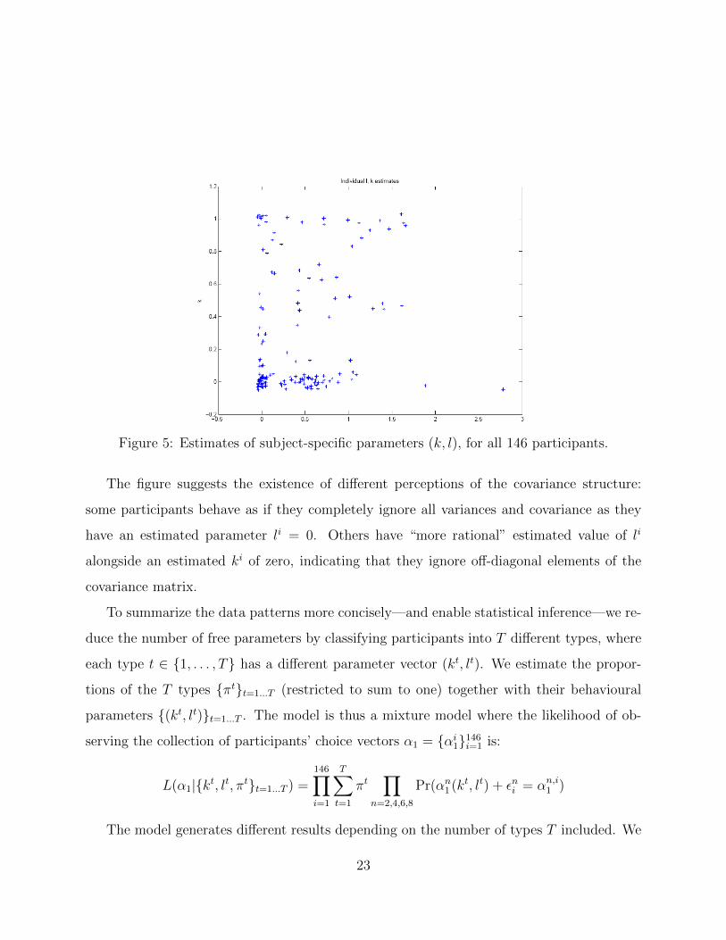
Figure 5: Estimates of subject-specific parameters (k, l), for all 146 participants.

The figure suggests the existence of different perceptions of the covariance structure:

some participants behave as if they completely ignore all variances and covariance as they

have an estimated parameter li = 0. Others have “more rational” estimated value of li

alongside an estimated ki of zero, indicating that they ignore off-diagonal elements of the

covariance matrix.

To summarize the data patterns more concisely—and enable statistical inference—we re-

duce the number of free parameters by classifying participants into T different types, where

each type t ∈ 1, . . . , T has a different parameter vector (kt, lt). We estimate the propor-

tions of the T types πtt=1...T (restricted to sum to one) together with their behavioural

parameters (kt, lt)t=1...T . The model is thus a mixture model where the likelihood of ob-

serving the collection of participants’ choice vectors α1 = αi1146i=1 is:

L(α1|kt, lt, πtt=1...T ) =146∏i=1

T∑t=1

πt∏

n=2,4,6,8

Pr(αn1 (kt, lt) + εni = αn,i1 )

The model generates different results depending on the number of types T included. We

23

ran the estimations for up to T = 5 and report the results for T ∈ 1, 2, 3 in Table 7. For

T = 4, 5, the results are qualitatively similar to the case T = 3 but the likelihood is scarcely

improved relative to T = 3.

T ll∗ (l1, k1, π1) (l2, k2, π2) (l3, k3, π3)

1 −2296.6 (0.43, 0, 1) − −

2 −2288.4 (0.39, 0, 0.91) (1.1, 1, 0.09) −

3 −2286.2 (0.45, 0, 0.58) (1.09, 1, 0.1) (0,−, 0.3)

Table 7: Estimates of parametric mixture model with T ∈ 1, 2, 3 types.

The table’s first row of entries shows the result under the restriction that all participants

belong to a single type, T = 1. The best-fitting indicate that the estimated single type in

this model completely ignores the off-diagonal elements of the covariance matrix (k1 = 0)

and only partially reacts to differences in the assets’ variances (l1 = 0.43). This resembles

the prediction CorrNeg yet echoes 1/n through substantial insensitivity to differences in

variance. This model is rejected in favor of the two-type model T = 2 (p < 0.01, likelihood-

ratio test), where the best-fitting two co-existent types are quite different in nature: the

primary type (π1 = 0.91) resembles the one estimated in the single-type model, while the

secondary type bears much closer semblance to the rational prediction of full appreciation

of correlation. Finally, with T = 3, the best-fitting parameter constellation also includes

a pure 1/N type. The result of the T = 3 estimation is thus not too far from a model

consisting of the three archetypical types CorrNeg, Rat and 1/n all appear: each of these

three extreme types is reasonably well approximated by one of the three estimated types.16

16Estimating a model that includes only the three extreme types, CorrNeg, Rat and 1/n, in unknown

proportion yields estimates markedly different from those in Table 7 and reminiscent of the linear regression

in Table 4: the 1/n type gets weight πsc1/n = 0.75, while the CorrNeg type gets only weight πscCorrNeg =

0.16. This shows that the first-listed type estimate in Table 7, which is similar to CorrNeg, would be much

less accurate if l = 1 was assumed instead of leaving l unrestricted.

24

However, the T = 2 specification is not rejected in favor of T = 3 (p=0.221): adding a 1/n

type does not significantly improve fit over the rational and (modified) CorrNeg type.

In sum, our most reliably estimated single type is that estimated when T = 1. We depict

that prediction in Figures 1 to 4 with an “x”. In each case, the x likes near the centre of the

data point cloud (and closely matches the sample means presented in Table 2).

6 Additional Demonstrations of Correlation Neglect

We designed two additional experimental tasks to elicit correlation neglect in ways other

than those of the previous sections. Different participants receive different instructions for

these additional tasks. As noted earlier, because all of the additional tasks appear after the

main part of the experiment, these differences in instructions could not affect the results

discussed in the previous sections.

A notable modification from the previously discussed problems is that the expected re-

turn varies across assets. Yet all additional tasks are portfolio-choice problems of the same

general format as in the experiment’s main part. Only very brief additional instructions are

therefore needed between the two parts of the experiment. Section 6.1 describes the first

set of additional tasks, presented to three different subgroups of participants after the main

experiment. Section 6.2 describes the second set of tasks, presented again to other subgroups

of participants. For the task described in Section 6.2, a set of new participants were used,

as described later.

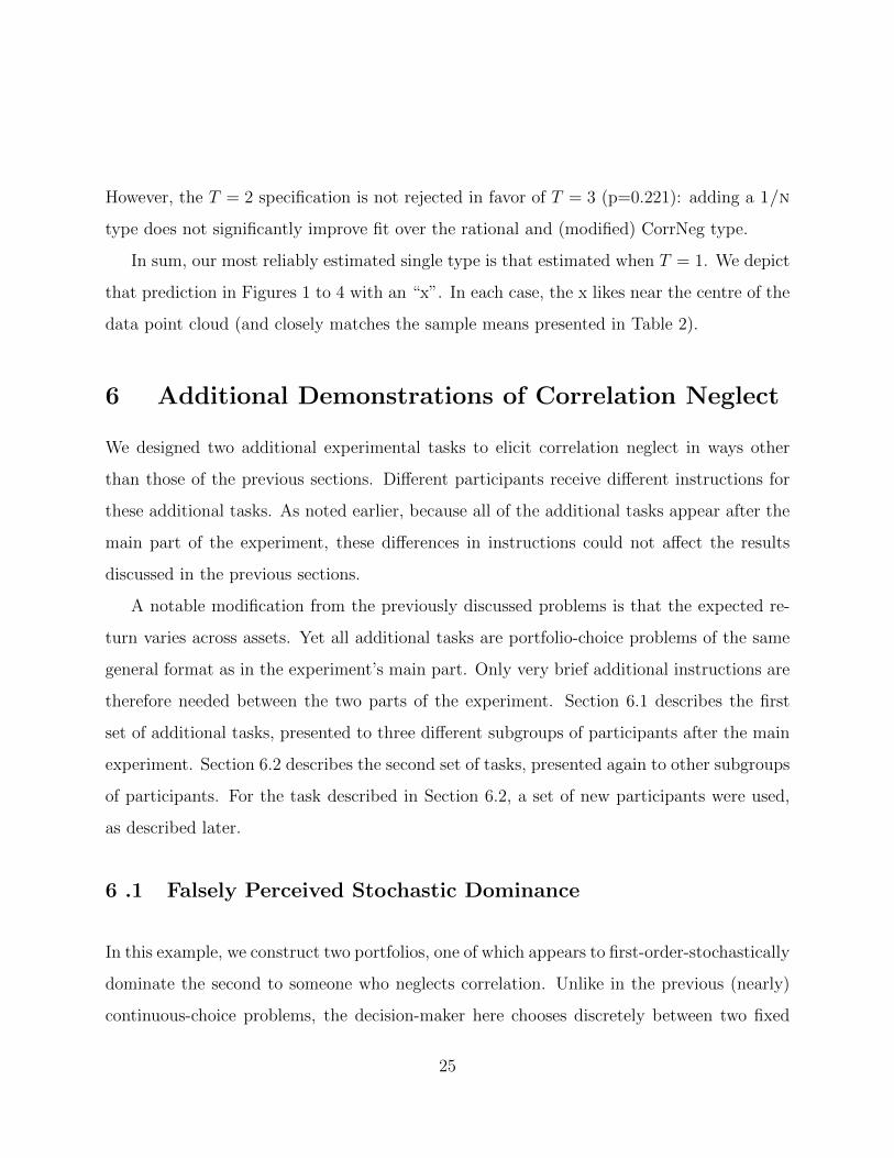
6 .1 Falsely Perceived Stochastic Dominance

In this example, we construct two portfolios, one of which appears to first-order-stochastically

dominate the second to someone who neglects correlation. Unlike in the previous (nearly)

continuous-choice problems, the decision-maker here chooses discretely between two fixed

25

portfolios, each one holding a strictly positive amount of both assets. The asset distributions

and contents of the two available portfolios have the property that a decision-maker who

ignores covariance, like the correlation neglector of the previous sections, falsely perceives a

first-order stochastic dominance relation between the two available portfolios.

[1] [2] [3]

U 30 20 12

V 10 12 30

Please indicate your preferred investment, by ticking the box:

I invest 52 points in Asset U and 8 points in Asset V .

I invest 26 points in Asset U and 34 points in Asset V .

Clearly, U has a higher return distribution than V , with a difference in means of 103

. This

makes the first choice relatively more attractive due to its high weight on U . On the

other hand, the negative correlation between the assets may entice a sufficiently risk averse

decision-maker to take the safer second choice.

Crucially, the task is designed such that a correlation neglector who ignores the negative

correlation would never choose the safe option. It is straightforward to show that if the

two assets are perceived to be independent then the first choice first-order stochastically

dominates the second choice.

The task was presented to 30 subjects, 29 of whom (97%) chose the first option. This

result is consistent with the presence of correlation neglectors. However, it may also be

driven by rational preference maximization—perhaps all of these 29 participants correctly

perceived the covariance structure but are not sufficiently risk averse to avoid the relatively

higher risk. To demonstrate the effect of the perception of the covariance structure, we

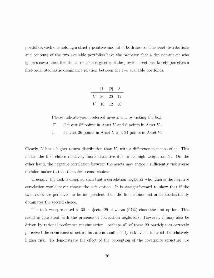
26

therefore repeat the task with 39 different participants, presenting the same portfolios in a

way that does away with any need to contemplate covariance.

[1] [2] [3]

U ′ 27.3 18.9 14.4

V ′ 15.5 18.7 22.2

Please indicate your preferred investment by ticking the box:

I invest 60 points in Asset U ′ and 0 points in Asset V ′.

I invest 0 points in Asset U ′ and 60 points in Asset V ′.

The reader can verify that the return distributions of assets U ′ and V ′ are identical to

the distributions resulting from the two choice options in the first problem, involving assets

U and V (up to rounding error). Therefore the two choice options in the second problem,

each allowing only investments of all wealth in one asset, are identical to those in the first

problem—a pure framing variation. Without any diversification opportunity, covariance

between the available options is irrelevant to the second problem, so that even correlation

neglectors would not err. The pair of problems therefore produces the possibility of preference

reversals for correlation neglectors. Indeed we see a significant change in behaviour: in the

second framing variation of the problem, only 20 out of 39 participants (51%) choose the

fist option.17 The difference between results in the two framing variations is significant at

p < 0.01 (Wilcoxon two-sample test).

17The result is further corroborated by additional framing variations that replace only one of the two

portfolios consisting of Assets U and V by a portfolio whose state-contingent return is explicitly presented.

34 subjects (all of whom are included in the analysis of Sections 2-5 but not that of Section 6 up until this

point) face the same binary task twice, in two different framing variations hard to recognize as identical.

In the first variation, the first option (52 points in U and 8 points in V ) appears as the option of investing

everything in U ′. In the second variation, the second option (26 points in U and 34 points in V ) is replaced

by the option of investing everything in V ′. Under both variations, correlation neglect is irrelevant, so that

27

6 .2 Ignorance of Abitrage

Not only may people who neglect correlation perceive first-order-stochastic dominance where

it is not, but they may fail to perceive it where it is. In our portfolio-choice setting, the

may choose one portfolio over a second that pays higher returns in every possible state.

We explore this possibility through two portfolio-choice problems that each use three assets.

Each problem is designed such that there exist portfolios combining two assets that statewise

dominate the third. Any investment in the third therefore violates “arbitrage freeness”.

These two tasks are presented at the end of the experiment (like those in Section 6.1) to 40

participants of the main experiment described in Section 2 and to 96 new participants. The

96 new participants first face the same instructions and tasks as in the main experiment, the

only difference being that in the four problems involving correlated assets (Choices 2, 4, 6, 8)

their choice options are restricted to two portfolios. (The results of these restricted tasks

essentially confirm the results of the previous sections and we skip them for brevity.) A total

of 136 participants completed the two tasks described here.

11. Invest each of your 60 points in Asset U ′′, Asset V ′′ or Asset W ′′, as given below.

[1] [2] [3]

U ′′ 15 38 7

V ′′ 39 5 16

W ′′ 20 15 13

In the first of the two additional tasks, Choice 11, participants choose their portfolio

a correlation neglector should behave exactly as in the case where both choice options are shown as U ′ and

V ′. Indeed, 18 out of 33 participants (55%) opt for the first choice option under the first framing variation

(one participant did not fill in the decision sheet) and 16 out of 34 participants under the second framing

variation.

28

weights on Assets U ′′, V ′′ and W ′′, as depicted above.18 One can check easily that asset W ′′

is dominated by a continuum of combinations of U ′′ and V ′′—in particular it is dominated

by 13U ′′+ 2

3V ′′ (with a expected return difference of 4 Euros—rather a large difference). This

arbitrage derives from the negative correlation of U ′′ and V ′′ that allows an effective insurance

against their respective low-return outcomes. But many participants appear to neglect the

hedging opportunity: the average portfolio weight of W ′′ is 0.257, close to the uniform

weight. (The average weights of U ′′ and V ′′ are 0.346 and 0.397 respectively.) Moreover,

the distribution of investments reveals that 84 out of 136 participants (75%) invest a strictly

positive wealth share in W ′′. That is, a large majority of subjects makes a dominated choice

in this task.

The last-mentioned result is even more pronounced in the second additional task:

12. Invest each of your 60 points in Asset X, Asset Y or Asset Z, as given below.

[1] [2] [3]

X 14 22 12

Y 27 5 16

Z 18 16 13

Here, Asset Z is dominated by a continuum of combinations of X and Y—for example

by 23X + 1

3Y . Only 19 out of 136 participants (14%) invested nothing in Z and thereby

avoided the dominated investment. The remaining 86% of subjects appear not to appreciate

the dominance relation that arises due to negative correlation of X and Y . The average

portfolio weights of X, Y and Z are 0.399, 0.308 and 0.293 respectively.

18In the experiment the asset labels are U , V and W (symbols that we already used for other participants’

problems).

29

7 Conclusion

This paper has presented a sequence of portfolio-choice experiments demonstrating that

people’s asset allocations depend strongly upon how financial assets are framed, in particular

whether the same asset span is generated using correlated or uncorrelated assets. At the

broadest level, participants systematically violate the “reduction of compound lotteries”

property that underlies the theory of choice under uncertainty: the same portfolio appeals

to people differently depending upon how it is constructed.

Our experiments also provide evidence that people succumb to a specific form of framing

effect in financial decision-making, namely they neglect correlation in asset returns. In

part, this may derive from the form of 1/n rule that Benartzi and Thaler (2001) observe

in financial decision-making, which also has been uncovered in other contexts. Simonson

(1990) as well as Read and Loewenstein (1995) have suggested that people use strategies of

“naive diversification” by instinctively diversifying their choices despite having underlying

preferences that do not warrant such diversification. For instance, a trick-or-treater who

prefers Mars to Snickers bars may too frequently choose Snickers over Mars so as not to end

up with an unbalanced candy supply. Indeed, restaurant-goers often seem reluctant to order

dishes that previously ordered by their companies, even when they know that they will not

share dishes.

In settings where people’s choice sets are imperfectly observed, the 1/n heuristic provides

the modeller with little guidance as to what predictions to make about behaviour. By

contrast, our model of correlation neglect predicts how people’s choices depart systematically

from what they would choose had they taken correlation into account fully. In a two-asset

setting, Proposition 1 establishes that when correlation is positive, correlation neglectors

diversify more than standard theory predicts—exaggerating the benefit of diversification—

while when correlation is negative they diversify too little—under-appreciating its benefit.

People who systematically under-appreciate correlation have a lower willingness to pay for

30

assets that hedge their portfolio risk and a higher willingness to pay for assets that magnify

their portfolio risk. Without perfect arbitrage (see, e.g., Shleifer (2000) for limits to arbi-

trage), a systematic under-appreciation of correlation may thus cause hedging opportunities

to be systematically underpriced in financial transactions or markets.

Finally, our data analysis provides novel evidence that once endowed with risk, people’s

dislike for more risk decreases. Koszegi and Rabin (2007) propose a theory of reference-

dependent risk preferences under which people with deterministic reference lotteries are

more averse to risk that those with stochastic reference lotteries. In the context of our

experiment, participants who bracket narrowly may become inoculated by unavoidable risk

against the pain of taking on discretionary risk. Experiments designed explicitly to test for

diminishing sensitivity to risk (variance) might help researchers better understand the scale

and scope of this phenomenon.

Although we have only examined it in the context of portfolio choice, correlation neglect

likely has implications in a variety of domains. For example, Enke and Zimmermann (2015)

provide evidence that people neglect the correlation between signals when these signals use a

common source. Of course, signals only serve as signals to the extent that people appreciate

the correlation between the signal realisation and the underlying state of the world. Rather

than act as a uniform general bias, the neglect of correlation is likely to bias perceptions

of some correlations far more than others. Our very simple environment has the advantage

that the only correlations present are those between asset returns, which are precisely those

correlations to which we believe people under-attend.

References

Benartzi, S.: 2001, Excessive extrapolation and the allocation of 401(k) accounts to company

stock?, Journal of Finance 56(5), 1747–1764.

31

Benartzi, S. and Thaler, R.: 2001, Naive diversification strategies in defined contribution

saving plans, American Economic Review 91(1), 79–98.

Brunnermeier, M.: 2009, Deciphering the liquidity and credit crunch 2007-2008, Journal of

Economic Perspectives 23(1), 77–100.

Ellis, A. and Piccione, M.: 2015, Complexity, correlation, and choice, Mimeo .

Enke, B. and Zimmermann, F.: 2015, Correlation neglect in belief formation, Mimeo .

Eyster, E. and Weizsacker, G.: 2011, Correlation neglect in financial decision-making, DIW

Berlin Discussion Paper (1104).

Gubaydullina, Z. and Spiwoks, M.: 2009, Portfolio diversification: an experimental study.

Hellwig, M.: 2009, Systemic risk in the financial sector: An analysis of the subprime-

mortgage financial crisis, De Economist 157(2), 129–207.

Kallir, I. and Sonsino, D.: 2009, The neglect of correlation in allocation decisions, Southern

Economic Journal 75(4), 1045–1045.

Koszegi, B. and Rabin, M.: 2007, Reference-dependent risk attitudes, American Economic

Review 97(4), 1047–1073.

Kroll, Y., Levy, H. and Rapoport, A.: 1988, Experimental tests of the separation theorem

and the capital asset pricing model, American Economic Review 78(3), 500–519.

Polkovnichenko, V.: 2005, Household portfolio diversification: A case for rank-dependent

preferences, Review of Financial Studies 18(4), 1467–1502.

Rabin, M. and Weizsacker, G.: 2009, Narrow bracketing and dominated choices, American

Economic Review 99(4), 1508–1543.

32

Read, D. and Loewenstein, G.: 1995, Diversification bias: Explaining the discrepancy in

variety seeking between combined and separated choices, Journal of Experimental Psy-

chology: Applied 1(1), 34–49.

Shleifer, A.: 2000, Inefficient markets: an introduction to behavioral finance, Oxford Univer-

sity Press.

Simonson, I.: 1990, The effect of purchase quantity and timing on variety seeking behavior,

Journal of Marketing Research 32, 150–162.

Tversky, A. and Kahneman, D.: 1981, The framing of decisions and the psychology of choice,

Science 211(4481), 453–458.

33

A Appendix: Proof

Proof of Proposition 1 Let

V =

σ21 kσ12

kσ12 σ22

.

be the covariance matrix. The variance of a portfolio investing share α in X1 is then

var(αX1 + (1 − α)x2) = α2σ21 + (1 − α)2σ2

2 + 2α(1 − α)σ12. At an interior minimum,

α1 =σ22−kσ12

σ21+σ2

2−2kσ12, so

sgn

(∂α1

∂k

)= sgn

(−σ12

(σ2

1 + σ22 − 2kσ12

)+ 2σ12

(σ2

2 − kσ12

))= sgn

(σ12

(σ2

2 − σ21

)).

Wlog assume that σ22−σ2

1 ≥ 0 so that α1 ≥ 12. When σ12 > 0, α1 is increasing in k, meaning

that a correlation neglector with k = 0 chooses a portfolio closer to 50-50 than a rational

agent. Conversely, when σ12 < 0, α1 is decreasing in k, meaning that a correlation neglector

with k = 0 chooses a portfolio further from 50-50 than a rational agent. Q.E.D.

B Appendix: Further Results on Ignored Dominance

Relation

This appendix presents the two remaining investment tasks, Choices 9 and 10, that are

presented together with the eight choice problems discussed in Sections 1-5. Both tasks use

two assets, where one asset statewise dominates the other.

9. Invest each of your 60 points in either Asset Q or Asset R, as given below.

[1] [2] [3] [4]

Q 16 15 20 21

R 14 15 19 18

34

10. Invest each of your 60 points in either Asset S or Asset T, as given below.

[1] [2] [3] [4]

S 18 17 19 18

T 16 16 17 17

The main difference between the two tasks is that in Choice 10, the minimum return of

asset S weakly exceeds the maximum return of Asset T , whereas the same is not true for Q

and R in Choice 9. Therefore, even the correlation neglector would recognise that any strictly

positive portfolio weight on T is statewise dominated (in the hypothetical state space of the

correlation neglector) by the portfolio that invests all wealth in S. By contrast, in Choice 9

the correlation neglector would not even perceive a first-order schochastic dominance relation

and may for some (very risk-averse) preferences invest a positive proportion of wealth in R,

which has illusory diversification benefit.19

The results indeed show a statistically significant difference between the two choice prob-

lems, yet the difference is small. In both, participants choose high portfolio weights on the

superior assets: in Choice 9, the average weight on Q was 0.85, while in Choice 10, the

average weight was 0.88 (N = 242).20 The difference is statistically significant at p = 0.004

(Wilcoxon test). The number of participants who invest a strictly positive proportion of

wealth in the dominated asset is also higher in Choice 9 (38%) than in Choice 10 (31%),

confirming that the statewise dominance is obeyed more stringently in the choice problem

where all correlation neglectors agree with the optimality of the dominating choice.

19The two choice problems have equal monetary incentives for a rational risk-neutral agent: the first asset

has a mean return of 18 and the second-listed asset a mean return of 16.5.20The reported results include the 96 additional participants who received some of the other problems

with a restricted choice set, see Section 6. The results for the main 146 participants are close to identical

but show somewhat lower significance levels.

35

Correlation Neglect in Portfolio Choice: Lab Evidence

Documents

Transcript of Correlation Neglect in Portfolio Choice: Lab Evidence