AP Calculus BC Notes - Asher Roberts
409
AP Calculus BC Notes Calculus: Early Transcendentals 8th Edition by James Stewart Asher Roberts For educational use only
-
Upload
khangminh22 -
Category
Documents
-
view
11 -
download
0
Transcript of AP Calculus BC Notes - Asher Roberts
AP Calculus BC Notes
Calculus: Early Transcendentals 8th Editionby James Stewart
Asher Roberts
For educational use only


Contents
1 Functions and Models 1
1.1 Four Ways to Represent a Function . . . . . . . . . . . . . . . 1
1.2 Mathematical Models . . . . . . . . . . . . . . . . . . . . . . . 8
1.3 New Functions from Old Functions . . . . . . . . . . . . . . . 14
1.4 Exponential Functions . . . . . . . . . . . . . . . . . . . . . . 19
1.5 Inverse Functions and Logarithms . . . . . . . . . . . . . . . . 21
2 Limits and Derivatives 26
2.1 The Tangent and Velocity Problems . . . . . . . . . . . . . . . 26
2.2 The Limit of a Function . . . . . . . . . . . . . . . . . . . . . 29
2.3 Calculating Limits Using the Limit Laws . . . . . . . . . . . . 33
2.4 The Precise Definition of a Limit . . . . . . . . . . . . . . . . 38
2.5 Continuity . . . . . . . . . . . . . . . . . . . . . . . . . . . . . 42
2.6 Limits at Infinity . . . . . . . . . . . . . . . . . . . . . . . . . 48
2.7 Derivatives and Rates of Change . . . . . . . . . . . . . . . . 55
2.8 The Derivative as a Function . . . . . . . . . . . . . . . . . . . 60
ii

Calculus - 0.0 Contents
3 Differentiation Rules 65
3.1 Derivatives of Polynomials and Exponentials . . . . . . . . . . 65
3.2 The Product and Quotient Rules . . . . . . . . . . . . . . . . 70
3.3 Derivatives of Trigonometric Functions . . . . . . . . . . . . . 73
3.4 The Chain Rule . . . . . . . . . . . . . . . . . . . . . . . . . . 76
3.5 Implicit Differentiation . . . . . . . . . . . . . . . . . . . . . . 80
3.6 Derivatives of Logarithmic Functions . . . . . . . . . . . . . . 86
3.7 Rates of Change in the Sciences . . . . . . . . . . . . . . . . . 90
3.8 Exponential Growth and Decay . . . . . . . . . . . . . . . . . 99
3.9 Related Rates . . . . . . . . . . . . . . . . . . . . . . . . . . . 103
3.10 Linear Approximations and Differentials . . . . . . . . . . . . 108
3.11 Hyperbolic Functions . . . . . . . . . . . . . . . . . . . . . . . 111
4 Applications of Differentiation 114
4.1 Maximum and Minimum Values . . . . . . . . . . . . . . . . . 114
4.2 The Mean Value Theorem . . . . . . . . . . . . . . . . . . . . 119
4.3 Derivatives and the Shape of a Graph . . . . . . . . . . . . . . 123
4.4 Indeterminate Forms and l’Hospital’s Rule . . . . . . . . . . . 130
4.5 Summary of Curve Sketching . . . . . . . . . . . . . . . . . . 135
4.6 Graphing with Calculus and Calculators . . . . . . . . . . . . 141
4.7 Optimization Problems . . . . . . . . . . . . . . . . . . . . . . 146
4.8 Newton’s Method . . . . . . . . . . . . . . . . . . . . . . . . . 152
iii

Calculus - 0.0 Contents
4.9 Antiderivatives . . . . . . . . . . . . . . . . . . . . . . . . . . 155
5 Integrals 160
5.1 Areas and Distances . . . . . . . . . . . . . . . . . . . . . . . 160
5.2 The Definite Integral . . . . . . . . . . . . . . . . . . . . . . . 165
5.3 The Fundamental Theorem of Calculus . . . . . . . . . . . . . 174
5.4 Indefinite Integrals and the Net Change Theorem . . . . . . . 180
5.5 The Substitution Rule . . . . . . . . . . . . . . . . . . . . . . 184
6 Applications of Integration 190
6.1 Areas Between Curves . . . . . . . . . . . . . . . . . . . . . . 190
6.2 Volumes . . . . . . . . . . . . . . . . . . . . . . . . . . . . . . 198
6.3 Volumes by Cylindrical Shells . . . . . . . . . . . . . . . . . . 203
6.4 Work . . . . . . . . . . . . . . . . . . . . . . . . . . . . . . . . 206
6.5 Average Value of a Function . . . . . . . . . . . . . . . . . . . 210
7 Techniques of Integration 212
7.1 Integration by Parts . . . . . . . . . . . . . . . . . . . . . . . 212
7.2 Trigonometric Integrals . . . . . . . . . . . . . . . . . . . . . . 218
7.3 Trigonometric Substitution . . . . . . . . . . . . . . . . . . . . 223
7.4 Integration by Partial Fractions . . . . . . . . . . . . . . . . . 229
7.5 Strategy for Integration . . . . . . . . . . . . . . . . . . . . . . 237
7.6 Integration Using Tables and CAS’s . . . . . . . . . . . . . . . 240
iv

Calculus - 0.0 Contents
7.7 Approximate Integration . . . . . . . . . . . . . . . . . . . . . 243
7.8 Improper Integrals . . . . . . . . . . . . . . . . . . . . . . . . 250
8 Further Applications of Integration 258
8.1 Arc Length . . . . . . . . . . . . . . . . . . . . . . . . . . . . 258
8.2 Area of a Surface of Revolution . . . . . . . . . . . . . . . . . 263
8.3 Applications to Physics and Engineering . . . . . . . . . . . . 266
8.4 Applications to Economics and Biology . . . . . . . . . . . . . 273
8.5 Probability . . . . . . . . . . . . . . . . . . . . . . . . . . . . 275
9 Differential Equations 280
9.1 Modeling with Differential Equations . . . . . . . . . . . . . . 280
9.2 Direction Fields and Euler’s Method . . . . . . . . . . . . . . 282
9.3 Separable Equations . . . . . . . . . . . . . . . . . . . . . . . 286
9.4 Models for Population Growth . . . . . . . . . . . . . . . . . . 291
9.5 Linear Equations . . . . . . . . . . . . . . . . . . . . . . . . . 296
9.6 Predator-Prey Systems . . . . . . . . . . . . . . . . . . . . . . 301
10 Parametric Equations and Polar Coordinates 304
10.1 Curves Defined by Parametric Equations . . . . . . . . . . . . 304
10.2 Calculus with Parametric Curves . . . . . . . . . . . . . . . . 309
10.3 Polar Coordinates . . . . . . . . . . . . . . . . . . . . . . . . . 316
10.4 Areas and Lengths in Polar Coordinates . . . . . . . . . . . . 323
v

Calculus - 0.0 Contents
10.5 Conic Sections . . . . . . . . . . . . . . . . . . . . . . . . . . . 327
10.6 Conic Sections in Polar Coordinates . . . . . . . . . . . . . . . 332
11 Infinite Sequences and Series 336
11.1 Sequences . . . . . . . . . . . . . . . . . . . . . . . . . . . . . 336
11.2 Series . . . . . . . . . . . . . . . . . . . . . . . . . . . . . . . . 345
11.3 The Integral Test and Estimates of Sums . . . . . . . . . . . . 354
11.4 The Comparison Tests . . . . . . . . . . . . . . . . . . . . . . 359
11.5 Alternating Series . . . . . . . . . . . . . . . . . . . . . . . . . 363
11.6 Absolute Convergence, Ratio and Root Tests . . . . . . . . . . 367
11.7 Strategy for Testing Series . . . . . . . . . . . . . . . . . . . . 372
11.8 Power Series . . . . . . . . . . . . . . . . . . . . . . . . . . . . 374
11.9 Representations of Functions as Power Series . . . . . . . . . . 378
11.10Taylor and Maclaurin Series . . . . . . . . . . . . . . . . . . . 383
11.11Applications of Taylor Polynomials . . . . . . . . . . . . . . . 393
Index 397
Bibliography 401
vi


Chapter 1
Functions and Models
1.1 Four Ways to Represent a Function
Definition 1.1.1. A function f is a rule that assigns to each element x in aset D exactly one element, called f(x), in a set E. The set D is called thedomain of the function. The number f(x) is the value of f at x. The set of allpossible values of f(x) as x varies throughout the domain is called the range.A symbol that represents a number in the domain of a function f is called anindependent variable. A symbol that represents a number in the range of f iscalled a dependent variable.
Definition 1.1.2. If f is a function with domain D, then its graph is the setof ordered pairs
(x, f(x)) | x ∈ D.
SECTION 1.1 Four Ways to Represent a Function 11
It’s helpful to think of a function as a machine (see Figure 2). If x is in the domain of the function f, then when x enters the machine, it’s accepted as an input and the machine produces an output f sxd according to the rule of the function. Thus we can think of the domain as the set of all possible inputs and the range as the set of all possible outputs.
The preprogrammed functions in a calculator are good examples of a function as a machine. For example, the square root key on your calculator computes such a function. You press the key labeled s (or sx ) and enter the input x. If x , 0, then x is not in the domain of this function; that is, x is not an acceptable input, and the calculator will indi-cate an error. If x > 0, then an approximation to sx will appear in the display. Thus the sx key on your calculator is not quite the same as the exact mathematical function f de!ned by f sxd ! sx .
Another way to picture a function is by an arrow diagram as in Figure 3. Each arrow connects an element of D to an element of E. The arrow indicates that f sxd is associated with x, f sad is associated with a, and so on.
The most common method for visualizing a function is its graph. If f is a function with domain D, then its graph is the set of ordered pairs
hsx, f sxdd | x [ Dj
(Notice that these are input-output pairs.) In other words, the graph of f consists of all points sx, yd in the coordinate plane such that y ! f sxd and x is in the domain of f.
The graph of a function f gives us a useful picture of the behavior or “life history” of a function. Since the y-coordinate of any point sx, yd on the graph is y ! f sxd, we can read the value of f sxd from the graph as being the height of the graph above the point x (see Figure 4). The graph of f also allows us to picture the domain of f on the x-axis and its range on the y-axis as in Figure 5.
0
y ! ƒ(x)
domain
range
x, ƒ
ƒ
f(1)f(2)
0 1 2 x xx
y y
EXAMPLE 1 The graph of a function f is shown in Figure 6.(a) Find the values of f s1d and f s5d.(b) What are the domain and range of f ?
SOLUTION(a) We see from Figure 6 that the point s1, 3d lies on the graph of f, so the value of f at 1 is f s1d ! 3. (In other words, the point on the graph that lies above x ! 1 is 3 units above the x-axis.)
When x ! 5, the graph lies about 0.7 units below the x-axis, so we estimate that f s5d < 20.7.
(b) We see that f sxd is de!ned when 0 < x < 7, so the domain of f is the closed inter-val f0, 7g. Notice that f takes on all values from 22 to 4, so the range of f is
hy | 22 < y < 4j ! f22, 4g Q
x(input)
ƒ(output)
f
FIGURE 2Machine diagram for a function f
fD E
ƒ
f(a)a
x
FIGURE 3Arrow diagram for f
FIGURE 4 FIGURE 5
x
y
0
1
1
FIGURE 6
The notation for intervals is given in Appendix A.
Copyright 2016 Cengage Learning. All Rights Reserved. May not be copied, scanned, or duplicated, in whole or in part. Due to electronic rights, some third party content may be suppressed from the eBook and/or eChapter(s).Editorial review has deemed that any suppressed content does not materially affect the overall learning experience. Cengage Learning reserves the right to remove additional content at any time if subsequent rights restrictions require it.
Example 1. The graph of a function f is shown in the figure.
(a) Find the values of f(1) and f(5).
(b) What are the domain and range of f?
1

Calculus - 1.1 Four Ways to Represent a Function
Example 2. Sketch the graph and find the domain and range of each function.
(a) f(x) = 2x− 1
(b) g(x) = x2
Example 3. If f(x) = 2x2 − 5x+ 1 and h 6= 0, evaluatef(a+ h)− f(a)
h.
2

Calculus - 1.1 Four Ways to Represent a Function
Example 4. When you turn on a hot-water faucet, the temperature T of thewater depends on how long the water has been running. Draw a rough graphof T as a function of the time t that has elapsed since the faucet was turnedon.
Example 5. A rectangular storage container with an open top has a volumeof 10 m3. The length of its base is twice its width. Material for the base costs$10 per square meter; material for the sides costs $6 per square meter. Expressthe cost of materials as a function of the width of the base.
3

Calculus - 1.1 Four Ways to Represent a Function
Example 6. Find the domain of each function.
(a) f(x) =√x+ 2
(b) g(x) =1
x2 − x
Theorem 1.1.1 (Vertical Line Test). A curve in the xy-plane is the graph ofa function of x if and only if no vertical line intersects the curve more thanonce.
Definition 1.1.3. Piecewise defined functions are defined by different formu-las in different parts of their domains.
Example 7. A function f is defined by
f(x) =
1− x if x ≤ −1,
x2 if x > −1.
Evaluate f(−2), f(−1), and f(0) and sketch the graph.
4

Calculus - 1.1 Four Ways to Represent a Function
Definition 1.1.4. The absolute value of a number a, denoted by |a|, is thedistance from a to 0 on the real number line.
|a| =
a if a ≥ 0,
−a if a < 0.
Example 8. Sketch the graph of the absolute value function f(x) = |x|.
SECTION 1.1 Four Ways to Represent a Function 17
Point-slope form of the equation of a line:
y 2 y1 ! msx 2 x1 dSee Appendix B.
EXAMPLE 9 Find a formula for the function f graphed in Figure 17.
SOLUTION The line through s0, 0d and s1, 1d has slope m ! 1 and y-intercept b ! 0, so its equation is y ! x. Thus, for the part of the graph of f that joins s0, 0d to s1, 1d, we have
f sxd ! x if 0 < x < 1
The line through s1, 1d and s2, 0d has slope m ! 21, so its point-slope form is
y 2 0 ! s21dsx 2 2d or y ! 2 2 x
So we have f sxd ! 2 2 x if 1 , x < 2
We also see that the graph of f coincides with the x-axis for x . 2. Putting this infor-mation together, we have the following three-piece formula for f :
f sxd ! Hx2 2 x0
if 0 < x < 1if 1 , x < 2if x . 2 Q
EXAMPLE 10 In Example C at the beginning of this section we considered the cost Cswd of mailing a large envelope with weight w. In effect, this is a piecewise de!ned function because, from the table of values on page 13, we have
Cswd !
0.981.191.401.61
if 0 , w < 1if 1 , w < 2if 2 , w < 3if 3 , w < 4
" " "
The graph is shown in Figure 18. You can see why functions similar to this one are called step functions—they jump from one value to the next. Such functions will be studied in Chapter 2. Q
SymmetryIf a function f satis!es f s2xd ! f sxd for every number x in its domain, then f is called an even function. For instance, the function f sxd ! x 2 is even because
f s2xd ! s2xd2 ! x 2 ! f sxd
The geometric signi!cance of an even function is that its graph is symmetric with respect to the y-axis (see Figure 19). This means that if we have plotted the graph of f for x > 0, we obtain the entire graph simply by re#ecting this portion about the y-axis.
If f satis!es f s2xd ! 2f sxd for every number x in its domain, then f is called an odd function. For example, the function f sxd ! x 3 is odd because
f s2xd ! s2xd3 ! 2x 3 ! 2f sxd
x
y
0 1
1
FIGURE 17
FIGURE 19 An even function
0 x_xf(_x) ƒ
x
y
C
0.50
1.00
1.50
0 1 2 3 54 w
FIGURE 18
Copyright 2016 Cengage Learning. All Rights Reserved. May not be copied, scanned, or duplicated, in whole or in part. Due to electronic rights, some third party content may be suppressed from the eBook and/or eChapter(s).Editorial review has deemed that any suppressed content does not materially affect the overall learning experience. Cengage Learning reserves the right to remove additional content at any time if subsequent rights restrictions require it.
Example 9. Find a formula for the function f graphed in thefigure.
5

Calculus - 1.1 Four Ways to Represent a Function
SECTION 1.1 Four Ways to Represent a Function 17
Point-slope form of the equation of a line:
y 2 y1 ! msx 2 x1 dSee Appendix B.
EXAMPLE 9 Find a formula for the function f graphed in Figure 17.
SOLUTION The line through s0, 0d and s1, 1d has slope m ! 1 and y-intercept b ! 0, so its equation is y ! x. Thus, for the part of the graph of f that joins s0, 0d to s1, 1d, we have
f sxd ! x if 0 < x < 1
The line through s1, 1d and s2, 0d has slope m ! 21, so its point-slope form is
y 2 0 ! s21dsx 2 2d or y ! 2 2 x
So we have f sxd ! 2 2 x if 1 , x < 2
We also see that the graph of f coincides with the x-axis for x . 2. Putting this infor-mation together, we have the following three-piece formula for f :
f sxd ! Hx2 2 x0
if 0 < x < 1if 1 , x < 2if x . 2 Q
EXAMPLE 10 In Example C at the beginning of this section we considered the cost Cswd of mailing a large envelope with weight w. In effect, this is a piecewise de!ned function because, from the table of values on page 13, we have
Cswd !
0.981.191.401.61
if 0 , w < 1if 1 , w < 2if 2 , w < 3if 3 , w < 4
" " "
The graph is shown in Figure 18. You can see why functions similar to this one are called step functions—they jump from one value to the next. Such functions will be studied in Chapter 2. Q
SymmetryIf a function f satis!es f s2xd ! f sxd for every number x in its domain, then f is called an even function. For instance, the function f sxd ! x 2 is even because
f s2xd ! s2xd2 ! x 2 ! f sxd
The geometric signi!cance of an even function is that its graph is symmetric with respect to the y-axis (see Figure 19). This means that if we have plotted the graph of f for x > 0, we obtain the entire graph simply by re#ecting this portion about the y-axis.
If f satis!es f s2xd ! 2f sxd for every number x in its domain, then f is called an odd function. For example, the function f sxd ! x 3 is odd because
f s2xd ! s2xd3 ! 2x 3 ! 2f sxd
x
y
0 1
1
FIGURE 17
FIGURE 19 An even function
0 x_xf(_x) ƒ
x
y
C
0.50
1.00
1.50
0 1 2 3 54 w
FIGURE 18
Copyright 2016 Cengage Learning. All Rights Reserved. May not be copied, scanned, or duplicated, in whole or in part. Due to electronic rights, some third party content may be suppressed from the eBook and/or eChapter(s).Editorial review has deemed that any suppressed content does not materially affect the overall learning experience. Cengage Learning reserves the right to remove additional content at any time if subsequent rights restrictions require it.
Example 10. The cost C(w) of mailing a large envelope withweight w is a piecewise defined function because, from the tableof values representing the function,
w (ounces) C(w) (dollars)0 < w ≤ 1 0.981 < w ≤ 2 1.192 < w ≤ 3 1.403 < w ≤ 4 1.61
......
we have
C(w) =
0.98 if 0 < w ≤ 1,
1.19 if 1 < w ≤ 2,
1.40 if 2 < w ≤ 3,
1.61 if 3 < w ≤ 4,...
The graph is shown in the figure.
Remark 1. Functions similar to the one in the previous exampleare called step functions.
Definition 1.1.5. If a function f satisfies f(−x) = f(x) for every number xin its domain, then f is called an even function.
Remark 2. The function f(x) = x2 is even because
f(−x) = (−x)2 = x2 = f(x).
Definition 1.1.6. If a function f satisfies f(−x) = −f(x) for every numberx in its domain, then f is called an odd function.
Remark 3. The function f(x) = x3 is odd because
f(−x) = (−x)3 = −x3 = −f(x).
6

Calculus - 1.1 Four Ways to Represent a Function
Example 11. Determine whether each of the following functions is even, odd,or neither even nor odd.
(a) f(x) = x5 + x
(b) g(x) = 1− x4
(c) h(x) = 2x− x2
Definition 1.1.7. A function f is called increasing on an interval I if
f(x1) < f(x2) whenever x1 < x2 in I.
It is called decreasing on I if
f(x1) > f(x2) whenever x1 < x2 in I.
7
Calculus - 1.2 Mathematical Models
1.2 Mathematical Models
Definition 1.2.1. We say y is a linear function of x if the graph of the functionis a line. The slope-intercept form of the equation of can be used to write aformula for the function as
y = f(x) = mx+ b
where m is the slope of the line and b is the y-intercept.
Example 1. (a) As dry air moves upward, it expands and cools. If the groundtemperature is 20°C and the temperature at a height of 1 km is 10°C,express the temperature T (in °C) as a function of the height h (in kilo-meters), assuming that a linear model is appropriate.
(b) Draw the graph of the function in part (a). What does the slope represent?
(c) What is the temperature at a height of 2.5 km?
8

Calculus - 1.2 Mathematical Models
Definition 1.2.2. An empirical model is a model based entirely on collecteddata.
YearCO2 level(in ppm)
YearCO2 level(in ppm)
1980 338.7 1998 366.51982 341.2 2000 369.41984 344.4 2002 373.21986 347.2 2004 377.51988 351.5 2006 381.91990 354.2 2008 385.61992 356.3 2010 389.91994 358.6 2012 393.81996 362.4
Example 2. The table lists the average carbon dioxidelevel in the atmosphere, measured in parts per millionat Mauna Loa Observatory from 1980 to 2012. Use thedata in the table to find a model for the carbon dioxidelevel.
9
Calculus - 1.2 Mathematical Models
Example 3. Use the linear model from the previous example to estimate theaverage CO2 level for 1987 and to predict the level for the year 2020. Accordingto this model, when will the CO2 level exceed 420 parts per million?
Definition 1.2.3. A function P is called a polynomial if
P (x) = anxn + an−1x
n−1 + · · ·+ a2x2 + a1x+ a0
where n is a nonnegative integer and the numbers a0, a1, a2, . . . , an are con-stants called the coefficients of the polynomial. If the leading coefficient an 6= 0,then the degree of the polynomial is n.
Remark 1. The function
P (x) = 2x6 − x4 +2
5x3 +
√2
is a polynomial of degree 6.
Remark 2. A polynomial of degree 1 is of the form P (x) = mx+ b and so it isa linear function. A polynomial of degree 2 is of the form P (x) = ax2 + bx+ cand is called a quadratic function. A polynomial of degree 3 is of the formP (x) = ax3 + bx2 + cx+ d and is called a cubic function.
10

Calculus - 1.2 Mathematical Models
Time(seconds)
Height(meters)
0 4501 4452 4313 4084 3755 3326 2797 2168 1439 61
Example 4. A ball is dropped from the upper observation deckof the CN Tower, 450 m above the ground, and its height h abovethe ground is recorded at 1-second intervals in the table. Find amodel to fit the data and use the model to predict the time atwhich the ball hits the ground.
30 CHAPTER 1 Functions and Models
parabola x ! y 2. [See Figure 13(a).] For other even values of n, the graph of y ! sn x is similar to that of y ! sx . For n ! 3 we have the cube root function f sxd ! s3 x whose domain is R (recall that every real number has a cube root) and whose graph is shown in Figure 13(b). The graph of y ! sn x for n odd sn . 3d is similar to that of y ! s3 x .
(b) ƒ=Œ„x
x
y
0(1, 1)
(a) ƒ=œ„x
x
y
0(1, 1)
(iii) a ! 21The graph of the reciprocal function f sxd ! x21 ! 1yx is shown in Figure 14. Its graph has the equation y ! 1yx, or xy ! 1, and is a hyperbola with the coordinate axes as its asymptotes. This function arises in physics and chemistry in connection with Boyle’s Law, which says that, when the temperature is constant, the volume V of a gas is inversely proportional to the pressure P:
V !CP
where C is a constant. Thus the graph of V as a function of P (see Figure 15) has the same general shape as the right half of Figure 14.
Power functions are also used to model species-area relationships (Exercises 30–31), illumination as a function of distance from a light source (Exercise 29), and the period of revolution of a planet as a function of its distance from the sun (Exercise 32).
Rational FunctionsA rational function f is a ratio of two polynomials:
f sxd !PsxdQsxd
where P and Q are polynomials. The domain consists of all values of x such that Qsxd ± 0. A simple example of a rational function is the function f sxd ! 1yx, whose domain is hx | x ± 0j; this is the reciprocal function graphed in Figure 14. The function
f sxd !2x 4 2 x 2 1 1
x 2 2 4
is a rational function with domain hx | x ± 62j. Its graph is shown in Figure 16.
Algebraic FunctionsA function f is called an algebraic function if it can be constructed using algebraic operations (such as addition, subtraction, multiplication, division, and taking roots) start-ing with polynomials. Any rational function is automatically an algebraic function. Here are two more examples:
f sxd ! sx 2 1 1 tsxd !x 4 2 16x 2
x 1 sx 1 sx 2 2ds3 x 1 1
FIGURE 13 Graphs of root functions
x1
y
10
y=!
FIGURE 14The reciprocal function
P
V
0
FIGURE 15Volume as a function of pressure at constant temperature
ƒ= 2x$-!+1!-4
x
20
y
20
FIGURE 16
Copyright 2016 Cengage Learning. All Rights Reserved. May not be copied, scanned, or duplicated, in whole or in part. Due to electronic rights, some third party content may be suppressed from the eBook and/or eChapter(s).Editorial review has deemed that any suppressed content does not materially affect the overall learning experience. Cengage Learning reserves the right to remove additional content at any time if subsequent rights restrictions require it.
Definition 1.2.4. A function of the form f(x) = xa, where ais a constant, is called a power function. If a = n, where n is apositive integer, f(x) = xn is a polynomial. If a = 1/n, wheren is a positive integer, f(x) = x1/n = n
√x is a root function. If
a = −1, f(x) = x−1 = 1/x is a reciprocal function, as shown inthe figure.
Definition 1.2.5. A rational function f is a ratio of two polynomials:
f(x) =P (x)
Q(x)
where P and Q are polynomials.
30 CHAPTER 1 Functions and Models
parabola x ! y 2. [See Figure 13(a).] For other even values of n, the graph of y ! sn x is similar to that of y ! sx . For n ! 3 we have the cube root function f sxd ! s3 x whose domain is R (recall that every real number has a cube root) and whose graph is shown in Figure 13(b). The graph of y ! sn x for n odd sn . 3d is similar to that of y ! s3 x .
(b) ƒ=Œ„x
x
y
0(1, 1)
(a) ƒ=œ„x
x
y
0(1, 1)
(iii) a ! 21The graph of the reciprocal function f sxd ! x21 ! 1yx is shown in Figure 14. Its graph has the equation y ! 1yx, or xy ! 1, and is a hyperbola with the coordinate axes as its asymptotes. This function arises in physics and chemistry in connection with Boyle’s Law, which says that, when the temperature is constant, the volume V of a gas is inversely proportional to the pressure P:
V !CP
where C is a constant. Thus the graph of V as a function of P (see Figure 15) has the same general shape as the right half of Figure 14.
Power functions are also used to model species-area relationships (Exercises 30–31), illumination as a function of distance from a light source (Exercise 29), and the period of revolution of a planet as a function of its distance from the sun (Exercise 32).
Rational FunctionsA rational function f is a ratio of two polynomials:
f sxd !PsxdQsxd
where P and Q are polynomials. The domain consists of all values of x such that Qsxd ± 0. A simple example of a rational function is the function f sxd ! 1yx, whose domain is hx | x ± 0j; this is the reciprocal function graphed in Figure 14. The function
f sxd !2x 4 2 x 2 1 1
x 2 2 4
is a rational function with domain hx | x ± 62j. Its graph is shown in Figure 16.
Algebraic FunctionsA function f is called an algebraic function if it can be constructed using algebraic operations (such as addition, subtraction, multiplication, division, and taking roots) start-ing with polynomials. Any rational function is automatically an algebraic function. Here are two more examples:
f sxd ! sx 2 1 1 tsxd !x 4 2 16x 2
x 1 sx 1 sx 2 2ds3 x 1 1
FIGURE 13 Graphs of root functions
x1
y
10
y=!
FIGURE 14The reciprocal function
P
V
0
FIGURE 15Volume as a function of pressure at constant temperature
ƒ= 2x$-!+1!-4
x
20
y
20
FIGURE 16
Copyright 2016 Cengage Learning. All Rights Reserved. May not be copied, scanned, or duplicated, in whole or in part. Due to electronic rights, some third party content may be suppressed from the eBook and/or eChapter(s).Editorial review has deemed that any suppressed content does not materially affect the overall learning experience. Cengage Learning reserves the right to remove additional content at any time if subsequent rights restrictions require it.
Remark 3. The function
f(x) =2x4 − x2 + 1
x2 − 4
is a rational function with domain x | x 6= ±2 and is graphedin the figure.
11

Calculus - 1.2 Mathematical Models
Definition 1.2.6. A function f is called an algebraic function if it can beconstructed using algebraic operations (such as addition, subtraction, multi-plication, division, and taking roots) starting with polynomials.
Remark 4. The functions
f(x) =√x2 + 1 g(x) =
x4 − 16x2
x+√x
+ (x− 2) 3√x+ 1
are algebraic.
Definition 1.2.7. Trigonometric functions are functions of an angle that re-late the angles of a triangle to the lengths of its sides.
Remark 5. The sine, cosine, and tangent functions are the most familiartrigonometric functions. The convention in calculus is that radian measureis always used, unless otherwise indicated.
Remark 6. For all values of x, we have
−1 ≤ sinx ≤ 1 − 1 ≤ cosx ≤ 1,
or equivalently,| sinx| ≤ 1 | cosx| ≤ 1.
Also, the periodic nature of these functions implies that
sin(x+ 2π) = sin x cos(x+ 2π) = cos x
for all values of x.
Example 5. What is the domain of the function f(x) =1
1− 2 cosx?
12

Calculus - 1.2 Mathematical Models
Definition 1.2.8. Exponential functions are functions of the form f(x) = bx,where the base b is a positive constant.
Definition 1.2.9. Logarithmic functions are functions of the form f(x) =logb x, where the base b is a positive constant.
Remark 7. Logarithmic functions are inverse functions of exponential func-tions.
Example 6. Classify the following functions as one of the types of functionsthat we have discussed.
(a) f(x) = 5x
(b) g(x) = x5
(c) h(x) =1 + x
1−√x
(d) u(t) = 1− t+ 5t4
13

Calculus - 1.3 New Functions from Old Functions
1.3 New Functions from Old Functions
Remark 1 (Vertical and Horizontal Shifts). Suppose c > 0. To obtain thegraph ofy = f(x) + c, shift the graph of y = f(x) a distance c units upwardy = f(x)− c, shift the graph of y = f(x) a distance c units downwardy = f(x− c), shift the graph of y = f(x) a distance c units to the righty = f(x+ c), shift the graph of y = f(x) a distance c units to the left
Remark 2 (Vertical and Horizontal Stretching and Reflecting). Suppose c > 1.To obtain the graph ofy = cf(x), stretch the graph of y = f(x) vertically by a factor of cy = (1/c)f(x), shrink the graph of y = f(x) vertically by a factor of cy = f(cx), shrink the graph of y = f(x) horizontally by a factor of cy = f(x/c), stretch the graph of y = f(x) horizontally by a factor of cy = −f(x), reflect the graph of y = f(x) about the x-axisy = f(−x), reflect the graph of y = f(x) about the y-axis
Example 1. Given the graph of y =√x, use transformations to graph y =√
x− 2, y =√x− 2, y = −
√x, y = 2
√x, and y =
√−x.
14

Calculus - 1.3 New Functions from Old Functions
Example 2. Sketch the graph of the function f(x) = x2 + 6x+ 10.
Example 3. Sketch the graphs of the following functions.
(a) y = sin 2x
(b) y = 1− sinx
15

Calculus - 1.3 New Functions from Old Functions
Example 4. The figure shows graphs of the number of hours of daylight asfunctions of time of the year at several latitudes. Given that Philadelphia islocated at approximately 40°N latitude, find a function that models the lengthof daylight at Philadelphia.
SECTION 1.3 New Functions from Old Functions 39
EXAMPLE 3 Sketch the graphs of the following functions.(a) y ! sin 2x (b) y ! 1 2 sin x
SOLUTION(a) We obtain the graph of y ! sin 2x from that of y ! sin x by compressing horizon-tally by a factor of 2. (See Figures 6 and 7.) Thus, whereas the period of y ! sin x is 2!, the period of y ! sin 2x is 2!y2 ! !.
x0
y
1
!2
!4
!
y=sin 2x
FIGURE 7
(b) To obtain the graph of y ! 1 2 sin x, we again start with y ! sin x. We re!ect about the x-axis to get the graph of y ! 2sin x and then we shift 1 unit upward to get y ! 1 2 sin x. (See Figure 8.)
x
12
y
!0 2!
y=1-sin x
!2
3!2 Q
EXAMPLE 4 Figure 9 shows graphs of the number of hours of daylight as functions of the time of the year at several latitudes. Given that Philadelphia is located at approxi-mately 408N latitude, "nd a function that models the length of daylight at Philadelphia.
0
2
4
6
8
10
12
14
16
18
20
Mar. Apr. May June July Aug. Sept. Oct. Nov. Dec.
Hours
60° N
50° N40° N30° N20° N
FIGURE 6
x0
y
1
!2 !
y=sin x
FIGURE 8
FIGURE 9 Graph of the length of daylight from
March 21 through December 21 at various latitudes
Source: Adapted from L. Harrison, Daylight, Twilight, Darkness and Time (New York: Silver, Burdett, 1935), 40.
Copyright 2016 Cengage Learning. All Rights Reserved. May not be copied, scanned, or duplicated, in whole or in part. Due to electronic rights, some third party content may be suppressed from the eBook and/or eChapter(s).Editorial review has deemed that any suppressed content does not materially affect the overall learning experience. Cengage Learning reserves the right to remove additional content at any time if subsequent rights restrictions require it.
16

Calculus - 1.3 New Functions from Old Functions
Example 5. Sketch the graph of the function y = |x2 − 1|.
Definition 1.3.1. The sum and difference functions are defined by
(f + g)(x) = f(x) + g(x) (f − g)(x) = f(x)− g(x).
Similarly, the product and quotient functions are defined by
(fg)(x) = f(x)g(x)
(f
g
)(x) =
f(x)
g(x), g(x) 6= 0.
Definition 1.3.2. Given two functions f and g, the composite function f g(also called the composition of f and g) is defined by
(f g)(x) = f(g(x)).
Example 6. If f(x) = x2 and g(x) = x−3, find the composite functions f gand g f .
17

Calculus - 1.3 New Functions from Old Functions
Example 7. If f(x) =√x and g(x) =
√2− x, find each of the following
functions and their domains.
(a) f g
(b) g f
(c) f f
(d) g g
Example 8. Find f g h if f(x) = x/(x+ 1), g(x) = x10, and h(x) = x+ 3.
Example 9. Given F (x) = cos2(x + 9), find functions f , g, and h such thatF = f g h.
18

Calculus - 1.4 Exponential Functions
1.4 Exponential Functions
Theorem 1.4.1 (Laws of Exponents). If a and b are positive numbers and xand y are any real numbers, then
1. bx+y = bxby 2. bx−y =bx
by3. (bx)y = bxy 4. (ab)x = axbx
Example 1. Sketch the graph of the function y = 3 − 2x and determine itsdomain and range.
Example 2. Use a graphing calculator to compare the exponential functionf(x) = 2x and the power function g(x) = x2. Which function grows morequickly when x is large?
Example 3. The half-life of strontium-90, 90Sr, is 25 years. This means thathalf of any given quantity of 90Sr will disintegrate in 25 years.
(a) If a sample of 90Sr has a mass of 24 mg, find an expression for the massm(t) that remains after t years.
19

Calculus - 1.4 Exponential Functions
(b) Find the mass remaining after 40 years, correct to the nearest milligram.
(c) Use a graphing calculator to graph m(t) and use the graph to estimatethe time required for the mass to be reduced to 5 mg.
Definition 1.4.1. We call the function f(x) = ex the natural exponentialfunction where e is the value of b in y = bx resulting in a tangent line at (0, 1)with slope 1.
Example 4. Graph the function y = 12e−x − 1 and state the domain and
range.
Example 5. Use a graphing device to find the values of x for which ex >1, 000, 000.
20

Calculus - 1.5 Inverse Functions and Logarithms
1.5 Inverse Functions and Logarithms
Definition 1.5.1. A function is a one-to-one function if it never takes on thesame value twice; that is,
f(x1) 6= f(x2) whenever x1 6= x2.
Theorem 1.5.1 (Horizontal Line Test). A function is one-to-one if and onlyif no horizontal line intersects its graph more than once.
Example 1. Is the function f(x) = x3 one-to-one?
Example 2. Is the function g(x) = x2 one-to-one?
Definition 1.5.2. Let f be a one-to-one function with domain A and rangeB. Then its inverse function f−1 has domain B and range A and is defined by
f−1(y) = x⇔ f(x) = y
for any y in B.
Example 3. If f(1) = 5, f(3) = 7, and f(8) = −10, find f−1(7), f−1(5), andf−1(−10).
Remark 1. The letter x is traditionally used as the independent variable, sowhen we concentrate on f−1 we usually reverse the roles of x and y to get
f−1(x) = y ⇔ f(y) = x.
By substituting for x and y, we get the following cancellation equations:
f−1(f(x)) = x for every x in A
f(f−1(x)) = x for every x in B
21

Calculus - 1.5 Inverse Functions and Logarithms
Example 4. Find the inverse function of f(x) = x3 + 2.
Remark 2. The graph of f−1 is obtained by reflecting the graph of f aboutthe line y = x.
Example 5. Sketch the graphs of f(x) =√−1− x and its inverse function
using the same coordinate axes.
Definition 1.5.3. The logarithmic function with base b, denoted by logb, isthe inverse function of the exponential function f(x) = bx with b > 0 andb 6= 1, i.e.,
logb x = y ⇔ by = x.
Remark 3. By the cancellation equations,
logb(bx) = x for every x ∈ R
blogb x = x for every x > 0.
Theorem 1.5.2 (Laws of Logarithms). If x and y are positive numbers, then
1. logb(xy) = logb x+ logb y
2. logb
(x
y
)= logb x− logb y
3. logb(xr) = r logb x (where r is any real number)
Example 6. Use the laws of logarithms to evaluate log2 80− log2 5.
22

Calculus - 1.5 Inverse Functions and Logarithms
Definition 1.5.4. The logarithm with base e is called the natural logarithmand is denoted by
loge x = lnx.
Example 7. Find x if ln x = 5.
Example 8. Solve the equation e5−3x = 10.
Example 9. Express ln a+ 12
ln b as a single logarithm.
Theorem 1.5.3 (Change of Base Formula). For any positive number b (b 6= 1),we have
logb x =lnx
ln b.
Proof. Let y = logb x. Then
by = x
y ln b = lnx
y =lnx
ln b.
Example 10. Evaluate log8 5 correct to six decimal places.
23

Calculus - 1.5 Inverse Functions and Logarithms
Example 11. Sketch the graph of the function y = ln(x− 2)− 1.
Definition 1.5.5. The inverse sine function or arcsine function, denoted bysin−1, is the inverse of the sine function on the restricted domain [−π/2, π/2].
Remark 4. By the cancellation equations,
sin−1(sinx) = x for − π
2≤ x ≤ π
2sin(sin−1 x) = x for − 1 ≤ x ≤ 1.
Example 12. Evaluate (a) sin−1(12) and (b) tan
(arcsin 1
3
).
Definition 1.5.6. The inverse cosine function or arccosine function, denotedby cos−1, is the inverse of the cosine function on the restricted domain [0, π].
Remark 5. By the cancellation equations,
cos−1(cosx) = x for 0 ≤ x ≤ π
cos(cos−1 x) = x for − 1 ≤ x ≤ 1.
Definition 1.5.7. The inverse tangent function or arctangent function, de-noted by tan−1, is the inverse of the tangent function on the restricted domain[−π/2, π/2].
24

Calculus - 1.5 Inverse Functions and Logarithms
Example 13. Simplify the expression cos(tan−1 x).
Remark 6. The remaining inverse trigonometric functions are
y = csc−1 x (|x| ≥ 1) ⇐⇒ csc y = x and y ∈ (0, π/2] ∪ (π, 3π/2]
y = sec−1 x (|x| ≥ 1) ⇐⇒ sec y = x and y ∈ [0, π/2) ∪ [π, 3π/2)
y = cot−1 x (|x| ∈ R) ⇐⇒ cot y = x and y ∈ (0, π).
25

Chapter 2
Limits and Derivatives
2.1 The Tangent and Velocity Problems
Remark 1. A tangent to a curve is a line that that touches the curve. A secantis a line that cuts a curve more than once.
Example 1. Find an equation of the tangent line to the parabola y = x2 atthe point P (1, 1).
26

Calculus - 2.1 The Tangent and Velocity Problems
t Q0.00 100.00.02 81.870.04 67.030.06 54.880.08 44.930.10 36.76
Example 2. The flash unit on a camera operates by storingcharge on a capacitor and releasing it suddenly when the flash isset off. The data in the table describe the charge Q remaining onthe capacitor (measured in microcoulombs) at time t (measuredin seconds after the flash goes off). Use the data to draw thegraph of this function and estimate the slope of the tangent lineat the point where t = 0.04. [Note: The slope of the tangent linerepresents the electric current flowing from the capacitor to theflash bulb (measured in microamperes).]
27

Calculus - 2.1 The Tangent and Velocity Problems
Example 3. Suppose that a ball is dropped from the upper observation deckof the CN Tower in Toronto, 450 m above the ground. Find the velocity ofthe ball after 5 seconds. [If the distance fallen after t seconds is denoted bys(t) and measured in meters, then Galileo’s law that the distance fallen by anyfreely falling body is proportional to the square of the time it has been fallingis expressed by the equation s(t) = 4.9t2.]
28

Calculus - 2.2 The Limit of a Function
2.2 The Limit of a Function
Definition 2.2.1. Suppose f(x) is defined when x is near the number a. Thenwe write
limx→a
f(x) = L
if we can make the values of f(x) arbitrarily close to L by restricting x to besufficiently close to a but not equal to a.
Example 1. Guess the value of limx→1
x− 1
x2 − 1.
Example 2. Estimate the value of limt→0
√t2 + 9− 3
t2.
Example 3. Guess the value of limx→0
sinx
x.
29

Calculus - 2.2 The Limit of a Function
Example 4. Investigate limx→0
sinπ
x.
Example 5. Find limx→0
(x3 +
cos 5x
10, 000
).
Definition 2.2.2. We write
limx→a−
f(x) = L
if we can make the values of f(x) arbitrarily close to L by taking x to besufficiently close to a with x less than a. Similarly, if we require that x begreater than a, we write
limx→a+
f(x) = L.
Example 6. Investigate the limit as t approaches 0 of the Heaviside functionH, defined by
H(t) =
0 if t < 0,
1 if t ≥ 0.
30

Calculus - 2.2 The Limit of a Function
Remark 1. limx→a
f(x) = L if and only if limx→a−
f(x) = L and limx→a+
f(x) = L.
y
0 x
y=©
1 2 3 4 5
1
3
4Example 7. Use the graph of g to state the values (if they exist)of the following:
(a) limx→2−
g(x) (b) limx→2+
g(x)
(c) limx→2
g(x) (d) limx→5−
g(x)
(e) limx→5+
g(x) (f) limx→5
g(x)
Definition 2.2.3. Let f be a function defined on both sides of a, exceptpossibly at a itself. Then
limx→a
f(x) =∞
means that the values of f(x) can be made arbitrarily large by taking x suffi-ciently close to a, but not equal to a. Similarly,
limx→a
f(x) = −∞
means that the values of f(x) can be made arbitrarily large negative by takingx sufficiently close to a, but not equal to a.
Example 8. Find limx→0
1
x2if it exists.
31

Calculus - 2.2 The Limit of a Function
Definition 2.2.4. The vertical line x = a is called a vertical asymptote ofthe curve y = f(x) if at least one of the following statements is true:
limx→a
f(x) =∞ limx→a−
f(x) =∞ limx→a+
f(x) =∞
limx→a
f(x) = −∞ limx→a−
f(x) = −∞ limx→a+
f(x) = −∞
Example 9. Find limx→3+
2x
x− 3and lim
x→3−
2x
x− 3.
Example 10. Find the vertical asymptotes of f(x) = tan x.
32

Calculus - 2.3 Calculating Limits Using the Limit Laws
2.3 Calculating Limits Using the Limit Laws
Theorem 2.3.1 (Limit Laws). Suppose that c is a constant and the limits
limx→a
f(x) and limx→a
g(x)
exist. Then
1. limx→a
[f(x) + g(x)] = limx→a
f(x) + limx→a
g(x)
2. limx→a
[f(x)− g(x)] = limx→a
f(x)− limx→a
g(x)
3. limx→a
[cf(x)] = c limx→a
f(x)
4. limx→a
[f(x)g(x)] = limx→a
f(x) · limx→a
g(x)
5. limx→a
f(x)
g(x)=
limx→a
f(x)
limx→a
g(x)if lim
x→ag(x) 6= 0
x
y
0
f
g1
1
Example 1. Use the Limit Laws and the graphs of f and g toevaluate the following limits, if they exist.(a) lim
x→−2[f(x) + 5g(x)]
(b) limx→1
[f(x)g(x)]
(c) limx→2
f(x)
g(x)
33

Calculus - 2.3 Calculating Limits Using the Limit Laws
Theorem 2.3.2 (Power and Root Laws). By repeatedly applying the ProductLaw and using some basic intuition we obtain the following:
6. limx→a
[f(x)]n =
[limx→a
f(x)
]nwhere n is a positive integer
7. limx→a
c = c
8. limx→a
x = a
9. limx→a
xn = an where n is a positive integer
10. limx→a
n√x = n√a where n is a positive integer
(If n is even, we assume that a > 0.)
11. limx→a
n√f(x) = n
√limx→a
f(x) where n is a positive integer[If n is even, we assume that lim
x→af(x) > 0.
]Example 2. Evaluate the following limits and justify each step.
(a) limx→5
(2x2 − 3x+ 4)
(b) limx→−2
x3 + 2x2 − 1
5− 3x
34

Calculus - 2.3 Calculating Limits Using the Limit Laws
Theorem 2.3.3 (Direct Substitution Property). If f is a polynomial or arational function and a is in the domain of f , then
limx→a
f(x) = f(a).
Example 3. Find limx→1
x2 − 1
x− 1.
Remark 1. If f(x) = g(x) when x 6= a, then limx→a
f(x) = limx→a
g(x), provided the
limits exist.
Example 4. Find limx→1
g(x) where
g(x) =
x+ 1 if x 6= 1,
π if x = 1.
Example 5. Evaluate limh→0
(3 + h)2 − 9
h.
35

Calculus - 2.3 Calculating Limits Using the Limit Laws
Example 6. Find limt→0
√t2 + 9− 3
t2.
Example 7. Show that limx→0|x| = 0.
Example 8. Prove that limx→0
|x|x
does not exist.
Example 9. If
f(x) =
√x− 4 if x > 4,
8− 2x if x < 4.
determine whether limx→4
f(x) exists.
36

Calculus - 2.3 Calculating Limits Using the Limit Laws
Example 10. The greatest integer function is defined by JxK = the largestinteger that is less than or equal to x. (For instance, J4K = 4, J4.8K = 4,JπK = 3, J
√2K = 1, J−1
2K = −1.) Show that lim
x→3JxK does not exist.
Theorem 2.3.4. If f(x) ≤ g(x) when x is near a (except possibly at a) andthe limits of f and g both exist as x approaches a, then
limx→a
f(x) ≤ limx→a
g(x).
Theorem 2.3.5 (The Squeeze Theorem). If f(x) ≤ g(x) ≤ h(x) when x isnear a (except possibly at a) and
limx→a
f(x) = limx→a
h(x) = L
thenlimx→a
g(x) = L.
Example 11. Show that limx→0
x2 sin1
x= 0.
37

Calculus - 2.4 The Precise Definition of a Limit
2.4 The Precise Definition of a Limit
Definition 2.4.1. Let f be a function defined on some open interval thatcontains the number a, except possibly at a itself. Then we write
limx→a
f(x) = L
if for every number ε > 0 there is a number δ > 0 such that
if 0 < |x− a| < δ then |f(x)− L| < ε.
Example 1. Use a graph to find a number δ such that if x is within δ of 1,then f(x) = x3 − 5x+ 6 is within 0.2 of 2.
38
Calculus - 2.4 The Precise Definition of a Limit
Example 2. Prove that limx→3
(4x− 5) = 7.
Definition 2.4.2.limx→a−
f(x) = L
if for every number ε > 0 there is a number δ > 0 such that
if a− δ < x < a then |f(x)− L| < ε.
Similarly,limx→a+
f(x) = L
if for every number ε > 0 there is a number δ > 0 such that
if a < x < a+ δ then |f(x)− L| < ε.
39

Calculus - 2.4 The Precise Definition of a Limit
Example 3. Prove that limx→0+
√x = 0.
Example 4. Prove that limx→3
x2 = 9.
40

Calculus - 2.4 The Precise Definition of a Limit
Definition 2.4.3. Let f be a function defined on some open interval thatcontains the number a, except possibly at a itself. Then
limx→a
f(x) =∞
means that for every positive number M there is a positive number δ suchthat
if 0 < |x− a| < δ then f(x) > M.
Similarly,limx→a
f(x) = −∞
means that for every negative number N there is a positive number δ suchthat
if 0 < |x− a| < δ then f(x) < N.
Example 5. Prove that limx→0
1
x2=∞.
41

Calculus - 2.5 Continuity
2.5 Continuity
Definition 2.5.1. A function f is continuous at a number a if
limx→a
f(x) = f(a).
We say that f is discontinuous at a (or f has a discontinuity at a) if f is notcontinuous at a.
y
0 x1 2 3 4 5
Example 1. Use the graph of the function f to determine thenumbers at which f is discontinuous.
Example 2. Where are each of the following functions discontinuous?
(a) f(x) =x2 − x− 2
x− 2
(b) f(x) =
1
x2if x 6= 0
1 if x = 0
42

Calculus - 2.5 Continuity
(c) f(x) =
x2 − x− 2
x− 2if x 6= 2
1 if x = 2
(d) f(x) = JxK
Definition 2.5.2. A function f is continuous from the right at a number a if
limx→a+
f(x) = f(a)
and f is continuous from the left at a if
limx→a−
f(x) = f(a).
Example 3. In which direction(s) is the function f(x) = JxK continuous?
Definition 2.5.3. A function f is continuous on an interval if it is continuousat every number in the interval. (If f is defined only on one side of an endpointof the interval, we understand continuous at the endpoint to mean continuousfrom the right or continuous from the left.)
43

Calculus - 2.5 Continuity
Example 4. Show that the function f(x) = 1−√
1− x2 is continuous on theinterval [−1, 1].
Theorem 2.5.1. If f and g are continuous at a and c is a constant, then thefollowing functions are also continuous at a:
1. f + g 2. f − g 3. cf
4. fg 5.f
gif g(a) 6= 0
Proof. All of these results follow from the Limit Laws. For example, f + g iscontinuous at a because
limx→a
(f + g)(x) = limx→a
[f(x) + g(x)]
= limx→a
f(x) + limx→a
g(x)
= f(a) + g(a)
= (f + g)(a).
Theorem 2.5.2. (a) Any polynomial is continuous everywhere; that is, it iscontinuous on R = (−∞,∞).
(b) Any rational function is continuous wherever it is defined; that is, it iscontinuous on its domain.
Proof. (a) LetP (x) = cnx
n + cn−1xn−1 + · · ·+ c1x+ c0
be a polynomial where c0, c1, . . . , cn are constants. Then
limx→a
xm = am m = 1, 2, . . . , n
implies that the function f(x) = xm is continuous. Since
limx→a
c0 = c0,
44

Calculus - 2.5 Continuity
the constant function is continuous as well, and therefore the productfunction g(x) = cxm is continuous. Since P is a sum of functions of thisform, it is continuous as well.
(b) Rational functions are quotients of polynomials, i.e.,
f(x) =P (x)
Q(x),
where P and Q are polynomials. Thus the above result implies that theyare continuous on their domains.
Example 5. Find limx→−2
x3 + 2x2 − 1
5− 3x.
Theorem 2.5.3. The following types of functions are continuous at everynumber in their domains:• polynomials • rational functions • root functions• trigonometric functions • inverse trigonometric functions• exponential functions • logarithmic functions
Example 6. Where is the function f(x) =lnx+ tan−1 x
x2 − 1continuous?
Example 7. Evaluate limx→π
sinx
2 + cos x.
45

Calculus - 2.5 Continuity
Theorem 2.5.4. If f is continuous at b and limx→a
g(x) = b, then limx→a
f(g(x)) =
f(b), i.e.,
limx→a
f(g(x)) = f
(limx→a
g(x)
).
Proof. Let ε > 0. Since f is continuous at b, we have limy→b f(y) = f(b) andso there exists δ1 > 0 such that
if 0 < |y − b| < δ1 then |f(y)− f(b)| < ε.
Since limx→a g(x) = b, there exists δ > 0 such that
if 0 < |x− a| < δ then |g(x)− b| < δ1.
By letting y = g(x) in the first statement, we get that 0 < |x− a| < δ impliesthat
∣∣f(g(x))− f(b)∣∣ < ε, i.e., limx→a f(g(x)) = f(b).
Example 8. Evaluate limx→1
arcsin
(1−√x
1− x
).
Theorem 2.5.5. If g is continuous at a and f is continuous at g(a), then thecomposite function f g given by (f g)(x) = f(g(x)) is continuous at a.
Proof. Since g is continuous at a, we have
limx→a
g(x) = g(a).
Since f is continuous at g(a), we have
limx→a
f(g(x)) = f
(limx→a
g(x)
)= f(g(a)),
which means f g is continuous.
46
Calculus - 2.5 Continuity
Example 9. Where are the following functions continuous?
(a) h(x) = sin(x2)
(b) F (x) = ln(1 + cosx)
Theorem 2.5.6 (Intermediate Value Theorem). Suppose that f is continuouson the closed interval [a, b] and let N be any number between f(a) and f(b),where f(a) 6= f(b). Then there exists a number c in (a, b) such that f(c) = N .
Example 10. Show that there is a root of the equation 4x3−6x2 +3x−2 = 0between 1 and 2.
47

Calculus - 2.6 Limits at Infinity
2.6 Limits at Infinity
Definition 2.6.1. Let f be a function defined on some interval (a,∞). Then
limx→∞
f(x) = L
means that the values of f(x) can be made arbitrarily close to L by requiringx to be sufficiently large.
Definition 2.6.2. Let f be a function defined on some interval (−∞, a). Then
limx→−∞
f(x) = L
means that the values of f(x) can be made arbitrarily close to L by requiringx to be sufficiently large negative.
Definition 2.6.3. The line y = L is called a horizontal asymptote of thecurve y = f(x) if either
limx→∞
f(x) = L or limx→−∞
f(x) = L.
0 x
y
2
2
Example 1. Find the infinite limits, limits at infinity, andasymptotes for the function f whose graph is shown.
Example 2. Find limx→∞
1
xand lim
x→−∞
1
x.
48

Calculus - 2.6 Limits at Infinity
Theorem 2.6.1. If r > 0 is a rational number, then
limx→∞
1
xr= 0.
If r > 0 is a rational number such that xr is defined for all x, then
limx→−∞
1
xr= 0.
Proof. By extending the limit laws to limits at infinity we get
limx→∞
1
xr= lim
x→∞
[1
x
]r=
[limx→∞
1
x
]r= 0r = 0
limx→−∞
1
xr= lim
x→−∞
[1
x
]r=
[lim
x→−∞
1
x
]r= 0r = 0.
Example 3. Evaluate
limx→∞
3x2 − x− 2
5x2 + 4x+ 1.
49

Calculus - 2.6 Limits at Infinity
Example 4. Find the horizontal and vertical asymptotes of the graph of thefunction
f(x) =
√2x2 + 1
3x− 5.
50

Calculus - 2.6 Limits at Infinity
Example 5. Compute limx→∞
(√x2 + 1− x).
Example 6. Evaluate limx→2+
arctan
(1
x− 2
).
Example 7. Evaluate limx→0−
e1/x.
Example 8. Evaluate limx→∞
sinx.
51

Calculus - 2.6 Limits at Infinity
Example 9. Find limx→∞
x3 and limx→−∞
x3.
Example 10. Find limx→∞
(x2 − x).
Example 11. Find limx→∞
x2 + x
3− x.
Example 12. Sketch the graph of y = (x− 2)4(x + 1)3(x− 1) by finding itsintercepts and its limits as x→∞ and as x→ −∞.
52

Calculus - 2.6 Limits at Infinity
Definition 2.6.4. Let f be a function defined on some interval (a,∞). Then
limx→∞
f(x) = L
means that for every ε > 0 there is a corresponding number N such that
if x > N then |f(x)− L| < ε.
Definition 2.6.5. Let f be a function defined on some interval (−∞, a). Then
limx→−∞
f(x) = L
means that for every ε > 0 there is a corresponding number N such that
if x < N then |f(x)− L| < ε.
Example 13. Use a graph to find a number N such that
if x > N then
∣∣∣∣∣ 3x2 − x− 2
5x2 + 4x+ 1− 0.6
∣∣∣∣∣ < 0.1.
Example 14. Prove that limx→∞
1
x= 0.
53

Calculus - 2.6 Limits at Infinity
Definition 2.6.6. Let f be a function defined on some interval (a,∞). Then
limx→∞
f(x) =∞
means that for every positive number M there is a corresponding positivenumber N such that
if x > N then f(x) > M.
Definition 2.6.7. Let f be a function defined on some interval (a,∞). Then
limx→∞
f(x) = −∞
means that for every negative number M there is a corresponding positivenumber N such that
if x > N then f(x) < M.
Definition 2.6.8. Let f be a function defined on some interval (−∞, a). Then
limx→−∞
f(x) =∞
means that for every positive number M there is a corresponding negativenumber N such that
if x < N then f(x) > M.
Definition 2.6.9. Let f be a function defined on some interval (−∞, a). Then
limx→−∞
f(x) = −∞
means that for every negative number M there is a corresponding negativenumber N such that
if x < N then f(x) < M.
54

Calculus - 2.7 Derivatives and Rates of Change
2.7 Derivatives and Rates of Change
Definition 2.7.1. The tangent line to the curve y = f(x) at the pointP (a, f(a)) is the line through P with slope
m = limx→a
f(x)− f(a)
x− a
provided that this limit exists.
Example 1. Find an equation of the tangent line to the parabola y = x2 atthe point P (1, 1).
Example 2. Use the alternative expression for the slope of a tangent line
m = limh→0
f(a+ h)− f(a)
h
to find an equation of the tangent line to the hyperbola y = 3/x at the point(3, 1).
55

Calculus - 2.7 Derivatives and Rates of Change
Definition 2.7.2. A function f describing the motion of an object along astraight line is called a position function and has velocity
v(a) = limh→0
f(a+ h)− f(a)
h
at time t = a.
Example 3. Suppose that a ball is dropped from the upper observation deckof the CN Tower, 450 m above the ground. Recall that the distance (in meters)fallen after t seconds is 4.9t2.(a) What is the velocity of the ball after 5 seconds?
(b) How fast is the ball traveling when it hits the ground?
56

Calculus - 2.7 Derivatives and Rates of Change
Definition 2.7.3. The derivative of a function f at a number a, denoted byf ′(a) is
f ′(a) = limh→0
f(a+ h)− f(a)
h,
or equivalently
f ′(a) = limx→a
f(x)− f(a)
x− aif this limit exists.
Example 4. Find the derivative of the function f(x) = x2 − 8x + 9 at thenumber a.
Example 5. Find an equation of the tangent line to the parabola y = x2 −8x+ 9 at the point (3,−6).
57

Calculus - 2.7 Derivatives and Rates of Change
Definition 2.7.4. Suppose y is a quantity that depends on another quantityx. Then y is a function of x and we write y = f(x). If x changes from x1 tox2, then the change in x (also called the increment of x) is
∆x = x2 − x1
and the corresponding change in y is
∆y = f(x2)− f(x1).
The average rate of change of y with respect x over the interval [x1, x2] is
∆y
∆x=f(x2)− f(x1)
x2 − x1
and the instantaneous rate of change of y with respect to x is
lim∆x→0
∆y
∆x= lim
x2→x1
f(x2)− f(x1)
x2 − x1
= f ′(x).
Example 6. A manufacturer produces bolts of a fabric with a fixed width.The cost of producing x yards of this fabric is C = f(x) dollars.(a) What is the meaning of the derivative of f ′(x)? What are its units?
(b) In practical terms, what does it mean to say that f ′(1000) = 9?
(c) Which do you think is greater, f ′(50) or f ′(500)? What about f ′(5000)?
58

Calculus - 2.7 Derivatives and Rates of Change
t D(t)1985 1945.91990 3364.81995 4988.72000 5662.22005 8170.42010 14, 025.2
Source: US Dept. of the Treasury
Example 7. Let D(t) be the US national debt at time t. Thetable gives approximate values of this function by providing endof year estimates, in billions of dollars, from 1985 to 2010. In-terpret and estimate the value of D′(2000).
59

Calculus - 2.8 The Derivative as a Function
2.8 The Derivative as a Function
Definition 2.8.1. The derivative of a function f is the function
f ′(x) = limh→0
f(x+ h)− f(x)
h
if this limit exists.
x
y
10
1
y=ƒ
FIGURE 1
Example 1. The graph of a function f is given. Use it to sketchthe graph of the derivative f ′.
Example 2. (a) If f(x) = x3 − x, find a formula for f ′(x).
(b) Illustrate this formula by comparing the graphs of f and f ′.
60

Calculus - 2.8 The Derivative as a Function
Example 3. If f(x) =√x, find the derivative of f . State the domain of f ′.
Example 4. Find f ′ if f(x) =1− x2 + x
.
Definition 2.8.2. The symbols D and d/dx are called differentiation opera-tors and are used as follows:
f ′(x) = y′ = lim∆x→0
∆y
∆x=dy
dx=df
dx=
d
dxf(x) = Df(x) = Dxf(x).
For fixed a, we use the notation
dy
dx
∣∣∣∣x=a
ordy
dx
]x=a
Definition 2.8.3. A function f is differentiable at a if f ′(a) exists. It is dif-ferentiable on an open interval (a, b) [or (a,∞) or (−∞, a) or (−∞,∞)] if itis differentiable at every number in the interval.
61

Calculus - 2.8 The Derivative as a Function
Example 5. Where is the function f(x) = |x| differentiable?
62

Calculus - 2.8 The Derivative as a Function
Theorem 2.8.1. If f is differentiable at a, then f is continuous at a.
Proof. If f is differentiable at a, we have
limx→a
[f(x)− f(a)] = limx→a
f(x)− f(a)
x− a(x− a)
= limx→a
f(x)− f(a)
x− a· limx→a
(x− a)
= f ′(a) · 0 = 0.
Therefore,
limx→a
f(x) = limx→a
[f(a) + (f(x)− f(a))]
= limx→a
f(a) + limx→a
[f(x)− f(a)]
= f(a) + 0 = f(a).
Definition 2.8.4. If the derivative f ′ of a function f has a derivative of itsown we call it the second derivative of f and denote it by
(f ′)′ = f ′′ =d
dx
(dy
dx
)=d2y
dx2
Example 6. If f(x) = x3 − x, find and interpret f ′′(x).
Definition 2.8.5. The instantaneous rate of change of velocity with respectto time is called the acceleration a(t) of an object. It is the derivative of thevelocity function, and therefore the second derivative of the position function:
a(t) = v′(t) = s′′(t).
63

Calculus - 2.8 The Derivative as a Function
Definition 2.8.6. The third derivative f ′′′ is the derivative of the secondderivative, denoted by
(f ′′)′ = f ′′′.
Definition 2.8.7. The instantaneous rate of change of acceleration with re-spect to time is called the jerk j(t) of an object. It is the derivative of theacceleration function, and therefore the third derivative of the position func-tion:
j(t) = a′(t) = v′′(t) = s′′′(t).
Definition 2.8.8. The fourth derivative f ′′′′ is usually denoted by f (4). Ingeneral, the nth derivative of f is denoted by f (n) and is obtained from f bydifferentiating n times. If y = f(x), we write
y(n) = f (n)(x) =dny
dxn
Example 7. If f(x) = x3 − x, find f ′′′(x) and f (4)(x).
64

Chapter 3
Differentiation Rules
3.1 Derivatives of Polynomials and Exponen-
tials
Theorem 3.1.1. The derivative of a constant function f(x) = c is 0, i.e.,
d
dx(c) = 0.
Proof.
f ′(x) = limh→0
f(x+ h)− f(x)
h= lim
h→0
c− ch
= limh→0
0 = 0.
Theorem 3.1.2.
d
dx(x) = 1
d
dx(x2) = 2x
d
dx(x3) = 3x2 d
dx(x4) = 4x3
Proof. All of these follow directly from the definition of the derivative, asabove.
Theorem 3.1.3 (The Power Rule). If n is a positive integer, then
d
dx(xn) = nxn−1.
Proof. Since
xn − an = (x− a)(xn−1 + xn−2a+ · · ·+ xan−2 + an−1),
65
Calculus - 3.1 Derivatives of Polynomials and Exponentials
we have
f ′(a) = limx→a
f(x)− f(a)
x− a= lim
x→a
xn − an
x− a= lim
x→a(xn−1 + xn−2a+ · · ·+ xan−2 + an−1)
= an−1 + an−2a+ · · ·+ aan−2 + an−1
= an−1 + an−1 + · · ·+ an−1 + an−1︸ ︷︷ ︸n
= nan−1.
Example 1. Find the derivative of each of the following:(a) f(x) = x6
(b) y = x1000
(c) y = t4
(d) f(r) = r3
Theorem 3.1.4 (The Power Rule (General Version)). If n is any real number,then
d
dx(xn) = nxn−1.
Example 2. Differentiate:
(a) f(x) =1
x2
(b) y =3√x2
Definition 3.1.1. The normal line to a curve C at a point P is the linethrough P that is perpendicular to the tangent line at P .
66

Calculus - 3.1 Derivatives of Polynomials and Exponentials
Example 3. Find equations of the tangent line and normal line to the curvey = x
√x at the point (1, 1).
Theorem 3.1.5 (The Constant Multiple Rule). If c is a constant and f is adifferentiable function, then
d
dx[cf(x)] = c
d
dxf(x).
Proof. Let g(x) = cf(x). Then
g′(x) = limh→0
g(x+ h)− g(x)
h= lim
h→0
cf(x+ h)− cf(x)
h
= limh→0
c
[f(x+ h)− f(x)
h
]= c lim
h→0
f(x+ h)− f(x)
h= cf ′(x).
Example 4. Find:
(a)d
dx(3x4)
(b)d
dx(−x)
Theorem 3.1.6 (The Sum Rule). If f and g are both differentiable, then
d
dx[f(x) + g(x)] =
d
dxf(x) +
d
dxg(x).
67

Calculus - 3.1 Derivatives of Polynomials and Exponentials
Proof. Let F (x) = f(x) + g(x). Then
F ′(x) = limh→0
F (x+ h)− F (x)
h
= limh→0
[f(x+ h) + g(x+ h)]− [f(x) + g(x)]
h
= limh→0
[f(x+ h)− f(x)
h+g(x+ h)− g(x)
h
]= lim
h→0
f(x+ h)− f(x)
h+ lim
h→0
g(x+ h)− g(x)
h= f ′(x) + g′(x).
Theorem 3.1.7 (The Difference Rule). If f and g are both differentiable, then
d
dx[f(x)− g(x)] =
d
dxf(x)− d
dxg(x).
Example 5. Findd
dx(x8 + 12x5 − 4x4 + 10x3 − 6x+ 5).
Example 6. Find the points on the curve y = x4− 6x2 + 4 where the tangentline is horizontal.
68
Calculus - 3.1 Derivatives of Polynomials and Exponentials
Example 7. The equation of motion of a particle is s = 2t3 − 5t2 + 3t + 4,where s is measured in centimeters and t in seconds. Find the acceleration asa function of time. What is the acceleration after 2 seconds?
Definition 3.1.2. e is the number such that limh→0
eh − 1
h= 1.
Theorem 3.1.8.d
dx(ex) = ex.
Example 8. If f(x) = ex − x, find f ′ and f ′′.
Example 9. At what point on the curve y = ex is the tangent line parallel tothe line y = 2x?
69

Calculus - 3.2 The Product and Quotient Rules
3.2 The Product and Quotient Rules
Theorem 3.2.1 (The Product Rule). If f and g are both differentiable, then
d
dx[f(x)g(x)] = f(x)
d
dx[g(x)] + g(x)
d
dx[f(x)].
Proof. By the definition of the derivative on the product,
d
dx[f(x)g(x)] = lim
h→0
f(x+ h)g(x+ h)− f(x)g(x)
h
= limh→0
f(x+ h)g(x+ h)− f(x+ h)g(x) + f(x+ h)g(x)− f(x)g(x)
h
= limh→0
f(x+ h)g(x+ h)− f(x+ h)g(x)
h+ lim
h→0
f(x+ h)g(x)− f(x)g(x)
h
= limh→0
f(x+ h)[g(x+ h)− g(x)]
h+ lim
h→0
g(x)[f(x+ h)− f(x)]
h
= limh→0
f(x+ h) limh→0
g(x+ h)− g(x)
h+ lim
h→0g(x) lim
h→0
f(x+ h)− f(x)
h
= f(x)d
dx[g(x)] + g(x)
d
dx[f(x)].
Example 1. (a) If f(x) = xex, find f ′(x).
(b) Find the nth derivative, f (n)(x).
70

Calculus - 3.2 The Product and Quotient Rules
Example 2. Differentiate the function f(t) =√t(a+ bt).
Example 3. If f(x) =√xg(x), where g(4) = 2 and g′(4) = 3, find f ′(4).
Theorem 3.2.2 (The Quotient Rule). If f and g are differentiable, then
d
dx
[f(x)
g(x)
]=g(x)
d
dx[f(x)]− f(x)
d
dx[g(x)]
[g(x)]2.
Proof. Similar to the Product Rule, except we add and subtract f(x)g(x) inthe numerator when applying the definition of the derivative.
71

Calculus - 3.2 The Product and Quotient Rules
Example 4. Let y =x2 + x− 2
x3 + 6. Find y′.
Example 5. Find an equation of the tangent line to the curve y = ex/(1+x2)at the point (1, 1
2e).
72

Calculus - 3.3 Derivatives of Trigonometric Functions
3.3 Derivatives of Trigonometric Functions
Theorem 3.3.1. The derivative of the sine function is the cosine function,i.e.,
d
dx(sinx) = cos x.
Example 1. Differentiate y = x2 sinx.
Theorem 3.3.2. The derivative of the cosine function is the negative sinefunction, i.e.,
d
dx(cosx) = − sinx.
Theorem 3.3.3. The derivative of the tangent function is the square of thesecant function, i.e.,
d
dx(tanx) = sec2 x.
Proof. By the Quotient Rule,
d
dx(tanx) =
d
dx
(sinx
cosx
)
=cosx
d
dx(sinx)− sinx
d
dx(cosx)
cos2 x
=cosx · cosx− sinx(− sinx)
cos2 x
=cos2 x+ sin2 x
cos2 x
=1
cos2 x= sec2 x.
73

Calculus - 3.3 Derivatives of Trigonometric Functions
Theorem 3.3.4. The derivatives of the trigonometric functions are
d
dx(sinx) = cos x
d
dx(cscx) = − cscx cotx
d
dx(cosx) = − sinx
d
dx(secx) = secx tanx
d
dx(tanx) = sec2 x
d
dx(cotx) = − csc2 x.
Example 2. Differentiate f(x) =secx
1 + tan x. For what values of x does the
graph of f have a horizontal tangent?
194 CHAPTER 3 Differentiation Rules
EXAMPLE 2 Differentiate f sxd −sec x
1 1 tan x. For what values of x does the graph
of f have a horizontal tangent?
SOLUTION The Quotient Rule gives
f 9sxd −s1 1 tan xd
ddx
ssec xd 2 sec x ddx
s1 1 tan xd
s1 1 tan xd2
−s1 1 tan xd sec x tan x 2 sec x ? sec2x
s1 1 tan xd2
−sec x stan x 1 tan2x 2 sec2xd
s1 1 tan xd2
−sec x stan x 2 1d
s1 1 tan xd2
In simplifying the answer we have used the identity tan2x 1 1 − sec2x.Since sec x is never 0, we see that f 9sxd − 0 when tan x − 1, and this occurs when
x − n ! 1 !y4, where n is an integer (see Figure 4).
Trigonometric functions are often used in modeling real-world phenomena. In par-ticular, vibrations, waves, elastic motions, and other quantities that vary in a periodic manner can be described using trigonometric functions. In the following example we discuss an instance of simple harmonic motion.
EXAMPLE 3 An object at the end of a vertical spring is stretched 4 cm beyond its rest position and released at time t − 0. (See Figure 5 and note that the downward direction is positive.) Its position at time t is
s − f std − 4 cos t
Find the velocity and acceleration at time t and use them to analyze the motion of the object.
SOLUTION The velocity and acceleration are
v −dsdt
−ddt
s4 cos td − 4 ddt
scos td − 24 sin t
a −dvdt
−ddt
s24 sin td − 24 ddt
ssin td − 24 cos t
The object oscillates from the lowest point ss − 4 cmd to the highest point ss − 24 cmd. The period of the oscillation is 2!, the period of cos t.
The speed is | v | − 4| sin t |, which is greatest when | sin t | − 1, that is, when cos t − 0. So the object moves fastest as it passes through its equilibrium position ss − 0d. Its speed is 0 when sin t − 0, that is, at the high and low points.
The acceleration a − 24 cos t − 0 when s − 0. It has greatest magnitude at the high and low points. See the graphs in Figure 6.
3
_3
_3 5
FIGURE 4 The horizontal tangents in Example 2
s
0
4
FIGURE 5
2
_2
√s a
π 2π t0
FIGURE 6
Copyright 2016 Cengage Learning. All Rights Reserved. May not be copied, scanned, or duplicated, in whole or in part. Due to electronic rights, some third party content may be suppressed from the eBook and/or eChapter(s).Editorial review has deemed that any suppressed content does not materially affect the overall learning experience. Cengage Learning reserves the right to remove additional content at any time if subsequent rights restrictions require it.
Example 3. An object at the end of a vertical spring is stretched to4 cm beyond its reset position and released at time t = 0. (See thefigure and note that the downward direction is positive.) Its positionat time t is
s = f(t) = 4 cos t.
Find the velocity and acceleration at time t and use them to analyze the motionof the object.
74

Calculus - 3.3 Derivatives of Trigonometric Functions
Example 4. Find the 27th derivative of cosx.
Example 5. Find limx→0
sin 7x
4x.
Example 6. Calculate limx→0
x cotx.
75

Calculus - 3.4 The Chain Rule
3.4 The Chain Rule
Theorem 3.4.1 (The Chain Rule). If g is differentiable at x and f is differen-tiable at g(x), then the composite function F = f g defined by F (x) = f(g(x))is differentiable at x and F ′ is given by the product
F ′(x) = f ′(g(x)) · g′(x).
Example 1. Find F ′(x) if F (x) =√x2 + 1.
Example 2. Differentiate (a) y = sin(x2) and (b) y = sin2 x.
76

Calculus - 3.4 The Chain Rule
Theorem 3.4.2 (The Power Rule Combined with the Chain Rule). If n isany real number and u = g(x) is differentiable, then
d
dx(un) = nun−1du
dx.
Example 3. Differentiate y = (x3 − 1)100.
Example 4. Find f ′(x) if f(x) =1
3√x2 + x+ 1
.
Example 5. Find the derivative of the function
g(t) =
(t− 2
2t+ 1
)9
.
77

Calculus - 3.4 The Chain Rule
Example 6. Differentiate y = (2x+ 1)5(x3 − x+ 1)4.
Example 7. Differentiate y = esinx.
Theorem 3.4.3. The derivative of the exponential function is
d
dx(bx) = bx ln b.
Proof. Sincebx = (eln b)x = e(ln b)x,
the Chain Rule gives
d
dx(bx) =
d
dx(e(ln b)x)
= e(ln b)x d
dx(ln b)x
= e(ln b)x · ln b= bx ln b.
78

Calculus - 3.4 The Chain Rule
Example 8. Findd
dx(2x).
Example 9. Find f ′(x) if f(x) = sin(cos(tan x)).
Example 10. Differentiate y = esec 3θ.
79

Calculus - 3.5 Implicit Differentiation
3.5 Implicit Differentiation
Definition 3.5.1. Implicit differentiation is the method of differentiation bothsides of an equation with respect to x, and then solving the equation for y′
when y = f(x).
Example 1. (a) If x2 + y2 = 25, finddy
dx.
(b) Find an equation of the tangent to the circle x2 + y2 = 25 at the point(3, 4).
80

Calculus - 3.5 Implicit Differentiation
Example 2. (a) Find y′ if x3 + y3 = 6xy.
(b) Find the tangent to the folium of Descartes x3 + y3 = 6xy at the point(3, 3).
(c) At what point in the first quadrant is the tangent line horizontal?
81

Calculus - 3.5 Implicit Differentiation
Example 3. Find y′ if sin(x+ y) = y2 cosx.
Example 4. Find y′′ if x4 + y4 = 16.
82

Calculus - 3.5 Implicit Differentiation
Theorem 3.5.1. The derivative of the arcsine function is
d
dx(sin−1 x) =
1√1− x2
.
Proof. Since y = sin−1 x means sin y = x and −π/2 ≤ y ≤ π/2, we havecos y ≥ 0. Thus we can differentiate to obtain
sin y = x
cos ydy
dx= 1
dy
dx=
1
cos y
=1√
1− sin2 y
=1√
1− x2.
Theorem 3.5.2. The derivative of the arctangent function is
d
dx(tan−1 x) =
1
1 + x2.
Proof. If y = tan−1 x, then tan y = x. Differentiating then gives us
tan y = x
sec2 ydy
dx= 1
dy
dx=
1
sec2 y
=1
1 + tan2 y
=1
1 + x2.
83
Calculus - 3.5 Implicit Differentiation
Example 5. Differentiate
(a) y =1
sin−1 x
(b) f(x) = x arctan√x.
Theorem 3.5.3. The derivatives of the Inverse Trigonometric Functions are
d
dx(sin−1 x) =
1√1− x2
d
dx(csc−1 x) = − 1
x√x2 − 1
d
dx(cos−1 x) = − 1√
1− x2
d
dx(sec−1 x) =
1
x√x2 − 1
d
dx(tan−1 x) =
1
1 + x2
d
dx(cot−1 x) = − 1
1 + x2.
84

Calculus - 3.5 Implicit Differentiation
Theorem 3.5.4. Suppose f is a one-to-one differentiable function and itsinverse function f−1 is also differentiable. Then f−1 has derivative
(f−1)′(x) =1
f ′(f−1(x))
provided that the denominator is not 0.
Proof. Since (f f−1)(x) = x, we have, by the chain rule,
(f f−1)(x) = x
(f f−1)′(x) = 1
f ′(f−1(x))(f−1)′(x) = 1
(f−1)′(x) =1
f ′(f−1(x)).
Example 6. If f(4) = 5 and f ′(4) = 23, find (f−1)′(5).
85

Calculus - 3.6 Derivatives of Logarithmic Functions
3.6 Derivatives of Logarithmic Functions
Theorem 3.6.1. The derivative of the logarithm function is
d
dx(logb x) =
1
x ln b.
Proof. Let y = logb x. Then by = x, so by differentiating we get
by = x
by(ln b)dy
dx= 1
dy
dx=
1
by ln b
=1
x ln b.
Theorem 3.6.2. The derivative of the natural logarithm is
d
dx(lnx) =
1
x.
Example 1. Differentiate y = ln(x3 + 1).
Example 2. Findd
dxln(sinx).
86

Calculus - 3.6 Derivatives of Logarithmic Functions
Example 3. Differentiate f(x) =√
lnx.
Example 4. Differentiate f(x) = log10(2 + sin x).
Example 5. Findd
dxln
x+ 1√x− 2
.
Example 6. Find f ′(x) if f(x) = ln |x|.
87

Calculus - 3.6 Derivatives of Logarithmic Functions
Definition 3.6.1. Logarithmic differentiation is the method of calculatingderivatives of functions by taking logarithms, differentiating implicitly, andthen solving the resulting equation for the derivative.
Example 7. Differentiate y =x3/4√x2 + 1
(3x+ 2)5.
Theorem 3.6.3 (The Power Rule). If n is any real number and f(x) = xn,then
f ′(x) = nxn−1.
Proof. Let y = xn. By logarithmic differentiation we get
y = xn
ln |y| = ln |x|n
= n ln |x| x 6= 0
y′
y=n
x
y′ = ny
x
= nxn
x= nxn−1.
88

Calculus - 3.7 Derivatives of Logarithmic Functions
Example 8. Differentiate y = x√x.
Theorem 3.6.4. The number e can be defined as the limit
e = limn→∞
(1 +
1
n
)n.
Proof. If f(x) = ln x, then f ′(1) = 1, so
f ′(1) = limh→0
f(1 + h)− f(1)
h= lim
x→0
f(1 + x)− f(1)
x
= limx→0
ln(1 + x)− ln 1
x= lim
x→0
1
xln(1 + x)
= limx→0
ln(1 + x)1/x = 1.
Thus
e = e1 = e
(limx→0
ln(1+x)1/x)
= limx→0
eln(1+x)1/x = limx→0
(1 + x)1/x.
Then if we let n = 1/x, n→∞ as x→ 0+, so we are done.
89
Calculus - 3.7 Rates of Change in the Sciences
3.7 Rates of Change in the Sciences
Example 1. The position of a particle is given by the equation
s = f(t) = t3 − 6t2 + 9t
where t is measured in seconds and s in meters.
(a) Find the velocity at time t.
(b) What is the velocity after 2 s? After 4 s?
(c) When is the particle at rest?
(d) When is the particle moving forward (that is, in the positive direction)?
90

Calculus - 3.7 Rates of Change in the Sciences
(e) Draw a diagram to represent the motion of the particle.
(f) Find the total distance traveled by the particle during the first five seconds.
(g) Find the acceleration at time t and after 4 s.
(h) Graph the position, velocity, and acceleration functions for 0 ≤ t ≤ 5.
91
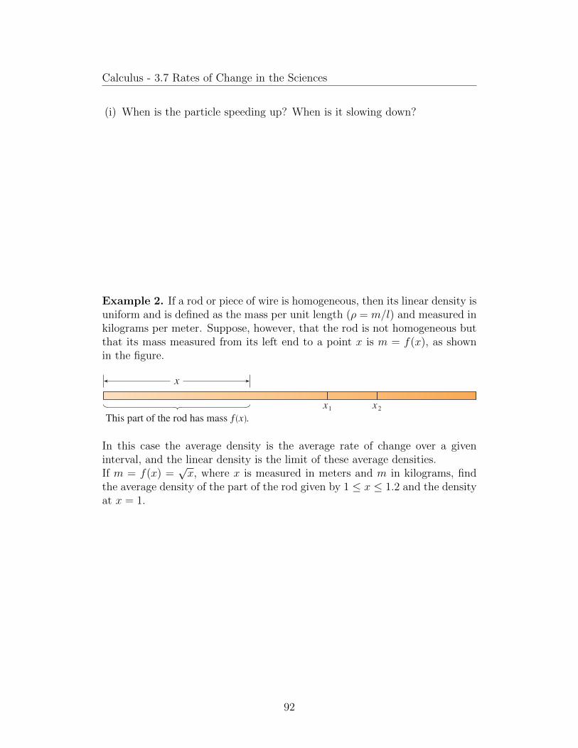
Calculus - 3.7 Rates of Change in the Sciences
(i) When is the particle speeding up? When is it slowing down?
Example 2. If a rod or piece of wire is homogeneous, then its linear density isuniform and is defined as the mass per unit length (ρ = m/l) and measured inkilograms per meter. Suppose, however, that the rod is not homogeneous butthat its mass measured from its left end to a point x is m = f(x), as shownin the figure.
226 CHAPTER 3 Differentiation Rules
( i) The particle speeds up when the velocity is positive and increasing (v and a are both positive) and also when the velocity is negative and decreasing (v and a are both negative). In other words, the particle speeds up when the velocity and acceleration have the same sign. (The particle is pushed in the same direction it is moving.) From Figure 3 we see that this happens when 1 , t , 2 and when t . 3. The particle slows down when v and a have opposite signs, that is, when 0 < t , 1 and when 2 , t , 3. Figure 4 summarizes the motion of the particle.
1
5
_5
√s
a
forward
slowsdown
slowsdown
backward
speedsup
speedsup
forward
t0
EXAMPLE 2 If a rod or piece of wire is homogeneous, then its linear density is uniform and is defined as the mass per unit length s! − myld and measured in kilograms per meter. Suppose, however, that the rod is not homogeneous but that its mass measured from its left end to a point x is m − f sxd, as shown in Figure 5.
x¡ x™This part of the rod has mass ƒ.
x
The mass of the part of the rod that lies between x − x1 and x − x2 is given by Dm − f sx2 d 2 f sx1d, so the average density of that part of the rod is
average density −DmDx
− f sx2 d 2 f sx1d
x2 2 x1
If we now let Dx l 0 (that is, x2 l x1), we are computing the average density over smaller and smaller intervals. The linear density ! at x1 is the limit of these average densities as Dx l 0; that is, the linear density is the rate of change of mass with respect to length. Symbolically,
! − limDx l 0
DmDx
−dmdx
Thus the linear density of the rod is the derivative of mass with respect to length.For instance, if m − f sxd − sx , where x is measured in meters and m in kilograms,
then the average density of the part of the rod given by 1 < x < 1.2 is
DmDx
− f s1.2d 2 f s1d
1.2 2 1−
s1.2 2 10.2
< 0.48 kgym
TEC In Module 3.7 you can see an animation of Figure 4 with an expression for s that you can choose yourself.
FIGURE 4
FIGURE 5
Copyright 2016 Cengage Learning. All Rights Reserved. May not be copied, scanned, or duplicated, in whole or in part. Due to electronic rights, some third party content may be suppressed from the eBook and/or eChapter(s).Editorial review has deemed that any suppressed content does not materially affect the overall learning experience. Cengage Learning reserves the right to remove additional content at any time if subsequent rights restrictions require it.
In this case the average density is the average rate of change over a giveninterval, and the linear density is the limit of these average densities.If m = f(x) =
√x, where x is measured in meters and m in kilograms, find
the average density of the part of the rod given by 1 ≤ x ≤ 1.2 and the densityat x = 1.
92

Calculus - 3.7 Rates of Change in the Sciences
Example 3. The average current during a time interval is the average rateof change of the net charge over that interval, and the current at a given timeis the limit of the average current (the rate at which charge flows through asurface, measured in units of charge per unit time). The quantity of chargeQ in coulombs (C) that has passed through a point in a wire up to time t(measured in seconds) is given by Q(t) = t3−2t2 +6t+2. [The unit of currentis an ampere (1 A = 1 C/s).] Find the current when(a) t = 0.5 s
(b) t = 1 s.
At what time is the current lowest?
93
Calculus - 3.7 Rates of Change in the Sciences
Example 4. The concentration of a reactant A is the number of moles (1mole = 6.022× 10²³ molecules) per liter and is denoted by [A] for a chemicalreaction
A + B→ C.
The average rate of reaction during a time interval is the average rate ofchange of the concentration of the product [C] over that interval, and the rateof reaction at a given time is the limit of the average rate of reaction.If one molecule of a product C is formed from one molecule of a reactant Aand one molecule of a reactant B, and the initial concentrations of A and Bhave a common value [A] = [B] = a moles/L, then
[C] =a2kt
akt+ 1
where k is a constant.
(a) Find the rate of reaction at time t.
(b) Show that if x = [C], then
dx
dt= k(a− x)2.
94

Calculus - 3.7 Rates of Change in the Sciences
(c) What happens to the concentration as t→∞?
(d) What happens to the rate of reaction as t→∞?
(e) What do the results of parts (c) and (d) mean in practical terms?
95

Calculus - 3.7 Rates of Change in the Sciences
Example 5. If a given substance is kept a constant temperature, then therate of change of its volume V with respect to its pressure P is the derivativedV/dP . The compressibility is defined by
isothermal compressibility = β = − 1
V
dV
dP.
The volume V (in cubic meters) of a sample of air at 25°C was found to berelated to the pressure P (in kilopascals) by the equation
V =5.3
P.
Determine the compressibility when P = 50 kPa.
Example 6. Let n = f(t) be the number of individuals in an animal or plantpopulation at time t. The average rate of growth during a time period is theaverage rate of change of the growth of the population over that time period,and the rate of growth at a given time is the limit of the average rate ofgrowth.Suppose that a population of bacteria doubles every hour. The populationfunction representing the bacteria’s growth can be found to be
n = n02t
where n0 is the initial population and the time t is measured in hours.Find the rate of growth for a colony of bacteria with an initial populationn0 = 100 after 4 hours.
96

Calculus - 3.7 Rates of Change in the Sciences
Example 7. The shape of a blood vessel can be modeled by a cylindrical tubewith radius R and length l as illustrated in the figure.
230 CHAPTER 3 Differentiation Rules
In Section 3.4 we showed that
ddx
sbx d − bx ln b
So the rate of growth of the bacteria population at time t is
dndt
−ddt
sn02td − n02t ln 2
For example, suppose that we start with an initial population of n0 − 100 bacteria. Then the rate of growth after 4 hours is
dndt
Zt−4
− 100 ? 24 ln 2 − 1600 ln 2 < 1109
This means that, after 4 hours, the bacteria population is growing at a rate of about 1109 bacteria per hour.
EXAMPLE 7 When we consider the flow of blood through a blood vessel, such as a vein or artery, we can model the shape of the blood vessel by a cylindrical tube with radius R and length l as illustrated in Figure 8.
R r
l
Because of friction at the walls of the tube, the velocity v of the blood is greatest along the central axis of the tube and decreases as the distance r from the axis increases until v becomes 0 at the wall. The relationship between v and r is given by the law of lami-nar flow discovered by the French physician Jean-Louis-Marie Poiseuille in 1840. This law states that
1 v −P
4!l sR2 2 r 2 d
where ! is the viscosity of the blood and P is the pressure difference between the ends of the tube. If P and l are constant, then v is a function of r with domain f0, Rg.
The average rate of change of the velocity as we move from r − r1 outward to r − r2 is given by
DvDr
−vsr2 d 2 vsr1d
r2 2 r1
and if we let Dr l 0, we obtain the velocity gradient, that is, the instantaneous rate of change of velocity with respect to r:
velocity gradient − limDr l 0
DvDr
−dvdr
Using Equation 1, we obtain
dvdr
−P
4!l s0 2 2rd − 2
Pr2!l
FIGURE 8 Blood flow in an artery
For more detailed information, see W. Nichols and M. O’Rourke (eds.), McDonald’s Blood Flow in Arteries: Theoretical, Experimental, and Clinical Principles, 5th ed. (New York, 2005).
Copyright 2016 Cengage Learning. All Rights Reserved. May not be copied, scanned, or duplicated, in whole or in part. Due to electronic rights, some third party content may be suppressed from the eBook and/or eChapter(s).Editorial review has deemed that any suppressed content does not materially affect the overall learning experience. Cengage Learning reserves the right to remove additional content at any time if subsequent rights restrictions require it.
The relationship between the velocity v of the blood and the distance r fromthe axis is given by the law of laminar flow
v =P
4ηl(R2 − r2)
where η is the viscosity of the blood and P is the pressure difference betweenthe ends of the tube. If P and l are constant, then v is a function of r withdomain [0, R]. The velocity gradient at a given time is the limit of the averagerate of change of the velocity.For one of the smaller human arteries we can take η = 0.027, R = 0.008 cm,l = 2 cm, and P = 4000 dynes/cm2. Find the speed at which blood is flowingat r = 0.002 and find the velocity gradient at that point.
97
Calculus - 3.7 Rates of Change in the Sciences
Example 8. Suppose C(x) is the total cost that a company incurs in produc-ing x units of a certain commodity. The function C is called a cost function.The instantaneous rate of change of cost with respect to the number of itemsproduced, called the marginal cost, is the limit of the average rate of changeof the cost.Suppose a company has estimated that the cost (in dollars) of producing xitems is
C(x) = 10, 000 + 5x+ 0.01x2.
Find the marginal cost at the production level of 500 items and compare it tothe actual cost of producing the 501st item.
98

Calculus - 3.8 Exponential Growth and Decay
3.8 Exponential Growth and Decay
Definition 3.8.1. The equation
dy
dt= ky
is called the law of natural growth (if k > 0) or the law of natural decay (ifk < 0). It is called a differential equation because it involves an unknownfunction y and its derivative dy/dt.
Theorem 3.8.1. The only solutions of the differential equation dy/dt = kyare the exponential functions
y(t) = y(0)ekt.
Definition 3.8.2. If P (t) is the size of a population at time t, then
k =1
P
dP
dt
is the growth rate divided by population, called the relative growth rate.
Example 1. Use the fact that the world population was 2560 million in 1950and 3040 million in 1960 to model the population of the world in the secondhalf of the 20th century. (Assume that the growth rate is proportional to thepopulation size.) What is the relative growth rate? Use the model to estimatethe world population in 1993 and to predict the population in the year 2020.
99

Calculus - 3.8 Exponential Growth and Decay
Definition 3.8.3. If m(t) is the mass remaining from an initial mass m0 of asubstance after time t, then the relative decay rate is
− 1
m
dm
dt.
It follows that the mass decays exponentially according to the equation
m(t) = m0ekt,
where the rate of decay is expressed in terms of half-life, the time required forhalf of any given quantity to decay.
Example 2. The half-life of radium-226 is 1590 years.
(a) A sample of radium-226 has a mass of 100 mg. Find a formula for themass of the sample that remains after t years.
(b) Find the mass after 1000 years correct to the nearest milligram.
(c) When will the mass be reduced to 30 mg?
100

Calculus - 3.8 Exponential Growth and Decay
Example 3. Newton’s Law of Cooling can be represented as a differentialequation
dT
dt= k(T − Ts),
where T is the temperature of the object at time t and Ts is the temperatureof the surroundings. The exponential function y(t) = y(0)ekt is a solution tothis differential equation when y(t) = T (t)− Ts.A bottle of soda pop at room temperature (72°F) is placed in a refrigeratorwhere the temperature is 44°F. After half an hour the soda pop has cooled to61°F.
(a) What is the temperature of the soda pop after another half hour?
(b) How long does it take for the soda pop to cool to 50°F?
101

Calculus - 3.8 Exponential Growth and Decay
Example 4. In general, if an amount A0 is invested at an interest rate r, thenafter t years it is worth A0(1 + r)t. Usually, however, interest is compoundedmore frequently, say, n times a year. Then in each compounding period theinterest rate is r/n and there are nt compounding periods in t years, so thevalue of the investment is
A0
(1 +
r
n
)nt.
Therefore, taking limits gives us the amount after t years as
A(t) = A0ert
when interest is continuously compounded. Determine the value of an invest-ment of $1000 after 3 years of continuously compounding 6% interest. Com-pare this to the value of the same investment compounded annually instead.
102

Calculus - 3.9 Related Rates
3.9 Related Rates
Example 1. Air is being pumped into a spherical balloon so that its volumeincreases at a rate of 100 cm3/s. How fast is the radius of the balloon increasingwhen the diameter is 50 cm?
103

Calculus - 3.9 Related Rates
Example 2. A ladder 10 ft long rests against a vertical wall. If the bottomof the ladder slides away from the wall at a rate of 1 ft/s, how fast is the topof the ladder sliding down the wall when the bottom of the ladder is 6 ft fromthe wall?
104

Calculus - 3.9 Related Rates
Example 3. A water tank has the shape of an inverted circular cone withbase radius 2 m and height 4 m. If water is being pumped into the tank ata rate of 2 m3/min, find the rate at which the water level is rising when thewater is 3 m deep.
105

Calculus - 3.9 Related Rates
Example 4. Car A is traveling west at 50 mi/h and car B is traveling northat 60 mi/h. Both are headed for the intersection of the two roads. At whatrate are the cars approaching each other when car A is 0.3 mi and car B is 0.4mi from the intersection?
106
Calculus - 3.9 Related Rates
Example 5. A man walks along a straight path at a speed of 4 ft/s. Asearchlight is located on the ground 20 ft from the path and is kept focusedon the man. At what rate is the searchlight rotating when the man is 15 ftfrom the point on the path closest to the searchlight?
107

Calculus - 3.10 Linear Approximations and Differentials
3.10 Linear Approximations and Differentials
Definition 3.10.1. The approximation
f(x) ≈ f(a) + f ′(a)(x− a)
is called the linear approximation or tangent line approximation of f at a. Thelinear function whose graph is this tangent line, that is,
L(x) = f(a) + f ′(a)(x− a)
is called the linearization of f at a.
Example 1. Find the linearization of the function f(x) =√x+ 3 at a = 1 and
use it to approximate the numbers√
3.98 and√
4.05. Are these approximationsoverestimates or underestimates?
108

Calculus - 3.10 Linear Approximations and Differentials
Example 2. For what values of x is the linear approximation
√x+ 3 ≈ 7
4+x
4
accurate to within 0.5? What about accuracy to within 0.1?
254 CHAPTER 3 Di!erentiation Rules
ics textbooks obtain the expression aT ! 2t sin ! for tangential acceleration and then replace sin ! by ! with the remark that sin ! is very close to ! if ! is not too large. [See, for exam ple, Physics: Calculus, 2d ed., by Eugene Hecht (Paci!c Grove, CA: Brooks/Cole, 2000), p. 431.] You can verify that the linearization of the function f sxd ! sin x at a ! 0 is Lsxd ! x and so the lin ear approximation at 0 is
sin x < x
(see Exercise 42). So, in effect, the derivation of the formula for the period of a pendulum uses the tangent line approximation for the sine function.
Another example occurs in the theory of optics, where light rays that arrive at shallow angles relative to the optical axis are called paraxial rays. In paraxial (or Gaussian) optics, both sin ! and cos ! are replaced by their linearizations. In other words, the linear approximations
sin ! < ! and cos ! < 1
are used because ! is close to 0. The results of calculations made with these approxima-tions became the basic theoretical tool used to design lenses. [See Optics, 4th ed., by Eugene Hecht (San Francisco, 2002), p. 154.]
In Section 11.11 we will present several other applications of the idea of linear approxi-mations to physics and engineering.
Di!erentialsThe ideas behind linear approximations are sometimes formulated in the terminology and notation of differentials. If y ! f sxd, where f is a differentiable function, then the differ-ential dx is an independent variable; that is, dx can be given the value of any real number. The differential dy is then de!ned in terms of dx by the equation
3 dy ! f 9sxd dx
So dy is a dependent variable; it depends on the values of x and dx. If dx is given a spe-ci!c value and x is taken to be some speci!c number in the domain of f , then the numer-ical value of dy is determined.
The geometric meaning of differentials is shown in Figure 5. Let Psx, f sxdd and Qsx 1 Dx, f sx 1 Dxdd be points on the graph of f and let dx ! Dx. The corresponding change in y is
Dy ! f sx 1 Dxd 2 f sxd
The slope of the tangent line PR is the derivative f 9sxd. Thus the directed distance from S to R is f 9sxd dx ! dy. Therefore dy represents the amount that the tangent line rises or falls (the change in the linearization), whereas Dy represents the amount that the curve y ! f sxd rises or falls when x changes by an amount dx.
EXAMPLE 3 Compare the values of Dy and dy if y ! f sxd ! x 3 1 x 2 2 2x 1 1 and x changes (a) from 2 to 2.05 and (b) from 2 to 2.01.
SOLUTION (a) We have
f s2d ! 23 1 22 2 2s2d 1 1 ! 9
f s2.05d ! s2.05d3 1 s2.05d2 2 2s2.05d 1 1 ! 9.717625
Dy ! f s2.05d 2 f s2d ! 0.717625
If dx ± 0, we can divide both sides of Equation 3 by dx to obtain
dydx
! f 9sxd
We have seen similar equations before, but now the left side can genuinely be interpreted as a ratio of differentials.
R
0 x
y
Îy
x
P
Q
dx=Îx
x+Îx
y=ƒ
S
dy
FIGURE 5
Copyright 2016 Cengage Learning. All Rights Reserved. May not be copied, scanned, or duplicated, in whole or in part. Due to electronic rights, some third party content may be suppressed from the eBook and/or eChapter(s).Editorial review has deemed that any suppressed content does not materially affect the overall learning experience. Cengage Learning reserves the right to remove additional content at any time if subsequent rights restrictions require it.
Definition 3.10.2. If y = f(x), where f is a differentiable func-tion, then the differential dx is an independent variable; that is,dx can be given the value of any real number. The differentialdy is then defined in terms of dx by the equation
dy = f ′(x)dx.
109

Calculus - 3.10 Linear Approximations and Differentials
Example 3. Compare the values ∆y and dy if y = f(x) = x3 + x2 − 2x + 1and x changes
(a) from 2 to 2.05
(b) from 2 to 2.01.
Example 4. The radius of a sphere was measured and found to be 21 cm witha possible error in measurement of at most 0.05 cm. What is the maximumerror in using this value of the radius to compute the volume of the sphere?
110

Calculus - 3.11 Hyperbolic Functions
3.11 Hyperbolic Functions
Definition 3.11.1. Functions that have the same relationship to the hyper-bola that trigonometric functions have to the circle are called hyperbolic func-tions and are defined as follows
sinhx =ex − e−x
2cschx =
1
sinhx
coshx =ex + e−x
2sechx =
1
coshx
tanhx =sinhx
coshxcothx =
coshx
sinhx.
Theorem 3.11.1 (Hyperbolic Identities).
sinh(−x) = − sinhx cosh(−x) = cosh x
cosh2 x− sinh2 x = 1 1− tanh2 x = sech2 x
sinh(x+ y) = sinhx cosh y + coshx sinh y
cosh(x+ y) = cosh x cosh y + sinhx sinh y.
Example 1. Prove
(a) cosh2 x− sinh2 x = 1
(b) 1− tanh2 x = sech2 x.
111

Calculus - 3.11 Hyperbolic Functions
Theorem 3.11.2 (Derivatives of Hyperbolic Functions).
d
dx(sinhx) = cosh x
d
dx(cschx) = − cschx cothx
d
dx(coshx) = sinhx
d
dx(sechx) = − sechx tanhx
d
dx(tanhx) = sech2 x
d
dx(cothx) = − csch2 x.
Example 2. Findd
dx(cosh
√x).
Theorem 3.11.3 (Inverse Hyperbolic Functions).
sinh−1 x = ln(x+√x2 + 1) x ∈ R
cosh−1 x = ln(x+√x2 − 1) x ≥ 1
tanh−1 x =1
2ln
(1 + x
1− x
)− 1 < x < 1.
Example 3. Show that sinh−1 x = ln(x+√x2 + 1).
112
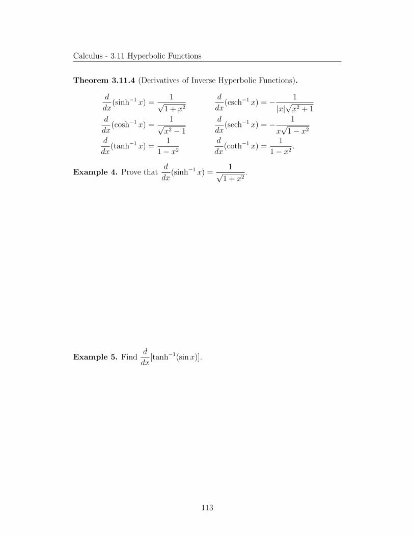
Calculus - 3.11 Hyperbolic Functions
Theorem 3.11.4 (Derivatives of Inverse Hyperbolic Functions).
d
dx(sinh−1 x) =
1√1 + x2
d
dx(csch−1 x) = − 1
|x|√x2 + 1
d
dx(cosh−1 x) =
1√x2 − 1
d
dx(sech−1 x) = − 1
x√
1− x2
d
dx(tanh−1 x) =
1
1− x2
d
dx(coth−1 x) =
1
1− x2.
Example 4. Prove thatd
dx(sinh−1 x) =
1√1 + x2
.
Example 5. Findd
dx[tanh−1(sinx)].
113

Chapter 4
Applications of Differentiation
4.1 Maximum and Minimum Values
Definition 4.1.1. Let c be a number in the domain D of a function f . Thenf(c) is the absolute maximum value (or global maximum value) of f on D iff(c) ≥ f(x) for all x in D and f(c) is the absolute minimum value (or globalminimum value) of f on D if f(c) ≤ f(x) for all x in D. These values arecalled extreme values of f .
Definition 4.1.2. The number f(c) is a local maximum value of f if f(c) ≥f(x) when x is near c and a local minimum value of f if f(c) ≤ f(x) when x isnear c. When we say near, we mean on an open interval containing c. Thesevalues are called local extreme values of f .
Example 1. For what values of x does f(x) = cosx take on its maximumand minimum values?
Example 2. Find all of the extreme values of f(x) = x2.
114

Calculus - 4.1 Maximum and Minimum Values
Example 3. Find all of the extreme values of f(x) = x3.
Example 4. Find all of the extreme values of f(x) = 3x4−16x3 +18x2 withinthe domain −1 ≤ x ≤ 4.
Theorem 4.1.1 (Extreme Value Theorem). If f is continuous on a closedinterval [a, b] then f attains an absolute maximum value f(c) and an absoluteminimum value f(d) at some numbers c and d in [a, b].
Theorem 4.1.2 (Fermat’s Theorem). If f has a local maximum or minimumat c, and if f ′(c) exists, then f ′(c) = 0.
Proof. Suppose f has a local maximum at c. Then, by definition, f(c) ≥ f(x)if x is near c, so if we let h > 0 be close to 0 we have
f(c) ≥ f(c+ h)
f(c+ h)− f(c) ≤ 0
f(c+ h)− f(c)
h≤ 0
h
limh→0+
f(c+ h)− f(c)
h≤ lim
h→0+0
f ′(c) ≤ 0.
If h < 0, the direction of the inequality is reversed and we get f ′(c) ≥ 0. Thuscombining these inequalities gives us f ′(c) = 0. A similar argument can beused to achieve the same result if f has a local minimum at c.
115

Calculus - 4.1 Maximum and Minimum Values
Example 5. Use the function f(x) = x3 to determine whether the converseof Fermat’s theorem is true.
Example 6. Does Fermat’s theorem apply to the function f(x) = |x|?
Definition 4.1.3. A critical number of a function f is a number c in thedomain of f such that either f ′(c) = 0 or f ′(c) does not exist.
Example 7. Find the critical numbers of x3/5(4− x).
116

Calculus - 4.1 Maximum and Minimum Values
Example 8. Find the absolute maximum and minimum values of the function
f(x) = x3 − 3x2 + 1 − 1
2≤ x ≤ 4.
Example 9. (a) Use a graphing device to estimate the absolute minimumand maximum values of the function f(x) = x− 2 sinx, 0 ≤ x ≤ 2π.
117

Calculus - 4.1 Maximum and Minimum Values
(b) Use calculus to find the exact minimum and maximum values.
Example 10. The Hubble Space Telescope was deployed on April 24, 1990,by the space shuttle Discovery. A model for the velocity of the shuttle duringthis mission, from liftoff at t = 0 until the solid rocket boosters were jettisonedat t = 126 seconds, is given by
v(t) = 0.001302t3 − 0.09029t2 + 23.61t− 3.083
(in feet per second). Using this model, estimate the absolute maximum andminimum values of the acceleration of the shuttle between liftoff and the jet-tisoning of the boosters.
118
Calculus - 4.2 The Mean Value Theorem
4.2 The Mean Value Theorem
Theorem 4.2.1 (Rolle’s Theorem). Let f be a function that satisfies the fol-lowing three hypotheses:
1. f is continuous on the closed interval [a, b].
2. f is differentiable on the open interval (a, b).
3. f(a) = f(b).
Then there is a number c in (a, b) such that f ′(c) = 0.
Proof. If f(x) = k, a constant, then f ′(x) = 0 for all x ∈ (a, b). If f(x) > f(a)for some x ∈ (a, b) then f has a local maximum for a number c ∈ (a, b) bythe extreme value theorem. Since f is differentiable on (a, b), f ′(c) = 0 byFermat’s theorem. By the same reasoning, f ′(c) = 0 if f(x) < f(a).
Example 1. How could Rolle’s theorem be applied to a position function thatmodels a ball thrown upward?
Example 2. Prove that the equation x3 +x−1 = 0 has exactly one real root.
119

Calculus - 4.2 The Mean Value Theorem
Theorem 4.2.2 (The Mean Value Theorem). Let f be a function that satisfiesthe following hypotheses:
1. f is continuous on the closed interval [a, b].
2. f is differentiable on the open interval (a, b).
Then there is a number c in (a, b) such that
f ′(c) =f(b)− f(a)
b− a
or, equivalently,f(b)− f(a) = f ′(c)(b− a).
Proof. Let h be the difference between f and the secant line to f on [a, b], i.e.,
h(x) = f(x)−[f(a) +
f(b)− f(a)
b− a(x− a)
].
Then h is continuous on [a, b] and differentiable on (a, b) because it is the sumof f and a first-degree polynomial, which are both continuous on [a, b] anddifferentiable on (a, b). Also,
h(a) = f(a)− f(a)− f(b)− f(a)
b− a(a− a) = 0
h(b) = f(b)− f(a)− f(b)− f(a)
b− a(b− a) = 0,
so h(a) = h(b). Therefore, by Rolle’s thereom, there is a number c in (a, b)such that h′(c) = 0, i.e.,
0 = h′(c) = f ′(c)− f(b)− f(a)
b− a,
which is equivalent to
f ′(c) =f(b)− f(a)
b− aas desired.
120

Calculus - 4.2 The Mean Value Theorem
Example 3. Find a number c in (0, 2) such that the slope of the secant lineis equal to the slope of the tangent line for the function f(x) = x3 − x.
Example 4. What does the mean value theorem say about the velocity of anobject moving in a straight line?
Example 5. Suppose that f(0) = −3 and f ′(x) ≤ 5 for all values of x. Howlarge can f(2) possibly be?
Theorem 4.2.3. If f ′(x) = 0 for all x in an interval (a, b), then f is constanton (a, b).
Proof. Let x1, x2 ∈ (a, b) be such that x1 < x2. By the mean value theoremfor f on [x1, x2], we get
f(x2)− f(x1) = f ′(c)(x2 − x1),
for some c ∈ (x1, x2). But f ′(x) = 0 for all x in this interval, so f(x2) = f(x1).Since x1 and x2 were chosen arbitrarily, f is constant on (a, b).
121

Calculus - 4.2 The Mean Value Theorem
Corollary 4.2.1. If f ′(x) = g′(x) for all x in an interval (a, b), then f − g isconstant on (a, b); that is f(x) = g(x) + c where c is a constant.
Proof. LetF (x) = f(x)− g(x).
ThenF ′(x) = f ′(x)− g′(x) = 0,
so F is constant by the previous theorem, and thus f − g is constant.
Example 6. Prove the identity tan−1 x+ cot−1 x = π/2.
122

Calculus - 4.3 Derivatives and the Shape of a Graph
4.3 Derivatives and the Shape of a Graph
Theorem 4.3.1 (Increasing/Decreasing Test).
(a) If f ′(x) > 0 on an interval, then f is increasing on that interval.
(b) If f ′(x) < 0 on an interval, then f is decreasing on that interval.
Proof. Let x1, x2 be two numbers on an interval where f ′(x) > 0 such thatx1 < x2. Then by the mean value theorem,
f(x2)− f(x1) = f ′(c)(x2 − x1)
for some c in the interval. But f ′(c) > 0 and x2−x1 > 0, so f(x2)−f(x1) > 0,i.e.,
f(x2) > f(x1)
in the interval. Since x1 and x2 were chosen arbitrarily, we are done, and thesecond half of the theorem is proved similarly.
Example 1. Find where the function f(x) = 3x4−4x3−12x2 +5 is increasingand where it is decreasing.
123

Calculus - 4.3 Derivatives and the Shape of a Graph
Theorem 4.3.2 (The First Derivative Test). Suppose that c is a critical num-ber of a continuous function f .
(a) If f ′ changes from positive to negative at c, then f has a local maximumat c.
(b) If f ′ changes from negative to positive at c, then f has a local minimumat c.
(c) If f ′ is positive to the left and to the right of c, or negative to the left andto the right of c, then f has no local minimum or maximum at c.
Example 2. Find the local minimum and maximum values of the function fin Example 1.
Example 3. Find the local maximum and minimum values of the function
g(x) = x+ 2 sinx 0 ≤ x ≤ 2π.
124

Calculus - 4.3 Derivatives and the Shape of a Graph
Definition 4.3.1. If the graph of f lies above all of its tangents on an intervalI, then it is called concave upward on I. If the graph of f lies below all of itstangents on I, it is called concave downward on I.
Theorem 4.3.3 (Concavity Test).
(a) If f ′′(x) > 0 for all x in I, then the graph of f is concave upward on I.
(b) If f ′′(x) < 0 for all x in I, then the graph of f is concave downward on I.
Example 4. The figure shows a population graph for Cyprian honeybeesraised in an apiary. How does the rate of population increase change overtime? When is this rate highest? Over what intervals is P concave upward orconcave downward?
296 CHAPTER 4 Applications of Differentiation
In Figure 6 tangents to these curves have been drawn at several points. In (a) the curve lies above the tangents and f is called concave upward on sa, bd. In (b) the curve lies below the tangents and t is called concave downward on sa, bd.
Definition If the graph of f lies above all of its tangents on an interval I, then it is called concave upward on I. If the graph of f lies below all of its tangents on I, it is called concave downward on I.
Figure 7 shows the graph of a function that is concave upward (abbreviated CU) on the intervals sb, cd, sd, ed, and se, pd and concave downward (CD) on the intervals sa, bd, sc, dd, and sp, q d.
a b c d e p q
B C
DP
x
y
0
CD CU CD CU CDCU
FIGURE 7
Let’s see how the second derivative helps determine the intervals of concavity. Look-ing at Figure 6(a), you can see that, going from left to right, the slope of the tangent increas es. This means that the derivative f 9 is an increasing function and therefore its derivative f 0 is positive. Likewise, in Figure 6(b) the slope of the tangent decreases from left to right, so f 9 decreases and therefore f 0 is negative. This reasoning can be reversed and suggests that the following theorem is true. A proof is given in Appendix F with the help of the Mean Value Theorem.
Concavity Test(a) If f 0sxd . 0 for all x in I, then the graph of f is concave upward on I.
(b) If f 0sxd , 0 for all x in I, then the graph of f is concave downward on I.
EXAMPLE 4 Figure 8 shows a population graph for Cyprian honeybees raised in an apiary. How does the rate of population increase change over time? When is this rate highest? Over what intervals is P concave upward or concave downward?
t
P
3
20
0Time (in weeks)
6 9 12 15
40
60
80
Number of bees(in thousands)
18
g
A
B
x
y
0
f
A
B
x
y
0
(a) Concave upward
(b) Concave downward
FIGURE 6
FIGURE 8
Copyright 2016 Cengage Learning. All Rights Reserved. May not be copied, scanned, or duplicated, in whole or in part. Due to electronic rights, some third party content may be suppressed from the eBook and/or eChapter(s).Editorial review has deemed that any suppressed content does not materially affect the overall learning experience. Cengage Learning reserves the right to remove additional content at any time if subsequent rights restrictions require it.
125

Calculus - 4.3 Derivatives and the Shape of a Graph
Definition 4.3.2. A point P on a curve y = f(x) is called an inflection pointif f is continuous there and the curve changes from concave upward to concavedownward or from concave downward to concave upward at P .
Example 5. Sketch a possible graph of a function f that satisfies the followingconditions:
(i) f ′(x) > 0 on (−∞, 1), f ′(x) < 0 on (1,∞).
(ii) f ′′(x) > 0 on (−∞,−2) and (2,∞), f ′′(x) < 0 on (−2, 2).
(iii) limx→−∞
f(x) = −2, limx→∞
f(x) = 0.
Theorem 4.3.4 (The Second Derivative Test). Suppose f ′ is continuous nearc.
(a) If f ′(c) = 0 and f ′′(c) > 0, then f has a local minimum at c.
(b) If f ′(c) = 0 and f ′′(c) < 0, then f has a local maximum at c.
126

Calculus - 4.3 Derivatives and the Shape of a Graph
Example 6. Discuss the curve y = x4− 4x3 with respect to concavity, pointsof inflection, and local maxima and minima. Use this information to sketchthe curve.
127
Calculus - 4.3 Derivatives and the Shape of a Graph
Example 7. Sketch the graph of the function f(x) = x2/3(6− x)1/3.
128

Calculus - 4.3 Derivatives and the Shape of a Graph
Example 8. Use the first and second derivatives of f(x) = e1/x, together withasymptotes, to sketch its graph.
129

Calculus - 4.4 Indeterminate Forms and l’Hospital’s Rule
4.4 Indeterminate Forms and l’Hospital’s Rule
Theorem 4.4.1 (L’Hospital’s Rule). Suppose f and g are differentiable andg′(x) 6= 0 on an open interval I that contains a (except possibly at a). Supposethat
limx→a
f(x) = 0 and limx→a
g(x) = 0
or thatlimx→a
f(x) = ±∞ and limx→a
g(x) = ±∞
(In other words, we have an indeterminate form of type 00
or ∞/∞.) Then
limx→a
f(x)
g(x)= lim
x→a
f ′(x)
g′(x).
if the limit on the right side exists (or is ∞ or −∞).
Example 1. Find limx→1
lnx
x− 1.
Example 2. Calculate limx→∞
ex
x2.
130

Calculus - 4.4 Indeterminate Forms and l’Hospital’s Rule
Example 3. Calculate limx→∞
lnx√x
.
Example 4. Find limx→0
tanx− xx3
.
131

Calculus - 4.4 Indeterminate Forms and l’Hospital’s Rule
Example 5. Find limx→π−
sinx
1− cosx.
Example 6. Evaluate limx→0+
x lnx.
132

Calculus - 4.4 Indeterminate Forms and l’Hospital’s Rule
Example 7. Compute limx→1+
(1
lnx− 1
x− 1
).
Example 8. Calculate limx→∞
(ex − x).
133

Calculus - 4.4 Indeterminate Forms and l’Hospital’s Rule
Example 9. Calculate limx→0+
(1 + sin 4x)cotx.
Example 10. Find limx→0+
xx.
134

Calculus - 4.5 Summary of Curve Sketching
4.5 Summary of Curve Sketching
Use the following guidelines when sketching curves by hand:
A. Domain
B. Intercepts
C. Symmetry
D. Asymptotes
E. Intervals of Increase or Decrease
F. Local Maximum and Minimum Values
G. Concavity and Points of Inflection
Example 1. Use the guidelines to sketch the curve y =2x2
x2 − 1.
135

Calculus - 4.5 Summary of Curve Sketching
Example 2. Sketch the graph of f(x) =x2
√x+ 1
.
136

Calculus - 4.5 Summary of Curve Sketching
Example 3. Sketch the graph of f(x) = xex.
137

Calculus - 4.5 Summary of Curve Sketching
Example 4. Sketch the graph of f(x) =cosx
2 + sin x.
138

Calculus - 4.5 Summary of Curve Sketching
Example 5. Sketch the graph of y = ln(4− x2).
139

Calculus - 4.5 Summary of Curve Sketching
Definition 4.5.1. Iflimx→∞
[f(x)− (mx+ b)] = 0
where m 6= 0, then the line y = mx + b is called a slant asymptote becausethe vertical distance between the curve y = f(x) and the line y = mx + bapproaches 0.
Example 6. Sketch the graph of f(x) =x3
x2 + 1.
140

Calculus - 4.6 Graphing with Calculus and Calculators
4.6 Graphing with Calculus and Calculators
Example 1. Graph the polynomial f(x) = 2x6 + 3x5 + 3x3 − 2x2. Use thegraphs of f ′ and f ′′ to estimate all maximum and minimum points and intervalsof concavity.
141

Calculus - 4.6 Graphing with Calculus and Calculators
Example 2. Draw the graph of the function
f(x) =x2 + 7x+ 3
x2
in a viewing rectangle that contains all the important features of the function.Estimate the maximum and minimum values and the intervals of concavity.Then use calculus to find these quantities exactly.
142

Calculus - 4.6 Graphing with Calculus and Calculators
Example 3. Graph the function f(x) =x2(x+ 1)3
(x− 2)2(x− 4)4.
143

Calculus - 4.6 Graphing with Calculus and Calculators
Example 4. Graph the function f(x) = sin(x + sin 2x). For 0 ≤ x ≤ π,estimate all maximum and minimum values, intervals of increase and decrease,and inflection points.
144
Calculus - 4.6 Graphing with Calculus and Calculators
Example 5. How does the graph of f(x) = 1/(x2 + 2x+ c) vary as c varies?
145
Calculus - 4.7 Optimization Problems
4.7 Optimization Problems
Example 1. A farmer has 2400 ft of fencing and wants to fence off a rect-angular field that borders a straight river. He needs no fence along the river.What are the dimensions of the field that has the largest area?
146

Calculus - 4.7 Optimization Problems
Example 2. A cylindrical can is to be made to hold 1 L of oil. Find thedimensions that will minimize the cost of the metal to manufacture the can.
147

Calculus - 4.7 Optimization Problems
Theorem 4.7.1 (First Derivative Test for Absolute Extreme Values). Supposethat c is a critical number of a continuous function f defined on an interval.
(a) If f ′(x) > 0 for all x < c and f ′(x) < 0 for all x > c, then f(c) is theabsolute maximum value of f .
(b) If f ′(x) < 0 for all x < c and f ′(x) > 0 for all x > c, then f(c) is theabsolute minimum value of f .
Example 3. Find the point on the parabola y2 = 2x that is closest to thepoint (1, 4).
148
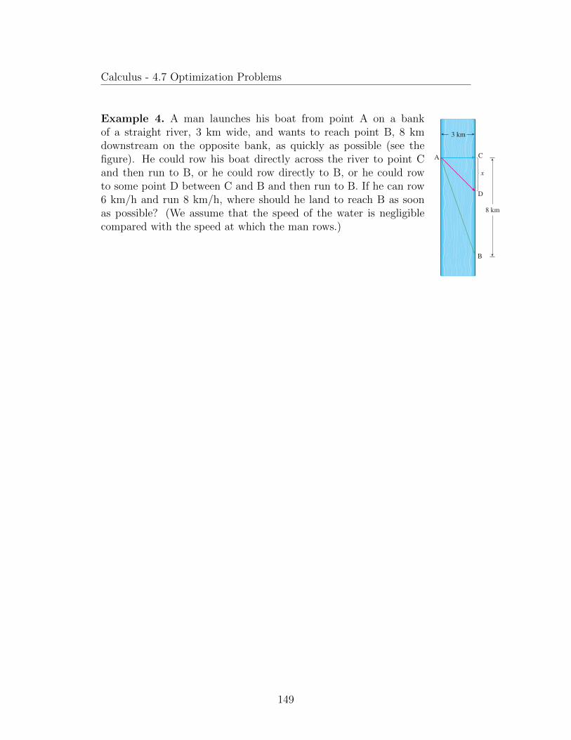
Calculus - 4.7 Optimization Problems
334 CHAPTER 4 Applications of Differentiation
(You should convince yourself that the minimum of d occurs at the same point as the minimum of d2, but d2 is easier to work with.) Note that there are no restrictions on y, so the domain is all real numbers. Differentiating, we obtain
f 9syd − 2s12 y 2 2 1dy 1 2sy 2 4d − y 3 2 8
so f 9syd − 0 when y − 2. Observe that f 9syd , 0 when y , 2 and f 9syd . 0 when y . 2, so by the First Derivative Test for Absolute Extreme Values, the absolute mini-mum occurs when y − 2. (Or we could simply say that because of the geometric nature of the problem, it’s obvious that there is a closest point but not a farthest point.) The corresponding value of x is x − 1
2 y 2 − 2. Thus the point on y 2 − 2x closest to s1, 4d is s2, 2d. [The distance between the points is d − sf s2d − s5 .] Q
EXAMPLE 4 A man launches his boat from point A on a bank of a straight river, 3 km wide, and wants to reach point B, 8 km downstream on the opposite bank, as quickly as possible (see Figure 7). He could row his boat directly across the river to point C and then run to B, or he could row directly to B, or he could row to some point D between C and B and then run to B. If he can row 6 kmyh and run 8 kmyh, where should he land to reach B as soon as possible? (We assume that the speed of the water is negli-gible compared with the speed at which the man rows.)
SOLUTION If we let x be the distance from C to D, then the running distance is | DB | − 8 2 x and the Pythagorean Theorem gives the rowing distance as
| AD | − sx 2 1 9 . We use the equation
time −distance
rate
Then the rowing time is sx 2 1 9 y6 and the running time is s8 2 xdy8, so the total time T as a function of x is
Tsxd −sx 2 1 9
61
8 2 x8
The domain of this function T is f0, 8g. Notice that if x − 0, he rows to C and if x − 8, he rows directly to B. The derivative of T is
T9sxd −x
6sx 2 1 9 2
18
Thus, using the fact that x > 0, we have
T9sxd − 0 &? x
6sx 2 1 9 −
18
&? 4x − 3sx 2 1 9
&? 16x 2 − 9sx 2 1 9d &? 7x 2 − 81
&? x −9
s7
The only critical number is x − 9ys7 . To see whether the minimum occurs at this critical number or at an endpoint of the domain f0, 8g, we follow the Closed Interval
8 km
C
D
B
A
3 km
x
FIGURE 7
Copyright 2016 Cengage Learning. All Rights Reserved. May not be copied, scanned, or duplicated, in whole or in part. Due to electronic rights, some third party content may be suppressed from the eBook and/or eChapter(s).Editorial review has deemed that any suppressed content does not materially affect the overall learning experience. Cengage Learning reserves the right to remove additional content at any time if subsequent rights restrictions require it.
Example 4. A man launches his boat from point A on a bankof a straight river, 3 km wide, and wants to reach point B, 8 kmdownstream on the opposite bank, as quickly as possible (see thefigure). He could row his boat directly across the river to point Cand then run to B, or he could row directly to B, or he could rowto some point D between C and B and then run to B. If he can row6 km/h and run 8 km/h, where should he land to reach B as soonas possible? (We assume that the speed of the water is negligiblecompared with the speed at which the man rows.)
149

Calculus - 4.7 Optimization Problems
Example 5. Find the area of the largest rectangle that can be inscribed in asemicircle of radius r.
150

Calculus - 4.7 Optimization Problems
Definition 4.7.1. If p(x) is the price per unit that a company can charge ifit sells x units, then p is called the demand function (or price function).If x units are sold, then the total revenue
R(x) = quantity× price = xp(x)
and R is called the revenue function. The derivative R′ of the revenue functionis called the marginal revenue function and is the rate of change of revenuewith respect to the number of units sold.If x units are sold, then the total profit is
P (x) = R(x)− C(x)
where C is the cost function and P is called the profit function. The marginalprofit function is P ′, the derivative of the profit function.
Example 6. A store has been selling 200 flat-screen TVs a week at $350each. A market survey indicates that for each $10 rebate offered to buyers, thenumber of TVs sold will increase by 20 a week. Find the demand function andthe revenue function. How large a rebate should the store offer to maximizeits revenue?
151
Calculus - 4.8 Newton’s Method
4.8 Newton’s Method
Theorem 4.8.1 (Newton’s Method). If xn is the nth approximation of a rootr for a function f then
xn+1 = xn −f(xn)
f ′(xn).
Example 1. Starting with x1 = 2, find the third approximation x3 to theroot of the equation x3 − 2x− 5 = 0.
152

Calculus - 4.8 Newton’s Method
Example 2. Use Newton’s method to find 6√
2 to eight decimal places.
153

Calculus - 4.8 Newton’s Method
Example 3. Find, correct to six decimal places, the root of the equationcosx = x.
154

Calculus - 4.9 Antiderivatives
4.9 Antiderivatives
Definition 4.9.1. A function F is called an antiderivative of f on an intervalI if F ′(x) = f(x) for all x in I.
Theorem 4.9.1. If F is an antiderivative of f on an interval I, then the mostgeneral antiderivative of f on I is
F (x) + C
where C is an arbitrary constant.
Proof. Follows by Corollary 4.2.1 to the mean value theorem.
Example 1. Find the most general antiderivative of each of the followingfunctions.
(a) f(x) = sinx
(b) f(x) = 1/x
(c) f(x) = xn, n 6= −1
155

Calculus - 4.9 Antiderivatives
Example 2. Find all functions g such that
g′(x) = 4 sinx+2x5 −
√x
x.
Example 3. Find f if f ′(x) = ex + 20(1 + x2)−1 and f(0) = −2.
156

Calculus - 4.9 Antiderivatives
Example 4. Find f if f ′′(x) = 12x2 + 6x− 4, f(0) = 4, and f(1) = 1.
354 CHAPTER 4 Applications of Differentiation
EXAMPLE 5 The graph of a function f is given in Figure 3. Make a rough sketch of an antiderivative F, given that Fs0d − 2.
SOLUTION We are guided by the fact that the slope of y − Fsxd is f sxd. We start at the point s0, 2d and draw F as an initially decreasing function since f sxd is negative when 0 , x , 1. Notice that f s1d − f s3d − 0, so F has horizontal tangents when x − 1 and x − 3. For 1 , x , 3, f sxd is positive and so F is increasing. We see that F has a local minimum when x − 1 and a local maximum when x − 3. For x . 3, f sxd is negative and so F is decreasing on s3, `d. Since f sxd l 0 as x l `, the graph of F becomes flatter as x l `. Also notice that F0sxd − f 9sxd changes from positive to negative at x − 2 and from negative to positive at x − 4, so F has inflection points when x − 2 and x − 4. We use this information to sketch the graph of the antiderivative in Figure 4. Q
Rectilinear MotionAntidifferentiation is particularly useful in analyzing the motion of an object moving in a straight line. Recall that if the object has position function s − f std, then the velocity function is vstd − s9std. This means that the position function is an antiderivative of the velocity function. Likewise, the acceleration function is astd − v9std, so the velocity function is an antiderivative of the acceleration. If the acceleration and the initial values ss0d and vs0d are known, then the position function can be found by antidifferentiating twice.
EXAMPLE 6 A particle moves in a straight line and has acceleration given by astd − 6t 1 4. Its initial velocity is vs0d − 2 6 cmys and its initial displacement is ss0d − 9 cm. Find its position function sstd.
SOLUTION Since v9std − astd − 6t 1 4, antidifferentiation gives
vstd − 6 t 2
21 4t 1 C − 3t 2 1 4t 1 C
Note that vs0d − C. But we are given that vs0d − 2 6, so C − 2 6 and
vstd − 3t 2 1 4t 2 6
Since vstd − s9std, s is the antiderivative of v:
sstd − 3 t 3
31 4
t 2
22 6t 1 D − t 3 1 2t 2 2 6t 1 D
This gives ss0d − D. We are given that ss0d − 9, so D − 9 and the required position function is
sstd − t 3 1 2t 2 2 6t 1 9 Q
An object near the surface of the earth is subject to a gravitational force that produces a downward acceleration denoted by t. For motion close to the ground we may assume that t is constant, its value being about 9.8 mys2 (or 32 ftys2).
EXAMPLE 7 A ball is thrown upward with a speed of 48 ftys from the edge of a cliff 432 ft above the ground. Find its height above the ground t seconds later. When does it reach its maximum height? When does it hit the ground?
1 2 30 4 x
y
y=ƒ
FIGURE 3
x
y
1
2
0
y=F(x)
1
FIGURE 4
Copyright 2016 Cengage Learning. All Rights Reserved. May not be copied, scanned, or duplicated, in whole or in part. Due to electronic rights, some third party content may be suppressed from the eBook and/or eChapter(s).Editorial review has deemed that any suppressed content does not materially affect the overall learning experience. Cengage Learning reserves the right to remove additional content at any time if subsequent rights restrictions require it.
Example 5. The graph of a function f is given in the figure.Make a rough sketch of an antiderivative F , given that F (0) = 2.
157
Calculus - 4.9 Antiderivatives
Example 6. A particle moves in a straight line and has acceleration given bya(t) = 6t+4. Its initial velocity is v(0) = −6 cm/s and its initial displacementis s(0) = 9 cm. Find its position function s(t).
158
Calculus - 4.9 Antiderivatives
Example 7. A ball is thrown upward with a speed of 48 ft/s from the edge of acliff 432 ft above the ground. Find its height above the ground t seconds later.When does it reach its maximum height? When does it hit the ground? [Formotion close to the ground we may assume that the downward acceleration gis constant, its value being about 9.8 m/s2 (or 32 ft/s2).]
159

Chapter 5
Integrals
5.1 Areas and Distances
Example 1. Use rectangles to estimate the area under the parabola y = x2
from 0 to 1.
160

Calculus - 5.1 Areas and Distances
Example 2. For the region in Example 1, show that the sum of the areas ofthe upper approximating rectangles approaches 1
3, that is,
limn→∞
Rn =1
3.
161

Calculus - 5.1 Areas and Distances
Definition 5.1.1. The area A of the region S that lies under the graph of thecontinuous function f is the limit of the sum of the areas of approximatingrectangles:
A = limn→∞
Rn = limn→∞
[f(x1)∆x+f(x2)∆x+ · · ·+f(xn)∆x] = limn→∞
n∑i=1
f(xi)∆x.
The last equality is an example of the use of sigma notation to write sumswith many terms more compactly.
Definition 5.1.2. Numbers x∗i in the ith subinterval [xi−1, xi] are called sam-ple points. We form lower (and upper) sums by choosing the sample points x∗iso that f(x∗i ) is the minimum (and maximum) value of f on the ith subinterval.
SECTION 5.1 Areas and Distances 371
2 De!nition The area A of the region S that lies under the graph of the contin-uous function f is the limit of the sum of the areas of approximating rectangles:
A ! limn l `
Rn ! limn l `
f f sx1d Dx 1 f sx2 d Dx 1 ! ! ! 1 f sxn d Dxg
It can be proved that the limit in De"nition 2 always exists, since we are assuming that f is continuous. It can also be shown that we get the same value if we use left endpoints:
A ! limn l `
Ln ! limn l `
f f sx0 d Dx 1 f sx1d Dx 1 ! ! ! 1 f sxn21d Dxg
In fact, instead of using left endpoints or right endpoints, we could take the height of the#ith rectangle to be the value of f at any number xi* in the ith subinterval fxi21, xig. We call the numbers x1*, x2*, . . . , xn* the sample points. Figure 13 shows approximating rectangles when# the sample points are not chosen to be endpoints. So a more general expression for the area of S is
A ! limn l `
f f sx1*d Dx 1 f sx2*d Dx 1 ! ! ! 1 f sxn* d Dxg
xixi-10
y
xa bx2⁄ ‹ xn-1
x¡* x™* x£* xn*xi*
Îx
f(xi*)
NOTE It can be shown that an equivalent de"nition of area is the following: A is the unique number that is smaller than all the upper sums and bigger than all the lower sums.We saw in Examples 1 and 2, for instance, that the area sA ! 1
3d is trapped between all#the left approximating sums Ln and all the right approximating sums Rn. The function in those examples, f sxd ! x 2, happens to be increasing on f0, 1g and so the lower sums arise from left endpoints and the upper sums from right endpoints. (See Figures 8 and 9.) In#gen eral, we form lower (and upper) sums by choosing the sample points xi* so that f sxi*d is the minimum (and maximum) value of f on the ith subinterval. (See Figure 14 and Exercises 7–8.)
0
y
xa b
3
4
FIGURE 13
FIGURE 14Lower sums (short rectangles) and
upper sums (tall rectangles)
Copyright 2016 Cengage Learning. All Rights Reserved. May not be copied, scanned, or duplicated, in whole or in part. Due to electronic rights, some third party content may be suppressed from the eBook and/or eChapter(s).Editorial review has deemed that any suppressed content does not materially affect the overall learning experience. Cengage Learning reserves the right to remove additional content at any time if subsequent rights restrictions require it.
Example 3. Let A be the area of the region that lies under the graph off(x) = e−x between x = 0 and x = 2.
(a) Using right endpoints, find an expression for A as a limit. Do not evaluatethe limit.
162

Calculus - 5.1 Areas and Distances
(b) Estimate the area by taking the sample points to be midpoints and usingfour subintervals and then ten subintervals.
163

Calculus - 5.1 Areas and Distances
Example 4. Suppose the odometer on a car is broken. Estimate the distancedriven in feet over a 30-second time interval by using the speedometer readingstaken every five seconds and recorded in the following table:
Time (s) 0 5 10 15 20 25 30Velocity (mi/h) 17 21 24 29 32 31 28
164

Calculus - 5.2 The Definite Integral
5.2 The Definite Integral
Definition 5.2.1. If f is a function defined for a ≤ x ≤ b, we divide theinterval [a, b] into n subintervals of equal width ∆x = (b − a)/n. We letx0(= a), x1, x2, . . . , xn(= b) be the endpoints of these subintervals and we letx∗1, x
∗2, . . . , x
∗n be any sample points in these subintervals, so x∗i lies in the ith
subinterval [xi−1, xi]. Then the definite integral of f from a to b is
ˆ b
a
f(x) dx = limn→∞
n∑i=1
f(x∗i )∆x
provided that this limit exists and gives the same value for all possible choicesof sample points. If it does exist, we say that f is integrable on [a, b].
Definition 5.2.2. The symbol´
is called an integral sign. In the notation´ baf(x)dx, f(x) is called the integrand and a and b are called the limits of
integration; a is the lower limit and b is the upper limit. The procedure ofcalculating an integral is called integration.
Definition 5.2.3. The sum
n∑i=1
f(x∗i )∆x
is called a Riemann sum and it can be used to approximate the definite integralof an integrable function within any desired degree of accuracy.
SECTION 5.2 The De!nite Integral 379
yba f sxd dx, f sxd is called the integrand and a and b are called the limits of integration;
a is the lower limit and b is the upper limit. For now, the symbol dx has no meaning by itself; yb
a f sxd dx is all one symbol. The dx simply indicates that the independent vari able is x. The procedure of calculating an integral is called integration.
NOTE 2 The de!nite integral yba f sxd dx is a number; it does not depend on x. In fact,
we could use any letter in place of x without changing the value of the integral:
yb
a f sxd dx ! yb
a f std dt ! yb
a f srd dr
NOTE 3 The sum
on
i!1 f sxi*d Dx
that occurs in De!nition 2 is called a Riemann sum after the German mathematician Bernhard Riemann (1826 –1866). So De!nition 2 says that the de!nite integral of an integrable function can be approximated to within any desired degree of accuracy by a Riemann sum.
We know that if f happens to be positive, then the Riemann sum can be interpreted as a sum of areas of approximating rectangles (see Figure 1). By comparing De!nition 2 with the de!nition of area in Section 5.1, we see that the de!nite integral yb
a f sxd dx can be interpreted as the area under the curve y ! f sxd from a to b. (See Figure 2.)
xi*0
y
xa
Îx y=ƒ
0
y
xab b
FIGURE 1 If f sxd > 0, the Riemann sum o f sxi*d Dx is the sum of areas of rectangles.
FIGURE 2 If f sxd > 0, the integral yb
a f sxd dx is the area under the curve y ! f sxd from a to b.
If f takes on both positive and negative values, as in Figure 3, then the Riemann sum is the sum of the areas of the rectangles that lie above the x-axis and the negatives of the areas of the rectangles that lie below the x-axis (the areas of the blue rectangles minus the areas of the gold rectangles). When we take the limit of such Riemann sums, we get the situation illustrated in Figure 4. A de!nite integral can be interpreted as a net area, that is, a difference of areas:
yb
a f sxd dx ! A1 2 A2
where A1 is the area of the region above the x-axis and below the graph of f , and A2 is the area of the region below the x-axis and above the graph of f .
NOTE 4 Although we have de!ned yba f sxd dx by dividing fa, bg into subintervals of
equal width, there are situations in which it is advantageous to work with subintervals of unequal width. For instance, in Exercise 5.1.16, NASA provided velocity"data at times that were not equally spaced, but we were still able to estimate the distance traveled. And there are methods for numerical integration that take advantage of unequal subintervals.
RiemannBernhard Riemann received his Ph.D. under the direction of the legendary Gauss at the University of Göttingen and remained there to teach. Gauss, who was not in the habit of praising other mathematicians, spoke of Riemann’s “creative, active, truly mathematical mind and gloriously fertile originality.” The de!nition (2) of an integral that we use is due to Riemann. He also made major contributions to the theory of functions of a complex variable, math-ematical physics, number theory, and the foundations of geometry. Riemann’s broad concept of space and geometry turned out to be the right setting, 50 years later, for Einstein’s general rela-tivity theory. Riemann’s health was poor throughout his life, and he died of tuberculosis at the age of 39.
0
y=ƒy
a b x
FIGURE 3
o f sxi*d Dx is an approximation to the net area.
y=ƒy
xa b0
FIGURE 4
yb
a f sxd dx is the net area.
Copyright 2016 Cengage Learning. All Rights Reserved. May not be copied, scanned, or duplicated, in whole or in part. Due to electronic rights, some third party content may be suppressed from the eBook and/or eChapter(s).Editorial review has deemed that any suppressed content does not materially affect the overall learning experience. Cengage Learning reserves the right to remove additional content at any time if subsequent rights restrictions require it.
165

Calculus - 5.2 The Definite Integral
Definition 5.2.4. A definite integral can be interpreted as a net area, thatis, a difference of areas:
ˆ b
a
f(x) dx = A1 − A2
where A1 is the area of the region above the x-axis and below the graph of f ,and A2 is the area of the region below the x-axis and the above the graph off .
SECTION 5.2 The De!nite Integral 379
yba f sxd dx, f sxd is called the integrand and a and b are called the limits of integration;
a is the lower limit and b is the upper limit. For now, the symbol dx has no meaning by itself; yb
a f sxd dx is all one symbol. The dx simply indicates that the independent vari able is x. The procedure of calculating an integral is called integration.
NOTE 2 The de!nite integral yba f sxd dx is a number; it does not depend on x. In fact,
we could use any letter in place of x without changing the value of the integral:
yb
a f sxd dx ! yb
a f std dt ! yb
a f srd dr
NOTE 3 The sum
on
i!1 f sxi*d Dx
that occurs in De!nition 2 is called a Riemann sum after the German mathematician Bernhard Riemann (1826 –1866). So De!nition 2 says that the de!nite integral of an integrable function can be approximated to within any desired degree of accuracy by a Riemann sum.
We know that if f happens to be positive, then the Riemann sum can be interpreted as a sum of areas of approximating rectangles (see Figure 1). By comparing De!nition 2 with the de!nition of area in Section 5.1, we see that the de!nite integral yb
a f sxd dx can be interpreted as the area under the curve y ! f sxd from a to b. (See Figure 2.)
xi*0
y
xa
Îx y=ƒ
0
y
xab b
FIGURE 1 If f sxd > 0, the Riemann sum o f sxi*d Dx is the sum of areas of rectangles.
FIGURE 2 If f sxd > 0, the integral yb
a f sxd dx is the area under the curve y ! f sxd from a to b.
If f takes on both positive and negative values, as in Figure 3, then the Riemann sum is the sum of the areas of the rectangles that lie above the x-axis and the negatives of the areas of the rectangles that lie below the x-axis (the areas of the blue rectangles minus the areas of the gold rectangles). When we take the limit of such Riemann sums, we get the situation illustrated in Figure 4. A de!nite integral can be interpreted as a net area, that is, a difference of areas:
yb
a f sxd dx ! A1 2 A2
where A1 is the area of the region above the x-axis and below the graph of f , and A2 is the area of the region below the x-axis and above the graph of f .
NOTE 4 Although we have de!ned yba f sxd dx by dividing fa, bg into subintervals of
equal width, there are situations in which it is advantageous to work with subintervals of unequal width. For instance, in Exercise 5.1.16, NASA provided velocity"data at times that were not equally spaced, but we were still able to estimate the distance traveled. And there are methods for numerical integration that take advantage of unequal subintervals.
RiemannBernhard Riemann received his Ph.D. under the direction of the legendary Gauss at the University of Göttingen and remained there to teach. Gauss, who was not in the habit of praising other mathematicians, spoke of Riemann’s “creative, active, truly mathematical mind and gloriously fertile originality.” The de!nition (2) of an integral that we use is due to Riemann. He also made major contributions to the theory of functions of a complex variable, math-ematical physics, number theory, and the foundations of geometry. Riemann’s broad concept of space and geometry turned out to be the right setting, 50 years later, for Einstein’s general rela-tivity theory. Riemann’s health was poor throughout his life, and he died of tuberculosis at the age of 39.
0
y=ƒy
a b x
FIGURE 3
o f sxi*d Dx is an approximation to the net area.
y=ƒy
xa b0
FIGURE 4
yb
a f sxd dx is the net area.
Copyright 2016 Cengage Learning. All Rights Reserved. May not be copied, scanned, or duplicated, in whole or in part. Due to electronic rights, some third party content may be suppressed from the eBook and/or eChapter(s).Editorial review has deemed that any suppressed content does not materially affect the overall learning experience. Cengage Learning reserves the right to remove additional content at any time if subsequent rights restrictions require it.
Theorem 5.2.1. If f is continuous on [a, b], or if f has only a finite number ofjump discontinuities, then f is integrable on [a, b]; that is, the definite integral´ baf(x)dx exists.
Theorem 5.2.2. If f is integrable on [a, b], then
ˆ b
a
f(x) dx = limn→∞
n∑i=1
f(xi)∆x
where
∆x =b− an
and xi = a+ i∆x.
166

Calculus - 5.2 The Definite Integral
Example 1. Express
limn→∞
n∑i=1
(x3i + xi sinxi)∆x
as an integral on the interval [0, π].
Theorem 5.2.3. The following formulas are true when working with sigmanotation:
n∑i=1
i =n(n+ 1)
2
n∑i=1
i2 =n(n+ 1)(2n+ 1)
6
n∑i=1
i3 =
[n(n+ 1)
2
]2
n∑i=1
c = nc
n∑i=1
cai = cn∑i=1
ai
n∑i=1
(ai + bi) =n∑i=1
ai +n∑i=1
bi
n∑i=1
(ai − bi) =n∑i=1
ai −n∑i=1
bi.
167

Calculus - 5.2 The Definite Integral
Example 2. (a) Evaluate the Riemann sum for f(x) = x3 − 6x, taking thesample points to be right endpoints and a = 0, b = 3, and n = 6.
(b) Evaluate
ˆ 3
0
(x3 − 6x) dx.
168

Calculus - 5.2 The Definite Integral
Example 3. (a) Set up an expression for
ˆ 3
1
ex dx as a limit of sums.
(b) Use a computer algebra system to evaluate the expression.
169

Calculus - 5.2 The Definite Integral
Example 4. Evaluate the following integrals by interpreting each in terms ofareas.
(a)
ˆ 1
0
√1− x2 dx
(b)
ˆ 3
0
(x− 1) dx
170

Calculus - 5.2 The Definite Integral
Theorem 5.2.4 (Midpoint Rule).
ˆ b
a
f(x) dx ≈n∑i=1
f(xi)∆x = ∆x[f(x1) + · · ·+ f(xn)]
where
∆x =b− an
and
xi =1
2(xi−1 + xi) = midpoint of [xi−1, xi].
Example 5. Use the Midpoint Rule with n = 5 to approximate
ˆ 2
1
1
xdx.
171

Calculus - 5.2 The Definite Integral
Theorem 5.2.5 (Properties of the Definite Integral).
1.
ˆ b
a
f(x) dx = −ˆ a
b
f(x) dx.
2.
ˆ a
a
f(x) dx = 0.
3.
ˆ b
a
c dx = c(b− a), where c is any constant.
4.
ˆ b
a
[f(x) + g(x)] dx =
ˆ b
a
f(x) dx+
ˆ b
a
g(x) dx.
5.
ˆ b
a
cf(x) dx = c
ˆ b
a
f(x) dx, where c is any constant.
6.
ˆ b
a
[f(x)− g(x)] dx =
ˆ b
a
f(x) dx−ˆ b
a
g(x) dx.
7.
ˆ c
a
f(x) dx+
ˆ b
c
f(x) dx =
ˆ b
a
f(x) dx.
Example 6. Use the properties of integrals to evaluate
ˆ 1
0
(4 + 3x2) dx.
172

Calculus - 5.2 The Definite Integral
Example 7. If it is known that
ˆ 10
0
f(x) dx = 17 and
ˆ 8
0
f(x) dx = 12, findˆ 10
8
f(x) dx.
Theorem 5.2.6 (Comparison Properties of the Integral).
8. If f(x) ≥ 0 for a ≤ x ≤ b, then
ˆ b
a
f(x) dx ≥ 0.
9. If f(x) ≥ g(x) for a ≤ x ≤ b, then
ˆ b
a
f(x) dx ≥ˆ b
a
g(x) dx.
10. If m ≤ f(x) ≤M for a ≤ x ≤ b, then
m(b− a) ≤ˆ b
a
f(x) dx ≤M(b− a).
Example 8. Use Property 10 to estimate
ˆ 1
0
e−x2
dx.
173

Calculus - 5.3 The Fundamental Theorem of Calculus
5.3 The Fundamental Theorem of Calculus
392 CHAPTER 5 Integrals
The Fundamental Theorem of Calculus is appropriately named because it establishes a con nection between the two branches of calculus: differential calculus and integral calculus. Differential calculus arose from the tangent problem, whereas integral calcu-lus arose from a seemingly unrelated problem, the area problem. Newton’s mentor at Cambridge, Isaac Barrow (1630 –1677), discovered that these two problems are actu-ally closely related. In fact, he realized that differentiation and integration are inverse processes. The Fundamental Theorem of Calculus gives the precise inverse relationship between the derivative and the integral. It was Newton and Leibniz who exploited this relationship and used it to develop calculus into a systematic mathema tical method. In particular, they saw that the Fundamental Theorem enabled them to compute areas and integrals very easily without having to compute them as limits of sums as we did in Sec-tions 5.1 and 5.2.
The first part of the Fundamental Theorem deals with functions defined by an equa-tion of the form
tsxd − y x
a f std dt
where f is a continuous function on fa, bg and x varies between a and b. Observe that t depends only on x, which appears as the variable upper limit in the integral. If x is a fixed number, then the integral yx
a f std dt is a definite number. If we then let x vary, the number yxa f std dt also varies and defines a function of x denoted by tsxd.
If f happens to be a positive function, then tsxd can be interpreted as the area under the graph of f from a to x, where x can vary from a to b. (Think of t as the “area so far” function; see Figure 1.)
EXAMPLE 1 If f is the function whose graph is shown in Figure 2 and tsxd − yx
0 f std dt, find the values of ts0d, ts1d, ts2d, ts3d, ts4d, and ts5d. Then sketch a rough graph of t.
SOLUTION First we notice that ts0d − y00 f std dt − 0. From Figure 3 we see that ts1d is
the area of a triangle:
ts1d − y1
0 f std dt − 1
2 s1 ? 2d − 1
1
0
y
ta bx
area=©
y=f(t)
FIGURE 1
t0
1
1
22
42
y
y=f(t)
FIGURE 2
of x at which tsxd starts to decrease. [Unlike the integral in Problem 2, it is impossible to evaluate the integral defining t to obtain an explicit expression for tsxd.]
(c) Use the integration command on your calculator or computer to estimate ts0.2d, ts0.4d, ts0.6d, . . . , ts1.8d, ts2d. Then use these values to sketch a graph of t.
(d) Use your graph of t from part (c) to sketch the graph of t9 using the interpretation of t9sxd as the slope of a tangent line. How does the graph of t9 compare with the graph of f ?
4. Suppose f is a continuous function on the interval fa, bg and we define a new function t by the equation
tsxd − yx
a f std dt
Based on your results in Problems 1–3, conjecture an expression for t9sxd.
Copyright 2016 Cengage Learning. All Rights Reserved. May not be copied, scanned, or duplicated, in whole or in part. Due to electronic rights, some third party content may be suppressed from the eBook and/or eChapter(s).Editorial review has deemed that any suppressed content does not materially affect the overall learning experience. Cengage Learning reserves the right to remove additional content at any time if subsequent rights restrictions require it.
Example 1. If f is the function whose graph is shown in thefigure and g(x) =
´ x0f(t) dt, find the values of g(0), g(1), g(2),
g(3), g(4), and g(5). Then sketch a rough graph of g.
Theorem 5.3.1 (The Fundamental Theorem of Calculus, Part 1). If f iscontinuous on [a, b], then the function g defined by
g(x) =
ˆ x
a
f(t) dt a ≤ x ≤ b
is continuous on [a, b] and differentiable on (a, b), and g′(x) = f(x).
Proof. If x and x+ h are in (a, b), then
g(x+ h)− g(x) =
ˆ x+h
a
f(t) dt−ˆ x
a
f(t) dt
=
(ˆ x
a
f(t) dt+
ˆ x+h
x
f(t) dt
)−ˆ x
a
f(t) dt
=
ˆ x+h
x
f(t) dt
174

Calculus - 5.3 The Fundamental Theorem of Calculus
394 CHAPTER 5 Integrals
Intuitively, we therefore expect that
t9sxd − limh l 0
tsx 1 h d 2 tsxd
h− f sxd
The fact that this is true, even when f is not necessarily positive, is the first part of the Fun damental Theorem of Calculus.
The Fundamental Theorem of Calculus, Part 1 If f is continuous on fa, bg, then the function t defined by
tsxd − y x
a f std dt a < x < b
is continuous on fa, bg and differentiable on sa, bd, and t9sxd − f sxd.
PROOF If x and x 1 h are in sa, bd, then
tsx 1 h d 2 tsxd − y x1h
a f std dt 2 y x
a f std dt
− Sy x
a f std dt 1 y x1h
x f std dtD 2 y x
a f std dt (by Property 5)
− y x1h
x f std dt
and so, for h ± 0,
tsx 1 h d 2 tsxdh
−1h
y x1h
x f std dt
For now let’s assume that h . 0. Since f is continuous on fx, x 1 h g, the Extreme Value Theorem says that there are numbers u and v in fx, x 1 h g such that f su d − m and f svd − M, where m and M are the absolute minimum and maximum values of f on fx, x 1 h g. (See Figure 6.)
By Property 8 of integrals, we have
mh < y x1h
x f std dt < Mh
that is, f su dh < yx1h
x f std dt < f svdh
Since h . 0, we can divide this inequality by h :
f su d <1h
y x1h
x f std dt < f svd
Now we use Equation 2 to replace the middle part of this inequality:
f su d <tsx 1 h d 2 tsxd
h< f svd
Inequality 3 can be proved in a similar manner for the case where h , 0. (See Exer-cise 77.)
We abbreviate the name of this theorem as FTC1. In words, it says that the derivative of a definite integral with respect to its upper limit is the inte-grand evaluated at the upper limit.
0
y
xx u √=x+h
y=ƒ
mM
FIGURE 6
2
3
TEC Module 5.3 provides visual evidence for FTC1.
Copyright 2016 Cengage Learning. All Rights Reserved. May not be copied, scanned, or duplicated, in whole or in part. Due to electronic rights, some third party content may be suppressed from the eBook and/or eChapter(s).Editorial review has deemed that any suppressed content does not materially affect the overall learning experience. Cengage Learning reserves the right to remove additional content at any time if subsequent rights restrictions require it.
and so, for h 6= 0,g(x+ h)− g(x)
h=
1
h
ˆ x+h
x
f(t) dt.
For now let’s assume that h > 0. Since f is continuous on [x, x+h], the Extreme Value Theorem says that there are numbers uand v in [x, x+ h] such that f(u) = m and f(v) = M , where mand M are the absolute minimum and maximum values of f on[x, x+ h]. (See the figure.)Then
mh ≤ˆ x+h
x
f(t) dt ≤Mh
f(u)h ≤ˆ x+h
x
f(t) dt ≤ f(v)h
f(u) ≤ 1
h
ˆ x+h
x
f(t) dt ≤ f(v)
f(u) ≤ g(x+ h)− g(x)
h≤ f(v).
This inequality can be proved in a similar manner for the case where h < 0.Now we let h → 0. Then u → x and v → x, since u and v lie between x andx+ h. Therefore
limh→0
f(u) = limu→x
f(u) = f(x) and limh→0
f(v) = limu→x
f(v) = f(x)
because f is continuous at x. We conclude, from the Squeeze Theorem, that
g′(x) = limh→0
g(x+ h)− g(x)
h= f(x).
If x = a or b, then this equation can be interpreted as a one-sided limit, andthus g is continuous on [a, b].
Example 2. Find the derivative of the function g(x) =
ˆ x
0
√1 + t2 dt.
175

Calculus - 5.3 The Fundamental Theorem of Calculus
Example 3. Find the derivative of the Fresnel function
S(x) =
ˆ x
0
sin(πt2/2) dt
and compare its graph with that of S(x) to visually confirm the fundamentaltheorem of calculus.
Example 4. Findd
dx
ˆ x4
1
sec t dt.
176

Calculus - 5.3 The Fundamental Theorem of Calculus
Theorem 5.3.2 (The Fundamental Theorem of Calculus, Part 2). If f iscontinuous on [a, b], then
ˆ b
a
f(x) dx = F (b)− F (a)
where F is any antiderivative of f , that is, a function such that F ′ = f .
Proof. Let g(x) =´ xaf(t) dt. By Part 1, g′(x) = f(x); that is, g is an an-
tiderivative of f . If F is any other antiderivative of f on [a, b], then, byCorollary 4.2.1,
F (x) = g(x) + C
for a < x < b. By continuity, this is also true for x ∈ [a, b], so again by Part 1,
g(a) =
ˆ a
a
f(t) dt = 0
and thus
F (b)− F (a) = [g(b) + C]− [g(a) + C]
= g(b) + C − 0− C= g(b)
=
ˆ b
a
f(t) dt.
Example 5. Evaluate the integral
ˆ 3
1
ex dx.
177

Calculus - 5.3 The Fundamental Theorem of Calculus
Remark 1. We often use the notation
F (x)]ba
= F (b)− F (a).
So the equation of the Fundamental Theorem of Calculus Part 2 can be writtenas ˆ b
a
f(x) dx = F (x)]ba
where F ′ = f.
Other common notations are F (x)|ba and [F (x)]ba.
Example 6. Find the area under the parabola y = x2 from 0 to 1.
Example 7. Evaluate
ˆ 6
3
dx
x.
178

Calculus - 5.3 The Fundamental Theorem of Calculus
Example 8. Find the area under the cosine curve from 0 to b, where0 ≤ b ≤ π/2.
Example 9. What is wrong with the following calculation?
ˆ 3
−1
1
x2dx =
x−1
−1
]3
−1
= −1
3− 1 = −4
3
179

Calculus - 5.4 Indefinite Integrals and the Net Change Theorem
5.4 Indefinite Integrals and the Net Change
Theorem
Definition 5.4.1. An antiderivative of f is called an indefinite integral where
ˆf(x) dx = F (x) means F ′(x) = f(x).
Example 1. Find the general indefinite integral
ˆ(10x4 − 2 sec2 x) dx.
Example 2. Evaluate
ˆcos θ
sin2 θdθ.
Example 3. Evaluate
ˆ 3
0
(x3 − 6x) dx.
180

Calculus - 5.4 Indefinite Integrals and the Net Change Theorem
Example 4. Find
ˆ 2
0
(2x3 − 6x+
3
x2 + 1
)dx and interpret the result in
terms of areas.
Example 5. Evaluate
ˆ 9
1
2t2 + t2√t− 1
t2dt.
181

Calculus - 5.4 Indefinite Integrals and the Net Change Theorem
Theorem 5.4.1 (Net Change Theorem). The integral of a rate of change isthe net change: ˆ b
a
F ′(x) dx = F (b)− F (a).
Example 6. A particle moves along a line so that its velocity at time t isv(t) = t2 − t− 6 (measured in meters per second).
(a) Find the displacement of the particle during the time period 1 ≤ t ≤ 4.
(b) Find the distance traveled during this time period.
182
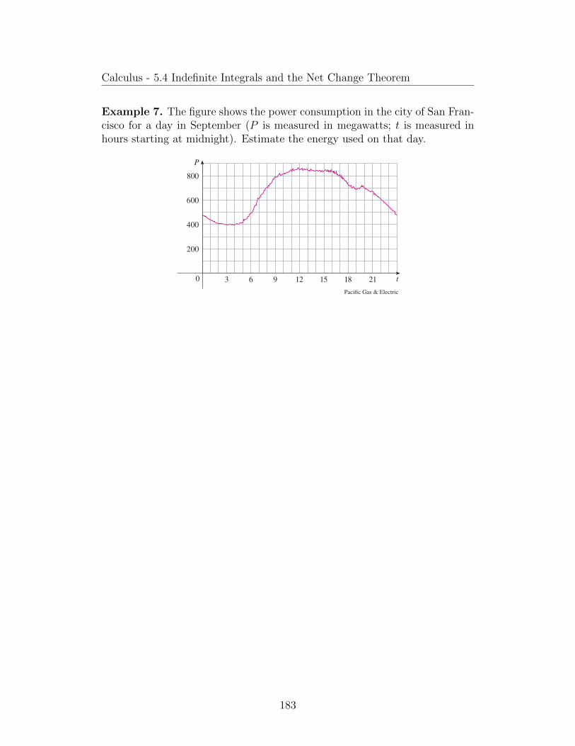
Calculus - 5.4 Indefinite Integrals and the Net Change Theorem
Example 7. The figure shows the power consumption in the city of San Fran-cisco for a day in September (P is measured in megawatts; t is measured inhours starting at midnight). Estimate the energy used on that day.
408 CHAPTER 5 Integrals
EXAMPLE 7 Figure 4 shows the power consumption in the city of San Francisco for a day in September (P is measured in megawatts; t is measured in hours starting at midnight). Estimate the energy used on that day.
P
0 181512963 t21
400
600
800
200
Pacific Gas & Electric
SOLUTION Power is the rate of change of energy: Pstd − E9std. So, by the Net Change Theorem,
y24
0 Pstd dt − y24
0 E9std dt − Es24d 2 Es0d
is the total amount of energy used on that day. We approximate the value of the integral using the Midpoint Rule with 12 subintervals and Dt − 2:
y24
0 Pstd dt < fPs1d 1 Ps3d 1 Ps5d 1 ∙ ∙ ∙ 1 Ps21d 1 Ps23dg Dt
< s440 1 400 1 420 1 620 1 790 1 840 1 850
1 840 1 810 1 690 1 670 1 550ds2d
− 15,840
The energy used was approximately 15,840 megawatt-hours.
How did we know what units to use for energy in Example 7? The integral y240 Pstd dt
is defined as the limit of sums of terms of the form Psti*d Dt. Now Psti*d is measured in megawatts and Dt is measured in hours, so their product is measured in megawatt-hours. The same is true of the limit. In general, the unit of measurement for yb
a f sxd dx is the product of the unit for f sxd and the unit for x.
FIGURE 4
A note on units
1–4 Verify by differentiation that the formula is correct.
1. y 1
x 2s1 1 x 2 dx − 2
s1 1 x 2
x1 C
2. y cos2 x dx − 12 x 1 1
4 sin 2x 1 C
3. y tan2 x dx − tan x 2 x 1 C
4. y xsa 1 bx dx −2
15b2 s3bx 2 2adsa 1 bxd3y2 1 C
5–18 Find the general indefinite integral.
5. y sx1.3 1 7x 2.5d dx
6. y s4 x5 dx
Copyright 2016 Cengage Learning. All Rights Reserved. May not be copied, scanned, or duplicated, in whole or in part. Due to electronic rights, some third party content may be suppressed from the eBook and/or eChapter(s).Editorial review has deemed that any suppressed content does not materially affect the overall learning experience. Cengage Learning reserves the right to remove additional content at any time if subsequent rights restrictions require it.
183

Calculus - 5.5 The Substitution Rule
5.5 The Substitution Rule
Theorem 5.5.1 (The Substitution Rule). If u = g(x) is a differentiable func-tion whose range is an interval I and f is continuous on I, then
ˆf(g(x))g′(x) dx =
ˆf(u) du.
Proof. If f = F ′, then, by the Chain Rule,
d
dx[F (g(x))] = f(g(x))g′(x).
Thus if u = g(x), then we have
ˆf(g(x))g′(x) dx = F (g(x)) + C = F (u) + C =
ˆf(u) du.
Example 1. Find
ˆx3 cos(x4 + 2) dx.
Example 2. Evaluate
ˆ √2x+ 1 dx.
184

Calculus - 5.5 The Substitution Rule
Example 3. Find
ˆx√
1− 4x2dx.
Example 4. Calculate
ˆe5x dx.
Example 5. Find
ˆ √1 + x2x5 dx.
185

Calculus - 5.5 The Substitution Rule
Example 6. Calculate
ˆtanx dx.
Theorem 5.5.2 (The Substitution Rule for Definite Integrals). If g′ is con-tinuous on [a, b] and f is continuous on the range of u = g(x), then
ˆ b
a
f(g(x))g′(x) dx =
ˆ g(b)
g(a)
f(u) du.
Proof. Let F be an antiderivative of f . Then F (g(x)) is an antiderivative off(g(x))g′(x), so by part 2 of the fundamental theorem of calculus, we have
ˆ b
a
f(g(x))g′(x) dx = F (g(x))]ba
= F (g(b))− F (g(a)).
By applying part 2 a second time, we also have
ˆ g(b)
g(a)
f(u) du = F (u)]g(b)g(a)
= F (g(b))− F (g(a)).
186

Calculus - 5.5 The Substitution Rule
Example 7. Evaluate
ˆ 4
0
√2x+ 1 dx.
Example 8. Evaluate
ˆ 2
1
dx
(3− 5x)2.
Example 9. Calculate
ˆ e
1
lnx
xdx.
187

Calculus - 5.5 The Substitution Rule
Theorem 5.5.3 (Integrals of Symmetric Functions). Suppose f is continuouson [−a, a].
(a) If f is even [f(−x) = f(x)], then
ˆ a
−af(x) dx = 2
ˆ a
0
f(x) dx.
(b) If f is odd [f(−x) = −f(x)], then
ˆ a
−af(x) dx = 0.
Proof. First we split the integral:
ˆ a
−af(x) dx =
ˆ 0
−af(x) dx+
ˆ a
0
f(x) dx = −ˆ −a
0
f(x) dx+
ˆ a
0
f(x) dx.
By substituting u = −x we get du = −dx and u = a when x = −a, so
−ˆ −a
0
f(x) dx = −ˆ a
0
f(−u) (−du) =
ˆ a
0
f(−u) du
and therefore ˆ a
−af(x) dx =
ˆ a
0
f(−u) du+
ˆ a
0
f(x) dx.
(a) If f is even then f(−u) = f(u), so
ˆ a
−af(x) dx =
ˆ a
0
f(u) du+
ˆ a
0
f(x) dx = 2
ˆ a
0
f(x) dx.
(b) If f is odd then f(−u) = −f(u), so
ˆ a
−af(x) dx = −
ˆ a
0
f(u) du+
ˆ a
0
f(x) dx = 0.
188

Calculus - 5.5 The Substitution Rule
Example 10. Evaluate
ˆ 2
−2
(x6 + 1) dx.
Example 11. Evaluate
ˆ 1
−1
tanx
1 + x2 + x4dx.
189

Chapter 6
Applications of Integration
6.1 Areas Between Curves
428 CHAPTER 6 Applications of Integration
In Chapter 5 we de!ned and calculated areas of regions that lie under the graphs of func-tions. Here we use integrals to !nd areas of regions that lie between the graphs of two functions.
Consider the region S that lies between two curves y ! f sxd and y ! tsxd and between the vertical lines x ! a and x ! b, where f and t are continuous functions and f sxd > tsxd for all x in fa, bg. (See Figure 1.)
Just as we did for areas under curves in Section 5.1, we divide S into n strips of equal width and then we approximate the ith strip by a rectangle with base Dx and height f sxi*d 2 tsxi*d. (See Figure 2. If we like, we could take all of the sample points to be right endpoints, in which case xi* ! xi.) The Riemann sum
on
i!1 f f sxi*d 2 tsxi*dg Dx
is therefore an approximation to what we intuitively think of as the area of S.
(a) Typical rectangle
x
y
b0 a
f(x i*)f(x i*) -g(x i*)
_g(x i*)x i*
Îx
(b) Approximating rectangles
x
y
b0 a
This approximation appears to become better and better as n l `. Therefore we de!ne the area A of the region S as the limiting value of the sum of the areas of these approxi mating rectangles.
A ! limn l `
on
i!1 f f sxi*d 2 tsxi*dg Dx
We recognize the limit in (1) as the de!nite integral of f 2 t. Therefore we have the fol lowing formula for area.
2 The area A of the region bounded by the curves y ! f sxd, y ! tsxd, and the lines x ! a, x ! b, where f and t are continuous and f sxd > tsxd for all x in fa, bg, is
A ! yb
a f f sxd 2 tsxdg dx
Notice that in the special case where tsxd ! 0, S is the region under the graph of f and our general de!nition of area (1) reduces to our previous de!nition (De!nition 5.1.2).
FIGURE 1 S ! hsx, yd | a < x < b, tsxd < y < f sxdj
0y=©
y=ƒ
S
x
y
ba
FIGURE 2
1
Copyright 2016 Cengage Learning. All Rights Reserved. May not be copied, scanned, or duplicated, in whole or in part. Due to electronic rights, some third party content may be suppressed from the eBook and/or eChapter(s).Editorial review has deemed that any suppressed content does not materially affect the overall learning experience. Cengage Learning reserves the right to remove additional content at any time if subsequent rights restrictions require it.
Definition 6.1.1. The area A of the region bounded by thecurves y = f(x), y = g(x), and the lines x = a, x = b, where fand g are continuous and f(x) ≥ g(x) for all x in [a, b], is
A = limn→∞
n∑i=1
[f(x∗i )− g(x∗i )]∆x =
ˆ b
a
[f(x)− g(x)] dx.
428 CHAPTER 6 Applications of Integration
In Chapter 5 we de!ned and calculated areas of regions that lie under the graphs of func-tions. Here we use integrals to !nd areas of regions that lie between the graphs of two functions.
Consider the region S that lies between two curves y ! f sxd and y ! tsxd and between the vertical lines x ! a and x ! b, where f and t are continuous functions and f sxd > tsxd for all x in fa, bg. (See Figure 1.)
Just as we did for areas under curves in Section 5.1, we divide S into n strips of equal width and then we approximate the ith strip by a rectangle with base Dx and height f sxi*d 2 tsxi*d. (See Figure 2. If we like, we could take all of the sample points to be right endpoints, in which case xi* ! xi.) The Riemann sum
on
i!1 f f sxi*d 2 tsxi*dg Dx
is therefore an approximation to what we intuitively think of as the area of S.
(a) Typical rectangle
x
y
b0 a
f(x i*)f(x i*) -g(x i*)
_g(x i*)x i*
Îx
(b) Approximating rectangles
x
y
b0 a
This approximation appears to become better and better as n l `. Therefore we de!ne the area A of the region S as the limiting value of the sum of the areas of these approxi mating rectangles.
A ! limn l `
on
i!1 f f sxi*d 2 tsxi*dg Dx
We recognize the limit in (1) as the de!nite integral of f 2 t. Therefore we have the fol lowing formula for area.
2 The area A of the region bounded by the curves y ! f sxd, y ! tsxd, and the lines x ! a, x ! b, where f and t are continuous and f sxd > tsxd for all x in fa, bg, is
A ! yb
a f f sxd 2 tsxdg dx
Notice that in the special case where tsxd ! 0, S is the region under the graph of f and our general de!nition of area (1) reduces to our previous de!nition (De!nition 5.1.2).
FIGURE 1 S ! hsx, yd | a < x < b, tsxd < y < f sxdj
0y=©
y=ƒ
S
x
y
ba
FIGURE 2
1
Copyright 2016 Cengage Learning. All Rights Reserved. May not be copied, scanned, or duplicated, in whole or in part. Due to electronic rights, some third party content may be suppressed from the eBook and/or eChapter(s).Editorial review has deemed that any suppressed content does not materially affect the overall learning experience. Cengage Learning reserves the right to remove additional content at any time if subsequent rights restrictions require it.
190

Calculus - 6.1 Areas Between Curves
Example 1. Find the area of the region bounded above by y = ex, boundedbelow by y = x, and bounded on the sides by x = 0 and x = 1.
Example 2. Find the area of the region enclosed by the parabolas y = x2
and y = 2x− x2.
191

Calculus - 6.1 Areas Between Curves
Example 3. Find the approximate area of the region bounded by the curvesy = x/
√x2 + 1 and y = x4 − x.
192

Calculus - 6.1 Areas Between Curves
430 CHAPTER 6 Applications of Integration
Sometimes it’s difficult, or even impossible, to find the points of intersection of two curves exactly. As shown in the following example, we can use a graphing calculator or computer to find approximate values for the intersection points and then proceed as before.
EXAMPLE 3 Find the approximate area of the region bounded by the curvesy − xysx 2 1 1 and y − x 4 2 x.
SOLUTION If we were to try to find the exact intersection points, we would have to solve the equation
x
sx 2 1 1− x 4 2 x
This looks like a very difficult equation to solve exactly (in fact, it’s impossible), so instead we use a graphing device to draw the graphs of the two curves in Figure 7. One intersection point is the origin. We zoom in toward the other point of intersection and find that x < 1.18. (If greater accuracy is required, we could use Newton’s method or solve numerically on our graphing device.) So an approximation to the area between the curves is
A < y1.18
0 F x
sx 2 1 12 sx 4 2 xdG dx
To integrate the first term we use the substitution u − x 2 1 1. Then du − 2x dx, and when x − 1.18, we have u < 2.39; when x − 0, u − 1. So
A < 12 y2.39
1
du
su 2 y1.18
0 sx 4 2 xd dx
− su g1
2.39
2 F x 5
52
x 2
2 G0
1.18
− s2.39 2 1 2s1.18d5
51
s1.18d2
2
< 0.785 n
EXAMPLE 4 Figure 8 shows velocity curves for two cars, A and B, that start side by side and move along the same road. What does the area between the curves represent? Use the Midpoint Rule to estimate it.
SOLUTION We know from Section 5.4 that the area under the velocity curve A rep-resents the distance traveled by car A during the first 16 seconds. Similarly, the area under curve B is the distance traveled by car B during that time period. So the area between these curves, which is the difference of the areas under the curves, is the distance between the cars after 16 seconds. We read the velocities from the graph and convert them to feet per second s1 miyh − 5280
3600 ftysd.
t 0 2 4 6 8 10 12 14 16
vA 0 34 54 67 76 84 89 92 95
vB 0 21 34 44 51 56 60 63 65
vA 2 vB 0 13 20 23 25 28 29 29 30
1.5
_1
_1 2y=x$-x
xœ„„„„„≈+1
y=
FIGURE 7
0
102030405060
A
B
2 4 6 8 10 12 14 16 t(seconds)
√ (mi/h)
FIGURE 8
Copyright 2016 Cengage Learning. All Rights Reserved. May not be copied, scanned, or duplicated, in whole or in part. Due to electronic rights, some third party content may be suppressed from the eBook and/or eChapter(s).Editorial review has deemed that any suppressed content does not materially affect the overall learning experience. Cengage Learning reserves the right to remove additional content at any time if subsequent rights restrictions require it.
Example 4. The figure shows the velocity curves for two cars,A and B, that start side by side and move along the same road.What does the area between the curves represent? Use the Mid-point Rule to estimate it.
193

Calculus - 6.1 Areas Between Curves
Example 5. The figure is an example of a pathogenesis curve for a measlesinfection. It shows how the disease develops in an individual with no immunityafter the measles virus spreads to the bloodstream from the respiratory tract.
SECTION 6.1 Areas Between Curves 431
We use the Midpoint Rule with n − 4 intervals, so that Dt − 4. The midpoints of the intervals are t1 − 2, t2 − 6, t3 − 10, and t4 − 14. We estimate the distance between the cars after 16 seconds as follows:
y16
0 svA 2 vBd dt < Dt f13 1 23 1 28 1 29g
− 4s93d − 372 ft n
EXAMPLE 5 Figure 9 is an example of a pathogenesis curve for a measles infection. It shows how the disease develops in an individual with no immunity after the measles virus spreads to the bloodstream from the respiratory tract.
0
N
t
Infectiousness begins
Symptomsappear
Infectiousnessends
Pathogenis cleared
Pathogenenters plasma
(days)10–11 12 2117–18
1000
1500
500
Num
ber o
f inf
ecte
d ce
lls p
er m
L o
f blo
od p
lasm
a
The patient becomes infectious to others once the concentration of infected cells becomes great enough, and he or she remains infectious until the immune system manages to prevent further transmission. However, symptoms don’t develop until the “amount of infection” reaches a particular threshold. The amount of infection needed to develop symptoms depends on both the concentration of infected cells and time, and corresponds to the area under the pathogenesis curve until symptoms appear. (See Exercise 5.1.19.)(a) The pathogenesis curve in Figure 9 has been modeled by f std − 2tst 2 21dst 1 1d. If infectiousness begins on day t1 − 10 and ends on day t2 − 18, what are the corre-sponding concentration levels of infected cells?(b) The level of infectiousness for an infected person is the area between N − f std and the line through the points P1st1, f st1dd and P2st2, f st2dd, measured in (cellsymL) ? days. (See Figure 10.) Compute the level of infectiousness for this particular patient.
SOLUTION(a) Infectiousness begins when the concentration reaches f s10d − 1210 cellsymL and ends when the concentration reduces to f s18d − 1026 cellsymL.
FIGURE 9 Measles pathogenesis curve
Source: J. M. Heffernan et al., “An In-Host Model of Acute Infection: Measles as a Case Study,”
Theoretical Population Biology 73 (2008): 134–47.
0
N
t(days)
10 18
f
P¡
P™
FIGURE 10
Copyright 2016 Cengage Learning. All Rights Reserved. May not be copied, scanned, or duplicated, in whole or in part. Due to electronic rights, some third party content may be suppressed from the eBook and/or eChapter(s).Editorial review has deemed that any suppressed content does not materially affect the overall learning experience. Cengage Learning reserves the right to remove additional content at any time if subsequent rights restrictions require it.
The patient becomes infectious to others once the concentration of infectedcells becomes great enough, and he or she remains infectious until the immunesystem manages to prevent further transmission. However, symptoms don’tdevelop until the “amount of infection” reaches a particular threshold. Theamount of infection needed to develop symptoms depends on both the con-centration of infected cells and time, and corresponds to the area under thepathogenesis curve until symptoms appear.
(a) The pathogenesis curve in the figure has been modeled by f(t) = −t(t −21)(t+1). If infectiousness begins on day t1 = 10 and ends on day t2 = 18,what are the corresponding concentration levels of infected cells?
194

Calculus - 6.1 Areas Between Curves
(b) The level of infectiousness for an infected person is the area betweenN = f(t) and the line through the points P1(t1, (f(t1)) and P2(t2, f(t2)),measured in (cells/mL)· days. Compute the level of infectiousness for thisparticular patient.
195

Calculus - 6.1 Areas Between Curves
Definition 6.1.2. The area between the curves y = f(x) and y = g(x) andbetween x = a and x = b is
A =
ˆ b
a
|f(x)− g(x)| dx.
Example 6. Find the area of the region bounded by the curves y = sinx,y = cosx, x = 0, and x = π/2.
196

Calculus - 6.1 Areas Between Curves
SECTION 6.1 Areas Between Curves 433
Observe that cos x > sin x when 0 < x < !y4 but sin x > cos x when !y4 < x < !y2. Therefore the required area is
A ! y!y2
0 | cos x 2 sin x | dx ! A1 1 A2
! y!y4
0 scos x 2 sin xd dx 1 y!y2
!y4 ssin x 2 cos xd dx
! fsin x 1 cos xg0
!y41 f2cos x 2 sin xg!y4
!y2
! S 1
s21
1
s22 0 2 1D 1 S20 2 1 1
1
s21
1
s2D ! 2s2 2 2
In this particular example we could have saved some work by noticing that the region is symmetric about x ! !y4 and so
A ! 2A1 ! 2 y!y4
0 scos x 2 sin xd dx Q
Some regions are best treated by regarding x as a function of y. If a region is bounded by curves with equations x ! f syd, x ! tsyd, y ! c, and y ! d, where f and t are con-tinuous and f syd > tsyd for c < y < d (see Figure 13), then its area is
A ! yd
c f f syd 2 tsydg dy
If we write xR for the right boundary and xL for the left boundary, then, as Fig ure 14 illustrates, we have
A ! yd
c sxR 2 xLd dy
Here a typical approximating rectangle has dimensions xR 2 xL and Dy.
EXAMPLE 7 Find the area enclosed by the line y ! x 2 1 and the parabola y 2 ! 2x 1 6.
SOLUTION By solving the two equations we !nd that the points of intersection are s21, 22d and s5, 4d. We solve the equation of the parabola for x and notice from Fig ure 15 that the left and right boundary curves are
xL ! 12 y 2 2 3 and xR ! y 1 1
x
y
_2
4
0
(_1, _2)
(5, 4)
xR=y+1
12xL= ¥-3
FIGURE 13
FIGURE 14
x
c
d
y
0
y=d
x=g(y) x=f(y)
y=c
Îy
0 x
y
c
dxRxL
xR-xL
Îy
FIGURE 15
Copyright 2016 Cengage Learning. All Rights Reserved. May not be copied, scanned, or duplicated, in whole or in part. Due to electronic rights, some third party content may be suppressed from the eBook and/or eChapter(s).Editorial review has deemed that any suppressed content does not materially affect the overall learning experience. Cengage Learning reserves the right to remove additional content at any time if subsequent rights restrictions require it.
Remark 1. Some regions are best treated by regarding x as afunction of y. If a region is bounded by curves with equationsx = f(y), x = g(y), y = c, and y = d, where f and g arecontinuous and f(y) ≥ g(y) for c ≤ y ≤ d (see the figure), thenits area is
A =
ˆ d
c
[f(y)− g(y)] dy.
Example 7. Find the area enclosed by the line y = x − 1 andthe parabola y2 = 2x+ 6.
197

Calculus - 6.2 Volumes
6.2 Volumes
Definition 6.2.1 (Definition of Volume). Let S be a solid that lies betweenx = a and x = b. If the cross-sectional area of S in the plane Px, throughx and perpendicular to the x-axis, is A(x), where A is a continuous function,then the volume of S is
V = limn→∞
n∑i=1
A(x∗i )∆x =
ˆ b
a
A(x) dx.
SeCtion 6.2 Volumes 439
Let’s divide S into n “slabs” of equal width Dx by using the planes Px1, Px2 , . . . to slice the solid. (Think of slicing a loaf of bread.) If we choose sample points xi* in fxi21, xig, we can approximate the ith slab Si (the part of S that lies between the planes Pxi21 and Pxi) by a cylinder with base area Asxi*d and “height” Dx. (See Figure 3.)
xi-1 xi
y
0 xx*i
Îx
S
a b
y
0 xx¶=ba=x¸ ⁄ x™ ‹ x¢ x∞ xß
The volume of this cylinder is Asxi*d Dx, so an approximation to our intuitive concep-tion of the volume of the ith slab Si is
VsSid < Asxi*d Dx
Adding the volumes of these slabs, we get an approximation to the total volume (that is, what we think of intuitively as the volume):
V < on
i−1 Asxi*d Dx
This approximation appears to become better and better as n l `. (Think of the slices as becoming thinner and thinner.) Therefore we define the volume as the limit of these sums as n l `. But we recognize the limit of Riemann sums as a definite integral and so we have the following definition.
Definition of Volume Let S be a solid that lies between x − a and x − b. If the cross-sectional area of S in the plane Px, through x and perpendicular to the x-axis, is Asxd, where A is a continuous function, then the volume of S is
V − limn l `
on
i−1Asxi*d Dx − yb
a Asxd dx
When we use the volume formula V − yba Asxd dx, it is important to remember that
Asxd is the area of a moving cross-section obtained by slicing through x perpendicular to the x-axis.
Notice that, for a cylinder, the cross-sectional area is constant: Asxd − A for all x. So our definition of volume gives V − yb
a A dx − Asb 2 ad; this agrees with the formula V − Ah.
ExamplE 1 Show that the volume of a sphere of radius r is V − 43 r 3.
SoLUtion If we place the sphere so that its center is at the origin, then the plane Px intersects the sphere in a circle whose radius (from the Pythagorean Theorem) is
FIGURE 3
It can be proved that this definition is independent of how S is situated with respect to the x-axis. In other words, no matter how we slice S with parallel planes, we always get the same answer for V.
Copyright 2016 Cengage Learning. All Rights Reserved. May not be copied, scanned, or duplicated, in whole or in part. Due to electronic rights, some third party content may be suppressed from the eBook and/or eChapter(s).
Editorial review has deemed that any suppressed content does not materially affect the overall learning experience. Cengage Learning reserves the right to remove additional content at any time if subsequent rights restrictions require it.
Example 1. Show that the volume of a sphere of radius r is V = 43πr3.
198

Calculus - 6.2 Volumes
Example 2. Find the volume of the solid obtained by rotating about the x-axis the region under the curve y =
√x from 0 to 1. Illustrate the definition
of volume by sketching a typical approximating cylinder.
Example 3. Find the volume of the solid obtained by rotating the regionbounded by y = x3, y = 8, and x = 0 about the y-axis.
199

Calculus - 6.2 Volumes
Example 4. The region R enclosed by the curves y = x and y = x2 is rotatedabout the x-axis. Find the volume of the resulting solid.
Example 5. Find the volume of the solid obtained by rotating the region inExample 4 about the line y = 2.
200

Calculus - 6.2 Volumes
Example 6. Find the volume of the solid obtained by rotating the region inExample 4 about the line x = −1.
444 CHAPTER 6 Applications of Integration
EXAMPLE 6 Find the volume of the solid obtained by rotating the region in Example 4 about the line x − 21.
SOLUTION Figure 11 shows a horizontal cross-section. It is a washer with inner radius 1 1 y and outer radius 1 1 sy , so the cross-sectional area is
Asyd − !souter radiusd2 2 !sinner radiusd2
− ! (1 1 sy )2 2 !s1 1 yd2
The volume is
V − y1
0 Asyd dy − ! y1
0 fs1 1 sy d2 2 s1 1 yd2 g dy
− ! y1
0 s2sy 2 y 2 y 2 d dy − !F 4y 3y2
32
y 2
22
y 3
3 G0
1
−!
2
x=_1
y
y
x0
x=œ„y
y
x=y
y
1 y1+y
1+œ„
n
We now find the volumes of three solids that are not solids of revolution.
EXAMPLE 7 Figure 12 shows a solid with a circular base of radius 1. Parallel cross- sections perpendicular to the base are equilateral triangles. Find the volume of the solid.
SOLUTION Let’s take the circle to be x 2 1 y 2 − 1. The solid, its base, and a typical cross-section at a distance x from the origin are shown in Figure 13.
Since B lies on the circle, we have y − s1 2 x 2 and so the base of the triangle ABC is | AB | − 2y − 2s1 2 x 2 . Since the triangle is equilateral, we see from Figure 13(c)
TEC Visual 6.2C shows how the solid in Figure 12 is generated.
FIGURE 12 Computer-generated picture of the solid in Example 7
y
x
FIGURE 13
FIGURE 11
y y60° 60° BA
C
œ„3y
(c) A cross-section
A
B(x, y)y=œ„„„„„„1-≈
(b) Its base
x
y
0
y
x
(a) The solid
0
A
x
B
1_1 x
yC
Copyright 2016 Cengage Learning. All Rights Reserved. May not be copied, scanned, or duplicated, in whole or in part. Due to electronic rights, some third party content may be suppressed from the eBook and/or eChapter(s).Editorial review has deemed that any suppressed content does not materially affect the overall learning experience. Cengage Learning reserves the right to remove additional content at any time if subsequent rights restrictions require it.
Example 7. The figure shows a solid with a circular base ofradius 1. Parallel cross-sections perpendicular to the base areequilateral triangles. Find the volume of the solid.
201

Calculus - 6.2 Volumes
Example 8. Find the volume of a pyramid whose base is a square with sideL and whose height is h.
Example 9. A wedge is cut out of a circular cylinder of radius 4 by two planes.One plane is perpendicular to the axis of the cylinder. The other intersectsthe first at an angle of 30° along a diameter of the cylinder. Find the volumeof the wedge.
202

Calculus - 6.3 Volumes by Cylindrical Shells
6.3 Volumes by Cylindrical Shells
Theorem 6.3.1 (Method of Cylindrical Shells). The volume of the solid inthe figure, obtained by rotating about the y-axis the region under the curvey = f(x) from a to b, is
V = limn→∞
n∑i=1
2πxif(xi)∆x =
ˆ b
a
2πxf(x) dx where 0 ≤ a ≤ b
and where xi is the midpoint of the ith subinterval [xi−1, xi].
450 Chapter 6 Applications of Integration
r2, and height h. Its volume V is calculated by subtracting the volume V1 of the inner cylinder from the volume V2 of the outer cylinder:
V − V2 2 V1
− r 22 h 2 r 2
1 h − sr 22 2 r 2
1 dh
− sr2 1 r1dsr2 2 r1dh
− 2r2 1 r1
2hsr2 2 r1d
If we let Dr − r2 2 r1 (the thickness of the shell) and r − 12 sr2 1 r1d (the average radius
of the shell), then this formula for the volume of a cylindrical shell becomes
V − 2rh Dr1
and it can be remembered as
V − [circumference][height][thickness]
Now let S be the solid obtained by rotating about the y-axis the region bounded by y − f sxd [where f sxd > 0], y − 0, x − a, and x − b, where b . a > 0. (See Figure 3.)
x
y
a b0
y=ƒ
a b x
y
0
y=ƒ
We divide the interval fa, bg into n subintervals fxi21, xig of equal width Dx and let xi
be the midpoint of the ith subinterval. If the rectangle with base fxi21, xig and height f sxid is rotated about the y-axis, then the result is a cylindrical shell with average radius xi , height f sxid, and thickness Dx (see Figure 4). So by Formula 1 its volume is
Vi − s2xidf f sxidg Dx
x
y
a b0
y=ƒ
xi–
a b0 x
y
xi-1xi
y=ƒ
x
y
a b0
y=ƒ
Therefore an approximation to the volume V of S is given by the sum of the volumes of
FIGURE 3
FIGURE 4
Copyright 2016 Cengage Learning. All Rights Reserved. May not be copied, scanned, or duplicated, in whole or in part. Due to electronic rights, some third party content may be suppressed from the eBook and/or eChapter(s).
Editorial review has deemed that any suppressed content does not materially affect the overall learning experience. Cengage Learning reserves the right to remove additional content at any time if subsequent rights restrictions require it.
Example 1. Find the volume of the solid obtained by rotating about they-axis the region bounded by y = 2x2 − x3 and y = 0.
203

Calculus - 6.3 Volumes by Cylindrical Shells
Example 2. Find the volume of the solid obtained by rotating about they-axis the region between y = x and y = x2.
Example 3. Use cylindrical shells to find the volume of the solid obtained byrotating about the x-axis the region under the curve y =
√x from 0 to 1.
204

Calculus - 6.3 Volumes by Cylindrical Shells
Example 4. Find the volume of the solid obtained by rotating the regionbounded by y = x− x2 and y = 0 about the line x = 2.
205

Calculus - 6.4 Work
6.4 Work
Definition 6.4.1. In general, if an object moves along a straight line withposition function s(t), then the force F on the object (in the same direction)is given by Newton’s Second Law of Motion as the product of its mass m andits acceleration a:
F = ma = md2s
dt2.
Definition 6.4.2. In the case of constant acceleration, the force F is alsoconstant and the work done is defined to be the product of the force F anddistance d that the object moves:
W = Fd work = force× distance.
Example 1. (a) How much work is done in lifting a 1.2-kg book off the floorto put it on a desk that is 0.7 m high? Use the fact that the accelerationdue to gravity is g = 9.8 m/s2.
(b) How much work is done in lifting a 20-lb weight 6 ft off the ground?
206

Calculus - 6.4 Work
Definition 6.4.3. If the force f(x) on an object is variable, then we definethe work done in moving the object from a to b as
W = limn→∞
n∑i=1
f(x∗i )∆x =
ˆ b
a
f(x) dx.
Example 2. When a particle is located a distance x feet from the origin, aforce of x2 + 2x pounds acts on it. How much work is done in moving it fromx = 1 to x = 3?
Theorem 6.4.1 (Hooke’s Law). The force required to maintain a springstretched x units beyond its natural length is proportional to x:
f(x) = kx
where k is a positive constant called the spring constant (see the figure). Hooke’sLaw holds provided that x is not too large. SECTION 6.4 Work 457
W − y0.08
0.05 800x dx − 800
x 2
2 G0.05
0.08
− 400fs0.08d2 2 s0.05d2g − 1.56 J Q
EXAMPLE 4 A 200-lb cable is 100 ft long and hangs vertically from the top of a tall building. How much work is required to lift the cable to the top of the building?
SOLUTION Here we don’t have a formula for the force function, but we can use an argument similar to the one that led to Definition 4.
Let’s place the origin at the top of the building and the x-axis pointing downward as in Figure 2. We divide the cable into small parts with length Dx. If xi* is a point in the ith such interval, then all points in the interval are lifted by approximately the same amount, namely xi*. The cable weighs 2 pounds per foot, so the weight of the ith part is (2 lbyft)(Dx ft) − 2Dx lb. Thus the work done on the ith part, in foot-pounds, is
s2Dxd ? xi* − 2xi* Dxforce distance
We get the total work done by adding all these approximations and letting the num-ber of parts become large (so Dx l 0):
W − limn l `
on
i−1 2xi*Dx − y100
0 2x dx
− x 2g100
0 − 10,000 ft-lb Q
EXAMPLE 5 A tank has the shape of an inverted circular cone with height 10 m and base radius 4 m. It is filled with water to a height of 8 m. Find the work required to empty the tank by pumping all of the water to the top of the tank. (The density of water is 1000 kgym3.)
x0frictionlesssurface
x0 x
ƒ=kx
(a) Natural position of spring (b) Stretched position of spring
0
100
x*i
x
Îx
FIGURE 2
If we had placed the origin at the bottom of the cable and the x-axis upward, we would have gotten
W − y100
0 2s100 2 xd dx
which gives the same answer.
Copyright 2016 Cengage Learning. All Rights Reserved. May not be copied, scanned, or duplicated, in whole or in part. Due to electronic rights, some third party content may be suppressed from the eBook and/or eChapter(s).Editorial review has deemed that any suppressed content does not materially affect the overall learning experience. Cengage Learning reserves the right to remove additional content at any time if subsequent rights restrictions require it.
207

Calculus - 6.4 Work
Example 3. A force of 40 N is required to hold a spring that has beenstretched from its natural length of 10 cm to a length of 15 cm. How muchwork is done in stretching the spring from 15 cm to 18 cm?
Example 4. A 200-lb cable is 100 ft long and hangs vertically from the topof a tall building. How much work is required to lift the cable to the top ofthe building?
208

Calculus - 6.4 Work
Example 5. A tank has the shape of an inverted circular cone with height10 m and base radius 4 m. It is filled with water to a height of 8 m. Find thework required to empty the tank by pumping all of the water to the top of thetank. (The density of water is 1000 kg/m3.)
209

Calculus - 6.5 Average Value of a Function
6.5 Average Value of a Function
Definition 6.5.1. The average value of a function f on the interval [a, b] is
fave =1
b− a
ˆ b
a
f(x) dx.
Example 1. Find the average value of the function f(x) = 1 + x2 on theinterval [−1, 2].
Theorem 6.5.1 (The Mean Value Theorem for Integrals). If f is continuouson [a, b], then there exists a number c in [a, b] such that
f(c) = fave =1
b− a
ˆ b
a
f(x) dx,
that is, ˆ b
a
f(x) dx = f(c)(b− a).
Proof. By applying the Mean Value Theorem for derivatives to the functionF (x) =
´ xaf(t)dt, we see that there exists a number c in [a, b] such that
F ′(c) =F (b)− F (a)
b− ad
dx
[ˆ x
a
f(t) dt
]∣∣∣∣∣c
=F (b)− F (a)
b− a
f(c) =1
b− a[F (b)− F (a)]
=1
b− a
ˆ b
a
f(x) dx.
210

Calculus - 6.5 Average Value of a Function
Example 2. Find a number c in the interval [−1, 2] that satisfies the meanvalue theorem for integrals for the function f(x) = 1 + x2.
Example 3. Show that the average velocity of a car over a time interval [t1, t2]is the same as the average of its velocities during the trip.
211

Chapter 7
Techniques of Integration
7.1 Integration by Parts
Theorem 7.1.1 (Formula for Integration by Parts). If f and g are differen-tiable functions then
ˆf(x)g′(x) dx = f(x)g(x)−
ˆg(x)f ′(x) dx,
or, equivalently, ˆu dv = uv −
ˆv du
where u = f(x) and v = g(x).
Proof. By the Product Rule,
d
dx[f(x)g(x)] = f(x)g′(x) + g(x)f ′(x)
f(x)g(x) =
ˆ[f(x)g′(x) + g(x)f ′(x)] dx
=
ˆf(x)g′(x) dx+
ˆg(x)f ′(x) dx
ˆf(x)g′(x) dx = f(x)g(x)−
ˆg(x)f ′(x) dx
212

Calculus - 7.1 Integration by Parts
Example 1. Find
ˆx sinx dx.
Example 2. Evaluate
ˆlnx dx.
213

Calculus - 7.1 Integration by Parts
Example 3. Find
ˆt2et dt.
214

Calculus - 7.1 Integration by Parts
Example 4. Evaluate
ˆex sinx dx.
215

Calculus - 7.1 Integration by Parts
Theorem 7.1.2 (Formula for Definite Integration by Parts). If f and g aredifferentiable on (a, b) and f ′ and g′ are continuous, then
ˆ b
a
f(x)g′(x) dx = f(x)g(x)]ba−ˆ b
a
g(x)f ′(x) dx.
Example 5. Calculate
ˆ 1
0
tan−1 x dx.
216

Calculus - 7.1 Integration by Parts
Example 6. Prove the reduction formula
ˆsinn x dx = − 1
ncosx sinn−1 x+
n− 1
n
ˆsinn−2 x dx
where n ≥ 2 is an integer.
217

Calculus - 7.2 Trigonometric Integrals
7.2 Trigonometric Integrals
Example 1. Evaluate
ˆcos3 x dx.
Example 2. Find
ˆsin5 x cos2 x dx.
218
Calculus - 7.2 Trigonometric Integrals
Remark 1. Sometimes it is easier to use the half-angle identities
sin2 x =1
2(1− cos 2x) and cos2 x =
1
2(1 + cos 2x)
to evaluate an integral.
Example 3. Evaluate
ˆ π
0
sin2 x dx.
Example 4. Find
ˆsin4 x dx.
219
Calculus - 7.2 Trigonometric Integrals
Example 5. Evaluate
ˆtan6 x sec4 x dx.
Example 6. Find
ˆtan5 θ sec7 θ dθ.
220
Calculus - 7.2 Trigonometric Integrals
Example 7. Find
ˆtan3 x dx.
Example 8. Find
ˆsec3 x dx.
221

Calculus - 7.2 Trigonometric Integrals
Remark 2. To evaluate the integrals (a)´
sinmx cosnx dx, (b)´
sinmx sinnx dx,or (c)
´cosmx cosnx dx, use the corresponding identity:
(a) sinA cosB =1
2[sin(A−B) + sin(A+B)]
(b) sinA sinB =1
2[cos(A−B)− cos(A+B)]
(c) cosA cosB =1
2[cos(A−B) + cos(A+B)].
Example 9. Evaluate
ˆsin 4x cos 5x dx.
222

Calculus - 7.3 Trigonometric Substitution
7.3 Trigonometric Substitution
Table of Trigonometric Substitutions
Expression Substitution Identity
√a2 − x2 x = a sin θ, −π
2≤ θ ≤ π
21− sin2 θ = cos2 θ
√a2 + x2 x = a tan θ, −π
2≤ θ ≤ π
21 + tan2 θ = sec2 θ
√x2 − a2
x = a sec θ, 0 ≤ θ ≤ π
2or π ≤ θ ≤ 3π
2sec2 θ − 1 = tan2 θ
Example 1. Evaluate
ˆ √9− x2
x2dx.
223

Calculus - 7.3 Trigonometric Substitution
Example 2. Find the area enclosed by the ellipse
x2
a2+y2
b2= 1.
224

Calculus - 7.3 Trigonometric Substitution
Example 3. Find
ˆ1
x2√x2 + 4
dx.
225

Calculus - 7.3 Trigonometric Substitution
Example 4. Find
ˆx√x2 + 4
dx.
Example 5. Evaluate
ˆdx√x2 − a2
, where a > 0.
226

Calculus - 7.3 Trigonometric Substitution
Example 6. Find
ˆ 3√
3/2
0
x3
(4x2 + 9)3/2dx.
227

Calculus - 7.3 Trigonometric Substitution
Example 7. Evaluate
ˆx√
3− 2x− x2dx.
228

Calculus - 7.4 Integration by Partial Fractions
7.4 Integration by Partial Fractions
Example 1. Find
ˆx3 + x
x− 1dx.
229

Calculus - 7.4 Integration by Partial Fractions
Example 2. Evaluate
ˆx2 + 2x− 1
2x3 + 3x2 − 2xdx.
230

Calculus - 7.4 Integration by Partial Fractions
Example 3. Find
ˆdx
x2 − a2, where a 6= 0.
231

Calculus - 7.4 Integration by Partial Fractions
Example 4. Find
ˆx4 − 2x2 + 4x+ 1
x3 − x2 − x+ 1dx.
232

Calculus - 7.4 Integration by Partial Fractions
Theorem 7.4.1. ˆdx
x2 + a2=
1
atan−1
(x
a
)+ C.
Example 5. Evaluate
ˆ2x2 − x+ 4
x3 + 4xdx.
233

Calculus - 7.4 Integration by Partial Fractions
Example 6. Evaluate
ˆ4x2 − 3x+ 2
4x2 − 4x+ 3dx.
234

Calculus - 7.4 Integration by Partial Fractions
Example 7. Write out the form of the partial fraction decomposition of thefunction
x3 + x2 + 1
x(x− 1)(x2 + x+ 1)(x2 + 1)3.
Example 8. Evaluate
ˆ1− x+ 2x2 − x3
x(x2 + 1)2dx.
235

Calculus - 7.4 Integration by Partial Fractions
Example 9. Evaluate
ˆ √x+ 4
xdx.
236

Calculus - 7.5 Strategy for Integration
7.5 Strategy for Integration
Example 1.
ˆtan3 x
cos3 xdx.
Example 2.
ˆe√x dx.
237

Calculus - 7.5 Strategy for Integration
Example 3.
ˆx5 + 1
x3 − 3x2 − 10xdx.
238

Calculus - 7.5 Strategy for Integration
Example 4.
ˆdx
x√
lnx.
Example 5.
ˆ √1− x1 + x
dx.
239

Calculus - 7.6 Integration Using Tables and CAS’s
7.6 Integration Using Tables and CAS’s
Example 1. The region bounded by the curves y = arctanx, y = 0, andx = 1 is rotated about the y-axis. Find the volume of the resulting solid.
Example 2. Use the Table of Integrals to find
ˆx2
√5− 4x2
dx.
240

Calculus - 7.6 Integration Using Tables and CAS’s
Example 3. Use the Table of Integrals to evaluate
ˆx3 sinx dx.
Example 4. Use the Table of Integrals to find
ˆx√x2 + 2x+ 4 dx.
241

Calculus - 7.6 Integration Using Tables and CAS’s
Example 5. Use a computer algebra system to find
ˆx√x2 + 2x+ 4 dx.
Example 6. Use a CAS to evaluate
ˆx(x2 + 5)8 dx.
Example 7. Use a CAS to find
ˆsin5 x cos2 x dx.
242

Calculus - 7.7 Approximate Integration
7.7 Approximate Integration
SECTION 7.7 Approximate Integration 515
example, it is impossible to evaluate the following integrals exactly:
y1
0 ex 2
dx y1
21 s1 1 x 3 dx
The second situation arises when the function is determined from a scienti!c experi-ment through instrument readings or collected data. There may be no formula for the function (see Example 5).
In both cases we need to !nd approximate values of de!nite integrals. We already know one such method. Recall that the de!nite integral is de!ned as a limit of Riemann sums,"so any Riemann sum could be used as an approximation to the integral: If we divide fa, bg into n subintervals of equal length Dx ! sb 2 adyn, then we have
yb
a f sxd dx < o
n
i!1 f sxi*d Dx
where x i* is any point in the ith subinterval fxi21, xig. If x i* is chosen to be the left end-point of the interval, then x i* ! xi21 and we have
yb
a f sxd dx < Ln ! o
n
i!1 f sxi21d Dx
If f sxd > 0, then the integral represents an area and (1) represents an approximation of this area by the rectangles shown in Figure 1(a). If we choose x i* to be the right endpoint, then x i* ! xi and we have
yb
a f sxd dx < Rn ! o
n
i!1 f sxid Dx
[See Figure 1(b).] The approximations Ln and Rn de!ned by Equations 1 and 2 are called the left endpoint approximation and right endpoint approximation, respectively.
In Section 5.2 we also considered the case where x i* is chosen to be the midpoint xi of the subinterval fxi21, xig. Figure 1(c) shows the midpoint approximation Mn, which appears to be better than either Ln or Rn.
Midpoint Rule
yb
a f sxd dx < Mn ! Dx f f sx1d 1 f sx2 d 1 # # # 1 f sxn dg
where Dx !b 2 a
n
and xi ! 12 sxi21 1 xid ! midpoint of fxi21, xig
Another approximation, called the Trapezoidal Rule, results from averaging the approximations in Equations 1 and 2:
yb
a f sxd dx <
12
Fon
i!1 f sxi21 d Dx 1 o
n
i!1 f sxid DxG !
Dx2
Fon
i!1 s f sxi21 d 1 f sxiddG
!Dx2
fs f sx0 d 1 f sx1dd 1 s f sx1d 1 f sx2 dd 1 # # # 1 s f sxn21d 1 f sxn ddg
!Dx2
f f sx0 d 1 2 f sx1d 1 2 f sx2 d 1 # # # 1 2 f sxn21d 1 f sxn dg
1
⁄ ¤– – ––
(a) Left endpoint approximation
y
x¸ ⁄ ¤ ‹ x¢
x¸ ⁄ ¤ ‹ x¢
‹ x¢
x0
(b) Right endpoint approximation
y
x0
x
(c) Midpoint approximation
y
0
FIGURE 1
2
Copyright 2016 Cengage Learning. All Rights Reserved. May not be copied, scanned, or duplicated, in whole or in part. Due to electronic rights, some third party content may be suppressed from the eBook and/or eChapter(s).Editorial review has deemed that any suppressed content does not materially affect the overall learning experience. Cengage Learning reserves the right to remove additional content at any time if subsequent rights restrictions require it.
Theorem 7.7.1 (Midpoint Rule).
ˆ b
a
f(x) dx ≈Mn = ∆x[f(x1) + f(x2) + · · ·+ f(xn)]
where
∆x =b− an
and
xi =1
2(xi−1 + xi) = midpoint of [xi−1, xi]. 516 CHAPTER 7 Techniques of Integration
Trapezoidal Rule
yb
a f sxd dx < Tn !
Dx2
f f sx0 d 1 2 f sx1d 1 2 f sx2 d 1 ! ! ! 1 2 f sxn21d 1 f sxn dg
where Dx ! sb 2 adyn and xi ! a 1 i Dx.
The reason for the name Trapezoidal Rule can be seen from Figure 2, which illustrates the case with f sxd > 0 and n ! 4. The area of the trapezoid that lies above the ith sub-interval is
Dx S f sxi21d 1 f sxid2 D !
Dx2
f f sxi21d 1 f sxidg
and if we add the areas of all these trapezoids, we get the right side of the Trapezoidal Rule.
EXAMPLE 1 Use (a) the Trapezoidal Rule and (b) the Midpoint Rule with n ! 5 to approximate the integral y2
1 s1yxd dx.
SOLUTION(a) With n ! 5, a ! 1, and b ! 2, we have Dx ! s2 2 1dy5 ! 0.2, and so the Trape-zoidal Rule gives
y2
1 1x
dx < T5 !0.22
f f s1d 1 2 f s1.2d 1 2 f s1.4d 1 2 f s1.6d 1 2 f s1.8d 1 f s2dg
! 0.1S 11
12
1.21
21.4
12
1.61
21.8
112D
< 0.695635
This approximation is illustrated in Figure 3.
(b) The midpoints of the "ve subintervals are 1.1, 1.3, 1.5, 1.7, and 1.9, so the Mid-point Rule gives
y2
1 1x
dx < Dx f f s1.1d 1 f s1.3d 1 f s1.5d 1 f s1.7d 1 f s1.9dg
!15
S 11.1
11
1.31
11.5
11
1.71
11.9D
< 0.691908
This approximation is illustrated in Figure 4. Q
In Example 1 we deliberately chose an integral whose value can be computed explic-itly so that we can see how accurate the Trapezoidal and Midpoint Rules are. By the Fundamental Theorem of Calculus,
y2
1 1x
dx ! ln xg 1
2! ln 2 ! 0.693147 . . .
The error in using an approximation is de"ned to be the amount that needs to be added to the approximation to make it exact. From the values in Example 1 we see that the
0
y
xx¸ ⁄ ¤ ‹ x¢
1 2
1 2
1xy=
1xy=
FIGURE 2 Trapezoidal approximation
FIGURE 3
FIGURE 4
yb
a f sxd dx ! approximation 1 error
Copyright 2016 Cengage Learning. All Rights Reserved. May not be copied, scanned, or duplicated, in whole or in part. Due to electronic rights, some third party content may be suppressed from the eBook and/or eChapter(s).Editorial review has deemed that any suppressed content does not materially affect the overall learning experience. Cengage Learning reserves the right to remove additional content at any time if subsequent rights restrictions require it.
Theorem 7.7.2 (Trapezoidal Rule).
ˆ b
a
f(x) dx ≈ Tn =∆x
2[f(x0)+2f(x1)+2f(x2)+· · ·+2f(xn−1)+f(xn)]
where ∆x = (b− a)/n and xi = a+ i∆x.
Example 1. Use (a) the Trapezoidal Rule and (b) the Midpoint
Rule with n = 5 to approximate the integral´ 2
1(1/x) dx.
243

Calculus - 7.7 Approximate Integration
Theorem 7.7.3 (Error Bounds). Suppose |f ′′(x)| ≤ K for a ≤ x ≤ b. If ETand EM are the errors in the Trapezoidal and Midpoint Rules, then
|ET | ≤K(b− a)3
12n2and |EM | ≤
K(b− a)3
24n2.
Example 2. How large should we take n in order to guarantee that the Trape-zoidal and Midpoint Rule approximations for
´ 2
1(1/x) dx are accurate to within
0.0001?
244

Calculus - 7.7 Approximate Integration
Example 3. (a) Use the Midpoint Rule with n = 10 to approximate the
integral´ 1
0ex
2dx.
(b) Give an upper bound for the error involved in this approximation.
245

Calculus - 7.7 Approximate Integration
Theorem 7.7.4 (Simpson’s Rule).
ˆ b
a
f(x) dx ≈ Sn =∆x
3[f(x0) + 4f(x1) + 2f(x2) + 4f(x3) + · · ·
+ 2f(xn−2) + 4f(xn−1) + f(xn)]
where n is even and ∆x = (b− a)/n.
SECTION 7.7 Approximate Integration 519
EXAMPLE 3 (a) Use the Midpoint Rule with n ! 10 to approximate the integral y1
0 ex 2
dx.(b) Give an upper bound for the error involved in this approximation.
SOLUTION(a) Since a ! 0, b ! 1, and n ! 10, the Midpoint Rule gives
y1
0 ex 2
dx < Dx f f s0.05d 1 f s0.15d 1 ! ! ! 1 f s0.85d 1 f s0.95dg
! 0.1fe 0.0025 1 e 0.0225 1 e 0.0625 1 e 0.1225 1 e 0.2025 1 e 0.3025
1 e 0.4225 1 e 0.5625 1 e 0.7225 1 e 0.9025g
< 1.460393
Figure 6 illustrates this approximation.
(b) Since f sxd ! ex 2, we have f 9sxd ! 2xex 2
and f 0sxd ! s2 1 4x 2dex 2. Also, since
0 < x < 1, we have x 2 < 1 and so
0 < f 0sxd ! s2 1 4x 2dex 2< 6e
Taking K ! 6e, a ! 0, b ! 1, and n ! 10 in the error estimate (3), we see that an upper bound for the error is
6es1d3
24s10d2 !e
400< 0.007 Q
Simpson’s RuleAnother rule for approximate integration results from using parabolas instead of straight line segments to approximate a curve. As before, we divide fa, bg into n subintervals of equal length h ! Dx ! sb 2 adyn, but this time we assume that n is an even number. Then on each consecutive pair of intervals we approximate the curve y ! f sxd > 0 by a parabola as shown in Figure 7. If yi ! f sxid, then Pisxi, yid is the point on the curve lying above xi. A typical parabola passes through three consecutive points Pi, Pi11, and Pi12.
0
y
xa=x¸ ⁄ x™ x¢x£ xß=bx!
P¸ P¡
P™P¢
P£
PßP!
0
y
xh_h
P¸(_h, y¸) P¡(0, ›)
P™(h, fi)
To simplify our calculations, we "rst consider the case where x0 ! 2h, x1 ! 0, and x2 ! h. (See Figure 8.) We know that the equation of the parabola through P0, P1, and
FIGURE 6
0
y
x1
y=ex2
Error estimates give upper bounds for the error. They are theoretical, worst-case scenarios. The actual error in this case turns out to be about 0.0023.
FIGURE 7 FIGURE 8
Copyright 2016 Cengage Learning. All Rights Reserved. May not be copied, scanned, or duplicated, in whole or in part. Due to electronic rights, some third party content may be suppressed from the eBook and/or eChapter(s).Editorial review has deemed that any suppressed content does not materially affect the overall learning experience. Cengage Learning reserves the right to remove additional content at any time if subsequent rights restrictions require it.
Example 4. Use Simpson’s Rule with n = 10 to approximate´ 2
1(1/x) dx.
246

Calculus - 7.7 Approximate Integration
Example 5. The figure shows data traffic on the link from the United Statesto SWITCH, the Swiss academic and research network, on February 10, 1998.D(t) is the data throughput, measured in megabits per second (Mb/s). UseSimpson’s Rule to estimate the total amount of data transmitted on the linkfrom midnight to noon on that day.
SECTION 7.7 Approximate Integration 521
EXAMPLE 4 Use Simpson’s Rule with n − 10 to approximate y21 s1yxd dx.
SOLUTION Putting f sxd − 1yx, n − 10, and Dx − 0.1 in Simpson’s Rule, we obtain
y2
1 1x
dx < S10
−Dx3
f f s1d 1 4 f s1.1d 1 2 f s1.2d 1 4 f s1.3d 1 ∙ ∙ ∙ 1 2 f s1.8d 1 4 f s1.9d 1 f s2dg
−0.13
S 11
14
1.11
21.2
14
1.31
21.4
14
1.51
21.6
14
1.71
21.8
14
1.91
12D
< 0.693150 Q
Notice that, in Example 4, Simpson’s Rule gives us a much better approximation sS10 < 0.693150d to the true value of the integral sln 2 < 0.693147. . .d than does the Trapezoidal Rule sT10 < 0.693771d or the Midpoint Rule sM10 < 0.692835d. It turns out (see Exercise 50) that the approximations in Simpson’s Rule are weighted averages of those in the Trapezoidal and Midpoint Rules:
S2 n − 13 Tn 1 2
3 Mn
(Recall that ET and EM usually have opposite signs and | EM | is about half the size of | ET |.)
In many applications of calculus we need to evaluate an integral even if no explicit formula is known for y as a function of x. A function may be given graphically or as a table of values of collected data. If there is evidence that the values are not changing rapidly, then the Trapezoidal Rule or Simpson’s Rule can still be used to find an approxi-mate value for yb
a y dx, the integral of y with respect to x.
EXAMPLE 5 Figure 9 shows data traffic on the link from the United States to SWITCH, the Swiss academic and research network, on February 10, 1998. Dstd is the data throughput, measured in megabits per second sMbysd. Use Simpson’s Rule to esti-mate the total amount of data transmitted on the link from midnight to noon on that day.
0
2
4
6
D8
3 6 9 12 15 18 21 24 t (hours)
SOLUTION Because we want the units to be consistent and Dstd is measured in mega-bits per second, we convert the units for t from hours to seconds. If we let Astd be the amount of data (in megabits) transmitted by time t, where t is measured in seconds, then A9std − Dstd. So, by the Net Change Theorem (see Section 5.4), the total amount
FIGURE 9
Copyright 2016 Cengage Learning. All Rights Reserved. May not be copied, scanned, or duplicated, in whole or in part. Due to electronic rights, some third party content may be suppressed from the eBook and/or eChapter(s).Editorial review has deemed that any suppressed content does not materially affect the overall learning experience. Cengage Learning reserves the right to remove additional content at any time if subsequent rights restrictions require it.
247

Calculus - 7.7 Approximate Integration
Theorem 7.7.5 (Error Bound for Simpson’s Rule). Suppose that |f (4)(x)| ≤K for a ≤ x ≤ b. If ES is the error involved in using Simpson’s Rule, then
|ES| ≤K(b− a)5
180n4.
Example 6. How large should we take n in order to guarantee that the Simp-son’s Rule approximation for
´ 2
1(1/x) dx is accurate to within 0.0001?
248

Calculus - 7.7 Approximate Integration
Example 7. (a) Use Simpson’s Rule with n = 10 to approximate the integral´ 1
0ex
2dx.
(b) Estimate the error involved in this approximation.
249

Calculus - 7.8 Improper Integrals
7.8 Improper Integrals
Definition 7.8.1 (Definition of an Improper Integral of Type 1).
(a) If´ taf(x) dx exists for every number t ≥ a, then
ˆ ∞a
f(x) dx = limt→∞
ˆ t
a
f(x) dx
provided this limit exists (as a finite number).
(b) If´ btf(x) dx exists for every number t ≤ b, then
ˆ b
−∞f(x) dx = lim
t→−∞
ˆ b
t
f(x) dx
provided this limit exists (as a finite number).
The improper integrals´∞af(x) dx and
´ b−∞ f(x) dx are called convergent if
the corresponding limit exists and divergent if the limit does not exist.
(c) If both´∞af(x) dx and
´ a−∞ f(x) dx are convergent, then we define
ˆ ∞−∞
f(x) dx =
ˆ a
−∞f(x) dx+
ˆ ∞a
f(x) dx.
In part (c) any real number a can be used.
Example 1. Determine whether the integral´∞
1(1/x) dx is convergent or
divergent.
250

Calculus - 7.8 Improper Integrals
Example 2. Evaluate
ˆ 0
−∞xex dx.
251
Calculus - 7.8 Improper Integrals
Example 3. Evaluate
ˆ ∞−∞
1
1 + x2dx.
252

Calculus - 7.8 Improper Integrals
Example 4. For what values of p is the integral
ˆ ∞1
1
xpdx
convergent?
253

Calculus - 7.8 Improper Integrals
Definition 7.8.2 (Definition of an Improper Integral of Type 2).
(a) If f is continuous on [a, b) and is discontinuous at b, then
ˆ b
a
f(x) dx = limt→b−
ˆ t
a
f(x) dx
if this limit exists (as a finite number).
(b) If f is continuous on (a, b] and is discontinuous at a, then
ˆ b
a
f(x) dx = limt→a+
ˆ b
t
f(x) dx
if this limit exists (as a finite number).
The improper integral´ baf(x) dx is called convergent if the corresponding limit
exists and divergent if the limit does not exist.
(c) If f has a discontinuity at c, where a < c < b, and both´ caf(x) dx and´ b
cf(x) dx are convergent, then we define
ˆ b
a
f(x) dx =
ˆ c
a
f(x) dx+
ˆ b
c
f(x) dx.
Example 5. Find
ˆ 5
2
1√x− 2
dx.
254

Calculus - 7.8 Improper Integrals
Example 6. Determine whether
ˆ π/2
0
secx dx converges or diverges.
Example 7. Evaluate
ˆ 3
0
dx
x− 1if possible.
255

Calculus - 7.8 Improper Integrals
Example 8.
ˆ 1
0
lnx dx.
256

Calculus - 7.8 Improper Integrals
Theorem 7.8.1 (Comparison Theorem). Suppose that f and g are continuousfunctions with f(x) ≥ g(x) ≥ 0 for x ≥ a.
(a) If´∞af(x) dx is convergent, then
´∞ag(x) dx is convergent.
(b) If´∞ag(x) dx is divergent, then
´∞af(x) dx is divergent.
Example 9. Show that
ˆ ∞0
e−x2
dx is convergent.
Example 10. Determine whether
ˆ ∞1
1 + e−x
xdx converges or diverges.
257

Chapter 8
Further Applications ofIntegration
8.1 Arc Length
Definition 8.1.1. The length L of the curve C with equation y = f(x),a ≤ x ≤ b, is
L = limn→∞
n∑i=1
|Pi−1Pi|
where Pi is the point (xi, f(xi)).
544 CHAPTER 8 Further Applications of Integration
What do we mean by the length of a curve? We might think of !tting a piece of string to the curve in Figure 1 and then measuring the string against a ruler. But that might be dif-!cult to do with much accuracy if we have a complicated curve. We need a precise de!ni-tion for the length of an arc of a curve, in the same spirit as the de!nitions we developed for the con cepts of area and volume.
If the curve is a polygon, we can easily !nd its length; we just add the lengths of the"line segments that form the polygon. (We can use the distance formula to !nd the distance between the endpoints of each segment.) We are going to de!ne the length of a general curve by !rst approximating it by a polygon and then taking a limit as the number of seg-ments"of the polygon is increased. This process is familiar for the case of a circle, where the cir cumference is the limit of lengths of inscribed polygons (see Figure 2).
Now suppose that a curve C is de!ned by the equation y ! f sxd, where f is continuous and a < x < b. We obtain a polygonal approximation to C by dividing the interval fa, bg into n subintervals with endpoints x0, x1, . . . , xn and equal width Dx. If yi ! f sxid, then the point Pisxi, yid lies on C and the polygon with vertices P0, P1, . . . , Pn, illustrated in"Fig ure 3, is an approximation to C.
y
P¸
P¡P™
Pi-1 Pi Pn
y=ƒ
0 xi¤ i-1 bx¡a x x
The length L of C is approximately the length of this polygon and the approximation gets better as we let n increase. (See Figure 4, where the arc of the curve between Pi21"and Pi"has been magni!ed and approximations with successively smaller values of Dx are shown.) Therefore we de!ne the length L of the curve C with equation y ! f sxd, a < x < b,"as"the limit of the lengths of these inscribed polygons (if the limit exists):
L ! limn l `
on
i!1| Pi21 Pi |
Notice that the procedure for de!ning arc length is very similar to the procedure we used for de!ning area and volume: We divided the curve into a large number of small parts. We then found the approximate lengths of the small parts and added them. Finally, we took the limit as n l `.
The de!nition of arc length given by Equation 1 is not very convenient for compu-tational purposes, but we can derive an integral formula for L in the case where f has a continuous derivative. [Such a function f is called smooth because a small change in x produces a small change in f 9sxd.]
If we let Dyi ! yi 2 yi21, then
| Pi21 Pi | ! ssxi 2 xi21 d2 1 syi 2 yi21 d2 ! ssDxd2 1 sDyid2
FIGURE 1
FIGURE 2
FIGURE 3
Pi-1
Pi
Pi-1
Pi
Pi-1
Pi
Pi-1
Pi
FIGURE 4
1
TEC Visual 8.1 shows an animation of Figure 2.
Copyright 2016 Cengage Learning. All Rights Reserved. May not be copied, scanned, or duplicated, in whole or in part. Due to electronic rights, some third party content may be suppressed from the eBook and/or eChapter(s).Editorial review has deemed that any suppressed content does not materially affect the overall learning experience. Cengage Learning reserves the right to remove additional content at any time if subsequent rights restrictions require it.
258

Calculus - 8.1 Arc Length
Theorem 8.1.1 (The Arc Length Formula). If f ′ is continuous on [a, b], thenthe length of the curve y = f(x), a ≤ x ≤ b, is
L =
ˆ b
a
√1 + [f ′(x)]2 dx =
ˆ b
a
√1 +
(dy
dx
)2
dx.
Proof. Let ∆yi = yi − yi−1. By the Mean Value Theorem, there is a numberx∗i between xi−1 and xi such that
f(xi)− f(xi−1) = f ′(x∗i )(xi − xi−1)
∆yi = f ′(x∗i )∆x.
Therefore,
|Pi−1Pi| =√
(∆x)2 + (∆yi)2 =√
(∆x)2 + [f ′(x∗i )∆x]2
=√
1 + [f ′(x∗i )]2√
(∆x)2 =√
1 + [f ′(x∗i )]2∆x.
Hence
limn→∞
n∑i=1
|Pi−1Pi| = limn→∞
n∑i=1
√1 + [f ′(x∗i )]
2∆x =
ˆ b
a
√1 + [f ′(x)]2 dx.
SECTION 8.1 Arc Length 545
By applying the Mean Value Theorem to f on the interval fxi21, xig, we find that there is a number xi* between xi21 and xi such that
f sxid 2 f sxi21 d − f 9sxi*dsxi 2 xi21 d
that is, Dyi − f 9sxi*d Dx
Thus we have
| Pi21 Pi | − ssDxd2 1 sDyid2 − ssDxd2 1 f f 9sxi*d Dxg2
− s1 1 [ f 9sxi*dg2 ssDxd2 − s1 1 f f 9sxi*dg2 Dx (since Dx . 0)
Therefore, by Definition 1,
L − limn l `
on
i−1| Pi21 Pi | − lim
n l ` o
n
i−1 s1 1 f f 9sxi*dg 2 Dx
We recognize this expression as being equal to
yb
a s1 1 f f 9sxdg2 dx
by the definition of a definite integral. We know that this integral exists because the func-tion tsxd − s1 1 f f 9sxdg2 is continuous. Thus we have proved the following theorem:
2 The Arc Length Formula If f 9 is continuous on fa, bg, then the length of the curve y − f sxd, a < x < b, is
L − yb
a s1 1 f f 9sxdg2 dx
If we use Leibniz notation for derivatives, we can write the arc length formula as follows:
L − yb
a Î1 1 S dy
dxD2
dx
EXAMPLE 1 Find the length of the arc of the semicubical parabola y 2 − x 3 between the points s1, 1d and s4, 8d. (See Figure 5.)
SOLUTION For the top half of the curve we have
y − x 3y2 dydx
− 32 x 1y2
and so the arc length formula gives
L − y4
1 Î1 1 S dy
dxD2
dx − y4
1 s1 1 9
4 x dx
If we substitute u − 1 1 94 x, then du − 9
4 dx. When x − 1, u − 134 ; when x − 4, u − 10.
3
(4, 8)
0 x
y
(1, 1)
¥=˛
FIGURE 5
Copyright 2016 Cengage Learning. All Rights Reserved. May not be copied, scanned, or duplicated, in whole or in part. Due to electronic rights, some third party content may be suppressed from the eBook and/or eChapter(s).Editorial review has deemed that any suppressed content does not materially affect the overall learning experience. Cengage Learning reserves the right to remove additional content at any time if subsequent rights restrictions require it.
Example 1. Find the length of the arc of the semicubicalparabola y2 = x3 between the points (1, 1) and (4, 8). (See thefigure.)
259

Calculus - 8.1 Arc Length
Remark 1. If a curve has the equation x = g(y), c ≤ y ≤ d, and g′(y) iscontinuous, then by interchanging the roles of x and y in the Arc LengthFormula, we obtain the following formula for its length:
L =
ˆ d
c
√1 + [g′(y)]2 dy =
ˆ d
c
√1 +
(dx
dy
)2
dy.
Example 2. Find the length of the arc of the parabola y2 = x from (0, 0) to(1, 1).
260

Calculus - 8.1 Arc Length
Example 3. (a) Set up an integral for the length of the arc of the hyperbolaxy = 1 from the point (1, 1) to the point (2, 1
2).
(b) Use Simpson’s Rule with n = 10 to estimate the arc length.
Theorem 8.1.2. If a smooth curve C (a curve that has a continuous deriva-tive) has the equation y = f(x), a ≤ x ≤ b, then s(x), the distance along Cfrom the initial point (a, f(a)) to the point (x, f(x)), is called the arc lengthfunction and is given by
s(x) =
ˆ x
a
√1 + [f ′(t)]2 dt.
261

Calculus - 8.1 Arc Length
Example 4. Find the arc length function for the curve y = x2− 18
lnx taking(1, 1) as the starting point.
262

Calculus - 8.2 Area of a Surface of Revolution
8.2 Area of a Surface of Revolution
552 Chapter 8 Further Applications of Integration
Putting this in Equation 1, we get
A − sr1l 1 r2ld
or
A − 2rl
where r − 12 sr1 1 r2 d is the average radius of the band.
Now we apply this formula to our strategy. Consider the surface shown in Figure 4, which is obtained by rotating the curve y − f sxd, a < x < b, about the x-axis, where f is positive and has a continuous derivative. In order to define its surface area, we divide the interval fa, bg into n subintervals with endpoints x0, x1, . . . , xn and equal width Dx, as we did in determining arc length. If yi − f sxid, then the point Pisxi, yid lies on the curve. The part of the surface between xi21 and xi is approximated by taking the line segment Pi21 Pi and rotating it about the x-axis. The result is a band with slant height l − | Pi21 Pi | and average radius r − 1
2 syi21 1 yid so, by Formula 2, its surface area is
2 yi21 1 yi
2 | Pi21 Pi |
As in the proof of Theorem 8.1.2, we have
| Pi21 Pi | − s1 1 f f 9sxi*dg2
Dx
where xi* is some number in fxi21, xig. When Dx is small, we have yi − f sxid < f sxi*d and also yi21 − f sxi21d < f sxi*d, since f is continuous. Therefore
2 yi21 1 yi
2 | Pi21 Pi | < 2 f sxi*d s1 1 f f 9sxi*dg2 Dx
and so an approximation to what we think of as the area of the complete surface of revo-lution is
on
i−12 f sxi*d s1 1 f f 9sxi*dg2 Dx
This approximation appears to become better as n l ` and, recognizing (3) as a Rie-mann sum for the function tsxd − 2 f sxd s1 1 f f 9sxdg2 , we have
limn l `
on
i−12 f sxi*d s1 1 f f 9sxi*dg2 Dx − yb
a2 f sxd s1 1 f f 9sxdg2 dx
Therefore, in the case where f is positive and has a continuous derivative, we define the surface area of the surface obtained by rotating the curve y − f sxd, a < x < b, about the x-axis as
S − yb
a2 f sxd s1 1 f f 9sxdg2 dx
2
x
y y=ƒ
P¸Pi-1
Pi
Pn
yi
0 x
y
a b
0 a b
FIGURE 4
3
4
Copyright 2016 Cengage Learning. All Rights Reserved. May not be copied, scanned, or duplicated, in whole or in part. Due to electronic rights, some third party content may be suppressed from the eBook and/or eChapter(s).
Editorial review has deemed that any suppressed content does not materially affect the overall learning experience. Cengage Learning reserves the right to remove additional content at any time if subsequent rights restrictions require it.
Definition 8.2.1. In the case where f is positive and hasa continuous derivative, we define the surface area of thesurface obtained by rotating the curve y = f(x), a ≤ x ≤ b,about the x-axis as
S = limn→∞
n∑i=1
2πf(x∗i )√
1 + [f ′(x∗i )]2∆x
=
ˆ b
a
2πf(x)√
1 + [f ′(x)]2 dx.
554 CHAPTER 8 Further Applications of Integration
EXAMPLE 1 The curve y − s4 2 x 2 , 21 < x < 1, is an arc of the circle x 2 1 y 2 − 4. Find the area of the surface obtained by rotating this arc about the x-axis. (The surface is a portion of a sphere of radius 2. See Figure 6.)
SOLUTION We have
dydx
− 12 s4 2 x 2 d21y2s22xd −
2x
s4 2 x 2
and so, by Formula 5, the surface area is
S − y1
21 2!y Î1 1 S dy
dxD2
dx
− 2! y1
21 s4 2 x 2 Î1 1
x 2
4 2 x 2 dx
− 2! y1
21 s4 2 x 2 Î4 2 x 2 1 x 2
4 2 x 2 dx
− 2! y1
21 s4 2 x 2
2
s4 2 x 2 dx − 4! y1
21 1 dx − 4!s2d − 8! n
EXAMPLE 2 The arc of the parabola y − x 2 from s1, 1d to s2, 4d is rotated about the y-axis. Find the area of the resulting surface.
SOLUTION 1 Using
y − x 2 and dydx
− 2x
we have, from Formula 8,
S − y 2!x ds
− y2
1 2!x Î1 1 S dy
dxD2
dx
− 2! y2
1 x s1 1 4x 2 dx
Substituting u − 1 1 4x 2, we have du − 8x dx. Remembering to change the limits of integration, we have
S − 2! y17
5 su ? 1
8 du
−!
4 y17
5 u 1y2 du −
!
4 f 2
3 u 3y2g 5
17
−!
6 (17s17 2 5s5 )
SOLUTION 2 Using
x − sy and dxdy
−1
2sy
x
y
1
FIGURE 6
Figure 6 shows the portion of the sphere whose surface area is computed in Example 1.
Figure 7 shows the surface of revolution whose area is computed in Example 2.
(2, 4)
(1, 1)
y=≈
x0
y
1 2
FIGURE 7
Copyright 2016 Cengage Learning. All Rights Reserved. May not be copied, scanned, or duplicated, in whole or in part. Due to electronic rights, some third party content may be suppressed from the eBook and/or eChapter(s).Editorial review has deemed that any suppressed content does not materially affect the overall learning experience. Cengage Learning reserves the right to remove additional content at any time if subsequent rights restrictions require it.
Example 1. The curve y =√
4− x2, −1 ≤ x ≤ 1, is an arc ofthe circle x2 + y2 = 4. Find the area of the surface obtained byrotating this arc about the x-axis. (The surface is a portion of asphere of radius 2. See the bottom figure.)
263
Calculus - 8.2 Area of a Surface of Revolution
Example 2. The arc of the parabola y = x2 from (1, 1) to (2, 4) is rotatedabout the y-axis. Find the area of the resulting surface.
264

Calculus - 8.2 Area of a Surface of Revolution
Example 3. Find the area of the surface generated by rotating the curvey = ex, 0 ≤ x ≤ 1, about the x-axis.
265

Calculus - 8.3 Applications to Physics and Engineering
8.3 Applications to Physics and Engineering
Definition 8.3.1. In general, the hydrostatic force exerted on a thin platewith area A square meters submerged in a fluid with density ρ kilograms percubic meter at a depth d meters below the surface of the fluid is
F = mg = ρgAd
where m is the mass and g is the acceleration due to gravity. The pressure P(in pascals) on the plate is defined to be the force per unit area:
P =F
A= ρgd.
558 CHAPTER 8 Further Applications of Integration
Among the many applications of integral calculus to physics and engineering, we con-sider two here: force due to water pressure and centers of mass. As with our previous applications to geometry (areas, volumes, and lengths) and to work, our strategy is to break up the phys ical quantity into a large number of small parts, approximate each small part, add the results (giving a Riemann sum), take the limit, and then evaluate the resulting integral.
Hydrostatic Pressure and ForceDeep-sea divers realize that water pressure increases as they dive deeper. This is because the weight of the water above them increases.
In general, suppose that a thin horizontal plate with area A square meters is sub-merged in a fluid of density ! kilograms per cubic meter at a depth d meters below the surface of the fluid as in Figure 1. The fluid directly above the plate (think of a column of liquid) has volume V − Ad, so its mass is m − !V − !Ad. The force exerted by the fluid on the plate is therefore
F − mt − !tAd
where t is the acceleration due to gravity. The pressure P on the plate is defined to be the force per unit area:
P −FA
− !td
The SI unit for measuring pressure is a newton per square meter, which is called a pascal (abbreviation: 1 Nym2 − 1 Pa). Since this is a small unit, the kilopascal (kPa) is often used. For instance, because the density of water is ! − 1000 kgym3, the pressure at the bottom of a swimming pool 2 m deep is
P − !td − 1000 kgym3 3 9.8 mys2 3 2 m
− 19,600 Pa − 19.6 kPa
An important principle of fluid pressure is the experimentally verified fact that at any point in a liquid the pressure is the same in all directions. (A diver feels the same pres-sure on nose and both ears.) Thus the pressure in any direction at a depth d in a fluid with mass density ! is given by
P − !td − "d
This helps us determine the hydrostatic force (the force exerted by a fluid at rest) against a vertical plate or wall or dam. This is not a straightforward problem because the pres-sure is not constant but increases as the depth increases.
EXAMPLE 1 A dam has the shape of the trapezoid shown in Figure 2. The height is 20 m and the width is 50 m at the top and 30 m at the bottom. Find the force on the dam due to hydrostatic pressure if the water level is 4 m from the top of the dam.
SOLUTION We choose a vertical x-axis with origin at the surface of the water and directed downward as in Figure 3(a). The depth of the water is 16 m, so we divide the
surface of fluid
dA
FIGURE 1
1
50 m
20 m
30 m
FIGURE 2
When using US Customary units, we write P − !td − "d, where " − !t is the weight density (as opposed to !, which is the mass density). For in stance, the weight density of water is " − 62.5 lbyft3.
Copyright 2016 Cengage Learning. All Rights Reserved. May not be copied, scanned, or duplicated, in whole or in part. Due to electronic rights, some third party content may be suppressed from the eBook and/or eChapter(s).Editorial review has deemed that any suppressed content does not materially affect the overall learning experience. Cengage Learning reserves the right to remove additional content at any time if subsequent rights restrictions require it.
Example 1. A dam has the shape of the trapezoid shown inthe figure. The height is 20 m and the width is 50 m at thetop and 30 m at the bottom. Find the force on the dam due tohydrostatic pressure if the water level is 4 m from the top of thedam.
266
Calculus - 8.3 Applications to Physics and Engineering
Example 2. Find the hydrostatic force on one end of a cylindrical drum withradius 3 ft if the drum is submerged in water 10 ft deep.
267

Calculus - 8.3 Applications to Physics and Engineering
Definition 8.3.2. In general, for a system of n particles with massesm1,m2, . . . ,mn located at the points x1, x2, . . . , xn on the x-axis,
560 CHAPTER 8 Further Applications of Integration
The total force is obtained by adding the forces on all the strips and taking the limit:
F − limn l`
on
i−1 62.5s7 2 yi*d 2s9 2 syi*d2 Dy
− 125 y3
23 s7 2 yd s9 2 y 2 dy
− 125 ? 7 y3
23 s9 2 y 2 dy 2 125 y3
23 ys9 2 y 2 dy
The second integral is 0 because the integrand is an odd function (see Theorem 5.5.7). The first integral can be evaluated using the trigonometric substitution y − 3 sin !, but it’s simpler to observe that it is the area of a semicircular disk with radius 3. Thus
F − 875 y3
23 s9 2 y 2 dy − 875 ? 1
2 "s3d2
−7875"
2< 12,370 lb n
Moments and Centers of MassOur main objective here is to find the point P on which a thin plate of any given shape bal ances horizontally as in Figure 5. This point is called the center of mass (or center of grav ity) of the plate.
We first consider the simpler situation illustrated in Figure 6, where two masses m1 and m2 are attached to a rod of negligible mass on opposite sides of a fulcrum and at distances d1 and d2 from the fulcrum. The rod will balance if
m1 d1 − m2 d2
This is an experimental fact discovered by Archimedes and called the Law of the Lever. (Think of a lighter person balancing a heavier one on a seesaw by sitting farther away from the center.)
Now suppose that the rod lies along the x-axis with m1 at x1 and m2 at x2 and the center of mass at x. If we compare Figures 6 and 7, we see that d1 − x 2 x1 and d2 − x2 2 x and so Equation 2 gives
m1sx 2 x1d − m2sx2 2 xd
m1 x 1 m2 x − m1 x1 1 m2 x2
x −m1 x1 1 m2 x2
m1 1 m2
The numbers m1 x1 and m2 x2 are called the moments of the masses m1 and m2 (with respect to the origin), and Equation 3 says that the center of mass x is obtained by adding the moments of the masses and dividing by the total mass m − m1 1 m2.
0⁄ –x ¤
¤-x–m¡ m™ x–x-⁄
In general, if we have a system of n particles with masses m1, m2, . . . , mn located at the points x1, x2, . . . , xn on the x-axis, it can be shown similarly that the center of mass
P
FIGURE 5 2
m¡ m™
d¡
fulcrum
d™
FIGURE 6
3
FIGURE 7
Copyright 2016 Cengage Learning. All Rights Reserved. May not be copied, scanned, or duplicated, in whole or in part. Due to electronic rights, some third party content may be suppressed from the eBook and/or eChapter(s).Editorial review has deemed that any suppressed content does not materially affect the overall learning experience. Cengage Learning reserves the right to remove additional content at any time if subsequent rights restrictions require it.
the center of mass x is the point on which a thin plate of any given shapebalances horizontally, and can be shown to be
x =
∑ni=1mixim
,
where mixi are called the moments of the masses mi and m =∑mi is the
total mass of the system.The sum of the individual moments
M =n∑i=1
mixi
is called the moment of the system about the origin.
Definition 8.3.3. In general, for a system of n particles with massesm1,m2, . . . ,mn located at the points (x1, y1), (x2, y2), . . . , (xn, yn) in the xy-plane
SECTION 8.3 Applications to Physics and Engineering 561
of the system is located at
x −o
n
i−1 mixi
on
i−1 mi
−o
n
i−1 mixi
m
where m − omi is the total mass of the system, and the sum of the individual moments
M − on
i−1 mixi
is called the moment of the system about the origin. Then Equation 4 could be rewrit-ten as mx − M, which says that if the total mass were considered as being concen- trated at the center of mass x, then its moment would be the same as the moment of the system.
Now we consider a system of n particles with masses m1, m2, . . . , mn located at the points sx1, y1d, sx2, y2 d, . . . , sxn , yn d in the xy-plane as shown in Figure 8. By analogy with the one-dimensional case, we define the moment of the system about the y-axis to be
My − on
i−1 mixi
and the moment of the system about the x-axis as
Mx − on
i−1 miyi
Then My measures the tendency of the system to rotate about the y-axis and Mx measures the tendency to rotate about the x-axis.
As in the one-dimensional case, the coordinates sx, yd of the center of mass are given in terms of the moments by the formulas
x −My
m y −Mx
m
where m − omi is the total mass. Since mx − My and my − Mx, the center of mass sx, yd is the point where a single particle of mass m would have the same moments as the system.
EXAMPLE 3 Find the moments and center of mass of the system of objects that have masses 3, 4, and 8 at the points s21, 1d, s2, 21d, and s3, 2d, respectively.
SOLUTION We use Equations 5 and 6 to compute the moments:
My − 3s21d 1 4s2d 1 8s3d − 29
Mx − 3s1d 1 4s21d 1 8s2d − 15
Since m − 3 1 4 1 8 − 15, we use Equations 7 to obtain
x −My
m−
2915
y −Mx
m−
1515
− 1
Thus the center of mass is s11415 , 1d. (See Figure 9.) n
4
FIGURE 8
m£ m¡
m™
y
0 x
‹y£
⁄
›
x2
fi5
6
7
y
0 x
8
4
3
center of mass
FIGURE 9
Copyright 2016 Cengage Learning. All Rights Reserved. May not be copied, scanned, or duplicated, in whole or in part. Due to electronic rights, some third party content may be suppressed from the eBook and/or eChapter(s).Editorial review has deemed that any suppressed content does not materially affect the overall learning experience. Cengage Learning reserves the right to remove additional content at any time if subsequent rights restrictions require it.
we define the moment of the system about the y-axis to be
My =n∑i=1
mixi
and the moment of the system about the x-axis to be
Mx =n∑i=1
miyi.
The coordinates (x, y) of the center of mass are given by
x =My
my =
Mx
m.
268
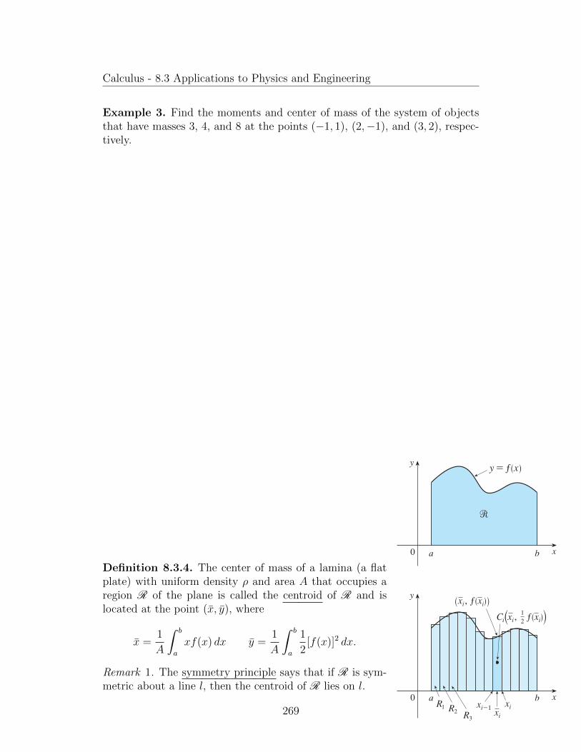
Calculus - 8.3 Applications to Physics and Engineering
Example 3. Find the moments and center of mass of the system of objectsthat have masses 3, 4, and 8 at the points (−1, 1), (2,−1), and (3, 2), respec-tively.
562 CHAPTER 8 Further Applications of Integration
Next we consider a !at plate (called a lamina) with uniform density ! that occupies a region 5 of the plane. We wish to locate the center of mass of the plate, which is called the centroid of 5. In doing so we use the following physical principles: The symmetry principle says that if 5 is symmetric about a line l, then the centroid of 5 lies on l. (If 5 is re!ected about l, then 5 remains the same so its centroid remains "xed. But the only "xed points lie on l.) Thus the centroid of a rectangle is its center. Moments should be de"ned so that if the entire mass of a region is concentrated at the center of mass, then its moments remain unchanged. Also, the moment of the union of two nonoverlapping regions should be the sum of the moments of the individual regions.
Suppose that the region 5 is of the type shown in Figure 10(a); that is, 5 lies between the lines x ! a and x ! b, above the x-axis, and beneath the graph of f, where f is a continuous function. We divide the interval fa, bg into n subintervals with endpoints x0, x1, . . . , xn and equal width Dx. We choose the sample point xi* to be the midpoint xi of the ith subinterval, that is, xi ! sxi21 1 xidy2. This determines the polygonal approxima-tion to 5 shown in Figure 10(b). The centroid of the ith approximating rectangle Ri is its center Ci(xi, 12 f sxid). Its area is f sxid Dx, so its mass is
! f sxid Dx
The moment of Ri about the y-axis is the product of its mass and the distance from Ci to the y-axis, which is xi. Thus
MysRid ! f! f sxid Dxg xi ! ! xi f sxid Dx
Adding these moments, we obtain the moment of the polygonal approximation to 5, and then by taking the limit as n l ` we obtain the moment of 5 itself about the y-axis:
My ! limnl `
on
i!1 !xi f sxid Dx ! ! yb
a x f sxd dx
In a similar fashion we compute the moment of Ri about the x-axis as the product of its mass and the distance from Ci to the x-axis (which is half the height of Ri):
MxsRid ! f! f sxid Dxg 12 f sxid ! ! ? 12 f f sxidg2 Dx
Again we add these moments and take the limit to obtain the moment of 5 about the x-axis:
Mx ! limnl `
on
i!1 ! ? 1
2 f f sxidg2 Dx ! ! yb
a
12 f f sxdg2 dx
Just as for systems of particles, the center of mass of the plate is de"ned so that mx ! My and my ! Mx. But the mass of the plate is the product of its density and its area:
m ! !A ! ! yb
a f sxd dx
FIGURE 10
Ci”xi, f(xi)’
xi
y
0 xa bR¡ R™ R£xi_1 xi
xi, f(xi)12
y
0 xa b
y=ƒ
!
Copyright 2016 Cengage Learning. All Rights Reserved. May not be copied, scanned, or duplicated, in whole or in part. Due to electronic rights, some third party content may be suppressed from the eBook and/or eChapter(s).Editorial review has deemed that any suppressed content does not materially affect the overall learning experience. Cengage Learning reserves the right to remove additional content at any time if subsequent rights restrictions require it.
Definition 8.3.4. The center of mass of a lamina (a flatplate) with uniform density ρ and area A that occupies aregion R of the plane is called the centroid of R and islocated at the point (x, y), where
x =1
A
ˆ b
a
xf(x) dx y =1
A
ˆ b
a
1
2[f(x)]2 dx.
Remark 1. The symmetry principle says that if R is sym-metric about a line l, then the centroid of R lies on l.
269

Calculus - 8.3 Applications to Physics and Engineering
Example 4. Find the center of mass of a semicircular plate of radius r.
Example 5. Find the centroid of the region bounded by the curves y = cosx,y = 0, x = 0, and x = π/2.
270

Calculus - 8.3 Applications to Physics and Engineering
564 CHAPTER 8 Further Applications of Integration
so Formulas 8 give
x −1A
y!y2
0 x f sxd dx − y!y2
0 x cos x dx
− x sin xg0
!y22 y!y2
0 sin x dx (by integration by parts)
−!
22 1
y −1A
y!y2
0 12 f f sxdg2 dx − 1
2 y!y2
0 cos2x dx
− 14 y!y2
0 s1 1 cos 2xd dx − 1
4 fx 1 12 sin 2xg 0
!y2 −
!
8
The centroid is (12 ! 2 1, 18 !) and is shown in Figure 12. n
If the region 5 lies between two curves y − f sxd and y − tsxd, where f sxd > tsxd, as illustrated in Figure 13, then the same sort of argument that led to Formulas 8 can be used to show that the centroid of 5 is sx, yd, where
x −1A
yb
a xf f sxd 2 tsxdg dx
y −1A
yb
a 12 hf f sxdg2 2 ftsxdg2 j dx
9
(See Exercise 51.)
EXAMPLE 6 Find the centroid of the region bounded by the line y − x and the parabola y − x 2.
SOLUTION The region is sketched in Figure 14. We take f sxd − x, tsxd − x 2, a − 0, and b − 1 in Formulas 9. First we note that the area of the region is
A − y1
0 sx 2 x 2 d dx −
x 2
22
x 3
3 G0
1
−16
Therefore
x −1A
y1
0 xf f sxd 2 tsxdg dx −
116
y1
0 xsx 2 x 2 d dx
− 6 y1
0 sx 2 2 x 3 d dx − 6F x 3
32
x 4
4 G0
1
−12
y −1A
y1
0 12 hf f sxdg2 2 ftsxdg2 j dx −
116
y1
0 12 sx 2 2 x 4 d dx
− 3F x 3
32
x 5
5 G0
1
−25
The centroid is s12 , 25 d. n
FIGURE 12
x
y
0
” -1, ’π8
π2
π2
y=cos x
FIGURE 14
x
y
0
” , ’25
12
y=x
y=≈
(1, 1)
FIGURE 13
xix
y
0 a b
!
y=ƒ
y=©
12Ci ” xi, !f(xi)+g(xi)"’
Copyright 2016 Cengage Learning. All Rights Reserved. May not be copied, scanned, or duplicated, in whole or in part. Due to electronic rights, some third party content may be suppressed from the eBook and/or eChapter(s).Editorial review has deemed that any suppressed content does not materially affect the overall learning experience. Cengage Learning reserves the right to remove additional content at any time if subsequent rights restrictions require it.
Theorem 8.3.1. If the region R lies between two curvesy = f(x) and y = g(x), where f(x) ≥ g(x), then the cen-troid of R is (x, y) where
x =1
A
ˆ b
a
x[f(x)− g(x)] dx
y =1
A
ˆ b
a
1
2[f(x)]2 − [g(x)]2 dx.
Example 6. Find the centroid of the region bounded by the line y = x andthe parabola y = x2.
271

Calculus - 8.3 Applications to Physics and Engineering
Theorem 8.3.2 (Theorem of Pappus). Let R be a plane region that lies en-tirely on one side of a line l in the plane. If R is rotated about l, then thevolume of the resulting solid is the product of the area A of R and the distanced traveled by the centroid of R.
Example 7. A torus is formed by rotating a circle of radius r about a line inthe plane of the circle that is a distance R (> r) from the center of the circle.Find the volume of the torus.
272

Calculus - 8.4 Applications to Economics and Biology
8.4 Applications to Economics and Biology
SECTION 8.4 Applications to Economics and Biology 569
In this section we consider some applications of integration to economics (consumer surplus) and biology (blood !ow, cardiac output). Others are described in the exercises.
Consumer SurplusRecall from Section 4.7 that the demand function psxd is the price that a company has to charge in order to sell x units of a commodity. Usually, selling larger quantities requires lowering prices, so the demand function is a decreasing function. The graph of a typical demand function, called a demand curve, is shown in Figure 1. If X is the amount of the commodity that can currently be sold, then P ! psXd is the current selling price.
At a given price, some consumers who buy a good would be willing to pay more; they bene"t by not having to. The difference between what a consumer is willing to pay and what the consumer actually pays for a good is called the consumer surplus. By "nding the total consumer surplus among all purchasers of a good, economists can assess the overall bene"t of a market to society.
To determine the total consumer surplus, we look at the demand curve and divide the interval f0, Xg into n subintervals, each of length Dx ! Xyn, and let xi* ! xi be the right endpoint of the ith subinterval, as in Figure 2. According to the demand curve, xi21 units would be purchased at a price of psxi21d dollars per unit. To increase sales to xi units, the price would have to be lowered to psxid dollars. In this case, an additional Dx units would be sold (but no more). In general, the consumers who would have paid psxid dol-lars placed a high value on the product; they would have paid what it was worth to them. So in paying only P dollars they have saved an amount of
ssavings per unitdsnumber of unitsd ! fpsxid 2 Pg Dx
Considering similar groups of willing consumers for each of the subintervals and adding the savings, we get the total savings:
on
i!1 fpsxid 2 Pg Dx
(This sum corresponds to the area enclosed by the rectangles in Figure 2.) If we let n l `, this Riemann sum approaches the integral
yX
0 fpsxd 2 Pg dx
which economists call the consumer surplus for the commodity.The consumer surplus represents the amount of money saved by consumers in pur-
chasing the commodity at price P, corresponding to an amount demanded of X. Figure#3 shows the interpretation of the consumer surplus as the area under the demand curve and above the line p ! P.
EXAMPLE 1 The demand for a product, in dollars, is
p ! 1200 2 0.2x 2 0.0001x 2
Find the consumer surplus when the sales level is 500.
SOLUTION Since the number of products sold is X ! 500, the corresponding price is
P ! 1200 2 s0.2ds500d 2 s0.0001ds500d2 ! 1075
FIGURE 1 A typical demand curve
0 x
p
P
X
(X, P)
p=p(x)
0 x
p
P
⁄ xi_1 xi X
(X, P)Îx-Pp(x )i
1
0 x
p
(X, P)P
X
p=p(x)
p=P
consumersurplus
FIGURE 3
Copyright 2016 Cengage Learning. All Rights Reserved. May not be copied, scanned, or duplicated, in whole or in part. Due to electronic rights, some third party content may be suppressed from the eBook and/or eChapter(s).Editorial review has deemed that any suppressed content does not materially affect the overall learning experience. Cengage Learning reserves the right to remove additional content at any time if subsequent rights restrictions require it.
Definition 8.4.1. The consumer surplus for a commodityis defined as ˆ X
0
[p(x)− P ] dx
where p(x) is the demand function, and P is the currentselling price for the amount of the commodity X that cancurrently be sold.
Example 1. The demand for a product, in dollars, is
p = 1200− 0.2x− 0.0001x2.
Find the consumer surplus when the sales level is 500.
273

Calculus - 8.4 Applications to Economics and Biology
Definition 8.4.2. The cardiac output of the heart is the volume of bloodpumped by the heart per unit time, that is, the rate of flow into the aorta. Itis given by
F =A´ T
0c(t) dt
where A is the amount of dye injected into the right atrium, [0, T ] is the timeinterval until the dye has cleared, and c(t) is the concentration of the dye attime t.
t c(t)0 01 0.42 2.83 6.54 9.85 8.96 6.17 4.08 2.39 1.110 0
Example 2. A 5-mg bolus of dye is injected into a right atrium.The concentration of the dye (in milligrams per liter) is mea-sured in the aorta at one-second intervals as shown in the table.Estimate the cardiac output.
274

Calculus - 8.5 Probability
8.5 Probability
Definition 8.5.1. The probability density function f of a continuous randomvariable X (a quantity whose values range over an interval of real numbers) isgiven by:
P (a ≤ X ≤ b) =
ˆ b
a
f(x) dx
where f(x) ≥ 0 for all x and
ˆ ∞−∞
f(x) dx = 1.
Example 1. Let f(x) = 0.006x(10 − x) for 0 ≤ x ≤ 10 and f(x) = 0 for allother values of x.
(a) Verify that f is a probability density function.
(b) Find P (4 ≤ X ≤ 8)
275

Calculus - 8.5 Probability
Example 2. Phenomena such as waiting times and equipment failure timesare commonly modeled by exponentially decreasing probability density func-tions. Find the exact form of such a function.
276

Calculus - 8.5 Probability
Definition 8.5.2. In general, the mean of any probability density function fis defined to be
µ =
ˆ ∞−∞
xf(x) dx.
Example 3. Find the mean of the exponential distribution of Example 2:
f(t) =
0 if t < 0,
ce−ct if t ≥ 0.
277

Calculus - 8.5 Probability
Example 4. Suppose the average waiting time for a customer’s call to beanswered by a company representative is five minutes.
(a) Find the probability that a call is answered during the first minute, as-suming that an exponential distribution is appropriate.
(b) Find the probability that a customer waits more than five minutes to beanswered.
278

Calculus - 8.5 Probability
Definition 8.5.3. When random phenomena are modeled by a normal distri-bution this means that the probability density function of the random variableX is a member of the family of functions
f(x) =1
σ√
2πe−(x−µ)2/(2σ2)
where the positive constant σ is called the standard deviation (a measure ofhow spread out the values of X are).
578 CHAPTER 8 Further Applications of Integration
Notice the result of Example 4(b): Even though the mean waiting time is 5 minutes, only 37% of callers wait more than 5 minutes. The reason is that some callers have to wait much longer (maybe 10 or 15 minutes), and this brings up the average.
Another measure of centrality of a probability density function is the median . That is a number m such that half the callers have a waiting time less than m and the other call-ers have a waiting time longer than m. In general, the median of a probability density function is the number m such that
y`
m f sxd dx − 1
2
This means that half the area under the graph of f lies to the right of m. In Exercise 9 you are asked to show that the median waiting time for the company described in Example 4 is approximately 3.5 minutes.
Normal DistributionsMany important random phenomena—such as test scores on aptitude tests, heights and weights of individuals from a homogeneous population, annual rainfall in a given loca-tion—are modeled by a normal distribution. This means that the probability density function of the random variable X is a member of the family of functions
f sxd −1
!s2" e2sx2#d2ys2! 2d
You can verify that the mean for this function is #. The positive constant ! is called the stan dard deviation; it measures how spread out the values of X are. From the bell-shaped graphs of members of the family in Figure 5, we see that for small values of ! the values of X are clustered about the mean, whereas for larger values of ! the values of X are more spread out. Statisticians have methods for using sets of data to estimate # and !.
x
y
0 m
12
s=2s=1
s=
The factor 1ys!s2" d is needed to make f a probability density function. In fact, it can be verified using the methods of multivariable calculus that
y`
2`
1!s2" e
2sx2#d2ys2! 2d
dx − 1
EXAMPLE 5 Intelligence Quotient (IQ) scores are distributed normally with mean 100 and standard deviation 15. (Figure 6 shows the corresponding probability density function.)(a) What percentage of the population has an IQ score between 85 and 115?(b) What percentage of the population has an IQ above 140?
3
The standard deviation is denoted by the lowercase Greek letter ! (sigma).
FIGURE 5 Normal distributions
x
y
0 60
0.01
80 100 120 140
0.02
FIGURE 6
Copyright 2016 Cengage Learning. All Rights Reserved. May not be copied, scanned, or duplicated, in whole or in part. Due to electronic rights, some third party content may be suppressed from the eBook and/or eChapter(s).Editorial review has deemed that any suppressed content does not materially affect the overall learning experience. Cengage Learning reserves the right to remove additional content at any time if subsequent rights restrictions require it.
Example 5. Intelligence Quotient (IQ) scores are distributednormally with mean 100 and standard deviation 15. (The figureshows the corresponding probability density function.)
(a) What percentage of the population has an IQ score between85 and 115?
(b) What percentage of the population has an IQ above 140?
279

Chapter 9
Differential Equations
9.1 Modeling with Differential Equations
Definition 9.1.1. In general, a differential equation is an equation that con-tains an unknown function and one or more of its derivatives. The order of adifferential equation is the order of the highest derivative that occurs in theequation. A function f is called a solution of a differential equation if theequation is satisfied when y = f(x) and its derivatives are substituted into theequation.
Example 1. Show that every member of the family of functions
y =1 + cet
1− cet
is a solution of the differential equation y′ = 12(y2 − 1).
280
Calculus - 9.1 Modeling with Differential Equations
Example 2. Find a solution of the differential equation y′ = 12(y2 − 1) that
satisfies the initial condition y(0) = 2.
281

Calculus - 9.2 Direction Fields and Euler’s Method
9.2 Direction Fields and Euler’s Method
Definition 9.2.1. In general, suppose we have a first-order differential equa-tion of the form
y′ = F (x, y)
where F (x, y) is some expression in x and y. If we draw short line segmentswith slope F (x, y) at several points (x, y), the result is called a direction field(or slope field).
Example 1.
(a) Sketch the direction field for the differential equation y′ = x2 + y2 − 1.
(b) Use part (a) to sketch the solution curve that passes through the origin.
282

Calculus - 9.2 Direction Fields and Euler’s Method
SECTION 9.2 Direction Fields and Euler’s Method 593
SOLUTION(a) We start by computing the slope at several points in the following chart:
x 22 21 0 1 2 22 21 0 1 2 . . .
y 0 0 0 0 0 1 1 1 1 1 . . .
y9 − x 2 1 y 2 2 1 3 0 21 0 3 4 1 0 1 4 . . .
Now we draw short line segments with these slopes at these points. The result is the direction field shown in Figure 5.
(b) We start at the origin and move to the right in the direction of the line segment (which has slope 21). We continue to draw the solution curve so that it moves parallel to the nearby line segments. The resulting solution curve is shown in Figure 6. Return-ing to the origin, we draw the solution curve to the left as well. n
The more line segments we draw in a direction field, the clearer the picture becomes. Of course, it’s tedious to compute slopes and draw line segments for a huge number of points by hand, but computers are well suited for this task. Figure 7 shows a more detailed, computer-drawn direction field for the differential equation in Example 1. It enables us to draw, with reasonable accuracy, the solution curves with y-intercepts 22, 21, 0, 1, and 2.
Now let’s see how direction fields give insight into physical situations. The simple electric circuit shown in Figure 8 contains an electromotive force (usually a battery or generator) that produces a voltage of Estd volts (V) and a current of Istd amperes (A) at time t. The circuit also contains a resistor with a resistance of R ohms (V) and an induc-tor with an inductance of L henries (H).
Ohm’s Law gives the drop in voltage due to the resistor as RI. The voltage drop due to the inductor is LsdIydtd. One of Kirchhoff’s laws says that the sum of the voltage drops is equal to the supplied voltage Estd. Thus we have
L dIdt
1 RI − Estd
which is a first-order differential equation that models the current I at time t.
EXAMPLE 2 Suppose that in the simple circuit of Figure 8 the resistance is 12 V, the inductance is 4 H, and a battery gives a constant voltage of 60 V.(a) Draw a direction field for Equation 1 with these values.(b) What can you say about the limiting value of the current?(c) Identify any equilibrium solutions.(d) If the switch is closed when t − 0 so the current starts with Is0d − 0, use the direc-tion field to sketch the solution curve.
SOLUTION(a) If we put L − 4, R − 12, and Estd − 60 in Equation 1, we get
4 dIdt
1 12I − 60 or dIdt
− 15 2 3I
0 x
y
1_1_2
1
2
-1
_2
2
FIGURE 5
1
3
_3
_3 3
FIGURE 7
0 x
y
1 2_1_2
1
2
-1
_2
FIGURE 6
R
E
switch
L
FIGURE 8
Copyright 2016 Cengage Learning. All Rights Reserved. May not be copied, scanned, or duplicated, in whole or in part. Due to electronic rights, some third party content may be suppressed from the eBook and/or eChapter(s).Editorial review has deemed that any suppressed content does not materially affect the overall learning experience. Cengage Learning reserves the right to remove additional content at any time if subsequent rights restrictions require it.
Example 2. Suppose that in the simple circuit of the figure theresistance is 12 Ω, the inductance is 4 H, and a battery gives aconstant voltage of 60 V.(a) Draw a direction field for
LdI
dt+RI = E(t)
with these values.
(b) What can you say about the limiting value of the current?
(c) Identify any equilibrium solutions.
(d) If the switch is closed when t = 0 so the current starts withI(0) = 0, use the direction field to sketch the solution curve.
283

Calculus - 9.2 Direction Fields and Euler’s Method
Theorem 9.2.1 (Euler’s Method). Approximate values for the solution of theinitial-value problem y′ = F (x, y), y(x0) = y0 with step size h, at xn = xn−1+h,are
yn = yn−1 + hF (xn−1, yn−1) n = 1, 2, 3, . . . .
Example 3. Use Euler’s method with step size 0.1 to construct a table ofapproximate values for the solution of the initial-value problem
y′ = x+ y y(0) = 1.
284

Calculus - 9.2 Direction Fields and Euler’s Method
Example 4. In Example 2 we discussed a simple electric circuit with resistance12 Ω, inductance 4 H, and a battery with voltage 60 V. If the switch is closedwhen t = 0, we modeled the current I at time t by the initial-value problem
dI
dt= 15− 3I I(0) = 0.
Estimate the current in the circuit half a second after the switch is closed.
285

Calculus - 9.3 Separable Equations
9.3 Separable Equations
Definition 9.3.1. A separable equation is a first-order differential equationin which the expression for dy/dx can be factored as a function of x times afunction of y. In other words, it can be written in the form
dy
dx= g(x)g(y).
Example 1. (a) Solve the differential equationdy
dx=x2
y2.
(b) Find the solution of this equation that satisfies the initial condition y(0) =2.
286

Calculus - 9.3 Separable Equations
Example 2. Solve the differential equationdy
dx=
6x2
2y + cos y.
Example 3. Solve the equation y′ = x2y.
287
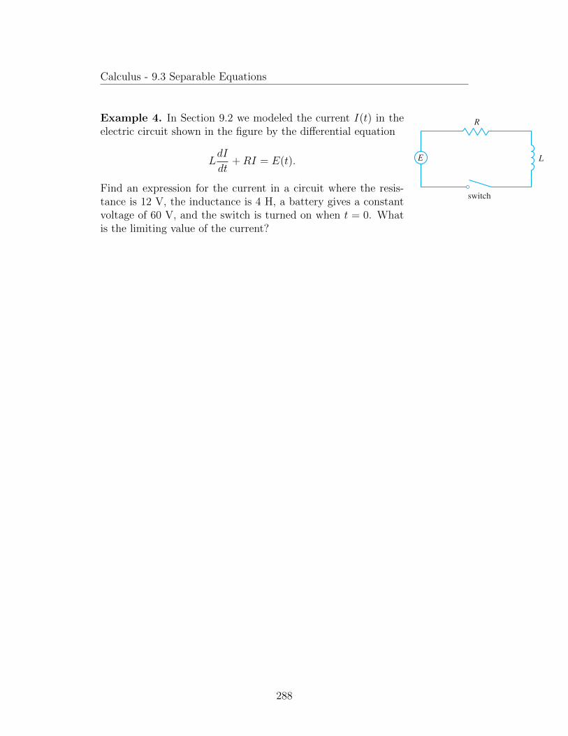
Calculus - 9.3 Separable Equations
SECTION 9.2 Direction Fields and Euler’s Method 593
SOLUTION(a) We start by computing the slope at several points in the following chart:
x 22 21 0 1 2 22 21 0 1 2 . . .
y 0 0 0 0 0 1 1 1 1 1 . . .
y9 − x 2 1 y 2 2 1 3 0 21 0 3 4 1 0 1 4 . . .
Now we draw short line segments with these slopes at these points. The result is the direction field shown in Figure 5.
(b) We start at the origin and move to the right in the direction of the line segment (which has slope 21). We continue to draw the solution curve so that it moves parallel to the nearby line segments. The resulting solution curve is shown in Figure 6. Return-ing to the origin, we draw the solution curve to the left as well. n
The more line segments we draw in a direction field, the clearer the picture becomes. Of course, it’s tedious to compute slopes and draw line segments for a huge number of points by hand, but computers are well suited for this task. Figure 7 shows a more detailed, computer-drawn direction field for the differential equation in Example 1. It enables us to draw, with reasonable accuracy, the solution curves with y-intercepts 22, 21, 0, 1, and 2.
Now let’s see how direction fields give insight into physical situations. The simple electric circuit shown in Figure 8 contains an electromotive force (usually a battery or generator) that produces a voltage of Estd volts (V) and a current of Istd amperes (A) at time t. The circuit also contains a resistor with a resistance of R ohms (V) and an induc-tor with an inductance of L henries (H).
Ohm’s Law gives the drop in voltage due to the resistor as RI. The voltage drop due to the inductor is LsdIydtd. One of Kirchhoff’s laws says that the sum of the voltage drops is equal to the supplied voltage Estd. Thus we have
L dIdt
1 RI − Estd
which is a first-order differential equation that models the current I at time t.
EXAMPLE 2 Suppose that in the simple circuit of Figure 8 the resistance is 12 V, the inductance is 4 H, and a battery gives a constant voltage of 60 V.(a) Draw a direction field for Equation 1 with these values.(b) What can you say about the limiting value of the current?(c) Identify any equilibrium solutions.(d) If the switch is closed when t − 0 so the current starts with Is0d − 0, use the direc-tion field to sketch the solution curve.
SOLUTION(a) If we put L − 4, R − 12, and Estd − 60 in Equation 1, we get
4 dIdt
1 12I − 60 or dIdt
− 15 2 3I
0 x
y
1_1_2
1
2
-1
_2
2
FIGURE 5
1
3
_3
_3 3
FIGURE 7
0 x
y
1 2_1_2
1
2
-1
_2
FIGURE 6
R
E
switch
L
FIGURE 8
Copyright 2016 Cengage Learning. All Rights Reserved. May not be copied, scanned, or duplicated, in whole or in part. Due to electronic rights, some third party content may be suppressed from the eBook and/or eChapter(s).Editorial review has deemed that any suppressed content does not materially affect the overall learning experience. Cengage Learning reserves the right to remove additional content at any time if subsequent rights restrictions require it.
Example 4. In Section 9.2 we modeled the current I(t) in theelectric circuit shown in the figure by the differential equation
LdI
dt+RI = E(t).
Find an expression for the current in a circuit where the resis-tance is 12 V, the inductance is 4 H, a battery gives a constantvoltage of 60 V, and the switch is turned on when t = 0. Whatis the limiting value of the current?
288

Calculus - 9.3 Separable Equations SECTION 9.3 Separable Equations 603
Orthogonal TrajectoriesAn orthogonal trajectory of a family of curves is a curve that intersects each curve of the family orthogonally, that is, at right angles (see Figure 7). For instance, each mem-ber of the family y − mx of straight lines through the origin is an orthogonal trajectory of the family x 2 1 y 2 − r 2 of concentric circles with center the origin (see Figure 8). We say that the two families are orthogonal trajectories of each other.
EXAMPLE 5 Find the orthogonal trajectories of the family of curves x − ky 2, where k is an arbitrary constant.
SOLUTION The curves x − ky 2 form a family of parabolas whose axis of symmetry is the x-axis. The first step is to find a single differential equation that is satisfied by all members of the family. If we differentiate x − ky 2, we get
1 − 2ky dydx
or dydx
−1
2ky
This differential equation depends on k, but we need an equation that is valid for all values of k simultaneously. To eliminate k we note that, from the equation of the given general parabola x − ky 2, we have k − xyy 2 and so the differential equation can be written as
dydx
−1
2ky−
1
2 xy 2 y
or dydx
− y2x
This means that the slope of the tangent line at any point sx, yd on one of the parabolas is y9 − yys2xd. On an orthogonal trajectory the slope of the tangent line must be the negative reciprocal of this slope. Therefore the orthogonal trajectories must satisfy the differ ential equation
dydx
− 22x y
This differential equation is separable, and we solve it as follows:
y y dy − 2y 2x dx
y 2
2− 2x 2 1 C
x 2 1y 2
2− C
where C is an arbitrary positive constant. Thus the orthogonal trajectories are the family of ellipses given by Equation 4 and sketched in Figure 9. n
Orthogonal trajectories occur in various branches of physics. For example, in an elec-trostatic field the lines of force are orthogonal to the lines of constant potential. Also, the streamlines in aerodynamics are orthogonal trajectories of the velocity-equipotential curves.
x
y
orthogonaltrajectory
FIGURE 7
x
y
orthogonaltrajectory
FIGURE 8
4
x
y
FIGURE 9
Copyright 2016 Cengage Learning. All Rights Reserved. May not be copied, scanned, or duplicated, in whole or in part. Due to electronic rights, some third party content may be suppressed from the eBook and/or eChapter(s).Editorial review has deemed that any suppressed content does not materially affect the overall learning experience. Cengage Learning reserves the right to remove additional content at any time if subsequent rights restrictions require it.
Definition 9.3.2. An orthogonal trajectory of a family of curvesis a curve that intersects each curve of the family orthogonally,that is, at right angles (see the figure).
Example 5. Find the orthogonal trajectories of the family ofcurves x = ky2, where k is an arbitrary constant.
289

Calculus - 9.3 Separable Equations
Example 6. A tank contains 20 kg of salt dissolved in 5000 L of water. Brinethat contains 0.03 kg of salt per liter of water enters the tank at a rate of 25L/min. The solution is kept thoroughly mixed and drains from the tank atthe same rate. How much salt remains in the tank after half an hour?
290

Calculus - 9.4 Models for Population Growth
9.4 Models for Population Growth
Definition 9.4.1. In general, if P (t) is the value of a quantity y at time t andif the rate of change of P with respect to t is proportional to its size P (t) atany time, then
dP
dt= kP
where k is a constant. This equation is sometimes called the law of naturalgrowth.
Theorem 9.4.1. The solution of the initial-value problem
dP
dt= kP P (0) = P0
isP (t) = P0e
kt.
Proof. The law of natural growth is a separable differential equation, so
dP
dt= kPˆ
dP
P=
ˆk dt
ln |P | = kt+ C
|P | = ekt+C = eCekt
P = Aekt,
where A (= ±eC or 0) is an arbitrary constant. Since P (0) = A, P (t) =P0e
kt.
Definition 9.4.2. The model for population growth known as the logisticdifferential equation is
dP
dt= kP
(1− P
M
),
where M is the carrying capacity, the maximum population that the environ-ment is capable of sustaining in the long run.
291

Calculus - 9.4 Models for Population Growth
Example 1. Draw a direction field for the logistic equation with k = 0.08and carrying capacity M = 1000. What can you deduce about the solutions?
292

Calculus - 9.4 Models for Population Growth
Theorem 9.4.2. The solution to the logistic equation is
P (t) =M
1 + Ae−ktwhere A =
M − P0
P0
.
Proof. The logistic equation is separable, so using partial fractions, we get
dP
dt= kP
(1− P
M
)ˆ
dP
P (1− P/M)=
ˆk dt
ˆM
P (M − P )dP =
ˆk dt
ˆ (1
P+
1
M − P
)dP =
ˆk dt
ln |P | − ln |M − P | = kt+ C
ln
∣∣∣∣M − PP
∣∣∣∣ = −kt− C∣∣∣∣M − PP
∣∣∣∣ = e−kt−C = e−Ce−kt
M − PP
= Ae−kt
M
P− 1 = Ae−kt
M
P= 1 + Ae−kt
P =M
1 + Ae−kt,
where A = ±e−C . If t = 0, we have
M − P0
P0
= Ae0 = A.
293

Calculus - 9.4 Models for Population Growth
Example 2. Write the solution of the initial-value problem
dP
dt= 0.08P
(1− P
1000
)P (0) = 100
and use it to find the population sizes P (40) and P (80). At what time doesthe population reach 900?
294

Calculus - 9.4 Models for Population Growth
Example 3. In the 1930s the biologist G. F. Gause conducted an experimentwith the protozoan Paramecium and used a logistic equation to model hisdata. The table gives his daily count of the population of protozoa. He esti-mated the initial relative growth rate to be 0.7944 and the carrying capacityto be 64.
t (days) 0 1 2 3 4 5 6 7 8 9 10 11 12 13 14 15 16P (observed) 2 3 22 16 39 52 54 47 50 76 69 51 57 70 53 59 57
Find the exponential and logistic models for Gause’s data. Compare the pre-dicted values with the observed values and comment on the fit.
295
Calculus - 9.5 Linear Equations
9.5 Linear Equations
Definition 9.5.1. A first-order linear differential equation is one that can beput into the form
dy
dx+ P (x)y = Q(x)
where P and Q are continuous functions on a given interval.
Theorem 9.5.1. To solve the linear differential equation y′ + P (x)y = Q(x),multiply both sides by the integrating factor I(x) = e
´P (x)dx and integrate both
sides.
Example 1. Solve the differential equationdy
dx+ 3x2y = 6x2.
296
Calculus - 9.5 Linear Equations
Example 2. Find the solution of the initial-value problem
x2y′ + xy = 1 x > 0 y(1) = 2.
297

Calculus - 9.5 Linear Equations
Example 3. Solve y′ + 2xy = 1.
298

Calculus - 9.5 Linear Equations
SECTION 9.2 Direction Fields and Euler’s Method 593
SOLUTION(a) We start by computing the slope at several points in the following chart:
x 22 21 0 1 2 22 21 0 1 2 . . .
y 0 0 0 0 0 1 1 1 1 1 . . .
y9 − x 2 1 y 2 2 1 3 0 21 0 3 4 1 0 1 4 . . .
Now we draw short line segments with these slopes at these points. The result is the direction field shown in Figure 5.
(b) We start at the origin and move to the right in the direction of the line segment (which has slope 21). We continue to draw the solution curve so that it moves parallel to the nearby line segments. The resulting solution curve is shown in Figure 6. Return-ing to the origin, we draw the solution curve to the left as well. n
The more line segments we draw in a direction field, the clearer the picture becomes. Of course, it’s tedious to compute slopes and draw line segments for a huge number of points by hand, but computers are well suited for this task. Figure 7 shows a more detailed, computer-drawn direction field for the differential equation in Example 1. It enables us to draw, with reasonable accuracy, the solution curves with y-intercepts 22, 21, 0, 1, and 2.
Now let’s see how direction fields give insight into physical situations. The simple electric circuit shown in Figure 8 contains an electromotive force (usually a battery or generator) that produces a voltage of Estd volts (V) and a current of Istd amperes (A) at time t. The circuit also contains a resistor with a resistance of R ohms (V) and an induc-tor with an inductance of L henries (H).
Ohm’s Law gives the drop in voltage due to the resistor as RI. The voltage drop due to the inductor is LsdIydtd. One of Kirchhoff’s laws says that the sum of the voltage drops is equal to the supplied voltage Estd. Thus we have
L dIdt
1 RI − Estd
which is a first-order differential equation that models the current I at time t.
EXAMPLE 2 Suppose that in the simple circuit of Figure 8 the resistance is 12 V, the inductance is 4 H, and a battery gives a constant voltage of 60 V.(a) Draw a direction field for Equation 1 with these values.(b) What can you say about the limiting value of the current?(c) Identify any equilibrium solutions.(d) If the switch is closed when t − 0 so the current starts with Is0d − 0, use the direc-tion field to sketch the solution curve.
SOLUTION(a) If we put L − 4, R − 12, and Estd − 60 in Equation 1, we get
4 dIdt
1 12I − 60 or dIdt
− 15 2 3I
0 x
y
1_1_2
1
2
-1
_2
2
FIGURE 5
1
3
_3
_3 3
FIGURE 7
0 x
y
1 2_1_2
1
2
-1
_2
FIGURE 6
R
E
switch
L
FIGURE 8
Copyright 2016 Cengage Learning. All Rights Reserved. May not be copied, scanned, or duplicated, in whole or in part. Due to electronic rights, some third party content may be suppressed from the eBook and/or eChapter(s).Editorial review has deemed that any suppressed content does not materially affect the overall learning experience. Cengage Learning reserves the right to remove additional content at any time if subsequent rights restrictions require it.
Example 4. Suppose that in the simple circuit of the figure theresistance is 12 V and the inductance is 4 H. If a battery gives aconstant voltage of 60 V and the switch is closed when t = 0 sothe current starts with I(0) = 0, find
(a) I(t),
(b) the current after 1 second, and
(c) the limiting value of the current.
299

Calculus - 9.5 Linear Equations
Example 5. Suppose that the resistance and inductance remain as in Example4 but, instead of the battery, we use a generator that produces a variablevoltage of E(t) = 60 sin 30t volts. Find I(t).
300

Calculus - 9.6 Predator-Prey Systems
9.6 Predator-Prey Systems
Definition 9.6.1. The equations
dR
dt= kR− aRW dW
dt= −rW + bRW
are known as the predator-prey equations, or the Lotka-Volterra equations. Asolution of this system of equations is a pair of functions R(t) and W (t) thatdescribe the populations of prey and predators as functions of time.
Example 1. Suppose that populations of rabbits and wolves are describedby the Lotka-Volterra equations with k = 0.08, a = 0.001, r = 0.02, andb = 0.00002. The time t is measured in months.
(a) Find the constant solutions (called the equilibrium solutions) and interpretthe answer.
301

Calculus - 9.6 Predator-Prey Systems
(b) Use the system of differential equations to find an expression for dW/dR.
(c) Draw a direction field for the resulting differential equation in the RW -plane. Then use that direction field to sketch some solution curves.
302

Calculus - 9.6 Predator-Prey Systems
(d) Suppose that, at some point in time, there are 1000 rabbits and 40 wolves.Draw the corresponding solution curve and use it to describe the changesin both population levels.
(e) Use part (d) to make sketches of R and W as functions of t.
303

Chapter 10
Parametric Equations and PolarCoordinates
10.1 Curves Defined by Parametric Equations
Definition 10.1.1. Suppose that x and y are both given as functions of athird variable t (called a parameter) by the equations
x = f(t) y = g(t)
(called parametric equations). Each value of t determines a point (x, y), whichwe can plot in a coordinate plane. As t varies, the point (x, y) = (f(t), g(t))varies and traces out a curve C, which we call a parametric curve.
Example 1. Sketch and identify the curve defined by the parametric equations
x = t2 − 2t y = t+ 1.
304

Calculus - 10.1 Curves Defined by Parametric Equations
Definition 10.1.2. In general, the curve with parametric equations
x = f(t) y = g(t) a ≤ t ≤ b
has initial point (f(a), g(a)) and terminal point (f(b), g(b)).
Example 2. What curve is represented by the following parametric equations?
x = cos t y = sin t 0 ≤ t ≤ 2π.
Example 3. What curve is represented by the given parametric equations?
x = sin 2t y = cos 2t 0 ≤ t ≤ 2π.
305

Calculus - 10.1 Curves Defined by Parametric Equations
Example 4. Find parametric equations for the circle with center (h, k) andradius r.
Example 5. Sketch the curve with parametric equations x = sin t, y = sin2 t.
306

Calculus - 10.1 Curves Defined by Parametric Equations
Example 6. Use a graphing device to graph the curve x = y4 − 3y2.
Example 7. The curve traced out by a point P on the circumference of acircle as the circle rolls along a straight line is called a cycloid (see the figure).If the circle has radius r and rolls along the x-axis and if one position of P isthe origin, find parametric equations for the cycloid.
SECTION 10.1 Curves Defined by Parametric Equations 643
EXAMPLE 6 Use a graphing device to graph the curve x − y 4 2 3y 2.
SOLUTION If we let the parameter be t − y, then we have the equations
x − t 4 2 3t 2 y − t
Using these parametric equations to graph the curve, we obtain Figure 9. It would be possible to solve the given equation sx − y 4 2 3y 2 d for y as four functions of x and graph them individually, but the parametric equations provide a much easier method. n
In general, if we need to graph an equation of the form x − tsyd, we can use the parametric equations
x − tstd y − t
Notice also that curves with equations y − f sxd (the ones we are most familiar with—graphs of functions) can also be regarded as curves with parametric equations
x − t y − f std
Graphing devices are particularly useful for sketching complicated parametric curves. For instance, the curves shown in Figures 10, 11, and 12 would be virtually impossible to produce by hand.
13
0
1
_1
_1 1
3.5
_3.5
_3.5 3.5
13
FIGURE 10 x − t 1 sin 5t y − t 1 sin 6t
FIGURE 11 x − sin 9t y − sin 10 t
FIGURE 12 x − 2.3 cos 10t 1 cos 23t y − 2.3 sin 10t 2 sin 23t
One of the most important uses of parametric curves is in computer-aided design (CAD). In the Laboratory Project after Section 10.2 we will investigate special paramet-ric curves, called Bézier curves, that are used extensively in manufacturing, especially in the auto motive industry. These curves are also employed in specifying the shapes of letters and other symbols in laser printers and in documents viewed electronically.
The Cycloid
EXAMPLE 7 The curve traced out by a point P on the circumference of a circle as the circle rolls along a straight line is called a cycloid (see Figure 13). If the circle has radius r and rolls along the x-axis and if one position of P is the origin, find parametric equations for the cycloid.
P
PP
TEC An animation in Module 10.1B shows how the cycloid is formed as the circle moves.
FIGURE 13
FIGURE 9
3
_3
_3 3
Copyright 2016 Cengage Learning. All Rights Reserved. May not be copied, scanned, or duplicated, in whole or in part. Due to electronic rights, some third party content may be suppressed from the eBook and/or eChapter(s).Editorial review has deemed that any suppressed content does not materially affect the overall learning experience. Cengage Learning reserves the right to remove additional content at any time if subsequent rights restrictions require it.
307

Calculus - 10.1 Curves Defined by Parametric Equations
Example 8. Investigate the family of curves with parametric equations
x = a+ cos t y = a tan t+ sin t.
What do these curves have in common? How does the shape change as aincreases?
308

Calculus - 10.2 Calculus with Parametric Curves
10.2 Calculus with Parametric Curves
Theorem 10.2.1. Suppose f and g are differentiable functions. Then for apoint on the parametric curve x = f(t), y = g(t), where y is also a differen-tiable function of x, we have
dy
dx=
dy
dtdx
dt
ifdx
dt6= 0.
Proof. Since y is a differentiable function of x, we have, by the Chain Rule,
dy
dt=dy
dx· dxdt.
Then if dxdt6= 0 we can divide by it, so
dy
dx=
dy
dtdx
dt
.
Theorem 10.2.2. Suppose f and g are differentiable functions. Then for apoint on the parametric curve x = f(t), y = g(t), where y is also a differen-tiable function of x, we have
d2y
dx2=
d
dt
(dy
dx
)dx
dt
ifdx
dt6= 0.
Proof. By the previous theorem,
d2y
dx2=
d
dx
(dy
dx
)=
d
dt
(dy
dx
)dx
dt
ifdx
dt6= 0.
309

Calculus - 10.2 Calculus with Parametric Curves
Example 1. A curve C is defined by the parametric equations x = t2, y =t3 − 3t.
(a) Show that C has two tangents at the point (3, 0) and find their equations
(b) Find the points on C where the tangent is horizontal or vertical.
(c) Determine where the curve is concave upward or downward.
(d) Sketch the curve.
310

Calculus - 10.2 Calculus with Parametric Curves
Example 2.
(a) Find the tangent to the cycloid x = r(θ − sin θ), y = r(1 − cos θ) at thepoint where θ = π/3.
(b) At what points is the tangent horizontal? When is it vertical?
311

Calculus - 10.2 Calculus with Parametric Curves
Theorem 10.2.3. If a curve is traced out once by the parametric equationsx = f(t) and y = g(t), α ≤ t ≤ β, then the area under the curve is given by
A =
ˆ β
α
g(t)f ′(t) dt
[or
ˆ α
β
g(t)f ′(t) dt
].
Proof. Since the area under the curve y = F (x) from a to b is A =´ baF (x) dx,
we can use the Substitution Rule for Definite Integrals with y = g(t) anddx = f ′(t) dt to get
A =
ˆ b
a
y dx =
ˆ β
α
g(t)f ′(t) dt.
SECTION 10.2 Calculus with Parametric Curves 651
Therefore the slope of the tangent is s3 and its equation is
y 2r2
− s3 Sx 2r!
31
rs3
2 D or s3 x 2 y − rS !
s3 2 2DThe tangent is sketched in Figure 2.
0
y
x2πr 4πr
(πr, 2r)(_πr, 2r) (3πr, 2r) (5πr, 2r)
π3¨=
(b) The tangent is horizontal when dyydx − 0, which occurs when sin " − 0 and 1 2 cos " ± 0, that is, " − s2n 2 1d!, n an integer. The corresponding point on the cycloid is ss2n 2 1d!r, 2rd.
When " − 2n !, both dxyd" and dyyd" are 0. It appears from the graph that there are vertical tangents at those points. We can verify this by using l’Hospital’s Rule as follows:
lim" l
2n !1 dydx
− lim" l
2n !1
sin "1 2 cos " − lim
" l
2n !1 cos "sin " − `
A similar computation shows that dyydx l 2` as " l 2n !2, so indeed there are vertical tangents when " − 2n !, that is, when x − 2n !r. n
AreasWe know that the area under a curve y − Fsxd from a to b is A − yb
a Fsxd dx, where Fsxd > 0. If the curve is traced out once by the parametric equations x − f std and y − tstd, # < t < $, then we can calculate an area formula by using the Sub stitution Rule for Definite Integrals as follows:
A − yb
a y dx − y$
# tstd f 9std dt For y#
$ tstd f 9std dtG
EXAMPLE 3 Find the area under one arch of the cycloid
x − rs" 2 sin "d y − rs1 2 cos "d
(See Figure 3.)
SOLUTION One arch of the cycloid is given by 0 < " < 2!. Using the Substitution Rule with y − rs1 2 cos "d and dx − rs1 2 cos "d d", we have
A − y2!r
0 y dx − y2!
0 rs1 2 cos "d rs1 2 cos "d d"
− r 2 y2!
0 s1 2 cos "d2 d" − r 2 y2!
0 s1 2 2 cos " 1 cos2"d d"
− r 2 y2!
0 f1 2 2 cos " 1 1
2 s1 1 cos 2"dg d"
− r 2 f 32 " 2 2 sin " 1 1
4 sin 2"g0
2!
− r 2 (32 ? 2!) − 3!r 2 n
FIGURE 2
The limits of integration for t are found as usual with the Substitution Rule. When x − a, t is either # or $. When x − b, t is the remaining value.
0
y
x2πr
FIGURE 3
The result of Example 3 says that the area under one arch of the cycloid is three times the area of the rolling circle that generates the cycloid (see Example 10.1.7). Galileo guessed this result but it was first proved by the French mathematician Roberval and the Italian mathematician Torricelli.
Copyright 2016 Cengage Learning. All Rights Reserved. May not be copied, scanned, or duplicated, in whole or in part. Due to electronic rights, some third party content may be suppressed from the eBook and/or eChapter(s).Editorial review has deemed that any suppressed content does not materially affect the overall learning experience. Cengage Learning reserves the right to remove additional content at any time if subsequent rights restrictions require it.
Example 3. Find the area under one arch of the cycloid
x = r(θ − sin θ) y = r(1− cos θ).
(See the figure.)
312

Calculus - 10.2 Calculus with Parametric Curves
Theorem 10.2.4. If a curve C is described by the parametric equations x =f(t), y = g(t), α ≤ t ≤ β, where f ′ and g′ are continuous on [α, β] and C istraversed exactly once as t increases from α to β, then the length of C is
L =
ˆ β
α
√(dx
dt
)2
+
(dy
dt
)2
dt.
Example 4. (a) Use the representation of the unit circle given by
x = cos t y = sin t 0 ≤ t ≤ 2π
to find its arc length.
(b) Use the representation of the unit circle given by
x = sin 2t y = cos 2t 0 ≤ t ≤ 2π
to find its arc length.
313

Calculus - 10.2 Calculus with Parametric Curves
Example 5. Find the length of one arch of the cycloid x = r(θ − sin θ),y = r(1− cos θ).
314

Calculus - 10.2 Calculus with Parametric Curves
Theorem 10.2.5. Suppose a curve C is given by the parametric equationsx = f(t), y = g(t), α ≤ t ≤ β, where f ′, g′ are continuous, g′(t) ≥ 0, isrotated about the x-axis. If C is traversed exactly once as t increases from αto β, then the area of the resulting surface is given by
S =
ˆ β
α
2πy
√(dx
dt
)2
+
(dy
dt
)2
dt.
Example 6. Show that the surface area of a sphere of radius r is 4πr2.
315

Calculus - 10.3 Polar Coordinates
10.3 Polar Coordinates
658 CHAPTER 10 Parametric Equations and Polar Coordinates
A coordinate system represents a point in the plane by an ordered pair of numbers called coordinates. Usually we use Cartesian coordinates, which are directed distances from two perpendicular axes. Here we describe a coordinate system introduced by Newton, called the polar coordinate system, which is more convenient for many purposes.
We choose a point in the plane that is called the pole (or origin) and is labeled O. Then we draw a ray (half-line) starting at O called the polar axis. This axis is usually drawn hor izontally to the right and corresponds to the positive x-axis in Cartesian coordinates.
If P is any other point in the plane, let r be the distance from O to P and let ! be the angle (usually measured in radians) between the polar axis and the line OP as in Fig- ure 1. Then the point P is represented by the ordered pair sr, !d and r, ! are called polar coordinates of P. We use the convention that an angle is positive if measured in the counterclockwise direction from the polar axis and negative in the clockwise direction. If P − O, then r − 0 and we agree that s0, !d represents the pole for any value of !.
We extend the meaning of polar coordinates sr, !d to the case in which r is negative by agreeing that, as in Figure 2, the points s2r, !d and sr, !d lie on the same line through O and at the same distance | r | from O, but on opposite sides of O. If r . 0, the point sr, !d lies in the same quadrant as !; if r , 0, it lies in the quadrant on the opposite side of the pole. Notice that s2r, !d represents the same point as sr, ! 1 "d.
EXAMPLE 1 Plot the points whose polar coordinates are given. (a) s1, 5"y4d (b) s2, 3"d (c) s2, 22"y3d (d) s23, 3"y4d
FIGURE 1
xO ¨
r
polar axis
P(r, )
FIGURE 2
(_r, )
O¨
(r, )
¨+π
where 0 < t < 1. Notice that when t − 0 we have sx, yd − sx0, y0 d and when t − 1 we have sx, yd − sx3, y3d, so the curve starts at P0 and ends at P3.
1. Graph the Bézier curve with control points P0s4, 1d, P1s28, 48d, P2s50, 42d, and P3s40, 5d. Then, on the same screen, graph the line segments P0P1, P1P2, and P2P3. (Exercise 10.1.31 shows how to do this.) Notice that the middle control points P1 and P2 don’t lie on the curve; the curve starts at P0, heads toward P1 and P2 without reaching them, and ends at P3.
2. From the graph in Problem 1, it appears that the tangent at P0 passes through P1 and the tangent at P3 passes through P2. Prove it.
3. Try to produce a Bézier curve with a loop by changing the second control point in Problem 1.
4. Some laser printers use Bézier curves to represent letters and other symbols. Experiment with control points until you find a Bézier curve that gives a reasonable representation of the letter C.
5. More complicated shapes can be represented by piecing together two or more Bézier curves. Suppose the first Bézier curve has control points P0, P1, P2, P3 and the second one has control points P3, P4, P5, P6. If we want these two pieces to join together smoothly, then the tangents at P3 should match and so the points P2, P3, and P4 all have to lie on this com- mon tangent line. Using this principle, find control points for a pair of Bézier curves that represent the letter S.
Copyright 2016 Cengage Learning. All Rights Reserved. May not be copied, scanned, or duplicated, in whole or in part. Due to electronic rights, some third party content may be suppressed from the eBook and/or eChapter(s).Editorial review has deemed that any suppressed content does not materially affect the overall learning experience. Cengage Learning reserves the right to remove additional content at any time if subsequent rights restrictions require it.
Definition 10.3.1. The polar coordinate system consists of apoint called the pole (or origin) O, a ray starting at the polecalled the polar axis, and other points P represented by (r, θ)where r is the distance from O to P and θ is the angle (usuallymeasured in radians) between the polar axis and the line OP asin the figure. r, θ are called polar coordinates of P .
Example 1. Plot the points whose polar coordinates are given.
(a) (1, 5π/4)
(b) (2, 3π)
(c) (2,−2π/3)
(d) (−3, 3π/4)
316

Calculus - 10.3 Polar Coordinates
Theorem 10.3.1. If the point P has Cartesian coordinates (x, y) and polarcoordinates (r, θ), then
x = r cos θ y = r sin θ
andr2 = x2 + y2 tan θ =
y
x.
Example 2. Convert the point (2, π/3) from polar to Cartesian coordinates.
Example 3. Represent the point with Cartesian coordinates (1,−1) in termsof polar coordinates.
Example 4. What curve is represented by the polar equation r = 2?
317

Calculus - 10.3 Polar Coordinates
Example 5. Sketch the polar curve θ = 1.
Example 6. (a) Sketch the curve with polar equation r = 2 cos θ.
(b) Find a Cartesian equation for this curve.
318

Calculus - 10.3 Polar Coordinates
Example 7. Sketch the curve r = 1 + sin θ.
Example 8. Sketch the curve r = cos 2θ.
319

Calculus - 10.3 Polar Coordinates
Theorem 10.3.2. The slope of the tangent line to a polar curve r = f(θ) is
dy
dx=
dr
dθsin θ + r cos θ
dr
dθcos θ − r sin θ
Proof. Regard θ as a parameter and write
x = r cos θ = f(θ) cos θ y = r sin θ = f(θ) sin θ.
Then by Theorem 10.2.1 and the product rule, we have
dy
dx=
dy
dθdx
dθ
=
dr
dθsin θ + r cos θ
dr
dθcos θ − r sin θ
.
Example 9.
(a) For the cardioid r = 1 + sin θ of Example 7, find the slope of the tangentline when θ = π/3.
320

Calculus - 10.3 Polar Coordinates
(b) Find the points on the cardioid where the tangent line is horizontal orvertical.
Example 10. Graph the curve r = sin(8θ/5).
321

Calculus - 10.3 Polar Coordinates
Example 11. Investigate the family of polar curves given by r = 1 + c sin θ.How does the shape change as c changes? (These curves are called limacons,after a French word for snail, because of the shape of the curves for certainvalues of c.)
322

Calculus - 10.4 Areas and Lengths in Polar Coordinates
10.4 Areas and Lengths in Polar Coordinates
SECTION 10.4 Areas and Lengths in Polar Coordinates 669
In this section we develop the formula for the area of a region whose boundary is given by a polar equation. We need to use the formula for the area of a sector of a circle:
A − 12 r 2!
where, as in Figure 1, r is the radius and ! is the radian measure of the central angle. Formula 1 follows from the fact that the area of a sector is proportional to its central angle: A − s!y2"d"r 2 − 1
2 r 2! . (See also Exercise 7.3.35.)Let 5 be the region, illustrated in Figure 2, bounded by the polar curve r − f s!d
and by the rays ! − a and ! − b, where f is a positive continuous function and where 0 , b 2 a < 2". We divide the interval fa, bg into subintervals with endpoints !0, !1, !2, . . . , !n and equal width D!. The rays ! − !i then divide 5 into n smaller regions with central angle D! − !i 2 !i21. If we choose !i* in the i th subinterval f!i21, !ig, then the area DAi of the ith region is approximated by the area of the sector of a circle with central angle D! and radius f s!i*d. (See Figure 3.)
Thus from Formula 1 we have
DAi < 12 f f s!i*dg2 D!
and so an approximation to the total area A of 5 is
A < on
i−1 12 f f s!i*dg2 D!
It appears from Figure 3 that the approximation in (2) improves as n l `. But the sums in (2) are Riemann sums for the function ts!d − 1
2 f f s!dg2, so
limn l `
on
i−1 12 f f s!i*dg2 D! − yb
a 12 f f s!dg2 d!
1¨
r
FIGURE 1
2
O
¨=b
¨=a
¨=¨i-1
¨=¨i
Ψ
f( i*)
FIGURE 3
O
¨=bb ¨=a
r=f(¨)
a
!
FIGURE 2
Investigate how the graph changes as the number a changes. In particular, you should identify the transitional values of a for which the basic shape of the curve changes.
4. The astronomer Giovanni Cassini (1625–1712) studied the family of curves with polar equations
r 4 2 2c2r 2 cos 2! 1 c 4 2 a4 − 0
where a and c are positive real numbers. These curves are called the ovals of Cassini even though they are oval shaped only for certain values of a and c. (Cassini thought that these curves might represent planetary orbits better than Kepler’s ellipses.) Investigate the variety of shapes that these curves may have. In particular, how are a and c related to each other when the curve splits into two parts?
Copyright 2016 Cengage Learning. All Rights Reserved. May not be copied, scanned, or duplicated, in whole or in part. Due to electronic rights, some third party content may be suppressed from the eBook and/or eChapter(s).Editorial review has deemed that any suppressed content does not materially affect the overall learning experience. Cengage Learning reserves the right to remove additional content at any time if subsequent rights restrictions require it.
Theorem 10.4.1. Let R be the region, illustrated in the figure,bounded by the polar curve r = f(θ) and by the rays θ = aand θ = b, where f is a positive continuous function and where0 < b− a ≤ 2π. The area A of the polar region R is
A =
ˆ b
a
1
2r2 dθ.
Example 1. Find the area enclosed by one loop of the four-leaved rose r =cos 2θ.
323

Calculus - 10.4 Areas and Lengths in Polar Coordinates
Example 2. Find the area of the region that lies inside the circle r = 3 sin θand outside the cardioid r = 1 + sin θ.
Example 3. Find all points of intersection of the curves r = cos 2θ and r = 12.
324

Calculus - 10.4 Areas and Lengths in Polar Coordinates
Theorem 10.4.2. The length of a curve with polar equation r = f(θ), a ≤θ ≤ b, is
L =
ˆ b
a
√r2 +
(dr
dθ
)2
dθ.
Proof. Regard θ as a parameter and write
x = r cos θ = f(θ) cos θ y = r sin θ = f(θ) sin θ.
Then by the product rule, we have
dy
dθ=dr
dθsin θ + r cos θ
dx
dθ=dr
dθcos θ − r sin θ.
Since cos2 θ + sin2 θ = 1,(dx
dθ
)2
+
(dy
dθ
)2
=
(dr
dθ
)2
cos2 θ − 2rdr
dθcos θ sin θ + r2 sin2 θ
+
(dr
dθ
)2
sin2 θ + 2rdr
dθsin θ cos θ + r2 cos2 θ
=
(dr
dθ
)2
+ r2,
so
L =
ˆ b
a
√(dx
dθ
)2
+
(dy
dθ
)2
dθ =
ˆ b
a
√r2 +
(dr
dθ
)2
dθ.
325

Calculus - 10.4 Areas and Lengths in Polar Coordinates
Example 4. Find the length of the cardioid r = 1 + sin θ.
326

Calculus - 10.5 Conic Sections
10.5 Conic Sections
Definition 10.5.1. Parabolas, ellipses, and hyperbolas are called conic sec-tions, or conics, because they result from intersecting a cone with a plane asshown in the figure.
674 Chapter 10 Parametric Equations and Polar Coordinates
In this section we give geometric definitions of parabolas, ellipses, and hyperbolas and derive their standard equations. They are called conic sections, or conics, because they result from intersecting a cone with a plane as shown in Figure 1.
ellipse hyperbolaparabola
parabolasA parabola is the set of points in a plane that are equidistant from a fixed point F (called the focus) and a fixed line (called the directrix). This definition is illustrated by Figure 2. Notice that the point halfway between the focus and the directrix lies on the parabola; it is called the vertex. The line through the focus perpendicular to the directrix is called the axis of the parabola.
In the 16th century Galileo showed that the path of a projectile that is shot into the air at an angle to the ground is a parabola. Since then, parabolic shapes have been used in designing automobile headlights, reflecting telescopes, and suspension bridges. (See Problem 22 on page 273 for the reflection property of parabolas that makes them so useful.)
We obtain a particularly simple equation for a parabola if we place its vertex at the origin O and its directrix parallel to the x-axis as in Figure 3. If the focus is the point s0, pd, then the directrix has the equation y − 2p. If Psx, yd is any point on the parabola,
axis
Ffocus
parabola
vertex directrix
FIGURE 2
51–54 Use a calculator to find the length of the curve correct to four decimal places. If necessary, graph the curve to determine the parameter interval.
51. One loop of the curve r − cos 2
52. r − tan , y6 < < y3
53. r − sins6 sin d
54. r − sinsy4d
55. (a) Use Formula 10.2.6 to show that the area of the surfacegenerated by rotating the polar curve
r − f sd a < < b
(where f 9 is continuous and 0 < a , b < ) about the polar axis is
S − yb
a 2r sin Îr 2 1 S dr
dD2
d
(b) Use the formula in part (a) to find the surface area gener-ated by rotating the lemniscate r 2 − cos 2 about thepolar axis.
56. (a) Find a formula for the area of the surface generated byrotating the polar curve r − f sd, a < < b (where f 9 is continuous and 0 < a , b < ), about the line − y2.
(b) Find the surface area generated by rotating the lemniscater 2 − cos 2 about the line − y2.
FIGURE 1 Conics
Copyright 2016 Cengage Learning. All Rights Reserved. May not be copied, scanned, or duplicated, in whole or in part. Due to electronic rights, some third party content may be suppressed from the eBook and/or eChapter(s).
Editorial review has deemed that any suppressed content does not materially affect the overall learning experience. Cengage Learning reserves the right to remove additional content at any time if subsequent rights restrictions require it.
674 CHAPTER 10 Parametric Equations and Polar Coordinates
In this section we give geometric definitions of parabolas, ellipses, and hyperbolas and derive their standard equations. They are called conic sections, or conics, because they result from intersecting a cone with a plane as shown in Figure 1.
ellipse hyperbolaparabola
ParabolasA parabola is the set of points in a plane that are equidistant from a fixed point F (called the focus) and a fixed line (called the directrix). This definition is illustrated by Figure 2. Notice that the point halfway between the focus and the directrix lies on the parabola; it is called the vertex. The line through the focus perpendicular to the directrix is called the axis of the parabola.
In the 16th century Galileo showed that the path of a projectile that is shot into the air at an angle to the ground is a parabola. Since then, parabolic shapes have been used in designing automobile headlights, reflecting telescopes, and suspension bridges. (See Problem 22 on page 273 for the reflection property of parabolas that makes them so useful.)
We obtain a particularly simple equation for a parabola if we place its vertex at the origin O and its directrix parallel to the x-axis as in Figure 3. If the focus is the point s0, p d, then the directrix has the equation y − 2p . If Psx, yd is any point on the parabola,
axis
Ffocus
parabola
vertex directrix
FIGURE 2
51–54 Use a calculator to find the length of the curve correct to four decimal places. If necessary, graph the curve to determine the parameter interval.
51. One loop of the curve r − cos 2!
52. r − tan !, "y6 < ! < "y3
53. r − sins6 sin !d
54. r − sins!y4d
55. (a) Use Formula 10.2.6 to show that the area of the surface generated by rotating the polar curve
r − f s!d a < ! < b
(where f 9 is continuous and 0 < a , b < ") about the polar axis is
S − yb
a 2"r sin ! Îr 2 1 S dr
d!D2
d!
(b) Use the formula in part (a) to find the surface area gener-ated by rotating the lemniscate r 2 − cos 2! about the polar axis.
56. (a) Find a formula for the area of the surface generated by rotating the polar curve r − f s!d, a < ! < b (where f 9 is continuous and 0 < a , b < "), about the line ! − "y2.
(b) Find the surface area generated by rotating the lemniscate r 2 − cos 2! about the line ! − "y2.
FIGURE 1 Conics
Copyright 2016 Cengage Learning. All Rights Reserved. May not be copied, scanned, or duplicated, in whole or in part. Due to electronic rights, some third party content may be suppressed from the eBook and/or eChapter(s).Editorial review has deemed that any suppressed content does not materially affect the overall learning experience. Cengage Learning reserves the right to remove additional content at any time if subsequent rights restrictions require it.
Definition 10.5.2. A parabola is the set of points in a planethat are equidistant from a fixed point F (called the focus) anda fixed line (called the directrix). This definition is illustratedby the figure. Notice that the point halfway between the focusand the directrix lies on the parabola; it is called the vertex. Theline through the focus perpendicular to the directrix is called theaxis of the parabola.
Theorem 10.5.1. An equation of the parabola with focus (0, p) and directrixy = −p is
x2 = 4py.
Theorem 10.5.2. An equation of the parabola with focus (p, 0) and directrixx = −p is
y2 = 4px.
327

Calculus - 10.5 Conic Sections
Example 1. Find the focus and directrix of the parabola y2 + 10x = 0 andsketch the graph.
676 CHAPTER 10 Parametric Equations and Polar Coordinates
EllipsesAn ellipse is the set of points in a plane the sum of whose distances from two fixed points F1 and F2 is a constant (see Figure 6). These two fixed points are called the foci (plural of focus). One of Kepler’s laws is that the orbits of the planets in the solar system are ellipses with the sun at one focus.
F¡ F™
P
F¡(_c, 0) F™(c, 0)0 x
yP(x, y)
FIGURE 6 FIGURE 7
In order to obtain the simplest equation for an ellipse, we place the foci on the x-axis at the points s2c, 0d and sc, 0d as in Figure 7 so that the origin is halfway between the foci. Let the sum of the distances from a point on the ellipse to the foci be 2a . 0. Then Psx, yd is a point on the ellipse when
| PF1 | 1 | PF2 | − 2a
that is, ssx 1 cd2 1 y 2 1 ssx 2 cd2 1 y 2 − 2a
or ssx 2 cd2 1 y 2 − 2a 2 ssx 1 cd2 1 y 2
Squaring both sides, we have
x 2 2 2cx 1 c 2 1 y 2 − 4a2 2 4assx 1 cd2 1 y 2 1 x 2 1 2cx 1 c 2 1 y 2
which simplifies to assx 1 cd2 1 y 2 − a2 1 cx
We square again:
a2sx 2 1 2cx 1 c 2 1 y 2 d − a4 1 2a2cx 1 c 2x 2
which becomes sa2 2 c 2 dx 2 1 a2 y 2 − a2sa2 2 c 2 d
From triangle F1F2P in Figure 7 we can see that 2c , 2a, so c , a and therefore a2 2 c 2 . 0. For convenience, let b 2 − a2 2 c 2. Then the equation of the ellipse becomes b 2x 2 1 a2 y 2 − a2b 2 or, if both sides are divided by a2b 2,
x 2
a2 1 y 2
b 2 − 1
Since b 2 − a2 2 c 2 , a2, it follows that b , a. The x-intercepts are found by setting y − 0. Then x 2ya2 − 1, or x 2 − a2, so x − 6a. The corresponding points sa, 0d and s2a, 0d are called the vertices of the ellipse and the line segment joining the vertices is called the major axis. To find the y-intercepts we set x − 0 and obtain y 2 − b 2, so y − 6b. The line segment joining s0, bd and s0, 2bd is the minor axis. Equation 3 is unchanged if x is replaced by 2x or y is replaced by 2y, so the ellipse is symmetric about both axes. Notice that if the foci coincide, then c − 0, so a − b and the ellipse becomes a circle with radius r − a − b.
We summarize this discussion as follows (see also Figure 8).
3
FIGURE 8 x 2
a2 1 y 2
b 2 − 1, a > b
(c, 0)0 x
y
abc
(0, b)
(_c, 0)
(0, _b)
(a, 0)(_a, 0)
Copyright 2016 Cengage Learning. All Rights Reserved. May not be copied, scanned, or duplicated, in whole or in part. Due to electronic rights, some third party content may be suppressed from the eBook and/or eChapter(s).Editorial review has deemed that any suppressed content does not materially affect the overall learning experience. Cengage Learning reserves the right to remove additional content at any time if subsequent rights restrictions require it.
Definition 10.5.3. An ellipse is the set of points in a plane thesum of whose distances from two fixed points F1 and F2 is aconstant (see the figure). These two fixed points are called thefoci (plural of focus).
Definition 10.5.4. If (−c, 0) and (c, 0) are the foci of an ellipse, the sum ofthe distances from a point on the ellipse to the foci are 2a > 0, and b2 = a2−c2,then the points (a, 0) and (−a, 0) are called the vertices of ellipse and the linesegment joining the vertices is called the major axis. The line segment joining(0, b) and (0,−b) is the minor axis.
Theorem 10.5.3. The ellipse
x2
a2+y2
b2= 1 a ≥ b > 0
has foci (±c, 0), where c2 = a2 − b2, and vertices (±a, 0).
Theorem 10.5.4. The ellipse
x2
b2+y2
a2= 1 a ≥ b > 0
has foci (0,±c), where c2 = a2 − b2, and vertices (0,±a).
328
Calculus - 10.5 Conic Sections
Example 2. Sketch the graph of 9x2 + 16y2 = 144 and locate the foci.
Example 3. Find an equation of the ellipse with foci (0,±2) and vertices(0,±3).
329

Calculus - 10.5 Conic Sections
SECTION 10.5 Conic Sections 677
4 The ellipsex 2
a2 1 y 2
b2 − 1 a > b . 0
has foci s6c, 0d, where c 2 − a2 2 b2, and vertices s6a, 0d.
If the foci of an ellipse are located on the y-axis at s0, 6cd, then we can find its equa-tion by interchanging x and y in (4). (See Figure 9.)
5 The ellipsex 2
b2 1 y 2
a2 − 1 a > b . 0
has foci s0, 6cd, where c 2 − a2 2 b2, and vertices s0, 6ad.
EXAMPLE 2 Sketch the graph of 9x 2 1 16y 2 − 144 and locate the foci.
SOLUTION Divide both sides of the equation by 144:
x 2
161
y 2
9− 1
The equation is now in the standard form for an ellipse, so we have a2 − 16, b2 − 9, a − 4, and b − 3. The x-intercepts are 64 and the y-intercepts are 63. Also, c 2 − a2 2 b2 − 7, so c − s7 and the foci are s6s7 , 0d. The graph is sketched in Figure 10. n
EXAMPLE 3 Find an equation of the ellipse with foci s0, 62d and vertices s0, 63d.
SOLUTION Using the notation of (5), we have c − 2 and a − 3. Then we obtain b2 − a2 2 c 2 − 9 2 4 − 5, so an equation of the ellipse is
x 2
51
y 2
9− 1
Another way of writing the equation is 9x 2 1 5y 2 − 45. n
Like parabolas, ellipses have an interesting reflection property that has practical con-se quences. If a source of light or sound is placed at one focus of a surface with elliptical cross-sections, then all the light or sound is reflected off the surface to the other focus (see Exercise 65). This principle is used in lithotripsy, a treatment for kidney stones. A reflector with elliptical cross-section is placed in such a way that the kidney stone is at one focus. High-intensity sound waves generated at the other focus are reflected to the stone and destroy it without damaging surrounding tissue. The patient is spared the trauma of surgery and recovers within a few days.
HyperbolasA hyperbola is the set of all points in a plane the difference of whose distances from two fixed points F1 and F2 (the foci) is a constant. This definition is illustrated in Figure 11.
Hyperbolas occur frequently as graphs of equations in chemistry, physics, biology, and economics (Boyle’s Law, Ohm’s Law, supply and demand curves). A particularly
FIGURE 9 x 2
b2 1 y 2
a2 − 1, a > b
0 x
y(0, a)
(0, c)
(b, 0)
(0, _c)
(_b, 0)
(0, _a)
FIGURE 10 9x 2 1 16y 2 − 144
0 x
y
(0, 3)
œ„7, 0
(4, 0)(_4, 0)
(0, _3)
_œ„7, 0
F™(c, 0)F¡(_c, 0) 0 x
y
P(x, y)
FIGURE 11 P is on the hyperbola when| PF1 | 2 | PF2 | − 62a.
Copyright 2016 Cengage Learning. All Rights Reserved. May not be copied, scanned, or duplicated, in whole or in part. Due to electronic rights, some third party content may be suppressed from the eBook and/or eChapter(s).Editorial review has deemed that any suppressed content does not materially affect the overall learning experience. Cengage Learning reserves the right to remove additional content at any time if subsequent rights restrictions require it.
Definition 10.5.5. A hyperbola is the set of all points in a planethe difference of whose distances from two fixed points F1 andF2 (the foci) is a constant. This definition is illustrated in thefigure.
Theorem 10.5.5. The hyperbola
x2
a2− y2
b2= 1
has foci (±c, 0), where c2 = a2 + b2, vertices (±a, 0), and asymptotes y =±(b/a)x.
Theorem 10.5.6. The hyperbola
y2
a2− x2
b2= 1
has foci (0,±c), where c2 = a2 + b2, vertices (0,±a), and asymptotes y =±(a/b)x.
Example 4. Find the foci and asymptotes of the hyperbola 9x2− 16y2 = 144and sketch its graph.
330

Calculus - 10.5 Conic Sections
Example 5. Find the foci and equation of the hyperbola with vertices (0,±1)and asymptote y = 2x.
Example 6. Find an equation of the ellipse with foci (2,−2), (4,−2), andvertices (1,−2), (5,−2).
Example 7. Sketch the conic 9x2−4y2−72x+ 8y+ 176 = 0 and find its foci.
331

Calculus - 10.6 Conic Sections in Polar Coordinates
10.6 Conic Sections in Polar Coordinates SECTION 10.6 Conic Sections in Polar Coordinates 683
polar axis. If the point P has polar coordinates sr, !d, we see from Figure 1 that
| PF | ! r | Pl | ! d 2 r cos !
Thus the condition | PF |y| Pl | ! e, or | PF | ! e | Pl |, becomes
r ! esd 2 r cos !d
If we square both sides of this polar equation and convert to rectangular coordinates, we get
x 2 1 y 2 ! e 2sd 2 xd2 ! e 2sd 2 2 2dx 1 x 2 d
or s1 2 e 2 dx 2 1 2de 2x 1 y 2 ! e 2d 2
After completing the square, we have
Sx 1e 2d
1 2 e 2D2
1 y 2
1 2 e 2 !e 2d 2
s1 2 e 2 d2
If e , 1, we recognize Equation 3 as the equation of an ellipse. In fact, it is of the form
sx 2 hd2
a 2 1 y 2
b 2 ! 1
where
h ! 2e 2d
1 2 e 2 a 2 !e 2d 2
s1 2 e 2 d2 b 2 !e 2d 2
1 2 e 2
In Section 10.5 we found that the foci of an ellipse are at a distance c from the center, where
c 2 ! a 2 2 b 2 !e 4d 2
s1 2 e 2 d2
This shows that c !e 2d
1 2 e 2 ! 2h
and con!rms that the focus as de!ned in Theorem 1 means the same as the focus de!ned in Section 10.5. It also follows from Equations 4 and 5 that the eccentricity is given by
e !ca
If e . 1, then 1 2 e 2 , 0 and we see that Equation 3 represents a hyperbola. Just as we did before, we could rewrite Equation 3 in the form
sx 2 hd2
a 2 2 y 2
b 2 ! 1
and see that
e !ca
where c 2 ! a 2 1 b 2 Q
y
xF
l (directrix)
x=d
r cos ¨
P
¨r
d
C
FIGURE 1
2
3
4
5
Copyright 2016 Cengage Learning. All Rights Reserved. May not be copied, scanned, or duplicated, in whole or in part. Due to electronic rights, some third party content may be suppressed from the eBook and/or eChapter(s).Editorial review has deemed that any suppressed content does not materially affect the overall learning experience. Cengage Learning reserves the right to remove additional content at any time if subsequent rights restrictions require it.
Theorem 10.6.1. Let F be a fixed point (called the focus) andl be a fixed line (called the directrix) in a plane. Let e be a fixedpositive number (called the eccentricity). The set of all points Pin the plane such that
|PF ||Pl|
= e
(that is, the ratio of the distance from F to the distance from lis the constant e) is a conic section. The conic is
(a) an ellipse if e < 1
(b) a parabola if e = 1
(c) a hyperbola if e > 1
Theorem 10.6.2. A polar equation of the form
r =ed
1± e cos θor r =
ed
1± e sin θ
represents a conic section with eccentricity e. The conic is an ellipse if e < 1,a parabola if e = 1, or a hyperbola if e > 1.
684 CHAPTER 10 Parametric Equations and Polar Coordinates
By solving Equation 2 for r, we see that the polar equation of the conic shown in Fig-ure!1 can be written as
r !ed
1 1 e cos !
If the directrix is chosen to be to the left of the focus as x ! 2d, or if the directrix is cho sen!to be parallel to the polar axis as y ! 6d, then the polar equation of the conic is given by the following theorem, which is illustrated by Figure 2. (See Exercises 21–23.)
(a) r= ed1+e cos ¨
y
xF
x=ddirectrix
(b) r= ed1-e cos ¨
xF
y
x=_ddirectrix
(c) r= ed1+e sin ¨
y
F x
y=d directrix
(d) r= ed1-e sin ¨
x
y
y=_d directrix
F
6 Theorem A polar equation of the form
r !ed
1 6 e cos ! or r !
ed1 6 e sin !
represents a conic section with eccentricity e. The conic is an ellipse if e , 1, a parabola if e ! 1, or a hyperbola if e . 1.
EXAMPLE 1 Find a polar equation for a parabola that has its focus at the origin and whose directrix is the line y ! 26.
SOLUTION Using Theorem 6 with e ! 1 and d ! 6, and using part (d) of Figure 2, we see that the equation of the parabola is
r !6
1 2 sin ! Q
EXAMPLE 2 A conic is given by the polar equation
r !10
3 2 2 cos !
Find the eccentricity, identify the conic, locate the directrix, and sketch the conic.
SOLUTION Dividing numerator and denominator by 3, we write the equation as
r !103
1 2 23 cos !
FIGURE 2 Polar equations of conics
Copyright 2016 Cengage Learning. All Rights Reserved. May not be copied, scanned, or duplicated, in whole or in part. Due to electronic rights, some third party content may be suppressed from the eBook and/or eChapter(s).Editorial review has deemed that any suppressed content does not materially affect the overall learning experience. Cengage Learning reserves the right to remove additional content at any time if subsequent rights restrictions require it.
Example 1. Find a polar equation for a parabola that has its focus at theorigin and whose directrix is the line y = −6.
332

Calculus - 10.6 Conic Sections in Polar Coordinates
Example 2. A conic is given by the polar equation
r =10
3− 2 cos θ.
Find the eccentricity, identify the conic, locate the directrix, and sketch theconic.
Example 3. Sketch the conic r =12
2 + 4 sin θ.
333
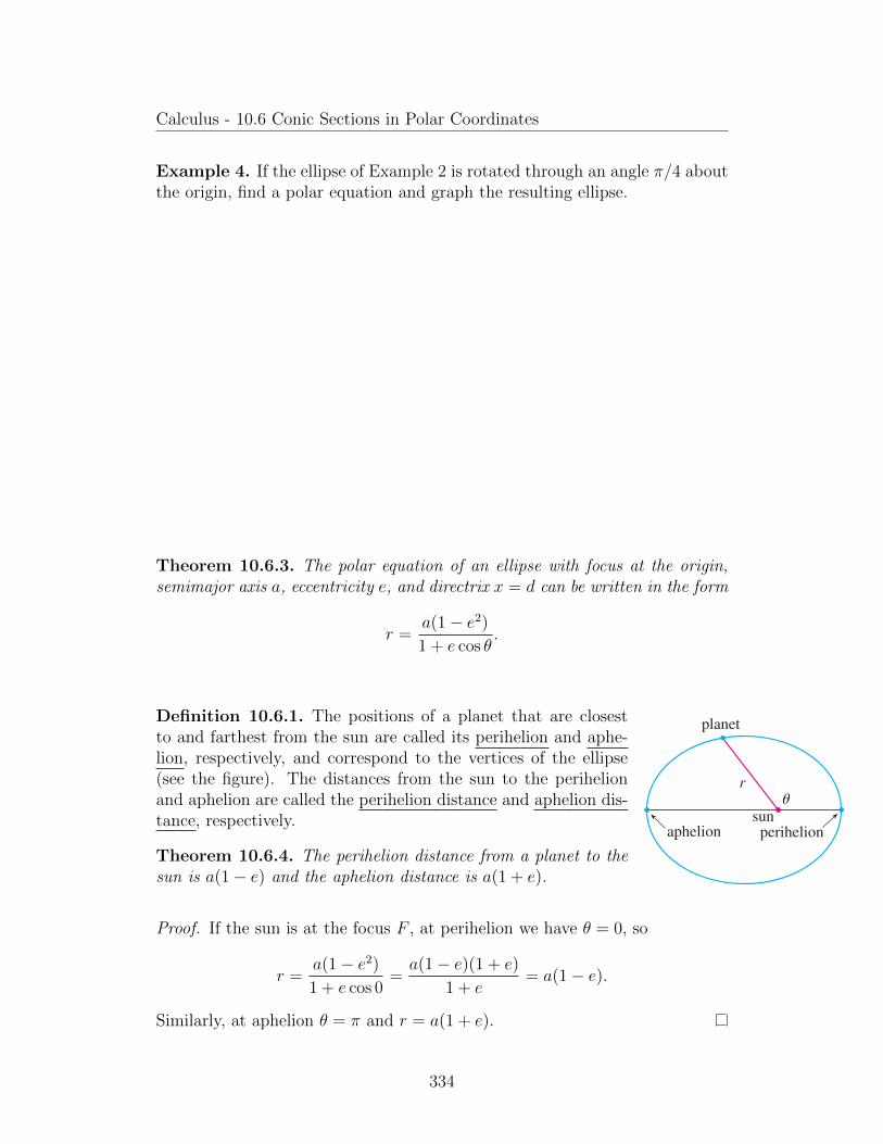
Calculus - 10.6 Conic Sections in Polar Coordinates
Example 4. If the ellipse of Example 2 is rotated through an angle π/4 aboutthe origin, find a polar equation and graph the resulting ellipse.
Theorem 10.6.3. The polar equation of an ellipse with focus at the origin,semimajor axis a, eccentricity e, and directrix x = d can be written in the form
r =a(1− e2)
1 + e cos θ.
SECTION 10.6 Conic Sections in Polar Coordinates 687
7 The polar equation of an ellipse with focus at the origin, semimajor axis a, eccentricity e, and directrix x − d can be written in the form
r −as1 2 e2d
1 1 e cos !
The positions of a planet that are closest to and farthest from the sun are called its peri helion and aphelion, respectively, and correspond to the vertices of the ellipse (see Figure 7). The distances from the sun to the perihelion and aphelion are called the perihelion distance and aphelion distance, respectively. In Figure 1 on page 683 the sun is at the focus F, so at perihelion we have ! − 0 and, from Equation 7,
r −as1 2 e2d
1 1 e cos 0−
as1 2 eds1 1 ed1 1 e
− as1 2 ed
Similarly, at aphelion ! − " and r − as1 1 ed.
8 The perihelion distance from a planet to the sun is as1 2 ed and the aphelion distance is as1 1 ed.
EXAMPLE 5 (a) Find an approximate polar equation for the elliptical orbit of the earth around the sun (at one focus) given that the eccentricity is about 0.017 and the length of the major axis is about 2.99 3 108 km.(b) Find the distance from the earth to the sun at perihelion and at aphelion.
SOLUTION(a) The length of the major axis is 2a − 2.99 3 108, so a − 1.495 3 108. We are given that e − 0.017 and so, from Equation 7, an equation of the earth’s orbit around the sun is
r −as1 2 e2d
1 1 e cos !−
s1.495 3 108d f1 2 s0.017d2g1 1 0.017 cos !
or, approximately,
r −1.49 3 108
1 1 0.017 cos !
(b) From (8), the perihelion distance from the earth to the sun is
as1 2 ed < s1.495 3 108ds1 2 0.017d < 1.47 3 108 km
and the aphelion distance is
as1 1 ed < s1.495 3 108ds1 1 0.017d < 1.52 3 108 km n
FIGURE 7
perihelionaphelionsun
planet
¨r
Copyright 2016 Cengage Learning. All Rights Reserved. May not be copied, scanned, or duplicated, in whole or in part. Due to electronic rights, some third party content may be suppressed from the eBook and/or eChapter(s).Editorial review has deemed that any suppressed content does not materially affect the overall learning experience. Cengage Learning reserves the right to remove additional content at any time if subsequent rights restrictions require it.
Definition 10.6.1. The positions of a planet that are closestto and farthest from the sun are called its perihelion and aphe-lion, respectively, and correspond to the vertices of the ellipse(see the figure). The distances from the sun to the perihelionand aphelion are called the perihelion distance and aphelion dis-tance, respectively.
Theorem 10.6.4. The perihelion distance from a planet to thesun is a(1− e) and the aphelion distance is a(1 + e).
Proof. If the sun is at the focus F , at perihelion we have θ = 0, so
r =a(1− e2)
1 + e cos 0=a(1− e)(1 + e)
1 + e= a(1− e).
Similarly, at aphelion θ = π and r = a(1 + e).
334

Calculus - 10.6 Conic Sections in Polar Coordinates
Example 5. (a) Find an approximate polar equation for the elliptical orbitof the earth around the sun (at one focus) given that the eccentricity isabout 0.017 and the length of the major axis is about 2.99× 10⁸ km.
(b) Find the distance from the earth to the sun at perihelion and at aphelion.
335

Chapter 11
Infinite Sequences and Series
11.1 Sequences
Definition 11.1.1. A sequence can be thought of as a list of numbers writtenin a definite order:
a1, a2, a3, a4, . . . , an, . . . .
The number a1 is called the first term, a2 is the second term, and in generalan is the nth term.A sequence can also be defined as a function whose domain is the set of positiveintegers. However, we usually write an instead of the function notation f(n)for the value of the function at the number n.The sequence a1, a2, a3, . . . is also denoted by
an or an∞n=1.
Example 1. Some sequences can be defined by giving a formula for the nthterm. In the following examples we give three descriptions of the sequence:one by using the preceding notation, another by using the defining formula,and a third by writing out the terms of the sequence. Notice that n doesn’thave to start at 1.
336

Calculus - 11.1 Sequences
(a)
n
n+ 1
∞n=1
an =n
n+ 1
1
2,2
3,3
4,4
5, . . . ,
n
n+ 1, . . .
(b)
(−1)n(n+ 1)
3n
an =
(−1)n(n+ 1)
3n
−2
3,3
9,− 4
27,
5
81, . . . ,
(−1)n(n+ 1)
3n, . . .
(c)
√n− 3
∞n=3
an =√n− 3, n ≥ 3
0, 1,√
2,√
3, . . . ,√n− 3, . . .
(d)
cos
nπ
6
∞n=0
an = cosnπ
6, n ≥ 0
1,
√3
2,1
2, 0, . . . , cos
nπ
6, . . .
Example 2. Find a formula for the general term an of the sequence3
5,− 4
25,
5
125,− 6
625,
7
3125, . . .
assuming that the pattern of the first few terms continues.
337

Calculus - 11.1 Sequences
Example 3. Here are some sequences that don’t have a simple defining equa-tion.
(a) The sequence pn, where pn is the population of the world as of January1 in the year n.
(b) If we let an be the digit in the nth decimal place of the number e, thenan is a well-defined sequence whose first few terms are
7, 1, 8, 2, 8, 1, 8, 2, 4, 5, . . ..
(c) The Fibonacci sequence fn is defined recursively by the conditions
f1 = 1 f2 = 1 fn = fn−1 + fn−2 n ≥ 3.
Each term is the sum of the two preceding terms. The first few terms are
1, 1, 2, 3, 5, 8, 13, 21, . . .
This sequence arose when the 13th-century Italian mathematician knownas Fibonacci solved a problem concerning the breeding of rabbits.
Definition 11.1.2. A sequence an has the limit L and we write
limn→∞
an = L or an → L as n→∞
if we can make the terms an as close to L as we like by taking n sufficientlylarge. If limn→∞ exists, we say the sequence converges (or is convergent).Otherwise, we say the sequence diverges (or is divergent).
Definition 11.1.3 (Precise Definition of the Limit of a Sequence). A sequencean has the limit L and we write
limn→∞
an = L or an → L as n→∞
if for every ε > 0 there is a corresponding integer N such that
if n > N then |an − L| < ε.
Theorem 11.1.1. If limx→∞ f(x) = L and f(n) = an when n is an integer,then limn→∞ an = L.
Definition 11.1.4. limn→∞ an =∞ means that for every positive number Mthere is an integer N such that
if n > N then an > M.
338

Calculus - 11.1 Sequences
Theorem 11.1.2 (Limit Laws for Sequences). If an and bn are convergentsequences and c is a constant, then
limn→∞
(an + bn) = limn→∞
an + limn→∞
bn
limn→∞
(an − bn) = limn→∞
an − limn→∞
bn
limn→∞
can = c limn→∞
an limn→∞
c = c
limn→∞
(anbn) = limn→∞
an · limn→∞
bn
limn→∞
anbn
=limn→∞
an
limn→∞
bnif lim
n→∞bn 6= 0
limn→∞
apn =
[limn→∞
an
]pif p > 0 and an > 0.
Theorem 11.1.3 (Squeeze Theorem for Sequences). If an ≤ bn ≤ cn forn ≥ n0 and lim
n→∞an = lim
n→∞cn = L, then lim
n→∞bn = L.
Theorem 11.1.4. If limn→∞
|an| = 0, then limn→∞
an = 0.
Proof. Since limn→∞ |an| = 0,
limn→∞
−|an| = 0 = − limn→∞
|an| = 0.
But −|an| ≤ an ≤ |an| for all n, so by the squeeze theorem for sequences,limn→∞ an = 0.
Example 4. Find limn→∞
n
n+ 1.
339

Calculus - 11.1 Sequences
Example 5. Is the sequence an =n√
10 + nconvergent or divergent?
Example 6. Calculate limn→∞
lnn
n.
Example 7. Determine whether the sequence an = (−1)n is convergent ordivergent.
340

Calculus - 11.1 Sequences
Example 8. Evaluate limn→∞
(−1)n
nif it exists.
Theorem 11.1.5. If limn→∞
an = L and the function f is continuous at L, then
limn→∞
f(an) = f(L).
Proof. Choose a particular n, say n0. By the definition of a limit of a sequence,given ε1 > 0 there exists an integer N , such that |an0 − L| < ε1 for n0 > N .Similarly, by the definition of continuity, the limit of f exists at L, so for ε2 > 0there exists ε1 > 0 such that if |an0 − L| < ε1 then |f(an0)− f(L)| < ε2. Thisis true for arbitrary ε2 > 0, so limn→∞ f(an) = f(L).
Example 9. Find limn→∞
sin(π/n).
341

Calculus - 11.1 Sequences
Example 10. Discuss the convergence of the sequence an = n!/nn, wheren! = 1 · 2 · 3 · · · · · n.
Example 11. For what values of r is the sequence rn convergent?
342
Calculus - 11.1 Sequences
Definition 11.1.5. A sequence an is called increasing if an < an+1 for alln ≥ 1, that is, a1 < a2 < a3 < · · · . It is called decreasing if an > an+1 for alln ≥ 1. A sequence is monotonic if it is either increasing or decreasing.
Example 12. Is the sequence
3
n+ 5
increasing or decreasing?
Example 13. Show that the sequence an =n
n2 + 1is decreasing.
343

Calculus - 11.1 Sequences
Definition 11.1.6. A sequence an is bounded above if there is a numberM such that
an ≤M for all n ≥ 1.
It is bounded below if there is a number m such that
m ≤ an for all n ≥ 1.
If it is bounded above and below, then an is a bounded sequence.
Theorem 11.1.6 (Monotonic Sequence theorem). Every bounded, monotonicsequence is convergent.
Example 14. Investigate the sequence an defined by the recurrence relation
a1 = 2 an+1 =1
2(an + 6) for n = 1, 2, 3, . . . .
344

Calculus - 11.2 Series
11.2 Series
Definition 11.2.1. In general, if we try to add the terms of an infinite se-quence an∞n=1 we get an expression of the form
a1 + a2 + a3 + · · ·+ an + · · ·
which is called an infnite series (or just a series) and is denoted, for short, bythe symbol
∞∑n=1
an or∑
an.
Definition 11.2.2. Given a series∑∞
n=1 an = a1 +a2 +a3 + · · · , let sn denoteits nth partial sum:
sn =n∑i=1
ai = a1 + a2 + · · ·+ an.
If the sequence sn is convergent and limn→∞ sn = s exists as a real number,then the series
∑an is called convergent and we write
a1 + a2 + · · ·+ an + · · · = s or∞∑n=1
= s.
The number s is called the sum of the series. If the sequence sn is divergent,then the series is called divergent.
Example 1. Find the sum of the series∑∞
n=1 an if the sum of the first n termsof the series is
sn = a1 + a2 + · · ·+ an =2n
3n+ 5.
345

Calculus - 11.2 Series
Example 2. Find the sum of the geometric series
a+ ar + ar2 + ar3 + · · ·+ arn−1 + · · · =∞∑n=1
arn−1 a 6= 0
where each term is obtained from the preceding one by multiplying it by thecommon ratio r.
346

Calculus - 11.2 Series
Example 3. Find the sum of the geometric series
5− 10
3+
20
9− 40
27+ · · · .
Example 4. Is the series∞∑n=1
22n31−n convergent or divergent?
347

Calculus - 11.2 Series
Example 5. A drug is administered to a patient at the same time every day.Suppose the concentration of the drug is Cn (measured in mg/mL) after theinjection on the nth day. Before the injection the next day, only 30% of thedrug remains in the bloodstream and the daily dose raises the concentrationby 0.2 mg/mL.
(a) Find the concentration after three days.
(b) What is the concentration after the nth dose?
(c) What is the limiting concentration?
348

Calculus - 11.2 Series
Example 6. Write the number 2.317 = 2.3171717 . . . as a ratio of integers.
Example 7. Find the sum of the series∞∑n=0
xn, where |x| < 1.
349

Calculus - 11.2 Series
Example 8. Show that the series∞∑n=1
1
n(n+ 1)is convergent, and find its
sum.
350

Calculus - 11.2 Series
Example 9. Show that the harmonic series
∞∑n=1
1
n= 1 +
1
2+
1
3+
1
4+ · · ·
is divergent.
351

Calculus - 11.2 Series
Theorem 11.2.1. If the series∞∑n=1
an is convergent, then limn→∞
an = 0.
Proof. Let sn = a1 + a2 + · · · + an. Then an = sn − sn−1. Since∑an
is convergent, the sequence sn is convergent. Let limn→∞ sn = s. Sincen− 1→∞ as n→∞, we also have limn→∞ sn−1 = s. Therefore
limn→∞
an = limn→∞
(sn − sn−1) = limn→∞
sn − limn→∞
sn−1 = s− s = 0.
Corollary 11.2.1 (Test for Divergence). If limn→∞
an does not exist or if limn→∞
an 6=
0, then the series∞∑n=1
an is divergent.
Proof. If the series is not divergent, then it is convergent, and so limn→∞ an = 0by Theorem 11.2.1. The result follows by contrapositive.
Example 10. Show that the series∞∑n=1
n2
5n2 + 4diverges.
352

Calculus - 11.2 Series
Theorem 11.2.2. If∑an and
∑bn are convergent series, then so are the
series∑can (where c is a constant),
∑(an + bn), and
∑(an − bn), and
(i)∞∑n=1
can = c∞∑n=1
an
(ii)∞∑n=1
(an + bn) =∞∑n=1
an +∞∑n=1
bn
(iii)∞∑n=1
(an − bn) =∞∑n=1
an −∞∑n=1
bn
Example 11. Find the sum of the series∞∑n=1
(3
n(n+ 1)+
1
2n
).
Remark 1. A finite number of terms doesn’t affect the convergence or diver-gence of a series. For instance, suppose that we were able to show that theseries
∞∑n=4
n
n3 + 1
is convergent. Since
∞∑n=1
n
n3 + 1=
1
2+
2
9+
3
28+∞∑n=4
n
n3 + 1
it follows that the entire series∑∞
n=1 n/(n3 + 1) is convergent. Similarly, if it
is known that the series∑∞
n=N+1 an converges, then the full series
∞∑n=1
an =N∑n=1
an +∞∑
n=N+1
an
is also convergent.
353

Calculus - 11.3 The Integral Test and Estimates of Sums
11.3 The Integral Test and Estimates of Sums
Theorem 11.3.1 (The Integral Test). Suppose f is a continuous, positive,decreasing function on [1,∞) and an = f(n). The the series
∑∞n=1 an is con-
vergent if and only if the improper integral´∞
1f(x) dx is convergent. In other
words:
(i) If
ˆ ∞1
f(x) dx is convergent, then∞∑n=1
an is convergent.
(ii) If
ˆ ∞1
f(x) dx is divergent, then∞∑n=1
an is divergent.
Proof. SECTION 11.3 The Integral Test and Estimates of Sums 725
Proof of the Integral TestWe have already seen the basic idea behind the proof of the Integral Test in Figures 1 and 2 for the series o 1yn2 and o 1ysn . For the general series o an, look at Figures!5!and!6.The area of the "rst shaded rectangle in Figure 5 is the value of f at the right endpoint of f1, 2g, that is, f s2d ! a2. So, comparing the areas of the shaded rectangles with the area under y ! f sxd from 1 to n, we see that
a2 1 a3 1 # # # 1 an < yn
1 f sxd dx
(Notice that this inequality depends on the fact that f is decreasing.) Likewise, Figure 6 shows that
yn
1 f sxd dx < a1 1 a2 1 # # # 1 an21
(i) If y`
1 f sxd dx is convergent, then (4) gives
on
i!2 ai < yn
1f sxd dx < y`
1 f sxd dx
since f sxd > 0. Therefore
sn ! a1 1 on
i!2 ai < a1 1 y`
1 f sxd dx ! M, say
Since sn < M for all n, the sequence hsn j is bounded above. Also
sn11 ! sn 1 an11 > sn
since an11 ! f sn 1 1d > 0. Thus hsn j is an increasing bounded sequence and so it is con vergent by the Monotonic Sequence Theorem (11.1.12). This means that o an is convergent.
(ii) If y`1 f sxd dx is divergent, then yn
1 f sxd dx l ` as n l ` because f sxd > 0. But (5) gives
yn
1f sxd dx < o
n21
i!1 ai ! sn21
and so sn21 l `. This implies that sn l ` and so o an diverges. Q
0 x
y
1 2 3 4 5 . . . n
y=ƒ
ana™ a£ a¢ a!
4
0 x
y
1 2 3 4 5 . . . n
y=ƒ
a™ a£ a¢a¡
an-1
FIGURE 6
5
1. Draw a picture to show that
o`
n!2
1n 1.3 , y`
1
1x 1.3 dx
What can you conclude about the series?
2. Suppose f is a continuous positive decreasing function forx > 1 and an ! f snd. By drawing a picture, rank the followingthree quantities in increasing order:
y6
1 f sxd dx o
5
i!1 ai o
6
i!2 ai
3–8 Use the Integral Test to determine whether the series is convergent or divergent.
3. o`
n!1 n23 4. o
`
n!1 n20.3
5. o`
n!1
25n 2 1
6. o`
n!1
1s3n 2 1d4
7. o`
n!1
nn2 1 1
8. o`
n!1 n2e2n3
Copyright 2016 Cengage Learning. All Rights Reserved. May not be copied, scanned, or duplicated, in whole or in part. Due to electronic rights, some third party content may be suppressed from the eBook and/or eChapter(s).Editorial review has deemed that any suppressed content does not materially affect the overall learning experience. Cengage Learning reserves the right to remove additional content at any time if subsequent rights restrictions require it.
(i) If´∞
1f(x) dx is convergent, then comparing the areas of the
rectangles with the area under y = f(x) from 1 to n in thetop figure, we see that
n∑i=2
ai = a2 + a3 + · · ·+ an ≤ˆ n
1
f(x) dx ≤ˆ ∞
1
f(x) dx
since f(x) ≥ 0. Therefore
sn = a1 +n∑i=2
ai ≤ a1 +
ˆ ∞1
f(x) dx = M, say.
Since sn ≤M for all n, the sequence sn is bounded above. Also
sn+1 = sn + an+1 ≥ sn
since an+1 = f(n+ 1) ≥ 0. Thus sn is an increasing bounded sequenceand so it is convergent by the Monotonic Sequence Theorem.
SECTION 11.3 The Integral Test and Estimates of Sums 725
Proof of the Integral TestWe have already seen the basic idea behind the proof of the Integral Test in Figures 1 and 2 for the series o 1yn2 and o 1ysn . For the general series o an, look at Figures!5!and!6.The area of the "rst shaded rectangle in Figure 5 is the value of f at the right endpoint of f1, 2g, that is, f s2d ! a2. So, comparing the areas of the shaded rectangles with the area under y ! f sxd from 1 to n, we see that
a2 1 a3 1 # # # 1 an < yn
1 f sxd dx
(Notice that this inequality depends on the fact that f is decreasing.) Likewise, Figure 6 shows that
yn
1 f sxd dx < a1 1 a2 1 # # # 1 an21
(i) If y`
1 f sxd dx is convergent, then (4) gives
on
i!2 ai < yn
1f sxd dx < y`
1 f sxd dx
since f sxd > 0. Therefore
sn ! a1 1 on
i!2 ai < a1 1 y`
1 f sxd dx ! M, say
Since sn < M for all n, the sequence hsn j is bounded above. Also
sn11 ! sn 1 an11 > sn
since an11 ! f sn 1 1d > 0. Thus hsn j is an increasing bounded sequence and so it is con vergent by the Monotonic Sequence Theorem (11.1.12). This means that o an is convergent.
(ii) If y`1 f sxd dx is divergent, then yn
1 f sxd dx l ` as n l ` because f sxd > 0. But (5) gives
yn
1f sxd dx < o
n21
i!1 ai ! sn21
and so sn21 l `. This implies that sn l ` and so o an diverges. Q
0 x
y
1 2 3 4 5 . . . n
y=ƒ
ana™ a£ a¢ a!
4
0 x
y
1 2 3 4 5 . . . n
y=ƒ
a™ a£ a¢a¡
an-1
FIGURE 6
5
1. Draw a picture to show that
o`
n!2
1n 1.3 , y`
1
1x 1.3 dx
What can you conclude about the series?
2. Suppose f is a continuous positive decreasing function forx > 1 and an ! f snd. By drawing a picture, rank the followingthree quantities in increasing order:
y6
1 f sxd dx o
5
i!1 ai o
6
i!2 ai
3–8 Use the Integral Test to determine whether the series is convergent or divergent.
3. o`
n!1 n23 4. o
`
n!1 n20.3
5. o`
n!1
25n 2 1
6. o`
n!1
1s3n 2 1d4
7. o`
n!1
nn2 1 1
8. o`
n!1 n2e2n3
Copyright 2016 Cengage Learning. All Rights Reserved. May not be copied, scanned, or duplicated, in whole or in part. Due to electronic rights, some third party content may be suppressed from the eBook and/or eChapter(s).Editorial review has deemed that any suppressed content does not materially affect the overall learning experience. Cengage Learning reserves the right to remove additional content at any time if subsequent rights restrictions require it.
(ii) If´∞
1f(x) dx is divergent, then
´ n1f(x) dx→∞ as n→∞
because f(x) ≥ 0. But the bottom figure shows that
ˆ n
1
f(x) dx ≤ a1 + a2 + · · ·+ an−1 =n−1∑i=1
ai = sn−1
and so sn−1 →∞, implying that sn →∞.
354

Calculus - 11.3 The Integral Test and Estimates of Sums
Example 1. Test the series∞∑n=1
1
n2 + 1for convergence or divergence.
Example 2. For what values of p is the series∞∑n=1
1
npconvergent? (This series
is called the p-series.)
355

Calculus - 11.3 The Integral Test and Estimates of Sums
Example 3. Determine whether each series converges or diverges.
(a)∞∑n=1
1
n3=
1
13+
1
23+
1
33+
1
43+ · · ·
(b)∞∑n=1
13√n
= 1 +13√
2+
13√
3+
13√
4+ · · ·
Example 4. Determine whether the series∞∑n=1
lnn
nconverges or diverges.
356

Calculus - 11.3 The Integral Test and Estimates of Sums
Definition 11.3.1. The remainder
Rn = s− sn = an+1 + an+2 + an+3 + · · ·
is the error made when sn, the sum of the first n terms, is used as an approx-imation to the total sum.
SECTION 11.3 The Integral Test and Estimates of Sums 723
Estimating the Sum of a SeriesSuppose we have been able to use the Integral Test to show that a series o an is conver-gent and we now want to !nd an approximation to the sum s of the series. Of course, any partial sum sn is an approximation to s because limn l ` sn ! s. But how good is such an approximation? To !nd out, we need to estimate the size of the remainder
Rn ! s 2 sn ! an11 1 an12 1 an13 1 " " "
The remainder Rn is the error made when sn, the sum of the !rst n terms, is used as an approximation to the total sum.
We use the same notation and ideas as in the Integral Test, assuming that f is decreas-ing on fn, d . Comparing the areas of the rectangles with the area under y ! f sxd for x . n in Figure 3, we see that
Rn ! a n11 1 a n12 1 " " " < y`
n f sxd dx
Similarly, we see from Figure 4 that
Rn ! an11 1 an12 1 " " " > y`
n11 f sxd d x
So we have proved the following error estimate.
2 Remainder Estimate for the Integral Test Suppose f skd ! ak, where f is a continuous, positive, decreasing function for x > n and o an is convergent. If Rn ! s 2 sn, then
y`
n11f sxd dx < Rn < y`
n f sxd dx
EXAMPLE 5(a) Approximate the sum of the series o1yn3 by using the sum of the !rst 10 terms.Estimate the error involved in this approximation.(b) How many terms are required to ensure that the sum is accurate to within 0.0005?
SOLUTION In both parts (a) and (b) we need to know y`n f sxd dx. With f sxd ! 1yx 3,
which satis!es the conditions of the Integral Test, we have
y`
n
1x 3 dx ! lim
t l ` F2
12x 2G
n
t
! limt l `
S21
2t 2 11
2n2D !1
2n2
(a) Approximating the sum of the series by the 10th partial sum, we have
o`
n!1
1n3 < s10 !
113 1
123 1
133 1 " " " 1
1103 < 1.1975
According to the remainder estimate in (2), we have
R10 < y`
10
1x 3 dx !
12s10d2 !
1200
So the size of the error is at most 0.005.
0 x
y
n
. . .
y=ƒ
an+1 an+2
FIGURE 4
0 x
y
an+1 an+2
n+1
. . .
y=ƒ
Copyright 2016 Cengage Learning. All Rights Reserved. May not be copied, scanned, or duplicated, in whole or in part. Due to electronic rights, some third party content may be suppressed from the eBook and/or eChapter(s).Editorial review has deemed that any suppressed content does not materially affect the overall learning experience. Cengage Learning reserves the right to remove additional content at any time if subsequent rights restrictions require it.
Theorem 11.3.2 (Remainder Estimate for the Integral Test).Suppose f(k) = ak, where f is a continuous, positive, decreasingfunction for x ≥ n and
∑an is convergent. If Rn = s− sn, then
ˆ ∞n+1
f(x) dx ≤ Rn ≤ˆ ∞n
f(x) dx.
Proof. Comparing the rectangles with the area under y = f(x)for x > n in the top figure, we see that
Rn = an+1 + an+2 + · · · ≤ˆ ∞n
f(x) dx.
Similarly, we see from the bottom figure that
Rn = an+1 + an+2 + · · · ≥ˆ ∞n+1
f(x) dx.
Example 5. (a) Approximate the sum of the series∑
1/n3 by using the sumof the first 10 terms. Estimate the error involved in this approximation.
357

Calculus - 11.3 The Integral Test and Estimates of Sums
(b) How many terms are required to ensure that the sum is accurate to within0.0005?
Corollary 11.3.1. Suppose f(k) = ak, where f is a continuous, positive,decreasing function for x ≥ n and
∑an is convergent. Then
sn +
ˆ ∞n+1
f(x) dx ≤ s ≤ sn +
ˆ ∞n
f(x) dx.
Example 6. Use Corollary 11.3.1 with n = 10 to estimate the sum of the
series∞∑n=1
1
n3.
358

Calculus - 11.4 The Comparison Tests
11.4 The Comparison Tests
Theorem 11.4.1 (The Comparison Test). Suppose that∑an and
∑bn are
series with positive terms.
(i) If∑bn is convergent and an ≤ bn for all n, then
∑an is also convergent.
(ii) If∑bn is divergent and an ≥ bn for all n, then
∑an is also divergent.
Proof. (i) Let
sn =n∑i=1
ai tn =n∑i=1
bi t =∞∑n=1
bn
Since both series have positive terms, the sequences sn and tn areincreasing (sn+1 = sn+an+1 ≥ sn). Also tn → t, so tn ≤ t for all n. Sinceai ≤ bi, we have sn ≤ tn. Thus sn ≤ t for all n. This means that sn isincreasing and bounded above and therefore converges by the MonotonicSequence Theorem. Thus
∑an converges.
(ii) If∑bn is divergent, then tn →∞ (since tn is increasing). But ai ≥ bi
so sn ≥ tn. Thus sn →∞. Therefore∑an diverges.
Example 1. Determine whether the series∞∑n=1
5
2n2 + 4n+ 3converges or di-
verges.
359

Calculus - 11.4 The Comparison Tests
Example 2. Test the series∞∑k=1
ln k
kfor convergence or divergence.
Theorem 11.4.2 (The Limit Comparison Test). Suppose that∑an and
∑bn
are series with positive terms. If
limn→∞
anbn
= c
where c is a finite number and c > 0, then either both series converge or bothdiverge.
Proof. Let m and M be positive numbers such that m < c < M . Becausean/bn is close to c for large n, there is an integer N such that
m <anbn
< M when n > N,
and sombn < an < Mbn when n > N.
If∑bn converges, so does
∑Mbn. Thus
∑an converges by part (i) of the
Comparison Test. If∑bn diverges, so does
∑mbn and part (ii) of the Com-
parison Test shows that∑an diverges.
360

Calculus - 11.4 The Comparison Tests
Example 3. Test the series∞∑n=1
1
2n − 1for convergence or divergence.
Example 4. Determine whether the series∞∑n=1
2n2 + 3n√5 + n5
converges or diverges.
361

Calculus - 11.4 The Comparison Tests
Example 5. Use the sum of the first 100 terms to approximate the sum ofthe series
∑1/(n3 + 1). Estimate the error involved in this approximation.
362

Calculus - 11.5 Alternating Series
11.5 Alternating Series
Definition 11.5.1. An alternating series is a series whose terms are alter-nately positive and negative.
Theorem 11.5.1 (Alternating Series Test). If the alternating series
∞∑n=1
(−1)n−1bn = b1 − b2 + b3 − b4 + b5 − b6 + · · · bn > 0
satisfies
(i) bn+1 ≤ bn for all n
(ii) limn→∞
bn = 0
then the series is convergent.
Proof.
SECTION 11.5 Alternating Series 733
Before giving the proof let’s look at Figure 1, which gives a picture of the idea behind the proof. We !rst plot s1 ! b1 on a number line. To !nd s2 we subtract b2, so s2 is to the left of s1. Then to !nd s3 we add b3, so s3 is to the right of s2. But, since b3 , b2, s3 is to the left of s1. Continuing in this manner, we see that the partial sums oscillate back and forth. Since bn l 0, the successive steps are becoming smaller and smaller. The even partial sums s2, s4, s6, . . . are increasing and the odd partial sums s1, s3, s5, . . . are decreasing. Thus it seems plausible that both are converging to some number s, which is the sum of"the series. Therefore we consider the even and odd partial sums separately in the following proof.
0 s¡s™ s£s¢ s!sß s
b¡-b™
+b£-b¢
+b!-bß
PROOF OF THE ALTERNATING SERIES TEST We !rst consider the even partial sums:
s2 ! b1 2 b2 > 0 since b2 < b1
s4 ! s2 1 sb3 2 b4 d > s2 since b4 < b3
In general s2n ! s2n22 1 sb2n21 2 b2n d > s2n22 since b2n < b2n21
Thus 0 < s2 < s4 < s6 < # # # < s2n < # # #
But we can also write
s2n ! b1 2 sb2 2 b3 d 2 sb4 2 b5 d 2 # # # 2 sb2n22 2 b2n21d 2 b2n
Every term in parentheses is positive, so s2n < b1 for all n. Therefore the sequence hs2n j of even partial sums is increasing and bounded above. It is therefore convergent by the Monotonic Sequence Theorem. Let’s call its limit s, that is,
lim n l `
s2n ! s
Now we compute the limit of the odd partial sums:
limnl`
s2n11 ! limnl`
ss2n 1 b2n11d
! limnl`
s2n 1 limnl`
b2n11
! s 1 0
! s
Since both the even and odd partial sums converge to s, we have lim n l ` sn ! s [see Exercise 11.1.92(a)] and so the series is convergent. Q
FIGURE 1
[by condition (ii)]
Copyright 2016 Cengage Learning. All Rights Reserved. May not be copied, scanned, or duplicated, in whole or in part. Due to electronic rights, some third party content may be suppressed from the eBook and/or eChapter(s).Editorial review has deemed that any suppressed content does not materially affect the overall learning experience. Cengage Learning reserves the right to remove additional content at any time if subsequent rights restrictions require it.
We first consider the even partial sums:
s2 = b1 − b2 ≥ 0 since b2 ≤ b1
s4 = s2 + (b3 − b4) ≥ s2 since b4 ≤ b3.
In general
s2n = s2n−2 + (b2n−1 − b2n) ≥ s2n−2 since b2n ≤ b2n−1.
Thus0 ≤ s2 ≤ s4 ≤ s6 ≤ · · · ≤ s2n ≤ · · · .
But we can also write
s2n = b1 − (b2 − b3)− (b4 − b5)− · · · − (b2n−2 − b2n−1)− b2n.
363

Calculus - 11.5 Alternating Series
Every term in parenthesis is positive, so s2n ≤ b1 for all n. Therefore, thesequence s2n of even partial sums is increasing and bounded above. It istherefore convergent by the Monotonic Sequence Theorem. Let’s call its limits, that is,
limn→∞
s2n = s.
Now we compute the limit of the odd partial sums:
limn→∞
s2n+1 = limn→∞
(s2n + b2n+1)
= limn→∞
s2n + limn→∞
b2n+1
= s+ 0
= s.
Since both the even and odd partial sums converge to s, we have limn→∞ sn = sand so the series is convergent.
Example 1. Determine whether the alternating harmonic series
1− 1
2+
1
3− 1
4+ · · · =
∞∑n=1
(−1)n−1
n
converges or diverges.
364

Calculus - 11.5 Alternating Series
Example 2. Determine whether the series∞∑n=1
(−1)n3n
4n− 1converges or diverges.
Example 3. Test the series∞∑n=1
(−1)n+1 n2
n3 + 1for convergence or divergence.
365

Calculus - 11.5 Alternating Series
Theorem 11.5.2 (Alternating Series Estimation Theorem). If s =∑
(−1)n−1bn,where bn > 0, is the sum of an alternating series that satisfies
(i) bn+1 ≤ bn and (ii) limn→∞
bn = 0
then|Rn| = |s− sn| ≤ bn+1.
Proof. We know from the proof of the Alternating Series Test that s lies be-tween any two consecutive partial sums sn and sn+1. (There we showed thats is larger than all the even partial sums. A similar argument shows that s issmaller than all the odd sums.) It follows that
|s− sn| ≤ |sn+1 − sn| = bn+1.
Example 4. Find the sum of the series∞∑n=0
(−1)n
n!correct to three decimal
places.
366

Calculus - 11.6 Absolute Convergence, Ratio and Root Tests
11.6 Absolute Convergence, Ratio and Root
Tests
Definition 11.6.1. A series∑an is called absolutely convergent if the series
of absolute values∑|an| is convergent.
Example 1. Is the series
∞∑n=1
(−1)n−1
n2= 1− 1
22+
1
32− 1
42+ · · ·
absolutely convergent?
Example 2. Is the series
∞∑n=1
(−1)n−1
n= 1− 1
2+
1
3− 1
4+ · · ·
absolutely convergent?
367

Calculus - 11.6 Absolute Convergence, Ratio and Root Tests
Definition 11.6.2. A series∑an is called conditionally convergent if it is
convergent but not absolutely convergent.
Theorem 11.6.1. If a series∑an is absolutely convergent, then it is conver-
gent.
Proof. Observe that the inequality
0 ≤ an + |an| ≤ 2|an|
is true because |an| is either an or −an. If∑an is absolutely convergent, then∑
|an| is convergent, so∑
2|an| is convergent. Therefore, by the ComparisonTest,
∑(an + |an|) is convergent. Then∑
an =∑
(an + |an|)−∑|an|
is the difference of two convergent series and is therefore convergent.
Example 3. Determine whether the series
∞∑n=1
cosn
n2=
cos 1
12+
cos 2
22+
cos 3
32+ · · ·
is convergent or divergent.
368

Calculus - 11.6 Absolute Convergence, Ratio and Root Tests
Theorem 11.6.2 (The Ratio Test).
(i) If limn→∞
∣∣∣∣an+1
an
∣∣∣∣ = L < 1, then the series∞∑n=1
an is absolutely convergent
(and therefore convergent).
(ii) If limn→∞
∣∣∣∣an+1
an
∣∣∣∣ = L > 1 or limn→∞
∣∣∣∣an+1
an
∣∣∣∣ = ∞, then the series∞∑n=1
an is
divergent.
(iii) If limn→∞
∣∣∣∣an+1
an
∣∣∣∣ = 1, the Ratio Test is inconclusive; that is, no conclusion
can be drawn about the convergence or divergence of∑an.
Example 4. Test the series∞∑n=1
(−1)nn3
3nfor absolute convergence.
Example 5. Test the convergence of the series∞∑n=1
nn
n!.
369

Calculus - 11.6 Absolute Convergence, Ratio and Root Tests
Theorem 11.6.3 (The Root Test).
(i) If limn→∞
n√|an| = L < 1, then the series
∞∑n=1
an is absolutely convergent
(and therefore convergent).
(ii) If limn→∞
n√|an| = L > 1 or lim
n→∞n√|an| = ∞, then the series
∞∑n=1
an is
divergent.
(iii) If limn→∞
n√|an| = 1, the Root Test is inconclusive.
Example 6. Test the convergence of the series∞∑n=1
(2n+ 3
3n+ 2
)n.
370

Calculus - 11.6 Absolute Convergence, Ratio and Root Tests
Definition 11.6.3. By a rearrangement of an infinite series∑an we mean a
series obtained by simply changing the order of the terms.
Remark 1. If∑an is an absolutely convergent series with sum s, then any
rearrangement of∑an has the same sum s.
Remark 2. If∑an is a conditionally convergent series and r is any real number
whatsoever, then there is a rearrangement of∑an that has a sum equal to r.
For example, if we multiply the alternating harmonic series
1− 1
2+
1
3− 1
4+
1
5− 1
6+
1
7− 1
8+ · · · = ln 2
by 12, we get
1
2− 1
4+
1
6− 1
8+ · · · = 1
2ln 2.
Then inserting zeros between the terms of this series gives
0 +1
2+ 0− 1
4+ 0 +
1
6+ 0− 1
8+ · · · = 1
2ln 2,
and we can add this to the alternating harmonic series to get
1 +1
3− 1
2+
1
5+
1
7− 1
4+ · · · = 3
2ln 2,
which is a rearrangement of the alternating harmonic series with a differentsum.
371

Calculus - 11.7 Strategy for Testing Series
11.7 Strategy for Testing Series
Example 1.∞∑n=1
n− 1
2n+ 1.
Example 2.∞∑n=1
√n3 + 1
3n3 + 4n2 + 2.
Example 3.∞∑n=1
ne−n2
.
372

Calculus - 11.7 Strategy for Testing Series
Example 4.∞∑n=1
(−1)nn3
n4 + 1.
Example 5.∞∑n=1
2k
k!.
Example 6.∞∑n=1
1
2 + 3n.
373

Calculus - 11.8 Power Series
11.8 Power Series
Definition 11.8.1. A power series is a series of the form
∞∑n=0
cnxn = c0 + c1x+ c2x
2 + c3x3 + · · ·
where x is a variable and the cn’s are constants called the coefficients of theseries.More generally, a series of the form
∞∑n=0
cn(x− a)n = c0 + c1(x− a) + c2(x− a)2 + · · ·
is called a power series in (x− a) or a power series centered at a or a powerseries about a.
Example 1. For what values of x is the series∞∑n=0
n!xn convergent?
374

Calculus - 11.8 Power Series
Example 2. For what values of x does the series∞∑n=1
(x− 3)n
nconverge?
Example 3. Find the domain of the Bessel function of order 0 defined by
J0(x) =∞∑n=0
(−1)nx2n
22n(n!)2.
375
Calculus - 11.8 Power Series
Theorem 11.8.1. For a given power series∞∑n=0
cn(x−a)n, there are only three
possibilities:
(i) The series converges only when x = a.
(ii) The series converges for all x.
(iii) There is a positive number R such that the series converges if |x−a| < Rand diverges if |x− a| > R.
Definition 11.8.2. The number R in case (iii) is called the radius of conver-gence of the power series. By convention, the radius of convergence is R = 0 incase (i) and R =∞ in case (ii). The interval of convergence of a power seriesis the interval that consists of all values of x for which the series converges.
Example 4. Find the radius of convergence and interval of convergence ofthe series
∞∑n=0
(−3)nxn√n+ 1
.
376

Calculus - 11.8 Power Series
Example 5. Find the radius of convergence and interval of convergence ofthe series
∞∑n=0
n(x+ 2)n
3n+1.
377

Calculus - 11.9 Representations of Functions as Power Series
11.9 Representations of Functions as Power
Series
Example 1. Express 1/(1 + x2) as the sum of a power series and find theinterval of convergence.
Example 2. Find a power series representation for 1/(x+ 2).
378

Calculus - 11.9 Representations of Functions as Power Series
Example 3. Find a power series representation of x3/(x+ 2).
Theorem 11.9.1. If the power series∑cn(x− a)n has radius of convergence
R > 0, then the function f defined by
f(x) = c0 + c1(x− a) + c2(x− a)2 + · · · =∞∑n=0
cn(x− a)n
is differentiable (and therefore continuous) on the interval (a−R, a+R) and
(i) f ′(x) = c1 + 2c2(x− a) + 3c3(x− a)2 + · · · =∞∑n=1
ncn(x− a)n−1
(ii)
ˆf(x) dx = C + c0(x− a) + c1
(x− a)2
2+ c2
(x− a)3
3+ · · ·
= C +∞∑n=0
cn(x− a)n+1
n+ 1.
The radii of convergence of the power series in Equations (i) and (ii) are bothR.
379

Calculus - 11.9 Representations of Functions as Power Series
Example 4. Find the derivative of the Bessel function
J0(x) =∞∑n=0
(−1)nx2n
22n(n!)2.
Example 5. Express 1/(1− x)2 as a power series using differentiation. Whatis the radius of convergence?
380

Calculus - 11.9 Representations of Functions as Power Series
Example 6. Find a power series representation for ln(1 +x) and its radius ofconvergence.
Example 7. Find a power series representation for f(x) = tan−1 x.
381

Calculus - 11.9 Representations of Functions as Power Series
Example 8. (a) Evaluate´
[1/(1 + x7)]dx as a power series.
(b) Use part (a) to approximate´ 0.5
0[1/(1 + x7)]dx correct to within 10−7.
382

Calculus - 11.10 Taylor and Maclaurin Series
11.10 Taylor and Maclaurin Series
Theorem 11.10.1. If f has a power series representation (expansion) at a,that is, if
f(x) =∞∑n=0
cn(x− a)n |x− a| < R
then its coefficients are given by the formula
cn =f (n)(a)
n!.
Definition 11.10.1. The Taylor series of the function f at a (or about a orcentered at a) is
f(x) =∞∑n=0
f (n)(a)
n!(x− a)n
= f(a) +f ′(a)
1!(x− a) +
f ′′(a)
2!(x− a)2 +
f ′′′(a)
3!(x− a)3 + · · · .
For the special case a = 0 the Taylor series becomes
f(x) =∞∑n=0
f (n)(0)
n!xn = f(0) +
f ′(0)
1!x+
f ′′(0)
2!x2 +
f ′′′(0)
3!x3 + · · · ,
which we call the Maclaurin Series.
Example 1. Find the Maclaurin series of the function f(x) = ex and its radiusof convergence.
383

Calculus - 11.10 Taylor and Maclaurin Series
Theorem 11.10.2. If f(x) = Tn(x)+Rn(x), where Tn is the nth-degree Taylorpolynomial of f at a, Rn is the remainder of the Taylor series, and
limn→∞
Rn(x) = 0
for |x− a| < R, then f is equal to the sum of its Taylor series on the interval|x− a| < R.
Theorem 11.10.3 (Taylor’s Inequality). If |f (n+1)(x)| ≤ M for |x − a| ≤ d,then the remainder Rn(x) of the Taylor series satisfies the inequality
|Rn(x)| ≤ M
(n+ 1)!|x− a|n+1 for |x− a| ≤ d.
Example 2. Prove that ex is equal to the sum of its Maclaurin series.
384

Calculus - 11.10 Taylor and Maclaurin Series
Example 3. Find the Taylor series f(x) = ex at a = 2.
Example 4. Find the Maclaurin series for sinx and prove that it representssinx for all x.
385

Calculus - 11.10 Taylor and Maclaurin Series
Example 5. Find the Maclaurin series for cosx.
Example 6. Find the Maclaurin series for the function f(x) = x cosx.
386
Calculus - 11.10 Taylor and Maclaurin Series
Example 7. Represent f(x) = sinx as the sum of its Taylor series centeredat π/3.
387

Calculus - 11.10 Taylor and Maclaurin Series
Example 8. Find the Maclaurin series for f(x) = (1 + x)k, where k is anyreal number.
388

Calculus - 11.10 Taylor and Maclaurin Series
Theorem 11.10.4 (The Binomial Series). If k is any real number and |x| < 1,then
(1 + x)k =∞∑n=0
(k
n
)xn = 1 + kx+
k(k − 1)
2!x2 +
k(k − 1)(k − 2)
3!x3 + · · ·
where the coefficients(k
n
)=k(k − 1)(k − 2) · · · (k − n+ 1)
n!
are called the binomial coefficients.
Example 9. Find the Maclaurin series for the function f(x) =1√
4− xand
its radius of convergence.
389

Calculus - 11.10 Taylor and Maclaurin Series
Example 10. Find the sum of the series1
1 · 2− 1
2 · 22+
1
3 · 23− 1
4 · 24+ · · · .
Example 11. (a) Evaluate´e−x
2dx as an infinite series.
(b) Evaluate´ 1
0e−x
2dx correct to within an error of 0.001.
390
Calculus - 11.10 Taylor and Maclaurin Series
Example 12. Evaluate limx→0
ex − 1− xx2
.
391

Calculus - 11.10 Taylor and Maclaurin Series
Example 13. Find the first three nonzero terms in the Maclaurin series for
(a) ex sinx
(b) tan x
392

Calculus - 11.11 Applications of Taylor Polynomials
11.11 Applications of Taylor Polynomials
Example 1. (a) Approximate the function f(x) = 3√x by a Taylor polyno-
mial of degree 2 at a = 8.
(b) How accurate is this approximation when 7 ≤ x ≤ 9?
393

Calculus - 11.11 Applications of Taylor Polynomials
Example 2. (a) What is the maximum error possible in using the approxi-mation
sinx ≈ x− x3
3!+x5
5!
when −0.3 ≤ x ≤ 0.3? Use this approximation to find sin 12° correct tosix decimal places.
(b) For what values of x is this approximation accurate to within 0.00005?
394

Calculus - 11.11 Applications of Taylor Polynomials
Example 3. In Einstein’s theory of special relativity the mass of an objectmoving with velocity v is
m =m0√
1− v2/c2
where m0 is the mass of an object when at rest and c is the speed of light.The kinetic energy of the object is the difference between its total energy andits energy at rest:
K = mc2 −m0c2.
(a) Show that when v is very small compared with c, this expression for Kagrees with classical Newtonian physics: K = 1
2m0v
2.
395

Calculus - 11.11 Applications of Taylor Polynomials
(b) Use Taylor’s Inequality to estimate the difference in these expressions forK when |v| ≤ 100 m/s.
396

Index
absolute maximum, 114absolute minimum, 114absolute value, 5absolutely convergent, 367acceleration, 63algebraic function, 12alternating series, 363alternating series test, 363antiderivative, 155aphelion, 334arc length, 258arccosine function, 24arcsine function, 24arctangent function, 24area, 162asymptote
horizontal, 48slant, 140vertical, 32
average rate of change, 58average value of a function, 210
binomial coefficients, 389bounded above, 344bounded below, 344bounded sequence, 344
cancellation equations, 21cardiac output, 274carrying capacity, 291center of mass, 268centroid, 269chain rule, 76common ratio, 346comparison test, 359
composite function, 17composition, 17concave downward, 125concave upward, 125conditionally convergent, 368conic sections, 327conics, 327consumer surplus, 273continuous
at a point, 42from the left, 43from the right, 43on an interval, 43
continuous random variable, 275convergent, 250
absolutely, 367conditionally, 368integral, 254sequence, 338series, 345
critical number, 116cubic function, 10cycloid, 307
decreasing sequence, 343definite integral, 165demand function, 151dependent variable, 1derivative
at a point, 57as a function, 60of a parametric curve, 309of an inverse function, 85second, 63third, 64
397

Calculus - 11.11 Index
differentiable, 61differential, 109differential equation, 99, 280
equilibrium solutions, 301linear, 296logistic, 291order, 280separable, 286solution, 280
differentiation operators, 61direction field, 282discontinuity, 42disk method for volume, 198divergent, 250
integral, 254sequence, 338series, 345
domain, 1
eccentricity, 332ellipse, 328
foci, 328major axis, 328minor axis, 328vertices, 328
empirical model, 9Euler’s method, 284even function, 6exponential function, 13extreme value theorem, 115extreme values, 114
Fermat’s theorem, 115Fibonacci sequence, 338first derivative test, 124force, 206Fresnel function, 176function, 1
algebraic, 12arccosine, 24arcsine, 24arctangent, 24composition, 17
cubic, 10even, 6exponential, 13hyperbolic, 111inverse, 21inverse cosine, 24inverse sine, 24inverse tangent, 24linear, 8logarithmic, 13, 22natural exponential, 20odd, 6one-to-one, 21piecewise, 4power, 11quadratic, 10rational, 11reciprocal, 11root, 11step, 6trigonometric, 12
fundamental theorem of calculus, 174
geometric series, 346greatest integer function, 37
half-life, 100harmonic series, 351horizontal asymptote, 48horizontal line test, 21hyperbolic functions, 111
implicit differentiation, 80increasing sequence, 343increment, 58indefinite integral, 180independent variable, 1infinite series, 345initial point, 305instantaneous rate of change, 58integrable, 165integral
definite, 165
398

Calculus - 11.11 Index
improper, 250indefinite, 180symmetric function, 188
integral sign, 165integral test, 354integrand, 165integrating factor, 296integration, 165
error bounds, 244integration by parts, 212intermediate value theorem, 47interval of convergence, 376inverse cosine function, 24inverse function, 21inverse sine function, 24inverse tangent function, 24
jerk, 64
L’Hospital’s rule, 130law of natural decay, 99law of natural growth, 99, 291length, 258limacon, 322limit, 29
at infinity, 48infinite, 31laws, 33of a sequence, 338precise definition, 38
limit comparison test, 360limits of integration, 165linear approximation, 108linear differential equation, 296linear function, 8linearization, 108local extreme, 114local maximum, 114local minimum, 114logarithmic differentiation, 88logarithmic function, 13, 22logistic differential equation, 291Lotka-Volterra equations, 301
lower limit, 165lower sum, 162
Maclaurin series, 383marginal profit function, 151marginal revenue function, 151maximum, 114mean, 277mean value theorem, 120
for integrals, 210midpoint rule, 171, 243minimum, 114moment, 268monotonic, 343
natural exponential function, 20natural logarithm, 23net area, 166Newton’s method, 152normal line, 66
odd function, 6one-to-one function, 21orthogonal trajectory, 289
p-series, 355parabola, 327
axis, 327directrix, 327focus, 327vertex, 327
parameter, 304parametric equations, 304partial sum, 345perihelion, 334piecewise function, 4polar axis, 316polar coordinates, 316
directrix, 332focus, 332
polynomial, 10position function, 56power function, 11power rule, 65, 88
399

Calculus - 11.11 Index
power series, 374preator-prey equations, 301pressure, 266price function, 151probability density function, 275product rule, 70profit function, 151
quadratic function, 10quotient rule, 71
radius of convergence, 376range, 1ratio test, 369rational function, 11rearrangement, 371reciprocal function, 11relative growth rate, 99remainder, 357
Taylor series, 384revenue function, 151Riemann sum, 165Rolle’s theorem, 119root function, 11root test, 370
sample points, 162second derivative, 63second derivative test, 126sequence, 336series, 345
alternating, 363coefficients, 374geometric, 346harmonic, 351Maclaurin, 383p-series, 355power, 374sum, 345Taylor, 383
shell method for volume, 203sigma notation, 162Simpson’s rule, 246
slant asymptote, 140slope field, 282spring constant, 207squeeze theorem, 37
for sequences, 339step function, 6substitution rule, 184surface area, 263symmetry principle, 269
tangent line, 55tangent line approximation, 108Taylor polynomial, 384Taylor series, 383terminal point, 305test for divergence, 352third derivative, 64trapezoidal rule, 243trigonometric function, 12
upper limit, 165upper sum, 162
value of a function, 1velocity, 56vertical asymptote, 32vertical line test, 4volume, 198
washer method for volume, 200work, 206
400

Bibliography
[1] Stewart, James. Calculus: Early Transcendentals. Boston, MA, USA: Cen-gage Learning, 2016. Print.
401