Anemia management in End Stage Renal Disease patients ...

Ph.D THESIS

Anemia management in End Stage Renal Diseasepatients undergoing dialysis: a comprehensive

approach through machine learning techniques andmathematical modeling

by

Carlo Barbieri

Supervisors

Dr. Jose David Martın GuerreroDr. Emilio Soria OlivasProf. Bernard Canaud

Electronic Engineering Department

University of Valencia

Valencia - March, 2016

Anemia management in End Stage Renal Disease patients undergoing

dialysis: a comprehensive approach through machine learning

techniques and mathematical modeling.

Carlo Barbieri, March 2016

Dpt. Enginyeria Electronica. Escola Tecnica Superior d’Enginyeria.

Dr. Jose David Martın Guerrero, PhD, Associate Professor in the Department of Electronic Engineering,

University of Valencia,

Dr. Emilio Soria Olivas, PhD, Associate Professor in the Department of Electronic Engineering, University

of Valencia,

Prof. Bernard Canaud, PhD, Professor in the UFR Medicine, Montpellier University I,

hereby state that:

Mr. Carlo Barbieri, M. Sc. in Physics, has carried out under our supervision the work entitled ”Anemia

management in End Stage Renal Disease patients undergoing dialysis: a comprehensive approach through

machine learning techniques and mathematical modeling.”, that is presented to earn the PhD degree .

Valencia - March 2016

Dr. Jose D. Martın Guerrero Dr. Emilio Soria Olivas Prof. Bernard Canaud Prof. Enrique Sanchis Peris

Head of the Department

Title: Anemia management in End Stage Renal Disease patients undergoing dialysis:

a comprehensive approach through machine learning techniques and

mathematical modeling.

Author: Carlo Barbieri

Advisors: Dr. Jose David Martin Guerrero

Dr. Emilio Soria Olivas

Prof. Bernard Canaud

The panel of the doctoral thesis formed by the doctors:

Chairman:

Vocal:

Secretary:

Agrees the qualification of

Valencia,

Contents

Objectives v

1 Introduction 1

1.1 Research motivation . . . . . . . . . . . . . . . . . . . . . . . . . . . . . . . . . . . . . 1

1.2 How to implement a decision support tool for anemia management in dialysis patients? 2

1.2.1 CKD and Dialysis . . . . . . . . . . . . . . . . . . . . . . . . . . . . . . . . . . 3

1.2.2 Secondary Anemia in End Stage Renal Disease (ESRD) Patients undergoing

dialysis . . . . . . . . . . . . . . . . . . . . . . . . . . . . . . . . . . . . . . . . 8

1.2.3 Dialysis: some definitions . . . . . . . . . . . . . . . . . . . . . . . . . . . . . . 13

2 Data preparation: from raw data to the anemia modeling dataset 17

2.1 Introduction . . . . . . . . . . . . . . . . . . . . . . . . . . . . . . . . . . . . . . . . . . 17

2.2 FME Clinical System . . . . . . . . . . . . . . . . . . . . . . . . . . . . . . . . . . . . . 18

2.2.1 Anemia related data . . . . . . . . . . . . . . . . . . . . . . . . . . . . . . . . . 19

2.3 Data preprocessing . . . . . . . . . . . . . . . . . . . . . . . . . . . . . . . . . . . . . . 23

2.3.1 Data Extraction . . . . . . . . . . . . . . . . . . . . . . . . . . . . . . . . . . . 24

2.3.2 Data Cleansing . . . . . . . . . . . . . . . . . . . . . . . . . . . . . . . . . . . . 24

2.3.3 Data Merging . . . . . . . . . . . . . . . . . . . . . . . . . . . . . . . . . . . . . 25

2.4 Statistical description of the anemia dataset . . . . . . . . . . . . . . . . . . . . . . . . 28

2.5 Conclusion . . . . . . . . . . . . . . . . . . . . . . . . . . . . . . . . . . . . . . . . . . 35

3 Modeling Red Blood Cells dynamic in dialysis patients affected by anemia 37

3.1 Introduction . . . . . . . . . . . . . . . . . . . . . . . . . . . . . . . . . . . . . . . . . . 37

3.2 Data . . . . . . . . . . . . . . . . . . . . . . . . . . . . . . . . . . . . . . . . . . . . . . 38

3.3 Mathematical modelling approach to simulate red blood cells dynamic . . . . . . . . . 39

3.3.1 Background Information . . . . . . . . . . . . . . . . . . . . . . . . . . . . . . . 39

3.3.2 Related Literature . . . . . . . . . . . . . . . . . . . . . . . . . . . . . . . . . . 39

3.3.3 Proposal . . . . . . . . . . . . . . . . . . . . . . . . . . . . . . . . . . . . . . . . 40

3.3.4 Main objectives . . . . . . . . . . . . . . . . . . . . . . . . . . . . . . . . . . . . 41

3.4 Model Description . . . . . . . . . . . . . . . . . . . . . . . . . . . . . . . . . . . . . . 41

i

3.4.1 ESA compartment . . . . . . . . . . . . . . . . . . . . . . . . . . . . . . . . . . 41

3.4.2 Stem cells compartments . . . . . . . . . . . . . . . . . . . . . . . . . . . . . . 42

3.4.3 Hemoglobin compartment . . . . . . . . . . . . . . . . . . . . . . . . . . . . . . 45

3.4.4 Fitting . . . . . . . . . . . . . . . . . . . . . . . . . . . . . . . . . . . . . . . . . 45

3.5 Results . . . . . . . . . . . . . . . . . . . . . . . . . . . . . . . . . . . . . . . . . . . . 45

Analysis and Simulations . . . . . . . . . . . . . . . . . . . . . . . . . . . . . . . 46

3.5.1 Analysis and Simulations . . . . . . . . . . . . . . . . . . . . . . . . . . . . . . 46

3.6 Conclusion . . . . . . . . . . . . . . . . . . . . . . . . . . . . . . . . . . . . . . . . . . 55

4 Machine Learning Approach 57

4.1 Introduction . . . . . . . . . . . . . . . . . . . . . . . . . . . . . . . . . . . . . . . . . . 57

4.2 Methods . . . . . . . . . . . . . . . . . . . . . . . . . . . . . . . . . . . . . . . . . . . . 59

4.2.1 Linear Models . . . . . . . . . . . . . . . . . . . . . . . . . . . . . . . . . . . . 59

4.2.2 Artificial Neural Networks . . . . . . . . . . . . . . . . . . . . . . . . . . . . . . 62

4.2.3 Support Vector Machines . . . . . . . . . . . . . . . . . . . . . . . . . . . . . . 63

4.2.4 Random Forests . . . . . . . . . . . . . . . . . . . . . . . . . . . . . . . . . . . 69

4.3 Model Setup . . . . . . . . . . . . . . . . . . . . . . . . . . . . . . . . . . . . . . . . . 70

4.3.1 Incorporation of drug administration into the model . . . . . . . . . . . . . . . 70

4.3.2 Exclusion Criteria . . . . . . . . . . . . . . . . . . . . . . . . . . . . . . . . . . 73

4.3.3 Data Splitting for Training, Validation and Test . . . . . . . . . . . . . . . . . 74

4.3.4 Managing NA values . . . . . . . . . . . . . . . . . . . . . . . . . . . . . . . . . 75

4.4 Prediction @1 month . . . . . . . . . . . . . . . . . . . . . . . . . . . . . . . . . . . . . 75

4.4.1 Results: Czech Republic . . . . . . . . . . . . . . . . . . . . . . . . . . . . . . . 77

4.4.2 Results: Portugal . . . . . . . . . . . . . . . . . . . . . . . . . . . . . . . . . . . 78

4.4.3 Results: Spain . . . . . . . . . . . . . . . . . . . . . . . . . . . . . . . . . . . . 80

4.4.4 Results: ALL . . . . . . . . . . . . . . . . . . . . . . . . . . . . . . . . . . . . . 82

4.4.5 Discussion . . . . . . . . . . . . . . . . . . . . . . . . . . . . . . . . . . . . . . . 84

4.5 Prediction @3 months . . . . . . . . . . . . . . . . . . . . . . . . . . . . . . . . . . . . 91

4.5.1 Results . . . . . . . . . . . . . . . . . . . . . . . . . . . . . . . . . . . . . . . . 91

4.5.2 Discussion . . . . . . . . . . . . . . . . . . . . . . . . . . . . . . . . . . . . . . . 92

5 Anemia Control Model: medical device certification and clinical evaluation 97

5.1 Anemia Control Model (ACM) . . . . . . . . . . . . . . . . . . . . . . . . . . . . . . . 97

5.1.1 Algorithm for optimal dose selection . . . . . . . . . . . . . . . . . . . . . . . . 98

5.1.2 ACM process . . . . . . . . . . . . . . . . . . . . . . . . . . . . . . . . . . . . . 101

5.1.3 Software Architecture Design . . . . . . . . . . . . . . . . . . . . . . . . . . . . 102

5.1.4 Server Network Layout . . . . . . . . . . . . . . . . . . . . . . . . . . . . . . . . 103

5.1.5 Communication diagram . . . . . . . . . . . . . . . . . . . . . . . . . . . . . . . 104

5.2 Medical Device Certification . . . . . . . . . . . . . . . . . . . . . . . . . . . . . . . . . 105

5.2.1 Introduction . . . . . . . . . . . . . . . . . . . . . . . . . . . . . . . . . . . . . 105

5.2.2 Intended Use of the Device . . . . . . . . . . . . . . . . . . . . . . . . . . . . . 105

5.2.3 What is NOT intended use of the device . . . . . . . . . . . . . . . . . . . . . . 109

5.2.4 Risk Assessment . . . . . . . . . . . . . . . . . . . . . . . . . . . . . . . . . . . 110

5.2.5 Risk Analysis . . . . . . . . . . . . . . . . . . . . . . . . . . . . . . . . . . . . . 114

5.3 ACM Clinical Evaluation . . . . . . . . . . . . . . . . . . . . . . . . . . . . . . . . . . 119

5.3.1 Study design and statistical analyses . . . . . . . . . . . . . . . . . . . . . . . . 121

5.3.2 Results . . . . . . . . . . . . . . . . . . . . . . . . . . . . . . . . . . . . . . . . 122

5.3.3 Discussion . . . . . . . . . . . . . . . . . . . . . . . . . . . . . . . . . . . . . . . 135

6 Conclusions and future work 137

6.1 General summary . . . . . . . . . . . . . . . . . . . . . . . . . . . . . . . . . . . . . . . 137

6.2 Scientific Publications . . . . . . . . . . . . . . . . . . . . . . . . . . . . . . . . . . . . 138

6.3 Latest results and future work . . . . . . . . . . . . . . . . . . . . . . . . . . . . . . . . 139

6.4 Final Conclusions . . . . . . . . . . . . . . . . . . . . . . . . . . . . . . . . . . . . . . . 140

Bibliography 143

Objectives

Kidney impairment has global consequences in the organism homeostasis and a disorder like Chronic

Kidney Disease (CKD) might eventually exacerbates into End Stage Renal Disease (ESRD) where

a complete renal replacement therapy like dialysis is necessary. Dialysis partially reintegrates the

blood filtration process; however, even when it is associated to a pharmacological therapy, this is

not sufficient to completely replace the renal endocrine role and causes the development of common

complications, like CKD secondary anemia (CKD-anemia)

The availability of exogenous Erythropoiesis Stimulating Agents (ESA, synthetic molecules with

similar structure and same mechanism of action as human erythropoietin) improved the treatment

of CKD-anemia although the clinical outcomes are still not completely successful. In particular, for

ERSD dialysis patients main difficulties in the selection of an optimal therapy dosing derive from the

high intra- and inter-individual response variability and the temporal discrepancy between the short

ESA permanence in the blood (hours) and the long Red Blood Cells lifespan (months).

The aim of this thesis is to describe the implementation of a decision support tool for anemia

management, the Anemia Control Model (ACM), to help physicians in prescribing ESA and Iron

therapy in their daily clinical practice. The journey to successfully develop such a tool implies the

achievement of different objectives. The first one is to develop a robust and sufficiently precise

predictive model for future hemoglobin blood concentration, which is the main marker of anemia.

Capability to predict how patients’ hemoglobin concentration responds to ESA and Iron therapy is

fundamental, because allows to simulate the outcome of different dosing options and, consequently,

to select the optimal one. Precision of the predictive model must be assessed against clinical targets,

which in the case of anemia management can be, in general terms, defined as following:

- Keep hemoglobin blood concentration in the range 10− 12g/dl;

- Avoid hemoglobin fluctuations (hemoglobin cycling);

- When possible reduce the ESA and Iron consumption.

Robustness of the predictive model means to have consistent performances over a diverse and huge

population.

A second objective is to embed the predictive model into a tool useable in a real clinical setting

and, most importantly, which guarantees patients’s safety. To be able to provide support at the point

v

of care, the tool needs to make use of the available data and must be very fast in processing huge

amount of information. To ensure patients’ safety means that risks related to the utilization of the

tool have to be estimated and, when possible, minimized.

Finally the model must be evaluated against anemia clinical outcomes. To achieve this objective

it is not sufficient to measure model performances on retrospective data, it is necessary to collect

data from a live utilization of the tool and evaluate how patients outcomes are influenced by the

introduction of the model in physicians’ clinical practice.

Chapter 1

Introduction

1.1 Research motivation

Kidneys are essential regulatory organs. Participating in the urine formation process they maintain

the organism water and electrolyte balance; in addition, kidneys accomplish a crucial endocrine role

and participate in strictly regulated physiological pathways, such as bone metabolism, blood pressure

control, and erythropoiesis. Kidney impairment, therefore, has global consequences in the organism

homeostasis and a disorder like Chronic Kidney Disease (CKD) eventually exacerbates into End

Stage renal Disease (ESRD) where a complete renal replacement therapy like dialysis is necessary.

Dialysis partially reintegrates the blood filtration process; however, even when it is associated to a

pharmacological therapy, this is not sufficient to completely replace the renal endocrine role and causes

the development of common complications, like CKD secondary anemia (CKD-anemia)

In general, anemia occurs when the erythrocyte, or Red Blood Cell (RBC), oxygen-carrying capac-

ity becomes insufficient to meet the physiological needs. It may be caused by a reduction in the number

of RBC or to a decreased RBC content of iron-hemoglobin (Hb), the functional oxygen transporter

element ). In normal people, kidneys secrete the erythropoiesis stimulating hormone (erythropoietin,

EPO) in response to hypoxia; in CKD patients, as the degeneration of the kidneys progresses, the

capability of producing EPO becomes ineffective, leading both to a failure of the RBC production and

to a contraction of the RBC lifespan

The availability of recombinant human erythropoietin and the subsequent development of other

EPO derivatives, that altogether go under the name of Erythropoiesis Stimulating Agents (ESA),

greatly improved the treatment of CKD-anemia. However, despite several years of experience with

ESA, there are still considerable discrepancies between treatment recommendations and clinical out-

comes. Several clinical studies have attempted to clarify this problem; nonetheless, while the desired

Hb blood concentration target has been validated and generally accepted (around 12 g/dl) an effective

ESA dosing scheme which allows a systematic achievement and, more important, the maintenance of

the desired therapeutic response is not available.

1

An optimal therapy dosing schedule encounters many difficulties mainly depending on the fact

that the final effect is strongly dependent on the high intra- and inter-individual variability; and that

exists a temporal discrepancy between the short ESA permanence in the blood (hours) and the long

RBCs lifespan (months).

On the other side in the recent years governments, insurance companies and in general public

or private medical institutions are heavily promoting Electronic Health Records (EHR), that is the

systematic collection of patient and population electronically-stored health information in a digital

format. In particular since 2004 Fresenius Medical Care EMEA (Europe, Middle East and Africa)

started the deployment of the clinical system EuCliD in its network of dialysis clinics. The availability

of this large database of patients’ data enable the application of machine learning techniques to identify

patterns in the data, work on patient similarity, clusterize their behavior and eventually utilize all

this information to optimize the therapy.

Recently, there has been an increasing interest in applying artificial intelligence in medicine; how-

ever, concrete applications in daily clinical practice are still relatively rare, and their impact on clinical

outcomes not completely understood.

Aim of this thesis is to is to address this gap in the context of renal anemia in patients undergo-

ing dialysis, exploring the potential of machine learning techniques to build an artificial intelligence

medical device (CE-marked) the Anemia Control Model (ACM) to progress from generic guidelines

to treatments tailored to the patient’s particular profile.

1.2 How to implement a decision support tool for anemia

management in dialysis patients?

The implementation of the decision support tool for anemia management, which goes under the name

of Anemia Control Model (ACM) can be divided in three phases which are schematized in Figure 1.1.

The modeling phase has been realized throughout four steps, which are described in Chapter 1,

Chapter 2 and Chapter 3 respectively:

- Firstly, with the help of physicians and biologists, a deep analysis on the main biological and

physiological mechanism behind secondary anemia in dialysis have been performed;

- Secondly, we performed a mapping between the relevant information for the problem in scope

and the available data;

- Thirdly we derived the optimal data model for the representation of the state of space of the

problem in scope;

- Finally the problem in scope has been addressed with two approaches, by means of a mathe-

matical model and machine learning algorithms.

2

Figure 1.1: Research Concept, from modeling to the use at the point of care

Focus of the model has been the prediction of future hemoglobin as a function of past patient

medical history (including drugs) and intravenous (IV) Darbepoetin α prescription. Once the best

perming model was selected the successive steps were to integrate it in to the clinical system in order

to start the clinical evaluation in four pilots clinics in three different countries. Additionally the ACM

has been certified as medical device, this is the argument of Chapter 5.

The distribution phase is currently in progress. Due to different clinical practice with respect to

the pilots clinics, models for different type EPOs and administration routes have been included into

the ACM, namely the model for short acting ESAs administered intravenously and the model for short

acting ESAs administered subcutaneously. This phase is currently ongoing, thus it’s not argument of

this thesis.

1.2.1 CKD and Dialysis

A basic medical and physiological background of Chronic Kidney Disease, Dialysis and Secondary

Anemia is necessary to properly understand the complexity of Anemia management for End Stage

Renal Disease (ESRD) dialysis patients. It is important to understand the effect of renal disease

progression and how the unpaired renal function is partially replaced with dialysis.

CKD is a degenerative disorder characterized by the progressive loss of renal functionality. CKD

may be initiated by various pathophyisiologic processes all converging to an irreversible decline in

the basic renal function, i.e. the glomerular filtration rate (GFR), see fugure 1.2. For this reason,

3

regardless of what the triggering event has been (mainly chronic hypertension, diabetes and glomeru-

lonephritis), CKD progression is measured in terms of decreased GFR and five stages of progression

have been defined according to it [69].

Figure 1.2: Renal Clearence

Stage Description eGFR (ml/min/1.73m2 )

1 Kidney damage with normal or increased GFR ≥ 90

2 Kidney damage with mild decreased GFR 60-89

3 Moderate decrease in GFR 30-59

4 Severe decrease in GFR 15-29

5 Kidney Failure (ESRD, Uremic Syndrome) ≤ 15 or dialysis

4

Healthy and fully functional kidneys exert two main functions, both essential for the maintenance of

the organism homeostasis. By their endocrine activity, they participate in strictly regulated biological

pathways, such as bone metabolism, blood pressure control, and erythropoiesis. Moreover, thanks to

their blood filtering activity, they preserve the body water and electrolyte balance by regulating fluid

volume and composition during the urine formation process. This allows the retention of essential

elements and the removal of noxious -or not useful- substances, such as uremic toxins see figure 1.3.

Figure 1.3: Renal Filtration Function

Variation in GFR is a crucial determinant of renal filtration function and it primarily depends on

the entity of the pressure at the biological filtering membranes (i.e. the fenestrate capillaries endothe-

lium and semi-permeable cell membrane). Indeed, the combination of opposite convective forces and

5

the porosity of the specialized cell filtering barriers permit an intense flow of water and small solutes

from the capillaries to the renal space, but prevent the transit of larger macromolecule, such as pro-

teins. Once the filtrate reaches the renal tubules, it undergoes a highly selective reabsorption process.

Reabsorption is regulated by a precise solute concentration equilibrium that permits necessary sub-

stances to diffuse, or to be actively transported, through the tubule membrane and re-enter the blood

stream. Conversely, unnecessary liquid and solutes are retained in the urine for elimination. Kidney

excretory capacity is usually expressed as renal clearance, i.e. the volume of plasma completely rinsed

of a substance per unit of time. In clinical practice clearance of substances which are at constant

steady-state concentration in the blood and that are almost completely excreted in the urine is used

as an estimator of GFR. For instance, creatinine is a small molecule derived from muscle metabolism

and it undergoes negligible tubular reabsorption; for this reason, creatinine clearance, or estimates

of creatinine clearance based on the serum creatinine level (conveniently corrected for some patients

characteristics) are used to measure eGFR (estimate GFR). Clearance of urea may be also used for

GFR estimation, although it is a less accurate indicator in that urea blood concentration strongly de-

pends on protein intake and is partially under hormonal control. Although serum urea and creatinine

concentrations are used to measure renal activity, accumulation of these molecules represents only a

surrogate marker for evaluation of the renal failure status. In fact, accumulation of many different

toxins contributes to the uremic syndrome. Toxins include water-soluble, hydrophobic, charged and

uncharged compounds, products of the protein and nucleic acid metabolism, and the so-called middle

molecule (by reason of their molecular mass between 500 and 1500 Da). Excretory function impair-

ment includes both retention of uremic toxins that should be excreted (uremia) and also loss in the

urine of important proteins that should be preserved (proteinuria). Nonetheless, uremia and protein-

uria are only a part of the global CKD metabolic and endocrine syndrome which ultimately causes

a general deregulation of all the basal functionalities normally controlled by the kidneys. Anemia,

vascular calcification, bone disease, water retention, systemic inflammation and malnutrition status

are thus common manifestation during the final stage of CKD. As CKD deteriorates, the hormonal

functions may be progressively substituted by specific pharmacological therapies, while a continuous

hemodialysis treatment attempts to reintegrates the kidneys blood purification activity until trans-

plantation becomes necessary for patient survival. Hemodialysis comprises many extracorporeal renal

replacement methodologies that, with different approaches and efficacy, aim at the same goal. In

figure 1.4 an hemodialysis system is schematized.

To mention, hemodiafiltration technique (HDF), try to mimic the kidney purification activity

combining convective and diffusive transports (i.e. ultrafiltration and dialysis) to enhance solute and

fluid exchange through a synthetic highly permeable membrane (high-flux dialyzer). This process aims

to achieve fluid composition and volume control [103]. Basically, during the ultrafiltration (UF) phase

the water excess is removed to obtain the desired fluid loss in the patient. UF usually exceeds the

optimal volume removal; therefore replacement fluid must be administered to reach the target fluid

6

Figure 1.4: A. Blood from an artery is pumped into (B) a dialyzer where it flows through the tubes,

which act a semipermeable membranes. The dialyzate, which has the same chemical composition as

the blood with the except for urea and the waste, flows in around the tubules. the waste product in

the blood diffuse through the semipermeable membrane into the dialyzate.

balance (reinfusion phase). At the same time, the highly controlled composition of the dialysis solution

(dialysate) permits removal of both large and small molecules to restore a balanced extracellular and

intracellular environment after reinfusion. Biocompatibility of the materials along with high exchange

volumes and UF rate are crucial determinants of HDF efficiency. Therefore, parameters like nature

and surface area of the membrane, trans-membrane pressure, blood flow, dialysate flow, and ultrapure

dilysate availability are constantly implemented to maximize the HDF efficiency. Generally, efficiency

of the hemodialysis treatment is measured in terms of dialysis adequacy and calculated as Kt/V, where

K represents the dialyzer clearance of urea, t the effective duration of the dialysis session, and V the

urea distribution volume. Although K is theoretically an intrinsic characteristic of the filter, in the

real practice it is also influenced by the effective blood flow, ultrafiltration, recirculation, and dialysis

fluid flow; in addition, actual duration of the dialysis session (t) can vary depending on incidents or

other emergency situations; finally, V strongly depends on body size, hydration status, weight, gender

and age of the patient. Given the difficulty of obtaining a precise measurement of the above mentioned

parameters Kt/V is usually evaluated by instrumental devices or calculated by reliable mathematical

models which provide accurate approximations of the treatment efficacy [21]. High efficiency dialysis

performances (i.e. high value of Kt/V) allow patients to reach an acceptable hydration status and

solute balance. Achievement of such equilibrated conditions also facilitates a better control of CKD

common complications, such as cardiovascular diseases and anemia that usually require an intense

pharmacological therapy. Specifically anemia is the focus of the present work and it is described in

7

depth hereunder.

1.2.2 Secondary Anemia in End Stage Renal Disease (ESRD) Patients

undergoing dialysis

As mentioned before, kidneys have a fundamental role in body water volume and composition control,

and in basal cell signaling hormonal regulation. Renal failure, therefore, has global consequences in the

organism homeostasis and, when kidney damage exacerbates into ESRD, a complete renal replacement

therapy or transplantation ultimately become necessary. Despite a stable dialysis partially substitutes

the impaired renal filtering activity even when it is associated to a pharmacological therapy, this is

not sufficient to completely replace the renal endocrine role and causes the development of common

complications, such as CKD secondary anemia (CKD-Anemia). In general, anemia occurs when the

physiological balance between blood loss and blood production is disturbed and it specifically refers

to a low blood oxygen carrying capacity. Anemic status may derive from an absolute decrease in

the amount of circulating erythrocytes (or Red Blood Cells, RBCs) or to a decreased RBC content

of iron-hemoglobin (Hb), the functional oxygen transporter element. Hence anemia is measured in

terms of low Hb plasma concentration (normally 13 g/dl) and low hematocrit (i.e. the percentage

of the blood occupied by RBCs, normally 40%). In normal people, kidneys produce the hormone

erythropoietin (EPO) in response to low oxygen levels; then, EPO stimulates the bone marrow (EPO

target organ), to generate new blood cells. In CKD patients, as the degeneration of the kidneys

progresses, the capability of producing erythropoietin becomes ineffective [118]. Hence, in the case

of CKD the main cause of anemia is a failure of the RBC production and a contraction of the RBC

lifespan secondary to a deficient EPO secretion from the degenerating kidneys. However, low levels of

erythropoietin are not the only cause of anemia in CKD; to mention, iron deficiency, uremic toxicity,

inflammation, malnutrition, increased bleeding events, and other conditions connected both to the

chronic disease and to the dialysis treatment exacerbate the anemia status in the End Stage Renal

Disease (ESRD) patients. The anemic status is perceived as a general sense of fatigue and weakness

but, with progression, the risk of severe consequences such as stroke, ischemia, vascular diseases, hos-

pitalization and mortality increases. Treatment of anemia is, therefore, of fundamental importance for

the patient survival, along with the treatment of the renal failure. The treatment of CKD secondary

anemia has greatly improved with the availability of recombinant human erythropoietin (rHuEPO) in

the late 1980s, leading to a considerable reduction in mortality and morbidity and to an improvement

in quality of life [30]. Prior to the discovery of rHuEPO, anemic patients with CKD were treated with

blood transfusions with all its disadvantages. Over the years many alternative compounds have been

identified and developed. These compounds that go under the generic name of ESA (Erythropoiesis

Stimulating Agents) have the same mechanism of action as rHuEPO, but have slightly different pri-

mary structures that allow improvements in the effectiveness and potency of the newest drugs [59].

Despite several years of experience with rHuEPO and ESA there are still considerable discrepancies

between treatment recommendations and clinical outcomes [55]. The major problems encountered in

8

the selection of an effective ESA therapy are due to some intrinsic characteristics of the drugs and to

the inconstant and hardly predictable biological response. More precisely, the main difficulties in the

prediction of the final ESA effect derive from the non-linear ESA dose/effect relationship, from the

high intra- and inter-individual response variability and from the temporal discrepancy between the

short ESA permanence in the blood (hours) and the long RBCs lifespan (months) which are the ESA

final target. Several clinical trials have attempted to clarify these problems; nonetheless, while the

systematic monitoring of the Hb levels during ESA therapy provided evidence that the optimal Hb

blood concentration is between 10 g/dl and 12 g/dl, and this therapeutic target is generally accepted,

an effective ESA dosing algorithm which allows the achievement and the maintenance of the target

is not available. Additionally in the recent year particular attention has been raised about the very

high cost of ESA therapies. As mentioned above, the ESA pharmacokinetics (i.e. the distribution and

elimination kinetics of the drug) and the pharmacodynamics (i.e. the biological effect that the drug

exerts after binding its target receptor) are two of the main determinants for a correct dose-response

prediction. The pharmacological behavior of ESAs depends both on the intrinsic characteristics of the

single ESA formulation that are given by its peculiar structure, and on the route of administration

(specially for short acting ESAs); for instance, subcutaneous administration implies a delayed but

extended response when compared with a same intravenous dose. Hence, while all ESAs have the

same mechanism of action, they differ in molecular structure, bioavailability, and in vivo potency. Al-

together, these characteristics delineate the clinical efficacy and safety of these agents, as well as their

versatility, especially in terms of dosing schedules. ESA action implies the activation of precursor cells

in the bone marrow to proliferate and finally differentiate into mature circulating RBC. This happens

through subsequent steps of maturation that can be altogether distinguished into an EPO-dependent

phase and an iron-dependent phase [12]. In the first stage the RBC precursors in the bone marrow

duplicate and mature in response to EPO stimuli; in this stage appropriate concentration of EPO in

the blood is essential for the cell survival and for enhancements in maturation. Subsequently, when

the precursors in the bone marrow reach the stage of erythroblasts the process of hemoglobinization

starts. Cells are then required to produce as much hemoglobin as they can contain to have the maxi-

mum oxygen transport efficiency. Hemoglobinization continues until the stage of reticulocytes which

are then released into the blood to complete their maturation process and become Hb-laden RBC. In

this second phase (iron- dependent phase) cells do not respond anymore to EPO, but they require an

adequate amount of iron (that represent the Hb functional domain essential for oxygen transport) to

conclude the maturation process, see figure.

In the present work we focused on a specific type of ESA, Darbepoetin α. Darbepoetin α is

a hyperglycosylated rHuEPO analogue with increased carbohydrate content. The modified molecu-

lar structure is responsible for an approximately fourfold lower EPO receptor binding activity than

rHuEPO (in vitro). Despite its lower binding capacity, it shows a threefold longer circulating half-life

and a significantly higher in vivo potency. Due to its longer half-life, and higher in vivo potency,

9

Figure 1.5: Erythropoiesis. Erythropoietin is required in the first stage of erythropoiesis (in which

multipotent stem cells form progenitor BFU-E and CFU-E cells) but not in the second stage (in

which precursor cells form erythroblasts and reticulocytes). The interval from stem cell to erythrob-

last is approximately 17 days, with 8 to13 days spent in the BFU and CFU stages. Erythropoietin

acts on BFU-E and CFU-E cells for approximately 7 to10 days. Sites of action of erythropoietin

and other growth factors during the stages of erythropoiesis are shown. The stippling indicates

potential apoptosis of progenitor cells. The erythropoietinindependent phase of erythropoiesis be-

gins with the erythroblast and ends with the released reticulocyte. Each erythroblast produces a

progeny of 32 cells, which must synthesize the appropriate amount of hemoglobin before they are

released into the circulation. Reticulocytes released into the circulation undergo volume surface area

remodeling but are subject to neocytolysis (premature death, which only occurs when erythropoietin

levels decline abruptly below a critical level) for up to 10 days as they traverse the spleen. Ab-

breviations: BFU-E, burst-forming unit-erythroid; CFU-E, colony-forming uniterythroid; GM-CSF,

granulocytemacrophage colony-stimulating factor; IGF-I, insulin-like growth factor I; IL-3, interleukin

3; SCF, stem cell factor.

10

a given dose of Darbepoetin can be administered less frequently than the same dose of rHuEPO to

achieve the same biological response. The behavior of Darbepoetin α in humans has been studied in

several studies and, when given intravenously (IV), it shows a half-life of about 24h. It remains into

circulation for few days at decreasing concentrations and presents a similar trend in healthy subjects

and in dialysis patients [2]. On the basis of these pharmacokinetics observations, the anemia therapy

protocols generally suggest Darbepoetin α weekly administrations. Nonetheless, knowing Darbepoetin

pharmacological properties is not sufficient for a correct anticipation of the final effect (i.e. increase

in Hb blood levels). Indeed, the actual Darbepoetin α action is explainable only if keeping into

consideration the whole RBC biological dynamics. RBC development implies that target stem cells

within the bone marrow respond to ESA stimuli activating a slow signal transduction which leads

to progenitor cells proliferation and differentiation until the stage of reticulocytes. This maturation

process requires about 13 days to be completed [9]; afterwards, immature reticulocytes are released

into the bloodstream for becoming mature Hb-laden RBCs that usually survive for about 120 days in

normal people, and about 20-50% less in ESRD patients [114].

Hence, the slow precursors transductional response to Darbepoetin α and the mature erythrocyte

lifespan have an impact on the Darbepoetin α therapy timing, determining both the delay on the

appearance of any detectable pharmacological effect after drug administration (due to the maturation

process), and the persisting pharmacological effect (which lasts as long as one RBC lifespan). In

addition, the whole process undergoes high variability due to individual characteristics. Clearly, the

treatment of anemia in CKD patients must both promote the production of erythroblasts (EPO sub-

stitution therapy) and ensure that iron levels are adequate to enable optimal hemoglobin formation in

the daughter cells. Indeed, CDK patients usually suffer a general condition of iron deficiency due both

to the increased iron losses and to the fact that the amount of iron absorbed from dietary sources

is not sufficient to meet the requirements for erythropoiesis; therefore, intravenous iron therapy is

intended to correct the impaired iron incorporation into red blood cells of these patients. However,

even after iron repletion therapy, iron utilization (measured by the iron status markers ferritin iron

stores within the cells- and transferrin circulating iron-) remains often suboptimal; consequently a

concurrent ESA therapy is required to efficiently treat CKD-associated anemia [117]. Additionally,

ESRD patients often exhibit chronic inflammation even in the absence of apparent infection or inflam-

matory conditions, because uremia itself represents an inflammatory status. Inflammation is usually

associated with iron sequestration from the blood in tissue storage (liver, heart, brain...), which finally

results in high ferritin and low transferrin levels [54]. Hence, many CKD patients suffer of functional

iron deficiency (i.e. high ferritin, low TSAT, as opposed to absolute iron deficiency charaterized by

low ferritin and low TSAT) and inadequate erythropoiesis despite the high stores of iron and the

ESA therapy, in a phenomenon known as EPO resistance. In this condition monitoring variation of

specific biological indicators of inflammation (such as C-reactive protein, leukocytes, neutrophils, etc),

in conjunction with the traditional anemia markers, may be useful for a more precise prediction of

ESA responsiveness and dose-response fluctuations.

All the mentioned factors are extremely hard to anticipate even for the most prepared nephrolo-

11

gists; consequently, despite the existence of approved CKD-anemia treatment guidelines and protocols,

patients undergo frequent dose adjustments which ultimately cause dangerous Hb blood level cyclic

fluctuations. International guidelines [56] along with internal protocols provide clear indication for

an equilibrated pharmacological approach. However, the real therapy policy strongly depends on the

clinician evaluations about the patient momentary conditions; as a consequence, it often originates

responses that are quite different than the physiologic erythropoietic process. Indeed, exogenous

administration of ESA biosimilars, like Darbepoetin α, is not rarely characterized by brief and dis-

continuous raises in EPO availability that are usually delayed and disproportionate compared to the

clinical or laboratory examination that initially justified a dose increase. Hence, with the purpose of

maintaining patient Hb concentration within a narrow target range, Darbepoetin α prescription often

undergoes rapid variations that ultimately causes abnormal cyclic raises and falls both in EPO and Hb

blood concentration. Hb fluctuations are not part the normal Hb homeostasis; hence, they may have

adverse impact on patient outcomes. Indeed, under normal conditions, EPO production is strictly

regulated to maintain constant oxygen availability to all the vital organs. In contrast, along with

hemoglobin cycling, also oxygen transport undergoes oscillations with consequent intermittent pe-

ripheral hypoxia which increases the risk for ischemic episodes or physiological compensative response

that may ultimately worsen patient conditions. The main adverse consequence of the Hb cycling

phenomenon is that it leads to a deleterious vicious cycle where clinicians respond to Hb variations

with changes in Darbepoetin α prescription that ultimately are the main cause of persistence in Hb

oscillations [37]. On the basis of what above described, it emerges that establishing a practical and

effective anemia-management protocol for the achievement and maintenance of the target Hb blood

level would require to simultaneously consider numerous factors concerning the patient general clinical

picture together with the drug kinetics. The complexity of this kind of data makes a correct interpre-

tation difficult when operated only on the basis of standard statistical analyses and on nephrologists

experience (due to the obvious limitations of the human cognitive abilities). This may ultimately

lead to wide variability and increased risk of errors in clinical practice with harmful consequences for

patient and rises in therapy costs which are very high and impacting on the healthcare systems. In

this situation, a complementary computational tool has a fundamental impact in assisting physicians

in making decision. Our challenge is, hence, the assessment of a powerful computational decision

support system which may assist the experts during Darbepoetin α and iron dosage prescription. The

objective analysis of the machine will compute a prediction of the Darbepoetin α dose-response trend

with respect to the high inter- and intra-individual variability (which includes cases of EPO resistance

and also depends on the patient inflammation status), the non-linear pharmacology of Darbepoetin

α, and the temporal discrepancy between the short-term changes of Darbepoetin α levels in the blood

and its long-term biological effect on the RBC response. This computational system, after promptly

evaluating informative patient parameters, would recommend to the healthcare personnel the appro-

priate iron and Darbepoetin α therapy policy for obtaining the best immediate patient outcome and

long-term clinical stability.

12

1.2.3 Dialysis: some definitions

KT/V Estimates: A precise determination of the actual urea kinetics of any patient at any dialysis

session requires complex measurements and calculations that are not always applicable to routine

hemodialysis. Therefore, several mathematical models for urea kinetics prediction have been developed

and provide close approximations of the actual Kt/V (For Kt/V the minimum requested by guidelines

is: 1.2-1.4, even if ideally higher values are desired).

Single Pool Kt/V: For the purposes of mathematical modeling, the body is considered as single

unified fluid pool, and it does not take into account urea diffusion movements between the body fluid

compartments (blood plasma, extracellular space and intracellular space)

spKt/V = -ln (R - 0.008*t) + (4 - 3.5*R) * UF/W

Where: R= ratio of postdialytic*/predialytic BUN (Blood Urea Nitrogen concentration); T =

effective dialysis time in hours; UF = ultrafiltrate volume in liters; W = patient weight in kilograms.

Post-dialysis urea level included in the spKt/V formula is measured right after the end of the dialysis

treatment; Urea rebound is not taken into account [21]

Double Pool and Equilibrated Kt/V: With increased dialyzer efficiency, urea removal from the

blood can exceed its diffusive transfer rate from the intracellular compartment to the extracellular

compartment. Due to this delayed urea diffusion, BUN level progressively increases over the 30-60

minutes after hemodialysis completion until urea concentration equilibrates among the different fluid

compartment (urea rebound process). Equilibration timing strongly vary among individuals, so mea-

suring equilibrated BUN is not applicable in the conventional outpatient haemodialysis setting. To

facilitate calculations, several mathematical models have been developed to allow a simple calcula-

tion of it [15]. Among them, the below reported one enable extrapolating eKt/V from the spKt/V

calculation [97]:

- eKt/V = art spKt/V (0.6 x art spKt/V/T) + 0.03

- eKt/V = ven spKt/V (0.47 x ven spKt/V /T) + 0.02

Where T is the dialysis treatment time in hours and t is the dialysis treatment time in minutes.

Formula 1 (artKt/V) is applicable if an arterial postdialytic urea sample is taken from an arteriovenous

access; Formula 2 (venKt/V) is applicable if a mixed venous urea sample is taken from a venovenous

access

Online Clearance Monitoring, OCM Ktv: By means of an indirect determination of BUN, OCM

device automatically calculate Kt/V at any dialysis session. OCM Kt/V is equivalent (although not

equal to) to spKt/V [66], [45].

Vascular Access: it represents the physical connection between the patient blood and the extracor-

poreal hemodialysis circuit, see figure 1.6. In hemodialysis, three primary methods are used to gain

13

access to the blood: Intravenous catheter, arteriovenous fistula (AV), synthetic graft.

Figure 1.6: Vascular Access

Dialysis Modality: different dialysis techniques exploit specific physical processes to enable fluid

and solute exchange. The most used methodologies are hemofiltration (HF), based on convenctive

force; conventional hemodialysis (HD), based on diffusive movements; hemodiafiltration (HDF) that

combine the previously described methods.

Dry Body Weight: normohydrated patient weight. It determines the amount of fluid the patient

should lose during dialysis (target weight).

Pre-dialysis Weight: patient actual weight before dialysis session initiation.

Post-dialysis Weight: patient actual weight after dialysis session completion.

Pre-dialysis Body Temperature: patient body temperature before the dialysis treatment.

Effective Dialysis Time: actual duration of one dialysis session (min).

Mean Blood Flow: Calculated as: (Blood Volume/Effective dialysis Time); up to 300-500 ml/min

in HDF.

Total Ultrafiltration: Fluid volume that is removed during dialysis treatment. Usually calculated

as difference in weight before and after dialysis (measured in liters).

Blood Volume: Total volume of processed blood (measured in liters).

14

Total Infusion: Total substitution volume reinfused in the patient (up to 25 liters in HDF).

Dialysate Flow: Dialysate flow rate (up to 600/800 ml/min).

15

Chapter 2

Data preparation: from raw data to

the anemia modeling dataset

The chapter is organized in four sections. In the first one a short introduction about how the data

will be used for deriving mathematical and machine learning models is given. The second section

provides an overview of the data source, i.e. Fresenius Medical Care (FME) Clinical System EuCliD

(E5) with a special focus on the area related to anemia management, however, a complete and detailed

description of E5 database structure is out of the scope of this thesis. Data preprocessing phase and

statistical description of the obtained datasets are matter of sections 3 and 4, respectively.

2.1 Introduction

As it will be described in the following sections, clinical system EuCliD 5 (E5) manages dialysis related

information, so first step to approach the anemia modeling has been to identify those areas of the

system, which are related to anemia. This task has been carried out with the help of domain experts,

that is physicians and biologists. After having established the relevant information for the problem in

scope, various tasks have been performed in order to generate a dataset designed for modelling pur-

poses. Obtaining models throughout machine learning algorithms is completely different from doing it

through mathematical equations. A fundamental separation between the two approaches is that, while

a mathematical model relays on a set of very strong hypotheses (in our case drug pharmacokinetics

and pharmacodynamics, red blood cells maturation process and half-life, etc.), a machine learning

algorithm does not. Specifically the mathematical model of erythropoiesis is designed to approximate

the underling physiological and biological hypotheses with the use of differential equations; those

equations, that are general, contain some constants to be fitted with the data in order to characterize

individual behaviors, i.e., the fitting is performed patient by patient. The mathematical model makes

17

use only of the subset of data that is either input or output of the equations. In principle, model

equations can be defined independently from the data, anyway our aim is to fit equations’ parame-

ters with real patients’ information, thus our mathematical model has been designed also taking into

consideration the available data.

On the other side, since the machine learning approach does not relay on strong hypotheses, it is

recommended to provide these models with as much information as possible, leaving to a subsequent

phase the identification of which information is actually relevant for optimizing the performances.

Additionally, a machine learning algorithm benefits from being provided with as much examples as

possible in order to have a better and a more general approximation of the problem.

Considering these differentiations between the two approaches we can distinguish between two

main steps in the generation of the datasets, first one is common to both approaches and is the

argument of this chapter. Second step, which is the derivation of the final datasets actually used for

each specific model, will be discussed later on within the chapters where mathematical and machine

learning models are described.

2.2 FME Clinical System

In 2004 FME started the development of the clinical system E5 with the aim to match two different

levels of data needs [109]:

- Local: for the everyday use in the dialysis centres.

- Corporate: to collect data for epidemiological and quality assurance purposes.

Considering this E5 has been designed following both local and corporate requirements, that is

from one side E5 is able to support all typical processes running in a dialysis clinic, on the other it

allows the collection of the main parameters contributing to patients clinical history. The first pilot

clinic implementation started in autumn 2004 in Italy, after that E5 rollout continued in the remaining

Italian clinics as well as in many other countries and its still in progress at the moment. Currently

more then 700 clinics in 24 countries are running E5 to support their daily processes (Fig. 2.1).

E5 is a multilingual and fully codified software using, as far as possible, international standard

coding tables (ICD10 [19], ISCED [20], ISCO-88 [21] etc.). Sensitive medical patient data are handled

ensuring confidentiality and it has been approved by the respective national or regional authorities.

Of course, the transfer of private patient data out of the dialysis center is not permitted and no access

to any type of sensitive patient information is allowed. The clinical system allows monitoring patients

from the admission along their clinical evolution, thus for each patient it is possible to reconstruct

18

Figure 2.1: EuCliD Module to record lab test results.

a very complete medical history that is of fundamental importance for the development of models

aiming to represent a dialysis patients population.

The system is running on top of two databases, the transactional database and the de-normalized

one which is the data source of the reporting system. The natural choice for extracting the information

needed to derive our models was to use the de-normalized database because in this database the

information is already consolidated for data mining purposes.

2.2.1 Anemia related data

The scope of this study is to investigate the anemia management problem, thus, in collaboration with

FME physicians, we first established the following macro areas of patient clinical history as related

for the objectives of our work:

- Demographic Data.

- Morbidity.

- Biochemical Parameters.

- Dialysis Treatment Data.

- Intra-dialysis Pharmacological Therapy.

- Transfusions.

Normally demographic data is recorded at the admission, then a clinical assessment is performed

and a dialysis prescription is elaborated. Dialysis prescription includes also drugs that have to be

administered intra-dialysis, like anemia-related drugs, while other types of drugs that have to be

19

taken at home are managed with a different prescription. Dialysis treatments are usually performed

three times per week, while laboratory test of the most important biochemical parameters are taken

on monthly or quarterly basis. Patients’ clinical follow up includes events like transfusion, surgeries,

occurrence of new diseases, etc. All these different aspect of dialysis patients clinical follow up are

managed by E5 throughout various task models and the relative information stored in dedicated

tables.

Within the above mentioned macro areas, we then identified the specific features to be extracted

from the databases in order to develop the anemia models. These features are briefly described in

Tables: 2.1, 2.2, 2.3, 2.4, 2.5 and 2.6.

Table 2.1: Patients’ demographic characteristics.

Parameter Description

Gender Patient gender, normally recorded at the admission

Size Patient size, normally recorded at the admission

Age Patient age, birth date is normally recorded at the admis-

sion, anyway for privacy just the year is considered in our

study, age is then calculated as difference between the year

of birth and the date of a specific event, laboratory test,

dialysis treatment...

Table 2.2: Patients’ Etiology and Morbidity characteristics


Etiology Disease that caused the renal failure

Comorbidity Presence of diseases or conditions other than the renal one

20

Table 2.3: List of monitored biochemical parameters related to anemia management or that are

important to characterize patients’ clinical condition.


Hemoglobin Main indicator of anemic condition, represents the blood

concentration of red blood cells (RBC), normally it is mea-

sured on monthly basis

Ferritin Indicator of iron storages, normally measured every month

or every three months depending on the specific clinical

practice

Transferrin Satura-

tion (TSAT)

Percentage of serum iron that is actually bound, normally

measured every month or every three months depending on

the specific clinical practice

C Reactive Protein Indicator of patient inflammation status. Can be measure

when there is the suspect of an infection or on quarterly

basis

Phosphate Phosphorus control is one of the main problem in dialysis

patients, in the context of anemia can also be an indirect

indicator of inflammation status. It is normally measured

on monthly basis

Leukocytes Indicator of inflammation status

MCV Mean red blood cells corpuscular volume

MCH Mean content of haemoglobin of the red blood cells

Albumin Indicator of patient nutritional status and indirect indicator

of inflammation status, measured normally on monthly or

quarterly basis

Sodium Indicator of patient homeostatic balance. Normally mea-


Potassium Indicator of patient homeostatic balance. Normally mea-


Calcium Indicator of patient homeostatic balance. Normally mea-


21

Table 2.4: Dialysis session related parameters.


Dry Body Weight Patient normal weight i.e. when patient is not fluid over-

loaded. Fluid overload has a dilution effect on hemoglobin

concentration, thus it is an important factor to be consid-

ered when correcting anemia

Pre-dialysis Weight Patient weight before starting the dialysis session

OcmKtV KtV is an indicator of dialysis adequacy, it is normally mea-

sured on monthly basis and calculated by measuring pre-

and post-dialysis Urea serum concentration. OcmKtV is an

estimation of the KtV performed by the dialysis machine

and thus available at every dialysis session

Dialysis Access Type of dialysis access (fistula, catheter...) used for the

dialysis session.

Treatment modal-

ity

Type of performed dialysis (hemodialysis, online hemodi-

afiltration...)

Ultrafiltration Rate Indicator of fluid removal rate

Treatment Time Duration of the dialysis session

BCM Overhydra-

tion

Measure of the over hydration status through the Body

Composition Monitor device

22

Table 2.5: Administered ESA, in the form of Darbepoetin, and Iron dosages.


Darbepoetin Dose Actual administered dose of Darbepoetin including the sub-

mission way (intravenous, subcutaneous )

Iron dose Actual administered dose of Iron including the submission

way (intravenous, subcutaneous )

Table 2.6: Alternative treatments or interventions


Transfusion In case of severe anemic status not curable throughout

ESA and Iron administrations patients may receive blood

transfusion. After a transfusion patient anemic status com-

pletely change, thus hemoglobin as well as all other RBC

related parameter are not anymore related to the history of

drug administrations

Hospitalization If patient conditions gets very problematic or if there is

need of a scheduled or unscheduled intervention patients

may be hospitalized for a period

2.3 Data preprocessing

Data sources are Czech Republic, Portugal and Spanish databases; for each country the same set of

features has been considered. Data preprocessing is a fundamental step for modeling purposes because

features must be organized in a fashion that maximizes the carried information and cleansed in order

to minimize the noise caused by erroneous records.

We can divide the preprocessing step in three phases:

- Data extraction.

- First step of data cleansing.

- Data merging.

23

2.3.1 Data Extraction

FME clinical system databases run on SQL server, thus data extraction has been performed throughout

SQL queries designed on the logical and semantical structure of the databases. Each query, apart from

the specific value to be extracted, always contains the patient code and the record reference date; those

two values are fundamental for properly construct the temporal line of the different events, which,

as previously mentioned, are often not synchronous. Depending on the type of variable, additional

information may be included, like for example unit of measure for physiological and biochemical

parameters or drug type and doses. At this stage, one table for each variable is obtained. All

the extracted information refers only to ERSD patients undergoing hemodialysis for whom anemia

has been treated with ESA therapy in the form of IV Darbepoietin and IV Iron, that is patients

not undergoing hemodialysis (pre-dialysis patients, peritoneal dialysis patients, transplanted patients

are excluded from the data extraction) as well as patients treated only with an ESA different from

Darbepoetin were excluded. For those patients that have been treated with more than one type of

ESA, only the records related to the period when they have been treated with Darbepoetin were

considered.

2.3.2 Data Cleansing

First step of data cleansing was applied directly at the moment of data extraction. At this stage only a

basic filtering of non-consistent data was performed, duplicates were removed as well as records clearly

incorrect (missing of mandatory information, dates in the future or too much in the past, etc...). In

table 2.7 applied ranges for the different variables are listed. It must be underlined that these ranges

are very wide (in general wider in respect to what is considered reasonable from a clinical point of

view). This choice have been made with the aim to keep at this stage as much information as possible

and to avoid too many interruptions in Hb time series, relying on the robustness of machine learning

methods in managing outliers and in any case leaving the a successive step a finer data cleansing

process. For each features unit of measure has been uniformed to a selected standard unit by means

of international conversion factors.

Additionally Hemoglobin records preceded by administration of ESA and Iron different from IV

darbepoetin alfa, and IV iron (sucrose or gluconate) have been removed.

24

Table 2.7: List of features with their ranges and unit.

Feature Range Unit of measure

Age [18 , 100] years

Haemoglobin [2 , 24] g/dl

Size [100 , 250] cm

Ferritin [0.01 , 7000] ng/l

Transferrin Saturation [0.01 , 110] %

Albumin [1 , 10] g/dl

Phosphate [1 , 15.5] mg/dl

Leukocytes [300 , 100000] no./mm3

MCV [30 , 250] fl

C Reactive Protein [0 , 300] mg/l

Sodium [90 , 180] mmol/l

Potassium [1 , 9.5] mmol/l

Calcium [4 , 18] mg/dl

OCMKTV [0 , 10] /

BCM Overhydration [-20 , 40] l

Pre-Dialysis Weight [30 , 250] kg

Dry Body Weight [20 , 250] kg

Treatment Time [0 , 600] min

Darbepoetin Dose [0 , 500] µg

Iron Dose [0 , 500] mg

2.3.3 Data Merging

Exploratory data analysis and modeling were realized in MATLAB, anyway for sake of reducing

computational complexity, a preliminary step of data merging was directly performed in SQL with the

aim to obtain a unique table of numerical records comprehending all the available features. Since the

most common anemia indicator is the Hb blood concentration, each record was constructed starting

from an Hb laboratory measure, then other biochemical parameters, treatment related data and

demographic information were merged to the Hb measure following rules that are specific for the

feature to be merged. This process was applied for all features with the exception of drugs (i.e. Iron

and Derbepoietin) which were not merged at this stage, due to the following reasons:

- Drugs information needs to be managed differently by the mathematical and machine learning

model.

- The mathematical model use the punctual time series of drug administrations, thus the detailed

25

information has to be preserved and merging would destroy this information.

- In the case of machine learning approach, to optimize the learning process, it has been funda-

mental to identify the most appropriate merging criteria for drugs, i.e. the one carrying the

maximum content of information and better representing drugs pharmacodynamics and phar-

macokinetics. For this reason this step have been left for a later stage of the study in order to

have the possibility to evaluate and compare different merging strategies.

Merging rules are described in table 2.8, it is important to consider that the final merging rule is

a combination of the selection criteria (i.e. take the last available measure of a specific feature) and

the time horizon where the criteria has to be applied (i.e. consider all measure taken in the 90 days

previous to the Hb measure). An example of this process is schematized in Fig. 2.2.

Figure 2.2: In the first case no Ferritin can be associated to the Hb measure because the last available

Ferritin lab is older then 90 days. In the second case two Ferritin measures are available within the

90 days time interval, thus the most recent one is selected.

26

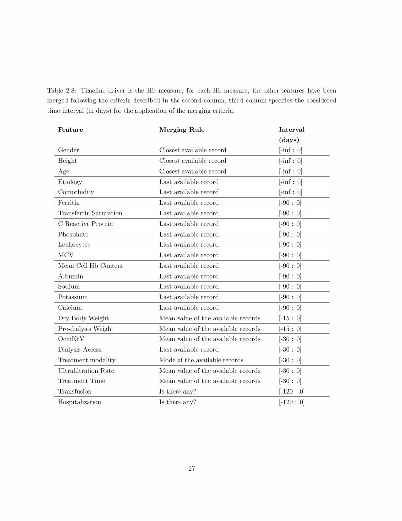
Table 2.8: Timeline driver is the Hb measure; for each Hb measure, the other features have been

merged following the criteria described in the second column; third column specifies the considered

time interval (in days) for the application of the merging criteria.

Feature Merging Rule Interval

(days)

Gender Closest available record [-inf : 0]

Height Closest available record [-inf : 0]

Age Closest available record [-inf : 0]

Etiology Last available record [-inf : 0]

Comorbidity Last available record [-inf : 0]

Ferritin Last available record [-90 : 0]

Transferrin Saturation Last available record [-90 : 0]

C Reactive Protein Last available record [-90 : 0]

Phosphate Last available record [-90 : 0]

Leukocytes Last available record [-90 : 0]

MCV Last available record [-90 : 0]

Mean Cell Hb Content Last available record [-90 : 0]

Albumin Last available record [-90 : 0]

Sodium Last available record [-90 : 0]

Potassium Last available record [-90 : 0]

Calcium Last available record [-90 : 0]

Dry Body Weight Mean value of the available records [-15 : 0]

Pre-dialysis Weight Mean value of the available records [-15 : 0]

OcmKtV Mean value of the available records [-30 : 0]

Dialysis Access Last available record [-30 : 0]

Treatment modality Mode of the available records [-30 : 0]

Ultrafiltration Rate Mean value of the available records [-30 : 0]

Treatment Time Mean value of the available records [-30 : 0]

Transfusion Is there any? [-120 : 0]

Hospitalization Is there any? [-120 : 0]

27

2.4 Statistical description of the anemia dataset

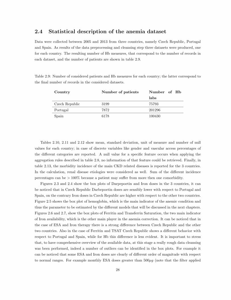
Data were collected between 2005 and 2013 from three countries, namely Czech Republic, Portugal

and Spain. As results of the data preprocessing and cleansing step three datasets were produced, one

for each country. The resulting number of Hb measures, that correspond to the number of records in

each dataset, and the number of patients are shown in table 2.9.

Table 2.9: Number of considered patients and Hb measures for each country; the latter correspond to

the final number of records in the considered datasets.

Country Number of patients Number of Hb

labs

Czech Republic 3199 75793

Portugal 7872 201296

Spain 6178 100430

Tables 2.10, 2.11 and 2.12 show mean, standard deviation, unit of measure and number of null

values for each country; in case of discrete variables like gender and vascular access percentages of

the different categories are reported. A null value for a specific feature occurs when applying the

aggregation rules described in table 2.8, no information of that feature could be retrieved. Finally, in

table 2.13, the morbidity incidence of the main CKD related diseases is reported for the 3 countries.

In the calculation, renal disease etiologies were considered as well. Sum of the different incidence

percentages can be > 100% because a patient may suffer from more then one comorbidity.

Figures 2.3 and 2.4 show the box plots of Darpepoetin and Iron doses in the 3 countries, it can

be noticed that in Czech Republic Darbepoetin doses are sensibly lower with respect to Portugal and

Spain, on the contrary Iron doses in Czech Republic are higher with respect to the other two countries.

Figure 2.5 shows the box plot of hemoglobin, which is the main indicator of the anemic condition and

thus the parameter to be estimated by the different models that will be discussed in the next chapters.

Figures 2.6 and 2.7, show the box plots of Ferritin and Transferrin Saturation, the two main indicator

of Iron availability, which is the other main player in the anemia correction. It can be noticed that in

the case of ESA and Iron therapy there is a strong difference between Czech Republic and the other

two countries. Also in the case of Ferritin and TSAT Czech Republic shows a different behavior with

respect to Portugal and Spain, while for Hb this difference is less evident. It is important to stress

that, to have comprehensive overview of the available data, at this stage a really rough data cleansing

was been performed, indeed a number of outliers can be identified in the box plots. For example it

can be noticed that some ESA and Iron doses are clearly of different order of magnitude with respect

to normal ranges. For example monthly ESA doses greater than 500µg (note that the filter applied

28

at the moment of extraction was 500µg for a single dose, which is clearly much to high), are for sure

due to a mistake in the data inputing. The same for Iron monthly doses higher than 600/800g. The

cases of hemoglobin, ferritin and TSAT show a similar pattern. Clearly these outliers were removed

when preparing the data for the modeling, on the other side, considering the huge number of records

of the datasets the number of outliers is very little and we can conclude that the quality of data is in

general very good.

Table 2.10: Statistics of Czech Republic dataset.

Feature Mean (std) UM Nulls

Gender (% of males) 55% 0

Size 168.07 (10.31) cm 273

Age 67 (13) years 0

VA (% of Fistula) 55 % 0

Hemoglobin 12.05 (1.53) g/dl 0

Ferritin 913.25 (625.35) ng/l 1027

Transferrin Saturation 36.12 (17.93) % 1832

Albumin 3.77 (0.41) g/dl 217

Phosphate 4.79 (1.44) mg/dl 126

Leukocytes 7.35e+03 (2.65e+03) no./mm 14

MCV 95.83 (6.30) fl 39

C Reactive Protein 11.47 (20.97) mg/l 474

OCMKtV 1.78 (0.39) / 21865

BCM Overhydration 1.79 (1.73) l 8746

Pre-dialysis weight 78.87 (18.68) kg 1660

Dry Body Weight 76.83 (18.32) kg 1845

Sodium 137.73 (3.56) mmol/l 32351

Potassium 4.92 (0.68) mmol/l 32342

Calcium 8.94 (0.78) mg/dl 95

UltrafiltrationRate 1.14 (0.37) mg/dl 19398

Treatment Time 264.48 (24.46) min 20933

29

Table 2.11: Statistics of Portuguese dataset.



Size 162.71 (9.22) cm 716

Age 68 (15) years 0

VA (% of Fistula) 65% 0


Ferritin 462.18 (292.56) ng/l 6182


Albumin 3.90 (0.49) g/dl 23064



MCV 94.32 (6.34) fl 6442


Sodium 137.80 (3.87) mmol/l 3169


Calcium 8.68 (0.73) mg/dl 477

OCMKTV 1.61 (0.36) / 13622






30

Table 2.12: Statistics of Spanish dataset.



Size 162.52 (10.26) cm 2852

Age 67 (14) years 0

VA (% of Fistula) 65 % 0


Ferritin 465.37 (379.54) ng/l 4033


Albumin 3.80 (0.46) g/dl 15583



MCV 95.72 (6.85) fl 5401


Sodium 138.45 (3.29) mmol/l 31203


Calcium 8.98 (0.67) mg/dl 756

OCMKTV 1.51 (0.48) / 55150






31

Table 2.13: Comorbidity Incidence for the 3 countries. Sum can be > 100% because a patient may

suffer from multiple diseases.

Disease CZ PT SP

Diabetes 48.9 % 34.4 % 34.9 %

Hypertension 77.9 % 75.2 % 79.1 %

Glomerulonephrite 17.5 % 8.4 % 11.5 %

Urinary Obstruction 1.8 % 1.4% 0.9 %

Polycystic 4.1 % 5.7% 7.5 %

Coronary Artery Disease 11.1 % 10.5 % 5.4 %

Congestive Heart Failure 16.5 % 20.7 % 22.6 %

Peripheral Vascular Disease 23.8 % 17.1% 9.1%

Cerebrovascular Disease 18.7 % 16.6% 12.7 %

Chronic Pulmonary Disease 13.1 % 8.3 % 13.4 %

0

500

1000

1500

2000

2500

3000

CZ SP PT

Darbepoetin Montlhy Dose

Figure 2.3: Box plots of monthly Darbepoetin doses distributions, expressed in µg, in Czech Republic,

Spain and Portugal. Some outliers, most probably due to errrors during the data input process, can be

noticed, nevertheless they are very few with respect to the huge number of records in the considered

datasets.

32

0

500

1000

1500

2000

2500

CZ SP PT

Iron

Figure 2.4: Box plots of monthly Iron doses distributions, expressed in mg, in Czech Republic, Spain

and Portugal. Some outliers clearly due to errrors during the data input process can be noticed,

nevertheless they are very few with respect to the huge number of records in the considered datasets.

5

10

15

20

CZ SP PT

Haemoglobin

Figure 2.5: Box plots of Hemoglobin distributions, expressed in g/dl in Czech Republic, Spain and Por-

tugal. Some outliers clearly due to errrors during the data input process can be noticed, nevertheless

they are very few with respect to the huge number of records in the considered datasets.

33

0

1000

2000

3000

4000

5000

6000

7000

CZ SP PT

Ferritin

Figure 2.6: Box plots of Ferritin distributions, expressed in ng/l, in Czech Republic, Spain and Por-

tugal. Some outliers clearly due to errrors during the data input process can be noticed, nevertheless

they are very few with respect to the huge number of records in the considered datasets.

0

20

40

60

80

100

CZ SP PT

Transferrin Saturation

Figure 2.7: Box plots of Transferrin Saturation distributions, expressed in %, in Czech Republic,

Spain and Portugal. Some outliers clearly due to errrors during the data input process can be noticed,

nevertheless they are very few with respect to the huge number of records in the considered datasets.

34

2.5 Conclusion

This chapter presented the datasets derived from FME clinical system EuClD. First important fact

to underline is the vastness of considered real life dialysis data, including patients characteristics, lab

values and drugs. This data allows to have a very extensive representation of the dialysis population,

and in particular of the anemia management protocols. All datasets have been constructed around

the hemoglobin laboratory value, this because hemoglobin is the main marker of anemia. Hemoglobin

is regularly measured on monthly basis, while other parameters are measured less often (on quarterly

basis, every six months, on demand...), for this reason in some cases there is a huge number of missing

values. With respect to the quality of the data it can be noticed that some outliers are present, which

is normal in a real life system, nevertheless the number of outliers is very low when compared with

the total number of available records. In summary the available datasets suits very well for the scope

of this thesis, that is to develop general and robust models applicable in real clinical practice.

35

Chapter 3

Modeling Red Blood Cells dynamic

in dialysis patients affected by

anemia

This chapter presents a mathematical model for erythropoiesis, that starting from a simulation of

red blood cells (RBCs) dynamic aims to predict haemoglobin concentrations over time as a function

of some patient characteristics and ESA therapy in the form of Darbepoetin alfa administered intra-

venously. First part of the chapter is dedicated to the description of the model, second part presents

the results of the model simulation on a set of examples.

3.1 Introduction

As extensively discussed in the first chapter, patients who suffer from ESRD tend to develop anemia

because of the minimal function of their kidneys and the consequent small basal level of EPO. For

this reason they are commonly treated with Erythropoetic Stimulating Agents (ESA).

Among the different types of ESAs, Recombinant Human Erythropoetin (rHuEPO), share struc-

tural homology with endogenous EPO and is characterized by a terminal half-life of around 8 hours,

Epoetin alfa and Epoetin beta are two common rHuEPO. Darbepoetin alfa is one of the other major

ESA and it is characterized by a terminal half-life of around 25 hours, thus allowing a less frequent

administration. ESA is normally administered to ERSD dialysis patients while they are receiving

dialysis, typical administration routs are intravenous (IV) and subcutaneous (SC). Changing the ad-

ministration route modifies the drug pharmacokinetics, because through SC administration, drug

release into the blood compartment is slower, while through IV administration is immediate. For this

reason SC administration is suggested for drugs with shorter terminal half-life, while for Darbepoetin

IV administration is commonly preferred for dialysis patients because it can be performed through

37

the dialysis access, thus there is no need to puncture the patient [59], [2], [83], [82], [88].

Several theoretical pharmacodynamic models describing the hematological response to rHuEPO

treatment have been developed during the last decade. Generally, these models are based on catenary,

precursor-dependent indirect response models with cell lifespan concept [110, 60, 65, 101, 61, 94, 62,

120]. The mechanistic nature of these models allows the assessment of dynamic changes of RBCs

and precursor cells during rHuEPO treatment including inter-compartmental differentiated kinetics

and retro-inhibition, but their mathematical complexity and elevated number of parameters to be

estimated have so far precluded their use and for the prediction of hemoglobin temporal evolution in

clinical setting.

In [35] an age-structured population model, described by transport equations, is able to describe the

recovery of the RBC mass after blood donation, the reaction of the body to pre-surgical administration

of Epoetin, and the changes in the number of erythrocytes in high altitude dwellers descending to sea

level.

In this work we focus on patients receiving IV Darbepoetin, utilizing real patients clinical data we

aim to predict hemoglobin temporal evolution towards the modeling of RBC dynamic, Darbepoetin

pharmacodynamics and pharmacokinetics. The model takes as input only Darbepoetin doses and

fits some patients parameters involved in the erythropoiesis. Data comes from FME Clinical System

EuCliD 5, as described in Chapter 2 treatment data are recorded in EuCliD during the daily clinical

practice, that is we have punctual information of ESA dosages, while hemoglobin as well as other

biochemical parameters are normally measured on monthly basis.

3.2 Data

One very important characteristic of the approach we followed is that some constant of the model

have to be fitted at patient level. To properly fit and test the model it is is necessary to consider

patients with a quite long anemia follow up, that is with a sufficient amount of haemoglobin measures.

Additionally only patients that during their entire history received ESA therapy only in the form of

Darbepoietin have been included in the study. This inclusion criteria is fundamental because different

ESA may have completely different pharmacodynamic which is one of the base process that the model

equations aims to represent and approximate.

The inputs for the mathematical model are Darbepoetin doses, patient gender and weight, whereas

the output is the patient hemoglobin evolution; therefore, only the following data cleansing steps have

been performed:

- ESA doses: Darbepoetin doses are normally expressed in micrograms. Drug administrations

expressed with unit of measures different from micorgrams have been corrected when possible.

In case of ambiguity, that is not clear way to reconvert the quantity to the standard unit of

measure, the patient has been discarded.

- Hemoglobin measures: hemoglobin values out of the interval 5 - 20 g/dl have been discarded.

38

- Patients with less than 2 years of anemia follow up (6 months for fitting the model and 18

months for testing the prediction) have been discarded

- Patients with more then 60 days of treatment interruption (hospitalisations, transfers etc...)

have been discarded

It is important also to remark that at this stage the aim of our mathematical model is not to

cover the entire available population (this will be done through the machine learning algorithms

discussed in the next chapters), but to analyse a subset of patients with different characteristics in

order to evaluate strengths and weakness of the model and understand which are the main drivers of

hemoglobin dynamics. In particular, this chapter shows the results obtained in a set of 200 patients

selected among those that passed the above mentioned criteria.

3.3 Mathematical modelling approach to simulate red blood

cells dynamic

3.3.1 Background Information

To motivate from the clinical point of view the problem studied in this chapter, we provide background

information about ESRD secondary anemia.

Two major problems are encountered when prescribing an adequate ESA dose:

- First, there is high inter- and intra-individual response variability owing to numerous clinical

and biological parameters affecting the dose-response relationship.

- Third, the biological effect of ESA administration lags behind and persists beyond dose changes

due to the long lifespan of mature erythrocytes and their precursors.

These problems are well known and have been studied in several research trials [110, 100, 101,

119] Nevertheless, while the necessity to systematically monitor hemoglobin and/or hematocrit

levels during therapy with ESA is generally accepted, no mathematical model able to predict

Darbepoetin dosing effect on hemoglobin fluctuations in real clinical setting has been so far

developed.

3.3.2 Related Literature

Based on the previous pharmacokinetic analyses [85, 4, 79, 81] Darbepoetin pharmacokinetic

parameters evaluated (terminal half-life, clearance, and volume of distribution at steady state)

are considered not dependent on dose and duration of administration [4].

39

Previous works also show that, the concept of the mean lifespan of a cell population as a

delay time in the system variable has been used in various mathematical models of cell kinetics

[10]. The idea of using a cell lifespan as a determinant of the removal rate was applied in the

pharmacokinetic/pharmacodynamic (PK/PD) area by Uherlinger et al. [110].

Among others, the hematopoietic cell populations are natural examples of biological systems

governed by lifespan-based processes of cell proliferation, differentiation, maturation, and senes-

cence. Consequently, their pharmacological effects could be adequately described by the lifespan-

based indirect response (LIDR) models, see also [101, 61, 104].

In [63] a pharmacokinetic and pharmacodynamic model of rHuEPO effect on reticulocyte ac-

counting for both stimulation of the proliferation of bone marrow progenitor cells and increase

of reticulocyte lifespans was applied to describe mean data from healthy subjects who received

a single subcutaneous doses of rHuEPO ranging from 20 to 160 kIU.

3.3.3 Proposal

Our model comprises three cell compartments whose dynamics are regulated by ordinary differ-

ential equations (ODEs) with constant delays. This choice was mainly driven by the fact that at

a certain time t cell concentration in the different compartments as well as the transition among

compartments is driven by the cells maturation distribution overt a time interval t − t0 where

t0 represents the cell maturation time for a specific compartement.

The two major pharmacodynamic determinants of erythropoiesis we considered are the trans-

ductional response of proliferating precursor cells of the erythroid line to erythropoetic agent

and the erythrocyte lifespan (see Chapter 1 for a more detailed explanation of these processes).

In our approach from one side we wished to decrease the degree of freedom and the computational

cost of the fitting, from the other we aimed to derive a model which could be fitted with actual

patient data and avoid the introduction not well know biological processes, like for example

inflammation.

For these reasons we considered only three model parameters and we set the others to be con-

stant. Two of them reflect biologically important characteristics, such as the plasma concen-

tration of endogenous EPO, which is to be fitted at patient level, and the cells lifespans, which

determine the delays in the differential equations and are chosen once for all the patients we are

considering, which is, clearly, an approximation.

The third parameter to be fitted accomplishes for a number of factors. When the precursors in

the bone marrow reach the stage of erythroblasts the process of hemoglobinization starts, during

this phase cells do not respond anymore to EPO, but they require an adequate amount of iron

to be effective in transporting oxygen [78].

Iron availability as well as inflammation and infection status strongly affect this last phase, all

these phenomena will be taken into account through a single parameter which regulates ESA

40

responsiveness in the second compartment. Value of this constant was fitted for each patient

using the first six months of clinical history, therefore main assumption for a precise prediction of

the model was that iron availability and patient inflammation status do not change significantly

in time.

3.3.4 Main objectives

As just mentioned fitting of model parameters makes use the first six hemoglobin laboratory

values, then the model runs over the remaining patient history predicting the hemoglobin con-

centration even very far in the future; in evaluating model performances this fact must been

taken into consideration. In principle in any point in time t the model could be fitted and run

for a limited time period, this would for sure improve model performances in terms of prediction

error, but our focus was more to verify whether the model was able to catch how ESA doses

affect the system dynamic rather then predicting the single hemoglobin measures.

3.4 Model Description

The mathematical model we present here is composed of a system of three differential equa-

tions representing the dynamic of the three considered compartments; i.e. ESA, stem cells and

hemoglobin respectively.

3.4.1 ESA compartment

Dialysis patients might have a residual production of endogenous EPO, to take into consideration

this phenomenon we made the following approximation:

- We assume the rate of endogenous EPO production in the liver and kidney to be constant

equal to zero.

- We denote by Eendg the constant endogenous EPO concentration in the plasma.

A reasonable value for the concentration Eendg might be the equivalent of a single-dose adminis-

tration of 100 units/kg of Epoetin alfa (or an equivalente mass of 12 mcg/kg of Darbepoetin) per

day. Therefore, considering a 70 kg patient, i.e., a dose of 7000 U (or 35 mcg, with a convertion

scale 1 : 200), a reasonable value for Eendg might be 702Vd

= 0.668 mcgml .

As we consider a constant endogenous EPO production, we will noy distinguish between rHuEPO

and endogenous EPO with respect to their action, and assume, therefore, that their effects on

41

erythropoiesis are identical. As a consequence, the overall concentration of EPO in plasma, Etot,

consists of the naturally produced erythropoietin Eendg and the administrered rHuEPO E:

Etot = E + Eendg.

In the case of an intravenous administration, the total amount of the agent is injected into a

vein within a very short time interval so that, without loss of generality, we can assume that

the amount of the exogenous hormone in plasma at t0, the time when the administration takes

place, is exactly equal to the amount of exogenous hormone administered. The result is a sudden

rise of the hormone plasma concentration followed by an exponential decay described by a first

order homogeneous linear ordinary differential equation with a constant elimination rate:

dE(t)

dt= −24

25log(2)E(t), E(t0) =

D0

Vd, (3.1)

where E(t) stands for the plasma concentration of the exogenous hormone at time t, t0 is the time

when the administration takes place, D0 the drug dose at t0 and Vd the volume of distribution

at steady state, which is chosen as Vd = 52.4 dl (that is, about 75 ml/kg). The decay rate of the

darbepoetin alfa is assumed to be proportional to the amount present with a half-life estimated

to be 25 hours [85, 79]. We refer to Equation (3.1) as the darbepoetin pharmacodynamics. Here

and throughout the rest of the chapter we assume that the drug amount in plasma is proportional

to the drug plasma concentration and Vd is the constant of proportionality.

In [26] Vd = 58.7 dl for a 70 kg participant (that is, 84 ml/kg), and ranges from 55 to 75 dl,

that is, from 79 to 107 ml/kg (vs. 64 ml/kg in [4], or 52.4 ml/kg in [85, Table 1]). As expected

from its large molecular weight and consistent with previous pharmacokinetic analysis, darbe-

poetin alfa’s volume of distribution in the central compartment (49 ml/kg, whereas 35 ml/kg

in the pheripheral compartment) was similar to the plasma volume (40-60 ml/kg), suggesting

confinement of the drug within the plasma circulation (see [26, Table II]).

Whereas in [4, Table III] darbepoetin and epoetin alfa’s volumes of distribution at steady state

were similar (62.1±26.2 ml/kg with terminal half-life of 23.9±16.9 h vs. 59.6±16.9 ml/kg with

a half-life of 6.3-6.1± 2.5 h), as well as their volume of distribution in the central compartment

(35.8± 11.7 h vs. 41.1± 8.81) and in the peripheral compartment (28.1± 23.6 h vs. 27.9± 9.16

h), indicating limited extravascular distribution for both molecules.

A single-dose pharmacokinetic study [85], the first report on intravenous administration of dar-

bepoetin alfa to humans, indicated that the volume of distribution at steady state for both

molecules darbepoetin alfa and epoetin alfa (52.4 ± 2 and 48.7 ± 2.1 ml/kg, respectively) was

approximately equivalent to, or slightly greater than, the plasma volume, whereas the terminal

half-life of darbepoetin alfa (25.3 h) was 3-fold longer than epoetin alfa (8.5 h, see also [107, 79]).

3.4.2 Stem cells compartments

We considered three different sub-compartments of stem cells produced in response to Darbe-

poetin administration:

42

- P is the bone marrow concentration of progenitor cells (BFU-E and CFU-E) and precursor

cells (proerythroblast, basophilic erythroblast), that belong to the strongly epo-dependent

survival stage.

- M is a fake middle compartment, which only serves as delay on the differentiation from the

class P to R, and corresponds to the iron-responsive and declining epo-dependent stage.

No evolution law is presented for this class, and we assume that as many M cells as P cells

are produced.

- R is the plasma concentration of red blood cells, measured in 1011cellsdl .

Their lifespans are denoted by TP , TI , and TR, respectively, and vary as follows: TP ∈[9, 16] ∩ N, TI ∈ [4, 9] ∩ N, and TR ∈ [70, 90] ∩ N, where N is the set of natural numbers.

The number of cells in a population is controlled by two processes: cell production and cell loss.

The net change in the cell number is determined then by the difference between the production

and elimination rate.

The fundamental assumption is that every cell in the population at any moment of time t is

assigned to have a constant specific lifespan. Each cell lives for the same period of time, TP

for cell P and TR for cell R, and then disappears in the next compartment (that is, the cells

undergo to maturation, and hence transform from one phase to another) or die.

In healthy adults lifespan of RBCs is about 100-120 days [51], while it is shorter in individuals

with iron deficiency [20, 25, 113], estimated to be about 70 days in patients with CKD in [71],

and about 60 days in ESRD patients in [110]. In accordance with those findings, the value of

TR is set equal to 70, although other studies [17, 106] show that the RBC lifespan in patients

undergoing epoetin-treatment increases and approaches values typical for a healthy individual.

This assumption determines the cell elimination rate since the number of cells that are lost

at time t must be equal to the number of cells that are born at the same time delayed by a

time, which is determined by the cell lifespans. Consequently, the rate of cells loss in a specific

compartment must be equal to the cell production rate of that compartment delayed by the

lifespan.

Even though, in general, the lifespan of a cell exposed to the drug can be longer than the lifespan

of a cell in absence of drug, we do not consider here time dependent lifespans.

The Hill function H(C) :=C

E50 + Cis used to describe the reticulocyte responses to rHuEPO

treatment, in particular the production of P cells, and E50 =100

Vdis the half maximal effective

concentration, that is, corresponds to the concentration where 50% of the population exhibit

a response, after a specified exposure duration (see [65, 61, 63] for the estimated value in case

of Epoetin Alfa administration). The sensitivity E50 is commonly used as a measure of drug’s

potency. If the parameter E50 is doubled, this implies that the drug is about twofold less potent.

The higher E50, the lower the drug effectiveness is. In other words, an increase in the E50 value

causes the same effect on the response curve as a proportional decrease in doses and vice versa.

43

The loss process is assumed to be a consequence of conversion to another cell type for P and

natural senescence for R, and is totally determined by their lifespan distribution.

To take into considerations that in the reality there are different drug exposure times according to

different cell maturity levels at the time of the administration, whereas we assume that the cells

of the same age will leave the population at the same time, we model the loss process by means

of weighted averages with constant coefficients of the previous day incoming rates. The constant

coefficient can be considered as weights determining the contribution of each point distribution

to the overall distribution. Our basic postulate is that cells have a different exposition time

to the drug according to their internal maturity level at the time of the administration, and

consequently the drug temporally changes the lifespan distribution, and hence the loss processes.

More precisely, the elimination rate from P describes the differentiation rate from P to R and

is given by a TP -day simple moving average of the previous incoming rates, that is, the sum

of the TP previous day incoming rates over the mean lifespan TP . The RBC death rate is a

weighted average of the previous incoming rates, which is a convex combination with coefficients

given by a Gaussian distribution with mean equal to about the RBC mean lifespan and variance

σ ∈ [10, 30] (to be chosen later on). The Gaussian distribution indicates that the drug effect

were stronger on TR-day old cells.

Finally, the production rate for R is equal to the elimination rate for P after the time period

given by TP + TI , as we assume that as many M cells as P cells are produced.

The evolution laws of the compartment P and R are given as follows:

P ′(t) = Cp1E(t)

E50 + E(t)P (t)− Cp1

1

9

9∑Tj=1

E(t− Tj)E50 + E(t− Tj)

P (t− Tj) P (t0) = P0

R′(t) = Cr1E(t− (TP + TI))

E50 + E(t− (TP + TI))P (t− (TP + TI))

−Cr1

SR

TP+TI+2TR∑Tj=TP+TI+1

G(Tj − (TP + TI)))E(t− Tj)

E50 + E(t− Tj)P (t− Tj) R(t0) = R0

where G(Tj) is the Gaussian distribution with mean 70, equal to the RBC lifespan, and variance

10 (or possibly 30) evaluated at time Tj .

The term SP,I,R :=1

SR

TP+TI+2TR∑Tj=TP+TI+1

G(Tj − (TP + TI)

)encompass the assumption that the RBC death rate is not fixed at 70 days but has a gaussian

distribution around the average RBC death rate. Even if there is no evidence that RBC lifespan

has a normal distribution, this assumption can be considered the most natural and indeed the

introduction of this term improved the model precision. SR =

2TR∑Tj=1

G(Tj)

is a normalization

factor.

44

In our simulations, lifespans: (TP ,TI ,TR) = (9, 4, 70). At the time t0 of the first administra-

tion, P0 = 1 and R0 = 1 (i.e., there are 1011 cells maturing from class P to R).

3.4.3 Hemoglobin compartment

The Hemoglobin H is computed in the following way as a function of R (the red blood cell):

H(t) = MCH×R(t), MCH = 2.7 for men; 2.4 for women.

where R(t) stands for the plasma concentration of red blood cells produced in responce to

Darbepoetin treatments, and MCH denotes the mean corpuscolar hemoglobin concentration

[115], defined as MCH :=Hb

RBC, and chosen as

MCH =

2.7

g

1011cellsfor a man.

2.4g

1011cellsfor a woman.

(3.2)

Referring to [111, 115, 93], normal values vary in [26, 34]picograms

cells=

10−12g

10−111011 cells=

10−1g

1011 cells, that is, in our units [2.6, 3.4]

g

1011 cells=

g/dl

1011 cells/dl.

3.4.4 Fitting

We aim to solve the following nonlinear data-fitting problem

minCp

1>0

Cr1>0

Een>0

6∑k=1

((H(t;Cp1 , C

r1 , Een)|t=dk −HLabTest(dk)

)2

where H(t) = MCH × R(t), is the solution of our model, HLabTest(dj), is the Hemoglobin lab

test at day dj , and {d1, . . . , d6}, is the set of six consecutive hemoglobin laboratory test days

(covering a period of 5 months) for a chosen patient. For each hemoglobin record we generate a

history in the time period [d1 − 90, d1] (covering a period of 3 months).

For each ESA administration the system of differential equations with constant delays has to be

solved.

The fitting of the derived solution H(t;Cp1 , Cr1 , Een) in [d1, d6] means to solve nonlinear least-

squares optimization problems.

3.5 Results

As already mentioned the main assumption of our model is that ESA responsiveness, which

is fitted during the first six months, does not vary significantly. ESA responsiveness can be

45

driven by different factors, main ones are iron availability and inflammation status. Therefore

we expect the model to have poor performances when the chosen patients are characterized by

one of the following occurrences:

- an oscillating inflammation level;

- an iron therapy or iron availability varying dramatically;

- in general when ESA responsiveness vary over time after the fitting period

Additionally patients hydration status has an impact on anemia because of the dilution effect

that over-hydration can have on haemoglobin blood concentration, also this parameter is not

taken into account at this stage.

3.5.1 Analysis and Simulations

In order to have a general evaluation of the model performances we first analyse results consid-

ering the entire selected cohort of patients. A first general analysis can be obtained computing

for each patient the mean absolute error (MAE) of the model over his complete follow up period,

that is from the seventh month (first sixt months are used for fitting the model parameters) to

the last available haemoglobin laboratory result. In other words, for a patient with N = 1, 2...n

hemoglobin laboratory results, defining ith real and simulated haemoglobin measure as Hbs and

Hbs respectively, model error is calculated as follow:

∑ni=7 |Hbr −Hbs|

n− 6(3.3)

In this way each patient is associated with a MAE, in evaluating the results it must be taken

into account that our model, using 6 months of history is predicting hemoglobin values very far

in the future (up to more then 2 years in the future), over such a long period patients condition

very likely change several time. Having as benchmark the typical patients hemoglobin variability

(guidelines for anemia management for dialysis patients aims to keep haemoglobin between 10-12

g/dl), a MAE of 0.8 can be accounted as very well representing the patient behavior. A MAE

below 1.2 g/dl can be considered reasonable while errors above 1.2 g/dl make the prediction for

that specific patient unrealistic. Given these thresholds, we acheived the following results:

-47

200(23.5%) of patients have MAE <= 0.8.

-91

200(45.5%) of patients have 0.8 < MAE <= 1.2.

-62

200(31.0%) of patients have MAE > 1.2.

46

This general characterization of the performances, even if gives a rough idea, does not take

into account for some important factors that must be be examined in order to well understand

strength a weakness of the model:

- Apart from the pure difference between predicted and actual haemoglobin value, it is very

important to understand whether the model is able to catch the RBC dynamic, that is

the haemoglobin fluctuation over time. Capacity of the model in anticipating haemoglobin

trends is a key factor.

- The average error over a long period can mislead, it is important to understand whether it

is caused by a constant false prediction or by outliers, whether it is biased or unbiased and

finally it must be weighted by the complexity of patient haemoglobin evolution.

- What is the cause of the prediction error.

- Is it possible to identify any bias in the model itself that could be removed?

To overcome the above mentioned approximations that a pure MAE based analysis implies, we

have selected a small group of representative patients to be analyzed in detail.

In figure 3.1 patient with initial high hemoglobin fluctuations that progressively smooths is

represented. Values in abscissa represent days from admission in FME clinics, thus this patient

had a follow up period of around two and an half years at the moment of data extraction.

First chart shows estimated dynamic of total EPO concentration (endogenous + exogenous) as

output of equation 3.1. Fitting is performed during the first 200 days (circled dots represent

haemoglobin values used for fitting), it has to be stressed that after this period no additional

input of data into the model is performed, with the exception of course of Darbepoietin doses.

In this case the model is very well performing, indeed the predicted hemoglobin (blue line) is

always very close to the actual one (red dots), also the initial hemoglobin fluctuations and the

subsequent stabilisation is well predicted. Only notable deviation occurs with laboratory test at

day 280 where the model overestimate the actual value, even so also in this case trend is caught,

indeed this point is a local maximum both in reality and in the simulation.

47

time in days0 100 200 300 400 500 600 700 800D

arbe

poet

in in

7g

0

50

par0=[0.15 0.36 0.3], hMEffD=200, RBCls=70 w var=10, (cpr,crbc,Epen0) = (25,38,24) /100

time in days0 100 200 300 400 500 600 700 800

Hb

in

g/dl

8

9

10

11

12

13

14

15

16

Figure 3.1: Good trend with small error. First chart from the top shows estimated dynamic of total

EPO concentration (endogenous+ exogenous). Second chart shows real (red dots) versus estimated

(blue line) hemoglobin temporal evolution; circled stars represent hemoglobin values use for the fitting.

48

In figure 3.2 a patient with high and continuous hemoglobin fluctuations over a follow up period

of around four years is represented. Also In this case the model is very well performing, even if

this patient present a higher and more prolonged hemoglobin variability with respect to 3.1, in

the context of anemia management such a patient can be considered complex and unpredictable.

time in days0 200 400 600 800 1000 1200D

arbe

poet

in in

7g

0

100


time in days0 200 400 600 800 1000 1200

Hb

in

g/dl

6

7

8

9

10

11

12

13

14

15

16

Figure 3.2: Good trend with small error. First chart from the top shows estimated dynamic of total

EPO concentration (endogenous+ exogenous). Second chart shows real (red dots) versus estimated

(blue line) hemoglobin temporal evolution; circled stars represent hemoglobin values use for the fitting.

49

Figure 3.3 shows a patient with a follow up period of almost 4 years. Again this patient is

more unstable repeat to the one shown in 3.1. Even so the model is very well performing in

anticipating the trends of hemoglobin fluctuations, even vey far in the future. On the other side

in this case, even if the trend is caught, after the first two years the hemoglobin concentration

tend to be underestimated. In such a case the model might be benefit for a additional fitting

process, because it looks like patient response to ESA therapy improved, putatively for a change

in patients conditions (iron availability, hydration, inflammation status...).

time in days0 200 400 600 800 1000 1200 1400D

arbe

poet

in in

7g

0

50


time in days0 200 400 600 800 1000 1200 1400

Hb

in

g/dl

7

8

9

10

11

12

13

14

Figure 3.3: Good trend with tendency to underestimate ESA response after the first two years. First

chart from the top shows estimated dynamic of total EPO concentration (endogenous+ exogenous).

Second chart shows real (red dots) versus estimated (blue line) hemoglobin temporal evolution; circled

stars represent hemoglobin values use for the fitting. Abscissa represent days from admission in FME

facilities.

50

In figure 3.4 model behavior is to some extend comparable to that in 3.3. Again hemoglobin

fluctuations are initially quite well predicted and after a period (around 500 days in this case)

predicted hemoglobin starts to deviate a bit from the actual one, but in this case, differently

from the previous example, the model tend to overestimate patient response to ESA therapy.

time in days0 100 200 300 400 500 600 700D

arbe

poet

in in

7g

0

50


time in days0 100 200 300 400 500 600 700

Hb

in

g/dl

8

9

10

11

12

13

14

15

16

Figure 3.4: Good trend with tendency to overestimate ESA response after the first one and an half

year. First chart from the top shows estimated dynamic of total EPO concentration (endogenous +

exogenous). Second chart shows real (red dots) versus estimated (blue line) hemoglobin temporal

evolution; circled stars represent hemoglobin values use for the fitting. Abscissa represent days from

admission in FME facilities.

51

In 3.5 another interesting situation is represented. In this case, hemoglobin fluctuations predicted

by the model are perfectly in phase with actual ones, but the amplitude of the oscillation is

smoothed.

time in days0 200 400 600 800 1000 1200 1400D

arbe

poet

in in

7g

0

50


time in days0 200 400 600 800 1000 1200 1400

Hb

in

g/dl

7

8

9

10

11

12

13

14

15

16

Figure 3.5: Hemoglobin oscillation are well aticipated by the model, but their amplitude is lower

than the actual one. First chart from the top shows estimated dynamic of total EPO concentration

(endogenous+exogenous). Second chart shows real (red dots) versus estimated (blue line) hemoglobin

temporal evolution; circled stars represent hemoglobin values use for the fitting. Abscissa represent

days from admission in FME facilities.

52

3.6 shows a case where the model is not at all able to catch the dynamic of patient response to

ESA therapy.

time in days0 100 200 300 400 500 600 700 800 900 1000D

arbe

poet

in in

7g

0

50


time in days0 100 200 300 400 500 600 700 800 900 1000

Hb

in

g/dl

8

9

10

11

12

13

14

15

Figure 3.6: Patient where the model is not able to predict hemoglobin dynamic. First chart from

the top shows estimated dynamic of total EPO concentration (endogenous + exogenous). Second

chart shows real (red dots) versus estimated (blue line) hemoglobin temporal evolution; circled stars

represent hemoglobin values use for the fitting. Abscissa represent days from admission in FME

facilities.

53

Finally 3.7 shows a case where the model prediction is completely wrong.

time in days0 200 400 600 800 1000 1200 1400D

arbe

poet

in in

7g

0

50

100


time in days0 200 400 600 800 1000 1200 1400

Hb

in

g/dl

7

8

9

10

11

12

13

14

15

16

Figure 3.7: Model prediction completely wrong. First chart from the top shows estimated dynamic

of total EPO concentration (endogenous + exogenous). Second chart shows real (red dots) versus

estimated (blue line) hemoglobin temporal evolution; circled stars represent hemoglobin values use for

the fitting. Abscissa represent days from admission in FME facilities.

54

3.6 Conclusion

This chapter has presented a mathematical model for the simulation of RBC dynamic in dialysis

patients affected by secondary anemia and treated with ESA therapy in the form of Darbepo-

etin. The model comprises two cell compartments whose dynamics are regulated by ODEs with

constant delays.

Considered pharmacodynamic determinants of erythropoiesis are transductional response of pro-

liferating precursor cells of the erythroid line to erythropoetic agent and the erythrocyte lifespan.

Model inputs are Darbepoietin doses, patient gender and weight. The considered equations com-

prise three parameters that have to be fitted using the first six month of patients history with

the aim to predict hemoglobin concentration over the remaining patient anemia followup. The

model comprises two cell compartments regulated by ODEs with constant delays. The funda-

mental assumption is that the rate of cell loss is equal to the production rate but is delayed by

the cell lifespan.

A very minimal dataset and a priori information are required in developing the model and

fitting the paramenters, which makes it useful in clinical settings where, oftentimes, very little

information is known about a given patient.

In general the obtained results showed an acceptable predicting error. Although the maximum

prediction error may seem high, it should be emphasized that both patients responsiveness to

darbepoetin alfa and inflammation levels are considered to be constant and, last but not least,

the critical assumption that the body is able to provide sufficient iron supply for erythropoiesis

at all times was made.

Summarizing the main cons of the presented work are:

- For the 30% of patients where the model is not well performing error can be very high

leading to even not realistic hemoglobin concentration; this fact may be a reason to prevent

the use of such a model in a real clinical setting;

- Computational cost of the model is quite high, this fact would also make its application in

a real clinical setting difficult.

- Fitting is required at patient level, thus application to a complete patients populations is

not straightforward.

On the other side, the following positve results have to be considered:

- The predicted hemoglobin concentration can be even years after the fitting period, and by

making use of few parameters the derived model is able to perform a reasonably accurate

prediction (MAE < 1.2g/dl) for 70% of the considered patients.

55

- Even for those patients where the prediction is completely wrong in terms of absolute

value of hemoglobin concentration, often the trend is still caught, meaning that the RBC

fluctuation dynamic is well simulated.

- Even if having cluster of patients where the model performances are poor in term of pre-

diction error is clearly negative, the model could be used to profile these patients and

potentially to understand the reason of their peculiar behavior.

Considering the above mentioned points, main novelty of the derived model is that it has been

applied on real patients not just to fit the available data but also to predict future hemoglobin

concentration along a large period of time with very promising results. This study also confirms

the potential utility of individualized models to assess effect of drug dosing. A potential appli-

cation of the model is to simulate different treatment policies in order to identify those that are

more suitable to be successful in achieving anemia targets [31]. Clearly a clinical evaluation it

is necessary before applying the model in a real clinical setting.

56

Chapter 4

Machine Learning Approach

This chapter presents several models devoted to predicting hemoglobin fluctuations in dialysis

patients affected by secondary anemia; these models are based on different machine learning

algorithms. First part of the chapter gives an overview of the theoretical background of these

algorithms. In the second part of the chapter the final model setup is presented, before describing

and evaluating the results of the models. The chapters concludes with the discussion of the model

dedicated to the long term hemoglobin prediction.

4.1 Introduction

As discussed in Chapter 1, kidneys accomplish a fundamental role in the control of erythropoiesis,

therefore, a disorder like Chronic Kidney Disease causes the development of ESRD secondary

anemia due to the incapability of kidneys to produce EPO. Additionally, ESRD patients suffer

a general inflammation status that causes an iron-deficiency which, in combination with other

ESRD-related conditions, contributes to exacerbate the anaemic status and to increase the risk

of severe consequences (not last hospitalization and death). The availability of recombinant hu-

man erythropoietin and the subsequent development of other EPO derivatives (that altogether

go under the name of Erythropoiesis Stimulating Agents, ESA) greatly improved the treatment

of ESRD-anemia. However, despite several years of experience with ESA, there are still consid-

erable discrepancies between treatment recommendations and clinical outcomes. Several clinical

studies have attempted to clarify this problem; nonetheless, while the desired hemoglobin blood

concentration target has been validated and generally accepted, an effective ESA dosing scheme

which allows a systematic achievement and, more important, the maintenance of the desired

therapeutic response is not available [32]. ESA action implies the binding to and the activation

of erythrocyte precursor cells in the bone marrow to trigger proliferation and differentiation

into circulating hemoglobin-laden RBC. Hence, in the first stage the RBC precursors mature

57

in response to EPO stimuli; subsequently, when the process of haemoglobinization starts, cells

mandatorly require an adequate amount of iron (essential for hemoglobin synthesis) to conclude

the maturation process and pass into the bloodstream where their lifespan is around 70 days

for a dialysis patient (120 for a healthy individual) [87] [30]. Timing and success of the process

strongly depends on iron availability, EPO concentration and EPO level fluctuations at the site

of action. Moreover, in the case of ESA therapy in CKD, erythropoiesis is also strongly in-

fluenced by momentary or general patient conditions; specifically, inflammation and individual

resistance to ESA treatment are two of the main determinants for drug response variability.

Hence, patient status, ESA pharmacokinetics (i.e. the distribution and elimination kinetics

of the drug in the organism) and ESA pharmacodynamics (i.e. the biological effect that the

drug exerts after binding its target receptor) are main determinants for a correct dose-response

prediction; however, they are not easily evaluable events.

Summarizing, the selection of a optimal therapy dosing schedule encounters many difficulties

mainly depending on the fact that:

- ESA dose-response relationship is non-linear.

- The final effect is strongly dependent on the high intra- and inter-individual variability.

- The existence of a temporal discrepancy between the short ESA permanence in the blood

(hours) and the long RBCs lifespan (months).

Chapter 2 has shown how the dialysis clinics under study offered a unique and extensive collection

of relevant patient information, but on the other side the high complexity of this kind of data

(multidimensional and non-linear) makes a correct interpretation difficult when operated only

on the basis of standard statistical analyses and on nephrologists experience (due to the obvious

limitations of the human cognitive abilities). This may ultimately lead to wide variability and

increased risk of errors in clinical practice with harmful consequences for patient and rises in

therapy costs. In this situation, a complementary computational tool can have a fundamental

impact in assisting physicians in making decision.

Given the complexity of the presented medical problem and the importance of the hemoglobin

variation prediction, we explored the use of Machine Learning (ML) techniques operating as pre-

dictors of the short term as well as long term response to EPO and Iron therapy for hemodialysis

patients affected by secondary anaemia. To address the scope, we essayed an innovative applica-

tion of the ML methodology, keeping into consideration the actual drug kinetics and the specific

biological dynamics, together with physiological patient information.

58

4.2 Methods

Machine Learning methodologies find an appropriate and powerful application in clinic and

therapy management being one of their main focus to generate predictions. After the definition

of a specific learning algorithm, the machine is trained on finite number of example patterns

of empirical data, from which it learns complex variable relationships. Based on the training

experience, the ML paradigm is then able to recognize correlations among new and unknown

dataset inferring reliable results in new cases. In our work we explored various machine learning

algorithms comparing them in terms of their accuracy in predicting hemoglobin fluctuations

[76].

4.2.1 Linear Models

In statistics, linear regression is an approach to model the relationship between a scalar variable

y and one or more explanatory variables denoted by X. The case of one explanatory variable

is called simple regression, while more than one explanatory variable is multiple regression, see

figure 4.1.

Figure 4.1: Linear Regression.

Linear regression was the first type of regression analysis to be studied rigorously, and to be

used extensively in practical applications. This is because models that depend linearly on their

unknown parameters are easier to fit than models that are non-linearly related to their parame-

ters and because the statistical properties of the resulting estimators are easier to determine. In

59

linear regression data are modeled using linear functions, the unknown model parameters being

estimated from the data. For a kth dimensional data sample xi, yi(i = 1, 2, . . . , n), a multiple

linear regression is defined by:

yi = b0 + b1xi1 + b2xi2 + . . .+ bkxik (4.1)

where n is the number of instances of the data sample.

Equivalently, in a more compact matrix form:

Y = X · b + E (4.2)

where

Y ≡

y1...

yn

(4.3)

is a column vector with n rows containing the values of the response variable;

X ≡

1 x11 · · · xk1...

.... . .

...

1 x1n · · · xkn

(4.4)

is a matrix with n rows and k + 1 columns containing for each column the values of the ex-

planatory variables for the n observations, plus a column (to refer to the intercept) containing

n values equal to 1;

b ≡

b0

b1...

bk

(4.5)

is a vector with k + 1 rows containing all the model parameters to be estimated on the basis of

the data (the intercept and the k slope coefficients relative to each explanatory variable); finally

60

E ≡

e1...

en

(4.6)

is a column vector of length n containing the error terms.

Whereas in the example of 4.1 the regression model is a line, in the case of multiple independent

variables it corresponds to a (k + 1) dimensional plane defined by the equation:

(yest)i = b0 + b1xi1 + b2xi2 + . . .+ bkxik (4.7)

To determine the fitted plane the vector of the parameters (a, b1, · · · , bk) must be estimated. Lin-

ear regression models are often fitted using the least squares method; in this case the parameters

are obtained minimizing the square of the Euclidean distance:

d2(y, yest) =

n∑i=1

(yi − yest)2. (4.8)

In matricial terms the solution is given by:

Yest = X · β, (4.9)

where

β = (X′ ·X)−1 ·X′ ·Y (4.10)

X′ being the transpose of X′.

Therefore the optimal fitted plane minimizing the error will be defined by:

Yest = X · (X′ ·X)−1 ·X′ ·Y ≡ H ·Y (4.11)

In geometric terms, the previous expression establishes that the optimal plane is obtained as

the projection of the observed vector Y ∈ <n on the (k + 1) dimensional hyperplane. Here, the

projection operator is the matrix H; in bivariate regression when a = 0 the projection operator

is b. In fact, for k = 1 the two parameters in β coincide with parameters a and b in the bivariate

case.

61

4.2.2 Artificial Neural Networks

Artificial Neural Networks (ANNs) are computational models inspired by the processing princi-

ples found in brains, and extensively used as function approximators in a variety of application

scenarios, from simple pattern-recognition tasks, to advanced symbolic manipulation They are

composed of computational units called neurons, which exchange information through weighted

connections; in figure 4.2 a typical neuron model is shown. Three basic components of the

neuron can be identified:

- A set of synapses each of which is characterized by a weight. Specifically a signal xj at

the input of synapse j connected to the neuron k is multiplied by the synaptic weight wkj .

The synaptic weight can be either positive or negative.

- An adding function for summing the weighted input signals. These operations constitute

a linear combination.

- An activation function to limit the amplitude of the output. The activation function plays

a very important role in how the neuron, and thus the entire neural network, responds to

the input signal; for example t can be linear or non linear, it can have a threshold or not.

Figure 4.2: Typical neuron model computational architecture

In mathematical terms the output yj of the jth neuron is calculated as follows:

yj(x,w) = ϕ(

n∑k=1

wjkxk + wj0) (4.12)

where wj = (wjk), k = 1, · · · , n are the weights, wj0 represent the bias, while ϕ is the activationfunction

which is typically nonlinear like the logisticsigmoid or the tanh functions [13].

62

There is a variety of ANN types, among them one of the most common is the Multilayer Per-

ceptron (MLP). MLP architecture is quite simple but very effective and flexible; in a MLP

neurons are organized in a variable number of layers: an input layer to which the data is fed;

an output layer where the result of computation is returned; and one or more than one hidden

layers in between. The input signal propagates through the network in a forward direction layer

by layer (indeed MLP belong to the class of the so called feed-forward neural networks). MLP

perform very well in solving a number of different problems, like pattern recognition, function

approximation, classification, non-linear data modeling and so on [47]. In figure 4.3 a classical

architecture for a MLP is shown.

Figure 4.3: Multilayer Perceptron scheme.

The ANN, presented with a collection of input-output pairs called the training set, learns by

example to approximate the relation between such pairs; to do so, it iteratively adjusts the

weights of its connections. If the learning phase is successful, the resulting model will be able to

generalize what it has learned to unseen examples: that is, given a new set of inputs (the test

set) the ANN should be able to predict the corresponding outputs with reasonable accuracy.

4.2.3 Support Vector Machines

Linear models as well as ANN are based on a mapping function y(x,w), which is governed by

the parameters w adapted during the training phase over a subset of the available data called

training set. Prediction over new data, called test or validation set, is then based only on the

learned parameter w. On the other side there are other kind of models which makes of the

training data (or of a part of it) also in the testing phase. Many linear parametric models can

make use of kernelfunctions of the form κ(x,x′) = φ(x)Tφ(x′) evaluated on the training data,

as, for example, the Support Vector Machine (SVM).

Support vector machine (SVM) is basically a linear machine with some special properties. In the

context of pattern classification the main idea behind a support vector machine is to individuate

a hyperplane (or a set of hyperplanes) that can produce a linearly separable solution to a

63

classification or regression problem. One of the most peculiar characteristics of the support

vector machine is that it can provide good generalization performances despite the fact that

they dont incorporate problem-domain knowledge. In the context of linear classification a binary

classification problem can be defined as follows, given the set of pairs:

{(xi, ti)}i = 1, 2, · · · , N (4.13)

where xi is the iih input and ti the corresponding binary target output, i.e. ti ∈ {−1, 1} and

y(x) = wTφ(x) + b (4.14)

where φ(x) denotes a fixed feature space transformation, while b is the bias parameter. If the

training dataset is linearly separable in the features space, thus it must exist at least a couple

(w, b) such that y(x) in the form of 4.13 satisfies:

y(xn) > 0,∀tn = +1 (4.15)

y(xn) < 0,∀tn = −1 (4.16)

Among the possibly multiple solutions to the problem in Equations (4.15) and (4.16), SVM

approach is to select the one that maximize the margin, that is the minimum distance between

the decision boundary and any of the samples, as illustrated for the two dimensional case in

figure 4.4.

The margin can be calculated as the orthogonal distance between the closest point of the dataset

and the derived hyperplane, since we are considering just points correctly classified, that is where

tny(xn) > 0, the perpendicular distance between the hyperplane and point xn is:

tny(xn)

‖w‖=tn(wTφ(xn) + b)

‖w‖(4.17)

therefore in order to maximize the margin the following equation has to be solved:

arg maxw,b

{ 1

‖w‖minn

[tn(wTφ(xn) + b)

]} (4.18)

Applying the transformation w → κw and b → κb distance to the separation hyperplane does

not change, thus for the closest point to the separation hyperplane it is possible to set:

64

Figure 4.4: The figures shows the case of the separating hyperplane and relative margins for the two

dimensional case. Solid and empty circles represent the two data clusters separated by the hyperplane.

tn(wTφ(xn) + b) = 1. (4.19)

The maximization problem in 4.18 is equivalent to minimize ‖w‖−1

This constraint problem can be solved introducing the Lagrange multipliers an ≥ 0 with n =

1, . . . , N , the Lagrangian function is thus defined as follows:

L(w, b,a) =1

2‖w‖2 −

N∑n=1

an{tn(wTφ(xn) + b)− 1} (4.20)

Setting the derivates with respect to w and b equal to zero we obtain:

N∑n=1

antnφ(xn) = w (4.21)

andN∑n=1

antn = 0 (4.22)

Solving with respect to w and b we obtain the dual representation of the maximum margin

problem:

65

˜L(a) =

N∑n=1

an −1

2

N∑n=1

N∑m=1

anamtntmκ(xn,xm) (4.23)

where:

an ≥ 0 n = 1, . . . , N,

∑Nn=1 antn = 0,

κ(x,x′) = φ(x)Tφ(x).

(4.24)

By means of the kernel functions κ the maximum margin approach can be applied even to feature

spaces with a dimensionality exceeding the number of records in the dataset. New records are

classified by means of the sign of the function:

y(x) =

N∑n=1

antnκ(x,xn) + b. (4.25)

A constrained optimization of this form satisfy the Karush−Kuhn−Tucker (KKT) conditions

that in this case imply:

an ≥ 0 n = 1, . . . , N,

tny(xn) ≥ 1

an{tny(xn)− 1}

(4.26)

Those records from the training set resulting in an = 0 will not contribute to the prediction in

Equation (4.25), the remaining records are called supportvectors, since for those points an > 0,

from third Equation in (4.26) we have that tny(xn) = 1, which means that they lie on the

maximum margin hyperplane. Therefore in SVM models maximum margin hyperplane is defined

by the support vectors, thus the solution of a classification problem is independent form the

other points [13].

In most of the cases its not possible to construct a separating hyperplane without cases of

misclassification, thus the target became to find an optimal hyperplane, which minimizes the

classification error; for these purpose we introduce the so called slack variables ξn, where

n = 1, . . . , N and ξn ≥ 0. When the data point is either on the margin boundary or inside it,

we have ξn = 0, for all other points ξn = |tn − y(xn)|. Therefore for records on the right side of

the separating hyperplane but inside the margin 0 < ξn ≤ 1, for points laying on the separating

66

hyperplane ξn = 1, while for misclassified records ξn > 1, see Figure 4.5. With the introduction

of the slack variables the costraint in (4.26) became:

tny(xn) ≥ 1− ξn (4.27)

Figure 4.5: Red and Green points represent the data clusters to be classified, in this case it is not

possible to find an hyperplane which perfectly separate the two clusters, in this example there is a

green point on the right side of the hyperplane and a red one on the left side. Slack variables ξi allow

some points to fall over the separation hyperplane but penalize them.

In this way, some records of the training dataset can be misclassified, allowing overlapping

between the two classes and is called soft margin constraint. The optimization problem corre-

spond then to the minimisation of the functional:

φ(w, ξ) =1

2‖w‖2 + C

N∑n=1

ξn (4.28)

Applying the Lagrangian multipliers we obtain:

67

˜L(a) =∑Nn=1 an −

1

2

∑Nn=1

∑Nm=1 anamtntmκ(xn,xm)

0 ≤ an ≤ C

∑Nn=1 antn = 0

(4.29)

The dual Lagrangian takes exactly the same form of the separable case, but with different

constraints. Predictors for the test records take the same form of Equation 4.25, that is:

y(x) =

N∑n=1

antnκ(x,xn) + b. (4.30)

Predicting future haemoglobin fluctuation is clearly a regression problem and SVM works also

as regressor preserving the same properties discusses so far. First of all, with respect to the

standard error function, to obtain a sparse solution the ε − intensive error function of the

form:

Eε(y(x)− t) =

0 if |y(x)− t| < ε

|y(x)− t| − ε otherwise(4.31)

where ε > 0 is introduced [112]. In this way whenever the difference between the actual target

and the model output is lower than ε prediction error is considered equal to 0.

For each data point in the training set two slack variables ξn ≥ 0 and ξn′ ≥ 0 have to be

introduced in order to permit the prediction to be outside the hypersphere centred in tn and of

radius ε:

y(xn) ≥ tn − ε− ξn

y(xn) ≤ tn + ε+ ξn′

(4.32)

thus the SVM regression error function take the form

C∑

n = 1N(ξn + ξn) +1

2‖w‖2 (4.33)

68

subject to the constrain in 4.32 and ξn ≥ 0, ξn ≥ 0. As for the classification problem the mini-

mization of the regression error in 4.33 can be obtained introducing the Lagrangian multipliers

and solving the dual problem [13].

4.2.4 Random Forests

When data is characterized by a high number of features interacting in complicated and nonlinear

ways, assembling a single global model can be very difficult. An alternative approach to nonlinear

regression is to sub-divide, or partition, the space into smaller regions, where the interactions

are more manageable; algorithms implementing this approach are called Tree Models. Tree

models are usually divided into Regression Trees, when the response variable is continuous, and

Classification Trees, when the response variable is discrete or qualitative (categorical). Figure 4.6

shows an example of a Classification Tree. Trees use the tree to represent a recursive partition,

where a set of n statistical units are progressively divided into groups, according to a division

rule that aims to maximize a homogeneity or purity measure of the response variable in each of

the obtained groups. Each of the terminal nodes, or leaves, of the tree represents a cell of the

partition, and has attached to it a simple model that applies in that cell only.

Given a response variable observation yi for classic regression trees, the model in each cell is

just a constant estimate of yi.That is, suppose that the points (x1, y2), (x2, y2)...(xk, yk) are all

the samples belonging to the leaf-node K, then model estimation is:

yest =1

K

K∑i=1

yi (4.34)

that is the mean of the dependent variable in that cell. To achieve this, it is necessary to specify

stopping criteria for the division process. Tree models do not require any assumption about the

probability distribution of the dependent variable y, thus can be considered as non-parametric

predictive models. They can in general be applied to any problem no matter which kind of data

the explanatory and dependent variables are holding [15].

To improve the classification (regression) accuracy of a single tree, ensemble of trees have been

considered, having each tree contributing to the prediction. Breiman definition of a Random

Forest is the following [16]:

- A Random Forest is a classifier consisting of a collection of tree-structured classifiers

h(x, yk), k = 1, . . .K where yk are independent random distributed vectors and each tree

casts a unit vote for the most popular class at input x.

69

Figure 4.6: Example of Classification Tree: each node (empty circles) implement a division rule, which

separate the data in two sub-groups depending on the values of a specific variable, in this way the

data belonging to a specific sub-group is more homogeneous with respect to the response variable

when compared to to the complete dataset.

4.3 Model Setup

4.3.1 Incorporation of drug administration into the model

Main concerns with previous ML implementations for hemoglobin levels prediction in anaemic

patients have often been the utilization of restricted populations of patients or the availability

of a scant amount of patient data and the incomplete correspondence between the model and

the true patient biology. In our case the paradigm model based on human physiology and

drug pharmacology brought an essential enhancement in the capacity of predicting haemoglobin

fluctuations. In addition, the size of the considered CKD patient population (distributed on

numerous clinics of different countries) made it possible to train the network on a uniquely wide

set of clinically relevant values, and to test it on a different, but still considerably vast, cohort

of data, so granting a reliable generalization of the model basically to the entire population.

Generalization is actually the most crucial aspect to be taken in consideration when aiming to

utilize the derived algorithms in real clinical setting where a yearly patients’ turnover around

20 % has to be taken into consideration. This means that not only the algorithm would have

to deal with continuously changing patient conditions but also with a constant inflow of new

patients.

70

A primary role in driving patient fluctuation of haemoglobin is carried by ESA and Iron dosages

action on RBC maturation. Additionally the other main player in the characterisation of the

system dynamic is RBC lifespan. To optimize models results it was thus fundamental to ag-

gregate drug administration data in a way that encompasses Darbepoetin kinetic and the RBC

dynamics. These medications are not administered with a fixed rate, their scheduling may vary

from patient to patient depending on patients’ charateristics or intra-patient changing condi-

tions. A first, intuitive way to aggregate drug data is to compute the accumulated doses between

two consecutive hemoglobin measures [76]; however, hemoglobin labs are not uniformly spaced

in time. In fact, although the standard protocol is to perform lab tests each month, for different

reasons it is possible, for example, to have lab tests separated by 15 days as well as 45 days;

in these cases, accumulated doses would not be comparable. Additionally in this way the min-

imum granularity for dose accumulation would be around 30 days (on average), and thus the

information about dose distribution within a month would be lost. To avoid these issues, we

approached the problem in a different way, that is by parametrically defining dose accumulation

intervals going backwards from the hemoglobin measure [8]. In other words, given a hemoglobin

measure at time t, denoted by Hb(t), and given a vector of time intervals T defined as:

T = {∆t0,∆t1, . . . ,∆tn}, (4.35)

the accumulated doses D(t) for a specific drug is a vector:

D = {D1, D2, . . . , Dn}, (4.36)

where Dk is the drug dose administered between time t−k−1∑i=0

∆ti and t−k∑i=0

∆ti, where ∆t0 is

an offset that could allow disregarding drug doses that were administered close enough to the

lab test measurement to be considered irrelevant with respect to that measurement. Moreover,

based on pharmacology and human biology, Darbepoetin can be estimated to continuously exert

its effect up to around 3 months, with declining potency, after administration (considering both

erythropoiesis and RBC life span); therefore the range of accumulated doses was designed to

cover this time interval.

The advantage of this approach is that it makes drug dosage histories comparable across records;

moreover, the use of a vector to parametrically define the intervals for accumulating doses

allows in an easy way the generation of a bunch of alternative datasets, each corresponding

to a different set of time intervals, in order to evaluate whether a dosage accumulation rule

works better with respect to another. In order to discover the optimal rule for feeding the

machine learning models with drug dosages information a series of steps have been made. Firstly,

taking into account the considerations discussed in Chapter 1 about RBC lifespan, Darbepoetin

pharmacodynamics and pharmacokinetics we defined the lower and upper boundaries of the time

interval over which consider the drug dosages. Secondly, within the defined time interval, we

71

tested different aggregation criteria comparing models results in terms of prediction capability.

A finer granularity of drug dosages holds more information, but on the other hand it increases

the number of input variables (i.e. the dimensionality of the state space), which might have a

negative impact on the model performances.

Two type of predictive models were developed, one estimating haemoglobin one month in the

future, the other three months in the future, consequently two types of datasets have been

generated, data aggregation rules for these two models are described in figures 4.7 and 4.8

respectively.

As mentioned for dialysis patients haemoglobin in routinely sampled on monthly basis, thus

the candidate model to be used in real clinical practice is the one predicting haemoglobin one

month in the future. Nonetheless we explored also the possibility to develop a model for the

prediction of haemoglobin levels three months in advance, because anticipation of the long-term

physiologic response (i.e. at 3 months) to the ESA/Iron therapy is a challenging task and

it is scientifically interesting, because of the fundamental importance for planning a successful

anemia correction strategy which takes into account the next haemoglobin steady state, avoiding

harmful haemoglobin cycling.

Hb(t)

t t-N days

Cumulated adm. EPO.

Hb(t+1)

t+1 month

Cumulated adm. Iron.

Cumulated adm. EPO

Cumulated adm. Iron

Past Future

Labs and other vars.

Figure 4.7: Scheme for haemoglobin prediction @1month.

72

Hb(t)

t t-90 days

Cumulated adm. EPO.

Hb(t+3)

t+3 months

Cumulated adm. Iron.

Cumulated adm. EPO

Cumulated adm. Iron

Past Future

Labs and other vars.

Figure 4.8: Scheme for haemoglobin prediction @3months.

4.3.2 Exclusion Criteria

Scope of the presented work is to obtain a reliable and general model which is usable during the

daily clinical practice for the prediction of haemoglobin fluctuation in dialysis patient affected

by secondary anemia. Therefore the model must be able to perform a prediction utilizing data

normally available in a live clinical setting as described in chapter 2.

Hemoglobin is normally sampled on monthly basis, clearly some deviations from this standard

schedule could happen, on the other side, considering that the aim of the model is to predict the

monthly haemoglobin variation, record to close, i.e. hb(t + 1) − hb(t) < 15gg or too far away,

i.e. hb(t+ 1)− hb(t) > 45gg, from each other have been discharged.

In case of the model predicting the long term haemoglobin variations criteria for discharging

records was: hb(t+ 3)− hb(t) < 60gg or .hb(t+ 3)− hb(t) > 120gg.

To perform a prediction at a certain point in time, the model needs at least data relative to the

previous 90 days of patient clinical history, plus the administered ESA and Iron therapy of the

successive month (or of the successive three months for the predictor @3 months). Therefore,

for the two models, patients with less than 4 or 6 months of anemia follow up were respectively

discharged.

ESA and Iron therapy are administered during the dialysis treatment, thus for patients tem-

porary out of the clinics it may be possible that the recorded drug administrations are not

corresponding to the actual ones. For this reason those records corresponding to patients which

overall were not present in the clinic for more than one month over the three considered by the

model were discharged.

Number of records and patients remaining after the application of the above mentioned exclusion

criteria are listed in table 4.1.

In order to to derive a robust model to be used in the real clinical setting differences among the

73

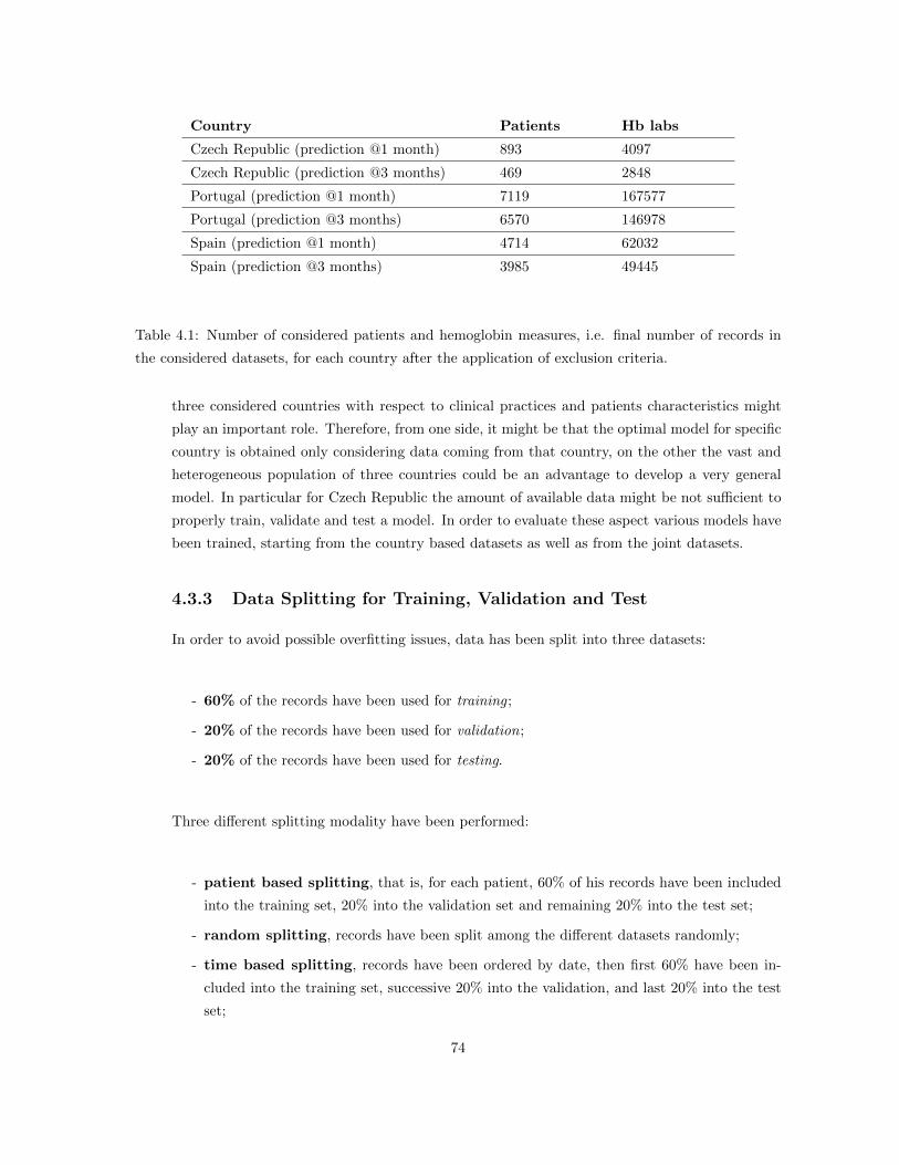
Country Patients Hb labs

Czech Republic (prediction @1 month) 893 4097

Czech Republic (prediction @3 months) 469 2848

Portugal (prediction @1 month) 7119 167577

Portugal (prediction @3 months) 6570 146978

Spain (prediction @1 month) 4714 62032

Spain (prediction @3 months) 3985 49445

Table 4.1: Number of considered patients and hemoglobin measures, i.e. final number of records in

the considered datasets, for each country after the application of exclusion criteria.

three considered countries with respect to clinical practices and patients characteristics might

play an important role. Therefore, from one side, it might be that the optimal model for specific

country is obtained only considering data coming from that country, on the other the vast and

heterogeneous population of three countries could be an advantage to develop a very general

model. In particular for Czech Republic the amount of available data might be not sufficient to

properly train, validate and test a model. In order to evaluate these aspect various models have

been trained, starting from the country based datasets as well as from the joint datasets.

4.3.3 Data Splitting for Training, Validation and Test

In order to avoid possible overfitting issues, data has been split into three datasets:

- 60% of the records have been used for training ;

- 20% of the records have been used for validation;

- 20% of the records have been used for testing.

Three different splitting modality have been performed:

- patient based splitting, that is, for each patient, 60% of his records have been included

into the training set, 20% into the validation set and remaining 20% into the test set;

- random splitting, records have been split among the different datasets randomly;

- time based splitting, records have been ordered by date, then first 60% have been in-

cluded into the training set, successive 20% into the validation, and last 20% into the test

set;

74

Aim of the patient based splitting was to evaluate whether model performances on the

validation and test sets would have benefit from having ”seen” the same patients also in the

training. On the other side the time based splitting approach would present a mixed situation.

Patients with a long history will have records in all three datasets. Old patients, deceased or

anyway not present in FME clinic since some years with respect to the moment of the data

extraction, will have records only in the training dataset. Patients recently admitted in the

clinics would appear only in the test set, for these patient the model need to perform the

prediction based on other patients behavior, thus good performances on the test set would

mean that the model had well generalised the undergoing process to unkwown patients. For the

classical random splitting 10 different randomisation were performed in order to avoid possible

biases in the population selection.

In all cases the test set was kept aside, best model have been selected based on the performance

on the validation set, once the model have been selected its performances have been measured

on the test set.

4.3.4 Managing NA values

As described in 2.8 the different features have been merged to haemoglobin records following

specific rules, clearly it could happen that given a certain haemoglobin record no information

was available for one or more features, for example it could happen that not Ferritin measure

was taken during the 90 days before the haemoglobin sampling, in this case this specific record

will hold some NA values. For each record NA values have been substituted with the mean

value of that specific feature calculate over the training set.

4.4 Prediction @1 month

In the following paragraphs the results of the various performed trials are reported. All models

have been implemented in Matlab, in particular for the ANN the Matlab Neural Network Toolbox

have been used.

Linear models have been obtained by means of a multilinear regression of the responses in y

(the future haemoglobin levels), on the predictors in X (the patient clinical data as previously

described), the coefficient vector is estimated on the training data and then tested on the vali-

dation and test sets. In this case to split the data in validation and test is redundant, but it has

been done in order to have comparable figures with the other models.

The ANN models have been implemented as a feed forward Multi Layer Perceptron, number of

hidden layers was varied from 1 to 3, with number of neurones in each layer varying from 2 to 20

with a step of 2 neurones. Additionally, for each configuration various random weight initialisa-

tions were run. Training of the network was accomplished by means of the Levenberg-Marquardt

75

algorithm, maximum number of epochs was considered equal to 300 (anyway convergence was

always achieved in a lower number of iterations).

The Random Forest models have been developed cycling over the number of trees (from 50 to

500 with a step of 50), while pruning has been performed imposing a minimum number of leaves

varying form 5 to 50 with a step of 5.

The SVM model has been implemented by means of Gaussian kernel functions, when fitting

the data different variances have been considered. Regarding the ε− intensive error functiondifferent values of the ε have been tried. Finally also for the constant C of equation (4.33)

various values have been considered:

- σ = (1.0000, 1.6681, 2.7826, 4.6416, 7.7426, 12.9155, 21.5443, 35.9381, 59.9484, 100.0000);

- ε = (0.0100, 0.1000, 0.2000, 0.3000, 0.4000, 0.5000);

- C = (0.0010, 0.0100, 0.1000, 1.0000, 10.0000, 100.0000);

Results of the different experiments are shown in tables 4.2 to 4.13; models errors ei are calculated

as actual - predicted haemoglobin and are evaluated in terms of Mean Absolute Error (MAE)

defined as:

MAE =1

n

n∑i=1

|ei| (4.37)

and errors quartiles, that is the three points that divide the data into four group, each one

comprising a quarter of the data and defined as follow:

- First quartile divides the lowest 25% of data from the highest 75%.

- Second quartile, also called the median, represents the values that split data set in half.

- Third quartile divides the highest 25% of data from the lowest 75%.

We selected these indices because they can give to physicians a well interpretable estimation

of model performances when compared with the clinical practice. All performance indices are

expressed in g/dl.

76

4.4.1 Results: Czech Republic

Data splitting at patient level

Results of the model derived on the Czech dataset where training, validation and test were split

at patient level are shown in table 4.2.

For the MLP model best results in terms of MAE were obtained by two hidden layers with 4

neurons in the first layer and 8 in the second.

Best results by means of the RF model have been obtained with 100 trees pruned with a minimum

of 10 leaves.

Table 4.2: Mean absolute errors and error quartiles obtained by the different models in the dataset

collected in Czech Republic (splitting performed at patient level). All indices are expressed in g/dl.

Model

Linear

MLP

SVM

RF

Training Validation Test

MAE Quartiles MAE Quartiles MAE Quartiles

0.68 -0.53 0.01 0.56 0.68 -0.55 -0.01 0.51 0.69 -0.54 0.00 0.55

0.65 -0.53 0.00 0.56 0.65 -0.52 0.01 0.49 0.66 -0.5 0.02 0.53

0.64 -0.52 -0.01 0.48 0.65 -0.52 -0.01 0.48 0.67 -0.52 -0.01 0.54

0.49 -0.39 -0.01 0.36 0.66 -0.55 -0.02 0.49 0.67 -0.55 -0.02 0.52

Data splitting based on records’ reference date

Results of the model derived on the Czech dataset where training, validation and test splitting

was based on records’ reference date are shown in table 4.3.




of 5 leaves.

77


collected in Czech Republic (splitting based on records’ reference date). All indices are expressed in

g/dl.

Model

Linear

MLP

SVM

RF



0.69 -0.54 0.02 0.57 0.67 -0.46 0.10 0.59 0.66 -0.43 0.03 0.57

0.66 -0.51 0.02 0.54 0.63 -0.39 0.11 0.60 0.64 0.39 0.08 0.58

0.65 -0.50 0.00 0.52 0.64 -0.41 0.09 0.60 0.64 -0.41 0.06 0.58

0.40 -0.30 0.01 0.32 0.65 -0.46 0.08 0.56 0.65 -0.45 0.06 0.56

Random Data splitting

Results of the model derived on the Czech dataset where training, validation and test splitting

was performed randomly are shown in table 4.4.




of 25 leaves.


collected in Czech Republic (random splitting). All indices are expressed in g/dl.

Model

Linear

MLP

SVM

RF



0.68 -0.52 0.03 0.56 0.66 -0.51 0.01 0.54 0.69 -0.54 0.01 0.54

0.65 -0.51 0.01 0.51 0.63 -0.50 -0.00 0.51 0.66 -0.53 -0.00 0.51

0.64 -0.49 -0.01 0.48 0.64 -0.53 -0.06 0.50 0.67 -0.57 -0.01 0.48

0.58 -0.44 0.02 0.46 0.64 -0.53 0.00 0.52 0.67 -0.55 -0.01 0.52

4.4.2 Results: Portugal


Results of the model derived on the Portuguese dataset where training, validation and test were

split at patient level are shown in table 4.5.

78




of 25 leaves.


collected in Portugal (splitting performed at patient level). All indices are expressed in g/dl.

Model

Linear

MLP

SVM

RF



0.65 -0.48 0.03 0.52 0.63 -0.49 -0.01 0.47 0.65 -0.51 -0.01 0.49

0.57 -0.43 0.02 0.47 0.57 -0.44 0.00 0.45 0.59 -0.44 0.02 0.47

0.60 -0.45 0.03 0.49 0.59 -0.46 0.01 0.46 0.61 -0.45 0.02 0.49

0.53 -0.37 0.05 0.45 0.60 -0.44 0.03 0.49 0.62 0.44 0.04 0.51


Results of the model derived on the Portuguese dataset where training, validation and test

splitting was based on records’ reference date are shown in table 4.6.




of 5 leaves.


collected in Portugal (splitting based on records’ reference date). All indices are expressed in g/dl.

Model

Linear

MLP

SVM

RF



0.65 -0.48 0.03 0.52 0.62 -0.50 0.00.48 0.64 -0.48 0.01 0.50

0.59 -0.45 0.02 0.48 0.58 -0.44 0.02 0.46 0.59 -0.41 0.04 0.50

0.60 -0.46 0.03 0.48 0.58 -0.44 0.03 0.47 0.60 -0.42 0.05 0.52

0.44 -0.29 0.05 0.38 0.59 -0.41 0.06 0.51 0.61 -0.40 0.07 0.54

79

Random data splitting

Results of the model derived on the Portuguese dataset where training, validation and test

splitting was based on random records selection are shown in table 4.7. For the MLP model best

results in terms of MAE were obtained by two hidden layers with 8 neurons in the first layer

and 16 in the second.


of 10 leaves.


collected in Portugal (random data splittingl). All indices are expressed in g/dl.

Model

Linear

MLP

SVM

RF



0.65 -0.4 0.03 0.51 0.64 -0.48 0.02 0.51 0.64 -0.47 0.03 0.52

0.59 -0.45 0.01 0.47 0.59 -0.45 0.01 0.47 0.59 -0.44 0.02 0.47

0.60 -0.45 0.02 0.48 0.60 -0.45 0.02 0.47 0.60 -0.45 0.02 0.48

0.44 -0.29 0.05 0.37 0.61 -0.43 0.05 0.51 0.61 -0.42 0.063 0.52

4.4.3 Results: Spain


Results of the model derived on the Spanish dataset where training, validation and test splitting

was performed at patient level are shown in table 4.8.




of 25 leaves.

80


collected in Spain (splitting performed at patient level). All indices are expressed in g/dl.

Model

Linear

MLP

SVM

RF



0.67 -0.50 0.02 .53 0.65 -0.51 0.0 0.50 0.65 -0.53 0.00 0.47

0.63 -0.47 0.02 0.50 0.62 -0.49 0.00 0.49 0.61 -0.50 0.01 0.46

0.64 -0.48 0.03 0.50 0.63 -0.50 0.01 0.50 0.62 -0.51 0.02 0.48

0.57 -0.39 0.05 0.48 0.64 -0.47 0.03 0.53 0.63 -0.49 0.034 0.50



was based on records’ reference date are shown in table 4.9.




of 25 leaves.


collected in Spain (splitting based on records’ reference date). All indices are expressed in g/dl.

Model

Linear

MLP

SVM

RF



0.68 -0.50 0.02 0.55 0.65 -0.46 0.05 0.55 0.63 -0.47 0.03 0.51

0.64 -0.48 0.02 0.51 0.62 -0.45 0.04 0.52 0.61 -0.46 0.04 0.49

0.65 -0.48 0.02 0.53 0.63 -0.46 0.05 0.54 0.61 -0.47 0.03 0.49

0.58 -0.37 0.07 0.51 0.64 -0.41 0.09 0.59 0.62 -0.41 0.09 0.54



was performed randomly are shown in table 4.10.


neurones in the first layer and 8 in the second.

81


of 10 leaves.


collected in Spain (random data splitting). All indices are expressed in g/dl.

Model

Linear

MLP

SVM

RF



0.67 -0.49 0.03 0.53 0.67 -0.50 0.02 0.53 0.66 -0.48 0.02 0.53

0.63 -0.47 0.02 0.51 0.63 -0.48 0.02 0.49 0.62 -0.46 0.02 0.50

0.63 -0.47 0.03 0.52 0.64 -0.49 0.02 0.50 0.63 -0.46 0.03 0.51

0.47 -0.30 0.06 0.41 0.65 -0.45 0.04 0.55 0.64 -0.43 0.06 0.56

4.4.4 Results: ALL


Results of the model derived on the joint datasets of Czech Republic, Portugal and Spain where

training, validation and test data splitting was performed at patient level are shown in table

4.11.




of 10 leaves.

Table 4.11: Mean absolute errors and error quartiles obtained by the different models in the joint

dataset (data splitting performed at patient level). All indices are expressed in g/dl.

Model

Linear

MLP

SVM

RF



0.65 -0.48 0.03 0.52 0.63 -0.50 0.00 0.48 0.64 -0.51 0.00 0.48

0.60 -0.46 0.01 0.48 0.59 -0.47 0.00 0.46 0.60 -0.47 0.01 0.47

0.61 -0.46 0.02 0.49 0.60 -0.46 0.02 0.48 0.61 -0.46 0.02 0.48

0.45 -0.30 0.05 0.37 0.61 -0.45 0.03 0.50 0.62 -0.45 0.04 0.50

82


Table 4.12 shows the results of the model derived on the joint datasets where training, validation

and test data splitting was performed considering records’ reference date.




of 25 leaves.


dataset (data splitting based on records’ reference date). All indices are expressed in g/dl.

Model

Linear

MLP

SVM

RF



0.66 -0.48 0.03 0.52 0.62 -0.48 0.02 0.49 0.63 -0.47 0.03 0.51

0.60 -0.48 0.00 0.46 0.58 -0.46 0.00 0.45 0.59 -0.44 0.02 0.48

0.61 -0.46 0.02 0.49 0.59 -0.45 0.02 0.48 0.60 -0.42 0.05 0.51

0.54 -0.36 0.06 0.46 0.60 -0.41 0.05 0.52 0.61 -0.40 0.07 0.55


Results of the model derived on the joint datasets with random data splitting for training,

validation and test are shown in table 4.13.




of 10 leaves.

83


dataset (random data splitting). All indices are expressed in g/dl.

Model

Linear

MLP

SVM

RF



0.65 -0.48 0.03 0.52 0.65 -0.49 0.03 0.52 0.64 -0.48 0.03 0.52

0.59 -0.45 0.02 0.48 0.60 -0.45 0.02 0.48 0.59 -0.45 0.02 0.48

0.60 -0.45 0.03 0.49 0.60 -0.45 0.03 0.49 0.60 -0.45 0.03 0.49

0.45 -0.29 0.05 0.38 0.62 -0.44 0.05 0.52 0.61 -0.44 0.04 0.52

4.4.5 Discussion

We have seen that the response to ESA therapy has a huge inter-individual variability. Causes

of this variability are multiple, some of them can be linked to the available data, like patient

weight, inflammation markers etc., thus during the learning phase the model should be able to

clusterize ESA response considering these parameters. On the other side there are are factors

which cannot be represented by the available features, one example is the endogenous production

of erythropoietin, which, as we have seen in Chapter 3, is a parameter which influence red blood

cells dynamic and thus important to characterize a patient.

In the recent years there have been several applications of predictive modeling to the anemia

management problem [17, 18, 36, 40, 41, 50, 73, 74, 75].

In [76], the authors of this paper carried out an evaluation of many different methods for

hemoglobin prediction in dialysis patients. Results were very promising but several problems

arose that make us think over a new approach. Firstly, since the most relevant value in the

prediction of a future value of hemoglobin, turned out to be the current hemoglobin level, this

produced a sort of delay in the prediction, since models were prone to predict most of the time

the current value of hemoglobin as the most likely one for a subsequent monitoring, too. This

delay occurred for all the tested models; the use of very sophisticated models did not improve

the prediction considerably, thus suggesting that there was a certain accuracy threshold that

could not be surpassed by means of using the same data structure with different methods; that

may also be linked to the fact that the systematic error committed by measuring machines did

not give a wide margin of improvement.

Therefore, we came up with the idea presented in this thesis that is rather focused on better

exploiting the available information and making more sensible predictions, i.e., predictions that

are aligned with the real behavior and lifespan of RBC and the effect produced by the drugs

administered to correct the anemia, mainly ESAs [8].

We extensively explored different approaches to model hemoglobin fluctuation in dialysis pa-

tients. In particular results of different algorithms, namely Linear Models, ANN, SVM and RF

84

have been compared over different datasets. Presented results show that ANN is the best model

in terms of prediction capability on the test set, even if performances of SVM and RF are very

close. On the other side Linear Models seem inadequate for the evaluated cases. Both ANN and

SVM performances are quite similar over training, validation and test datasets, while RF shows

a tendency to overfit the training data. Models seems to benefit from been derived on the joint

datasets, while splitting modality does not have a relevant influence on the performances, said

that random splitting seems to be slightly preferable because it is the most general, indeed has

the most stable performances in the different dataset. Error histograms of the Linear, ANN,

SVM and RF models derived on the joint dataset randomly split into training, validation and

test set are shown in figures 4.9, 4.10, 4.11 and 4.12 respectively.

−15 −10 −5 0 5 100

0.2

0.4

0.6

0.8

1

1.2

1.4

1.6

1.8

2x 10

4 Training Error

−10 −5 0 5 100

1000

2000

3000

4000

5000

6000

7000

Validation Error

−10 −5 0 5 100

1000

2000

3000

4000

5000

6000

7000

Test Error

Figure 4.9: Linear Model, random data splitting: histogram of prediction errors, calculated as actual

- predicted haemoglobin, results are expressed in g/dl

−10 −5 0 5 100

0.5

1

1.5

2

2.5x 10

4 Training Error

−10 −5 0 5 100

1000

2000

3000

4000

5000

6000

7000

Validation Error

−10 −5 0 5 100

1000

2000

3000

4000

5000

6000

7000

Test Error

Figure 4.10: ANN, random data splitting: histogram of prediction errors, calculated as actual -

predicted haemoglobin, results are expressed in g/dl

85

−10 −5 0 5 100

0.2

0.4

0.6

0.8

1

1.2

1.4

1.6

1.8

2x 10

4 Training Error

−10 −5 0 5 100

1000

2000

3000

4000

5000

6000

7000

Validation Error

−10 −5 0 5 100

1000

2000

3000

4000

5000

6000

7000

Test Error

Figure 4.11: SVM, random data splitting: histogram of prediction errors, calculated as actual -

predicted haemoglobin, results are expressed in g/dl

−10 −5 0 5 100

0.5

1

1.5

2

2.5

3x 10

4 Training Error

−10 −5 0 5 100

1000

2000

3000

4000

5000

6000

7000

Validation Error

−10 −5 0 5 100

1000

2000

3000

4000

5000

6000

7000

Test Error

Figure 4.12: RF, random data splitting: histogram of prediction errors, calculated as actual - predicted

haemoglobin, results are expressed in g/dl

These results confirm that algorithm like the ANN are able to learn and generalize complex data.

Additionally, the fact that joining data coming from different countries, where patients char-

acteristics as well as treatment practice are different, is beneficial for the model, demonstrates

that this kind of algorithms are capable to well separate clusters of biased and heterogeneous

data.

In addition to the numerical values provided in the previous paragraphs, it is useful to visualize

the temporal evolution of individual patients comparing the actual value of Hb that was measured

and the Hb value predicted by the MLP model. To this end, Figures 4.13, 4.14, 4.15, 4.16,

4.17 and 4.18 show some examples of predicted versus actual hemoglobin fluctuation along the

patient’s history. Figures 4.13 and 4.14 are examples of patients in whom the prediction was

very good, indeed MAE for these two patients was 0.31 and 0.52, i.e. in both cases below the

average of the population. Analyzing more in details these two examples it can be noticed that

86

for patient in Figure 4.13 hemoglobin is more stable with respect to patient in Figure 4.13,

nevertheless the case of Figure 4.13 shows the ability of the model to anticipate abrupt changes

in hemoglobin concentration, which are armful for the patient, and this might be very useful in

the clinical practice. Figures 4.15 and 4.16 reports the cases of two patients where the model

perfomances are in line with those of the average population, indeed MAE is 0.58 and 0.60

respectively. Also in the case the ability of the model to anticipate hemoglobin fluctuation is

quite evident. Figures 4.16 shows also an interesting fact, focusing at the first five hemoglobin

measures it can be notices the they are quite stable in the range of 12−13g/dl, with the exception

of the fourth values that is around 7, in the case model prediction is completely wrong. On the

other side this sudden drop and successive jump of the hemoglobin is very unlikely real, the

only clinical explanation would be a important bleeding followed by a transfusion, but most

probably it is either an error in the lab or a reporting mistake. Either cases are situation where

clearly the model cannot anticipate, indeed in general the prediction error is very high it cab

be often explained by intercurrent events. Figure 4.17 and 4.18 represent a case where model

performances are below the average, indeed for these patients MAE is 0.74 and 0.78 respectively.

In these two cases there is sometime a discrepancy between predicted and actual hemoglobin

concentration, nevertheless also in this two cases there is a quite reasonable correlation between

the model prediction and the actual hemoglobin measures.

Time0 2 4 6 8 10 12 14 16

Hb(t

)

4

5

6

7

8

9

10

11

12

13

14

15

16

17

18

19

20Patient temporal evolution: model (blue) vs real (red); MAE=0.31206

Figure 4.13: Predicted vs actual hemoglobin temporal evolution for a specific patient: a case where

the accuracy is very good if compared with the average of the considered population, MAE = 0.31

A main limitation of the presented study is that is is restricted to one kind of ESA, namely,

Darbepoietin, reason of choosing Darbepoetin it is because it was the most commonly admin-

87

Time0 5 10 15 20 25 30 35 40 45

Hb(t

)

4

5

6

7

8

9

10

11

12

13

14

15

16

17

18

19



the accuracy is good if compared with the average of the considered population, MAE = 0.52

istered ESA in the countries under study. As shown in [73], prediction models can deal with

different kinds of ESA, being the kind of ESA one of the inputs to the model. Indeed a model

for Epoetin Beta has been recently developed and its performances are very comparable to those

of the model for Darbepoetin described in this chapter.

88

Time0 5 10 15 20 25 30 35

Hb(t

)

4

5

6

7

8

9

10

11

12

13

14

15

16

17

18

19


Figure 4.15: Predicted vs actual hemoglobin temporal evolution for a specific patient with a quite

high hemoglobin variability: a case where the accuracy is similar to the average of the considered

population, MAE = 0.58.

Time0 5 10 15 20 25 30 35 40

Hb(t

)

4

5

6

7

8

9

10

11

12

13

14

15

16

17

18

19


Figure 4.16: Predicted vs actual hemoglobin temporal evolution for a specific patient with a mainly

stable hemoglobin: a case where the accuracy is similar to the average of the considered population,

MAE = 0.60

89

Time0 5 10 15 20 25 30 35

Hb(t

)

4

5

6

7

8

9

10

11

12

13

14

15

16

17

18

19



the accuracy is below the average, MAE = 0.74

Time0 5 10 15 20 25

Hb(t

)

4

5

6

7

8

9

10

11

12

13

14

15

16

17

18

19



the accuracy is below the average, MAE = 0.78

90

4.5 Prediction @3 months

A discussed in the previous paragraphs hemoglobin sampling is typically performed on monthly

base, thus ESA and Iron therapy are adjusted, if needed, on a monthly basis as well. Never-

theless, anticipation of the long-term physiologic response (i.e. at 3 months) is of fundamental

importance for planning a successful strategy which takes into account the next hemoglobin

steady state, avoiding harmful hemoglobin cycling. In this section, we describe the model de-

rived to predict the long term, 3 months, response to ESA and Iron therapy. [7]. Prediction

performances depending on the dataset (joint or country based) and splitting modality (time,

patient or random based) have been extensively explored in the previous paragraphs, so we don’t

report here the results of all the performed experiments, but just those of the models derived

on the joint dataset where data were split randomly in training, validation and test, which also

in this case resulted the best approach for deriving better performing and more stable models.

4.5.1 Results

In table 4.14 results of Linear, ANN, SVM, RF models are shown. Figures 4.19 represents the

error histograms of the best performing model that resulted to be the ANN.


collected in joint dataset (random splitting). All indices are expressed in g/dl.

Model

Linear

MLP

SVM

RF



0.86 -0.65 0.01 0.67 0.86 -0.65 0.02 0.66 0.87 -0.67 0.00 0.65

0.77 -0.59 0.01 0.61 0.77 -0.59 0.01 0.60 0.77 -0.60 0.00 0.59

0.78 -0.60 0.01 0.62 0.78 -0.61 0.01 0.63 0.78 -0.61 0.01 0.60

0.77 -0.59 0.01 0.61 0.77 -0.59 0.01 0.60 0.77 -0.60 0.00 0.59

91

-10 -5 0 5 100

2000

4000

6000

8000

10000

12000

14000Training Error

-10 -5 0 5 100

500

1000

1500

2000

2500

3000

3500

4000

4500Validation Error

-10 -5 0 5 100

500

1000

1500

2000

2500

3000

3500

4000

4500Test Error

Figure 4.19: ANN Model, random data splitting: histogram of prediction errors, calculated as actual

- predicted haemoglobin, results are expressed in g/dl

4.5.2 Discussion

Presented results show that prediction error for the model @3months increases with respect to

that of the model @1month. This can be expected, because the model, with the exception of

drug prescription, can only make use of the data available at time t thus the probability that

patient conditions change or that an intercurrent event happens between time t and time t+ 3,

that is over a period of 3 months, are higher with respect to the model @1month. Nevertheless

as it can be seen from figure 4.20, representing the scatter plot of real vs predicted Hb variation

@3months (calculated as Hb(t + 3) −Hb(t)) for the test dataset, there is a strong correlation

between actual and predicted Hb variations. This means that even if with some deviations the

model is in general able to catch the Hb long term trend.

Among the considered patients’ population, four have been selected and reported as typical

examples of Hb concentrations behavior over time (figures 4.21, 4.22 4.23 and 4.24). In each

graph the red lines represent the observed Hb patient quarterly variations over time, while

the blue lines describe the predicted Hb model simulation during the same period of time. In

particular, figure 4.23 reports the case of a patient for whom the model displayed an average

performance, i.e. where MAE is close to the sample population mean (in this specific case, MAE

of 0.78). Simulation and real outcome display very similar trends and, although the prediction

not always exactly corresponds to the actual Hb value, the model was always able to maintain

the same tendency as the real data. Figures 4.21 and 4.22 describe patients for whom the model

displayed an optimal performance and very high precision in anticipating quarterly Hb variations;

92

−10 −8 −6 −4 −2 0 2 4 6 8 10−10

−8

−6

−4

−2

0

2

4

6

8

10

Hb(t+3) − Hb(t)

Target

Model P

red

iction

Figure 4.20: Scatter plot of predicted vs actual Hb variation @3months, calculated asHb(t+3)−Hb(t),in the test dataset

in fact, MAE resulted below the average (MAE = 0.45g/dl and MAE = 0.53g/dl, respectively),

as clearly illustrated by the proximity of the predicted and the observed Hb values. Finally,

figure 4.24 shows a simulation where MAE = 0.89g/dl, that is below the average performance.

Although the MAE is above the average, still the model is able to predict the tendency of the

Hb variation over time.

93

0 5 10 15 20 25 30−7

−6

−5

−4

−3

−2

−1

0

1

2

3

4

5

6

7

Time

Hb(t

+3)−

Hb(t

)

Patient temporal evolution: model(blue) vs real(red)

Figure 4.21: Predicted vs actual hemoglobin quarterly variation, calculated as Hb(t+ 3)−Hb(t), for

a specific patient: a case of very good accuracy when compared with the overall model perfomance

0 5 10 15 20 25 30−7

−6

−5

−4

−3

−2

−1

0

1

2

3

4

5

6

7

Time

Hb(t

+3)−

Hb(t

)



a specific patient: a case of good accuracy when compared with the overall model perfomance

94

0 5 10 15 20 25 30 35 40−7

−6

−5

−4

−3

−2

−1

0

1

2

3

4

5

6

7

Time

Hb(t

+3)−

Hb(t

)



a specific patient: a case of average accuracy when compared with the overall model perfomance

0 10 20 30 40 50 60−7

−6

−5

−4

−3

−2

−1

0

1

2

3

4

5

6

7

Time

Hb(t

+3)−

Hb(t

)



a specific patient: a case of bad accuracy when compared with the overall model perfomance

95

Chapter 5

Anemia Control Model: medical

device certification and clinical

evaluation

This chapter presents the Anemia Control Model (ACM), a medical device designed in order to

support physicians in prescribing Iron and ESA (in the form of Darbepoetin) therapy to dialysis

patients affected by secondary anemia. Main component of the ACM is the predictive model

for hemoglobin fluctuation which has been discussed in the previous chapter, second one is an

algorithm for optimal dose selection. Predictive models based on machine learning techniques

have been extensively used in the medical field, nevertheless, to the author’s knowledge, these

predictive modes have never been evaluated in the context of CE medical device regulation. In

particular in this chapter the novel approach followed to perform a systematic risk assessment of

the predictive model is described. Another limitation of most of the predictive models developed

in the recent year is that they have never been utilized in the real clinical practice or, when

this happened, the utilization has been very limited. On the contrary the ACM it has been

implemented and utilized by physicians in a large patients cohort from four different clinics.

The chapter is organised in the following way: in the first part a description of the ACM

is provided, second part is dedicated to the medical device certification, finally, in the third,

results of ACM utilisation during the clinical evaluation of the tool are reported.

5.1 Anemia Control Model (ACM)

Complexity of anemia management for dialysis patients have been examined in Chapter 1.

97

Several attempts to optimize ESA dosing based on general patient population data have already

been developed by means of artificial neural network techniques [39, 41, 73]. Other approaches

towards therapy optimization have been developed in [3, 11, 40, 74].

In Chapter 4 various machine learning techniques have been explored in order to derive a model

able to predict hemoglobin fluctuations for a large cohort of ESRD patients undergoing dialysis.

Different models had similar performances, anyway the best one resulted the Artificial Neural

Network model trained on the joint datatset of Czech Republic, Portugal and Spain where data

were randomly split in training, validation and test. Prediction error of this model in terms

of MAE was inferior to 0.6g/dl. European best practice as well as FME internal guidelines

establish the target range of 10 − 12g/dl for hemoglobin concentration, thus we could assume

that the performances of the predictive model makes it suitable for a potential appellation in real

clinical practice. In addition to that the ANN model, once trained, is very quick in processing

patients records, which is fundamental for a practical application. Summarizing the following

key factors have been achieved:

- the model is very general in the sense that has been developed and validated over a very

large and composite patients population, thus it is reasonable to assume that obtained

performances can be replicated in a ”live” setting;

- a MAE lower than 0.6 g/dl and even more important 92% of errors < 1g/dl if compared

with the difficulties of achieving guidelines targets make the model a potentially valid tool

to support physicians when prescribing ESA and Iron to correct anemia in dialysis patients;

- model makes use of data available on line in the clinical system EuCliD and is able to

process it in a very short time data from a large number of patients;

- feature analysis highlights that one of the main drivers of the predicted future Hb is ESA

drug prescription, which is actually a parameter that can be controlled and thus its effect

simulated by the model as a set of possible actions.

It must be mentioned that before ACM implementation, FME started a program for standard-

izing Iron dosages depending on ferritin and transferrin saturation levels through a rule-based

algorithm. In order to avoid conflict with this program it has been decided to adapt ACM to

this program, that is, ACM has to take as input iron doses selected through this algorithm

and calculate the optimal Darbepoetin dose to achieve the above mentioned objectives, which

is actually what more influences the next hemoglobin level and the most complex task.

5.1.1 Algorithm for optimal dose selection

A natural use of a the predictive model we developed is to use it to simulate different doses and

then select the dose achieving the desired outcome. Clearly the optimal dose selection depends on

98

the established targets for anemia management. In our case these targets implements European

guidelines as well as FME standards, which in general terms set the following objectives for the

ACM:

- maximize the probability that 10g/dl ≤ Hb ≤ 12g/dl;

- avoid abrupt changes in Hb levels that might be harmful for the patient, in oder words

10g/dl ≤ hb ≤ 12g/dl will not always be the desired outcome for the next month, for

example for a patient with Hb = 8g/dl target for next month would be around 9g/dl;

- keep hemoglobin concentration stable for longer period of time;

- when possible minimize the use of Darbepoetin, rationale behind this objective is twofold,

firstly a lower utilization of Darbepoetin lowers the risk of its side effects, secondly it

optimize costs (ESA drugs are normally very expensive).

These challenges have been tackled by defining a reward function R which assigns a reward to

each possible action which for ESA and Iron doses, as listed in tables 5.1 and 5.2 respectively.

Table 5.1: Possible ESA dosages.

Monthly Dose Single Dose Scheduling

10µg 10µg 6th dialysis of the month

20µg 10µg 3rd and 9th dialysis of the month

30µg 10µg 3rd, 7th, 11th dialysis of the month

40µg 10µg once a week

60µg 20µg 3rd, 7th, 11th dialysis of the month







Reward function R is computed as the sum of two penalization terms:

99

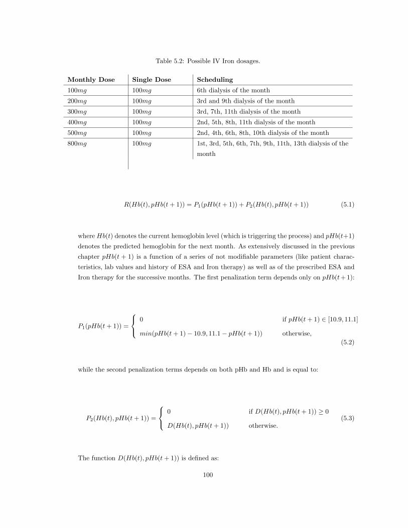
Table 5.2: Possible IV Iron dosages.

Monthly Dose Single Dose Scheduling

100mg 100mg 6th dialysis of the month

200mg 100mg 3rd and 9th dialysis of the month

300mg 100mg 3rd, 7th, 11th dialysis of the month

400mg 100mg 2nd, 5th, 8th, 11th dialysis of the month

500mg 100mg 2nd, 4th, 6th, 8th, 10th dialysis of the month

800mg 100mg 1st, 3rd, 5th, 6th, 7th, 9th, 11th, 13th dialysis of the

month

R(Hb(t), pHb(t+ 1)) = P1(pHb(t+ 1)) + P2(Hb(t), pHb(t+ 1)) (5.1)

where Hb(t) denotes the current hemoglobin level (which is triggering the process) and pHb(t+1)

denotes the predicted hemoglobin for the next month. As extensively discussed in the previous

chapter pHb(t + 1) is a function of a series of not modifiable parameters (like patient charac-

teristics, lab values and history of ESA and Iron therapy) as well as of the prescribed ESA and

Iron therapy for the successive months. The first penalization term depends only on pHb(t+ 1):

P1(pHb(t+ 1)) =

0 if pHb(t+ 1) ∈ [10.9, 11.1]

min(pHb(t+ 1)− 10.9, 11.1− pHb(t+ 1)) otherwise,

(5.2)

while the second penalization terms depends on both pHb and Hb and is equal to:

P2(Hb(t), pHb(t+ 1)) =

0 if D(Hb(t), pHb(t+ 1)) ≥ 0

D(Hb(t), pHb(t+ 1)) otherwise.(5.3)

The function D(Hb(t), pHb(t+ 1)) is defined as:

100

D(Hb(t), pHb(t+ 1)) = (maxDelta(Hb(t))− |Hb(t)− pHb(t+ 1)|) · 100 (5.4)

The function maxDelta(Hb(t)) has the following form:

maxDelta(Hb(t)) =

1 if Hb(t) ≤ 8.5

1 +8.5−Hb(t)

3.8if 8.5 < Hb < 10.3

0.5 if 10.3 ≤ Hb ≤ 11.3

0.5 + 0.7 · (Hb(t)− 11.2)

1.2if 11.3 < Hb ≤ 13

1.2 if Hb ≥ 13

(5.5)

The shape of reward function R is represented in figure 5.1.

16

Haemoglobin Lab Values

141210

ESA Reward Function

8605

Predicted Haemoglobins10

15

-1200

-1000

-800

-600

-400

-200

0

20

Rew

ard

Figure 5.1: Reward Function

5.1.2 ACM process

Typical process for anemia management in a dialysis clinic is that after any hemoglobin eval-

uation (normally performed on monthly basis) physicians review and adjust ESA and Iron

101

prescriptions if needed. Considering this, ACM has been designed with the aim to generate

ESA and Iron therapy suggestions (the latter based on the rule based algorithm) every time a

new hemoglobin value is recorded; additionally, in order to perform an optimal prediction, ACM

needs updated clinical information for each specific patient. Taking into consideration these

facts we can identify the following key factors that must drive ACM design:

- ACM is not just the ANN-based predictive model, it is a far more complex tool which must

be able to communicate with a clinical system;

- ACM must be designed as a service to be called by the clinical system which has to be the

driver of the process;

- Criteria to trigger a call to the ACM are part of the clinical system business logic, even if

clearly these criteria must be compliant with ACM specifications;

- No updated clinical information may persist in ACM;

- ACM defines the data model that the clinical system must provide to the ACM, this data

model can be in principle different from that needed by the predictive algorithm (and

actually it is different);

- Therefore, once the ACM receives the clinical system request, first step is to process the

data in order to ”prepare” records in the format needed by the predictive algorithm, second

step is to simulate various outcomes as function of the possible dose prescriptions, finally

optimal dose has to be selected depending on the established targets;

- Once the optimal prescription is selected a response has to be sent to the clinical system.

The above mentioned points define the framework for ACM development.

5.1.3 Software Architecture Design

As discussed in the previous chapter the predictive algorithm has been developed following

the Machine Learning paradigm; in particular the model has been developed using the Matlab

Artificial Neural Network Toolbox. Finally the model has been compiled in a Microsoft .Net

library (dll) and wrapped in a web service developed within the Microsoft .Net Framework.

The main architectural ideas are:

- Application has no user interface

- Communication between third party systems and the application is performed through a

Web Service, which exposed ACM methods and defines the communication protocol and

schema

102

- The application does not store any patient data, all the information needed to elaborate

the prediction has to be provided from the third party system

- Calls to ACM are synchronous and performed by the third party system

- Calculation of the optimal dose is performed through two main steps

1. Simulation of different actions (ESA doses)

2. Selection of the action with the best result

Figure 5.2 schematizes the integration process between the clinical system and the ACM.

Figure 5.2: ACM workflow.

5.1.4 Server Network Layout

Anemia Control Model (ACM) algorithm is wrapped in a web service, which exposes ACM

functionality to third-party systems (the clinical systems). Third-party systems can be located

103

within the same local network of ACM or accessible through the WAN. ACM is designed to be a

centralized application; thus installation and maintenance have to be managed centrally. ACM

in principle can be available for different third party systems. In figure 5.3 the server network

layout is schematized.

Figure 5.3: Network layout.

5.1.5 Communication diagram

Third party system and ACM communicate through HTTP web service calls. Third party

system calls the web service sending the necessary information (patients clinical data) to the

ACM, which process them and send back a response (anemia drug therapy recommendations),

5.4.

104

Figure 5.4: Web Service communication schema.

5.2 Medical Device Certification

5.2.1 Introduction

In order to fulfill the Medical Device Directive (MDD) a vast and complete documentation

covering all aspects of the device life cycle has to be provided, the sum of this documentation

is called Technical File. The complete Technical File is not fully described in this thesis, firstly

due to its length (around 100 different documents); secondly, because part of the documentation

is not really related to the specificity of the ACM. Therefore we will focus only on the the main

aspects that, in our opinion, had to be considered in order to certify a predictive algorithm as

medical device under the European regulation, namely the Intended Use of the device and the

Risk Analysis. To our knowledge ACM is the first case of predictive modeling tool certified

as medical device. Risk Analysis is the core of the MDD procedure because assess the safety

of the device. On the other side to properly define the device Intended Use is of fundamental

importance because it is the device intended use that mainly define which risks are related to

its use and how they have to be evaluated and, if necessary, mitigated.

5.2.2 Intended Use of the Device

Intended use file is basically composed of two chapters:

- What is the intended use of the device;

- What is NOT the intended use of the device.

105

In order to properly specify the device intended use an important document to be produced is

the General Description, which aims to summarize the main functionalities of the device and to

whom the Intended Use refers to. Main points discussed in these documents are reported in the

following paragraphs.

Short description of the device / system

Anemia Control Model (ACM) is a software application, which is intended to support doctors

in the anemia drug therapy managing. In particular the software is supposed to analyze patient

data and to perform a suggestion for the best Erythropoiesis Stimulating Agents (ESA) /Iron

pharmacological treatment (dosage and scheduling) for maintaining the hemoglobin level within

the target range. Therefore, ACM system provides a dosage/scheduling suggestion for ESA

and Iron medicaments. Then doctors are required to evaluate case by case whether the ACM

suggestion is safe for the patient; afterwards, basing on their experience, they may formulate

the drug prescription following the software recommendation or decide to formulate their own

drug prescription.

ACM receives (as an input) essential information from the third party. Then it elaborates the

provided information to compute an ESA/Iron therapy strategy. Thus, the ESA/Iron dose

suggestion elaborated by the ACM algorithm is sent to the same clinical system as an output.

Therefore ACM is not designed to be utilized or administered by an external user, ACM consumer

is the third party system. ACM does not store or manipulate any data, only utilizes data to

elaborate drug recommendations.

Description of sub-systems / options

ACM is mainly composed of two sub-systems:

- A predictor model which depending on the input data forecasts the response to ESA and

Iron therapy for a specific patient;

- An algorithm that using the predictor model extracts the optimal ESA / Iron therapy to

achieve the established clinical outcome for anemia management.

List of device composition / materials used

ACM is a computer program wrapped in a service application; it is not part of a physical device,

thus:

- No material has been used to manufacture it;

- It does not include any component other that the software itself;

- It is not composed by any medicinal substance, tissue or blood product;

- Characteristics like sterile condition do not apply in this case;

106

Development context of the device, Patient population and medical indication

As mentioned in the previous sections, ACM is composed of a predictor model and of a policy

extractor. For completeness and to give a proper idea of the kind of information that must be

presented in the General Description document, in this section we repeat in a concise way what

already discussed in the previous chapters of this thesis.

The predictor model is implemented as a Multi Layer Perceptron. Artificial Neural Networks

are computational models inspired by the processing principles found in brains, and extensively

used as function approximators in a variety of application scenarios. They are composed of com-

putational units called neurons, exchanging information through weighted connections. Neurons

are organized in a variable number of layers: an input layer to which the data is fed; an output

layer where the result of computation is returned; and one of more hidden layers in between. The

ANN, presented with a collection of input-output pairs called the training set, learns by example

to approximate the relation between such pairs; to do so, it iteratively adjusts the weights of its

connections. If the learning phase is successful, the resulting model will be able to generalize

what it has learned to unseen examples: that is, given a new set of inputs (the test set) the

ANN should be able to predict the corresponding outputs with reasonable accuracy. In order

to ensure good generalization abilities, we applied the typical machine learning paradigm, i.e.

data has been divided in three datasets; on for training, one for validation and one for testing.

The policy extractor is implemented through an algorithm that consist of:

- A set of environment states S;

- A set of actions A;

- A set of rules to reward actions;

- A set of rules to control anomalous situation;

- A selection criteria for the optimal action based on above-mentioned points;

In our case the state S(t) represents patient clinical status at time t, while the action A(t)

represent the suggested ESA / Iron dose. The set of actions available to the agent are restricted

(e.g., use of available dosages). Basically, given clinical targets provided by experts (or simply

implementing guidelines) the policy extractor algorithm simulates different dosages in order to

select the one able to achieve these targets.

Specific upper limits of ESA and Iron dosages, as well as hemoglobin upper limits for ESA

therapy interruption have been imposed to the machine as specified by the anemia therapy

guidelines, so that dangerously high drug doses, are automatically blocked and no ESA therapy

is administered when hemoglobin concentration is over 13g/d.

Patient population is composed of ESRD adult patients undergoing stable hemodialysis (HD).

Pre-dialysis, Peritoneal dialysis, internal care patients and children (age < 18 years) are ex-

cluded from the study. Any other general condition (such as, for instance, chronic or acute

107

comorbidities, gender or age, etc.) does not influence the inclusion of the patients. ACM has

been created to facilitate the prediction of a correct anemia therapy with the lowest error.

Therefore, although all HD patients are generally included in the study, the ACM system finds

a fundamental application on a special HD population, namely patients suffering Chronic Kid-

ney Disease (CKD) secondary anemia (defined as low levels of plasma hemoglobin) receiving

a pharmacological treatment for correction (i.e., ESA therapy and/or Iron supplementation).

Moreover, special conditions may occur and some patients may become temporary not eligible

for ACM prediction. They will not be excluded from the study; however, ACM analysis may be

suspended, case-by-case, until all the necessary criteria are satisfied again. For any HD patient

in the clinics the secondary inclusion criteria are:

- A history of dialysis therapy >= 3 months;

- Enough clinical and biochemical records during the 3 months preceding the ACM elabora-

tion;

- No blood transfusion during the 3 months preceding the ACM elaboration;

- Unique administration of intravenous (IV) Darbepoetin alpha as ESA during the 3 months

preceding the ACM elaboration;

- Unique administration of intravenous (IV) Iron preparation during the 3 months preceding

the ACM elaboration;

- Absence of errors in the input data format;

Although any ESRD patient who satisfies the above-mentioned conditions may be ideally in-

cluded in the present study, for safety reasons, we are going to validate the ACM system on a

restricted population. Hence, in a first phase of the evaluation, only patients from four pilots

clinics (one in Portugal; two in Spain; one in Czech Republic) will be initially included. There-

after, depending on the study outcome, we will be able to extend the use of ACM on the general

ESRD population.

What is intended use of the device

The following ACM intended uses are the closest to the definition of a medical device:

- Recommendation of the best ESA/Iron drug dosage and scheduling;

- Anemia therapy outcome prediction.

Major aim of ACM is maintenance of patient hemoglobin level within established targets assuring

patients’ safety; hence, its utilization respects the following policy:

- ACM suggestions cannot become actual prescriptions without external medical interven-

tion;

108

- ACM utilization implies continuous clinician supervision and control action so that expert

nephrologists always perform prescriptions after viewing both the software outcome and

the patient clinical conditions;

- ACM algorithm has been trained on real patient retrospective data, i.e. actual biochemi-

cal/clinical data together with actual administered drug quantities. Therefore, the system

has learnt true therapeutic policies and it elaborates new data basing on that past experi-

ence;

- Specific lower and upper limits ESA or Iron dosages as well as hemoglobin upper limits for

ESA therapy interruption have been imposed to the machine as specified by the anemia

international guidelines, so that dangerously high drug doses, are automatically blocked

and no ESA therapy is administered when hemoglobin concentration is over 13 g/dl;

- It must also be mentioned that, since ACM has been trained on real doctor prescriptions

it is programmed for respecting the limits learnt from the real medical experience. Indeed,

during the preliminary validation phase, ACM never suggested a dose out of the normal

range used by doctors.

5.2.3 What is NOT intended use of the device

Obviously it is not possible to list all the functionality and uses the system is not supposed to

provide. However, the following enumeration might be helpful to distinct the intended use more

precisely:

- ACM does not formulate any drug prescription autonomously;

- ACM does not include or administer any kind of substance;

- ACM does not give mandatory treatment indications;

- ACM only suggests a therapy regimen;

- expert nephrologists must evaluate the machine suggestion and decide whether or not

performing the drug prescription following the suggestion;

- ESA / Iron therapy is just a part of anemia treatment, physicians, as they normally do,

have to consider the overall patient clinical condition in order to evaluate ACM ESA / Iron

suggestion and in any case take all the necessary measures to optimally treat the patient;

- ACM elaborates data as they are provided;

- Recognizing erroneous data or peculiar patient conditions is not the aim of the present

software; however an additional ACM functionality allows giving an alert when very un-

usual values for specific parameters are registered (e.g. very high / low plasma level of

hemoglobin);

- If not sufficient information is provided to ACM, no therapy suggestion will be performed.

109

ACM is not a manufacture product but an application service which has to be installed on a

central server in headquarter and accessed remotely by the clinical system used to record drug

prescriptions of anemia management. Therefore, when used under the conditions and for the

purposes intended, it will not compromise the clinical condition or the safety of patients or users

due to:

- The ergonomic features of the device;

- The package, the transport, or the storage;

- The direct contact with production materials (both synthetic or natural, including materials

of animal origin);

- The risk of toxicity, flammability, explosion, material deterioration, infections, any kind of

contamination or incompatibility with biological tissues;

- The risk of electric accidents;

- Mechanical and thermal risks;

- The production of contaminants or residues;

- The incorporation, the administration, or the leaking of any kind of substance in/from the

device (medicaments or any other, including blood derivatives);

- The respect of sterile conditions the emission of radiation;

- The use in conjunction to other medical devices;

5.2.4 Risk Assessment

The core part of the MDD certification is the Risk Assessment, which has the aim to identify,

classify and reduce potential risks caused by the use of the medical device.

Risk of an hazardous event is considered a combination of the probability that the event oc-

curs and its severity. Therefore, in order to quantify the hazard risk, probability and severity

categories have to defined.

In assessing the risks it is fundamental to consider the intended use of the device, that is to tailor

the risks definition to the functionalities of the device. Finally criteria for risk acceptability have

to be defined in order to perform the risk evaluation and the risk control.

Identification of the Risks

Risks in the use of ACM may concern only patients, and basically derive exclusively from an er-

roneous dosage elaboration. ACM incorrect outcomes may cause from uncritical (asymptomatic

and totally reversible) to catastrophic events (including patient death). On the basis of the haz-

ard we defined five classes of risk (see below). In addition to the device intrinsic random error,

110

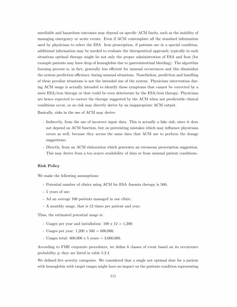
unreliable and hazardous outcomes may depend on specific ACM limits, such as the inability of

managing emergency or acute events. Even if ACM contemplate all the standard information

used by physicians to select the ESA Iron prescription, if patients are in a special condition,

additional information may be needed to evaluate the therapeutical approach; typically in such

situations optimal therapy might be not only the proper administration of ESA and Iron (for

example patients may have drop of hemoglobin due to gastrointestinal bleeding). The algorithm

learning process is, in fact, generally less efficient for unusual occurrences and this diminishes

the system prediction efficiency during unusual situations. Nonetheless, prediction and handling

of these peculiar situations is not the intended use of the system. Physicians intervention dur-

ing ACM usage is actually intended to identify those symptoms that cannot be corrected by a

mere ESA/iron therapy or that could be even deteriorate by the ESA/iron therapy. Physicians

are hence expected to correct the therapy suggested by the ACM when not predictable clinical

conditions occur, so no risk may directly derive by an inappropriate ACM output.

Basically, risks in the use of ACM may derive:

- Indirectly, from the use of incorrect input data. This is actually a fake risk, since it does

not depend on ACM function, but on preexisting mistakes which may influence physicians

errors as well, because they access the same data that ACM use to perform the dosage

suggestions;

- Directly, from an ACM elaboration which generates an erroneous prescription suggestion.

This may derive from a too scarce availability of data or from unusual patient conditions.

Risk Policy

We make the following assumptions:

- Potential number of clinics using ACM for ESA Anemia therapy is 500;

- 5 years of use;

- Ad an average 100 patients managed in one clinic;

- A monthly usage, that is 12 times per patient and year;

Thus, the estimated potential usage is:

- Usages per year and installation: 100 x 12 = 1,200;

- Usages per year: 1,200 x 500 = 600,000;

- Usages total: 600,000 x 5 years = 3,000,000.

According to FME corporate procedures, we define 6 classes of event based on its occurrence

probability p; they are listed in table 5.2.4

We defined five severity categories. We considered that a single not optimal dose for a patient

with hemoglobin with target ranges might have no impact on the patients condition representing

111

Table 5.3: Probability classes.

N Class Probability

6 Frequent p ≥ 10−2

5 Probable 10−3 ≤ p < 10−2

4 Occasional 10−5 ≤ p < 10−3

3 Remote 10−7 ≤ p < 10−5

2 Improbable 10−9 ≤ p < 10−7

1 Incredible p < 10−9

a not critical situation (lowest severity category). On the contrary, a continuous incorrect drug

regimen may lead the patients to irreversible dangerous conditions, including death. Severity

categories are described in table 5.2.4.

Examples of the different Severity Categories are the following:

- Negligible Risk, hemoglobin level slightly and temporary out of range due to an erroneous

ESA/Iron dosing. 9 < Hb < 10; 12 < Hb < 13. No evident sign or symptom. Dose

adjustment is sufficient for reestablishing patient condition within 1 month.

- Marginal Risk, hemoglobin level temporary out of range due to erroneous ESA/Iron dosing.

8 < Hb ≤ 9; 13 ≤ Hb < 14. Mild signs and symptoms of anemia or ESA/Iron over-dosage

appear. Consequent dose adjustments are sufficient for reestablishing patient condition in

a time period ≤ 2 months.

- Critical Risk, when hemoglobin levels are constantly out of target range, major symptoms

of treatment inadequacy appear. Continuous Hb < 9 or Hb > 13. In case of severe anemic

condition a strong intervention for correction is then needed (e.g. transfusion); in case of too

high hemoglobin concentration ESA therapy must be interrupted (Hb > 13 g/dl). Patients

dialyzed with arteriovenous fistula are more subject to develop site access thrombosis, this

aspect must be considered when evaluating the risks.

- Serious Risk, a completely erroneous high dose of ESA or Iron may cause severe adverse

cardiovascular reactions, stroke or death. Risk also varies depending on the vascular access

type. A prolonged ESA/Iron under-dosage may cause deterioration of the anemic status

and lead to death. Any medical intervention may be not sufficient to cease the exacerbation

of the patient condition and/or cause the death of one patient.

- Catastrophic Risk, it is not applicable in this case, ACM provides personalized suggestions,

thus a potentially wrong suggestion can affect only the patients for whom it has been

computed.

112

Table 5.4: Severity Categories.

N Class FME Definition Description

1 Negligible Malfunction without a signifi-

cant consequence

Reversible (in one month) and

non-life-threatening harm with

no symptoms

2 Marginal Evident temporary disturbance

of the well being of one patient,

user or third party per occur-

rence

Reversible and non-life-

threatening harm with mild

symptoms

3 Critical No death, but serious tempo-

rary deterioration in state of the

health of one patient, user or

third party per occurrence

Live threatening harm

4 Serious Death or serious deterioration in

the state of health with perma-

nent impairment of one patient,

user or third party per occur-

rence

Severe impairment of patient

conditions or death of one pa-

tient

5 Catastrophic Death or serious deterioration in

the state of health with perma-

nent impairment of more than

one patient, user or third parties

per occurrence

Severe impairment of several pa-

tients conditions or death of

more than one patient

As mentioned, both probability of an hazardous event and its severity have to be taken in

consideration to evaluate the risk. The idea behind this approach is that an hazard causing

severe consequences might be acceptable in case it happens very rarely, while an hazard with

milder consequences will not be accepted in case it is frequent. Therefore, having defined classed

of probability as well as classes of severity, we define the risk as the severity class multiplied

by the probability class. In this way a range of risks going from 1 (an hazard event occurring

very rarely, p < 10−9, with negligible consequences) to 30 (an hazard event occurring frequently,

p ≥ 10−2, with catastrophic consequences). Considering that, as explained above, ACM cannot

cause catastrophic events, the actual risk range is from 1 to 24.

According to corporate procedures, we define acceptances ranges as follows:

- Broadly acceptable: Risk < 10;

- As low as reasonably practicable (ALARP): 10 ≤ Risk < 15;

113

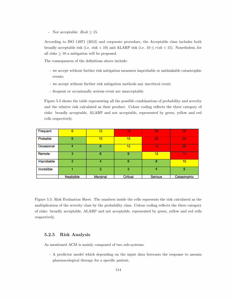
- Not acceptable: Risk ≥ 15.

According to ISO 14971 (2012) and corporate procedure, the Acceptable class includes both

broadly acceptable risk (i.e. risk < 10) and ALARP risk (i.e. 10 ≤ risk < 15). Nonetheless, for

all risks ≥ 10 a mitigation will be proposed.

The consequences of the definitions above include:

- we accept without further risk mitigation measures improbable or unthinkable catastrophic

events;

- we accept without further risk mitigation methods any uncritical event;

- frequent or occasionally serious event are unacceptable.

Figure 5.5 shows the table representing all the possible combinations of probability and severity

and the relative risk calculated as their product. Colour coding reflects the three category of

risks: broadly acceptable, ALARP and not acceptable, represented by green, yellow and red

cells respectively.

Figure 5.5: Risk Evaluation Sheet. The numbers inside the cells represents the risk calculated as the

multiplication of the severity class by the probability class. Colour coding reflects the three category

of risks: broadly acceptable, ALARP and not acceptable, represented by green, yellow and red cells

respectively.

5.2.5 Risk Analysis

As mentioned ACM is mainly composed of two sub-systems:

- A predictor model which depending on the input data forecasts the response to anemia

pharmacological therapy for a specific patient;

114

- An algorithm that using the predictor model extracts the optimal policy to achieve the

established clinical outcome for anemia management.

The predictor model is the base for the policy extractor that is the model used in runtime

environment to generate ESA Iron dosages suggestions. Considering this, the actual risk for

a wrong dosage suggestion is related to the possibility of an erroneous prediction of predictive

model. Our approach is therefore to evaluate the probability of an erroneous prediction and its

consequences in all those situations that could generate a risk for the patient.

First we examine the system using FMEA (Failure mode and effects analysis) and PHA (Process

Hazard Analysis) for different errors resulting in an observable (faulty) system behavior. An

example of a (faulty) system behavior is the wrong prediction of next hemoglobin level. ACM

elaborates therapy suggestions only if provided with the necessary information to perform the

prediction of ESA Iron therapy response; therefore, when not enough information is provided to

ACM no suggestion will be elaborated and physicians will have to perform their own prescription

as they normally do. No risk is therefore associated to possible erroneous ACM behavior due to

lack of information.

In a second step we evaluate hazards and respective risks caused by this system behavior. In

order to derive risks from hazards we assess the probability and the severity of the respective

harm. After the risk analysis, 24 risks have been identified trying to span all different cases,

from very low, through normal, up to very high hemoglobin’s values; a couple of examples of

defined risks are shown in tables 5.5 and 5.6. Probability is assessed using the available data, for

example for risk R0001 given the test dataset (X,Y ) where X ≡ (x1, · · · ,xN ) is the set of input

vectors (patient data as described in Chapter 4) and Y ≡ (y1, · · · , yN ) is the corresponding set

of output (next Hb level), the actual future hemoglobin HBa(t + 1) and the predicted future

hemoglobin HBp(t+ 1), the prediction error is e ≡ HBa(t+ 1)−HBp(t+ 1) we have:

p(Hb < 7g/dl|X) =

count(Hb < 7g/l)

N

p(e > 1.5g/dl|X) =e > 1.5g/l

NProbability = p(Hb < 7g/dl|X) · p(err > 1.5g/dl|X)

(5.6)

115

Table 5.5: Example of potential risk generated by the use of ACM.

Risk Number R0001

Cause(s) and conse-

quences

Patient is in special clinical conditions or erroneous data

are provided to ACM, thus the model does not contem-

plate some important information to correctly perform the

prediction of the next hemoglobin level Patient anemic sta-

tus is highly critical (Hb < 7g/dl). The predicted next

hemoglobin level overestimates the actual one of more than

1.5g/dl.

Probability 1 · 10−5

Comment In some peculiar situation it is possible that patient re-

sponse to therapy is strongly influenced by factors other

than those considered by the model. The model is thus

not able to correctly predict the next hemoglobin level and

specifically overestimates it. This could eventually lead to

an ESA Iron under-dosage.

Behavior ESA / Iron under dosage

Hazard Very critical anemic status not solved

Impact Patient

Severity Level 4

Probability Level 4

Risk Level 16

116

Table 5.6: Example of potential risk generated by the use of ACM.

Risk Number R0007

Cause(s) and conse-

quences

Patient is in special clinical conditions or erroneous data

are provided to ACM, thus the model does not contemplate

some important information to correctly perform the pre-

diction of the next hemoglobin level. Patient anemic status

is within target (11g/dl < Hb ≤ 12g/dl). Predicted next

hemoglobin level underestimate actual one which increase

for two consecutive months, error > 1.5g/dl

Probability 3 · 10−5

Comment In some peculiar situation it is possible that patient re-

sponse to therapy is strongly influenced by factors other

than those considered by the model. The model is thus

not able to correctly predict the next hemoglobin level and

specifically underestimate it. This could eventually lead to

an ESA Iron over-dosage.

Behavior ESA Iron over dosage

Hazard Patient goes over targets

Impact Patient

Severity Level 1

Probability Level 4

Risk Level 4

117

Risk Evaluation and Risk Control

Following step is to evaluate the identified risks and to mitigate them when possible. In our case

mitigation is basically the fact that ACM is just generating suggestions, thus the doctor can

evaluate and in case reject suggested doses that are not optimal for the patient. It is important

to distinguish between doses with an undesired but also unexpected outcome from those where

the undesired outcome can be expected. In the first case, that can be caused by different reasons

like intercurrent events or very unusual clinical condition, there is no real error from ACM and

the doctor would have most probably committed the same mistake, so in this case ACM is not

generating an additional risk. In the second case the doctor, by his experience and knowledge of

a specific patient, may have more information respect to ACM and identify that the suggested

dose is not optimal. Anyway it is very difficult to distinguish among these two situation, thus,

to be on the safe side, we considered any error from ACM to be potential a risk for the patient.

A mitigation is proposed for all the risks ≥ 10. In our case, this range includes both the

unacceptable risks and the ALARP risks. For the two risks presented as example the relative

mitigation is described in tables 5.7 and 5.8.

Table 5.7: Mitigation of Risk R0001.

Risk Number R0001

Risk Very critical anemic status not solved

Mitigation ACM just provides a therapy suggestion, physicians have to

evaluate patient conditions and to prescribe by themselves the

actual drug dosages; therefore in this case, as specified in the

user manual, if they have indications that ACM suggestions

may be wrong they will not follow it and, as they normally

do, they will formulate their own prescription and they will

perform any other action to solve understand patients critical

anemic status (i.e. transfusion). Probability level goes from 4

to 2. Severity level remains 4.

Table 5.8: Mitigation of Risk R0007.

Risk Number R0007

Risk Mild anemic status not solved

Mitigation No mitigation needed.

118

Finally figures 5.6 and 5.7 represent the risk evaluation sheets before and after risk control, it

can be noticed that after risk control no unacceptable risks remain.

Figure 5.6: Risk Evaluation Sheet before risk control, in each cell the corresponding number of risks

belonging to that category (Probability and Severity) is reported.

Figure 5.7: Risk Evaluation Sheet after risk control, in each cell the corresponding number of risks

belonging to that category (Probability and Severity) is reported.

5.3 ACM Clinical Evaluation

Anemia management in end-stage renal disease patients (ESRD) receiving hemodialysis and

treated by erythropoietic stimulating agents (ESA) has become over the last few years a com-

plex and challenging situation. On one side, best clinical practices require to achieve several

objectives at the same time, both at the patient and at the facility level. On the other side,

119

the complexity and the heterogeneity of ESRD population presenting with different medical

profiles and diverse sensitivity to ESAs need personalized and permanent dose adjustments of

ESA and iron supplementation. Briefly, anemia correction in ESKD patients is facing four main

challenges:

- Target hemoglobin levels have been reduced and window has been narrowed (10 to 12

g/dl) according to the results of main recent randomized trials [27, 108, 96] and a large

meta-analysis [98];

- Hemoglobin variability needs to be minimized to prevent undesired effects in fragile patients

[28],[121],[67].

- Dosage of erythropoietic stimulating agents has to be reduced to mitigate ESA-related

hazards [33].

- Cost-related issues have also emerged as an additional hurdle questioning cost-benefits value

of ESA to treat anemia in dialysis patients [105].

Target hemoglobin of 10 to 12 g/dl is narrow considering that must be reach for all for all ESRD

patients whatever the treatment modality or the medical state (fluid status, comorbid profile) of

the patient [92, 58, 70, 9]. Hemoglobin variability is a common pattern in hemodialysis patients,

observed in 82 to 90% of ESA treated patients [28, 29, 44].

Although controversial, this feature has been associated in several studies with poor outcomes

in ESRD patients [28, 121, 67, 102, 14, 89, 68, 99, 43]. Now, it is interesting noting that this

phenomenon is unanimously recognized, but still several concerns persist related to its definition

and/or quantification [121, 67, 53, 24] its causes [22, 23, 91, 1] and its clinical meaning and value

[116, 19].

ESA dosing regimen and ESA resistance are other serious concerns in anemia management of

ESKD patients. ESA resistance, observed in 10 to 20% of ESKD patients, is recognized as

an indicator of poor outcome usually associated with comorbid state and chronic inflammatory

state [122, 6, 90].

Cost-related issues of ESA treatment are a clear consequence of all undesired phenomena pre-

viously cited. In addition, this cost-related issue may override clinical benefits and patient

perceived value of ESA treatment.

Since the introduction of ESAs and IV Iron, most of the clinical trials have focused on hemoglobin

and iron targets in ESKD patients. There is a shortage of clinical trials studying the optimal

strategy for treating anemia and iron repletion in order to reduce hemoglobin variability and

ESA consumption. The importance of guided clinical protocols for managing ESA and iron have

been highlighted by several studies [49],[42].

In recent years, a variety of predictive algorithms based on sophisticated modeling approaches

have been proposed to predict Hb levels in ESRD patients and to offer a personalized treatment;

120

their promising results suggest that such approaches can be powerful tools for anemia manage-

ment in dialysis patients [18, 36, 40, 41, 50, 73, 74, 75]. Some of these algorithms have also been

tested in a clinical setting, albeit often on relatively small cohorts of patients [17, 38, 86, 77].

All these factors have thus to be considered when evaluating the clinical impact of ACM imple-

mentation as guidance for the anemia management.

5.3.1 Study design and statistical analyses

We performed a two-years evaluation (June 2012 June 2014) consisting in two periods: the

first period was considered as the control phase (standard care of anemia treatment), lasting

12 months before implementing ACM guidance; the second period was considered as the inter-

ventional phase (ACM guided care of anemia treatment), lasting additional 12 months. ACM

was implemented in four FME clinic: Motol Prague (CZ), Cartagena and San Pedro del Pinatar

(SP), and Lumiar (PT).

Patients treated in FME network are informed that their data collected through the clinical

system EuCliD might be used for scientific purposes and they are asked to sign a consent form

if they agree. All data were anonymized when transferred to the calculation center and were

disclosed only to their referent physician.

The study was conducted in compliance with recognized international standards and approved

by FME Medical Board. Standard anemia management relies on a stepwise protocol that was

implemented in the network since February 2012 consisting in these guidelines:

- Both ESA (darbepoetin) and iron (iron sucrose) therapies are administrated in the blood

venous line, after the dialyzer, at the end of dialysis session to maintain the hemoglobin

target in the range 10-12 g/dl and the ferritin target in the range 450-650 ng/mL, respec-

tively

- No suggestion is given for administering ESA and iron on a specific day of the week

- Dry body weight probing and fluid management are guided monthly by body composition

evaluation through multi-frequency bioimpedance spectroscopy (BIA)

- Eryhtropoietic response is monitored using usual hematology parameters (MCV, TSAT,

MCHC) and inflammation marker (CRP) No regular supplementation in vitamins and/or

nutrients and/or trace elements is requested. This supplementation relies on deficiencies

when needed.

The effects of ACM were assessed both at the dialysis facility level and at the patient level using

traditional key indicators of anemia treatment as primary outcome and mortality, cardiovascular

events, hospitalizations and transfusions as secondary outcome.

At the dialysis facility level, the percentage of hemoglobin in target (10-12 g/dl) and the mean

ESA administered dose (considered as ESA consumption expressed as dose per patient per

121

kg per month) were considered as primary outcome, a sub analysis was performed for the

confirmed recommendations. Cardiovascular events, identified by means of ICD-10 coding, were

classified as follows: death from cardiac origin, intercurrent cardiovascular event, occurrence

of new cardiac condition, or hospitalization due to cardiovascular event. All circulatory events

including cerebrovascular, peripheral arterial and vein diseases were considered as cardiovascular

diseases. In this analysis all patients treated in the four clinics where ACM was implemented

have been considered.

At the patient level, the hemoglobin trend over time has been evaluated too. For consistency,

only patients who had 6 months minimum of regular monthly anemia follow up both before

and after ACM entrance were included in this analysis. Individual hemoglobin fluctuation was

estimated from hemoglobin standard deviation over the period of observation as well as the

percentage of hemoglobin values in target. The same parameters were evaluated also for the

sub-population where at least 2/3 of the suggestions were confirmed. These parameters were

also separately analyzed for patients grouped according to their vascular access (AV fistula or

graft and catheter). All analyses were performed in Matlab. The t-test was used to compare

normally distributed data; Wilcoxon test was used on non-normally distributed data; Fisher test

was used for proportions. When applicable, data were expressed as mean ± standard deviation.

For all the tests, a p-value less than 0.05 was considered statistically significant.

5.3.2 Results

Outcome at dialysis facility level

Baseline characteristics of ESKD patients participating in the study are presented in Table 5.9.

It must be noticed that 60% of the patients are part of both populations, that is, they were

treated in the pilot clinics both before and after ACM introduction. As shown in the Table,

the two populations that contributed to the study (before and after ACM entrance) were quite

similar both in clinical characteristics and laboratory data.

Primary (percentage of hemoglobin in target, ESA and Iron consumption) and secondary out-

comes (deaths, hospitalizations, cardiovascular events and transfusions) are presented in Table

5.10. Results are shown as mean ± SD for the two periods, with the respective p-values. It

is of interest noting that with guided care Darbepoetin and iron consumption decreased by

12% and 7.5% respectively, while at the same time the percentage of hemoglobin values within

target (10-12 g/dl) increased by 6.8%. Moreover, the contribution of ACM may be underlined

by the percentage of hemoglobin values in target when the ACM suggestions were confirmed,

which reaches 83.5%, whereas for not confirmed suggestions the in-target percentage is just

65.7%. Regarding secondary outcomes, all adverse events consistently tend to decrease after

ACM entrance while not reaching statistical significance, but that could be due to their relative

low prevalence and/or to the too short period of observation. The effect of vascular access on

122

primary outcome has been analyzed separately. Results are presented in table 5.11 using the

same key indicators but divided in two categories as AV fistula/graft and central venous catheter

(CVC). Interestingly, it can be noted that only patients with AV fistula/graft reduced Darbo and

iron consumptions, by 18% and 10% respectively, after ACM entrance. In patients bearing CVC,

Darbepoetin and iron consumptions did not change after entering ACM supported care. In addi-

tion, one can note that Darbepoetin and iron consumption are 41% and 28% respectively higher

with CVC compared to AV fistula/graft. Nevertheless, the role of ACM appears beneficial for

both types of vascular accesses. Percentage of hemoglobin in target is 84.6% and 75.9% with AV

fistula/graft and CVC respectively after acceptance of ACM suggestion, while it falls to 69.2%

and 51.4% when ACM suggestion was not accepted. The role of C-reactive protein concentra-

tions on ACM performance is difficult to assess in this study. Frequency of CRP measurements

were not comparable in the different countries and in the two periods of the study. In Portugal

(Lumiar) only 36 measurements, mainly infected patients, were performed during the year before

ACM implementation, while 1062 measurements were performed after ACM implementation. In

Spain (Cartagena), 1258 measurements were performed before ACM enrollment and 1077 after.

In this case, CRP remained stable over the two periods, 10.69(±19.03) and 10.41(±17.00). In

Czech Republic (Motol), we had 367 measurements before and 988 measurements after ACM

enrollment. In this case, CRP decreased from 19.85(±38.23) to 8.26(±18.57). Putatively this

effect may be partially attributed to the significant reduction of IV Iron administration during

ACM supported care period in this clinic.

123

Table 5.9: Patients’ characteristics in the two periods under study in the population analysis

Control ACM guidance p-value

Nr. of Patients 656 645

Age (years) 63.59± 15.54 63.84± 15.46 0.7755

gender (% of men) 62.5%) 61.8%) 0.8193

Pts initiating RRT 71(10.8%) 66(10.2%) 0.7865

Comorbidities

Coronary Artery Disease 9.1% 8.7% 0.7715

Congestive Heart Failure 22.4% 22.6% 0.9471

Peripheral Vascular Disease 28.5% 28.7% 0.9511

Cerebrovascular Disease 17.4% 17.8% 0.8843

Chronic Pulmonary Disease 14.6% 14.3% 0.8749

Diabetes 31.3% 30.7% 0.8573

Charlosn Index 6.45± 3.93 6.56± 3.93 0.6545

Etiology

Diabetes 21.5% 22.0% 0.8404

Hypertension 19.1% 19.7% 0.7794

Ch. Glomerulonephritis 21.8% 20.9% 0.7353

Urinary Obst/Ch Int Nephritis 1.7% 1.6% 0.9999

Polycystic 5.9% 6.4% 0.8177

Others 30.0% 29.5% 0.7154

Vascular Access

Fistula 65.2% 65.4% 0.9536

Catheter 20.1% 18.9% 0.6245

Graft 14.6% 16.3% 0.4443

Treatment Modality

HDF Online 93.0% 92.6% 0.4681

HD 5.0% 6.0% 0.4676

Others 2.0% 1.4% 0.4443

Laboratory Test Values

Hemoglobin (g/dl) 11.32± 1.08 11.19± 1.07 0.0225

Ferritin (g/dl) 651.2± 572.1 629.9± 409.4 0.4441

TSAT (%) 31.9± 10.9 32.4± 10.0 0.4192

Albumin (g/dl) 3.90± 0.45 3.92± 0.38 0.4414

Calcium (mg/dl) 8.79± 0.60 8.92± 0.62 < 0.001

Phosphate (mmol/l) 4.37± 1.07 4.30± 1.02 0.2112

Potassium (mmol/l) 4.95± 0.65 4.92± 0.62 0.4499

PTH (ng/l) 353.1± 304.4 356.3± 315.3 0.8526

EKTV 1.67± 0.42 1.70± 0.31 0.5365

SPKTV 1.90± 0.47 1.94± 0.36 0.4549

124

Table 5.10: Primary and secondary outcomes at facility level.

Control ACM p-value

Consumptions

Darbepoetin consumption per month per patient (g/mo) 75.94± 107.57 66.51± 90.19 < 0.001

Darbepoetin quantity per month per patient per kg

(g/kg/mo)

1.14± 1.62 1.01± 1.41 < 0.001

Iron quantity per month per patient (mg/mo) 166.93± 199.68 154.54± 164.03 < 0.001

Iron quantity per month per patient per kg (mg/kg/mo) 2.47± 2.97 2.30± 2.52 < 0.001

Hb Control: % of Hb in target

All (6498 Hb measurements) 70.8% 77.6.% < 0.001

Darbo confirmations: 4327 Hb measurements (66.59 %) 83.5%

Darbo not confirmed: 2171 Hb measurements (33.41 %) 65.7%

Secondary outcomes

Deaths 60(9.1%) 42 (6.5%) 0.0803

Num cardio events per patient 0.43± 0.86 0.37± 0.81 0.2364

Patients with cardio events 27.4% 24.8% 0.2841

Hospitalization days per patient 6.65± 15.89 5.69± 12.85 0.2341

Num of transfusions per patient 0.46± 1.32 0.31± 1.04 0.1629

Patients with transfusion events 6.55% 4.34% 0.0877

125

Table 5.11: Primary outcomes at facility level divided by vascular access.

Control ACM p-value

PATIENTS WITH FISTULA

Consumptions

Darbepoetin consumption per month per patient (g/mo) 72.59± 106.67 59.68± 82.61 < 0.001


(g/kg/mo)

1.10± 1.61 0, 92± 1.31 < 0.001

Iron quantity per month per patient (mg/mo) 161.22± 194.99 145.10± 159.00 < 0.001

Iron quantity per month per patient per kg (mg/kg/mo) 2.39± 2.89 2.16± 2.44 < 0.001


All (5352 Hb measurements) 72.0% 80.0.% < 0.001



PATIENTS WITH CATHETER

Consumptions

Darbepoetin consumption per month per patient (g/mo) 93.23± 110.9 101.04± 115.5 0.9642


(g/kg/mo)

1.36± 1.66 1.51± 1.73 0.8691

Iron quantity per month per patient (mg/mo) 194.02± 219.55 202.34± 180.06 0.5823

Iron quantity per month per patient per kg (mg/kg/mo) 2.84± 3.29 3.04± 2.79 0.3123


All (1049 Hb measurements) 63.9% 64.3% 0.7509



126

Outcome at patient level

In order to evaluate the effect of ACM guidance at patient level and assess whether is there any

impact on hemoglobin cycling we focused just on patient with a sufficiently long and continuos

anemia follow up both before and after ACM entrance. In Figure 5.8 the selection flow chart

of ESKD patients enrolled in the Hemoglobin trend analysis is reported. Within the considered

population 460 patients had at least 6 months of follow up both before and after ACM entrance

and thus included in the analysis: 77 patients were excluded because of missing hemoglobin

values in the temporal series, main reasons being hospitalizations and vacations; among the

remaining 383 patients, 234 had 66% of confirmations or more. Table 5.12 shows the character-

istics of two cohorts of patients: entire population (all patients); selected population (> 66.6%

confirmed) consisting in 234 patients for whom at least 2/3 of ACM suggestions were confirmed

by physicians.

Figure 5.8: Flow chart schematizing the patient enrolment criteria for the analysis at patient level.

Drop out reasons and final number of patients included in the analyses are outlined.

Primary and secondary outcomes of ESKD patients enrolled in the ACM support process are

reported in Table 5.13. ACM entrance brought a slight increase in the variability of Darbepoetin

doses, measured as mean difference between subsequent Darbo doses (Mean Absolute Delta

Darbo Doses in table 5.13). Nevertheless, at the same time ACM entrance lead to a considerable

decrease in Hb fluctuation together with a significant increase in the percentage of patients

with hemoglobin values in target. Figure 5.9 shows the distributions of hemoglobin standard

deviations, used as a proxy of hemoglobin variability, before and after ACM entrance in the

two cohorts ((a) All patients; (b) Selected patients). In both cohorts, hemoglobin variability

decreased after ACM entrance, this effect being stronger in patients having a high percentage

of confirmed ACM suggestions (Figure 5.9 b).

Figures 5.10 and 5.11 show the clinical evolution for two sample patients, including hemoglobin

concentrations (top panel) and corresponding therapeutic interventions (middle and lower panel)

over time of study. The vertical dotted line represents ACM entrance; each Hb data point is

paired with the ESA/iron dose suggested by ACM at that point in time. Green circles represents

Hb values resulting from an ACM suggestion confirmed by the physician. These two patents

127

Figure 5.9: Histograms of Hb standard deviations before and after ACM entrance: a) histograms

related to all patients data; b) histograms related to patients having at least 66.6% of confirmed ACM

suggestions.

are interesting because they have an history of hemoglobin cycling, so they can be considered

complex and for them outcomes have not been achieved. Another important aspect of this two

patients is that for them physicians decided to constantly follow ACM suggestions with just an

exception for the first suggestion for patient in 5.11. In general it can be noticed that after ACM

entrance, hemoglobin values were stabilized. In particular the case of 5.11 is very interesting; first

ACM suggestion was to interrupt ESA therapy, even if hemoglobin was in target (point on the

dotted line), the physician in this case didn’t accept the suggestion and continued the EA therapy,

the result of this was that hemoglobin of next month was above target. After that, the physician

started to trust ACM and to constantly accept the suggestions. Patient outcomes before and

after ACM support, both for the global and the selected group of patients, are presented in Table

5.13. In both groups, hemoglobin variability is reduced quite consistently, ESA consumption is

reduced and the percentage of patients in target is increased after ACM entrance. Interestingly,

secondary outcomes also tend to improve after ACM entrance, particularly in the group with

ACM suggestions mostly accepted. In this latter case, the incidence of adverse events decreased

almost uniformly. Patients were also grouped based on their vascular access (AV fistula/graft

and catheter), and primary outcomes were evaluated separately for these two groups (see Tables

5.15 and 5.3.2). Interestingly, a decrease in Hb variability and an increase of patients with Hb

in target is noticeable in all sub-groups. This trend is also more marked in the group of patients

with approved ACM suggestion. Nevertheless, it is of note that Darbepoetin consumption

decreased by 22% only in patients with AV fistula/graft, whereas in patients with catheter the

dose remained unchanged or higher.

128

Figure 5.10: Hb series and ESA/Iron administrations for a sample patient (1). At the top, Hb

temporal evolution for a sample patient is plotted. The vertical dotted line represents the time of

ACM introduction, green circles identify Hb values resulting from confirmed suggestions. The central

and bottom part of the figure show administrations of ESA and Iron, respectively.

129

Figure 5.11: Hb series and ESA/Iron administrations for a sample patient (2). In this case, the first

ACM suggestion was not confirmed (as marked by the red circle on the resulting Hb value), whereas

all subsequent ones were. Correspondingly, a reduction in Hb cycling can be observed.

130

Table 5.12: Characteristics of the two cohorts of patients analyzed in the patient longitudinal analysis.

All patients > 66% of confirmations

Nr. of Patines 383 234

Average follow up peridod (months) 11.1± 1.6 11.0± 1.8

Age (years) 65.2± 14.9 65.5± 14.7

Gender (% of men) 59.3% 58.5%

Comorbidities

Coronary Artery Disease 8.6% 7.7%

Congestive Heart Failure 21.4% 20.9%

Peripheral Vascular Disease 29.8% 30.3%

Cerebrovascular Disease 18.5% 19.2%

Chronic Pulmonary Disease 15.1% 16.7%

Diabetes 22.7% 30.3%

Charlosn Index 7.8± 3.1 7.9± 3.0

Etiology

Diabetes 19.6% 22.2%

Hypertension 18.0% 20.5%

Ch. Glomerulonephritis 23.0% 20.1%

Urinary Obst/Ch Int Nephritis 2.6% 1.7%

Polycystic 6.5% 4.7%

Others 30.3% 30.8%

Vascular Access

Fistula 68.9% 70.1%

Catheter 13.8% 13.9%

Graft 17.2% 16.0%

Treatment Modality

HDF Online 94.0% 94.4%

HD 4.0% 2.4%

Others 2.0% 3.2%

131

Table 5.13: Outcomes of the patient longitudinal analysis. The top of the table shows results for the

larger group of patients, whereas the bottom part shows outcomes for patients having at least 2/3 of

ACM suggestions confirmed.


All patients (383)

Primary Outcomes:

Hb standard deviation (g/dl) 0.95± 0.41 0.83± 0.33 < 0.001

Patients with more than 66.6% of Hb in target 46.0% 58.7%) < 0.001

Mean Darbo Doses (µg) 73.64± 93.61 59.29± 70.13 < 0.001

Mean Absolute Delta Darbo Doses (µg) 24.54± 30.98 31.05± 28.22 < 0.001

Mean Ferritin (µg/l) 645.60± 480.12 669.46± 386.50 < 0.005

Std Ferritin (µg/l) 192.22± 148.27 163.36± 106.22 < 0.001

Mean Absolute Delta Iron Doses (mg) 76.08± 66.36 75.81± 46.82 0.9504

Secondary Outcomes:






Patients with at least 66.6% of confir-

mations (234)

Primary Outcomes:




Mean Absolute Delta Darbo Doses (µg) 26.02± 27.51 32.05± 27.27 0.011

Mean Ferritin (µg/l) 748.22± 508.09 763.28± 392.96 0.3229

Std Ferritin (µg/l) 218.99± 161.64 176.01± 109.08 < 0.001


Secondary Outcomes:






132

Table 5.14: Outcomes of the patient longitudinal analysis for the cohort of patient treated with

catether. The top of the table shows results for the larger group of patients, whereas the bottom part

shows outcomes for patients having at least 2/3 of ACM suggestions confirmed.

Table 5.15: Outcomes of the patient longitudinal analysis for the cohort of patient treated with fistula

or graft. The top of the table shows results for the larger group of patients, whereas the bottom part

shows outcomes for patients having at least 2/3 of ACM suggestions confirmed.


Patients with Fistula or Graft (330)

Primary Outcomes:






Std Ferritin (µg/l) 195.07± 154.49 164.91± 108.58 < 0.001


C-Reactive Protein (mg/l) 11.78± 17.73 10.08± 13.12 0.2262


mations (200)

Primary Outcomes:

Hb standard deviation (g/dl) 0.98± 0.43 0.770.26 < 0.001





Std Ferritin (µg/l) 224.33± 170.00 181.09± 113.21 < 0.001



133


Patients with catether (53)

Primary Outcomes:

Hb standard deviation (g/dl) 0.99± 0.37 0.86± 0.36 0.0732

Patients with more than 66.6% of Hb in target 47.5% 61.7%) 0.1721

Mean Darbo Doses (µg) 89.95± 90.05 95.28± 92.33 0.7653



Std Ferritin (µg/l) 176.56± 107.58 152.24± 87.71 0.2132




mations (200)

Primary Outcomes:



Mean Darbo Doses (µg) 85.85± 94.43 97.07± 83.88 0.6229



Std Ferritin (µg/l) 191.45± 106.24 137.09± 57.46 0.0186



134

5.3.3 Discussion

In this international (involving three countries) pilot study, we performed a direct comparison

between standard anemia management (by expert nephrologists following established guidelines)

and ACM supported anemia management. To our knowledge, this is the first interventional study

conducted at a large scale in an unselected population of patients on dialysis (common population

characteristics) comparing the standard care of anemia treatment based on best clinical practices

with a guided care. The results at facility level showed that implementation of a decision

support system (ACM) is feasible, acceptable and helpful for physicians in a large dialysis

network, improving anemia treatment outcomes. Briefly, hemoglobin target was achieved and

maintained in a larger proportion of patients (from 70.8% to 77.6%), and Darbepoetin and iron

consumption were significantly reduced over time (12.4% and 9.2%, respectively). Transfusions,

and cardiovascular morbidity and mortality tend to be reduced but significance was not achieved,

likely due to unpowered size of events. Similar results were obtained at patient level, with a

significant decrease in hemoglobin standard deviation after ACM entrance (from 0.95± 0.41 to

0.83 ± 0.33 gr/dl). All these indicators are even stronger when considering those cases when

ACM suggestions were approved. Our results showed that a decrease in Hb variability and an

increase in the percentage of patients having at least 66.6% of Hb in target can be observed

in all the analyzed sub-groups; again, this trend is stronger for patients with high percentage

of confirmations. Nevertheless a decrease in mean Darbepoetin dose can be observed only in

patients having a fistula as vascular access. This finding is not against the validity and the

accuracy of the ACM, but rather underlines the deleterious effects of catheter use on ESA

consumption (blood loss, inflammation) as reported by others.

Our findings suggest that tight control of anemia is better achieved by means of the ACM support

tool, minimizing fluctuations and hazards of human prescription. ACM provides a feedback

control loop closer to physiologic regulation, and reduces prescription patterns that may react

too quickly to hemoglobin concentration changes. ACM guided prescription integrates past Hb

trend variations and is likely to provide a buffer period of ESA and iron dose adjustment.

The present study has some limitations. It is not a randomized or blinded controlled trial, and the

monitoring period is not long enough to assess the impact of the ACM model on cardiovascular

morbidity and mortality related to anemia management. Now that the ACM is set and in place,

we will extend the follow-up period to assess secondary outcomes, short term acting ESA will be

included in the model to generalize the use to the entire dialysis network, with a more specific

cost-effectiveness monitoring.

135

Chapter 6

Conclusions and future work

6.1 General summary

The aim of this thesis has been to describe the development of the Anemia Control Model (ACM),

a tool designed to support physicians in managing anemia for ESRD patines undergoing dialysis.

Five main pillars constitute the foundation of this work:

- Understanding the medical problem;

- Availability of the data needed to derive the models;

- Mathematical and Machine Learning modeling;

- Development of a product usable at the point of care;

- Medical device certification and clinical evaluation of the developed product.

The understanding of the medical problem is fundamental for two reasons: firstly because the

medical problem must be the driver of the product scope and consequently of its design; secondly

because a good understanding of the medical problem is of fundamental importance to develop

optimized models. In the case of anemia management the drug dosing is an important task where

predictive models could support physicians to improve the treatment quality. In particular,

considering that hemoglobin is the typical parameter used to measure anemia, our model were

tailored to predict hemoglobin response to the two main drugs normally used to correct anemia,

that is ESA and Iron. In a mathematical model based on differential equations, like the one

presented in this thesis, the knowledge of the main physiological processes related to anemia

is the base to properly design the equations. A machine learning approach in principle can be

built with no hypotesis, because it relays in learning from data, nevertheless knowledge of the

137

domain helps to make better use of the available data. The medical problem has been discussed

in Chapter 1.

The availability of a huge database of very well structured data was basic for the development of

models. Quality of the data is another important aspect. Chapter 2 gives the reader an overview

of the available data..

The core of the ACM is the capability to predict for each patient the future hemoglobin concen-

trations as a function of past patient’s clinical history and future drug prescription. By means

of well performing and personalized predictive model it is possible to simulate how, for each

specific patient, different doses would affect hemoglobin trends. Mathematical and machine

learning models present both advantages and limitations. Chapter 3 describes the mathemati-

cal model and analyzes its performances, while Chapter 4 is dedicated to the machine learning

models. In our case the machine learning approach resulted more suitable for our scope, because

its was well performing on the entire population, more stable and, once trained, very quick in

elaborating the prediction.

Once the predictive model was obtained, the next step was to wrap it into a service that could

be consumed by a third party system (for example an app or a clinical system) where physicians

could benefit from the model prediction capability. To achieve that, firstly an algorithm for

the dose selection was developed; secondly, a data structure for the communication with the

third party system was defined; finally, the whole package was wrapped in a web service. These

arguments have been discussed in the first part of Chapter 5.

Mistakes in ESA or Iron dosing might have serious consequences on patients’ health, for this

reason ACM intended use was limited to provide dose suggestions only; physicians must evaluate

them and decide whether to accept or reject them. Nevertheless, such a tool could be considered

as Medical Device under European Medical Device Directive (MDD); for this reason, to be on

the safe side, it was decided to certify the ACM as medical device. A novel approach was

developed to perform the risk assessment, the main idea being that ACM might generate risks

when a dose suggestion is produced based on a wrong prediction. To assess this risk the model

error distribution over the test set was utilized as estimation of the error distribution of the

live system. Finally, a clinical evaluation of the ACM in three pilot clinics has been performed

before deciding to roll-out the tool in more clinics. These arguments have been discussed in the

second part of Chapter 5.

6.2 Scientific Publications

Several scientific results have been produced during the development of this thesis, described in

a number of scientific publications, which are here listed:

- Barbieri, C., Bolzoni, E., Mari, F., et al., (2016), ”Performance of a Predictive Model

for Long-Term Hemoglobin Response to Darbepoetin and Iron Administration in a Large

138

Cohort of Hemodialysis Patients”, PLOS one, 11(3): e0148938

- Barbieri, C., Mari, F., Stopper, A., et al., (2015), ”A new machine learning approach for

predicting the response to anemia treatment in a large cohort of End Stage Renal Disease

patients undergoing dialysis.”, Computers in Biology and Medicine 2015; 61:56-61;

- Martinez-Martinez, J.M. Escandell-Montero, P, Barbieri, C., et al., (2014), ”Prediction

of the Hemoglobin level in hemodialysis patients using machine learning techniques.” Com-

puter Methods and Programs in Biomedicine, vol 117, pp 208217;

- Escandell-Montero, P., Chermisi, M., Martnez-Mart, J.M., Gmez-Sanchis, J., Barbieri,

C., et al., (2014), ”Optimization of anemia treatment in hemodialysis patients via rein-

forcement learning, Artif. Intell. Med. 62 (1), 4760;

and the oral communication:

- Molina, M., Barbieri, C., Albaladejo, M., et al., (2016), ”APLICACION DE UN MOD-

ELO DE INTELIGENCIA ARTIFICIAL EN EL CONTROL DE LA ANEMIA DEL PA-

CIENTE EN HEMODILISIS: VARIABILIDAD.”, XXXVIII Congreso Anual de la Sociedad

Espaola de Dialisis y Trasplante.

In addition to the publications listed above, the paper ”An international observational study

suggests that artificial intelligence for clinical decision support optimizes anemia management

in hemodialysis patients.”, by Barbieri, C., Molina., M., et al., which summarizes the results

of the ACM implementation in the pilot clinics (as described in Chapter 5), has been accepted

by the journal Kidney International. At this stage it is not possible to make a reference to this

paper because it has not yet been published.

6.3 Latest results and future work

This dissertation thoroughly describes the journey for developing the ACM, where, with respect

to the erythropoiesis stimulating agent (ESA), we focused on IV Darbepoetin. The reason

behind this choice was that this particular ESA was the most used one in the countries selected for

piloting the ACM. Another ESA very commonly used is Epoetin Beta. Epoetin Beta, differently

from Darbepoetin which is a long acting ESA (half life in blood around 24 hours), is a short

acting ESA (half life in blood of around 8 hours). Even being two different types of drug, when

applying machine learning techniques, the approach can be exactly the same, indeed a predictive

model for Epoetin Beta was also developed, and the results were very similar with respect to

the Darbepoetin model. Therefore now the ACM is able to manage (i.e. to provide suggestions)

also to patients treated with Epoetin Beta, because the type of ESA is now an additional input

parameter of the ACM, which, based on it, selects the proper algorithm to be used. After the

good results of the pilots, ACM has been rolled out in more clinics, very positively, all results

139

achieved in the pilots have been confirmed in a larger patient population, obtaining also in this

case an increase of hemoglobins in target, a reduction of hemoglobin cycling and a reduction in

ESA consumption.

Future work can be divided into two main streamlines:

- Development of a predictive model for Mircera (another type of ESA);

- Replication of the ACM paradigm for other dialysis related conditions, like for example the

Mineral Bone Disorder (MBD).

Half life of Mircera is around 140 hours, which is significantly longer than that of Darbepoetin

. From one side this pharmacokinetic characteristic of Mircera makes its action more similar

to the physiological action of endogenous EPO, which is continuously produced in a healthy

individual. From the other, if an erroneous dose is administered its effects last much longer,

making a correction much more difficult, specially when the dose was higher than the needed

one. For this reason a predictive model anticipating the long term effect of a Mircera dose might

be a very useful tool to support physicians.

MBD is another common condition of dialysis patients and, like in the case of anemia, it requires

a proper drug therapy, which it is often very difficult to assess. Without giving details about

which drugs are used to treat the MBD and how they interact with the very complex biochemical

mechanisms behind this condition, what can be underlined is that, with respect to anemia where

only ESA and Iron come into play and the main challenge is the dosing, in the case of MBD

dosing it is just one part of the physicians’ tasks. Indeed, the first challenge that a physician must

face is to select the combination of drugs that better suit for the specific patient condition, once

this task is performed the following step is to properly adjust the dosing. Another difference with

respect to the anemia is that for MBD more than one parameter have to be optimized, namely

Calcium, Phosphorus and Parathyroid Hormone (PTH) blood concentration. Considering those

aspects, the first main challenge from the modeling perspective is to develop a predictive model

with multiple outputs and which is able to work with different combinations of drugs. A second

challenge would be to develop a reward function which is able to manage situations where not

all three targets can be achieved; in other words, a reward function that it is able to measure

what is more important for the patient, and thus to sacrifice the achievement of an outcome of

a specific parameter in favour of the outcome of another one.

6.4 Final Conclusions

Chapter 4 of this thesis describes the predictive model which is the core of the decision support

tool for anemia management, the Anemia Control Model (ACM). Precision of the model was

measured in terms of Mean Absolute Error in prediction, which resulted inferior to 0.6g/dl.

Another important measure is that 92% of errors were lower than 1g/dl. European best practice

140

as well as FME internal guidelines establish the target range of 10− 12g/dl for hemoglobin con-

centration, thus we could assume that the performance of the predictive model makes it suitable

for a potential application in real clinical practice, specially if compared with the difficulties of

achieving guidelines targets. In addition to that, the model is very robust, it has been developed

and validated over a very large and composite patients population and resulted in having very

stable performances also in the set of unseen examples (the test set). This means that the model

is working with similar performances on patients with very diverse characteristics. These results

demonstrate that the first objective of this work, that is to develop a robust and sufficiently

precise predictive model for future hemoglobin blood concentration, was successfully achieved.

Some key points of the obtained predictive model for hemoglobin concentration have to be

highlighted:

- Drug dosages is one of the main predictor of hemoglobin variation;

- Once compiled the model is very quick in processing patient data, thus it is possible to

simulate for each patient how his/her future hemoglobin will be affected by different doses;

- These simulations allow to select which dose achieve the desired clinical targets, this selec-

tion is a deterministic process.

- The selected dose can be proposed as a suggestion to the physician, which will be ultimately

in charge to perform the actual prescription;

- The combination of the predictive model and the dose selection algorithm has been wrapped

in a web service, defining a communication protocol between the ACM and potentially any

third party system able to provide the model with the necessary data;

- Results of the predictive model on the test set provide a good estimation of the possible

prediction errors in a live setting.

These facts allowed to develop a tool actually useable at the point of care and whose safety for

the patient could be estimated. These two factors represent another important achievement of

the presented work.

Indeed the ACM has been evaluated in an international (involving three countries) clinical evalu-

ation, where a direct comparison between standard anemia management (by expert nephrologists

following established best clinical practices) and ACM supported anemia management has been

performed. Purpose of the ACM is to facilitate the physicians decision-making in devising a

personalized anemia therapy for their patients. At facility level, after ACM introduction the

percentage of hemoglobin values within target range increased, the ESA and Iron consumption

decreased, and hemoglobin cycling was reduced. Our work confirms that a decision support sys-

tem based on predictive modeling can achieve improvements in a large, unselected population of

patients. In addition, it provides a clinical proof of the beneficial effects of deploying the ACM

in everyday practice, as part of the nephrological routine practice. In summary, our findings

141

confirm that a tighter control of anemia can be achieved by means of ACM support, therefore

the third main objective of this work has been successfully accomplished.

142

Bibliography

[1] Agarwal, R., Davis, J. L., Smith, L., (2008), ”Serum albumin is strongly associated with erythro-

poietin sensitivity in hemodialysis patients.”, Clin J Am Soc Nephrol; 3: 98-104

[2] Agoram B., Sutjandra L., Sullivan J.T., (2007), Population pharmacokinetics of darbepoetin alfa

in healthy subjects., British journal of clinical pharmacology, vol. 63, no. 1, pp. 41-52.

[3] Akabua, E., Inanc, I., Gaweda, A. E., et al., (2015), ”Individualized model discovery: The case of

anemia patients.” Computer Methods and Programs in Biomedicine 118:23-33

[4] Allon M., Kleinman K., Walczyk M., Kaupke C., et al., (2002), ”Pharmacokinetics and pharmaco-

dynamics of darbepoetin alfa and epoetin in patients undergoing dialysis.”, Clinical Pharmacology

& Therapeutics 72, no.5, pp. 546-555

[5] Arbib M. A., (2002), ”The Handbook of Brain Theory and Neural Networks.”, Second Edition,

The MIT Press.

[6] Barany P., Divino Filho J.C., Bergstrom J., (1997), ”High C-reactive protein is a strong predictor

of resistance to erythropoietin in hemodialysis patients.” Am J Kidney Dis 29: 565-568.

[7] Barbieri, C., Bolzoni, E., Mari, F., et al., (2016), ”Performance of a Predictive Model for Long-Term

Hemoglobin Response to Darbepoetin and Iron Administration in a Large Cohort of Hemodialysis

Patients”, PLOS one, 11(3): e0148938

[8] Barbieri, C., Mari, F., Stopper, A., et al., (2015), ”A new machine learning approach for predicting

the response to anemia treatment in a large cohort of End Stage Renal Disease patients undergoing

dialysis.”, Computers in Biology and Medicine 2015; 61:56-61

[9] Barrett B. J., Fenton S.S., Ferguson B., et al., (1999), ”Clinical practice guidelines for the manage-

ment of anemia coexistent with chronic renal failure. Canadian Society of Nephrology.”, JAmSoc

Nephrol, 10(Suppl 13):S292-S296,

[10] Belair J., Mackey M. C., Mahaffy J. M., (1995), ”Age-structured and two-delay models for ery-

thropoiesis.”, Math Biosci 128, 317-346.

[11] Bellazzi, R., Siviero, C., (1994) ”Mathematical modeling of erythropoietin therapy in uremic ane-

mia. Does it improve cost-effectiveness?”, Hemoglobin pp. 154-164.

[12] Besarab A., Coyne D. W., (2010), Iron supplementation to treat anemia in patients with chronic

kidney disease., Nature reviews. Nephrology, vol. 6, no. 12, pp. 699-710.

[13] Bishop, C. M., (2009), ”Pattern Recognition and Machine Learning”, Springer Science + Business

Media, LLC, 233 Spring Street, New York, NY 10013, USA.

143

[14] Boudville, N. C., Djurdjev, O., Macdougall, I. C., et al., (2009), ”Hemoglobin variability in nondial-

ysis chronic kidney disease: examining the association with mortality.”, Clin J Am Soc Nephrol, 4

(7): 1176-1182.

[15] Breiman, L., J. Friedman, R. Olshen, and C. Stone., (1984) ”Classification and Regression Trees.”,

Boca Raton, FL: CRC.

[16] Breiman, L., (2001) ”Random Forests. Machine Learning”, vol 45, no. 1, pp5-32.

[17] Brier, M. E., Gaweda, A. E., Dailey, A., et al., (2010), ”Randomized trial of model predictive

control for improved anemia management.” Clin J Am Soc Nephrol 5:814-820

[18] Brier, M. Gaweda, A., (2011), ”Predictive modeling for improved anemia management in dialysis

patients.” Curr. Opin. Nephrol. Hypertens. 20 (6), 573-576.

[19] Brunelli, S. M., Lynch, K. E., Ankers, E. D., et al., (2008) ”Association of hemoglobin variability

and mortality among contemporary incident hemodialysis patients.” Clin J Am Soc Nephrol, 3 (6):

1733-1740.

[20] Card, R.T., Weintraub, L.R., (1971) ”Metabolic abnormalities of erythrocytes in severe iron defi-

ciency.”, Blood 37:725-732.

[21] Daugirdas T., (1993) Second generation logarithmic estimates of single-pool variable volume Kt/V:

an analysis error, vol. 4, pp. 1205-1213.

[22] De Francisco A.L.M., Stenvinkel P., Vaulont S., (2009) ”Inflammation and its impact on anaemia in

chronic kidney disease: from haemoglobin variability to hyporesponsiveness.” NDT Plus, 2 [Suppl

1]: i18-i26.

[23] Dellanna, F., Hetzel, G. R., Backus, G. et al. (2006), ”Hb-variation in ESRD patientsassociation

between risk factors and ESA dose.”, [abstract SA-PO028], Presented at American Society of

Nephrology Annual Congress, 14-19 November , San Diego, USA.

[24] De Nicola, L., Conte, G., Chiodini, P., Cianciaruso, B., et al., (2007) ”Stability of target hemoglobin

levels during the first year of epoetin treatment in patients with chronic kidney disease.”, Clin J

Am Soc Nephrol, 2 (5):938-946

[25] Diez-Ewald, M., Layrisse. M., (1968), ”Mechanisms of hemolysis in iron deficiency anemia: further

studies.” Blood 32:884-894.

[26] Doshi, S., Chow, A., Perez Ruixo, J. J., (2010) ”Exposure-Response Modeling of Darbepoetin Alfa

in Anemic Patients With Chronic Kidney Disease Not Receiving Dialysis.”, J Clin Pharmacol, 50,

pp. 75S-90S

[27] Dreke, T. B., Locatelli, F., Clyne, N., et al., (2006) ”Normalization of haemoglobin levels in patients

with chronic kidney disease and anemia.”, N EnglJ Med: 355: 2071-2084

[28] Ebben, J. P., Gilbertson, D. T., Foley, R. N., at al. (2006) ”Hemoglobin level variability: associa-

tions with comorbidity, intercurrent events, and hospitalizations.” Clin J Am Soc Nephrol, 1, (6):

1205-1210.

[29] Eckardt, K. U., Kim, J., Kronenberg, F., et al. (2010) ”Hemoglobin variability does not predict

mortality in European hemodialysis patients.”, J Am Soc Nephrol, 21 (10): 1765-1775.

144

[30] Elliott, S., Pham, E., Macdougall, I. C., (2008) Erythropoietins: a common mechanism of action.

Experimental hematology, vol. 36, no. 12, pp. 1573-84.

[31] Escandell-Montero, P., Chermisi, M., Martnez-Mart, J.M., et al., (2014), ”Optimization of anemia

treatment in hemodialysis patients via reinforcement learning, Artif. Intell. Med. 62 (1), 47-60.

[32] Foley, R. N. , (2011) ”Treatment of anemia in chronic kidney disease: known, unknown, and both.”,

Journal of blood medicine 2 103-112.

[33] Fishbane, S., Besarab, A. (2007) ”Mechanism of Increased Mortality Risk with ErythropoietinTreat-

ment to Higher Hemoglobin Targets.” Clin J Am Soc Nephrol, 2: 1274-1282.

[34] Freise, K. J., Widness, J. A., Schmidt R. L., et al. (2007) ”Pharmacodynamic analysis of time-

variant cellular disposition: reticulocyte disposition changes in phlebotomized sheep.”, J Pharama-

cokinet Pharmacodyn 34, pp. 519-547.

[35] Fuertinger, D. H., Kappel, F., Thijssen, S. (2012) ”A model of erythropoiesis in adults with sufficient

iron availability.” J. Math. Biol. 66(6):1209-40.

[36] Gabutti, L. , Ltscher, N., Bianda, J., et al., (2006), ”Would artificial neural networks implemented

in clinical wards help nephrologists in predicting epoetin responsiveness?” BMC Nephrol. 7, 13.

[37] Garred, L. J., et al., (1991), ”Mathematical Modeling of Erythropoietin Therapy”. ASAIO Trans-

actions, 37: M457-M459.

[38] Gaweda, A.E., Aronoff, G.R., Jacobs, A.A., et al., (2014) ,”Individualized anemia management

reduces hemoglobin variability in hemodialysis patients.” J Am Soc Nephrol., 25(1): 159-166

[39] Gaweda, A. E., Jacobs, A., Brier, M. E., Zurada, J. M., (2003), ”Pharmacodynamic population

analysis in chronic renal failure using artificial neural networks a comparative study.” Neural Netw

16:841-845.

[40] Gaweda, A. E., Muezzinoglu, M. K., Aronoff, G. R., et al., (2005), ”Individualization of pharma-

cological anemia management using reinforcement learning.” Neural Netw 18:826-834

[41] Gaweda, A. E., Jacobs, A. A., Brier, M.E., (2008), ”Application of fuzzy logic to predicting ery-

thropoietic response in hemodialysis patients. Int J Artif Organs 31:1035-1042.

[42] Gaweda, A. E., Nathanson, B. H., Jacobs, A. A., et al. (2010) ”Determining optimum hemoglobin

sampling for anemia management from every-treatment data.” Clin J Am Soc Nephrol, 5 (11)

1939-1945.

[43] Gilbertson, D. T., Ebben, J. P., Foley, R. N., at al. (2008) ”Hemoglobin level variability: associa-

tions with mortality. Clin J Am Soc Nephrol, 3 (1): 133-138.

[44] Gilbertson, D. T., Peng, Y., Bradbury, B., et al. (2009) ”Hemoglobin level variability: anemia

management among variability groups.” Am J Nephrol, 30 (6): 491-498.

[45] Gross M., Maierhofer , A., Tetta, C., Snecal, L., Canaud, B. (2007) Online clearance measurement

in high-efficiency hemodiafiltration., Kidney international, vol. 72, no. 12, pp. 1550-3.

[46] Harker, L. A., Roskos, L. K., Marzec, U. M., et al. (2000) ”Effects of megakaryocyte growth and

development factor on platelet production, platelet life span, and platelet function in healthy human

volunteers.”, Blood 95, 2514-2522

145

[47] Haykin, S. (1999) ”Neural Networks a comprehensive foundation.” Pearson Education, Upper Sad-

dle River, NJ, USA, 2nd edition.

[48] Hill, A. V. (1910) ”The possible effects of the aggregation of the molecules of haemoglobin on its

dissociation curves.” The journal of Physiology (London) Band 40, Supplement, S. iv-vii.

[49] Ho, W. R., Germain, M. J., Garb, J., Picard, S, et al. (2010) ”Use of 12x/month monitoring with a

computer algorithm reduces haemoglobin variability.” Nephrol Dial Transplant, 25 (8): 2710-2714

[50] Jacobs, A., Lada, P., Zurada, J. M., et al., (2001), ”Predictors of hematocrit in hemodialysis

patients as determined by artificial neural networks, J. Am. Nephrol. 12, 387.

[51] Jandl, J. H., (1987), ”Blood: Textbook of Hematology.” Little, Brown and Company, Boston

[52] Jelkmann, W., (1992) ”Erythropoietin: structure, control of production, and function,” Physiol

Rev.;72(2):449-89.

[53] Kalantar-Zadeh, K., Aronoff, G. R. (2009) ”Hemoglobin variability in anemia of chronic kidney

disease.” J Am Soc Nephrol, 20 (3): 479-487

[54] Kalantar-Zadeh, K., (2004) Association between serum ferritin and measures of inflammation,

nutrition and iron in haemodialysis patients. Nephrology Dialysis Transplantation, vol. 19, no. 1,

pp. 141-149, .

[55] Kalicki, R. M., Uehlinger, D. E., (2008) Red cell survival in relation to changes in the hematocrit:

more important than you think. Blood purification, vol. 26, no. 4, pp. 355-60.

[56] KDOQI (2007) KDOQI clinical practice guideline and clinical practice recommendations for anemia

in chronic kidney disease: 2007 update of hemoglobin target, American Journal of Kidney Diseases,

vol. 50, no. 3, pp. 471-530.

[57] KDOQI (2002) KDOQI clinical practice guidelines for chronic kidney disease: evaluation classifica-

tion, and stratification. Kidney Disease Outcome Quality Initiative., American Journal of Kidney

Disease, vol. 39, no. 2, Suppl 2, pp. S1-246.

[58] KDOQI (2006) ”Clinical Practice Guidelines and Clinical Practice Recommendations for Anemia

in Chronic Kidney Disease.” Am J Am Dis, 45 (Suppl 3): S1-S132.

[59] Kiss, Z., Elliott, S., Jedynasty, K., et al. (2010) Discovery and basic pharmacology of erythropoiesis-

stimulating agents (ESAs), including the hyperglycosylated ESA, darbepoetin alfa: an update of

the rationale and clinical impact., European journal of clinical pharmacology, vol. 66, no. 4, pp.

331-40.

[60] Krzyzanski, W., Jusko, W. J. (1997) ”Mathematical formalism for the properties of four basic

models of indirect pharmacodynamic responses.” Pharmacokinet Biopharm 25, 107-123.

[61] Krzyzanski, W. , Jusko, W. J. ,Wacholtz, M. C., Minton N.,Cheung W. K. (2005) ”Pharmacokinetic

and pharmacodynamic modeling of recombinant human erythropoietin after multiple subcutaneous

doses in healthy subjects.” Eur J Pharm Sci, 295-306.

[62] Krzyzanski, W., Perez-Ruixo, J. J. (2007) ”An assessment of recombinant human erythropoietin

effect on reticulocyte production rate and lifespan distribution in healthy subjects.” Pharm Res 24,

758-771.

146

[63] Krzyzanski, W., Perez-Ruixo, J. J., Vermeulen A., (2008), ”Basic pharmacodynamic models for

agents that alter the lifespan distribution of natural cells.” Journal of Pharmacokinetics and Phar-

macodynamics 35, 349-377.

[64] Krzyzanski, W., Ramakrishnan, R., Jusko, W. J., (1993), ”Basic pharmacodynamic models for

agents that alter production of natural cells.”, J Pharmacokinet Biopharm 21, 457-478

[65] Krzyzanski, W., Ramakrishnan, R., Jusko, W. J., (1999), ”Basic pharmacodynamic models for

agents that alter production of natural cells.” J Pharmacokinetics and Biopharmaceutics 27 no.5,

pp. 467-489

[66] Kuhlmann, U. , et al., (2001), Accuracy and safety of online clearance monitoring based on con-

ductivity variation., Nephrology, Dialysis, Transplantation, vol. 16, no. 5, pp. 1053-8.

[67] Lacson, E., Ofsthun, N., Lazarus, J. M., (2003), ”Effect of variability in anemia management on

hemoglobin outcomes in ESRD.” Am J Kidney Dis, 41, (1): 111-124.

[68] Lau, J. H., Gangji, A. S., Rabbat, C. G., Brimble, K. S., (2010), ”Impact of haemoglobin and ery-

thropoietin dose changes on mortality: a secondary analysis of results from a randomized anaemia

management trial.” Nephrol Dial Transplant, 25 (12): 4002-4009

[69] Levey, A. S., et al., (2005), Definition and classification of chronic kidney disease: A position

statement from Kidney Disease: Improving Global Outcomes (KDIGO), Kidney International, vol.

67, pp. 2089-2100.

[70] Locatelli, F., Aljama, P., Brny, P, Canaud, B., et al., (2004), ”Revised European best practice

guidelines for the management of anaemia in patients with chronic renal failure.” Nephrol Dial

Transplant 19 [Suppl 2]:ii1-47.

[71] Ly, J., Marticorena, R., Donnelly, S., (2004), ”Red blood cell survival in chronic renal failure.”

American Journal of Kidney Diseases 44:715-719.

[72] F. Maduell et al., (1997), Validation of different methods to calculate Kt/V considering postdialysis

rebound., Nephrology Dialysis Transplantation, vol. 12, pp. 1928-1933.

[73] Martin-Guerrero, J. D., Soria-Olivas, E., Camps-Valls, G., et al., (2003), ”Use of neural networks

for dosage individualisation of erythropoietin in patients with secondary anemia to chronic renal

failure.”, Comput BiolMed 33:361-373.

[74] Martin-Guerrero, J. D., Camps-Valls, G., Soria-Olivas, E., et al., (2003), ”Dosage individualization

of erythropoietin using a profile-dependent support vector regression.” IEEE Trans Biomed Eng

50:1136-1142.

[75] Martin-Guerrero, J.D. , Gomez, F., Soria-Olivas, E., et al., (2009), ”A reinforcement learning

approach for individualizing erythropoietin dosages in hemodialysis patients, Expert Syst. Appl.

36 (6), 9737-9742.

[76] Martinez-Martinez, J.M. Escandell-Montero, P, Barbieri, C., et al., (2014), ”Prediction of the

Hemoglobin level in hemodialysis patients using machine learning techniques.” Computer Methods

and Programs in Biomedicine, vol 117, pp 208-217.

[77] McCarthy, J. T., Hocum, C. L., Albright, R. C., et al., (2014), ”Biomedical system dynamics

to improve anemia control with darbepoetin alfa in long-term hemodialysis patients.” Mayo Clin

Proc., 89(1): 87-94.

147

[78] McDonagh, K. T. , (2011), ”Red Blood Cell Biochemistry and Physiology,” in Concise Guide to

Hematology, Oxford, Schmaier, A. H. and Lazarus, H. M.

[79] Macdougall, I C., (2002), ”Optimizing the use of erythropoietic agents - parmacokinetic and phar-

macodynamic considerations.” Nephrol Dial Transplant, 17, Suppl 5, 66-70.

[80] Macdougall, I. C., (2003) ”Use of recombinant erythropoietins in the setting of renal disease.”

In S.G. Elliot G. Molineaux, M.A. Foote, editor, Erythropoietins and Erythropoiesis: Molecular,

Cellular, Preclinical and Clinical Biology, 153-159, Birkhauser Verlag.

[81] Macdougall, I. C., Cooper, A., (2002), ”Erythropoietin resistance: the role of inflammation and

pro-inflammatory cytokines.” Nephrol. Dial. Transplant., 17, 39-43.

[82] Macdougall, I. C., Gray, S. J., Elston, O., et al., (1999), Pharmacokinetics of novel erythropoiesis

stimulating protein compared with epoetin alfa in dialysis patients., J. Am. Soc. Nephrol., vol. 10,

no. 11, pp. 2392-5.

[83] Macdougall, I. C., Padhi, D., Jang, G., (2007), Pharmacology of darbepoetin alfa, Nephrol. Dial.

Transplant., vol. 22, no. Suppl.4, pp. iv2-iv9.

[84] Macdougall, I. C., Roberts, D. E., Coles, G. A., Williams, J. D., (1991), ”Clinical pharmacokinetics

of epoetin (recombinant human erythropoietin).” Clin Pharmacokinet 20, 99-113.

[85] Macdougall, I. C., Gray, S. J,, Elston, O., et al., (1999) ”Pharmacokinetics of novel erythropoiesis

stimulating protein compared with epoetin alfa in dialysis patients.” J Am Soc Nephrol, 10 (11),

2392-2395

[86] Lines, S.W., Lindley, E.J., Tattersall, J.E., Wright, M.J., (2012) ”A predictive algorithm for the

management of anaemia in haemodialysis patients based on ESA pharmacodynamics: better results

for less work.”, Nephrol Dial Transplant., 27(6): 2425-2429.

[87] Ly, J. J.,Marticorena, R., Donnelly, S., (2004), Red blood cell survival in chronic renal failure,

American Journal of Kidney Diseases, vol. 44, no. 4, pp. 715-719.

[88] Mcmahon, B. F. G. ,Vargas, R., Ryan, M., et al., (1990) Pharmacokinetics and Effects of Recombi-

nant Human Erythropoietin After Intravenous and Subcutaneous Injections in Healthy Volunteers.

vol. 76, no. 9, pp. 1718-1722.

[89] Minutolo, R., Chiodini, P., Cianciaruso, B., Pota, A., et al. (2009) ”Epoetin therapy and hemoglobin

level variability in nondialysis patients with chronic kidney disease.” Clin J Am Soc Nephrol, 4,

(3):552-559

[90] Molina, M., Navarro, M. J., Palacios, M.E., et al., (2007) ”Importance of ultrapure dialysis liquid in

response to the treatment of renal anaemia with darbepoetin in patients receiving haemodialysis.”

Nephrology; 27(2): 196-201

[91] Mueller, H. J., Hahn, K., Schneider, H.W., et al. ”Contributing factors to Hb-cycling in a large

cohort of ESRD patients in Germany”, [abstract Downloaded from http://ckj.oxfordjournals.org/

by guest on January 15, 2015, ”Consequences of inflammation in chronic kidney disease” i25 SA-

PO019]. Presented at American Society of Nephrology Annual Congress, 14-19 November 2006,

San Diego, USA

[92] National Kidney Foundation, (2001), ”NKF-K/DOQI Clinical Practice Guidelines for Anemia of

Chronic Kidney Disease”. Am J Kidney Dis, 37(Suppl 1):S182-S238.

148

[93] Nichols, B., Shrestha, R. P., Horowitz, J., et al., (2011), ”Simplification of an erythropoiesis model

for design of anemia management protocols in end stage renal disease.”, 33rd Annual International

Conference of the IEEE EMBS Boston, Massachusetts USA, August 30 - September 3, Conf Proc

IEEE Eng Med Biol Soc. 2011, 83-6.

[94] Perez-Ruixo, J. J., Kimko, H. C., Chow, A. T., et al. (2005) ”Population cell life span models

for effects of drugs following indirect mechanisms of action.”, J Pharmacokinet Pharmacodyn, 32,

767-793.

[95] Perez-Ruixo, J. J, Krzyzanski, W., Hing, J., (2008) ”Pharmacodynamic analysis of recombinant hu-

man erythropoietin effect on reticulocyte production rate and age distribution in healthy subjects.”

Clin Pharmacokinet, 46, 399-415

[96] Pfeffer, M. A., Burdmann, E. A., Chen, C. Y., et al., (2009) ”A Trial of Darbepoetin Alfa in Type

2 Diabetes and Chronic Kidney Disease.”, N Engl J Med, 361:2019-2032

[97] Pflederer, B. R., Torrey, C., Priester-Coary, A., Lau, H., Daugirdas, J. T., (1995) Estimating equi-

librated Kt/V from an intradialytic sample: effects of access and cardiopulmonary recirculations.,

Kidney international, vol. 48, no. 3, pp. 832-7.

[98] Phrommintikul, A., Haas, S. J., Elsik, M., Krum, H., (2007), ”Mortality and target haemoglobin

concentrations in anaemic patients with chronic kidney disease treated with erythropoietin: a

meta-analysis.”, Lancet 369: 381-388

[99] Pisoni, R. L., Bragg-Gresham, J. L., Fuller, D. S., Morgenstern, H., Canaud, B, et al., (2011) ”Fa-

cility level interpatient hemoglobin variability in hemodialysis centers participating in the Dialysis

Outcomes and Practice Patterns Study (DOPPS): Associations with mortality, patient character-

istics, and facility practices.” Am J Kidney Dis, 57 (2): 266-275

[100] Ramakrishnan, R., Cheung, W.K., Farrell, F., Joffee, L., Jusko W.J., (2003), ”Pharmacokinetic

and pharmacodynamic modeling of recombinant human erythropoietin after intravenous and sub-

cutaneous dose administration in cynomolgus monkeys.” J Pharmacol Exp Ther, 306 324-331.

[101] Ramakrishnan, R., Cheung, W.K., Wacholtz, M.C., Minton, N., Jusko, W.J., (2004), ”Pharma-

cokinetic and pharmacodynamic modeling of recombinant human erythropoietin after single and

multiple doses in healthy volunteers.”, J Clin Pharmacol, 44, 991-1002.

[102] Regidor, D. L., Kopple, J. D., Kovesdy, C. P., Kilpatrick, R. D., et al., (2006), ”Associations

between changes in hemoglobin and administered erythropoiesis-stimulating agent and survival in

hemodialysis patients.”, J Am Soc Nephrol, 17, (4): 1181-1191

[103] Ronco, C., Canaud, B., Aljama, P., (2007), Hemodiafiltration.,Contributions to Nephrology,

Karger.

[104] Samtani, M. N, Perez-Ruixo, J. J., Brown, K., Cerneus, D., Molloy, C., (2007) ”Pharmacokinetic

and pharmacodynamic model of pegylated thrombopoietin mimetic peptide in healthy subjects:

comparison of verification procedures for assessing model predictability.” In: Abstracts of the XVI

annual meeting of the population approach group in Europe. Abstr. 1220

[105] Schiller, B., Doss, S., De Cock, E.,, Del Aguila, N.A.,, Nissenson, A. R., (2008) ”Costs of managing

anemia with erythropoiesis-stimulating agents during hemodialysis: A time and motion study.”,

Hemodialysis Int, 12 (4): 441-449.

149

[106] Schwartz, A. B., Kahn, S. B., Kelch, B., et al., (1992), ”RBC improved survival due to recombinant

human erythropoietin explains effectiveness of less frequent, low dose subcutaneous therapy.” Clin

Nephrol 38:283-289

[107] Simmons, A. (1973) ”Basic Hematology.”, Charles C Thomas, Springfield, Illinois.

[108] Singh, A. K., Szczech, L., Tang, K. L., Barnhart, et al., (2006)” Correction of anemia with epoetin

alfa in chronic kidney disease.” N Engl J Med; 355: 2085-2098

[109] Stopper, A. ,Amato, C. ,Gioberge, S., Giordana, G., Marcelli, D., Gatti, E., (2006), ”Managing

Complexity at Dialysis Service Centers across Europe” Blood Purif. 2007;25(1):77-89. Epub.

[110] Uehlinger, D. E., Gotch, F. A., Sheiner L. B., (1992), ”A pharmacodynamic model of erythropoi-

etin therapy for uremic anemia.” Clin Pharmacol Ther 51, 76-89.

[111] Vajpayee, N., Graham, S. S., Bem, S., (2011), ”Basic examination of blood and bone marrow.”

McPherson RA, Pincus MR. Henry’s Clinical Diagnosis and Management by Laboratory Methods.

22nd ed. Philadelphia, PA: Saunders, an imprint of Elsevier Inc., Chapter 30, 509-535

[112] Vapnik, V. N., (1995), ”The nature of statistical learning theory.” Springer

[113] Verloop, M. C., Van der Wolk, M., Heier, A. J. (1960), ”Radioactive iron studies in patients with

iron deficiency anemia with concurrent abnormal hemolysis. Blood 15:791-806.

[114] Vos, F. E., Schollum, J. B., Coulter, C. V., et al., (2011), Red blood cell survival in long-term

dialysis patients., American journal of kidney diseases, vol. 58, no. 4, pp. 591-8.

[115] http:\\en.wikipedia.org\wiki\Mean corpuscular hemoglobin concentration

[116] Weinhandl, E. D., Peng, Y., Gilbertson, D. T., Bradbury, B. D., Collins, A. J. (2011) ”Hemoglobin

variability and mortality: confounding by disease severity.” Am J Kidney Dis, 57, (2): 255-265

[117] Wish, J. B. , (2006), Assessing iron status: beyond serum ferritin and transferrin saturation.

Clinical journal of the American Society of Nephrology: CJASN, vol. 1 Suppl 1, pp. S4-8.

[118] Wojchowski, D. M., Menon, M. P. , Sathyanarayana, P., et al., (2006), Erythropoietin-dependent

erythropoiesis: new insights and questions, Blood cells, molecules and diseases, vol. 36, pp. 232 -

238.

[119] Woo, S., Krzyzanski, W., Jusko, W.J., (2006), ”Pharmacokinetic and pharmacodynamic modeling

of recombinant human erythropoietin after intravenous and subcutaneous administration in rats.”,

J Pharmacol Exp Ther, 319, 1297-1306

[120] Woo, S., Jusko, W.J. (2007) ”Interspecies comparisons of pharmacokinetics and pharmacodynam-

ics of recombinant human erythropoietin (rHuEPO).” Drug Metab Dispos, 35, 1672-1678

[121] Yang, W., Israni, R. K., Brunelli, S. M., Joffe, M. M., Fishbane, S, Feldman, H. I., (2007),

”Hemoglobin variability and mortality in ESRD.” J Am Soc Nephrol, 18 (12): 3164-3170.

[122] Zhang, Y., Thamer, M., Stefanik, K., Kaufman, J., Cotter, D.J., (2004), ”Epoetin requirements

predict mortality in hemodialysis patients.” Am J Kidney Dis 44 : 866-876.

150

Anemia management in End Stage Renal Disease patients

undergoing dialysis: a comprehensive approach through machine

learning techniques and mathematical modeling.

Carlo Barbieri, March 2016

Anemia management in End Stage Renal Disease patients ...

Documents

Transcript of Anemia management in End Stage Renal Disease patients ...