Analyzing High-Density Oligonucleotide GeneExpression Array DataEric E. Schadt,1,2* Cheng Li,3 Cheng Su,4 and Wing H. Wong3

1Department of Biomathematics, University of California, Los Angeles, California 900952Departments of Bioinformatics and Biomathematics, Roche Bioscience, Palo Alto, California 943043Department of Statistics, University of California, Los Angeles, California 900954Department of Biomathematics, Roche Bioscience, Palo Alto, California 94304

Abstract We have developed methods and identified problems associated with the analysis of data generated byhigh-density, oligonuceotide gene expression arrays. Our methods are aimed at accounting for many of the sources ofvariation that make it difficult, at times, to realize consistent results. We present here descriptions of some of thesemethods and how they impact the analysis of oligonucleotide gene expression array data. We will discuss the processof recognizing the “spots” (or features) on the Affymetrix GeneChipT probe arrays, correcting for background andintensity gradients in the resulting images, scaling/normalizing an array to allow array-to-array comparisons, monitoringprobe performance with respect to hybridization efficiency, and assessing whether a gene is present or differentiallyexpressed. Examples from the analyses of gene expression validation data are presented to contrast the differentmethods applied to these types of data. J. Cell. Biochem. 80:192–202, 2000. © 2000 Wiley-Liss, Inc.

The use of microarray technologies to moni-tor gene expression in model organisms, celllines, and human tissues has become an impor-tant part of biological research over the lastseveral years [Wodicka et al., 1997; Der et al.,1998; Alon et al., 1999]. Teasing apart bio-chemical pathways, identifying genes respon-sible for a particular phenotype, and assessingthe effect of a drug compound on the expressionlevels of any number of genes have all bene-fited from expression array technology. Whilemany of these early successes clearly demon-strate the importance of this technology, theexperiments have centered on profiling simplemodel organisms or laboratory cell lines. Geneexpression experiments performed at RocheBioscience (RBS) have exhibited a more com-plicated variation structure (with respect tothe expression intensities) when profiling morecomplex samples, such as human and murinetissue samples. The more complicated varia-tion structure is most probably due to the ge-

netic and environmental heterogeneity of thesemore complex samples.

Given this more complicated variation struc-ture, we found it useful to enhance the methodsused to analyze the GeneChip probe array datato account for as much of the technology vari-ation possible. While we have found that themethods used to analyze expression data pro-vided by the GeneChip software often yieldhigh-quality results, the false positive andfalse negative gene presence/differential ex-pression call rates, we realized in a portion ofreplicate human and murine GeneChip expres-sion experiments, could be improved throughthe development of our own methods to analyzeexpression array data. Given the scarcity ofmany tissue samples and the small size ofmany of the mouse tissue samples, the numberof hybridizations that can be done for any givenexperiment is often less than optimal. Thesmall number of array hybridizations for manyof our experiments (e.g., having only one or twosamples per time point, which makes it diffi-cult, if not impossible, to estimate the within-time-point biological variation), while usefulwhen looking at one or two genes, is problem-atic when looking at thousands of genes simul-taneously, and really demands developingmore sophisticated algorithms to further re-

Research was supported in part by a grant to UCLA fromthe Roche Frontiers Program.*Correspondence to: Eric Schadt, Roche Bioscience, 1401Hillview Avenue, Palo Alto, CA 93404. E-mail:eric.schadt@roche.comReceived 29 July 1999; Accepted 13 October 1999

Journal of Cellular Biochemistry 80:192–202 (2000)

© 2000 Wiley-Liss, Inc.

duce the signal variation within and betweenarrays. Furthermore, a portion of the arrays wehave analyzed had noticeable signal anoma-lies, which included intensity gradients (brightedges and fluorescing streaks), glue smears(broad fluorescing strokes resulting from thechip packaging process), and dark spots (re-gions where the signal is artificially low). Fig-ure 1 illustrates some of these problems. Wehave found that the normalization and back-ground correction methods currently availableto analyze probe array data can be enhanced tobetter account for such problems, and thatmany of the underlying assumptions on whichthese methods depend do not hold in a signifi-cant percentage of the experiments we haveanalyzed. Finally, we have found it useful tosupplement the gene detection and differentialexpression detection methods employed by theGeneChip software with our own methods, tomake these results easier to interpret at thebiological level and to provide a more quanti-tative measure of significance on whether agene is present or differentially expressed.

We will discuss in more general terms someof the methods and tools we have developed tofacilitate the analysis of GeneChip data; meth-ods aimed at reducing variation at a variety of

sources, variation that serves only to obscurethe very biological variation we are actuallyinterested in detecting. We will begin with abrief overview of the oligonucleotide expressionarray technology developed by Affymetrix, andthen proceed to describe each of the low-levelanalysis methods we have found useful in an-alyzing gene expression array data.

OVERVIEW OF THE OLIGONUCLEOTIDEEXPRESSION ARRAY TECHNOLOGY

There are several publications discussing thefundamentals of the oligonuceotide expressionarray technology [see, e.g., Lockhart, 1996, orthe supplement to Nature Genetics, Volume21, January, 1999]. However, for our purposesin this article, it will be useful to review some ofthe elements of the probe array analysis pro-vided by the GeneChipt software. As describedby Lockhart et al. [1996], genes are repre-sented on a probe array by some number ofsequences (typically 20) of a particular length(typically 25 nucleotides) that uniquely iden-tify the genes and, ostensibly, have relativelyuniform hybridization characteristics, with re-spect to the experimental protocol used inthese experiments. Each oligonucleotide, orprobe, is synthesized in a small region (thelength and width of the features are either 50 mmfor the low-density arrays or 24 mm for thehigh-density arrays), which can contain any-where from 106 to 107 copies of a given probe.Designed to correspond to the perfect match(PM) oligonucleotide pulled from a gene se-quence (or EST), is a mismatch (MM) oligonu-cleotide in which, typically, the center baseposition of the oligo has been mutated; the MMprobes give some estimate of the random hy-bridization and cross hybridization signals, al-though, as we can see in Figure 2, there is anonlinear functional relationship between thepaired PM and MM probe intensities.

Ostensibly, this functional relationshipstems from the hybridization kinetics of thedifferent probe sequences and from nonspecificRNA hybridizations. Figure 2 illustrates a hy-pothetical tiling pattern of probes pulled from agene sequence, the length of the probes, andhow each PM probe is paired with a corre-sponding MM probe, and the intensity differ-ential between PM and MM features when agene is present in a sample (i.e., high intensityfor the designed perfect match probes, low in-tensity for the corresponding mismatch

Fig. 1. A contaminated D array from the Murine 6500 Af-fymetrix GeneChipT set. Several particles are highlighted byarrows and are thought to be torn pieces of the chip cartridgeseptum, potentially resulting from repeatedly pipetting the tar-get into the array.

193Analyzing Gene Expression Array Data

probes). RNA samples are prepared accordingto the protocol defined by Lockhart [1996], andthen the labeled RNA sample is hybridized tothe corresponding probes on the array. Thearray then goes through an automatedstaining/washing process using the Affymetrixfluidics station, and upon completion of thisprocess, the array is scanned using the Af-fymetrix confocal laser scanner. The scannergenerates an image of the array by excitingeach feature with its laser, detecting the re-sulting photon emissions from the fluores-cently labeled RNA that has hybridized to theprobes in the feature, and converting the de-tected photon emissions into a 16-bit intensityvalue. The images generated by the scannerare then ready for analysis. We can determinewhether a gene is present and the quantity atwhich it is present by examining various sta-tistics formed from the PM/MM feature inten-sities. Most of the statistics used are based onPM/MM differences (e.g., the average differ-ence intensity and the positive fraction andpositive/negative fraction statistics describedlater) and the PM/MM ratio (e.g., the averagelog-ratio). When a gene transcript is actuallypresent, one would expect the PM intensities tobe significantly greater than the MM intensi-ties, which would be reflected in the PM/MMdifferences, ratios and associated statistics.

The GeneChip software supplied by Af-fymetrix to process array images from thescanner performs all of the fundamental oper-ations necessary to analyze an array, including(1) image segmentation, (2) background correc-tion, (3) scaling/normalizing arrays for array-to-array comparisons, (4) calculation of statis-tics to indicate whether a gene transcript ispresent, and (5) calculation of statistics to in-dicate whether a gene transcript is differen-tially expressed. As will be detailed by Schadtet al. [1999], we have developed and imple-mented our own algorithms for each of theoperations listed above. We will discuss manyof these methods in a less technical mannerthroughout the remainder of this article. For amore detailed description of these methods andfor a more exhaustive comparison of thesemethods with currently available ones, refer toSchadt et al. [1999].

Computing Reliable Feature Intensities

Image Segmentation. In analyzing geneexpression array data generated by the Af-fymetrix GeneChipt technology, perhaps thesimplest operation to perform is that of seg-menting the image. The GeneChip softwareemploys a dynamic gridding algorithm to seg-ment the image and then uses a percentilealgorithm to compute the feature intensitiesonce the feature boundaries have been deter-mined [Lockhart et al., 1996]. We describe, inSchadt et al. [1999], our own image-processingalgorithm. Employing our own image segmen-tation algorithm allowed us to directly analyzethe distribution of pixel intensities for a givenfeature, devise new algorithms to compute fea-ture intensities, and directly estimate the blur-ring effects that can affect probe intensity cal-culations. The image files generated by theAffymetrix GeneChipt scanner are 16-bit, bi-nary image files, with header information pre-pended as described in the GATC specification[GATC Consortium, 1998]. Except for anoma-lous examples (e.g., when the laser in the Af-fymetrix GeneChipt scanner is not properlyaligned or when the image is extremely bright),we have found it straightforward to computerobust feature intensity estimates for a probearray. Aligning the basic grid to an image todetermine the feature locations is greatly sim-plified because the arrays contain alignmentfeatures at each corner of the image (thesefeatures can be seen in Fig. 1), which, when

Fig. 2. Hypothetical arrangement of oligonucleotides selectedto interrogate a single gene transcript (top). The perfect match(PM) and mismatch (MM) probes designed to correspond to agene are synthesized in adjacent features (middle of figure). Theintensity plot represents the sort of hybridization intensities wesee for genes that are present at a moderately high abundance(bottom). Note the functional dependency of the MM intensityon the PM intensity; further note that, as expected, this func-tional dependency is not linear with respect to PM intensity.

194 Schadt et al.

used in conjunction with the known featuresizes, can be used to compute the locations ofeach feature.

Once the basic grid has been aligned, weallow the grid to “deform” at each feature loca-tion when computing the intensity of the signalat that location. Toward this end, we have im-plemented an adaptive pixel selection algo-rithm. At current scanner resolutions and fea-ture sizes, a feature generally consists of 64pixels. For each feature defined in the basicgrid, we first compute its coefficient of varia-tion (CV), which is a function of the pixel in-tensities for that feature. Then we remove apixel row or column from the feature in order toattain the greatest reduction in CV, if this re-duction is judged to be statistically significant.This process continues until we can no longerachieve a significant reduction in the CV oruntil the modified feature size has been re-duced to a predefined threshold (typically 16pixels). After removing outliers, we computethe modified feature mean and standard devi-ation using the selected pixels. Data will bepresented in Schadt et al. [1999] to demon-strate the significant reduction in variation be-tween replicate samples that is achieved inusing our adaptive pixel selection algorithm,when compared to the percentile algorithmthat is currently most frequently used.

Background/Gradient Correction. Com-puting the raw feature intensities representsonly the beginning in obtaining high-quality in-tensity measurements for each feature. Back-ground noise correction is instrumental for de-termining intensities that accurately reflectthe amount of RNA present for each gene on anarray. The GeneChip software corrects forbackground variation by segmenting an imageinto 16 (by default) squares that cover the en-tire image. For each block, the lower 2% (bydefault) of the feature intensities for that blockare averaged, and this average is subtractedfrom each feature in the block. One assumptionimplicit in this method is that feature-to-feature background variation is not significant.We have found this to be true in many cases,but then there are many other cases in whichthis assumption breaks down. Figure 3 illus-trates the usefulness of computing a back-ground intensity value for each feature by an-alyzing the neighbors of that feature. Theimage shown in Figure 3 represents the lower-right portion of an array covered by four of the

background correcting blocks described above.The intensity values listed in these blocks werecomputed using the Affymetrix algorithm de-scribed above. Because of the dark scar in theupper left block, the background intensity forthis block is severely underestimated since thelower 2% of the feature intensities in this blockare represented by features in the area devoidof signal. By examining the features surround-ing a given feature and taking the median ofsome number of these surrounding features(we eliminate the brightest features from con-sideration since the brightest features are notgenerally informative in estimating the back-ground intensity), the median background forthe features in the rectangular region of theupper-left block was estimated to be 2,034,compared to the intensity estimate 803 com-puted using the GeneChip algorithm. For thegene in question, this resulted in a fourfoldincrease in the average log-ratio for the gene,which, in general, has a significant impact onassessing whether a gene is present. This lo-calized method of background correction alsogoes far in reducing intensity gradients/strokesacross an image. As one would expect, back-ground correction rarely affects the PM/MMdifferences.

Artifact Detection. Any number of con-taminants can cause large numbers of adjacentfeatures to fluoresce brightly, thus obscuringthe true hybridization intensities for these fea-

Fig. 3. The lower right portion of a C array from the low-density Murine 6500 Affymetrix GeneChipT set. See thebackground/gradient correction section for details on thisimage.

195Analyzing Gene Expression Array Data

tures (see Fig. 1). Note that some of the arti-facts in Figure 1 cover from 40 to 1001 fea-tures (the feature sizes in this image are 50mm; in the currently available high-density ar-rays, the feature sizes are 24 mm, which leadsto bigger problems when array debris ispresent, since the features have one-fourth thearea). Because this array debris can cover somany features, the summary statistics com-puted for the corresponding genes can begreatly affected, since the true hybridizationsignal will be obscured and a false signal willbe given in its place. To extract meaningfulinformation from these cases, users shouldmask the problem areas to prevent the ob-structed features from being used in the anal-ysis. While the GeneChip software has a toolthat allows users to manually mask out theproblem features, this process is tedious andcan take several hours for a single array; be-cause this process is so time consuming, scien-tists are usually loathe to mask out problemregions on an array. We have developed a semi-automated way to mask problem regions on anarray that reduces the time needed to maskthese problem regions. We have developed pro-totype software that allows users to click on animage problem region using the mouse, whichinvokes a function that recursively connectsneighboring features with similar intensities.If the ratio of adjacent features (starting withthe feature highlighted by the mouse click) iswithin a particular interval (we currently usethe interval [0.70, 1.43]), then those featuresare automatically masked; the correspondingPM (MM) feature is masked when a given fea-

ture is masked. Figure 4 demonstrates thisprocess. We are currently working on methodsto completely automate the artifact detectionprocedure.

Allowing for Array-to-Array Comparisons:Scaling and Normalization

Scaling and normalization present one of thegreatest challenges in getting the most fromGeneChip data. Unlike the microarray technol-ogy in which multiple samples are competi-tively hybridized to an array, each GeneChipprobe array has only a single sample hybrid-ized to it. Therefore, to compare two or morearrays, the arrays must be brought into thesame scale, or one array must be normalizedagainst another. The GeneChip software cur-rently assumes intensity differences betweentwo or more arrays are linearly related with azero y-intercept. This allows us to define a verysimple and robust normalization factor:

b̂ 5

Oi51

N

~PMi 2 MMi!Chip2

Oi51

N

~PMi 2 MMi!Chip1

,

where N is the number of features on an array.b̂ is an unbiased estimate of the slope of aweighted, linear least squares regression.Therefore, to normalize chip1 against chip2, weset

~PMi 2 MMi!Chip1new 5 b~PMi 2 MMi!Chip1

old .

Fig. 4. The feature-level im-age on the left represents a por-tion of the pixel-level imageshown in, displayed using ourprototype gene expression soft-ware prior to masking. We cur-rently mask at the feature levelbecause masking at the pixellevel can have undesirable ef-fects on feature intensity calcu-lations. Several spot artifactsare visible in this image (brightyellow spots of irregular shapesand sizes). The image on theright has been masked using thesemiautomated masking tech-nique described in the text; themasked spots are highlighted inblue.

196 Schadt et al.

for all i 5 1..N. Here the superscripts are usedto distinguish the intensity values in chip 1before and after the normalization. By examin-ing many arrays, we found this linear methodof normalization to be adequate in many cases,but in many other cases, the linear relationshipsimply does not hold (see Fig. 5). We havefound that the distribution of the low-intensitysignals behave differently than the distribu-tion of the high-intensity signals; graphs 3, 4,and 5 in Figure 5 illustrates this point. Thelow-intensity/high-intensity distribution dif-ferences will often yield b estimates in whichthe estimate for the low-intensity signals is10–50% less than or greater than the estimatefor the high-intensity signals. Again, this canhave a significant impact on reliably detectingdifferentially expressed genes.

To account for these differences in behavioracross the dynamic range of an array, we applychange-point detection techniques to deter-mine at which intensity point the slope of thelinear regression line changes (i.e., where todefine the low-intensity/high-intensity signalboundary) as we sweep through the dynamicrange of the array. This results in dividingarrays into two intensity blocks, where a linearregression can be performed in each block, sothat arrays are normalized one block at a time.

There are several problems in applying thissort of change-point analysis to obtain a nor-malization curve, including the fact that thenormalization curve is piece-wise linear, thatis, at the change-point, the normalization curveis not analytic. To eliminate this problem, wecurrently employ a smoothing spline technique

Fig. 5. Five graph representations of four normalization meth-ods. The x-axis and y-axis for each graph represent the inten-sities of two arrays, where the intensities on the y-axis are to benormalized to the intensities on the x-axis. Graph 1 normalizesthe array on the y-axis against the array on the x-axis using anordinary least-squares regression, without assuming a zero y-intercept; the slope of this line (which represents the normal-ization factor) is given by b 5 0.757, with a statistically signif-icant positive y-intercept. Graph 2 uses the Affymetrix methodof scaling (ordinary least-squares regression with a zeroy-intercept). The third graph uses the smoothing spline normal-ization method; note the slight shift in slope between intensities

2,000 and 3,000. The behavior of the spline between intensities0 and 2,000 is given by graph 4, which is an ordinary leastsquares regression on intensities less than 2,000; the behaviorof the spline for intensities . 2,000 is given by graph 5. Notethe difference in slope between graph 4 (b 5 0.818) and graph5 (b 5 0.716) the slope in graph 5 is 87% the slope of graph 4.While this change-point is subtle (it represents the typical non-linear behavior seen between arrays), note that a signal inten-sity of 5,000 on the y-axis array gets taken to an intensity valueof 4,200 using the GeneChipT normalization method, and to anintensity value of 3,580 using the smoothing spline normaliza-tion method.

197Analyzing Gene Expression Array Data

[Hastie and Tibshirani, 1997], which is capableof picking up the slope changes across the dy-namic range of an array and, simultaneously,keeping the curve smooth at the variouschange-points. This work will be more fullydescribed in Schadt et al. [1999], but Figure 5demonstrates the nonlinearity in the expres-sion signals that can arise.

Finally, it is worth noting that the mediancoefficient of variation for probe intensitiesover a set of replicate experiments is typicallylowest when smoothing spline normalization isemployed (compared to no normalization andlinear normalization methods). For a set of sixreplicate, high-density, Affymetrix Human6800 GeneChipt arrays generated at RBS forvalidation purposes, the median coefficient ofvariation (CV) for the probe intensities acrossthe six replicates was only 7.5%, after normal-izing five of the six arrays to the sixth using thesmoothing spline method. The correspondingmedian CVs for the raw probe intensities (nonormalization) and the probe intensity differ-ences normalized using the GeneChip softwarewere 32.3% and 8.9%, respectively.

Interestingly enough, the median CV for theraw probe intensities was 36.4% after normal-izing the probe intensity differences using theGeneChip software. This suggests that normal-izing on probe intensity differences does noth-ing to reduce the variation in the raw probeintensities. We are currently investigatingwhether it is best to normalize on the probeintensity differences or on the raw probe inten-sities.

ASSESSING GENE PRESENCE ANDDIFFERENTIAL EXPRESSION SIGNIFICANCE

For the gene expression experiments to beuseful, one must be able to assess whethergenes are present or differentially expressed.The methods Affymetrix employs to determinewhether a gene is present are similar to themethods used to determine whether a gene isdifferentially expressed. Therefore, only thegene presence calls will be discussed here. Asdescribed by Lockhart et al. [1996], the meth-ods Affymetrix can employ to determine if agene is present or absent depend on a variety ofstatistics:

1. PositiveFraction 5 the number of PM/MMdifferences that are significantly positive,

where significance is determined by an em-pirically determined threshold constant.

2. Average Log2Ratio

5

10~Oi51

N log~PMi/MMi!!

N , where N is the

number of probe pairs for the gene andPMi, and MMi indicate the perfect matchand corresponding mismatch feature in-tensities, respectively, for feature i.

3.PositiveNegative 5 the number of PM/MM differ-

ences that are significantly positive dividedby the number that are significantly nega-tive. As in 1, the significances of thePM/MM differences are determined by anempirically determined threshold con-stant.

These statistics and the associated empiri-cally determined parameters are used to esti-mate the parameters of a decision tree, whichis then used to classify genes as present, mar-ginally present, or absent. The GeneChip soft-ware associates significances with each classi-fication, but biologically, they are difficult tointerpret. Furthermore, scientists use theseclassifications as a means of filtering genes(e.g., a scientist may simply exclude all genesfrom consideration that were not classifiedpresent). This can turn out to be a rather un-fortunate mistake as it is often the case thatgenes are at the threshold of being detected bythe decision tree, and so, filtering on the cate-gorical calls for these genes can result in miss-ing many potentially informative genes. Also,the default parameters of the decision tree areestimated and set using data generated inter-nally at Affymetrix. These parameter esti-mates are not automatically updated (the pa-rameters can be changed manually by users) asusers generate significant amounts of data,and so, the parameter estimates generated byAffymetrix will not typically coincide with es-timates that would obtain if all historical datawere taken into account.

To give users of this technology a moremeaningful way to filter data, we propose test-ing the presence of a gene based on two simplenull hypotheses:

PMi 5D

MMi andPMi

MMi5D MMi

PMifor i 5 1..N,

198 Schadt et al.

where N, PMi, and MMi are as defined above,and the 5 indicates the intensities are equal indistribution. Because normality assumptionsfor probe intensities often do not hold and be-cause the probe pairs are not necessarily inde-pendent [Alon et al., 1999], we have developeda randomization test, which will be describedin more detail in Schadt et al. [1999], in whichthe following statistics are computed to empir-ically estimate the distributions of the PM/MMdifferences and the PM/MM ratios:

Sk 5 Oi51

N

~21!Ii~PMi 2 MMi!,

and

Rk 5 Oi51

N S PMi

MMiD ~21!Ii

,

where Ii is a random indicator function, N isthe number of probe pairs for the gene, and k 51..M, where M is the number of permutationsconsidered. Each of the M sums for Sk and Rkare then stored in sorted lists, S and R, respec-tively. Then the sums:

S0 5 Oi51

N

~PMi 2 MMi!,

and

R0 5 Oi51

N S PMi

MMiD ,

are computed and these values are comparedagainst the sorted lists. A quantitative mea-surement of significance is formed by deter-mining where S0 and R0 would be inserted inthe respective sorted lists and then dividingthe index value at this insert position by thenumber of elements in the list. It can be shownthat this measurement of significance for thePM/MM differences is asymptotic to theP-value given by the t statistic, when the un-derlying assumptions for this distribution aremet [Cox and Hinkley, 1979]. The resultingP-values can then be used to augment the callsmade by the GeneChip software and to quan-titatively assess the significance of the genecalls.

Table 1 illustrates the usefulness of the ran-domization test P-values described above, aswell as the potential danger in filtering genesbased on the GeneChip software categoricalcalls. The associated P-values allow a morequantitative assessment of the presence or ab-sence of a gene. For example, gene W in thistable demonstrates that the A call in sample1 has a significant P-value, which is consistentwith the other 3 P calls for the other samples.The consistency of the other calls and the factthat these samples are replicates would indi-cate that the GeneChip software has given afalse negative call for this sample, while theP-value accurately reflects that the gene ispresent. The same sort of randomization testcan be applied in determining whether a geneis differentially expressed. For differential ex-pression, the difference of the PM/MM differ-ences or the log of the ratio of the PM/MMratios are the statistics we have found most

TABLE I.

GeneS1

ADIS1

CALL S1 PVS2

ADIS2

CALL S2 PVS3

ADIS3

CALL S3 PVS4

ADIS4

CALL S4 PV

W 192.61 A 0.0033 160.75 P 8.77E-05 219.52 P 0.0018 174.32 P 0.0007X 137.10 P 0.0925 203.21 A 0.1021 145.22 A 0.6661 137.46 A 0.4925Y 145.42 P 0.0026 131.57 P 0.0017 180.42 P 0.0068 162.29 P 0.0028Z 26.38 A 0.4776 222.91 A 0.7213 23.69 A 0.4925 36.28 A 0.7773

aFour genes are represented in this table across 4 replicate samples (S1, S2, S3, and S4) hybridized to the Affymetrix Human6800 High-Density GeneChip™. Each sample has three columns associated with it: 1) ADI gives the average differenceintensity for the gene of interest, 2) CALL gives the GeneChip™ gene presence call for the gene of interest (A for absent, Pfor present), and 3) PV is the p-value for the average difference, randomization test described in the text. Gene W is calledA in one of four of the replicate samples, while the p-value is significant for all four samples. Gene X is called A in three offour of the replicate samples while none of the p-values are significant at the 0.05 significance level. Genes Y and Z areconsistently called P and A, respectively, with consistently significant and non-significant p-values.

199Analyzing Gene Expression Array Data

useful in reliably detecting differential expres-sion. The permutation test does not addressthe probe dependency problem, but as probesequence data becomes available, we will incor-porate the dependency structure into thesetests.

ASSESSING PROBE PERFORMANCE

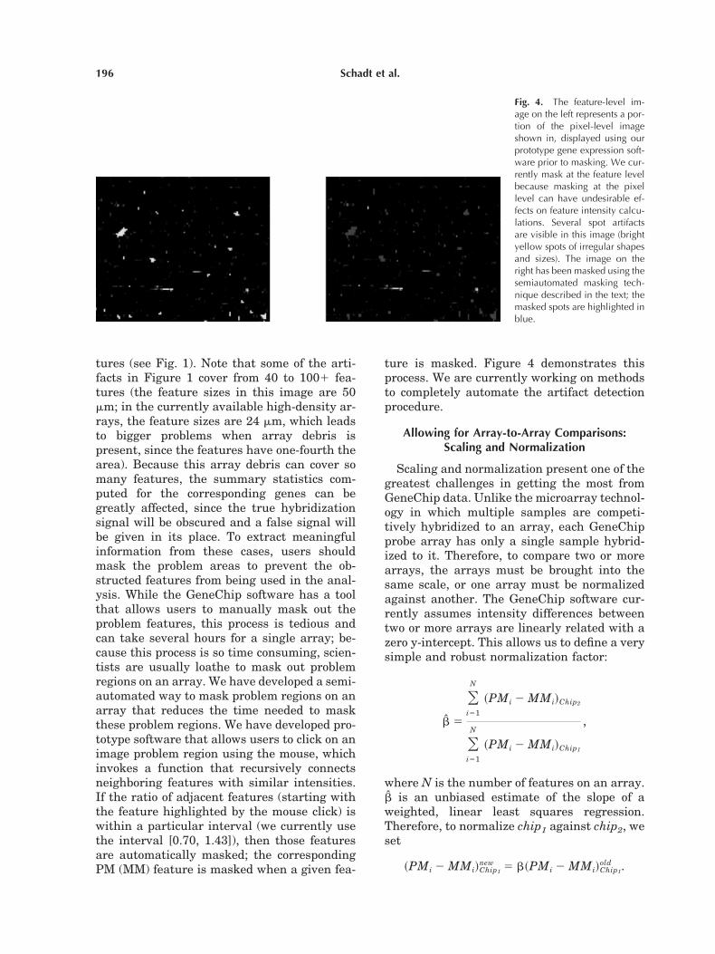
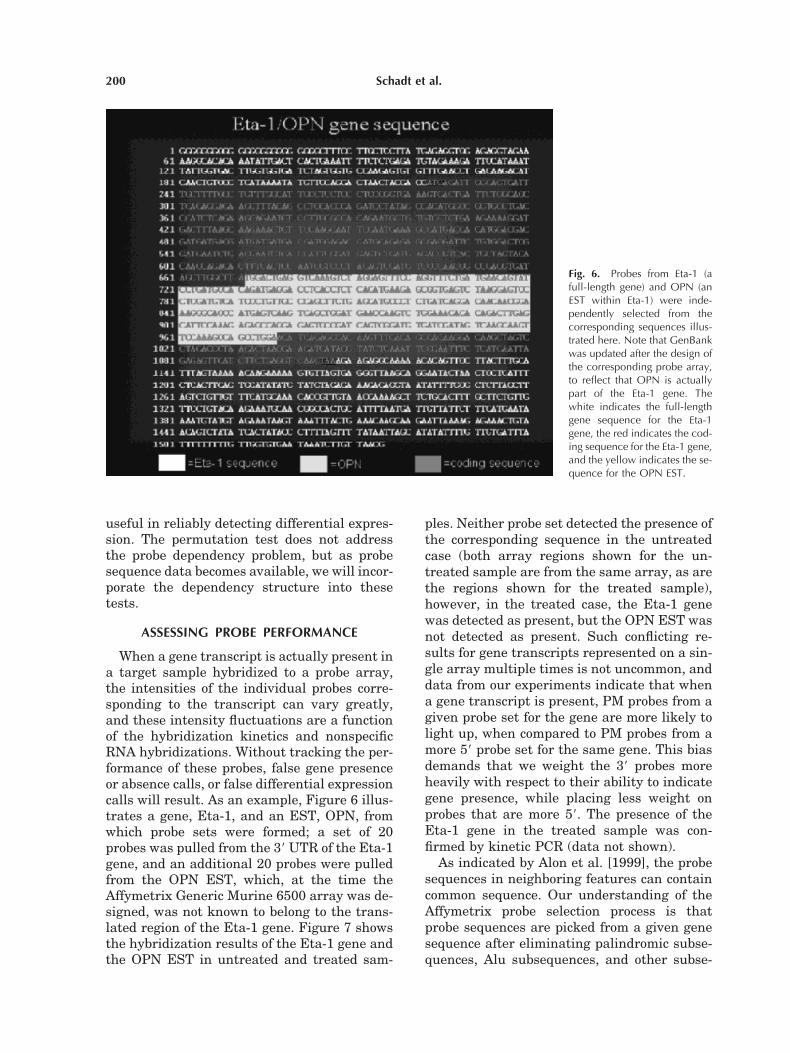
When a gene transcript is actually present ina target sample hybridized to a probe array,the intensities of the individual probes corre-sponding to the transcript can vary greatly,and these intensity fluctuations are a functionof the hybridization kinetics and nonspecificRNA hybridizations. Without tracking the per-formance of these probes, false gene presenceor absence calls, or false differential expressioncalls will result. As an example, Figure 6 illus-trates a gene, Eta-1, and an EST, OPN, fromwhich probe sets were formed; a set of 20probes was pulled from the 39 UTR of the Eta-1gene, and an additional 20 probes were pulledfrom the OPN EST, which, at the time theAffymetrix Generic Murine 6500 array was de-signed, was not known to belong to the trans-lated region of the Eta-1 gene. Figure 7 showsthe hybridization results of the Eta-1 gene andthe OPN EST in untreated and treated sam-

ples. Neither probe set detected the presence ofthe corresponding sequence in the untreatedcase (both array regions shown for the un-treated sample are from the same array, as arethe regions shown for the treated sample),however, in the treated case, the Eta-1 genewas detected as present, but the OPN EST wasnot detected as present. Such conflicting re-sults for gene transcripts represented on a sin-gle array multiple times is not uncommon, anddata from our experiments indicate that whena gene transcript is present, PM probes from agiven probe set for the gene are more likely tolight up, when compared to PM probes from amore 59 probe set for the same gene. This biasdemands that we weight the 39 probes moreheavily with respect to their ability to indicategene presence, while placing less weight onprobes that are more 59. The presence of theEta-1 gene in the treated sample was con-firmed by kinetic PCR (data not shown).

As indicated by Alon et al. [1999], the probesequences in neighboring features can containcommon sequence. Our understanding of theAffymetrix probe selection process is thatprobe sequences are picked from a given genesequence after eliminating palindromic subse-quences, Alu subsequences, and other subse-

Fig. 6. Probes from Eta-1 (afull-length gene) and OPN (anEST within Eta-1) were inde-pendently selected from thecorresponding sequences illus-trated here. Note that GenBankwas updated after the design ofthe corresponding probe array,to reflect that OPN is actuallypart of the Eta-1 gene. Thewhite indicates the full-lengthgene sequence for the Eta-1gene, the red indicates the cod-ing sequence for the Eta-1 gene,and the yellow indicates the se-quence for the OPN EST.

200 Schadt et al.

quences that are homologous to other gene se-quences, among a host of other exclusioncriteria aimed at making the hybridizationcharacteristics of a probe relatively uniform.Under such circumstances, it is not always pos-sible to pick probes that are do not containcommon sequence or that have hybridizationcharacteristics that are similar to the “ideal”probe. Therefore, it is imperative that the com-mon sequence structure and hybridizationcharacteristics be accounted for in computingaverage intensity statistics and in determiningwhether a gene transcript is present or differ-entially expressed.

Current protocols do not call for high tem-perature hybridizations, and so, variations inthe melting temperature can have a significantimpact on the PM/MM differences, which, inturn, can greatly impact gene presence or dif-ferential expression detection. If the meltingtemperature is too high, relative to the exper-imental protocols defined by Affymetrix (theseprotocols call for carrying out the hybridizationfor 16 h at 45°C in a rotisserie oven set at60 RPM), then the PM as well as the corre-sponding MM features will bind the RNAtightly, thus giving small PM/MM differences,which could severely bias gene presence anddifferential expression calls. Other serious vari-ations we have seen with respect to hybridiza-tion efficiencies include arrays that have abrighter median probe intensity (over the en-

tire array) than a baseline array, but whichhave PM/MM differences that are less than thedifferences of the baseline array. This wouldseem to indicate that the intensity signals forthe PM features of the “bright” array are sat-urated, and that the intensity signals for thecorresponding MM features are boosted, givinglower PM/MM differences.

If a significant number of PM features arereaching this saturation point, the data on thearray are completely unreliable. In fact, thiscan lead to very misleading results, since whenthe arrays are compared, if normalizationtakes place on the PM/MM differences, genesthat are actually up-regulated in the “bright”array may be called down-regulated. Similarly,genes that are actually present in the “bright”array may be called absent. We currently ex-amine PM/MM differences as well as PM/MMsums, since information lost in the PM/MMdifference may be partially recovered usingboth statistics.

The probe sequences contain a plethora ofinformation that could be used to enhance cur-rent gene expression and differential expres-sion detection algorithms. For instance, knowl-edge of the probe sequences would allow thehybridization efficiency (and hence, the qualityof the probe) to be assessed based on theprobe’s position in the gene sequence, on its GCcontent, on its GC trend, or on any other at-tribute of the probe sequence that would be

Fig. 7. The OPN and Eta-1 probe setson the Affymetrix Murine 6500 Gene-ChipT array. The 20 probe pairs repre-senting the OPN and Eta-1 sequencesare outlined in white. The top row(OPN) indicates no detectable expres-sion of the OPN EST in the untreated(control) and treated (bleomycin) sam-ples. The bottom row (Eta-1) indicatesno detectable expression of Eta-1 inthe untreated sample but definite ex-pression in the treated sample. The un-treated data shown for OPN and Eta-1are from the same array hybridization,as are the treated data. As shown inFigure 6, OPN and Eta-1 represent thesame gene. The probes for Eta-1 werepulled from the 39 UTR of the gene,while the OPN probes were pulledfrom the coding region of the gene (thearea highlighted in yellow in Fig. 6).

201Analyzing Gene Expression Array Data

highly predictive of its ability to efficiently hy-bridize (this would include things like alterna-tive splicing, SNPs, etc.) Current systems donot provide for any sort of quality score for theprobes on an array (i.e., past arrays are notused to assess performance of probes in futureexperiments). We strongly believe such a scor-ing system for the probes would greatly im-prove gene detection algorithms and the abilityto quantify levels of a gene transcript when agene transcript is actually present.

CONCLUSION

The various methods discussed in this articlego further than currently available methods inaccounting for many of the sources of variationthat can obscure the very biological variation thetechnology aims to detect. Clearly, there is muchfurther to go in analyzing gene expression arraydata. Sophisticated background/gradient correc-tion methods, scaling/normalization methods,methods to assess a probe’s hybridization effi-ciency, and methods to detect gene presence ordifferential expression, only begin to approachthe goal of extracting as much information aspossible from these data. Power analysis, intro-ducing orthogonal biological factors to increasethe information content of these data, and build-ing on the current clustering techniques usedto explore gene expression data [Eisen, 1998;Tamayo, 1999], will all be necessary to get themost from this technology. Furthermore, as ex-pression libraries become widely available, wewill be able to estimate the variation struc-tures of genes in a variety of tissue and acrossmany different organisms, which will result inmore informative differential expression anal-yses. Making better use of the currently avail-able sequence information will enhance probeselection algorithms, thus increasing the effi-ciency of the probes and better accounting forthe many complicated biological phenomena(e.g., alternative splice sites) that are currentlynot well understood. Of course, these issuesrepresent only the computational aspects ofthis technology and do not even begin to ad-dress the sort of informatics infrastructure nec-essary to intelligently store and mine this typeof expression data, which, at RBS, has alreadyhit the terabyte scale.

The ability to simultaneously monitor tens ofthousands of genes across a series of experi-ments is truly a great technology breakthroughfor the biomedical and life sciences. However,these types of high-throughput assays gener-ate data that require sophisticated computa-tional and statistical techniques for their anal-ysis. By spending the time to develop suchmethods up front, we believe the better qualitydata that result, will make it possible to detectmany of the more subtle gene expression pat-terns and gene interactions that give rise to allof the complexities of living systems.

ACKNOWLEDGMENTS

We thank Renu Heller, Gary Peltz, John Al-lard, Fengrong Zuo, Andrew Grupe, and DeeAud of Roche Bioscience for providing us withthe gene expression array data.

REFERENCES

Alon U, Barkai N, Notterman DA, Gish K, Ybarra S, MackD, Levine AJ. 1999. Broad patterns of gene expressionrevealed by clustering analysis of tumor and normalcolon tissues probed by oligonucleotide arrays. Proc NatlAcad Sci USA 96:6745–6750.

Cox DR, Hinkley DV. 1979. Theoretical statistics. London:Chapman and Hall.

Der SD, Zhou A, Williams BRG, Silverman RH. 1998.Identification of genes differentially regulated by inter-feron a, b, or g using oligonucleotide arrays. Proc NatlAcad Sci USA 95:15623–15628.

Eisen MB, Spellman PT, Brown PO, Botstein D. 1998.Cluster analysis and display of genome-wide expressionpatterns. Proc Natl Acad Sci USA 95:14863–14868.

Eisenberg DS, Crothers DM. 1979. Physical chemistry:with applications to the life sciences. Menlo Park, CA:Benjamin/Cummings Publishing Company.

GATC Consortium. 1998. GATC Specifications: SoftwareSpecifications. Available at http://www.gatconsortium.org/.

Hastie TJ, Tibshirani RJ. 1997. Generalized additive mod-els. New York: Chapman and Hall.

Lockhart DJ, Dong H, Byrne MC, Follettie MT, GallowMV, Chee MS, et al. 1996. Expression monitoring byhyrbridization to high-density oligonucleotide arrays.Nature Biotechnol 14:1675–1680.

Tamayo P, Slonim D, Mesirov J, Zhu Q, Kitareewan S,Dmitrovsky E, Lander ES, Golub TR. 1999. Interpretingpatterns of gene expression with self-organizing maps:methods and application to hematopoietic differentia-tion. Proc Natl Acad Sci USA 96:2907–2912.

Wodicka L, Dong H, Mittmann M, Ho MH, Lockhart DJ.1997. Genome-wide expression monitoring in Saccharo-myces cerevisiae. Nature Biotechnol 5:1359–1366.

202 Schadt et al.