
Analysis tools and methods for tritium data taking with ... - CORE
258
Analysis tools and methods for tritium data taking with the KATRIN experiment Zur Erlangung des akademischen Grades eines Doktors der Naturwissenschaften von der KIT-Fakult¨ at f¨ ur Physik des Karlsruher Instituts f¨ ur Technologie genehmigte Dissertation von M. Sc. Florian Heizmann aus Stuttgart-Bad Cannstatt Referent: Prof. Dr. G. Drexlin Institut f¨ ur Experimentelle Teilchenphysik, KIT Korreferent: Prof. Dr. U. Husemann Institut f¨ ur Experimentelle Teilchenphysik, KIT Korreferent: Dr. K. Valerius Institut f¨ ur Kernphysik, KIT Tag der m¨ undlichen Pr¨ ufung: 14.12.2018 KIT – Die Forschungsuniversit¨ at in der Helmholtz-Gemeinschaft www.kit.edu
-
Upload
khangminh22 -
Category
Documents
-
view
0 -
download
0
Transcript of Analysis tools and methods for tritium data taking with ... - CORE

Analysis tools and methods fortritium data taking with the
KATRIN experiment
Zur Erlangung des akademischen Grades einesDoktors der Naturwissenschaften
von der KIT-Fakultat fur Physikdes Karlsruher Instituts fur Technologie
genehmigteDissertation
von
M. Sc. Florian Heizmann
aus Stuttgart-Bad Cannstatt
Referent: Prof. Dr. G. Drexlin
Institut fur Experimentelle Teilchenphysik, KIT
Korreferent: Prof. Dr. U. Husemann
Institut fur Experimentelle Teilchenphysik, KIT
Korreferent: Dr. K. Valerius
Institut fur Kernphysik, KIT
Tag der mundlichen Prufung: 14.12.2018
KIT – Die Forschungsuniversitat in der Helmholtz-Gemeinschaft www.kit.edu
Declaration of authorship Herewith I affirm that I wrote the current thesis on myown and without the usage of any other sources or tools than the cited ones andthat this thesis has not been handed neither in this nor in equal form at any otherofficial commission.
Erklarung der Selbststandigkeit Hiermit versichere ich, die vorliegende Arbeitselbststandig angefertigt zu haben und keine Hilfsmittel jenseits der kenntlich gemachtenverwendet zu haben. Weiterhin habe ich weder diese noch eine aquivalente Versiondieser Arbeit bei einer anderen Prufungskommission vorgelegt.
Karlsruhe, 27.11.2018
. . . . . . . . . . . . . . . . . . . . . . . . . . . . . . . . .Florian Heizmann

ABSTRACT
The KArlsruhe TRItium Neutrino (Katrin) experiment is targeted to determinethe neutrino mass with an unprecedented sensitivity of 200 meV (90 % C.L.). Tothis end, Katrin employs an intense gaseous tritium source combined with a pre-cision retardation spectrometer of MAC-E-filter type. Since the completion of theKatrin beamline in the fall of 2016, several pivotal milestones towards the start ofneutrino-mass measurements have been achieved. In the thesis at hand, a tritiumsource gas model for the latest one among these milestones, the First Tritium cam-paign in May and June 2018, is developed and validated by several measures. Thisgas model is used for the analysis of the first Katrin tritium spectra, includingvarious approaches to account for gas model related systematic effects. Strategiesfor performing a blind neutrino mass analysis of the upcoming Katrin neutrinomass data are developed, subject to a critical comparison, and tested on kryptoncommissioning data. Besides its main goal of neutrino mass search, Katrin offersthe potential to probe physics beyond the neutrino mass. For three example cases,the statistical sensitivity is evaluated and compared to existing limits.
Das KArlsruhe TRItium Neutrino (Katrin) Experiment ist konstruiert, um dieNeutrinomasse mit einer bisher unerreichten Sensitivitat von 200 meV (90 % C.L.)zu bestimmen. Dafur kombiniert Katrin eine starke gasformige Tritiumquelle miteinem hochauflosendem MAC-E-Filter-Spektrometer. Seit der Fertigstellung des ex-perimentellen Aufbaus im Herbst 2016 hat das Katrin-Experiment mehrere zentraleMeilensteine erreicht. In der vorliegenden Arbeit wird ein Gasmodell fur den letztendieser Meilensteine – die erste Tritium-Zirkulation in der Tritium-Quelle im Maiund Juni 2018 – vorgestellt, und mit unterschiedlichen Messmethoden verglichen.Mit Hilfe des Gasmodells werden die ersten Tritiumspektren analysiert, wobei ver-schiedene Methoden zur Berucksichtigung von Systematiken am Beispiel des Gas-modells untersucht werden. Vorbereitend auf die kommenden Neutrinomassendatenwerden in dieser Arbeit Methoden fur eine blinde Neutrinomassenanalyse von β-Zerfall-basierten Tritiumspektren vorgestellt, miteinander verglichen, und an Handvon Kryptondaten getestet. Die Arbeit schließt mit einem Ausblick auf das Po-tential von Katrin, Physik jenseits der Neutrinomasse zu untersuchen. Fur dreiBeispiele wird exemplarisch die statistische Sensitivitat von Katrin bestimmt undmit bestehenden experimentellen Erkenntnissen verglichen.

INTRODUCTION
Neutrinos fill a special role in particle physics, astrophysics and cosmology sincethey link the physics of the microcosm with the largest scales of the universe. Thispremise of the neutrinos to contribute to our understanding of a broad range ofopen questions in modern astroparticle physics is based on their particle nature andcharacteristics. The absolute neutrino mass scale probes the mass generation ofthe Standard Model of particle physics. Katrin represents the most recent effort todetermine the absolute mass scale of neutrinos in a model-independent way, after thepredecessor experiments in Mainz [Kra+05] and Troitsk [Ase+11] could determinean upper limit of 2 eV (95 % C.L.) [Tan+18].
Motivation Located at the Karlsruhe Institute of Technology, the Katrin ex-periment is targeted to determine the effective electron neutrino mass with an un-precedented sensitivity of 200 meV (90 % C.L.), based on three net years worth ofdata (corresponding to approximately five calendar years of data-taking). To reachthis ambitious goal, Katrin combines an ultra-luminous tritium source with high-resolution β-spectroscopy. In the course of the past two years, Katrin successfullycompleted several milestones, ranging from first transmission of electrons throughthe entire beam line in 2016 to first recording of tritium β-decay spectra in 2018.The strategies and technical framework for the high-level analysis of tritium spectraform the basis for analysing the upcoming neutrino mass data. In order to preventhuman observer’s bias, a widely used method is the one of a blind analysis. How-ever, since blinding was not applied in any of the previous β-decay neutrino massexperiments, appropriate analysis techniques and their implementation need to bedeveloped from the ground up.
i

ii Introduction
Objectives The objectives of this thesis are all closely linked to the tritium sourceof the Katrin experiment. They span the complete analysis chain of the Ka-trin experiment, from sensor-informed gas dynamics simulation to the high-leveltritium spectrum analysis. In particular, these research goals include the following:
� The development and preparation of the source model for use in neutrinomass analysis. This requires extensions towards reading of sensor data andcombining magnetic field and gas dynamics calculations.
� Blind analysis methods suitable for Katrin’s neutrino mass analysis shouldbe identified, designed, implemented in the analysis framework, and subjectto thorough testing and a critical comparative evaluation.
� The potential of Katrin to constrain various new physics scenarios beyondthe neutrino mass shall be explored through sensitivity studies.
Outline
1. In chapter 1, a brief overview of the current status of the field of neutrinophysics is given.
2. The measuring principle and key components of the Katrin experiment arepresented in the second chapter 2.
3. As it is the central Katrin component with regard to the thesis at hand, thetritium source is presented in more detail in chapter 3.
4. The various parts forming the source model of the Katrin experiment aredescribed in chapter 4, covering temperature, gas flow, and magnetic fields.
5. This source model is then used to analyse spectra from the First Tritium com-missioning campaign (chapter 5) of the Katrin experiment, a major milestonetowards neutrino mass data taking.
6. In order to be prepared for an unbiased neutrino mass analysis, methods for ablind analysis of β-decay spectra are introduced and tested on simulations aswell as on krypton commissioning data in chapter 6.
7. An outlook towards the interesting potential to employ precision measurementsof the tritium β-decay spectrum for the exploration of new physics opportuni-ties beyond the neutrino mass search is given in chapter 7.
8. The findings of this work are summarised in the concluding chapter 8.
ii

CONTENTS
1. Neutrino physics 11.1. The story of the neutrino – or “what we know” . . . . . . . . . . . . . 1
1.1.1. Postulation and discovery of the neutrino . . . . . . . . . . . . 21.1.2. Neutrinos in the Standard Model of particle physics . . . . . . 31.1.3. Neutrino flavour mixing – or why neutrinos need mass . . . . 4
1.2. Current research – or “what we do not know” . . . . . . . . . . . . . . 111.2.1. Can neutrinos explain the missing anti-matter? . . . . . . . . 111.2.2. Extensions to the Standard Model - or how neutrinos might
get their mass . . . . . . . . . . . . . . . . . . . . . . . . . . . 121.3. Determination of the neutrino mass . . . . . . . . . . . . . . . . . . . 14
1.3.1. Model-dependent determination . . . . . . . . . . . . . . . . . 141.3.2. Model-independent determination . . . . . . . . . . . . . . . . 15
2. The KArlsruhe TRItium Neutrino Experiment 192.1. Neutrino mass from tritium β-decay . . . . . . . . . . . . . . . . . . . 192.2. Components of the KATRIN experiment . . . . . . . . . . . . . . . . 20
2.2.1. The Windowless Gaseous Tritium Source . . . . . . . . . . . . 212.2.2. Monitoring of the source parameters . . . . . . . . . . . . . . 232.2.3. Transport section . . . . . . . . . . . . . . . . . . . . . . . . . 252.2.4. Spectrometers section . . . . . . . . . . . . . . . . . . . . . . . 272.2.5. Detector section . . . . . . . . . . . . . . . . . . . . . . . . . . 30
2.3. Modelled count rate . . . . . . . . . . . . . . . . . . . . . . . . . . . . 302.4. Analysis tools and software at the KATRIN experiment . . . . . . . . 31
3. The Windowless Gaseous Tritium Source 353.1. Key parameters . . . . . . . . . . . . . . . . . . . . . . . . . . . . . . 35
3.1.1. Column density . . . . . . . . . . . . . . . . . . . . . . . . . . 353.1.2. Temperature . . . . . . . . . . . . . . . . . . . . . . . . . . . 363.1.3. Tritium purity . . . . . . . . . . . . . . . . . . . . . . . . . . . 363.1.4. Magnetic field . . . . . . . . . . . . . . . . . . . . . . . . . . . 363.1.5. Plasma potential . . . . . . . . . . . . . . . . . . . . . . . . . 37
3.2. Systematic uncertainties and requirements related to the WGTS . . . 373.3. Technical realisation . . . . . . . . . . . . . . . . . . . . . . . . . . . 38
3.3.1. Temperature stabilisation and calibration . . . . . . . . . . . . 393.3.2. Gas flow (Inner loop system) . . . . . . . . . . . . . . . . . . . 40
iii
iv Contents
3.3.3. Magnet set-up . . . . . . . . . . . . . . . . . . . . . . . . . . . 41
4. Source modelling 434.1. General concepts, notation . . . . . . . . . . . . . . . . . . . . . . . . 43
4.1.1. Intermediate Knudsen formula . . . . . . . . . . . . . . . . . . 464.1.2. Boltzmann equation and distribution function . . . . . . . . . 47
4.2. Temperature model . . . . . . . . . . . . . . . . . . . . . . . . . . . . 484.2.1. Temperature sensors . . . . . . . . . . . . . . . . . . . . . . . 484.2.2. Temperature correlations . . . . . . . . . . . . . . . . . . . . . 484.2.3. Temperature homogeneity . . . . . . . . . . . . . . . . . . . . 49
4.3. Gas dynamics model, nominal KATRIN set-up . . . . . . . . . . . . . 524.3.1. Gas flow in the central 10 m beam tube (A1-A3) . . . . . . . . 534.3.2. Pumping section - DPS1 (B1-B3) . . . . . . . . . . . . . . . . 554.3.3. Complete gas model . . . . . . . . . . . . . . . . . . . . . . . 574.3.4. Calibration of the column density . . . . . . . . . . . . . . . . 574.3.5. Neutrino mass uncertainty . . . . . . . . . . . . . . . . . . . . 59
4.4. Gas dynamics model, First Tritium set-up . . . . . . . . . . . . . . . 604.4.1. Statement of the problem . . . . . . . . . . . . . . . . . . . . 604.4.2. Derivation of the injection rate . . . . . . . . . . . . . . . . . 624.4.3. Intermediate Knudsen flow . . . . . . . . . . . . . . . . . . . . 634.4.4. Boltzmann equation . . . . . . . . . . . . . . . . . . . . . . . 654.4.5. Column density, injection rate and pressure controlled buffer
vessel . . . . . . . . . . . . . . . . . . . . . . . . . . . . . . . 664.4.6. Discussion of sources of uncertainties . . . . . . . . . . . . . . 674.4.7. Estimation of the (deuterium) column density uncertainty . . 694.4.8. Estimation of injection pressure from krypton capillary pressure 724.4.9. Discussion . . . . . . . . . . . . . . . . . . . . . . . . . . . . . 74
4.5. Magnetic field . . . . . . . . . . . . . . . . . . . . . . . . . . . . . . . 754.5.1. Magnetic field model . . . . . . . . . . . . . . . . . . . . . . . 754.5.2. Magnetic field measurement system . . . . . . . . . . . . . . . 764.5.3. Magnetic field measurements . . . . . . . . . . . . . . . . . . . 784.5.4. Discussion . . . . . . . . . . . . . . . . . . . . . . . . . . . . . 82
4.6. Conclusion . . . . . . . . . . . . . . . . . . . . . . . . . . . . . . . . . 84
5. Analysis of First Tritium data 875.1. Experimental set-up . . . . . . . . . . . . . . . . . . . . . . . . . . . 875.2. Operating conditions . . . . . . . . . . . . . . . . . . . . . . . . . . . 89
5.2.1. Temperature stability . . . . . . . . . . . . . . . . . . . . . . . 905.2.2. Gas circulation stability . . . . . . . . . . . . . . . . . . . . . 905.2.3. Tritium concentration stability . . . . . . . . . . . . . . . . . 925.2.4. Magnetic field stability . . . . . . . . . . . . . . . . . . . . . . 92
5.3. Analysis of tritium β-decay spectra . . . . . . . . . . . . . . . . . . . 925.3.1. Analysis cuts . . . . . . . . . . . . . . . . . . . . . . . . . . . 945.3.2. Agreement between model and data . . . . . . . . . . . . . . . 965.3.3. Fit parameter pixel distribution . . . . . . . . . . . . . . . . . 965.3.4. Fit parameter stability . . . . . . . . . . . . . . . . . . . . . . 975.3.5. Systematic effects due to column density uncertainty . . . . . 1005.3.6. Appended runs . . . . . . . . . . . . . . . . . . . . . . . . . . 1035.3.7. Overview of the effective endpoint estimates . . . . . . . . . . 105
iv

Contents v
5.3.8. Systematic effects due to slicing the WGTS . . . . . . . . . . 1065.3.9. Test of the scattering implementation . . . . . . . . . . . . . . 107
5.4. Estimation of the column density via additional detectors . . . . . . . 1095.4.1. Estimation of the column density via the FBM . . . . . . . . . 1095.4.2. Estimation of the column density via PULCINELLA . . . . . 1175.4.3. Discussion . . . . . . . . . . . . . . . . . . . . . . . . . . . . . 122
5.5. Conclusion . . . . . . . . . . . . . . . . . . . . . . . . . . . . . . . . . 124
6. Blind analysis and methods 1276.1. Motivation . . . . . . . . . . . . . . . . . . . . . . . . . . . . . . . . . 127
6.1.1. Observer’s bias . . . . . . . . . . . . . . . . . . . . . . . . . . 1276.1.2. Goal of blind analysis in KATRIN . . . . . . . . . . . . . . . . 128
6.2. Sensitivity definition and derivation . . . . . . . . . . . . . . . . . . . 1296.2.1. Sensitivity as discovery potential . . . . . . . . . . . . . . . . 1306.2.2. Adaption of the total neutrino mass uncertainty . . . . . . . . 1306.2.3. Methodology to derive the necessary level of blinding . . . . . 130
6.3. Blind analysis methods . . . . . . . . . . . . . . . . . . . . . . . . . . 1316.3.1. Data blinding . . . . . . . . . . . . . . . . . . . . . . . . . . . 1326.3.2. Model blinding . . . . . . . . . . . . . . . . . . . . . . . . . . 140
6.4. Sensitivity estimates . . . . . . . . . . . . . . . . . . . . . . . . . . . 1466.4.1. Data blinding . . . . . . . . . . . . . . . . . . . . . . . . . . . 1466.4.2. Model blinding . . . . . . . . . . . . . . . . . . . . . . . . . . 1516.4.3. Summary . . . . . . . . . . . . . . . . . . . . . . . . . . . . . 154
6.5. Application of the blinding methods to krypton data . . . . . . . . . 1546.5.1. Window blinding . . . . . . . . . . . . . . . . . . . . . . . . . 1566.5.2. Energy smearing . . . . . . . . . . . . . . . . . . . . . . . . . 1586.5.3. Summary . . . . . . . . . . . . . . . . . . . . . . . . . . . . . 159
6.6. Discussion . . . . . . . . . . . . . . . . . . . . . . . . . . . . . . . . . 1616.6.1. Reduced statistics . . . . . . . . . . . . . . . . . . . . . . . . . 1616.6.2. Window blinding . . . . . . . . . . . . . . . . . . . . . . . . . 1626.6.3. Energy smearing . . . . . . . . . . . . . . . . . . . . . . . . . 1626.6.4. Final states distribution smearing . . . . . . . . . . . . . . . . 1626.6.5. Imperfect energy loss function . . . . . . . . . . . . . . . . . . 1636.6.6. Implicit blinding . . . . . . . . . . . . . . . . . . . . . . . . . 1636.6.7. Unblinding . . . . . . . . . . . . . . . . . . . . . . . . . . . . 165
6.7. Conclusion and outlook . . . . . . . . . . . . . . . . . . . . . . . . . . 165
7. Physics beyond the neutrino mass 1677.1. Light bosons . . . . . . . . . . . . . . . . . . . . . . . . . . . . . . . . 168
7.1.1. Behaviour of the spectral shape by introducing a light boson . 1687.1.2. Statistical sensitivity for eV-scale light bosons . . . . . . . . . 1727.1.3. Statistical sensitivity for keV-scale light bosons . . . . . . . . 1747.1.4. Discussion and comparison to existing bounds . . . . . . . . . 175
7.2. Right-handed currents in presence of eV-scale sterile neutrinos . . . . 1787.2.1. Spectral shape due to right-handed currents . . . . . . . . . . 1787.2.2. Parameter inference with right-handed currents . . . . . . . . 1847.2.3. Statistical sensitivity to constrain the right-handed coupling . 185
7.3. Relic neutrinos . . . . . . . . . . . . . . . . . . . . . . . . . . . . . . 1877.3.1. Theory of the relic neutrino background and detection techniques188
v
vi Contents
7.3.2. Induced β-decay spectrum . . . . . . . . . . . . . . . . . . . . 1907.3.3. Parameter inference with relic neutrinos . . . . . . . . . . . . 1947.3.4. Statistical sensitivity to constrain the relic neutrino background194
7.4. Conclusion . . . . . . . . . . . . . . . . . . . . . . . . . . . . . . . . . 198
8. Summary and Conclusions 201
Appendix 205A. Source modelling . . . . . . . . . . . . . . . . . . . . . . . . . . . . . 205
A.1. Temperature . . . . . . . . . . . . . . . . . . . . . . . . . . . 205A.2. First Tritium set-up . . . . . . . . . . . . . . . . . . . . . . . 205A.3. Magnetic field measurements . . . . . . . . . . . . . . . . . . . 205
B. Analysis of First Tritium data . . . . . . . . . . . . . . . . . . . . . . 206B.1. Estimation of the column density . . . . . . . . . . . . . . . . 206
C. Blind analysis & methods . . . . . . . . . . . . . . . . . . . . . . . . 206C.1. Sensitivity estimates . . . . . . . . . . . . . . . . . . . . . . . 206C.2. Window blinding . . . . . . . . . . . . . . . . . . . . . . . . . 208C.3. Imperfect energy loss function . . . . . . . . . . . . . . . . . . 209
D. Physics beyond the neutrino mass . . . . . . . . . . . . . . . . . . . . 211D.1. Experiment configuration for the new physics studies . . . . . 211D.2. Light bosons . . . . . . . . . . . . . . . . . . . . . . . . . . . . 211
List of Figures 215
List of Tables 219
List of Acronyms 221
Index 223
Bibliography 225
Acknowledgements 247
vi

CHAPTER 1
NEUTRINO PHYSICS
“Neutrino: Another a-tom in the lepton family. There are three different kinds.[...] They win the minimalist contest: zero charge, zero radius, and very possibly
zero mass.”– Leon M. Lederman in [LT93], 1993 –
From the very beginning of neutrino physics, the unique attributes of neutrinosdescribed by L. Lederman in the quote above put neutrinos into the mystery boxof particle physics. Another piece in this mystery puzzle was added when the non-zero mass of neutrinos was discovered by neutrino oscillation experiments [Ahm+01,Fuk+98]. The unique combination of interacting only weakly while being the mostabundant massive particles in nature empowers neutrinos to help unravelling someof the outstanding open questions in particle physics and cosmology. Neutrinos pro-vide the link from the smallest structures in the universe up to the largest, possiblyholding a key to understanding the origin of matter and the structure formation inthe early universe. Those answers are closely linked to the particle characteristics ofthe neutrino like charge, spin, chirality, and mass. Especially the latter is of specialinterest for cosmologists and particle physicists, as it probes the mass generationmechanism of the Standard Model (SM) of particle physics as well as the develop-ment of the universe on cosmological scales. The Katrin experiment is dedicatedto determining the effective electron anti-neutrino mass with unprecedented sensi-tivity of 200 meV (90 % C.L.) in a laboratory experiment. This chapter aims to givean overview of the current status of neutrino physics as the context in which theKatrin experiment (see ch. 2) is carried out.
1.1. The story of the neutrino – or “what we know”
Though neutrinos were postulated about 100 years ago, it took decades and a vastnumber of dedicated experiments to acquire the knowledge about neutrinos that wehave today. This section will briefly recapitulate the theoretical and experimentalefforts taken to learn about what has become to be known as “ghost particle”.
1

2 1. Neutrino physics
Figure 1.1.: Project Poltergeist. Left side shows the experimental set-up, rightside the sandwich principle. Figure adapted from [Sut16].
1.1.1. Postulation and discovery of the neutrino
It was in the beginning of the 20th century, a time often referred to as a “golden ageof physics” when Chadwick published his findings about the continuous shape of thespectrum of electrons emitted in β-decay [Cha14], which should mark the start ofwhat is today known as neutrino physics.
The continuous β-spectrum – or why we need the neutrino The continuousβ-decay spectrum measured by Chadwick in 1914 [Cha14] could not be explained atthat time as β-decay was thought of as a two-body decay. In a “desperate attempt”to circumvent the apparent non-conservation of energy and momentum, Pauli pos-tulated a third particle to be produced in β-decay [PKW64]. After Fermi came upwith a point-like interaction model as theory of the β-decay [Fer34], experimentalistsstruggled for decades to detect the postulated ghostly particle.
Project Poltergeist and successive discoveries Due to the predicted low crosssection of the order of 10−44 cm2 [BP34], the experimental detection took until 1956,when Cowan and Reines successfully carried out their“Project Poltergeist”[Cow+56]near the Savannah River nuclear power plant. Cowan and Reines used the largeelectron (anti-) neutrino flux of the nuclear reactor to detect the inverse β+-decayproducts, positron e+ and neutron n:
νe + p→ e+ + n. (1.1)
A unique identifier was found by using a sandwich layout of target and detectormaterial. The “meat” of the sandwich consisted of a water tank with dissolvedcadmium salt as target while the “bread” was made of liquid scintillator tanks withattached photomultiplier tubes (PMT). This layout enables safe discrimination ofa neutrino signal. Neutrino signals are identified as two delayed gamma-ray pulses.The first gamma pulse is due to prompt annihilation of the positron with an electronin the target tank, while the second gamma pulse is emitted due to the neutron beingcaptured by cadmium after a some µs long, moderated random walk.
Soon after, the second neutrino species was detected at the Brookhaven NationalLaboratory [Dan+62] by investigating the charged pion decay
π+ → µ+ + νµ and π− → µ− + νµ. (1.2)
2

1.1. The story of the neutrino – or “what we know” 3
The pions were produced by shooting 15 GeV protons from the Alternating GradientSynchrotron onto a beryllium target. Danby et al. managed to obtain a pure neutrinobeam by focussing the pion beam onto a massive iron block. The neutrinos in turnwere detected via a spark chamber that could differentiate between the straight trackof a muon and the electromagnetic shower of an electron. Thereby it was shown thatthere must be another neutrino species, called muon neutrino.
Last but not least, the tau neutrino completed the neutrino family. Perl et al. an-nounced an anomalous lepton production in e+e− collisions at SLAC-LBL [Per+75],but it took another 25 years until the discovery was confirmed [Kod+01]. At Fer-milab’s Tevatron, accelerated 800 GeV protons were shot onto a tungsten target,resulting in tau neutrinos via the decay of charmed mesons
D+S → τ+ + ντ and D−S → τ− + ντ. (1.3)
A series of lead, concrete and iron shields filtered out most of the background,enabling the detection of the residual tau-neutrinos via alternating steel and nuclearemulsion plates. The signature of a tau neutrino is then the decay of the producedtau-lepton, visible by a kink in the recorded trajectory. After applying all cuts, theDONUT collaboration harvested a total of four tau neutrino events [Kod+01].
Hints for the existence of a third generation of neutrinos already came from theobserved decay width of the Z0 boson. An early analysis of the decay width andcross section found the best fit at Nν = 3.27 ± 0.30 [Dec+89] with subsequentimprovements through the combination of more data sets from several detectors.
1.1.2. Neutrinos in the Standard Model of particle physics
The aforementioned three different flavours of neutrinos can be matched in the Stan-dard Model (SM) of particle physics to three different charged leptons of the sameflavour, forming the three weak isospin doublets. Neutrinos in the SM are un-charged, stable fermions interacting only via the weak force. This combination isunique in the SM, and it enables neutrinos to be their own anti-particle. The beautyof the SM is its concise description of the elementary particles and their origin ofmass by virtue of the Higgs-mechanism. Verification of the Higgs prediction wasannounced in 2012, when the ATLAS and the CMS collaborations published the dis-covery of a Higgs-like particle [ATL12, CMS12]. This major breakthrough togetherwith the previously found neutrino-related characteristics of the weak interactioncontribute to the beauty of the overall picture of the successful Standard Model.Among those previously found characteristics are the violation of parity of the weakinteraction [Wu+57] and the helicity of neutrinos [GGS58].
Helicity of neutrinos In 1957, Wu et al. discovered the parity violation of the weakinteraction by using a magnetised 60Co β-source [Wu+57]. Verified by subsequentexperiments as in [GLW57], Wu and coworkers could show that the β-electrons favouremission anti-parallel to the nuclear spin, resulting in maximum parity violationof the weak interaction. This finding was also confirmed when Goldhaber et al.
3
4 1. Neutrino physics
mass →charge →
spin →
<2 eV <0.19 MeV <18.2 MeV 91.2 GeV
0.511 MeV 105.7 MeV 1.777 GeV 80.4 GeV
4.7 MeV 95 MeV 4.2 GeV 0
2.2 MeV 1.28 GeV 173.0 GeV 0 125.2 GeV
0 0 0 0
-1 -1 -1 ±1
-1/3 -1/3 -1/3 0
2/3 2/3 2/3 0 0
1/2 1/2 1/2 1
1/2 1/2 1/2 1
1/2 1/2 1/2 1
1/2 1/2 1/2 1 0
electronneutrino
muonneutrino
tauneutrino
Z boson
electron muon tauon W boson
down quark strange quark bottom quark photon
up quark charm quark top quark gluon Higgs boson
leptons
quarks
gauge
bosons
νe νµ ντ Z
e µ τ W
d s b γ
u c t g H
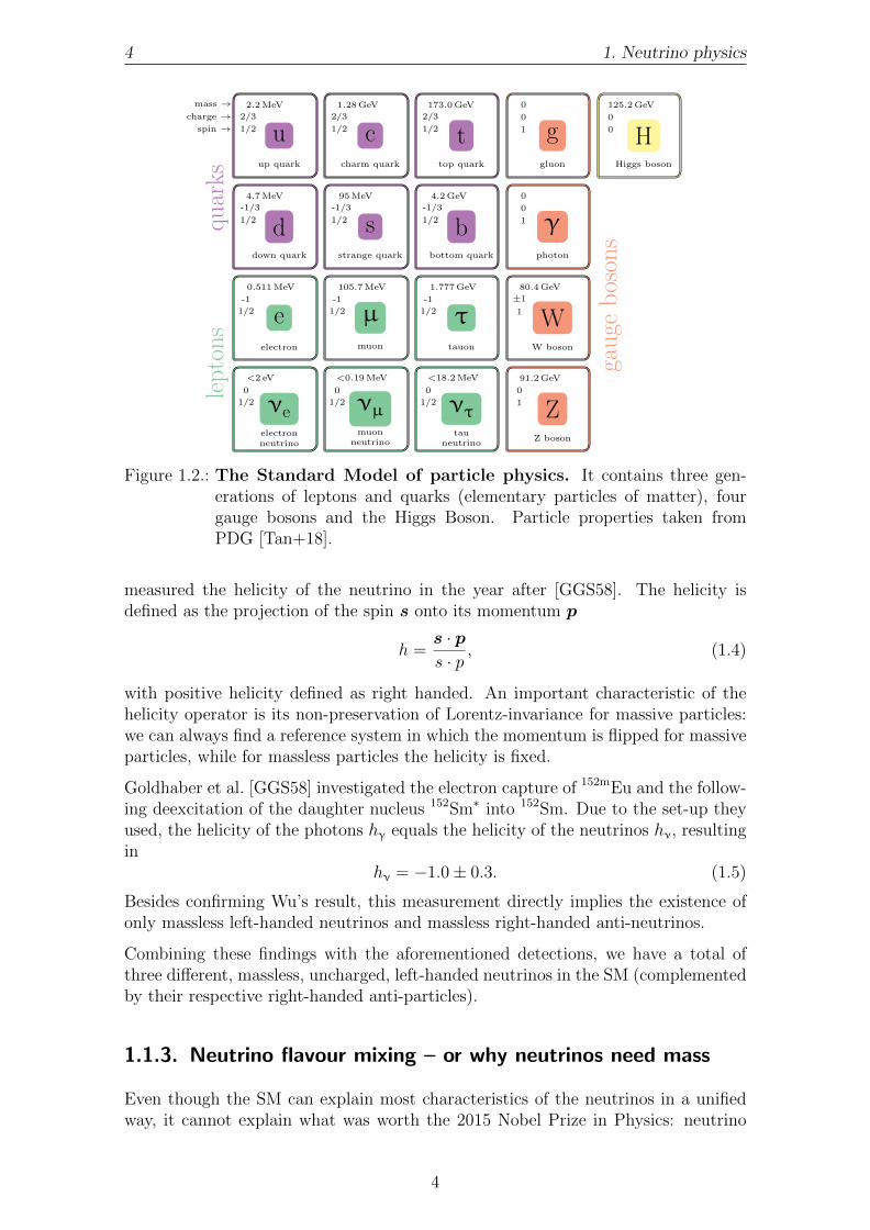
Figure 1.2.: The Standard Model of particle physics. It contains three gen-erations of leptons and quarks (elementary particles of matter), fourgauge bosons and the Higgs Boson. Particle properties taken fromPDG [Tan+18].
measured the helicity of the neutrino in the year after [GGS58]. The helicity isdefined as the projection of the spin s onto its momentum p
h = s · ps · p
, (1.4)
with positive helicity defined as right handed. An important characteristic of thehelicity operator is its non-preservation of Lorentz-invariance for massive particles:we can always find a reference system in which the momentum is flipped for massiveparticles, while for massless particles the helicity is fixed.
Goldhaber et al. [GGS58] investigated the electron capture of 152mEu and the follow-ing deexcitation of the daughter nucleus 152Sm∗ into 152Sm. Due to the set-up theyused, the helicity of the photons hγ equals the helicity of the neutrinos hν, resultingin
hν = −1.0± 0.3. (1.5)
Besides confirming Wu’s result, this measurement directly implies the existence ofonly massless left-handed neutrinos and massless right-handed anti-neutrinos.
Combining these findings with the aforementioned detections, we have a total ofthree different, massless, uncharged, left-handed neutrinos in the SM (complementedby their respective right-handed anti-particles).
1.1.3. Neutrino flavour mixing – or why neutrinos need mass
Even though the SM can explain most characteristics of the neutrinos in a unifiedway, it cannot explain what was worth the 2015 Nobel Prize in Physics: neutrino
4

1.1. The story of the neutrino – or “what we know” 5
Figure 1.3.: Solar neutrino flux. Flux of 8B solar neutrinos of µ or τ type ver-sus electron neutrino flux. Dotted diagonal band shows the predictionby Bahcall et al. [BPB01], solid band shows the flux derived from Su-perK and SNO measurements. Figure reprinted with permission fromref. [Ahm+01]. Copyright 2018 by the American Physical Society.
oscillations. T. Kajita (SuperK collaboration) and A. B. McDonald (SNO collab-oration) received the prize “for the discovery of neutrino oscillations, which showsthat neutrinos have mass” [The15].
The solar neutrino problem The results of the SNO collaboration also solved along-standing mismatch between the Standard Solar Model (SSM) prediction and themeasured flux of solar neutrinos. Ever since the first results of Davis’ Homestakeexperiment [DHH68], the measured solar neutrino flux was just 1/3 of the SSMprediction by Bahcall [Bah64a, Bah64b]. Davis used a radio-chemical method tomeasure the neutrino flux from the sun via the transformation process
37Cl + νe
inv. decay−−−−−⇀↽−−−−−capture
37Ar + e−, (1.6)
where he had to extract fewer than 100 37Ar atoms out of the 600 t of liquid per-chlorethylene inside the Homestake gold mine. A proportional counter could thenbe used to detect the electron capture of 37Ar as it resulted in a 2.8 keV Auger elec-tron during the deexcitation of the produced 37Cl∗. Though Davis lost informationabout the energy and the direction of the neutrinos by that method, he was ableto calculate the neutrino flux that corresponds to the number of argon decays heobserved. The solar neutrino flux deficit he determined was also confirmed by e.g.the GALLEX experiment [Ham+99], as well as by the first real-time experimentKamiokande [Fuk+96].
In 2001, the SNO experiment finally resolved the solar neutrino problem and showedthe SSM to be correct [Ahm+01]. The unique feature of the SNO experimentwas that it could not only measure the elastic neutrino-electron scattering and the
5

6 1. Neutrino physics
Figure 1.4.: Atmospheric neutrinos zenith angle distributions. Upward-goingparticles with cos θ < 0, downward-going cos θ > 0. Hatched regionshows the MC expectation for no oscillations, bold line is the best-fitexpectation for νµ ↔ ντ oscillations. Figure reprinted with permissionfrom ref. [Fuk+98]. Copyright 2018 by the American Physical Society.
charged current (CC) process, but it could also measure the neutral current (NC)process, which is sensitive to all three flavours. In order to discriminate between thetwo, SNO made use of heavy water D2O as target for the solar neutrinos
νe + D→ p + p + e− (CC) (1.7)
να + D→ p + n + να (α = e,µ, τ) (NC). (1.8)
Even more, the SNO experiment found the electron neutrinos to only contribute 1/3of the overall flux, the latter being in excellent agreement with the SSM prediction,compare fig. 1.3.
Atmospheric neutrino deficit The same behaviour was found for a different neu-trino flavour by the SuperK experiment. The large volume of SuperK enabled thestudy of atmospheric neutrinos [Fuk+98]. Those neutrinos are produced as spalla-tion products of cosmic rays interacting with the Earth’s atmosphere. The atmo-spheric neutrinos travel through the Earth and may interact with matter to producemuons. Those muons in turn cause a sharp Cherenkov ring in the SuperK detec-tor, in contrast to the diffuse EM-shower of electrons. As the muons are producedforward-peaked with regard to the neutrino momentum, spatial information is pre-served. This enables investigations of the zenith-angle distribution of the neutrinos,which is expected to be flat as the cosmic rays hit the Earth isotropically. How-ever, SuperK observed a significant deficit for up-going muon neutrinos [Fuk+98],compare fig. 1.4.
Neutrino mixing The solution to both problems, the solar neutrino deficit as wellas the atmospheric neutrino deficit, is found by a process called neutrino oscilla-tions. This process enables neutrinos to be produced as e.g. electron neutrinos
6

1.1. The story of the neutrino – or “what we know” 7
and be detected as muon neutrinos. The theoretical description was developed inthe 50’s and 60’s by Pontecorvo [Pon57, Pon58, Pon68], and Maki, Nakagawa, andSakata [MNS62]. The weak interaction creates the neutrinos in one of their weakflavour eigenstate |να〉 (α = e,µ, τ). When neutrinos travel through spacetime, theyare in a mass eigenstate |νi〉 (i = 1, 2, 3) with well-defined masses. The connec-tion between the weak flavour eigenstate and the mass eigenstate is what enablesthe neutrino oscillation mechanism. It can be thought of as a rotation matrix, theso-called PMNS matrix U , named after the founders of the formalism. The 3 × 3matrix transforms weak flavour eigenstates into mass eigenstates via [Pon57, Pon58,MNS62]
|να〉 =∑i
Uαi |νi〉 and |νi〉 =∑α
U∗αi |να〉 , (1.9)
defining U as
U =
Ue1 Ue2 Ue3
Uµ1 Uµ2 Uµ3
Uτ1 Uτ2 Uτ3
(1.10)
=
c12c13 s12c13 s13e−iδ
−s12c23 − c12s23s13eiδ c12c23 − s12s23s13eiδ s23c13
s12s23 − c12c23s13eiδ −c12s23 − s12c23s13eiδ c23c13
·
1 0 00 eiα21/2 00 0 eiα31/2
,
with sij = sin θij and cij = cos θij. This leaves us with the following fundamentalparameters describing neutrino mixing:
1. three mixing angles θ12, θ13, θ23,
2. depending on the Dirac or Majorana nature of the neutrinos, a Dirac CPviolation phase δ = [0, 2π], and two Majorana CP violation phases α21, α31,
3. three neutrino masses m1, m2, m3.
Depending whether neutrinos are Dirac or Majorana neutrinos, we have seven (simi-lar to the CKM matrix for quarks) or nine additional parameters to describe particleinteractions with three massive neutrinos.
For the case of n neutrino flavours and accompanying massive neutrinos, the mixingmatrix (1.10) has to be extended to an n × n matrix, having n · (n − 1)/2 mixingangles and masses, plus (n − 1)(n − 2)/2 Dirac CP-phases or (n − 1) MajoranaCP-phases [Tan+18].
Neutrino oscillations As shown by e.g. Giunti [Giu04], the covariant fully-relativistictreatment of neutrino oscillations results in the same transition probability as theclassical derivation via the Schrodinger equation. For reasons of simplicity, we willstick to the latter and further derive the calculations for one dimension x only.
In vacuum, the mass eigenstates |νi〉 are physical eigenstates of the free HamiltonianH with energy eigenvalues Ei, H |νi〉 = Ei |νi〉. The propagation along x can be
7

8 1. Neutrino physics
treated as plane wave solutions |νi(x, t)〉 to the Schrodinger equation
H |νi(x, t)〉 = i~∂
∂t|νi(x, t)〉 , (1.11)
with|νi(x, t)〉 = e−
i~ (Eit−pix) |νi〉 . (1.12)
The time dependency of the mass eigenstates may now be used to find the timedependency of the flavour eigenstates as
|να(x, t)〉 (1.9)=∑i
Uαi |νi(x, t)〉(1.12)=
∑i
Uαie− i
~ (Eit−pix) |νi〉
(1.9)=∑i,β
Uαie− i
~ (Eit−pix)U∗βi∣∣∣νβ⟩ , (1.13)
where we have introduced a second flavour β. At times t > 0, this shows that agenerated pure flavour α may evolve into a different flavour β, with an amplitude of
Aνα→νβ(x, t) =
⟨νβ∣∣∣να(x, t)
⟩ (1.13)=∑i
UαiU∗βie− i
~ (Eit−pix) , (1.14)
and a time- and space-dependent transition probability of
Pνα→νβ(x, t) =
∣∣∣Aνα→νβ(x, t)
∣∣∣2 (1.14)=∑i,j
UαiU∗βiU
∗αjUβje
− i~ (Eit−pix)e
i~(Ejt−pjx).
(1.15)
As all currently observed neutrinos have energies in the MeV range [Tan+18] withmasses less than 2 eV (see sec. 1.3), we can treat neutrinos in the ultra-relativisticlimit mic
2 � pic ≈ E, resulting in
Ei =√m2i c
4 + p2i c
2 ≈ pic+ m2i c
4
2E . (1.16)
Together with the travelled distance of the neutrinos x = L = v · t ≈ c · t, we canrewrite the exponent of eq. (1.12) as
Eit− pix(1.16)=
(pic+ m2
i c4
2E
)· t− piL = m2
i c3
2L
E. (1.17)
Now the well-known mass squared differences appear in the transition probability as
Pνα→νβ(x, t) (1.17)=
∑i,j
UαiU∗βiU
∗αjUβje
− i~
∆m2ijc
3
2LE = Pνα→νβ
(L,E), (1.18)
using ∆m2ij = m2
i −m2j .
Two flavour oscillations For a system with two flavours α and β, eq. (1.18) reducesto
Pνα→νβ(L,E) = sin2(2θ) sin2
(∆m2c3
4~L
E
), (1.19)
8
1.1. The story of the neutrino – or “what we know” 9
with the mixing angle θ and the two-dimensional rotation matrix
U =
cos θ sin θ− sin θ cos θ
. (1.20)
From eq. (1.19), we can intuitively see the oscillation mechanism characteristics.Generated with the same energy, heavier mass eigenstates travel at lower phasevelocity than the lighter ones, resulting in changing interference of the correspondingflavour components. Thereby, we can detect a neutrino created in flavour state α asneutrino of flavour β with the probability given in eq. (1.15) and (1.19), respectively.The “survival probability” to detect the neutrino in the flavour it was generated is
Pνα→να(L,E) = 1− Pνα→νβ
(L,E). (1.21)
A key characteristic for each oscillation type is its amplitude defined by the mixingangle θij, and its frequency defined by the mass difference ∆m2
ij. A full oscillationcycle in the two flavour case is defined as the so-called oscillation length
Losc = 4π ~E∆m2c3 . (1.22)
Note that the absolute mass scale is not accessible from the determination of theoscillation parameters. From eq. (1.19) we can see the parameters of interest ofoscillation experiments: they use the energy E and the travelled distance L of theneutrinos to determine the mixing angle and the squared mass difference.
Experimental results Over the last decades, a vast number of experiments de-termined the oscillation parameters of mixing angle and mass squared differenceusing different neutrino sources, detection baselines and techniques. An overview ofpresent results is given in tab. 1.1, obtained from the listings in [Tan+18].
A direct measurement of θ13 is possible with reactor neutrino experiments, usingthe large flux of νe from nuclear power plants. As the energy of these neutrinosis limited to about 10 MeV [Tan+18], the only channel that can be observed is theνe-disappearance. In order to study reactor neutrinos, mostly liquid scintillators areused to identify the inverse β-decay events from νe + p → e+ + n. The detectionprinciple is identical to the one used by Cowan and Reines for the detection of theneutrino [Cow+56], a prompt positron signal followed by a delayed neutron captureto reject background events. Commonly, gadolinium-doped liquid scintillator is usedto effectively detect the neutrons. Most recent experiments in the field of reactorneutrino measurements are Double Chooz [Abe+12a, Abe+12b], Daya Bay [An+12,An+13], and RENO [Ahn+12]. In order to mitigate systematic effects, all of themused a multiple detector set-up with at least two detectors, a detector near (about400 m) and far (about 1 km) from the power plant. The near detector providesthe calibration for the νe-disappearance measured by the far detector, enabling thedetermination of θ13 ≈ 8° [Tan+18] listed in tab. 1.1. A future reactor neutrinoexperiment is JUNO [Li14], a 20 kton detector at medium-distance (50 km) but withvery good energy resolution to determine the neutrino mass ordering [Tan+18].
For historical reasons, measurements of θ12 are typically associated with solar neu-trino experiments, while θ23 is attributed to atmospheric neutrino experiments (same
9

10 1. Neutrino physics
Neutrino Energy [MeV]
1−10 1 10
ee
, P
eνSurvival probability for
0
0.1
0.2
0.3
0.4
0.5
0.6
0.7
0.8
0.9
1
Figure 1.5.: Energy dependent survival probability of solar neutrinos. Errorbars represent 1σ theo.+exp. uncertainties, error band states the pre-diction of MSW-LMA solution. Figure reprinted with permission fromref. [Tan+18]. Copyright 2018 by the American Physical Society.
for the corresponding mass squared differences). Solar neutrino experiments nowa-days usually rely on detecting the Cherenkov light of the charged particles in alarge water tank, resulting from the solar neutrino interaction. In contrast tothe reactor neutrino mixing angle θ13, the solar neutrino oscillation experimentsSuperK and SNO, complemented by the reactor disappearance experiment Kam-LAND [Egu+03, Ara+05] showed a rather large (though not maximal) mixing ofθ12 ≈ 34° [Abe+16] with a mass difference ∆m2
21 of order 10−5 eV2 [Gan+13]. Withthe measurement of the low-energy solar neutrinos, KamLAND [Gan+15, Abe+11]and Borexino [Ago+17a, Ago+17b] could show that the MSW-LMA1 is the solutionto the solar neutrino problem (sec. 1.1.3). The MSW effect results in an effectivelyhigher mass for the electron neutrinos in matter, due to CC-interactions, and isenergy dependent. Spectroscopic measurements by Borexino revealed [Ago+17a,Ago+17b] that the best agreement is found with the LMA solution of the MSWeffect, see fig. 1.5.
Atmospheric neutrino experiments like SuperK mostly use the Cherenkov tech-nique to detect neutrinos produced by the spallation processes of cosmic rays inthe Earth’s atmosphere. The characteristics of atmospheric neutrinos were mainlydetermined by SuperK, and nowadays are constrained by accelerator disappearanceexperiments [Tan+18]. Both, mixing angle and mass difference, are larger thanfor the solar neutrinos. The particle data group uses data from MINOS [Ada+14],IceCube [Aar+15], NOvA [Ada+17], and T2K [Abe+17] to estimate the mixing an-
1Mikheyev, Smirnov, and Wolfenstein predicted the influence of matter on neutrino oscilla-tions [MS86, Wol78]. LMA is short for large mixing angle.
10
1.2. Current research – or “what we do not know” 11
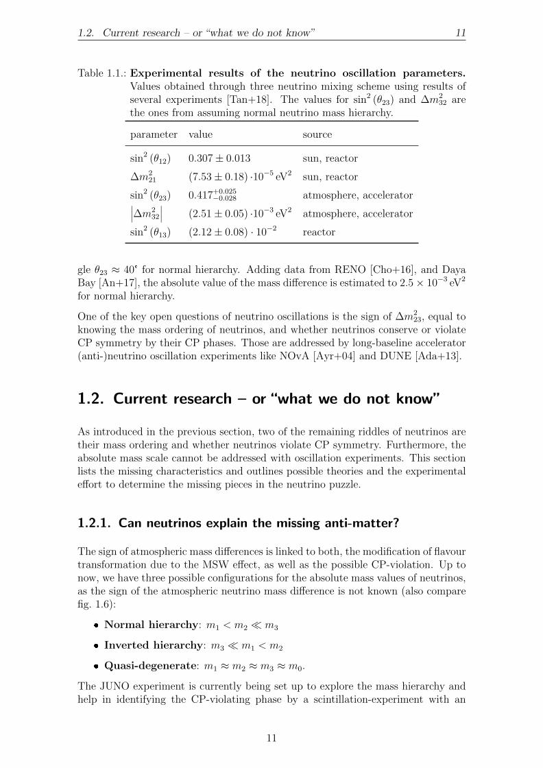
Table 1.1.: Experimental results of the neutrino oscillation parameters.Values obtained through three neutrino mixing scheme using results ofseveral experiments [Tan+18]. The values for sin2 (θ23) and ∆m2
32 arethe ones from assuming normal neutrino mass hierarchy.
parameter value source
sin2 (θ12) 0.307± 0.013 sun, reactor
∆m221 (7.53± 0.18) ·10−5 eV2 sun, reactor
sin2 (θ23) 0.417+0.025−0.028 atmosphere, accelerator∣∣∣∆m2
32
∣∣∣ (2.51± 0.05) ·10−3 eV2 atmosphere, accelerator
sin2 (θ13) (2.12± 0.08) · 10−2 reactor
gle θ23 ≈ 40° for normal hierarchy. Adding data from RENO [Cho+16], and DayaBay [An+17], the absolute value of the mass difference is estimated to 2.5× 10⁻³ eV2
for normal hierarchy.
One of the key open questions of neutrino oscillations is the sign of ∆m223, equal to
knowing the mass ordering of neutrinos, and whether neutrinos conserve or violateCP symmetry by their CP phases. Those are addressed by long-baseline accelerator(anti-)neutrino oscillation experiments like NOvA [Ayr+04] and DUNE [Ada+13].
1.2. Current research – or “what we do not know”
As introduced in the previous section, two of the remaining riddles of neutrinos aretheir mass ordering and whether neutrinos violate CP symmetry. Furthermore, theabsolute mass scale cannot be addressed with oscillation experiments. This sectionlists the missing characteristics and outlines possible theories and the experimentaleffort to determine the missing pieces in the neutrino puzzle.
1.2.1. Can neutrinos explain the missing anti-matter?
The sign of atmospheric mass differences is linked to both, the modification of flavourtransformation due to the MSW effect, as well as the possible CP-violation. Up tonow, we have three possible configurations for the absolute mass values of neutrinos,as the sign of the atmospheric neutrino mass difference is not known (also comparefig. 1.6):
� Normal hierarchy: m1 < m2 � m3
� Inverted hierarchy: m3 � m1 < m2
� Quasi-degenerate: m1 ≈ m2 ≈ m3 ≈ m0.
The JUNO experiment is currently being set up to explore the mass hierarchy andhelp in identifying the CP-violating phase by a scintillation-experiment with an
11

12 1. Neutrino physics
∆m2 ∆m2
0
m21
m22
m23
0
m23
m21
m22
∆m221, solar
∆m232, atmospheric
∆m232, atmospheric
∆m221, solar
νe νµ ντ
normal hierarchy inverted hierarchy
Figure 1.6.: Neutrino mass hierarchy. Left side shows the normal hierarchy, rightside the inverted one; the quasi-degenerate case is not shown. Thesquared mass differences are not to scale. The flavours are symbolisedby the different colours: orange for electron, green for muon, and purplefor tau flavour. Figure drawn after [Tan+18].
energy resolution of 3 %/MeV. This unprecedented energy resolution will enableresolving the tiny difference between normal and inverted mass ordering in the sub-dominant atmospheric neutrino oscillation pattern [An+16]. With the mass orderingknown, determining the CP-violating phase is possible with long-baseline accelerator(anti-)neutrino oscillation experiments like NOvA [Ayr+04] and DUNE [Ada+13].For long-baseline accelerator experiments, there might be a degeneracy in the CP-phase δ and the mass ordering. However a separate measurement of the mass or-dering like provided from JUNO [An+16] would resolve this degeneracy and enabledetermination of both, mass hierarchy and CP-phase.
The determination of the CP-phase might eventually help to resolve one of thegreatest cosmological and particle physics mysteries: the dominance of matter overanti-matter in the universe. CP violation in the neutrino sector could potentiallylead to the so-called leptogenesis [FY86, KRS85], resulting in a lepton asymmetry,which is in turn linked to the baryon asymmetry in the universe and thereby to thematter-to-antimatter relation.
One mechanism which nicely links the CP-violation and thereby the matter-anti-matter ratio to the generation of neutrino mass is the see-saw mechanism [FY86,Min77, GRS79, Yan80, MS80, SV80], which will be discussed in the next section.
1.2.2. Extensions to the Standard Model - or how neutrinosmight get their mass
In the SM, the mass of a particle is generated via coupling to the Higgs field φ. TheHiggs field has several ground states, connected via SU(2) gauge transformations.
12

1.2. Current research – or “what we do not know” 13
Therefore we can choose a ground state according to the vacuum expectation value
〈φ〉 = 1√2
0v
, (1.23)
being the only free parameter in the SM which bears the dimension of mass [PS95].The coupling of the fermions to the Higgs field is of Yukawa type, resulting in theLagrangian [PS95]
LFermion (φ,A, ψ) = ψγµDµψ +Gψψφψ, (1.24)
with the gauge covariant derivative Dµ. Using the Euler-Lagrange mechanism, theFermion-Higgs Lagrangian eq. (1.24), and left- and right-handed currents via ψ =ψL + ψR [PS95] results in the equation of motion for a Higgs-field coupled fermion
i/∂ψL −Gψ√
2
0v
ψR = 0. (1.25)
We can now identify the mass term by comparison with the Dirac equation(i/∂ −m
)ψ = 0, (1.26)
where we see the maximum parity violation of the weak interaction. The neutrinooscillations results discussed in sec. 1.1.3 showed that neutrinos have mass. Thesimplest way to add a neutrino mass would be using an additional right-handedneutrino field νR which would not participate in the weak interaction. However,though this would give neutrinos mass in the same way as the charged leptons gettheir mass (Dirac mass), it would require an additional Yukawa coupling strength.The latter would need to be much smaller than the other particles Yukawa couplingto match the smallness of the neutrino mass.
As neutrinos are uncharged particles, a more elegant solution is the combinationof the Majorana mechanism with the see-saw mechanism [Min77, GRS79, Yan80,MS80, SV80]. For reasons of simplicity, only the case of one neutrino flavour isconsidered. Decomposing the Dirac Lagrangian into its chiral components results intwo Dirac equations, with the Majorana mass in the Lagrangian
LML/R = −1
2mL/R νCL/R νL/R. (1.27)
Together with the Dirac mass LD = −mDνν (ν = νL +νR), we have the overall massterm LD+M = LD + LM
L + LMR , which can be shortened to
LD+M = −12N
TL MNL with NL =
νL
νCR
and M =
mL mD
mD mR
. (1.28)
The see-saw mechanism [Min77, GRS79, Yan80, MS80, SV80] now provides twoessential ingredients for neutrino mass generation. First, it enables a small mixingangle between left- and right-handed neutrinos, which is needed since right-handed
13
14 1. Neutrino physics
(sterile) neutrinos have not been observed yet. Second, it enables small active neu-trino masses, as we can choose mL = 0 [Min77, GRS79, Yan80, MS80, SV80] andmD � mR , so that the following masses are generated:
m1 ≈m2
D
mR
and m2 ≈ mR. (1.29)
Therefore, the neutrino mass m1 can become small, and likewise the mixing angletan 2θ = 2mD/mR. Accordingly, the active νL would mainly consist of the light ν1and the sterile νR of the heavy ν2, which agrees with current observations in theneutrino sector.
1.3. Determination of the neutrino mass
Now that we have the reasoning for a non-zero neutrino mass from oscillation exper-iments, let us discuss some experiments that take on the challenge of determiningthe absolute mass scale of neutrinos. While some of them rely on underlying model-assumptions (sec. 1.3.1), the model-independent experiments rely on conservation ofenergy and momentum only (sec. 1.3.2).
1.3.1. Model-dependent determination
In this section, the model-dependent neutrino mass estimation methods based onobservational cosmology, the search for 0νββ-decay, and supernova neutrinos will bediscussed. Note, that each of these methods makes some intrinsic (model) assump-tion to infer the neutrino mass. The discussion in this section follows the textbookby Perkins [Per09].
Cosmology Nowadays, the strongest claimed limits on the neutrino mass comefrom analyses of the Cosmic Microwave Background (CMB), with most recent mea-surements of the CMB by the Planck collaboration [Agh+18]. In the CMB spectrum,the cosmological fingerprint of massive neutrinos is a suppression of the power spec-trum on small scales [Agh+18], linked to the relativistic free-streaming of neutrinosafter their decoupling. Using the Λ-CDM model2, the upper part of the multi-pole CMB spectrum, and constraints from baryonic acoustic oscillations [Beu+11,Ros+15, Ala+17], an upper limit on the sum of neutrino masses of∑
i
mi < 0.12 eV (95 % C.L.) (1.30)
has been inferred. It has to be noted that, although this limit is quite stringent, itencompasses a dependence on the validity of the underlying Λ-CDM model, as wellas on the different observational data sets combined to achieve the result. In theabove-quoted paper [Agh+18], the Planck collaboration states limits which rangeup to 0.60 eV. A model-independent measurement of neutrino masses through alaboratory experiment would therefore ideally supplement cosmological observations.
2The Λ-CDM model uses a cosmological constant Λ for dark energy and cold dark matter (CDM)to describe the development of the universe after the Big Bang. Due to its good agreementwith cosmological observations [Agh+18], it is often referred to as standard model of Big Bangcosmology.
14

1.3. Determination of the neutrino mass 15
Supernova neutrinos During the core-collapse of a supernova (type Ib, Ic, II),99 % of the gravitational energy released is emitted in the form of neutrinos at MeVenergies, with a burst length of about 10 s [Per09]. The observation of the neutrinoburst signal of the supernova SN1987A enables to determine the the measured arrivaltime difference of two neutrinos ass
∆t = t2 − t1 = ∆t0 + Lc3m2ν
2
(1E2
2− 1E2
1
). (1.31)
With the measured ∆t, and the energies E1, E2 of the neutrinos, only the emissiontime difference ∆t0 = t02−t01 and the neutrino mass mν are unknown. Using a modelfor the neutrino emission in the core-collapse supernova, ∆t0 can be constrained,enabling an estimation of the neutrino mass. Loredo and Lamb derive an upperlimit from the neutrino burst signal of SN1987A as [LL02]
mν < 5.7 eV (95 % C.L.). (1.32)
Neutrino-less double beta-decay As introduced in sec. 1.2.2, the see-saw mech-anism provides a nice explanation for the smallness of the active neutrino mass. Ifneutrinos are their own anti-particles, so-called Majorana particles, this would enablea very rare decay, the double β-decay without emission of neutrinos [DKT85] (0νββ).Therein, a virtual neutrino is exchanged between the decaying nuclei which is possi-ble due to the Majorana nature. From the observed half life of a 0νββ-decay T 0νββ
1/2 ,the effective Majorana neutrino mass can be determined via (see e.g. ref. [EM17])
〈mββ〉2 ≤∣∣∣∣∣
3∑i=1
U2eimi
∣∣∣∣∣2
= 1G0νββ ·
∣∣∣M0νββ∣∣∣2 · T 0νββ
1/2
, (1.33)
with the phase space factor G0νββ, and the nuclear matrix element M0νββ. Theestimated neutrino mass strongly depends on the uncertainty of the calculated nu-clear matrix element. Most recent estimations of the effective Majorana mass by theMajorana [Aal+18], GERDA [Ago+18], EXO-200 [Alb+18], and CUORE [Ald+18]experiment result in values in the range
〈mββ〉 < 0.11− 0.52 eV (90 % C.L.). (1.34)
The to date most stringent limit on on the effective Majorana neutrino mass is statedby the KamLAND-Zen collaboration [Gan+16] as
〈mββ〉 < 0.061− 0.165 eV (90 % C.L.). (1.35)
It has to be noted that in the squared sum of the mixing matrix elements cancel-lations may occur due to the Majorana phases. This particular feature, in turn,may give access to the Majorana phases α1,2 by comparison of 〈mββ〉 to a model-independent measurement.
1.3.2. Model-independent determination
In order to determine the neutrino mass in a direct, model-independent way, themost promising candidate today is investigating the kinematics of single β-decay.
15

16 1. Neutrino physics
Thereby, the only prerequisites are energy and momentum conservation, with noassumption made on the nature of the neutrinos. The neutrino mass manifests inform of missing energy in the β-decay
AZN →A
Z+1 N′ + e− + νe. (1.36)
Using Fermi’s Golden Rule [Fer34], the β-decay rate can be derived [KAT05, Dre+13](neglecting for now possible final states of the daughter molecule)
dΓdE
=G2F · cos θC · |M |2
2π3 · F (Z + 1, E) · p · (E +me)
·√
(E0 − E)2 −m2νe·Θ(E0 − E −mνe
), (1.37)
with Fermi’s coupling constant GF, Cabibbo angle θC, transition matrix element M ,Fermi function F (Z + 1, E), kinetic energy and momentum of the electron E, p,mass of the electron me, endpoint of the β-decay spectrum E0 = Q −me, and thedecay energy Q. An exemplary tritium β-decay spectrum and the effect of a non-zeroneutrino mass are shown in fig. 1.7.
0 5 10 15 20
energy (keV)
0
1
dΓ
dE
(eV−
1s−
1)
×10−13
−2 −1 0E − E0 (eV)
0
2
4
dΓ
dE
(eV−
1s−
1)
×10−21
mν = 0 eV
mν = 1 eV
Figure 1.7.: Tritium decay spectrum. Left side shows the full-range tritium β-decay spectrum, right side an enlarged endpoint region.
Several experiments are currently in their commissioning phase or being set up inorder to explore the kinematics of β-decay with unprecedented sensitivity. The mostpromising techniques are a calorimetric approach followed by the ECHo [Gas+17]and HOLMES [Nuc+18] collaborations, a cyclotron radiation approach followed byProject 8 [MF09] and the MAC-E filter approach [BPT80, KR83, LS85, Pic+92] fol-lowed by the Mainz [Kra+05], Troitsk [Ase+11], and Katrin experiments [KAT05].
Calorimetric approach The ECHo [Gas+17] and HOLMES [Nuc+18] collabora-tions investigate the electron capture on 163Ho, with aQ-value of 2.8 keV. Like for theβ-decay spectrum, the rate close to the spectral endpoint depends on the neutrinomass squared [LV11]. Therefore, the ECHo and HOLMES collaborations aim fora high energy resolution combined with a detector read out by microwave SQUIDmultiplexing. The ECHo experiment determines the released energy via MetallicMagnetic Calorimeters, which are measuring the change in magnetisation due to thetemperature increase of the detector [Bur+08]. With a projected energy resolutionof ∆E < 3 eV, and a set-up of up to 105 detectors, a sub-eV neutrino mass sensi-tivity may be reached [Dre+13]. For HOLMES, the Transition Edge Sensor (TES)technology is pursued [Nuc+18].
16

1.3. Determination of the neutrino mass 17
Cyclotron radiation approach The idea of the Project 8 experiment is to observesingle electrons from tritium β-decay via their cyclotron radiation emitted in a mag-netic field [MF09]. The power emitted by each electron depends on its relativevelocity (and thereby the energy) as well as its pitch angle relative to the magneticfield. With a finite minimum observation time of 30µs [MF09] as the minimum timebetween electron-gas scattering, the required long electron path length favours anelectron trap configuration [MF09, Dre+13]. An obvious choice is a magnetic bottlewith increased magnetic field at both ends of the tritium gas-filled tube. Microwaveantenna arrays around the tube and at both ends can be used to detect the emittedcyclotron radiation and to reconstruct the electron’s energy. In recent work, theProject 8 collaboration showed the promising detection technique to achieve energyresolutions of about 3 eV at energies of about 30 keV, achieved in the successful mea-surement of 83mKr-lines [Asn+15, Esf+17]. In a staged approach, the near-term aimof Project 8 is to achieve 2 eV sensitivity (90 % C.L.) with a molecular tritium sourceand to further explore a novel atomic tritium source technique to probe the invertedhierarchy mass scale on a longer perspective [Esf+17].
MAC-E filter approach The most recent model-independent limits on the neutrinomass come from the Mainz [Kra+05] and the Troitsk [Ase+11] experiment using theMAC-E filter technique to analyse the tritium β-decay spectrum. The MAC-E filteruses magnetic adiabatic collimation with electrostatic energy analysis, it is describedin more detail in sec. 2.2.4. An ideal β-emitter for neutrino mass determination fromkinematics is tritium, due to the following advantages:
� favourably low β-decay Q-value of 18.6 keV,
� super-allowed decay, so no energy dependence and corrections of the nucleartransition matrix element are needed,
� short half life of T1/2 = 12.3 yr (related to the previous item),
� mother and daughter nucleus have low Z values, leading to simple electroninteractions and low inelastic scattering probability.
Note that β-decay spectroscopy estimates an effective neutrino mass as incoherentsum of the neutrino mass eigenstates
m2νe
=3∑i=1|Uei|2 ·m2
i , (1.38)
as present energy resolutions of spectroscopic experiments cannot resolve the differ-ent mass eigenstates. Combining the Mainz limit of 2.3 eV (95 % C.L.) [Kra+05]and the Troitsk limit of 2.05 eV (95 % C.L.) [Ase+11] for the effective electron (anti-)neutrino mass results in the currently most stringent model-independent limit [Tan+18]of
mνe< 2.0 eV (95 % C.L.). (1.39)
The Katrin experiment is targeted to determine the neutrino mass with a one orderof magnitude better sensitivity than the existing limit. Katrin has successfullyperformed a sequence of dedicated commissioning phases, using electrons from aphoto electron source, conversion electrons from 83mKr [Are+18b, Are+18a], andjust recently first tritium β-decay data [Are+19]. Details about its experimentalset-up are presented in the next chapter.
17


CHAPTER 2
THE KARLSRUHE TRITIUM NEUTRINO EXPERIMENT
The KArlsruhe TRItium Neutrino (KATRIN) Experiment is dedicated to determin-ing the neutrino mass with an unprecedented sensitivity of 200 meV (90 % C.L.).Compared to the predecessor experiments at Mainz and Troitsk, this is a sensitivitygain of a factor of 10. Since the observable is the neutrino mass square, this requiresan overall improvement of the neutrino mass square uncertainty of a factor of 100.In order to achieve this aspiring goal, KATRIN performs high precision spectroscopyof the tritium β-decay spectrum close to the endpoint at 18.6 keV.
This chapter gives an overview of the measuring principle of Katrin (sec. 2.1), theset-up that allows to realise this measuring principle (sec. 2.2), and the analysissoftware used to access and analyse the produced data (sec. 2.4).
2.1. Neutrino mass from tritium β-decay
Katrin investigates the β-decay of molecular tritium
T2 →(
3HeT)+
+ e− + νe. (2.1)
The decay rate can be derived using Fermi’s Golden Rule [Fer34]
dΓdE
=G2F · cos θC · |M |2
2π3 · F (Z + 1, E) · p · (E +me)
·∑fs
Pfs · frad(E − Efs) · εfs ·√ε2fs −m2
νe·Θ(εfs −mνe
), (2.2)
with the parameters GF, θC, M , F (Z,E), electron kinetic energy E, electron momen-tum p, electron mass me, and tritium endpoint E0 defined according to eq. (1.37). Asan extension to the single-nucleus treatment of eq. (1.37), this equation also consid-ers molecular effects via the final states energy Efs, resulting in a reduced endpointenergy of εfs = E0−E−Efs. Due to interaction of the electron with virtual photonsin the Coulomb field of the nucleus, the emitted electrons lose energy. This energyloss is implemented into the spectrum calculation as radiative corrections by thefactor frad(E − Efs) according to the recommendations by Repko and Wu [RW83].
19

20 2. The KArlsruhe TRItium Neutrino Experiment
Spectrometers and detector sectionMain spectrometerPre-
spectrometerDetectorCPSDPS2-F
Transport sectionWGTS cryostat
DPS
1-F
DPS
1-R
Rearsection
-8 m -5 m0 m
+5 m +8 m
16 m
70 m
Figure 2.1.: KATRIN set-up. The individual components fulfil specific tasks toenable reaching the 200 meV sensitivity:
� Rear section - monitoring and calibration of the tritium source
� WGTS - providing a stable activity of 1011 s−1
� DPS - tritium removal
� CPS - tritium removal
� Pre-spectrometer - pre-selection of the high-energy part of the β-decay spec-trum
� Main spectrometer - high-resolution β-decay spectroscopy
� Detector - counting the transmitted electrons
Katrin analyses the decay spectrum according to eq. (2.2) via the MAC-E filterprinciple [BPT80, KR83, LS85, Pic+92]. The (effective) neutrino mass is thenextracted as a shape distortion close to the endpoint. The MAC-E filter acts as ahigh-pass filter, resulting in a measurement of an integrated spectrum by stepping theretardation potential [KAT05, Kle+18]. Using a response function to describe theelectron transport through the experiment, this integrated spectrum reads [Kle+18]
N(U) = 12NT
E0∫qU
dΓdE·R(E,U) dE. (2.3)
Thereby, the signal rate depends on the number of tritium nuclei in the source NT,the retarding voltage of the spectrometer U , and the response function R(E,U)(only considering electrons emitted in direction of the detector, see sec. 2.2.4).
2.2. Components of the KATRIN experiment
The 70 m long set-up that Katrin uses to measure the integrated count rates ineq. (2.3) is depicted in fig. 2.1. Electrons originating from β-decay in the ultra-luminous Windowless Gaseous Tritium Source (WGTS, sec. 2.2.1) are magneticallyguided via the transport section (sec. 2.2.3) to the energy analysing spectrometersection (sec. 2.2.4). Those passing the spectrometers are finally counted at the detec-tor (sec. 2.2.5). Several instruments monitor the activity, stability and composition
20

2.2. Components of the KATRIN experiment 21
of the tritium gas (sec. 2.2.2), which is continuously injected into the WGTS andpumped out at both ends.
2.2.1. The Windowless Gaseous Tritium Source
In order to reach the unprecedented neutrino mass sensitivity of 200 meV, Ka-trin makes use of a large β-decay rate of 1011 s−1 provided by per-mille stable circu-lation of tritium gas in the Windowless Gaseous Tritium Source (WGTS) [Gro+08,Bab+12, PSB15, HS17]. A daily throughput of about 40 g of tritium in a closed gasloop system results in a longitudinally integrated gas column density in the WGTSbeam tube of N = 5× 10²¹ m−2 or roughly 300µg of tritium. Tritium is injectedwith a pressure of about 3 µbar in the centre of the 10 m long beam tube and pumpedout at both ends via turbomolecular pumps (TMPs). On their way to the pumpports, the tritium molecules may decay, leaving the daughter molecule in a possiblyexcited final state (see sec. 2.2.2). Electrons originating from the tritium decay aremagnetically guided to both ends of the WGTS. The rear section uses the incom-ing electron flux for monitoring purposes (see sec. 2.2.2) while the other half of theelectrons is used to perform neutrino mass spectroscopy with the spectrometers anddetector section (sec. 2.2.4). In order to account for effects that affect the electron’senergy on their way to the detector, the concept of a response function [KAT05,Kle+18] is introduced. The source-related quantities of interest are the energy lossε of the electrons due to scattering on residual gas, which is described by the en-ergy loss function f(ε) [KAT05, Kle+18], and the scattering probabilities for s-foldscattering, Ps(z, θ). The energy loss per scattering solely depends on the scatteringcross section, as investigations by S. Groh showed the scattering attributed angu-lar change to be negligible [Gro15]. The scattering probabilities Ps(z, θ) in generaldepend on the longitudinal density profile in the WGTS and the pitch angle of theelectrons relative to the magnetic field lines.
Energy loss function The total scattering cross section consists of an elastic partand an inelastic part. In refs. [Gei64, Liu87], the elastic scattering cross sec-tion σel = 0.29× 10⁻²² m2 was shown to be one order of magnitude smaller thanthe inelastic part, which is measured by Aseev et al. to σinel = (3.40 ± 0.07) ·10−22 m2 [Ase+00]. As the neutrino mass uncertainty raised by neglecting the elasticscattering cross section is about 5× 10⁻⁵ eV2, it is often neglected in the modelling ofthe β-decay spectrum. Aseev et al. determined the inelastic scattering cross sectionby fitting an empirical model to the energy loss function spectrum. The empir-ical model consists of a low-energy Gaussian describing the (discrete) excitationprocesses and a high-energy Lorentzian for the continuum due to ionisation of thetritium molecules
f(ε) =
A1 · e−2(ε−ε1ω1
)2
, ε < εc
A2 · ω22
ω22+4(ε−ε2)2 , ε ≥ εc
, (2.4)
with A1 = (0.204± 0.001) eV−1, A2 = (0.0556± 0.0003) eV−1, ω1 = (1.85± 0.02) eV,ω2 = (12.5± 0.1) eV, fixed ε1 = 12.6 eV, and ε2 = (14.30± 0.02) eV. The transitionfrom one to the other part of the energy loss function eq. (2.4) is smooth due tothe chosen critical energy of εc = 14.09 eV. Multiple scattering is accounted for via
21

22 2. The KArlsruhe TRItium Neutrino Experiment
convolving the energy loss function f(ε) with itself, compare the right-hand panel infig. 2.2.
0 10 20 30 40 500.0
0.1
0.2
0.00 0.010
10
20
energy loss ε (eV)
f(ε
)
0 10 20 30 40 500.00
0.02
0.04
0.06
0.00 0.010.0
0.2
0.4
0.6
energy loss ε (eV)
f(ε
)∗f
(ε)
Figure 2.2.: Energy loss function. Left-hand side shows the energy loss for singlescattering, right-hand side for two-fold scattering. The enlarged regionsshow the elastic scattering contribution. Figure adapted from [Kle+18].
Scattering probabilities In order to take into account spatial inhomogeneities ofthe magnetic field or the gas distribution in the source, the model partitions thesource into so-called voxels (volume elements). The longitudinal extent of the voxelsis given by the length of the source divided by the number of slices used, and theazimuthal and radial segmentation can be chosen as to magnetically map the pixelsof the detector (see fig. 2.3). The probability for an electron to reach the detector
−L/2 0 +L/2z
WGTS transport, spectrometer section FPD
Figure 2.3.: Voxelisation concept. Each pixel j can be mapped onto correspond-ing voxels in the source. These voxels ares stacked longitudinally (in-dex i) to calculate the rate for pixel j. Figure adapted from [Kle+18].
after undergoing s-fold scattering in the source depends on the total scattering crosssection σtot and on the source geometry conditions, starting position and startingpitch angle θ (angle between electron momentum and magnetic field, θ = ∠(p,B)).Both source conditions define the effective column density Neff that the electron hasto pass. Electrons with a larger pitch angle take a longer path through the source andtherefore “see” an increased effective column density. The effective column density
22
2.2. Components of the KATRIN experiment 23
for an electron starting at longitudinal position z is
Neff(z, θ) = 1cos θ
L/2∫z
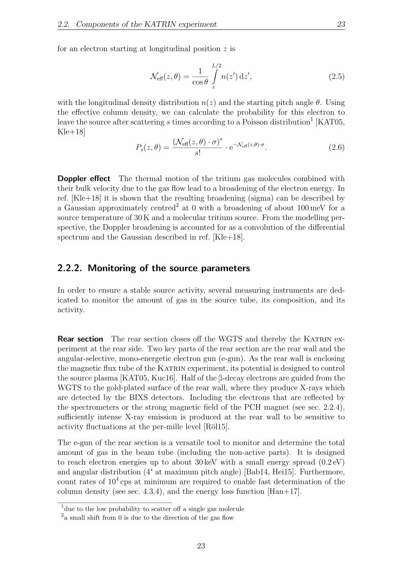
n(z′) dz′, (2.5)
with the longitudinal density distribution n(z) and the starting pitch angle θ. Usingthe effective column density, we can calculate the probability for this electron toleave the source after scattering s times according to a Poisson distribution1 [KAT05,Kle+18]
Ps(z, θ) = (Neff(z, θ) · σ)s
s! · e−Neff(z,θ)·σ. (2.6)
Doppler effect The thermal motion of the tritium gas molecules combined withtheir bulk velocity due to the gas flow lead to a broadening of the electron energy. Inref. [Kle+18] it is shown that the resulting broadening (sigma) can be described bya Gaussian approximately centred2 at 0 with a broadening of about 100 meV for asource temperature of 30 K and a molecular tritium source. From the modelling per-spective, the Doppler broadening is accounted for as a convolution of the differentialspectrum and the Gaussian described in ref. [Kle+18].
2.2.2. Monitoring of the source parameters
In order to ensure a stable source activity, several measuring instruments are ded-icated to monitor the amount of gas in the source tube, its composition, and itsactivity.
Rear section The rear section closes off the WGTS and thereby the Katrin ex-periment at the rear side. Two key parts of the rear section are the rear wall and theangular-selective, mono-energetic electron gun (e-gun). As the rear wall is enclosingthe magnetic flux tube of the Katrin experiment, its potential is designed to controlthe source plasma [KAT05, Kuc16]. Half of the β-decay electrons are guided from theWGTS to the gold-plated surface of the rear wall, where they produce X-rays whichare detected by the BIXS detectors. Including the electrons that are reflected bythe spectrometers or the strong magnetic field of the PCH magnet (see sec. 2.2.4),sufficiently intense X-ray emission is produced at the rear wall to be sensitive toactivity fluctuations at the per-mille level [Rol15].
The e-gun of the rear section is a versatile tool to monitor and determine the totalamount of gas in the beam tube (including the non-active parts). It is designedto reach electron energies up to about 30 keV with a small energy spread (0.2 eV)and angular distribution (4° at maximum pitch angle) [Bab14, Hei15]. Furthermore,count rates of 104 cps at minimum are required to enable fast determination of thecolumn density (see sec. 4.3.4), and the energy loss function [Han+17].
1due to the low probability to scatter off a single gas molecule2a small shift from 0 is due to the direction of the gas flow
23
24 2. The KArlsruhe TRItium Neutrino Experiment
Final states As introduced in eq. (2.2), we may find the daughter molecule ofthe molecular tritium β-decay in an excited state. The excitation of the daughtermolecule can be of rotational, vibrational, and electronic nature. Each of the pos-sible excited states has its own specific endpoint of εfs = E0 − E − Efs, compareeq. (2.2). As the final states energy is missing energy for the electron, it is crucialfor a direct neutrino mass experiment like Katrin to use highly accurate calcu-lations of the final states distributions. About 57 % of the T2-decays go into therovibronically-broadened electronic ground state [JSF99]. As there are also otherhydrogen isotopologues present in the source gas, each decaying species (T2, DT,HT) needs to be weighted according to its abundance. Calculations for the finalstates of the different hydrogen isotopologues have been performed in refs. [SJF00,Dos+06, DT08] and give the excitation energy relative to the molecular recoil en-ergy of (HeT)+. The calculations also provide separate distributions for the differentinitial quantum state in terms of molecular angular momentum J . The J states arepopulated according to a temperature dependent Boltzmann distribution [Kle+18]
PJ(T ) ∝ gs · gJ · e−∆EJkBT , (2.7)
with kB the Boltzmann constant, T the temperature, ∆EJ the energy difference tothe electronic ground state, the rotational degeneracy of the distribution gJ , andthe spin degeneracy of the nuclei gs. The rotational degeneracy factor is given bygJ = 2J + 1, while gs = 1 for the heteronuclear molecules DT and HT. For thespin-coupling T2, gs depends on the ortho-para ratio λ of the molecules [BPR15,Kle+18].
When comparing the overall decay energy (Q-value) to the maximum electron energyE0, the molecular recoil energy Erec ≈ E · me
m(3HeT)+
≈ 1.7 eV needs to be taken into
account. Over the last 50 eV of the electron spectrum, Erec only changes by about6 meV [KAT05].
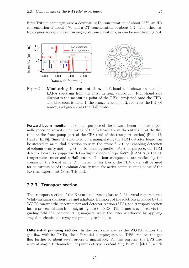
LARA As outlined in the previous paragraph, it is very important to know thecomposition of the source gas at all times as it determines the mixing of the β-spectra from the different tritiated isotopologues: the final state distribution of theT2, DT, and HT daughter molecule ions 3HeT+, 3HeD+, and 3HeH+ differ substan-tially. In [Bab+12], a requirement on the precision of the tritium purity monitoringof 10−3 is derived from the argumentation that a precise monitoring of εT combinedwith a precise observation of the activity via the BIXS monitors at the rear wallenables conclusive monitoring of the column density. To reach the per-mille require-ment, a dedicated LAser RAman (LARA) system was developed [Fis+11, Sch13,Fis14]. LARA uses the principle of Raman spectroscopy to determine the isotopiccomposition of the source gas. Photons from a laser with a wavelength of 532 nmscatter off gas molecules in an optical cell, which is part of the inner tritium circu-lation loop. The inelastically scattered (red-shifted) photons are spectroscopicallyanalysed and recorded. Each of the six hydrogen isotopologues has a characteristicrotational-vibrational excitation which contributes to the resulting Raman spectrum.By taking into account an elaborate calibration method [Sch13, Zel17], the accurategas composition can be extracted. An example of a LARA spectrum taken duringthe First Tritium campaign is shown in fig. 2.4. The ratios of the integrated intensi-ties give the concentrations of the different isotopologues. Typical values during the
24
2.2. Components of the KATRIN experiment 25
First Tritium campaign were a dominating D2 concentration of about 93 %, an HDconcentration of about 6 %, and a DT concentration of about 1 %. The other iso-topologues are only present in negligible concentrations, as can be seen from fig. 2.4.
5001000 raw spectrum
fitted spectrum
4000350030002500
Raman shift (cm−1)
0
25T2 DT HT H2
inte
nsi
ty(a
rb.
u.)
D2 (O1)
D2
D2 (S1)
HD
Figure 2.4.: Monitoring instrumentation. Left-hand side shows an exampleLARA spectrum from the First Tritium campaign. Right-hand sideillustrates the measuring point of the FBM, projected onto the FPD.The blue cross is diode 1, the orange cross diode 2, red cross the Pt1000sensor, and green cross the Hall probe.
Forward beam monitor The main purpose of the forward beam monitor is per-mille precision activity monitoring of the β-decay rate in the outer rim of the fluxtube at the front pump port of the CPS (end of the transport section) [Bab+12,Hau18, Ell18]. Since it is mounted on a manipulator, the FBM detector board canbe steered in azimuthal direction to scan the entire flux tube, enabling detectionof column density and magnetic field inhomogeneities. For that purpose, the FBMdetector board is equipped with two Si-pin diodes of type S5971 [HAM18], a Pt1000temperature sensor and a Hall sensor. The four components are marked by thecrosses on the board in fig. 2.4. Later in this thesis, the FBM data will be usedfor an estimation of the column density from the active commissioning phase of theKatrin experiment (First Tritium).
2.2.3. Transport section
The transport section of the Katrin experiment has to fulfil several requirements.While ensuring collision-free and adiabatic transport of the electrons provided by theWGTS towards the spectrometer and detector section (SDS), the transport sectionhas to prevent tritium from migrating into the SDS. The former is achieved via theguiding field of superconducting magnets, while the latter is achieved by applyingstaged mechanic and cryogenic pumping techniques.
Differential pumping section In the very same way as the WGTS reduces thegas flow with its TMPs, the differential pumping section (DPS) reduces the gasflow further by about seven orders of magnitude. For this purpose, the DPS usesa set of staged turbo-molecular pumps of type Leybold Mag W 2800 [ide10], which
25
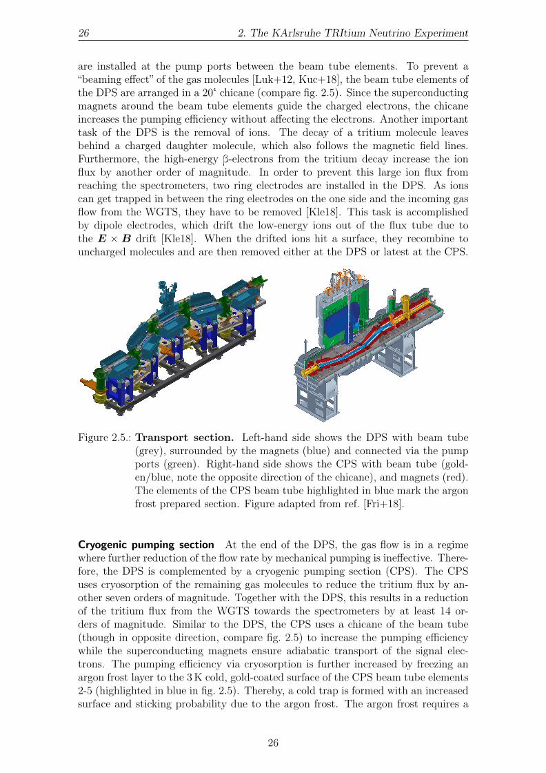
26 2. The KArlsruhe TRItium Neutrino Experiment
are installed at the pump ports between the beam tube elements. To prevent a“beaming effect” of the gas molecules [Luk+12, Kuc+18], the beam tube elements ofthe DPS are arranged in a 20° chicane (compare fig. 2.5). Since the superconductingmagnets around the beam tube elements guide the charged electrons, the chicaneincreases the pumping efficiency without affecting the electrons. Another importanttask of the DPS is the removal of ions. The decay of a tritium molecule leavesbehind a charged daughter molecule, which also follows the magnetic field lines.Furthermore, the high-energy β-electrons from the tritium decay increase the ionflux by another order of magnitude. In order to prevent this large ion flux fromreaching the spectrometers, two ring electrodes are installed in the DPS. As ionscan get trapped in between the ring electrodes on the one side and the incoming gasflow from the WGTS, they have to be removed [Kle18]. This task is accomplishedby dipole electrodes, which drift the low-energy ions out of the flux tube due tothe E × B drift [Kle18]. When the drifted ions hit a surface, they recombine touncharged molecules and are then removed either at the DPS or latest at the CPS.
Figure 2.5.: Transport section. Left-hand side shows the DPS with beam tube(grey), surrounded by the magnets (blue) and connected via the pumpports (green). Right-hand side shows the CPS with beam tube (gold-en/blue, note the opposite direction of the chicane), and magnets (red).The elements of the CPS beam tube highlighted in blue mark the argonfrost prepared section. Figure adapted from ref. [Fri+18].
Cryogenic pumping section At the end of the DPS, the gas flow is in a regimewhere further reduction of the flow rate by mechanical pumping is ineffective. There-fore, the DPS is complemented by a cryogenic pumping section (CPS). The CPSuses cryosorption of the remaining gas molecules to reduce the tritium flux by an-other seven orders of magnitude. Together with the DPS, this results in a reductionof the tritium flux from the WGTS towards the spectrometers by at least 14 or-ders of magnitude. Similar to the DPS, the CPS uses a chicane of the beam tube(though in opposite direction, compare fig. 2.5) to increase the pumping efficiencywhile the superconducting magnets ensure adiabatic transport of the signal elec-trons. The pumping efficiency via cryosorption is further increased by freezing anargon frost layer to the 3 K cold, gold-coated surface of the CPS beam tube elements2-5 (highlighted in blue in fig. 2.5). Thereby, a cold trap is formed with an increasedsurface and sticking probability due to the argon frost. The argon frost requires a
26

2.2. Components of the KATRIN experiment 27
few days of warming up the CPS in order to regenerate the frost layer about every60 d [KAT05].
2.2.4. Spectrometers section
Katrin makes use of a spectrometer tandem to perform high-precision β-decay spec-troscopy of the electrons produced in the tritium source. The tandem consists of apre-spectrometer to filter the low-energy electrons, followed by the main spectrom-eter to perform the high precision spectral analysis. One of the keys for the successof the Katrin experiment is the ultra-high vacuum achieved in the spectrome-ters section, as low-energy electrons have a very large cross-section for scatteringwith residual gas. Both spectrometers are therefore operated at pressures below10−11 mbar [Are+16].
Pre-spectrometer In order to enable the precision β-decay spectroscopy of thehigh-energy end of the β-spectrum with the main spectrometer, the pre-spectrometeruses an energy barrier up to a design value of 18.3 keV. This pre-filtering reducesthe β-decay electron flux by seven orders of magnitude and thereby minimises back-ground due to residual gas ionisation. Successful countermeasures to mitigate back-ground caused by a Penning trap are e.g. the Penning wiper method [Pra11, Pra+12].
Main spectrometer After the pre-filtering in the pre-spectrometer, the electronsreach the main spectrometer. The task of this key component of the Katrin exper-iment is to perform the high-precision spectroscopy of the tritium β-decay endpoint.In order to achieve the required superior energy resolution of 0.93 eV, the main spec-trometer combines magnetic adiabatic collimation with electrostatic retardation, theso-called MAC-E filter principle [BPT80, KR83, LS85, Pic+92] which will be out-lined in the following.
Magnetic adiabatic collimation The magnetic guiding field along the Katrinbeam line results in gyration of the electrons around the magnetic field lines due tothe Lorentz force. The kinetic energy of the electrons is shared by the longitudinaland a transverse component relative to the magnetic field:
Ekin = E‖ + E⊥ = E cos2 θ + E sin2 θ, (2.8)
with the pitch angle θ defined as the polar angle between the electron momentumand the magnetic field, θ = ∠(p,B). The electrostatic retardation potential can onlyanalyse the fraction of the energy that is parallel to the electric field direction (E‖).Therefore, the momenta of the electrons need to be aligned as parallel as possiblevia the magnetic adiabatic collimation. This principle and further characteristics ofthe main spectrometer will now be discussed in detail:
� Adiabatic guiding of the electrons. With the minimised change of themagnetic field along one cyclotron cycle in the main spectrometer, adiabatic
27

28 2. The KArlsruhe TRItium Neutrino Experiment
guiding of the electrons is ensured. Then, the product γ · µ of relativis-tic Lorentz factor γ and the magnetic moment µ is a constant of the mo-tion [Jac99]: in the non-relativistic limit where γ = 1, this results in
µ = E⊥B
= const. (2.9)
(Note that γ = 1.04 ≈ 1 for electrons at the tritium endpoint energy of18.6 keV.) As the electrostatic retarding potential only analyses the longitudi-nal part of the energy, the transverse part E⊥ needs to be minimised in orderto obtain a good energy resolution. This is achieved by two superconductingmagnets at both ends of the spectrometer (with a distance of about 22 m inbetween, see fig. 2.6), resulting in a minimum magnetic (stray) field Bmin in themiddle of the spectrometer. As described by eq. (2.9), this drop of the mag-netic field strength minimises the transverse energy accordingly, enabling theenergy analysis in the so-called analysing plane via an electrostatic retardingpotential.
� Energy resolution. The ratio of minimum and maximum magnetic fieldstrength defines the fraction of transverse energy that cannot be analysed bythe MAC-E filter, which is often referred to as energy resolution ∆E:
∆EE
= Bmin
Bmax
. (2.10)
For electron energies around the endpoint of E = 18.6 keV, the design min-imum magnetic field of Bmin = 0.3 mT, and the design maximum magneticfield of Bmax = 6 T, this results in a filter width of ∆E = 0.93 eV.
� Conservation of magnetic flux. In order to ensure transport of all signalelectrons, the magnetic flux
Φ =∫A
B dA, (2.11)
defined by the tritium source has to be conserved. With the low magnetic fieldof 0.3 mT in the analysing plane, this results in a diameter of the flux tube ofabout 10 m in the centre of the main spectrometer.
� Magnetic mirror. Adiabatic guiding of the electrons from the tritium sourceto the detector establishes a fixed relation between pitch angle and magneticfield. Two arbitrary points on the path of the electrons are related via
sin2 θ1
sin2 θ2= B1
B2. (2.12)
The maximum pitch angle of tritium β-decay electrons is defined by the ratioof source magnetic field BS and the maximum magnetic field along the beamline Bmax, which usually is the PCH magnet on the detector side of the mainspectrometer:
θmax = arcsin√
BS
Bmax
= 50.8°, (2.13)
with design values of BS = 3.6 T, and Bmax = 6 T.
28

2.2. Components of the KATRIN experiment 29
STS/PS FPD
Bmax
Bmin
qE
B
p
Figure 2.6.: MAC-E filter principle. The electron momentum is almost parallelto the minimum magnetic field in the centre of the main spectrometer(length of the arrows not to scale). Aligning minimum magnetic fieldand maximum retarding potential qU yields the unprecedented filterwidth of 0.93 eV. Figure adapted from ref. [Hac17].
Electrostatic retardation Using the principle of magnetic adiabatic collimationdiscussed above, the energy of the electrons can be studied via application of a (neg-ative) electrostatic potential in the analysing plane. Only electrons with longitudinalenergy larger than the electrostatic potential can pass the analysing plane and reachthe detector. In that way, both spectrometers act as high-pass filters, resulting inthe measurement of an integrated β-decay spectrum as indicated in eq. (2.3).
Transmission function Combining the above-mentioned MAC-E filter character-istics of magnetic adiabatic collimation and electrostatic retardation results in thetransmission probability for electrons to pass the main spectrometer. It can beanalytically described by the transmission function T (E, qU) [KAT05, Kle+18]
T (E,U) =
0 for E < qU
1−√
1− E−qUE
BS
Bmin
1−√
1− BS
Bmax
for qU ≤ E ≤ qU + ∆E
1 for E > qU + ∆E
. (2.14)
Response function Combining all effects that influence the electrons on their wayfrom their creation in the tritium source up to passing the analysing plane of the mainspectrometer results in the aforementioned response function R(E,U). It combinesthe transmission function of the main spectrometer T (E,U) (see eq. (2.14)) with
29

30 2. The KArlsruhe TRItium Neutrino Experiment
the energy loss function of the source f(ε) (eq. (2.4)) as
Ri,j(E,U) =E−qU∫ε=0
θmax∫θ=0
∑s
T cycls,i,j (E − ε, θ, U) · Ps,i(θ) · fs(ε) dε sin θ dθ, (2.15)
with the indices s, i, j denoting the number of scatterings s and the voxel i, j aspreviously introduced [KAT05, Kle14, Kle+18]. The label cycl indicates that thetransmission function also needs to be corrected for energy loss due to cyclotronradiation [Kle+18].
2.2.5. Detector section
After passing the analysing plane of the main spectrometer, the signal electrons reachthe detector section. A 148-pixel silicon pin diode wafer counts these signal elec-trons with high efficiency required as εdet,j ≥ 90 % [KAT05], which was confirmed inref. [Ams+15] (the index j indicates the pixel of the detector). The signal electronsare guided to the focal plane detector (FPD) wafer by two superconducting magnets,the PCH magnet with the maximum magnetic field (6 T) of the Katrin experimentand the detector magnet (3.6 T). In order to increase the detection efficiency andreduce backscattering effects, a post-acceleration electrode is used to add anotherconstant 10 keV of energy to the signal electrons. At the port between the twomagnets (compare fig. 2.7), calibration sources can be installed to determine the de-tection efficiency and energy calibration of each single pixel. One of these calibrationsources is the Precision Ultra-Low Current Integrating Normalization Electrometerfor Low-Level Analysis (PULCINELLA) [Ams+15], which can be used as a Faradaycup to detect an electron flux. This method will be used to estimate the columndensity from the active commissioning phase of the Katrin experiment.
2.3. Modelled count rate
Now that all components of the Katrin experiment were introduced and theirrespective importance for the measured spectrum described, the integrated countrate measured by the FPD pixel j for a given potential of the main spectrometer Ucan be written as [Kle+18]
Nj(U) = 12 εdet,j ·
∑i
·∞∫qU
(dΓdE
)C,D
(m2ν, E0) ·Ri,j(E,U) dE, (2.16)
with the indices C,D denoting theoretical corrections C, and the Doppler effect con-volution D (see sec. 2.2.1) which both affect the differential spectrum of the tritiumdecay given in eq. (2.2). The response function Ri,j(E,U) is given in eq. (2.15).
30

2.4. Analysis tools and software at the KATRIN experiment 31
detector wafer
detector magnet
pinch magnet
main spectrometer
Figure 2.7.: Detector section. The magnetic flux tube is highlighted in green,while the orange part in front of the detector wafer depicts the post-acceleration electrode. At the port between the two magnets, calibrationsources can be installed. Figure adapted from ref. [Ams+12].
2.4. Analysis tools and software at the KATRINexperiment
In order to enable the neutrino mass analysis of Katrin data at the level of spectrumfitting, a number of successive data layers process the raw data acquired by variousdetectors (like FPD and FBM), and sensors (like Pt500 sensors of the WGTS).The first processing step of detector data is by a Detector Data Acquisition (DAQ)system based on Field Programmable Gate Array (FPGA) architecture. Operatorsusually interact with the detectors via the Object-oriented Real-time Control andAcquisition (ORCA) software [Phy18]. The various sensors and devices used tooperate and control the beam line of the Katrin experiment are referred to as slowcontrol data. The slow control data consists of several different architectures likeSiemens SIMATIC Process Control System 7 (PCS7) [Sie18] or LabVIEW [NI16].The former is mainly used in safety-relevant systems as to control the magnets andcryostats inside the TLK (Tritium Laboratory Karlsruhe) while the latter is morecommon to readout sensors that e.g. measure the magnetic field.
The central connection to all Katrin data is provided by the KDBServer logic [Kle14].It provides user access to the slow control SQL database ADEI [Kle14] and the de-tector run data via KaLi [Kle14]. Another layer is currently in development, whichis a quality cut database that enables automatic determination of the data quality ofa Katrin run. Originally designed to analyse detector data, the Building Elementsfor ANalysis Sequence (BEANS) package developed by S. Enomoto [Cen18] usesKaLi to access slow control data and is therefore an ideal candidate to implement
31
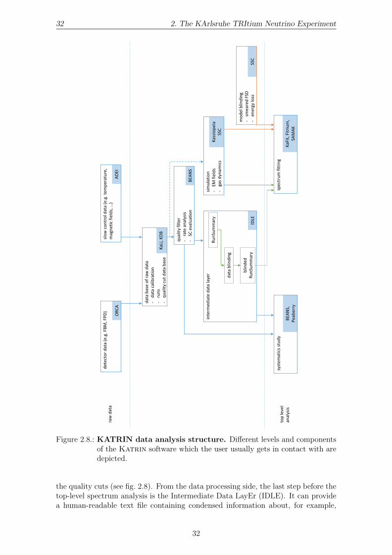
32 2. The KArlsruhe TRItium Neutrino Experiment
OR
CA
det
ecto
rd
ata
(e.g
. FB
M, F
PD
)
AD
EI
slo
wco
ntr
old
ata
(e.g
. tem
per
atu
re,
mag
net
icfi
eld
s, …
)
dat
ab
ase
of
raw
dat
a-
dat
aca
libra
tio
n-
run
s-
qu
alit
ycu
td
ata
bas
eKa
Li, K
DB
qu
alit
yfi
lter
-ra
te a
nal
ysis
-SC
eva
luat
ion
BEA
NS
inte
rmed
iate
dat
ala
yer
IDLE
Ru
nSu
mm
ary
dat
ab
lind
ing
blin
ded
Ru
nSu
mm
ary
BEA
NS,
Pe
aber
ry
syst
emat
ics
stu
dy
KaFi
t, F
itri
um
, SA
MA
K
spec
tru
mfi
ttin
g
sim
ula
tio
n-
EM f
ield
s-
gas
dyn
amic
sKa
ssio
pei
aSS
C
mo
del
blin
din
g-
smea
red
FSD
-en
ergy
loss
SSC
raw
dat
a
top
leve
lan
alys
is
Figure 2.8.: KATRIN data analysis structure. Different levels and componentsof the Katrin software which the user usually gets in contact with aredepicted.
the quality cuts (see fig. 2.8). From the data processing side, the last step before thetop-level spectrum analysis is the Intermediate Data LayEr (IDLE). It can providea human-readable text file containing condensed information about, for example,
32
2.4. Analysis tools and software at the KATRIN experiment 33
the number of counts per pixel for each high voltage of the main spectrometer, orthe mean and stability of a temperature sensor of the WGTS. Thereby, this filesummarises relevant data for each run into a so-called run summary. The run sum-mary can then easily be accessed by the top-level analysis tools for spectrum fitting.Potential data blinding strategies will be integrated into the intermediate data layer.
Parallel to this data processing chain, the model building chain also uses sensordata, for instance, to calculate the magnetic fields using the measured currentsof the superconducting magnets. The publicly available particle tracking softwareKassiopeia [Fur+15, Fur+17] was developed specifically for the needs of the Ka-trin experiment to precisely calculate particle tracks in complex electromagneticfield geometries. It can also model stochastic processes such as scattering, withan interface e.g. to use SSC-calculated density profiles in the WGTS. The Sourceand Spectrum Calculation (SSC) suite implements the calculation of differentialand integrated tritium and krypton spectra, accounting for the Katrin experimentcharacteristics. For that purpose, SSC needs to model the gas dynamical proper-ties of the tritium source and the electromagnetic properties of the spectrometerpart to calculate the response function. The development of SSC was started byW. Kafer [Kaf12] and M. Hotzel [Hot12], followed by M. Kleesiek [Kle14, Kle+18],S.Groh [Gro15], and L. Kuckert [Kuc16]. In the course of this thesis, substantialextensions are implemented in the gas modelling part of SSC as well as in its spectralmodelling with respect to physics beyond the neutrino mass.
The final step in Katrin (tritium) spectrum data analysis as used in this work isthen comparison of the SSC modelled spectrum to the run summaries produced byIDLE via KaFit [Kle14].
33

CHAPTER 3
THE WINDOWLESS GASEOUS TRITIUM SOURCE
The main task of the Windowless Gaseous Tritium Source (WGTS) is to providea per-mille stable electron-rate originating from tritium β-decay. This can be splitinto two separate requirements: a stable magnetic field for stable transport of theelectrons and a stable amount of tritium for a stable source activity. The chapterat hand gives an overview of the key parameters in sec. 3.1, the challenges that areimposed by the above requirements in sec. 3.2, and their technical implementationin the WGTS in sec. 3.3.
3.1. Key parameters
The key parameters defining the activity S provided by the WGTS and detectedby the FPD are the amount of gas, represented by the column density N , and thefraction of tritium therein, represented by the tritium purity εT. Therefore
S ∝ N · AS · εT · a(θmax), (3.1)
with the source cross section AS and a factor for the acceptance angle a(θmax) =a(BS) which is related to the magnetic field in the source BS.
3.1.1. Column density
The column density N is defined as the longitudinally integrated number density nof the gas molecules inside the beam tube
N (pin, pout, T (r)) =Lfront∫−Lrear
n (r, pin, pout, T (r)) dz, (3.2)
which in general depends on injection pressure pin, outlet pressure pout, and the beamtube temperature T (r) at spatial coordinate r. Obviously, the larger N is, the largeris the activity. However, larger N also means increased scattering probability forthe signal electrons, leading to an increased systematic uncertainty for the neutrinomass, which will be discussed in the next sec. 3.2.
35

36 3. The Windowless Gaseous Tritium Source
3.1.2. Temperature
The temperature T of the WGTS influences several effects which need to be ac-counted for in the modelling. On the one hand, a low temperature is favoured sinceit enables a high column density at relatively low injection pressures. Plus, a lowtemperature reduces broadening of the electron spectrum due to the Doppler effectthough it can be modelled easily [Kle+18]. On the other hand, for temperaturesbelow 27 K, tritium clusters form and gas freezes on the beam tube walls [KAT05].Both latter effects cause complicated distortions to the electron spectrum and shouldtherefore be avoided.
3.1.3. Tritium purity
In order to maximise the source activity in eq. (3.1), the tritium purity needs to bemaximised. Pure tritium gas forms T2 molecules, however due to exchange reactionsthe other hydrogen isotopologues (DT, HT, D2, HD, and H2) are also present in thesource gas. The fraction of active gas, represented by the tritium nuclei, is definedas the tritium purity εT. Defining cx as the concentration of isotopologue x in thesource gas1, we can calculate
εT = cT2 + cDT + cHT
2 , with∑x
cx = 1. (3.3)
Though the fraction of non-T2 isotopologues DT and HT is small, it needs to beincluded in the modelling of final states of the decaying molecules. Therefore, theconcentrations of hydrogen isotopologues are monitored via the LARA system (seesec. 2.2.2).
3.1.4. Magnetic field
In order to transport the electrons from the source to the main spectrometer for theenergy analysis, they need to be guided magnetically. Maximising the mapped fluxtube, a strong magnetic field at the source BS enables a relatively small cross-sectionof the source beam tube which is desired from gas dynamics considerations. Further-more, a strong BS increases the fraction of electrons that can surpass the magneticmirror built by the PCH magnet (as the strongest magnet in the Katrin set-up)and therefore increases the signal strength:
a(θmax) ∝ (1− cos θmax), with θmax = arcsin√
BS
BPCH
. (3.4)
For homogeneous starting conditions of the electrons, the source magnetic field needsto be as homogeneous as possible. The homogeneity of the source magnetic fielddirectly influences the homogeneity of the path length and therefore the scatteringprobabilities of the electrons.
1Also compare ref. [Zel18].
36

3.2. Systematic uncertainties and requirements related to the WGTS 37
3.1.5. Plasma potential
The longitudinal magnetic field of the WGTS confines any charged particles in-side the beam tube. Together with the ionised daughter molecule from the β-decay and secondary ionisation processes, the β-decay electrons may form a coldplasma [KAT05]. The plasma potential distribution is influenced by space charges,the beam tube steel surface potential in radial direction, and the rear wall potentialin longitudinal direction [Kuc16] because the magnetic field lines hit the rear wallsurface. Since the rear wall surface is covered with gold, the work function differencebetween the rear wall gold surface and the beam tube stainless steel surface is about1 eV, requiring the rear wall surface potential to be controlled [Kuc16].
3.2. Systematic uncertainties and requirementsrelated to the WGTS
Already in the Design Report [KAT05], the Katrin collaboration lists most of thelargest identified sources of systematic uncertainty on the neutrino mass to be relatedwith the WGTS. Any uncertainty related to the starting position of the β-decayelectrons defined in the source causes a systematic difference between modelled andmeasured spectrum and thereby a systematic shift of the observable of interest, ∆m2
ν.The Katrin systematics budget is currently undergoing a detailed re-evaluation
Table 3.1.: Systematic uncertainties related to the WGTS. This table liststhe identified systematic uncertainties from the Design Report [KAT05],related to unaccounted for shifts of WGTS key parameters. Values givenfor one Katrin run of 2 h [KAT05]. The systematics budget is currentlyundergoing a detailed re-evaluation by H. Seitz-Moskaliuk [Sei19] andcan only serve as a guideline.
source of syst. syst. shift requirement achieved
uncertainty ∆m2ν (10−3 eV2) on the parameter
variations of N < 1.5 2× 10⁻³ see sec. 5.2
inlet pressure pin 2× 10⁻³ see sec. 5.2
outlet pressure pout 6× 10⁻² see sec. 5.2
temperature T 2× 10⁻³ see sec. 5.2
tritium purity εT 2× 10⁻³ < 10−3 [Sch13, Fis14]
magnetic field BS tbd [Sei19]
inhomogeneity < 2 2× 10⁻³ tbd
drift tbd [Sei19] 2× 10⁻³/3 months 2× 10⁻⁴/1 month [Are+18c]
fluctuations tbd [Sei19] 2× 10⁻³ 2× 10⁻⁵ [Are+18c]
by H. Seitz-Moskaliuk [Sei19] as the first commissioning measurements [Are+18b,
37
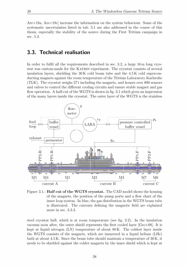
38 3. The Windowless Gaseous Tritium Source
Are+18a, Are+18c] increase the information on the system behaviour. Some of thesystematic uncertainties listed in tab. 3.1 are also addressed in the course of thisthesis, especially the stability of the source during the First Tritium campaign insec. 5.2.
3.3. Technical realisation
In order to fulfil all the requirements described in sec. 3.2, a large 16 m long cryo-stat was custom-made for the Katrin experiment. The cryostat consists of severalinsulation layers, shielding the 30 K cold beam tube and the 4.5 K cold supercon-ducting magnets against the room temperature of the Tritium Laboratory Karlsruhe(TLK). The cryostat weighs 27 t including the magnets, and houses over 800 sensorsand valves to control the different cooling circuits and ensure stable magnet and gasflow operation. A half-cut of the WGTS is shown in fig. 3.1 which gives an impressionof the many layers inside the cryostat. The outer layer of the WGTS is the stainless
M5 M4 M1 M2 M3 M7 M6
current A current B current C
PP
2-R
PP
1-R
PP
1-F
PP
2-F
permeatorexhaust
buffervessel
feedloop
pressure controlledbuffer vessel
pb
flow-meter
q
LARA
εT
qin
Figure 3.1.: Half cut of the WGTS cryostat. The CAD model shows the housingof the magnets, the position of the pump ports and a flow chart of theinner loop system. In blue, the gas distribution in the WGTS beam tubeis illustrated. The currents defining the magnetic field are explainedmore in sec. 3.3.3.
steel cryostat hull, which is at room temperature (see fig. 3.2). In the insulationvacuum soon after, the outer shield represents the first cooled layer [Gro+08]. It iskept at liquid nitrogen (LN) temperature of about 80 K. The coldest layer insidethe WGTS consists of the magnets, which are immersed in a liquid helium (LHe)bath at about 4.5 K. Since the beam tube should maintain a temperature of 30 K, itneeds to be shielded against the colder magnets by the inner shield which is kept at
38
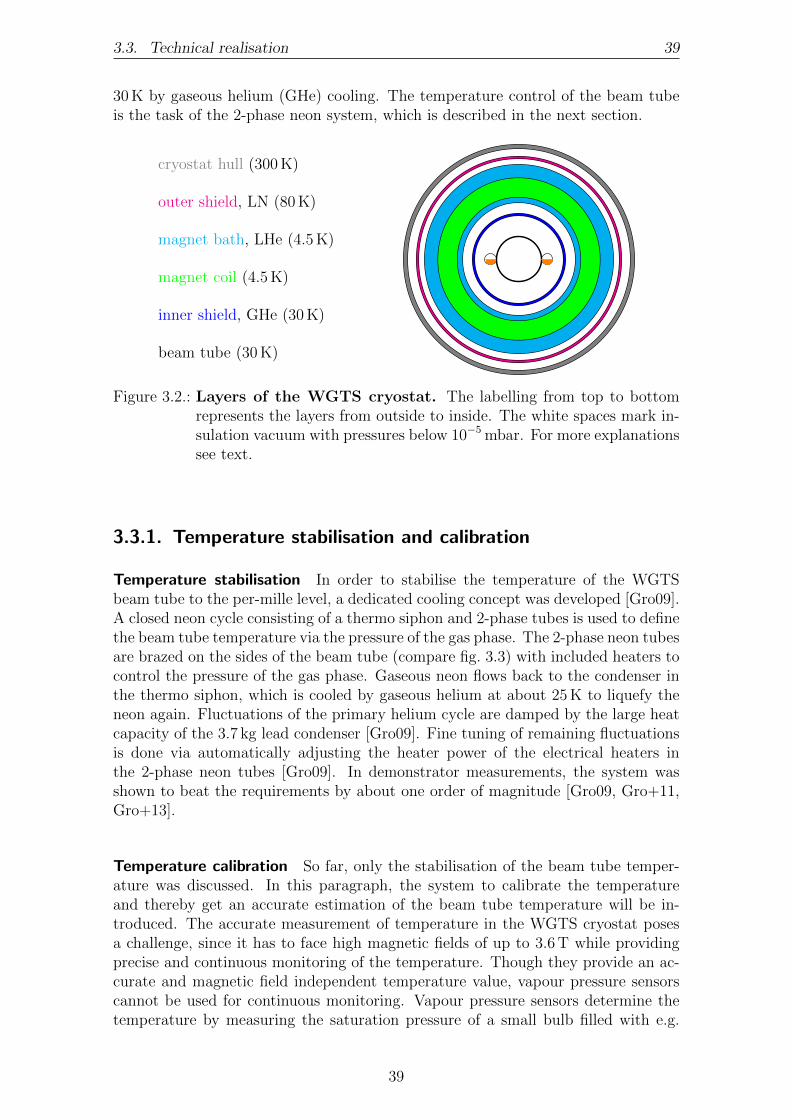
3.3. Technical realisation 39
30 K by gaseous helium (GHe) cooling. The temperature control of the beam tubeis the task of the 2-phase neon system, which is described in the next section.
cryostat hull (300 K)
outer shield, LN (80 K)
magnet bath, LHe (4.5 K)
magnet coil (4.5 K)
inner shield, GHe (30 K)
beam tube (30 K)
Figure 3.2.: Layers of the WGTS cryostat. The labelling from top to bottomrepresents the layers from outside to inside. The white spaces mark in-sulation vacuum with pressures below 10−5 mbar. For more explanationssee text.
3.3.1. Temperature stabilisation and calibration
Temperature stabilisation In order to stabilise the temperature of the WGTSbeam tube to the per-mille level, a dedicated cooling concept was developed [Gro09].A closed neon cycle consisting of a thermo siphon and 2-phase tubes is used to definethe beam tube temperature via the pressure of the gas phase. The 2-phase neon tubesare brazed on the sides of the beam tube (compare fig. 3.3) with included heaters tocontrol the pressure of the gas phase. Gaseous neon flows back to the condenser inthe thermo siphon, which is cooled by gaseous helium at about 25 K to liquefy theneon again. Fluctuations of the primary helium cycle are damped by the large heatcapacity of the 3.7 kg lead condenser [Gro09]. Fine tuning of remaining fluctuationsis done via automatically adjusting the heater power of the electrical heaters inthe 2-phase neon tubes [Gro09]. In demonstrator measurements, the system wasshown to beat the requirements by about one order of magnitude [Gro09, Gro+11,Gro+13].
Temperature calibration So far, only the stabilisation of the beam tube temper-ature was discussed. In this paragraph, the system to calibrate the temperatureand thereby get an accurate estimation of the beam tube temperature will be in-troduced. The accurate measurement of temperature in the WGTS cryostat posesa challenge, since it has to face high magnetic fields of up to 3.6 T while providingprecise and continuous monitoring of the temperature. Though they provide an ac-curate and magnetic field independent temperature value, vapour pressure sensorscannot be used for continuous monitoring. Vapour pressure sensors determine thetemperature by measuring the saturation pressure of a small bulb filled with e.g.
39

40 3. The Windowless Gaseous Tritium Source
beam tube at 30 K 2-phase neon tube
Pt500 + vapourpressure sensor
neon return linegaseousneonhelium outlet
27 K
helium inlet25 K
liquidneon
con-denser
Figure 3.3.: Beam tube cooling concept. Neon is circulated in a closed cycle viaa condenser. The vapour pressure defines the temperature of the beamtube and is controlled via heater wires. Adapted from ref. [Fis14].
neon. However, the fill-level of the vapour pressure sensors can neither be guaran-teed nor tested during standard Katrin operation, plus the filling of the vapourpressure sensors induces heat load onto the source tube due to the condensing neon.On the other hand, resistance sensors like the used Pt500 face a magnetic field de-pendence [Gro+11]. The solution therefore is to thermally couple a vapour pressuresensor and a Pt500 sensor to the beam tube [Gro09, Gro+11, Gro+13]. This combi-nation enables calibration of the Pt500 sensors by the vapour pressure sensors oncethe magnetic field is set. After filling the vapour pressure sensor half with condensedneon, the thermalisation takes about 30 min [Mar17, Hac17]. Then the temperatureof the Pt500 sensor can be calibrated to the vapour pressure sensor temperature.Afterwards, the vapour pressure sensor is emptied again, causing a local temperaturedrop of the beam tube.
The absolute accuracy on the temperature measurement by the Pt500 sensors af-ter applying the calibration via the vapour pressure sensors was estimated by A.Marsteller to 8.27 mK [Mar17]. However, a careful re-evaluation became necessarydue to changes in the readout procedure. H. Seitz-Moskaliuk estimates a new abso-lute accuracy of 159.77 mK for the currently used readout configuration, which canbe improved to 82 mK if a larger current is used for the read out [Sei19]. Though afactor of 10 larger than in previous estimates, the 82 mK still meet the requirementof 150 mK for the final states distribution. Furthermore, the temperature homo-geneity exceeds the required 30 mK from the Design Report with a value of about500 mK, see sec. 4.2.3. In order to reasonably estimate the temperature profile withthis larger inhomogeneity, a larger uncertainty on the accuracy of each sensor canbe tolerated.
3.3.2. Gas flow (Inner loop system)
Katrin relies on a per-mille stable (tritium) gas column density inside the WGTSbeam tube. Gas is injected in the centre of the beam tube and pumped out at
40

3.3. Technical realisation 41
both ends, compare fig. 3.1. Therefore, a stable column density – that is a stableamount of gas inside the beam tube – requires a stable injection and stable pumping.The stable circulation of gas is provided by the so-called inner loop system, whichconsists of more than 100 sensors and valves to control the gas flow [Bab+12]. Astable injection rate qin and a stable inlet pressure pin are achieved by a stablepressure in the pressure controlled buffer vessel and a stable temperature along theconnection pipe. A stable pumping rate is achieved by a constant rotation speed2
of the turbo molecular pumps (TMPs) attached to the four pump ports (PP) of theWGTS, compare fig. 3.1. There are 12 TMPs3 of type Oerlikon Leybold MAG W2800 in total which have a pumping speed of about 2000 l s−1 for H2 each [ide10]. Theconductance of the tube between pump and pump port reduces the higher pumpingspeed of approximately 3000 l s−1 for T2 [Mal07] to the same effective pumping speedas for hydrogen of about 2000 l s−1.
Figure 3.4.: Injection chamber.Left: a CAD model of the injection chamber show-ing the 415 orifices. Right: a sketch of the longitudinal cross section.Figure adapted from ref. [Kuc+18].
Tritium is injected at the centre of the beam tube through 415 2 mm orifices, seefig. 3.4. The dimensions of the orifices guarantee a shock-wave free injection withoutturbulences. Test measurements [Stu10, Pri13, PB13, PSB15] showed the pressurein the pressure controlled buffer vessel pb and the pumping speed to exceed therequirements from the Design Report [KAT05].
In its design configuration, the inner loop system provides a per-mille stable tritiumcolumn density N of 5× 10²¹ m−2 (≡ 300 µg) by circulating a daily amount of about40 g of tritium. This throughput requires buffering of about 15 g of tritium in severalvessels. However, the inner loop system can also provide stable circulation of deu-terium D2 for commissioning and characterisation purposes. For the First Tritiumcampaign, the nominal gas throughput was achieved with the main gas constituentbeing D2 with only trace amounts of tritium εT ≈ 0.5 % [Are+19].
3.3.3. Magnet set-up
The WGTS magnet system is housed inside a 16 m long cryostat, see fig. 3.1. In-side the cryostat, the magnets are cooled with liquid helium to a temperature of4.5 K [Are+18c]. In total seven superconducting solenoids define the magnetic field
2stable on the 10−4 level3four at each PP1 and two at each PP2
41

42 3. The Windowless Gaseous Tritium Source
of the WGTS, plus the possibility of azimuthally steering the flux tube via fourmagnetic dipoles on both ends (dipoles mounted around M5 and M6). The threecentral magnet modules M1, M2, and M3 are each about 3 m long and provide analmost homogeneous field for the central beam tube by the help of two compensationcoils at each end of the module. In order to reduce the stored magnetic energy ofthe current circuits, the seven modules are split into three circuits, current A (M5,M4, M1), current B (M1, M2), and current C (M7, M6) (compare fig. 3.1).
The magnetic field drift of the WGTS has to be smaller than 0.03 % per month [Are+18c]and fluctuations below 0.2 % per run [KAT05]. Since the magnets of the WGTS areoperated in driven mode, the best precision in field monitoring can be reached viamonitoring the current. Though there are current readouts before the current is fedinto the cryostat, the most accurate and precise current sensors are inside the powersupply with an accuracy better than 0.001 73 % [Are+18c, LEM18].
First commissioning measurements with the complete Katrin beam line duringthe First Light campaign [Are+18b] revealed that lower magnetic fields of 70 % ofthe design values should be used in order to minimise the risk for a quench in thecomplex Katrin magnet setup [Are+18c]. Thus, the magnetic field of the WGTShas a new set-point at 2.5 T instead of the nominal 3.6 T.
42

CHAPTER 4
SOURCE MODELLING
“I can never satisfy myself until I can make a mechanical model of a thing. If I canmake a mechanical model, I can understand it.”
– William Thomson, 1. Baron Kelvin, 1884 –
In order to reach the Katrin design sensitivity for the effective neutrino mass of200 meV (90 % C.L.), a cumulative amount of about 40 g of gaseous tritium is circu-lated daily in a windowless source section. As the gas flow through the WindowlessGaseous Tritium Source (WGTS) significantly influences the generation and trans-port of the β-decay electrons, an accurate gas model is of fundamental importance.The combination of gas model and magnetic field model enables fundamental un-derstanding of the origin of the signal electrons that are detected by the FPD.This chapter presents the comprehensive gas model covering all regimes of rarefiedgas dynamics and its first application to gas flow consisting of deuterium and traceamounts of tritium1. Furthermore, first results from commissioning measurements ofa magnetic stray field measuring system developed for monitoring the magnetic fieldof the WGTS are presented and compared to simulations. Together, the gas modeland the magnetic field model form the source model, defining the starting conditionsfor the β-decay electron spectroscopy used to determine the effective neutrino mass.
4.1. General concepts, notation
Let us start the source modelling with introducing some general concepts and nota-tions which will be used throughout this chapter. The source model needs to describethe distribution of the gas inside the WGTS beam tube and the corresponding mag-netic field. Gas is injected at the centre of the beam tube (defined as z = 0 insource model coordinates) and pumped out at both ends via turbomolecular pumps.Though the WGTS beam tube is 16 m long in total with a radius of R = 4.5 cm,99 % of the gas is in the central 10 m of the beam tube. The corresponding magneticfield in the central beam tube is required to be homogeneous with a design value of3.6 T.1As used in the First Tritium campaign in May and June 2018.
43

44 4. Source modelling
The main task of the gas model is to estimate the gas column density N which isthe longitudinally integrated2 amount of gas in the beam tube
N =Lfront∫−Lrear
n(z) dz, (4.1)
with Lrear ≈ Lfront defining the length in backward (negative z) and forward (towardsdetector, positive z) longitudinal direction. In order to calculate the column densityN , the distribution of the molecules number density n = N/V needs to be known.The number density is related to the pressure p via the volume V , the temperatureT , the total number of molecules N , and the Boltzmann constant kB in the idealgas law
pV = NkBT. (4.2)
One of the key parameters to derive the density distribution n(z) is the mass flowrate M . It is directly related to the throughput q, which can be derived by dividingeq. 4.2 by the time t
q = pV
t= kBT
m· N ·m
t= kBT
m· M = v2
m
2 · M, (4.3)
with the mass of the gas molecule m and the most probable speed3 vm =√
2kBT/m.If the gas flow is isothermal with a constant temperature along the beam tube,both M and q are constant along the beam tube. However, temperature variationsalong the beam tube cause throughput variations while the mass flow rate is alwaysconstant provided there is no additional source of gas.
A tube can also be characterised in terms of its conductivity C, which is the inverseof the resistance of the tube
C = q
∆p, (4.4)
with the pressure difference ∆p = pin − pout between inlet and outlet. The WGTSgas dynamics covers the whole range of rarefied gases, which is usually characterisedin terms of the rarefaction parameter δ
δ =√π
2a
λ=√π
21Kn
, (4.5)
with the characteristic scale of the gas flow a = R, the mean free path λ, and theKnudsen number Kn. The mean free path
λ =√πη
2p
√2kBT
m=√πη
2p vm (4.6)
represents the average distance travelled by a gas molecule between collisions and isrelated to the shear stress viscosity of the gas η. We can differentiate between threegas flow regimes, which lead to different methods to calculate the gas flow:
2For this introduction, we will focus on one-dimensional gas flow since L� R, with L the lengthof the beam tube in the z-direction.
3Not to be confused with the average thermal speed v =√
8kBT/(πm) of the Boltzmann dis-tributed velocities v.
44
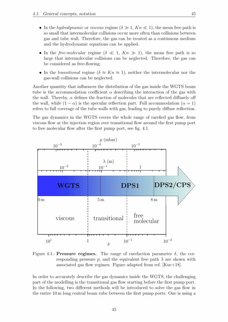
4.1. General concepts, notation 45
� In the hydrodynamic or viscous regime (δ � 1, Kn� 1), the mean free path isso small that intermolecular collisions occur more often than collisions betweengas and tube wall. Therefore, the gas can be treated as a continuous mediumand the hydrodynamic equations can be applied.
� In the free-molecular regime (δ � 1, Kn � 1), the mean free path is solarge that intermolecular collisions can be neglected. Therefore, the gas canbe considered as free-flowing.
� In the transitional regime (δ ≈ Kn ≈ 1), neither the intermolecular nor thegas-wall collisions can be neglected.
Another quantity that influences the distribution of the gas inside the WGTS beamtube is the accommodation coefficient α describing the interaction of the gas withthe wall. Thereby, α defines the fraction of molecules that are reflected diffusely offthe wall, while (1− α) is the specular reflection part. Full accommodation (α = 1)refers to full coverage of the tube walls with gas, leading to purely diffuse reflection.
The gas dynamics in the WGTS covers the whole range of rarefied gas flow, fromviscous flow at the injection region over transitional flow around the first pump portto free molecular flow after the first pump port, see fig. 4.1.
δ101 1 10−1 10−2
viscous transitional freemolecular
0 m 5 m 8 m
WGTS DPS1 DPS2/CPS
λ (m)
10−2 10−1 1
p (mbar)
10−3 10−4 10−5
Figure 4.1.: Pressure regimes. The range of rarefaction parameter δ, the cor-responding pressure p, and the equivalent free path λ are shown withassociated gas flow regimes. Figure adapted from ref. [Kuc+18].
In order to accurately describe the gas dynamics inside the WGTS, the challengingpart of the modelling is the transitional gas flow starting before the first pump port.In the following, two different methods will be introduced to solve the gas flow inthe entire 10 m long central beam tube between the first pump ports. One is using a
45

46 4. Source modelling
phenomenological formula derived from measurements (intermediate Knudsen flow,sec. 4.1.1) and one is solving the Boltzmann equation (sec. 4.1.2), which is describingthe theory of gas dynamics.
4.1.1. Intermediate Knudsen formula
In the limit of laminar viscous flow, the gas flow through a long tube can be describedby Poiseuille’s law. However, Kundt and Warburg [KW75] showed that Poiseuille’slaw has limited accuracy when the radius of the tube is of the order of the mean freepath. Christiansen [Chr90] found that there is a smooth transition from Poiseuilleflow to free molecular flow. By applying a series of measurements of the conductivityof tubes, Knudsen [Knu09] found a phenomenological relation which describes themeasured conductivity for both extremes, viscous and molecular flow. Even moreimportant for us, his formula can also describe the transitional regime by combiningthe viscous and molecular flow conductivities.
In eq. (13) [Knu09], Knudsen states the flow rate through cylindrical tubes. Con-verting to our naming scheme, we can rewrite his formula as [Glu03]
q = (Dvis p+X Dmol)pin − pout
L= CKnudsen · (pin − pout), (4.7)
with p the pressure between pin and pout, L = Lrear, Lfront the length of the tube inrear and front direction4, and Dvis and Dmol identified as the viscous and molecularflow rate coefficients
Dvis = πR4
8η and Dmol = 23π vmR
3. (4.8)
These coefficients are pressure independent and determined by the geometry andtemperature of the tube, as well as by the gas species. The coefficient X can beidentified from Knudsen’s formula as
X = 1 + 2Y1 + 2.47Y , with Y =
√m
kBT
Rp
η. (4.9)
As the pressure ratio pout/pin is expected to be small, the average pressure simplifiesto p = pin/2. From eq. (4.7), the differential equation for the pressure profile can bederived by (pin − pout)/L→ −∂p/∂z to [Glu03]
q = −Dvis p∂p
∂z−X Dmol
∂p
∂z. (4.10)
This differential equation can be solved by e.g. variable separation, enabling cal-culation of the inlet pressure and the pressure profile depending on the boundaryconditions pout/pin, the throughput q, the temperature T , and the gas species. Allother terms are set by the geometry of the WGTS. Note that this method of deter-mining the pressure (or, equivalently, density) profile of the WGTS is purely basedon the phenomenological formula of Knudsen. The conductance estimated with theintermediate Knudsen formula eq. (4.7) and his measured values for hydrogen atroom temperature deviate by about 6− 7 %, which can be taken as the lower limitof the accuracy of the Knudsen formula. In order to get more accurate results, theBoltzmann equation needs to be solved (see sec. 4.1.2).
4Due to a slight longitudinal asymmetry caused by the injection chamber, Lrear and Lfront differby 7 cm.
46

4.1. General concepts, notation 47
4.1.2. Boltzmann equation and distribution function
The number of particles in the phase space volume dr dv at time t is defined viadN = f(t, r,v)dr dv with spatial coordinate r and velocity v. Therein, the one-particle velocity distribution function f(t, r,v) solves the Boltzmann equation, whichin absence of external forces can be written as
∂f
∂t+ v · ∂f
∂r= Q(f, f∗), (4.11)
with the collision integral Q(f, f∗) describing the collision between two gas particleswith distribution functions f and f∗. The Boltzmann equation eq.(4.11) can onlybe solved analytically with simplifications to the collision integral, and numericallyonly for simple cases [SS98].
Due to the large length-to-radius ratio L/R of about 100, we will consider the flow tobe fully developed and reduce the calculation to one dimension for this introduction.In order to solve the Boltzmann equation, the key is the mass flow rate M sinceit is constant in absence of additional sources of gas. We will use the methods ofF. Sharipov [Sha97, SS98] in the following, defining the mass flow rate through across-section of the tube as
M = πR3
vm
(−GP(δ) dp
dz+GT(δ) p(z)
T (z)dT
dz
), (4.12)
with radius of the beam tube R, the local pressure p(z), the local temperature T (z)and the rarefaction parameter δ defined by eq. (4.5). The dimensionless reducedflow rates GP(δ) (Poiseuille flow) and GT(δ) (thermal creep) characterise the gasflow in terms of δ, so they are independent of the gas species. The gas species inturn influences δ, e.g. via its mass. Tabulated values as well as a parametrisation forGP and GT can be found in the literature as functions of the rarefaction parameterδ [SS98, Sha16]
GP = 83√π
1 + 0.04 δ0.7 ln δ1 + 0.78 δ0.8 +
(δ
4 + σP(α))
δ
1 + δ, (4.13)
GT =
4
3√π
+ 0.825(1 + ln δ)δ − (1.18− 0.61 ln δ)δ2 for δ ≤ 1,σT(α)δ− 1.75
δ2 + 1.47
δ3 − 0.5
δ4 for δ > 1.
(4.14)
The interpolation formula for GP, eq. (4.13), reproduces numerical results obtainedwith the S-model [Sha16] within 0.2 %. However, agreement between the numer-ical S-model results for GP and results based on a hard-sphere model for the gasmolecules [LH90] match within 2 % [Sha16], which also holds for comparisons toexperimental data [Sha08]. Since the pressure profile in eq. (4.12) is mainly deter-mined by GP, the 2 % uncertainty also hold for the pressure profile. On the otherhand this means that the column density determined via integration of the pressureequivalent density profile also has about 2 % uncertainty from the dimensionless flowrate coefficients.
In general, the reduced flow rates GP and GT depend on the gas-surface interactionwhich is described by the accommodation coefficient α, varying between 0 (no gas
47

48 4. Source modelling
on the beam tube wall) and 1 (full accommodation of the beam tube wall). Theaccommodation coefficient affects the viscous Poiseuille σP and thermal slip coeffi-cients σT
5 which in term influence GP and GT [SS98]. However, it has to be notedthat the dependence of σT on α is negligible compared to σP [Sha04b].
In the simple case of isothermal flow, the temperature gradient is zero and we cancalculate the mass flow rate via z integration as
M = πr30pin
vmδinL
∫ δin
δout
GP(δ) dδ, (4.15)
with the injection and outlet pressure equivalent rarefaction parameters δin and δout.In case of non-isothermal flow, the longitudinal distribution δ(z) has to be calculatedby numerical finite difference schemes from eq. (4.12) as shown in [Sha96, Sha97,SS98].
4.2. Temperature model
The beam tube of the WGTS is designed to have a per-mille stable and homogeneoustemperature. In order to control the temperature of the gas inside the WGTS,resistance sensors are brazed onto the beam tube. As 99 % of the gas column densityare inside the central 10 m long beam tube between the first pump ports (comparefig. 3.1), this is the most important part for temperature modelling. This sectionpresents commissioning results and the temperature distribution as it is used for thegas dynamics modelling.
4.2.1. Temperature sensors
At the central 10 m long beam tube, in total 24 Pt500 sensors measure the temper-ature distribution along the beam tube. As introduced in sec. 3.3.1, those sensorsneed to be calibrated by vapour pressure sensors to compensate for their magneticfield dependence. Once calibrated, the sensors have an accuracy of 159.77 mK in theworst case scenario [Sei19]. Most of the sensors sit on top (90°) and bottom (270°)of the beam tube (compare fig. 3.3 and fig. 4.2), with only two diagonal sensors at45° and 225° at both ends of the beam tube. Two of the sensors (one of the frontdiagonal and one bottom in front side) cannot be used for analysis due to invalidtemperature readings, see fig. 4.2. Not indicated on fig. 4.2 is the position of thetemperature sensors relative to the beam tube cooling, the interested reader can findthis information in the appendix in fig. A.1.
4.2.2. Temperature correlations
If the temperature of the beam tube is regulated via the 2-phase cooling system, thesensor readings should be correlated. In fact, investigations by A. Marsteller [Mar17]during commissioning measurements without gas in the beam tube showed perfect
5The slip coefficients influence the tangential velocity of the gas near the beam tube wall.
48

4.2. Temperature model 49
90°45°
270°225°
5124 5120 5118 5116 5114 5112 5110 5108 5106 5102
5123 5119 5117 5115 5113 5111 5109 5107 5105 5101
5122
5121
5104
5103
x
y
z
y
2-phase neoncooling
copper block
vapour pressure sensor
Pt500 sensor
Figure 4.2.: Temperature sensor positions. The numbers indicate the sensor ID,malfunctioning sensors are highlighted in yellow. Schematic inspired byref. [Hot12].
correlation with Pearson’s r values of 1. The perfect correlation was obtained becausethe beam tube temperature was varied within 2 K over two days. During stableoperation the readout fluctuations of about 0.5 mK prohibit correlation coefficients of1 since the beam tube temperature is stable on the per-mille level, see sec. 5.2.1. Thisis confirmed by fig. 4.3, where some of the temperature sensors appear less correlatedthan others. However, it is concluded that this difference is due to the fact thatreadout fluctuations on the order 0.5 mK [Mar17] are dominating the temperaturefluctuations, which are the same order of magnitude (see sec. 5.2.1).
4.2.3. Temperature homogeneity
In the Design Report [KAT05], the temperature homogeneity of the central 10 mlong beam tube was specified to be better than 30 mK. This section will showthat this requirement can not be met, however it will be shown, that the increasedtemperature at the rear side does not harm the estimation of the column densitynor the neutrino mass sensitivity as it can be accounted for in the gas model.
Temperature simulations by L. Kuckert [Kuc16] showed, that the heat load from thepump ports via thermal radiation from the TMPs is the main source for temperatureinhomogeneity of the beam tube. As the beam tube cooling ends about 25 cm beforethe pump port and the bellow connecting beam tube and pump port has no activecooling, it is expected that both ends of the WGTS might get warmer than thecentre of the WGTS. Commissioning measurements with the Demonstrator set-upof the WGTS confirmed that expectation [Hot12]. Moreover, these commissioningmeasurements showed that there is a difference between the front side inhomogene-ity and the rear side inhomogeneity of the temperature of the beam tube ends. Asa conclusion, the beam tube was turned around to have the higher temperature
49

50 4. Source modelling
RTP-3-5101
RTP-3-5102
RTP-3-5104
RTP-3-5105
RTP-3-5107
RTP-3-5108
RTP-3-5110
RTP-3-5111
RTP-3-5112
RTP-3-5113
RTP-3-5115
RTP-3-5116
RTP-3-5117
RTP-3-5118
RTP-3-5119
RTP-3-5120
RTP-3-5121
RTP-3-5122
RTP-3-5123
RTP-3-5124
RTP-3-5101
RTP-3-5102
RTP-3-5104
RTP-3-5105
RTP-3-5107
RTP-3-5108
RTP-3-5110
RTP-3-5111
RTP-3-5112
RTP-3-5113
RTP-3-5115
RTP-3-5116
RTP-3-5117
RTP-3-5118
RTP-3-5119
RTP-3-5120
RTP-3-5121
RTP-3-5122
RTP-3-5123
RTP-3-5124
0.4
0.5
0.6
0.7
0.8
0.9
1
1.0000 0.7506
0.7506 1.0000
0.9093
0.9093
0.8458
0.8458 1.0000
0.8904
0.8904
0.7756
0.7756
0.8737
0.8737 1.0000
0.8884
0.8884
0.8217
0.8217
0.8906
0.8906
0.9238
0.9238 1.0000
0.8467
0.8467
0.7749
0.7749
0.8880
0.8880
0.9159
0.9159
0.9149
0.9149 1.0000
0.4768
0.4768
0.8650
0.8650
0.6442
0.6442
0.6059
0.6059
0.6491
0.6491
0.6487
0.6487 1.0000
0.8378
0.8378
0.7514
0.7514
0.8379
0.8379
0.8889
0.8889
0.8987
0.8987
0.8643
0.8643
0.5909
0.5909 1.0000
0.7967
0.7967
0.7622
0.7622
0.8482
0.8482
0.8748
0.8748
0.8607
0.8607
0.9150
0.9150
0.6968
0.6968
0.8335
0.8335 1.0000
0.8649
0.8649
0.8071
0.8071
0.8690
0.8690
0.9330
0.9330
0.9059
0.9059
0.8909
0.8909
0.6528
0.6528
0.9037
0.9037
0.8629
0.8629 1.0000
0.8527
0.8527
0.6941
0.6941
0.8290
0.8290
0.8879
0.8879
0.8879
0.8879
0.8580
0.8580
0.5085
0.5085
0.9241
0.9241
0.8060
0.8060
0.8933
0.8933 1.0000
0.3784
0.3784
0.7536
0.7536
0.5695
0.5695
0.5053
0.5053
0.5120
0.5120
0.5786
0.5786
0.8881
0.8881
0.4299
0.4299
0.6455
0.6455
0.5444
0.5444
0.3789
0.3789 1.0000
0.7023
0.7023
0.8559
0.8559
0.7908
0.7908
0.7735
0.7735
0.7916
0.7916
0.7778
0.7778
0.7810
0.7810
0.7336
0.7336
0.7682
0.7682
0.7940
0.7940
0.6947
0.6947
0.7582
0.7582 1.0000
0.8507
0.8507
0.8082
0.8082
0.8782
0.8782
0.8876
0.8876
0.8615
0.8615
0.8690
0.8690
0.6602
0.6602
0.8156
0.8156
0.8464
0.8464
0.8761
0.8761
0.8204
0.8204
0.6505
0.6505
0.8535
0.8535 1.0000
0.5702
0.5702
0.7558
0.7558
0.6815
0.6815
0.6559
0.6559
0.6580
0.6580
0.6664
0.6664
0.7175
0.7175
0.6049
0.6049
0.6632
0.6632
0.6679
0.6679
0.5691
0.5691
0.7692
0.7692
0.9286
0.9286
0.8170
0.8170 1.0000
0.7890
0.7890
0.7651
0.7651
0.8396
0.8396
0.8254
0.8254
0.8132
0.8132
0.8372
0.8372
0.6252
0.6252
0.7752
0.7752
0.8297
0.8297
0.8215
0.8215
0.7661
0.7661
0.6589
0.6589
0.8855
0.8855
0.9154
0.9154
0.8665
0.8665 1.0000
0.7026
0.7026
0.6969
0.6969
0.7359
0.7359
0.6839
0.6839
0.6889
0.6889
0.6649
0.6649
0.4996
0.4996
0.6709
0.6709
0.6198
0.6198
0.6955
0.6955
0.6421
0.6421
0.4662
0.4662
0.8308
0.8308
0.7854
0.7854
0.8256
0.8256
0.8383
0.8383 1.0000
0.7668
0.7668
0.8729
0.8729
0.8325
0.8325
0.7500
0.7500
0.7982
0.7982
0.7590
0.7590
0.7323
0.7323
0.7103
0.7103
0.7396
0.7396
0.7670
0.7670
0.6797
0.6797
0.7154
0.7154
0.9341
0.9341
0.8644
0.8644
0.8920
0.8920
0.8824
0.8824
0.8465
0.8465 1.0000
0.7318
0.7318
0.7858
0.7858
0.7841
0.7841
0.7223
0.7223
0.7463
0.7463
0.7173
0.7173
0.6168
0.6168
0.6989
0.6989
0.6838
0.6838
0.7360
0.7360
0.6672
0.6672
0.6096
0.6096
0.9175
0.9175
0.8505
0.8505
0.9172
0.9172
0.9021
0.9021
0.9303
0.9303
0.9452
0.9452 1.0000
0.7140
0.7140
0.8525
0.8525
0.8063
0.8063
0.7033
0.7033
0.7283
0.7283
0.7210
0.7210
0.7436
0.7436
0.6650
0.6650
0.7259
0.7259
0.7345
0.7345
0.6275
0.6275
0.7841
0.7841
0.9021
0.9021
0.8623
0.8623
0.8974
0.8974
0.8987
0.8987
0.8174
0.8174
0.9453
0.9453
0.9177
0.9177 1.0000
1.0000+0.0000-0.0000
0.7505+0.0035-0.0035
0.7505+0.0035-0.0035
1.0000+0.0000-0.0000
0.9093+0.0014-0.0014
0.9093+0.0014-0.0014
0.8458+0.0023-0.0023
0.8458+0.0023-0.0023
1.0000+0.0000-0.0000
0.8904+0.0017-0.0017
0.8904+0.0017-0.0017
0.7756+0.0030-0.0030
0.7756+0.0030-0.0030
0.8737+0.0019-0.0019
0.8737+0.0019-0.0019
1.0000+0.0000-0.0000
0.8884+0.0017-0.0017
0.8884+0.0017-0.0017
0.8217+0.0026-0.0026
0.8217+0.0026-0.0026
0.8906+0.0017-0.0017
0.8906+0.0017-0.0017
0.9238+0.0012-0.0012
0.9238+0.0012-0.0012
1.0000+0.0000-0.0000
0.8467+0.0023-0.0023
0.8467+0.0023-0.0023
0.7750+0.0032-0.0032
0.7750+0.0032-0.0032
0.8880+0.0017-0.0018
0.8880+0.0017-0.0018
0.9159+0.0013-0.0013
0.9159+0.0013-0.0013
0.9149+0.0013-0.0013
0.9149+0.0013-0.0013
1.0000+0.0000-0.0000
0.4768+0.0061-0.0061
0.4768+0.0061-0.0061
0.8650+0.0020-0.0020
0.8650+0.0020-0.0020
0.6442+0.0047-0.0047
0.6442+0.0047-0.0047
0.6059+0.0048-0.0048
0.6059+0.0048-0.0048
0.6491+0.0044-0.0044
0.6491+0.0044-0.0044
0.6488+0.0044-0.0044
0.6488+0.0044-0.0044
1.0000+0.0000-0.0000
0.8379+0.0023-0.0023
0.8379+0.0023-0.0023
0.7514+0.0034-0.0034
0.7514+0.0034-0.0034
0.8379+0.0024-0.0024
0.8379+0.0024-0.0024
0.8890+0.0017-0.0017
0.8890+0.0017-0.0017
0.8987+0.0016-0.0016
0.8987+0.0016-0.0016
0.8643+0.0021-0.0020
0.8643+0.0021-0.0020
0.5909+0.0048-0.0048
0.5909+0.0048-0.0048
1.0000+0.0000-0.0000
0.7968+0.0030-0.0030
0.7968+0.0030-0.0030
0.7623+0.0034-0.0034
0.7623+0.0034-0.0034
0.8482+0.0023-0.0023
0.8482+0.0023-0.0023
0.8748+0.0019-0.0019
0.8748+0.0019-0.0019
0.8607+0.0022-0.0022
0.8607+0.0022-0.0022
0.9150+0.0014-0.0014
0.9150+0.0014-0.0014
0.6967+0.0041-0.0041
0.6967+0.0041-0.0041
0.8336+0.0025-0.0025
0.8336+0.0025-0.0025
1.0000+0.0000-0.0000
0.8649+0.0021-0.0021
0.8649+0.0021-0.0021
0.8072+0.0027-0.0027
0.8072+0.0027-0.0027
0.8691+0.0020-0.0020
0.8691+0.0020-0.0020
0.9330+0.0011-0.0011
0.9330+0.0011-0.0011
0.9059+0.0015-0.0015
0.9059+0.0015-0.0015
0.8909+0.0017-0.0017
0.8909+0.0017-0.0017
0.6528+0.0043-0.0043
0.6528+0.0043-0.0043
0.9037+0.0015-0.0015
0.9037+0.0015-0.0015
0.8629+0.0021-0.0021
0.8629+0.0021-0.0021
1.0000+0.0000-0.0000
0.8528+0.0022-0.0022
0.8528+0.0022-0.0022
0.6941+0.0041-0.0041
0.6941+0.0041-0.0041
0.8290+0.0026-0.0026
0.8290+0.0026-0.0026
0.8879+0.0018-0.0018
0.8879+0.0018-0.0018
0.8879+0.0018-0.0018
0.8879+0.0018-0.0018
0.8580+0.0023-0.0023
0.8580+0.0023-0.0023
0.5085+0.0058-0.0058
0.5085+0.0058-0.0058
0.9241+0.0011-0.0011
0.9241+0.0011-0.0011
0.8060+0.0031-0.0031
0.8060+0.0031-0.0031
0.8933+0.0017-0.0017
0.8933+0.0017-0.0017
1.0000+0.0000-0.0000
0.3784+0.0065-0.0065
0.3784+0.0065-0.0065
0.7536+0.0032-0.0032
0.7536+0.0032-0.0032
0.5695+0.0052-0.0052
0.5695+0.0052-0.0052
0.5053+0.0054-0.0054
0.5053+0.0054-0.0054
0.5120+0.0054-0.0054
0.5120+0.0054-0.0054
0.5787+0.0049-0.0049
0.5787+0.0049-0.0049
0.8881+0.0015-0.0015
0.8881+0.0015-0.0015
0.4298+0.0060-0.0060
0.4298+0.0060-0.0060
0.6454+0.0044-0.0044
0.6454+0.0044-0.0044
0.5446+0.0050-0.0050
0.5446+0.0050-0.0050
0.3788+0.0064-0.0064
0.3788+0.0064-0.0064
1.0000+0.0000-0.0000
0.7024+0.0038-0.0038
0.7024+0.0038-0.0038
0.8559+0.0020-0.0020
0.8559+0.0020-0.0020
0.7909+0.0029-0.0029
0.7909+0.0029-0.0029
0.7735+0.0030-0.0030
0.7735+0.0030-0.0030
0.7917+0.0028-0.0028
0.7917+0.0028-0.0028
0.7779+0.0031-0.0031
0.7779+0.0031-0.0031
0.7810+0.0029-0.0029
0.7810+0.0029-0.0029
0.7335+0.0036-0.0036
0.7335+0.0036-0.0036
0.7683+0.0032-0.0032
0.7683+0.0032-0.0032
0.7940+0.0028-0.0028
0.7940+0.0028-0.0028
0.6947+0.0039-0.0039
0.6947+0.0039-0.0039
0.7583+0.0031-0.0031
0.7583+0.0031-0.0031
1.0000+0.0000-0.0000
0.8507+0.0022-0.0022
0.8507+0.0022-0.0022
0.8083+0.0027-0.0027
0.8083+0.0027-0.0027
0.8783+0.0018-0.0018
0.8783+0.0018-0.0018
0.8876+0.0017-0.0016
0.8876+0.0017-0.0016
0.8615+0.0020-0.0020
0.8615+0.0020-0.0020
0.8691+0.0019-0.0019
0.8691+0.0019-0.0019
0.6601+0.0043-0.0043
0.6601+0.0043-0.0043
0.8157+0.0027-0.0027
0.8157+0.0027-0.0027
0.8464+0.0023-0.0023
0.8464+0.0023-0.0023
0.8762+0.0018-0.0018
0.8762+0.0018-0.0018
0.8204+0.0026-0.0026
0.8204+0.0026-0.0026
0.6505+0.0041-0.0041
0.6505+0.0041-0.0041
0.8535+0.0020-0.0020
0.8535+0.0020-0.0020
1.0000+0.0000-0.0000
0.5703+0.0049-0.0049
0.5703+0.0049-0.0049
0.7557+0.0030-0.0030
0.7557+0.0030-0.0030
0.6815+0.0039-0.0040
0.6815+0.0039-0.0040
0.6560+0.0041-0.0041
0.6560+0.0041-0.0041
0.6580+0.0040-0.0040
0.6580+0.0040-0.0040
0.6663+0.0040-0.0040
0.6663+0.0040-0.0040
0.7176+0.0034-0.0034
0.7176+0.0034-0.0034
0.6049+0.0047-0.0047
0.6049+0.0047-0.0047
0.6632+0.0041-0.0041
0.6632+0.0041-0.0041
0.6680+0.0042-0.0042
0.6680+0.0042-0.0042
0.5690+0.0050-0.0050
0.5690+0.0050-0.0050
0.7691+0.0029-0.0029
0.7691+0.0029-0.0029
0.9287+0.0010-0.0010
0.9287+0.0010-0.0010
0.8170+0.0024-0.0024
0.8170+0.0024-0.0024
1.0000+0.0000-0.0000
0.7891+0.0028-0.0028
0.7891+0.0028-0.0028
0.7651+0.0031-0.0031
0.7651+0.0031-0.0031
0.8395+0.0022-0.0022
0.8395+0.0022-0.0022
0.8254+0.0024-0.0024
0.8254+0.0024-0.0024
0.8131+0.0025-0.0025
0.8131+0.0025-0.0025
0.8371+0.0023-0.0023
0.8371+0.0023-0.0023
0.6253+0.0045-0.0045
0.6253+0.0045-0.0045
0.7752+0.0031-0.0031
0.7752+0.0031-0.0031
0.8297+0.0023-0.0023
0.8297+0.0023-0.0023
0.8215+0.0025-0.0025
0.8215+0.0025-0.0025
0.7662+0.0032-0.0032
0.7662+0.0032-0.0032
0.6589+0.0041-0.0041
0.6589+0.0041-0.0041
0.8855+0.0016-0.0016
0.8855+0.0016-0.0016
0.9155+0.0012-0.0012
0.9155+0.0012-0.0012
0.8665+0.0019-0.0019
0.8665+0.0019-0.0019
1.0000+0.0000-0.0000
0.7026+0.0037-0.0037
0.7026+0.0037-0.0037
0.6969+0.0038-0.0038
0.6969+0.0038-0.0038
0.7359+0.0032-0.0032
0.7359+0.0032-0.0032
0.6840+0.0040-0.0039
0.6840+0.0040-0.0039
0.6889+0.0038-0.0038
0.6889+0.0038-0.0038
0.6649+0.0041-0.0041
0.6649+0.0041-0.0041
0.4997+0.0055-0.0055
0.4997+0.0055-0.0055
0.6709+0.0041-0.0041
0.6709+0.0041-0.0041
0.6197+0.0046-0.0046
0.6197+0.0046-0.0046
0.6955+0.0039-0.0039
0.6955+0.0039-0.0039
0.6421+0.0043-0.0043
0.6421+0.0043-0.0043
0.4663+0.0057-0.0057
0.4663+0.0057-0.0057
0.8308+0.0024-0.0024
0.8308+0.0024-0.0024
0.7855+0.0029-0.0029
0.7855+0.0029-0.0029
0.8257+0.0024-0.0024
0.8257+0.0024-0.0024
0.8384+0.0022-0.0022
0.8384+0.0022-0.0022
1.0000+0.0000-0.0000
0.7668+0.0032-0.0032
0.7668+0.0032-0.0032
0.8729+0.0019-0.0019
0.8729+0.0019-0.0019
0.8325+0.0024-0.0024
0.8325+0.0024-0.0024
0.7500+0.0033-0.0033
0.7500+0.0033-0.0033
0.7982+0.0027-0.0027
0.7982+0.0027-0.0027
0.7590+0.0032-0.0032
0.7590+0.0032-0.0032
0.7322+0.0034-0.0034
0.7322+0.0034-0.0034
0.7103+0.0039-0.0039
0.7103+0.0039-0.0039
0.7397+0.0035-0.0035
0.7397+0.0035-0.0035
0.7670+0.0032-0.0032
0.7670+0.0032-0.0032
0.6797+0.0042-0.0042
0.6797+0.0042-0.0042
0.7154+0.0036-0.0036
0.7154+0.0036-0.0036
0.9341+0.0009-0.0009
0.9341+0.0009-0.0009
0.8644+0.0019-0.0019
0.8644+0.0019-0.0019
0.8921+0.0015-0.0015
0.8921+0.0015-0.0015
0.8824+0.0016-0.0016
0.8824+0.0016-0.0016
0.8465+0.0022-0.0022
0.8465+0.0022-0.0022
1.0000+0.0000-0.0000
0.7318+0.0033-0.0033
0.7318+0.0033-0.0033
0.7858+0.0028-0.0028
0.7858+0.0028-0.0028
0.7841+0.0027-0.0027
0.7841+0.0027-0.0027
0.7224+0.0035-0.0035
0.7224+0.0035-0.0035
0.7464+0.0031-0.0031
0.7464+0.0031-0.0031
0.7173+0.0035-0.0035
0.7173+0.0035-0.0035
0.6168+0.0043-0.0043
0.6168+0.0043-0.0043
0.6990+0.0039-0.0039
0.6990+0.0039-0.0039
0.6839+0.0039-0.0039
0.6839+0.0039-0.0039
0.7360+0.0034-0.0034
0.7360+0.0034-0.0034
0.6671+0.0042-0.0042
0.6671+0.0042-0.0042
0.6097+0.0043-0.0043
0.6097+0.0043-0.0043
0.9175+0.0012-0.0012
0.9175+0.0012-0.0012
0.8505+0.0020-0.0020
0.8505+0.0020-0.0020
0.9172+0.0012-0.0012
0.9172+0.0012-0.0012
0.9021+0.0014-0.0014
0.9021+0.0014-0.0014
0.9303+0.0011-0.0011
0.9303+0.0011-0.0011
0.9452+0.0008-0.0008
0.9452+0.0008-0.0008
1.0000+0.0000-0.0000
0.7140+0.0036-0.0036
0.7140+0.0036-0.0036
0.8525+0.0020-0.0020
0.8525+0.0020-0.0020
0.8063+0.0025-0.0025
0.8063+0.0025-0.0025
0.7033+0.0036-0.0036
0.7033+0.0036-0.0036
0.7283+0.0033-0.0033
0.7283+0.0033-0.0033
0.7210+0.0035-0.0035
0.7210+0.0035-0.0035
0.7436+0.0032-0.0032
0.7436+0.0032-0.0032
0.6650+0.0042-0.0042
0.6650+0.0042-0.0042
0.7260+0.0035-0.0035
0.7260+0.0035-0.0035
0.7345+0.0034-0.0034
0.7345+0.0034-0.0034
0.6276+0.0044-0.0044
0.6276+0.0044-0.0044
0.7841+0.0028-0.0028
0.7841+0.0028-0.0028
0.9022+0.0013-0.0013
0.9022+0.0013-0.0013
0.8623+0.0019-0.0019
0.8623+0.0019-0.0019
0.8974+0.0014-0.0014
0.8974+0.0014-0.0014
0.8987+0.0014-0.0014
0.8987+0.0014-0.0014
0.8174+0.0025-0.0025
0.8174+0.0025-0.0025
0.9454+0.0008-0.0008
0.9454+0.0008-0.0008
0.9177+0.0011-0.0011
0.9177+0.0011-0.0011
1.0000+0.0000-0.0000
Figure 4.3.: Temperature correlations. As explained in the text, the reason fornot having perfect correlation is the fluctuations of the readout.
at the rear side, due to electrons starting from the rear side contributing less tothe measured β-decay spectrum6. Comparison of the simulated and the measuredtemperature increase showed that the simulation gives overstated values [Kuc16].Furthermore, the simulations suggest that the azimuthal temperature profile at theend of the beam tube can be well described by a sin2 φ relation with the temperatureof the 2-phase neon cooling tube (at φ = 0,π, compare fig. 3.3) as lower limit andthe top/bottom temperature (at φ = π/2, 3π/2) as upper limit. With this assump-tion the following azimuthal beam tube temperature profile T (φ, z) at longitudinalposition z can be extrapolated
T (φ, z) = T0 + ∆Tt,b(z) · sin2 φ, (4.16)
with T0 the temperature of the 2-phase neon cooling tube and ∆Tt,b(z) = Tt,b(z)−T0the difference to the top/bottom temperature. As described in sec. 4.2.1, the major-ity of the temperature sensors sit symmetrically on the top and bottom of the beamtube, compare fig. 4.2. Therefore, the reading of the temperature sensors definesTt,b(z), together with a splines interpolation [Gal+02]. It has to be noted that thetop and bottom longitudinal temperature profile might be different, but the connec-tion between top and bottom is smooth due to the 2-phase neon cooling tubes settingthe reference temperature T0, compare fig. 4.4. The figure shows the azimuthal tem-perature profile as expected at the position of the first and last top/bottom sensorpair. Furthermore, it reveals that diagonal sensors can not be directly comparedto the azimuthal temperature profile at the position of the outermost top/bottom
6Electrons from the rear end have much higher probability to scatter out of the measuring windowthan electrons from the front end.
50

4.2. Temperature model 51
−150 −100 −50 0 50 100 150
φ (◦)
29.8
30.0
30.2
30.4
30.6
30.8
T(K
)
bottom top rear model
front model
rear data
front data
Ne temp.
Figure 4.4.: Azimuthal beam tube temperature distribution. The figureshows the expected sin2 φ temperature dependence, with sensor datafrom both ends of the beam tube. Background colours indicate the yposition on the beam tube. The diagonal sensors visualised by dashederror bars are shifted 2 cm towards the centre compared to the top/bot-tom sensors which can explain the offset.
sensor pair. The reason might be that the true temperature maximum is betweenthe last and second-to-last temperature sensor, which is not accessible via measure-ment. Also note that this discrepancy is within 2σ of the uncertainty on the sensorreading; plus the diagonal sensors only measure at the very end of the beam tube,where the effect on the column density is negligible. From fig. 4.5 it follows thatthe temperature has its maximum not at the last sensors as expected from temper-ature simulations of L. Kuckert [Kuc16], but presumably at the next pair, which islocated 20 cm closer to the centre of the WGTS. The diagonal sensors show a highertemperature than the outer sensors, though they are only 2 cm closer to the centre.Therefore, the temperature simulations cannot be verified, which is the reason forusing interpolation of sensor readings instead of a complete model. Furthermore ithas to be noted that the gas dynamics uncertainty induced by a wrong temperatureassumption in the outlet region will be shown to be negligible and the uncertaintyon the β-decay spectrum modelling is even less.
In order to derive the temperature inside the beam tube, the gas distribution needsto be respected. This will be discussed in the next section, as well as the differentcomponents that combine to the gas dynamics model of the WGTS.
51

52 4. Source modelling
−4 −2 0 2 4
z (m)
29.8
30.0
30.2
30.4
30.6
30.8
T(K
)
top model
bottom model
top data
bottom data
diag data
Figure 4.5.: Longitudinal beam tube temperature distribution. The figureshows sensor data as well as the splines-interpolated profile.
4.3. Gas dynamics model, nominal KATRIN set-up
As already introduced in sec. 4.1, the gas flow in the WGTS covers the whole rangeof rarefied gases. Starting in the viscous regime at the injection point (A1 in fig. 4.6),the gas reaches the transitional regime before the first pump port (PP1, region B1in fig. 4.6). Before leaving the WGTS cryostat, the gas reaches the free molecularflow in the region around the second pump port (PP2, region B3 in fig. 4.6). Eachrarefaction regime requires different modelling techniques in order to properly de-scribe the gas flow, therefore the complete gas model of the WGTS consists of severaldifferent parts (compare fig. 4.6). These parts are connected via the condition ofequal mass flow rate at their boundary.
Figure 4.6.: Scheme of the model geometries. The schematic drawing visualisesthe different regions for the gas dynamics calculations and the respectivedimensionality. Figure shows the scheme for front direction only, reardirection is symmetric with respect to the injection chamber. Figureadapted from ref. [Kuc+18].
52

4.3. Gas dynamics model, nominal KATRIN set-up 53
The following section gives an overview of the applied techniques to describe the gasflow in the respective regime for the nominal Katrin set-up. This refers to settingsdescribed in the Design Report [KAT05], treating the gas as pure molecular tritiumwith a column density of 5× 10²¹ m−2. At the end of this section, an estimation ofthe total gas model related systematic neutrino mass uncertainty is given.
4.3.1. Gas flow in the central 10 m beam tube (A1-A3)
As about 99 % of the (tritium) gas is contained within the central 10 m long beamtube, this domain’s gas flow needs more attention than the following regions. Thelarge length-to-radius ratio L/R of about 100 enables the use of a one-dimensionalfully developed flow for most of the beam tube. Only at the inlet and outlet regions,more dimensions have to be added. Following the introduction in sec. 4.1.2, theconcept to derive the density profile is described in [Sha97, SS98]. The first toimplement these concepts into the Katrin source and spectrum calculation packageSSC was M. Hotzel [Hot12], followed by L. Kuckert [Kuc16]. In order to derive thelongitudinal density profile or pressure profile equivalent, eq. (4.12) needs to besolved for dp/dz via the constant mass flow rate M . Parameters influencing thederivation of the density profile are:
� Tabulated values for dimensionless GP and GT [Sha97, SS98].
� Inlet pressure pin at the centre of the 10 m long beam tube, defined via thepressure controlled buffer vessel pb (compare fig. 3.1).
� Outlet pressure pout at both ends of the beam tube, defined via the pumpingprobability of the DPS1 (see fig. 4.6).
� Temperature profile of the beam tube T (z), defined via the 2-phase neon cool-ing system described in sec. 3.3.1.
� Throughput q and mass flow rate M , which are also related to the pressurecontrolled buffer vessel.
� Viscosity η, accommodation coefficient α, and mass m of the gas.
The best estimation of input parameters via sensor data can be given for the tem-perature profile (see sec. 4.2), all other sensors sit outside the WGTS cryostat andtherefore the uncertainty on the corresponding input parameter of the gas dynamicssimulation would exceed the 0.2 % requirement on the column density N . Further-more it needs to be stressed that the uncertainty on the dimensionless flow ratecoefficients GP and GT is about 2 % [Sha97, SS98], already exceeding the columndensity uncertainty budget of 0.2 % [KAT05].
4.3.1.1. Gas and surface characteristics
In order to constrain the input parameters for the density profile calculation, letus start with the characteristics of the circulated gas, viscosity η, accommodationcoefficient α and mass of the molecule m. The mass is determined by the circulatedgas species and considered known. However, for tritium there is no data availablefor the accommodation coefficient α or the viscosity η at 30 K. These quantities
53

54 4. Source modelling
are estimated from either deuterium or helium data and therefore have quite largeuncertainties as discussed in the following.
Accommodation coefficient As introduced in sec. 4.1.2, the accommodation co-efficient α determines the viscous slip coefficient σP and the thermal slip coefficientσT [SS98]. However, the thermal slip coefficient σT can be treated as independent ofα if compared to the viscous slip coefficient’s σP(α) [Sha04b]. The physical mean-ing of α is the fraction of gas molecules that scatter diffusely off the beam tubewall. Consequently, (1−α) molecules undergo specular reflection. Diffuse scatteringmeans that the gas particles lose all initial information. They are thermalised withthe beam tube wall temperature and have velocities according to the Maxwell distri-bution. In contrast, specular reflection means that the gas molecules retain angulardistribution and velocity of the gas molecules. The first to work out a model for thediffuse scattering was Knudsen [Knu09] who used the cosine law, nowadays knownas Lamberts law, to describe the reflection of the gas molecules. Cercignani andLampis [CL71] split up the accommodation coefficient into a perpendicular and atangential part relative to the surface and thereby derived an improved version ofKnudsen’s scattering kernel. Recent measurements of the (tangential) accommoda-tion coefficient of helium on stainless steel at room temperature resulted in a valueof 0.912± 0.004 [Had+12]. Since the beam tube surface of the WGTS is also stain-less steel but the temperature is one order of magnitude lower than in [Had+12],α = 0.9 is taken as an extreme lower limit. It is considered safe to assume fullaccommodation, that is α = 1, as standard value for tritium in the WGTS.
Viscosity Similar to the non-existing data for α, measured values for the tritiumviscosity ηT2 at 30 K are also not available. Therefore it is derived from hydrogenand deuterium using the mass ratio of the isotopologues. Assael et al. relate theviscosities to the masses of the isotopologues hydrogen H2 and deuterium D2 as
ηD2
ηH2
√mH2
mD2
= 1. (4.17)
However, they find that eq. (4.17) using hydrogen data from [AMW86] states a 7 %overstated value of ηD2 compared to measurements [AMW87]. Such an overstate-ment presumably exists also in the tritium-deuterium viscosity relation; however dueto the smaller relative mass difference it is assumed to be below 7 %. It is there-fore reasonable to estimate the overstatement of ηT2 by 5 %. The resulting tritiumviscosity is then
ηT2 = 0.95√mT2
mD2
· ηD2 ≈ 2.425× 10⁻⁶ Pa s. (4.18)
Using the 7 % difference between deuterium data and estimation via eq. (4.17), theuncertainty on the estimated tritium viscosity eq. (4.18) is taken to be 10 %.
4.3.1.2. End effects (A1, A3)
Over a wide range, the gas flow in the WGTS tube can be considered a fully devel-oped flow. However, in the inlet as well as in the outlet regions, local distortions from
54

4.3. Gas dynamics model, nominal KATRIN set-up 55
the fully developed flow may occur. As 99 % of the gas is inside the central beamtube, one might consider using only the central beam tube calculation to estimatethe column density. If doing so, the end effect correction can be used to account forthe fact that the inlet and outlet should be modelled in 2D. Both end effects causedistortions on the order of cm [Kuc16, Kuc+18]. They can be accounted for usingan effective length in solving eq. (4.12) [SS98, PVS14] which enables use of 1D calcu-lations for the whole beam tube. The usage of the effective length causes differencesin mass flow rate M and throughput q of up to 5 %. However the effective lengthcauses opposite effects for inlet and outlet regions, leading to partial cancellationwhen integrating the density profile. Therefore, the column density is only affectedto less than 1 % [Kuc+18].
4.3.1.3. Pseudo-3D profile
An inherent limitation of the 1D calculation is the non-treatment of an azimuthaltemperature gradient. As shown in sec. 4.2.3, the heat load from the pump portscan cause a warming of the parts of the beam tube that are not in contact withthe 2-phase neon cooling. Therefore, an azimuthal temperature gradient can causeradial and azimuthal flow and thereby change the density distribution. The max-imum of the azimuthal temperature distribution is determined by the longitudinaltemperature gradient, which was shown to be about 0.5 K between the centre andthe end of the central beam tube (see sec. 4.2.3). Due to this limited gradient of∆T/L ≈ 0.1 K/m, we can treat longitudinal and azimuthal flow separately [Sha09].Assuming a maximal temperature deviation of 1 K, the resulting average columndensity difference compared to the 1D isothermal calculation is 0.15 % [Kuc+18].Pre-calculated azimuthal density distributions can be used to correct for a giventemperature profile by weighing them with the maximum temperature difference ata certain cross-section. Thereby, a pseudo-3D density profile can be derived, describ-ing the density distribution at every point in the central WGTS beam tube [Hot12,Kuc16, Kuc+18].
4.3.2. Pumping section - DPS1 (B1-B3)
The density distribution in the pump ports defines the outlet pressure of the centralbeam tube. Due to the small rarefaction parameter δ ≤ 0.5 in the pumping sectionof the WGTS, the flow is no longer viscous and can therefore no longer be treatedin 1D. Full 3D simulations are required to model the complex geometry of the pumpports (compare B1 and B3 in fig. 4.6) [Kuc+18].
4.3.2.1. First pump port (B1)
At the entrance of the first pump port, the gas is in the transitional regime withδ ≈ 0.5. A direct simulation Monte Carlo DSMC [Bir94] approach with 107 particlesis chosen for numerical calculations of the density distribution. The geometry issimplified where possible to reduce computational costs. For example, the tubesconnecting pump port and TMPs are replaced by pumping probabilities Wpump. A
55
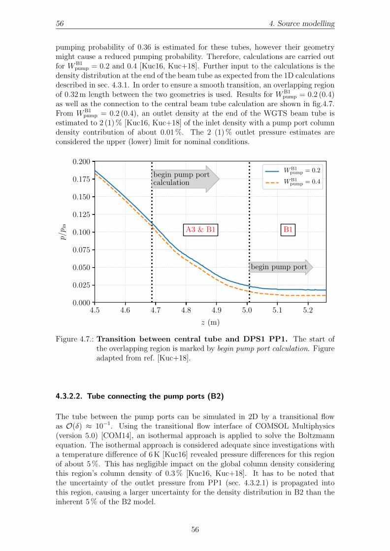
56 4. Source modelling
pumping probability of 0.36 is estimated for these tubes, however their geometrymight cause a reduced pumping probability. Therefore, calculations are carried outfor WB1
pump = 0.2 and 0.4 [Kuc16, Kuc+18]. Further input to the calculations is thedensity distribution at the end of the beam tube as expected from the 1D calculationsdescribed in sec. 4.3.1. In order to ensure a smooth transition, an overlapping regionof 0.32 m length between the two geometries is used. Results for WB1
pump = 0.2 (0.4)as well as the connection to the central beam tube calculation are shown in fig.4.7.From WB1
pump = 0.2 (0.4), an outlet density at the end of the WGTS beam tube isestimated to 2 (1) % [Kuc16, Kuc+18] of the inlet density with a pump port columndensity contribution of about 0.01 %. The 2 (1) % outlet pressure estimates areconsidered the upper (lower) limit for nominal conditions.
4.5 4.6 4.7 4.8 4.9 5.0 5.1 5.2
z (m)
0.000
0.025
0.050
0.075
0.100
0.125
0.150
0.175
0.200
p/p i
n
A3 & B1 B1
begin pump portcalculation
begin pump port
WB1pump = 0.2
WB1pump = 0.4
Figure 4.7.: Transition between central tube and DPS1 PP1. The start ofthe overlapping region is marked by begin pump port calculation. Figureadapted from ref. [Kuc+18].
4.3.2.2. Tube connecting the pump ports (B2)
The tube between the pump ports can be simulated in 2D by a transitional flowas O(δ) ≈ 10−1. Using the transitional flow interface of COMSOL Multiphysics(version 5.0) [COM14], an isothermal approach is applied to solve the Boltzmannequation. The isothermal approach is considered adequate since investigations witha temperature difference of 6 K [Kuc16] revealed pressure differences for this regionof about 5 %. This has negligible impact on the global column density consideringthis region’s column density of 0.3 % [Kuc16, Kuc+18]. It has to be noted thatthe uncertainty of the outlet pressure from PP1 (sec. 4.3.2.1) is propagated intothis region, causing a larger uncertainty for the density distribution in B2 than theinherent 5 % of the B2 model.
56

4.3. Gas dynamics model, nominal KATRIN set-up 57
4.3.2.3. Second pump port (B3)
Considering the small rarefaction parameter δ ≈ 10−2, the last part of the WGTSgas model geometry can be modelled using a molecular flow approach. As the tem-perature changes significantly from about 30 K at the second pump port (PP2) toroom temperature at the WGTS exit (connection to DPS2-F and rear section re-spectively), the 3D molecular flow interface of COMSOL [COM14] is applied [Kuc16,Kuc+18]. It has to be noted that the uncertainty of the outlet pressure of the cen-tral beam tube is propagated all the way to this domain, causing relatively largeuncertainties on the density distribution. However, as this region contributes theleast to the overall column density, its effect on the global column density can beneglected [Kuc16].
4.3.3. Complete gas model
The baseline to connect the different domains of the WGTS gas model is the calcu-lation of the gas flow in the central 10 m long beam tube. Inlet and outlet regionsare scaled accordingly, propagating uncertainties on the outlet pressure of the cen-tral beam tube all the way down to the global outlet pressure of the WGTS. Thecomposite density distribution for the complete WGTS is shown in fig. 4.8. Over-all reduction factors for gas flow and density are calculated to be about 400 and2000 [Kuc+18].
Since the uncertainty of the pure simulation of the column density is exceeding therequirement of 0.2 % by one order of magnitude, it is necessary that a measurementof the column density is used as calibration for the overall column density. Oncecalibrated, the source model gives a precise prediction of column density changesconsidering changes of operating parameters such as temperature and inlet pres-sure [Kuc16, Kuc+18]. The following section gives an overview of such a calibrationmeasurement, its requirements, and potential outcome.
4.3.4. Calibration of the column density
As outlined in the previous sections, the uncertainty on the column density dueto uncertainties of the simulation parameters of the density profile exceeds the re-quirement of 0.2 % by about one order of magnitude. However, in terms of neutrinomass analysis, it is not the column density that enters the analysis, but the prod-uct of column density N and total inelastic electron-gas scattering cross section σvia calculation of the scattering probabilities (compare sec. 2.2.1) [Kuc16, Kuc+18,Kle+18]. This product needs to be known to
∆(N · σ)N · σ
≤ 0.2 %. (4.19)
As the uncertainty on the inelastic scattering cross-section is stated with 2 % [Ase+00],it is absolutely necessary to determine N ·σ from a dedicated measurement to reachthe 0.2 % requirement.
57
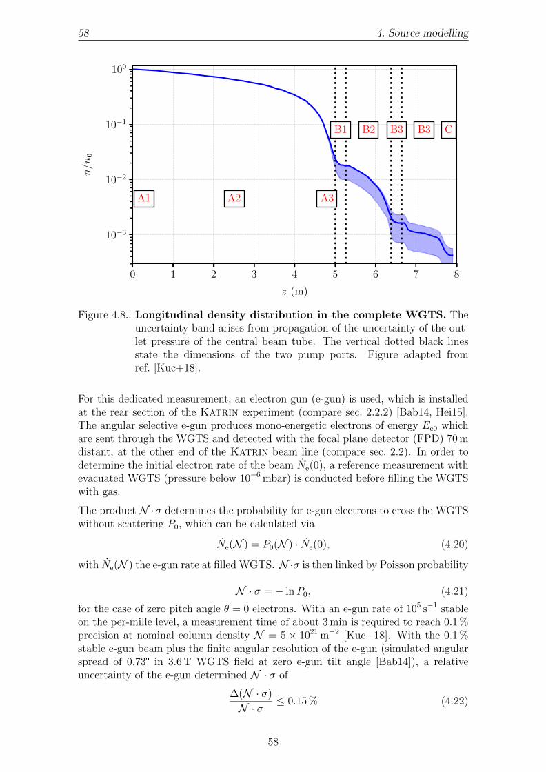
58 4. Source modelling
0 1 2 3 4 5 6 7 8
z (m)
10−3
10−2
10−1
100
n/n
0
A1 A2 A3
B1 B2 B3 B3 C
Figure 4.8.: Longitudinal density distribution in the complete WGTS. Theuncertainty band arises from propagation of the uncertainty of the out-let pressure of the central beam tube. The vertical dotted black linesstate the dimensions of the two pump ports. Figure adapted fromref. [Kuc+18].
For this dedicated measurement, an electron gun (e-gun) is used, which is installedat the rear section of the Katrin experiment (compare sec. 2.2.2) [Bab14, Hei15].The angular selective e-gun produces mono-energetic electrons of energy Ee0 whichare sent through the WGTS and detected with the focal plane detector (FPD) 70 mdistant, at the other end of the Katrin beam line (compare sec. 2.2). In order todetermine the initial electron rate of the beam Ne(0), a reference measurement withevacuated WGTS (pressure below 10−6 mbar) is conducted before filling the WGTSwith gas.
The product N ·σ determines the probability for e-gun electrons to cross the WGTSwithout scattering P0, which can be calculated via
Ne(N ) = P0(N ) · Ne(0), (4.20)
with Ne(N ) the e-gun rate at filled WGTS. N ·σ is then linked by Poisson probability
N · σ = − lnP0, (4.21)
for the case of zero pitch angle θ = 0 electrons. With an e-gun rate of 105 s−1 stableon the per-mille level, a measurement time of about 3 min is required to reach 0.1 %precision at nominal column density N = 5× 10²¹ m−2 [Kuc+18]. With the 0.1 %stable e-gun beam plus the finite angular resolution of the e-gun (simulated angularspread of 0.73° in 3.6 T WGTS field at zero e-gun tilt angle [Bab14]), a relativeuncertainty of the e-gun determined N · σ of
∆(N · σ)N · σ
≤ 0.15 % (4.22)
58

4.3. Gas dynamics model, nominal KATRIN set-up 59
is calculated [Kuc16]. The e-gun determined N ·σ can then be used to calibrate thedensity profile calculation. Though the uncertainty of the scattering cross-section σprevents translation of N · σ to N with the 0.15 % uncertainty, it enables use of thecalibrated density profile for prediction of column density changes with the requireduncertainty [Kuc16, Kuc+18]. Since changes of the column density can be modelledon the per-mille level or better [Kuc+18], the total uncertainty of the gas model is infact determined by the measurement of the e-gun. The next section will present theneutrino mass uncertainty resulting from the accuracy of the e-gun measurement.
4.3.5. Neutrino mass uncertainty
With the product of column density and scattering cross-section N · σ being con-strained to 0.2 % by the measurement described in sec. 4.3.4, the resulting neutrinomass uncertainty can be estimated from ensemble tests [Kle14, Kle+18, Kuc+18].The investigations were performed by L. Kuckert [Kuc16] and are briefly summarisedbelow.
� The dominating effect is the first order effect of having a 0.2 % different N · σin the model and the generated data. It results in a neutrino mass squaredshift (C in fig. 4.9) of
∆m2ν
∣∣∣C
= (−2.62± 0.25) · 10−3 eV2. (4.23)
� The second order effect of the accuracy of the gas density profile (difference ofup to 5 % from two different models) for fixed column density yields a neutrinomass squared shift of (A in fig. 4.9)
∆m2ν
∣∣∣A
= (−0.75± 0.24) · 10−3 eV2. (4.24)
� Another second order effect is the limited column density accuracy of 2 % whileN · σ is assumed to be known precisely. This effect results in (B in fig. 4.9)
∆m2ν
∣∣∣B
= (−0.26± 0.25) · 10−3 eV2. (4.25)
� A combined ensemble test of all above mentioned effects yields the total gasmodel related uncertainty on the neutrino mass squared of (ABC in fig. 4.9)
∆m2ν
∣∣∣ABC
= (−3.06± 0.24) · 10−3 eV2. (4.26)
A summary of the outlined gas dynamics related systematic uncertainties on theneutrino mass is given in fig. 4.9 [Kuc+18]. It can be concluded that the DesignReport estimated uncertainty can not be met if the Design Report requirement isinterpreted as an accuracy requirement. However, it has been shown that relativechanges can be modelled with an uncertainty well below the requirement [Kuc16,Kuc+18]. Furthermore, the estimated neutrino mass uncertainty from the accuracyof the gas model in combination with calibration by the RS e-gun is well below thelimit of a single systematic uncertainty if assuming that the number of systematicuncertainties in the Design Report is complete. The overall Katrin systematic un-certainty budget is currently undergoing a detailed revision [Sei19] which will revealwhether the uncertainty of the described e-gun measurement needs to be improvedto reduce the systematic uncertainty related to the gas dynamics description.
59

60 4. Source modelling
0 1 2 3 4 5 6 7×10⁻³
A
B
C
ABC
[Kuc1
6,K
uc+
18]
Des
ign
Rep
ort
lim
itsi
ngl
esy
stem
atic
negative neutrino mass shift ∆m2ν (eV2)
total gas model related
0.2 % N · σ uncertainty
uncertainty of N and σwith N · σ fixed
uncertainty of densitydistribution
gas model related
Figure 4.9.: Gas dynamics related neutrino mass uncertainty. The differ-ent effects investigated in [Kuc16, Kuc+18] and the requirement fromthe Design Report [KAT05] are shown. For further details, see textor [Kuc+18]. Figure adapted from ref. [Kuc+18].
4.4. Gas dynamics model, First Tritium set-up
In the last three years, Katrin has achieved several commissioning milestones andwill start neutrino mass data taking in early 2019. The first transmission of tritiumβ-decay electrons presents the latest major achievement towards long-term neutrinomass operation (compare chapter 5). For the first time, trace amounts of tritiumwere injected into the WGTS and the β-decay electrons were observed with the FPDdetector on the other end of the Katrin set-up.
This section will present the gas dynamics model developed from scratch specificallyfor the First Tritium campaign and discuss the uncertainty on the modelled gasdistribution and consequently the uncertainty on the modelled column density.
4.4.1. Statement of the problem
The notation used throughout this section will be the same as in the introductionsec. 4.1 and the description of the gas dynamics for the nominal Katrin set-upsec. 4.3, however the gas specific characteristics as viscosity will be used for deu-terium. The major difference between the First Tritium setup and the nominalKatrin operation was the tritium concentration εT. In nominal set-up, the tritiumconcentration will be εT ≥ 0.95 while in the First Tritium set-up trace amountsεT ≈ 5× 10⁻³ were used with deuterium as carrier gas. A further difference to thenominal set-up arises from the non-availability of the e-gun during the First Tritiumcampaign. Since no e-gun means no possibility to calibrate the calculated columndensity as outlined in sec. 4.3.4, different procedures need to be used to estimate theinput parameters for the gas profile calculation.
60

4.4. Gas dynamics model, First Tritium set-up 61
4.4.1.1. Choice of input parameters
As outlined in sec. 4.3, the dominant uncertainty in the calculation of the columndensity is the uncertainty on the pre-calculated dimensionless Poiseuille and thermalcreep coefficients GP and GT of about 2 %. Since this presents the lower uncertaintylimit of the column densityN achievable from calculations, it was decided to performcalculations for the central beam tube only. Using the list of input parameters insec. 4.3.1, two possibilities are left:
� Estimate the injection rate and therefore the throughput of the WGTS fromthe flow meter between the two buffer vessels of the inner loop (see fig. 3.1).Then use the throughput to calculate the mass flow rate and recursively esti-mate the density profile.
� Estimate the injection pressure from the measured pressure at the kryptoncapillary. The krypton capillary is used for the injection of krypton into theinjection chamber (shown in fig. 3.4) in the high temperature mode of theWGTS and is equipped with a pressure sensor.
When operating the inner loop in a closed circle, there is no additional source ofgas between pressure controlled buffer vessel at pB and the injection chamber at pch
which in turn defines the injection pressure into the beam tube, pin. During thestart-up of the gas circulation, gas might adsorb on the wall of the capillary feedingthe injection chamber and thereby cause a reduction of the initial mass flow rate.However, once stable circulation is established in terms of buffer vessel pressurestability on the per-mille level, there is no decrease or increase of the mass flowrate between buffer vessel and injection chamber. This would enable estimation ofthe mass flow rate and thereby the throughput of the WGTS from the flow metermeasurement.
Calculating the injection pressure from the pressure gauge at the krypton capillaryon the other hand requires solving two differential equations, one to translate thepressure at the gauge (room temperature) into a pressure at the injection chamber(30 K) and one to translate the pressure from injection chamber to the inlet pressurein the beam tube itself.
It is therefore considered reasonable to use the flow meter and the pressure in thebuffer vessel to estimate the injection rate into the WGTS source tube. Then one canapply a finite difference scheme to solve for the longitudinal density distribution andthereby estimate the column density. The pressure gauge at the krypton capillarywill be used as a cross-check for the recursively calculated injection pressure.
4.4.1.2. Choice of methods to calculate the column density
Due to the importance of the column density for the modelling of the measuredβ-decay spectrum, two different methods are used to estimate the density profilefrom the injection rate. One is the phenomenological formula found by Knud-sen [Knu09] (introduced in sec. 4.1.1) and the other one is solving the Boltzmannequation by applying a finite difference scheme [Sha97, SS98, Sha08, Sha16] (intro-duced in sec. 4.1.2). Integrating each density profile yields the respective columndensity estimate.
61
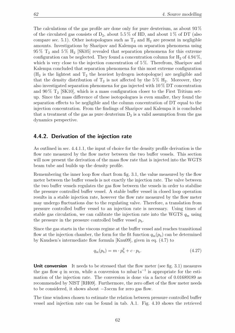
62 4. Source modelling
The calculations of the gas profile are done only for pure deuterium, as about 93 %of the circulated gas consists of D2, about 5.5 % of HD, and about 1 % of DT (alsocompare sec. 5.1). Other isotopologues such as T2 and H2 are present in negligibleamounts. Investigations by Sharipov and Kalempa on separation phenomena using95 % T2 and 5 % H2 [SK05] revealed that separation phenomena for this extremeconfiguration can be neglected. They found a concentration column for H2 of 4.94 %,which is very close to the injection concentration of 5 %. Therefrom, Sharipov andKalempa concluded that separation phenomena for this most extreme configuration(H2 is the lightest and T2 the heaviest hydrogen isotopologue) are negligible andthat the density distribution of T2 is not affected by the 5 % H2. Moreover, theyalso investigated separation phenomena for gas injected with 10 % DT concentrationand 90 % T2 [SK10], which is a mass configuration closer to the First Tritium set-up. Since the mass difference of these isotopologues is even smaller, they found theseparation effects to be negligible and the column concentration of DT equal to theinjection concentration. From the findings of Sharipov and Kalempa it is concludedthat a treatment of the gas as pure deuterium D2 is a valid assumption from the gasdynamics perspective.
4.4.2. Derivation of the injection rate
As outlined in sec. 4.4.1.1, the input of choice for the density profile derivation is theflow rate measured by the flow meter between the two buffer vessels. This sectionwill now present the derivation of the mass flow rate that is injected into the WGTSbeam tube and builds up the density profile.
Remembering the inner loop flow chart from fig. 3.1, the value measured by the flowmeter between the buffer vessels is not exactly the injection rate. The valve betweenthe two buffer vessels regulates the gas flow between the vessels in order to stabilisethe pressure controlled buffer vessel. A stable buffer vessel in closed loop operationresults in a stable injection rate, however the flow rate measured by the flow metermay undergo fluctuations due to the regulating valve. Therefore, a translation frompressure controlled buffer vessel to an injection rate is necessary. Using times ofstable gas circulation, we can calibrate the injection rate into the WGTS qin usingthe pressure in the pressure controlled buffer vessel pb.
Since the gas starts in the viscous regime at the buffer vessel and reaches transitionalflow at the injection chamber, the form for the fit function qin(pb) can be determinedby Knudsen’s intermediate flow formula [Knu09], given in eq. (4.7) to
qin(pb) = m · p2b + c · pb. (4.27)
Unit conversion It needs to be stressed that the flow meter (see fig. 3.1) measuresthe gas flow q in sccm, while a conversion to mbar l s−1 is appropriate for the esti-mation of the injection rate. The conversion is done via a factor of 0.01689189 asrecommended by NIST [RH09]. Furthermore, the zero offset of the flow meter needsto be considered, it shows about −3 sccm for zero gas flow.
The time windows chosen to estimate the relation between pressure controlled buffervessel and injection rate can be found in tab. A.1. Fig. 4.10 shows the retrieved
62
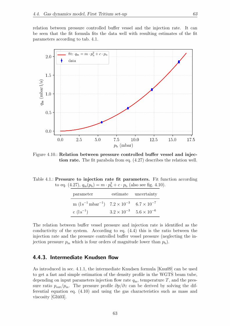
4.4. Gas dynamics model, First Tritium set-up 63
relation between pressure controlled buffer vessel and the injection rate. It canbe seen that the fit formula fits the data well with resulting estimates of the fitparameters according to tab. 4.1.
Figure 4.10.: Relation between pressure controlled buffer vessel and injec-tion rate. The fit parabola from eq. (4.27) describes the relation well.
Table 4.1.: Pressure to injection rate fit parameters. Fit function accordingto eq. (4.27), qin(pb) = m · p2
b + c · pb (also see fig. 4.10).
parameter estimate uncertainty
m (l s−1 mbar−1) 7.2× 10⁻³ 6.7× 10⁻⁷
c (l s−1) 3.2× 10⁻³ 5.6× 10⁻⁶
The relation between buffer vessel pressure and injection rate is identified as theconductivity of the system. According to eq. (4.4) this is the ratio between theinjection rate and the pressure controlled buffer vessel pressure (neglecting the in-jection pressure pin which is four orders of magnitude lower than pb).
4.4.3. Intermediate Knudsen flow
As introduced in sec. 4.1.1, the intermediate Knudsen formula [Knu09] can be usedto get a fast and simple estimation of the density profile in the WGTS beam tube,depending on input parameters injection flow rate qin, temperature T , and the pres-sure ratio pout/pin. The pressure profile ∂p/∂z can be derived by solving the dif-ferential equation eq. (4.10) and using the gas characteristics such as mass andviscosity [Glu03].
63

64 4. Source modelling
From eq. (4.10) (with q = qin), we can derive an equation for pin by variable sepa-ration and integration. Using the boundary conditions p(z = 0) = pin and a fixedpressure ratio ap = pout/pin = const yields
pin = −B ±√B2 − 4AC2A , (4.28)
with A = 0.5Dvis · (1 − a2p), B = X Dmol · (1 − ap) and C = −qin L. Iteratively
solving eq. (4.28) for pin until convergence7 yields the inlet pressure pin. Integratingeq. (4.7) from z = 0 to z enables a simple formula for the pressure profile, using theabove calculated inlet pressure pin as
p(z) = −B′ ±
√B′2 − 4A′C ′
2A′ , (4.29)
with A′ = 0.5Dvis, B′ = X Dmol and C ′ = qin z − A′ p2
in − B′ pin. Obtaining thenumber density profile is then trivial via eq. (4.2).
4.4.3.1. Temperature dependence
It has to be stressed that the formula eq. (4.29) derived from [Knu09, Glu03] assumesconstant temperature along the beam tube when solving for pin. Calculating thecolumn density for a beam tube temperature of T = 30 K and 30.5 K yields a columndensity difference of 0.2 % when adapting the viscosity according to its temperaturedependence stated in [AMW87]. Since the deuterium viscosity change from 30 K to30.5 K is about 1.7 % and the quoted uncertainty on the viscosity is 2 %, we can alsouse the same viscosity for both temperatures, resulting in a column density differenceof 0.8 %. This difference is the upper limit of the temperature related uncertainty tothe Knudsen flow since it assumes 0.5 K temperature difference for the whole beamtube. As shown in sec. 4.2.3, the longitudinal temperature deviation only reaches0.5 K at the rear end of the beam tube; therefore the realistic effect on the columndensity is even smaller.
4.4.3.2. Pure tritium
In order do get an estimate for the uncertainty of this alternative calculation ofthe column density, the result is compared to calculations by F. Sharipov for puretritium [Sha04a]. Using the same conditions (T = 27 K, qin = 1.853 mbar l s−1,pout = 0 and Lfront = Lrear = L = 5 m, and viscosity according to eq. (4.18)8), theKnudsen flow results in a column density of N = 4.98× 10²¹ m−2.
Compared to the 5× 10²¹ m−2 estimate of Sharipov, this is a deviation of 0.4 %. Asdiscussed in sec. 4.1.1, this is within the uncertainty of the intermediate Knudsenformula. It has to be noted that the estimate of Sharipov has a model-relateduncertainty of 2 % [Sha04a], so it can be concluded that the Knudsen formula canbe used as a simple cross-check of calculations based on solving the Boltzmannequation.
7Convergence here is defined as p′in−pin
pin< 10−6.
8Including the temperature dependence of the deuterium viscosity according to [AMW87].
64

4.4. Gas dynamics model, First Tritium set-up 65
4.4.3.3. Pure deuterium
Repeating the calculations from sec. 4.4.3.2 with the same input parameters butwith pure deuterium as gas (also adapting the viscosity) results in a column densityof 4.48× 10²¹ m−2. Due to the lighter mass of the deuterium, causing a larger mostprobable speed vm at the same temperature, it is expected that the column densityfor deuterium compared to tritium is about 10 % lower.
For realistic input parameters (T = 30 K, qin = 1.85 mbar l s−1, pout/pin = 0.02,Lfront = 5.0075 m, Lrear = 5.0745 m), the Knudsen-based column density estimate is
N = 4.52× 10²¹ m−2. (4.30)
4.4.4. Boltzmann equation
As described in sec. 4.3.4, the nominal set-up requires a calibration of the columndensity in order to reach the necessary accuracy. The calibration by the e-gun enablesone to find the input parameters for the density profile calculation such that theestimated column density and the WGTS flow rate match the e-gun measurement.However, as described in sec. 4.4.1, the e-gun was not available during the FirstTritium campaign. Furthermore, the gas model before this thesis was only able todeal with pure tritium T2. Therefore, in the course of this thesis, the intermediateKnudsen flow was implemented which can be used to calculate the density profileand column density for deuterium and tritium, directly using the injection rate.One drawback of the Knudsen implementation (compare sec. 4.4.3.1) is its lack ofmodelling temperature gradients. As introduced in sec. 4.1.2, solving the Boltzmannequation is one way to include temperature gradients. In contrast to the Knudsenformula, eq. (4.12) can deal with temperature driven flow. Therefore, another typeof gas model was implemented, which is similar to the one described in sec. 4.3.1 butuses the WGTS flow rate as an input parameter instead of an output parameter.Furthermore, the new implementation is generalised for dealing with tritium anddeuterium. Describing hydrogen gas dynamics would only require including thehydrogen viscosity from [AMW86].
4.4.4.1. Determining the density profile
The principle for deriving the density profile remains the same as in sec. 4.3.1.Converting the injection rate into a mass flow rate enables iterative calculation ofthe pressure profile using eq. (4.12) and the formulas for the dimensionless Poiseuilleand thermal flow rates GP (4.13) and GT (4.14). The mass flow rate M can beobtained from the injection flow rate qin from eq. (4.3) as
M = m
kBTqin. (4.31)
It has to be stressed that the gas flow q has to be scaled with the temperature,while the mass flow rate M is temperature independent and constant provided thereis no additional source of gas. Knowing the mass flow rate, we can recursivelycalculate the pressure profile via a finite numerical difference scheme, which also
65
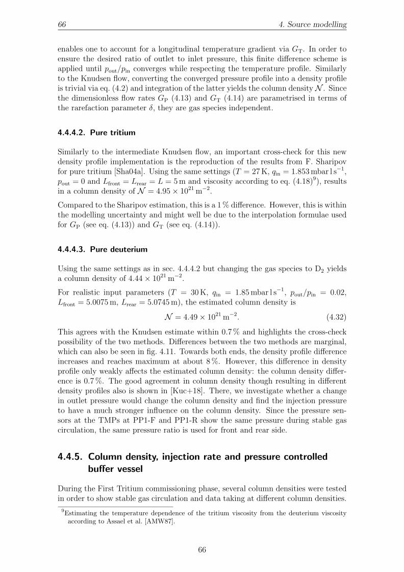
66 4. Source modelling
enables one to account for a longitudinal temperature gradient via GT. In order toensure the desired ratio of outlet to inlet pressure, this finite difference scheme isapplied until pout/pin converges while respecting the temperature profile. Similarlyto the Knudsen flow, converting the converged pressure profile into a density profileis trivial via eq. (4.2) and integration of the latter yields the column densityN . Sincethe dimensionless flow rates GP (4.13) and GT (4.14) are parametrised in terms ofthe rarefaction parameter δ, they are gas species independent.
4.4.4.2. Pure tritium
Similarly to the intermediate Knudsen flow, an important cross-check for this newdensity profile implementation is the reproduction of the results from F. Sharipovfor pure tritium [Sha04a]. Using the same settings (T = 27 K, qin = 1.853 mbar l s−1,pout = 0 and Lfront = Lrear = L = 5 m and viscosity according to eq. (4.18)9), resultsin a column density of N = 4.95× 10²¹ m−2.
Compared to the Sharipov estimation, this is a 1 % difference. However, this is withinthe modelling uncertainty and might well be due to the interpolation formulae usedfor GP (see eq. (4.13)) and GT (see eq. (4.14)).
4.4.4.3. Pure deuterium
Using the same settings as in sec. 4.4.4.2 but changing the gas species to D2 yieldsa column density of 4.44× 10²¹ m−2.
For realistic input parameters (T = 30 K, qin = 1.85 mbar l s−1, pout/pin = 0.02,Lfront = 5.0075 m, Lrear = 5.0745 m), the estimated column density is
N = 4.49× 10²¹ m−2. (4.32)
This agrees with the Knudsen estimate within 0.7 % and highlights the cross-checkpossibility of the two methods. Differences between the two methods are marginal,which can also be seen in fig. 4.11. Towards both ends, the density profile differenceincreases and reaches maximum at about 8 %. However, this difference in densityprofile only weakly affects the estimated column density: the column density differ-ence is 0.7 %. The good agreement in column density though resulting in differentdensity profiles also is shown in [Kuc+18]. There, we investigate whether a changein outlet pressure would change the column density and find the injection pressureto have a much stronger influence on the column density. Since the pressure sen-sors at the TMPs at PP1-F and PP1-R show the same pressure during stable gascirculation, the same pressure ratio is used for front and rear side.
4.4.5. Column density, injection rate and pressure controlledbuffer vessel
During the First Tritium commissioning phase, several column densities were testedin order to show stable gas circulation and data taking at different column densities.
9Estimating the temperature dependence of the tritium viscosity from the deuterium viscosityaccording to Assael et al. [AMW87].
66
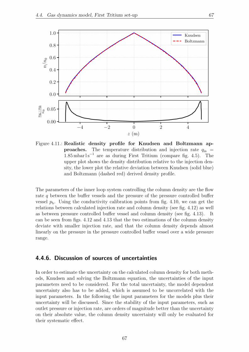
4.4. Gas dynamics model, First Tritium set-up 67
0.0
0.2
0.4
0.6
0.8
1.0
n/n
0
Knudsen
Boltzmann
−4 −2 0 2 4
z (m)
0.00
0.05
nK−n
B
nB
Figure 4.11.: Realistic density profile for Knudsen and Boltzmann ap-proaches. The temperature distribution and injection rate qin =1.85 mbar l s−1 are as during First Tritium (compare fig. 4.5). Theupper plot shows the density distribution relative to the injection den-sity, the lower plot the relative deviation between Knudsen (solid blue)and Boltzmann (dashed red) derived density profile.
The parameters of the inner loop system controlling the column density are the flowrate q between the buffer vessels and the pressure of the pressure controlled buffervessel pb. Using the conductivity calibration points from fig. 4.10, we can get therelations between calculated injection rate and column density (see fig. 4.12) as wellas between pressure controlled buffer vessel and column density (see fig. 4.13). Itcan be seen from figs. 4.12 and 4.13 that the two estimations of the column densitydeviate with smaller injection rate, and that the column density depends almostlinearly on the pressure in the pressure controlled buffer vessel over a wide pressurerange.
4.4.6. Discussion of sources of uncertainties
In order to estimate the uncertainty on the calculated column density for both meth-ods, Knudsen and solving the Boltzmann equation, the uncertainties of the inputparameters need to be considered. For the total uncertainty, the model dependentuncertainty also has to be added, which is assumed to be uncorrelated with theinput parameters. In the following the input parameters for the models plus theiruncertainty will be discussed. Since the stability of the input parameters, such asoutlet pressure or injection rate, are orders of magnitude better than the uncertaintyon their absolute value, the column density uncertainty will only be evaluated fortheir systematic effect.
67
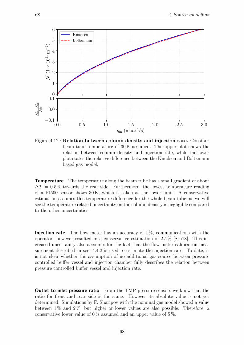
68 4. Source modelling
0
1
2
3
4
5
6
N(1×
1021
m−
2)
Knudsen
Boltzmann
0.0 0.5 1.0 1.5 2.0 2.5 3.0qin (mbar l/s)
−0.1
0.0
0.1
NK−N
B
NB
Figure 4.12.: Relation between column density and injection rate. Constantbeam tube temperature of 30 K assumed. The upper plot shows therelation between column density and injection rate, while the lowerplot states the relative difference between the Knudsen and Boltzmannbased gas model.
Temperature The temperature along the beam tube has a small gradient of about∆T = 0.5 K towards the rear side. Furthermore, the lowest temperature readingof a Pt500 sensor shows 30 K, which is taken as the lower limit. A conservativeestimation assumes this temperature difference for the whole beam tube; as we willsee the temperature related uncertainty on the column density is negligible comparedto the other uncertainties.
Injection rate The flow meter has an accuracy of 1 %, communications with theoperators however resulted in a conservative estimation of 2.5 % [Stu18]. This in-creased uncertainty also accounts for the fact that the flow meter calibration mea-surement described in sec. 4.4.2 is used to estimate the injection rate. To date, itis not clear whether the assumption of no additional gas source between pressurecontrolled buffer vessel and injection chamber fully describes the relation betweenpressure controlled buffer vessel and injection rate.
Outlet to inlet pressure ratio From the TMP pressure sensors we know that theratio for front and rear side is the same. However its absolute value is not yetdetermined. Simulations by F. Sharipov with the nominal gas model showed a valuebetween 1 % and 2 %; but higher or lower values are also possible. Therefore, aconservative lower value of 0 is assumed and an upper value of 5 %.
68

4.4. Gas dynamics model, First Tritium set-up 69
0.0 2.5 5.0 7.5 10.0 12.5 15.0 17.5 20.0pb (mbar)
0
1
2
3
4
5
6
N(1
021
m−
2)
Knudsen
Boltzmann
Figure 4.13.: Relation between column density and pressure in the pressurecontrolled buffer vessel. A constant beam tube temperature of 30 Kis assumed.
Deuterium viscosity Assael et at. [AMW87] state a 2 % uncertainty on their esti-mated deuterium viscosity values.
Accommodation coefficient As outlined in sec. 4.3.1, there exist no measure-ments of the accommodation of deuterium or hydrogen in the temperature regimewe are interested in. Hadj et al give a value of α = 0.912 ± 0.004 [Had+12] forthe accommodation coefficient of helium on warm stainless steel. Therefore, a con-servative value of α = 0.9 is taken as lower limit of the accommodation coefficientof deuterium at 30 K, while the upper limit is 1 (full accommodation). It has tobe noted that accounting for the accommodation coefficient is only possible in the‘Boltzmann’ density model via the dimensionless flow rates GP and GT.
4.4.7. Estimation of the (deuterium) column density uncertainty
In order to see the effects of the uncertainties of the individual input parameterson the column density, each parameter is varied separately and the correspondingcolumn density calculated. For example, the viscosity depends on the temperature,therefore changes in this one parameter propagate changes to all other parameters.
Input parameter effects on the column density estimate The result of deflect-ing one input parameter (which might influence others) is shown in fig. 4.14. Forboth simulation variants, we can see similar effects. We also see the previous state-ment, that the temperature dependence of the column density estimation is rather
69
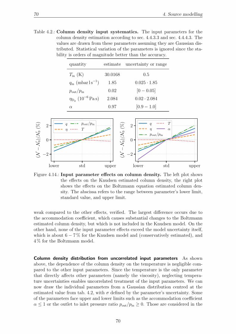
70 4. Source modelling
Table 4.2.: Column density input systematics. The input parameters for thecolumn density estimation according to sec. 4.4.3.3 and sec. 4.4.4.3. Thevalues are drawn from these parameters assuming they are Gaussian dis-tributed. Statistical variation of the parameters is ignored since the sta-bility is orders of magnitude better than the accuracy.
quantity estimate uncertainty or range
Tin (K) 30.0168 0.5
qin (mbar l s−1) 1.85 0.025 · 1.85pout/pin 0.02 [0− 0.05]ηD2 (10−6 Pa s) 2.084 0.02 · 2.084α 0.97 [0.9− 1.0]
lower std upper
−2
0
2
(N−N
0)/N
0(%
) q
η
pout/pin
T
lower std upper
−2
0
2(N−N
0)/N
0(%
) q
η
pout/pin
T
α
Figure 4.14.: Input parameter effects on column density. The left plot showsthe effects on the Knudsen estimated column density, the right plotshows the effects on the Boltzmann equation estimated column den-sity. The abscissa refers to the range between parameter’s lower limit,standard value, and upper limit.
weak compared to the other effects, verified. The largest difference occurs due tothe accommodation coefficient, which causes substantial changes to the Boltzmannestimated column density, but which is not included in the Knudsen model. On theother hand, none of the input parameter effects exceed the model uncertainty itself,which is about 6− 7 % for the Knudsen model and (conservatively estimated), and4 % for the Boltzmann model.
Column density distribution from uncorrelated input parameters As shownabove, the dependence of the column density on the temperature is negligible com-pared to the other input parameters. Since the temperature is the only parameterthat directly affects other parameters (namely the viscosity), neglecting tempera-ture uncertainties enables uncorrelated treatment of the input parameters. We cannow draw the individual parameters from a Gaussian distribution centred at theestimated value from tab. 4.2, with σ defined by the parameter’s uncertainty. Someof the parameters face upper and lower limits such as the accommodation coefficientα ≤ 1 or the outlet to inlet pressure ratio pout/pin ≥ 0. Those are considered in the
70

4.4. Gas dynamics model, First Tritium set-up 71
underlying distributions.
Drawing 104 times from these distributions and estimating the column density yieldsa distribution of the column density. From that distribution, we can estimate thelower and upper uncertainty of the column density related to input parameters.Using the column density calculated with best estimate input parameters as centralvalue, searching the 1σ confidence interval yields the upper and lower uncertaintyrespectively.
Thereby, the column density for the Knudsen model is estimated to be
NK,input =(4.5+0.1−0.1
)× 1021 m−2, (4.33)
which evaluates to an input parameter related uncertainty on the column density of2 %, compare fig. 4.15.
For the Boltzmann equation solving model, the column density distribution resultsin
NB,input =(4.4+0.1−0.2
)× 1021 m−2, (4.34)
which evaluates to an input parameter related uncertainty on the column density of+3 % (−4 %). Note that the Boltzmann method has a larger uncertainty than theKnudsen model because of inclusion of variations on the accommodation coefficientα. This also explains why the distribution of the Boltzmann estimated columndensity is slightly skewed; it is because the input parameter α has a distributioncut-off at 1 (compare fig. 4.15).
4.25 4.50 4.75
N (m−2) ×1021
0
500
1000
entr
ies
3.5 4.0 4.5
N (m−2) ×1021
0
500
1000
entr
ies
Figure 4.15.: Systematic distribution of column density due to input pa-rameters. The left plot shows the effects on the Knudsen estimatedcolumn density, the right plot shows the effects on the Boltzmann equa-tion estimated column density.
Total uncertainty on the column density In order to get the total column densityuncertainty for the First Tritium set-up, the input parameter estimated uncertaintyand the model dependent uncertainty have to be added. Since they are uncorrelated,we can use the square root of the squared sum.
For the Knudsen estimated uncertainty, this yields
NK =(4.5+0.3−0.3
)× 1021 m−2, (4.35)
which is a relative uncertainty of ±7 %. As expected, the model related uncertaintyof 7 % dominates over the input related uncertainty of 2 %.
71

72 4. Source modelling
For the Boltzmann estimated total uncertainty is found to
NB =(4.4+0.2−0.3
)× 1021 m−2, (4.36)
which equals a relative uncertainty of +5 % (−6 %). Here, the input parametersuncertainty cannot be neglected because it is comparable to the model related un-certainty of (conservatively estimated) 4 %.
4.4.8. Estimation of injection pressure from krypton capillarypressure
Due to the non-availability of the e-gun during the First Tritium campaign, othermethods have to be used to access the validity of the gas dynamics simulations. Oneof them is using the pressure measured in the krypton capillary, attached to the in-jection chamber. The krypton capillary is the analogue of the tritium capillary, andis used to inject krypton in the high temperature mode of the WGTS. During FirstTritium, the injection chamber was filled via the tritium capillary while the valveafter the krypton capillary pressure sensor was closed, compare fig. 4.16. The closedvalve prevents a mass flow as through an open tube, however the temperature dif-ference between injection chamber at 30 K and pressure sensor at room temperaturerequires solving a differential equation to translate the pressure sensor measurementinto an injection chamber pressure. Furthermore, the injection pressure in the beamtube requires another differential equation to account for the gas flow through theinjection capillaries (compare fig. 4.16 and fig. 3.4). The following section will dealwith solving the two differential equations to estimate the injection pressure fromthe pressure measured at the pressure gauge at the krypton capillary.
pKr
pin, beam tube
injection chamber
Tca
pilla
ry
Kr capillary
TKr = 295 K
pch, Tch = 30 K
Figure 4.16.: Sketch of the krypton capillary. Geometry is not to scale. Thedistance between Kr pressure sensor and injection chamber is about7 m. Gas inflow is through the T capillary.
4.4.8.1. Krypton capillary pressure to injection chamber pressure
Since the valve behind the pressure sensor of the krypton capillary was closed forthe First Tritium measurements (compare fig. 4.16), the pressure gradient from
72

4.4. Gas dynamics model, First Tritium set-up 73
the pressure sensor to the injection chamber is caused by the temperature gradi-ent. This leads to the so-called thermomolecular pressure effect. As shown by F.Sharipov [Sha96], we can relate the pressures at both ends of a long tube via theirtemperature ratio through a simple formula
pKr
pch
=(TKr
Tch
)γ, (4.37)
if there is no gas flow between the two locations. The coefficient γ thereby dependson many factors such as tube geometry and gas species [Sha96]. To estimate γ, adifferential equation needs to be solved [Sha96]
dPdT
= PTQP(δchP/T )QT(δchP/T ) , (4.38)
with dimensionless flow rates QP(δ) and QT(δ), δ = δchP/T , and dimensionlesspressure P = p/pch and temperature T = T/Tch relative to the injection chamber.The differential equation eq. (4.38) can be solved by applying a numerical differencescheme as outlined by Sharipov [Sha96]. This estimates the pressure at the posi-tion of the pressure gauge. However, we are interested in the other direction: wewant to use the measured pressure at the gauge to estimate the injection chamberpressure. Therefore, a bisection search is applied until the estimated pressure at thegauge matches the measured value, the corresponding pch is then the pressure at theinjection chamber. γ can also be estimated easily via eq. (4.37).
To solve the differential equation, we need the pre-calculated dimensionless flowrates from Sharipov [Sha96], temperatures according to the sketch in fig. 4.16, massof deuterium, temperature dependent viscosity of deuterium [AMW87], α = 1, andthe diameter of the krypton capillary of 1 cm [Mar18]. Furthermore, the kryptonpressure sensor showed a reading of pKr = 12.8× 10⁻³ mbar during the times usedfor comparison to simulations (10th June 2018). Applying the iterative numericaldifference scheme results in a pressure at the injection chamber of
pch = 6.2× 10⁻³ mbar and γ = 0.32. (4.39)
4.4.8.2. Injection chamber to injection pressure
With the estimate of the injection chamber pressure from sec. 4.4.8.1, we can nowcalculate the injection pressure. Sharipov [Sha04a] calculated a relation betweeninjection chamber pressure and injection pressure for tritium by assuming a freemolecular regime. He argues that this is possible since the numerical calculationsfor a short channel presented in [SS98] showed the flow rate to be independent of therarefaction parameter for small δ < 1. Using the orifice geometry of 2 mm diameterand length, we can estimate the rarefaction parameter to about δch = 0.8 < 1.Since the injection pressure is expected to be smaller than the chamber pressure, wecan state that the relation δ < 1 is satisfied and we may use the same principle asSharipov [Sha04b].
73

74 4. Source modelling
With the dimensionless length L = lorifice/rorifice = 2, we can calculate the transmis-sion probability W through an orifice via [SS98]
W = 1 + L2
4 −L4 ·
√L2 + 4−
[(8− L2)
√L2 + 4 + L3 − 16
]2
72L√L2 + 4− 288 ln
[L/2 +
√L2/4 + 1
] . (4.40)
With the transmission probability W , we can relate the throughput q0 = q/415 forone of the 415 orifice to the injection pressure pin as [SS98, Sha04b]
pin = pch − q
√2TchmD2/(π kB)
273.15 · 415 r2orifice ·W (L)
. (4.41)
Using the pressure pch = 6.2× 10⁻³ mbar estimated above, the injection pressure isestimated to be
pin = 3.12× 10⁻³ mbar. (4.42)
Comparing this to the injection pressure calculated from the density profile of theKnudsen model (3.02× 10⁻³ mbar) and the Boltzmann estimate (2.99× 10⁻³ mbar)yields a difference of 3 % and 4 %, respectively.
The agreement is remarkably good, despite the many assumptions that were madein the estimation of the injection pressure via the krypton pressure gauge. However,DSMC simulations for tritium by F. Sharipov [Sha10] of the ratio between injectionchamber and injection pressure suggest a larger injection pressure than estimated viathe method used in this section. Assuming that the ratio is the same for deuterium(1.8), the estimated injection pressure would be 3.4× 10⁻³ mbar, which would yielda difference to the gas dynamics model estimated injection pressure of about 12 %.
4.4.9. Discussion
Since e-gun measurements of the column density were not yet available for the FirstTritium campaign, a new way of modelling the column density was developed in thiswork. The most reliable input parameter for the calculations is estimation of the in-jection rate from a calibration of the pressure controlled buffer vessel. Furthermore,the dominating gas species in the First Tritium campaign was deuterium insteadof tritium. Therefore, two new models were developed using the calculated injec-tion rate as input parameter to estimate the density profile and thereby the columndensity. Both models are generalised for the gas species and therefore they are alsovalid for tritium. One model uses a phenomenological formula derived by Knud-sen [Knu09] and the other is obtained from solving the Boltzmann equation [SS98].In order to give a reliable estimation of the density profile, the temperature read-ings of the beam tube Pt500 sensors were implemented in the simulation framework.Both models agree within one percent in their estimated column density despite thedifference in density profiles of up to 8 %.
A cross-check of the calculated injection pressure with an estimation from the pres-sure measured at the krypton capillary resulted in agreement with the two modelswithin 5− 6 %. However, the uncertainty of this estimate is not yet determined and
74
4.5. Magnetic field 75
may well be of the order of 10 % as shown in a comparative calculation by Sharipov.Further comparative measurements of the column density with two different detec-tors will be discussed in the First Tritium chapter in sec. 5.4.
In order to enable fast fitting of the measured tritium spectra, the calculations ofthe column density from the injection rate were included into the automatic runprocessing intermediate data layer IDLE (see sec. 2.4).
The uncertainties found for the column density estimate of the First Tritium non-standard set-up (6 − 7 %) are one order of magnitude larger than the required un-certainty in the nominal Katrin set-up (0.2 %). Similarly to the nominal tritiumoperation gas model, a calibration measurement with the e-gun will decrease thisuncertainty and enable an accurate estimation of the column density. It has to benoted that the gas model for the nominal tritium operation is ready to be used.With the e-gun calibration measurements foreseen to be available, the gas modelrelated neutrino mass uncertainty is projected to stay within the budget for onesingle systematic [Kuc+18].
4.5. Magnetic field
The magnetic field of the WGTS BS defines the starting magnetic field of the tritiumβ-decay electrons. As such, it defines the maximum acceptance angle via θmax =arcsin
√BS/Bmax (compare eq. (2.13)). Electrons with initial polar angles larger
than θmax are magnetically reflected at the maximum magnetic field in the set-up,Bmax
10. A lower magnetic field in the source therefore increases the fraction ofelectrons reaching the detector without undergoing scattering processes. This wouldincrease the number of electrons in the endpoint region. Besides, the synchrotronradiation emitted by the electrons is also related to the source magnetic field, itdecreases the kinetic energy of the electrons.
Monte Carlo investigations with a global Katrin model by S. Groh [Gro15] revealedthat the required accuracy on the source magnetic field is below 1 %. Groh gives anallowed relative deviation range of [−8.3, 6.4] × 10−3 for the absolute value of thesource magnetic field for Design Report settings [KAT05]. This section will introducethe most recent source model and compare it with stray field measurements beforeclosing with a discussion of the results.
4.5.1. Magnetic field model
As introduced in sec. 3.3.3, the magnetic field of the WGTS is defined by sevensuperconducting magnets with two booster coils each. The field inside the central10 m long beam tube is homogeneous with a slight unavoidable drop between thelong modules M1, M2, and M3 (see fig. 3.1). Fig. 4.17 shows the model of the super-conducting magnets, with the resulting nominal 3.6 T field. Since the magnets shrinkduring cool down, a cooling factor of 0.997 for the length of the modules is assumed inthe model, estimated from the linear expansion coefficient of ≈ 10 µm m−1 K−1 and
10In the nominal set-up, the maximum magnetic field is at the PCH magnet.
75
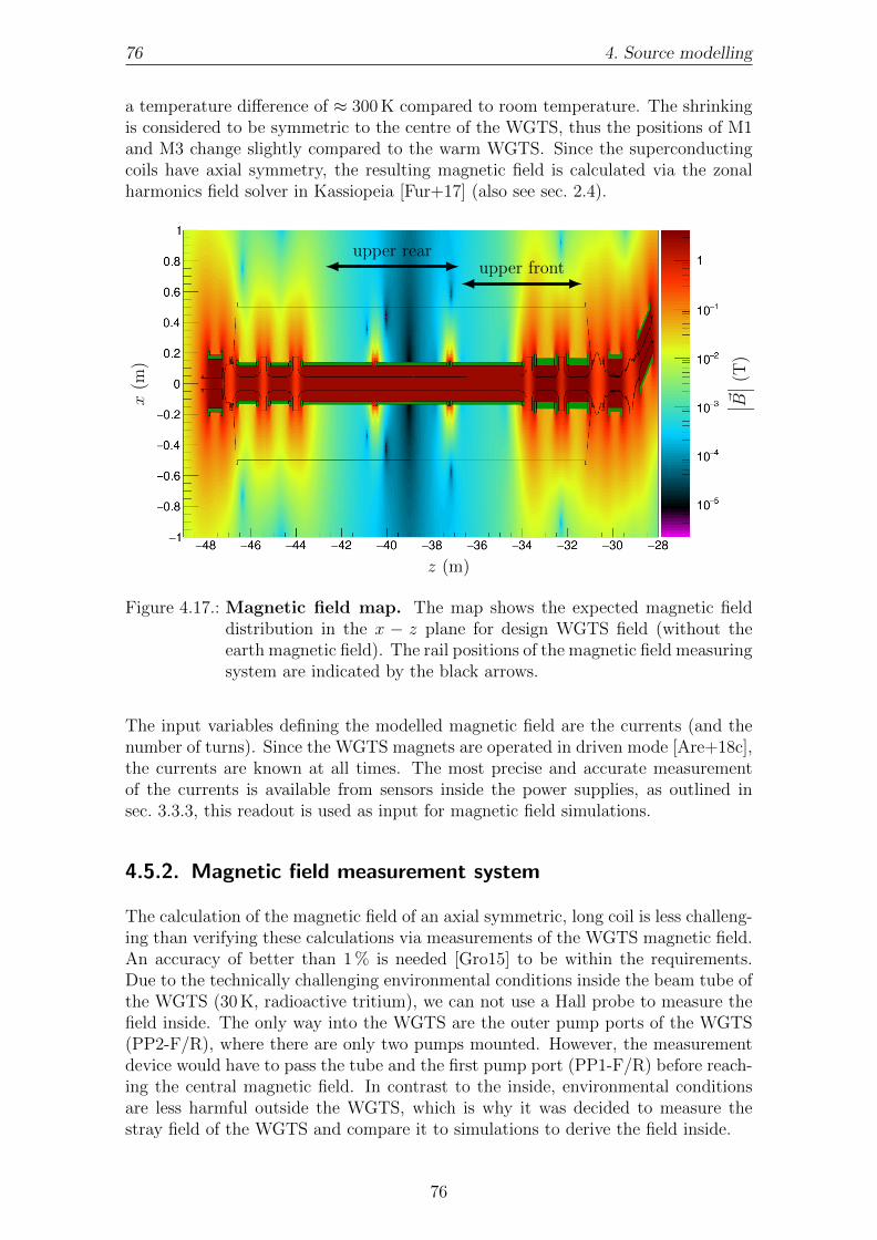
76 4. Source modelling
a temperature difference of ≈ 300 K compared to room temperature. The shrinkingis considered to be symmetric to the centre of the WGTS, thus the positions of M1and M3 change slightly compared to the warm WGTS. Since the superconductingcoils have axial symmetry, the resulting magnetic field is calculated via the zonalharmonics field solver in Kassiopeia [Fur+17] (also see sec. 2.4).
upper frontupper rear
∣ ∣ ∣~ B∣ ∣ ∣(T)
z (m)
x(m
)
Figure 4.17.: Magnetic field map. The map shows the expected magnetic fielddistribution in the x − z plane for design WGTS field (without theearth magnetic field). The rail positions of the magnetic field measuringsystem are indicated by the black arrows.
The input variables defining the modelled magnetic field are the currents (and thenumber of turns). Since the WGTS magnets are operated in driven mode [Are+18c],the currents are known at all times. The most precise and accurate measurementof the currents is available from sensors inside the power supplies, as outlined insec. 3.3.3, this readout is used as input for magnetic field simulations.
4.5.2. Magnetic field measurement system
The calculation of the magnetic field of an axial symmetric, long coil is less challeng-ing than verifying these calculations via measurements of the WGTS magnetic field.An accuracy of better than 1 % is needed [Gro15] to be within the requirements.Due to the technically challenging environmental conditions inside the beam tube ofthe WGTS (30 K, radioactive tritium), we can not use a Hall probe to measure thefield inside. The only way into the WGTS are the outer pump ports of the WGTS(PP2-F/R), where there are only two pumps mounted. However, the measurementdevice would have to pass the tube and the first pump port (PP1-F/R) before reach-ing the central magnetic field. In contrast to the inside, environmental conditionsare less harmful outside the WGTS, which is why it was decided to measure thestray field of the WGTS and compare it to simulations to derive the field inside.
76

4.5. Magnetic field 77
In order to reach the required accuracy with stray field measurements, positioningof the measurement device is crucial. Simulations showed that the position has tobe known to the order of 1 mm to reach an accuracy below 0.5 % when comparingthe measured to the simulated magnetic field.
To meet this requirement, a system of well-defined position measurement and accu-rate and precise magnetic field measurement was developed. The position is con-strained to only one degree of freedom, which is longitudinal movement along thecryostat of the WGTS, measured by a rope sensor. The magnetic field is determinedvia a three-axis Hall probe with well defined magnetic field sensitive volume.
Figure 4.18.: Magnetic field measuring setup. The panorama includes all threerails (upper front, upper rear, and lower center) used for the measure-ments. The inlets show the mounting of the Hall probe and the readoutunit on top of the Bosch EcoSlide© [Bos18], plus the mounting of therope sensor (lower right picture).
Hall probe The magnetic field measurement device which fulfils the requirementof an accuracy better than 0.5 % plus a well-defined and accurately known magneticfield sensitive volume is an integrated three axis Hall probe in a SENIS 3-Axis DigitalTeslameter 3MH3A-0.1%-200mT [SEN18]. For the measured magnetic field, theproducer lists an accuracy of better 0.1 % of full range (200 mT) and resolution of0.02 mT.
The Hall probe and its readout are mounted onto a 45 × 45 × 160 mm aluminiumBosch EcoSlide© [Bos18], which can move 5-6 m along the 45 × 45 mm aluminiumrails. Fig. 4.18 shows the mounting of the Hall probe and its readout as well asthe assembled slide. It has to be noted that special care was taken to have onlynon-magnetic materials in the set-up in order not to disturb the measurements.
Rope sensor As outlined before, the position of the Hall probe has to be known tosub-mm precision. Since the assembly has only one degree of freedom, the parameterof interest here is the longitudinal position of the slide. The chosen WayCon ropesensors SX80 [Way18b] and SX135 [Way18a] have a linearity deviation of less than0.02 % over the full measurement range. Linearity here describes the relation between
77
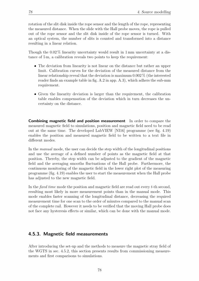
78 4. Source modelling
rotation of the slit disk inside the rope sensor and the length of the rope, representingthe measured distance. When the slide with the Hall probe moves, the rope is pulledout of the rope sensor and the slit disk inside of the rope sensor is turned. Withan optical system, the number of slits is counted and transformed into a distanceresulting in a linear relation.
Though the 0.02 % linearity uncertainty would result in 1 mm uncertainty at a dis-tance of 5 m, a calibration reveals two points to keep the requirement:
� The deviation from linearity is not linear on the distance but rather an upperlimit. Calibration curves for the deviation of the measured distance from thelinear relationship reveal that the deviation is maximum 0.002 % (the interestedreader finds an example table in fig. A.2 in app. A.3), which adhers the sub-mmrequirement.
� Given the linearity deviation is larger than the requirement, the calibrationtable enables compensation of the deviation which in turn decreases the un-certainty on the distance.
Combining magnetic field and position measurement In order to compare themeasured magnetic field to simulations, position and magnetic field need to be readout at the same time. The developed LabVIEW [NI16] programme (see fig. 4.19)enables the position and measured magnetic field to be written to a text file indifferent modes.
In the manual mode, the user can decide the step width of the longitudinal positionsand use the average of a defined number of points as the magnetic field at thatposition. Thereby, the step width can be adjusted to the gradient of the magneticfield and the averaging smooths fluctuations of the Hall probe. Furthermore, thecontinuous monitoring of the magnetic field in the lower right plot of the measuringprogramme (fig. 4.19) enables the user to start the measurement when the Hall probehas adjusted to the new magnetic field.
In the fixed time mode the position and magnetic field are read out every t-th second,resulting most likely in more measurement points than in the manual mode. Thismode enables faster scanning of the longitudinal distance, decreasing the requiredmeasurement time for one scan to the order of minutes compared to the manual scanof the complete rail. However it needs to be verified that the moving Hall probe doesnot face any hysteresis effects or similar, which can be done with the manual mode.
4.5.3. Magnetic field measurements
After introducing the set-up and the methods to measure the magnetic stray field ofthe WGTS in sec. 4.5.2, this section presents results from commissioning measure-ments and first comparisons to simulations.
78

4.5. Magnetic field 79
Figure 4.19.: Magnetic field measuring programme. The screen shot shows theuser interface of the developed LabVIEW [NI16] programme.
4.5.3.1. Manual versus fixed time mode
Before comparing the measurements to simulations, it needs to be verified that thefixed time mode does not introduce any bias and the maximum possible velocityneeds to be obtained. A comparison between a scan with fixed time mode and withmanual mode is shown on fig. 4.20. The figure shows a scan of the upper front rail,which is mounted along M3, M7, and M6 (compare fig. 4.17). Fig. 4.20 reveals thatfor a driving velocity below 0.01 m s−1 (lower plot), the magnetic field inside thestrong stray field region above 10 mT matches better than 0.5 % between manualand fixed time mode (middle plot). The time for completing the fixed time scan is20 min, which is half the time for completing the manual scan (40 min).
4.5.3.2. Forward versus backward scan
During the measurements it was discovered that for the upper front rail (in directionof DPS2-F), the scan in backwards direction ran more smoothly than the one inforward direction. The reason for this is in the movement of the slide. In forward
79

80 4. Source modelling
0
10
20
30
|~ B|(
mT
)
fixed time
manual
−10−1−10−2
010−210−1
rel.
diff
.
0 1000 2000 3000 4000
longitudinal distance (mm)
−0.01
0.00
v z(m
/s)
Figure 4.20.: Magnetic field measuring modes. The data was taken directlyafter the ramp of the WGTS magnets on 8th September 2018. Bothmodes in the upper plot have uncertainty bands/bars, though they aretoo small to be visible. The middle plot shows the relative deviation(Bf − Bm)/Bm and the lower plot shows the velocity of the fixed timemode in the longitudinal direction.
direction the operator has to turn a crank, while in backward direction the pullingforce of the rope sensor moves the slide. As mentioned in sec. 4.5.3.1, there must bean upper limit of velocity in the fixed time mode which causes a hysteresis of the Hallprobe. This was tested with a fast forward and backward scan of the upper frontrail, see fig. 4.21. Figure 4.21b shows forward and backward scans with a velocityone order of magnitude larger than on fig. 4.21a. This results in a hysteresis effectof the measured magnetic field difference on the %-level which would not fulfil therequirements. However, the standard scan velocity shown in fig. 4.21a shows no suchhysteresis effect, favouring a velocity of about 0.01 m s−1. It has to be noted that thevelocity should be constant over the whole range, even short deviations are directlyvisible in the middle relative difference plot (see e.g. the peak around 3100 mm).Therefore, the backwards scans are compared to simulations since they have a muchsmoother velocity profile than the forward scans.
80
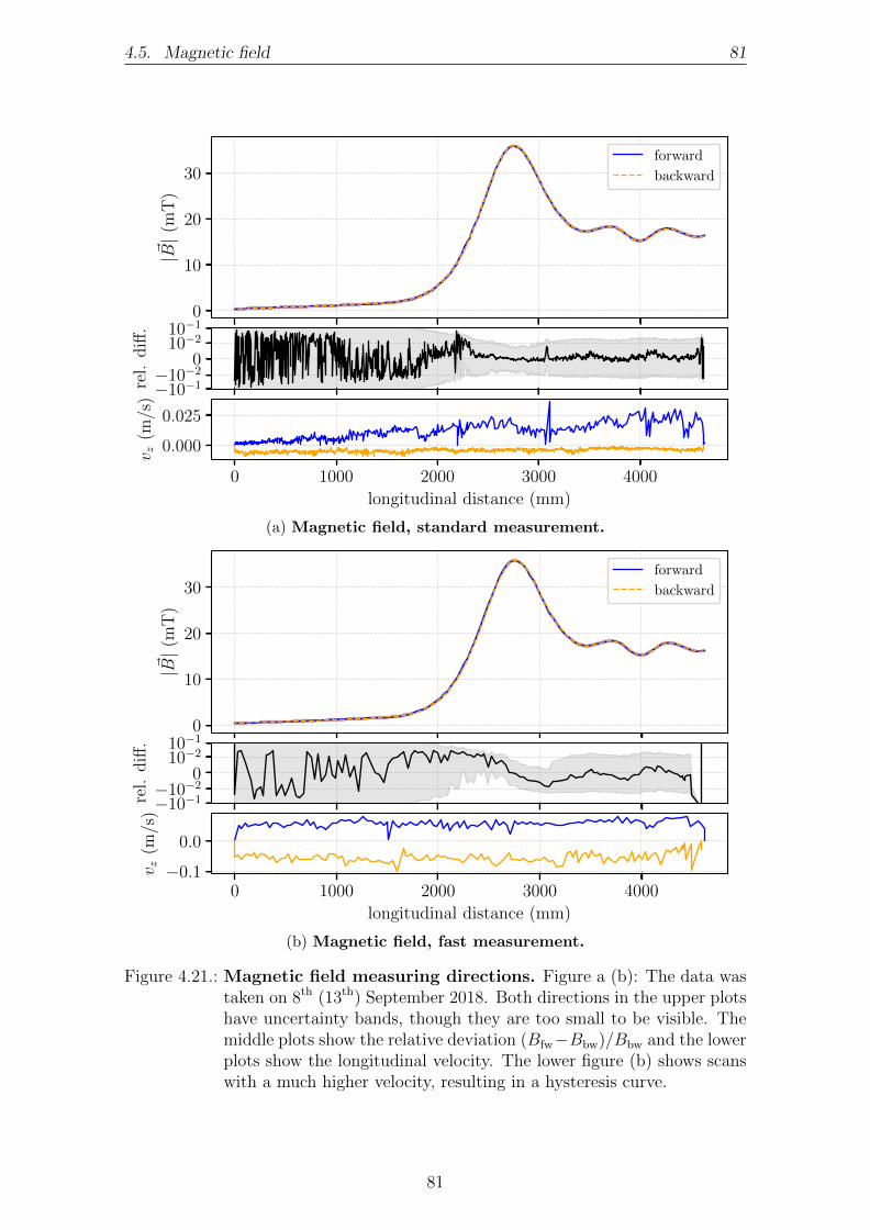
4.5. Magnetic field 81
0
10
20
30|~ B|(
mT
)forward
backward
−10−1−10−2
010−210−1
rel.
diff
.
0 1000 2000 3000 4000
longitudinal distance (mm)
0.000
0.025
v z(m
/s)
(a) Magnetic field, standard measurement.
0
10
20
30
|~ B|(
mT
)
forward
backward
−10−1−10−2
010−210−1
rel.
diff
.
0 1000 2000 3000 4000
longitudinal distance (mm)
−0.1
0.0
v z(m
/s)
(b) Magnetic field, fast measurement.
Figure 4.21.: Magnetic field measuring directions. Figure a (b): The data wastaken on 8th (13th) September 2018. Both directions in the upper plotshave uncertainty bands, though they are too small to be visible. Themiddle plots show the relative deviation (Bfw−Bbw)/Bbw and the lowerplots show the longitudinal velocity. The lower figure (b) shows scanswith a much higher velocity, resulting in a hysteresis curve.
81
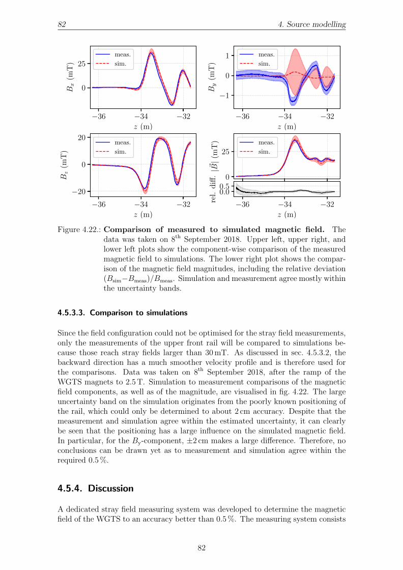
82 4. Source modelling
−36 −34 −32
z (m)
0
25Bx
(mT
)
meas.
sim.
−36 −34 −32
z (m)
−1
0
1
By
(mT
)
meas.
sim.
−36 −34 −32
z (m)
−20
0
20
Bz
(mT
)
meas.
sim.
0
25
|~ B|(
mT
) meas.
sim.
−36 −34 −32
z (m)
0.00.5
rel.
diff
.
Figure 4.22.: Comparison of measured to simulated magnetic field. Thedata was taken on 8th September 2018. Upper left, upper right, andlower left plots show the component-wise comparison of the measuredmagnetic field to simulations. The lower right plot shows the compar-ison of the magnetic field magnitudes, including the relative deviation(Bsim−Bmeas)/Bmeas. Simulation and measurement agree mostly withinthe uncertainty bands.
4.5.3.3. Comparison to simulations
Since the field configuration could not be optimised for the stray field measurements,only the measurements of the upper front rail will be compared to simulations be-cause those reach stray fields larger than 30 mT. As discussed in sec. 4.5.3.2, thebackward direction has a much smoother velocity profile and is therefore used forthe comparisons. Data was taken on 8th September 2018, after the ramp of theWGTS magnets to 2.5 T. Simulation to measurement comparisons of the magneticfield components, as well as of the magnitude, are visualised in fig. 4.22. The largeuncertainty band on the simulation originates from the poorly known positioning ofthe rail, which could only be determined to about 2 cm accuracy. Despite that themeasurement and simulation agree within the estimated uncertainty, it can clearlybe seen that the positioning has a large influence on the simulated magnetic field.In particular, for the By-component, ±2 cm makes a large difference. Therefore, noconclusions can be drawn yet as to measurement and simulation agree within therequired 0.5 %.
4.5.4. Discussion
A dedicated stray field measuring system was developed to determine the magneticfield of the WGTS to an accuracy better than 0.5 %. The measuring system consists
82
4.5. Magnetic field 83
of a three-axis Hall probe mounted onto a rail parallel to the WGTS cryostat axiswith a rope sensor to determine the longitudinal distance. Two different measuringmodes were developed for the readout, an all-manual mode with manual selection ofthe distances and a fixed time mode which automatically measures the magnetic fieldand position every t-th second. Both modes were found to produce the same resultsif the velocity of the moving Hall probe is below 0.01 m s−1. For larger velocities theresults between forward and backward scan show a hysteresis effect.
No conclusive argument could be found from comparison to simulations becausethe uncertainty on the positioning of the rail (not the longitudinal distance of theHall probe) is about 2 cm, which is one order of magnitude above the sub-mmrequirements found in sec. 4.5.2. However, the measuring system will remain inplace, allowing the sub-mm accurate determination of its positioning via combinedlaser tracker and FaroArm® [FAR18] measurements. Using this knowledge, the datacan either be re-analysed or new data will be acquired to get more conclusive insightsinto the magnetic field of the WGTS. Another improvement would be a steppermotor which guarantees smooth movement of the Hall probe in both directions fora more accurate determination of the stray field in the fixed time mode.
Concerning additional measurements, dedicated settings for the magnetic field shouldbe considered. An asymmetric setting with only one of the three WGTS current cir-cuits active (and no other field on e.g. DPS2-F or CPS) would allow determinationof the positioning of the coils inside the cryostat if the positioning of the rail isknown to sub-mm accuracy. The increase of the stray field caused by that asym-metric setting would furthermore decrease the uncertainty on the measurement inthe high-field region and also allow for reliable comparisons with simulations for theother two rails (upper rear and lower center).
The ultimate determination of the magnetic field inside the WGTS however canbe done via the angular-selective electron gun (e-gun) installed at the rear section.Using a well-characterised superconducting magnet such as the PCH magnet, thetransmission edge of the e-gun at an arbitrary pitch angle can be found by varyingthe magnetic field of the PCH until all e-gun electrons are magnetically reflected.Thereby, the pitch angle of the e-gun is calibrated against the magnetic field of thePCH and can then be used to calibrate the magnetic field of the WGTS in thesame way. The accuracy of this measurement is determined by the knowledge ofthe magnetic field of the PCH magnet (0.2 %11) since the angular resolution of thee-gun is constant for both measurements.
11This value is estimated from the 6.01 T NMR measurement by C. Schonfeld [Sch15] and the6.00 T simulated field using the measured current of 86.98 A.
83
84 4. Source modelling
4.6. Conclusion
An accurate modelling of the electron spectrum of tritium β-decay requires accurateknowledge of the processes in the windowless gaseous tritium source. One of themajor systematic effects arises from the description of the energy loss processes dueto inelastic electron-gas scattering. Closely linked to that is the modelling of the gasflow and the magnetic field in the source section.
In order to reach the required accuracy of the description of gas flow, the temperaturedistribution in the central source tube needs to be included in the gas model. Insec. 4.2, recent commissioning measurement data is used to derive a sensor based yetmodel motivated temperature profile of the beam tube. Towards the rear end, thehomogeneity criterion of the beam tube temperature can not be maintained becausethe temperature increase is about 0.5 K. Since the temperature profile is stable onthe per-mille level, this temperature increase can be accounted for in the modellingof the gas dynamics and does therefore not impact the neutrino mass sensitivity.
The comprehensive gas dynamics model developed over the course of several theses(notably, [Hot12, Kuc16] and the thesis at hand) is presented in sec. 4.3. In orderto describe the gas flow through the whole WGTS, several modelling techniquesneed to be applied and smoothly connected to provide the density distribution n(z)and thereby the column density N in the 16 m long beam tube. Furthermore, acalibration measurement by an angular selective, mono-energetic e-gun is discussedwhich is necessary to reach the required 0.2 % accuracy on the parameter of interestfor the scattering model, N · σ. With this calibration measurement it is possibleto keep the neutrino mass uncertainty related to the description of gas dynamicsat 3.06× 10⁻³ eV2, which is below the limit of a single systematic derived from theDesign Report [KAT05, Kuc+18].
In May and June 2018, the first spectra of electrons stemming from tritium β-decaywere recorded by the Katrin experiment. For the data analysis of that major com-missioning milestone, two dedicated gas models were derived. This was necessary,because the carrier gas for the trace amounts of tritium was deuterium and the abovementioned e-gun calibration measurements had not yet been carried out. Therefore,a calibration of the pressure controlled buffer vessel is used to estimate the injectionrate into the WGTS and therefrom recursively calculate the deuterium density pro-file. Calculations were restricted to the central 10 m long beam tube which contains99 % of the gas column. The dominant uncertainty for the phenomenological Knud-sen formula is the model related uncertainty while for the model derived from solvingthe Boltzmann equation the input parameter uncertainties are also significant. Asdeuterium has a smaller mass than tritium, the same throughput causes an about10 % lower column density. For most of the tritium spectrum scans, the deuteriumcolumn density is estimated to be about 4.5× 10²¹ m−2, with a total uncertainty of5(7) % for Boltzmann (Knudsen) based flow.A cross-check of the amount of gas in the injection region estimated by the dis-cussed gas models was performed by translating the pressure gauge measurementat the krypton capillary into an injection pressure. Agreement was found within3− 4 %, depending on the model. However, it has to be noted that the uncertaintyof this comparative calculation might well be of the order of 10 % when assumingthe same relative difference for tritium obtained by a DSMC [Bir94] simulation by
84

4.6. Conclusion 85
F. Sharipov [Sha10].
Besides the distribution of the gas inside the source, the magnetic field of the sourceis very important for modelling the electron-gas scattering as it determines the pathlength of the electrons through the gas. Since measurements inside the beam tubeare not possible, a stray field measurement system was designed, developed, andsuccessfully commissioned. Several readout configurations were tested in order tofind the most suitable compromise between speed and accuracy of the measurement.The approach by constantly moving a Hall probe along a rail is considered to bea good compromise, provided the driving speed is below 0.01 m s−1. Comparisonbetween simulation and measurement does not reveal a disagreement. However,the global position of the rails needs to be measured by means of laser trackeror FaroArm® [FAR18], which can be done after the current measurement phase.This accurate determination of the position will enable a conclusive comparison ofmeasurement and simulation.
Experimental verification of the overall source model requires the RS e-gun, whichis currently in its commissioning phase. Measurement strategies have been proposedon procedures to use the e-gun for an accurate determination of the column densityN and the magnetic field. With the comprehensive gas model and the magneticfield calibrated or verified by the e-gun, the source model is ready to be used in theanalysis of the upcoming neutrino mass data.
85


CHAPTER 5
ANALYSIS OF FIRST TRITIUM DATA
“In the fields of observation, chance favours only the prepared mind.”– Louis Pasteur, 1854 –
Katrin aims to determine the effective electron neutrino mass by analysis of the β-decay spectrum of tritium. On the road to neutrino mass data taking, several majormilestones were completed during the past two years. After the first transmission ofelectrons throughout the complete Katrin set-up in 2016 [Are+18b] and the suc-cessful spectroscopy of 83mKr-lines in 2017 [Are+18b, Are+18a], first tritium spectrawere recorded in spring 2018. This chapter will present results from these commis-sioning measurements with regard to experiment characterisation and comparisonsto the modelled tritium spectrum.
5.1. Experimental set-up
For the first detection of tritium β-decay electrons in the spring 2018 engineeringrun, the Katrin experiment used slightly different settings than will be used forthe neutrino mass data taking. Tritium was only present in the WGTS in traceamounts, with the main constituent of the gas being D2. The resulting tritiumpurity of about 0.5 % reduces the activity by about a factor of 200 compared tonominal neutrino mass operations with a tritium purity of εT > 95 %. Due to thedifferent gas content in the WGTS, a different gas dynamics model was developedand used for the estimation of the gas distribution in the source tube (comparesec. 4.4). Besides this difference, all major components of the set-up are in theirfinal configuration.
The (molecular) gas column density of the runs analysed in this chapter is estimatedfrom the gas model to be aboutN = 4.5× 10²¹ m−2, with the tritium column densityscaled by the tritium purity and accounting for the number of atoms in the gasmolecules. Due to the low concentrations of tritium, almost all tritium is present asDT.
87

88 5. Analysis of First Tritium data
Further important settings to be accounted for during analysis are the slightly in-homogeneous magnetic and electric fields in the analysing plane of the main spec-trometer, which is shown in fig. 5.1. It has to be noted that the measurements wereperformed with a factor three worse energy resolution than the designed 0.93 eV tomitigate the volume effect of the background rate [Har15, Tro18]. For a retardingenergy of 18 600 eV, the resulting width of the transmission function is
∆E = 0.63 mT4.2 T · 18 600 eV = 2.8 eV. (5.1)
6.288
6.29
6.292
6.294
6.296
6.298
6.3
6.302
6.304
6.306
01
2 3
45
678
910
11
12 1314
15
16
17
1819
20
2122
23
24 25
26
27
28
29
3031
32
3334
35
3637
38
39
40
41
4243
44
4546
47
48 49
50
51
52
53
54
55
56
57
58
59
60
61
62
63
64
65
6667
68
6970
71
72 73
74
75
76
77
78
79
80
81
82
83
84
85
86
87
88
89
9091
92
9394
95
96 97
98
99
100
101
102
103
104
105
106
107
108
109
110
111
112
113
114115
116
117
118
119
120 121
122123
124
125
126
127
128
129
130
131
132
133
134
135
136
137
138139
140
141
142
143
144 145
146
147
Bana (G)
16973.06
16973.08
16973.1
16973.12
16973.14
16973.16
16973.18
01
2 3
45
678
910
11
12 1314
15
16
17
1819
20
2122
23
24 25
26
27
28
29
3031
32
3334
35
3637
38
39
40
41
4243
44
4546
47
48 49
50
51
52
53
54
55
56
57
58
59
60
61
62
63
64
65
6667
68
6970
71
72 73
74
75
76
77
78
79
80
81
82
83
84
85
86
87
88
89
9091
92
9394
95
96 97
98
99
100
101
102
103
104
105
106
107
108
109
110
111
112
113
114115
116
117
118
119
120 121
122
123
124
125
126
127
128
129
130
131
132
133
134
135
136
137
138139
140
141
142
143
144 145
146
147
qU (eV)
Figure 5.1.: Analysing plane. The left side shows the magnetic field in theanalysing plane mapped onto the FPD. The right side shows the mappedretarding potential (using a low retarding energy of 16 975 eV as exam-ple).
The overall magnetic field setting of the Katrin experiment was at 70 % of its designvalue, so therefore the WGTS and FPD were at about 2.5 T instead of the designed3.6 T.
In order to account for the expected low statistics in the endpoint region due tothe low tritium concentrations, a measuring time distribution was chosen over awider energy interval than the 30 eV from the Design Report [KAT05]. With closerspaced and longer measuring time at points close to the endpoint and wider spacedand shorter measuring time at points far away from the endpoint, the resultingmeasuring time distribution (MTD) is shown in fig. 5.2. In the endpoint regionqU ∈ [18555, 18615] eV, the sub runs were spaced in 10 eV steps with 900 s per subrun. The least measuring time was spent in the high statistics region, for qU ∈[16975, 18175] eV each sub run was 100 s long.
As outlined in sec. 2.2.4, the calculation of the expected rate requires the usageof a response function [KAT05, Kle+18] which accounts for all effects the electronmay face on its way to the detector. Amongst those the most significant are thescattering off gas molecules in the source tube and the magnetic field and analysingpotential in the main spectrometer. For an example retarding energy of 16 975 eVof the example run 40667, the model based response function is shown in fig. 5.3.Note that the width of the transmission step and the height of the zero-scattering
88
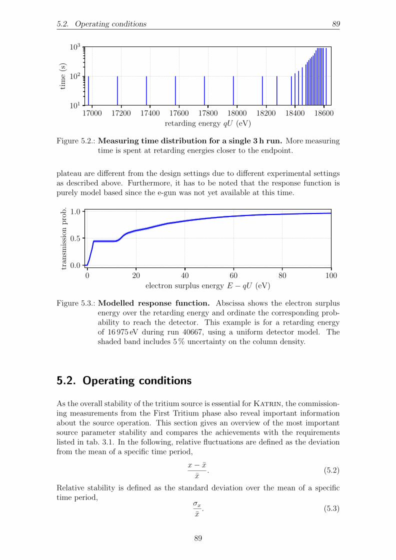
5.2. Operating conditions 89
17000 17200 17400 17600 17800 18000 18200 18400 18600
retarding energy qU (eV)
101
102
103
tim
e(s
)
Figure 5.2.: Measuring time distribution for a single 3 h run. More measuringtime is spent at retarding energies closer to the endpoint.
plateau are different from the design settings due to different experimental settingsas described above. Furthermore, it has to be noted that the response function ispurely model based since the e-gun was not yet available at this time.
0 20 40 60 80 100
electron surplus energy E − qU (eV)
0.0
0.5
1.0
tran
smis
sion
pro
b.
Figure 5.3.: Modelled response function. Abscissa shows the electron surplusenergy over the retarding energy and ordinate the corresponding prob-ability to reach the detector. This example is for a retarding energyof 16 975 eV during run 40667, using a uniform detector model. Theshaded band includes 5 % uncertainty on the column density.
5.2. Operating conditions
As the overall stability of the tritium source is essential for Katrin, the commission-ing measurements from the First Tritium phase also reveal important informationabout the source operation. This section gives an overview of the most importantsource parameter stability and compares the achievements with the requirementslisted in tab. 3.1. In the following, relative fluctuations are defined as the deviationfrom the mean of a specific time period,
x− xx
. (5.2)
Relative stability is defined as the standard deviation over the mean of a specifictime period,
σxx. (5.3)
89

90 5. Analysis of First Tritium data
An overview of the estimated run-averaged relative stabilities as well as the meanand standard deviation of the source parameters over all runs is given in tab. 5.1.Note that the requirements of the experimental conditions are mostly valid for onesingle run, which is why the stability will be evaluated run-wise.
5.2.1. Temperature stability
In order to characterise the achieved temperature stability of the WGTS beam tube,the sensor with the worst stability over the complete analysed time interval is takenas a conservative estimate. Even at a relative stability of 8.5× 10⁻⁵, the sensor200-RTP-3-5104 still surpasses the requirement for one run by almost two orders ofmagnitude, calculated for the time span of about four days. The relative fluctuationsas defined in eq. (5.2) are shown for the example run 40667 on the left side offig. 5.4, while the right side shows the histogram of the relative stabilities for allruns. Comparing to the requirement of 2× 10⁻³ relative stability per run in theDesign Report [KAT05], we can conclude that the average relative stability of (6.4±0.5)× 10−5 exceeds this requirement by almost two orders of magnitude.
21h 22h 23htime
−0.002
0.000
0.002
Tre
l.fl
uct
uat
ion
0.00005 0.00010 0.00015T rel. stab. per run
0
10
entr
ies
Figure 5.4.: Temperature stability. The left side shows the temperature fluc-tuations in run 40667 (7th June 2018), with the requirements as redhorizontal lines. The right side shows the histogram of the run-wiserelative stability values.
5.2.2. Gas circulation stability
As the temperature of the WGTS beam tube exceeds its stability requirements, thecolumn density stability is mainly determined through the stability of the injectionrate and the outlet pressure, both related to the inner loop system. The correspond-ing sensors measure the pressure controlled buffer vessel pb, the pressure in thekrypton capillary looking at the injection chamber pKr, and the outlet pressure pout
represented by the pressure at the TMPs of the pump ports (compare fig. 3.1). Asfor the temperature stability, the inner loop parameters also exceed the requirements(compare fig. 5.5):
� pb: achieved average relative stability per run of (9.8± 0.005)× 10−5, required2× 10−3 per run
90

5.2. Operating conditions 91
� pKr: achieved average relative stability per run of (3.2± 0.2)× 10−4, required2× 10−3 per run
� pout: achieved average relative stability per run of (1.7± 0.3)× 10−3 at PP1-Rand (2.0± 1.9)× 10−4 at PP1-F, required 6× 10⁻² per run
21h 22h 23htime
−0.002
0.000
0.002
p bre
l.fl
uct
uat
ion
0.000095 0.000100pb rel. stab. per run
0
5
entr
ies
21h 22h 23htime
−0.002
0.000
0.002
p Kr
rel.
flu
ctu
atio
n
0.0002 0.0004pKr rel. stab. per run
0
5
10en
trie
s
21h 22h 23htime
−0.05
0.00
0.05
p PP
1-R
rel.
flu
ctu
atio
n
0.000 0.002 0.004pPP1-R rel. stab. per run
0
5
10
entr
ies
21h 22h 23htime
−0.05
0.00
0.05
p PP
1-F
rel.
flu
ctu
atio
n
0.000 0.002 0.004pPP1-F rel. stab. per run
0
10
20
entr
ies
Figure 5.5.: Gas circulation stability. The left side shows the fluctuations in run40667 (7th June 2018), with the requirements as red horizontal lines.The right side shows the histogram of the run-wise relative stabilityvalues.
91

92 5. Analysis of First Tritium data
5.2.3. Tritium concentration stability
Due to the trace amounts of tritium used in the First Tritium campaign, the precisionper single LARA measurement (60 s) is not expected to be within the specificationsof 1× 10⁻³ as required for the nominal tritium purity εT > 0.95. The average relativestability per run determined from LARA data is found to be (4.48 ± 0.05) × 10−2,which exceeds 1× 10⁻³. However, it has to be noted that the design operationof the tritium source will have tritium as the main constituent of the source gas,which will enable LARA to monitor the tritium purity with a precision on the per-mille level. When using the stability of the (dominant) D2 concentration as anestimate for the stability of the tritium concentration, an average relative stabilityper run of (6.9 ± 0.1) × 10−4 is obtained, which would fulfil the 10−3 requirement(see fig. 5.6). Furthermore, the LARA group presented updated analysis results forthe isotopologue concentrations with about a factor of three improved uncertaintyon the DT concentration [KZ18]. Thus, also the precision on the tritium purity willimprove when using this re-analysed data.
20h 21h 22h 23htime
−0.002
0.000
0.002
c D2
rel.
flu
ctu
atio
n
0.0006 0.0007 0.0008cD2 rel. stab. per run
0.0
2.5
5.0
entr
ies
Figure 5.6.: LARA determined D2 concentration stability. The left side showsthe fluctuations in run 40667 (7th June 2018), with the requirements asred horizontal lines. The right side shows the histogram of the run-wiserelative stability values.
5.2.4. Magnetic field stability
As already demonstrated in [Are+18c], the magnetic field of the WGTS fulfils itsrequirements. This is also confirmed from the relative stability during the FirstTritium campaign, which is found to be (2.3 ± 0.6) × 10−6 averaged over all runs(required 2× 10⁻³).
5.3. Analysis of tritium β-decay spectra
After introducing the operating conditions of the experiment during the First Tri-tium campaign, this section will now cover inference of the parameters of interest(effective endpoint E0,eff, amplitude Amp and background rate Bg). The endpointis always referred to as effective, since the work function difference between mainspectrometer and source is not yet known.
92

5.3. Analysis of tritium β-decay spectra 93
21h 22h 23htime
−0.002
0.000
0.002
I WG
TS
rel.
flu
ctu
atio
n
0.000000 0.000005 0.000010IWGTS rel. stab. per run
0
10
20
entr
ies
Figure 5.7.: Magnetic field current stability. The left side shows the fluctuationsin run 40667 (7th June 2018), with the requirements as red horizontallines. The right side shows the histogram of the run-wise relative sta-bility values.
Table 5.1.: Source parameters overview. Note that the mean µ and standarddeviation σ are given for the whole data taking period analysed, whilethe relative stability per run is the run-averaged relative stability, whichneeds to fulfil the requirements stated in sec. 3.2.
parameter mean µ sigma σ rel. stab. per run requirement
T 30.076 K 2.5 mK (6.4± 0.5) 10−5 2× 10⁻³
pb 15.8 mbar 0.002 mbar (9.8± 0.05) 10−5 2× 10⁻³
pKr 12.8× 10⁻³ mbar 0.002× 10⁻³ mbar (3.2± 0.2) 10−4 2× 10⁻³
pout PP1-R 3.1× 10⁻⁵ mbar 1.7× 10⁻⁷ mbar (1.7± 0.3) 10−3 6× 10⁻²
pout PP1-R 3.1× 10⁻⁵ mbar 0.4× 10⁻⁷ mbar (2.0± 1.9) 10−4 6× 10⁻²
IWGTS 215.9 A 0.001 mA (2.3± 0.6) 10−6 2× 10⁻³
εT 0.56 % 0.03 % (4.48± 0.05) 10−2 1× 10⁻³
cD2 93.44 % 0.14 % (6.9± 0.1) 10−4 -
After introducing the analysis cuts used for this section, comparisons of model anddata from the Very First Tritium campaign will be shown in sec. 5.3.2. The pixeldistribution of the fit parameters will be shown in sec. 5.3.3 before investigating thefit parameter stability from the First Tritium campaign in sec. 5.3.4. One of themajor systematic uncertainties in the First Tritium set-up was the column densityN [Are+19], its impact on the analysis is discussed in sec. 5.3.5 in order to enablea more sound estimate of the fit parameters. It needs to be stressed here that thecolumn density is certainly not the only systematic uncertainty. For a completeestimate of the effective endpoint, other systematic effects also need to be taken intoaccount, however in this thesis the focus is on the column density and its uncertaintyas estimated in sec. 4.4.7.
93

94 5. Analysis of First Tritium data
5.3.1. Analysis cuts
Though the tritium spectrum was scanned over a wide energy range of about 1.6 keV,the focus of this thesis is on analysis of the last 400 eV. Notably, thefit modelis optimised for fitting in a narrow energy window around the endpoint (i.e. anenergy dependence of the inelastic scattering cross section is not taken into account).Moreover, the onset of electronic final states and the uncertainty of their excitationprobabilities will play a role for larger analysis windows deeper into the spectrum.Hence, stronger systematic effects are expected when fitting data from a wider energyrange. If not mentioned otherwise, the lower limit of the energy analysing windowis at E0−400 eV (that is including the data point taken at 18 175 eV). The last datapoint was taken at 18 615 eV.
Concerning the pixel related cuts, we have to account for an imperfect mapping ofthe geometrical source cross section onto the detector, as can be seen from fig. 5.8.Therefore the two outermost rings are excluded from the analysis, as well as the pixelsshadowed by the FBM which was in monitoring position throughout First Tritium.It needs to be stressed that when not using all pixels for the fit, amplitude andbackground are not scaled accordingly. That means that the estimated amplitudeand background are not valid for the whole detector but only for the analysed part.
The term uniform detector refers to using the detector as one single pixel with rateequal to the sum of all pixels, except for the removed pixels. This is the standardform of fitting used in the following. For pixel-wise fitting, the energy width of theanalysing window has to be doubled to 0.9 keV in order to get enough statistics fora reasonable estimate of the fit parameters.
0
100
200
300
400
500
600
cou
nt
rateN
(cp
s)
Figure 5.8.: High rate pixel distribution. Example run 40667, for a retardingenergy of qU = 16 975 eV.
5.3.1.1. Parameter inference
A central role in parameter inference is assigned to the likelihood function L. Itdefines the probability for an observation given a specific model. The Katrin like-
94

5.3. Analysis of tritium β-decay spectra 95
lihood function for a standard four parameter (m2ν, E0,eff, Amp, Bg) fit is given
as [Kle14]
L(m2ν, E0,eff, Amp,Bg|Nobs) =
∏i
p(Nobs,i|Ntheo,i(qUi,m2
ν, E0,eff, Amp,Bg)), (5.4)
with the retarding potentials qUi denoting the high voltage corresponding to theobserved events Nobs,i. The expected number of events Ntheo,i is calculated accord-ingly, depending on the neutrino mass squared m2
ν, the effective endpoint of thetritium spectrum1 E0,eff, the signal amplitude Amp, and the background rate Bg.p(Nobs,i|Ntheo,i) defines the probability for a single observation Nobs,i given an as-sumption Ntheo,i. The best-fit parameters are defined as maximising the likelihoodfunction L and are found by evaluating the likelihood function for various differentinput parameters. When analysing for the neutrino mass as parameter of interest,the so-called nuisance parameters effective endpoint, amplitude, and backgroundrate are of secondary interest. In general it is numerically more convenient to min-imise the negative log likelihood function − lnL instead of maximising the likelihoodfunction L:
− lnL = −∑i
ln p(Nobs,i|Ntheo,i(qUi,m2
ν, E0,eff, Amp,Bg)). (5.5)
In case the probability distribution p can be approximated by a Gaussian distribu-tion, the negative log likelihood function converges to a χ2 function2
−2 lnL =∑i
(Nobs,i −Ntheo,i(qUi,m2
ν, E0,eff, Amp,Bg)σi
)2
+ const.,
with the statistical uncertainty σi of an observation Nobs,i. Since in particular theβ-decay electrons obey Poisson statistics, a Poisson likelihood statistic χ2
λ,p is imple-mented [BC84] as
χ2λ,p = 2
∑i
Ntheo,i(qUi,m2ν, E0,eff, Amp,Bg)−Nobs,i
+Nobs,i · ln(
Nobs,i
Ntheo,i(qUi,m2ν, E0,eff, Amp,Bg)
). (5.6)
This statistic yields the same parameter and uncertainty estimates as the maximumlikelihood method [BC84, Kle14], and additionally enables goodness-of-fit estimationas it asymptotically obeys a χ2 distribution.
One way to include systematic uncertainties of the model into the fit procedureis introducing another fit parameter ξ for each systematic uncertainty ξ. Knowl-edge about the systematic uncertainty (for example from calibration measurementsor simulations) can be incorporated into the likelihood as a penalty term (pullmethod) [Kle14]
χ2(m2ν, E0,eff, Amp,Bg, ξ|Nobs) = χ2(m2
ν, E0,eff, Amp,Bg|Nobs) + ξ − ξ
σξ
2
, (5.7)
1Katrin will determine an effective endpoint, which amongst others is influenced by the workfunction difference between WGTS and main spectrometer.
2This is also valid for a Poisson distribution with expectation value µ ≤ 25.
95

96 5. Analysis of First Tritium data
with the estimated uncertainty σξ of the systematic effect ξ. This method will beused to include the uncertainty of the simulated column density into the uncertaintyof the best-fit effective endpoint (see sec. 5.3.5.2). Note that no neutrino massanalysis is performed on the First Tritium data, i.e. the neutrino mass is set to zeroin all fits. This leaves the effective endpoint as parameter of interest to test thedifferent analysis methods presented in the following.
5.3.2. Agreement between model and data
The very first injection of tritium into the WGTS (in the following referred to asVery First Tritium) was achieved through the controlled gas release from a totalnumber of four sample cylinders.
Very first tritium Instead of continuously supporting the inner loop with a con-stant amount of tritium via the feed loop (see fig. 3.1), this set-up used samplecylinders filled with tritium which were attached to the permeator. Via a handvalve, the cylinder was emptied and filled into the inner loop system. At somepoint, the valve regulating the flow between buffer vessel and pressure controlledbuffer vessel fully opened in order to keep the pressure stable. At this point, thebuffer vessel ran empty as did the activity injected into the source (see fig. 5.9).Therefore the activity during the Very First Tritium runs remained stable only overlimited periods of time, despite all other parameters such as source temperaturebeing within their specifications. The Very First Tritium spectra taken with thisset-up show very good agreement with the prediction by the model, as can be seenfrom fig. 5.10.
10:00 12:00 14:00 16:00
day time (H:M)
−0.2
−0.1
0.0
rel.
dev
.,(y−y 0
)/y 0
qpb
pKr
10:00 12:00 14:00 16:00
day time (H:M)
−0.5
0.0
0.5
rel.
dev
.,(y−y)/y
N
NcDT
A
Figure 5.9.: Decrease of activity. The reconstructed activity A (right) decreasesdue to gas circulation based on sample cylinders for the Very First Tri-tium set-up (left). Data from 19th May 2018.
5.3.3. Fit parameter pixel distribution
As the FPD measures the incoming electron flux with 148 pixels, each pixel mea-sures its own β-spectrum. Correcting for the radial and azimuthal dependence ofthe magnetic and electric field in the analysing plane (compare fig. 5.1), we can fiteach pixel separately. The resulting run-averaged distribution of the fit parameters
96

5.3. Analysis of tritium β-decay spectra 97
17000 17500 18000 18500
retarding energy qU (eV)
101
103
105
cou
nt
rateN
(cp
s)
model
data
102
105
N(c
ps)
fit
data
17000 17500 18000 18500
retarding energy qU (eV)
−202
res.
(σ)
Figure 5.10.: Model to data comparison. Data from an initial scan with tritiumdata, run 40263. Left: model with initial values only, no fit. Right:model with fit parameters E0,eff, Amp, and Bg. Data from 19th May2018.
is shown in fig. 5.11. In order to enable pixel-wise fitting per run, the energy windowwas increased to 0.9 keV below the endpoint. This appears justified, since here weare only interested in the relative pixel-based trend of the fit parameters instead oftheir absolute accuracy. From the segmented figure, we can see that the effectiveendpoint and amplitude parameters show no structure over the detector. However,the background rate has the same radial and azimuthal structure as found in previ-ous background investigations [Sch14, Har15]. From the centre to the outside, thebackground rate increases due to the volume effect of the main spectrometer [Sch14,Har15, Tro18]. The top-bottom asymmetry might be explained by a misalignmentbetween detector and main spectrometer [Blo18].
5.3.4. Fit parameter stability
As shown in sec. 5.2, the Katrin experiment was running with stable conditionsduring the First Tritium measurement phase with the design gas circulation. Datafrom the First Tritium campaign is used in this section to investigate the fit parame-ter stability. From fig. 5.12 it can be seen that this also holds for the fit parameters.Effective endpoint E0,eff, amplitude Amp, and background Bg vary within their sta-tistical uncertainty, with one outlier marked for the amplitude. The deviation isshown relative to the mean and the error bars reflect the statistical uncertainty only.The binned distribution of the minimised chi-squared, normalised to the number ofdegrees of freedom, is shown in fig. 5.13. Due to the small number of runs, the result-ing distribution is rather flat. An example correlation matrix for a three-parameterfit (E0,eff, Amp, Bg) can be found in the appendix in fig. B.3.
97
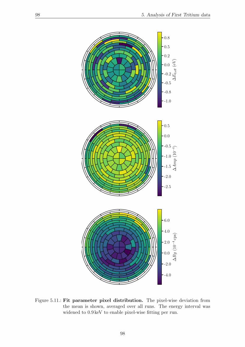
98 5. Analysis of First Tritium data
-1.0
-0.8
-0.5
-0.2
0.0
0.2
0.5
0.8
∆E
0,e
ff(e
V)
-2.5
-2.0
-1.5
-1.0
-0.5
0.0
0.5
∆Amp
(10−
4)
-4.0
-2.0
0.0
2.0
4.0
6.0
∆Bg
(10−
4cp
s)
Figure 5.11.: Fit parameter pixel distribution. The pixel-wise deviation fromthe mean is shown, averaged over all runs. The energy interval waswidened to 0.9 keV to enable pixel-wise fitting per run.
98
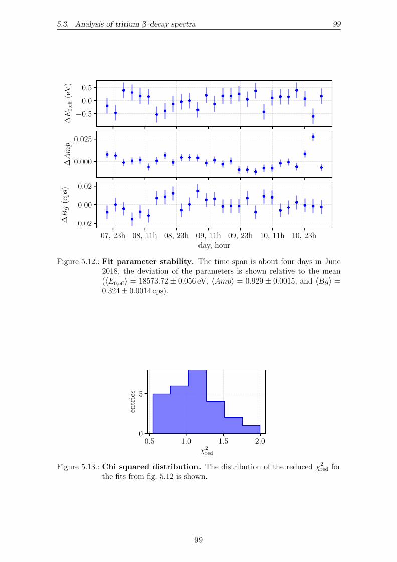
5.3. Analysis of tritium β-decay spectra 99
−0.5
0.0
0.5
∆E
0,e
ff(e
V)
0.000
0.025
∆Amp
07, 23h 08, 11h 08, 23h 09, 11h 09, 23h 10, 11h 10, 23hday, hour
−0.02
0.00
0.02
∆Bg
(cp
s)
Figure 5.12.: Fit parameter stability. The time span is about four days in June2018, the deviation of the parameters is shown relative to the mean(〈E0,eff〉 = 18573.72 ± 0.056 eV, 〈Amp〉 = 0.929 ± 0.0015, and 〈Bg〉 =0.324± 0.0014 cps).
0.5 1.0 1.5 2.0χ2
red
0
5
entr
ies
Figure 5.13.: Chi squared distribution. The distribution of the reduced χ2red for
the fits from fig. 5.12 is shown.
99
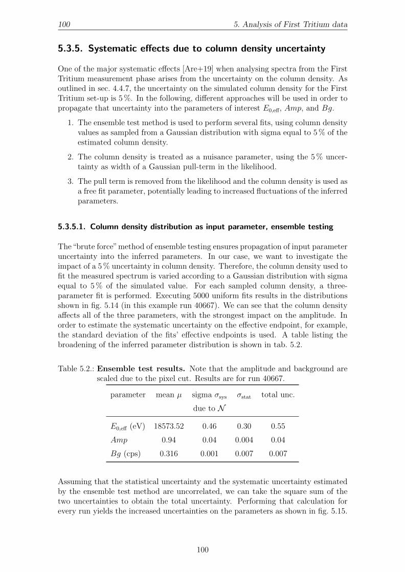
100 5. Analysis of First Tritium data
5.3.5. Systematic effects due to column density uncertainty
One of the major systematic effects [Are+19] when analysing spectra from the FirstTritium measurement phase arises from the uncertainty on the column density. Asoutlined in sec. 4.4.7, the uncertainty on the simulated column density for the FirstTritium set-up is 5 %. In the following, different approaches will be used in order topropagate that uncertainty into the parameters of interest E0,eff, Amp, and Bg.
1. The ensemble test method is used to perform several fits, using column densityvalues as sampled from a Gaussian distribution with sigma equal to 5 % of theestimated column density.
2. The column density is treated as a nuisance parameter, using the 5 % uncer-tainty as width of a Gaussian pull-term in the likelihood.
3. The pull term is removed from the likelihood and the column density is used asa free fit parameter, potentially leading to increased fluctuations of the inferredparameters.
5.3.5.1. Column density distribution as input parameter, ensemble testing
The“brute force”method of ensemble testing ensures propagation of input parameteruncertainty into the inferred parameters. In our case, we want to investigate theimpact of a 5 % uncertainty in column density. Therefore, the column density used tofit the measured spectrum is varied according to a Gaussian distribution with sigmaequal to 5 % of the simulated value. For each sampled column density, a three-parameter fit is performed. Executing 5000 uniform fits results in the distributionsshown in fig. 5.14 (in this example run 40667). We can see that the column densityaffects all of the three parameters, with the strongest impact on the amplitude. Inorder to estimate the systematic uncertainty on the effective endpoint, for example,the standard deviation of the fits’ effective endpoints is used. A table listing thebroadening of the inferred parameter distribution is shown in tab. 5.2.
Table 5.2.: Ensemble test results. Note that the amplitude and background arescaled due to the pixel cut. Results are for run 40667.
parameter mean µ sigma σsys σstat total unc.
due to N
E0,eff (eV) 18573.52 0.46 0.30 0.55
Amp 0.94 0.04 0.004 0.04
Bg (cps) 0.316 0.001 0.007 0.007
Assuming that the statistical uncertainty and the systematic uncertainty estimatedby the ensemble test method are uncorrelated, we can take the square sum of thetwo uncertainties to obtain the total uncertainty. Performing that calculation forevery run yields the increased uncertainties on the parameters as shown in fig. 5.15.
100

5.3. Analysis of tritium β-decay spectra 101
−1
0
1
∆E
0,e
ff(e
V)
−0.1
0.0
0.1
∆Amp
−0.5 0.0 0.5
∆N (1021 m−2)
−0.02
0.00
0.02
∆Bg
(10−
1cp
s)
−1 0 1∆E0,eff (eV)
−0.1 0.0 0.1∆Amp
Figure 5.14.: Parameter distribution from ensemble test. 5000 fits were per-formed for run 40667 with fit parameters E0,eff, Amp, and Bg.
5.3.5.2. Column density as constrained parameter
In addition to the powerful but costly ensemble test method, we can also use the pullmethod (see sec. 5.3.1.1) to introduce the column density as an additional parameterto the fit model. For the fitting, we use the knowledge we have about that param-eter, which is its central value and its uncertainty estimated from simulations (seesec. 4.4.7). The additional degree of freedom broadens the likelihood and thereforeincreases the uncertainty on the estimated parameters of interest. The results areshown for the run 40667 in tab. 5.3. Using the pull method for all runs leads tothe run-wise variation of the fit parameters as shown in fig. 5.16. Most significantly,the outlier in the statistical only evolution of the amplitude in fig. 5.12 disappeared.Furthermore, the estimated uncertainties and inferred parameters are compatiblewith the estimates of the ensemble test method.
101
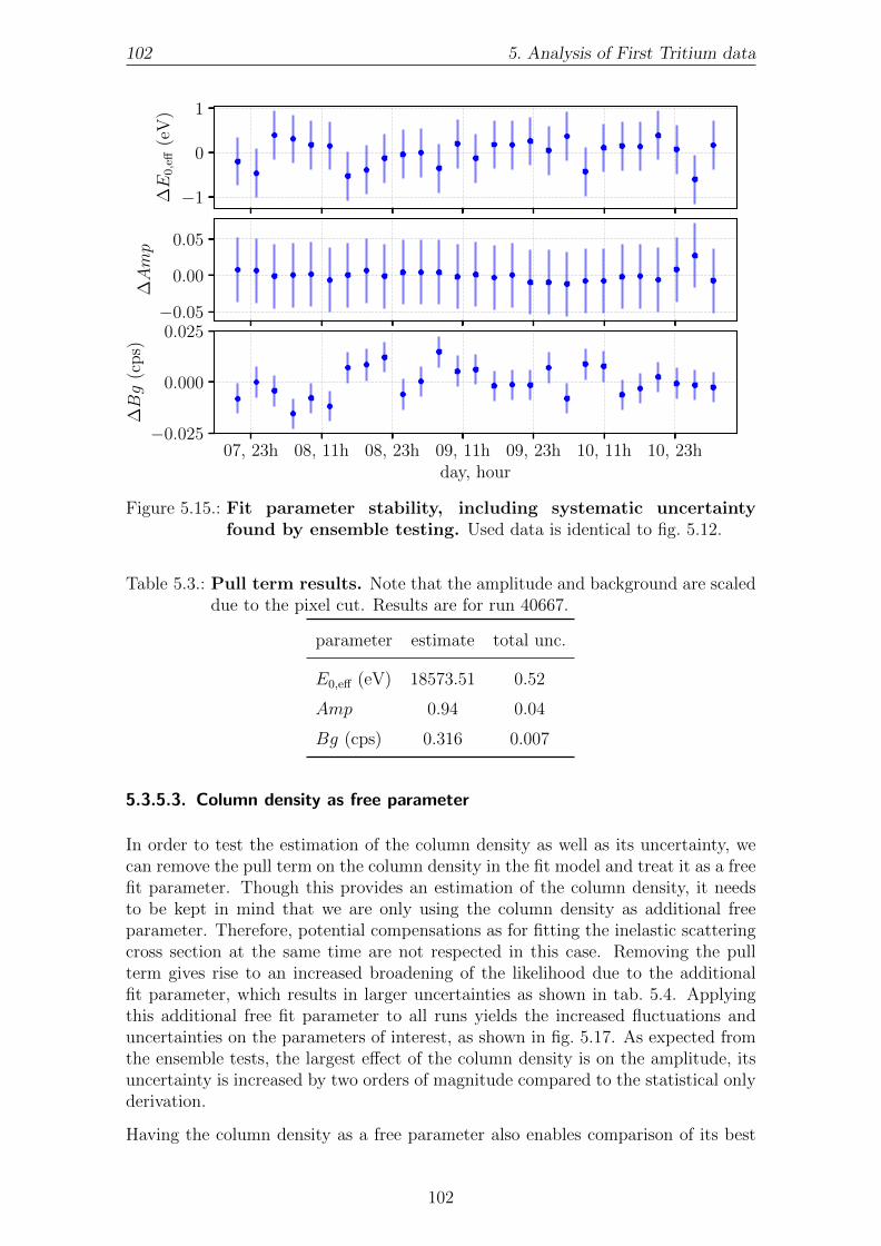
102 5. Analysis of First Tritium data
−1
0
1
∆E
0,e
ff(e
V)
−0.05
0.00
0.05
∆Amp
07, 23h 08, 11h 08, 23h 09, 11h 09, 23h 10, 11h 10, 23hday, hour
−0.025
0.000
0.025
∆Bg
(cp
s)
Figure 5.15.: Fit parameter stability, including systematic uncertaintyfound by ensemble testing. Used data is identical to fig. 5.12.
Table 5.3.: Pull term results. Note that the amplitude and background are scaleddue to the pixel cut. Results are for run 40667.
parameter estimate total unc.
E0,eff (eV) 18573.51 0.52
Amp 0.94 0.04
Bg (cps) 0.316 0.007
5.3.5.3. Column density as free parameter
In order to test the estimation of the column density as well as its uncertainty, wecan remove the pull term on the column density in the fit model and treat it as a freefit parameter. Though this provides an estimation of the column density, it needsto be kept in mind that we are only using the column density as additional freeparameter. Therefore, potential compensations as for fitting the inelastic scatteringcross section at the same time are not respected in this case. Removing the pullterm gives rise to an increased broadening of the likelihood due to the additionalfit parameter, which results in larger uncertainties as shown in tab. 5.4. Applyingthis additional free fit parameter to all runs yields the increased fluctuations anduncertainties on the parameters of interest, as shown in fig. 5.17. As expected fromthe ensemble tests, the largest effect of the column density is on the amplitude, itsuncertainty is increased by two orders of magnitude compared to the statistical onlyderivation.
Having the column density as a free parameter also enables comparison of its best
102

5.3. Analysis of tritium β-decay spectra 103
−1
0
1
∆E
0,e
ff(e
V)
−0.05
0.00
0.05
∆Amp
−0.025
0.000
0.025
∆Bg
(cp
s)
07, 23h 08, 11h 08, 23h 09, 11h 09, 23h 10, 11h 10, 23hday, hour
−0.25
0.00
0.25
∆N
(102
1m−
2)
Figure 5.16.: Fit parameter stability, including systematic uncertaintyfound by pull method. The data used is identical to fig. 5.12.
fit value to other column density estimates. For example for run 40667, the best fitis at 4.41× 10²¹ m−2 and the uncertainty found by profiling the likelihood functionis 0.59× 10²¹ m−2, which is a relative uncertainty of 13 %. Furthermore, for thisexample run the fitted and the estimated (4.46× 10²¹ m−2) column density agreevery well.
5.3.6. Appended runs
In contrast to averaging the fit results of each run which is fit separately, this anal-ysis method appends all the runs and fits them together. This results in multipledata points for one retarding energy. In order to have a reasonable estimate of theexperiment’s condition over this longer time period, the mean value of each sensoris used, justified by the stable conditions of the Katrin experiment (see sec. 5.2).Appending the runs and including the column density as systematic uncertainty viathe above mentioned pull-method results in
Emulti,pull0,eff = 18574.34± 0.22 eV, (5.8)
while the free column density result gives
Emulti,free0,eff = 18574.40± 0.24 eV. (5.9)
103

104 5. Analysis of First Tritium data
Table 5.4.: Free fit parameter results. Note that the amplitude and backgroundare scaled due to the pixel cut. Results are for run 40667.
parameter estimate total unc.
E0,eff (eV) 18573.43 1.23
Amp 0.95 0.13
Bg (cps) 0.316 0.008
N (1021 m−2) 4.41 0.59
−2.5
0.0
2.5
∆E
0,e
ff(e
V)
−0.25
0.00
0.25
∆Amp
−0.025
0.000
0.025
∆Bg
(cp
s)
07, 23h 08, 11h 08, 23h 09, 11h 09, 23h 10, 11h 10, 23hday, hour
−1
0
1
∆N
(102
1m−
2)
Figure 5.17.: Fit parameter stability, including systematic uncertaintyfound by free parameter. The data used is identical to fig. 5.12.
Note that the quoted values do not include a sizeable systematic uncertainty due towork function effects for example. In order to access the absolute endpoint, thoseneed to be considered. The free column density estimate with this method is
Nmulti,free = (4.6± 0.12)× 1021 m−2, (5.10)
with statistical uncertainty only.
104
5.3. Analysis of tritium β-decay spectra 105
5.3.7. Overview of the effective endpoint estimates
This section summarises the different estimates of the effective endpoint displayedin fig. 5.18.
For comparison, the expected value of the effective endpoint estimated from T-3Heatomic mass difference measurements is shown. Following the discussion of Ottenand Weinheimer [OW08], the mass difference needs to be“[...] corrected for the differ-ence in the electronic binding energy ∆EB between the atomic mother/daughter pairand the actual mother/daughter systems of the experiment [...]”[OW08]. With the T-3He atomic mass difference ∆M(3He,T) = 18592.01±0.07 eV as determined by My-ers et al. [Mye+15], the electronic binding energy difference ∆EB = 16.3 eV [Sou86,OW08], the T2 recoil energy Erec = 1.7 eV (see sec. 2.2.2), and the work functiondifference ∆φ = 0.3± 0.5 eV [Sle17] between main spectrometer and tritium source,the expected effective endpoint is estimated to
E0,eff = ∆M(3He,T)−∆EB − Erec −∆φ (5.11)
= 18 592.0 eV− 16.3 eV− 1.7 eV− 0.3 eV = 18 573.7 eV. (5.12)
In order to fit one common endpoint, the energies of the modelled final states dis-tributions of the different hydrogen isotopologues are shifted such that the commonmodelled endpoint (used to fit) is the one of T2 [Dos07]. Therefore, the T2 values of∆EB and Erec are used to calculate the expected effective endpoint though the mostabundant tritium gas species during First Tritium was DT.The main uncertainty of the expected effective endpoint is due to the uncertaintyof the work function difference ∆φ. In the preliminary analysis of gaseous 83mKrmeasurements by M. Slezak, the 0.5 eV uncertainty on the work function differenceis dominated by the uncertainty of the gamma-ray energy [Sle17]. An additionaluncertainty has to be added when using work function analysis results from gaseous83mKr measurements for the analysis of tritium measurements, as the two measure-ments use different gas temperatures (about 100 K for 83mKr mode, but 30 K fortritium mode) and different gas species3. This difference in set-up could be expectedto affect the work function of the source beam tube differently, through adsorption.In order to account for this extra uncertainty, the Katrin effective endpoint isconservatively estimated to be within a 1 eV interval around 18 573.7 eV [WVH].
Figure 5.18 shows that all effective endpoint estimates presented in this thesis lieinside this interval. The estimates labelled“mean”denote the mean over all runs andthe uncertainty is the error of the mean. For comparison, the single run estimateof run 40667 is also shown. The estimates labelled “multi” are obtained from fittingall runs together as described in sec. 5.3.6. The inclusion of the column densityas a systematic effect results in larger estimates of the effective endpoint, whichunderlines the importance of treating systematic effects.
Furthermore, it has to be stressed that the estimates shown in fig. 5.18 only includethe column density as a systematic effect. Further systematic uncertainties arisefrom the 2 % uncertainty on the inelastic scattering cross section, the absolute value
3Additionally, there was a short venting of the WGTS beam tube, exposing the beam tube surfaceto laboratory air in July 2017 [Jan17]. This eventual change in surface conditions translates toan uncertainty on the work function difference development between the 83mKr and the FirstTritium campaign.
105

106 5. Analysis of First Tritium data
of the magnetic fields, and the tritium purity, to name only a few. This section onlygives the effects related to the column density, detailed investigations for the otherinput parameters are also required in order to get the complete picture.
2.5 3.0 3.5 4.0 4.5E0,eff (eV) +1.857×10⁴
40667 stat only
40667 sys ensemble
40667 sys constraint
40667 sys free
mean stat only
mean stat + ensemble
mean sys constraint
mean sys free
multi stat only
multi sys constraint
multi sys free
PRELIMINARY
Figure 5.18.: Overview of the effective endpoint estimates. The black lineshows the expected value as determined from the T-3He mass differenceand the relevant binding energies. The grey band represents a 1 eV es-timated uncertainty range of the expected Katrin effective endpoint.An important role therein is attributed to the uncertainty of the workfunction difference between main spectrometer and WGTS beam tube.Note that the only systematic uncertainty for which the impact onthe endpoint measurement is investigated here in detail is the columndensity.
5.3.8. Systematic effects due to slicing the WGTS
In the fits presented so far, an average column density was assumed along the WGTSbeam tube to calculate average scattering probabilities [Kuc+18, Kle+18]. If we nowwant to respect the longitudinal density profile and also include the small magneticfield inhomogeneities in the central source tube due to the gaps existing between the3 m long coils (compare fig. 4.17), we have to divide the 10 m long beam tube intolateral slices. Each slice is calculated to contain the same magnetic flux mappedfrom the detector, so the radius of a slice close to a pump port is larger than inthe centre due to the lower magnetic field. S. Groh investigated the effect of theslicing on the neutrino mass [Gro15] and recommended a number of 200 slices.However, as each slice has its own β-spectrum and response function accountingfor the integrated density in front of that particular slice, fitting with slicing is very
106

5.3. Analysis of tritium β-decay spectra 107
costly in computation time. For the First Tritium settings, the effect of the numberof slices is investigated using the effective endpoint, and results are shown in fig. 5.19.We can see that the change in effective endpoint estimate levels off for increasingnumber of slices, as expected. The more slices, the better the sliced density profilefollows the unbinned density profile. For the low statistics of the First Tritium datathe slicing does not appear to have a strong effect compared to the final set-up. Ifusing a sliced WGTS for fitting, it is recommended to use at least 50 slices. A largernumber of slices does not significantly affect the estimation of the effective endpoint,but is very costly in computation time.
0 25 50 75 100 125 150 175 200number of WGTS slices
0.0
0.1
0.2
0.3
∆E
0,e
ff(e
V)
Figure 5.19.: Effect of WGTS slicing. The shift of the effective endpoint relativeto the 200 slices estimate is shown, averaged over all runs.
5.3.9. Test of the scattering implementation
Close to the endpoint of the tritium spectrum, the signal rate S = N − Bg isproportional to the zero-scattering probability P0 and the number of tritium atomsseen by the detector, represented by the column density N times the tritium purityεT:
S ∝ P0 · εT · N . (5.13)
Assuming a constant tritium purity, the signal ratio of two different column densitiescan be used to investigate the scattering implementation in the spectrum model.Scaling the signal ratio with the inverse of the column density ratio yields the ratioof the zero-scattering probabilities at e.g. 10 eV below the endpoint:
P0
P00
= S
S0· N0
N, (5.14)
107

108 5. Analysis of First Tritium data
with the index 0 indicating the reference measurement. Due to the low statistics inthe endpoint region, the uncertainties will be large even without including system-atic uncertainties on e.g. the column densities. In fig. 5.20, the ratio of the signalrates scaled with the column density ratio is displayed for two column densitiesN = 1.09× 10²¹ m−2 and N0 = 4.46× 10²¹ m−2. The corresponding zero-scatteringprobability ratio is 1.8, shown as the black line in the endpoint region. It can be seenthat indeed, the statistical uncertainties are sizeable – and within these uncertaintiesthe model matches the data. No conclusions on the zero-scattering probabilities canbe drawn as the statistical uncertainties are already too large.
The scattering investigations will be simplified and much more detailed once thee-gun of the rear section starts operating. As mentioned in sec. 4.3.4, it will be usedto accurately determine the product of column density and inelastic scattering crosssection, which in turn enables determining the zero-scattering probability.
18200 18250 18300 18350 18400 18450 18500 18550
retarding energy qU (eV)
1.00
1.25
1.50
1.75
2.00
2.25
2.50
2.75
3.00
S S0·N
0 N
P0/P00
model
data
Figure 5.20.: Test of scattering implementation. The signal ratio of the N =1.09× 10²¹ m−2 column density runs and theN0 = 4.46× 10²¹ m−2 col-umn density runs, scaled by the respective column densities, statisticaluncertainty only, is shown. The red line is using the fit result fromthe spectra and the black line illustrates the expected zero scatteringprobability ratio.
108

5.4. Estimation of the column density via additional detectors 109
5.4. Estimation of the column density via additionaldetectors
This section presents ways to estimate and cross-check the column density simula-tions by using data from the active commissioning of Katrin. The data availableduring First Tritium stems from the Forward Beam Monitor (FBM), the PULCINELLAdisk in front of the Focal Plane Detector (FPD) and from the FPD itself. Each of themethods faces different challenges, which will be addressed in detail in this section.
5.4.1. Estimation of the column density via the FBM
In order to compare the simulated value of the column density to measured data,one possibility is using the FBM. Comparing its integrated rate NFBM (above someenergy threshold Eth) to the theoretical decay rate Ntheo (also integrated from Eth)yields information about the number of active gas atoms and thereby about thecolumn density. The rate is proportional to the activity in the source, which itselfdepends on the number of tritium atoms:
NFBM
∣∣∣E≥Eth
= Ntheo
∣∣∣E≥Eth
· εdet · nT · a(θmax), (5.15)
with the FBM detection efficiency εdet, the number of tritium atoms mapped onto theFBM nT and the maximum acceptance angle θmax defining the fraction of electronsthat can arrive at the FBM, a(θmax). The column density enters through the numberof tritium atoms (see sec. 5.4.1.2), enabling estimation of the column density froma rearranged form of eq. (5.15) as
N =NFBM
∣∣∣E≥Eth
Ntheo
∣∣∣E≥Eth
· εdet · cDT · AWGTS · (1− cos θmax) · 0.5. (5.16)
In the following, the factors of eq. (5.15) (or eq. (5.16) equivalently) will be discussedindividually.
An overview of the runs used is given in tab. 5.5. All runs were taken in June 2018.
Table 5.5.: FBM run overview.
run purpose duration
145-147 100 % N 2:14 h
247 FBM background 1 h272-274 50 % N 3 h278-280 25 % N 3 h331-333 75 % N 3 h
109

110 5. Analysis of First Tritium data
5.4.1.1. Maximum acceptance angle
In contrast to the usual θmax being defined by the relation between source and PCHmagnetic field, at the location of the FBM θmax is defined by the relation betweensource BS = 2.5 T and CPS magnetic field BCPS since the maximum magnetic fieldbetween WGTS and the FBM is BCPS = 4 T:
θmax = arcsin√
BS
BCPS
= 52.5°. (5.17)
The maximum acceptance angle defines the fraction of electrons arriving at theFBM:
a (θmax) =
θmax∫0
sin θ dθ
π∫0
sin θ dθ= 1− cos θmax
2 . (5.18)
The uncertainty on the maximum acceptance angle is determined by the uncertaintyon the magnetic fields. In sec. 5.2.4 it was shown that the relative stability of themagnetic fields is better than 1× 10⁻⁵, leaving the systematic uncertainty of 1 % asdominant uncertainty of the magnetic fields.
5.4.1.2. Number of tritium atoms
The number of tritium atoms in the cross-section A in the WGTS can be estimatedvia
nT = 2 · N · A · εT, (5.19)
with N being the total column density and εT ≈ 0.56% the tritium purity. Due tothe low tritium concentration in the First Tritium campaign of Katrin, almost allof the tritium occurs in form of DT. Therefore, the number of tritium atoms canalso be estimated via
nT = N · A · cDT, (5.20)
with cDT ≈ 1.04 % being the DT concentration in the gas inside WGTS. During the1 h time scale of a FBM run, the fluctuation of the DT concentration was 0.02 %. Forthe systematic uncertainty of the DT concentration in First Tritium data, LARAgives an absolute number of about 0.16 %. Re-analysed LARA data yields a factorthree improved uncertainty on the estimated DT concentration [KZ18]. To ensureconsistency with the spectral analysis results presented in this chapter, it was decidedto not use this updated LARA data for the column density estimation.
5.4.1.3. Fluxtube mapping
In order to compare the predicted to the measured FBM rate, the effective WGTScross-section and therefore the flux tube seen by the each of the two FBM diodesneeds to be determined. The magnetic field at the position of the FBM diodes isBFBM = 0.8 T, while the source is at BS = 2.5 T. This means that the FBM sees
110

5.4. Estimation of the column density via additional detectors 111
fewer electrons as if it was located at BS. The result is a lower effective detectionarea of the FBM diodes, estimated from conservation of the magnetic flux φ:
φFBM = φWGTS → AWGTS1,2 = AFBM ·BFBM
BWGTS
= 1.35 mm2 ·BFBM1,2/BS, (5.21)
with BFBM1,2 the magnetic field at the position of diode 1 and 2, (BFBM1 , BFBM2) =(0.8191, 0.8197) T and the photosensitive area of AFBM = 1.35± 0.05 mm2 [Hau18].Using BS = 2.5 T results in (AWGTS1 , AWGTS2) = (0.44, 0.44) mm2.
Though the Hall sensor of the FBM board can determine the magnetic field ofthe FBM, it is positioned a small distance away from the two diodes on the FBMboard (compare fig. 2.4). Including an offset of the whole FBM detector board of(x, y) = (0.26, 2.7) mm [Ell18], the author found a z component of the magnetic fieldat the position of the Hall probe from Kassiopeia simulations of −0.8029±0.0005 T.The Hall probe measured a magnetic field of −0.7973 T, which yields a difference tothe simulation corresponding to 0.7 %. Together with the 1 % general uncertainty onmagnetic fields, this amounts to a systematic uncertainty of 1.2 % on the magneticfield at the position of the diodes. The magnetic field of the WGTS has the 1 %systematic uncertainty estimated for the First Tritium settings [Are+19]. The un-certainty on the effective WGTS cross-section is then determined via bootstrapping,considering the uncertainties on the individual factors of eq. (5.21).
5.4.1.4. FBM rate prediction
Since the FBM diodes are of Si-pin type, the FBM has some intrinsic energy reso-lution ∆EFWHM = 2.4 keV. The theoretical β-spectrum needs to be convolved withthe detector resolution function in order to estimate the column density. The ef-fect of the FBM energy resolution is shown in fig. 5.21: as expected, it smears thetheoretical spectrum to both sides, at lower and higher energies. The FBM rate
0 5 10 15 20
energy (keV)
0
1
dΓ/dE
(eV−
1s−
1) ×10−13
decay rate
FBM response
5 10 15Eth (keV)
0.00
0.25
0.50
ε det
Figure 5.21.: FBM rate prediction. Left: we see the smearing towards lower andhigher energies caused by the intrinsic FBM energy resolution. Right:the energy threshold dependent detection efficiency is shown. Datakindly provided by N. Haußmann [Hau18].
per tritium atom is estimated as the sum over all final states, convolved with thedetector resolution G(E, ε):
Ntheo
∣∣∣E≥Eth
=∞∫
Eth
∞∫−∞
G(E − ε) ·∑fs
Pfs ·dΓ(ε)dE
∣∣∣∣∣fs
dε dE (5.22)
111

112 5. Analysis of First Tritium data
Besides the energy resolution of the FBM, there are various other effects to be takeninto account. One of them is the backscattering of electrons off the surface of theFBM, causing a reduction of the estimated rate. Since the FBM diodes are of Si-pintype [HAM18], they have a non-zero dead layer. If electrons deposit energy in thisregion, the deposited energy cannot be detected by the FBM. Such dead layer effectswere investigated by N. Haußmann [Hau18] and E. Ellinger [Ell18] via measurementsand KESS4 simulations. Using dead layer measurements by E. Ellinger [Ell18], N.Haußmann finds energy threshold dependent upper and lower limits for the FBMdetection efficiency εdet. The results for εdet are shown in fig. 5.21 and yield for thethreshold energy Eth = 5 keV used in
εdet = 0.49 +0.07−0.06. (5.23)
In fig. 5.21, the uncertainty band represents the dead layer thickness estimate of350± 50 nm with lower dead layer thickness resulting in higher detection efficiency.The estimation of the detection efficiency also includes backscattering onto the FBMdue to the magnetic mirror effect.
5.4.1.5. FBM rate estimation
The measured rate at the FBM is estimated via integration of the measured spectrumabove some threshold Eth. Since the energy estimation of the FBM for electrons withenergies below 5 keV is not reliable, we set Eth = 5 keV. Also note that the cut wasdone on the ADC equivalent (166) instead of the calibrated energy (5 keV).
The applied calibration is of the form
E = 31.747 eV/channel · ADC− 241.357 eV channel 1 (5.24)
E = 31.892 eV/channel · ADC− 262.987 eV channel 2 (5.25)
The rate estimation is then the integration of the ADC spectrum from 166 ADC (theinterested reader can find the spectrum plots in app. B.1); the time dependence isshown in fig. 5.22 for a sampling time of 60 s. A horizontal line is fit in fig. 5.22
06:43 06:57 07:12 07:26 07:40
time (hour:min)
2
3
rate
(cp
s)
channel 1
channel 2
14:24 15:00 15:36 16:12
time (hour:min)
1850
1900
rate
(cp
s)
channel 1
channel 2
Figure 5.22.: FBM estimated rate. Left side: background run 247 (11th June2018). Right side: signal runs 145-147 (6th June 2018).
which enables estimation of the rate in a specific time interval. In order to estimate
4Katrin Electron Scattering in Silicon Simulation (KESS) package developed by P. Ren-schler [Ren11].
112

5.4. Estimation of the column density via additional detectors 113
the signal rate, the background rate needs to be subtracted. The signal rates weredetermined from runs 145-147, while run 247 was taken as background run when theFBM was outside the active flux tube (compare tab. 5.6). The systematic uncertainty
Table 5.6.: FBM fitted rate.
quantity fit value fit uncertainty
NFBM,tot,1
∣∣∣E≥Eth
(cps) 1849.2 0.5
NFBM,tot,2
∣∣∣E≥Eth
(cps) 1875.2 0.5
NFBM,bg,1
∣∣∣E≥Eth
(cps) 2.2 0.03
NFBM,bg,2
∣∣∣E≥Eth
(cps) 1.8 0.02
NFBM,sig,1
∣∣∣E≥Eth
(cps) 1847.0 0.5
NFBM,sig,2
∣∣∣E≥Eth
(cps) 1873.3 0.5
assigned to the two rates is estimated as the distance to the mean, resulting inσNFBM,sys
= 13.0 cps.
5.4.1.6. Uncertainty estimation
The uncertainties of the factors of eq. (5.16) are propagated to an uncertainty onthe estimated column density via ensemble testing. A summary of the uncertaintiesis given in tab. 5.7; note that the systematic uncertainties are given in relativepercentage values. In order to estimate the column density uncertainty, each item oftab. 5.7 is sampled from a Gaussian distribution centred at the estimated value withσ being the estimated uncertainty. With a number of 105 samples, the statisticaland systematic distribution of the column density can be estimated with a precisionof 0.3 %, yielding the statistical and systematic uncertainty of the column densityestimate via the FBM. Lower and upper uncertainties are estimated as the columndensity representing a cumulative 34 % below and above the column density estimate,comparable to a 1σ interval of a Gaussian distribution. The resulting statistical andsystematic distributions of the column density are shown in fig. 5.23 and listed intab. 5.7.
5.4.1.7. Column density
Ignoring energy loss processes in the source, one can rearrange eq. (5.15) in order toestimate the column density with eq. (5.16). Combining the estimates of the factorsas listed in tab. 5.7 results in an estimate of the column density from the measuredFBM rate of (estimate ± stat. ± sys.)
NFBM =(4.59 +0.07
−0.06+1.14−0.93
)× 1021 m2. (5.26)
Compared to the expected value from gas dynamic simulations of 4.46× 10²¹ m−2,this is a deviation of 3 % which presents good agreement within the estimated uncer-tainty. It has to be noted that one of the main uncertainties of the column density
113
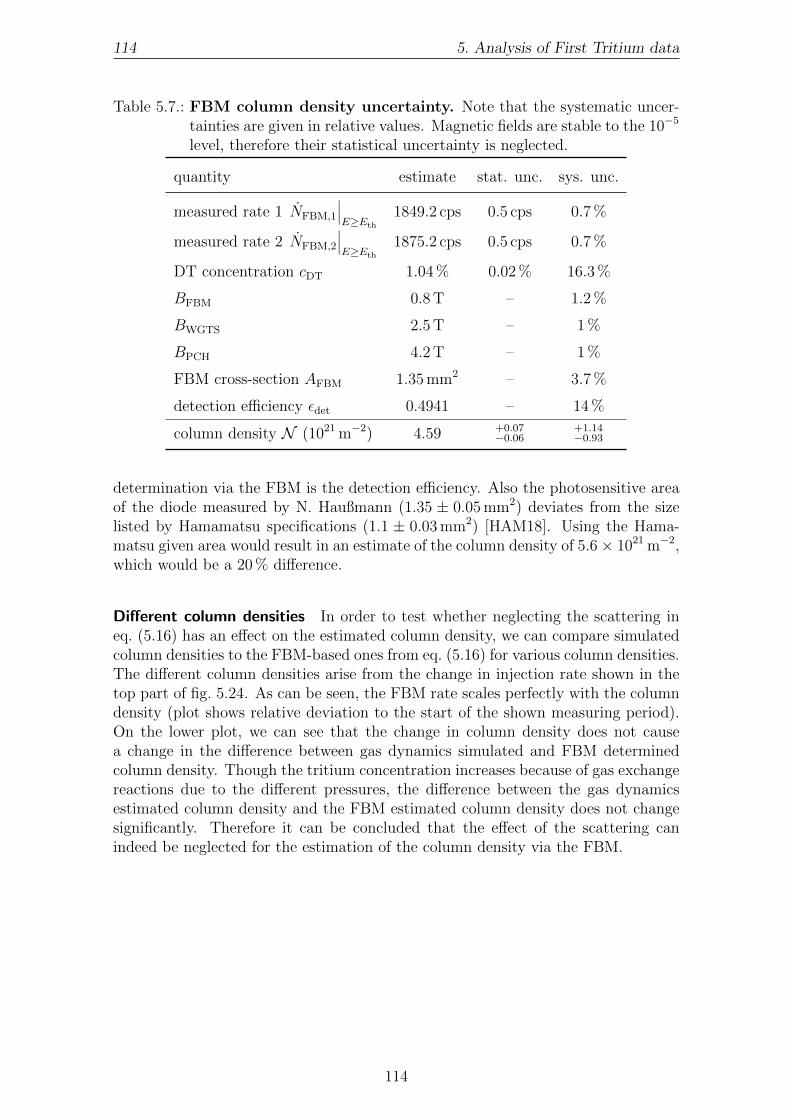
114 5. Analysis of First Tritium data
Table 5.7.: FBM column density uncertainty. Note that the systematic uncer-tainties are given in relative values. Magnetic fields are stable to the 10−5
level, therefore their statistical uncertainty is neglected.
quantity estimate stat. unc. sys. unc.
measured rate 1 NFBM,1
∣∣∣E≥Eth
1849.2 cps 0.5 cps 0.7 %
measured rate 2 NFBM,2
∣∣∣E≥Eth
1875.2 cps 0.5 cps 0.7 %
DT concentration cDT 1.04 % 0.02 % 16.3 %BFBM 0.8 T – 1.2 %BWGTS 2.5 T – 1 %BPCH 4.2 T – 1 %FBM cross-section AFBM 1.35 mm2 – 3.7 %detection efficiency εdet 0.4941 – 14 %column density N (1021 m−2) 4.59 +0.07
−0.06+1.14−0.93
determination via the FBM is the detection efficiency. Also the photosensitive areaof the diode measured by N. Haußmann (1.35 ± 0.05 mm2) deviates from the sizelisted by Hamamatsu specifications (1.1 ± 0.03 mm2) [HAM18]. Using the Hama-matsu given area would result in an estimate of the column density of 5.6× 10²¹ m−2,which would be a 20 % difference.
Different column densities In order to test whether neglecting the scattering ineq. (5.16) has an effect on the estimated column density, we can compare simulatedcolumn densities to the FBM-based ones from eq. (5.16) for various column densities.The different column densities arise from the change in injection rate shown in thetop part of fig. 5.24. As can be seen, the FBM rate scales perfectly with the columndensity (plot shows relative deviation to the start of the shown measuring period).On the lower plot, we can see that the change in column density does not causea change in the difference between gas dynamics simulated and FBM determinedcolumn density. Though the tritium concentration increases because of gas exchangereactions due to the different pressures, the difference between the gas dynamicsestimated column density and the FBM estimated column density does not changesignificantly. Therefore it can be concluded that the effect of the scattering canindeed be neglected for the estimation of the column density via the FBM.
114

5.4. Estimation of the column density via additional detectors 115
3.0 3.5 4.0 4.5 5.0 5.5 6.0 6.5stat distribution (m−2) ×1021
0
500
1000
entr
ies
3.0 3.5 4.0 4.5 5.0 5.5 6.0 6.5sys distribution (m−2) ×1021
0
1000
entr
ies
Figure 5.23.: FBM determined column density uncertainty. The upper panelshows the statistical distribution, while the lower one shows the sys-tematic distribution. 105 samples were diced.
115

116 5. Analysis of First Tritium data
Figure 5.24.: FBM estimate of different column densities. Upper plot showsthe variation of the injection rate and the FBM rate. Lower plot showsthe difference between simulated and FBM determined column density(left ordinate), and the DT concentration (right ordinate). Data from11th June to 13th June 2018.
116

5.4. Estimation of the column density via additional detectors 117
5.4.2. Estimation of the column density via PULCINELLA
The main purpose of PULCINELLA is calibration of the FPD [Ams+15]. However,the measured electron flux of PULCINELLA can also be used to estimate the columndensity. PULCINELLA is a titanium disk in front of the FPD, equipped with apico ammeter. The idea for connecting the measured current (converted into anelectron rate) to the theoretical prediction is the same as for the FBM as describedin sec. 5.4.1:
NPULCINELLA
∣∣∣E≥Eth
= Ntheo
∣∣∣E≥Eth
· εdet · nT · a(θmax), (5.27)
with the detection efficiency εdet, the number of tritium atoms visible by PULCINELLAnT and the maximum acceptance angle θmax. The maximum acceptance angle andthe detection area will be different, though, from sec. 5.4.1 since the PULCINELLAdisk is positioned at a different magnetic field than the FBM. In the following onlythe coefficients which are different from the column density estimation via FBM insec. 5.4.1 are discussed. An overview of the runs used is given in tab. 5.8; all runswere taken on 5th June 2018.
Table 5.8.: PULCINELLA run overview.
run purpose duration
40495 position determination first 130 s40498 tritium signal 1 min40500 PULCINELLA background 10 min
5.4.2.1. Maximum acceptance angle
The PULCINELLA disc is located in front of the FPD in the pump port betweenPCH and detector magnet. Therefore, the relevant maximum magnetic field is the4.2 T magnetic field of the PCH magnet:
θmax = arcsin√
BS
BPCH
= 50.8°, (5.28)
which defines the fraction of detectable electrons according to eq. (5.18).
The uncertainty on the maximum acceptance angle is determined by the uncertaintyon the magnetic fields. In sec. 5.2.4 it was shown that the relative stability of themagnetic fields is better than 1× 10⁻⁵, leaving the systematic uncertainty of 1 % asdominant uncertainty of the magnetic fields.
5.4.2.2. Flux tube mapping
In order to compare the predicted to the measured PULCINELLA rate, the WGTSflux tube seen by PULCINELLA needs to be determined accurately. Since themain focus of the PULCINELLA measurements was not on determining the columndensity, the PULCINELLA position was not well-determined in advance.
117

118 5. Analysis of First Tritium data
Determining the position of PULCINELLA The only way to determine the po-sition of the PULCINELLA disk in the Katrin global coordinate system is to useits shadow on the FPD. Usually, PULCINELLA covers the entire FPD, during themeasurements discussed in this section however there was a slight offset, comparefig. 5.25 (from run 40495, see tab. 5.8). This offset can be estimated using the shadowof PULCINELLA on the FPD. Due to the crescent-shaped form of the shadow, aring can be fit onto the FPD in order to determine the origin of PULCINELLA.
01
2 3
45
678
910
11
12 1314
15
16
17
1819
20
2122
23
24 25
26
27
28
29
3031
32
3334
35
3637
38
39
40
41
4243
44
4546
47
48 49
50
51
52
53
54
55
56
57
58
59
60
61
62
63
64
65
6667
68
6970
71
72 73
74
75
76
77
78
79
80
81
82
83
84
85
86
87
88
89
9091
92
9394
95
96 97
98
99
100
101
102
103
104
105
106
107
108
109
110
111
112
113
114115
116
117
118
119
120 121
122
123
124
125
126
127
128
129
130
131
132
133
134
135
136
137
138139
140
141
142
143
144 145
146
147
103
102
101
1
10−1
10−2
rate
(cps)
0.05− 0.04 0.03 0.02 0.01 0 0.01 0.02 0.03 0.04 0.050.05
0.04
0.03
0.02
0.01
0
0.01
0.02
0.03
0.04
0.05
− − − −−
−
−
−
−
FPD x coordinate (m)
FP
Dy
coor
din
ate
(m)
104
103
102
101
1
(x, y) = (1.75,−1.75) mm
R = 43.3 mm
Figure 5.25.: PULCINELLA shadow on FPD. Run number 40495, comparetab. 5.8. The left side shows the pixel mapping of the shadow, thecolour scale denotes the measured rate (cps). The right side showsthe fit ring representing the PULCINELLA position. Note the pixelweighting of the electron hits.
The fit ring can then be used to track electrons from the FPD to the PULCINELLAdisk in order to get the image of the ring on PULCINELLA5. The fit PULCINELLAradius is 2.6 mm larger than the nominal 110.5 mm PULCINELLA radius. This isexpected since the origin of the electrons is the ring fit onto the FPD; this ring islarger than the mapped PULCINELLA radius due to pixels being half-shadowed.From the position of the ring on PULCINELLA, the relative shift of PULCINELLAin Katrin global coordinates can be obtained, see tab. 5.9.
Determining the WGTS cross-section seen by PULCINELLA The cross-sectionof the WGTS seen by PULCINELLA can be determined by tracking simulations ofelectrons from PULCINELLA to the center of the WGTS. In the simulation, 30× 103
electrons were created uniformly distributed across the PULCINELLA surface andthen tracked towards the WGTS (see fig. 5.26). Binning the final azimuthal positionin the WGTS enables numerical determination of the cross-section. A grid of 48×48bins for the 0.045 × 0.045 m2 area of interest yields an area per bin of 3.516 mm2.The effective cross-section of the WGTS seen by PULCINELLA is then determinedby multiplying the number of bins, 1482, with non-zero entries with the area per
5This was done using a disk with a larger diameter than PULCINELLA in order to ensure thatthe electrons are terminated correctly.
118

5.4. Estimation of the column density via additional detectors 119
Table 5.9.: PULCINELLA position determination.
position Katrin coordinates (mm) FPD coordinates (mm)
origin FPD (−0.96, 3.29) (0, 0)origin PULCINELLA (1.40, 8.55) –
ring FPD (0.79, 1.54) (1.75,−1.75)ring PULCINELLA (5.89, 4.05) –
shift of PULCINELLA (4.50,−4.50) –
bin:
AWGTS = 1482 · 3.516 mm2 = 52.1 cm2 (5.29)
A visualisation of the effective cross-section of the WGTS is shown in fig. 5.26 onthe right side. Note the cut-out there due to the shadow of the FBM board, causedby the monitoring position of the FBM.
Figure 5.26.: PULCINELLA to WGTS mapping. Left side shows the 30× 103
simulated electrons created on the PULCINELLA surface. Right sideshows those electrons reaching the centre of the WGTS, the colourscale denotes the number of entries. Bin size is 3.516 mm2. Note thecut-out due to the FBM shadow.
The systematic uncertainty of the determination of the effective cross-section of theWGTS is conservatively estimated to 5 %, which includes uncertainty due to wronglyaccounted misalignments and an uncertainty on the determination of the area itself.
119

120 5. Analysis of First Tritium data
5.4.2.3. PULCINELLA rate prediction
The rate prediction for PULCINELLA is less complicated than for the FBM becausePULCINELLA does not have an intrinsic energy resolution. This leaves us with
Ntheo
∣∣∣E≥Eth
=∞∫
Eth
∑fs
Pfs ·dΓ(ε)dE
∣∣∣∣∣fs
dE. (5.30)
This time the threshold energy is given by the highest blocking potential betweenWGTS and PULCINELLA, which is the high voltage at the pre-spectrometer (PS):the inner electrode of the PS was set to Eth = −500 V. This gives
Ntheo
∣∣∣E≥Eth
= 1.66× 10⁻⁹ cps. (5.31)
Besides the “threshold”, the detection efficiency also needs to be taken into ac-count. GEANT4 simulations by E. Forstner [FG18] showed a backscattering prob-ability for electrons from the disk of 2.06 % for zero-degree incident electrons, withPULCINELLA at 0 V and including the magnetic mirror effect. During the mea-surements discussed in this section, the PULCINELLA disk was at 200 V posi-tive potential, thereby increasing the detection efficiency for electrons. The de-tection efficiency at 200 V is estimated by fitting a straight line to the simulatedεdet(U) = 1− Pbackscatter(U) by E. Forstner, see fig. 5.28:
εdet(200 V) = 0.9795. (5.32)
The systematic uncertainty related to the detection efficiency is estimated to be 5 %.This is a rather conservative value, which accounts for the simulations of E. Forstnerbeing done only for zero incident angle; the magnetic mirror effects for electrons withlarger impinging angle is even larger than for zero incident angle.
5.4.2.4. PULCINELLA rate estimation
The PULCINELLA disk acts as a Faraday cup: it measures a continuous current ofelectrons with a pico-amperemeter. The measured current can be translated into anelectron rate via
NPULCINELLA
∣∣∣E≥Eth
= −Ie. (5.33)
During the First Tritium campaign, there was one 1 min signal (40498) and one10 min background (40500) run with PULCINELLA at stable column density (com-pare tab. 5.8). The corresponding currents are shown in fig. 5.27. Fit results of aconstant as well as the corresponding uncertainty are shown in tab. 5.10, along withthe converted electron rate N .
Note that the positive background current leads to a negative electron rate. Sincethe background run showed a positive current, its deduction leads to a more negativesignal current resulting in the measured electron rate
NPULCINELLA
∣∣∣E≥Eth
= 8.13× 10⁷ cps. (5.34)
Besides the statistical uncertainty of the measured rate listed in tab. 5.10, the system-atic uncertainty on the measured rate is 3 %, as shown by Amsbaugh et al. [Ams+15].
120

5.4. Estimation of the column density via additional detectors 121
0 200 400 600
time (s)
−20
−10
0cu
rren
t(p
A)
0 20 40 60
time (s)
−20
−10
0
curr
ent
(pA
)
Figure 5.27.: PULCINELLA measured current. Left: FPD run 40500 (5th June2018), PULCINELLA background. Right: FPD run 40498 (5th June2018), PULCINELLA signal.
Table 5.10.: PULCINELLA fit current and electron rate.
quantity fit value fit error
Itot (pA) -12.22 0.23
Ntot (cps) 7.63× 10⁷ 0.14× 10⁷
Ibg (pA) 0.80 0.01
Nbg (cps) -0.50× 10⁷ 0.01× 10⁷
Isig (pA) -13.02 0.23
Nsig (cps) 8.13× 10⁷ 0.14× 10⁷
5.4.2.5. Uncertainty estimation
An overview of the estimated uncertainties of the factors of eq. (5.27) is given intab. 5.11. Note that the systematic uncertainties are given in relative percentagevalues. The uncertainty on the column density is estimated via ensemble testing.Each item of tab. 5.11 is sampled from a Gaussian distribution centred at the esti-mated value with σ being the estimated uncertainty. Some of the distributions havelower and upper limits, for example the detection efficiency cannot be larger than 1.The distribution of the detection efficiency is shown as an example in fig. 5.28.
Using 105 samples from the distributions of the factors of eq. (5.27), the distributionof the estimated column density can be determined with a precision of 0.3 %. Fromthe statistical and systematic distribution of the column density, the statistical andsystematic uncertainties are determined as the ±34 % interval around the estimatedvalue. The resulting statistical and systematic distributions of the column densityare shown in fig. 5.29 and listed in tab. 5.11.
5.4.2.6. Column density
Combining the estimates of the factors as listed in tab. 5.11 and discussed in this sec-tion results in an estimate of the column density from the measured PULCINELLA
121

122 5. Analysis of First Tritium data
Table 5.11.: PULCINELLA column density uncertainty. Note that the sys-tematic uncertainties are given in relative values. Magnetic fields arestable to the 10−5 level, therefore their statistical uncertainty is ne-glected.
quantity estimate stat. unc. sys. unc.
measured rate NPULCINELLA
∣∣∣E≥Eth
8.13× 10⁷ cps 0.14× 10⁷ cps 3 %
DT concentration cDT 1.07 % – 14 %BWGTS 2.5 T – 1 %BPCH 4.2 T – 1 %eff. WGTS cross-section AWGTS 52.1 cm2 – 5 %detection efficiency εdet 0.9795 – 5 %column density N (1021 m−2) 4.92 +0.09
−0.09+0.78−0.79
0 5 10
PULCINELLA potential (kV)
0.980
0.985
ε det
simulation
fit
0.8 0.9 1.0εdet
0
500
entr
ies
Figure 5.28.: PULCINELLA detection efficiency. Left: A straight line is fitto the simulation by E. Forstner [FG18]. Right: Possible detectionefficiency distribution. Note the upper limit of 1. The dotted red linedenotes the 1σ lower systematic uncertainty. 105 samples were diced.
current of (estimate ± stat. ± sys.)
NPULCINELLA =(4.92 +0.09
−0.09+0.78−0.79
)× 1021 m2. (5.35)
Compared to the expected value from gas dynamic simulations of 4.46× 10²¹ m−2,this is a deviation of 9 % which is in agreement within the estimated uncertainty ofthe PULCINELLA determination.
5.4.3. Discussion
Three different methods have been presented in this chapter to estimate the col-umn density from the data. One is fitting the column density as an additional fitparameter, another one is using the FBM detector, and the last one is using thePULCINELLA disk in front of the FPD. The best agreement with the simulatedcolumn density can be found for one single run fit (e.g. 40667) and for fitting multi-ple runs together (appended runs). Good agreement is also given between simulation
122

5.4. Estimation of the column density via additional detectors 123
3.0 3.5 4.0 4.5 5.0 5.5 6.0 6.5stat distribution (m−2) ×1021
0
500
1000en
trie
s
3.0 3.5 4.0 4.5 5.0 5.5 6.0 6.5sys distribution (m−2) ×1021
0
1000
entr
ies
Figure 5.29.: PULCINELLA determined column density uncertainty. Theupper panel shows the statistical distribution, while the lower oneshows the systematic distribution. 105 samples were diced.
and measurement by the PULCINELLA disk, as well as the FBM estimate. Fur-thermore, the previous chapter includes an estimation of the inlet pressure by themeasured pressure at the krypton capillary, see sec. 4.4.8. Calculating the columndensity corresponding to the estimated inlet pressure of 0.3115µbar yields a columndensity of 4.65× 10²¹ m−2 from the pressure at the krypton capillary, which is ingood agreement with the simulated column density.
An overview of the discussed column density estimates is given in fig. 5.30. It canbe seen that all estimates agree within their uncertainties. However, the simulatedcolumn density seems to be underestimated as most other estimates result in largervalues. In order to match the measured and the simulated column density estima-tion, the input parameters of the simulation might be varied inside their uncertaintiesestimated in sec. 4.4.7. Using input parameters α = 1 (instead of α = 0.97), and anoutlet to inlet pressure ratio of 0.05 (instead of 0.02) results in perfect agreementbetween the Boltzmann based simulation and the values determined by the differentmeasurements, with a column density value of 4.6× 10²¹ m−2 (see the dotted blackline in fig. 5.30). With the Knudsen based simulation and an outlet to inlet pressureof 0.05, the same column density is estimated (4.6× 10²¹ m−2)6. These are stronghints that the input parameters α = 1 and pout/pin = 0.05 describe the D2 domi-nated gas dynamics better than α = 0.97 and pout/pin = 0.02. However, no decisiveconclusion can be drawn as the uncertainties of all measurements are larger than theones of the simulation. Column density estimates via fitting the spectrum currentlyonly include the 2 % uncertainty on the inelastic scattering cross-section [Ase+00].As mentioned before, the re-analysed LARA data results in a factor three decreased
6Note that the Knudsen flow has no accommodation coefficient parameter α.
123
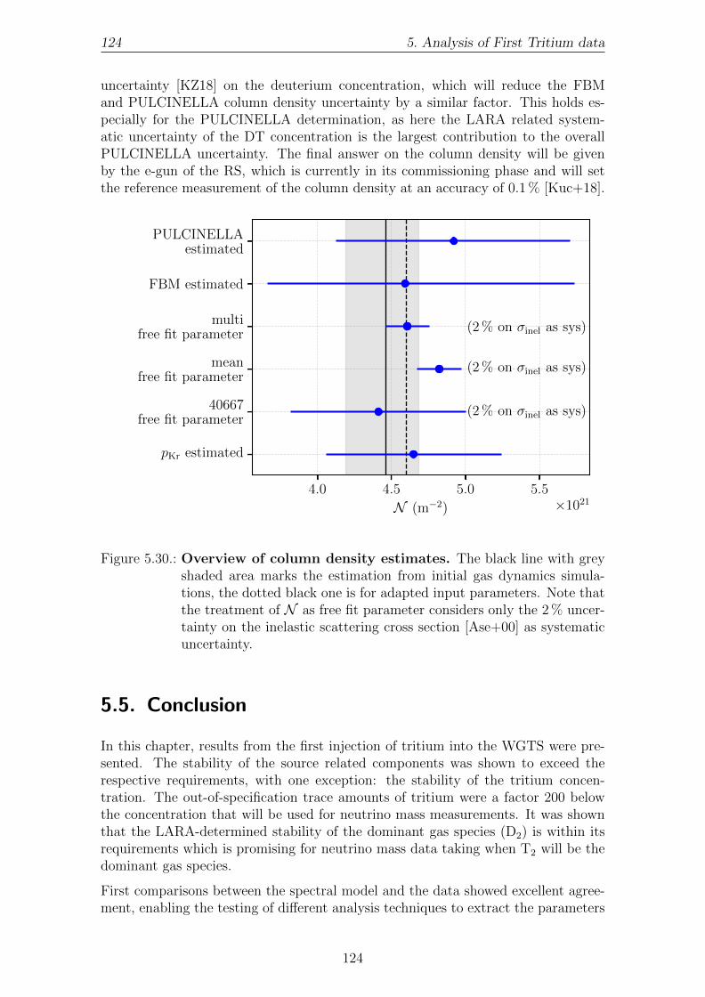
124 5. Analysis of First Tritium data
uncertainty [KZ18] on the deuterium concentration, which will reduce the FBMand PULCINELLA column density uncertainty by a similar factor. This holds es-pecially for the PULCINELLA determination, as here the LARA related system-atic uncertainty of the DT concentration is the largest contribution to the overallPULCINELLA uncertainty. The final answer on the column density will be givenby the e-gun of the RS, which is currently in its commissioning phase and will setthe reference measurement of the column density at an accuracy of 0.1 % [Kuc+18].
4.0 4.5 5.0 5.5
N (m−2) ×1021
pKr estimated
40667free fit parameter
meanfree fit parameter
multifree fit parameter
FBM estimated
PULCINELLAestimated
(2 % on σinel as sys)
(2 % on σinel as sys)
(2 % on σinel as sys)
Figure 5.30.: Overview of column density estimates. The black line with greyshaded area marks the estimation from initial gas dynamics simula-tions, the dotted black one is for adapted input parameters. Note thatthe treatment of N as free fit parameter considers only the 2 % uncer-tainty on the inelastic scattering cross section [Ase+00] as systematicuncertainty.
5.5. Conclusion
In this chapter, results from the first injection of tritium into the WGTS were pre-sented. The stability of the source related components was shown to exceed therespective requirements, with one exception: the stability of the tritium concen-tration. The out-of-specification trace amounts of tritium were a factor 200 belowthe concentration that will be used for neutrino mass measurements. It was shownthat the LARA-determined stability of the dominant gas species (D2) is within itsrequirements which is promising for neutrino mass data taking when T2 will be thedominant gas species.
First comparisons between the spectral model and the data showed excellent agree-ment, enabling the testing of different analysis techniques to extract the parameters
124

5.5. Conclusion 125
of interest E0,eff, Amp, and Bg. Estimates of the effective endpoint E0,eff werepresented including the systematics due to the column density uncertainty, amongstthese treating the column density as nuisance parameter via a pull term, as a free fitparameter, or using ensemble testing of the column density. All estimates of E0,eff
are within the assumed spread of E0,eff due to the unknown work function difference.
In order to test the column density simulations from sec. 4.4, estimations of thecolumn density via the additional detectors FBM and PULCINELLA were given.The free spectrum parameter estimate, the FBM estimate, the PULCINELLA es-timate, the krypton capillary estimate, and the simulation estimate of the columndensity were found to agree within their respective uncertainties. From comparisonsof the simulated column density estimate and the one obtained from various othermethods, it seems as if the best agreement is found for an accommodation coefficientα = 1 and an outlet to inlet pressure ratio of pout/pin = 0.05, resulting in a columndensity of N = 4.6× 10²¹ m−2 for Boltzmann and Knudsen based flow. With thetritium purity increased by a factor of 200 for the neutrino mass data taking, theLARA determined εT will have an accuracy on the order of 1 %. With all otheruncertainties reduced, this will enable a PULCINELLA-based estimation of the col-umn density with uncertainty also on the percent level. In order to further decreaseuncertainties on the column density determination, a cross-check between e-gun,FBM, and PULCINELLA measurements with active source gas is recommended.
Dedicated measurements with the RS e-gun to determine the column density andto test the gas dynamics model of the source are an integral part of the STS-IIIameasurement programme (autumn 2018). As the Katrin experiment was shownto be stable well within its requirements, the start of neutrino mass data takingwith increased tritium concentration is planned for spring 2019 after a maintenancebreak, with final hardware works, during the winter 2018/19.
125

CHAPTER 6
BLIND ANALYSIS AND METHODS
“It is also desirable to emphasize the importance of the human equation in accuratemeasurements such as these. It is easier than is generally realized to unconsciously
work toward a certain value.”– Frank Dunnington, 1933 –
The goal of the Katrin experiment is to determine the (effective) neutrino mass byanalysis of the tritium β-decay spectrum. In order to reduce the influence of humanobserver’s bias, a blind analysis can be performed. In this chapter, several methodsfor blind neutrino mass analysis of Katrin-data will be presented and their effectwill be tested on simulated data as well as 83mKr-data and T-data from the FirstTritium campaign of the Katrin experiment.
6.1. Motivation
The requirement to apply blind analysis techniques arises from the observer’s bias:in general, data analysts have expectations of what the result should be, whichmay cause them to unconsciously work toward that expected value. One way toprevent this observer’s bias is by performing a blind analysis of the data. Thisblinding requires obscuring of some part of the physics results until such a timethat they cannot influence subsequent analysis steps. In Katrin, our observable ofinterest is the neutrino mass squared m2
ν which we obtain by comparing a measuredintegrated tritium β-spectrum to a model prediction. In order to worsen the neutrinomass sensitivity and thereby hide the observable of interest, two blinding paths canbe followed: either we hide some physics details of our model, resulting in modelblinding, or we artificially modify the analysed data set, in a well-controlled andstrictly-reversible way, resulting in data blinding. This chapter will present anddiscuss adequate methods for a blind analysis of Katrin data.
6.1.1. Observer’s bias
One of the most famous examples of an observer’s bias is the story of CleverHans [Pfu07]. In 1904, Wilhelm von Osten claimed that Hans could perform arith-
127
128 6. Blind analysis and methods
metic and other intellectual tasks such as adding numbers. The issue was that Hanswas a horse. Wilhelm von Osten – a retired teacher confident in his methods – arguedthat he taught Hans to answer his questions by tapping his hoof. No tricks could befound at first and after this miracle of a horse received worldwide attention [Hey04,The04], the founder and director of the Psychological Institute of Berlin, Prof. Dr.Carl Stumpf, was officially asked to investigate the Clever Hans phenomenon. To-gether with his student, Oskar Stumpf, they could prove that Clever Hans was notable to perform arithmetic operations but was indeed very clever: Hans could onlyanswer those questions where the questioner knew the result and where Hans couldsee the questioner’s face although it did not matter who asked the questions [Pfu07].This lead to the conclusion that Hans could detect tiny changes in the facial ex-pression of the questioner and stopped tapping as soon as the number of hoof tapsreached the correct number. This Clever Hans effect was not only a major break-through in psychology but also shows a clear observer’s bias: Hans answered thequestions such that the result matched the expectation of the questioner.
But it is not only this kind of observer’s bias that threatens accurate results: asshown by Klein and Roodman from speed of light measurements published overan entire century [KR05], researchers are rather conservative about their estimatedresults if they disagree with previous measurements of that quantity. Even thoughthey used different techniques, four experiments in a row stated a value that was17 km s−1 off previous and following experiments. The reason for this may have beenthat the experiments compared their estimated value to the most recent published.If their value was off, they would search for a source causing such systematic shiftuntil their value matched the previous result. This is only one example for scientistsstopping to search for systematic uncertainties when their result matches a certainoutcome.
The systematic uncertainty caused by the observer’s bias cannot be estimated whenpublishing the results, but only in a historic view, as shown by Klein and Rood-man [KR05]. This is a fundamental difference between observer’s bias and any otherkind of bias in a measurement, requiring a kind of analysis that prohibits the ob-server’s bias. In the following, this kind of analysis is called blind analysis, becausethe analyst does not know the final answer or initial trend (the neutrino mass mν)of his experiment before the analysis is complete.
6.1.2. Goal of blind analysis in KATRIN
As concluded in sec. 6.1.1, the general goal of blind analysis is to avoid biases in dataanalysis. With this kind of analysis technique, the data is analysed in a way thatthe final answer remains unknown before the analysis is complete, preventing theanalyst from tuning intermediate results and cuts to arrive at the expected answer.On the other hand with the decision to perform a blind analysis, there is the com-mitment beforehand to publish the result when unblinding, barring all consequences.One of the first to apply blind analysis techniques in physics was F. Dunnington inhis measurement of e/m [Dun33]. His estimation of e/m was directly proportionalto the angle between electron source and detector. Therefore Dunnington had hismachinist select angles close to but not exactly at the optimal value and keepingthese angles secret. This hiding of the angles made Dunnington blind to the final
128

6.2. Sensitivity definition and derivation 129
answer and therefore unable to tune his analysis towards an expected value. Onlyafter Dunnington finished his analysis, he had his machinist reveal the angles used,enabling Dunnington to calculate the final answer. The example of Dunningtoncannot be easily translated to Katrin, since the measuring concepts are fundamen-tally different with the neutrino mass manifesting as a shape distortion close to theendpoint of the β-decay spectrum.
In general, however, performing a blind analysis does not mean
� that you never look at the data,
� that you are not allowed to correct for a mistake once you find one,
� that your analysis is inevitably correct, or
� that a non-blind analysis is necessarily wrong.
In Katrin, the main physics goal is to extract the value or limit on the neutrinomass. Though there will be other types of analyses such as searches for sterileneutrinos, right handed currents, light bosons, or relic neutrinos, all of which requiredifferent blinding techniques, focus will be on developing blind analysis techniquesfor neutrino mass analysis in the following. This implies hiding the value or limit onthe neutrino mass from the analyst. The most stringent limit on the neutrino mass iscurrently the limit obtained from the analysis of Mainz and Troitsk data [Tan+18]:
mν ≤ 2.0 eV. (6.1)
In order to be conservative and to circumvent problems like those in the speed of lightmeasurements mentioned in sec. 6.1.1, the requirement for each blinding techniquefor Katrin neutrino mass analysis is defined to prevent intermediate neutrino masssensitivities any better than
mν ≤ 2.0 eV (90 % C.L.) before unblinding, (6.2)
(that is, any better than what is already established empirical knowledge). Unblind-ing will then yield the full sensitivity.
6.2. Sensitivity definition and derivation
Katrin will measure an integrated tritium β-decay spectrum [KAT05]. In the stan-dard Katrin neutrino mass analysis, the spectrum will be compared to a modelcontaining four variable fit parameters [KAT05, Kle14]:
1. (effective) neutrino mass squared m2ν,
2. endpoint E0,
3. signal amplitude Amp,
4. background rate Bg.
First a definition of the sensitivity for the neutrino mass needs to be derived to beable to compare the different blinding methods. The sensitivity will be defined interms of discovery potential, expressed in terms of standard deviations, and the cor-responding total uncertainty. Then the methodology on how to derive the necessarylevel of blinding to prevent sensitivities better than eq. (6.2) will be defined.
129

130 6. Blind analysis and methods
6.2.1. Sensitivity as discovery potential
In the Katrin Design Report [KAT05], the sensitivity for the neutrino mass is seenas the neutrino mass which can be determined at a significance of 1.645σ. Assumingnormal distribution of the best fit estimate m2
ν, this translates into a 90 % C.L. upperlimit. In other words, the sensitivity is the discovery potential representing a 1.645σdistance of the best fit estimate m2
ν to the null-hypothesis 0:
discovery potential = m2ν − 0
σm
2ν tot
(6.3)
requiring the sensitivity to fulfil the following relation:
1.645 = m2ν − 0
σm
2ν tot
. (6.4)
6.2.2. Adaption of the total neutrino mass uncertainty
In the Katrin Design Report [KAT05], the total uncertainty σm
2ν tot
is composed of
the uncorrelated statistical (σm
2νstat
) and systematic (σm
2νsys
) uncertainties:
σDRm
2ν tot
=√σm
2ν
2stat
+ σm
2ν
2sys. (6.5)
The different blinding methods are expected to result in two different effects onthe estimated neutrino mass squared: either in an increased statistical uncertaintyσm
2νstat
or in a systematic shift δm
2ν
of the estimated neutrino mass squared m2ν with
respect to the true neutrino mass squared m2νtrue:
δm
2ν
= m2ν −m2
νtrue. (6.6)
In order to be able to compare the different blinding methods, one common definitionof the total uncertainty is needed. For this work it was decided to adapt eq. (6.5) toinclude the systematic neutrino mass shift into the sensitivity calculations as follows:
σm
2ν tot
=√σm
2ν
2stat
+ σm
2ν
2sys
+ δm
2ν
2. (6.7)
This implementation treats the introduced neutrino mass shift as new, unknownsystematic uncertainty uncorrelated to all others.
6.2.3. Methodology to derive the necessary level of blinding
Using eq. (6.2), eq. (6.4), and eq. (6.7), the methodology to derive the necessarylevel of blinding can be described:
1. for the blinding parameters of each blinding method (smearing values, mea-suring times, window widths, et cetera), calculate the total uncertainty σ
m2ν tot
from eq. (6.7) for various true neutrino masses,
130

6.3. Blind analysis methods 131
2. use this to find the intersection points between the 1.645σ discovery poten-tial (6.4) and the lines for the various blinding parameters: the abscissa ofthese intersection points is the sensitivity,
3. plot the sensitivity against the various blinding parameters to obtain the blind-ing parameter required to not exceed a certain sensitivity limit,e.g. 2 eV (90 % C.L.) for the first KATRIN neutrino mass analysis.
6.3. Blind analysis methods
100
101
102
mν = 0 eV
mν = 1 eV
−0.01
0.00
−50 −40 −30 −20 −10 0
101
102
N(c
ps)
rel.
diff
.t
(d)
retarding energy qU − E0 (eV)
Figure 6.1.: Integrated spectrum with MTD. The neutrino mass sensitive regionis shown by comparing a spectrum with neutrino mass mν = 1 eV (red)to a spectrum without neutrino mass mν = 0 eV (blue). The peak of themeasuring time distribution (MTD) sits in the region where the neutrinomass has the largest distortion relative to the zero mass spectrum.
In order to establish useful blinding and unblinding strategies, the effect and signa-ture of a non-zero neutrino mass in the tritium spectrum needs to be understood.Figure 6.1 shows the effect of two different neutrino masses: a non-zero neutrinomass results in a shape distortion of the β-spectrum close to the endpoint, with po-sition and relative strength of the distortion depending on the neutrino mass. Sincethe neutrino mass in Katrin is determined via a four-parameter (see sec. 6.2) fitto the measured data, blinding can be performed in two ways: either blind the fitmodel (model blinding) or blind the measured data (data blinding). From fig. 6.1,an obvious way to hide the neutrino mass signature is to decrease the significanceof a hypothetical signal by increasing the statistical uncertainty (reduced statistics).This implies, for example, using only one run (scan) of the tritium β-spectrum at atime, that is, at typically only a few hours. It has to be noted that all runs can beanalysed and inspected individually, just not combined. Another possibility would
131

132 6. Blind analysis and methods
be to apply a blinding method mostly used in rare-decay searches, such as 0νββ-decays (e.g. GERDA blind analysis [Ago+13]): the region where a potential signalis expected to show up remains hidden from the analysts. Only after the completeanalysis chain is developed and fixed, the signal region is opened. Applying thismethod to the Katrin neutrino mass analysis (window blinding) may require hid-ing a broad energy window from the analysts: fig. 6.1 shows that a 2 eV neutrinomass, for example, would require a window width of about 20 eV, in the range of[E0 − 20 eV, E0] to successfully hide the signal of the neutrino mass, which will beshown in sec. 6.4.1.2. Another method discussed in the following is an artificialsmearing of the neutrino mass signal by convolving the β-spectrum with a Gaussian.This may be performed in different ways: either in terms of data blinding actingdirectly on the measured spectrum (energy smearing) or in terms of model blind-ing, either smearing the distribution of the modelled final states (FSD smearing)or smearing the energy loss function of the electrons (energy loss smearing). All ofthese blinding methods will be described in more detail and results from their teston commissioning measurements will be presented.
6.3.1. Data blinding
The most powerful way to perform a blind analysis is blinding the data. This givesmaximum control over which data is released and which not: if the neutrino mass ishidden by blinded data, the analysts can not get access to the original data for neu-trino mass analysis development and thereby can not tune any cut towards expectedneutrino masses. However, data blinding introduces the risk that the original datacontains unexpected features as reported by Lobashev et al. [Lob+99a].
In the following, three different methods leading to blinded data sets will be pre-sented. For each of the methods, ensemble tests were performed on simulated datain order to inspect the effect of the blinding method on the parameter of interest,the neutrino mass. The settings for these simulations can be found in tab. C.2. Mostimportant is to note that a larger magnetic field in the analysing plane together withan increased background (225 mcps, a factor of 23 higher compared to the designreference background level of 10 mcps [KAT05]). These settings were assumed, sinceall measurements with the Katrin set-up so far showed an increased and volumedependent background rate [Har15, Blo18, Tro18]. A total of 104 fits were performedper setting for each blinding method.
6.3.1.1. Reduced statistics
In the starting phase of the initial neutrino-mass runs, the neutrino mass sensitivityof Katrin will be driven by the statistical uncertainty. Due to the unprecedentedactivity of the Katrin tritium source, the statistical uncertainty will decrease fast:In this section it is investigated by ensemble testing how many hours of measuringtime can be allowed to be analysed in order to not exceed the 2 eV sensitivity. Theoutcome will not only be useful to determine the maximum length of one spectralscan at Katrin, but also for determining the time intervals in which unblindedKatrin data will be released.
132

6.3. Blind analysis methods 133
0
1
succ
ess/
tota
lfi
ts
2
3
4
σm
2 ν(e
V2)
200400600
measuring time (min)
0.2
0.4
0.6
0.8
m2 ν
(eV
2)
[×10−
1]
−1
0
1
2E
0−
1857
5(e
V)
[×10−
3]
0
2
4
Amp−
1[×
10−
4]
−1.5
−1.0
−0.5
Bg−
225
(mcp
s)[×
10−
1]
0.996
0.997
0.998
0.999
1.000
χ2 re
d
1.5
2.0
2.5
3.0
σE
0(e
V)
[×10−
1]
1.0
1.5
2.0
σAmp
[×10−
2]
0.4
0.6
0.8
1.0
σBg
(mcp
s)[×
10−
2]
1.84
1.86
1.88
1.90
σχ
2 red
[×10−
1]
Figure 6.2.: Measuring time dependence of fit parameters. Plots share thex-axis. All fits were successful (upper plot). A clear dependence of thestandard deviation of the best fit values (middle plot) on the measuringtime can be seen. There is no clear dependence of the best fit meanvalues (lower plot) on the measuring time.
First it is tested whether the reduced statistics method causes other effects besidesincreasing the statistical uncertainty on the neutrino mass. Such effects may be asystematic shift of one of the four standard fit parameters, a substantial increase ofthe χ2 or a decrease in number of successful fits. A good indicator to investigatethese effects is the live time dependent distribution of the best fit estimates for a
133
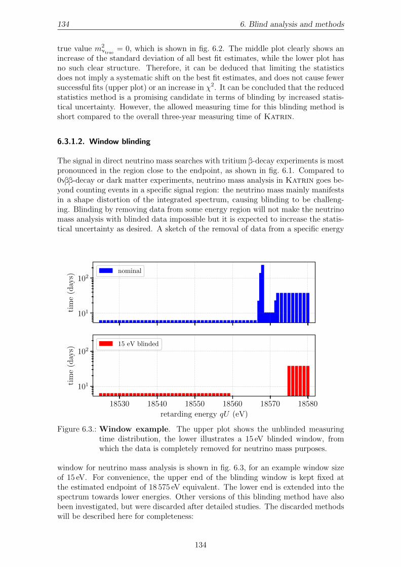
134 6. Blind analysis and methods
true value m2νtrue
= 0, which is shown in fig. 6.2. The middle plot clearly shows anincrease of the standard deviation of all best fit estimates, while the lower plot hasno such clear structure. Therefore, it can be deduced that limiting the statisticsdoes not imply a systematic shift on the best fit estimates, and does not cause fewersuccessful fits (upper plot) or an increase in χ2. It can be concluded that the reducedstatistics method is a promising candidate in terms of blinding by increased statis-tical uncertainty. However, the allowed measuring time for this blinding method isshort compared to the overall three-year measuring time of Katrin.
6.3.1.2. Window blinding
The signal in direct neutrino mass searches with tritium β-decay experiments is mostpronounced in the region close to the endpoint, as shown in fig. 6.1. Compared to0νββ-decay or dark matter experiments, neutrino mass analysis in Katrin goes be-yond counting events in a specific signal region: the neutrino mass mainly manifestsin a shape distortion of the integrated spectrum, causing blinding to be challeng-ing. Blinding by removing data from some energy region will not make the neutrinomass analysis with blinded data impossible but it is expected to increase the statis-tical uncertainty as desired. A sketch of the removal of data from a specific energy
101
102
tim
e(d
ays)
nominal
18530 18540 18550 18560 18570 18580
retarding energy qU (eV)
101
102
tim
e(d
ays)
15 eV blinded
Figure 6.3.: Window example. The upper plot shows the unblinded measuringtime distribution, the lower illustrates a 15 eV blinded window, fromwhich the data is completely removed for neutrino mass purposes.
window for neutrino mass analysis is shown in fig. 6.3, for an example window sizeof 15 eV. For convenience, the upper end of the blinding window is kept fixed atthe estimated endpoint of 18 575 eV equivalent. The lower end is extended into thespectrum towards lower energies. Other versions of this blinding method have alsobeen investigated, but were discarded after detailed studies. The discarded methodswill be described here for completeness:
134
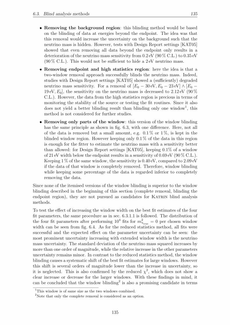
6.3. Blind analysis methods 135
� Removing the background region: this blinding method would be basedon the blinding of data at energies beyond the endpoint. The idea was thatthis removal would increase the uncertainty on the background such that theneutrino mass is hidden. However, tests with Design Report settings [KAT05]showed that even removing all data beyond the endpoint only results in adeterioration of the neutrino mass sensitivity from 0.2 eV (90 % C.L.) to 0.35 eV(90 % C.L.). This would not be sufficient to hide a 2 eV neutrino mass.
� Removing endpoint and high statistics region: here the idea is that atwo-window removal approach successfully blinds the neutrino mass. Indeed,studies with Design Report settings [KAT05] showed a (sufficiently) degradedneutrino mass sensitivity. For a removal of [E0 − 30 eV, E0 − 23 eV] ∧ [E0 −19 eV, E0], the sensitivity on the neutrino mass is decreased to 2.12 eV (90 %C.L.). However, the data from the high statistics region is precious in terms ofmonitoring the stability of the source or testing the fit routines. Since it alsodoes not yield a better blinding result than blinding only one window1, thismethod is not considered for further studies.
� Removing only parts of the window: this version of the window blindinghas the same principle as shown in fig. 6.3, with one difference. Here, not allof the data is removed but a small amount, e.g. 0.1 % or 1 %, is kept in theblinded window region. However keeping only 0.1 % of the data in this regionis enough for the fitter to estimate the neutrino mass with a sensitivity betterthan allowed: for Design Report settings [KAT05], keeping 0.1% of a windowof 21 eV width below the endpoint results in a sensitivity of 0.69 eV (90 % C.L.).Keeping 1 % of the same window, the sensitivity is 0.40 eV, compared to 2.09 eVif the data of that window is completely removed. Therefore, window blindingwhile keeping some percentage of the data is regarded inferior to completelyremoving the data.
Since none of the itemised versions of the window blinding is superior to the windowblinding described in the beginning of this section (complete removal, blinding theendpoint region), they are not pursued as candidates for Katrin blind analysismethods.
To test the effect of increasing the window width on the best fit estimates of the fourfit parameters, the same procedure as in sec. 6.3.1.1 is followed. The distribution ofthe four fit parameters after performing 104 fits for m2
νtrue= 0 per chosen window
width can be seen from fig. 6.4. As for the reduced statistics method, all fits weresuccessful and the expected effect on the parameter uncertainty can be seen: themost prominent uncertainty increasing with extended window width is the neutrinomass uncertainty. The standard deviation of the neutrino mass squared increases bymore than one order of magnitude, while the relative increase in the other parametersuncertainty remains minor. In contrast to the reduced statistics method, the windowblinding causes a systematic shift of the best fit estimates for large windows. Howeverthis shift is several orders of magnitude lower than the increase in uncertainty, soit is neglected. This is also confirmed by the reduced χ2, which does not show aclear increase or decrease for the larger windows. With these findings in mind, itcan be concluded that the window blinding2 is also a promising candidate in terms
1This window is of same size as the two windows combined.2Note that only the complete removal is considered as an option.
135

136 6. Blind analysis and methods
0
1
succ
ess/
tota
lfi
ts
0.0
0.5
1.0
1.5
σm
2 ν(e
V2)
0 10 20 30
window width (eV)
−5
−4
−3
−2
−1
0
m2 ν
(eV
2)
[×10−
1]
−1.5
−1.0
−0.5
0.0
E0−
1857
5(e
V)
[×10−
2]
0
2
4
6
Amp−
1[×
10−
4]
−0.8
−0.6
−0.4
−0.2
0.0
Bg−
225
(mcp
s)[×
10−
2]
1.002
1.004
1.006
1.008
χ2 re
d
0
1
2
3
4
5
σE
0(e
V)
[×10−
2]
0.5
1.0
1.5
2.0
σAmp
[×10−
3]
8.9
9.0
9.1
9.2
σBg
(mcp
s)[×
10−
5]
2.00
2.25
2.50
2.75
3.00
σχ
2 red
[×10−
1]
Figure 6.4.: Window width dependence of fit parameters. Plots share the x-axis, results are shown for three years of data. All fits were successful(upper plot). A clear dependence of the standard deviation of the bestfit values (middle plot) on the window width can be seen. There is aminor dependence of the best fit mean values (lower plot) on the windowwidth.
of blinding by increased statistical uncertainty.
136

6.3. Blind analysis methods 137
6.3.1.3. Energy smearing
Another blinding method aims to hide the neutrino mass by smearing the energyof the measured spectrum. Thereby the neutrino mass shape distortion of the inte-grated spectrum should be hidden and the neutrino mass sensitivity deteriorated. Incontrast to the two data blinding methods mentioned so far (see sec. 6.3.1.1, 6.3.1.2),the energy smearing of the measured spectrum is not expected to increase the sta-tistical uncertainty on the neutrino mass but to give a shifted neutrino mass as thebest fit. This would have the advantage that fits to the blinded data could be used asa stability criterion for data quality checks on blinded data with the same statisticalprecision as the unblinded data.
A common way to introduce a smearing to data is by convolution with a Gaussian.One example is including a finite energy resolution to model the detector responsefunction of a Si-pin diode3 or including the Doppler broadening in the spectrumcalculation [Kle+18] (also see sec. 2.2.1). The intuitive approach is to smear theenergy of each single electron and then move it from its original energy bin to a newone. This strict implementation would require smearing the differential spectrum toget a smeared integrated spectrum. Though this single-event smearing was droppedin favour of a spectrum-wide smearing, the energy smearing is still a smearing of thedifferential spectrum.
Methodology In the following, a run is defined as one scan over the whole mea-surement range. Each run contains subruns with index i representing the electroncounts Ni from measuring at the respective entry (Ui, ti). Since the high-voltageat the spectrometer represents a high-pass filter, the counts Ni are the number ofelectrons with energies E ≥ qUi. The energy smearing will be applied run-wise,meaning each scan is smeared independently from the other scans. Since the runwill contain a non-uniform distribution of measuring times ti (compare fig. 6.3), weuse the integrated rates spectrum as
Ni = Ni
ti. (6.8)
From the integrated rate spectrum Ni, a differential rate spectrum dNi/dE is de-rived by applying a spline interpolation. In order to enable universal usage of thissmearing method independent of the underlying measuring time distribution, splinesinterpolation was chosen4: the interpolation enables differentiation and evaluationat intermediate steps ∆Uj < ∆Ui, making the method independent of the high-voltage steps ∆Ui of the spectrum scan. In the following, the evaluation step width∆Uj is chosen to be ∆Uj = 5 mV, a value which is a good compromise between fastcomputation and accuracy of the result. The differential spectrum to be smeared is
dNj
dE. (6.9)
3For example the FBM, see sec. 5.4.1.4 or the FPD, see sec. 2.2.5.4The gsl splines package of the GNU scientific library [Gal+02] was used.
137

138 6. Blind analysis and methods
Rate difference spectrum Since the integrated rate is monotonously decreasingfor larger energies, the direct differentiation of the integrated spectrum leads tonegative values. This is expected because the differentiation describes the slope ofthe integrated spectrum. Numerical differentiation yields the rate difference in theinterval [Uj−1, Uj)
∆Nj = Nj − Nj−1 = dNj
dE·∆Ej, (6.10)
with ∆Ej = q∆Uj. This is the spectrum we want to smear. The smearing by aconvolution with a Gaussian Gj,k changes the rates ∆Nj at voltage Uj according totheir neighbouring points k on both sides of j. Let the Gaussian function be
Gj,k(Ej, Ek, σblind) = 1√2σ2
blind
· exp(−(Ej − Ek)2
2σ2blind
). (6.11)
Let the convolution ∆Nj ∗ Gj,k = ∆N ′j define the smeared rate differences and letC−1j = ∑
kGj,k be a normalisation factor. The smeared rate differences are thendefined as
∆N ′j = ∆Nj ∗Gj,k = Cj∑k
∆Nk ·Gj,k = Cj∑k
dNk
dE·∆Uk ·Gj,k. (6.12)
∆N ′j now describes the smeared rate changes in the interval [Uj−1, Uj).
Smeared integrated rate spectrum Until this point, the steps to derive thesmeared rate difference spectrum to base j (representing the finer interpolationsteps) have been outlined. In order to get the smeared integrated rate spectrumto base i (representing the measured high-voltage steps ∆Ui), the interpolated ∆N ′jneed to be summed up:
∆N ′i =∑
Ui−1≤Uj<Ui
∆N ′j. (6.13)
In fig. 6.5, the effects of two extreme smearing values are shown: one small 0.1 eVand one large 3 eV smearing. From smearing the rate difference spectrum, it isexpected that the small smearing follows the rate fluctuations while the large smear-ing smoothes the rate difference spectrum. Indeed, the large smearing cancels thePoisson fluctuations and smoothes the spectrum, while for a small smearing theestimated smeared rate difference spectrum matches the original one.
Calculating the smeared integrated rates can now be done recursively,
N ′i−1 = N ′i −∆N ′i , (6.14)
which reveals a requirement of this algorithm: the measuring points need to besorted in i in increasing energies qUi. Since random scanning strategies are alsounder consideration, this will require an intermediate sorting step in the processingchain. Further constraints are due to the recursive calculation: on both sides ofthe measured spectrum, measuring points within a 5σblind range are to be removedfrom the smeared spectrum since there are not enough smearing contributions frompoints beyond the measurement range. However this is a minor concern, since therewill be enough points on both sides of the spectrum. This behaviour is also a reasonwhy a 20 eV wider scan range was utilised for the simulations used here.
138

6.3. Blind analysis methods 139
qU − E0 (eV)
∆Ni
and
∆N′ i
(cps)
∆N′ j
(cps)
∆Ni
∆N ′i ∆N ′j
(a) Smearing of 0.1 eV.
qU − E0 (eV)
∆Ni
and
∆N′ i
(cps)
∆N′ j
(cps)
∆Ni
∆N ′i ∆N ′j
(b) Smearing of 3 eV.
Figure 6.5.: Rate difference spectra. Smearing of (a) 0.1 eV and (b) 3 eV. Thesmall smearing clearly represents the fluctuations of the randomisedoriginal spectrum (∆Ni below ∆N ′i), while the larger smearing smoothesany such fluctuations.
From the relative difference of the original integrated spectrum Ni and the smearedintegrated spectrum N ′i , the sign of the estimated neutrino mass squared shift canbe estimated. A decrease of the smeared spectrum in the signal region would pre-fer a positive neutrino mass squared while an increase prefers a negative neutrinomass squared as best fit estimates. Choosing the recursive calculation as definedin eq. (6.14) prefers a negative neutrino mass squared as shown in fig. 6.6. Theeffect of the smearing on the integrated spectrum is exactly opposite to the one ofa positive neutrino mass squared: the smearing increases the rate at the position ofthe neutrino mass signal, whereas a positive m2
ν would lead to a rate decrease (com-pare fig. 6.1). Thereby, it is expected that the energy smearing causes unidirectionalshifts of the best fit neutrino mass squared in negative direction, which would mimican unaccounted systematic effect.
As shown by Robertson et al. [RK88], an unaccounted systematic effect caused byan energy broadening is expected to result in a shift towards negative neutrino masssquared values which can be approximated as5 of δ
m2ν≈ −2σ2. Indeed, this be-
haviour can be seen in fig. 6.7. χ2red has a minimum around σblind = 1 eV (lower plot)
while the uncertainties of the fit parameters – represented by the standard devia-tions of the best fit values (middle plot) – do not show a significant increase. Mostprominent is the negative parabola describing the shift of the best fit neutrino masssquared: the true neutrino mass was mtrue = 0 for all fits, but the estimated bestfit neutrino mass squared follows the estimated −2σ2
blind relation. The fact that theenergy smearing of the measured spectrum in simulations only affects the neutrinomass makes this blinding method a very promising candidate. It would allow testingof the fitting algorithms on the (nearly) complete measured spectrum, enabling therun-wise fit parameter estimation (e.g., endpoint or neutrino mass squared) as an
5This approximation is derived from Taylor expansion for zero-limit. Therefore, large smearingvalues may cause neutrino mass squared shifts deviating from that approximation.
139

140 6. Blind analysis and methods
−40 −30 −20 −10 0qU − E0 (eV)
0
20
40
60
80
100
Ni
andN′ i
(cp
s)
0.0
0.1
0.2
0.3
0.4
0.5
(N′ i−Ni)/N
i
N ′i
Ni
relative change
Figure 6.6.: 3 eV energy smearing effect on the integrated spectrum. Theshape distortion mimics a negative neutrino mass squared: it increasesthe rate in the endpoint region (also compare fig. 6.1).
experiment stability diagnostic: concerning the stability, the interest is not on theabsolute value but on the relative change, reflected by the statistical uncertainty onthe parameter estimates.
6.3.2. Model blinding
So far, data blinding methods have been discussed; this section will now cover twomodel blinding methods. In both cases, an imperfect model is used to ensure that theestimated neutrino mass is not the final answer. It has to be noted that every modelblinding method requires awareness of the analysts; it may easily happen that the“correct” model is used before unblinding, revealing possibilities for experimenter’sbias. However, the model blinding intrinsically does not require any changes to themeasured data, making it less pervasive for the analysis chain.
The two model blinding methods discussed in the following both are based on smear-ing some essential parts of the model. One is based on smearing the distributionof final states (FSD smearing) while the other is based on smearing the energy lossfunction (energy loss smearing).
It has to be noted that the model blinding methods results presented in the followingand in sec. 6.4 were obtained not by ensemble testing but by comparing spectrawithout any Poisson randomisation. Thereby, a systematic shift is also expected forthe smearing of the final states and for using an imperfect energy loss model; bothof which will degrade the sensitivity on the neutrino mass as will be discussed insec. 6.4.
140

6.3. Blind analysis methods 141
0
1
succ
ess/
tota
lfi
ts
6
7
8
σm
2 ν(e
V2)
[×10−
2]
0 1 2
smearing (eV)
−0.8
−0.6
−0.4
−0.2
0.0
m2 ν
(eV
2)
[×10
1]
3
4
5
6E
0−
1857
5(e
V)
[×10−
3]
−2
−1
0
1
2
Amp−
1[×
10−
4]
0
1
2
3
4
5
Bg−
225
(mcp
s)[×
10−
1]
0.5
1.0
1.5
χ2 re
d
5.8
6.0
6.2
6.4
6.6
6.8
σE
0(e
V)
[×10−
3]
6.85
6.90
6.95
σAmp
[×10−
4]
8.6
8.7
8.8
8.9
9.0
9.1
σBg
(mcp
s)[×
10−
5]
1
2
3
4
σχ
2 red
[×10−
1]
Figure 6.7.: Energy smearing dependence of fit parameters. Plots share thex-axis, results are shown for three years of data. All fits were successful(upper plot). There is a minor dependence of the standard deviationof the best fit values (middle plot) on the smearing value. There is aclear dependence of the mean of the best fit neutrino mass (lower plot)on the smearing value: it follows the −2σ2 expectation. Minor shiftsof the other mean best fit values can also be observed, in hand with anincreasing χ2
red for large smearings.
141
142 6. Blind analysis and methods
6.3.2.1. Final states distribution smearing
The FSD smearing method is based on the idea that the sensitivity for the neutrinomass is worsened by using a smeared final states distribution (FSD). If this blindingmethod is used, all members of the analysis team have to use a smeared version ofthe FSD until the collaboration decides that all analysis steps are approved and allcuts are fixed. Only then, after unblinding, the original unsmeared FSD set may beused to perform the final fit on the data.
The FSD defines the probability of the daughter molecule to decay into a givenfinal state fs with some excitation energy Efs after the β-decay (see sec. 2.2.2).Since there are no precise measurements of the FSD of the hydrogen isotopologues,Katrin analysis relies on precise theoretical calculations. Several groups have cal-culated the FSD with slightly different results (for example, [SF97a, SF97b, SJF00],and [Dos+06, DT08]). The final states have discrete energies, which may be subjectto rebinning in order to reduce computation time. This chapter will deal with thefinal states for T2 as calculated in [SJF00]. Though the gas composition in the sourcewill also contain DT and HT as tritiated molecules, the focus here is on showing theprincipal understanding of the effect of smeared final states. It should also be notedthat for a tritium purity εT > 95% as required in the Design Report [KAT05], theT2 fraction is more than 90% of all the gas in the source and therefore dominatesover other tritiated molecules.
Smeared distribution In the source and spectrum calculation (SSC) package of theKatrin simulation and analysis framework KASPER, the final states distribution isaccounted for by a summation over all possible final states of the daughter moleculefor a certain electron energy, see sec. 2.2.2. The final states fs reduce the phasespace ϕν(E) of the neutrino at a certain electron kinetic energy E:
ϕν(E) =∑fs
Pfs ·(E0 − E − Efs
)·√(
E0 − E − Efs)2−m2
ν, (6.15)
∀(E0 − E − Efs
)2≤ m2
ν.
Smearing of the final states distribution is considered in a similar way to the energysmearing of the spectrum: a suitable discretisation of the FSD needs to be foundwhich is convolved with a Gaussian of a certain σblind, representing the smearing ofthe FSD. The binning ∆Efs,i of the smeared FSD is constrained such that it shouldbe smaller than the aimed σblind. Reasonable values for σblind are values larger than0.1 eV which is the lower limit set by the Doppler broadening. Similar to eq. (6.12),the smeared probabilities are then defined via
P ′fs,i = C ·∑
Efs,j∈Efs,i±5σblind
Gj(Efs,j, Efs,i, σblind) · Pfs,j, (6.16)
with j denoting the unbinned final states distribution, G the Gaussian function beingdefined according to eq. (6.11), and the normalisation factor C taking into accountthe binning effect and ensuring probability conservation:
C =
∑jPfs,j∑
iP ′fs,i
. (6.17)
142

6.3. Blind analysis methods 143
−5 0 5 10 15 20 25 30 35 40
Efs (eV)
0.00
0.01
0.02
0.03
0.04
0.05
0.06
0.07Pfs
rebinned
smearing 1.0 eV
smearing 2.0 eV
smearing 3.0 eV
Figure 6.8.: FSD smearing effect. Smeared and unsmeared (T2) excitation prob-abilities as a function of excitation energy Efs. The rebinned final statesin blue have the same binning (∆Efs,i = 0.1 eV) as the smeared finalstates.
The result of a smearing value of σblind = 1, 2, 3 eV on the final states distributionis shown in fig. 6.8. Note that the larger smearing values result in smearing anincreasing amount of the probabilities into negative final states energies. The effectof the FSD smearing on the integrated spectrum is shown in fig. 6.9 for an examplesmearing of 3 eV. Note the opposite effect compared to energy smearing: the FSDsmearing mimics a positive neutrino mass squared because it decreases the rate inthe endpoint region. Therefore it is expected that the FSD smearing results in aunidirectional positive shift of the neutrino mass squared. Also note the differencein notation of the relative change compared to energy smearing; this is due to energysmearing acting on data while FSD smearing acts on the model side.
Probability conservation The smearing of the final states by construction con-serves the probability due to the normalisation factor C. Negative final states ener-gies are to be expected for large smearing values O(1 eV), since the smeared groundstate extends until negative energies. Negative final states energies can easily beabsorbed into the estimated endpoint, see eq. (6.15). The lower bound of the finalstates energies was set to −∆Efs,i − 5σblind, thereby ensuring that the tails of thesmeared ground state J = 0 are included.
6.3.2.2. Imperfect energy loss
The principle of using an artificial imperfect energy loss function is similar to theFSD smearing discussed in sec. 6.3.2.1: the model fit to the data is worsened onpurpose in order to reduce sensitivity for the neutrino mass.
143

144 6. Blind analysis and methods
−40 −30 −20 −10 0
qU − E0 (eV)
0
20
40
60
80
100Ni
andN′ i
(cp
s)
−0.5
−0.4
−0.3
−0.2
−0.1
0.0
(Ni−N′ i)/N′ i
Ni
N ′i
relative change
Figure 6.9.: 3 eV FSD smearing effect on the integrated spectrum. Theshape distortion mimics a positive neutrino mass squared: it decreasesthe rate in the endpoint region. Note the difference in notation of therelative change compared to energy smearing (fig. 6.6).
Besides the final states of the daughter molecule, another important ingredient ofthe spectral analysis is the energy loss function [KAT05, Kle+18]. The energy lossfunction f(ε) describes the probability for an electron to lose an amount of energyε due to inelastic scattering on residual gas molecules in the tritium source. It isaccounted for via an s-fold convolution for s-times scattering [Kle+18] (also comparesec. 2.2.1) in the response function.
Base energy loss function In the following, the empirical energy loss functionmeasured by Aseev et al. [Ase+00] will be used as reference energy loss function.Aseev et al. find the energy loss function to be a superposition of a Gaussian functiondescribing the excitation of bound states up to the ionisation energy of about 15 eVand a Lorentzian function for the ionisation continuum (also see sec. 2.2.1):
f(ε) =
A1 · exp
(−2(ε−ε1)2
w21
)for ε < εc
A2 · w22
w22+4(ε−ε2)2 for ε ≥ εc
, (6.18)
with the critical energy εc defining the smooth transition between the two parts ofthe energy loss function. The values of the energy loss function parameters A1, A2,ε1, ε2, ω1, ω2 are chosen according to the findings of Aseev et al. [Ase+00] (comparesec. 2.2.1).
In the source and transport section characterisation measurements, there are dedi-cated time slots to determine the energy loss function in deuterium with an angular-selective, mono-energetic electron gun installed at the rear section of the Katrin ex-periment (see sec. 2.2.2). Though the energy loss function will be slightly different
144

6.3. Blind analysis methods 145
in tritium, its result is expected to be representative. This enables use of the deu-terium energy loss function for a blind analysis of upcoming tritium data. However,since the result will be so similar, it is not expected to have a sufficient blindingeffect. Therefore, this section will discuss modifications of the energy loss functionby means of using wrong excitation/ionisation ratios. The ratio is defined via thetwo amplitudes A1 and A2. When this ratio is changed, also the critical energy hasto be adapted in order to ensure a smooth transition.
Definition of imperfect energy loss Let the artificially distorted amplitudes be
A′1(η) = A1 · (1− η), (6.19)
A′2(η) = A2 · (1 + η), (6.20)
then the critical energy is obtained via solving
A1 · exp(−2(ε− ε1)2
w21
)= A2 ·
w22
w22 + 4(ε− ε2)2 . (6.21)
Analytical solutions can be obtained by a Taylor expansion. The interested readercan find the result for εc for different η in app. C.3.
η
η
η
ε (eV)
f(ε
)(e
V−
1 )
Figure 6.10.: Imperfect energy loss function. Results shown for several excita-tion/ionisation share changes. The transition from excitation to ion-isation remains smooth; ε+ and ε− merge as η → ηmax. Credits V.Sibille.
The effect of the changed excitation/ionisation ratio defined via η can be studiedin fig. 6.10. The transition between excitation and ionisation remains smooth evenfor large ratio changes. As η → ηmax (the maximum ratio change6), the ionisationthreshold changes and the two roots ε+ and ε− merge towards a single value. Alsonote that the sign of η matters; this enables positive or negative shifts of the neutrinomass [Hei+18].
6Defined by requiring the root of the solution of eq. (6.21) to be positive.
145
146 6. Blind analysis and methods
6.4. Sensitivity estimates
After having introduced the blinding methods (sec. 6.3) and the derivation of therespective sensitivity (sec. 6.2), this section will cover the sensitivity estimates foreach of the blinding methods. First results of the data blinding methods will bepresented, then results of the model blinding methods.
A difference worth mentioning is the way the sensitivity is calculated: for the datablinding methods, full ensemble tests were performed with 104 fits per blinding set-ting, while for the model blinding, only fits to spectra without Poisson randomisation(so no ensemble testing) were applied. Nonetheless, the result is comparable sincethe likelihood of the neutrino mass squared is extended towards negative values in away that it has a parabolic shape [Kle+18]. This extension is especially importantfor maximising the likelihood function at neutrino masses around zero. Since bothmodel blinding methods are based on introducing a systematic shift of the neutrinomass squared, the results will also hold for ensemble tests.
6.4.1. Data blinding
As described in sec. 6.3.1, the data blinding sensitivity estimates are based on en-semble tests with settings according to tab. C.2. The steps followed in this sectionare defined in sec. 6.2.3.
6.4.1.1. Reduced statistics
To derive the sensitivity in dependence of the measuring time according to the stepsoutlined in sec. 6.2.3, ensemble tests were performed for true neutrino mass squared
m2ν,true ∈ [0.00, 0.04, 0.25, 0.64, 1.00, 2.25, 4.00] eV2. (6.22)
Discovery potential The estimation of the discovery potential contains steps 1and 2 of sec. 6.2.3. First the total uncertainty on the neutrino mass squared σ
m2ν
for each true neutrino mass and each measuring time is calculated. Initially, roughestimates of the measuring time dependence of the sensitivity revealed that a 2 eV(90% C.L.) sensitivity will be achieved after a measuring time of ≈ 400 min. There-fore, measuring times of
[100, 200, 300, 350, 400, 500, 600] min (6.23)
were chosen. The resulting discovery potential is shown in fig. 6.11 for true neutrinomass values up to 2 eV. From the figure, the expected behaviour can be drawn:increased measuring time results in stronger discovery potential values.
Sensitivity To then estimate the sensitivity, the intersection of the discovery poten-tial curves for the different measuring times and the horizontal line defining 1.645σ isdetermined (step 3 from sec. 6.2.3): in fig. 6.11, the x-values of the intersection points
146

6.4. Sensitivity estimates 147
0.00 0.25 0.50 0.75 1.00 1.25 1.50 1.75 2.00true mν (eV)
0.0
0.5
1.0
1.5
2.0d
isco
very
pot
enti
al(σ
tot) sensitivity limit
100 min
200 min
300 min
350 min
400 min
500 min
600 min
Figure 6.11.: Discovery potential for reduced statistics blinding. Differentcolours/line styles show the duration of the analysed run. Sensitivitiesare defined by the intersection with the greyed 1.645σ region.
with the greyed 1.645σtot region define the sensitivity. Figure 6.12 shows the sensi-tivity dependent on the measuring time. We can read off that after 400 min ≈ 6.5 hthe 2 eV current limit will be exceeded. Though this is plenty of time for one runto be completed, this is a short time interval considering that Katrin is looking atdata taking periods of several years.
6.4.1.2. Window blinding
To derive the sensitivity in dependence of the window blinding width, again the stepsoutlined in sec. 6.2.3 are carried out. As in sec. 6.4.1.1, the sensitivity estimates areperformed for true neutrino mass squared values of
m2ν,true ∈ [0.00, 0.04, 0.25, 0.64, 1.00, 2.25, 4.00] eV2. (6.24)
Section 6.4.1.1 showed that Katrin will have a measuring time dependent sensitivityon the neutrino mass. Therefore, the different intervals in which Katrin mightpublish results require different blinding configurations. For the window blindingand the energy smearing method, neutrino mass data equivalent to 30 days, oneyear, and three years of pure measuring time is investigated. In the hypotheticalscenario where Katrin may publish data according to these intervals, this also willmean that the 2 eV sensitivity is only relevant for the first blinded data. The resultof these first 30 days of data can then be used as a new lower limit for the blindedsensitivity of the next data taking period. Thereby, the window width may stayconstant if the increase in statistics due to increased measuring time matches thelimit obtained from analysis of the previous data set.
147
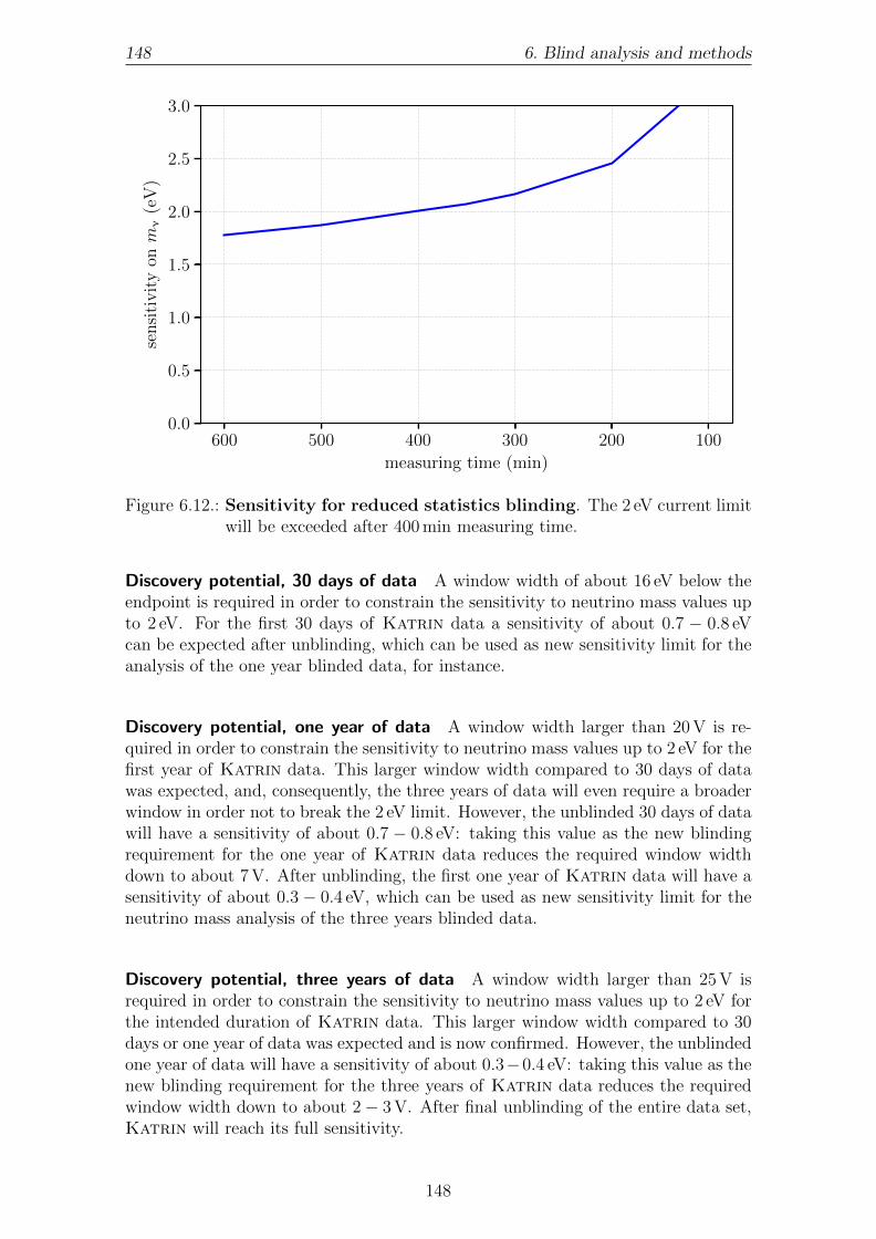
148 6. Blind analysis and methods
100200300400500600
measuring time (min)
0.0
0.5
1.0
1.5
2.0
2.5
3.0
sen
siti
vit
yon
mν
(eV
)
Figure 6.12.: Sensitivity for reduced statistics blinding. The 2 eV current limitwill be exceeded after 400 min measuring time.
Discovery potential, 30 days of data A window width of about 16 eV below theendpoint is required in order to constrain the sensitivity to neutrino mass values upto 2 eV. For the first 30 days of Katrin data a sensitivity of about 0.7 − 0.8 eVcan be expected after unblinding, which can be used as new sensitivity limit for theanalysis of the one year blinded data, for instance.
Discovery potential, one year of data A window width larger than 20 V is re-quired in order to constrain the sensitivity to neutrino mass values up to 2 eV for thefirst year of Katrin data. This larger window width compared to 30 days of datawas expected, and, consequently, the three years of data will even require a broaderwindow in order not to break the 2 eV limit. However, the unblinded 30 days of datawill have a sensitivity of about 0.7 − 0.8 eV: taking this value as the new blindingrequirement for the one year of Katrin data reduces the required window widthdown to about 7 V. After unblinding, the first one year of Katrin data will have asensitivity of about 0.3 − 0.4 eV, which can be used as new sensitivity limit for theneutrino mass analysis of the three years blinded data.
Discovery potential, three years of data A window width larger than 25 V isrequired in order to constrain the sensitivity to neutrino mass values up to 2 eV forthe intended duration of Katrin data. This larger window width compared to 30days or one year of data was expected and is now confirmed. However, the unblindedone year of data will have a sensitivity of about 0.3−0.4 eV: taking this value as thenew blinding requirement for the three years of Katrin data reduces the requiredwindow width down to about 2− 3 V. After final unblinding of the entire data set,Katrin will reach its full sensitivity.
148

6.4. Sensitivity estimates 149
Sensitivity To estimate the sensitivities for the three data sets mentioned in thissection, the intersection points of the discovery potentials with the 1.645σ greyedregion are found. Plotting these as a function of the window width yields the blindedsensitivity curves shown in fig. 6.13. It can be seen that the first Katrin neutrinomass data would require a blinding window width of 16 V in order to constrain thesensitivity to neutrino mass values up to 2 eV. 30 days of Katrin data is expectedto have a sensitivity of about 0.7− 0.8 eV, which taken as new blinding limit wouldyield a window width of about 7 V for the first year of Katrin neutrino mass data.Again, taking the upper limit derived from the first year (about 0.3− 0.4 eV) as thenew blinding limit yields a required window of at least 2− 3 V for the blind analysisof the full three years of Katrin data. If this step-wise approach is not followed, ithas to be noted that the 2 eV limit requires much larger windows for the one yearand three years of Katrin data.
0 5 10 15 20 25 30
window width (V)
1
2
3
4
sen
siti
vit
yon
mν
(eV
)
30 d
1 yr
3 yr
Figure 6.13.: Sensitivity for window blinding. In this scenario, the 2 eV limit canbe met with different window widths for the different data sets. Theupper limit derived from the shorter data taking period will serve asblinding limit for the next longer data taking period. Window widthslarger than 25 V lead to fitting problems for the 30 days of data.
6.4.1.3. Energy smearing
As for the window blinding method, different measuring times are also worth inves-tigating for the energy smearing method. This is because less measuring time resultsin larger statistical fluctuations, which might be diluted by large smearing values.It is expected that at some point, the increased smearing outweighs the statisticalfluctuations and thereby worsens the sensitivity beyond the statistical uncertainty.Furthermore, it is expected that the neutrino mass squared shift induced by the
149

150 6. Blind analysis and methods
energy smearing follows a −2σ2smear relation [RK88], resulting in a parabola for the
total uncertainty eq. (6.7).
Discovery potential A smearing of about 1 eV is required for the first 30 daysof data. This matches the expectation of δ
m2ν≈ −2σ2
smear and confirms that thestatistical uncertainty of the first 30 days will have to be compensated for by a largeartificial systematic effect to reach sufficient blinding. The same smearing is requiredfor one year and three years of data, which confirms that the sensitivity needs to bedecreased by the systematic effect caused by the smearing.
Sensitivity As for the window blinding, the sensitivity for each of the three datasets (30 days, one year, three years) is evaluated separately and shown in one plot.The intersection points of the discovery potentials with the 1.645σ greyed regionare found and the results shown as a function of the energy smearing. Fig. 6.14confirms the expectation from the discovery potential plots, in that the sensitivity isindependent of the statistics above smearing values of σsmear ≈ 0.75 eV since this iswhere the smearing starts to dominate over statistics. Similar to the window blind-ing, different smearing values can be chosen for the different data sets, respectingthe fact that the upper limit from the last analysed data set can be taken as newblinding limit.
If the step-wise data approach is not followed, the energy smearing - in contrast tothe window blinding methods - does not require larger smearing values for the longerdata periods, due to the method being based on a deliberate systematic influencerather than worse statistics.
Knowledge of the analysts So far, no assumptions have been made concerning theanalysis of the energy smeared Katrin data. The estimation of the total uncertaintyvia eq. (6.7) assumes that the analysts know the systematic uncertainty caused bythe blinding. However the approximate relation of δ
m2ν≈ −2σ2
smear enables analyststo estimate the level of smearing used and in theory correct for the smearing effect.Therefore it is foreseen to hide the smearing value and only reveal to the analysts thatthe smearing was chosen from some interval. For now, let us assume we chose from auniform distribution of the smearing values in the interval [a, b]. This would requirethe analysts to make assumptions about the smearing. One natural assumptionwould be using the mean of the uniform distribution to estimate the smearing relatedneutrino mass shift and account for it in the analysis. However, this would requireinclusion of the distribution of all possible neutrino mass shifts as an uncertainty;the neutrino mass shift δ
m2ν
in eq. (6.7) becomes the standard deviation of a uniformdistribution:
δm
2ν→ σ2
blind = (β − α)2
12 , (6.25)
with α ≈ −2a2 and β ≈ −2b2 representing the minimum and maximum neutrinomass squared shift. If we sample the smearing from the maximum interval [0, b], thiswill become
σ2blind = β2
12 , (6.26)
150
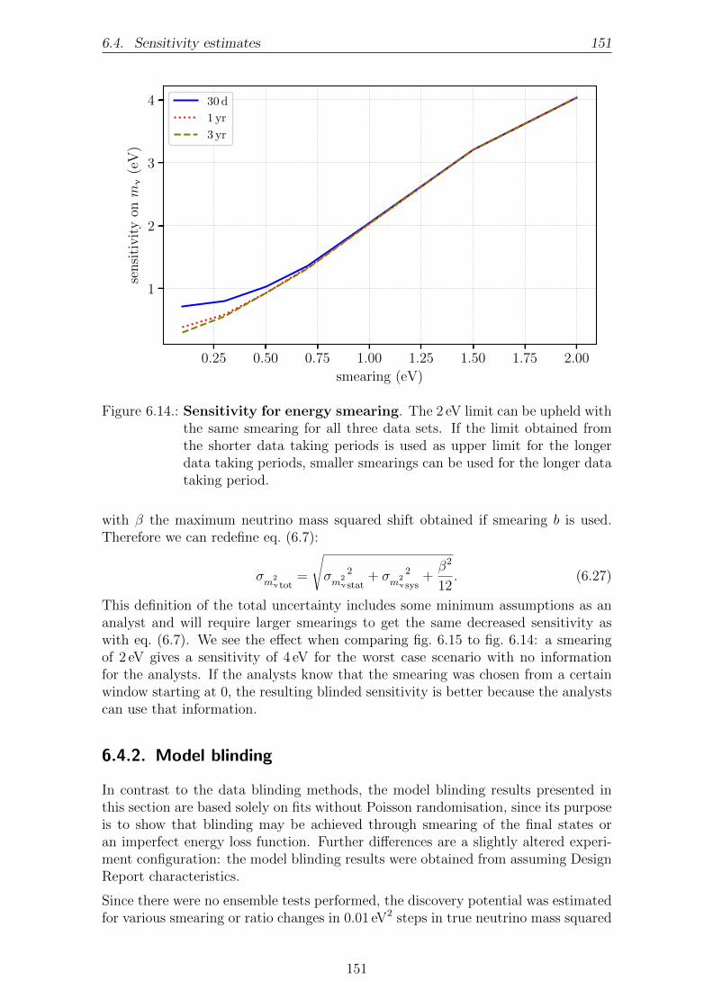
6.4. Sensitivity estimates 151
0.25 0.50 0.75 1.00 1.25 1.50 1.75 2.00
smearing (eV)
1
2
3
4
sen
siti
vit
yon
mν
(eV
)
30 d
1 yr
3 yr
Figure 6.14.: Sensitivity for energy smearing. The 2 eV limit can be upheld withthe same smearing for all three data sets. If the limit obtained fromthe shorter data taking periods is used as upper limit for the longerdata taking periods, smaller smearings can be used for the longer datataking period.
with β the maximum neutrino mass squared shift obtained if smearing b is used.Therefore we can redefine eq. (6.7):
σm
2ν tot
=√σm
2ν
2stat
+ σm
2ν
2sys
+ β2
12 . (6.27)
This definition of the total uncertainty includes some minimum assumptions as ananalyst and will require larger smearings to get the same decreased sensitivity aswith eq. (6.7). We see the effect when comparing fig. 6.15 to fig. 6.14: a smearingof 2 eV gives a sensitivity of 4 eV for the worst case scenario with no informationfor the analysts. If the analysts know that the smearing was chosen from a certainwindow starting at 0, the resulting blinded sensitivity is better because the analystscan use that information.
6.4.2. Model blinding
In contrast to the data blinding methods, the model blinding results presented inthis section are based solely on fits without Poisson randomisation, since its purposeis to show that blinding may be achieved through smearing of the final states oran imperfect energy loss function. Further differences are a slightly altered experi-ment configuration: the model blinding results were obtained from assuming DesignReport characteristics.
Since there were no ensemble tests performed, the discovery potential was estimatedfor various smearing or ratio changes in 0.01 eV2 steps in true neutrino mass squared
151
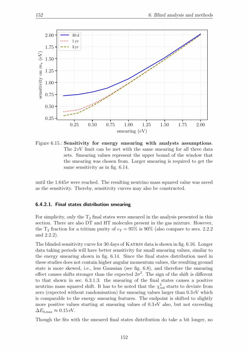
152 6. Blind analysis and methods
0.25 0.50 0.75 1.00 1.25 1.50 1.75 2.00
smearing (eV)
0.25
0.50
0.75
1.00
1.25
1.50
1.75
2.00se
nsi
tivit
yon
mν
(eV
)30 d
1 yr
3 yr
Figure 6.15.: Sensitivity for energy smearing with analysts assumptions.The 2 eV limit can be met with the same smearing for all three datasets. Smearing values represent the upper bound of the window thatthe smearing was chosen from. Larger smearing is required to get thesame sensitivity as in fig. 6.14.
until the 1.645σ were reached. The resulting neutrino mass squared value was savedas the sensitivity. Thereby, sensitivity curves may also be constructed.
6.4.2.1. Final states distribution smearing
For simplicity, only the T2 final states were smeared in the analysis presented in thissection. There are also DT and HT molecules present in the gas mixture. However,the T2 fraction for a tritium purity of εT = 95% is 90% (also compare to secs. 2.2.2and 2.2.2).
The blinded sensitivity curve for 30 days of Katrin data is shown in fig. 6.16. Longerdata taking periods will have better sensitivity for small smearing values, similar tothe energy smearing shown in fig. 6.14. Since the final states distribution used inthese studies does not contain higher angular momentum values, the resulting groundstate is more skewed, i.e., less Gaussian (see fig. 6.8), and therefore the smearingeffect causes shifts stronger than the expected 2σ2. The sign of the shift is differentto that shown in sec. 6.3.1.3: the smearing of the final states causes a positiveneutrino mass squared shift. It has to be noted that the χ2
red starts to deviate fromzero (expected without randomisation) for smearing values larger than 0.3 eV whichis comparable to the energy smearing features. The endpoint is shifted to slightlymore positive values starting at smearing values of 0.3 eV also, but not exceeding∆E0,max ≈ 0.15 eV.
Though the fits with the smeared final states distribution do take a bit longer, no
152

6.4. Sensitivity estimates 153
0.2 0.4 0.6 0.8 1.0
FSD smearing (eV)
0.5
1.0
1.5
2.0
2.5
3.0se
nsi
tivit
yon
mν
(eV
)
Figure 6.16.: Sensitivity for FSD smearing. The 2 eV limit can be met witha similar smearing value as for the energy smearing (O(1 eV), com-pare fig. 6.14). This result represents 30 days of simulated data. Thelonger data sets will only have better blinded sensitivity for small FSDsmearing values, below 0.5 eV.
strong bias in any of the other estimated parameters could be observed. More im-portantly, the method can blind the neutrino mass by inducing a (positive) neutrinomass squared shift.
6.4.2.2. Imperfect energy loss function
As mentioned in sec. 6.3.2.2, the modification of the energy loss function offers thepossibility to control the sign of the induced neutrino mass shift. Indeed, fig. 6.17reveals that the neutrino mass sensitivity is decreased in both directions of the ratiochange η. From eqs. (6.18), (6.19), and (6.20) it can be understood that a positiveη causes a reduction of the relative excitation share (and increase of the ionisationshare), and vice versa for negative values of η. Figure 6.17 covers both extremes, alarge artificial increase of the ionisation share (positive η) as well as a large increaseof the excitation share (negative η). Due to the construction via eqs. (6.19) and(6.20), there is a maximum value of 0.597 for η [Sib18]. Since the positive η cannotprovide sufficient blinded sensitivities, the negative η need to be explored. Howeverit has to be noted that the required η ≈ −0.7 results in a very different energy lossfunction than the original one (compare fig. 6.10). Furthermore, it does not onlyhide the neutrino mass but also causes large biases to the other parameters [Sib18],which is the reason why this method is considered inferior to the other blindingmethods discussed so far.
153
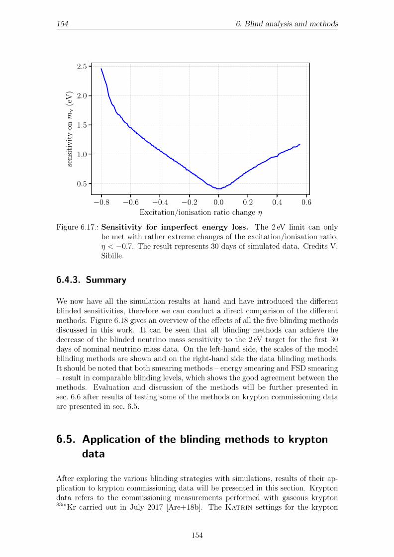
154 6. Blind analysis and methods
−0.8 −0.6 −0.4 −0.2 0.0 0.2 0.4 0.6
Excitation/ionisation ratio change η
0.5
1.0
1.5
2.0
2.5se
nsi
tivit
yon
mν
(eV
)
Figure 6.17.: Sensitivity for imperfect energy loss. The 2 eV limit can onlybe met with rather extreme changes of the excitation/ionisation ratio,η < −0.7. The result represents 30 days of simulated data. Credits V.Sibille.
6.4.3. Summary
We now have all the simulation results at hand and have introduced the differentblinded sensitivities, therefore we can conduct a direct comparison of the differentmethods. Figure 6.18 gives an overview of the effects of all the five blinding methodsdiscussed in this work. It can be seen that all blinding methods can achieve thedecrease of the blinded neutrino mass sensitivity to the 2 eV target for the first 30days of nominal neutrino mass data. On the left-hand side, the scales of the modelblinding methods are shown and on the right-hand side the data blinding methods.It should be noted that both smearing methods – energy smearing and FSD smearing– result in comparable blinding levels, which shows the good agreement between themethods. Evaluation and discussion of the methods will be further presented insec. 6.6 after results of testing some of the methods on krypton commissioning dataare presented in sec. 6.5.
6.5. Application of the blinding methods to kryptondata
After exploring the various blinding strategies with simulations, results of their ap-plication to krypton commissioning data will be presented in this section. Kryptondata refers to the commissioning measurements performed with gaseous krypton83mKr carried out in July 2017 [Are+18b]. The Katrin settings for the krypton
154

6.5. Application of the blinding methods to krypton data 155
0.5 1.0 1.5 2.0sensitivity on mν (eV)
0.2
0.3
0.4
0.5
0.6
0.7
0.8
0.9
1.0
FS
Dsm
eari
ng
(eV
)
0
20
40
60
80
100
Liv
e-ti
me
(h)
0.2
0.4
0.6
0.8
1.0E
xci
tati
on/i
onis
atio
nch
ange−η
0.0
2.5
5.0
7.5
10.0
12.5
15.0
17.5
20.0
Win
dow
wid
th(V
)
0.2
0.3
0.4
0.5
0.6
0.7
0.8
0.9
1.0
En
ergy
smea
rin
g(e
V)
Figure 6.18.: Sensitivity summary. The 2 eV limit can be met with every blindingmethod. These results represent 30 days of simulated data.
commissioning measurements are described in detail in [Are+18b] and will brieflybe recapitulated here. The gaseous 83mKr campaign served as a first test run ofpure 83mKr spectroscopy without any carrier gas. Gaseous 83mKr was injected at thepump port PP2-F of the WGTS cryostat (compare sec. 3) via a dedicated kryptongenerator [Are+18b, SVS17, Sen+18] and pumped out at the CPS which was theonly active pump running. A further difference in the krypton-mode set-up is thebeam tube temperature of the WGTS: in 83mKr mode, the temperature is increasedfrom 30 K (tritium mode) to 100 K to prevent 83mKr freeze-out.
In the course of this thesis, the 83mKr data is used to establish a first technical imple-mentation of the necessary tools on a real data set and as a cross-check and validationof the data blinding methods. Therefore, the main interest is on relative changesof the parameters when fitting blinded instead of unblinded data. Despite markeddifference between the mono-energetic krypton conversion electron lines comparedto the continuous β-decay spectrum, this test implementation yields helpful insightsbecause the krypton line spectrum is well known. Therefore, the impact on blindingtechniques on the reconstruction of the spectrum can be studied. The krypton runused for the fits is run 33165, with run summary version 2c (also compare tab. 6.1).
83mKr produces a conversion-electron spectrum containing several lines. In the fol-lowing, focus will be on investigating the data blinding effect on the K-32 conversionline from 83mKr. In the differential spectrum, the lines are defined as a Voigt pro-file with a Gaussian broadening [Are+18b]. The integrated spectrum of a line hasthe inverse transmission form, as can be seen from fig. 6.19 (for the cuts used seetab. 6.1). Similar to tritium fitting, krypton fitting requires four parameters:
1. background rate Bg,
2. line position,
155
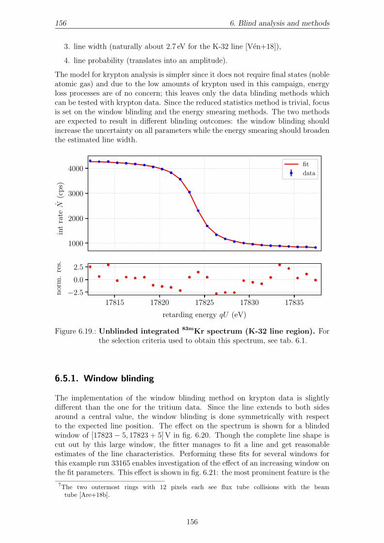
156 6. Blind analysis and methods
3. line width (naturally about 2.7 eV for the K-32 line [Ven+18]),
4. line probability (translates into an amplitude).
The model for krypton analysis is simpler since it does not require final states (nobleatomic gas) and due to the low amounts of krypton used in this campaign, energyloss processes are of no concern; this leaves only the data blinding methods whichcan be tested with krypton data. Since the reduced statistics method is trivial, focusis set on the window blinding and the energy smearing methods. The two methodsare expected to result in different blinding outcomes: the window blinding shouldincrease the uncertainty on all parameters while the energy smearing should broadenthe estimated line width.
1000
2000
3000
4000fit
data
17815 17820 17825 17830 17835
retarding energy qU (eV)
−2.5
0.0
2.5
int
rateN
(cp
s)n
orm
.re
s.
Figure 6.19.: Unblinded integrated 83mKr spectrum (K-32 line region). Forthe selection criteria used to obtain this spectrum, see tab. 6.1.
6.5.1. Window blinding
The implementation of the window blinding method on krypton data is slightlydifferent than the one for the tritium data. Since the line extends to both sidesaround a central value, the window blinding is done symmetrically with respectto the expected line position. The effect on the spectrum is shown for a blindedwindow of [17823 − 5, 17823 + 5] V in fig. 6.20. Though the complete line shape iscut out by this large window, the fitter manages to fit a line and get reasonableestimates of the line characteristics. Performing these fits for several windows forthis example run 33165 enables investigation of the effect of an increasing window onthe fit parameters. This effect is shown in fig. 6.21: the most prominent feature is the
7The two outermost rings with 12 pixels each see flux tube collisions with the beamtube [Are+18b].
156
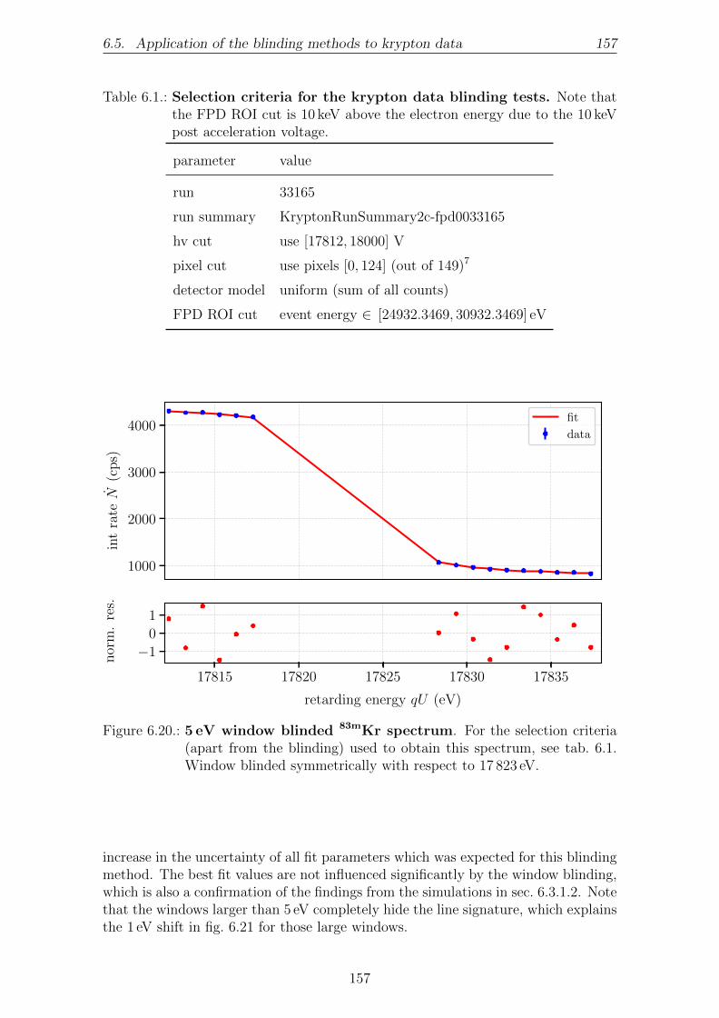
6.5. Application of the blinding methods to krypton data 157
Table 6.1.: Selection criteria for the krypton data blinding tests. Note thatthe FPD ROI cut is 10 keV above the electron energy due to the 10 keVpost acceleration voltage.
parameter value
run 33165
run summary KryptonRunSummary2c-fpd0033165
hv cut use [17812, 18000] V
pixel cut use pixels [0, 124] (out of 149)7
detector model uniform (sum of all counts)
FPD ROI cut event energy ∈ [24932.3469, 30932.3469] eV
1000
2000
3000
4000fit
data
17815 17820 17825 17830 17835
retarding energy qU (eV)
−1
0
1
int
rateN
(cp
s)n
orm
.re
s.
Figure 6.20.: 5 eV window blinded 83mKr spectrum. For the selection criteria(apart from the blinding) used to obtain this spectrum, see tab. 6.1.Window blinded symmetrically with respect to 17 823 eV.
increase in the uncertainty of all fit parameters which was expected for this blindingmethod. The best fit values are not influenced significantly by the window blinding,which is also a confirmation of the findings from the simulations in sec. 6.3.1.2. Notethat the windows larger than 5 eV completely hide the line signature, which explainsthe 1 eV shift in fig. 6.21 for those large windows.
157

158 6. Blind analysis and methods
0
1
succ
ess/
tota
lfi
ts
0.00
0.25
0.50
0.75
1.00
σp
os
(eV
)
0.0 2.5 5.0 7.5
window width (eV)
3.50
3.75
4.00
4.25
4.50
Lin
ep
os(e
V)
[+1.
782×
104]
0.8
0.9
1.0L
ine
wid
th(e
V)2
[×10
1]
3.12
3.14
3.16
3.18
Lin
ep
rob
[×10
3]
7.05
7.10
7.15
7.20
7.25
7.30
Bg
(cp
s)[×
102]
1.5
2.0
2.5
3.0
χ2 re
d
0.0
0.5
1.0
1.5
2.0
2.5
σw
idth
(eV
)2
1
2
3
4
5
σpro
b[×
101]
0.25
0.50
0.75
1.00
1.25
σBg
(cp
s)[×
101]
−4
−2
0
2
4
σχ
2 red
[×10−
2]
Figure 6.21.: Window width dependence of 83mKr fit parameters. Plots sharethe x-axis, results are for run 33165. There is a clear increase of allparameter uncertainties with increasing window width.
6.5.2. Energy smearing
To test the energy smearing method, the same algorithm was used as presented insec. 6.3.1.3. However, due to the limited energy range scanned in the krypton mea-surements, it is expected that large smearings will result in very distorted spectra.The reason is that on both edges of the scanned energy range the smearing willcause artefacts due to non-conservation of counts. Nonetheless the most prominent
158

6.5. Application of the blinding methods to krypton data 159
feature should be the broadening of the line width, regardless of what happens tothe other parameters. Indeed, fig. 6.22 shows that, for an extreme smearing value of5 eV, the line width is broadened significantly. Though the smearing in this example
1000
2000
3000
4000fit
data
17815 17820 17825 17830 17835
retarding energy qU (eV)
0
100
int
rateN
(cp
s)n
orm
.re
s.
Figure 6.22.: 5 eV energy smeared 83mKr spectrum. For the selection criteriaused to obtain this spectrum, see tab. 6.1.
is rather extreme, the fitter manages to estimate reasonable values for the fit pa-rameters except for the background: due to the large smearing and small number ofmeasurement points above the line position, which could catch the smeared countsfrom lower voltages, the smeared counts at the upper energy edge are lost. Thatleads to a negative estimate of the background rate in this extreme case, which isattributed to the small scanned energy range. In nominal neutrino mass measure-ments, voltage steps at least 10− 20 V above the endpoint are foreseen which wouldcatch smearing values up to 4 eV with 5σsmear. Investigating the effect of differentsmearings for the example run 33615 yields the systematic change of the smearingto the estimated parameters. Indeed, fig. 6.23 reveals that besides a large increasein χ2
red, the line width is increased by the smearing. The strong dependence of thebackground rate can be explained by the end effects caused by the smearing; thereare simply not enough measuring points above the line position to catch the smearedcounts. Notably uninfluenced by the smearing is the line position, which changes –as expected – only marginally with the smearing.
6.5.3. Summary
The test of the two data blinding methods, energy smearing and window blinding,on krypton data may also be used to perform a blind analysis of future kryptonspectra with Katrin. Though the krypton spectrum (mono-energetic line) is notdirectly comparable to the tritium spectrum (continuous spectrum), this represents
159

160 6. Blind analysis and methods
0
1
succ
ess/
tota
lfi
ts
0.5
1.0
1.5
σp
os
(eV
)[×
10−
2]
0 2 4
smearing (eV)
6
7
8
9
Lin
ep
os(e
V)
[×10−
2+
1.78
245×
104]
0.0
0.5
1.0
1.5L
ine
wid
th(e
V)2
[×10
2]
3.5
4.0
4.5
Lin
ep
rob
[×10
3]
0
2
4
6
Bg
(cp
s)[×
102]
0.5
1.0
1.5
2.0
2.5
χ2 re
d[×
101]
0
1
2
3
σw
idth
(eV
)2
0.5
1.0
1.5
2.0
σpro
b[×
101]
0.2
0.4
0.6
0.8
1.0
1.2
σBg
(cp
s)[×
101]
−4
−2
0
2
4
σχ
2 red
[×10−
2]
Figure 6.23.: Energy smearing dependence of 83mKr fit parameters. Plotsshare the x-axis, results are for run 33165. There is a clear increaseof the line width and also large changes in χ2
red and the estimatedbackground rate observed.
an important cross-check. More importantly, this proof of principle is the first testof the implementation of the data blinding technique into the complete data-analysischain of Katrin from the Intermediate Data LayEr (IDLE) to the run summarystage and fitting software.
160
6.6. Discussion 161
6.6. Discussion
Performing a blind analysis always comes at a price during the blind phase andrequires careful planning beforehand. At Katrin, the cost of an unbiased neutrinomass analysis is either the complication of estimation of nuisance parameters andsystematics (data blinding) or the blinding is hard to control and enforce (modelblinding). However, there are ways to reduce these costs of the targeted blindingstrategy, which will be discussed in this section.
Data versus model blinding The most distinctive difference between data andmodel blinding is the implied level of control. If applying data blinding, all the usershave to use the blinded data, for model blinding it is in the responsibility of theanalysts to use the blinded model. A possible way to supervise the implementationof blinding is to use a hash in the model that checks whether, for instance, thesmeared final states are used in the neutrino mass fit. When only fitting endpoint,amplitude and background the unsmeared final states could even be used. Thischeck is mainly meant to prevent fitting the neutrino mass with unblinded model byaccident rather than forcing users to use the blinded model.
First Tritium conclusions One major outcome of the First Tritium campaign isthe fact that the model describes the data rather well [Are+19], also see sec. 5.3,and the fits work out of the box without applying a-posteriori modifications to themodel. This opens new perspectives also for the blind analysis: run-wise fits tothe unblinded data can be included in the automated run-processing right after thegeneration of the run summaries, as shown in fig. 2.8. These fits either hide theneutrino mass if fit or fix the neutrino mass, such that the fit results can be usedas a stability control and thereby as a measure of data quality. A crucial point ofthese automated fits is that the cuts (ROI of the FPD, energy range of the tritiumspectrum, etc.) are fixed before the data taking period starts and are left unchanged.
Implicit blinding A different option, which has not been discussed so far, is im-plicit blinding. This would give users full access to all data, with the possibility tosystematically check the effect of adapting cuts in the analysis. The collaborationacceptance of any kind of analysis related to the neutrino mass would then implypoint-by-point cross-checks and validation of all analysis steps. In order to maintainand safeguard unbiased neutrino mass data analysis, all cuts need to be justifiedwithout considering their effect on the neutrino mass. However, there is still the riskof unconsciously working towards an expected value without blinding.
6.6.1. Reduced statistics
The reduced statistics method provides access to the whole energy range analysedwith Katrin, without causing any changes to the shape of the spectrum. However,the β-spectrum measurement will be statistics dominated in the beginning. There-fore, the sensitivity will improve quickly and within 6 − 7 h of measuring time, the2 eV limit will be exceeded. That drastically reduces the blinded time range for a
161

162 6. Blind analysis and methods
statistically blind neutrino mass analysis and relies on automated fits in the runprocessing to detect long-term drifts of fit parameters or systematic effects.
6.6.2. Window blinding
Hiding the events within a specific window around the signal region to perform anunbiased analysis is a technique well-known, for instance, from 0νββ decay searches(see e.g. [Ago+13]). As a data blinding method it provides strong control andcan also be used to perform blind analysis of data taken after the first unblinding.Simulations in this work reveal that the removal of a window below the endpoint doesnot lead to a systematic bias of the parameter estimates8, while the uncertainty onthe neutrino mass can be increased by increasing the window width. As a downside,the window has to be quite large (about 16 V) for the first neutrino mass analysisand also studies of systematic effects in the endpoint region are complicated. Inorder to use all data available, these studies would need to be done by analysts notinvolved in neutrino mass analysis. On the other hand, the closer Katrin gets tothe end of neutrino mass data taking, the smaller the window can be in order to be“blind enough”. Together with the long-term experience gained at that point, thismakes the window blinding method a suitable candidate for the final neutrino massanalysis of Katrin data.
6.6.3. Energy smearing
The idea of smearing out the neutrino mass signal in Katrin data intrinsicallyinvolves a change of the spectral shape which might also smear out unexpectedfeatures in the spectrum. The shift of the estimated blinded neutrino mass has afixed direction, for which an expectation of δm2
ν ≈ −2σ2smear can be applied. However,
despite the strong control due to its data blinding nature, the energy smearing allowsfull access to the whole spectrum, providing full statistics to detect relative drifts.Also note that the smearing will happen in the automated run processing insidethe intermediate data layer (IDLE), resulting in blinded run summaries (comparefig. 2.8). The raw data will always be available for full check of systematics. It isconsidered unlikely that analysts are willing to rebuild the complete analysis chainfrom raw data until preprocessed run summaries to get unblinded neutrino massdata. Also note the effect of analysts knowing the range the smearing was chosenfrom: this knowledge combined with the fixed direction of the shift requires largersmearing values (see sec. 6.4.1.3).
6.6.4. Final states distribution smearing
Similar to the energy smearing, the smearing of the final states distribution relieson hiding the neutrino mass signal in a change of the spectral shape. The maindifference is that the FSD smearing applies model blinding and therefore is built onthe responsibility of the users. The model blinding is targeted to prevent accidentally
8Since it does not cause a modification to the spectral shape.
162
6.6. Discussion 163
revealing the unblinded neutrino mass by misconfiguration of the fitting program,for example. Therefore, it is foreseen to implement a check whether the smearedfinal states are used to fit the neutrino mass. This can be implemented via a hashand opens the possibility of having all data available unblinded. The most recentversion of the final states calculation is not yet made available collaboration-wide,which would enable providing first the “blinded” final states. In an unblinding event,the unsmeared, more accurate final states distribution might then be provided to allanalysts at the same time.
6.6.5. Imperfect energy loss function
As found in sec. 6.4.2.2, the change to the energy loss function to hide the neutrinomass has to be relatively extreme, as shown in this work, though it would providefull statistics of the complete measured spectrum. Despite being a model blindingtechnique and therefore relying on the responsibility of the users, blinding by usingan imperfect energy loss function also faces other issues, as it causes stronger effectson the nuisance parameters than for instance the final states or the energy smearingtechnique. Furthermore, the final Katrin energy loss function has not been mea-sured yet, which intrinsically has some blinding effect. Measuring the energy lossfunction of 18.6 keV electrons in inactive deuterium gas is one of the critical pointsof the STS-IIIa commissioning measurements (conducted in autumn 2018). Thoughthis is not the final T2 energy loss function, discussions during the analysis of the D2energy loss function reveal enough information to construct an energy loss functionthat is deemed “good enough” to break the 2 eV sensitivity limit targeted for thefirst blind analysis. Furthermore, the effect of an artificially worse energy loss func-tion has only been studied on the empirically derived energy loss function formulafrom the Troitsk experiment [Ase+00]. This empirically adapted parametrisationstill shows discrepancies with theoretical calculations [Tro18]. The implications ofthese findings on the applicability of the method on Katrin neutrino mass analysisare therefore not clear at this point.
6.6.6. Implicit blinding
When discussing about blinding techniques, it should not be forgotten that oneoption is to refrain from installing an explicit blinding scheme, but to rely on implicitblinding instead. Despite posing the risk of experimenter’s bias, this would allowfull access by everyone to the complete spectrum measured by Katrin. Detectionof relative drifts would be possible with full statistics as would be systematic studiesin the endpoint region. The experimenter’s bias might as well be caught in thewell-established and accepted analysis review procedure which might reveal a poorbasis or justification for choosing a specific cut (except for its effect on the neutrinomass). However, even if assuming 100% transparency of the analysis, the check ofthe analysis can only be done after the analysis is complete and might not revealthe bias.
163
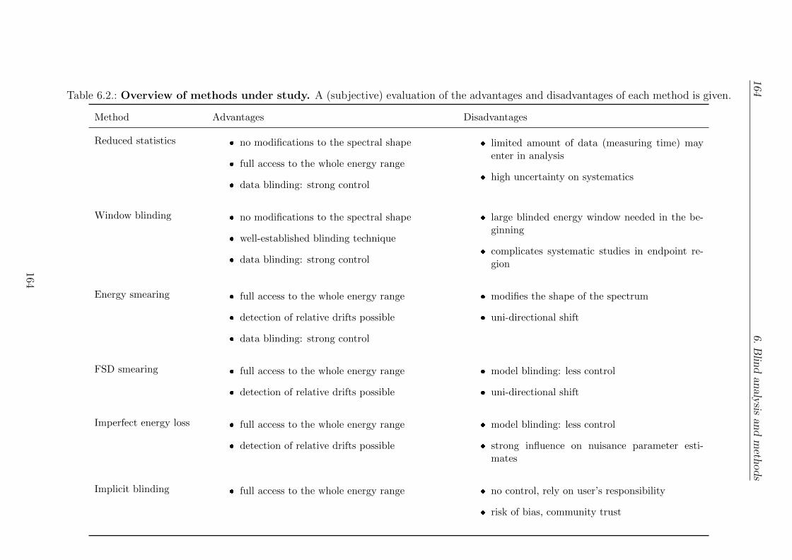
1646.
Blin
dan
alysis
and
meth
ods
Table 6.2.: Overview of methods under study. A (subjective) evaluation of the advantages and disadvantages of each method is given.
Method Advantages Disadvantages
Reduced statistics � no modifications to the spectral shape
� full access to the whole energy range
� data blinding: strong control
� limited amount of data (measuring time) mayenter in analysis
� high uncertainty on systematics
Window blinding � no modifications to the spectral shape
� well-established blinding technique
� data blinding: strong control
� large blinded energy window needed in the be-ginning
� complicates systematic studies in endpoint re-gion
Energy smearing � full access to the whole energy range
� detection of relative drifts possible
� data blinding: strong control
� modifies the shape of the spectrum
� uni-directional shift
FSD smearing � full access to the whole energy range
� detection of relative drifts possible
� model blinding: less control
� uni-directional shift
Imperfect energy loss � full access to the whole energy range
� detection of relative drifts possible
� model blinding: less control
� strong influence on nuisance parameter esti-mates
Implicit blinding � full access to the whole energy range � no control, rely on user’s responsibility
� risk of bias, community trust
164

6.7. Conclusion and outlook 165
6.6.7. Unblinding
If the Katrin collaboration decides to perform a blind analysis, commitment is madeto publish the result swiftly after unblinding. There is also the option to publish ablinded and an unblinded result, posing full transparency to the community and allinformation about the analysis. What is still to be defined is the road to unblinding:which criteria does the respective analysis need to fulfil, which checkpoints doesit have to pass? Answers to those questions are directly related to the blindingtechnique used, therefore these criteria can only be fully defined after the decisionfor a certain blinding strategy has been made.
As a collaboration it is certainly a great moment to unblind an analysis. Independentof the method used, an “unblinding event” will bring together many members of theKatrin collaboration in one place. The revealing of the blinding key is eithergranting access to the unblinded data or allowing analysts to use the unblindedmodel. Either way, the final analysis can be performed during this “unblindingevent” and the result published shortly afterwards.
6.7. Conclusion and outlook
None of the Katrin predecessor neutrino mass β-decay experiments (Los Alamos,Troitsk, and Mainz) performed a blind analysis of the measured tritium spectrum.This makes the presented blinded studies the first application of blinding techniquesin neutrino mass β-decay spectroscopy. Intrinsically, this involved testing variousmethods with respect to their potential to blind the neutrino mass to a level com-parable to the current experimental knowledge of bounds on the neutrino mass.
In the course of this chapter, two different roads for a blind neutrino mass analysisof Katrin data have been presented: data and model blinding. The three datablinding methods (reduced statistics, window blinding, and energy smearing) andtwo model blinding methods (FSD smearing and imperfect energy loss function)were investigated not only with simulations and ensemble tests, but also have beensuccessfully implemented for and tested on krypton data. An application of theblinding tests to tritium data from the First Tritium campaign has been startedin the scope of this thesis, and is currently still under investigation – with verypromising preliminary results. All methods presented so far enable performing ablind neutrino mass analysis of Katrin data with an artificially decreased sensitivitybelow the current limit on the neutrino mass.
The discussion of the individual strengths and weaknesses of the five methods yieldedseveral points in favour or against each specific method (compare tab. 6.2). Con-cerning the first neutrino mass analysis of Katrin data, the author favours to blindthe model. Though the commissioning measurements from the First Tritium cam-paign [Are+19] showed great agreement between model and data, the nominal highstatistics data from a tritium purity larger by a factor of 200 might reveal featuresthat are hidden in the low statistics of the First Tritium data. Therefore, it isproposed to use the first 30 d of nominal Katrin data as a test run with auto-mated unblinded fits9 while applying FSD smearing model blinding on the analyst
9With fixed cuts in the run processing chain, either hiding or fixing the neutrino mass estimate.
165

166 6. Blind analysis and methods
side. The smeared final states will be provided to the analysts beforehand, withthe smearing value hidden. As discussed in sec. 6.6.4, the analysts have to ensurethat any neutrino mass analysis they perform before unblinding is using the smearedversion of the final states via a hash-check in the fitter. Due to the importance ofthe first neutrino mass data, it could be considered to blind the data additionallyto the model. For a combination of energy smearing and final states smearing withboth smearings unknown, it is impossible to guess the neutrino mass shift as thetwo cause opposite effects. After the first “unblinding event”, Katrin could thusenvision a neutrino mass sensitivity in the sub-eV range.
This intermediate sensitivity would subsequently serve as the blinded limit for thenext data taking period. Since in this scenario the unblinded FSD would havebeen distributed in the course of the unblinding, either a new method has to beused for the next 1 yr of data taking, or a new version of the blinded FSD has tobe distributed. During the first 30 d of nominal Katrin operation, more cross-checks and data quality measures will be established aside to fit parameter stabilityto ensure adequate operation of the Katrin experiment. This will enable usingdata blinding to ensure unbiased analysis of the next Katrin neutrino mass data.Furthermore, the amount of data blinding necessary to meet the 0.7-0.8 eV sensitivitywith the 1 yr data is reduced a lot compared to the initial 2 eV: for window blinding,the window can be as small as about 7 V while the energy smearing can be as smallas 0.5 eV (without revealing its interval) or 0.75 eV (if revealing its interval). Alsothe experience gained during the Krypton and the First Tritium campaigns plus thefirst 30 d of nominal Katrin data will help in determining whether Katrin runsas expected. For the full 3 yrs of Katrin data, the window blinding is the methodfavoured by the author: it requires only a window of about 2 − 3 V to hold the0.3−0.4 eV sensitivity which could be targeted within about the first year of nominalKatrin data. Compared to the measuring time interval that could be spread overmore than 50 V, this is a price that might seem affordable to get a well-trusted andwell-received final neutrino mass analysis. The energy smearing, by contrast, wouldintrinsically impose a change of the spectral shape which might hide features over abroader range than the 2− 3 V hidden by the window blinding.
166
CHAPTER 7
PHYSICS BEYOND THE NEUTRINO MASS
“All of physics is either impossible or trivial. It is impossible until you understandit, and then it becomes trivial.”
– Sir Ernest Rutherford –
The evidence of non-zero neutrino masses [Fuk+98, Ahm+01] has opened the doortowards an extension of the established Standard Model of particle physics (SM):in the SM, neutrinos are treated as massless (see sec. 1.1.2) and a consistent the-ory to explain the non-zero mass has not yet been established. In this sense, thedetermination of the neutrino mass itself already will shed a light on “new physics”.
But besides determining the neutrino mass with sensitivity improved by one orderof magnitude, the precision tritium β-spectrum to be measured with Katrin alsopromises a chance at testing interesting new physics. One such opportunity, exam-ined in [Mer+15], are sterile neutrinos at the keV scale, which form well-motivatedcandidates for warm dark matter, or at the eV scale [FB11, SH11, EO12, Kle14], mo-tivated through various anomalies observed in short-baseline neutrino oscillations.In the thesis at hand, three more cases are investigated:
1. exotic light bosons which could be emitted during the β-decay, resulting in a4-body decay,
2. hypothetical right-handed currents which might occur symmetrically to thestandard left handed currents of the weak interaction,
3. the capture of relic neutrinos which trace back to the very beginning of ouruniverse.
This chapter describes how the corresponding physics models are implemented inthe Katrin analysis and simulation frameworks SSC and KaFit. Thereby, thesensitivity of Katrin to constrain parameters of these new physics models can betested. At the end of this chapter, a conclusion summarises the findings and givesan overview of the results.
167
168 7. Physics beyond the neutrino mass
7.1. Light bosons
New physics often is expected to manifest at high energies. However, with recentmore stringent bounds on heavy particles from collider experiments, the interest ofparticle-physics phenomenology is also drawn towards “light” new physics. With anenergy range in the β-decay of tritium of up to 18.6 keV, the Katrin experimentis well positioned to probe new physics on the eV to keV-scale. The following sec-tion will deal with the hypothetical emission of light bosons (pseudoscalar or vectorbosons) from the neutrino and electron of tritium β-decay. This scenario was recentlyproposed by W. Rodejohann and coworkers and has been studied in [Arc+18]. In thecourse of the thesis at hand, the proposed scenarios were implemented into the Ka-trin analysis framework to derive the statistical sensitivity of Katrin in terms ofconstraining the additional emission of eV-scale light bosons, which is also describedin ref. [Arc+18]. The keV-scale statistical sensitivity included in the same work wasderived by M. Slezak and is described in this chapter to complete the picture of thetwo different mass regimes.
First, the experimental electron spectrum with this additional new interaction isintroduced. Afterwards, the potential of Katrin to constrain the additional emis-sion of light bosons in β-decay is estimated for the current Katrin set-up1, thatis, in a limited energy range close to the spectral endpoint, and also for a potentialmodification with a future TRISTAN-like detector [Mer+15, Mer+18] to access thefull energy range in a differential spectrum measurement.
7.1.1. Behaviour of the spectral shape by introducing a lightboson
The standard β-decay investigated by Katrin is a three-body decay resulting in thetransformation of tritium into helium and production of an electron anti-neutrinotogether with an electron (see eq. 2.1). The decay energy of 18.6 keV may alsoproduce additional particles like a light boson with masses up to 18.6 keV, whichwould result in a four-body decay
T→ 3He+ + e− + νe + X , (7.1)
with X being the new light boson, either of pseudoscalar or vector boson type.
The emission of this new light boson would result in a modified maximum energy ofthe emitted electron (with T representing 3H):
Emax′
e =m2
T2 − (mT
3He
+ +mν +mX)2 +m2e
2mT2
, (7.2)
see eq. (10) of ref. [Arc+18]. In the aforementioned work, several well-motivatedscenarios are derived for the emission of such a new boson.
Since the exact analytical representation is highly cumbersome, a suitable approxi-mation can be used for the decay rate:
dΓdEe
= K
√Ee
me
− 11− Ee
Emax′
e
n F (Z,Ee) . (7.3)
1The experimental settings assumed can be found in the appendix D.1.
168

7.1. Light bosons 169
Therein, F (Z,Ee) is the Fermi function describing the interaction between the out-going electron and the helium nucleus. K is a normalisation factor related to thecoupling gX. Both K and the index n are specific for the given type of boson. Thedifferent types of bosons are introduced in the following.
A. Pseudoscalars emitted from neutrinos: In majoron models [CMP81, SV82],pseudoscalars X may couple to neutrinos ν, represented by the Lagrangian
LA = i gνX ν γ5 νX . (7.4)
FormX < 100 eV which is about the range testable in the standard Katrin set-up, Arcadi et al. [Arc+18] find K ' 10−25g2
νX and n ' 2.
B. Pseudoscalars emitted from electrons : In axion models or one-loop level ma-joron models [CMP81, SV82], pseudoscalars X may also couple to electrons e,represented by the Lagrangian
LB = i geX e γ5 e X . (7.5)
Again, for mX < 100 eV, Arcadi et al. [Arc+18] find K ' 10−27g2eX and n ' 4.
C. Vector bosons emitted from neutrinos : A Z-like coupling to left-handed2 mass-less neutrinos is represented by the Lagrangian
LC = gνL ν γµ PL νXµ + h.c. , (7.6)
with the left-handed projection operator PL = 12(1 − γ5). For mX < 100 eV,
Arcadi et al. [Arc+18] find K ' 7× 10⁻²²g2νL(keV/mX)2 and n ' 4. Note
the characteristic 1/m2X divergence due to the coupling to a non-conserved
current [DLP17b, DLP17a].
D. Vector bosons emitted from electrons: A Z-like coupling to electrons3 wouldresult in the following Lagrangian
LD = e γµ (geL PL + geR PR) e Xµ + h.c. . (7.7)
As a simplification, the generally different couplings to the different chiralitieswill be taken to be equal, geL = geR = geV . For mX < 100 eV, Arcadi etal. [Arc+18] find K ' 7× 10⁻²²g2
eV (keV/mX)2 and n ' 4. Note again thecharacteristic 1/m2
X divergence due to the coupling to a non-conserved cur-rent [DLP17b, DLP17a]. Since the X = Z′ coupling to electrons or neutrinosonly shows differences for boson masses above 1 keV [Arc+18], they are treatedas being equal on the eV scale.
E. Vector bosons emitted from neutrinos and electrons : In contrast to the casesC and D, this type of vector boson couples to the conserved electron-numbercurrent jLe
through the Lagrangian
LE = gLe jαLe
Xα = gLe (νeγαPLνe + eγαe) Xα . (7.8)
This coupling has a qualitatively different behaviour than for C or D: the twodivergences from C and D cancel each other such that K is approximatelyconstant for mX < 100 eV. For mX < 100 eV, Arcadi et al. [Arc+18] findK ' 4× 10⁻²⁴g2
Leand n ' 2.
2Massless neutrinos can only be left-handed.3massive electrons can be either left- or right-handed
169

170 7. Physics beyond the neutrino mass
For better readability and overview, tab. 7.1 summarises the different origins ofthe new light boson introduced in the aforementioned list, with gX representing thedifferent coupling of each boson type. For an overview of K and n over the wholeenergy range of 18.6 keV, the reader is referred to fig. D.6 in the appendix. Theexpected produced electron rates of the different types are shown in fig. 7.1.
Table 7.1.: Overview of production mechanisms for new light bosons. Thetable summarises the various production mechanisms with values K andn approximated for small mX < 100 eV (compare fig. D.6).
Mechanism K/g2X n
A: Pseudoscalars emitted from neutrinos 10−25 2
B: Pseudoscalars emitted from electrons 10−27 4
C: Vector bosons emitted from neutrinos 7× 10⁻¹⁶ · (eV/mX)2 4
D: Vector bosons emitted from electrons 7× 10⁻¹⁶ · (eV/mX)2 4
E: Vector bosons emitted from ν and e 5× 10⁻²⁴ 2
−30 −25 −20 −15 −10 −5 0 5energy E − E0 (eV)
10−34
10−32
10−30
10−28
10−26
10−24
10−22
10−20
10−18
dec
ayra
ted
Γ/dE
(eV
s)−
1
std β-decay, mν = 0 eV
std β-decay, mν = 10 eV
A: νγ5νX
B: eγ5eX
C: νγµPLνXµ
D: eγµeXµ
E: jµLeXµ
Figure 7.1.: Decay rates for various scenarios as a function of E − E0. Thestandard β-decay w/o neutrino mass (a large neutrino mass of mν =10 eV is assumed for better visualisation), as well as the decay ratesexpected for the additional emission of a light boson X with gX = 1,mX = 10 eV are visualised. Figure from ref. [Arc+18].
In order to compare the theoretical prediction for the light bosons to data takenby the Katrin experiment, several modifications to the theoretical form givenin eq. (7.3) are applied. The extensions mostly account for characteristics of thegaseous, molecular tritium source of the experiment. In the end, the decay rate for
170
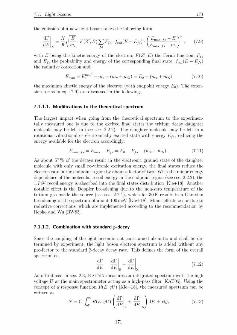
7.1. Light bosons 171
the emission of a new light boson takes the following form:
dΓdE
∣∣∣∣∣X
= K
~
√E
me
· F (Z ′, E)∑fs
Pfs · frad(E − Efs) ·(Emax, fs − EEmax, fs +me
)n, (7.9)
with E being the kinetic energy of the electron, F (Z ′, E) the Fermi function, Pfsand Efs the probability and energy of the corresponding final state, frad(E − Efs)the radiative correction and
Emax = Emax′
e −me − (mν +mX) = E0 − (mν +mX) (7.10)
the maximum kinetic energy of the electron (with endpoint energy E0). The exten-sion terms in eq. (7.9) are discussed in the following.
7.1.1.1. Modifications to the theoretical spectrum
The largest impact when going from the theoretical spectrum to the experimen-tally measured one is due to the excited final states the tritium decay daughtermolecule may be left in (see sec. 2.2.2). The daughter molecule may be left in arotational-vibrational or electronically excited state with energy Efs, reducing theenergy available for the electron accordingly:
Emax, fs = Emax − Efs = E0 − Efs − (mν +mX) . (7.11)
As about 57 % of the decays result in the electronic ground state of the daughtermolecule with only small ro-vibronic excitation energy, the final states reduce theelectron rate in the endpoint region by about a factor of two. With the minor energydependence of the molecular recoil energy in the endpoint region (see sec. 2.2.2), the1.7 eV recoil energy is absorbed into the final states distribution [Kle+18]. Anothernotable effect is the Doppler broadening due to the non-zero temperature of thetritium gas inside the source (see sec. 2.2.1), which for 30 K results in a Gaussianbroadening of the spectrum of about 100 meV [Kle+18]. Minor effects occur due toradiative corrections, which are implemented according to the recommendation byRepko and Wu [RW83].
7.1.1.2. Combination with standard β-decay
Since the coupling of the light boson is not constrained ab initio and shall be de-termined by experiment, the light boson electron spectrum is added without anypre-factor to the standard β-decay decay rate. This defines the form of the overallspectrum as
dΓdE
= dΓdE
∣∣∣∣∣β
+ dΓdE
∣∣∣∣∣X
. (7.12)
As introduced in sec. 2.3, Katrin measures an integrated spectrum with the highvoltage U at the main spectrometer acting as a high-pass filter [KAT05]. Using theconcept of a response function R(E, qU) [Kle+18], the measured spectrum can bewritten as
N = C∫ ∞qU
R(E, qU) dΓ
dE
∣∣∣∣∣β
+ dΓdE
∣∣∣∣∣X
dE +Bg, (7.13)
171
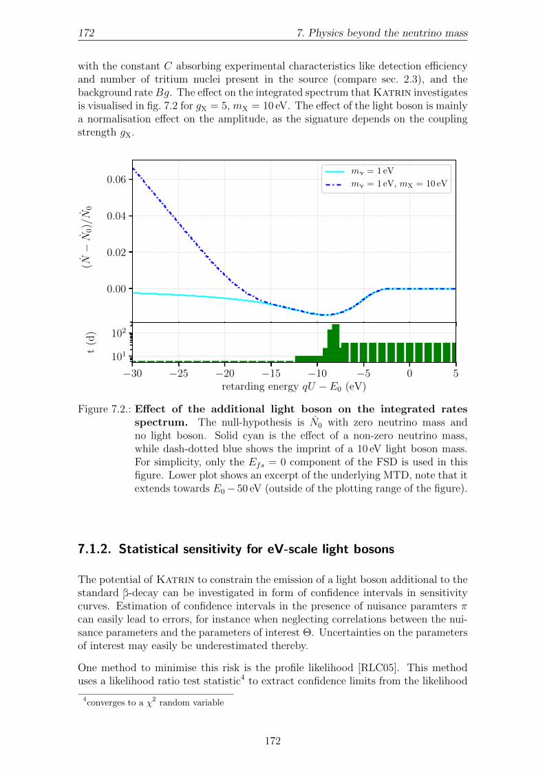
172 7. Physics beyond the neutrino mass
with the constant C absorbing experimental characteristics like detection efficiencyand number of tritium nuclei present in the source (compare sec. 2.3), and thebackground rateBg. The effect on the integrated spectrum that Katrin investigatesis visualised in fig. 7.2 for gX = 5, mX = 10 eV. The effect of the light boson is mainlya normalisation effect on the amplitude, as the signature depends on the couplingstrength gX.
0.00
0.02
0.04
0.06mν = 1 eV
mν = 1 eV, mX = 10 eV
−30 −25 −20 −15 −10 −5 0 5retarding energy qU − E0 (eV)
101
102
(N−N
0)/N
0t
(d)
Figure 7.2.: Effect of the additional light boson on the integrated ratesspectrum. The null-hypothesis is N0 with zero neutrino mass andno light boson. Solid cyan is the effect of a non-zero neutrino mass,while dash-dotted blue shows the imprint of a 10 eV light boson mass.For simplicity, only the Efs = 0 component of the FSD is used in thisfigure. Lower plot shows an excerpt of the underlying MTD, note that itextends towards E0− 50 eV (outside of the plotting range of the figure).
7.1.2. Statistical sensitivity for eV-scale light bosons
The potential of Katrin to constrain the emission of a light boson additional to thestandard β-decay can be investigated in form of confidence intervals in sensitivitycurves. Estimation of confidence intervals in the presence of nuisance paramters πcan easily lead to errors, for instance when neglecting correlations between the nui-sance parameters and the parameters of interest Θ. Uncertainties on the parametersof interest may easily be underestimated thereby.
One method to minimise this risk is the profile likelihood [RLC05]. This methoduses a likelihood ratio test statistic4 to extract confidence limits from the likelihood
4converges to a χ2 random variable
172

7.1. Light bosons 173
function, similar to the χ2 method. The profile likelihood is defined as
Lp(Θ) = L(Θ, π(Θ)) (7.14)
with π(Θ) the function maximising the likelihood L with respect to its nuisance
parameters π. With the best fit estimate Θ, the likelihood ratio test statistic can bedefined as
λ(Θ) = Lp(Θ)Lp(Θ)
. (7.15)
Now the profile likelihood is scanned to obtain values for Θ where the evaluation ofeq. (7.14) increases by a specific factor. One example is finding the 1σ intervals ofa single parameter Θ. Likelihood values are searched for Θ where −2∆ logLp(Θ) =−2 log λ = 1. To obtain exclusion or sensitivity curves, several values of Θ are usedto compare the likelihood against the null-hypothesis while at each point minimisingthe likelihood with respect to the nuisance parameters.
10−3 10−2 10−1 100 101
boson mass mX (eV)
10−13
10−11
10−9
10−7
10−5
10−3
10−1
101
103
105
cou
pli
ngg X
(A) ββ-decay (A) mesondecay
(A) CMB
(A) ∆NCMBeff
(A) SN1987A
(A) IceCube
(B) solar lifetime
(B) (g − 2)e
A: νγ5νX
B: eγ5eX
Figure 7.3.: Statistical sensitivity for eV-scale pseudoscalars. The lines rep-resent the 90 % C.L. statistical sensitivity of Katrin for types A, B(defined according to tab. 7.1). The parameter regions allowed fromconstraints discussed in sec. 7.1.4 are marked as shaded areas.
For the potential of Katrin to constrain the additional emission of light bosons inβ-decay, there are two parameters of interest: gX and mX. Therefore, the likelihoodfor non-vanishing (gX,mX) is compared to the null-hypothesis of no light boson (0, 0).In details, this means minimisation of the likelihood over m2
ν, E0, Amp and bg (m2ν is
a nuisance parameter in this case) for every point in the 2-dim grid (g,mX). Then itis possible to find likelihood ratios corresponding to 90 % C.L. Next, the five differentscenarios introduced in sec. 7.1.1 will be inspected one by one.
A. Pseudoscalars emitted from neutrinos : the form of the spectrum suggests in-creasing sensitivity with increasing coupling gX (see tab. 7.1). The sensitivity
173

174 7. Physics beyond the neutrino mass
curves in fig. 7.3 confirm this expectation. Furthermore it can be seen thatthe sensitivity decreases again for masses larger than 10 eV: the sensitivity onthe mass mX is affected by the range of retarding energies of the MTD. Sincethe MTD used to obtain the sensitivity curves only extends towards 50 eV be-low the endpoint (see sec. D.1 in the appendix), masses larger than 50 eV lieoutside the measuring interval.
B. Pseudoscalars emitted from electrons: the branching ratio for this couplingis rather small compared to the other production mechanisms. Rather largecouplings gX are required in order for Katrin to be sensitive towards thiskind of light bosons. This expectation is confirmed from fig. 7.3: the couplingstrength reachable is four to five orders of magnitude larger than the couplingwhich can be probed for bosons of type A (pseudoscalar coupled to neutrinos).As for type A, masses larger than 50 eV are outside the MTD used for thesestudies and are therefore not testable.
C. & D. Vector bosons emitted from neutrinos or electrons : Since the electronspectra of production mechanisms C and D are the same for eV-scale bosons(compare tab. 7.1), the sensitivity curve is the same for both. In contrastto types A and B, the spectrum for coupling to C and D exhibits a 1/m2
X
divergence in the normalisation factor K (compare eq. (7.3) and tab. 7.1).Therefore, small boson masses mX are strongly favoured, which should leadto higher sensitivity of Katrin for smaller boson masses. This expectation isconfirmed from fig. 7.4: in contrast to cases A and B, Katrin has increasedstatistical sensitivity to bosons of type C and D towards lower boson masses.Concerning larger boson masses, the limitations by the width of the MTD canbe seen.
E. Vector bosons emitted from neutrinos and electrons : From the spectral form,a similar behaviour as for type A is expected (compare tab. 7.1). Figure 7.4confirms this expectation, with best sensitivity for light bosons with mass oforder eV.
7.1.3. Statistical sensitivity for keV-scale light bosons
An extension of the study, included in ref. [Arc+18], tests the statistical sensitivityof a differential measurement of the complete tritium β-spectrum towards probing ofhigher boson masses. These results are summarised here for the sake of completingthe picture5. The study foresees to replace the FPD with a detector with an energyresolution of 300 eV [Mer+18] (one order of magnitude better) and thereby have theenergy of the electrons determined by the detector, while the main spectrometer onlyguides the electrons to the detector. The measurement time foreseen for this newset-up is also three years, with a current estimate of the background of 2 mcps/keV(based on measurements with the current FPD detector [Har15]).
With the above mentioned profile likelihood method plus a Gaussian pull term onthe neutrino mass of 2 eV6, the sensitivity of a TRISTAN-like set-up towards the
5The keV-scale study was conducted by M. Slezak.6The value representing the current neutrino mass limit from β-decay [Tan+18].
174
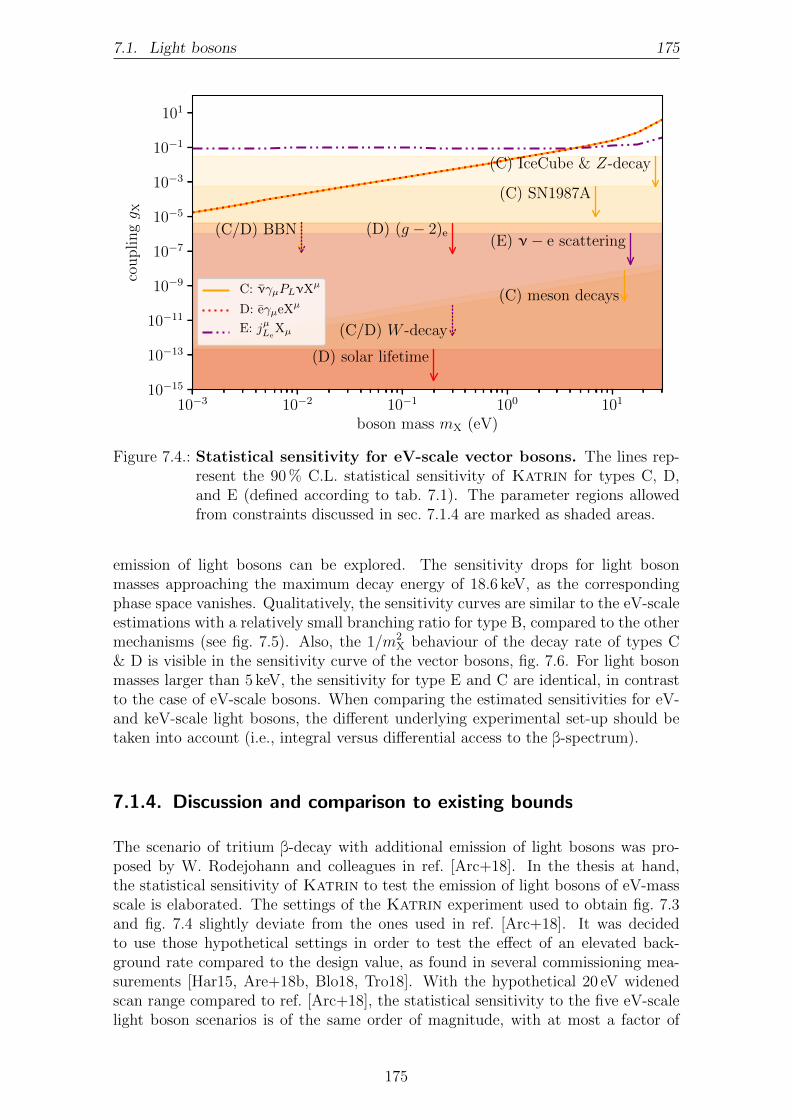
7.1. Light bosons 175
10−3 10−2 10−1 100 101
boson mass mX (eV)
10−15
10−13
10−11
10−9
10−7
10−5
10−3
10−1
101
cou
pli
ngg X
(C) IceCube & Z-decay
(C) SN1987A
(C/D) BBN
(C) meson decays
(C/D) W -decay
(D) solar lifetime
(D) (g − 2)e(E) ν− e scattering
C: νγµPLνXµ
D: eγµeXµ
E: jµLeXµ
Figure 7.4.: Statistical sensitivity for eV-scale vector bosons. The lines rep-resent the 90 % C.L. statistical sensitivity of Katrin for types C, D,and E (defined according to tab. 7.1). The parameter regions allowedfrom constraints discussed in sec. 7.1.4 are marked as shaded areas.
emission of light bosons can be explored. The sensitivity drops for light bosonmasses approaching the maximum decay energy of 18.6 keV, as the correspondingphase space vanishes. Qualitatively, the sensitivity curves are similar to the eV-scaleestimations with a relatively small branching ratio for type B, compared to the othermechanisms (see fig. 7.5). Also, the 1/m2
X behaviour of the decay rate of types C& D is visible in the sensitivity curve of the vector bosons, fig. 7.6. For light bosonmasses larger than 5 keV, the sensitivity for type E and C are identical, in contrastto the case of eV-scale bosons. When comparing the estimated sensitivities for eV-and keV-scale light bosons, the different underlying experimental set-up should betaken into account (i.e., integral versus differential access to the β-spectrum).
7.1.4. Discussion and comparison to existing bounds
The scenario of tritium β-decay with additional emission of light bosons was pro-posed by W. Rodejohann and colleagues in ref. [Arc+18]. In the thesis at hand,the statistical sensitivity of Katrin to test the emission of light bosons of eV-massscale is elaborated. The settings of the Katrin experiment used to obtain fig. 7.3and fig. 7.4 slightly deviate from the ones used in ref. [Arc+18]. It was decidedto use those hypothetical settings in order to test the effect of an elevated back-ground rate compared to the design value, as found in several commissioning mea-surements [Har15, Are+18b, Blo18, Tro18]. With the hypothetical 20 eV widenedscan range compared to ref. [Arc+18], the statistical sensitivity to the five eV-scalelight boson scenarios is of the same order of magnitude, with at most a factor of
175
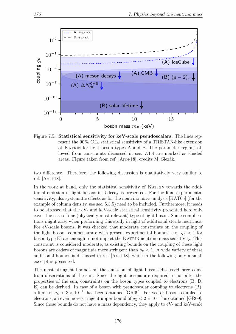
176 7. Physics beyond the neutrino mass
0 5 10 15
boson mass mX (keV)
10−13
10−10
10−7
10−4
10−1
102co
up
lingg X (A) IceCube
(A) meson decays(A) CMB
(A) ∆NCMBeff
(B) solar lifetime
(B) (g − 2)e
A: νγ5νX
B: eγ5eX
Figure 7.5.: Statistical sensitivity for keV-scale pseudoscalars. The lines rep-resent the 90 % C.L. statistical sensitivity of a TRISTAN-like extensionof Katrin for light boson types A and B. The parameter regions al-lowed from constraints discussed in sec. 7.1.4 are marked as shadedareas. Figure taken from ref. [Arc+18], credits M. Slezak.
two difference. Therefore, the following discussion is qualitatively very similar toref. [Arc+18].
In the work at hand, only the statistical sensitivity of Katrin towards the addi-tional emission of light bosons in β-decay is presented. For the final experimentalsensitivity, also systematic effects as for the neutrino mass analysis [KAT05] (for theexample of column density, see sec. 5.3.5) need to be included. Furthermore, it needsto be stressed that the eV- and keV-scale statistical sensitivity presented here onlycover the case of one (physically most relevant) type of light boson. Some complica-tions might arise when performing this study in light of additional sterile neutrinos.For eV-scale bosons, it was checked that moderate constraints on the coupling ofthe light boson (commensurate with present experimental bounds, e.g. gX < 1 forboson type E) are enough to not impact the Katrin neutrino mass sensitivity. Thisconstraint is considered moderate, as existing bounds on the coupling of these lightbosons are orders of magnitude more stringent than gX < 1. A wide variety of theseadditional bounds is discussed in ref. [Arc+18], while in the following only a smallexcerpt is presented.
The most stringent bounds on the emission of light bosons discussed here comefrom observations of the sun. Since the light bosons are required to not alter theproperties of the sun, constraints on the boson types coupled to electrons (B, D,E) can be derived. In case of a boson with pseudoscalar coupling to electrons (B),a limit of gX < 3× 10⁻¹¹ has been obtained [GR09]. For vector bosons coupled toelectrons, an even more stringent upper bound of gX < 2× 10⁻¹³ is obtained [GR09].Since those bounds do not have a mass dependency, they apply to eV- and keV-scale
176

7.1. Light bosons 177
0 5 10 15
boson mass mX (keV)
10−15
10−12
10−9
10−6
10−3
100
103
cou
plin
gg X
(C) IceCubeand Z-decay
(C) meson decays
(C) BBN
(C/D) W decay
(D) solar lifetime
(D) BBN(E) ν− e scattering
C: νγµPLνXµ
D: eγµeXµ
E: jµLe
Xµ
Figure 7.6.: Statistical sensitivity contours for keV-scale vector bosons. Thelines represent the 90 % C.L. statistical sensitivity of a TRISTAN-likeextension of Katrin for light boson types C, D, and E. The parameterregions allowed from constraints discussed in sec. 7.1.4 are marked asshaded areas. Figure taken from ref. [Arc+18], credits M. Slezak.
bosons alike.
In contrast to bounds on bosons coupled to electrons, the bounds on neutrino cou-pled bosons are less stringent. For pseudoscalars coupled to neutrinos (A), withmX < 1 eV, neutrino annihilation becomes relevant. The corresponding coupling isconstrained by Planck CMB data to gX < 1.2× 10⁻⁷ [AH14]. For vector bosonscoupled to neutrinos (C), the most stringent bound is estimated from meson decaysto gX < 2.2× 10⁻¹⁰mX
eV[BF17].
The bounds discussed so far are all below the parameter range accessible with Ka-trin or the TRISTAN-modified Katrin set-up7. However, it has to be noted thatthe laboratory experiment bounds from figs. 7.3, 7.4, 7.5, 7.6 are extrapolated fromenergies in the MeV range [Arc+18]. Furthermore, the IceCube [IM14] and Z-decaywidth [LDB14] constraints may be probed with both Katrin set-ups for boson typeC, and with TRISTAN for type A additionally (for an overview of all bounds, seetab. D.5). Therefore, an analysis of future Katrin and TRISTAN data with re-spect to the emission of the light boson states discussed in this chapter represents acomplementary approach to new physics at low energies on the eV and keV scale.
7For discussion of the intermediate bounds, the reader is referred to ref. [Arc+18].
177

178 7. Physics beyond the neutrino mass
7.2. Right-handed currents in presence of eV-scalesterile neutrinos
Numerous previous works have covered the sensitivity of Katrin to sterile neutri-nos on the eV [FB11, Kle14] as well as keV scale [Mer+15]. A model which couldnaturally lead to observable sterile neutrino masses and the seesaw mechanism isthe Left-Right Symmetric Model (LRSM) [PS74, MP75, SM75]. As an extensionto the Standard Model, it would restore parity on high energy scales by addingright-handed currents. W. Rodejohann and coworkers derived the general spectrumfor tritium β-decay electrons with right-handed currents in presence of sterile neu-trinos [BHR14]. Subsequently, N. Steinbrink et al. derived a model-independentparametrisation of this spectrum for eV-scale sterile neutrinos [Ste17, Ste+17]. Thework at hand contributed substantially to the derivation of the statistical sensitiv-ity of Katrin to constrain the right-handed currents in presence of eV-scale sterileneutrinos in ref. [Ste+17] via an independent implementation of the spectra into aKatrin simulation and analysis framework. In addition to ref. [Ste+17], the sta-tistical sensitivity of Katrin in the thesis at hand is evaluated for the scenarioof an elevated background rate, based on a slightly different underlying measuringtime distribution. The model-independent parametrisation of the LRSM used inref. [Ste+17] is also the foundation of the results presented in this thesis.
First, a short introduction into the parametrisation is given, then exemplary MCMCresults are shown before stating the statistical sensitivity of Katrin to constrainright-handed currents in presence of eV-scale sterile neutrinos.
7.2.1. Spectral shape due to right-handed currents
In addition to the standard β-decay spectrum, we here deal with right-handed cur-rents in presence of eV-scale sterile neutrinos. In ref. [Ste+17], a derivation of amodel-independent parametrisation is given. Similar to the three active neutrinosbeing represented by one effective neutrino mass (see eq. (1.38)), the three addi-tional sterile neutrinos from the LRSM are represented by one effective neutrinomass since it is possible to have at least one light sterile neutrino [Bor16]. The ac-tive neutrino mass in the following is defined as the light (electron-) neutrino massml and the sterile neutrino mass as the heavy neutrino mass mh. In line with thestandard neutrino mixing, the active-sterile mixing is described by the mixing angleθ as sin θ2 = |Ue4|2. Ignoring a potential CP-violating phase in the neutrino mixingmatrix enables describing the mixing by a 2 × 2 rotation matrix. With some fur-ther re-parametrisation, it is possible to come up with a simpler form of the generalspectrum derived in [BHR14].
178

7.2. Right-handed currents in presence of eV-scale sterile neutrinos 179
7.2.1.1. Basic form of the spectrum
In refs. [Ste17, Ste+17], a model-independent parametrisation of the β-decay spec-trum with right-handed currents in presence of eV-scale sterile neutrinos is derived:
dΓdE
= dΓ′
dE
∣∣∣∣∣h
sin2 θeff + dΓ′
dE
∣∣∣∣∣l
cos2 θeff
+ cLR ·(
dΓ′
dE
∣∣∣∣∣h
mh
E0 − E− dΓ′
dE
∣∣∣∣∣l
ml
E0 − E
),
(7.16)
with (aLL + aRR) being absorbed into the amplitude (x = h, l):
dΓ′
dE
∣∣∣∣∣x
= (aLL + aRR) · dΓdE
∣∣∣∣∣x
. (7.17)
Therein, dΓdE
∣∣∣x
is the β-spectrum with neutrino x as defined in eq. (1.37). The
parametrisation of the interference term cLR is given as [Ste+17]):
cLR = aLR
aLL + aRR
· me
me + E0· cos θ sin θ, (7.18)
with the approximation E ≈ E0 in the endpoint region. The mixing angle ineq. (7.16) is an effective mixing angle, defined via
(aLL + aRR) sin2 θeff = aLL sin2 θ + aRR cos2 θ, (7.19)
(aLL + aRR) cos2 θeff = aLL cos2 θ + aRR sin2 θ. (7.20)
Since aLL ≈ 1 and aLR, aRR ≈ 0, the effective mixing angle θeff will essentially beequal to the physical mixing angle θ, causing the factor (aLL + aRR) to be 1 andtherefore negligible in eq. (7.17). This model-independent parametrisation enablesalso to cover other conceivable mechanisms that need not to be based on left-rightsymmetry but cause the same effect on the β-spectrum.
The signature of β-decay electrons from right-handed currents in presence of lightsterile neutrinos looks very similar to the one of sterile neutrinos without right-handed currents. At E0−mh, there is a kink in the spectrum, where the contributionof the heavy (sterile) neutrino mass mh ends [Mer+15]. There is, however, oneessential difference: the right-handed current may cause constructive and destructiveinterference. In the extreme case, this will manifest as a reduction of the rate, as canbe seen from fig. 7.7. For the case of destructive interference (negative cLR), the rateis reduced for E < E0 −mh (the heavy sterile part) and goes back to the standardcase for E0 − mh < E < E0 (where only the light active neutrino contributes).For the case of constructive interference, the effect is the opposite. The boost andreduction are slightly more pronounced for the heavy (sterile) neutrino mass due tothe mν/Eν proportionality inside the interference term in eq. (7.16). Without theright-handed coupling interference term, the standard superposition of two spectrawith different neutrino masses is observed, which manifests as a kink at E0 −mh asdescribed in [Mer+15].
In order to show the mass dependency, the interference term is fixed to cLR = 0.2with sin2 θeff = 0.2 while the heavy (sterile) neutrino mass is varied. From fig. 7.8it can be seen that the boost magnitude increases only slightly with mh, but theregion spans over a wider energy interval for larger mh. As expected, the positionof the kink is defined by mh. These effects are less pronounced, when respecting thefinal states of the daughter molecule, as will be described in the next section.
179

180 7. Physics beyond the neutrino mass
−10 −8 −6 −4 −2 0E − E0 (eV)
0.6
0.7
0.8
0.9
1.0d
iffra
tera
tio
dΓ/dE| rh
c/
dΓ/dE| β
cLR = 0.2
cLR = 0.1
cLR = 0
cLR = -0.1
cLR = -0.2
Figure 7.7.: Effect of the right-handed coupling. Shown is the ratio of a spec-trum with left-right interference according to eq. (7.16) to a standardβ-decay spectrum for different interference cLR. Constant parametersare sin2 θeff = 0.2, mh = 2 eV and ml = 0.2 eV.
7.2.1.2. Model extensions
As introduced before (compare eq. (1.37) and eq. (2.2)), the basic form of the spec-trum needs to be modified for several experimental effects. Since these modifica-tions only affect the electron spectrum, they are treated in the same way (also seesec. 7.1.1). This section introduces the implementation of the final states into theright-handed currents spectrum. Since the final states can effectively be seen as a re-duction of the maximum electron energy E0, the implementation is straightforward.Equation (7.16) becomes
dΓdE
=∑fs
Pfs
dΓ′
dE
∣∣∣∣∣h
sin2 θeff + dΓ′
dE
∣∣∣∣∣l
cos2 θeff
+ cLR ·(
dΓ′
dE
∣∣∣∣∣h
mh
E0 − Efs − E− dΓ′
dE
∣∣∣∣∣l
ml
E0 − Efs − E
).
(7.21)
The effect of the final states on the spectrum is exactly the same as for the lightbosons or the standard β-decay, the maximum kinetic energy of the electron is re-duced and so is the electron rate close to the endpoint. Furthermore, the final statessmear out distinct features of the spectrum, which can be seen from fig. 7.9 andfig. 7.10. Especially the position of the kink is not as clearly visible as before, whichholds for all heavy neutrino masses (see fig. 7.10). Besides extending the modelimplementation by the final states, it needs to be respected that Katrin measuresan integrated spectrum
N = C ·∫ ∞qU
R(E, qU) dΓdE
dE +Bg, (7.22)
180

7.2. Right-handed currents in presence of eV-scale sterile neutrinos 181
−10 −8 −6 −4 −2 0E − E0 (eV)
0.6
0.7
0.8
0.9
1.0d
iffra
tera
tio
dΓ/dE| rh
c/
dΓ/dE| β
mh = 4.0 eV
mh = 2.0 eV
mh = 1.0 eV
mh = 0.5 eV
Figure 7.8.: Effect of the heavy (sterile) neutrino mass. Shown is the ratioof a spectrum with left-right interference according to eq. (7.16) to astandard β-decay spectrum for different heavy (sterile) neutrino massesmh. Constant parameters are sin2 θeff = 0.2, cLR = 0.2 and ml = 0.2 eV.
also compare sec. 2.3. In the following, the same Katrin parameters as for the lightboson estimates will be used (described in sec. D.1 and summarised in tab. D.4 inthe appendix). With these settings, we can investigate the effect of the right-handedcurrent coupling on the measured integrated spectrum.
In the integrated spectrum, the effect of the right-handed currents is weakened dueto the integration. However, large interference values still have an effect on the shapeof the integrated spectrum. The effect itself is similar to the effect on the differentialspectrum, as can be seen from fig. 7.11 and fig. 7.12.
Compared to the differential spectrum, the relative cLR signature is less pronouncedby one order of magnitude for the same parameter combinations. In the differentialspectrum, the parameters chosen cause a relative difference to the standard β-decayspectrum of up to 40 %, while in the integrated spectrum of only about 3 %. Still,the signal strength clearly increases with higher mh (see fig. 7.12). Figure 7.12 alsoimplies that heavy mh ≥ 1 eV stretch the signal beyond the Katrin measuringinterval assumed for the work in this thesis, while for smaller mh ≤ 1 eV the signal isessentially fully contained within the 50 eV measuring interval. This points towardslimits for the sensitivity of Katrin towards“heavier”sterile neutrinos. It is expectedthat there is a maximum sensitivity for the right-handed currents in presence ofsterile neutrino masses below 50 eV, similar to the light bosons in sec. 7.1.
181

182 7. Physics beyond the neutrino mass
−10 −8 −6 −4 −2 0E − E0 (eV)
0.6
0.7
0.8
0.9
1.0d
iffra
tera
tio
dΓ/dE| rh
c/
dΓ/dE| β
cLR = 0.2
cLR = 0.1
cLR = 0
cLR = -0.1
cLR = -0.2
Figure 7.9.: Effect of the right-handed coupling with final states. Shown isthe ratio of a spectrum with left-right interference according to eq. (7.21)to a standard β-decay spectrum for different interference cLR. Constantparameters are sin2 θeff = 0.2, mh = 2 eV and ml = 0.2 eV. Comparedto fig. 7.7, the kink is smeared out.
−10 −8 −6 −4 −2 0E − E0 (eV)
0.6
0.7
0.8
0.9
1.0
diff
rate
rati
od
Γ/dE| rh
c/
dΓ/dE| β
mh = 4.0 eV
mh = 2.0 eV
mh = 1.0 eV
mh = 0.5 eV
Figure 7.10.: Effect of the heavy (sterile) neutrino mass with final states.Shown is the ratio of a spectrum with left-right interference accordingto eq. (7.21) to a standard β-decay spectrum for different heavy (sterile)neutrino masses mh. Constant parameters are sin2 θeff = 0.2, cLR = 0.2and ml = 0.2 eV. Again, the kink is smeared out by the final states.
182
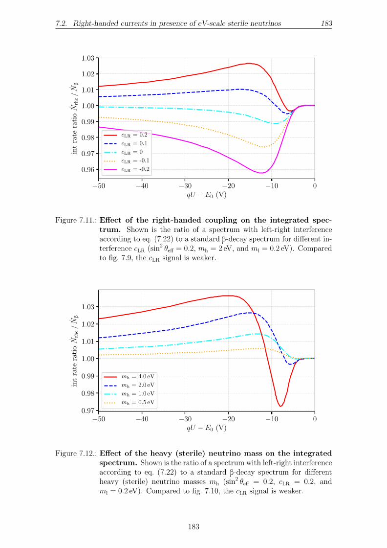
7.2. Right-handed currents in presence of eV-scale sterile neutrinos 183
−50 −40 −30 −20 −10 0qU − E0 (V)
0.96
0.97
0.98
0.99
1.00
1.01
1.02
1.03
int
rate
rati
oN
rhc/Nβ
cLR = 0.2
cLR = 0.1
cLR = 0
cLR = -0.1
cLR = -0.2
Figure 7.11.: Effect of the right-handed coupling on the integrated spec-trum. Shown is the ratio of a spectrum with left-right interferenceaccording to eq. (7.22) to a standard β-decay spectrum for different in-terference cLR (sin2 θeff = 0.2, mh = 2 eV, and ml = 0.2 eV). Comparedto fig. 7.9, the cLR signal is weaker.
−50 −40 −30 −20 −10 0qU − E0 (V)
0.97
0.98
0.99
1.00
1.01
1.02
1.03
int
rate
rati
oN
rhc/Nβ
mh = 4.0 eV
mh = 2.0 eV
mh = 1.0 eV
mh = 0.5 eV
Figure 7.12.: Effect of the heavy (sterile) neutrino mass on the integratedspectrum. Shown is the ratio of a spectrum with left-right interferenceaccording to eq. (7.22) to a standard β-decay spectrum for differentheavy (sterile) neutrino masses mh (sin2 θeff = 0.2, cLR = 0.2, andml = 0.2 eV). Compared to fig. 7.10, the cLR signal is weaker.
183

184 7. Physics beyond the neutrino mass
7.2.2. Parameter inference with right-handed currents
Fitting an additional three parameters for the right-handed currents in presence ofeV-scale sterile neutrinos is challenging. The free parameter cLR will easily lead toplain wrong estimation of the other parameters due to its interference nature. There-fore it was decided to use a Metropolis-Hastings MCMC [Met+53] to marginalisethe likelihood function for parameter inference. It has proven to be a very robustand reliable algorithm which can be tuned to estimate solutions for tricky problems.
Concerning the settings of the MCMC, a burn-in phase of up to 2× 10⁵ steps waschosen and a total chain length of at least 106 steps with a proposal acceptance rateof 0.234. In each step, the simulated measurement and the spectrum obtained withthe inferred parameters are compared and the parameters are adapted accordinglyvia acceptance of the proposal. During the burn-in phase, the MCMC varies theparameters in a wide range to find the parameter regions where the MCMC mightconverge. These regions are then explored in detail in the remaining steps to resultin the shown posterior distributions of the fit parameters. In order to circumventlow effective sample sizes due to the long burn-in phase, multiple chains were runin parallel to ensure effective sample sizes of order 1000 for each setting. Flat priorswere used for all parameters, representing physical constraints in terms of lower andupper limits as shown in tab. 7.2.
Table 7.2.: Priors on the parameters. The heavy neutrino mass is kept fixed.
param lower bound upper bound
m2l (eV2) 0 100
E0 (eV) 18475 18675
Amp 0.5 1.5
Bg (cps) 0 1
sin2 θeff 0 1
cLR −1 1
The marginalised posterior distribution for an example MCMC run with fixed m2h =
16 eV2, and true m2l = 0 eV2, E0 = 18 575 eV, Amp = 1, Bg = 0.4 cps, sin2 θeff = 0.1,
cLR = 0 is visualised in fig. 7.13. A slight bias of the estimated endpoint E0 andthe right-handed coupling cLR is visible, with strong anti-correlation of the twoparameters. Furthermore, larger light neutrino masses are favoured by negativeright-handed couplings, as evident from eq. (7.21). Similar results were obtainedin ref. [Ste+17] with a Differential Evolution Markov Chain Monte Carlo [Bra06]algorithm and the Katrin nominal operational settings.
In order to minimise the bias of cLR and E0, a constraint on E0 is considered. Penningtrap measurements have the potential to constrain the 3He-3H mass difference downto 30 meV [Str+14], which could be translated into a corresponding constraint onthe Q-value of the tritium β-decay spectrum. In order to use this constraint on theQ-value as a constraint on E0 for the analysis of Katrin data, also the absolute
184

7.2. Right-handed currents in presence of eV-scale sterile neutrinos 185
0.0
0.2
∆E
0(e
V)
0.998
1.000
Amp
−0.5
0.0
0.5
∆Bg
(cp
s)[×
10−
3]
0.1
0.2
sin
2θ e
ff
0 1m2
l (eV2)
−0.1
0.0
c LR
0.0 0.2∆E0 (eV)
0.9975 1.0000Amp
−0.5 0.0 0.5
∆Bg (cps) [×10−3]
0.1 0.2sin2 θeff
Figure 7.13.: Posterior parameter distributions. True values are m2l = 0 eV2,
E0 = 18 575 eV, Amp = 1, Bg = 0.4 cps, sin2 θeff = 0.1, cLR = 0 andfixed m2
h = 16 eV2. The yellow lines mark the 90 % credible region.
energy scale of Katrin needs to be determined. In particular, this comprises thework function difference between the source and the main-spectrometer, as well aspotential plasma effects inside the source [Kuc16], and the final states of the tritiumdaughter molecule [BPR15]. All these effects need to be known to the meV level aswell, which is why a conservative constraint on the endpoint of 50 meV is used tominimise the bias. In the next section, sensitivity estimates for cLR are given for freeand constrained endpoint, for different heavy neutrino masses.
7.2.3. Statistical sensitivity to constrain the right-handedcoupling
Up to now, the heavy (sterile) neutrino mass was kept fixed during the MCMCrun. In ref. [Ste+17], we show that the posterior distributions for sin2 θeff, m2
h and
185
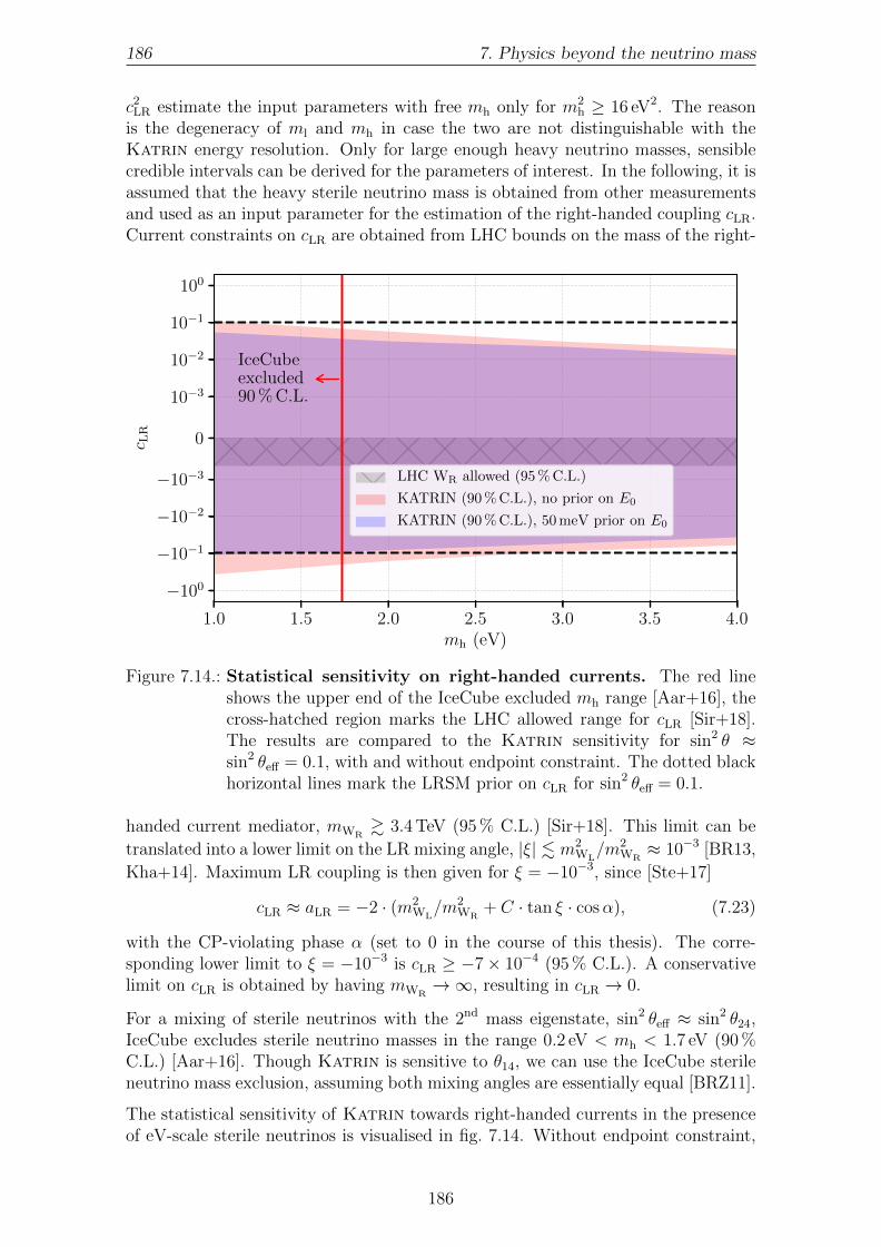
186 7. Physics beyond the neutrino mass
c2LR estimate the input parameters with free mh only for m2
h ≥ 16 eV2. The reasonis the degeneracy of ml and mh in case the two are not distinguishable with theKatrin energy resolution. Only for large enough heavy neutrino masses, sensiblecredible intervals can be derived for the parameters of interest. In the following, it isassumed that the heavy sterile neutrino mass is obtained from other measurementsand used as an input parameter for the estimation of the right-handed coupling cLR.Current constraints on cLR are obtained from LHC bounds on the mass of the right-
1.0 1.5 2.0 2.5 3.0 3.5 4.0mh (eV)
−100
−10−1
−10−2
−10−3
0
10−3
10−2
10−1
100
c LR
IceCubeexcluded90 % C.L.
LHC WR allowed (95 % C.L.)
KATRIN (90 % C.L.), no prior on E0
KATRIN (90 % C.L.), 50 meV prior on E0
Figure 7.14.: Statistical sensitivity on right-handed currents. The red lineshows the upper end of the IceCube excluded mh range [Aar+16], thecross-hatched region marks the LHC allowed range for cLR [Sir+18].The results are compared to the Katrin sensitivity for sin2 θ ≈sin2 θeff = 0.1, with and without endpoint constraint. The dotted blackhorizontal lines mark the LRSM prior on cLR for sin2 θeff = 0.1.
handed current mediator, mWR& 3.4 TeV (95 % C.L.) [Sir+18]. This limit can be
translated into a lower limit on the LR mixing angle, |ξ| . m2WL/m2
WR≈ 10−3 [BR13,
Kha+14]. Maximum LR coupling is then given for ξ = −10−3, since [Ste+17]
cLR ≈ aLR = −2 · (m2WL/m2
WR+ C · tan ξ · cosα), (7.23)
with the CP-violating phase α (set to 0 in the course of this thesis). The corre-sponding lower limit to ξ = −10−3 is cLR ≥ −7× 10⁻⁴ (95 % C.L.). A conservativelimit on cLR is obtained by having mWR
→∞, resulting in cLR → 0.
For a mixing of sterile neutrinos with the 2nd mass eigenstate, sin2 θeff ≈ sin2 θ24,IceCube excludes sterile neutrino masses in the range 0.2 eV < mh < 1.7 eV (90 %C.L.) [Aar+16]. Though Katrin is sensitive to θ14, we can use the IceCube sterileneutrino mass exclusion, assuming both mixing angles are essentially equal [BRZ11].
The statistical sensitivity of Katrin towards right-handed currents in the presenceof eV-scale sterile neutrinos is visualised in fig. 7.14. Without endpoint constraint,
186
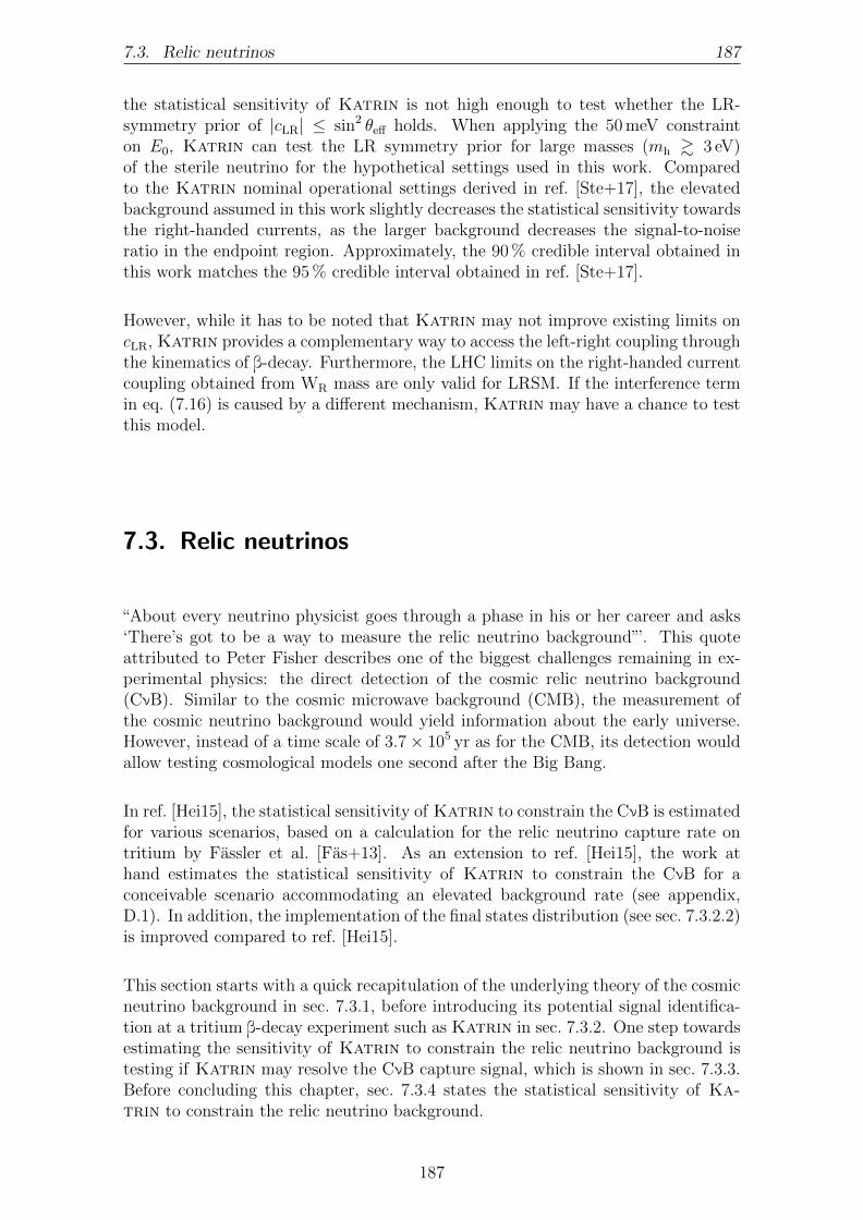
7.3. Relic neutrinos 187
the statistical sensitivity of Katrin is not high enough to test whether the LR-symmetry prior of |cLR| ≤ sin2 θeff holds. When applying the 50 meV constrainton E0, Katrin can test the LR symmetry prior for large masses (mh & 3 eV)of the sterile neutrino for the hypothetical settings used in this work. Comparedto the Katrin nominal operational settings derived in ref. [Ste+17], the elevatedbackground assumed in this work slightly decreases the statistical sensitivity towardsthe right-handed currents, as the larger background decreases the signal-to-noiseratio in the endpoint region. Approximately, the 90 % credible interval obtained inthis work matches the 95 % credible interval obtained in ref. [Ste+17].
However, while it has to be noted that Katrin may not improve existing limits oncLR, Katrin provides a complementary way to access the left-right coupling throughthe kinematics of β-decay. Furthermore, the LHC limits on the right-handed currentcoupling obtained from WR mass are only valid for LRSM. If the interference termin eq. (7.16) is caused by a different mechanism, Katrin may have a chance to testthis model.
7.3. Relic neutrinos
“About every neutrino physicist goes through a phase in his or her career and asks‘There’s got to be a way to measure the relic neutrino background”’. This quoteattributed to Peter Fisher describes one of the biggest challenges remaining in ex-perimental physics: the direct detection of the cosmic relic neutrino background(CνB). Similar to the cosmic microwave background (CMB), the measurement ofthe cosmic neutrino background would yield information about the early universe.However, instead of a time scale of 3.7× 10⁵ yr as for the CMB, its detection wouldallow testing cosmological models one second after the Big Bang.
In ref. [Hei15], the statistical sensitivity of Katrin to constrain the CνB is estimatedfor various scenarios, based on a calculation for the relic neutrino capture rate ontritium by Fassler et al. [Fas+13]. As an extension to ref. [Hei15], the work athand estimates the statistical sensitivity of Katrin to constrain the CνB for aconceivable scenario accommodating an elevated background rate (see appendix,D.1). In addition, the implementation of the final states distribution (see sec. 7.3.2.2)is improved compared to ref. [Hei15].
This section starts with a quick recapitulation of the underlying theory of the cosmicneutrino background in sec. 7.3.1, before introducing its potential signal identifica-tion at a tritium β-decay experiment such as Katrin in sec. 7.3.2. One step towardsestimating the sensitivity of Katrin to constrain the relic neutrino background istesting if Katrin may resolve the CνB capture signal, which is shown in sec. 7.3.3.Before concluding this chapter, sec. 7.3.4 states the statistical sensitivity of Ka-trin to constrain the relic neutrino background.
187
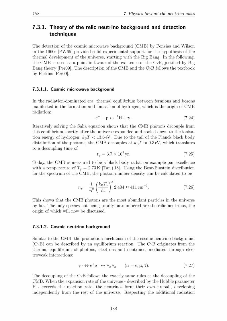
188 7. Physics beyond the neutrino mass
7.3.1. Theory of the relic neutrino background and detectiontechniques
The detection of the cosmic microwave background (CMB) by Penzias and Wilsonin the 1960s [PW65] provided solid experimental support for the hypothesis of thethermal development of the universe, starting with the Big Bang. In the following,the CMB is used as a point in favour of the existence of the CνB, justified by BigBang theory [Per09]. The description of the CMB and the CνB follows the textbookby Perkins [Per09].
7.3.1.1. Cosmic microwave background
In the radiation-dominated era, thermal equilibrium between fermions and bosonsmanifested in the formation and ionisation of hydrogen, which is the origin of CMBradiation:
e− + p↔ 1H + γ. (7.24)
Iteratively solving the Saha equation shows that the CMB photons decouple fromthis equilibrium shortly after the universe expanded and cooled down to the ionisa-tion energy of hydrogen, kBT < 13.6 eV. Due to the tail of the Planck black bodydistribution of the photons, the CMB decouples at kBT ≈ 0.3 eV, which translatesto a decoupling time of
tγ = 3.7× 10⁵ yr. (7.25)
Today, the CMB is measured to be a black body radiation example par excellencewith a temperature of Tγ = 2.73 K [Tan+18]. Using the Bose-Einstein distributionfor the spectrum of the CMB, the photon number density can be calculated to be
nγ = 1π2
(kBTγ~c
)3
2.404 ≈ 411 cm−3. (7.26)
This shows that the CMB photons are the most abundant particles in the universeby far. The only species not being totally outnumbered are the relic neutrinos, theorigin of which will now be discussed.
7.3.1.2. Cosmic neutrino background
Similar to the CMB, the production mechanism of the cosmic neutrino background(CνB) can be described by an equilibrium reaction. The CνB originates from thethermal equilibrium of photons, electrons and neutrinos, mediated through elec-troweak interactions:
γγ ↔ e+e− ↔ νανα (α = e,µ, τ). (7.27)
The decoupling of the CνB follows the exactly same rules as the decoupling of theCMB. When the expansion rate of the universe - described by the Hubble parameterH - exceeds the reaction rate, the neutrinos form their own fireball, developingindependently from the rest of the universe. Respecting the additional radiation
188

7.3. Relic neutrinos 189
contributions from fermions (compare eq. (7.27) to eq. (7.24)), the decoupling energycan be estimated to kBT ≈ 3 MeV. This energy translates to a decoupling time of
tν = 1 s. (7.28)
Using the Fermi-Dirac distribution for the spectrum of the CνB allows estimatingtoday’s temperature of the CνB from the measured CMB temperature:
Tν =( 4
11
)1/3Tγ = 1.95 K. (7.29)
Similarly, today’s number density of the CνB can be estimated from today’s CMBnumber density:
nν = gν2
1π2
(kBTν~c
)3 34 · 2.404 · nγ = 336 cm−3. (7.30)
This shows that the number densities of CMB (7.26) and of CνB (7.30) are indeedcomparable. The remarkable difference, however, is that neutrinos are proven to havea non-zero rest mass [Fuk+98, Ahm+01] – a discovery so influential to fundamentalphysics that it got rewarded with a Nobel prize in 2015 [The15]. From a cosmologicalperspective, the finite mass of neutrinos leads to the hypothesis that the – todaynon-relativistic – relic neutrinos of the CνB may cluster on accumulations of colddark matter (CDM) or baryonic matter.
7.3.1.3. Cosmic neutrino background clustering
In ref. [RW04], Ringwald and Wong describe potential forms of a localised cosmicneutrino background overdensity with focus on clustering on CDM. Ringwald andWong estimate the neutrino clustering based on a NFW8 profile as lower boundand the clustering based on the present Milky Way mass profile as upper bound.Ringwald and Wong conclude that the true relic neutrino overdensity η = nν/nν
might lie somewhere in between. At the position of our solar system (8 kpc distanceto center of Milky Way), Ringwald and Wong estimate overdensity factors between1.4 and 20. The larger the neutrino mass is, the larger is the local relic neutrinooverdensity: larger mass reduces the velocity of thermal relics. Another possibilityfor a locally increased density of the relic neutrinos is neutrino clustering similar tothe baryon overdensity in galaxy clusters as found by Lazauskas et al [LVV08]. Thiswould enable overdensities of 103 to 104 for a cluster size of 50 Mpc. Combiningnow these two results, Fassler et al. [Fas+13] scale down the cluster-scale findingsof Lazauskas to the scale of the Milky Way. This would enable overdensities ofη ≈ 106 inside the Milky Way. Even higher overdensities are estimated by Hwangand Ma [HM05], who use high neutrino clustering factors (102 to 1014) as explanationfor the GZK cut-off9 [Gre66, ZK66]. This small excerpt of conceivable origins of alocal relic neutrino overdensity inside the Milky Way motivates efforts in finallydetecting the cosmic neutrino background.
8Navarro, Frenk and White [NFW96] derive a universal dark matter profile with two parameters:density and radius.
9The GZK cut-off proposes an explanation for the cut-off of the ultra-high energetic cosmic rays,as those protons may interact with the CMB [Gre66, ZK66].
189

190 7. Physics beyond the neutrino mass
7.3.1.4. Cosmic neutrino background detection
An experimenter trying to detect the CνB has to face two fundamental challenges:the solely weak interaction of neutrinos in general and the particularly low energy ofthe CνB. Several possibilities for the CνB detection are proposed in the literature:from resonant absorption of ultra-high-energy cosmic ray neutrinos on the low-energyCνB leading to a boosted “Z burst” [FKR02] over “detecting the mechanical force onmacroscopic targets due to the ‘neutrino wind’” [Hag99] to induced β-decay [Fas+11,Bar+18]. The following investigation will focus on the possible signal identificationof the CνB at Katrin.
Already proposed by Weinberg in 1962 [Wei62], the induced β-decay is a neutrinocapture process transforming the β-decay into a two body problem:
AZN + νe → A
Z+1N′ + e− and A
ZN + νe → AZ−1N
′ + e+. (7.31)
The induced β-decay has the advantage of lacking any energy threshold. Fassleret al. derive the reaction rate for this process as the capture rate [Fas+11] (oneincoming neutrino per volume V ):
dΓν =∑ 1
V|〈f |T | i〉|2 2πδ(Ee + Ef − Ei − Eν) dpe
(2π)3 , (7.32)
with i and f initial and final state, Ei and Ef initial and final energy and T the tran-sition matrix element. Since the neutrinos are found to be massive particles [Fuk+98,Ahm+01] (also compare sec. 1.1.3) with yet unknown mass, this process received newinterest: the signal of the relic neutrino capture is a sharp line, located one neutrinomass above the endpoint of the β-decay electron spectrum (cf. fig. 7.15). Calcu-lating the transition matrix element in eq. (7.32) and integrating over the electronmomenta yields [Fas+11]:
Γν(3H) = 1π
(GF cosϑC)2F0(Z + 1, Ee)[BF(3H) +BGT(3H)
]peEe
1V
(7.33)
= 4.2 · 10−25ηνeyr−1 =: Γ′ν(3H)η, (7.34)
with 1/V = ηνe〈nνe〉 and 〈nνe
〉 = 56 cm−3. The reaction rate derived in eq. (7.34)will serve as fundamental input for the identification of the potential signal of theCνB in Katrin, discussed in the next section.
7.3.2. Induced β-decay spectrum
In sec. 7.3.1.4, the electron production rate stemming from the capture of relicneutrinos was derived. Taking one more step towards estimating the sensitivity ofKatrin for measuring the relic neutrino background, one needs to include somecharacteristics of the Katrin experiment.
7.3.2.1. Basic form
From eq. (7.34), the CνB capture signal would be an infinitesimally sharp line,located one neutrino mass above the endpoint at E0+mν. Since Katrin measures an
190

7.3. Relic neutrinos 191
−20 −15 −10 −5 0 5E − E0 (eV)
10−21
10−20
10−19
10−18
10−17d
iffra
ted
Γ/dE
(eV
s)−
1
std diff spec
CνB diff spec
−20 −15 −10 −5 0 5qU − E0 (V)
10−3
10−2
10−1
100
101
int
rateN
(cp
s)
std int spec
CνB int spec
combined int spec
Figure 7.15.: Basic spectrum - Upper panel: the relic neutrino capture signal (red)is modelled as a Gaussian peak at E0 + mν (see eq. (7.35)). Lowerpanel: the peak manifests as a shoulder in the spectrum as measuredby Katrin. Spectra for mν = 1 eV and η = 1012, no background rateincluded.
integrated spectrum, the line needs to be integrated: this leads to the conclusion thatthe sharp line can be approximated by a Gaussian with a width of 10 meV. Thoughthis might seem an arbitrary choice: it is not. As long as it is smaller than e.g. theDoppler broadening, the width of the CνB-Gaussian only influences the differentialspectrum and its integrability. Due to the signal being a normalised Gaussian,
191

192 7. Physics beyond the neutrino mass
the integration will yield the same result for the count rate even if σCνB differs.Therefore, σCνB = 10 meV was chosen because it increases the numerical stability ofthe integration. The capture (and therefore decay) rate for the CνB induced β-decaythereby takes the following form:
dΓdE
:= Γ′ν(3H) · η · e−(E−(E0+mν))2/2σ2
CνB√2πσ2
CνB
. (7.35)
In the modelled spectrum of fig. 7.15, the CνB signal is at 18 576 eV as expectedfor an example neutrino mass of mν = 1 eV. The distance between the maximumenergy of the standard β-decay spectrum (shown in dotted blue) and the CνB signal(solid red) is exactly 2mν = 2 eV.
7.3.2.2. Model extensions
As for the standard β-decay spectrum, light bosons and the potential right handedcurrents: the basic spectrum expected for the relic neutrinos described in sec. 7.3.2.1needs to be extended and refined to include effects of the Katrin set-up into thefit model. Here only the final states as one of the dominating influences will bediscussed.
The effect of the final states manifests in a shift and a broadening of the CνB sig-nal: at a probability Pfs, the daughter molecule may be left in an electronically orrotational-vibrational excited final state fs with an excitation energy Efs. The finalstate energy reduces the maximum kinetic energy E0 of the electron, therefore thedecay rate becomes
dΓdE
∣∣∣∣∣CνB
=∑fs
Γ′ν(3H) · η · Pfs ·e−(E−(E0−Efs+mν))2
/2σ2CνB√
2πσ2CνB
. (7.36)
As for the light bosons in sec. 7.1.1.1, also a 100 meV rebinned version of the finalstates is used due to the Doppler effect being of the same size. The effect of the finalstates on the CνB spectrum is visualised in fig. 7.16: the electronically excited statesshow up deep in the standard β-decay spectrum (beneath E0− 20 eV). Anyway, thelarge count rate of the standard β-decay spectrum will hide the visibility of theCνB electrons in this region.
7.3.2.3. Combination with standard β-decay
The Superposition of the CνB decay rate and the standard β-decay rate gives thecombined decay rate as a sum:
dΓdE
= dΓdE
∣∣∣∣∣β
+ dΓdE
∣∣∣∣∣CνB
. (7.37)
With the concept of a response function R(E, qU) [Kle+18], the measured integratedspectrum can be written as
N ∝∫ ∞qU
R(E, qU) dΓ
dE
∣∣∣∣∣β
+ dΓdE
∣∣∣∣∣CνB
dE . (7.38)
192

7.3. Relic neutrinos 193
−50 −40 −30 −20 −10 0E − E0 (eV)
10−21
10−20
10−19
10−18
10−17d
iffra
ted
Γ/dE
(eV
s)−
1
std diff spec
CνB diff spec
−50 −40 −30 −20 −10 0qU − E0 (V)
10−3
10−2
10−1
100
101
int
rateN
(cp
s)
std int spec
CνB int spec
combined int spec
Figure 7.16.: Spectrum - Upper panel: the relic neutrino capture signal (red) isshifted to lower energies due to the final states. Lower panel: thestrength of the CνB signal shoulder is reduced compared to fig. 7.15.Spectra for mν = 1 eV and η = 1012, no background rate included.
From eq. (7.38), we expect to see the shape of the response function in the CνB partof the integrated spectrum. This is nicely confirmed by fig. 7.15 and 7.16: themodulation of the CνB signal towards lower retardation voltage values is due to theshape of the response function. With lower retardation voltage, also the inelasticallyscattered electrons from CνB capture reach the detector, causing an increase of theCνB signal. However, this increase is not visible in the combined spectrum due to
193

194 7. Physics beyond the neutrino mass
the large signal rate from the standard β-decay farther away from the endpoint.
7.3.3. Parameter inference with relic neutrinos
First estimates of the potential of Katrin to constrain the relic neutrino backgroundcan be gathered from fits. Even more, important insights into the correlations ofthe additional fit parameter η with the standard four parameters can be gained.To investigate this, 1000 fits were performed. In each fit, a simulated measurement(including Poisson randomisation of the counts) was compared to a model and thefive fit parameters m2
ν, E0, Amp, bg and η were minimised via Minuit2 of the ROOTframework [BR97]. The Katrin settings used were the same as for the other sim-ulations in this chapter and can be found in sec. D.1 and tab. D.4 in the appendix.The first thing to be mentioned here is the effect of the sharp line of the CνB signal:
Table 7.3.: Exemplary best fit estimates of the parameters. 1000 fits withη = 1012 and neutrino mass mν = 1 eV were performed.
param true µ σ
m2ν (eV2) 1.0 1.000 0.003
E0 (eV) 18575 18575.000 0.002
Amp 1.0 1.000 0.0001
bg (cps) 0.4 0.400 0.0001
η 1× 10¹² 9.995× 10¹¹ 8.1× 10⁹
it requires a lot of integration steps in the regions where the FSD-smeared signalis expected. Otherwise, the numerical instability of the integration prevents correctreproduction of the true values. Results from the 1000 simulated Katrin measure-ments and following fits are shown in fig. 7.17. Since the CνB signal position directlydepends on the neutrino mass, see eq. 7.36, there is a correlation between mν andη. In terms of potential signal identification, a positive point is that there seems notto be a distinct bias of one of the estimated parameters.
All parameters reproduce their respective true value, which is also demonstratedin the overview presented in tab. 7.3. Furthermore, the additional fit parameter ηshows correlations with all the four standard parameters, which reveals the challengeof including the CνB signal into the fits. Also, a first hint as to the potential ofKatrin to constrain the relic neutrino background occurs: the 1σ uncertainty on ηis 8.1× 10⁹, so Katrin is expected to be able to set constraints on η at the level ofapproximately 1010.
7.3.4. Statistical sensitivity to constrain the relic neutrinobackground
The potential of Katrin to constrain the relic neutrino background can be seenin fig. 7.18. In the course of this thesis, the statistical sensitivity to the local relic
194

7.3. Relic neutrinos 195
neutrino overdensity η is estimated to be of order 1010. This value is one order ofmagnitude larger than the one estimated by Kaboth et al. [KFM10], which can beexplained by the different experimental settings. Mostly it is the background thatlimits the potential of Katrin, as outlined in ref. [Hei15]. Furthermore, as alsodiscussed in ref. [Hei15], Kaboth et al. use a simplified model for the Katrin exper-iment (no detection efficiency, simpler scattering model, larger amount of effectivecolumn density), which is why it is refrained from giving a quantitative comparisonhere.
Current limits on η from β-decay experiments trace back to the Los Alamos [Rob+91]and Troitsk [Lob+99b] experiment, which were motivated by the negative neutrinomass squared estimates. Katrin will be capable of improving this limit by atleast one order of magnitude in the current set-up. In fig. 7.18, also the estimatesintroduced in sec. 7.3.1.3 are shown. The baseline of the overdensity is given byη = 1, which corresponds to no local clustering of the relic neutrinos. Estimates ofthe relic neutrino overdensity based on the clustering of dark matter, baryons, aswell as combinations of both, range from 1 to 106 [RW04, LVV08, Fas+13].
In the scope of this thesis, also CνB-adapted MTDs are tested for their effect onthe sensitivity on η. However, the increase in sensitivity is found to be only minor.No order of magnitude increase can be achieved, even with a “CνB-focused” MTD.The reason is the dominant effect of the background rate, which generally limits theKatrin sensitivity for the CνB. For larger neutrino masses, the statistical sensitivityis found to improve marginally by about a factor 1.4.
While Katrin most likely will not be able to detect the CνB, it can rule out spec-ulative models about the origin of the GZK cut-off [HM05] and improve existingβ-decay limits on η by at least one order of magnitude.
Note that only the statistical sensitivity is investigated in this thesis. In order toderive an upper limit from the neutrino mass data, also systematic effects need tobe studied very carefully.
195
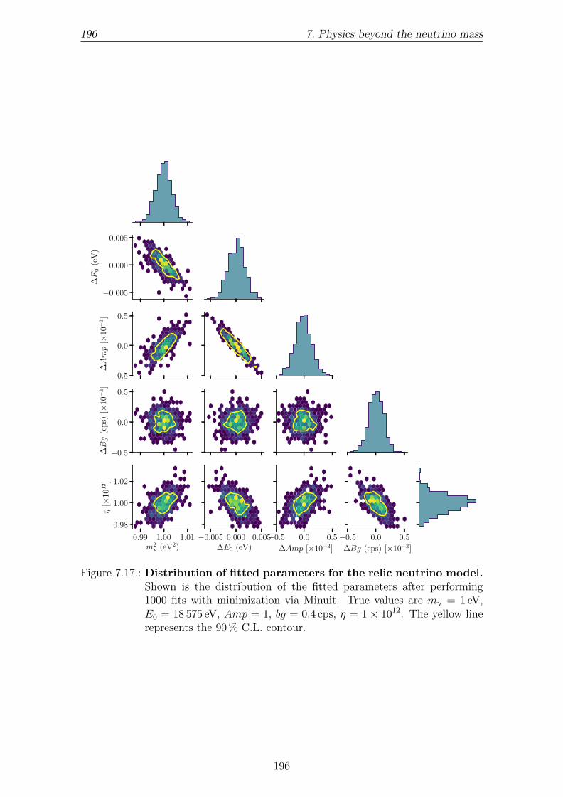
196 7. Physics beyond the neutrino mass
−0.005
0.000
0.005
∆E
0(e
V)
−0.5
0.0
0.5
∆Amp
[×10−
3]
−0.5
0.0
0.5
∆Bg
(cp
s)[×
10−
3]
0.99 1.00 1.01m2ν (eV2)
0.98
1.00
1.02
η[×
1012]
−0.005 0.000 0.005∆E0 (eV)
−0.5 0.0 0.5
∆Amp [×10−3]
−0.5 0.0 0.5
∆Bg (cps) [×10−3]
Figure 7.17.: Distribution of fitted parameters for the relic neutrino model.Shown is the distribution of the fitted parameters after performing1000 fits with minimization via Minuit. True values are mν = 1 eV,E0 = 18 575 eV, Amp = 1, bg = 0.4 cps, η = 1× 10¹². The yellow linerepresents the 90 % C.L. contour.
196

7.3. Relic neutrinos 197
0.2 0.4 0.6 0.8 1.0 1.2 1.4 1.6 1.8 2.0mν (eV)
100
102
104
106
108
1010
1012
1014
1016
η
Robertson et al. [Rob+91]
Hwang et al. [HM05]
Lobashev et al. [Lob+99b]
this work
Kaboth et al. [KFM10]
Fassler et al. [Fas+13]
Lazauskas et al. [LVV08]
Ringwald andWong [RW04]
extrapolation from [RW04]
Figure 7.18.: Statistical sensitivity for relic neutrinos. Shown is the statisti-cal sensitivity of Katrin for the detection of the CνB (solid blue).The values obtained by Robertson et al. [Rob+91] and Lobashev etal. [Lob+99b] present upper limits obtained from β-decay spectroscopy(Los Alamos and Troitsk neutrino mass experiments). The other valuesfor the CνB overdensity are predictions from various models.
197
198 7. Physics beyond the neutrino mass
7.4. Conclusion
In this chapter, three different examples for expanding the physics reach of Ka-trin beyond the neutrino mass search have been studied: light bosons, right-handedcurrents and relic neutrinos. For each of these study cases, the possible signature inthe β-decay spectrum measured by Katrin was derived, from including the inter-action into the differential spectrum of the physics model and finally the integratedspectrum including all the experimental characteristics of the Katrin apparatus.The ability of Katrin to resolve the specific new kind of interaction was testedthrough performing either ensemble tests or MCMC runs. Finally, the statisticalsensitivity of Katrin for the respective scenario was estimated.
Light bosons were considered to couple to either the neutrino, the electron orboth in the β-decay, leading to the emission of either pseudoscalar or axial vectorbosons in a modified four-body decay. The resulting spectrum derived by Arcadi etal. [Arc+18] has the observables mass mX and coupling gX of the boson with a shapevery similar to the standard β-decay spectrum. The coupling of the light boson gX
was found to be strongly correlated with its mass mX and the standard fit parametersendpoint E0 and amplitude Amp. Due to the parametrisation of the spectrum(divergence in mX by virtue of a non-conserved current), the best sensitivity forthe coupling can be derived for eV-scale vector bosons coupling to either neutrinoor electron. It can potentially allow to test the constraints by IceCube of order10−2 [IM14]. For pseudoscalars coupling to electrons, Katrin will most likely notbe able to set a competitive limit: it would need couplings gX of O(104) in orderfor Katrin to exclude the null-hypothesis at 1.645σ. Pseudoscalars coupling toneutrinos have a stronger imprint on the spectrum: here the best sensitivity is oforder O(10−1). Finally, the sensitivity of Katrin for vector bosons coupling toelectron and neutrino and thereby conserving the weak current is estimated to beof order O(10−1), as well. For keV-scale light bosons however, the large statisticsof a differential TRISTAN detector upgrade to Katrin enables testing existinglimits for all types except pseudoscalars coupling to electrons, though most likely nolower limits than the existing ones can be placed from either standard Katrin or aTRISTAN-like extension data.
Right-handed currents in presence of eV-scale sterile neutrinos were consideredto arise exemplarily by left-right symmetry of the weak interaction. The inter-action was parametrised by Steinbrink et al. [Ste+17] in a model-independent, yetmodel-motivated way that also covers interactions not necessarily based on left-rightsymmetry but also encompassing any other mechanism causing the same signaturein the spectrum. In addition to the sterile mixing angle θeff and the mass of theheavy sterile neutrino mh, this parametrisation introduces an interference term cLR.The interference might be positive or negative, thus causing interesting effects onthe spectrum. In this work as well as in ref. [Ste+17], strong correlations of thesethree additional fit parameters with the standard four parameters were found. Inhand with these strong correlations, a bias is observed in the posterior distributionof the endpoint obtained by an MCMC run, in agreement with [Ste+17]. The sensi-tivity regarding sin2 θeff and cLR is estimated for different fixed values of the sterileneutrino mass. Without constrained endpoint, Katrin will most likely not be ableto test the LR-symmetry of the potential sterile neutrinos. However, future externalmeasurements of the endpoint by Penning trap experiments combined with the pre-
198
7.4. Conclusion 199
cision determination of the absolute energy scale of the Katrin experiment mightreach an accuracy of about 50 meV. These constraints should enable Katrin to testthe LR-symmetry of potential sterile neutrinos and provide a complementary wayto access the right-handed coupling additional to LHC bounds [Sir+18].
Already in [KFM10, Hei15], the potential of Katrin to constrain the relic neu-trino background was investigated. This work was substantially refined in thescope of this thesis by a consistent implementation of the signal in the Katrin anal-ysis framework and the use of realistic experimental settings. Since the position ofthe potential signal depends only on the neutrino mass, the additional parameterintroduced was the local overdensity of the CνB, η, as it defines the amplitude of thesignal. The (local) CνB overdensity η also shows correlations with the standard fourfit parameters for the neutrino mass search. The potential of Katrin to constrainthe relic neutrino background was found to be of η ≈ O(1010) (90 % C.L.), withnegligible dependence on the neutrino mass. Though the sensitivity of Katrin to-wards the relic neutrino background is orders of magnitude away from testing mostof the predictions, it will improve existing direct limits from β-decay experiments byat least one order of magnitude.
Besides its main scientific goal, the determination of the neutrino mass, Katrin of-fers the possibility to search for a wide variety of interesting new physics. As ahigh-precision experiment, Katrin will be able to perform independent, kinematics-based tests of physics beyond the neutrino mass. The three categories investigatedin this work exemplarily give a hint and outlook of the kind of physics search possiblewith Katrin.
199


CHAPTER 8
SUMMARY AND CONCLUSIONS
The project of the thesis at hand evolves around the commissioning, simulation, andcharacterisation of the Windowless Gaseous Tritium Source, as well as analysing thefirst tritium spectra for the Katrin experiment located at the Karlsruhe Instituteof Technology (KIT). This includes testing individual temperature sensors for shortcircuits in the cryostat to spectral fitting and statistical analysis of tritium data.Key findings of this journey will be summarised in the following, before concludingthis chapter with an outlook on the near future.
Source modelling An essential cornerstone for the work presented in this thesisis the extension and uniform integration of the source model. The input from var-ious sensor readings (temperature, gas flow) is implemented to allow near-onlinecalculation of the source density distribution and to initiate the spectrum modelcomputation. In the course of the First Tritium campaign, the sensor informationwas used to provide a run-wise estimation of the column density in the WGTS tothe individual fitting teams of the Katrin analysis group, enabling the high-leveltritium spectrum fitting. Temperature readings and gas flow readings are now in-tegrated into the gas dynamics part of the source and spectrum calculation (SSC)framework. Thereby, two new methods were implemented to calculate the sensorbased (deuterium) column density using the estimated gas injection rate. The in-creased flexibility of the two generalised gas models allows their usage for deuterium(commissioning) and tritium mode of the source, particularly when the e-gun is notavailable to provide column density calibration measurements. For most of the FirstTritium runs, the D2 column density is estimated to be 4.5× 10²¹ m−2, with a rela-tive uncertainty of about 5 %. A cross-check via the pressure of the Krypton capillaryshowed good agreement within about 3-4 %. Moreover, a dedicated WGTS magneticstray field measurement system was designed, developed and commissioned. Afterproper position determination, its measurements can be used to validate and anchorthe magnetic field simulations of the WGTS.
Analysis of First Tritium data With the sensor based source model, it was pos-sible to analyse the tritium spectra taken during the Very First Tritium and theFirst Tritium commissioning campaigns. The agreement between spectral model
201

202 8. Summary and Conclusions
and the data was found to be very good, therefore several analysis methods for thetritium spectrum could be tested. Different methods to include systematic effectswere investigated using the column density simulated by the source model as an il-lustrative example. The resulting estimates of the effective endpoint were comparedagainst each other, as well as to the expected value obtained from T-3He atomicmass difference measurements [Mye+15]. All estimates were found to agree withinthe assumed range of 1 eV (a sizeable uncertainty stemming from the current ac-curacy of the absolute energy scale of the Katrin experiment [WVH]). From theappended run estimation with the column density as free fit parameter, a columndensity of (4.61 ± 0.12) × 1021 m−2 was found, which is within the uncertainty ofthe simulation result. Additional estimations of the column density were possibledue to the active commissioning. The FBM and PULCINELLA estimates also agreewith the column density simulation. Adapting the model input parameters for theslightly higher column density estimate of the aforementioned independent detectorsand fit results yields excellent agreement (N = 4.6× 10²¹ m−2) for Boltzmann andKnudsen based flow for an accommodation coefficient α = 1 (instead of 0.97) andan outlet to inlet pressure ratio of pout/pin = 0.05 (instead of 0.02).
Blind analysis and methods Looking ahead, the neutrino mass data taking of Ka-trin is about to begin in early 2019. As a key outcome of this thesis, several possibleschemes for performing a blind analysis were developed. Three data blinding tech-niques (reduced statistics, window blinding, and energy smearing) and two modelblinding techniques (imperfect energy loss function and FSD smearing) were investi-gated and their effect on the neutrino mass estimation quantified. After evaluation ofthe latter, four blinding techniques are considered viable for Katrin neutrino massanalysis. For the first neutrino mass data, two blinding techniques are favoured,namely FSD and energy smearing. Application of either one will introduce a unidi-rectional artificial shift of the reconstructed neutrino mass. As the two techniquesyield opposite signs for this shift, a combination of both methods is considered asthe strongest blinding scheme plausible for the first neutrino mass data. Note thatthe model blinding techniques rely on the analyst’s responsibility and are meant toprevent accidental bias by analysing unblinded data. Since the raw data will alwaysbe available unblinded to check for systematic effects, the only data blinded will beneutrino mass data. That is, the data blinding will be applied in the intermediatedata layer such that the high-level neutrino mass analysis will work on blinded runsummaries. The generation of blinded run summaries was tested successfully, alongwith the FSD smearing model blinding technique. All methods tested on krypton(and tritium) data worked as expected. Based on the findings of this thesis, a pro-posal of viable techniques and a recommended strategy will be put forward for theKatrin collaboration to deliberate and decide on.
Physics beyond the neutrino mass Besides serving its main scientific goal, themodel-independent determination of the effective electron neutrino mass, the Ka-trin data can be used to probe various interesting models of physics beyond theStandard Model. In the course of this thesis, three such opportunities were subjectto a detailed investigation: the statistical sensitivity of Katrin to constrain theadditional emission of light bosons in β-decay, the existence of right-handed cur-rents in presence of eV-scale sterile neutrinos, and the relic neutrino background
202
203
was investigated. Though the sensitivity of Katrin towards the additional emis-sion of light vector bosons or pseudoscalars is found not to surpass existing limitsfor the present Katrin set-up, Katrin may provide a complementary limit. In aTRISTAN-like future extension for a differential measurement of the tritium spec-trum, the large statistics available from the full tritium spectrum enables testingexisting limits e.g. from IceCube [IM14]. The statistical sensitivity of Katrin to-wards right handed currents in β-decay was found to be not competitive to existingconstraints from LHC data; however, Katrin can provide a model-independentcross-check. The latter is especially important as the LHC bounds are based on LR-symmetry, while Katrin can probe different effects that may result in this modelindependent parametrisation. The findings of the right handed currents match theones obtained in ref. [Ste+17], though this thesis assumes slightly different Ka-trin settings. The latter mainly accommodate for a scenario with an elevated back-ground rate, a decreased energy resolution due to higher analysing plane magneticfield, and an extended energy range of the measurement interval. These alternativesettings were also used to re-evaluate Katrin’s statistical sensitivity to constrainthe relic neutrino background. Katrin will be able to improve the existing directlimit on the local relic neutrino overdensity by at least one order of magnitude andthereby also exclude some of the more progressive astrophysical models. However,most predictions of the relic neutrino overdensity are clearly below the sensitivity ofthe Katrin experiment.
Conclusions The focus of this thesis was on the opportunities offered by the uniquetritium source of the Katrin experiment. The automated estimation of the columndensity based on a gas model using sensor data enabled first comparisons betweenthe modelled and the measured tritium spectra. It was shown that the Katrin ex-periment is performing as expected and ready for the start of neutrino mass datataking, including a possible blind analysis. Furthermore, the unique tritium sourcepaired with the high-resolution electrostatic spectrometer enables testing aspects ofhypothetical new physics beyond the Standard Model, thus allowing to broaden thescientific reach of the experiment beyond the hunt for the neutrino mass.
Outlook In the course of the past two years, the Katrin collaboration has suc-cessfully accomplished several important milestones en route to the start of neutrinomass data taking: from completing the beam line in 2016, to recording first high-resolution spectra of 83mKr-conversion electron lines in 2017, up to the measuring offirst tritium β-spectra in 2018. During the time of writing this thesis, another im-portant milestone is reached, which is the extensive commissioning phase with thee-gun at the rear section. Together with the measurements of the column densitydeveloped in the course of this thesis, the e-gun will enable accurate and precisedetermination of the column density in the nominal tritium set-up. In early 2019,Katrin will start its eagerly awaited nominal tritium running, which will allow thestart of the physics harvest to be continued over the next years.
203


APPENDIX
A. Source modelling
A.1. Temperature
Fig. A.1 shows a CAD model of the connection of the central WGTS beam tubeto the pump port PP1-R. It can be seen that the beam tube cooling does not startright at the pump port and that the temperature sensors only are placed in regionwith active beam tube cooling.
A.2. First Tritium set-up
Table A.1.: Times used for the injection rate calibration. Only times withensured stable circulation were chosen, year is 2018.
start end
06-11, 0:00 h 06-12, 5:00 h
06-12, 7:00 h 06-12, 15:00 h
06-12, 17:00 h 06-13, 7:00 h
06-13, 15:00 h 06-14, 8:00 h
06-14, 19:00 h 06-15, 6:00 h
06-15, 8:00 h 06-15, 21:00 h
A.3. Magnetic field measurements
As described in sec. 4.5.2, the longitudinal position of the hall probe needs to bedetermined with a sub-mm uncertainty. WayCon states a 0.02 % linearity deviationof the rope sensor, however the calibration certificate in fig. A.2 provided by WayConlists a maximum linearity deviation of 0.002 %.
205

206 8. Appendix
Figure A.1.: Connection between beam tube and pump port. The positionof the Pt500 temperature sensors as well as the 2-phase neon coolingand the pump port cooling are shown in copper.
B. Analysis of First Tritium data
B.1. Estimation of the column density
During the readout of the FBM spectrum, it was discovered that the cut is betterto be done on the ADC spectrum, not on the calibrated one: when cutting at 5 keVon the calibrated spectrum, the result is shown in fig. B.4. Therefore, the rate wasestimated by cutting on the ADC equivalent of 5 keV, which is also shown on fig. B.4.
C. Blind analysis & methods
C.1. Sensitivity estimates
It has to be noted that not all methods have been tested with the exact samesettings of the background rate Bg and energy resolution. However, the high levelof blinding required for the first Katrin neutrino mass data requires effects insystematic or statistic uncertainty one order of magnitude larger than the effect ofan elevated background rate: if the MTD is adapted for an elevated background
206

C. Blind analysis & methods 207
0,0
02
Max
Dev
iatio
n
[% o
f M
R]:
Cal
ibra
tion
Cer
tific
ate
Pos
.Ref
. S
yste
m
[mm
]M
easu
red
Val
ue:
Dev
iatio
n [%
of
MR
]
Com
men
t:
Way
Con
Pos
ition
smes
stec
hnik
Gm
bH
Meh
lbee
rens
tr. 4
82
024
Tau
fkirc
hen
ww
w.w
ayco
n.de
-0,0
00
-0,0
07
15
9,5
45
22
39
,00
0-0
,00
1
31
9,9
52
44
82
,75
0-0
,00
1
47
9,9
88
67
21
,25
0-0
,00
1
64
0,0
85
89
61
,00
0-0
,00
1
79
9,9
81
11
19
8,2
50
-0,0
00
96
0,0
67
13
43
7,5
00
-0,0
00
11
20
,10
31
56
74
,75
0-0
,00
1
12
79
,96
91
79
12
,25
0-0
,00
0
14
40
,00
52
01
51
,00
00
,00
0
16
00
,11
22
23
90
,75
00
,00
0
17
59
,95
72
46
27
,00
00
,00
1
19
19
,95
42
68
65
,00
00
,00
1
20
80
,01
02
91
04
,00
00
,00
1
22
40
,01
63
13
42
,00
00
,00
1
23
99
,87
23
35
78
,75
00
,00
2
25
60
,03
83
58
18
,75
00
,00
1
27
19
,98
43
80
56
,25
00
,00
1
28
80
,00
14
02
94
,25
00
,00
1
30
40
,06
74
25
33
,75
00
,00
2
32
00
,03
34
47
71
,00
00
,00
1
33
59
,91
94
70
07
,50
00
,00
1
35
19
,97
54
92
46
,25
00
,00
1
36
80
,04
15
14
84
,50
00
,00
1
38
39
,98
75
37
22
,50
00
,00
1
40
00
,07
45
59
61
,00
00
,00
1
41
60
,08
05
81
99
,50
00
,00
1
43
19
,98
66
04
36
,00
00
,00
1
44
80
,00
26
26
74
,50
00
,00
1
46
40
,06
86
49
12
,75
00
,00
0
47
99
,96
46
71
49
,75
00
,00
1
49
60
,00
06
93
88
,00
00
,00
1
51
20
,07
77
16
27
,00
00
,00
0
52
80
,06
37
38
65
,00
00
,00
1
54
39
,96
97
61
01
,25
00
,00
0
56
00
,06
57
83
40
,75
00
,00
0
57
59
,97
18
05
77
,00
0-0
,00
0
59
19
,97
78
28
16
,00
00
,00
1
60
80
,07
38
50
54
,25
0-0
,00
0
62
40
,07
08
72
92
,50
0-0
,00
0
63
99
,99
58
95
29
,00
0-0
,00
1
65
60
,05
29
17
67
,50
0-0
,00
1
67
19
,97
89
40
04
,50
0-0
,00
1
68
79
,96
49
62
42
,00
0-0
,00
1
70
39
,98
09
84
80
,75
0-0
,00
1
72
00
,02
61
00
71
8,5
00
-0,0
02
73
59
,93
21
02
95
6,2
50
-0,0
01
75
19
,99
81
05
19
4,2
50
-0,0
02
76
80
,07
51
07
43
4,2
50
-0,0
01
78
39
,97
11
09
67
0,7
50
-0,0
01
80
00
,00
71
11
91
0,0
00
-0,0
00
0,0
00
17
55
88
10
Ser
.Nr.
:
04
80
63
l18
00
61
El.S
er.N
r.:
Fr,
16
. M
rz 2
01
8D
ate:
SX
13
5-8
-14
-L-K
R0
5-L
02
Sen
sor:
-0,0
07
Min
Dev
iatio
n
[% o
f M
R]:
21
Tem
p.[°
C]
+/-
1:M
ark
us
Sto
rmE
dito
r:
Pos
.Ref
. S
yste
m
[mm
]M
easu
red
Val
ue:
Dev
iatio
n [%
of
MR
]
-0,0
04
16
0,0
46
22
31
,00
00
,00
0
31
9,9
52
44
68
,25
00
,00
1
47
9,9
08
67
05
,75
00
,00
0
64
0,0
15
89
45
,75
00
,00
1
80
0,0
21
11
18
4,0
00
0,0
01
95
9,9
37
13
42
2,0
00
0,0
01
11
20
,02
31
56
60
,50
00
,00
0
12
80
,07
91
78
99
,25
00
,00
0
14
39
,91
52
01
36
,75
00
,00
1
15
99
,96
12
23
75
,00
00
,00
1
17
60
,07
82
46
14
,25
00
,00
0
19
19
,96
42
68
51
,00
00
,00
0
20
80
,02
02
90
90
,50
00
,00
0
22
40
,01
63
13
28
,50
00
,00
0
24
00
,00
23
35
67
,25
00
,00
1
25
59
,95
83
58
04
,25
00
,00
0
27
20
,00
43
80
43
,75
00
,00
1
28
80
,02
14
02
82
,00
00
,00
0
30
39
,98
74
25
19
,75
00
,00
0
32
00
,15
34
47
59
,75
0-0
,00
0
33
59
,96
94
69
96
,75
00
,00
1
35
19
,96
54
92
34
,50
00
,00
0
36
79
,92
15
14
71
,75
0-0
,00
0
38
39
,89
75
37
10
,00
00
,00
0
39
99
,94
35
59
47
,25
0-0
,00
2
41
60
,05
05
81
87
,75
0-0
,00
1
43
20
,02
66
04
25
,50
0-0
,00
1
44
80
,12
26
26
66
,00
0-0
,00
0
46
39
,98
86
49
03
,00
00
,00
0
48
00
,04
46
71
41
,25
0-0
,00
1
49
59
,89
06
93
77
,75
0-0
,00
0
51
20
,00
67
16
17
,25
0-0
,00
1
52
80
,05
37
38
57
,00
0-0
,00
0
54
39
,96
97
60
93
,50
0-0
,00
1
56
00
,04
57
83
33
,50
0-0
,00
0
57
60
,05
18
05
71
,25
0-0
,00
1
59
19
,96
78
28
09
,25
0-0
,00
0
60
79
,90
38
50
46
,75
00
,00
0
62
39
,94
98
72
85
,50
0-0
,00
0
63
99
,99
68
95
23
,75
0-0
,00
1
65
60
,06
29
17
63
,00
0-0
,00
1
67
20
,07
89
40
02
,25
0-0
,00
0
68
80
,04
49
62
40
,00
0-0
,00
0
70
39
,98
09
84
78
,25
00
,00
0
72
00
,01
61
00
71
6,2
50
-0,0
00
73
60
,01
21
02
95
6,0
00
0,0
01
75
19
,98
81
05
19
3,0
00
0,0
00
76
80
,05
51
07
43
3,2
50
0,0
01
78
40
,05
11
09
67
1,5
00
0,0
01
80
00
,01
71
11
91
0,0
00
0,0
02
0,3
59
-8,0
00
Incr
/mm
Sen
sor
runs
out
:S
enso
r ru
ns in
:
0,0
10
-0,0
10
-0,0
08
-0,0
06
-0,0
04
-0,0
02
0,0
00
0,0
02
0,0
04
0,0
06
0,0
08
Po
siti
on
[m
m]
90
00
,00,0
10
00
,02
00
0,0
30
00
,04
00
0,0
50
00
,06
00
0,0
70
00
,08
00
0,0
Ru
n I
n
Ru
n O
ut
Lin
eari
ty D
evi
ati
on
[%
of
MR
]
35
7,4
20
Inde
x-P
ulse
Dis
tanc
e [m
m]
Ref
eren
ce-S
yste
m:
Sca
ncon
Inc
rem
enta
l Enc
oder
(12
500
Incr
/Tur
n)
13
,98
91
Sen
sitiv
ity:
Figure A.2.: Rope sensor calibration table. This table for one of the used SX135rope sensor underlines that the accuracy of the distance measurementis within the sub-mm requirement.
rate of 0.225 cps1 instead of designed 0.01 cps [KAT05], the estimated neutrino mass
1F. Harms found an increased spectrometer background rate of 691 ± 1 mcps in commissioningmeasurements with different settings than the ones used in this thesis [Har15].
207

208 8. Appendix
E0,eff
Amp
Bg
1 −0.833116 −0.283638
−0.833116 1 0.207279−0.283638 0.207279 1
(8.1)
Figure B.3.: Correlation matrix of the fit parameters. The values were ob-tained from the example run 40667.
Energy (keV)4 6 8 10 12 14 16 18 20 22 24
Cou
nts
0
100
200
300
400
500
600
700
800
900
1000310×
Channel 1
Channel 2
ADC0 200 400 600 800 1000 1200 1400 1600 1800 2000
Cou
nts
0
20
40
60
80
100
310×
Channel 1
Channel 2
Figure B.4.: FBM spectra. Left: energy-calibrated spectrum, right: ADC rawspectrum. FBM runs analysed: 145-147 (June 6, 2018).
sensitivity decreases to 0.24 eV instead of 0.20 eV. In contrast, a sensitivity as highas 2 eV is to be reached with blind analysis of the first neutrino mass data.
Table C.2.: Settings for data blinding. Some of them differ from the DesignReport [KAT05] and were adapted to account for higher background.
setting Design Report data blinding
Bg (cps) 0.01 0.225
BS (T) 3.6 3.6
BAna (G) 3 9
BPCH (T) 6.0 6.0
N (m2) 5× 10²¹ 5× 10²¹
εT 0.95 0.95
C.2. Window blinding
In tab. C.3, exemplary neutrino mass sensitivity estimates are shown to underlinethe principal understanding of the effect of this method described in sec. 6.3.1.2.Only after removing all data up to the estimated endpoint (row 5 in tab. C.3), asignificant worsening of the neutrino mass can be observed. Also note that though
208

C. Blind analysis & methods 209
nearly 70% of the measuring time needs to be blinded, this translates to hiding about20% of all events measured in that time.
Table C.3.: Sensitivities for different partial blinding schemes for the neu-trino mass region. Also compare fig. 6.3. Standard settings fromDesign Report used [KAT05]. This will look different for more realis-tic values of background and MTD and is shown here to underline theprincipal understanding of this blinding method.
blinded % blinded % blinded σm
2ν
90 % CL sens
window (eV) of MTD of events (eV2) on mν (eV)
– 0.0 0.0 0.017 0.198
[E0 − 4.5, E0 − 4] 34.6 0.4 0.029 0.235
[E0 − 9, E0 − 4] 43.5 0.9 0.040 0.268
[E0 − 14, E0 − 4] 49.0 3.9 0.041 0.269
[E0 − 14, E0] 61.6 4.0 0.612 1.004
[E0 − 19, E0] 67.1 14.0 1.570 1.607
[E0 − 21, E0] 69.3 21.4 2.652 2.089
C.3. Imperfect energy loss function
In fig. C.5, the different εc are shown for several changes of the excitation/ionisationratio η. Note that due to the form of eq. (6.21), the root yields a positive and anegative solution. Since the negative solution refers to the left side of the Gaussianfunction, the critical energy that is needed for this analysis is defined by the positivesolution of the root. Exemplary, no change of the ratios (η = 0) yields εc = 14.09 eV.
209

210 8. Appendix
Figure C.5.: Energy loss critical energy. X axis is the change of the excita-tion/ionisation ratio, y axis shows the resulting solutions of eq. (6.21).Figure taken from ref. [Sib18], credits V. Sibille.
210
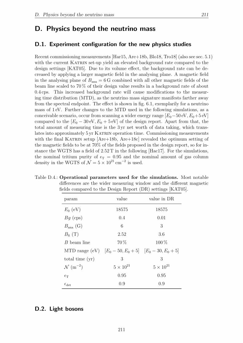
D. Physics beyond the neutrino mass 211
D. Physics beyond the neutrino mass
D.1. Experiment configuration for the new physics studies
Recent commissioning measurements [Har15, Are+18b, Blo18, Tro18] (also see sec. 5.1)with the current Katrin set-up yield an elevated background rate compared to thedesign settings [KAT05]. Due to its volume effect, the background rate can be de-creased by applying a larger magnetic field in the analysing plane. A magnetic fieldin the analysing plane of Bana = 6 G combined with all other magnetic fields of thebeam line scaled to 70 % of their design value results in a background rate of about0.4 cps. This increased background rate will cause modifications to the measur-ing time distribution (MTD), as the neutrino mass signature manifests farther awayfrom the spectral endpoint. The effect is shown in fig. 6.1, exemplarily for a neutrinomass of 1 eV. Further changes to the MTD used in the following simulations, as aconceivable scenario, occur from scanning a wider energy range [E0−50 eV, E0+5 eV]compared to the [E0 − 30 eV, E0 + 5 eV] of the design report. Apart from that, thetotal amount of measuring time is the 3 yr net worth of data taking, which trans-lates into approximately 5 yr Katrin operation time. Commissioning measurementswith the final Katrin setup [Are+18b, Are+18c] revealed the optimum setting ofthe magnetic fields to be at 70% of the fields proposed in the design report, so for in-stance the WGTS has a field of 2.52 T in the following [Hac17]. For the simulations,the nominal tritium purity of εT = 0.95 and the nominal amount of gas columndensity in the WGTS of N = 5× 1021 cm−2 is used.
Table D.4.: Operational parameters used for the simulations. Most notabledifferences are the wider measuring window and the different magneticfields compared to the Design Report (DR) settings [KAT05].
param value value in DR
E0 (eV) 18575 18575
Bg (cps) 0.4 0.01
Bana (G) 6 3
BS (T) 2.52 3.6
B beam line 70 % 100 %MTD range (eV) [E0 − 50, E0 + 5] [E0 − 30, E0 + 5]
total time (yr) 3 3
N (m−2) 5× 10²¹ 5× 10²¹
εT 0.95 0.95
εdet 0.9 0.9
D.2. Light bosons
211

212 8. Appendix
10−3 10−2 10−1 100 101 102 103 104
boson mass mX (eV)
10−26
10−23
10−20
10−17
10−14
10−11
K/g
2 X
A: νγ5νX
B: eγ5eX
C: νγµPLνXµ
D: eγµeXµ
E: jµLeXµ
10−3 10−2 10−1 100 101 102 103 104
boson mass mX (eV)
2.0
2.5
3.0
3.5
4.0
n
A: νγ5νX
B: eγ5eX
C: νγµPLνXµ
D: eγµeXµ
E: jµLeXµ
Figure D.6.: Parameters for the spectrum approximation of the lightbosons. Note the increasing K for small mX for mechanisms C and D.Figure adapted from ref. [Arc+18].
212
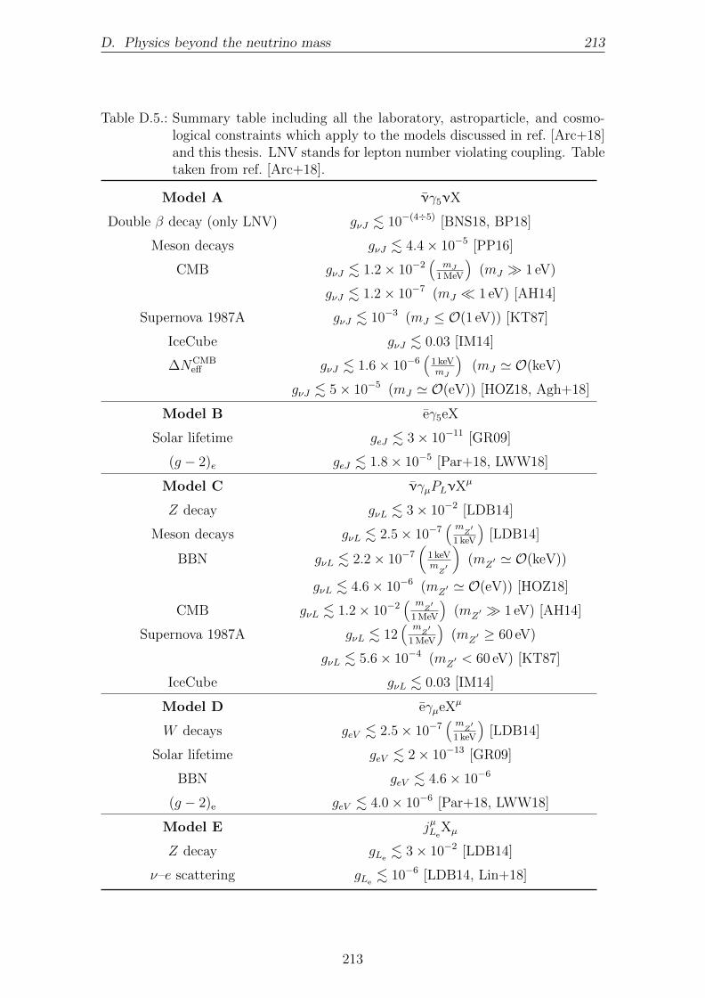
D. Physics beyond the neutrino mass 213
Table D.5.: Summary table including all the laboratory, astroparticle, and cosmo-logical constraints which apply to the models discussed in ref. [Arc+18]and this thesis. LNV stands for lepton number violating coupling. Tabletaken from ref. [Arc+18].
Model A νγ5νX
Double β decay (only LNV) gνJ . 10−(4÷5) [BNS18, BP18]
Meson decays gνJ . 4.4× 10⁻⁵ [PP16]
CMB gνJ . 1.2× 10⁻²(
mJ1 MeV
)(mJ � 1 eV)
gνJ . 1.2× 10⁻⁷ (mJ � 1 eV) [AH14]
Supernova 1987A gνJ . 10−3 (mJ ≤ O(1 eV)) [KT87]
IceCube gνJ . 0.03 [IM14]
∆NCMBeff gνJ . 1.6× 10⁻⁶
(1 keVmJ
)(mJ ' O(keV)
gνJ . 5× 10⁻⁵ (mJ ' O(eV)) [HOZ18, Agh+18]
Model B eγ5eX
Solar lifetime geJ . 3× 10⁻¹¹ [GR09]
(g − 2)e geJ . 1.8× 10⁻⁵ [Par+18, LWW18]
Model C νγµPLνXµ
Z decay gνL . 3× 10⁻² [LDB14]
Meson decays gνL . 2.5× 10⁻⁷( m
Z′
1 keV
)[LDB14]
BBN gνL . 2.2× 10⁻⁷(
1 keVmZ′
)(mZ
′ ' O(keV))
gνL . 4.6× 10⁻⁶ (mZ′ ' O(eV)) [HOZ18]
CMB gνL . 1.2× 10⁻²( m
Z′
1 MeV
)(mZ
′ � 1 eV) [AH14]
Supernova 1987A gνL . 12( m
Z′
1 MeV
)(mZ
′ ≥ 60 eV)gνL . 5.6× 10⁻⁴ (mZ
′ < 60 eV) [KT87]
IceCube gνL . 0.03 [IM14]
Model D eγµeXµ
W decays geV . 2.5× 10⁻⁷( m
Z′
1 keV
)[LDB14]
Solar lifetime geV . 2× 10⁻¹³ [GR09]
BBN geV . 4.6× 10⁻⁶
(g − 2)e geV . 4.0× 10⁻⁶ [Par+18, LWW18]
Model E jµLeXµ
Z decay gLe. 3× 10⁻² [LDB14]
ν–e scattering gLe. 10−6 [LDB14, Lin+18]
213


LIST OF FIGURES
1.1. Neutrinos - Project Poltergeist . . . . . . . . . . . . . . . . . . . . . . 21.2. Neutrinos - Standard Model of particle physics . . . . . . . . . . . . . 41.3. Neutrinos - solar neutrino flux . . . . . . . . . . . . . . . . . . . . . . 51.4. Neutrinos - atmospheric neutrinos zenith angle distributions . . . . . 61.5. Neutrinos - energy dependent surivival probability of solar neutrinos . 101.6. Neutrinos - Neutrino mass hierarchy . . . . . . . . . . . . . . . . . . 121.7. Neutrinos - tritium decay spectrum . . . . . . . . . . . . . . . . . . . 16
2.1. KATRIN: set-up . . . . . . . . . . . . . . . . . . . . . . . . . . . . . 202.2. KATRIN: energy loss function . . . . . . . . . . . . . . . . . . . . . . 222.3. KATRIN: voxelisation concept . . . . . . . . . . . . . . . . . . . . . . 222.4. KATRIN: monitoring instrumentation . . . . . . . . . . . . . . . . . 252.5. KATRIN: transport section . . . . . . . . . . . . . . . . . . . . . . . 262.6. KATRIN: MAC-E filter principle . . . . . . . . . . . . . . . . . . . . 292.7. KATRIN: detector section . . . . . . . . . . . . . . . . . . . . . . . . 312.8. KATRIN: data analysis structure . . . . . . . . . . . . . . . . . . . . 32
3.1. WGTS: half cut of the cryostat . . . . . . . . . . . . . . . . . . . . . 383.2. WGTS: layers of the cryostat . . . . . . . . . . . . . . . . . . . . . . 393.3. WGTS: beam tube cooling concept . . . . . . . . . . . . . . . . . . . 403.4. WGTS: injection chamber . . . . . . . . . . . . . . . . . . . . . . . . 41
4.1. Source model: pressure regimes . . . . . . . . . . . . . . . . . . . . . 454.2. Source model: temperature sensor positions . . . . . . . . . . . . . . 494.3. Source model: temperature correlations . . . . . . . . . . . . . . . . . 504.4. Source model: azimuthal beam tube temperature distribution . . . . 514.5. Source model: longitudinal beam tube temperature distribution . . . 524.6. Source model: scheme of the model geometries . . . . . . . . . . . . . 524.7. Source model: transition between central tube and DPS1 PP1 . . . . 564.8. Source model: longitudinal density distribution in the complete WGTS 584.9. Source model: gas dynamics related neutrino mass uncertainty . . . . 604.10. Source model: relation between pressure controlled buffer vessel and
injection rate . . . . . . . . . . . . . . . . . . . . . . . . . . . . . . . 634.11. Source model: realistic density profile for Knudsen and Boltzmann
approaches . . . . . . . . . . . . . . . . . . . . . . . . . . . . . . . . . 674.12. Source model: relation between column density and injection rate. . . 68
215
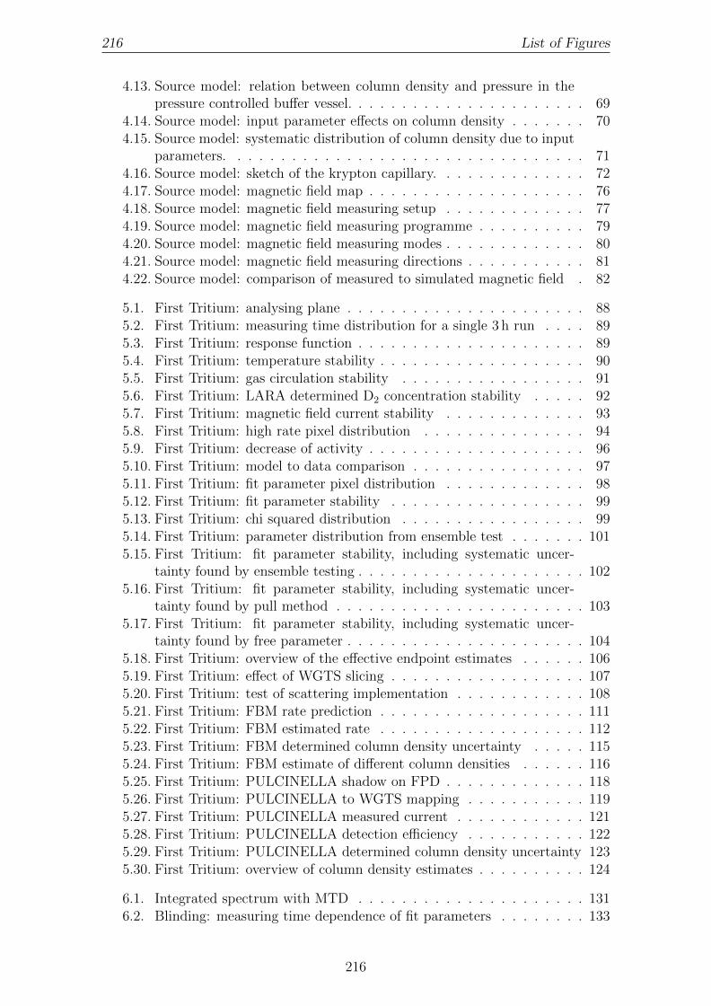
216 List of Figures
4.13. Source model: relation between column density and pressure in thepressure controlled buffer vessel. . . . . . . . . . . . . . . . . . . . . . 69
4.14. Source model: input parameter effects on column density . . . . . . . 704.15. Source model: systematic distribution of column density due to input
parameters. . . . . . . . . . . . . . . . . . . . . . . . . . . . . . . . . 714.16. Source model: sketch of the krypton capillary. . . . . . . . . . . . . . 724.17. Source model: magnetic field map . . . . . . . . . . . . . . . . . . . . 764.18. Source model: magnetic field measuring setup . . . . . . . . . . . . . 774.19. Source model: magnetic field measuring programme . . . . . . . . . . 794.20. Source model: magnetic field measuring modes . . . . . . . . . . . . . 804.21. Source model: magnetic field measuring directions . . . . . . . . . . . 814.22. Source model: comparison of measured to simulated magnetic field . 82
5.1. First Tritium: analysing plane . . . . . . . . . . . . . . . . . . . . . . 885.2. First Tritium: measuring time distribution for a single 3 h run . . . . 895.3. First Tritium: response function . . . . . . . . . . . . . . . . . . . . . 895.4. First Tritium: temperature stability . . . . . . . . . . . . . . . . . . . 905.5. First Tritium: gas circulation stability . . . . . . . . . . . . . . . . . 915.6. First Tritium: LARA determined D2 concentration stability . . . . . 925.7. First Tritium: magnetic field current stability . . . . . . . . . . . . . 935.8. First Tritium: high rate pixel distribution . . . . . . . . . . . . . . . 945.9. First Tritium: decrease of activity . . . . . . . . . . . . . . . . . . . . 965.10. First Tritium: model to data comparison . . . . . . . . . . . . . . . . 975.11. First Tritium: fit parameter pixel distribution . . . . . . . . . . . . . 985.12. First Tritium: fit parameter stability . . . . . . . . . . . . . . . . . . 995.13. First Tritium: chi squared distribution . . . . . . . . . . . . . . . . . 995.14. First Tritium: parameter distribution from ensemble test . . . . . . . 1015.15. First Tritium: fit parameter stability, including systematic uncer-
tainty found by ensemble testing . . . . . . . . . . . . . . . . . . . . . 1025.16. First Tritium: fit parameter stability, including systematic uncer-
tainty found by pull method . . . . . . . . . . . . . . . . . . . . . . . 1035.17. First Tritium: fit parameter stability, including systematic uncer-
tainty found by free parameter . . . . . . . . . . . . . . . . . . . . . . 1045.18. First Tritium: overview of the effective endpoint estimates . . . . . . 1065.19. First Tritium: effect of WGTS slicing . . . . . . . . . . . . . . . . . . 1075.20. First Tritium: test of scattering implementation . . . . . . . . . . . . 1085.21. First Tritium: FBM rate prediction . . . . . . . . . . . . . . . . . . . 1115.22. First Tritium: FBM estimated rate . . . . . . . . . . . . . . . . . . . 1125.23. First Tritium: FBM determined column density uncertainty . . . . . 1155.24. First Tritium: FBM estimate of different column densities . . . . . . 1165.25. First Tritium: PULCINELLA shadow on FPD . . . . . . . . . . . . . 1185.26. First Tritium: PULCINELLA to WGTS mapping . . . . . . . . . . . 1195.27. First Tritium: PULCINELLA measured current . . . . . . . . . . . . 1215.28. First Tritium: PULCINELLA detection efficiency . . . . . . . . . . . 1225.29. First Tritium: PULCINELLA determined column density uncertainty 1235.30. First Tritium: overview of column density estimates . . . . . . . . . . 124
6.1. Integrated spectrum with MTD . . . . . . . . . . . . . . . . . . . . . 1316.2. Blinding: measuring time dependence of fit parameters . . . . . . . . 133
216

List of Figures 217
6.3. Blinding: window example . . . . . . . . . . . . . . . . . . . . . . . . 1346.4. Blinding: window width dependence of fit parameters . . . . . . . . . 1366.5. Blinding: energy smearing, rate differences spectra . . . . . . . . . . . 1396.6. Blinding: 3 eV energy smearing effect on the integrated spectrum . . 1406.7. Blinding: energy smearing dependence of fit parameters . . . . . . . . 1416.8. Blinding: FSD smearing effect . . . . . . . . . . . . . . . . . . . . . . 1436.9. Blinding: 3 eV FSD smearing effect on the integrated spectrum . . . . 1446.10. Blinding: imperfect energy loss function . . . . . . . . . . . . . . . . 1456.11. Blinding: discovery potential for reduced statistics blinding . . . . . . 1476.12. Blinding: sensitivity for reduced statistics blinding . . . . . . . . . . . 1486.13. Blinding: sensitivity for window blinding . . . . . . . . . . . . . . . . 1496.14. Blinding: sensitivity for energy smearing . . . . . . . . . . . . . . . . 1516.15. Blinding: sensitivity for energy smearing with analysts assumptions . 1526.16. Blinding: sensitivity for FSD smearing . . . . . . . . . . . . . . . . . 1536.17. Blinding: sensitivity for imperfect energy loss . . . . . . . . . . . . . 1546.18. Blinding: sensitivity summary . . . . . . . . . . . . . . . . . . . . . . 1556.19. Blinding: unblinded 83mKr spectrum . . . . . . . . . . . . . . . . . . 1566.20. Blinding: 5 V window blinded 83mKr spectrum . . . . . . . . . . . . . 1576.21. Blinding: window width dependence of 83mKr fit parameters . . . . . 1586.22. Blinding: 5 eV energy smeared 83mKr spectrum . . . . . . . . . . . . . 1596.23. Blinding: energy smearing dependence of 83mKr fit parameters . . . . 160
7.1. Light boson: decay rates for various scenarios . . . . . . . . . . . . . 1707.2. Light boson: effect of the additional light boson on the integrated
spectrum . . . . . . . . . . . . . . . . . . . . . . . . . . . . . . . . . . 1727.3. Light boson: statistical sensitivity for eV-scale pseudoscalars . . . . . 1737.4. Light boson: statistical sensitivity for eV-scale vector bosons . . . . . 1757.5. Light boson: statistical sensitivity for keV-scale vector bosons . . . . 1767.6. Light boson: statistical sensitivity contours for keV-scale vector bosons1777.7. Right-handed currents: effect of the right-handed coupling . . . . . . 1807.8. Right-handed currents: effect of the heavy (sterile) neutrino mass . . 1817.9. Right-handed currents: effect of the right-handed coupling with final
states . . . . . . . . . . . . . . . . . . . . . . . . . . . . . . . . . . . 1827.10. Right-handed currents: effect of the heavy (sterile) neutrino mass
with final states . . . . . . . . . . . . . . . . . . . . . . . . . . . . . . 1827.11. Right-handed currents: effect of the right-handed coupling on the
integrated spectrum . . . . . . . . . . . . . . . . . . . . . . . . . . . . 1837.12. Right-handed currents: effect of the heavy (sterile) neutrino mass on
the integrated spectrum . . . . . . . . . . . . . . . . . . . . . . . . . 1837.13. Right-handed currents: posterior parameter distribution . . . . . . . 1857.14. Right-handed currents: statistical sensitivity . . . . . . . . . . . . . . 1867.15. Relic neutrinos: basic spectrum . . . . . . . . . . . . . . . . . . . . . 1917.16. Relic neutrinos: spectrum . . . . . . . . . . . . . . . . . . . . . . . . 1937.17. Relic neutrinos: distribution of fitted parameters . . . . . . . . . . . . 1967.18. Relic neutrinos: sensitivity . . . . . . . . . . . . . . . . . . . . . . . . 197
A.1. Source model: connection between beam tube and pump port . . . . 206A.2. Source model: rope sensor calibration table . . . . . . . . . . . . . . . 207B.3. First Tritium: correlation matrix . . . . . . . . . . . . . . . . . . . . 208
217

218 List of Figures
B.4. First Tritium: FBM spectra . . . . . . . . . . . . . . . . . . . . . . . 208C.5. Blinding: solutions to the critical energy loss energy . . . . . . . . . . 210D.6. Light boson: parameters for the spectrum approximation . . . . . . . 212
218
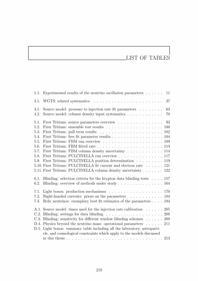
LIST OF TABLES
1.1. Experimental results of the neutrino oscillation parameters . . . . . . 11
3.1. WGTS: related systematics . . . . . . . . . . . . . . . . . . . . . . . 37
4.1. Source model: pressure to injection rate fit parameters . . . . . . . . 634.2. Source model: column density input systematics . . . . . . . . . . . . 70
5.1. First Tritium: source parameters overview . . . . . . . . . . . . . . . 935.2. First Tritium: ensemble test results . . . . . . . . . . . . . . . . . . . 1005.3. First Tritium: pull term results . . . . . . . . . . . . . . . . . . . . . 1025.4. First Tritium: free fit parameter results . . . . . . . . . . . . . . . . . 1045.5. First Tritium: FBM run overview . . . . . . . . . . . . . . . . . . . . 1095.6. First Tritium: FBM fitted rate . . . . . . . . . . . . . . . . . . . . . . 1135.7. First Tritium: FBM column density uncertainty . . . . . . . . . . . . 1145.8. First Tritium: PULCINELLA run overview . . . . . . . . . . . . . . . 1175.9. First Tritium: PULCINELLA position determination . . . . . . . . . 1195.10. First Tritium: PULCINELLA fit current and electron rate . . . . . . 1215.11. First Tritium: PULCINELLA column density uncertainty . . . . . . . 122
6.1. Blinding: selection criteria for the krypton data blinding tests . . . . 1576.2. Blinding: overview of methods under study . . . . . . . . . . . . . . . 164
7.1. Light boson: production mechanisms . . . . . . . . . . . . . . . . . . 1707.2. Right-handed currents: priors on the parameters . . . . . . . . . . . . 1847.3. Relic neutrinos: exemplary best fit estimates of the parameters . . . . 194
A.1. Source model: times used for the injection rate calibration . . . . . . 205C.2. Blinding: settings for data blinding . . . . . . . . . . . . . . . . . . . 208C.3. Blinding: sensitivity for different window blinding schemes . . . . . . 209D.4. Physics beyond the neutrino mass: operational parameters . . . . . . 211D.5. Light boson: summary table including all the laboratory, astroparti-
cle, and cosmological constraints which apply to the models discussedin this thesis . . . . . . . . . . . . . . . . . . . . . . . . . . . . . . . . 213
219


LIST OF ACRONYMS
BEANS Building Elements for ANalysis Sequence
BIXS Beta Induced X-ray Spectroscopy
CAD Computer-Aided Design
CC Charged Current
CDM Cold Dark Matter
CKM Cabibbo-Kobayashi-Maskawa quark mixing matrix
CMB Cosmic Microwave Background
CνB Cosmic Neutrino Background
CPS Cryogenic Pumping Section
DAQ Data Acquisition system
DPS Differential Pumping Section
DSMC Direct Simulation Monte Carlo
FBM Forward Beam Monitor
FPD Focal Plane Detector
FPGA Field Programmable Gate Array
FSD Final States Distribution
GHe Gaseous Helium
IDLE Intermediate Data Layer
KaFit Fit environment for Katrin-spectra
KASPER Katrin C++ software package
KATRIN KArlsruhe TRItium Neutrino (experiment)
KESS Katrin Electron Scattering in Silicon Simulation package,MC simulation code for low-energy electron interactions insilicon detectors
221
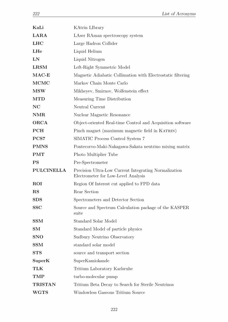
222 List of Acronyms
KaLi KAtrin LIbrary
LARA LAser RAman spectroscopy system
LHC Large Hadron Collider
LHe Liquid Helium
LN Liquid Nitrogen
LRSM Left-Right Symmetric Model
MAC-E Magnetic Adiabatic Collimation with Electrostatic filtering
MCMC Markov Chain Monte Carlo
MSW Mikheyev, Smirnov, Wolfenstein effect
MTD Measuring Time Distribution
NC Neutral Current
NMR Nuclear Magnetic Resonance
ORCA Object-oriented Real-time Control and Acquisition software
PCH Pinch magnet (maximum magnetic field in Katrin)
PCS7 SIMATIC Process Control System 7
PMNS Pontecorvo-Maki-Nakagawa-Sakata neutrino mixing matrix
PMT Photo Multiplier Tube
PS Pre-Spectrometer
PULCINELLA Precision Ultra-Low Current Integrating NormalizationElectrometer for Low-Level Analysis
ROI Region Of Interest cut applied to FPD data
RS Rear Section
SDS Spectrometers and Detector Section
SSC Source and Spectrum Calculation package of the KASPERsuite
SSM Standard Solar Model
SM Standard Model of particle physics
SNO Sudbury Neutrino Observatory
SSM standard solar model
STS source and transport section
SuperK SuperKamiokande
TLK Tritium Laboratory Karlsruhe
TMP turbo-molecular pump
TRISTAN Tritium Beta Decay to Search for Sterile Neutrinos
WGTS Windowless Gaseous Tritium Source
222

INDEX
Blind analysis, 127, 131Data blinding, 132, 146Model blinding, 140, 151
Blind analysis sensitivity, 129Blind analysis sensitivity estimates, 146Boltzmann equation, 47
Clever Hans, 127Column density, 109, 122
Deuterium, 66, 102Tritium, 57
Detection of the neutrino specieselectron neutrino, 2muon neutrino, 3tau neutrino, 3
Energy loss function, 21Energy smearing blinding, 137, 149Experiment stability, 89
Final states, 24First Tritium, 87Forward beam monitor, 25FSD smearing blinding, 142, 152
Gas dynamics, 43First Tritium set-up, 60Nominal set-up, 52
Imperfect energy loss blinding, 143, 153Intermediate Knudsen flow, 46
Laser raman spectroscopy, 24Light bosons, 168
Neutrino, 1New physics, 167
Observer’s bias, 127
Pitch angle, 27Project Poltergeist, 2
Reduced statistics blinding, 132, 146Relic neutrinos, 187Right-handed currents, 178
Scattering probabilities, 22Sensitivity, 130Source modelling, 43
Gas model, 52, 60Magnetic field model, 75Temperature model, 48
Standard Model, 3
Window blinding, 134, 147Windowless Gaseous Tritium Source,
35
223


BIBLIOGRAPHY
[Aal+18] C. E. Aalseth et al. “Search for Neutrinoless Double-β Decay in 76Gewith the MAJORANA DEMONSTRATOR”. In: Physical ReviewLetters 120.13 (2018), p. 132502. doi: 10.1103/PhysRevLett.120.132502. arXiv: 1710.11608 [nucl-ex].
[Aar+15] M. G. Aartsen et al. “Determining neutrino oscillation parameters fromatmospheric muon neutrino disappearance with three years of IceCubeDeepCore data”. In: Physical Review D 91.7 (2015), p. 072004. doi:10.1103/PhysRevD.91.072004. arXiv: 1410.7227 [hep-ex].
[Aar+16] M. G. Aartsen et al. “Searches for Sterile Neutrinos with the IceCubeDetector”. In: Physical Review Letters 117.7 (2016), p. 071801. doi:10.1103/PhysRevLett.117.071801. arXiv: 1605.01990 [hep-ex].
[Abe+11] S. Abe et al. “Measurement of the 8B Solar Neutrino Flux with theKamLAND Liquid Scintillator Detector”. In: Physical Review C 84(2011), p. 035804. doi: 10.1103/PhysRevC.84.035804. arXiv: 1106.0861 [hep-ex].
[Abe+12a] Y. Abe et al. “Indication of Reactor νe Disappearance in the DoubleChooz Experiment”. In: Physical Review Letters 108 (2012), p. 131801.doi: 10.1103/PhysRevLett.108.131801. arXiv: 1112.6353 [hep-
ex].
[Abe+12b] Y. Abe et al. “Reactor νe disappearance in the Double Chooz experi-ment”. In: Physical Review D 86 (5 2012), p. 052008. doi: 10.1103/PhysRevD.86.052008.
[Abe+16] K. Abe et al. “Solar Neutrino Measurements in Super-Kamiokande-IV”.In: Physical Review D 94.5 (2016), p. 052010. doi: 10.1103/PhysRevD.94.052010. arXiv: 1606.07538 [hep-ex].
[Abe+17] K. Abe et al. “Measurement of neutrino and antineutrino oscillationsby the T2K experiment including a new additional sample of νe interac-tions at the far detector”. In: Physical Review D 96.9 (2017), p. 092006.doi: 10.1103/PhysRevD.96.092006. arXiv: 1707.01048 [hep-ex].Erratum in: Physical Review D 98.1 (2018), p. 019902. doi: 10.1103/PhysRevD.98.019902.
225

226 Bibliography
[Ada+13] C. Adams et al. “The Long-Baseline Neutrino Experiment: ExploringFundamental Symmetries of the Universe”. In: (2013). arXiv: 1307.
7335 [hep-ex].
[Ada+14] P. Adamson et al.“Combined Analysis of νµ Disappearance and νµ → νeAppearance in MINOS Using Accelerator and Atmospheric neutrinos”.In: Physical Review Letters 112 (2014), p. 191801. doi: 10.1103/PhysRevLett.112.191801. arXiv: 1403.0867 [hep-ex].
[Ada+17] P. Adamson et al. “Measurement of the Neutrino Mixing Angle θ23in NOvA”. In: Physical Review Letters 118.15 (2017), p. 151802. doi:10.1103/PhysRevLett.118.151802. arXiv: 1701.05891 [hep-ex].
[Agh+18] N. Aghanim et al. “Planck 2018 results. VI. Cosmological parameters”.In: (2018). arXiv: 1807.06209 [astro-ph.CO].
[Ago+13] M. Agostini et al. “Results on Neutrinoless Double-β Decay of 76Gefrom Phase I of the GERDA Experiment”. In: Physical Review Letters111.12 (2013), p. 122503. doi: 10.1103/PhysRevLett.111.122503.arXiv: 1307.4720 [nucl-ex].
[Ago+17a] M. Agostini et al. “First Simultaneous Precision Spectroscopy of pp,7Be, and pep Solar Neutrinos with Borexino Phase-II”. In: (2017). arXiv:1707.09279 [hep-ex].
[Ago+17b] M. Agostini et al. “Improved measurement of 8B solar neutrinos with1.5 kt y of Borexino exposure”. In: (2017). arXiv: 1709.00756 [hep-
ex].
[Ago+18] M. Agostini et al. “Improved Limit on Neutrinoless Double-β Decayof 76Ge from GERDA Phase II”. In: Physical Review Letters 120.13(2018), p. 132503. doi: 10.1103/PhysRevLett.120.132503. arXiv:1803.11100 [nucl-ex].
[AH14] M. Archidiacono and S. Hannestad.“Updated constraints on non-standardneutrino interactions from Planck”. In: Journal of Cosmology and As-troparticle Physics 1407 (2014), p. 046. doi: 10.1088/1475- 7516/2014/07/046. arXiv: 1311.3873 [astro-ph.CO].
[Ahm+01] Q. R. Ahmad et al. “Measurement of the rate of νe + d → p + p + e−
interactions produced by 8B solar neutrinos at the Sudbury NeutrinoObservatory”. In: Physical Review Letters 87 (2001), p. 071301. doi:10.1103/PhysRevLett.87.071301. arXiv: nucl-ex/0106015 [nucl-
ex].
[Ahn+12] J. K. Ahn et al. “Observation of Reactor Electron Antineutrinos Dis-appearance in the RENO Experiment”. In: Physical Review Letters 108(19 2012), p. 191802. doi: 10.1103/PhysRevLett.108.191802.
[Ala+17] S. Alam et al. “The clustering of galaxies in the completed SDSS-IIIBaryon Oscillation Spectroscopic Survey: cosmological analysis of theDR12 galaxy sample”. In: Monthly Notices of the Royal AstronomicalSociety 470.3 (2017), pp. 2617–2652. doi: 10.1093/mnras/stx721.arXiv: 1607.03155 [astro-ph.CO].
226

Bibliography 227
[Alb+18] J. B. Albert et al. “Search for Neutrinoless Double-Beta Decay withthe Upgraded EXO-200 Detector”. In: Physical Review Letters 120.7(2018), p. 072701. doi: 10.1103/PhysRevLett.120.072701. arXiv:1707.08707 [hep-ex].
[Ald+18] C. Alduino et al. “First Results from CUORE: A Search for LeptonNumber Violation via 0νββ Decay of 130Te”. In: Physical Review Letters120.13 (2018), p. 132501. doi: 10.1103/PhysRevLett.120.132501.arXiv: 1710.07988 [nucl-ex].
[Ams+12] J. F. Amsbaugh et al. Prototype focal-plane detector system for the KA-TRIN experiment. Technical report. KATRIN detector section workinggroup, Jan. 2012. url: https://fuzzy.fzk.de/bscw/bscw.cgi/d722700/FPD_System_Prototype_Jan2012.pdf.
[Ams+15] J. Amsbaugh et al. “Focal-plane detector system for the KATRIN ex-periment”. In: Nuclear Instruments and Methods in Physics ResearchSection A: Accelerators, Spectrometers, Detectors and Associated Equip-ment 778 (2015), pp. 40–60. doi: 10.1016/j.nima.2014.12.116.
[AMW86] M. J. Assael, S. Mixafendi, and W. A. Wakeham. “The Viscosity andThermal Conductivity of Normal Hydrogen in the Limit of Zero Den-sity”. In: Journal of Physical and Chemical Reference Data 15.4 (1986),pp. 1315–1322. doi: 10.1063/1.555764.
[AMW87] M. J. Assael, S. Mixafendi, and W. A. Wakeham. “The Viscosity ofNormal Deuterium in the Limit of Zero Density”. In: Journal of Physicaland Chemical Reference Data 16.2 (1987), pp. 189–192. doi: 10.1063/1.555778.
[An+12] F. P. An et al. “Observation of Electron-Antineutrino Disappearance atDaya Bay”. In: Physical Review Letters 108 (17 2012), p. 171803. doi:10.1103/PhysRevLett.108.171803.
[An+13] F. P. An et al. “Improved Measurement of Electron Antineutrino Dis-appearance at Daya Bay”. In: Chinese Physics C 37 (2013), p. 011001.doi: 10.1088/1674-1137/37/1/011001. arXiv: 1210.6327 [hep-ex].
[An+16] F. P. An et al. “Neutrino Physics with JUNO”. In: Journal of PhysicsG 43.3 (2016), p. 030401. doi: 10.1088/0954-3899/43/3/030401.arXiv: 1507.05613 [physics.ins-det].
[An+17] F. P. An et al. “Measurement of electron antineutrino oscillation basedon 1230 days of operation of the Daya Bay experiment”. In: PhysicalReview D 95.7 (2017), p. 072006. doi: 10.1103/PhysRevD.95.072006.arXiv: 1610.04802 [hep-ex].
[Ara+05] T. Araki et al. “Measurement of neutrino oscillation with KamLAND:Evidence of spectral distortion”. In: Physical Review Letters 94 (2005),p. 081801. doi: 10.1103/PhysRevLett.94.081801. arXiv: hep-ex/0406035 [hep-ex].
[Arc+18] G. Arcadi et al. “Tritium beta decay with additional emission of newlight bosons”. In: (2018). arXiv: 1811.03530 [hep-ph].
227

228 Bibliography
[Are+16] M. Arenz et al. “Commissioning of the vacuum system of the KA-TRIN Main Spectrometer”. In: Journal of Instrumentation 11 (2016),P04011. doi: 10.1088/1748-0221/11/04/P04011. arXiv: 1603.01014[physics.ins-det].
[Are+18a] M. Arenz et al. “Calibration of high voltages at the ppm level by thedifference of 83mKr conversion electron lines at the KATRIN experi-ment”. In: The European Physical Journal C 78.5 (2018), p. 368. doi:10.1140/epjc/s10052-018-5832-y.
[Are+18b] M. Arenz et al. “First transmission of electrons and ions through theKATRIN beamline”. In: Journal of Instrumentation 13.04 (2018), P04020.doi: 10.1088/1748-0221/13/04/P04020.
[Are+18c] M. Arenz et al. “The KATRIN Superconducting Magnets: Overviewand First Performance Results”. In: Journal of Instrumentation 13.08(2018), T08005. doi: 10.1088/1748-0221/13/08/T08005.
[Are+19] M. Arenz et al. Results from first tritium β-spectroscopy of the KATRINexperiment. Forthcoming work. 2019.
[Ase+00] V. N. Aseev et al. “Energy loss of 18 keV electrons in gaseous T2 andquench condensed D2 films”. In: The European Physical Journal D 10(1 2000), pp. 39–52. doi: 10.1007/s100530050525.
[Ase+11] V. N. Aseev et al. “Upper limit on the electron antineutrino mass fromthe Troitsk experiment”. In: Physical Review D 84 (11 2011), p. 112003.doi: 10.1103/PhysRevD.84.112003.
[Asn+15] D. M. Asner et al. “Single electron detection and spectroscopy via rela-tivistic cyclotron radiation”. In: Physical Review Letters 114.16 (2015),p. 162501. doi: 10.1103/PhysRevLett.114.162501. arXiv: 1408.5362[physics.ins-det].
[ATL12] ATLAS Collaboration. “Observation of a new particle in the search forthe Standard Model Higgs boson with the ATLAS detector at the LHC”.In: Physics Letters 716 (2012), pp. 1–29. doi: 10.1016/j.physletb.2012.08.020. arXiv: 1207.7214 [hep-ex].
[Ayr+04] D. S. Ayres et al. “NOvA: Proposal to Build a 30 Kiloton Off-AxisDetector to Study νµ → νe Oscillations in the NuMI Beamline”. In:(2004). arXiv: hep-ex/0503053 [hep-ex].
[Bab+12] M. Babutzka et al. “Monitoring of the operating parameters of theKATRIN Windowless Gaseous Tritium Source”. In: New Journal ofPhysics 14.10 (2012), p. 103046. doi: 10.1088/1367-2630/14/10/103046.
[Bab14] M. Babutzka. “Design and development for the Rearsection of the KA-TRIN experiment”. PhD thesis. Karlsruher Institut fur Technologie(KIT), 2014. doi: 10.5445/IR/1000045598.
[Bah64a] J. N. Bahcall. “Solar Neutrino Cross Sections and Nuclear Beta Decay”.In: Physical Review 135 (1B July 1964), B137–B146. doi: 10.1103/PhysRev.135.B137.
228
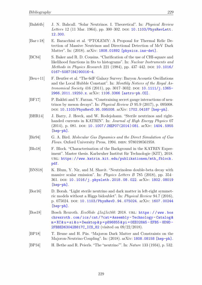
Bibliography 229
[Bah64b] J. N. Bahcall. “Solar Neutrinos. I. Theoretical”. In: Physical ReviewLetters 12 (11 Mar. 1964), pp. 300–302. doi: 10.1103/PhysRevLett.12.300.
[Bar+18] E. Baracchini et al. “PTOLEMY: A Proposal for Thermal Relic De-tection of Massive Neutrinos and Directional Detection of MeV DarkMatter”. In: (2018). arXiv: 1808.01892 [physics.ins-det].
[BC84] S. Baker and R. D. Cousins. “Clarification of the use of CHI-square andlikelihood functions in fits to histograms”. In: Nuclear Instruments andMethods in Physics Research 221 (1984), pp. 437–442. doi: 10.1016/0167-5087(84)90016-4.
[Beu+11] F. Beutler et al. “The 6dF Galaxy Survey: Baryon Acoustic Oscillationsand the Local Hubble Constant”. In: Monthly Notices of the Royal As-tronomical Society 416 (2011), pp. 3017–3032. doi: 10.1111/j.1365-2966.2011.19250.x. arXiv: 1106.3366 [astro-ph.CO].
[BF17] P. Bakhti and Y. Farzan.“Constraining secret gauge interactions of neu-trinos by meson decays”. In: Physical Review D 95.9 (2017), p. 095008.doi: 10.1103/PhysRevD.95.095008. arXiv: 1702.04187 [hep-ph].
[BHR14] J. Barry, J. Heeck, and W. Rodejohann. “Sterile neutrinos and right-handed currents in KATRIN”. In: Journal of High Energy Physics 07(2014), p. 081. doi: 10.1007/JHEP07(2014)081. arXiv: 1404.5955[hep-ph].
[Bir94] G. A. Bird. Molecular Gas Dynamics and the Direct Simulation of GasFlows. Oxford University Press, 1994. isbn: 9780198561958.
[Blo18] F. Block. “Characterisation of the Background in the KATRIN Exper-iment”. Master thesis. Karlsruher Institut fur Technologie (KIT), 2018.url: https://www.katrin.kit.edu/publikationen/mth_fblock.pdf.
[BNS18] K. Blum, Y. Nir, and M. Shavit. “Neutrinoless double-beta decay withmassive scalar emission”. In: Physics Letters B 785 (2018), pp. 354–361. doi: 10.1016/j.physletb.2018.08.022. arXiv: 1802.08019[hep-ph].
[Bor16] D. Borah. “Light sterile neutrino and dark matter in left-right symmet-ric models without a Higgs bidoublet”. In: Physical Review 94.7 (2016),p. 075024. doi: 10.1103/PhysRevD.94.075024. arXiv: 1607.00244[hep-ph].
[Bos18] Bosch Rexroth. EcoSlide 45x45x160. 2018. url: https://www.bos
chrexroth.com/ics/cat/?cat=Assembly- Technology- Catalog&
m=XC&u=si&o=Desktop&p=p896855&pi=0EE028A5- EFB5- 8D9D-
2FBBED63042B817C_ICS_82 (visited on 09/22/2018).
[BP18] T. Brune and H. Pas. “Majoron Dark Matter and Constraints on theMajoron-Neutrino Coupling”. In: (2018). arXiv: 1808.08158 [hep-ph].
[BP34] H. Bethe and R. Peierls.“The“neutrino””. In: Nature 133 (1934), p. 532.
229

230 Bibliography
[BPB01] J. N. Bahcall, M. H. Pinsonneault, and S. Basu. “Solar Models: Cur-rent Epoch and Time Dependences, Neutrinos, and HelioseismologicalProperties”. In: The Astrophysical Journal 555.2 (2001), p. 990. url:http://stacks.iop.org/0004-637X/555/i=2/a=990.
[BPR15] L. I. Bodine, D. S. Parno, and R. G. H. Robertson. “Assessment ofmolecular effects on neutrino mass measurements from tritium β decay”.In: Physical Review C 91.3 (2015), p. 035505. doi: 10.1103/PhysRevC.91.035505. arXiv: 1502.03497 [nucl-ex].
[BPT80] G. Beamson, H. Q. Porter, and D. W. Turner. “The collimating andmagnifying properties of a superconducting field photoelectron spec-trometer”. In: Journal of Physics E: Scientific Instruments 13.1 (1980),p. 64. doi: 10.1088/0022-3735/13/1/018.
[BR13] J. Barry and W. Rodejohann. “Lepton number and flavour violationin TeV-scale left-right symmetric theories with large left-right mixing”.In: Journal of High Energy Physics 09 (2013), p. 153. doi: 10.1007/JHEP09(2013)153. arXiv: 1303.6324 [hep-ph].
[BR97] R. Brun and F. Rademakers. “ROOT: An object oriented data analysisframework”. In: Nuclear Instruments and Methods in Physics A 389(1997), pp. 81–86. doi: 10.1016/S0168-9002(97)00048-X.
[Bra06] C. J. F. T. Braak. “A Markov Chain Monte Carlo version of the ge-netic algorithm Differential Evolution: easy Bayesian computing forreal parameter spaces”. In: Statistics and Computing 16.3 (Sept. 2006),pp. 239–249. issn: 1573-1375. doi: 10.1007/s11222-006-8769-1.
[BRZ11] J. Barry, W. Rodejohann, and H. Zhang.“Light Sterile Neutrinos: Mod-els and Phenomenology”. In: Journal of High Energy Physics 07 (2011),p. 091. doi: 10.1007/JHEP07(2011)091. arXiv: 1105.3911 [hep-ph].
[Bur+08] A. Burck et al.“Microstructured Magnetic Calorimeter with a Meander-Shaped Pickup Coil”. In: Journal of Low Temperature Physics 151.1(Apr. 2008), pp. 337–344. issn: 1573-7357. doi: 10.1007/s10909-
007-9659-4.
[Cen18] Center for Experimental Nuclear Physics and Astrophysics. AnnualReport 2018. Technical report. Universtiy of Washington, 2018. url:https://www.npl.washington.edu/sites/default/files/annual-
reports/2018-CENPA-Annual-Report.pdf (visited on 10/28/2018).
[Cha14] J. Chadwick. “Intensitatsverteilung im magnetischen Spectrum der β-Strahlen von Radium B + C”. In: Verhandlungen der Deutschen Physikalis-chen Gesellschaft 16 (1914), p. 383.
[Cho+16] J. H. Choi et al. “Observation of Energy and Baseline Dependent Reac-tor Antineutrino Disappearance in the RENO Experiment”. In: PhysicalReview Letters 116.21 (2016), p. 211801. doi: 10.1103/PhysRevLett.116.211801. arXiv: 1511.05849 [hep-ex].
[Chr90] C. Christiansen. “Die atmolytische Stromung der Gase”. In: Annalender Physik 277.11 (Jan. 1890), pp. 565–587. issn: 1521-3889. doi: 10.1002/andp.18902771115.
230
Bibliography 231
[CL71] C. Cercignani and M. Lampis. “Kinetic models for gas-surface interac-tions”. In: Transport Theory and Statistical Physics 1.2 (1971), pp. 101–114. doi: 10.1080/00411457108231440. eprint: https://doi.org/10.1080/00411457108231440.
[CMP81] Y. Chikashige, R. N. Mohapatra, and R. D. Peccei. “Are there realgoldstone bosons associated with broken lepton number?” In: PhysicsLetters B 98 (1981), pp. 265–268. doi: 10.1016/0370-2693(81)90011-3.
[CMS12] CMS Collaboration. “Observation of a new boson at a mass of 125GeV with the CMS experiment at the LHC”. In: Physics Letters B 716(2012), pp. 30–61. doi: 10.1016/j.physletb.2012.08.021. arXiv:1207.7235 [hep-ex].
[COM14] COMSOL Multiphysics. Introduction to COMSOL Multiphysics. 2014.url: http://cdn.comsol.com/documentation/5.0.1.276/IntroductionToCOMSOLMultiphysics.pdf (visited on 10/25/2018).
[Cow+56] C. L. Cowan et al. “Detection of the Free Neutrino: a Confirmation”.In: Science 124.3212 (1956), pp. 103–104. issn: 0036-8075. doi: 10.1126/science.124.3212.103.
[Dan+62] G. Danby et al. “Observation of High-Energy Neutrino Reactions andthe Existence of Two Kinds of Neutrinos”. In: Physical Review Letters9 (1 July 1962), pp. 36–44. doi: 10.1103/PhysRevLett.9.36.
[Dec+89] D. Decamp et al.“Determination of the number of light neutrino species”.In: Physics Letters B 231 (1989), p. 519. doi: 10.1016/0370-2693(89)90704-1.
[DHH68] R. Davis, D. S. Harmer, and K. C. Hoffman.“Search for Neutrinos fromthe Sun”. In: Physical Review Letters 20 (21 May 1968), pp. 1205–1209.doi: 10.1103/PhysRevLett.20.1205.
[DKT85] M. Doi, T. Kotani, and E. Takasugi.“Double Beta Decay and MajoranaNeutrino”. In: Progress of Theoretical Physics Supplement 83 (1985),p. 1. doi: 10.1143/PTPS.83.1.
[DLP17a] J. A. Dror, R. Lasenby, and M. Pospelov. “Dark forces coupled to non-conserved currents”. In: Physical Review D 96.7 (2017), p. 075036. doi:10.1103/PhysRevD.96.075036. arXiv: 1707.01503 [hep-ph].
[DLP17b] J. A. Dror, R. Lasenby, and M. Pospelov. “New constraints on lightvectors coupled to anomalous currents”. In: Physical Review Letters119.14 (2017), p. 141803. doi: 10.1103/PhysRevLett.119.141803.arXiv: 1705.06726 [hep-ph].
[Dos+06] N. Doss et al. “Molecular effects in investigations of tritium molecule βdecay endpoint experiments”. In: Physical Review C 73 (2006), p. 025502.doi: 10.1103/PhysRevC.73.025502.
[Dos07] N. Doss. “Calculated final state probability distributions for T2 β-decaymeasurements”. PhD thesis. University College London, 2007. url: https://www.npl.washington.edu/TRIMS/sites/sand.npl.washingt
on.edu.TRIMS/files/manuals-documentation/Doss_thesis_2007.
pdf.
231
232 Bibliography
[Dre+13] G. Drexlin et al. “Current Direct Neutrino Mass Experiments”. In: Ad-vances in High Energy Physics 2013 (2013). doi: 10 . 1155 / 2013 /
293986.
[DT08] N. Doss and J. Tennyson. “Excitations to the electronic continuumof 3HeT+ in investigations of T2 β-decay experiments”. In: Journal ofPhysics B 41.12 (2008), pp. 125701+. issn: 0953-4075. doi: 10.1088/0953-4075/41/12/125701.
[Dun33] F. G. Dunnington. “A Determination of e/m for an Electron by a NewDeflection Method”. In: Physical Review 43 (6 Mar. 1933), pp. 404–416.doi: 10.1103/PhysRev.43.404.
[Egu+03] K. Eguchi et al. “First results from KamLAND: Evidence for reactoranti-neutrino disappearance”. In: Physical Review Letters 90 (2003),p. 021802. doi: 10.1103/PhysRevLett.90.021802. arXiv: hep-ex/0212021 [hep-ex].
[Ell18] E. Ellinger. “Development and investigation of the Forward Beam Mon-itor for the KATRIN experiment”. Forthcoming work. PhD thesis. Ber-gische Universitat Wuppertal, 2018.
[EM17] J. Engel and J. Menendez. “Status and future of nuclear matrix el-ements for neutrinoless double-beta decay: a review”. In: Reports onProgress in Physics 80.4 (2017), p. 046301. doi: 10.1088/1361-6633/aa5bc5. arXiv: 1610.06548 [nucl-th].
[EO12] A. Esmaili and P. L. G. Orlando. “KATRIN sensitivity to sterile neu-trino mass in the shadow of lightest neutrino mass”. In: Physical ReviewD 85 (11 2012), p. 117301. doi: 10.1103/PhysRevD.85.117301.
[Esf+17] A. A. Esfahani et al. “Determining the neutrino mass with cyclotronradiation emission spectroscopy - Project 8”. In: Journal of PhysicsG 44.5 (2017), p. 054004. doi: 10.1088/1361-6471/aa5b4f. arXiv:1703.02037 [physics.ins-det].
[FAR18] FARO Technologies Inc. FaroArm®. 2018. url: https://www.faro.com/de-de/produkte/industrielle-messtechnik/faroarm/ (visitedon 09/24/2018).
[Fas+11] A. Fassler et al. “Tritium and rhenium as a probe of cosmic neutrinobackground”. In: Journal of Physics G 38 (2011), p. 075202. doi: 10.1088/0954-3899/38/7/075202.
[Fas+13] A. Fassler et al. “Search for the Cosmic Neutrino Background and KA-TRIN”. In: Romanian Journal of Physics 58.9-10 (2013), pp. 1221–1231. arXiv: 1304.5632 [nucl-th].
[FB11] J. Formaggio and J. Barrett. “Resolving the reactor neutrino anomalywith the KATRIN neutrino experiment”. In: Physics Letters B 706.1(2011), pp. 68–71. doi: 10.1016/j.physletb.2011.10.069.
[Fer34] E. Fermi. “Versuch einer Theorie der β-Strahlen.” In: Zeitschrift furPhysik 88.3–4 (1934), pp. 161–177. doi: 10.1007/BF01351864.
[FG18] E. Forstner and F. Gluck.“Electron backscattering at the FBM Faradaycup and the Pulcinella disk”. Internal report. 2018.
232
Bibliography 233
[Fis+11] S. Fischer et al. “Monitoring of tritium purity during long-term circu-lation in the KATRIN test experiment LOOPINO using laser Ramanspectroscopy”. In: Fusion Science and Technology 60.3 (2011), pp. 925–930. url: http://www.ans.org/pubs/journals/fst/a_12567.
[Fis14] S. Fischer. “Commissioning of the KATRIN Raman system and dura-bility studies of optical coatings in glove box and tritium atmospheres”.PhD thesis. Karlsruher Institut fur Technologie (KIT), 2014. doi: 10.5445/IR/1000043697.
[FKR02] Z. Fodor, S. D. Katz, and A. Ringwald. “Determination of AbsoluteNeutrino Masses from Bursts of Z Bosons in Cosmic Rays”. In: PhysicalReview Letters 88 (17 Apr. 2002), p. 171101. doi: 10.1103/PhysRevLett.88.171101.
[Fri+18] F. Friedel et al. “Time-dependent simulation of the flow reduction ofD2 and T2 in the KATRIN experiment”. In: (2018). arXiv: 1807.10126[physics.ins-det]. url: https://arxiv.org/abs/1807.10126.
[Fuk+96] Y. Fukuda et al. “Solar Neutrino Data Covering Solar Cycle 22”. In:Physical Review Letters 77 (9 Aug. 1996), pp. 1683–1686. doi: 10.
1103/PhysRevLett.77.1683.
[Fuk+98] Y. Fukuda et al. “Evidence for oscillation of atmospheric neutrinos”.In: Physical Review Letters 81 (1998), pp. 1562–1567. doi: 10.1103/PhysRevLett.81.1562. arXiv: hep-ex/9807003 [hep-ex].
[Fur+15] D. Furse et al. Kassiopeia: Simulation of electric and magnetic fieldsand particle tracking. 2015. url: https://github.com/KATRIN-Experiment/Kassiopeia.
[Fur+17] D. Furse et al. “Kassiopeia: a modern, extensible C++ particle trackingpackage”. In: New Journal of Physics 19.5 (2017), p. 053012. doi: 10.1088/1367-2630/aa6950.
[FY86] M. Fukugita and T. Yanagida. “Baryogenesis without grand unifica-tion”. In: Physics Letters B 174 (1986), pp. 45–47. doi: 10.1016/0370-2693(86)91126-3.
[Gal+02] M. Galassi et al. “GNU scientific library”. In: Network Theory Ltd 3(2002). url: http://www.gnu.org/software/gsl/.
[Gan+13] A. Gando et al. “Reactor on-off antineutrino measurement with Kam-LAND”. In: Physical Review 88.3 (2013), p. 033001. doi: 10.1103/PhysRevD.88.033001. arXiv: 1303.4667 [hep-ex].
[Gan+15] A. Gando et al. “7Be solar neutrino measurement with KamLAND”. In:Physical Review C 92.5 (2015), p. 055808. doi: 10.1103/PhysRevC.92.055808. arXiv: 1405.6190 [hep-ex].
[Gan+16] A. Gando et al. “Search for Majorana Neutrinos near the Inverted MassHierarchy Region with KamLAND-Zen”. In: Physical Review Letters117.8 (2016), p. 082503. doi: 10.1103/PhysRevLett.117.082503.arXiv: 1605.02889 [hep-ex]. Addendum in: Physical Review Letters117.10 (2016), p. 109903. doi: 10.1103/PhysRevLett.117.109903.
233

234 Bibliography
[Gas+17] L. Gastaldo et al. “The electron capture in 163Ho experiment – ECHo”.In: The European Physical Journal Special Topics 226.8 (2017), pp. 1623–1694. doi: 10.1140/epjst/e2017-70071-y.
[Gei64] J. Geiger. “Streuung von 25 keV-Elektronen an Gasen”. In: Zeitschriftfur Physik 181.4 (Aug. 1964), pp. 413–425. issn: 0044-3328. doi: 10.1007/BF01380873.
[GGS58] M. Goldhaber, L. Grodzins, and A. W. Sunyar. “Helicity of Neutrinos”.In: Physical Review 109 (3 Feb. 1958), pp. 1015–1017. doi: 10.1103/PhysRev.109.1015.
[Giu04] C. Giunti. “Theory of neutrino oscillations”. In: Proceedings, 16th Con-ference on High Energy Physics (IFAE 2004): Turin, Italy, April 14-16,2004. 2004, pp. 427–438. doi: 10.1142/9789812702074_0005. arXiv:hep-ph/0409230 [hep-ph].
[Glu03] Gluck, F. “Gas flow in the WGTS tube”. Internal report. 2003. url:https://fuzzy.fzk.de/bscw/bscw.cgi/d736618/120410_FGlueck_
gasflow-in-the-WGTS-tube.pdf.
[GLW57] R. L. Garwin, L. M. Lederman, and M. Weinrich. “Observations of theFailure of Conservation of Parity and Charge Conjugation in MesonDecays: The Magnetic Moment of the Free Muon”. In: Physical Review105 (1957), pp. 1415–1417. doi: 10.1103/PhysRev.105.1415.
[GR09] P. Gondolo and G. Raffelt. “Solar neutrino limit on axions and keV-mass bosons”. In: Physical Review 79 (2009), p. 107301. doi: 10.1103/PhysRevD.79.107301. arXiv: 0807.2926 [astro-ph].
[Gre66] K. Greisen. “End to the cosmic ray spectrum?” In: Physical ReviewLetters 16 (1966), pp. 748–750. doi: 10.1103/PhysRevLett.16.748.
[Gro+08] S. Grohmann et al. “Cryogenic design of the KATRIN source cryostat”.In: AIP Conference Proceedings 985 (2008), pp. 1277–1284. doi: 10.1063/1.2908483.
[Gro+11] S. Grohmann et al. “Precise temperature measurement at 30 K in theKATRIN source cryostat”. In: Cryogenics 51.8 (2011), pp. 438–445.doi: 10.1016/j.cryogenics.2011.05.001.
[Gro+13] S. Grohmann et al. “The thermal behaviour of the tritium source inKATRIN”. In: Cryogenics 55-56.0 (2013), pp. 5–11. doi: 10.1016/j.cryogenics.2013.01.001.
[Gro09] S. Grohmann. “Stability analyses of the beam tube cooling system inthe KATRIN source cryostat”. In: Cryogenics 49.8 (2009), pp. 413–420.doi: 10.1016/j.cryogenics.2009.06.001.
[Gro15] S. Groh. “Modeling of the response function and measurement of trans-mission properties of the KATRIN experiment”. PhD thesis. KarlsruherInstitut fur Technologie (KIT), 2015. doi: 10.5445/IR/1000046546.
[GRS79] M. Gell-Mann, P. Ramond, and R. Slansky. “Complex Spinors andUnified Theories”. In: Conference Proceedings C790927 (1979), pp. 315–321. arXiv: 1306.4669 [hep-th].
234

Bibliography 235
[Hac17] M. T. Hackenjos. “KATRIN ”First Light” - Commissioning and Mod-elling of the Beamline”. PhD thesis. Karlsruher Institut fur Technologie(KIT), 2017. doi: 10.5445/IR/1000078933.
[Had+12] M. Hadj-Nacer et al.“Experimental study of the gas flows through chan-nels with circular cross sections”. In: Journal of Physics: ConferenceSeries 362.1 (2012), p. 012025. url: http://stacks.iop.org/1742-6596/362/i=1/a=012025.
[Hag99] C. Hagmann. “A Relic neutrino detector”. In: AIP Conference Pro-ceedings 478.1 (1999), pp. 460–463. doi: 10.1063/1.59428. arXiv:astro-ph/9902102 [astro-ph].
[Ham+99] W. Hampel et al. “GALLEX solar neutrino observations: results forGALLEX IV”. In: Physics Letters B 447.1 (1999), pp. 127–133. issn:0370-2693. doi: 10.1016/S0370-2693(98)01579-2.
[HAM18] HAMAMATSU. Si PIN photodiodes. 2018. url: https://www.hamamatsu.com/resources/pdf/ssd/s5971_etc_kpin1025e.pdf (visited on10/20/2018).
[Han+17] V. Hannen et al. “Deconvolution of the energy loss function of theKATRIN experiment”. In: Astroparticle Physics 89 (2017), pp. 30–38.doi: 10.1016/j.astropartphys.2017.01.010.
[Har15] F. Harms. “Characterization and Minimization of Background Pro-cesses in the KATRIN Main Spectrometer”. PhD thesis. KarlsruherInstitut fur Technologie (KIT), 2015. doi: 10.5445/IR/1000050027.
[Hau18] N. Haussmann. “Simulation and measurement of the Forward BeamMonitor detector signal in KATRIN”. Forthcoming work. PhD thesis.Bergische Universitat Wuppertal, 2018.
[Hei+18] F. Heizmann et al. “Status of the unbiased neutrino mass analysis ofKATRIN data (‘Blinding’)”. Internal report. 2018. url: https://neutrino.ikp.kit.edu/katrin/images/1/10/Blinding-report-2018-
02-13.pdf.
[Hei15] F. Heizmann. “Optimization of a KATRIN source analysis tool and in-vestigations of the potential to constrain the relic neutrino background”.Master thesis. Karlsruher Institut fur Technologie (KIT), 2015. url:http://www.katrin.kit.edu/publikationen/mth_heizmann.pdf.
[Hey04] E. T. Heyn. “BERLIN’S WONDERFUL HORSE – He Can Do AlmostEverything But Talk - How He Was Taught”. In: The New York Times(Sept. 1904). url: https://timesmachine.nytimes.com/timesmachine/1904/09/04/101396572.pdf.
[HM05] W.-Y. P. Hwang and B.-Q. Ma.“Detection of cosmic neutrino clusteringby cosmic ray spectra”. In: New Journal of Physics 7 (2005), p. 41. doi:10.1088/1367-2630/7/1/041. arXiv: astro-ph/0502377 [astro-
ph].
[Hot12] M. Hotzel. “Simulation and analysis of source-related effects for KA-TRIN”. PhD thesis. Karlsruher Institut fur Technologie (KIT), 2012.doi: 10.5445/IR/1000031259.
235

236 Bibliography
[HOZ18] G.-y. Huang, T. Ohlsson, and S. Zhou. “Observational Constraints onSecret Neutrino Interactions from Big Bang Nucleosynthesis”. In: Phys-ical Review D 97 (2018), p. 075009. doi: 10.1103/PhysRevD.97.
075009. arXiv: 1712.04792 [hep-ph].
[HS17] F. Heizmann and H. Seitz-Moskaliuk. “The Windowless Gaseous Tri-tium Source (WGTS) of the KATRIN experiment”. In: Journal of Physics:Conference Series 888.1 (2017), p. 012071. doi: 10.1088/1742-6596/888/1/012071.
[ide10] idealvac. TURBOVAC and MAG, Excerpt from the Oerlikon LeyboldVacuum Full Line Catalog. 2010. url: https://www.idealvac.com/files/brochures/Oerlikon_Leybold_TurboVac_SpecSheet.pdf
(visited on 09/30/2018).
[IM14] K. Ioka and K. Murase. “IceCube PeV-EeV neutrinos and secret in-teractions of neutrinos”. In: Progress of Theoretical and ExperimentalPhysics 2014.6 (2014), 061E01. doi: 10.1093/ptep/ptu090. arXiv:1404.2279 [astro-ph.HE].
[Jac99] J. D. Jackson. Classical electrodynamics. Vol. 3. John Wiley & Sons,Inc., 1999. isbn: 047130932X.
[Jan17] A. Jansen. Vakuumeinbruch Beamtube. Elog entry. July 2017. url: https://ikp-neu-katrin.ikp.kit.edu/elog/WGTS-Main/143.
[JSF99] S. Jonsell, A. Saenz, and P. Froelich. “Neutrino-mass determinationfrom tritium β decay: Corrections to and prospects of experimentalverification of the final-state spectrum”. In: Physical Review C 60 (31999), p. 034601. doi: 10.1103/PhysRevC.60.034601.
[Kaf12] W. Kafer. “Sensitivity studies of the KATRIN experiment”. PhD thesis.Karlsruher Institut fur Technologie (KIT), 2012. doi: 10.5445/IR/1000026021.
[KAT05] KATRIN collaboration. KATRIN Design Report. FZKA scientific re-port 7090. 2005. url: http://bibliothek.fzk.de/zb/berichte/FZKA7090.pdf.
[KFM10] A. Kaboth, J. A. Formaggio, and B. Monreal. “Sensitivity of neutrinomass experiments to the cosmic neutrino background”. In: Physical Re-view D 82 (6 Sept. 2010), p. 062001. doi: 10.1103/PhysRevD.82.062001.
[Kha+14] V. Khachatryan et al. “Search for heavy neutrinos and W bosons withright-handed couplings in proton-proton collisions at
√s = 8 TeV”. In:
The European Physical Journal C 74.11 (2014), p. 3149. doi: 10.1140/epjc/s10052-014-3149-z. arXiv: 1407.3683 [hep-ex].
[Kle+18] M. Kleesiek et al. “β-Decay Spectrum, Response Function and Statis-tical Model for Neutrino Mass Measurements with the KATRIN Ex-periment”. In: Submitted to Eur. Phys. J. C. (2018). In review. arXiv:1806.00369 [physics.data-an].
[Kle14] M. Kleesiek. “A Data-Analysis and Sensitivity-Optimization Frame-work for the KATRIN Experiment”. PhD thesis. Karlsruher Institutfur Technologie (KIT), 2014. doi: 10.5445/IR/1000043301.
236

Bibliography 237
[Kle18] M. Klein. “Tritium ions in KATRIN: detection, blocking and removal”.To be published. PhD thesis. Karlsruher Institut fur Technologie (KIT),2018.
[Knu09] M. Knudsen. “Die Gesetze der Molekularstromung und der innerenReibungsstromung der Gase durch Rohren”. In: Annalen der Physik333.1 (Jan. 1909), pp. 75–130. issn: 1521-3889. doi: 10.1002/andp.19093330106.
[Kod+01] K. Kodama et al.“Observation of tau neutrino interactions”. In: PhysicsLetters B 504.3 (2001), pp. 218–224. issn: 0370-2693. doi: 10.1016/S0370-2693(01)00307-0.
[KR05] J. R. Klein and A. Roodman. “Blind analysis in nuclear and parti-cle physics”. In: Annual Review of Nuclear and Particle Science 55.1(2005), pp. 141–163. doi: 10.1146/annurev.nucl.55.090704.151521.
[KR83] P. Kruit and F. H. Read. “Magnetic field paralleliser for 2π electron-spectrometer and electron-image magnifier”. In: Journal of Physics E:Scientific Instruments 16.4 (1983), p. 313. url: http://stacks.iop.org/0022-3735/16/i=4/a=016.
[Kra+05] C. Kraus et al. “Final results from phase II of the Mainz neutrino masssearch in tritium β decay”. In: The European Physical Journal C 40.4(2005), pp. 447–468. doi: 10.1140/epjc/s2005-02139-7.
[KRS85] V. A. Kuzmin, V. A. Rubakov, and M. E. Shaposhnikov.“On anomalouselectroweak baryon-number non-conservation in the early universe”. In:Physics Letters B 155 (1985), p. 36. doi: 10.1016/0370-2693(85)91028-7.
[KT87] E. W. Kolb and M. S. Turner. “Supernova SN 1987a and the SecretInteractions of Neutrinos”. In: Physical Review D 36 (1987), p. 2895.doi: 10.1103/PhysRevD.36.2895.
[Kuc+18] L. Kuckert et al.“Modelling of gas dynamical properties of the KATRINtritium source and implications for the neutrino mass measurement”.In: Vacuum 158 (2018), pp. 195–205. doi: 10.1016/j.vacuum.2018.09.036.
[Kuc16] L. Kuckert. “The Windowless Gaseous Tritium Source of the KATRINExperiment – Characterisation of Gas Dynamical and Plasma Proper-ties”. PhD thesis. Karlsruher Institut fur Technologie (KIT), 2016. doi:10.5445/IR/1000065077.
[KW75] A. Kundt and E. Warburg. “Ueber Reibung und Warmeleitung verdun-nter Gase”. In: Annalen der Physik 231.5 (Jan. 1875), pp. 337–365. issn:1521-3889. doi: ark:/12148/bpt6k15239z.
[KZ18] B. Krasch and G. Zeller. Laser Raman spectroscopy @KATRIN. July 17,2018. url: https://neutrino.ikp.kit.edu/katrin/images/b/b0/20180709_analysis_workshop_LARA.pptx (visited on 11/09/2018).
[LDB14] R. Laha, B. Dasgupta, and J. F. Beacom.“Constraints on New NeutrinoInteractions via Light Abelian Vector Bosons”. In: Physical Review D89.9 (2014), p. 093025. doi: 10.1103/PhysRevD.89.093025. arXiv:1304.3460 [hep-ph].
237

238 Bibliography
[LEM18] LEM. ITN 600-S ULTRASTAB. 2018. url: https://www.lem.com/en/itn-600s-ultrastab (visited on 09/19/2018).
[LH90] S. K. Loyalka and S. A. Hamoodi. “Poiseuille flow of a rarefied gasin a cylindrical tube: Solution of linearized Boltzmann equation”. In:Physics of Fluids A: Fluid Dynamics 2.11 (1990), pp. 2061–2065. doi:10.1063/1.857681. eprint: https://doi.org/10.1063/1.857681.
[Li14] Y.-F. Li. “Overview of the Jiangmen Underground Neutrino Observa-tory (JUNO)”. In: International Journal of Modern Physics: Confer-ence Series 31 (2014), p. 1460300. doi: 10.1142/S2010194514603007.arXiv: 1402.6143 [physics.ins-det].
[Lin+18] M. Lindner et al. “Neutrino-electron scattering: general constraints onZ ′ and dark photon models”. In: Journal of High Energy Physics 05(2018), p. 098. doi: 10.1007/JHEP05(2018)098. arXiv: 1803.00060[hep-ph].
[Liu87] J. W. Liu. “Total cross sections for high-energy electron scattering byH2 (1Σ+
g ), N2 (1Σ+g ), and O2 (3Σ−g )”. In: Physical Review A 35 (2 Jan.
1987), pp. 591–597. doi: 10.1103/PhysRevA.35.591.
[LL02] T. J. Loredo and D. Q. Lamb. “Bayesian analysis of neutrinos observedfrom supernova SN-1987A”. In: Physical Review D 65 (2002), p. 063002.doi: 10 . 1103 / PhysRevD . 65 . 063002. arXiv: astro - ph / 0107260
[astro-ph].
[Lob+99a] V. M. Lobashev et al. “Direct search for mass of neutrino and anomalyin the tritium beta spectrum”. In: Physics Letters B B460 (1999),pp. 227–235. doi: 10.1016/S0370-2693(99)00781-9.
[Lob+99b] V. M. Lobashev et al. “Neutrino mass and anomaly in the tritium beta-spectrum. Results of the ’Troitsk nu mass’ experiment”. In: NuclearPhysics B - Proceedings Supplements 77 (1999), pp. 327–332. doi: 10.1016/S0920-5632(99)00438-7.
[LS85] V. M. Lobashev and P. E. Spivak. “A method for measuring the elec-tron antineutrino rest mass”. In: Nuclear Instruments and Methods inPhysics Research Section A: Accelerators, Spectrometers, Detectors andAssociated Equipment 240.2 (1985), pp. 305–310. doi: 10.1016/0168-9002(85)90640-0.
[LT93] L. M. Lederman and D. Teresi. The God Particle. Dell Publishing, 1993.isbn: 0385312113.
[Luk+12] S. Lukic et al. “Measurement of the gas-flow reduction factor of the KA-TRIN DPS2-F differential pumping section”. In: Vacuum 86.8 (2012),pp. 1126–1133. doi: 10.1016/j.vacuum.2011.10.017.
[LV11] M. Lusignoli and M. Vignati. “Relic Antineutrino Capture on 163-Hodecaying Nuclei”. In: Physics Letters B B697 (2011), pp. 11–14. doi:10.1016/j.physletb.2011.01.047. arXiv: 1012.0760 [hep-ph].Erratum in: Physics Letters B 701 (2011), p. 673. doi: 10.1016/j.physletb.2011.06.008.
238

Bibliography 239
[LVV08] R. Lazauskas, P. Vogel, and C. Volpe. “Charged current cross sectionfor massive cosmological neutrinos impinging on radioactive nuclei”.In: Journal of Physics G 35 (2008), p. 025001. doi: 10.1088/0954-3899/35/2/025001. arXiv: 0710.5312 [astro-ph].
[LWW18] J. Liu, C. E. M. Wagner, and X.-P. Wang. “A light complex scalarfor the electron and muon anomalous magnetic moments”. In: (2018).arXiv: 1810.11028 [hep-ph].
[Mal07] O. B. Malyshev. “Characterisation of a turbo-molecular pumps by aminimum of parameters”. In: Vacuum 81.6 (2007). Proceedings of theEuropean Vacuum Conference (EVC-9), pp. 752–758. issn: 0042-207X.doi: https://doi.org/10.1016/j.vacuum.2005.11.055.
[Mar17] A. Marsteller. “Measurement of Temperature Stability and Homogene-ity of the KATRIN WGTS Cryostat”. Master thesis. Karlsruher Institutfur Technologie (KIT), 2017. url: https://www.katrin.kit.edu/publikationen/mth_marsteller.pdf.
[Mar18] A. Marsteller. Private communication. 2018.
[Mer+15] S. Mertens et al. “Sensitivity of Next-Generation Tritium Beta-DecayExperiments for keV-Scale Sterile Neutrinos”. In: Journal of Cosmologyand Astroparticle Physics 1502 (2015), p. 020. doi: 10.1088/1475-7516/2015/02/020. arXiv: 1409.0920 [physics.ins-det].
[Mer+18] S. Mertens et al. “A novel detector system for KATRIN to search forkeV-scale sterile neutrinos”. In: (2018). arXiv: 1810.06711 [physics.ins-det].
[Met+53] N. Metropolis et al. “Equation of state calculations by fast computingmachines”. In: Journal of Chemical Physics 21 (1953), pp. 1087–1092.doi: 10.1063/1.1699114.
[MF09] B. Monreal and J. A. Formaggio. “Relativistic Cyclotron Radiation De-tection of Tritium Decay Electrons as a New Technique for Measuringthe Neutrino Mass”. In: Physical Review D 80 (2009), p. 051301. doi:10.1103/PhysRevD.80.051301. arXiv: 0904.2860 [nucl-ex].
[Min77] P. Minkowski. “µ → eγ at a rate of one out of 109 muon decays?”In: Physics Letters B 67 (1977), pp. 421–428. doi: 10.1016/0370-2693(77)90435-X.
[MNS62] Z. Maki, M. Nakagawa, and S. Sakata. “Remarks on the unified modelof elementary particles”. In: Progress of Theoretical Physics 28 (1962),pp. 870–880. doi: 10.1143/PTP.28.870.
[MP75] R. N. Mohapatra and J. C. Pati. “A Natural Left-Right Symmetry”. In:Physical Review D D11 (1975), p. 2558. doi: 10.1103/PhysRevD.11.2558.
[MS80] R. N. Mohapatra and G. Senjanovic. “Neutrino Mass and SpontaneousParity Violation”. In: Physical Review Letters 44 (1980). [,231(1979)],p. 912. doi: 10.1103/PhysRevLett.44.912.
239

240 Bibliography
[MS86] S. P. Mikheyev and A. Y. Smirnov. “Resonant amplification of ν os-cillations in matter and solar-neutrino spectroscopy”. In: Il Nuovo Ci-mento C 9.1 (Jan. 1986), pp. 17–26. issn: 0390-5551. doi: 10.1007/BF02508049.
[Mye+15] E. G. Myers et al. “Atomic Masses of Tritium and Helium-3”. In: Phys-ical Review Letters 114 (1 2015), p. 013003. doi: 10.1103/PhysRevLett.114.013003.
[NFW96] J. F. Navarro, C. S. Frenk, and S. D. M. White. “The Structure of colddark matter halos”. In: The Astrophysical Journal 462 (1996), pp. 563–575. doi: 10.1086/177173. arXiv: astro-ph/9508025 [astro-ph].
[NI16] NI. National Instruments - LabVIEW. 2016. url: http://www.ni.com/en-us/shop/labview.html (visited on 09/20/2018).
[Nuc+18] A. Nucciotti et al. “Status of the HOLMES Experiment to DirectlyMeasure the Neutrino Mass”. In: Journal of Low Temperature Physics(2018). doi: 10 . 1007 / s10909 - 018 - 2025 - x. arXiv: 1807 . 09269
[physics.ins-det].
[OW08] E. W. Otten and C. Weinheimer. “Neutrino mass limit from tritium βdecay”. In: Reports on Progress in Physics 71.8 (2008), p. 086201. doi:10.1088/0034-4885/71/8/086201.
[Par+18] R. H. Parker et al. “Measurement of the fine-structure constant as atest of the Standard Model”. In: Science 360.6385 (2018), pp. 191–195.issn: 0036-8075. doi: 10.1126/science.aap7706.
[PB13] F. Priester and B. Bornschein. “TriToP - A compatibility experimentwith turbomolecular pumps under tritium atmosphere”. In: Vacuum98.0 (2013), pp. 22–28. doi: 10.1016/j.vacuum.2012.09.006.
[Per+75] M. L. Perl et al. “Evidence for Anomalous Lepton Production in e+−e−Annihilation”. In: Physical Review Letters 35 (22 Dec. 1975), pp. 1489–1492. doi: 10.1103/PhysRevLett.35.1489.
[Per09] D. H. Perkins. Particle astrophysics. 10. Oxford University Press, 2009.
[Pfu07] O. Pfungst. Das Pferd des Herrn von Osten (Der kluge Hans). EinBeitrag zur experimentellen Tier- und Menschen-Psychologie. Leipzig:Barth, 1907. url: https://archive.org/details/daspferddesherr00stumgoog.
[Phy18] Physics and Astronomy Department. Object-oriented Real-time Controland Acquisition. 2018. url: http://orca.physics.unc.edu/~markhowe/Orca_Help/Home.html.
[Pic+92] A. Picard et al. “A solenoid retarding spectrometer with high resolu-tion and transmission for keV electrons”. In: Nuclear Instruments andMethods in Physics Research Section B: Beam Interactions with Ma-terials and Atoms 63.3 (1992), pp. 345–358. doi: 10 . 1016 / 0168 -
583X(92)95119-C.
[PKW64] W. E. F. Pauli, R. Kronig, and V. F. Weisskopf. Collected scientificpapers. Offener Brief an die Gruppe der Radioaktiven bei der Gauvere-instagung zu Tubingen (datiert 4. Dez. 1930). New York, NY: Inter-science, 1964.
240
Bibliography 241
[Pon57] B. Pontecorvo. “Mesonium and anti-mesonium”. In: Journal of Experi-mental and Theoretical Physics 6 (1957), p. 429.
[Pon58] B. Pontecorvo. “Inverse beta processes and nonconservation of leptoncharge”. In: Journal of Experimental and Theoretical Physics 7 (1958),pp. 172–173.
[Pon68] B. Pontecorvo. “Neutrino Experiments and the Problem of Conserva-tion of Leptonic Charge”. In: Journal of Experimental and TheoreticalPhysics 26 (1968), pp. 984–988.
[PP16] P. S. Pasquini and O. L. G. Peres. “Bounds on Neutrino-Scalar YukawaCoupling”. In: Physical Review D 93 (2016), p. 053007. doi: 10.1103/PhysRevD.93.053007. arXiv: 1511.01811 [hep-ph]. Erratum in:Physical Review D 93 (2016), p. 079902. doi: 10.1103/PhysRevD.93.079902.
[Pra+12] M. Prall et al. “The KATRIN pre-spectrometer at reduced filter en-ergy”. In: New Journal of Physics 14.7 (2012), p. 073054. doi: 10.
1088/1367-2630/14/7/073054.
[Pra11] M. Prall.“Background Reduction of the KATRIN Spectrometers: Trans-mission Function of the Pre-Spectrometer and Systematic Test of theMain-Spectrometer Wire Electrode”. PhD thesis. Westfalische Wilhelms-Universitat Munster, 2011. url: http://www.researchgate.net/
publication/238418212_Transmission_Function_of_the_Pre-
Spectrometer_and_Systematic_Tests_of_the_Main-Spectrometer
_Wire_Electrode_%28PHD_thesis%29.
[Pri13] F. Priester. “Tritiumtechnologie fur die fensterlose Quelle WGTS vonKATRIN”. German. PhD thesis. Karlsruher Institut fur Technologie(KIT), 2013. doi: 10.5445/IR/1000035699.
[PS74] J. C. Pati and A. Salam. “Lepton Number as the Fourth Color”. In:Physical Review D 10 (1974), pp. 275–289. doi: 10.1103/PhysRevD.10.275. Erratum in: Physical Review D 11 (1975), p. 703. doi: 10.1103/PhysRevD.11.703.2.
[PS95] M. E. Peskin and D. V. Schroeder. An Introduction to Quantum FieldTheory. Ed. by D. Pines. Westview Press, 1995. isbn: 9780813345437.
[PSB15] F. Priester, M. Sturm, and B. Bornschein.“Commissioning and detailedresults of KATRIN inner loop tritium processing system at TritiumLaboratory Karlsruhe”. In: Vacuum 116 (2015), pp. 42–47. doi: 10.1016/j.vacuum.2015.02.030.
[PVS14] S. Pantazis, D. Valougeorgis, and F. Sharipov. “End corrections forrarefied gas flows through circular tubes of finite length”. In: Vacuum101 (2014), pp. 306–312. issn: 0042-207X. doi: 10.1016/j.vacuum.2013.09.015.
[PW65] A. A. Penzias and R. W. Wilson. “A Measurement of Excess AntennaTemperature at 4080 Mc/s.” In: The Astrophysical Journal 142 (1965),pp. 419–421.
241

242 Bibliography
[Ren11] P. Renschler. “KESS - A new Monte Carlo simulation code for low-energy electron interactions in silicon detectors”. PhD thesis. KarlsruherInstitut fur Technologie (KIT), 2011. doi: 10.5445/IR/1000024959.
[RH09] J. E. Ricker and J. H. Hendricks. Unit Conversions. NIST. 2009. url:https://www.nist.gov/pml/div685/grp01/unit_conversions.
[RK88] R. G. H. Robertson and D. A. Knapp. “Direct Measurements of Neu-trino Mass”. In: Annual Review of Nuclear and Particle Science 38.1(1988), pp. 185–215. doi: 10.1146/annurev.ns.38.120188.001153.
[RLC05] W. A. Rolke, A. M. Lopez, and J. Conrad.“Limits and confidence inter-vals in the presence of nuisance parameters”. In: Nuclear Instrumentsand Methods in Physics A551 (2005), pp. 493–503. doi: 10.1016/j.nima.2005.05.068. arXiv: physics/0403059 [physics].
[Rob+91] R. G. H. Robertson et al. “Limit on anti-electron-neutrino mass fromobservation of the beta decay of molecular tritium”. In: Physical ReviewLetters 67 (1991), pp. 957–960. doi: 10.1103/PhysRevLett.67.957.
[Rol15] M. Rollig. “Tritium analytics by beta induced X-ray spectrometry”.PhD thesis. Karlsruher Institut fur Technologie (KIT), 2015. doi: 10.5445/IR/1000054050.
[Ros+15] A. J. Ross et al. “The clustering of the SDSS DR7 main Galaxy sample- I. A 4 per cent distance measure at z = 0.15”. In: Monthly Noticesof the Royal Astronomical Society 449.1 (2015), pp. 835–847. doi: 10.1093/mnras/stv154. arXiv: 1409.3242 [astro-ph.CO].
[RW04] A. Ringwald and Y. Y. Y. Wong. “Gravitational clustering of relic neu-trinos and implications for their detection”. In: Journal of Cosmologyand Astroparticle Physics 0412 (2004), p. 005. doi: 10.1088/1475-7516/2004/12/005. arXiv: hep-ph/0408241 [hep-ph].
[RW83] W. Repko and C.-E. Wu. “Radiative corrections to the end point of thetritium β decay spectrum”. In: Physical Review C 28 (6 1983), pp. 2433–2436. issn: 0556-2813. doi: 10.1103/physrevc.28.2433.
[Sch13] M. Schlosser. “Accurate calibration of the Raman system for the Karl-sruhe Neutrino Experiment”. PhD thesis. Karlsruher Institut fur Tech-nologie (KIT), 2013. doi: 10.1007/978-3-319-06221-1.
[Sch14] J. S. Schwarz. “The Detector System of the KATRIN Experiment -Implementation and First Measurements with the Spectrometer”. PhDthesis. Karlsruher Institut fur Technologie (KIT), 2014. doi: 10.5445/IR/1000042772.
[Sch15] C. Schonfeld.“Commissioning of the KATRIN Pinch Magnet”. Bachelorthesis. Karlsruher Institut fur Technologie (KIT), 2015. url: https:/ / fuzzy . fzk . de / bscw / bscw . cgi / d1236629 / BA2015 - Sch % C3 %
B6nfeld.pdf.
[Sei19] H. Seitz-Moskaliuk. “Characterisation of the KATRIN tritium sourceand minimisation of systematic effects”. Forthcoming work. PhD thesis.Karlsruher Institut fur Technologie (KIT), 2019.
242

Bibliography 243
[Sen+18] J. Sentkerestiova et al. “Gaseous 83mKr generator for KATRIN”. In:Journal of Instrumentation 13.04 (2018), P04018. doi: 10.1088/1748-0221/13/04/P04018.
[SEN18] SENIS. 3-Axis Digital Teslameter 3MH3A-0.1%-200mT. 2018. url: http://c1940652.r52.cf0.rackcdn.com/5a7090adb8d39a6f2d002
12a/Magnetic-Teslameter-3MH3A-Datasheet-r3.pdf (visited on09/22/2018).
[SF97a] A. Saenz and P. Froelich. “Effect of final-state interactions in allowedβ decays. I. General formalism”. In: Physical Review C 56 (1997),pp. 2132–2161. doi: 10.1103/PhysRevC.56.2132.
[SF97b] A. Saenz and P. Froelich. “Effect of final-state interactions in allowedβ decays. II. Reliability of the β-decay spectrum for T2”. In: PhysicalReview C 56 (1997), pp. 2162–2184. doi: 10.1103/PhysRevC.56.2162.
[SH11] A. Sejersen Riis and S. Hannestad. “Detecting sterile neutrinos withKATRIN like experiments”. In: Journal of Cosmology and AstroparticlePhysics 2011.02 (2011), p. 011. doi: 10.1088/1475-7516/2011/02/011.
[Sha04a] F. Sharipov. “Calculations of tritium flow between the buffer vesselup to the first vacuum system”. Internal report. 2004. url: https:
//fuzzy.fzk.de/bscw/bscw.cgi/d100305/10-ME-2102-0.pdf.
[Sha04b] F. Sharipov. “Data on the velocity slip and temperature jump coeffi-cients [gas mass, heat and momentum transfer]”. In: 5th InternationalConference on Thermal and Mechanical Simulation and Experiments inMicroelectronics and Microsystems, 2004. EuroSimE 2004. Proceedingsof the. May 2004, pp. 243–249. doi: 10.1109/ESIME.2004.1304046.
[Sha08] F. Sharipov. “Analytical and Numerical Calculations of Rarefied GasFlows”. In: Handbook of Vacuum Technology. Wiley-VCH, 2008. Chap. 5,pp. 163–220. isbn: 9783527407231.
[Sha09] F. Sharipov.“Gas Circulation Due an Azimuthal Temperature Distribu-tion Over a Micro-Tube Wall”. In: Proceedings, ASME 2009 7th Inter-national Conference on Nanochannels, Microchannels, and Minichan-nels: Pohang, South Korea, June 22-24, 2009. 43499. 2009, pp. 373–381. doi: 10.1115/ICNMM2009-82028.
[Sha10] F. Sharipov. “Tritium flow through a non-symmetrical source. Simula-tion of gas flow through an injection hole.” Internal report. 2010. url:https://fuzzy.fzk.de/bscw/bscw.cgi/d100305/10-ME-2109-
0.pdf.
[Sha16] F. Sharipov. Rarefied Gas Dynamics. Fundamentals for Research andPractice. Wiley - VCH, 2016. isbn: 9783527413263.
[Sha96] F. Sharipov. “Rarefied gas flow through a long tube at any temperatureratio”. In: Journal of Vacuum Science & Technology A 14.4 (1996),pp. 2627–2635. doi: 10.1116/1.579991. eprint: https://doi.org/10.1116/1.579991.
243
244 Bibliography
[Sha97] F. Sharipov. “Rarefied gas flow through a long tube at arbitrary pres-sure and temperature drops”. In: Journal of Vacuum Science & Tech-nology A 15.4 (1997), pp. 2434–2436. doi: 10.1116/1.580904. eprint:https://doi.org/10.1116/1.580904.
[Sib18] V. Sibille. “Energy loss blinding”. Internal report. 2018. url: https://neutrino.ikp.kit.edu/katrin/images/5/53/Energy_loss_
modifications.pdf.
[Sie18] Siemens. SIMATIC PCS 7. 2018. url: https://w3.siemens.com/mcms/process-control-systems/en/distributed-control-system-
simatic-pcs-7/Pages/distributed-control-system-simatic-
pcs-7.aspx (visited on 09/22/2018).
[Sir+18] A. M. Sirunyan et al. “Search for heavy resonances decaying to a topquark and a bottom quark in the lepton+jets final state in proton-proton collisions at 13 TeV”. In: Physics Letters B 777 (2018), pp. 39–63. doi: 10.1016/j.physletb.2017.12.006. arXiv: 1708.08539
[hep-ex].
[SJF00] A. Saenz, S. Jonsell, and P. Froelich. “Improved Molecular Final-StateDistribution of HeT+ for the β-Decay Process of T2”. In: Physical Re-view Letters 84 (2000), pp. 242–245. doi: 10.1103/PhysRevLett.84.242.
[SK05] F. Sharipov and D. Kalempa. “Separation phenomena in the tritiumsource and numerical simulations of turbo-molecular pumps”. Internalreport. 2005. url: https://fuzzy.fzk.de/bscw/bscw.cgi/d968578/10-ME-2112-0.pdf.
[SK10] F. Sharipov and D. Kalempa. “Separation phenomenon in the Win-dowless Gaseous Tritium Source of KATRIN experiment. Ternary mix-tures”. Internal report. 2010. url: https://fuzzy.fzk.de/bscw/bscw.cgi/d932757/10-ME-2108-0.pdf.
[Sle17] M. Slezak. “Analysis of the gaseous 83mKr source measurements”. talkpresented at 33rd KATRIN collaboration meeting. Oct. 2017. url: https://fuzzy.fzk.de/bscw/bscw.cgi/d1186394/95-TRP-6316-P4-
MSlezak.pdf.
[SM75] G. Senjanovic and R. N. Mohapatra. “Exact Left-Right Symmetry andSpontaneous Violation of Parity”. In: Physical Review D 12 (1975),p. 1502. doi: 10.1103/PhysRevD.12.1502.
[Sou86] P. C. Souers. Hydrogen Properties for Fusion Energy. University of Cal-ifornia Press, 1986. isbn: 0-520-05500-4.
[SS98] F. Sharipov and V. Seleznev.“Data on Internal Rarefied Gas Flows”. In:Journal of Physical and Chemical Reference Data 27.3 (1998), pp. 657–706. doi: 10.1063/1.556019.
[Ste+17] N. M. N. Steinbrink et al. “Statistical sensitivity on right-handed cur-rents in presence of eV scale sterile neutrinos with KATRIN”. In: Jour-nal of Cosmology and Astroparticle Physics 1706.06 (2017), p. 015. doi:10.1088/1475-7516/2017/06/015. arXiv: 1703.07667 [hep-ph].
244

Bibliography 245
[Ste17] N. M. N. Steinbrink. “Beyond-Standard Model Neutrino Physics Sen-sitivity with KATRIN”. PhD thesis. Westfalische Wilhelms-UniversitatMunster, 2017.
[Str+14] S. Streubel et al. “Toward a more accurate Q value measurement oftritium: status of THe-Trap”. In: Applied Physics B 114.1 (Jan. 2014),pp. 137–145. issn: 1432-0649. doi: 10.1007/s00340-013-5669-x.
[Stu10] M. Sturm.“Aufbau und Test des Inner-Loop-Systems der Tritiumquellevon KATRIN”. German. PhD thesis. Karlsruher Institut fur Technolo-gie (KIT), 2010. doi: 10.5445/IR/1000019355.
[Stu18] M. Sturm. Private communication. 2018.
[Sut16] C. Sutton. “Ghosts in the machine”. In: CERN courier (2016). url:https://cerncourier.com/ghosts-in-the-machine/.
[SV80] J. Schechter and J. W. F. Valle. “Neutrino Masses in SU(2) x U(1)Theories”. In: Physical Review D 22 (1980), p. 2227. doi: 10.1103/PhysRevD.22.2227.
[SV82] J. Schechter and J. W. F. Valle. “Neutrino Decay and SpontaneousViolation of Lepton Number”. In: Physical Review 25 (1982), p. 774.doi: 10.1103/PhysRevD.25.774.
[SVS17] J. Sentkerestiova, D. Venos, and M. Slezak.“Gaseous 83mKr generator ofmonoenergetic electrons based on 83Rb deposited in zeolite”. In: Journalof Physics: Conference Series 888.1 (2017), p. 012072. doi: 10.1088/1742-6596/888/1/012072.
[Tan+18] M. Tanabashi et al. “Review of Particle Physics”. In: Physical ReviewD 98 (3 Aug. 2018), p. 030001. doi: 10.1103/PhysRevD.98.030001.
[The04] The London Standard. ““CLEVER HANS” AGAIN – Expert Commis-sion Decides That the Horse Actually Reasons”. In: The New YorkTimes (Oct. 1904). url: https : / / timesmachine . nytimes . com /
timesmachine/1904/10/02/120289067.pdf.
[The15] The Royal Swedish Academy of Sciences. Metamorphosis in the particleworld. Press release. 2015. url: https://www.nobelprize.org/prizes/physics/2015/press-release/ (visited on 10/19/2018).
[Tro18] N. Trost.“Modeling and measurement of Rydberg-State mediated Back-ground at the KATRIN Main Spectrometer”. To be published. PhDthesis. Karlsruher Institut fur Technologie (KIT), 2018.
[Ven+18] D. Venos et al. “Properties of 83mKr conversion electrons and theiruse in the KATRIN experiment”. In: Journal of Instrumentation 13.02(2018), T02012. doi: 10.1088/1748-0221/13/02/T02012.
[Way18a] WayCon. Seilzugsensor Serie SX135. 2018. url: https://www.waycon.de/fileadmin/seilzugsensoren/Seilzug-Sensor-SX135.pdf
(visited on 09/22/2018).
[Way18b] WayCon. Seilzugsensor Serie SX80. 2018. url: https://www.wayc
on.de/fileadmin/seilzugsensoren/Seilzug- Sensor- SX80.pdf
(visited on 09/22/2018).
245

246 Bibliography
[Wei62] S. Weinberg. “Universal Neutrino Degeneracy”. In: Physical Review 128(3 Nov. 1962), pp. 1457–1473. doi: 10.1103/PhysRev.128.1457.
[Wol78] L. Wolfenstein. “Neutrino oscillations in matter”. In: Physical ReviewD 17 (9 May 1978), pp. 2369–2374. doi: 10.1103/PhysRevD.17.2369.
[Wu+57] C. S. Wu et al. “Experimental Test of Parity Conservation in BetaDecay”. In: Physical Review 105 (1957), pp. 1413–1414. doi: 10.1103/PhysRev.105.1413.
[WVH] C. Weinheimer, K. Valerius, and F. Heizmann. Erwartete Unsicherheitauf den effektiven KATRIN Endpunkt. Private communication.
[Yan80] T. Yanagida.“Horizontal Symmetry and Masses of Neutrinos”. In: Progressof Theoretical Physics 64 (1980), p. 1103. doi: 10.1143/PTP.64.1103.
[Zel17] G. Zeller. “Development of a calibration procedure and calculation ofthe uncertainty budget for the KATRIN laser Raman system”. Masterthesis. Karlsruher Institut fur Technologie (KIT), 2017. url: https://www.katrin.kit.edu/publikationen/mth-Zeller.pdf.
[Zel18] G. Zeller. Remarks on updates in RunSummary2f. July 4, 2018. url:https://neutrino.ikp.kit.edu/katrin/images/0/09/RemarksOn
RunSummary2f-LARA.pdf (visited on 11/08/2018).
[ZK66] G. T. Zatsepin and V. A. Kuzmin. “Upper limit of the spectrum of cos-mic rays”. In: Journal of Experimental and Theoretical Physics Letters4 (1966), pp. 78–80.
246

ACKNOWLEDGEMENTS
Finally, I want to express my gratitude that I was given the chance of being partof the lively Katrin collaboration during this work. I would like to thank all thepersons who supported me friendly and professionally to complete this thesis. Inparticular, I want to give thanks to
� Prof. Guido Drexlin for the possibility to perform this interesting and chal-lenging work in the framework of the Katrin collaboration,
� Prof. Ulrich Husemann for the evaluation of this thesis as second reviewer,
� Dr. Kathrin Valerius for her inspiring and caring supervision, her infectiousenthusiasm for physics, and her support for my stay in the U.S.,
� Prof. Diana Parno (CMU) and Prof. Joe Formaggio (MIT) for inviting me toCMU and MIT,
� the Karlsruhe School of Elementary Particle and Astroparticle Physics: Scienceand Technology (KSETA), especially Dr. Irmgard Langbein, for supportingmy doctoral project, enabling several business trips, and facilitating my par-ticipation in the MBA fundamentals programme of the HECTOR businessschool,
� the Karlsruhe House of Young Scientists (KHYS), especially Gaby Weick, forenabling and supporting my stay in the U.S. at CMU and MIT,
� Dr. Ferenc Gluck for the support with the gas dynamics calculations, magneticfields and general numerical problems,
� Prof. Felix Sharipov for the support with the gas dynamics calculations,
� Dr. Valerian Sibille and Dr. Joachim Wolf for the huge support and fruitfuldiscussions concerning blind analysis of Katrin data,
� Hendrik Seitz-Moskaliuk for legendary double rooms at various conferences,with the highlight of the shared Neutrino2016 poster prize,
� Dr. Alexander Jansen for skilful and professional management of the WGTStask,
� Maximilian Kristen, Klaus Mehret, and Steffen Lichter for the fast supportwith the WGTS magnetic field measuring system,
247

248 Acknowledgements
� Heike Boltz and the WGTS team for the inspiring atmosphere and technicalinsights during the (electrical) WGTS commissioning,
� Alexander Marsteller for answering my endless questions about the loop sys-tem,
� Karol Debowski and Manuel Klein for the nice office atmosphere,
� Manuel Klein for sharing the pressure of the same defense date and the filmcareer,
� Dr. Martin Babutzka and Dr. Laura Kuckert as former office mates,
� all members of Kathrin’s YIG, for the nice and productive working atmosphere,
� the secretaries and assistants Marion Behechti, Diana Fellner, Katharina Fis-cher, Anna Friedrich, Brigitte Gering, Barabara Lepold, and Eva Porter forfriendly and fast support in administrative procedures,
� Thomas Csabo for providing fast support with (laboratory) laptops,
� Dr. Marco Kleesiek and Prof. Sanshiro Enomoto for exhaustive C++ and otherprogramming support,
� all readers and correctors of this thesis,
� Dr. Moritz Hackenjos, Anton Huber, and Carsten Rottele for being colleaguesand friends at the same time,
� C. Schurle, J. Faiß, and S. Koch for the “writing holidays”, and A. Fiedler forthe (short) distractions during writing this thesis,
� all who have been forgotten on this list...
Special thanks goes to my family and all my friends.
The biggest thank you is for my girlfriend Carola Schurle for her tireless supportand distraction, especially in the final phase of this thesis. Thank you for being mylight!
248