University of Tennessee, Knoxville University of Tennessee, Knoxville

TRACE: Tennessee Research and Creative TRACE: Tennessee Research and Creative

Exchange Exchange

Doctoral Dissertations Graduate School

12-2013

Analysis, Prototyping, and Design of an Ionization Profile Monitor Analysis, Prototyping, and Design of an Ionization Profile Monitor

for the Spallation Neutron Source Accumulator Ring for the Spallation Neutron Source Accumulator Ring

Dirk A. Bartkoski University of Tennessee - Knoxville, dirk.bartkoski@yahoo.com

Follow this and additional works at: https://trace.tennessee.edu/utk_graddiss

Part of the Engineering Physics Commons, and the Other Physics Commons

Recommended Citation Recommended Citation Bartkoski, Dirk A., "Analysis, Prototyping, and Design of an Ionization Profile Monitor for the Spallation Neutron Source Accumulator Ring. " PhD diss., University of Tennessee, 2013. https://trace.tennessee.edu/utk_graddiss/2555

This Dissertation is brought to you for free and open access by the Graduate School at TRACE: Tennessee Research and Creative Exchange. It has been accepted for inclusion in Doctoral Dissertations by an authorized administrator of TRACE: Tennessee Research and Creative Exchange. For more information, please contact trace@utk.edu.

To the Graduate Council:

I am submitting herewith a dissertation written by Dirk A. Bartkoski entitled "Analysis,

Prototyping, and Design of an Ionization Profile Monitor for the Spallation Neutron Source

Accumulator Ring." I have examined the final electronic copy of this dissertation for form and

content and recommend that it be accepted in partial fulfillment of the requirements for the

degree of Doctor of Philosophy, with a major in Physics.

Geoffrey Greene, Major Professor

We have read this dissertation and recommend its acceptance:

Marianne Breinig, Jeffrey A. Holmes, Takeshi Egami

Accepted for the Council:

Carolyn R. Hodges

Vice Provost and Dean of the Graduate School

(Original signatures are on file with official student records.)

Analysis, Prototyping, and Design of an Ionization Profile

Monitor for the Spallation Neutron Source Accumulator Ring

A Dissertation Presented for the

Doctor of Philosophy Degree

The University of Tennessee, Knoxville

Dirk A. Bartkoski

December 2013

ii

Dedication

This work is dedicated to my Lord and Savior Jesus Christ without whose direction I would

have never pursued a deeper understanding of the universe through physics.

iii

Acknowledgements

I would like to first thank my advisors Dr. Craig Deibele who brought the field of

electromagnetics from the textbook to reality. Special thanks are also in order to Dr. Jeff

Holmes without whose help I may have never passed some of my classes. Thanks are

necessary to all the SNS diagnostic group technicians who taught me many useful laboratory

skills and accelerator physics group members who helped me Python coding to Monte Carlo

methods. I would also like to thank Kerry Ewald and Yarom Polsky who were instrumental

in turning ideas into actual designs.

Thanks also go to my best friend Tim for his uncanny ability to provide the much

needed occasional distraction. My mom, whose constant prayers and encouragement

reminded me I wasn’t alone and my dad, whose daily example of integrity, hard work, and

perseverance taught me what true success required.

Finally, I can never thank enough my wife Kerri. Her constant encouragement,

support, unwavering faith in me, and perpetual joy sustained me more than I can ever say.

Her presence in my life for the last few years of my doctoral journey kept me sane and a

constant reminder that path I was called to was the right one and the end was always in sight

if you knew which direction to look.

iv

Abstract

The Spallation Neutron Source (SNS) located in the Oak Ridge National Laboratory is

comprised of a 1 GeV linear H- [H^-] accelerator followed by an accumulator ring that

delivers high intensity 1 μs [microsecond] long pulses of 1.5x1014

[1.5x10^14] protons to a

liquid mercury target for neutron production by spallation reaction. With its strict 0.01% total

beam loss condition, planned power upgrade, and proposed second target station, SNS ring

beam-profile diagnostics capable of monitoring evolving beam conditions during high-power

conditions are crucial for efficient operation and improvement. By subjecting ionized

electrons created during beam interactions with the residual gas to a uniform electric field

perpendicular to the beam direction, a profile may be collected based on the relation between

measured ionized particle current and the beam density responsible for ionization. This form

of nondestructive profile beam profile diagnostic known as an Ionization Profile Monitor

(IPM). Introducing a magnetic field parallel to the electric field constrains the transverse

particle motion to produce spatially accurate profiles. Presented in this work is the analysis

and design of an IPM for the SNS ring capable of measuring turn-by-turn profiles with a 10%

spatial accuracy for a fully accumulated high intensity proton beam. A theoretical framework

is developed for the IPM operational principles and estimations for system design parameters

are made based on calculations and measurement data. Detailed simulations are presented

which are also used to determine design details and experimental results from a proof-of-

principle IPM test chamber are reported and analyzed. Finally, a complete system design is

presented based on the design criteria and simulation optimization that meets the required

IPM system objectives.

v

Table of Contents

Background and Overview 1 Chapter 1

1.1 The Need for Non-Destructive Profile Measurement ........................................ 2

1.1.1 The Spallation Neutron Source ................................................................... 2

1.1.2 Beam Loss and Diagnostics ........................................................................ 4

1.1.3 Ionization Profile Monitor Overview.......................................................... 7

1.2 History of IPM Development ............................................................................. 9

1.2.1 Early IPMs (1965 – 2002)........................................................................... 9

1.2.2 Modern IPMs (2002 – 2012)..................................................................... 12

1.3 SNS IPM Design Criteria ................................................................................. 16

1.4 Overall Organization ........................................................................................ 18

Theoretical Analysis 19 Chapter 2

2.1 Beam-Gas Interaction ....................................................................................... 20

2.1.1 Interaction Model ...................................................................................... 20

2.1.2 Relativistic Energy Transfer ..................................................................... 24

2.1.3 Energy Loss .............................................................................................. 32

2.1.4 Ionization .................................................................................................. 37

2.2 IPM Ionization Estimation ............................................................................... 40

2.2.1 Residual Gas Composition ........................................................................ 42

2.2.2 IPM Pressure ............................................................................................. 45

2.2.3 Ion Estimation ........................................................................................... 56

vi

2.2.4 Electron Estimation ................................................................................... 59

2.2.5 Plasma Considerations .............................................................................. 64

2.3 IPM Signal Estimation ..................................................................................... 65

2.3.1 Channeltron Detector ................................................................................ 66

2.3.2 Residual Gas Sensitivity ........................................................................... 73

2.3.3 Profile Generation ..................................................................................... 78

2.3.4 Measured Signal........................................................................................ 80

2.3.5 Theoretical Summary ................................................................................ 82

Simulation Analysis 84 Chapter 3

3.1 Particle Trajectory Study .................................................................................. 85

3.1.1 IPM Beam Range ...................................................................................... 85

3.1.2 Beam Space Charge .................................................................................. 87

3.1.3 Trajectory Simulation ............................................................................... 97

3.1.4 Ion Collection Field Analysis ................................................................. 106

3.1.5 Measured Ion Profile Characteristics ...................................................... 109

3.1.6 Electron Collection Field Analysis ......................................................... 112

3.2 Spatial Accuracy ............................................................................................. 115

3.2.2 Resolution and Statistical Errors ............................................................. 116

3.2.3 Field Uniformity Induced Errors ............................................................ 126

3.2.4 Secondary Particle Source Error ............................................................. 129

3.2.5 Spatial Accuracy Estimation ................................................................... 134

3.3 Time Resolution ............................................................................................. 135

3.3.1 Collection Times ..................................................................................... 136

vii

3.3.2 Signal Processing .................................................................................... 139

3.3.3 Transmission Line Effects ...................................................................... 145

3.3.4 Electronics Effects .................................................................................. 153

3.4 Simulation Summary ...................................................................................... 155

Prototyping and Measurement 157 Chapter 4

4.1 IPM Test Chamber ......................................................................................... 158

4.1.1 Design Considerations ............................................................................ 158

4.1.2 Test Chamber Design .............................................................................. 158

4.2 Test Chamber Results and Modifications ...................................................... 162

4.2.2 Test Chamber Measurements .................................................................. 163

4.2.3 Test Chamber Modifications................................................................... 165

4.2.4 Test Chamber RF Noise .......................................................................... 169

4.3 Test Chamber Signal Study ............................................................................ 169

4.3.1 Ion Signal ................................................................................................ 169

4.3.2 Electron Signal ........................................................................................ 175

4.4 IPM Test Chamber Conclusions ..................................................................... 179

IPM System Design 181 Chapter 5

5.1 Electrode Design ............................................................................................ 181

5.1.1 Field Uniformity Optimization ............................................................... 182

5.1.2 Vacuum Breakdown................................................................................ 185

5.1.3 Field Reduction ....................................................................................... 188

5.1.4 Insulating Standoffs ................................................................................ 192

5.1.5 Secondary Electron Suppression Mesh ................................................... 199

viii

5.1.6 Electrode Summary ................................................................................. 203

5.2 Magnet Design ............................................................................................... 205

5.2.1 Magnet Design Estimation ...................................................................... 205

5.2.2 Design Simulation ................................................................................... 207

5.2.3 Magnetic Field Evaluation ...................................................................... 208

5.2.4 Magnet Summary .................................................................................... 216

5.3 Detector Assembly ......................................................................................... 218

5.3.1 Channeltron Housing .............................................................................. 218

5.3.2 Detector Cabling and Feedthroughs ........................................................ 219

5.3.3 Actuator................................................................................................... 221

5.4 Vacuum Chamber ........................................................................................... 222

5.4.1 Alignment and Installation ...................................................................... 222

5.4.2 Wakefield Slats ....................................................................................... 223

5.4.3 Detector-Beam Coupling Mitigation ...................................................... 225

5.5 High Voltage Feedthrough ............................................................................. 227

5.5.1 HVF Air Side .......................................................................................... 229

5.5.2 HVF Vacuum Side .................................................................................. 231

5.6 IPM Design Summary .................................................................................... 234

Summary 238 Chapter 6

6.1 Overall Project Summary ............................................................................... 238

6.2 Future Work ................................................................................................... 239

6.3 Final Remarks ................................................................................................. 241

Bibliography 242

ix

Appendices 263

Appendix A Model Assumptions ............................................................................ 264

Appendix B Cross Section & Rutherford Scattering ............................................... 270

Appendix C Relativistic Beam Characteristics ....................................................... 279

Appendix D Beam Envelope Parameters ................................................................ 283

Vita 288

x

List of Tables

Table 1.1 List of selected IPMs and their characteristics. ...................................................... 15

Table 1.2 IPM system requirements for fully accumulated 1x1014

ppp beam........................ 17

Table 2.1 IPM gas values of density at NTP (NTP: 20 C, 1 atm), first excitation energy Eex

and ionization energy EI, mean ionization/excitation energy I, and effective energy to

produce an ion-electron pair WI. ..................................................................................... 33

Table 2.2 Values of the total number of ionized particles nT and primary ionized particles np

for selected gases. Values of nT and np are given in ion pairs·cm-1

·atm-1

and where the

values are at NTP. ........................................................................................................... 41

Table 2.3 Calculated pressure fractions for constituent pure gases in the IPM residual gas .. 45

Table 3.1 Calculated RMS beam sizes and full beam sizes with safety margins along with the

beam pipe radius at the IPM location. ............................................................................ 86

xi

List of Figures

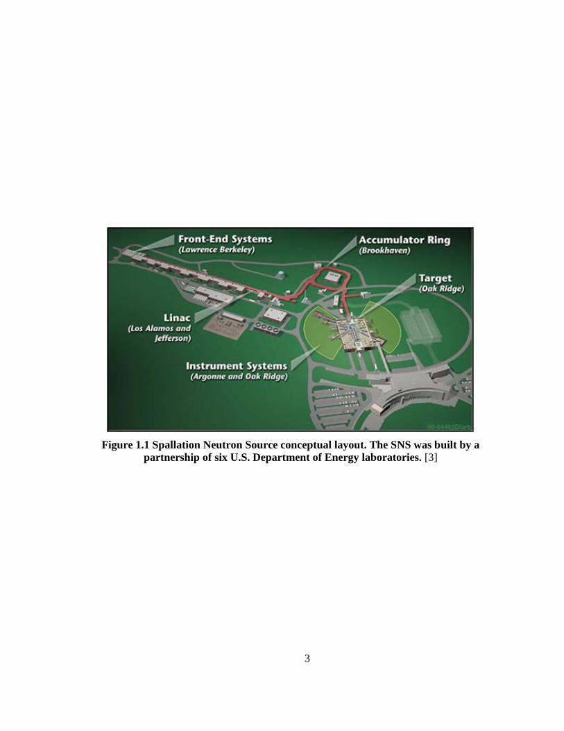
Figure 1.1 Spallation Neutron Source conceptual layout. The SNS was built by a partnership

of six U.S. Department of Energy laboratories. [3] .......................................................... 3

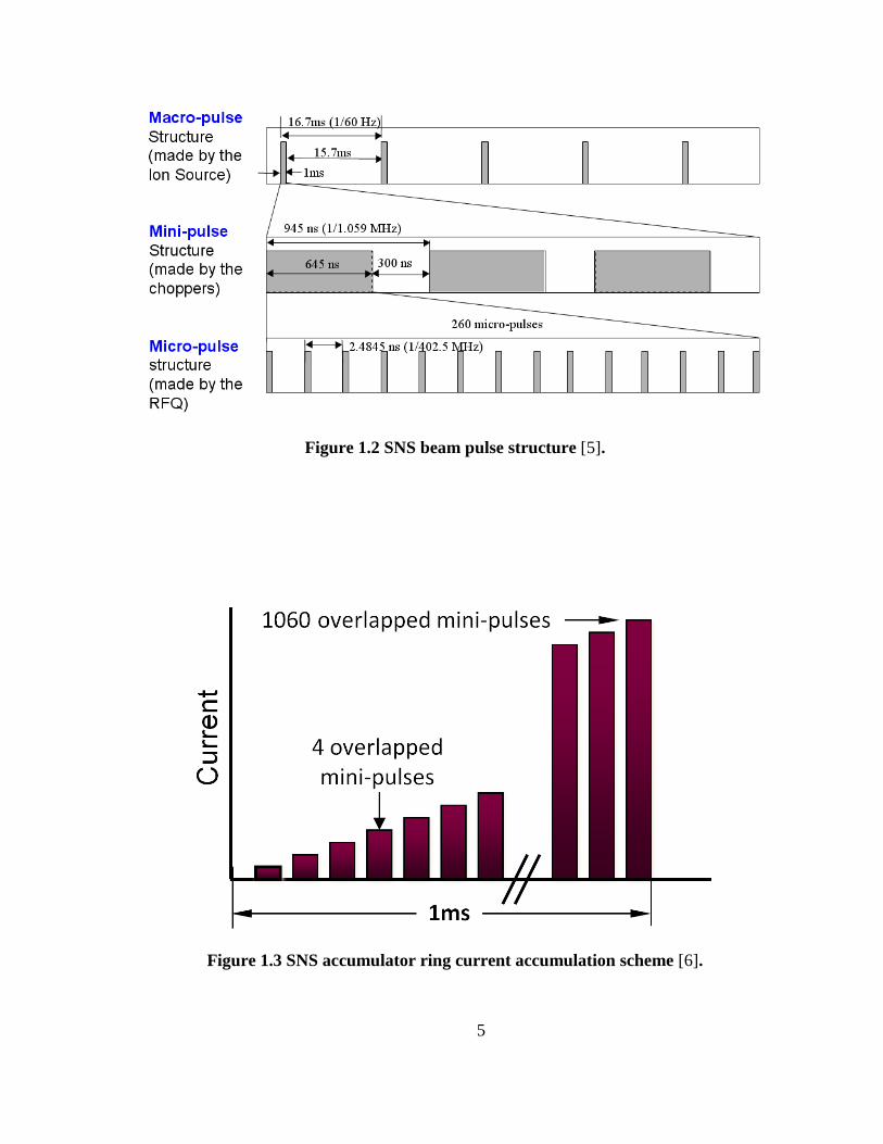
Figure 1.2 SNS beam pulse structure [5]. ................................................................................. 5

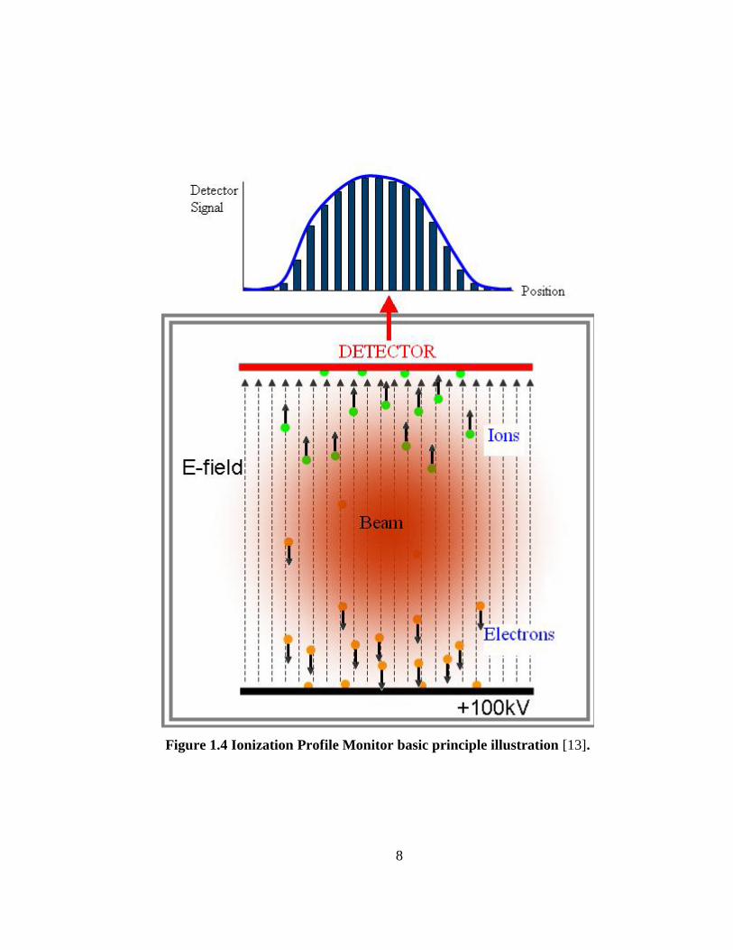
Figure 1.3 SNS accumulator ring current accumulation scheme [6]. ....................................... 5

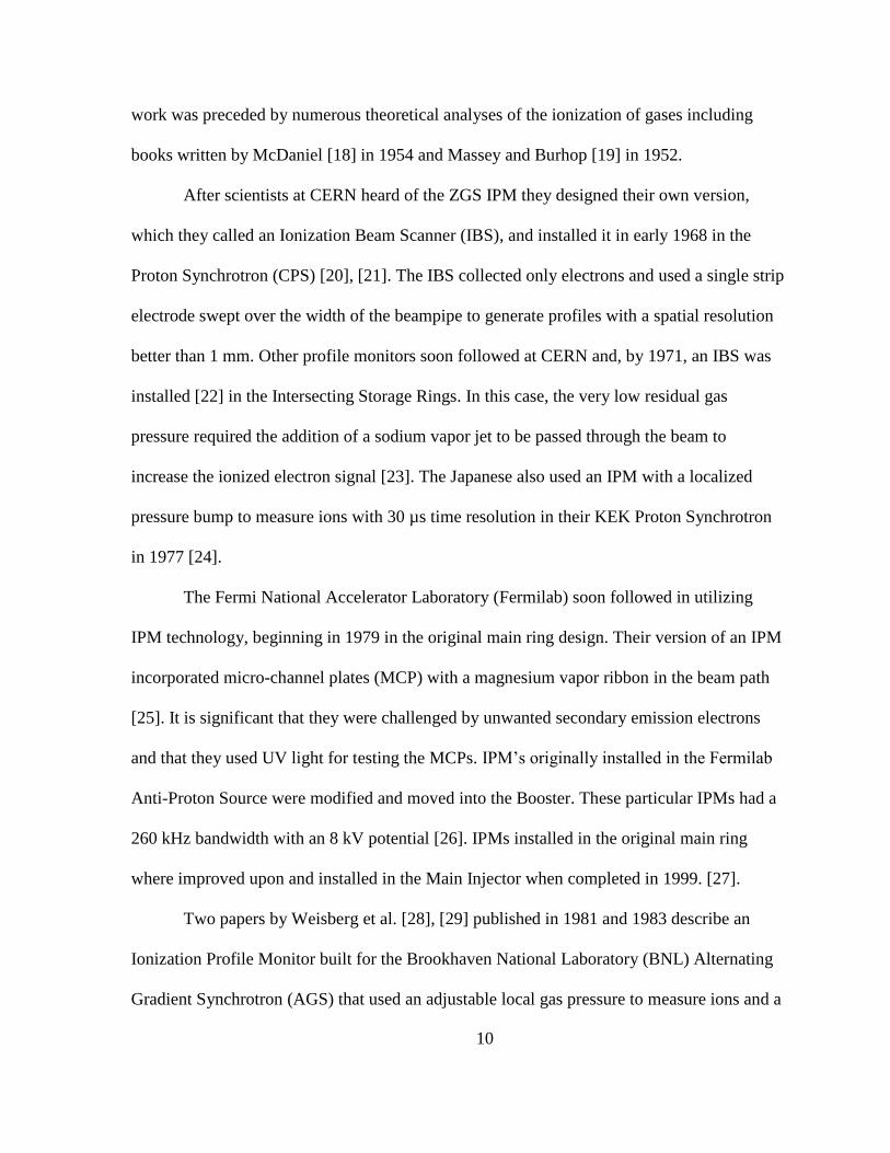
Figure 1.4 Ionization Profile Monitor basic principle illustration [13]. ................................... 8

Figure 2.1 Two types of collisions defined by impact parameter and the orbital electron

radius a. Close or Hard collisions are those where b ≈ a and Far or Soft collisions are

those in which b >> a. ..................................................................................................... 24

Figure 2.2 An example of the relative probability of the different processes responsible for

energy transfer as a function of the energy transfer. Emax is the maximum kinematically

allowed energy transfer. .................................................................................................. 26

Figure 2.3 (a) Lab frame showing an incident proton with momentum p scattering off of an

orbital electron with impact parameter b. (b) Collision as seen in the center-of-mass

(CM) frame. (c) Center-of-mass equivalent frame when mp >> me where CM becomes

the rest frame of the proton. ............................................................................................ 26

Figure 2.4 Graphical representation of the infinitesimal interaction volume of an incident

particle with mass M at an impact parameter b............................................................... 33

Figure 2.5 Pictorial representation of the ionization of gas molecules by an energetic proton p

showing ionized electrons and secondary ionizing rays . ............................................ 41

Figure 2.6 Residual gas analysis taken upstream of the RF cavities in the SNS ring D straight

xii

on October 26, 2007. Molecule/atom names for the main gas components are labeled

above their respective peaks ........................................................................................... 43

Figure 2.7 Temperature change in the beam pipe wall with heat loss due to convection and

radiation for a convection heat transfer coefficient of 10 W/m2 K. ................................ 48

Figure 2.8 Drawing showing SNS ring D straight downstream of the RF cavities. The

proposed IPM location is shown in the box. Cold cathode vacuum gauges (CCG), ion

pumps (IP), and sector gate valves (SGV) are shown along with their respective

longitudinal distances...................................................................................................... 50

Figure 2.9 Graphical representation of a periodic vacuum chamber model with period of 2L

and pumping speed S. ..................................................................................................... 51

Figure 2.10 Pressure profile between identical lumped pumps using IPM location parameters

with gas desorption rates taken from literature [95] for a fully accumulated beam. ...... 54

Figure 2.11 Cold cathode gauge pressures surrounding the IPM location in addition to the

beam particles in the ring shown for the beginning of the 2012 winter run period starting

in November 2012. CCG A02 is located downstream of the IPM and is located between

ion pumps while CCG D12 is located upstream and sits directly over top of an ion

pump. .............................................................................................................................. 55

Figure 2.12 Graph of the total number ion-electron pairs created at the IPM location as a

function of the number of protons present in each turn for 8 scale and 9 scale pressures.

......................................................................................................................................... 58

Figure 2.13 Graphical representation of electron cloud generation leading to multipacting.. 60

Figure 2.14 Simulation of electron cloud formation in the SNS ring for the first turn of

accumulation in the presence of varying uniform electric field strengths [132],[133]. .. 62

xiii

Figure 2.15 (Left) Graphical representation of a Channeltron detector showing basic

principles of operation in addition to substrate structure of lead silicate glass tube walls.

(Right) Actual photo of a 4800 series Channeltron with custom mounting tabs. ........... 66

Figure 2.16 Gain of four different 4800 series Channeltrons. ................................................ 68

Figure 2.17 Typical 4700 series Channeltron gain linearity. .................................................. 68

Figure 2.18 Channeltron relative ion detection efficiency. [140] ........................................... 69

Figure 2.19 Channeltron electron detection efficiency. [140] ................................................ 69

Figure 2.20 Dimensional layout of a 4800 series Channeltron. [140] .................................... 71

Figure 2.21 Graphical representation of the statistical error σσ associated with the measured

profile width σN for the actual distribution of width σ0. .................................................. 74

Figure 2.22 The percentage of the measured width the error assumes for each turn during an

accumulation cycle is shown for varying pressures or the equivalent number of

accumulation cycle repetitions. ....................................................................................... 75

Figure 2.23 The percent change in the profile width as a function of a percent change in gas

pressure for the first turn at different gas pressures or the equivalent number of

aggregated accumulation cycle at 10-9

Torr. ................................................................... 78

Figure 2.24 Graphical representation of the turn-by-turn profile generation process showing

the collection all particles at a detector position for each turn and multiple

accumulations then moving the detector transversely until the beam width has been

spanned. .......................................................................................................................... 79

Figure 2.25 Expected IPM signals for different detector positions on the last turn of a

1.5x1014

proton beam in the SNS ring. Collected current represents the current of

detected incoming ionized particles adjusted for ion and electron efficiencies. Measured

xiv

current is the output current of the Channeltron with a 106 gain. ................................... 81

Figure 2.26 Channeltron output current for center detector position of a Gaussian beam as a

function of ring accumulation turn for two different Channeltron gain settings. The

approximate 4800 series linear current maximum is also shown. .................................. 82

Figure 3.1 Graphical representation of the fields contributing to the distortion of particle

trajectories in the IPM with an upper plate held at potential V creating a uniform electric

field. ................................................................................................................................ 88

Figure 3.2 Trajectories of positive ions in uniform (a) 10kV (b) 30kV (c) 100kV positive

electric potentials subject to a space charge field produced by a uniform circular

distribution of charge for a fully accumulated beam. ..................................................... 90

Figure 3.3 Electron trajectory in a uniform circular distribution of charge with a -100 kV

uniform electric bias potential. ....................................................................................... 91

Figure 3.4 IPM simulated 100 eV electron trajectories with uniform circular space charge at

the end of accumulation for (a) a -40 kV electric bias potential and no external magnetic

compared to (b) with the same bias potential but including a 300 G external magnetic

field. ................................................................................................................................ 93

Figure 3.5 Definition of Guiding Center motion for a negatively charged particle in a uniform

field. ................................................................................................................................ 96

Figure 3.6 (a) Correlated SNS accumulator ring injection painting scheme. (b) Simulated

beam distribution from correlated painting (blue) with space charge (red) including

horizontal transverse profiles. [157] ............................................................................. 102

Figure 3.7 The cumulative probability distribution shown as a function of energy transfer or

ionized electron kinetic energy from water molecules showing the maximum and

xv

minimum energy transfers where EI is the ionization energy. ...................................... 104

Figure 3.8 Simulated measured IPM profile RMS sizes σ as a function of electric bias

potential for ions with a uniform circular distribution. ................................................. 107

Figure 3.9 Simulated IPM profiles sizes as a function of injected turn number for hydrogen

ions in a 240 kV electric bias potential. ........................................................................ 108

Figure 3.10 Extrapolation of simulated H2+ beam sizes to find the true beam. The linear fit

uses only the data points representing the highest bias potentials due to the nonlinearity

exhibited by strong beam coupling at lower potentials. ............................................... 110

Figure 3.11 Hydrogen ion trajectories in a 120 kV bias potential with uniform circular space

charge showing the mixing of particles generated at varying heights .......................... 111

Figure 3.12 The measured particle positions as a function of initial horizontal position for

selected vertical initial position. An ion experiencing no space that is produced within

Channeltron 1 will be collected within the same Channeltron. .................................... 111

Figure 3.13 Simulated IPM profiles sizes as a function of external magnetic field from

electrons with a uniform circular distribution and space charge at the end of the

accumulation cycle in a -50 kV uniform bias potential. ............................................... 113

Figure 3.14 Simulated IPM profiles with uniform distributed electrons in uniform circular

space charge with random initial velocities on turn 1060 in a -50 kV bias potential and

300 G magnetic field. .................................................................................................... 114

Figure 3.15 Three-dimensional 100 eV electron trajectories in a -40 kV bias potential and

300 G magnetic field showing guiding center longitudinal motion. ............................ 114

Figure 3.16 Representation of the Monte Carlo simulation method used to estimate errors. (a)

Gaussian beam distribution normalized to the number of ionized particles where the

xvi

dark bars show the area integrated to determine the measurement profile. (b) Red circles

representing the integrated beam profile are surrounded by a random Gaussian

distribution of error points where the width of the distribution is the input error. (c)

Each set of randomly chosen data points from the error distribution is fitted using a

Nonlinear Weighted Least Squares (NLWLS) method. (d) The standard deviations from

the fitted Gaussians are histogrammed where the 𝛍 - beam represents the systematic

error and is the statistical error................................................................................. 118

Figure 3.17 Systematic percent error shown for Bins/beam representing adjacent bins and

variable bin size as the independent variable for the Bin Width Function and Bins/beam

representing a fixed bin width and variable number of bins as the independent variable

for Monte Carlo simulation of measured beam size. .................................................... 121

Figure 3.18 Beam size statistical error due to positioning errors on the Channeltron location.

....................................................................................................................................... 122

Figure 3.19 Statistical error due to constant noise sources characterized by the signal-to-noise

ratio for a range of Bins/beam. ...................................................................................... 124

Figure 3.20 Statistical error due to the effects of constant and relative noise on the measured

beam size for Bins/beam = 3.7. ..................................................................................... 127

Figure 3.21 Finite element calculation of the potential of a flat electrode showing field non-

uniformity. .................................................................................................................... 128

Figure 3.22 Graphical representation of the process by which ions produced in beam-gas

interactions produce secondary electrons which are collected with original ionized

electrons in the IPM electron collection mode. ............................................................ 133

xvii

Figure 3.23 (a) Gaussian distributions for the nominal beam size, distribution of secondary

electrons produced by ions in a 120 kV bias potential and SEY = 1, and combined

secondary and initial distribution. (b) Measured beam and combined distributions. ... 133

Figure 3.24 Percent error on the beam size due to ion-induced secondary electrons as a

function SEY and electric bias potential. ...................................................................... 133

Figure 3.25 The time to collect all particles from a nominal beam distribution on the last turn

as a function of external bias voltage for hydrogen and water ions. ............................. 137

Figure 3.26 (a) Representative measured distributions from primary electrons and secondary

electrons from H2O+ ions, where the secondary distribution has been convolved with the

Gaussian distribution in (b) representing the spread in collection times due to the

particle height distribution. ........................................................................................... 137

Figure 3.27 Graphical representation of the effects of dispersion and long rise times leading

to turn mixing and amplitude errors.............................................................................. 140

Figure 3.28 Fourier analysis of a square wave. .................................................................... 142

Figure 3.29 Representation of signal rise time. .................................................................... 142

Figure 3.30 Lumped circuit element model of a transmission line of length l with

characteristic impedance Z0, source resistance ZS, and load resistance ZL. R’, L’, G’, and

C’ are resistance, inductance, conductance, and capacitance per unit length,

respectively. .................................................................................................................. 145

Figure 3.31 Two-port network transmission line representation. ......................................... 147

Figure 3.32 Network analyzer measurement of the forward transmission parameter for a 70 m

long coaxial transmission line measured from 30 kHz to 1 GHz. (Top) Log magnitude

of S21 in units of decibels (dB). (Bottom) Phase of S21 in units of degrees with 280.13 ns

xviii

of electrical delay removed. .......................................................................................... 149

Figure 3.33 System response for a 70 m long coaxial cable with a Gaussian input signal

showing attenuation, magnitude dispersion, and phase dispersion. Circle points show

input rise time, squares output rise time, and diamonds output fall time. .................... 150

Figure 3.34 System response for a 20 cm long open wire with a 0.381 mm diameter. ........ 153

Figure 3.35 Pictorial representation of aliasing. ................................................................... 154

Figure 4.1 IPM test chamber setup and components consisting of chamber, high voltage bias

plate, high voltage feedthrough, high voltage, power supply cable, and Channeltron

assembly ........................................................................................................................ 159

Figure 4.2 (Left) Experimental setup of high voltage test under UHV conditions. (Middle)

Air side of the HV bias plate feedthrough with electrically insulating Kapton tape.

(Right) Installed IPM test chamber. .............................................................................. 162

Figure 4.3 Screen shot of a ring beam current monitor measurement for a production beam,

where the vertical axis is the BCM current in amps and the horizontal axis is time. ... 163

Figure 4.4 First IPM test chamber ion measurement with 60 kV bias and 1 kV Ctron voltage

after initial beam line installation. ................................................................................ 164

Figure 4.5 IPM test chamber ion measurement with 0 kV bias and 0 kV Ctron voltage from

the installation version of the test chamber showing beam-induced signal. ................. 164

Figure 4.6 (a) Originally installed IPM test chamber layout showing beam-induced signal

paths. (b) Modified chamber with image current isolation. .......................................... 166

Figure 4.7 (Left) Channeltron wired for isolated feedthrough. (Right) Channeltron with

grounded shield. ............................................................................................................ 166

Figure 4.8 IPM test chamber ion measurement with a 1.33 kV Ctron bias and 30 kV electrode

xix

voltage with averaging for a modified test chamber including isolated feedthroughs,

detector shielding can with opening mesh, and shielded cabling. ................................ 168

Figure 4.9 IPM test chamber electron measurement with a 1.26 kV Ctron bias and -

20 kV electrode voltage with averaging for a modified test chamber including isolated

feedthroughs, detector shielding can with opening mesh, and shielded cabling. ......... 168

Figure 4.10 Test chamber measurement with no beam with RF cavities on. ....................... 170

Figure 4.11 Test chamber measurement with no beam with RF cavities off. ...................... 170

Figure 4.12 Test chamber measurement with no beam, RF cavities on, and grounded

amplifier casing. ............................................................................................................ 170

Figure 4.13 Test chamber ion signal after background subtraction and inversion for the fully

modified test chamber with isolated feedthroughs, detector shield with opening, shielded

cabling, high-bandwidth amplifier, and grounded amplifier casing. ............................ 171

Figure 4.14 Test chamber electron signal after background subtraction and inversion for the

fully modified test chamber with isolated feedthroughs, detector shield with opening,

shielded cabling, high-bandwidth amplifier, and grounded amplifier casing. .............. 171

Figure 4.15 Individual turns in a 5 μs window of test chamber ion data for the fully modified

test chamber with isolated feedthroughs, detector shield with opening, shielded cabling,

high-bandwidth amplifier, and grounded amplifier casing. .......................................... 172

Figure 4.16 Smoothed ion signals as a function of Channeltron voltage from the fully

modified test chamber. .................................................................................................. 172

Figure 4.17 Fully modified test chamber smoothed ion signals as a function of Channeltron

voltage, normalized to signal maximum. ...................................................................... 174

Figure 4.18 (a) BCM screenshot for 100 μs of beam storage. (b) Test chamber smoothed ion

xx

signals as a function of Channeltron voltage for a stored beam. .................................. 174

Figure 4.19 Raw fully modified IPM test chamber data along with background subtracted and

averaged data for a 1.5 kV Ctron bias ion signal with a 60 kV electrode. ................... 175

Figure 4.20 Fully modified test chamber smoothed electron signals as a function of

Channeltron voltage. ..................................................................................................... 176

Figure 4.21 Fully modified Test chamber smoothed electron signals as a function of

Channeltron voltage normalized to signal maximum. .................................................. 176

Figure 4.22 Raw fully modified test chamber electron data along with background subtracted

and averaged data for a 1.4 kV Ctron bias with a -50 kV electrode. ............................ 177

Figure 4.23 (a) BCM screenshot for 100 μs of beam storage. (b) Test chamber smoothed

electron signals as a function of Channeltron voltage for a stored beam. .................... 178

Figure 4.24 (a) BCM screenshot for a decimated 100 μs of beam storage. (b) Test chamber

smoothed electron signals as a function of Channeltron voltage for a decimated stored

beam. ............................................................................................................................. 178

Figure 4.25 IPM test chamber electron data for a fixed Ctron bias as a function of electrode

voltage. .......................................................................................................................... 179

Figure 5.1 Graphical representation of the electrode optimization method and parameters. 182

Figure 5.2 (Left) 2D particle trajectory setup. (Right) Comparison of the particle deviation

due to field nonuniformity at different heights, along with particle spread.................. 183

Figure 5.3 (a) Longitudinal electrode particle trajectories. (b) Percentage of top beam

particles collected due longitudinal field nonuniformity. ............................................. 185

Figure 5.4 IPM bias electrode alignment tolerance illustration. ........................................... 186

Figure 5.5 Typical Paschen curve. ........................................................................................ 187

xxi

Figure 5.6 Corner charge calculation setup. ......................................................................... 189

Figure 5.7 Transverse and longitudinal electrode profiles with field reduction caps. .......... 192

Figure 5.8 (a) 3D electrode model. (b) Electrode optimization quarter model showing

enhanced meshing in high field regions........................................................................ 193

Figure 5.9 Quarter model of IPM chamber and electrode with electrostatic surface electric

field simulation results for detailed optimized dimensions. ......................................... 193

Figure 5.10 Three representative theories of the middle stage of surface flashover. [206] .. 195

Figure 5.11 (a) Perfect contact triple point. (b) Imperfect contact triple point. (c) Recessed

contact triple point. ....................................................................................................... 197

Figure 5.12 Electrode-standoff interface with recess. .......................................................... 198

Figure 5.13 (Left) Representation of ion-induced secondary electron noise from a solid

electrode. (Right) Secondary electron noise reduction with electrode mesh. ............... 199

Figure 5.14 Model for effective secondary electron yield calculation. ................................ 200

Figure 5.15 Electron profile spatial resolution as a factor of the mesh open fraction. ......... 202

Figure 5.16 Optimized electrode with secondary electron suppression mesh. ..................... 202

Figure 5.17 Close up of 2D FEM electrostatic calculation of mesh wires showing field lines

whose color corresponds to electric field magnitude. ................................................... 202

Figure 5.18 Maximum electric field simulation results for a selection of commercially

available stainless steel woven meshes ......................................................................... 203

Figure 5.19 Orthographic projections of finalized electrode and isometric view of electrode

and standoffs. ................................................................................................................ 204

Figure 5.20 Magnet design calculation diagram. .................................................................. 206

Figure 5.21 IPM dipole magnet representation..................................................................... 207

xxii

Figure 5.22 IPM dipole longitudinal magnetic flux density simulation with arrows showing

field direction and arrow size and color representing field magnitude. ........................ 209

Figure 5.23 Transverse slice of the magnetic core showing flux density magnitude. .......... 209

Figure 5.24 IPM dipole transverse magnetic flux density simulation. Arrows show the field

direction and magnitude as well as the current direction in the coils. .......................... 210

Figure 5.25 IPM magnetic flux along a vertical line in the horizontal center of the magnet.

....................................................................................................................................... 210

Figure 5.26 Horizontal particle deviation due to magnetic field errors for simulated and

uniform magnetic fields ................................................................................................ 211

Figure 5.27 IPM dipole higher order integrated multipole components for a reference radius

of 12.48 cm. [228] ......................................................................................................... 215

Figure 5.28 Orthographic, top, front, and side views of the finalized IPM magnet. ............ 217

Figure 5.29 (Left) Close up of the end of the support arm holding the Channeltron detectors.

(Right) Full Channeltron arm assembly with bellows. ................................................. 219

Figure 5.30 Channeltron assembly with 5-sided shielding block. ........................................ 220

Figure 5.31 Cutaway of IPM vacuum chamber showing the inner floor plate. .................... 220

Figure 5.32 Vacuum side illustration of the vacuum feedthrough flange containing two sets

of isolated signal and high voltage feedthroughs for Channeltron operation. .............. 221

Figure 5.33 Successive steps showing wakefield production upon passage of a Gaussian

beam (Left) through an aperture and (Right) by a cavity [234]. ................................... 224

Figure 5.34 Vacuum chamber detector slot with image current path slats. .......................... 224

Figure 5.35 Diagram of grounded well boundary conditions. .............................................. 225

Figure 5.36 Electric field lines entering a grounded well showing attenuation. ................... 228

xxiii

Figure 5.37 (Left) EMI honeycomb. [237] (Right) Location of honeycomb above detectors.

....................................................................................................................................... 228

Figure 5.38 Simulated field attenuation for EMI honeycombs with 3.175 mm openings and

varying depths. .............................................................................................................. 228

Figure 5.39 Cutaway view of air side of the high voltage feedthrough with protective

enclosure. ...................................................................................................................... 230

Figure 5.40 HVF electric field reducing screw cap. ............................................................. 230

Figure 5.41 Complete HVF connection to the electrode. ..................................................... 232

Figure 5.42 (Left) HVF COMSOL model with cutaway showing interior cross section.

(Right) Simulation vacuum electric field magnitude results with insulating sleeve

surrounding exposed conductor. ................................................................................... 232

Figure 5.43 HVF test chamber with 4 mm center conductor diameter and 19.8 cm vacuum

cylinder inner diameter. ................................................................................................ 233

Figure 5.44 IPM vacuum chamber interior. .......................................................................... 235

Figure 5.45 Horizontal IPM exploded front view. ................................................................ 236

Figure 5.46 Horizontal IPM chamber exploded rear view. .................................................. 236

Figure 5.47 Complete IPM system with horizontal and vertical profile monitors. .............. 237

Figure B.1 Lab frame representation of scattering of projectile P by target T separated by

impact parameter b where subscript i indicates initial values and subscript f denotes

final values. rm and rM are the respective distances from the projectile and target

particles to the center of mass at a particular time. ....................................................... 271

Figure B.2 (a) Two particle collision in the center of mass reference frame. (b) Single particle

equivalent of two-particle collision via a radial force . ........................................ 272

xxiv

Figure B.3 Scattering geometry for an elastic collision giving the change in momentum as a

function of initial momentum and scattering angle. ..................................................... 274

Figure B.4 Physical model of classical cross section. .......................................................... 275

Figure B.5 Physical representation of the differential scattering cross-section [245]. ......... 277

Figure C.1 Particle with charge q at rest in system S’ moving with a velocity v relative to S

and passing a point P with impact parameter b............................................................. 280

Figure C.2 Graphical representation of the fields of a uniformly moving charged particle. (a)

& (b) Fields at point P in Figure C.1 as a function of time [74]. (c) & (d) Spatial

representation of the electric field lines emanating from the position of a charge at rest

and with velocity 90% the speed of light, respectively. [246] ...................................... 282

Figure D.1 Curvilinear beam particle coordinate system. .................................................... 284

Figure D.2 Graphical representation of betatron oscillation about the ideal trajectory of a

particle traversing focusing and defocusing quadrupoles. Quadrupole elements are

represented with optical lenses. .................................................................................... 285

Figure D.3 (a) Phase space ellipse for a single particle showing the dimensions of the ellipse

defined through Twiss parameters and individual particle locations in phase space as a

function of different longitudinal locations sn. (b) Phase space ellipses for an entire

beam for different fractions of the encompassed beam. ............................................... 287

1

Chapter 1

Background and Overview

“Count what is countable, measure what is measurable, and what is not measurable, make

measurable.” - Galileo Galilei

The greatest discoveries in history would have remained little more than ideas and

scribbles on paper without the tools used to test them. From the prism Isaac Newton used to

prove the composition of light to the Hubble Space Telescope used to confirm the expansion

of the universe, the advancement of physics is inextricably linked to the pursuit of better

instrumentation. No better example may be found than the pursuit to understand the atom. In

1927, when Sir Ernest Rutherford began an examination of the atomic structure with α-

particles, he expressed his desire for ‘a copious supply’ of far higher energy particles to

members of the Royal Society of London, and the era of the particle accelerator was born [1].

The earliest linear accelerator built by John D. Cockcroft and Ernest Walton was 8

feet long with an energy of 800 keV and the first circular accelerator, known as a cyclotron,

could fit in the palm of the hand with its 4 inch diameter. In comparison, today’s largest

accelerator, the Large Hadron Collider (LHC) synchrotron, has a diameter of over 5 miles

and utilizes superconductors to reach energies up to 3.5 TeV. Without the instrumentation

2

that allows physicists to control and diagnose the particle beam, even the greatest accelerator

in the world would be useless. The research presented here proposes a beam diagnostic tool

known as an Ionization Profile Monitor (IPM) for the Spallation Neutron Source (SNS) that

provides a non-destructive method of measuring the beam profile not yet realized in the SNS

accumulator ring.

1.1 The Need for Non-Destructive Profile

Measurement

While accelerator-driven spallation neutron production may be financially more expensive

than neutrons created through reactor-based nuclear fission, the spallation reaction has the

advantage that it can be pulsed with relative ease. Pulsed spallation neutron sources offer

advantages in improved signal-to-noise ratios and also lend themselves to studies involving

high energy resolution through time-of-flight techniques [2]. Spallation is the process in

which a heavy nucleus emits a large number of nucleons, i.e. neutrons, as a result of

bombardment by a high-energy particle, such as a proton in the case of SNS.

1.1.1 The Spallation Neutron Source

The Spallation Neutron Source is one of the world’s most powerful accelerator-based pulsed

neutron sources. Located at the Oak Ridge National Laboratory in Oak Ridge, Tennessee,

USA, the SNS is a third generation neutron source that provides pulses of neutrons for

research in neutron scattering. SNS begins with the ion source (see figure 1.1 for a layout of

the SNS facility), where 1 ms long macro-pulses of H- ions are produced in a magnetically-

confined plasma at a rate of 60 Hz.

A Low Energy Beam Transport (LEBT) line transfers the ions into a 2.5 MeV Radio

3

Figure 1.1 Spallation Neutron Source conceptual layout. The SNS was built by a

partnership of six U.S. Department of Energy laboratories. [3]

4

Frequency Quadrupole (RFQ) accelerator that defines the bunching structure for RF

acceleration. After the RFQ, a Medium Energy Beam Transport (MEBT) section prepares the

beam for the linear accelerator (linac) to accelerate the particles to approximately 88% the

speed of light. An electrostatic chopper, in the LEBT, with a 50 ns rise time, along with a

traveling wave chopper with a 20 ns rise time in the MEBT, cut 300 ns gaps to a level of

1x10-3

and 1x10-6

respectively, in the 1 ms macro-pulse to create a succession of mini-pulses.

The linac begins with two warm sections, a drift tube linac (DTL) and a coupled

cavity linac (CCL), that accelerate the beam to 186 MeV. The latter portion of the linac is

comprised of a liquid helium cooled, niobium superconducting linac (SCL) that finishes the

acceleration. Upon exiting the linac, the 1 GeV H- ions pass through a high energy beam

transport line (HEBT) to a foil where they are stripped of electrons. The time structure of the

resulting proton beam in the ring can be seen in figure 1.2.

The ring accumulates 1060 individual 645 ns long mini-pulses with a peak beam

current of 38 mA to a full intensity of 1.5x1014

protons per pulse, as illustrated in figure 1.3.

This 1 µs high intensity pulse is transported to a liquid mercury target at a rate of 60 pulses

per second with an average beam power of 1.4 MW. The spallation reaction produces a range

of energetic neutrons which are then moderated and sent to a variety of experiments [3], [4].

1.1.2 Beam Loss and Diagnostics

SNS is a user facility whose primary function is to provide a steady and consistent supply of

neutrons for scattering experiments. As such, beam availability is a top priority. Key

components to achieving maximum beam availability are the prevention of beam related

damage to accelerator components and a reduction of residual radiation activation to allow

for quick and safe access for maintenance personnel. While the high intensity beam of SNS

5

Figure 1.2 SNS beam pulse structure [5].

Figure 1.3 SNS accumulator ring current accumulation scheme [6].

6

provides high fluxes of neutrons for users, it also presents unique challenges for operation. In

order to achieve the required beam availability of at least 95% for SNS, a loss percentage of

no more than 0.01% of the total beam is required [4]. This is an unprecedented low-loss level

considering that, previously, the lowest loss high intensity machine was PSR at the Los

Alamos Neutron Science Center. Fractional losses in PSR are 0.3% and 10% at ISIS in the

U.K. [7]. For SNS, the 10-4

loss requirement translates into an uncontrolled beam loss no

greater than 1 W/m and a loss current of 1 nA/m. This puts a very high importance on beam

control.

Transverse beam profiles are an important diagnostic that allows physicists to

characterize many beam parameters including width, emittance, halo, and position [8].

Monitoring the transverse distribution of the beam pulse during accumulation ensures the

proper orbit is maintained which in turn allows for control of losses. Wirescanners provide

the primary method of beam profile measurement, and this diagnostic tool works by passing

a wire through the beam and measuring the current generated on the wires. The generated

current is proportional to the beam density at the position of the wire. As the position of the

wire is swept across the beam, the beam density profile is measured. [9].

There are 44 wirescanners installed throughout the SNS accelerator, however, they

are not suitable for full beam power. It has been shown in [10] that the temperature of a

conventional carbon wire would be over 2200 K for a fully accumulated 1 MW beam in the

ring, while the maximum practical failure temperature for a carbon wire is 1600 K [11]. Only

short pulses, on the order of 100 µs with a repetition rate of 10 Hz, could be used in the ring

for a standard wirescanner profile measurement. Wirescanners are used for the full intensity

beam only in the latter parts of the accelerator where the beam makes a single pass. The Ring

7

to Target Beam Transfer line (RTBT), for example, uses wirescanners to measure profiles

because the RTBT duty factor is 0.006%, as opposed to the ring duty factor of 6%. This

allows sufficient cooling between successive pulses such that the maximum wire temperature

is ~400 K [10]. It is not feasible to use an interceptive form of profile measurement in the

ring and therefore non-intrusive profile systems must be used.

The SNS ring lacks a complete set of profile diagnostics. Recently a prototype non-

intrusive profile monitor that measures the deflection of an electron beam passing through

the proton beam has been used to measure the beam profile [12]. It is desirable, however, to

have a more complete set of diagnostic tools to complement the current profile monitor,

especially as the SNS ring encounters higher intensity instabilities and loss corresponding to

the beam power ramp from 1 MW to 1.4 MW and eventually to 3 MW.

1.1.3 Ionization Profile Monitor Overview

This research focuses on a non-destructive form of profile measurement that uses the residual

gas found in the beam pipe as the medium for generating the profile signal. Ionization profile

monitors work on the basic principle depicted in figure 1.4. While all accelerators require a

vacuum within the beam pipe to limit disturbances to the beam by air molecules, no vacuum

is perfect and highly energetic beam particles incident on residual gas molecules can ionize

the gas into ion-electron pairs. The density of the residual gas ionization is proportional to the

beam density distribution. By placing an electric field across the ionized gas ions or

electrons, depending on the bias of the electric potential, can be accelerated toward a

detector. The signal on the detector is measured as function of position and the signal level is

proportional to the beam density at that location.

There are a number of variations on the basic principle that have been used

8

Figure 1.4 Ionization Profile Monitor basic principle illustration [13].

9

successfully and IPMs are designed for the particular application as needed. Due to the low

intensity of the profile being generated from high vacuum beam-gas interactions, the ionized

gas signal must be amplified. Many IPMs use a single or multiple Multi-Channel Plates

(MCP) to amplify the signal onto a detector array. Depending on the type of time resolution

required, a wire array or strip electrodes can be used to deliver high time resolution 100 ns.

Alternatively, a CCD camera may be used to measure light created by impinging electrons on

a phosphor screen to achieve spatial resolutions around 100 µm [14]. Some accelerators with

exceptionally low vacuums must create localized pressure bumps to ensure that there are

enough ions to obtain a profile.

1.2 History of IPM Development

1.2.1 Early IPMs (1965 – 2002)

Ionization profile monitor technology has been in development for over forty years. Among

its earliest uses was the profile measurement of intense beams at the Budker Institute of

Nuclear Physics (BINP) in Russia [15]. One of the earliest publications on a residual gas

based profile monitor was a paper by Fred Hornstra, Jr. and William H. Deluca [16] in the

1967 International Conference on High Energy Accelerators. They describe a novel method

of measuring beam profiles by detecting ionization products created from a proton beam

passing through a 1x10-6

Torr vacuum in the Zero Gradient Synchrotron (ZGS) at Argonne

National Laboratory (ANL). Their system collected both ions and electrons using a 10 kV

electrostatic potential and a system bandwidth of 200 kHz. It was quickly discovered that the

beam space charge had a significant effect on the measured beam profile widths and the

study of profile spreading has been a major issue in IPM development ever since [17]. Their

10

work was preceded by numerous theoretical analyses of the ionization of gases including

books written by McDaniel [18] in 1954 and Massey and Burhop [19] in 1952.

After scientists at CERN heard of the ZGS IPM they designed their own version,

which they called an Ionization Beam Scanner (IBS), and installed it in early 1968 in the

Proton Synchrotron (CPS) [20], [21]. The IBS collected only electrons and used a single strip

electrode swept over the width of the beampipe to generate profiles with a spatial resolution

better than 1 mm. Other profile monitors soon followed at CERN and, by 1971, an IBS was

installed [22] in the Intersecting Storage Rings. In this case, the very low residual gas

pressure required the addition of a sodium vapor jet to be passed through the beam to

increase the ionized electron signal [23]. The Japanese also used an IPM with a localized

pressure bump to measure ions with 30 µs time resolution in their KEK Proton Synchrotron

in 1977 [24].

The Fermi National Accelerator Laboratory (Fermilab) soon followed in utilizing

IPM technology, beginning in 1979 in the original main ring design. Their version of an IPM

incorporated micro-channel plates (MCP) with a magnesium vapor ribbon in the beam path

[25]. It is significant that they were challenged by unwanted secondary emission electrons

and that they used UV light for testing the MCPs. IPM’s originally installed in the Fermilab

Anti-Proton Source were modified and moved into the Booster. These particular IPMs had a

260 kHz bandwidth with an 8 kV potential [26]. IPMs installed in the original main ring

where improved upon and installed in the Main Injector when completed in 1999. [27].

Two papers by Weisberg et al. [28], [29] published in 1981 and 1983 describe an

Ionization Profile Monitor built for the Brookhaven National Laboratory (BNL) Alternating

Gradient Synchrotron (AGS) that used an adjustable local gas pressure to measure ions and a

11

14 Gs magnet for electrons. An MCP and 64 strip detector was used to measure profiles with

a time resolution of 0.1 ms. In [30], Thern provides a theoretical correction to the error due to

space charge in the AGS IPM profiles; however, this theory lacked a good agreement with

the Monte Carlo simulations of ionized particle trajectories and cast doubt on the validity of

the correction.

By 1988 the ISIS neutron source in England had 5 non-destructive profile monitors

using a single detector called a Channeltron1 to measure electrons by sweeping across the

transverse beam direction with a 50 kV/m bias field [31].

Three gas monitors were installed at the (DESY) facility and were among the first to

view the beam width with a screen and camera [32], [33]. In 1988 Hornstra [34] described a

“separated function feature” which allowed the most critical components of the system to be

placed outside the vacuum. This work was later expanded upon by Wittenburg [32] in 1992.

In a paper discussing experiences with gas ionization he went into detail about various

aspects of the system, such as noise and field shaping. The system was upgraded to use

MCPs, part of a migration over time away from camera detection systems [35] and toward

the use of IPMs to measure the beam’s transverse emittance.

A series of papers follow the development in the 1990s of residual gas profile

monitors in the Tandem – ALPI accelerator at the Istituto Nazionale di Fisica Nucleare

Legnaro Laboratory (INFN -LNL) . Ceci, Valentino [36], and Variale [37] authored a

number of papers beginning with a preliminary study of an IPM system and outlining the

version they were planning on using, which consisted of multiple MCPs and a phosphor

1 Channeltron is a registered trademark of PHOTONIS USA.

12

screen with 70 µm spatial resolution. Later Bellato ,et al [38] discussed first test results and

the eventual commissioning of the system .

Other IPMs in use by the 1990s were located at the Test Storage Ring (TSR) in

Germany, where they were used to measure beam heating and cooling mechanisms [39], and

at the French accelerator Grand Accelerator d’Ions Lourds (GANIL), in which two IPMs

were designed to measure the transverse distribution and the longitudinal time distribution

[40]. In [41] an IPM is described for the Brookhaven National Laboratory (BNL) Relativistic

Heavy Ion Collider (RHIC) that uses a 0.14 T magnet and a 3 kV bias potential to measure

averaged profiles of proton beams and single bunch gold beam profiles. Sellyey and

Gilpatrick authored two papers [42], [43] that describe the design and testing of an IPM

designed for future high intensity beams. Included in their research is the analysis of the

radiation resistance of a number of components common to IPMs. In particular they state that

the MCP is usable with a total dose of >10 Mrad, which would also apply to a Channeltron

because they are made of the same materials. CERN continued to update their profile

monitors when, in 1997, an IPM modified from an older Duetshes Elektron-Synchrotron

(DESY) version, was used in the Super Proton Synchrotron (SPS) [22].

1.2.2 Modern IPMs (2002 – 2012)

While new IPM systems continue to be designed and installed, much of the work has

focused on improving existing systems and addressing issues that affect IPM performance

and accuracy. Among new profile monitors developed in recent years is an IPM designed and

built for the Fermilab Tevatron to diagnose emittance blow up during the ramping of the

beam energy. Beginning in 2003 a series of papers [44–46] describes a system largely based

on the Fermilab Injector IPM that uses electrons to measure individual proton and antiproton

13

bunches. It uses a localized pressure leak and an MCP onto anode strips, and as of 2006 it

had successfully used a 0.2 T magnet to measure proton bunch mismatches with 60 ns time

resolution.

Other new systems include an IPM for the Japan Proton Accelerator Research

Complex (J-PARC) that was designed to measure electrons with a 300 G magnetic field and -

40 kV potential without the need of an MCP, due to the 1 Pa level vacuum [47], [48]. Later

studies [49], [50] show the successful use of Monte Carlo simulations to determine the

necessary electric and magnetic field values as well as to simulate turn-by-turn profiles using

ions. Ishida in 2005 [51] showed that an IPM would not be suitable for the J-PARC neutrino

beamline because the induced background was too high for the use of electrons and space-

charge was too high to use ions. A paper lead by Forck in 2005 [52] and a presentation given

at the 2010 International Particle Accelerator Conference (IPAC) [14] give an overview of

IPM technology to date. They compare phosphor screen and MCP types of detectors as well

as most current types of minimally invasive profile measurement techniques, highlighting the

common practice of using ions to measure low current beams and electrons for high current

beams.

Federico Roncarolo studied the accuracy of the CERN IPMs used in the SPS for

eventual use in the LHC for his doctoral research. He found good agreement with

wirescanners to 1%, except for beam sizes of less than 500 µm, and provided a detailed

analysis of statistical errors found in profile measurements [53]. A new IPM was also

developed at CERN for the Low Energy Ion Ring (LEIR) that measured profiles from a

2x10-12

Torr vacuum [54], [55]. IPM technology is also being utilized to measure non-

particle-based beams as documented in the 2008 paper [56], in which an IPM is used to

14

collect ions created by soft laser light generated by the Free Electron Laser at the FLASH

facility in DESY. A pressure bump of xenon is used to measure profiles with a 50 µm spatial

resolution. An IPM prototype has been tested at the Helmholtz Centre for Heavy Ion

Research (GSI) in Germany [57] for eventual use in the International Fusion Material

Irradiation Facility (IFMIF), which will test suitable materials for use in future fusion

reactors.

Many older IPMs have undergone upgrades as the technology has matured. The SPS

at CERN, for example, was upgraded in 2003 to increase spatial resolution to lower than 0.1

mm [58]. Liakin reported improvements to the SIS heavy ion synchrotron at GSI in which

higher potential end caps where used as a unique method of longitudinal field flattening [59].

Four IPMs at RHIC saw important upgrades that solved problems related to RF coupling to

the beam, dynamic gain reduction of the MCPs from high signal fluxes, background from

radiation spray, background form electron cloud buildup, and permanent MCP damage from

high integrated signal flux [60]. In [61], [62] an interesting type of two-dimensional IPM is

described that used a curved electrode to separate the velocities of the ionization products to

measure vertical as well horizontal profiles simultaneously.

Recent work on IPM systems includes the upgrade of the current IPM system at the

ISIS synchrotron and also fundamental EM studies of the IPM geometry and trajectory of

particles in more complicated electric field configurations. It was determined that there

existed a large error due the non-linearity of the drift field [63]. Later papers, including [64],

[65], and recently in 2010 [66], outline major upgrades to the ISIS IPMs that include

replacing the single moving Channeltron with 40 stationary ones and a method of

Channeltron calibration that allows blocks of 4 gain-matched Channeltrons to be controlled

15

by their own power supply. The differential gain setup enables uniform profile amplification

in addition to a width correction model that allows for profiles to be measured in real time.

Challenges with beam space charge have been identified since the first use of IPMs.

Experience with space charge distortion led Thern (1987) [30] to publish a paper describing a

model for this distortion as well as formulas for correcting it. Due to the importance of

understanding this phenomenon many other groups produced work studying the calibration

of ionized profiles. Amundson and colleagues (2003) [67] produced a calibration for the

Fermilab Booster IPM in which they presented a formula for calibration and compared the

results with real data with sufficient accuracy for their purposes.

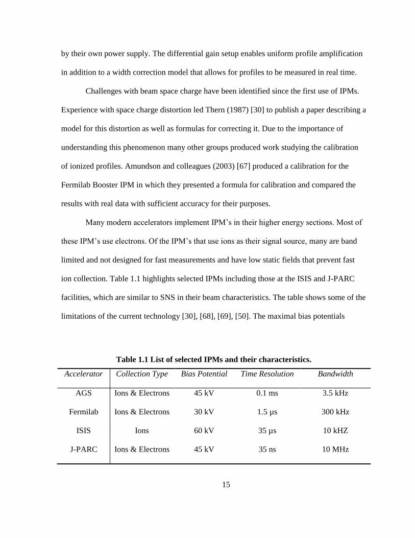
Many modern accelerators implement IPM’s in their higher energy sections. Most of

these IPM’s use electrons. Of the IPM’s that use ions as their signal source, many are band

limited and not designed for fast measurements and have low static fields that prevent fast

ion collection. Table 1.1 highlights selected IPMs including those at the ISIS and J-PARC

facilities, which are similar to SNS in their beam characteristics. The table shows some of the

limitations of the current technology [30], [68], [69], [50]. The maximal bias potentials

Table 1.1 List of selected IPMs and their characteristics.

Accelerator Collection Type Bias Potential Time Resolution Bandwidth

AGS Ions & Electrons 45 kV 0.1 ms 3.5 kHz

Fermilab Ions & Electrons 30 kV 1.5 µs 300 kHz

ISIS Ions 60 kV 35 µs 10 kHZ

J-PARC Ions & Electrons 45 kV 35 ns 10 MHz

16

currently used are on the order of 50 - 60 kV. Average time resolutions for modern IPMs are

100 ns with the lowest being 35 ns. Profile monitors based on residual gas ionization have

become a standard beam diagnostic tool in today’s high current accelerators as they continue

to be built and improved upon.

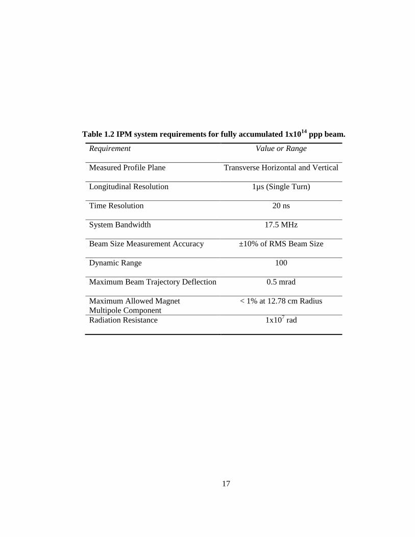
1.3 SNS IPM Design Criteria

It is the goal of this project to produce a complete IPM system design capable of parasitically

measuring turn-by-turn transverse beam profiles in the SNS accumulator ring. The beam

width accuracy must be comparable to that of currently employed profile diagnostic tools. As

part of this project, a thorough analysis is presented to ensure measurement reliability. IPM

system requirements are defined for a fully accumulated 1MW nominal beam consisting of

1x1014

ppp and are summarized in table 1.2. In order to measure the single turn 1 µs long

bunches, the system must have sufficient bandwidth and dispersion correction to measure a

bunch rise time of at least 20 ns with a dynamic range of 100 for a nominal beam. The

measured beam profile width should be within ±10% of RMS beam size when compared to

the profile width calculated from the beam optics at the IPM location.

For the system to be able to run parasitically during production-beam operation mode,

the beam upon leaving the IPM region must be negligibly affected in its trajectory and

dynamics by the IPM magnets and electrodes. Therefore, if the IPM produces multipole

components in the magnetic field of greater than 1% measured at a distance of 12.78 cm

from the magnet center, these will produce higher order distortions to the beam particle

trajectories that cannot be compensated.

As with all ring vacuum chamber components, the same secondary electron

17

Table 1.2 IPM system requirements for fully accumulated 1x1014

ppp beam.

Requirement Value or Range

Measured Profile Plane Transverse Horizontal and Vertical

Longitudinal Resolution 1µs (Single Turn)

Time Resolution 20 ns

System Bandwidth 17.5 MHz

Beam Size Measurement Accuracy ±10% of RMS Beam Size

Dynamic Range 100

Maximum Beam Trajectory Deflection 0.5 mrad

Maximum Allowed Magnet

Multipole Component

< 1% at 12.78 cm Radius

Radiation Resistance 1x107 rad

18

mitigation treatment must be applied to the IPM in order to reduce instabilities resulting from

electron build-up. While the performance requirements for the system put lower limits on

many of the design aspects, budgetary concerns will place upper limits on the size of some of

the larger and more expensive components. Likewise, the location in the ring tunnel will set

limits on some physical dimensions, such as the 4.2 m longitudinal distance allocated for

both horizontal and vertical systems and the 2.54 m ceiling height.

1.4 Overall Organization

The remainder of this work is broken into five chapters. Chapter 2 describes the theoretical

basis for the IPM system. A description of the beam-gas interaction presents the principles of

gas ionization and estimates for electron-ion pair production. Study of the residual gas and

SNS ring pressure then allows for estimation of the expected signal. Analysis of the residual

gas sensitivity and profile generation method is also presented.

Chapter 3 is a description of the simulation studies and basic system parameter

determination. Also offered in this chapter is a description of the computational method used

to simulated ionized particle trajectories. A large portion of chapter 3 is dedicated to the

analysis of measured errors expected in the system, methods for the error reduction, as well

as an estimation measured profile accuracy.

Chapter 4 summarizes the results of an IPM test chamber built and installed in the

ring to test the basic IPM proof-of-principle while chapter 5 outlines the completed design in

detail for each of major system components. The summary chapter, chapter 6, recapitulates

the main design elements in relation to the design goals, briefly describes future work and

possible system upgrades, concluding with some final remarks.

19

Chapter 2

Theoretical Analysis

The following chapter will present an analysis of IPMs based on first principals that will

translate the measurement requirements of table 1.2 into system specifications and a

foundation for their reliability. A theoretical foundation for the principle of residual gas

ionization by an energetic incident particle is developed leading to an estimate of the number

of ion-electron pairs created. A study of the residual gas is performed analyzing measured

pressure data from the IPM location and applying vacuum physics to understand the residual

gas density and characteristics. Mechanisms of ionization are examined to determine the

measured signal characteristics and errors induced by low initial particle statistics are

addressed. Finally, after a description of the detector to be used, estimates for the measured

signals expected are given along with a method of producing complete turn-by-turn beam

profiles.

Design Considerations

A number of variations of the IPM exist. One of the goals of this project was to develop a

simple design that meets the necessary specifications and that extends the technological state-

of-the-art. Of the two types of IPM detection methods, use of a phosphor screen or direct

20

collection of ionized particles as discussed in section 1.1.3, the method of measuring

ionization products directly eliminates the need for a camera and thus will be the method

considered here.

A beam’s passage through residual gas produces ions and electrons; both of which

can be used to measure profiles. It will be shown in the following analysis that both of the

particle types involve their own challenges. While ion collection is a simpler method of

measurement, profiles acquired through this method present challenges that make it difficult

to fulfill the system requirements as stated in table 1.2. Therefore, electron collection will be

the primary design focus. However, even though electron collection will provide the required

profile accuracy, it is desirable to design the system with the capability of measuring ions or

electrons. This will allow for the comparison of the two profile methods and provide a test

bed for the development of ion-based IPM profiles in high intensity accelerators.

Additionally, it is advantageous because the design of an ion collection system requires only

straightforward modifications to a system developed for electrons.

2.1 Beam-Gas Interaction

A detailed analysis of the physics involved in the implementation of a residual-gas-based

beam profile monitor is necessary in order to design a system capable of measuring reliable

and accurate profiles. An understanding of the interaction between the beam and the residual

gas is fundamental toward the design of a non-destructive profile monitor.

2.1.1 Interaction Model

It is first necessary to develop a model for the beam-gas interaction. A complete quantum

mechanical model would not only be extremely complex, but unnecessary as a number of

21

simplifications may be made that allow for easier analysis without loss of solution integrity.

Beam Properties

The requirements on the particle beam for the nuclear spallation process are such that

incoming protons must have wavelengths ~1.3 fm, the range of the strong force, or the proton

will interact with the nucleus as a whole and not individual nucleons. The de Broglie

wavelength is

(2.1)

where h is Planck’s constant. For protons with mass , energy K =

100 MeV, and momentum √ ⁄ the wavelength is 2.7 fm. The lower

energy limit for a proton to produce spallation reactions is approximately 100 MeV and

optimal energies are in the GeV range [70], which can be seen from the probability for

nuclear collisions by an incident proton, ⁄ . Here,

R, the range of the proton, is a monotonically increasing function of proton energy and

is the proton nuclear collision length [71]. The probability for a spallation reaction

is significant only when the proton range is large compared to the collision mean free path,

which happens with energies of 1-2 GeV.

Protons incident on the Hg target in the SNS have been accelerated to a kinetic

energy K of 1 GeV, and when combined with their rest energy = 938 MeV, give a total

energy of 1.938 GeV. We define the Lorentz factor by

√ (2.2)

where

22

(2.3)

and c is the speed of light in vacuum. Thus, a proton having 1 GeV kinetic energy has

, , and a relativistic velocity of 88% the speed of light or m/s.

Beam-Gas Model Assumptions

Although an energetic charged particle will interact with matter in the surrounding region,

not all possible interaction processes need to be considered given the IPM conditions. A

detailed analysis of the various forces and interaction mechanisms experienced by a beam

particle passing through a gas has been done and may be found in Appendix A. The

following summary of the results therein will form the basis for further study of the

ionization process:

1) Of the four fundamental forces through which the incident proton may interact

with the gas, gravity and the weak force, whose strengths, relative to the

strong nuclear interaction, are 10-6

and 10-39

respectively, may be ignored due

to their weakness.

2) The low gas density associated with a 10-8

Torr vacuum means that nuclear

collisions governed by the strong force, with a range 10-15

m, are highly

improbable.

3) In the laboratory frame, the electric force given by Coulomb’s law is primarily

responsible for energetic collisions, considering that the magnetic field is

much smaller than the electric field for orbital electrons and may be ignored.

4) The small size of the nucleus in comparison to the atomic size and the low gas

density make nuclear excitations through proton-nucleus Coulomb

interactions negligible.

23

5) Energy loss by bremsstrahlung from beam particles interacting with the

residual gas may be considered negligible due to the small momentum change

experienced by the 1 GeV protons.

6) Charge exchange during beam-gas collisions is negligible due to the small

collision cross-section for the process for energetic incident particles.

7) Coherent scattering may be ignored considering the diffuse nature of the gas

compared to the proton wavelength.

8) The wavelength of the 1 GeV proton, (see Appendix A

for calculation), is sufficiently small compared to the electron wavelength

~10-9

m and atomic dimensions ~10-10

m that collisions may be treated

classically.

9) The energetic proton interacts with gas molecules through the most weakly

bound electrons and thus Coulomb collisions with complex gas molecules

may be characterized as proton collisions with valence electrons.

10) The velocity of the proton is sufficiently high compared to the gas thermal

velocity and the electron velocity that gas molecules and atomic electrons may

be considered at rest. Incident proton-atom interactions may be calculated as

proton-electron interactions in the proton rest frame

11) Within the limits of maximum and minimum energy transfers, proton-gas

collisions may be considered elastic.

The complex behavior of beam-gas interactions leading to ionization may be

simplified to classical incoherent elastic and inelastic Coulomb interactions between

energetic protons and stationary orbital electrons. With this model, an analysis of the

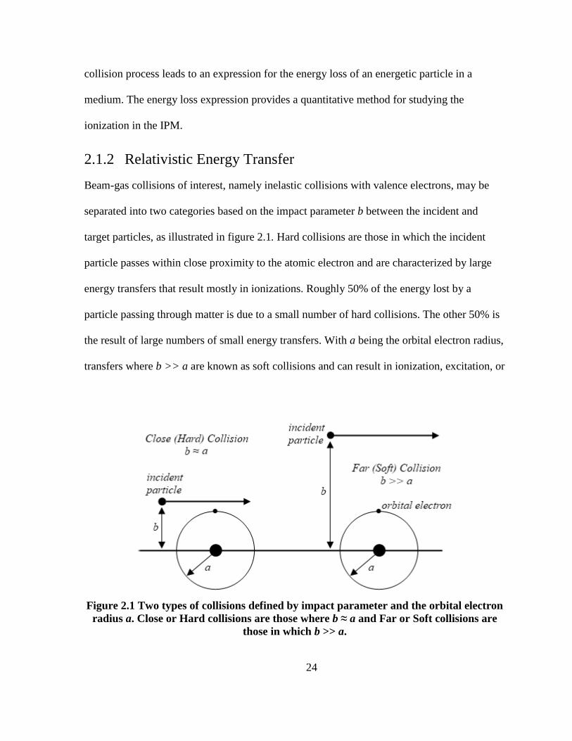
24

collision process leads to an expression for the energy loss of an energetic particle in a

medium. The energy loss expression provides a quantitative method for studying the

ionization in the IPM.

2.1.2 Relativistic Energy Transfer

Beam-gas collisions of interest, namely inelastic collisions with valence electrons, may be

separated into two categories based on the impact parameter b between the incident and

target particles, as illustrated in figure 2.1. Hard collisions are those in which the incident

particle passes within close proximity to the atomic electron and are characterized by large

energy transfers that result mostly in ionizations. Roughly 50% of the energy lost by a

particle passing through matter is due to a small number of hard collisions. The other 50% is

the result of large numbers of small energy transfers. With a being the orbital electron radius,

transfers where b >> a are known as soft collisions and can result in ionization, excitation, or

Figure 2.1 Two types of collisions defined by impact parameter and the orbital electron

radius a. Close or Hard collisions are those where b ≈ a and Far or Soft collisions are

those in which b >> a.

25

atomic polarization.

The probability of particular interaction processes is given by a Landau distribution

[72], [73] and may be seen qualitatively in figure 2.2. While figure 2.2 shows a general case,

it does elucidate some of the basic principles of the inelastic energy transfer processes due to

soft collisions. There is a relatively high probability of excitation up to the ionization energy

after which ionization dominates. The probability then decreases with increasing energy to a

maximum allowed energy transfer.

Energy Transfer

The minimum and maximum energy transferred may be derived through elastic Coulomb

collisions also known as Rutherford scattering. For energy transfers significantly larger than

the binding energy required to remove an electron from its atomic orbit, the electron may be

considered free (see figure 2.3 (a) for the lab frame illustration). Therefore, proton-molecular

collisions may be viewed as an incident proton elastically colliding with a free stationary

electron. Collision analysis is simplified when viewed in the center-of-mass frame and a

complete explanation of transformation to the center of mass may be found in Appendix B.

Figure 2.3 (b) is a depiction of the collision in the center-of-mass frame with equal

scattering angles . When transforming to the center-of-mass frame from the lab, position

and velocity become that of the proton since mp >> me (see Appendix B for derivation). In

the proton rest frame shown in figure 2.3 (c) where the electron now has momentum

, the collision is identical to Rutherford scattering for an energetic particle by an

attractive force. In the lab frame the electron undergoes large energy transfers corresponding

to large scattering angle, but the massive protons scatter through small angles and travel in

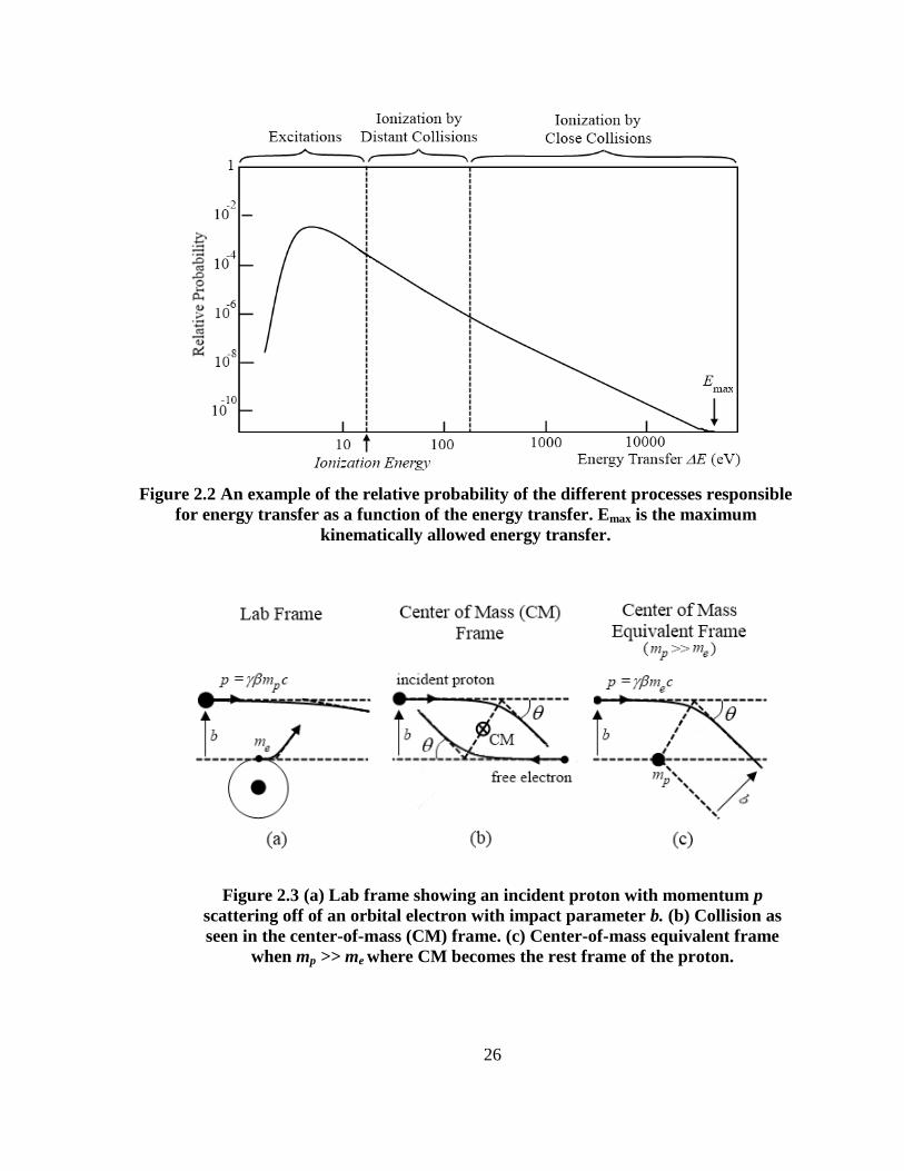
26

Figure 2.2 An example of the relative probability of the different processes responsible

for energy transfer as a function of the energy transfer. Emax is the maximum

kinematically allowed energy transfer.

Figure 2.3 (a) Lab frame showing an incident proton with momentum p

scattering off of an orbital electron with impact parameter b. (b) Collision as

seen in the center-of-mass (CM) frame. (c) Center-of-mass equivalent frame

when mp >> me where CM becomes the rest frame of the proton.

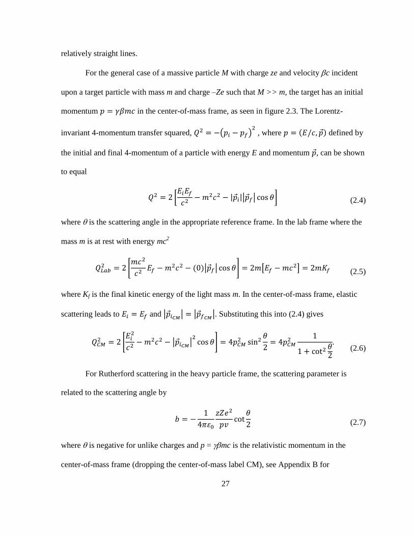
27

relatively straight lines.

For the general case of a massive particle M with charge ze and velocity c incident

upon a target particle with mass m and charge –Ze such that M >> m, the target has an initial

momentum in the center-of-mass frame, as seen in figure 2.3. The Lorentz-

invariant 4-momentum transfer squared, ( ) , where defined by

the initial and final 4-momentum of a particle with energy E and momentum , can be shown

to equal

[

| || | ] (2.4)

where is the scattering angle in the appropriate reference frame. In the lab frame where the

mass m is at rest with energy mc2

[

| | ] [ ] (2.5)

where Kf is the final kinetic energy of the light mass m. In the center-of-mass frame, elastic

scattering leads to and | | |

|. Substituting this into (2.4) gives

[

|

| ]

(2.6)

For Rutherford scattering in the heavy particle frame, the scattering parameter is

related to the scattering angle by

(2.7)

where is negative for unlike charges and p = mc is the relativistic momentum in the

center-of-mass frame (dropping the center-of-mass label CM), see Appendix B for

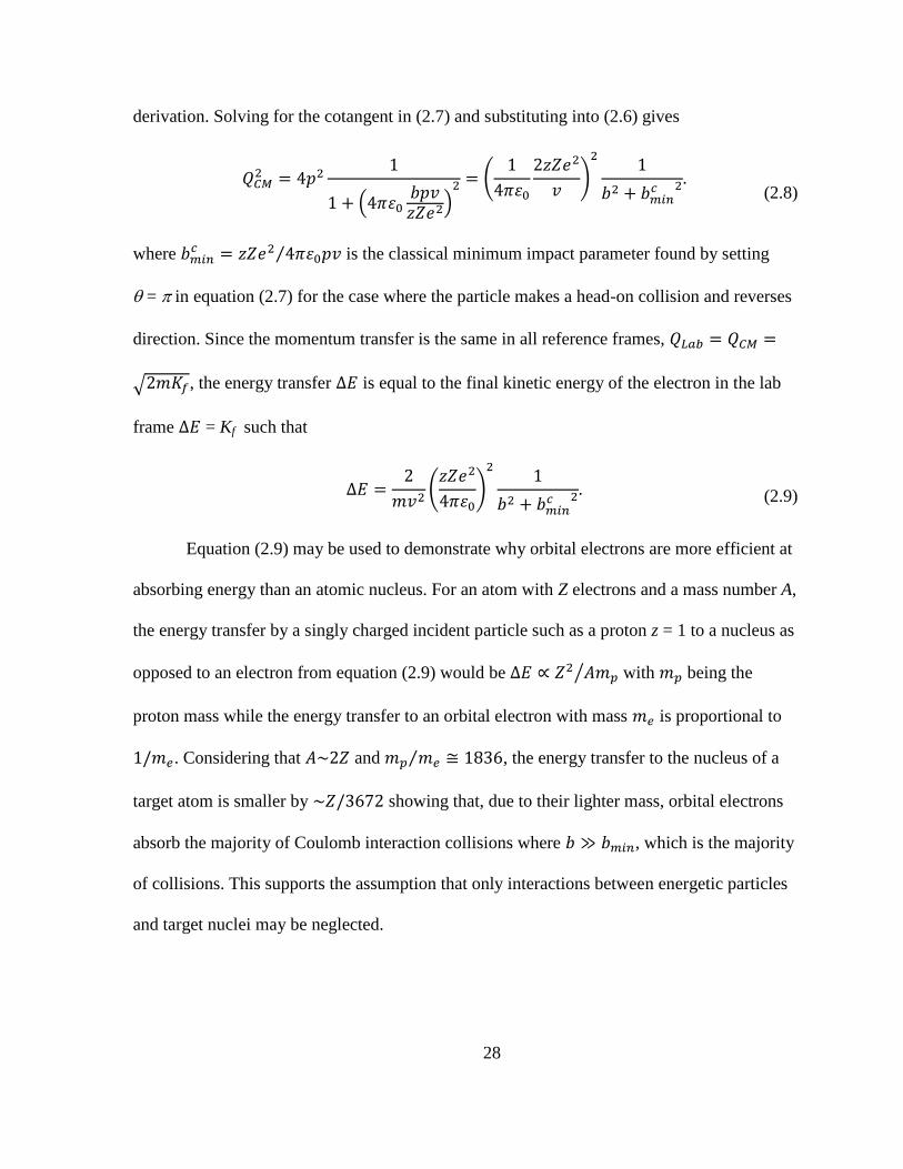
28

derivation. Solving for the cotangent in (2.7) and substituting into (2.6) gives

( )

(

)

(2.8)

where ⁄ is the classical minimum impact parameter found by setting

= in equation (2.7) for the case where the particle makes a head-on collision and reverses

direction. Since the momentum transfer is the same in all reference frames,

√ , the energy transfer is equal to the final kinetic energy of the electron in the lab

frame = Kf such that

(

)

(2.9)

Equation (2.9) may be used to demonstrate why orbital electrons are more efficient at

absorbing energy than an atomic nucleus. For an atom with Z electrons and a mass number A,

the energy transfer by a singly charged incident particle such as a proton z = 1 to a nucleus as

opposed to an electron from equation (2.9) would be ⁄ with being the

proton mass while the energy transfer to an orbital electron with mass is proportional to

. Considering that and ⁄ , the energy transfer to the nucleus of a

target atom is smaller by showing that, due to their lighter mass, orbital electrons

absorb the majority of Coulomb interaction collisions where , which is the majority

of collisions. This supports the assumption that only interactions between energetic particles

and target nuclei may be neglected.

29

Maximum Energy Transfer

The energy transfer has a maximum value allowed by kinematics at the minimum impact

parameter . This classical minimum impact parameter varies inversely as the velocity

squared, , so that the impact parameter becomes very small for large velocities.

However, the uncertainty principle requires that the impact parameter can be no less than the

uncertainty in the incident particle’s position. By setting the minimum parameter equal to the

de Broglie wavelength of the incident particle, having mass m with momentum in

the heavy particle rest frame, and utilizing the de Broglie wavelength equation, ⁄ , the

quantum-mechanical minimum impact parameter2 becomes

(2.10)

For the case of 1 GeV protons,

, which justifies use of the quantum-

mechanical minimum impact parameter in the derivation of the total energy loss cross

section.

The maximum allowed energy transfer in a relativistic elastic head-on collision is

found through kinematics to be

(

) (

)

(2.11)

In the event , is a sufficient approximation for protons with

kinetic energies < 340 GeV. The maximum energy transfer given by equation (2.11) for a

1 GeV proton is 2.9 MeV or 0.3% of the proton kinetic energy. This result gives credence to

2 Alternative derivations in the literature [75], [85], [89] use the Heisenberg uncertainty principle to derive the

minimum quantum impact parameter

with the same result expect replacing h with .

30

the assumption that the change of momentum to the proton is very small and that the proton

trajectory undergoes very small deviations.

Minimum Energy Transfer

Examining the energy transfer equation (2.9), it would seem that as . Again,

this is an erroneous conclusion due to the classically based collision analysis and the fact that

we neglected binding energy and assumed a free electron. From quantum mechanics it is

known that bound systems may only absorb energy in quantized amounts. For the case of

energy transfer due to relativistic Coulomb fields, the field of a relativistic charged particle

with velocity varies in time as where b is the impact parameter (see

Appendix C for a derivation of relativistic electromagnetic fields).

The ground state target electron may be approximated as a harmonic oscillator with

frequency . If the time the incident particle interacts with the electron is long compared

to the electron orbital period , then the electron will respond adiabatically. It will absorb

energy slowly over many oscillations, transitioning to lower excited states and returning to

the ground state without appreciable energy transfer. However, if the characteristic frequency

of the incident field, , is close to the resonance frequency of the electron there will be a

large energy transfer. The limiting condition is ⁄ , which means ⁄ .

Now for the real case of an atom with Z elections, each electron may act as a set of

oscillators with frequencies corresponding to the transition energies, where fi is related to the

ith energy . The energy transfer to a single electron is [74]. By summing all

the contributions from all Z electrons, the electronic binding energy for an atom may then be

characterized by a weighted geometric mean of frequencies fi with weights wi such that

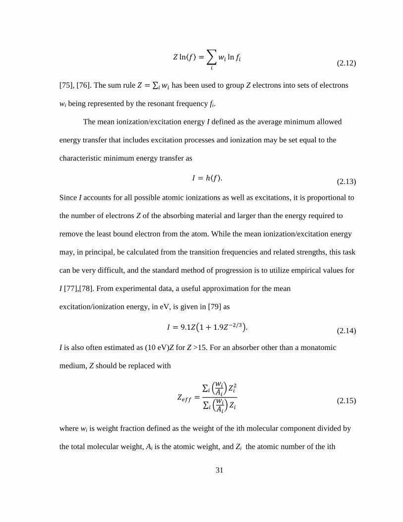
31

⟨ ⟩ ∑

(2.12)

[75], [76]. The sum rule ∑ has been used to group Z electrons into sets of electrons

wi being represented by the resonant frequency fi.

The mean ionization/excitation energy I defined as the average minimum allowed

energy transfer that includes excitation processes and ionization may be set equal to the

characteristic minimum energy transfer as

⟨ ⟩ (2.13)

Since I accounts for all possible atomic ionizations as well as excitations, it is proportional to

the number of electrons Z of the absorbing material and larger than the energy required to

remove the least bound electron from the atom. While the mean ionization/excitation energy

may, in principal, be calculated from the transition frequencies and related strengths, this task

can be very difficult, and the standard method of progression is to utilize empirical values for

I [77],[78]. From experimental data, a useful approximation for the mean

excitation/ionization energy, in eV, is given in [79] as

( ) (2.14)

I is also often estimated as (10 eV)Z for Z >15. For an absorber other than a monatomic

medium, Z should be replaced with

∑ (

)

∑ (

)

(2.15)

where wi is weight fraction defined as the weight of the ith molecular component divided by

the total molecular weight, Ai is the atomic weight, and Zi the atomic number of the ith

32

element of the molecule.

Values of I have been compiled in table 2.1 for various gases relevant to the IPM

system, each with corresponding atomic number Z, mass number A, and density . Eex and EI

are the energies required to produce the first excited stated and to remove the first electron,

respectively. The W-value WI in table 2.1, to be defined shortly, is a measure of the amount

of energy actually required to form an ion-electron pair. As a general rule, about half the

energy from an incident particle transferred to an absorbing atom or molecule is spent on

excitation, and so the energy to form an ion pair WI is always larger than the ionization

energy and roughly twice EI [80]. From empirical observations, such as WI in table 2.1, the

energy to create ion-electron pairs is ~30 eV and is fairly constant for most gases and types

of incident particles [81].

2.1.3 Energy Loss

An energetic particle loses energy to the surrounding medium through excitations and

ionizations. The number of ion-electron pairs created as the incident particle traverses a

thickness of the target material may be calculated from the energy lost by the particle and the

energy required for ionization WI. Continuing with the same model as before, where an

incident heavy particle interacts with an atomic electron such that the electron may be

considered free and at rest, the total energy lost by the energetic particle with charge number

z, charge ze , and momentum Mv is the energy loss per electron collision times the number

of electrons in the surrounding medium.

By using the expression for the energy transfer due to a single collision at an impact

parameter b, from equation (2.9) and the illustration in figure 2.4 showing the

infinitesimal interaction volume dV at b, the differential total energy loss is given by

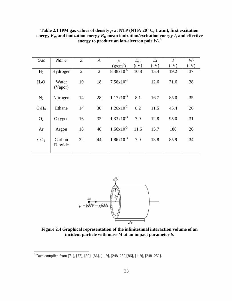
33

Table 2.1 IPM gas values of density at NTP (NTP: 20 C, 1 atm), first excitation

energy Eex and ionization energy EI, mean ionization/excitation energy I, and effective

energy to produce an ion-electron pair WI.3

Gas Name Z A (g/cm

3)

Eex

(eV)

EI

(eV)

I

(eV)

WI

(eV)

H2 Hydrogen 2 2 8.38x10-5

10.8 15.4 19.2 37

H2O Water

(Vapor)

10 18 7.56x10-4

12.6 71.6 38

N2 Nitrogen 14 28 1.17x10-3

8.1 16.7 85.0 35

C2H6 Ethane 14 30 1.26x10-3

8.2 11.5 45.4 26

O2 Oxygen 16 32 1.33x10-3

7.9 12.8 95.0 31

Ar Argon 18 40 1.66x10-3

11.6 15.7 188 26

CO2 Carbon

Dioxide

22 44 1.86x10-3

7.0 13.8 85.9 34

Figure 2.4 Graphical representation of the infinitesimal interaction volume of an

incident particle with mass M at an impact parameter b.

3 Data compiled from [71], [77], [80], [86], [119], [248–252][86], [119], [248–252].

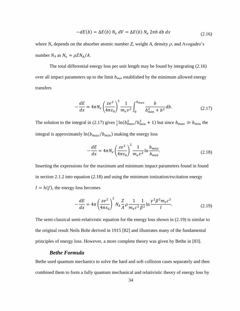
34

(2.16)

where Ne depends on the absorber atomic number Z, weight A, density , and Avogadro’s

number NA as .

The total differential energy loss per unit length may be found by integrating (2.16)

over all impact parameters up to the limit bmax established by the minimum allowed energy

transfers

The solution to the integral in (2.17) gives

⁄ but since the

integral is approximately ⁄ making the energy loss

(

)

(2.18)

Inserting the expressions for the maximum and minimum impact parameters found in found

in section 2.1.2 into equation (2.18) and using the minimum ionization/excitation energy

⟨ ⟩, the energy loss becomes

(

)

(2.19)

The semi-classical semi-relativistic equation for the energy loss shown in (2.19) is similar to

the original result Neils Bohr derived in 1915 [82] and illustrates many of the fundamental

principles of energy loss. However, a more complete theory was given by Bethe in [83].

Bethe Formula

Bethe used quantum mechanics to solve the hard and soft collision cases separately and then

combined them to form a fully quantum mechanical and relativistic theory of energy loss by

(

)

∫

(2.17)

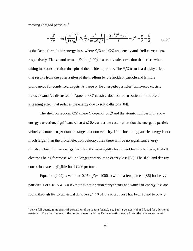
35

moving charged particles.4

(

)

[

] (2.20)

is the Bethe formula for energy loss, where and C/Z are density and shell corrections,

respectively. The second term, , in (2.20) is a relativistic correction that arises when

taking into consideration the spin of the incident particle. The term is a density effect

that results from the polarization of the medium by the incident particle and is more

pronounced for condensed targets. At large , the energetic particles’ transverse electric

fields expand (as discussed in Appendix C) causing absorber polarization to produce a

screening effect that reduces the energy due to soft collisions [84].

The shell correction, C/Z where C depends on and the atomic number Z, is a low

energy correction, significant when , under the assumption that the energetic particle

velocity is much larger than the target electron velocity. If the incoming particle energy is not

much larger than the orbital electron velocity, then there will be no significant energy

transfer. Thus, for low energy particles, the most tightly bound and fastest electrons, K shell

electrons being foremost, will no longer contribute to energy loss [85]. The shell and density

corrections are negligible for 1 GeV protons.

Equation (2.20) is valid for 0.05 < < 1000 to within a few percent [86] for heavy

particles. For 0.01 < < 0.05 there is not a satisfactory theory and values of energy loss are

found through fits to empirical data. For < 0.01 the energy loss has been found to be

4 For a full quantum mechanical derivation of the Bethe formula see [85]. See also[74] and [253] for additional

treatment. For a full review of the correction terms in the Bethe equation see [93] and the references therein.

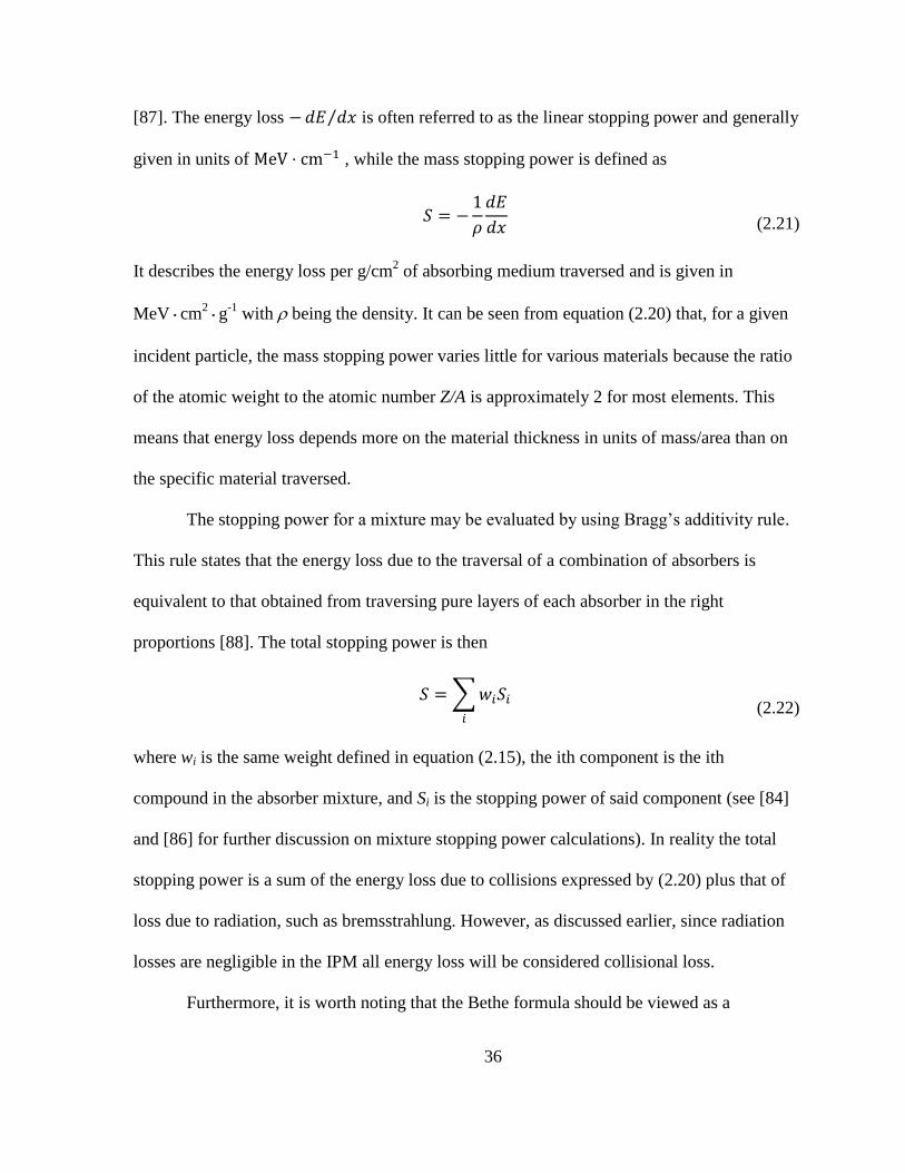
36

[87]. The energy loss ⁄ is often referred to as the linear stopping power and generally

given in units of , while the mass stopping power is defined as

(2.21)

It describes the energy loss per g/cm2 of absorbing medium traversed and is given in

MeVcm2g

-1 with being the density. It can be seen from equation (2.20) that, for a given

incident particle, the mass stopping power varies little for various materials because the ratio

of the atomic weight to the atomic number Z/A is approximately 2 for most elements. This

means that energy loss depends more on the material thickness in units of mass/area than on

the specific material traversed.

The stopping power for a mixture may be evaluated by using Bragg’s additivity rule.

This rule states that the energy loss due to the traversal of a combination of absorbers is

equivalent to that obtained from traversing pure layers of each absorber in the right

proportions [88]. The total stopping power is then

∑

(2.22)

where wi is the same weight defined in equation (2.15), the ith component is the ith

compound in the absorber mixture, and Si is the stopping power of said component (see [84]

and [86] for further discussion on mixture stopping power calculations). In reality the total

stopping power is a sum of the energy loss due to collisions expressed by (2.20) plus that of

loss due to radiation, such as bremsstrahlung. However, as discussed earlier, since radiation

losses are negligible in the IPM all energy loss will be considered collisional loss.

Furthermore, it is worth noting that the Bethe formula should be viewed as a

37

statistical average over many discrete interactions. The energy loss distribution, shown in

figure 2.2, shows that a single energetic particle will undergo many small energy transfers

and a few large energy transfers. Thus, individual particle energy losses may have large

fluctuations. It is important to remember that the energy loss by an energetic particle is a

stochastic process of hard and soft collisions that may result in an average energy loss less

than the ionization energy of the absorber [74].

2.1.4 Ionization

Secondary Ionization

As an energetic particle passes through a medium it transfers energy to orbital electrons.

When the energy transfer is larger than the ionization energy of the atom or molecule, the

electron will be ejected from its orbit. Ejected electrons with energies larger than the

ionization energy of the material may produce further ionization and these electrons are often

referred to as rays. Their energies may assume any value from the minimum cut off energy,

~15 eV for most gases, as seen by EI in table 2.1, to the kinetically allowed maximum kinetic

energy, which is 2.9 MeV for 1 GeV protons.

The probability of a electron receiving an energy between E and E+dE has been

shown in [89] to be ⁄ , meaning that the majority of electrons with the ability to cause

secondary ionization occur with lower energies. In addition, through kinematics it may be

shown that the emission angle of rays relative to the path of the incident particle as a

function of ray energy E is given by

(2.23)

where is the maximum allowed kinetic energy. Because most electrons have low

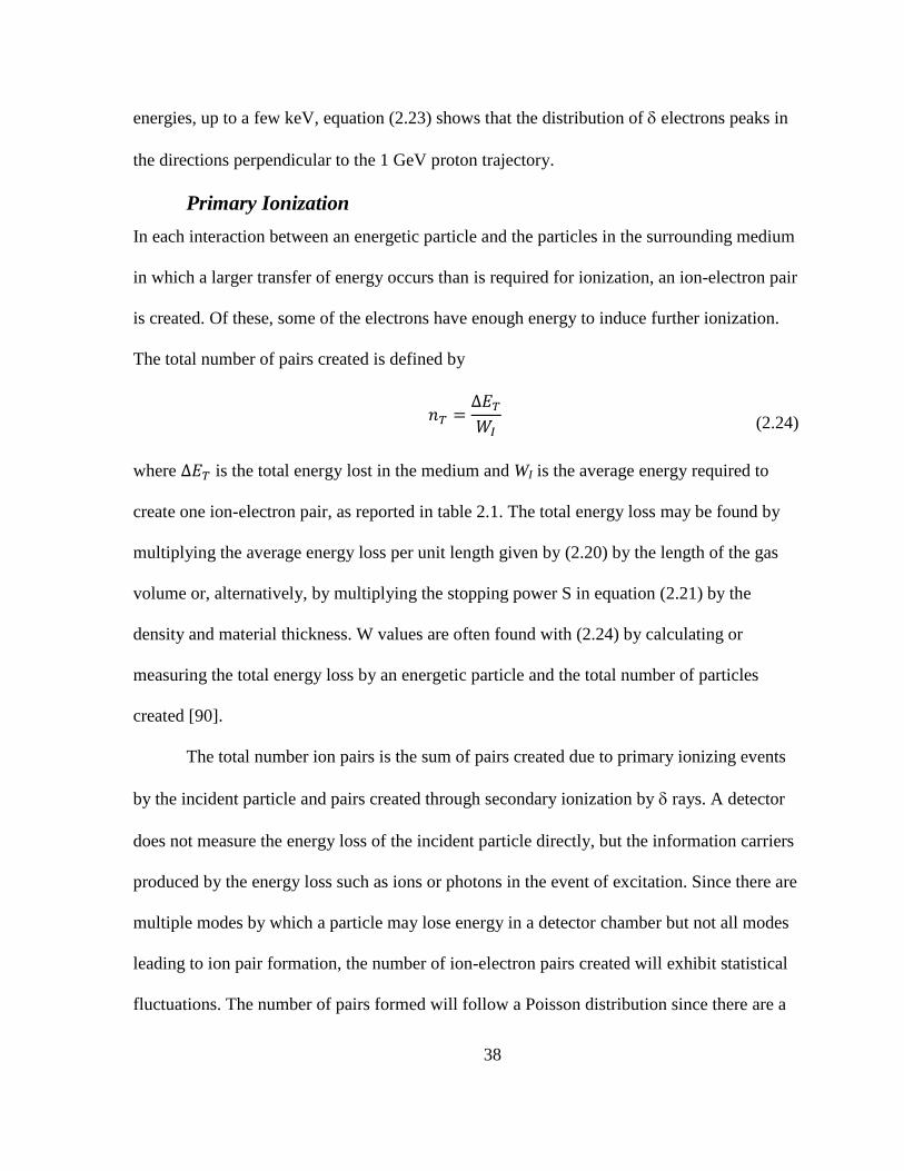
38

energies, up to a few keV, equation (2.23) shows that the distribution of electrons peaks in

the directions perpendicular to the 1 GeV proton trajectory.

Primary Ionization

In each interaction between an energetic particle and the particles in the surrounding medium

in which a larger transfer of energy occurs than is required for ionization, an ion-electron pair

is created. Of these, some of the electrons have enough energy to induce further ionization.

The total number of pairs created is defined by

(2.24)

where is the total energy lost in the medium and WI is the average energy required to

create one ion-electron pair, as reported in table 2.1. The total energy loss may be found by

multiplying the average energy loss per unit length given by (2.20) by the length of the gas

volume or, alternatively, by multiplying the stopping power S in equation (2.21) by the

density and material thickness. W values are often found with (2.24) by calculating or

measuring the total energy loss by an energetic particle and the total number of particles

created [90].

The total number ion pairs is the sum of pairs created due to primary ionizing events

by the incident particle and pairs created through secondary ionization by rays. A detector

does not measure the energy loss of the incident particle directly, but the information carriers

produced by the energy loss such as ions or photons in the event of excitation. Since there are

multiple modes by which a particle may lose energy in a detector chamber but not all modes

leading to ion pair formation, the number of ion-electron pairs created will exhibit statistical

fluctuations. The number of pairs formed will follow a Poisson distribution since there are a

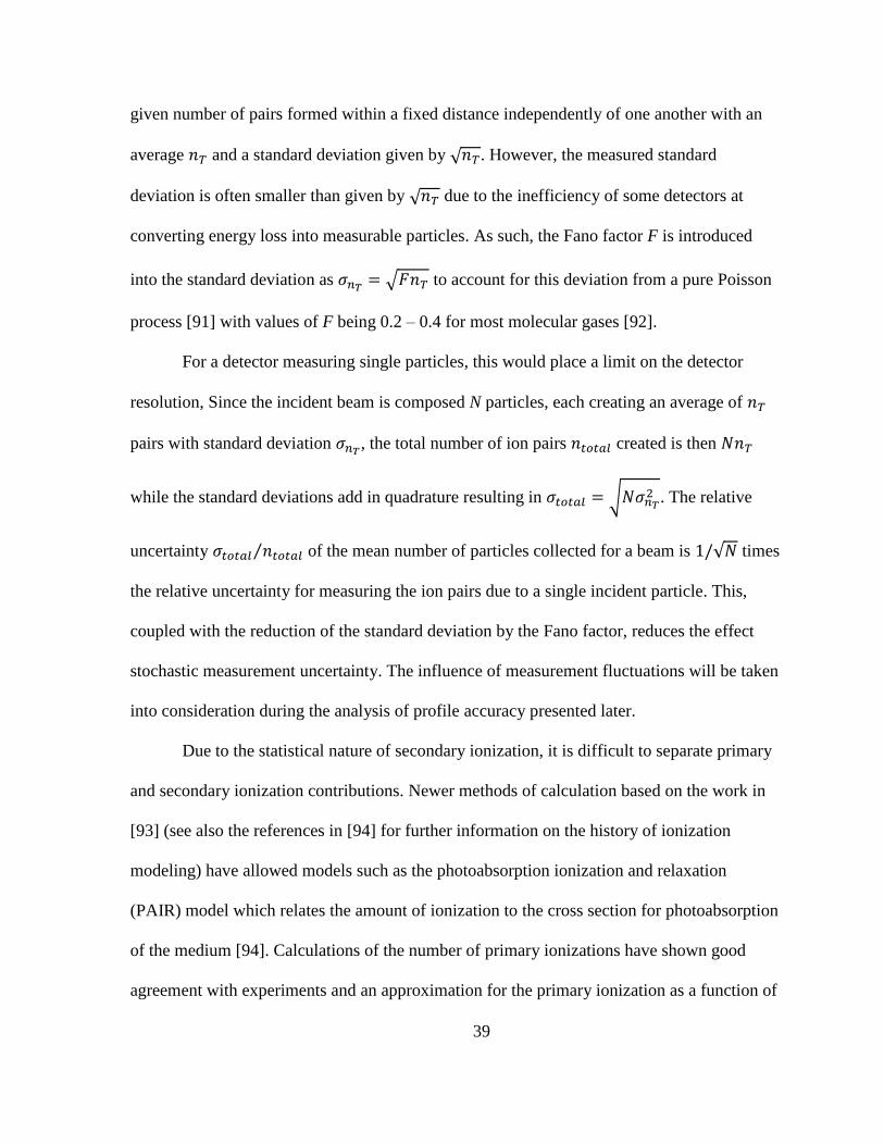
39

given number of pairs formed within a fixed distance independently of one another with an

average and a standard deviation given by √ . However, the measured standard

deviation is often smaller than given by √ due to the inefficiency of some detectors at

converting energy loss into measurable particles. As such, the Fano factor F is introduced

into the standard deviation as √ to account for this deviation from a pure Poisson

process [91] with values of F being 0.2 – 0.4 for most molecular gases [92].

For a detector measuring single particles, this would place a limit on the detector

resolution, Since the incident beam is composed N particles, each creating an average of

pairs with standard deviation , the total number of ion pairs created is then

while the standard deviations add in quadrature resulting in √ . The relative

uncertainty ⁄ of the mean number of particles collected for a beam is √ times

the relative uncertainty for measuring the ion pairs due to a single incident particle. This,

coupled with the reduction of the standard deviation by the Fano factor, reduces the effect

stochastic measurement uncertainty. The influence of measurement fluctuations will be taken

into consideration during the analysis of profile accuracy presented later.

Due to the statistical nature of secondary ionization, it is difficult to separate primary

and secondary ionization contributions. Newer methods of calculation based on the work in

[93] (see also the references in [94] for further information on the history of ionization

modeling) have allowed models such as the photoabsorption ionization and relaxation

(PAIR) model which relates the amount of ionization to the cross section for photoabsorption

of the medium [94]. Calculations of the number of primary ionizations have shown good

agreement with experiments and an approximation for the primary ionization as a function of

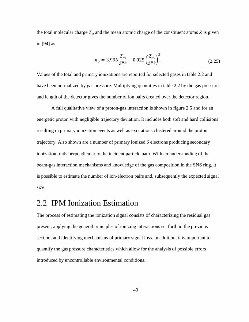
40

the total molecular charge Zm and the mean atomic charge of the constituent atoms is given

in [94] as

(

)

(2.25)

Values of the total and primary ionizations are reported for selected gases in table 2.2 and

have been normalized by gas pressure. Multiplying quantities in table 2.2 by the gas pressure

and length of the detector gives the number of ion pairs created over the detector region.

A full qualitative view of a proton-gas interaction is shown in figure 2.5 and for an

energetic proton with negligible trajectory deviation. It includes both soft and hard collisions

resulting in primary ionization events as well as excitations clustered around the proton

trajectory. Also shown are a number of primary ionized electrons producing secondary

ionization trails perpendicular to the incident particle path. With an understanding of the

beam-gas interaction mechanisms and knowledge of the gas composition in the SNS ring, it

is possible to estimate the number of ion-electron pairs and, subsequently the expected signal

size.

2.2 IPM Ionization Estimation

The process of estimating the ionization signal consists of characterizing the residual gas

present, applying the general principles of ionizing interactions set forth in the previous

section, and identifying mechanisms of primary signal loss. In addition, it is important to

quantify the gas pressure characteristics which allow for the analysis of possible errors

introduced by uncontrollable environmental conditions.

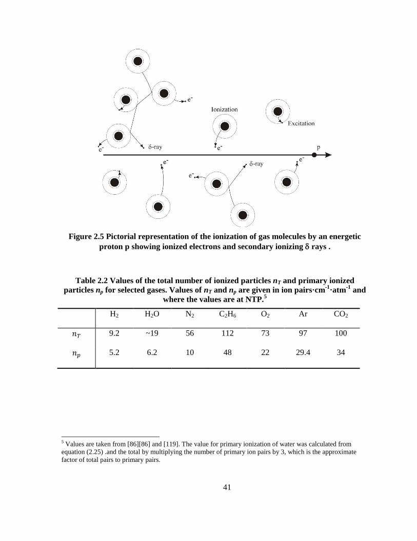
41

Figure 2.5 Pictorial representation of the ionization of gas molecules by an energetic

proton p showing ionized electrons and secondary ionizing rays .

Table 2.2 Values of the total number of ionized particles nT and primary ionized

particles np for selected gases. Values of nT and np are given in ion pairs·cm-1

·atm-1

and

where the values are at NTP.5

H2 H2O N2 C2H6 O2 Ar CO2

9.2 ~19 56 112 73 97 100

5.2 6.2 10 48 22 29.4 34

5 Values are taken from [86][86] and [119]. The value for primary ionization of water was calculated from

equation (2.25) .and the total by multiplying the number of primary ion pairs by 3, which is the approximate

factor of total pairs to primary pairs.

42

2.2.1 Residual Gas Composition

Considering that the number of ion pairs produced is related to the target gas as illustrated in

table 2.2, identifying the individual gases and their fractional contributions is necessary for

further calculations. The composition of the residual gas is determined primarily by the

outgassing properties of the accelerator components, air leaks, and the pumping efficiency of

the gas constituents. Vacuum chamber components in SNS are made from 316 stainless steel.

Unbaked stainless steel thermal outgassing rates per square centimeter of surface area for a

few common accelerator vacuum gas components such as H2, H2O, CO2, and CO are 7x10-12

,

3x10-10

, 5x10-13

, and 5x10-12

, respectively, in units of - - [95].

In order to reduce instabilities caused by secondary electrons, which will be discussed

in more detail later, all components installed in the SNS ring undergo interior TiN coating. It

has been found that this coating acts as a partial hydrogen barrier reducing the hydrogen

outgassing rate [96]. While an initial estimation would conclude that water dominates the

residual gas, the Gamma TiTan 300L Ion Pumps used in the ring are inefficient at pumping

hydrogen and noble gases [97].

Residual Gas Analysis

A residual gas analysis (RGA) was taken using a Stanford Research System RGA with 100 u

scanning capability [98] upstream of the IPM location. The RGA is an open ion source that

uses ~70 eV electrons to ionize gas molecules after which a quadrupole filter measures the

currents of different ion species based on their charge-to-mass ratio. The RGA assumes that

all ion species measured are singly ionized and plots the currents measured for different

masses. An RGA taken on October 26, 2007 upstream of the RF section in the SNS ring D

Straight is shown in figure 2.6. Each pure gas has a specific fragmentation pattern known as a

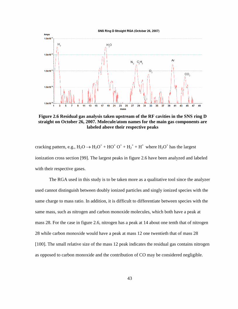
43

Figure 2.6 Residual gas analysis taken upstream of the RF cavities in the SNS ring D

straight on October 26, 2007. Molecule/atom names for the main gas components are

labeled above their respective peaks

cracking pattern, e.g., H2O H2O+ + HO

+ O

+ + H2

+ + H

+ where H2O

+ has the largest

ionization cross section [99]. The largest peaks in figure 2.6 have been analyzed and labeled

with their respective gases.

The RGA used in this study is to be taken more as a qualitative tool since the analyzer

used cannot distinguish between doubly ionized particles and singly ionized species with the

same charge to mass ratio. In addition, it is difficult to differentiate between species with the

same mass, such as nitrogen and carbon monoxide molecules, which both have a peak at

mass 28. For the case in figure 2.6, nitrogen has a peak at 14 about one tenth that of nitrogen

28 while carbon monoxide would have a peak at mass 12 one twentieth that of mass 28

[100]. The small relative size of the mass 12 peak indicates the residual gas contains nitrogen

as opposed to carbon monoxide and the contribution of CO may be considered negligible.

44

Partial Pressure Calculation

The currents measured with an RGA are not a straightforward superposition from the

fractional composition of the pure gases. The actual amount of a pure gas found with an

RGA depends on a number of factors including the probability of ionizing a particular mass

fragment, the probability that the resulting ion will enter and pass through the quadrupole, the

fact that RGAs differ in sensitivity to different ionization products, and most RGAs,

including the one used, are calibrated to be sensitive to mass 28, or nitrogen.

The equation relating RGA current peak at mass B from gas A, IAB, to the partial

pressure of gas A is

(2.26)

where is the mass 28, or nitrogen, fragmentation factor, XFA is the ionization

probability for gas A, and TFB is the transmission factor, which is a measure of how many

ions of mass B make it through the detector. DFB is a relative current detection factor for

mass B, and S is an instrument-specific sensitivity factor to mass 28 in Amps/Torr [101].

For example, the partial pressure of hydrogen with a main peak at mass 2 is

where the detection factor DF is usually set to 1

[101]. The current taken from figure 2.6 is 3.2x10-11

amps and the fragmentation factor

and ionization probability are found in commonly used tables such as in [101] with

, . The quadrupole transmission factor relative to nitrogen is 28/B [102],

therefore, 5.47x10

-9 Torr.

While the RGA is not a reliable source for absolute pressure measurements, equation

(2.26) may be used to calculate the fractional pressure composition. Table 2.3 shows

45

Table 2.3 Calculated pressure fractions for constituent pure gases in the IPM residual

gas

H2 H2O N2 C2H6 O2 Ar CO2

⁄ 0.113 0.739 0.029 0.032 0.010 0.069 0.007

calculated pressure fractions based on the RGA in figure 2.6. For estimations, the residual

gas may be simplified as 11% hydrogen, 74% water, and 15% other, where other has a

weighted mass of ~34 u. It can be seen that the IPM residual gas is primarily composed of

water vapor and therefore the larger mass of water will place limitations on the IPM ion

collection mode. The IPM will be designed with a vacuum port capable of affixing a residual

gas analyzer in order to allow for vacuum studies of the system and comparison with

theoretical calculations.

2.2.2 IPM Pressure

In order to achieve the 1 W/m beam loss requirement, the SNS ring was designed to limit the

beam lost through residual gas interactions such as nuclear scattering, multi-Coulomb

scattering, and residual gas ionization. Of the beam-loss mechanisms, the residual gas density

is a limiting source [103] as it contributes to an instability, referred to as the e-p instability,

which arises from the coupling of electrons freed through residual gas ionizations, beam loss,

or ionized residual gas particles releasing secondary electrons after contacting the beam pipe.

The secondary electrons are then accelerated by the beam-wall potential and receive enough

energy to release tertiary electrons, leading to an electron cloud accumulation known as

multipacting [104].

To mitigate the aforementioned gas-related instabilities, in addition to the TiN coating

46

that reduces secondary electron emission, the SNS ring was designed to operate with a 10-9

Torr scale vacuum [103].

Residual-Gas Temperature

In the ultra-high vacuum (UHV) regime, ~10-9

Torr, the mean free path of gas molecules is

much larger than the dimensions of the volume. For gas particles with an abundance-

weighted average diameter of 2.8 Å, the mean free path, defined in Appendix A eq. (A.6) for

a pressure range P of 10-8

to 10-9

Torr and temperature of 70¬F is ~50 km, while the beam

pipe diameter is 25.4 cm. In this vacuum regime, known as molecular flow, collisions

between gas molecules are rare and collective fluid behavior may be ignored. Gas properties

are characterized by collisions with the chamber walls and consequently, the temperature is

determined by the chamber walls.

In addition to ambient temperature, the beam image current is a possible heat source.

The positively charged proton beam’s electric fields induce currents in the surrounding pipe

wall. The 300 series stainless steel used for the accelerator structure has a finite conductivity

of ~1.3 S/m. This results ([74] and [105]) in exponentially decaying fields and currents

that depend on distance d within the conductor as ⁄ . The decay constant δ is the skin

depth defined by

√

(2.27)

where μ is the magnetic permeability and is the frequency of the electromagnetic field.

Furthermore, the electric fields drop off much more rapidly leaving the image current

generated by the more deeply penetrating magnetic field as the dominant contributor to

resistive wall heating [105].

47

A simple calculation shows that beam-induced resistive wall heating is not a

significant factor in residual gas temperature. The average power ⟨ ⟩ dissipated due to a peak

beam current is ⟨ ⟩ , where DF is the macro-pulse duty factor of 0.06

and the resistance of the pipe R is the length divided by the conductivity times the cross-

sectional area A of the conducting region. The cross-sectional area may be approximated as

where r is the pipe inner radius of 12.7 cm.

For a peak ring beam current of 90 A, ring length of 248 m, and skin depth (for a 1

MHz ring frequency) of 4 mm, the average power dissipated is 276 W for the whole ring

during a 16.7 ms accumulation cycle. The conservation of energy requires the internal energy

change of the beam pipe be equal to the net energy flow in and out of the pipe walls. In the

absence of work, the internal energy change per unit time ⁄ , where m is mass

and c the specific heat, is equal to the power going in Pbeam minus the heat transfer out

through convection and radiation

with AS

being the surface area, ε the emissivity, σ the Stefan-Boltzmann constant, Ts the surrounding

ambient temperature, and h the convection heat transfer coefficient.

The equation for the temperature within the pipe walls

(2.28)

may be solved numerically. The results are shown in figure 2.7 for an input beam-induced

heat load of 276 W, emissivity of polished stainless steel of 0.17 [106], the mass found from

the density of 8000 kgm-3

and the volume of the 4 mm thick pipe wall, and a specific heat

capacity of stainless steel of 502 Jkg-1K

-1. The surface area was assumed to be that of the

outer surface since the vacuum inside the chamber precludes heat loss due to air flow, and

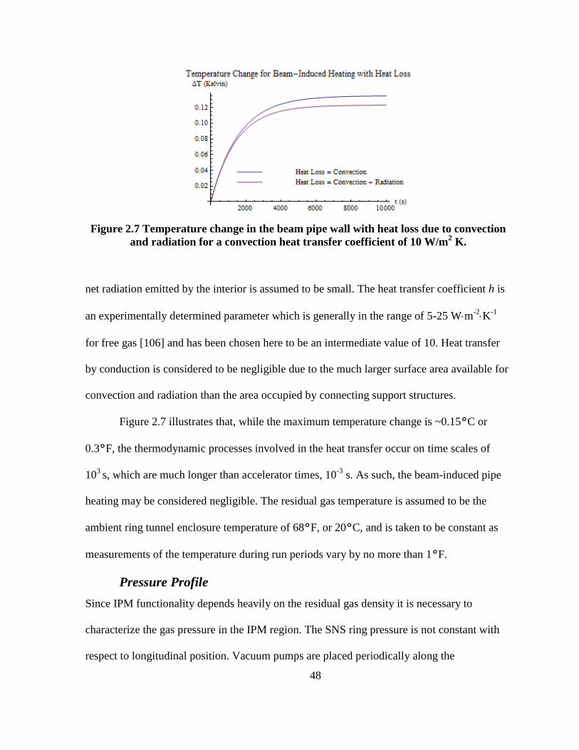
48

Figure 2.7 Temperature change in the beam pipe wall with heat loss due to convection

and radiation for a convection heat transfer coefficient of 10 W/m2 K.

net radiation emitted by the interior is assumed to be small. The heat transfer coefficient h is

an experimentally determined parameter which is generally in the range of 5-25 Wm-2K

-1

for free gas [106] and has been chosen here to be an intermediate value of 10. Heat transfer

by conduction is considered to be negligible due to the much larger surface area available for

convection and radiation than the area occupied by connecting support structures.

Figure 2.7 illustrates that, while the maximum temperature change is ~0.15°C or

0.3°F, the thermodynamic processes involved in the heat transfer occur on time scales of

103

s, which are much longer than accelerator times, 10-3

s. As such, the beam-induced pipe

heating may be considered negligible. The residual gas temperature is assumed to be the

ambient ring tunnel enclosure temperature of 68°F, or 20°C, and is taken to be constant as

measurements of the temperature during run periods vary by no more than 1°F.

Pressure Profile

Since IPM functionality depends heavily on the residual gas density it is necessary to

characterize the gas pressure in the IPM region. The SNS ring pressure is not constant with

respect to longitudinal position. Vacuum pumps are placed periodically along the

49

accelerating structure at irregular intervals and, consequently, the gas pressure is at a

minimum at the pump locations with maxima in between. The proposed location for the IPM,

shown in figure 2.8, is downstream of the RF section in the ring D straight. Figure 2.8 also

shows the locations of vacuum ion pumps (IP) and cold cathode gauges (CCG) used for

pressure measurements.

The most probable speed of ideal gas molecules with molecular mass m and

temperature T based on a Maxwell-Boltzmann distribution is

For a temperature of 68¬F and an average mass of 18.7 u, the average velocity of the residual

gas is 288 m/s. Gas particles will travel 0.3 mm during the 1 μs ring pulses and 30 cm during

an accumulation period of 1 ms. Consequently, the time it takes molecules to reach a pump is

long compared to the events of interest. Therefore, global pressure may be considered

constant with respect to time. There are processes that may affect local pressure. A simple

analytical model may be used to calculate the pressure profile between the vacuum pumps on

either side of the IPM location. The gas flow rate, or throughput, is defined through the

pressure P in Torr and volume flow rate S in liter/s as

(2.30)

Additionally, the throughput between two points may be defined [107] by

(2.31)

where C is the conductance in liter/s of the structure between those two points and ∆P is the

change in pressure. In the molecular flow regime, the conductance does not depend on

√

(2.29)

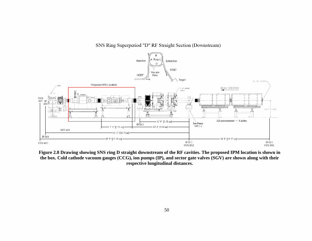
50

Figure 2.8 Drawing showing SNS ring D straight downstream of the RF cavities. The proposed IPM location is shown in

the box. Cold cathode vacuum gauges (CCG), ion pumps (IP), and sector gate valves (SGV) are shown along with their

respective longitudinal distances.

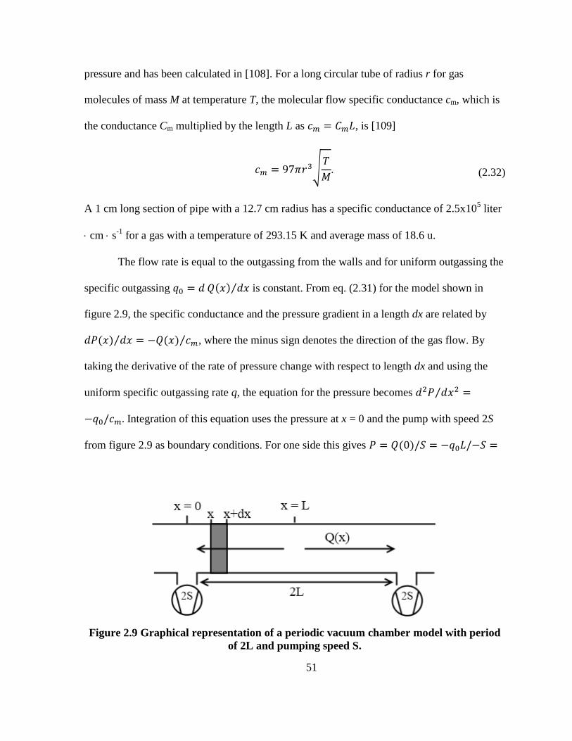
51

pressure and has been calculated in [108]. For a long circular tube of radius r for gas

molecules of mass M at temperature T, the molecular flow specific conductance cm, which is

the conductance Cm multiplied by the length L as , is [109]

√

(2.32)

A 1 cm long section of pipe with a 12.7 cm radius has a specific conductance of 2.5x105 liter

cm s-1

for a gas with a temperature of 293.15 K and average mass of 18.6 u.

The flow rate is equal to the outgassing from the walls and for uniform outgassing the

specific outgassing ⁄ is constant. From eq. (2.31) for the model shown in

figure 2.9, the specific conductance and the pressure gradient in a length dx are related by

⁄ ⁄ , where the minus sign denotes the direction of the gas flow. By

taking the derivative of the rate of pressure change with respect to length dx and using the

uniform specific outgassing rate q, the equation for the pressure becomes ⁄

Integration of this equation uses the pressure at x = 0 and the pump with speed 2S

from figure 2.9 as boundary conditions. For one side this gives

Figure 2.9 Graphical representation of a periodic vacuum chamber model with period

of 2L and pumping speed S.

52

and, due to symmetry, the flow at the middle of the tube is Q(L) = 0. The pressure at a

position x from the pump is [110]

The result is a parabolic pressure profile between the pumps. The matter is complicated by

the presence of the beam.

Ion-Induced Desorption

A uniform cylindrical beam of length L and charge eN where e is the elementary charge and

N is the number of accumulated particles, has a potential inside the beam radius a of

[

(

)] (2.34)

where b is the vacuum chamber radius. Ions created by a fully accumulated beam of 1.5x1014

particles will accelerate through potentials from ~ 5 kV to ~15 kV depending on location

[111]. Energetic residual gas ions can desorb gas from the pipe walls. The molecular

desorption yield η, defined as the number of molecules desorbed per incident ion, is a

function of the incident particle energy as well as the surface and surface condition. SNS

vacuum chambers are unbaked due to the risk of leaking by large aperture flanges caused by

the relative thermal motion induced by in-situ baking [112]. As such, the unbaked ion

desorption yield for stainless steel ranges from ~5 to ~10 for incident particle energies above

a few keV [113].

The ionization cross section, derived using the Bethe theory [114], [115], is given by

(

) (2.33)

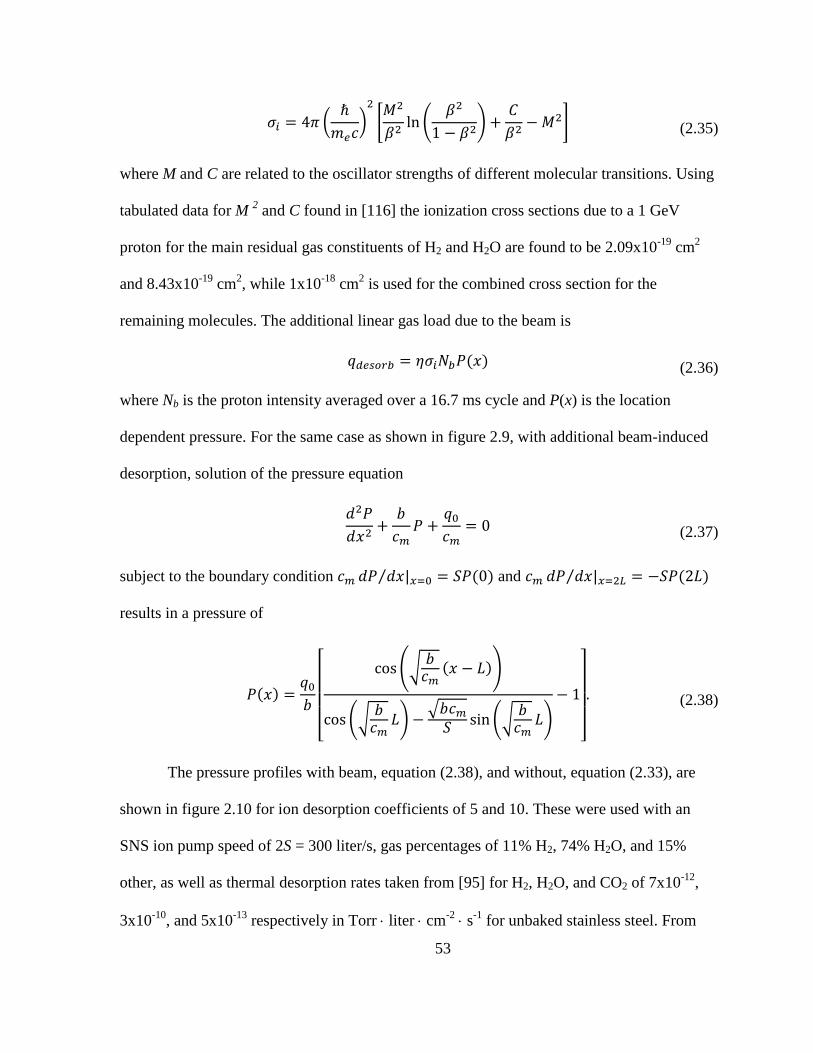
53

(

)

[

(

)

] (2.35)

where M and C are related to the oscillator strengths of different molecular transitions. Using

tabulated data for M 2 and C found in [116] the ionization cross sections due to a 1 GeV

proton for the main residual gas constituents of H2 and H2O are found to be 2.09x10-19

cm2

and 8.43x10-19

cm2, while 1x10

-18 cm

2 is used for the combined cross section for the

remaining molecules. The additional linear gas load due to the beam is

(2.36)

where Nb is the proton intensity averaged over a 16.7 ms cycle and P(x) is the location

dependent pressure. For the same case as shown in figure 2.9, with additional beam-induced

desorption, solution of the pressure equation

(2.37)

subject to the boundary condition | ⁄ and | ⁄

results in a pressure of

[ (√

)

(√

) √

(√

)

]

(2.38)

The pressure profiles with beam, equation (2.38), and without, equation (2.33), are

shown in figure 2.10 for ion desorption coefficients of 5 and 10. These were used with an

SNS ion pump speed of 2S = 300 liter/s, gas percentages of 11% H2, 74% H2O, and 15%

other, as well as thermal desorption rates taken from [95] for H2, H2O, and CO2 of 7x10-12

,

3x10-10

, and 5x10-13

respectively in Torr liter cm-2

s-1

for unbaked stainless steel. From

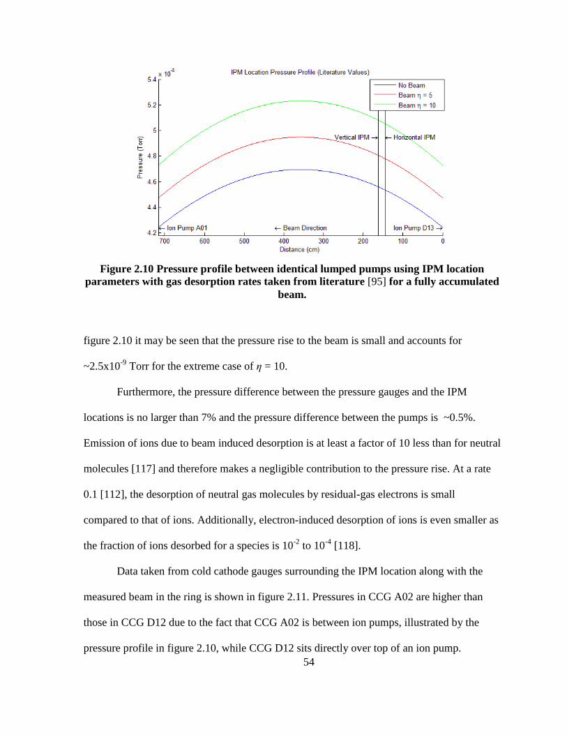
54

Figure 2.10 Pressure profile between identical lumped pumps using IPM location

parameters with gas desorption rates taken from literature [95] for a fully accumulated

beam.

figure 2.10 it may be seen that the pressure rise to the beam is small and accounts for

~2.5x10-9

Torr for the extreme case of η = 10.

Furthermore, the pressure difference between the pressure gauges and the IPM

locations is no larger than 7% and the pressure difference between the pumps is ~0.5%.

Emission of ions due to beam induced desorption is at least a factor of 10 less than for neutral

molecules [117] and therefore makes a negligible contribution to the pressure rise. At a rate

0.1 [112], the desorption of neutral gas molecules by residual-gas electrons is small

compared to that of ions. Additionally, electron-induced desorption of ions is even smaller as

the fraction of ions desorbed for a species is 10-2

to 10-4

[118].

Data taken from cold cathode gauges surrounding the IPM location along with the

measured beam in the ring is shown in figure 2.11. Pressures in CCG A02 are higher than

those in CCG D12 due to the fact that CCG A02 is between ion pumps, illustrated by the

pressure profile in figure 2.10, while CCG D12 sits directly over top of an ion pump.

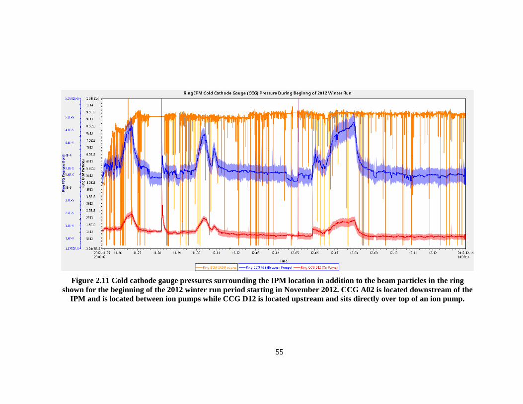
55

Figure 2.11 Cold cathode gauge pressures surrounding the IPM location in addition to the beam particles in the ring

shown for the beginning of the 2012 winter run period starting in November 2012. CCG A02 is located downstream of the

IPM and is located between ion pumps while CCG D12 is located upstream and sits directly over top of an ion pump.

56

Evidence for a beam induced pressure rise may be seen at the beginning of the run period

during initial ramping of the beam and following periods when there is no beam in the ring

for more than a few hours. After a period of approximately a day, the pressure decreases as

the beam induced gas load is removed, and an equilibrium pressure is reached.

Barring any significant loss of beam, the pressure remains relatively constant at

approximately 2x10-9

Torr in the IPM location but this value varies by about a factor of 2.

Additionally, a long term study of multiple run cycles reveals that the overall pressure may

vary by a factor of 10 depending on vacuum system maintenance. As such, it is necessary to

design the IPM vacuum chamber with ports that will allow for monitoring the residual gas

pressure and with a port for a residual gas analyzer. A pressure of 2x10-9

Torr corresponds to

a residual gas density of 6.59x107 gas molecules cm

-3 at 20°C.

2.2.3 Ion Estimation

As an energetic proton travels around the SNS ring, it interacts with neutral gas molecules of

different species, ionizing a fraction of residual gas. The ionization products will have a

certain probability to create secondary ionization products from the residual gas.

Furthermore, ions accelerated by the beam toward the beam pipe wall desorb additional gas

molecules, thus increasing the gas pressure. With the analysis performed in the previous

sections, it is now possible to estimate the amount of ionized gas that is available for

collection.

At normal atmospheric pressure, energetic incident particles passing through a gas

produce primary electrons which then can produce further ionization products. However, at

the UHV pressures used in the IPM, the electron scattering mean free path is very long

compared to the chamber dimensions. The scattering cross sections for ~keV electrons on

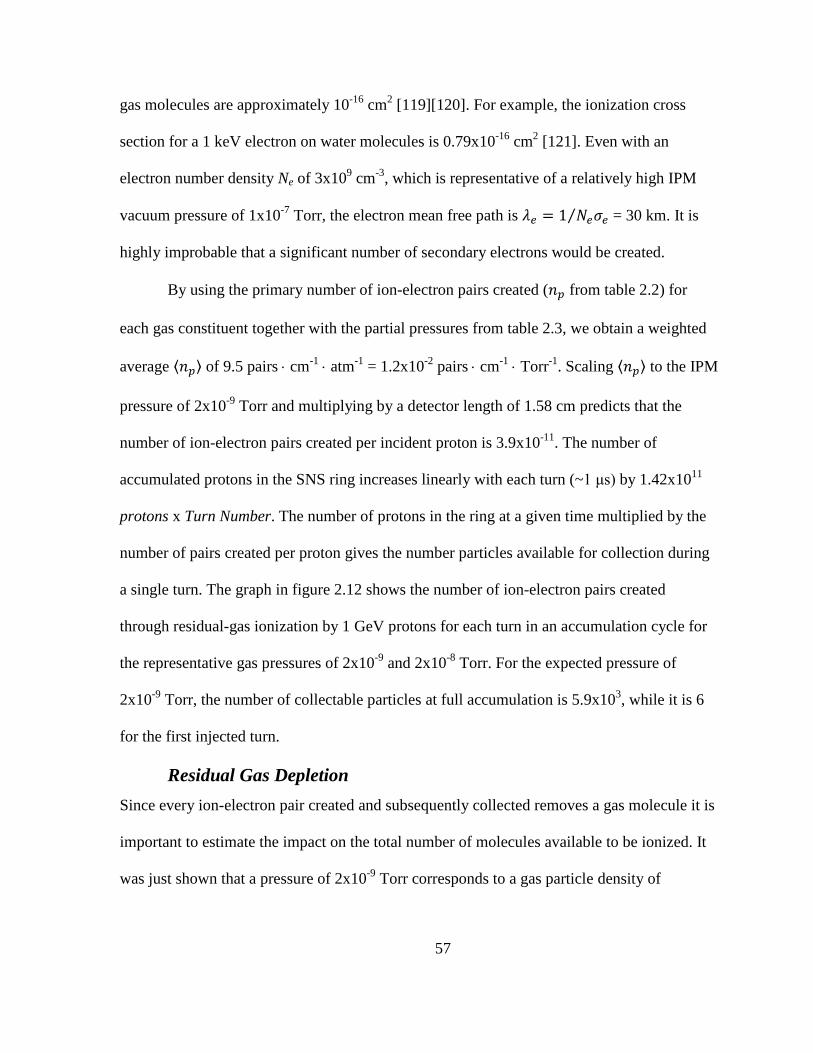
57

gas molecules are approximately 10-16

cm2 [119][120]. For example, the ionization cross

section for a 1 keV electron on water molecules is 0.79x10-16

cm2 [121]. Even with an

electron number density Ne of 3x109 cm

-3, which is representative of a relatively high IPM

vacuum pressure of 1x10-7

Torr, the electron mean free path is ⁄ = 30 km. It is

highly improbable that a significant number of secondary electrons would be created.

By using the primary number of ion-electron pairs created ( from table 2.2) for

each gas constituent together with the partial pressures from table 2.3, we obtain a weighted

average ⟨ ⟩ of 9.5 pairs cm-1

atm-1

= 1.2x10-2

pairs cm-1

Torr-1

. Scaling ⟨ ⟩ to the IPM

pressure of 2x10-9

Torr and multiplying by a detector length of 1.58 cm predicts that the

number of ion-electron pairs created per incident proton is 3.9x10-11

. The number of

accumulated protons in the SNS ring increases linearly with each turn (~1 μs) by 1.42x1011

protons x Turn Number. The number of protons in the ring at a given time multiplied by the

number of pairs created per proton gives the number particles available for collection during

a single turn. The graph in figure 2.12 shows the number of ion-electron pairs created

through residual-gas ionization by 1 GeV protons for each turn in an accumulation cycle for

the representative gas pressures of 2x10-9

and 2x10-8

Torr. For the expected pressure of

2x10-9

Torr, the number of collectable particles at full accumulation is 5.9x103, while it is 6

for the first injected turn.

Residual Gas Depletion

Since every ion-electron pair created and subsequently collected removes a gas molecule it is

important to estimate the impact on the total number of molecules available to be ionized. It

was just shown that a pressure of 2x10-9

Torr corresponds to a gas particle density of

58

Figure 2.12 Graph of the total number ion-electron pairs created at the IPM location as

a function of the number of protons present in each turn for 8 scale and 9 scale

pressures.

6.59x107 cm

-3. The detectable volume within the IPM is approximately 800 cm

3 resulting in

~5x1010

gas molecules capable of producing measurable particles. Based on the previous

assumption that the vacuum remains unchanged during an accumulation period, the number

of gas molecules is assumed to remain static during an injection cycle. The total number of

protons passing through the IPM during accumulation is

∑

(2.39)

where is the final proton number and Turns is the number of mini-pulses.

From the number of primary ion-electron pairs created, the total number of gas

molecules removed from the detectable volume is where is the number

of primary pairs created per proton in the detector region. The total number of pairs for

= 1.5x1014

protons and Turns = 1060 is 6.3x106 pairs. Only 0.013% of the original gas is

ionized in one accumulation. Therefore, the depletion of the residual gas by ionization and

59

removal of ions and electrons is expected to be negligible.

2.2.4 Electron Estimation

The estimation of electrons is similar to that of ions but with a few additional considerations.

It has been well established that an energetic proton will interact with neutral gas molecules

in such a way to remove the least bound valence electrons. Ionization products consist of one

ion and one electron. The probability of double ionization leading to two electrons per

incident proton and possible dissociation of molecules is significantly less than that of single

ionization, and can therefore be considered a negligible contribution. For example, the ratio

of double ionization to single ionization cross sections for energetic protons on H2 as

measured by experimental methods in [122] is on the order of 10-4

and the ratio for H2O

found in [123] is 10-2

. While double ionization may not be an important factor in the electron

signal there are additional electron production mechanisms that warrant analysis.

Electron Cloud

Electrons present in the ring arise from a few different sources. Beam-induced ionization

produces the same number of electrons as ions and these electrons are useful for measuring

beam profiles because their distribution is a function of the beam density. Other sources of

electrons provide no information useful for profile generation and their presence is a source

of profile signal contamination. Aside from ionization, one of the largest contributions of

electrons relevant to the IPM is electron cloud generation by beam-induced multipacting

[124].

The phenomenon of the electron cloud, briefly discussed in section 2.2.2, is shown

graphically in figure 2.13. Electrons present before the arrival of the proton beam, whether

they were created through residual gas ionization or due to protons striking the vacuum

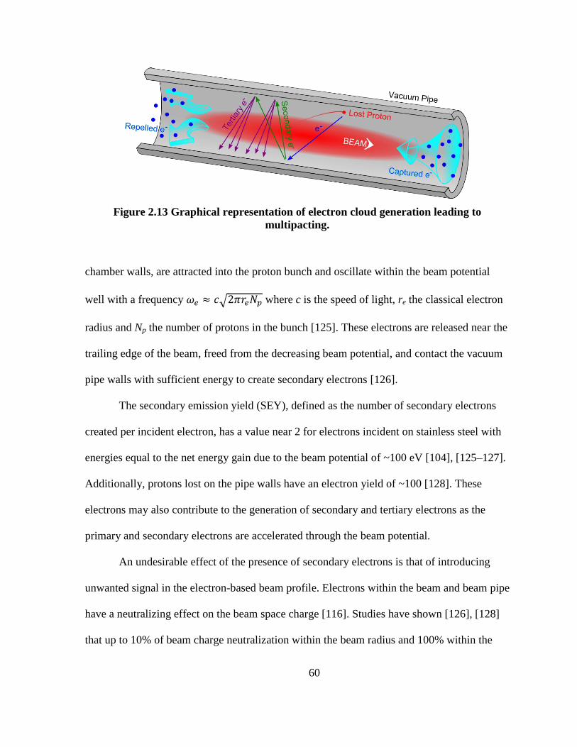
60

Figure 2.13 Graphical representation of electron cloud generation leading to

multipacting.

chamber walls, are attracted into the proton bunch and oscillate within the beam potential

well with a frequency √ where c is the speed of light, re the classical electron

radius and Np the number of protons in the bunch [125]. These electrons are released near the

trailing edge of the beam, freed from the decreasing beam potential, and contact the vacuum

pipe walls with sufficient energy to create secondary electrons [126].

The secondary emission yield (SEY), defined as the number of secondary electrons

created per incident electron, has a value near 2 for electrons incident on stainless steel with

energies equal to the net energy gain due to the beam potential of ~100 eV [104], [125–127].

Additionally, protons lost on the pipe walls have an electron yield of ~100 [128]. These

electrons may also contribute to the generation of secondary and tertiary electrons as the

primary and secondary electrons are accelerated through the beam potential.

An undesirable effect of the presence of secondary electrons is that of introducing

unwanted signal in the electron-based beam profile. Electrons within the beam and beam pipe

have a neutralizing effect on the beam space charge [116]. Studies have shown [126], [128]

that up to 10% of beam charge neutralization within the beam radius and 100% within the

61

beam pipe could be expected.

Electron Cloud Mitigation: TiN Coating

Experience with electron cloud related instabilities in the Proton Storage Ring (PSR) at Los

Alamos [129] led to an electron cloud mitigation measure that was also designed into the

SNS ring. It was found [112], [130], [131] that a ~100 μm coating of titanium nitride (TiN)

lowers the peak SEY of stainless steel from 2.5 to ~1.5. It is therefore standard practice to

coat all inner vacuum chamber surfaces in the SNS ring with TiN. As such, the IPM vacuum

chamber will be coated using a magnetron DC sputtering method described in [112].

Electron Cloud Mitigation: Clearing Electrode

The IPM uses electrodes transverse to the beam direction to separate and accelerate the ions

and electrons produced during residual gas ionization toward a detector. The electric

potential produced by the electrode has the benefit of acting as a clearing field in reference to

the electron cloud. Simulations, presented in figure 2.14, show the electron cloud build up

due to trailing-edge multipacting during the first turn of an SNS accumulation cycle. Also

shown in figure 2.14 are the electron cloud line densities for a region with a uniform electric

field. It can be seen that electron cloud density decreases with increasing field strength.

An electric field of 2 kV/m lowers the peak electron cloud density by over three

orders of magnitude. The actual field strength used in the IPM will be on the order of 102

kV/m. Once the IPM bias field is larger than a few kilovolts, the electrode potential is larger

than the beam potential and therefore prevents the generation of secondary electrons.

Furthermore, within the IPM chamber, any neutralization effects of the electron cloud will

also be insignificant. Electron noise from the electron cloud may be considered negligible in

relation to the IPM measured beam profile.

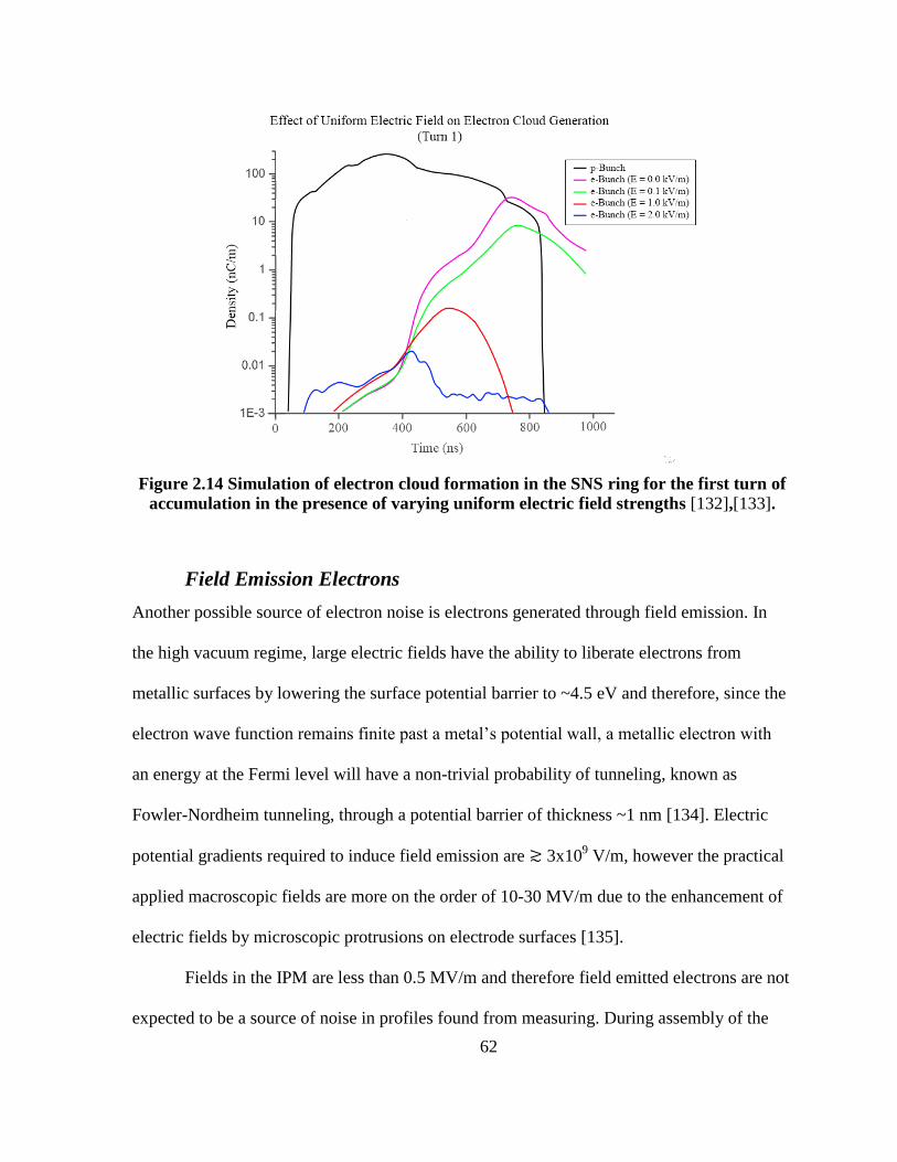
62

Figure 2.14 Simulation of electron cloud formation in the SNS ring for the first turn of

accumulation in the presence of varying uniform electric field strengths [132],[133].

Field Emission Electrons

Another possible source of electron noise is electrons generated through field emission. In

the high vacuum regime, large electric fields have the ability to liberate electrons from

metallic surfaces by lowering the surface potential barrier to ~4.5 eV and therefore, since the

electron wave function remains finite past a metal’s potential wall, a metallic electron with

an energy at the Fermi level will have a non-trivial probability of tunneling, known as

Fowler-Nordheim tunneling, through a potential barrier of thickness ~1 nm [134]. Electric

potential gradients required to induce field emission are 3x109 V/m, however the practical

applied macroscopic fields are more on the order of 10-30 MV/m due to the enhancement of

electric fields by microscopic protrusions on electrode surfaces [135].

Fields in the IPM are less than 0.5 MV/m and therefore field emitted electrons are not

expected to be a source of noise in profiles found from measuring. During assembly of the

63

final system a precautionary technique of hand polishing the electrode with a diamond paste

should be used in order to reduce microscopic protuberances [136]. This is important not

only for the consideration of field emission electrons, but for reduction of possible arcing

sites at higher field regions of the electrode. Furthermore, it would be informative, on

completion of the IPM chamber, to pump down to high vacuum, energize the electrode, and

measure the dark current present without the influence of the beam in order to ensure there is

not a significant source of background electron noise.

Other Loss Mechanisms

At normal atmospheric pressures, newly created ionization products would begin to diffuse

within the gas and undergo a variety of collisions that would result in signal loss.

Recombination is the process in which positive ions and electrons combine to become stable,

charge neutral, molecules. In the IPM, although ions are no longer guaranteed to have a

Maxwellian distribution of velocities, their mean free paths may be estimated as √

where is the ideal gas mean free path. Ions in UHV travel kilometers before interacting

with a particle. Electrons, due to their light mass, have collision lengths ~4 times longer than

those of ions [119]. The UHV in the IPM make recombination or any other form of post-

ionization collision leading to signal loss negligible.

Furthermore, it is well known [81], [119], [137] that ionization chambers, which are

gas filled detectors that collect the by-products of ionizing radiation through the use of

electric potentials, prevent recombination by separating the charged particles using high

electric field gradients. IPM electric fields enhance the effects of the UHV by further acting

to prevent recombination.

It may be concluded that sources of electrons that would pollute the measured profile

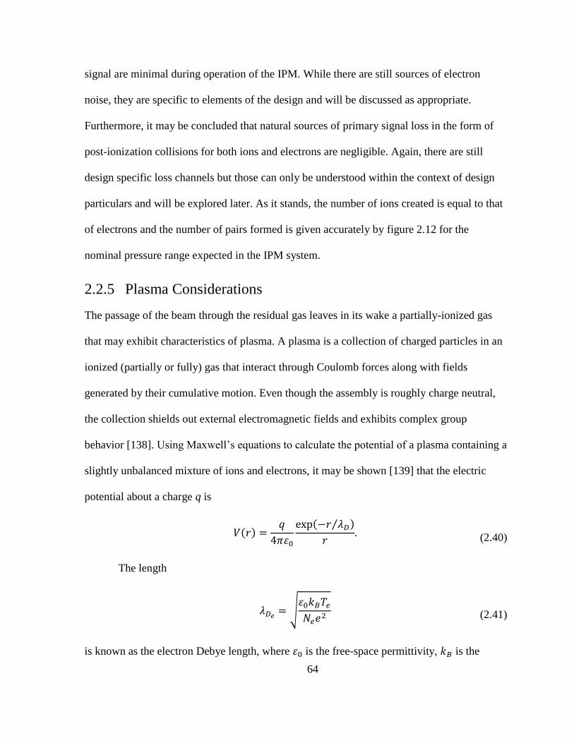
64

signal are minimal during operation of the IPM. While there are still sources of electron

noise, they are specific to elements of the design and will be discussed as appropriate.

Furthermore, it may be concluded that natural sources of primary signal loss in the form of

post-ionization collisions for both ions and electrons are negligible. Again, there are still

design specific loss channels but those can only be understood within the context of design

particulars and will be explored later. As it stands, the number of ions created is equal to that

of electrons and the number of pairs formed is given accurately by figure 2.12 for the

nominal pressure range expected in the IPM system.

2.2.5 Plasma Considerations

The passage of the beam through the residual gas leaves in its wake a partially-ionized gas

that may exhibit characteristics of plasma. A plasma is a collection of charged particles in an

ionized (partially or fully) gas that interact through Coulomb forces along with fields

generated by their cumulative motion. Even though the assembly is roughly charge neutral,

the collection shields out external electromagnetic fields and exhibits complex group

behavior [138]. Using Maxwell’s equations to calculate the potential of a plasma containing a

slightly unbalanced mixture of ions and electrons, it may be shown [139] that the electric

potential about a charge q is

⁄

(2.40)

The length

√

(2.41)

is known as the electron Debye length, where is the free-space permittivity, is the

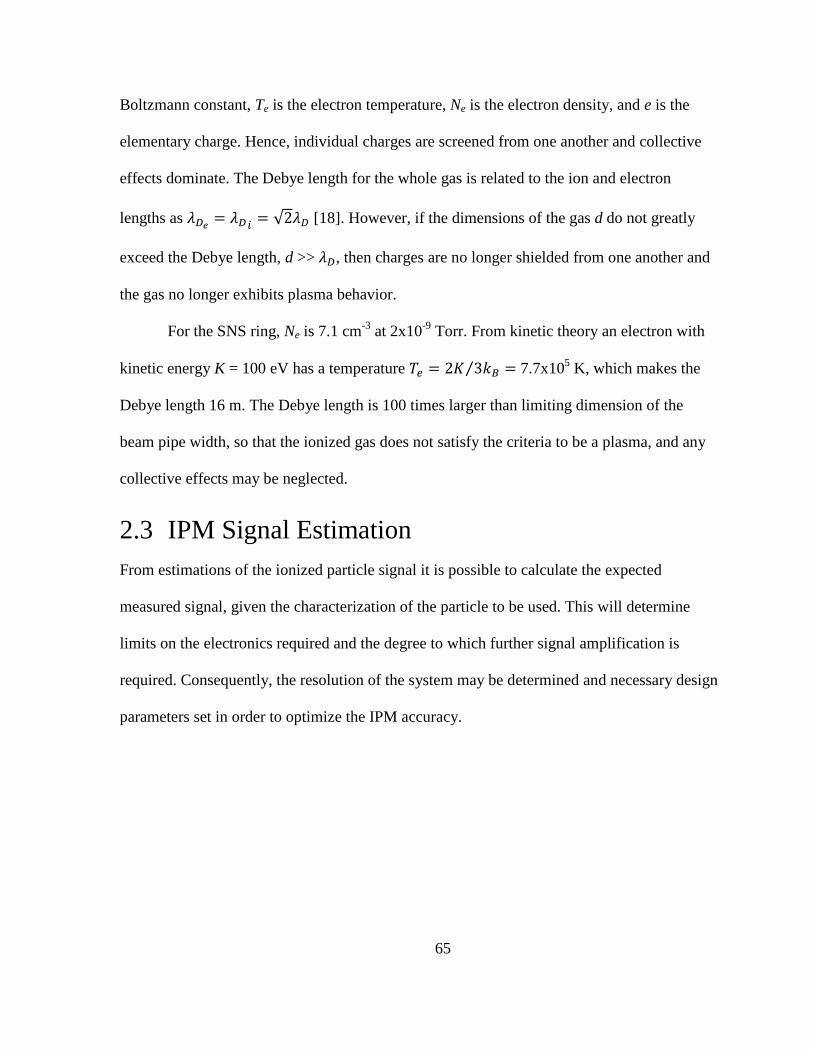
65

Boltzmann constant, Te is the electron temperature, Ne is the electron density, and e is the

elementary charge. Hence, individual charges are screened from one another and collective

effects dominate. The Debye length for the whole gas is related to the ion and electron

lengths as

√ [18]. However, if the dimensions of the gas d do not greatly

exceed the Debye length, d >> , then charges are no longer shielded from one another and

the gas no longer exhibits plasma behavior.

For the SNS ring, Ne is 7.1 cm-3

at 2x10-9

Torr. From kinetic theory an electron with

kinetic energy K = 100 eV has a temperature ⁄ 7.7x105 K, which makes the

Debye length 16 m. The Debye length is 100 times larger than limiting dimension of the

beam pipe width, so that the ionized gas does not satisfy the criteria to be a plasma, and any

collective effects may be neglected.

2.3 IPM Signal Estimation

From estimations of the ionized particle signal it is possible to calculate the expected

measured signal, given the characterization of the particle to be used. This will determine

limits on the electronics required and the degree to which further signal amplification is

required. Consequently, the resolution of the system may be determined and necessary design

parameters set in order to optimize the IPM accuracy.

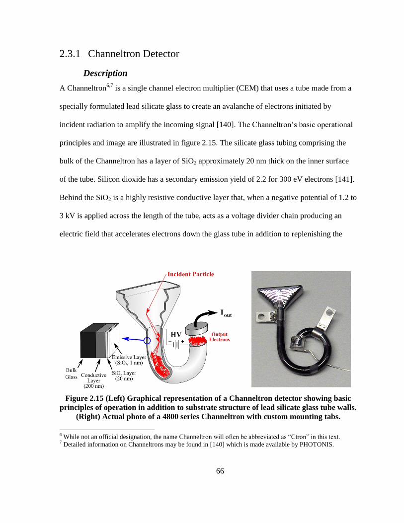
66

2.3.1 Channeltron Detector

Description

A Channeltron6,7

is a single channel electron multiplier (CEM) that uses a tube made from a

specially formulated lead silicate glass to create an avalanche of electrons initiated by

incident radiation to amplify the incoming signal [140]. The Channeltron’s basic operational

principles and image are illustrated in figure 2.15. The silicate glass tubing comprising the

bulk of the Channeltron has a layer of SiO2 approximately 20 nm thick on the inner surface

of the tube. Silicon dioxide has a secondary emission yield of 2.2 for 300 eV electrons [141].

Behind the SiO2 is a highly resistive conductive layer that, when a negative potential of 1.2 to

3 kV is applied across the length of the tube, acts as a voltage divider chain producing an

electric field that accelerates electrons down the glass tube in addition to replenishing the

Figure 2.15 (Left) Graphical representation of a Channeltron detector showing basic

principles of operation in addition to substrate structure of lead silicate glass tube walls.

(Right) Actual photo of a 4800 series Channeltron with custom mounting tabs.

6 While not an official designation, the name Channeltron will often be abbreviated as “Ctron” in this text.

7 Detailed information on Channeltrons may be found in [140] which is made available by PHOTONIS.

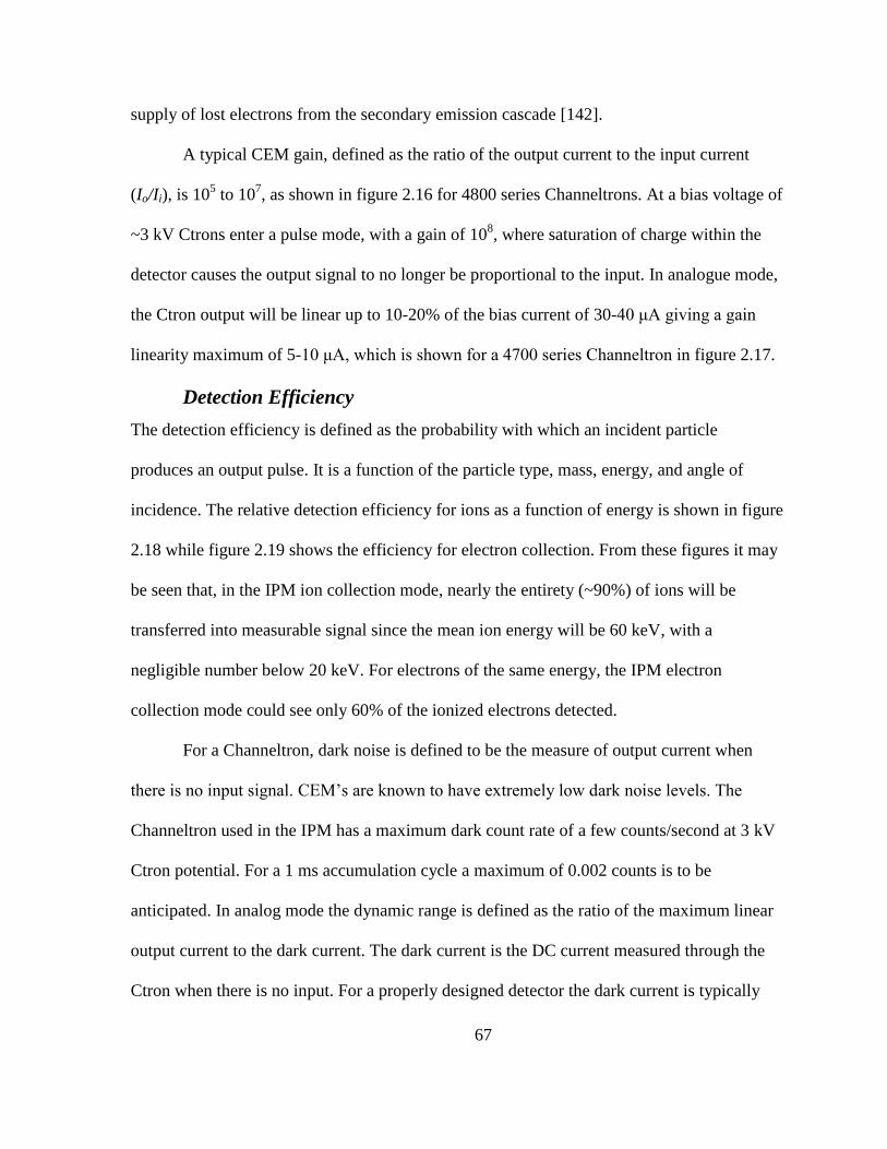
67

supply of lost electrons from the secondary emission cascade [142].

A typical CEM gain, defined as the ratio of the output current to the input current

(Io/Ii), is 105 to 10

7, as shown in figure 2.16 for 4800 series Channeltrons. At a bias voltage of

~3 kV Ctrons enter a pulse mode, with a gain of 108, where saturation of charge within the

detector causes the output signal to no longer be proportional to the input. In analogue mode,

the Ctron output will be linear up to 10-20% of the bias current of 30-40 μA giving a gain

linearity maximum of 5-10 μA, which is shown for a 4700 series Channeltron in figure 2.17.

Detection Efficiency

The detection efficiency is defined as the probability with which an incident particle

produces an output pulse. It is a function of the particle type, mass, energy, and angle of

incidence. The relative detection efficiency for ions as a function of energy is shown in figure

2.18 while figure 2.19 shows the efficiency for electron collection. From these figures it may

be seen that, in the IPM ion collection mode, nearly the entirety (~90%) of ions will be

transferred into measurable signal since the mean ion energy will be 60 keV, with a

negligible number below 20 keV. For electrons of the same energy, the IPM electron

collection mode could see only 60% of the ionized electrons detected.

For a Channeltron, dark noise is defined to be the measure of output current when

there is no input signal. CEM’s are known to have extremely low dark noise levels. The

Channeltron used in the IPM has a maximum dark count rate of a few counts/second at 3 kV

Ctron potential. For a 1 ms accumulation cycle a maximum of 0.002 counts is to be

anticipated. In analog mode the dynamic range is defined as the ratio of the maximum linear

output current to the dark current. The dark current is the DC current measured through the

Ctron when there is no input. For a properly designed detector the dark current is typically

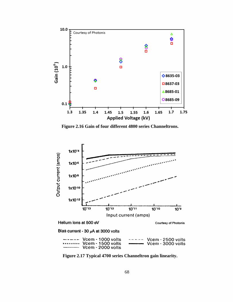
68

Figure 2.16 Gain of four different 4800 series Channeltrons.

Figure 2.17 Typical 4700 series Channeltron gain linearity.

69

Figure 2.18 Channeltron relative ion detection efficiency. [140]

Figure 2.19 Channeltron electron detection efficiency. [140]

70

1 pA at a gain of 106. Noise generated from the detector is not expected to be a problem.

While Channeltron gain is a function of incident particle mass, there is little deviation in

response characteristics for the range of masses measured in the IPM.

There is experimental evidence [143],[144] that CEMs in magnetic fields have a

decreased efficiency when the magnetic field strength increases to a magnitude that the

cyclotron radius of the electrons inside the CEM tube becomes comparable to the radius of

the tube. The electrons are curved into the opposing wall before gaining sufficient energy to

generate a cascade. Upon completion of the system and before installation, it will be

necessary to characterize the Ctron efficiency as a function of magnetic field strength.

Operational Considerations

It will be necessary to operate the Channeltron in the analog mode in order to distinguish

between measured current amplitudes of each accumulated pulse. Consequently, prior to

installation, it will be necessary to characterize each installed Ctron with a calibrated source

such as an electron gun to determine the optimum operating potential which is proportional

to its gain. The 4800 series Channeltron has a maximum operating pressure of 5x10-6

Torr.

An operational protection limit will be included in the system electronics to turn off the

detector in the event the pressure rises to 10-6

Torr.

Individual Channeltron gains can vary greatly. The final IPM system will have a pair

of Channeltrons installed. It will be necessary to specify to the manufacturer that a set of two

detectors have matching gains. The rise time is defined as the time it takes the output pulse to

go from 10% to 90% of its final amplitude. This is approximately 3-5 ns for Ctrons, which is

sufficiently fast to resolve the 20 ns rise time of the beam pulse, as will be shown in a later

section. The Channeltron opening is 4 mm wide by 15.8 mm long as shown in the

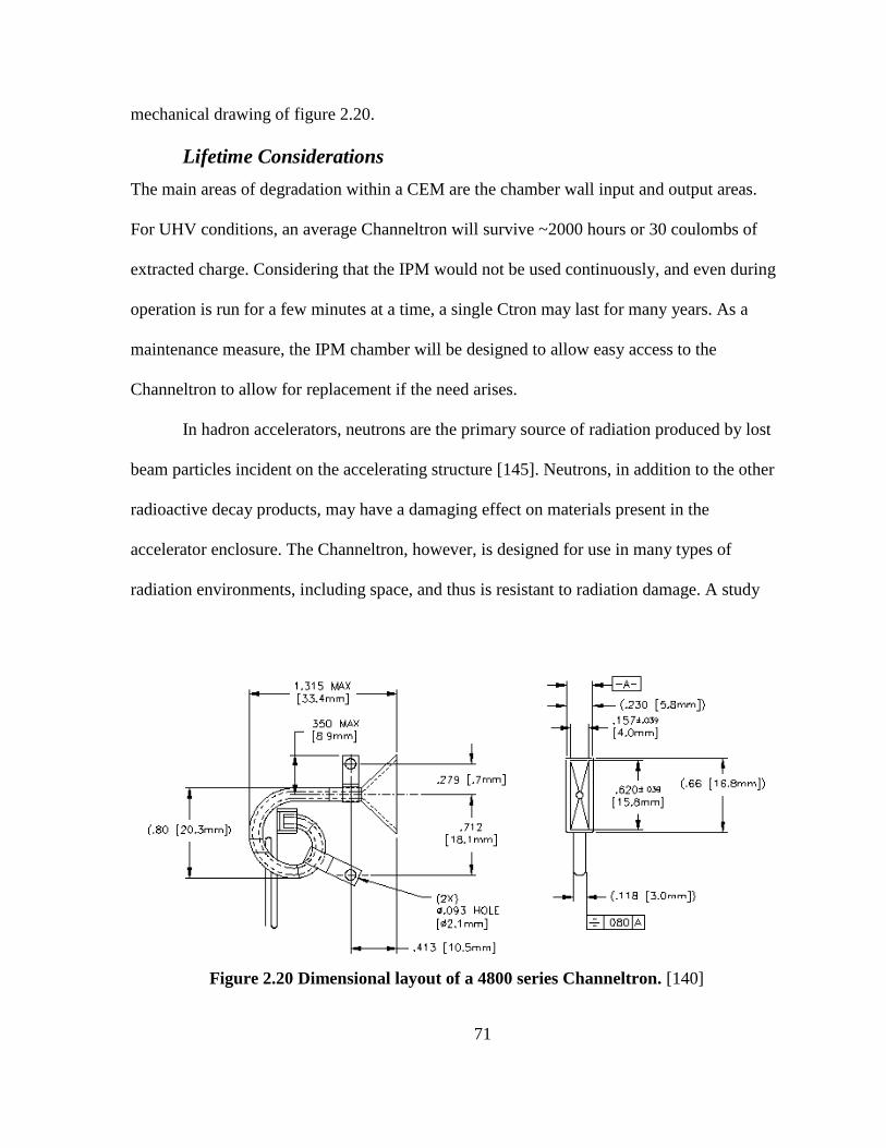
71

mechanical drawing of figure 2.20.

Lifetime Considerations

The main areas of degradation within a CEM are the chamber wall input and output areas.

For UHV conditions, an average Channeltron will survive ~2000 hours or 30 coulombs of

extracted charge. Considering that the IPM would not be used continuously, and even during

operation is run for a few minutes at a time, a single Ctron may last for many years. As a

maintenance measure, the IPM chamber will be designed to allow easy access to the

Channeltron to allow for replacement if the need arises.

In hadron accelerators, neutrons are the primary source of radiation produced by lost

beam particles incident on the accelerating structure [145]. Neutrons, in addition to the other

radioactive decay products, may have a damaging effect on materials present in the

accelerator enclosure. The Channeltron, however, is designed for use in many types of

radiation environments, including space, and thus is resistant to radiation damage. A study

Figure 2.20 Dimensional layout of a 4800 series Channeltron. [140]

72

[146] was done on MCPs showing that no permanent damage was done after exposure to 106

rads of radiation. Beam loss monitors around the IPM location experience a measured dose

rate of ~3 rad/hr. Assuming 5000 hours of beam time per year gives a dose of 15 krad/year.

Assuming that the MCP radiation rate applies to Channeltrons and considering that they are

constructed of the same materials, the IPM Ctron should last at least 70 years based on

radiation lifetime alone.

Channeltron vs. MCP

The Channeltron is based on the same principal as the MCP and with multiple MCPs it is

possible to produce gains similar to that of a single Ctron. As discussed in section 1.2, many

IPMs use MCPs as their method for ionized particle collection and amplification. A brief

justification is necessary for choosing the Channeltron over the MCP. It was one of the initial

goals of the project to produce the simplest IPM design possible that fulfilled the

measurement requirements.

MCP arrays, while having the ability to measure the entire beam region at once,

suffer from a loss of uniformity in gain as the MCP ages due to the beam distribution [147].

Since the entire MCP array uses the same bias voltage, it is not possible to adjust the gain for

various portions of the MCP. Furthermore, MCPs require a particle detector in the form of a

phosphor screen and camera or anode strips. Additionally, Channeltron lifetimes are about 10

times longer than those of MCPs. The Channeltron provides the simplest and most robust

form of particle detector for the SNS IPM system.

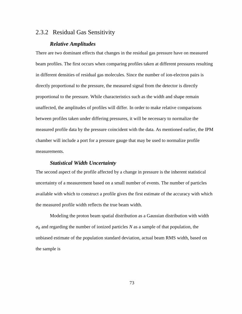
73

2.3.2 Residual Gas Sensitivity

Relative Amplitudes

There are two dominant effects that changes in the residual gas pressure have on measured

beam profiles. The first occurs when comparing profiles taken at different pressures resulting

in different densities of residual gas molecules. Since the number of ion-electron pairs is

directly proportional to the pressure, the measured signal from the detector is directly

proportional to the pressure. While characteristics such as the width and shape remain

unaffected, the amplitudes of profiles will differ. In order to make relative comparisons

between profiles taken under differing pressures, it will be necessary to normalize the

measured profile data by the pressure coincident with the data. As mentioned earlier, the IPM

chamber will include a port for a pressure gauge that may be used to normalize profile

measurements.

Statistical Width Uncertainty

The second aspect of the profile affected by a change in pressure is the inherent statistical

uncertainty of a measurement based on a small number of events. The number of particles

available with which to construct a profile gives the first estimate of the accuracy with which

the measured profile width reflects the true beam width.

Modeling the proton beam spatial distribution as a Gaussian distribution with width

and regarding the number of ionized particles N as a sample of that population, the

unbiased estimate of the population standard deviation, actual beam RMS width, based on

the sample is

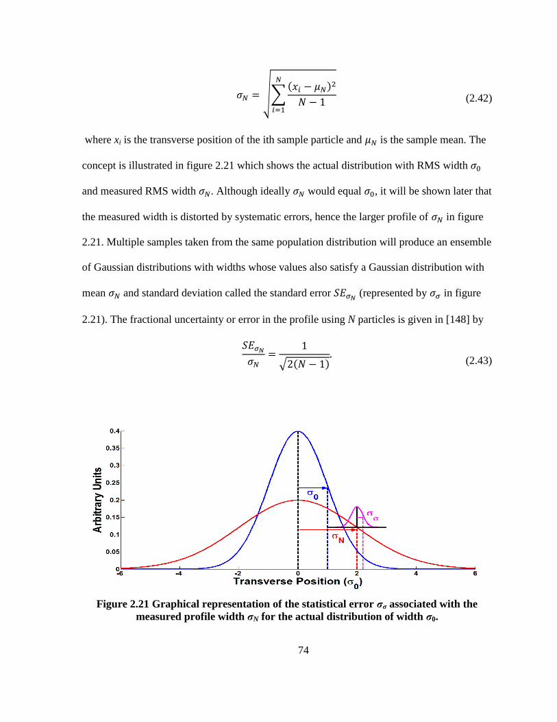
74

√∑

(2.42)

where xi is the transverse position of the ith sample particle and is the sample mean. The

concept is illustrated in figure 2.21 which shows the actual distribution with RMS width

and measured RMS width . Although ideally would equal , it will be shown later that

the measured width is distorted by systematic errors, hence the larger profile of in figure

2.21. Multiple samples taken from the same population distribution will produce an ensemble

of Gaussian distributions with widths whose values also satisfy a Gaussian distribution with

mean and standard deviation called the standard error (represented by in figure

2.21). The fractional uncertainty or error in the profile using N particles is given in [148] by

√

(2.43)

Figure 2.21 Graphical representation of the statistical error σσ associated with the

measured profile width σN for the actual distribution of width σ0.

75

Figure 2.22 shows the fractional error, given by equation (2.43), in percentages of the

measured distribution width for each turn during the accumulation for a range of residual gas

pressures. At 2x10-9

Torr, the error in the measured width decreases from 33% on the first

turn to ~1% because of an increasing number of protons and a resulting increase in

measurable ionization products. This means that on the first turn the measured width could

not be guaranteed to be more accurate than ± 0.33 at 2x10-9

Torr.

In order to reduce the statistical error, more samples are needed. Therefore, based on

the assumption that the beam during each accumulation cycle is identical under the same

operating conditions, it is possible to reduce the statistical error due to low detectable signal

by summing the contributions at the same turn for multiple cycles. The number of measured

particles scales linearly with the number of measured cycles, and the errors decrease in

inverse proportion to the square root of the number of measurements, as shown in

Figure 2.22 The percentage of the measured width the error assumes for each turn

during an accumulation cycle is shown for varying pressures or the equivalent number

of accumulation cycle repetitions.

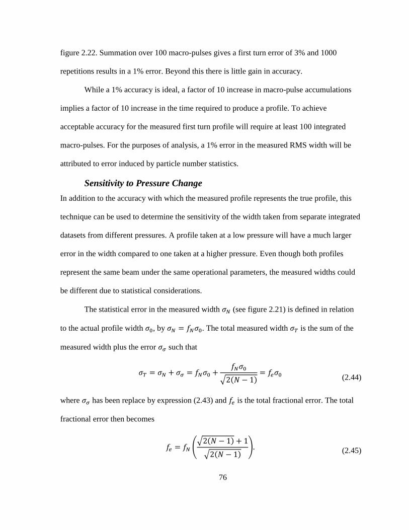
76

figure 2.22. Summation over 100 macro-pulses gives a first turn error of 3% and 1000

repetitions results in a 1% error. Beyond this there is little gain in accuracy.

While a 1% accuracy is ideal, a factor of 10 increase in macro-pulse accumulations

implies a factor of 10 increase in the time required to produce a profile. To achieve

acceptable accuracy for the measured first turn profile will require at least 100 integrated

macro-pulses. For the purposes of analysis, a 1% error in the measured RMS width will be

attributed to error induced by particle number statistics.

Sensitivity to Pressure Change

In addition to the accuracy with which the measured profile represents the true profile, this

technique can be used to determine the sensitivity of the width taken from separate integrated

datasets from different pressures. A profile taken at a low pressure will have a much larger

error in the width compared to one taken at a higher pressure. Even though both profiles

represent the same beam under the same operational parameters, the measured widths could

be different due to statistical considerations.

The statistical error in the measured width (see figure 2.21) is defined in relation

to the actual profile width , by . The total measured width is the sum of the

measured width plus the error such that

√

(2.44)

where has been replace by expression (2.43) and is the total fractional error. The total

fractional error then becomes

(√

√ ) (2.45)

77

The percent difference in the total measured profile width is

(2.46)

where the subscripts 1 and 2 denote the total widths measured at two different pressures.

Substituting equation (2.45) into (2.46) gives an expression for the change in width as a

function of change in pressure, using where is the efficiency

of the detector, is the number of macro-pulses being summed over, the number

of protons in a single mini-pulse, the number of primary ion-electron pairs created by a

single proton in the length of the detector per Torr, and P is the pressure. The expression is

√ √

√ (√ )

(2.47)

For a given detector efficiency, number of accumulations, and turn, the change in the

width may be compared to the change in pressure as shown in figure 2.23. Increases in

pressure reduce the width due to an increase in residual gas particles. The main consequence

of summing over multiple macro-pulses is to reduce the effect of a change in pressure on the

width. Furthermore, figure 2.23 shows that decreases in pressure can cause very large

increases in the width. Asymptotically, the width approaches a limit representing a situation

in which the measured pressure has been reduced to such a degree that number of measurable

particles approach one and, consequently, the width is undefined.

Figure 2.23 shows that for 10 accumulations, Nacc = 10, a 1% change in the width

occurs at an 11% decrease in the pressure at a base pressure of 1x10-9

Torr, or at 1

accumulation at a pressure of 1x10-8

Torr. The same change in the width coincides with a

change of 29% for 100 accumulations, Nacc = 100, and 61% for Nacc = 1000 all at a pressure

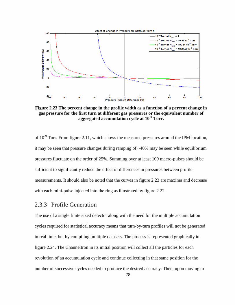
78

Figure 2.23 The percent change in the profile width as a function of a percent change in

gas pressure for the first turn at different gas pressures or the equivalent number of

aggregated accumulation cycle at 10-9

Torr.

of 10-9

Torr. From figure 2.11, which shows the measured pressures around the IPM location,

it may be seen that pressure changes during ramping of ~40% may be seen while equilibrium

pressures fluctuate on the order of 25%. Summing over at least 100 macro-pulses should be

sufficient to significantly reduce the effect of differences in pressures between profile

measurements. It should also be noted that the curves in figure 2.23 are maxima and decrease

with each mini-pulse injected into the ring as illustrated by figure 2.22.

2.3.3 Profile Generation

The use of a single finite sized detector along with the need for the multiple accumulation

cycles required for statistical accuracy means that turn-by-turn profiles will not be generated

in real time, but by compiling multiple datasets. The process is represented graphically in

figure 2.24. The Channeltron in its initial position will collect all the particles for each

revolution of an accumulation cycle and continue collecting in that same position for the

number of successive cycles needed to produce the desired accuracy. Then, upon moving to

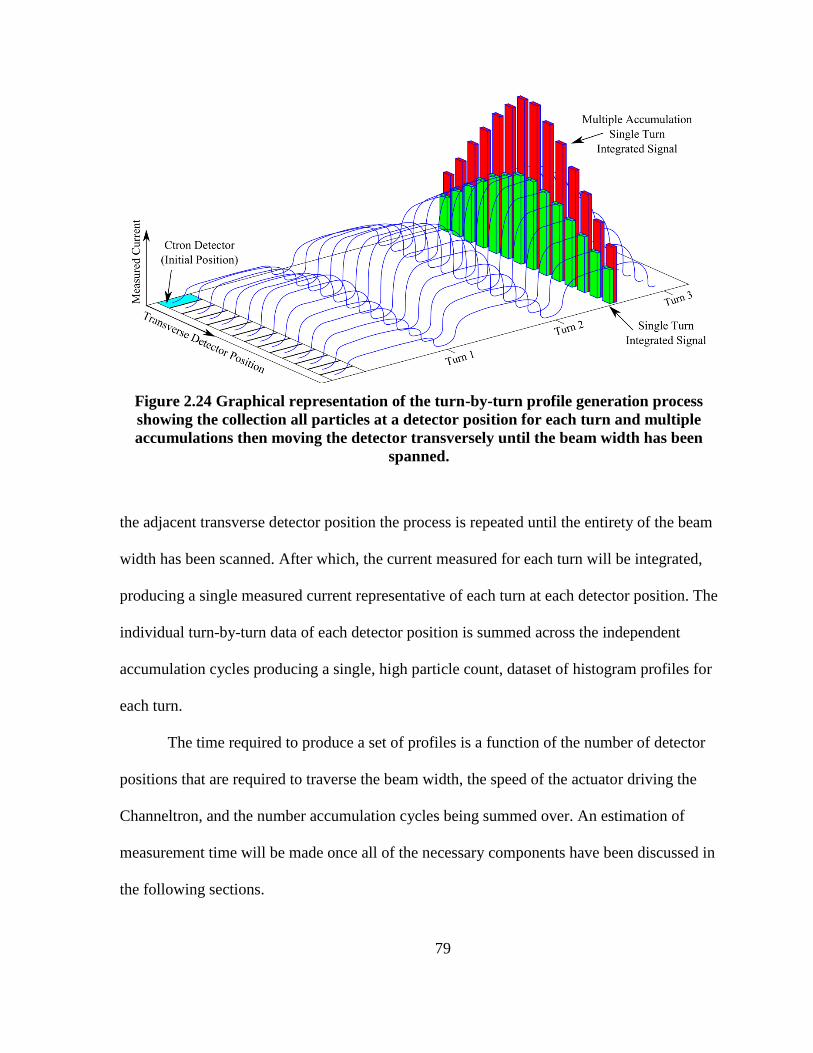
79

Figure 2.24 Graphical representation of the turn-by-turn profile generation process

showing the collection all particles at a detector position for each turn and multiple

accumulations then moving the detector transversely until the beam width has been

spanned.

the adjacent transverse detector position the process is repeated until the entirety of the beam

width has been scanned. After which, the current measured for each turn will be integrated,

producing a single measured current representative of each turn at each detector position. The

individual turn-by-turn data of each detector position is summed across the independent

accumulation cycles producing a single, high particle count, dataset of histogram profiles for

each turn.

The time required to produce a set of profiles is a function of the number of detector

positions that are required to traverse the beam width, the speed of the actuator driving the

Channeltron, and the number accumulation cycles being summed over. An estimation of

measurement time will be made once all of the necessary components have been discussed in

the following sections.

80

2.3.4 Measured Signal

Based on the estimated ionization, detector efficiency, and detector amplification it is

possible to estimate signals expected to be seen by the IPM system during an accumulation

cycle. A Gaussian beam is used to approximate the ring beam profile with an RMS width of

1.5 cm. Since all the ionized particles are to be summed together for each revolution during

the accumulation cycle, the calculated measured currents will be averages over a 1 μs ring

period.

For the first turn of an accumulation period of a nominal beam with mini-pulse

average current of 22 mA, where there are expected to be ~6 collectable particles, a single

Channeltron position is likely to measure only one ion or electron. This means that the

minimum measurable signal for a single Channeltron is 0.16 pA. The current measured from

the Channeltron with the bias voltage set to produce a 106 will result in a current of 0.16 µA

measurable from any one Channeltron in span of the first turn. Measured currents increase

linearly with the ring current, and the distribution of currents for individual Channeltrons

integrated over the final turn is shown in figure 2.25.

Represented therein are three distributions: the number of ion-electron pairs and the

associated average current over one turn, the current associated with the collected ions

adjusted for a detector efficiency of 0.9 and the measured Channeltron current with 106 gain,

and the collected and measured electron currents adjusted for a detector efficiency of 0.6, all

at a pressure of 2x10-9

Torr. Channeltron currents of 60-90 μA would be expected on the last

turn of an accumulation cycle.

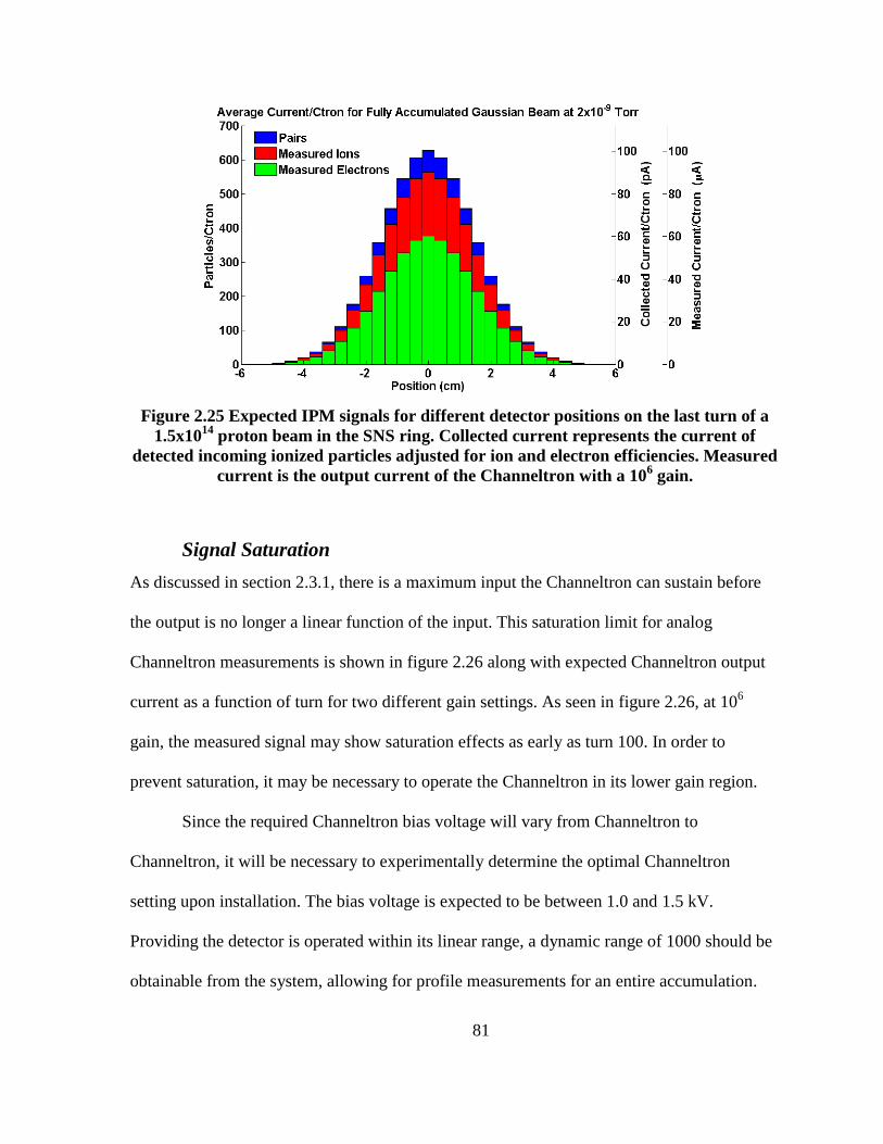
81

Figure 2.25 Expected IPM signals for different detector positions on the last turn of a

1.5x1014

proton beam in the SNS ring. Collected current represents the current of

detected incoming ionized particles adjusted for ion and electron efficiencies. Measured

current is the output current of the Channeltron with a 106 gain.

Signal Saturation

As discussed in section 2.3.1, there is a maximum input the Channeltron can sustain before

the output is no longer a linear function of the input. This saturation limit for analog

Channeltron measurements is shown in figure 2.26 along with expected Channeltron output

current as a function of turn for two different gain settings. As seen in figure 2.26, at 106

gain, the measured signal may show saturation effects as early as turn 100. In order to

prevent saturation, it may be necessary to operate the Channeltron in its lower gain region.

Since the required Channeltron bias voltage will vary from Channeltron to

Channeltron, it will be necessary to experimentally determine the optimal Channeltron

setting upon installation. The bias voltage is expected to be between 1.0 and 1.5 kV.

Providing the detector is operated within its linear range, a dynamic range of 1000 should be

obtainable from the system, allowing for profile measurements for an entire accumulation.

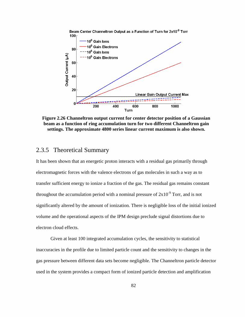
82

Figure 2.26 Channeltron output current for center detector position of a Gaussian

beam as a function of ring accumulation turn for two different Channeltron gain

settings. The approximate 4800 series linear current maximum is also shown.

2.3.5 Theoretical Summary

It has been shown that an energetic proton interacts with a residual gas primarily through

electromagnetic forces with the valence electrons of gas molecules in such a way as to

transfer sufficient energy to ionize a fraction of the gas. The residual gas remains constant

throughout the accumulation period with a nominal pressure of 2x10-9

Torr, and is not

significantly altered by the amount of ionization. There is negligible loss of the initial ionized

volume and the operational aspects of the IPM design preclude signal distortions due to

electron cloud effects.

Given at least 100 integrated accumulation cycles, the sensitivity to statistical

inaccuracies in the profile due to limited particle count and the sensitivity to changes in the

gas pressure between different data sets become negligible. The Channeltron particle detector

used in the system provides a compact form of ionized particle detection and amplification

83

with large dynamic range. While it possible for the Channeltron to go into saturation, initial

testing of the detector should prove sufficient to find the optimum detector settings.

Analysis of the fundamental theory of the IPM operational concepts has shown that it

is possible to generate and collect a sufficient number of ionized residual gas particles to

produce transverse beam profiles for each revolution during an accumulation cycle in the

SNS ring.

84

Chapter 3

Simulation Analysis

With an understanding of the fundamental principles of residual gas ionization and of the use

of the ionization products in the measurement of beam profiles with an Ionization Profile

Monitor established in chapter 2, it is now possible to analyze the details of producing

accurate profiles. The bulk of this chapter will include simulations performed to understand

the effects of a variety of system parameters.

The following chapter begins with a study of ionized particle trajectories in the IPM

system and describes the simulation program and techniques used. Particle trajectory analysis

is used to predict the necessary fields required to produce profiles that meet the design goals.

A study of the spatial accuracy is then done to analyze and estimate the possible sources of

measurement error and the system requirements needed to keep the errors within the proper

tolerances. Research on the time resolution and signal processing aspects of the design is

presented in order to guarantee the IPM’s ability to satisfy the turn-by-turn measurement

requirement. Finally, a set of design parameters is presented based on the complete analysis

to be used in developing the final system.

85

3.1 Particle Trajectory Study

The profile produced by an Ionization Profile Monitor is not a simple function of the initial

positions of the ionized gas molecules. Fields used to accelerate the ions or electrons as well

as the fields attributable to the beam itself have a significant impact on the measured profile.

In order to understand and characterize these effects and to select design parameters to

mitigate them, simulations were performed to model the trajectories of ionized particles in

the IPM environment.

3.1.1 IPM Beam Range

It is first necessary to define a physical range within which the beam is expected to reside.

The beam pipe diameter in the location of the IPM is 25.4 cm. Attempting to design a system

that uses the entire pipe width as the measurement range would result in system dimensions

that are both physically unrealistic for the ring tunnel space and prohibitively expensive.

Because the beam occupies only a small fraction of the beam pipe, an estimate of the

maximum expected beam size is more relevant for sizing the IPM.

Beam particles oscillate about an ideal trajectory dictated by the magnets in an

accelerator lattice in such a way that the transverse beam dimensions are a function of the

longitudinal position along the beam path. The beam width at a particular location is given by

√ (3.1)

Where the emittance is a constant for a given accelerating structure and the beta function

is a longitudinal position-dependent factor describing the transverse envelope of the beam

particle trajectories (see Appendix D for a complete description of the emittance and beta

function as well as a detailed explanation of the beam width).

86

The nominal unnormalized RMS emittance for the SNS ring is equal for both

transverse directions and is mm mrad and

mm mrad for the emittance encompassing 99% of the beam particles [4] (refer to

Appendix D for definitions of the 99% and RMS emittances). The beta function at the

location of the IPM as calculated from the ring lattice structure is 7 m and 9 m.

Allowing for a 20% error in the beta function as well as ±5 mm deviation in the beam

centroid, the full beam radius including errors is

√ (3.2)

A compiled list of RMS beam sizes and full beam sizes, given in table 3.1, shows that a

transverse width of 6-7 cm should be sufficient to measure the entire beam. Because the

estimated beam width is only 28% of the pipe diameter, designing the system to the realistic

beam size constitutes a significant savings in cost and size. One of the benefits of the chosen

IPM location is that the horizontal and vertical beam sizes are very similar. This means that

Table 3.1 Calculated RMS beam sizes and full beam sizes with safety margins along

with the beam pipe radius at the IPM location.

Radius Value

Beam Pipe 12.7 cm

1.3 cm

1.5 cm

2.9 cm

3.3 cm

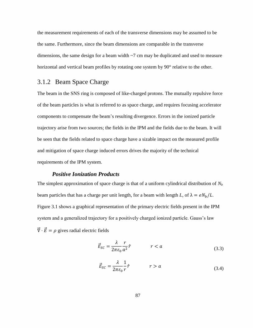
87

the measurement requirements of each of the transverse dimensions may be assumed to be

the same. Furthermore, since the beam dimensions are comparable in the transverse

dimensions, the same design for a beam width ~7 cm may be duplicated and used to measure

horizontal and vertical beam profiles by rotating one system by 90° relative to the other.

3.1.2 Beam Space Charge

The beam in the SNS ring is composed of like-charged protons. The mutually repulsive force

of the beam particles is what is referred to as space charge, and requires focusing accelerator

components to compensate the beam’s resulting divergence. Errors in the ionized particle

trajectory arise from two sources; the fields in the IPM and the fields due to the beam. It will

be seen that the fields related to space charge have a sizable impact on the measured profile

and mitigation of space charge induced errors drives the majority of the technical

requirements of the IPM system.

Positive Ionization Products

The simplest approximation of space charge is that of a uniform cylindrical distribution of Nb

beam particles that has a charge per unit length, for a beam with length L, of .

Figure 3.1 shows a graphical representation of the primary electric fields present in the IPM

system and a generalized trajectory for a positively charged ionized particle. Gauss’s law

gives radial electric fields

(3.3)

(3.4)

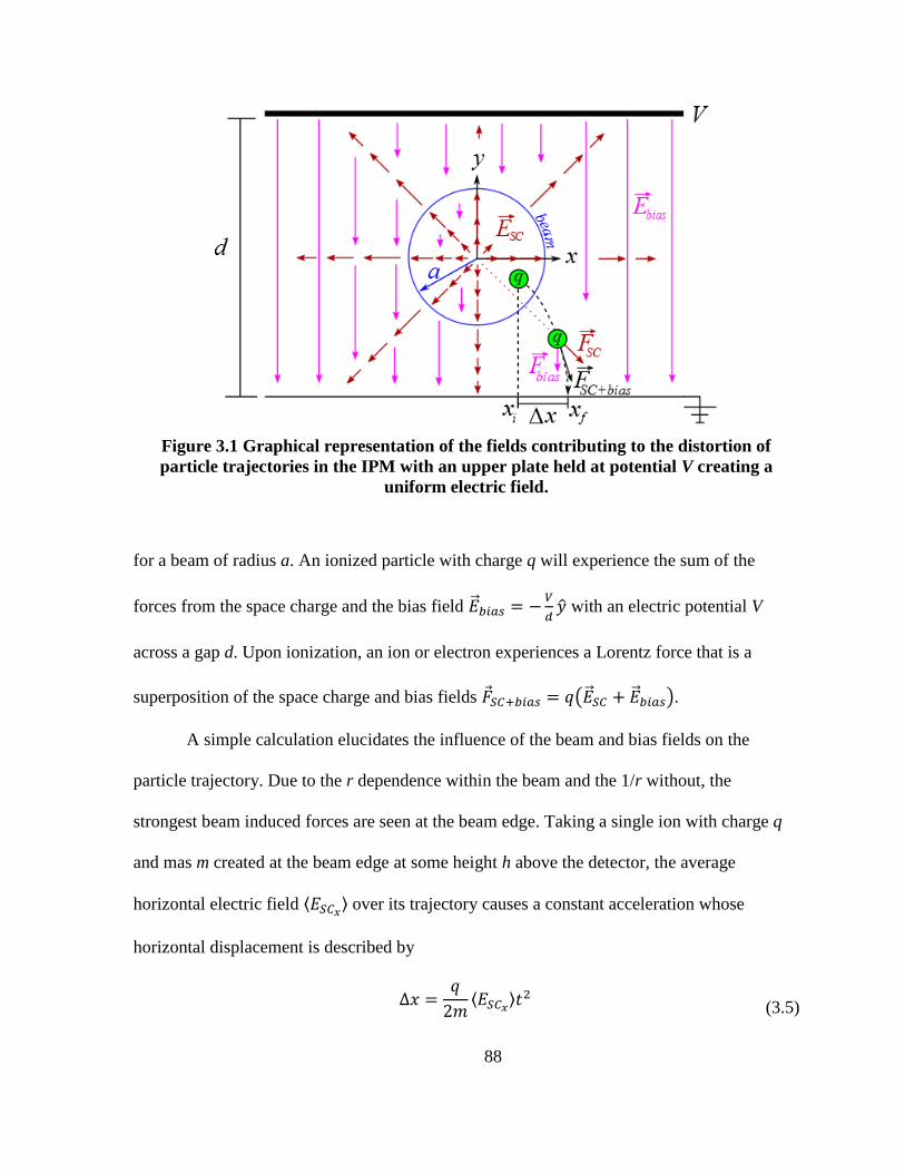
88

Figure 3.1 Graphical representation of the fields contributing to the distortion of

particle trajectories in the IPM with an upper plate held at potential V creating a

uniform electric field.

for a beam of radius a. An ionized particle with charge q will experience the sum of the

forces from the space charge and the bias field

with an electric potential V

across a gap d. Upon ionization, an ion or electron experiences a Lorentz force that is a

superposition of the space charge and bias fields ( ).

A simple calculation elucidates the influence of the beam and bias fields on the

particle trajectory. Due to the r dependence within the beam and the 1/r without, the

strongest beam induced forces are seen at the beam edge. Taking a single ion with charge q

and mas m created at the beam edge at some height h above the detector, the average

horizontal electric field ⟨ ⟩ over its trajectory causes a constant acceleration whose

horizontal displacement is described by

⟨

⟩ (3.5)

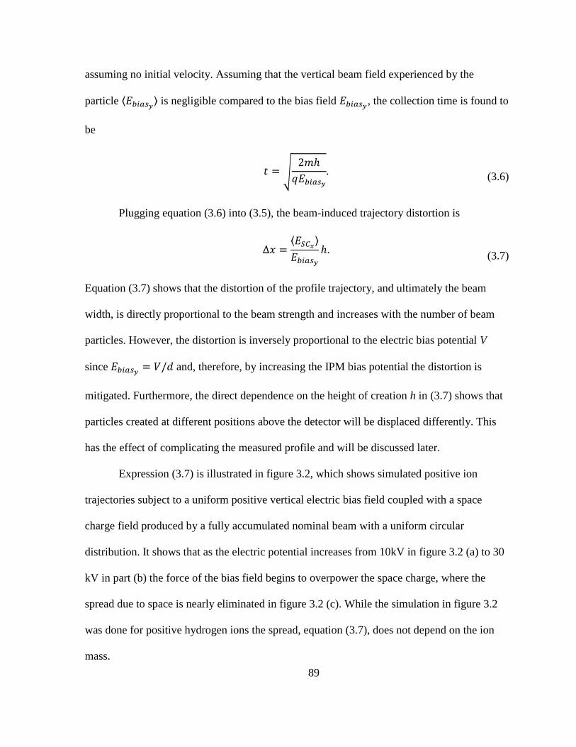
89

assuming no initial velocity. Assuming that the vertical beam field experienced by the

particle ⟨ ⟩ is negligible compared to the bias field , the collection time is found to

be

√

(3.6)

Plugging equation (3.6) into (3.5), the beam-induced trajectory distortion is

⟨

⟩

(3.7)

Equation (3.7) shows that the distortion of the profile trajectory, and ultimately the beam

width, is directly proportional to the beam strength and increases with the number of beam

particles. However, the distortion is inversely proportional to the electric bias potential V

since and, therefore, by increasing the IPM bias potential the distortion is

mitigated. Furthermore, the direct dependence on the height of creation h in (3.7) shows that

particles created at different positions above the detector will be displaced differently. This

has the effect of complicating the measured profile and will be discussed later.

Expression (3.7) is illustrated in figure 3.2, which shows simulated positive ion

trajectories subject to a uniform positive vertical electric bias field coupled with a space

charge field produced by a fully accumulated nominal beam with a uniform circular

distribution. It shows that as the electric potential increases from 10kV in figure 3.2 (a) to 30

kV in part (b) the force of the bias field begins to overpower the space charge, where the

spread due to space is nearly eliminated in figure 3.2 (c). While the simulation in figure 3.2

was done for positive hydrogen ions the spread, equation (3.7), does not depend on the ion

mass.

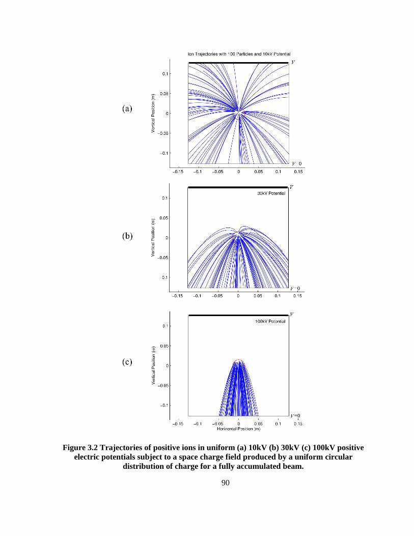
90

Figure 3.2 Trajectories of positive ions in uniform (a) 10kV (b) 30kV (c) 100kV positive

electric potentials subject to a space charge field produced by a uniform circular

distribution of charge for a fully accumulated beam.

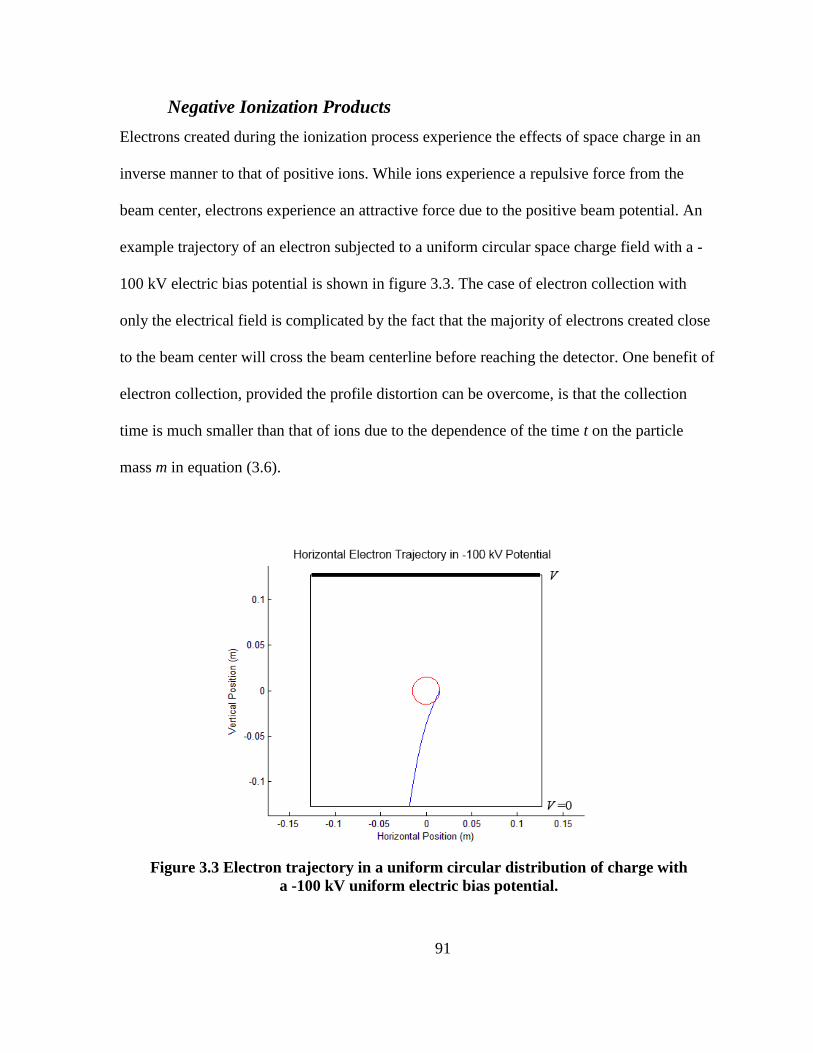
91

Negative Ionization Products

Electrons created during the ionization process experience the effects of space charge in an

inverse manner to that of positive ions. While ions experience a repulsive force from the

beam center, electrons experience an attractive force due to the positive beam potential. An

example trajectory of an electron subjected to a uniform circular space charge field with a -

100 kV electric bias potential is shown in figure 3.3. The case of electron collection with

only the electrical field is complicated by the fact that the majority of electrons created close

to the beam center will cross the beam centerline before reaching the detector. One benefit of

electron collection, provided the profile distortion can be overcome, is that the collection

time is much smaller than that of ions due to the dependence of the time t on the particle

mass m in equation (3.6).

Figure 3.3 Electron trajectory in a uniform circular distribution of charge with

a -100 kV uniform electric bias potential.

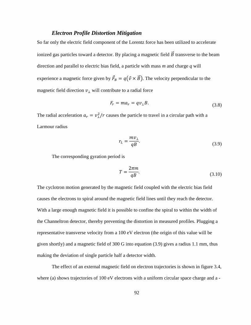
92

Electron Profile Distortion Mitigation

So far only the electric field component of the Lorentz force has been utilized to accelerate

ionized gas particles toward a detector. By placing a magnetic field transverse to the beam

direction and parallel to electric bias field, a particle with mass m and charge q will

experience a magnetic force given by ( ). The velocity perpendicular to the

magnetic field direction will contribute to a radial force

(3.8)

The radial acceleration causes the particle to travel in a circular path with a

Larmour radius

(3.9)

The corresponding gyration period is

(3.10)

The cyclotron motion generated by the magnetic field coupled with the electric bias field

causes the electrons to spiral around the magnetic field lines until they reach the detector.

With a large enough magnetic field it is possible to confine the spiral to within the width of

the Channeltron detector, thereby preventing the distortion in measured profiles. Plugging a

representative transverse velocity from a 100 eV electron (the origin of this value will be

given shortly) and a magnetic field of 300 G into equation (3.9) gives a radius 1.1 mm, thus

making the deviation of single particle half a detector width.

The effect of an external magnetic field on electron trajectories is shown in figure 3.4,

where (a) shows trajectories of 100 eV electrons with a uniform circular space charge and a -

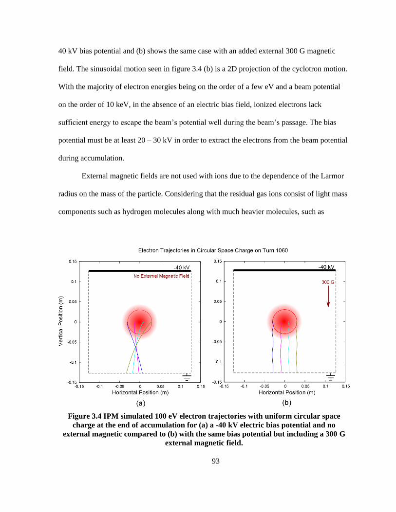
93

40 kV bias potential and (b) shows the same case with an added external 300 G magnetic

field. The sinusoidal motion seen in figure 3.4 (b) is a 2D projection of the cyclotron motion.

With the majority of electron energies being on the order of a few eV and a beam potential

on the order of 10 keV, in the absence of an electric bias field, ionized electrons lack

sufficient energy to escape the beam’s potential well during the beam’s passage. The bias

potential must be at least 20 – 30 kV in order to extract the electrons from the beam potential

during accumulation.

External magnetic fields are not used with ions due to the dependence of the Larmor

radius on the mass of the particle. Considering that the residual gas ions consist of light mass

components such as hydrogen molecules along with much heavier molecules, such as

Figure 3.4 IPM simulated 100 eV electron trajectories with uniform circular space

charge at the end of accumulation for (a) a -40 kV electric bias potential and no

external magnetic compared to (b) with the same bias potential but including a 300 G

external magnetic field.

94

water, the magnetic fields to produce the necessary cyclotron motion for the largest of ions

are unrealistically large. For example, an ionized water molecule with a thermal initial

velocity vector perpendicular to the magnetic field would require a flux density of ~600 G to

produce the same radius as that of electrons. Therefore, external magnetic fields are used in

electron collection only.

Beam Magnetic Field and Longitudinal Motion

The beam current produces a magnetic field that is capable of interacting with ionized gas

particles. Like the beam-induced electric field, the magnetic field is directly proportional to

the number of beam particles and therefore increases linearly during accumulation.

Continuing with the example of a uniform cylinder of charge, the magnetic fields are

(3.11)

(3.12)

where is the azimuthal direction and the beam velocity. The effect of magnetic field is

less than that of the beam’s electric field, as discussed in section 2.1.1 and shown in

Appendix A. A 15 kV round beam potential has a magnetic field of ~10 G, at least an order

of magnitude less than the external field required for electron collection. Due to the lack of

longitudinal beam field, the ionized particle motion is primarily in the plane perpendicular to

the beam path. There is, however, a mechanism by which charged particles in transverse

fields may gain longitudinal motion.

Since the magnetic field produces a force that is always perpendicular to the velocity,

the cyclotron motion does not change the particle’s kinetic energy. For a constant external

magnetic field , the helical velocity of a particle may be decomposed into components

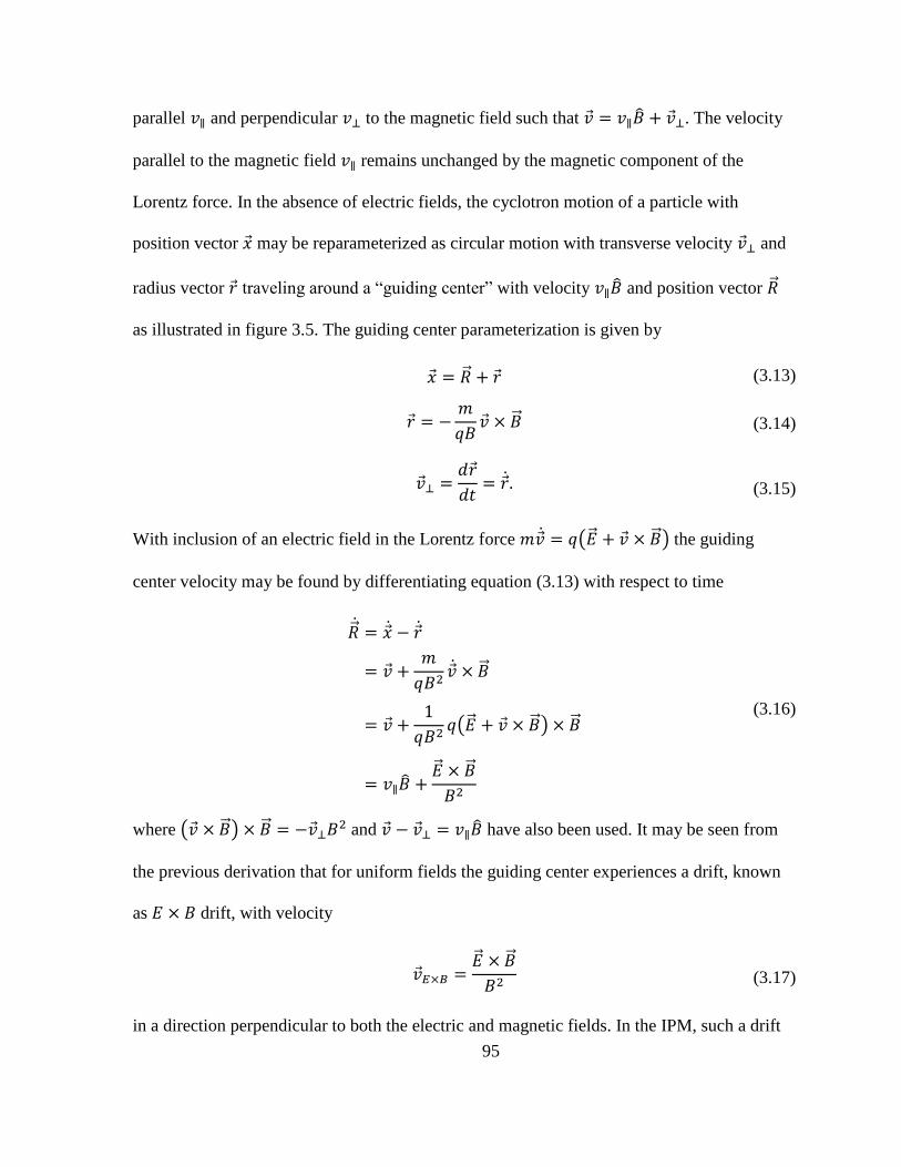
95

parallel and perpendicular to the magnetic field such that . The velocity

parallel to the magnetic field remains unchanged by the magnetic component of the

Lorentz force. In the absence of electric fields, the cyclotron motion of a particle with

position vector may be reparameterized as circular motion with transverse velocity and

radius vector traveling around a “guiding center” with velocity and position vector

as illustrated in figure 3.5. The guiding center parameterization is given by

(3.13)

(3.14)

(3.15)

With inclusion of an electric field in the Lorentz force ( ) the guiding

center velocity may be found by differentiating equation (3.13) with respect to time

( )

(3.16)

where ( ) and have also been used. It may be seen from

the previous derivation that for uniform fields the guiding center experiences a drift, known

as drift, with velocity

(3.17)

in a direction perpendicular to both the electric and magnetic fields. In the IPM, such a drift

96

Figure 3.5 Definition of Guiding Center motion for a negatively charged particle in a

uniform field.

causes motion in the longitudinal direction. For the case of drift, it has shown in [74]

that the equation (3.17) is only valid for | | | | since the reverse case causes the particle

to simply be accelerated in direction of E.

In the IPM, drift would be the result of errors in the alignment of the external

electric and magnetic fields. For example, a 300 G magnetic field with a misaligned electric

field having a 10 kV perpendicular electric component results in = 1.3x106 m/s. In

20 ns this results in a longitudinal drift of 2.6 cm. Between the permutations of the beam

field and external fields there are a number of possible longitudinal drift mechanisms.

In addition to drift there are guiding center velocities arising from various

aspects of the beam-external field coupling. The equations for different drifts will be stated

here while in-depth derivation and analysis of each may be found in [74], [149], [150] and

the references therein. A guiding center drift arising from non-uniform electric and uniform

magnetic fields, such as the beam’s electric field and external magnetic field, takes the form

(

)

(3.18)

where is Larmour radius. Additional drifts arise purely from nonuniformities in magnetic

97

field. The gradient B drift or drift is the result of the Larmour radius changing as the

particle passes between regions of varying magnetic field magnitude. This longitudinal drift

would be caused by a similar variation of the beam’s 1/r magnetic field. It is

(3.19)

A form of drift occurs when the magnetic field lines curve, as they do around the beam. The

curvature drift velocity is

(3.20)

where is a vector from the center of the magnetic curvature to the particle position.

The cumulative motion produced by the various drifts is difficult to estimate simply.

It is not necessary to find exact analytical values for the longitudinal drift as all possible

drifts are accounted for during simulation of the particle trajectories, which will be discussed

in the next section. Furthermore, it will be shown during analysis of particle trajectories that

the electron drifts are not significant except in the most extreme of external field

misalignments. While the effect of longitudinal motion would be to move individual

electrons initially created above the detector region past the detector during their time of

flight, since the entire mini-pulse is being summed over, the result of longitudinal drifts on

the distribution as a whole would be to shift a few nanoseconds worth of pulse data at the

beginning and end of a pulse.

3.1.3 Trajectory Simulation

Even the simple case of a uniform bias field coupled with a uniform circular beam

distribution with fields given by equations (3.3) and (3.4) results in equations of motion

98

√

(3.21)

√

(3.22)

outside of the beam radius a. The second-order coupled differential equations are best solved

with numerical methods. For complex space charge fields, simulations are the only method

for tracking charged particles in IPM fields such as those in figure 3.2 and figure 3.3.

Profile Benchmarking Method

A robust particle tracking program can accommodate any configuration of beam particle

distribution as well as external electric and magnetic fields. Furthermore, it is desirable to be

able to track ionized particles in fields produced by specific SNS ring beam configurations.

Due to the lack of profile diagnostics in the ring, experimental verification of the measured

IPM beam profiles will be done in the manner that ring profiles are currently measured.

Wirescanners located in the RTBT measure beam profiles. These profiles are used to

calculate the expected profile at different locations in the ring based on the beam optics.

Upon installation, the IPM profiles will be compared to calculated beam-based profiles for

benchmarking the accuracy of the system. Upon successful measurement of profiles, the IPM

will provide a useful benchmark tool the SNS ring beam transport simulation code ORBIT.

ORBIT

Part of the goal of this project was to write a module for the ORBIT simulation code. ORBIT

(Objective Ring Beam Injection and Tracking) is a particle tracking code developed at SNS

for beam dynamics studies in the ring [151],[152]. It uses a particle-in-cell method that

groups sections of beam into “macro-particles” and calculates the space charge from each

macro-particle. This, together with other collective and external forces, is then used to

99

propagate a “herd” of macro-particles through the accelerating structure [153]. Originally

written in C++, ORBIT utilizes the object-oriented language to track herds of macro-particles

through nodes which describe the actions experienced by beam particles traversing different

ring components. The ORBIT code is now migrating to the Python scripting language by

building Python interpreters around the existing ORBIT code. During the IPM project, only

portions of ORBIT have been functional in the Python version. In anticipation of the

completion of PyORBIT (Python ORBIT), it was decided to do any IPM ORBIT

programming in Python.

IPM Module

PyORBIT includes an electron cloud module that contains all the necessary tools to simulate

the effect of the electron cloud in the ring. Included in the electron cloud module is a particle

tracking class that contains methods for tracking charged particles in electric and magnetic

fields, including the effects of the beam space charge. The IPM module is based on the

electron cloud particle tracking module. The simulation process goes as follows:

1) Basic beam parameters such as number of beam particles and size of the beam

are chosen in order to determine the space charge.

2) Electric and magnetic external bias field strengths are specified. Field

distribution may also be chosen in order to study the effect of field errors on

particle trajectories.

3) The beam space charge distribution is chosen.

4) Ionized particle initial conditions are set including: type of particle, random or

specified initial positions, and type of initial velocities.

5) Particles are tracked subject to the Lorentz force in the prescribed fields until

100

each particle has contacted the IPM chamber boundary.

6) Trajectory and simulation data is collected and dumped in a series of output

files.

Tracking in the IPM module is done by using a 4th

Order Runge-Kutta method which

is an iterative approximation for first order differential equations of the form

with initial value and ⁄ . For a step size h, the 4th

Order Runge-Kutta

method [154] is

(

)

(

)

(3.23)

where n = 0,1,2,3… is the step number. Each step in the Runge-Kutta method gives

essentially a weighted average of a point at the end of interval h estimated by the slope at the

beginning, slopes in the middle based on the previous estimates, and a fourth point estimated

from the slope of the third point. With greater weight placed on the middle two point

estimates, the error on each step is of order .

Solving the three equations of motion and (like those in equations (3.21) and

(3.22)) for the charged particle trajectories in the IPM may be done by rewriting the three

second-order equations as six first order equations. For example,

101

( ) (3.24)

for the x coordinate where ( ) is a function found from the Lorentz force for

a charge particle subject to the superposition of bias and space charge fields. Given initial

conditions and

, the equations in (3.24) along with the

corresponding equations for the y and z components are solved with the Runge-Kutta method

to give particle trajectories.

Beam Profile Approximation

While the beam in SNS linac has a Gaussian transverse distribution, the beam profile in the

ring is more complex due to the nature of the requirements for the beam on the target. In

order to preserve the target, while minimizing the effects of space charge in the ring to limit

instabilities and beam loss, the beam must be painted over as large a phase space volume as

possible [155]. While the final beam size at the target is determined by 5 quadrupoles at the

end of the RTBT, the beam’s density profile is determined by the injection of the beam into

the ring. A set of 4 chicane dipoles along with horizontal and vertical fast kicker dipoles pass

the beam from the linac through the foils for stripping and painting into the ring.

Painting is accomplished by moving the closed orbit diagonally away from the

stripping foil as an increasing function of time allowing each successive injected beam pulse

to fill larger and larger spatial areas [156]. The correlated painting scheme is represented in

figure 3.6 (a) with the arrows showing the direction of the movement of the closed orbit.

Correlated painting produces a spatial particle distribution in the ring shown in figure 3.6 (b)

where the red distribution is the correlated distribution with space charge included.

Transverse profiles, without (blue) and with (red) the effects of space charge, for the

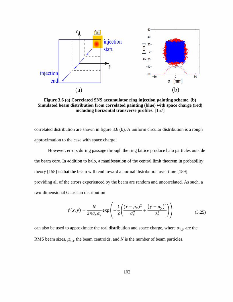
102

Figure 3.6 (a) Correlated SNS accumulator ring injection painting scheme. (b)

Simulated beam distribution from correlated painting (blue) with space charge (red)

including horizontal transverse profiles. [157]

correlated distribution are shown in figure 3.6 (b). A uniform circular distribution is a rough

approximation to the case with space charge.

However, errors during passage through the ring lattice produce halo particles outside

the beam core. In addition to halo, a manifestation of the central limit theorem in probability

theory [158] is that the beam will tend toward a normal distribution over time [159]

providing all of the errors experienced by the beam are random and uncorrelated. As such, a

two-dimensional Gaussian distribution

(

(

( )

)) (3.25)

can also be used to approximate the real distribution and space charge, where are the

RMS beam sizes, the beam centroids, and N is the number of beam particles.

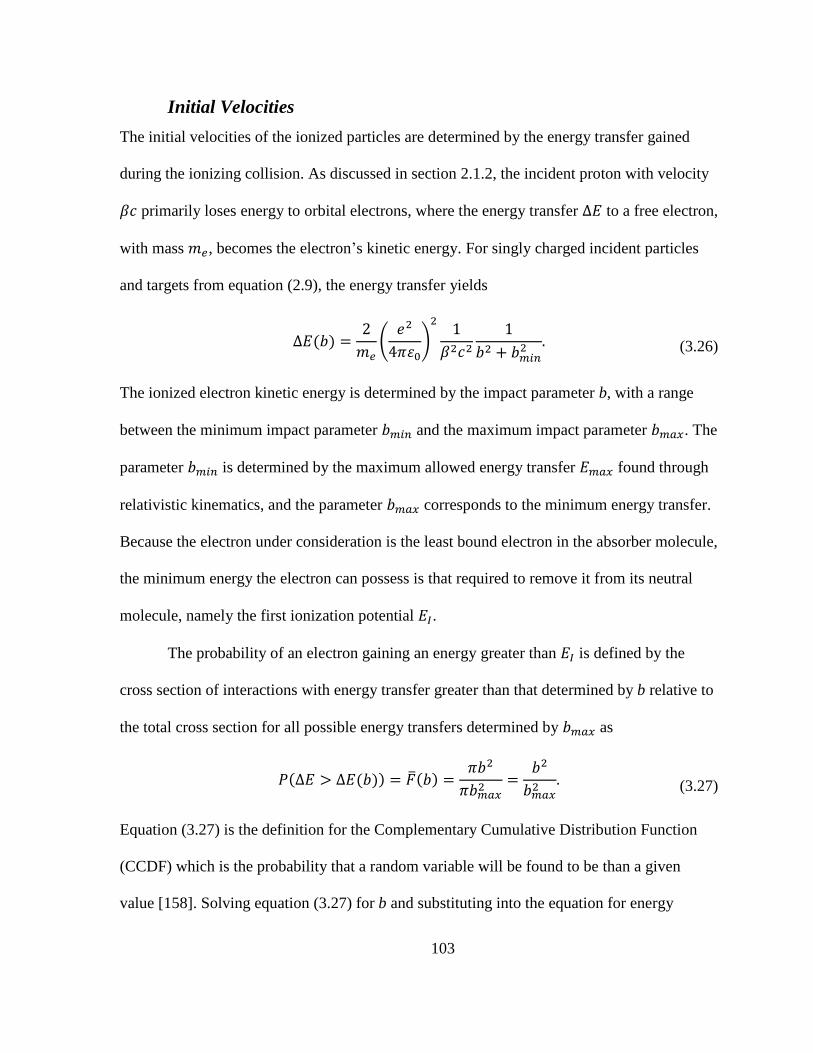
103

Initial Velocities

The initial velocities of the ionized particles are determined by the energy transfer gained

during the ionizing collision. As discussed in section 2.1.2, the incident proton with velocity

primarily loses energy to orbital electrons, where the energy transfer to a free electron,

with mass , becomes the electron’s kinetic energy. For singly charged incident particles

and targets from equation (2.9), the energy transfer yields

(

)

(3.26)

The ionized electron kinetic energy is determined by the impact parameter b, with a range

between the minimum impact parameter and the maximum impact parameter . The

parameter is determined by the maximum allowed energy transfer found through

relativistic kinematics, and the parameter corresponds to the minimum energy transfer.

Because the electron under consideration is the least bound electron in the absorber molecule,

the minimum energy the electron can possess is that required to remove it from its neutral

molecule, namely the first ionization potential .

The probability of an electron gaining an energy greater than is defined by the

cross section of interactions with energy transfer greater than that determined by b relative to

the total cross section for all possible energy transfers determined by as

(3.27)

Equation (3.27) is the definition for the Complementary Cumulative Distribution Function

(CCDF) which is the probability that a random variable will be found to be than a given

value [158]. Solving equation (3.27) for b and substituting into the equation for energy

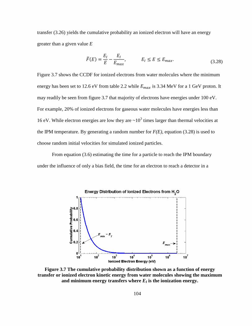
104

transfer (3.26) yields the cumulative probability an ionized electron will have an energy

greater than a given value E

(3.28)

Figure 3.7 shows the CCDF for ionized electrons from water molecules where the minimum

energy has been set to 12.6 eV from table 2.2 while is 3.34 MeV for a 1 GeV proton. It

may readily be seen from figure 3.7 that majority of electrons have energies under 100 eV.

For example, 20% of ionized electrons for gaseous water molecules have energies less than

16 eV. While electron energies are low they are ~103 times larger than thermal velocities at

the IPM temperature. By generating a random number for F(E), equation (3.28) is used to

choose random initial velocities for simulated ionized particles.

From equation (3.6) estimating the time for a particle to reach the IPM boundary

under the influence of only a bias field, the time for an electron to reach a detector in a

Figure 3.7 The cumulative probability distribution shown as a function of energy

transfer or ionized electron kinetic energy from water molecules showing the maximum

and minimum energy transfers where EI is the ionization energy.

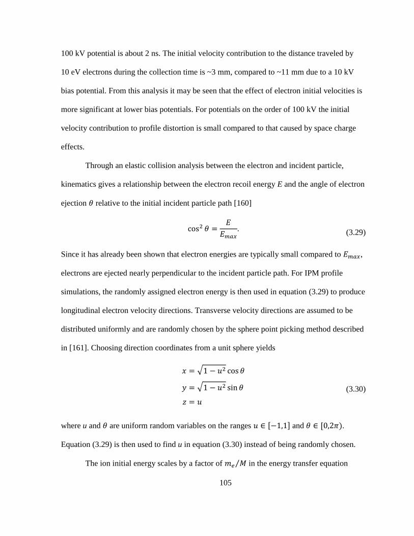
105

100 kV potential is about 2 ns. The initial velocity contribution to the distance traveled by

10 eV electrons during the collection time is ~3 mm, compared to ~11 mm due to a 10 kV

bias potential. From this analysis it may be seen that the effect of electron initial velocities is

more significant at lower bias potentials. For potentials on the order of 100 kV the initial

velocity contribution to profile distortion is small compared to that caused by space charge

effects.

Through an elastic collision analysis between the electron and incident particle,

kinematics gives a relationship between the electron recoil energy E and the angle of electron

ejection relative to the initial incident particle path [160]

(3.29)

Since it has already been shown that electron energies are typically small compared to ,

electrons are ejected nearly perpendicular to the incident particle path. For IPM profile

simulations, the randomly assigned electron energy is then used in equation (3.29) to produce

longitudinal electron velocity directions. Transverse velocity directions are assumed to be

distributed uniformly and are randomly chosen by the sphere point picking method described

in [161]. Choosing direction coordinates from a unit sphere yields

√

√

(3.30)

where u and are uniform random variables on the ranges [ ] and [ .

Equation (3.29) is then used to find u in equation (3.30) instead of being randomly chosen.

The ion initial energy scales by a factor of ⁄ in the energy transfer equation

106

(3.26) compared to the electron energies, where M is the ion mass. Considering that ⁄ is

never greater than ⁄ , the kinetic energy gained by ions during ionizing

collisions is less than their thermal energies. Consequently, ions of mass M with a

temperature T are given random velocities v determined by a Maxwellian probability

distribution of speed

√(

)

(3.31)

with directions randomly chosen using the method describe by equations (3.30). While ions

are given initial velocities in simulations, the RMS velocity is inversely proportional to

the particle mass, making 2 km/s for hydrogen molecules and 640 m/s for water.

During a single 1 µs pulse in the ring, hydrogen ions will drift ~2mm and water ions will

drift about 0.6 mm. Therefore, ion initial velocities do not contribute significantly to the

trajectory and the ions may be considered at rest for qualitative studies.

3.1.4 Ion Collection Field Analysis

Ion Collection Bias Potential

With the IPM simulation program incorporating all the applicable forces and initial

conditions, it is possible to predict the magnitude of electric bias potential needed to

overcome the space charge distortion. The same initial uniform circular particle distribution

was used to simulate the measured IPM profiles for a range of electric bias voltages for a

beam with uniform circular space charge at the end of the accumulation cycle. The results are

shown in figure 3.8 along with marker lines showing the initial RMS size, RMS size plus

10%, and RMS size plus 20% of the initial distribution. The most dramatic effect of the bias

107

potential is seen below 200 kV above which improvements in the measured profile are only

moderate. From figure 3.8 it may be seen that a measured beam size with a 10% distortion

may be achieved with a 500 kV bias while a 20% increase in the measure width is reached

with a 240 kV potential. Hydrogen and water molecules were also simulated, showing that

the distortion is not a function of ion mass as predicted by equation (3.7).

Figure 3.8 makes clear the difficulty of collecting ions. The 500 kV potential required

to meet the beam size system requirement is an exceedingly difficult technical challenge

considering the limited space afforded by the IPM chamber and safety specifications needed

for such a high voltage. Even a 240 kV potential provides a degree of technical challenge

beyond the scope of the safety limitations delineated for this system. For ions, mitigation of

beam induced profile spreading is not possible purely through hardware design within the

IPM design parameters.

Figure 3.8 Simulated measured IPM profile RMS sizes σ as a function of electric bias

potential for ions with a uniform circular distribution.

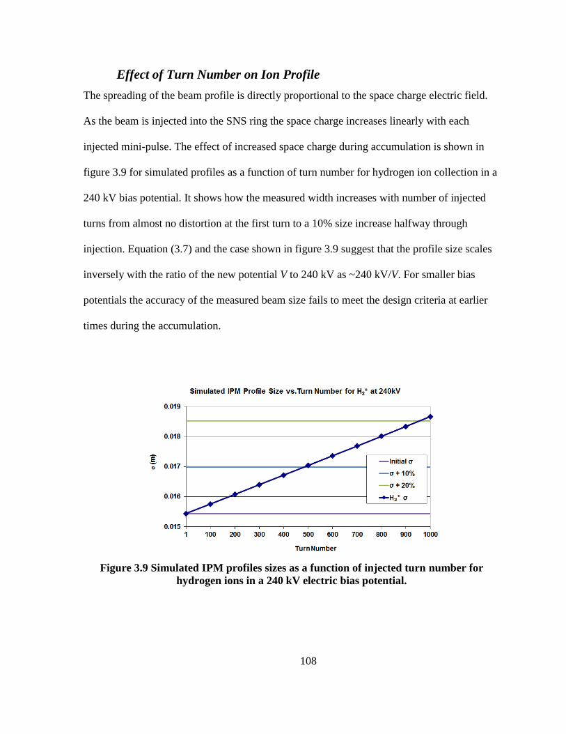
108

Effect of Turn Number on Ion Profile

The spreading of the beam profile is directly proportional to the space charge electric field.

As the beam is injected into the SNS ring the space charge increases linearly with each

injected mini-pulse. The effect of increased space charge during accumulation is shown in

figure 3.9 for simulated profiles as a function of turn number for hydrogen ion collection in a

240 kV bias potential. It shows how the measured width increases with number of injected

turns from almost no distortion at the first turn to a 10% size increase halfway through

injection. Equation (3.7) and the case shown in figure 3.9 suggest that the profile size scales

inversely with the ratio of the new potential V to 240 kV as ~240 kV/V. For smaller bias

potentials the accuracy of the measured beam size fails to meet the design criteria at earlier

times during the accumulation.

Figure 3.9 Simulated IPM profiles sizes as a function of injected turn number for

hydrogen ions in a 240 kV electric bias potential.

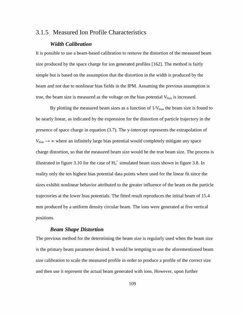
109

3.1.5 Measured Ion Profile Characteristics

Width Calibration

It is possible to use a beam-based calibration to remove the distortion of the measured beam

size produced by the space charge for ion generated profiles [162]. The method is fairly

simple but is based on the assumption that the distortion in the width is produced by the

beam and not due to nonlinear bias fields in the IPM. Assuming the previous assumption is

true, the beam size is measured as the voltage on the bias potential Vbias is increased.

By plotting the measured beam sizes as a function of 1/Vbias the beam size is found to

be nearly linear, as indicated by the expression for the distortion of particle trajectory in the

presence of space charge in equation (3.7). The y-intercept represents the extrapolation of

Vbias → ∞ where an infinitely large bias potential would completely mitigate any space

charge distortion, so that the measured beam size would be the true beam size. The process is

illustrated in figure 3.10 for the case of H2+ simulated beam sizes shown in figure 3.8. In

reality only the ten highest bias potential data points where used for the linear fit since the

sizes exhibit nonlinear behavior attributed to the greater influence of the beam on the particle

trajectories at the lower bias potentials. The fitted result reproduces the initial beam of 15.4

mm produced by a uniform density circular beam. The ions were generated at five vertical

positions.

Beam Shape Distortion

The previous method for the determining the beam size is regularly used when the beam size

is the primary beam parameter desired. It would be tempting to use the aforementioned beam

size calibration to scale the measured profile in order to produce a profile of the correct size

and then use it represent the actual beam generated with ions. However, upon further

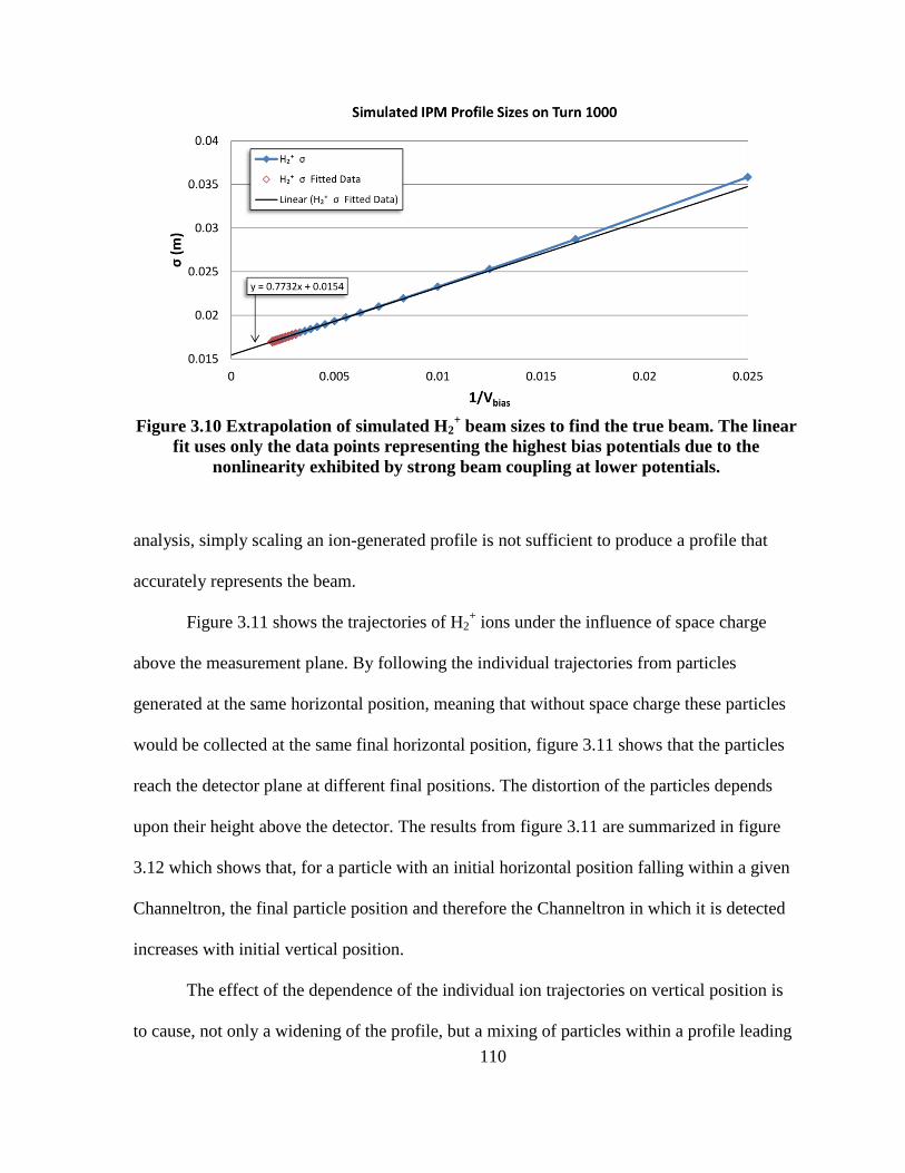
110

Figure 3.10 Extrapolation of simulated H2+ beam sizes to find the true beam. The linear

fit uses only the data points representing the highest bias potentials due to the

nonlinearity exhibited by strong beam coupling at lower potentials.

analysis, simply scaling an ion-generated profile is not sufficient to produce a profile that

accurately represents the beam.

Figure 3.11 shows the trajectories of H2+ ions under the influence of space charge

above the measurement plane. By following the individual trajectories from particles

generated at the same horizontal position, meaning that without space charge these particles

would be collected at the same final horizontal position, figure 3.11 shows that the particles

reach the detector plane at different final positions. The distortion of the particles depends

upon their height above the detector. The results from figure 3.11 are summarized in figure

3.12 which shows that, for a particle with an initial horizontal position falling within a given

Channeltron, the final particle position and therefore the Channeltron in which it is detected

increases with initial vertical position.

The effect of the dependence of the individual ion trajectories on vertical position is

to cause, not only a widening of the profile, but a mixing of particles within a profile leading

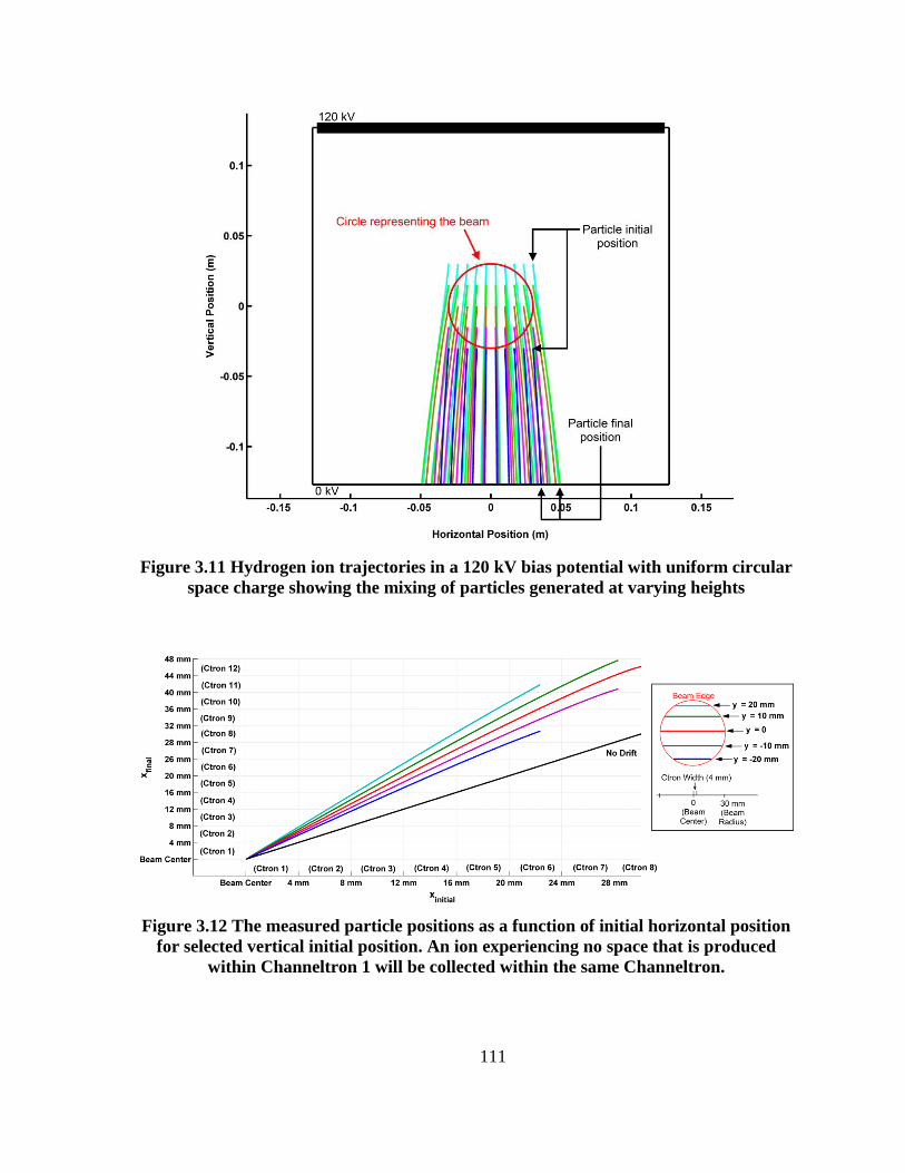
111

Figure 3.11 Hydrogen ion trajectories in a 120 kV bias potential with uniform circular

space charge showing the mixing of particles generated at varying heights

Figure 3.12 The measured particle positions as a function of initial horizontal position

for selected vertical initial position. An ion experiencing no space that is produced

within Channeltron 1 will be collected within the same Channeltron.

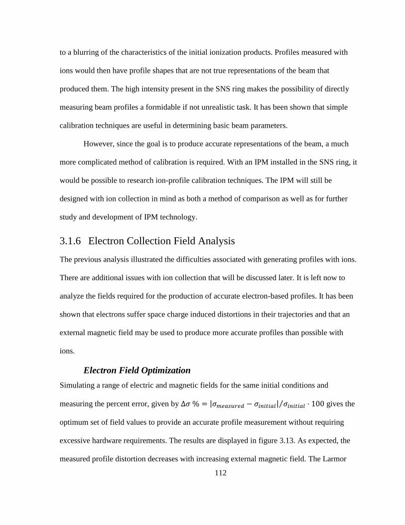
112

to a blurring of the characteristics of the initial ionization products. Profiles measured with

ions would then have profile shapes that are not true representations of the beam that

produced them. The high intensity present in the SNS ring makes the possibility of directly

measuring beam profiles a formidable if not unrealistic task. It has been shown that simple

calibration techniques are useful in determining basic beam parameters.

However, since the goal is to produce accurate representations of the beam, a much

more complicated method of calibration is required. With an IPM installed in the SNS ring, it

would be possible to research ion-profile calibration techniques. The IPM will still be

designed with ion collection in mind as both a method of comparison as well as for further

study and development of IPM technology.

3.1.6 Electron Collection Field Analysis

The previous analysis illustrated the difficulties associated with generating profiles with ions.

There are additional issues with ion collection that will be discussed later. It is left now to

analyze the fields required for the production of accurate electron-based profiles. It has been

shown that electrons suffer space charge induced distortions in their trajectories and that an

external magnetic field may be used to produce more accurate profiles than possible with

ions.

Electron Field Optimization

Simulating a range of electric and magnetic fields for the same initial conditions and

measuring the percent error, given by | | ⁄ gives the

optimum set of field values to provide an accurate profile measurement without requiring

excessive hardware requirements. The results are displayed in figure 3.13. As expected, the

measured profile distortion decreases with increasing external magnetic field. The Larmor

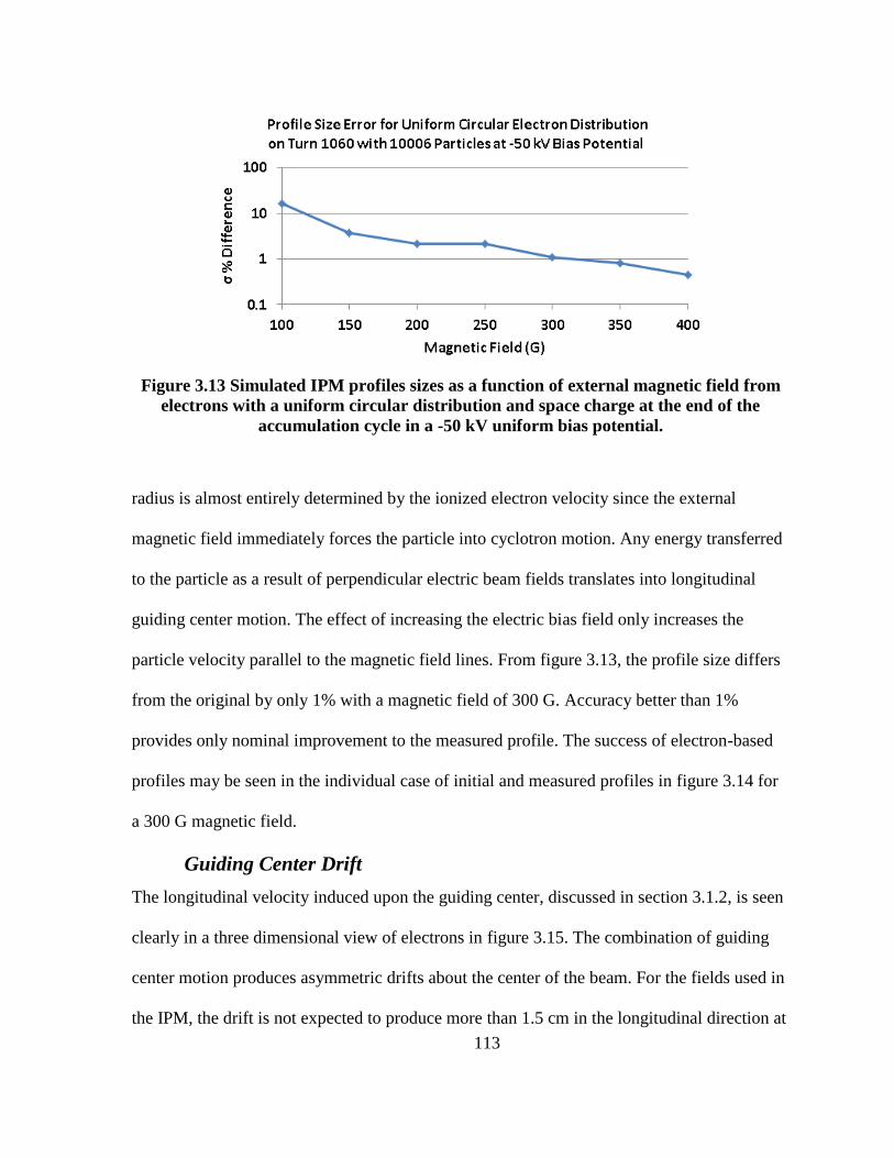
113

Figure 3.13 Simulated IPM profiles sizes as a function of external magnetic field from

electrons with a uniform circular distribution and space charge at the end of the

accumulation cycle in a -50 kV uniform bias potential.

radius is almost entirely determined by the ionized electron velocity since the external

magnetic field immediately forces the particle into cyclotron motion. Any energy transferred

to the particle as a result of perpendicular electric beam fields translates into longitudinal

guiding center motion. The effect of increasing the electric bias field only increases the

particle velocity parallel to the magnetic field lines. From figure 3.13, the profile size differs

from the original by only 1% with a magnetic field of 300 G. Accuracy better than 1%

provides only nominal improvement to the measured profile. The success of electron-based

profiles may be seen in the individual case of initial and measured profiles in figure 3.14 for

a 300 G magnetic field.

Guiding Center Drift

The longitudinal velocity induced upon the guiding center, discussed in section 3.1.2, is seen

clearly in a three dimensional view of electrons in figure 3.15. The combination of guiding

center motion produces asymmetric drifts about the center of the beam. For the fields used in

the IPM, the drift is not expected to produce more than 1.5 cm in the longitudinal direction at

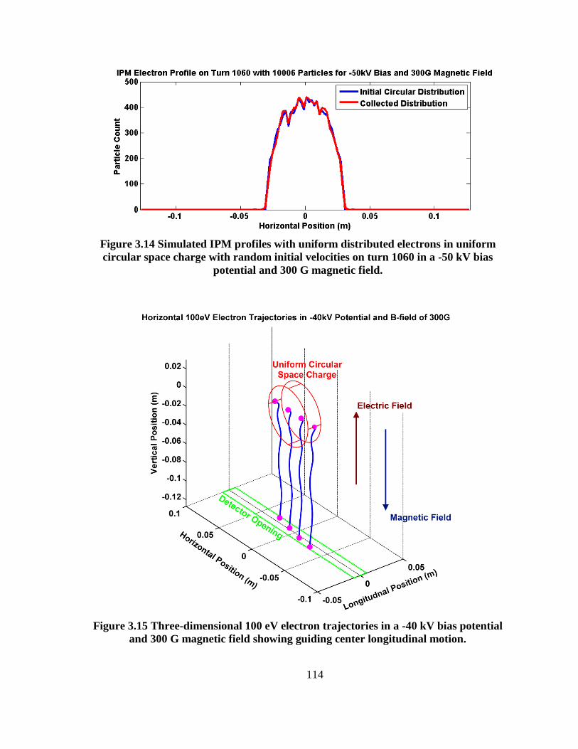
114

Figure 3.14 Simulated IPM profiles with uniform distributed electrons in uniform

circular space charge with random initial velocities on turn 1060 in a -50 kV bias

potential and 300 G magnetic field.

Figure 3.15 Three-dimensional 100 eV electron trajectories in a -40 kV bias potential

and 300 G magnetic field showing guiding center longitudinal motion.

115

the detector, as shown in figure 3.15, and therefore is not expected to be an issue. Even if the

external electric field were extremely misaligned to produce a perpendicular component of -

20 kV to the external magnetic field, the additional drift would only be on the order of

microns. Therefore, longitudinal motion due to field alignment errors will be considered

negligible.

3.2 Spatial Accuracy

With an understanding of the trajectories in the IPM and a determination of the necessary

field values, it is now possible to analyze more completely the accuracy of the collected

measurement. Spatial accuracy defines the ability of the measured distribution to replicate

the actual beam distribution and the certainty with which it is known. An accurate

measurement requires not only a mitigation of beam-induced profile distortion, as previously

discussed, but the counting of additional errors arising from the measurement process. Some

errors may be removed from the final profile while others will be accumulated to characterize

the measurement accuracy.

Error Definition

A few errors present in an IPM profile have been discussed, such as the error due to space

charge distortion and the error due to small-number statistics. There are a number of other

error sources that will be considered and it will be useful for further discussion to define

nomenclature for the next few sections. The most useful way to categorize the effect of

various profile error sources is to study their effect on the measured rms beam size .

The error in measuring a beam with rms beam size may be separated into a

systematic component and a statistical or random component . A systematic error

is defined to be the portion of the difference between a measured quantity and its actual

116

value, where this portion is consistent in all measurements as a result of the way in which the

measurement is made [163]. One example is the profile distortion due to space charge.

Systematic errors may be reduced with corrections or system improvements while random

errors are due to stochastic variations, such as signal amplitude fluctuations from low particle

numbers, and represent the uncertainty of the measurement The measured beam size is a

combination of the true beam size and the error contributions such that

. The relative error on the beam size is defined by

(3.32)

where and are the systematic and statistical relative errors. The percent error,

found by multiplying equation (3.32) by 100, will be the primary error expression used.

3.2.2 Resolution and Statistical Errors

It is necessary to obtain an estimate of the statistical errors present in an IPM profile in order

to understand how each type of error affects the measured beam size. Following an analysis

found in [53] and [164], it is possible to numerically analyze errors due to stochastic

processes and spatial resolution by using a Monte Carlo method. The following simulations

assume a Gaussian beam distribution with rms beam size of 15 mm and center at 0 in both

transverse directions. Furthermore, much of the following analysis will consider only the

error on the final measured profile, meaning that any noise present is due to the entire

electrical path of the signal including electronics.

Monte Carlo Simulation

Error estimation is based on a Monte Carlo approach which is uses an idealized model to

generate a large ensemble of measurement possibilities due to assumed errors. The spread of

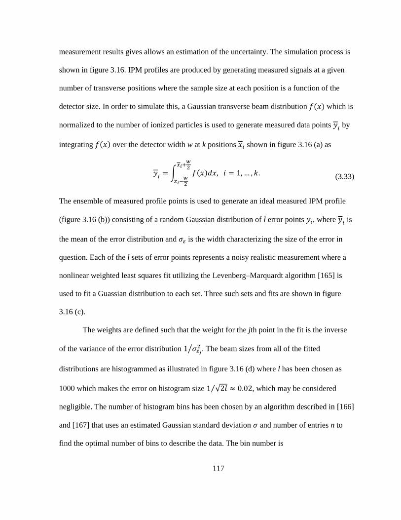
117

measurement results gives allows an estimation of the uncertainty. The simulation process is

shown in figure 3.16. IPM profiles are produced by generating measured signals at a given

number of transverse positions where the sample size at each position is a function of the

detector size. In order to simulate this, a Gaussian transverse beam distribution which is

normalized to the number of ionized particles is used to generate measured data points by

integrating over the detector width w at k positions shown in figure 3.16 (a) as

∫

(3.33)

The ensemble of measured profile points is used to generate an ideal measured IPM profile

(figure 3.16 (b)) consisting of a random Gaussian distribution of l error points , where is

the mean of the error distribution and is the width characterizing the size of the error in

question. Each of the l sets of error points represents a noisy realistic measurement where a

nonlinear weighted least squares fit utilizing the Levenberg–Marquardt algorithm [165] is

used to fit a Guassian distribution to each set. Three such sets and fits are shown in figure

3.16 (c).

The weights are defined such that the weight for the jth point in the fit is the inverse

of the variance of the error distribution ⁄ . The beam sizes from all of the fitted

distributions are histogrammed as illustrated in figure 3.16 (d) where l has been chosen as

1000 which makes the error on histogram size √ ⁄ , which may be considered

negligible. The number of histogram bins has been chosen by an algorithm described in [166]

and [167] that uses an estimated Gaussian standard deviation and number of entries n to

find the optimal number of bins to describe the data. The bin number is

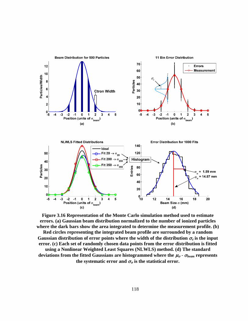
118

Figure 3.16 Representation of the Monte Carlo simulation method used to estimate

errors. (a) Gaussian beam distribution normalized to the number of ionized particles

where the dark bars show the area integrated to determine the measurement profile. (b)

Red circles representing the integrated beam profile are surrounded by a random

Gaussian distribution of error points where the width of the distribution is the input

error. (c) Each set of randomly chosen data points from the error distribution is fitted

using a Nonlinear Weighted Least Squares (NLWLS) method. (d) The standard

deviations from the fitted Gaussians are histogrammed where the 𝛍 - beam represents

the systematic error and is the statistical error.

119

√ (3.34)

The systematic error is the difference between the mean of the beam size fits and the true

beam size . The rms size of the beam sizes characterizes the spread of the possible

beam widths measured in the presence of noise and defines the statistical uncertainty of the

measured IPM profile rms size.

Resolution Error

The resolution error arises from the size of the Channeltron and the fact that information

within the width of a single detector is summed together and the details lost. Due to the

nature of the IPM, which has a fixed width detector that can take measurements at an

increasing number of locations up to the limit that one Channeltron position is immediately

adjacent to the next, there is also an error due to the number of Ctron positions or bins used.

The larger the number of bins used the more highly the resulting fit is constrained, which

leads to a more accurate measurement of the beam size. Furthermore, it has been discussed in

section 2.3.2 that the number of ionized particles can have a large influence on the measured

profile, especially at low particle numbers.

The systematic error due to resolution may be analytically calculated for the case

where there are no gaps between bins [53]. The measured beam size, in the absence of any

distorting fields or other errors, would be the standard deviation of the random final

measured particle position. Furthermore, the final particle positions are the sum of two

random variables, the initial random particle positions and the random position associated

uncertainty of location within a single Channeltron. The standard deviation of the sum of two

uncorrelated and independent variables is √ where and

120

are the individual standard deviations. For the case of a Gaussian beam with standard

deviation and a Channeltron where all the particles entering it are uniformly

distributed over a width w, the measured beam size is

√

(3.35)

where is the standard deviation of a normalized uniform distribution of a particle

⁄ . It is useful to define the resolution as the number of Ctrons or bins that fit

within one rms beam size by a single quantity Bins per Sigma or defined as

⁄

(3.36)

By substituting equations (3.35) and (3.36) into (3.32) it has been shown [53] that

√

⁄ (3.37)

As a result of (3.37), if the bins are adjacent, increasing the number of bins or ⁄

decreases the bins size and systematic error.

Two cases are presented in figure 3.17. Equation (3.37), referred to as the Bin Width

Function, is plotted as a function of ⁄ meaning that the bin edges touch and the

bin width is changing. The Bin Width Function gives the resolution for a detector for a given

bin size and, for the IPM with a maximum8 ⁄ = 15 mm/4 mm = 3.75, the

systematic error is 0.3%. This is confirmed by Monte Carlo simulations, which are displayed

by the other curves of Figure 3.17, for the case where ⁄ represents a fixed

8 The maximum ⁄ for the IPM corresponds to the case where there a sufficient number of

Channeltrons such that each Channeltron touches the next with no gaps.

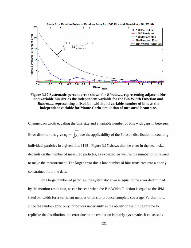
121

Figure 3.17 Systematic percent error shown for Bins/beam representing adjacent bins

and variable bin size as the independent variable for the Bin Width Function and

Bins/beam representing a fixed bin width and variable number of bins as the

independent variable for Monte Carlo simulation of measured beam size.

Channeltron width equaling the bins size and a variable number of bins with gaps in between.

Error distributions give √ due the applicability of the Poisson distribution to counting

individual particles in a given time [148]. Figure 3.17 shows that the error in the beam size

depends on the number of measured particles, as expected, as well as the number of bins used

to make the measurement. The larger error due a low number of bins translates into a poorly

constrained fit to the data.

For a large number of particles, the systematic error is equal to the error determined

by the monitor resolution, as can be seen when the Bin Width Function is equal to the IPM

fixed bin width for a sufficient number of bins to produce complete coverage. Furthermore,

since the random error only introduces uncertainty in the ability of the fitting routine to

replicate the distribution, the error due to the resolution is purely systematic. It exists sans

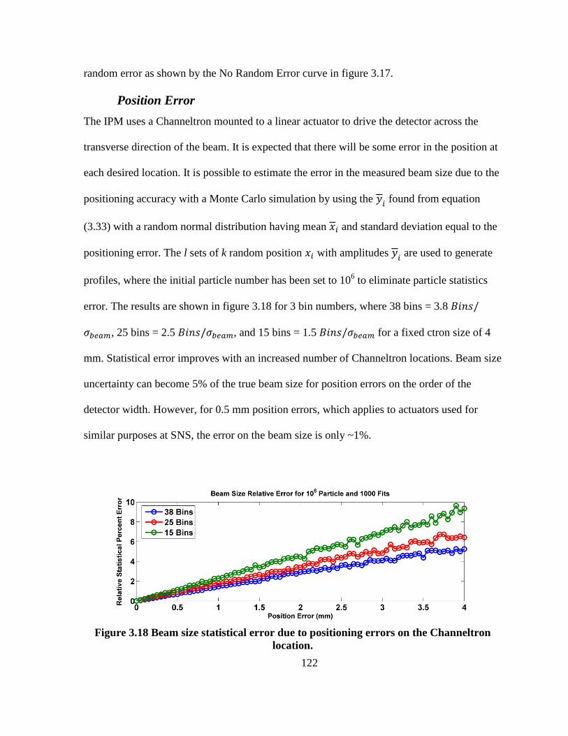
122

random error as shown by the No Random Error curve in figure 3.17.

Position Error

The IPM uses a Channeltron mounted to a linear actuator to drive the detector across the

transverse direction of the beam. It is expected that there will be some error in the position at

each desired location. It is possible to estimate the error in the measured beam size due to the

positioning accuracy with a Monte Carlo simulation by using the found from equation

(3.33) with a random normal distribution having mean and standard deviation equal to the

positioning error. The l sets of k random position with amplitudes are used to generate

profiles, where the initial particle number has been set to 106 to eliminate particle statistics

error. The results are shown in figure 3.18 for 3 bin numbers, where 38 bins = 3.8

, 25 bins = 2.5 , and 15 bins = 1.5 for a fixed ctron size of 4

mm. Statistical error improves with an increased number of Channeltron locations. Beam size

uncertainty can become 5% of the true beam size for position errors on the order of the

detector width. However, for 0.5 mm position errors, which applies to actuators used for

similar purposes at SNS, the error on the beam size is only ~1%.

Figure 3.18 Beam size statistical error due to positioning errors on the Channeltron

location.

123

Electronic Noise Error

Noise inherent in the electronics of the data acquisition chain will create an uncertainty in the

data leading to an error in the measured beam size. There are a number of noise sources

arising from the flow of electricity and the process of digitizing analog signals that are not

dependent on the incoming particles and are represented by a constant . Notationally it is

prudent to characterize noise sources by their signal-to-noise ratio (SNR), which is defined to

be the ratio of the measured signal power or amplitude to the noise power

amplitude as

(

)

(3.38)

or, expressed in the logarithmic9 decibel scale, as

(

) (

) (3.39)

In the following simulations is taken to be the maximum of the input

normal distribution representing the amplitude of the measured voltage, and the noise voltage

√ ⁄ is the error width .

Thermal noise or Johnson-Nyquist noise is a measurable current present in electronic

devices in the absence of an applied voltage irrespective of material and circuit geometry

[168]. Arising from the random thermal agitation of charges in a conductor with temperature

T and signal bandwidth , the thermal noise voltage is [169]

√ (3.40)

9 In this text the base-10 logarithm will be denoted and the natural logarithm .

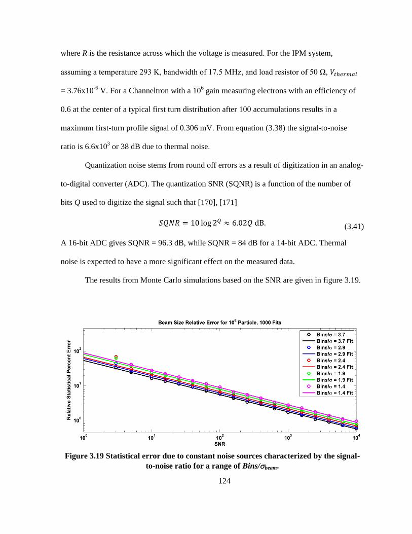
124

where R is the resistance across which the voltage is measured. For the IPM system,

assuming a temperature 293 K, bandwidth of 17.5 MHz, and load resistor of 50 Ω,

= 3.76x10-6

V. For a Channeltron with a 106 gain measuring electrons with an efficiency of

0.6 at the center of a typical first turn distribution after 100 accumulations results in a

maximum first-turn profile signal of 0.306 mV. From equation (3.38) the signal-to-noise

ratio is 6.6x103 or 38 dB due to thermal noise.

Quantization noise stems from round off errors as a result of digitization in an analog-

to-digital converter (ADC). The quantization SNR (SQNR) is a function of the number of

bits Q used to digitize the signal such that [170], [171]

(3.41)

A 16-bit ADC gives SQNR = 96.3 dB, while SQNR = 84 dB for a 14-bit ADC. Thermal

noise is expected to have a more significant effect on the measured data.

The results from Monte Carlo simulations based on the SNR are given in figure 3.19.

Figure 3.19 Statistical error due to constant noise sources characterized by the signal-

to-noise ratio for a range of Bins/beam.

125

Since the type of SNR is not specified it may be taken as the total SNR representing all

sources of constant noise. The error due to noise can become quite large for signal-to-noise

ratios less than 100. However, for the SNR due to thermal noise the percent error in the

measured beam size is ~1% for the maximum . It is interesting to note that the

data for a particular is well parameterized by the line

such that

(3.42)

except for signal-to-noise ratios < 5 where the error is large compared to the signal height,

making profile fitting difficult.

Following an analysis shown in [53], it may be shown that, by plotting the K

parameter from the fits for each data set, the fitting parameter K is

√

(3.43)

Equation (3.43) in conjunction with the fact that the fitted value of m in (3.42) is 1/2 yields

an estimate for the statistical noise error for a SNR defined by (3.38) as

√

√

(3.44)

For a given detector resolution, if the noise and signal can be calculated or measured, the

uncertainty on the measured beam size due to random noise may be found with equation

(3.44).

In addition to constant sources of noise there is also the possibility of relative noise

sources, such as nonlinearity in amplifier gain [164]. This effect is analyzed by simulating a

Gaussian error that is the combination of individual errors representing a constant noise

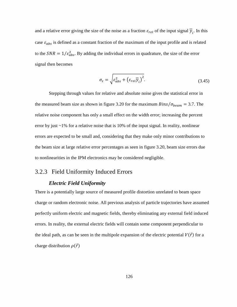
126

and a relative error giving the size of the noise as a fraction of the input signal . In this

case is defined as a constant fraction of the maximum of the input profile and is related

to the ⁄ . By adding the individual errors in quadrature, the size of the error

signal then becomes

√ (

) (3.45)

Stepping through values for relative and absolute noise gives the statistical error in

the measured beam size as shown in figure 3.20 for the maximum ⁄ 3.7. The

relative noise component has only a small effect on the width error; increasing the percent

error by just ~1% for a relative noise that is 10% of the input signal. In reality, nonlinear

errors are expected to be small and, considering that they make only minor contributions to

the beam size at large relative error percentages as seen in figure 3.20, beam size errors due

to nonlinearities in the IPM electronics may be considered negligible.

3.2.3 Field Uniformity Induced Errors

Electric Field Uniformity

There is a potentially large source of measured profile distortion unrelated to beam space

charge or random electronic noise. All previous analysis of particle trajectories have assumed

perfectly uniform electric and magnetic fields, thereby eliminating any external field induced

errors. In reality, the external electric fields will contain some component perpendicular to

the ideal path, as can be seen in the multipole expansion of the electric potential for a

charge distribution

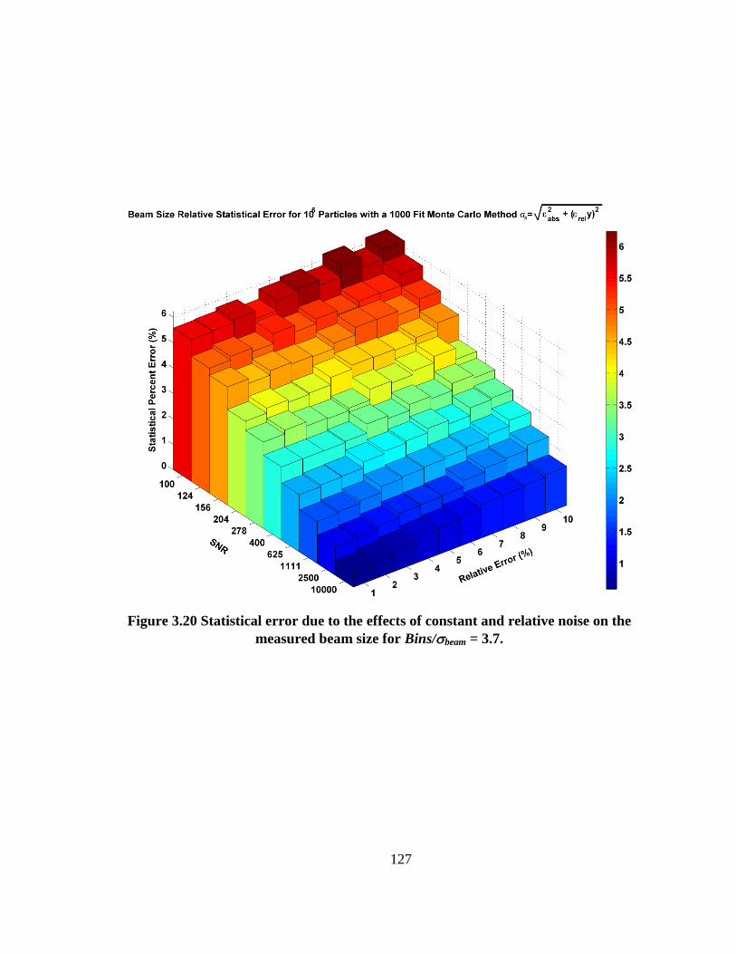
127

Figure 3.20 Statistical error due to the effects of constant and relative noise on the

measured beam size for Bins/beam = 3.7.

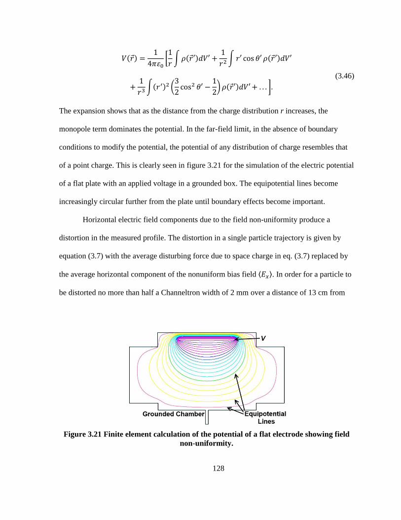
128

[

∫

∫

∫ (

) ]

(3.46)

The expansion shows that as the distance from the charge distribution r increases, the

monopole term dominates the potential. In the far-field limit, in the absence of boundary

conditions to modify the potential, the potential of any distribution of charge resembles that

of a point charge. This is clearly seen in figure 3.21 for the simulation of the electric potential

of a flat plate with an applied voltage in a grounded box. The equipotential lines become

increasingly circular further from the plate until boundary effects become important.

Horizontal electric field components due to the field non-uniformity produce a

distortion in the measured profile. The distortion in a single particle trajectory is given by

equation (3.7) with the average disturbing force due to space charge in eq. (3.7) replaced by

the average horizontal component of the nonuniform bias field ⟨ ⟩. In order for a particle to

be distorted no more than half a Channeltron width of 2 mm over a distance of 13 cm from

Figure 3.21 Finite element calculation of the potential of a flat electrode showing field

non-uniformity.

129

the top the beam to the detector, the ratio of the average horizontal field component to the

field magnitude must not exceed ⟨ ⟩ = 1.5%. From the resolution study, a distortion of

should add less than 0.5% error to the measured beam width. By manipulating the electrode

geometry and size it possible to produce a uniform field over the region of the beam. The

optimization of electrode geometry for field uniformity will be approached in a later chapter.

Magnetic field Uniformity

The magnetic field uniformity is simplified due to the symmetry and nature of the dipole

magnet used. The charged particles are confined to spiral around the field lines, thus,

nonlinearities in the magnetic field uniformity would produce distortions in the measured

particle trajectories. It is important to choose a magnet design that yields the greatest field

uniformity. It will be shown in a later section when the details and simulations of the magnet

are discussed that the magnetic field produces a negligible error in the particle trajectories.

3.2.4 Secondary Particle Source Error

It was discussed in section 2.2.4 that beam-induced secondary electrons should contribute

negligibly to a profile measurement. However, there are other forms of secondary particles

that will contribute. In the case of electron collection there are two sources of secondary

electrons in addition to beam-induced secondaries and field emission electrons.

Potential Electron Emission

An energetic ion striking a metallic surface interacts with electrons in the metal and may be

neutralized through a process called Auger neutralization [172], [173]. This is the case in

IPM electron collection when ions created during the beam passage are accelerated by the

beam and strike the high voltage bias electrode of the detector. If the neutralization energy,

or ionization energy, of the ion is twice the work function of the target, then an electron in

130

the valence band of the metal can quantum mechanically tunnel into the ion’s potential well

and fill a vacant state [174]. The energy released in this Auger type transition may then be

transferred to liberate a second electron in a process that is often described as potential

electron emission. A simple expression utilizing the ionization energy Ei, target work

function w, and Fermi energy of the metal EF may be used to define the secondary electron

yield as [175]

(3.47)

For the case of an ionized water molecule with Ei = 12.6 eV incident on stainless steel, which

has a work function of ~4.4 eV, and a Fermi energy (for iron) of ~11.1 eV, the number of

secondary electrons per incident ion due to potential emission is 0.023.

Ion-Induced Secondary Electrons

Secondary electrons due to the transfer of energy through kinetic impact of beam particles

with the accelerator chamber walls has been analyzed, but electrons from accelerated IPM

ions may also be created through kinetic emission. Ions in the IPM will strike the electrode

with energies on the order of 60 keV, which is well above the stainless steel work function.

The process of secondary electron creation is the same for heavy charged particle energy

transfer where the ion experiences hard and soft collisions that transfer energy to absorber

electrons. Ion-induced secondary electron yields have been the focus of a number of studies

due to their influence on particle detectors [176], [177].

An expression for SEY due to kinetic impact has been developed [178] as a function

of the angle the incident particle makes with a direction normal to the target surface

131

(3.48)

The specific yield in equation (3.48) is a material-dependent parameter that defines the

number of secondaries created per unit energy loss and has been found to have a value of

10.1 for protons normally incident on type 304 stainless steel [176]. is the electronic

stopping power and has been calculated for a 60 keV proton on 304 stainless steel with the

program SRIM (The Stopping and Range of Ions in Matter) [179] to be 0.283 MeV cm2

mg-1

. The constant C in equation (3.48) is a scaling factor that has been normalized to C = 1

for protons.

Given a specific yield of a proton on a given material, the SEY may be scaled for

other ions impacting the same material. It has been shown [180] that heavy ions are less

efficient at the production of secondary electrons and the scaling factor has an average value

of 0.32 [181]. Lastly, due to the electromagnetic boundary condition that the electric field be

perpendicular to an equipotential surface, in this case the electrode surface, the dominant bias

field accelerating the ions is normal to the electrode meaning that most ions are incident at

. The secondary emission yield is at a minimum due to the ⁄ behavior.

The IPM in electron collection mode would produce primarily 60 keV H2O+

molecules normally incident on the stainless steel electrode, producing 0.92 electrons per ion

by equation (3.48). It is interesting to note that eq. (3.48) gives an SEY of 2.85 for 60 keV

protons, which is approximately the same SEY quoted in section 2.2.4 for the electron-

induced secondaries. As such the TiN coating used for electron cloud reduction reduces the

electron induced secondaries to 1.5 and, since it is known [178] that ion induced secondaries

only escape from a surface depth of ~10 nm, it is possible that the 100 nm TiN would

132

produce a similar reduction of the ion secondary emission yield. An ion SEY of 1.5 due to

protons would have a heavy ion SEY scaled to 0.48. Two different studies [176], [182] give

examples of ion-induced SEY in which normally incident 28 MeV protons on stainless steel

give SEY= 0.14 and obliquely incident 5 keV argon ions on TiN coated stainless steel SEY =

0.57. Without exact data of incident ion secondary yields in the 60 keV range, it will be

assumed that the IPM ion-induced SEY = 0.5.

Secondary Electron Error

The production of secondary electrons by ionization products will cause an error in measured

beam profiles. The process, shown graphically in figure 3.22, by which secondary electrons

contribute to a source of systematic error goes as follows: positive ions produced during

beam-gas interactions are accelerated toward the bias electrode held at a negative potential V

where they strike the electrode surface producing secondary electrons. These secondary

electrons are then accelerated away from the electrode in a helical motion produced by the

external magnetic field until they are collected in the Channeltron detector, indistinguishable

from the true beam-produced electrons. The problem lies in the fact that the positive ions

undergo trajectory distortions resulting in an unwanted secondary electron profile that is

collected with the beam-electron profile.

As a limiting case, simulations for SEY = 1 are shown in figure 3.23 (a) for electrons

created by gas ionization due to a nominal Gaussian beam with an rms beam size of 22 mm,

for secondary electrons produced by the gas ions striking a negative electrode at 120 kV, and

the combined distribution. The primary electron profile and combined measured distribution

(with significant error) are shown in figure 3.23 (b). Errors in the measured electron

distribution are a function of the secondary emission yield as illustrated in figure 3.24. The

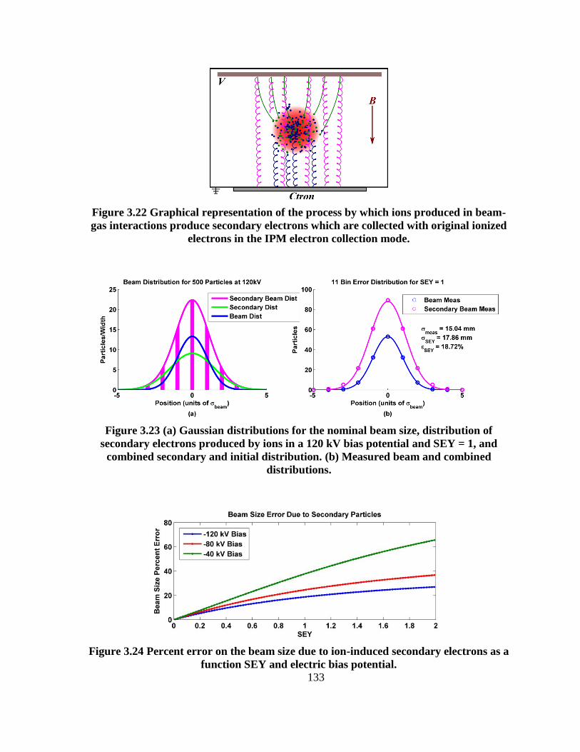
133

Figure 3.22 Graphical representation of the process by which ions produced in beam-

gas interactions produce secondary electrons which are collected with original ionized

electrons in the IPM electron collection mode.

Figure 3.23 (a) Gaussian distributions for the nominal beam size, distribution of

secondary electrons produced by ions in a 120 kV bias potential and SEY = 1, and

combined secondary and initial distribution. (b) Measured beam and combined

distributions.

Figure 3.24 Percent error on the beam size due to ion-induced secondary electrons as a

function SEY and electric bias potential.

134

error in the measured profile becomes large >10% at values of SEY larger than 0.4.

Additionally, the secondary electron profile is related to the electric bias potential due to the

ion profile spreading. This is shown for three different values of bias potential where the ion

profile sizes determining the secondary electron contribution have been taken from figure

3.24. It is necessary to have a large bias potential for electron collection.

It can be seen from figure 3.24 that for the beam size error that = 12% for SEY =

0.5. This analysis reveals that a method of ion-induced secondary electron suppression must

be included in the IPM design in order to produce electron profiles that meet the required

accuracy. It should be noted that secondary electron errors are not an issue during ion

collection since electrons produced at a positively biased electrode will not be accelerated to

the detector.

3.2.5 Spatial Accuracy Estimation

It can be seen that there are a number of systematic and random errors that contribute to the

measured profile accuracy and beam size. It is now possible to estimate the error of the final

measured beam size due to the individual errors studied. Due to the independent and

uncorrelated nature of each error the final error may considered to be the convolution of

individual Gaussian beam error distributions. The errors may be added in quadrature, where

the systematic component includes the resolution error , field uniformity error ,

secondary electron error , and space charge profile spreading . The statistical error

includes the error on the position , absolute errors defined by the signal-to-noise ratio

, encompassing thermal noise and quantization noise, relative errors from electronics

nonlinearities , and the uncertainty on the beam size due to the number of particles .

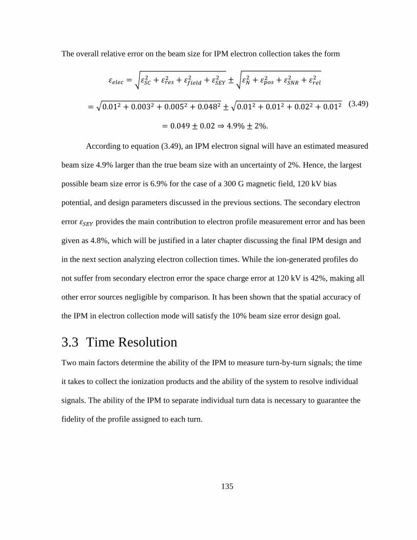
135

The overall relative error on the beam size for IPM electron collection takes the form

√

√

√ √

(3.49)

According to equation (3.49), an IPM electron signal will have an estimated measured

beam size 4.9% larger than the true beam size with an uncertainty of 2%. Hence, the largest

possible beam size error is 6.9% for the case of a 300 G magnetic field, 120 kV bias

potential, and design parameters discussed in the previous sections. The secondary electron

error provides the main contribution to electron profile measurement error and has been

given as 4.8%, which will be justified in a later chapter discussing the final IPM design and

in the next section analyzing electron collection times. While the ion-generated profiles do

not suffer from secondary electron error the space charge error at 120 kV is 42%, making all

other error sources negligible by comparison. It has been shown that the spatial accuracy of

the IPM in electron collection mode will satisfy the 10% beam size error design goal.

3.3 Time Resolution

Two main factors determine the ability of the IPM to measure turn-by-turn signals; the time

it takes to collect the ionization products and the ability of the system to resolve individual

signals. The ability of the IPM to separate individual turn data is necessary to guarantee the

fidelity of the profile assigned to each turn.

136

3.3.1 Collection Times

Ion Collection

Positively charged ions arising from beam-gas interactions are accelerated by the beam space

charge and external electric bias field toward the Channeltron detector. Neglecting its initial

thermal velocity, an ion will travel for a time t given by equation (3.6) which depends on the

mass m and vertical electric field component Ey as √ . The collection time is larger

for more massive ions, so that, as the beam passes through the IPM gas region and produces

a variety of ions as outlined in section 2.2.1, the ions will arrive at the detector over a range

of times.

Simulations done for a nominal fully accumulated beam calculated the time to collect

all of the ions as a function of external bias voltage. The results, reported in figure 3.25, show

the dependence of collection time on bias voltage for two different particle species. As

expected, the collection time increases with particle mass. There is a 300 ns gap at the end of

every beam pulse to allow for extraction from the ring. Particles created at the end of a beam

pulse must be collected within the gap or they will be collected during a following turn,

thereby mixing the turns and leading to errors and uncertainty in the final measurements. It

can be seen from figure 3.25 that the primary ion signal from H2O+ will be collected within

the 300 ns gap with a voltage of 120 kV.

The collection time limit determines the necessary minimum value of the electric

potential chosen as the design parameter. Hydrogen ions are collected within the time allotted

at the chosen potential. Figure 3.26 illustrates the effect of the delay in electrons created by

ion-induced secondaries. They are delayed and spread in time due to the transverse ion

distribution. The secondary electron distribution in figure 3.26 (a) is represented by a

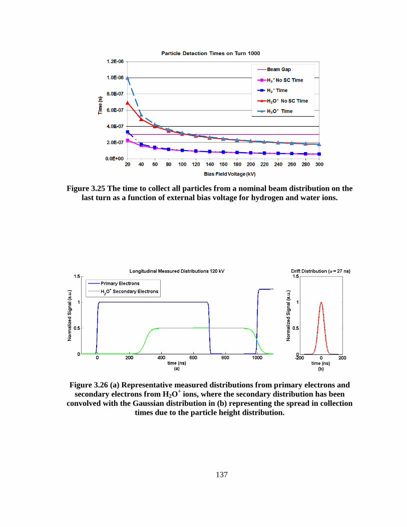
137

Figure 3.25 The time to collect all particles from a nominal beam distribution on the

last turn as a function of external bias voltage for hydrogen and water ions.

Figure 3.26 (a) Representative measured distributions from primary electrons and

secondary electrons from H2O+ ions, where the secondary distribution has been

convolved with the Gaussian distribution in (b) representing the spread in collection

times due to the particle height distribution.

138

convolution of a Gaussian distribution (figure 3.26 (b)) of collection times with a standard

deviation found from simulating H2O+ ions trajectories. The convolution smears out the

primary distribution. The height is scaled so that the area under the secondary curve, or the

integrated turn signal, is ½ the area under the primary curve, from assuming a secondary

emission yield of 0.5 electrons per ion.

The small number of heavy ions created at the end of a pulse will not be collected

within the turn and will contribute to the following pulse. Heavier ions than water constitute

approximately 15% of the total ion signal and the heaviest ion, CO2+, will have a collection

time that scales from water as √

⁄ . Heavy ions from the last 25% of the beam

To pass through the detector region have the possibility of being collected in the next pulse.

However, this represents <4% of total beam ions, and the effect of delinquent heavy ions will

be considered negligible.

Electron Collection

Electron collection time considerations are more straightforward than those for ions. An

electron at the top edge of the beam under the influence of a 0.47 MV/mm bias field,

neglecting initial velocity, will take 2 ns to reach the detector. With ~1 ns spread in arrival

times due to electrons arriving from different heights, the longest electron times are <10 ns,

which is trivial compared to pulse length. Thus, there is no difficulty in collecting turn-by-

turn electrons. While this holds true for primary ionized electrons, it does not hold true for

those secondary electrons created through ion impact with the electrode.

Effects of Collection Time on Secondary Electrons

In electron collection mode, the primary ionized electrons are quickly accelerated toward the

detector, while the ions take hundreds of nanoseconds to reach the electrode surface as

139

outlined earlier. As such, while the secondary electrons themselves make the transit from the

electrode to the detector in 2.5 ns, the time scale of their measurement is based on the ions.

This would cause a similar problem with turn-by-turn signal mixing as was described for ion

collection. A solution is possible that simultaneously eliminates turn-by-turn mixing and

reduces the error due to secondary electrons in the individual turn profiles.

By gating the Channeltron signal to omit signals during the beam gap the electrons

due to secondary emission may be isolated from the primary electrons. The only electrons

collected 20 ns after the end of beam pulse will be those created by ion-induced secondary

electron emission. Ctron signal gating may be done most easily during data processing by

matching the measured IPM signal with the SNS Ring timing signal to exclude IPM signal

data during the gap. Considering a nominal 1 µs pulse with a 700 ns beam and 300 ns gap, a

41% reduction in secondary electron signal may be achieved. This partially justifies the

secondary electron error quoted in the analysis of spatial resolution. Without beam gap

secondary electron gating would be 7.2%.

3.3.2 Signal Processing

There are additional factors outside of particle collection times that contribute to the ability

of the system to resolve turn-by-turn data. The Ctron signal passes through cables and

amplifiers which all affect the final measurement. It is important to determine the effect of

the signal path in order to guarantee that the measured signal is an accurate representation.

The RF bunching structure of the beam will be ignored since the IPM sums the signal over

each turn. Mini-pulses from a 1 ms long macro-pulse are injected in the ring at a frequency of

1.056 MHz, where the mini-pulses have been shaped by the LEBT and MEBT choppers. The

LEBT chopper uses four electrostatic deflections to create 300 ns beam gaps while the

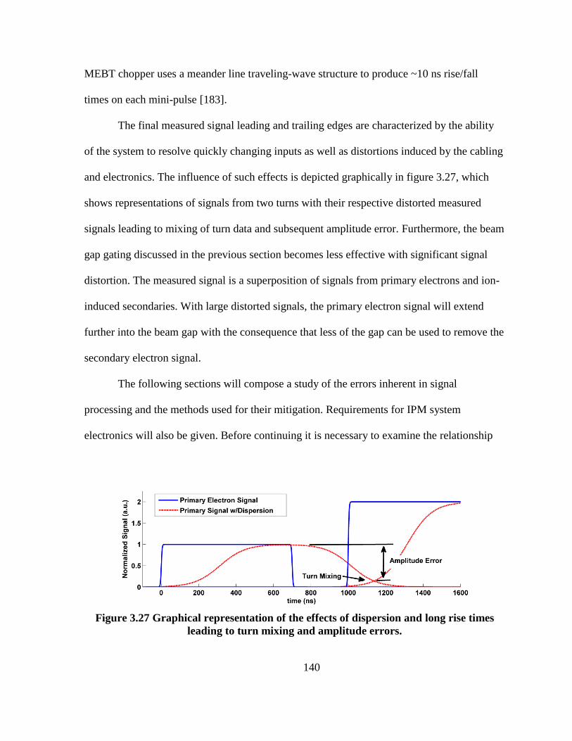
140

MEBT chopper uses a meander line traveling-wave structure to produce ~10 ns rise/fall

times on each mini-pulse [183].

The final measured signal leading and trailing edges are characterized by the ability

of the system to resolve quickly changing inputs as well as distortions induced by the cabling

and electronics. The influence of such effects is depicted graphically in figure 3.27, which

shows representations of signals from two turns with their respective distorted measured

signals leading to mixing of turn data and subsequent amplitude error. Furthermore, the beam

gap gating discussed in the previous section becomes less effective with significant signal

distortion. The measured signal is a superposition of signals from primary electrons and ion-

induced secondaries. With large distorted signals, the primary electron signal will extend

further into the beam gap with the consequence that less of the gap can be used to remove the

secondary electron signal.

The following sections will compose a study of the errors inherent in signal

processing and the methods used for their mitigation. Requirements for IPM system

electronics will also be given. Before continuing it is necessary to examine the relationship

Figure 3.27 Graphical representation of the effects of dispersion and long rise times

leading to turn mixing and amplitude errors.

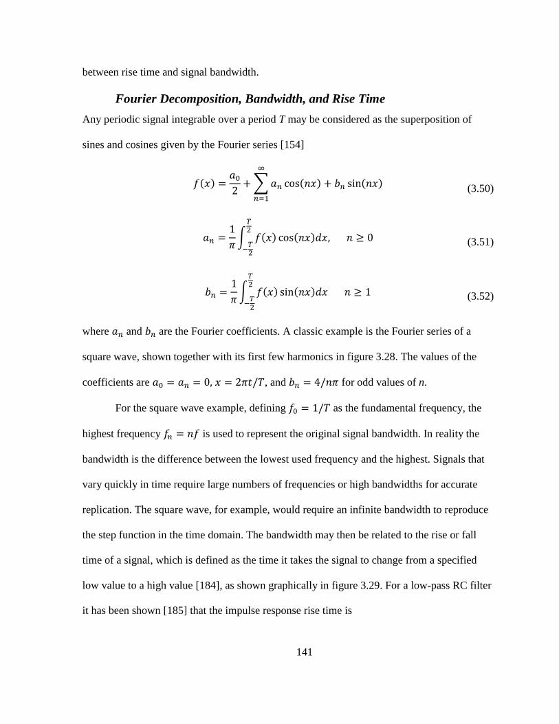
141

between rise time and signal bandwidth.

Fourier Decomposition, Bandwidth, and Rise Time

Any periodic signal integrable over a period T may be considered as the superposition of

sines and cosines given by the Fourier series [154]

∑

(3.50)

∫

(3.51)

∫

(3.52)

where and are the Fourier coefficients. A classic example is the Fourier series of a

square wave, shown together with its first few harmonics in figure 3.28. The values of the

coefficients are , and for odd values of n.

For the square wave example, defining as the fundamental frequency, the

highest frequency is used to represent the original signal bandwidth. In reality the

bandwidth is the difference between the lowest used frequency and the highest. Signals that

vary quickly in time require large numbers of frequencies or high bandwidths for accurate

replication. The square wave, for example, would require an infinite bandwidth to reproduce

the step function in the time domain. The bandwidth may then be related to the rise or fall

time of a signal, which is defined as the time it takes the signal to change from a specified

low value to a high value [184], as shown graphically in figure 3.29. For a low-pass RC filter

it has been shown [185] that the impulse response rise time is

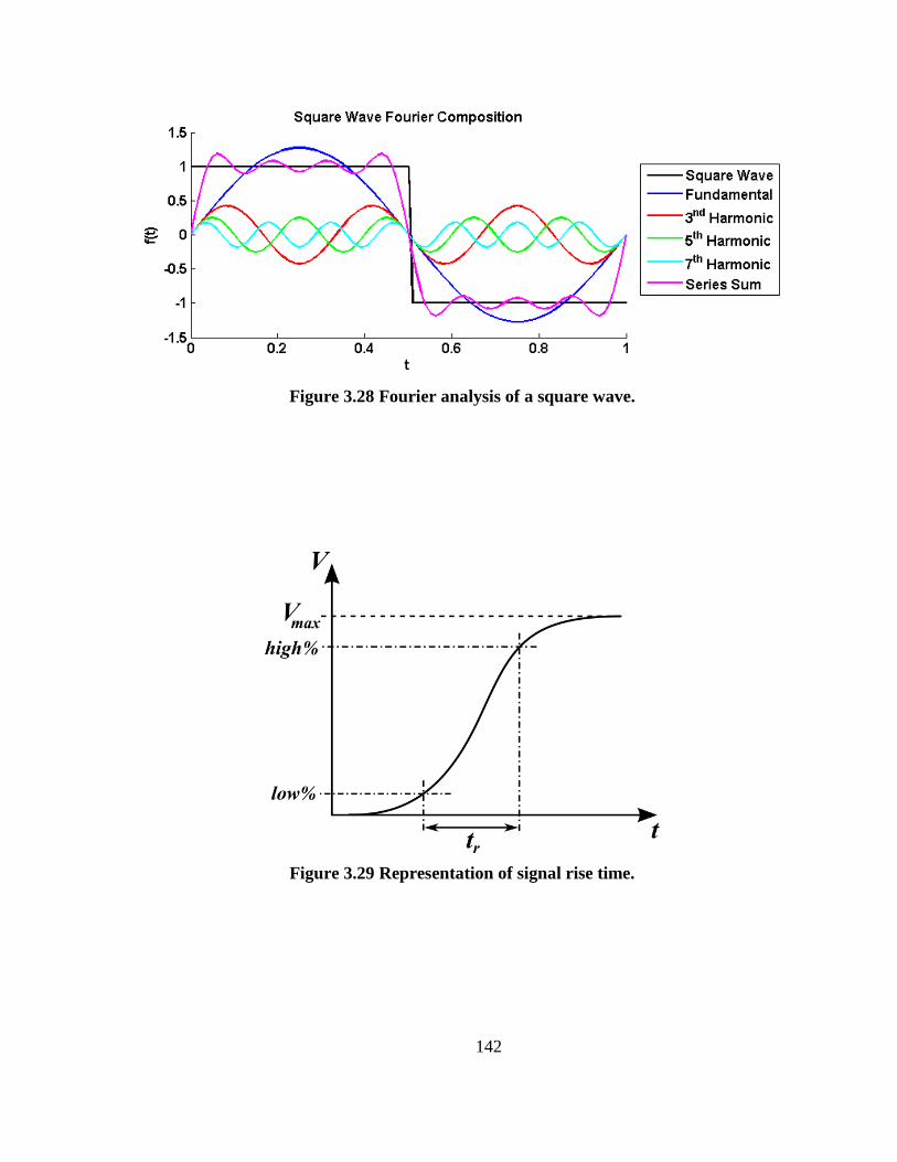
142

Figure 3.28 Fourier analysis of a square wave.

Figure 3.29 Representation of signal rise time.

143

(3.53)

where is the frequency at which the signal, in the frequency domain, has decreased by

3 dB and represents the bandwidth for a signal measured from 10% to 90% of the signal

maximum in the time domain. Equation (3.53) is often used a rule-of thumb estimate for

more complex signals, and for a 20 ns mini-pulse it gives a required bandwidth of 17.5 MHz.

However, bandwidth definitions are rather arbitrary and a more useful definition will be use

shortly.

Fourier Transform

While the Fourier series illustrates the principle of spectral decomposition, in practice it is

only applicable for periodic signals. However, it may generalized to arbitrary non-periodic

functions by using Euler’s identity

(3.54)

to recast equation in (3.50) with into a compact complex form [186]

∑ ⁄

∫

(3.55)

Non-periodic functions may be found as , which makes the fundamental angular

frequency ⁄ become infinitesimally small. Correspondingly,

→ making

the combination a continuous variable taking any value between and . With

this limiting procedure, it can be shown [186] that the Fourier series (3.55) becomes the

Fourier transform

144

∫

(3.56)

and the inverse Fourier transform

∫

(3.57)

The complex Fourier series and Fourier transform introduce negative frequencies

which act to split the energy of the signal in the frequency domain over a positive set of

frequencies and their negative frequency counterparts. The frequency domain of a signal has

many useful properties that will be exploited shortly.

Transfer Function

A transfer function H(t) relates the input of a system X(t) to the output of a system Y(t) in the

time domain in such a way that the output maybe found through convolution

(3.58)

The benefit of equation (3.58) is that convolution in the time becomes multiplication in the

frequency domain. Once the transfer function is known, the output may be found by taking

the inverse Fourier transform of the frequency domain response

(3.59)

For example an ideal cable would have an output signal identical to the input signal with a

transfer function , which is a Dirac delta function in the time domain.

Unfortunately no real cable has ideal characteristics and various distortions are introduced

during the ~300 m of cable length from the IPM location to the signal processing chassis in

the Ring Service Building (RSB).

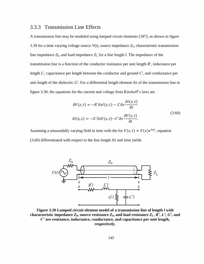
145

3.3.3 Transmission Line Effects

A transmission line may be modeled using lumped circuit elements [187], as shown in figure

3.30 for a time varying voltage source V(t), source impedance ZS, characteristic transmission

line impedance Z0, and load impedance ZL for a line length l. The impedance of the

transmission line is a function of the conductor resistance per unit length Rʹ, inductance per

length Lʹ, capacitance per length between the conductor and ground Cʹ, and conductance per

unit length of the dielectric Gʹ. For a differential length element of the transmission line in

figure 3.30, the equations for the current and voltage from Kirchoff’s laws are

(3.60)

Assuming a sinusoidally varying field in time with the for , equation

(3.60) differentiated with respect to the line length and time yields

Figure 3.30 Lumped circuit element model of a transmission line of length l with

characteristic impedance Z0, source resistance ZS, and load resistance ZL. R’, L’, G’, and

C’ are resistance, inductance, conductance, and capacitance per unit length,

respectively.

146

(3.61)

known as the telegrapher’s equations, where √ is the

propagation constant.

Transmission Line Solutions

Solutions to the telegrapher’s equations give the voltage and current in a transmission line.

They are composed of traveling waves

(3.62)

where and terms represent the incident and reflected voltage waves, respectively, and

√

(3.63)

is the characteristic impedance of the transmission line. The complex propagation constant is

separated into its real and imaginary parts in equation (3.62) as where is an

attenuation factor. It can be seen that if is the phase of the traveling wave, a phase

advance of 2π occurs when is multiplied by the wavelength . The factor ⁄

is the wave number which may be used to define the phase velocity of the transmission

line, which is

{√ }

(3.64)

From formula (3.64) is can be seen that the velocity is a function of the wave frequency .

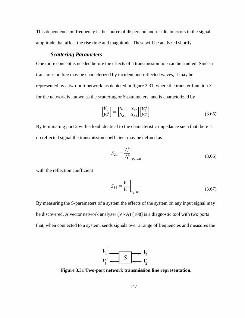
147

This dependence on frequency is the source of dispersion and results in errors in the signal

amplitude that affect the rise time and magnitude. These will be analyzed shortly.

Scattering Parameters

One more concept is needed before the effects of a transmission line can be studied. Since a

transmission line may be characterized by incident and reflected waves, it may be

represented by a two-port network, as depicted in figure 3.31, where the transfer function S

for the network is known as the scattering or S-parameters, and is characterized by

[

] [

] [

] (3.65)

By terminating port 2 with a load identical to the characteristic impedance such that there is

no reflected signal the transmission coefficient may be defined as

|

(3.66)

with the reflection coefficient

|

(3.67)

By measuring the S-parameters of a system the effects of the system on any input signal may

be discovered. A vector network analyzer (VNA) [188] is a diagnostic tool with two ports

that, when connected to a system, sends signals over a range of frequencies and measures the

Figure 3.31 Two-port network transmission line representation.

148

response. As a way of illustrating the effects the cable on the actual signal, the scattering

parameters were measured for a 70 m long RFS Cellflex SCF 14-50 coaxial cable. The

results of the VNA measurement are reported in figure 3.32 where the magnitude of

transmission parameter | | shown in the top trace and given in logarithmic units of dB,

shows attenuation at higher frequencies.

The attenuation is a combination resistive loss by the copper, dielectric loses from the

shielding, and loss of magnitude due to dispersion. The phase , shown in the

bottom trace with units of degrees, has had the electrical delay of cable removed in order

to remove the phase changes introduced by varying the input frequency due to

where the cable has 280.13 ns. While an ideal cable would have zero shift in

phase for all frequencies, clearly the real cable introduces a shift, see figure 3.32, and this

shift in phase is what results in phase dispersion.

Transmission Line Distortion

The measured S-parameters may be used to analyze the effect of a length of cable on signal

with beam characteristics. A normalized Gaussian pulse centered at zero with a standard

deviation chosen so that the 10% to 90% rise is equal to 10 ns is used as the input signal

⁄ . Its Fourier transform is also a Gaussian √ ⁄ . The cable

transfer function becomes

| | (3.68)

and therefore allows the system response to be found through the application of equation

(3.59), as illustrated in figure 3.33. The system response shows a number of important

characteristics typical of transmission lines. The loss of magnitude is a result of attenuation

and magnitude dispersion.

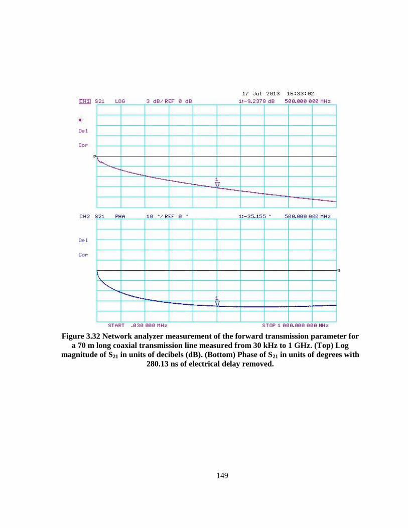
149

Figure 3.32 Network analyzer measurement of the forward transmission parameter for

a 70 m long coaxial transmission line measured from 30 kHz to 1 GHz. (Top) Log

magnitude of S21 in units of decibels (dB). (Bottom) Phase of S21 in units of degrees with

280.13 ns of electrical delay removed.

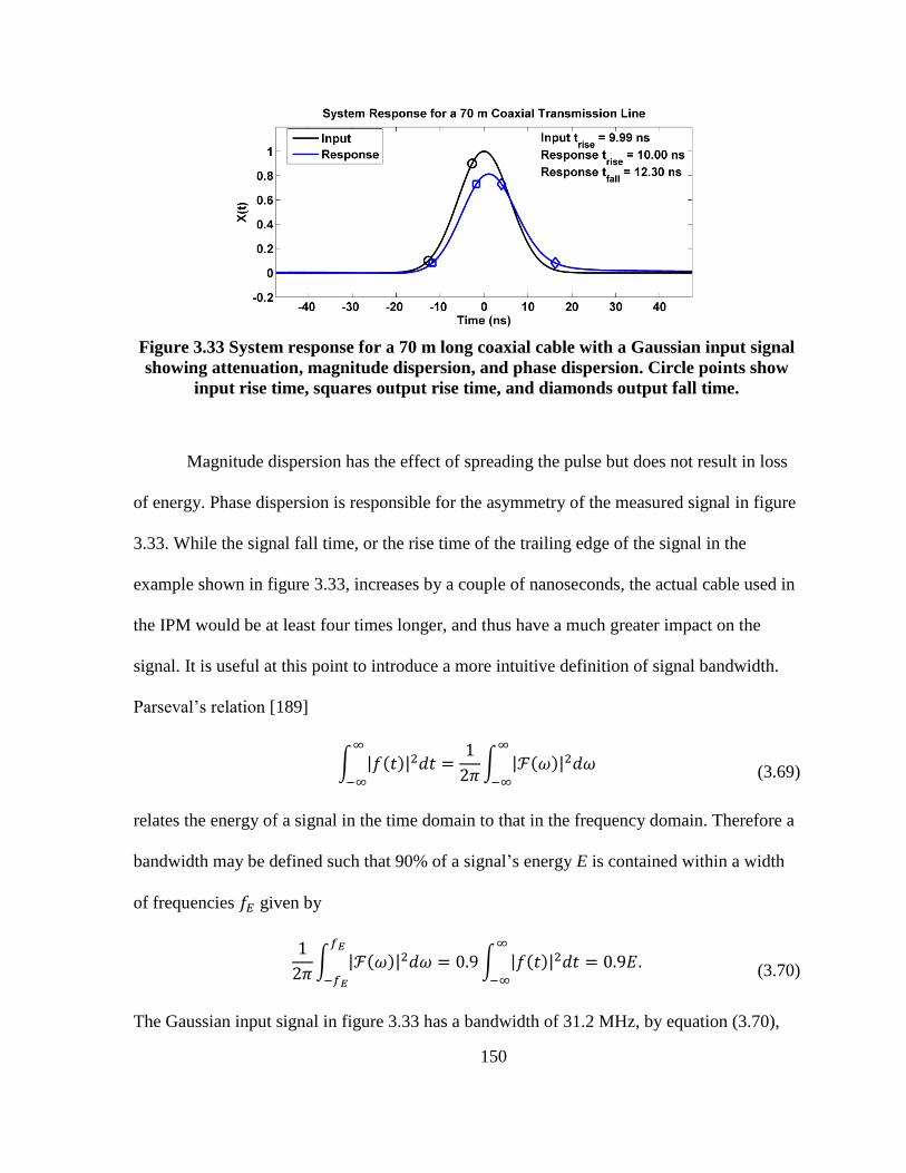
150

Figure 3.33 System response for a 70 m long coaxial cable with a Gaussian input signal

showing attenuation, magnitude dispersion, and phase dispersion. Circle points show

input rise time, squares output rise time, and diamonds output fall time.

Magnitude dispersion has the effect of spreading the pulse but does not result in loss

of energy. Phase dispersion is responsible for the asymmetry of the measured signal in figure

3.33. While the signal fall time, or the rise time of the trailing edge of the signal in the

example shown in figure 3.33, increases by a couple of nanoseconds, the actual cable used in

the IPM would be at least four times longer, and thus have a much greater impact on the

signal. It is useful at this point to introduce a more intuitive definition of signal bandwidth.

Parseval’s relation [189]

∫ | |

∫ | |

(3.69)

relates the energy of a signal in the time domain to that in the frequency domain. Therefore a

bandwidth may be defined such that 90% of a signal’s energy E is contained within a width

of frequencies given by

∫ | |

∫ | |

(3.70)

The Gaussian input signal in figure 3.33 has a bandwidth of 31.2 MHz, by equation (3.70),

151

for a 10 ns rise time, which is more signal-specific than formula (3.53).

Composite Rise Time

For the IPM system with an input signal rise time including a detector, cabling, and

electronics, the final measured rise time [190] is

√

(3.71)

or in the frequency domain

√

(3.72)

where the more conservative 3 dB bandwidth has been used. The amplifiers and electronics

for the system will need to be chosen with sufficient bandwidth that the combined rise time is

not more than 20 ns. For example, a pulse with a 10 ns rise time going through a Channeltron

which has a 3-5 ns rise time followed by a 10 ns cable rise time and 13.2 ns of electronics

rise time would have a resultant rise time of 20 ns.

Cable De-Embedding

It is possible to reduce the effect of the cable through digital signal processing techniques. If

the transmission parameter of a cable can be measured with a network analyzer, then

once the signal has been digitized, a filter can be applied that reverses the effect of cable

dispersion and returns the original signal. The process, described in detail in [191], applies a

filter of the form

(3.73)

where is a windowing function chosen to take advantage of the full spectrum of

152

frequencies under consideration and is the electrical time delay. By using the

aforementioned technique, the distortions produced by the ~300 m cable length may be

mitigated, allowing for better turn-by-turn resolution. Furthermore, de-embedding methods

may be used on any linear circuit element.

Open Wire Effects

Another aspect of the signal path is the connection from the Ctron to the cable carrying the

signal to the electronics. The Channeltron electron multiplication tube terminates in a metal

cap with a wire to transport the charge. This wire is subject to capacitive coupling to the

surrounding chamber as well as to dispersion due to self-inductance. Current in the wire

generates a magnetic field according to Ampere’s law. If the current is varying in time a

voltage will be produced in the conductor according to Faraday’s law, which acts according

to Lenz’s law to generate a current producing a magnetic field opposed to the original. A

conductor’s property to generate a self-imposed opposing magnetic field is known as self-

inductance.

The self-inductance of an open straight wire of length l and diameter d in centimeters

has been shown [192] to be

[ (

)

] (3.74)

given in units of nanohenries, and is valid for frequencies at which the skin effect is

negligible. Formula (3.74) becomes

[ (

) ] (3.75)

for higher frequency signals where there is no current in the interior of the conductor. The

transmission parameter for the open wire may modeled with a simple inductor in series with

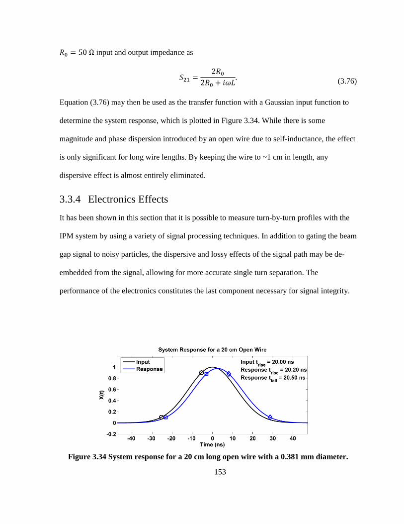
153

input and output impedance as

(3.76)

Equation (3.76) may then be used as the transfer function with a Gaussian input function to

determine the system response, which is plotted in Figure 3.34. While there is some

magnitude and phase dispersion introduced by an open wire due to self-inductance, the effect

is only significant for long wire lengths. By keeping the wire to ~1 cm in length, any

dispersive effect is almost entirely eliminated.

3.3.4 Electronics Effects

It has been shown in this section that it is possible to measure turn-by-turn profiles with the

IPM system by using a variety of signal processing techniques. In addition to gating the beam

gap signal to noisy particles, the dispersive and lossy effects of the signal path may be de-

embedded from the signal, allowing for more accurate single turn separation. The

performance of the electronics constitutes the last component necessary for signal integrity.

Figure 3.34 System response for a 20 cm long open wire with a 0.381 mm diameter.

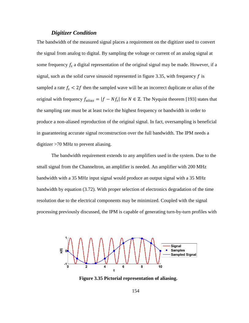
154

Digitizer Condition

The bandwidth of the measured signal places a requirement on the digitizer used to convert

the signal from analog to digital. By sampling the voltage or current of an analog signal at

some frequency a digital representation of the original signal may be made. However, if a

signal, such as the solid curve sinusoid represented in figure 3.35, with frequency is

sampled a rate then the sampled wave will be an incorrect duplicate or alias of the

original with frequency | | for . The Nyquist theorem [193] states that

the sampling rate must be at least twice the highest frequency or bandwidth in order to

produce a non-aliased reproduction of the original signal. In fact, oversampling is beneficial

in guaranteeing accurate signal reconstruction over the full bandwidth. The IPM needs a

digitizer >70 MHz to prevent aliasing.

The bandwidth requirement extends to any amplifiers used in the system. Due to the

small signal from the Channeltron, an amplifier is needed. An amplifier with 200 MHz

bandwidth with a 35 MHz input signal would produce an output signal with a 35 MHz

bandwidth by equation (3.72). With proper selection of electronics degradation of the time

resolution due to the electrical components may be minimized. Coupled with the signal

processing previously discussed, the IPM is capable of generating turn-by-turn profiles with

Figure 3.35 Pictorial representation of aliasing.

155

electrons.

3.4 Simulation Summary

A thorough study through simulation of various aspects IPM system, using the ORBIT IPM

module to model track ionized particle trajectories, was performed. Based on fundamental

principles, an IPM system is capable of delivering turn-by-turn profiles in the SNS ring with

an accuracy of 10% on the rms beam size using electrons. Furthermore, it has been shown in

this section that it is possible to measure profiles with sufficient time resolution by using a

variety of signal processing techniques. In addition to gating the beam gap signal to noisy

particles the dispersive and lossy effects of the signal path may be de-embedded from the

signal, allowing for more accurate single turn separation.

Design Parameters

With the completion of the analysis of the system operation it is now possible to outline a list

of design parameters with which to use in developing a physical system.

1) The beam pipe diameter in the IPM location is 25.4 cm but the effective

diameter over which IPM fields need to be designed is 60 mm.

2) A 120 kV bias potential is required to reduce the profile spreading for ions

and the errors from ion-induced secondary electrons, as well as to mitigate

turn mixing due to ion collection times.

3) In electron collection mode a 300 G magnetic field is required to confine

electrons to a Larmor radius such that the particle trajectory distortion is half

of a Channeltron width.

4) Approximately 38 Channeltron measurement positions are needed across the

IPM range in order to minimize systematic measurement errors.

156

5) The actuator driving the detector needs to have a position accuracy of

±0.5 mm.

6) Deviations in the ionized particle trajectory due to nonuniformity in the IPM

electric bias and magnetic fields over the beam region must be less than or

equal to half the Channeltron width.

7) Titanium nitride coating and secondary electron suppression must be included

in the final design.

8) Care must be taken to minimize the Channeltron’s open wire length to <1 cm.

With the outlined parameters it is possible to design an ionization profile monitor capable of

measuring transverse profiles that meet the system requirements in table 1.2.

157

Chapter 4

Prototyping and Measurement

The theoretical basis and system analysis presented in the previous chapters provides an

argument for the validity and ability of the IPM system to accurately measure beam profiles

and outlines the necessary parameters a design would have to meet to do so. However, in

order to guarantee the operational principles as well to determine unforeseen aspects of the

accelerator environment, a prototype was needed before a final design could be established.

Consequently, this chapter discusses the IPM test chamber that was built and installed along

with the results of measurements and modifications that were added.

This chapter is composed of a description of the test chamber design and installation

as well as considerations that went into the initial design. A summary of the progression of

the test chamber is given along with modifications. Results of a study of the ion and electron

signals are given followed by a summary of the design parameters derived from the test

chamber data that are necessary to the final design.

158

4.1 IPM Test Chamber

4.1.1 Design Considerations

The IPM test chamber was conceived as a simple system that incorporated the main

operational principles of the full-scale IPM but that could be built quickly and cheaply with

minimal inconvenience to the accelerator’s operation. As such, the primary focus of the test

chamber was to show that a Channeltron-based system could measure turn-by-turn profiles.

Since the only methods of Ctron profile measurement are either moving the detector with

some form of actuator or having multiple Channeltrons requiring several power supplies,

generating a full transverse profile was beyond the scope of the test chamber.

An IPM test chamber consisting of a single Channeltron fixed in the center of the

transverse beam dimension with a high voltage electrode of arbitrary geometry located

directly opposite the detector, to supply a bias voltage, was sufficient to test the basic IPM

properties. A power supply was required to bias the Channeltron and a separate high voltage

supply was required for the bias plate. An amplifier and oscilloscope were used to measure

the Ctron current.

4.1.2 Test Chamber Design

Vacuum Chamber

It was desirable to use as many off-the-shelf components in the construction as possible in

order to keep cost and construction time low. The IPM test chamber vacuum chamber is a 10

x 8 inch 304 stainless steel Conflat 4-way cross with 0.062 inch thick walls. The 10 inch

diameter cross pipe connects to the beam pipe and the 8 inch pipe is used for the detector and

high voltage (HV) plate. Figure 4.1 shows the full setup of the test chamber. Conflat flanges

159

Figure 4.1 IPM test chamber setup and components consisting of chamber, high voltage

bias plate, high voltage feedthrough, high voltage, power supply cable, and Channeltron

assembly

160

with vacuum seal rings were used to mount to the main chamber.

High Voltage Bias

The high voltage bias plate is a 6 inch diameter circular disc mounted directly over top of the

Channeltron where all the plate edges have a 0.25 in radius. An edge radius allows a high

voltage to be applied without arcing inside the vacuum chamber (an in-depth arcing

mitigation study will be presented in the next chapter). The bias plate is held in place by a set

screw that tightens to the center conductor of a HV 70 kV vacuum feedthrough. The air side

of the HV feedthrough has a 7 in diameter cylindrical grounded metal enclosure that provides

personnel safety against high voltage and arcing dangers. The shielding enclosure also serves

the purpose of supporting the end section of the HV cable connecting the power supply to the

HV feedthrough. A chain of twelve 470 Ω, 5 W resistors imbedded into the end of the cable

act as a load for power supply protection so, in the event of an arc, the surge of current will

be dissipated across the resistor chain and not damage the supply. Unfortunately, this makes

the last 3 feet of the HV cable very stiff and thus requires support. The shielding enclosure

also has an access port so that the connection to the HV feedthrough may be made.

A Glassman WR Series 100 kV high voltage power supply with digital readouts and

reversible polarity was used. By removing the outer cover of the unit and changing a module,

the polarity of the potential supplied to the bias plate may be reversed; allowing for test

chamber measurement of ions or electrons. The power supply was located in the ring service

building basement.

161

Channeltron Assembly

The Channeltron assembly consists of an L-bracket to which was attached an electrically

insulating Macor10

[194] block. A single detector was mounted to the block in the center of

the beam pipe such that its longest opening dimension was perpendicular to the beam

direction. Two vacuum feedthroughs passed the Ctron biasing conductor and the signal wire.

A Spellman 3 kV reversible polarity high voltage power supply was used to operate the

Channeltron. In order to shield the Channeltron from the electric fields produced by the

beam, a flat wire mesh disc approximately 3 inches in diameter was fixed to the Ctron

mounting bracket and centered over the detector opening.

Installation

Upon acquisition and assembly of the components, the test chamber was leak tested to ensure

compatibility with the SNS ring vacuum. Additionally, a high voltage test was performed

before installation to verify the capabilities of the system. The setup for the high voltage test,

performed with the vacuum chamber at 10-8

Torr, is shown in the left image of figure 4.2.

The middle of figure 4.2 shows the shielding enclosure with the access panel removed to

reveal the high voltage feedthrough for the bias plate with electrically insulating Kapton11

[195] tape to reduce arcing. A bias plate voltage of 60 kV was achieved. A section of empty

beam pipe was removed and the IPM test chamber was installed in the ring D straight, just

upstream of the RF section and directly in front of the wall current monitor. The right image

in figure 4.2 shows the final installation. The actual IPM will be located on the downstream

side of the RF cavities.

10

Macor is a registered trademark of Corning Inc. 11

Kapton is a registered trademark of E.I. du Pont de Nemours and Company

162

Figure 4.2 (Left) Experimental setup of high voltage test under UHV conditions.

(Middle) Air side of the HV bias plate feedthrough with electrically insulating Kapton

tape. (Right) Installed IPM test chamber.

4.2 Test Chamber Results and Modifications

Achieving the desired results in the IPM test chamber proved challenging and involved a

process of trial and error. There were a number of unforeseen elements of the accelerator

environment that had a significant effect on the measured signal. The final outcome was

productive both in providing a proof-of-principle measurement as well as in elucidating a

variety of issues that needed to be addressed in the final design. While the actual process of

producing successful test chamber results was an iterative progression of measurement and

chamber modification, the following section will summarize the measurements taken and the

modifications made to address system problems.

Desired Test Chamber Result

A correct Ctron measurement of the beam in the ring should be characterized by DC current

pulses with no AC behavior. Furthermore, since the Ctron functions as an electron source and

the current direction is defined as opposite the flow of electrons, the voltage measured across

the oscilloscope load resistor is negative. A measured test chamber signal on an oscilloscope

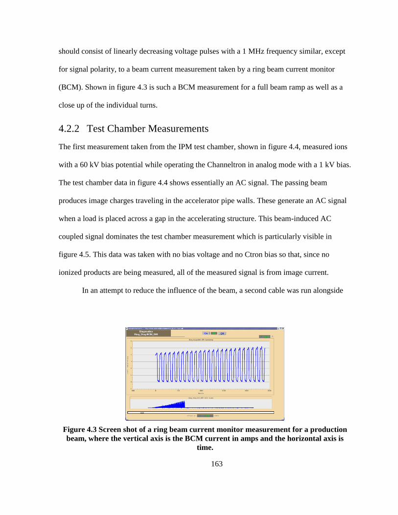
163

should consist of linearly decreasing voltage pulses with a 1 MHz frequency similar, except

for signal polarity, to a beam current measurement taken by a ring beam current monitor

(BCM). Shown in figure 4.3 is such a BCM measurement for a full beam ramp as well as a

close up of the individual turns.

4.2.2 Test Chamber Measurements

The first measurement taken from the IPM test chamber, shown in figure 4.4, measured ions

with a 60 kV bias potential while operating the Channeltron in analog mode with a 1 kV bias.

The test chamber data in figure 4.4 shows essentially an AC signal. The passing beam

produces image charges traveling in the accelerator pipe walls. These generate an AC signal

when a load is placed across a gap in the accelerating structure. This beam-induced AC

coupled signal dominates the test chamber measurement which is particularly visible in

figure 4.5. This data was taken with no bias voltage and no Ctron bias so that, since no

ionized products are being measured, all of the measured signal is from image current.

In an attempt to reduce the influence of the beam, a second cable was run alongside

Figure 4.3 Screen shot of a ring beam current monitor measurement for a production

beam, where the vertical axis is the BCM current in amps and the horizontal axis is

time.

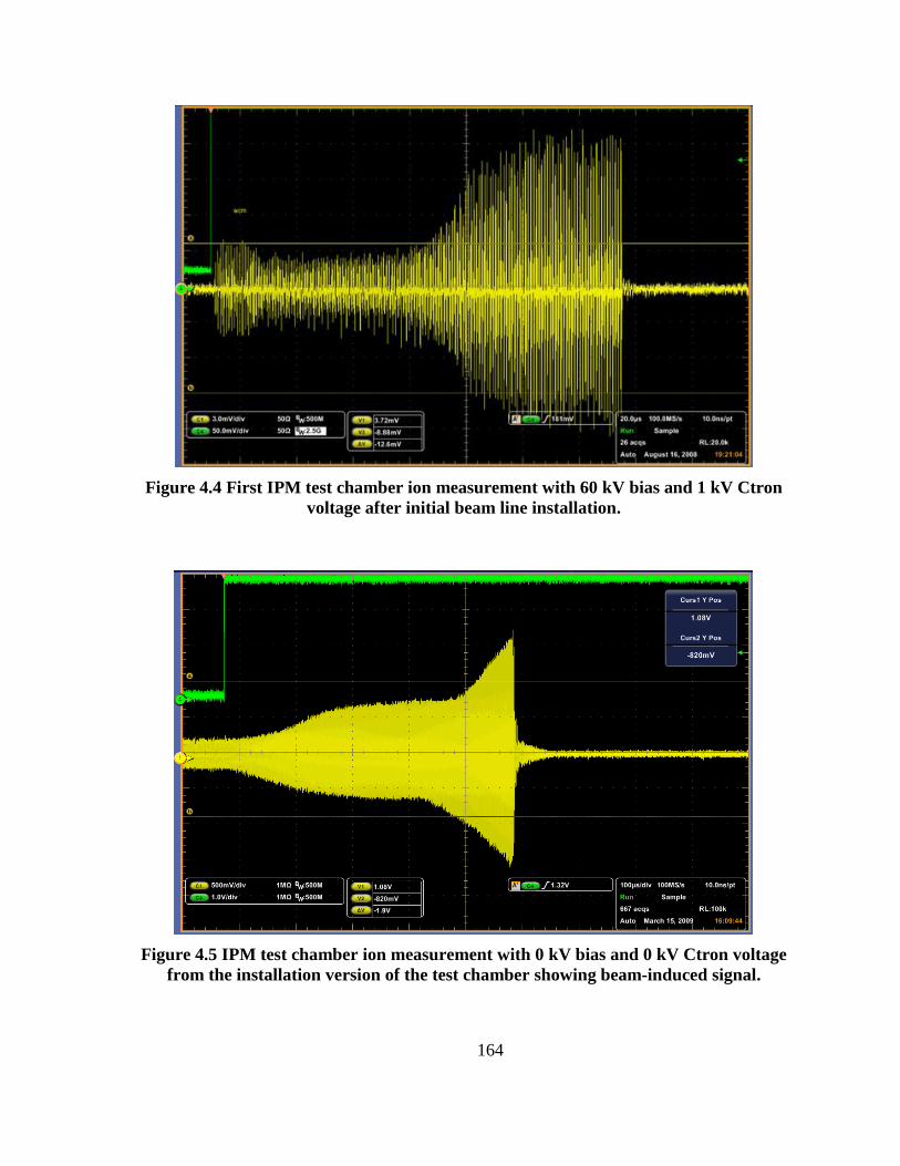
164

Figure 4.4 First IPM test chamber ion measurement with 60 kV bias and 1 kV Ctron

voltage after initial beam line installation.

Figure 4.5 IPM test chamber ion measurement with 0 kV bias and 0 kV Ctron voltage

from the installation version of the test chamber showing beam-induced signal.

165

the original cables and connected to the beam pipe in order to subtract the common mode

from the Channeltron signal. This proved unsuccessful and the additional cable was left

unterminated in tunnel. Furthermore, additional measurements revealed that the unterminated

cable measured a significant amount of signal, suggesting that the tunnel environment was

inducing parasitic noise through the cabling. A measurement using electrons was done by

reversing the polarity of the bias plate potential. Results were also inconclusive due to the

large AC signal.

4.2.3 Test Chamber Modifications

Vacuum Chamber and Cabling Modifications

Upon analysis of the original test chamber design, a number of design flaws became

apparent. Figure 4.6 (a) shows an analysis of the initial test chamber. The Ctron signal

coaxial cable was grounded to the beam pipe, which constituted a direct path for image

current to enter the signal. Furthermore, much of the detector and wiring were exposed to the

beam, allowing capacitive coupling by the beam into the measurement.

The test chamber was modified as explained in figure 4.6 (b) to include isolated

feedthroughs that allowed the Ctron signal cable’s ground to be floated from the beam pipe.

A picture of the Channeltron with ground isolation wiring is shown at the left of figure 4.7,

while the right side shows a cutaway drawing of the detector inside a grounded metal

shielding can with an opening at the Ctron entrance to isolate the detector from the beam.

Later, the shield enclosure was also modified to include a metal mesh over the detection

opening to further reduce capacitive coupling. While the modifications did clean the IPM

signal to some degree there is was still a significant contribution of environmental noise

coupled into the actual

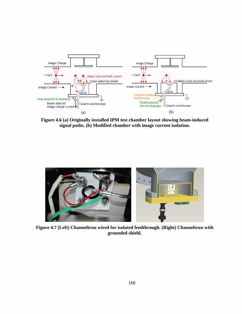
166

Figure 4.6 (a) Originally installed IPM test chamber layout showing beam-induced

signal paths. (b) Modified chamber with image current isolation.

Figure 4.7 (Left) Channeltron wired for isolated feedthrough. (Right) Channeltron with

grounded shield.

167

measurement.

Upon further examination it was determined that the cable being used for the Ctron

signal was an unshielded cable which followed a path that ran next to the nearby RF cavities.

New fully shielded cables were run, one for the Ctron signal and one for background

subtraction, along a path away from the RF cavities. Also, a FEMTO DHCPA-100 high

speed current amplifier was used in the RSB just before the oscilloscope to amplify the

signal.

Modified Measurement Results

Measurements were taken for a production quality beam ~800 kW, figure 4.3. Test chamber

results for ions and electrons are reported in figure 4.8 and figure 4.9. With the previously

discussed test chamber modifications, a signal was finally measured that showed the beam

ramping. Unfortunately the variable gain amplifier used only had a bandwidth of 1 MHz,

which was insufficient to resolve turn-by-turn behavior

While this iteration of the test chamber proved successful in generating a

measurement of the beam ramping by measuring ionization products, there was still

excessive AC coupling. Since the amplifier was at the end of the signal path it was

amplifying parasitic cable noise as well as the desired signal. By placing the amplifier in the

tunnel immediately after the test chamber, it would be possible to greatly increase the signal

to noise ratio.

The electron measurement in figure 4.9 exhibited behavior that resembled saturation

due to the flattening of the data near the end of accumulation cycle. An unknown oscillation

was also present at the beginning of the ramp. Results from a study of the electron signal

peculiarities will be given shortly.

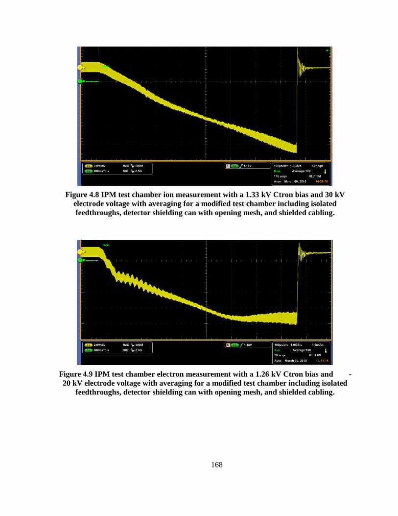
168

Figure 4.8 IPM test chamber ion measurement with a 1.33 kV Ctron bias and 30 kV

electrode voltage with averaging for a modified test chamber including isolated

feedthroughs, detector shielding can with opening mesh, and shielded cabling.

Figure 4.9 IPM test chamber electron measurement with a 1.26 kV Ctron bias and -

20 kV electrode voltage with averaging for a modified test chamber including isolated

feedthroughs, detector shielding can with opening mesh, and shielded cabling.

169

4.2.4 Test Chamber RF Noise

RF Interference Measurement Results

A FEMTO HCA-40M-100K-C current amplifier with a 40 MHz bandwidth and 105 gain was

installed in the ring tunnel within a meter of the test chamber. However, initial measurements

showed a considerable AC signal. Further study, presented in figure 4.11, revealed that, for

the condition of no beam present, no electrode voltage, and the Channeltron turned off, there

was an AC signal from the test chamber when the RF cavities were on (figure 4.10) and none

when they were off (figure 4.11). By grounding the amplifier casing, the RF noise could be

significantly reduced, as displayed in figure 4.12.

RF Mitigation

With a modified test chamber and grounded amplifier, the IPM test chamber was finally able

to produce turn-by-turn beam measurements. Data from an ion measurement is shown in

figure 4.13 with electron results in figure 4.14. In both measurements the background was

subtracted by using a 0 kV Ctron bias measurement along with an inversion of the data to

compare to BCM waveforms. Individual turns may be seen in the 5μs snapshot displayed in

figure 4.15, which was taken from the figure 4.13 ion signal, which has a frequency of

~1.03 MHz.

4.3 Test Chamber Signal Study

4.3.1 Ion Signal

While the ion signal showed the best correlation with BCM measurements, it still exhibited

undesirable behavior. In order to explore the signal, measurements were taken for a range of

Channeltron biases to determine whether the effects where related to the detector or to a

combination of the beam and residual gas. A 2000 point moving average was used to

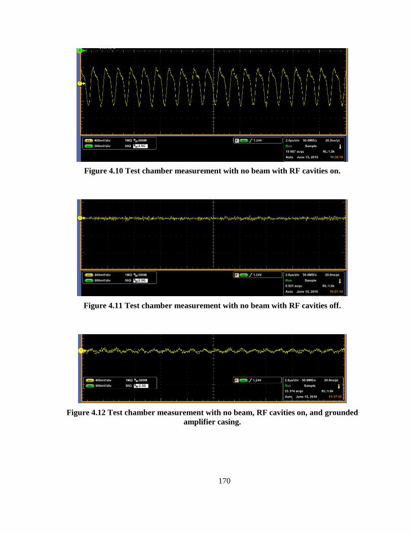
170

Figure 4.10 Test chamber measurement with no beam with RF cavities on.

Figure 4.11 Test chamber measurement with no beam with RF cavities off.

Figure 4.12 Test chamber measurement with no beam, RF cavities on, and grounded

amplifier casing.

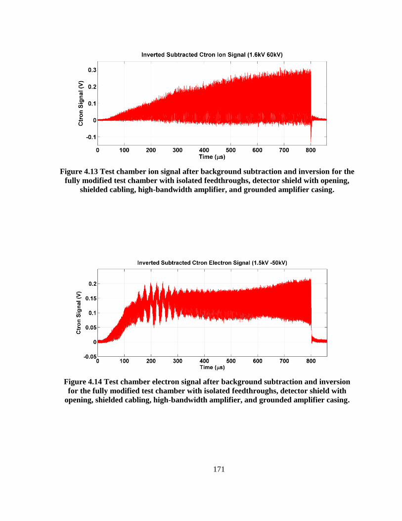
171

Figure 4.13 Test chamber ion signal after background subtraction and inversion for the

fully modified test chamber with isolated feedthroughs, detector shield with opening,

shielded cabling, high-bandwidth amplifier, and grounded amplifier casing.

Figure 4.14 Test chamber electron signal after background subtraction and inversion

for the fully modified test chamber with isolated feedthroughs, detector shield with

opening, shielded cabling, high-bandwidth amplifier, and grounded amplifier casing.

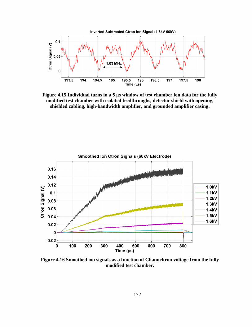
172

Figure 4.15 Individual turns in a 5 μs window of test chamber ion data for the fully

modified test chamber with isolated feedthroughs, detector shield with opening,

shielded cabling, high-bandwidth amplifier, and grounded amplifier casing.

Figure 4.16 Smoothed ion signals as a function of Channeltron voltage from the fully

modified test chamber.

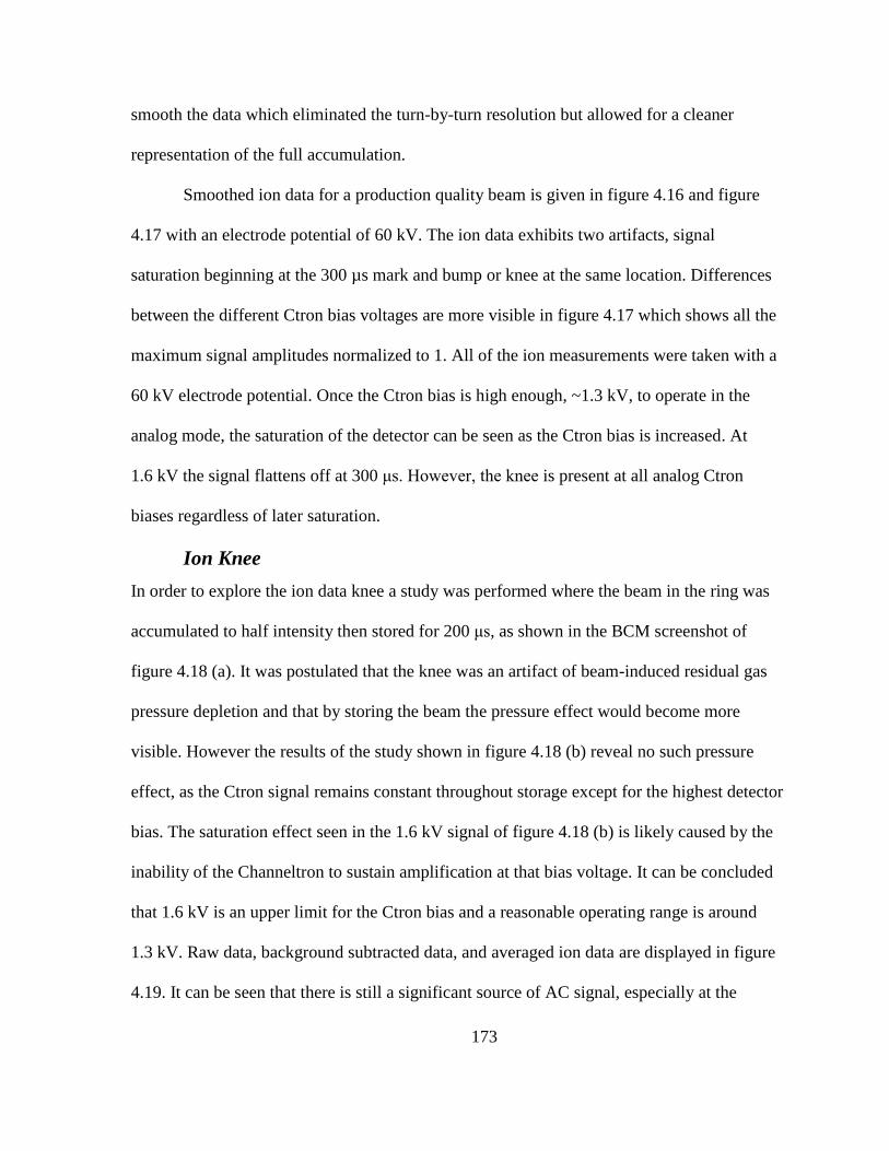
173

smooth the data which eliminated the turn-by-turn resolution but allowed for a cleaner

representation of the full accumulation.

Smoothed ion data for a production quality beam is given in figure 4.16 and figure

4.17 with an electrode potential of 60 kV. The ion data exhibits two artifacts, signal

saturation beginning at the 300 µs mark and bump or knee at the same location. Differences

between the different Ctron bias voltages are more visible in figure 4.17 which shows all the

maximum signal amplitudes normalized to 1. All of the ion measurements were taken with a

60 kV electrode potential. Once the Ctron bias is high enough, ~1.3 kV, to operate in the

analog mode, the saturation of the detector can be seen as the Ctron bias is increased. At

1.6 kV the signal flattens off at 300 μs. However, the knee is present at all analog Ctron

biases regardless of later saturation.

Ion Knee

In order to explore the ion data knee a study was performed where the beam in the ring was

accumulated to half intensity then stored for 200 μs, as shown in the BCM screenshot of

figure 4.18 (a). It was postulated that the knee was an artifact of beam-induced residual gas

pressure depletion and that by storing the beam the pressure effect would become more

visible. However the results of the study shown in figure 4.18 (b) reveal no such pressure

effect, as the Ctron signal remains constant throughout storage except for the highest detector

bias. The saturation effect seen in the 1.6 kV signal of figure 4.18 (b) is likely caused by the

inability of the Channeltron to sustain amplification at that bias voltage. It can be concluded

that 1.6 kV is an upper limit for the Ctron bias and a reasonable operating range is around

1.3 kV. Raw data, background subtracted data, and averaged ion data are displayed in figure

4.19. It can be seen that there is still a significant source of AC signal, especially at the

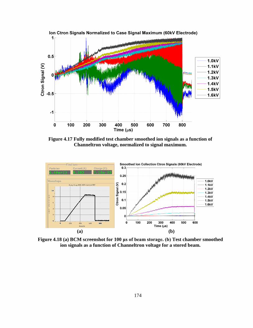
174

Figure 4.17 Fully modified test chamber smoothed ion signals as a function of

Channeltron voltage, normalized to signal maximum.

(a) (b)

Figure 4.18 (a) BCM screenshot for 100 μs of beam storage. (b) Test chamber smoothed

ion signals as a function of Channeltron voltage for a stored beam.

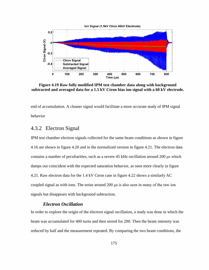
175

Figure 4.19 Raw fully modified IPM test chamber data along with background

subtracted and averaged data for a 1.5 kV Ctron bias ion signal with a 60 kV electrode.

end of accumulation. A cleaner signal would facilitate a more accurate study of IPM signal

behavior

4.3.2 Electron Signal

IPM test chamber electron signals collected for the same beam conditions as shown in figure

4.16 are shown in figure 4.20 and in the normalized version in figure 4.21. The electron data

contains a number of peculiarities, such as a severe 45 kHz oscillation around 200 μs which

damps out coincident with the expected saturation behavior, as seen more clearly in figure

4.21. Raw electron data for the 1.4 kV Ctron case in figure 4.22 shows a similarly AC

coupled signal as with ions. The noise around 200 μs is also seen in many of the raw ion

signals but disappears with background subtraction.

Electron Oscillation

In order to explore the origin of the electron signal oscillation, a study was done in which the

beam was accumulated for 400 turns and then stored for 200. Then the beam intensity was

reduced by half and the measurement repeated. By comparing the two beam conditions, the

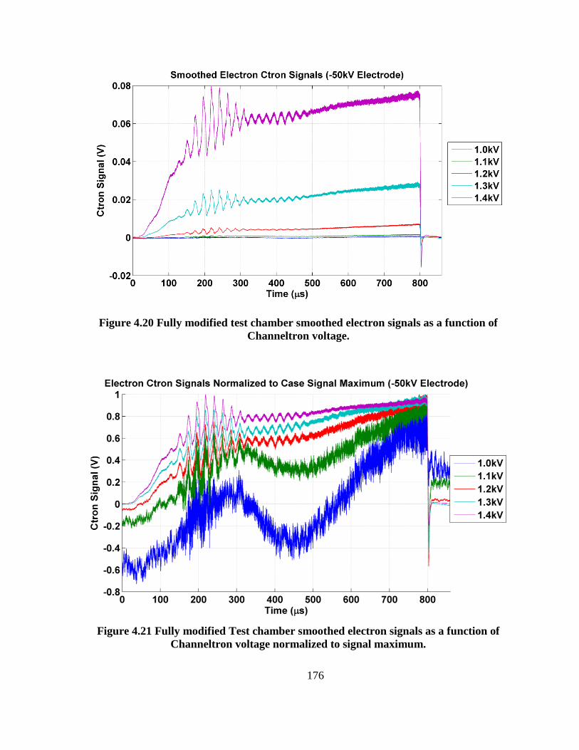
176

Figure 4.20 Fully modified test chamber smoothed electron signals as a function of

Channeltron voltage.

Figure 4.21 Fully modified Test chamber smoothed electron signals as a function of

Channeltron voltage normalized to signal maximum.

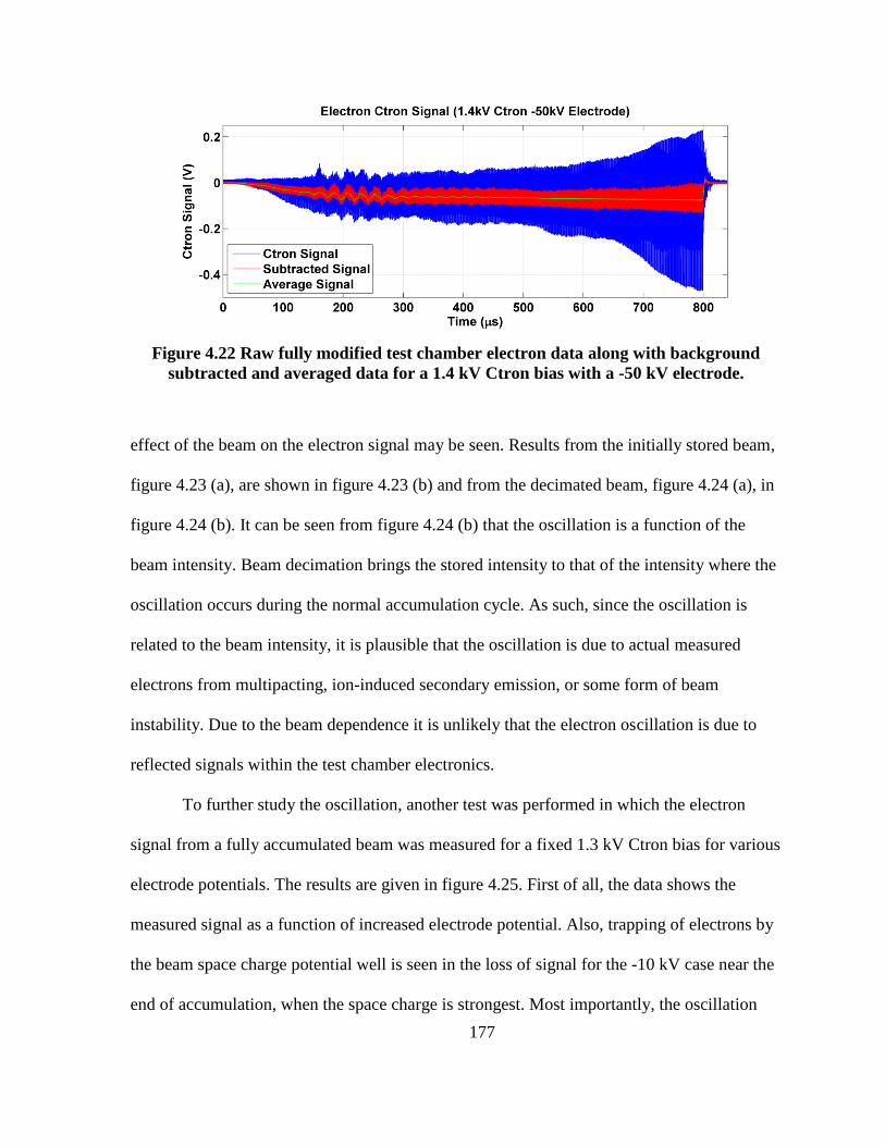
177

Figure 4.22 Raw fully modified test chamber electron data along with background

subtracted and averaged data for a 1.4 kV Ctron bias with a -50 kV electrode.

effect of the beam on the electron signal may be seen. Results from the initially stored beam,

figure 4.23 (a), are shown in figure 4.23 (b) and from the decimated beam, figure 4.24 (a), in

figure 4.24 (b). It can be seen from figure 4.24 (b) that the oscillation is a function of the

beam intensity. Beam decimation brings the stored intensity to that of the intensity where the

oscillation occurs during the normal accumulation cycle. As such, since the oscillation is

related to the beam intensity, it is plausible that the oscillation is due to actual measured

electrons from multipacting, ion-induced secondary emission, or some form of beam

instability. Due to the beam dependence it is unlikely that the electron oscillation is due to

reflected signals within the test chamber electronics.

To further study the oscillation, another test was performed in which the electron

signal from a fully accumulated beam was measured for a fixed 1.3 kV Ctron bias for various

electrode potentials. The results are given in figure 4.25. First of all, the data shows the

measured signal as a function of increased electrode potential. Also, trapping of electrons by

the beam space charge potential well is seen in the loss of signal for the -10 kV case near the

end of accumulation, when the space charge is strongest. Most importantly, the oscillation

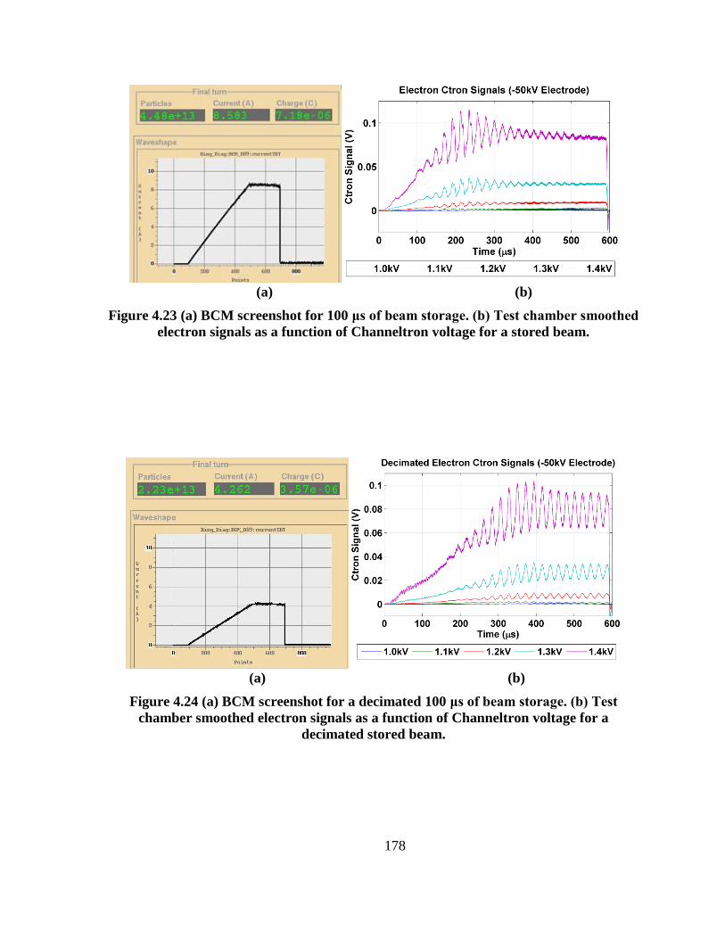
178

(a) (b)

Figure 4.23 (a) BCM screenshot for 100 μs of beam storage. (b) Test chamber smoothed

electron signals as a function of Channeltron voltage for a stored beam.

(a) (b)

Figure 4.24 (a) BCM screenshot for a decimated 100 μs of beam storage. (b) Test

chamber smoothed electron signals as a function of Channeltron voltage for a

decimated stored beam.

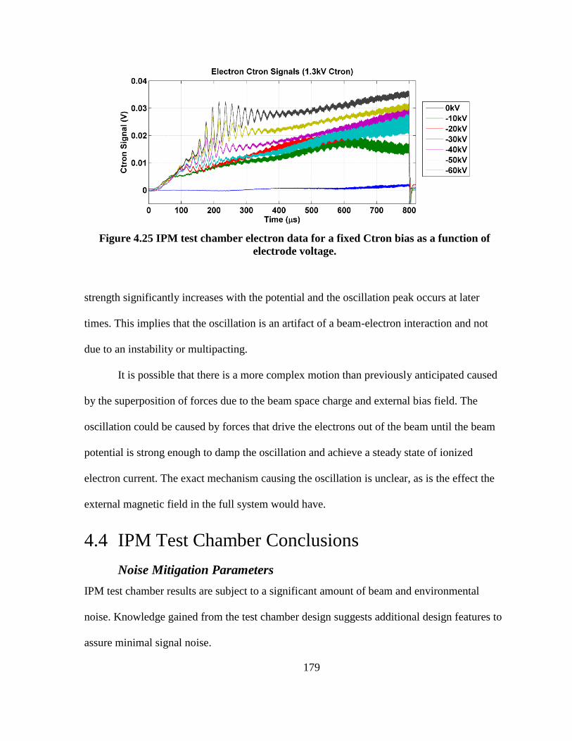
179

Figure 4.25 IPM test chamber electron data for a fixed Ctron bias as a function of

electrode voltage.

strength significantly increases with the potential and the oscillation peak occurs at later

times. This implies that the oscillation is an artifact of a beam-electron interaction and not

due to an instability or multipacting.

It is possible that there is a more complex motion than previously anticipated caused

by the superposition of forces due to the beam space charge and external bias field. The

oscillation could be caused by forces that drive the electrons out of the beam until the beam

potential is strong enough to damp the oscillation and achieve a steady state of ionized

electron current. The exact mechanism causing the oscillation is unclear, as is the effect the

external magnetic field in the full system would have.

4.4 IPM Test Chamber Conclusions

Noise Mitigation Parameters

IPM test chamber results are subject to a significant amount of beam and environmental

noise. Knowledge gained from the test chamber design suggests additional design features to

assure minimal signal noise.

180

1) In order to isolate the Channeltron from beam image current, isolated

feedthroughs must be used and signal cable grounds must be floated from

beam pipe.

2) Capacitive coupling from the beam directly to the detector hardware may be

prevented by installing a fully encompassing grounded shield.

3) A method of background subtraction is necessary for accelerator environment

noise.

4) Amplifiers installed in the ring tunnel must have grounded casings to reduce

RF noise.

5) All cabling needs to shielded and cable paths chosen such that proximity to

significant RF sources is reduced.

Signal Study Conclusions

Results from the final test chamber showed that the system is capable of measuring turn-by-

turn signals. While the measurements taken do not fully explain the ion data knee, current

postulations regard it as related to difficulty in differentiating between signal and noise. The

electron oscillation is related to the beam intensity and electrode potential. Reduction of

secondary electrons as well as the introduction of the electron collection magnet could have a

significant effect on the electron signal. Further measurements with a complete IPM system

will be necessary to characterize the electron behavior.

181

Chapter 5

IPM System Design

With the completion of an analysis of the fundamental principles for IPM operation,

simulations to determine the design parameters, and experimental system verification with

the test chamber, a final system can be designed. This chapter will describe the final design

by major component such as the electrode, magnet, vacuum chamber, detector assembly,

cabling, and high voltage feedthrough. Design considerations and methods will be presented

for each component. Individual components will be related to the larger system framework

culminating in a completed system.

5.1 Electrode Design

One of the components of the IPM system that nearly the entire system is built around is the

bias electrode. Its size determines the vacuum chamber dimensions which in turn determines

the magnet dimensions. The electrode was primarily designed with field uniformity in mind

and then modified to accommodate additional aspects such as arcing mitigation and

secondary electron reduction.

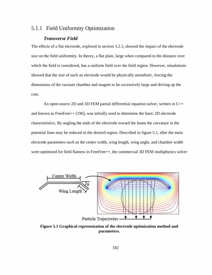
182

5.1.1 Field Uniformity Optimization

Transverse Field

The effects of a flat electrode, explored in section 3.2.3, showed the impact of the electrode

size on the field uniformity. In theory, a flat plate, large when compared to the distance over

which the field is considered, has a uniform field over the field region. However, simulations

showed that the size of such an electrode would be physically unrealistic, forcing the

dimensions of the vacuum chamber and magnet to be excessively large and driving up the

cost.

An open-source 2D and 3D FEM partial differential equation solver, written in C++

and known as FreeFem++ [196], was initially used to determine the basic 2D electrode

characteristics. By angling the ends of the electrode toward the beam the curvature in the

potential lines may be reduced in the desired region. Described in figure 5.1, after the main

electrode parameters such as the center width, wing length, wing angle, and chamber width

were optimized for field flatness in FreeFem++, the commercial 3D FEM multiphysics solver

Figure 5.1 Graphical representation of the electrode optimization method and

parameters.

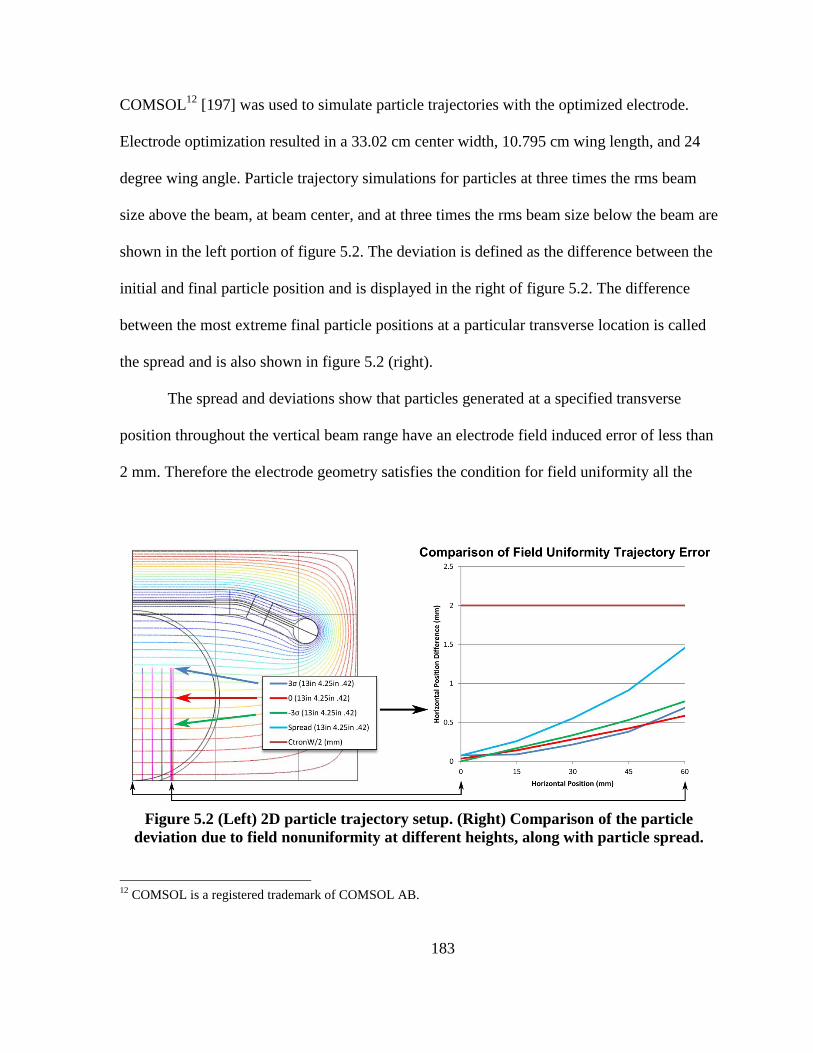
183

COMSOL12

[197] was used to simulate particle trajectories with the optimized electrode.

Electrode optimization resulted in a 33.02 cm center width, 10.795 cm wing length, and 24

degree wing angle. Particle trajectory simulations for particles at three times the rms beam

size above the beam, at beam center, and at three times the rms beam size below the beam are

shown in the left portion of figure 5.2. The deviation is defined as the difference between the

initial and final particle position and is displayed in the right of figure 5.2. The difference

between the most extreme final particle positions at a particular transverse location is called

the spread and is also shown in figure 5.2 (right).

The spread and deviations show that particles generated at a specified transverse

position throughout the vertical beam range have an electrode field induced error of less than

2 mm. Therefore the electrode geometry satisfies the condition for field uniformity all the

Figure 5.2 (Left) 2D particle trajectory setup. (Right) Comparison of the particle

deviation due to field nonuniformity at different heights, along with particle spread.

12

COMSOL is a registered trademark of COMSOL AB.

184

way out to 60 mm from the beam center.

Longitudinal Field

The longitudinal field distribution suffers from limitations in the flexibility of the electrode

longitudinal geometry. Due to the condition that the electrode must not reduce the aperture of

the beam pipe, longitudinal field shaping wings extending around the ionization region may

not be used as they were for the transverse electrode dimension. Field uniformity is then only

accomplished by electrode size. Limitations on the longitudinal length of the vacuum

chamber due to the associated cost mean that a completely uniform longitudinal field is not

possible.

A simulation of the longitudinal electrode potential and particle trajectories is given

in figure 5.3 (a). Particles experience an outward force from the electrode centerline due to

field nonuniformity. Depending on the height above the detector, particles created in the

volume above the Channeltron will miss the detector opening. This lost signal contributes to

profile errors as discussed in section 3.2. The number of particles collected is a function of

the longitudinal electrode because larger longitudinal lengths yield flatter central fields.

Particles from the top of the beam are most affected. Figure 5.3 (b) gives the percentage

collected from the top of the beam as a function of electrode length. Due to spatial

constraints, a longitudinal electrode length of 25.4 cm was chosen. From figure 5.3 (b), 42%

of the top particles will be lost. To minimize profile errors from low-signal statistics, the

number of collected accumulation cycles must be increased to compensate for longitudinal

particle losses. The number of summed macro-pulses should be increased from 100, given in

section 2.3.2, to 200 to guarantee sufficient signal, especially in the first few turns.

185

(a) (b)

Figure 5.3 (a) Longitudinal electrode particle trajectories. (b) Percentage of top beam

particles collected due longitudinal field nonuniformity.

Alignment Tolerance

A 2D transverse simulation was performed in which the optimized electrode was rotated

about its center to determine the effect of a misalignment inside the vacuum chamber. If the

flat center part of the electrode is not parallel with detector plane, particles will receive a

trajectory displacement. Results of the study showed that a maximum angle of 0.7 degree

between the electrode center and detector plane could be tolerated before the particles were

displaced more than 2 mm. This corresponds to a 6.3 mm tolerance in the difference between

the bottom edges of the ends of the electrode and the plane of detection depicted in figure

5.4. Actual alignment errors are expected to less than a few millimeters, as specified in the

design documents.

5.1.2 Vacuum Breakdown

Applying a high voltage across a gas filled gap can cause arcing between the electrode

surfaces. The design of HV components to deal with such phenomena has been the subject of

much study [134], [198], [199]. The voltage at which a gas will break down and sustain an

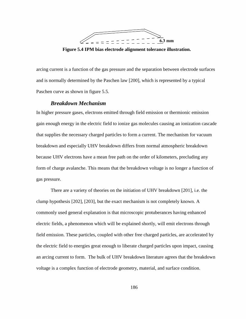
186

Figure 5.4 IPM bias electrode alignment tolerance illustration.

arcing current is a function of the gas pressure and the separation between electrode surfaces

and is normally determined by the Paschen law [200], which is represented by a typical

Paschen curve as shown in figure 5.5.

Breakdown Mechanism

In higher pressure gases, electrons emitted through field emission or thermionic emission

gain enough energy in the electric field to ionize gas molecules causing an ionization cascade

that supplies the necessary charged particles to form a current. The mechanism for vacuum

breakdown and especially UHV breakdown differs from normal atmospheric breakdown

because UHV electrons have a mean free path on the order of kilometers, precluding any

form of charge avalanche. This means that the breakdown voltage is no longer a function of

gas pressure.

There are a variety of theories on the initiation of UHV breakdown [201], i.e. the

clump hypothesis [202], [203], but the exact mechanism is not completely known. A

commonly used general explanation is that microscopic protuberances having enhanced

electric fields, a phenomenon which will be explained shortly, will emit electrons through

field emission. These particles, coupled with other free charged particles, are accelerated by

the electric field to energies great enough to liberate charged particles upon impact, causing

an arcing current to form. The bulk of UHV breakdown literature agrees that the breakdown

voltage is a complex function of electrode geometry, material, and surface condition.

187

Figure 5.5 Typical Paschen curve.

Maximum UHV Field Limit

The IPM electrode poses a significant arcing hazard. An arcing event has the potential to

permanently damage system components as well as to degrade the ring vacuum. Ensuring the

electrode and chamber are designed well within an arcing limit is a high design priority.

Much of high voltage design in the ultrahigh vacuum limit is based on experimental results

for specific electrode materials and geometries.

A review of high voltage design literature shows that stainless steel in the 10-5

to 10-8

Torr range can sustain a maximum electric field of ~6 kV/mm before vacuum breakdown, for

electrode gaps on the order of a few centimeters [201]. Other sources [134], [204] predict a

maximum breakdown for clean, well-conditioned surfaces at a DC 120 kV potential of

6.7 kV/mm. In order to account for uncertainties attributed to the IPM electrode, a maximum

field limit of 4.5 kV/mm was adopted. This includes a 32% safety margin.

Electrode Preparation

Further steps should be taken in the preparation and operation of the electrode to reduce

possible arcing. A study [198] gave experimental evidence that polishing the electrode

surface to remove imperfections can have a significant effect on arcing stability.

Furthermore, surface preparation techniques discussed in [134] should be followed. These

188

include a 25 μm “mirror” polish and an ultrasonic bath of trichloroethylene, acetone,

methanol and distilled water while keeping the electrode in as clean an environment as

possible. It should be noted that isopropyl alcohol should be avoided as a cleaning agent on

steel as it becomes trapped in the steel surface and constitutes a significant outgassing source

[69]. Deinoized water may be used as a substitute. Conditioning is a process where, upon

installation or chamber venting, the electrode voltage is slowly raised until an arc occurs and

then held at that potential until the voltage is stable for ~1 minute. This allows the electric

field to “burn off” small surface impurities leading to more stable operation at higher

potentials. This technique was used successfully during installation and operation of the IPM

test chamber.

5.1.3 Field Reduction

Parallel Plane Effect

Electrode arcing mitigation consists of identifying the electric field contributions,

determining the controllable physical variables, and optimizing in accordance with the

previously determined field limit. The first and simplest electrode field contribution is that of

the fields produced by flat surfaces parallel to the flat chamber walls. These parallel planes

separated by a distance d produce a uniform electric field given by

(5.1)

for a potential V. According to equation (5.1), the distance between flat electrodes for a

120 kV potential and 4.5 kV/mm field is 27 mm. This sets the minimum distance

between the electrode and the chamber walls.

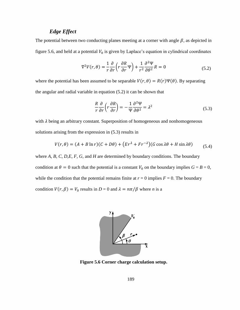
189

Edge Effect

The potential between two conducting planes meeting at a corner with angle , as depicted in

figure 5.6, and held at a potential is given by Laplace’s equation in cylindrical coordinates

(

)

(5.2)

where the potential has been assumed to be separable . By separating

the angular and radial variable in equation (5.2) it can be shown that

(

)

(5.3)

with being an arbitrary constant. Superposition of homogeneous and nonhomogeneous

solutions arising from the expression in (5.3) results in

( ) (5.4)

where A, B, C, D,E, F, G, and H are determined by boundary conditions. The boundary

condition at such that the potential is a constant on the boundary implies G = B = 0,

while the condition that the potential remains finite at r = 0 implies F = 0. The boundary

condition results in D = 0 and ⁄ where n is a

Figure 5.6 Corner charge calculation setup.

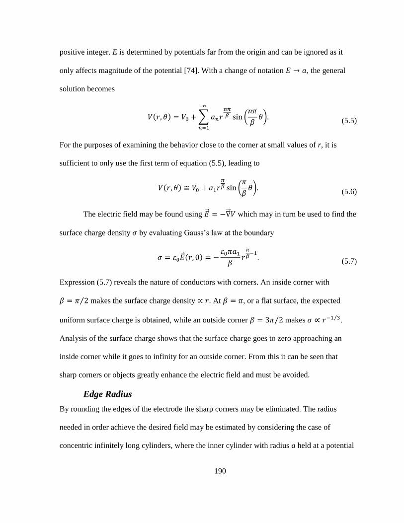
190

positive integer. E is determined by potentials far from the origin and can be ignored as it

only affects magnitude of the potential [74]. With a change of notation , the general

solution becomes

∑ (

)

(5.5)

For the purposes of examining the behavior close to the corner at small values of r, it is

sufficient to only use the first term of equation (5.5), leading to

(

)

(5.6)

The electric field may be found using which may in turn be used to find the

surface charge density by evaluating Gauss’s law at the boundary

(5.7)

Expression (5.7) reveals the nature of conductors with corners. An inside corner with

⁄ makes the surface charge density . At , or a flat surface, the expected

uniform surface charge is obtained, while an outside corner ⁄ makes ⁄ .

Analysis of the surface charge shows that the surface charge goes to zero approaching an

inside corner while it goes to infinity for an outside corner. From this it can be seen that

sharp corners or objects greatly enhance the electric field and must be avoided.

Edge Radius

By rounding the edges of the electrode the sharp corners may be eliminated. The radius

needed in order achieve the desired field may be estimated by considering the case of

concentric infinitely long cylinders, where the inner cylinder with radius a held at a potential

191

represents the electrode edge and the outer grounded cylinder of radius b represents the

chamber wall. Axial symmetry guarantees no angular dependence, and according to Gauss’s

law the electric field at a radial position r from the center is given by

( ⁄ )

(5.8)

Using the fact the field is a maximum on the inner cylinder surface, equation (5.8) solved for

the outer cylinder radius b is minimized when a = 27 mm. The gap between the inner and

outer cylinder is then 45 mm. Instead of making a solid electrode of thickness 60 mm, which

would be extremely heavy, or a hollow electrode which would be difficult to fabricate, a

single solid stainless steel electrode of thickness 6.35 mm with cylindrical endcaps may be

used, as illustrated in figure 5.7.

Corner Radius

The second source of field enhancement occurs at the four corners of the electrode. While

rounding the edges generates curvature in a single plane, the corners must be rounded in two

dimensions, which further increases the field and requires larger radii. Effects of corner

radiusing may be initially estimated using concentric spheres with an inner sphere of radius a

at potential and outer grounded sphere with radius b. The electric field at a distance r

between the spheres is

(5.9)

Setting yields an inner radius a of 54 mm, corresponding to a minimum

gap of 54 mm.

192

Figure 5.7 Transverse and longitudinal electrode profiles with field reduction caps.

Modeling and Optimization

Using the previous estimations, a 3D model was built in COMSOL, figure 5.8 (a), to

simulate and optimize the electrode geometry based on the maximum field limit. In order to

achieve simulation accuracy a fine mesh of tetrahedral elements was used for modeling the

curved regions. Figure 5.8 (b) illustrates how finer meshing parameters were used on curves

and in regions of two- plane curvature where the highest electric fields were expected.

Optimal electrode geometry was achieved by adjusting parameters such as the edge and

corner radii as well as the chamber dimensions.

The results of an electrostatic simulation of the electrode in the IPM chamber are

presented in figure 5.9 showing surface electric field magnitude along with dimensions of the

finalized electrode and vacuum chamber. A maximum field of 4.5 kV/mm occurs on the

corner radius, which satisfies the UHV arcing limit. Further simulations showed that the

chamber modifications as well as the addition of end caps produced no significant

modifications to the particle trajectories.

5.1.4 Insulating Standoffs

Preceding analysis of the electrode has omitted any form of support structure. In order to

hold it in place while maintaining electrical isolation, a dielectric insulating standoff must be

used. Introduction of such an insulator adds new arcing paths that must be taken into

consideration. Bulk breakdown occurs when the electric field in the volume of the dielectric

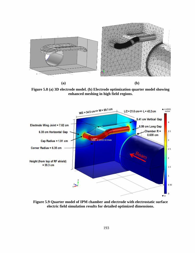
193

(a) (b)

Figure 5.8 (a) 3D electrode model. (b) Electrode optimization quarter model showing

enhanced meshing in high field regions.

Figure 5.9 Quarter model of IPM chamber and electrode with electrostatic surface

electric field simulation results for detailed optimized dimensions.

194

is large enough to cause a significant number of electrons to be excited into the material’s

conduction band, forming a current. When the dielectric begins to conduct the electrical

breakdown current can permanently damaging the insulator.

Bulk electrical breakdown is represented by the material’s dielectric strength, which

is the maximum field tolerable. The dielectric strength has a value of 11 kV/mm for the

insulators being considered here [205]. Insulator breakdown is of little concern in the IPM

since the fields are guaranteed to be lower than 4.5 kV/mm and even less on the flat surfaces.

A more significant source of insulator arcing exists that requires special design

considerations.

Surface Flashover Mechanism

Surface flashover is a major source of insulator arcing and refers to an arcing path that

develops along an insulator surface, often at electric fields lower than for bulk breakdown.

While surface flashover has been the subject of much study [206–208], a complete theory has

not been reached. Origination of surface flashover is generally attributed to electron emission

by field or thermal emission from a triple point. A triple point is an interface where the

insulator contacts the electrode and shares a boundary with a vacuum or gas. This point is

subject to enhanced electric fields and will be discussed shortly.

Theories [206] for the formation stage of flashover are illustrated in figure 5.10,

where the left model represents triple point emitted electrons striking the insulator surface,

causing an avalanche of secondaries. The middle model represents bursts of electrons that

form successive charged regions creating an avalanche mechanism. The right image of figure

5.10 illustrates theories not involving avalanches, such as gas discharge from the insulator

surface by electron impact. It is generally agreed upon that the final stage of flashover occurs

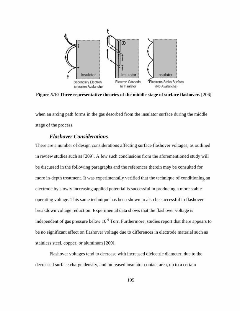
195

Figure 5.10 Three representative theories of the middle stage of surface flashover. [206]

when an arcing path forms in the gas desorbed from the insulator surface during the middle

stage of the process.

Flashover Considerations

There are a number of design considerations affecting surface flashover voltages, as outlined

in review studies such as [209]. A few such conclusions from the aforementioned study will

be discussed in the following paragraphs and the references therein may be consulted for

more in-depth treatment. It was experimentally verified that the technique of conditioning an

electrode by slowly increasing applied potential is successful in producing a more stable

operating voltage. This same technique has been shown to also be successful in flashover

breakdown voltage reduction. Experimental data shows that the flashover voltage is

independent of gas pressure below 10-6

Torr. Furthermore, studies report that there appears to

be no significant effect on flashover voltage due to differences in electrode material such as

stainless steel, copper, or aluminum [209].

Flashover voltages tend to decrease with increased dielectric diameter, due to the

decreased surface charge density, and increased insulator contact area, up to a certain

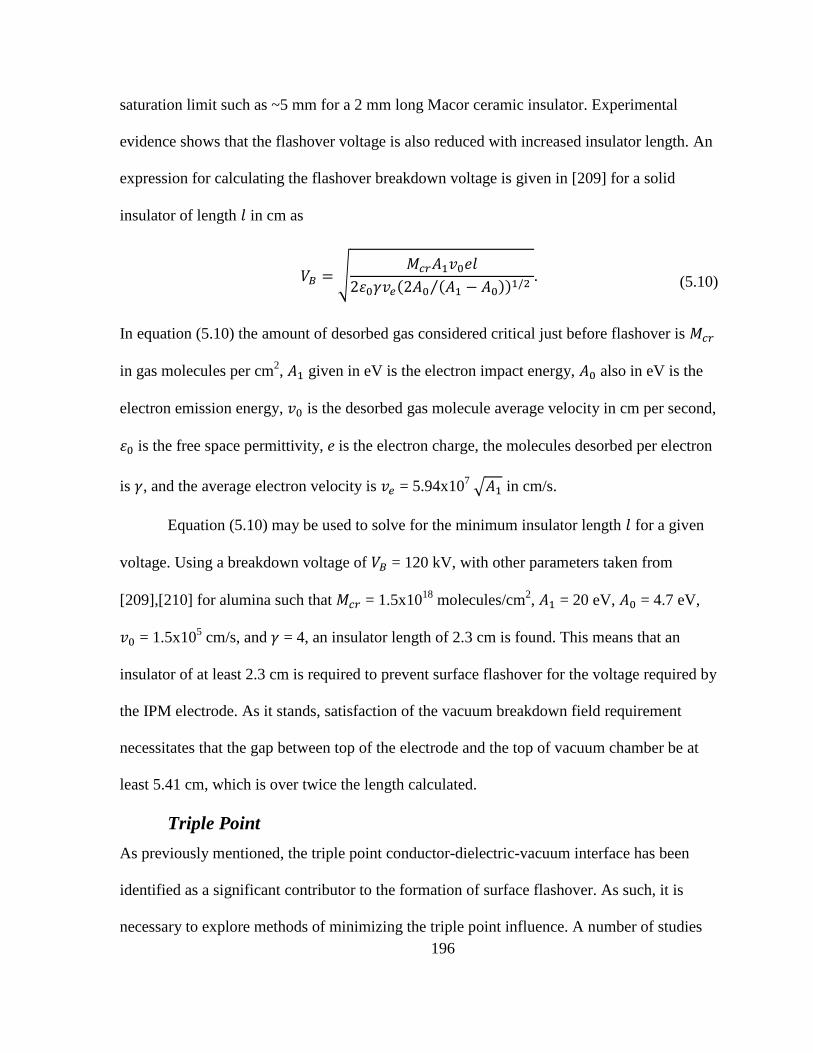
196

saturation limit such as ~5 mm for a 2 mm long Macor ceramic insulator. Experimental

evidence shows that the flashover voltage is also reduced with increased insulator length. An

expression for calculating the flashover breakdown voltage is given in [209] for a solid

insulator of length in cm as

√

⁄ (5.10)

In equation (5.10) the amount of desorbed gas considered critical just before flashover is

in gas molecules per cm2, given in eV is the electron impact energy, also in eV is the

electron emission energy, is the desorbed gas molecule average velocity in cm per second,

is the free space permittivity, e is the electron charge, the molecules desorbed per electron

is , and the average electron velocity is = 5.94x107 √ in cm/s.

Equation (5.10) may be used to solve for the minimum insulator length for a given

voltage. Using a breakdown voltage of = 120 kV, with other parameters taken from

[209],[210] for alumina such that = 1.5x1018

molecules/cm2, = 20 eV, = 4.7 eV,

= 1.5x105 cm/s, and = 4, an insulator length of 2.3 cm is found. This means that an

insulator of at least 2.3 cm is required to prevent surface flashover for the voltage required by

the IPM electrode. As it stands, satisfaction of the vacuum breakdown field requirement

necessitates that the gap between top of the electrode and the top of vacuum chamber be at

least 5.41 cm, which is over twice the length calculated.

Triple Point

As previously mentioned, the triple point conductor-dielectric-vacuum interface has been

identified as a significant contributor to the formation of surface flashover. As such, it is

necessary to explore methods of minimizing the triple point influence. A number of studies

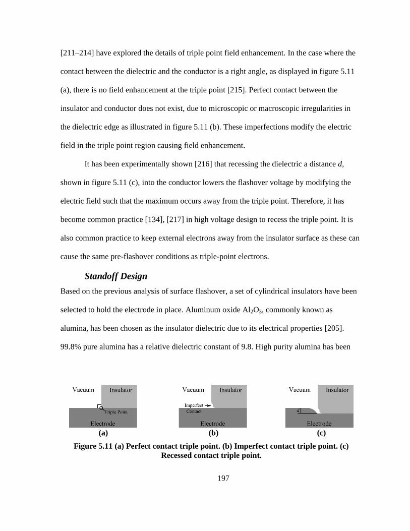
197

[211–214] have explored the details of triple point field enhancement. In the case where the

contact between the dielectric and the conductor is a right angle, as displayed in figure 5.11

(a), there is no field enhancement at the triple point [215]. Perfect contact between the

insulator and conductor does not exist, due to microscopic or macroscopic irregularities in

the dielectric edge as illustrated in figure 5.11 (b). These imperfections modify the electric

field in the triple point region causing field enhancement.

It has been experimentally shown [216] that recessing the dielectric a distance d,

shown in figure 5.11 (c), into the conductor lowers the flashover voltage by modifying the

electric field such that the maximum occurs away from the triple point. Therefore, it has

become common practice [134], [217] in high voltage design to recess the triple point. It is

also common practice to keep external electrons away from the insulator surface as these can

cause the same pre-flashover conditions as triple-point electrons.

Standoff Design

Based on the previous analysis of surface flashover, a set of cylindrical insulators have been

selected to hold the electrode in place. Aluminum oxide Al2O3, commonly known as

alumina, has been chosen as the insulator dielectric due to its electrical properties [205].

99.8% pure alumina has a relative dielectric constant of 9.8. High purity alumina has been

(a) (b) (c)

Figure 5.11 (a) Perfect contact triple point. (b) Imperfect contact triple point. (c)

Recessed contact triple point.

198

successfully used in other areas of the SNS accelerator and is easily purchased off the shelf

from a number of vendors. Four 1.27 cm diameter unglazed 99.5% alumina 6.35 cm long

standoffs are fitted into 6.35 mm deep recessed holes with a 3.3 mm hole edge radius, as

shown in figure 5.12. The insulators are on the opposite side of the electrode from the beam

and the electrode produces strong electric field lines parallel to the standoff surface. Because

of this, and the presence of the external magnetic field, electrons produced away from the

insulator are not expected to be a source of flashover initiation.

The electrode has a mass of 19.1 kg giving it a weight of 187 N. With a tensile

strength of 25,000 psi, four 1.27 cm diameter alumina standoffs could hold a force of 43 kN

normal to the standoff endface, which is well above the electrode weight in the horizontal

IPM system. Flexural strength describes the maximum bending force a material can

withstand and is significant for the vertical IPM system, where the electrode is held in place

by four alumina standoffs connected to the vacuum chamber sidewall.

A force perpendicular to the standoff cylindrical axis is applied by the weight of the

electrode. A flexural strength of 49,000 psi is reported 99.5% alumina [205] for the same

standoffs as in the horizontal system resulting in a supportable tangential weight of 171 kN,

which is also well above the electrode weight. Furthermore, with a shear modulus G =

22x106 psi, length l = 6.35 cm, r = 6.35 mm radius, and a = (187 N)/4 shear force, the

Figure 5.12 Electrode-standoff interface with recess.

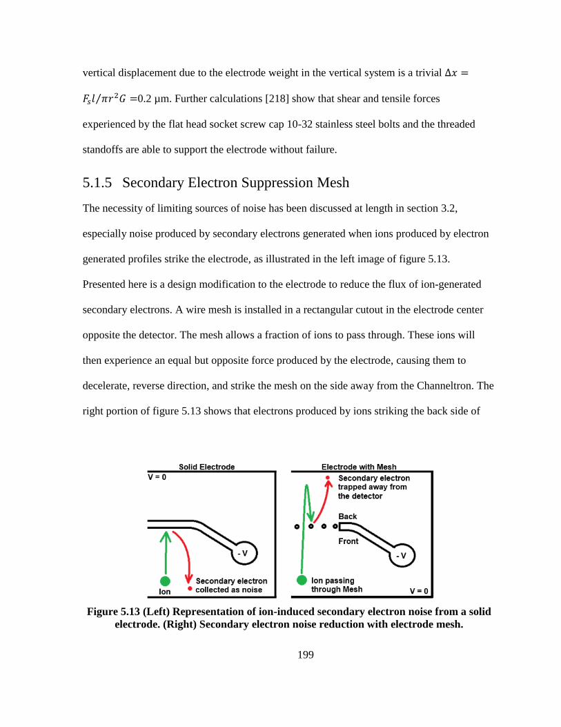
199

vertical displacement due to the electrode weight in the vertical system is a trivial

⁄ 0.2 µm. Further calculations [218] show that shear and tensile forces

experienced by the flat head socket screw cap 10-32 stainless steel bolts and the threaded

standoffs are able to support the electrode without failure.

5.1.5 Secondary Electron Suppression Mesh

The necessity of limiting sources of noise has been discussed at length in section 3.2,

especially noise produced by secondary electrons generated when ions produced by electron

generated profiles strike the electrode, as illustrated in the left image of figure 5.13.

Presented here is a design modification to the electrode to reduce the flux of ion-generated

secondary electrons. A wire mesh is installed in a rectangular cutout in the electrode center

opposite the detector. The mesh allows a fraction of ions to pass through. These ions will

then experience an equal but opposite force produced by the electrode, causing them to

decelerate, reverse direction, and strike the mesh on the side away from the Channeltron. The

right portion of figure 5.13 shows that electrons produced by ions striking the back side of

Figure 5.13 (Left) Representation of ion-induced secondary electron noise from a solid

electrode. (Right) Secondary electron noise reduction with electrode mesh.

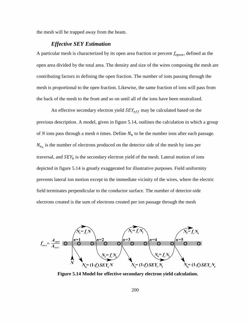
200

the mesh will be trapped away from the beam.

Effective SEY Estimation

A particular mesh is characterized by its open area fraction or percent , defined as the

open area divided by the total area. The density and size of the wires composing the mesh are

contributing factors in defining the open fraction. The number of ions passing through the

mesh is proportional to the open fraction. Likewise, the same fraction of ions will pass from

the back of the mesh to the front and so on until all of the ions have been neutralized.

An effective secondary electron yield may be calculated based on the

previous description. A model, given in figure 5.14, outlines the calculation in which a group

of N ions pass through a mesh n times. Define to be the number ions after each passage.

is the number of electrons produced on the detector side of the mesh by ions per

traversal, and is the secondary electron yield of the mesh. Lateral motion of ions

depicted in figure 5.14 is greatly exaggerated for illustrative purposes. Field uniformity

prevents lateral ion motion except in the immediate vicinity of the wires, where the electric

field terminates perpendicular to the conductor surface. The number of detector-side

electrons created is the sum of electrons created per ion passage through the mesh

Figure 5.14 Model for effective secondary electron yield calculation.

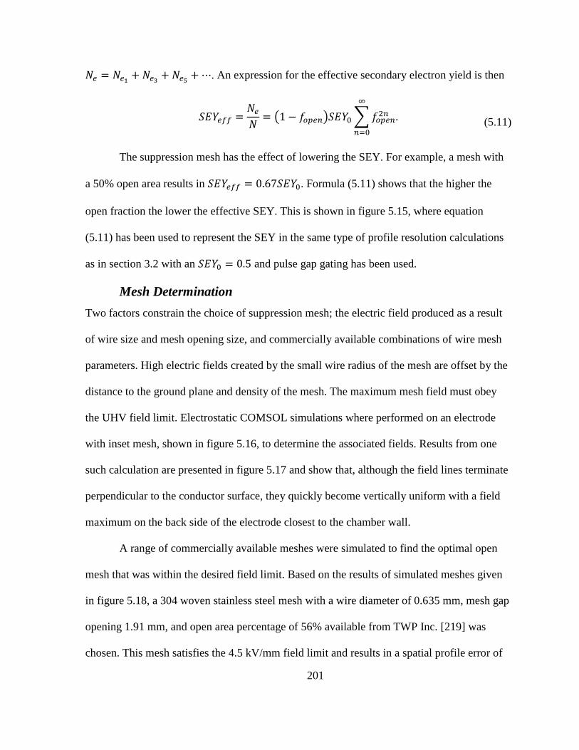
201

. An expression for the effective secondary electron yield is then

( ) ∑

(5.11)

The suppression mesh has the effect of lowering the SEY. For example, a mesh with

a 50% open area results in . Formula (5.11) shows that the higher the

open fraction the lower the effective SEY. This is shown in figure 5.15, where equation

(5.11) has been used to represent the SEY in the same type of profile resolution calculations

as in section 3.2 with an and pulse gap gating has been used.

Mesh Determination

Two factors constrain the choice of suppression mesh; the electric field produced as a result

of wire size and mesh opening size, and commercially available combinations of wire mesh

parameters. High electric fields created by the small wire radius of the mesh are offset by the

distance to the ground plane and density of the mesh. The maximum mesh field must obey

the UHV field limit. Electrostatic COMSOL simulations where performed on an electrode

with inset mesh, shown in figure 5.16, to determine the associated fields. Results from one

such calculation are presented in figure 5.17 and show that, although the field lines terminate

perpendicular to the conductor surface, they quickly become vertically uniform with a field

maximum on the back side of the electrode closest to the chamber wall.

A range of commercially available meshes were simulated to find the optimal open

mesh that was within the desired field limit. Based on the results of simulated meshes given

in figure 5.18, a 304 woven stainless steel mesh with a wire diameter of 0.635 mm, mesh gap

opening 1.91 mm, and open area percentage of 56% available from TWP Inc. [219] was

chosen. This mesh satisfies the 4.5 kV/mm field limit and results in a spatial profile error of

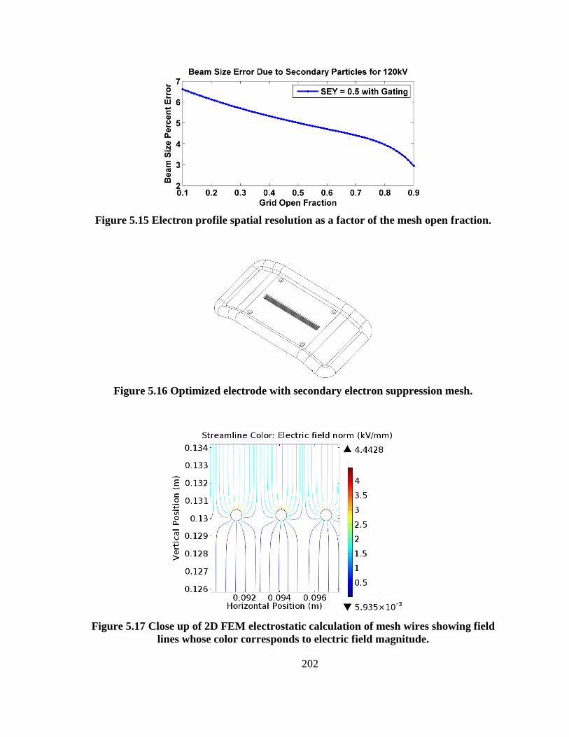
202

Figure 5.15 Electron profile spatial resolution as a factor of the mesh open fraction.

Figure 5.16 Optimized electrode with secondary electron suppression mesh.

Figure 5.17 Close up of 2D FEM electrostatic calculation of mesh wires showing field

lines whose color corresponds to electric field magnitude.

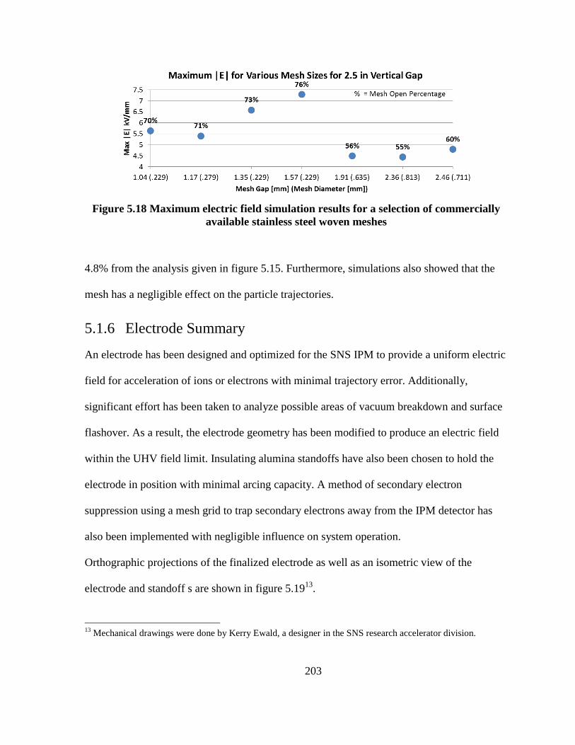
203

Figure 5.18 Maximum electric field simulation results for a selection of commercially

available stainless steel woven meshes

4.8% from the analysis given in figure 5.15. Furthermore, simulations also showed that the

mesh has a negligible effect on the particle trajectories.

5.1.6 Electrode Summary

An electrode has been designed and optimized for the SNS IPM to provide a uniform electric

field for acceleration of ions or electrons with minimal trajectory error. Additionally,

significant effort has been taken to analyze possible areas of vacuum breakdown and surface

flashover. As a result, the electrode geometry has been modified to produce an electric field

within the UHV field limit. Insulating alumina standoffs have also been chosen to hold the

electrode in position with minimal arcing capacity. A method of secondary electron

suppression using a mesh grid to trap secondary electrons away from the IPM detector has

also been implemented with negligible influence on system operation.

Orthographic projections of the finalized electrode as well as an isometric view of the

electrode and standoff s are shown in figure 5.1913

.

13

Mechanical drawings were done by Kerry Ewald, a designer in the SNS research accelerator division.

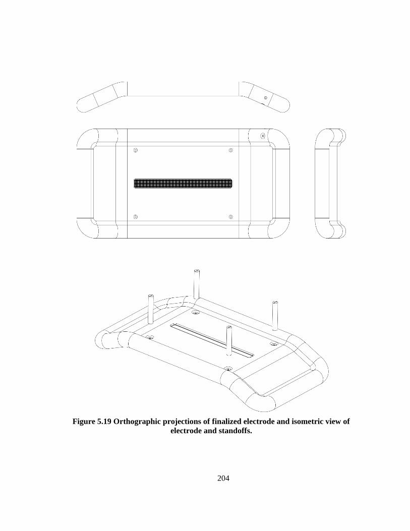
204

Figure 5.19 Orthographic projections of finalized electrode and isometric view of

electrode and standoffs.

205

Electrode Beam Deflection

One of the IPM system requirements is that it has a negligible effect on the beam trajectory

such that a 1 GeV proton is deflected ≤ 0.5 mrad. A deflection of this magnitude is

correctable by downstream corrector magnets. The amount of deflection by the IPM

electrode may be calculated for 1 GeV proton by assuming that the proton with a longitudinal

momentum of 1.696 GeV/c experiences a force qE = 1.602x10-19

C120 kV/25.4 cm =

7.57x10-14

N over a distance of 38.1 cm. At a velocity of 0.88c, the impulse produced by the

electrode imparts a 205 keV/c transverse momentum to the proton. The angle of deflection is

then tan-1

(205 keV/1.696 GeV) = 0.12 mrad which is within the deflection limit. Thus, no

corrector system is required for the electrode deflection.

5.2 Magnet Design

As with the electrode, field uniformity will drive the IPM magnet design subject to the

considerations of cost and size. An electromagnet will be used because the ability to adjust

the field strength allows the influence of the IPM on beam dynamics to be completely

removed if necessary. The magnet will be outside of the vacuum enclosure which allows for

simpler operation and installation but increases the size. Also, the dipole moment must be

analyzed to ascertain the need for a corrector magnet, and the higher order magnetic field

multipole components must be 1% of the dipole moment to prevent more complex

distortions of the particle orbit per the system design requirement.

5.2.1 Magnet Design Estimation

The basic magnet parameters may be estimated by using a simple C-magnet to represent an

IPM magnet with gap for inserting the vacuum chamber. A diagram, given in figure 5.20,

206

Figure 5.20 Magnet design calculation diagram.

shows a magnet with a core length , permeability , gap length with a

permeability of air , and cross section of a magnetic coil with N turns, each carrying a

current I. A ferromagnetic material such as iron is assumed for the core and taken to be

linear, isotropic, and homogenous such that is constant and ⁄ .

Stoke’s theorem applied to Ampere’s law allows the current in the coils to be related

to the associated magnetic field H and flux density B as

∮

(5.12)

No flux leakage has been as been assumed for the core and the core-air boundary follows the

magnetic boundary condition

( ) (5.13)

where is a vector normal to the boundary leading to

Assuming a 10% loss of magnetic field in the gap due to fringing effects such that

G, equation (5.14) results in 13475 Aturns for a 50.8 cm gap. Depending on the

number of coil turns chosen, the required current can be estimated, such as 13 A

(5.14)

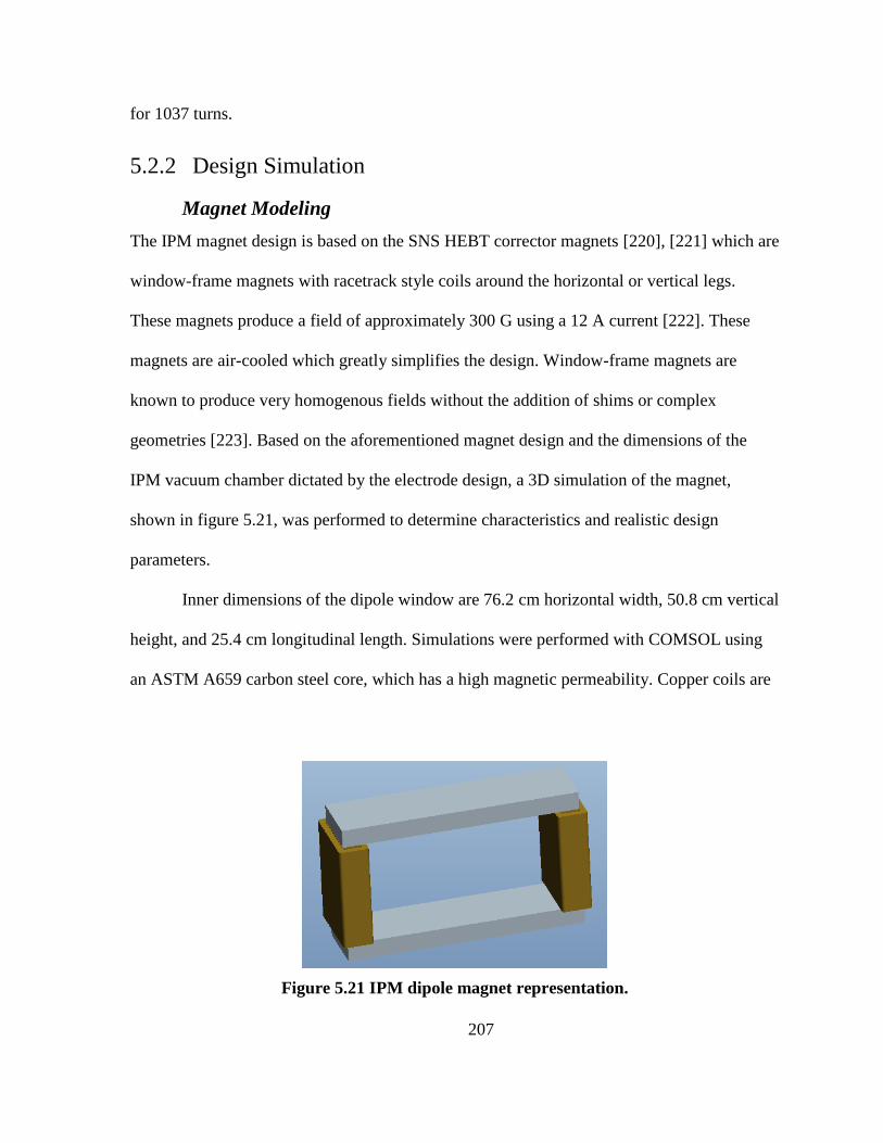
207

for 1037 turns.

5.2.2 Design Simulation

Magnet Modeling

The IPM magnet design is based on the SNS HEBT corrector magnets [220], [221] which are

window-frame magnets with racetrack style coils around the horizontal or vertical legs.

These magnets produce a field of approximately 300 G using a 12 A current [222]. These

magnets are air-cooled which greatly simplifies the design. Window-frame magnets are

known to produce very homogenous fields without the addition of shims or complex

geometries [223]. Based on the aforementioned magnet design and the dimensions of the

IPM vacuum chamber dictated by the electrode design, a 3D simulation of the magnet,

shown in figure 5.21, was performed to determine characteristics and realistic design

parameters.

Inner dimensions of the dipole window are 76.2 cm horizontal width, 50.8 cm vertical

height, and 25.4 cm longitudinal length. Simulations were performed with COMSOL using

an ASTM A659 carbon steel core, which has a high magnetic permeability. Copper coils are

Figure 5.21 IPM dipole magnet representation.

208

represented by the brown regions in figure 5.21, where the number of windings and current

was varied to achieve the desired field over the Channeltron region.

Longitudinal Field Results

Due to the short longitudinal pole length compared to the magnet aperture, much of the

magnetic field is lost to edge fringing effects. A simulation, shown in figure 5.22, of the

magnetic flux density outside the core of the IPM dipole magnet in a plane parallel to the

longitudinal axis reveals the fringing effect of the magnet. As such, an increased number of

turns was required to produce the 300 G central field. The final magnet design is comprised

of two coils consisting 1008 turns of 8 AWG gauge coated copper wire with a 0.254 mm

Kapton electrically insulating barrier between the coils and the steel core. A 13 A current

allows the magnet to produce the required field while still allowing it to be air cooled.

Core Saturation

The thickness of the core was determined in order to prevent magnetic saturation of the steel.

Steel has a magnetic saturation between 1.6-2.2 T [224]. With a thickness of 7.62 cm, the

magnetic flux density in the bulk of the core is ~1 T, as seen in figure 5.23. The present

design is well within the magnetic saturation limit coincident with production of the required

central field.

5.2.3 Magnetic Field Evaluation

Transverse Field Error

It is important to evaluate the transverse field magnitude and uniformity. Transverse

magnetic flux arrows with size and color determined by field magnitude are given in figure

5.24 along with black arrows showing the direction of the current in the coils. A more

quantitative view the field uniformity is seen in figure 5.25, which shows that the magnitude

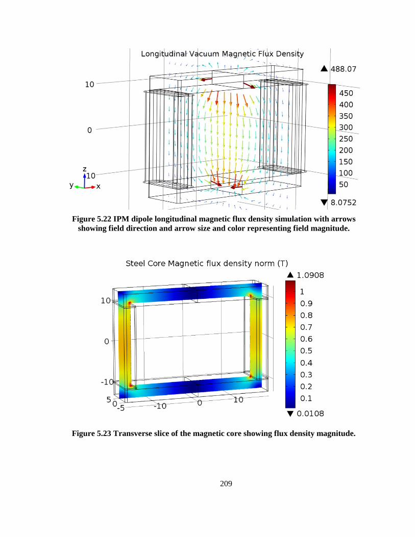
209

Figure 5.22 IPM dipole longitudinal magnetic flux density simulation with arrows

showing field direction and arrow size and color representing field magnitude.

Figure 5.23 Transverse slice of the magnetic core showing flux density magnitude.

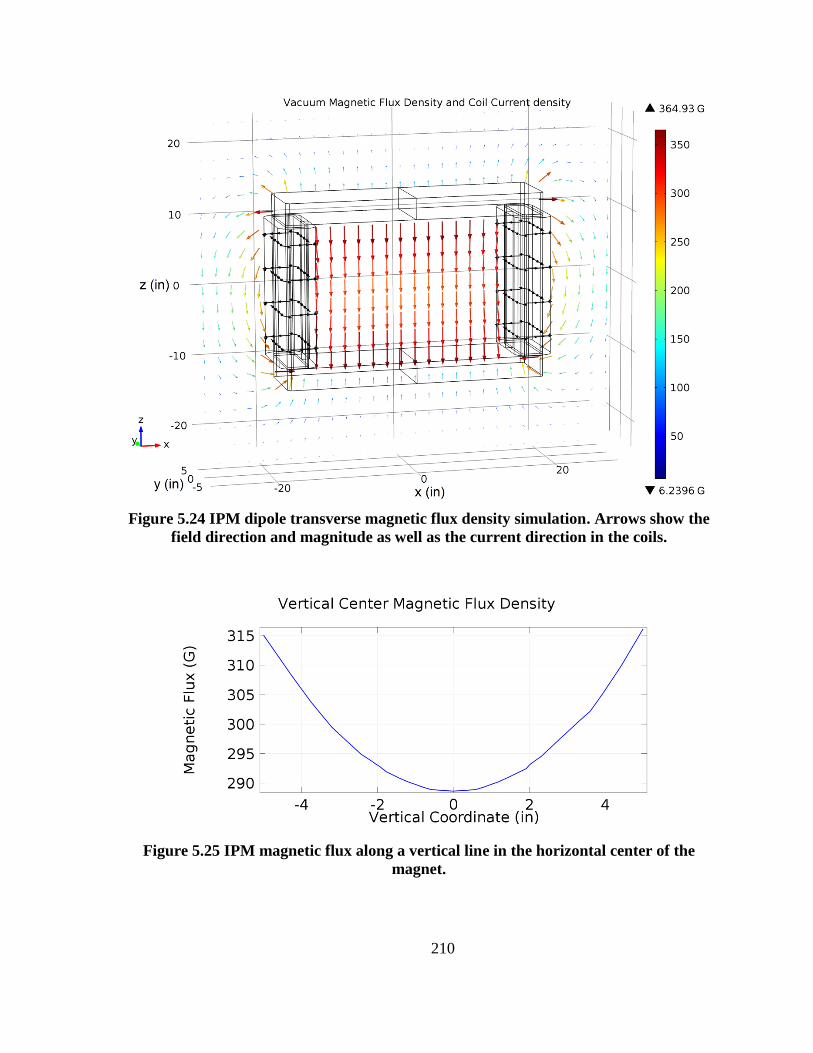
210

Figure 5.24 IPM dipole transverse magnetic flux density simulation. Arrows show the

field direction and magnitude as well as the current direction in the coils.

Figure 5.25 IPM magnetic flux along a vertical line in the horizontal center of the

magnet.

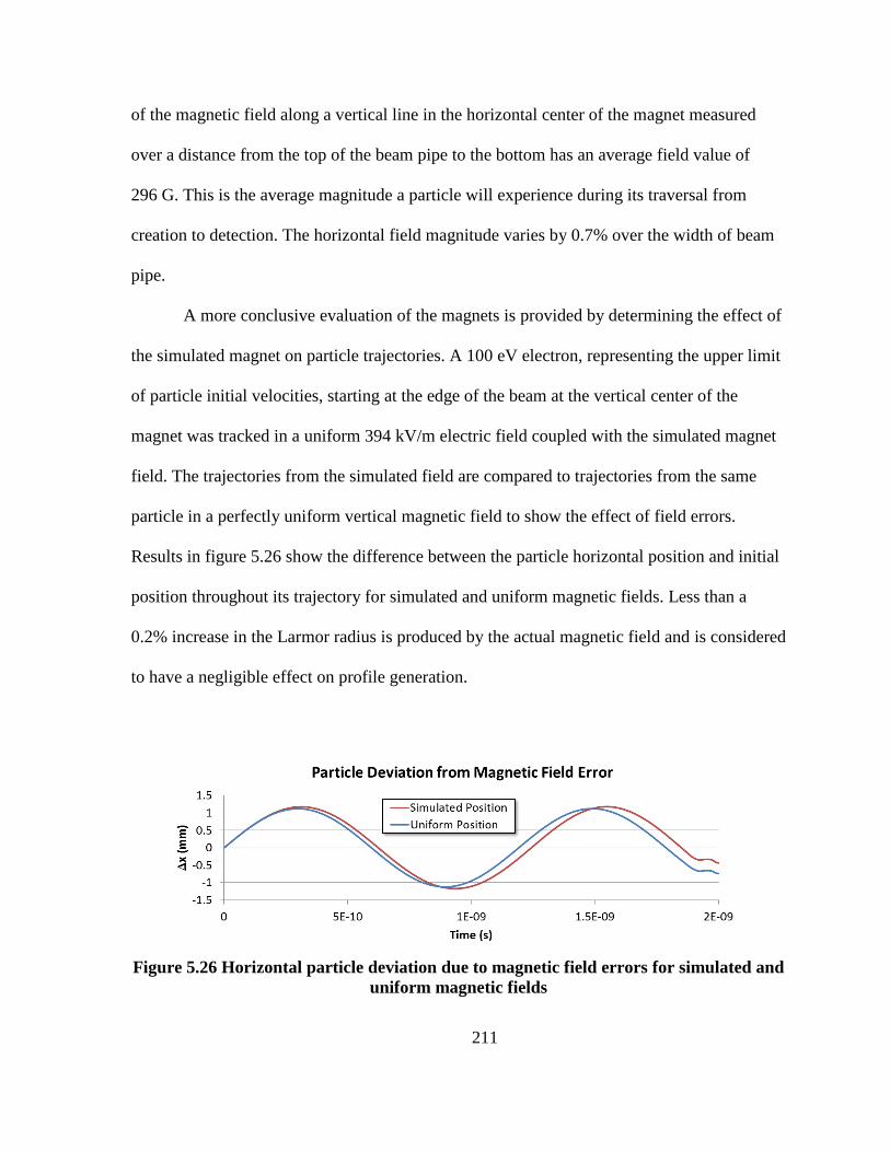
211

of the magnetic field along a vertical line in the horizontal center of the magnet measured

over a distance from the top of the beam pipe to the bottom has an average field value of

296 G. This is the average magnitude a particle will experience during its traversal from

creation to detection. The horizontal field magnitude varies by 0.7% over the width of beam

pipe.

A more conclusive evaluation of the magnets is provided by determining the effect of

the simulated magnet on particle trajectories. A 100 eV electron, representing the upper limit

of particle initial velocities, starting at the edge of the beam at the vertical center of the

magnet was tracked in a uniform 394 kV/m electric field coupled with the simulated magnet

field. The trajectories from the simulated field are compared to trajectories from the same

particle in a perfectly uniform vertical magnetic field to show the effect of field errors.

Results in figure 5.26 show the difference between the particle horizontal position and initial

position throughout its trajectory for simulated and uniform magnetic fields. Less than a

0.2% increase in the Larmor radius is produced by the actual magnetic field and is considered

to have a negligible effect on profile generation.

Figure 5.26 Horizontal particle deviation due to magnetic field errors for simulated and

uniform magnetic fields

212

Magnet Multipole Analysis

The previous analysis has shown that the magnet will provide the field required to generate

accurate profiles, but the effect of the magnet field on the beam motion is also critical. If the

magnet were to introduce a large distortion in the proton trajectories, the downstream

magnets would not be able to compensate, causing beam loss. There are two aspects of the

IPM magnet that require compensation. The real magnetic field may be decomposed into a

combination of “pure” multipole fields, which will be derived shortly, with the dipole field

producing a uniform kick to all particles. Dipole field compensation will be addressed in a

subsequent section. Higher order multipole fields produce more complex particle motion and

are more easily corrected due to their small relative amplitude.

Consider a 2D magnetic field . Maxwell’s equations

in a current free, static region give leading to

(5.15)

and so that

(5.16)

Equations (5.15) and (5.16) are known as the Cauchy-Reimann equations and form a set of

conditions that guarantee that the two real-valued functions and , defined on

the real plane , may be represented together as an analytic function of one variable

on the complex plane that is holomorphic or complex-analytic [189]. The

complex function is

213

(5.17)

Because is analytic it may be expanded in a power series [154]. Consequently, equation

(5.17) may be expanded about the origin as

∑

(5.18)

where the complex expansion coefficients are . The power series converges

within a circle | | where, for a magnetic field, r is the largest radius inscribed in the

magnet poles creating the field.

The right-hand side of equation (5.18) is a sum of individual multipole fields with

each n representing a “pure” field. For the first few components, the multipoles have names,

such as n = 1 dipole, n = 2 quadrupole, n = 3 sextupole, n = 4 octopole, and so forth. A

magnet designed to create a particular multipole has 2n pole tips. In order to simplify the

multipole component units, a reference radius is often employed [225] and along with a

conversion to cylindrical coordinate, equation (5.18) becomes

∑ (

)

(5.19)

where √ and .

By representing the complex expansion coefficients in the phasor form as

| | , it can be seen that the phase simply determines the field

orientation. As such, the pure multipole is defined as “normal” if and “skew” if

⁄ . corresponds to the normal multipole components and the skew

components. A normal dipole field, for example, is a purely vertical field while a skew dipole

214

is horizontal. As a matter of convention, multipole components are often normalized to 10-4

of magnitude of the main field component

| | (5.20)

i.e. for a dipole magnet [226] with expressed in “units”.

It has been shown [225] that if M measurements of the radial and azimuthal

components of a magnetic field are taken on a circle of radius at for

then the coefficients may be found using the discrete Fourier

transform

( ⁄ ) ∑

(5.21)

Here, in equation (5.21) for the field components measured at each point .

Furthermore, the previous analysis considered a two-dimensional field while the actual

transverse field components also vary in the longitudinal direction . This may be accounted

for by solving for the integrated field components over the longitudinal pole distance L

∫

∑

(

)

(5.22)

where and

are the normal and skew integrated field components [227].

IPM Multipole Results

IPM magnet multipoles are calculated by finding the azimuthal and radial field components

on the surface of a cylinder whose axis is coincident longitudinal dipole axis. The cylinder

has a radius, also used as the reference radius, which is the maximum acceptance of the SNS

ring 12.78 cm. Integrating the field components of the 25.4 cm longitudinal

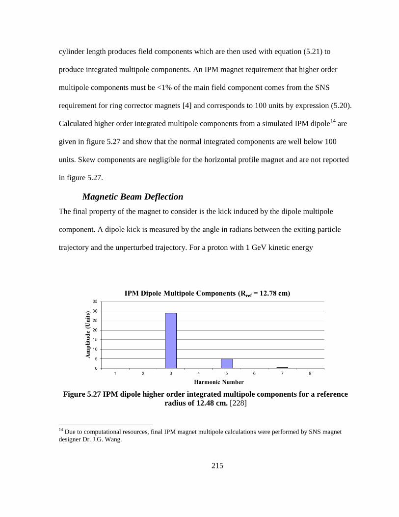
215

cylinder length produces field components which are then used with equation (5.21) to

produce integrated multipole components. An IPM magnet requirement that higher order

multipole components must be <1% of the main field component comes from the SNS

requirement for ring corrector magnets [4] and corresponds to 100 units by expression (5.20).

Calculated higher order integrated multipole components from a simulated IPM dipole14

are

given in figure 5.27 and show that the normal integrated components are well below 100

units. Skew components are negligible for the horizontal profile magnet and are not reported

in figure 5.27.

Magnetic Beam Deflection

The final property of the magnet to consider is the kick induced by the dipole multipole

component. A dipole kick is measured by the angle in radians between the exiting particle

trajectory and the unperturbed trajectory. For a proton with 1 GeV kinetic energy

Figure 5.27 IPM dipole higher order integrated multipole components for a reference

radius of 12.48 cm. [228]

14

Due to computational resources, final IPM magnet multipole calculations were performed by SNS magnet

designer Dr. J.G. Wang.

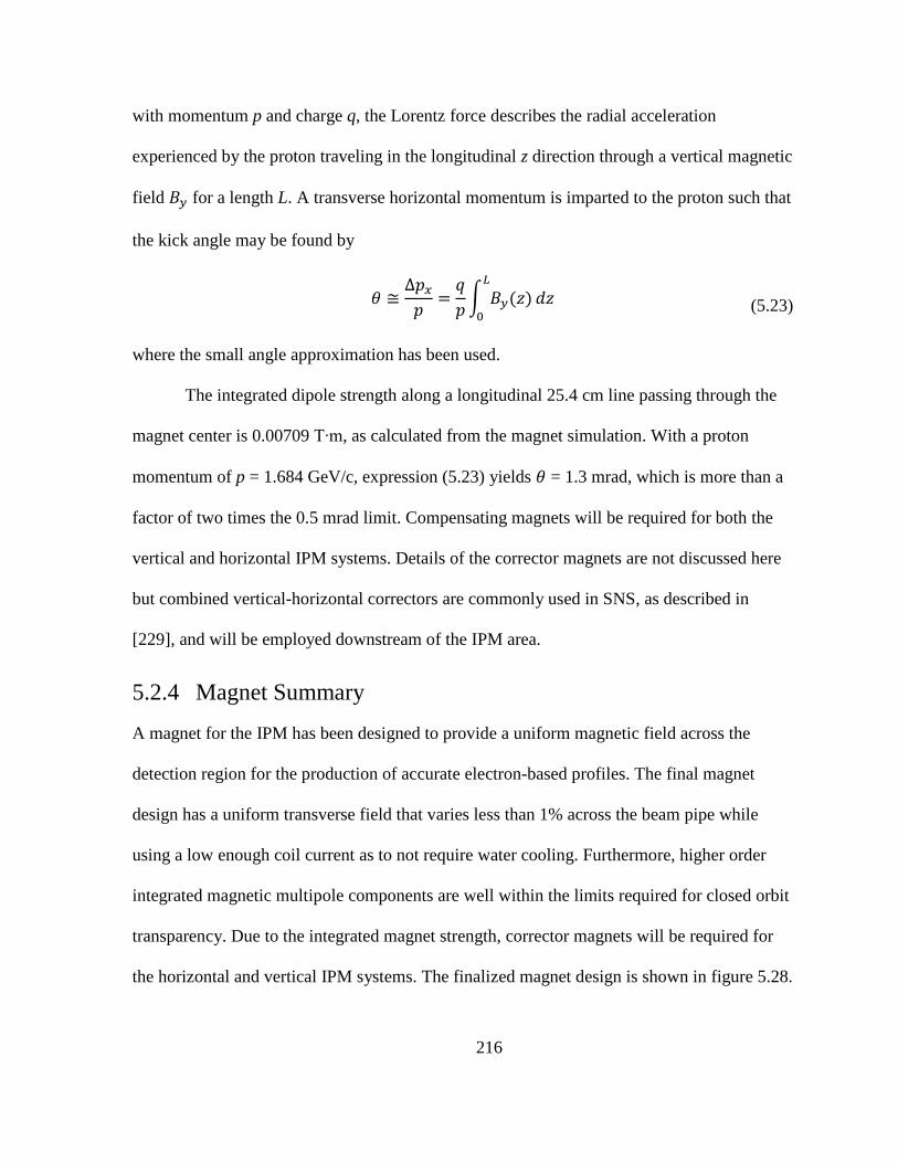
216

with momentum p and charge q, the Lorentz force describes the radial acceleration

experienced by the proton traveling in the longitudinal z direction through a vertical magnetic

field for a length L. A transverse horizontal momentum is imparted to the proton such that

the kick angle may be found by

∫

(5.23)

where the small angle approximation has been used.

The integrated dipole strength along a longitudinal 25.4 cm line passing through the

magnet center is 0.00709 T∙m, as calculated from the magnet simulation. With a proton

momentum of p = 1.684 GeV/c, expression (5.23) yields = 1.3 mrad, which is more than a

factor of two times the 0.5 mrad limit. Compensating magnets will be required for both the

vertical and horizontal IPM systems. Details of the corrector magnets are not discussed here

but combined vertical-horizontal correctors are commonly used in SNS, as described in

[229], and will be employed downstream of the IPM area.

5.2.4 Magnet Summary

A magnet for the IPM has been designed to provide a uniform magnetic field across the

detection region for the production of accurate electron-based profiles. The final magnet

design has a uniform transverse field that varies less than 1% across the beam pipe while

using a low enough coil current as to not require water cooling. Furthermore, higher order

integrated magnetic multipole components are well within the limits required for closed orbit

transparency. Due to the integrated magnet strength, corrector magnets will be required for

the horizontal and vertical IPM systems. The finalized magnet design is shown in figure 5.28.

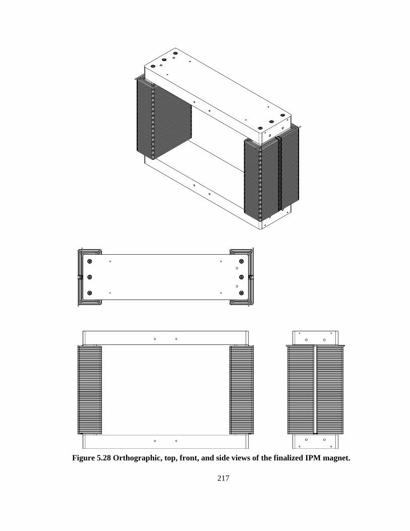
217

Figure 5.28 Orthographic, top, front, and side views of the finalized IPM magnet.

218

5.3 Detector Assembly

The detector assembly is comprised of a mechanism that drives the detector across the beam

dimension to be measured as well as the housing that secures the Channeltron. This area of

the design incorporates many isolation elements necessary to mitigate image current

coupling. Furthermore, detector cabling inside the vacuum chamber, a possible source of

beam induced noise, and efforts to shield and isolate the IPM signal from the accelerating

environment will be discussed.

5.3.1 Channeltron Housing

As was found in the IPM test chamber, a significant amount of AC coupled beam signal is

introduced into the measurement, and shielding is required to obtain a useful profile. An

effort was made to ensure the Channeltron housing, or the portion of the detector assembly to

which the detector is attached, was shielded as much as possible.

Channeltron Support

The Channeltron is held by a stainless steel support arm, the end of which is displayed in the

left image of figure 5.29. Two detectors are mounted on the arm to allow for background

subtraction and to act as spares in the event of a detector failure. Macor insulators are used to

electrically isolate the Ctrons from the metal support. The support arm is attached at right

angles to the actuator drive assembly, which is shown in the right of figure 5.29. A swivel

mechanism has been incorporated into the support arm connection to the drive shaft that

allows for a 90° rotation, making the entire assembly a linear unit for easy installation and

removal.

219

Figure 5.29 (Left) Close up of the end of the support arm holding the Channeltron

detectors. (Right) Full Channeltron arm assembly with bellows.

Detector Shielding

To protect the immediate area of the detectors, a grounded metal shield encloses the

Channeltrons and can be seen in figure 5.30. The 5-sided Ctron shielding box travels

underneath a solid metal plate forming an inner floor within the IPM vacuum chamber.

Depicted in figure 5.31, the vacuum chamber inner floor plate serves to shield the Ctron

assembly as well as to provide a flat boundary for electric field uniformity. Collected

particles pass through a rectangular slot in the inner floor and enter the detectors, whose

openings travel coincidentally with the floor slot.

5.3.2 Detector Cabling and Feedthroughs

Cabling used in the vacuum chamber requires special considerations due to the ultrahigh

vacuum. Each of the two Channeltrons requires a high voltage bias cable and a signal cable.

Cables used in the IPM vacuum chamber will be 26 AWG, 50 Ω coaxial cable rated to

1x10-10

Torr with Accu-FastTM

floating connectors on the feedthrough end available off-the-

shelf from Accu-Glass

[230]. Accu-Glass

also carries ultrahigh vacuum isolated

feedthroughs which allow the ground conductor to be insulated from the surrounding

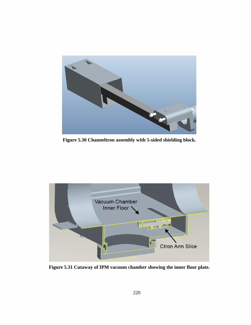
220

Figure 5.30 Channeltron assembly with 5-sided shielding block.

Figure 5.31 Cutaway of IPM vacuum chamber showing the inner floor plate.

221

structure. A 700 V DC feedthrough with an SMA connector on the air-side and a 5 KV DC, 5

Amp high voltage feedthrough with BNC air-side connector are set into a flange, illustrated

in figure 5.32, for vacuum-to-air signal and bias voltage transfer. Signal cables on the air side

the IPM to the Ring Service building will also be shielded from cables run away from the RF

cavities.

5.3.3 Actuator

The final detector assembly component is the actuator used to drive the Channeltrons across

the beam. By using an actuator similar to wirescanner actuators used elsewhere in the

accelerator [231], the same drive electronics may be used for the IPM with slight

modifications.The IPM actuator is a Parker 404XE series linear actuator [232] which has

been modified for radiation environments . With a positional accuracy of 90 µm and a

bidirectional repeatability of ±20 µm, a maximum estimated position accuracy of 90 µm +

20 µm = 0.11 mm is obtained, which satisfies the condition for the profile error given in

Figure 5.32 Vacuum side illustration of the vacuum feedthrough flange containing two

sets of isolated signal and high voltage feedthroughs for Channeltron operation.

222

section 3.2.2 .

Measurement speed is a factor of actuator limitations, driver software, motor

controllers, and vacuum load. Based on similar SNS systems a realistic speed of 5 mm/s will

be assumed [233]. If it is assumed that 200 accumulation measurements are required at 30

measurement positions spaced 5 mm apart at a production rate of 60 Hz , the resulting

approximate profile measurement time is

⁄ = 2.2 minutes. The assumed measurement spacing will be justified later.

While the final system measurement may differ, it should not exceed 5 minutes in the most

extreme case.

5.4 Vacuum Chamber

5.4.1 Alignment and Installation

Included in the vacuum chamber support stand are alignment mechanisms that allow for

vertical and horizontal alignment with the beam center. Furthermore, a positioning system

has been designed into the magnet and chamber to permit alignment of the magnetic field.

Other installation aspects have been considered such as a removable front face of the vacuum

chamber that allows interior access for electrode installation. Also, a 7.62x17.48 cm port was

added to the bottom of the chamber, underneath the detector slot, to grant easy access to the

Channeltrons in the event that detector repair or replacement is needed. This also allows

simplified removal of the entire detector assembly if needed. Finally, a 3.81 cm diameter port

has been included that can be used for in-situ vacuum pressure measurements or residual gas

analysis.

223

5.4.2 Wakefield Slats

Wakefield Production

A relativistic charged particle has longitudinal field components that are Lorentz contracted

to form a disc perpendicular to the particle velocity, as derived in Appendix C. In a perfectly

conducting accelerating pipe the particle’s electromagnetic fields terminate on image charges

which move synchronously with the moving particle. However, in reality, the finite

conductivity of the accelerating structure causes the image charge to lag behind the beam

particle, resulting in trailing electromagnetic fields known as wakefields [234].

Wakefields affect trailing beam particles and can lead to instabilities [235],[105].

Obstacles can also produce wakefields as beam energy is trapped in or behind accelerating

structure aperture changes or cavities. This is illustrated in figure 5.33 which shows electric

field lines for a Gaussian beam passing through an aperture in the left image and passing by a

cavity in the right image. Wakefields can be seen forming in both cases. Efforts to reduce

accelerating geometries that contribute to wakfield production were incorporated into the

IPM vacuum chamber.

Detector Slot Image Current Modification

A discontinuity is introduced directly across the beam path by the detector slot in the IPM

vacuum chamber inner floor plate. As such, a continuous path for beam image current was

added across the slot in the form slats. The detector slot, depicted in figure 5.34, is formed

with a row of 3.99 mm wide cutouts separated by 0.762 mm slats, parallel to the beam

direction and crossing the detector opening. The effect on the profile is to reduce the number

of measurement points by requiring nonadjacent Channeltron position. However, by the

analysis of section 3.2.2, this reduces the number of to 3.16 which, by

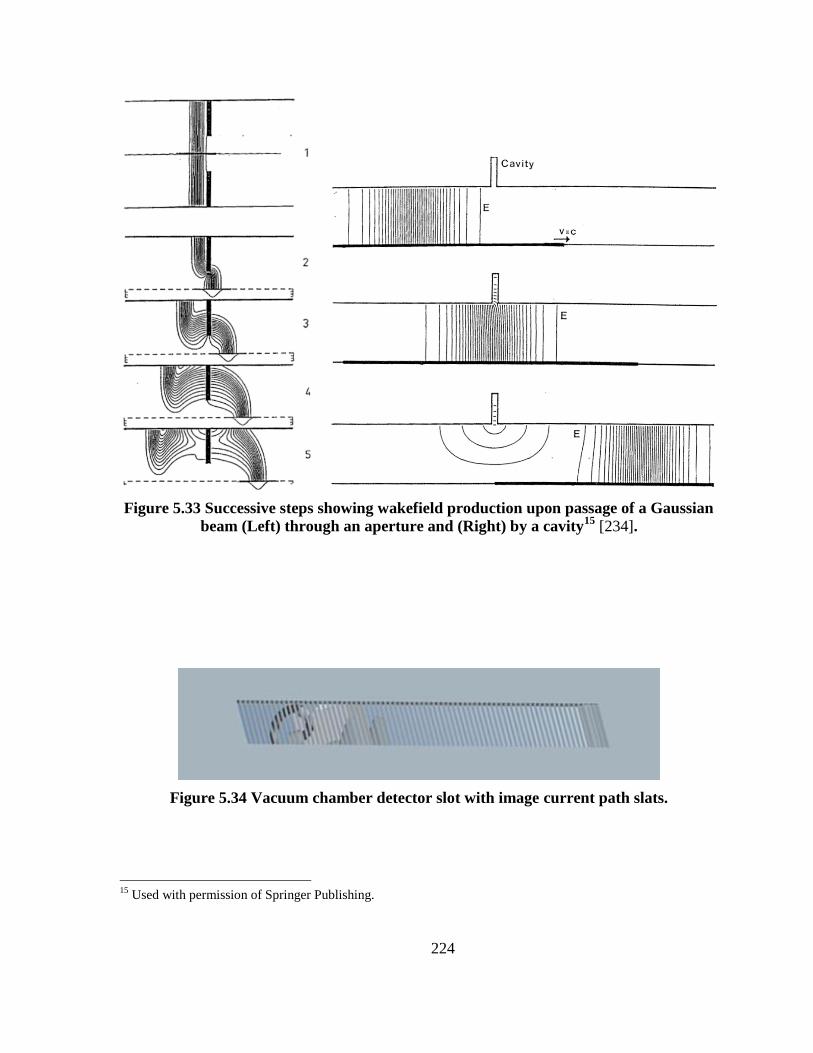
224

Figure 5.33 Successive steps showing wakefield production upon passage of a Gaussian

beam (Left) through an aperture and (Right) by a cavity15

[234].

Figure 5.34 Vacuum chamber detector slot with image current path slats.

15

Used with permission of Springer Publishing.

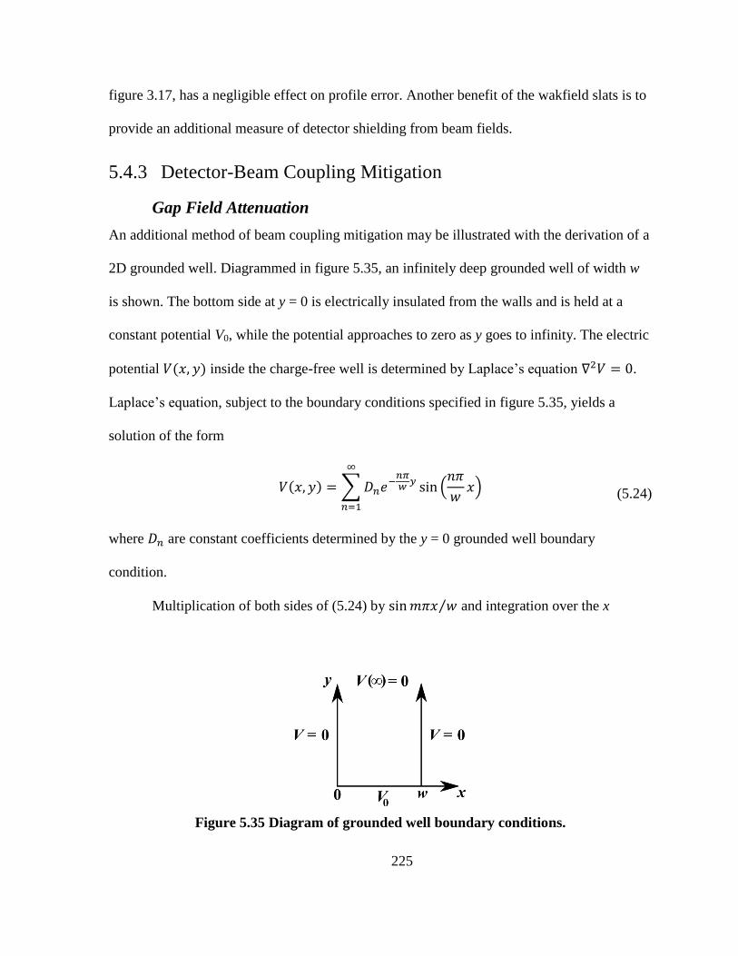
225

figure 3.17, has a negligible effect on profile error. Another benefit of the wakfield slats is to

provide an additional measure of detector shielding from beam fields.

5.4.3 Detector-Beam Coupling Mitigation

Gap Field Attenuation

An additional method of beam coupling mitigation may be illustrated with the derivation of a

2D grounded well. Diagrammed in figure 5.35, an infinitely deep grounded well of width w

is shown. The bottom side at y = 0 is electrically insulated from the walls and is held at a

constant potential V0, while the potential approaches to zero as y goes to infinity. The electric

potential inside the charge-free well is determined by Laplace’s equation .

Laplace’s equation, subject to the boundary conditions specified in figure 5.35, yields a

solution of the form

∑

(

)

(5.24)

where are constant coefficients determined by the y = 0 grounded well boundary

condition.

Multiplication of both sides of (5.24) by ⁄ and integration over the x

Figure 5.35 Diagram of grounded well boundary conditions.

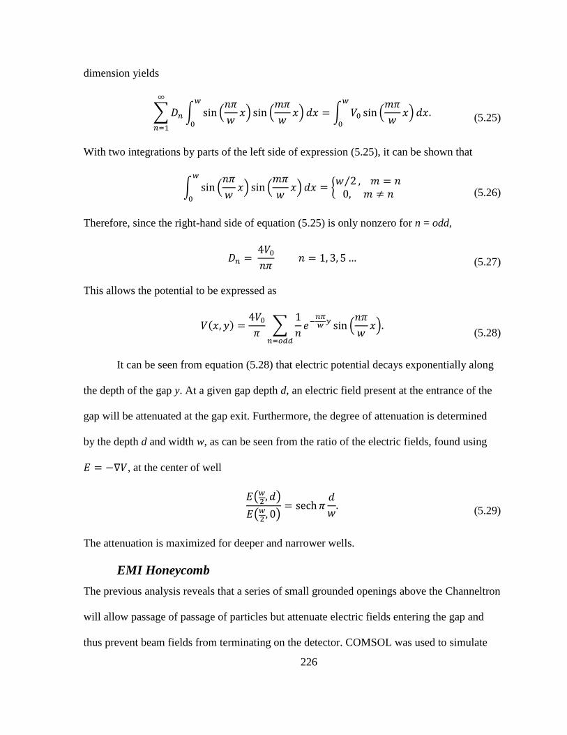
226

dimension yields

∑ ∫ (

) (

)

∫ (

)

(5.25)

With two integrations by parts of the left side of expression (5.25), it can be shown that

∫ (

) (

)

{ ⁄

(5.26)

Therefore, since the right-hand side of equation (5.25) is only nonzero for n = odd,

(5.27)

This allows the potential to be expressed as

∑

(

)

(5.28)

It can be seen from equation (5.28) that electric potential decays exponentially along

the depth of the gap y. At a given gap depth d, an electric field present at the entrance of the

gap will be attenuated at the gap exit. Furthermore, the degree of attenuation is determined

by the depth d and width w, as can be seen from the ratio of the electric fields, found using

, at the center of well

( )

( )

(5.29)

The attenuation is maximized for deeper and narrower wells.

EMI Honeycomb

The previous analysis reveals that a series of small grounded openings above the Channeltron

will allow passage of passage of particles but attenuate electric fields entering the gap and

thus prevent beam fields from terminating on the detector. COMSOL was used to simulate

227

this phenomenon for a 2D grounded opening in the floor of the IPM vacuum chamber shown

in figure 5.36. It shows electric field lines entering the gap and terminating on the gap walls

in accordance with the electric boundary condition, thus illustrating field attenuation in the

gap.

Metallic honeycombs used to reduce electromagnetic interference, or EMI, displayed

in figure 5.37 (left), are commercially available in a variety of sizes. By placing one just

above the detector, as shown in figure 5.37 (Right), further beam isolation is achieved. Figure

5.38 shows results from simulations on a range of available gap width-depth combinations

conducted to find the honeycomb parameters that optimize attenuation while minimizing the

influence on the overall design, i.e. shorter gap depth. Due to availability, a gap opening of

3.175 mm was chosen and was found to have an attenuation of 89 dB with a depth of

3.2 mm. These honeycomb parameters reduce the electric field by four orders of magnitude

and can be found in off-the-shelf laser welded panels [236]. These do not use adhesives to

bond the mesh together, which is a high vacuum requirement.

5.5 High Voltage Feedthrough

In order to bring the electrode to the necessary potential for particle collection, a high voltage

vacuum feedthrough (HVF) is required. Two aspects of the feedthrough necessitate

consideration; both the air-side and the vacuum-side of feedthrough and the electrode

connection must be analyzed for arcing hazards.

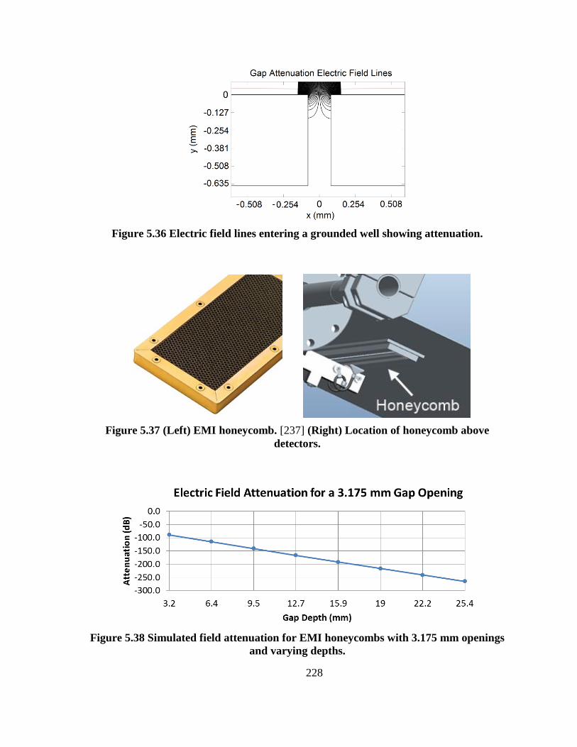
228

Figure 5.36 Electric field lines entering a grounded well showing attenuation.

Figure 5.37 (Left) EMI honeycomb. [237] (Right) Location of honeycomb above

detectors.

Figure 5.38 Simulated field attenuation for EMI honeycombs with 3.175 mm openings

and varying depths.

229

5.5.1 HVF Air Side

Feedthrough and Air-Side Arcing Hazard

A 125kV high voltage feedthrough with 304 stainless steel housing, conductor and alumina

ceramic insulator is affixed to the upper portion of the vacuum chamber in line with the

electrode. Proximity to the surrounding accelerating structure introduces an arcing hazard.

While the dielectric strength of atmospheric pressure air is 3 MV/m [238], the rule-of-thumb

to prevent arcing in air is 2.54 cm of distance to ground per 10 kV. For a 120 kV potential,

this would require a ~30 cm radius of clearance around the HVF. This is not realistically

feasible.

Arcing Mitigation

The air-side HVF arcing solution comes in the form of a high dielectric strength potting

material. Potting is accomplished by surrounding the HVF in a grounded metal enclosure, as

illustrated in figure 5.39, then filling the enclosure with an epoxy resin. Araldite

CW1312/HY1300 [239], for example, has a dielectric strength of 12 kV/mm. A minimum

distance inside the HVF enclosure of 5.56 cm results in an electric field of 2.16 kV/mm,

which is well below the epoxy breakdown limit. The enclosure, HVF, and short high voltage

cable attaching to the HVF are potted together as a single unit which is then mounted to the

vacuum chamber.

This modular design allows for simplified replacement or repair. Upon exiting the

HVF enclosure the high voltage cable connects to a 125 kV rated, 15 kΩ, potted resistor box

located in the tunnel close to the IPM location. This box receives the high voltage cable from

the electrode power supply located in the RSB. As an additional measure of field reduction,

figure 5.40 shows a cap designed to fit over the HVF connector threads to receive the high

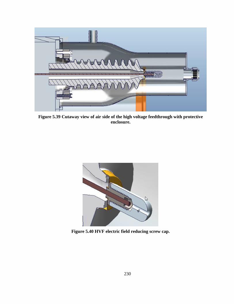
230

Figure 5.39 Cutaway view of air side of the high voltage feedthrough with protective

enclosure.

Figure 5.40 HVF electric field reducing screw cap.

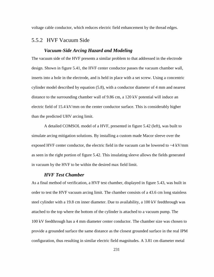
231

voltage cable conductor, which reduces electric field enhancement by the thread edges.

5.5.2 HVF Vacuum Side

Vacuum-Side Arcing Hazard and Modeling

The vacuum side of the HVF presents a similar problem to that addressed in the electrode

design. Shown in figure 5.41, the HVF center conductor passes the vacuum chamber wall,

inserts into a hole in the electrode, and is held in place with a set screw. Using a concentric

cylinder model described by equation (5.8), with a conductor diameter of 4 mm and nearest

distance to the surrounding chamber wall of 9.86 cm, a 120 kV potential will induce an

electric field of 15.4 kV/mm on the center conductor surface. This is considerably higher

than the predicted UHV arcing limit.

A detailed COMSOL model of a HVF, presented in figure 5.42 (left), was built to

simulate arcing mitigation solutions. By installing a custom made Macor sleeve over the

exposed HVF center conductor, the electric field in the vacuum can be lowered to ~4 kV/mm

as seen in the right portion of figure 5.42. This insulating sleeve allows the fields generated

in vacuum by the HVF to be within the desired max field limit.

HVF Test Chamber

As a final method of verification, a HVF test chamber, displayed in figure 5.43, was built in

order to test the HVF vacuum arcing limit. The chamber consists of a 43.6 cm long stainless

steel cylinder with a 19.8 cm inner diameter. Due to availability, a 100 kV feedthrough was

attached to the top where the bottom of the cylinder is attached to a vacuum pump. The

100 kV feedthrough has a 4 mm diameter center conductor. The chamber size was chosen to

provide a grounded surface the same distance as the closest grounded surface in the real IPM

configuration, thus resulting in similar electric field magnitudes. A 3.81 cm diameter metal

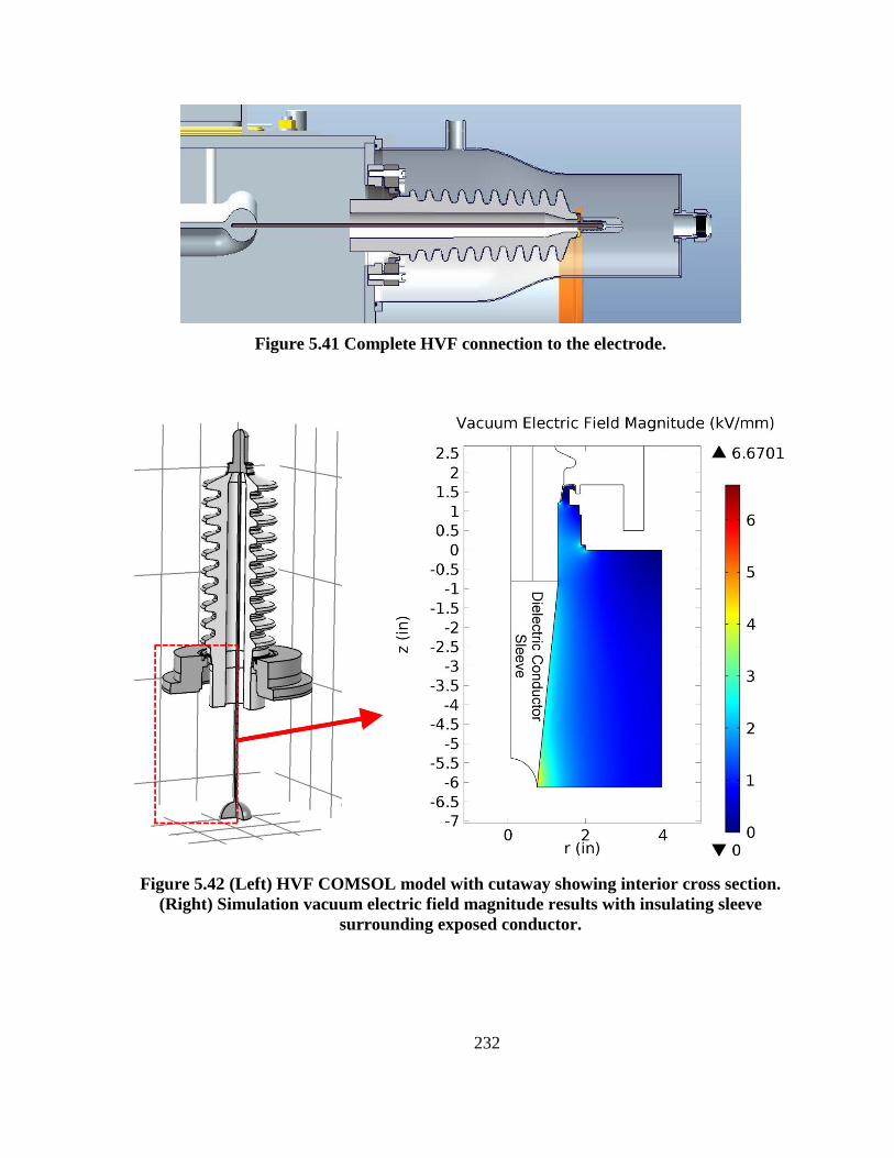
232

Figure 5.41 Complete HVF connection to the electrode.

Figure 5.42 (Left) HVF COMSOL model with cutaway showing interior cross section.

(Right) Simulation vacuum electric field magnitude results with insulating sleeve

surrounding exposed conductor.

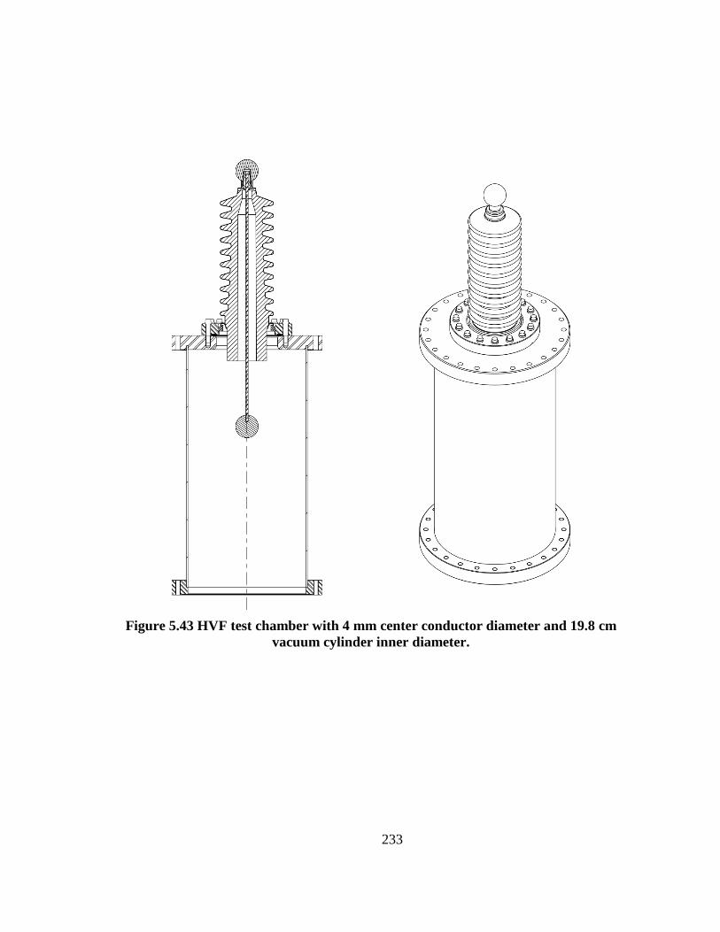
233

Figure 5.43 HVF test chamber with 4 mm center conductor diameter and 19.8 cm

vacuum cylinder inner diameter.

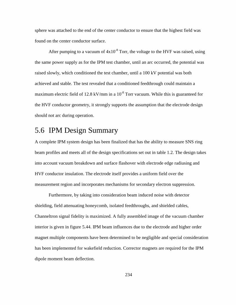
234

sphere was attached to the end of the center conductor to ensure that the highest field was

found on the center conductor surface.

After pumping to a vacuum of 4x10-8

Torr, the voltage to the HVF was raised, using

the same power supply as for the IPM test chamber, until an arc occurred, the potential was

raised slowly, which conditioned the test chamber, until a 100 kV potential was both

achieved and stable. The test revealed that a conditioned feedthrough could maintain a

maximum electric field of 12.8 kV/mm in a 10-8

Torr vacuum. While this is guaranteed for

the HVF conductor geometry, it strongly supports the assumption that the electrode design

should not arc during operation.

5.6 IPM Design Summary

A complete IPM system design has been finalized that has the ability to measure SNS ring

beam profiles and meets all of the design specifications set out in table 1.2. The design takes

into account vacuum breakdown and surface flashover with electrode edge radiusing and

HVF conductor insulation. The electrode itself provides a uniform field over the

measurement region and incorporates mechanisms for secondary electron suppression.

Furthermore, by taking into consideration beam induced noise with detector

shielding, field attenuating honeycomb, isolated feedthroughs, and shielded cables,

Channeltron signal fidelity is maximized. A fully assembled image of the vacuum chamber

interior is given in figure 5.44. IPM beam influences due to the electrode and higher order

magnet multiple components have been determined to be negligible and special consideration

has been implemented for wakefield reduction. Corrector magnets are required for the IPM

dipole moment beam deflection.

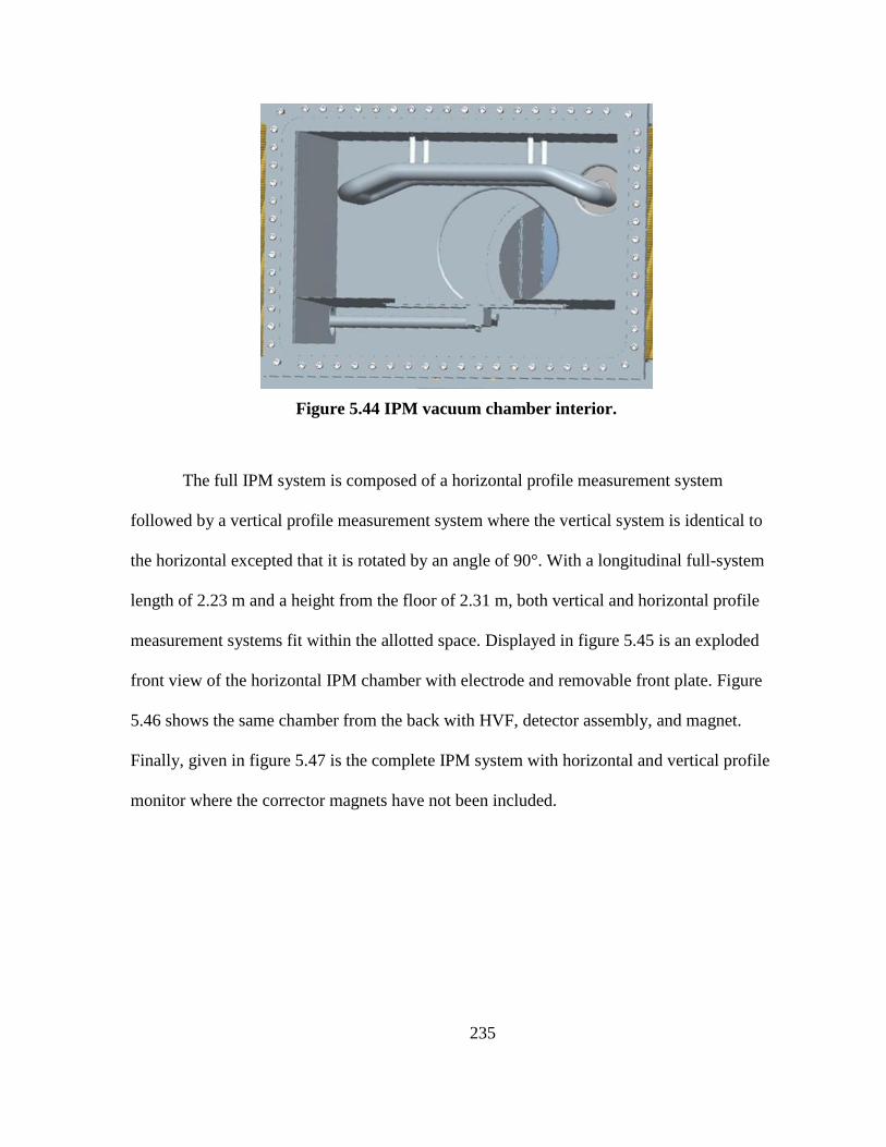
235

Figure 5.44 IPM vacuum chamber interior.

The full IPM system is composed of a horizontal profile measurement system

followed by a vertical profile measurement system where the vertical system is identical to

the horizontal excepted that it is rotated by an angle of 90°. With a longitudinal full-system

length of 2.23 m and a height from the floor of 2.31 m, both vertical and horizontal profile

measurement systems fit within the allotted space. Displayed in figure 5.45 is an exploded

front view of the horizontal IPM chamber with electrode and removable front plate. Figure

5.46 shows the same chamber from the back with HVF, detector assembly, and magnet.

Finally, given in figure 5.47 is the complete IPM system with horizontal and vertical profile

monitor where the corrector magnets have not been included.

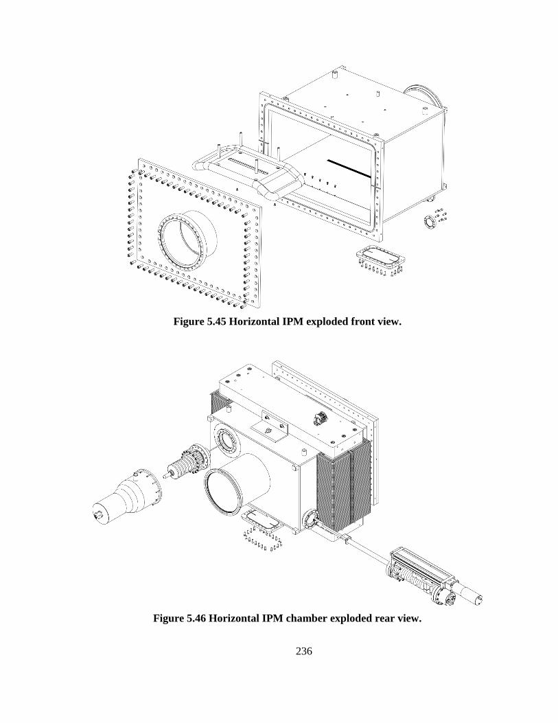
236

Figure 5.45 Horizontal IPM exploded front view.

Figure 5.46 Horizontal IPM chamber exploded rear view.

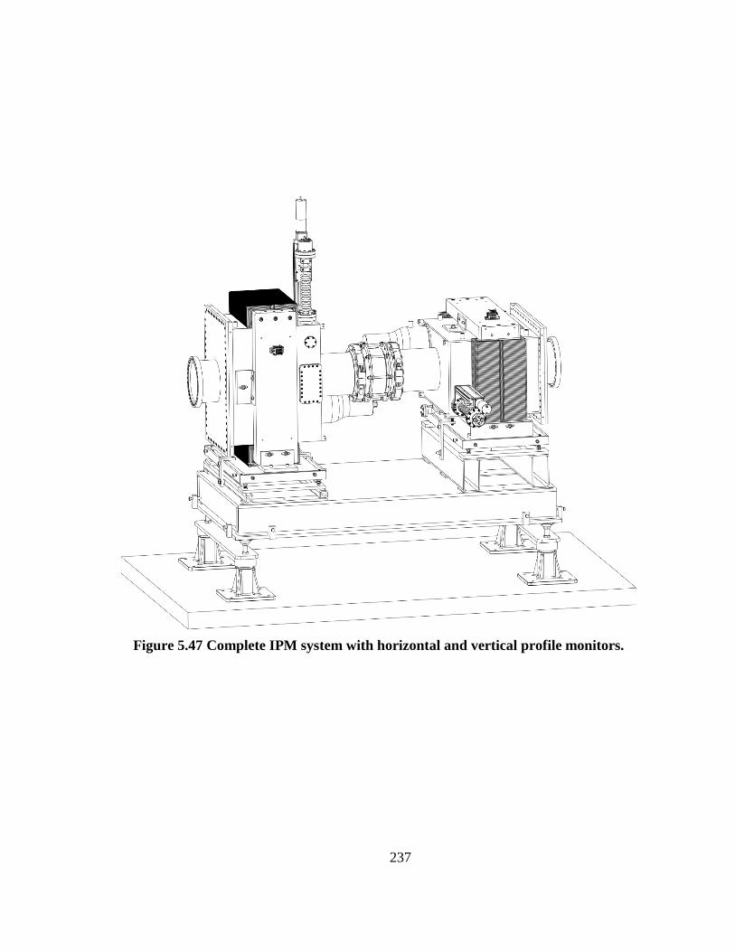
237

Figure 5.47 Complete IPM system with horizontal and vertical profile monitors.

238

Chapter 6

Summary

6.1 Overall Project Summary

This work presents the study, analysis, and design of an ionization profile monitor system for

the SNS ring. A history of IPM development was presented that showed the technological

development and current state of this type of beam diagnostic. A set of design parameters

required to produce accurate turn-by-turn profiles for a production quality beam in SNS was

then set forth. Based on first principles, the basic assumptions necessary to develop a

theoretical framework for an IPM were proposed, which required the derivation of the theory

of beam-gas interaction based on relativistic energy transfer. Beam energy loss leading to

primary and secondary ionization was analyzed in order to determine pair production values

for various gases. A detailed study of the residual gas at the IPM location through an RGA

and pressure analysis allowed the estimation of ions and electrons created through ionization.

Additionally, an analysis of the SNS electron cloud was performed to determine its influence

on IPM profiles.

Once estimates for the expected signal had been determined, based on theoretical

examination of measured gas data, a simulation study was reported that analyzed the IPM

239

operational parameters through particle trajectory tracking. The SNS ORBIT Runge-Kutta

tracker was used as a building block to study longitudinal and transverse particle trajectory

properties in a variety of electric and magnetic fields including beam space charge. Based on

the trajectory study, design parameters and system limitations were established leading to

profile measurement with electrons.

A detailed system accuracy study was performed based on a Monte Carlo method of

profile generation subject to expected errors. The spatial accuracy was estimated and

revealed further system constraints required in order to meet the design criteria. Likewise,

investigation of the time resolution led to a data acquisition regime that preserves turn-by-

turn resolution. The importance of secondary electron emission noise was identified as a

major source of profile error.

An IPM test chamber was designed and built to test the basic IPM principles of turn-

by-turn measurement with a Channeltron. The test chamber was vital in identifying

unanticipated sources of beam and environmental signal noise. Results of the test chamber

modifications gave rise to further design criteria necessary to obtain clean ionized particle

measurements. Finally, each of the major IPM system design components was outlined in

detail. Theoretical justification was given for many of the design decisions and all previously

determined design criteria were implemented.

6.2 Future Work

While this work presents a detailed description and design of an SNS IPM system, a

significant effort is required to bring the design to a physical and usable conclusion. Along

with the design drawings, the majority of the components have been specified and quoted for

240

pricing. At the time of this writing, the cost for the complete IPM, composed of horizontal

and vertical monitors, was ~$500,000 with an approximate lead time of 1 year for

fabrication. Upon receipt of components, system assembly and lab testing in order to verify

the system’s ability to operate at the required voltage, measurement and verification of

magnet multipole strengths, testing of Channeltron operation, and cable distortion need to be

performed. Subsequently, upon assembly of the actuator and detector, Labview code needs to

be developed for the system’s data acquisition, signal processing, actuator control, and power

supply management. Considering that the final goal is control room usability, the IPM

software must be made user-friendly and compatible with the SNS accelerator control

system.

Furthermore, SNS protocol requires the system to have built in safety features, such

as a power supply shut off mechanism in the event of accelerator maintenance for the

purpose of personnel protection. The IPM must also be tied into the larger accelerator

protection system. Finally, commissioning of the IPM requires installation in the beamline

and troubleshooting of unexpected system errors. Inevitably some measure of system

modification will be required. Once the IPM profile accuracy has been compared with

ORBIT simulations and the electron scanner profile monitor, the system may be turned over

to accelerator operators as a verified ring profile diagnostic tool.

While it was determined the IPM would not be able to produce ion-based profiles

with the required spatial accuracy, the system design supports ion collection. It was a goal of

this project to design a system capable of measuring ion profiles that could eventually be

used to study ion profile measurement methods. Determining a beam-based space-charge

profile calibration would be a significant contribution to IPM technology and the system

241

proposed here has the capability to support such research

Upon successful installation and operation of the IPM, an upgrade to the system

would involve replacing the movable single detector with an array of detectors. A row of

contiguous detectors would eliminate the necessity for an actuator while greatly reducing

measurement time. Such an upgrade would require a power supply control system for each

detector as well as a method for in-situ detector calibration.

6.3 Final Remarks

An ionization profile monitor has been designed for the SNS ring that has the ability to

measure turn-by-turn horizontal and transverse beam profiles for a full 60 Hz, production

quality beam. With a measurement time of <5 minutes, the IPM system will have an

estimated transverse measurement accuracy of 4.9% with a 2% uncertainty using ionized

electrons. Signal processing and system design allows for 1 μs resolution with a rise time

20 ns or a 3 dB bandwidth ≥17.5 MHz. In order to sustain a 120 kV potential the IPM

electrode has been designed to sustain a maximum 4.5 kV/mm electric field. Additionally,

higher order magnet multipole components are <1% at a reference radius of 12.78 cm. While

the electrode produces <0.5 mrad of beam deflection, the IPM magnets do not and therefore

require corrector magnets. In conclusion, an IPM system design satisfying all of the required

design criteria has been successfully completed for the Spallation Neutron Source

accumulator ring.

242

Bibliography

243

[1] E. Rutherford, “Address of the President, Sir Ernest Rutherford, O.M., at the

Anniversary Meeting, November 30, 1927,” Proceedings of the Royal Society A:

Mathematical, Physical and Engineering Sciences, vol. 117, no. 777, pp. 300–316,

Jan. 1928.

[2] C. R. Gould, G. L. Greene, F. Plasil, and W. M. Snow, “WORKSHOP SUMMARY:

FUNDAMENTAL NEUTRON PHYSICS IN THE UNITED STATES: AN

OPPORTUNITY IN NUCLEAR, PARTICLE, AND ASTROPHYSICS FOR THE

NEXT DECADE,” in Fundamental Physics with Pulsed Neutron Beams, 2001, pp. 1–

8.

[3] “Spallation Neutron Source,” 2012. [Online]. Available:

http://neutrons.ornl.gov/facilities/SNS/. [Accessed: 02-Jun-2012].

[4] S. Henderson, “SNS Parameters List R13,” Spallation Neutron Source, Oak Ridge,

Tennessee, 2005.

[5] M. P. Stockli, “The SNS Chopper System.” Spallation Neutron Source, Oak Ridge,

Tennessee, p. 4, 2002.

[6] S. Assadi, “SNS Beam Instrumentations for High Power Operations,” in The

Eighteenth Meeting of the International Collaboration of Advanced Neutron Sources

(ICANS), 2007, p. 4.

[7] C. Sibley, “MACHINE PROTECTION STRATEGIES FOR HIGH POWER

ACCELERATORS *,” in Particle Accelerator Conference, 2003, pp. 607–611.

[8] R. E. Shafer, “Beam Position Monitoring,” in AIP Conference Proceedings, 1990, vol.

212, pp. 26–58.

[9] J. Galayda, “Beam Profile Measurements,” in AIP Conference Proceedings 212:

Accelerator Instrumentation, E. R. Beadle and V. J. Castillo, Eds. Upton, New York:

AIP, 1989, pp. 59–86.

[10] C. J. Liaw and P. R. Cameron, “CARBON WIRE HEATING DUE TO

SCATTERING IN THE SNS,” in Particle Accelerator Conference, 2001, no. 2, pp.

2365–2367.

[11] M. A. Plum et al., “Beam Diagnostics in the SNS Linac,” in Tenth Beam

Instrumentation Workshop, 2002, pp. 195–202.

[12] W. Blokland, S. Cousineau, D. Malyutin, and S. Starostenko, “ELECTRON

SCANNER FOR SNS RING PROFILE MEASUREMENTS,” in DIPAC 2009, 2009,

pp. 3–5.

244

[13] S. Payne, “Fast gas ionisation beam profile monitor for the ISIS Proton Synchrotron.”

p. 42.

[14] P. Forck, “MINIMAL INVASIVE BEAM PROFILE MONITORS FOR HIGH

INTENSE HADRON BEAMS,” in International Particle Accelerator Conference,

2010, pp. 1261–1265.

[15] V. Dudnikov, “Self-stamilization of e-p Instability and Accumulation of a

Superintense Circulating Beam.” Upton, New York, p. 54, 2006.

[16] F. Hornstra and W. H. DeLuca, “NONDESTRUCTIVE BEAM PROFILE

DETECTION SYSTEMS FOR THE ZERO GRADIENT SYNCHROTRON,” in Sixth

International Conference on High Energy Accelerators, 1967, pp. 374–377.

[17] W. H. DeLuca, “Beam Detection Using Residual Gas Ionization,” IEEE Transactions

on Nuclear Science, vol. 16, no. 3, pp. 813 – 822, 1969.

[18] E. W. McDaniel, Collision Phenomena in Ionized Gases. New York, Wiley, 1964.

[19] H. S. W. Massey and E. H. S. Burhop, Electronic and Ionic Collision Impact

Phenomena. Oxford: Clarendon Press, 1952.

[20] W. H. Deluca and M. F. Shea, “A Nondestructive Linac Beam Density Profile

Monitor,” in Proton Linear Accelerator Conference, 1968, pp. 190–197.

[21] C. D. Johnson and L. Thorndahl, “THE CPS GAS-IONIZATiON BEAM

SCANNER,” in Symposium on Beam Intensity Measurement, 1968, pp. 909–913.

[22] A. Barlow et al., “Instrumentation and beam diagnostics in the ISR,” in 8th

International Conference on High-energy Accelerators, 1971, pp. 426–430.

[23] B. Vosicki and K. Zankel, “THE SODIUM CURTAIN BEAM PROFILE MONITOR

OF THE ISR,” IEEE Transactions on Nuclear Science, vol. 22, no. 3, pp. 1475–1478,

1975.

[24] H. Ishimaru, Z. Igarashi, K. Muto, and S. Shibata, “Beam Profile Measurements for

KEK 12 GeV Proton Synchrotron,” IEEE Transactions on Nuclear Science, vol. 24,

no. 3, pp. 1821–1823, Jun. 1977.

[25] T. Hardek, W. Kells, and H. Lai, “Very Low Intensity Storage-Ring Profile Monitor,”

IEEE Transactions on Nuclear Science, vol. NS-28, no. 3, pp. 2219–2221, 1981.

[26] J. R. Zagel, D. Chen, and J. Crisp, “Fermilab Booster Ion Profile Monitor System

Using LabView,” in Beam Instrumentation Workshop, 1994, no. 4, pp. 384–390.

245

[27] J. R. Zagel, A. A. Hahn, J. L. Crisp, and C. Jensen, “IMPROVEMENTS TO THE

FERMILAB IONIZATION PROFILE MONITOR SYSTEMS *,” in Particle

Accelerator Conference, 1999, pp. 2164–2166.

[28] H. L. Weisberg, “Beam Profile Monitors for the AGS.” Upton, New York, pp. 1–9,

1981.

[29] H. Weisberg, E. Gill, P. Ingrassia, and E. Rodger, “An Ionization Profile Monitor for

the Brookhaven AGS,” IEEE Transactions on Nuclear Science, vol. 30, no. 4, pp.

2179–2181, Aug. 1983.

[30] R. E. Thern, “Space Charge Distortion in the Brookhaven Ionization Profile Monitor,”

in PAC 1987, 1987, pp. 646–648.

[31] M. R. Harold et al., “Diagnostics and Commissioning Progress on ISIS,” in European

Particle Accelerator Conference, 1988, pp. 347–349.

[32] K. Wittenburg, “Experience with the Residual Gas Ionization Beam Profile Monitors

at the DESY Proton Accelerators,” in 3rd European Particle Accelerator Conference,

1992, pp. 1–5.

[33] J. Schwarz, “Beam measurement with rest-gas ionizations monitor in PETRA,” in

PcaPac 2000, 2000.

[34] F. Hornstra, “RESIDUAL GAS IONIZATION BEAM PROFILE MONITORS FOR

THE HERA PROTON MACHINES,” in 1st EPAC, 1988, pp. 1160–1162.

[35] K. Wittenburg, “Transversal Emittance Measurement,” in Harz-Seminar, 1992.

[36] N. Ceci et al., “Preliminary Study for a Residual Gas Beam Profile Monitor,” in 5th

European Particle Accelerator Conference, 1996, pp. 1642–1644.

[37] V. Variale et al., “First test results for a residual gas beam profile monitor,”

Proceedings of the 1997 Particle Accelerator Conference, vol. 2, pp. 2169–2170,

1998.

[38] M. Bellato, A. Dainelli, and M. Poggi, “Commissioning and Developments of the

ALPI Diagnostics System,” in 4th European Particle Accelerator Conference, 1994,

pp. 1512–1514.

[39] B. Hochadel et al., “A residual-gas ionization beam profile monitor for the Heidelberg

Test Storage Ring TSR,” Nuclear Instruments and Methods in Physics Research

Section A: Accelerators, Spectrometers, Detectors and Associated Equipment, vol.

343, no. 2–3, pp. 401–414, Apr. 1994.

246

[40] J.-L. P. Vignet, R. M. Anne, Y. R. Georget, R. E. Hue, and C. H. Tribouillard, “Beam

monitors based on residual gas ionization,” in 7th Beam Instrumentation Workshop,

1996.

[41] P. Cameron et al., “The RHIC Ionization Beam Profile Monitor,” Proceedings of the

1999 Particle Accelerator Conference, vol. 3, pp. 2114–2116, 1999.

[42] W. C. Sellyey and J. D. Gilpatrick, “A compact residual gas ionization profile monitor

(rgipm) system,” in Particle Accelerator Conference, 1999, pp. 2152–2154.

[43] W. C. Sellyey, J. D. Gilpatrick, and R. Senior, “Bench test of a residual gas ionization

profile monitor (RGIPM),” in PAC 2001, 2001, vol. 2, pp. 1318–1320.

[44] A. Jansson et al., “Tevatron Ionization Profile Monitor,” Batavia, IL, 2003.

[45] A. Jansson et al., “An Ionization Profile Monitor for the Tevatron,” in 2005 Particle

Accelerator Conference, 2005, pp. 2227–2229.

[46] A. Jansson et al., “TEVATRON IONIZATION PROFILE MONITORING,” in EPAC

2006, 2006, pp. 159–167.

[47] Y. Sato et al., “Development of Residual Gas Ionization Profile Monitor for High

Intensity Proton Beams,” IEEE Nuclear Science Symposium Conference Record, 2005,

vol. 2, pp. 1043–1046, 2005.

[48] S. Lee et al., “DESIGN STUDY OF A NONDESTRUCTIVE BEAM PROFILE AND

HALOS MONITOR BASED ON RESIDUAL GAS IONIZATION FOR THE J-

PARC RCS,” in The 14th Symposium on Accelerator Science and Technology, 2003,

no. November.

[49] K. Satou, N. Hayashi, S. Lee, and T. Toyama, “A PROTOTYPE OF RESIDUAL GAS

IONIZATION PROFILE MONITOR FOR J-PARC RCS,” in EPAC 2006, 2006, no.

1, pp. 1163–1165.

[50] K. Satou et al., “BEAM PROFILE MONITORING OF THE J-PARC 3 GeV RAPID

CYCLING SYNCHROTRON,” in EPAC 2008, 2008, pp. 1275–1277.

[51] R. Ishida, “R & D of Beam Monitors at J-PARC Neutrino Beamline,” University of

Tokyo, 2005.

[52] P. Forck, A. Bank, T. Giacomini, and A. Peters, “PROFILE MONITORS BASED ON

RESIDUAL GAS INTERACTION,” in DIPAC, 2005, no. 03, pp. 223–227.

[53] F. Roncarolo, “Accuracy of the Transverse Emittance Measurements of the CERN

Large Hadron Collider,” IPEP Institut de physique de l’energie et des particules, 2005.

247

[54] C. Bal, V. Prieto, R. Sautier, and G. Tranquille, “FIRST RESULTS FROM THE LEIR

IONISATION PROFILE MONITORS,” in Proceedings of DIPAC 2007, 2007, pp.

120–122.

[55] E. Mahner, “Technical Design of the LEIR Vacuum System Technical Design of the

LEIR Vacuum System,” Geneva, Switzerland, 2002.

[56] M. Sachwitz, A. Hofmann, S. Pauliuk, K. Tiedtke, and H. Wabnitz, “IONIZATION

PROFILE MONITOR TO DETERMINE SPATIAL AND ANGULAR STABILITY

OF FEL RADIATION OF FLASH,” in EPAC 2008, 2008, pp. 1266–1268.

[57] J. Egberts et al., “DETAILED EXPERIMENTAL CHARACTERIZATION OF AN

IONIZATION PROFILE MONITOR,” in DIPAC, 2011, pp. 3–5.

[58] G. Ferioli, C. Fischer, J. Koopman, and F. Roncarolo, “BEAM STUDIES MADE

WITH THE SPS IONIZATION PROFILE MONITOR,” in DIPAC, 2003, pp. 116–

118.

[59] D. Liakin, V. Skachkov, P. Forck, and T. Giacomini, “Improving the Reliability of

IPM,” in DIPAC 2005, 2005, vol. 29, no. 6, pp. 150–152.

[60] R. Connolly, R. Michnoff, and S. Tepikian, “Residual-Gas-Ionization Beam Profile

Monitors in RHIC,” in 2005 Particle Accelerator Conference, 2005, pp. 230–234.

[61] M. Poggi et al., “Activity of Diagnostics Laboratory,” Africa. pp. 1–2, 2006.

[62] M. Poggi et al., “TWO-DIMENSIONAL IONIZATION BEAM PROFILE

MEASUREMENT,” in DIPAC 2009, 2009, pp. 384–386.

[63] B. G. Pine, C. M. Warsop, and S. J. Payne, “Modelling of Diagnostics for Space

Charge Studies on the ISIS Synchrotron,” in EPAC 2006, 2006, vol. 3, pp. 1082–1084.

[64] S. J. Payne, P. G. Barnes, G. M. Cross, A. Pertica, and S. A. Whitehead, “A SELF

CALIBRATING REAL TIME MULTI-CHANNEL PROFILE MONITOR FOR THE

ISIS PROTON SYNCHROTRON,” in DIPAC 2007, 2007, pp. 364–366.

[65] R. E. Williamson, B. G. Pine, S. J. Payne, and C. M. Warsop, “ANALYSIS OF

MEASUREMENT ERRORS IN RESIDUAL GAS IONISATION PROFILE

MONITORS IN A HIGH INTENSITY PROTON BEAM,” in EPAC 2008, 2008, pp.

1317–1319.

[66] S. A. Whitehead, P. G. Barnes, G. M. Cross, S. J. Payne, and A. Pertica, “MULTI-

CHANNELTRON BASED PROFILE MONITOR AT THE ISIS PROTON

SYNCHROTRON,” in BIW 2010, 2010, pp. 1–5.

248

[67] J. Amundson, J. Lackey, P. Spentzouris, G. Jungman, and L. Spentzouris, “Calibration

of the Fermilab Booster Ionization Profile Monitor,” Physical Review Special Topics -

Accelerators and Beams, vol. 6, no. 10, pp. 1–15, Oct. 2003.

[68] J. Zagel, “Personal Communication.” .

[69] S. Payne, “Personal Communication.” .

[70] A. Kowalczyk, “Proton induced spallation reactions in the energy range 0 . 1 - 10

GeV,” Jagiellonian University, 2007.

[71] D. Filges and F. Goldenbaum, Handbook of Spallation Research. Weinheim,

Germany: Wiley-VCH Verlag GmbH & Co. KGaA, 2009.

[72] S. Meroli, D. Passeri, and L. Servoli, “Energy loss measurement for charged particles

in very thin silicon layers,” Journal of Instrumentation, vol. 6, no. 06, pp. P06013–

P06013, Jun. 2011.

[73] L. D. Landau, “On the Energy Loss of Fast Particles by Ionisation,” in Collected

Papers of L. D. Landau, First., D. Ter Haar, Ed. London, England: Gordon and

Breach, Science Publishers, 1965, pp. 417–424.

[74] J. D. Jackson, Classical Electrodynamics, Third. Hoboken, NJ: Wiley, 1999, pp. 1–

808.

[75] I. Hutchinson, “Chapter 6 Collisions of Charged Particles,” MIT Open Courseware -

Electromagnetic Interactions - Readings, 2005. [Online]. Available:

http://ocw.mit.edu/courses/nuclear-engineering/22-105-electromagnetic-interactions-

fall-2005/readings/chap6.pdf.

[76] M. Inokuti and J. E. Turner, “MEAN EXCITATION ENERGIES FOR STOPPING

POWER AS DERIVED FROM OSCILLATOR-STRENGTH DISTRIBUTIONS,” in

Sixth Symposium on Microdosimetry, 1978, pp. 675–687.

[77] M. J. Berger and S. M. Seltzer, “Tables of Energy Losses and Ranges of Electrons and

Positrons,” National Aeronautics and Space Administration, Washington, D.C., 1964.

[78] S. M. Seltzer and M. J. Berger, “Evaluation of the collision stopping power of

elements and compounds for electrons and positrons,” The International Journal of

Applied Radiation and Isotopes, vol. 33, no. 11, pp. 1189–1218, Nov. 1982.

[79] E. Segrè, Nuclei and Particles: An Introduction to Nuclear and Subnuclear Physics,

Second. Reading, MA: Benjamin-Cummings Pub Co, 1977.

[80] W. H. Tait, Radiation Detection. London, UK: Butterworth Inc., 1980.

249

[81] G. F. Knoll, Radiation Detection and Measurement, Third. Chinchester, New York:

Wiley, 2000.

[82] N. Bohr, “LX. On the decrease of velocity of swiftly moving electrified particles in

passing through matter,” Philosophical Magazine Series 6, vol. 30, no. 178, pp. 581–

612, Oct. 1915.

[83] H. Bethe, “Zur Theorie des Durchgangs schneller Korpuskularstrahlen durch Materie,”

Annalen der Physik, vol. 397, no. 3, pp. 325–400, 1930.

[84] D. Groom, “Energy loss in matter by heavy particles,” Particle Data Group, Note

PDG-93-06, 1993.

[85] B. J. McParland, Nuclear Medicine Radiation Dosimetry. London: Springer London,

2010.

[86] K. Nakamura and (Particle Data Group), “Review of Particle Physics,” Journal of

Physics G: Nuclear and Particle Physics, vol. 37, no. 7A, p. 075021, Jul. 2010.

[87] J. Lindhard, “On the properties of a gas of charged particles,” Matematisk Fysiske

Meddelelser - Kongelige Dankse Videnskabernes Selskab, vol. 28, no. 8, 1954.

[88] D. I. Thwaites, “Bragg’s Rule of Stopping Power Additivity: A Compilation and

Summary of Results,” Radiation Research, vol. 95, no. 3, pp. 495–518, 1983.

[89] B. Rossi, High-energy Particles. New York, NY: Prentice-Hall Incorporated, 1965.

[90] S. Sasaki, T. Sanami, K. Saito, K. Iijima, H. Tawara, and T. Murakami, “W-values for

heavy ions in gases,” in 2009 IEEE Nuclear Science Symposium Conference Record

(NSS/MIC), 2009, pp. 702–705.

[91] U. Fano, “Ionization Yield of Radiations. II. The Fluctuations of the Number of Ions,”

Physical Review, vol. 72, no. 1, pp. 26–29, Jul. 1947.

[92] I. K. Bronic, “On a relation between the W value and the Fano factor,” Journal of

Physics B: Atomic, Molecular and Optical Physics, vol. 25, no. 8, pp. L215–L218,

Apr. 1992.

[93] W. W. M. Allison and J. H. Cobb, “Relativistic Charged Particle Identification by

Energy Loss,” Annual Review of Nuclear and Particle Science, vol. 30, no. 1, pp. 253–

298, Dec. 1980.

[94] I. B. Smirnov, “Modeling of ionization produced by fast charged particles in gases,”

Nuclear Instruments and Methods in Physics Research Section A: Accelerators,

Spectrometers, Detectors and Associated Equipment, vol. 554, no. 1–3, pp. 474–493,

250

Dec. 2005.

[95] A. G. Mathewson and O. Gröbner, “Thermal Outgassing and Beam Induced

Desorption,” in Handbook of Accelerator Physics and Engineering, A. W. Chao and

M. Tigner, Eds. Singapore: World Scientific Publishing Co. Pte. Ltd., 1998, pp. 224–

227.

[96] P. He, H. C. Hseuh, M. Maples, R. Todd, D. Weiss, and D. Wilson, “Hydrogen

Outgassing and Surface Properties of TiN-Coated Stainless Steel Chambers,” in First

International Workshop on Materials and Vacuum, 2003, vol. 671, pp. 292–299.

[97] J. Price and C. Stone, “Private Commincation.” .

[98] “Models RGA100 , Residual Gas Analyzer Operating Manual and Programming

Reference,” vol. 8. Stanford Research Systems, Sunnyvale, CA, 2009.

[99] E. C. Montenegro, “Fragmentation of water by heavy ions,” Journal of Physics:

Conference Series, vol. 194, no. 1, p. 012049, Nov. 2009.

[100] “Cracking Patterns,” Hiden Analytical, 2013. [Online]. Available:

http://www.hidenanalytical.com/index.php/en/cracking-patterns. [Accessed: 10-May-

2013].

[101] “Partial Pressures vs. Total Pressure for an Open Ion Source RGA,” Leybold Inficon

Tech Note, 1991. [Online]. Available:

http://www.inficon.com/download/en/Partial_pressures.pdf.

[102] K. Jousten, Ed., Handbook of Vacuum Technology. Weinheim, Germany: Wiley-VCH

Verlag GmbH & Co. KGaA, 2008, pp. 646–647.

[103] H. C. Hseuh, C. J. Liaw, and M. Mapes, “DESIGN OF THE SNS ACCUMULATOR

RING VACUUM SYSTEMS,” in Particle Accelerator Conference, 1999, pp. 1345–

1347.

[104] A. G. Ruggiero and M. Blaskiewicz, “The Electron-Proton Effects in Intense Proton

Bunches,” BNL/NSNS, Upton, New York, Tech. Note #8, 1997.

[105] A. W. Chao, Physics of Collective Beam Instabilities in High Energy Accelerators.

New York, NY: Wiley-Interscience, 1993.

[106] Y. A. Cengel and M. Boles, Thermodynamics: An Engineering Approach, 4th ed. New

York, NY: McGraw-Hill, 2001, pp. 152–153.

[107] N. Marquardt, “Introduction to the Principles of Vacuum Physics,” in CERN

Accelerator School: Vacuum Techonolgy, 1999, pp. 1–24.

251

[108] S. Zheng, “Conductance Calculation - Molecular Flow, Long Tube of Circular Cross

Section,” Fermilab, Batavia, IL, Tech. Rep. ssc-gem-tn-93-382, 1993.

[109] G. Guignard, “Selection of Formulae Concerning Proton Storage Rings,” CERN,

Geneva, Switzerland, Yellow Report 10, 1977.

[110] K. M. Welch, “The pressure profile in a long outgassing vacuum tube,” Vacuum, vol.

23, no. 8, pp. 271–276, Aug. 1973.

[111] A. Aleksandrov, S. Assadi, S. Cousineau, V. Danilov, S. Henderson, and M. Plum,

“FEASIBILITY STUDY OF USING AN ELECTRON BEAM FOR PROFILE

MEASUREMENTS IN THE SNS ACCUMULATOR RING.,” in PAC 2005, 2005,

vol. 2, no. 3, pp. 2586–2588.

[112] H. Hseuh et al., “DESIGN AND IMPLEMENTATION OF SNS RING VACUUM

SYSTEM WITH SUPPRESSION OF ELECTRON CLOUD INSTABILITY,” in 31st

Advanced ICFA Beam Dynamics Workshop on Electron-Cloud Effects, 2004, pp. 119–

122.

[113] O. Gröbner, “DYNAMIC OUTGASSING,” in CAS-CERN Accelerator School, 1999,

no. 3, pp. 127–138.

[114] F. Rieke and W. Prepejchal, “Ionization Cross Sections of Gaseous Atoms and

Molecules for High-Energy Electrons and Positrons,” Physical Review A, vol. 6, no. 4,

pp. 1507–1519, Oct. 1972.

[115] M. Inokuti, “Inelastic Collisions of Fast Charged Particles with Atoms and

Molecules—The Bethe Theory Revisited,” Reviews of Modern Physics, vol. 43, no. 3,

pp. 297–347, Jul. 1971.

[116] Y. Baconnier, “Neutralization of Accelerator Beams by Ionization of the Residual

Gas,” in CAS - CERN Accelerator School: General Accelerator Physics, 1985, pp.

267–297.

[117] J. de Segovia, “A review of electron stimulated desorption processes influencing the

measurement of pressure or gas composition in ultra high vacuum systems,” Vacuum,

vol. 47, no. 4, pp. 333–340, Apr. 1996.

[118] N. Hilleret, “Non-Thermal Outgassing,” in CAS - CERN Accelerator School: Vacuum

in Accelerators, 2007, pp. 87–116.

[119] F. Sauli, “Principles of Operation of Multiwire Proportional and Drift Chambers,”

Geneva, Switzerland, 1977.

[120] a. Muñoz et al., “Single electron tracks in water vapour for energies below 100eV,”

252

International Journal of Mass Spectrometry, vol. 277, no. 1–3, pp. 175–179, Nov.

2008.

[121] Y.-K. Kim et al., “Electron-Impact Cross Sections for Ionization and Excitation,” in

NIST Chemistry WebBook, NIST Standard Reference Database Number 102, P. J.

Linstrom and W. G. Mallard, Eds. Gaithersburg, MD: National Institute of Standards

and Technology. [Online]. Available: http://webbook.nist.gov. [Accessed: 23-Jan-

2013].

[122] A. Edwards, R. Wood, A. Beard, and R. Ezell, “Single and double ionization of H2 by

electrons and protons,” Physical Review A, vol. 37, no. 10, pp. 3697–3701, May 1988.

[123] A. M. Sayler, E. Wells, K. D. Games, and I. Ben-Itzhak, “Velocity dependence of

electron removal and fragmentation of water molecules caused by fast proton impact,”

AIP Conference Proceedings, vol. 576, no. 2001, pp. 33–35, 2001.

[124] M. Blaskiewicz, M. Furman, M. Pivi, and R. Macek, “Electron cloud instabilities in

the Proton Storage Ring and Spallation Neutron Source,” Physical Review Special

Topics - Accelerators and Beams, vol. 6, no. 1, p. 014203, Jan. 2003.

[125] J. Wei and R. J. Macek, “ELECTRON-CLOUD EFFECTS IN HIGH-INTENSITY

PROTON ACCELERATORS,” in ECLOUD ’02 Workshop, 2002.

[126] J. Wei et al., “ELECTRON-CLOUD MITIGATION IN THE SPALLATION

NEUTRON SOURCE RING ,” in PAC, 2003, pp. 2598–2600.

[127] M. Furman and M. Pivi, “Probabilistic model for the simulation of secondary electron

emission,” Physical Review Special Topics - Accelerators and Beams, vol. 5, no. 12,

pp. 1–31, Dec. 2002.

[128] M. Pivi and M. A. Furman, “MITIGATION OF THE ELECTRON-CLOUD EFFECT

IN THE PSR AND SNS PROTON STORAGE RINGS BY TAILORING THE

BUNCH PROFILE,” in 20th Particle Accelerator Conference, 2003, pp. 3222–3225.

[129] R. J. Macek et al., “ELECTRON PROTON TWO-STREAM INSTABILITY AT THE

PSR,” in PAC 2001, 2001.

[130] P. He et al., “SECONDARY ELECTRON EMISSION MEASUREMENTS FOR TIN

COATING ON THE STAINLESS STEEL OF SNS ACCUMULATOR RING

VACUUM CHAMBER,” in EPAC 2004, 2004, pp. 5–8.

[131] R. Todd, P. He, H. C. Hseuh, and D. Weiss, “Summary on Titanium Nitride Coating

of SNS Ring Vacuum Chambers,” in Proceedings of the 2005 Particle Accelerator

Conference, 2005, pp. 3088–3090.

253

[132] J. A. Holmes, “Private Communication.” .

[133] A. Shishlo, “Private Communication.” .

[134] R. V. Latham et al., High Voltage Vacuum Insulation: Basic Concepts and

Technological Practice. San Diego, CA: Academic Press Limited, 1995.

[135] E. B. Podgorsak, “1 Introduction to Modern Physics,” in Radiation Physics for

Medical Physics, Second., vol. 54, no. 1, Heidelberg, Germany: Springer, 2010, pp. 1–

75.

[136] C. K. Sinclair, H. F. Dylla, T. L. Siggins, D. Manos, L. Wu, and T. J. Venhaus,

“DRAMATIC REDUCTION OF DC FIELD EMISSION FROM LARGE AREA

ELECTRODES BY PLASMA-SOURCE ION IMPLANTATION,” in PAC 2001,

2001, pp. 610–612.

[137] N. Tsoulfanidis, Measurement and Detection of Radiation, First. Washington, D.C.:

Hemisphere Publising, 1983.

[138] R. F. Post, “Plasma Physics in the 20th Century,” in Twentieth Century Physics,

Volume III., L. M. Brown, P. A, and B. Pippard, Eds. New York, NY: Bristol and

American Institute of Physics Press, 1995.

[139] K. Miyamoto, “Fundamentals of Plasma Physics and Controlled Fusion,” National

Institute for Fusion Science, Nagoya, Japan, NIFS-PROC-48, 2000.

[140] “CHANNELTRON HANDBOOK,” Burle Industries. [Online]. Available:

http://www.photonisusa.com/.

[141] F. Cardarelli, Materials Handbook: A Concise Desktop Reference, 2nd ed. London,

England: Springer-Verlag, 2008.

[142] L. Heroux and H. E. Hinteregger, “Resistance Strip Magnetic Photomultiplier for the

Extreme Ultraviolet,” Review of Scientific Instruments, vol. 31, no. 3, p. 280, 1960.

[143] Y. B. Hahn, R. E. Hebner, D. R. Kastelein, and K. J. Nygaard, “Channeltron Gain in

Magnetic Fields,” Review of Scientific Instruments, vol. 43, no. 4, p. 695, 1972.

[144] T. L. Chenevert and P. W. Zitzewitz, “Performance of a spiralled continuous electron

multiplier in a magnetic field,” Review of Scientific Instruments, vol. 48, no. 12, pp.

1601–1602, 1977.

[145] R. H. Thomas, “Radiation Sources,” in Handbook of Accelerator Physics and

Engineering, A. W. Chao and M. Tigner, Eds. Singapore: World Scientific Publishing

Co. Pte. Ltd., 1998, pp. 598–605.

254

[146] J. G. Timothy and R. L. Bybee, “Effects of 1-MeV gamma radiation on a multi-anode

microchannel array detector tube.,” The Review of scientific instruments, vol. 50, no.

6, p. 743, Jun. 1979.

[147] H. H. Refsum, B. Dehning, and J. Koopman, “SIMULATION OF AN ELECTRON

SOURCE BASED CALIBRATING SYSTEM FOR AN IONISATION PROFILE

MONITOR,” in DIPAC 2005, 2005, pp. 160–162.

[148] J. R. Taylor, An Introduction to Error Analysis: The Study of Uncertainties in Physical

Measurements, Second. Sausalito, CA: University Science Books, 1997, pp. 297–298.

[149] H. J. de Blank, “Guiding Center Motion,” Fusion Science and Technology, vol. 49, no.

2T, pp. 59–66, 2006.

[150] J. Cary and A. Brizard, “Hamiltonian theory of guiding-center motion,” Reviews of

Modern Physics, vol. 81, no. 2, pp. 693–738, May 2009.

[151] J. D. Galambos, J. A. Holmes, and D. K. Olsen, “ORBIT User Manual,” SNS-ORNL-

AP Tech. Note 11, 1999.

[152] J. Galambos, S. Danilov, D. Jeon, J. Holmes, D. Olsen, and A. Luccio, “ORBIT – A

RING INJECTION CODE WITH SPACE CHARGE,” IEEE, New York, New York,

1999.

[153] J. A. Holmes, J. D. Galambos, D. K. Olsen, J. H. Whealton, M. Blaskiewicz, and A.

Luccio, “A PARTICLE-IN-CELL MODEL FOR SPACE CHARGE DYNAMICS IN

RINGS,” in EPAC, 1998, pp. 1109–1111.

[154] S. Hassani, Mathematical Physics: A Modern Introduction to Its Foundations. New

York, NY: Springer-Verlag, 1999, pp. 387–394.

[155] A. V. Fedotov, N. Malitsky, and J. Wei, “SPACE-CHARGE SIMULATIONS FOR

THE SPALLATION NEUTRON SOURCE (SNS) RING USING UNIFIED

ACCELERATOR LIBRARIES,” Brookhaven National Laboratory, Upton, New

York, Tech. Note BNL/SNS No. 086, 2001.

[156] J. Beebe-Wang, Y. . Y. Lee, D. Raparia, and J. Wei, “Transverse Phase Space Painting

for SNS Accumulator Ring Injection,” in PAC 1999, 1999, pp. 1743–1745.

[157] J. Beebe-Wang, Y. Y. Lee, D. Raparia, J. Wei, C. R. Prior, and S. Machida, “BEAM

PROPERTIES IN THE SNS ACCUMULATOR RING DUE TO TRANSVERSE

PHASE SPACE PAINTING,” in EPAC 2000, 2000, vol. 2, pp. 1465–1467.

[158] D. D. Wackerly, W. Mendenhall III, and R. L. Scheaffer, Mathematical Statistics with

Applications, Sixth. Pacific Grove, CA: Duxbury Press, 2002, pp. 346–354.

255

[159] D. A. Edwards and M. J. Syphers, An Introduction to the Physics of High Energy

Accelerators. Weinheim, Germany: Wiley-VCH Verlag GmbH, 1993.

[160] E. Kobetich and R. Katz, “Energy Deposition by Electron Beams and δ Rays,”

Physical Review, vol. 170, no. 2, pp. 391–396, Jun. 1968.

[161] E. W. Weisstein, “Sphere Point Picking,” MathWorld--A Wolfram Web Resource.

[Online]. Available: http://mathworld.wolfram.com/SpherePointPicking.html.

[Accessed: 19-Apr-2013].

[162] K. Wittenburg, “Zum Auflösungsvermögen der Restgasionisations -

Strahlprofilmonitore,” PKTR, Note 70, 1991.

[163] T. He, C. Huang, B. M. Blum, J. A. Stankovic, and T. Abdelzaher, “JCGM 100:2008

Evaluation of measurement data — Guide to the expression of uncertainty in

measurement,” 2008. [Online]. Available:

http://www.bipm.org/utils/common/documents/jcgm/JCGM_100_2008_E.pdf.

[Accessed: 22-Apr-2012].

[164] M. Plum, “Error in beam width and beam position measured with SNS linac wire

scanner system,” Spallation Neutron Source, Oak Ridge, Tennessee, SNS-Note-Diag

75, 2002.

[165] G. A. F. Seber and C. J. Wild, Nonlinear Regression. Hoboken, NJ: Wiley-

Interscience, 2003.

[166] D. W. Scott, “On optimal and data-based histograms,” Biometrika, vol. 66, no. 3, pp.

605–610, 1979.

[167] D. W. Scott, “Multivariate Density Estimation and Visualization.” Berlin, Germany,

2004.

[168] D. V Perepelitsa, “Johnson Noise and Shot Noise,” no. 2. MIT Department of Physics,

Cambridge, MA, 2006.

[169] C. D. Motchenbacher and J. A. Connelly, Low-Noise Electronic System Design.

Wiley-Interscience, 1993.

[170] W. Kester, “Taking the Mystery out of the Infamous Formula,‘SNR = 6.02N +

1.76dB,’ and Why You Should Care,” Analog Devices, Norwood, MA, MT-001,

2008.

[171] C. Man, “Quantization Noise: An Expanded Derivation of the Equation, SNR = 6.02

N + 1.76 dB,” Analog Devices, Norwood, MA, MT-229, 2010.

256

[172] M. Cazalilla, N. Lorente, R. Muiño, J.-P. Gauyacq, D. Teillet-Billy, and P. Echenique,

“Theory of Auger Neutralization of Ions at the Surface of a Diamond-Type

Semiconductor,” Physical Review B, vol. 122, no. 1, pp. 13991–14006, Nov. 1961.

[173] M. Kireeff Covo et al., “Beam energy scaling of ion-induced electron yield from

K^{+} impact on stainless steel,” Physical Review Special Topics - Accelerators and

Beams, vol. 9, no. 6, p. 063201, Jun. 2006.

[174] H. Hagstrum, “Theory of Auger Ejection of Electrons from Metals by Ions,” Physical

Review, vol. 96, no. 2, pp. 336–365, Oct. 1954.

[175] L. M. Kishinevsky, “Estimation of electron potential emission yield dependence on

metal and ion parameters,” Radiation Effects, vol. 19, no. 1, pp. 23–27, Jan. 1973.

[176] P. Thieberger, A. L. Hanson, D. B. Steski, V. Zajic, S. Y. Zhang, and H. Ludewig,

“Secondary Electron Yields and Their Dependence on the Angle of Incidence on

Stainless Steel Surfaces for Three Energetic Ion Beams,” Brookhaven National

Laboratory, Upton, New York, BNL/SNS Tech. Note 064, 1999.

[177] T. A. Thornton and J. N. Anno, “Secondary electron emission from 0.5–2.5-MeV

protons and deuterons,” Journal of Applied Physics, vol. 48, no. 4, p. 1718, 1977.

[178] E. Sternglass, “Theory of Secondary Electron Emission by High-Speed Ions,”

Physical Review, vol. 108, no. 1, pp. 1–12, Oct. 1957.

[179] J. F. Ziegler, J. P. Biersack, and M. D. Ziegler, SRIM - The Stopping and Range of

Ions in Matter, Second. Morrisville, NC: SRIM Co., 2009.

[180] D. Hasselkamp, Particle Induced Electron Emission II. New York, NY: Springer-

Verlag, 1992.

[181] P. Stoltz, M. Furman, J.-L. Vay, A. Molvik, and R. Cohen, “Numerical simulation of

the generation of secondary electrons in the High Current Experiment,” Physical

Review Special Topics - Accelerators and Beams, vol. 6, no. 5, p. 054701, May 2003.

[182] S. Kato and M. Nishiwaki, “Secondary Electron Emission from Metals and

Graphites,” in Accelerator Technical Design Report for J-PARC, Tsukuba, Japan:

JAERI/KEK Accelerator Group, 2003, pp. 7–13. [Online]. Available:

http://hadron.kek.jp/~accelerator/TDA/tdr2003/.

[183] S. Nath et al., “BEAM BEHAVIOR THROUGH THE SNS CHOPPER SYSTEM,” in

LINAC2002, 2002, pp. 2–4.

[184] W. S. Levine, Ed., The Control Handbook. Boca Raton, FL: CRC Press Inc., 1996, p.

158.

257

[185] T. J. Sobering, “Bandwidth and Risetime,” Kansas State University, Manhattan, KS,

Technote 2, 2002.

[186] R. K. R. Yarlagadda, Analog and Digital Signals and Systems. Boston, MA: Springer

US, 2010.

[187] G. Metzger and J. P. Vabre, Transmission Lines with Pulse Excitation. New York,

NY: Academic Press Inc., 1969, p. 5.

[188] Agilent, “Network Analyzer Basics,” Analysis. pp. 1–94, 1998.

[189] G. B. Arfken and H. J. Weber, Mathematical Methods for Physicists, Sixth.

Burlington, MA: Elsevier Academic Press, 2005, pp. 952–53.

[190] G. E. J. Valley and H. Wallman, Eds., Vacuum Tube Amplifiers. New York, NY:

Dover Publications Inc., 1948, p. 77.

[191] A. Polisetti, C. Deibele, M. Schulte, and S. Assadi, “De-embedding a Cable Using FIR

Signal Processing Techniques.” .

[192] E. B. Rosa, “The Self and Mutual Inductances of Linear Conductors,” Bullietin of the

Bureau of Standards, vol. 4, no. 2, pp. 301–344, 1907.

[193] C. E. Shannon, “Communication In The Presence Of Noise,” Proceedings of the

IEEE, vol. 86, no. 2, pp. 447–457, Feb. 1998.

[194] “Macor,” Corning Inc.: Lighting & Materials, 2009. [Online]. Available:

http://psec.uchicago.edu/ceramics/MACOR Data Sheet.pdf.

[195] “Summary of Properties for Kapton Polyimide Films,” Dupont, 2012. [Online].

Available:

http://www2.dupont.com/Kapton/en_US/assets/downloads/pdf/summaryofprop.pdf.

[196] F. Hecht, “FreeFem++ v3.23,” 2013. [Online]. Available:

http://www.freefem.org/ff++/index.htm. [Accessed: 08-Dec-2013].

[197] “COMSOL,” 2013. [Online]. Available: http://www.comsol.com/. [Accessed: 08-Dec-

2013].

[198] D. W. Williams and W. T. Williams, “Initiation of electrical breakdown in vacuum,”

Journal of Physics D: Applied Physics, vol. 6, no. 6, pp. 734–743, Apr. 1973.

[199] G. Bacchin, F. Forlani, and N. Minnaja, “Electrical breakdown in ultrahigh vacuum,”

Il Nuovo Cimento B Series 10, vol. 46, no. 1, pp. 128–131, Nov. 1966.

258

[200] F. Paschen, “Ueber die zum Funkenübergang in Luft, Wasserstoff und Kohlensäure

bei verschiedenen Drucken erforderliche Potentialdifferenz,” Annalen der Physik, vol.

273, no. 5, pp. 69–96, 1889.

[201] D. Alpert, D. A. Lee, E. M. Lyman, and H. E. Tomaschke, “Initiation of Electrical

Breakdown in Ultrahigh Vacuum,” Journal of Vacuum Science and Technology, vol.

1, no. 2, p. 35, Nov. 1964.

[202] L. Cranberg, “The Initiation of Electrical Breakdown in Vacuum,” Journal of Applied

Physics, vol. 23, no. 5, pp. 518–522, 1952.

[203] V. A. Nevrovsky, “Clump Hypothesis and Mechanisms of Breakdown Initiation in

Centimeter Vacuum Gaps,” in 2006 International Symposium on Discharges and

Electrical Insulation in Vacuum, 2006, pp. 45–47.

[204] S. Humpheries, “Electric field limits for vacuum breakdown,” Field Precision

Software Tips, 2011. [Online]. Available: http://fieldp.com/myblog/2011/electric-

field-limits-vacuum-breakdown/.

[205] “Properties, Alumina Material,” Superior Technical Ceramics, 2010. [Online].

Available: www.ceramics.net.

[206] H. C. Miller, “Surface Flashover of Insulators,” IEEE Transactions on Electrical

Insulation, vol. 24, no. 5, pp. 765–786, 1989.

[207] H. C. Miller, “Flashover of insulators in vacuum: review of the phenomena and

techniques to improved holdoff voltage,” IEEE Transactions on Electrical Insulation,

vol. 28, no. 4, pp. 512–527, 1993.

[208] Tumiran, M. Maeyama, H. Imada, S. Kobayashi, and Y. Saito, “Flashover from

surface charge distribution on alumina insulators in vacuum,” IEEE Transactions on

Dielectrics and Electrical Insulation, vol. 4, no. 4, pp. 400–406, 1997.

[209] A. S. Pillai and R. Hackam, “Surface flashover of solid insulators in atmospheric air

and in vacuum,” Journal of Applied Physics, vol. 58, no. 1, pp. 146–153, Oct. 1985.

[210] A. S. Pillai and R. Hackam, “Modification of electric field at the solid insulator–

vacuum interface arising from surface charges on the solid insulator,” Journal of

Applied Physics, vol. 54, no. 3, p. 1302, 1983.

[211] T. Takuma, “Field behaviour at a triple junction in composite dielectric

arrangements,” IEEE Transactions on Electrical Insulation, vol. 26, no. 3, pp. 500–

509, Jun. 1991.

[212] T. Kawamoto and T. Takuma, “Abnormality of electric field at a wedgelike edge of a

259

conductor or a dielectric interface and methods for its relaxation,” Electrical

Engineering in Japan, vol. 159, no. 1, pp. 1–8, Apr. 2007.

[213] T. Takuma and T. Kawamoto, “Field enhancement at a triple junction in arrangements

consisting of three media,” IEEE Transactions on Dielectrics and Electrical

Insulation, vol. 14, no. 3, pp. 566–571, Jun. 2007.

[214] W. Stygar et al., “Flashover of a vacuum-insulator interface: A statistical model,”

Physical Review Special Topics - Accelerators and Beams, vol. 7, no. 7, pp. 1–21, Jul.

2004.

[215] M. S. Chung, B.-G. Yoon, P. H. Cutler, and N. M. Miskovsky, “Theoretical analysis

of the enhanced electric field at the triple junction,” Journal of Vacuum Science &

Technology B: Microelectronics and Nanometer Structures, vol. 22, no. 3, p. 1240,

2004.

[216] A. S. Pillai and R. Hackam, “Influence of metal-insulator junction on surface flashover

in vacuum,” Journal of Applied Physics, vol. 61, no. 11. p. 4992, 1987.

[217] J. M. Wetzer and P. A. A. F. Wouters, “HV Design of Vacuum Components,” in IEEE

Transactions on Dielectrics and Electrical Insulation, 1995, vol. 2, no. 2, pp. 202–

209.

[218] Y. Polsky, “Private Communication.” .

[219] “Product Datasheet: 10 Mesh T304 Stainless . 025 " Wire Dia . 36 Inch Wide,” TWP

Inc., 2013. [Online]. Available: http://www.twpinc.com/wire-

mesh/TWPCAT_12/p_010X010S0250W36T.

[220] J. Tuozzolo, J. Brodowski, G. Danby, J. Jackson, and W. Meng, “Magnets for the

National Spallation Neutron Source Accumulator Ring,” in Proceedings of the 1997

Particle Accelerator Conference (Cat. No.97CH36167), 1998, vol. 3, pp. 3233–3235.

[221] R. Thern, “BOOSTER RING CORRECTION MAGNETS,” Brookhaven National

Laboratory, Upton, New York, Tech. Note 224, 1994.

[222] T. Hunter, S. Heimsoth, D. LeBon, R. McBrien, and J. G. Wang, “Progress and Status

in SNS Magnet Measurements at ORNL,” in Proceedings of the 2005 Particle

Accelerator Conference, 2005, pp. 609–611.

[223] T. Zickler, “Basic design and engineering of normal-conducting, iron-dominated

electromagnets,” in CERN Accelerator School CAS 2009: Specialized Course on

Magnets (CERN-2010-004), 2011, pp. 65–102.

[224] A. G. Clegg, P. Beckley, E. C. Snelling, and R. V. Major, “Magnetic Materials,” in

260

Electrical Engineer’s Reference Book, Sixteenth., M. A. Laughton and D. F. Warne,

Eds. Burlington, MA: Elsevier Science, 2003.

[225] A. Wolski, “Maxwell’s Equations for Magnets,” in CERN Accelerator School CAS

2009: Specialized Course on Magnets (CERN-2010-004), 2011, pp. 1–38.

[226] A. K. Jain and P. Wanderer, “Accelerator Magnets,” in Handbook of Accelerator

Physics and Engineering, A. W. Chao and M. Tigner, Eds. Singapore: World

Scientific Publishing Co. Pte. Ltd., 1998, p. 406.

[227] K. Halbach, “Special Topics in Magnetics,” in Handbook of Accelerator Physics and

Engineering, A. W. Chao and M. Tigner, Eds. Singapore: World Scientific Publishing

Co. Pte. Ltd., 1998, p. 446.

[228] J. G. Wang, “Private Communication.” .

[229] S.-V. Badea, N. Tsoupas, J. Tuozzolo, and J. Alduino, “BUILDING A FAMILY OF

CORRECTOR MAGNETS FOR SNS FACILITY,” in PAC 2003, 2003, pp. 2138–

2140.

[230] “Virtual Catalog,” Accu-Glass Products, Inc., 2013. [Online]. Available:

http://accuglassproducts.com/virtual_catalog.php.

[231] M. A. Plum, W. Christensen, R. E. M. Sr, and C. R. Rose, “THE SNS LINAC WIRE

SCANNER SYSTEM,” in Particle Accelerator Conference, 2003, pp. 2485–2487.

[232] “404XE Catalog,” Parker Hannifin Corporation, 2009. [Online]. Available:

http://divapps.parker.com/divapps/emn/pdf/XE/404XE.pdf.

[233] C. Long, “Private Communication.” .

[234] T. Weiland and R. Wanzenberg, “Wake Fields and Impedances,” in Joint US-CERN

PAS, 1990, pp. 1–54.

[235] F. Zhou, “Wakefield Induced Correlated Energy Spread and Emittance Growth at TTF

FEL,” DESY-MPY, Hamburg, Germany, TESLA FEL-Report 1999-05, 1999.

[236] “Honeycomb Ventilation Panels (3000 series),” MAJR Products, 2013. [Online].

Available: http://majr.com/emi-rfi-product/shielded-ventilation-panels-3000-

series/honeycomb-ventilation-panels/.

[237] “Series 8000 Honeycomb Vents,” Tech-Etch, 2011. [Online]. Available:

http://www.tech-etch.com/shield/8000series.html.

[238] A. Hong, “Dielectric Strength of Air,” The Physics Factbook, 2000. [Online].

261

Available: http://hypertextbook.com/facts/2000/AliceHong.shtml.

[239] “Araldite - CW1312/HY1300 - Encapsulant, Epoxy,” Farnell element 14, 2013.

[Online]. Available: http://uk.farnell.com/araldite/cw1312-hy1300/encapsulant-epoxy-

1kg/dp/147590?Ntt=cw1312.

[240] H. D. Young and R. A. Freedman, Sears and Zemansky’s University Physics: with

Modern Physics, 11th ed. San Francisco, CA: Addison-Wesley, 2003.

[241] J. W. Rohlf, Modern Physics from alpha to Z0. Weinheim, Germany: John Wiley &

Sons, 1994.

[242] C. R. Nave, “Mean Free Path, Molecular Collisions,” 2010. [Online]. Available:

http://hyperphysics.phy-astr.gsu.edu/hbase/kinetic/menfre.html#c2. [Accessed: 06-

Apr-2012].

[243] M. Nič, J. Jirát, B. Košata, A. Jenkins, and A. McNaught, Eds., IUPAC Compendium

of Chemical Terminology, 2nd ed. Research Triagle Park, NC: IUPAC, 2009.

[244] E. B. Podgorsak, Radiation Physics for Medical Physicists, Second. Heidelberg,

Germany: Springer, 2010.

[245] S. T. Thornton and A. Rex, Modern Physics for Scientists and Engineers, Third.

Boston, MA: Brooks/Cole, Cengage Learning, 2005.

[246] R. P. Feynman, R. B. Leighton, and M. Sands, The Feynman Lectures on Physics:

Volume II, First. Reading, MA: Addison-Wesley, 1968, pp. 26–3.

[247] T. P. Wangler, RF Linear Accelerators. Weinheim, Germany: Wiley-VCH Verlag

GmbH & Co. KGaA, 2008, pp. 203–205.

[248] R. Sternheimer, S. Seltzer, and M. Berger, “Density effect for the ionization loss of

charged particles in various substances,” Physical Review B, vol. 26, no. 11, pp. 6067–

6076, Dec. 1982.

[249] D. K. Brice, “Stopping powers for electrons and positrons (ICRU report 37;

International commission on radiation units and measurements, Bethesda, Maryland,

USA, 1984),” Nuclear Instruments and Methods in Physics Research Section B: Beam

Interactions with Materials and Atoms, vol. 12, no. 1, pp. 187–188, Aug. 1985.

[250] J. H. Miller, W. E. Wilson, S. T. Manson, and M. E. Rudd, “Differential cross sections

for ionization of water vapor by high-velocity bare ions and electrons,” The Journal of

Chemical Physics, vol. 86, no. 1, p. 157, 1987.

[251] S. G. Lias, “Ionization Energy Evaluation,” in NIST Chemistry WebBook, NIST

262

Standard Reference Database Number 69, P. J. Linstrom and W. G. Mallard, Eds.

Gaithersburg, MD: National Institute of Standards and Technology. [Online].

Available: http://webbook.nist.gov. [Accessed: 12-Jul-2012].

[252] G. Choppin, J.-O. Liljenzin, and J. Rydberg, Radiochemistry and Nuclear Chemistry,

3rd ed. Woburn, MA: Butterworth-Heinemann, 2002.

[253] M. Jarrell and C. Ebner, “Chapter Thirteen: Charged Particle Collisions , Energy Loss

, Scattering,” 2001. [Online]. Available:

http://www.phys.lsu.edu/~jarrell/COURSES/ELECTRODYNAMICS/Chap13/chap13.

pdf. [Accessed: 18-Jul-2012].

[254] S. Y. Lee, Accelerator Physics, 2nd ed. Toh Tuck Link, Singapore: World Scientific

Publishing Co. Pte. Ltd., 2004.

263

Appendices

264

Appendix A

Model Assumptions

Fundamental Interactions

Of the observable fundamental interactions, strong, weak, electromagnetic and gravity, the

strong force, responsible for holding protons and neutrons together in the nucleus and quarks

together to form hadrons, is the strongest. The relative strengths of these forces, e.g. weak

and strong, may be compared through their dimensionless coupling constants that determine

the strength of the force in an interaction. From observed data it has been found that the

nuclear strong force coupling constant [240]. The electromagnetic force coupling

constant is known as the “fine structure constant” and is defined as ⁄ .

Thus, the strong force is two orders of magnitude stronger than the electromagnetic force.

The strengths of the weak and strong forces may be compared through decay times

for separate processes governed by each that yield the same products. The result is that

⁄ [241]. The ratio of the gravitational force to the electromagnetic force is

found by dividing the force due to gravity between two particles by the force due to the

electric field of those same two particles. Using the forces between an electron and a proton,

since the orbital electrons are the primary interaction particle with the incident proton, this

yields ⁄ ⁄ so . Because gravity and the

weak force are orders of magnitude smaller than the strong and electromagnetic forces, they

constitute negligible contributions to the interaction between a charged particle and an

absorbing medium.

The electromagnetic interaction expressed by the Lorentz force,

265

( ) (A.1)

has infinite range, as seen by the ⁄ behavior of both the electric field contribution in

Coulomb’s law

(A.2)

where is the permittivity of free space, and the magnetic field of a charge q moving with

constant velocity ,

(A.3)

where r is the distance from the charge to the observation point and is the unit vector in the

direction of r. While the strong force is the strongest of the possible interactions, its range is

on the order of a few femtometers. Therefore, the nuclear interaction cross-section is

typically less than that for Coulomb interactions. This fact coupled with the low IPM gas

density, makes the probability of nuclear reactions negligible.

The magnitude of the transverse component of the magnetic field of a relativistic

charged particle with velocity may be shown (see Appendix C for a derivation of

relativistic charged particle fields) to be

| |

| | (A.4)

The magnetic component of the Lorentz force (A.1) experienced by an orbital electron with

charge q and velocity due to a relativistic projectile is then

(A.5)

where is the magnitude of the electric field portion of the Lorentz force. The orbital

266

velocity of a ground state electron is related to the speed of light and the fine structure

constant as , which is 0.007c. Using this with the SNS proton velocity of , we

obtain a magnetic field component which is 0.6% that of the electric field. Therefore, the

magnetic field may be considered as a negligible contribution to the ionizing force.

Coulomb interactions between high energy protons and residual gas molecules are the

primary mechanism for the energy transfer required for ionization in the IPM. Elastic

collisions are those in which energy is transferred from one particle to another but the total

kinetic energy and momentum is conserved. Collisions in which a negligible fraction of

kinetic energy is transferred to the target particle are also considered elastic. Coulomb

scattering is the general term used to describe elastic Coulomb collisions, and most

interactions can be characterized as elastic within certain limits. In inelastic collisions, kinetic

energy is transformed into intrinsic energy such as nuclear excitation, atomic excitation,

ionization, radiation, or charge exchange. However, in the IPM residual gas, it is not

necessary to consider all electromagnetic energy transfer processes.

As with the case of nuclear interactions via the strong force, nuclear excitations to

higher energy states due to Coulomb collisions with the nucleus are negligible.

Bremsstrahlung is a form of electromagnetic radiation produced by the deceleration, or

deflection, of an energetic charged particle by another. While it is possible to produce

bremsstrahlen through inelastic Coulomb collisions of beam protons with the nucleus of a

gas molecule, the process is negligible due to the mass dependence of the bremsstrahlung

cross section and the high mass of baryons.

Charge exchange, the process by which a charge is transferred from a neutral atom or

molecule to an ion, is normally the most important inelastic collision due to the relatively

267

small amount of energy required when to compared to other processes. However, for the case

of 1 GeV protons, ⁄ , where v is the relative velocity and u is the atomic electron

velocity. In this highly energetic region the charge exchange cross-section falls off very

rapidly with increasing relative velocity v. For example, the cross-section falls off as for

the transfer of a 1s neutral gas electron into a 1s state with the proton. Charge exchange may

therefore be considered inconsequential when compared to ionization and excitation cross-

sections that fall off as [19].

Coherent effects arise from the diffraction of the incoming particle wave with the

target particle as well as interference produced by the superposition of incident and diffracted

waves from several atoms at once. This type of scattering is primarily governed by the

interatomic spacing given by the mean free path between particles where n is the

particle density and is the particle cross-section. The mean free path, defined as the average

distance between collisions, in an ideal gas of identical particles having a Maxwellian

distribution with temperature T and pressure P, can be shown [242] to be

√

(A.6)

where is Boltzmann’s constant and d is the diameter of the gas molecule. For a nominal

IPM of pressure of Torr and an average molecular diameter of , the mean

free path of the IPM gas prior to beam passage is 4.2 km. The de Broglie wavelength for a 1

GeV proton is . Because coherent scattering requires the wavelength of the

incident particle be on the order of the interatomic distance between target particles, the

proton wavelength means that coherent scattering can be ignored.

Energetic heavy charged particles primarily lose energy through incoherent inelastic

268

Coulomb collisions with orbital electrons resulting in excitation and ionization. In excitation,

atomic electrons absorb energy exactly equal to the energy between electronic excitation

states. Due to the ⁄ behavior of the Coulomb force and to screening by the inner

electrons, the outermost electrons are most weakly bound to the nucleus and therefore require

the least energy to remove. This energy is referred to as the ionization energy, while the term

binding energy is used to refer to the energy required to remove all of the electrons from an

atom [243]. When analyzing the energy transfer required for ionization, the complicated case

of proton collisions with gaseous molecules can be simplified to collisions with the valence

electron having the least ionization energy.

Point-Particle Assumption

Additional simplifications may be made. The 1 GeV proton de Broglie wavelength is small

compared to the electron wavelength of ~10-9

m and to atomic dimensions of ~10-10

m.

Therefore, diffraction effects with individual atoms or electrons are negligible and the proton

can be regarded as a point particle, thus allowing collisions to be treated classically. The

kinetic energy of gas molecules derived from kinetic theory and the ideal gas law allow for

the calculation of the root-mean-squared velocity for ideal gas molecules with temperature T

and mass m through the equation

√

(A.7)

As seen in section 2.2.1, the lightest molecule in the IPM residual gas is the hydrogen

molecule and thus characterizes the fastest gas particle. Using the hydrogen molecule

mass and a temperature of 297 K, equation (A.7) gives an RMS velocity of 1914 m/s. The

proton velocity is 5 orders of magnitude larger and the residual gas can be considered to be at

269

rest. Likewise, the velocity of a ground state electron is less than 1% the speed of light, and

so the energetic protons collide with orbital electrons that are assumed to be at rest.

270

Appendix B

Cross Section & Rutherford Scattering

Center-of-Mass Frame

Elastic coulomb scattering, also known as Rutherford scattering after Earnest Rutherford

whose experiments and derivations helped define the current atomic structure, can be derived

classically by studying the kinematics of elastic collisions between charged particles

interacting through the Coulomb force. The same result may be acquired with quantum

mechanics as well and may be found in [244].

Consider a projectile particle of mass m and initial momentum with initial

position incident on a target particle with mass M, initial

position, and momentum

in the Lab frame. The center-of-mass position vector and velocity vector, and

, are given by

(B.1)

(B.2)

(B.3)

where and are the projectile and target velocities and is the reduced mass. Figure

B.1 shows a scattering diagram in the lab frame where the particles are separated by an

impact parameter b defined as the perpendicular distance between the projectile velocity

and the target.

A collision is specified by scattering angles and by representing the collision in

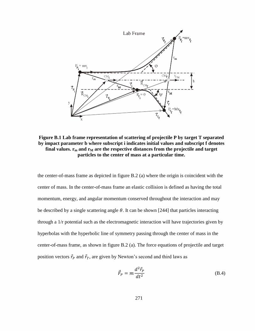
271

Figure B.1 Lab frame representation of scattering of projectile P by target T separated

by impact parameter b where subscript i indicates initial values and subscript f denotes

final values. rm and rM are the respective distances from the projectile and target

particles to the center of mass at a particular time.

the center-of-mass frame as depicted in figure B.2 (a) where the origin is coincident with the

center of mass. In the center-of-mass frame an elastic collision is defined as having the total

momentum, energy, and angular momentum conserved throughout the interaction and may

be described by a single scattering angle . It can be shown [244] that particles interacting

through a 1/r potential such as the electromagnetic interaction will have trajectories given by

hyperbolas with the hyperbolic line of symmetry passing through the center of mass in the

center-of-mass frame, as shown in figure B.2 (a). The force equations of projectile and target

position vectors and , are given by Newton’s second and third laws as

(B.4)

272

(a)

(b)

Figure B.2 (a) Two particle collision in the center of mass reference frame. (b) Single

particle equivalent of two-particle collision via a radial force .

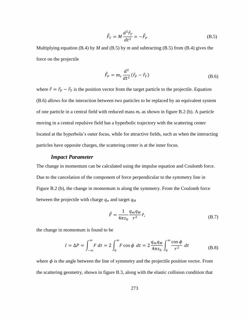
273

(B.5)

Multiplying equation (B.4) by M and (B.5) by m and subtracting (B.5) from (B.4) gives the

force on the projectile

(B.6)

where is the position vector from the target particle to the projectile. Equation

(B.6) allows for the interaction between two particles to be replaced by an equivalent system

of one particle in a central field with reduced mass mr as shown in figure B.2 (b). A particle

moving in a central repulsive field has a hyperbolic trajectory with the scattering center

located at the hyperbola’s outer focus, while for attractive fields, such as when the interacting

particles have opposite charges, the scattering center is at the inner focus.

Impact Parameter

The change in momentum can be calculated using the impulse equation and Coulomb force.

Due to the cancelation of the component of force perpendicular to the symmetry line in

Figure B.2 (b), the change in momentum is along the symmetry. From the Coulomb force

between the projectile with charge qm and target qM

(B.7)

the change in momentum is found to be

∫

∫

∫

(B.8)

where is the angle between the line of symmetry and the projectile position vector. From

the scattering geometry, shown in figure B.3, along with the elastic collision condition that

274

Figure B.3 Scattering geometry for an elastic collision giving the change in momentum

as a function of initial momentum and scattering angle.

| | | | the change in momentum is found to be

(B.9)

Since b is perpendicular to the momentum at all times

(B.10)

Solving (B.10) for and substituting into (B.8), along with a change of limits to the angle

between the symmetry line and the hyperbolic asymptotes, gives

∫

(B.11)

By integrating equation (B.11) and solving for the impact parameter b can be found to be

related to the scattering angle through

(B.12)

where

(B.13)

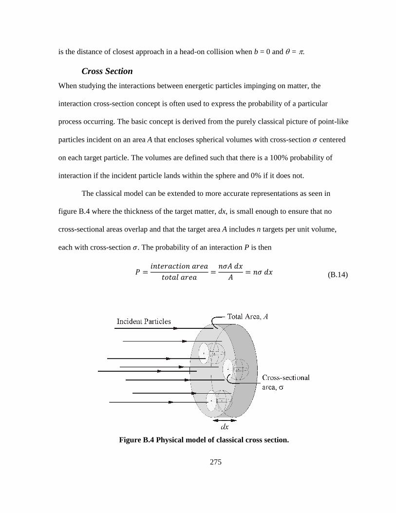
275

is the distance of closest approach in a head-on collision when b = 0 and = .

Cross Section

When studying the interactions between energetic particles impinging on matter, the

interaction cross-section concept is often used to express the probability of a particular

process occurring. The basic concept is derived from the purely classical picture of point-like

particles incident on an area A that encloses spherical volumes with cross-section centered

on each target particle. The volumes are defined such that there is a 100% probability of

interaction if the incident particle lands within the sphere and 0% if it does not.

The classical model can be extended to more accurate representations as seen in

figure B.4 where the thickness of the target matter, dx, is small enough to ensure that no

cross-sectional areas overlap and that the target area A includes n targets per unit volume,

each with cross-section . The probability of an interaction P is then

(B.14)

Figure B.4 Physical model of classical cross section.

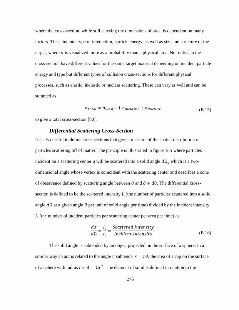
276

where the cross-section, while still carrying the dimensions of area, is dependent on many

factors. These include type of interaction, particle energy, as well as size and structure of the

target, where is visualized more as a probability than a physical area. Not only can the

cross-section have different values for the same target material depending on incident particle

energy and type but different types of collision cross-sections for different physical

processes, such as elastic, inelastic or nuclear scattering. These can vary as well and can be

summed as

(B.15)

to give a total cross-section [80].

Differential Scattering Cross-Section

It is also useful to define cross-sections that give a measure of the spatial distribution of

particles scattering off of matter. The principle is illustrated in figure B.5 where particles

incident on a scattering center q will be scattered into a solid angle which is a two-

dimensional angle whose vertex is coincident with the scattering center and describes a cone

of observance defined by scattering angle between and . The differential cross-

section is defined to be the scattered intensity Is (the number of particles scattered into a solid

angle at a given angle per unit of solid angle per time) divided by the incident intensity

Io (the number of incident particles per scattering center per area per time) as

The solid angle is subtended by an object projected on the surface of a sphere. In a

similar way an arc is related to the angle it subtends, , the area of a cap on the surface

of a sphere with radius r is . The element of solid is defined in relation to the

(B.16)

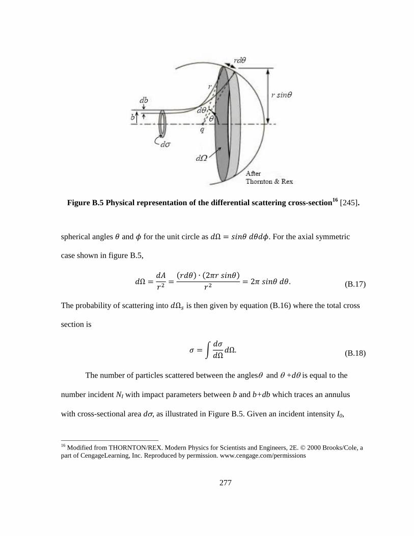
277

Figure B.5 Physical representation of the differential scattering cross-section16

[245].

spherical angles and for the unit circle as . For the axial symmetric

case shown in figure B.5,

(B.17)

The probability of scattering into is then given by equation (B.16) where the total cross

section is

∫

(B.18)

The number of particles scattered between the angles and +d is equal to the

number incident NI with impact parameters between b and b+db which traces an annulus

with cross-sectional area d, as illustrated in Figure B.5. Given an incident intensity I0,

16

Modified from THORNTON/REX. Modern Physics for Scientists and Engineers, 2E. © 2000 Brooks/Cole, a

part of CengageLearning, Inc. Reproduced by permission. www.cengage.com/permissions

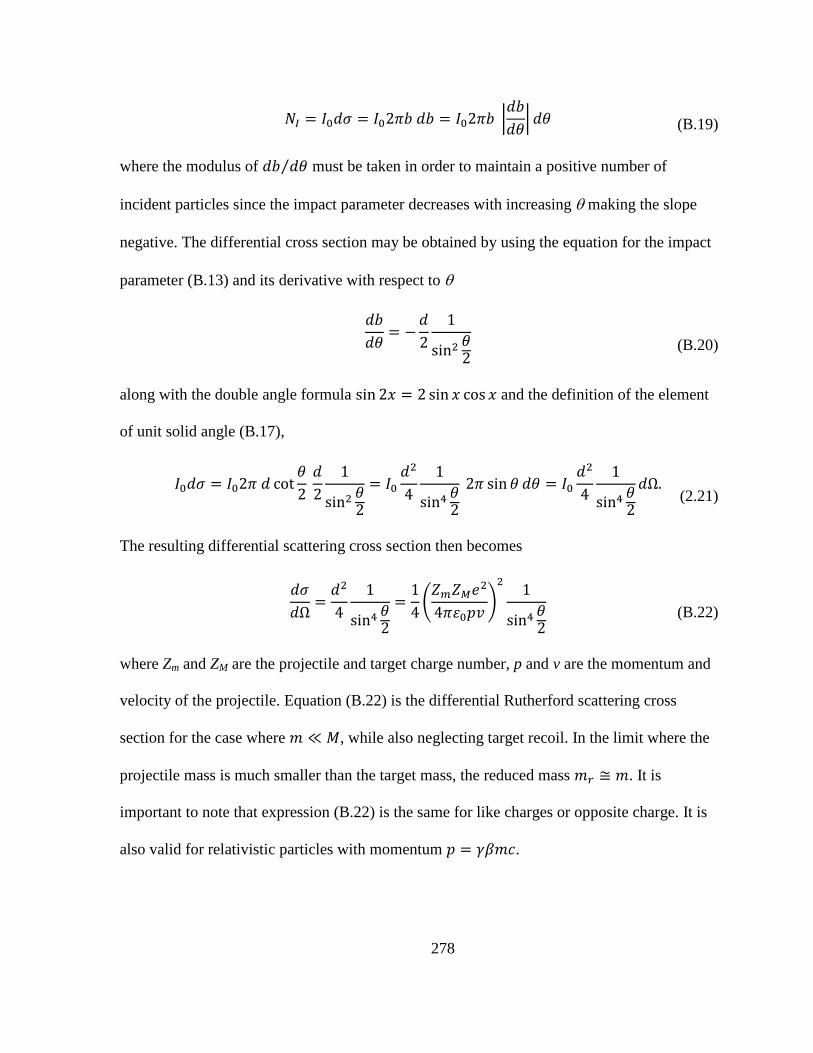
278

|

| (B.19)

where the modulus of ⁄ must be taken in order to maintain a positive number of

incident particles since the impact parameter decreases with increasing making the slope

negative. The differential cross section may be obtained by using the equation for the impact

parameter (B.13) and its derivative with respect to

(B.20)

along with the double angle formula and the definition of the element

of unit solid angle (B.17),

(2.21)

The resulting differential scattering cross section then becomes

(

)

(B.22)

where Zm and ZM are the projectile and target charge number, p and v are the momentum and

velocity of the projectile. Equation (B.22) is the differential Rutherford scattering cross

section for the case where , while also neglecting target recoil. In the limit where the

projectile mass is much smaller than the target mass, the reduced mass . It is

important to note that expression (B.22) is the same for like charges or opposite charge. It is

also valid for relativistic particles with momentum .

279

Appendix C

Relativistic Beam Characteristics

In order to gain a complete understanding of relativistic energy transfer leading to residual

gas ionization, it is necessary to analyze the electromagnetic fields of moving charges.

Beginning with Maxwell’s equations in matter17

(C.1)

(C.2)

(C.3)

(C.4)

where and are the constitutive relations for a linear, homogeneous, isotropic

medium in which is the permittivity and the permeability.

A particle moving with a velocity can be considered at rest in a system S’

moving with the same velocity relative to a stationary system S as illustrated in figure C.1.

The particle with point charge q has a uniform radial electric field in S’ given by Coulomb’s

law. At time t = t’ = 0 the origins of S and S’ are coincident and the particle passes a point P

in system S with coordinates (0,0,b) and (0,-vt’,b) in S’. The Lorentz transformation for a

boost along the direction is given by

17

is the “del” operator in Cartesian coordinates with arrows denoting vectors and

carets unit vectors.

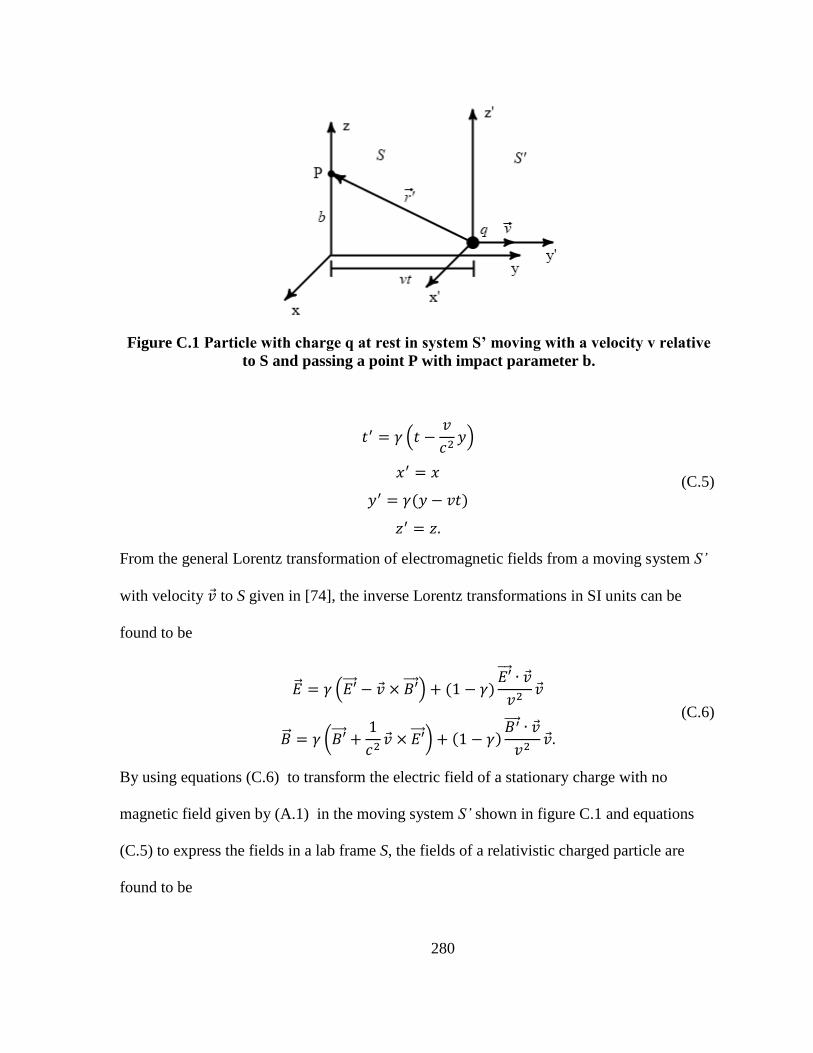
280

Figure C.1 Particle with charge q at rest in system S’ moving with a velocity v relative

to S and passing a point P with impact parameter b.

(

)

(C.5)

From the general Lorentz transformation of electromagnetic fields from a moving system S’

with velocity to S given in [74], the inverse Lorentz transformations in SI units can be

found to be

( )

(

)

(C.6)

By using equations (C.6) to transform the electric field of a stationary charge with no

magnetic field given by (A.1) in the moving system S’ shown in figure C.1 and equations

(C.5) to express the fields in a lab frame S, the fields of a relativistic charged particle are

found to be

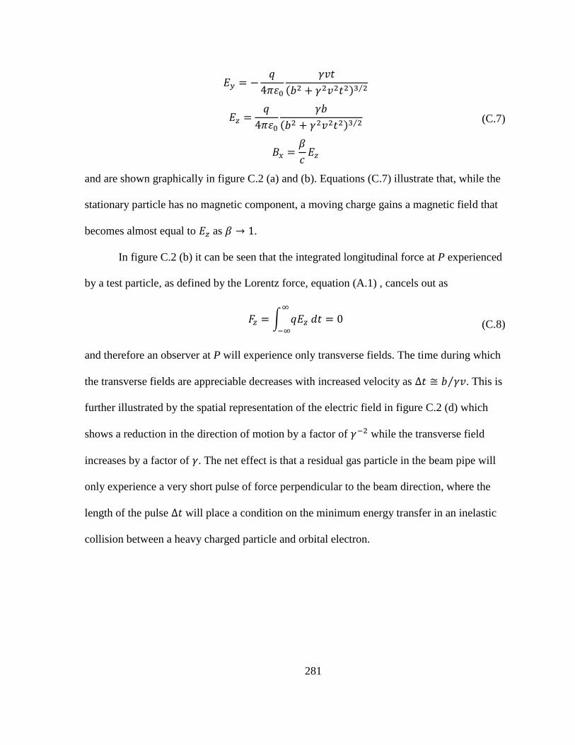
281

⁄

⁄

(C.7)

and are shown graphically in figure C.2 (a) and (b). Equations (C.7) illustrate that, while the

stationary particle has no magnetic component, a moving charge gains a magnetic field that

becomes almost equal to as .

In figure C.2 (b) it can be seen that the integrated longitudinal force at P experienced

by a test particle, as defined by the Lorentz force, equation (A.1) , cancels out as

∫

(C.8)

and therefore an observer at P will experience only transverse fields. The time during which

the transverse fields are appreciable decreases with increased velocity as ⁄ . This is

further illustrated by the spatial representation of the electric field in figure C.2 (d) which

shows a reduction in the direction of motion by a factor of while the transverse field

increases by a factor of . The net effect is that a residual gas particle in the beam pipe will

only experience a very short pulse of force perpendicular to the beam direction, where the

length of the pulse will place a condition on the minimum energy transfer in an inelastic

collision between a heavy charged particle and orbital electron.

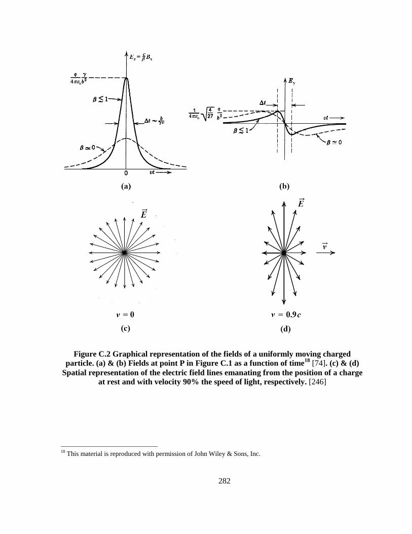
282

Figure C.2 Graphical representation of the fields of a uniformly moving charged

particle. (a) & (b) Fields at point P in Figure C.1 as a function of time18

[74]. (c) & (d)

Spatial representation of the electric field lines emanating from the position of a charge

at rest and with velocity 90% the speed of light, respectively. [246]

18

This material is reproduced with permission of John Wiley & Sons, Inc.

283

Appendix D

Beam Envelope Parameters

Beam Coordinates

An accelerator utilizes electromagnetic fields in the form of the Lorentz force

( ) (D.1)

to accelerate and guide a charged particle to its final destination. Since magnetic fields can do

no work, longitudinal electric fields are used for acceleration while magnetic fields are used

to manipulate the particle trajectory. There exists a reference or ideal trajectory that a particle

would follow if it passed without error through all accelerator components. However, due to

errors induced by accelerating fields in addition to the natural divergence of a beam of like-

charged particles, individual particles follow paths that deviate from the reference path and

without a form of focusing would quickly be lost.

A standard coordinate system used in accelerator applications is shown in figure D.1

which defines a longitudinal coordinate that is tangential to the ideal trajectory and

orthogonal unit vectors and defining the transverse plane whose origin is at location s

along the ideal beam path. The local reference trajectory radius is ρ(s).

Transverse Dynamics

For an accelerating structure composed mainly of linear focusing elements and for small

displacements around the reference trajectory, the magnetic field, which by design has no

longitudinal component, may be expanded to first order as

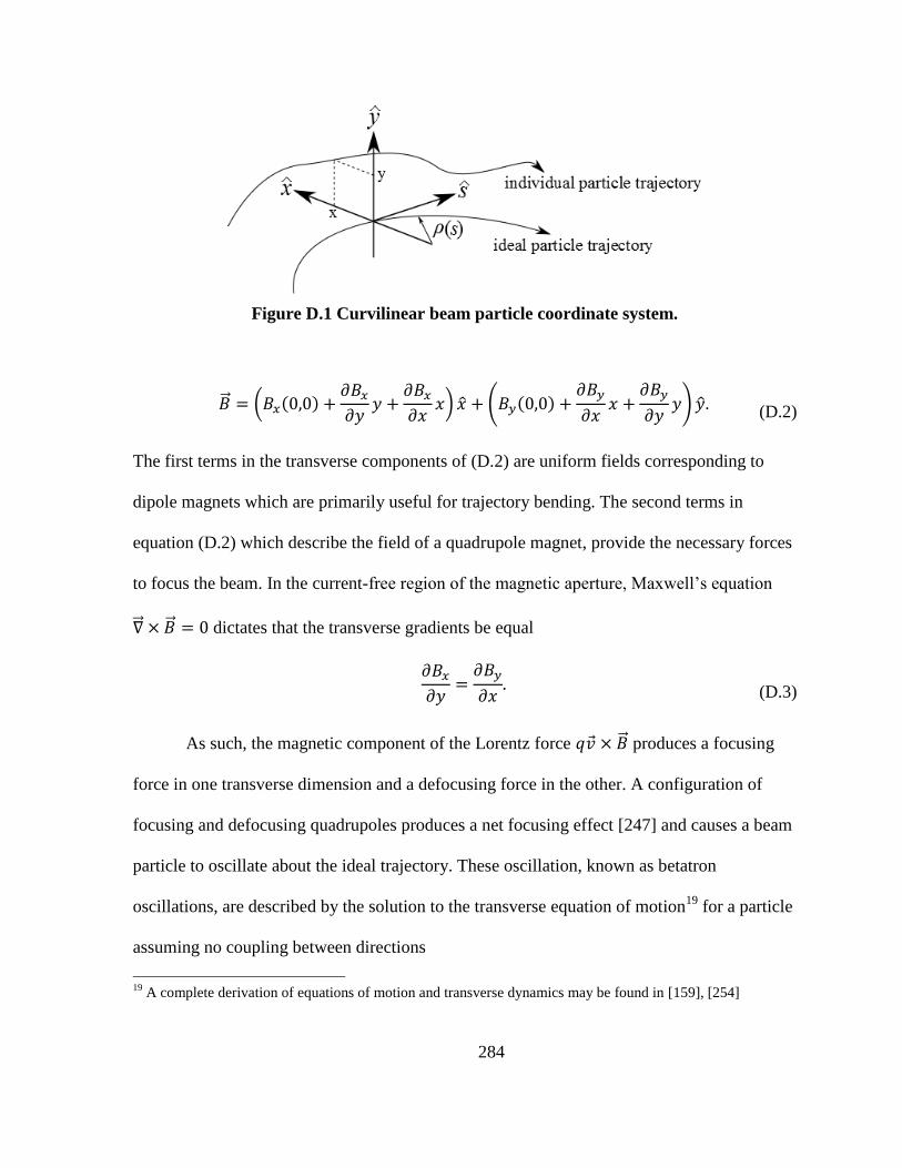
284

Figure D.1 Curvilinear beam particle coordinate system.

(

) (

) (D.2)

The first terms in the transverse components of (D.2) are uniform fields corresponding to

dipole magnets which are primarily useful for trajectory bending. The second terms in

equation (D.2) which describe the field of a quadrupole magnet, provide the necessary forces

to focus the beam. In the current-free region of the magnetic aperture, Maxwell’s equation

dictates that the transverse gradients be equal

(D.3)

As such, the magnetic component of the Lorentz force produces a focusing

force in one transverse dimension and a defocusing force in the other. A configuration of

focusing and defocusing quadrupoles produces a net focusing effect [247] and causes a beam

particle to oscillate about the ideal trajectory. These oscillation, known as betatron

oscillations, are described by the solution to the transverse equation of motion19

for a particle

assuming no coupling between directions

19

A complete derivation of equations of motion and transverse dynamics may be found in [159], [254]

285

(D.4)

acts as a position dependent restoring force and is proportional to the quadrupole field

gradient during passage through a quadrupole magnet.

The solutions to equations (D.4), which is called Hill’s equation, have the form of

generalized harmonic oscillators [159]. The solution in the horizontal transverse dimension is

√ (D.5)

where is the position dependent phase of the particle and the initial phase. is

called the beta function and describes the envelope inside which a particle oscillates about

the reference trajectory as illustrated in figure D.2. The beta function is one of three

parameters, known as Twiss or Courant-Snyder parameters characterizing the transverse

motion. The remaining parameters are

Figure D.2 Graphical representation of betatron oscillation about the ideal trajectory of

a particle traversing focusing and defocusing quadrupoles. Quadrupole elements are

represented with optical lenses.

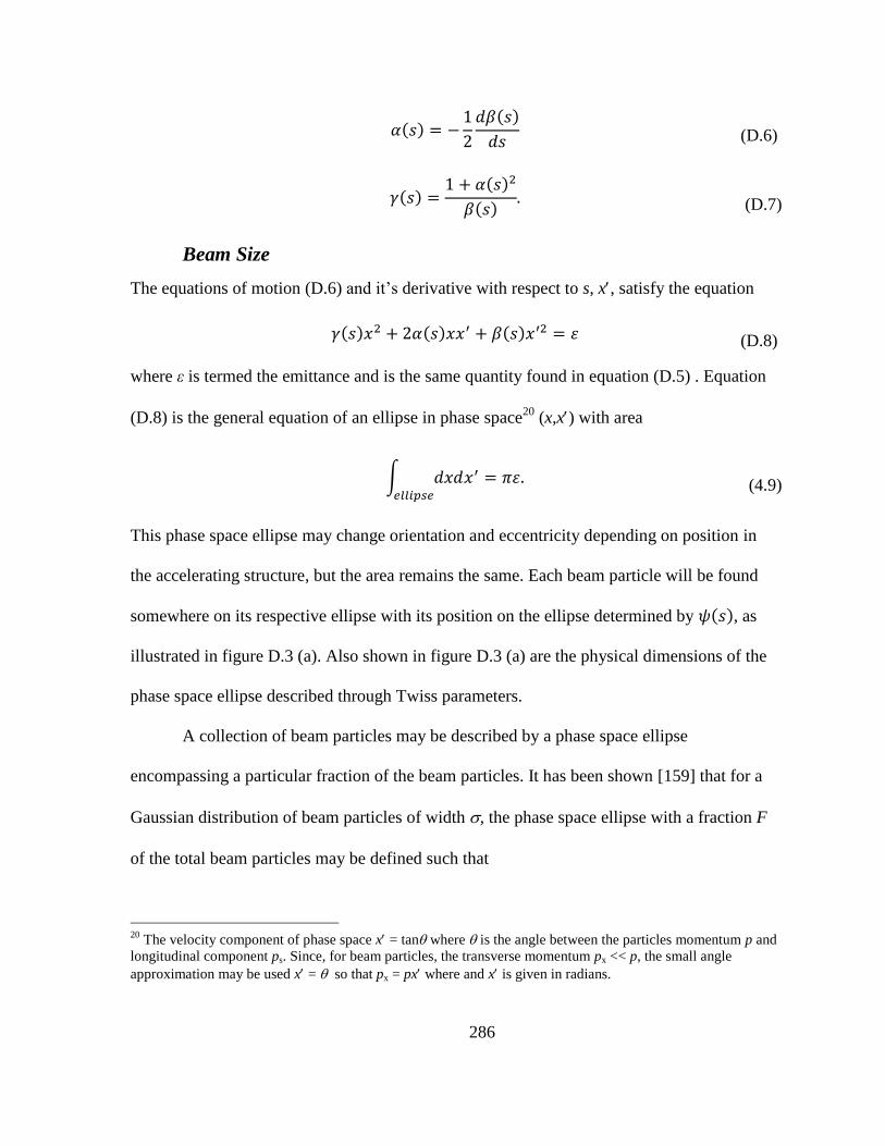
286

(D.6)

(D.7)

Beam Size

The equations of motion (D.6) and it’s derivative with respect to s, x, satisfy the equation

(D.8)

where ε is termed the emittance and is the same quantity found in equation (D.5) . Equation

(D.8) is the general equation of an ellipse in phase space20

(x,x) with area

∫

(4.9)

This phase space ellipse may change orientation and eccentricity depending on position in

the accelerating structure, but the area remains the same. Each beam particle will be found

somewhere on its respective ellipse with its position on the ellipse determined by , as

illustrated in figure D.3 (a). Also shown in figure D.3 (a) are the physical dimensions of the

phase space ellipse described through Twiss parameters.

A collection of beam particles may be described by a phase space ellipse

encompassing a particular fraction of the beam particles. It has been shown [159] that for a

Gaussian distribution of beam particles of width , the phase space ellipse with a fraction F

of the total beam particles may be defined such that

20

The velocity component of phase space x = tan where is the angle between the particles momentum p and

longitudinal component ps. Since, for beam particles, the transverse momentum px << p, the small angle

approximation may be used x = so that px = px where and x is given in radians.

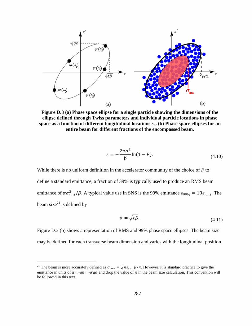
287

Figure D.3 (a) Phase space ellipse for a single particle showing the dimensions of the

ellipse defined through Twiss parameters and individual particle locations in phase

space as a function of different longitudinal locations sn. (b) Phase space ellipses for an

entire beam for different fractions of the encompassed beam.

(4.10)

While there is no uniform definition in the accelerator community of the choice of F to

define a standard emittance, a fraction of 39% is typically used to produce an RMS beam

emittance of . A typical value use in SNS is the 99% emittance . The

beam size21

is defined by

√ (4.11)

Figure D.3 (b) shows a representation of RMS and 99% phase space ellipses. The beam size

may be defined for each transverse beam dimension and varies with the longitudinal position.

21

The beam is more accurately defined as √ . However, it is standard practice to give the

emittance in units of and drop the value of in the beam size calculation. This convention will

be followed in this text.

288

Vita

Dirk Alan Bartkoski was born in Christiansburg, VA., on April 30, 1982. His father

moved the family to Blacksburg, Co. to pursue a career in mine management. The Bartkoski

family moved to Kentucky, where Dirk spent his childhood years being homeschooled. In

1996, he moved to Belmont, Ohio where he graduated high school through homeschooling

and received his GED. After spending one year at the Ohio University Eastern Campus in a

general engineering degree, he went to Oral Roberts University in Tulsa, OK. where he

graduated with a B.S. in Engineering Physics and a minor in Math.

Dirk moved to Knoxville, TN in the fall of 2004 where he entered the Astronomy and

Physics Department at the University of Tennessee. He began working with the Accelerator

Physics group at the Spallation Neutron Source accelerator (SNS) located at the Oak Ridge

National Laboratory in Oak Ridge, TN which is where he performed research that lead to his

graduation in December of 2005 with a Master’s degree in Physics from the University of

Tennessee. After moving from the Physics group to the Beam Instrumentation Group at SNS

he began work on his doctoral degree of which he is currently pursuing and plans on

completing at the end of 2013. Upon graduation he plans on pursuing a post-doctoral position

in accelerator physics and possibly writing fantasy and fiction.