Analysis of time delay difference due to parametric mismatch in matched filter channels

INTERNATIONAL JOURNAL OF CIRCUIT THEORY AND APPLICATIONSInt. J. Circ. Theor. Appl. (2014)Published online in Wiley Online Library (wileyonlinelibrary.com). DOI: 10.1002/cta.2007

Analysis of time delay difference due to parametric mismatch inmatched filter channels‡

Guillermo Stuarts*,† and Pedro Julián

Department of Electrical and Computer Engineering and Instituto de Investigaciones en Ingeniería Eléctrica (IIIE),Universidad Nacional del Sur - CONICET, Bahía Blanca, Argentina

SUMMARY

This paper presents an analysis of the time delay difference between the outputs of two matched filter channels,in the presence of parametric mismatch. A theorem for computing the cross-correlation value between twosignals is developed. From the cross-correlation theorem, expressions are developed that estimate the effectof parametric mismatch in the differential time delay (DTD) for filters of arbitrary type and order and input signalsof arbitrary form. The accuracy of these expressions is simulated and then demonstrated experimentally using acarefully designed setup. Filter design considerations that attempt to minimize spurious DTD in high-precisiontime delay estimation systems are presented. Copyright © 2014 John Wiley & Sons, Ltd.

Received 18 June 2013; Revised 21 May 2014; Accepted 29 May 2014

KEY WORDS: mismatch; matched filters; time delay difference; filter design

1. INTRODUCTION

The estimation of the time delay of a signal captured by spatially separated sensors plays a key role inmany source localization and target tracking applications, such as communications, acoustics,geophysics, sonar systems and sensor networks [1–8]. Signal conditioning and filtering is anessential and unavoidable part in all of them, at the very first stage of the analog front-end. The useof a filter in the signal path introduces a phase shift that depends on the filter parameters. A slightdifference between the filter parameters of two channels creates a frequency dependent phasedifference that will be interpreted by the processing stage as a delay difference produced by a shiftof the target source [9].

As an example, consider the system described in [10], where two channels (presumably identical)are used to condition the output of microphones with fourth-order switched-capacitors bandpassfilters. The bandpass frequency range of these filters is from 100 to 300Hz, and the purpose of thesystem is to measure the delay between the two signals with a precision of 5μs, which means 1°accuracy in the bearing angle estimation. However, if a 0.5% mismatch is considered in the filterscut-off frequencies, a spurious time delay of 14.81μs appears at the output when a single-tonesignal of 200Hz is used. Moreover, if a 90Hz noise source is added, the spurious time delay couldbe as much as 38.1 μs. This shows that for high accuracy sensor systems, even a small parametermismatch can induce errors much higher than the targeted precision.

Parameter differences amongst devices inside an integrated circuit are much smaller than the overallprocess spread specifications. As such components have experienced exactly the same technological

*Correspondence to: Guillermo Stuarts, Department of Electrical and Computer Engineering and Instituto de Investigacionesen Ingeniería Eléctrica (IIIE), Universidad Nacional del Sur - CONICET, Av. Alem 1253, Bahía Blanca, Argentina.

†E-mail: [email protected]‡An earlier version of this paper was presented at the 2011 EAMTA Conference and was published in its proceedings [9].

Copyright © 2014 John Wiley & Sons, Ltd.

G. STUARTS AND P. JULIÁN

treatments, they are generally much more similar than devices made on different dies at differenttimes in the process life cycle. However, even between matched components on the same die,parametric differences are observed. These differences, indicated with the term parametricmismatch, can be divided into two categories, namely random mismatch and systematic mismatch[11]. Random mismatch is generally attributable to microscopic device fluctuations, such asrandom dopant fluctuations [12], lithographic edge roughness [13], or grain boundary effects [14].Systematic mismatch effects are generally associated with circuit design and/or layoutimperfections. There are also some process technology related causes that can give rise to this typeof mismatch, such as etch effect, litography steps, well-proximity effects and local stressasymmetries [15, 16].

This paper presents an analysis of the time delay difference between the outputs of two matchedfilter channels, in the presence of parametric mismatch. The analysis begins considering a singlefrequency tone, which allows deriving exact expressions for the time delay difference arising whendifferent order and type filters are used. When the signal is composed of more than one frequencytone, the outputs of the channels are different, and there is no closed expression for the time delaydifference. In this case, we propose the use of the time delay that minimizes the cross-correlationbetween the two outputs. Closed form expressions are found that together with reasonablesimplifications lead to practical design considerations. In fact, the analysis reveals that forapplications requiring high accuracy, analog filtering must be restricted to very low order filters. Insuch cases, if further filtering is required by the application, it should be performed in the digitaldomain after the corresponding A/D conversion. Otherwise, the time delay to be measured will becompletely overridden by the filters parametric mismatch. The results of the different analysis areexperimentally demonstrated using a carefully designed setup.

2. TIME DELAY ANALYSIS

To begin the analysis, it is illustrative to explain the situation of a first-order low-pass filter, excitedwith a single-tone sinusoid. In such case, the system’s frequency response has the following form:

H jwð Þ ¼ a= jωþ bð Þ: (1)

Therefore, the phase is given by

ϕ ¼ tan�1 ω=bð Þ: (2)

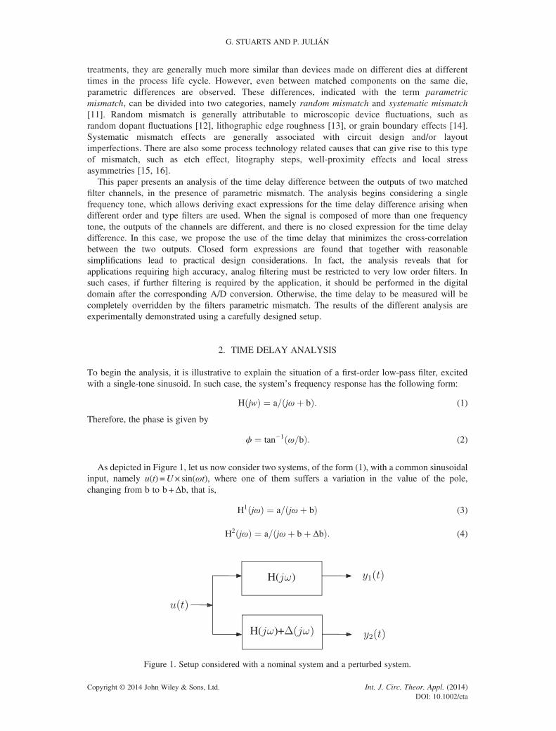
As depicted in Figure 1, let us now consider two systems, of the form (1), with a common sinusoidalinput, namely u(t) =U× sin(ωt), where one of them suffers a variation in the value of the pole,changing from b to b +Δb, that is,

H1 jωð Þ ¼ a= jωþ bð Þ (3)

H2 jωð Þ ¼ a= jωþ bþ Δbð Þ: (4)

Figure 1. Setup considered with a nominal system and a perturbed system.

Copyright © 2014 John Wiley & Sons, Ltd. Int. J. Circ. Theor. Appl. (2014)DOI: 10.1002/cta

ANALYSIS OF TIME DELAY DIFFERENCE IN MATCHED FILTER CHANNELS

Accordingly, the outputs will differ in phase. Actually, both outputs will be of the following form:

y1 tð Þ ¼ ∥H1 ωð Þ∥U�sin ωt þ ϕ1 ωð Þð Þ (5)

y2 tð Þ ¼ ∥H2 ωð Þ∥U�sin ωt þ ϕ2 ωð Þð Þ: (6)

The electronic design will try to minimize the difference between the two filters, so it makes sense toassume that Δb≪ b and perform a linearization of y2 as a function of b. Considering a variation Δbaround the point b, we obtain

ϕ2 ωð Þ ¼ tan�1 ω=bð Þ þ ω= ω2 þ b2� �� Δb: (7)

If we define the differential time delay (DTD) as the time difference between the two output signals,then the DTD corresponding to this system is

δ ωð Þ ¼ ϕ1 ωð Þ � ϕ2 ωð Þð Þ=ω ¼ Δb= ω2 þ b2� �

: (8)

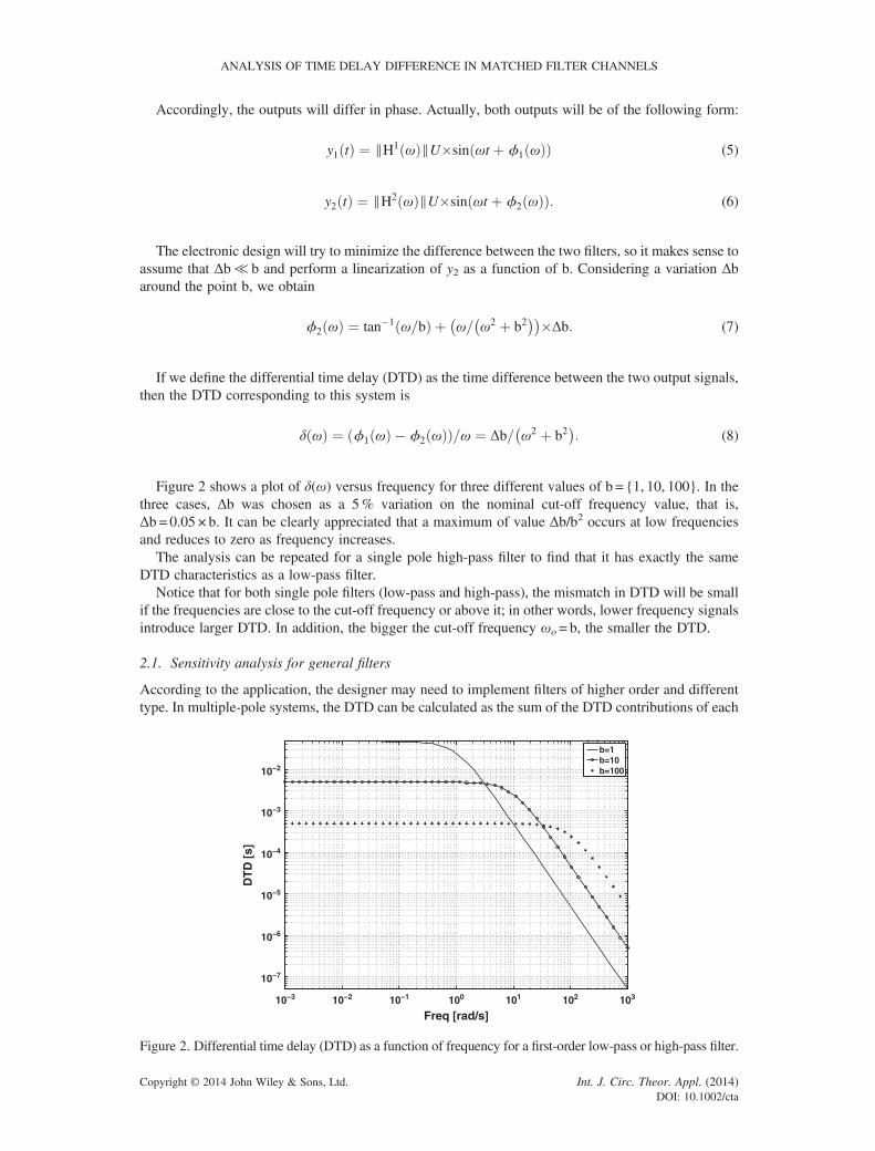
Figure 2 shows a plot of δ(ω) versus frequency for three different values of b = {1, 10, 100}. In thethree cases, Δb was chosen as a 5% variation on the nominal cut-off frequency value, that is,Δb = 0.05 × b. It can be clearly appreciated that a maximum of value Δb/b2 occurs at low frequenciesand reduces to zero as frequency increases.

The analysis can be repeated for a single pole high-pass filter to find that it has exactly the sameDTD characteristics as a low-pass filter.

Notice that for both single pole filters (low-pass and high-pass), the mismatch in DTD will be smallif the frequencies are close to the cut-off frequency or above it; in other words, lower frequency signalsintroduce larger DTD. In addition, the bigger the cut-off frequency ωo = b, the smaller the DTD.

2.1. Sensitivity analysis for general filters

According to the application, the designer may need to implement filters of higher order and differenttype. In multiple-pole systems, the DTD can be calculated as the sum of the DTD contributions of each

10−3 10−2 10−1 100 101 102 103

10−7

10−6

10−5

10−4

10−3

10−2

DT

D [

s]

Freq [rad/s]

b=1b=10b=100

Figure 2. Differential time delay (DTD) as a function of frequency for a first-order low-pass or high-pass filter.



pole. This means that a second-order filter with a double pole at the cut-off frequency will produce aDTD twice as high as the single pole case.

Regarding filter type, a typical choice is a Butterworth filter that exhibits maximally flat magnituderesponse, or a Bessel filter, with maximally linear phase response, which is suitable for audioapplications because it preserves the shape of the wave. Another type of filters that will beconsidered is the critically damped filter (CDF), in which all the poles are found at the cut-offfrequency and on the real axis.

A more general expression is needed for these kinds of systems:

H sð Þ ¼∏N

i¼1

mis2 þ cisþ dinis2 þ aisþ bi

(9)

where the phase is given by

φ jωð Þ ¼XNi¼1

arctanciω

di � miω2

� �� arctan

aiωbi � niω2

� �� : (10)

If two systems are considered, with a small variation on some of their parameters, then it is possibleto derive an expression for the DTD that generalizes (8):

δ ωð Þ ¼XNi¼1

di � miω2ð ÞΔci � ciΔdi þ ciω2Δmi

ciωð Þ2 þ di � miω2ð Þ2 �XNi¼1

bi � niω2ð ÞΔai � aiΔbi þ aiω2Δniaiωð Þ2 þ bi � niω2ð Þ2 : (11)

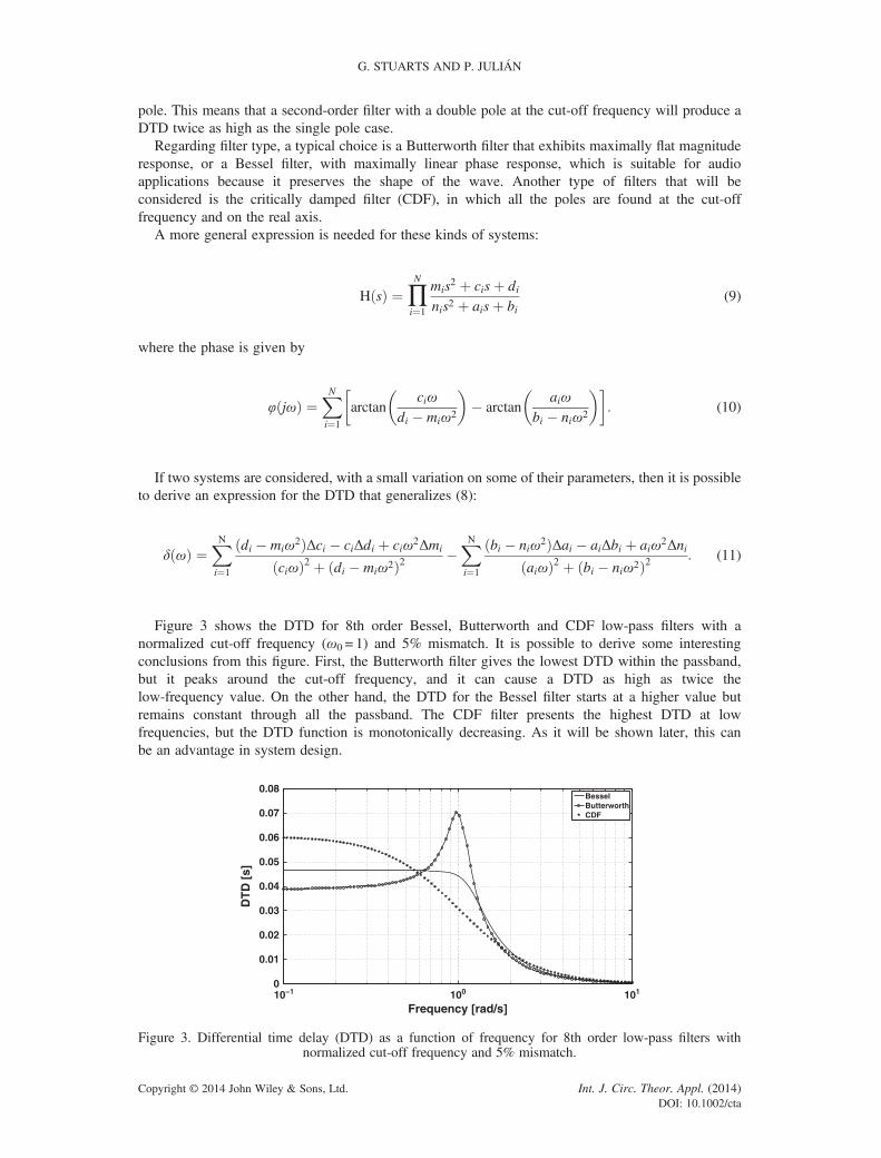
Figure 3 shows the DTD for 8th order Bessel, Butterworth and CDF low-pass filters with anormalized cut-off frequency (ω0 = 1) and 5% mismatch. It is possible to derive some interestingconclusions from this figure. First, the Butterworth filter gives the lowest DTD within the passband,but it peaks around the cut-off frequency, and it can cause a DTD as high as twice thelow-frequency value. On the other hand, the DTD for the Bessel filter starts at a higher value butremains constant through all the passband. The CDF filter presents the highest DTD at lowfrequencies, but the DTD function is monotonically decreasing. As it will be shown later, this canbe an advantage in system design.

10−1 100 1010

0.01

0.02

0.03

0.04

0.05

0.06

0.07

0.08

Frequency [rad/s]

DT

D [

s]

BesselButterworthCDF

Figure 3. Differential time delay (DTD) as a function of frequency for 8th order low-pass filters withnormalized cut-off frequency and 5% mismatch.



2.2. Analysis for several frequency components

If the input to the linear system contains more than one frequency component, and the two systemshave a parametric difference, every frequency component is delayed by a different amount, and thetwo systems produce in general two different signals. This means that it is not possible to find atime delay δ such that one of the outputs can be delayed to match the other. Therefore, it isnecessary to introduce different criteria for DTD.

In this work, we propose the cross-correlation as the tool to define the time delay between twosignals that are different. Given two signals s1(t) and s2(t), the cross-correlation is defined as

Rs1;s2 τð Þ ¼ E s1 tð Þs2 t � τð Þ½ � (12)

where E denotes expectation [1]. The argument τ that maximizes (12) provides an estimate of the DTD,that is,

δ ¼ argmaxRs1;s2 τð Þ: (13)

The choice of (13) is based on the widespread use of this mathematical tool for matching closelyrelated signals and even for estimating time delay between signals [1–4].

Without loss of generality, we consider for this case, a system like the one illustrated in Figure 1,where the input has the following form:

u tð Þ ¼XNi¼1

Ui sin ωitð Þ (14)

then the two outputs y1(t) and y2(t) will be of the following form:

y1 tð Þ ¼XNi¼1

∥H1 ωið Þ∥Ui sin ωi t þ δ1i ωið Þ� �� þ n1 tð Þ

y2 tð Þ ¼XNi¼1

∥H2 ωið Þ∥Ui sin ωi t þ δ2i ωið Þ� �� þ n2 tð Þ;(15)

where n1(t) and n2(t) are zero-mean and uncorrelated noise signals.In the following, we will consider that the parametric variation is small enough such that

‖H1(ωi)‖≈ ‖H2(ωi)‖, for i= 1, 2,.. N, and we will note ai = ‖H(ωi)‖Ui. In addition, and without lossof generality, we will consider y1(t) as reference and assume that δ1(ωi) = 0, for i = 1, 2,.. N, so thatthe individual DTD between the tones, is given by δ(i)≜ δ2(ωi)� δ1(ωi).

§ Having introduced theseconsiderations, we can formulate the following theorem that states the result of the cross-correlationbetween two outputs of the aforementioned form.

Theorem 1Let us consider two signals y1, y2 formed as the sum of N tones with magnitude ak and frequencies ωk,where ωk≠ωn for k≠ n and individual differential delays δk, that is,

y1 tð Þ ¼XNk¼1

ak sin ωktð Þ þ n1 tð Þ (16)

y2 tð Þ ¼XNk¼1

ak sin ωk t þ δk� �� þ n2 tð Þ (17)

§This notation is used for the sake of conciseness.



then, the cross-correlation between them can be approximated by

R̂y1y2 τð Þ ¼XNk¼1

a2k2cos ωk τ þ δk

� �� : (18)

ProofSee The Appendix. ∎

Using the results of Theorem 18, it is possible to approximate the DTD as the time τ* that maximizes(18). In fact, τ* is obtained from the solution of

∂R̂∂τ

¼ 0; (19)

which is given byXNk¼1

a2kωk sin ωk δk þ τ� �� ¼ 0: (20)

In order to analyse the results of this theorem, it is illustrative to consider the input signal as a sum oftwo frequency tones and calculate the DTD between the output signals. Let

y1 tð Þ ¼ a1 sin ω1tð Þ þ a2 sin ω2tð Þ þ n1 tð Þy2 tð Þ ¼ a1 sin ω1 t þ δ1

� �� þ a2 sin ω2 t þ δ2� �� þ n2 tð Þ; (21)

according to (18), the cross-correlation between them is given by

R̂ τð Þ ¼ a21cos ω1 δ1 þ τ

� �� 2

þ a22cos ω2 δ2 þ τ

� �� 2

: (22)

The maximum value of R̂ τð Þ is obtained from solving dR̂ τð Þ=dτ ¼ 0 where also d2R̂ τð Þ=dτ2 < 0,which is given by

a21ω1 sin ω1 δ1 þ τ� ��

2¼ � a22ω2 sin ω2 δ2 þ τ

� �� 2

: (23)

Two cases can be considered here. Let us first examine the case where each individual delay and thesolution delay are small compared to the period of the signal frequencies, that is,ωi(τ + δ(i))≪1 for i=1, 2.

(1) Individual DTD small compared to 1/ωi and i = 1, 2: In this case, we can approximatesin(ωi(τ + δ(i))) ≅ωi(τ + δ(i)), so that (23) reduces to

a21ω21 δ1 þ τ� � ¼ �a22ω

22 δ2 þ τ� �

: (24)

A simple algebraic manipulation yields the value for τ:

τ ¼ αδ1 þ 1� αð Þδ2 (25)

where

α ¼ ω21a

21

ω21a

21 þ ω2

2a22

1� αð Þ ¼ ω22a

22

ω21a

21 þ ω2

2a22

: (26)

Several interesting conclusions can be drawn from (25). First of all, notice that the composite DTDis the convex combination of the two individual delays, thus, the DTD is always going to be an



intermediate value, that is, a value in the set

Λ ¼ min δ1; δ2� �

;max δ1; δ2� ��

: (27)

This means that if the filter type is such that its DTD function is monotonicallydecreasing, then the low-frequency DTD value can be used as an upper bound of thesystem DTD, for any composition of the input signal.

Secondly, notice from (26) that whether the composite DTD is closer to one delay or the other isdependent on the square of the frequency and the square of the amplitude. Therefore, for high orderfilters where amplitude attenuation grows faster than frequency, the relative amplitude of one toneversus the other has more influence on the composite DTD than the relative values of the frequencies.

Thirdly, notice that if the amplitudes of the tones are equivalent, then the composite DTD is closer tothe individual DTD of the higher frequency signal, which is always smaller for monotonicallydecreasing DTD functions.

The following examples illustrate these points.

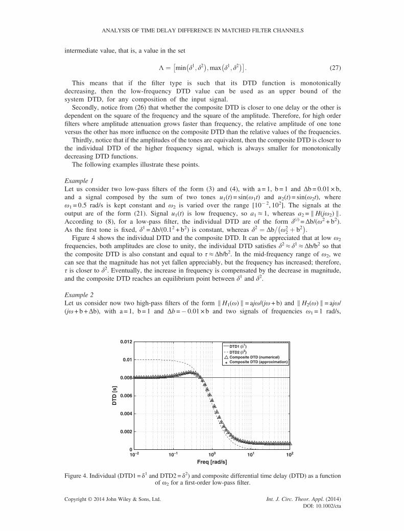
Example 1Let us consider two low-pass filters of the form (3) and (4), with a = 1, b = 1 and Δb = 0.01 × b,and a signal composed by the sum of two tones u1(t) = sin(ω1t) and u2(t) = sin(ω2t), whereω1 = 0.5 rad/s is kept constant and ω2 is varied over the range [10� 2, 102]. The signals at theoutput are of the form (21). Signal u1(t) is low frequency, so a1≈ 1, whereas a2 = ∥H(jω2) ∥.According to (8), for a low-pass filter, the individual DTD are of the form δ(i) =Δb/(ω2 + b2).As the first tone is fixed, δ1 =Δb/(0.12 + b2) is constant, whereas δ2 ¼ Δb= ω2

2 þ b2� �

.Figure 4 shows the individual DTD and the composite DTD. It can be appreciated that at low ω2

frequencies, both amplitudes are close to unity, the individual DTD satisfies δ2≈ δ1≈Δb/b2 so thatthe composite DTD is also constant and equal to τ≈Δb/b2. In the mid-frequency range of ω2, wecan see that the magnitude has not yet fallen appreciably, but the frequency has increased; therefore,τ is closer to δ2. Eventually, the increase in frequency is compensated by the decrease in magnitude,and the composite DTD reaches an equilibrium point between δ1 and δ2.

Example 2Let us consider now two high-pass filters of the form ∥H1(ω)∥= ajω/(jω + b) and ∥H2(ω)∥ = ajω/(jω+ b +Δb), with a = 1, b = 1 and Δb =� 0.01 × b and two signals of frequencies ω1 = 1 rad/s,

10−2 10−1 100 101 1020

0.002

0.004

0.006

0.008

0.01

0.012

Freq [rad/s]

DT

D [

s]

DTD1 (δ1)

DTD2 (δ2)Composite DTD (numerical)Composite DTD (approximation)

Figure 4. Individual (DTD1 = δ1 and DTD2= δ2) and composite differential time delay (DTD) as a functionof ω2 for a first-order low-pass filter.



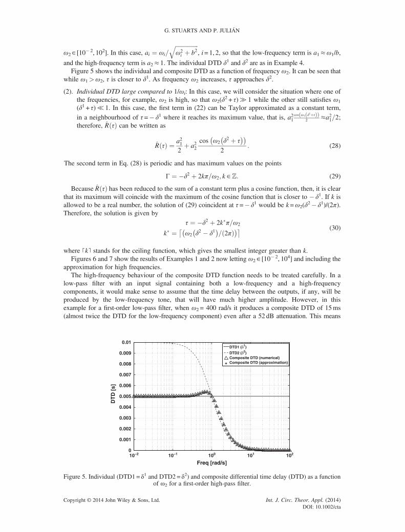
ω2∈ [10� 2, 102]. In this case, ai ¼ ωi=ffiffiffiffiffiffiffiffiffiffiffiffiffiffiffiffiω2i þ b2

q, i=1, 2, so that the low-frequency term is a1≈ω1/b,

and the high-frequency term is a2≈ 1. The individual DTD δ1 and δ2 are as in Example 4.Figure 5 shows the individual and composite DTD as a function of frequency ω2. It can be seen that

while ω1>ω2, τ is closer to δ1. As frequency ω2 increases, τ approaches δ2.

(2). Individual DTD large compared to 1/ωi: In this case, we will consider the situation where one ofthe frequencies, for example, ω2 is high, so that ω2(δ2 + τ)≫ 1 while the other still satisfies ω1

(δ1 + τ)≪ 1. In this case, the first term in (22) can be Taylor approximated as a constant term,

in a neighbourhood of τ =� δ1 where it reaches its maximum value, that is, a21cos ω1 δ1þτð Þð Þ

2 ≈a21=2;therefore, R̂ τð Þ can be written as

R̂ τð Þ ¼ a212þ a22

cos ω2 δ2 þ τ� �� 2

: (28)

The second term in Eq. (28) is periodic and has maximum values on the points

Γ ¼ �δ2 þ 2kπ=ω2; k ∈ℤ: (29)

Because R̂ τð Þ has been reduced to the sum of a constant term plus a cosine function, then, it is clearthat its maximum will coincide with the maximum of the cosine function that is closer to � δ1. If k isallowed to be a real number, the solution of (29) coincident at τ =� δ1 would be k=ω2(δ2� δ1)/(2π).Therefore, the solution is given by

τ ¼ �δ2 þ 2k�π=ω2

k� ¼ ω2 δ2 � δ1� �

= 2πð Þ� �� (30)

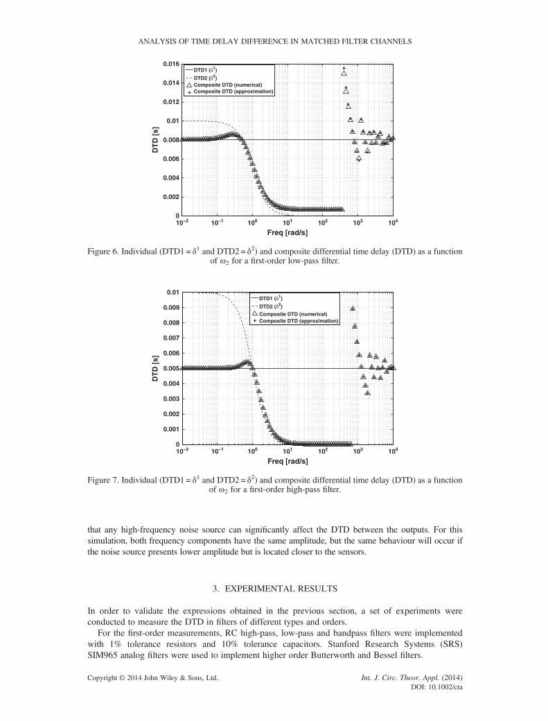
where ⌈k⌉ stands for the ceiling function, which gives the smallest integer greater than k.Figures 6 and 7 show the results of Examples 1 and 2 now letting ω2 ∈ [10� 2, 104] and including the

approximation for high frequencies.The high-frequency behaviour of the composite DTD function needs to be treated carefully. In a

low-pass filter with an input signal containing both a low-frequency and a high-frequencycomponents, it would make sense to assume that the time delay between the outputs, if any, will beproduced by the low-frequency tone, that will have much higher amplitude. However, in thisexample for a first-order low-pass filter, when ω2 = 400 rad/s it produces a composite DTD of 15ms(almost twice the DTD for the low-frequency component) even after a 52 dB attenuation. This means

10−2 10−1 100 101 1020

0.001

0.002

0.003

0.004

0.005

0.006

0.007

0.008

0.009

0.01

Freq [rad/s]

DT

D [

s]

DTD1 (δ1)


Figure 5. Individual (DTD1= δ1 and DTD2 = δ2) and composite differential time delay (DTD) as a functionof ω2 for a first-order high-pass filter.


10−2 10−1 100 101 102 103 1040

0.002

0.004

0.006

0.008

0.01

0.012

0.014

0.016

Freq [rad/s]

DT

D [

s]

DTD1 (δ1)


Figure 6. Individual (DTD1 = δ1 and DTD2= δ2) and composite differential time delay (DTD) as a functionof ω2 for a first-order low-pass filter.

10−2 10−1 100 101 102 103 1040

0.001

0.002

0.003

0.004

0.005

0.006

0.007

0.008

0.009

0.01

Freq [rad/s]

DT

D [

s]

DTD1 (δ1)


Figure 7. Individual (DTD1 = δ1 and DTD2= δ2) and composite differential time delay (DTD) as a functionof ω2 for a first-order high-pass filter.


that any high-frequency noise source can significantly affect the DTD between the outputs. For thissimulation, both frequency components have the same amplitude, but the same behaviour will occur ifthe noise source presents lower amplitude but is located closer to the sensors.

3. EXPERIMENTAL RESULTS

In order to validate the expressions obtained in the previous section, a set of experiments wereconducted to measure the DTD in filters of different types and orders.

For the first-order measurements, RC high-pass, low-pass and bandpass filters were implementedwith 1% tolerance resistors and 10% tolerance capacitors. Stanford Research Systems (SRS)SIM965 analog filters were used to implement higher order Butterworth and Bessel filters.



The input signal was generated with the SRS-DS360 low-distortion signal generator, which canprovide single and dual tone signals with variable frequencies up to 200KHz.

The acquisition is a critical step of the DTD estimation. In order to obtain a good result from thecross-correlation, at least 10 periods of the waveforms must be sampled [4]. Moreover, the samplingperiod must be at least 20 times smaller than the target DTD in order to have 5% accuracy. Thisimposes a limitation on the sampling speed and memory of the acquisition system. For example, inorder to measure a DTD of 1μs between two 50Hz signals, the sampling frequency needs to behigher than 20MHz (50 ns period), and in order to acquire 10 periods of each waveform, the systemmust be able to store 8 million points.

For these experiments, the acquisition was performed with a Wavemaster 804Zi-A LeCroy digitaloscilloscope, which allows 40GS/s and has a memory of 20 million points per channel. The inputchannels, including probes, can also be a source of spurious DTD, so they need to be characterizedin order to compensate their mismatch before performing any measurement. Twenty cycles of eachwaveform were acquired and then trimmed the data vectors from the first to the last zero-crossing,both with positive edge. Every step of the frequency sweep was measured at least 10 times, andthen the resulting DTD was averaged.

The cross-correlation was performed by the xcorr routine in Matlab, which also requires a highamount of memory and system resources. For example, in order to run the xcorr routine on twovectors of 180MB each, the system needs at least 7GB of RAM memory.

3.1. High-pass RC filters

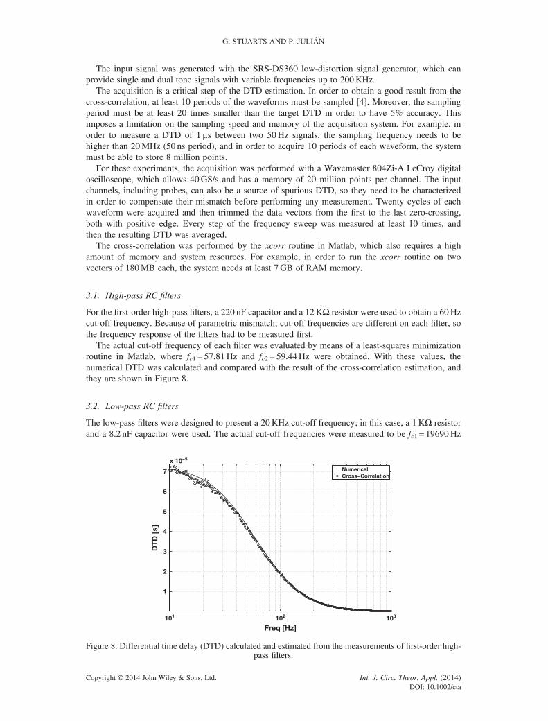
For the first-order high-pass filters, a 220 nF capacitor and a 12KΩ resistor were used to obtain a 60Hzcut-off frequency. Because of parametric mismatch, cut-off frequencies are different on each filter, sothe frequency response of the filters had to be measured first.

The actual cut-off frequency of each filter was evaluated by means of a least-squares minimizationroutine in Matlab, where fc1 = 57.81Hz and fc2 = 59.44Hz were obtained. With these values, thenumerical DTD was calculated and compared with the result of the cross-correlation estimation, andthey are shown in Figure 8.

3.2. Low-pass RC filters

The low-pass filters were designed to present a 20KHz cut-off frequency; in this case, a 1KΩ resistorand a 8.2 nF capacitor were used. The actual cut-off frequencies were measured to be fc1 = 19690Hz

101 102 103

1

2

3

4

5

6

7

x 10−5

Freq [Hz]

DT

D [

s]

NumericalCross−Correlation

Figure 8. Differential time delay (DTD) calculated and estimated from the measurements of first-order high-pass filters.



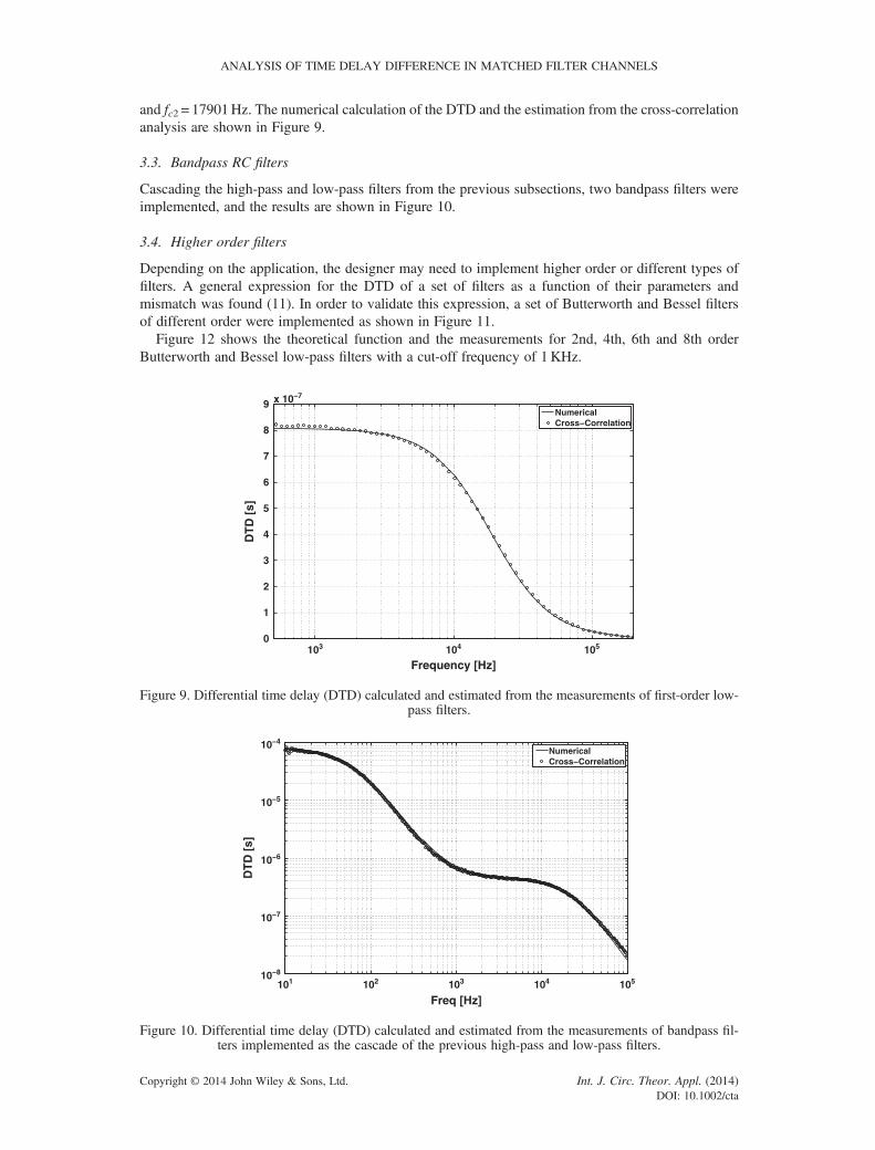
and fc2 = 17901Hz. The numerical calculation of the DTD and the estimation from the cross-correlationanalysis are shown in Figure 9.

3.3. Bandpass RC filters

Cascading the high-pass and low-pass filters from the previous subsections, two bandpass filters wereimplemented, and the results are shown in Figure 10.

3.4. Higher order filters

Depending on the application, the designer may need to implement higher order or different types offilters. A general expression for the DTD of a set of filters as a function of their parameters andmismatch was found (11). In order to validate this expression, a set of Butterworth and Bessel filtersof different order were implemented as shown in Figure 11.

Figure 12 shows the theoretical function and the measurements for 2nd, 4th, 6th and 8th orderButterworth and Bessel low-pass filters with a cut-off frequency of 1KHz.

103 104 1050

1

2

3

4

5

6

7

8

9 x 10−7

Frequency [Hz]

DT

D [

s]


Figure 9. Differential time delay (DTD) calculated and estimated from the measurements of first-order low-pass filters.

101 102 103 104 10510−8

10−7

10−6

10−5

10−4

Freq [Hz]

DT

D [

s]


Figure 10. Differential time delay (DTD) calculated and estimated from the measurements of bandpass fil-ters implemented as the cascade of the previous high-pass and low-pass filters.


102 103 1040

1

2

3

4

5

6

7

8 x 10−5

Freq [Hz]

DT

D [

s]

Butterworth (theoretical)Bessel (theoretical)Butterworth (measurement)Bessel (measurement)

Figure 12. Theoretical and measured differential time delay (DTD) for Butterworth and Bessel low-passfilters of different orders.

Figure 11. Filter setup used to perform the measurements.


Several conclusions can be drawn from Figure 12. First of all, an increase in the order of the filterproduces a higher DTD. The 8th order filters show a low-frequency DTD four times higher than thevalue for the 2nd order case. This means that from the delay estimation perspective, it is notconvenient to increase the filter order. Secondly, Butterworth filters always show a lower DTD atlow frequencies than the Bessel filters. As the order increases, the difference is more appreciable.Finally, Bessel filters exhibit a monotonically decreasing DTD function, while the DTD forButterworth filters shows a peak around the cut-off frequency.

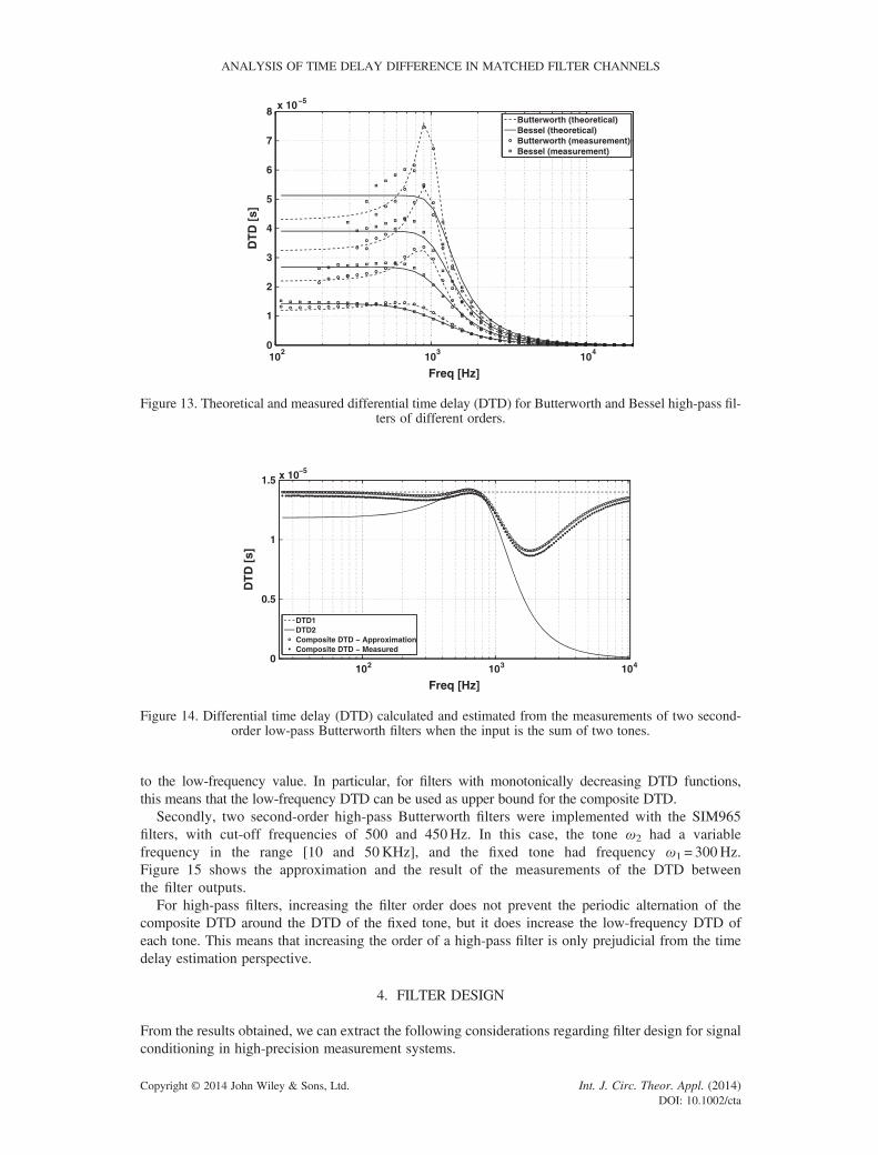
The same conclusions hold for high-pass filters, as can be seen in Figure 13. In this case, because of thestrong attenuation at low frequencies, 6th and 8th order filters show a higher error in the measured DTD.

3.5. Multitone input

Expressions (25) and (30) provide an estimation of the DTDwhen the input is a combination of two tones.In order to validate these expressions, the filter setup of Figure 11 was implemented. The input signal wasconstructed as the sum of a constant frequency tone ω1 = 500Hz and a variable frequency tone ω2 in therange [25 and 10KHz]. Firstly, two Butterworth second-order low-pass filters were implemented withthe SIM965 filters, with cut-off frequencies of 1 and 950Hz. Figure 14 shows the approximation andthe result of the measurements of the DTD between the filter outputs.

This figure shows an important result. For second (and higher) order low-pass filters, the attenuation onthe high-frequency tone is such that no periodic alternation will occur when the composite DTD converges


102

103

104

0

1

2

3

4

5

6

7

8x 10−5

Freq [Hz]

DT

D [

s]

Butterworth (theoretical)Bessel (theoretical)Butterworth (measurement)Bessel (measurement)

Figure 13. Theoretical and measured differential time delay (DTD) for Butterworth and Bessel high-pass fil-ters of different orders.

102 103 1040

0.5

1

1.5 x 10−5

Freq [Hz]

DT

D [

s]

DTD1DTD2Composite DTD − ApproximationComposite DTD − Measured

Figure 14. Differential time delay (DTD) calculated and estimated from the measurements of two second-order low-pass Butterworth filters when the input is the sum of two tones.


to the low-frequency value. In particular, for filters with monotonically decreasing DTD functions,this means that the low-frequency DTD can be used as upper bound for the composite DTD.

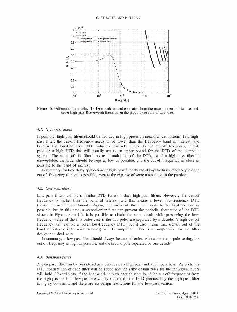
Secondly, two second-order high-pass Butterworth filters were implemented with the SIM965filters, with cut-off frequencies of 500 and 450Hz. In this case, the tone ω2 had a variablefrequency in the range [10 and 50KHz], and the fixed tone had frequency ω1 = 300Hz.Figure 15 shows the approximation and the result of the measurements of the DTD betweenthe filter outputs.

For high-pass filters, increasing the filter order does not prevent the periodic alternation of thecomposite DTD around the DTD of the fixed tone, but it does increase the low-frequency DTD ofeach tone. This means that increasing the order of a high-pass filter is only prejudicial from the timedelay estimation perspective.

4. FILTER DESIGN

From the results obtained, we can extract the following considerations regarding filter design for signalconditioning in high-precision measurement systems.


101 102 103 104 1050

0.1

0.2

0.3

0.4

0.5

0.6

0.7

0.8

0.9

1 x 10−4

Freq [Hz]

DT

D [

s]

DTD1DTD2Composite DTD − ApproximationComposite DTD − Measured

Figure 15. Differential time delay (DTD) calculated and estimated from the measurements of two second-order high-pass Butterworth filters when the input is the sum of two tones.


4.1. High-pass filters

If possible, high-pass filters should be avoided in high-precision measurement systems. In a high-pass filter, the cut-off frequency needs to be lower than the frequency band of interest, andbecause the low-frequency DTD value is inversely related to the cut-off frequency, it willproduce a high DTD that will usually act as an upper bound for the DTD of the completesystem. The order of the filter acts as a multiplier of the DTD, so if a high-pass filter isunavoidable, the order should be kept as low as possible, and the cut-off frequency as close aspossible to the band of interest.

In summary, for time delay applications, a high-pass filter should always be first-order and present acut-off frequency as high as possible, even at the expense of some attenuation in the passband.

4.2. Low-pass filters

Low-pass filters exhibit a similar DTD function than high-pass filters. However, the cut-offfrequency is higher than the band of interest, and this means a lower low-frequency DTD(hence a lower upper bound). Again, the order of the filter needs to be kept as low aspossible, but in this case, a second-order filter can prevent the periodic alternation of the DTDshown in Figures 4 and 6. It is possible to obtain the same result while preserving the low-frequency value of the first-order case if the two poles are separated by a decade. A high cut-offfrequency will exhibit a lower low-frequency DTD, but it also means that signals out of theband of interest (like noise sources) will be amplified. This is a compromise for the filterdesigner to deal with.

In summary, a low-pass filter should always be second order, with a dominant pole setting, thecut-off frequency as high as possible, and the second pole separated by one decade.

4.3. Bandpass filters

A bandpass filter can be considered as a cascade of a high-pass and a low-pass filter. As such, theDTD contribution of each filter will be added and the same design rules for the individual filterswill hold. Nevertheless, if the bandwidth is high enough (that is, if the cut-off frequencies fromthe high-pass and the low-pass are widely separated), the DTD produced by the high-pass filteris highly dominant, and there are no design restrictions for the low-pass section.


10−1 100 101 102 103 104 105 1060

0.2

0.4

0.6

0.8

1

1.2

1.4

1.6

1.8

2 x 10−5

Freq [Hz]

DT

D [

s]

4th order band−pass filterProposed filter

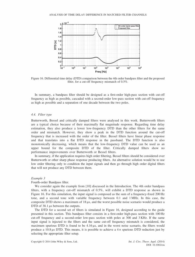
Figure 16. Differential time delay (DTD) comparison between the 4th order bandpass filter and the proposedfilter, for a cut-off frequency mismatch of 0.5%.


In summary, a bandpass filter should be designed as a first-order high-pass section with cut-offfrequency as high as possible, cascaded with a second-order low-pass section with cut-off frequencyas high as possible and a separation of one decade between the two poles.

4.4. Filter type

Butterworth, Bessel and critically damped filters were analysed in this work. Butterworth filtersare a typical choice because of their maximally flat magnitude response. Regarding time delayestimation, they also produce a lower low-frequency DTD than the other filters for the sameorder and mismatch. However, they show a peak in the DTD function around the cut-offfrequency that is increased with the order of the filter. Bessel filters have linear phase responseand that translates into a flat DTD response in the passband. The DTD function is alsomonotonically decreasing, which means that the low-frequency DTD value can be used as anupper bound for the composite DTD of the filter. Critically damped filters show noperformance improvements over Butterworth or Bessel filters.

In summary, if the application requires high order filtering, Bessel filters should be considered overButterworth or other sharp phase response producing filters. An alternative solution would be to uselow order filtering only to condition the input signals and then go through high order digital filtersthat will not produce any DTD between them.

Example 3Fourth-order Bandpass filter.

We consider again the example from [10] discussed in the Introduction. The 4th order bandpassfilters, with a frequency cut-off mismatch of 0.5%, will exhibit a DTD response as shown inFigure 16. For this simulation, the input signal is composed as the sum of a frequency-fixed 200Hztone, and a second tone with variable frequency between 0.1 and 1MHz. In this case, thecomposite DTD shows a maximum of 18 μs, and the worst possible noise scenario would produce aDTD of 38.1 μs between the outputs.

The DTD for a second set of filters is simulated in Figure 16, designed according to the guidepresented in this section. This bandpass filter consists in a first-order high-pass section with 100Hzcut-off frequency and a second-order low-pass section with poles at 300 and 3KHz. If the sameinput signal is injected to the filters and the same cut-off frequency mismatch is considered, themaximum spurious DTD is found to be 4.16 μs, and in the worst noise scenario, the filters wouldproduce a 10.8μs DTD. This means, it is possible to achieve a 4 × spurious DTD reduction just byselecting the appropriate filter setup.



5. CONCLUSIONS

Several expressions were developed for the estimation of time delay as a function of filter parameters.The case of a single tone going through a filter was analysed, and expression (11) was proposed as anestimation for the differential time delay between the outputs of two generalized filters of any order.Experimental and simulated results show good matching with the actual numerical calculation.

The cross-correlation between the outputs was selected as the tool to derive expressions for theestimation of the DTD when the input is a multitone signal. A set of measurements was performedon filters of different type and order to validate the results.

From the obtained results, we can conclude that for applications where the DTD between two channels iscritical, the order of the signal conditioning filter must be minimized. The lowest cut-off frequency is themost critical because it produces the greatest impact on the DTD; therefore, high-pass filters should beavoided if possible or otherwise placed as close as possible to the band of interest. Low-pass filtersshould be second order, with cut-off frequency as high as possible, and with the two poles separated onedecade. In this case, the DTD will be only slightly higher than the first-order case, and the second polewill provide enough attenuation to prevent the periodic high-frequency DTD oscillations. These resultsclearly suggest the need to perform the minimum required filtering at the front-end circuitry, leaving thehigher order filtering for a digital stage, where filter pairs can be implemented without mismatch.

APPENDIXProof of Theorem 1

ProofLet two signals y1(t) and y2(t), where y1(t) is constituted as a sum of N sinusoidal signals of magnitudeak and frequency ωk (k = 1, 2,.., N) and y2(t) is such that each of its components presents a time delay δk

(k = 1, 2,.., N) with respect to the components of y1(t), that is,

y1 tð Þ ¼XNk¼1

ak sin ωktð Þ þ n1 tð Þ (A1)

y2 tð Þ ¼XNk¼1

ak sin ωk t þ δk� �� þ n2 tð Þ; (A2)

where n1(t) and n2(t) are zero-mean, uncorrelated noise signals. The cross-correlation between them isgiven by

Ry1;y2 τð Þ ¼ E y1 tð Þy2 t þ τð Þ½ � (A3)

where E denotes expectation. Because of the finite observation time, however, Ry1y2 τð Þ can only be es-timated. For ergodic processes, an estimate of the cross-correlation is given by

R̂y1y2 τð Þ ¼ limT→∞

12T

Z T

�Ty1 tð Þy2 t þ τð Þdt (A4)

where

y1 tð Þy2 t þ τð Þ ¼XNk¼1

ak sin ωktð ÞXNk¼1

ak sin ωk t þ δk þ τ� ��

¼XNk¼1

a2k sin ωktð Þ sin ωk t þ δk þ τ� ��

þXNk¼1

XNl¼1

l≠k

� akal sin ωktð Þ sin ωl t þ δl þ τ� ��

(A5)



Because sin(α)sin(β) = 1/2[cos(α� β)� cos(α + β)], the second term of (A5) is

akal sin ωktð Þ sin ωl t þ δl þ τ� �� ¼

¼ akal2

cos ωk � ωlð Þt � ωl δl þ τ� ��

� akal2

cos ωk þ ωlð Þt þ ωl δl þ τ� ��

then

Z T

�Takal sin ωktð Þ sin ωl t þ δl þ τ

� �� ¼

¼ akal2

Z T

�Tcos ωk � ωlð Þt � ωl δl þ τ

� �� akal2

Z T

�Tcos ωk þ ωlð Þt þ ωl δl þ τ

� ��

Each of the terms in (A7) is an integral of a cosine function between �T and T. Because the integral ofa full period is null, its value can be bounded by the area of a cosine half cycle, which has a value of 2.Then,

∥E akal sin ωktð Þ sin ωl t þ δl þ τ� ��

∥ ¼ ∥li mT→∞

12T

Z T


� �� dt∥

¼ li mT→∞

12T

∥Z T


� �� dt∥

≤ li mT→∞

12T

∥akal2

Z T

�Tcos ωk � ωlð Þt � ωl δl þ τ

� �� dt∥

�li mT→∞

12T

∥akal2

Z T

�Tcos ωk þ ωlð Þt þ ωl δl þ τ

� �� dt∥

≤ li mT→∞

12T

∥akal2

2∥� limT→∞12T

∥akal2

2∥ ¼ 0:

Because

∥E akal sin ωktð Þ sin ωl t þ δl þ τ� ��

∥ ¼ 0

then

E akal sin ωktð Þ sin ωl t þ δl þ τ� �� ¼ 0: (A8)

On the other hand,

a2k sin ωktð Þ sin ωk t þ δk þ τ� �� ¼ a2k

2cos ωk δk þ τ

� �� a2k2

cos 2ωkt þ ωk δk þ τ� ��

(A9)

then

E a2k sin ωktð Þ sin ωk t þ δk þ τ� �� ¼ E

a2k2

cos ωk δk þ τ� ��

� Ea2k2


(A10)

The second term in (A10) is of the same form as each of the terms in (A7), so

Ea2k2


¼ 0: (A11)

(A6)

(A7)



For the first term of (A10), we have that

Ea2k2


¼ limT→∞

12T

Z T

�T

a2k2


dt: (A12)

Because the integrand does not depend on t, it results

Ea2k2


¼ limT→∞

12T

Z T

�T

a2k2


dt

¼ a2k2


limT→∞

12T

Z T

�Tdt

¼ a2k2


limT→∞

12T

T � �Tð Þ½ �

¼ a2k2


: (A13)

Therefore, from (A11) and (A13), it results

E a2k sin ωktð Þ sin ωk t þ δk þ τ� �� ¼ a2k

2cos ωk δk þ τ

� �� (A14)

Finally, from (A8) and (A14), we find that

R̂y1y2 τð Þ ¼XNk¼1

a2k2

cos ωk t þ δk� ��

:

∎

REFERENCES

1. Knapp C, Carter G. The generalized correlation method for estimation of time delay. IEEE Transactions onAcoustics, Speech, and Signal Processing 1976; ASSP-24(4):320–327.

2. Azaria M, Hertz D. Time delay estimation by generalized cross correlation methods. IEEE Transactions on Acous-tics, Speech, and Signal Processing 1984; ASSP-32(2):280–285.

3. Goblirsch DM, Horak DT. Error analysis of correlation methods for estimation of time delays in sensor signals.Proceedings of the American Control Conference, Boston, MA, USA, 1985; 526–529.

4. Zou Q, Lin Z.Measurement time requirement for generalized cross-correlation based time-delay estimation. Proceedingsof the IEEE International Symposium on Circuits and Systems ISCAS 2002, Phoenix, Arizona, USA, vol. 3, 2002.

5. Gong Y, Li L, Zhao X. Time delays of arrival estimation for sound source location based on coherence method incorrelated noise environments. In 2010 Second International Conference on Communication Systems, Networksand Applications (ICCSNA), vol. 1. IEEE: Hong Kong, 2010; 375–378 [Online]. Available: http://ieeexplore.ieee.org/stamp/stamp.jsp?arnumber=5588749

6. Erol-Kantarci M, Mouftah H, Oktug S. A survey of architectures and localization techniques for underwater acousticsensor networks. IEEE Communications Surveys & Tutorials 2011; 13(3):487–502 [Online]. Available: http://ieeexplore.ieee.org/stamp/stamp.jsp?arnumber=5714973

7. Shen J, Molisch A, Salmi J. Accurate passive location estimation using TOA measurements. IEEE Transactions onWireless Communications 2012; 11(6):2182–2192 [Online]. Available: http://ieeexplore.ieee.org/stamp/stamp.jsp?arnumber=6184254

8. He H, Wu L, Lu J, Qiu X, Chen J. Time difference of arrival estimation exploiting multichannel spatio-temporalprediction. IEEE Transactions on Audio, Speech and Language Processing 2013; 21(3):463–475. [Online].Available: http://ieeexplore.ieee.org/stamp/stamp.jsp?arnumber=6327613

9. Stuarts G, Julian P. Analysis of time delay difference due to parametric mismatch in matched filter channels. 2011Argentine School of Micro-Nanoelectronics, Technology and Applications, EAMTA 2011, Aug. 2011; 95–101.

10. Chacon-Rodriguez A, Martin-Pirchio F, Sanudo S, Julian P. A low-power integrated circuit for interaural time delayestimation without delay lines. IEEE Transactions on Circuits and Systems II 2009; 56(7):575–579.

11. Tuinhout H, Wils N, Andricciola P. Parametric mismatch characterization for mixed-signal technologies. IEEEJournal of Solid-State Circuits 2010; 45(9):1687–1696.

12. Stolk PA, Widdershoven FP, Klaassen DBM. Modeling statistical dopant fluctuations in MOS transistors. IEEETransactions on Electron Devices 1998; 45(9):1960–1971.

13. Croon JA, Sansen W, Maes HE. Matching Properties of Deep Sub-Micron MOS Transistors. Springer: Dordrecht,The Netherlands, 2005. ISBN:0-387-24314-3.


http://ieeexplore.ieee.org/stamp/stamp.jsp?arnumber=6327613


14. Tuinhout HP, Montree AH, Schmitz J, Stolk PA. Effects of gate depletion and boron penetration on matching of deepsubmicron CMOS transistors. In Proceedings of the International Electron Devices Meeting IEDM ’97. TechnicalDigest. IEEE: Washington, DC, USA, 1997; 631–634.

15. Wils N, Tuinhout HP, Meijer M. Characterization of STI edge effects on CMOS variability. IEEE Transactions onSemiconductor Manufacturing 2009; 22(1):59–65.

16. Tuinhout HP, Bretveld A, Peters WCM. Measuring the span of stress asymmetries on high-precision matched devices.Proceedings of the International Conference on Microelectronic Test Structures ICMTS ’04, 2004; 117–122.


Analysis of time delay difference due to parametric mismatch in matched filter channels

Documents

Transcript of Analysis of time delay difference due to parametric mismatch in matched filter channels