TI 2008-058/3 Tinbergen Institute Discussion Paper

Analysis of Spatial Disparities by a Structural Equations Model

Maria Francesca Cracolici1

Miranda Cuffaro2

Peter Nijkamp1,3

1 Free University Amsterdam; 2 University of Palermo; 3 Tinbergen Institute.

Tinbergen Institute The Tinbergen Institute is the institute for economic research of the Erasmus Universiteit Rotterdam, Universiteit van Amsterdam, and Vrije Universiteit Amsterdam. Tinbergen Institute Amsterdam Roetersstraat 31 1018 WB Amsterdam The Netherlands Tel.: +31(0)20 551 3500 Fax: +31(0)20 551 3555 Tinbergen Institute Rotterdam Burg. Oudlaan 50 3062 PA Rotterdam The Netherlands Tel.: +31(0)10 408 8900 Fax: +31(0)10 408 9031 Most TI discussion papers can be downloaded at http://www.tinbergen.nl.

ANALYSIS OF SPATIAL DISPARITIES BY A STRUCTURA L EQUATIONS

MODEL

Maria Francesca Cracolici*, Miranda Cuffaro† and Peter Nijkamp*

*Department of Spatial Economics Free University Amsterdam The Netherlands cracolici@feweb.vu.nl

pnijkamp@feweb.vu.nl †Department of National Accounting and Analysis of Social Processes University of Palermo Palermo Italy

cuffaro@unipa.it pn276mcmc

Abstract This paper presents a new analytical framework for assessing spatial disparities among

countries. It takes for granted that the analysis of a country’s performance cannot be limited solely to either economic or social factors. The aim of the paper is to combine relevant economic and non-economic (mainly social) aspects of a country’s performance in an integrated logical framework.

Based on this idea, a structural simultaneous equation model will be presented and estimated in order to explore the direction of the causal relationship between the economic and the non-economic aspects of a country’s performance. Furthermore, an exploration of the trajectory that each country has registered over time along a virtuous path will be offered. By means of a matrix persistency/transition analysis, the countries will be classified in clusters of good/bad performance.

One of the most interesting conclusions concerns the inability of most countries to turn the higher educational skills of the population into greater economic performance over time. In addition, our analysis also shows that making an accurate picture record and formulating related policy aiming at environmental care is highly desirable. It is surprising that only a few countries have reached a favourable economic and environmental performance simultaneously. Keywords: Socio-economic well-being, living standards, structural simultaneous equation model JEL-classification code: P46

1

1. Introduction

The measurement of a country’s welfare is one of the most critical and highly debated

issues in economic research. The snappy title of Davidson’s book highlights one of the most

relevant and debated topics of the recent literature: “You can’t eat GNP” (Davidson, 2000).

This publication addresses the hypothesis that GNP (or GDP) per capita can not be considered

as the only indicator of the performance of a country because it does not capture the overall

well-being of population.

Nevertheless, it has become rather common to rank the performance of countries or

regions by assessing their levels of development (or growth) in terms of GDP. But this

approach has often been strongly criticized. As the World Bank has written: “The basic

objective of development is to create an enabling environment for people to enjoy long,

healthy and creative lives. But it is often forgotten in the immediate concern with the

accumulation of commodities and financial wealth” (World Bank, 2001, p. 9).

The conventional economic view has frequently prompted much criticism based on

the observation that “people derive utility or well-being not merely from the command over

income alone” (Neumayer, 2003, p.276). This observation takes for granted that the standard

GDP index is unable to capture the real inequalities among countries in terms of the different

– sometimes contrasting – dimensions of the well-being of populations. GDP is at best only a

partial measure (or proxy) of a multi-dimensional welfare concept incorporating both the

economic and the non-economic aspects of human life (see Sen, 1985, 1987; Khan, 1991;

Dasgupta, 1990).

Since the 1990s however, there have been some new attempts in the literature to come

up with more appropriate indicators. The first is the World Bank’s Human Development

Index (HDI), a composite indicator based on GDP per capita, life expectancy at birth, and the

adult literacy rate (UNDP, 1990). These features represent, respectively, three main aspects of

an individual’s life, viz. access to resources; health conditions; and the opportunity to enjoy a

basic education.

Although the HDI is the most frequently used indicator for measuring the

development differentials among countries, it has been much criticized, in particular regarding

its simple weighting of each variable, and the high correlation between GDP and certain

crucial background variables.

In 2005 a special issue of the Review of Income and Wealth was entirely dedicated to

‘Inequality and Multidimensional Well-being’, while in 2007 one of its calls for papers was

mainly addressed to specific related themes, such as: measuring well-being from objective

and subjective perspectives, constructing macro indicators of well-being, measuring economic

well-being among regions, and so forth.

In 2001 an original and stimulating study (Hobijn and Franses, 2001) drew

economists’ attention to the need to extend the evaluation of a country’s performance to

2

encompass relevant measures of living standards. In so doing, they have thus readdressed the

spatial convergence issue – so prominent in the economic growth literature – and presented

evidence that convergence in GDP does not necessarily imply convergence in living

standards, the latter being defined by daily calorie supply, protein calorie supply, infant

mortality, life expectancy at birth, and so forth.

In our view, and in agreement with the above-mentioned literature about the need to

follow a multidimensional approach to the analysis of national or regional well-being, the

assessment of a country’s performance cannot be limited solely to either the economic or the

non-economic aspects. Both aspects must be considered simultaneously, and within a

consistent framework.

More specifically, the level of GDP in a country is viewed as its ability to provide its

inhabitants with proper opportunities to enjoy good economic, social, and environmental

conditions of life. An increase in per-capita GDP is considered as a basic prerequisite for

improvement in the living standards of a population, viz. better health services, more secure

livelihoods, greater access to education, better working conditions, security against crime,

more satisfying leisure time, a healthy and sustainable environment, etc. On the other hand,

better living standards constitute a good basis to enhance productivity and, in turn, GDP.

In the light of these considerations, in the remainder of this paper we shall propose a

simultaneous equation system to take into account various relevant aspects, economic and

non-economic, related to the living conditions of the population. In the literature, these

aspects are often also called, respectively, economic and non-economic well-being (see, e.g.,

Osberg and Sharpe, 2005; McGillivray, 2005; McGillivray and Shorrocks, 2005). The main

idea is to identify a cycle where an increasing amount of GDP per capita (i.e. the economic

dimension of a country’s performance) produces a higher level of non-economic aspects, viz.

better health conditions, longer life prospects, higher percentage of educated population,

balance between work and free time, etc. Similarly, if a country has a high level of non-

economic well-being factors it is more able to manage its resources in order to increase its

income and productivity. Consequently, it seems plausible to hypothesize that there exists a

bidirectional relationship between the economic and non-economic dimensions of country

performance, and this question will be further analysed in the present paper.

Using a simultaneous equation model, we explore whether there is a bidirectional

causal relationship between the economic and the non-economic aspects that characterize

country performance, and how strong the intensity of this mutual causality is.

To this end, we have designed a simultaneous equation model (SEM), where each

relevant dimension of well-being is represented by an explanatory equation, and where each

equation contains both endogenous and exogenous variables. By means of our SEM, we can

control the possible endogeneity problem between economic and non-economic variables.

The model is based partly on both the conventional production function theory and partly on

the most recent empirical literature on economic growth. Using an extensive database, the

3

model is estimated for 64 countries for the period 1980-1999; the sample involves mainly

developing countries, but it has also been implemented for a few developed countries.

After a brief literature review presented in Section 2, a first attempt to build an

operational framework for the analysis of country performance is provided in Section 3; our

empirical model and the data used are also presented there. Empirical results and some

concluding remarks are presented in Sections 4 and 5, respectively.

2. The Multifaceted Performance of a Country.

The economic analysis of regional growth and its distribution already has a long

history and dates back to the early work of Solow (1956), where he argues that, in a

neoclassical economic world, the growth rate of a region (measured in per capita income) is

inversely related to its initial per capita income, a thesis which offers an optimistic

perspective for poor regions. This convergence idea has attracted much attention and has

prompted interesting qualitative research on evolving convergence versus persistent

disparities (see, e.g., Barro and Sala-i-Martin, 1992).

This stream of research has dominated the economic analysis of a country’s welfare,

though recently a new approach, involving also non-economic aspects of a country’s well-

being is emerging. Concerning the latter, some economists consider GDP per capita as a very

limited measure of the level of a country’s well-being, because it does not consider the

consequences of economic development on the lives of people (e.g. air, sea and water

pollution, increases in certain rare diseases, congestion, cost of urbanization, etc.); nor does it

capture the real-life conditions of populations (UNDP, 1990; Hobijn and Franses, 2001;

Neumayer, 2003; Marchante and Ortega, 2006).

In 1973 Kuznets made this challenging assertion: “The most distinctive feature of

modern economic growth is the combination of a high rate of aggregate growth with

disrupting effects and new problems” (Kuznets, 1973, p.257). This statement implies that the

national accounting framework should be expanded so that it considers both certain costs (i.e.

pollution, urban concentration, commuting, etc.) and positive returns (i.e. better health,

greater longevity, more leisure, less income inequality, etc.).

In the light of these suggestions, the economic literature has proposed different

measures of a country’s performance. The one most widely used is the HDI based on a

concept of human development which involves both an economic dimension, measured by

GDP per capita, and a dimension linked mainly to social aspects, measured by life expectancy

and the literacy rate. It has been inspired by Sen’s development theory, according to which a

country’s development is a matter not only of long-run economic growth but also of

opportunities for people, in both the high and the low growth cycle (Sen, 1984).

Yet, after the first Report on HDI (UNDP, 1990), many criticisms were made of the

index. Indeed, it has sometimes even been considered a redundant indicator that provides little

4

additional information on inter-country development levels with respect to traditional GDP

(McGillivray, 1991; Desai, 1991; Dasgupta and Weale, 1992; Sagar and Najam, 1998).

Nevertheless, the framework for calculating the index has remained substantially unchanged

in UNDP’s subsequent annual reports; only a few corrections have been made to take account

of gender differentials or income distribution.

The specific literature of the 1990s comprised a number of critical proposals for the

improvement of the HDI. For example, since the indicators of the three dimensions of HDI

were closely correlated, a principal component method was proposed in order to use a linear

combination of these indicators (Noorbakhsh, 1998; McGillivray, 1991).

Further, Sagar and Najam (1998) proposed a more in-depth revision of HDI involving

multiplication of the three component variables instead of using their arithmetic average, a

logarithmic treatment of GDP, and the incorporation of an inequality measure into the index.

In fact, only the second Report calculated the distribution-adjusted HDI for 53 countries

(UNDP, 1991, pp.17-18), and this was available until 1994, although since that year the

distribution-adjusted HDI has been omitted.

Notwithstanding its limitations, the HDI is particularly relevant to developing

countries, where the basic dimensions depicted by the three indicators have not yet been fully

accomplished. By contrast, regarding the developed countries, a decent standard of living,

longevity, and primary education have already been achieved by most people. Consequently,

multiple significant and suitable indicators, which take account of the different aspects of

living appear to be necessary.

Recently, in fact, Marchante and Ortega (2006), in a study conducted to measure the

quality of life and economic convergence across Spanish regions, have used an alternative

augmented composite indicator (AHDI) in the context of HDI. In particular, they considered

alternatively three different per-capita income measures (total personal income minus grants,

GVA, and total disposable income) and six quality of life indicators (life expectancy at birth,

the infant survival rate, the probability at birth of surviving to the age of 60, the adult literacy

rate, the mean years of schooling of the working age population, and the long-term

unemployment rate). Moreover, they applied an averaged arithmetic mean scheme with

(arbitrary) weights for the variables transformed by an achievement index.

Cuffaro et al. (2008) analysed the performance of Italian regions by using both

different categories of consumption expenditure as proxies of the economic aspects of well-

being, and indicators of health and diet conditions, education, labour market, etc. as proxies

for the social aspects of well-being. Their analysis showed that it was possible for high levels

of economic well-being to coexist with a high level of non-economic well-being.

Furthermore, since the 1980s – after the creation of the United Nations World

Commission on Environment and Development – some economists have highlighted that the

environment, like the social aspects of life, is an essential element of well-being or country

performance. In 1989 Daly and Cobb, proposed the ISEW, viz. the first Index of Sustainable

5

Economic Welfare; it attempted to integrate the economic aspects of an economy, as depicted

by the conventional national accounting, with the social (i.e. income distribution inequality)

and the environmental (i.e. air and water pollution) aspects.

ISEW was criticized very soon (see, e.g., Neumayer 1999, 2000) for the arbitrary

selection of its component variables and for the method of aggregation and construction.

After that, various indices, such as the Living Planet index, the Ecological Footprint, the

Environmental Performance Index and so forth, were proposed (see, e.g., Bohringer and

Jochem, 2007).

At present, there is a big debate among ecological economists concerning the

appropriate way to define a multidimensional index of sustainability, combining the

economic, social and environmental aspects of human life (Pulselli et al., 2006; Distaso,

2007). Actually, the assessment of the environmental aspects is very important in developed

countries where growth and technological progress may become ‘uneconomic’, worsening the

life of citizens, by, for example, air and water pollution. Even in developing countries the

policies towards environmental problems constitutes a plus point for those governments.

Moreover, considering this feature in a multidimensional measure of country performance

could produce a more significant ranking of territorial areas.

Although a number of efforts have been made to obtain a more comprehensive index

of multidimensional well-being or country performance, many methodological issues still

need to be explored more deeply, concerning how to integrate the above-mentioned different

aspects in a unique measure (i.e. a composite indicator).

The above considerations indicate that many dimensions should be considered for the

analysis of a country’s performance. So, how are these dimensions linked? To this end, an

operational framework including the economic and the non-economic (social and

environmental) aspects of country performance will now be presented in Section 3. It is a first

attempt to provide a conceptual and structural framework for the analysis of country

performance. The empirical model will also be presented.

3. A Conceptual Scheme for the Analysis of a Country’s Performance

3.1 Introductory remarks

In our view, an endeavour to combine the economic and the social aspects of a

country’s performance and to link static and dynamic analysis requires a general framework

like the one depicted in Figure 1. This has been inspired by Sen’s development theory,

according to which a country’s development is a matter not only of long-run economic growth

but also of opportunities for people, in both the high and the low growth cycle (Sen, 1984).

<<Insert figure 1 about here>>

6

In this scheme, both the economic and the non-economic aspects of a country

contribute to its performance. By introducing the time dimension, we can refer to income

growth (i.e. the improvement in living conditions) and to human development (i.e. the

improvement in non-economic aspects of living).

As a rule of thumb, we expect a strong relationship between both economic and non-

economic aspects, between income growth and human development. As far as we know, there

are no empirical studies about the first relation, and there are only few studies about the

second one. While some economists (Zuvekas, 1979) have found that economic growth and

human development are unrelated, some others have found strong support for the opposite

hypothesis.

Mazumdar (2000) found evidence that in the middle- and low-income countries there

is one-way causal relationship between the two phenomena1, but only up to a certain level of

income, after which growth and human development move independently. The results, as

highlighted by the author, vary with respect to both the three different indicators of human

development and the different income level clusters. In particular, for the low and middle-

income countries human development precedes economic growth, that is, low social

development implies low labour productivity and in turn low income.

Moreover, Ranis et al. (2000) demonstrated an ‘iterative process’ between the

improvement in human development and economic growth “as a necessary but not sufficient

condition for achieving such improvements”. They conclude that “economic growth itself will

not be sustained unless preceded or accompanied by improvements in human development”

(p. 213).

In agreement with the previous empirical evidence, we define an operational scheme

based on the argumentation that, in the long run, the causal relationship between the economic

and the non-economic aspects may reveal two paths: high levels of economic well-being

contribute to high levels of non-economic well-being through households, firms and the

public sector. It does so through households because they spend a higher proportion of their

income on education, health and culture; through firms because they devote a higher

proportion of their profits to create a safer labour environment, to finance R&D to control

pollution, etc.; and through the government because it allocates a higher proportion of its

resources to education, health, and the environment. Conversely, high levels of non-economic

well-being contribute to high levels of economic well-being through various channels. For

example, high levels of health and education raise the productivity of workers, facilitate the

acquisition of skills, and promote technological progress and ICT usage. In their turn, these

factors help to significantly increase the level of output (and also its composition), exports,

and per capita disposable income.

1 The test is performed by using three single linear equations between GDP per capita (as a standard measure of economic growth) and, respectively, life expectancy at birth, infant survival rate, and adult literacy rate; the latter three variables are proxies for human development.

7

More specifically, a high level of economic well-being should support the formation

of a high level of such human capabilities as improved health or knowledge. Improving

human capabilities means increasing the efficiency of the use made by people of their own

capabilities for work or leisure (UNDP, 1997). In synthesis, the performance of country is

defined by a cycle, viz. a bidirectional path that moves both from the economic dimensions to

the non-economic ones and from the non-economic dimensions to the economic ones.

So, how should we measure the economic and the non-economic aspects of a

country’s performance?

3.2 The economic and the non-economic aspects

In our analysis, the economic dimension of country performance, viz. the access to

economic resources – as argued by UNDP (1997) – is evaluated by the traditional GDP per

capita. We hypothesize that the ability of a country to satisfy the basic needs of population

comes from the opportunities and the efficiency to manage its human, material, and natural

capital. From a theoretical point of view, the latter are inputs of the GDP production process.

In the long run, the capacity of the economy to grow fast pushes up the non-economic

aspects of a country. Regarding these, very little attention has been paid to which particular

indicators have to be chosen. Indeed, it is not immediately obvious at the outset, because the

decision also depends on the main features of the countries analysed: for instance, whether

they are developed or developing.

Many studies do not devote much attention to this problem. For example, the

indicators chosen by Hobijn and Franses (2001) – who analyse both developed and

developing countries simultaneously – can well discriminate between the two groups of

countries, but they fail to take account of different levels of well-being within developed

countries. In fact, when measured on these indicators (viz. daily protein, calorie supply, infant

mortality rate, and life expectancy at birth) developed countries are quite homogeneous. Later,

Neumayer (2003) criticized the previous authors and tested (on the same data set used by

Hobijn and Franses) for convergence with different indicators of well-being, namely life

expectancy, infant survival, education enrolment, literacy, and telephone and television

availability. The wider range of indicators considered offsets the bias due to the analysis of

developed and developing countries simultaneously. As a matter of fact, Neumayer reached

different results compared with those of Hobijn and Franses that suggest strong evidence of

convergence most of the indicators.

More recently, Giles and Feng (2005), analysing 14 OECD countries, considered five

measures of well-being: namely, life expectancy, the Gini index of income inequality, the

poverty rate, the tertiary education participation rate, and carbon dioxide (CO2) emissions.

Also, MacGillivray (2005) for a selected number of developing countries examines a

number of indicators, including measures of poverty, inequality, health status, education

status, gender bias, empowerment, governance, and subjective well-being. He found that most

8

of the commonly used indicators are highly correlated to income and, as a consequence, they

are not able to give any more information than income can. Moreover, he raises the problem

of the possible endogeneity between income and non-economic indicators.

In the light of the aforementioned literature, we think that the choice of indicators

should be based on the main characteristics of countries (viz. developed or developing; low,

medium or high income, etc.), and on their capacity to catch the relative heterogeneity among

countries, but avoiding possible redundant statistical information. Obviously, in order to

perform significant comparisons between countries, there would have to be wide agreement

on the chosen indicators.

In particular, as our analysis concerns a relevant share of developing countries, we

think that, in line with the literature, the main dimensions of non-economic well-being should

be related to long life prospects (i.e. life expectancy at birth), health (i.e. infant survival rate as

the inverse of infant mortality rate), and education (i.e. literacy rate) status.

In relation to the first indicator, as Ram and Schultz (1979, p.402) pointed out “the

satisfaction (utility) that people derive from a longer life span must be substantial”; linked to

this one, there is the infant survival rate, which, if it is very high, tends to raise the life

expectancy. Finally, the literacy rate is “a direct measure of achievement, one basic sign of

human beings’ minimum education” (Mazumdar, 2000, p.301).

In addition to these dimensions, we think that the quality of the environment is worth

considering when measuring country performance. As ecological economics points out: “The

economic system is a subsystem of the system which is the environment. The economy depends

upon the environment, what happens in the economy affects the environment, and changes in

the environment affect the economy. Regarded as two systems, the economy and the

environment are interdependent” (Common and Stagl, 2005, p.218).

The well-known Kuznets curve (EKC) predicts pollution increases until a certain level

of income (viz. $5000-$8000), as developing countries “grow first and clean up later”. A

recent paper (Dasugpta et al., 2006) demonstrates that this argument is incorrect and find

evidence that an environmental governance is also possible for developing countries. More

specifically, their results suggest that policy actions are sufficient to reduce air pollution

significantly, even in those cities of overcrowded and poor countries. This is an important

result that makes it possible to take the environment into account when assessing developing

countries’ well-being.

An empirical model of country performance, including the economic and the non-

economic aspects will be proposed in Section 3.2. By using a simultaneous equation model,

we verify if a bidirectional relationship exists between the economic and the non-economic

dimensions for 64 countries in the world for the years 1980-1999.

9

3.3 Model and data

To define the model and to choose the key variables to include in it, the guidelines

from the most relevant literature quoted above have been followed. In particular, by means of

a simultaneous equation model (SEM), an empirical application of the operational scheme has

been performed. By using SEM, we attempt to arrange and to combine in a synthetic and

structural way the suggestions from the literature, in order to capture the effects of the

relationship between the economic and the non-economic aspects that charactize country

performance, viz. the simultaneous relationships between the economic and the non-economic

aspects of country well-being (see Figure 1). As far as we know, this approach is the first

attempt to arrange the different dimensions of country performance, controlling for

endogeneity.

The endogenous variables in our SEM are gross domestic product (gdp), literacy rate

(li ), life expectancy (le), and pollution indicator (pol).

We use as exogenous variables the following: working age population at t-1 as a proxy

for labour input (labour-1); the share of gross capital formation at t-1 (capform-1) in GDP, as a

proxy for material capital input; telephone mainlines (telp) as a proxy for technology

progress; television set availability (tels) as a proxy for information diffusion, which

indirectly affects gdp, and directly the literacy rate (li ) and life expectancy (le); educational

enrolment to primary, secondary and tertiary school (ee) as a determinant of the literacy rate

and indirectly of gdp; the urbanization rate (urb), as a determinant of pollution in terms of

emission of CO2.

We assume that the exogenous variables are determining the endogenous variables by

the following equations system.

1 11 1 12 1 13 14 15 1it it it it it it itgdp labor capform telp le liα β β β β β ε− −= + + + + + + ; (1)

2 21 22 23 2it it it it itli gdp ee telsα β β β ε= + + + + ; (2)

3 31 32 33 3it it it it itle li tels gdpα β β β ε= + + + + ; (3)

4 41 42 43 4it it it it itpol gdp urb telsα β β β ε= + + + + . (4)

Clearly, the explanatory structure of the above SEM is co-determined by data

availability. The first equation – according to production theory – captures the variables that

are likely to influence the GDP production process, i.e. the exogenous variables previously

described and the endogenous ones le and li that affect the productivity and, consequently, the

10

rise of income2. The gdp as an economic dimension directly affects the country performance,

but also indirectly, through its effect on the explanation of other endogenous variables.

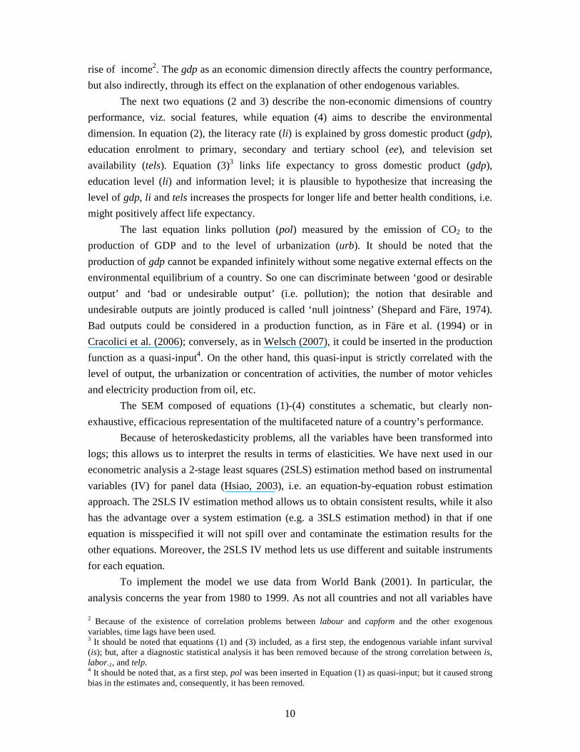
The next two equations (2 and 3) describe the non-economic dimensions of country

performance, viz. social features, while equation (4) aims to describe the environmental

dimension. In equation (2), the literacy rate (li ) is explained by gross domestic product (gdp),

education enrolment to primary, secondary and tertiary school (ee), and television set

availability (tels). Equation (3)3 links life expectancy to gross domestic product (gdp),

education level (li ) and information level; it is plausible to hypothesize that increasing the

level of gdp, li and tels increases the prospects for longer life and better health conditions, i.e.

might positively affect life expectancy.

The last equation links pollution (pol) measured by the emission of CO2 to the

production of GDP and to the level of urbanization (urb). It should be noted that the

production of gdp cannot be expanded infinitely without some negative external effects on the

environmental equilibrium of a country. So one can discriminate between ‘good or desirable

output’ and ‘bad or undesirable output’ (i.e. pollution); the notion that desirable and

undesirable outputs are jointly produced is called ‘null jointness’ (Shepard and Färe, 1974).

Bad outputs could be considered in a production function, as in Färe et al. (1994) or in

Cracolici et al. (2006); conversely, as in Welsch (2007), it could be inserted in the production

function as a quasi-input4. On the other hand, this quasi-input is strictly correlated with the

level of output, the urbanization or concentration of activities, the number of motor vehicles

and electricity production from oil, etc.

The SEM composed of equations (1)-(4) constitutes a schematic, but clearly non-

exhaustive, efficacious representation of the multifaceted nature of a country’s performance.

Because of heteroskedasticity problems, all the variables have been transformed into

logs; this allows us to interpret the results in terms of elasticities. We have next used in our

econometric analysis a 2-stage least squares (2SLS) estimation method based on instrumental

variables (IV) for panel data (Hsiao, 2003), i.e. an equation-by-equation robust estimation

approach. The 2SLS IV estimation method allows us to obtain consistent results, while it also

has the advantage over a system estimation (e.g. a 3SLS estimation method) in that if one

equation is misspecified it will not spill over and contaminate the estimation results for the

other equations. Moreover, the 2SLS IV method lets us use different and suitable instruments

for each equation.

To implement the model we use data from World Bank (2001). In particular, the

analysis concerns the year from 1980 to 1999. As not all countries and not all variables have 2 Because of the existence of correlation problems between labour and capform and the other exogenous variables, time lags have been used. 3 It should be noted that equations (1) and (3) included, as a first step, the endogenous variable infant survival (is); but, after a diagnostic statistical analysis it has been removed because of the strong correlation between is, labor-1, and telp. 4 It should be noted that, as a first step, pol was been inserted in Equation (1) as quasi-input; but it caused strong bias in the estimates and, consequently, it has been removed.

11

data availability over the period analysed, we made an appropriate choice of either countries

or variables. Hence, we use observations at five-year intervals, around 1980, 1985, 1990,

1995 and 1999. In most cases, these are an average of five annual observations centred on the

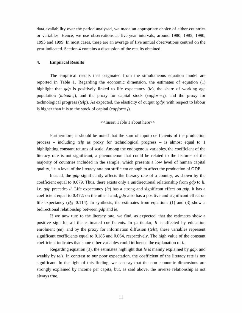
year indicated. Section 4 contains a discussion of the results obtained.

4. Empirical Results

The empirical results that originated from the simultaneous equation model are

reported in Table 1. Regarding the economic dimension, the estimates of equation (1)

highlight that gdp is positively linked to life expectancy (le), the share of working age

population (labour-1), and the proxy for capital stock (capform-1), and the proxy for

technological progress (telp). As expected, the elasticity of output (gdp) with respect to labour

is higher than it is to the stock of capital (capform-1).

<<Insert Table 1 about here>>

Furthermore, it should be noted that the sum of input coefficients of the production

process – including telp as proxy for technological progress – is almost equal to 1

highlighting constant returns of scale. Among the endogenous variables, the coefficient of the

literacy rate is not significant, a phenomenon that could be related to the features of the

majority of countries included in the sample, which presents a low level of human capital

quality, i.e. a level of the literacy rate not sufficient enough to affect the production of GDP.

Instead, the gdp significantly affects the literacy rate of a country, as shown by the

coefficient equal to 0.679. Thus, there exists only a unidirectional relationship from gdp to li ,

i.e. gdp precedes li . Life expectancy (le) has a strong and significant effect on gdp, it has a

coefficient equal to 0.472; on the other hand, gdp also has a positive and significant effect on

life expectancy (β33=0.114). In synthesis, the estimates from equations (1) and (3) show a

bidirectional relationship between gdp and le.

If we now turn to the literacy rate, we find, as expected, that the estimates show a

positive sign for all the estimated coefficients. In particular, li is affected by education

enrolment (ee), and by the proxy for information diffusion (tels); these variables represent

significant coefficients equal to 0.185 and 0.064, respectively. The high value of the constant

coefficient indicates that some other variables could influence the explanation of li .

Regarding equation (3), the estimates highlight that le is mainly explained by gdp, and

weakly by tels. In contrast to our poor expectation, the coefficient of the literacy rate is not

significant. In the light of this finding, we can say that the non-economic dimensions are

strongly explained by income per capita, but, as said above, the inverse relationship is not

always true.

12

Finally, regarding the environmental dimension, there exists a positive relationship

between gdp and pol, i.e. a marginal increase of gdp produces an almost proportional increase

of production of CO2. Among the other variables, as expected, it is relevant to mention the

effect of urbanization on pol; in fact it is reasonable to believe that a high urbanization rate

directly and indirectly affects the level of pollution through an increasing use of urban

transport, high consumption of energy, electricity, and water, etc.

The coefficient of tels has a negative and significant sign, indicating that the

information acts positively on the decrease of pollution.

In conclusion, a bidirectional causality relationship exists between gdp and life

expectancy (le), while only a unidirectional one exists between gdp and li . Why does li not

affect gdp? For developing countries, this factor is likely to be connected to the composition

of the population characterized by low educated people employed in low productivity and

traditional sectors (i.e. agriculture) which weakly affect the production of gdp. For developed

countries, the unidirectional relationship may reflect the inability of countries to adequately

employ their human capital with a high level of education and skills. Thus, in the long run,

this could lead countries – with a high level of gdp and li – to have a poor status, i.e. low gdp

and li .

The positive and significant effect of gdp on all social and environmental dimensions

highlights that a good level of the economic dimension is a basic condition to achieve a good

social-enviromental performance.

Actually, the estimates from the model give us relevant information on the ‘average

behaviour’ across countries and over years. If we want to obtain more detailed information for

each country at each time point, it would be useful to explore growth rates of economic (i.e.

gdp) and social-environmental performance (i.e. le, li and pol). For this aim and in order to

obtain a dynamic interpretation of our empirical results, we classify the countries in four

groups:

i) High high (HH) – countries with a rate of economic and social-environmental growth

greater than the average value;

ii) Low high (LH) – countries characterized by a growth rate of gdp lower than the

average value and a social or environmental performance (i.e. le, li and pol) greater

than the average value;

iii) High low (HL) – countries characterized by a growth rate of gdp greater than the

average value and a growth rate of social or environmental performance lower than the

average value;

iv) Low low (LL) – countries characterized by a growth rate of gdp and social or

environmental performance lower than the average value.

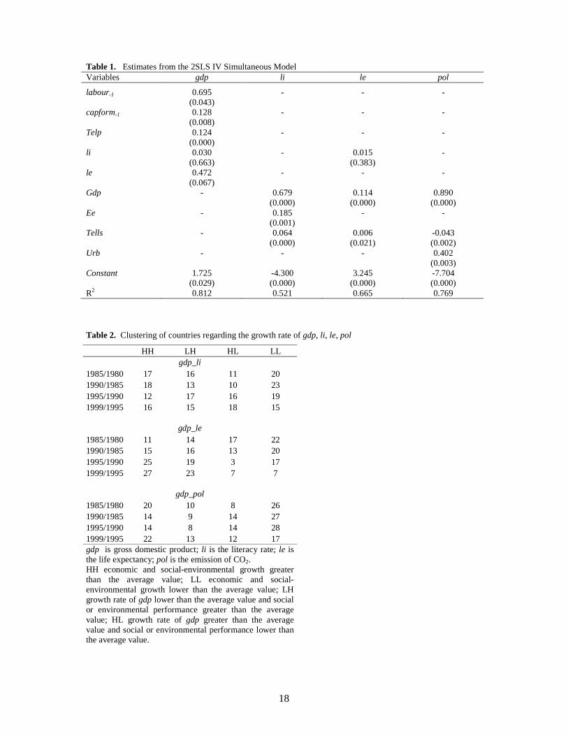
Table 2 shows the clustering of countries in the four groups according to growth rate

of gdp, and le, li and pol, respectively. With respect to gdp and le, we note that the number of

13

countries with an excellent performance (i.e. the group H-H) is increasing over the time; it

passes from 11 – at the first time point – to 27 at the last time point. In contrast, it is

interesting to observe the number of countries with a bad performance (i.e. the group L-L)

decreases over time, declining from 22 to 7. All this is the expression of the bidirectional

causality relationship between gdp and le highlighted by the simultaneous model, i.e. a high

rate growth of gdp supports the expectancy of a longer life, but, conversely, a lower rate

growth of le, i.e. the worst human health conditions, causes a country achieve lower growth

and productivity in terms of gdp. Further, the countries included in the cluster HL decrease by

of about 50 percent while the countries in the cluster LH increase over time.

Regarding the relationship between gdp and li , the clustering of the countries does not

highlight a clear relationship between the two variables as was obtained from the

simultaneous equation model; the number of the clusters is almost stable over time for the HH

and the LH ones, while the number of countries increases weakly in the HL cluster and

decreases in the LL one.

With respect to gdp and pol, only the cluster LL shows a significant change in the number of

countries included in it, while we note the number of countries is almost stable in the clusters

HH, HL and LH. In particular, we expected an increase of units in the HL cluster and, in

contrast, a decrease of units in HH one, if countries with high growth rate of gdp had audited

the environmental damage associated with economic growth.

In the light of these results, it would be interesting to trace the performance of each

country in terms of growth rates for the period analysed, viz. 1980-1999. Tables 3 and 4

summarize the movements of countries from the start period (1980-1985) to the end period

(1995-1999). In particular, Table 4 can be interpreted as a matrix of the transition/ persistency

status of countries. In fact, the main diagonal shows the persistency status of countries with

respect to their beginning status (i.e. HH, LH, HL and LL); on the contrary the units above

and below the main diagonal indicate the countries that move from a certain start status to a

different end status.

Regarding the relationship between gdp and le and li , respectively, we can say that a

unit follows a virtuous path if it moves directly from the cluster LL to HH or LH; that means

reaching a good economic performance matches social goals. Further, a country follows a

virtuous path just as much if it moves from status HL and LH to HH. With respect to the first

path (from HL to HH), a territorial unit is able to manage its economic growth efficiently in

order to increase its social development. Concerning the second path, i.e. from LH to HH, a

country exploits the good conditions of its people in terms of a high level of education and

high health conditions to contribute to increase its economic growth.

In particular from Table 4, we note that the number of countries following a virtuous

path is greater with respect to le (30) than to li (10). This result, already highlighted by the

estimates of our model, confirms the bidirectional causal relationship between gdp and le. In

14

other words, a high level of life expectancy has been an easier goal to reach for many

countries, while a high level of education is a more difficult goal to achieve.

Relating to gdp and pol, a country proceeds along a virtuous path if it moves from the

cluster HH to HL, but also from LL and LH to HL. In fact, it is important for both developed

and developing countries to reach an economic growth process by monitoring the level of

pollution through specific actions. From Table 4, we can count only 10 countries that have a

virtuous status, i.e. the monitoring of environment has been a difficult problem to manage for

the majority of countries. The polarization of countries in the clusters HH (20 countries) and

LL (26 countries) indicates that a high level of economic growth implies a social cost in terms

of environmental damage; on the other hand, a low economic growth is not likely to imply

environmental damage.

5. Conclusion

We have proposed a rational scheme in which future research on economic, social, and

environmental performance of countries can be positioned and nested. By using a structural

simultaneous equation model, we have estimated the intensity of causal relationships among

economic, social and environmental variables, and we have controlled for endogeneity.

Obviously, our scheme is not exhaustive and additional aspects could be considered as

well (e.g. ones related to income inequality, quality of diet, time and leisure, etc.).

Nevertheless, at this moment, our analysis is a new attempt to integrate the economic, social,

and environmental aspects of countries’ performances simultaneously.

By using a simultaneous equation model, our attempt represents a novel

methodological approach to analyse a multidimensional phenomenon on such as country

well-being, traditionally treated by means of statistical multivariate methods or composite

indicators.

The estimations show that gdp is a basic condition to obtain a good social

performance: a high level of gdp permits inhabitants to have a longer life expectancy and to

achieve a higher level of education. But the other side of the coin is that high levels of gdp

increase the level of pollution. In particular for developing countries, this insight implies that

policy makers have to pay attention to controlling and monitoring the negative effects of

economic growth on the environment.

Furthermore, the empirical analysis reveals a strong bidirectional relationship between

gdp (the economic performance indicator) and one of the social performance indicators, life

expectancy.

In contrast, a unidirectional relationship between gdp and li has been found. This

result could be related to a slower response of gdp to human capital changes, viz. a higher

quality level of human capital does not turn immediately into a higher level of gdp.

15

As our empirical analysis has mainly concerned developing countries, we may

hypothesize that the countries analysed have not reached the minimum threshold that permits

them to move from an economy characterized by a low productivity level to a country

characterized by a high productivity level .

Finally, the results obtained show that life expectancy does not serve to distinguish

between the countries, while the literacy rate and CO2 emissions are better able to capture the

differences between countries in terms of their social and environmental dimensions. In

particular, with respect to the literacy rate a similar result has been obtained from McGillivray

(2005).

From a policy point of view, the above result indicates that, for most of the countries

that were examined, more efforts should have been made to improve their social and

environmental performance, viz. in order to increase the level of the literacy rate and to

control the CO2 emissions. More specifically, in agreement with several strands of the

literature, the policy response to spatial inequality or disparity could be based on:

• supply-side policy of a Keynesian nature, with a pronounced interest in public spending

in less privileged regions;

• growth pole strategies, with a clear emphasis on a concentrated growth impulse in a few

designated place or areas;

• infrastructure policy, with the aim of creating the necessary physical conditions (e.g.

improvement of accessibility) in order to enhance the competitive capabilities of regions;

• self-organizing policy, where regions are encouraged to get their acts together on the

basis of their own indigenous strength with a limited role of governments;

• suprastructure policy, in which regions are provided with favourable R&D conditions,

educational facilities, knowledge centres, and the like, in order to create the conditions

for self-sustained development.

In summary, our paper has tried to investigate and explore country performance

regarding all aspects, economic and non-economic, simultaneously. Further, as the results

obtained from the model give us insights into the average behaviour of countries over time, a

matrix of persistency and transition status has been made. This analysis confirms the

empirical results derived from the model, and highlights the inability of most countries, over

time, either to turn the higher educational skills of their population into greater gdp or to

improve the level of education in order to move from a low productivity economy to a higher

productivity one.

References Barro, R. and X. Sala-i-Martin, Convergence, Journal of Political Economy, vol. 100, 1992, pp. 223-251.

16

Bohringer, C. and P.E.P. Jochem, Measuring the Immeasurable - A Survey of Sustainability Indices, Ecological Economics, vol. 63, 1-8, 2007, pp. 1-8.

Common, M. and S. Stagl, Ecological Economics, An Introduction, Cambridge University Press, Cambridge, 2005.

Cracolici, M.F., M. Cuffaro and P. Nijkamp, Sustainable Tourist Development in Italian Holiday Destinations, Research Memorandum, 14-2006, Free University, Amsterdam, The Netherlands, 2006.

Cuffaro, M., M.F. Cracolici and P.Nijkamp, Measuring the Performance of Italian Regions on Social and Economic Dimensions, Scienze Regionali, Italian Journal of Regional Science, vol. 7, 2008, pp. 27-47.

Daly, H.E. and J.B. Cobb, For the Common Good: Redirecting the Economy towards Community, the Environment and a Sustainable Future, Beacon Press, Boston, 1989.

Dasgupta, P., Well-Being and the Extent of its Realization in Poor Countries, The Economic Journal, vol. 100, 1990, pp. 1-32.

Dasgupta, P. and M. Weale, On Measuring the Quality of Life, World Development, vol. 20, no. 1, 1992, pp. 119-131.

Dasgupta, S., K. Hamilton, K.D. Pandey, and D.Wheeler, Environment During Growth: Accounting for Governance and Vulnerability, World Development, vol. 34, 2006, pp. 1597-1611.

Davidson, Eric. A., You Can’t Eat GNP: Economics As If Ecology Mattered, Perseus, Cambridge, MA, 2000. Desai, M., Human Development: Concepts and Measurement, European Economic Review, , vol. 35, 1991, pp.

350-357. Distaso, A., Well-being and/or Quality of Life in EU Countries through a Multidimensional Index of

Sustainability, Ecological Economics, vol. 64, 2007, pp. 163-180. Färe, R., S. Grosskopf and P. Roos, Productivity and Quality Changes in Swedish Pharmacies, Discussion Paper,

Southern Illinois University, Carbondale. IL, 1994. Giles, D.E.A. and H. Feng, Output and Well-being Industrialized Nations in the Second Half of the 20th

Century: Testing for Convergence Using Fuzzy Clustering Analysis, Structural Change and Economic Dynamics, vol. 16, 2005, pp. 285-308.

Hobijn, B. and P.H. Franses, Are Living Standards Converging?, Structural Change and Economic Dynamics, vol. 12, 2001, pp. 171-200.

Hsiao, C., Analysis of Panel Data, Cambridge, Cambridge University Press, 2003. Khan, H., Measurement and Determinants of Socioeconomic Development: a Critical Conspectus, Social

Indicators Research, vol. 24, 1991, pp. 153-175. Kuznets, S., Modern Economic Growth: Findings and Reflections, The American Economic Review, vol. 63, no.

3, 1973, pp. 247-258. Marchante, A.J. and B. Ortega, Quality of Life and Economic Convergence across Spanish Regions, 1980-2001,

Regional Studies, vol. 40, no. 5, 2006, pp. 471-483. Mazumdar, K., Causal Flow Between Well-Being and Per Capita Real Gross Domestic Product, Social

Indicators Research, vol. 50, 2000, pp. 297-313. McGillivary, M., The Human Development Index: Yet an other Redundant Composite Development Indicator?,

World Development, vol. 19, no. 10, 1991, pp. 1461-1468. McGillivary, M., Measuring Non-Economic Well-Being Achievement, Review of Income and Wealth, vol. 51,

2005, pp. 337-364. McGillivary, M. and A. Shorrocks, Inequality and Multidimensional Well-Being, Review of Income and Wealth,

vol. 51, 2005, pp. 193-200, Neumayer, E., The ISEW – Not an Index of Sustainable Economic Welfare, Social Indicators Research, vol. 48,

1999, pp. 77-101, 1999. Neumayer, E., On the Methodology of ISEW, GPI and Related Measures: Some Constructive Suggestions and

Some Doubt on the Threshold Hypothesis, Ecological Economics, vol. 34, 2000, pp. 347-361. Neumayer, E., Beyond Income: Convergence in Living Standards, Big Time, Structural Change and Economic

Dynamics, vol. 14, 2003, pp. 275-296. Noorbakhsh, F., A Modified Human Development Index, World Development, vol. 26, 1998, pp. 517-528. Osberg, L. and A. Sharpe, How Should We Measure the ‘Economic’ Aspects of Well-Being?, Review of Income

and Wealth, vol. 51, no. 2, 2005, pp. 311-336. Pulselli, F.M., F. Ciampalini, E. Tiezzi and C. Zappia, The Index of Sustainable Economic Welfare (ISEW) for a

Local Authority: A Case Study in Italy, Ecological Economics, vol. 60, 2006, pp. 271-281. Ram, R. and T.W. Schultz, Life Span, Health, Savings, and Productivity, Economic Development and Cultural

Change, vol. 27, 1979, pp. 399-421. Ranis, G., F. Stewart and A. Ramirez, Economic Growth and Human Development, World Development, vol.

28, 2000, pp. 197-219.

17

Sagar A.D. and A. Najam, The Human Development Index: a Critical Review, Ecological Economics, vol. 25, no. 33, 1998, pp. 249-264.

Sen, A., Resources, Values and Development, Basic Blackwell, Oxford, 1984. Sen, A., Commodities and Capabilities, North Holland Press, Amsterdam, 1985. Sen, A., Standard of Living, Cambridge University Press, New York, 1987. Shephard. R. and R. Färe, The Law of Diminishing Returns, Zeitschrift fur Nationalokonomie, vol. 34, 1974, pp.

69-90. Solow, R., A Contribution to the Theory of Economic Growth, Quarterly Journal of Economics, vol. 70, 1956,

pp. 65-94. UNDP, Human Development Report, Oxford University Press, New York, 1990. UNDP, Human Development Report, Oxford University Press, New York, 1991. UNDP, Human Development Report, Oxford University Press, New York, 1997. Welsch, H., Environmental Welfare Analysis: A Life Satisfaction Approach, Ecological Economics, vol. 62,

2007, pp. 544-551. World Bank, World Development Indicators, World Bank, Washington, 2001. Zuvekas, C. Jr., Economic Development, St Martin’s Press, New York, 1979.

18

Table 1. Estimates from the 2SLS IV Simultaneous Model Variables gdp li le pol labour-1 0.695 - - - (0.043) capform-1 0.128 - - - (0.008) Telp 0.124 - - - (0.000) li 0.030 - 0.015 - (0.663) (0.383) le 0.472 - - - (0.067) Gdp - 0.679 0.114 0.890 (0.000) (0.000) (0.000) Ee - 0.185 - - (0.001) Tells - 0.064 0.006 -0.043 (0.000) (0.021) (0.002) Urb - - - 0.402 (0.003) Constant 1.725 -4.300 3.245 -7.704 (0.029) (0.000) (0.000) (0.000) R2 0.812 0.521 0.665 0.769

Table 2. Clustering of countries regarding the growth rate of gdp, li , le, pol

HH LH HL LL gdp_li

1985/1980 17 16 11 20 1990/1985 18 13 10 23 1995/1990 12 17 16 19 1999/1995 16 15 18 15

gdp_le 1985/1980 11 14 17 22 1990/1985 15 16 13 20 1995/1990 25 19 3 17 1999/1995 27 23 7 7

gdp_pol 1985/1980 20 10 8 26 1990/1985 14 9 14 27 1995/1990 14 8 14 28 1999/1995 22 13 12 17 gdp is gross domestic product; li is the literacy rate; le is the life expectancy; pol is the emission of CO2. HH economic and social-environmental growth greater than the average value; LL economic and social-environmental growth lower than the average value; LH growth rate of gdp lower than the average value and social or environmental performance greater than the average value; HL growth rate of gdp greater than the average value and social or environmental performance lower than the average value.

19

Table 3. Movements of countries over time relating to cross-tabulated growth rates of gdp and li, le and pol gdp_li gdp_le gdp_pol

1985/1980

1990/1985

1995/1990

1999/1995

1985/1980

1990/1985

1995/1990

1999/1995

1985/1980

1990/1985

1995/1990

1999/1995

1 Algeria HL LL LH HH HH LH LH HH HL LL LL HL

2 Argentina LL LL HL HL LL LL HH HH LL LL HL HH

3 Brazil LL LL HL LL LL LL HH LH LL LL HL LH

4 Burkina Faso HL LL LL HL HL LL LL HL HL LH LL HL

5 Burundi HL LL LL LL HL LL LL LH HH LL LL LH

6 Cameroon HH LH LH HH HH LH LL HL HH LL LH HL

7 Central African Republic LL LL LL LL LL LL LL LL LH LL LL LL

8 Chile LH HH HL HH LH HH HH HH LL HH HL HH

9 China HH HH HH HH HL HL HL HH HH HL HH HH

10 Colombia LH HL HL LL LL HL HH LH LH HL HL LL

11 Congo, Dem. Rep. LL LL LL LL LL LL LL LL LL LL LL LL

12 Congo, Rep. HH LH LH LH HL LL LL LL HL LH LL LL

13 Costa Rica LH HL HL HH LL HL HH HH LL HL HH HL

14 Cote d'Ivoire LL LL LL HL LL LL LL HL LH LL LL HH

15 Cyprus HH HH HH HH HL HL HL HH HL HH HL HH

16 Ecuador LH LH LH LH LL LL LH LH LH LL LH LL

17 Egypt, Ar. Rep. HL HL LL HL HH HH LH HH HH HL LL HH

18 El Salvador LL LL HL LL LH LH HH LH LL LH HH LH

19 Gambia, The LL LL LL HL LH LH LH HH LL LL LL HL

20 Ghana LL LH LH HH LH LH LH HL LH LL LL HL

21 Greece LH LH LH HH LL LH LL HH LH LL LL HH

22 Guatemala LL LL HL LL LL LH HH LH LL LH HL LH

23 Honduras LL LL LL LL LH LH LH LH LL LH LH LH

24 Hungary HH LH LL HL HL LL LL HH HL LL LL HH

25 India HL HL HL HL HH HH HH HH HH HH HH HH

26 Indonesia HH HH HH LH HH HH HH LH HH HH HH LL

27 Iran, Islamic Rep. HL LH HH HH HH LH HH HH HH LH HL HH

28 Israel HH HH HH LH HL HL HH LH HH HL HH LL

29 Italy HH HH LH LL HL HL LL LH HL HL LL LL

30 Jamaica LH HL LL LL LL HL LH LH LL HH LL LH

31 Japan HH HH LH LH HL HL LL LH HL HL LL LH

32 Kenya LH HH LH LH LH HL LL LL LL HH LL LL

33 Korea, Rep. HH HH HH HH HL HH HH HH HH HH HH HH

34 Kuwait LL HH HL LL LL HH HH LH LL HL HH LL

35 Madagascar LL LL LL LL LL LL LH LH LL LL LL LL

36 Malawi LL LL LL HL LL LL LL HL LL LL LL HL

37 Malaysia HH HH HH LH HL HL HH LH HH HH HH LH

38 Mali LL LL LL HL LH LL LL HL LL LL LL HL

39 Malta HH HH HH HH HL HL HH HH HH HH HL HH

40 Mauritius HL HL HL HL HL HH HH HH HH HH HH HH

41 Mexico LH LH LH HL LL LL LH HH LL LL LL HH

42 Morocco HL HL LL HL HH HH LH HH HH HL LH HH

43 Nepal HL HL HL HL HH HH HH HH HH HL HH HH

44 Nicaragua LL LL LL HL LH LH LH HH LL LH LL HH

45 Oman HH LH LH LH HH LH LH LH HH LL LL LL

46 Pakistan HL HL HL LL HH HH HH LH HH HH HL LH

47 Paraguay LH LH LH LH LL LL LH LH LL LH LH LL

48 Peru LH LH HH LH LH LH HH LH LL LL HL LH

49 Philippines LH HH LH LH LL HH LH LH LL HH LH LH

50 Rwanda LL LL LL HH LH LL LL HH LH LL LL HL

20

51 Senegal LL LL LL HL LH LH LH HH LL LL LL HL

52 Singapore HH HH HH HH HL HL HH HH HL HH HH HH

53 South Africa LL LL LL LL LH LH LL LL LH LL LL LL

54 Sri Lanka HL HL HL HL HL HL HH HH HH HL HH HH

55 Swaziland LH HH LH LL LH HH LH LL LL HL LL LL

56 Syrian ArHL Republic LL LL HL HL LH LH HH HH LH LL HL HL

57 Thailand HH HH HH LH HL HH HL LH HH HH HH LH

58 Trinidad and ToLHgo LH LL LL HL LL LL LH HH LH LL LH HH

59 Tunisia HH LL HL HH HH LH HH HH HH LL HL HH

60 Turkey HH HH HH LH HL HH HH LH HH HL HL LH

61 Uruguay LH HH HH HH LL HL HH HH LL HL HL HH

62 Venezuela, RB LH LH LH LH LL LL LH LH LL LL LH LL

63 Zambia LL LL LH LH LL LL LL LL LL LL LL LL

64 Zimbawe LH LH LH HH LL LL LL HL LL LH LL HL gdp is gross domestic product; li is the literacy rate; le is the life expectancy; pol is the emission of CO2. HH economic and social-environmental growth greater than the average value; LL economic and social-environmental growth lower than the average value; LH growth rate of gdp lower than the average value and social or environmental performance greater than the average value; HL growth rate of gdp greater than the average value and social or environmental performance lower than the average value.

Table 4. Persistency/transition matrix from 1980 to 1999 gdp_li

HH LH HL LL HH 7 8 1 1 LH 5 6 2 3 HL 2 0 7 2 LL 2 1 8 9

gdp_le

HH LH HL LL HH 7 3 1 0 LH 6 3 2 3 HL 8 7 1 1 LL 6 10 3 3

gdp_pol

HH LH HL LL HH 11 5 1 3 LH 3 0 3 4 HL 3 1 2 2 LL 5 7 6 8

gdp is gross domestic product; li is the literacy rate; le is the life expectancy; pol is the emission of CO2. HH economic and social-environmental growth greater than the average value; LL economic and social-environmental growth lower than the average value; LH growth rate of gdp lower than the average value and social or environmental performance greater than the average value; HL growth rate of gdp greater than the average value and social or environmental performance lower than the average value.

21

COUNTRY PERFORMANCE

ECONOMIC ASPECTS

Economic Well-being

NON ECONOMIC ASPECTS

Non-economic well-being

Static view

Economic Growth Human Development

Dynamic view

Figure 1. Operational scheme for the assessment of economic and non-economic performance of countries