analYsis oF emPiriCal CHaraCteristiCs in tHe Pert metHoD

issn 2029-8234 (online)BUsiness sYstems and eConomiCsno. 2 (1), 2012

analYsis oF emPiriCal CHaraCteristiCs in tHe Pert metHoD

radek DoskoČil, karel DoUBraVskÝBrno University of technology, Faculty of Business and management,

Department of informatics kolejní 2906/4, Brno, Czech republic

Phone no.: +420541143718, +420541143722 e-mail: [email protected], [email protected]

abstract. The paper generally deals with the effects of a change in variance activities when computing the node and activity criticality of a Pert network diagram. The main aim of the paper is to analyse the effects of a change in variance activities for two different approaches used when computing node and activity criticality. in order to achieve the aim, a hypothesis is formed that the change in variance activity should affect the computation of the criticality probability of nodes and activities. The analysis is applied to a sample Pert network diagram comprising 9 nodes and 14 activities. a time analysis is developed using the Pert method and node and activity criticality is computed using both approaches. The computed results serve as input for further statistical processing.

keywords: network graphs, stochastic graph, Pert method, node criticality.jel classification: C44, C12.

introduction

Project management is nowadays a widely discussed discipline. This fact is sub-stantiated by numerous scientific articles, books and publications dealing with these problems (Bergantiños, Vidal-Puga, 2009; Garcia et all., 2005). This discipline is also included in the courses of numerous faculties focusing on economy both in the Czech republic and abroad. experts are also associated in various professional organisations or associations (společnost pro projektové řízení Česká republika, 2011; international Project management association, 2011). Project managers and other members of the project team use different tools, techniques or methods in project management. if we take a closer look at these tools, we will find out that in certain cases the manner of their application varies, depending on the approach of individual authors. one of the various approaches is node criticality computation in the Pert method (Program evaluation

8 BUsiness sYstems and eConomiCsno. 2 (1), 2012

and review technique) generally using two different approaches to the computation. neither approach considers mutual size of variances of the individual activities. This fact might affect appropriateness of use of one or the other approach. The computation of node criticality is one part of a probability analysis. in the framework of this analysis criticality of activities is also computed (depending on the user needs), together with computation of the probability of meeting the planned deadlines (Jablonský, 2002).

The purpose of the present paper is to compare the two different approaches with regard to activity variations. For the purpose of the comparison the authors defined the assumption that the change of activity variance can affect the computation of node and activity criticality. The defined issue is demonstrated on a sample case of a Pert network diagram consisting of 9 nodes and 14 activities (rais, Doskočil, 2006).

Materials and methods

Three estimated times of activity duration were used in the network diagram – the optimistic, the most likely and the pessimistic one. subsequently, mean times of activ-ity duration [1] were calculated using the formula (Plevný, Žižka, 2005):

, [1]

where: i, j - node number, tij - time of activity duration, aij - optimistic estimate of activity duration, mij - estimate of most likely activity duration, bij - pessimistic estimate of activity duration.

Variances [2] and standard deviations [3] of activity duration were also calculated. The following formulas were used for the calculations:

, [2]

. [3]

For the purpose of the time analysis the basic time characteristics were further calculated on the basis of standard equations. Further information can also be found in literature (Černá, 2008; Wisniewski, 1996).

Using an incidence matrix, the possible earliest times of nodes [4] were calculated on the basis of the following formulas:

, [4]

where: i, j - node number, ETNj - earliest time of node, EFTij - earliest Finish time of activity,

9radek DoskoČil, karel DoUBraVskÝ. analYsis oF emPiriCal CHaraCteristiCs in tHe Pert metHoD

ESTij - earliest start time of activity, tij - activity duration.

The permissible latest times of nodes [5] were calculated using the following formulas:

, [5]

where: i, j - node number, LTNi - permissible latest time of node, LFTij - permissible latest start time of activity, LFTij - permissible latest Finish time of activity, tij - activity duration.

There are two generally used approaches to variance computation needed for a node criticality analysis.

The first approach is based on the assumption that variances of earliest times of nodes [6] correspond to the calculated variances of earliest Finish times of activities and the one is selected that pertains to the maximum duration to the earliest Finish times of activities coinciding with the respective node.

, [6]

where: i, j - node number, σ2ETNi - variance of earliest time of node, σ2EFTij - variance of earliest Finish time of activity, k - number of nodes.

in the first approach, variances of permissible latest times of nodes [7] corre-spond to the calculated variances of the permissible latest start times of activities and the one is selected that pertains to the minimum duration of the permissible latest start times of activities coinciding with the respective node (Gross, 2003).

, [7]

where: i, j - node number, σ2LTNj - variance of permissible latest time of node, σ2LSTij - variance of permissible latest start time of activity, k - number of nodes.

The second approach is based on the assumption that variances of earliest time of nodes [8] correspond to the calculated variances of earliest Finish times of activities and the one is selected which shows the maximum value of the ones coinciding with the respective node.

, [8]

where: i, j - node number,


σ2ETNi - variance of earliest time of node, σ2EFTij - variance of earliest Finish time of activity, k - number of nodes.

Variances of permissible latest times of nodes [9] correspond to the calculated variances of the permissible latest start times of activities and the one is selected that shows the maximum value of the ones coinciding with the respective node (operační analýza [Operational Analysis], 2003).

, [9]

where: i, j - node number, σ2LTNj - variance of permissible latest time of node, σ2LSTij - variance of permissible latest start time of activity, k - number of nodes.

When looking for the probability at which non-critical nodes become critical it is sufficient to specify the probability of the interference margin of the node to equal or be less than zero, i.e. probability [10]:

, [10]

where: i, j - node number, P - probability, IMi - interference margin, LTNi - permissible latest time of node,ETNj - earliest time of node.

The calculated value (parameter) of the standardised normal distribution for node [11] will be:

, [11]

where: i, j - node number, u - value of standardized normal distribution, LTNi - permissible latest time of node, ETNj - earliest time of node, σ2LTNj - variance of permissible latest time of node, σ2ETNi - variance of earliest time of node.

The calculated value (parameter) of the standardised normal distribution for ac-tivities [12] will be:

, [12]

where: i, j - node number,


u - value of standardized normal Distribution, LTNi - latest time of node, ETNj - earliest time of node, tij - activity duration mean times, σ2LTNj - variance of the latest time of node, σ2ETNi - variance of the earliest time of node, σ2tij - variance of activity duration times.

The sought probability will be the value of distribution function F(u), found for example in statistical tables or using appropriate software (Gross, 2003).

to verify the hypothesis, selected apparatus of mathematical statistics will be used, in particular instruments of hypothesis testing and t-test. Further information can be found in literature (mathews, 2005; Wonnacott, 1990).

results

The network diagram consisting of 9 nodes and 14 activities had three estimates of times of activity duration set: optimistic (aij), most likely (mij) and pessimistic (bij) (see table 1). index i represents the initial activity node and index j the end activity node.

table 1 further includes calculated mean times of activity durations tij [1], their variances σ2tij [2] and standard deviations σtij [3]. The calculated variances of activities (1;4) and (4;6) show that their values differ in size from all other activity variances.

Table 1. Calculation of mean activity Duration and Variance

i j aij mij bij tij σ2tij σ tij

1 2 5 6 13 7.00 1.78 1.331 3 2 3 4 3.00 0.11 0.331 4 4 4 20 6.67 7.11 2.672 3 0 0 0 0.00 0.00 0.002 6 2 5 8 5.00 1.00 1.002 7 5 5 5 5.00 0.00 0.003 6 3 5 7 5.00 0.44 0.674 5 5 6 7 6.00 0.11 0.334 6 2 5 15 6.17 4.69 2.175 8 1 3 5 3.00 0.44 0.676 8 0 0 0 0.00 0.00 0.006 9 7 7 7 7.00 0.00 0.007 9 2 8 8 7.00 1.00 1.008 9 3 6 9 6.00 1.00 1.00

table 2 and 5 represent the incidence matrix of the network diagram. its inside cells include calculated mean times of activity duration (see table 1). The last but one column includes earliest times of nodes (ETNi) calculated with formula [4] and the last but one row includes permissible latest times of nodes (LTNj) calculated with formula [5].


Tabl

e 2.

inci

denc

e m

atrix

– a

ppro

ach

i

i1

23

45

67

89

ETN

iσ2 ET

Ni

12.

67(2

.78)

7.00

(1.7

8)6.

67(0

.56)

3.00

(0.1

1)0.

00(8

.67)

6.67

(7.1

1)0.

000.

007.

00 (1

.78)

3.00

(0.1

1)6.

67 (7

.11)

29.

67(0

.44)

7.00

(1.7

8)9.

67(1

.00)

12.0

0(2

.78)

9.67

(1.0

0)12

.00

(1.7

8)7.

001.

780.

00 (0

.00)

5.00

(1.0

0)5.

00 (0

.00)

39.

67(0

.44)

12.0

0(2

.22)

7.00

1.78

5 (0

.44)

46.

67(1

.56)

12.6

7(7

.22)

8.50

(4.6

9)12

.83

(11.

81)

6.67

7.11

6.00

(0.1

1)6.

17 (4

.69)

512

.67

(1.4

4)15

.67

(7.6

7)12

.67

7.22

3.00

(0.4

4)

615

.67

(1.0

0)12

.83

(11.

81)

14.6

7(0

.00)

19.8

3(1

1.81

)12

.83

11.8

10.

00 (0

.00)

7.00

(0.0

0)

714

.67

(1.0

0)19

.00

(2.7

8)12

.00

1.78

7.00

(1.0

0)

815

.67

(1.0

0)21

.67

(8.6

7)15

.67

7.67

6.00

(1.0

0)9

21.6

78.

67LT

Ni

0.00

9.67

9.67

6.67

12.6

714

.67

14.6

715

.67

21.6

7σ2 LT

Ni

8.67

1.00

0.44

1.56

1.44

0.00

1.00

1.00

0.00


The next stage of the node criticality analysis is represented by the calculation of variances of time characteristics on the level of both nodes (earliest and latest times of nodes) and activities. incidence matrix is again used for practical processing where only some of the time characteristics values and their variances are entered. Further information can be found in literature (Gross, 2003).

The following part of the text includes results of both examined approaches to variance calculations.

approach i

table 2 shows the network diagram incidence matrix. its inside cells include cal-culated variances of activity durations (see table 1). The last column includes variances of earliest times of nodes calculated on the basis of the first approach [6], i.e. the variances correspond to the calculated variances of activities and the one is selected that pertains to the maximum duration of earliest Finish times of activities coincid-ing with the respective node. The last row includes variances of latest times of nodes calculated on the basis of the first approach [7], i.e. the variances correspond to the calculated variances of activities and the one is selected that pertains to the minimum duration of the latest start times of activities coinciding with the respective node.

table 3 summarises the values of the above tables needed for the node criticality calculation. The first row shows node numbers, and the second interference margins. The third one shows values of the parameter of standardised normal distribution [11] and the matching values of distribution function of standardised normal distribution (fourth row), corresponding to the node criticality probability [10].

Table 3. node Criticality Calculation – approach i

I 1 2 3 4 5 6 7 8 9IMi 0.00 2.67 2.67 0.00 0.00 1.83 2.67 0.00 0.00U 0.00 –1.60 –1.79 0.00 0.00 –0.53 –1.60 0.00 0.00

F(u) 0.50 0.05 0.04 0.50 0.50 0.29 0.05 0.50 0.50

table 4 provides the necessary data for the computation of activities criticality based on the above-mentioned calculations. index i represents the initial activity node (the first row), and index j the final activity node (the second row).The third row gives the values of the parameter of standardised normal distribution [12], and the corre-sponding values of the distribution function of the standardised normal distribution (the fourth row), which correspond to the activities criticality probability.

Table 4. activities Criticality Computation – approach i

I 1 1 1 2 2 2 3 4 4 5 6 6 7 8J 2 3 4 3 6 7 6 5 6 8 8 9 9 9U –1.60 –8.94 0.00 –1.79 –1.60 –1.60 –1.79 0.00 –0.53 0.00 –0.79 –0.53 –1.60 0.00

F(u) 0.05 0.00 0.50 0.04 0.05 0.05 0.04 0.50 0.30 0.50 0.21 0.30 0.05 0.50


Tabl

e 5.

inci

denc

e m

atrix

– a

ppro

ach

ii

i1

23

45

67

89

ETN

iσ2 ET

Ni

12.

67(3

.78)

7.00

(1.7

8)6.

67(1

.56)

3.00

(0.1

1)0.

00(1

2.81

)6.

67(7

.11)

0.00

0.00

7.00

(1.7

8)3.

00 (0

.11)

6.67

(7.1

1)

29.

67(1

.44)

7.00

(1.7

8)9.

67(2

.00)

12.0

0(2

.78)

9.67

(1.0

0)12

.00

(1.7

8)7.

001.

780.

00 (0

.00)

5.00

(1.0

0)5.

00 (0

.00)

39.

67(1

.44)

12.0

0(2

.22)

7.00

1.78

5 (0

.44)

46.

67(1

.56)

12.6

7(7

.22)

8.50

(5.6

9)12

.83

(11.

81)

6.67

7.11

6.00

(0.1

1)6.

17 (4

.69)

512

.67

(1.4

4)15

.67

(7.6

7)12

.67

7.22

3.00

(0.4

4)

615

.67

(1.0

0)12

.83

(11.

81)

14.6

7(0

.00)

19.8

3(1

1.81

)12

.83

11.8

10.

00 (0

.00)

7.00

(0.0

0)

714

.67

(1.0

0)19

.00

(2.7

8)12

.00

1.78

7.00

(1.0

0)

815

.67

(1.0

0)21

.67

(8.6

7)15

.67

11.8

16.

00 (1

.00)

921

.67

12.8

1LT

Ni

0.00

9.67

9.67

6.67

12.6

714

.67

14.6

715

.67

21.6

7σ2 LT

Ni

12.8

12.

0014

45.

691.

441.

001.

001.

000.

00


approach ii

table 5 shows the network diagram incidence matrix. its inside cells include cal-culated variances of activity durations (see table 1). The last column includes variances of earliest times of nodes calculated with the second approach [8], i.e. the variances correspond to the calculated variances of activities and the one is selected that pertains to the maximum variance of the possible variances of activities coinciding with the respective node. The last row includes variances of latest times of nodes calculated on the basis of the second approach [9], i.e. the variances correspond to the calculated variances of activities and the one is selected that pertains to the maximum duration of the latest start times of activities coinciding with the respective node.

table 6 summarises the values of the above tables needed for node criticality cal-culation. The first row shows node numbers, and the second interference margins. The third one shows values of the parameter of standardised normal distribution [11] and the matching values of distribution function of standardised normal distribution (last row), corresponding to the node criticality probability [10].

Table 6. node Criticality Calculation – approach ii

I 1 2 3 4 5 6 7 8 9IMi 0.00 2.67 2.67 0.00 0.00 1.83 2.67 0.00 0.00U 0.00 –1.37 –1.49 0.00 0.00 –0.51 –1.60 0.00 0.00

F(u) 0.50 0.09 0.07 0.50 0.50 0.30 0.05 0.50 0.50

table 7 provides the necessary data for the computation of activities criticality based on the above-mentioned calculations. index i represents the initial activity node (first row), and index j the final activity node (second row).The third row gives the values of the parameter of standardised normal distribution [12], and the correspond-ing values of the distribution function of the standardised normal distribution (fourth row), which correspond to the activities criticality probability.

Table 7. activities Criticality Computation – approach ii

I 1 1 1 2 2 2 3 4 4 5 6 6 7 1J 2 3 4 3 6 7 6 5 6 8 8 9 9 2U –1.37 –5.35 0.00 –1.49 –1.37 –1.60 –1.49 0.00 –0.51 0.00 –0.79 –0.53 –1.60 0.00

F(u) 0.09 0.00 0.50 0.07 0.09 0.05 0.07 0.50 0.30 0.50 0.21 0.30 0.05 0.50

discussion

Values from the last column (node criticality probability) of tables 4 and 6 were used for further calculations. The performed analyses show that the probable critical path is identical whichever of the two approaches is used. The only difference is shown by the


values of F(u) of nodes 2, 3 and 6. The question is whether this difference is statistically significant or not. to find this out the statistical apparatus of hypothesis testing was used.

The values of the calculated probabilities for both approaches were included in two data files. to compare the values in these data files there was the t-test for two basic files. The basic conditions of use of this test are data normality and independence. The shapiro-Wilcoxon test was used to verify data normality. The requirement of independ-ence of the values of both files appears to be the key requirement. regarding the nature of the calculations where two probability values were specified for each node the re-quirement of independence might be violated. to verify the independence the Pearson correlation coefficient was calculated and the test of independence of two characters was performed. The calculated Pearson coefficient equalled 0.998. This value indicated a strong linear correlation between the found probability values. This assumption was further verified by the independence test. The null hypothesis of this test can be for-mulated as follows: The probability values are independent. The alternative hypothesis is: The probability values correlate. For the selected significance level α = 0.05 the test criterion t = 50.521 was calculated and the critical value 365.2)7(975,0 =t was specified. as the value of the test criterion was higher than the critical value (50.521 > 2.365), the null hypothesis was rejected and the alternative hypothesis was accepted. This means that the probability values correlated (were not independent).

For this reason the calculated probability values were considered paired values. to find out whether the difference between the probability values was statistically signifi-cant or not thet-test for paired values was used. For that reason the difference was calcu-lated on the basis of probability pairs for each node. The values formed a new data file. The basic characteristics were calculated for this data file: the selected mean 008.0−=x and the standard deviation 013.0=s . The basic assumptions for use of t-test for paired values include the assumption of data normality. The normality of data (obtained as the difference between probabilities) was verified by the shapiro-Wilcoxon test. The p-value was calculated for the selected significance level α = 0.05 with the result p = 0.15. as the p-value was higher than the selected significance level the null hypothesis was not rejected (the difference values were normally distributed). Thus the basic condition was fulfilled and the pair t-test calculation could be performed. The null hypothesis says that the differences between the calculated probabilities are close to zero (i.e. both approaches yield similar results). The alternative hypothesis says that the differences are significantly different from zero (i.e. both approaches yield different results). The calculated charac-teristics (selected mean and standard deviation) were used for the calculation of the test criterion t = –1.846. For the selected significance level the critical value 306.2)8(975,0 =t was specified. as the absolute value of the test criterion was lower than the critical value (1.846 < 2.306), the null hypothesis was not rejected (the probability differences are close to zero). in our case this means that the differences between the calculated prob-abilities were not statistically significant, and therefore the change of activity variances did not affect the calculation of the node criticality probability.

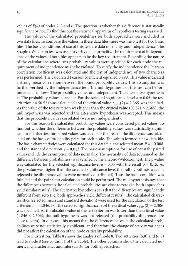
For illustration, table 8 shows the analysis of node 8. two activities (5;8) and (6;8) lead to node 8 (see column 1 of the table). The other columns show the calculated nu-merical characteristics and intervals 3σ for both approaches.


Table 8. analysis of node 8

approach i approach iimean

duration (μ)

Variance (σ2) μ – 3σ μ + 3σ

mean duration

(μ)

Variance (σ2) μ – 3σ μ + 3σ

node 8 15.67 7.66 7.37 23.97 15.67 11.8 5.36 25.96activity (5;8) 15.67 7.66 7.37 23.97 15.67 7.66 7.37 23.97activity (6;8) 12.84 11.8 2.53 23.14 12.84 11.8 2.53 23.14

if the first approach is used, the node characteristics will always correspond to the characteristics (mean duration, variance) of one of the activities. The upper threshold of interval 3σ i.e. (μ + 3σ) of node 8 is identical with the upper threshold of interval 3σ of activity (5;8). as soon as activity (5;8), which is the longest of the activities leading to node 8, ends, the activities starting from node 8 can begin.

if the second approach is used, the mean time of the node will correspond to the maximum mean time of activities leading to node 8. The variance of node 8 will cor-respond to the maximum variance of activities leading to node 8. This approach incor-porates a time margin for activities starting from node 8. in our case the value of the margin is (25.96 – 23.97). This margin need not be obvious in the case when a situation occurs that the maximum value of the mean duration of activities and its maximum variance apply to the same activity. This situation would correspond to the first ap-proach where no margin is applied.

table 9 summarises the results of both approaches of activities criticality compu-tation. The first and second row defines the node number. The third and fourth row gives probabilities of their criticality according to the first and second approach, re-spectively.

Table 9. activities Criticality

i 1 1 1 2 2 2 3 4 4 5 6 6 7 8j 2 3 4 3 6 7 6 5 6 8 8 9 9 9

F(u)approach i 0.05 0.00 0.50 0.04 0.05 0.05 0.04 0.50 0.30 0.50 0.21 0.30 0.05 0.50approach ii 0.09 0.00 0.50 0.07 0.09 0.05 0.07 0.50 0.30 0.50 0.21 0.30 0.05 0.50

The values of the calculated probabilities for the two are represented by two data files. in order to compare the values in these data files, the application of the t-test for two basic files would be useful. The basic conditions for the application of this test include data normality, and their independence. in order to test the independence, the calculation of the Pearson’s correlation coefficient and the test of independence of two attributes were used. The Pearson’s correlation coefficient appears to be 0.998. This value indicates strong linear dependence between the ascertained values of probability. Besides, this presumption was verified by an independence test. The null hypothesis of


the test can be formulated probability values are independent. an alternative hypothesis is formulated probability values are dependent. For the selected level of importance α = 0.05, a p-value was calculated, being 3.33∙10-5. as this value was lower than the selected level of importance, the null hypothesis was rejected and the alternative hypothesis was accepted. This means that the probability values are dependent.

in addition to the test of node criticality, a paired t-test could be used. a basic prerequisite for the performance of a paired t-test is data normality. Data normality (obtained from the probability difference) was checked using the shapiro-Wilcoxon test. For the selected level of importance α = 0.05, a p-value was calculated, being 0.005. as the p-value is less than the selected level of importance, we reject the null hypothesis (the values of the differences have not normal distribution). Therefore, nonparametric (Wilcoxon) test was used. For the selected level of importance α = 0.05, a p-value was calculated, being 0.10. as the p-value is greater than the selected level of importance, we do not reject the null hypothesis. This hypothesis is formulated that the calculated probabilities do not significantly differ from each other (both approaches provide the same results).

The problem under investigation was applied to network diagrams with a variety of nodes and activities. The results of these analyses are consistent with the sample example, therefore the null hypotheses have not been rejected, and the two approaches do not differ.

Conclusion

The present paper deals with analysis of the effect of a change of activity variance in two different approaches to the node and activity criticality calculation. These ap-proaches were presented on a sample of the Pert network diagram consisting of 9 nodes and 14 activities. The results of both approaches were subsequently subject to a statistical examination showing that the two approaches yielded identical results. The initially formulated hypothesis thus was not confirmed, which could be interpreted as follows: Changes of variance of activities do not affect node and activity criticality. The probability values of nodes are statistically identical and the probability values of activities are also statistically identical. This indicates that when choosing the approach to node and activity criticality computation, the user of the Pert method need not consider the size of the initially calculated activity variances.

references

Bergantiños, G., Vidal-Puga, J. (2009). a value for Pert problems. international Game Theory review, 11(4), 419–436.

Černá, a. (2008). metody operačního management. Praha: oeconomica publishers.Garcia, P. J. et all. (2005). The two-sided Power Distribution for the treatment of the Uncertainty

in Pert. statistical methods and applications, 14(2), 209–222.Gross, i. (2003). kvantitativní metody v manažerském rozhodování. Praha: Grada Publishing a.s.


Herreri’as-Velasco, J.m. et all. (2011). revisiting the Pert mean and variance, european Journal of operational research, 210(2), 448–451.

international project management association. (2011). retrieved august 20, 2011 from http://www.impa.ch/

Jablonský, J. (2002). operační výzkum; kvantitativní modely pro ekonomické rozhodování. Praha: Professional Publishing.

mathews, P. (2005). Design of experiments with minitab. milwaukee: asQ Quality Press.Faculty of applied science. (2003). operation analysis. Plzeň: West Bohemian University in

Plzen.Plevný, m., Žižka, m. (2005). modelování a optimalizace v manažerském rozhodování. Plzeň:

West Bohemian University in Plzen.Premachandra, i. m. (2001). an approximation of the activity duration distribution in Pert.

Computers & operations research, 28(5), 443–452.rais, k., Doskočil, r. (2006). operační a systémová analýza i. Brno: BUt in Brno, Faculty of

Business and management.society for Project management Czech republic. (2011). retrieved august 24, 2011 from http://

www.cspr.cz/Wisniewski, m. (1996). metody manažerského rozhodování. Praha: Grada Publishing, spol. s r.o.Wonnacott, t. H., Wonnacott, r. J. (1990). introductory statistics for Business and economics.

oxford: Wiley.

perT MeTodo eMpirinių paraMeTrų analiZė

radek DoskoČil, karel DoUBraVskÝBrno technologijos universitetas

Santrauka. straipsnyje nagrinėjama Pert tinklinės diagramos veiklų (darbų) trukmės dispersijos įtaka apskaičiuojant diagramos viršūnes ir kritinį veiklų kelią. Pagrindinis straipsnio tikslas yra išanalizuoti veiklų trukmės dispersijos poveikį, kai diagramos viršūnės ir kritinis veik-lų kelias skaičiuojami dviem skirtingais Pert metodais. Šiam tikslui buvo suformuluota pra-dinė hipotezė, kad veiklų trukmės dispersija turi reikšmės vertinant viršūnių ir veiklų kritines tikimybes. analizei panaudota tinklinė Pert diagrama, kurią sudaro 9 viršūnės ir 14 veiklų. Viršūnių ir kritinės veiklos laiko analizė atlikta dviem skirtingais Pert metodais. Gauti rezul-tatai yra tolesnio statistinio nagrinėjimo pagrindas.

reikšminiai žodžiai: tinklinės diagramos, stochastinė diagrama, Pert metodas, kritinis susikirtimo taškas.

analYsis oF emPiriCal CHaraCteristiCs in tHe Pert metHoD

Documents

Transcript of analYsis oF emPiriCal CHaraCteristiCs in tHe Pert metHoD