Software Piracy: An Empirical Analysis

Imagem

Nicolas Dias Gomes

Software Piracy: An Empirical Analysis

Tese de Doutoramento em Economia, Apresentada à Faculdade de Economia da Universidade de Coimbra

Orientada pelos Orientadores: Prof. Doutor Luís Miguel Alçada Tomás Almeida e

Prof. Doutor Pedro André Ribeiro Madeira da Cunha Cerqueira.

Setembro de 2014

Nicolas Dias Gomes

Software Piracy: An Empirical Analysis

Tese de Doutoramento em Economia, apresentada à Faculdade de

Economia da Universidade de Coimbra para obtenção do grau de Doutor

Orientadores: Prof. Doutor Luís Miguel Alçada Tomás Almeida e Prof. Doutor Pedro André Ribeiro Madeira da Cunha Cerqueira

Coimbra, 2014

i

Acknowledgments

I would like to tank both my PhD advisors, Pedro Cerqueira and Luís Alçada for the support

and continuous suggestions, critical feedback done and careful reading.

I would like to thank my brother, for correcting my work.

I would like to thank my mother for all the support done since the beginning.

iii

Abstract

Chapter 2 summary

As the devices that used software became more available to the masses the problem of

software piracy increases. Recent theoretical works have attempted to model the

phenomenon of software piracy; others tried to describe empirically the determinants that

may explain this phenomenon. The empirical literature in the latter case is still in its infancy.

This chapter reviews the theoretical literature focusing on three major models: those dealing

with diffusion models, with network externalities and with game theory. It also presents the

empirical literature where we identify eight stylized results that reflect the main

macroeconomic variables in five dimensions that explain software piracy: the Economic,

Cultural, Educational, Technological and Legal and dimensions.

Chapter 3 summary

This chapter studies the determinants of software piracy losses along five major

macroeconomic dimensions: Technological, Educational, Institutional, Access to

Information and Labor force. The study was conducted based on a large dataset available

from 1994 to 2010 and comprising 81 countries.

As for the Technological dimension, more patents by residents increases piracy losses while

the effect of R&D is opposite (decreases piracy losses). In terms of the Educational

dimension the results obtained show that more spending on education increase the piracy

losses but, at the same time, more schooling years have the opposite effect. In the

Institutional dimension, more corrupt free nations have low piracy levels. Regarding the

Access to Information, it seems that access to Internet diminishes the losses while the share

of Internet broadband subscriptions has no effect. The results show that, regarding the Labor

dimension, employment in services has a deterrent effect while labor force with higher

education and youth unemployment increases piracy losses.

Chapter 4 summary

This chapter explores the relation between the levels of taxation among different types of

households and the levels of software piracy from 1996 to 2010, in the European Union

(EU). It extends previous work by introducing large sets of panel data for the EU and its

various regions. We estimate our model using the fixed effect, comparing results from the

iv

Euro Area and the Countries that joined EU in 2004 and 2007. Results show that levels of

taxation increase the levels of software piracy losses; moreover these results depend on

marital status and number of children. The weight of taxation on GDP (e.g. the taxes on

consumption) increases piracy losses while the impact of inflation is negative and marginal.

Additional to this we also found that the relative importance of these taxes in relation to total

taxation can affect this phenomenon. An increase in the weight of capital taxation would

decrease software piracy while this effect was opposite when considering the relative

importance of consumption taxes.

Chapter 5 summary

In this chapter we construct a panel data set from 2000 to 2011 for the EU 28, studying the

impact of education on the levels of software piracy in a country.

When an aggregated analysis is made, e.g. considering all ISCED (International Standard

Classification of Education) levels, expenditure on public educational institutions as well as

public spending on education have a deterrent effect on piracy, being significant. However,

the effect of financial aid to students is positive. When the analysis is made taking into

account the ISCED 1997 disaggregation, expenditure on ISCED 5-6 has a negative and

significant effect. Taking into account the type of educational institutions, more expenditure

on ISCED 1 to 4 will lower piracy. We also found that more financial help to students on

higher levels of education, e.g. ISCED 5-6, have a positive and significant effect. Finally,

more years of schooling of both primary and secondary education will have a deterrent effect

on software piracy.

Chapter 6 summary

This chapter analyses the interactions between software piracy and economic growth using

a simultaneous equation approach to a panel of countries for which information on software

piracy is available for 1995, 2000, 2005 and 2010. This allows us to establish the interactions

between these variables, but also to measure the direct and indirect effects of other variables

that have shown relevancy for both economic growth and software piracy. Results indicate

that there exist a concave nonlinear relationship between software piracy and economic

growth.

v

Keywords: Software Piracy, Copyright, Intellectual Property Rights, System GMM, Panel

data, personal taxation, Education, ISCED classification, Economic Growth, 3SLS

JEL Classification: C12, C23, C33, C50, C51, C70, D85, H20, I21, L86, O34, O40 O52

vii

Resumo

Resumo do Capítulo 2

Há medida que os computadores que usam software se disseminaram, o problema da

pirataria informática surgiu. Estudos teóricos recentes modelaram o fenómeno da pirataria;

outros tentaram explicar empiricamente os determinantes que podem explicar este

fenómeno. A literatura empírica ainda está em sua infância. Este capítulo analisa a literatura

teórica com foco em três grandes modelos: aqueles que lidam com modelos de difusão, as

externalidades de rede e com a teoria dos jogos. Apresenta, também, a literatura empírica

em que identificamos oito resultados estilizados que refletem as principais variáveis em

cinco dimensões macroeconómicas que explicam a pirataria de software: económicas,

culturais, educacionais, tecnológicas e dimensões legais.


Este capítulo estuda os determinantes das perdas resultantes da pirataria de software ao longo

de cinco dimensões macroeconômicas principais: tecnológica, dimensões educacionais,

aspectos institucionais, força de trabalho e acesso à informação utilizando um conjunto

grande de dados disponíveis de 1994-2010, composto por 81 países.

Quanto à dimensão tecnológica, mais patentes por residentes aumenta as perdas de pirataria

enquanto o efeito do I&D é oposta (diminui as perdas de pirataria). Em termos da dimensão

educacional, os resultados obtidos mostram que mais gastos em educação aumentam as

perdas de pirataria, mas, ao mesmo tempo, mais anos de escolaridade têm o efeito oposto.

Na dimensão institucional, as nações livres de corrupção, têm baixos níveis de pirataria. Em

relação ao acesso à informação, parece que o acesso à Internet diminui as perdas, enquanto

a quota de assinaturas de banda larga à Internet não tem efeito. Os resultados mostram que,

em relação à Força de Trabalho, o emprego nos serviços tem um efeito dissuasor, enquanto

força de trabalho com o ensino superior e o desemprego dos jovens aumenta as perdas de

pirataria.


Este capítulo explora a relação entre níveis de tributação entre os diferentes tipos de famílias

na União Europeia e os níveis de pirataria de software entre 1996-2010. Melhora estudos

anteriores na medida em que introduz dados em painel, estudando a União Europeia e as

viii

diferentes regiões. Nós estimamos o nosso modelo utilizando o efeito fixo (FE), comparando

os resultados a partir da zona do euro e os países que aderiram à UE em 2004 e 2007. Os

resultados mostram que os níveis de tributação aumentam os níveis de pirataria de software.

Além disso, estes resultados dependem do estado civil das famílias e do número de filhos.

O peso da tributação sobre um PIB na Economia (Produto Interno Bruto), ou seja, os

impostos sobre o consumo têm um efeito positivo sobre os prejuízos da pirataria, enquanto

o impacto da inflação é negativa e marginal sobre a pirataria de software. Alem disto, a

importância relativa desses impostos em relação ao peso total de impostos pode afetar este

fenômeno. Um aumento no peso da tributação do capital diminuiria a pirataria de software,

enquanto este efeito foi oposto ao considerar a importância relativa dos impostos sobre o

consumo.


Neste capítulo vamos construir um painel de dados entre 2000-2011 para a UE 28, estudando

o impacto da educação sobre os níveis de pirataria de software.

Quando uma análise de agregados é feita, e.g. considerando todos os níveis de ISCED

(Classificação Internacional Tipo da Educação), gastos com instituições educacionais

públicas, bem como os gastos públicos com a educação tem um efeito dissuasor sobre a

pirataria, sendo significativo. No entanto, o efeito de ajuda financeira aos estudantes é

positivo. Quando a análise é feita tendo em conta a desagregação ISCED 1997, as despesas

com ISCED 5-6 tem um efeito negativo e significativo. Tendo em conta o tipo de instituições

de ensino, mais despesas com ISCED 1-4 irá reduzir a pirataria. Também encontramos que

mais ajuda financeira aos estudantes nos níveis mais elevados do ensino, por exemplo,

ISCED 5-6, tem um efeito positivo e significativo. Por fim, mais anos de escolaridade do

ensino primário e secundário terá um efeito dissuasor sobre a pirataria de software.


Este capítulo analisa as interações entre a pirataria de software e o crescimento económico

através de uma abordagem de equações simultâneas, utilizando um painel de países para os

quais informações sobre a pirataria está disponível para 1995, 2000, 2005 e 2010. O que nos

permite estabelecer as interações entre essas variáveis, mas também para medir os efeitos

diretos e indiretos de outras variáveis que mostraram relevância para o crescimento

ix

económico e a pirataria de software. Os resultados indicam que existe uma relação não linear

côncava entre a pirataria de software e crescimento económico.

Palavras-chave: Pirataria de Software, Direitos Autorais, Direitos de Propriedade Intelectual, Sistema GMM, dados em Painel, impostos sobre o rendimento do trabalho, Educação, classificação ISCED, Crescimento Económico, 3SLS

Classificação JEL: C12, C23, C33, C50, C51, C70, D85, H20, I21, L86, O34, O40 O52

xi

Table of Contents

ACKNOWLEDGMENTS ................................................................................................... I

ABSTRACT ....................................................................................................................... III

RESUMO .......................................................................................................................... VII

LIST OF TABLES ........................................................................................................... XV

LIST OF FIGURES ...................................................................................................... XVII

CHAPTER 1 INTRODUCTION ..................................................................................... 1

CHAPTER 2 SOFTWARE PIRACY: A CRITICAL SURVEY OF THE

THEORETICAL AND EMPIRICAL LITERATURE .................................................... 7

2.1 INTRODUCTION ............................................................................................................. 9

2.2 THEORETICAL LITERATURE ...................................................................................... 11

DIFFUSION MODELS .................................................................................................. 12

NETWORK EXTERNALITIES ........................................................................................ 13

GAME THEORY MODELS ........................................................................................... 14

2.3 EMPIRICAL LITERATURE ............................................................................................ 17

ECONOMIC DIMENSIONS ............................................................................................ 18

CULTURAL DIMENSIONS ............................................................................................ 20

EDUCATIONAL DIMENSIONS ...................................................................................... 22

TECHNOLOGICAL DIMENSIONS .................................................................................. 23

LEGAL DIMENSIONS ................................................................................................... 26

2.4 CONCLUSIONS ............................................................................................................. 31

BSA PUBLICATIONS .......................................................................................... 32

CHAPTER 3 DETERMINANTS OF WORLDWIDE SOFTWARE PIRACY

LOSSES 43

xii

3.1 INTRODUCTION ........................................................................................................... 45

3.2 EVOLUTION OF THE SOFTWARE PIRACY LOSSES AND RATES OVER THE YEARS ........ 48

3.3 VARIABLES AND POSSIBLE EFFECTS ........................................................................... 53

TECHNOLOGICAL DIMENSION .................................................................................... 53

EDUCATIONAL DIMENSION ........................................................................................ 54

ACCESS TO INFORMATION ......................................................................................... 55

INSTITUTIONAL DIMENSIONS ..................................................................................... 56

LABOR FORCE DIMENSION ......................................................................................... 57

GENERAL ECONOMETRIC MODEL .............................................................................. 58

3.4 EMPIRICAL EVIDENCE ................................................................................................ 60

DATA, ECONOMETRIC SPECIFICATION AND SUMMARY STATISTICS............................. 60

EMPIRICAL APPLICATION ........................................................................................... 65

3.5 CONCLUSION ............................................................................................................... 73

METHODOLOGY USED BY THE BSA ................................................................. 75

ADDITIONAL REGRESSIONS ............................................................................ 76

LIST OF COUNTRIES IN THE SAMPLE .............................................................. 85

CHAPTER 4 EFFECTS OF TAXATION ON SOFTWARE PIRACY ACROSS

THE EUROPEAN UNION ............................................................................................... 87

4.1 INTRODUCTION ........................................................................................................... 89

4.2 THE STRUCTURE OF TAXES IN THE EUROPEAN UNION .............................................. 91

THE VALUE ADDED TAX IN THE EU .......................................................................... 92

CORPORATE INCOME TAX IN THE EU ........................................................................ 93

THE PERSONAL INCOME TAX IN THE EU ................................................................... 95

4.2.3.1 The Effective taxation level on households .......................................................... 96

BRIEF SUMMARY ....................................................................................................... 98

4.3 DATA AND DESCRIPTION OF THE VARIABLES ........................................................... 100

DEPENDENT VARIABLE ........................................................................................... 100

ECONOMIC DIMENSION ........................................................................................... 100

HICPH AS A PROXY OF SOFTWARE PRICE ................................................................ 101

TAX DIMENSION ...................................................................................................... 101

4.3.4.1 Household taxation .............................................................................................. 101

xiii

4.3.4.2 Relative importance of taxes ............................................................................... 103

SUMMARY STATISTICS ............................................................................................ 103

4.4 EMPIRICAL STUDY .................................................................................................... 107

TESTING THE PRESENCE OF UNIT ROOTS .................................................................. 107

EMPIRICAL RESULTS ................................................................................................ 109

4.4.2.1 Effects of taxation on software piracy losses ...................................................... 109

4.4.2.2 Additional Results ............................................................................................... 114

4.5 CONCLUSION ............................................................................................................. 119

ADDITIONAL SUMMARY STATISTICS ............................................................. 120

ADDITIONAL REGRESSIONS WITH DIFFERENT INFLATIONS ......................... 122

REGRESSIONS WITH THE REMAINING HOUSEHOLDS TYPES ....................... 123

REGRESSIONS WITH THE REMAINING REGIONS ........................................ 126

UNIT ROOT FORMULAS ................................................................................. 128

THE DIFFERENT REGIONS OF THE EUROPEAN UNION ................................... 129

ROBUSTNESS CHECK .................................................................................... 131

CHAPTER 5 EDUCATION AND SOFTWARE PIRACY IN THE EUROPEAN

UNION 133

5.1 INTRODUCTION ......................................................................................................... 135

5.2 DISTRIBUTION OF STUDENTS IN PRIVATE AND PUBLIC EDUCATIONAL INSTITUTIONS

138

5.3 DATA AND VARIABLE DESCRIPTION ......................................................................... 143

DEPENDENT VARIABLE (SOFTWARE PIRACY) ......................................................... 143

CONTROL VARIABLES ............................................................................................. 144

EDUCATION DIMENSION .......................................................................................... 145

5.3.3.1 Non-financial educational dimension ................................................................. 145

5.3.3.2 Financial educational dimension ......................................................................... 146

5.4 EMPIRICAL EVIDENCE .............................................................................................. 148

ECONOMETRIC SPECIFICATION ................................................................................ 148

SUMMARY STATISTICS ............................................................................................ 149

5.5 EFFECTS OF PUBLIC SPENDING ON EDUCATION IN SOFTWARE PIRACY ................... 152

CONTROL VARIABLES ............................................................................................. 152

xiv

EDUCATIONAL DIMENSION ...................................................................................... 153

5.5.2.1 Non-financial educational dimension .................................................................. 153

5.5.2.2 Financial Educational dimension ........................................................................ 155

5.6 EFFECTS ON SOFTWARE PIRACY OF EXPENDITURE ON EDUCATION ON DIFFERENT

TYPES OF INSTITUTIONS ..................................................................................................... 157

5.7 CONCLUSIONS ........................................................................................................... 161

UNIT ROOT TEST ......................................................................................... 162

ROBUSTNESS CHECKS ............................................................................... 163

THE ISCED CLASSIFICATION .................................................................... 165

CHAPTER 6 ECONOMIC GROWTH AND SOFTWARE PIRACY .................... 169

6.1 INTRODUCTION ......................................................................................................... 171

6.2 DATA AND ECONOMETRIC SPECIFICATION ............................................................. 173

ECONOMIC GROWTH EQUATION ............................................................................... 174

SOFTWARE PIRACY EQUATION ................................................................................. 176

6.2.2.1 Economic dimension ........................................................................................... 176

6.2.2.2 Access to information .......................................................................................... 177

6.2.2.3 Educational dimension ........................................................................................ 177

6.2.2.4 Technological dimensions. .................................................................................. 177

6.3 EMPIRICAL APPLICATION ........................................................................................ 179

EMPIRICAL EVIDENCE .............................................................................................. 179

6.4 CONCLUSION ............................................................................................................. 183

RELATIONSHIP BETWEEN PIRACY AND GROWTH ....................................... 184

CHAPTER 7 FINAL CONCLUSIONS ....................................................................... 187

REFERENCES ................................................................................................................. 193

xv

List of Tables

TABLE 3.1 SUMMARY STATISTICS ......................................................................................... 64

TABLE 3.2 DYNAMIC MODEL USING ONE-STEP SYSTEM GMM ............................................. 67

TABLE 3.3 DYNAMIC MODEL USING ONE-STEP SYSTEM GMM (CONT.) ................................ 69

TABLE 3.4 DYNAMIC MODEL USING ONE-STEP SYSTEM GMM (CONT.) ................................ 72

TABLE 3.5 TWO-STEP SYSTEM GMM ................................................................................... 76

TABLE 3.6 TWO-STEP SYSTEM GMM (CONT.) ...................................................................... 77

TABLE 3.7 TWO-STEP SYSTEM GMM (CONT.) ...................................................................... 78

TABLE 3.8 ONE-STEP SYSTEM GMM FOR LOSSES PER GDP ................................................ 79

TABLE 3.9 ONE-STEP SYSTEM GMM FOR LOSSES PER GDP (CONT.) ................................... 80

TABLE 3.10 ONE-STEP SYSTEM GMM FOR LOSSES PER GDP (CONT.) ................................. 81

TABLE 3.11 TWO-STEP SYSTEM GMM FOR LOSSES PER GDP .............................................. 82

TABLE 3.12 TWO-STEP SYSTEM GMM FOR LOSSES PER GDP (CONT.) ................................. 83

TABLE 3.13 TWO-STEP SYSTEM GMM FOR LOSSES PER GDP (CONT.) ................................ 84

TABLE 3.14 LIST OF COUNTRIES IN THE SAMPLE ................................................................... 85

TABLE 4.1 STANDARD VAT RATE APPLIED IN 2012 .............................................................. 93

TABLE 4.2 CORPORATE INCOME TAX RATE APPLIED IN 2012 ................................................ 94

TABLE 4.3 AVERAGE EARNINGS ON THE EU IN 2010 ............................................................ 97

TABLE 4.4 NET EARNINGS IN 2010 ........................................................................................ 99

TABLE 4.5 SUMMARY STATISTICS ....................................................................................... 104

TABLE 4.6 IPS AND FISHER TYPE UNIT ROOT TESTS ........................................................... 108

TABLE 4.7 TAX RATE ON LABOR ON DIFFERENT HOUSEHOLDS IN EU27 .............................. 111

TABLE 4.8 TAX RATES ON NOT EURO VS NEW COUNTRIES ........................................... 113

TABLE 4.9 RELATIVE IMPORTANCE OF TAXATION IN THE EU27 .......................................... 115

TABLE 4.10. RELATIVE IMPORTANCE OF TAXATION IN THE NOT EURO AND EURO

COUNTRIES ................................................................................................................. 116

TABLE 4.11 RELATIVE IMPORTANCE OF TAXATION IN THE NEW AND OLD COUNTRIES ...... 118

TABLE 4.12 DETAILED SUMMARY STATISTICS FOR EURO AND NON EURO ZONE ................ 120

TABLE 4.13 DETAILED SUMMARY STATISTICS FOR OLD AND NEW COUNTRIES ................. 121

TABLE 4.14 REGRESSIONS WITH THE DIFFERENT INFLATION TYPES .................................... 122

TABLE 4.15 REMAINING HOUSEHOLDS FOR EU 27 .............................................................. 123

xvi

TABLE 4.16 REMAINING HOUSEHOLDS FOR THE COUNTRIES OUTSIDE THE EURO ZONE ..... 124

TABLE 4.17 REMAINING HOUSEHOLDS FOR THE NEW COUNTRIES ..................................... 125

TABLE 4.18 THE DIFFERENT HOUSEHOLDS TYPES FOR THE OLD COUNTRIES ..................... 126

TABLE 4.19 THE DIFFERENT HOUSEHOLDS TYPES FOR THE EURO ZONE ........................... 127

TABLE 4.20 ADDITIONAL RESULTS ..................................................................................... 131

TABLE 5.1 DISTRIBUTION OF STUDENTS ON PUBLIC AND PRIVATE EDUCATIONAL

INSTITUTIONS FROM ISCED 1 TO ISCED 3 ................................................................. 141

TABLE 5.2 DISTRIBUTION OF STUDENTS ON PUBLIC AND PRIVATE EDUCATIONAL

INSTITUTIONS FROM ISCED 4 TO ISCED 6 ................................................................. 142

TABLE 5.3 SUMMARY STATISTICS ....................................................................................... 150

TABLE 5.4 PUBLIC EXPENDITURE ON EDUCATION FOR ALL THE ISCED LEVELS ................. 154

TABLE 5.5 DETAILED PUBLIC EXPENDITURE ON EDUCATION FOR THE DIFFERENT ISCED

LEVELS ........................................................................................................................ 156

TABLE 5.6 EXPENDITURE ON PUBLIC AND PRIVATE EDUCATION AND ON PUBLIC EDUCATION

FOR ALL THE ISCED LEVELS ....................................................................................... 157

TABLE 5.7 EXPENDITURE ON PUBLIC AND PRIVATE EDUCATION AND ON PUBLIC EDUCATION

FOR THE DIFFERENT ISCED LEVELS ............................................................................ 160

TABLE 5.8 UNIT ROOT TEST ................................................................................................ 162

TABLE 5.9 ROBUSTNESS USING HFCEPC FROM DIFFERENT PRODUCTS/SERVICES ............... 163

TABLE 5.10 ROBUSTNESS CHECK USING PATENT APPLICATIONS ICT .................................. 164

TABLE 6.1 SUMMARY STATISTICS ALL SAMPLE ................................................................... 178

TABLE 6.2 3SLS REGRESSIONS ........................................................................................... 182

xvii

List of Figures

FIGURE 3.1 EVOLUTION OF SOFTWARE PIRACY LOSSES ....................................................... 48

FIGURE 3.2 LOSSES / GDP ON ALL REGIONS ......................................................................... 49

FIGURE 3.3 EVOLUTION OF SOFTWARE PIRACY RATES ......................................................... 50

FIGURE 3.4 SOFTWARE PIRACY RATES ON SELECTED REGIONS ............................................. 51

FIGURE 3.5 SOFTWARE PIRACY LOSSES ON SELECTED REGIONS ........................................... 52

FIGURE 3.6 LOSSES / GDP ON SELECTED REGIONS ................................................................ 52

FIGURE 3.7 RELATIONSHIP BETWEEN VARIABLES ................................................................. 59

FIGURE 4.1 EVOLUTION OF SOFTWARE PIRACY RATES ON THE EUROPEAN UNION ............. 105

FIGURE 4.2 EVOLUTION OF SOFTWARE PIRACY LOSSES ON THE EUROPEAN UNION ........... 106

FIGURE 5.1 DISTRIBUTION OF STUDENTS ON PUBLIC AND PRIVATE EDUCATIONAL

INSTITUTIONS IN 2010 ................................................................................................. 139

FIGURE 5.2 PIRACY TREND .................................................................................................. 151

FIGURE 6.1 CONCAVE RELATIONSHIP IN MODEL 1 ............................................................... 184




1

Chapter 1 Introduction

3

During the past decade, the information society witnessed a huge development

across the globe. In 1994, the use of Internet was very small (less than 1 user per 100

habitants) while in 2010 this number increased to 52/100 Internet users1. Information is

widely available and almost instantly accessible with a simple click on the mouse. This

access to information was developed alongside to the new technologies, namely the Internet

and Computers. But to be able to access this information operating systems that are installed

on Computers are necessary. Some of these operating systems are free, based on Linux; on

the other side we have proprietary systems such as Microsoft® Windows and the Apple®

Mac OS X. Furthermore, in each of these operating systems, complementary software can

be used to facilitate and take profit of this global access (communication tools, productivity

and media suites, and games).

These developments also brought problems to the society; on one side we have

programs such virus that could access private information. As an example of the extremely

large number of treats, Kaspersky lab products neutralized 5 188 740 554 cyber-attacks, and

almost 3 billion malwares attacks. Out of the 3 billion malwares, 1.8 million malicious and

potentially unwanted programs were detected. We also have pirates that for the sake of

visibility (or personal ideology of open access to software) will hack software; they will

break its protection and distribute it to the general public for free. This is known as software

piracy that can be defined as the unauthorized use of software that is copyright protected.

This phenomenon has been increasing over the years (see Figure 3.1) and can bring

harmful consequences for countries and firms, because taxes are not collected and jobs are

lost. Since 1994 the Business Software Alliance (BSA) provides estimates for this

phenomenon across a large group of countries.

Due to the importance of the software piracy, with losses that represent more than

62.7$ billion in 2013 (BSA, 2014), this thesis will study this phenomenon trying to find the

major macroeconomic determinants that may explain it. Software piracy is a relatively recent

phenomenon and follows the technological development of a country; e.g., greater access to

global digital content increases the ease of obtaining information and utilities to break the

protection of the protected software and simultaneously increases the ease of finding and

distribute this software after unprotected. Chapter 2 of this thesis has the main objective to

1 Data based on the World Development Indicators of the World Bank.

4

provide an introduction to the problem, and consist on a survey of the literature on software

piracy in which we systematize previous findings in a series of stylized facts that may

constitute the basis for future empirical literature. Chapter 3 gives a broad picture of the

software piracy phenomenon across all the countries present in official publications. Chapter

4 and Chapter 5 focus on this phenomenon across the European Union to give a detailed

analysis of previous findings. Finally in Chapter 6 we will try to find what are the effects of

the software piracy on economic growth. We now provide a detailed summary of the main

chapters; in each one we identify the main objectives, methodology, brief conclusions and

also the relationships between the different chapters.

Chapter 2 presents a systematic review of the empirical literature on software

piracy in which we identify several stylized facts across five major macroeconomic

dimensions: economic, cultural, educational, technological and legal/institutional

dimensions. Surveys on theory that can explain software piracy already exist, namely Peitz

and Waelbroeck (2006a) and Belleflamme and Peitz (2010). We also provide some

advantages of theoretical works. This work focuses essentially on economic theory

(describing the different approaches, game theory, diffusion models and network

externalities) and empirical results found that can be applied to the economy and will be the

building blocks for the remaining thesis.

In Chapter 3 we investigate the major worldwide macroeconomic dimensions that

can affect software piracy losses. This variable (piracy losses) is present in the official

publications, but no empirical work has focused on its determinants. This variable provides

different results (compared with piracy rates) as it measures different realities; for instance,

United States has low piracy rates but represent huge losses, comparable to the European

Union as a whole. This work tries to identify which of the macroeconomic dimensions,

including the structure of the Labor force; Technological dimension; Access to Information,

Educational dimension and the correct functioning of Institutions, that can explain this

phenomenon. The majority of empirical studies used cross-sectional data or panel data for a

short period of time. We contribute to the debate on this problem because we introduce a

large dataset from 1994 to 2010 corresponding to 81 countries. It was found that the dataset

was persistent and to take into account this, we implemented a dynamic panel data analysis

using the System GMM proposed by Arellano and Bover (1995) and Blundell and Bond

(1998).

5

After studying this phenomenon worldwide we investigate a relatively small group

of countries; the European Union, in chapters four and five (fixed effect model will be used).

Chapter 4 identifies what are the consequences of personal taxation on the disposable

income that will be used to spend on digital goods. This chapter also uses software piracy

losses as a dependent variable. The main question that we try to answer is how the level of

taxation and the taxation structure will affect households. Data on different households are

provided by the Eurostat (from 1996 to 2010), the effective level of taxation is available for

thirteen households that are representative of the population.

European Union has several taxes, we consider those that are more representative,

e.g. the personal income tax (PIT), corporate income tax (CIT) and value added tax (VAT).

We provide a comprehensive analysis of these taxes as well as the effective taxation level of

households that include social security contributions. We found that taxation positively

affect software piracy, e.g., it increases piracy, although this depends of income and number

of children. To assess the validity of our results we also split the sample into the different

regions, only on countries outside the euro and the countries that recently entered in 2004

and 2007 significance was maintained. The final question that we tried to answer was the

relative importance of these three taxes (PIT, CIT and VAT) as a share of total taxation.

Results indicate that there is still room in reducing the impact of taxation on consumption.

On Chapter 5 we study the effects of education on software piracy, namely focusing

on financial aspects. We introduce as a dependent variable the software piracy rates (from

2000 to 2011). The main contribution to the empirical literature is the introduction of

educational dimension reflecting financial aspects as opposed to previous studies (Goel &

Nelson, 2009) that only used non-financial variables such as literacy rate. Furthermore our

analysis disaggregates this expenditure into the different levels of education (primary,

secondary and tertiary education). Results show that spending on education will reduce

software piracy but at the same time more financial aid to students will increase it.

In Chapter 6 we present a different perspective of this phenomenon; we extend the

results found by Andrés and Goel (2012), which using a cross sectional analysis found that

software piracy affected economic growth, although this relation was not robust. This

chapter identifies what are the consequences of software piracy on economic growth. To

take into account the effects of software piracy on economic growth and the effects of

economic growth on software piracy we, implement a system of equations using the 3SLS

6

(3 stage least squares) for the years 1995, 2000, 2005 and 2010 for the 75 countries present

in the official publications. To implement this analysis we introduced a full set of country

dummies (fixed effects). Proceeding this way we obtained robust results. We found that

piracy has a concave relationship on economic growth.

Finally, Chapter 7 concludes. We summarize the main findings and possible

limitations, providing future paths for research.

7

Chapter 2 Software Piracy: A critical survey of the theoretical and empirical literature

9

2.1 Introduction

Technology has evolved over the years and is present in almost everything we use.

Common examples of that fact are the computers and the Internet. Computers and the

Internet play an important role in our lives; they increase the productivity of firms, make life

easier for households allowing, for instance, home banking or online shopping. Other

examples can be added; perhaps one of the tools that most significantly improved the

productivity of enterprises was the replacement of the typewriter by the computer. That

device has been used since the 19th century when Christopher Sholes developed the first

modern typewriter in 1866. Other devices have benefited from these developments and with

miniaturization of components. Examples are the smartphones, tablets, laptops, etc.

The above-mentioned devices cannot run without the software; only with it can we

exploit its full potential. An operating system will start and control these machines, but tools

like Microsoft® Office to produce professional documents are also required, which can

increase the initial price. Software and hardware are protected by Copyright laws. It is in the

first case that these copyright laws must be better enforced, due to the nature of the software:

i) it can be reproduced at almost no cost, with the same quality as the original , ii) it is easily

modified by hackers that beat the protective barriers and iii) it is easily distributed.

Software piracy occurs when there is an unauthorized use duplication or sale of

commercially available software (Moores & Dhillon, 2000) that is protected under national

or international copyright laws. This piracy can come in many forms2. Software piracy

affects profits of firms because potential software units are not sold. Additional to this it can

affect levels of employment. Annually, Business Software Alliance (BSA) publishes

estimates of piracy losses and rates for a large group of countries (Annex I provides a

detailed summary of the Annual reports). At the moment these estimates are one of the most

reliable ones. Nevertheless the full methodology is not publicly available as it uses

2 Softlifting: purchasing a single licensed copy of software and loading the same copy onto several computers, contrary to the license terms; Internet: making unauthorized copies of copyrighted software available to others electronically; Software counterfeiting: the illegal duplication and distribution of copyrighted software in a form designed to make it appear to be legitimate; OEM unbundling: selling stand-alone software that was intended to be bundled with specific accompanying hardware; Hard disk loading: installing unauthorized copies of software onto the hard disks of personal computers, often as an incentive for the end user to buy the hardware from that particular hardware dealer and Renting: unauthorized rental of software for temporary use, like you would a video.

10

confidential information provided by its members (Adobe®, AVG®, Intel®, Microsoft®,

Symantec® are some of the members; they cover both the hardware and software industry).

These estimates have been widely used in empirical works to analyze the underlining factors

that affect software piracy. See, for instance, (Andrés, 2006a).

We must separate two types of piracy: the commercial type in which we buy a DVD

from the black market - in this case the reseller has profits and compete with other firms (the

competition is asymmetrical3); and the end-user piracy, when consumers use, at home

software that is not sold. Commercial piracy is a form of counterfeiting; it can be used both

in hardware and software industry. There are some actions that firms can implement to

protect software. One is in the courts, enforcing anti-piracy laws. Other actions can involve

updating programs, introducing mechanisms that can detect pirated products making them

unusable to the user. Some piracy can be beneficial for the software developer (Lahiri &

Dey, 2013; Lu & Poddar, 2012).

Due to the growing importance of software piracy, as a consequence of global

digitalization of the economy, the main goal of this chapter is to provide a comprehensive

survey of the theoretical and empirical literature that will serve as building blocks for future

empirical studies that are still in their infancy. The main conclusions of the empirical works

are summarized in a series of eight stylized results.

This work is built on recent works by Peitz and Waelbroeck (2006b), who made a

critical review of the recent theoretical literature that addresses the economic consequences

of end-user copying and, more recently, Belleflamme and Peitz (2010), who made a review

of the theoretical developments made on the subject of digital piracy, in which software

piracy is included.

The chapter is organized as follows: section 2.2 reviews the theoretical literature

focusing the main strategies adopted by authors to model this problem which are diffusion

models, network externalities and game theory models; in section 2.3 the empirical literature

on software piracy is reviewed, describing the stylized facts; finally section 2.4 concludes.

3 Some authors that model this phenomenon are Peitz and Waelbroeck (2004); Peitz and Waelbroeck (2006a); Duchêne and Waelbroeck (2005) and Zhang (2002).

11

2.2 Theoretical Literature

Different studies from different areas of knowledge present important conclusions

for the firms, software developers, consumers and governments. These agents are important

to prevent piracy; they can enforce Intellectual Property Rights Protection, can deter

consumers from using illegal software through positive incentives (e.g. inclusion of printed

manual with legal software) or negative incentives (e.g. increasing penalties from using

illegal software - these penalties can range from fines to prison). This section focuses on

three theoretical methodologies.

The first theoretical model considered will be the diffusion model (see Bass

(1969)); we introduce this model because it can predict potential sales of software or

potential software piracy.

Another type of models analyzed will be the ones that introduce network

externalities. A network effect can be defined as the additional benefit that a consumer

retrieves from a product as more consumers use it. For example, a small group of consumers

of an operating system has little technical support. As other users start to use it, more

technical support is introduced which beneficiate all users; this can be seen as an advantage.

As the use of a certain operating system increases it also increases the probability

of virus attacks; this could represent a risky situation because when a person or a “team”

develops a virus, their main objective may be to maximize damage. Other objectives may be

less harmful, or even benefic, like a simple alert to a detected security hole in the system.

Some pirated software downloaded from the Internet bring unwanted “presents” in the form

of Trojans or Virus. After downloaded they attack computers that run, mainly, Windows®

operating systems. Anti-virus software such as Kaspersky detect and neutralize millions of

threats every year. As the number of consumers increases, some will purchase illicit

software; nevertheless the majority will purchase licit software. Based on Givon, Mahajan,

and Muller (1995), some of pirates will purchase or licentiate the software in a later period.

Models that use game theory can model the behavior of consumers or firms; it is

defined as “the study of mathematical models of conflict and cooperation between intelligent

rational decision-makers” (Myerson, 1997). These models allow policymakers to optimize

the degree of software protection. Two of the most common representations of game theory

models are in the extensive form and in the normal form. In the first case the policymaker

12

draws a tree where the different branches represent the different outcomes of the game, and

moves of players are sequential in time. The normal form is represented by a matrix that

shows the players, strategies and payoffs4.

Diffusion Models

We start our analysis by describing the diffusion model first proposed by Bass

(1969). This model describes the process of how new products get adopted as an interaction

between users and potential users; it models the behavior of the innovator and imitators.

Since its publication in 1969, many extensions were introduced; one example was the

introduction of prices in the model. The Formula for this model is given by

(2.1)

where m is the market potential, p is the coefficient of external influence, q is the coefficient

of internal influence and is the number of companies or consumers at time t. Mass media

coverage of a certain software product affect p, while q is affected by "word-of-mouth" or

other influence from those already using the product. Knowing the parameters of interest,

we can use this model to forecast the potential use of products. Sultan, Farley, and Lehmann

(1990) found that the average value of p is 0.03 and q is 0.38. With these results, this model

could be implemented in many areas such as marketing or management.

With known parameters, this model could be applied to the problem of software

piracy. Givon et al. (1995) used a diffusion model based on Bass (1969) that could track

shadow diffusion (e.g. piracy) and legal diffusion over time. This model is applied to word

processor and spreadsheet software in the United Kingdom; it is analyzed what are the effects

of word-of-mouth and pirates. Results show that pirates were responsible for piracy (piracy

rate was very high) but, at the same time, they generate an increase of more than 80% in

software sales. Shadow diffusion (which is imitation) positively affects legal diffusion

4 One example of this game is the prisoner’s dilemma used in Economics. Other games that are more complex may have more players and many periods that must be implemented mathematically.

13

(which is innovation). A consumer that pirates today software can, in the future, purchase

the software. Prasad and Mahajan (2003) also find evidences that the control of piracy and

of software prices can be used to promote sales.

More recently Liu, Cheng, Tang, and Eryarsoy (2011) developed an analytical

model that embodied recent empirical findings on software diffusion. The model is

constituted by innovators that are influenced by external factors (e.g. reviews, parameter p)

and imitators that buy the software because of word-to-mouth influence from previous

owners of software (parameter q). Results show that depending on the pricing schemes, a

lower demand of innovators implies a higher profit from implementing multiple price

schemes5.

Summary: Having the ability to control piracy led to several important results: i)

the effect of piracy on legal sales (which was positive); ii) track piracy over time and iii) the

ability to optimize how many different configurations and prices can a product have and still

manage to obtain a high profit for the firm.

Network externalities

Network externality have been studied by some authors like Conner and Rumelt

(1991), Slive and Bernhardt (1998), Shy and Thisse (1999) and D. S. Banerjee (2003). They

argue that with the presence of network externalities it is profitable for software developers

to allow some degree of piracy. Network externalities affect the valuation that consumers

make of software, as the value of it is dependent on the number of users. An example of a

productivity tool that beneficiate with this effect is the Microsoft® Office. Other examples

are econometric tools that benefit with the increasing number of users (both legal and

illegal); some of these users will develop modules that will permit to compute additional

econometric models not initially available with the program.

Authors such as Poddar (2002) tries to show that the existence of externalities

cannot be generalized as the only explanation for the existence of software piracy when there

is commercial benefit in using illicit software. More access to information won’t necessarily

5 Windows 7 has various versions; Basic, Home Premium, Professional and Ultimate. Each of these versions has different prices (www.windows.com).

14

mean more sales of illicit software. A model is developed to show that, even with network

externalities, it is preferable to protect software instead of allowing some level of piracy. It

is assumed the existence of three types of consumer: one that buys, one that pirates and other

that do not use any software. It is shown that having the option of protection and non-

protection, it is always profitable to protect with or without network externalities. Others

argue (see Rasmussen (2003)) that, with network externalities, some degree of piracy is

beneficial for a software monopoly company (e.g. Microsoft® and Apple®). The level of

network effects explains the degree of protection. With a high level of network externalities

it is beneficial to have lower protection. In a monopoly, market competition induces firm to

choose a low level of protection.

More recently Lu and Poddar (2012) found that piracy rates depend on three

parameters: the consumers’ willingness to pay the product, the quality of the pirated product

and the strength of IPR protection that prevails in the economy.

Summary: When software piracy is for personal use, network externalities are

beneficial but, when this illicit behavior has a commercial nature, even with network

externalities software piracy is not efficient. One example is illustrative of the benefits of a

network externality on software: as the number of consumers increase, valuation of each one

increases because more technical support becomes available. Some degree of piracy is

beneficial to Companies, as some of these pirates will purchase the software in a later time.

Game Theory Models

As levels of software protection can vary, game theory allows modeling what level

of protection is appropriate for a given software. Altinkemer and Guan (2003) develop a

game theory model to analyze firms’ protection strategies for online software distribution.

The basic setup of the models is as follows: there is a software market and two firms A and

B present in both periods s1 and s2. Each firm produces software in period s1 an upgrade

version in period s2; they both maximize profit. Consumers purchase, in each period, one

unit of software. The quality of the pirated software is assumed to be the same as the original

( . This assumption is not far from the truth, if all the software components are

present and functional; one single line of code (missed or corrupted) can make the software

unusable. Many times the most significant differences between the original and the cracked

15

software are related to the package presentation and printed materials. Additional to these

two firms a firm that pirates firm’s A software is introduced (AP) behaving the same as firms

A and B.

Piracy is present in period s1 when the price of AP is between firm A and B. In this

situation firm B has higher pricing power in period s1 but the market combined share of

firm’s A products (legitimate and pirate) is larger. A firm that protects the software has more

pricing power that a firm that does nothing. In period s2, two scenarios can occur: pirate

software stays in the market or disappears. In the first case, the price of firm A is always

lower than the price of firm B. In the second scenario (pirate software disappears), if firm A

has many costumers in period s1, a higher pricing power in period s2 will be achieved.

Sometimes it is beneficial to allow some piracy in their products, knowing that, in the future,

consumers will be locked to that software. When possible, firms implement protection with

the updates that, when detect pirated products, influence pirates to purchase the software

(sometimes with incentives like considering the pirated copy legit as long as the update are

performed legally).

More recently, in a study analyzing a copyright owner and several pirates that sell

the same information good, and compete with each other, Kiema (2008) has considered the

costs incurred by pirates, namely fixed costs and “advertising costs”. One important

conclusion is that, as the quality of pirated copies increase, the revenue of pirates decrease.

D. S. Banerjee (2011) shows that the socially optimal monitoring rate can prevent

piracy and there is no investment in anti-copying technology in equilibrium.

A group of software’s that suffers from piracy is the video-game industry. Gürtler

(2005) considers both software and hardware game industry. Home consoles can be

modified, losing their warranty. This modification allows the use of contents other than

games and in non-original supports. Additional to this, games must be hacked in order to be

reproduced in a DVD or Blue-Ray. Some firms make both games and consoles, while others

sell and/or develop only games for other firm’s consoles. Consoles can be expensive but they

are purchased only once; one the other hand games are constantly being purchased. Some

firms can allow some piracy. With this, they expect to increase the profits coming from the

hardware. In the theoretical framework developed by Gürtler (2005) there are four firms:

two competing in the market of hardware and video games (F1 and F2) and two firms

compete only in the market of video games (F3 and F4). Firm F1 compete with firm F3 and

16

firm F2 compete with firm F4. With complete market covering (e.g. consumers choose to

purchase hardware and software), both firms have the same probability of being affected by

software piracy (they set the same level of protection). With partial market covering (e.g.

some consumers will not purchase software at all) F1 chooses the lowest possible level of

copy protection. This is also true for F2.

Alliances such as Business Software Alliance implement policies to deter piracy

and its findings can influence anti-piracy laws. Jaisingh (2009) analyze how innovation with

piracy is affected by policies implemented by these alliances. He develops a model in which

there are three agents: a firm that develops the software, a pirate that creates an illegal copy

and an alliance, such as Business Software Alliance, that implements anti-piracy policies.

Firms and consumers share the market, being the consumers heterogeneous, which will

depend on ethics and the cost of piracy. Depending on the quality and the level of policy

implemented by the Business Software Alliance, the firm can choose to set a low price to

make unprofitable (low policy) to pirate, or a high price allowing some piracy (high policy).

It is possible to increase the surplus of legal users allowing at the same time firms to

maximize its profits, depending on the bargaining power of both Governments and the

Business Software Alliance. When Business Software Alliance set an aggressive policy

against software piracy, making the perceived cost of using illegal software higher by the

end-users, in some cases will increase software piracy and decrease software quality.

Summary: These models allowed determining the optimal level of protection in the

presence of piracy. A firm can shift the profits from the software to the hardware products,

in a first moment, allowing (and even encouraging) some level of piracy; then it is

implemented more protection in the form of hardware protection or software updates.

Protection in the Software and Hardware is important to deter piracy.

17

2.3 Empirical literature

Empirical literature has used the estimates provided by the Business Software

Alliance to explain the phenomenon of software piracy. One measure that is present in all

the studies is the Gross Domestic Product per capita (GDPpc). Several approaches were

used: surveys using respondents from universities and in the labor market; longitudinal/panel

studies and cross sectional studies; the last two rely on macroeconomic data. Results

presented by these studies are very important complementing each other and, at the same

time, they provide actions for policymakers.

Empirical literature that uses surveys can obtain richer results, being able to model

each parameter (age, sex, income), but it relies on the willingness of the respondents to

answer truthfully. Even if the inquiry is anonymous, due to the nature of the crime, they may

sometimes underestimate responses. Surveys are used in a particular group of the population

(students, business users) in a particular city. Many questionnaires rely on a likert scale6.

When respondents answer questions it is possible that they go to the extremes or the middle

(neither agree nor disagree), which can be sometimes a problem. In 2010 Business Software

Alliance, with the help of IPSOS, performed a survey on 15000 computer users7 to measure

the commercial value of unlicensed software and the piracy rates.

When surveys are implemented they suffer from a population bias problem, which

can influence the main findings and extension of results. These studies covered specific

population, like students Ram D. Gopal and Sanders (1998), Butt (2006), Higgin (2006) and

Gan and Koh (2006) or business users Lau (2004). To overcome these problems authors

such as Ram D. Gopal and Sanders (1998) and Holm (2003) used a cross sectional model

that explained the phenomenon at a country level, complementing the results from the

surveys.

Several factors can influence questionnaires, from the group of people surveyed, to

the age, sex and location of the survey. Among the questions that can be asked we can find

the following:

6 A Likert scale is a psychometric scale commonly involved in research that employs questionnaires. It is the most widely used approach to scaling responses in survey research, such that the term is often used interchangeably with rating scale. Usually it is divided into 5 ordinal values: 1. Strongly disagree, 2. Disagree; 3. Neither agree nor disagree; 4. Agree and 5. Strongly agree. See Wuensch, Karl L. (October 4, 2005). "What is a Likert Scale? and How Do You Pronounce 'Likert? 7 For more information see http://portal.bsa.org/globalpiracy2010/

18

- Do you use pirated software and how often do you use it?

- Do you use legal, illegal or open source software?

- Income plays an important factor in the choice to pirate?

- Culture, education or legal system plays an important factor in this decision?

These four examples can measure simultaneously several influences that the cross-

sectional or panel data analyses can lose. The location in which the survey is made can affect

results. Lau (2004) conducted a survey in Hong Kong, which is a place with one of the

highest piracy rates compared with the Western Europe (+33%), North America (+21%) and

the European Union (+35%); in 2010 the piracy rate in Hong Kong was 45%. The main

conclusion of this study is that knowledge of software copyright law and the availability of

original software have direct effects on self-reported leniency towards software piracy.

Being the empirical literature an important source for both policymakers and

researchers, but being at the same time still in it’s infancy, we compile the major

macroeconomic findings found by previous authors. Several dimensions have been found to

affect piracy: Economic, Cultural, Educational, Technological and Legal dimensions; these

will be discussed on the next subsections.

Economic dimensions

Stylized fact 1: Gross Domestic Product per capita affects negatively software piracy and Gross Domestic Product Growth is influenced by the correct enforcement of Intellectual

Property Rights.

Income affects the decision to purchase or to pirate by the consumers or firms. One

measure that is present in many studies on the determinants of software piracy is the Gross

Domestic Product per capita. Some examples are Ram D. Gopal and Sanders (1998),

Marron and Steel (2000) and Goel and Nelson (2009). The results show that an increase in

income can decrease software piracy. Other measures can be used that reflect the levels of

income of a country; Holm (2003) used the Gross National Income per capita (GNIpc) and

obtained the same results. Levels of income are heterogeneous among countries,

19

furthermore, many software products are sold at the same price across countries; examples

are movies, video games and music. Shin, Gopal, Sanders, and Whinston (2004) split the

GDPpc into two subsamples: one which represents income less than 6 000$ and other that

represents more than 6 000$. In countries that have GDPpc less than 6 000$, income affects

negatively software piracy (-0.0032), but when GDPpc is higher than 6 000$, this negative

effect becomes marginal (-0.0008). This result indicate that on households that have more

disposable income the fraction of the income that is allocated to software is reduced. On the

other hand, when the income is low this fraction increases. Increasing income on households

with less income will result in less software piracy.

Other authors studied what were the effects of piracy on economic growth. In spite

of high piracy rates, indicating that property rights protection were not perfect, Andrés and

Goel (2012) found that the existence of software piracy increased economic growth. Using

an index of Intellectual property Rights, Park and Ginarte (1997) and Falvey, Foster, and

Greenaway (2006), found that intellectual property rights could promote growth.

Stylized fact 2: Income inequality measured by the GINI index affects negatively software

piracy.

Additional work was done in explaining these differences using the GINI Index. To

check this, Fischer and Andrés (2005) used a sample of 71 countries to analyze the

relationship between income distribution and software piracy rates. To analyze this income

inequality it is used quintile shares. This quintile analysis is divided into three classes: Q1 is

low-income class; Q2-Q4 is middle-income class and Q5 is upper-income class. Software

piracy is a middle class crime in Latin America, Caribbean, East Asia and the Pacific

Regions. Software piracy is a crime committed by middle and lower class in the Central Asia

and Eastern Europe and is an upper class crime in Western Europe and North America. In a

recent study and using a sample of 35 countries, Andrés (2006b) found income inequality to

be negatively related with software piracy; more equal societies have higher piracy rates.

In a theoretical paper Poddar (2005) tried to study differences of software piracy

across countries; using the same variables of interest (GINI index), but with opposite results.

Poddar (2005) developed a model that assumes that software firms undertake R&D to

prevent piracy, which can be replicated with measures of IPR (Intellectual Property Rights

20

protection). He considers three types of consumers: one that buys, one that pirates and other

that do not use any type of software. These consumers are a simplification of the reality; in

real life each one can, at the same time, use both legal and illegal software. A high income

gap between users and a low protection cannot prevent software piracy. When this gap is

reduced and with the existence of some protection, there is a probability of mitigating

software piracy. This result was studied by Fischer and Andrés (2005) and Andrés (2006b)

using the GINI index8.

Stylized fact 3: HDI affects positively software piracy

Software piracy can affect the development of a country; software development and

distribution activities gives jobs to thousands of people, but these jobs are not necessarily

made available where we buy the software. It can happen that national companies outsource

software development to countries with highly qualified labor force but with lower wages.

Using a panel data combining three years (1995, 2000 and 2002), Bezmen and Depken

(2005) study this phenomenon. The measure of economic development is introduced with

the HDI (Human Development Index). They used an equation system. In the first equation,

piracy rates were the dependent variable and, in the second HDI where the dependent

variable. This measure was used by Boyce (2011) introducing GINI index as well. In both

works this variable increase software piracy rates.

Cultural dimensions

Stylized fact 4: Hofstede cultural dimensions explain levels of software piracy across

countries.

8 This variable “measures the extent to which the distribution of income among individuals, within an economy, deviates from a perfectly equal distribution”. A low value of this index represents an equal society while a high value represents an extremely unequal society. Source: Key Indicators of the Labour Market (KILM):2001-2002, International Labour Organization, Geneva, 2002, page 704.

21

The Hofstede cultural dimensions (see G. Hofstede (2004)) cover several

dimensions: power distance (PDI)9, individualism (IDV), uncertainty avoidance (UAI)10 and

masculinity (MAS)11. They represent “four anthropological problem areas that different

national societies handle differently: ways of coping with inequality, ways of coping with

uncertainty, the relationship of the individual with her or his primary group, and the

emotional implications of having been born as a girl or as a boy”12. They allow a comparative

analysis between the national culture and the levels of software piracy. Although this

measure allows a rich analysis, but suffers some drawbacks as it does not vary over time,

and the sample covered is not large enough. In 1991 it was introduced a fifth dimension: the

Long-Term Orientation (LTO)13. This dimension was developed by Minkov (2007). More

recently, in 2010, it was introduced a sixth dimension: the Indulgence versus Restraint

(IVR)14, developed by Geert Hofstede, Hofstede, and Minkov (2010).

Nevertheless, several authors used these dimensions to explain the levels of

software piracy rates across countries. Some examples are Marron and Steel (2000), Moores

(2003), Shin et al. (2004)15 and Kovačić (2007). These studies used a cross sectional

analysis, covering at most 72 observations. Results show that individualism is negative and

significant. Additional to this, Masculinity has a negative value and power distance a positive

value. Other studies analyzed the effect of religion on the decision to pirate. Al-Rafee and

Rouibah (2010) found that religion factors affect the decision to pirate. This was done with

a questionnaire saying that, based on the individual religion, software piracy was stealing.

9 This dimension expresses the degree to which the less powerful members of a society accept and expect that power is distributed unequally 10 The uncertainty avoidance dimension expresses the degree to which the members of a society feel uncomfortable with uncertainty and ambiguity. 11 The masculinity side of this dimension represents a preference in society for achievement, heroism, assertiveness and material reward for success. 12 http://www.geerthofstede.nl/ 13 The long-term orientation dimension can be interpreted as dealing with society’s search for virtue. 14 Indulgence stands for a society that allows relatively free gratification of basic and natural human drives related to enjoying life and having fun. 15 These authors used collectivism, which is the opposite of individualism. The high side of this dimension, called Individualism, can be defined as a preference for a loosely-knit social framework in which individuals are expected to take care of themselves and their immediate families only. Its opposite, Collectivism, represents a preference for a tightly-knit framework in society in which individuals can expect their relatives or members of a particular in-group to look after them in exchange for unquestioning loyalty. A society's position on this dimension is reflected in whether people’s self-image is defined in terms of “I” or “we.”

22

Educational dimensions

Stylized fact 5: Overall level of Education affects negatively the levels of software

piracy.

Education plays an important factor in the construction of the perception of an

individual towards using or not legal or illegal software. Several questions are raised with

this respect: (i) more education can affect the levels of software piracy? ; (ii) education can

bring an increase use of legal, illegal or both types of software? Several dimensions related

to education can be used, from the literacy rate to the level of education attained. A challenge

is posed on the availability of data for large group of countries. The World Bank, namely the

World Development Indicators (WDI) has information on several dimensions related to

education from the school enrolment ratio (primary, secondary, and tertiary), expenditure on

education and years of primary and secondary schooling. The Eurostat provides a broader

picture, introducing additional financial and not financial measures, but information is only

available for a small group of countries (the European Union).

In spite of a broad range of variables available in this dimension, but due to data

restrictions, cross-sectional analysis has been implemented restricting the analysis. This

dimension has been studied by Marron and Steel (2000) and Andrés (2006b) with the

introduction of average years of secondary education of people with more than 25 years old

(Barro & Lee, 2013). Their results show that more education reduces software piracy. Goel

and Nelson (2009) and Andrés and Goel (2011) used literacy rate; this variable has a positive

sign. The statistical significance of this variable in the first study was at most 5% but, in the

second study, significance was not achieved. Literacy rate omits the level of education

attained; a person can be literate and have a low level of education. It also omits the various

ISCED (International Standard Classification of education) levels. Measures that reflect the

specific level attained by person measured by the ISCED 1997 or ISCED 2011 classification,

reflect the expenditure on education and can improve results. Other measure that has been

studied by MacDonald and Fougere (2003) is the inclusion of the word “software piracy” in

textbooks. For this purpose he analyzes the MIS textbooks. Software piracy is present on

72% of the textbooks; Ethics is present in 67%, software license in 50%, copyright (50%)

and Intellectual Property 39%. This is only an example of a particular field of knowledge;

23

introduction of additional fields of knowledge such as Management and Economics could

improve results.

Technological dimensions

Stylized fact 6: Types of software protection affects levels of software piracy.

Choice of type of Internet access and associated services will depend on its price,

availability and the utility given by additional services, which will affect the availability of

software.

Before the rise of the Internet, software piracy was made with the replication of the

original software, from its original support, to several pirated CDs or floppy-disks;

protection was both in the software itself in the form of serial keys, some with many digits,

and requiring a special number that was provided by telephone as an additional protection

barrier. The hardware protection in PC software is generally attached to the support (CD,

Floppy, etc.) and not in the PC itself; functional copies were more difficult to produce. It is

often hacked with more or less effort.

There are different ways to protect software; some of these are License Keys and

Product Activation16 (Anckaert, Sutter, & Bosschere, 2004). Djekic and Loebbecke (2007)

studies the influence of technical copy protections on application software piracy, following

Ram D. Gopal and Sanders (1997), Prasad and Mahajan (2003) and Anckaert et al. (2004),

they distinguish between software-based and hardware-based technical copy protections. A

survey is conducted using 219 professional users and an amateur group. Software based

protection and hardware based protection are analyzed separately.

Personal context variables are always significant and positive. This context is

represented by income, requirements of usage in the workplace and the intensity of

16 One example is the Windows Genuine Advantage (WGA). It is an anti-piracy system created by Microsoft that enforces online validation of the licensing of several recent Microsoft Windows operating systems when accessing several services, such as Windows Update, and downloading Windows components from the Microsoft Download Center. In Windows 7, WGA is renamed Windows Activation Technology. WGA consists of two components: an installable component called WGA Notifications that hooks into Winlogon and validates the Windows license upon each logon and an ActiveX control that checks the validity of the Windows license when downloading certain updates from the Microsoft Download Center or Windows Update. http://en.wikipedia.org/wiki/Windows_Genuine_Advantage

24

application software usage. These variables affect more the amateur group. Legal software

use that is protected with license key or product activation is higher in the amateur group

while software that is protected with hardware protection is higher in the professional group.

This work shows that being able to work properly with software can affect their valuation of

the software; the full capabilities and price of the software are understood. Some productivity

tools like Photoshop® can be pirated by home users but the full capabilities are not used.

This can be seen by the firm as a loss, but this might not be completely true if we consider

an inexperienced user. On the other hand if this software is used illegally at the workplace

this is not true; it is a loss, the worker knows how to use the software at its full.

When the hardware protection and Software protection is overcome by hackers, the

next step is to upload the software, which will depend on the type of Internet access and

upload speeds. Hackers may use public Internet providers such as universities. Broadband

Internet access plays an important role in the decisions to download legal or illegal software

by potential pirates. One of the first studies in Europe that focuses on the demand for

broadband Internet services in Austria focusing on residential consumers, was conducted by

Cardona, Schwarz, Yurtoglu, and Zulehner (2009). Using 3000 households and analyzing

four types of Internet access: narrowband, cable, DSL and mobile, they found that demand

for DSL is elastic and cable networks are likely to be in the same market as DSL connections.

This study must be contextualized; narrowband was the first to arrive and it is not an option

anymore. The three remaining services will strongly depend on the development of the

infrastructures. Since this study, Internet services have evolved. In A1, an Internet provider

in Austria fixed the typical prices of Internet at speeds of 50MBPS and 100MBPS to 29,90€

and 44,90€ respectively.

Choice of alternative types of Internet access will depend on price, availability, but

also the utility that consumers give to this service. Some are willing to pay more for the same

service. Using a large sample of individuals, Rosston, Savage, and Waldman (2010) study

this phenomenon, comparing experience users to inexperience users. In their sample, 5799

were experience users and 479 inexperience users. The willingness to pay is estimated which

is represented by the marginal utility of changing from one service (Internet speed) to other

service but with higher speeds. In this context an experienced user is a user that had used

Internet more than twelve months. Several measures are included in their analysis; cost,

25

connection speed, reliability, use Internet away from home, watch high definition content,

interaction with health specialists and being able to perform free videophone calls over the

Internet. An experienced household is willing to pay 59$ for a basic service17, 85$ for a

premium service18 and 98$ for a premium plus service19, while an inexperienced user is only

willing to pay 31$, 59$ and 71$ respectively for an improvement on these services. These

results show that being able to work with Internet will affect its utility and that the

willingness to pay for additional services depend as well on his utility.

These numbers reported here cannot be extended to countries in Europe; the

willingness to pay in Europe would be far less than the reported by this study. Infrastructures

in Europe allow smaller prices and higher speeds. Each country has several Internet

providers that cover a small geographical area while the USA has the same geographical

area as Europe, which can make difficult the development of infrastructures that allow higher

Internet speeds. Prices for a service of home phone & Internet cost 37$; home phone,

Internet & Wireless cost 89.94$ and Home Phone, Internet & TV cost 93.94$ for an Internet

speed of 30MBPS in AT&T20. VOO, a Internet provider in Belgium offers Internet,

Telephone and Television for 62,41€ for Internet speeds of 50MBPS and 81.96€ for

100MBPS21. With respect to mobile broadband Internet access, Portugal is ahead of

countries such as the United States, both in speeds and prices. In the US, Verizon sells mobile

broadband plans that range from 2GB-30$/Month to 10GB-80$/Month22. For the same

Internet speeds, Internet providers in Europe offer a lower price than those in the USA. In

the USA Internet speeds only reach 30MBPS while in Europe these speeds can reach

50MBPS or 100MBPS.

17 “Basic” Internet service has fast speed and less reliable service 18 “Premium” service has fast speed, very reliable service and the ability to designate some downloads as high priority 19 “Premium Plus” service has fast speed, very reliable service plus all other activities bundled into the service 20 http://www.att.com/gen/general?pid=11623&CI=CJ_AFFILIATE&RI=CJ1&RD=37922269&source=ECdAAT11600aff12A&CJPID=2432921 21 http://www.voo.be/fr/pack/trio/ 22 http://www.verizonwireless.com/b2c/plan-information/?page=mobileBroadband

26

Legal dimensions

Stylized fact 7: Rule of Law affects levels of software piracy.

Some of the World Governance Indicators (WGI) that analyze several dimensions

like the effectiveness of the legal system were used both in cross-sectional and panel data.

They represent six dimensions: Voice and Accountability23, Political Stability and Absence

of Violence/Terrorism24, Government Effectiveness25, Regulatory Quality26, Rule of law and

Control of Corruption27. The rule of Law reflects perceptions of the extent to which agents

have confidence in and abide by the rules of society, and in particular the quality of contract

enforcement, property rights, the police, and the courts, as well as the likelihood of crime

and violence28. Rule of Law was used by Andrés (2006a); Goel and Nelson (2009); Png

(2010) and Boyce (2011) having mixed signs. Introduction of additional measures such as

the Government effectiveness could improve results.

The use of the WGI have no significance if we consider homogeneous countries

such as the European Union; small variations exist but they cannot explain this phenomenon.

More recently Andrés and Goel (2011) analyze the impact that corruption has on the levels

of software piracy. They construct a corruption perception index29 that measures the level of

corruption in a country. This measure is different than those provided by the World Bank30;

this index is not available for many countries of the European Union. More corruption

resulted in more piracy.

23 Voice and accountability captures perceptions of the extent to which a country's citizens are able to participate in selecting their government, as well as freedom of expression, freedom of association, and a free media. 24 Political stability and absence of violence measures the perceptions of the likelihood that the government will be destabilized or overthrown by unconstitutional or violent means, including domestic violence and terrorism 25 Government effectiveness captures perceptions of the quality of public services, the quality of the civil service and the degree of its independence from political pressures, the quality of policy formulation and implementation, and the credibility of the government's commitment to such policies. 26 Regulatory quality captures perceptions of the ability of the government to formulate and implement sound policies and regulations that permit and promote private sector development. 27 Control of corruption captures perceptions of the extent to which public power is exercised for private gain, including both petty and grand forms of corruption, as well as "capture" of the state by elites and private interests. 28 http://info.worldbank.org/governance/wgi/index.asp 29 This Index is measured as: log higher values means higher corruption. 30 They consulted the www.transparency.org webpage in order to make this alternative index.

27

Stylized fact 8: International organizations can prevent software piracy, enforcing

copyright treaties, making pressure and improving software protection.

Software is Copyright protected; unfortunately it is often pirated. This piracy can

come in the form of commercial software, corporate piracy or softlifting, which occurs when

a software is copied to computers, violating licensing agreement. Due to the high market that

software has (computers, tables, smartphones, consoles), this industry have been subject of

several campaigns (on the Internet, journal, etc.) to deter potential pirates. Nowadays

Business Software Alliance serves as a group pressure to ensure property rights protection.

These can come in the form of trade secrets, patents, licensing, copyright, civil liberties (they

grant civil rights to software owners) and criminal liabilities. Unfortunately not all countries

offers strong property rights protection. Examples of these are countries with piracy above

80% that are present in the least developing countries (Africa, Latin America). On the other

end, there are countries that protect software such as the USA; the piracy rate is only 20%.

(See Clifford and Jin (1997)).

The exponential growth of the information society led to a necessity of protection

of the owners of these advances (hardware industry and software industry). Countries must

implement protection mechanisms. Shadlen, Schrank, and Kurtz (2005) study in what extend

software protection is sufficient to deter piracy. Many Companies like Microsoft® have his

headquarters in the US, but sell the products worldwide. At home they are protected by

strong intellectual property rights laws; the problem arises when dealing with countries that

don’t have this type of protection and do not signed international treaties or do not make part

of international organizations. They analyze the direct pressures exerted by the US (US

Special 30131), for the foreign countries to increase or to exert more efficiently intellectual

property rights protection. Bilateral Political Pressures, TRIPS32 and Trade dependence on

31 The Special 301 Report is prepared annually by the Office of the United States Trade Representative (USTR) under Section 301 as amended of the Trade Act of 1974. The reports identify trade barriers to US companies and products due to the intellectual property laws, such as copyright, patents and trademarks, in other countries. Each year the USTR must identify countries which do not provide "adequate and effective" protection of intellectual property rights or "fair and equitable market access to United States persons that rely upon intellectual property rights". http://en.wikipedia.org/wiki/Special_301_Report 32 Agreement on Trade-Related Aspects of Intellectual Property Rights

28

US can explain the levels of piracy in these countries. Software protection must be

accompanied and legislated by international organizations.

Countries which make part of international organization have power to propose

actions to protect their domestic market. Andrés (2006a) constructed an index of copyright

protection for the European Union that measures in what extend software is protected.

Within the European Union each country must transpose Norms and Directives that deal

with copyright laws, but some room is left for each country to legislate. It is difficult for an

Index to capture all legal aspects; some cannot be quantified into numbers. For the

construction of this index the author used two proxy’s for the strength of software protection:

i) membership in international copyright treaties - this variable includes the signatories of

the Bern convention (1886), WIPO (1996) and TRIPs (1994) and ii) enforcement provisions

which is a measure of severity of punishments (jail, fines) and how these laws are being

applied (Ostergard, 2000; Samuelson, 1999). In the absence of theoretical background the

author uses the same weight for each country. It is used a panel data analysis using 69

observation for 1994, 1997 and 2000. Fixed effects model was adopted; the Index had

negative effects, which means that a lack of protection can increase piracy. This index is

constructed based on homogeneous countries that must obey to minimum rules set by the

European Commission.

International organizations are important to enforce Intellectual Property Rights;

examples are the WTO (World Trade Organization) and WIPO (World Intellectual Property

Organization). Dordi (2008) analyzes the improvements made, namely the road that resulted

in the ACTA (Anti-Counterfeiting Trade Agreement)33. In the European Union, Regulation

(1383/2003) and the Directive (2004/48/CE) provide a good level of enforcement of

intellectual property rights. The final version was published on April of 2011, being not yet

in force34. This treaty has a problem of not including developing countries.

33 The Anti-Counterfeiting Trade Agreement (ACTA) is a multinational treaty for the purpose of establishing international standards for intellectual property rights enforcement. The agreement aims to establish an international legal framework for targeting counterfeit goods, generic medicines and copyright infringement on the Internet, and would create a new governing body outside existing forums, such as the World Trade Organization, the World Intellectual Property Organization, or the United Nations. 34 The Negotiators where: Australia, Canada, the European Union, Japan, Mexico, Morocco, New Zealand, Korea, Singapore, Switzerland and the United States and the signatories where the United States, the European Union and 22 of its Member States, Australia, Canada, Japan, Morocco, New Zealand, Singapore, and South Korea.

29

When macroeconomic data is available on variables such as the type of legal system

(Goel & Nelson, 2009), effectiveness of courts and legal implications, econometric methods

such as OLS (ordinary least squares), FE (fixed effects) or RE (random effects) are used.

However, these variables miss the behavior of each potential software consumer. To

empirically analyze this behavior, a survey is implemented that allow a richer analysis. Using

a sample of students at a leading college of business administration, summing 319

observations, 190 females and 129 males, Al-Rafee and Rouibah (2010) studied the impact

that religious factors, awareness factors and legal factors has in the decision to pirate. The

author splits the group into four treatment groups performing a pre and post questionnaire:

(i) the control group that reflects the unchanged behavior, (ii) legal and (iii) awareness

groups are supported, the (iv) religious group is rejected. Awareness and religion factors

have impact on the decision to pirate; legal factors was not significant. More information on

legal consequences of violating property rights will lower piracy.

These results support that our perception evolves over time, being the most

important factor the awareness of penalties related to violation of property rights. In a cross

sectional data the results that relate to awareness factors and legal factors can be

implemented with the World Governance Indicators, namely the rule of law and government

effectiveness.

More recently Hashim, Kannan, and Wegener (2009) extending the model of Beck

and Ajzen (1991) of the theory of planned behavior35 introduce an additional variable that is

a message of anti-piracy.

The model proposed by Ajzen (1991) assumes that the individual has behavioral

beliefs, normative beliefs and control beliefs, that will affect its perception of the reality, the

attitude towards the behavior, subjective norms and perceived behavioral control,

respectively. Each individual gives different importance to these factors; these affect its

intention and behavior. The perceived behavior control can predict the behavior. In this

survey, pirates will be nudged by this message and will not undertake deviant behavior. A

survey was made on 218 undergraduates students at a large university in the Midwest region

35 In psychology, the theory of planned behavior is a theory about the link between attitudes and behavior. The concept was proposed by Icek Ajzen to improve on the predictive power of the theory of reasoned action by including perceived behavioral control. For additional information see http://people.umass.edu/aizen/tpb.diag.html

30

of the United States. Out of these 218, 98 questionnaires presented a message of anti-piracy.

They identify in witch circumstances an individual is susceptible to exogenous nudging from

a software company. The anti-piracy message can affect the behavior of a software pirate.

Chtouki (2008) addresses the effects on Government and Law of this crime;

depending on the legal systems, punishments are different. Depending on the severity of the

crime or the perception of the infringing, the penalty will be set accordingly. European Union

sets the basic copyright principles but leaves the rest to the Member-States. United States

are more severe with respect to this crime. Availability of software affects the choice to

pirate or not Lau (2004). Some software is released simultaneously worldwide, such as an

operating system. Other are that we must wait months until the official release in a country

(video-games).

31

2.4 Conclusions

Software firms face the problem of software piracy. With the global digitalization

of content this phenomenon will only worsen. Firms suffering from this phenomenon will

have difficulties promoting new jobs, profits are not taxed, etc. This will lead to an overall

increase in software price in order to maintain the same revenue. On the other side the

“shadow economy” in which illicit software is sold will bloom and create jobs. To combat

this, Companies such as Microsoft® sell their Office suit at different prices that attract

consumers with low valuation for their software.

Nowadays the only methodology that covers a large group of countries over a large

period of time is the one provided by the Business Software Alliance. Over the years this

methodology was improved with the introduction of more countries and consumers in the

analysis. These estimates were used in empirical studies analysis. Nevertheless, the studies

relied on small samples (in-cross section) and in the panel data analysis; few years were

studied. Further research must be implemented considering these five dimensions. Empirical

works can be extended to allow a disaggregated analysis in the educational dimension; for

instance, education can be divided into ISCED 1997 levels. This disaggregation will help

policymakers to better implement policies. Additional, more indicators that reflect the

effectiveness of Governments must be used to analyze the laws and the legal system.

32

BSA Publications

In this annex we will review the publications presented by the Business Software

Alliance (BSA) over the years of 1994 to 2010. Among other studies, annually the BSA

presents annual software piracy reports; these reports begun in 1994. They report the results

of software piracy rates and losses for the previous year for a large group of countries. For

example, the report presented in 2005 reports the results of piracy rates and losses of the

previous year (2004). Unfortunately not all reports are available since the beginning, bearing

this in mind we try to give a broad picture of the main findings of those that are available,

summarizing the main findings.

The “1998 Global Software Piracy Report” (BSA & SIIA, 1998) was the fourth in

the series36; it was developed by IPRC (International Planning and Research Corporation)

for the BSA and SIIA (Software & Information Industry Association). In this year the global

piracy rates had dropped below 40% from 49% in 1994. It had a declining pattern over the

years. The study presented six reasons for this decline, among other there was the reduction

of software price but this relation may be weak, especially if we speak of reductions from a

previously high value ( for example 4 000$ to 2 000$). The software becomes obsolete

quickly. Economic recession brought lower losses to Asia, Eastern Europe and the Middle

East that would happen without a recession. Eastern Europe had the highest piracy rates, in

part because of Russia. The lowest piracy rates were in North America and Western Europe.

Latin America, El Salvador, Guatemala and Paraguay presented one of the highest piracy

rates, but this was a systemic problem. The Unites States had a piracy rate of 25% but

represented 28% of all losses. Western Europe represented 25%. These two markets

represents approximately the same size.

This methodology applied and developed by IPRC was a methodology that

analyzed two data sets, the demand for new software application and the legal supply of new

software applications. PC shipments were collected from proprietary and confidential data

supplied by BSA member Companies. They had into account home vs. non home segments

and replacements PCs vs. new units. They separated “Replacement Shipments” that replace

old and obsolete Computers from “New Shipments”, this variable measured the growth of

36 Information on the previous reports is not available

33

the capacity installed. It also had into account the base PC capacity installed, namely which

measure is taking into account “white-collar workers”. The level of penetration of PC was

ranked into five magnitude scales. Software demand was developed from market research

on the US market. They developed ratios for the amount of software installed on each PC.

A weak point that must be referred here is the use exclusively of one market (US); it can

happen that it is not representative of others, especially Europe and Asia.

These ratios were calculated by the four shipments groups and for each of the five

magnitude classes:

1. Home - New shipments,

2. Non-Home - New shipments,

3. Home - Replacing Shipments, and

4. Non-Home - Replacement Shipments.

Piracy rates are not homogeneous for every type of product, because of that, IPRC

estimated 3 tiers of applications; General Productivity Applications37, Professional

Applications38, and Utilities39. One limitation is that they do not present separate piracy rates

for different types of products, in the final reports. Each of these categories presented

different challenges, if they were analyzed separately it could improve the knowledge of the

problem.

For the PC shipped they had taken into account four dimensions:

1. Home vs. Non-Home,

2. New PCs vs. Replacement PCs,

3. Level of Technological Development, and

4. Software Application Tier.

This resulted of an estimate of total software installed both legal and illegal. This

was the demand side!

37 1. Databases, 2. Presentations Graphics, 3. Project Management, 4. Spreadsheets, 5. Word Processing. 386. Accounting, 7. C.Languages, 8. Curricular, 9. Desktop Publishing, 10. Other Languages, 11. Professional Drawing and Painting, 12. Programming Tools. 39 13. Application Utilities, 14. Calendar & Scheduling, 15. Clips, 16. Communications, 17. Education Administration & Productivity, 18. Electonic Mail, 19. Fonts, 20. Forms, 21. General Business, 22. Internet Access and Tools, 23. Personal and Business Productivity, 24. PIM’s, 25. System Utilities and 26. Training.

34

The supply side was given by the members of BSA that volunteered their

proprietary shipments data. With this it was possible to estimate software shipments. This

data was collected in each country and by each type of software. Only business software

applications were used40. The data on Supply shipments didn’t covered all the Companies.

For the rest, an uplift factor reflecting an estimate of shipments by Companies participating

in the study as a percentage of software shipped by all US software Publishers was

considered. One limitation of this methodology was that they only considered Business

Applications, although referring this in their report, only a full knowledge of the market can

have an impact on the actions that policymakers take to reduce the problem.

To estimate the total shipments of the world, IPRC applied a second uplift factor

that was: software shipped by US software publishers as a percent of software shipped by

all software publishers. The difference between software application installed (demand) and

applications legally shipped (supply) gave the amount of software pirated. Multiplying the

average price of the software by the number of legal and illegal units gave the total market

value. (BSA, 2002).

The “SIIA’s Report on Global Software Piracy 2000” (BSA & SIIA, 2000) was the

sixth annual report. In 1999 the worldwide revenue losses rose to 21.6 billion dollars, from

around 11 billion in 1999, in part because of the massification of use of both Software and

PC. Software & Information Industry Association (SIIA) presented some important ideas that

were relevant, namely legal aspects. A strong intellectual property protection leads to higher

investment in a country which encourages local software industries to compete with bigger

multinational Companies, promoting employment. But for this benefits to have effects there

must be laws, and these laws must met the requirements of the WTO (World Trade

Organization), TRIPs (Agreement on Trade-Related Aspects of Intellectual Property

Rights), WIPO (World Intellectual Property Organization) and Bern convention. But this is

not enough, these laws must be effectively enforced, the legal system must work without

much delays and the public opinion must be educated. These treaties provide a minimum of

protection that must be enforced by all his participants, without exception. The United States

in 1999 changed the law, with respect of pirated software, fixing fines that ranged from 200$

to 100 000$, and of course jail.

40 The following applications were excluded: Recreation, Home Creativity, Home Education, Integrated, Personal Finance, Reference Software and Tax Programs.

35

There are different types of software piracy: Softlifting41, Internet42, Software

counterfeiting43, OEM unbundling44, Hard disk loading45 and Renting46. The most important

is the Internet and Software counterfeiting. The Internet has been growing, being the place

that people search for pirated software, but it has risks. Buying and selling illegal software

to a person brings risks, depending on the country and legal system. But this type of software

sometimes comes with virus; don’t have valuable support and documentation. SIIA set’s

Benchmark for intellectual property rights, these are the minimum that the countries must

enforce. Annually SIIA and the US government present the Special 301 Report47, in this

report are the countries that must improve its protection.

The “Seventh annual BSA Global Software Piracy Study” (BSA, 2002) was

published in early 2002. There was a decline in losses by 6.7%, relative to 2000,

corresponding to 10.7 billion dollars. In the year 2001 the dollar was strong relative to other

currencies, the decline was only because of this. Additionally to this, the legal market for

software decreased in 2001 because of the recession. This recession had a strong impact on

technological spending. In this research they found that there exists a minimum piracy,

similar to natural unemployment rate. It is impossible to reduce it to zero. IPRC found that

there exists several factor for a continuous decline on piracy, like reduced price and increased

government cooperation. Eastern Europe, North America and the Middle East/Africa

assisted a decline in losses, while Asia/Pacific and Easter Europe an increase. North America

and Eastern Europe were below the average global piracy rate but they represented 18% and

24% of total losses, representing Asia a total of 43% of total losses.

In the “Eight Annual BSA Global Software Piracy Study” (BSA, 2003), they

analyzed the evolution of software piracy rates and losses from 1994 to 2002. In almost all

regions the piracy losses increased, North America and Western Europe were below the

mean piracy rate, but represented 41% of the losses. From 1994 to 2002 the piracy rates

41 purchasing a single licensed copy of software and loading the same copy onto several computers, contrary to the license terms 42 making unauthorized copies of copyrighted software available to others electronically 43 the illegal duplication and distribution of copyrighted software in a form designed to make it appear to be legitimate 44 selling stand-alone software that was intended to be bundled with specific accompanying hardware 45 installing unauthorized copies of software onto the hard disks of personal computers, often as an incentive for the end user to buy the hardware from that particular hardware dealer 46 unauthorized rental of software for temporary use, like you would a video 47 http://www.iipa.com/special301.html

36

declined, in Middle East dropped from 80% to 49%, Latin America dropped 23 percentage

points (pp.), Western Europe 17 pp., Eastern Europe 14 pp., Asia/Pacific 13 pp. and North

America 8 pp.. North America was the region that dropped less, this can result in the fact

that in 1994 it already had a low piracy rate. When we reach piracy of 20% or 30% it is

difficult to drop more, because there will be always someone pirating a software, this

percentage don’t mean necessarily a bad future, sometimes a pirate user, likes and then

purchases the software.

The “First Annual BSA and IDC Global Software” (BSA, 2004), was the first

report in which BSA changed its consultant to International Data Corporation (IDC). With

this change, the methodology to calculate piracy rates and losses changed. IDC used its

proprietary statistics for software and hardware shipments, and conducted more than 5600

interviews in 1548 countries. IDC expanded the market of software, now including beyond

business applications, operating systems, consumer-oriented software (games, personal

finance and reference) and local-language software. Because of this the revenue losses

increased in relation to the previous year. Eastern Europe had a piracy rate of 71% and

US/Canada 23%, this differences comes because different prices, taxes, different levels of

protection of intellectual property rights and cultural differences. Software piracy has several

negative effects, the report presented some of them; local software industries crippled from

competing with high-quality pirated software from abroad, loss of tax and jobs. A low piracy

rate, depending of the size of the market can result in huge losses. Example of this is the

US/Canada having 7 232 000 Million dollars of losses. From this year onward the measure

of losses is in thousands (1000$=1$).

The basic methodology implemented by IDC is:

1) Determine how much packaged software was put into use in 2003;

2) Determine how much packaged software has been paid for during the year;

3) Subtract one from the other to get the amount of pirated software.

One flaw of this methodology is because of the use of confidential information.

The step-by-step process implemented by IDC is as follows:

48 The countries are: China Malaysia, Taiwan, Spain, Romania, Brazil, Bolivia, Chile, Colombia, Mexico, Costa Rica, Dominican Republic, Guatemala, Kuwait and the United States

37

PC Shipments; Quarterly, IDC collect data for more than 60 countries. For

the 30+ countries the data were or collected in the countries or modeled. PC includes

desktops, laptops and tablets.

PC installed base; this is captured though tracking exercises.

Software Revenue; they measure annually for 60+ countries, results from

interviews. For the countries not covered by IDC the data were collected in-country or

modeled regionally based on IDC’s “rest-of-region estimates”.

Software shipments (Legitimate); these result from average system values

estimated country-by-country and regional analysis for five software categories

(collaboration, office, security, operating system, others), they result from interviews and

IDC’ pricing trackers. They adjusted for software sold OEM and sold separately. Software

unit’s shipments were derived from taking revenues and dividing by the average system

values.

Software Load is the amount of software units installed or pre-installed

(OEM). IDC survey the 15 countries. These results serve to populate IDC’s input model for

the other countries. In software load IDC takes into account some factors49.

Total Software base is the amount of software, legitimate and pirated installed

during the year. It equals the number of PC getting new software multiplied by the average

number of software package per PC.

Pirated software is the difference between paid-for and the total software

base. –Piracy rate is the percentage of total packages that are pirated.

Regional piracy rate, this is the regional piracy rate taking into account

software installed in the region.

Value of pirated Software is the retail value of pirated software. The value of

Pirated software equals: Legitimate market over (1-piracy rate) minus Legitimate market.

(Source: First Annual BSA an IDC piracy study)

“Second Annual BSA and IDC Global Software Piracy study” (BSA, 2005), they

found that the value of pirated software increased as a result of the fact that the global PC

49 Software running on new computers; New software running on existing computers, software obtained from retired computers, Software obtained for free as shareware or open source and Software running and non-Windows OS

38

software industry grew over six percent, and the dollar fell against other currencies. Piracy

rates decreased in 37 countries and increased in 34. The worldwide software piracy rate fell

from 36% to 35%. IDC expanded its survey now including 38 countries (23 country increase

and 7000 more interviews). With this, the data were more reliable.

“Third annual BSA and IDC Global Software Piracy Study” (BSA, 2006), in this

study they found that losses increased by over 1.6$ billion. In 51 countries piracy rates

dropped and increased in only 19 countries. PC unit shipments grew 16 percent in the last

year. The growth of the losses is due to the growth of the market. PC software piracy in the

emerging countries is a problem that deserves special attention. In this year IDC introduced

statistics for six new countries. IDC presented five steps to reduce software piracy:

Implement the WIPO Copyright Treaty, Create Strong and Workable Enforcement

Mechanisms as Required by TRIPS, Step up Enforcement with Dedicated Resources,

Increase Public Education and Awareness and Lead by Example. It was found that countries

with higher piracy rates had a lower software-to-hardware ratio.

“Fourth annual BSA and IDC Global Software Piracy Study” (BSA, 2007), in this

study they found that piracy rates dropped in 62 countries and increased in only 13. The size

of the market grew considerably; losses from piracy rose by more than 5$ billion which is

equivalent to a 15% increase. In half countries for every 1$ purchased legitimately 2$ worth

was obtained illegally. The worldwide software piracy was 35%, the same as in the previous

year. Three new countries were added, Armenia, Azerbaijan and Moldova. In 2005 the

pirated value in the emerging countries was 18$ and in developed world was 22$; in 2006

in the developed world, the paid for values were 58$ and in the emerging countries only 7$.

“Fifth annual BSA and IDC Global Software Piracy Study” (BSA, 2008), in this

year of the 108 countries analyzed, piracy rate dropped in 67 and increased only in 8. The

PC market grew fast in the BRICS, because of this the worldwide software piracy rate

increased to 38%. The size of the market grew significantly and the value of US$ dropped

7% against other currencies; this led to an increase of losses by 8$ billion. Russia piracy rate

dropped seven percentage points to 73%. The access of Broadband by the emerging

countries led to an increase of supply of pirated software. The percentage of PC shipments

in the emerging markets was 46%, and 17% of PC Software Market; in the BRICS, 24% of

PC shipments, but they only had 7% of PC Software Market. In this year five new countries

39

were added, they were: Bangladesh, Iraq, Libya, Sri Lanka and Yemen. IDC identified

several trends that can lead to a downward pressure or upward pressure50.

“Sixth annual BSA and IDC Global Software Piracy Study” (BSA, 2009), in 2008

PC software piracy dropped in 52% of the countries and remain the same in 35%. The

worldwide piracy rate increased to 41% from 38% in 2007. The value of unlicensed software

grew 11% to 53$ billion, but if we exclude the effect of exchange rate, it only grew 5% to

50.2$ billion. The exchange rate played an important role. The emerging markets accounted

for 45% of PC Hardware market, but only 20% of the PC software market. The lowest piracy

rates were in US, Japan, New Zealand and Luxembourg while the highest were in Central

and Easter Europe, with an average of 61%. The software can get in our home in different

ways51, some of these not legal. The crisis didn’t had a significant impact on consumers, and

on business users. IDC identified factors that can help lowering piracy52 and factors driving

up piracy53. This year survey were a result of surveys in 24 different countries, with distinct

realities.

“Seventh annual BSA and IDC Global Software Piracy Study” (BSA, 2010b), in

2009 the installation of unlicensed software dropped in 54 countries and rose in 19, it was

good if this drop was in all, but because of the heterogeneity of countries this is not possible

to achieve. The worldwide piracy rate dropped to 41%. PC shipments to consumers rose

17% while in business dropped 15%. Software piracy was higher in the consumers than on

business because in this sector they have audits to their software. As part of the input to

determine software piracy rates, IDC takes into account several factors, some of these are:

PC shipments growth, consumer vs. business ownership, broadband access, desktop-to-

laptop-mix, etc54. IDC takes into account freeware software, representing 12.22% of the

market, which is low. Sometimes the quality of this software is better. IDC analyzed

software-as-a-service (SaaS), but it had a weak impact. It is a good choice especially if the

software needs continuously upgrades and training is necessary in a regular basis (because

50 For more details see page 8 of the “Fifth annual BSA and IDC Global Software Piracy Study” 51 See page 2 of the “Sixth annual BSA and IDC Global Software Piracy Study” 52 These factors are: Vendor legalization efforts, Vendor agreements with original equipment manufacturer (OEM), Technical advances, Software asset management (SAM), Government-led educational and enforcement, New distribution agreements, Public-private partnerships and Globalization. 53 These factors are: Broadband, Faster grow in high piracy segments, emerging market growth, Economic slowdown 54 For more details see page 5 of the report

40

of the complexity). In this year IDC analyzed a mix of 28 countries from various regions,

conducting surveys on 6000 consumers and 4300 business users.

“Eighth annual BSA and IDC Global Software Piracy Study” (BSA, 2011), in 2010

the commercial value of software piracy grew fourteen percent, PC shipments to emerging

economies was bigger than those on mature markets and in the emerging economies

accounted for more than half of the software pirated. This year the BSA study covered a total

of 116 countries, using a methodology that incorporates “182 discrete data inputs for each”.

This year BSA counted with Ipsos Public Affairs to make surveys on PC users on 32

countries. The commercial value of software pirated doubled since 2003. The piracy rate

dropped in 51 economies and increased in only 15. BSA estimated that there are 1.4 billion

PC installed worldwide. Consumers represented a total of 52% of installed PC compared to

the 43% three years ago. The results of the surveys were important; 81% of PC user value

legal software over illegal software, but 41% of PC users in emerging markets think that

“acquiring” software downloaded from peer-to-peer networks in probably legal. This shows

that a better education in this area must be done in these economies. This survey consisted

of 15000 PC users both in Emerging markets55 and Mature markets56, these surveys were

conducted online or in-person. Since 2003 the methodology were improved, introducing new

elements.

For the non-survey countries IDC uses proxies. To estimate software load in these

countries, IDC uses correlations between the known software loads from survey countries

and their scores on emerging market measures published by the International

Telecommunication Union, called the ICT Developments Index. It also considers other

correlations such as gross domestic product per capita, PC penetration and measures of

institutional strength57.

"Annually", BSA publishes studies referring the impact of lowering the piracy rate

(BSA, 2010a). In the study they refer what are the benefits of lowering the piracy rate by

ten-points from 2008-2011. In this report they used 42 countries that represented more than

55 These countries are: Argentina Republic (AR), Brazil (BR), China (CN), Chile (CL), Colombia (CO), Czech Republic (CZ), India (IN), Indonesia (ID), Republic of Korea (KR), Malaysia (MY), Mexico (MX), Nigeria (NG), Poland (PL), Russian Federation (RU), Saudi Arabia (SA), South Africa (ZA), Thailand (TH), Turkey (TR), Ukraine (UA), Vietnam (VN). 56 These countries are: Australia (AU), Canada (CA), France (FR), Germany (DE), Italy (IT), Japan (JP), Netherlands (NL), Spain (ES), Sweden (SE), Switzerland (CH), United Kingdom (GB), United States (US). 57 see page 10 of the report “Eight annual BSA and IDC Global Software Piracy Study”

41

90% of the IT market. Globally, the reduction would lead to an increase in GDP (measure

in millions) of 141 000$, a creation of 600000 jobs and tax revenue (measure in millions) of

24 000$. Analyzing the Western Europe, this would mean an increase in GDP of 35 787$, a

creation of jobs of 53878 and taxes of 9 322$. This increase of taxes is important in the Euro

Countries because of the (<3% of GDP) budget deficit requirements. This increase in taxes

would lead to a decrease in deficit or with the same deficit; improve the Economy,

implementing expansionary policies to help the economies to growth.

In the “2011 BSA global software piracy study” (BSA, 2012) it was conducted a

survey with the main goal to view the attitudes of consumers towards the use of illicit

software. This survey was conducted on 14700 computer users in a total of 33

markets/countries that represent 82% of the global PC Market. This task was conducted by

Ipsos Public Affairs on January and February of 2012. Results indicate that 57% of software

users admit they pirate. Those that pirate often represent 31%, out of these; 5% say they

pirate “all of the time”, 9% “most of the time” and 17% “occasionally”. In the group that

says “most of the time” are the young and male individuals. 26% admit they pirate, but only

“rarely”. Other important result is that 4 in 10 people (38% of the sample) say they “never”

pirate. All of the time/ Most of the time or Occasionally software pirate users are the most

voracious pirates; on their Computers, 55% of software is pirated. Other important

conclusion is that pirates in Emerging economies install almost four times as many programs

as those on mature markets.

Globally, the software pirate rates are 42%. The commercial value of unlicensed

software rose to 63.4$ billions in 2011. This high value of piracy is due to the large impact

of the emerging economies, representing 56% of the world PC shipments in 2011. Piracy

rate on Emerging markets is 68% and in Mature ones is only 24%. Two of the most big

Economies in the World are the US and China, US as a piracy rate of 19% but losses of 10$

billion, China as a piracy rate of 77% and losses of 9$ billion.

Although the market for PC is large, 1.5 billion personal computers with 32 billion

software programs with a commercial value of 261$ billion; the market for Tables is slowly

increasing, 80 million tablets in 2011 running 3.7 billion apps with a commercial value of

7$ billion.

Surveys to determine software piracy include 182 data inputs (provided by IDC),

on 116 markets either online or in-person. To improve the methodology from this year

42

onward, 11 countries will be surveyed annually and 42 countries will be surveys at least once

every two to three years.

The “BSA Global Software survey” (BSA, 2014) of 2014 was published two years

after its predecessor. This year it was conducted surveys on IT managers. Surveys were

conducted in early 2014 on 20000 consumers and enterprises PC users in 34

markets/countries and on 2000 IT managers in 20 countries. As in the previous report we

have represented 116 markets.

Less that 50% of IT managers are confident that their organizations are using legal

software. Furthermore they have several concerns about Malware when using illicit

software, namely: i) Loss of data (39%), ii) Data breaches (50%), iii) Time and cost do

disinfect (39%) and iv) Loss of IP or proprietary information (38%). Other major finding is

that only 35% of Companies have written policies regarding the use of legal software. In

regard to consumer users, they do not use illicit software or because of unauthorized access

by hackers (69%) or due to loss of data) (59%).

Worldwide, 43% of software installed is pirated with a total value of unlicensed

software of 62.7$ billion in 2013. This is a result of the growing popularity of the tablet PC;

in emerging markets, PC are still dominant. Emerging markets represent 56% of PC in use

and 73% of total unlicensed software.

43

Chapter 3 Determinants of worldwide software piracy losses

*A first version of this chapter was presented at the 15th annual Infer Conference, Orleans,

May 28-June 1, 2013.

** It was also presented at the PhD Workshop in Economics; School of Economics and

Management, University of Minho June 25 of 2013

45

3.1 Introduction

In the past decades we have witnessed a huge development on hardware and

software industries. Some examples of these developments were the “Windows®” and

"Apple® Macintosh” operating systems with its friendly user interfaces. These operating

systems are used in working environments, and the equipment in which they operate are very

expensive. Both Mac OS and Windows® operating systems evolved over several releases.

For example Windows® 8 evolved from its predecessor, the Windows® 7, bringing new

features such as a new UI (user interface). As the personal computers became more powerful,

it made possible to develop software to an increasing array of applications as, for instance,

music and digital edition.

With these developments it came also the need to improve the existing software to

meet the requirements of consumers. These improvements came at a cost; continuous

research and development are needed by companies in order to maintain quality and keep

update with the changes in technology. The cost of these investments is passed to consumers

in the form of a license; the consumer pays a license to use the software during a certain

amount of time (normally annually and with updates granted within this period) or buys a

perpetual license for that particular software (normally with reduced prices for future

updates). This perpetual license is not really “perpetual” as software becomes obsolete

quickly. Updates on operating systems and hardware are released within regular periods of

time and, sometimes, these upgrades turn old software versions unusable (applications,

drivers, system extensions, etc.). Investment on software must also be done into its hardware

or software protections against piracy because software has the characteristic of being easily

distributed with virtually no cost associated.

The massive use of computers and the Internet made the problem of software piracy

potentially more severe, as the pirated software can be uploaded in the Internet within

increasingly shorter periods of time. Before the expansion of Internet usage, only hard copies

were available which were easier to track. To prevent this phenomenon, companies must

invest to avoid pirated software from being used in addition to the investment to meet the

speciation of potential consumers. Pirated software starts its journey when the original

program protection is bypassed by another program or action performed by hackers. The

investment that the companies make must incorporate different layers of protection.

46

Unfortunately the software protections are often hacked. To cover these costs the companies

must increase R&D, which increases the initial prices, but these prices sometimes take away

potential buyers. In recent years, and due to the need of the information being available

anywhere and anytime, many software products offer online services that replace the need

of the software being installed in the computer. These software can be free of charge or, to

access its full capabilities, may be necessary an user registration fee. Because each time the

user uses the software, he must be identified and logged-in, the risk of piracy is reduced.

Due to the increase importance of the software piracy phenomenon, previous

research studied the determinants of software piracy resorting to the software piracy rates as

the dependent variable58. However, official publications also report the software piracy

losses and to our knowledge no empirical work conducted an analysis of this variable.

Both piracy rates and losses measure the illicit behavior in a country. In the first

case it measures the percentage of software that is being illegally used at a given time, but it

omits the importance of the software industry in the economy. We can have a low piracy

rate and huge losses; example of this is the USA. On the other side countries with piracy rate

above 90% may represent little impact on this industry due to the small domestic software

markets. Piracy losses measure the benefit to the economy national income in lowering

piracy.

Our contribution to the literature is as follows:

(i) We will examine what are the determinants of software piracy losses

along five dimensions: the technological development, the level of education, the

correct functioning of institutions the availability of information and the structure

of the labor force;

(ii) We will use a panel methodology that provides consistent estimates

when the dataset is persistent: the System-GMM proposed by Arellano and Bover

(1995) and Blundell and Bond (1998).

The structure of the chapter is the following: section 3.1 presents a brief survey of

the empirical literature on software piracy that used cross sectional and panel data analysis.

Section 3.2 describes the piracy rates and losses presented by the Business Software

58 Due to data restrictions previous research used two main methodologies: cross-sectional and panel data using classical methods due to small time periods.

47

Alliance59 (BSA) since 1994 in different regions of the world; section 3.3 explains the

various dimensions and possible effects. Section 3.4 describes the econometric specification

and the results, and section 3.5 concludes.

59 Business Software Alliance is a group pressure that estimates annually the software piracy losses and rates across different groups of countries.

48

3.2 Evolution of the software piracy losses and rates over the

years

This section describes the evolution of the piracy rates and losses since 1994 for

different regions of the world using the data provided by the BSA.

Figure 3.1 presents the evolution of the piracy losses over the last 17 years measured

at current prices (BSA, 2011) in millions of dollars. Piracy losses for each region are the

result of the sum of the losses for all countries in that region60. The piracy rates and losses

are annually published by the BSA, with the help of an external consultant. In the period of

2002-2003, BSA changed its consultant from International Planning and Research

Corporation (IPRC) to IDC and, consequently, the results were substantially different.

Furthermore in 2002 BSA included other types of software such as operating system and

games; as previously the reports only included business applications. This figure clearly

shows this changed occurred in 2002 as there is a big jump from 2002 to 2003.

Figure 3.1 Evolution of Software Piracy Losses

60 All estimations from countries take into account the exchange rate of the dollar against national currencies

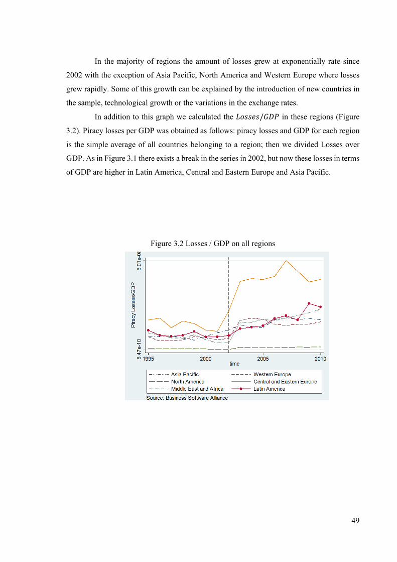
49

In the majority of regions the amount of losses grew at exponentially rate since

2002 with the exception of Asia Pacific, North America and Western Europe where losses

grew rapidly. Some of this growth can be explained by the introduction of new countries in

the sample, technological growth or the variations in the exchange rates.

In addition to this graph we calculated the / in these regions (Figure

3.2). Piracy losses per GDP was obtained as follows: piracy losses and GDP for each region

is the simple average of all countries belonging to a region; then we divided Losses over

GDP. As in Figure 3.1 there exists a break in the series in 2002, but now these losses in terms

of GDP are higher in Latin America, Central and Eastern Europe and Asia Pacific.

Figure 3.2 Losses / GDP on all regions

50

Figure 3.3 Evolution of Software Piracy Rates

Figure 3.3 presents the evolution of the piracy rates. The relationship between the

piracy rates and losses is not linear; losses increased over time while piracy rates fell. This

decrease was not so drastic in 2002 compared to the losses increases. North America and

Western Europe have the lowest piracy rates. These rates have been decreasing more rapidly

until 2002 and, after this period, the rates had a smother pattern. In the case of Middle East

and Africa, and Latin America, software piracy decreased rapidly until 2002, then increased

slowly. Png (2010) found that when surveys are not applied, the software piracy rates are

based on national income; it also found that the yearly rate of decrease of the piracy rates

before 2003 were 2.0 (p.p), while the period after 2003 this rate of decrease fell to 1.1 (p.p)

for the non-survey countries.

51

For a closer look, we also report the software piracy rates on three regions of the

world: BRIC61, United States and European Union from 2003 until 2010 (Figure 3.4). The

piracy rates in European Union and United States have been more or less constant over the

last 8 years. In the BRICs piracy rates have been steadily falling slowly, but still represent

over 70% of the software used.

Figure 3.4 Software Piracy rates on selected regions

The existence of low piracy rates don’t necessarily means lower losses. Figure 3.5

and 3.6 shows the piracy losses on the three regions; piracy losses have been growing at a

more or less constant rate on United States and European Union. The amount of losses almost

tripled in eight years in the BRICs. When losses are analyzed as a proportion of GDP, the

importance of the losses in the BRICs is even higher when compared with the EU and USA.

This can represent the ineffective implementation of copyright laws. Anyway, the losses in

terms of GDP have (in any of the three regions) been more or less constant during the

analyzed period.

61Brazil, Russia, India and China

52

Figure 3.5 Software Piracy Losses on selected regions

Figure 3.6 Losses / GDP on selected regions

53

3.3 Variables and possible effects

This section describes some of the variables used in previous research, introducing

new ones. We group them into five dimensions. Theoretical background exists but at the

individual/firm level. See, for instance, (Bae & Choi, 2006; Lu & Poddar, 2012). In general,

studies focus on the behavior of individuals towards piracy, modeling the benefits to

software firms on improved software protection, awareness and the effects of the

environment (network externalities). These benefits will affect the country economy on

various levels, namely in how access to information is controlled and how better protection

can be implemented.

Literature at the macroeconomic level is still in its infancy. A measure of income

(namely GDP) is used in many studies as a determinant of piracy (see for instance (Andrés,

2006a). Goel and Nelson (2009) provide some macroeconomic determinants using cross-

sectional data. The main purpose of this chapter is to provide an historical view of the

problem using a panel data analysis. We can define piracy as a function of the various

dimensions: Technological, Educational, Access to Information, Institutional Dimension

and Labor force. In the Labor force dimension we introduce new variables in the economic

literature that affect piracy, namely the structure of the labor force and the education of active

population.

Technological dimension

Technological dimensions can affect levels of software piracy. Expenditure on

research and development (R&D) has been found to affect negatively software piracy

(Marron & Steel, 2000). As with Marron and Steel (2000) we introduce this variable that

may also affect piracy losses. In our case this variable indicates investment that is made on

software protection, namely software code. This variable also makes part of the educational

dimension.

Additional to this variable we introduce two variables that capture this dimension.

To our knowledge no empirical work as studies these specific variables. They are the patent

and the trademark applications done by residents and non-residents.

54

Patent applications are worldwide patent applications filed through the Patent

Cooperation Treaty procedure or with a national patent office for exclusive rights for an

invention (this can be a product or a process). The protection of this product can reach up to

20 years. Patents can be filed by domestic or by foreign applicants.

Trademark applications filed are application to register a trademark with a national

or regional Intellectual Property (IP) office. A trademark is a distinctive sign that identifies

certain goods or services as those produced or provided by a specific region, person or

enterprise. A trademark provides protection to the owner of the mark by ensuring the

exclusive right to use it to identify goods or services, or to authorize another to use it in

exchange for a license or royalty. The period of protection varies. Direct resident trademark

applications are those filed by domestic applicants directly at a given national IP office while

those that are filed by applicants from abroad are called “direct nonresident trademark

applications”. The registration of a patent or a trademark has costs for the firm, but these are

necessary in order to protect their products.

All these variables are expected to have a negative effect on piracy losses although

the existence of a patent is not sufficient to prevent piracy; the enforcement trough strict

regulation is also necessary. More technological advanced countries have more legal

protection and, at the same time, firm’s owner of the technology are also more close to the

market and can detect more easily illegal software.

Educational dimension

In all countries there is a pre-determined number of years of schooling that a child

needs to complete, and this number may vary from one country to another. During this

period, children have specific subjects that require the usage of computers and Internet. This

early introduction to new technologies will improve productivity of future workers. In some

subjects, professors introduce the concept of illegal software and the risks associated with

their use. The introduction of other concepts such as copyright can reduce the future use of

illegal software. MacDonald and Fougere (2003) studied this effect analyzing MIS

(Management Information Systems) textbooks. Previous research introduced the effective

schooling years that students have (variables retrieved from the Barro and Lee (2013)

dataset). Marron and Steel (2000) and Andrés (2006b) found that more schooling years

55

reduce piracy. This variable is not available annually, we will introduce a proxy variable that

indicates years of schooling that a country offers. More years of schooling indicate that

children understand and are aware about the consequence of using illegal software. This

variable includes years of schooling of primary education based on the ISCED 199762

(ISCED 1) and secondary education based on the ISCED 1997 (ISCED 2 and 3). This

indicator reveals the total education that a country offers. This variable may or may not have

a negative effect.

Other variables could be used such as literacy rate (see Goel and Nelson (2009))

having a positive impact (increase) on piracy. But in this case, literacy rate omits the different

levels of education; a person can be literate and lack the ability to use computers and

software.

No previous research focused on the financial effects that expenditure on education

could have on piracy. A measure that reflects the expenditure that is made on education will

be introduced. More public expenditure on education as a percentage of GDP can reduce

illegal software that students use; this will also result in more quality of education. This

financial help can go both to public or private institutions. This variable is expected to affect

negatively software piracy losses.

Access to information

Technology has evolved over the years. Today it is difficult or even impossible to

live without it. Hardware and software industry have profited with these developments but,

with the dissemination of the Internet, it was also possible to download huge amounts of

information, some of which not legal, such as pirated software. Authors such as Goel and

Nelson (2009) analyzed the effects that internet and computer users have on piracy, results

showed that more users of these devices reduces piracy. More recently Boyce (2011) found

that broadband penetration rate and Internet access reduces piracy. Most modern mobile

phones uses an operating system, some of which may even replace the computer (in some

specific tasks - the case of smartphones).

62 International Standard Classification of Education

56

We will introduce four variables that measure the availability of information

(telephone, fixed broadband Internet subscriber, Internet and mobile users).

Telephone lines are physical and fixed lines that connect a subscriber's terminal

equipment to the public switched telephone network and that have a port on a telephone

exchange. Integrated services digital network channels and fixed wireless subscribers are

included. Fixed broadband Internet subscribers are the number of broadband subscribers

with a digital subscriber line, cable modem, or other high-speed technology. Internet users

are people with access to the worldwide network. Mobile cellular telephone subscriptions

are subscriptions to a public mobile telephone service using cellular technology, which

provide access to the public switched telephone network. Post-paid and prepaid

subscriptions are included.

All these variables affect the availability of software; more usage of these devises

would lead to an increase in software piracy losses.

Institutional Dimensions

Past literature has found that institutional factors play an important role on piracy (see

(Knack & Keefer, 1995)). Following D. Banerjee, Khalid, and Sturm (2005) and Goel and

Nelson (2009) we introduce four institutional factors that can explain levels of software

piracy, they are business freedom, trade freedom, freedom from corruption and financial

freedom. Better institutions are associated with lower piracy losses.

Business freedom indicates if firms can be established easily with little bureaucracy.

Trade freedom indicates if countries promote trade or not, for example putting high tariff

rates on foreign products such as software or hardware products. Freedom from corruption

can tell us how the legal system work, if officials are corrupt and if illegal activities such as

piracy pass unpunished. Finally financial freedom measures banking efficiency and

independence of government control. A correct functioning of the banking sector will

promote credit to the economy, sometimes indispensable to purchase software in the case of

expensive ones.

57

Labor force dimension

Computer skills are acquired at school or at the workplace; these can range from

browsing the Internet, sending e-mails or working on business applications such as word

processors or spreadsheets. Different jobs require different types of software; some include

imaging suits, others productivity or econometric tools, etc. We will consider three variables

that reflect the structure of the labor force of the population: employment in the primary

sector (Agriculture), employment in the secondary sector (Industry) and employment in the

tertiary sector (Service).

In agriculture when the production is intensive, software helps to improve

efficiency; e.g. controlling various elements of a greenhouse such as the temperature or

humidity. In the industrial sector, the use of specialized software is “normal”, as it comes

with the machine and, in many situations, is developed and used by the firms internally, thus

is not for sale. The software cannot be used outside of the environment that was intended to

work. Big firms develop the software, or commission its development (outsource) to a

specialized company (due to smaller costs). The services sector uses specialized software of

accounting, taxation and productivity. Depending on the different needs, the software can

cost thousands of dollars, but it comes with technical support, extremely valuable in order

to maintain productivity and prevent failures. The costs associated with the acquisition of

these types of software can be deduced during a certain amount of time, reducing taxable

profits.

Employment in these sectors may have impact on software piracy losses. Firms

want to maximize profit; in some cases, due to budgetary restrictions, employers can

introduce some illicit software that will benefit both employers and employees. The

introduction of illicit software has associated risks that are, for instance, the result from

external audits that can impose severe fines. In spite of this, some firms may be willing to

take them. Certain types of jobs, namely in the service sector, can be done from home, as in

market research. In many cases workers wanting to do their jobs at home due to reduced

costs may seek illicit software to implement their research. In this case there is only a residual

risk of internal audits finding illicit software. This may lead an increase of software piracy

losses.

Additional to these variables we introduce the education of the labor force. We will

consider labor force with primary, secondary and tertiary education. The labor force of a

58

country plays an important role on the growth of the economy (Barro, 2013a). If it is

constituted by labor force with low education, this will lead to low productivity and,

consequently, to small economic growth. Also, if the labor force is constituted by highly

qualified people, this will lead to increased productivity which improves the standards of

living. These highly qualified employees will use computers and software. More education

of the labor force characterizes a double-edged sword context: on one side there are more

users of computers and software but, at the same time, some of the consumers will use illicit

software63.

Chen, Chen, and Yeh (2010) found that unemployment has a negative effect

(reduce) on software piracy rates. Their sample was small and reflected a small group of

homogeneous countries where the psychological aspects could be determinant.

Another measure that reflects both an income dimension and social dimension is

the unemployment. We will use the total and youth unemployment that reflects people within

15-24 years without work and the total unemployment rate. Both variables are expected to

have a positive effect on piracy losses. An unemployed person has less disposable income

and spends more time at home. Sometimes it is necessary to use certain software to start

working (in the case of self-employment), but the lack of money can shift consumers from

legal to illegal copies to fill their needs.

General Econometric Model

These five dimensions interfere with each other as, for example, education in a

country will affect the type of jobs of workers, more service-orientated or more for the

industry. In addition, employment levels will be affected by the type of education. More

technologically advanced countries that rely on high R&D promote more effectively the

protection of invents and the level of education of workers. Access to information can be

seen as affecting all dimensions at the same time because more information in the form of

knowledge will affect education levels and its quality, will permit access to innovations

patented or not, and will also affect productivity of workers and access to employment

63 We should note that the education of the labor force represents both a labor force dimension and educational dimension.

59

opportunities advertised on the different Media. Institutional dimension also affect all

dimensions at the same time, free countries have better education, technology, better access

to information and qualified labor force.

Figure 3.7 also show the relation between variables. Piracy is affecting all

dimensions but also being influenced by them. Furthermore, all dimensions are linked

together influencing each other.

Figure 3.7 Relationship between variables

Equation 3.1 shows the general econometric model.

, , , ,

(3.1)

60

3.4 Empirical evidence

Data, econometric specification and summary statistics

Previous econometric studies relied on cross-section or panel data analysis. In the

panel data models periods of study were relatively short. To our knowledge, this work is the

first to introduce a large time span in the analysis. Figure 3.1 shows that software piracy

losses are highly persistent over time and that its value follows closely the GDP (see Figure

3.2); its value is always increasing over time. Soto (2009) examined the properties of System

GMM when the sample is small and the series is persistent, which is applicable to our dataset.

This estimator was found to have lower bias and higher efficiency than the OLS or the fixed-

effects estimator and, furthermore, the gain in efficiency from the two-step estimator is

almost inexistent; both the one and two-step distributions are virtually the same. Based on

these results we will report the one-step System GMM.

Our dataset is constituted by macroeconomic variables retrieved from the World

Development Indicators and the Heritage Foundation64 available for the countries present in

the publications provided by the BSA and comprising 81 countries from 1994 until 2010.

Variables were chosen based on their relevance and suitability and in their availability

through all the period in the analysis. Due to the persistence of the piracy losses, we will use

a dynamic panel data analysis, namely the Arellano and Bover (1995) and Blundell and Bond

(1998) estimator. This estimator was developed because the lagged-level instruments of the

original Arellano and Bond (1991) estimator become weak when the autoregressive process

becomes too persistent or when the ratio of the variance of the panel-level effects and the

variance of the idiosyncratic error becomes too large. The System GMM uses both level and

first-difference of the lagged dependent variable as instruments.

The dependent variable is the piracy losses due to pirated software, and it’s

measured in millions of dollars. The independent variables measure various dimensions of a

country: Technological dimensions, Educational dimension, Access to Information,

Institutional Dimension and Labor Force dimension. In our analysis we will use the nominal

GDP (GDP)65 as a control variable.

64 www.heritage.org 65 GDP is measured in current US dollars - this variable will be considered as endogenous and used to control the market dimension.

61

The estimator used poses some problems, namely in the case of too many

instruments. When the instrument count is high they may fail to expunge their endogenous

components and biasing coefficient estimates toward those from non-instrumenting

estimators as discussed by Roodman (2009b). With the limitation of lags we overcome this

problem, e.g. the number of instruments higher than the number of countries. In the end of

each regression we report the number of instruments used and also, through our analysis, the

number of instruments will be smaller than the number of countries following Roodman

(2009a).

The econometric specification is given in equation 3.2 as follows:

,

(3.2)

i =1,…,81 represents the countries and t =1994,…,2010 the time periods

The variable Losses is the piracy losses measured in millions of dollars and GDP is

the Gross Domestic Product at current prices. Additional to this we could also consider

as a dependent variable that represents the relative importance of the piracy losses

in relation to GDP66.

is a vector of labor force. It reflects the labor force dimension and it’s constituted

by the labor force, type of employment and unemployment.

(3.3)

were Labp is the labor force with primary education, Labs is the labor force with

secondary education, Labt is the labor force with tertiary education, Empagri is the

66 To assess the validity of both assumptions we performed regressions. In both cases the variables maintain the same coefficient, being the only difference the magnitude of these. We opted by the absolute value of Losses as it provided best estimates, maintaining significance.

62

employment in agriculture, Empind is the employment in industry, Empserv is the

employment in the services sector. Unempyouth is the unemployment of people from 15 to

24 years old, we also introduce Unemp that is the total unemployment.

is a vector that represents the technological dimension and it’s constituted by

patents, trademarks and the research and development.

& (3.4)

R&D represents the research and development expenditure as a percentage of GDP,

Patres are the patent applications done by residents, Patnon are the patent applications done

by nonresidents. Tradres is the trademark applications done directly by residents and the

Tradnon is the trademark applications done directly by nonresident. Both patents and

trademarks are in logarithms.

is a vector of the education dimensions. It combines years of schooling and

public expenditure in the different levels of education (primary, secondary and tertiary) as a

percentage of GDP.

(3.5)

is the duration in years of primary education, Yschoolsec is the

duration in years of secondary education. Exppri, Expsec and Expter is expenditure on

primary, secondary and tertiary education as a share of GDP. Pubexp represents public

expenditure on education as a percentage of GDP.

63

The vector represents the various variables that represent access to information.

(3.6)

Fbis is fixed broadband Internet subscribers, Mobile is mobile cellular

subscriptions, is the phone lines and Net is the access to the Internet. These variables

are measured per 100 people. We introduce logarithms in this dimension.

Vector represents the institutional dimension.

(3.7)

Variables are business freedom (BusFreed), trade freedom (TradFreed), freedom

from corruption (CorrFreed) and financial freedom (FinFreed)

Additional to these variables, a dummy variable (Change) will be introduced that

reflects the change in methodology provided by the BSA. Before 2003 it will have a value

of 0 and of 1 afterwards. We will also introduce a set of time dummies.

Table 3.1 presents the descriptive statistics of the various dimensions. In 2010 data

for software piracy losses was available for 81 countries. Every year the BSA improves its

estimates performing more surveys; initially surveys were made on 15 countries67 (BSA,

2003); in 2010, surveys were made on 3268 countries (BSA, 2010b), a total of 15000

computer users were inquired. Since 1994 a total of 1217 observations are available.

67 Bolivia; Brazil; Chile; China; Colombia; Costa Rica; Dominican Republic; Guatemala; Kuwait; Malaysia; Mexico; Romania; Spain; Taiwan and the United States. 68 Emerging markets include: Argentina; Brazil; China; Chile; Colombia; Czech Republic; India; Indonesia; Korea, Republic of; Malaysia; Mexico; Nigeria; Poland; Russian Federation; Saudi Arabia; South Africa; Thailand; Turkey; Ukraine; Vietnam. Mature markets include: Australia; Canada; France; Germany; Italy; Japan; Netherlands; Spain; Sweden; Switzerland; United Kingdom; United States.

64

Table 3.1 Summary statistics

Variables Obs. Mean Std. Dev. Min Max Losses 1217 353.80 929.37 0.902 9515 Losses/GDP 1217 0.00082 0.00088 0.000088 0.016 GDP 1373 478804.7 1400089 1170.785 1.44e+07

Labor Force dimension Empagri 1176 15.81 15.90 .2 72.2 Empind 1177 24.78 6.24 6.5 43.1 Empserv 1177 58.79 14.42 13.3 87.4 Labp 781 29.92 17.68 0 89 Labs 775 43.13 16.89 2.9 80.2 Labt 781 23.94 10.68 0 66.1 Unempyouth 1006 17.43 9.33 2.2 629 Unemp 1200 8.49 5.04 0.9 36.4

Technological dimension Patres 1186 12211.37 49331.09 2 384201 Patnon 1196 6987.64 21961.23 1 248249 Tradres 1174 23936.59 64011.48 1 973460 Tradnon 1177 6356.59 7613.16 33 67838 R&D 862 1.12 .98 .02 4.8

Educational dimension Pubexp 726 4.81 1.42 2.20e-06 9.51 Yschoolpri 1375 5.43 .99 3 8 Yschoolsec 1130 6.54 1.01 4 9

Access to Information dimension Net 1341 23.41 25.73 0.00 95.63 Fbis 928 7.11 9.77 0.00 38.10 Phone 1366 29.39 19.51 0.61 74.69 Mobile 1367 48.56 45.15 0.00 195.57

Institutional dimension BusFreed 1256 50.59 24.53 10 100 TradFreed 1256 70.62 13.37 36.3 100 CorrFreed 1256 72.08 13.23 0 95 FinFreed 1256 59.19 18.02 10 90

Notes: Std. Dev. represents the standard deviation; Min the minimum and Max the maximum.

65

Empirical application

This section presents the empirical results for the various dimensions. Some of our

variables in education don’t vary over time and, consequently, the fixed effect was not the

best choice as it omits invariant regressors. Based on the Hausman test, Andrés (2006a),

Chen et al. (2010) and Boyce (2011) found that the fixed effect was more appropriated in

panel data analysis. Traditional methods such as fixed effects or random effects produce

inconsistent estimates when the lagged dependent variable enters as a regressor. Due to the

nature of our dataset (extremely unbalanced when considering certain dimensions), we will

split our analysis into 15 regressions in the dynamic model. In all of them there will be

control variables for each dimension. Our results will be conducted using the one-step

System GMM69.

For the System GMM to be applicable there must be no evidence of second order

autocorrelation AR(2). Additional to this, instrument must be valid. To test this we report

the Hansen test for validity of instruments (Hansen, 1982). This test assumes, under the null

hypothesis, that instruments are valid and it’s a robust version of the Sargan test70; one

problem that may occur is that it can be weakened by a proliferation of instruments. We also

report the number of instruments following Roodman (2009a).

Table 3.2, Table 3.3 and Table 3.4 presents the regressions within each dimension.

All of the regressions include control variables for the remaining dimensions. The control

variable in the educational dimension is the result of the sum of primary and secondary

schooling years, “School”. In the Technological dimension, variables were constructed

providing the best estimates; the sum of patents from residents and nonresidents,

“ln(Patents)”; the sum of trademark from residents and nonresidents, “ln(Trademark)”.

When necessary, we also summed the total patents and trademarks, “ln(Legal)”; this variable

give us a general idea of the overall demand for this kind of protection.

Columns 1 through 5 summarize the results from the labor force. From these results

we conclude that the higher the share of people working in the services sector the lower will

be the piracy losses. This can be seen in columns 1, 2 and 4 where the base sector (omitted

69 The two-step System GMM is presented in Annex because the gains from the one-step to the two-step System GMM are marginal Soto (2009). In the two-step System GMM we take into account the corrected covariance matrix proposed by Windmeijer (2005). 70 This test is also reported. It´s not affected by the proliferation of instruments, but it’s not robust.

66

variable)71 was the share of people working in the agriculture sector or in the industrial

sector. In either case the share of people working in the services sector has a negative

significant impact in the piracy losses. If we use the services sector as the base sector

(column 3 or 5) the industrial and agricultural sectors have positive and significant impact

(although the significance of the agricultural sector is not robust across specifications)

pointing to the same conclusion: the higher the share in these sectors (and lower in the service

sector) the higher will be the losses due to software piracy. This result was unexpected.

As for the labor qualifications referred above, we have to omit one of the education

variables and use it as the base case. In this case the higher the share of workers with tertiary

education the higher will be the losses due to piracy. Furthermore, the results indicate that

is the division between the share of the workers with the tertiary education and the others

that matters. This can be seen in columns 1 and 2 when we consider the share with primary

education; the estimated coefficient of the share with secondary education is close to zero

and non-significant. The same result is obtained in column 4 when we use the secondary

education share as the base and analyze the estimate of the share with primary of education.

This result is in line with what we expected.

Another important variable present in the labor force is the youth unemployment.

This variable combined with the level of education of the labor force and access to

technology will determine the use of software at home. This variable has always a positive

impact, but it was significant only in regressions 1 through 5 in which labor force and type

of employment were present. There are other types of unemployment. Some examples are

the long-run unemployment and total unemployment. The first variable was not suited as the

reduced number of observations made difficult to estimate with this methodology. As an

additional robustness check we included total unemployment; significance was not present,

nevertheless it maintains the positive coefficient.

71 We should note that the sum of the three sectors adds up to 1, so we cannot have the three variables simultaneously in the regression due to multicolinarity. In this case we consider one sector as the base one (and omit it from the regression) and the coefficients of the others sectors are the differential impacts between each sector and the base sector.

67

Table 3.2 Dynamic model using one-step System GMM

Variables 1 2 3 4 5 L.ln(losses) 0.572*** 0.513*** 0.586*** 0.579*** 0.460*** (6.930) (5.121) (6.310) (7.081) (4.072) ln(GDP) 0.282** 0.308*** 0.326*** 0.274** 0.404** (2.524) (3.009) (3.397) (2.563) (2.312) ln(Mobile) -0.005 -0.025 (-0.124) (-0.627) ln(Mobile)*Change 0.348** (2.168) ln(Phone) 0.148 0.054 (0.701) (0.347) ln(Phone)*Change 0.018 -0.102 (0.098) (-0.600) ln(Fbis) 0.026 (0.731) ln(Fbis)*Change 0.066 (1.014) Empagric 0.016* -0.021 0.019** (1.720) (-1.473) (2.368) Empind 0.021* 0.016 0.026** 0.028** (1.727) (1.410) (2.344) (2.523) Empserv -0.012** -0.013** -0.033*** (-2.159) (-1.972) (-3.029) Labp -0.014* 0.004 -0.015* (-1.734) (0.685) (-1.729) Labs -0.004 -0.004 -0.014* -0.013* (-0.756) (-0.604) (-1.753) (-1.839) Labt 0.016** 0.009 0.021** (2.009) (0.821) (2.328) Unempyouth 0.013** 0.014** 0.012** 0.013** 0.010** (2.279) (2.522) (2.158) (2.241) (2.182) ln(Patents) -0.006 0.001 -0.022 -0.007 -0.001 (-0.199) (0.022) (-0.535) (-0.200) (-0.049) ln(Trademarks) 0.071 0.090** 0.048 0.069 0.054 (1.481) (2.042) (0.718) (1.195) (0.797) School 0.021 0.048 -0.153 -0.011 -0.034 (0.220) (0.464) (-1.161) (-0.119) (-0.248) TradFreed 0.009 0.009 0.001 (1.410) (1.222) (0.070) BusFreed 0.002 0.008 (0.643) (1.587) Change 0.413*** -1.000* 0.351 0.749 0.359** (4.124) (-1.657) (0.497) (1.161) (2.349) Constant -7.755*** -8.072*** -6.466*** -5.597** -8.861*** (-2.993) (-3.034) (-2.695) (-2.243) (-2.880) Observations 501 501 501 507 415 Countries 61 61 61 61 59 AR1 -4.596 -4.334 -4.489 -4.591 -3.587 p-value [0.000] [0.000] [0.000] [0.000] [0.000] AR2 -0.0340 0.417 -0.441 -0.339 0.300 p-value [0.973] [0.677] [0.659] [0.735] [0.764] Instruments 53 53 53 53 51 Sargan 80.39 78.18 78.64 73.51 79.39 p-value [0.000] [0.000] [0.000] [0.000] [0.000] Hansen 42.47 37.52 40.84 37.26 42.20 p-value [0.180] [0.311] [0.195] [0.321] [0.107]

Notes: Dependent variable is ln(losses). Robust t-statistics in parentheses; *, ** and *** represent statistical significance at 10%, 5% and 1% respectively. L.ln(losses) and L.ln(GDP) were considered as two endogenous instruments. Only one lag was used as instrument.

68

Columns 6 through 10 show the different variables in the Technological dimension.

Patents and trademarks offer protection for those who innovate; this protection can be done

by residents or by non-residents that will protect their product. In columns 9 and 10

ln(Patents) has a significant positive impact on the losses, as ln(Trademarks) is non-

significant. When a disaggregated analysis is made on the origin of patents and trademarks

applicants (columns 6 to 8) the trademarks continue to not have a significant impact in losses.

In terms of the number of patents is the number of patents done by residents that have a

significant impact on losses. A final variable that was found to have a strong effect in

deterring software piracy losses was R&D, which has always a negative coefficient. This can

indicates that investment is being implemented correctly, namely in writing software code

that protects software from hackers.

The positive coefficient of patents and the negative coefficient of R&D at first may

appear odd, but it can be explained as follows: a company makes a breakthrough after many

years of research, what will allow increased productivity, efficiency and protection for

different components of the company products. This can also be extended to other products

from other companies. In order to protect this discovery, the company will file a patent of

the discovery that will allow some level of protection from other companies and from

potential pirates. The existence of the patent by itself it’s not synonym of protection; national

Intellectual Property offices must also be able to enforce and protect them. The positive

coefficient can be explained by the existence of patents that are the result of research, but

the lack of power exerted by national IP offices will not prevent piracy in spite of the

existence of patents.

All regressions control for institutional dimensions. Tests were performed using

variables that represent institutional factors, the reported ones provide the best estimates.

Only Freedom from Corruption Index (CorrFreed) (column 8) presented significance. This

index ranges from 0, high corruption, to 100, no corruption. Results show that low levels of

corruption leads to less piracy losses. Goel and Nelson (2009) and Andrés and Goel (2011)

also found that in more corrupt nations, software piracy was higher.

69

Table 3.3 Dynamic model using one-step System GMM (cont.)

Variables 6 7 8 9 10 L.ln(losses) 0.514*** 0.610*** 0.552*** 0.544*** 0.541*** (5.457) (6.410) (5.570) (5.028) (4.909) ln(GDP) 0.347*** 0.294** 0.448*** 0.387*** 0.387*** (3.033) (2.143) (2.706) (2.843) (2.788) ln(Mobile) -0.013 0.075 0.076 0.169** 0.148 (-0.145) (0.679) (0.674) (2.166) (1.642) ln(Mobile)*Change 0.267* 0.009 -0.025 0.097 (1.802) (0.054) (-0.156) (0.621) ln(Fbis) 0.002 -0.016 -0.004 0.003 0.005 (0.044) (-0.617) (-0.177) (0.101) (0.174) Unemp 0.000 -0.019 -0.013 (0.011) (-1.245) (-0.854) Unempyouth 0.011 0.011 (1.268) (1.316) School 0.079 -0.062 0.032 0.058 0.067 (0.985) (-0.614) (0.334) (0.553) (0.636) R&D -0.307*** -0.134* -0.021 -0.260** -0.265** (-3.188) (-1.901) (-0.290) (-2.396) (-2.500) ln(Patres) 0.131** (2.571) ln(Patnon) 0.017 (0.491) ln(Tradres) 0.123 -0.052 (1.505) (-0.433) ln(Tradnon) -0.082 0.006 (-1.429) (0.098) ln(Patents) 0.056** 0.058** (2.009) (2.163) ln(Trademarks) -0.036 -0.037 (-0.665) (-0.668) CorrFreed -0.008** (-2.000) TradFreed -0.004 0.001 -0.001 (-0.586) (0.127) (-0.141) Change -0.664 0.311 0.459 0.345*** -0.062 (-1.134) (0.498) (0.719) (2.855) (-0.099) Constant -8.148*** -5.597** -9.336*** -9.481*** -9.339*** (-3.327) (-2.561) (-3.267) (-3.377) (-3.313) Observations 478 473 472 411 411 Countries 75 75 75 66 66 AR1 -3.035 -3.277 -3.345 -3.606 -3.583 p-value [0.002] [0.001] [0.001] [0.000] [0.000] AR2 0.499 0.195 0.309 -0.200 -0.142 p-value [0.618] [0.846] [0.757] [0.842] [0.887] Instruments 51 51 51 51 51 Sargan 62.12 70.54 67.59 58.87 58.80 p-value [0.002] [0.000] [0.001] [0.007] [0.005] Hansen 35.78 44.43 42.84 33.86 33.36 p-value [0.385] [0.132] [0.142] [0.523] [0.499]


70

Regarding education we included financial and non-financial measures. The first

perspective was never considered in previous studies and, in the second case, variables used

on previous research were literacy rate and the average years of schooling of people age 25

and over (Barro & Lee, 2013). Both of these variables have the problem of data availability.

To overcome this problem we will introduce a proxy variable that indicates the years of

schooling of both primary and secondary education offered by the educational system of a

country. This variable is not perfect as it omits the education attained, but it offers us a

benchmark. Additional to this, we will introduce a variable that indicates spending on

education. Columns 11 through 15 show the results.

Columns 11 through 13 present the years of schooling. As in the labor force

dimension, we include the education of the labor force; results are robust. An increase of

years of primary and secondary education appears to have a negative impact on piracy losses,

but only in the first case this variable is significant across all regressions with a coefficient

of around -0.250.

The financial aspects of education are presented in columns 14 and 15. Public

spending on education can go both to public or private institutions and depending on the

different levels of education different resources are allocated. Public expenditure on

education has a positive effect and is significant at 1% (column 15). This public spending

can also go directly to students through direct help in the form of scholarships. There are

many ways a student can use this help. Some examples are: acquisition of computer,

software, access to the Internet, etc. This will increase the availability to digital content such

as music, software and movies. We were expecting a negative impact; nevertheless this may

indicate that more access to digital content can also increase the availability of illegal

software. Only with increase awareness this problem can be mitigated.

Several alternative hypotheses were considered with different variables within the

dimension that reflect the access to information. The access to Internet – ln(Net) – has a

negative and significant effect on losses (columns 14 and 15), while the access to a

broadband connection has no impact on losses (columns 5 through 10). This is clearly

unexpected, but seems that access to Internet reduces the losses because of increased

awareness of the problem by the consumers, because countries with a higher share of people

connected to the Internet are able to track those who use illicit software, or simply because

71

you can download and buy the software directly from the original company and not from

local intermediaries - many of them may be selling pirated software. These results are in

accordance with the findings of Boyce (2011).

To assess the validity of our findings we also performed regressions in which the

dependent variable was a fraction of GDP, ln(Losses/GDP) (see Annex III). In these

regressions only the dimension related to the labor force was statistically significant being

robust across all regressions. In the technological dimension, patents applicants from

residents maintained significance. Variable that represents access to information, namely

Internet users, and mobile subscriptions, maintained statistical significance.

72

Table 3.4 Dynamic model using one-step System GMM (cont.)

Variables 11 12 13 14 15 L.ln(losses) 0.555*** 0.551*** 0.541*** 0.577*** 0.617*** (6.908) (7.951) (7.338) (6.213) (6.180) ln(GDP) 0.450*** 0.360*** 0.382*** 0.387*** 0.297*** (5.051) (4.260) (4.743) (3.816) (2.914) ln(Mobile) -0.019 -0.022 -0.012 0.029 (-0.548) (-0.689) (-0.349) (0.427) ln(Mobile)*Change 0.356*** (2.690) ln(Net) -0.100* -0.158* (-1.886) (-1.806) R&D -0.143* -0.181** (-1.785) (-2.123) Yschoolpri -0.242* -0.236*** -0.259*** (-1.830) (-3.343) (-3.522) Yschoolsec -0.037 -0.112 -0.026 (-0.272) (-1.267) (-0.245) Pubexp 0.150** 0.180*** (2.382) (2.771) Labp -0.016** 0.002 (-2.473) (0.438) Labs -0.021*** -0.010* (-2.576) (-1.847) Labt 0.011* 0.014*** (1.890) (2.580) Unemp 0.001 -0.010 -0.005 -0.010 0.003 (0.054) (-1.014) (-0.484) (-0.682) (0.153) ln(Legal) -0.035* -0.005 -0.010 0.010 0.042 (-1.788) (-0.207) (-0.363) (0.543) (1.657) CorrFreed -0.002 -0.004 (-0.655) (-0.922) TradFreed 0.001 0.002 (0.190) (0.381) FinFreed -0.002 (-0.468) Change 0.379*** 0.426*** 0.411*** 0.478*** -1.008* (4.357) (5.414) (4.636) (4.650) (-1.917) Constant -6.049*** -5.552*** -6.225*** -8.355*** -6.948*** (-2.988) (-3.414) (-3.764) (-3.992) (-3.381) Observations 515 521 515 441 441 Countries 64 64 64 66 66 AR1 -4.290 -4.281 -4.145 -3.740 -3.824 p-value [0.000] [0.000] [0.000] [0.000] [0.000] AR2 -0.387 -0.469 -0.275 -0.552 0.126 p-value [0.699] [0.639] [0.783] [0.581] [0.900] Instruments 55 55 55 47 47 Sargan 73.64 93.63 80.82 73.21 51.85 p-value [0.001] [0.000] [0.000] [0.000] [0.011] Hansen 41.64 46.05 44.08 43.78 35.21 p-value [0.357] [0.203] [0.265] [0.099] [0.276]


73

3.5 Conclusion

This chapter examined the impact of several dimensions that might explain the

phenomenon of software piracy losses. Due to the nature of our dataset and the availability

of information we opted to use a dynamic panel data analysis that could track the growth of

piracy losses over time. We found that several dimensions could explain this growth; Labor

Force, Technological, Educational, Access to Information and Institutional.

The labor force was one of the dimensions considered. Higher levels of education

resulted in more losses, but a higher share of employment in the service sector has a negative

impact on losses. This is a result of more access to information by employees with higher

education and the capability to track illicit content through internal audits in the service

sector.

In the technological dimensions, patents and trademarks were analyzed as one of

the explanations of software piracy. Patents were significant and positive; they grant a

protection for those who innovate but other factors must be considered (that could explain

the positive sign) such as the effectiveness of this protection and the punishment for those

who infringe the law. Our findings suggest that more protection in the form of trademarks

or patents can in some cases reduce losses. Another variable introduced was R&D, which

was found to have a negative effect on software piracy losses.

The results from the education dimensions show that more years of schooling have

a deterrent effect on piracy. When our analysis turns to financial aspects of education, more

spending means more piracy losses.

More Access to information has mixed results on piracy losses. This can be

explained by the nature of the different devices used to access digital content, for example

through the Internet.

The correct functioning of institutions can reduce piracy. Our results show that less

corruption is associated with lower piracy losses.

BSA provide some blueprints in order to reduce piracy, namely to “modernize IP Laws

to account for new innovations”, these innovations that are patented both at home and

abroad, have different results. Better attention should be given on the origin of patents and

trademarks, providing better protection. In 2012, the ninth edition of the BSA (2012) global

piracy study presented some “blueprints” to reduce, or at least mitigate piracy. One of these

74

solutions is the increase of public education and awareness. Results show that more

education reduces piracy although special attention must be made on educational

expenditure. Better attention must be done on the different sectors of activity that are the

building blocks of the economy of a country.

Although this chapter had provided new insights on the major macroeconomic

determinants of losses caused by piracy, lack of data on some dimensions reduced the

number of observations and weakened the possible conclusions. Further analysis using panel

data and introducing large time span should be followed. Using small group of countries

such as the European Union, or an in deep analysis of the various dimensions, could provide

valuable tools for policymakers as changes in education can only be viewed in the long-run.

Further research introducing additional variables such as taxation must be followed.

75

Methodology used by the BSA

To determine the software piracy rates and losses the Business Software Alliance

has at his disposal huge amounts of information, being able to conduct extensive surveys in

the population. In the estimates of 2010, presented in the eighth annual BSA study, the BSA

relied on Ipsos Public Affairs that conducted more than 15000 surveys on business and

consumer PC users. A brief description of the methodology is presented in the report and

reproduced here.

The methodology was the following to obtain piracy rates:

(II.3.1)

To obtain the total software units installed it was used the following:

#

(II.3.2)

The legitimate software units and the unlicensed software units are given by the

following expressions:

(II.3.3)

(II.3.4)

Finally the commercial value of unlicensed software is given by:

#

(II.3.5)

Business Software Alliance uses confidential information to achieve these results; it does

provide us, in their annually reports, the basic methodology, omitting many variables that

are used.

76

Additional regressions

Table 3.5 Two-step System GMM

Variables 16 17 18 19 20 L.ln(losses) 0.598*** 0.475*** 0.538*** 0.583*** 0.442*** (7.044) (3.965) (4.599) (6.395) (2.972) ln(GDP) 0.294** 0.333*** 0.386*** 0.301** 0.412** (2.417) (3.323) (2.814) (2.362) (2.221) ln(Mobile) -0.008 -0.047 (-0.223) (-1.345) ln(Mobile)*Change 0.410** (2.095) ln(Phone) 0.017 -0.104 (0.080) (-0.795) ln(Phone)*Change -0.080 -0.094 (-0.340) (-0.579) ln(Fbis) 0.040 (0.833) ln(Fbis)*Change 0.091 (1.277) Empagric 0.009 -0.030* 0.020* (0.825) (-1.652) (1.651) Empind 0.022 0.012 0.021 0.019 (1.583) (0.930) (1.196) (1.420) Empserv -0.015* -0.012 -0.040*** (-1.806) (-1.552) (-2.815) Labp -0.010 0.005 -0.006 (-0.939) (0.654) (-0.565) Labs -0.004 -0.003 -0.012 -0.007 (-0.608) (-0.487) (-1.244) (-0.885) Labt 0.021* 0.007 0.024*** (1.852) (0.498) (2.921) Unempyouth 0.013*** 0.013*** 0.009 0.012** 0.008* (2.634) (3.164) (1.630) (2.460) (1.806) ln(Patents) -0.012 -0.005 -0.009 -0.003 -0.001 (-0.305) (-0.150) (-0.212) (-0.079) (-0.026) ln(Trademarks) 0.071 0.115** 0.018 0.060 0.050 (1.284) (2.257) (0.250) (0.875) (0.681) School 0.052 0.093 -0.189 0.048 -0.107 (0.389) (1.111) (-0.986) (0.386) (-0.741) TradFreed 0.007 0.007 -0.003 (0.921) (1.006) (-0.242) BusFreed 0.000 0.005 (0.088) (0.827) Change 0.370*** -1.209* 0.732 0.676 0.322* (3.091) (-1.709) (0.852) (1.120) (1.896) Constant -8.225*** -9.212*** -6.338* -5.908** -8.046*** (-2.864) (-4.066) (-1.934) (-2.338) (-2.803) Observations 501 501 501 507 415 Countries 61 61 61 61 59 AR1 -3.464 -3.115 -3.391 -3.325 -2.389 p-value [0.001] [0.002] [0.001] [0.001] [0.017] AR2 -0.0700 0.472 -0.717 -0.468 0.0549 p-value [0.944] [0.637] [0.474] [0.640] [0.956] Instruments 53 53 53 53 51 Sargan 80.39 78.18 78.64 73.51 79.39 p-value [0.000] [0.000] [0.000] [0.000] [0.000] Hansen 42.47 37.52 40.84 37.26 42.20 p-value [0.180] [0.311] [0.195] [0.321] [0.107]

Notes: Dependent variable is ln(losses). Robust t-statistics in parentheses; *, ** and *** represent statistical significance at 10%, 5% and 1% respectively. L.ln(losses) and L.ln(GDP) were considered as two endogenous instruments. Only one lag was used as instrument

77

Table 3.6 Two-step System GMM (cont.)

Variables 21 22 23 24 25 L.ln(losses) 0.502*** 0.603*** 0.575*** 0.564*** 0.560*** (4.620) (5.889) (5.418) (4.021) (4.117) ln(GDP) 0.365** 0.273* 0.396** 0.385** 0.395** (2.527) (1.761) (2.529) (2.045) (2.197) ln(Mobile) -0.042 0.047 0.102 0.082 0.043 (-0.441) (0.345) (0.825) (0.802) (0.403) ln(Mobile)*Change 0.277* 0.032 -0.022 0.098 (1.899) (0.170) (-0.153) (0.570) ln(Fbis) 0.008 -0.027 -0.007 0.008 0.012 (0.181) (-0.798) (-0.187) (0.185) (0.284) Unemp -0.003 -0.020 -0.004 (-0.121) (-1.162) (-0.203) Unempyouth 0.012 0.012 (0.968) (0.934) School 0.146 -0.049 0.053 0.113 0.120 (1.475) (-0.415) (0.433) (0.540) (0.566) R&D -0.353** -0.091 0.050 -0.320* -0.328* (-2.561) (-0.881) (0.406) (-1.893) (-1.920) ln(Patres) 0.148*** (2.741) ln(Patnon) 0.011 (0.273) ln(Tradres) 0.150 -0.045 (1.346) (-0.345) ln(Tradnon) -0.108 0.035 (-1.558) (0.465) ln(Patents) 0.057* 0.060* (1.830) (1.808) ln(Trademarks) -0.032 -0.035 (-0.417) (-0.464) CorrFreed -0.009* (-1.667) TradFreed -0.006 0.004 0.001 (-0.648) (0.360) (0.116) Change -0.680 0.251 0.446 0.359** -0.046 (-1.087) (0.344) (0.827) (2.480) (-0.064) Constant -9.117*** -5.173* -8.861*** -10.085*** -10.052*** (-2.611) (-1.764) (-2.636) (-3.525) (-3.739) Observations 478 473 472 411 411 Countries 75 75 75 66 66 AR1 -2.790 -2.704 -2.900 -2.385 -2.375 p-value [0.005] [0.007] [0.004] [0.017] [0.018] AR2 0.378 0.0593 0.212 -0.153 -0.0864 p-value [0.705] [0.953] [0.832] [0.878] [0.931] Instruments 51 51 51 51 51 Sargan 62.12 70.54 67.59 58.87 58.80 p-value [0.002] [0.000] [0.001] [0.007] [0.005] Hansen 35.78 44.43 42.84 33.86 33.36 p-value [0.385] [0.132] [0.142] [0.523] [0.499]


78

Table 3.7 Two-step System GMM (cont.)

Variables 26 27 28 29 30 L.ln(losses) 0.565*** 0.578*** 0.575*** 0.580*** 0.535*** (5.289) (5.904) (5.429) (4.903) (3.997) ln(GDP) 0.422*** 0.291*** 0.339*** 0.384** 0.350** (3.410) (2.904) (2.825) (2.537) (2.275) ln(Mobile) -0.001 -0.022 -0.007 -0.040 (-0.026) (-0.589) (-0.159) (-0.574) ln(Mobile)*Change 0.415** (2.515) ln(Net) -0.088 -0.064 (-1.656) (-0.728) R&D -0.175* -0.226** (-1.842) (-2.466) Yschoolpri -0.305** -0.239*** -0.245*** (-2.004) (-2.773) (-3.273) Yschoolsec -0.040 -0.090 0.013 (-0.254) (-0.754) (0.089) Pubexp 0.144* 0.198** (1.799) (2.520) Labp -0.015** 0.004 (-2.417) (0.520) Labs -0.024*** -0.012 (-2.687) (-1.628) Labt 0.012 0.013** (1.254) (2.036) Unemp 0.001 -0.010 -0.004 -0.013 0.007 (0.072) (-0.864) (-0.374) (-0.739) (0.383) ln(Legal) -0.025 0.019 -0.002 0.006 0.051 (-1.108) (0.544) (-0.034) (0.267) (1.390) CorrFreed -0.000 -0.002 (-0.103) (-0.405) TradFreed 0.005 0.003 (0.645) (0.319) FinFreed -0.004 (-0.486) Change 0.377*** 0.429*** 0.395*** 0.450*** -1.225* (3.713) (4.524) (3.386) (4.562) (-1.833) Constant -5.255** -4.801** -5.646** -8.248*** -8.122*** (-2.155) (-2.588) (-2.457) (-2.745) (-2.759) Observations 515 521 515 441 441 Countries 64 64 64 66 66 AR1 -3.510 -3.497 -3.388 -2.891 -2.374 p-value [0.000] [0.000] [0.001] [0.004] [0.018] AR2 -0.370 -0.273 -0.189 -0.749 -0.418 p-value [0.712] [0.785] [0.850] [0.454] [0.676] Instruments 55 55 55 47 47 Sargan 73.64 93.63 80.82 73.21 51.85 p-value [0.001] [0.000] [0.000] [0.000] [0.011] Hansen 41.64 46.05 44.08 43.78 35.21 p-value [0.357] [0.203] [0.265] [0.099] [0.276]


79

Table 3.8 One-Step System GMM for Losses per GDP

Variables 31 32 33 34 35 L.ln(Losses/GDP) 0.657*** 0.627*** 0.605*** 0.670*** 0.594*** (5.925) (5.571) (6.148) (7.723) (3.753) ln(Mobile) -0.013 -0.027 (-0.306) (-0.635) ln(Mobile)*Change 0.167 (1.378) ln(Phone) -0.131 -0.174 (-0.308) (-0.507) ln(Phone)*Change 0.070 0.040 (0.300) (0.179) ln(Fbis) -0.010 (-0.203) ln(Fbis)*Change 0.018 (0.278) Empagric 0.013 -0.003 0.012 (0.932) (-0.140) (0.984) Empind -0.005 -0.013 0.021 0.026 (-0.233) (-0.531) (1.161) (1.361) Empserv -0.014** -0.017** -0.013 (-2.236) (-2.436) (-0.813) Labp -0.011 0.006 -0.019** (-1.065) (0.879) (-2.304) Labs -0.006 -0.004 -0.016* -0.023*** (-1.021) (-0.552) (-1.760) (-2.686) Labt 0.010 0.008 0.020** (1.213) (0.902) (2.169) Unempyouth 0.027*** 0.026*** 0.028*** 0.023*** 0.027*** (2.883) (2.680) (3.619) (3.003) (3.409) School -0.075 -0.111 -0.057 0.071 0.218 (-0.370) (-0.527) (-0.267) (0.413) (0.949) ln(Patents) 0.033 0.027 0.047 0.018 0.014 (0.909) (0.707) (0.880) (0.367) (0.337) ln(Trademarks) -0.044 -0.025 -0.061 -0.026 -0.016 (-0.832) (-0.502) (-0.760) (-0.310) (-0.181) TradFreed 0.001 -0.003 0.010 (0.220) (-0.451) (0.957) BusFreed 0.003 0.011* (0.439) (1.793) Change 0.305*** -0.406 0.060 0.082 0.282 (2.887) (-0.808) (0.068) (0.100) (1.461) Constant -0.935 -0.704 -2.506 -2.593 -6.274 (-0.326) (-0.238) (-1.043) (-0.971) (-1.638) Observations 501 501 501 507 415 Countries 61 61 61 61 59 AR1 -4.032 -4.118 -4.079 -3.975 -3.205 p-value [0.000] [0.000] [0.000] [0.000] [0.001] AR2 -0.479 -0.246 -0.570 -0.484 0.520 p-value [0.632] [0.806] [0.569] [0.628] [0.603] Instruments 51 51 51 51 50 Sargan 75.79 74.86 63.56 73.20 61.96 p-value [0.000] [0.000] [0.001] [0.000] [0.001] Hansen 35.39 35.21 35.49 36.49 35.64 p-value [0.402] [0.364] [0.352] [0.310] [0.301]

Notes: Dependent variable is ln(losses/GDP). Robust t-statistics in parentheses; *, ** and *** represent statistical significance at 10%, 5% and 1% respectively. L.ln(Losses/GDP) was considered as an endogenous instruments. Lags 1 through 3 were used (columns 31 to 34).

80

Table 3.9 One-Step System GMM for Losses per GDP (cont.)

Variables 36 37 38 39 40 L.ln(Losses/GDP) 0.649*** 0.687*** 0.616*** 0.611*** 0.611*** (7.595) (9.005) (9.024) (5.304) (5.237) ln(Mobile) 0.045 0.114 0.097 0.291* 0.278 (0.500) (0.944) (0.634) (1.690) (1.530) ln(Mobile)*Change 0.128 0.049 0.067 0.033 (0.893) (0.401) (0.536) (0.176) ln(Fbis) -0.023 -0.046** -0.037 -0.036 -0.035 (-0.682) (-2.054) (-1.450) (-0.846) (-0.830) Unemp 0.009 -0.002 0.008 (0.501) (-0.121) (0.328) Unempyouth 0.016* 0.016* (1.901) (1.936) School -0.011 -0.074 -0.026 0.013 0.008 (-0.127) (-0.938) (-0.288) (0.096) (0.056) R&D -0.163** -0.053 0.059 -0.181* -0.186 (-2.568) (-0.798) (0.562) (-1.714) (-1.641) ln(Patres) 0.053 (1.613) ln(Patnon) -0.004 (-0.201) ln(Tradres) 0.057 -0.019 (1.333) (-0.252) ln(Tradnon) -0.040 0.007 (-0.817) (0.107) ln(Patents) 0.047 0.049 (1.623) (1.510) ln(Trademarks) -0.048 -0.049 (-1.049) (-1.038) TradFreed -0.003 0.001 0.001 (-0.344) (0.126) (0.093) CorrFreed -0.005 (-1.389) Change -0.253 0.060 0.036 0.239* 0.101 (-0.421) (0.122) (0.069) (1.717) (0.133) Constant -2.818** -2.134* -2.801* -4.282** -4.162* (-2.256) (-1.785) (-1.921) (-2.061) (-1.900) Observations 478 473 472 411 411 Countries 75 75 75 66 66 AR1 -3.929 -4.168 -3.959 -3.179 -3.128 p-value [0.000] [0.000] [0.000] [0.001] [0.001] AR2 0.499 0.259 0.329 -0.0575 -0.0327 p-value [0.617] [0.796] [0.742] [0.954] [0.974] Instruments 50 61 61 50 50 Sargan 75.71 91.85 88.29 57.51 57.90 p-value [0.000] [0.000] [0.000] [0.001] [0.001] Hansen 46.08 54.98 50.35 38.83 38.20 p-value [0.081] [0.171] [0.270] [0.301] [0.284]

Notes: Dependent variable is ln(losses/GDP). Robust t-statistics in parentheses; *, ** and *** represent statistical significance at 10%, 5% and 1% respectively. L.ln(Losses/GDP) was considered as an endogenous instruments. Lags 1 through 3 were used (column 36, 39 and 40) and lags 1 through 4 were used in column 37 and 38.

81

Table 3.10 One-Step System GMM for Losses per GDP (cont.)

Variables 41 42 43 44 45 L.ln(Losses/GDP) 0.540*** 0.595*** 0.530*** 0.656*** 0.686*** (4.456) (5.514) (4.427) (6.100) (6.139) ln(Mobile) -0.006 -0.035 -0.018 0.019 (-0.150) (-1.209) (-0.501) (0.170) ln(Mobile)*Change 0.283** (2.364) ln(Net) -0.114** -0.154 (-2.428) (-1.375) R&D -0.019 -0.097 (-0.267) (-1.289) Yschoolpri -0.244 -0.045 -0.196 (-1.104) (-0.312) (-1.069) Yschoolsec 0.029 0.104 0.074 (0.168) (0.794) (0.447) Pubexp 0.167 0.177 (1.640) (1.478) Labp -0.013 0.004 (-1.420) (0.786) Labs -0.023** -0.011** (-2.301) (-1.963) Labt 0.016** 0.013* (2.272) (1.716) Unemp 0.029** 0.017 0.025* 0.013 0.021 (2.010) (1.539) (1.881) (0.885) (1.212) ln(Legal) 0.003 -0.004 0.002 0.022 0.030 (0.137) (-0.211) (0.088) (1.155) (1.498) CorrFreed 0.002 -0.002 (0.268) (-0.655) TradFreed -0.004 -0.000 (-0.894) (-0.039) FinFreed -0.003 (-0.531) Change 0.377*** 0.334*** 0.380*** 0.378*** -0.824* (3.354) (3.452) (3.464) (3.258) (-1.682) Constant -1.451 -3.740** -3.073* -3.528*** -3.344*** (-0.874) (-2.474) (-1.789) (-3.575) (-3.553) Observations 515 521 515 441 441 Countries 64 64 64 66 66 AR1 -4.479 -4.682 -4.276 -4.216 -3.814 p-value [0.000] [0.000] [0.000] [0.000] [0.000] AR2 -0.459 -0.360 -0.325 -1.040 -0.575 p-value [0.646] [0.719] [0.746] [0.298] [0.565] Instruments 53 53 53 57 46 Sargan 79.42 93.71 84.29 63.31 46.60 p-value [0.000] [0.000] [0.000] 0.0297 0.0357 Hansen 47.10 44.32 43.84 53.65 40.73 p-value [0.148] [0.222] [0.238] [0.151] [0.113]

Notes: Dependent variable is ln(losses/GDP). Robust t-statistics in parentheses; *, ** and *** represent statistical significance at 10%, 5% and 1% respectively. L.ln(Losses/GDP) was considered as an endogenous instruments. Lags 1 through 3 were used (columns 41, 42, 43 and 45) and lags 1 through 4 (column 44).

82

Table 3.11 Two-Step System GMM for Losses per GDP

Variables 46 47 48 49 50 L.ln(Losses/GDP) 0.649*** 0.660*** 0.640*** 0.679*** 0.632*** (6.044) (6.334) (6.812) (6.613) (4.543) ln(Mobile) -0.007 -0.018 (-0.204) (-0.430) ln(Mobile)*Change 0.162 (1.421) ln(Phone) -0.196 -0.193 (-0.406) (-0.452) ln(Phone)*Change 0.069 -0.046 (0.280) (-0.196) ln(Fbis) 0.002 (0.026) ln(Fbis)*Change -0.025 (-0.517) Empagric 0.011 -0.000 0.011 (0.842) (-0.018) (1.083) Empind -0.014** -0.018** -0.008 (-2.209) (-2.170) (-0.445) Empserv -0.011 -0.016 0.015 0.010 (-0.481) (-0.744) (0.631) (0.419) Labp -0.012 0.005 -0.020*** (-1.222) (0.875) (-2.824) Labs -0.006 -0.006 -0.018** -0.020** (-1.122) (-0.810) (-2.215) (-2.309) Labt 0.010 0.009 0.015 (1.000) (1.151) (1.355) Unempyouth 0.024** 0.023*** 0.025*** 0.020*** 0.023** (2.479) (2.737) (2.778) (2.718) (2.662) School -0.127 -0.159 -0.017 0.032 0.117 (-0.622) (-1.241) (-0.072) (0.202) (0.547) ln(Patents) 0.033 0.035 0.048 0.028 0.021 (0.699) (0.634) (0.753) (0.619) (0.681) ln(Trademarks) -0.039 -0.041 -0.052 -0.035 -0.016 (-0.716) (-0.688) (-0.714) (-0.465) (-0.186) BusFreed 0.001 0.008 (0.142) (1.025) TradFreed 0.003 0.001 0.012 (0.453) (0.082) (0.830) Change 0.278*** -0.417 0.011 0.363 0.321 (3.008) (-0.887) (0.012) (0.419) (1.567) Constant -0.335 0.652 -2.093 -2.336 -4.506 (-0.109) (0.252) (-0.741) (-0.733) (-1.172) Observations 501 501 501 507 415 Countries 61 61 61 61 59 AR1 -3.509 -3.696 -3.543 -3.348 -2.680 p-value [0.000] [0.000] [0.000] [0.001] [0.001] AR2 -0.630 -0.335 -0.615 -0.719 0.162 p-value [0.529] [0.738] [0.539] [0.472] [0.871] Instruments 51 51 51 51 50 Sargan 75.79 74.86 63.56 73.20 61.96 p-value [0.000] [0.000] [0.001] [0.000] [0.001] Hansen 35.39 35.21 35.49 36.49 35.64 p-value [0.402] [0.364] [0.352] [0.310] [0.301]

Notes: Dependent variable is ln(losses/GDP). Robust t-statistics in parentheses; *, ** and *** represent statistical significance at 10%, 5% and 1% respectively. L.ln(Losses/GDP) was considered as an endogenous instruments. . Lags 1 through 3 were used (columns 46 to 50).

83

Table 3.12 Two-Step System GMM for Losses per GDP (cont.)

Variables 51 52 53 54 55 L.ln(Losses/GDP) 0.644*** 0.680*** 0.571*** 0.614*** 0.612*** (6.213) (7.534) (5.959) (4.504) (4.489) ln(Mobile) 0.028 0.155 0.180 0.224 0.202 (0.213) (1.329) (1.078) (1.005) (0.968) ln(Mobile)*Change 0.094 0.016 0.069 0.061 (0.534) (0.109) (0.602) (0.334) ln(Fbis) -0.025 -0.052* -0.057* -0.025 -0.020 (-0.617) (-1.757) (-1.843) (-0.535) (-0.409) Unemp 0.004 0.001 0.017 (0.160) (0.051) (0.892) Unempyouth 0.016 0.016 (1.521) (1.548) School 0.005 -0.066 -0.033 -0.047 -0.061 (0.052) (-0.799) (-0.322) (-0.266) (-0.350) R&D -0.152* -0.034 0.067 -0.208 -0.221 (-1.853) (-0.393) (0.476) (-1.627) (-1.539) ln(Patres) 0.052 (1.569) ln(Patnon) 0.001 (0.062) ln(Tradres) 0.054 0.009 (0.972) (0.116) ln(Tradnon) -0.038 0.005 (-0.589) (0.057) ln(Patents) 0.047 0.049 (1.588) (1.613) ln(Trademarks) -0.047 -0.051 (-1.137) (-1.215) TradFreed -0.000 0.002 0.001 (-0.005) (0.193) (0.079) CorrFreed -0.005 (-1.048) Change -0.125 0.200 0.083 0.218 -0.042 (-0.180) (0.332) (0.181) (1.588) (-0.054) Constant -3.141** -2.487 -3.740** -3.286 -2.911 (-1.986) (-1.597) (-2.076) (-1.406) (-1.284) Observations 478 473 472 411 411 Countries 75 75 75 66 66 AR1 -3.193 -3.516 -3.279 -2.495 -2.465 p-value [0.001] [0.000] [0.001] [0.013] [0.014] AR2 0.344 0.314 0.480 -0.219 -0.224 p-value [0.731] [0.753] [0.631] [0.827] [0.823] Instruments 50 61 61 50 50 Sargan 75.71 91.85 88.29 57.51 57.90 p-value [0.000] [0.000] [0.000] [0.001] [0.001] Hansen 46.08 54.98 50.35 38.83 38.20 p-value [0.081] [0.171] [0.270] [0.301] [0.284]

Notes: Dependent variable is ln(losses/GDP). Robust t-statistics in parentheses; *, ** and *** represent statistical significance at 10%, 5% and 1% respectively. L.ln(Losses/GDP) was considered as an endogenous instruments. Lags 1 through 3 were used (column 51, 54 and 55) and lags 1 through 4 were used in column 52 and 53.

84

Table 3.13 Two-Step System GMM for Losses per GDP (Cont.)

Variables 56 57 58 59 60 L.ln(Losses/GDP) 0.593*** 0.609*** 0.538*** 0.644*** 0.694*** (4.012) (4.887) (4.375) (4.835) (5.021) ln(Mobile) -0.006 -0.031 -0.024 0.036 (-0.156) (-0.833) (-0.536) (0.209) ln(Mobile)*Change 0.339* (1.726) ln(Net) -0.098** -0.192 (-2.328) (-1.218) R&D -0.011 -0.125 (-0.103) (-1.204) Yschoolpri -0.176 -0.001 -0.129 (-0.754) (-0.009) (-0.686) Yschoolsec 0.072 0.153 0.151 (0.364) (0.915) (0.710) Pubexp 0.139 0.174 (1.618) (1.227) Labp -0.013 0.003 (-1.356) (0.505) Labs -0.023** -0.011 (-2.111) (-1.589) Labt 0.015 0.013 (1.518) (1.228) Unemp 0.030** 0.020* 0.025** 0.015 0.031 (2.233) (1.666) (2.035) (0.885) (1.409) ln(Legal) 0.013 0.012 0.025 0.012 0.030 (0.455) (0.473) (0.745) (0.533) (0.923) CorrFreed 0.002 -0.003 (0.375) (-0.739) TradFreed -0.002 0.004 (-0.222) (0.373) FinFreed -0.003 (-0.433) Change 0.354*** 0.310*** 0.364*** 0.364*** -1.028 (2.650) (3.027) (3.053) (3.016) (-1.280) Constant -1.904 -4.642* -4.550* -3.301*** -3.286*** (-1.000) (-1.930) (-1.713) (-3.380) (-3.585) Observations 515 521 515 441 441 Countries 64 64 64 66 66 AR1 -3.261 -3.282 -3.229 -3.166 -2.736 p-value [0.001] [0.001] [0.001] [0.002] [0.006] AR2 -0.313 -0.338 -0.305 -1.058 -0.694 p-value [0.755] [0.735] [0.760] [0.290] [0.488] Instruments 53 53 53 57 46 Sargan 79.42 93.71 84.29 63.31 46.60 p-value [0.000] [0.000] [0.000] [0.030] [0.036] Hansen 47.10 44.32 43.84 53.65 40.73 p-value [0.148] [0.222] [0.238] [0.151] [0.113]

Notes: Dependent variable is ln(losses/GDP). Robust t-statistics in parentheses; *, ** and *** represent statistical significance at 10%, 5% and 1% respectively. L.ln(Losses/GDP) was considered as an endogenous instruments. Lags 1 through 3 were used (columns 56, 57, 58 and 60) and lags 1 through 4 (column 59).

85

List of countries in the sample

Table 3.14 List of countries in the sample

Western Europe Eastern Europe America Middle East and Africa Asia Pacific Austria Albania Argentina Algeria Australia

Belgium Armenia Bolivia Egypt China Denmark Azerbaijan Brazil Israel Hong Kong Finland Bosnia and Herzegovina Canada Jordan India France Bulgaria Chile South Africa Indonesia

Germany Croatia Colombia Morocco Japan Greece Czech Republic Costa Rica Tunisia New Zealand Iceland Estonia Ecuador Turkey The PhilippinesIreland Hungary Guatemala Mauritius Saudi Arabia

Italy Romania Panama Vietnam Norway Russia Paraguay South Korea

The Netherlands Latvia Peru Pakistan Poland Lithuania United States Singapore

Portugal Slovakia Nicaragua Sri Lanka Cyprus Slovenia Uruguay Thailand Malta Ukraine Mexico Malaysia

Luxembourg Kazakhstan Spain Serbia

United Kingdom Moldova Sweden

Switzerland

87

Chapter 4 Effects of taxation on software piracy across the European Union

*A first version of this chapter was presented at the 16th annual Infer Conference, Pescara,

May 28-31, 2014.

89

4.1 Introduction

European Union is characterized by a high level of personal taxation and, at the same

time, countries in the Euro Area face budgetary restrictions that prevent lowering this tax.

Taxation will affect household disposable income. This will reflect in its purchase decision

towards the acquisition of consumer goods such as software. Due to this we will analyze the

impact that personal income tax (PIT) has on software piracy levels, as household taxation

can contribute to the shadow economy (Schneider, Buehn, & Montenegro, 2010).

Being able to disaggregate the different taxation levels among different incomes that

represent households we try to answer the following questions:

i) Reducing taxation can prevent the software piracy phenomenon?

ii) If yes, how to implement this reduction on the different households that

represent potential software buyers.

iii) Finally we will try to ask if this reduction must be differentiated based on the

different EU regions that also represent different levels of development.

The personal income tax is very heterogeneous among countries; it is progressive and

in some cases can exceed 50% of annual income.

Levels of household income can affect their purchasing decisions; as their incomes

increase non-essential goods such as video games will be sought. On the other side we have

households with low income that cannot afford these types of goods. Being the personal

income tax progressive, households with higher income will be more affected by taxes. With

the disposable income that remains after taxes, they will face the decision on what type of

goods to purchase. It can happen that more taxes will shift the consumption from legal to

illicit software.

Up to our knowledge the effects of taxation on software piracy were not studied on

previous empirical research. This work attempts to see the relationship between the level of

taxation of workers and the level of software piracy in a country. Additionally, other taxes

will be considered, reflecting indirect taxation and social security contributions made by

households. We will use Eurostat data which provides estimates from different levels of

income that represent different types of households. With this division it’s possible to

measure thirteen types of households that vary according to marital status and number of

90

children’s. Households represent potential buyers or pirates of software. Our sample is

constituted by the European Union over the period of 1996 to 2010.

The level of personal income tax in a country is an aggregated variable, measuring

only the overall tax rate, e.g. the rates applied. This variable is aggregated and, to understand

better the effects of taxation on households, we introduce the effective levels of direct

taxation on these households that include both the personal income tax and social security

contributions. Another important variable introduced was the relative importance of these

taxes on total taxation72.

We found that the weight of taxation on GDP, namely the taxes on consumption,

increase piracy. The results suggest that there is room to increase the importance of corporate

taxation, while an increase on indirect taxation leads to more piracy.

Section 4.2 describes the structure of taxes in the European Union and briefly describes

the personal income tax, value added tax and corporate income tax. Section 4.3 describes the

variables used and presents some summary statistics. In section 4.4 we test the presence of

unit roots of the variables; we provide the econometric specification and present the effects

of taxation on the different types of households. Furthermore we also consider the relative

importance of the three main taxes analyzed in section 4.2 as a share of total taxation. Finally,

section 4.5 concludes.

72 We also compared the different regions of the European Union, namely the New Countries and Countries outside the Euro Zone and the results were maintained and were significant.

91

4.2 The structure of taxes in the European Union

This section describes the general tax policy of the European Union focusing

essentially on three taxes; value added tax (VAT), corporate income tax (CIT) and personal

income tax (PIT). This tax policy derives from the treaty establishing the European

Community, namely, the article 3, which eliminates “Customs duties (…) and of all other

measures having equivalent effect” between Member States, and try to “ensuring that

competition in the common market is not distorted”; article 93 which deals with indirect

taxation; other taxes have their base legislation on articles 94, 96 and 97, which includes

corporate income tax and personal income tax.

The Community pursues general objectives due to the creation of the single market

and the monetary union. These are: (i) preventing huge differences in indirect taxation to

prevent distorting competition within the single market; (ii) to fill the gaps in the legislation

that sometimes permit tax evasion and to prevent or mitigate double taxation; (iii) to prevent

the harmful effect of tax competition, namely the migration of both firms and persons to

countries with lower taxation.

The final objective of this tax policy is to not distort competition among Member

States and, at the same time, promote financial sustainability. The Maastricht treaty

introduced some important aspects, such as the limitation of Government’s ability to finance

public expenditure by borrowing.

The Stability and Growth Pact imposes to the participating Member States of the

European Union a budget deficit lower than 3% of GDP. During the process of integration

towards the Euro, countries had to prevent movements above 2.25% relative to ECU73

(European Currency Unit) which was a fictional currency composed by the currencies of the

Member States. Later on, in 1993, the bandwidth increased to 15% as a result of the 1992

crisis of the European Monetary System. Another important rule is that the annual average

inflation should be no more than 1.5% above than the verified in the three EU Member States

with the lowest inflation rate. Public debt must be lower than 60% or presenting a declining

pattern. The final criteria stated that the long-term interest rates should not be more than

73Europa.eu/legislation_summaries/economic_and_monetary_affairs/introducing_euro_practical_aspects/I25007_pt.htm

92

2.0% above than the average of the 3 EU Member States with the lowest ones. The next

subsections describe these taxes in detail.

The Value Added Tax in the EU

In May 2001 the Commission published the “Tax policy in the European Union -

Priorities for the years ahead”. The main conclusion of the report is that a “high degree of

harmonization is essential in the indirect tax field”. The transitory system of VAT was

“complicated susceptible to fraud and out of date”.

The treaty establishing the European Community, art 93, provides the basis for the

harmonization of indirect taxation (VAT). In 11 April of 1967 was published the first

directive of VAT, which stated that all Member States must replace their whole indirect

taxation by a common system. The goal of this publication was of “de-taxing” of exports

and “re-taxing” of imports.

More recently, in 2006, was published the VAT directive (see Council Directive

(2006/112/EC)). This directive amended the sixth VAT directive of 1977 (see Sixth Council

Directive (77/388/EEC)) of 17 May, combining in a single document all the relevant

legislation that was previously scattered.

With respect to the rate of VAT, Member States must apply rates within a

predetermined band. The minimum standard rate is 15%, subject to review every two years.

Member States have the option to apply one or two rates called “reduced rates” that must be

over 5%; the goods in which the reduced rates are applied are listed in Annex H of the

amended sixth VAT directive.

Member States must abolish “luxury” or higher rates. Due to the fact that we are in

a transitional system of VAT, there exist derogations for certain Member States; they can

apply a “zero rate”, a “super-reduced” rate or a “parking” rate. The maximum standard rate

allowed is 25%, which is in vigor on Denmark and Sweden (see COM (331)). Table 4.1

presents the Standard VAT rate. Overall, small variations on VAT are verified, being the

minimum standard rate applied in Luxembourg. On average in the European Union, the

average VAT rate is around 21%.

93

Table 4.1 Standard VAT rate applied in 2012

Country VAT Belgium 21 Bulgaria 20

Czech Republic 20 Denmark 25 Cyprus 17

Germany 19 Estonia 20 Ireland 23 Greece 23 Spain 18 France 21.2 Italy 21

Latvia 22 Lithuania 21

Luxembourg 15 Hungary 27

Malta 18 Netherlands 19

Austria 20 Poland 23

Portugal 23 Romania 24 Slovenia 20 Slovakia 20 Finland 23 Sweden 25

UK 17.5 EU Average 21,08

Notes: Standard tax rate is reported. Results are based on Taxation trends in European Union 2012 edition. EU Average is a simple mean of the European Union Countries.

Corporate Income Tax in the EU

Taxation of Companies is generally described in art. 94. The treaty doesn’t impose

rules directly. Instead, there are bilateral tax treaties involving both Member States and third

countries that fill this gap in legislation. The main goal of this legislation is to prevent tax

evasion and elimination of double taxation. In 1990 it was published the “Guidelines for

company taxation” (SEC (90) 601, 1990) which focused on the mergers directive (see

Council Directive (90/434/EEC)), the parent companies and subsidiaries directive (see

Corrigendum to Council Directive (90/435/EEC)) and the arbitration procedure convention

(90/436/EEC).

94

Over the years it was proposed that the rates were placed within a band. Initially, in

1975, the Commission published a draft in which the rates were placed between 45% and

55%. In 1999 the “Report of the Committee of independent Experts on Company Taxation”

recommended a harmonization of corporate taxation, being the rates between 30% and 40%.

Table 4.2 presents the corporate income tax (CIT) applied to firms’ profits. The CIT

correspond in many countries to one quarter of the taxable profit. We also have that on

average 20% of profits are taxed.

Table 4.2 Corporate Income Tax rate applied in 2012

Country CIT Belgium 33.99 Bulgaria 10

Czech Republic 19 Denmark 25 Cyprus 10

Germany 15 Estonia 21 Ireland 12.5 Greece 20 Spain 20 France 33.33 Italy 27.5

Latvia 15 Lithuania 15

Luxembourg 28.8 Hungary 19

Malta 35 Netherlands 25

Austria 25 Poland 19

Portugal 25 Romania 16 Slovenia 20 Slovakia 19 Finland 24.5 Sweden 26.3

UK 24 EU Average 19,85

Notes: Nominal tax applied to CIT. Results based on Taxation trends in European Union 2012 edition. EU Average is a simple mean of the European Union Countries.

95

The Personal Income Tax in the EU

Personal income tax was left to the Member States to legislate, even in the situation

of full integration74. Nevertheless, this tax policy established some actions, namely

elimination of tax obstacles to cross-border activities (e.g. elimination or at least mitigation

of double taxation). In the absence of harmonization, the European Court of Justice stated

that the fundamental Treaty principles must be respected on the free movement of workers,

services and capital, and the freedom of establishment (Articles 39, 43, 49 and 56 of the EC

Treaty). Discrimination on the basis of nationality is forbidden. The treaty also states that

every citizen of the Union has the right to move and reside freely within the territory of the

Member States (Article 18 of the Treaty). The personal income tax is legislated by each

country central authority (Central Governments), and in some cases such as in Germany, the

local authorities receive a large share of this tax (the federal government and Länder

Government receives 45% each and municipalities receives 15% of total taxation). Due to

the large heterogeneity of legislation and rates applied across the European Union, we will

only discuss some important aspects of this tax.

We can classify the personal income tax on three groups75 on the basis on the tax

complexity. The first group of countries has a flat tax rate (Bulgaria, Czech Republic,

Denmark, Estonia, Hungary, Latvia, Lithuania, Romania, Slovakia and Sweden). The

second group of countries is where the top rate is 50% or more (Austria, Belgium, Denmark,

Netherlands, Sweden and UK). Finally the third group of countries is characterized by a

large number of brackets or “special cases” (Germany, Ireland, Greece, Spain, France, Italy,

Luxembourg, Malta, Poland, Portugal, Slovenia, Finland and Cyprus).

In the third group referred, an important characteristic of this tax is the amount of

taxable income within each bracket. Sometimes the difference of taxable income between

the lowest tax rate and the highest tax bracket is high, like, for instance in France. In Belgium

this gap is lower. Another feature of this tax is the taxable income within each bracket. To

understand these characteristics we provide some examples for 2010.

France had 5 brackets; in the fourth, the applicable rate was 30% for an income that

range from 26 420 to 70 829 euros; a total amount of 44 409 euros was taxed at this rate.

74 See "Tax Policy in the European Union - Priorities for the years ahead" (COM, 2001 (260) 260) of 23 May 2001 75 This classification was based on “Taxation trends in the European Union” 2011 edition

96

Portugal had 8 brackets; the equivalent one was the fourth at 35,5% from an income ranging

from 18 375 to 42 259 euros; a total of 23 884 euros was taxed at this rate. In Belgium, with

5 brackets, the equivalent one was the second at 30%; it ranged from 7 900 to 11 240 euros;

only 3 340 euros were taxed at this rate. From these three examples it can be seen that taxes

are heterogeneous. For Belgium a rate of 50% was applicable to income higher than 34 330€.

France had a tax of 41% applicable to income more than 70 830€ and Portugal had a tax of

46,5% for income higher than 153 300€.

4.2.3.1 The Effective taxation level on households

Although the taxes shown until now appear to be high, the final tax that households

pay also includes the social security contribution. Higher levels of taxation can also mean

higher social protection, so people are willing to accept such fact and obey social norms. To

the personal income tax we must sum the contributions to social security that are mandatory;

they can range from 10% in case of employees, to more than 20% in the case of employers

but also we must subtract deductions that the different tax legal systems allow. This will

result in the effective taxation levels of households that will be used in the empirical analysis.

Contributions to social security vary greatly among countries. In some situations employees

must pay more than 20% related to contributions to social security systems; Germany,

Slovenia and Slovakia are some examples76. Rates paid by employers are even bigger,

accounting to more than 30%, in Slovakia, Czech Republic and Estonia.

Deductions play an important role in order to mitigate the levels of taxation; they

differ across countries. Some of these deductions include education and health care

expenses, and they can represent a percentage spend within a certain limit or a fixed value.

Information on deductions are only available since 200077.

Table 4.3 shows the average wage in the European Union. It shows that having

childrens affect the level of taxes and social security contributions. These values are a simple

mean of all countries; they hide huge differences among them. To show these differences

table 4.4 presents the net earnings for each type of household and for each country in 2010.

76 This information was based on the “Taxation Trends in The European Union, 2011 edition”. 77 Information was obtained from http://ec.europa.eu/taxation_customs/tedb/taxSearch.html

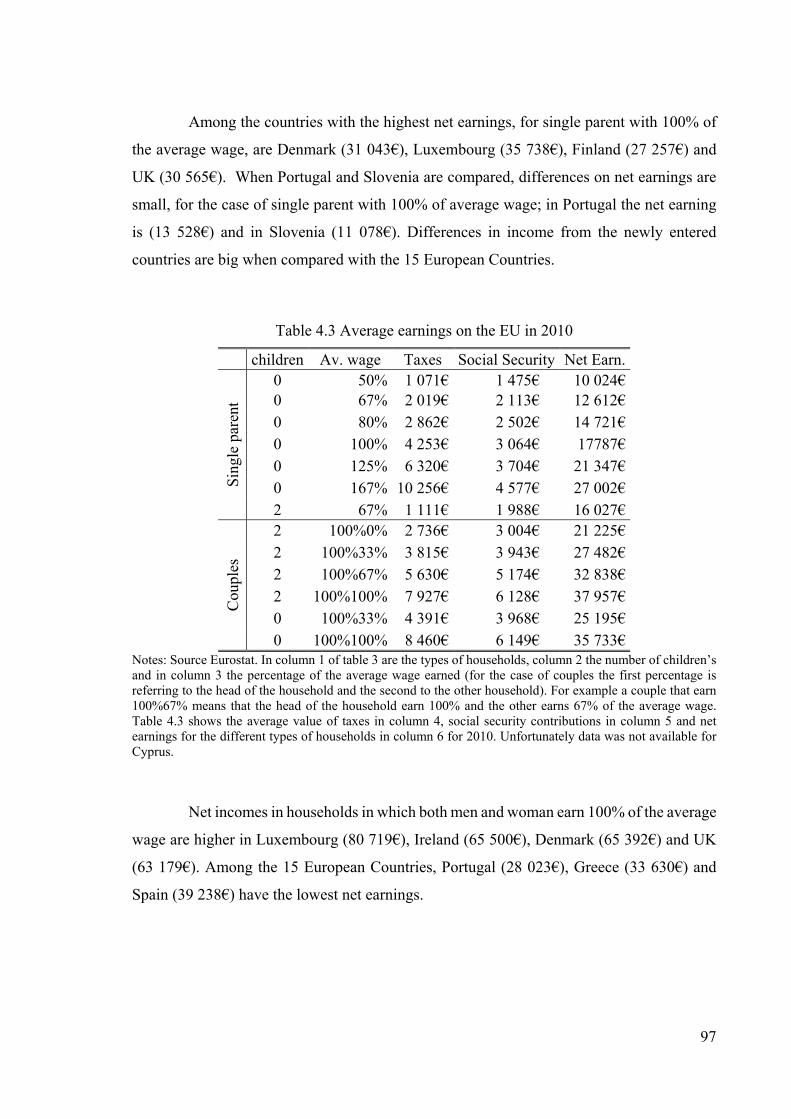
97

Among the countries with the highest net earnings, for single parent with 100% of

the average wage, are Denmark (31 043€), Luxembourg (35 738€), Finland (27 257€) and

UK (30 565€). When Portugal and Slovenia are compared, differences on net earnings are

small, for the case of single parent with 100% of average wage; in Portugal the net earning

is (13 528€) and in Slovenia (11 078€). Differences in income from the newly entered

countries are big when compared with the 15 European Countries.

Table 4.3 Average earnings on the EU in 2010

children Av. wage Taxes Social Security Net Earn.

Sin

gle

pare

nt

0 50% 1 071€ 1 475€ 10 024€ 0 67% 2 019€ 2 113€ 12 612€ 0 80% 2 862€ 2 502€ 14 721€ 0 100% 4 253€ 3 064€ 17787€ 0 125% 6 320€ 3 704€ 21 347€ 0 167% 10 256€ 4 577€ 27 002€ 2 67% 1 111€ 1 988€ 16 027€

Cou

ples

2 100%0% 2 736€ 3 004€ 21 225€ 2 100%33% 3 815€ 3 943€ 27 482€ 2 100%67% 5 630€ 5 174€ 32 838€ 2 100%100% 7 927€ 6 128€ 37 957€ 0 100%33% 4 391€ 3 968€ 25 195€ 0 100%100% 8 460€ 6 149€ 35 733€

Notes: Source Eurostat. In column 1 of table 3 are the types of households, column 2 the number of children’s and in column 3 the percentage of the average wage earned (for the case of couples the first percentage is referring to the head of the household and the second to the other household). For example a couple that earn 100%67% means that the head of the household earn 100% and the other earns 67% of the average wage. Table 4.3 shows the average value of taxes in column 4, social security contributions in column 5 and net earnings for the different types of households in column 6 for 2010. Unfortunately data was not available for Cyprus.

Net incomes in households in which both men and woman earn 100% of the average

wage are higher in Luxembourg (80 719€), Ireland (65 500€), Denmark (65 392€) and UK

(63 179€). Among the 15 European Countries, Portugal (28 023€), Greece (33 630€) and

Spain (39 238€) have the lowest net earnings.

98

Brief Summary

In conclusion, although the EU Commission have provided tools for the

harmonization of taxes, there are still huge discrepancies in their respective levels. We have

covered only three taxes, but there are others equally important. There exist 27 Member

States; from these, 17 are in the Euro Area. There are 27 different legislations. Commission

has provided basic tools for harmonization, but seeing the current level of indirect taxes,

personal and corporate income tax, “Richer” economies like Germany have a lower or equal

level of taxation on personal income tax that some “poor” economies like Portugal.

99

Table 4.4 Net earnings in 2010 Single Parent Couple # Children’s None Two None Two Average wage 50% 67% 80% 100% 125% 167% 67% 100%33% 100%100% 100% 100%33% 100%67% 100%100%

Belgium 15 298€ 17 837€ 20 256€ 23 989€ 28 254€ 35 229€ 23 000€ 36 074€ 48 006€ 32 460€ 40 745€ 46 447€ 52 678€ Bulgaria 1 536€ 2 058€ 2 458€ 3 072€ 3 840€ 5 130€ 2 488€ 4 086€ 6 144€ 3 502€ 4 515€ 5 560€ 6 574€

Czech Republic 4 913€ 6 223€ 7 272€ 8 844€ 10 809€ 14 085€ 8 590€ 12 229€ 17 688€ 12 042€ 14 189€ 16 726€ 19 185€ Denmark 16 282€ 21 237€ 25 201€ 31 043€ 37 323€ 46 533€ 29 856€ 42 369€ 62 085€ 36 673€ 45 676€ 55 587€ 65 392€ Germany 14 533€ 18 315€ 21 227€ 25 381€ 30 614€ 39 119€ 23 349€ 36 631€ 50 762€ 33 564€ 41 351€ 48 636€ 55 697€ Estonia 3 984€ 5 192€ 6 157€ 7 606€ 9 417€ 12 435€ 6 474€ 10 383€ 15 212€ 8 429€ 11 206€ 13 620€ 16 035€ Ireland 18 559€ 22 383€ 26 075€ 30 950€ 35 795€ 43 871€ 31 981€ 45 820€ 61 900€ 37 942€ 49 420€ 57 596€ 65 500€ Greece 7 360€ 9 813€ 11 776€ 14 231€ 17 104€ 21 715€ 10 795€ 20 823€ 30 852€ 17 085€ 22 973€ 28 861€ 33 630€ Spain 11 102€ 13 460€ 15 778€ 19 154€ 23 270€ 30 003€ 15 062€ 26 777€ 38 307€ 21 000€ 27 242€ 33 544€ 39 238€ France 13 818€ 16 739€ 19 823€ 24 449€ 29 524€ 37 668€ 19 294€ 33 479€ 48 899€ 27 930€ 36 986€ 43 995€ 51 705€ Italy 10 968€ 13 816€ 16 092€ 19 527€ 23 388€ 29 321€ 17 842€ 27 643€ 39 054€ 23 068€ 29 807€ 35 496€ 40 905€

Latvia 2 919€ 3 860€ 4 579€ 5 685€ 7 067€ 9 390€ 4 685€ 7 664€ 11 369€ 6 788€ 8 489€ 10 370€ 12 195€ Lithuania 2 798€ 3 638€ 4 280€ 5 268€ 6 503€ 8 589€ 5 511€ 7 210€ 10 537€ 5 786€ 7 367€ 9 063€ 10 693€

Luxembourg 20 581€ 26 188€ 30 276€ 35 738€ 42 173€ 52 879€ 35 971€ 53 426€ 73 197€ 48 078€ 60 948€ 71 404€ 80 719€ Hungary 3 383€ 4 292€ 5 018€ 6 109€ 7 169€ 8 989€ 5 581€ 8 564€ 12 217€ 7 267€ 9 723€ 11 559€ 13 376€

Malta 8 224€ 10 587€ 12 394€ 14 914€ 17 986€ 22 885€ 12 634€ 20 389€ 29 828€ 16 639€ 20 889€ 26 001€ 30 328€ Netherlands 17 527€ 21 618€ 24 981€ 30 130€ 36 579€ 45 864€ 28 042€ 42 950€ 60 260€ 34 297€ 45 785€ 54 583€ 63 095€

Austria 15 693€ 19 435€ 22 429€ 26 789€ 31 946€ 41 529€ 25 236€ 38 176€ 53 578€ 32 619€ 43 337€ 51 406€ 58 777€ Poland 3 656€ 4 809€ 5 731€ 7 113€ 8 842€ 11 723€ 5 165€ 9 617€ 14 227€ 7 748€ 10 174€ 12 479€ 14 784€

Portugal 7 556€ 9 729€ 11 249€ 13 528€ 16 377€ 20 351€ 11 358€ 19 458€ 27 056€ 15 882€ 20 528€ 24 224€ 28 023€ Romania 2 068€ 2 719€ 3 209€ 3 972€ 4 918€ 6 527€ 3 264€ 5 246€ 7 945€ 4 451€ 5 576€ 7 008€ 8 229€ Slovenia 6 395€ 7 884€ 9 161€ 11 078€ 13 431€ 16 886€ 11 296€ 15 375€ 22 155€ 14 911€ 17 889€ 21 216€ 23 986€ Slovakia 3 973€ 5 042€ 5 898€ 7 182€ 8 786€ 11 483€ 6 051€ 10 243€ 14 364€ 8 930€ 112 501€ 13 233€ 15 372€ Finland 15 701€ 19 949€ 22 895€ 27 257€ 32 354€ 40 767€ 23 593€ 38 463€ 54 514€ 29 783€ 40 989€ 49 732€ 57 040€ Sweden 15 399€ 19 969€ 23 625€ 28 893€ 33 935€ 41 350€ 22 800€ 39 722€ 57 786€ 31 724€ 42 553€ 51 694€ 60 617€

UK 16 404€ 21 124€ 24 901€ 30 565€ 37 629€ 47 720€ 26 797€ 42 248€ 61 130€ 33 252€ 44 935€ 53 738€ 63 179€

Notes: Cyprus was missing. Source Eurostat. Line 1 of table 4.4 shows the type of households, line 2 shows the number of children’s and line 3 the average wage.

100

4.3 Data and description of the variables

Our dataset was constructed using the official publications provided by the Business

Software Alliance and the Eurostat.

Dependent Variable

The dependent variable is the software piracy losses at current prices78 from 1996 to

2010 BSA (2012). Software piracy can be defined as the unauthorized use of software that

is protected by nationals or international Intellectual Property Rights. Some of this use can

be a result of lack of enforcement of these laws. The software piracy losses measures the

commercial value of the software that is currently being used trough illicit means and is a

result of extensive surveys done over the years by the Business Software Alliance (BSA)

with the help of International Data Corporation (IDC) and IPSOS BSA (2012). A total of 33

observations were missing for Estonia, Latvia, Lithuania and Luxembourg. Png (2010)

found that when surveys are not applied, the software piracy rates are based on national

income; it also found that the yearly rate of decrease of the piracy rates before 2003 were

2.0 (p.p), while the period after 2003 this rate of decrease fell to 1.1 (p.p) for the non-survey

countries. With this in mind we will introduce a variable that will reflect this change79. More

formally, software piracy can be defined as the unauthorized use of software that is protected

by nationals or international Intellectual Property Rights. Some of this use can be a result of

lack of enforcement of these laws.

Economic Dimension

Following Goel and Nelson (2009) and Andrés and Goel (2011) we will use the

logarithm of real GDPpc80 as a measure of national income. GDP measures the income of a

78 We will introduce a variable, the HICP that reflects the change in prices of products at current prices 79 Piracy rates have a decreasing pattern while the piracy losses are increasing over the years. This dummy variable reflects the break in the series, as the Business Software alliance change its consultant and methodology in this period. 80 GDPpc takes into account Purchasing Power Parity and is measured at current prices.

101

country and also the ability to purchase goods such as software products. The higher the

GDP, the higher households have the ability to purchase consumer goods. This is a control

variable and is expected to have a negative effect as a result of increased disposable income

that allows to purchase goods.

HICPH as a proxy of software price

Software’s prices can affect the decisions to purchase or to use illegal software. A good

choice would be based upon the prices of both hardware and software. Unfortunately that

information can be misleading as in certain cases, such as the Microsoft Office or the prices

of computers are almost the same across the countries. We used the Harmonized indices of

consumer prices (HICPH) as a proxy for these prices but also due to the fact that piracy

losses are at current prices. We will introduce three measures that reflect the overall costs of

living; i) costs of communications - examples of these costs are the price of phone calls and

prices of telephones (HICPHgcomm); ii) costs of cultural services - examples are price of

music, films, games, books and newspapers (HICPHgculture81) and iii) overall costs of

products (HICPHgall). Harmonized indices of consumer prices (HICPHs) give comparable

measures of inflation for the countries and country groups where they are produced. They

are economic indicators that measure the change over time of the prices of consumer goods

and services acquired by households. These variables are expected to have a positive impact

(increase piracy) as a result of increase of price on goods, in which software is included.

Tax dimension

4.3.4.1 Household taxation

Labor costs include several dimensions such as social security contributions and

family allowances that are captured by this variable. One of the independent variables will

be the different tax rates applied to different types of households. It represents only one

81 These variables were retrieved in the official web site of the Eurostat and describe the rate of change from one year to another.

102

variable that can be decomposed into several tax levels. We will consider several hypotheses

that vary according to the marital status, the existence of children in the constitution of the

household and the percentage of the average wage that is earned. Several alternative types

of households will be analyzed as independent variables:

Single person with no children and 50%, 67%, 80%, 100%, 125% and 167% of the

average wage (AW) respectively;

Single person with two children and 67% of the AW;

Married couple with two children and the following levels of the AW: husband

100% / wife 0%, husband 100% / wife 33%, husband 100% / wife 67% and husband

100% / wife 100%;

Married couple with no children and 100% of the AW for the husband and 33% for

the wife and husband 100% / wife 100%;

Hereafter we will use “SP” to denote single parent, “C” to denote couples; the number

of children’s will be “t” for two children’s and “n” for no children’s. SPn67 represents a

single parent household that earns 67% of the average wage and do not have children, SPt67

represents a similar household with the same income but with two children. Another

example is Cn10033, where 100% represents the income that the head of the household earn

and 33% represents the income that the other member of the household earns in comparison

to the average wage - they do not have children; Ct100100 represents couples that have two

children and both households earn 100% of the average wage.

On each of these dimensions (representative households) we will consider the average

tax rate that is defined as the income tax on gross wage earnings plus the employee's social

security contributions, less universal cash benefits, expressed as a percentage of gross wage

earnings82. We expect that this variable will increase software piracy, although with the

harmonization that the European Union has set over the years, this positive impact may

become marginal.

82 http://epp.eurostat.ec.europa.eu/cache/ITY_SDDS/EN/earn_net_esms.htm

103

4.3.4.2 Relative importance of taxes

We will introduce the relative importance of taxes on labor and consumption relative

to GDP83. The impact of these taxes is expected to be positive, although they do not measure

the direct level of taxation, e.g., they do not measure the actual rate but the importance of

the tax on the economy.

Summary Statistics

Table 4.5 presents the summary statistics for each variable that will be analyzed. These

results show that, in some circumstances, some households don’t pay any type of tax, as in

the case of SPt67 and Ct100. Family allowances in these households is higher than the actual

tax, which explains this negative impact. The negative value of taxes on SPt67 and Ct100

indicates that these households not only do not pay taxes but receive a net subsidy from the

Government. Higher values of taxes are present when there are no children’s. Additional to

these statistics we also provide the graphs of software piracy rates and losses for each

country. The maximum piracy rate of 98% was in 1997 in Bulgaria. Since then, these rates

have been decreasing in all countries. Figure 4.1 presents this decrease on all European

Union Countries. Figure 4.2 presents the evolution of software piracy losses.

83 They comprise detailed tax and social contribution receipts for the general government sector as a share of GDP or as a share of total taxation (we have information on VAT, labor and capital taxes)

104

Table 4.5 Summary statistics

Variable Obs. Mean Std. Dev. Min Max Losses 372 318.86 575.03 0.97 3191 SPn50 402 19.72 7.58 0.15 39.26 SPn100 402 27.20 8.00 6.30 44.95 SPn125 402 29.67 8.26 8.46 48.37 SPn167 402 32.60 8.56 12.67 52.58 SPt67 402 5.29 10.24 -21.56 24.69 SPn67 402 23.04 7.81 3.52 41.39 SPn80 402 24.90 7.94 4.8 43.17 Cn100100 402 27.20 7.92 6.3 44.95 Cn10033 402 23.84 7.59 5.68 41.39 Ct100 402 14.83 8.58 -8.6 31.11 Ct100100 402 23.15 7.52 0.46 41.68 Ct10033 402 17.44 7.59 0.6 36.48 Ct10067 402 20.41 7.63 5.4 39.6 lGDPpc 405 9.77 0.52 8.37 11.15 GDPg 378 4.26 5.82 -18.49 15.91 HICPHall 405 94.55 16.63 5.01 139.62 HICPHgall 377 4.25 9.50 -1.7 154.8 HICPHcommu 404 100.24 21.72 1.81 206.34 HICPHgcommu 377 2.04 18.25 -14 237.5 HICPHculture 404 95.72 12.52 5.74 120.09 HICPHgculture 377 2.83 9.71 -4.9 146.6 Itaxcons 401 21.05 4.47 11.1 34.2 Itaxlab 401 34.66 6.74 18.8 49.3 TaxconsGDP 405 12 1.66 7.3 17.2 TaxconsTotal 405 33.63 6.09 22.8 54 TaxlabGDP 405 17.44 5.31 9 32 TaxlabTotal 405 46.99 7.89 27 62.5 TaxcapTotal 405 19.51 6.71 5.2 35

Notes: Std. Dev. represents the standard deviation; Min the minimum and Max the maximum.

105

Figure 4.1 Evolution of Software Piracy rates on the European Union

106

Figure 4.2 Evolution of Software Piracy Losses on the European Union

107

4.4 Empirical Study

When dealing with a panel-data analysis, we must choose the appropriate estimator

but also ensure that our variables produce the best results. One problem that can occur in a

panel of countries is the existence of one or more non-stationary variables. The existence of

such variables can be problematic resulting in spurious regressions (Granger & Newbold,

1974). We start by testing the stationarity of the variables using unit-root tests. Next we

empirically estimate our model using the fixed effect model following Andrés (2006a);

Chen et al. (2010) and Boyce (2011), that showed that based on Hausman tests (Hausman,

1978) the fixed effect was the most appropriate for the analysis.

Testing the presence of unit roots

To check if our series are stationary we implemented a procedure proposed by Im,

Pesaran, and Shin (2003), henceforth IPS. Other tests are available but rely on balanced

panels which is not the case. Equation 4.1 shows a model with a first order autoregressive

component:

Δ , (4.1)

where 1, … , represents the Member States; 1, … , indexes time; is

the variables that we want to test; is independently distributed normal for all i and t and

has heterogeneous variance . This test assumes that all the panel dataset is non-stationary

under the null hypothesis : 0 against the alternative hypothesis that some panels are

stationary : 0. To be able to get significance it is necessary at least 10 observations

per country, which is not the case on software piracy losses. In this variable we performed

the Fisher type tests I. Choi (2001) that has the same assumption of the IPS test. In this

framework four tests are available: Inverse chi-squared; Inverse normal; Inverse logit and

Modified inverse chi-squared. Based on I. Choi (2001) simulations results, the inverse

normal Z statistic offers the best trade-off between size and power. The IPS test is performed

on the independent variables.

Table 4.6 presents the result of these tests for each variable. It can be seen that

almost all the variables seem to be stationary or integrated of order zero I(0). The exception

108

goes to the natural logarithm of Gross Domestic Product per capita at Purchasing Power

Parity and the Harmonized indices of consumer prices that may be considered as having unit

roots. To prevent this problem we introduce the real GDP growth and the inflation rate

(HICPHg). Both variables are stationary.

After establishing that our regressors are stationary, we can proceed with the fixed

effect model.

Table 4.6 IPS and Fisher type Unit root tests

Level 1stdifference Dependent Variable ln(Losses) -1.336* -12.105***Independent Variables SPn50 -3.871*** - SPn67 -3.584*** - SPn80 -4.015*** - SPn100 -3.349*** - SPn125 -3.525*** - SPn167 -3.456*** - SPt67 -4.637*** - Cn10033 -3.165*** - Cn100100 -3.694*** - Ct100 -4.060*** - Ct10033 -3.817*** - Ct10067 -3.428*** - Ct100100 -3.654*** - lGDPpc -0.278 -6.628*** Itaxlab -3.313*** - Itaxcons -3.588*** - HICPH 0.731 -4.826*** HICPHg -6.783*** - HICPHcomm 1.7637 -6.388*** HICPHgcomm -4.455*** HICPHculture 2.3157 -4.853*** HICPHgculture -4.498*** - TaxconsGDP -3.620*** - TaxconsTotal -3.725*** - TaxlabGDP -2.770*** - TaxlabTotal -3.786*** - TaxcapTotal -4.333*** -

Notes: In the dependent variable we performed the Fisher type test presenting the inverse normal Z statistic. In the Independent variables the IPS test is used and the statistics is presented. It was included a trend and subtracted cross-sectional mean. It was tested under the null hypothesis that all panels contain unit roots against the alternative that some panels are stationary. *** and * corresponds to a significance level of 1% and 10% respectively.

109

Empirical results

4.4.2.1 Effects of taxation on software piracy losses

We start our analysis by introducing the different tax rates on labor applied to

households as well as the importance of direct and indirect taxes as a share of GDP. The

different regions of Europe will be analyzed when they present significance.

We can specify our dependent variable, software piracy losses ln(Losses) as a

function of: i) the importance of taxation on labor as a share of GDP (TaxlabGDP); ii) the

importance of taxation on consumption as a share of GDP (TaxconsGDP); iii) the growth

rate of harmonized index of consumer prices index for all products (HICPHg); iv) growth of

real gross domestic product per capita (GDPg); and v) the variable tax will assume thirteen

different types of households. will assume the different levels of taxation that each

of these households incur. 1, … ,13 represents the different types of households that are:

SPn50, SPn67, SPn80, SPn100, SPn125, SPn167, SPt67, Cn10033, Cn100100, Ct100,

Ct10033, Ct10067, Ct100100. Additional to this we include a dummy variable that reflects

the change in methodology used by the Business software alliance occurred in 2002

(change). The dependent variable is in natural logarithms.

Equation 4.2 and 4.3 summarizes the estimated model

ln

(4.2)

where

(4.3)

where i=1,…27 represents the Member States, t=1996,…,2010 represents the time,

represents the error term. HICPHgall is the growth of all the prices, HICPHgcomm is the

growth of prices in telecommunications and HICPHgculture is the growth of prices in

products such as movies, culture or books.

Estimates of the piracy rates are projected from national income in the non-survey

countries. Initially, the surveys only covered 15 countries. From these, only one country of

the European Union was present: Spain (First Annual BSA and IDC Global Software). In

110

the report of 2010, 32 countries were present in the surveys. From those countries, Czech

Republic, Poland, France, Germany, Italy, Netherland, Spain, Sweden and United Kingdom

make part of the European Union (Eight annual BSA and IDC global software piracy study).

In each of the regressions reported we present the Hansen-test statistic that is a

robust version of the Hausman test (Schaffer & Stillman, 2010). The Hausman test assumes

under the null hypothesis that the random effect (RE) estimates is consistent. The fixed

effects estimator uses the orthogonally conditions that the regressors are uncorrelated with

the idiosyncratic error. Furthermore, one of the assumptions of the random effect is that it

uses the additional orthogonally conditions that the regressors are uncorrelated with the

group-specific error; the Hansen-test84 treats this assumption as additional orthogonally

conditions (it is a test of over identifying restrictions). Rejecting the null hypothesis favors

the fixed effect model.

Table 4.7 presents the results for the entire sample (EU27). The impact of prices is

similar in the different categories of products; we only report the results for the inflation of

overall products (In Annex VI we report the remaining possibilities). We dropped taxation

of households that were not significant (in Annex VII we report the remaining cases).

Column 2 through 5 shows the estimates for the different types of households, as with

previous studies (Chen et al., 2010); the GDPg is not significant in the majority of

regressions.

We can observe a negative and marginal impact of inflation on overall products.

Many software prices, such as productivity suits, are constant over the years, not suffering

with the inflation of a Country. In fact some software prices decreases over the years;

examples are games and movies. In many software products, Companies internalize the

value of VAT, making software prices almost the same across European Countries. These

variables were always significant at 1%.

84 These additional orthogonality conditions are overidentifying restrictions. The test is implemented by xtoverid using the artificial regression approach described by Arellano (1993) and Wooldridge (2010, pp. 290-291), in which a random effects equation is reestimated, augmented with additional variables consisting of the original regressors transformed into deviations-from-mean form. The test statistic is a Wald test of the significance of these additional regressors. Under conditional homoskedasticity, this test statistic is asymptotically equivalent to the usual Hausman fixed-vs-random effects test; with a balanced panel, the artificial regression and Hausman test statistics are numerically equal. See Arellano (1993) for an exact statement.

111

Another important variable introduced was the relative importance of taxes; the

positive effect of TaxconsGDP indicates that all the different types of indirect taxation play

an important role in explaining software piracy. Changing these taxes determines the

behavior of consumers when facing choices of purchasing goods. This variable was

significant, which indicates that reducing indirect taxation could be beneficial for reducing

piracy, because more disposable income is available to households to spend on goods.

Table 4.7 Tax rate on labor on different households in EU27

Variables 1 2 3 4 5 GDPg 0.009 0.009 0.009 0.010* 0.008 (1.386) (1.421) (1.419) (1.904) (1.366) TaxconsGDP 0.065** 0.056** 0.059** 0.068*** 0.071** (2.402) (2.303) (2.304) (2.628) (2.514) HICPHgall -0.004*** -0.004*** -0.004*** -0.004*** -0.004*** (-3.756) (-3.333) (-3.111) (-3.735) (-3.541) SPn50 0.021** (2.070) SPn67 0.021* (1.876) SPn80 0.019* (1.671) Cn10033 0.018* (1.680) Change 0.991*** 1.000*** 0.995*** 1.056*** 0.952*** (14.113) (14.028) (13.870) (15.061) (14.538) Constant 2.914*** 2.628*** 2.515*** 2.455*** 2.484*** (8.796) (6.448) (5.381) (4.936) (4.738) Observations 349 346 346 346 346

0.880 0.882 0.881 0.875 0.877 0.875 0.877 0.876 0.871 0.872

Countries 27 27 27 27 27 Hansen-Test 4.9e+04 1543.99 628.96 606.66 471.79 p-value [0.000] [0.000] [0.000] [0.000] [0.000]

Notes: Dependent variable is ln(Losses). All regressions were estimates with time dummies. Robust t-statistics are in parentheses. Degrees of freedom of t-distribution for n>120 are: critical values at 10% are 1.645; at 5% is 1.960 and at 1% are 2.576. *, ** and *** represent significance at 10%, 5% and 1% respectively. All EU represent the 27 Member states of the European Union

The additional variables that represent taxation of the different households have the

expected positive impact, which indicates that they affect negatively the final disposable

income that will be used to purchase these types of products. Only on those households that

do not have children and earn less than 100% of the average wage are positively and

significantly affected.

112

The positive effect of taxation on Single parents is more severe on households that

earn less and this positive value decreases as households earn more. This result indicates that

households can allocate more of their disposable income on digital content as their income

increases (Shin et al., 2004). The same pattern applies to Couples that do not have children;

only on households that earn less than 100% of the average wage, significance is present.

Knowing the main results including the EU27, we provide additional regressions in

which we compare “Euro” and “Not Euro” zone, and the 15 original countries of the EU

(“Old”) and the “New Countries”. Results on household taxation were only significant on

“Not Euro” and “New” countries85. Table 5.8 presents the results.

In these regions we also observe the lack of significance of GDPg across many

regressions. One of the main differences resides in the significance of household taxation

across the different regions. In the countries not belonging to the Euro Zone household

taxation has a strong coefficient, being significant (column 7 to 10). When the “Euro” Zone

is examined (see Annex D), the coefficients are marginal and close to zero. This can be a

result of the fact that countries in the sample belongs to the North of Europe that is

characterized by a high level of taxation.

Table 4.8, columns 12 to 15 shows the “New” countries; many of these countries

have a low flat rate (Bulgaria and Estonia are some examples). Since 2008 Bulgaria has a

10% flat rate tax system (Commission, 2012, p. 66). The region that represents the “Old”

countries doesn’t have significance, although with similar coefficient sizes (see Annex VIII).

In all regressions the Hansen-test favors the fixed effect model with a significance

of 1%. The dummy variable that represented the change in methodology is positive which

indicates that software piracy losses have increased over the years. Also as Figure 4.2

presented, a dramatic change occurred in 2002/2003, which was captures by this variable.

85 The remaining regions are reported in annex.

113

Table 4.8 Tax rates on NOT EURO VS NEW Countries

NOT EURO NEW Variables 6 7 8 9 10 11 12 13 14 15 GDPg 0.008 0.005 0.004 0.008 0.008 0.009* 0.009 0.008 0.011** 0.010* (1.361) (0.868) (0.710) (1.194) (1.184) (1.656) (1.634) (1.578) (2.025) (1.912) TaxconsGDP 0.099** 0.051* 0.058* 0.058 0.073 0.067** 0.060** 0.063** 0.071** 0.074** (2.554) (1.725) (1.712) (1.509) (1.552) (2.303) (2.196) (2.281) (2.287) (2.113) HICPHgall -0.003*** -0.004*** -0.004*** -0.004*** -0.004*** -0.005*** -0.005*** -0.005*** -0.004*** -0.004*** (-2.871) (-4.100) (-3.524) (-3.471) (-3.395) (-4.818) (-5.317) (-4.965) (-3.933) (-3.823) SPn50 0.025** 0.025** (2.408) (2.685) SPn67 0.023* 0.020* (1.818) (1.720) SPn80 0.022* 0.013 (1.694) (0.951) Cn10033 0.022* 0.013 (1.908) (0.969) Change 1.240*** 0.948*** 0.951*** 1.084*** 1.078*** 0.809*** 0.790*** 0.783*** 0.891*** 0.924*** (16.673) (8.011) (7.906) (12.227) (13.106) (12.585) (12.459) (12.548) (12.358) (11.877) Constant 2.403*** 2.557*** 2.446*** 2.364*** 2.198** 1.747*** 1.440*** 1.449*** 1.434** 1.355* (5.153) (5.135) (3.814) (3.331) (2.691) (5.261) (3.871) (3.169) (2.426) (2.064) Observations 131 131 131 131 131 155 152 152 152 152

0.895 0.929 0.925 0.922 0.923 0.902 0.908 0.903 0.898 0.896 0.885 0.919 0.916 0.913 0.914 0.893 0.898 0.893 0.888 0.886

Countries 10 10 10 10 10 12 12 12 12 12 Hansen-Test 1039.47 5.7e+08 2605.19 3178.44 2015.02 753.247 8257.18 8283.31 78.65 227.09 p-value [0.000] [0.000] [0.000] [0.000] [0.000] [0.000] [0.000] [0.000] [0.000] [0.000]

Notes: Dependent variable is ln(Losses). All regressions were estimates with time dummies. Robust t-statistics are in parentheses. “Not Euro” represents the countries that are outside the Euro Area. “NEW” represents the 10 countries that recently entered in 2004 and 2007.

114

4.4.2.2 Additional Results

After establishing that both indirect and direct taxation on households affect

positively software piracy, we examine if the relative importance in the Economy of these

taxes can also affect this phenomenon. The relative importance of these taxes can be

measured as a percentage of total taxation. In many countries, the importance of Capital,

Labor and Consumption taxes accounts for almost one hundred percent of all taxes existing

in a country.

Equation 4.4 describes the general econometric specification that will be used

ln

(4.4)

where TaxcapTot, TaxlabTot and TaxconsTot are the importance of taxes on

capital, labor and consumption respectively as a share of total taxation. These three variables

cannot be present at the same time as the sum of them represents almost 100% of total

taxation.

So as:

≅ 1 (4.5)

To prevent a high level of multicolinearity we omit one variable at a time that will

serve as a base tax level. For instance if we omit the , solving the above

equation relatively to that variable and replacing in equation 5.4 we get:

ln

(4.6)

From equation (4.6) is easy to check the interpretation of the coefficient as a 1 pp.

increase in the share of the respective tax with an associate decrease of 1 pp. in the share of

the Consumption Tax (the base case).

Anyway, we report all possible combinations in the regressions that serve as a

robustness check. With this omission we can interpret the coefficients of the remaining taxes

115

as the differential impact between a specific tax and the base one. The control variables

(GDPg and HICPHgall) maintained the coefficients.

Table 4.9 presents the results for the entire sample. Columns 16 to 18 show the

different combinations of these taxes. Significance on the variables that represent the

importance of taxes was only present when taxation of labor and capital were considered

together (column 16); the negative impact of TaxcapTot86 indicates that an increase of the

relative importance of capital taxation and a reduction of consumption taxation, will lead to

less piracy (substitution effect). In spite of this statistical significance, column 18 shows that

this result is not strong, which can be a result of the complex tax systems and the difficulty

in reducing direct taxation.

Table 4.9 Relative importance of taxation in the EU27

Variables 16 17 18 GDPg 0.012* 0.013* 0.013* (1.646) (1.685) (1.657) HICHgall -0.003** -0.003** -0.003** (-2.595) (-2.530) (-2.558) TaxcapTot -0.027* 0.003 (-1.667) (0.172) TaxlabTot -0.030 -0.004 (-1.556) (-0.229) TaxconsTot 0.029 0.026 (1.508) (1.599) Change 1.265*** 1.266*** 1.266*** (20.785) (20.889) (20.833) Constant 5.592*** 2.615*** 2.942*** (4.836) (3.128) (2.845) Observations 349 349 349

0.845 0.845 0.845 0.840 0.840 0.840

Countries 27 27 27 Hansen-Test 3.5e+04 1.1e+04 9853.72 p-value [0.000] [0.000] [0.000]

Notes: Dependent variable is ln(Losses). All regressions were estimates with time dummies. Robust t-statistics are in parentheses.

86 In the European Union, this tax represents on average 19.51% of total taxation. The personal taxation represents, on average, 47% of total taxation, which indicates that the rates applied are high. On the other side, the rates applied to capital are relatively low.

116

Table 4.10 presents the results for the different EU regions that were significant;

the “Not Euro” and “Euro” zone.

Table 4.10. Relative importance of taxation in the Not Euro and EURO Countries

NOT EURO EURO VARIABLES 19 20 21 22 23 24 GDPg 0.000 0.001 0.000 0.022** 0.022** 0.022** (0.047) (0.172) (0.064) (2.142) (2.149) (2.137) HICHgall -0.006*** -0.006*** -0.007*** -0.046*** -0.046*** -0.046*** (-3.985) (-3.922) (-4.107) (-2.680) (-2.660) (-2.629) TaxcapTot -0.013 0.041 -0.032* -0.023 (-0.614) (1.579) (-1.775) (-1.209) TaxlabTot -0.054** -0.044* -0.010 0.022 (-2.447) (-1.707) (-0.485) (1.196) TaxconsTot 0.052** 0.010 0.009 0.031* (2.299) (0.495) (0.434) (1.710) Change 1.214*** 1.220*** 1.214*** 1.201*** 1.202*** 1.203*** (13.781) (13.972) (13.864) (12.948) (12.970) (12.935) Constant 6.567*** 1.181 5.488** 4.840*** 3.904*** 1.670 (5.186) (1.092) (3.144) (4.042) (4.243) (1.343) Observations 131 131 131 218 218 218

0.894 0.893 0.894 0.835 0.835 0.835 0.884 0.883 0.884 17 17 17

Countries 10 10 10 0.827 0.826 0.826 Hansen-Test 1095.60 862.59 828.46 904.727 1072.968 1150.520 p-value [0.000] [0.000] [0.000] [0.000] [0.000] [0.000]

Notes: Dependent variable is ln(Losses). All regressions were estimates with time dummies. Robust t-statistics are in parentheses. “Not Euro” represents the countries that are outside the Euro Area.

Columns 19 to 21 present the results for the “Not Euro” Zone. TaxlabTot is

significant at 5% with a negative impact on piracy which indicates that if we increase the

importance of this tax and at the same time decrease the importance of consumption tax

(base tax), this will decrease piracy. If we consider the capital tax as the base tax, we observe

that TaxlabTot maintains its coefficient, being significant at 10%. In this case an increase of

labor tax and, at the same time, a decrease of capital taxation (the base tax) will also lead to

less piracy. TaxconsTot is significant at 5% with a positive impact (increases piracy) when

we omit labor tax. In this case an increase of consumption tax and a decrease of labor tax

(base tax) will increase piracy although this result is not robust.

117

Columns 22 to 24 shows the “Euro” Zone; in this situation TaxlabTot loses

significance. This is an unexpected result as in the Euro Zone the importance of this tax is

smaller than those outside the Euro Zone, although this difference is marginal87.

Table 4.11 presents the results for the “New” and “Old” countries. Columns 25 to

27 presents the “New” Countries. When we consider the consumption tax as the base one,

we can observe that it is possible to reduce piracy choosing capital or labor tax. Both

variables are significant with a negative impact. If we increase TaxlabTot and reduce

consumption taxation (base tax), this will decrease piracy; we can also, in alternative,

increase TaxcapToT and reduce consumption tax. Although this will depend of the

advantages and disadvantages of changing one of these taxes.

When we consider both TaxcapTot and TaxconTot, TaxconTot is positive and

significant which indicates that if we increase this tax and decrease the base tax (labor tax),

this will increase piracy. Also when the base tax is the capital tax, TaxconsTot maintain the

significance with a positive impact; an increase of this tax and a decrease of capital tax (the

base tax) will increase piracy. Columns 28 to 30 shows the “Old” countries; in this case none

of the variables are significant.

87 On average in the Euro Zone this tax represents 47.7% of total taxation while on the remaining countries this value is of 46.6%.

118

Table 4.11 Relative importance of taxation in the New and Old Countries

NEW OLD Variables 25 26 27 28 29 30 GDPg -0.001 0.000 -0.000 0.026* 0.026* 0.026* (-0.088) (0.052) (-0.029) (1.836) (1.842) (1.832) HICHgall -0.004*** -0.004*** -0.004*** -0.054* -0.053 -0.053* (-3.097) (-2.985) (-3.061) (-1.671) (-1.636) (-1.653) TaxcapTot -0.036*** 0.019 -0.016 -0.022 (-3.130) (0.846) (-0.455) (-0.844) TaxlabTot -0.056** -0.022 0.006 0.021 (-2.496) (-0.974) (0.204) (0.821) TaxconsTot 0.054** 0.034*** -0.008 0.014 (2.316) (2.794) (-0.267) (0.395) Change 1.216*** 1.223*** 1.216*** 1.225*** 1.225*** 1.227*** (12.265) (12.186) (12.077) (13.372) (13.498) (13.540) Constant 5.657*** 0.122 2.204 4.716** 5.391*** 3.256 (4.840) (0.106) (1.768) (2.337) (4.681) (1.627) Observations 155 155 155 194 194 194

0.871 0.870 0.871 0.858 0.858 0.858 0.861 0.860 0.861 15 15 15

Countries 12 12 12 0.850 0.850 0.849 Hansen-Test 703.36 567.91 587.98 1054.141 1061.812 1201.264 p-value [0.000] [0.000] [0.000] [0.000] [0.000] [0.000]

Notes: Dependent variable is ln(Losses). All regressions were estimates with time dummies. Robust t-statistics are in parentheses. “New” represents the 10 countries that recently entered in 2004 and 2007.

119

4.5 Conclusion

This chapter analyzed the impact that levels of taxation have on software piracy.

Previous econometric studies have relied on cross-sectional and panel data studies. Our

contribution to the empirical literature is in the fact that we introduce a new analysis that

studies the effect of taxation on different households types as well as introducing a large

panel dataset for the European Union and its different regions. Results are valuable for

policymakers, especially within the common market of the European Union.

Results indicate that personal taxation affects differently the households. An

increase in taxation on households that have smaller income appears to increase piracy, being

this impact more pronounced on these households than those that earn more. These results

were also founded when the different regions of the EU were considered, although only

significant on “Not Euro” and the “New” countries. Having more access to digital content

combined with reduced incomes may result on using illegal software, for example

downloading illegal music instead of purchasing them.

Further analysis was conducted with the relative importance of personal tax, capital

tax and consumption tax as a share of total taxation. Results showed that even if its not

possible to reduce the number of taxes or the actual rates applied, there appear to be some

benefit in reducing the impact of taxation on consumption. These results were heterogeneous

among the different regions. To promote effective measures to prevent piracy, effective

policies are necessary targeting each group of countries and the different tax types (PIT, CIT

and CIT).

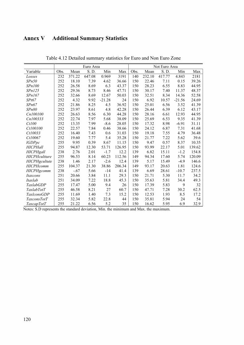
120

Additional Summary Statistics

Table 4.12 Detailed summary statistics for Euro and Non Euro Zone

Euro Area Not Euro Area Variable Obs. Mean S. D. Min Max Obs. Mean S. D. Min Max Losses 232 371.22 647.08 0.969 3191 140 232.10 417.77 4.843 2181 SPn50 252 18.10 7.39 4.62 36.66 150 22.46 7.11 0.15 39.26 SPn100 252 26.58 8.69 6.3 43.37 150 28.23 6.55 8.83 44.95 SPn125 252 29.36 8.73 8.46 47.71 150 30.17 7.40 11.37 48.37 SPn167 252 32.66 8.69 12.67 50.03 150 32.51 8.34 14.36 52.58 SPt67 252 4.32 9.92 -21.28 24 150 6.92 10.57 -21.56 24.69 SPn67 252 21.86 8.25 4.5 36.92 150 25.01 6.56 3.52 41.39 SPn80 252 23.97 8.61 4.8 42.28 150 26.44 6.39 6.12 43.17 Cn100100 252 26.63 8.56 6.30 44.28 150 28.16 6.61 12.93 44.95 Cn100333 252 22.74 7.97 5.68 38.09 150 25.69 6.53 9.35 41.39 Ct100 252 13.35 7.99 -8.6 28.05 150 17.32 8.98 -6.91 31.11 Ct100100 252 22.57 7.84 0.46 38.66 150 24.12 6.87 7.31 41.68 Ct10033 252 16.40 7.43 0.6 31.03 150 19.18 7.55 4.79 36.48 Ct10067 252 19.60 7.77 5.4 35.28 150 21.77 7.22 5.62 39.6 lGDPpc 255 9.95 0.39 8.67 11.15 150 9.47 0.57 8.37 10.35 HICPHall 255 94.87 12.30 53.71 126.95 150 93.99 22.17 5.01 139.62 HICPHgall 238 2.76 2.01 -1.7 12.2 139 6.82 15.11 -1.2 154.8 HICPHcultture 255 96.53 8.14 60.23 112.56 149 94.34 17.60 5.74 120.09 HICPHgcultute 238 1.46 2.17 -2.6 12.4 139 5.17 15.49 -4.9 146.6 HICPHcomm 255 104.37 21.30 38.86 206.34 149 93.17 20.63 1.81 124.6 HICPHgcomm 238 -.67 5.66 -14 41.4 139 6.69 28.61 -10.7 237.5 Itaxcons 251 20.66 3.84 11.1 29.3 150 21.71 5.30 11.7 34.2 Itaxlab 251 34.09 7.22 18.8 45.3 150 35.63 5.81 34.4 49.3 TaxlabGDP 255 17.47 5.00 9.4 26 150 17.39 5.83 9 32 TaxlabTotT 255 46.58 8.21 27 60.7 150 47.71 7.28 30.2 62.5 TaxlconsGDP 255 11.69 1.40 7.3 15.2 150 12.53 1.93 8.5 17.2 TaxconsTotT 255 32.34 5.82 22.8 44 150 35.81 5.94 24 54 TaxcapTotT 255 21.22 6.56 5.2 35 150 16.62 5.95 6.9 32.9

Notes: S.D represents the standard deviation, Min. the minimum and Max. the maximum.

121

Table 4.13 Detailed Summary Statistics for Old and New Countries

Old Countries New Countries Variable Obs. Mean S. D. Min Max Obs. Mean S.D. Min Max Losses 207 519.27 703.61 16 3191 165 67.44 108.90 0.969 648 SPn50 225 20.91 7.85 4.62 39.26 177 18.22 6.95 0.15 31.31 SPn100 225 29.73 7.79 16.49 44.95 177 23.97 7.04 6.3 38.81 SPn125 225 32.63 7.93 18.76 48.37 177 25.90 7.07 8.46 42.52 SPn167 225 36.15 8 21.47 52.58 177 28.09 6.97 12.67 45.14 SPt67 225 7.79 8.87 -21.28 21.41 177 2.12 10.98 -21.56 24.69 SPn67 225 25.01 7.79 11.47 41.39 177 20.53 7.09 3.52 32.32 SPn80 225 27.20 7.94 13.89 43.17 177 21.95 6.91 4.8 32.82 Cn100100 225 29.68 7.80 17.43 44.95 177 24.05 6.88 6.3 38.81 Cn100333 225 25.52 7.82 10.45 41.39 177 21.71 6.73 5.68 34.25 Ct100 225 17.23 7.64 -2.17 31.11 177 11.78 8.75 -8.6 28.97 Ct100100 225 25.63 7.42 11.14 41.68 177 19.99 6.40 0.46 31.74 Ct10033 225 19.50 7.79 2.02 36.48 177 14.82 6.44 0.6 27.8 Ct10067 225 22.77 7.77 6.23 39.6 177 17.41 6.29 5.4 30.84 lGDPpc 225 10.11 0.29 9.38 11.15 180 9.36 0.42 8.37 10.11 HICPHall 225 96.17 9.47 72.68 117.68 180 92.52 22.47 5.01 139.62 HICPHgall 210 2.21 1.13 -1.7 5.4 167 6.95 13.77 -1.2 154.8 HICPHcultture 225 97.90 5.55 76.84 109.43 179 93.00 17.39 5.74 120.09 HICPHgcultute 210 0.83 1.47 -2.6 6.5 167 5.34 14.12 -4.9 146.6 HICPHcomm 225 106.43 12.98 83.84 156.36 179 92.47 27.32 1.81 206.34 HICPHgcomm 210 -1.93 3.11 -14 7.1 167 7.05 26.41 -13.6 237.5 Itaxcons 221 22.10 4.86 12.6 34.2 180 19.77 3.54 11.1 28.2 Itaxlab 221 35.69 7.02 21.6 49.3 180 33.40 6.23 18.8 42.6 TaxlabGDP 225 19.59 5.60 9.7 32 180 14.74 3.38 9 20.8 TaxlabTotT 225 48.50 7.86 32.5 62.5 180 45.12 7.53 27 57.2 TaxlconsGDP 225 11.71 1.57 7.3 16.4 180 12.36 1.71 8.5 17.2 TaxconsTotT 225 29.99 4.66 22.8 41.3 180 38.17 4.38 27.9 54 TaxcapTotT 225 21.68 5.78 10.9 34.9 180 16.81 6.83 5.2 35


122

Additional regressions with different inflations

Table 4.14 Regressions with the different inflation types

Variables 31 32 33 34 35 36 37 38 39 40 GDPg 0.008 0.008 0.008 0.009* 0.007 0.008 0.007 0.007 0.009* 0.006 (1.259) (1.279) (1.270) (1.777) (1.241) (1.273) (1.187) (1.195) (1.645) (1.130) TaxconsGDP 0.065** 0.055** 0.058** 0.068*** 0.070** 0.065** 0.054** 0.058** 0.067*** 0.070*** (2.369) (2.232) (2.234) (2.579) (2.466) (2.485) (2.298) (2.324) (2.711) (2.590) HICPHgculture -0.005*** -0.004** -0.004** -0.004** -0.004** (-2.927) (-2.366) (-2.454) (-2.549) (-2.544) HICPHgcomm -0.002*** -0.003*** -0.003*** -0.002*** -0.003*** (-4.944) (-5.207) (-4.845) (-4.275) (-4.738) SPn50 0.021** 0.022** (2.043) (2.216) SPn67 0.021* 0.022** (1.862) (2.019) SPn80 0.019* 0.019* (1.658) (1.781) Cn10033 0.018* 0.019* (1.663) (1.857) Change 0.981*** 0.991*** 0.984*** 1.048*** 0.942*** 0.982*** 0.988*** 0.982*** 1.050*** 0.940*** (13.673) (13.426) (13.287) (14.775) (14.135) (13.733) (13.746) (13.606) (14.847) (14.093) Constant 2.926*** 2.647*** 2.536*** 2.469*** 2.503*** 2.918*** 2.640*** 2.522*** 2.452*** 2.479*** (8.664) (6.333) (5.323) (4.890) (4.708) (9.436) (6.982) (5.841) (5.302) (5.124) Observations 349 346 346 346 346 349 346 346 346 346

0.880 0.883 0.882 0.875 0.878 0.880 0.883 0.882 0.876 0.878 Countries 27 27 27 27 27 27 27 27 27 27

0.875 0.877 0.876 0.871 0.873 0.875 0.878 0.877 0.871 0.873 Hansen-Test 4.9e+04 1642.431 596.044 629.708 464.450 7.3e+04 1412.206 590.781 586.600 479.283 p-value [0.000] [0.000] [0.000] [0.000] [0.000] [0.000] [0.000] [0.000] [0.000] [0.000]


123

Regressions with the remaining households types

Table 4.15 Remaining households for EU 27 Variables 41 42 43 44 45 46 47 48 49 GDPg 0.011* 0.014** -0.013*** 0.013** 0.015** 0.015** 0.014** 0.015** 0.015** (1.817) (2.440) (-2.759) (2.055) (2.403) (2.422) (2.430) (2.421) (2.432) TaxconsGDP 0.065** 0.065** 0.062* 0.062** 0.084*** 0.078*** 0.076*** 0.082*** 0.086*** (2.252) (2.157) (1.717) (2.044) (2.948) (3.058) (3.220) (3.034) (2.991) HICPHgall -0.004*** -0.004*** -0.007*** -0.004*** -0.003** -0.003*** -0.003*** -0.003* -0.003** (-4.139) (-4.160) (-8.192) (-3.433) (-2.370) (-2.857) (-2.594) (-2.031) (-2.144) SPn100 0.007 (0.589) SPn125 0.000 (0.033) SPn167 0.001 (0.063) SPt67 -0.001 (-0.180) Cn100100 0.012 (1.116) Ct100 0.003 (0.418) Ct10033 0.009 (1.011) Ct10067 0.011 (1.072) Ct100100 0.012 (1.152) Change 1.234*** 1.259*** 1.102*** 1.286*** 1.135*** 1.134*** 1.140*** 1.134*** 1.141*** (20.537) (21.341) (20.553) (21.783) (18.888) (18.887) (18.665) (19.009) (18.692) Constant 2.781*** 2.938*** 3.091*** 2.961*** 2.336*** 2.697*** 2.593*** 2.449*** 2.357*** (4.801) (4.978) (4.284) (7.933) (4.060) (7.522) (7.009) (5.024) (4.401) Observations 346 346 346 346 346 346 346 346 346

0.851 0.850 0.861 0.854 0.866 0.866 0.867 0.867 0.867 Countries 27 27 27 27 27 27 27 27 27

0.846 0.845 0.855 0.848 0.862 0.861 0.861 0.862 0.862 Hansen-Test 1182.253 1108.583 1244.960 2.4e+04 251.157 1257.545 914.464 408.865 380.457 p-value [0.000] [0.000] [0.000] [0.000] [0.000] [0.000] [0.000] [0.000] [0.000]


124

Table 4.16 Remaining households for the countries outside the EURO Zone Variables 50 51 52 53 54 55 56 57 58 GDPg 0.005 0.005 0.004 0.003 0.009 0.008 0.009 0.008 0.009 (1.009) (0.877) (0.719) (0.602) (1.224) (1.144) (1.177) (1.182) (1.193) TaxconsGDP 0.071** 0.074* 0.074* 0.076* 0.083* 0.077* 0.070* 0.085* 0.088* (1.961) (1.808) (1.667) (1.724) (1.730) (1.794) (1.756) (1.820) (1.818) HICPHgall -0.004*** -0.004*** -0.004*** -0.004*** -0.003*** -0.004*** -0.003*** -0.003** -0.003** (-3.016) (-3.465) (-4.065) (-3.478) (-2.693) (-3.136) (-3.166) (-2.120) (-2.027) SPn100 0.015 (1.162) SPn125 0.007 (0.620) SPn167 -0.002 (-0.213) SPt67 0.004 (0.583) Cn100100 0.014 (1.018) Ct100 0.009 (0.904) Ct10033 0.012 (1.260) Ct10067 0.013 (1.120) Ct100100 0.014 (1.026) Change 1.126*** 1.117*** 1.112*** 1.113*** 1.147*** 1.128*** 1.130*** 1.140*** 1.143*** (10.767) (11.051) (11.227) (11.343) (18.085) (16.799) (17.156) (17.440) (17.977) Constant 2.345*** 2.546*** 2.854*** 2.715*** 2.252** 2.569*** 2.556*** 2.315*** 2.223** (3.053) (3.184) (3.452) (4.490) (2.499) (4.478) (4.939) (3.024) (2.615) Observations 131 131 131 131 131 131 131 131 131

0.918 0.917 0.916 0.917 0.914 0.914 0.915 0.915 0.915 Countries 10 10 10 10 10 10 10 10 10

0.909 0.906 0.906 0.907 0.905 0.905 0.906 0.906 0.905 Hansen-Test 3130.502 1.3e+07 3.9e+05 1191.196 6665.099 419.068 4145.801 1.1e+06 1.1e+05 p-value [0.000] [0.000] [0.000] [0.000] [0.000] [0.000] [0.000] [0.000] [0.000]


125

Table 4.17 Remaining households for the NEW countries Variables 59 60 61 62 63 64 65 66 67 GDPg -0.016*** -0.016*** -0.016*** -0.016*** -0.016*** -0.016*** -0.016*** -0.016*** -0.016*** (-3.425) (-3.269) (-3.134) (-2.742) (-3.337) (-3.081) (-3.207) (-3.143) (-3.193) TaxconsGDP 0.074* 0.070* 0.064 0.071** 0.078* 0.071** 0.071** 0.075** 0.079** (1.913) (1.793) (1.609) (1.989) (1.803) (1.989) (2.024) (2.042) (2.096) HICPHgall -0.008*** -0.008*** -0.008*** -0.008*** -0.008*** -0.008*** -0.008*** -0.008*** -0.008*** (-12.417) (-14.285) (-14.908) (-15.217) (-10.975) (-15.299) (-15.214) (-11.960) (-13.031) SPn100 0.007 (0.488) SPn125 -0.001 (-0.105) SPn167 -0.011 (-1.097) SPt67 -0.001 (-0.163) Cn100100 0.010 (0.639) Ct100 -0.001 (-0.229) Ct10033 0.002 (0.288) Ct10067 0.008 (0.692) Ct100100 0.009 (0.882) Change 0.920*** 0.923*** 0.929*** 0.924*** 0.916*** 0.924*** 0.920*** 0.911*** 0.910*** (18.832) (18.198) (17.989) (19.599) (17.614) (19.408) (19.712) (18.507) (18.774) Constant 1.756** 1.984*** 2.345*** 1.947*** 1.620* 1.956*** 1.923*** 1.775*** 1.671*** (2.488) (2.892) (3.426) (4.554) (1.930) (4.665) (4.537) (3.313) (2.970) Observations 152 152 152 152 152 152 152 152 152

0.880 0.880 0.881 0.880 0.880 0.880 0.880 0.880 0.881 Countries 12 12 12 12 12 12 12 12 12

0.868 0.867 0.869 0.867 0.868 0.867 0.867 0.868 0.869 Hansen-Test 6.0e+09 2218.358 979.056 361.686 1775.228 2.2e+08 2.7e+04 7663.393 8.2e+05 p-value [0.000] [0.000] [0.000] [0.000] [0.000] [0.000] [0.000] [0.000] [0.000]


126

regressions with the remaining regions

Table 4.18 The different Households types for the OLD countries Variables 68 69 70 71 72 73 74 75 76 77 78 79 80 81 GDPg 0.022* 0.022* 0.021* 0.021* 0.021* 0.021* 0.021* 0.019* 0.020* 0.021* 0.018* 0.018* 0.019* 0.020* (1.777) (1.860) (1.764) (1.788) (1.780) (1.816) (1.857) (1.742) (1.776) (1.787) (1.645) (1.755) (1.776) (1.799) TaxconsGDP 0.055 0.055 0.062 0.061 0.058 0.058 0.062 0.064 0.062 0.057 0.063 0.065 0.065 0.061 (0.842) (0.827) (0.952) (0.949) (0.877) (0.867) (0.948) (0.980) (0.945) (0.865) (0.963) (1.002) (1.001) (0.926) HICPHgculture -0.062** -0.062** -0.061** -0.061* -0.061** -0.061** -0.059* -0.068** -0.059* -0.061** -0.062** -0.060** -0.061** -0.061** (-2.339) (-2.303) (-2.187) (-2.132) (-2.214) (-2.163) (-1.968) (-2.908) (-2.071) (-2.185) (-2.272) (-2.246) (-2.214) (-2.235) SPn50 -0.002 (-0.145) SPn67 0.009 (0.517) SPn80 0.013 (0.746) SPn100 0.008 (0.501) SPn125 0.007 (0.378) SPn167 0.015 (0.693) SPt67 0.008 (0.983) Cn10033 0.015 (0.794) Cn100100 0.007 (0.440) Ct100 0.020 (0.907) Ct10033 0.021 (1.019) Ct10067 0.018 (0.903) Ct100100 0.013 (0.722) Change 1.238*** 1.236*** 1.245*** 1.249*** 1.244*** 1.243*** 1.242*** 1.237*** 1.255*** 1.242*** 1.242*** 1.259*** 1.249*** 1.242*** (15.829) (17.004) (15.988) (16.042) (16.082) (16.296) (15.749) (15.206) (15.870) (16.001) (14.903) (14.930) (15.310) (15.269) Constant 4.025*** 4.073*** 3.725*** 3.606*** 3.755*** 3.757*** 3.402** 3.862*** 3.566*** 3.800*** 3.601*** 3.481*** 3.505*** 3.619*** (5.115) (4.605) (4.002) (3.786) (3.714) (3.267) (2.876) (4.819) (3.532) (3.835) (3.799) (3.594) (3.512) (3.549) Observations 194 194 194 194 194 194 194 194 194 194 194 194 194 194

0.856 0.856 0.856 0.856 0.856 0.856 0.857 0.857 0.857 0.856 0.859 0.859 0.858 0.857 Countries 15 15 15 15 15 15 15 15 15 15 15 15 15 15

0.849 0.849 0.849 0.849 0.849 0.849 0.850 0.850 0.850 0.849 0.852 0.852 0.851 0.850 Hansen-Test 1.2e+04 2613.756 1134.045 1526.225 1692.318 1773.026 1942.547 946.576 1230.159 1401.549 1051.507 580.610 525.371 635.569 p-value [0.000] [0.000] [0.000] [0.000] [0.000] [0.000] [0.000] [0.000] [0.000] [0.000] [0.000] [0.000] [0.000] [0.000]

127

Table 4.19 The different Households types for the EURO Zone Variables 82 83 84 85 86 87 88 89 90 91 92 93 94 95 GDPg 0.022** 0.023** 0.021** 0.020** 0.021** 0.021** 0.021** 0.022** 0.021** 0.020** 0.021** 0.021** 0.020** 0.020** (2.446) (2.302) (2.077) (2.157) (2.200) (2.227) (2.247) (2.287) (2.177) (2.121) (2.220) (2.311) (2.233) (2.245) TaxconsGDP 0.081*** 0.075** 0.073** 0.074** 0.074** 0.074** 0.077** 0.073** 0.073** 0.077** 0.073** 0.073** 0.075** 0.076** (2.833) (2.525) (2.472) (2.492) (2.362) (2.249) (2.258) (2.463) (2.445) (2.308) (2.516) (2.525) (2.457) (2.328) HICPHgculture -0.048** -0.048** -0.049** -0.049** -0.049** -0.049** -0.049** -0.048** -0.049** -0.049** -0.049** -0.049** -0.049** -0.049** (-2.409) (-2.376) (-2.448) (-2.389) (-2.383) (-2.391) (-2.316) (-2.241) (-2.394) (-2.353) (-2.428) (-2.405) (-2.453) (-2.368) SPn50 -0.008 (-0.534) SPn67 0.006 (0.275) SPn80 0.009 (0.445) SPn100 0.002 (0.095) SPn125 0.001 (0.045) SPn167 0.007 (0.319) SPt67 -0.002 (-0.400) Cn10033 0.001 (0.045) Cn100100 0.010 (0.443) Ct100 0.000 (0.049) Ct10033 0.002 (0.096) Ct10067 0.008 (0.422) Ct100100 0.006 (0.363) Change 1.199*** 1.174*** 1.177*** 1.178*** 1.179*** 1.179*** 1.178*** 1.181*** 1.179*** 1.179*** 1.178*** 1.179*** 1.178*** 1.179*** (13.041) (13.453) (12.598) (12.787) (12.820) (12.833) (12.726) (12.861) (13.094) (12.703) (12.853) (12.915) (12.837) (12.944) Constant 2.827*** 3.097*** 2.845*** 2.734*** 2.910*** 2.934*** 2.703** 2.970*** 2.939*** 2.669*** 2.958*** 2.940*** 2.792*** 2.800*** (8.893) (6.833) (5.511) (4.198) (4.220) (3.697) (2.911) (8.727) (4.382) (3.303) (7.915) (6.278) (4.737) (4.374) Observations 218 215 215 215 215 215 215 215 215 215 215 215 215 215

0.839 0.836 0.836 0.836 0.836 0.836 0.836 0.836 0.836 0.836 0.836 0.836 0.836 0.836 Countries 17 17 17 17 17 17 17 17 17 17 17 17 17 17

0.829 0.826 0.825 0.826 0.825 0.825 0.826 0.825 0.825 0.826 0.825 0.825 0.826 0.826 Hansen-Test 8626.827 1041.778 808.702 853.152 918.880 751.863 823.716 2.7e+04 530.353 732.485 4742.566 2869.755 930.655 975.902 p-value [0.000] [0.000] [0.000] [0.000] [0.000] [0.000] [0.000] [0.000] [0.000] [0.000] [0.000] [0.000] [0.000] [0.000]

128

Unit root Formulas

We present the mathematical expressions used to compute the unit root tests of section

(4.1). In this chapter we presented in which the output has an asymptotic standard

normal distribution.

We rewrite equation (1)

Δ , (IX.4.1)

Consider

_ ∑ (IX.4.2)

where

∆ ,

, ,

(IX.4.3)

We have that ∆ ∆ , … , ∆ , , , … , , and

and

∆ (IX.4.4)

then

√ ∑

∑ (IX.4.5)

Both and are obtained by linearly interpolating the values shown in Im et

al. (2003).

In the variable in which we performed the Fisher type test we presented the inverse normal

Z statistics that has the following mathematical expression.

√∑ Φ (IX.4.6)

Were Φ is the inverse of the standard normal cumulative distribution function and

~ 0,1 .

129

The different regions of the European Union

The regions of Europe that will be analyzed here show different stages of

development, which can affect the enforcements of laws and Government effectiveness.

European Union has grown since its original creation (1952) with the European Coal and

Steel Community (ECSC) and the European Economic Community (EEC) formed by

Belgium, France, Federal Republic of Germany, Italy, Luxembourg and Netherlands. In

1973 entered Denmark, Ireland and the United Kingdom; later on in 1981 Greece entered.

Its geographical domain expanded including many countries, such as Portugal and Spain that

entered in 1986. With the Maastricht Treaty (1993) it was established the current name

“European Union”. Austria, Sweden and Finland joined in 1995. In 2004 10 countries

entered: Czech Republic, Estonia, Hungary, Latvia, Lithuania, Poland, Slovakia, Slovenia,

Malta and Cyprus. In 2007 two more entered, Romania and Bulgaria. They represent two

distinct realities (level of economic development, culture and language). Some of the new

countries (Estonia, Latvia and Lithuania) came from the Union of Soviet Socialist Republics

(USSR).

The Euro Zone is constituted by 17 countries88, some of which recently entered the

European Union. Countries that entered the Euro Zone must obey certain rules that were set

in order to prevent inflation. A deficit less than 3% of the GDP, a debt less or equal than

60%, are part of the third stage of European Economic and Monetary Union (EMU) to adopt

the euro as their currency. Additional to these criteria they had to obey an inflation rate that

had to be at most, 1.5% points above the average of the three best performing Member States

of the EU and also the nominal long-term interest rate must not be more than 2 percentage

points higher than in the three lowest Member States. The rule of Government debt was

relaxed to allow more countries to enter. (For a detailed description see art 104, 121 and 122

of the EC Treaty)

These criteria obey a certain principle; they suppose an average growth rate of 2%,

deficit can be above 3% in extraordinary circumstances such as crisis. Unfortunately the

crises stroke the European Union with the sovereign debt crisis. The objective of excessive

deficit procedures is to prevent and sanction countries that did not meet these criteria. Not

88 Austria, Belgium, Cyprus, Estonia, Finland, France, Germany, Greece, Ireland, Italy, Luxembourg, Malta, Netherlands, Portugal, Slovakia, Slovenia and Spain.

130

one or two countries failed to meet these criteria; almost all of them. Examples are Austria,

Italy, Portugal, France, and Ireland. Instead of sanctions it was proposed deadlines to the

Member States to meet these criteria. This can affect the use of fiscal policies in order to

promote expansionary policies, for example reducing the VAT rate on software products.

131

Robustness Check

Table 4.20 Additional Results

Variables 96 97 98 GDPg 0.008 0.008 0.010

(1.349) (1.266) (1.585) TaxconsGDP 0.068*** 0.063** 0.061**

(2.843) (2.658) (2.435) HICPHgall -0.010** -0.010** -0.004***

(-2.477) (-2.489) (-3.320) SPn50 0.024* 0.024* 0.021**

(1.893) (1.914) (2.081) School -0.120 -0.119

(-1.287) (-1.320) Net 0.003 0.003

(0.901) (1.032) Change 0.932*** 0.977*** 0.945***

(8.991) (11.925) (9.989) Constant 3.863** 3.973*** 2.505***

(2.660) (2.785) (5.788) Observations 324 324 346

0.880 0.880 0.883 Countries 27 27 27

0.874 0.874 0.877 Hansen-test 2064.071 5560.705 1066.475

p-value [0.000] [0.000] [0.000] Notes: Dependent variable is ln(Losses). All regressions were estimates with time dummies. Robust t-statistics are in parentheses. School is the total years of schooling offered in a country and net is the internet users. Both variables were retrieved from the WDI of the World Bank.

133

Chapter 5 Education and Software piracy in the

European Union

* A first version of this chapter was presented in the PhD student workshop; School of

Economics and Management, University of Minho July 3rd 2014

135

5.1 Introduction

The problem of software piracy has been growing over the years as a result of the

exponential development and dissemination of the Internet and Computers. Since original

conception of WWW protocol by Tim Berners-Lee in 198989, Internet speeds have increased

exponentially exceeding nowadays more than 100MBPS90. The ability to interact with the

information society in its different interface types (Computers, Tablets, Smartphones, etc.)

doesn’t come with the individual; the required knowledge is acquired in many cases at school

or at the workplace. Furthermore, to take advantages of some of the functionalities of these

devices it is necessary to have a certain level of skills acquired on school or at the work place

or even self-taught. With better education comes also the knowledge to download illegal

software without being caught by national Intellectual Property authorities. Education can

affect the use of software, nevertheless, books in which content is taught also shape the

knowledge acquired at the different levels of education, introduction of moral concepts can

affect student’s perception of illicit behaviour.

The content relating to Intellectual Property Rights in schoolbooks can shape and

prevent future use of illicit software. In a recent study MacDonald and Fougere (2003)

analysed in what extent the software piracy phenomenon is present in MIS (Management

Information Science) textbooks using Index Citation91. The main result found by these

authors was that software piracy was present on 72%, ethics was present in 67%, software

license in 50%, copyright in 50% and intellectual property in 39%.

Recent literature (Goel & Nelson, 2009) focused solely on the literacy rate

indicator a factor that could explain this phenomenon, having established a positive effect

between literacy and software piracy. There have been attempts to explain piracy rates with

other variables such as the years of schooling of people with age 25 and over (see Andrés

(2006b)); in this case more schooling years resulted in less piracy. In our opinion we must

also understand what happens in each level of education, from pre-primary to university, in

89 http://www.webfoundation.org/vision/history-of-the-web/ 90 Many Internet providers in the European Union such as VOO in Belgium, Vodafone in the different countries that operates, offer these speeds. 91 They used a 5-point likert scale in which 5 represents a perfect coverage: software piracy obtained 1.4; software license 0.9; Intellectual Property 1.0; Ethics 1.3 and Copyright 1.2. These results show that software piracy must be better taught in the courses of MIS.

136

order to promote concrete measures that Governments can implement with the help of

national Intellectual Property Offices and European Union authorities. To Know in what

levels of education is necessary to act primarily to mitigate piracy is essential as well as set

different approaches at each level.

This chapter departs from the empirical literature focusing on the financial aspects of

education, for example, considering the expenditure that the Governments put in different

levels of education (measured in percentage of GDPpc or GDP). This approach also allows

us to analyse how this expenditure is made on the different ISCED (International Standard

Classification of Education) levels from 0 to 692. We also introduce non-financial dimensions

that reflect years of education offered in a country. The International Standard Classification

of Education (ISCED) was designed by UNESCO in the early 1970’s to serve “as an

instrument suitable for assembling, compiling and presenting statistics of education both

within individual countries and internationally”. The present classification, now known as

ISCED 1997, was approved by the UNESCO General Conference at its 29th session in

November 1997. With this method it is possible to compare statistics on education in

different countries worldwide.

European Countries have different dimensions (sizes) and, depending on their

budgetary restrictions and level of taxation, they can spend more or less on education.

Students at different levels of education receive help to continue his/her studies; this help

comes in several forms such as scholarships. Normally, the higher the level of education

attained the more expenses students incur on. Governments carefully attribute this financial

help to those students with less income in order for them to continue the studies. We will

analyse if the financial aid to students can influence their behaviour towards using legal or

illegal software.

Expenditure on education can go to public and/or private education institutions. We

will analyse how these expenditure on both types of institutions can be used to mitigate or

even prevent the software piracy phenomenon.

92 ISCED 0- Pre-primary education; ISCED 1- Primary education or first stage of basic education; ISCED 2- Lower secondary or second stage of basic education; ISCED 3- Upper secondary education; ISCED 4- Post-secondary non-tertiary education; ISCED 5- First Stage of tertiary education; ISCED 6- Second Stage of tertiary education.

137

This work studies the effects of education on software piracy, focusing on non-

financial and financial measures, namely the investment (or lack of) in education, as a factor

that can explain piracy in the European Union.

The main questions that we try to answer are the following:

(i) More years of schooling offered in a country will reduce piracy?

(ii) More resources allocated to education can prevent software piracy?

(iii) In which levels the Governments must allocate more resources and in what

type of institutions?

(iv) Financial aid to students can prevent or even make disappear software

piracy?

This chapter is organized as follows: section 5.2 makes a cross-country comparison

of the students distribution according to different types of educational institutions. Section

5.3 describes the dataset, variables and methodology used; section 5.4 presents the empirical

work; finally, section 5.5 concludes.

138

5.2 Distribution of Students in Private and Public educational

institutions

Education and its quality can affect a student as its future performance in the

workplace depends on the skills learned in school; more time at school increases student’s

future income (Mulligan, 1999) and his perception of the reality, e.g. of social norms and a

better understanding of the national legal system (Hoskins, D'Hombres, & Campbell, 2008).

From the earliest times that parents face the decision to choose in which type of

educational institution should enroll their children. Several factors affect this decision such

as the quality of the institution, the education of parents, their financial constraints, etc.

These educational institutions can be classified into public and private. In the first case, they

are controlled and managed directly by a public education authority or agency93; in the

second case they are controlled and managed by a non-governmental organization (e.g. a

Church, Trade Union or business enterprise)94. Both types usually provide additional

curricular activities such as Music, Chess and different types of Sports. Governments can

also provide financial help to private institutions by means of national education system

specific protocols.

Within the European Union framework, there are several frameworks that promote

the development of countries95 where educational institutions are included. One example of

a mechanism to develop the regions is the European Regional Development Fund (ERDF -

see Council Regulation - EC (1783/1999)). The main objective is to promote regional

development. These countries must promote policies to help fund allocation to education

that in turn will lower piracy and promote economic growth. Another important fund is the

European Social Fund (ESF - see Council Regulation - EC (1784/1999)). This fund has the

objective to promote active labour market policies and prevent unemployment. One of the

objectives is the promotion of education and training for the individuals. These funds serve

to promote the education in a country, among other things.

Figure 5.1 shows the percentage of students that are attending public and private

educational institutions in all educational levels. All ISCED levels are jointly considered. To

93 http://stats.oecd.org/glossary/detail.asp?ID=2194 94 http://stats.oecd.org/glossary/detail.asp?ID=2123 95 Countries receive structural funds in order to develop and promote growth (see Council Regulation (EC) (1260/1999))

139

obtain the percentage of students on public institutions, we divided the number of students

and pupils on public institutions by the total student population (both public and private). In

the same way to obtain the percentage of students on private institutions we divided the

students and pupils in private institutions by the total student population.

Countries such as Belgium and United Kingdom have a great percentage of almost

50% of students on private educational institutions. Nevertheless, in the United Kingdom

this percentage has declined over the years. Information on Netherlands was only available

in 2000 and only 26% were in public institutions. In many countries the percentages of

students on public institutions is declining over time in favour of private institutions. In 2010,

the highest levels of students in public educational institutions were present on Greece

(96%), Lithuania (96%), Slovenia (95%), Ireland (94%) and Bulgaria with 93%. The lowest

student population on public institutions was on Belgium (44%) and United Kingdom (64%).

Figure 5.1 Distribution of students on public and private educational institutions in 2010

Notes: Source, Eurostat. Authors’ calculations.

0%10%20%30%40%50%60%70%80%90%100%

Belgium

Bulgaria

Czech Rep

ublic

Den

mark

Germany

Estonia

Ireland

Greece

Spain

France

Italy

Cyprus

Latvia

Lithuania

Luxembourg

Hungary

Malta

Austria

Poland

Portugal

Romania

Slovenia

Slovakia

Finland

Swed

en

United

Kingdom

Distribution of students on educational instuitutions

Public Private

140

Table 5.1 and Table 5.2 present the different ISCED levels for public and private

educational institutions. The ISCED 5 is a result of the sum of the ISCED 5A96 and ISCED

5B97. It can be seen that Governments through public institutions play an important role in

providing education for the young. The majority of countries have more than 90% of the

student population in ISCED 1 through 6. Private institutions also play an important role on

higher educational levels, namely ISCED 5 and 6 on Latvia. The distribution of students

according to the type of institution varies among countries, and when the different levels of

ISCED are considered, there are differences in each country.

96 First stage of tertiary education - Syllabuses that are theoretically based, research preparatory or giving access to professions with high skills requirements (level 5A). 97 First stage of tertiary education - Syllabuses practically oriented and occupationally specific (level 5B).

141

Table 5.1 Distribution of students on public and private educational institutions from ISCED 1 to ISCED 3

ISCED 1 ISCED 2 ISCED 3 Public Private Public Private Public PrivateCountries 2000 2005 2010 2000 2005 2010 2000 2005 2010 2000 2005 2010 2000 2005 2010 2000 2005 2010 Belgium 46% 45% 46% 54% 55% 54% 42% 43% 40% 58% 57% 60% 40% 42% 43% 60% 58% 57% Bulgaria 100% 100% 99% 0% 0% 1% 100% 99% 98% 0% 1% 2% 99% 98% 97% 1% 2% 3% Czech Republic 99% 99% 98% 1% 1% 2% 98% 98% 97% 2% 2% 3% 90% 87% 86% 10% 13% 14% Denmark 89% 88% 86% 11% 12% 14% 78% 76% 74% 22% 24% 26% 98% 98% 98% 2% 2% 2% Germany 98% 97% 96% 2% 3% 4% 93% 92% 91% 7% 8% 9% 93% 92% 93% 7% 8% 7% Estonia 99% 98% 96% 1% 2% 4% 99% 98% 97% 1% 2% 3% 99% 97% 97% 1% 3% 3% Ireland 99% 99% 99% 1% 1% 1% 100% 100% NA 0% 0% NA 99% 99% 98% 1% 1% 2% Greece 93% 93% 93% 7% 7% 7% 95% 95% 95% 5% 5% 5% 94% 94% 96% 6% 6% 4% Spain 67% 68% 68% 33% 32% 32% 67% 68% 69% 33% 32% 31% 79% 78% 78% 21% 22% 22% France 85% 85% 85% 15% 15% 15% 79% 79% 78% 21% 21% 22% 70% 70% 68% 30% 30% 32% Italy 93% 93% 93% 7% 7% 7% 97% 96% 96% 3% 4% 4% 94% 95% 89% 6% 5% 11% Cyprus 96% 94% 92% 4% 6% 8% 90% 87% 82% 10% 13% 18% 89% 87% 83% 11% 13% 17% Latvia 99% 99% 99% 1% 1% 1% 99% 99% 99% 1% 1% 1% 99% 98% 98% 1% 2% 2% Lithuania 100% 100% 99% 0% 0% 1% 100% 100% 99% 0% 0% 1% 100% 100% 99% 0% 0% 1% Luxembourg 93% 93% 91% 7% 7% 9% 79% 80% 81% 21% 20% 19% 85% 84% 84% 15% 16% 16% Hungary 95% 94% 91% 5% 6% 9% 95% 93% 91% 5% 7% 9% 91% 85% 79% 9% 15% 21% Malta 64% 62% 59% 36% 38% 41% 70% 65% 62% 30% 35% 38% 89% 93% 92% 11% 7% 8% Netherlands 31% NA NA 69% NA NA 25% NA NA 75% NA NA 8% NA NA 92% NA NA Austria 96% 95% 94% 4% 5% 6% 93% 92% 91% 7% 8% 9% 91% 88% 89% 9% 12% 11% Poland 99% 98% 97% 1% 2% 3% 99% 98% 96% 1% 2% 4% 94% 91% 86% 6% 9% 14% Portugal 90% 90% 88% 10% 10% 12% 90% 88% 81% 10% 12% 19% 85% 82% 76% 15% 18% 24% Romania NA 100% 100% NA 0% 0% NA 100% 100% NA 0% 0% 99% 99% 97% 1% 1% 3% Slovenia 100% 100% 100% 0% 0% 0% 100% 100% 100% 0% 0% 0% 98% 96% 97% 2% 4% 3% Slovakia 96% 95% 94% 4% 5% 6% 95% 94% 94% 5% 6% 6% 93% 89% 86% 7% 11% 14% Finland 99% 99% 99% 1% 1% 1% 96% 96% 96% 4% 4% 4% 90% 86% 84% 10% 14% 16% Sweden 97% 94% 92% 3% 6% 8% 97% 92% 88% 3% 7% 12% 98% 92% 84% 2% 8% 16% United Kingdom 95% 95% 95% 5% 5% 5% 94% 94% 79% 6% 7% 21% 30% 25% 54% 70% 75% 46%

142

Table 5.2 Distribution of students on public and private educational institutions from ISCED 4 to ISCED 6

ISCED 4 ISCED 5 ISCED 6 Public Private Public Private Public PrivateGEO/TIME 2000 2005 2010 2000 2005 2010 2000 2005 2010 2000 2005 2010 2000 2005 2010 2000 2005 2010 Belgium 19% 17% 14% 81% 83% 86% 44% 45% 43% 56% 55% 57% 38% 44% 55% 62% 56% 45% Bulgaria 81% 49% 20% 19% 51% 80% 89% 83% 78% 11% 17% 22% 100% 99% 98% 0% 1% 2% Czech Republic 71% 71% 79% 29% 29% 21% 95% 90% 84% 5% 10% 16% 100% 100% 100% 0% 0% 0% Denmark NA 100% NA 0% 0% 0% NA 99% 98% NA 1% 2% NA 100% NA NA 0% NA Germany 96% 94% 92% 4% 6% 8% NA 91% 88% NA 9% 12% NA NA NA NA NA NA Estonia 89% 92% 91% 11% 8% 9% 19% 18% 17% 81% 82% 83% NA NA NA NA NA NA Ireland 100% 100% 100% 0% 0% 0% 95% 92% 95% 5% 8% 5% 98% 97% 98% 2% 3% 2% Greece 77% 72% NA 23% 28% NA NA NA NA NA NA NA NA NA NA NA NA NA Spain 75% NA NA 25% NA NA 87% 86% 85% 13% 14% 15% 96% 95% 95% 4% 5% 5% France 72% 66% 59% 28% 34% 41% 85% 83% 80% 15% 17% 20% 100% 100% 99% 0% 0% 1% Italy 76% 79% 21% 24% 21% 79% 94% 94% 91% 6% 6% 9% 97% 96% 96% 3% 4% 4% Cyprus NA NA NA NA NA NA NA NA 29% NA NA 71% NA NA NA NA NA NA Latvia 98% 94% 86% 2% 6% 14% 2% 4% 6% 98% 96% 94% 0% 0% NA 100% 100% NA Lithuania NA 100% 100% NA 0% 0% 96% 92% 88% 4% 8% 12% NA 100% 99% NA 0% 1% Luxembourg NA 100% NA NA 0% NA NA NA NA NA NA NA NA NA NA NA NA NA Hungary 95% 67% 61% 5% 33% 39% 87% 85% 83% 13% 15% 17% 98% 95% 93% 2% 5% 7% Malta 100% 100% 100% 0% 0% 0% 100% 100% 100% 0% 0% NA 100% 100% NA 0% 0% NA Netherlands NA NA NA NA NA NA 31% NA NA 69% NA NA 79% NA NA 21% NA NA Austria 85% 82% 81% 15% 18% 19% 92% 86% 83% 8% 14% 17% 100% 100% 98% 0% 0% 2% Poland 45% 46% 23% 55% 54% 77% 72% 70% 67% 28% 30% 33% 92% 92% 93% 8% 8% 7% Portugal NA 28% 87% NA 72% 13% 68% 73% 76% 32% 27% 24% 87% 89% 93% 13% 11% 7% Romania 59% 49% 56% 41% 51% 44% 71% 77% NA 29% 23% NA NA 100% 98% NA 0% 2% Slovenia 100% 98% 99% 0% 2% 1% NA 92% 87% NA 8% 13% NA 88% 87% NA 12% 13% Slovakia 84% 75% 81% 16% 25% 19% 100% 98% 83% 0% 2% 17% 100% 99% 97% 0% 1% 3% Finland 72% 87% 85% 28% 13% 15% 88% 89% NA 12% 11% NA 100% 100% NA 0% 0% NA Sweden 94% 98% 49% 6% 14% 51% 94% 93% 91% 6% 7% 9% 93% 93% 93% 7% 7% 7% United Kingdom NA NA NA NA NA NA NA NA NA NA NA NA NA NA NA NA NA NA

143

5.3 Data and variable description

The construction of our dataset was based on the official statistics provided by the

Eurostat website, from 2000 to 2011. Additional to this, the software piracy rates were

retrieved from the official annual reports provided by the Business Software Alliance (BSA,

2003, 2004, 2005, 2010b, 2012). Data on the number of years of both primary and secondary

education offered by each country were drawn from the World Development Indicators

(WDI) provided by the World Bank.

Dependent Variable (Software Piracy)

Before a software product is released to the public it is necessary many hours of

work (sometimes millions of euros in R&D), after of which the product is finalized and all

bugs are eliminated. The feedback of possible software bugs is usually provided by testers98

in early stages of software development (Alpha and Beta versions). Costs associated with

software can vary; different categories of products (games, movies, productivity software)

will have different mean prices. After a software product is finished the owner will seek

copyright protection on a national or International Property Office. The software price will

not reflect the actual hard copy but a license, and this price should take into account all

previous costs devoted to its development. Not paying this license constitutes a crime

(software piracy).

The dependent variable is the software piracy rates that represent the percentage of

software that is illegally used. We can define Software Piracy as the unauthorized use of

software, being for leisure or work, without paying a license to the owner. The Business

Software Alliance provides an aggregate estimate of software piracy in a country and several

categories of products are considered: General Productivity Applications99, Professional

98 http://www.istqb.org/ 99 1. Databases, 2. Presentations Graphics, 3. Project Management, 4. Spreadsheets, 5. Word Processing.

144

Applications100, and Utilities101. They also included operating systems, consumer-oriented

software (games, personal finance and reference) and local-language software.

Software piracy can come in different forms: i) Softlifting, when we purchase a

single licensed copy of the software and load it on multiple computers, contrary to the license

terms; ii) Internet piracy occurs when we make unauthorized copies of copyrighted software

available to others electronically, for example, lending to friends; iii) Software counterfeiting

is the illegal duplication and distribution of copyrighted software in a form designed to make

it appear to be legitimate; iv) OEM unbundling occurs when selling stand-alone software

that was intended to be bundled with specific accompanying hardware; v) Hard disk loading

installing consists of putting unauthorized copies of software onto the hard disks of personal

computers, often as an incentive for the end user to buy the hardware from that particular

hardware dealer; and vi) renting when unauthorized rental of software for temporary use is

made similar to what occurs in Films.

Control Variables

This subsection describes variables, found by previous authors as affecting software

piracy in a country. Variables affect the disposable income of households by means of

personal income, taxation or inflation.

Previous authors found that the Gross Domestic per capita negatively affected the

levels of software piracy (Goel & Nelson, 2009; Ram D. Gopal & Sanders, 1998; Marron &

Steel, 2000). In Chapter 4 we found that, in the European Union, the impact of this variable

was marginal. We will introduce a proxy variable that will represent the expenditure of

households: household’s final consumption expenditure per capita102. This variable is

expected to have a negative impact on piracy, e.g., more expenditure on goods and services

reduces piracy as they have more disposable income.

1006. Accounting, 7. Languages, 8. Curricular, 9. Desktop Publishing, 10. Other Languages, 11. Professional Drawing and Painting, 12. Programming Tools. 101 13. Application Utilities, 14. Calendar & Scheduling, 15. Clips, 16. Communications, 17. Education Administration & Productivity, 18. Electronic Mail, 19. Fonts, 20. Forms, 21. General Business, 22. Internet Access and Tools, 23. Personal and Business Productivity, 24. PIM’s, 25. System Utilities and 26. Training. 102 Final consumption expenditure (ESA95, 3.75-3.99) consists of expenditure incurred by residential institutional units on goods or services that are used for the direct satisfaction of the individual needs or wants or the collective needs of members of the community.

145

A measure of taxation in a country will be used (as with Chapter 4 The relative

importance of consumption, corporate and labour taxation as a share of total GDP will be

used. These taxes have a strong effect on an economy being households affected by them.

The consumption taxation taxes their expenditure on goods and services, capital taxation

taxes their income from deposits and labour taxation taxes their income. All taxes are

expected to have a positive impact.

A control variable that measures the inflation of a country will be used; this variable

allows a comparison of the evolution of prices across the European Union. Several

dimensions can be considered here. In Chapter 4 we considered inflation of overall products,

cultural products and communications. Results were similar in all categories of products.

These variables were found to affect negatively software piracy losses, being this effect

significant but marginal (values ranged from -0.004 to -0.006). Our analysis in this chapter

focus on a different dependent variable, so these values may be different. Inflation may not

affect software prices directly; nevertheless an increase on overall prices will affect the

disposable income of households. This variable is expected to have a positive effect on

software piracy.

Education dimension

This subsection introduces the education dimension, describing both non-financial and

financial variables that can affect piracy. The non-financial measure of education will affect

the future income of households as higher education can represent more job opportunities

with better salaries. In the financial aspects, more resources allocated would provide better

curricula and greater awareness by students about illicit content and about the consequences

of their use. Resources could also be applied into the acquisition of software for personal

use.

5.3.3.1 Non-financial educational dimension

We introduce a non-financial variable in the educational dimension that will reflect

the education offered by a country in the primary and secondary levels. In Chapter 3 we

studied this variable, analysing all countries present in the official publications provided by

146

the Business Software Alliance. Both primary and secondary education had a negative impact

on piracy, which indicates that more time spent at school reduces the risk of using illicit

software. In our analysis we will consider the total schooling years offered by a country at

both primary and secondary levels. This variable is expected to have a negative impact on

piracy.

H1: More schooling years on primary and secondary education will lower piracy

5.3.3.2 Financial educational dimension

Expenditure on education can come from local Governments and Central

Governments but usually the Central Government redistributes the income from taxes to the

ministry of education that by turn will use it on schools and universities. Our main objective

is to find if education plays an important role in deterring software piracy and, for that

purpose, we will examine, when possible, the different ISCED levels.

Spending on education can come from different sources; one of these is the financial

aid to students103 as a percentage of total public expenditure on education. This variable is

disaggregated into ISCED 1-4 and 5-6. This financial aid can come in the form of

scholarships due to the low income of the parents, or can result from good grades and good

behaviour. This variable is expected to have a negative effect. When considering the possible

effect that this variable has on piracy we must consider the education of students, e.g. more

education can also represent more knowledge of how to use and seek illegal software. This

financial help can also provide resources to spend improving the access to digital content for

example with the possibility to buy access to both Internet (at higher speeds) and a Personal

Computer (of higher performance).

H2: Financial aid to students considering all ISCED levels has a negative effect

on Software Piracy.

103 Financial aid to pupils and students as % of total public expenditure on education, for all levels of education combined or on ISCED 1-4 and ISCED 5-6.

147

So far, previous authors only considered non-financial indicators such as literacy

rates or years of schooling based on Barro and Lee (2013) dataset. To improve previous

research we will introduce the annual expenditure on public and private104 educational

institutions per student/pupil compared to GDPpc. We will also consider the impact of

public spending on education compared to GDP105 (in both cases we expect the same results).

Unfortunately the Eurostat don’t provide a disaggregated analysis into public and private

educational institutions. More spending on educational institutions can result in better

curricula and also better resources to connect schools to the digital economy, for example

offering higher Internet speeds and better computers for students. A disaggregated analysis

using ISCED 0, ISCED 1, ISCED 2-4 and ISCED 5-6 will be considered.

H3: More spending on Education at all levels will reduce software piracy.

These resources must be made available to students and also increasing student’s

awareness when using software. Moreover, these resources also increase the potential for

practicing software piracy. We expect that more educational expenditure on education will

reduce piracy, although we expect a positive effect on higher educational levels as a result

of better access to the digital world. We expect that the impact on the different educational

levels may be different.

104 Annual expenditure on public and private educational institutions per pupil compared to GDP per capita for all levels of education combined based on full-time equivalents or on ISCED 1, ISCED 2-4 and ISCED 5-6.

105 Total public expenditure on education as % of GDP, for all levels of education combined and on ISCED 1, ISCED 2-4 and ISCED 5-6

148

5.4 Empirical Evidence

Econometric Specification

In this section we provide the econometric specification that will be used. We can

divide our analysis in two: one, considering the effects of public spending and other,

analysing in what type of educational institutions expenditure is made. The main

methodology used will be the fixed effect model as it was found by Andrés (2006a) and in

Chapter 4 to be suited for the analysis within the European Union.

In model 6.1 we include the variables that will be used in the first analysis. The

general econometric specification is given by:

ln

(6.1)

where PR is the software piracy rate, HFCEpc is the consumption of households

(both in natural logarithms); tax is the sum of tax on consumption as a share of GDP

(TaxConsGDP), labour taxation as a share of GDP (TaxlabGDP) and capital taxation as a

share of GDP (TaxCapGDP). .

School represents the total number of years of schooling offered by a country, which is the

sum of both primary and secondary education. ; HICPHg

is the inflation for the overall products in a country.

PubExpall is the total public spending on education as a share of GDP; this variable

can be decomposed into PubExp0, PubExp1, PubExp24 and PubExp56, which represent the

ISCED 0, 1, 2-4 and 5-6 respectively. Financial aid to students is given by AIDall, which

can also be decomposed into AID14 and AID56, associated with ISCED 1-4 and ISCED 5-

6 respectively. A variable that reflects the change in the methodology provided by the

Business Software Alliance is introduced (change)106. represents the error term and is

a panel specific component. i indexes the countries, i = 1,…,28 and t the time t =

2000,…,2010.

106 Based on the results of Png (2010).

149

In equation 6.2 and 6.3 we provide the econometric specification for the remaining

analysis, e.g. assessing in what type of educational institution to invest in order to lower

piracy and in what levels.

ln

(6.2)

ln

(6.3)

PubPriall is the expenditure on public and private educational institutions per

student as a percentage of GDPpc. Puball is educational expenditure only on public

institutions. The first variable can be decomposed into PubPri1, PubPri24 and PubPri56,

representing expenditure on the different ISCED levels. The second variable can be

decomposed into Pub1, Pub24 and Pub56 (related again with their ISCED levels).

Summary Statistics

Table 5.3 presents the summary statistics for the entire sample. Luxembourg has

the minimum piracy rate, which is 20%. This rate has been constant over the last three years.

Bulgaria has the highest rate at 78% in 2000. With respect to financial aid, it can be seen that

more resources are allocated into higher levels of education. This also happens in relation to

expenditure on education on both public and private educational institutions. Public

spending on education on the different ISCED levels show that less spending is devoted to

lower educational levels, on ISCED 1 on average 1.34% of GDP is devoted to education

while in ISCED 2-4, 2.23%. This increase does not reflect only an increase on the number

of pupils in higher levels, but also that expenditure per student, either when we just consider

the public or the public and private expenditure, is also higher in higher levels of education,

as can be seen when we compare the Pub and PubPri variables across education levels. The

maximum value of inflation occurred in Romania in 2000. Figure 5.2 also shows the trend

in software piracy rates over the last years.

150

Table 5.3 Summary Statistics

Variable Obs. Mean Std. Dev. Min Max PR 329 43.60 13.77 20.00 78.00

ln(HFCEpc) 336 9.41 0.74 7.31 10.51 Primary 336 5.32 1.04 4.00 8.00

Secondary 336 6.98 1.08 5.00 9.00 school 336 12.30 0.48 11.00 13.00

TaxConsGDP 334 12.15 1.87 7.3 19.2 TaxCapGDP 334 7.02 2.48 1.7 14 TaxLabGDP 334 17.19 5.1 9.1 30.8

HICPHg 336 3.46 3.88 -1.70 45.70 Change 336 0.75 0.43 0.00 1.00

PubExpall 319 5.28 1.15 2.88 8.81 PubExp0 294 0.56 0.24 0.00 1.61 PubExp1 300 1.34 0.47 0.49 2.69 PubExp24 301 2.23 0.60 0.71 5.31 PubExp56 290 1.23 0.43 0.51 2.71

AIDall 316 6.56 4.29 0.00 23.10 AID14 303 4.25 3.68 0.00 20.90 AID56 306 16.30 11.30 0.10 59.00 Puball 296 25.54 4.90 16.30 48.20 Pub1 301 20.93 5.13 9.80 39.00 Pub24 301 25.48 6.61 13.00 73.10 Pub56 283 40.98 12.26 18.50 95.90

PubPriall 277 25.60 3.91 17.40 43.50 PubPri1 281 21.07 5.00 10.90 37.60 PubPri24 281 25.49 5.76 13.00 63.00 PubPri56 279 38.29 7.13 21.40 56.00


151

Figure 5.2 Piracy trend

152

5.5 Effects of public spending on education in software piracy

In this subsection we present the empirical results for public spending on education.

We start by introducing an aggregated analysis, and then we examine what happens in the

different ISCED levels. In each of the regressions reported we present the Hansen-test

statistic that is a robust version of the Hausman test (Schaffer & Stillman, 2010). When

performing estimation we must choose the appropriate estimation for the analysis. In our

framework we could use the random effect (RE) or the fixed effect model. The Hausman

test assumes, under the null hypothesis, that the RE estimator is consistent. The fixed effects

estimator uses orthogonality conditions where the regressors are uncorrelated with the

idiosyncratic error term. On the other hand, the random effect model assumes on top of this

that the regressors are uncorrelated with the group-specific error; Hansen-test treats this

assumption as an additional orthogonality condition. In this case, rejecting the null

hypothesis favours the fixed effect model. We also report in Annex XII the unit root tests of

the variables used, namely the Fisher type unit root test (I. Choi, 2001). In this framework

four tests are available: Inverse chi-squared; Inverse normal; Inverse logit and Modified inverse

chi-squared. Based on I. Choi (2001) simulations results, the inverse normal Z statistic offers the

best trade-off between size and power. All variables are stationary.

Control Variables

Table 5.4 presents the preliminary results. In column 1 to 3 we provide the baseline

model in which only the control variables are present; variables have the expected values

and are significant with the exception of tax.

The first variable introduced that represent an economic dimension, was the

household final consumption expenditure (ln(HFCEpc)). This variable has a negative value,

which indicates that when final consumption of goods increases (also means that households

have more money available), this reduces software piracy. Several categories of goods can

be considered in this type of consumption: durable goods, semi-durable goods and non-

durable goods. We can interpret the magnitude effect of the change in software piracy rate

resulting from change in independent variable by one standard deviation. If we consider the

153

-5.874 coefficient and the standard deviation of 0.74 on the HFCEpc, multiplying the two

results in a reduction of piracy of -4.3 point.

Durable goods in the framework of the digital economy can be seen as a purchase

of a computer or a printer. Semi-durable goods are software products. This purchase can be

annual in the case of software such as Antivirus or productivity software in which annual

releases are available in a regular basis (e.g. Matlab). Computer and Console games can also

be considered a semi-durable good, as the time to amortize them is fairly low, with the

exception of certain RPG (Role Play Games) types. Examples of non-durable goods are

toners and other consumables (paper, ink). Households also have more money to spend on

services; examples of which are the monthly Internet fees, but also annual software

subscriptions. One example in the gaming framework is the annual Playstation Plus

subscription that allows the user to play many games and purchase others with smaller prices.

Another variable introduced that affects income, namely by changing the price of

products, was the inflation rate. While in many cases software products are not affected by

inflation, being its prices constant over the years, the effect of inflation have a positive effect

on software piracy being significant at 5%. Our initially hypothesis is also supported. This

effect indicates that an increase of overall products prices can lead to less disposable income

of households to purchase non-essential goods such as movies or music. Households will

shift their consumption to illicit software. Increasing this variable by one standard deviation

would result in an increase of piracy of 0.44 points (3.88*0.115).

The final control variable introduced measures the relative importance of taxation;

significance was not present.

Educational dimension

5.5.2.1 Non-financial educational dimension

Within this dimension, we introduced the total years of schooling offered by a

country measured by the school, primary and secondary variables. This variable has a

negative impact on piracy supporting our initial hypothesis. This is not a measure of

education attained but a measured of education offered. Results indicate that when a country

changes its years of schooling in both primary and secondary education, it can reduce piracy,

but the effects may not be verified immediately after the change. These changes must be

154

made with caution has there are countries in which this value is extremely high (13 years in

Germany and Ireland are two examples). In this case an increase is not feasible. But there

are countries that have only 11 years of schooling (Bulgaria); this value was increase to 12

years in 2003. A change in one standard deviation of this variable results in an improvement

of software piracy of (-2.479*1.04) -2.57 in primary and (-2.239*1.07) -2.4 in secondary

education. When a detailed analysis is made on the ISCED levels (Table 5.5), both primary

and secondary are significant across specifications.

Table 5.4 Public expenditure on Education for all the ISCED levels

VARIABLES 1 2 3 4 5 ln(HFCEpc) -5.874*** -5.510*** -5.437*** -1.761 -2.333* (-4.967) (-4.708) (-4.435) (-1.040) (-1.867) HICPHg 0.097 0.095 0.095 0.115** 0.178** (1.392) (1.351) (1.373) (2.417) (2.016) Primary -1.651 -1.355 -2.479* -2.026 (-1.021) (-0.906) (-1.729) (-1.195) Secondary -1.974 -1.689 -2.239 -1.925 (-1.015) (-0.921) (-1.258) (-0.936) School -1.376 (-1.029) TaxConsGDP 0.003 (0.007) TaxLabGDP -0.391 (-1.064) TaxCapGDP 0.187 (0.531) Tax -0.064 -0.068 -0.022 0.119 (-0.270) (-0.291) (-0.118) (0.767) AIDall 0.070 (0.617) AID14 -0.010 (-0.093) AID56 0.087** (1.976) PubExpall -1.164** -1.168** (-2.418) (-2.398) Change -1.947** -1.993** -2.009** -3.722*** -3.252*** (-2.225) (-2.250) (-2.272) (-2.607) (-2.733) Constant 127.991*** 117.944*** 115.364*** 97.331*** 90.359*** (4.941) (4.894) (5.498) (3.912) (3.685) Observations 327 327 327 308 285 Countries 28 28 28 28 27

0.487 0.476 0.476 0.560 0.544 0.464 0.456 0.457 0.534 0.515

Hansen test 73.090 72.380 115.641 1008.522 783.704 p-value [0.000] [0.000] [0.000] [0.000] [0.000]

Notes: Dependent variable is PR (piracy rates). All regressions were estimates with time dummies. Robust t-statistics are in parentheses. Degrees of freedom of t-distribution for n>120 are: critical values at 10% are 1.645; at 5% are 1.960 and at 1% are 2.576. *, ** and *** represent significance at 10%, 5% and 1% respectively.

155

5.5.2.2 Financial Educational dimension

In columns 4 and 5 of Table 5.4 we introduce the public spending on education as

a share of GDP and financial aid to students. Our initial hypothesis within this dimension is

also supported. Results show that public spending on education can reduce software piracy

but, at the same time, financial help given to students may have a positive impact on piracy.

When an aggregated analysis is made on financial aid to students, there is a positive

impact of 0.070 without significance. In column 5 we present a disaggregated analysis

(AID14, and AID56): AID14 is negative but not significant; only on higher levels of

education, e.g. AID56, significance was present with a coefficient of 0.087. This positive

impact can be explained by more availability of digital content provided to students but also

more knowledge to seek and download illegal software without being caught. As predicted,

different impacts on the different levels of education are present. The negative impact on

educational expenditure can be explained by more resources available to teachers that will

promote educational methods that will be passed to students improving their perception of

the new technologies. More resources on education can also be used to control Internet

access points using the central server. That policy could limit bandwidth when seeking illicit

content. A change in one standard deviation of these variable results in an change of

software piracy of 1 point (0.087*12.26) for AID56 and -1.34 points (-1.168*1.15) for

PubExpall.

After establishing our baseline model we consider a disaggregated analysis based

on the different ISCED levels. Table 5.5 presents the results. In column 6 we include all

expenditures on the different educational levels; as expected they have a negative effect on

software piracy. Significance was found on PubExp56 at 1% with a coefficient of -4.031. In

the ISCED that ranges from 5 to 6, students are in the University. During this period of their

life they begin to learn with the new technologies and preparing to the labour market within

its respective fields of study.

Increase awareness through, for example, an improved curriculum, could reduce

piracy. But, as results show, financial help to students have a positive effect. The promotion

of consumption of legal software is not an easy task; even software with a reduced price is

pirated.

156

Columns 7 to 12 investigate the individual effects on the different ISCED levels;

PubExp56 has the same impact and significance. This result indicates that the first step to

reduce piracy is in the university graduates that, by turn, will teach their children and will

adopt measures to reduce piracy. Young graduates that will work either at firms or in

teaching will increase the awareness of the new generations. An increase by one standard

deviation of PubExp56 would decrease piracy by 1.78 points (-4.162*0.43). Hansen test

favours the fixed effect model on all regressions with a significance of 1%.

Table 5.5 Detailed Public expenditure on Education for the different ISCED levels

Variables 6 7 8 9 10 11 12 ln(HFCEpc) -1.578 -1.467 -1.592 -1.495 -1.164 -1.262 -1.131 (-1.293) (-1.077) (-1.160) (-1.065) (-0.991) (-1.026) (-1.008) Primary -3.328*** -2.762* -2.857* -2.719** -3.254*** -3.104*** -3.316*** (-2.721) (-1.958) (-1.912) (-2.254) (-3.269) (-2.640) (-3.321) Secondary -3.602** -2.979* -3.148* -2.817* -3.505*** -3.618*** -3.794*** (-2.492) (-1.804) (-1.852) (-1.922) (-2.923) (-2.613) (-3.193) TaxConsGDP 0.236 0.090 0.137 0.167 0.198 0.534** 0.534** (0.846) (0.270) (0.420) (0.505) (0.697) (2.271) (2.294) TaxLabGDP 0.002 -0.231 -0.144 -0.163 -0.021 -0.095 0.028 (0.009) (-0.986) (-0.620) (-0.656) (-0.105) (-0.464) (0.145) HICPHg 0.162** 0.182*** 0.179*** 0.164*** 0.170*** 0.199*** 0.187*** (2.394) (2.877) (2.929) (2.576) (2.661) (3.179) (3.023) AIDall 0.099 0.028 0.043 0.046 0.088 (0.979) (0.254) (0.398) (0.430) (0.945) AID14 -0.001 0.025 (-0.013) (0.263) AID56 0.088** 0.072 (2.205) (1.549) PubExp0 -0.388 -0.258 0.319 (-0.193) (-0.167) (0.155) PubExp1 -0.757 -1.154 (-0.593) (-0.860) PubExp24 -0.180 -0.591 (-0.410) (-1.197) PubExp56 -4.031*** -4.162*** -2.821** (-3.223) (-3.270) (-2.094) Change -4.817*** -5.463*** -5.663*** -5.547*** -4.883*** -5.851 -4.973*** (-3.984) (-4.193) (-4.269) (-4.199) (-4.120) (-1.233) (-4.702) Constant 105.730*** 97.346*** 99.518*** 95.311*** 100.337*** 92.165*** 94.449*** (5.260) (4.234) (4.106) (4.493) (5.520) (4.479) (5.558) Observations 284 286 288 289 286 267 268 Countries 27 28 28 28 27 27 27

0.603 0.569 0.573 0.567 0.594 0.574 0.583 0.570 0.538 0.543 0.537 0.565 0.540 0.549

Hansen test 801.993 654.661 1046.784 3514.025 1382.423 1154.172 2068.230 p-value [0.000] [0.000] [0.000] [0.000] [0.000] [0.000] [0.000]

Notes: Dependent variable is PR (piracy rates). All regressions were estimates with time dummies. Robust t-statistics are in parentheses. *, ** and *** represent significance at 10%, 5% and 1% respectively

157

5.6 Effects on software piracy of expenditure on education on

different types of institutions

Having established that more public spending on education as a share of GDP

reduces software piracy, this section now investigates in what type of educational institutions

more resources must be allocated in order to prevent piracy. Expenditure is measured per

student/pupil as a percentage of GDPpc. As in with the previous case, we present first an

aggregated analysis, which is shown in Table 5.6.

Table 5.6 Expenditure on public and private education and on public education for all the

ISCED levels Public Institutions Public and Private institutions

Variables 13 14 15 16 ln(HFCEpc) -2.031 -1.994* -0.921 -0.697

(-1.159) (-1.652) (-0.476) (-0.567) School -0.817 -0.451 -2.694** -2.504**

(-0.751) (-0.358) (-2.182) (-2.000) Tax -0.053 0.026 -0.182 0.019

(-0.304) (0.196) (-0.927) (0.115) HICPHg 0.110*** 0.164** 0.214 0.292*

(3.298) (2.455) (1.382) (1.742) AIDall -0.007 0.080

(-0.059) (0.737) AID14 -0.121 -0.012

(-1.520) (-0.147) AID56 0.094* 0.108**

(1.830) (2.328) Puball -0.189** -0.156*

(-2.156) (-1.733) PubPriall -0.107 -0.091

(-1.176) (-1.206) Change -3.068** -2.907*** -3.772*** -3.819***

(-2.397) (-2.615) (-2.846) (-3.404) Constant 79.508*** 68.825*** 93.312*** 79.109***

(3.826) (3.627) (4.095) (4.074) Observations 287 264 273 259

Countries 28 27 27 27 0.601 0.621 0.528 0.553 0.576 0.593 0.497 0.519

Hansen test 9.3e+04 6615.450 815.291 863.573 p-value [0.000] [0.000] [0.000] [0.000]

Notes: Dependent variable is PR (piracy rates). All regressions were estimates with time dummies. Robust t-statistics are in parentheses. *, ** and *** represent significance at 10%, 5% and 1% respectively.

158

Columns 13 to 16 show the results for expenditure on public and on public and

private institutions. A disaggregated analysis on public and private educational institutions

is not possible, nevertheless it has a negative effect on piracy. Significance is only present

when we only consider expenditure on public educational institutions. More expenditure on

education compared to GDPpc will lower piracy.

Results for the control variables are maintained but losing some significance. We

can also observe that financial aid to students on ISCED 5-6 has a positive effect being

significant at least at 10%. Financial aid to students helps to mitigate the problem of software

piracy when students are still young, but it has not the desired effect on higher levels. To

prevent this it is necessary to implement direct measures that lead students to think that using

illicit software is not appropriate, or indirect measures such as a substantial software price

reduction of “online software” when compared to the traditional retail versions. This policy

is already in practice with respect to Office 365 for students; they can acquire a license for

four years for 79 euros. To benefit from this measure it is only necessary a proof such as

student number (ISIC) or university email. Results suggest that resources must be focused

essentially on public educational institutions, which, in the majority of countries, are also

the predominant ones. More formally, a change in one standard deviation of this variable

results in an improvement of software piracy of -0.76 (-0.156*4.9) points; in this case it does

not reach a 1% improvement.

Years of schooling are only significant when both types of educational institutions

are considered, having the expected sign.

Finally, Table 5.7 presents a disaggregated analysis according to the different

ISCED levels. When all levels are considered together (column 17 and 18), expenditure on

public institutions on ISCED 2-4 and ISCED 5-6 is negative and significant at least at 5%.

A disaggregated analysis is made on the remaining columns (19 to 21). All variables that

represent public expenditure are negative and significant.

The remaining columns show the expenditure both on public and private

educational institutions. Column 22 shows the expenditure on the different ISCED levels

considered together. None are significant. A disaggregated (column 23 to 25) analysis show

that more expenditure per student on lower levels, e.g, ISCED1 to ISCED 4 will lower

piracy. We also confirm that in all regressions the Hansen-test favours the fixed effect model.

159

Measures to promote ethics can be easily implemented in private institutions as an

extra-curricular activity, but this will depend on the willingness of each school. In private

schools oriented to business and law this is easily implemented, while in schools more

oriented to arts, this may not be so effective. Public institutions have more restrict rules and

some face severe financial constraints that can prevent the implementation of additional

extra-curricular activities. Considering both public and private educational institutions, if we

change by one standard deviation PubPri1 and PubPri24, this will decrease piracy by 1.14

points (-0.228*5) and 0.78 points (-0.135*5.76), respectively. Based on the results, more

expenditure per studentis more effective on lower levels of education.

160

Table 5.7 Expenditure on public and private education and on public education for the different ISCED levels

Public Institutions Public and Private Institutions Variables 17 18 19 20 21 22 23 24 25 ln(HFCEpc) -5.861*** -5.987*** -5.426*** -5.968*** -6.650*** -4.445*** -4.390*** -5.316*** -6.045*** (-4.562) (-4.925) (-4.326) (-5.361) (-6.013) (-3.346) (-3.449) (-4.374) (-5.015) School -0.131 -0.066 -0.233 0.059 -0.042 -2.008 -2.133 -1.808 -2.058 (-0.096) (-0.053) (-0.151) (0.048) (-0.032) (-1.270) (-1.293) (-1.224) (-1.295) Tax -0.048 0.106 0.054 0.085 0.047 0.110 0.083 0.076 -0.010 (-0.234) (0.602) (0.311) (0.473) (0.244) (0.552) (0.415) (0.355) (-0.042) HICPHg 0.081** 0.115* 0.111 0.124 0.144 0.307** 0.316** 0.299* 0.314** (2.508) (1.737) (1.146) (1.506) (1.639) (2.023) (2.045) (1.945) (2.022) AIDall -0.087 (-0.822) AID14 -0.097 -0.130 -0.103 -0.154* -0.010 -0.018 0.000 -0.013 (-1.092) (-1.473) (-1.231) (-1.686) (-0.094) (-0.175) (0.001) (-0.117) AID56 0.016 0.069 0.059 0.046 0.081** 0.085** 0.074* 0.077 (0.221) (1.289) (1.173) (0.626) (1.971) (2.037) (1.786) (1.617) Pub1 -0.072 -0.075 -0.188* (-0.637) (-0.604) (-1.792) Pub24 -0.102* -0.111** -0.148** (-1.915) (-2.083) (-2.089) Pub56 -0.063** -0.065** -0.092*** (-2.062) (-2.063) (-2.649) PubPri1 -0.170 -0.228** (-1.219) (-2.173) PubPri24 -0.079 -0.135*** (-1.264) (-2.577) PubPri56 -0.000 -0.024 (-0.007) (-0.433) change -1.589* -1.402 -1.242 -1.242 -1.338 -1.404 -1.420 -1.491* -1.589* (-1.863) (-1.577) (-1.481) (-1.498) (-1.455) (-1.603) (-1.616) (-1.720) (-1.796) Constant 110.628*** 104.276*** 98.555*** 98.780*** 108.841*** 108.949*** 110.102*** 114.003*** 124.654*** (5.641) (6.245) (4.890) (5.593) (5.496) (5.117) (5.102) (5.210) (5.629) Observations 272 252 265 265 258 259 259 259 261 Countries 26 26 27 27 26 27 27 27 27

0.553 0.549 0.516 0.528 0.511 0.465 0.461 0.457 0.443 0.527 0.518 0.488 0.502 0.483 0.429 0.430 0.425 0.412

Hansen test 1677.655 1160.316 527.681 1151.464 1158.328 391.824 120.626 266.095 297.185 p-value [0.000] [0.000] [0.000] [0.000] [0.000] [0.000] [0.000] [0.000] [0.000]

Notes: Dependent variable is PR (piracy rates). All regressions were estimates with time dummies. Robust t-statistics are in parentheses. *, ** and *** represent significance at 10%, 5% and 1% respectively.

161

5.7 Conclusions

This chapter analysed the effects that expenditure on education has in deterring

software piracy. We compared the different ISCED levels according to the 1997

classification. This classification will be replaced by a new ISCED 2011 methodology that

will begin in 2013 and will take into account a more disaggregated analysis.

Results on the impact of educational expenditure on software piracy were based on

the 28 Member States of the European Union from 2000 to 2010. Based on previous

literature (Andrés, 2006a; Chen et al., 2010) and also on Chapter 4 we used the fixed effect

model that was also the most appropriate according with the Hansen test.

More years of schooling on both primary and secondary education will reduce

piracy. In spite of this, this may be difficult to implement in some countries that have already

high number of schooling years.

We found that more educational expenditures have a deterrent effect on piracy

while financial help to students, favours availability of digital content. This will increase the

probability of the search and use of illicit software. When a more detailed analysis is made

on the different ISCED 1997 classifications, we found strong evidence that expenditure on

ISCED 5-6 as a share of GDP can lead to a software piracy decrease. This expenditure can

be promoted by national governments, for example with an increase in the quality of school

manuals. When the analysis considers the type of institution in which the expenditure is

made, more expenditure on ISCED 1 to ISCED 4 per pupil/student as a percentage of GDPpc

leads to less piracy.

Even if national Governments have financial constraints, namely budgetary deficits

that prevent more resources allocated to improve their education, an increase of these

expenses could reduce piracy. Within the European Union, structural funds should be better

allocated in this area.

162

Unit Root test

Table 5.8 Unit root test

Variable Inverse Normal Z Statistic

PR -10.4580*** ln(HFCEpc) -6.2472***

Primary -9.3080*** Secondary -7.1065***

School -11.2991*** TaxConsGDP -8.2616*** TaxCapGDP -9.6379*** TaxLabGDP -6.3579***

HICPHg -11.1203*** Pubexpall -6.6238*** Pubexp0 -7.2837*** Pubexp1 -6.5188***

Pubexp24 -7.8452*** Pubexp56 -8.4047***

AIDall -8.3605*** AID14 -9.4367*** AID56 -6.6238*** Puball -5.0545*** Pub1 -5.8668***

Pub24 -4.7734*** Pub56 -7.3692***

PubPriall -6.2092*** PubPri1 -5.6190***

PubPri24 -6.0002*** PubPri56 -7.7283***

Notes: Unit root Fisher-type test. In all variables it was subtracted cross-sectional means and included a drift term. This test assumes under the null hypothesis that all panels contain unit roots against the alternative hypothesis that at least some panels are stationary. Due to the nature of the panel dataset, being extremely unbalanced this test was the only one available.

163

Robustness Checks

Table 5.9 robustness using HFCEpc from different products/services

VARIABLES 26 27 28 29 30 ln(HFCEpc) -5.695*** (-5.061) Ln(HFCEpcdurable) -1.460** (-2.018) Ln(HFCEpcsemidurable) -1.534 (-1.506) Ln(HFCEpcnondurable) -5.285*** (-5.459) Ln(HFCEpcservices) -4.641*** (-4.149) School -2.403 -3.394** -2.900 -2.560 -2.600 (-1.183) (-2.307) (-1.460) (-1.310) (-1.302) tax 0.057 0.065 0.065 0.023 0.009 (0.274) (0.306) (0.299) (0.108) (0.038) HICPHg 0.068 0.104** 0.107** 0.088 0.077 (1.163) (2.040) (1.998) (1.574) (1.244) AIDall 0.059 0.121 0.057 0.095 0.080 (0.587) (1.206) (0.546) (0.963) (0.769) PubexpGDPall -1.706*** -1.966*** -1.849*** -2.048*** -1.873*** (-4.190) (-4.698) (-4.234) (-4.472) (-4.336) change -1.285 -1.834** -1.927*** -1.141 -1.151 (-1.534) (-2.429) (-2.650) (-1.492) (-1.358) Constant 133.649*** 103.494*** 97.936*** 127.533*** 123.866*** (5.030) (4.880) (3.733) (5.082) (4.703) Observations 308 285 286 286 286 Countries 28 26 26 26 26

0.498 0.444 0.442 0.499 0.482 0.476 0.417 0.415 0.475 0.457


Notes: HFCEpc durable goods (HFCEpcdurable), HFCEpc semi-durable goods (HFCEpcsemidurable), HFCEpc non-durable goods (HFCEpcnondurable), HFCEpc in services (HFCEpcservices). Robust t-statistics in parentheses. *** p<0.01, ** p<0.05, * p<0.1

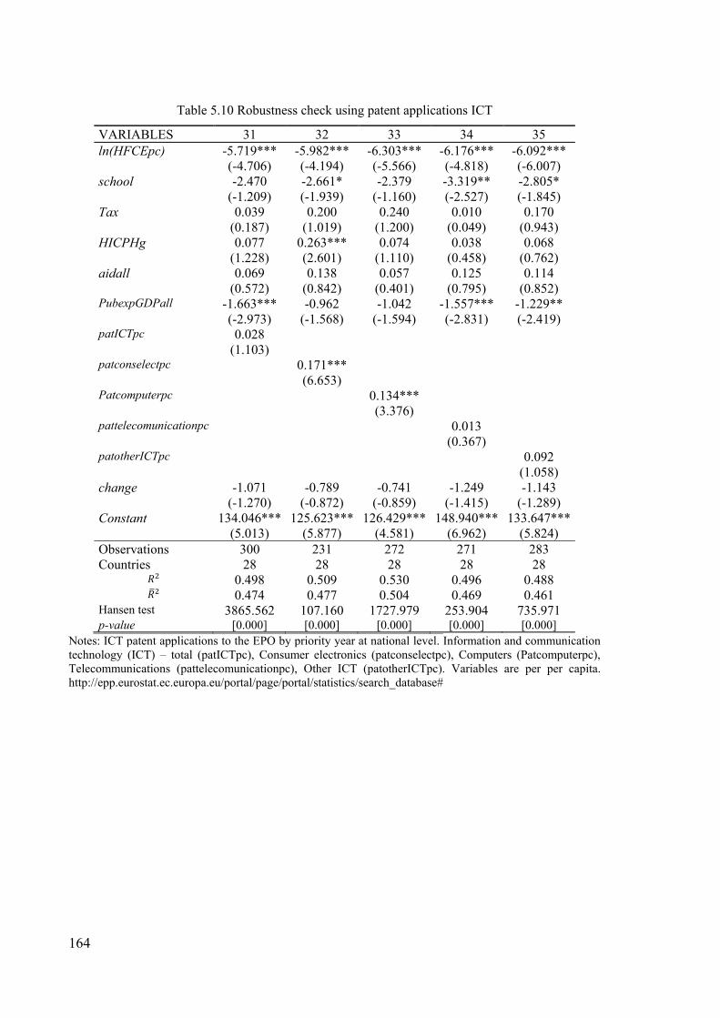
164

Table 5.10 Robustness check using patent applications ICT

VARIABLES 31 32 33 34 35 ln(HFCEpc) -5.719*** -5.982*** -6.303*** -6.176*** -6.092*** (-4.706) (-4.194) (-5.566) (-4.818) (-6.007) school -2.470 -2.661* -2.379 -3.319** -2.805* (-1.209) (-1.939) (-1.160) (-2.527) (-1.845) Tax 0.039 0.200 0.240 0.010 0.170 (0.187) (1.019) (1.200) (0.049) (0.943) HICPHg 0.077 0.263*** 0.074 0.038 0.068 (1.228) (2.601) (1.110) (0.458) (0.762) aidall 0.069 0.138 0.057 0.125 0.114 (0.572) (0.842) (0.401) (0.795) (0.852) PubexpGDPall -1.663*** -0.962 -1.042 -1.557*** -1.229** (-2.973) (-1.568) (-1.594) (-2.831) (-2.419) patICTpc 0.028 (1.103) patconselectpc 0.171*** (6.653) Patcomputerpc 0.134*** (3.376) pattelecomunicationpc 0.013 (0.367) patotherICTpc 0.092 (1.058) change -1.071 -0.789 -0.741 -1.249 -1.143 (-1.270) (-0.872) (-0.859) (-1.415) (-1.289) Constant 134.046*** 125.623*** 126.429*** 148.940*** 133.647*** (5.013) (5.877) (4.581) (6.962) (5.824) Observations 300 231 272 271 283 Countries 28 28 28 28 28

0.498 0.509 0.530 0.496 0.488 0.474 0.477 0.504 0.469 0.461


Notes: ICT patent applications to the EPO by priority year at national level. Information and communication technology (ICT) – total (patICTpc), Consumer electronics (patconselectpc), Computers (Patcomputerpc), Telecommunications (pattelecomunicationpc), Other ICT (patotherICTpc). Variables are per per capita. http://epp.eurostat.ec.europa.eu/portal/page/portal/statistics/search_database#

165

The ISCED classification

The International Standard Classification of Education (ISCED) was designed by

UNESCO in the early 1970’s to serve “as an instrument suitable for assembling, compiling

and presenting statistics of education both within individual countries and internationally”.

The present classification, now known as ISCED 1997, was approved by the UNESCO

General Conference at its 29th session in November 1997. With this method it is possible to

compare statistics on education in different countries worldwide.

This classification is divided into six categories:

ISCED 0- Pre-primary education

ISCED 1- Primary education or first stage of basic education

ISCED 2- Lower secondary or second stage of basic education

ISCED 3- Upper secondary education

ISCED 4- Post-secondary non-tertiary education

ISCED 5- First Stage of tertiary education

ISCED 6- Second Stage of tertiary education.

Each of these categories is characterized by being progressive; each additional level

represents more complex subjects taught. When this methodology was implemented, and to

facilitate a more detailed analysis within each level of education, some levels were

disaggregated. For example the ISCED 3 was divided into 3A, 3B and 3C. Some of these

would lead directly to the labor market. Each level has variable proxy’s that make possible

its calculation; for example, the main criteria for determining the ISCED 6 is the ability to

make research-oriented content and submission of thesis or dissertation, the subsidiary

criteria is the ability to prepare graduates for faculty and research posts. We now define each

level of the ISCED level.

- ISCED 0, (pre-primary) is the initial stage of organized instruction; it is designed

primarily to introduce very young children to a school-type environment. One example

is the kinder garden.

- ISCED 1 is designed to give students a sound basic education in reading, writing and

mathematics along with an elementary understanding of other subjects such as history,

geography, natural science, social science, art and music. In some cases religious

166

instruction is featured. Example of this is the primary education that, in many cases

represents 4 years of schooling.

- ISCED 2 is designed to complete the provision of basic education which began at

ISCED 1. The educational aim is to lay the foundation for lifelong learning and human

development on which countries may expand, systematically, further educational

opportunities. The programmes at this level are usually on a more subject-oriented

pattern using more specialized teachers and more often several teachers conducting

classes in their field of specialization. This level of education sometimes coincides

with the compulsory education.

- ISCED 3 begins after the compulsory education. The entrance age to this level is

typically 15 or 16 years. The educational programmes included at this level typically

require the completion of some 9 years of full-time education (since the beginning of

level 1) for admission or a combination of education and vocational or technical

experience and with as minimum entrance requirements the completion of level 2.

- ISCED 4 captures programmes that straddle the boundary between upper-secondary

and post-secondary education from an international point of view, even though they

might clearly be considered as upper-secondary or post-secondary programmes in a

national context.

- ISCED 5 level or tertiary programmes are characterized by a theoretical background

that will serve for the labor market in future. Depending on the areas, it can range from

4 to 6 years of schooling. Some areas will allow an internship in the final year to apply

the theory learned. This level of education will allow the progression to level 6 that is

a research program.

- ISCED 6 is reserved for tertiary programmes which lead to the award of an advanced

research qualification. The programmes are therefore devoted to advanced study and

original research and are not based on course-work only (examples of these are the

Master and PhD programs; some have subjects that will help the future research).

Source: Unesco. International Standard Classification of Education I S C E D 1997.

Unesco Institute for Statistics. May 2006, Re-edition

This methodology suffers some deficiencies; the disaggregation is small which can

limit international comparisons, for example at a university level. This methodology has 16

167

years, in 2011 it was published an improvement to this classification with the ISCED 2011.

Unfortunately for an econometric analysis we must use the old methodology. International

organization such as the EUROSTAT, World Bank and OECD will implement these new

measures. It is expected that the first international education data collections using ISCED

2011 will begin in 2013 or 2014.

The new ISCED 2011 levels will be disaggregated into:

ISCED 0- Less than primary

ISCED 1- Primary

ISCED 2- Lower secondary

ISCED 3- Upper secondary

ISCED 4- Post-secondary non-tertiary

ISCED 5- Short-cycle tertiary

ISCED 6- Bachelor or equivalent

ISCED 7- Master or equivalent

ISCED 8- Doctoral or equivalent

ISCED 9- Not elsewhere classified

This new classification will allow an in deep analysis of the different levels of

education, at the university level, allowing international comparisons. Previous ISCED level

included many types of education in the same level, unfortunately, even in the ISCED 1997

classification, financial indicators for each dimension is not available (e.g. ISCED 1,2,3

separately).

169

Chapter 6 Economic growth and software piracy

171

6.1 Introduction

The literature on software piracy, which can be seen as a subgroup of studies about

Intellectual Property Rights (IPR, henceforth), has focused either in studying its

determinants or its impact on economic growth.

Examples of the studies that focused on the determinants are: Shadlen et al. (2005)

which studied if the level of software protection and also if international mechanisms, such

as Copyright laws, can mitigate piracy. They analyze the direct pressures exerted by the US

(US Special 301107), for the foreign countries to increase or to exert more efficiently IPR

protection. Lack of enforcement of Bilateral Political Pressures, TRIPS108 and Trade

dependence on US can explain the levels of piracy in these countries. Others authors, such

as (Andrés (2006a); Goel and Nelson (2009)) have done more comprehensive studies (see

also Chapter 3 Summing up, these authors found that economic dimensions measured by

the introduction of GDP have a negative impact on piracy; higher income leads to less piracy.

In terms of the impact on economic growth, most of the empirical literature has

focused not specifically on software piracy but on the impact of IPR protection on Economic

growth (Falvey et al., 2006; Gould & Gruben, 1996; Park & Ginarte, 1997). From these

studies we can conclude that IPR protection favors economic growth, being this impact

slightly higher on more open economies. Also IPR protection appears to favor low and

higher income economies while in the middle-income countries this is not necessarily true.

Exceptions to this holistic type of analysis are the works of Andrés and Goel (2012) and

Rodriguez-Montemayor (2013),which focused specifically on the effects of software piracy.

Andrés and Goel (2012) found that software piracy rates affected positively economic

growth. Rodriguez-Montemayor (2013) considered the effect of genuine and unlicensed

software on income. When both variables were considered separately they had a positive

impact, but when both were introduced simultaneously the unlicensed software reduced the

107 The Special 301 Report is prepared annually by the Office of the United States Trade Representative (USTR) under Section 301 as amended of the Trade Act of 1974. The reports identify trade barriers to US companies and products due to the intellectual property laws, such as copyright, patents and trademarks, in other countries. Each year the USTR must identify countries which do not provide "adequate and effective" protection of intellectual property rights or "fair and equitable market access to United States persons that rely upon intellectual property rights".

108 Agreement on Trade-Related Aspects of Intellectual Property Rights

172

income of the country However, up to our knowledge, these two approaches have not been

combined. As is referred in several papers, software piracy has an effect on growth, but

growth is one of the determinants of software piracy. This chapter will try to bridge that gap

by estimating simultaneous the two effects and measure the effect of piracy on growth and

vice-versa.

To answer these questions we used data from the official publications of the

Business Software Alliance (BSA), World Development Indicators (WDI) and Barro and Lee

(2013). A simultaneous equation approach (3SLS) for the years 1995, 2000, 2005 and 2010,

comprising 75 countries will be used in the analysis.

This chapter is organized as follows: section 6.2 presents the variables and

econometric specification; section 6.3 presents the empirical work. Finally, section 6.4

concludes.

173

6.2 Data and Econometric Specification

Many factors can affect the economic growth of a country, especially innovation in

the form of investment (gross capital formation), consumption (GDPpc) and protection of

inventions (patents and trademarks). Other variables such as the software piracy in a country

can also have negative impact on growth, as potential software sales are lost. On the other

hand, the existence of some piracy can have a positive effect on growth as workers

productivity may increase, due to access to more software tools. One of the determinants of

software piracy is the national income of a country and, in this perspective; economic growth

may have a role in this impact. To take into account this simultaneity (e.g. piracy affects

economic growth and vice-versa) we will consider a system of equations that can explain

this phenomenon.

We will use the 3SLS estimator which is suited when we have a system of structural

equations in which one of them include one or more endogenous variables among the

explanatory variables (Zellner & Theil, 1962). Another advantage of the 3SLS is that it is

more efficient to capture the interrelation between equations and the causal and feedback

effects between the variables (AlDakhil, 1998; Wooldridge, 2010).

To construct our model, we retrieved our data from the Word Development

Indicators (WDI)109 of the World Bank, the official publications of the Business Software

Alliance110 and for the educational dimension we retrieved data on schooling years of the

Barro and Lee (2013) dataset111 for 1995, 2000, 2005 and 2010; for a total of 75 countries.

Our model is defined in equation 6.1 and 6.2.

6.1

Z (6.2)

109 Available at http://data.worldbank.org/data-catalog/world-development-indicators ; these correspond to the control variables 110 The values of Software Piracy Rates 111 Data available at http://www.barrolee.com/data/dataexp.htm

174

The dependent variables are the GDP growth per capita ( ), and the

software piracy rates measured in percentage ( ). The vector represents the control

variables in the growth equation and the vector Z the control variables in the piracy rate

equation; these are explained in the following subsection.

The software piracy rates (BSA, 2003, 2011) measures the percentage of unlicensed

software that is used illegally and, as explained before, its effect on growth is dubious.

In economic growth it is common to use five years’ intervals to prevent results

being affected by business cycles (Barro & Sala-i-Martin, 2003, p. 534). In 2002/2003

occurred a change of the methodology used by the Business Software Alliance to compute

piracy rates (Png, 2010). As with previous studies, we also consider five period time spans

leaving two periods before and after the change in methodology. When implementing the

econometric specification, the dataset is reduced to three time periods. In our model we also

introduce country dummies represented by and also time dummies. Regarding variable

indexes, i represents the countries, t the time periods and represents the error terms. is

the first difference operator.

Economic growth equation

Equation 6.3 shows the main determinants of economic growth, extending the

neoclassical growth model that is a function of capital and labor (Solow, 1956). In our model

the growth equation is a function of several variables.

5.

(6.3)

i=1,…,75 and t=2000,2005,2010

175

We introduce the GDP per capita112 ) lagged five periods that is measured

at 2005 constant prices. It is expected to have a negative effect based on the results of Romer

(1990). In Economic growth we have absolute convergence when poorer economies growth,

in per capita terms, faster than richer economies (Barro & Sala-i-Martin, 2003, p. 45). We

will test this hypothesis against different groups of countries. To test this absolute

convergence, we will also use a dummy variable DEV which takes the value 1 if it is a low

or a lower-middle-income country and zero otherwise.

Another variable introduced is the gross capital formation growth ( ) measured

at constant prices. It is expected to promote growth following, between others, Goel and

Ram (1994).

We also include the growth rate of labor force ( ). This variable can have mixed

results (Aiginger, 2005) and labor policies can also affect economic growth. It can affect

positively economic growth because less inactive persons are in the economy. Less social

contributions in the form of subsidies to unemployed will be paid. Furthermore, these

workers will have more money to spend on the economy. On the other side this variable can

affect negatively economic growth because an overwhelming supply of labor force can drive

salaries down, following the law of demand and supply. This will lead to less disposable

income of workers. Also, more workers can increase pressure on the countries resources and

have a detrimental effect on growth.

Inflation rate (inflation) may affect economic growth. This variable has been found

to negatively affect economic growth (Barro, 2013b). It represents the evolution of prices

over the years.

The export growth ( Export) of goods and services indicates how the national

economy is performing. Andraz and Rodrigues (2010) analyzed the impact on exports for

the Portuguese economy over the period of 1977 to 2004. Results show that exports increase

economic growth in the long run.

A variable that reflects access to digital content is the Internet users (Net). This

variable indicates the level of access to the World Wide Web (WWW) measured per 100

people. More access to information will increase the consumption of digital goods that will

increase national income (C. Choi & Hoon Yi, 2009; Clarke, 2008). Additional to this we

112 This variable takes into account purchase power parity

176

will introduce broadband access (FBIS), mobile cellular subscriptions (Mobile) and

telephone users (Phone).

Human capital can affect economic growth and, in fact, Barro (2013a) found that it

had a positive effect on economic growth. In our model we consider the total effective year

of schooling that students have, considering a broad age group of people with age 15 and

over (school) (Barro & Lee, 2013). More schooling years indicates that employees can be

more productive with the same limited resources.

Software piracy equation

The equation (6.4) describes the macroeconomic determinants of software piracy.

ln ln

(6.4)

It is a result of the sum of dimensions that represent economic aspects, access to

information, educational and variables that describe technological dimensions.

6.2.2.1 Economic dimension

Several measures of income were considered in previous studies. Goel and Nelson

(2009) considered the GDPpc having a deterrent effect on piracy. Another measured

considered using a sample of European Countries (EU 27) in Chapter 4 was the .

This variable had a positive effect but was not significant. Using a panel of 75 countries for

1995, 2000 and 2002; Bezmen and Depken (2005) also found a positive relationship between

and software piracy.

177

6.2.2.2 Access to information

Access to information measures the availability of digital content and is represented

by the variables Net, FBIS, Phone, Mobile that will affect the availability of software (both

legal and illegal). It is expected to affect negatively piracy based on the results of Goel and

Nelson (2009), Boyce (2011) and in Chapter 3

6.2.2.3 Educational dimension

The educational dimension is represented by the number of effective schooling

years in a country (school) (Barro & Lee, 2013) (the same as in the growth equation). More

schooling years indicate that students are aware of the consequences of using digital content

in an illicit way. Nevertheless, they may seek this content. Previous authors found that this

dimension affects negatively piracy in a country using different variables. Years of schooling

of population age 25 and over have a negative effect, without significance (Andrés, 2006b).

This variable is only available in 5 years’ time periods. Extending this result in Chapter 3

we used the years of schooling offered in a country that was also found to have a negative

impact on piracy, being significant.

6.2.2.4 Technological dimensions.

The final dimension considered is the technological one; we introduce the patents

and trademark applicants done both by residents and non-residents. A trademark is a result

of a distinctive sign that identifies a specific product; can represent letters, symbols,

drawings, etc. It is sought in order to prevent unfair competition113 by competitors. A patent

is an exclusive right granted for an invention, which is a product or a process that provides,

in general, a new way of doing something, or offers a new technical solution to a problem.

In both cases these types of protection can be sought by the residents of a country that offers

113 Unfair competition in a sense means that the competitors compete on unequal terms, because favorable or disadvantageous conditions are applied to some competitors but not to others; or that the actions of some competitors actively harm the position of others with respect to their ability to compete on equal and fair terms.

178

protection, but can also be sought by foreigners that want the protection of their products

abroad. We use these variables per capita in natural logarithms.

Total patents ln(Patpc) is a result of the sum of patents done by residents and by

non-residents. In the same way total trademarks ln(Tradpc) is the result of the sum of

trademark applicants from residents and non-residents. Both variables were retrieved from

the WDI of the World Bank and are measured in per capita terms. It is expected that these

variables can affect software piracy in a country (based on Chapter 3 although the signs can

be mixed.

Table 6.1 presents the basic summary statistics of the variables used.

Table 6.1 Summary statistics all sample

Variable Obs. Mean Std. Dev. Min. Max. Endogenous variables

GDPpc 297 0.0341 0.0328 -0.1150 0.1374 PR 273 0.5986 0.2106 0.2 0.99 Exogenous variables

GDI 295 .0786 0.127 -.424 0.752 GDPpc 298 15451.88 12144.47 813.35 52313.91

Lab 300 0.0133 0.0176 -0.0454 0.0611 Inflation 294 0.1037 0.3022 -0.0370 3.7675

Export 295 0.1048 0.0973 -0.518 0.89 Net 293 24.89 27.05 0.0001 95 Phone 299 28.68 20.11 0.24 73.04 FBIS 195 8.60 10.54 0 37.99 Mobile 300 51.43 47.38 0 195.57 School 300 8.81 2.33 1.62 13.1

273 0.4026 0.2520 0.04 0.98 ln(Tradpc) 285 -6.99 1.15 -10.32 -3.64 ln(Patpc) 275 -9.11 1.63 -13.32 -5.67 DEV 300 0.24 0.43 0 1


179

6.3 Empirical Application

Empirical evidence

This section presents the empirical results of the growth equation (see equation 1)

and the piracy rate equation (see equation 2) using the 3SLS. In the empirical analysis we

introduced country and time dummies to take into account our panel data.

In the growth equation we introduced the initial GDP measured by the L5.GDPpc,

without significance. In Model 2 and 4 we introduce an alternative measure of income on

the growth equation. DEV is a dummy variable that represents low income and lower-

middle-income countries based on the division of the WDI. We found evidence of absolute

convergence (due to the significance of DEV), which indicates that poor economies growth

faster, in per capita terms, than advanced economies. GDPpcg represents the economic

dimension in the piracy rate equation. Results show that more income growth leads to more

piracy because the software market is more mature, e.g., there are more products available

to sell in stores and online retailers. This is a robust result, being always significant at 1%.

Regarding gross domestic investment results show that, as expected, it affects

positively economic growth, being significant at 1% across specifications.

As Andrés and Goel (2012) some of our results show that the growth of the labor

force results in lower economic growth (model 2 and 4). However, not only the result is not

robust across equations, but it is never statistically significant.

Another important variable that can affect the growth is the inflation that a country

has annually. A high level of inflation, which indicates an overall increase in prices, will

have a negative effect on household consumptions, has their disposable income is reduced

by this phenomenon, decreasing their standard of living (Barro, 2013b). It was expected that

this variable had a negative effect on growth and a positive effect on software piracy.

However, although the point estimations were positive in both models, they were never

statistically significant.

We also considered the effect of exports of goods and services ( Export). Exports

represent the importance of goods and services that are produced nationally, and sold to the

rest of the world. As expected it has a positive effect (Andraz & Rodrigues, 2010) being

significant. More production of goods such as merchandize or services will increase profits

180

of firms, which will offer more work to the nationals that, in turn, will increase national

income.

Four measures that represent access to digital content were introduced in the growth

equation (Net, Mobile, Phone and FBIS). All these variables measure the usage per 100

inhabitants.

We can observe that these variables can affect economic growth in two ways. The

first way represents a positive impact: more access to information leads to increase

productivity as people will seek better ways to do their jobs, and more consumption of digital

goods (C. Choi & Hoon Yi, 2009; Clarke, 2008) which is represented by the access to

broadband (FBIS) variable. The other effect that Internet users have is a negative one: as

more users access at the same time the network, they will decrease the overall Internet traffic

speeds which will potentially lower productivity. This negative effect can be seen especially

on firms that need the Internet to work on a daily basis such as online retail stores, consulting

and distribution of digital content such as games, movies or music. This negative effect is

represented by the access to the Internet (Net) variable. Results are surprising and suggest

that, for attaining a sustainable growth, it is necessary good infrastructures, but these must

represent quality. In our case the simple access to the Internet is not sufficient to attain

growth; it is necessary broadband access. Both variables are robust.

These variables also affect the piracy rate equation. They represent access to

information dimension. Results shows that having the ability to search digital content don’t

necessarily mean that people will seek illegal software. Although even people that always

sought legal software can seek illegal content at some point in their life. This result indicates

that infrastructures that can seek potential pirates are well developed and that they are used

efficiently by national Governments.

Results show that the education offered by a country has a positive effect on

economic growth, results also obtained by Barro (2013a). This indicates that more years of

schooling will lead to higher productivity. To assess the impact of education on the piracy

rate equation, we also introduced total years of schooling (school). This variable has a

negative impact on piracy (reduces piracy). However in both cases the estimator was not

significant. A negative impact was found by Andrés (2006b) using a cross-sectional data

181

analysis. Other measures exist such as literacy rate (see Goel and Nelson (2009)), and

education expenditure (see Chapter 5

To see the impact of piracy on economic growth we introduced the piracy rate (PR)

and squared PR. We found a negative coefficient on the quadratic term of the piracy rate,

thus indicating a concave relation between PR and growth. As can be seen in Annex XV,

until a certain level of piracy it will promote economic growth but at a diminishing rate,

achieving a maximum around 80%. From this level onwards, increases in PR will lead to

smaller levels of economic growth. This indicates that the potential benefits of using illegal

software to the economy due to a marginal increase in PR will be smaller as PR increases

and eventually they will be overtaken by losses. Our results are opposed to the ones found

by Andrés and Goel (2012), who found a convex relationship. However we should note that

these authors used a cross sectional approach, which does not consider the time dimension,

which is captured in our approach.

Finally we also introduced in the piracy rate equation a dimension that measures

technological development in a country. The benefits of a higher level of protection can be

seen in the negative effect of trademarks, being significant at 1%. Firms may seek on national

and international Intellectual Property Office protection for their products (brands, logos,

drawings) and due to the high value added that they bring to the economy they are protected.

Another variable in this dimension that was introduced was the patent applicants. A patent

occurs when an innovation is present on a product that can differentiate it against other

products. One example of an innovation is a new process that can be implemented that will

increase units produced with the same amount of resources. We also have a negative impact

on this variable, although statistically insignificant. These results indicate that national and

international Intellectual Property Rights Offices appear to protect well both trademarks and

patents, although only the first is significant.

182

Table 6.2 3SLS regressions

Model 1 Model 2 Model 3 Model 4 VARIABLES 1 2 3 4 5 6 7 8 GDPpc PR GDPpc PR GDPpc PR GDPpc PR

GDPpc 0.9813*** 1.0473*** 0.9737*** 1.0184*** (0.2048) (0.2061) (0.2006) (0.1971) L5.GDPpc -0.000001 -0.0000001 (0.0000) (0.0000) DEV -0.4160*** -0.3798*** (0.1109) (0.0887)

GDI 0.0779*** 0.0824*** 0.0779*** 0.0829*** (0.0168) (0.0165) (0.0176) (0.0172)

Lab 0.0339 -0.0361 0.0463 -0.0286 (0.1554) (0.1468) (0.1622) (0.1542) Inflation 0.0398 0.0378 0.0432 0.0408 (0.0394) (0.0377) (0.0409) (0.0392)

Export 0.1119*** 0.1084*** 0.1148*** 0.1121*** (0.0319) (0.0301) (0.0325) (0.0303) Net -0.0006* 0.0003 -0.0006* 0.0003 (0.0003) (0.0005) (0.0003) (0.0005) Phone -0.0003 -0.0008 -0.0002 -0.0008 (0.0005) (0.0007) (0.0005) (0.0007) FBIS 0.0012** -0.0025*** 0.0008 -0.0019*** 0.0013** -0.0026*** 0.0009* -0.0020*** (0.0006) (0.0008) (0.0005) (0.0007) (0.0006) (0.0008) (0.0005) (0.0007) Mobile -0.0001 -0.0005** -0.0002 -0.0004** -0.0001 -0.0005*** -0.0002 -0.0005** (0.0002) (0.0002) (0.0002) (0.0002) (0.0002) (0.0002) (0.0002) (0.0002) School 0.0051 -0.0033 0.0037 -0.0055 0.0045 -0.0038 0.0035 -0.0055 (0.0075) (0.0117) (0.0074) (0.0118) (0.0079) (0.0117) (0.0078) (0.0117) PR 1.9232*** 1.9846*** 2.0492*** 2.0805*** (0.4706) (0.4555) (0.4733) (0.4426)

-1.1991*** -1.2273*** -1.2744*** -1.2862*** (0.3744) (0.3570) (0.3802) (0.3506) ln(Tradpc) -0.0382*** -0.0413*** -0.0383*** -0.0416*** (0.0129) (0.0124) (0.0129) (0.0123) ln(Patpc) -0.0066 -0.0081 -0.0069 -0.0081 (0.0053) (0.0053) (0.0052) (0.0052) correlation -0.64761 -0.66758 -0.64759 -0.6622 Observations 172 172 173 173 173 173 174 174 R-squared 0.234 0.981 0.196 0.981 0.179 0.981 0.153 0.981

Standard errors in parentheses, *** p<0.01, ** p<0.05, * p<0.1. Correlation is the correlation errors of equation 1 and 2.

183

6.4 Conclusion

This chapter analyzed the effect of software piracy on economic growth. To

implement this analysis it was introduced a system of equation using the 3SLS for a large

panel of countries for which information on software piracy was available (1995, 2000, 2005

and 2010 spanning 75 countries). This allowed us to control simultaneously the two

reciprocal problems, e.g., software piracy affect economic growth combined with the effect

of economic growth on piracy.

We found that access to the digital economy through Internet access is not sufficient

to promote growth; broadband access must be made available to the population in order to

foster growth. Variables regarding access to information negatively affected software piracy

rates.

We analyzed the nonlinear relationship of piracy on economic growth with the

introduction of the square of this variable. Results showed that there is evidence of a concave

relationship between piracy rates and economic growth. For lower levels of piracy rate, a

marginal increase on it will increase the growth rate, however this increase will be smaller

the bigger is the level piracy rate, and from around 80% marginal increases in PR will lead

to smaller levels of economic growth. This indicates that the potential benefits of using

illegal software to the economy due to a marginal increase in PR will be smaller as PR

increases and eventually they will be overtaken by losses.

184

Relationship between piracy and growth

Figure 6.1 Concave relationship in model 1


0

0,1

0,2

0,3

0,4

0,5

0,6

0,7

0,8

0,9

1 5 9

13

17

21

25

29

33

37

41

45

49

53

57

61

65

69

73

77

81

85

89

93

97

101

GD

Ppc

gro

wth

Piracy Rate

Concave relationship Model 1

0

0,1

0,2

0,3

0,4

0,5

0,6

0,7

0,8

0,9

1 5 9

13

17

21

25

29

33

37

41

45

49

53

57

61

65

69

73

77

81

85

89

93

97

101

GD

Ppc

gro

wth

Piracy Rate


185



0

0,1

0,2

0,3

0,4

0,5

0,6

0,7

0,8

0,9

1 5 9

13

17

21

25

29

33

37

41

45

49

53

57

61

65

69

73

77

81

85

89

93

97

101

GD

Ppc

gro

wth

Piracy Rate


0

0,1

0,2

0,3

0,4

0,5

0,6

0,7

0,8

0,9

1 5 9

13

17

21

25

29

33

37

41

45

49

53

57

61

65

69

73

77

81

85

89

93

97

101

GD

Ppc

gro

wth

Piracy Rate


187

Chapter 7 Final Conclusions

189

This work tried to study the main macroeconomic determinants of software piracy.

The main objective was to provide a comprehensive understanding of the software piracy

phenomenon, first with a global approach using all countries for which information on

software piracy data is available, then analyzing a specific region, the European Union. Our

work departs from previous empirical literature in the sense that we provide a cross country

time series approach to the problem from a large time span as opposed to simple cross

sectional data.

Empirical literature on this specific topic is still relatively new, and due to data

restrictions on certain dimensions, the majority of studies opted for a cross country analysis.

The objective of Chapter 1 was to provide an introduction to the problem of

software piracy and its relevance for the economy and the benefits in its reduction.

The main objective of Chapter 2 was to provide a detailed summary of previous

empirical findings, systematizing them on stylized facts that were used in subsequent

chapters. Literature only focused on systematizing theoretical works; our major contribution

was in systematizing empirical ones. The major difficulty faced here was on the proliferation

of methodologies and results found by different areas of studies that made difficult a

systematization of results in the field of economics.

Chapter 3 used results from some stylized facts encountered in Chapter 2

expanding it to new variables. The main focused was on the determinants of software piracy

losses, the methodology used was the System GMM because the dataset was persistent over

the years. When determining the causes of software piracy it was taken into account the

break in the series occurred in 2002/2003 that was a result of the change in methodology to

compute software piracy. The major macroeconomic dimensions that represented labor

force, technological, educational and access to information and institutional dimensions

were significant, and could explain this phenomenon. Although the methodology was

appropriate for this analysis, a detailed comparison of continents and levels of developments

were not possible. Future empirical work must take into account whenever possible the

different realities of countries and the division of continents present in the official

publications.

190

After establishing that these macroeconomic determinants were significant we

proceeded our analysis for the European Union. A more detailed analysis on variables was

available on the Eurostat website which were used in the subsequent chapters.

Chapter 4 described the effects that taxation can have on several typical households

of the European Union. We also used the Software piracy losses as a dependent variable, but

in this case, due to small number of observations, we used the fixed effect model that was

also found to be appropriate when analyzing this phenomenon of Europe (Andrés, 2006a).

Results showed that taxation had a positive effect on software piracy but affecting differently

the households. To further assess our results we split our sample into Old Countries (15

European Countries) and the Euro Zone (17 European Countries). Results were only

significant on the New countries (12 European Countries) and outside the Euro Zone (10

European Countries). These results can be used by the European Commission and the

European Patent Office when assessing and promoting policies to reduce piracy and the use

of other illicit content, even one based on hardware.

We also choose to analyze the determinants of software piracy in the European

Union, focusing on the effects that education expenditure has on piracy in a county in

Chapter 5 We introduced software piracy rates as a dependent variable. Several estimations

were possible but we choose the fixed effects as with the previous chapter. Two measures of

expenditure were introduced, public expenditure on education, measured as a share of GDP,

that comes from national Governments budgets and also the expenditure that is made on

private and public educational institutions measured as a percentage of GDPpc. Another

measure was introduced that reflected the financial aid to students as a share of GDP. Results

showed that more expenditure on education considering all ISCED levels will reduce

software piracy. A detailed analysis was made considering a detailed disaggregation based

on the different ISCED levels; results showed that more expenditure on ISCED 5-6, will

reduce piracy. The other dimension introduced that measured the financial aid to students

had a positive impact on piracy. These results indicate that for reducing piracy, resources

must be better allocated, for example trough funds that come from the European Union.

Both Chapter 4 and Chapter 5 presented a detailed analysis with a detailed

disaggregation of variables measuring household taxation and educational expenditure.

191

Having established the major macroeconomic dimensions in the previous chapters

we provided a detailed analysis of the effects of piracy on economic growth in Chapter 6

We implemented a panel data analysis using 3SLS (3 Stage Least Squares). New

technologies can improve productivity but lack of protection can result in less investment

because software companies have less incentive to invest because returns of their investment

on R&D will be smaller. Results show that software piracy will reduce economic growth.

One possible limitation was that with this methodology it was not possible to divide the

sample into the different continents. Future empirical works studying the effects of this illicit

behavior on economic growth must take into account this disaggregation.

Overall, this thesis makes a substantial contribution to the empirical literature in the

sense that it provides the major determinants of software piracy considering a large time

span and large country sample. This work can also be used as the foundation of future

theoretical works focusing on policy implications of several actions that policymakers can

choose. It also provides the baseline requirements to construct an index that can be used to

measure the illicit behavior in the subject of the digital economy, namely software piracy.

193

References

Sixth Council Directive 77/388/EEC of 17 May 1977 on the harmonization of the laws of

the Member States relating to turnover taxes - Common system of value added tax:

uniform basis of assessment.

90/434/EEC, C. D. (1990). Council Directive 90/434/EEC of 23 July 1990 on the common

system of taxation applicable to mergers, divisions, transfers of assets and exchanges

of shares concerning companies of different Member States Official Journal L 225 ,

20/08/1990 P. 0001 - 0005 Retrieved from http://eur-

lex.europa.eu/LexUriServ/LexUriServ.do?uri=CELEX:31990L0434:en:HTML.

90/435/EEC, C. t. C. D. (1997). Corrigendum to Council Directive 90/435/EEC of 23 July

1990 on the common system of taxation applicable in the case of parent companies

and subsidiaries of different Member States (Official Journal of the European

Communities No L 225 of 20 August 1990). Official Journal of the European

Communities Retrieved from http://new.eur-lex.europa.eu/legal-

content/EN/TXT/?uri=OJ:L:1997:016:TOC.

Convention on the elimination of double taxation in connection with the adjustment of

profits of associated enterprises - Final Act - Joint Declarations - Unilateral

Declaracions.

Communication from the commission to the council, the European parliament and the

economic and social committee: tax policy in the European Union priorities for the

years ahead. (2001).

331, C. (2010). COUNCIL DIRECTIVE amending Directive 2006/112/EC on the common

system of value added tax, with regard to the duration of the obligation to respect a

minimum standard rate.

Council Regulation (EC) No 1260/1999 of 21 June 1999 laying down general provisions on

the Structural Funds.

Council Regulation (EC) No 1383/2003 of 22 July 2003 concerning customs action against

goods suspected of infringing certain intellectual property rights and the measures to

be taken against goods found to have infringed such rights (2003).

194

Council Regulation (EC) No 1783/1999 of the European Parliament and the Council of 12

June 1999 on the European Regional Development Fund.

Council Regulation (EC) No 1784/1999 of the European Parliament and the Council of 12

July 1999 on the European Social Fund.

DIRECTIVE 2004/48/CE DU PARLEMENT EUROPÉEN ET DU CONSEIL DU 29

AVRIL 2004 RELATIVE AU RESPECT DES DROITS DE PROPRIÉTÉ

INTELLECTUELLE (Texte présentant de l’intérêt pour l’EEE) (2004).

Council Directive 2006/112/EC of 28 November 2006 on the common system of value added

tax (2006).

Aiginger, K. (2005). Labour market reforms and economic growth - the European experience

in the 1990s. Journal of Economic Studies, 32(6), 540-573. doi:

http://dx.doi.org/10.1145/962081.962088

Ajzen, I. (1991). The theory of planned behavior. Organizational Behavior and Human

Decision Processes, 50(2), 179-211. doi: http://dx.doi.org/10.1016/0749-

5978(91)90020-T

Al-Rafee, S., & Rouibah, K. (2010). The fight against digital piracy: An experiment.

Telematics and Informatics, 27(3), 283-292. doi:

http://dx.doi.org/10.1016/j.tele.2009.12.002

AlDakhil, K. (1998). A method for estimating simultaneous equations models with time-

series and cross-section data. Journal of King Saud University - Administrative

Sciences, 10(1), 13-28.

Altinkemer, K., & Guan, J. (2003). Analyzing Protection Strategies for Online Software

Distribution. . J. Electron. Commerce Res., 4(1), 34-48.

Anckaert, B., Sutter, B. D., & Bosschere, K. D. (2004). Software piracy prevention through

diversity. Paper presented at the Proceedings of the 4th ACM workshop on Digital

rights management, Washington DC, USA.

Andraz, J. M., & Rodrigues, P. M. M. (2010). What causes economic growth in Portugal:

exports or inward FDI? Journal of Economic Studies, 37(3), 267-287.

195

Andrés, A. R. (2006a). The relationship between copyright software protection and piracy:

Evidence from europe. European Journal of Law and Economics, 21(1), 29-51. doi:

http://dx.doi.org/10.1007/s10657-006-5670-5

Andrés, A. R. (2006b). Software piracy and income inequality. Applied Economics Letters,

13(2), 101-105. doi: http://dx.doi.org/10.1080/13504850500390374

Andrés, A. R., & Goel, R. K. (2011). Corruption and Software Piracy: A Comparative

Perspective. Policy & Internet, 3(3), 1-22. doi: http://dx.doi.org/10.2202/1944-

2866.1088

Andrés, A. R., & Goel, R. K. (2012). Does software piracy affect economic growth?

Evidence across countries. Journal of Policy Modeling, 34(2), 284-295. doi:

http://dx.doi.org/10.1016/j.jpolmod.2011.08.014

Arellano, M. (1993). On the testing of correlated effects with panel data. Journal of

Econometrics, 59(1–2), 87-97. doi: http://dx.doi.org/10.1016/0304-4076(93)90040-

C

Arellano, M., & Bond, S. (1991). Some Tests of Specification for Panel Data: Monte Carlo

Evidence and an Application to Employment Equations. The Review of Economic

Studies, 58(2), 277-297. doi: http://dx.doi.org/10.2307/2297968

Arellano, M., & Bover, O. (1995). Another look at the instrumental variable estimation of

error-components models. Journal of Econometrics, 68(1), 29-51. doi:

http://dx.doi.org/10.1016/0304-4076(94)01642-D

Bae, S. H., & Choi, J. P. (2006). A model of piracy. Information Economics and Policy,

18(3), 303-320. doi: http://dx.doi.org/10.1016/j.infoecopol.2006.02.002

Banerjee, D., Khalid, A. M., & Sturm, J.-E. (2005). Socio-economic development and

software piracy. An empirical assessment. Applied Economics, 37(18), 2091-2097.

doi: 10.1080/00036840500293276

Banerjee, D. S. (2003). Software piracy: a strategic analysis and policy instruments.

International Journal of Industrial Organization, 21(1), 97-127. doi:

http://dx.doi.org/10.1016/S0167-7187(01)00090-X

196

Banerjee, D. S. (2011). On the sufficiency of regulatory enforcement in combating piracy.

Journal of Regulatory Economics, 40(2), 160-176. doi:

http://dx.doi.org/10.1007/s11149-011-9154-3

Barro, R. J. (2013a). Education and Economic Growth. Annals of Economics and Finance,

14(2), 301-328.

Barro, R. J. (2013b). Inflation and Economic Growth. Annals of Economics and Finance,

14(1), 121-144.

Barro, R. J., & Lee, J. W. (2013). A new data set of educational attainment in the world,

1950–2010. Journal of Development Economics, 104(0), 184-198. doi:

http://dx.doi.org/10.1016/j.jdeveco.2012.10.001

Barro, R. J., & Sala-i-Martin, X. (2003). Economic Growth, 2nd Edition (Vol. 1): The MIT

Press.

Bass, F. M. (1969). A New Product Growth for Model Consumer Durables. Management

Science, 15(5), 215-227. doi: http://dx.doi.org/10.1287/mnsc.15.5.215

Beck, L., & Ajzen, I. (1991). Predicting dishonest actions using the theory of planned

behavior. Journal of Research in Personality, 25.

Belleflamme, P., & Peitz, M. (2010). Digital Piracy: Theory: CESifo Group Munich.

Bezmen, T. L., & Depken, C. A. (2005). The Impact of Software Piracy on Economic

Development. Conference paper, Academy of Economics and Finance.

Blundell, R., & Bond, S. (1998). Initial conditions and moment restrictions in dynamic panel

data models. Journal of Econometrics, 87(1), 115-143. doi:

http://dx.doi.org/10.1016/S0304-4076(98)00009-8

Boyce, J. A. (2011). International determinants of software piracy. (M.A., Economics),

California State University. Retrieved from http://hdl.handle.net/10211.9/1087

BSA. (2002). Seventh Annual BSA Global Software Piracy Study. BSA.

BSA. (2003). Eight Annual BSA Global Software Piracy Study: Trend in Software Piracy

1994-2002. Business Software Alliance.

BSA. (2004). First Annual BSA and IDC Global Software Piracy Study. Business Software

Alliance.

197

BSA. (2005). Second annual BSA and IDC global software piracy study. Business Software

Alliance.

BSA. (2006). Third annual BSA and IDC Global Software Piracy Study. Business Software

Alliance.

BSA. (2007). Fourth Annual BSA and IDC Global Software Piracy Study. Business Software

Alliance.

BSA. (2008). Fifth Annual BSA and IDC Global Software Piracy Study. Business Software

Alliance.

BSA. (2009). Sixth Annual BSA and IDC Global Software Piracy Study. Business Software

Alliance.

BSA. (2010a). Economic Benefits of Reducing Piracy. BUsiness SOftware Alliance.

BSA. (2010b). Seventh Annual BSA and IDC Global Software Piracy Study. Business

Software Alliance.

BSA. (2011). Eighth Annual Global Software Piracy Study. Business Software Alliance.

BSA. (2012). Shadow Market: 2011 BSA Global Software Piracy Study. Business Software

Alliance.

BSA. (2014). The Compliance Gap: BSA Global Software Survey. Business Software

Alliance.

BSA, & SIIA, S. a. I. I. A. (1998). 1998 Global Software Piracy Report.

BSA, & SIIA, S. a. I. I. A. (2000). SIIA’s Report on Global Software Piracy 2000.

Butt, A. (2006). Comparative analysis of Software Piracy Determinants among Pakistani

and Canadian University Students: Demographics, Ethical Attitudes and Socio-

Economic Factors. (Thesis (M.Sc.)), Simon Fraser University. Retrieved from

http://summit.sfu.ca/item/3607

Cardona, M., Schwarz, A., Yurtoglu, B. B., & Zulehner, C. (2009). Demand estimation and

market definition for broadband Internet services. Journal of Regulatory Economics,

35(1), 70-95. doi: http://dx.doi.org/10.1007/s11149-008-9076-x

198

Chen, C.-C., Chen, C.-P., & Yeh, C.-Y. (2010). Determinants of Software Piracy: Evidence

from Far East Countries. Journal of International and Global Economic Studies,

3(2).

Choi, C., & Hoon Yi, M. (2009). The effect of the Internet on economic growth: Evidence

from cross-country panel data. Economics Letters, 105(1), 39-41. doi:

http://dx.doi.org/10.1016/j.econlet.2009.03.028

Choi, I. (2001). Unit root tests for panel data. Journal of International Money and Finance,

20(2), 249-272. doi: http://dx.doi.org/10.1016/S0261-5606(00)00048-6

Chtouki, Y. A. (2008). Software Piracy in the Arab World: Effects and Solutions.

Clarke, G. R. G. (2008). Has the internet increased exports for firms from low and middle-

income countries? Information Economics and Policy, 20(1), 16-37. doi:

http://dx.doi.org/10.1016/j.infoecopol.2007.06.006

Clifford, M. K. J., & Jin, H. I. (1997). Software piracy and its legal implications. Inf.

Manage., 31(5), 265-272. doi: http://dx.doi.org/10.1016/s0378-7206(96)01090-7

Commission, E. (2011). Taxation trends in the European Union: Data for the EU Member

States, Iceland and Norway. eurostst Statistical books.

Commission, E. (2012). Taxation Trends for the EUropean Union, Data for the EU Member

States, Iceland and Norway. eurostst Statistical books.

Conner, K. R., & Rumelt, R. P. (1991). Software Piracy: An Analysis of Protection

Strategies. Management Science, 37(2), 125-139. doi:

http://dx.doi.org/10.1287/mnsc.37.2.125

Djekic, P., & Loebbecke, C. (2007). Preventing application software piracy: An empirical

investigation of technical copy protections. The Journal of Strategic Information

Systems, 16(2), 173-186. doi: http://dx.doi.org/10.1016/j.jsis.2007.05.005

Dordi, C. (2008). Impact of counterfeiting on international trade. Retrieved from

http://www.europarl.europa.eu/activities/committees/studies.do?language=EN

Duchêne, A., & Waelbroeck, P. (2005). Peer-to-Peer, Piracy and the Copyright Law:

Implications for Consumers and Artists. In L. N. TAKEYAMA, W. J. Gordon & R.

199

Towse (Eds.), Developments In The Economics Of Copyright: Research And

Analysis: Edward Elgar.

Falvey, R., Foster, N., & Greenaway, D. (2006). Intellectual Property Rights and Economic

Growth. Review of Development Economics, 10(4), 700-719. doi:

http://dx.doi.org/10.1111/j.1467-9361.2006.00343.x

Fischer, J., A. V. , & Andrés, A. R. (2005). Is Software Piracy a Middle Class Crime?

Investigating the inequality-piracy channel: Department of Economics, University of

St. Gallen.

Gan, L. L., & Koh, H. C. (2006). An empirical study of software piracy among tertiary

institutions in Singapore. Information & Management, 43(5), 640-649. doi:

http://dx.doi.org/10.1016/j.im.2006.03.005

Givon, M., Mahajan, V., & Muller, E. (1995). Software Piracy: Estimation of Lost Sales and

the Impact on Software Diffusion. Journal of Marketing Research, 59(1).

Goel, R. K., & Nelson, M. (2009). Determinants of software piracy: economics, institutions,

and technology. The Journal of Technology Transfer, 34(6), 637-658. doi:

http://dx.doi.org/10.1007/s10961-009-9119-1

Goel, R. K., & Ram, R. (1994). Research and Development Expenditures and Economic

Growth: A Cross-Country Study. Economic Development and Cultural Change,

42(2), 403-411.

Gopal, R. D., & Sanders, G. L. (1997). Preventive and deterrent controls for software piracy.

Journal of Management Information Systems, 13(4), 29-47.

Gopal, R. D., & Sanders, G. L. (1998). International Software Piracy: Analysis of Key Issues

and Impacts. Information Systems Research, 9(4), 380-397. doi:

http://dx.doi.org/10.1287/isre.9.4.380

Gould, D. M., & Gruben, W. C. (1996). The role of intellectual property rights in economic

growth. Journal of Development Economics, 48(2), 323-350. doi:

http://dx.doi.org/10.1016/0304-3878(95)00039-9

Granger, C. W. J., & Newbold, P. (1974). Spurious regressions in econometrics. Journal of

Econometrics, 2(2), 111-120. doi: http://dx.doi.org/10.1016/0304-4076(74)90034-7

200

Gürtler, O. (2005). On Strategic Enabling of Product Piracy in the Market for Video Games:

University of Bonn, Germany.

Hansen, L. P. (1982). Large Sample Properties of Generalized Method of Moments

Estimators. Econometrica, 50(4), 1029-1054.

Hashim, M. J., Kannan, K. N., & Wegener, D. T. (2009). Nudging the Digital Pirate: An

Empirical Investigation of the Conversion of Digital Pirates to Paying Customers.

Purdue University.

Hausman, J. A. (1978). Specification Tests in Econometrics. Econometrica, 46(6), 1251-

1271.

Higgin, G. E. (2006). Gender Differences in Software Piracy: The Mediating Roles of Self-

Control Theory and Social Learning Theory. Journal of Economic Crime

Management, 4(1).

Hofstede, G. (2004). Geert Hofstede cultural dimensions.

Hofstede, G., Hofstede, G. J., & Minkov, M. (2010). Cultures and Organizations: Software

of the Mind (3 ed.): McGraw-Hill USA.

Holm, H. J. (2003). Can economic theory explain piracy behavior? The B.E. Journal of

Economic Analysis & Policy, 3(1), 1-18.

Hoskins, B., D'Hombres, B., & Campbell, J. (2008). Does Formal Education Have an Impact

on Active Citizenship Behaviour? European Educational Research Journal, 7(3).

doi: http://dx.doi.org/10.2304/eerj.2008.7.3.386

Im, K. S., Pesaran, M. H., & Shin, Y. (2003). Testing for unit roots in heterogeneous panels.

Journal of Econometrics, 115(1), 53-74. doi: http://dx.doi.org/10.1016/S0304-

4076(03)00092-7

Jaisingh, J. (2009). Impact of piracy on innovation at software firms and implications for

piracy policy. Decision Support Systems, 46(4), 763-773. doi:

http://dx.doi.org/10.1016/j.dss.2008.11.018

Kiema, I. (2008). Commercial piracy and intellectual property policy. Journal of Economic

Behavior & Organization, 68(1), 304-318. doi:

http://dx.doi.org/10.1016/j.jebo.2008.03.005

201

Knack, S., & Keefer, P. (1995). Institutions and economic performance: Cross-country tests

using alternative institutional measures. Economics & Politics, 7(3), 207-227. doi:

10.1111/j.1468-0343.1995.tb00111.x

Kovačić, Z. J. (2007). Determinants of worldwide software piracy. Paper presented at the

InSITE conference Ljubljana, Slovenia.

Lahiri, A., & Dey, D. (2013). Effects of Piracy on Quality of Information Goods.

Management Science, 59(1), 245-264. doi:

http://dx.doi.org/10.1287/mnsc.1120.1578

Lau, K. W. 劉. (2004). A Model Of Self-Reported Leniency Towards Software Piracy In

HONG KONG. (Doctor of Philosophy Ph.D.), City University of Hong Kong.

Retrieved from http://hdl.handle.net/2031/4574

Liu, Y., Cheng, H. K., Tang, Q. C., & Eryarsoy, E. (2011). Optimal software pricing in the

presence of piracy and word-of-mouth effect. Decision Support Systems, 51(1), 99-

107. doi: http://dx.doi.org/10.1016/j.dss.2010.11.032

Lu, Y., & Poddar, S. (2012). Accommodation or deterrence in the face of commercial piracy:

the impact of intellectual property rights protection. Oxford Economic Papers, 64(3),

518-538. doi: http://dx.doi.org/10.1093/oep/gpr052

MacDonald, L. E., & Fougere, K. T. (2003). Software piracy: A study of the extent of

coverage in introductory MIS textbooks. Journal of Information Systems Education,

13(4).

Marron, D. B., & Steel, D. G. (2000). Which countries protect intellectual property? The

case of software piracy. Economic Inquiry, 38(2), 159-174. doi:

http://dx.doi.org/10.1111/j.1465-7295.2000.tb00011.x

Minkov, M. (2007). What makes us different and similar: A new interpretation of the World

Values Survey and other cross-cultural data. Sofia, Bulgaria: Klasika i Stil.

Moores, T. T. (2003). The effect of national culture and economic wealth on global software

piracy rates. Communications of the ACM, 46(9), 207-215. doi:

http://dx.doi.org/10.1145/903893.903939

202

Moores, T. T., & Dhillon, G. (2000). Software Piracy: A View from Hong Kong.

Communications of the ACM, 43(12), 88-93. doi:

http://dx.doi.org/10.1145/355112.355129

Mulligan, C. B. (1999). Galton versus the Human Capital Approach to Inheritance. Journal

of Political Economy, 107(S6), S184-S224.

Myerson, R. B. (1997). Game Theory: Analysis of Conflict: Harvard University Press.

Ostergard, R. L. (2000). The Measurement of Intellectual Property Rights Protection.

Journal of International Business Studies, 31(2), 349-360.

Park, W. G., & Ginarte, J. C. (1997). Intellectual Property Rights and Economic Growth.

Contemporary Economic Policy, 15(3), 51-61. doi: http://dx.doi.org/10.1111/j.1465-

7287.1997.tb00477.x

Parliament, E. (2009). Fact Sheets on the European Union, 2009 Edition. Retrieved from

http://bookshop.europa.eu/en/fact-sheets-on-the-european-union-pbBAAA08001/.

Peitz, M., & Waelbroeck, P. (2004). File-Sharing, Sampling, and Music Distribution: Free

University of Berlin, Humboldt University of Berlin, University of Bonn, University

of Mannheim, University of Munich.

Peitz, M., & Waelbroeck, P. (2006a). Piracy of digital products: A critical review of the

theoretical literature. Information Economics and Policy, 18(4), 449-476. doi:

http://dx.doi.org/10.1016/j.infoecopol.2006.06.005

Peitz, M., & Waelbroeck, P. (2006b). Why the music industry may gain from free

downloading — The role of sampling. International Journal of Industrial

Organization, 24(5), 907-913. doi: http://dx.doi.org/10.1016/j.ijindorg.2005.10.006

Png, I. P. L. (2010). On the reliability of software piracy statistics. Electronic Commerce

Research and Applications, 9(5), 365-373. doi:

http://dx.doi.org/10.1016/j.elerap.2010.03.004

Poddar, S. (2002). Network Externality and Software Piracy: World Institute for

Development Economic Research (UNU-WIDER).

203

Poddar, S. (2005). Why Software Piracy Rates Differ – A Theoretical Analysis. National

University of Singapore, Department of Economics: National University of

Singapore, Department of Economics.

Prasad, A., & Mahajan, V. (2003). How many pirates should a software firm tolerate?: An

analysis of piracy protection on the diffusion of software. International Journal of

Research in Marketing, 20(4), 337-353. doi:

http://dx.doi.org/10.1016/j.ijresmar.2003.02.001

Rasmussen, H. B. (2003). Explaining Software Piracy. CEBR Student Paper 2003-03

University of Copenhagen. Retrieved from

http://citeseerx.ist.psu.edu/viewdoc/download?doi=10.1.1.194.6517&rep=rep1&typ

e=pdf

Rodriguez-Montemayor, E. (2013). The Positive 'Premium' of Genuine Software: A

Macroeconomic Approach. doi: http://dx.doi.org/10.2139/ssrn.2236684

Romer, P. M. (1990). Human capital and growth: Theory and evidence. Carnegie-Rochester

Conference Series on Public Policy, 32(0), 251-286. doi:

http://dx.doi.org/10.1016/0167-2231(90)90028-J

Roodman, D. (2009a). How to do xtabond2: An introduction to difference and system GMM

in Stata. Stata Journal, 9(1), 86-136.

Roodman, D. (2009b). A Note on the Theme of Too Many Instruments*. Oxford Bulletin of

Economics and Statistics, 71(1), 135-158. doi: http://dx.doi.org/10.1111/j.1468-

0084.2008.00542.x

Rosston, G., Savage, S., & Waldman, D. (2010). Household Demand for Broadband Internet

in 2010. The B.E. Journal of Economic Analysis & Policy, 10(1). doi:

http://dx.doi.org/10.2202/1935-1682.2541

Samuelson, P. (1999). Implications of the Agreement on Trade Related Aspects of

Intellectual Property Rights for Cultural Dimensions of National Copyright Laws.

Journal of Cultural Economics, 23(1-2), 95-107. doi:

http://dx.doi.org/10.1023/A:1007501702581

Schaffer, M., E., & Stillman, S. (2010). XTOVERID: Stata module to calculate tests of

overidentifying restrictions after xtreg, xtivreg, xtivreg2, xthtaylor (Version

204

S456779): Boston College Department of Economics. Retrieved from

http://ideas.repec.org/c/boc/bocode/s456779.html

Schneider, F., Buehn, A., & Montenegro, C. E. (2010). New Estimates for the Shadow

Economies all over the World. International Economic Journal, 24(4), 443-461. doi:

http://dx.doi.org/10.1080/10168737.2010.525974

SEC (90) 601, U. (1990). Guidelines on Company Taxation. SEC (90) 601 final, 20 April

1990. [EU Commission - SEC Document]. Retrieved from http://aei.pitt.edu/955/

Shadlen, K. C., Schrank, A., & Kurtz, M. J. (2005). The Political Economy of Intellectual

Property Protection: The Case of Software. International Studies Quarterly, 49(1),

45-71. doi: http://dx.doi.org/10.1111/j.0020-8833.2005.00334.x

Shin, S. K., Gopal, R. D., Sanders, G. L., & Whinston, A. B. (2004). Global software piracy

revisited. Communications of the ACM, 47(1), 103-107. doi:

http://dx.doi.org/10.1145/962081.962088

Shy, O., & Thisse, J.-F. (1999). A Strategic Approach to Software Protection*. Journal of

Economics & Management Strategy, 8(2), 163-190. doi:

http://dx.doi.org/10.1111/j.1430-9134.1999.00163.x

Slive, J., & Bernhardt, D. (1998). Pirated for Profit. Canadian Journal of Economics, 31(4),

886-899.

Solow, R. M. (1956). A Contribution to the Theory of Economic Growth. The Quarterly

Journal of Economics, 70(1), 65-94. doi: http://dx.doi.org/10.2307/1884513

Soto, M. (2009). System GMM estimation with a small sample: Barcelona Graduate School

of Economics.

Sultan, F., Farley, J. U., & Lehmann, D. R. (1990). A Meta‐Analysis of Applications of

Diffusion Models. Journal of Marketing Research, 27.

Treaty Establishing the European Coal and Steel Community, 18 April 1951, 261 U.N.T.S.

140. Expired 23 July 2002.

Treaty on European Union (EU), 7 February 1992, 1992 O.J. (C 191) 1, 31 I.L.M. 253.

UNION, E. (2006). Consolidated Versions of the Treaty on European Union and of the

Treaty Establishing the European Community. Retrieved from http://eur-

205

lex.europa.eu/LexUriServ/LexUriServ.do?uri=OJ:C:2006:321E:0001:0331:EN:PD

F.

Windmeijer, F. (2005). A finite sample correction for the variance of linear efficient two-

step GMM estimators. Journal of Econometrics, 126(1), 25-51. doi:

http://dx.doi.org/10.1016/j.jeconom.2004.02.005

Wooldridge, J. M. (2010). Econometric Analysis of Cross Section and Panel Data (Vol. 1):

The MIT Press.

Zellner, A., & Theil, H. (1962). Three-Stage Least Squares: Simultaneous Estimation of

Simultaneous Equations. Econometrica, 30(1).

Zhang, M. X. (2002). Stardom, Peer-to-peer and the Socially Optimal Distribution of Music.

Software Piracy: An Empirical Analysis

Documents

Transcript of Software Piracy: An Empirical Analysis