Analysis of cyclic phenomena in a gasoline direct injection ...
219
Analysis of cyclic phenomena in a gasoline direct injection engine of flow and mixture formation using Large-Eddy Simulation and high-speed Particle Image Velocimetry Am Fachbereich Maschinenbau an der Technischen Universität Darmstadt zur Erlangung des Grades eines Doktor-Ingenieurs (Dr.-Ing.) genehmigte Dissertation vorgelegt von M. Sc. Franck Nicollet aus Echirolles Erstgutachter: Prof. Dr. rer. nat. Andreas Dreizler Zweitgutachter: Prof. Dr.-Ing. Christian Hasse Darmstadt 2018
-
Upload
khangminh22 -
Category
Documents
-
view
1 -
download
0
Transcript of Analysis of cyclic phenomena in a gasoline direct injection ...

Analysis of cyclic phenomena in a gasoline direct injection engine
of flow and mixture formation using
Large-Eddy Simulation and high-speed Particle Image Velocimetry
Am Fachbereich Maschinenbau an der Technischen Universität Darmstadt
zur Erlangung des Grades eines Doktor-Ingenieurs (Dr.-Ing.)
genehmigte
Dissertation
vorgelegt von
M. Sc. Franck Nicollet
aus Echirolles
Erstgutachter: Prof. Dr. rer. nat. Andreas Dreizler Zweitgutachter: Prof. Dr.-Ing. Christian Hasse
Darmstadt 2018

II
Franck Nicollet: Analysis of cyclic phenomena in a gasoline direct injection engine of flow and mixture formation using Large-Eddy Simulation and high-speed Particle Image Velocimetry
Darmstadt, Technische Universität Darmstadt, Jahr der Veröffentlichung der Dissertation auf TUprints: 2019 Tag der mündlichen Prüfung: 19.12.2018
Veröffentlicht unter CC BY-SA 4.0 International https://creativecommons.org/licences/

III
Eigenständigkeitserklärung Hiermit erkläre ich, dass ich die vorliegende Arbeit, abgesehen von den in ihr ausdrücklich genannten Hilfen, selbständig verfasst habe. Stuttgart, den 13. Januar 2019 Franck Nicollet

IV

V
Danksagung Diese Arbeit ist in den letzten fünf Jahren während meiner Tätigkeit als Berechnungsingenieur in der Forschung/Vorentwicklung bei der Daimler AG in Stuttgart-Untertürkheim entstanden. Sie ist das Ergebnis der Zusammenarbeit zwischen Daimler AG, der Technische Universität Darmstadt (TUD) und dem IFP Energies nouvelles (IFPEN). Mein besonderer Dank geht an Professor Andreas Dreizler für die Möglichkeit, bei ihm am Fachgebiet Reaktive Strömungen und Messtechnik (RSM) der TUD zu promovieren und für seine wertvollen Anregungen bei der Anfertigung der Dissertation. Ebenso bedanke ich mich bei Professor Christian Hasse für seine Bereitschaft zur Übernahme des Koreferats. Mein größter Dank richtet sich an Dr. Christian Krüger, der mir ermöglicht hat, in seinem Team diese spannende Arbeit durchzuführen. Seine Diskussionsbereitschaft und seine ständige Förderung waren der Ursprung von vielen neuen Ideen und Methoden, die zum Erfolg dieser Arbeit beigetragen haben. Bei Dr. Jürgen Schorr bedanke ich mich für die Unterweisung der PIV-Messtechnik und die Unterstützung bei der Messungsauswertung. Ein großer Dank geht auch an meine Diagnostik-Kollegen Dr. Matthias Zahn, Dr. Katsuyoshi Koyanagi, Nico Rödel, Günter Kukutschka und Emre Baykara für die kompetente Hilfe im Labor und die freundliche Arbeitsatmosphäre. Danke ebenso Dr. Nils Laudenbach für die Erstellung der Spraymessungen und die wertvollen Diskussionen. Während meiner Promotion dürfte ich einige Zeit im IFPEN verbringen. Bei Dr. Christian Angelberger möchte ich mich für den regelmäßigen fachlichen Austausch und die technische Beratung ganz herzlich bedanken. Danke Dr. Edouard Nicoud für die neue und entscheidende Wandbehandlung in AVBP und für die effiziente Zusammenarbeit. Ein weiteres Dankeschön gilt Dr. António Pires da Cruz für meine schnelle Integration in seinem Team. Seinen Mitarbeitern Dr. Cécile Péra, Dr. Karine Truffin, Dr. Olivier Colin, Dr. Nicolas Iafrate, Dr. Stéphane Jay, Dr. Anthony Robert und Nicolas Gillet möchte ich auch un grand merci für ihre Zeit sagen. Ein herzlicher Dank geht auch an die Kollegen von der TUD. Bei Dr. Benjamin Böhm bedanke ich mich für sein Interesse an meiner Arbeit und für seine kräftige Unterstützung bei der Zusammenstellung der Veröffentlichungen. Danke Dr. Johannes Bode für den gelungenen Versuch die experimentelle und numerische Welt näher zu bringen. Danke Christian Fach und Florian Zentgraf für den Beistand bei der Vorbereitung meiner Doktorprüfung. Abschließend möchte ich mich bei meinen Eltern und meiner Frau für die uneingeschränkte Unterstützung und ihr Verständnis während der Promotion herzlich bedanken. Ihnen widme ich diese Arbeit. Stuttgart, den 13. Januar 2019 Franck Nicollet

VI

VII
à mes parents à Olga

VIII
IX
Zusammenfassung Die verbindlichen Regularien der Europäischen Kommission zur Reduktion der CO2-Flottenemissionen bis 2020 erfordern neue Konzepte für die Entwicklung neuer saubereren und effizienteren Verbrennungsmotoren. Im Teillastbereich von Ottomotoren können Magerbrennverfahren wie der Schicht- und Homogenmagerbetrieb große Vorteile hinsichtlich Kraftstoffverbrauch und CO2-Emissionen erzielen. Sie ermöglichen einen Motorbetrieb mit Luftüberschuss ohne Drosselverluste und bei thermodynamisch vorteilhaften Bedingungen. Magerbrennverfahren sind jedoch anfällig für Verbrennungsinstabilitäten. Strömungsmessungen mit high-speed Particle Image Velocimetry (PIV) zeigen, dass die Zyklus-zu-Zyklus-Schwankungen (CCV) des Indizierten Mitteldrucks (IMEP) direkt auf die CCV des innenmotorischen Strömungsfeldes im Schichtbetrieb zurückzuführen sind.
Ziel der vorliegenden Arbeit ist ein erweitertes Verständnis der drei-dimensionalen Zylinderinnenströmung, die statistische signifikante Wechselwirkungen auf die CCV des IMEP aufzeigen. Zu diesem Zweck werden experimentelle und numerische Untersuchung der zyklischen Schwankungen der Zylinderinnenströmung im Schichtbetrieb kombiniert. Der Versuchsträger ist ein optisch zugänglicher Einzylindermotor, dessen Geometrie den aktuellen M274-Vollmotor von Mercedes-Benz entspricht. Mittels PIV-Messungen werden die instantanen Strömungsfelder gleichzeitig in zwei Ebenen vermessen. An dem gleichen Aggregat werden zahlreiche Arbeitsspiele mit der Large-Eddy Simulation (LES) berechnet. Der Forschungscode AVBP von IFPEN und CERFACS ist für diese Arbeit aufgrund des explizit akustischen LES-Solvers mit weniger numerischer Viskosität und der hohen Rechengitter-Qualität gewählt worden.
Derzeit gibt es keine universelle Vorgehensweise für die LES-Validierung sowie klare Aussagen über deren erforderlichen Detaillierungsgrad. In dieser Arbeit wird eine neue Methodik zur LES-Validierung auf Basis lokaler und globaler Strömungsstrukturen vorgestellt, genannt „PIV-guided LES validation strategy“. Dabei werden das gemittelte Strömungsfeld sowie die Strömungsfluktuationen von Simulation und Messergebnissen verglichen. Mittels konditionierter Statistik kann die Hypothese aus den PIV-Messungen bzgl. der Entstehung einer aufwärtsgerichteten Strömung unter der Zündkerze bestätigt werden. Die hierfür verantwortlichen 3D-Strömungsstrukturen werden extrahiert und klassifiziert. Schließlich werden lokale Strömungskennzahlen abgeleitet, die mit der CCV des PMI korrelieren. Um das ganze Potential der LES zu evaluieren, wird ein Vergleich zwischen zwei Zentraldifferenzen-schemata unterschiedlicher Diskretisierungsordnung für die Konvektion durchgeführt. Die Information über die Interaktion des lokalen und globalen Luft-Kraftstoff-Verhältnisses (𝜆) mit der fluktuierenden Zylinderinnenströmung ist im Rahmen der experimentellen Dateien nicht vorhanden. In dieser Arbeit wird ein Lagrange’sches Strahlmodell für die Gemischbildungssimulation in LES erstellt. Aus einer transienten Düseninnenströmungssimulation mit den Reynolds-gemittelten Navier-Stokes-Gleichungen (RANS) wird der turbulenz-induzierte Primärzerfall des Piezo-Injektors modelliert und durch ein Interface an der LES gekoppelt. Ein hochauflösendes strahladaptives Rechennetz wird in LES verwendet. Die Modellvalidierung erfolgt mit Strahldiagnostik in einer Hochdruckkammer. Eine neue Strategie für das bewegte Rechengitter wird entwickelt, um die Integration der obengenannten Methodik mit dem akustischen LES-Solver zu ermöglichen. Dadurch kann die Gemischbildung im Schichtbetrieb berechnet werden. Eine Korrelation zwischen den Strömungskennzahlen vor der Einspritzung und der 𝜆-Verteilung vor der Zündung wird untersucht.
Die zeitliche und räumliche Auflösung der einzelnen Prozesse in LES erlaubt eine vollständige Wirkkettenanalyse vom Strömungszustand vor der Einspritzung bis zum Luft-Kraftstoff-Verhältnis an der Zündkerze zum Zündzeitpunkt. Dadurch werden die Kenntnisse über das Schichtbrennverfahren erweitert, und Lösungen zum Reduzieren der zyklischen Schwankungen aufgezeigt. Diese Arbeit unterstreicht, dass PIV und LES eine notwendige Ergänzung zu einander darstellen, um ein komplexes Strömungsproblem zu analysieren.
X
Abstract The European Commission legislation concerning the reduction of CO2 emission limits until 2020, has encouraged the car manufacturers to develop cleaner and more efficient combustion engines. Strategies for lean gasoline combustion using stratified operation in the lower part load range and ultra-lean homogeneous operation for higher engine loads have a huge potential to reduce fuel consumption and CO2 emissions. Improved de-throttling at low loads in combination with favourable gas properties and reduced wall heat losses are the main benefits. However, high-speed Particle Image Velocimetry (PIV) measurements have shown that the cycle-to-cycle variation (CCV) of the in-cylinder flow correlate significantly with the CCV of the indicated mean effective pressure (IMEP) in stratified engine operation. The goal of this research work is to understand the 3D-flow phenomena in the chain of in-cylinder processes leading to the CCV of the IMEP. The current PhD thesis comprises a joint experimental and numerical investigation of the in-cylinder flow in a direct injection spark ignition (DISI) engine during stratified engine operation. High-speed PIV measurements are carried out quasi simultaneously in the central tumble and the intake valve plane in an optically accessible single-cylinder engine derived from the Mercedes-Benz’s M274 production engine. Multi-cycle Large-Eddy Simulation (LES) is performed on the same engine geometry with the research code AVBP co-developed by IFPEN and CERFACS. AVBP was chosen among other commercial Computational Fluid Dynamics (CFD) codes due to its low-dissipative explicit acoustic solver and high mesh quality standards. As there is today no universal reliable LES validation strategy available, the question remains open on which level of detail a validation is required. A new PIV-guided LES validation strategy based on the local and global in-cylinder flow structures is proposed. The main targets are defined: First, to reproduce the experiments in terms of the mean flow structures and flow fluctuations; secondly, using conditional statistics to confirm the flow hypothesis derived from PIV that reveals the formation of a local ‘upward flow’ below the spark-plug impacting combustion; thirdly, to extract a more detailed understanding of the 3D in-cylinder flow structures leading to the formation of the ‘upward flow’; finally, to identify the key in-cylinder flow parameter influencing the CCV of the IMEP. In order to assess the full potential of LES, the flow prediction using the 2nd and 3rd-order centred in space convective schemes Lax-Wendroff and TTGC is also performed. In the experiments, the missing link between the CCV of the in-cylinder flow and the CCV of the IMEP is the air-fuel ratio (lambda) information within the cylinder. The Lagrangian spray simulation in LES of the Piezo-actuated Pintle-type injector (Bosch HDEV 4.1) is addressed in this research work. The primary droplet break-up process is derived from the transient internal-nozzle flow simulation computed with the Reynolds-Averaged Navier-Stokes equations (RANS). The initialisation of the spray is achieved through a coupling interface in the LES computational model. A methodology featuring a spray adaptive region is developed and validated against closed-volume chamber spray measurements. The integration of the validated spray methodology into the gas-exchange mesh is achieved using a new moving-mesh strategy specially developed for the explicit acoustic LES solver of AVBP. A multi-cycle LES with injection is performed in stratified engine operation with the aim to investigate the CCV of the key in-cylinder flow parameters before the injection and the CCV of the lambda distribution at ignition time. A complete chain of cause-and-effect of the successive in-cylinder processes is derived, starting from the in-cylinder flow characteristics before the injection until the lambda distribution around the spark-plug at the start of combustion. Those findings increase significantly the level of knowledge and understanding of spray-guided combustion systems. Solutions are proposed to reduce the CCV of the IMEP in the current engine configuration. The PhD thesis underlines the necessary complementarity of PIV and LES to solve complex 3D-flow problem.
XI
Table of contents List of symbols XV List of tables XVI List of figures XVII Chapter 1 Introduction 1 1.1 Industrial context and motivation 1 1.2 State-of-the-art 2 1.3 Objectives 3 1.4 Plan of the thesis 4 Chapter 2 Simulation of turbulent flows 5 2.1 Turbulent flows 5 2.2 RANS 7 2.3 LES 11 2.3.1 Classification of the different LES 12 2.3.2 Principles of filtering in LES 12 2.3.3 LES with implicit filtering 13 2.3.4 LES with explicit filtering 15 2.3.5 LES solver with implicit time advancement 16 2.3.6 LES solver with explicit time advancement 17 2.3.6 Boundary conditions in LES 18 2.3.7 Commutation errors 20 2.3.8 LES code for the research project 20 2.4 AVBP 21 2.4.1 Cell-vertex approach 21 2.4.2 Numerical convective schemes 23 2.4.3 Artificial viscosity 26 2.4.4 Solid wall boundary condition: the no-slip wall law 27 2.4.5 Mesh and Morph-Map method 27 2.4.6 Arbitrary Lagrangian-Euler (ALE) method 29 Chapter 3 Simulation of the fuel injection 31 3.1 Equation for dispersed two-phase flows 31 3.2 The Discrete Droplet Model 32 3.3 Sub-models for the single-droplet approach 33 3.3.1 Droplet kinematics 33 3.3.2 Droplet equations of motion 34 3.3.3 Droplet evaporation model of Spalding 35 3.3.4 Secondary droplet break-up 38 3.4 Influence of the gas-phase turbulence 41 3.5 RANS-LES coupling interface 42 3.5.1 Primary droplet break-up 43 3.5.2 Internal nozzle-flow simulation in RANS 44 3.5.3 Flow data look-up table for LES 45 3.6 Initialisation and injection of the droplets 46 3.6.1 Initialisation of the droplets 46 3.6.2 Injection of the droplets 47
XII
Chapter 4 In-cylinder flow analysis using PIV and LES in stratified engine operation 49 4.1 High-speed PIV measurements campaigns 49 4.1.1 High-speed single-plane PIV 50 4.1.2 High speed dual-plane PIV 51 4.1.3 Strategy to use high-speed PIV measurements for LES validation 52 4.2 Current knowledge of the M274-engine in-cylinder flow 53 4.2.1 RANS: State of the art 53 4.2.2 High speed PIV: chain of processes 57 4.2.3 High speed PIV: influence of the spark-plug 60 4.3 Mean flow field LES validation guided with single-plane high-speed PIV 62 4.3.1 Numerical setup 62 4.3.2 Validation strategy 63 4.3.3 Validation results 65 4.4 LES validation with dual-plane high-speed PIV 71 4.4.1 CFD model and numerical setup 72 4.4.2 LES validation of the mean flow field 72 4.4.3 LES validation of the cyclic velocity variations 74 4.5 LES in-cylinder flow analysis 77 4.5.1 Conditional statistics in PIV based on correlation analysis 77 4.5.2 Conditional statistics in LES 83 4.5.3 Validation of the high-speed PIV hypothesis using 2D planes 85 4.5.4 Validation of the high-speed PIV hypothesis using 3D-flow analysis 91 4.5.5 Visual analysis of the 3D flow field 94 4.5.6 Analysis of the 3D tumble rotation axis 97 4.6 Higher-order LES: 2nd vs. 3rd-order convective schemes 101 4.6.1 CFD model and numerical setup 101 4.6.2 Comparison of the mean flow field in the central tumble plane 101 4.6.3 Comparison of the cyclic velocity fluctuations in the central tumble plane 103 4.6.4 Comparison of the mean flow field in the intake stroke 105 4.6.5 Analysis of the tumble number evolution 107 4.7 Summary 109 Chapter 5 Spray simulation of an outward-opening Piezo-actuated Pintle-type injector
using LES 111 5.1 Spray characteristics of the Piezo injector 111 5.2 Validation of the spray simulation in a closed-volume chamber pressurized at 6bar 115 5.2.1 Droplet initial conditions 115 5.2.2 Numerical setup 116 5.2.3 Meshes for the mesh study 116 5.2.4 Combined mesh and convective scheme study 119 5.2.5 Determination of the droplet scale factor 128 5.2.6 Influence of the total number of parcels 129 5.2.7 New interpolation algorithm for the gas-liquid phase coupling 131 5.2.8 ‘Best-practice’ methodology 131 5.3 Validation of the spray simulation in a closed-volume chamber pressurized at 1bar 132 5.3.1 Setup and boundary conditions 132 5.3.2 Validation results 132 5.3.3 New post-processing method for the spray validation 135 5.4 Summary 137

XIII
Chapter 6 Fuel-air mixture formation in stratified engine operation using LES 139 6.1 CFD model and numerical setup 139 6.1.1 New meshing strategy for the stratified injection 140 6.1.2 Numerical setup 142 6.1.3 Droplet boundary conditions 143 6.2 Stratified injection in LES 144 6.3 Spray fluctuation analysis during the 2nd injection 145 6.3.1 Definition of the spray geometrical parameters 145 6.3.2 Correlation analysis 146 6.3.3 Conditional statistics 148 6.3.4 Analysis of the spray tilting phenomenon 152 6.4 Analysis of the fuel-air mixture 154 6.4.1 Analysis of the global fuel-air mixture distribution 154 6.4.2 Analysis of the local fuel-air mixture distribution 156 6.5 Summary: chain of cause-and-effect in LES 159 Chapter 7 Fuel-air mixture formation in ultra-lean homogeneous engine operation using LES 161 7.1 New moving-mesh methodology 161
7.1.1 Adaptation and validation of the spray adaptive mesh 161 7.1.2 Description of the new moving-mesh strategy 164 7.2 Simulation of the fuel-air mixture formation 168 7.2.1 Numerical setup 168 7.2.2 Droplet boundary conditions 168 7.2.3 Fuel-air mixture analysis 169 7.3 Summary 176 Chapter 8 Conclusion and outlook 177 Appendix 181 Appendix A Influence of the initial droplet size distribution in LES 181 Bibliography 185

XIV

XV
List of symbols symbol unit explanation
𝛼 [°] Plane angle αleft [°] Spray angle parameter αright [°] Spray angle parameter 𝛼 [-] Coefficient for the Taylor expansion for TTGC 𝛽 [-] Coefficient for the Taylor expansion for TTGC 𝛾 [-] Coefficient for the Taylor expansion for TTGC ∆ [m] Implicit filter size ∆ [m] Explicit filter size ∆𝑡 [s] Time step of the simulation ∆𝑥 [m] Cell size δ [m] Thickness of the turbulent boundary layer
𝛿 [-] Kronecker delta ε [m²/s³] Dissipation rate of the kinetic energy 𝜁 [m] Droplet surface 𝜅 [-] Wavenumber κη [m] Kolmogorov scale 𝜅 [-] Von Kármán constant κL [m] Integral length scale Λ [m] Wavelength 𝜆 W/m/K Thermal conductivity 𝜇 [kg/m/s] Dynamic viscosity 𝜇 [kg/m/s] Turbulent viscosity
𝜇 [kg/m/s] Numerical viscosity 𝜐 [m²/s] Kinematic viscosity 𝜋 [-] Pi-number 𝜌 [kg/m³] Density Σ [-] Sum operator
𝜎 [-] Coefficient of the k-ε turbulence model 𝜎 [-] Coefficient of the k-ε turbulence model Φ [-] Fuel-air equivalence ratio
Φ [kg/s] Conductive flux of the gas Φ [kg/s] Convective flux of the gas 𝜑 [-] Test function in finite element approach Φ [kg/s] Conductive flux at the droplet Φ [kg/s] Convective flux at the droplet 𝜏 [s] Characteristic time for droplet break-up 𝜏 [kg/m/s²] Viscous stress tensor
𝜏 [kg/m/s²] Resolved subfilter-scale stresses 𝜏 [kg/m/s²] Modelled subgrid-scale stresses 𝜏 Kg/m/s² Wall shear stress Ω [-] Computational domain Ω [-] Computational cell j

XVI
List of tables
4.1 Engine characteristics and operating conditions 50 4.2 Parameters of the recorded images in the PIV measurements 51 4.3 Parameters of the recorded images in the PIV measurements (Campaign3) 52 4.4 Mesh description 65 4.5 Test quantity 𝐷 of the two-sample Kolmogorov-Smirnov test between LES
(35cycles) and high-speed PIV (300cycles) in Region1_PIV 77
4.6 Test quantity 𝐷 of the two-sample Kolmogorov-Smirnov test between LES (35cycles) and high-speed PIV (300cycles) in Region2_PIV
77
4.7 Test quantity 𝐷 of the two-sample Kolmogorov-Smirnov test using the 2nd and 3rd-order convective schemes compared to high-speed PIV
104
5.1 Experimental setup 112 5.2 Meshing setups of the four meshes investigated 118 5.3 Minimum cell volume, average time-step and CPU-time of the 4 meshes run
during 𝑡 = 0.5 𝑚𝑠 with 96 Cores 118
5.4 Comparison of the key spray parameters at t = 0.5 ms between simulation and experiments using the four meshes and the 2nd-order convective scheme Lax-Wendroff. 𝑝 = 6 𝑏𝑎𝑟
123
5.5 Comparison of the key spray parameters at t = 0.5 ms between simulation and experiments using the four meshes and the 3rd-order convective scheme TTGC. 𝑝 = 6 𝑏𝑎𝑟
123
5.6 Comparison of the key spray parameters at t = 0.5 ms between simulation and experiments using different droplet scale-factor 𝐾 values, Mesh3 and Lax-Wendroff. 𝑝 = 6 𝑏𝑎𝑟
128
5.7 Comparison of the key spray parameters at t = 0.5 ms between simulation and experiments using Mesh2, Mesh3 and the 2nd-order convective scheme Lax- Wendroff. 𝑝 = 1 𝑏𝑎𝑟
133
6.1 Injection parameters for the stratified injection 139 6.2 Length parameters of the final control volume around the spark-plug 157 7.1 Meshing setups of Chamber_Mesh3 and Chamber_Mesh5 163 7.2 Minimum cell volume, average time-step and CPU-time of Chamber_Mesh3
and Chamber_Mesh5 run during 𝑡 = 0.5 𝑚𝑠 with 96 cores 163
7.3 Comparison of the key spray parameters at t = 0.5 ms between simulation and experiments using Chamber_Mesh3, Chamber_Mesh5 and the ‘Lagrangian setup’
163
7.4 Starting and ending crank-angle position for the five computational phases of the homogenous injection with Gas_Exchange_Model5
166
7.5 Crank-angle positions for the analysis of the fuel-air mixture preparation in LES with Gas_Exchange_Model5
169
XVII
List of figures
1.1 The three engine operations on the M274 engine. Reproduced from [91] 2 2.1 Energy spectrum 6 2.2 Dimensionless mean streamwise velocity versus dimensionless wall distance, with
𝜅 = 0.41 and 𝐶 = 5.5. Reproduced from [89] 10
2.3 Difference between RANS and LES 11 2.4 Classification of the different LES approaches 12 2.5 LES resolved energy spectrum using implicit filtering 13 2.6 LES resolved energy spectrum using explicit filtering 16 2.7 Description of the waves at an outlet pressure boundary 19 2.8 Left: gathering operation; Right: scattering operation 21 2.9 Definition of the vectors for a triangular cell 22 2.10 Morph-map method used in AVBP 28 2.11 Vertex displacements with ALE 29 3.1 Control volume ascribed to vertex 2 for the two-way coupling operation 33 3.2 Gas-liquid momentum exchange. Left: standard algorithm; Right: enhanced
algorithm 35
3.3 Sketch of the heat fluxes and temperature profile of an isolated droplet 38 3.4 Droplet break-up regimes according to Pilch and Erdman [76] (Reproduced from
[57]) 39
3.5 Schematic illustration of the Kelvin-Helmholtz model 41 3.6 Different types of primary break-up: a) Blob-Method from Reitz and Diwakar
[70], b) droplet-size distribution [74], c) Sheet atomisation from Dombrowski and Johns [71] and d) turbulent induced break-up from Wu. Et al. [72] and [73]. Reproduced from [57]
43
3.7 Description of the computational domain for the internal nozzle-flow simulation in RANS
45
4.1 Top left: Experimental set-up: Schematic side and top views of the optically accessible engine with a single plane PIV system. Top right: Side view of the optically accessible engine. Bottom: 2D-view of the engine central tumble plane
50
4.2 Experimental set-up; Left: Schematic side view of the optical engine; (reproduced from [48]).Right: Top view of the cylinder head, including the two PIV systems and the laser paths
52
4.3 Top: CFD domain of the optically-accessible M274 engine. Left: mesh of the cylinder @ BDC. Middle: mesh in the intake valve region @maximum lift. Right: mesh in the spark-plug and injector regions
54
4.4 Average velocity magnitude (Vxz). Left: RANS. Right: PIV results averaged over 200 cycles (Campaign2)
55
4.5 Flow-map. Top to bottom: Main in-cylinder flows and representation of the primary and secondary flow interactions, tumble front/center and upward flow
56
4.6 Conditionally-averaged flow field at 40°CA bTDC for the cycles with the smallest (left) and largest (right) spray wall distance (SWD) of the second injection. Every 4th vector is shown. (Reproduced from [45])
57
4.7 Distribution of the normalized spatially-averaged velocity magnitude for all 300 cycles (top) in the Region1_PIV. Conditionally-averaged flow field from 45-90° CA bTDC for the cycles with the largest (middle) and smallest (bottom) velocity magnitude in box. Every 4th vector is shown. (Reproduced from [47])
58
XVIII
4.8 Combustion duration (MFB05-MFB50) (left) and IMEP (right) versus the normalized ‘upward flow’ velocity for 300 cycles. Conditional averages of IMEP and corresponding cycles are shown for the two classes by the inserted zones. (Reproduced from [47])
59
4.9 Average in-plane velocity magnitude (Vxz) in the central tumble plane High-speed PIV results average over 200 cycles every 3rd, 4th vector is shown. Top:@262.5°CA bTDC. Bottom: @40°CA bTDC including the Region1_PIV. Left: Campaign1 without spark-plug. Right: Campaign2 without spark-plug
60
4.10 Left: spatially-averaged velocity distribution in the box defined in Fig. 4.9. Right: cumulative spatial average velocity in the box defined in Fig. 4.9
61
4.11 PIV-guided LES validation strategy for the mean flow field in LES 63 4.12 Comparison of the mesh topology of Model1_coarse and Model1_fine 66 4.13 Comparison of the ratio μt / μ @295°CA bTDC. Left: Model1_coarse; Right:
Model1_fine 66
4.14 Average in-plane velocity magnitude (Vxz) in the central tumble plane @250°CA bTDC: LES results averaged over 12 cycles (Left: Model1_coarse, Middle: Model1_fine). Right: High-speed PIV results averaged over 200 cycles (Campaign2) every (3rd 4th) vector shown
67
4.15 Average velocity magnitude (Vmag) along the cylinder surface @radius = 39 mm and @250°CA bTDC: LES results averaged over 12 cycles (Left: Model1_coarse, Right: Model1_fine)
67
4.16 Average in-plane velocity magnitude (Vxz) in the central tumble plane @190°CA bTDC: LES results averaged over 12 cycles (Left: Model1_coarse, Middle: Model1_fine). Right: High-speed PIV results averaged over 200 cycles (Campaign1) every (3rd 4th) vector shown
68
4.17 Average in-plane velocity magnitude (Vxz) in the central tumble plane @ 40°CA bTDC: LES results averaged over 12 cycles (Left: Model1_coarse, Middle: Model1_fine). Right: High-speed PIV results averaged over 200 cycles (Campaign2) every (3rd 4th) vector shown
69
4.18 Tumble center evolution in high-speed PIV (Campaign2) and LES (Model1_fine and Model1_coarse).LES results averaged over 12 cycles. High-speed PIV results averaged over 200 cycles
70
4.19 Description of Model2. Middle: CFD domain. Top: mesh at the interface between the plenum and the intake port. Bottom: Left: mesh in the valve region. Bottom: Middle: mesh in the valve curtain region. Bottom: Right: mesh in the spark-plug/injector region
71
4.20 Left: min. cell volume and simulation time-step in the intake and compression stroke with Model2. Right: cumulative CPU-time in the intake and compression stroke with Model2
72
4.21 Average in-plane velocity magnitude (Vxz) in the central tumble plane @60-40°CA bTDC.Top: LES results averaged over 35 cycles. Bottom: High-speed PIV results averaged over 300cycles (Campaign3)
73
4.22 Average in-plane velocity magnitude (Vxz) in the intake valve plane @60-40°CA bTDC.Top: LES results averaged over 35 cycles. Bottom: High-speed PIV results averaged over 300cycles (Campaign3)
73
4.23 Spatial average velocity distribution comparisons between LES (Model2) and high-speed PIV (Campaign3) in Region1_PIV located in the central tumble plane
74
4.24 Spatial averaged velocity distribution comparisons between LES (Model2) and high-speed PIV (Campaign3) in Region2_PIV located in the intake valve plane
74
4.25 Mean velocity and standard deviation comparisons between LES (Model2) and high-speed PIV (Campaign3) in Region1_PIV located in the central tumble plane
75
XIX
4.26 Mean velocity and standard deviation comparisons between LES (Model2) and high-speed PIV (Campaign3) in Region2_PIV located in the intake valve plane
75
4.27 Comparison of the cumulative distribution of the spatial average velocity between LES (Model2, 35 cycles) and high-speed PIV (Campaign3, 300cycles) in Region1_PIV located in the central tumble plane. The location of test quantity 𝐷 of the two-sample K-S test are included
76
4.28 Comparison of the cumulative distribution of the spatial average velocity between LES (Model2, 35 cycles) and high-speed PIV (Campaign3, 300cycles) in Region2_PIV located in the intake valve in the intake valve plane. The location of test quantity 𝐷 of the K-S test are included
76
4.29 Top: Pmax (left) and MFB50 (right) vs. spatial average velocity in Region2_PIV_Pmax for 300 cycles. Middle: correlation map between flow velocity @40°CA bTDC and Pmax (left) / MFB50 (right). Bottom: Pmax (left) and MFB50 (right) vs. spatial average velocity in Region1_PIV_Pmax 300 cycles
80
4.30 Distribution of the high-speed PIV spatial average velocity magnitude for all 300 cycles in Region1_PIV_Pmax (right) and Region2_PIV_Pmax (left) together with the 10% extreme cycles. High-speed PIV ensemble average velocity over 300 cycles (Campaign3) every (3rd 4th) vector shown with Region1_PIV_Pmax and Region2_PIV_Pmax used for the conditional statistics (middle)
81
4.31 Conditionally-averaged high-speed PIV flow field from 60-40° CA bTDC for the cycles with the 10% largest (top) and 10% smallest (bottom) velocity magnitude in Region1_PIV_Pmax. Every 4th vector is shown
82
4.32 Conditionally-averaged high-speed PIV flow field from 60-40° CA bTDC for the cycles with the 10% smallest (top) and 10% largest (bottom) velocity magnitude in Region2_PIV_Pmax. Every 4th vector is shown
82
4.33 Distribution of the spatial average velocity magnitude for all 35 cycles in Region1_PIV_Pmax (right) and Region2_PIV_Pmax (left) together with the 12% extreme cycles. LES ensemble average velocity over 35 cycles (Model2) together with Region1_PIV_Pmax and Region1_PIV_Pmax used for the conditional statistics (middle)
83
4.34 Conditionally-averaged LES flow field from 60-40° CA bTDC for the cycles with the 12% largest (top) and 12% smallest (bottom) velocity magnitude in Region1_PIV_Pmax
84
4.35 Conditionally-averaged LES flow field from 60-40° CA bTDC for the cycles with the 12% smallest (top) and 12% largest (bottom) velocity magnitude in Region2_PIV_Pmax
85
4.36 Conditionally-averaged LES flow field from 60-40° CA bTDC for the cycles with the 12% largest velocity magnitude in Region1_PIV_Pmax. Left: in-plane velocity (Vxz) in both valve planes (y = -18 mm and y = 18 mm) and in the central tumble plane. Right: velocity to central plane (Vy_tcp) normal to planes defined at y = -8 mm and y = 8 mm)
87
4.37 Conditionally-averaged LES flow field from 60-40° CA bTDC for the cycles with the 12% smallest velocity magnitude in Region1_PIV_Pmax. Left: in-plane velocity (Vxz) in both valve planes (y = -18 mm and y = 18 mm) and in the central tumble plane. Right: velocity to central plane (Vy_tcp) normal to planes defined at y = -8 mm and y = 8 mm)
88
4.38 Conditionally-averaged LES flow field from 60-40° CA bTDC for the cycles with the 12% largest velocity magnitude in Region2_PIV_Pmax. Left: in-plane velocity (Vxz) in both valve planes (y = -18 mm and y = 18 mm) and in the central tumble plane. Right: velocity to central plane (Vy_tcp) normal to planes defined at y = - 8 mm and y = 8 mm)
89
XX
4.39 Conditionally-averaged LES flow field from 60-40° CA bTDC for the cycles with the 12% smallest velocity magnitude in Region2_PIV_Pmax. Left: in-plane velocity (Vxz) in both valve planes (y = -18 mm and y = 18 mm) and in the central tumble plane. Right: velocity to central plane (Vy_tcp) normal to planes defined at y = -8 mm and y = 8 mm)
90
4.40 Definition of the in-cylinder flow rotational motions: Tumble (𝑇 ), cross-tumble (𝑇 ) and swirl (𝑆 )
91
4.41 Left: Swirl number vs. spatial average velocity in Region1_PIV_Pmax from LES in domain x > 0. Right: Cross-tumble number vs. vs. spatial average velocity in Region1_PIV_Pmax from LES in domain x > 0
92
4.42 Left: Swirl number vs. spatial average velocity in Region2_PIV_Pmax from LES in domain x > 0. Right: Cross-tumble number vs. vs. spatial average velocity in Region2_PIV_Pmax from LES in domain x > 0
93
4.43 Isosurface for y > 0 of the velocity magnitude (Vmag = 14 m/s) from the conditionally-averaged flow field based on Region1_PIV_Pmax for for the two cases: “12% high” (red) and “12% low” (green) -Isosurface colored by the flow velocity in z-direction
95
4.44 Isosurface for y > 0 of the velocity magnitude (Vmag = 14 m/s) from the conditionally-averaged flow field based on Region1_PIV_Pmax for the two cases: “12% high” (red) and “12% low” (green) -Isosurface colored by the flow velocity in z-direction
96
4.45 Definition of the 3D tumble rotation axis 98 4.46 Isosurface of 𝛤 (𝛤 = 0.75) from the conditionally-averaged flow field based
on Region1_PIV_Pmax for the two cases: “12% high”(red) and “12% low”(green) at 60°CA bTDC. Isosurface colored by the orientation angle 𝛼
100
4.47 Velocity streamlines from the conditionally-averaged flow field based on Region1_PIV_Pmax for the two cases: “12% high”(red) and “12% low”(green) at 60°CA bTDC. Streamlines colored by their z-coordinates
100
4.48 Ensemble average in-plane velocity (Vxz) in the central tumble plane @60-40°CA bTDC. Left: LES results averaged over 23 cycles using the 2nd-order convective scheme Lax-Wendroff. Middle: LES results averaged over 23 cycles using the 3rd-order convective scheme TTGC.Right: High-speed PIV results averaged over 300cycles (Campaign3)
102
4.49 Spatial average velocity distribution in Region1_PIV located in the central tumble plane. Top: comparisons between LES (2nd-order convective scheme) and high-speed PIV (Campaign3)-Bottom: comparisons between LES (3rd-order convective scheme) and high-speed PIV (Campaign3) (LES: 23cycles, high-speed PIV: 300 cycles)
103
4.50 Mean velocity and standard deviation comparisons between LES (2nd and 3rd-order convective schemes) and high-speed PIV (Campaign3) in Region1_PIV located in the central tumble plane
104
4.51 Comparison of the cumulative distribution of the spatial average velocity between LES (2nd and 3rd-order convective schemes, 23 cycles) and high-speed PIV (Campaign3, 300 cycles) in Region1_PIV located in the central tumble plane. The location of test quantity 𝐷 of the two-sample K-S test are included
105
4.52 Average in-plane velocity magnitude (Vxz) in the central tumble plane @277°CA bTDC: LES results averaged over 23 cycles: 2nd (left) & 3rd-order (middle) convective schemes with Model2 -Right: High-speed PIV results averaged over 300 cycles (Campaign3) every (3rd 4th) vector shown
106
XXI
4.53 Average in-plane velocity magnitude (Vxy) in the swirl plane z = -5 mm @277°CA bTDC: LES results averaged over 23 cycles: 2nd (left) & 3rd-order (right) convective schemes with Model2
106
4.54 Average velocity magnitude (Vmag) along the cylinder surface @radius = 39 mm and @270°CA bTDC: LES results averaged over 23 cycles: 2nd (left) and 3rd-order (right) convective schemes with Model2
107
4.55 Tumble number evolution of the ensemble-averaged flow field over 23 cycles of the 2nd and 3rd-order convective schemes with Model2. Tumble number variation of the 23 cycles @260°CA bTDC and 65°CA bTDC
108
5.1 Spray measurements in a closed chamber @0.5 ms for 6bar (left) and 1bar (right) air pressure. Top side view of the spray using the shadowgraphy technique with background illumination. Bottom: view from below the spray where the light sheet, located at z = 15 mm (left) and z = 35 mm (right) illuminates the particles and the streaks in the spray
113
5.2 Gas velocity (Vxz) @t = 0.5 ms in the middle plane of the injector (RANS) during the Lagrangian spray simulation of a Piezo-type injector in a chamber pressurized at 6 bar
114
5.3 Left: velocity magnitude from the RANS internal nozzle-flow simulation @t = 0.5 ms. Right: needle lift profile used in the RANS internal nozzle-flow simulation
115
5.4 Droplet diameter distribution (𝐾 = 1) along the nozzle orifice at the exit of the injector (left) with the corresponding droplet velocity (right) extracted from the internal nozzle-flow simulation in RANS
116
5.5 Comparison of the cumulative CPU-time of Gas-echange_Model2 with the estimated cumulative CPU-time of Gas-echange_Model2 with Mesh3 for the stratified operation on 450cores
117
5.6 Comparison of the four meshes using different mesh refinement level in the spray adaptive region
118
5.7 Comparison of the spray at t = 0.5 ms computed with the four meshes using the 2nd-order convective scheme Lax-Wendroff. The parcels are colored by their droplet diameter values. 𝑝 = 6 𝑏𝑎𝑟
120
5.8 Comparison of the spray at t = 0.5 ms computed with the four meshes using the 3rd-order convective scheme TTGC. The parcels are colored by their droplet diameter values. 𝑝 = 6 𝑏𝑎𝑟
120
5.9 Comparison of the spray at t = 0.5 ms computed with the four meshes using the 2nd-order convective scheme Lax-Wendroff. The parcels are colored by their droplet diameter values. 𝑝 = 6 𝑏𝑎𝑟
121
5.10 Comparison of the spray at t = 0.5 ms computed with the four meshes using the 3rd-order convective scheme TTGC. The parcels are colored by their droplet diameter values. 𝑝 = 6 𝑏𝑎𝑟
121
5.11 Comparison of the spray at t = 0.5 ms computed with the four meshes using the 2nd-order convective scheme Lax-Wendroff. The parcels are colored by their droplet diameter values. 𝑝 = 6 𝑏𝑎𝑟
122
5.12 Comparison of the spray at t = 0.5 ms computed with the four meshes using the 3rd-order convective scheme TTGC. The parcels are colored by their droplet diameter values. 𝑝 = 6 𝑏𝑎𝑟
122
5.13 Comparison of the velocity Vxz at t = 0.5 ms in the injector middle plane for the four meshes. Left: using the 2nd-order convective scheme Lax-Wendroff. Right: using the 3rd-order convective scheme TTGC. 𝑝 = 6 𝑏𝑎𝑟
125
5.14 Comparison of the ratio μt / μ at t = 0.5 ms in the injector middle plane for the four meshes. Left: using the 2nd-order convective scheme Lax-Wendroff. Right: using the 3rd-order convective scheme TTGC. 𝑝 = 6 𝑏𝑎𝑟
126
XXII
5.15 Comparison of the turbulent viscosity μt at t = 0.5 ms in the injector middle plane with the Mesh3. Left: using the 2nd-order convective scheme Lax-Wendroff. Right: using the 3rd-order convective scheme TTGC. 𝑝 = 6 𝑏𝑎𝑟
127
5.16 Comparison of the spray at t = 0.5 ms, computed using Mesh3, Lax-Wendroff And different values for the droplet scale factor 𝐾 , with the experiments.𝑃 = 6𝑏𝑎𝑟. Simulation: the parcels are colored by their droplet diameter values. Experiments: spray pattern using the shadowgraphy technique with background illumination
128
5.17 Comparison of the spray at t = 0.5 ms, computed using Mesh3, Lax-Wendroff and different values for the droplet scale-factor 𝐾 , with the experiments. View from below the spray. 𝑝 = 6 𝑏𝑎𝑟. Simulation: the parcels located at z > 15 mm are colored by their droplet diameter values. Experiments: Shadowgraphy technique where the spray was illuminated by a light sheet, located at z = 15 mm
129
5.18 Comparison of the spray at t = 0.5 ms, computed using Mesh3, Lax-Wendroff and different number of parcels, with the experiments. 𝑝 = 6 𝑏𝑎𝑟. Simulation: the parcels are colored by their droplet diameter values. Experiments: spray pattern using the shadowgraphy technique with background illumination
130
5.19 Comparison of the spray at t = 0.5 ms, computed using Mesh3, Lax-Wendroff and different number of parcels, with the experiments. View from below the spray. 𝑝 = 6 𝑏𝑎𝑟. Simulation: the parcels located at z > 15 mm are colored by their droplet diameter values. Experiments: Shadowgraphy technique where the spray as illuminated by a light sheet, located at z = 15 mm
130
5.20 Comparison of the spray at t = 0.5 ms, computed using Mesh3, Lax-Wendroff and two different interpolation algorithms for the gas-droplet coupling, with the experiments. 𝑝 = 6 𝑏𝑎𝑟.Simulation: the parcels are colored by their droplet diameter values. Experiments: spray pattern using the shadowgraphy technique with background illumination
131
5.21 Comparison of the spray at t = 0.5 ms, computed with Mesh2 and Mesh3 using the 2nd-order convective scheme Lax-Wendroff, with the experiments. 𝑝 =1 𝑏𝑎𝑟. Simulation: the parcels are colored by their droplet diameter values. Experiments: spray pattern using the shadowgraphy technique with background illumination
133
5.22 Comparison of the spray at t = 0.5 ms, computed with Mesh2 and Mesh3 using the 2nd-order convective scheme Lax-Wendroff, with the experiments. View from below the spray. 𝑝 = 1 𝑏𝑎𝑟. Simulation: the parcels located at z > 35 mm are colored by their droplet diameter values. Experiments: Shadowgraphy technique where the spray was illuminated by a light sheet, located at z = 35 mm
134
5.23 Comparison of the ratio μt / μ at t = 0.5 ms in the injector middle plane for Mesh2 and Mesh3 using 𝑝 = 1 𝑏𝑎𝑟 and the 2nd-order convective scheme Lax- Wendroff
135
5.24 Comparison of the spray at t = 0.5 ms, computed with Mesh3 using the 2nd-order convective scheme Lax-Wendroff, with the experiments. 𝑝 = 1 𝑏𝑎𝑟. Simulation: Total droplet frontal area in ��-direction. Experiments: spray pattern using the shadowgraphy technique with background illumination
136
5.25 Comparison of the spray at t = 0.5 ms, computed with Mesh3 using the 2nd-order convective scheme Lax-Wendroff, with the experiments. 𝑝 = 6 𝑏𝑎𝑟. Simulation: Total droplet frontal area in ��-direction. Experiments: spray pattern using the shadowgraphy technique with background illumination
137
XXIII
6.1 Injection timing used in the stratified injection simulation. The ignition timing is marked in red
140
6.2 Mesh in the central tumble plane from Gas-exchange_Model2 (top) and Stratified_Model3 (bottom) with the separation layer (red) at 40°CA bTDC
141
6.3 Comparison between Gas-exchange_Model2 and Stratified_Model3 of the total cell number (left) and minimum cell volume (right) in the intake and compression stroke
142
6.4 Droplet diameter distribution along the nozzle orifice of the injector (top) with the corresponding droplet velocity (bottom) for the first (left), second (middle) and third (right) injections, extracted from RANS
143
6.5 Three consecutive injections of the stratified combustion mode taken from the LES cycle23. The parcels are colored by their droplet diameter values
144
6.6 Definition of the parameters for the spray tilting of the 2nd injection @27°CA bTDC 146 6.7 αright versus spatial average velocity in Region1_LES_αright (top) and
Region2_LES_αright (bottom) for 35 LES cycles. Middle: correlation map between the flow velocity in the central plane @40°CA bTDC and αright
147
6.8 Distribution of the spatial average velocity (Vxz) for all 35 cycles for Region1_LES_αright (right) and Region2_LES_αright (left) together with the 12% extreme cycles. Middle: Ensemble average LES velocity over 35 cycles (Gas- exchange_Model2)
148
6.9 Conditionally-averaged LES flow field at 40° CA bTDC for the cycles with the 12% largest and 12% smallest velocity magnitude in Region1_LES_αright (right) and Region2_LES_αright (left)
149
6.10 In-plane velocity (Vxz) of the conditionally-averaged LES flow field from 60-40° CA bTDC for the cycles with the 12% largest and smallest velocity magnitude in Region1_LES_αright
150
6.11 In-plane velocity (Vxz) of the conditionally-averaged LES flow field from 60-40° CA bTDC for the cycles with the 12% largest and smallest velocity magnitude in Region2_LES_αright
151
6.12 Evolution of the in-plane instantaneous velocity (Vxz) of the cycle 3 (left) and 15 (right) belonging respectively to the lowest and largest velocity in Region1_LES_αright and inversely in Region2_LES_αright at 40°CA bTDC
153
6.13 Top: Two-dimensional spray pattern at 27°CA bTDC of the cycle 3 (left) and 15 (right) belonging respectively to the lowest and largest velocity in Region1_LES_αright and inversely in Region2_LES_αright at 40°CA bTDC. Bottom: corresponding in-plane instantaneous velocity (Vxz) of the cycle 3 (left) and 15 (right)
154
6.14 Equivalence ratio at 23.5°CA bTDC in the central tumble plane together with the isosurface of the equivalence ratio equal to 1 in the region defined by y>0. at 23.5°CA bTDC. Top: averaged equivalence ratio over 35 LES cycles. Instantaneous equivalence ratio from the cycles with the 12% smallest (left) and largest (right) velocity magnitude in Region1_LES_αright at 40°CA bTDC. From top to bottom: cycles 3,6,25,35 (left) and 15,16,26,32 (right)
156
6.15 Definition of the control volume for the local fuel-air equivalence ratio analysis at 23.5°CA bTDC
157
6.16 Spatial average equivalence ratio in the control volume, defined in Fig. 6.14, versus spatial average velocity in Region1_LES_αright (top) and Region2_LES_αright (bottom) for 35 LES cycles. Middle: correlation map between the flow velocity in the central plane @40°CA bTDC and the spatial average equivalence ratio at 23.5°CA bTDC in the control volume
158
6.17 Final chain of cause-and-effect in LES summarizing the results of this chapter 160

XXIV
7.1 Comparison of Chamber_Mesh3 (left) and Chamber_Mesh5 (right) together with the spray refinement zones
162
7.2 Comparison of the spray at t = 0.5 ms, computed with Chamber_Mesh3 and Chamber_Mesh5 using the ‘Lagrangian setup, with the experiments. 𝑃 = 1 𝑏𝑎𝑟. Simulation: the parcels are colored by their droplet diameter values. Experiments: spray pattern using the shadowgraphy technique with background illumination
164
7.3 Description of the new moving-mesh strategy 165 7.4 Mesh in the intake valve plane from Gas_Exchange_Model5 @ 278.502°CA
bTDC with the separation layers (red), the buffer zone and the curtain zone (blue)
165
7.5 Mesh in the central tumble plane @ 278.502°CA bTDC from Gas_Exchange_Model4 (left) and Gas_Exchange_Model5 (right) with the separation layer (red)
166
7.6 Injection timing used in the homogeneous injection simulation together with the corresponding computational meshes of Gas_Exchange_Model5
167
7.7 Total cell number: Comparison between Gas_Exchange_Model4 and Gas_Exchange_Model5
167
7.8 Droplet diameter distribution along the nozzle orifice of the injector with the corresponding droplet velocity extracted from the RANS-LES coupling interface from the internal nozzle- flow simulation in RANS
169
7.9 Fuel-air equivalence ratio at 284.5°CA bTDC in the central tumble plane for an ultra-lean homogeneous operation. The injected parcels are colored in black
170
7.10 Fuel-air equivalence ratio at 278.5°CA bTDC in the central tumble plane for an ultra-lean homogeneous operation. The injected parcelts are colored in black
171
7.11 Fuel-air equivalence ratio at 230.0°CA bTDC in the central tumble plane for an ultra-lean homogeneous operation. The injected parcels are clored in black
172
7.12 Fuel-air equivalence ratio at 180.0°CA bTDC in the central tumble plane for an ultra-lean homogeneous operation. The injected parcels are colored in black
173
7.13 Fuel-air equivalence ratio at 130.0°CA bTDC in the central tumble plane for an ultra-lean homogeneous operation. The injected parcels are colored in black
174
7.14 Fuel-air equivalence ratio at 90.0°CA bTDC in the central tumble plane for an ultra-lean homogeneous operation. The injected parcels are clored in black
175
7.15 Fuel-air equivalence ratio at 40.0°CA bTDC in the central tumble plane for an ultra-lean homogeneous operation. The size of the velocity vector are proportional to their velocity intensities
176
A1 Comparison of the spray at t = 0.2 ms, computed using Mesh3, Lax-Wendroff and three different droplet initialisations. 𝑝 = 6 𝑏𝑎𝑟. Constant-size parcels colored by their droplet velocity values
182
A2 Comparison of the spray at t = 0.3 ms, computed using Mesh3, Lax-Wendroff and three different droplet initialisations. 𝑝 = 6 𝑏𝑎𝑟. Constant-size parcels colored by their droplet velocity values
182
A3 Comparison of the spray at t = 0.4 ms, computed using Mesh3, Lax-Wendroff and three different droplet initialisations. 𝑝 = 6 𝑏𝑎𝑟. Constant-size parcels colored by their droplet velocity values
183
A4 Comparison of the spray at t = 0.5 ms, computed using Mesh3, Lax-Wendroff and three different droplet initialisations, with the experiments. 𝑝 = 6 𝑏𝑎𝑟 Simulation: the parcels from the simulation are colored by their droplet velocity values. Experiments: spray pattern using the shadowgraphy technique with background illumination
183

XXV

XXVI
1
Chapter 1
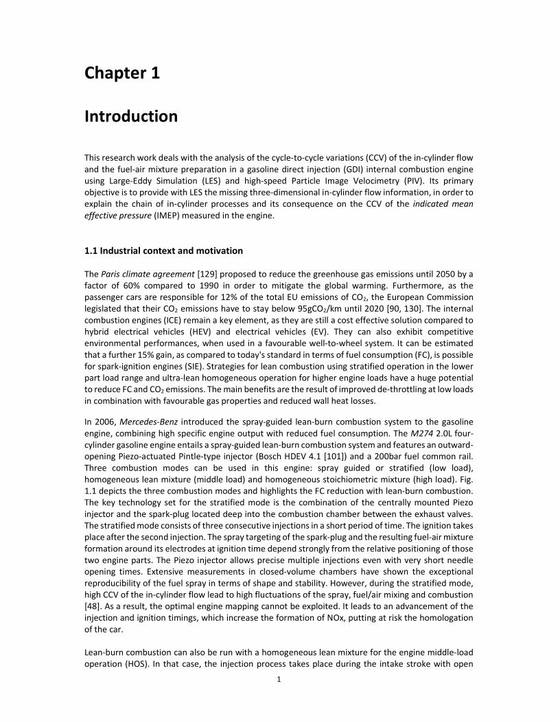
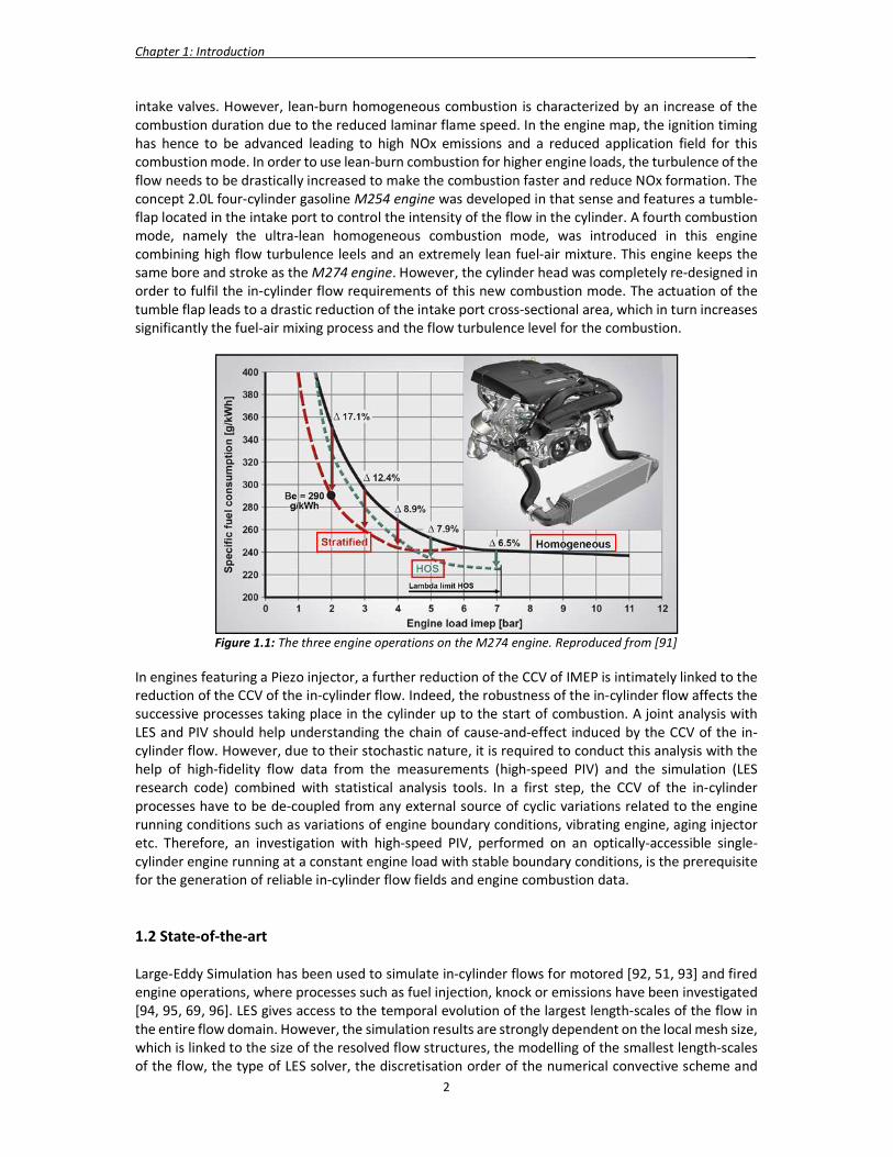
Introduction This research work deals with the analysis of the cycle-to-cycle variations (CCV) of the in-cylinder flow and the fuel-air mixture preparation in a gasoline direct injection (GDI) internal combustion engine using Large-Eddy Simulation (LES) and high-speed Particle Image Velocimetry (PIV). Its primary objective is to provide with LES the missing three-dimensional in-cylinder flow information, in order to explain the chain of in-cylinder processes and its consequence on the CCV of the indicated mean effective pressure (IMEP) measured in the engine. 1.1 Industrial context and motivation The Paris climate agreement [129] proposed to reduce the greenhouse gas emissions until 2050 by a factor of 60% compared to 1990 in order to mitigate the global warming. Furthermore, as the passenger cars are responsible for 12% of the total EU emissions of CO2, the European Commission legislated that their CO2 emissions have to stay below 95gCO2/km until 2020 [90, 130]. The internal combustion engines (ICE) remain a key element, as they are still a cost effective solution compared to hybrid electrical vehicles (HEV) and electrical vehicles (EV). They can also exhibit competitive environmental performances, when used in a favourable well-to-wheel system. It can be estimated that a further 15% gain, as compared to today's standard in terms of fuel consumption (FC), is possible for spark-ignition engines (SIE). Strategies for lean combustion using stratified operation in the lower part load range and ultra-lean homogeneous operation for higher engine loads have a huge potential to reduce FC and CO2 emissions. The main benefits are the result of improved de-throttling at low loads in combination with favourable gas properties and reduced wall heat losses. In 2006, Mercedes-Benz introduced the spray-guided lean-burn combustion system to the gasoline engine, combining high specific engine output with reduced fuel consumption. The M274 2.0L four-cylinder gasoline engine entails a spray-guided lean-burn combustion system and features an outward-opening Piezo-actuated Pintle-type injector (Bosch HDEV 4.1 [101]) and a 200bar fuel common rail. Three combustion modes can be used in this engine: spray guided or stratified (low load), homogeneous lean mixture (middle load) and homogeneous stoichiometric mixture (high load). Fig. 1.1 depicts the three combustion modes and highlights the FC reduction with lean-burn combustion. The key technology set for the stratified mode is the combination of the centrally mounted Piezo injector and the spark-plug located deep into the combustion chamber between the exhaust valves. The stratified mode consists of three consecutive injections in a short period of time. The ignition takes place after the second injection. The spray targeting of the spark-plug and the resulting fuel-air mixture formation around its electrodes at ignition time depend strongly from the relative positioning of those two engine parts. The Piezo injector allows precise multiple injections even with very short needle opening times. Extensive measurements in closed-volume chambers have shown the exceptional reproducibility of the fuel spray in terms of shape and stability. However, during the stratified mode, high CCV of the in-cylinder flow lead to high fluctuations of the spray, fuel/air mixing and combustion [48]. As a result, the optimal engine mapping cannot be exploited. It leads to an advancement of the injection and ignition timings, which increase the formation of NOx, putting at risk the homologation of the car. Lean-burn combustion can also be run with a homogeneous lean mixture for the engine middle-load operation (HOS). In that case, the injection process takes place during the intake stroke with open
Chapter 1: Introduction _
2
intake valves. However, lean-burn homogeneous combustion is characterized by an increase of the combustion duration due to the reduced laminar flame speed. In the engine map, the ignition timing has hence to be advanced leading to high NOx emissions and a reduced application field for this combustion mode. In order to use lean-burn combustion for higher engine loads, the turbulence of the flow needs to be drastically increased to make the combustion faster and reduce NOx formation. The concept 2.0L four-cylinder gasoline M254 engine was developed in that sense and features a tumble-flap located in the intake port to control the intensity of the flow in the cylinder. A fourth combustion mode, namely the ultra-lean homogeneous combustion mode, was introduced in this engine combining high flow turbulence leels and an extremely lean fuel-air mixture. This engine keeps the same bore and stroke as the M274 engine. However, the cylinder head was completely re-designed in order to fulfil the in-cylinder flow requirements of this new combustion mode. The actuation of the tumble flap leads to a drastic reduction of the intake port cross-sectional area, which in turn increases significantly the fuel-air mixing process and the flow turbulence level for the combustion.
Figure 1.1: The three engine operations on the M274 engine. Reproduced from [91]
In engines featuring a Piezo injector, a further reduction of the CCV of IMEP is intimately linked to the reduction of the CCV of the in-cylinder flow. Indeed, the robustness of the in-cylinder flow affects the successive processes taking place in the cylinder up to the start of combustion. A joint analysis with LES and PIV should help understanding the chain of cause-and-effect induced by the CCV of the in-cylinder flow. However, due to their stochastic nature, it is required to conduct this analysis with the help of high-fidelity flow data from the measurements (high-speed PIV) and the simulation (LES research code) combined with statistical analysis tools. In a first step, the CCV of the in-cylinder processes have to be de-coupled from any external source of cyclic variations related to the engine running conditions such as variations of engine boundary conditions, vibrating engine, aging injector etc. Therefore, an investigation with high-speed PIV, performed on an optically-accessible single-cylinder engine running at a constant engine load with stable boundary conditions, is the prerequisite for the generation of reliable in-cylinder flow fields and engine combustion data. 1.2 State-of-the-art Large-Eddy Simulation has been used to simulate in-cylinder flows for motored [92, 51, 93] and fired engine operations, where processes such as fuel injection, knock or emissions have been investigated [94, 95, 69, 96]. LES gives access to the temporal evolution of the largest length-scales of the flow in the entire flow domain. However, the simulation results are strongly dependent on the local mesh size, which is linked to the size of the resolved flow structures, the modelling of the smallest length-scales of the flow, the type of LES solver, the discretisation order of the numerical convective scheme and
Chapter 1: Introduction _
3
the modelling of the flow closed to the walls. In view of the underlying assumptions, LES is not predictive yet and requires validation in order to ensure the reliability of the simulation in view of a future usage for the engine development. Many groups have validated their simulations of motored in-cylinder flows using PIV measurements [92, 93, 97]. The validation is typically based on the comparison of velocity profiles along selected lines. Janas et al. [51] have extended this analysis by comparing the evolution of the tumble vortex center during compression. For a more complete understanding of the differences between PIV measurements and LES other metrics as for example a proper orthogonal decomposition (POD) or relevance index (RI) have been proposed [97]. All presented comparisons showed overall good or at least reasonable agreement, although differences were observed locally. Even though these differences are assumed to be small, they might become crucial, since a correct prediction of flow features, like the intake flow for example, are of utmost importance to capture the global in-cylinder flow correctly [97]. In the Darmstadt Engine Workshop [131] led by Böhm the topic LES validation is addressed with PIV using two well-documented engine geometries. State-of-the-art for the liquid injection in LES is the Lagrangian method. This method was validated on single and multi-hole injectors with round nozzles. They showed a satisfactory reproduction of liquid and gas penetrations, opening angles and fuel mass fraction profiles of the closed-volume chamber spray measurements. However, the simulation of the Piezo injector was only performed in RANS [57], using the Lagrangian approach, pointing out the extreme importance of the droplet initialisation and the resolution of the spray adaptive mesh.
Particle image velocimetry has been used extensively to capture in-cylinder flow fields within a plane [84]. High-speed PIV provides crank-angle resolved flow fields and has been used to investigate the CCV of the in-cylinder flow in a single plane [85, 87, 88]. Stiehl et al. [45, 46] investigated the interaction of the CCV variations of the spray with the in-cylinder flow in stratified engine operation. This work highlighted the importance of a local flow structure before the injection, which affected the robustness of the spray. Stiehl [110] assumed that three-dimensional flow phenomena were linked to the appearance of this local flow structure. On the same engine Bode et al. [48] utilized a quasi-simultaneous multi-plane time-resolved PIV approach to investigate the flows evolution in the intake valve plane and in the central tumble plane. From the flow analysis in both planes, Bode [104] confirmed the assumption of Stiehl. He stated that a momentum transfer, occurring from the intake plane towards the central tumble plane, was responsible for the appearance of the local flow structure before the injection. The measurement of the three-dimensional flow field was performed by Brücker et al. [111] using Stereo PIV in several planes using two cameras. This methodology allows the measurement of the normal velocity component to the plane, but the reconstruction of the three-dimensional flow field is only based on the mean flow field. To visualize the instantaneous three-dimensional flow field, Baum et al. [86] used tomographic PIV within few millimetre thick volumes surrounding the central tumble plane. However, due to the reduced size of the measurement volume, the dominant large-scale structures of the in-cylinder flow are not captured with tomographic PIV. An alternative approach is the high-speed scanning PIV, which was operatively used by Bode [104] for the first time in an engine. Using an acousto-optic deflector (AOD) scanner as proposed by Li et al. [112], successive measurements of the instantaneous flow field can be performed in several planes, which allow the three-dimensional mean flow field to be later reconstructed. Despite recent improvements of PIV approaches, flow field measurements are limited to planes or thin volumes. Important regions of the flow, as for example the flow in the intake port and the valve gap, remain inaccessible. 1.3 Objectives The goal of this research work is to understand, via a joint analysis using high-speed PIV and LES, the three-dimensional (3D) flow phenomena in the chain of in-cylinder processes leading to the CCV of the IMEP in stratified engine operation. The optically-accessible single-cylinder derived from the M274 engine will be considered for these investigations as well as the LES research code AVBP [109].

Chapter 1: Introduction _
4
The multiple publications on LES of in-cylinder flows have highlighted that there is today no universal reliable LES validation strategy available and the question remains open on which level of detail a validation is required. Depending on the engine operation of interest, different global and local flow structures are susceptible to influence directly the outcome of the combustion process. LES validations of the in-cylinder flow field based on these local flow quantities have never been addressed. In this research project, the key in-cylinder flow patterns affecting the combustion process in stratified operation will be isolated from a correlation analysis between the high-speed PIV flow fields and the engine combustion data. They will be used to drive the validation process of the LES in-cylinder flow in terms of mean flow and local CCV of the flow. From a global mesh sensitivity study, a robust methodology will be iteratively derived for the selected research code AVBP, which features a low-dissipative explicit acoustic LES solver and high mesh quality standards. In order to fully assess the potential of LES in predicting accurately the in-cylinder flows, the 2nd and 3rd-order accurate in space and time convective schemes will be investigated. Based on the validated LES flow fields, two crucial 3D flow structures, with respect to the combustion process outcome, will be extracted, using conditional averaging and inputs from high-speed PIV. These flow structures will be quantified by the visual observation of their 3D rotation axis computed using an extension of the Г-criterion [50] in 3D. In the experiments, the missing link between the CCV of the in-cylinder flow and the CCV of the IMEP is the fuel-air mixture distribution in the cylinder. However, spray simulation in LES of a Piezo injector has never been addressed when it comes to model the primary droplet break-up, using a coupling interface between the transient internal-nozzle flow simulation in RANS and LES. A new methodology will be derived and validated against closed-volume chamber spray measurements. Its integration into the gas-exchange mesh will require the development of a new-moving mesh strategy adapted for the explicit acoustic LES solver. A multi-cycle fuel-air mixture formation will be performed and a correlation will be made between the CCV of the key in-cylinder flow parameters and the CCV of the fuel-air mixture distribution at the beginning of the combustion. Finally a new methodology for the simulation of the fuel-air mixture formation in ultra-lean homogeneous combustion will be developed. As a pilot application, few cycles will be computed with the M254 engine geometry. The CCV of the fuel-air mixture distribution and the in-cylinder flow will be analysed. 1.4 Plan of the thesis This thesis is divided into eight chapters. Following the introduction chapter, the second chapter deals with the fundamentals of numerical simulations of turbulent flows. The different simulation techniques and the various LES approaches will be discussed including the one used in AVBP. The third chapter presents the methods in AVBP for the spray simulation. The improvements made to AVBP and the newly implemented methodology for the simulation of the Piezo injector will be shown. The fourth chapter covers the simulation, the validation and the analysis of the LES in-cylinder flow together with high-speed PIV. The extraction of the key in-cylinder flow parameters from the experiments, using a correlation analysis, will be explained. The new PIV-guided LES validation strategy derived in this work will be presented. A multi-cycle LES with the 2nd and 3rd-order convective schemes will be investigated. New analysis tools including conditional statistics and the 3D Г-criterion will be introduced and applied to isolate the three-dimensional flow structures linked to the CCV of the IMEP. The fifth chapter describes the methodology development for the spray simulation of the Piezo injector (BOSCH HDEV4.1) in a cold closed-volume chamber with LES. The validated results will be presented. The sixth chapter covers the multi-cycle simulation and the analysis of the fuel-air mixture formation in stratified engine operation. The new moving-mesh strategy including the spray adaptive mesh will be described. The CCV of the spray fluctuation and the fuel-air mixture distribution will be quantified and correlated with the CCV of the key in-cylinder flow parameters. The seventh chapter describes the methodology development and the analysis of a multi-cycle fuel-air mixture formation in ultra-lean homogeneous engine operation in the M254 engine. The findings made in this research project are summarized in the last chapter. The perspectives concerning the future of LES for internal combustion engines will be also discussed.

5
Chapter 2
Simulation of turbulent flows This chapter covers the numerical simulation of turbulent flows, called computational fluid dynamics (CFD). The CFD simulation is today widely used in the academia and in the industry, in order to investigate complex three-dimensional flow problems. Due to its success and ease of use, expensive experimental measurements have been progressively replaced by CFD investigations in the industry. As a result, a complete virtual product development can be achieved combining Computer-Aided Engineering (CAE), CFD and optimisation tools. In the automotive industry, the combustion engine development process is leading in this direction, too. However, depending on the level of flow resolution required in the optimisation process, two different CFD techniques can be used, namely Reynolds-Averaged Navier-Stokes equations (RANS) simulation and Large-Eddy Simulation (LES), which differ significantly from each other. This chapter is divided into two main parts. The first one is devoted to the CFD techniques used to simulate the in-cylinder engine flow. After a short introduction on turbulent flows, the main conceptual differences between RANS and LES is first described together with their corresponding formulations of the fluid mechanics equations. Secondly, as there is today not a unique way to perform LES, the various LES approaches found in the literature are detailed and compared. Finally, the justification to use the software AVBP in this research work is presented. The second part of this chapter deals with the description of AVBP, emphasizing on the following features: solver, numerical schemes, mesh requirements and moving-mesh strategy. 2.1 Turbulent flows Turbulent flows are characterized by a high Reynolds number, which describes the ratio of the inertial and viscous forces:
𝑅𝑒 = (2.1)
where 𝑢, 𝐿 are a characteristic velocity and length scale of the flow and 𝜇 the dynamic viscosity of the fluid. Contrary to laminar flows, which feature low Reynolds number and are controlled by the viscosity of the flow, turbulent flows feature stochastic flow fluctuations and mixing processes. Turbulent flows entail eddies structures of different sizes 𝑙, which can be classified in the so-called Energy spectrum (Fig. 2.1) using their wavenumber 𝜅:
𝜅 = (2.2)
The large scale eddies are directly influenced by the surrounding geometry and contain most of the kinetic energy. Their motion is dominated by the inertial forces and is barely affected by the viscous forces. The integral length scale of the flow κL falls into this category. The small scale eddies are located in regions, where viscous forces dominate and where the kinetic energy is dissipated and converted into thermal energy. The smallest length scale of the flow is denoted the Kolmogorov scale κη. The higher the Reynolds number of the flow, the wider the Energy spectrum, as smaller scale eddies are generated. Kolmogorov in 1941 [1] postulated that a transfer of kinetic energy from the largest to the smallest scales takes place. He described it with the energy cascade. He showed that an intermediate range of length scales exists, called the inertial subrange, whose characteristics rely solely on the

Chapter 2: Simulation of turbulent flows _
6
dissipation rate of the kinetic energy ε. A universal formulation of the kinetic energy transfer process was derived:
𝐸(𝜅) = 𝐶𝜀 / 𝜅 / , C is a universal constant value [20] (2.3)
Figure 2.1: Energy spectrum
Engine in-cylinder flows fall into the category of turbulent flows. Their Reynolds numbers are well above the critical Reynolds number (𝑅𝑒 ≈ 2300), where the transition from laminar to turbulent flow occurs in a channel flow [20]. High speed PIV measurements have confirmed the randomness nature of these flows [45, 46, 47]. Another feature of the engine in-cylinder flows is the linear scaling of the flow turbulent kinetic energy with the engine rotation speed i.e. piston speed. Engine in-cylinder flows are also treated as compressible flows, due to the very high Mach number (𝑀 > 0.3) observed locally in the valve gap or at high engine speed during the intake and exhaust strokes. The Mach number is defined as follows:
𝑀 = (2.4)
where 𝑢 is the flow velocity and 𝑐 the speed of sound. The governing equations of fluid mechanics are called the Navier-Stokes equations and consist of three equations:
- the continuity equation - the momentum transport equation - the energy transport equation
The Navier-Stokes equations are the derivation of three fundamental physical principles upon which all fluid dynamics is based:
- conservation of the mass - Newton’s second law (�� = 𝑚��) - conservation of the energy
In case of a multi-species fluid flow, the behaviour of each chemical species is described using an additional species transport equation. The transport equations, also named conservation equations, contains a temporal term, a convective term, a diffusive term and a source term. They can be derived for compressible and incompressible flows. In case of a three-dimensional compressible flow, the conservative variables are:
- the density 𝜌 - the three dimensional velocity field 𝑢 - the enthalpy ℎ - the mass fractions 𝑌 of the N species
These equations are detailed hereafter in the context of RANS and LES.
Chapter 2: Simulation of turbulent flows _
7
2.2 RANS The RANS equations describe the averaged equations of fluid mechanics using the Reynolds decomposition. Each instantaneous variable 𝑓 is split into a mean 𝑓 and a fluctuating component 𝑓 (Eq. (2.5)). 𝑓 is defined as the ensemble average over a large number of realizations at the same instant and under identical conditions.
𝑓 = 𝑓 + 𝑓 with 𝑓 = 0 and 𝑓 =∆
∫ 𝑓(𝑡)𝑑𝑡∆ (2.5)
As a result, the Reynolds decomposition introduces new unclosed quantities. They need to be modelled using turbulence models, in order to solve the system of fluid mechanics equations. The mass-weighted average (Eq. (2.6)), using the density of the flow 𝜌, is called the Favre average [2]. It is recommended for compressible flows, as the Reynolds decomposition for compressible flow would lead to several additional unclosed correlations between the variable 𝑓 and the density fluctuations 𝜌 𝑓 . Eq. (2.5) becomes Eq. (2.7) after applying the Favre average.
𝑓 = (2.6)
𝑓 = 𝑓 + 𝑓 with 𝑓 = 0 (2.7)
The RANS equations for non-reactive flows, including the transport of species, are: Averaged continuity equation
+ (��𝑢 ) = 𝑆 (2.8)
Averaged momentum transport equation
+ ��𝑢 𝑢 +
= 𝜏 − ��𝑢 𝑢 + 𝑆 (2.9)
Averaged enthalpy transport equation
+ ��𝑢 ℎ = + �� − �� ∑ 𝑉 , 𝑌 ℎ − ��𝑢 ℎ + 𝜏 + 𝑆 (2.10)
Averaged species transport equation
+ ��𝑢 𝑌 = + −��𝐷 − ��𝑢 𝑌 + 𝑆 (2.11)
where: - 𝜏 is the viscous stress tensor: 𝜏 = 2𝜇 𝑆 − 𝑆 (2.12)
- 𝑆 is the strain rate tensor: 𝑆 = + (2.13)
- =+ 𝑢 =
+ 𝑢
+ 𝑢 (2.14)
- 𝛿 is the Kronecker delta - 𝑆 , 𝑆 , 𝑆 and 𝑆 are the source terms from the coupling with the Lagrangian phase - 𝑌 is the mass fraction of the species 𝑘 - 𝐷 is the diffusion coefficient of the species 𝑘 - 𝑉 , is the 𝑖 component of the diffusion velocity 𝑉 of the species 𝑘 - 𝜆 is the thermal conductivity - 𝜇 is the kinematic viscosity

Chapter 2: Simulation of turbulent flows _
8
Four unknown quantities have appeared after the Reynold decomposition. They need to be modelled in terms of mean quantities in order to close the system of equations:
- The Reynolds stresses (��𝑢 𝑢 ) - The turbulent flux of energy (��𝑢 ℎ ) - The species turbulent mass flux (��𝑢 𝑌 )
- The pressure-velocity correlation (𝑢 ). This term is like in most RANS codes neglected here.
Closure of the momentum transport equation The Boussinesq approximation, also called the eddy-viscosity model, assumes that the Reynolds stress tensor 𝜏 may be modelled in the same way as the viscous stress tensor 𝜏 with respect to 𝑆 . The eddy viscosity model approximates the effects of the turbulent motions on the mean flow by a diffusive process based on a turbulent viscosity:
𝜏 = ��𝑢 𝑢 = −2𝜇 𝑆 − 𝑆 + ��𝑘 (2.15)
where: - 𝜇 is referred to as the turbulent viscosity - 𝑘 is the turbulent kinetic energy of the turbulent fluctuations: 𝑘 = ∑ 𝑢 𝑢 (2.16)
The turbulent viscosity is used to close the momentum transport equation. It has the same dimension as the molecular viscosity. Therefore, it increases the global viscosity of the simulated flow. The most common approach to evaluate the turbulent viscosity is the use of the two-equation 𝑘 − 𝜀 turbulence model [3], which gives:
𝜇 = ��𝐶 , 𝐶 =0.09 (2.17)
where 𝑘 and 𝜀 are respectively the turbulent kinetic energy and its dissipation rate. Their spatial and temporal evolutions are described using the following transport equations:
+ (��𝑢 𝑘) = 𝜇 + + 𝑃 − ��𝜀 (2.18)
+ (��𝑢 𝜀) = 𝜇 + + 𝐶 𝑃 − 𝐶 �� (2.19)
The source term 𝑃 is defined as:
𝑃 = ��𝑢 𝑢 (2.20)
The Boussinesq approximation is used for the Reynolds stresses ��𝑢 𝑢 . Four closure coefficients are required in the 𝑘 − 𝜀 turbulence model. Their standard values are [61]:
𝜎 =1.0, 𝜎 =1.3, 𝐶 =1.44, 𝐶 =1.92 (2.21) Closure of the enthalpy transport equation The turbulent flux of energy (��𝑢 ℎ ) is linked to the averaged enthalpy ℎ using the gradient transport assumption of the Fourier’s law:
��𝑢 ℎ = − (2.22)
where 𝑃𝑟 is referred to as the turbulent Prandtl number and describes the ratio of turbulent transport of mass and turbulent transport of energy:

Chapter 2: Simulation of turbulent flows _
9
𝑃𝑟 = 𝜇 (2.23)
Closure of the species transport equation The species turbulent mass flux (��𝑢 𝑌 ) is linked to the averaged concentration 𝑌 of the species 𝑘 using the gradient transport assumption of the Fick’s law:
��𝑢 𝑌 = − (2.24)
where 𝑆 , is referred to as the turbulent Schmidt number of the species 𝑘 and describes the ratio of turbulent transport of momentum and turbulent transport of mass:
𝑆 , =,
(2.25)
where 𝐷 , is the turbulent diffusivity coefficient of the species 𝑘. It is common practice to assume a similarity between the turbulent heat and species transport processes. The turbulent Schmidt number and the turbulent Prandtl number are hence taken as equal. In RANS, the turbulent motions of all the turbulent spectrum scales are modelled and included into the Reynolds stress tensor and the turbulent diffusivity. This is the approach used to include the effect of the turbulence on the different ensemble-average flow variables. As a result, the viscous stresses, the diffusion of the species and the diffusion of energy are greatly amplified compared to in a laminar flow case. Furthermore, the higher the turbulent kinetic energy of the flow, the higher the difference between the turbulent viscosity and the molecular viscosity. The overall viscosity of the flow, i.e. the sum of the molecular and the turbulent viscosity, leads to the fact that the turbulent flows computed in RANS have a much reduced effective Reynolds number compared to the real flow. This is the reason for the viscous aspect of the RANS turbulent flow fields. Solid wall boundary condition: the standard wall functions The engine in-cylinder flow is a wall-bounded flow and particular care has to be taken concerning the estimation of the flow momentum and heat fluxes in the turbulent boundary layers. Experimental studies have shown that the internal zone of a stationary, fully established turbulent boundary layer of thickness 𝛿 without adverse pressure gradient can be subdivided into three distinct sub-layers [134]. Their locations are directly dependent on the distance from the wall and are encompassed within 0.1 𝛿. Their dimensionless velocity as a function of the dimensionless wall distance is shown in Fig. 2.2. Starting from the wall one finds:
- The viscous sub-layer in which the flow is dominated by viscous forces. The flow is taken to be as laminar because turbulent transport is negligible compared to molecular diffusion.
- The buffer sub-layer is seen as a transition region between the laminar and turbulent flow. In this region turbulent transport and molecular diffusion are assumed to have similar intensities.
- The inertial sub-layer, also known as ‘log-law region’ due to its logarithmic velocity profile, in
which turbulent transport clearly dominates over molecular diffusion. This region acts as an interface between the internal zone of the turbulent boundary layer and its external zone, where the flow is fully turbulent i.e. in the range from 0.1 𝛿 to 𝛿.
For the high-Reynolds number version of the 𝑘 − 𝜀 turbulence model, applying the no-slip condition on the walls yields unsatisfactory results. The usual way to impose the no-slip conditions in that case and account for boundary layers is the use of the standard wall functions, as originally proposed by Launder and Spalding [114]. In the near wall region, the turbulence-model equations are not solved to overcome the need for resolving the viscous sub-layer structure. Instead, empirical laws based on the

Chapter 2: Simulation of turbulent flows _
10
assumed distributions of velocity, temperature and turbulence parameters across the boundary layer are used to predict the logarithmic velocity profile in the near-wall cell. The standard wall functions cover the log-law region of the boundary layer, as depicted in Fig 2.2. The size of the near-wall cell should be selected in a way that its centroid lies within this region, so that the standard wall functions remain valid. The normalised distance from the wall 𝑦 is used to assess the near-wall cell centroid distance from the wall 𝑦. The dimensionless velocity 𝑢 parallel to the wall as a function of 𝑦 reads:
𝑢 = 𝑦 , 𝑦 ≤ 𝑦
ln(𝑦 ) + 𝐶 , 𝑦 > 𝑦 (2.26)
with
𝑦 = , 𝑢 = , 𝜏 = 𝜇 and 𝑢 = (2.27)
where: 𝜏 is the wall shear stress, 𝑢 is the shear velocity, 𝑢 is the flow velocity parallel to the wall, 𝜅 is the Von Karman constant, 𝜐 the kinematic viscosity and 𝐶 a constant and 𝑦 satisfies the equation:
𝑦 − ln(𝑦 ) + 𝐶 = 0 (2.28)
Figure 2.2: Dimensionless mean streamwise velocity versus dimensionless wall distance, with
𝜅 = 0.41 and 𝐶 = 5.5. Reproduced from [89] Following the same principles, additional algebraic relations provide the remaining information for the temperature and turbulence parameters [120]. The domain of validity of the standard wall functions in the log-law region is constrained by 11.6 < 𝑦 < 100. Although they are commonly used for in-cylinder flow simulation, high-speed micro particle image velocimetry (µ-PIV) of boundary-layer flow measurements have shown that they cannot capture the dynamics of boundary-layer flows in the compression stroke of ICE [142]. Non-equilibrium wall functions have addressed the shortcoming of the standard ‘equilibrium’ wall functions by retaining the transient information of the flow. They showed some improvements [143]. For the low-Reynolds number version of the 𝑘 − 𝜀 turbulence model, the near-wall regions are treated identically as the flow away from the walls with an additional no-slip condition imposed at the wall-boundary cell faces. The boundary layers are hence computed entirely by solving the mass, momentum and turbulence equations, which implies a very fine mesh close to the wall and a huge increase of the cell count in the computational model. In order to resolve the viscous sublayer, a near-wall cell size corresponding to 𝑦 ≈ 1 is generally used.

Chapter 2: Simulation of turbulent flows _
11
2.3 LES LES resolves the instantaneous length scales of the flow larger than a given filter size Δ, whereas the effects of the small length scales, called subgrid-scale (SGS) stresses, are modelled with a subgrid-model (Fig. 2.3). Compared to RANS, LES gives access to the unsteady behaviour of the flow and is computationally more expensive. RANS is directly providing an ensemble average solution of the flow. Instead, LES requires the computation of several realizations, called flow passes or engine cycles, in order to gather enough statistical flow information and compute an ensemble average solution. A mesh refinement in LES implies a broader turbulent spectrum resolved and more statistical flow information, whereas in RANS it means simply a better resolution of the mean flow field. As the cell size tends to zero, LES becomes a Direct Numerical Simulation (DNS), where all turbulent length scales of the flow are resolved. This kind of simulation is currently too prohibitive in terms of computation time and size of the CFD model for any industrial engine application. Classical RANS simplifications commonly used to reduce the computational costs, such as using a 2D-geometry or symmetry boundary conditions, cannot be retained anymore in LES. Instead, a reliable computation of the instantaneous large length scales of the flow requires the simulation of the exact three-dimensional geometry.
Figure 2.3: Difference between RANS and LES
The nature of the unclosed terms is different in RANS and in LES and affects massively the value of the turbulent viscosity in the subgrid model. In RANS all the turbulent scale motions of the turbulent spectrum are modelled, which leads to a turbulent viscosity typically of the order 1000 times larger than the molecular viscosity. However, as only the turbulent scale motions smaller than the cut-off length scale are modelled in LES, the level of turbulent viscosity is only of the order of 10 to 100 times larger than the molecular viscosity depending on the mesh resolution used [28]. Due to the reduced turbulent viscosity in LES, the numerical viscosity 𝜇 plays a crucial role in the accuracy of the computation in LES and has to be kept much smaller than 𝜇 . Over the years, LES has been used extensively in the academia. Lots of publications and PhDs have been published on this topic as mentionned in chapter 1, even international conferences dedicated solely to LES such LES4ICE [116] have been set up to attract researcher and engineers from diverse working fields (industry, OEMs, academia). However as the numerical viscosity is a major issue in LES, various approaches have been reported to:
- filter the LES equations - model the subgrid-scales - integrate the LES equations - choose the convective numerical scheme
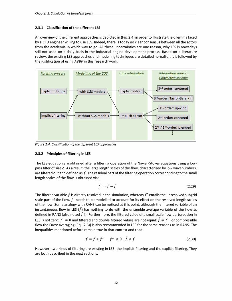
Chapter 2: Simulation of turbulent flows _
12
2.3.1 Classification of the different LES An overview of the different approaches is depicted in (Fig. 2.4) in order to illustrate the dilemma faced by a CFD engineer willing to use LES. Indeed, there is today no clear consensus between all the actors from the academia in which way to go. All these uncertainties are one reason, why LES is nowadays still not used on a daily basis in the industrial engine development process. Based on a literature review, the existing LES approaches and modelling techniques are detailed hereafter. It is followed by the justification of using AVBP in this research work.
Figure 2.4: Classification of the different LES approaches 2.3.2 Principles of filtering in LES The LES equation are obtained after a filtering operation of the Navier-Stokes equations using a low-pass filter of size Δ. As a result, the large length scales of the flow, characterized by low wavenumbers, are filtered out and defined as 𝑓. The residual part of the filtering operation corresponding to the small length scales of the flow is obtained via:
𝑓 = 𝑓 − 𝑓 (2.29)
The filtered variable 𝑓 is directly resolved in the simulation, whereas 𝑓 entails the unresolved subgrid scale part of the flow. 𝑓 needs to be modelled to account for its effect on the resolved length scales of the flow. Some analogy with RANS can be noticed at this point, although the filtered variable of an instantaneous flow in LES (𝑓) has nothing to do with the ensemble average variable of the flow as defined in RANS (also noted 𝑓 !). Furthermore, the filtered value of a small scale flow perturbation in LES is not zero: 𝑓 ≠ 0 and filtered and double filtered values are not equal: 𝑓 ≠ 𝑓. For compressible flow the Favre averaging (Eq. (2.6)) is also recommended in LES for the same reasons as in RANS. The inequalities mentioned before remain true in that context and read:
𝑓 = 𝑓 + 𝑓 𝑓 ≠ 0 𝑓 ≠ 𝑓 (2.30) However, two kinds of filtering are existing in LES: the implicit filtering and the explicit filtering. They are both described in the next sections.
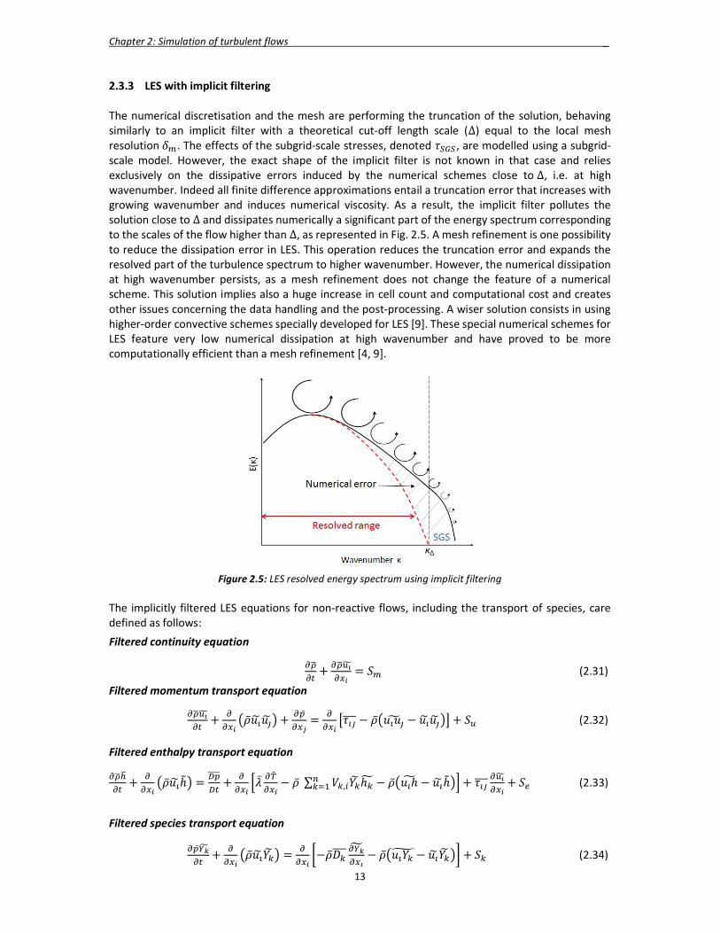
Chapter 2: Simulation of turbulent flows _
13
2.3.3 LES with implicit filtering The numerical discretisation and the mesh are performing the truncation of the solution, behaving similarly to an implicit filter with a theoretical cut-off length scale (∆) equal to the local mesh resolution 𝛿 . The effects of the subgrid-scale stresses, denoted 𝜏 , are modelled using a subgrid-scale model. However, the exact shape of the implicit filter is not known in that case and relies exclusively on the dissipative errors induced by the numerical schemes close to ∆, i.e. at high wavenumber. Indeed all finite difference approximations entail a truncation error that increases with growing wavenumber and induces numerical viscosity. As a result, the implicit filter pollutes the solution close to ∆ and dissipates numerically a significant part of the energy spectrum corresponding to the scales of the flow higher than ∆, as represented in Fig. 2.5. A mesh refinement is one possibility to reduce the dissipation error in LES. This operation reduces the truncation error and expands the resolved part of the turbulence spectrum to higher wavenumber. However, the numerical dissipation at high wavenumber persists, as a mesh refinement does not change the feature of a numerical scheme. This solution implies also a huge increase in cell count and computational cost and creates other issues concerning the data handling and the post-processing. A wiser solution consists in using higher-order convective schemes specially developed for LES [9]. These special numerical schemes for LES feature very low numerical dissipation at high wavenumber and have proved to be more computationally efficient than a mesh refinement [4, 9].
Figure 2.5: LES resolved energy spectrum using implicit filtering
The implicitly filtered LES equations for non-reactive flows, including the transport of species, care defined as follows:
Filtered continuity equation
+ = 𝑆 (2.31)
Filtered momentum transport equation
+ ��𝑢 𝑢 +
= 𝜏 − �� 𝑢 𝑢 − 𝑢 𝑢 + 𝑆 (2.32)
Filtered enthalpy transport equation
+ ��𝑢 ℎ = + �� − �� ∑ 𝑉 , 𝑌 ℎ − �� 𝑢 ℎ − 𝑢 ℎ + 𝜏 + 𝑆 (2.33)
Filtered species transport equation
+ ��𝑢 𝑌 = −��𝐷 − �� 𝑢 𝑌 − 𝑢 𝑌 + 𝑆 (2.34)
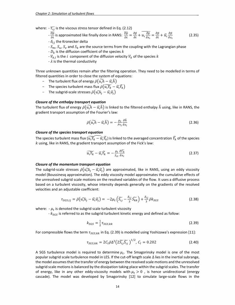
Chapter 2: Simulation of turbulent flows _
14
where: - 𝜏 is the viscous stress tensor defined in Eq. (2.12)
- is approximated like finally done in RANS: =+ 𝑢 =
+ 𝑢
(2.35)
- 𝛿 the Kronecker delta - 𝑆 , 𝑆 , 𝑆 and 𝑆 are the source terms from the coupling with the Lagrangian phase - 𝐷 is the diffusion coefficient of the species 𝑘 - 𝑉 , is the 𝑖 component of the diffusion velocity 𝑉 of the species 𝑘 - 𝜆 is the thermal conductivity
Three unknown quantities remain after the filtering operation. They need to be modelled in terms of filtered quantities in order to close the system of equations:
- The turbulent flux of energy �� 𝑢 ℎ − 𝑢 ℎ - The species turbulent mass flux �� 𝑢 𝑌 − 𝑢 𝑌 - The subgrid-scale stresses �� 𝑢 𝑢 − 𝑢 𝑢
Closure of the enthalpy transport equation The turbulent flux of energy �� 𝑢 ℎ − 𝑢 ℎ is linked to the filtered enthalpy ℎ using, like in RANS, the gradient transport assumption of the Fourier’s law:
�� 𝑢 ℎ − 𝑢 ℎ = − (2.36)
Closure of the species transport equation The species turbulent mass flux (𝑢 𝑌 − 𝑢 𝑌 ) is linked to the averaged concentration 𝑌 of the species 𝑘 using, like in RANS, the gradient transport assumption of the Fick’s law:
𝑢 𝑌 − 𝑢 𝑌 = − (2.37)
Closure of the momentum transport equation The subgrid-scale stresses �� 𝑢 𝑢 − 𝑢 𝑢 are approximated, like in RANS, using an eddy viscosity model (Boussinesq approximation). The eddy viscosity model approximates the cumulative effects of the unresolved subgrid scale motions on the resolved variables of the flow. It uses a diffusive process based on a turbulent viscosity, whose intensity depends generally on the gradients of the resolved velocities and an adjustable coefficient:
𝜏 , = �� 𝑢 𝑢 − 𝑢 𝑢 = −2𝜇 𝑆 − 𝑆 + ��𝑘 (2.38)
where: - 𝜇 is denoted the subgrid scale turbulent viscosity - 𝑘 is referred to as the subgrid turbulent kinetic energy and defined as follow:
𝑘 = 𝜏 , (2.39)
For compressible flows the term 𝜏 , in Eq. (2.39) is modelled using Yoshizawa’s expression [11]:
𝜏 , = 2𝐶 ��∆ 2𝑆 𝑆 /
, 𝐶 = 0.202 (2.40) A SGS turbulence model is required to determine 𝜇 . The Smagorinsky model is one of the most popular subgrid scale turbulence model in LES. If the cut-off length scale ∆ lies in the inertial subrange, the model assumes that the transfer of energy between the resolved scale motions and the unresolved subgrid scale motions is balanced by the dissipation taking place within the subgrid scales. The transfer of energy, like in any other eddy-viscosity models with 𝜇 > 0 , is hence unidirectional (energy cascade). The model was developed by Smagorinsky [12] to simulate large-scale flows in the
Chapter 2: Simulation of turbulent flows _
15
meteorology field, but was rapidly extended to many other application fields due to its relative simplicity and accuracy. In this model, the SGS turbulent viscosity is expressed as follows:
𝜇 = ��(𝐶 ∆) 2𝑆 𝑆 /
(2.41)
where 𝐶 is the so-called Smagorinsky coefficient and ∆ is equal to the local mesh resolution 𝛿 . In the case of homogeneous isotropic turbulence, it was shown [13] that 𝐶 ≈ 0.18. Other studies on channel flows [14, 15] have shown that 𝐶 ≈ 0.1 in high velocity gradient regions. 𝐶 is clearly flow dependent. In an engine, due to the complex nature of the in-cylinder flow, the ideal 𝐶 values would theoretically vary in time and space. Some improvements were hence made to the Smagorinsky model. The Smagorinsky dynamic model [21] was developed to derive the subgrid scale dissipation, based on the resolved eddies information, using an additional test filter. An automatic procedure determines automatically the value of 𝐶 in time and space and encouraging results were reported [22, 23]. However, engine in-cylinder flow simulations [17] exhibited similar results between the Smagorinsky and the Smagorinsky dynamic models and a computational time increase of 5% with the Smagorinsky dynamic model. It was also shown [16, 17] that the Smagorinsky models tended to be too dissipative especially near the walls. The Sigma model [16] was developed to reduce the dissipation coming from the SGS model close to the wall. Only minor improvements of the flow-field velocity resolution compared to the Smagorinsky models were reported in engine in-cylinder flow simulations [17].
2.3.4 LES with explicit filtering Contrary to implicit filtering, where the computed velocity field is directly associated with the ‘grid’ filtered velocity, the explicit filtering introduces an explicitly defined filter operator with a cut-off length scale ∆ larger than the local mesh resolution 𝛿 . The filtered variable 𝑓 is defined as:
𝑓(𝑥) = ∫ 𝑓(𝑥 ) 𝐹∆(𝑥 − 𝑥 )𝑑𝑥 (2.42)
where 𝐹∆ is the LES explicit filter with a cut-off length scale ∆. Several filters have been tested and reported in the past [4, 5, 6, 7, 10]. Using explicit filtering implies that an additional closure term appears in the filtered momentum equation, representing the grid-resolved scales below ∆, as shown in Fig. 2.6. These are called the resolved subfilter-scale stresses, denoted 𝜏 . Eq. (2.32) can be rewritten as
+ ��𝑢 𝑢 +
= 𝜏 − 𝜏 , − 𝜏 , + 𝑆 (2.43)
The SGS stresses are approximated with a SGS turbulent model, like in the implicit filtering approach. Explicit filtering has the potential of reducing the truncation errors [4] by transferring the crucial portion of the turbulence spectrum to lower wavenumbers, which are less affected by numerical errors. An adequate choice of the filter cut-off length scale, depending on the numerical scheme used, can filter out the poorly resolved small scales. It is then possible to reconstruct 𝜏 from the filtered velocity in term of well-resolved wavenumbers by using an invertible filter [5, 6]. Another non-negligible advantage of the explicit filtering is to decouple the filter cut-off length-scale with the grid resolution and link it to the turbulence quantities instead. This approach makes it theoretically possible to obtain grid independent LES solutions. However, it was noticed that by removing the high wavenumber content of the solution, ‘explicit filtering reduces the effective resolution of the simulation compared with the dynamic range supported by the mesh‘ [7, 8]. Explicit filtering requires an additional filtering operation, a reconstruction operation and ideally a finer mesh compared to implicit filtering. The computational costs are thus increased. Furthermore, a mesh refinement study using implicit filtering has shown a much faster improvement of the statistics of the flow compared to explicit filtering [7].
Chapter 2: Simulation of turbulent flows _
16
Figure 2.6: LES resolved energy spectrum using explicit filtering
2.3.5 LES solver with implicit time advancement In an implicit time advancement solver, the solution at the new time level (t + Δt) is not dependent entirely on the current time level (t), but also on the new time level (t + Δt). The solvable equations are mixed with the known solution at the current time level (t) and the unknown solution at the new time level (t + Δt). It requires solving a system of simultaneous equations using an iterative process. An implicit time advancement solver is unconditionally stable, i.e. no constraint on the time step, but computationally expensive.
Numerics The implicit time advancement is widely used in RANS. The existing RANS CFD codes, industrial (Star-CD [120], Star-CCM+ [121], CFX [123], FIRE [122], FLUENT [124], CONVERGE [125]) or not (Kiva [127], Open-Foam [126]), are nowadays offering the possibility to perform LES in addition to RANS. The numeric schemes developed for RANS are used in the same way for LES, although the nature of the flow simulated is completely different between RANS and LES. In RANS, a viscous flow with low effective Reynolds number is resolved, whereas in LES the inertial effects of the flow play a major role, as the effective Reynolds number is much closer to the real one. As mentioned in 2.3.3, the numerical dissipation coming from the truncation errors is especially dependent on the numerical convective scheme used. It can be assimilated to a numerical viscosity, which adds to the molecular and turbulent viscosities, to form a global viscosity in the simulation and affect the effective Reynolds number of the simulated flow. However, to exclude the risk of having simulation results that mainly depend on the numerical schemes, the numerical viscosity should be at least one order of magnitude lower than the sum of the molecular and turbulent viscosity. The numerical scheme requirements for RANS and LES are hence different. In RANS, the natural high viscosity of the simulated flow allows the use of high dissipative numerical convective schemes, which feature low spatial order (1st-order Upwind, blended 2nd order central/upwind). Those high dissipative numerical schemes are very stable, due to the numerical damping effect they introduce, and are not too demanding in terms of mesh quality and mesh resolution in high gradient zones. In LES, where high level of precision in terms of convection is required, the use of theses numerical schemes will progressively introduce dissipation and dispersive errors on the middle and small scales of the flow. The minimal requirement would be the use of a 2nd-order centred convective scheme. However, bad quality cells or insufficient mesh refinement in high gradient zones could give rise to numerical oscillations with this numerical scheme, affecting the solution accuracy and the stability of the simulation. Furthermore, implicit time advancement solvers allow the use of high time steps, tempting the user to run fast simulations. This is also a source of numerical dissipation as small time scales of the flow are not resolved anymore.
Chapter 2: Simulation of turbulent flows _
17
Subgrid-scale modelling In the aforementioned codes, the RANS turbulence model has been replaced by a LES-SGS model using the standard Eddy-viscosity hypothesis. However, the numerical viscosity issues encountered with the aforementioned codes have motivated the usage of LES without SGS models, also called Implicit LES (ILES) or Monotonically Integrated Large-Eddy Simulations (MILES) [18]. The goal here is to use as an advantage the huge numerical dissipation that LES solvers with implicit time advancement generate, in order to reproduce the effect of the SGS. In other words, the SGS model is replaced by the truncation errors of the convective numerical scheme. The energy cascade assumption from Kolmogorov is still valid, as there is a process, which dissipates the energy from the smallest resolved scales [18] and there is no risk of energy accumulation at these scales. However, there is no proof than numerical dissipation matches the SGS stresses in every circumstances, as it is directly linked to the numerical scheme and the mesh resolution used [24, 25]. 2.3.6 LES solver with explicit time advancement In an explicit time advancement solver, the solution at the new time level (t + Δt) is computed from the known solution at the current time level (t). The equations are solved by simply advancing in time. However, to ensure computational stability, the time step has to be small enough. The Courant-Friedrichs-Lewy condition (CFL ≤ 1) is a necessary condition for convergence. It provides the maximal value for the time step during the simulation:
∆
∆≤ 1 (2.44)
where u is the gas velocity in a cell and ∆𝑥 the cell size. In the case of an acoustic explicit solver the speed of sound is taken into account in addition to the gas velocity in the cell. As a result, the time steps of an explicit solver are much smaller than with an implicit solver.
Numerics Research LES codes have been developed in different academia (Stanford [117], CERFACS [109]) to purely study LES by fulfilling its numerical requirements in terms of solver, numerical schemes and mesh quality. Those codes use explicit time advancement solvers, which offer a much better scaling of the computational time with the number of CPUs compared to implicit time advancement solvers. This also allows the possibility to compute bigger CFD models: either more refined or by including additional geometrical parts in the simulation in order to be less dependent on the boundary conditions. The time advancement resolves all relevant flow time scales (CFL ≤ 1) and even the acoustic time scales (CFL_ac ≤ 1) in applications like engine or gas turbine simulation. However, in an explicit acoustic time advancement solver, the time step is proportional to the smallest cell volume in the computational model hence implying extreme care during the mesh generation process. In those codes, high-order convective numerical schemes, specially developed for LES, are generally used. They feature low level of numerical dissipation in order to accurately resolve the large scale of the flow and control the dissipation exclusively with the SGS model. One academic test, often used to assess the numerical dissipation of a numerical scheme, is the simulation of the homogeneous isotropic turbulence (HIT) without SGS model [119]. Without numerical dissipation coming from high-order convective schemes, the energy accumulates at the small scales leading to an exponential explosion of enstrophy and energy [26]. A low-order convective scheme would manage to remove the energy with its own numerical dissipation. Typical high-order convective schemes are the 2nd-order and 3rd-order centred scheme and schemes specially developed for LES like the 3rd-order Taylor-Galerkin finite element schemes TTGC [9].
Chapter 2: Simulation of turbulent flows _
18
Mesh requirements The computational mesh plays also an important role, when associated with high-order convective schemes. High quality meshes that do not provide any ‘preferential direction’ effect are used combined with a large mesh resolution in high gradient zones. However, in simulations using moving mesh, numerical instability could arise due to some numerical perturbations induced by a non-perfect mesh. Indeed, bad quality cells or insufficient mesh refinement in high gradient zones could give rise to numerical oscillations (called wiggles) with centred numerical schemes. In that case, the numerical dissipation introduced by the numerical scheme is not large enough to avoid them grow and pollute the solution. Artificial viscosity is often used and sporadically added in those critical regions to damp the wiggles out [27, 28]. An unstructured mesh offers a clear advantage compared to a structured mesh for the engine simulation in LES, as it is easier to mesh complex geometries and control the deformation of the tetrahedral cells. However, the number of cells obtained is higher and it is more difficult to create suitable high-order numerical schemes than for a structured mesh. 2.3.7 Boundary conditions in LES
Solid wall boundary condition Like in RANS, two strategies are available to predict the flow momentum and heat fluxes near the wall:
- Approximate the velocity profile using the standard wall-functions (described in 2.2) that are only valid in the log-law region of the turbulent boundary layer: 11.6 < 𝑦 < 100.
- Resolve the velocity profile in the boundary layer starting from the viscous sub-layer: 𝑦 < 5.
The mesh at the wall needs to be refined accordingly depending: First on the strategy used for the description of the flow near the wall; secondly on the bulk velocity of the flow, as 𝑦 scales up with the intensity of the shear velocity. The use of the standard wall functions is very popular in RANS. It has also shown encouraging results in LES using structured, unstructured and hybrid meshes for flows in a channel and in the Dellenback flow bench [30, 89]. The resolution of the velocity profile in the boundary layer is not practicable using unstructured mesh as the number of cells massively increases. The only solution is the use of additional prism layers along the wall. In the motored engine in-cylinder flow simulation [29] the first layer had a thickness of 5 µm and a total of 15 layers were used. Using an implicit time advancement it was reported that 𝑦 < 5 was achieved at the wall, allowing the resolution of the viscous layer. Such a mesh resolution is not practicable from a computational time point of view in combination with an explicit acoustic time advancement solver, as the simulation time step would be infinitely small. However, thin prism layers feature very high aspect ratio, which is known to give a preferential direction to the flow. In other words, with such mesh structure at the wall one could guide artificially the flow in one direction i.e. parallel to the wall. In RANS, unrealistic interactions of the flow with the piston bowl were noticed in engine in-cylinder flow simulation in the case of high aspect ratio in the prism layers [115]. A sensitivity study on this topic could be interesting in the context of LES. Other wall modelling approaches have been developed in the context of LES in order to avoid resolving the smallest length scales of the flow and the strongest velocity gradients of the viscous sub-layer [135]. Those are the detached-eddy simulation (DES) and the two-layer model (TLM):
- DES is also known as a hybrid URANS/LES method. It consists of performing on the same computational mesh a URANS in the near wall region or in regions where the grid resolution is not sufficiently fine to resolve smaller flow structures, and a LES in the core-flow region. This technique is applied successfully to external aerodynamics of aircraft wings and to automotive aerodynamics [136, 137]. For engine in-cylinder flow simulation, only Hasse et al. [138] reported on DES applied to a simplified engine setup. In this study, 10 computed cycles were averaged and compared to experimental velocity fields. Good agreements were claimed. However, two major drawbacks of DES can be mentioned: First, the definition of the two regions in the computational domain is not straightforward and relies on an a priori estimation based on the local turbulence length scale; secondly, as different numerical methods may have

Chapter 2: Simulation of turbulent flows _
19
to be used in the URANS and LES regions, special attention has to be paid to their interface in order to avoid numerical instabilities as explained in [139].
- TLM is a zonal approach and contrary to DES it is based on a decomposition of the computational domain into two distinct meshes: one for the near-wall zone and one for the core-flow zone. In the near-wall zone, the simplified set of boundary layer equations are solved, where the effect of the turbulent structures is modelled through a turbulent viscosity combined with a damping function to ensure the correct near-wall behaviour [140]. LES is computed in the core-flow zone. Cabot [141] found good agreements with DNS and experiments in a channel-flow simulation. However, the TLM technique is restrained to relatively simple geometries and is not practicable for engine in-cylinder flow simulation for the following reasons: First, an estimation of the boundary layer thickness is required beforehand to decompose the computational domain in two meshes, which is extremely complex given the nature of the flow in an engine; secondly, a smooth transition of the cell size between the two zones is required to avoid the appearance of numerical instabilities.
Non-reflecting pressure boundary
The standard pressure boundary condition used in RANS induces a reflexion of the outgoing waves back into the computational domain. In LES, this phenomenon can have dramatic consequences as spurious waves, also called ‘ghost’ waves, stay in the computational domain, pollute the flow solution and even lead in some extreme cases to a simulation crash. Non-reflecting pressure boundary conditions are thus required in LES. They provide a special treatment at the pressure boundary location. They let the spurious waves escape the computational domain and at the same time impose the desired pressure value. They are called characteristic boundary conditions and imply a decomposition of the variations of the conservative variables into a set of outgoing and ingoing waves in the normal direction of the pressure boundary. The following waves are present:
- the pressure waves (ℒ ) - the stress waves (ℒ , ℒ , ℒ ) - the entropic wave (ℒ ) - the species waves (ℒ , 𝐾 = 1, 𝑁 )
The pressure waves propagate at the speed of sound, whereas the others propagate at the flow velocity. A characteristic analysis is generally performed [41, 42] leading to the determination of the wave amplitudes of each characteristic waves. At a non-reflecting pressure boundary conditions (Fig. 2.7), ℒ , ℒ , ℒ , ℒ and ℒ are allowed to leave the computational domain. The amplitude of the pressure wave is usually imposed using a linear relaxation method [43, 44]. This method approximates the pressure wave amplitude, based on the difference between the local pressure on the boundary face and the user imposed pressure. As a result, some minor pressure drift compared to the target pressure is generally observed in LES at the pressure boundary location. Today, most of the CFD codes offer non-reflecting boundary conditions for LES.
Figure 2.7: Description of the waves at an outlet pressure boundary
Chapter 2: Simulation of turbulent flows _
20
2.3.8 Commutation errors The filtered LES equations have been derived based on the assumption that the filtering operator commutes with partial derivatives, which is true only for constant filter cut-off length scale (∆):
,= (2.45)
So-called commutation errors arise when spatially and temporally varying filter cut-off length scales are used [31]. The meshes used in LES encompass a wide range of cell size for results accuracy and data handling reasons. So spatial commutation errors (SCE) are always present. However it was shown [4] that if ∆ does not vary spatially faster than linearly, the spatial commutation errors have the same order of magnitude as the truncation errors of the convective numerical scheme used and could be neglected. Regarding the temporal commutation errors (TCE) using a moving mesh in an engine simulation, they were found to increase with the instantaneous deformation rate of the mesh [32]. Nevertheless, it was concluded that they do not influence the solution for moderate compression ratios (< 10) and engine speeds (< 3000 rpm). The commutation errors are hence generally ignored in LES. 2.3.9 LES code for the research project The different approaches to perform LES have been presented based on a literature review. It was shown that the main reason, why different strategies have been thought and developed for LES, was the numerical dissipation introduced by the convective numerical scheme. This is today the weakest link in many CFD codes. Most of the approaches presented in this review are in fact a work-around solution in order to cope with high dissipative numerical scheme rather than a real solution to this issue. The aim of LES is to get access to the statistical information of the flow, which is dependent on the correct resolution and convection of the turbulent motions ranging from small to large length scales. The LES solver with acoustic explicit time advancement (CFL_ac ≤ 1) combined with a low dissipative high-order numerical scheme offers today a clear advantage regarding the correct computation of the flow structures, compared to other CFD codes. Furthermore, the better scaling of the computational time versus the number of cores makes it especially attractive for the simulation of very large CFD models, in comparison to an implicit time advancement solver. The AVBP research code co-developed by IFPEN and CERFACS [109] was chosen for this research work including:
- an unstructured computational mesh - the standard Smagorinsky SGS model - the standard wall-functions - the non-reflecting pressure boundary conditions NSCBC (Navier-Stokes Characteristic
Boundary Conditions) [109] The strategy for the multi-cycle LES consisted in computing consecutive engine cycles, starting from an arbitrary initial flow field. The first 2 cycles were used as ‘initialisation’ cycles and were not taken into account in the flow analysis. A sequence of inter-dependent cycles was naturally obtained, which is particularly important in case of internal residual exhaust gas or complex valve timing strategies. The other approach would have relied on a random perturbation of a realistic initial flow field or on a random perturbation of the intake pressure boundary. Parallel jobs could be run in order to reduce the overall CPU time. However, this approach was not used, as the definition of a random perturbation is not trivial and difficult to quantify.
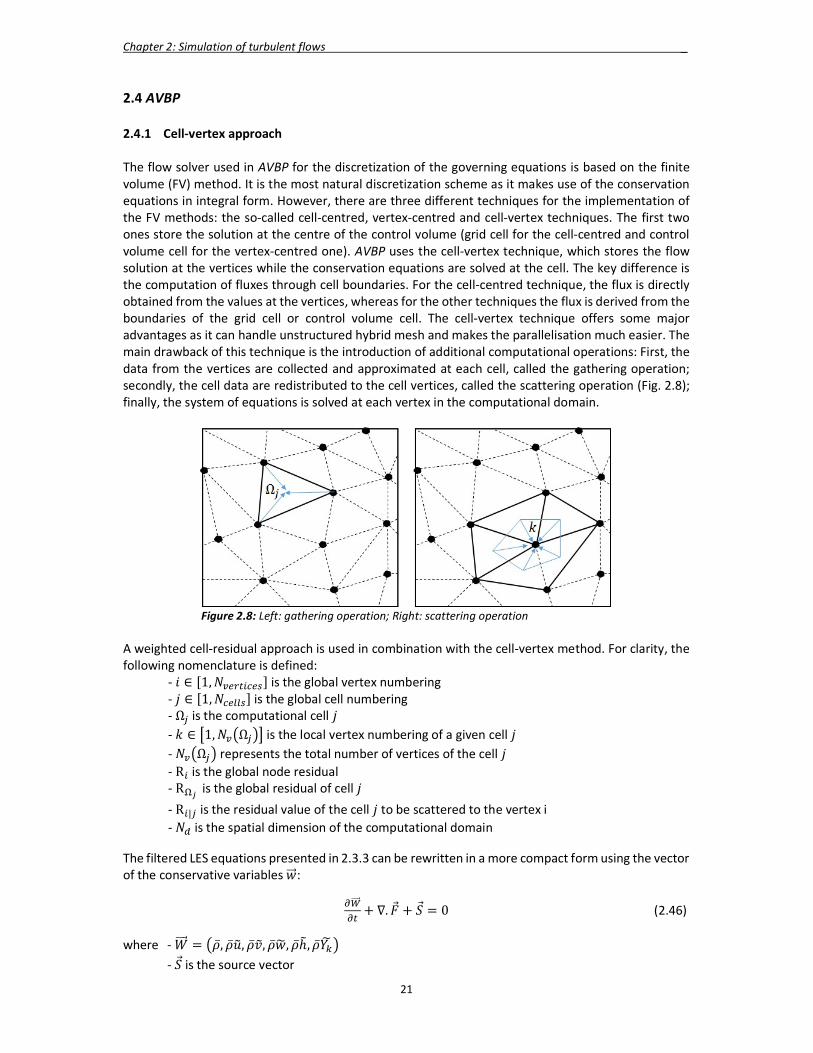
Chapter 2: Simulation of turbulent flows _
21
2.4 AVBP 2.4.1 Cell-vertex approach The flow solver used in AVBP for the discretization of the governing equations is based on the finite volume (FV) method. It is the most natural discretization scheme as it makes use of the conservation equations in integral form. However, there are three different techniques for the implementation of the FV methods: the so-called cell-centred, vertex-centred and cell-vertex techniques. The first two ones store the solution at the centre of the control volume (grid cell for the cell-centred and control volume cell for the vertex-centred one). AVBP uses the cell-vertex technique, which stores the flow solution at the vertices while the conservation equations are solved at the cell. The key difference is the computation of fluxes through cell boundaries. For the cell-centred technique, the flux is directly obtained from the values at the vertices, whereas for the other techniques the flux is derived from the boundaries of the grid cell or control volume cell. The cell-vertex technique offers some major advantages as it can handle unstructured hybrid mesh and makes the parallelisation much easier. The main drawback of this technique is the introduction of additional computational operations: First, the data from the vertices are collected and approximated at each cell, called the gathering operation; secondly, the cell data are redistributed to the cell vertices, called the scattering operation (Fig. 2.8); finally, the system of equations is solved at each vertex in the computational domain.
Figure 2.8: Left: gathering operation; Right: scattering operation
A weighted cell-residual approach is used in combination with the cell-vertex method. For clarity, the following nomenclature is defined:
- 𝑖 ∈ [1, 𝑁 ] is the global vertex numbering - 𝑗 ∈ [1, 𝑁 ] is the global cell numbering - Ω is the computational cell 𝑗 - 𝑘 ∈ 1, 𝑁 Ω is the local vertex numbering of a given cell 𝑗 - 𝑁 Ω represents the total number of vertices of the cell 𝑗 - R is the global node residual - R
is the global residual of cell 𝑗
- R | is the residual value of the cell 𝑗 to be scattered to the vertex i - 𝑁 is the spatial dimension of the computational domain
The filtered LES equations presented in 2.3.3 can be rewritten in a more compact form using the vector of the conservative variables 𝑤:
+ ∇. �� + 𝑆 = 0 (2.46)
where - �� = ��, ��𝑢, ��𝑣, ��𝑤, ��ℎ, ��𝑌 - 𝑆 is the source vector

Chapter 2: Simulation of turbulent flows _
22
- �� is the flux tensor, which can be divided in three distinct terms: The inviscid term (𝐹), the viscous term (𝐹 ) and the turbulent subgrid-scale terms (𝐹 ).
�� = 𝐹 + 𝐹 + 𝐹 (2.47)
The volume integral of Eq. (2.46) over the cell Ω , neglecting the source and the viscous terms for clarity, gives:
∮
𝑑Ω + ∮ ∇. ��
𝑑Ω = 0 (2.48)
Using the Gauss’s theorem stating that the outward flux of a vector field through a closed surface is equal to the volume integral of the divergence over the region inside the surface, Eq. (2.48) becomes:
∮
𝑑Ω + ∮ ��. 𝑑��
∑ = 0 (2.49)
The residual 𝑅 at the cell Ω is obtained using:
𝑅 = − ∮ ��. 𝑑��
∑ (2.50)
The residual 𝑅 is computed at each cell by linearly integrating the flux at the cell faces. In the case of tetrahedral cells, a mid-point rule is used, assuming that the flux varies linearly along their triangular faces. The discrete formulation of the residual becomes:
𝑅 = ∑ ��. ∈ ∆�� , (2.51)
where : -∆�� , is the average of the area-weighted normal for triangular faces linked to the vertex 𝑘
∆�� , = ∑ −,
∈ / ∈ 𝑛 and ∑ ∆�� ,
∈ = 0 (2.52)
-𝑁 is the number of space dimensions -𝑛 is the area weighted normal vector of face 𝑓 as shown in Fig. 2.9 -𝑁 , is the number of vertices of face 𝑓 -𝑉 is the volume of the cell
Figure 2.9: Definition of the vectors for a triangular cell
Once the residual is known at the cell, it is necessary to express this quantity at each vertex of the cell in order to solve the system of equations and advance in time. The vertex residual is named 𝑅 and Eq. (2.46) becomes:
= −𝑅 (2.53)

Chapter 2: Simulation of turbulent flows _
23
where: 𝑅 = ∑ 𝐷 , ∈ 𝑉 𝑅 (2.54)
𝐷 is called the distribution matrix. During the scattering process it redistributes a weighted residual
of the cell Ω to each cell vertex 𝑘. The conservation is maintained if ∑ 𝐷 ∈ = 𝐼, where 𝐼 is the unit
matrix. The expression of the distribution matrix is dependent on the numerical scheme used. 𝑉 is the control volume associated to each vertex 𝑘. 𝑉 is linked to the cell volume by the following expression:
𝑉 = ∑ , ∈ (2.55)
In the case of inviscid flows the vertex residual is solely dependent on 𝑊. However when considering viscous flows, the information of the gradient ∆�� for the diffusive terms is required at each vertex. In that case, the cell based gradient is, like in Eq. (2.49), approximated using the Gauss’s theorem. The gradient at the vertex location is then derived using a volume-weighted average of the cell-based gradients:
∆�� = ∑ 𝑉 , ∈ (∆��) (2.56)
In AVBP the conservative variable 𝑊 is computed iteratively during the simulation using an acoustic explicit time advancement. Eq. (2.46) becomes:
𝑊( )
= 𝑊( )
− ∆𝑡. 𝑅( ) (2.57)
Compared to an implicit time advancement solver, which is unconditionally stable but computationally more expensive, the acoustic explicit solver has to restrict the time step of the simulation ∆𝑡 for stability reasons:
∆𝑡 ≤ 𝐶𝐹𝐿_𝑎𝑐 ( )
‖ ‖,
(2.58)
where 𝑐 is the speed of sound, 𝑢 is the flow velocity, 𝑉 is the smallest volume cell in the computational domain. The final choice of the value for the 𝐶𝐹𝐿_𝑎𝑐 number is left to the user. Usual values lie between 0.7 and 0.9. 2.4.2 Numerical convective schemes
Lax-Wendroff scheme This scheme is the adaptation for the cell-vertex formulation of the classical Lax-Wendroff numerical scheme developed by Lax and Wendroff [38]. Its accuracy is of second-order in space in time and is based on a one-step Taylor expansion in time of the conservative variable 𝑊. The one-step time marching is handled by a Runge-Kutta method. Despite being a forward in time and centred in space scheme, it is a robust scheme due to the presence of an additional diffusive term. The time integration is performed using a second order Taylor series expansion.
( ) ( )
∆= +
∆+ 𝒪(∆𝑡 ) (2.59)
Lax and Wendroff proposed to replace the first and second temporal derivatives with the spatial derivatives considering Eq. (2.46):
= −(∇. 𝐹) (2.60)

Chapter 2: Simulation of turbulent flows _
24
= − (∇. 𝐹) (2.61)
= −∇. (2.62) = ∇. (𝒜∇. 𝐹) (2.63)
where 𝒜 is the Jacobian matrix of convective fluxes. Substituting Eq. (2.63) and Eq. (2.62) into Eq. (2.59) leads to:
( ) ( )
∆= −(∇. 𝐹) +
∆(∇. (𝒜∇. 𝐹) ) + 𝒪(∆𝑡 ) (2.64)
It can be shown that the distribution matrix introduced in Eq. (2.54) takes the following form in combination with the Lax-Wendroff scheme:
𝐷 = 𝐼 −∆
𝒜 . ∆𝑛 , (2.65)
In the above expression, two terms can be recognized: the first one corresponds to the centred differences and the second one comes from the Lax-Wendroff methodology. This second term is the dissipative and stabilizing term of the Lax-Wendroff scheme. The solution at time (𝑛 + 1) of the conservative variable 𝑊 at each vertex 𝑘 of the computational domain is hence given by:
𝑊( )
= 𝑊( )
− ∆𝑡 ∑ 𝐷 , ∈ 𝑉 𝑅 (2.66)
Two-step Taylor Galerkin (TTGC) scheme
TTGC is a version of the two-step Taylor-Galerkin (TTG) schemes. This family of schemes is based on the finding that finite-volume methods in a cell-vertex formulation can be interpreted as a finite-element approach, allowing the development of Taylor-Galerkin type schemes. This finite element scheme is third-order accurate in time and space and centred in space. Furthermore, it is a two-step temporal scheme handled by a Runge-Kutta method. This high-order scheme was created by Colin and Rudgyard [37]. This scheme was specifically developed for unsteady LES in order to reduce the numerical dissipation at high wavenumber, i.e. for flow length scale of the order of Δ. Compared to the Lax-Wendroff scheme, it showed a reduced numerical dispersion for middle wavenumber (flow length scales comprised between 4Δ and 10Δ) and a smaller numerical dissipation for all wavenumbers. It uses the Galerkin’s finite element method, which is compatible with the cell-vertex approach of AVBP. The two-step Taylor series expansion in time is expressed in a predictor-corrector way and reads:
( ) ( )
∆= 𝛼 + 𝛽 ∆𝑡 + 𝒪(∆𝑡 ) (2.67)
( ) ( )
∆= + 𝛾 ∆𝑡 + 𝒪(∆𝑡 ) (2.68)
where 𝛼 = 0.49, 𝛽 = , 𝛾 = − 𝛼 derived from [37]. The first and second temporal derivatives are replaced by the spatial ones considering Eq. (2.46) and the proposal of Lax and Wendroff mentioned previously:
( ) ( )
∆= −𝛼 (∇. 𝐹) + 𝛽 ∆𝑡(∇. (𝒜∇. 𝐹) ) + 𝒪(∆𝑡 ) (2.69)
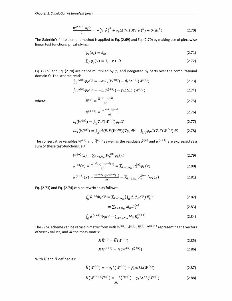
Chapter 2: Simulation of turbulent flows _
25
( ) ( )
∆= − ∇. 𝐹 + 𝛾 ∆𝑡(∇. (𝒜∇. 𝐹) ) + 𝒪(∆𝑡 ) (2.70)
The Galerkin’s finite element method is applied to Eq. (2.69) and Eq. (2.70) by making use of piecewise linear test functions 𝜑 satisfying:
𝜑 (𝑥 ) = 𝛿 (2.71)
∑ 𝜑 (𝑥) = 1, 𝑥 ∈ Ω (2.72) Eq. (2.69) and Eq. (2.70) are hence multiplied by 𝜑 and integrated by parts over the computational domain Ω. The scheme reads:
∫ 𝑅 ( )𝜑 𝑑𝑉 = −𝛼 𝐿 (𝑊( ))
− 𝛽 ∆𝑡𝐿𝐿 (𝑊( )) (2.73)
∫ 𝑅( )𝜑 𝑑𝑉 = −𝐿 (𝑊( ))
− 𝛾 ∆𝑡𝐿𝐿 (𝑊( )) (2.74)
where: 𝑅 ( ) =
( ) ( )
∆ (2.75)
𝑅( ) = ( )
∆ (2.76)
𝐿 (𝑊( )) = ∫ ∇. 𝐹(𝑊( ))𝜑 𝑑𝑉 (2.77)
𝐿𝐿 (𝑊( )) = ∫ 𝒜(∇. 𝐹(𝑊( )))∇𝜑 𝑑𝑉
− ∫ 𝜑 𝒜(∇. 𝐹(𝑊( ))𝑑𝑆 (2.78)
The conservative variables 𝑊( ) and 𝑊( ) as well as the residuals 𝑅
( ) and 𝑅( ) are expressed as a sum of these test-functions, e.g.:
𝑊( )(𝑥) = ∑ 𝑊( )
𝜑 (𝑥) , (2.79)
𝑅 ( )(𝑥) =
( )( ) ( )( )
∆= ∑ 𝑅
( )𝜑 (𝑥)
, (2.80)
𝑅( )(𝑥) =( )
( )( )
∆= ∑ 𝑅
( )𝜑 (𝑥)
, (2.81) Eq. (2.73) and Eq. (2.74) can be rewritten as follows:
∫ 𝑅 ( )Φ 𝑑𝑉 = ∑ ∫ 𝜙 𝜙 𝑑𝑉
, 𝑅
( ) (2.82)
= ∑ 𝑀 𝑅( )
, (2.83)
∫ 𝑅( )Φ 𝑑𝑉 =
∑ 𝑀 𝑅( )
, (2.84) The TTGC scheme can be recast in matrix form with 𝑊( ), 𝑊( ), 𝑅
( ), 𝑅( ) representing the vectors of vertex values, and 𝑀 the mass-matrix:
𝑀𝑅( ) = 𝐻(𝑊( )) (2.85)
𝑀𝑅( ) = 𝐻(𝑊( ), 𝑊( )) (2.86) With 𝐻 and 𝐻 defined as:
𝐻 𝑊( ) = −𝛼 𝐿 𝑊( ) − 𝛽 ∆𝑡𝐿𝐿(𝑊( )) (2.87)
𝐻 𝑊( ), 𝑊( ) = −𝐿 𝑈( ) − 𝛾 ∆𝑡𝐿𝐿(𝑊( )) (2.88)

Chapter 2: Simulation of turbulent flows _
26
The mass-matrix has to be inverted. However, an exact mass-matrix inversion operation is too computationally intensive, considering the high number of cells in the computational domain and the high number of time steps due to the explicit time advancement scheme. Instead, the mass-matrix is inverted locally using an iterative Jacobi method [39]. The increase of the computational time due to the two-step time integration and the iterative calculation of the inversion of the mass matrix, was found to be 2.5 time higher compared to the Lax-Wendroff scheme [27]. Furthermore, it was shown that TTGC was more accurate and less computationally costly than using a global mesh refinement strategy combined with the Lax-Wendroff scheme [27]. The order of accuracy of a numerical scheme quantifies the rate of convergence of a numerical approximation of a differential equation with respect to the exact solution. The mesh size is one important parameter, as a mesh refinement automatically reduces the error between the exact solution and the approximated one. Furthermore, the order of accuracy of the numerical scheme impacts the rate of error reduction. If the cell size of the mesh is halved, the error is reduced by a factor 2 for a first-order scheme, by a factor 4 for a second-order scheme and by a factor 8 for a third-order scheme. With a high-order scheme, as the error decreases more rapidly with the cell size, it is expected to reach quickly a grid independent solution on a coarse mesh than with a low-order scheme. However, this statement does not automatically imply that a high-order scheme is necessarily more accurate than a low-order scheme. It depends in a first place on the mesh resolution used. 2.4.3 Artificial viscosity The Lax-Wendroff and TTGC convective numerical schemes are centred in space. They are known to give rise to high frequency numerical oscillations (wiggles) in under-resolved high gradient regions with bad quality cells or insufficient mesh refinement. These oscillations, if they are not damped out at their onset, could grow and propagate in the computational domain. As a result, they pollute the flow solution and can influence the numerical stability of the simulation. The introduction of a so-called artificial viscosity can strongly attenuate these oscillations. There are two models in AVBP for the artificial viscosity: a 2nd-order artificial viscosity (𝑑 ) and a 4th-order artificial viscosity (𝑑 ). They are included in the governing equation (Eq. 2.53) as follows:
= −𝑅 + 𝑑 + 𝑑 (2.89)
The 2nd-order artificial viscosity (𝒅𝒊𝟐)
The 2nd-order artificial viscosity is only used in regions, where local under-resolved high gradients (energy and species) are present. It behaves like a normal viscosity and dissipates those high gradients. Several sensors (𝜁) are used for the gradient detections and require an accurate calibration to ensure that the additional viscosity is only applied locally in the high gradient regions and not at the wrong locations in the computational model. The sensor values oscillate between zero, where no artificial viscosity is required, and one, where high gradients are detected. In the present research work, the sensor developed by Colin [27] is used. The 2nd-order artificial viscosity is applied to the transport equations of enthalpy, species and momentum and is defined as follows:
𝑑 =𝑺𝒎𝒖𝟐
∆∑ 𝑊 − 𝑊
∈ (2.90)
where 𝑊 is the average value of 𝑊 within the cell Ω and 0≤ 𝜁 ≤ 1.
The 4th-order artificial viscosity (𝒅𝒊𝟒)
The 4th-order artificial viscosity acts as a background viscosity everywhere in the computational domain and dissipates the high frequency oscillations. It does not have any sensor and is hence added everywhere except in the regions detected by the sensor of the 2nd-order artificial viscosity. The 4th-order artificial viscosity is applied to the transport equations of enthalpy and species and not to the
Chapter 2: Simulation of turbulent flows _
27
momentum transport equation in order to prevent a global dissipation of the small flow scales. Its definition reads:
𝑑 =𝑺𝒎𝒖𝟒
∆∑ (∇𝑊) . (𝑋 − 𝑋 ) − 𝑊 − 𝑊
∈ (2.91)
𝑆𝑚𝑢4 = max (0, 𝑆𝑚𝑢4 − 𝑆𝑚𝑢2𝜁 ) (2.92)
where 𝑋 is the average value of 𝑋 within the cell Ω . Each artificial viscosity model has a tuning parameter (𝑆𝑚𝑢2 and 𝑆𝑚𝑢4) that allows the user to increase the amount of artificial viscosity applied in the computational model. Standard values for these parameters, derived from validated test cases, are provided in the user manual of AVBP [109]. However, one should keep in mind that forcing the simulation to run with excessive amount of artificial viscosity would massively dissipate the flow structures and reduce the fidelity of the LES. Following a simulation crash due to numerical instabilities, a new mesh generation using an increased mesh resolution in the region showing some issues, usually solves the problems. 2.4.4 Solid wall boundary condition: the no-slip wall law A widely used implementation of the standard wall functions is based on the so-called free-slip approach. Hereby the tangential velocity component at the wall nodes is not explicitly imposed, while the tangential viscous friction is fixed at the wall boundaries using the value of 𝜏 obtained from the standard wall functions. In order to ensure mass conservation the wall normal velocity is set to zero at the end of each iteration. In such a free-slip formulation, the tangential velocity component at the wall is a free parameter. For cell-centred schemes, the normal and tangential vectors are uniquely defined at each cell face. However, for cell-vertex schemes, as the flow variables and the normal vectors are stored at each cell vertex, the definition of the normal vector is not unique anymore when geometrical corners are encountered. As a result, the free tangential velocity component could lead to the computation of unphysical flow orientations and the appearance of unrealistic flow detachments. As the engine geometry entails many sharp edges, this free-slip formulation is not considered for the engine in-cylinder flow simulation. Instead, the so-called no-slip wall law boundary condition (NSWL) developed and validated by Nicoud et al. [30], is used. To overcome the aforementioned shortcomings of the free-slip formulation, the normal and tangential velocity are set to zero. The normal gradient of the tangential velocity at the wall is computed followed by the estimation of the wall shear
stress 𝜏 from the standard wall functions. At the first off-wall vertex a corrected turbulent viscosity is imposed and reads:
𝜇 , =
,
− 𝜇 (2.93)
The no-slip wall law boundary condition uses the standard wall functions for the prediction of the flow momentum and heat fluxes near the wall and is valid on any type of wall cells. 2.4.5 Mesh and Morph-Map method Several meshes need to be generated in order to cover one engine cycle, as AVBP uses the Morph-Map technique during the simulation. As illustrated in fig. 2.10, it consists in using one mesh, deform it until a cell quality criteria is not reached anymore and map the LES solution onto the next mesh. One engine cycle encompasses several, so called, calculation phases. Each phase is ascribed to one mesh and run for a couple of crank-angle degrees. All the meshes are generated before running the simulation using the commercial software Centaur [118]. The CFD model is divided into different zones in which the mesh movement can be allowed or not. Each engine part is made of multiple panel geometries. Different control parameters can be used to control the meshing setup:
- The base cell size and the closest distance between the panels for the surface mesh. - The base cell size and the growth ratio for the volume mesh.
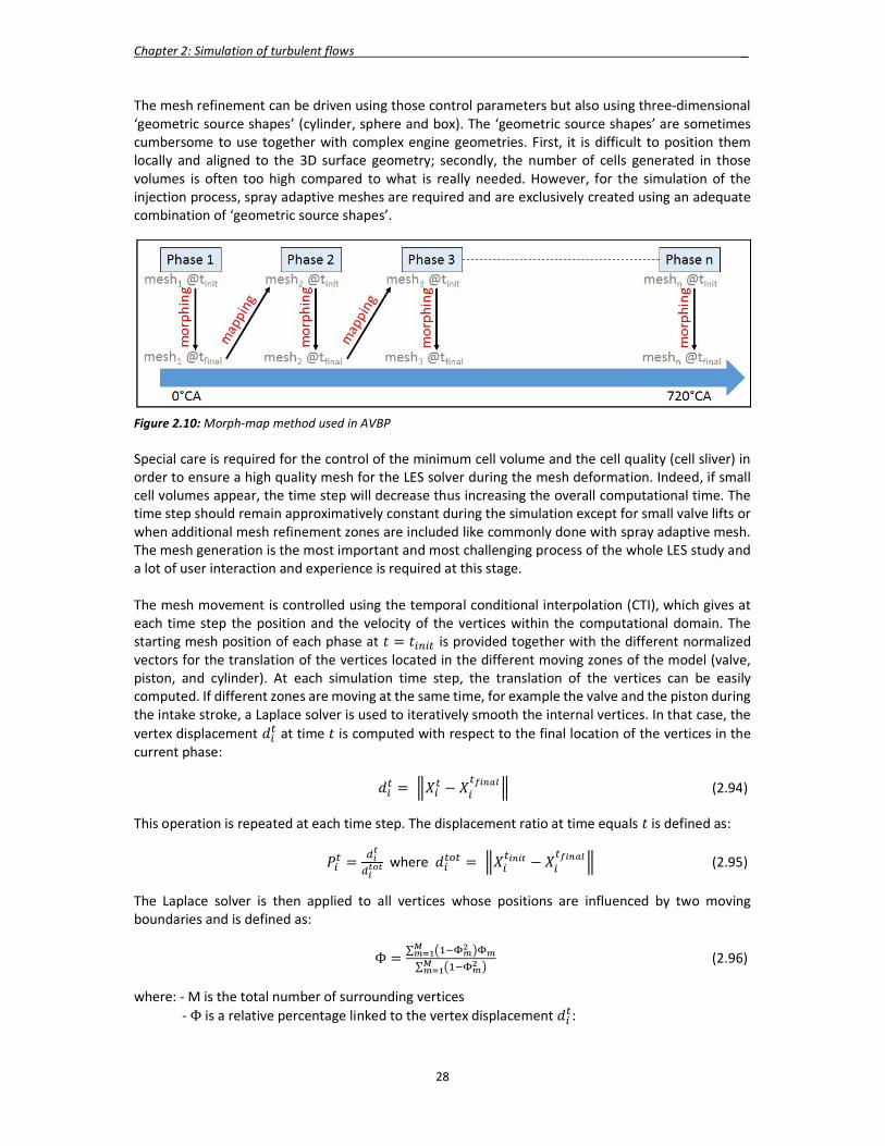
Chapter 2: Simulation of turbulent flows _
28
The mesh refinement can be driven using those control parameters but also using three-dimensional ‘geometric source shapes’ (cylinder, sphere and box). The ‘geometric source shapes’ are sometimes cumbersome to use together with complex engine geometries. First, it is difficult to position them locally and aligned to the 3D surface geometry; secondly, the number of cells generated in those volumes is often too high compared to what is really needed. However, for the simulation of the injection process, spray adaptive meshes are required and are exclusively created using an adequate combination of ‘geometric source shapes’.
Figure 2.10: Morph-map method used in AVBP Special care is required for the control of the minimum cell volume and the cell quality (cell sliver) in order to ensure a high quality mesh for the LES solver during the mesh deformation. Indeed, if small cell volumes appear, the time step will decrease thus increasing the overall computational time. The time step should remain approximatively constant during the simulation except for small valve lifts or when additional mesh refinement zones are included like commonly done with spray adaptive mesh. The mesh generation is the most important and most challenging process of the whole LES study and a lot of user interaction and experience is required at this stage. The mesh movement is controlled using the temporal conditional interpolation (CTI), which gives at each time step the position and the velocity of the vertices within the computational domain. The starting mesh position of each phase at 𝑡 = 𝑡 is provided together with the different normalized vectors for the translation of the vertices located in the different moving zones of the model (valve, piston, and cylinder). At each simulation time step, the translation of the vertices can be easily computed. If different zones are moving at the same time, for example the valve and the piston during the intake stroke, a Laplace solver is used to iteratively smooth the internal vertices. In that case, the vertex displacement 𝑑 at time 𝑡 is computed with respect to the final location of the vertices in the current phase:
𝑑 = 𝑋 − 𝑋 (2.94)
This operation is repeated at each time step. The displacement ratio at time equals 𝑡 is defined as:
𝑃 = where 𝑑 = 𝑋 − 𝑋 (2.95)
The Laplace solver is then applied to all vertices whose positions are influenced by two moving boundaries and is defined as:
Φ =∑
∑ (2.96)
where: - M is the total number of surrounding vertices - Φ is a relative percentage linked to the vertex displacement 𝑑 :
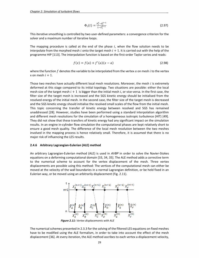
Chapter 2: Simulation of turbulent flows _
29
Φ (𝑡) = (2.97)
This iterative smoothing is controlled by two user-defined parameters: a convergence criterion for the solver and a maximum number of iterative loops. The mapping procedure is called at the end of the phase 𝑖, when the flow solution needs to be interpolate from the morphed mesh 𝑖 onto the target mesh 𝑖 + 1. It is carried out with the help of the programme HIP [113]. The interpolation function is based on the first-order Taylor series and reads:
𝑓(𝑥) = 𝑓(𝑎) + 𝑓 (𝑎)(𝑥 − 𝑎) (2.98) where the function 𝑓 denotes the variable to be interpolated from the vertex 𝑎 on mesh 𝑖 to the vertex x on mesh 𝑖 + 1. Those two meshes have actually different local mesh resolutions. Moreover, the mesh 𝑖 is extremely deformed at this stage compared to its initial topology. Two situations are possible: either the local mesh size of the target mesh 𝑖 + 1 is bigger than the initial mesh 𝑖, or vice-versa. In the first case, the filter size of the target mesh is increased and the SGS kinetic energy should be initialised from the resolved energy of the initial mesh. In the second case, the filter size of the target mesh is decreased and the SGS kinetic energy should initialise the resolved small scales of the flow from the initial mesh. This topic concerning the transfer of kinetic energy between resolved and SGS has remained unaddressed [28]. However, studies have been performed using a standard interpolation algorithm and different mesh resolutions for the simulation of a homogeneous isotropic turbulence (HIT) [49]. They did not show that these transfers of kinetic energy had any significant impact on the simulation results. In an engine in-cylinder flow simulation the computational phases are kept relatively short to ensure a good mesh quality. The difference of the local mesh resolution between the two meshes involved in the mapping process is hence relatively small. Therefore, it is assumed that there is no major risk of influencing the LES results. 2.4.6 Arbitrary Lagrangian-Eulerian (ALE) method An arbitrary Lagrangian-Eulerian method (ALE) is used in AVBP in order to solve the Navier-Stokes equations on a deforming computational domain [33, 34, 35]. The ALE method adds a corrective term to the numerical scheme to account for the vertex displacement of the mesh. Three vertex displacements are possible using this method: The vertices of the computational mesh can either be moved at the velocity of the wall boundaries in a normal Lagrangian definition, or be held fixed in an Eulerian way, or be moved using an arbitrarily displacement (Fig. 2.11).
Figure 2.11: Vertex displacements with ALE
The numerical schemes presented in 2.3.3 for the solving of the filtered LES equations on fixed meshes have to be modified using the ALE formalism, in order to take into account the effect of the mesh displacement [36]. At every iteration, the ALE method ascribes to each vertex a displacement velocity,

Chapter 2: Simulation of turbulent flows _
30
which is assumed to be constant during one computational time step. This assumption is justified by the fact that the movement of the mesh is supposed to be linear during each time step of the simulation with an explicit time advancement solver. This allows to take into account the movement of the vertices in the numerical scheme formulation. The conservative variable 𝑊 and the flux 𝐹 are now considered to be functions of the mesh position 𝑋 and time: 𝑊(𝑋, 𝑡) and 𝐹(𝑋, 𝑡). The difference in formalism of the spatial integration of the schemes on moving meshes comes from the Leibniz transport theorem [49]. It describes the variations of the integral of the variable 𝜓(𝑥, 𝑡) on a time-varying domain 𝑉(𝑡) moving at the velocity ��(𝑥, 𝑡) and gives:
∫ 𝜓(𝑥, 𝑡)𝑑𝑉 = ∫ + ∇. ��𝜓 𝑑𝑉
( )
( ) (2.99)
Applying the Leibniz transport theorem to Eq. 2.48, it becomes:
∮
𝑑Ω + ∮ ∇. (�� + ����
𝑑Ω = 0 (2.100)
The numerical schemes for moving meshes in AVBP fulfil the geometric conservation law (GCL) that is to say the conservation of the cell volumes and cell face areas [36]. In order to illustrate the changes applied to the original Lax-Wendroff numerical scheme with the ALE formalism a brief overview is provided hereafter. The full derivation of the ALE method for the Lax-Wendroff and TTGC numerical schemes was published by Moureau [49].
Lax-Wendroff scheme for moving-meshes From [36] after including the ALE correction factor in Eq. (2.66) it becomes:
𝑊( )
= 𝑊( )
− ∆𝑡( )
( ) 𝑅 + 𝑅 _ (2.101)
where:
𝑅 =( ) ( )
∆ ( )
𝑊( ) (2.102)
𝑅 _ =( )
∑ 𝑉( )
, ∈ + 𝐷 , 𝑅 + 𝑅 (2.103)
𝐷 , =∆
( )𝒜
( )− �� . ∆𝑛 ,
( ) (2.104)
𝑅 =( )
∑ ��( )
− 𝑊( )
�� ∈ . ∆𝑛 ,
( ) (2.105)
𝑅 =
( )
( )∑ ��.
∈ ∆𝑛 ,
( ) (2.106)
Compared to the expression of the Lax-Wendroff scheme for static meshes, several modifications can be observed. As this scheme is centred, all the geometrical quantities (normal vectors and cell volumes) are now computed in the middle of the computational time step i.e. at t=n+1/2. Furthermore, the correction factors introduced by the ALE can be split into two categories:
- The ALE corrections due to the variation of the cell volumes: 𝑅 and 𝑅 .
- The ALE corrections due to the movement of the vertices: 𝐷 , and 𝑅 .
31
Chapter 3
Simulation of the fuel injection The present chapter covers the methodology used in AVBP for the simulation of the dispersed flow, formed by the atomized fuel droplets within the spray. As the outward-opening Piezo-actuated Pintle-type injector was of particular interest in this research work, improvements were made in AVBP to make the simulation of this type of injector possible. Furthermore, additional sub-models were implemented to increase the droplet description accuracy. This chapter is divided into six parts. The first one presents the general equation for the dispersed two-phase flows. The second part introduces the discrete droplet model used in AVBP to solve the spray equation and the methods used. In a third part, the sub-models required to model the processes acting on the single droplet are described. It includes the newly implemented interpolation algorithm for the gas-liquid coupling and the droplet secondary break-up model. The fourth part deals with the difference in gas-phase turbulence between RANS and LES. The fifth part presents the methodology developed to couple the internal nozzle-flow simulation in RANS with the Lagrangian spray simulation in LES, in order to model accurately the droplet primary break-up of the Piezo injector. Finally the derivation of the droplet initialisation and the droplet injection procedure is addressed in the last part. 3.1 Equation for dispersed two-phase flows The spray can be categorised as a dispersed flow that contains evaporating droplets of various sizes travelling at different velocities. In a spray simulation, it would be too computationally expensive to calculate for each time 𝑡 the values of droplet position ��, droplet radius 𝑟, droplet velocity �� and droplet temperature 𝑇 of each droplet within a spray consisting of hundreds of millions of droplets. Instead, a statistical description of the spray is considered using the droplet probability distribution function (PDF) 𝑓(��, 𝑢, 𝑟 , 𝑇 , 𝑡). Therefore, the probable number of droplets per unit volume at time 𝑡, which are located between 𝑥 and �� + 𝑑𝑥 and characterised by a velocity between �� and 𝑣 + 𝑑𝑣, a radius between 𝑟 and 𝑟 + 𝑑𝑟 and a temperature between 𝑇 and 𝑇 + 𝑑𝑇 is described with the probability distribution function 𝑓. In total 𝑓 is a function in nine-dimensional space that could be extended to eleven if droplet deformation and deformation velocity are included in the distribution function. The temporal and spatial evolution of 𝑓 is described by a transport equation, called the Williams spray equation [58, 59], which was derived in analogy to the transport equations of the gas phase:
= − 𝑓 − 𝑓 − 𝑓 − 𝑓 − 𝑓 (3.1)
is the acceleration of the droplet, whereas and are respectively the rate of change of the droplet radius and temperature due to evaporation and heating. The equation entails the source term 𝑓 that enables the creation or removal of droplet found in processes like the droplet break-up or the droplet coalescence. As the individual terms of the spray equations can be further expressed with functions and differential equations, the direct solving of the spray equation is generally impracticable. Moreover, the discretisation of the equation in the nine independent dimensions would lead to very high computational memory and power requirements.
Chapter 3: Simulation of the fuel injection _
32
3.2 The Discrete Droplet Model An alternative approach to the direct solving of the William spray equation, used in most CFD-codes (Kiva, Star-CD, FIRE, Converge, ANSYS etc.) and in this research work, is the discrete droplet model (DDM) proposed by Dukowicz [60]. A Monte-Carlo method is used in order to perform an approximation of the exact solution of 𝑓. Applying the Monte-Carlo method to the William spray equation means that only a discrete number of all the droplets is calculated in detail. It is assumed that the properties and the behaviour of all the droplets in the spray can be approximately represented by these discrete droplets. However, to match the total injected mass, each representative droplet is given a class of several droplets with identical size, temperature, velocity etc., which have exactly the same properties like the representative one. This class of equal droplets is called parcels. The spray is hence described by a stochastic system of a discrete number of parcels that are tracked through the computational domain in a Lagrangian manner. The collection of the parcels at time 𝑡 during the simulation represents a discretized solution of the probability distribution function of the spray. In return, it implies the modelling of the processes acting on a single droplet corresponding to the different terms of the Williams spray equation (Eq. 3.1). It is viewed as the standard approach in today’s engine spray simulations. The gas phase is described using the Navier-Stokes equations as explained in chapter 2, using an Eulerian formulation. The flow quantities are described as a function of a point in space (related to a fixed coordinate system) and time, whereas it is done as a function of a particle and time in the Lagrangian description. The dispersed phase and the gas phases interact with each other as momentum, energy and mass have to be exchanged. The sources terms in the transport equations of the gas phase, described in chapter 2, allow the increase or decrease of momentum, energy and mass in each grid cell. The influence of the gas phase on a moving parcel is taken into consideration using sub-models, which are based on the local flow data of the cell encompassing the parcel. The gas-phase source terms of each grid cell are hence obtained by considering the global rates of change of momentum, mass and energy of all parcels inside the cell. Due to the coupling with the gas phase, significant influence of the local mesh size and mesh topology are observed on the results of the spray simulation using the discrete droplet model. A spray simulation requires a customized spray adaptive mesh starting at the exit of the nozzle. Its meshing-setup requirements depend solely on the characteristics of the spray and require very small cell size at the exit of the injector to capture the local length scales of the flow. It could be a fastidious task to figure out the optimal meshing setup and require lots of experience. Furthermore, in the computational domain defined by the spray adaptive mesh, statistical convergence of the spray should be achieved. As a result, not only the number of cells have to be increased in this domain, but also the ratio of parcels per cell. It implies in return a huge number of parcels required for the spray simulation [57,61]. Droplet-gas coupling or ‘two-way’ coupling In the filtered continuity, momentum, energy and species equations of LES (Eqs. 2.28-2.31) the exchange of mass, momentum and energy with the dispersed phase is described by the source terms 𝑆 , 𝑆 , 𝑆 and 𝑆 . In AVBP, the coupling is defined at the vertex locations of the computational cells [109]. A control volume is hence created around the vertex 𝑗 of the cell containing a droplet as shown in Fig. 3.1. The contribution of each droplet is weighted by its inverse distance factor to the vertex 𝑗 and gives:
𝑊 =/
∑ / ,
(3.2)
where: - 𝑑 is the distance from the droplet to the vertex 𝑗 of the cell 𝑖 - 𝑑 is the distance from the droplet to the vertex 𝑘 of the cell 𝑖 - 𝑁 is the total number of vertex in the cell 𝑖

Chapter 3: Simulation of the fuel injection _
33
Figure 3.1: Control volume ascribed to vertex 2 for the two-way coupling operation The source terms, computed at the vertex location, are defined as follows:
𝑆 = ∑ 𝑊 (𝑥 , )�� , (3.3)
𝑆 = ∑ 𝑊 (𝑥 , )(−𝑚 , 𝐹 , + 𝑔 + �� , 𝑢 , ) (3.4)
𝑆 = ∑ 𝑊 (𝑥 , )(−𝑚 , �� , + 𝑔 . 𝑢 , + �� , 𝑢 , − Φ , ) (3.5)
𝑆 = ∑ 𝑊 (𝑥 , )�� , (3.6) 3.3 Sub-models for the single-droplet approach In the single-droplet approach, the various processes acting on each single droplet need to be modelled. Those include the exchange processes of mass, momentum and heat between the single droplet and the gas phase and the secondary droplet break-up. So-called sub-models are implemented to capture the aforementioned processes in the simulation. They are presented hereafter. 3.3.1 Droplet kinematics In the Lagrangian formulation of the discrete droplet model, the single-droplet i.e. parcel is characterised by its position �� , velocity 𝑢 , mass 𝑚 , radius 𝑟 and temperature 𝑇 . The system of equations describing the temporal evolution of the motion, mass and temperature of each droplet reads:
𝒟 ,
𝒟= 𝑢 , (3.7)
𝑚𝒟 ,
𝒟= ∑ �� , + 𝑔 (3.8)
𝒟
𝒟= �� (3.9)
𝑚𝒟 , ( )
𝒟= Φ (3.10)
where: ∑ �� , are the forces acting on the droplet, 𝑔 the gravity force, and �� the source term for the mass due to the evaporation of the droplet and Φ the source term for the sensible enthalpy.
Chapter 3: Simulation of the fuel injection _
34
3.3.2 Droplet equations of motion The motion of the droplet is driven by Eqs. 3.7-3.8. The considered force acting on a droplet was the drag force �� , caused by the relative velocity of the droplet to the surrounding gas phase. It results in a deceleration of the droplet and an acceleration of the gas due to the exchange of momentum. �� can be expressed as:
�� = 𝜌 𝐶 𝐴 |𝑢 − 𝑢 |(𝑢 − 𝑢 ) (3.11)
where: 𝜌 is the gas density, 𝐴 the frontal area of the droplet, i.e. for a spherical droplet (𝐴 = 𝜋𝑟 ), �� is the gas velocity. 𝐶 is the drag coefficient. In order to quantify the flow regime around the droplet, the particle Reynolds number is defined:
𝑅𝑒 =| |
(3.12)
where 𝜇 is the kinematic viscosity of the gas.
In this research project, the formulation of the drag coefficient proposed by Schiller and Naumann [67] using solid particles was chosen, as it is one of the most popular in CFD codes:
𝐶 = 1 + 0.15𝑅𝑒 . 𝑅𝑒 ≤ 1000 (3.13)
𝐶 = 0.438 𝑅𝑒 > 1000 However, as mentioned in [68] the drag coefficient is lower for a droplet than for a spherical solid particle due to the droplet deformation. In this research work, no droplet deformation was taken into account. The computed drag forces are hence likely to be overestimated in the simulation and should be kept in mind when analysing the results. The drag force is the dominant force influencing the motion of the droplet. Nevertheless, additional forces are acting on the droplets such as the pressure (buoyancy) force, the added mass force and the Basset force. The droplet equation of motion including all the four forces is referred to as the Basset-Boussinesq-Oseen (BBO) equation. However, it was shown that if the density of the dispersed flow is much higher than the gas flow (𝜌 /𝜌 > 10 ) then these additional forces could be neglected [69]. As a result, the droplet equations of motion read:
,= 𝑢 , (3.14)
,
=, ,
+ 𝑔 (3.15)
where 𝑢 , is the interpolated filtered gas velocity at the position of the droplet and 𝜏 is the relaxation time of the droplet defined by:
𝜏 = (3.16)
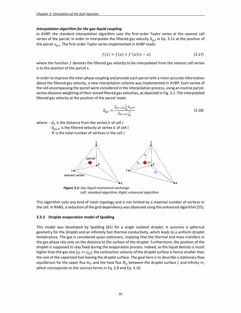
Chapter 3: Simulation of the fuel injection _
35
Interpolation algorithm for the gas-liquid coupling In AVBP, the standard interpolation algorithm uses the first-order Taylor series at the nearest cell vertex of the parcel, in order to interpolate the filtered gas velocity 𝑢 , in Eq. 3.15 at the position of the parcel 𝑥 , . The first-order Taylor series implemented in AVBP reads:
𝑓(𝑥) = 𝑓(𝑎) + 𝑓 (𝑎)(𝑥 − 𝑎) (3.17)
where the function 𝑓 denotes the filtered gas velocity to be interpolated from the nearest cell vertex 𝑎 to the position of the parcel x. In order to improve the inter-phase coupling and provide each parcel with a more accurate information about the filtered gas velocity, a new interpolation scheme was implemented in AVBP. Each vertex of the cell encompassing the parcel were considered in the interpolation process, using an inverse parcel-vertex distance weighting of their stored filtered gas velocities, as depicted in Fig. 3.2. The interpolated filtered gas velocity at the position of the parcel reads:
𝑢 , =∑ , ,
,
∑ ,
(3.18)
where: - 𝑑 is the distance from the vertex 𝑘 of cell 𝑖 - 𝑢 , , is the filtered velocity at vertex 𝑘 of cell 𝑖 - 𝑁 is the total number of vertices in the cell 𝑖
Figure 3.2: Gas-liquid momentum exchange Left: standard algorithm; Right: enhanced algorithm
This algorithm suits any kind of mesh topology and is not limited by a maximal number of vertices in the cell. In RANS, a reduction of the grid dependency was observed using this enhanced algorithm [55]. 3.3.3 Droplet evaporation model of Spalding This model was developed by Spalding [81] for a single isolated droplet. It assumes a spherical geometry for the droplet and an infinitely fast thermal conductivity, which leads to a uniform droplet temperature. The gas is considered quasi-stationary, implying that the thermal and mass transfers in the gas phase rely only on the distance to the surface of the droplet. Furthermore, the position of the droplet is supposed to stay fixed during the evaporation process. Indeed, as the liquid density is much higher than the gas one (𝜌 >> 𝜌 ), the contraction velocity of the droplet surface is hence smaller than the one of the vaporized fuel leaving the droplet surface. The goal here is to describe a stationary flow equilibrium for the vapor flux �� and the heat flux Φ between the droplet surface 𝜁 and infinity ∞, which corresponds to the sources terms in Eq. 3.9 and Eq. 3.10.

Chapter 3: Simulation of the fuel injection _
36
Mass transfer at the droplet surface Due to the spherical droplet geometry, only the flux variations in radial direction are considered. The continuity equation and the vapour transport equation from the droplet surface to a spherical shell of radius 𝑟 reads:
4𝜋𝜌 𝑢(𝑟) 𝑟 = 𝐶 (3.19)
4𝜋𝜌 𝑢(𝑟) 𝑟 𝑌 (𝑟) − 4𝜋𝐷 𝜌 𝑟 ( )
= 𝐶 (3.20)
where: 𝐶 is the total mass flux �� , 𝐶 the vapor mass flux �� , 𝐷 the diffusivity coefficient of the vaporized fuel and 𝑌 the vaporized-fuel mass fraction. Since �� = − �� , the integration of 𝑢 in Eq. 3.19 followed by the integration of Eq. 3.20 between the droplet surface 𝜁 and infinity ∞ lead to:
�� = 𝜋𝑆 𝐷 𝜌 𝑑 𝑙𝑛(1 + 𝐵 ) (3.21)
where: 𝐵 is the Spalding mass transfer number: 𝐵 =( ) ( )
( ) (3.22)
and 𝑆 is the Sherwood number. Due to the relative velocity between the droplet and the surrounding gas, the effect of an increased mass transport can be described by the Sherwood number. It is taken equal to two in the case of a quiescent environment. The inclusion of the influence of a relative velocity was proposed in [82] and reads:
𝑆 = 2 + 0.6𝑅𝑒 . 𝑆𝑐 / (3.23)
where 𝑆𝑐 is the Schmidt number describing the ratio of the momentum diffusivity and mass diffusivity:
S𝑐 = (3.24)
The vaporized-fuel mass fraction at the droplet surface is given by:
𝑌 (𝜁) =( )
(3.25)
where: 𝑃 is the gas pressure around the droplet, 𝑀 the molecular mass of fuel, 𝑀 the molecular mass of the surrounding gas and 𝑃 (𝑇 ) the saturated pressure of vapour at the droplet surface belonging to the droplet temperature. The vapour pressure is derived from the Clausius-Clapeyron equation:
𝑃 𝑇 = 𝑃 𝑒𝑥𝑝ℒ
1 − (3.26)
where: (𝑃 , 𝑇 ) is a known point on the vapour pressure curve, 𝑅 = 8.31𝐽/𝑚𝑜𝑙. 𝐾 the gas constant and ℒ the latent heat of evaporation. Evolution of the droplet diameter: the d²-law The temporal evolution of the droplet diameter 𝑑 during the time step ∆𝑡 is described by:
�� = 𝜋𝜌 𝑑 (3.27)
Using Eq. 3.21, it becomes:
𝑑 = 𝑑 , − ln (𝐵 + 1) ∆𝑡 (3.28)
where 𝑑 , is the initial droplet diameter.
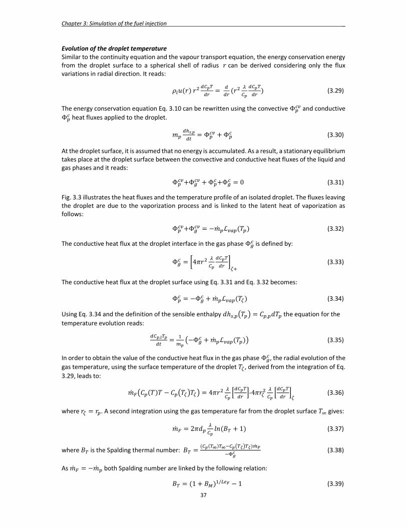
Chapter 3: Simulation of the fuel injection _
37
Evolution of the droplet temperature Similar to the continuity equation and the vapour transport equation, the energy conservation energy from the droplet surface to a spherical shell of radius 𝑟 can be derived considering only the flux variations in radial direction. It reads:
𝜌 𝑢(𝑟) 𝑟 = (𝑟 ) (3.29)
The energy conservation equation Eq. 3.10 can be rewritten using the convective Φ and conductive Φ heat fluxes applied to the droplet.
𝑚 , = Φ + Φ (3.30)
At the droplet surface, it is assumed that no energy is accumulated. As a result, a stationary equilibrium takes place at the droplet surface between the convective and conductive heat fluxes of the liquid and gas phases and it reads:
Φ +Φ + Φ +Φ = 0 (3.31)
Fig. 3.3 illustrates the heat fluxes and the temperature profile of an isolated droplet. The fluxes leaving the droplet are due to the vaporization process and is linked to the latent heat of vaporization as follows:
Φ +Φ = −�� ℒ (𝑇 ) (3.32)
The conductive heat flux at the droplet interface in the gas phase Φ is defined by:
Φ = 4𝜋𝑟 (3.33)
The conductive heat flux at the droplet surface using Eq. 3.31 and Eq. 3.32 becomes: Φ = −Φ + �� ℒ (𝑇 ) (3.34)
Using Eq. 3.34 and the definition of the sensible enthalpy 𝑑ℎ , 𝑇 = 𝐶 , 𝑑𝑇 the equation for the temperature evolution reads:
, = −Φ + �� ℒ (𝑇 ) (3.35)
In order to obtain the value of the conductive heat flux in the gas phase Φ , the radial evolution of the gas temperature, using the surface temperature of the droplet 𝑇 , derived from the integration of Eq. 3.29, leads to:
�� 𝐶 (𝑇 )𝑇 − 𝐶 𝑇 𝑇 = 4𝜋𝑟 -4𝜋𝑟 (3.36)
where 𝑟 = 𝑟 . A second integration using the gas temperature far from the droplet surface 𝑇 gives:
�� = 2𝜋𝑑 𝑙𝑛(𝐵 + 1) (3.37)
where 𝐵 is the Spalding thermal number: 𝐵 =( ( ) )
(3.38)
As �� = −�� both Spalding number are linked by the following relation:
𝐵 = (1 + 𝐵 ) / − 1 (3.39)

Chapter 3: Simulation of the fuel injection _
38
where 𝐿𝑒 is the Lewis number describing the ratio of thermal diffusivity to mass diffusivity:
𝐿𝑒 = (3.40)
Φ is finally obtained using Eq. 3.37 and Eq. 3.38 as a function of the variables at the droplet surface and far from the droplet:
Φ = ℵ 𝜋𝑑 (𝐶 𝑇 𝑇 − 𝐶 (𝑇 )𝑇 ) ( ) (3.41)
where ℵ is the Nusselt number representing the ratio of convective to conductive heat transfer at the droplet surface:
ℵ = 2 + 0.55𝑅𝑒 . 𝑃𝑟 / (3.42)
where 𝑃𝑟 is the Prandtl number describing the ratio of momentum diffusivity and conductive diffusivity:
𝑃𝑟 = (3.43)
The combination of Eq. 3.41 and Eq. 3.35 leads to the temporal evolution of the droplet temperature 𝑇 :
, = �� ℒ 𝑇 − ℵ 𝜋𝑑 (𝐶 𝑇 𝑇 − 𝐶 (𝑇 )𝑇 ) ( ) (3.44)
Figure 3.3: Sketch of the heat fluxes and temperature profile of an isolated droplet 3.3.4 Secondary droplet break-up The droplet break-up process describes the detachment of liquid fragments from a liquid element under the effect of the aerodynamic forces and the fluid properties. Considering an injector spray, two distinct break-up processes successively take place:
- The primary break-up, which represents the disintegration of the liquid jet into droplets at the exit of the injector nozzle. This process is detailed in 3.5.1.
- The secondary break-up, which characterises the further splitting of the droplets into smaller ones. The modelling of this process is described hereafter.
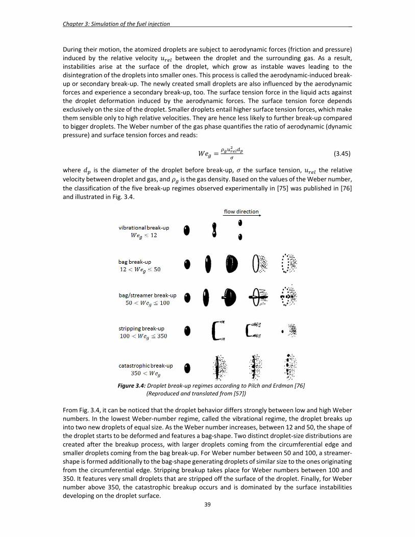
Chapter 3: Simulation of the fuel injection _
39
During their motion, the atomized droplets are subject to aerodynamic forces (friction and pressure) induced by the relative velocity 𝑢 between the droplet and the surrounding gas. As a result, instabilities arise at the surface of the droplet, which grow as instable waves leading to the disintegration of the droplets into smaller ones. This process is called the aerodynamic-induced break-up or secondary break-up. The newly created small droplets are also influenced by the aerodynamic forces and experience a secondary break-up, too. The surface tension force in the liquid acts against the droplet deformation induced by the aerodynamic forces. The surface tension force depends exclusively on the size of the droplet. Smaller droplets entail higher surface tension forces, which make them sensible only to high relative velocities. They are hence less likely to further break-up compared to bigger droplets. The Weber number of the gas phase quantifies the ratio of aerodynamic (dynamic pressure) and surface tension forces and reads:
𝑊𝑒 = (3.45)
where 𝑑 is the diameter of the droplet before break-up, 𝜎 the surface tension, 𝑢 the relative velocity between droplet and gas, and 𝜌 is the gas density. Based on the values of the Weber number, the classification of the five break-up regimes observed experimentally in [75] was published in [76] and illustrated in Fig. 3.4.
Figure 3.4: Droplet break-up regimes according to Pilch and Erdman [76] (Reproduced and translated from [57]) From Fig. 3.4, it can be noticed that the droplet behavior differs strongly between low and high Weber numbers. In the lowest Weber-number regime, called the vibrational regime, the droplet breaks up into two new droplets of equal size. As the Weber number increases, between 12 and 50, the shape of the droplet starts to be deformed and features a bag-shape. Two distinct droplet-size distributions are created after the breakup process, with larger droplets coming from the circumferential edge and smaller droplets coming from the bag break-up. For Weber number between 50 and 100, a streamer-shape is formed additionally to the bag-shape generating droplets of similar size to the ones originating from the circumferential edge. Stripping breakup takes place for Weber numbers between 100 and 350. It features very small droplets that are stripped off the surface of the droplet. Finally, for Weber number above 350, the catastrophic breakup occurs and is dominated by the surface instabilities developing on the droplet surface.
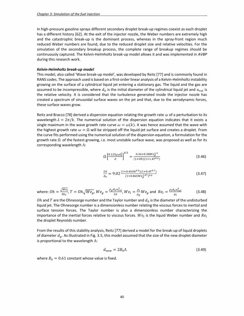
Chapter 3: Simulation of the fuel injection _
40
In high-pressure gasoline sprays different secondary droplet break-up regimes coexist as each droplet has a different history [62]. At the exit of the injector nozzle, the Weber numbers are extremely high and the catastrophic break-up is the dominant process, whereas in the spray-front region much reduced Weber numbers are found, due to the reduced droplet size and relative velocities. For the simulation of the secondary breakup process, the complete range of breakup regimes should be continuously captured. The Kelvin-Helmholtz break-up model allows it and was implemented in AVBP during this research work. Kelvin-Helmholtz break-up model This model, also called ‘Wave break-up model’, was developed by Reitz [77] and is commonly found in RANS codes. The approach used is based on a first-order linear analysis of a Kelvin-Helmholtz instability growing on the surface of a cylindrical liquid jet entering a stationary gas. The liquid and the gas are assumed to be incompressible, where 𝑑 is the initial diameter of the cylindrical liquid jet and 𝑢 is the relative velocity. It is considered that the turbulence generated inside the injector nozzle has created a spectrum of sinusoidal surface waves on the jet and that, due to the aerodynamic forces, these surface waves grow. Reitz and Bracco [78] derived a dispersion equation relating the growth rate 𝜔 of a perturbation to its wavelength 𝜆 = 2𝜋/𝑘. The numerical solution of the dispersion equation indicates that it exists a single maximum in the wave growth rate curve 𝜔 = 𝜔(𝑘). It was hence assumed that the wave with the highest growth rate 𝜔 = Ω will be stripped off the liquid-jet surface and creates a droplet. From the curve fits performed using the numerical solution of the dispersion equation, a formulation for the growth rate Ω of the fastest growing, i.e. most unstable surface wave, was proposed as well as for its corresponding wavelength Λ:
Ω.
.
=. . .
( )( . . ) (3.46)
= 9.02( . . )( . . )
( . . ) . (3.47)
where: 𝑂ℎ = , 𝑇 = 𝑂ℎ 𝑊𝑒 , 𝑊𝑒 = , 𝑊𝑒 = 𝑊𝑒 and 𝑅𝑒 = (3.48)
𝑂ℎ and 𝑇 are the Ohnesorge number and the Taylor number and 𝑑 is the diameter of the undisturbed liquid jet. The Ohnesorge number is a dimensionless number relating the viscous forces to inertial and surface tension forces. The Taylor number is also a dimensionless number characterizing the importance of the inertial forces relative to viscous forces. 𝑊𝑒 is the liquid Weber number and 𝑅𝑒 the droplet Reynolds number. From the results of this stability analysis, Reitz [77] derived a model for the break-up of liquid droplets of diameter 𝑑 . As illustrated in Fig. 3.5, this model assumed that the size of the new droplet diameter is proportional to the wavelength Λ:
𝑑 = 2𝐵 Λ (3.49)
where 𝐵 = 0.61 constant whose value is fixed.

Chapter 3: Simulation of the fuel injection _
41
Figure 3.5: Schematic illustration of the Kelvin-Helmholtz model One feature of this model is that the parent droplet does not experience an instantaneous break-up, but instead its diameter is continuously reduced during its motion. The rate of the droplet diameter reduction at a certain time 𝑡 depends on one hand on the difference between the actual value of droplet diameter 𝑑 and an equilibrium droplet size given by the new droplet diameter computed 𝑑 , and on the other hand on the characteristic time 𝜏 for the actual droplet diameter to achieve the equilibrium droplet diameter. It is described as follows:
= − (3.50)
𝜏 = 3.788 𝐵 (3.51)
where 𝐵 is an adjustable model constant, which leads to an increase or decrease of the spray penetration. Its optimal value is obtained by comparing the computed spray with the one observed in the measurements. A value of 𝐵 = 10 was proved to be realistic in RANS for the simulation of the Piezo-type injector. This model was implemented in AVBP for this research project keeping the same model constants 𝐵 and 𝐵 like in RANS for consistency reasons. To compensate the reduction of droplet mass during the continuous reduction of the droplet diameter, two possibilities exist. Either a new parcel containing the child droplets can be created and introduced in the simulation at the parent-droplet location. In this case, the size of the child droplets is equal to the equilibrium droplet diameter (Eq. 3.49) and the number of droplets in the parcel is computed based on the parent-droplet mass loss during the time step, as described in Eq. 3.67 where 𝑚 = 𝑚 and 𝑑 = 𝑑 . The new child droplets become parent droplets and are also subject to further break-up. The main drawback of this approach is the uncontrolled generation of new parcels during the simulation. As the total number of injected parcels is generally high to achieve a good statistical convergence of the spray, this number will be amplified. Furthermore, the computational time and the storage capacity would be also negatively affected. As a result, a second strategy was implemented in AVBP, which consists in keeping the same number of parcels in the model during the break-up process. After the computation of the new droplet diameter, the number of droplets in the parcel is increased accordingly, in order to keep the mass of the parcel constant and avoid any loss of injected fuel mass during the simulation. 3.4 Influence of the gas-phase turbulence The discrete droplet model approach can be used in RANS and LES for the spray simulation. All the physical processes, acting on each individual droplet in the computational model, are considered using the aforementioned sub-models linked either to the gas ensemble-average flow variables (RANS) or to the gas filtered-flow variables (LES). However, there are significant differences in time-scales between RANS and LES.
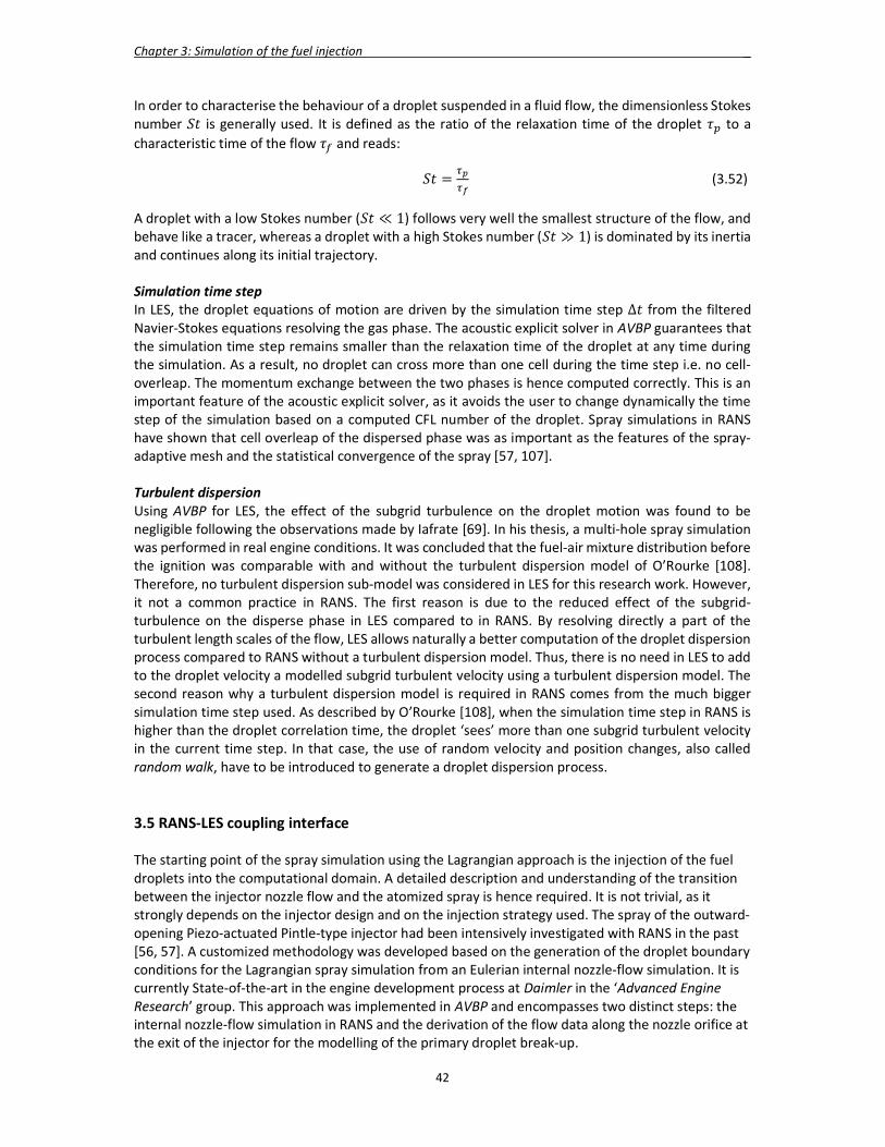
Chapter 3: Simulation of the fuel injection _
42
In order to characterise the behaviour of a droplet suspended in a fluid flow, the dimensionless Stokes number 𝑆𝑡 is generally used. It is defined as the ratio of the relaxation time of the droplet 𝜏 to a characteristic time of the flow 𝜏 and reads:
𝑆𝑡 = (3.52)
A droplet with a low Stokes number (𝑆𝑡 ≪ 1) follows very well the smallest structure of the flow, and behave like a tracer, whereas a droplet with a high Stokes number (𝑆𝑡 ≫ 1) is dominated by its inertia and continues along its initial trajectory. Simulation time step In LES, the droplet equations of motion are driven by the simulation time step ∆𝑡 from the filtered Navier-Stokes equations resolving the gas phase. The acoustic explicit solver in AVBP guarantees that the simulation time step remains smaller than the relaxation time of the droplet at any time during the simulation. As a result, no droplet can cross more than one cell during the time step i.e. no cell-overleap. The momentum exchange between the two phases is hence computed correctly. This is an important feature of the acoustic explicit solver, as it avoids the user to change dynamically the time step of the simulation based on a computed CFL number of the droplet. Spray simulations in RANS have shown that cell overleap of the dispersed phase was as important as the features of the spray-adaptive mesh and the statistical convergence of the spray [57, 107]. Turbulent dispersion Using AVBP for LES, the effect of the subgrid turbulence on the droplet motion was found to be negligible following the observations made by Iafrate [69]. In his thesis, a multi-hole spray simulation was performed in real engine conditions. It was concluded that the fuel-air mixture distribution before the ignition was comparable with and without the turbulent dispersion model of O’Rourke [108]. Therefore, no turbulent dispersion sub-model was considered in LES for this research work. However, it not a common practice in RANS. The first reason is due to the reduced effect of the subgrid-turbulence on the disperse phase in LES compared to in RANS. By resolving directly a part of the turbulent length scales of the flow, LES allows naturally a better computation of the droplet dispersion process compared to RANS without a turbulent dispersion model. Thus, there is no need in LES to add to the droplet velocity a modelled subgrid turbulent velocity using a turbulent dispersion model. The second reason why a turbulent dispersion model is required in RANS comes from the much bigger simulation time step used. As described by O’Rourke [108], when the simulation time step in RANS is higher than the droplet correlation time, the droplet ‘sees’ more than one subgrid turbulent velocity in the current time step. In that case, the use of random velocity and position changes, also called random walk, have to be introduced to generate a droplet dispersion process. 3.5 RANS-LES coupling interface The starting point of the spray simulation using the Lagrangian approach is the injection of the fuel droplets into the computational domain. A detailed description and understanding of the transition between the injector nozzle flow and the atomized spray is hence required. It is not trivial, as it strongly depends on the injector design and on the injection strategy used. The spray of the outward-opening Piezo-actuated Pintle-type injector had been intensively investigated with RANS in the past [56, 57]. A customized methodology was developed based on the generation of the droplet boundary conditions for the Lagrangian spray simulation from an Eulerian internal nozzle-flow simulation. It is currently State-of-the-art in the engine development process at Daimler in the ‘Advanced Engine Research’ group. This approach was implemented in AVBP and encompasses two distinct steps: the internal nozzle-flow simulation in RANS and the derivation of the flow data along the nozzle orifice at the exit of the injector for the modelling of the primary droplet break-up.
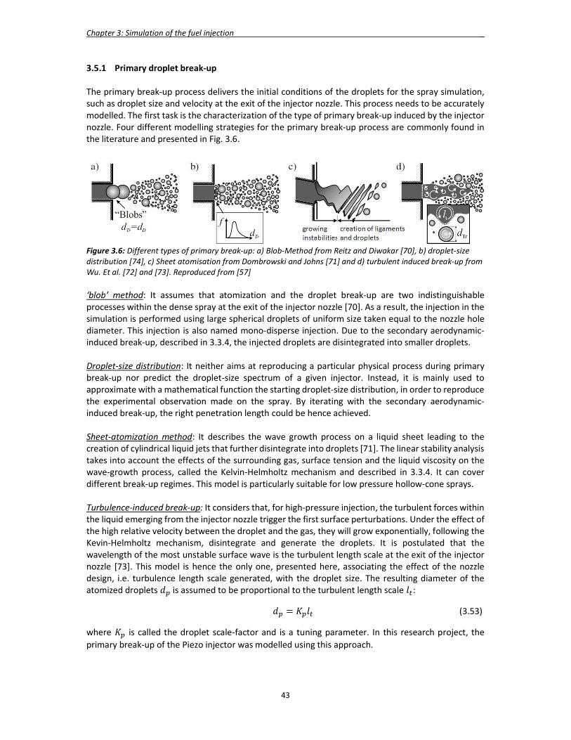
Chapter 3: Simulation of the fuel injection _
43
3.5.1 Primary droplet break-up The primary break-up process delivers the initial conditions of the droplets for the spray simulation, such as droplet size and velocity at the exit of the injector nozzle. This process needs to be accurately modelled. The first task is the characterization of the type of primary break-up induced by the injector nozzle. Four different modelling strategies for the primary break-up process are commonly found in the literature and presented in Fig. 3.6.
Figure 3.6: Different types of primary break-up: a) Blob-Method from Reitz and Diwakar [70], b) droplet-size distribution [74], c) Sheet atomisation from Dombrowski and Johns [71] and d) turbulent induced break-up from Wu. Et al. [72] and [73]. Reproduced from [57] ‘blob’ method: It assumes that atomization and the droplet break-up are two indistinguishable processes within the dense spray at the exit of the injector nozzle [70]. As a result, the injection in the simulation is performed using large spherical droplets of uniform size taken equal to the nozzle hole diameter. This injection is also named mono-disperse injection. Due to the secondary aerodynamic-induced break-up, described in 3.3.4, the injected droplets are disintegrated into smaller droplets. Droplet-size distribution: It neither aims at reproducing a particular physical process during primary break-up nor predict the droplet-size spectrum of a given injector. Instead, it is mainly used to approximate with a mathematical function the starting droplet-size distribution, in order to reproduce the experimental observation made on the spray. By iterating with the secondary aerodynamic-induced break-up, the right penetration length could be hence achieved. Sheet-atomization method: It describes the wave growth process on a liquid sheet leading to the creation of cylindrical liquid jets that further disintegrate into droplets [71]. The linear stability analysis takes into account the effects of the surrounding gas, surface tension and the liquid viscosity on the wave-growth process, called the Kelvin-Helmholtz mechanism and described in 3.3.4. It can cover different break-up regimes. This model is particularly suitable for low pressure hollow-cone sprays. Turbulence-induced break-up: It considers that, for high-pressure injection, the turbulent forces within the liquid emerging from the injector nozzle trigger the first surface perturbations. Under the effect of the high relative velocity between the droplet and the gas, they will grow exponentially, following the Kevin-Helmholtz mechanism, disintegrate and generate the droplets. It is postulated that the wavelength of the most unstable surface wave is the turbulent length scale at the exit of the injector nozzle [73]. This model is hence the only one, presented here, associating the effect of the nozzle design, i.e. turbulence length scale generated, with the droplet size. The resulting diameter of the atomized droplets 𝑑 is assumed to be proportional to the turbulent length scale 𝑙 :
𝑑 = 𝐾 𝑙 (3.53)
where 𝐾 is called the droplet scale-factor and is a tuning parameter. In this research project, the primary break-up of the Piezo injector was modelled using this approach.

Chapter 3: Simulation of the fuel injection _
44
The modelling of the turbulence-induced primary break-up, occurring in such high fuel-pressure injector, requires a detailed description of the turbulent length-scale at the exit of the injector nozzle. The experimental measurements cannot provide this information, as it is practically impossible to measure such small flow length-scales in a dense spray region. At this point, only the simulation results from an internal nozzle-flow simulation allow to get access to the local flow information at the exit of the injector nozzle. In this research project, a coupling interface, linking the internal nozzle-flow simulation in RANS to the Lagrangian spray simulation in LES, was hence implemented in AVBP in order to derive realistic boundary conditions for the injected droplets. The coupling procedure is described in the following section. 3.5.2 Internal nozzle-flow simulation in RANS The goal was first to simulate the flow inside the injector nozzle following a transient needle profile and secondly to extract the flow information at the exit of the nozzle. The needle lift profile was derived from the measured injector’s current signal and from the injection parameters used in the measurements. Additionally to the start of injection and injection duration parameters, the injection rate slope in piezo-driven injector can be adjusted by altering the applied current. As a result, the needle response speed allows to be controlled during the opening and closing phases of the injection, as well as the resulting droplet spectrum and mass flow rate. As the design of the injector is perfectly axisymmetric, a moving two-dimensional sector mesh of 0.5 𝑑𝑒𝑔 was generated with hexahedral elements as depicted in Fig. 3.7. 30 cells were defined in the computational domain normal to the flow direction and were compressed and expanded following the given needle lift profile, varying between ℎ = 0 𝜇𝑚 and ℎ = 35 𝜇𝑚. Three chemical species were considered in the simulation: n-heptane (fuel), air and vaporised n-heptane coming from a potential cavitation effect. Two pressure boundary conditions were ascribed: for the fuel at the inlet of the model 𝑃 = 200 𝑏𝑎𝑟 and for the air at the outlet of the model 𝑃 . Depending on the engine operations or the closed-volume chamber investigated, the value of 𝑃 should correspond to the pressure in the volume surrounding the injector before the injection process. Cyclic boundary conditions were used in the rest of the model. The High-Reynolds standard 𝑘 − 𝜀 turbulence model was used in combination with the standard wall-laws. A constant density value was used for the fuel 𝜌 = 685 𝑘𝑔/𝑚³ and the air 𝜌 = 1.225 𝑘𝑔/𝑚³. The coupling interface was positioned at the exit of injector nozzle using an internal boundary. In each of the 30 cells along the defined internal boundary, the flow and cell data were saved during the simulation. It comprised the cell velocity 𝑢 , the cell normal vector 𝑠 , the cell mass flux �� , the turbulent kinetic energy 𝑘 , the rate of dissipation 𝜀 , the species concentration 𝛼 and the coordinates of the cells �� . The simulation time 𝑡 was driven by the injection duration provided as input with the needle lift profile and was run with a constant time step ∆𝑡 = 1. 10 𝑠. The data at the coupling interface were saved at each time step during the simulation.
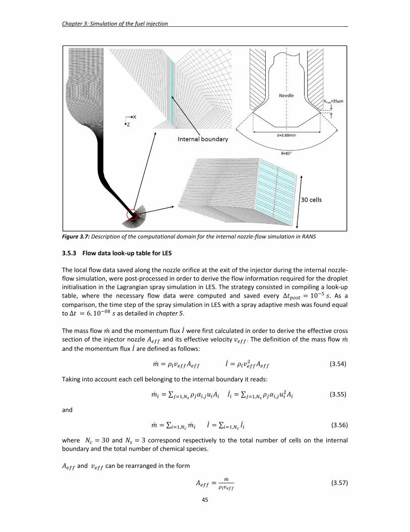
Chapter 3: Simulation of the fuel injection _
45
Figure 3.7: Description of the computational domain for the internal nozzle-flow simulation in RANS 3.5.3 Flow data look-up table for LES The local flow data saved along the nozzle orifice at the exit of the injector during the internal nozzle-flow simulation, were post-processed in order to derive the flow information required for the droplet initialisation in the Lagrangian spray simulation in LES. The strategy consisted in compiling a look-up table, where the necessary flow data were computed and saved every ∆𝑡 = 10 𝑠. As a comparison, the time step of the spray simulation in LES with a spray adaptive mesh was found equal to ∆𝑡 = 6. 10 𝑠 as detailed in chapter 5. The mass flow �� and the momentum flux 𝐼 were first calculated in order to derive the effective cross section of the injector nozzle 𝐴 and its effective velocity 𝑣 . The definition of the mass flow �� and the momentum flux 𝐼 are defined as follows:
�� = 𝜌 𝑣 𝐴 𝐼 = 𝜌 𝑣 𝐴 (3.54)
Taking into account each cell belonging to the internal boundary it reads:
�� = ∑ 𝜌 𝛼 , 𝑢 𝐴 , 𝐼 = ∑ 𝜌 𝛼 , 𝑢 𝐴
, (3.55)
and
�� = ∑ ��, 𝐼 = ∑ 𝐼, (3.56)
where 𝑁 = 30 and 𝑁 = 3 correspond respectively to the total number of cells on the internal boundary and the total number of chemical species. 𝐴 and 𝑣 can be rearranged in the form
𝐴 = (3.57)
Chapter 3: Simulation of the fuel injection _
46
𝑣 =
(3.58)
Following the assumption that a turbulence-induced primary break-up takes place at the exit of the injector nozzle, the turbulent length-scale 𝑙 was computed at each cell location along the internal boundary at the exit of the injector nozzle assuming isotropy:
𝑙 =/
(3.59)
The final look-up table entails 𝐴 , 𝑣 and the distributions of 𝑙 and �� /�� in the 30 cells along the internal boundary as a function of time. 3.6 Initialisation and injection of the droplets 3.6.1 Initialisation of the droplets The look-up table was provided as an input file to the Lagrangian spray simulation in LES. First the total injected fuel mass, computed from the look-up table at 𝑡 = 𝑡 , had to be corrected in order to take into account the real value given by the injection quantity baseline of the Piezo-injector 𝑚 _ . The mass correction factor 𝐾 was hence defined as follows:
𝐾 =_
∫ 𝜌 𝑣 𝐴 𝑑𝑡 (3.60)
Secondly, the total number of parcels 𝑛 to be injected had to be determined. In order to achieve a satisfactory statistical statistics of the spray a high quantity of parcels per cell was required. Based on the investigations in a closed-volume chamber presented in chapter 5, a value of 1.2. 10
parcels/mg of injected fuel was found reasonable. Furthermore, it was considered that each parcel carried the same mass of fuel. Thereby the mass of a parcel 𝑚 was computed at the beginning of the simulation and reads:
𝑚 = _ (3.61)
Then, the droplet diameter 𝑑 was derived based on the turbulent length scale of the flow and on the droplet scale-factor 𝐾 as follows:
𝑑 = 𝐾 𝑙 (3.62)
At any time during the simulation, the required droplet data could be generated from the transient flow data of the look-up table using simple interpolation techniques. The droplet scale-factor 𝐾 was a tuning parameter, whose value was iteratively derived by comparing the spray simulation results with the spray measurements in a closed-volume chamber, as presented in chapter 5. However, at very small needle lifts, the critical Reynolds number (𝑅𝑒 ≈ 2300), where the transition from laminar to turbulent flow in a channel flow occurs, could not be reached. The assumption of a turbulence-induced primary break-up was not valid anymore. As a result, a constant droplet diameter equal to the hydraulic diameter 𝑑 was hence assumed in that case. 𝑑 was computed based on the effective cross section of injector nozzle as follows:
𝑑 = (3.63)
where 𝑑 = 3.88 𝑚𝑚 is the nozzle diameter of the injector.
Chapter 3: Simulation of the fuel injection _
47
Finally the injected droplet velocity was defined using:
𝑣 = (3.64)
3.6.2 Injection of the droplets The injection procedure is described hereafter and was repeated for each time step during the simulation. The droplets were injected along the coupling interface of the LES model. For the stochastic modelling of the spray, random numbers were required. A file containing 1.106 equally distributed random numbers between 0 and 1 was generated. For consistency and repeatability reasons, the set of random numbers was always taken from this file in this research project. At the time 𝑡 , the injected mass 𝑑𝑚 in the time step ∆𝑡 was computed by interpolating the effective cross section of the injector nozzle 𝐴 and its effective velocity 𝑣 between the times 𝑡 and 𝑡 encompassing 𝑡 + ∆ in the look-up table. It was first assessed if 𝑑𝑚 was larger than 𝑚 . If not, the mass was stored and added up to the calculated injected mass in the next time step, whereas in the other case a new parcel could be created. The droplet diameter was randomly determined with the Monte-Carlo method [80]. Two distribution functions were considered along the 𝑁 = 30 cells at the exit of the nozzle hole: the droplet size distribution 𝑑 , and the distribution of the mass flow normalized by the maximal cell mass flow �� /��
. A first random number 𝑝 was drawn from the
interval [0; 1] and converted into an index 𝑗 of the interval [1; 𝑁 ] using the following transformation:
𝑗 = 𝑖𝑛𝑡(𝑝. (𝑁 − 1) + 0.5) + 1 (3.65)
The decision to keep 𝑗 was controlled by the value of a second random number 𝑞, if the following condition was fulfilled:
𝑞 < �� /�� (3.66)
In that case, the droplet diameter was defined by 𝑑 = 𝑑 , . If this condition was not met, a new set of two random numbers has to be drawn again and the test repeated. The number of identical droplets encompassed in the parcel was derived using:
𝑁 = (3.67)
The polar angle 𝜃 of the injected parcel was kept constant and equal to the geometrical angle of the injector 𝜃 = 85 𝑑𝑒𝑔, as shown in Fig. 3.7. Moreover two random numbers m, 𝑛, taken from the random number file mentioned above, were used to position the droplet randomly in both vertical and circumferential directions along the exit of the nozzle hole of the injector. The vertical position of the droplet was defined using:
𝑧 = 𝑧 + (𝑚 − 0.5) ∗ ℎ (3.68)
where 𝑧 corresponded to the middle position of the coupling interface and ℎ the needle lift. The azimuthal angle was obtained via:
𝜙 = 360 ∗ 𝑛 (3.69)

Chapter 3: Simulation of the fuel injection _
48
49
Chapter 4 In-cylinder flow analysis using PIV and LES in stratified engine operation The present chapter covers the simulation and the analysis of the engine in-cylinder flow in LES together with high-speed PIV. The main goal was to develop a LES methodology, validated with high-speed PIV, which can reproduce the high-speed PIV results in terms of mean velocity and cyclic velocity fluctuations of the flow in the corresponding measurement planes. As observed in high-speed PIV, the CCV of the in-cylinder flow imply the presence of extreme cycles producing different types of in-cylinder flow structures. They lead to different outcome on the combustion process [45, 46, 47 and 48]. However, based on the two-dimensional information of the measured flow in high-speed PIV, a hypothesis could be derived concerning their formation [47]. The other expectation from this chapter was to validate the above-mentioned hypothesis by investigating the three-dimensional flow field in LES and propose a sound explanation based on the different in-cylinder flow phenomena observed. Finally, the last goal was to assess the possibility of increasing the accuracy of the in-cylinder flow prediction using a higher-order convective scheme in a multi-cycle LES. This chapter is divided into six main parts. The first part describes the high-speed PIV measurements campaigns carried out in this research project in order to generate the required in-cylinder flow velocity data for the LES flow validation. The second part is devoted to the current in-cylinder flow knowledge gained with RANS and high-speed PIV in the M274 engine. The third and fourth part deals with the LES validation of the mean flow field and cyclic velocity variations in two distinct planes, i.e. intake valve plane and central tumble plane. The fifth part covers the LES in-cylinder flow analysis, where new post-processing methods were introduced to first validate the high-speed PIV flow hypothesis and secondly to explain its origin from the different three-dimensional flow phenomena observed. The last part of this chapter deals with high-order convective schemes in LES, where a comparison between the 2nd and 3rd-order accurate in time and space convective schemes is made in terms of prediction of the mean flow field and the cyclic velocity variations. 4.1 High-speed PIV measurement campaigns Particle image velocimetry (PIV) has been extensively used to capture in-cylinder flows [84] by providing flow fields within a plane. High speed PIV provides crank-angle resolved flow fields and has been utilized to investigate cycle-to-cycle fluctuations [85, 87, 88]. To visualize the 3D-flow Baum et al. [86] used tomographic PIV within few millimetre thick volumes surrounding the central tumble plane. The level of complexity and accuracy of the high-speed PIV measurement techniques have hence increased over the years, allowing highly resolved flow velocity measurements inside the engine cylinder. Despite recent improvements of PIV approaches, flow field measurements are limited to planes or thin volumes and other important regions of the flow such as flows in the intake port and the valve gap remain inaccessible.
Three high-speed PIV measurement campaigns were run during this research project using the same optically accessible engine geometry in order to provide accurate in-cylinder flow data for the LES validation. Two distinct measurement techniques, developed in cooperation with the Technische Universität Darmstadt for the measurement of in-cylinder flows, were used: the single-plane high-speed PIV and the quasi-simultaneous dual-plane high-speed PIV. The first and the second
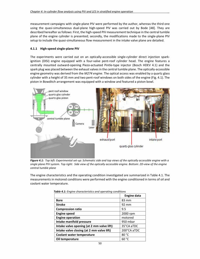
Chapter 4: In-cylinder flow analysis using PIV and LES in stratified engine operation _
50
measurement campaigns with single-plane PIV were performed by the author, whereas the third one using the quasi-simultaneous dual-plane high-speed PIV was carried out by Bode [48]. They are described hereafter as follows: First, the high-speed PIV measurement technique in the central tumble plane of the engine cylinder is presented; secondly, the modifications made to the single-plane PIV setup to include the quasi-simultaneous flow measurement in the intake valve plane are detailed. 4.1.1 High-speed single-plane PIV The experiments were carried out on an optically-accessible single-cylinder direct injection spark-ignition (DISI) engine equipped with a four-valve pent-roof cylinder head. The engine features a centrally mounted outward-opening Piezo-actuated Pintle-type injector (Bosch HDEV 4.1) and the spark plug was placed between the exhaust valves in the central tumble plane. The optically-accessible engine geometry was derived from the M274 engine. The optical access was enabled by a quartz glass cylinder with a height of 35 mm and two pent-roof windows on both sides of the engine (Fig. 4.1). The piston in Bowditch arrangement was equipped with a window and featured a piston bowl.
Figure 4.1: Top left: Experimental set-up: Schematic side and top views of the optically accessible engine with a single plane PIV system. Top right: Side view of the optically accessible engine. Bottom: 2D-view of the engine central tumble plane The engine characteristics and the operating condition investigated are summarized in Table 4.1. The measurements in motored conditions were performed with the engine conditioned in terms of oil and coolant water temperature.
Table 4.1: Engine characteristics and operating conditions Engine data Bore 83 mm Stroke 92 mm Compression ratio 9.5 Engine speed 2000 rpm Engine operation motored Intake manifold pressure 950 mbar Intake valve opening (at 2 mm valve lift) 35°CA aTDC Intake valve closing (at 2 mm valve lift) 200°CA aTDC Coolant water temperature 80 °C Oil temperature 60 °C
Chapter 4: In-cylinder flow analysis using PIV and LES in stratified engine operation _
51
For the time resolved two-dimensional two-component (2D2C) PIV measurements, a dual cavity frequency doubled Nd:YVO4 laser (Edgewave IS120, 532 nm, 1 mJ/pulse) was used. The light sheet was focused with cylindrical lenses (f = 500 mm) to 0.5 mm (FWHM) thick light sheets. A concave cylindrical lens (f = -50 mm) together with a concave cylindrical lens at the bottom of the piston window generated a divergent light sheet enlarging the field-of-view. Silicon oil droplets (~ 0.5 μm mean diameter) were seeded into a large plenum volume prior to the intake port to ensure homogeneous seeding densities using a cyclone based droplet seeder (Palas AGK 2000). A 12-bit CMOS camera (Vision Research Phantom v1610 1280x800 active pixel) was used to record the scattered light in the central tumble plane. A variable pulse separation ‘dt’ was optimized for the velocity scale of each phase. Two datasets were taken. In the first dataset (Campaign1), the spark plug was removed and replaced by a dummy spark-plug, which was chopped off and filled with silicon in order to have a planar surface on the cylinder head side. The measurements were performed during intake and compression strokes from 360°CA bTDC up to TDC. At 2000 rpm a double image was captured every 1.5° CA and 200 consecutive cycles were recorded. The second dataset (Campaign2) was generated using the same experimental setup but with the spark plug in place and oriented at 180° i.e. with the electrodes parallel to the central tumble plane. The PIV post processing was carried out with the commercial software Davis 8.2.2 (LaVision). To eliminate phase-steady artefacts, a background image was calculated by taking the minimal appearing intensity over all cycles for each pixel. This operation was performed for each recorded crank angle degree (CAD) and the respective background image was subtracted from each image. Afterwards, an 8x8 pixel sliding Gaussian background subtraction and a local intensity normalization (5x5 pixels) was applied. The vector fields were calculated with a decreasing interrogation window size from 64x64 to 32x32 pixels and an overlap of 75%. Important parameters of the PIV images are presented in Table 4.2. Vectors with a peak ratio below 1.7 were removed. Further inaccurate vectors were identified by neighbour comparison of the median and replaced by vector choices of higher order. Finally, local noise in the order of the spatial resolution was reduced with a 3x3 top hat filter. Table 4.2: Parameters of the recorded images in the PIV measurements
Flow field without spark plug (Campaign1)
Flow field with spark plug (Campaign2)
Recorded CAD 360°-0°CA bTDC 360°-0°CA bTDC Number of cycles 200 200 Vector spacing 0.65 mm 0.65 mm Final interrogation area 2.6 mm 2.6 mm Field-of-view 83 x 45 mm 83 x 45 mm
4.1.2. High-speed dual-plane PIV Bode et al. [47] utilized a quasi-simultaneous multi-plane time-resolved PIV approach to investigate the in-cylinder flow evolution from the mid-valve plane into the central tumble plane. The measurements were performed in the same optically accessible single-cylinder direct injection spark-ignition (DISI) engine and using the same motored operating condition as in Campaign1 and Campaign2. The time resolved two-dimensional two-component (2D2C) PIV measurements were performed quasi simultaneously in the central tumble plane and the mid intake valve plane. For this purpose, two independent PIV systems were utilized (Fig. 4.2). Each cavity of the two dual cavity frequency doubled ND:YVO4 lasers (Edgewave IS411-DE, 532 nm, 0.7 mJ/pulse; Edgewave IS120, 532 nm, 1 mJ/pulse) operated at 4 kHz. The parallel light sheets were 18 mm apart, focused with cylindrical lenses (f = 500 mm) to 0.5 mm (FWHM) thick light sheets. A concave cylindrical lens (f = -50 mm) together with a concave cylindrical lens at the bottom of the piston window generated a divergent light sheet, which enlarged the field-of-view. The same Silicon oil droplets and droplet seeder were used as in Campaign1 and Campaign2. Two 12 bit CMOS cameras (camera1: Vision Research

Chapter 4: In-cylinder flow analysis using PIV and LES in stratified engine operation _
52
Phantom v1610 1280x800 active pixel; camera2: Photron SA-X2 1024x768 active pixel) were mounted on both sides of the optical engine to record the scattered light in the central- and mid-intake valve plane. Both cameras were operated at 8 kHz double frame mode. Camera 1 was focused on the intake valve plane, while camera 2 was focused on the central tumble plane. To avoid any background interference from the unfocused plane, each cavity of the lasers operated at half of the camera frequency (4 kHz). The two lasers fired alternatingly with a double pulse, while the variable pulse separation dt was optimized from the velocity scale of each phase. Every second unfocused double frame of each camera was deleted during post processing. At 2000 rpm every 3rd CAD was recorded in each plane while the two planes were recorded with a temporally offset of 1.5°CA. The parameters of the recorded images in both planes are given in Table 4.3. The same methodology as for the single-plane PIV, described in 4.1.1, was used in Davis 8.2.2 to post-process the PIV data.
Figure 4.2: Experimental set-up; Left: Schematic side view of the optical engine; (reproduced from [48]) Right: Top view of the cylinder head, including the two PIV systems and the laser paths Table 4.3: Parameters of the recorded images in the PIV measurements (Campaign3)
Mid-intake valve plane (z = 18 mm) Central plane (z = 0 mm) Recorded CAD 106.5°-1.5°CA bTDC 105°-0°CA bTDC Number of cycles 300 300 Vector spacing 0.49 mm 0.65 mm Final interrogation area 1.96 mm 2.6 mm Field-of-view 74.5 x 45 mm 83 x 45 mm
4.1.3. Strategy to use PIV measurements for LES validation The three aforementioned measurement campaigns were planned sequentially in order to guide the LES validation process. The difficulty level to capture in LES the in-cylinder flow features observed in high-speed PIV was increased progressively. The analysis of the results coming from RANS and high-speed PIV (Campaign2) could provide beforehand a detailed understanding of the global and local in-cylinder mean flow structures during the intake and compression strokes of the M274 engine. The validation of the mean flow field in LES was a key milestone in this research project. However, due to the deep positioning of the spark-plug in the combustion chamber for the stratified operation, the flow observations made in RANS and in high-speed PIV pointed out a strong interaction of the incoming intake flow with the spark-plug during the intake stroke. It led to the formation of more complex and fluctuating in-cylinder flow structures. As a result, the validation process of the mean flow field in LES was hence performed in a first step
Chapter 4: In-cylinder flow analysis using PIV and LES in stratified engine operation _
53
using a global mesh study guided with high-speed PIV. The goal was to reproduce the flow structures observed in Campaign1 in the central tumble plane. This strategy had two advantages:
- The meshing process was made easier, as the detailed geometry of the spark-plug was not meshed. It also reduced the total cell count and the computation time.
- The number of engine cycles to compute in LES were reduced, as the mean in-cylinder flow motions were relatively simpler than with the spark-plug geometry. It hence shortened the overall time to derive a first reliable set of meshing and numerical setups for the LES.
In a second step, the final LES validation of the mean flow field was performed with the spark-plug geometry using high-speed PIV (Campaign3) in two distinct planes, i.e. intake valve plane and central tumble plane. It was followed by a validation of the LES cyclic velocity variations. Finally, a comparison between the Lax-Wendroff and TTGC convective schemes was made in terms of prediction of the mean flow field and the cyclic velocity variations against the high-speed PIV results from Campaign3. 4.2 Current knowledge of the M274-engine in-cylinder flow The combination of RANS and high-speed PIV is today state-of-the-art at Daimler in the ‘Advanced Engine Research’ group. This interaction is required to develop a universal meshing strategy and choose the suitable sub-models in RANS for the reproduction of the ensemble-averaged high-speed PIV results from the optically-accessible engine. Once the RANS methodology is validated, the combined mean flow analysis, 3D in RANS and 2D in high-speed PIV, allows the understanding of the in-cylinder flow phenomena taking place in the cylinder. Further development of the engine geometry can be carried out based on the knowledge gained. However, when dealing with cyclic velocity fluctuations, only hypothesis regarding their origins and formations can be derived from RANS. These flow hypothesis can today only be explicitly validated with high-speed PIV on the optically-accessible engine by investigating iteratively different engine geometry concepts. RANS cannot speed up this understanding process as it only provides a mean flow information. 4.2.1 RANS: State of the art
CFD model For the CFD simulation of the engine in-cylinder flow, the commercial code Star-CD from Siemens is used. The hexahedral mesh is generated using the meshing software es-ice [147] and the simulation is performed with Star-CD V4. A multicycle CFD analysis is generally performed using an implicit RANS solver with a standard k-Epsilon/High Reynolds number turbulence model, the standard wall functions described in 2.2 and a multidimensional second-order differencing scheme (MARS) for the convective flux. The boundary conditions are taken from a Triple-Pressure-Analysis model (TPA). The TPA model is calibrated based on the three pressure signals (intake, exhaust and cylinder) provided by the measurements on the engine. The mesh size, the correct definition of the zones, where the local mesh refinement is applied, the size of the prism layers at the walls and the mesh of the important parts in the combustion chamber (spark-plug, injector and pressure sensor) are the key factors for reliable CFD results. As a feature for the stratified combustion, the spark-plug position is positioned quite low in the combustion chamber with respect to the injector. A very strong interaction takes place between the intake airflow and the spark-plug. As a result, a fine meshing of the internal volume of the spark-plug is found crucial to capture this flow interaction in the CFD simulation. The CFD model comprises 5.2 Million cells with cell sizes ranging from 0.1 to 0.4 mm. Fig. 4.3 shows the computational model as well as some insights into the mesh.
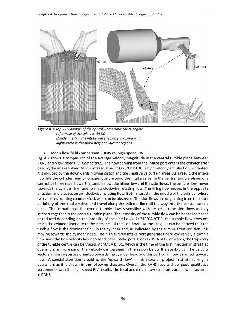
Chapter 4: In-cylinder flow analysis using PIV and LES in stratified engine operation _
54
Figure 4.3: Top: CFD domain of the optically-accessible M274 engine Left: mesh of the cylinder @BDC Middle: mesh in the intake valve region @maximum lift Right: mesh in the spark-plug and injector regions
Mean flow field comparison: RANS vs. high-speed PIV Fig. 4.4 shows a comparison of the average velocity magnitude in the central tumble plane between RANS and high-speed PIV (Campaign2). The flow coming from the intake port enters the cylinder after passing the intake valves. At low intake valve-lift (275°CA bTDC) a high velocity annular flow is created. It is induced by the downwards moving piston and the small valve curtain areas. As a result, the intake flow fills the cylinder nearly homogenously around the intake valve. In the central tumble plane, one can notice three main flows: the tumble flow, the filling flow and the side flows. The tumble flow moves towards the cylinder liner and forms a clockwise rotating flow. The filling flow moves in the opposite direction and creates an anticlockwise rotating flow. Both interact in the middle of the cylinder where two vortices rotating counter-clock wise can be observed. The side flows are originating from the outer periphery of the intake valves and travel along the cylinder liner all the way into the central tumble plane. The formation of the overall tumble flow is sensitive with respect to the side flows as they interact together in the central tumble plane. The intensity of the tumble flow can be hence increased or reduced depending on the intensity of the side flows. At 210°CA bTDC, the tumble flow does not reach the cylinder liner due to the presence of the side flows. At this stage, it can be noticed that the tumble flow is the dominant flow in the cylinder and, as indicated by the tumble front position, it is moving towards the cylinder head. The high tumble intake port generates here exclusively a tumble flow since the flow velocity has increased in the intake port. From 120°CA bTDC onwards, the trajectory of the tumble centre can be traced. At 40°CA bTDC, which is the time of the first injection in stratified operation, an increase of the velocity can be seen in the region below the spark-plug. The velocity vectors in this region are oriented towards the cylinder head and this particular flow is named ‘upward flow’. A special attention is paid to the ‘upward flow’ in this research project in stratified engine operation, as it is shown in the following chapters. Overall, the RANS results show good qualitative agreements with the high-speed PIV results. The local and global flow structures are all well captured in RANS.

Chapter 4: In-cylinder flow analysis using PIV and LES in stratified engine operation _
55
Figure 4.4: Average velocity magnitude (Vxz). Left: RANS. Right: PIV results averaged over 200 cycles (Campaign2)

Chapter 4: In-cylinder flow analysis using PIV and LES in stratified engine operation _
56
Map of the relevant flow structures The observed local and global flow structures in the central tumble plane were further analysed based on the 3D flow field of the simulation in RANS. A map of the characteristic flow structures was derived to describe the in-cylinder flow of the M274 engine (Fig. 4.5). Four global flow structures are formed during the intake stroke. ‘Flow number 1’ moves towards the cylinder liner and forms the clockwise tumble flow. ‘Flow number 2’ fills the cylinder at the back of the intake valve. The balance between the intensity of ‘flow number 1’ and ‘flow number 2’ characterises the type of intake port fitted on the engine. For tumble intake ports, ‘flow number 1’ dominates over ‘flow number 2’, whereas they tend to have similar intensities for filling intake ports. ‘Flow number 3’ and ‘flow number 4’ originate from the outer periphery of the intake valves. ‘Flow number 3’ is guided by the cylinder liner, whereas ‘flow number 4’ travels towards the centre of the cylinder and interacts with the spark-plug. The outcome of the interaction of ‘flow number 1’ and ‘flow number 3’ impacts the strength of the overall tumble flow structure, which develops in the cylinder after intake valve closing (IVC). This tumble flow structure is characterised by a tumble front and a tumble vortex centre, which can be traced in the compression stroke. At 40°CA bTDC an upward flow appears below the spark-plug, as depicted in Fig. 4.4. The goal of the flow-map was first to help validating the computed 2D flow field with high-speed PIV and secondly to have a clear understanding of the global flow phenomena responsible for the formation of the observed 2D flow structures. Furthermore, the flow-map was used as a guideline for the LES analysis in order to define the required post-processing strategy to validate LES with high-speed PIV. In engine development projects at Daimler such flow-map assists the engineers in characterizing the in-cylinder flow in engines. Further developments of the intake ports and combustion chambers are hence based on the flow-map. Each flow presented in the flow-map, as well as its interactions with the others and with the surrounding geometry, could be hence addressed separately and further optimised.
Figure 4.5: Flow-map. Top to bottom: Main in-cylinder flows and representation of the primary and secondary flow interactions, tumble front/center and upward flow
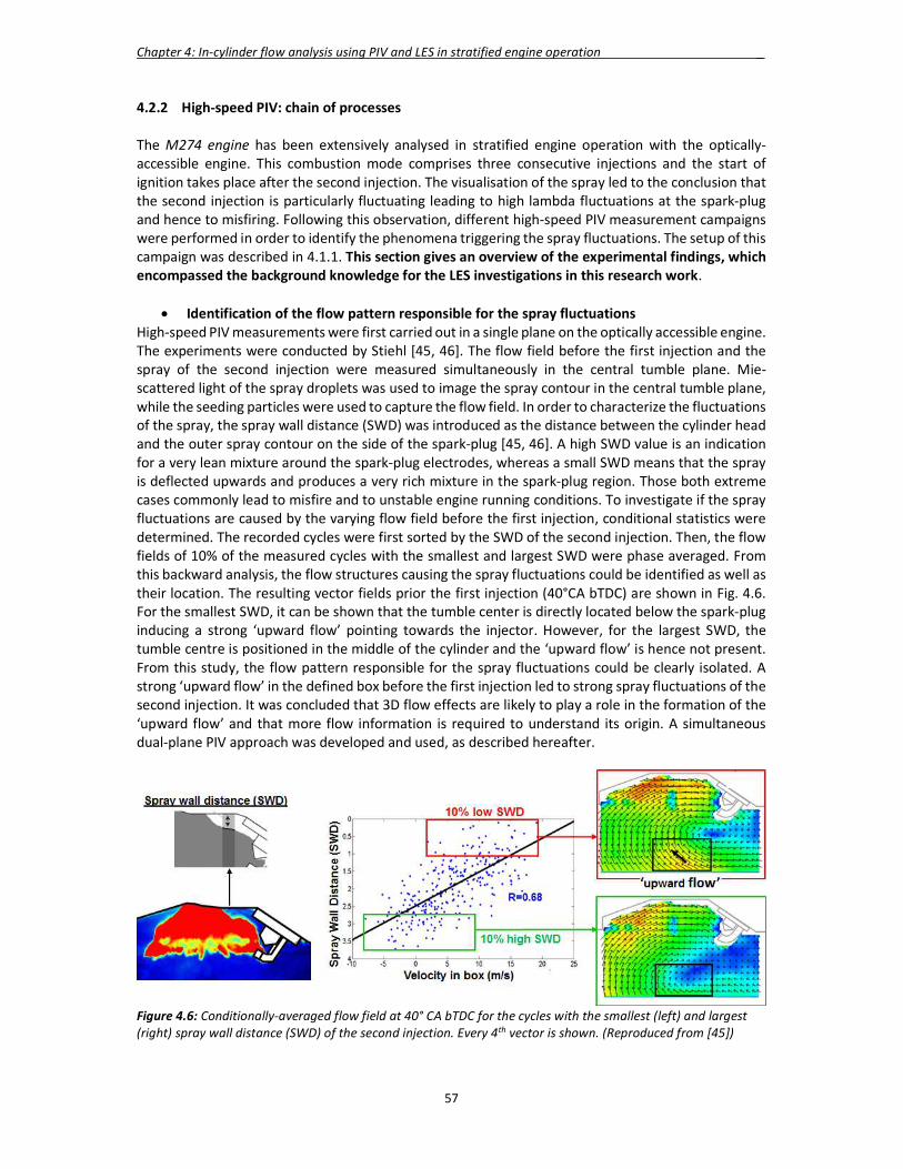
Chapter 4: In-cylinder flow analysis using PIV and LES in stratified engine operation _
57
4.2.2 High-speed PIV: chain of processes The M274 engine has been extensively analysed in stratified engine operation with the optically-accessible engine. This combustion mode comprises three consecutive injections and the start of ignition takes place after the second injection. The visualisation of the spray led to the conclusion that the second injection is particularly fluctuating leading to high lambda fluctuations at the spark-plug and hence to misfiring. Following this observation, different high-speed PIV measurement campaigns were performed in order to identify the phenomena triggering the spray fluctuations. The setup of this campaign was described in 4.1.1. This section gives an overview of the experimental findings, which encompassed the background knowledge for the LES investigations in this research work.
Identification of the flow pattern responsible for the spray fluctuations High-speed PIV measurements were first carried out in a single plane on the optically accessible engine. The experiments were conducted by Stiehl [45, 46]. The flow field before the first injection and the spray of the second injection were measured simultaneously in the central tumble plane. Mie-scattered light of the spray droplets was used to image the spray contour in the central tumble plane, while the seeding particles were used to capture the flow field. In order to characterize the fluctuations of the spray, the spray wall distance (SWD) was introduced as the distance between the cylinder head and the outer spray contour on the side of the spark-plug [45, 46]. A high SWD value is an indication for a very lean mixture around the spark-plug electrodes, whereas a small SWD means that the spray is deflected upwards and produces a very rich mixture in the spark-plug region. Those both extreme cases commonly lead to misfire and to unstable engine running conditions. To investigate if the spray fluctuations are caused by the varying flow field before the first injection, conditional statistics were determined. The recorded cycles were first sorted by the SWD of the second injection. Then, the flow fields of 10% of the measured cycles with the smallest and largest SWD were phase averaged. From this backward analysis, the flow structures causing the spray fluctuations could be identified as well as their location. The resulting vector fields prior the first injection (40°CA bTDC) are shown in Fig. 4.6. For the smallest SWD, it can be shown that the tumble center is directly located below the spark-plug inducing a strong ‘upward flow’ pointing towards the injector. However, for the largest SWD, the tumble centre is positioned in the middle of the cylinder and the ‘upward flow’ is hence not present. From this study, the flow pattern responsible for the spray fluctuations could be clearly isolated. A strong ‘upward flow’ in the defined box before the first injection led to strong spray fluctuations of the second injection. It was concluded that 3D flow effects are likely to play a role in the formation of the ‘upward flow’ and that more flow information is required to understand its origin. A simultaneous dual-plane PIV approach was developed and used, as described hereafter.
Figure 4.6: Conditionally-averaged flow field at 40° CA bTDC for the cycles with the smallest (left) and largest (right) spray wall distance (SWD) of the second injection. Every 4th vector is shown. (Reproduced from [45])
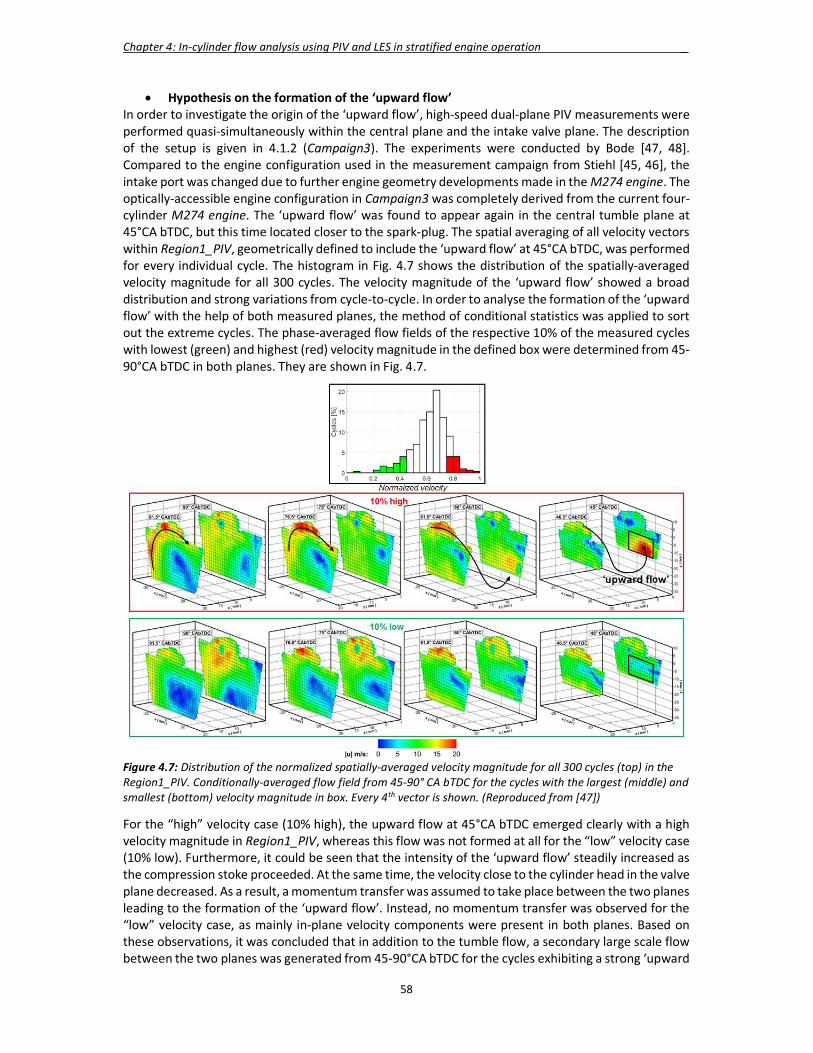
Chapter 4: In-cylinder flow analysis using PIV and LES in stratified engine operation _
58
Hypothesis on the formation of the ‘upward flow’ In order to investigate the origin of the ‘upward flow’, high-speed dual-plane PIV measurements were performed quasi-simultaneously within the central plane and the intake valve plane. The description of the setup is given in 4.1.2 (Campaign3). The experiments were conducted by Bode [47, 48]. Compared to the engine configuration used in the measurement campaign from Stiehl [45, 46], the intake port was changed due to further engine geometry developments made in the M274 engine. The optically-accessible engine configuration in Campaign3 was completely derived from the current four-cylinder M274 engine. The ‘upward flow’ was found to appear again in the central tumble plane at 45°CA bTDC, but this time located closer to the spark-plug. The spatial averaging of all velocity vectors within Region1_PIV, geometrically defined to include the ‘upward flow’ at 45°CA bTDC, was performed for every individual cycle. The histogram in Fig. 4.7 shows the distribution of the spatially-averaged velocity magnitude for all 300 cycles. The velocity magnitude of the ‘upward flow’ showed a broad distribution and strong variations from cycle-to-cycle. In order to analyse the formation of the ‘upward flow’ with the help of both measured planes, the method of conditional statistics was applied to sort out the extreme cycles. The phase-averaged flow fields of the respective 10% of the measured cycles with lowest (green) and highest (red) velocity magnitude in the defined box were determined from 45-90°CA bTDC in both planes. They are shown in Fig. 4.7.
Figure 4.7: Distribution of the normalized spatially-averaged velocity magnitude for all 300 cycles (top) in the Region1_PIV. Conditionally-averaged flow field from 45-90° CA bTDC for the cycles with the largest (middle) and smallest (bottom) velocity magnitude in box. Every 4th vector is shown. (Reproduced from [47])
For the “high” velocity case (10% high), the upward flow at 45°CA bTDC emerged clearly with a high velocity magnitude in Region1_PIV, whereas this flow was not formed at all for the “low” velocity case (10% low). Furthermore, it could be seen that the intensity of the ‘upward flow’ steadily increased as the compression stoke proceeded. At the same time, the velocity close to the cylinder head in the valve plane decreased. As a result, a momentum transfer was assumed to take place between the two planes leading to the formation of the ‘upward flow’. Instead, no momentum transfer was observed for the “low” velocity case, as mainly in-plane velocity components were present in both planes. Based on these observations, it was concluded that in addition to the tumble flow, a secondary large scale flow between the two planes was generated from 45-90°CA bTDC for the cycles exhibiting a strong ‘upward
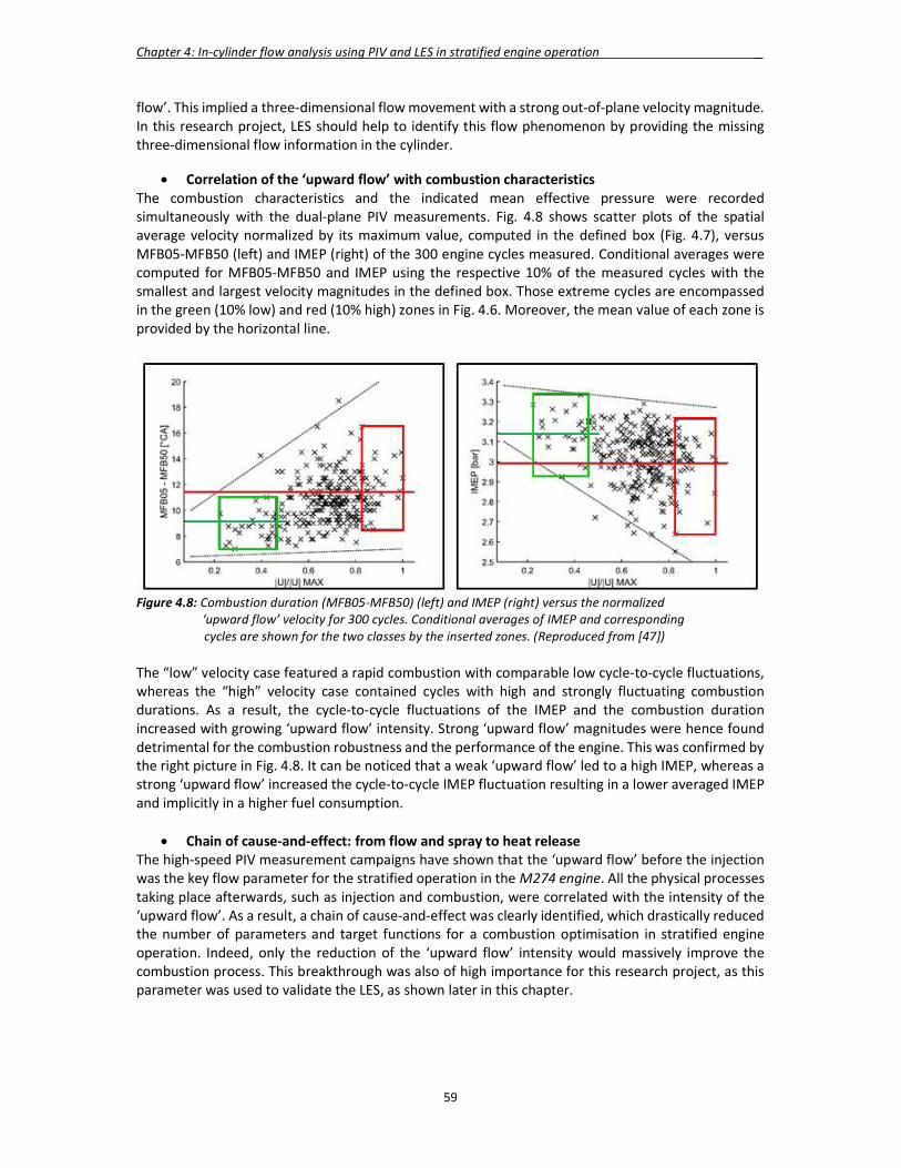
Chapter 4: In-cylinder flow analysis using PIV and LES in stratified engine operation _
59
flow’. This implied a three-dimensional flow movement with a strong out-of-plane velocity magnitude. In this research project, LES should help to identify this flow phenomenon by providing the missing three-dimensional flow information in the cylinder.
Correlation of the ‘upward flow’ with combustion characteristics The combustion characteristics and the indicated mean effective pressure were recorded simultaneously with the dual-plane PIV measurements. Fig. 4.8 shows scatter plots of the spatial average velocity normalized by its maximum value, computed in the defined box (Fig. 4.7), versus MFB05-MFB50 (left) and IMEP (right) of the 300 engine cycles measured. Conditional averages were computed for MFB05-MFB50 and IMEP using the respective 10% of the measured cycles with the smallest and largest velocity magnitudes in the defined box. Those extreme cycles are encompassed in the green (10% low) and red (10% high) zones in Fig. 4.6. Moreover, the mean value of each zone is provided by the horizontal line.
Figure 4.8: Combustion duration (MFB05-MFB50) (left) and IMEP (right) versus the normalized ‘upward flow’ velocity for 300 cycles. Conditional averages of IMEP and corresponding
cycles are shown for the two classes by the inserted zones. (Reproduced from [47]) The “low” velocity case featured a rapid combustion with comparable low cycle-to-cycle fluctuations, whereas the “high” velocity case contained cycles with high and strongly fluctuating combustion durations. As a result, the cycle-to-cycle fluctuations of the IMEP and the combustion duration increased with growing ‘upward flow’ intensity. Strong ‘upward flow’ magnitudes were hence found detrimental for the combustion robustness and the performance of the engine. This was confirmed by the right picture in Fig. 4.8. It can be noticed that a weak ‘upward flow’ led to a high IMEP, whereas a strong ‘upward flow’ increased the cycle-to-cycle IMEP fluctuation resulting in a lower averaged IMEP and implicitly in a higher fuel consumption.
Chain of cause-and-effect: from flow and spray to heat release The high-speed PIV measurement campaigns have shown that the ‘upward flow’ before the injection was the key flow parameter for the stratified operation in the M274 engine. All the physical processes taking place afterwards, such as injection and combustion, were correlated with the intensity of the ‘upward flow’. As a result, a chain of cause-and-effect was clearly identified, which drastically reduced the number of parameters and target functions for a combustion optimisation in stratified engine operation. Indeed, only the reduction of the ‘upward flow’ intensity would massively improve the combustion process. This breakthrough was also of high importance for this research project, as this parameter was used to validate the LES, as shown later in this chapter.

Chapter 4: In-cylinder flow analysis using PIV and LES in stratified engine operation _
60
4.2.3 High-speed PIV: influence of the spark-plug The spark-plug location plays a crucial role in the stratified operation and is directly linked to the position of the centrally mounted Piezo injector. The spray targeting of the spark-plug and the resulting fuel-air mixture formation around its electrodes before the ignition depends solely on the relative positioning of those two engine parts. As a result, the spark-plug has to penetrate deeply in the combustion chamber in order to ignite properly the local fuel-air mixture. The consequences of the interaction between the incoming intake flow and the spark-plug on the global in-cylinder flow formation in the central tumble plane was quantified using high-speed PIV. Two different engine configurations were investigated with high-speed PIV: without the spark-plug (Campaign1) and with the spark-plug mounted on the engine (Campaign2). Fig. 4.9 shows the average in-plane velocity (Vxz) results for each configuration in the intake stroke @262.5°CA bTDC and before the start of injection in stratified operation @40°CA bTDC. The in-plane velocity Vxz was spatially averaged in the defined Region1_PIV used in Campaign3 for each cycle. In this research project Vxz was defined as follows:
𝑉𝑥𝑧 = (𝑉𝑥 + 𝑉𝑧 ) . (4.1) The results confirmed that, due to the large penetration of the spark-plug in the combustion chamber, a very strong interaction of the incoming intake flow with the spark-plug took place and influenced the global in-cylinder flow motion. Without the spark-plug, the incoming intake flow reached the cylinder liner and the generated tumble flow was much stronger. The introduction of the spark-plug modified the balance between the tumble flow and the side flow. The difference in the x-direction of the black lines, sketched in Fig. 4.9 @262.5°CA bTDC, clearly indicated that the intensity of the side flows was higher with the spark-plug and led to a reduced tumble flow intensity. As a result, the magnitude of the ‘upward flow’, @40°CA bTDC in the Region1_PIV defined in Campaign3, was found lower with the spark-plug.
Figure 4.9: Average in-plane velocity magnitude (Vxz) in the central tumble plane -High-speed PIV results average over 200 cycles every 3rd, 4th vector is shown -Top:@262.5°CA bTDC; Bottom: @40°CA bTDC including the Region1_PIV -Left: Campaign1 without spark-plug; Right: Campaign2 without spark-plug
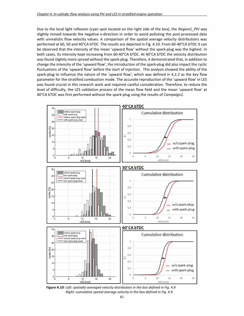
Chapter 4: In-cylinder flow analysis using PIV and LES in stratified engine operation _
61
Due to the local light reflexion (cyan spot located on the right side of the box), the Region1_PIV was slightly moved towards the negative x-direction in order to avoid polluting the post-processed data with unrealistic flow velocity values. A comparison of the spatial average velocity distributions was performed at 60, 50 and 40°CA bTDC. The results are depicted in Fig. 4.10. From 60-40°CA bTDC it can be observed that the intensity of the mean ‘upward flow’ without the spark-plug was the highest. In both cases, its intensity kept increasing from 60-40°CA bTDC. At 40°CA bTDC the velocity distribution was found slightly more spread without the spark-plug. Therefore, it demonstrated that, in addition to change the intensity of the ‘upward flow’, the introduction of the spark-plug did also impact the cyclic fluctuations of the ‘upward flow’ before the start of injection. This analysis showed the ability of the spark-plug to influence the nature of the ‘upward flow’, which was defined in 4.2.2 as the key flow parameter for the stratified combustion mode. The accurate reproduction of the ‘upward flow’ in LES was found crucial in this research work and required careful consideration. Therefore, to reduce the level of difficulty, the LES validation process of the mean flow field and the mean ‘upward flow’ at 40°CA bTDC was first performed without the spark-plug using the results of Campaign1.
Figure 4.10: Left: spatially-averaged velocity distribution in the box defined in Fig. 4.9 -Right: cumulative spatial average velocity in the box defined in Fig. 4.9.
Chapter 4: In-cylinder flow analysis using PIV and LES in stratified engine operation _
62
4.3 Mean flow field LES validation guided with single-plane high-speed PIV The aim of any predictive CFD simulation is to capture the correct in-cylinder flow structures following an engine design variation without any input from experiments. In that sense, LES is not predictive yet and needs to be validated first before it can be used in the engine development process. Today, there is no universal reliable LES validation strategy available. The question remains open on which level of detail a validation is required. Depending on the process of interest, different quantities for comparison as well as different level of agreement might be needed. The objective here was to present a new validation strategy, where high-speed PIV was used in a first place to identify the relevant quantities and flow regions in the cylinder. The validation of the LES was performed by direct comparisons with the high-speed PIV findings. The ultimate goal of this strategy was to build up a reliable LES dataset, complementary to the already existing high-speed PIV one. By combining the strengths of numerical simulations and experiments, further analysis of the cycle-to-cycle variations of the flow were made easier and more reliable. Moving from RANS to LES meant a huge increase of data and flow field information available. The size of the CFD models had massively increased and several cycles had to be computed. A clear validation strategy or definition of the flow problem was hence required beforehand, so that the data could be handled efficiently. This part presents the LES results of the motored in-cylinder flow together with a comprehensive validation strategy. The PIV measurements were directly used to guide the meshing procedure. The mesh was iteratively optimized and the PIV measurements helped to identify the regions were further improvements were needed. The previous validated RANS simulation of this engine configuration together with the flow map, derived from a combined flow analysis of RANS and high-speed PIV (presented in 4.2.1) were also used. They provided additional inputs to validate the different 3D-flow structure interactions responsible for the evolution of the tumble flow within the central tumble plane. From this comprehensive mesh study, two selected meshes are shown and discussed, in order to illustrate the importance of the mesh resolution on the local flow structures. For an accurate comparison between LES and the PIV measurements, a standard post-processing tool was developed allowing a similar post-processing and visualization of the experimental and numerical results. This iterative validation with high-speed PIV was conducted without the spark-plug geometry, in order to make sure that the main global and local in-cylinder flow features could be well captured in LES. The corresponding PIV measurements were taken from Campaign1. 4.3.1 Numerical setup The computational domain included the complete optically accessible engine geometry comprising the intake plenum and the exhaust port, like for the RANS case (Fig. 4.3). The piston crevices were not taken into account in the present study. Indeed, the target was only the reproduction of the in-cylinder flow in motored condition during the intake and compression strokes up to the start of injection in stratified operation. The in-cylinder pressure trace would hence not match perfectly between simulation and experiments, due to the difference in compression ratio. In the experimental study performed by Janas [51], the piston crevices were also omitted. Although some discrepancies could be noticed between the cylinder pressure evolutions from LES and experiments, the in-cylinder flow structures were claimed well captured in the simulation. The numerical setup of the simulation comprised the no-slip wall law (NSWL) based on standard wall functions [49], combined with the 2nd-order in space and time Lax-Wendroff convective scheme and the Smagorinsky subgrid scale turbulence model with the Smagorinsky coefficient 𝐶𝑠 = 0.18 . A maximum acoustic CFL_ac value of 0.9 was used to limit the time step throughout the simulation. Moreover the 2nd-order and 4th-order artificial viscosity coefficients were always kept constant (smu2 = 5.10-2 and smu4 = 8.10-3). The in-/outflow boundary conditions and wall temperatures were taken from a TPA model calibrated with the measurements recorded during Campaign2. On the intake side, a constant static pressure (Pint = 950 mbar) was applied at the entrance of the plenum using a NSCBC method to allow outgoing waves to leave the computational domain with minimum reflexions. The same pressure value was used to

Chapter 4: In-cylinder flow analysis using PIV and LES in stratified engine operation _
63
initialize the flow field in the CFD domain. On the exhaust side a transient static pressure profile was applied at the exhaust pressure sensor position, located 38 cm downstream from the exhaust valve seats, also using NSCBC. A maximum of 12 consecutive LES cycles were run for the mean flow field validation. The first two LES cycles were considered as ‘initialization cycles’ and were not taken into account for the flow analysis. 4.3.2 Validation strategy
Description of the process The mesh study was performed addressing separately the different engine parts. It was found that the global flow structures and the resulting tumble flow rotation speed were particularly dependent on the mesh resolution. Therefore, a particular attention was put on the setup of the mesh during the entire engine cycle. The overall mesh size, the adequate definition of the zones, where the mesh needed to be refined, as well as the size of the cells at the walls have been addressed separately for each engine component. During the mesh study, a multi-cycle LES run was performed (between 5 to 12 cycles) for every cell size change. The LES flow fields were then analysed and compared with the high-speed PIV measurements. This approach allowed to converge iteratively (15 iterations) towards a robust CFD model reproducing the experimental results over the entire engine cycle. The strategy followed during the mesh study is depicted in Fig. 4.11 and can be summarized as follows:
Figure 4.11: PIV-guided LES validation strategy for the mean flow field in LES
The maximal cell size at the walls was first derived iteratively based on the local y+ values computed at the wall during the simulation. In order to stay within the standard wall-law validity domain, y+ was kept below a value of 100. The smallest cell sizes at the walls are located in the regions where the flow velocities is the highest (bottom part of the intake port, valves and upper part of the combustion chamber). All regions were investigated even the plenum and in the transition domain between the plenum and the intake manifold, which is often neglected in LES studies.
A mesh variation was then performed in the regions known to influence the in-cylinder flow:
valves, valve curtains, intake port, cylinder, cylinder head and piston. In this work, the piston

Chapter 4: In-cylinder flow analysis using PIV and LES in stratified engine operation _
64
and the cylinder regions were always meshed in the same way. Each engine part was made of multiple panel geometries in Centaur. The meshing set-up consisted of four control parameters: - The base cell size and the closest distance between the panels for the surface mesh. - The base cell size and the growth ratio for the volume mesh. The mesh refinement was exclusively driven using those control parameters and not using ‘geometric source shapes’ (cylinder, sphere and box). Indeed, the ‘geometric source shapes’ were found unsuitable for local mesh refinement in combination with a complex engine geometry. First, it was difficult to position them locally and aligned to the 3D surface geometry; secondly the number of cells generated in those volumes was often too high, compared to what was really needed. Each ensemble-averaged LES result was compared to PIV. The aim was to derive a global understanding of the local change of mesh resolution on the LES results.
The regions of minimal cell volume were always monitored because they determined the
overall time step of the simulation with the explicit solver. As a result, special care was taken on the control of the minimum cell volumes especially during mesh deformation. Furthermore, to ensure high-quality mesh standards, the control of the cell distortion (sliver) was also addressed. Incremental improvements of the mesh were achieved either by adjusting the meshing parameters in Centaur or by re-discretizing the surfaces in the model geometry. As several meshes had to be generated to cover one engine cycle, the mesh quality optimisation had to be repeated for each mesh. Thereby, the mesh generation using the software Centaur turned out to be a crucial but very time consuming. An automated mesh generation process had been developed recently for AVBP and could reduce the overall meshing time. This last feature was not used in this project.
Validation criteria
The validation criteria encompassed numerical and flow validation criteria. The numerical validation criterion was based on the local turbulent to molecular viscosity ratio and was used as an indicator for the mesh refinement in the regions of high flow velocities. This criterion reduced the influence of the subgrid-model in the regions, where the flow has to be well captured. The target ratio was set to be < 50 as proposed by Angelberger in [28]. For a reliable validation process, the relevant flow structures were first identified. In 4.2, the ‘upward flow’ intensity in the central tumble plane was identified to be the key flow parameter linked to cycle-to-cycle fluctuations of the spray and IMEP. The formation of the tumble flow in this plane was found to be sensitive to the three-dimensional out-of-plane flows in RANS. A characterization of these 3D flow structures during intake and compression strokes and their mutual interactions were sketched in a flow map (Fig. 4.5). It was hence required to understand and assess the evolution of the tumble flow. With the nomenclature of the flow map, it was shown in 4.1 that the flow distribution in the valve gap was responsible for the resulting in-cylinder flow motion. As a result, the accurate capturing of the four identified flow features are required in LES in order to get the correct tumble flow rotation speed and tumble centre trajectory in the cylinder. The LES mean flow field was used to compare the evolution of the main flow structures in the central tumble plane with the high-speed PIV results. The focus was put on the following flow structures:
Evolution of ‘flow number 1’ identified by its leading edge (‘tumble front’) during the intake stroke
Interaction of ‘flow number 1’ and ‘flow number 2’ during the intake stroke Intensity and time of appearance of the ‘upward flow’ at 40°CA bTDC (a typical injection timing
for stratified combustion) Tumble centre position during compression
These four flow validation criteria were analysed separately on each mesh run in LES using a standard post-processing tool.
Chapter 4: In-cylinder flow analysis using PIV and LES in stratified engine operation _
65
Standard post-processing tool It was recognized [102] that a common platform was required to compare LES and PIV results in a fair and reproducible way. A standard post-processing tool has been developed over the last years at Daimler in the ‘Advanced Engine Research’ group in order to analyse and display the measurement results from different PIV measurement campaigns in the same manner. In this project, the standard post-processing tool was extended to the LES results. For the present validation, the LES and PIV velocity fields were first extracted from the central tumble plane. The commercial software Ensight was used to convert the LES flow data into a text file. Then, a user-subroutine in Matlab [132] imported them into the workspace of Matlab. Concerning the high-speed PIV results, a Matlab integrated function could transfer directly the La Vision’s DAVIS [103] format file into the workspace of Matlab. Then, the LES and high-speed PIV data were mapped onto a common 2D-Cartesian grid of 0.5 mm cell size for the flow analysis. The same Matlab routines were used to post-process the mapped LES and high-speed PIV flow data. This procedure ensured that exactly the same processing steps and definitions of the quantities of interest were applied to both the simulations and the experimental results. The second advantage was the possibility to plot the flow fields using the same setup and grid resolution, which turned out to be a massive advantage, when comparing small flow structures between LES and high-speed PIV results. Finally, the data handling and data archiving was found very efficient, as each mapped dataset could be saved in a re-usable Matlab database. 4.3.3 Validation results The goal of the global mesh study was to identify the necessary mesh requirements for LES to yield accurate reproduction of the high-speed PIV measurements. The final best practice mesh, named Model1_fine and whose meshing setup is depicted in Table 4.4, included the following features. The total amount of tetrahedral elements ranged from 20 million @TDC to 44 million @BDC and the cell size was 0.35 to 0.5 mm in the intake port and cylinder. At valve opening and valve closing, the cell size within the valve curtain was 60 µm. A set of 120 meshes was required to cover one engine cycle. In this section, the mean flow field validation results were presented using two meshes. This comparison was shown in order to point out the crucial effect of the base mesh resolution on local flow structures. The mesh of the 14th iteration, named Model1_coarse, of the aforementioned mesh study was selected. Model1_coarse was compared to the final mesh Model1_fine. Table 4.4 summarizes their meshing setups. In Model1_coarse, the cell size in the cylinder was 0.75 mm instead of 0.5 mm. Furthermore, the cell size in the vicinity of the intake valves and the seat area was in the range of 0.35-0.5 mm instead of 0.35 mm. However, the cell size at the wall was already optimised in order to achieve y+ < 100 in both models. The cell size at the wall was hence kept the same in Model1_fine and Model1_coarse to preserve wall friction and enable a fair comparison. The two meshes are depicted in Fig. 4.12. Table 4.4: Mesh description
Model1_coarse Model1_fine Number of cells 1223.106 2044.106 Cell size int. valve 0.350.5 mm 0.35 mm Cell size valve curtain 0.060.5 mm 0.060.5 mm Cell size cylinder 0.50.75 mm 0.5 mm

Chapter 4: In-cylinder flow analysis using PIV and LES in stratified engine operation _
66
Figure 4.12: Comparison of the mesh topology of Model1_coarse and Model1_fine
Assessment of the viscosity ratio The ratio of the turbulent viscosity (𝜇 ) to the molecular viscosity (𝜇) was first computed in order to isolate the regions, where the subgrid-model is particularly active and the flow not well captured. Fig. 4.13 shows a comparison of this viscosity ratio for both meshes in the intake valve plane. The crank angle position was taken @295°CA bTDC, where the intake valve lift is relatively small (5 mm) and the flow velocity high. The target viscosity ratio was set to be <50 as proposed by Angelberger in [28].
Figure 4.13: Comparison of the ratio μt / μ @295°CA bTDC -Left: Model1_coarse; Right: Model1_fine Many regions in Model1_coarse exhibited viscosity ratio values higher than 50. They were located nearly everywhere in the cylinder. From the analytical definition of the turbulent viscosity (Eq. (2.38)), these regions are located where high shear stresses and coarse cells are present. However, the region
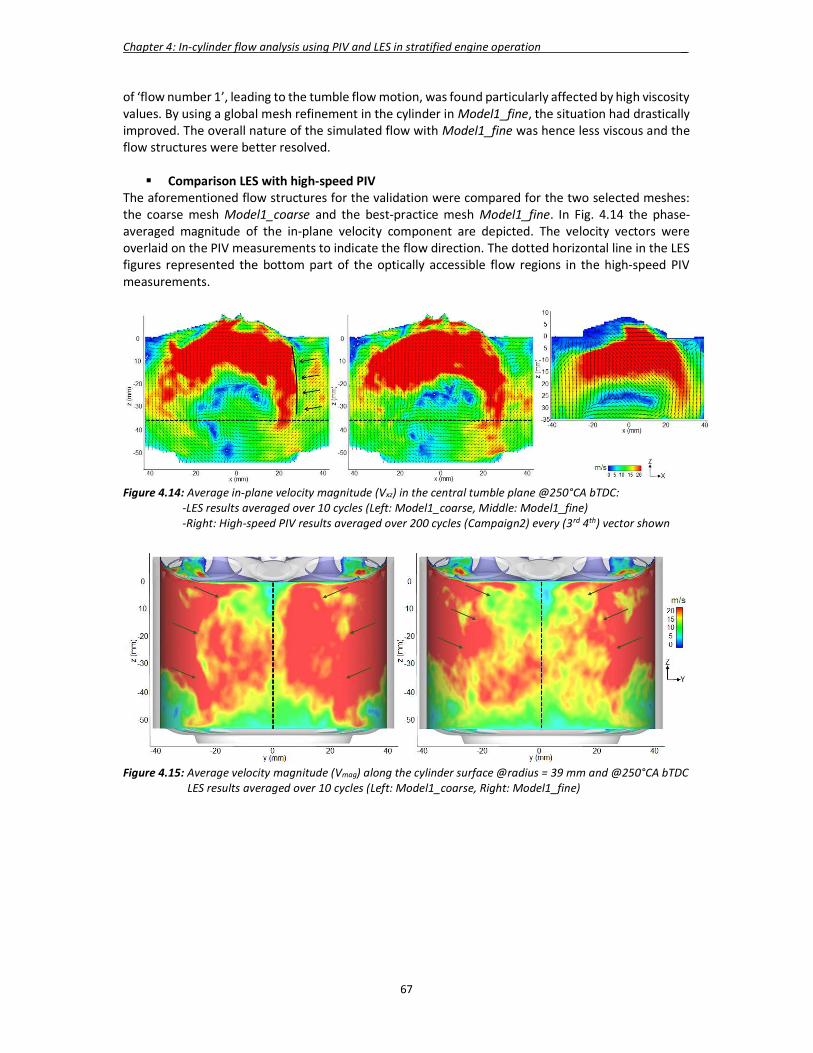
Chapter 4: In-cylinder flow analysis using PIV and LES in stratified engine operation _
67
of ‘flow number 1’, leading to the tumble flow motion, was found particularly affected by high viscosity values. By using a global mesh refinement in the cylinder in Model1_fine, the situation had drastically improved. The overall nature of the simulated flow with Model1_fine was hence less viscous and the flow structures were better resolved.
Comparison LES with high-speed PIV The aforementioned flow structures for the validation were compared for the two selected meshes: the coarse mesh Model1_coarse and the best-practice mesh Model1_fine. In Fig. 4.14 the phase-averaged magnitude of the in-plane velocity component are depicted. The velocity vectors were overlaid on the PIV measurements to indicate the flow direction. The dotted horizontal line in the LES figures represented the bottom part of the optically accessible flow regions in the high-speed PIV measurements.
Figure 4.14: Average in-plane velocity magnitude (Vxz) in the central tumble plane @250°CA bTDC: -LES results averaged over 10 cycles (Left: Model1_coarse, Middle: Model1_fine) -Right: High-speed PIV results averaged over 200 cycles (Campaign2) every (3rd 4th) vector shown
Figure 4.15: Average velocity magnitude (Vmag) along the cylinder surface @radius = 39 mm and @250°CA bTDC
LES results averaged over 10 cycles (Left: Model1_coarse, Right: Model1_fine)

Chapter 4: In-cylinder flow analysis using PIV and LES in stratified engine operation _
68
Figure 4.16: Average in-plane velocity magnitude (Vxz) in the central tumble plane @190°CA bTDC: -LES results averaged over 10 cycles (Left: Model1_coarse, Middle: Model1_fine) -Right: High-speed PIV results averaged over 200 cycles (Campaign1) every (3rd 4th) vector shown Fig. 4.14 shows the flow in the central tumble plane during the intake stroke at 250° CA bTDC, where the velocity distribution were characterized by a high velocity annular flow induced from the valves and the downward moving piston. The majority of the flow entered the cylinder through the valve gap over the front side of the valve leading to a strong ‘flow number 1’, which moved towards the cylinder liner and formed the clockwise tumble flow. A stagnation region was found, where the incoming flow impinged on the flow reversed by the piston on the left side of the tumble vortex centre. The LES results gave access to the flow information close to the cylinder walls. It revealed a lower velocity region between ‘flow number 1’ and the cylinder liner, strong enough to keep ‘flow number 1’ away from the liner and redirected it downwards towards the piston. This flow originating from the outer periphery of the intake valves, was redirected by the cylinder walls and travelled along the cylinder all the way into the central plane and was labelled as ‘flow number 3’ in Fig.4.5. Fig. 4.15 shows ‘flow number 3’ from both intake valves along a circumferential surface located at 2.5 mm from the cylinder liner. It revealed how they impinged on each other in the central tumble plane and were redirected downwards towards the piston. The formation of the overall tumble flow was sensitive with respect to ‘flow number 3’. This could be seen from the LES results, where an overall good agreement was found for both meshes in Fig. 4.14, but a difference was seen in the region where ‘flow number 1’ and ‘flow number 3’ interacted. In Model1_coarse, ‘flow number 3’ was stronger and higher velocity regions were extended further towards the cylinder head pushing ‘flow number 1’ towards the centre of the cylinder. Instead, ‘flow number 3’ was found weaker in Model1_fine and in the PIV results. Fig. 4.15 confirmed these observations as it showed that the ‘flow number 3’ intensities were much stronger for Model1_coarse than for Model1_fine. It was an additional hint that Model1_coarse was not adequate to capture the main flow features. Despite equal velocity magnitudes of ‘flow number 1’ for both meshes, this small difference in the tumble roll-up led to a lag in the tumble front compared to the measurements, as shown more clearly in Fig. 4.16 at 190°CA bTDC. The tumble flow had already performed nearly an entire revolution and the simulations nicely showed how the tumble centre was positioned centrally within the piston bowl at this timing. As a result, the shape and position of the tumble was centred in the cylinder, leading to a very similar shape of the high velocity tumble flow for both meshes. The main difference was the tumble front location being ~5 mm lower for Model1_coarse with a corresponding shift of the tumble vortex centre. Furthermore, as the intake flow path starting from the airbox towards the plenum was positioned perpendicular to the central tumble plane of the engine (Fig. 4.3), the in-cylinder flow could be expected to be slightly asymmetrical. Fig. 4.15 shows that strong differences could be observed between the ‘flow number 3’ intensities ,coming from both intake valves, leading to a stronger asymmetrical flow in the cylinder with Model1_coarse compared to Model1_fine.

Chapter 4: In-cylinder flow analysis using PIV and LES in stratified engine operation _
69
Upward flow As discussed earlier, small variations in the tumble roll-up implied small differences of the tumble front location i.e. of the tumble flow rotational speed. This led to a time shift of the appearance of the important ‘upward flow’ below the spark plug, as shown in Fig. 4.17 at 40°CA bTDC. The local and global flow structures were very similar in LES and PIV. One could clearly identify the global tumble flow with its corresponding tumble centre, the ‘upward flow’ above the piston and the low velocity region in the vicinity of the tumble center. While the flow structures and the tumble vortex centres were identical for both meshes, the magnitude of the ‘upward flow’ for Model1_fine showed better qualitative agreement with high-speed PIV. For Model1_coarse the magnitude of the ‘upward flow’ was found much lower.
Figure 4.17: Average in-plane velocity magnitude (Vxz) in the central tumble plane @ 40°CA bTDC: -LES results averaged over 10 cycles (Left: Model1_coarse, Middle: Model1_fine) -Right: High-speed PIV results averaged over 200 cycles (Campaign2) every (3rd 4th) vector shown Γ criterion The evolution of the tumble flow during the compression stroke was further characterized by the tumble vortex centre. The Γ criterion as proposed by Graftieux [50] was used to determine the global centre of rotation in a two-dimensional flow region (i.e. tumble centre for in-cylinder flows). At each position 𝑝(𝑥, 𝑦) in the domain, the angle 𝛾 (𝑙, 𝑚) between every velocity vector at the position (𝑙, 𝑚) and its connection vector 𝑝(𝑥, 𝑦) were calculated. The Γ criterion (Eq. 4.2) was applied to the 𝑁 velocity vectors present in the analyzed region. The global center of rotation was found where Γ had the highest value.
Γ(𝑥, 𝑦) = ∑ sin 𝛾 (𝑙, 𝑚) (4.2) This criterion was applied by Stiehl [45] to high-speed PIV results in order to compare two intake port geometries or by Janas [51] to compare LES results with high-speed PIV measurements for validation. The Γ criterion was applied to the mean flow fields from 110 to 50°CA bTDC. Fig. 4.18 shows the tumble centre evolution for the PIV measurements (represented by the crosses) and both LES (filled circles for Model1_fine and hollow circles for Model1_coarse). The same two-dimensional flow domain in the central tumble plane was used for LES and PIV. The evolution of the tumble centre path from both simulations was in good agreement with the measurements. The tumble centre positions with Model1_fine were found somehow closer to the measurements. Differences of the averaged tumble location were in the order of 1 mm. With the current engine geometry, the tumble centre moved from the middle of the cylinder toward the exhaust valves until 70°CA bTDC. From 70-50°CA bTDC, its direction changed and became parallel to the cylinder z-axis.

Chapter 4: In-cylinder flow analysis using PIV and LES in stratified engine operation _
70
Figure 4.18: Tumble centre evolution in high-speed PIV (Campaign2) and LES (Model1_fine and Model1_coarse).LES results averaged over 10 cycles. High-speed PIV results averaged over 200 cycles The locations of the tumble centre were found very similar for both simulations despite the observed differences early during the intake stroke. Even though the tumble vortex centre trajectory was well captured in LES, this criterion was not sufficient for the LES mean flow validation. Indeed, the tumble centre position was barely affected by the changes of the local flow structures observed visually in Fig. 4.14-17. The difference in intensity and time of appearance of the ‘upward flow’ between Model1_fine and Model1_coarse could not be explained by their respective tumble centre paths. Therefore, the visual observation of the local 2D flow structures together with the understanding of the flow interactions (flow number 14) cannot be replaced by the sole ‘tumble vortex centre’ validation criterion. The validation strategy put in place allowed to converge iteratively towards a robust meshing setup for LES. The most relevant mean flow structures of the experimental results could be captured in LES during the intake and compression strokes. The local flow features observed in high-speed PIV were also addressed during the LES validation process and were found in good agreement with the experimental results. The most important validation breakthrough was the reproduction of the intensity and the time of appearance of the mean ‘upward flow’ before the start of injection in stratified engine operation. This validation strategy was named PIV-guided LES validation strategy and 2.1 Mio CPU-hours were consumed to reach a validated setup for the LES.
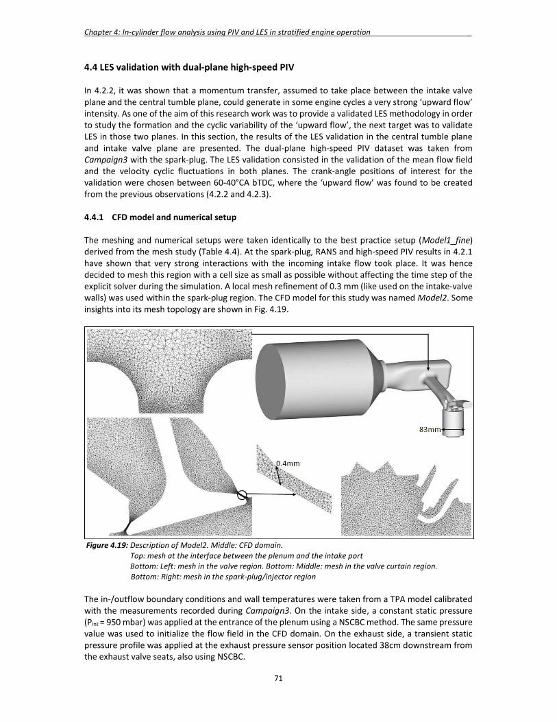
Chapter 4: In-cylinder flow analysis using PIV and LES in stratified engine operation _
71
4.4 LES validation with dual-plane high-speed PIV In 4.2.2, it was shown that a momentum transfer, assumed to take place between the intake valve plane and the central tumble plane, could generate in some engine cycles a very strong ‘upward flow’ intensity. As one of the aim of this research work was to provide a validated LES methodology in order to study the formation and the cyclic variability of the ‘upward flow’, the next target was to validate LES in those two planes. In this section, the results of the LES validation in the central tumble plane and intake valve plane are presented. The dual-plane high-speed PIV dataset was taken from Campaign3 with the spark-plug. The LES validation consisted in the validation of the mean flow field and the velocity cyclic fluctuations in both planes. The crank-angle positions of interest for the validation were chosen between 60-40°CA bTDC, where the ‘upward flow’ was found to be created from the previous observations (4.2.2 and 4.2.3). 4.4.1 CFD model and numerical setup The meshing and numerical setups were taken identically to the best practice setup (Model1_fine) derived from the mesh study (Table 4.4). At the spark-plug, RANS and high-speed PIV results in 4.2.1 have shown that very strong interactions with the incoming intake flow took place. It was hence decided to mesh this region with a cell size as small as possible without affecting the time step of the explicit solver during the simulation. A local mesh refinement of 0.3 mm (like used on the intake-valve walls) was used within the spark-plug region. The CFD model for this study was named Model2. Some insights into its mesh topology are shown in Fig. 4.19.
Figure 4.19: Description of Model2. Middle: CFD domain.
Top: mesh at the interface between the plenum and the intake port Bottom: Left: mesh in the valve region. Bottom: Middle: mesh in the valve curtain region. Bottom: Right: mesh in the spark-plug/injector region The in-/outflow boundary conditions and wall temperatures were taken from a TPA model calibrated with the measurements recorded during Campaign3. On the intake side, a constant static pressure (Pint = 950 mbar) was applied at the entrance of the plenum using a NSCBC method. The same pressure value was used to initialize the flow field in the CFD domain. On the exhaust side, a transient static pressure profile was applied at the exhaust pressure sensor position located 38cm downstream from the exhaust valve seats, also using NSCBC.
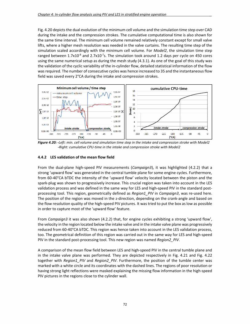
Chapter 4: In-cylinder flow analysis using PIV and LES in stratified engine operation _
72
Fig. 4.20 depicts the dual evolution of the minimum cell volume and the simulation time step over CAD during the intake and the compression strokes. The cumulative computational time is also shown for the same time interval. The minimum cell volume remained relatively constant except for small valve lifts, where a higher mesh resolution was needed in the valve curtains. The resulting time step of the simulation scaled accordingly with the minimum cell volume. For Model2, the simulation time step ranged between 1.7x10⁻⁸ and 2.7x10⁻⁷s. The simulation took around 1.2 days per cycle on 450 cores using the same numerical setup as during the mesh study (4.3.1). As one of the goal of this study was the validation of the cyclic variability of the in-cylinder flow, detailed statistical information of the flow was required. The number of consecutive cycles was hence increased to 35 and the instantaneous flow field was saved every 2°CA during the intake and compression strokes.
Figure 4.20: -Left: min. cell volume and simulation time step in the intake and compression stroke with Model2 -Right: cumulative CPU-time in the intake and compression stroke with Model2 4.4.2 LES validation of the mean flow field From the dual-plane high-speed PIV measurements (Campaign3), it was highlighted (4.2.2) that a strong ‘upward flow’ was generated in the central tumble plane for some engine cycles. Furthermore, from 60-40°CA bTDC the intensity of the ‘upward flow’ velocity located between the piston and the spark-plug was shown to progressively increase. This crucial region was taken into account in the LES validation process and was defined in the same way for LES and high-speed PIV in the standard post-processing tool. This region, geometrically defined as Region1_PIV in Campaign3, was re-used here. The position of the region was moved in the z-direction, depending on the crank-angle and based on the flow resolution quality of the high-speed PIV pictures. It was tried to put the box as low as possible in order to capture most of the ‘upward flow’ feature. From Campaign3 it was also shown (4.2.2) that, for engine cycles exhibiting a strong ‘upward flow’, the velocity in the region located below the intake valve and in the intake valve plane was progressively reduced from 60-40°CA bTDC. This region was hence taken into account in the LES validation process, too. The geometrical definition of this region was carried out in the same way for LES and high-speed PIV in the standard post-processing tool. This new region was named Region2_PIV. A comparison of the mean flow field between LES and high-speed PIV in the central tumble plane and in the intake valve plane was performed. They are depicted respectively in Fig. 4.21 and Fig. 4.22 together with Region1_PIV and Region2_PIV. Furthermore, the position of the tumble center was marked with a white circle and its coordinates with the dashed lines. The regions of poor resolution or having strong light reflections were masked explaining the missing flow information in the high-speed PIV pictures in the regions close to the cylinder wall.

Chapter 4: In-cylinder flow analysis using PIV and LES in stratified engine operation _
73
The most important flow features were well captured in LES compared to high-speed PIV in both planes. The evolution of the tumble centres was in good agreement with the measurements. Furthermore, the differences of the averaged tumble location were in the order of 2.5 mm, which was somehow slightly higher compared to the case without the spark-plug (4.3.3) in the central tumble plane, but still reasonable. In the central tumble plane, the flow velocities in the region below the injector and their decreasing trend were all well captured in LES from 60-40°CA bTDC. In Region1_PIV, the trend of increasing velocities was also reproduced accurately in LES. However, the flow velocities appeared to be visually lower in LES compared to the measurements. The ‘upward flow’ was not as well captured as with Model1_fine during the mesh study without the spark-plug (4.3.3). In the intake valve plane, the decreasing flow velocity trend in Region2_PIV was also correct in LES. Furthermore, the intensity of the flow velocity in that region matched very well the ones observed in high-speed PIV.
Figure 4.21: Average in-plane velocity magnitude (Vxz) in the central tumble plane @60-40°CA bTDC
-Top: LES results averaged over 35 cycles with Region1_PIV -Bottom: High-speed PIV results averaged over 300cycles (Campaign3) with Region1_PIV
Figure 4.22: Average in-plane velocity magnitude (Vxz) in the intake valve plane @60-40°CA bTDC
-Top: LES results averaged over 35 cycles with Region2_PIV -Bottom: High-speed PIV results averaged over 300cycles (Campaign3) with Region2_PIV
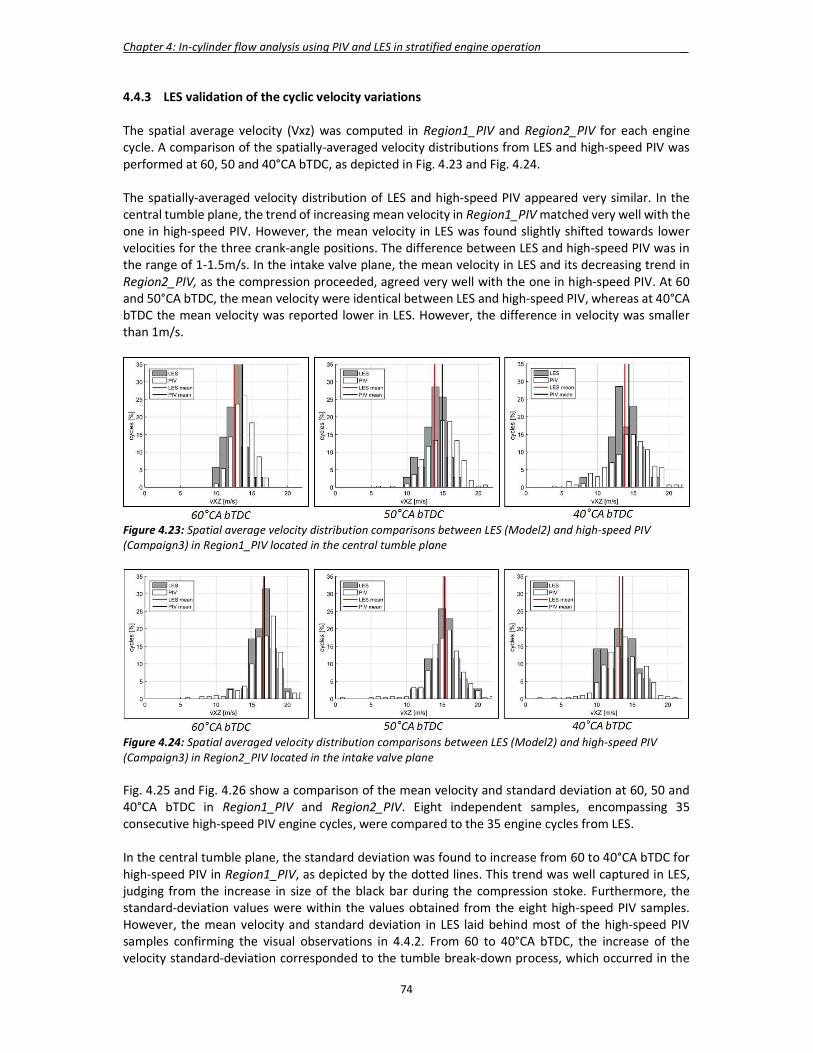
Chapter 4: In-cylinder flow analysis using PIV and LES in stratified engine operation _
74
4.4.3 LES validation of the cyclic velocity variations The spatial average velocity (Vxz) was computed in Region1_PIV and Region2_PIV for each engine cycle. A comparison of the spatially-averaged velocity distributions from LES and high-speed PIV was performed at 60, 50 and 40°CA bTDC, as depicted in Fig. 4.23 and Fig. 4.24. The spatially-averaged velocity distribution of LES and high-speed PIV appeared very similar. In the central tumble plane, the trend of increasing mean velocity in Region1_PIV matched very well with the one in high-speed PIV. However, the mean velocity in LES was found slightly shifted towards lower velocities for the three crank-angle positions. The difference between LES and high-speed PIV was in the range of 1-1.5m/s. In the intake valve plane, the mean velocity in LES and its decreasing trend in Region2_PIV, as the compression proceeded, agreed very well with the one in high-speed PIV. At 60 and 50°CA bTDC, the mean velocity were identical between LES and high-speed PIV, whereas at 40°CA bTDC the mean velocity was reported lower in LES. However, the difference in velocity was smaller than 1m/s.
Figure 4.23: Spatial average velocity distribution comparisons between LES (Model2) and high-speed PIV (Campaign3) in Region1_PIV located in the central tumble plane
Figure 4.24: Spatial averaged velocity distribution comparisons between LES (Model2) and high-speed PIV (Campaign3) in Region2_PIV located in the intake valve plane Fig. 4.25 and Fig. 4.26 show a comparison of the mean velocity and standard deviation at 60, 50 and 40°CA bTDC in Region1_PIV and Region2_PIV. Eight independent samples, encompassing 35 consecutive high-speed PIV engine cycles, were compared to the 35 engine cycles from LES. In the central tumble plane, the standard deviation was found to increase from 60 to 40°CA bTDC for high-speed PIV in Region1_PIV, as depicted by the dotted lines. This trend was well captured in LES, judging from the increase in size of the black bar during the compression stoke. Furthermore, the standard-deviation values were within the values obtained from the eight high-speed PIV samples. However, the mean velocity and standard deviation in LES laid behind most of the high-speed PIV samples confirming the visual observations in 4.4.2. From 60 to 40°CA bTDC, the increase of the velocity standard-deviation corresponded to the tumble break-down process, which occurred in the
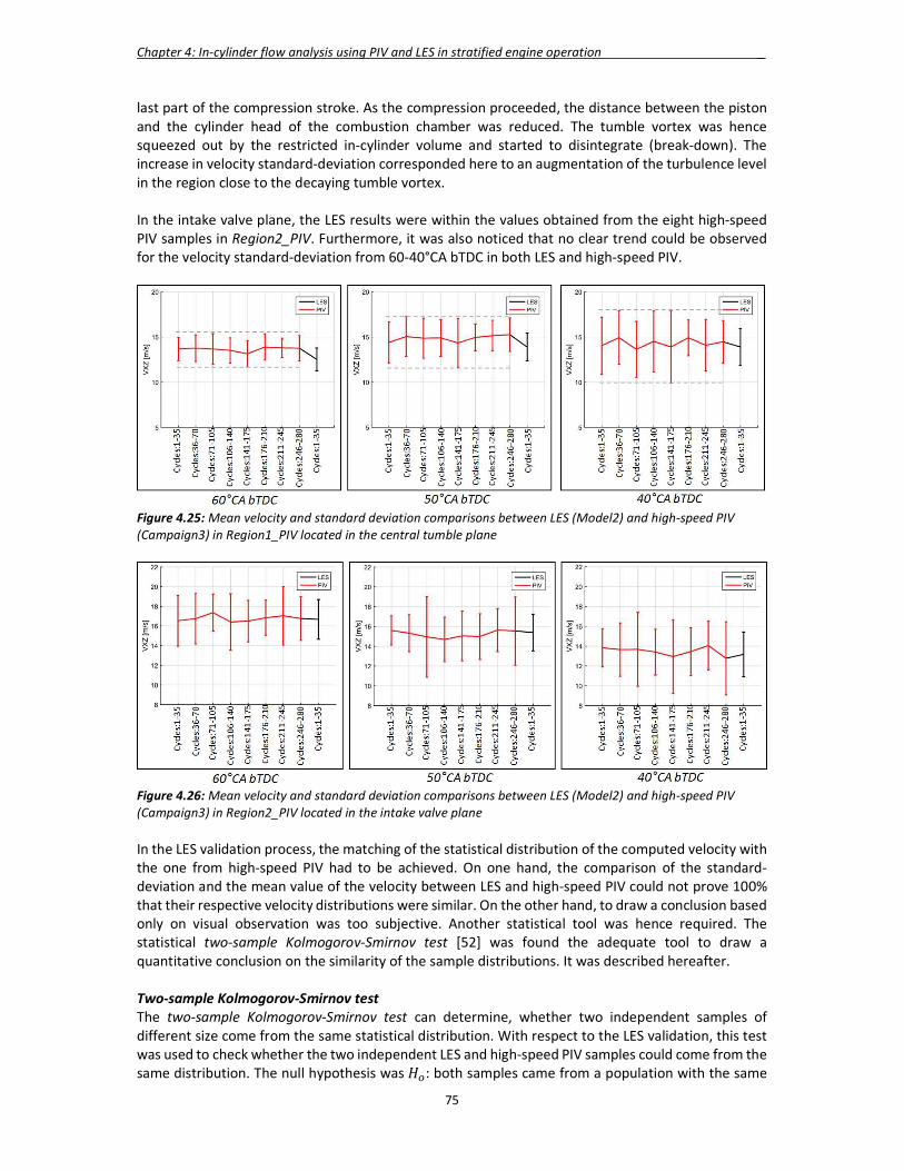
Chapter 4: In-cylinder flow analysis using PIV and LES in stratified engine operation _
75
last part of the compression stroke. As the compression proceeded, the distance between the piston and the cylinder head of the combustion chamber was reduced. The tumble vortex was hence squeezed out by the restricted in-cylinder volume and started to disintegrate (break-down). The increase in velocity standard-deviation corresponded here to an augmentation of the turbulence level in the region close to the decaying tumble vortex. In the intake valve plane, the LES results were within the values obtained from the eight high-speed PIV samples in Region2_PIV. Furthermore, it was also noticed that no clear trend could be observed for the velocity standard-deviation from 60-40°CA bTDC in both LES and high-speed PIV.
Figure 4.25: Mean velocity and standard deviation comparisons between LES (Model2) and high-speed PIV (Campaign3) in Region1_PIV located in the central tumble plane
Figure 4.26: Mean velocity and standard deviation comparisons between LES (Model2) and high-speed PIV (Campaign3) in Region2_PIV located in the intake valve plane In the LES validation process, the matching of the statistical distribution of the computed velocity with the one from high-speed PIV had to be achieved. On one hand, the comparison of the standard-deviation and the mean value of the velocity between LES and high-speed PIV could not prove 100% that their respective velocity distributions were similar. On the other hand, to draw a conclusion based only on visual observation was too subjective. Another statistical tool was hence required. The statistical two-sample Kolmogorov-Smirnov test [52] was found the adequate tool to draw a quantitative conclusion on the similarity of the sample distributions. It was described hereafter. Two-sample Kolmogorov-Smirnov test The two-sample Kolmogorov-Smirnov test can determine, whether two independent samples of different size come from the same statistical distribution. With respect to the LES validation, this test was used to check whether the two independent LES and high-speed PIV samples could come from the same distribution. The null hypothesis was 𝐻 : both samples came from a population with the same

Chapter 4: In-cylinder flow analysis using PIV and LES in stratified engine operation _
76
distribution. The first sample cumulative distribution functions YLES(Vxz) with a sample size n = 35 was compared to the second sample cumulative distribution function YPIV(Vxz) with m = 300. A test quantity 𝐷 was defined as the maximum vertical deviation between the cumulative distributions of both samples:
𝐷 = max |𝑌 (Vxz) − 𝑌 (Vxz)| . (4.3)
𝐻 was rejected as soon as 𝐷 exceeded the critical value Dα:
D = K (4.4)
where Kα is the inverse of the Kolmogorov distribution taken from [26] and depends on the significance value α. It is common practice to use a significance level α = 0.05 in the two sample Kolmogorov-Smirnov test [26]. In the present case, the associated critical value was D . = 0.243. The two-sample Kolmogorov-Smirnov test was applied to the spatial average velocity in Region1_PIV and Region2_PIV computed for all engine cycles from LES and high-speed PIV. Fig. 4.27 and Fig. 4.28 show the cumulative spatially-averaged velocity distributions of LES and high-speed PIV respectively in Region1_PIV and Region2_PIV. The test quantities were computed at 60, 50 and 40°CA bTDC and are summarized in Table 4.5 and Table 4.6.
Figure 4.27: Comparison of the cumulative distribution of the spatial average velocity between LES (Model2, 35 cycles) and high-speed PIV (Campaign3, 300 cycles) in Region1_PIV located in the central tumble plane. The location of test quantity 𝐷 of the two-sample K-S test are included
Figure 4.28: Comparison of the cumulative distribution of the spatial average velocity between LES (Model2, 35 cycles) and high-speed PIV (Campaign3, 300 cycles) in Region2_PIV located in the intake valve in the intake valve plane. The location of test quantity 𝐷 of the K-S test are included In Region1_PIV, the null hypothesis was only accepted at 40°CA bTDC as the test quantity was below D . . Therefore, from a statistical point of view, it was concluded that the spatially-averaged velocity distribution from LES was not significantly different to the one from high-speed PIV in Region1_PIV at 40° CA bTDC. At 60 and 50°CA bTDC the two-sample Kolmogorov-Smirnov test failed because of its high sensitivity to the tiny shift (1-1.5m/s!) of the LES cumulative spatially-averaged velocity distributions compared to the high-speed PIV ones. Nevertheless, the shape of the LES cumulative spatially-averaged velocity distribution looked comparable to the high-speed PIV one.

Chapter 4: In-cylinder flow analysis using PIV and LES in stratified engine operation _
77
However, as it was shown earlier, the characteristics of the ‘upward flow’ at 40°CA bTDC remained the most important feature to capture here, as it influenced the chain of cause-and-effect in stratified engine operation. From the validation procedure, it could be stated that the LES results in the central tumble plane were fully validated with high-speed PIV in terms of global mean flow field, average velocity magnitude and standard-deviation in Region1_PIV. At 40°CA bTDC before the start of injection, it was additionally demonstrated that the spatially-averaged velocity distribution from LES and the one from high-speed PIV were not significantly different. At 60 and 50°CA bTDC, both averaged velocity magnitude distributions were found very close.
Table 4.5: Test quantity 𝐷 of the two-sample Kolmogorov-Smirnov test Between LES (35cycles) and high-speed PIV (300cycles) in Region1_PIV
𝑫 60°CA bTDC 0.43 50°CA bTDC 0.28 40°CA bTDC 0.195
In Region2_PIV the null hypothesis was accepted from 60-40° CA bTDC, as all test quantities were below D . . Therefore, from a statistical point of view, it was concluded that the spatially-averaged velocity distribution from LES was not significantly different to the one from high-speed PIV in Region2_PIV from 60-40° CA bTDC. Thereby, the LES flow fields in the intake valve plane were fully validated with the ones from high-speed PIV, in terms of global mean flow field and cyclic velocity fluctuation in Region2_PIV.
Table 4.6: Test quantity 𝐷 of the two-sample Kolmogorov-Smirnov test between LES (35cycles) and high-speed PIV (300cycles) in Region2_PIV
𝑫 60°CA bTDC 0.074 50°CA bTDC 0.09 40°CA bTDC 0.09
The same analysis is performed later in this chapter (4.6) using the 3rd-order convective scheme TTGC with the aim to improve the spatially-averaged velocity distribution in Region1_PIV from 60-50°CA bTDC. 4.5 LES in-cylinder flow analysis The features of the computed flow with LES in Region1_PIV were successfully validated with high-speed PIV (Campaign3) paving the way to the understanding of the ‘upward flow’ formation. The main goals of this section were: First to isolate the extreme cycles linked to a strong ‘upward flow’; secondly, to find out the flow phenomena responsible for its creation, before the start of injection in stratified engine operation, using the LES three-dimensional flow field information. 4.5.1 Conditional statistics in PIV based on correlation analysis The results from high-speed dual-plane PIV (Campaign3) and LES (Model2) consisted of multiple engine cycles. Conditional statistics were used successfully in the PIV analysis, as presented in 4.2.2, in order to extract the measured extremes cycles exhibiting strong ‘upward flow’ and weak ‘upward flow’ at 40°CA bTDC. It was thereby decided to use the conditional statistics for the 35 LES cycles, too.
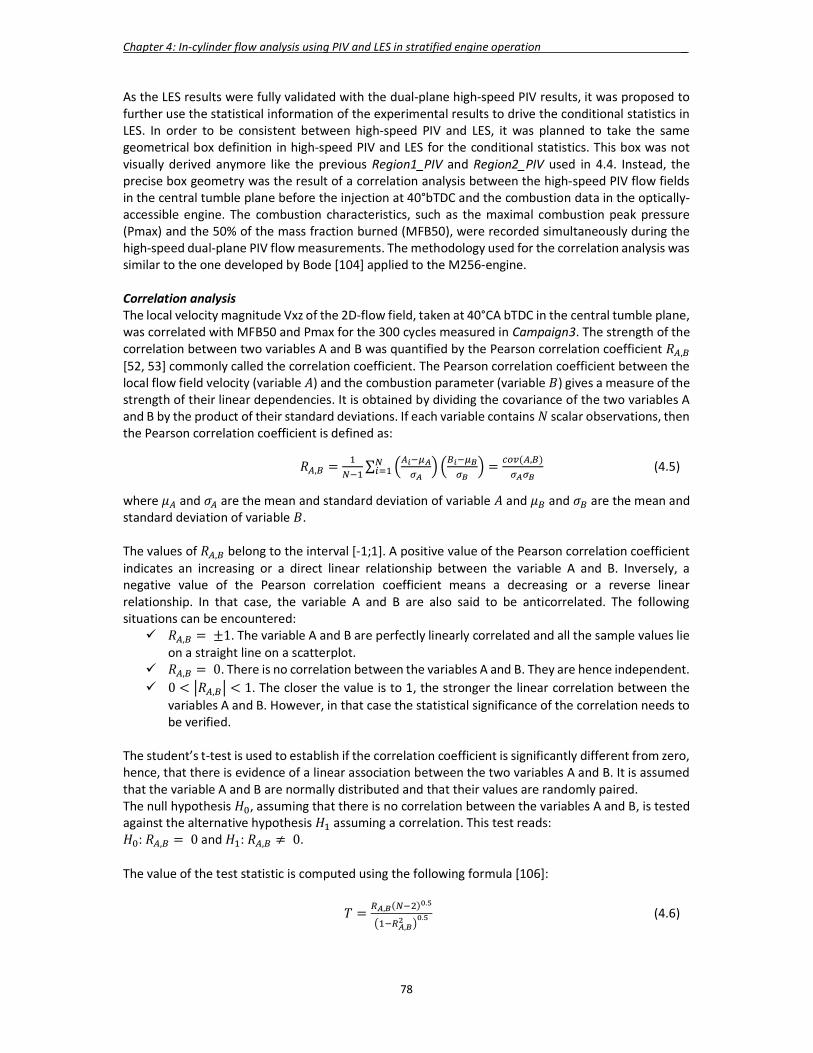
Chapter 4: In-cylinder flow analysis using PIV and LES in stratified engine operation _
78
As the LES results were fully validated with the dual-plane high-speed PIV results, it was proposed to further use the statistical information of the experimental results to drive the conditional statistics in LES. In order to be consistent between high-speed PIV and LES, it was planned to take the same geometrical box definition in high-speed PIV and LES for the conditional statistics. This box was not visually derived anymore like the previous Region1_PIV and Region2_PIV used in 4.4. Instead, the precise box geometry was the result of a correlation analysis between the high-speed PIV flow fields in the central tumble plane before the injection at 40°bTDC and the combustion data in the optically-accessible engine. The combustion characteristics, such as the maximal combustion peak pressure (Pmax) and the 50% of the mass fraction burned (MFB50), were recorded simultaneously during the high-speed dual-plane PIV flow measurements. The methodology used for the correlation analysis was similar to the one developed by Bode [104] applied to the M256-engine. Correlation analysis The local velocity magnitude Vxz of the 2D-flow field, taken at 40°CA bTDC in the central tumble plane, was correlated with MFB50 and Pmax for the 300 cycles measured in Campaign3. The strength of the correlation between two variables A and B was quantified by the Pearson correlation coefficient 𝑅 , [52, 53] commonly called the correlation coefficient. The Pearson correlation coefficient between the local flow field velocity (variable 𝐴) and the combustion parameter (variable 𝐵) gives a measure of the strength of their linear dependencies. It is obtained by dividing the covariance of the two variables A and B by the product of their standard deviations. If each variable contains 𝑁 scalar observations, then the Pearson correlation coefficient is defined as:
𝑅 , = ∑ =( , ) (4.5)
where 𝜇 and 𝜎 are the mean and standard deviation of variable 𝐴 and 𝜇 and 𝜎 are the mean and standard deviation of variable 𝐵. The values of 𝑅 , belong to the interval [-1;1]. A positive value of the Pearson correlation coefficient indicates an increasing or a direct linear relationship between the variable A and B. Inversely, a negative value of the Pearson correlation coefficient means a decreasing or a reverse linear relationship. In that case, the variable A and B are also said to be anticorrelated. The following situations can be encountered:
𝑅 , = ±1. The variable A and B are perfectly linearly correlated and all the sample values lie on a straight line on a scatterplot.
𝑅 , = 0. There is no correlation between the variables A and B. They are hence independent. 0 < 𝑅 , < 1. The closer the value is to 1, the stronger the linear correlation between the
variables A and B. However, in that case the statistical significance of the correlation needs to be verified.
The student’s t-test is used to establish if the correlation coefficient is significantly different from zero, hence, that there is evidence of a linear association between the two variables A and B. It is assumed that the variable A and B are normally distributed and that their values are randomly paired. The null hypothesis 𝐻 , assuming that there is no correlation between the variables A and B, is tested against the alternative hypothesis 𝐻 assuming a correlation. This test reads: 𝐻 : 𝑅 , = 0 and 𝐻 : 𝑅 , ≠ 0. The value of the test statistic is computed using the following formula [106]:
𝑇 = , ( ) .
,. (4.6)
Chapter 4: In-cylinder flow analysis using PIV and LES in stratified engine operation _
79
Based on the significance level α chosen for the test and N, the critical value 𝑇∝, is compared to the result of the test statistic in order to draw a decision.
- If 𝑇 > 𝑇∝, the null hypothesis is rejected in a favour of the alternative. It can be concluded that there is sufficient evidence at the significance level α to conclude that there is a linear relationship between variable A and B.
- If 𝑇 < 𝑇∝, the null hypothesis is accepted. There is no sufficient evidence at the significance level α to conclude that there is a linear relationship between variable A and B.
The critical values can be found tabulated in the literature [105, 106] or could be directly computed with commercial software like Matlab or Excel [133]. A significance value of 1% was chosen as proposed by Bode in [104]. Using 𝑁 = 300 cycles and α = 1%, a critical Pearson correlation coefficient 𝑅∝, could be derived based on the value of 𝑇∝, . It was found 𝑅∝, = 0.149. It implies that for every Pearson correlation coefficient greater than 𝑅∝, , the linear correlation between the variables A and B can be considered as statistically significant. Two so-called ‘correlation maps’ were hence generated in the central tumble plane, as shown in Fig. 4.29. They provided the information on how well the local flow field velocity vector at 40°CA bTDC was correlated with both the MFB50 and the combustion peak pressure. Correlation map between the flow velocity Vxz and Pmax Two well-correlated regions could be identified: a first region located below the spark-plug and a second one located below the cylinder head on the intake side. In the first region, the flow velocity was found anticorrelated with Pmax, which meant that an increase of the flow velocity at 40°CA bTDC in this region reduced the maximal peak pressure during the combustion. As a result, strong flow velocities in the first region implied a reduced combustion performance. This region corresponded to the known region encompassing the ‘upward flow’ and was named Region1_PIV_Pmax. In the second region, the flow velocity was directly correlated with Pmax, which meant that an increase of the flow velocity at 40°CA bTDC increased as well the maximal peak pressure during the combustion. Thereby, strong flow velocities in the second region led to a better combustion process. This region was newly found from this correlation analysis and was called Region2_PIV_Pmax. The spatial averaging of the velocity Vxz was computed in the two aforementioned regions. Fig. 4.29 shows the scatter plots of the spatial average velocity computed in Region1_PIV_Pmax and Region2_PIV_Pmax, as a function of Pmax for the 300 engine cycles. The Pearson correlation coefficient in Region1_PIV_Pmax was equal to -0.39 and the one in Region2_PIV_Pmax equal to 0.37. Those values being higher than the critical Pearson correlation coefficient (0.149) defined above, it confirmed that the findings had statistical significance and that a strong linear correlation between the local flow velocity Vxz in both regions and Pmax existed. Furthermore, it showed that the flow velocity, in Region1_PIV_Pmax and Region2_PIV_Pmax, had adverse outcomes on the combustion process. Correlation map between the flow velocity Vxz and MFB50 The same regions i.e. Region1_PIV_Pmax and Region2_PIV_Pmax could also be identified from the correlation analysis between the local velocity Vxz and MFB50. In Region1_PIV_Pmax, the flow velocity was found directly correlated with MFB50. As a result, strong flow velocities in this region implied an increased combustion duration i.e. a worse combustion performance. In Region2_PIV_Pmax, the flow velocity was anticorrelated with MFB50. Thereby, strong flow velocities in this region led to a shorter combustion duration. Moreover, Fig. 4.29 shows the scatter plots of the spatial average velocity computed in Region1_PIV_Pmax and Region2_PIV_Pmax versus MFB50 for the 300 engine cycles. A clear linear relationship was found between the flow velocity and MFB50. The Pearson correlation coefficient in Region1_PIV_Pmax was equal to 0.36 and the one in Region2_PIV_Pmax to -0.41.
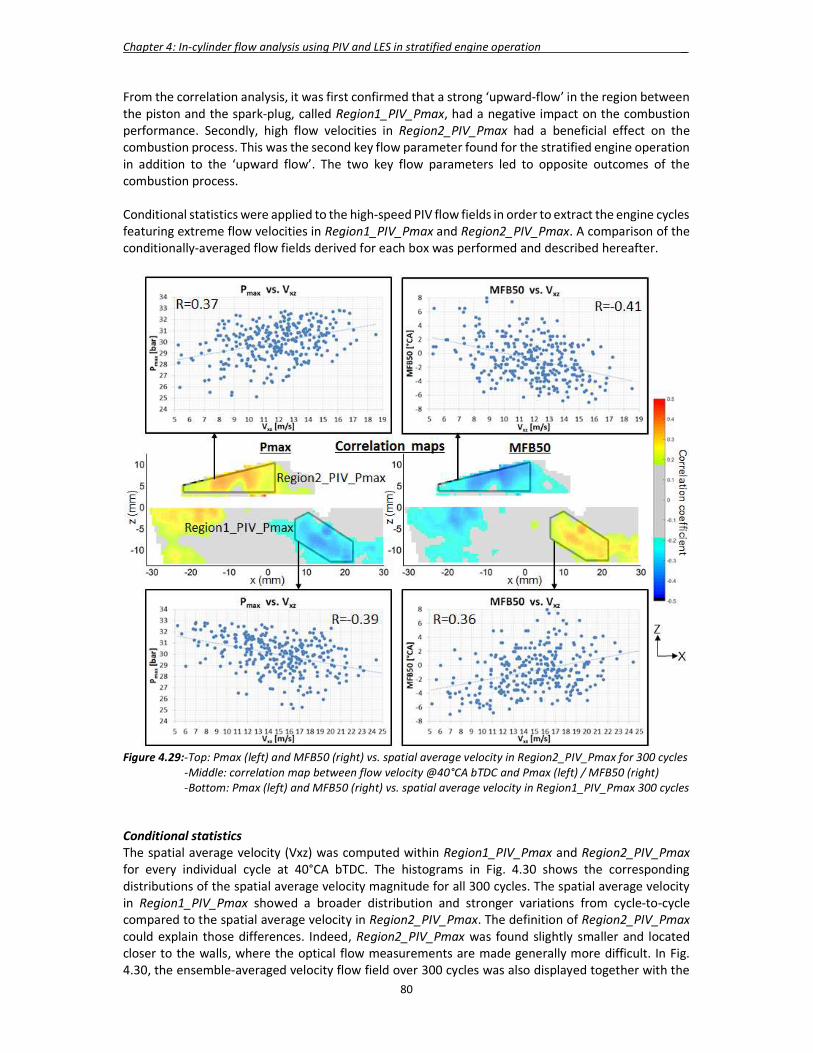
Chapter 4: In-cylinder flow analysis using PIV and LES in stratified engine operation _
80
From the correlation analysis, it was first confirmed that a strong ‘upward-flow’ in the region between the piston and the spark-plug, called Region1_PIV_Pmax, had a negative impact on the combustion performance. Secondly, high flow velocities in Region2_PIV_Pmax had a beneficial effect on the combustion process. This was the second key flow parameter found for the stratified engine operation in addition to the ‘upward flow’. The two key flow parameters led to opposite outcomes of the combustion process. Conditional statistics were applied to the high-speed PIV flow fields in order to extract the engine cycles featuring extreme flow velocities in Region1_PIV_Pmax and Region2_PIV_Pmax. A comparison of the conditionally-averaged flow fields derived for each box was performed and described hereafter.
Figure 4.29:-Top: Pmax (left) and MFB50 (right) vs. spatial average velocity in Region2_PIV_Pmax for 300 cycles
-Middle: correlation map between flow velocity @40°CA bTDC and Pmax (left) / MFB50 (right) -Bottom: Pmax (left) and MFB50 (right) vs. spatial average velocity in Region1_PIV_Pmax 300 cycles Conditional statistics The spatial average velocity (Vxz) was computed within Region1_PIV_Pmax and Region2_PIV_Pmax for every individual cycle at 40°CA bTDC. The histograms in Fig. 4.30 shows the corresponding distributions of the spatial average velocity magnitude for all 300 cycles. The spatial average velocity in Region1_PIV_Pmax showed a broader distribution and stronger variations from cycle-to-cycle compared to the spatial average velocity in Region2_PIV_Pmax. The definition of Region2_PIV_Pmax could explain those differences. Indeed, Region2_PIV_Pmax was found slightly smaller and located closer to the walls, where the optical flow measurements are made generally more difficult. In Fig. 4.30, the ensemble-averaged velocity flow field over 300 cycles was also displayed together with the
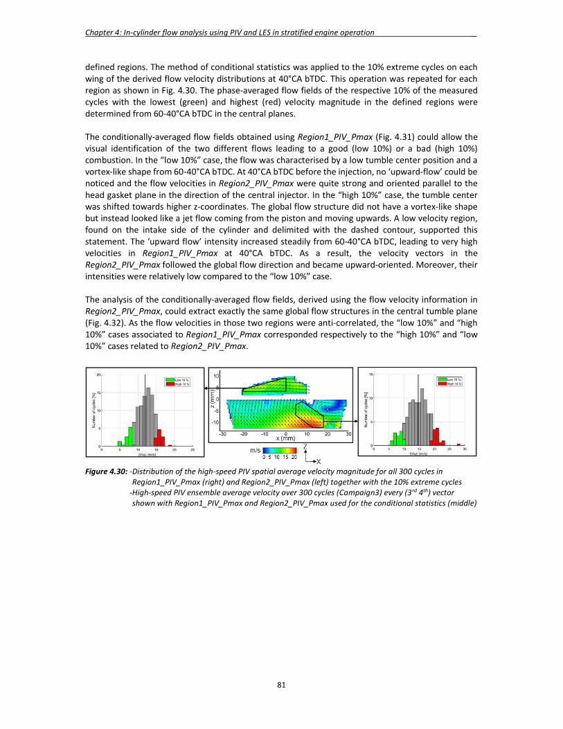
Chapter 4: In-cylinder flow analysis using PIV and LES in stratified engine operation _
81
defined regions. The method of conditional statistics was applied to the 10% extreme cycles on each wing of the derived flow velocity distributions at 40°CA bTDC. This operation was repeated for each region as shown in Fig. 4.30. The phase-averaged flow fields of the respective 10% of the measured cycles with the lowest (green) and highest (red) velocity magnitude in the defined regions were determined from 60-40°CA bTDC in the central planes. The conditionally-averaged flow fields obtained using Region1_PIV_Pmax (Fig. 4.31) could allow the visual identification of the two different flows leading to a good (low 10%) or a bad (high 10%) combustion. In the “low 10%” case, the flow was characterised by a low tumble center position and a vortex-like shape from 60-40°CA bTDC. At 40°CA bTDC before the injection, no ‘upward-flow’ could be noticed and the flow velocities in Region2_PIV_Pmax were quite strong and oriented parallel to the head gasket plane in the direction of the central injector. In the “high 10%” case, the tumble center was shifted towards higher z-coordinates. The global flow structure did not have a vortex-like shape but instead looked like a jet flow coming from the piston and moving upwards. A low velocity region, found on the intake side of the cylinder and delimited with the dashed contour, supported this statement. The ‘upward flow’ intensity increased steadily from 60-40°CA bTDC, leading to very high velocities in Region1_PIV_Pmax at 40°CA bTDC. As a result, the velocity vectors in the Region2_PIV_Pmax followed the global flow direction and became upward-oriented. Moreover, their intensities were relatively low compared to the “low 10%” case. The analysis of the conditionally-averaged flow fields, derived using the flow velocity information in Region2_PIV_Pmax, could extract exactly the same global flow structures in the central tumble plane (Fig. 4.32). As the flow velocities in those two regions were anti-correlated, the “low 10%” and “high 10%” cases associated to Region1_PIV_Pmax corresponded respectively to the “high 10%” and “low 10%” cases related to Region2_PIV_Pmax.
Figure 4.30: -Distribution of the high-speed PIV spatial average velocity magnitude for all 300 cycles in Region1_PIV_Pmax (right) and Region2_PIV_Pmax (left) together with the 10% extreme cycles -High-speed PIV ensemble average velocity over 300 cycles (Campaign3) every (3rd 4th) vector shown with Region1_PIV_Pmax and Region2_PIV_Pmax used for the conditional statistics (middle)

Chapter 4: In-cylinder flow analysis using PIV and LES in stratified engine operation _
82
Figure 4.31: Conditionally-averaged high-speed PIV flow field from 60-40° CA bTDC for the cycles with the 10% largest (top) and 10% smallest (bottom) velocity magnitude in Region1_PIV_Pmax. Every 4th vector is shown
Figure 4.32: Conditionally-averaged high-speed PIV flow field from 60-40° CA bTDC for the cycles with the 10% smallest (top) and 10% largest (bottom) velocity magnitude in Region2_PIV_Pmax. Every 4th vector is shown The combined analysis using a statistical correlation analysis and conditional statistics could allow the identification of two global flow structures in the central tumble plane having opposite effects on the combustion process. A vortex-like flow together with high horizontal-oriented flow velocities in Region2_PIV_Pmax led to an improved combustion, whereas an upward jet-flow structure combined with high flow velocities in Region1_PIV_Pmax caused the opposite effect. The explanation for their formations could only be derived based on the analysis of the three-dimensional flow field in LES. However, in order to extract the extreme cycles, conditional statistics had to be successfully applied to the computed LES engine cycles.

Chapter 4: In-cylinder flow analysis using PIV and LES in stratified engine operation _
83
4.5.2 Conditional statistics in LES The previous analysis was repeated using this time the LES results. For consistency reasons between high-speed PIV and LES, the same region definitions, defined in 4.5.1 (Region1_PIV_Pmax and Region2_PIV_Pmax), were used for the conditional statistics in LES. 35 consecutive LES engine cycles (Model2) were considered for this analysis. The local velocity magnitude (Vxz) was spatially averaged within both regions for every individual cycle at 40°CA bTDC. The histograms in Fig. 4.33 shows the respective distributions of the spatial average velocity for all 35 cycles. The ensemble-averaged velocity flow field over 35 cycles was also depicted in 4.29 together with Region1_PIV_Pmax and Region2_PIV_Pmax. The method of conditional statistics was applied to the 4 extreme cycles (12%) on each wing of the derived flow velocity distributions at 40°CA bTDC. The analysis was performed for each region as shown in Fig. 4.34-35. The phase-averaged flow fields, in the central tumble plane of the respective 12% of the computed LES cycles with lowest (green) and highest (red) velocity magnitude in the defined regions, were determined from 60-40°CA bTDC. The conditionally-averaged LES flow fields obtained using Region1_PIV_Pmax, as depicted in Fig. 4.34, could allow the reproduction of the same two different global flow structures, identified in high-speed PIV, which led to a good (12%low) or a bad (12%high) combustion process. The differences between those two flow structures were even clearer in LES. Indeed, in the “low 12%” case, the vortex-like flow with the high horizontal-oriented flow velocities in Region2_PIV_Pmax could be well captured. Furthermore, LES could provide an insight into the core region of this rotating flow, delimited with the dashed contour. In this region, the flow velocities were quite low, hence confirming the existence of a globally rotating flow in the cylinder. This area was masked in high-speed PIV due to the strong light reflexions observed in the gasket area.
Figure 4.33: -Distribution of the spatial average velocity magnitude for all 35 cycles in Region1_PIV_Pmax (right) and Region2_PIV_Pmax (left) together with the 12% extreme cycles. -LES ensemble average velocity over 35 cycles (Model2) together with Region1_PIV_Pmax and Region1_PIV_Pmax used for the conditional statistics (middle)
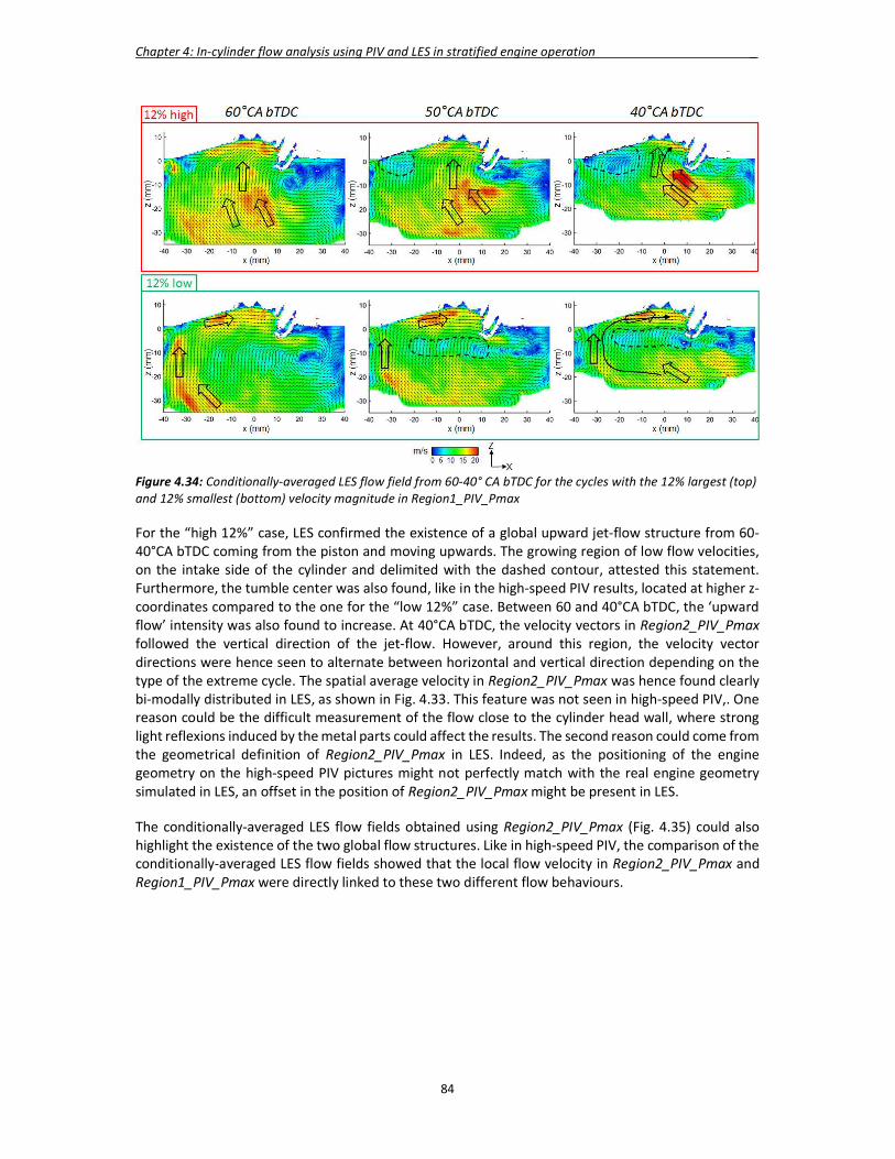
Chapter 4: In-cylinder flow analysis using PIV and LES in stratified engine operation _
84
Figure 4.34: Conditionally-averaged LES flow field from 60-40° CA bTDC for the cycles with the 12% largest (top) and 12% smallest (bottom) velocity magnitude in Region1_PIV_Pmax For the “high 12%” case, LES confirmed the existence of a global upward jet-flow structure from 60-40°CA bTDC coming from the piston and moving upwards. The growing region of low flow velocities, on the intake side of the cylinder and delimited with the dashed contour, attested this statement. Furthermore, the tumble center was also found, like in the high-speed PIV results, located at higher z-coordinates compared to the one for the “low 12%” case. Between 60 and 40°CA bTDC, the ‘upward flow’ intensity was also found to increase. At 40°CA bTDC, the velocity vectors in Region2_PIV_Pmax followed the vertical direction of the jet-flow. However, around this region, the velocity vector directions were hence seen to alternate between horizontal and vertical direction depending on the type of the extreme cycle. The spatial average velocity in Region2_PIV_Pmax was hence found clearly bi-modally distributed in LES, as shown in Fig. 4.33. This feature was not seen in high-speed PIV,. One reason could be the difficult measurement of the flow close to the cylinder head wall, where strong light reflexions induced by the metal parts could affect the results. The second reason could come from the geometrical definition of Region2_PIV_Pmax in LES. Indeed, as the positioning of the engine geometry on the high-speed PIV pictures might not perfectly match with the real engine geometry simulated in LES, an offset in the position of Region2_PIV_Pmax might be present in LES. The conditionally-averaged LES flow fields obtained using Region2_PIV_Pmax (Fig. 4.35) could also highlight the existence of the two global flow structures. Like in high-speed PIV, the comparison of the conditionally-averaged LES flow fields showed that the local flow velocity in Region2_PIV_Pmax and Region1_PIV_Pmax were directly linked to these two different flow behaviours.

Chapter 4: In-cylinder flow analysis using PIV and LES in stratified engine operation _
85
Figure 4.35: Conditionally-averaged LES flow field from 60-40° CA bTDC for the cycles with the 12% smallest (top) and 12% largest (bottom) velocity magnitude in Region2_PIV_Pmax Conditional statistics were successfully applied to the 35 consecutive LES engine cycles in the two flow regions Region1_PIV_Pmax and Region2_PIV_Pmax of the central tumble plane. The two global flow structures, identified in high-speed PIV and leading to opposite outcomes of the combustion process, could be well reproduced in LES. These results showed as well the ability of LES to capture the two local key flow parameters for the stratified engine operation, based on the region definitions coming from the correlation analysis between the high-speed PIV flow fields and the combustion data. 4.5.3 Validation of the high-speed PIV hypothesis using 2D planes The high-speed PIV hypothesis, presented in 4.2.2, stated that a momentum transfer, taking place from the intake valve planes towards the central tumble plane, was responsible for the formation of the ‘upward flow’ at 40°CA bTDC. To verify this statement, a further flow field analysis was carried out using additional two-dimensional planes. The investigation of the two-dimensional conditionally-averaged LES flow fields was extended to both intake valve planes defined at y = -18 mm and y = 18 mm. For the detection of a potential momentum transfer between the intake valve planes and the central tumble plane, two additional planes, called halfway planes, were defined between the aforementioned planes at y = -8 mm and y = 8 mm. The out-of-plane velocity component towards the central plane Vy_tcp was monitored on those two planes. The conditionally-averaged LES flow field, based on Region1_PIV_Pmax, was first analysed. Fig. 4.36 shows, for the “high” velocity case (12% high), the evolution of the in-plane flow velocity Vxz in the intake and central tumble planes and the out-of-plane velocity modulus |Vy_tcp| in the halfway planes from 60-40°CA bTDC. Higher flow rotation velocities could be noticed in the intake valve planes compared to the central tumble plane. Furthermore, the intensity of the flow velocity in the intake valve planes continuously decreased, while the intensity of the ‘upward flow’ simultaneously increased. The same flow characteristics as in the dual-plane high-speed PIV analysis (4.2.2) could be reproduced in LES for the cycles having strong ‘upward flow’ at 40°CA bTDC. To verify this hypothesis, the out-of-plane velocity modulus |Vy_tcp| was investigated in the halfway planes. Fig. 4.36 shows that |Vy_tcp| was already non-negligible at 60°CA bTDC. Like for the ‘upward flow’, |Vy_tcp| increased strongly up to 40°CA bTDC especially close to the cylinder and piston walls on the exhaust
Chapter 4: In-cylinder flow analysis using PIV and LES in stratified engine operation _
86
side. It proved the existence of a momentum transfer, which could be described as follows. Two three-dimensional flows, called ‘secondary flows’, moved circularly from both intake valve planes along the cylinder liner and in the direction of the central tumble plane. After colliding with each other in the central tumble plane, they were deflected towards the intake side hence creating the ‘upward flow’. The secondary-flow path starting from the intake valve plane at y = 18 mm was sketched in Fig. 4.36. Conversely, for the “low” velocity case (12% low), very similar flow rotation velocities were noticed in the intake valve planes and central tumble plane (Fig. 4.37). As a result, nearly no momentum transfer happened in that case. Compared to the “high” velocity case, extremely reduced values of |Vy_tcp| were observed in the halfway planes and could confirm this statement. The identical analysis was performed with the conditionally-averaged LES flow fields based on Region2_PIV_Pmax for the “high” velocity case (12% high) and the “low” velocity case (12% low), as shown in Fig. 4.38-4.39. The same secondary flow phenomenon could be derived from the “low” velocity case. The analysis of the conditionally-averaged LES flow field using several two-dimensional planes could provide some valuable insights into the three-dimensional flow phenomena taking place in the cylinder. For the extreme cycles leading to the formation of a strong ‘upward flow’, LES confirmed that a momentum transfer took place between the intake valve planes and the central tumble plane from 60-40°CA bTDC. The existence of two secondary flows was identified. The hypothesis, derived from the high-speed PIV analysis, could be hence validated with LES. A further validation of this hypothesis was performed using the three-dimensional information of the in-cylinder flow field provided by LES as described in the next part.
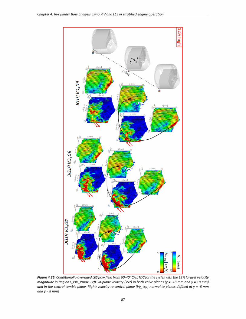
Chapter 4: In-cylinder flow analysis using PIV and LES in stratified engine operation _
87
Figure 4.36: Conditionally-averaged LES flow field from 60-40° CA bTDC for the cycles with the 12% largest velocity magnitude in Region1_PIV_Pmax. Left: in-plane velocity (Vxz) in both valve planes (y = -18 mm and y = 18 mm) and in the central tumble plane. Right: velocity to central plane (Vy_tcp) normal to planes defined at y = -8 mm and y = 8 mm)

Chapter 4: In-cylinder flow analysis using PIV and LES in stratified engine operation _
88
Figure 4.37: Conditionally-averaged LES flow field from 60-40° CA bTDC for the cycles with the 12% smallest velocity magnitude in Region1_PIV_Pmax. Left: in-plane velocity (Vxz) in both valve planes (y = -18 mm and y = 18 mm) and in the central tumble plane. Right: velocity to central plane (Vy_tcp) normal to planes defined at y = -8 mm and y = 8 mm)
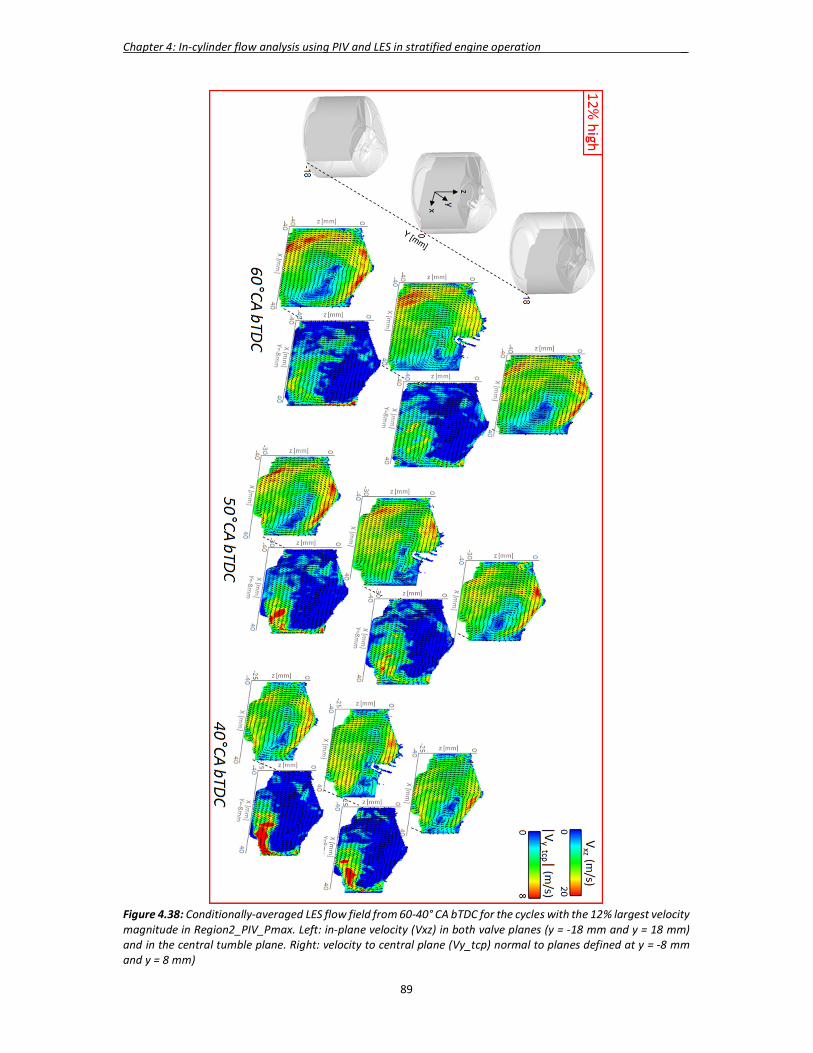
Chapter 4: In-cylinder flow analysis using PIV and LES in stratified engine operation _
89
Figure 4.38: Conditionally-averaged LES flow field from 60-40° CA bTDC for the cycles with the 12% largest velocity magnitude in Region2_PIV_Pmax. Left: in-plane velocity (Vxz) in both valve planes (y = -18 mm and y = 18 mm) and in the central tumble plane. Right: velocity to central plane (Vy_tcp) normal to planes defined at y = -8 mm and y = 8 mm)
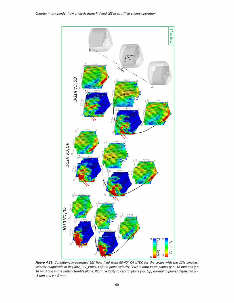
Chapter 4: In-cylinder flow analysis using PIV and LES in stratified engine operation _
90
Figure 4.39: Conditionally-averaged LES flow field from 60-40° CA bTDC for the cycles with the 12% smallest velocity magnitude in Region2_PIV_Pmax. Left: in-plane velocity (Vxz) in both valve planes (y = -18 mm and y = 18 mm) and in the central tumble plane. Right: velocity to central plane (Vy_tcp) normal to planes defined at y = -8 mm and y = 8 mm)

Chapter 4: In-cylinder flow analysis using PIV and LES in stratified engine operation _
91
4.5.4 Validation of the high-speed PIV hypothesis using 3D-flow analysis The secondary flow motion implied a three-dimensional flow movement in the computational domain. It featured, in the region defined by x > 0, a strong out-of-plane velocity magnitude with respect to the central tumble plane. It was proposed to characterise the flow field in this domain using a three-dimensional flow analysis. Usually, the global in-cylinder flow could be decomposed into three distinct flow rotational motions, as depicted in Fig. 4.40:
- the tumble motion around the y-axis named 𝑇 - the cross-tumble motion around the x-axis named 𝑇 - the swirl motion around the z-axis named 𝑆
The intensity of those flow motions are generally defined by dimensionless numbers, which are the tumble number, the cross-tumble number and the swirl number. In the present case, as the secondary flow motion entails mainly out-of-plane velocities, only cross-tumble and swirl motions were considered in the domain defined by x > 0 and marked by the red dashed lines. However, due to the symmetrical engine geometry, the global swirl and cross-tumble motions of the mean in-cylinder flow field are null. Indeed, the in-cylinder flow features a clockwise and an anti-clockwise swirl motions in the domains defined respectively by y > 0 and y < 0, i.e. Domain1 and Domain2 in Fig. 4.40. Those two swirl motions cancel out if the global symmetric mean flow is considered. The same argumentation can be used for the cross-tumble motion. The cross-tumble and the swirl numbers were hence computed separately in Domain1 and Domain2. Their formula read:
𝑇 , = 𝑇 , =∑ [( ) ( ) ]
,
∑ [( ) ( )²] ,
(4.8)
𝑆 , = 𝑆 , =∑ [( ) ( ) ]
,
∑ [( ) ( )²] ,
(4.9)
where: - 𝑁 is the total number of cells in the computational domain - 𝑁 is the engine rotation speed - 𝑋 , 𝑌 , 𝑍 are the coordinates of a defined reference point
Figure 4.40: Definition of the in-cylinder flow rotational motions:
Tumble (𝑇 ), cross-tumble (𝑇 ) and swirl (𝑆 )
For the swirl and cross-tumble number calculations their reference points were taken in the intake valve planes (𝑋 = 0 mm; 𝑌 = -18 mm and 𝑋 = 0 mm; 𝑌 = 18 mm) and at midway between the
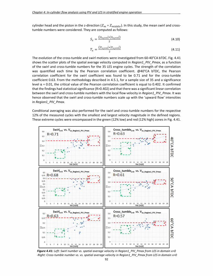
Chapter 4: In-cylinder flow analysis using PIV and LES in stratified engine operation _
92
cylinder head and the piston in the z-direction (𝑍 = 𝑍 ). In this study, the mean swirl and cross-tumble numbers were considered. They are computed as follows:
𝑆 = , , (4.10)
𝑇 = , , (4.11)
The evolution of the cross-tumble and swirl motions were investigated from 60-40°CA bTDC. Fig. 4.41 shows the scatter plots of the spatial average velocity computed in Region1_PIV_Pmax, as a function of the swirl and cross-tumble numbers for the 35 LES engine cycles. The strength of the correlation was quantified each time by the Pearson correlation coefficient. @40°CA bTDC, the Pearson correlation coefficient for the swirl coefficient was found to be 0.71 and for the cross-tumble coefficient 0.63. From the methodology described in 4.5.1, for a sample size of 35 and a significance level α = 0.01, the critical value of the Pearson correlation coefficient is equal to 0.402. It confirmed that the findings had statistical significance (R>0.402) and that there was a significant linear correlation between the swirl and cross-tumble numbers with the local flow velocity in Region1_PIV_Pmax. It was hence observed that the swirl and cross-tumble numbers scale up with the ‘upward flow’ intensities in Region1_PIV_Pmax. Conditional averaging was also performed for the swirl and cross-tumble numbers for the respective 12% of the measured cycles with the smallest and largest velocity magnitude in the defined regions. These extreme cycles were encompassed in the green (12% low) and red (12% high) zones in Fig. 4.41.
Figure 4.41: Left: Swirl number vs. spatial average velocity in Region1_PIV_Pmax from LES in domain x>0
-Right: Cross-tumble number vs. vs. spatial average velocity in Region1_PIV_Pmax from LES in domain x>0
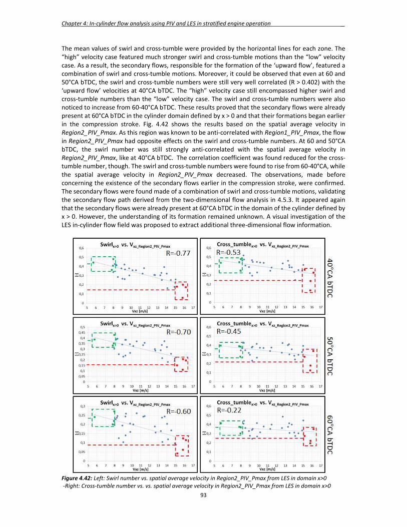
Chapter 4: In-cylinder flow analysis using PIV and LES in stratified engine operation _
93
The mean values of swirl and cross-tumble were provided by the horizontal lines for each zone. The “high” velocity case featured much stronger swirl and cross-tumble motions than the “low” velocity case. As a result, the secondary flows, responsible for the formation of the ‘upward flow’, featured a combination of swirl and cross-tumble motions. Moreover, it could be observed that even at 60 and 50°CA bTDC, the swirl and cross-tumble numbers were still very well correlated (R > 0.402) with the ‘upward flow’ velocities at 40°CA bTDC. The “high” velocity case still encompassed higher swirl and cross-tumble numbers than the “low” velocity case. The swirl and cross-tumble numbers were also noticed to increase from 60-40°CA bTDC. These results proved that the secondary flows were already present at 60°CA bTDC in the cylinder domain defined by x > 0 and that their formations began earlier in the compression stroke. Fig. 4.42 shows the results based on the spatial average velocity in Region2_PIV_Pmax. As this region was known to be anti-correlated with Region1_PIV_Pmax, the flow in Region2_PIV_Pmax had opposite effects on the swirl and cross-tumble numbers. At 60 and 50°CA bTDC, the swirl number was still strongly anti-correlated with the spatial average velocity in Region2_PIV_Pmax, like at 40°CA bTDC. The correlation coefficient was found reduced for the cross-tumble number, though. The swirl and cross-tumble numbers were found to rise from 60-40°CA, while the spatial average velocity in Region2_PIV_Pmax decreased. The observations, made before concerning the existence of the secondary flows earlier in the compression stroke, were confirmed. The secondary flows were found made of a combination of swirl and cross-tumble motions, validating the secondary flow path derived from the two-dimensional flow analysis in 4.5.3. It appeared again that the secondary flows were already present at 60°CA bTDC in the domain of the cylinder defined by x > 0. However, the understanding of its formation remained unknown. A visual investigation of the LES in-cylinder flow field was proposed to extract additional three-dimensional flow information.
Figure 4.42: Left: Swirl number vs. spatial average velocity in Region2_PIV_Pmax from LES in domain x>0 -Right: Cross-tumble number vs. vs. spatial average velocity in Region2_PIV_Pmax from LES in domain x>0

Chapter 4: In-cylinder flow analysis using PIV and LES in stratified engine operation _
94
4.5.5 Visual analysis of the 3D-flow field The three-dimensional conditionally-averaged LES flow fields, based on the extreme spatial average velocities in Region1_PIV_Pmax, were considered. The investigation of the flow velocity magnitude evolution was undertaken for both “high” (12% high) and “low” (12% low) velocity cases. The commercial software Ensight was used for the visual analysis. An isosurface of the in-cylinder flow velocity magnitude, defined for Vmag = 14 m/s, was computed and coloured by the velocity component in z-direction Vz. For clarity reasons, as the rendering of a three-dimensional flow surface was not easy to achieve in a two-dimensional picture, only the isosurface in the cylinder region defined by y > 0 was shown. The analysis was performed from 60-40°CA bTDC as displayed in Fig. 4.43. For the “high” velocity case, a three-dimensional jet flow, moving from the piston towards the cylinder head of the combustion chamber, appeared in the middle of the cylinder between 60-40°CA bTDC. This flow structure was already identified using the two-dimensional flow analysis in high-speed PIV and LES. The visual observation in Fig. 4.43 confirmed that the jet flow structure was the dominant flow structure in the cylinder, judging by its isosurface size and its vertical velocity intensity. Furthermore, it also made no doubt that this flow structure was already well developed at 60°CA BTDC and that its onset would take place earlier in time, either in the intake or in the compression stroke. The second flow structure, which could be recognized in the cylinder and located around the jet flow structure, was the global rotating tumble vortex. For the “low” velocity case, no such jet flow structure was created. One could only observed the outer periphery of the global rotating tumble vortex. From 60-40°CA bTDC its intensity decreased, due to the ongoing tumble break-down process. However, its rotational characteristics were conserved, as already pointed out from the PIV and LES results in the central tumble plane (Fig. 4.31 and Fig. 4.34).
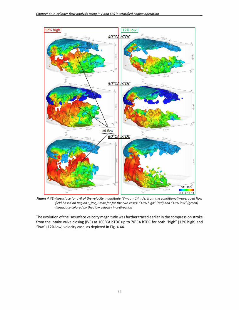
Chapter 4: In-cylinder flow analysis using PIV and LES in stratified engine operation _
95
Figure 4.43:-Isosurface for y>0 of the velocity magnitude (Vmag = 14 m/s) from the conditionally-averaged flow field based on Region1_PIV_Pmax for for the two cases: “12% high” (red) and “12% low” (green) -Isosurface colored by the flow velocity in z-direction The evolution of the isosurface velocity magnitude was further traced earlier in the compression stroke from the intake valve closing (IVC) at 160°CA bTDC up to 70°CA bTDC for both “high” (12% high) and “low” (12% low) velocity case, as depicted in Fig. 4.44.

Chapter 4: In-cylinder flow analysis using PIV and LES in stratified engine operation _
96
Figure 4.44: -Isosurface for y>0 of the velocity magnitude (Vmag = 14 m/s) from the conditionally-averaged flow field based on Region1_PIV_Pmax for for the two cases: “12% high” (red) and “12% low” (green) -Isosurface colored by the flow velocity in z-direction
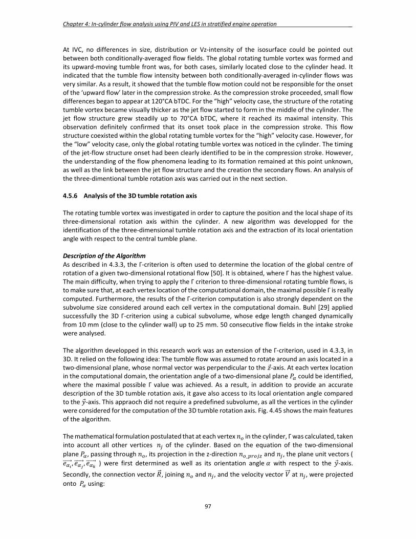
Chapter 4: In-cylinder flow analysis using PIV and LES in stratified engine operation _
97
At IVC, no differences in size, distribution or Vz-intensity of the isosurface could be pointed out between both conditionally-averaged flow fields. The global rotating tumble vortex was formed and its upward-moving tumble front was, for both cases, similarly located close to the cylinder head. It indicated that the tumble flow intensity between both conditionally-averaged in-cylinder flows was very similar. As a result, it showed that the tumble flow motion could not be responsible for the onset of the ‘upward flow’ later in the compression stroke. As the compression stroke proceeded, small flow differences began to appear at 120°CA bTDC. For the “high” velocity case, the structure of the rotating tumble vortex became visually thicker as the jet flow started to form in the middle of the cylinder. The jet flow structure grew steadily up to 70°CA bTDC, where it reached its maximal intensity. This observation definitely confirmed that its onset took place in the compression stroke. This flow structure coexisted within the global rotating tumble vortex for the “high” velocity case. However, for the “low” velocity case, only the global rotating tumble vortex was noticed in the cylinder. The timing of the jet-flow structure onset had been clearly identified to be in the compression stroke. However, the understanding of the flow phenomena leading to its formation remained at this point unknown, as well as the link between the jet flow structure and the creation the secondary flows. An analysis of the three-dimentional tumble rotation axis was carried out in the next section. 4.5.6 Analysis of the 3D tumble rotation axis The rotating tumble vortex was investigated in order to capture the position and the local shape of its three-dimensional rotation axis within the cylinder. A new algorithm was developped for the identification of the three-dimensional tumble rotation axis and the extraction of its local orientation angle with respect to the central tumble plane. Description of the Algorithm As described in 4.3.3, the Γ-criterion is often used to determine the location of the global centre of rotation of a given two-dimensional rotational flow [50]. It is obtained, where Γ has the highest value. The main difficulty, when trying to apply the Γ criterion to three-dimensional rotating tumble flows, is to make sure that, at each vertex location of the computational domain, the maximal possible Γ is really computed. Furthermore, the results of the Γ-criterion computation is also strongly dependent on the subvolume size considered around each cell vertex in the computational domain. Buhl [29] applied successfully the 3D Γ-criterion using a cubical subvolume, whose edge length changed dynamically from 10 mm (close to the cylinder wall) up to 25 mm. 50 consecutive flow fields in the intake stroke were analysed. The algorithm developped in this research work was an extension of the Γ-criterion, used in 4.3.3, in 3D. It relied on the following idea: The tumble flow was assumed to rotate around an axis located in a two-dimensional plane, whose normal vector was perpendicular to the 𝑧-axis. At each vertex location in the computational domain, the orientation angle of a two-dimensional plane 𝑃 could be identified, where the maximal possible Γ value was achieved. As a result, in addition to provide an accurate description of the 3D tumble rotation axis, it gave also access to its local orientation angle compared to the ��-axis. This appraoch did not require a predefined subvolume, as all the vertices in the cylinder were considered for the computation of the 3D tumble rotation axis. Fig. 4.45 shows the main features of the algorithm. The mathematical formulation postulated that at each vertex 𝑛 in the cylinder, Γ was calculated, taken into account all other vertices 𝑛 of the cylinder. Based on the equation of the two-dimensional plane 𝑃 , passing through 𝑛 , its projection in the z-direction 𝑛 _ and 𝑛 , the plane unit vectors ( 𝑒 , 𝑒 , 𝑒 ) were first determined as well as its orientation angle 𝛼 with respect to the ��-axis.
Secondly, the connection vector ��, joining 𝑛 and 𝑛 , and the velocity vector 𝑉 at 𝑛 , were projected onto 𝑃 using:
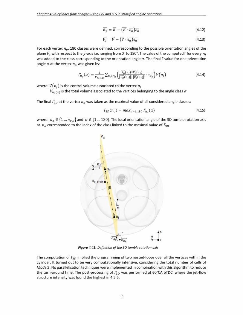
Chapter 4: In-cylinder flow analysis using PIV and LES in stratified engine operation _
98
𝑅 = 𝑅 − 𝑅 ∙ 𝑒 𝑒 (4.12)
𝑉 = 𝑉 − 𝑉 ∙ 𝑒 𝑒 (4.13)
For each vertex 𝑛 , 180 classes were defined, corresponding to the possible orientation angles of the plane 𝑃 with respect to the ��-axis i.e. ranging from 0° to 180°. The value of the computed Γ for every 𝑛 was added to the class corresponding to the orientation angle 𝛼. The final Γ value for one orientation angle 𝛼 at the vertex 𝑛 was given by:
𝛤 (𝛼) =( )
∑ ×
∙ ∙ 𝑒 𝑉 𝑛
∈ (4.14)
where: 𝑉 𝑛 is the control volume associated to the vertex 𝑛 𝑉 ( ) is the total volume associated to the vertices belonging to the angle class 𝛼
The final 𝛤 at the vertex 𝑛 was taken as the maximal value of all considered angle classes:
𝛤 (𝑛 ) = 𝑚𝑎𝑥 , 𝛤 (𝛼) (4.15)
where: 𝑛 ∈ 1 … 𝑛 and 𝛼 ∈ {1 … 180}. The local orientation angle of the 3D tumble rotation axis at 𝑛 corresponded to the index of the class linked to the maximal value of 𝛤 .
Figure 4.45: Definition of the 3D tumble rotation axis The computation of 𝛤 implied the programming of two nested-loops over all the vertices within the cylinder. It turned out to be very computationally intensive, considering the total number of cells of Model2. No parallelisation techniques were implemented in combination with this algorithm to reduce the turn-around time. The post-processing of 𝛤 was performed at 60°CA bTDC, where the jet-flow structure intensity was found the highest in 4.5.5.
Chapter 4: In-cylinder flow analysis using PIV and LES in stratified engine operation _
99
Results The analysis of the rotating tumble vortex was considered using the three-dimensional conditionally-averaged LES flow fields, based on Region1_PIV_Pmax. 𝛤 was computed for both “high” (12% high) and “low” (12% low) velocity cases. The visual representation of the 𝛤 field was performed using an isosurface defined for 𝛤 = 0.75 and coloured by the orientation angle 𝛼 of the local tumble plane compared to the ��-axis. Fig. 4.46 shows a comparison of the 𝛤 -isosurfaces for both velocity cases. The crank-angle position was taken at 60°CA bTDC for the reasons explained earlier. For the “low” velocity case, the shape of the three-dimensional rotation axis of the flow looked like a ‘sausage’. Its diameter was kept nearly constant over an long distance in the cylinder, indicating a smooth repartition of the momentum of the flow along it. The isosurface colors revealed that the orientation of the tumble plane 𝛼 was approximately parallel to the central tumble plane (i.e. 𝛼 ≈ 90° compared to the ��-axis) within a large domain of the cylinder. This region is marked by the two black lines in the range [-20 mm < y < 20 mm]. The intake valve planes, located at y = -18 mm and y = 18 mm, were encompassed in this domain. The orientation of the tumble plane was bent towards the ��-axis in the region close to the wall. It could be hence stated that, for the “low” velocity case, the part of the rotating tumble vortex, oriented parallel to the central tumble plane, was dominant in the cylinder and covered ~50% of the cylinder volume. For the “high” velocity case, the shape of the three-dimensional rotation axis of the flow looked like a ‘croissant’. First, the middle part of the three-dimensional rotation axis had a bigger diameter compared to the one of the “low” velocity case. Secondly, a sudden isosurface diameter reduction took place at a distance estimated to be ~1/3 cylinder radius from the wall. It hence indicated a less homogeneous distribution of the flow momentum in the cylinder compared to the “low” velocity case. The color repartition on the isosurface showed that the orientation angle 𝛼 of the tumble plane was nearly parallel to the central tumble plane within a much reduced domain [-10 mm < y < 10 mm] compared to the “low” velocity case. It indicated that in the remaining cylinder volume, whose cylinder radius was comprised in the ranges [-41.5 mm < y < -10 mm] and [10 mm < y < 41.5 mm], the orientation of the tumble planes were tilted towards the ��-axis. A rotation angle of the order of 60° could be noticed in the ranges [-25 mm < y < -15 mm] and [25 mm < y < 15 mm], which encompassed the intake valve planes. This indicated that the part of the tumble vortex flow, travelling upwards from the piston in the direction of the cylinder head, did not move along the cylinder wall like in the central tumble plane for 𝛼 = 90° anymore. Instead, due to the tilted tumble plane angle, the upward flow movement of the tumble vortex flow took place in the center of cylinder, hence giving rise to the upward jet-flow structure. In order to illustrate these statements, Fig, 4.47 shows the velocity streamlines of the flow for both velocity cases at 60°CA bTDC. The seeding of the streamlines was achieved using 40 seeding locations on a plane located on the intake side of the cylinder. For the “low” velocity case the direction of the streamlines was mostly aligned with the central tumble plane (𝛼 ≈ 90° compared to the ��-axis as described earlier), whereas for the “high” velocity case their directions were oblique with respect to the central tumble plane and pointing towards the intake valve plane. First, it confirmed the findings made above concerning the local tilting of the tumble plane along the three-dimensional rotation axis; secondly it explained why the velocities were found higher in both intake planes in comparison to the central tumble plane. For the “high” velocity case, as the rotating tumble vortex was bent, the rotating flows in the domain y < 0 and y > 0 interacted with each other in the middle of the cylinder. It was the root cause for the upward jet-flow structure formation. Furthermore, the interaction of the in-cylinder flow, rotating around the bent tumble rotation axis, with the wall on the exhaust side generated the secondary flows. They moved from both sides (y < 0 and y > 0) downwards along the cylinder liner and were later deflected by the piston in the upwards z-direction. As a result, the secondary flows created the ‘upward flow’ found under the spark-plug. The flow interaction with the walls occurred closed to the y-coordinates of the intake valve planes (y = -18 mm and y = 18 mm) and confirmed the

Chapter 4: In-cylinder flow analysis using PIV and LES in stratified engine operation _
100
observations made above in 4.2.2 and 4.5.3 that a momentum transfer took place between the intake valve planes and the central tumble plane.
Figure 4.46: -Isosurface of 𝛤 (𝛤 = 0.75) from the conditionally-averaged flow field based on Region1_PIV_Pmax for the two cases: “12% high”(red) and “12% low”(green) at 60°CA bTDC -Isosurface colored by the orientation angle 𝛼
Figure 4.47: -Velocity streamlines from the conditionally-averaged flow field based on Region1_PIV_Pmax for the two cases: “12% high”(red) and “12% low”(green) at 60°CA bTDC -Streamlines colored by their z-coordinates
In this reasearch project, the formation of the ‘upward flow’ had been fully understood using different post-processing methods. The extreme LES cycles, where strong and low ‘upward flows’ were observed, could be extracted using conditional statistics. The two and three-dimensional analysis of the conditionally-averaged flow fields proved that first an upward jet-flow structure was formed in the middle of the cylinder during the compression stroke. Secondly, the secondary flows coming from the momentum transfer between the intake and central tumble planes generated the ‘upward flow’ below

Chapter 4: In-cylinder flow analysis using PIV and LES in stratified engine operation _
101
the spark-plug before the injection. The rotating tumble vortex was not found perpendicular to the central tumble plane and its bending structure was responsible for the creation of the upward jet-flow structure detected in the middle of the cylinder. Furthermore, the interaction of the bent rotating tumble flow with the cylinder walls produced the secondary flows, which in turn created the ‘upward flow’ confirmed the momentum transfer existence between the intake valve and central tumble planes. After a successful validation using the high-speed PIV measurement results, LES could later confirmed the PIV-hypothesis, derived from the high-speed PIV analysis, by providing valuable three-dimensional flow information. However, the analysis of the cyclic velocity variations in Region1_PIV_Pmax at 60 and 50°CA bTDC (4.4.5) showed that the two-sample Kolmogorov-Smirnov test failed and that discrepancies existed between LES and high-speed PIV. The reason found was the slightly underestimated flow velocities computed in LES. In order to try to improve the accuracy of the flow computation in LES, another multi-cycle LES was performed using a higher-order convective numerical scheme. 4.6 Higher-order LES: 2nd vs. 3rd-order convective schemes The 3rd-order accurate in time and space convective scheme TTGC, specially developed for the explicit LES solver AVBP, was selected for this study. The results were analysed using the same two-dimensional flow analysis as the ones presented in 4.4.4 for the mean flow field validation and in 4.4.5 for the cyclic velocity fluctuations. A direct comparison was made to the results obtained with the 2nd-order accurate in time and space convective scheme Lax-Wendroff and the high-speed PIV (Campaign3) in the central tumble plane. 4.6.1 CFD model and numerical setup The 3rd-order in time and space convective scheme TTGC was used in combination with the current CFD model (Model2) and its existing numerical setup. As mentioned in chapter 2, the computational time using TTGC is x2.5 higher than with Lax-Wendroff. In order to remove the influence of changed boundary conditions, the starting flow field information was taken from the previous computation with Lax-Wendroff before intake valve opening. Only the intake and compression strokes were re-computed with TTGC. To ensure enough flow information for the validation of the cyclic variability of the flow, 23 consecutive LES cycles were simulated and the instantaneous flow field was saved every 2°CA. A CFL_ac value of 0.7 was used to control the time step in the simulation, as required with TTGC [109]. Moreover, the same 2nd-order and 4th-order artificial viscosity coefficients could be kept constant (smu2 = 5.10-2 and smu4 = 8.10-3) throughout the simulation, confirming the very high grid quality and the adequate definition of the mesh refinement zones of Model2. 4.6.2 Comparison of the mean flow field in the central tumble plane In order to assess the mean flow field results obtained with TTGC, a comparison was performed with the results obtained from the simulation using Lax-Wendroff and high-speed PIV (Campaign3). For a fair comparison between the 3rd and 2nd-order convective schemes, the same 23 LES cycles were taken and ensemble averaged. The mean flow field results were depicted in Fig. 4.48 from 60-40°CA bTDC. Region1_PIV, presented in 4.4.4, was used to monitor the ‘upward flow’. Furthermore, the regions of poor resolution or having strong light reflections were kept masked explaining the missing flow information in the high-speed PIV pictures in the regions close to the cylinder wall. With the 3rd-order convective scheme, the velocity in Region1_PIV increased progressively from 60-40°CA bTDC, like observed in high-speed PIV and with the 2nd-order convective scheme. However, the flow velocities in that region were found definitely closer to the ones observed in high-speed PIV. At

Chapter 4: In-cylinder flow analysis using PIV and LES in stratified engine operation _
102
40°CA bTDC considerable improvements could be noticed compared to the 2nd-order convective scheme. The 3rd-order scheme could also provide a better insight into the core of the tumble rotating flow, delimited by the dashed contour at 40°CA bTDC. This low flow velocity region was found better resolved. It could not be directly compared with high-speed PIV, due to the light reflexion observed in the gasket area, but the high-speed PIV results of Campaign2, depicted in Fig. 4.48, proved the existence of this core region. The position of the tumble centre was also computed and marked with the dashed lines and the white circle. The evolution of the tumble centre path of the 3rd-order convective scheme agreed better with the measurements compared to the 2nd-order convective scheme especially in the x-direction. At 40°CA bTDC, a difference of 2 mm was noticed between the two convective schemes. As mentioned earlier, the location and orientation of the tumble rotation axis influenced the creation of the jet flow and the ‘upward flow’. Therefore, the better reproduction of the high upward flow velocities with the 3rd-order convective scheme was due to a more accurate capturing of the rotating tumble vortex. Furthermore, the flow velocities in the region below the injector and their decreasing trend were all well captured with the 3rd-order convective scheme from 60-40°CA bTDC. However, the velocity magnitudes appeared slightly lower compared to the measurements and to the ones obtained with the 2nd-order convective scheme.
Figure 4.48: Ensemble average in-plane velocity (Vxz) in the central tumble plane @60-40°CA bTDC
-Left: LES results averaged over 23 cycles using the 2nd-order convective scheme Lax-Wendroff -Middle: LES results averaged over 23 cycles using the 3rd-order convective scheme TTGC -Right: High-speed PIV results averaged over 300cycles (Campaign3)
From the mean flow field comparison in the central tumble plane, it could be stated that the main improvement brought by the 3rd-order convective scheme was the better capturing of the rotating tumble vortex and the resulting ‘upward flow’ at 40°CA bTDC. The comparison of the cyclic velocity variation in Region1_PIV was also addressed and the results are detailed hereafter.

Chapter 4: In-cylinder flow analysis using PIV and LES in stratified engine operation _
103
4.6.3 Comparison of the cyclic velocity fluctuations in the central tumble plane The spatial average velocity was calculated in Region1_PIV for each engine cycle. A comparison of the spatial average velocity-magnitude distributions between LES, using the 2nd-order and 3rd-order convective schemes, and high-speed PIV (Campaign3) was performed at 60, 50 and 40°CA bTDC. The velocity distributions entailed 23 engine cycles for LES and 300 engine cycles for high-speed PIV, as shown in Fig. 4.49.
Figure 4.49: Spatial average velocity distribution in Region1_PIV located in the central tumble plane -Top: comparisons between LES (2nd-order convective scheme) and high-speed PIV (Campaign3) -Bottom: comparisons between LES (3rd-order convective scheme) and high-speed PIV (Campaign3) (LES: 23cycles, high-speed PIV: 300 cycles) With the 3rd-order convective scheme TTGC, the mean velocity matched better with the experimental values and the trend of increasing mean velocity from 60-40°CA bTDC was also well reproduced. Noticeable improvements in flow velocity predictions could be underlined, in comparison with the results obtained using the 2rd-order convective scheme Lax-Wendroff. The mean velocity and the velocity standard deviation in Region1_PIV were further analysed at 60, 50 and 40°CA bTDC. 13 independent samples of 23 consecutive high-speed PIV engine cycles were compared to the 23 LES engine cycles, computed with the 2nd and 3rd-order convective schemes (Fig. 4.50). Like explained in 4.4.5, the standard deviation of the velocity increased from 60 to 40°CA bTDC due to the tumble break-down process. This trend was relatively well captured in LES using the 2nd-order convective scheme with a sample size of 35 engine cycles (4.4.5), although its velocity standard deviation and mean velocity laid behind most of the high-speed PIV samples. The same conclusion could be drawn with a reduced sample size of 23 engine cycles. However, the 3rd-order convective scheme improved significantly the simulation results. Apart from computing a higher mean velocity, it provided a more accurate prediction of the standard deviation of the ‘upward flow’ in Region1_PIV. Indeed, the standard-deviation values coming from the 3rd-order convective scheme were within the middle-range values of the 13 high-speed PIV samples. Important improvements were observed especially at 60 and 50 °CA bTDC, where the velocity distributions failed to pass the two-sample Kolmogorov-Smirnov test with the 2nd-order convective scheme (4.4.5).

Chapter 4: In-cylinder flow analysis using PIV and LES in stratified engine operation _
104
Figure 4.50: Mean velocity and standard deviation comparisons between LES (2nd and 3rd-order convective schemes) and high-speed PIV (Campaign3) in Region1_PIV located in the central tumble plane Two-sample Kolmogorov-Smirnov test The two-sample Kolmogorov-Smirnov test was used to check whether the two independent LES and high-speed PIV samples taken in Region1_PIV could come from the same distribution. The LES cumulative distribution functions had a sample size n = 23 and the one from high-speed PIV a sample size m = 300. As null hypothesis, it was assumed that both samples originate from the same distribution. In the present case, for a significance value α = 0.05, the null hypothesis was rejected if the test quantity 𝐷 (4.2) exceeded the critical value D . = 0.243. The test quantity were computed at 60, 50 and 40°CA bTDC and the results obtained were summarised in Table 4.7. Moreover, Fig. 4.51 shows the cumulative spatial average velocity distributions in Region1_PIV coming from LES, with the 2nd and 3rd-order convective schemes, and from high-speed PIV. The computed test quantities 𝐷 are also depicted in Fig. 4.51.
Table 4.7: Test quantity 𝐷 of the two-sample Kolmogorov-Smirnov test using the 2nd and 3rd-order convective schemes compared to high-speed PIV
LES: 2nd-order LES: 3rd-order 60°CA bTDC 0.39 0.08 50°CA bTDC 0.29 0.15 40°CA bTDC 0.22 0.20
In the case of the 2nd-order convective scheme, the null hypothesis was only accepted at 40°CA bTDC confirming the results made with a LES sample size of 35 engine cycles. However, significant improvements were noticed with the 3rd-order convective scheme, whose null hypothesis was always accepted. Therefore, from a statistical point of view, the spatial average velocity-magnitude distribution from LES, with the 3rd-order convective scheme, was not significantly different to the one from high-speed PIV in Region1_PIV between 60-40°CA bTDC. As a result, their cumulative velocity distributions fitted very well especially in the range 60-50°CA bTDC compared to the 2nd-order convective scheme. Nevertheless, the characteristics of the ‘upward flow’ at 40°CA bTDC remained the most important feature to capture in stratified engine operation. From the results presented, the computed cyclic velocity fluctuations in LES agreed well with the high-speed PIV ones at that crucial crank-angle position and location in the cylinder. Therefore, both convective schemes were able to provide the correct spatial average velocity-magnitude distribution in Region1_PIV before the injection.
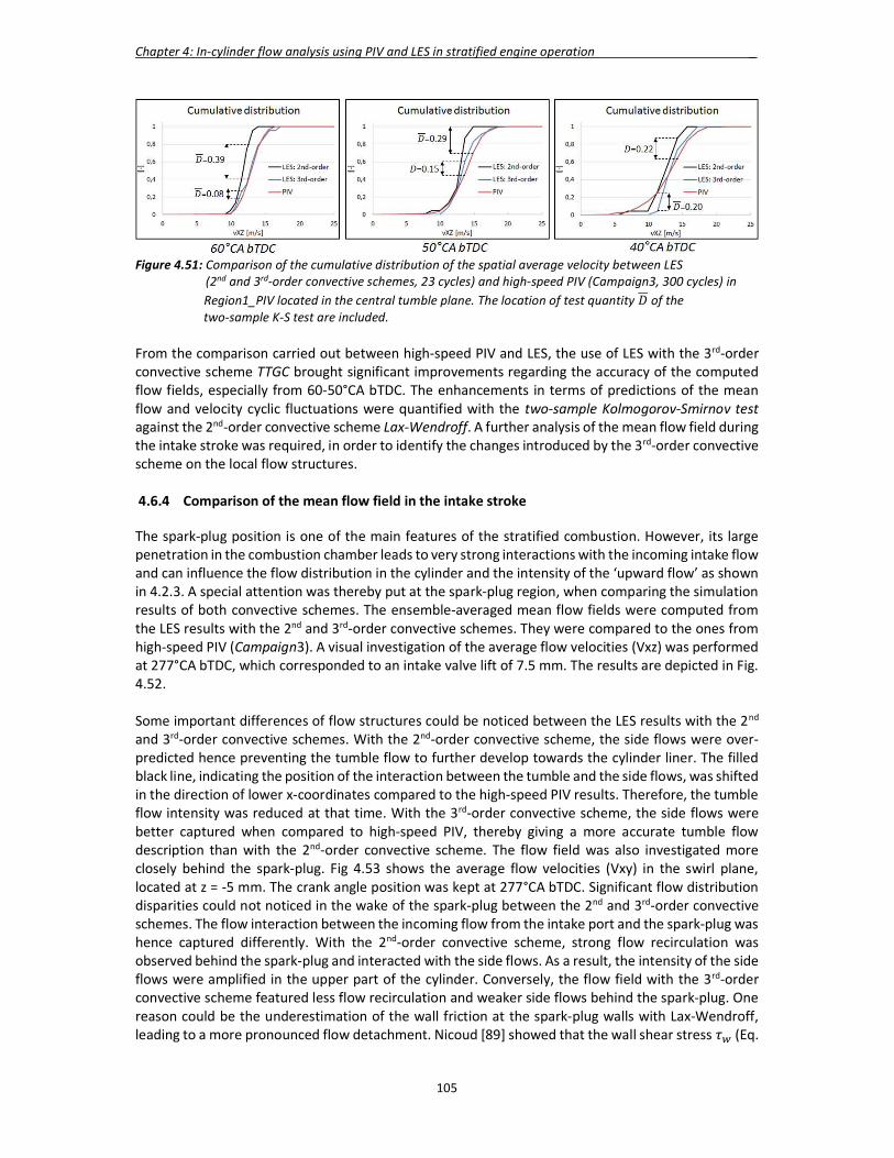
Chapter 4: In-cylinder flow analysis using PIV and LES in stratified engine operation _
105
Figure 4.51: Comparison of the cumulative distribution of the spatial average velocity between LES (2nd and 3rd-order convective schemes, 23 cycles) and high-speed PIV (Campaign3, 300 cycles) in Region1_PIV located in the central tumble plane. The location of test quantity 𝐷 of the two-sample K-S test are included. From the comparison carried out between high-speed PIV and LES, the use of LES with the 3rd-order convective scheme TTGC brought significant improvements regarding the accuracy of the computed flow fields, especially from 60-50°CA bTDC. The enhancements in terms of predictions of the mean flow and velocity cyclic fluctuations were quantified with the two-sample Kolmogorov-Smirnov test against the 2nd-order convective scheme Lax-Wendroff. A further analysis of the mean flow field during the intake stroke was required, in order to identify the changes introduced by the 3rd-order convective scheme on the local flow structures. 4.6.4 Comparison of the mean flow field in the intake stroke The spark-plug position is one of the main features of the stratified combustion. However, its large penetration in the combustion chamber leads to very strong interactions with the incoming intake flow and can influence the flow distribution in the cylinder and the intensity of the ‘upward flow’ as shown in 4.2.3. A special attention was thereby put at the spark-plug region, when comparing the simulation results of both convective schemes. The ensemble-averaged mean flow fields were computed from the LES results with the 2nd and 3rd-order convective schemes. They were compared to the ones from high-speed PIV (Campaign3). A visual investigation of the average flow velocities (Vxz) was performed at 277°CA bTDC, which corresponded to an intake valve lift of 7.5 mm. The results are depicted in Fig. 4.52. Some important differences of flow structures could be noticed between the LES results with the 2nd and 3rd-order convective schemes. With the 2nd-order convective scheme, the side flows were over-predicted hence preventing the tumble flow to further develop towards the cylinder liner. The filled black line, indicating the position of the interaction between the tumble and the side flows, was shifted in the direction of lower x-coordinates compared to the high-speed PIV results. Therefore, the tumble flow intensity was reduced at that time. With the 3rd-order convective scheme, the side flows were better captured when compared to high-speed PIV, thereby giving a more accurate tumble flow description than with the 2nd-order convective scheme. The flow field was also investigated more closely behind the spark-plug. Fig 4.53 shows the average flow velocities (Vxy) in the swirl plane, located at z = -5 mm. The crank angle position was kept at 277°CA bTDC. Significant flow distribution disparities could not noticed in the wake of the spark-plug between the 2nd and 3rd-order convective schemes. The flow interaction between the incoming flow from the intake port and the spark-plug was hence captured differently. With the 2nd-order convective scheme, strong flow recirculation was observed behind the spark-plug and interacted with the side flows. As a result, the intensity of the side flows were amplified in the upper part of the cylinder. Conversely, the flow field with the 3rd-order convective scheme featured less flow recirculation and weaker side flows behind the spark-plug. One reason could be the underestimation of the wall friction at the spark-plug walls with Lax-Wendroff, leading to a more pronounced flow detachment. Nicoud [89] showed that the wall shear stress 𝜏 (Eq.
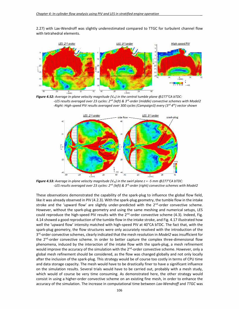
Chapter 4: In-cylinder flow analysis using PIV and LES in stratified engine operation _
106
2.27) with Lax-Wendroff was slightly underestimated compared to TTGC for turbulent channel flow with tetrahedral elements.
Figure 4.52: Average in-plane velocity magnitude (Vxz) in the central tumble plane @277°CA bTDC: -LES results averaged over 23 cycles: 2nd (left) & 3rd-order (middle) convective schemes with Model2 -Right: High-speed PIV results averaged over 300 cycles (Campaign3) every (3rd 4th) vector shown
Figure 4.53: Average in-plane velocity magnitude (Vxy) in the swirl plane z = -5 mm @277°CA bTDC: -LES results averaged over 23 cycles: 2nd (left) & 3rd-order (right) convective schemes with Model2 These observations demonstrated the capability of the spark-plug to influence the global flow field, like it was already observed in PIV (4.2.3). With the spark-plug geometry, the tumble flow in the intake stroke and the ‘upward flow’ are slightly under-predicted with the 2nd-order convective scheme. However, without the spark-plug geometry and using the same meshing and numerical setups, LES could reproduce the high-speed PIV results with the 2nd-order convective scheme (4.3). Indeed, Fig. 4.14 showed a good reproduction of the tumble flow in the intake stroke, and Fig. 4.17 illustrated how well the ‘upward flow’ intensity matched with high-speed PIV at 40°CA bTDC. The fact that, with the spark-plug geometry, the flow structures were only accurately resolved with the introduction of the 3rd-order convective schemes, clearly indicated that the mesh resolution in Model2 was insufficient for the 2nd-order convective scheme. In order to better capture the complex three-dimensional flow phenomena, induced by the interaction of the intake flow with the spark-plug, a mesh refinement would improve the accuracy of the simulation with the 2nd-order convective scheme. However, only a global mesh refinement should be considered, as the flow was changed globally and not only locally after the inclusion of the spark-plug. This strategy would be of course too costly in terms of CPU time and data storage capacity. The mesh would have to be drastically finer to have a significant influence on the simulation results. Several trials would have to be carried out, probably with a mesh study, which would of course be very time consuming. As demonstrated here, the other strategy would consist in using a higher-order convective scheme on an existing fine mesh, in order to enhance the accuracy of the simulation. The increase in computational time between Lax-Wendroff and TTGC was
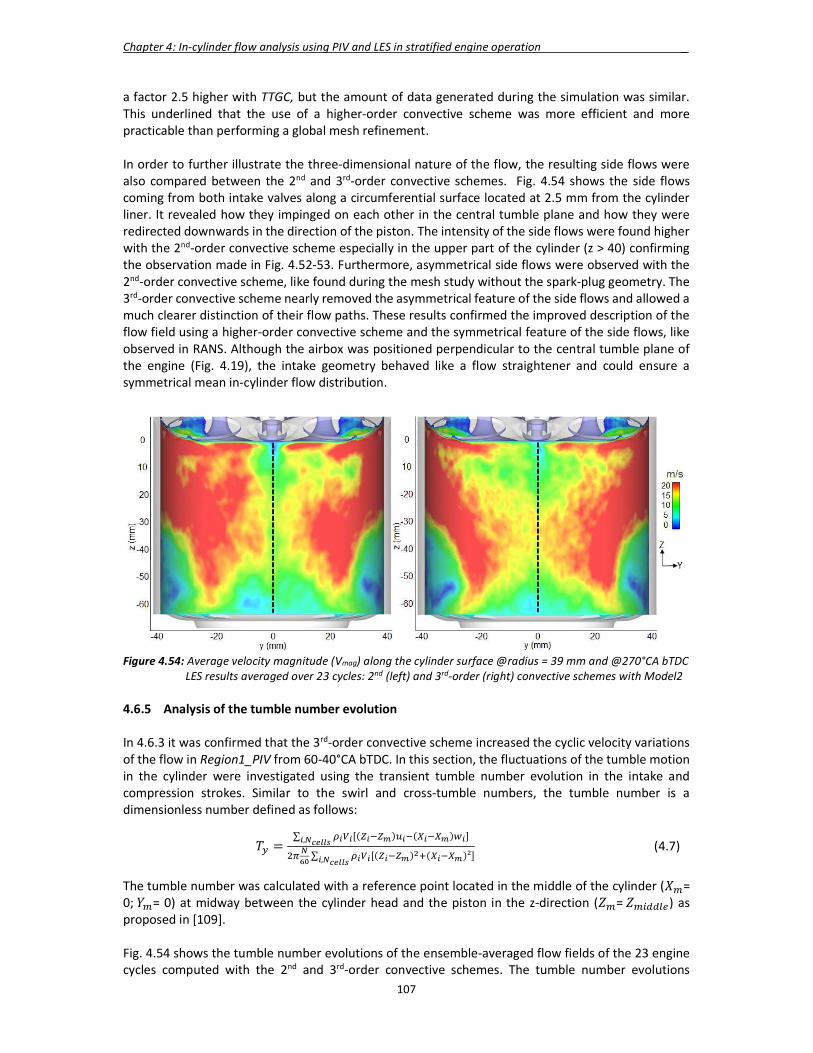
Chapter 4: In-cylinder flow analysis using PIV and LES in stratified engine operation _
107
a factor 2.5 higher with TTGC, but the amount of data generated during the simulation was similar. This underlined that the use of a higher-order convective scheme was more efficient and more practicable than performing a global mesh refinement. In order to further illustrate the three-dimensional nature of the flow, the resulting side flows were also compared between the 2nd and 3rd-order convective schemes. Fig. 4.54 shows the side flows coming from both intake valves along a circumferential surface located at 2.5 mm from the cylinder liner. It revealed how they impinged on each other in the central tumble plane and how they were redirected downwards in the direction of the piston. The intensity of the side flows were found higher with the 2nd-order convective scheme especially in the upper part of the cylinder (z > 40) confirming the observation made in Fig. 4.52-53. Furthermore, asymmetrical side flows were observed with the 2nd-order convective scheme, like found during the mesh study without the spark-plug geometry. The 3rd-order convective scheme nearly removed the asymmetrical feature of the side flows and allowed a much clearer distinction of their flow paths. These results confirmed the improved description of the flow field using a higher-order convective scheme and the symmetrical feature of the side flows, like observed in RANS. Although the airbox was positioned perpendicular to the central tumble plane of the engine (Fig. 4.19), the intake geometry behaved like a flow straightener and could ensure a symmetrical mean in-cylinder flow distribution.
Figure 4.54: Average velocity magnitude (Vmag) along the cylinder surface @radius = 39 mm and @270°CA bTDC LES results averaged over 23 cycles: 2nd (left) and 3rd-order (right) convective schemes with Model2 4.6.5 Analysis of the tumble number evolution In 4.6.3 it was confirmed that the 3rd-order convective scheme increased the cyclic velocity variations of the flow in Region1_PIV from 60-40°CA bTDC. In this section, the fluctuations of the tumble motion in the cylinder were investigated using the transient tumble number evolution in the intake and compression strokes. Similar to the swirl and cross-tumble numbers, the tumble number is a dimensionless number defined as follows:
𝑇 =∑ [( ) ( ) ]
,
∑ [( ) ( )²] ,
(4.7)
The tumble number was calculated with a reference point located in the middle of the cylinder (𝑋 = 0; 𝑌 = 0) at midway between the cylinder head and the piston in the z-direction (𝑍 = 𝑍 ) as proposed in [109]. Fig. 4.54 shows the tumble number evolutions of the ensemble-averaged flow fields of the 23 engine cycles computed with the 2nd and 3rd-order convective schemes. The tumble number evolutions
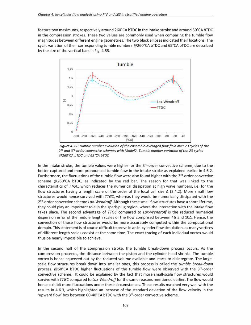
Chapter 4: In-cylinder flow analysis using PIV and LES in stratified engine operation _
108
feature two maximums, respectively around 260°CA bTDC in the intake stroke and around 60°CA bTDC in the compression strokes. These two values are commonly used when comparing the tumble flow magnitudes between different engine geometries. The two black ellipses indicated their locations. The cyclic variation of their corresponding tumble numbers @260°CA bTDC and 65°CA bTDC are described by the size of the vertical bars in Fig. 4.55.
Figure 4.55: Tumble number evolution of the ensemble-averaged flow field over 23 cycles of the 2nd and 3rd-order convective schemes with Model2. Tumble number variation of the 23 cycles @260°CA bTDC and 65°CA bTDC
In the intake stroke, the tumble values were higher for the 3rd-order convective scheme, due to the better-captured and more pronounced tumble flow in the intake stroke as explained earlier in 4.6.2. Furthermore, the fluctuations of the tumble flow were also found higher with the 3rd-order convective scheme @260°CA bTDC, as indicated by the red bar. The reason for that was linked to the characteristics of TTGC, which reduces the numerical dissipation at high wave numbers, i.e. for the flow structures having a length scale of the order of the local cell size Δ (2.4.2). More small flow structures would hence survived with TTGC, whereas they would be numerically dissipated with the 2nd-order convective scheme Lax-Wendroff. Although these small flow structures have a short lifetime, they could play an important role in the spark-plug region, where the interaction with the intake flow takes place. The second advantage of TTGC compared to Lax-Wendroff is the reduced numerical dispersion error of the middle length scales of the flow comprised between 4Δ and 10Δ. Hence, the convection of those flow structures would be more accurately computed within the computational domain. This statement is of course difficult to prove in an in-cylinder flow simulation, as many vortices of different length scales coexist at the same time. The exact tracing of each individual vortex would thus be nearly impossible to achieve. In the second half of the compression stroke, the tumble break-down process occurs. As the compression proceeds, the distance between the piston and the cylinder head shrinks. The tumble vortex is hence squeezed out by the reduced volume available and starts to disintegrate. The large-scale flow structures break down into smaller ones, this process is called the tumble break-down process. @60°CA bTDC higher fluctuations of the tumble flow were observed with the 3rd-order convective scheme. It could be explained by the fact that more small-scale flow structures would survive with TTGC compared to Lax-Wendroff for the same reasons mentioned earlier. The flow would hence exhibit more fluctuations under these circumstances. These results matched very well with the results in 4.6.3, which highlighted an increase of the standard deviation of the flow velocity in the ‘upward flow’ box between 60-40°CA bTDC with the 3rd-order convective scheme.
Chapter 4: In-cylinder flow analysis using PIV and LES in stratified engine operation _
109
4.7 Summary In this chapter a new methodology, called the ‘PIV-guided LES validation strategy’, was developed in order to validate the LES in-cylinder mean flow field, by direct comparisons with the PIV results in the central tumble plane. Using this meshing setup, the mean flow field and the cyclic velocity fluctuations in LES were validated with high-speed dual-plane PIV from 60-40°CA bTDC. LES could confirm the PIV hypothesis concerning the formation of the ‘upward flow’ and provided valuable three-dimensionnal flow information. The formation of the critical ‘upward flow’ in stratified engine operation, was hence fully understood using different flow analysis. The extreme LES cycles, where strong ‘upward flow’ intensity were observed, could be extracted using conditional statistics. The two and three-dimensional analysis of the conditional average flow fields proved that an upward jet-flow structure was formed in the middle of the cylinder during the compression stroke due to the bent 3D rotating axis of the tumble vortex. It resulted in the creation of secondary flows along the cylinder walls, which in turn generated the ‘upward flow’ before the injection. It was also shown that the 3rd-order accurate in time and space convective scheme TTGC could enhance the accuracy of the computed in-cylinder flow fields, especially in the intake stroke and from 60-50°CA bTDC. The improvements in terms of predictions of the mean flow and cycle-to-cycle velocity variations were quantified against the 2nd-order convective scheme Lax-Wendroff. Although the computational time was increased by a factor 2.5, the strategy consisting in relying on a higher-order convective scheme to improve the accuracy of the computed solution in LES was considered the best one. In the following chapters Model2 was renamed Gas-exchange_Model2 for clarity reasons.

Chapter 4: In-cylinder flow analysis using PIV and LES in stratified engine operation _
110

111
Chapter 5
Spray simulation of an outward-opening Piezo-actuated Pintle-type injector using LES The present chapter covers the validation of the spray simulation of an outward-opening Piezo-actuated Pintle-type injector (BOSCH HDEV4 [101]) with LES. Using the methodology presented in chapter 3, the main goal was to develop a reliable meshing strategy and numerical set-up in order to reproduce the spray measurements, carried out in a cold closed-volume chamber. The cold closed-volume chamber is widely used to analyse the mixing and the aerodynamic processes of the Piezo injector’s spray, which are the main factors for the fuel-air mixture formation. From the observations made in the optically-accessible engine, the resulting spray shape is known to be strongly dependent on the air density in the combustion chamber [57]. As a consequence, two different air pressures, 𝑝 = 1 𝑏𝑎𝑟 and 𝑝 = 6 𝑏𝑎𝑟, were investigated in the cold closed-volume chamber, in order to mimic the air density found in the engine cylinder before the start of injection in homogenous and stratified engine operations. In homogeneous engine operation, the injection process takes place during the intake stroke with opened intake valves resulting in a cylinder air density close to the atmospheric conditions. However, in stratified engine operation the start of injection is delayed up to the end of the compression stroke, which results in a higher air density due to the increased cylinder pressure and temperature. The other goal of this chapter was to guarantee, that the derived meshing strategy could be realistically integrated into the gas-exchange mesh (Gas-exchange_Model2). Indeed, the simulation of the fuel-air mixture formation in stratified and homogenous engine operations would have to be performed with moving meshes in chapter 6 and chapter 7. This chapter is divided into three main parts. The first one describes the spray characteristics of the outward-opening Piezo-actuated Pintle-type injector from the spray experiments carried out in a cold closed-volume chamber pressurized at 1 bar and 6 bar. The key spray parameters are extracted and quantified in view of the LES validation. The second part covers the validation of the computed spray in LES for the 6 bar case. The starting point for the spray simulation is the generation of the droplet initial conditions with the RANS-LES coupling interface, as presented in 3.2. Using the sub-models and the droplet injection procedure described in 3.1 and 3.2, the effect of the mesh topology combined with the 2nd and 3rd-order convective schemes are investigated. The optimal value of the droplet scale-factor 𝐾 , the influence of the total number of parcels as well as the improved interpolation algorithm for the gas-liquid coupling are also quantified. The last part of this chapter comprises the spray validation for the 1 bar case and the derivation of a universal simulation setup for the spray simulation of the Piezo injector in LES 5.1 Spray characteristics of the Piezo injector The experimental investigation of the spray was performed using a constant air temperature in the closed-volume chamber 𝑇 = 20 °𝐶. The fuel rail pressure 𝑝 = 200 𝑏𝑎𝑟 was similar to the one found in engine running conditions and n-heptane was chosen as a fuel. The measured fuel temperature was 𝑇 = 20 °𝐶. The experimental setup is summarized in Table 5.1.

Chapter 5: Spray simulation of an outward-opening Piezo-actuated Pintle-type injector using LES _
112
Table 5.1: Experimental setup Fuel C7H16 Fuel pressure 200 𝑏𝑎𝑟 Fuel temperature 20 °𝐶 Chamber air pressure 1 𝑏𝑎𝑟 𝑎𝑛𝑑 6 𝑏𝑎𝑟 Chamber air temperature 20 °C Single injection duration 1 𝑚𝑠 Defined time for the spray analysis 0.5 𝑚𝑠
Two measurement campaigns were performed in order to visualize the spray from two different perspectives:
- The goal of the first measurement campaign was the analysis of the global shape of the spray looking from the side. The measurement consisted in a single injection with an injection duration of 𝑡 = 1 𝑚𝑠. The optical measurement technique used was the shadowgraphy with background illumination. The spray was recorded every ∆𝑡 = 0.03 𝑚𝑠, starting from 𝑡 _ = 0.4 𝑚𝑠, with a camera positioned perpendicular to the injector axis in front of the spray. The background illumination was achieved using a LED lamp located behind the spray. Ten spray measurements were performed. They were afterwards averaged in order to obtain the mean spray picture of the Piezo injector. It was decided to analyse the spray characteristics at 𝑡 = 0.5 𝑚𝑠 as the spray was already well developed and a longer injection time was not relevant for the engine applications.
- The second measurement campaign consisted in observing a slice of the spray at 𝑡 = 0.5 𝑚𝑠.
The light source came from a laser. A laser light sheet, illuminating the spray perpendicular to the injector axis, was located at 𝑧 = 15 𝑚𝑚 and 𝑧 = 35 𝑚𝑚 respectively for the 6 bar and 1 bar cases. The camera was positioned below the spray parallel to the injector axis pointing in the upwards direction. Only one spray measurement was performed here.
The results of these two measurements campaigns were depicted in Fig. 5.1. The main characteristics of the Piezo injector could be summarized as follows. As an outward-opening nozzle, the displacement and the geometry of the direct actuated needle generates a symmetrical hollow-cone spray, which is ideal for central mounting position like in the M274’s engine configuration. However, the final shape of the spray and its penetration length are strongly dependent on the air density in the volume encompassing the injector. The primary atomization of the liquid sheet exiting the injector features a so-called turbulent break-up and occurs in two steps. The turbulence inside the nozzle creates perturbations on the liquid surface. These perturbations grow instable due to the aerodynamic interactions with the surrounding gas and finally break into ligaments. These ligaments swiftly disintegrate into droplets, under the influence of the surface tension and the gas forces [55]. The secondary break-up of the created droplets takes place solely under the influence of the aerodynamic forces as described in chapter 3. The spray for the 1 bar case is shown on the right side of Fig. 5.1. In homogeneous engine operations, the injection is triggered early during the intake stroke, i.e. with intake valves open, in order to ensure a homogenous fuel-air mixture at the ignition time. Close-to-ambient pressure conditions are thus met in the cylinder during the injection. Following a short time (180µs) for the needle to reach its maximal lift (35µm), the atomised droplets enter the closed chamber with high velocities. The spray penetrates deeply in the chamber at a constant angle (~85deg) and stays undisturbed, as the aerodynamic forces have a reduced effect on the droplets under low air density conditions. However, a local torus-shaped structure can be observed halfway between the injector and the spray front. It corresponds to a recirculation zone containing droplets with low Stokes number, which were ejected from the spray due to the air entrainment induced by the spray. The curved shape of the spray front, observed in the experiments, may be linked to the weak spray density in this region. It is investigated later in this

Chapter 5: Spray simulation of an outward-opening Piezo-actuated Pintle-type injector using LES _
113
chapter. Finally, string-like structures, also called ‘streaks’, can be observed at the surface of the spray in the bottom right-hand picture of Fig. 5.1. There are still uncertainties concerning their formation and their relationship to the internal nozzle flow. Streaks take their origin directly in the injector nozzle and travel along the spray. According to Marchi et al. [145], streaks are formed by air bubbles and/or cavitation pockets in the gap between the needle and the seat. The air cavitation pockets shape the liquid sheet into separated streaks. Using a VOF-LES simulation, Befrui et al. [146] showed that the boundary layer detachment of the liquid phase within the nozzle was the primary cause of the streak formation. Ambient air is then ingested into the nozzle up to the location of the flow detachment and Kelvin-Helmholtz instabilities are created on the liquid-air interface. It leads to an earlier atomization of the spray and to the creation of the connecting-regions between the different streaks. Experiments have shown that high injection pressures increase the number of streaks in the spray [145]. It was also observed that the number of streaks as well as their locations were always kept the same for one given injector but could vary between injectors of the same production batch. Internal nozzle geometry and manufacturing tolerances can hence influence the formation of streaks, so do the external geometry of the nozzle housing and the pintle shape [144]. Streaks contain large-size droplets and were found to enhance the robustness of the spray against changing airflow directions in a closed-volume chamber.
Figure 5.1: Spray measurements in a cold closed-chamber @0.5ms for 6 bar (left) and 1 bar (right) air pressure. Top: side view of the spray using the shadowgraphy technique with background illumination Bottom: view from below the spray where the light sheet, located at z = 15 mm (left) and z = 35 mm (right) illuminates the particles and the streaks in the spray The 6 bar case is closer to the conditions found in the stratified engine operation. Due to the higher air density in the closed chamber, the aerodynamic forces on the droplets increase and the secondary break-up process is particularly effective. Furthermore, the shear layers and the momentum transfer between the spray and the air rise up, leading to a higher air entrainment into the spray. As a result, two main vortices are formed: an outer clockwise-rotating vortex positioned outside the spray and an inner anticlockwise-rotating vortex located inside the spray. The spray penetration is hence drastically reduced compared to the 1 bar case. These two vortices were reproduced in the spray simulation in RANS and are depicted in Fig. 5.2. Around the outer vortex, a large torus-shaped recirculation zone is created. As the local mixture in this zone will be ignited, the outer-vortex characteristics play a major

Chapter 5: Spray simulation of an outward-opening Piezo-actuated Pintle-type injector using LES _
114
role in the stratified engine operation for two reasons. First, an intensive mixing process between the vaporized fuel and the gas phase takes place avoiding the creation of local high fuel-air ratio regions; secondly, the intensities of the flow velocity and the turbulent kinetic energy are reduced in comparison to the core region of the spray. As a result, better flow and mixture conditions are guaranteed at the ignition time around the spark-plug. The core region of the spray is characterised by an upward suction effect, also called ‘chimney-effect’ due to the increased air entrainment induced by the spray itself. This flow phenomena gives birth to the inner vortex and a second torus-shaped recirculation zone. The smallest droplets having low Stokes number have the ability to follow the movement of the gas and are found in the recirculation zones, whereas the biggest ones are located at the front of the spray without deviating much from their initial injection direction. Finally, streaks are also found in the 6 bar case, as illustrated in the bottom left-hand picture of Fig. 5.1.
Figure 5.2: Gas velocity (Vxz) @0.5ms in the middle plane of the injector (RANS) during the Lagrangian spray simulation of a Piezo-type injector in a chamber pressurized at 6 bar
Spray validation criteria For the validation of the spray simulation of the Piezo-type injector in LES, the following key spray parameters were selected based on the experimental results (Fig. 5.1):
the global spray width L4 the spray penetration L3 the width of the spray up to the upper edge of the torus-shaped structure L1 the upper-edge position of the torus-shaped structure L2 the lower-edge position of the torus-shaped structure L5 for the 1 bar case
To facilitate the visual comparison between the results from the simulation and experiments, standard boxes (red boxes in Fig. 5.1) were included in the spray pictures, based on the aforementioned experimental key spray parameters. Furthermore, additional considerations were put on the local spray patterns, which were found difficult to quantify numerically in Fig. 5.1. The first feature concerned, for the 1 bar case, the rounded form of the torus-shaped structure of the spray included in the violet boxes in Fig. 5.1. The second one was the rounded shape of the upper part of the torus-shaped structure, encompassed in the region delimited by the green boxes in Fig. 5.1, for the 6 bar case. Finally the visual aspect of the slice of the spray at z = 15 mm (6 bar) and z = 35 mm (1 bar) was also taken into account for the validation of the simulation results.
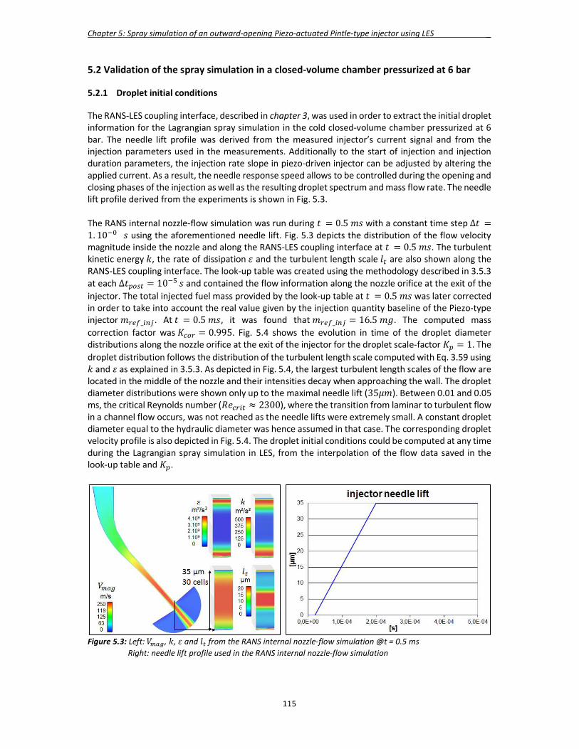
Chapter 5: Spray simulation of an outward-opening Piezo-actuated Pintle-type injector using LES _
115
5.2 Validation of the spray simulation in a closed-volume chamber pressurized at 6 bar 5.2.1 Droplet initial conditions The RANS-LES coupling interface, described in chapter 3, was used in order to extract the initial droplet information for the Lagrangian spray simulation in the cold closed-volume chamber pressurized at 6 bar. The needle lift profile was derived from the measured injector’s current signal and from the injection parameters used in the measurements. Additionally to the start of injection and injection duration parameters, the injection rate slope in piezo-driven injector can be adjusted by altering the applied current. As a result, the needle response speed allows to be controlled during the opening and closing phases of the injection as well as the resulting droplet spectrum and mass flow rate. The needle lift profile derived from the experiments is shown in Fig. 5.3. The RANS internal nozzle-flow simulation was run during 𝑡 = 0.5 𝑚𝑠 with a constant time step ∆𝑡 =1. 10 𝑠 using the aforementioned needle lift. Fig. 5.3 depicts the distribution of the flow velocity magnitude inside the nozzle and along the RANS-LES coupling interface at 𝑡 = 0.5 𝑚𝑠. The turbulent kinetic energy 𝑘, the rate of dissipation 𝜀 and the turbulent length scale 𝑙 are also shown along the RANS-LES coupling interface. The look-up table was created using the methodology described in 3.5.3 at each ∆𝑡 = 10 𝑠 and contained the flow information along the nozzle orifice at the exit of the injector. The total injected fuel mass provided by the look-up table at 𝑡 = 0.5 𝑚𝑠 was later corrected in order to take into account the real value given by the injection quantity baseline of the Piezo-type injector 𝑚 _ . At 𝑡 = 0.5 𝑚𝑠, it was found that 𝑚 _ = 16.5 𝑚𝑔. The computed mass correction factor was 𝐾 = 0.995. Fig. 5.4 shows the evolution in time of the droplet diameter distributions along the nozzle orifice at the exit of the injector for the droplet scale-factor 𝐾 = 1. The droplet distribution follows the distribution of the turbulent length scale computed with Eq. 3.59 using 𝑘 and 𝜀 as explained in 3.5.3. As depicted in Fig. 5.4, the largest turbulent length scales of the flow are located in the middle of the nozzle and their intensities decay when approaching the wall. The droplet diameter distributions were shown only up to the maximal needle lift (35𝜇𝑚). Between 0.01 and 0.05 ms, the critical Reynolds number (𝑅𝑒 ≈ 2300), where the transition from laminar to turbulent flow in a channel flow occurs, was not reached as the needle lifts were extremely small. A constant droplet diameter equal to the hydraulic diameter was hence assumed in that case. The corresponding droplet velocity profile is also depicted in Fig. 5.4. The droplet initial conditions could be computed at any time during the Lagrangian spray simulation in LES, from the interpolation of the flow data saved in the look-up table and 𝐾 .
Figure 5.3: Left: 𝑉 , 𝑘, 𝜀 and 𝑙 from the RANS internal nozzle-flow simulation @t = 0.5 ms Right: needle lift profile used in the RANS internal nozzle-flow simulation
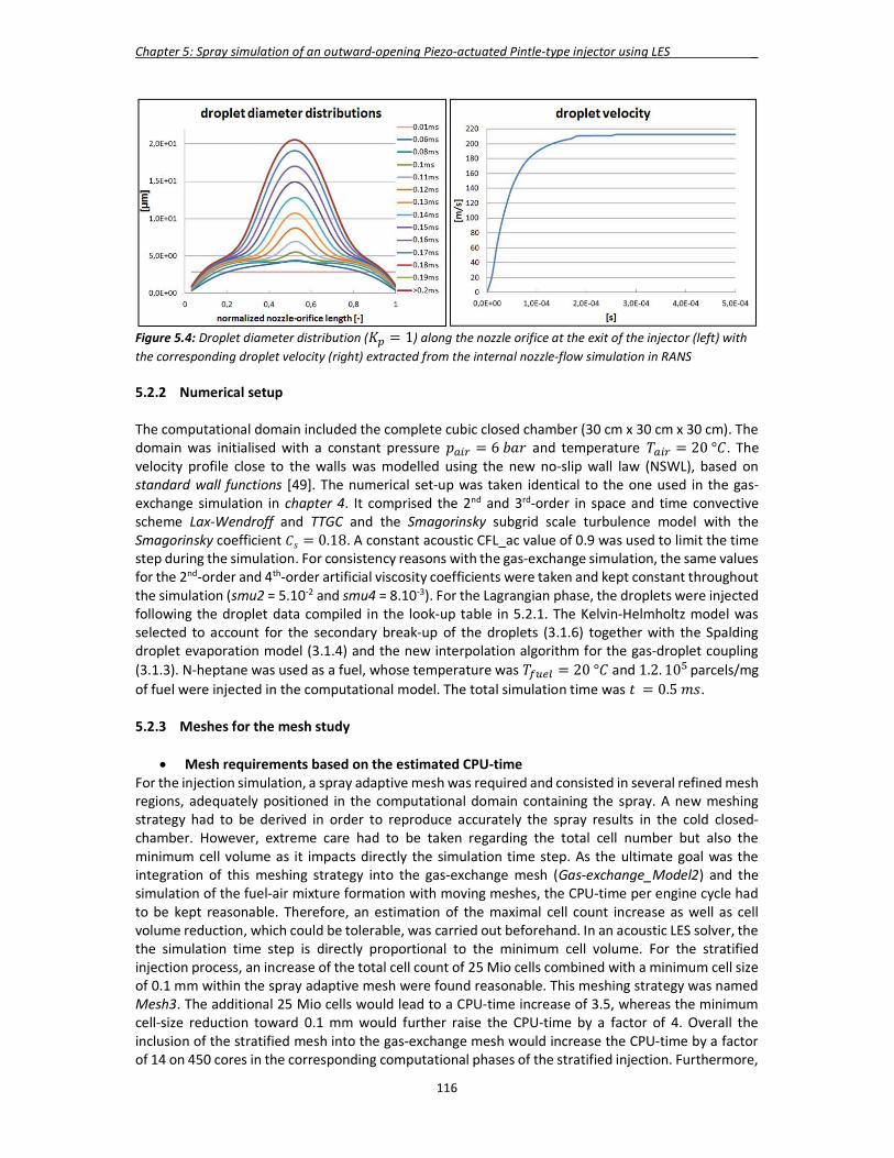
Chapter 5: Spray simulation of an outward-opening Piezo-actuated Pintle-type injector using LES _
116
Figure 5.4: Droplet diameter distribution (𝐾 = 1) along the nozzle orifice at the exit of the injector (left) with the corresponding droplet velocity (right) extracted from the internal nozzle-flow simulation in RANS 5.2.2 Numerical setup The computational domain included the complete cubic closed chamber (30 cm x 30 cm x 30 cm). The domain was initialised with a constant pressure 𝑝 = 6 𝑏𝑎𝑟 and temperature 𝑇 = 20 °𝐶. The velocity profile close to the walls was modelled using the new no-slip wall law (NSWL), based on standard wall functions [49]. The numerical set-up was taken identical to the one used in the gas-exchange simulation in chapter 4. It comprised the 2nd and 3rd-order in space and time convective scheme Lax-Wendroff and TTGC and the Smagorinsky subgrid scale turbulence model with the Smagorinsky coefficient 𝐶𝑠 = 0.18. A constant acoustic CFL_ac value of 0.9 was used to limit the time step during the simulation. For consistency reasons with the gas-exchange simulation, the same values for the 2nd-order and 4th-order artificial viscosity coefficients were taken and kept constant throughout the simulation (smu2 = 5.10-2 and smu4 = 8.10-3). For the Lagrangian phase, the droplets were injected following the droplet data compiled in the look-up table in 5.2.1. The Kelvin-Helmholtz model was selected to account for the secondary break-up of the droplets (3.1.6) together with the Spalding droplet evaporation model (3.1.4) and the new interpolation algorithm for the gas-droplet coupling (3.1.3). N-heptane was used as a fuel, whose temperature was 𝑇 = 20 °𝐶 and 1.2. 10 parcels/mg of fuel were injected in the computational model. The total simulation time was 𝑡 = 0.5 𝑚𝑠. 5.2.3 Meshes for the mesh study
Mesh requirements based on the estimated CPU-time For the injection simulation, a spray adaptive mesh was required and consisted in several refined mesh regions, adequately positioned in the computational domain containing the spray. A new meshing strategy had to be derived in order to reproduce accurately the spray results in the cold closed-chamber. However, extreme care had to be taken regarding the total cell number but also the minimum cell volume as it impacts directly the simulation time step. As the ultimate goal was the integration of this meshing strategy into the gas-exchange mesh (Gas-exchange_Model2) and the simulation of the fuel-air mixture formation with moving meshes, the CPU-time per engine cycle had to be kept reasonable. Therefore, an estimation of the maximal cell count increase as well as cell volume reduction, which could be tolerable, was carried out beforehand. In an acoustic LES solver, the the simulation time step is directly proportional to the minimum cell volume. For the stratified injection process, an increase of the total cell count of 25 Mio cells combined with a minimum cell size of 0.1 mm within the spray adaptive mesh were found reasonable. This meshing strategy was named Mesh3. The additional 25 Mio cells would lead to a CPU-time increase of 3.5, whereas the minimum cell-size reduction toward 0.1 mm would further raise the CPU-time by a factor of 4. Overall the inclusion of the stratified mesh into the gas-exchange mesh would increase the CPU-time by a factor of 14 on 450 cores in the corresponding computational phases of the stratified injection. Furthermore,

Chapter 5: Spray simulation of an outward-opening Piezo-actuated Pintle-type injector using LES _
117
as depicted in Fig. 5.5, this would mean an overall CPU-time increase of 3 hours per cycle on 450 cores compared to the gas-exchange simulation with Gas-exchange_Model2.
Figure 5.5: Comparison of the cumulative CPU-time of Gas-echange_Model2 with the estimated cumulative CPU-time of Gas-echange_Model2 with Mesh3 for the stratified operation on 450 cores
Characteristics of the different meshes Based on the aforementioned meshing requirements for the spray adaptive mesh, Mesh3 was built and optimized in Centaur. Finding the right balance between fine and coarse cells without overshooting the pre-defined maximal cell number was the main difficulty. Two coarse meshes, named Mesh1 and Mesh2, were also generated in order to estimate the reduction in solution accuracy by decreasing the CPU-time. Furthermore, a fourth mesh, featuring a very fine mesh and named Mesh4, was also created. The goal here was to check the grid convergence between Mesh3 and Mesh4, knowing that it was not realistic to integrate Mesh4 into the gas-exchange mesh for CPU-time reasons. In order to control the local mesh refinement, 6 distinct zones were defined in Centaur using volumetric sources of different shapes. Zone1 was first defined. Its dimension was taken equal to the engine cylinder at half stroke and had a cell size of 0.5 mm like in the gas-exchange mesh. This zone was kept identical in the four meshes. A spray adaptive domain was introduced starting with 0.3 mm cell size in Mesh1 and being progressively reduced up to 0.075 mm in Mesh4. Due to the geometry of the Piezo-type injector, a 360° mesh refinement needed to be considered, implying a swift increase of the total cell count in the domain while reducing the cell size. Thus, only local mesh refinements in the spray region were favoured. The depth of Zone2 was 35 mm in 𝑧-direction and 30 mm for Zone3 and Zone4. Table 5.2 summarizes the meshing setup for each mesh and their total number of cells, confirming the big differences in model size between the four meshes. Mesh4 was the finest mesh, which was possible to generate. The parallel mesh generation took around 11.8 hours using 16 cores. Unfortunately, it was not possible to produce a mesh with cell sizes smaller than 0.075 mm due to convergence issues with the internal mesh smoother of Centaur. The smallest achievable cell size was hence defined at the exit of the injector and along the spray in Zone6 and Zone4 of Mesh4. This cell size was 2.1 times bigger than the nozzle-hole at the maximal injector needle lift. As a result, the length scale of the flow at the exit of the injector nozzle could not be resolved in LES. The resolution of such flow length scales would require a cell size of ~3µm, like Hermann proposed for RANS [57] to capture accurately the shear layers and the air-entrainment process. However, it is a factor 25 smaller compared to what is currently feasible in Centaur. Furthermore, the time step of the simulation would scale down by the same factor and the total cell count would skyrocket making such simulation unrealistic with an acoustic explicit solver like AVBP. It could also be noticed that the total cell count had more than doubled when changing the cell size of 0.1 mm in Mesh3 to 0.075 mm in Mesh4, hence confirming the rapid cell count increase when performing a mesh refinement with tetrahedral elements. The four meshes are depicted in Fig. 5.6 with their refinement zone locations.
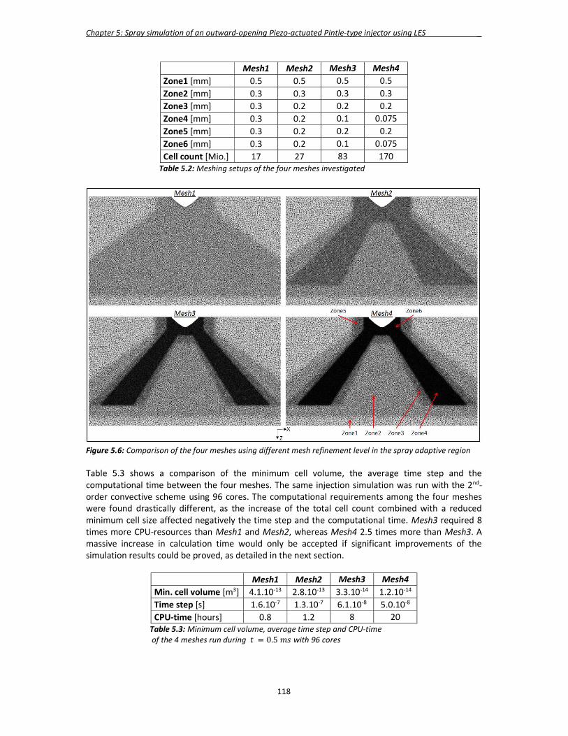
Chapter 5: Spray simulation of an outward-opening Piezo-actuated Pintle-type injector using LES _
118
Mesh1 Mesh2 Mesh3 Mesh4 Zone1 [mm] 0.5 0.5 0.5 0.5 Zone2 [mm] 0.3 0.3 0.3 0.3 Zone3 [mm] 0.3 0.2 0.2 0.2 Zone4 [mm] 0.3 0.2 0.1 0.075 Zone5 [mm] 0.3 0.2 0.2 0.2 Zone6 [mm] 0.3 0.2 0.1 0.075 Cell count [Mio.] 17 27 83 170
Table 5.2: Meshing setups of the four meshes investigated
Figure 5.6: Comparison of the four meshes using different mesh refinement level in the spray adaptive region Table 5.3 shows a comparison of the minimum cell volume, the average time step and the computational time between the four meshes. The same injection simulation was run with the 2nd-order convective scheme using 96 cores. The computational requirements among the four meshes were found drastically different, as the increase of the total cell count combined with a reduced minimum cell size affected negatively the time step and the computational time. Mesh3 required 8 times more CPU-resources than Mesh1 and Mesh2, whereas Mesh4 2.5 times more than Mesh3. A massive increase in calculation time would only be accepted if significant improvements of the simulation results could be proved, as detailed in the next section.
Mesh1 Mesh2 Mesh3 Mesh4 Min. cell volume [m3] 4.1.10-13 2.8.10-13 3.3.10-14 1.2.10-14 Time step [s] 1.6.10-7 1.3.10-7 6.1.10-8 5.0.10-8 CPU-time [hours] 0.8 1.2 8 20
Table 5.3: Minimum cell volume, average time step and CPU-time of the 4 meshes run during 𝑡 = 0.5 𝑚𝑠 with 96 cores
Chapter 5: Spray simulation of an outward-opening Piezo-actuated Pintle-type injector using LES _
119
5.2.4 Combined mesh and convective scheme study A higher mesh resolution leads to an improvement of the solution accuracy. In order to quantify the gain in accuracy in the Lagrangian spray simulation, a mesh study was performed with the aforementioned meshes. Moreover, similar to the gas-exchange simulation, the 2nd and 3rd-order convective schemes Lax-Wendroff and TTGC were also compared so as to verify if the 3rd-order convective scheme always performs better on four different mesh resolutions. The droplet scale-factor 𝐾 was taken equal to unity, like in RANS. The three-dimensional shapes of the sprays were first analysed from the side view at 𝑡 = 0.5 𝑚𝑠. The commercial software Ensight was used, where the parcels were coloured by the value of their representative droplet diameters and plotted using an identical size. The sprays computed on the four meshes with Lax-Wendroff are shown in Fig. 5.7 and with TTGC in Fig. 5.8. First, the shape of the spray was found strongly dependent on the local mesh size used. The spray width and penetration length were higher with reduced mesh cell sizes. Furthermore, flow structures could be noticed on the spray surface. With Mesh1 only large flow structures were observed on the spray surface and their positions and number could be determined from the spray front. The spray featured a relative smooth contour. As the mesh was further refined, additional smaller flow structures were computed along the spray surface leading to a more resolved spray shape. However, as illustrated in Fig. 5.9-5.12, the positions of the low frequency flow structures of Mesh1 were kept the same. Indeed, only higher frequency flow structures were added on top of them. As the mesh was refined, a more accurate description of the spray surface was obtained in LES. Secondly, the flow structures on the spray surface could not be linked to the streaks observed in the experiments. Streaks took their origin inside the injector nozzle and no streak information was taken into account for the generation of the droplet boundary conditions with the look-up table. The flow structures highlighted in the simulation take their origin from the Kelvin-Helmholtz instabilities, created on the interface between the liquid and the gas phase during the injection process. For the stochastic modelling of the spray and the location of the injected parcels in LES, random numbers were used from a file containing 1.106 equally distributed random numbers between 0 and 1. For consistency and repeatability reasons, the set of random numbers was always taken from this file in this research project. Another set of random numbers would lead to different locations of the observed flow structures on the spray surface in the simulation.
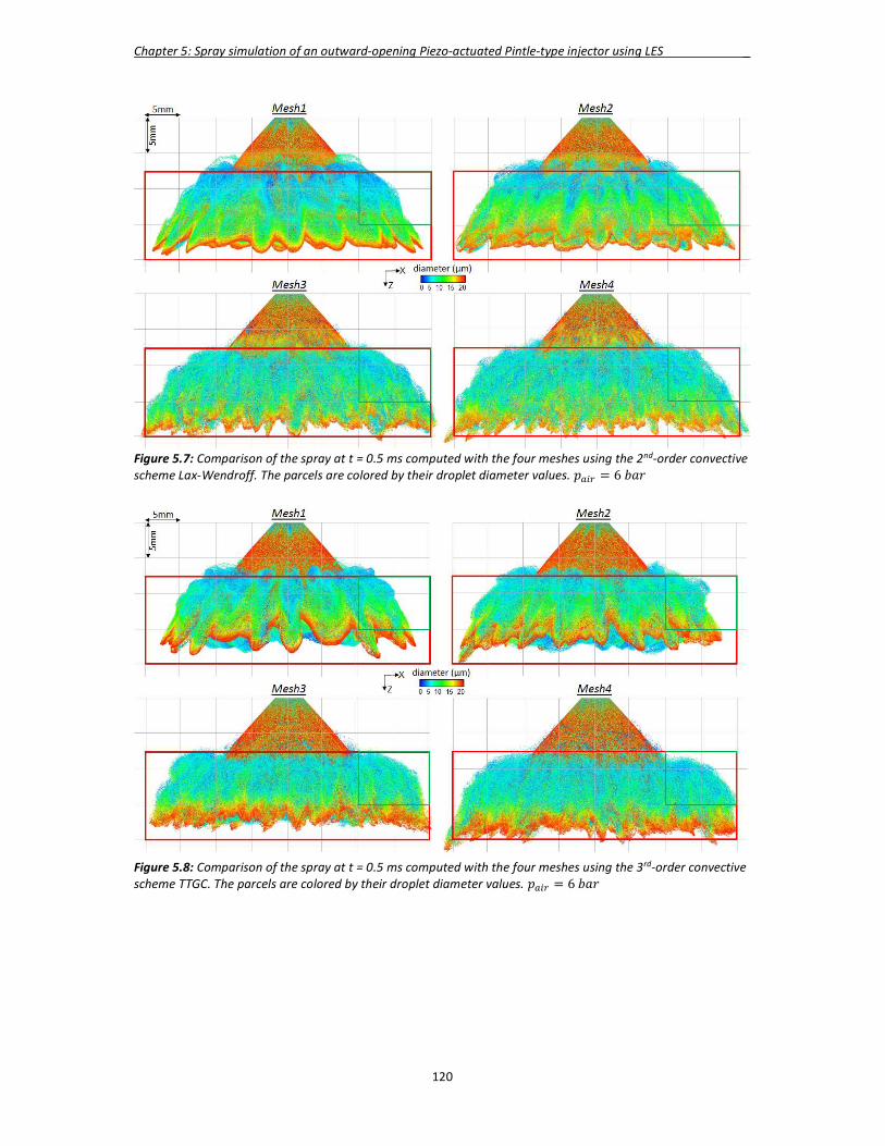
Chapter 5: Spray simulation of an outward-opening Piezo-actuated Pintle-type injector using LES _
120
Figure 5.7: Comparison of the spray at t = 0.5 ms computed with the four meshes using the 2nd-order convective scheme Lax-Wendroff. The parcels are colored by their droplet diameter values. 𝑝 = 6 𝑏𝑎𝑟
Figure 5.8: Comparison of the spray at t = 0.5 ms computed with the four meshes using the 3rd-order convective scheme TTGC. The parcels are colored by their droplet diameter values. 𝑝 = 6 𝑏𝑎𝑟
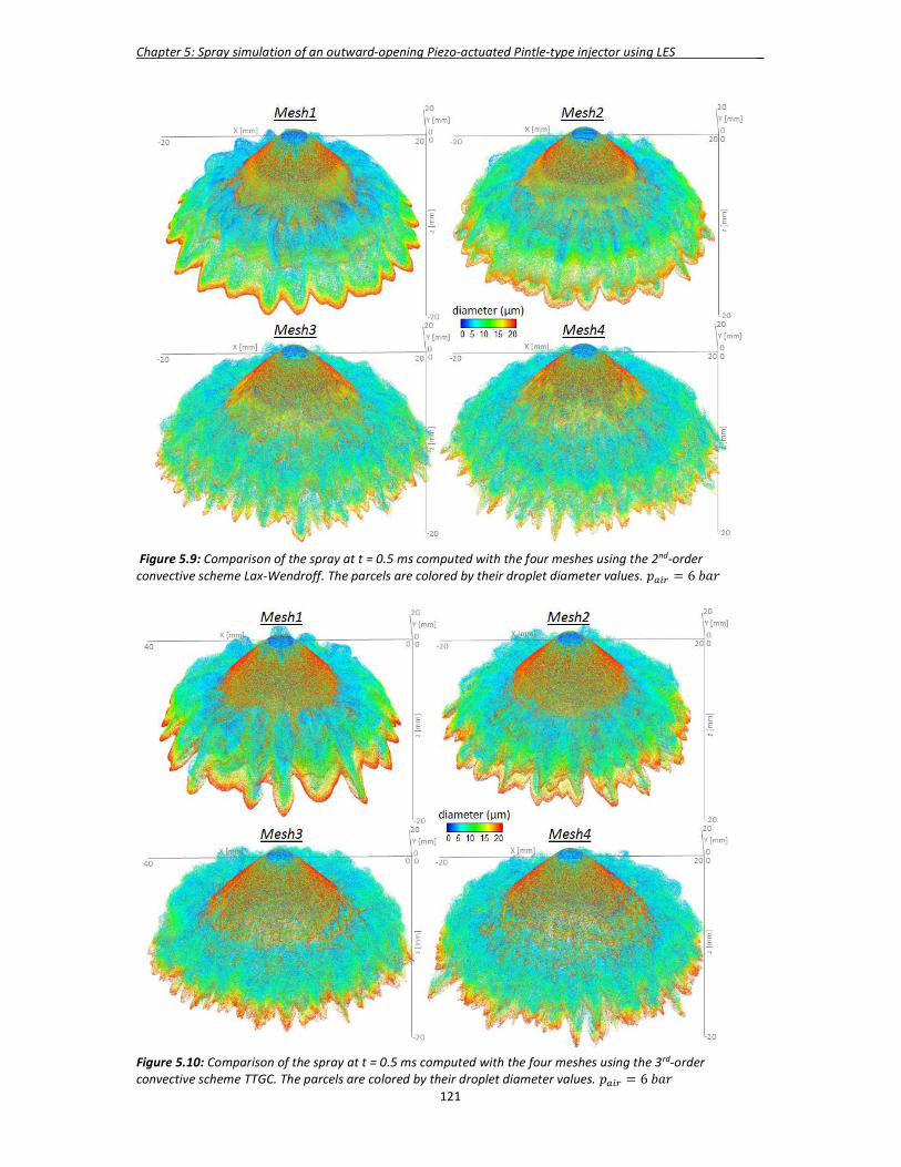
Chapter 5: Spray simulation of an outward-opening Piezo-actuated Pintle-type injector using LES _
121
Figure 5.9: Comparison of the spray at t = 0.5 ms computed with the four meshes using the 2nd-order convective scheme Lax-Wendroff. The parcels are colored by their droplet diameter values. 𝑝 = 6 𝑏𝑎𝑟
Figure 5.10: Comparison of the spray at t = 0.5 ms computed with the four meshes using the 3rd-order convective scheme TTGC. The parcels are colored by their droplet diameter values. 𝑝 = 6 𝑏𝑎𝑟

Chapter 5: Spray simulation of an outward-opening Piezo-actuated Pintle-type injector using LES _
122
Figure 5.11: Comparison of the spray at t = 0.5 ms computed with the four meshes using the 2nd-order convective scheme Lax-Wendroff. The parcels are colored by their droplet diameter values. 𝑝 = 6 𝑏𝑎𝑟
Figure 5.12: Comparison of the spray at t = 0.5 ms computed with the four meshes using the 3rd-order convective scheme TTGC. The parcels are colored by their droplet diameter values. 𝑝 = 6 𝑏𝑎𝑟

Chapter 5: Spray simulation of an outward-opening Piezo-actuated Pintle-type injector using LES _
123
Finally, it was found that the shape of the spray and the local flow structures were strongly dependent on the convective scheme used. Table 5.4-5.5 summarized the values of the key spray parameters obtained with the four meshes and the two convective schemes. They were compared to the experimental results presented in 5.1. The spray width (L4) and penetration length (L3) were computed based on the averaged position of hundred parcels located the farthest from the injection location. The width of the spray up to the upper edge of the torus-shaped structure (L1) and the upper-edge position of the torus-shaped structure (L2) were derived from the visual observation of the sprays.
Table 5.4: Comparison of the key spray parameters at t = 0.5 ms between simulation and experiments using the four meshes and the 2nd-order convective scheme Lax-Wendroff. 𝑝 = 6 𝑏𝑎𝑟
Mesh1 Mesh2 Mesh3 Mesh4 Experiments L1 [mm] 16 16 18 18 18 L2 [mm] 7 7 8 8 7.5 L3 [mm] 18 18 20 20 20 L4 [mm] 36.5 37.5 40 41 40
Table 5.5: Comparison of the key spray parameters at t = 0.5 ms between simulation and experiments using the four meshes and the 3rd-order convective scheme TTGC. 𝑝 = 6 𝑏𝑎𝑟
Mesh1 Mesh2 Mesh3 Mesh4 Experiments L1 [mm] 16 16 18 18 18 L2 [mm] 7 7 8.5 8 8 L3 [mm] 17.5 17.5 18.5 20 20 L4 [mm] 35 35,5 39 40 40
With the 2nd-order convective scheme Lax-Wendroff, the lowest spray width (L4) and penetration length (L3) were always obtained with Mesh1 and Mesh2, indicating that their mesh resolutions were not adequate. Furthermore, the results with Mesh3 and Mesh4 were both similar to the experiments. The upper location of the torus-shaped structure (L2) was in agreement with the experiments so did the width of the upper part of the spray (L1) and the penetration length (L3). The grid convergence was hence achieved with Mesh3 and a further mesh refinement with Mesh4 did not significantly improve the simulation results. In combination with the 3rd-order convective scheme TTGC, high grid dependencies were observed. The lowest spray width and penetration length were also obtained with Mesh1 and Mesh2. However, these results were found worse than the ones with the 2nd-order convective scheme Lax-Wendroff on the same coarse meshes. As the mesh was further refined, more small-scale flow structures were present along the spray with the 3rd-order convective scheme TTGC compared to the 2nd-order convective scheme Lax-Wendroff. Improvements of the spray description were particularly noticed with Mesh3 and Mesh4. The global form of the spray, especially the torus-shaped recirculation zone, in the region delimited by the green boxes in Fig. 5.7-5.8, was visually more compact i.e. less diffuse with TTGC compared to Lax-Wendroff. The distributions of the parcels within the spray were also different between the two schemes. With TTGC, the spray front encompassed clearly the biggest droplets, whereas with Lax-Wendroff it consisted of a mix of different droplet sizes confirming the increased diffusivity of this numerical scheme. Contrary to Lax-Wendroff, TTGC did not reach a grid convergence with Mesh3. A further mesh refinement with Mesh4 still improved drastically the simulation results. However, with Lax-Wendroff, the key spray parameters with Mesh4 was comparable to the ones using Mesh3 and Mesh4.
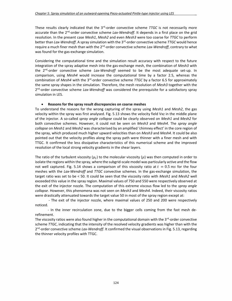
Chapter 5: Spray simulation of an outward-opening Piezo-actuated Pintle-type injector using LES _
124
These results clearly indicated that the 3rd-order convective scheme TTGC is not necessarily more accurate than the 2nd-order convective scheme Lax-Wendroff. It depends in a first place on the grid resolution. In the present case Mesh1, Mesh2 and even Mesh3 were too coarse for TTGC to perform better than Lax-Wendroff. A spray simulation with the 3rd-order convective scheme TTGC would hence require a much finer mesh than with the 2nd-order convective scheme Lax-Wendroff, contrary to what was found for the gas-exchange simulation.
Considering the computational time and the simulation result accuracy with respect to the future integration of the spray adaptive mesh into the gas-exchange mesh, the combination of Mesh3 with the 2nd-order convective scheme Lax-Wendroff seemed to be the most adequate set-up. In comparison, using Mesh4 would increase the computational time by a factor 2.5, whereas the combination of Mesh4 with the 3rd-order convective scheme TTGC by a factor 6.5 for approximately the same spray shapes in the simulation. Therefore, the mesh resolution of Mesh3 together with the 2nd-order convective scheme Lax-Wendroff was considered the prerequisite for a satisfactory spray simulation in LES.
Reasons for the spray result discrepancies on coarse meshes To understand the reasons for the wrong capturing of the spray using Mesh1 and Mesh2, the gas velocity within the spray was first analysed. Fig. 5.13 shows the velocity field Vxz in the middle plane of the injector. A so-called spray angle collapse could be clearly observed on Mesh1 and Mesh2 for both convective schemes. However, it could not be seen on Mesh3 and Mesh4. The spray angle collapse on Mesh1 and Mesh2 was characterised by an amplified ‘chimney effect’ in the core region of the spray, which produced much higher upward velocities than on Mesh3 and Mesh4. It could be also pointed out that the velocity profiles along the spray path were thinner with a finer mesh and with TTGC. It confirmed the less dissipative characteristics of this numerical scheme and the improved resolution of the local strong velocity gradients in the shear layers. The ratio of the turbulent viscosity (𝜇 ) to the molecular viscosity (𝜇) was then computed in order to isolate the regions within the spray, where the subgrid-scale model was particularly active and the flow not well captured. Fig. 5.14 shows a comparison of this viscosity ratio at 𝑡 = 0.5 𝑚𝑠 for the four meshes with the Lax-Wendroff and TTGC convective schemes. In the gas-exchange simulation, the target ratio was set to be < 50. It could be seen that the viscosity ratio with Mesh1 and Mesh2 well exceeded this value in the spray region. Maximal values of 750 and 550 were respectively observed at the exit of the injector nozzle. The computation of this extreme viscous flow led to the spray angle collapse. However, this phenomena was not seen on Mesh3 and Mesh4. Indeed, their viscosity ratios were drastically attenuated towards the target value 50 in most of the spray region except at:
- The exit of the injector nozzle, where maximal values of 250 and 200 were respectively noticed. - In the inner recirculation zone, due to the bigger cells coming from the fast mesh de-refinement. The viscosity ratios were also found higher in the computational domain with the 3rd-order convective scheme TTGC, indicating that the intensity of the resolved velocity gradients was higher than with the 2nd-order convective scheme Lax-Wendroff. It confirmed the visual observations in Fig. 5.13, regarding the thinner velocity profiles with TTGC.

Chapter 5: Spray simulation of an outward-opening Piezo-actuated Pintle-type injector using LES _
125
Figure 5.13: Comparison of the velocity Vxz at t = 0.5 ms in the injector middle plane for the four meshes -Left: using the 2nd-order convective scheme Lax-Wendroff -Right: using the 3rd-order convective scheme TTGC. 𝑝 = 6 𝑏𝑎𝑟

Chapter 5: Spray simulation of an outward-opening Piezo-actuated Pintle-type injector using LES _
126
Figure 5.14: Comparison of the ratio μt / μ at t = 0.5 ms in the injector middle plane for the four meshes -Left: using the 2nd-order convective scheme Lax-Wendroff -Right: using the 3rd-order convective scheme TTGC. 𝑝 = 6 𝑏𝑎𝑟
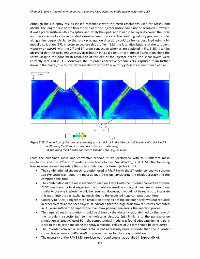
Chapter 5: Spray simulation of an outward-opening Piezo-actuated Pintle-type injector using LES _
127
Although the LES spray results looked reasonable with the mesh resolutions used for Mesh3 and Mesh4, the length scale of the flow at the exit of the injector nozzle could not be resolved. However, it was a prerequisite in RANS to capture accurately the upper and lower shear layers between the spray and the air as well as the associated air-entrainment process. The resulting velocity gradient profile, along a line perpendicular to the spray propagation direction, could be hence described using a bi-modal distribution [57]. In order to analyse this profile in LES, the local distributions of the turbulent viscosity on Mesh3 with the 2nd and 3rd-order convective schemes are depicted in Fig. 5.15. It can be observed that the turbulent viscosity distribution in LES did feature a bi-modal distribution along the spray. Despite the poor mesh resolution at the exit of the injector nozzle, the shear layers were correctly captured in LES. Moreover, the 3rd-order convective scheme TTGC captured them further down in the model, due to the better resolution of the flow velocity gradients as mentioned earlier.
Figure 5.15: Comparison of the turbulent viscosity μt at t = 0.5 ms in the injector middle plane with the Mesh3 -Left: using the 2nd-order convective scheme Lax-Wendroff -Right: using the 3rd-order convective scheme TTGC. 𝑝 = 6 𝑏𝑎𝑟 From the combined mesh and convective scheme study, performed with four different mesh resolutions and the 2nd and 3rd-order convective schemes Lax-Wendroff and TTGC, the following lessons were learned regarding the spray simulation of a Piezo injector in LES:
The combination of the mesh resolution used in Mesh3 with the 2nd-order convective scheme Lax-Wendroff was found the most adequate set-up, considering the result accuracy and the computational time.
The combination of the mesh resolution used on Mesh3 with the 3rd-order convective scheme TTGC was found critical regarding the simulation result accuracy. A finer mesh resolution, similar to the one in Mesh4, would be required. However, it would not be realistic to integrate this mesh into the gas-exchange mesh, due to the expected huge computational time.
Contrary to RANS, a higher mesh resolution at the exit of the injector nozzle was not required in order to capture the shear layers. It indicated that the large-scale flow structures computed in LES were sufficient to capture the main flow phenomena during the injection process.
The required mesh resolution should be driven by the viscosity ratio, defined by the ratio of the turbulent viscosity (𝜇 ) to the molecular viscosity (𝜇). Similarly to the gas-exchange simulation, a target value of 50 in the computational model was found adequate. In the regions close to the injector and along the spray a maximal cell size of 0.1 mm should be considered.
The 3rd-order convective scheme TTGC is not necessarily more accurate than the 2nd-order convective scheme Lax-Wendroff on coarse meshes for the spray simulation.
The necessity of the RANS-LES interface was found crucial, as detailed in [Appendix A].
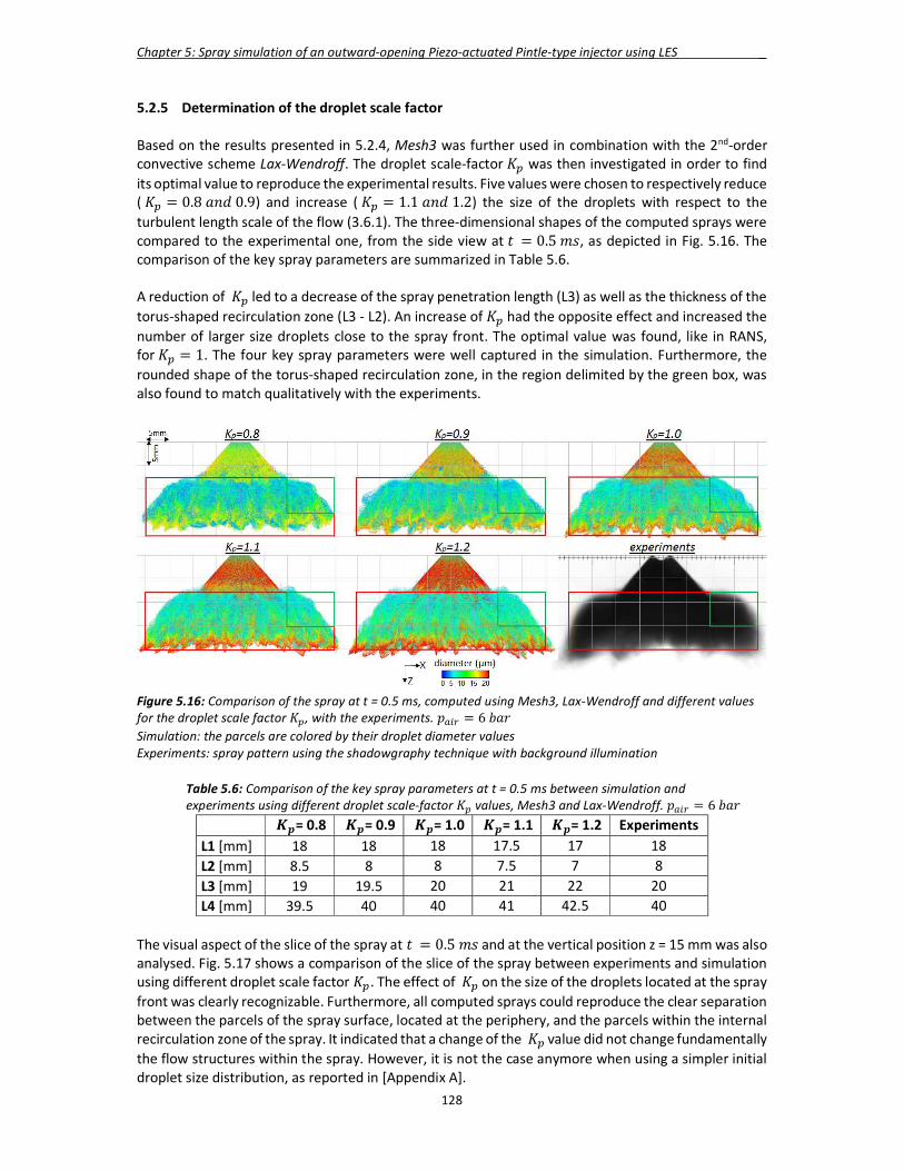
Chapter 5: Spray simulation of an outward-opening Piezo-actuated Pintle-type injector using LES _
128
5.2.5 Determination of the droplet scale factor Based on the results presented in 5.2.4, Mesh3 was further used in combination with the 2nd-order convective scheme Lax-Wendroff. The droplet scale-factor 𝐾 was then investigated in order to find its optimal value to reproduce the experimental results. Five values were chosen to respectively reduce ( 𝐾 = 0.8 𝑎𝑛𝑑 0.9) and increase ( 𝐾 = 1.1 𝑎𝑛𝑑 1.2) the size of the droplets with respect to the turbulent length scale of the flow (3.6.1). The three-dimensional shapes of the computed sprays were compared to the experimental one, from the side view at 𝑡 = 0.5 𝑚𝑠, as depicted in Fig. 5.16. The comparison of the key spray parameters are summarized in Table 5.6. A reduction of 𝐾 led to a decrease of the spray penetration length (L3) as well as the thickness of the torus-shaped recirculation zone (L3 - L2). An increase of 𝐾 had the opposite effect and increased the number of larger size droplets close to the spray front. The optimal value was found, like in RANS, for 𝐾 = 1. The four key spray parameters were well captured in the simulation. Furthermore, the rounded shape of the torus-shaped recirculation zone, in the region delimited by the green box, was also found to match qualitatively with the experiments.
Figure 5.16: Comparison of the spray at t = 0.5 ms, computed using Mesh3, Lax-Wendroff and different values for the droplet scale factor 𝐾 , with the experiments. 𝑝 = 6 𝑏𝑎𝑟 Simulation: the parcels are colored by their droplet diameter values Experiments: spray pattern using the shadowgraphy technique with background illumination
Table 5.6: Comparison of the key spray parameters at t = 0.5 ms between simulation and experiments using different droplet scale-factor 𝐾 values, Mesh3 and Lax-Wendroff. 𝑝 = 6 𝑏𝑎𝑟
𝑲𝒑= 0.8 𝑲𝒑= 0.9 𝑲𝒑= 1.0 𝑲𝒑= 1.1 𝑲𝒑= 1.2 Experiments L1 [mm] 18 18 18 17.5 17 18 L2 [mm] 8.5 8 8 7.5 7 8 L3 [mm] 19 19.5 20 21 22 20 L4 [mm] 39.5 40 40 41 42.5 40
The visual aspect of the slice of the spray at 𝑡 = 0.5 𝑚𝑠 and at the vertical position z = 15 mm was also analysed. Fig. 5.17 shows a comparison of the slice of the spray between experiments and simulation using different droplet scale factor 𝐾 . The effect of 𝐾 on the size of the droplets located at the spray front was clearly recognizable. Furthermore, all computed sprays could reproduce the clear separation between the parcels of the spray surface, located at the periphery, and the parcels within the internal recirculation zone of the spray. It indicated that a change of the 𝐾 value did not change fundamentally the flow structures within the spray. However, it is not the case anymore when using a simpler initial droplet size distribution, as reported in [Appendix A].
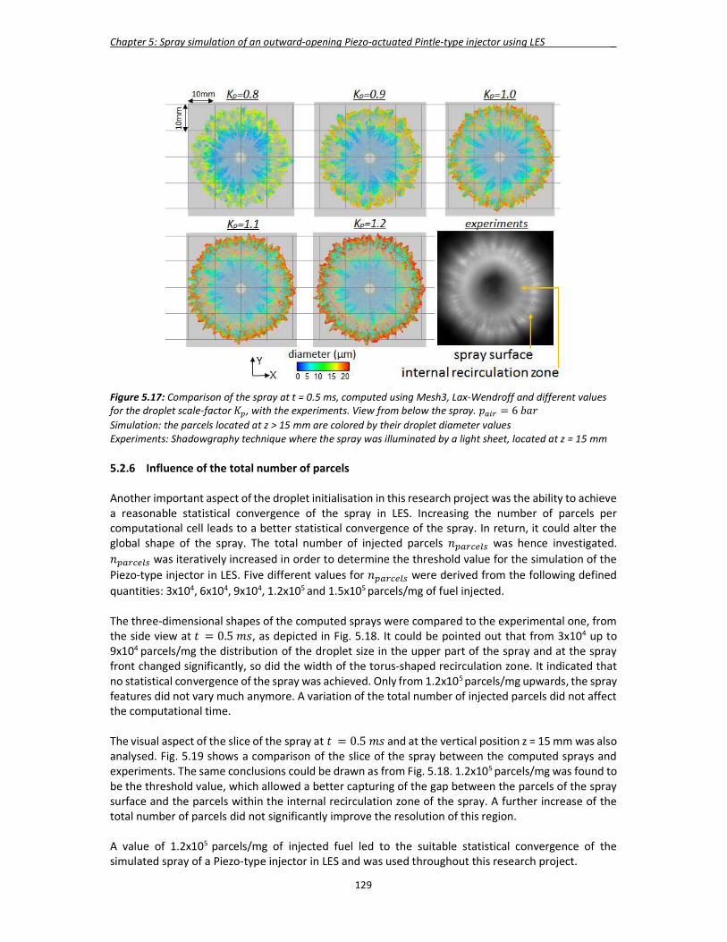
Chapter 5: Spray simulation of an outward-opening Piezo-actuated Pintle-type injector using LES _
129
Figure 5.17: Comparison of the spray at t = 0.5 ms, computed using Mesh3, Lax-Wendroff and different values for the droplet scale-factor 𝐾 , with the experiments. View from below the spray. 𝑝 = 6 𝑏𝑎𝑟 Simulation: the parcels located at z > 15 mm are colored by their droplet diameter values Experiments: Shadowgraphy technique where the spray was illuminated by a light sheet, located at z = 15 mm
5.2.6 Influence of the total number of parcels Another important aspect of the droplet initialisation in this research project was the ability to achieve a reasonable statistical convergence of the spray in LES. Increasing the number of parcels per computational cell leads to a better statistical convergence of the spray. In return, it could alter the global shape of the spray. The total number of injected parcels 𝑛 was hence investigated. 𝑛 was iteratively increased in order to determine the threshold value for the simulation of the Piezo-type injector in LES. Five different values for 𝑛 were derived from the following defined quantities: 3x10⁴, 6x10⁴, 9x10⁴, 1.2x10⁵ and 1.5x10⁵ parcels/mg of fuel injected. The three-dimensional shapes of the computed sprays were compared to the experimental one, from the side view at 𝑡 = 0.5 𝑚𝑠, as depicted in Fig. 5.18. It could be pointed out that from 3x10⁴ up to 9x10⁴ parcels/mg the distribution of the droplet size in the upper part of the spray and at the spray front changed significantly, so did the width of the torus-shaped recirculation zone. It indicated that no statistical convergence of the spray was achieved. Only from 1.2x10⁵ parcels/mg upwards, the spray features did not vary much anymore. A variation of the total number of injected parcels did not affect the computational time. The visual aspect of the slice of the spray at 𝑡 = 0.5 𝑚𝑠 and at the vertical position z = 15 mm was also analysed. Fig. 5.19 shows a comparison of the slice of the spray between the computed sprays and experiments. The same conclusions could be drawn as from Fig. 5.18. 1.2x10⁵ parcels/mg was found to be the threshold value, which allowed a better capturing of the gap between the parcels of the spray surface and the parcels within the internal recirculation zone of the spray. A further increase of the total number of parcels did not significantly improve the resolution of this region. A value of 1.2x10⁵ parcels/mg of injected fuel led to the suitable statistical convergence of the simulated spray of a Piezo-type injector in LES and was used throughout this research project.

Chapter 5: Spray simulation of an outward-opening Piezo-actuated Pintle-type injector using LES _
130
Figure 5.18: Comparison of the spray at t = 0.5 ms, computed using Mesh3, Lax-Wendroff and different number of parcels, with the experiments. 𝑝 = 6 𝑏𝑎𝑟 Simulation: the parcels are colored by their droplet diameter values Experiments: spray pattern using the shadowgraphy technique with background illumination
Figure 5.19: Comparison of the spray at t = 0.5 ms, computed using Mesh3, Lax-Wendroff and different number of parcels, with the experiments. View from below the spray. 𝑝 = 6 𝑏𝑎𝑟 Simulation: the parcels located at z > 15 mm are colored by their droplet diameter values Experiments: Shadowgraphy technique where the spray was illuminated by a light sheet, located at z = 15 mm

Chapter 5: Spray simulation of an outward-opening Piezo-actuated Pintle-type injector using LES _
131
5.2.7 New interpolation algorithm for the gas-liquid coupling A new interpolation scheme for the gas-liquid phase coupling was implemented in AVBP and presented in 3.3.2. It was aimed at providing a more accurate information about the filtered gas velocity at the parcel location. The flow information of all the vertices, belonging to the cell encompassing one parcel, was hence taken into account using an inverse parcel-vertex distance weighting. The standard interpolation algorithm in AVBP used the 1st-order Taylor series at the nearest cell vertex of the parcel instead. The implementation of this algorithm in AVBP was motivated by the fact that the spray simulation could not be run successfully with the standard interpolation algorithm of AVBP on coarse meshes like Mesh1 and Mesh2, even with smaller time steps. The three-dimensional shapes of the computed sprays with Mesh3, using both interpolation algorithms, were compared to the experimental one, from the side view at 𝑡 = 0.5 𝑚𝑠, as depicted in Fig. 5.20. The main difference between the results of the two interpolation algorithms was linked to the resolution of the torus-shaped recirculation zone of the spray. With the new algorithm, this zone was thinner and its shape, in the region delimited by the green box, more curved compared to the spray computed with the standard interpolation algorithm of AVBP. The spray penetration was hence shorter and the spray shape more compact with the new interpolation algorithm. The spray shape was hence found qualitatively closer to the experiments. Using more than one vertex for the interpolation of the filtered gas velocity at the parcel location allowed the parcels to deviate more easily from their initial propagation directions and increase their dispersions within the spray. The improved inter-phase coupling capability of the new interpolation algorithm for the gas-liquid coupling was used as default in this research project.
Figure 5.20: Comparison of the spray at t = 0.5 ms, computed using Mesh3, Lax-Wendroff and two different interpolation algorithms for the gas-liquid phase coupling, with the experiments. 𝑝 = 6 𝑏𝑎𝑟 Simulation: the parcels are colored by their droplet diameter values Experiments: spray pattern using the shadowgraphy technique with background illumination 5.2.8 ‘Best practice’ methodology From the spray simulation results presented for the 1 bar case, a ‘Best-practice’ methodology could be derived. It allowed an accurate reproduction of the experimental measurements and a reasonable computational time. The final setup for the Lagrangian spray simulation was named Lagrangian setup in the rest of this work and included the following important features:
RANS-LES coupling interface for the droplet initialisation with a droplet scale factor 𝐾 = 1. Any other droplet initialisation would lead to inaccurate results as detailed in [Appendix A].
Spray adaptive mesh: meshing setup similar to Mesh3. 2nd-order convective scheme Lax-Wendroff. Total number of parcels using 1.2. 10 parcels/mg of injected fuel. New interpolation algorithm for the gas-liquid coupling.

Chapter 5: Spray simulation of an outward-opening Piezo-actuated Pintle-type injector using LES _
132
The Lagrangian setup was found compatible with the numerical setup, used for the gas-exchange simulation in chapter 4. The remaining features, taken identically for the spray simulation and the gas-exchange simulation, were the followings:
Fixed 2nd and 4th-order artificial viscosity coefficients (smu2 = 5.10-2 and smu4 = 8.10-3). Constant CFL_ac value of 0.9. No-slip wall law (NSWL).
5.3 Validation of the spray simulation in a closed-volume chamber pressurized at 1 bar 5.3.1 Setup and boundary conditions The validation of the spray was repeated in the same cold closed-volume chamber, which was this time pressurized at 1 bar. The Lagrangian setup was assessed in order to obtain a universal validated setup for the spray simulation of the Piezo injector in LES. In the experiments for the 1 bar case, depicted in Fig. 5.1 , the spray penetration and the spray width were found higher than for the 6 bar case. Due to the diminution of the air pressure in the closed-chamber, the magnitude of the shear stresses between the air and the liquid phase was reduced. Furthermore, in homogenous engine operation the injection duration is increased due to the higher engine load requested by the driver. It was hence decided to investigate a lower mesh resolution (Mesh2) in addition to Mesh3. The aim was to reduce the computational time and quantify the impact of a coarser mesh on the results. The RANS-LES coupling interface was first required to generate the droplet initial conditions, similarly to the previous 6 bar case. Secondly, based on the Lagrangian setup, the spray simulation was performed in LES and the results compared with the experiments. The computational domain was initialised with a constant pressure 𝑝 = 1 𝑏𝑎𝑟 and temperature 𝑇 = 20 °𝐶. The initial droplet information was extracted from another internal nozzle-flow simulation in RANS, performed with 𝑃 = 1 𝑏𝑎𝑟. The look-up table was created using the methodology described in 3.5.3 at each ∆𝑡 = 10 𝑠 and contained the flow information along the RANS-LES coupling interface at the exit of the injector. The total injected fuel mass provided by the look-up table at 𝑡 = 0.5 𝑚𝑠 was corrected in the same way as for the 6 bar case, using the injection quantity baseline of the piezo-injector. The computed mass correction factor was 𝐾 = 0.998. Mesh2 and Mesh3 were both considered in the spray validation process and the rest of the numerical setup was taken identically to the Lagrangian setup. The total simulation time was 𝑡 = 0.5 𝑚𝑠. 5.3.2 Validation results The three-dimensional shapes of the sprays were first analysed from the side view at 𝑡 = 0.5 𝑚𝑠. The parcels were coloured by the value of their representative diameters and plotted using an identical size. The sprays computed on Mesh2 and Mesh3 were shown in Fig. 5.21 together with the experimental results.
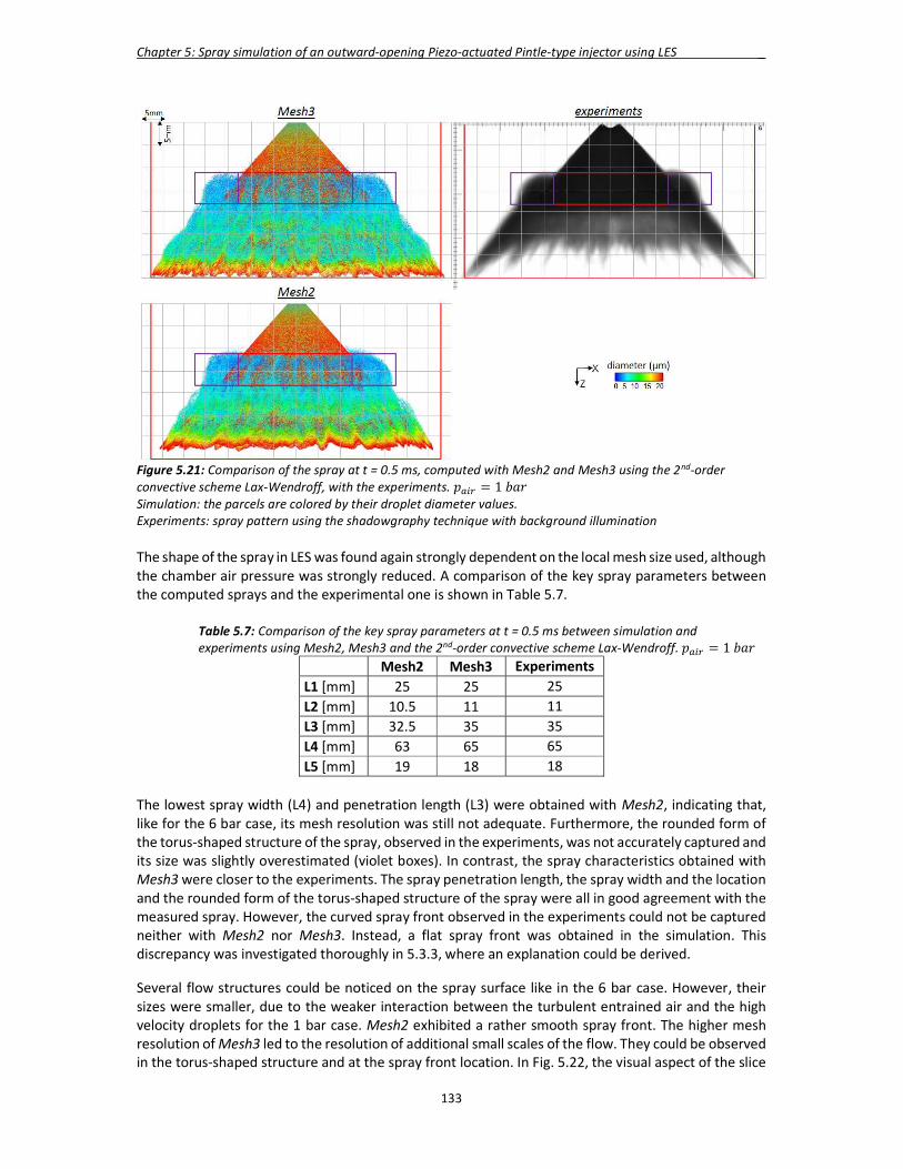
Chapter 5: Spray simulation of an outward-opening Piezo-actuated Pintle-type injector using LES _
133
Figure 5.21: Comparison of the spray at t = 0.5 ms, computed with Mesh2 and Mesh3 using the 2nd-order convective scheme Lax-Wendroff, with the experiments. 𝑝 = 1 𝑏𝑎𝑟 Simulation: the parcels are colored by their droplet diameter values. Experiments: spray pattern using the shadowgraphy technique with background illumination The shape of the spray in LES was found again strongly dependent on the local mesh size used, although the chamber air pressure was strongly reduced. A comparison of the key spray parameters between the computed sprays and the experimental one is shown in Table 5.7.
Table 5.7: Comparison of the key spray parameters at t = 0.5 ms between simulation and experiments using Mesh2, Mesh3 and the 2nd-order convective scheme Lax-Wendroff. 𝑝 = 1 𝑏𝑎𝑟
Mesh2 Mesh3 Experiments L1 [mm] 25 25 25 L2 [mm] 10.5 11 11 L3 [mm] 32.5 35 35 L4 [mm] 63 65 65 L5 [mm] 19 18 18
The lowest spray width (L4) and penetration length (L3) were obtained with Mesh2, indicating that, like for the 6 bar case, its mesh resolution was still not adequate. Furthermore, the rounded form of the torus-shaped structure of the spray, observed in the experiments, was not accurately captured and its size was slightly overestimated (violet boxes). In contrast, the spray characteristics obtained with Mesh3 were closer to the experiments. The spray penetration length, the spray width and the location and the rounded form of the torus-shaped structure of the spray were all in good agreement with the measured spray. However, the curved spray front observed in the experiments could not be captured neither with Mesh2 nor Mesh3. Instead, a flat spray front was obtained in the simulation. This discrepancy was investigated thoroughly in 5.3.3, where an explanation could be derived. Several flow structures could be noticed on the spray surface like in the 6 bar case. However, their sizes were smaller, due to the weaker interaction between the turbulent entrained air and the high velocity droplets for the 1 bar case. Mesh2 exhibited a rather smooth spray front. The higher mesh resolution of Mesh3 led to the resolution of additional small scales of the flow. They could be observed in the torus-shaped structure and at the spray front location. In Fig. 5.22, the visual aspect of the slice
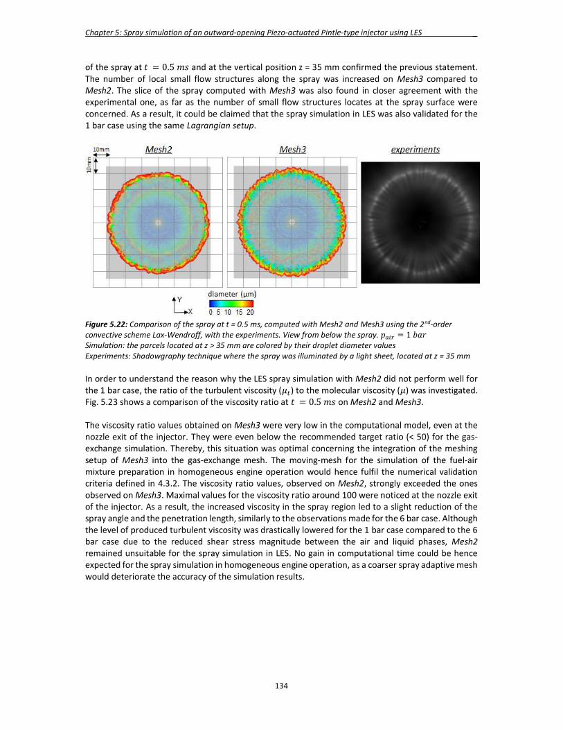
Chapter 5: Spray simulation of an outward-opening Piezo-actuated Pintle-type injector using LES _
134
of the spray at 𝑡 = 0.5 𝑚𝑠 and at the vertical position z = 35 mm confirmed the previous statement. The number of local small flow structures along the spray was increased on Mesh3 compared to Mesh2. The slice of the spray computed with Mesh3 was also found in closer agreement with the experimental one, as far as the number of small flow structures locates at the spray surface were concerned. As a result, it could be claimed that the spray simulation in LES was also validated for the 1 bar case using the same Lagrangian setup.
Figure 5.22: Comparison of the spray at t = 0.5 ms, computed with Mesh2 and Mesh3 using the 2nd-order convective scheme Lax-Wendroff, with the experiments. View from below the spray. 𝑝 = 1 𝑏𝑎𝑟 Simulation: the parcels located at z > 35 mm are colored by their droplet diameter values Experiments: Shadowgraphy technique where the spray was illuminated by a light sheet, located at z = 35 mm In order to understand the reason why the LES spray simulation with Mesh2 did not perform well for the 1 bar case, the ratio of the turbulent viscosity (𝜇 ) to the molecular viscosity (𝜇) was investigated. Fig. 5.23 shows a comparison of the viscosity ratio at 𝑡 = 0.5 𝑚𝑠 on Mesh2 and Mesh3. The viscosity ratio values obtained on Mesh3 were very low in the computational model, even at the nozzle exit of the injector. They were even below the recommended target ratio (< 50) for the gas-exchange simulation. Thereby, this situation was optimal concerning the integration of the meshing setup of Mesh3 into the gas-exchange mesh. The moving-mesh for the simulation of the fuel-air mixture preparation in homogeneous engine operation would hence fulfil the numerical validation criteria defined in 4.3.2. The viscosity ratio values, observed on Mesh2, strongly exceeded the ones observed on Mesh3. Maximal values for the viscosity ratio around 100 were noticed at the nozzle exit of the injector. As a result, the increased viscosity in the spray region led to a slight reduction of the spray angle and the penetration length, similarly to the observations made for the 6 bar case. Although the level of produced turbulent viscosity was drastically lowered for the 1 bar case compared to the 6 bar case due to the reduced shear stress magnitude between the air and liquid phases, Mesh2 remained unsuitable for the spray simulation in LES. No gain in computational time could be hence expected for the spray simulation in homogeneous engine operation, as a coarser spray adaptive mesh would deteriorate the accuracy of the simulation results.
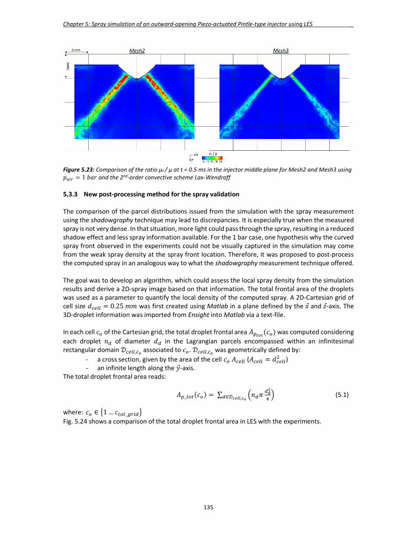
Chapter 5: Spray simulation of an outward-opening Piezo-actuated Pintle-type injector using LES _
135
Figure 5.23: Comparison of the ratio μt / μ at t = 0.5 ms in the injector middle plane for Mesh2 and Mesh3 using 𝑝 = 1 𝑏𝑎𝑟 and the 2nd-order convective scheme Lax-Wendroff 5.3.3 New post-processing method for the spray validation The comparison of the parcel distributions issued from the simulation with the spray measurement using the shadowgraphy technique may lead to discrepancies. It is especially true when the measured spray is not very dense. In that situation, more light could pass through the spray, resulting in a reduced shadow effect and less spray information available. For the 1 bar case, one hypothesis why the curved spray front observed in the experiments could not be visually captured in the simulation may come from the weak spray density at the spray front location. Therefore, it was proposed to post-process the computed spray in an analogous way to what the shadowgraphy measurement technique offered. The goal was to develop an algorithm, which could assess the local spray density from the simulation results and derive a 2D-spray image based on that information. The total frontal area of the droplets was used as a parameter to quantify the local density of the computed spray. A 2D-Cartesian grid of cell size 𝑑 = 0.25 𝑚𝑚 was first created using Matlab in a plane defined by the �� and 𝑧-axis. The 3D-droplet information was imported from Ensight into Matlab via a text-file. In each cell 𝑐 of the Cartesian grid, the total droplet frontal area 𝐴 (𝑐 ) was computed considering each droplet 𝑛 of diameter 𝑑 in the Lagrangian parcels encompassed within an infinitesimal rectangular domain 𝒟 , associated to 𝑐 . 𝒟 , was geometrically defined by:
- a cross section, given by the area of the cell 𝑐 𝐴 (𝐴 = 𝑑 ) - an infinite length along the ��-axis.
The total droplet frontal area reads:
𝐴 _ (𝑐 ) = ∑ 𝑛 𝜋∈𝒟 , (5.1)
where: 𝑐 ∈ 1 … 𝑐 _ Fig. 5.24 shows a comparison of the total droplet frontal area in LES with the experiments.

Chapter 5: Spray simulation of an outward-opening Piezo-actuated Pintle-type injector using LES _
136
Figure 5.24: Comparison of the spray at t = 0.5 ms, computed with Mesh3 using the 2nd-order convective scheme Lax-Wendroff, with the experiments. 𝑝 = 1 𝑏𝑎𝑟 Simulation: Total droplet frontal area in ��-direction Experiments: spray pattern using the shadowgraphy technique with background illumination The simulated spray looked much closer to the measured spray in Fig. 5.24 compared to Fig. 5.21. Three main regions could be clearly identified:
- The first region consisted of the upper region of the spray including the torus-shape structure delimited by the red box in Fig. 5.24. The spray in this region was very dense. The global torus-shape structure was well captured in the simulation, confirming the observation made in 5.3.2.
- The core region of the spray below the first region featured a less dense spray. This region is defined by the green trapezoid in Fig. 5.24. Furthermore, on both sides of the trapezoid, marked by the orange crosses, the spray appeared denser. Indeed, due to the side view of a rotational symmetrical spray, the total amount of droplets was higher at the extremities of the spray than in the core region of the spray. These two spray features in the simulation agreed very well with the experiments.
- Further down, towards the spray front, a fourth region, bounded by the blue lines, revealed a very poor spray density in the simulation. Fig. 5.21 unveiled that only high diameter droplets were present in that region. However, in the experiments no spray shadows could be observed at all there. Only on both sides of this region in the ±��-direction, the spray became visible again due to the side view perspective as explained earlier. The observation of the measured spray led to the wrong conclusion that the spray front featured a curved shape. The spray simulation results contradicted this statement and proved, that it was simply not possible to capture the spray front accurately with the shadowgraphy measurement technique, due to the weak spray density in the 1 bar case.
The new post-processing method, based on the computation of the droplet frontal area, was hence found more accurate to interpret the spray simulation results in weak spray density regions compared to the parcel distribution plot. It could also highlight the limitations of the shadowgraphy measurement technique in that particular case. For the 6 bar case, where the spray is denser due to the reduced spray penetration, no significant additional information could be gained using the new post-processing method, as depicted in Fig. 5.25.
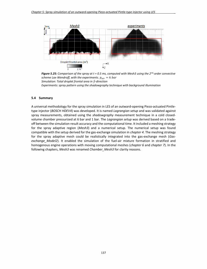
Chapter 5: Spray simulation of an outward-opening Piezo-actuated Pintle-type injector using LES _
137
Figure 5.25: Comparison of the spray at t = 0.5 ms, computed with Mesh3 using the 2nd-order convective scheme Lax-Wendroff, with the experiments. 𝑝 = 6 𝑏𝑎𝑟 Simulation: Total droplet frontal area in ��-direction Experiments: spray pattern using the shadowgraphy technique with background illumination 5.4 Summary A universal methodology for the spray simulation in LES of an outward-opening Piezo-actuated Pintle-type injector (BOSCH HDEV4) was developed. It is named Lagrangian setup and was validated against spray measurements, obtained using the shadowgraphy measurement technique in a cold closed-volume chamber pressurized at 6 bar and 1 bar. The Lagrangian setup was derived based on a trade-off between the simulation result accuracy and the computational time. It included a meshing strategy for the spray adaptive region (Mesh3) and a numerical setup. The numerical setup was found compatible with the setup derived for the gas-exchange simulation in chapter 4. The meshing strategy for the spray adaptive mesh could be realistically integrated into the gas-exchange mesh (Gas-exchange_Model2). It enabled the simulation of the fuel-air mixture formation in stratified and homogenous engine operations with moving computational meshes (chapter 6 and chapter 7). In the following chapters, Mesh3 was renamed Chamber_Mesh3 for clarity reasons.

Chapter 5: Spray simulation of an outward-opening Piezo-actuated Pintle-type injector using LES _
138

139
Chapter 6
Fuel-air mixture formation in stratified engine operation using LES The present chapter covers the simulation and the analysis of the fuel-air mixture formation in stratified engine operation, combining the validated LES flow fields (chapter 4) and the validated spray model (chapter 5). The first goal was the creation of a new moving-mesh strategy to allow the LES multi-cycle simulation of the fuel-air mixture formation in a reasonable CPU-time. A set of moving computational meshes, including the spray adaptive region (Chamber_Mesh3) into the existing Gas-exchange_Model2, were generated in order to cover the period of time between the start of injection (38.8°CA bTDC) and TDC. The second objective was the reproduction in LES of the spray fluctuations of the second injection observed in high-speed PIV by Stiehl [45, 46]. 35 computed flow fields were extracted from the multi-cycle gas-exchange simulation (chapter 4) and mapped onto the newly created mesh before the start of injection. The simulation of the stratified injection process was performed using the mapped flow field for the initialisation of the computational domain. In total 35 consecutive stratified injections were computed in LES. The third target was to understand the consequences of the spray fluctuations on the fuel-air mixture distribution globally and around the spark-plug at the beginning of the combustion. The last goal of this chapter was to analyse the chain of processes involved in the stratified engine operation, and understand the interactions between the in-cylinder flow characteristics, the injection and the fuel-air mixture distribution. These four goals are treated in four distinct parts within the present chapter. 6.1 CFD model and numerical setup The stratified injection process consists of three consecutive injections taking place over a short period of time. The injection timing is defined by three injection durations ti1, ti2 and ti3 and two pause times tp12 and tp23 respectively after the first and the second injections. Table 6.1 recapitulated the injection parameters corresponding to the stratified engine operation at 2000 rpm and 4 bar IMEP selected for this research work.
Table 6.1: Injection parameters for the stratified injection Start of injection 38.8°CA bTDC ti1 250 µs ti2 125 µs ti3 80 µs tp12 562 µs tp23 313 µs Start of ignition 25.5°CA bTDC
The needle lift profile was obtained from the injector characteristics and from the injection parameters used in the experiments (Table 6.1). As explained in 5.2.1, the slope of the injection rate of a Piezo-injector could be adjusted with the applied current. This feature was also taken into account for the derivation of the needle lift profile, which is shown in Fig. 6.1.

Chapter 6: Fuel-air mixture formation in stratified engine operation using LES _
140
Figure 6.1: Injection timing used in the stratified injection simulation. The ignition timing is marked in red
The stratified injection process comprised five distinct phases. As described later in 6.2, each of them had a particular function in the complex fuel-air mixture formation mechanism and required to be correctly captured in the simulation. Therefore, the validated Lagrangian setup for the spray simulation in LES (chapter 5) was integrated into Gas-exchange_Model2 (chapter 4). The different integration steps were described hereafter. 6.1.1 New meshing strategy for the stratified injection The inclusion of the spray adaptive mesh (Chamber_Mesh3) into Gas-exchange_Model2 implied the generation of smaller cells compared to the ones used for the gas-exchange simulation. These cells could not be deformed over a long period of time. Because of their reduced size, they were found rapidly badly distorted and their quality criteria reached quickly the critical limit. It led to a reduction of the time step with the explicit acoustic LES solver and to a huge number of meshes to cover the stratified injection process. This issue represented the first disadvantage of using the Map-Morph technique for in-cylinder flow simulations with very small cells. The second drawback appeared during the simulation using the temporal conditional interpolation (CTI). Due to the increased number of cells in the cylinder, the computation of the displacement of their associated vertices turned out to be extremely time consuming with the Laplace solver. Furthermore, it was sometimes found that the Laplace solver could not reach its convergence criteria and produced very deformed cells with small volumes. It hence negatively affected the time step of the simulation as well as its stability. The meshing setup for the spray adaptive mesh was derived from the LES spray simulation in the closed chamber (chapter 5) without moving boundaries in the computational domain. The position of the mesh was hence fixed over time. In order to guarantee the reproduction of the flow phenomena and the spray knowledge gained with the Lagrangian setup, the integrated Chamber_Mesh3 into the gas-exchange mesh had also to stay static during the simulation of the fuel-air mixture formation. It would hence remove the unknown influence of the changing cell size and the cell deformation rate in the spray adaptive mesh on the simulation results. Furthermore, consistency with the original Lagrangian setup would be achieved. A new moving-mesh strategy was developed for the simulation of the fuel-air mixture formation in LES in order to remove all the aforementioned disadvantages. The cylinder domain was split into two distinct regions:
- The first one included the spray adaptive mesh and the surrounding small-size cells. This region was kept static during the simulation and corresponded to the upper part of the cylinder domain. The bottom part of this region was delimited by a separation layer, located further

Chapter 6: Fuel-air mixture formation in stratified engine operation using LES _
141
down in the cylinder, where the cell sizes were coarser and in the same order of magnitude as the ones found in Gas-exchange_Model2 (~0.5 mm).
- The second region started from the defined separation layer and encompassed the rest of the cylinder domain. This region was characterised by a coarse mesh, which was allowed to be deformed.
A significant reduction of the number of meshes was achieved by allowing only the vertices of the second region with larger cells to move. The newly generated Stratified_Model3 for the simulation of the fuel-air mixture formation was created using this new moving-mesh strategy. The rest of the meshing-setup was kept similar to Gas-exchange_Model2. The geometrical definition and the creation of the separation layer were performed with the CAE software CatiaV5 [128]. As the meshes were generated up to TDC, a particular attention was put into the control of the minimal clearance between the separation layer and the piston surface, in order to avoid the creation of very small cells in Centaur. The optimal shape of the separation layer was found to have a ‘’V-shape’’ and offered two advantages. First, the spark-plug was fully encompassed in the static region allowing a finer mesh resolution around it; secondly, the surface of the piston moving upwards during the simulation stayed nearly parallel to the separation layer. The creation of distorted cells between those two surfaces was hence avoided when the clearance decreased. Fig. 6.2 shows a comparison at 40°CA bTDC of the meshes coming from Gas-exchange_Model2 and Stratified_Model3. The separation layer is marked in red.
Figure 6.2: Mesh in the central tumble plane from Gas-exchange_Model2 (top) and Stratified_Model3 (bottom) with the separation layer (red) at 40°CA bTDC

Chapter 6: Fuel-air mixture formation in stratified engine operation using LES _
142
The original spray adaptive mesh of Chamber_Mesh3 was found to expand deeper than the separation layer location. As a result, small-size cells were produced in the moving mesh region putting at risk the new moving-mesh strategy. Thereby, it was decided to reduce the depth of the spray adaptive mesh, keeping the rest of the meshing setup unmodified. As illustrated in Fig. 6.3, Stratified_Model3 had 25.106 cells more than Gas-exchange_Model2 after the inclusion of the spray adaptive mesh. The minimum cell volume in the computational model was heavily reduced and the simulation time step scaled down accordingly. As expected, the simulation time step was similar to the one in the closed-volume chamber spray simulation (chapter 5) as the minimum cell size was the same in both models.
Figure 6.3: Comparison between Gas-exchange_Model2 and Stratified_Model3 of the total cell number (left) and minimum cell volume (right) in the intake and compression strokes The computation of the stratified injection process was achieved using five meshes, i.e. five distinct computational phases with the newly generated Stratified_Model3. As a comparison, Gas-exchange_Model2 needed only three computational phases to cover the same period of time. The introduction of the separation layer had introduced additional constraints for the vertex displacement in the moving mesh region of the cylinder, explaining the increased number of meshes. However, it was absolutely justified in order to achieve the highest possible cell quality without deforming excessively the shape of the cells. The starting and ending crank-angle positions of the five computational phases were manually adjusted to match the five periods characterising the stratified injection process. Fig. 6.1 shows the injector needle lift profile together with the corresponding computational phases during the stratified injection process. Phase1, Phase3 and Phase5 covered respectively the first, second and third injections, whereas Phase2 and Phase4 included the two pause times after the first and the second injections. The simulation took around 18hours on 96 cores to run one stratified injection simulation with the five consecutive computational phases. 6.1.2 Numerical setup The numerical setup was taken over from the Lagrangian setup. As liquid fuel interaction with the spark-plug geometry cannot be avoided in stratified engine operation, the slip droplet-wall interaction model was selected. No formation of liquid film was considered at the wall, as it was not the focus of this study. Following the approach of Iafrate [69], the normal velocity component of the droplet was set to zero when the droplet reached the wall, allowing its further motion parallel to the wall. The injected fuel mass for the injection was derived from the injection quantity baseline of the Piezo-injector. On the gas side, the aforementioned setup also matched with the one used in Gas-exchange_Model2 for the gas-exchange simulation and was hence conserved. 35 computed flow fields were extracted from the multi-cycle gas-exchange simulation (chapter 4) and mapped onto Stratified_Model3 before the start of injection at 38.8°CA bTDC. They provided the initial flow fields for the corresponding 35 stratified injection simulations that were run successively with Stratified_Model3. The instantaneous flow field and the droplet information were saved every 0.5°CA during the simulation in order to guarantee enough post-processing data for the analysis of the fuel-air mixture formation.
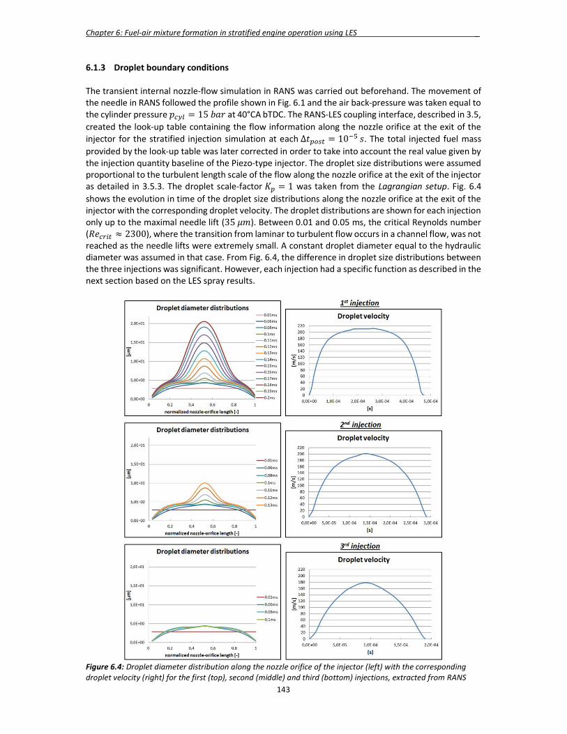
Chapter 6: Fuel-air mixture formation in stratified engine operation using LES _
143
6.1.3 Droplet boundary conditions The transient internal nozzle-flow simulation in RANS was carried out beforehand. The movement of the needle in RANS followed the profile shown in Fig. 6.1 and the air back-pressure was taken equal to the cylinder pressure 𝑝 = 15 𝑏𝑎𝑟 at 40°CA bTDC. The RANS-LES coupling interface, described in 3.5, created the look-up table containing the flow information along the nozzle orifice at the exit of the injector for the stratified injection simulation at each ∆𝑡 = 10 𝑠. The total injected fuel mass provided by the look-up table was later corrected in order to take into account the real value given by the injection quantity baseline of the Piezo-type injector. The droplet size distributions were assumed proportional to the turbulent length scale of the flow along the nozzle orifice at the exit of the injector as detailed in 3.5.3. The droplet scale-factor 𝐾 = 1 was taken from the Lagrangian setup. Fig. 6.4 shows the evolution in time of the droplet size distributions along the nozzle orifice at the exit of the injector with the corresponding droplet velocity. The droplet distributions are shown for each injection only up to the maximal needle lift (35 𝜇𝑚). Between 0.01 and 0.05 ms, the critical Reynolds number (𝑅𝑒 ≈ 2300), where the transition from laminar to turbulent flow occurs in a channel flow, was not reached as the needle lifts were extremely small. A constant droplet diameter equal to the hydraulic diameter was assumed in that case. From Fig. 6.4, the difference in droplet size distributions between the three injections was significant. However, each injection had a specific function as described in the next section based on the LES spray results.
Figure 6.4: Droplet diameter distribution along the nozzle orifice of the injector (left) with the corresponding droplet velocity (right) for the first (top), second (middle) and third (bottom) injections, extracted from RANS
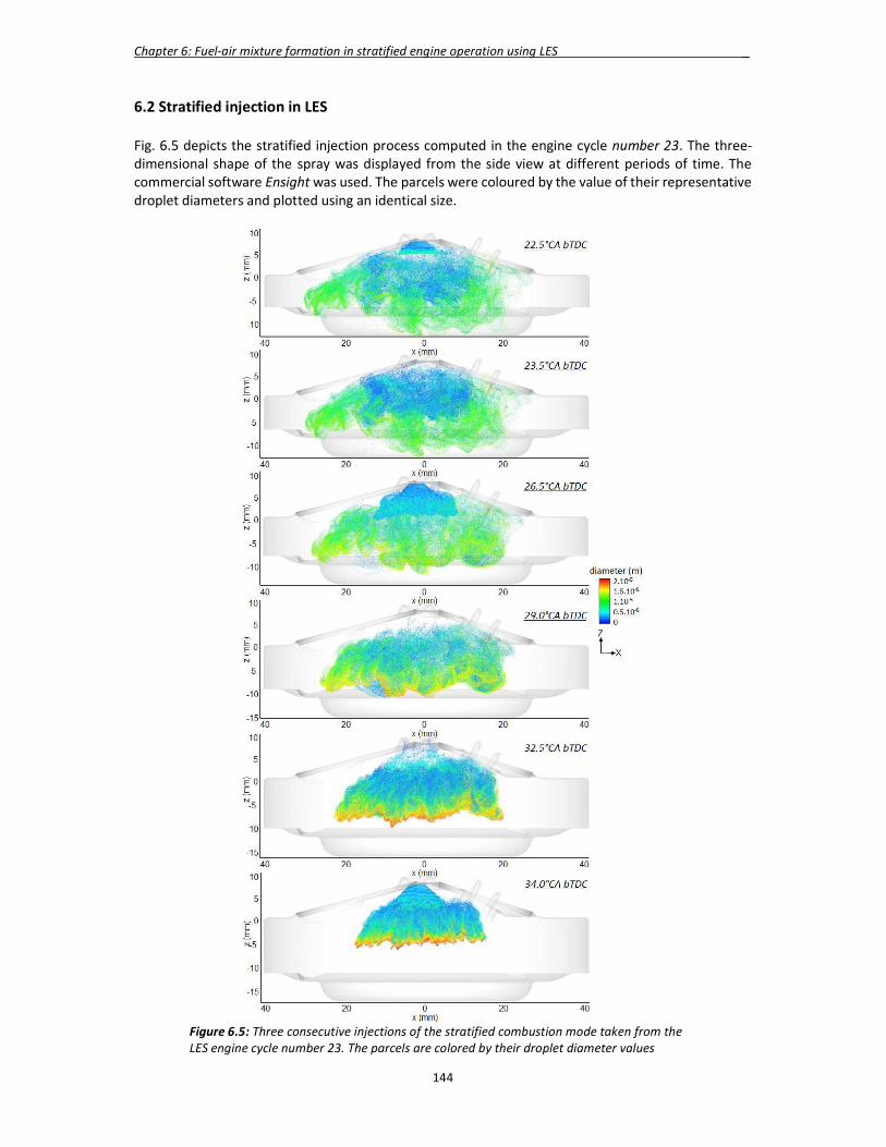
Chapter 6: Fuel-air mixture formation in stratified engine operation using LES _
144
6.2 Stratified injection in LES Fig. 6.5 depicts the stratified injection process computed in the engine cycle number 23. The three-dimensional shape of the spray was displayed from the side view at different periods of time. The commercial software Ensight was used. The parcels were coloured by the value of their representative droplet diameters and plotted using an identical size.
Figure 6.5: Three consecutive injections of the stratified combustion mode taken from the LES engine cycle number 23. The parcels are colored by their droplet diameter values

Chapter 6: Fuel-air mixture formation in stratified engine operation using LES _
145
In stratified engine operation, the first injection duration depends on the engine load. It is the main injection, where most of the fuel is injected into the cylinder. The pause time until the start of the second injection controls the evaporation process of the injected fuel. At maximal needle lift, the maximal droplet size is close to 20 µm and the injected droplet velocity reaches to 210 m/s. Although the mass flow rate of a Piezo-injector is twice as big as in a multi-hole injector, the spray penetration is reduced by half and its evaporation rate by four when injecting at the end of the compression stroke [54]. As a result, no wall wetting takes place, except at the spark-plug location, due to its deep positioning in the cylinder as illustrated in the three pictures at the bottom of Fig. 6.5. The second injection, depicted in the third picture from the top in Fig. 6.5, was characterised by a needle lift reaching 70 % of the maximal needle lift. The largest droplet size was lowered by a factor of two but the droplet velocities still reached 200 m/s. The penetration length of the spray was hence reduced so that the fuel-air mixture, formed locally in the torus-shaped structure of the spray, could be ignited at the end of this injection. As the droplet sizes in this region were much smaller than in the core of the spray, the combustion process was found extremely sensitive to the fluctuation of the second injection and the in-cylinder flow [46, 47]. Finally, the third injection featured an even smaller needle lift and droplet size spectrum, as shown in the top picture of Fig. 6.5. The role of this last injection was to sustain the early phase of the combustion by generating additional turbulence. 6.3 Spray fluctuation analysis during the 2nd injection From the 35 stratified injections computed in LES, the fluctuations of the spray of the second injection were investigated. Stiehl performed the same analysis in the optically-accessible single-cylinder DISI [45, 46]. The tilting of the spray had to be first carefully quantified to reproduce the high-speed PIV observations. The understanding of the flow phenomena, which led to the spray fluctuations, could be derived afterwards. 6.3.1 Definition of the spray geometrical parameters The main difficulty was to choose the suitable crank-angle position during the second injection, where the analysis of the spray could be performed. A compromise had to be made between the spray penetration length and the flow momentum within the spray. High spray penetration was noticed for crank-angle positions located on the decreasing slope of the injection profile i.e. closing needle. Due to the reduced velocity of the injected droplets, the flow momentum within the spray was weaker making the spray more sensitive to the variation of the flow field velocity. As a result, the detection of the spray front was found more difficult to achieve for such crank-angle positions. Therefore, it was decided to carry out the spray analysis at 27°CA bTDC, which was 0.5°CA after the maximal needle lift of the second injection. The flow momentum within the spray was still very high and the spray penetration deep enough to perform a reliable spray front detection. The investigations made on fluctuating sprays with high-speed PIV had all shown that the spray was already deflected at maximal needle lift in the 2nd injection [45, 46]. Based on these experimental observations, the crank-angle chosen for the analysis of the spray in LES was hence assumed consistent. From the examination of the 35 sprays at 27°CA bTDC, cyclic variations of the global spray shape could be clearly observed. However, it was concluded that it was nearly impossible to quantify the cyclic variations of the spray, based on the three-dimensional information of the spray in LES. Its shape was found extremely complex. Moreover, some parcels from the first injection were still present in the cylinder making the parcel distinction between the two injections difficult.
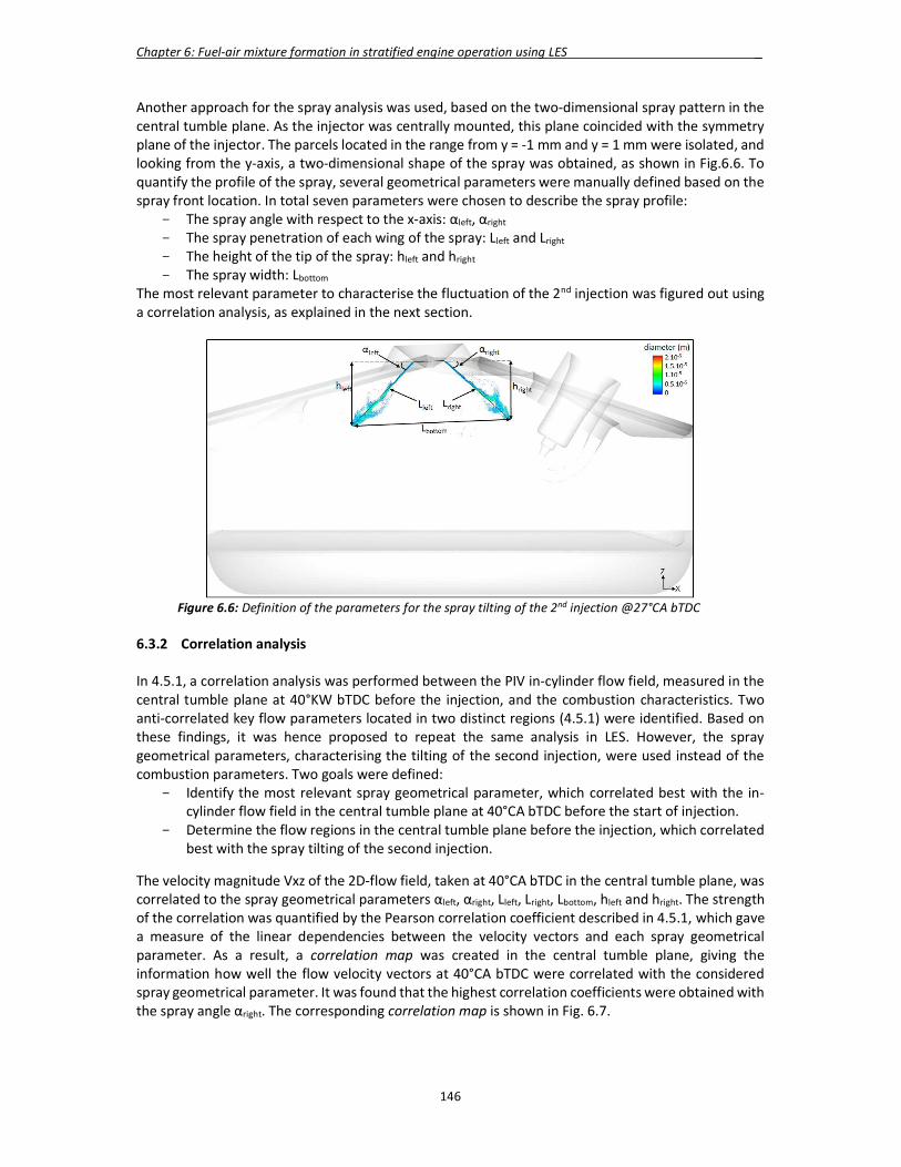
Chapter 6: Fuel-air mixture formation in stratified engine operation using LES _
146
Another approach for the spray analysis was used, based on the two-dimensional spray pattern in the central tumble plane. As the injector was centrally mounted, this plane coincided with the symmetry plane of the injector. The parcels located in the range from y = -1 mm and y = 1 mm were isolated, and looking from the y-axis, a two-dimensional shape of the spray was obtained, as shown in Fig.6.6. To quantify the profile of the spray, several geometrical parameters were manually defined based on the spray front location. In total seven parameters were chosen to describe the spray profile:
- The spray angle with respect to the x-axis: αleft, αright - The spray penetration of each wing of the spray: Lleft and Lright - The height of the tip of the spray: hleft and hright - The spray width: Lbottom
The most relevant parameter to characterise the fluctuation of the 2nd injection was figured out using a correlation analysis, as explained in the next section.
Figure 6.6: Definition of the parameters for the spray tilting of the 2nd injection @27°CA bTDC 6.3.2 Correlation analysis In 4.5.1, a correlation analysis was performed between the PIV in-cylinder flow field, measured in the central tumble plane at 40°KW bTDC before the injection, and the combustion characteristics. Two anti-correlated key flow parameters located in two distinct regions (4.5.1) were identified. Based on these findings, it was hence proposed to repeat the same analysis in LES. However, the spray geometrical parameters, characterising the tilting of the second injection, were used instead of the combustion parameters. Two goals were defined:
- Identify the most relevant spray geometrical parameter, which correlated best with the in-cylinder flow field in the central tumble plane at 40°CA bTDC before the start of injection.
- Determine the flow regions in the central tumble plane before the injection, which correlated best with the spray tilting of the second injection.
The velocity magnitude Vxz of the 2D-flow field, taken at 40°CA bTDC in the central tumble plane, was correlated to the spray geometrical parameters αleft, αright, Lleft, Lright, Lbottom, hleft and hright. The strength of the correlation was quantified by the Pearson correlation coefficient described in 4.5.1, which gave a measure of the linear dependencies between the velocity vectors and each spray geometrical parameter. As a result, a correlation map was created in the central tumble plane, giving the information how well the flow velocity vectors at 40°CA bTDC were correlated with the considered spray geometrical parameter. It was found that the highest correlation coefficients were obtained with the spray angle αright. The corresponding correlation map is shown in Fig. 6.7.
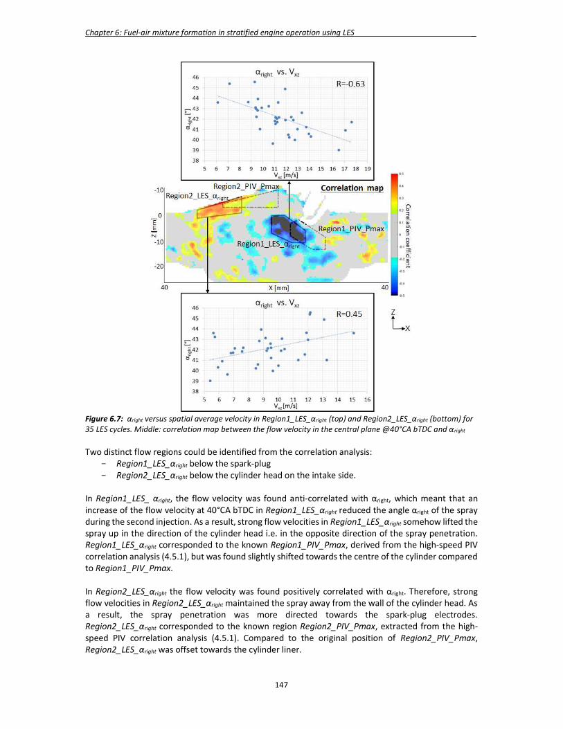
Chapter 6: Fuel-air mixture formation in stratified engine operation using LES _
147
Figure 6.7: αright versus spatial average velocity in Region1_LES_αright (top) and Region2_LES_αright (bottom) for 35 LES cycles. Middle: correlation map between the flow velocity in the central plane @40°CA bTDC and αright
Two distinct flow regions could be identified from the correlation analysis:
- Region1_LES_αright below the spark-plug - Region2_LES_αright below the cylinder head on the intake side.
In Region1_LES_ αright, the flow velocity was found anti-correlated with αright, which meant that an increase of the flow velocity at 40°CA bTDC in Region1_LES_αright reduced the angle αright of the spray during the second injection. As a result, strong flow velocities in Region1_LES_αright somehow lifted the spray up in the direction of the cylinder head i.e. in the opposite direction of the spray penetration. Region1_LES_αright corresponded to the known Region1_PIV_Pmax, derived from the high-speed PIV correlation analysis (4.5.1), but was found slightly shifted towards the centre of the cylinder compared to Region1_PIV_Pmax. In Region2_LES_αright the flow velocity was found positively correlated with αright. Therefore, strong flow velocities in Region2_LES_αright maintained the spray away from the wall of the cylinder head. As a result, the spray penetration was more directed towards the spark-plug electrodes. Region2_LES_αright corresponded to the known region Region2_PIV_Pmax, extracted from the high-speed PIV correlation analysis (4.5.1). Compared to the original position of Region2_PIV_Pmax, Region2_LES_αright was offset towards the cylinder liner.

Chapter 6: Fuel-air mixture formation in stratified engine operation using LES _
148
Fig. 6.7 shows the scatter plots of the spatial average velocity, computed in Region1_LES_αright and Region2_LES_αright as a function of αright for the 35 LES cycles. The Pearson correlation coefficient in Region1_LES_αright was found to be -0.63 and in Region2_LES_αright 0.45. For a sample size of 35 and a significance level α = 0.01, the critical value of the Pearson correlation coefficient is equal to 0.402, following the methodology described in 4.5.1. It confirmed that the findings had statistical significance and that there was a strong linear correlation between the local flow velocity in both regions and the tilting of the spray of the 2nd injection.
From the correlation analysis between the tilting of the spray of the 2nd injection and the flow velocity before the injection, the existence of the two anti-correlated flow regions, found in high-speed PIV, was confirmed. Their positions were slightly different but their meanings remained the same. Strong flow velocities in Region2_LES_αright and Region2_PIV_Pmax stabilised the position of the spray during the second injection and improved the combustion. Instead, strong flow velocities in Region1_LES_αright and Region1_PIV_Pmax deflected the spray and deteriorated the combustion. 6.3.3 Conditional statistics Conditional statistics were used in the two new regions derived previously in order to extract the extreme engine cycles. The goal was to compare the conditionally-averaged flow fields in LES obtained with these two regions and with the regions coming from the PIV correlation analysis in 4.5.1. The conditional analysis, presented in 4.5.1, was repeated considering this time Region1_LES_αright and Region2_LES_αright. The spatial average velocity (Vxz) within the two regions was first computed for every individual cycle at 40°CA bTDC. The histograms in Fig. 6.8 shows the respective distributions of the spatial average velocity magnitude for all 35 cycles. The ensemble-averaged velocity flow field over 35 cycles was also plotted together with the defined regions. The method of conditional statistics was applied to the 12% extreme cycles on each wing of the flow velocity distributions of each region, as shown in Fig. 6.8.
Figure 6.8: Distribution of the spatial average velocity (Vxz) for all 35 cycles for Region1_LES_αright (right) and Region2_LES_αright (left) together with the 12% extreme cycles. Middle: Ensemble average LES velocity over 35 cycles (Gas-exchange_Model2)

Chapter 6: Fuel-air mixture formation in stratified engine operation using LES _
149
The phase-averaged flow fields of the respective 12% of the 35 LES cycles with the lowest (green) and highest (red) velocity magnitude in the defined regions were determined from 60-40°CA bTDC in the central planes. Fig. 6.9 depicts the conditionally-averaged LES flow fields computed with Region1_LES_αright and Region2_LES_αright at 40°CA bTDC. Although the region definition in the central plane before the start of injection was slightly different to the region definition coming from the PIV correlation analysis, the conditionally-averaged LES flow fields looked similar to the previous ones in Fig.4.34-35.
Figure 6.9: Conditionally-averaged LES flow field at 40° CA bTDC for the cycles with the
12% largest and 12% smallest velocity magnitude in Region1_LES_αright (right) and Region2_LES_αright (left) In order to further validate the conditionally-averaged flow field obtained at 40°CA bTDC, this analysis was extended to both intake valve planes defined at y = -18 mm and y = 18 mm from 60-40°CA bTDC. As shown in Fig. 6.10 and Fig. 6.11, the formation of the jet-flow in the middle of the cylinder and the secondary flow along the cylinder wall, were well reproduced for the cases exhibiting strong ‘upward flow’ (12% high) in Region1_LES_αright and the “low” velocity case (12% low) in Region2_LES_αright. The higher velocities in the intake valve planes and their decreasing intensity trend were also well captured. The momentum transfer, taking place from the intake valve plane to the central tumble plane, could be clearly recognized, too. Furthermore, for the “low” velocity case in Region1_LES_αright and the “high” velocity case in Region2_LES_αright, similar in-plane velocity intensities were reported in all planes, hinting at the presence of the expected global tumble vortex. The conditionally-averaged flow fields matched very well with the ones using Region1_PIV_Pmax and Region2_PIV_Pmax shown in chapter 4 (Fig. 4.36-39). The reproduction of the two different global flow structures in the central tumble plane i.e. jet-flow structure and global tumble vortex, could be achieved using the conditional statistics applied in the new Region1_LES_αright and Region2_LES_αright. It confirmed that the same flow phenomena were responsible for the fluctuation of the spray during the second injection (LES correlation results) and the stability of the combustion (PIV correlation results). The two associated key flow parameters influenced the second injection as follows: a strong ‘upward flow’ in Region1_LES_αright implied a fluctuation of the spray, whereas a strong horizontal-oriented flow in Region2_LES_αright stabilised it. The results were found consistent with the experimental results from Stiehl [45, 46].
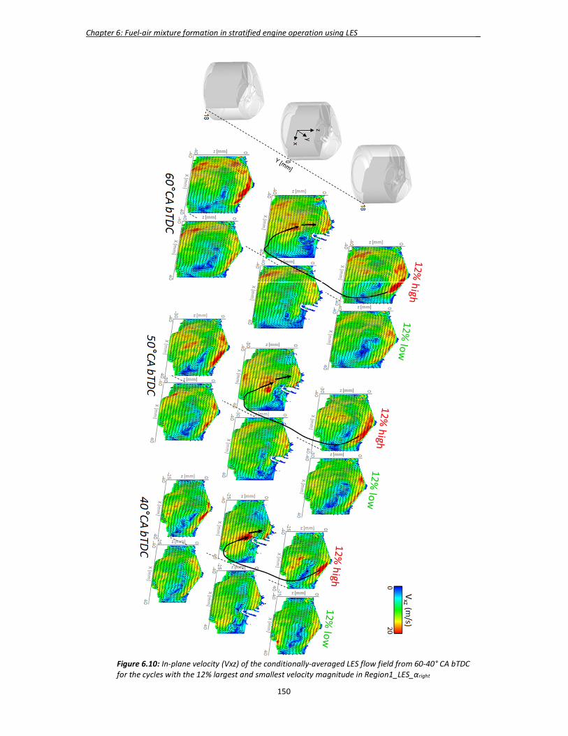
Chapter 6: Fuel-air mixture formation in stratified engine operation using LES _
150
Figure 6.10: In-plane velocity (Vxz) of the conditionally-averaged LES flow field from 60-40° CA bTDC for the cycles with the 12% largest and smallest velocity magnitude in Region1_LES_αright
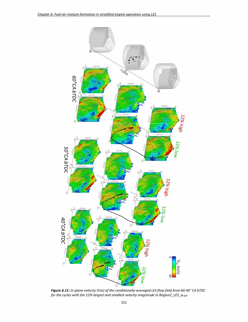
Chapter 6: Fuel-air mixture formation in stratified engine operation using LES _
151
Figure 6.11: In-plane velocity (Vxz) of the conditionally-averaged LES flow field from 60-40° CA bTDC for the cycles with the 12% largest and smallest velocity magnitude in Region2_LES_αright
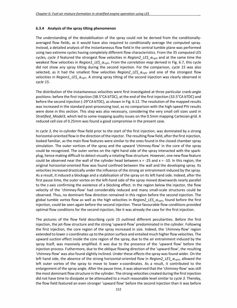
Chapter 6: Fuel-air mixture formation in stratified engine operation using LES _
152
6.3.4 Analysis of the spray tilting phenomenon The understanding of the destabilisation of the spray could not be derived from the conditionally-averaged flow fields, as it would have also required to conditionally average the computed spray. Instead, a detailed analysis of the instantaneous flow field in the central tumble plane was performed using two extreme cycles having completely different flow characteristics. From the 35 computed LES cycles, cycle 3 featured the strongest flow velocities in Region2_LES_αright and at the same time the weakest flow velocities in Region1_LES_αright. From the correlation map derived in Fig. 6.7, this cycle did not show any spray tilting during the second injection. For the comparison, cycle 15 was also selected, as it had the smallest flow velocities Region2_LES_αright and one of the strongest flow velocities in Region1_LES_αright. A strong spray tilting of the second injection was clearly observed in cycle 15. The distribution of the instantaneous velocities were first investigated at three particular crank-angle positions: before the first injection (38.5°CA bTDC), at the end of the first injection (33.5°CA bTDC) and before the second injection (-29°CA bTDC), as shown in Fig. 6.12. The resolution of the mapped results was increased in the standard post-processing tool, as no comparison with the high-speed PIV results were done in this section. This step was also necessary, considering the very small cell sizes used in Stratified_Model3, which led to some mapping quality issues on the 0.5mm mapping Cartesian grid. A reduced cell size of 0.25mm was found a good compromise in the present case. In cycle 3, the in-cylinder flow field prior to the start of the first injection, was dominated by a strong horizontal-oriented flow in the direction of the injector. The resulting flow field, after the first injection, looked familiar, as the main flow features were similar to the ones found in the closed chamber spray simulation. The outer vortices of the spray and the upward ‘chimney-flow’ in the core of the spray could be recognized. The outer vortex on the right-hand side of the spray interacted with the spark-plug, hence making difficult to detect visually a rotating flow structure. However, one new flow feature could be observed near the wall of the cylinder head between x = -25 and x = -10. In this region, the original horizontal-oriented flow was found confined between the wall and the developing spray. Its velocities increased drastically under the influence of the strong air entrainment induced by the spray. As a result, it induced a blockage and a stabilisation of the spray on its left hand side. Indeed, after the first pause time, the outer vortex on the left-hand side of the spray moved downwards nearly parallel to the z-axis confirming the existence of a blocking effect. In the region below the injector, the flow velocity of the ‘chimney-flow’ had considerably reduced and many small-scale structures could be observed. Thus, no dominant flow direction remained in this region before the second injection. The global tumble vortex flow as well as the high velocities in Region2_LES_αright, found before the first injection, could be seen again before the second injection. These favourable flow conditions provided optimal flow conditions for the second injection, like it was already the case for the first injection. The pictures of the flow field describing cycle 15 outlined different peculiarities. Before the first injection, the jet-flow structure and the strong ‘upward-flow’ predominated in the cylinder. Following the first injection, the core region of the spray increased in size. Indeed, the ‘chimney-flow’ region extended to lower z-coordinates up to the piston surface and entailed much higher flow velocities. The upward suction effect inside the core region of the spray, due to the air entrainment induced by the spray itself, was massively amplified. It was due to the presence of the ‘upward flow’ before the injection process. Futhermore, due to the oblique flowing direction of the ‘upward flow’, the resulting ‘chimney-flow’ was also found slightly inclined. Under these effects the spray was found wider. On the left hand side, the absence of the strong horizontal-oriented flow in Region2_LES_αright, allowed the left outer vortex of the spray to move to lower x-coordinates. As a result, it contributed to the enlargement of the spray angle. After the pause time, it was observed that the ‘chimney-flow’ was still the most dominant flow structure in the cylinder. The strong velocities created during the first injection did not have time to dissipate or be attenuated to a much reasonable level similar to cycle 3. Thereby, the flow field featured an even stronger ‘upward flow’ before the second injection than it was before
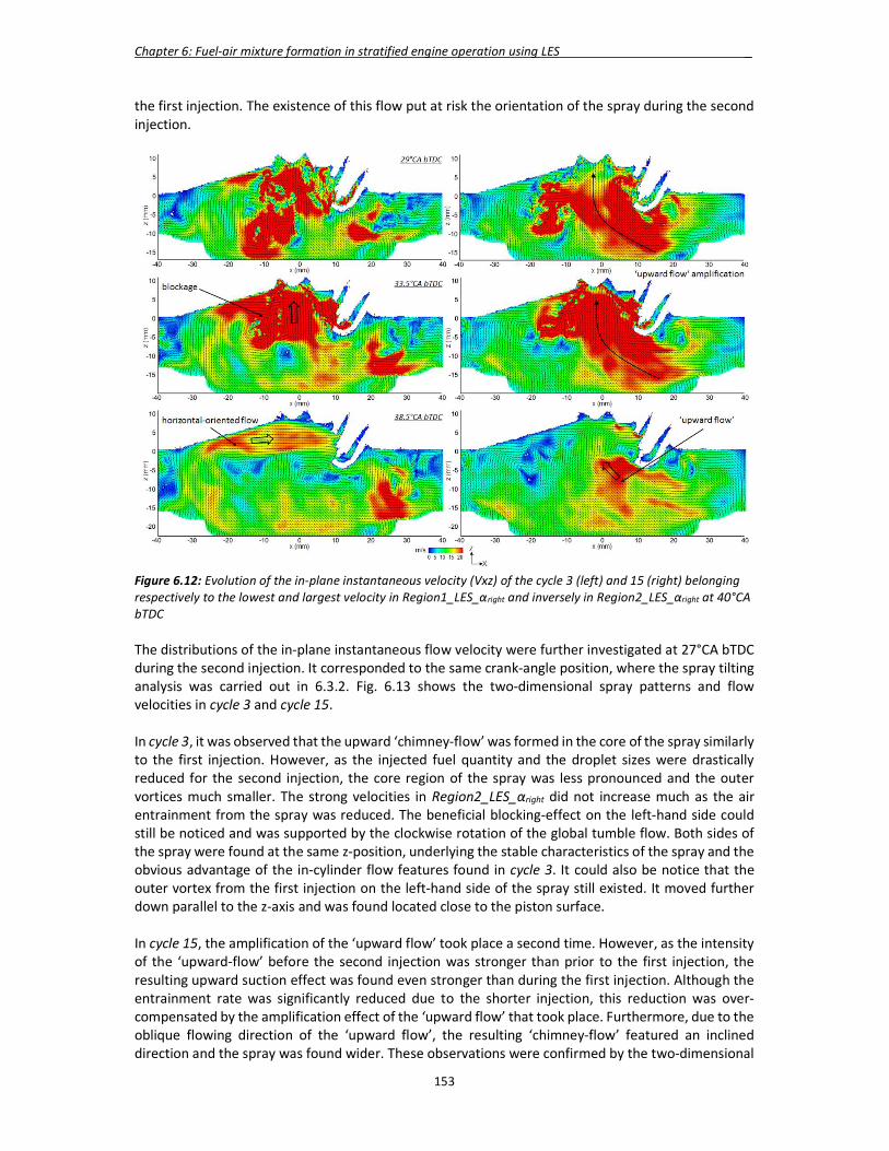
Chapter 6: Fuel-air mixture formation in stratified engine operation using LES _
153
the first injection. The existence of this flow put at risk the orientation of the spray during the second injection.
Figure 6.12: Evolution of the in-plane instantaneous velocity (Vxz) of the cycle 3 (left) and 15 (right) belonging respectively to the lowest and largest velocity in Region1_LES_αright and inversely in Region2_LES_αright at 40°CA bTDC The distributions of the in-plane instantaneous flow velocity were further investigated at 27°CA bTDC during the second injection. It corresponded to the same crank-angle position, where the spray tilting analysis was carried out in 6.3.2. Fig. 6.13 shows the two-dimensional spray patterns and flow velocities in cycle 3 and cycle 15. In cycle 3, it was observed that the upward ‘chimney-flow’ was formed in the core of the spray similarly to the first injection. However, as the injected fuel quantity and the droplet sizes were drastically reduced for the second injection, the core region of the spray was less pronounced and the outer vortices much smaller. The strong velocities in Region2_LES_αright did not increase much as the air entrainment from the spray was reduced. The beneficial blocking-effect on the left-hand side could still be noticed and was supported by the clockwise rotation of the global tumble flow. Both sides of the spray were found at the same z-position, underlying the stable characteristics of the spray and the obvious advantage of the in-cylinder flow features found in cycle 3. It could also be notice that the outer vortex from the first injection on the left-hand side of the spray still existed. It moved further down parallel to the z-axis and was found located close to the piston surface. In cycle 15, the amplification of the ‘upward flow’ took place a second time. However, as the intensity of the ‘upward-flow’ before the second injection was stronger than prior to the first injection, the resulting upward suction effect was found even stronger than during the first injection. Although the entrainment rate was significantly reduced due to the shorter injection, this reduction was over-compensated by the amplification effect of the ‘upward flow’ that took place. Furthermore, due to the oblique flowing direction of the ‘upward flow’, the resulting ‘chimney-flow’ featured an inclined direction and the spray was found wider. These observations were confirmed by the two-dimensional

Chapter 6: Fuel-air mixture formation in stratified engine operation using LES _
154
spray pattern, where a clear tilting of the spray was observed. It emphasized the detrimental nature of the ‘upward flow’ before the start of the stratified injection process. It was found that each injection could amplify the intensity of the ‘upward flow’, leading to far too high velocity magnitudes during the second injection and to the deflection of the spray. The pause time between the first and the second injection was too short to allow these high velocities to dissipate naturally. Like observed in cycle 3, the outer vortex from the first injection on the left-hand side of the spray was still alive. However, its position was moved at a higher z-coordinate and a lower x-coordinate due to the wider angle of the spray. The flow phenomena involved in the fluctuation of the spray during the second injection were clearly identified. The interaction process between the in-cylinder flow and the spray was found crucial to control the stability of the spray.
Figure 6.13: Top: Two-dimensional spray pattern at 27°CA bTDC of the cycle 3 (left) and 15 (right) belonging respectively to the lowest and largest velocity in Region1_LES_αright and inversely in Region2_LES_αright at 40°CA bTDC Bottom: corresponding in-plane instantaneous velocity (Vxz) of the cycle 3 (left) and 15 (right) 6.4 Analysis of the fuel-air mixture In stratified engine operation, the ignition takes place immediately after the second injection process. The fluctuating spray orientation during the second injection was expected to have important repercussions on the formation of the fuel-air mixture. The fuel-air mixture information is a key parameter for the combustion process but cannot be easily captured experimentally in the combustion chamber. It was hence proposed to analyse the fuel-air mixture in LES globally in the combustion chamber and locally around the spark-plug. The aim was to extend the understanding of the chain of cause-and-effect up to the beginning of the combustion process. 6.4.1 Analysis of the global fuel-air mixture distribution The concentration of the fuel-air mixture was characterized using the fuel-air equivalence ratio φ. It is defined as the ratio of the fuel-to-oxidizer ratio to the stoichiometric fuel-to-oxidizer ratio. It describes the proportion of fuel relative to the amount of fuel that potentially could be burnt with the available oxidizer. For stoichiometric mixture, the equivalence ratio is defined to be φ = 1. φ > 1 describes fuel-rich mixtures, i.e. excess fuel, whereas φ < 1 defines fuel-lean mixtures i.e. excess oxidizer. Mathematically it gives,
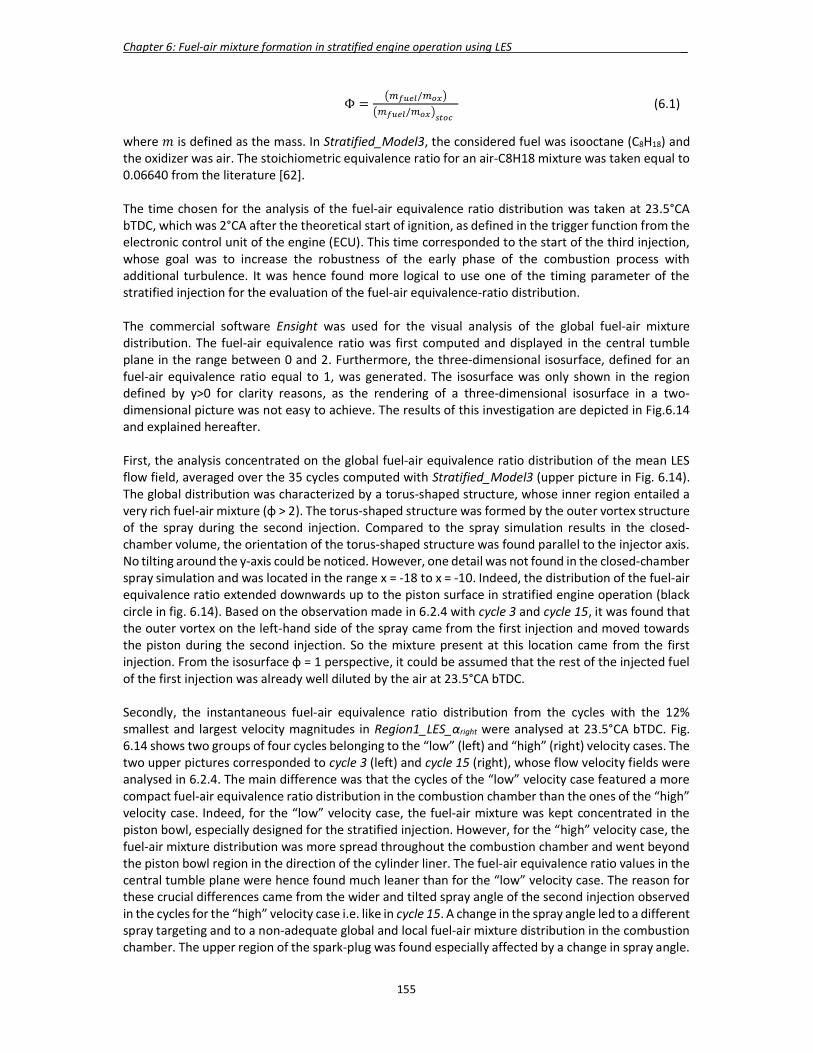
Chapter 6: Fuel-air mixture formation in stratified engine operation using LES _
155
Φ =/
/ (6.1)
where 𝑚 is defined as the mass. In Stratified_Model3, the considered fuel was isooctane (C8H18) and the oxidizer was air. The stoichiometric equivalence ratio for an air-C8H18 mixture was taken equal to 0.06640 from the literature [62]. The time chosen for the analysis of the fuel-air equivalence ratio distribution was taken at 23.5°CA bTDC, which was 2°CA after the theoretical start of ignition, as defined in the trigger function from the electronic control unit of the engine (ECU). This time corresponded to the start of the third injection, whose goal was to increase the robustness of the early phase of the combustion process with additional turbulence. It was hence found more logical to use one of the timing parameter of the stratified injection for the evaluation of the fuel-air equivalence-ratio distribution. The commercial software Ensight was used for the visual analysis of the global fuel-air mixture distribution. The fuel-air equivalence ratio was first computed and displayed in the central tumble plane in the range between 0 and 2. Furthermore, the three-dimensional isosurface, defined for an fuel-air equivalence ratio equal to 1, was generated. The isosurface was only shown in the region defined by y>0 for clarity reasons, as the rendering of a three-dimensional isosurface in a two-dimensional picture was not easy to achieve. The results of this investigation are depicted in Fig.6.14 and explained hereafter. First, the analysis concentrated on the global fuel-air equivalence ratio distribution of the mean LES flow field, averaged over the 35 cycles computed with Stratified_Model3 (upper picture in Fig. 6.14). The global distribution was characterized by a torus-shaped structure, whose inner region entailed a very rich fuel-air mixture (φ > 2). The torus-shaped structure was formed by the outer vortex structure of the spray during the second injection. Compared to the spray simulation results in the closed-chamber volume, the orientation of the torus-shaped structure was found parallel to the injector axis. No tilting around the y-axis could be noticed. However, one detail was not found in the closed-chamber spray simulation and was located in the range x = -18 to x = -10. Indeed, the distribution of the fuel-air equivalence ratio extended downwards up to the piston surface in stratified engine operation (black circle in fig. 6.14). Based on the observation made in 6.2.4 with cycle 3 and cycle 15, it was found that the outer vortex on the left-hand side of the spray came from the first injection and moved towards the piston during the second injection. So the mixture present at this location came from the first injection. From the isosurface φ = 1 perspective, it could be assumed that the rest of the injected fuel of the first injection was already well diluted by the air at 23.5°CA bTDC. Secondly, the instantaneous fuel-air equivalence ratio distribution from the cycles with the 12% smallest and largest velocity magnitudes in Region1_LES_αright were analysed at 23.5°CA bTDC. Fig. 6.14 shows two groups of four cycles belonging to the “low” (left) and “high” (right) velocity cases. The two upper pictures corresponded to cycle 3 (left) and cycle 15 (right), whose flow velocity fields were analysed in 6.2.4. The main difference was that the cycles of the “low” velocity case featured a more compact fuel-air equivalence ratio distribution in the combustion chamber than the ones of the “high” velocity case. Indeed, for the “low” velocity case, the fuel-air mixture was kept concentrated in the piston bowl, especially designed for the stratified injection. However, for the “high” velocity case, the fuel-air mixture distribution was more spread throughout the combustion chamber and went beyond the piston bowl region in the direction of the cylinder liner. The fuel-air equivalence ratio values in the central tumble plane were hence found much leaner than for the “low” velocity case. The reason for these crucial differences came from the wider and tilted spray angle of the second injection observed in the cycles for the “high” velocity case i.e. like in cycle 15. A change in the spray angle led to a different spray targeting and to a non-adequate global and local fuel-air mixture distribution in the combustion chamber. The upper region of the spark-plug was found especially affected by a change in spray angle.
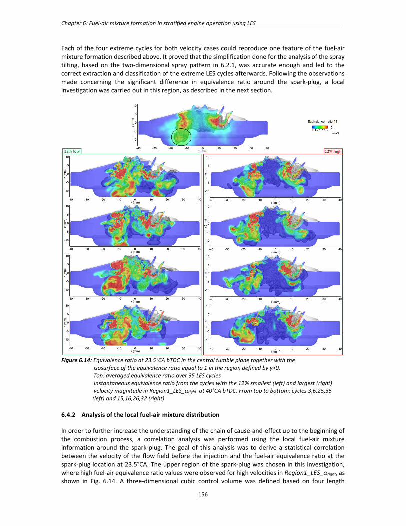
Chapter 6: Fuel-air mixture formation in stratified engine operation using LES _
156
Each of the four extreme cycles for both velocity cases could reproduce one feature of the fuel-air mixture formation described above. It proved that the simplification done for the analysis of the spray tilting, based on the two-dimensional spray pattern in 6.2.1, was accurate enough and led to the correct extraction and classification of the extreme LES cycles afterwards. Following the observations made concerning the significant difference in equivalence ratio around the spark-plug, a local investigation was carried out in this region, as described in the next section.
Figure 6.14: Equivalence ratio at 23.5°CA bTDC in the central tumble plane together with the isosurface of the equivalence ratio equal to 1 in the region defined by y>0. Top: averaged equivalence ratio over 35 LES cycles Instantaneous equivalence ratio from the cycles with the 12% smallest (left) and largest (right) velocity magnitude in Region1_LES_αright at 40°CA bTDC. From top to bottom: cycles 3,6,25,35 (left) and 15,16,26,32 (right) 6.4.2 Analysis of the local fuel-air mixture distribution In order to further increase the understanding of the chain of cause-and-effect up to the beginning of the combustion process, a correlation analysis was performed using the local fuel-air mixture information around the spark-plug. The goal of this analysis was to derive a statistical correlation between the velocity of the flow field before the injection and the fuel-air equivalence ratio at the spark-plug location at 23.5°CA. The upper region of the spark-plug was chosen in this investigation, where high fuel-air equivalence ratio values were observed for high velocities in Region1_LES_αright, as shown in Fig. 6.14. A three-dimensional cubic control volume was defined based on four length

Chapter 6: Fuel-air mixture formation in stratified engine operation using LES _
157
parameters Lx1, Lx2, Ly and Lz. Its symmetry plane coincided with the central tumble plane. The centre of the control volume was taken at the surface of the lower electrode and was positioned aligned with the middle point between the two electrodes with respect to the z-axis. An iterative process, based on the correlation analysis described afterwards, allowed the determination of the best fitting length parameters. The final control volume is shown in Fig. 6.15 together with the definition of the length parameters.
Figure 6.15: Definition of the control volume for the local fuel-air equivalence ratio analysis at 23.5°CA bTDC
Correlation analysis A correlation analysis was performed between the instantaneous flow fields of the computed LES cycles before the injection and the fuel-air equivalence ratio in a control volume around the spark-plug at the beginning of the combustion process. The local velocity magnitude (Vxz) of the 2D-flow field taken at 40°CA bTDC from the central tumble plane was correlated to the spatially-averaged fuel-air equivalence ratio at 23.5°CA bTDC in the control volume. The strength of the correlation was quantified by a correlation coefficient, which gave a measure of the linear dependencies between the velocity vectors and the fuel-air equivalence ratio. As a result, a correlation map was created addressing all the velocity vectors in the central tumble plane. The aim of this statistical analysis was to confirm that the visual observations, made with the fuel-air equivalence ratio in the upper region of the spark-plug, were indeed linked to the difference in flow characteristics @40°CA bTDC, as shown in Fig. 6.14. Assuming that these observations were correct, the two known key flow parameters and their respective regions should also be correlated with the fuel-air equivalence ratio in the upper region of the spark-plug. Therefore, the size of the control volume was iteratively optimized in order to achieve the highest spatially-averaged correlation factor in the existing Region1_LES_αright. The final length parameters of the control volume are summarised in Table 6.2 and the corresponding correlation map is shown in Fig. 6.16.
Table 6.2: Length parameters of the final control volume around the spark-plug Parameters Lx1 Lx2 Ly Lz
Length (mm) 2,5 4,5 4,5 9,0 The existing Region1_LES_αright and Region2_LES_αright could be reproduced from the correlation analysis, as shown in Fig. 6.16. In Region1_LES_αright, the flow velocity was found positively correlated with the spatially-averaged fuel-air equivalence ratio in the control volume around the spark-plug. Furthermore, the scatter plot of the spatial average velocity in Region1_LES_αright as a function of the spatially-averaged fuel-air equivalence ratio (top picture in Fig. 6.16) shows that a Pearson correlation coefficient of 0.65 was achieved. This value was higher than the critical Pearson coefficient (0.402) for a sample size of 35 and a significance level α = 0.01 (6.3.2) and confirmed the strong linear correlation of the findings. It was shown in 6.3.2 that the flow velocity was anti-correlated with the spray parameter αright in this region. It hence confirmed that an increase of the flow velocity at 40°CA bTDC
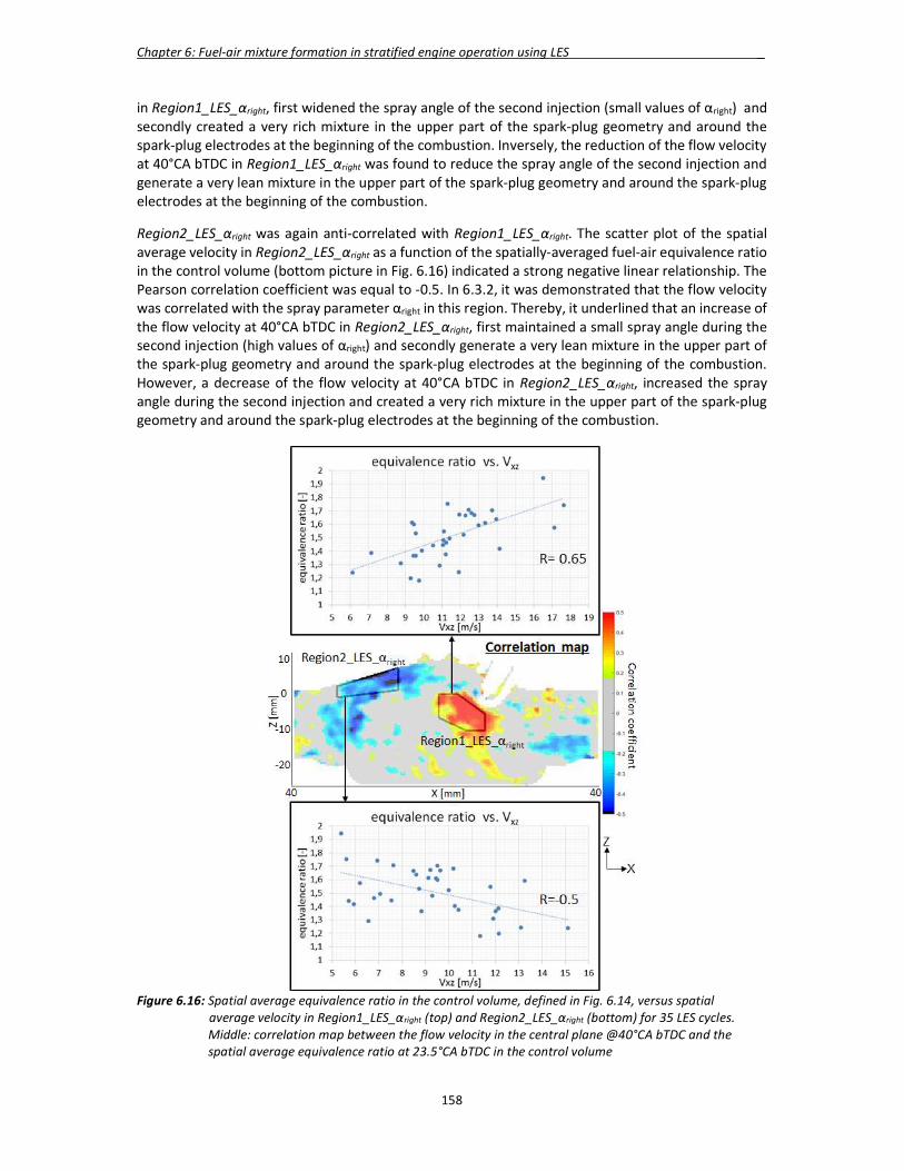
Chapter 6: Fuel-air mixture formation in stratified engine operation using LES _
158
in Region1_LES_αright, first widened the spray angle of the second injection (small values of αright) and secondly created a very rich mixture in the upper part of the spark-plug geometry and around the spark-plug electrodes at the beginning of the combustion. Inversely, the reduction of the flow velocity at 40°CA bTDC in Region1_LES_αright was found to reduce the spray angle of the second injection and generate a very lean mixture in the upper part of the spark-plug geometry and around the spark-plug electrodes at the beginning of the combustion.
Region2_LES_αright was again anti-correlated with Region1_LES_αright. The scatter plot of the spatial average velocity in Region2_LES_αright as a function of the spatially-averaged fuel-air equivalence ratio in the control volume (bottom picture in Fig. 6.16) indicated a strong negative linear relationship. The Pearson correlation coefficient was equal to -0.5. In 6.3.2, it was demonstrated that the flow velocity was correlated with the spray parameter αright in this region. Thereby, it underlined that an increase of the flow velocity at 40°CA bTDC in Region2_LES_αright, first maintained a small spray angle during the second injection (high values of αright) and secondly generate a very lean mixture in the upper part of the spark-plug geometry and around the spark-plug electrodes at the beginning of the combustion. However, a decrease of the flow velocity at 40°CA bTDC in Region2_LES_αright, increased the spray angle during the second injection and created a very rich mixture in the upper part of the spark-plug geometry and around the spark-plug electrodes at the beginning of the combustion.
Figure 6.16: Spatial average equivalence ratio in the control volume, defined in Fig. 6.14, versus spatial average velocity in Region1_LES_αright (top) and Region2_LES_αright (bottom) for 35 LES cycles.
Middle: correlation map between the flow velocity in the central plane @40°CA bTDC and the spatial average equivalence ratio at 23.5°CA bTDC in the control volume

Chapter 6: Fuel-air mixture formation in stratified engine operation using LES _
159
The fluctuating flow field before the start of the stratified injection was proved to influence the local distribution of the fuel-air equivalence ratio around the spark-plug at the beginning of the combustion. Thereby, it confirmed the visual observations made in 6.3.2. The main reason for the fluctuating equivalence ratio at the spark-plug location was found to be the variation of the spark-plug targeting during the second injection. The LES results could exhibit two extreme situations:
- The fuel-air equivalence ratio in the upper part of the spark-plug geometry and around the spark-plug electrodes is too rich at the beginning of the combustion. This is caused by an increased spray angle during the second injection. The reasons are either very high velocities in Region1_LES_αright or very low velocities in Region2_LES_αright before the start of injection.
- The fuel-air equivalence ratio in the upper part of the spark-plug geometry and around the spark-plug electrodes is too lean at the beginning of the combustion. This is caused by a reduced spray angle during the second injection. The reasons are either very high velocities in Region2_LES_αright or very low velocities in Region1_LES_αright before the start of injection.
LES could further expand the level of understanding of the chain of cause-and-effect up to the beginning of the combustion process. Those findings could explain the observations made on the engine test bench, while running in stratified operation. A change of the penetration depth of the spark-plug inside the combustion chamber would affect the combustion robustness of the engine. By excessively reducing the penetration length of the spark-plug, the spark-plug electrodes would be subject to a very lean mixture for very low velocities in Region1_LES_αright before the start of injection. As a result, the engine would experience misfire or uncomplete combustion, which will affect the fuel consumption, the raw emissions and the driving comfort. Thus, stratified engine operation would not provide a robust combustion process for this configuration. The same effect would be obtained by increasing the penetration depth of the spark-plug too much. In that particular case, a very lean mixture would be formed around the spark-plug electrodes for very high velocities in Region1_LES_αright before the start of injection. In that case, most of the fuel would be located between the upper part of the spark-plug and the wall of the cylinder head. LES was able to provide the missing link, i.e. the local fuel-air mixture information around the spark-plug, between the CCV of the flow before the injection and the CCV of the IMEP observed experimentally. Useful information could be hence extracted from LES to help understanding and reducing the CCV of the IMEP in stratified engine operation. Assuming that the combustion duration could be correlated to the local fuel-air equivalence ratio around the spark-plug electrodes at the ignition time, LES would agree with the results from the correlation map between the flow velocity before the injection and the combustion characteristics on the optically-accessible engine presented in 4.5.1. Indeed, high flow velocities before the start of injection in Region1_PIV_Pmax and Region2_PIV_Pmax were shown to have the same effect on MFB50 as high flow velocities in Region1_LES_αright and Region2_LES_αright on the local fuel-air equivalence ratio around the spark-plug at the beginning of the combustion in LES. The same effect was also found between experiments and LES in case of low flow velocities. Therefore, it could be claimed that the chain of cause-and-effect computed in LES was fully validated with the experimental data of the optically-accessible engine. 6.5 Summary: chain of cause-and-effect in LES An overview of the complete chain of cause-and-effect derived in LES for the stratified engine operation is shown in Fig. 6.17. The final chain of cause-and-effect could be summarized as follows. Two local key flow parameters were identified in two distinct regions i.e. Region1_LES_αright and Region2_LES_αright before the start of the stratified injection process:
- The first local key flow parameter in Region1_LES_αright, also called ‘upward flow’, was found to increase the tilting of the spray during the second injection when its intensity grew and
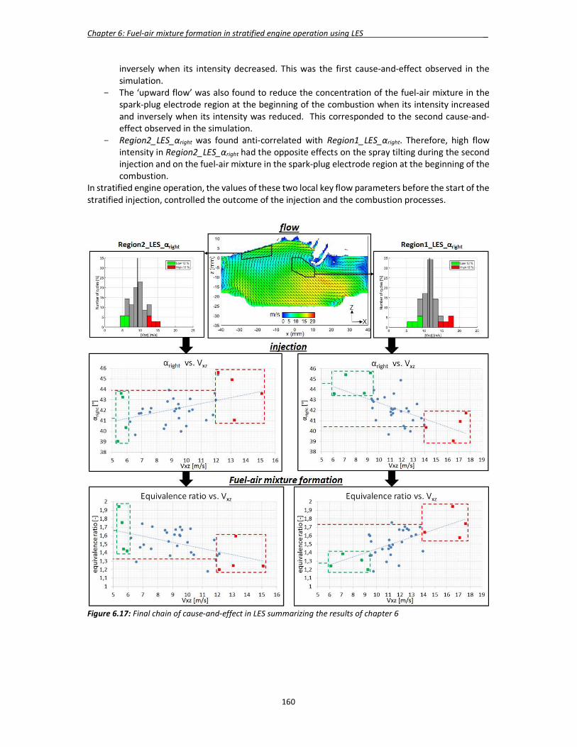
Chapter 6: Fuel-air mixture formation in stratified engine operation using LES _
160
inversely when its intensity decreased. This was the first cause-and-effect observed in the simulation.
- The ‘upward flow’ was also found to reduce the concentration of the fuel-air mixture in the spark-plug electrode region at the beginning of the combustion when its intensity increased and inversely when its intensity was reduced. This corresponded to the second cause-and-effect observed in the simulation.
- Region2_LES_αright was found anti-correlated with Region1_LES_αright. Therefore, high flow intensity in Region2_LES_αright had the opposite effects on the spray tilting during the second injection and on the fuel-air mixture in the spark-plug electrode region at the beginning of the combustion.
In stratified engine operation, the values of these two local key flow parameters before the start of the stratified injection, controlled the outcome of the injection and the combustion processes.
Figure 6.17: Final chain of cause-and-effect in LES summarizing the results of chapter 6

161
Chapter 7
Fuel-air mixture formation in ultra-lean homogeneous engine operation using LES This chapter covers the methodology development, the simulation and the analysis of the fuel-air mixture formation in an ultra-lean homogeneous engine operation in the M254 engine. The chosen engine operation was at 2000rpm with a global fuel-air equivalence ratio of 0.66. It corresponded to an indicated mean effective pressure of 6bar. The M254 engine was fitted with an intake system featuring a plate and a tumble flap in the intake port. The intensity of the tumble flow in the cylinder could be drastically increased by reducing the cross-sectional area of the intake port. It was achieved by closing the tumble flap in the intake port. In this research work, the tumble flap position was kept open. This investigation combined:
- The validated LES in-cylinder flow fields of the M254 engine using the high-speed PIV results from Bode [104]. The multi-cycle LES was computed by Nicoud [89] using the same methodology as for the M274 engine.
- The validated spray methodology, presented in chapter 5 in the cold closed-volume chamber at 𝑝 = 1 𝑏𝑎𝑟.
As a pilot application, the main goal was to develop an innovative moving-mesh strategy that kept the spray adaptive mesh undistorted during the injection process in the intake stoke with open intake valves. This is covered in the first part of the chapter. In the second part, the simulation of the fuel-air mixture-formation of six engine cycles, randomly selected from the gas-exchange simulation of the M254 engine, was performed. It is followed by a quantification of the homogeneity of the fuel-air mixture and its cyclic variation in the cylinder during the intake and compression strokes.
7.1 New moving-mesh methodology The injection process during the ultra-lean homogenous combustion mode comprised a single injection, which needed to be correctly captured using the Lagrangian setup developed in chapter 5. A static spray adaptive mesh had hence to be integrated into the CFD model used for the gas-exchange simulation of the M254 engine. However, the movement of the intake valves during the injection made the inclusion of the static mesh more difficult than for the stratified engine operation. Therefore, a new moving-mesh methodology was developed. The different integration steps are described hereafter. 7.1.1 Adaptation and validation of the spray adaptive mesh Mesh generation The Lagrangian setup recommended to use Chamber_Mesh3 for an accurate reproduction of the spray in the closed-volume chamber. However, the inclusion of the spray adaptive mesh Chamber_Mesh3 into the gas exchange mesh of the M254 engine, turned out to produce more than 100 Mio cells in the computational model. This was regarded as too computationally expensive. Moreover, knowing that the minimal cell size was equal to 0.1 mm, it would have implied a further reduction of the simulation time step, which was not acceptable. A coarsening of the spray adaptive mesh was thus required. Various strategies were investigated, trying to preserve as much as possible the original features of Chamber_Mesh3.
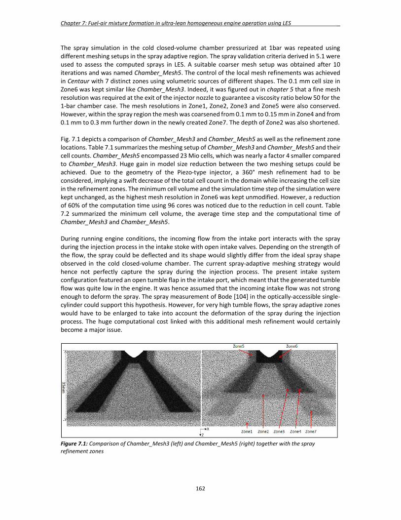
Chapter 7: Fuel-air mixture formation in ultra-lean homogeneous engine operation using LES _
162
The spray simulation in the cold closed-volume chamber pressurized at 1bar was repeated using different meshing setups in the spray adaptive region. The spray validation criteria derived in 5.1 were used to assess the computed sprays in LES. A suitable coarser mesh setup was obtained after 10 iterations and was named Chamber_Mesh5. The control of the local mesh refinements was achieved in Centaur with 7 distinct zones using volumetric sources of different shapes. The 0.1 mm cell size in Zone6 was kept similar like Chamber_Mesh3. Indeed, it was figured out in chapter 5 that a fine mesh resolution was required at the exit of the injector nozzle to guarantee a viscosity ratio below 50 for the 1-bar chamber case. The mesh resolutions in Zone1, Zone2, Zone3 and Zone5 were also conserved. However, within the spray region the mesh was coarsened from 0.1 mm to 0.15 mm in Zone4 and from 0.1 mm to 0.3 mm further down in the newly created Zone7. The depth of Zone2 was also shortened. Fig. 7.1 depicts a comparison of Chamber_Mesh3 and Chamber_Mesh5 as well as the refinement zone locations. Table 7.1 summarizes the meshing setup of Chamber_Mesh3 and Chamber_Mesh5 and their cell counts. Chamber_Mesh5 encompassed 23 Mio cells, which was nearly a factor 4 smaller compared to Chamber_Mesh3. Huge gain in model size reduction between the two meshing setups could be achieved. Due to the geometry of the Piezo-type injector, a 360° mesh refinement had to be considered, implying a swift decrease of the total cell count in the domain while increasing the cell size in the refinement zones. The minimum cell volume and the simulation time step of the simulation were kept unchanged, as the highest mesh resolution in Zone6 was kept unmodified. However, a reduction of 60% of the computation time using 96 cores was noticed due to the reduction in cell count. Table 7.2 summarized the minimum cell volume, the average time step and the computational time of Chamber_Mesh3 and Chamber_Mesh5. During running engine conditions, the incoming flow from the intake port interacts with the spray during the injection process in the intake stoke with open intake valves. Depending on the strength of the flow, the spray could be deflected and its shape would slightly differ from the ideal spray shape observed in the cold closed-volume chamber. The current spray-adaptive meshing strategy would hence not perfectly capture the spray during the injection process. The present intake system configuration featured an open tumble flap in the intake port, which meant that the generated tumble flow was quite low in the engine. It was hence assumed that the incoming intake flow was not strong enough to deform the spray. The spray measurement of Bode [104] in the optically-accessible single-cylinder could support this hypothesis. However, for very high tumble flows, the spray adaptive zones would have to be enlarged to take into account the deformation of the spray during the injection process. The huge computational cost linked with this additional mesh refinement would certainly become a major issue.
Figure 7.1: Comparison of Chamber_Mesh3 (left) and Chamber_Mesh5 (right) together with the spray refinement zones
Chapter 7: Fuel-air mixture formation in ultra-lean homogeneous engine operation using LES _
163
Table 7.1: Meshing setups of Chamber_Mesh3 and Chamber_Mesh5 Chamber_Mesh3 Chamber_Mesh5
Zone1 [mm] 0.5 0.5 Zone2 [mm] 0.3 0.3 Zone3 [mm] 0.2 0.2 Zone4 [mm] 0.1 0.15 Zone5 [mm] 0.2 0.2 Zone6 [mm] 0.1 0.1 Zone7 [mm] 0.1 0.3 Cell count [Mio] 83 23
Table 7.2: Minimum cell volume, average time step and CPU-time of Chamber_Meh3 and Chamber_Mesh5 run during 𝑡 = 0.5 𝑚𝑠 with 96 cores
Chamber_Mesh3 Chamber_Mesh5 Min. cell volume [m3] 3.3.10-14 3.3.10-14 Time step [s] 6.1.10-8 6.1.10-8 CPU-time [hours] 8.1 3.1
Spray validation The three-dimensional shape of the spray was analysed from the side view at 𝑡 = 0.5 𝑚𝑠. The parcels were coloured by the value of their representative droplet diameters and plotted using an identical size. The sprays computed with Chamber_Mesh3 and Chamber_Mesh5 are shown in Fig. 7.2 together with the experimental results. The shape of the spray in LES was found again influenced by the local mesh size used. A comparison of the key spray parameters between the computed sprays and the experimental one is shown in Table 7.3. Compared to Chamber_Mesh3, slightly lower spray width (-1 mm) and penetration length (-1 mm) were obtained with Chamber_Mesh5. Furthermore, the rounded form of the torus-shaped structure of the spray, in the region delimited by the violet boxes, was not as accurately captured as with Chamber_Mesh3. Its size was somehow overestimated and its upper edge located higher. The small flow structures observed on the spray surface and at the spray front with Chamber_Mesh3 were not resolved anymore on the coarse Chamber_Mesh5. However, during the injection process in the intake stroke, the importance of the small flow structures, formed along the spray surface, could be regarded as small because of the dominating flow structures originating from the incoming intake flow. Furthermore, due to their small time scales they tend to dissipate quickly and hence are not transported over a long distance in the computational model. From the simulation results obtained with Chamber_Mesh5 and the Lagrangian setup, it could be claimed that the LES spray simulation still agreed globally with the measurements. The spray adaptive mesh setup of Chamber_Mesh5 was hence included into the gas-exchange mesh of the M254 engine using a new moving-mesh strategy described in the next part.
Table 7.3: Comparison of the key spray parameters at t = 0.5 ms between simulation and experiments using Chamber_Mesh3, Chamber_Mesh5 and the Lagrangian setup. 𝑝 = 1 𝑏𝑎𝑟
Chamber_Mesh3 Chamber_Mesh5 Experiments L1 [mm] 25 27 25 L2 [mm] 11 10.5 11 L3 [mm] 35 34 35 L4 [mm] 65 64 65 L5 [mm] 19 18 18
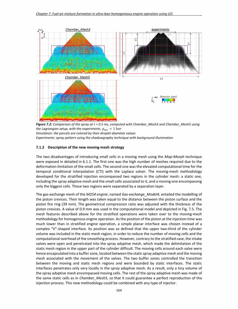
Chapter 7: Fuel-air mixture formation in ultra-lean homogeneous engine operation using LES _
164
Figure 7.2: Comparison of the spray at t = 0.5 ms, computed with Chamber_Mesh3 and Chamber_Mesh5 using the Lagrangian setup, with the experiments. 𝑝 = 1 𝑏𝑎𝑟 Simulation: the parcels are colored by their droplet diameter values Experiments: spray pattern using the shadowgraphy technique with background illumination 7.1.2 Description of the new moving-mesh strategy The two disadvantages of introducing small cells in a moving mesh using the Map-Morph technique were exposed in detailed in 6.1.1. The first one was the high number of meshes required due to the deformation limitation of the small cells. The second one was the elevated computational time for the temporal conditional interpolation (CTI) with the Laplace solver. The moving-mesh methodology developed for the stratified injection encompassed two regions in the cylinder mesh: a static one, including the spray adaptive mesh and the small cells associated to it, and a moving one encompassing only the biggest cells. Those two regions were separated by a separation layer.
The gas-exchange mesh of the M254 engine, named Gas-exchange_Model4, entailed the modelling of the piston crevices. Their length was taken equal to the distance between the piston surface and the piston fire ring (39 mm). The geometrical compression ratio was adjusted with the thickness of the piston crevices. A value of 0.9 mm was used in the computational model and depicted in Fig. 7.5. The mesh features described above for the stratified operations were taken over to the moving-mesh methodology for homogenous engine operation. As the position of the piston at the injection time was much lower than in stratified engine operation, a simple planar interface was chosen instead of a complex “V”-shaped interface. Its position was so defined that the upper two-third of the cylinder volume was included in the static mesh region, in order to reduce the number of moving cells and the computational overhead of the smoothing process. However, contrary to the stratified case, the intake valves were open and penetrated into the spray adaptive mesh, which made the delimitation of the static mesh region in the upper part of the cylinder difficult. The moving cells around each valve were hence encapsulated into a buffer zone, located between the static spray adaptive mesh and the moving mesh associated with the movement of the valves. The two buffer zones controlled the transition between the moving and static mesh regions and were bounded by static interfaces. The static interfaces penetrates only very locally in the spray adaptive mesh. As a result, only a tiny volume of the spray adaptive mesh encompassed moving cells. The rest of the spray adaptive mesh was made of the same static cells as in Chamber_Mesh5, so that it could guarantee a perfect reproduction of the injection process. This new methodology could be combined with any type of injector.
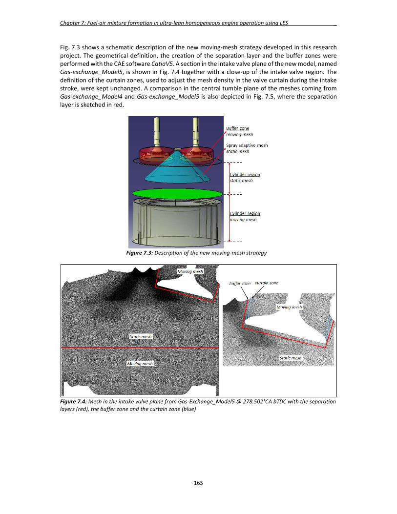
Chapter 7: Fuel-air mixture formation in ultra-lean homogeneous engine operation using LES _
165
Fig. 7.3 shows a schematic description of the new moving-mesh strategy developed in this research project. The geometrical definition, the creation of the separation layer and the buffer zones were performed with the CAE software CatiaV5. A section in the intake valve plane of the new model, named Gas-exchange_Model5, is shown in Fig. 7.4 together with a close-up of the intake valve region. The definition of the curtain zones, used to adjust the mesh density in the valve curtain during the intake stroke, were kept unchanged. A comparison in the central tumble plane of the meshes coming from Gas-exchange_Model4 and Gas-exchange_Model5 is also depicted in Fig. 7.5, where the separation layer is sketched in red.
Figure 7.3: Description of the new moving-mesh strategy
Figure 7.4: Mesh in the intake valve plane from Gas-Exchange_Model5 @ 278.502°CA bTDC with the separation layers (red), the buffer zone and the curtain zone (blue)
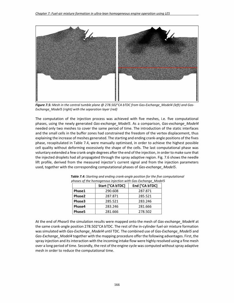
Chapter 7: Fuel-air mixture formation in ultra-lean homogeneous engine operation using LES _
166
Figure 7.5: Mesh in the central tumble plane @ 278.502°CA bTDC from Gas-Exchange_Model4 (left) and Gas-Exchange_Model5 (right) with the separation layer (red) The computation of the injection process was achieved with five meshes, i.e. five computational phases, using the newly generated Gas-exchange_Model5. As a comparison, Gas-exchange_Model4 needed only two meshes to cover the same period of time. The introduction of the static interfaces and the small cells in the buffer zones had constrained the freedom of the vertex displacement, thus explaining the increase of meshes generated. The starting and ending crank-angle positions of the fives phase, recapitulated in Table 7.4, were manually optimised, in order to achieve the highest possible cell quality without deforming excessively the shape of the cells. The last computational phase was voluntary extended a few crank-angle degrees after the end of the injection, in order to make sure that the injected droplets had all propagated through the spray adaptive region. Fig. 7.6 shows the needle lift profile, derived from the measured injector’s current signal and from the injection parameters used, together with the corresponding computational phases of Gas-exchange_Model5.
Table 7.4: Starting and ending crank-angle position for the five computational phases of the homogenous injection with Gas-Exchange_Model5
Start [°CA bTDC] End [°CA bTDC] Phase1 290.608 287.871 Phase2 287.871 285.521 Phase3 285.521 283.246 Phase4 283.246 281.666 Phase5 281.666 278.502
At the end of Phase5 the simulation results were mapped onto the mesh of Gas-exchange_Model4 at the same crank-angle position 278.502°CA bTDC. The rest of the in-cylinder fuel-air mixture formation was simulated with Gas-Exchange_Model4 until TDC. The combined use of Gas-Exchange_Model5 and Gas-Exchange_Model4 together with the mapping procedure offer the following advantages. First, the spray injection and its interaction with the incoming intake flow were highly resolved using a fine mesh over a long period of time. Secondly, the rest of the engine cycle was computed without spray adaptive mesh in order to reduce the computational time.
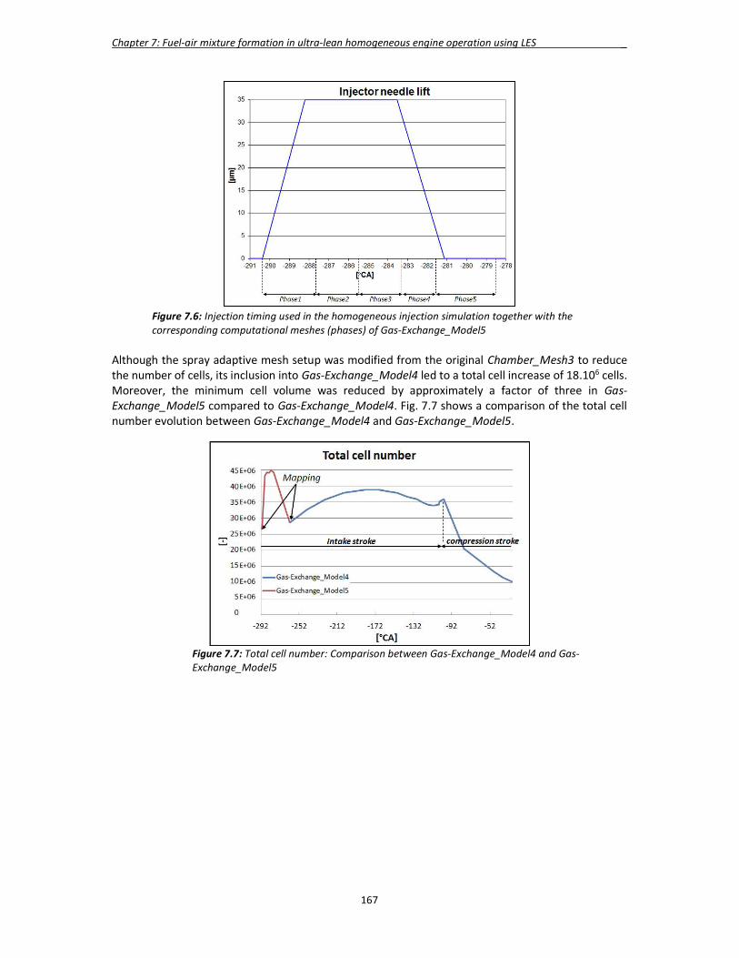
Chapter 7: Fuel-air mixture formation in ultra-lean homogeneous engine operation using LES _
167
Figure 7.6: Injection timing used in the homogeneous injection simulation together with the corresponding computational meshes (phases) of Gas-Exchange_Model5
Although the spray adaptive mesh setup was modified from the original Chamber_Mesh3 to reduce the number of cells, its inclusion into Gas-Exchange_Model4 led to a total cell increase of 18.106 cells. Moreover, the minimum cell volume was reduced by approximately a factor of three in Gas-Exchange_Model5 compared to Gas-Exchange_Model4. Fig. 7.7 shows a comparison of the total cell number evolution between Gas-Exchange_Model4 and Gas-Exchange_Model5.
Figure 7.7: Total cell number: Comparison between Gas-Exchange_Model4 and Gas-Exchange_Model5

Chapter 7: Fuel-air mixture formation in ultra-lean homogeneous engine operation using LES _
168
7.2 Simulation of the fuel-air mixture formation 7.2.1 Numerical setup The numerical setup was taken identical as the Lagrangian setup derived from the spray simulation in the cold closed-volume chamber. The slip droplet-wall interaction model was selected without formation of a liquid film at the wall, as it was not the focus of this study. The injected fuel mass for each injection was derived from the injection quantity baseline of the piezo-injector. On the gas side, the aforementioned setup also matched with the one used in Gas-Exchange_Model4 for the in-cylinder flow simulation. The boundary conditions for LES were obtained from a Triple-Pressure-Analysis model (TPA). The TPA model was calibrated based on the three pressure signals (intake, exhaust and cylinder) from the experiments of Bode [104]. The chemical species required for the air description in the CFM combustion model [89] were included in Gas-Exchange_Model4. For consistency reasons with the gas-exchange and spray validation simulations, the same values were kept for the 2nd and 4th-order artificial viscosity coefficients (smu2 = 5.10-2 and smu4 = 8.10-3). However, due to the strong incoming flow from the intake port and its interaction with the spray, some difficulties were experienced while running the injection simulation. The acoustic CFL_ac was hence reduced to 0.6 to guarantee the stability of the simulation. The other strategy would have been to keep the CFL_ac = 0.9 and increase the artificial viscosity. This path was not followed here as it would have deteriorated the accuracy of the simulation. Six out of the 20 engine cycles, computed by Nicoud [89] under the aforementioned operating conditions, were taken for the investigation in this research project. The selection of the cycles was randomly made. The instantaneous flow field of each of the six cycles, computed with Gas-Exchange_Model4, was first mapped at 290.608°CA bTDC on the first mesh of Gas-Exchange_Model5 corresponding to Phase1. It provided the initial flow field for the injection simulation. Six simulations were run up to TDC combining Gas-Exchange_Model5 for the injection simulation and Gas-Exchange_Model4 for the rest of the fuel-air mixture formation simulation. The instantaneous flow field was saved every 0.5°CA during the injection process and every 2°CA in the intake and compression strokes, in order to guarantee enough post-processing data. The size of the post-processing dataset exported for the software Ensight was 110 GB per cycle. For one engine cycle, it took 36 hours on 96 cores to run the injection simulation with Gas-Exchange_Model5 and 43 hours on 432 cores with Gas-Exchange_Model4 for the rest of the computation up to TDC. The higher computational time compared to the M274 engine was due to the increased number of chemical species required in the CFM combustion model. 7.2.2 Droplet boundary conditions The transient internal nozzle-flow simulation in RANS was carried out beforehand. The movement of the needle in RANS followed the profile shown in Fig. 7.6 and the air back-pressure was taken equal to the cylinder pressure 𝑝 = 1.1 𝑏𝑎𝑟 at 290.6°CA bTDC. The RANS-LES coupling interface, described in 3.5, created the look-up table containing the flow information along the nozzle orifice at the exit of the injector for the ultra-lean homogeneous operation. The total injected fuel mass provided by the look-up table was then corrected, in order to take into account the real value given by the injection quantity baseline of the Piezo-type injector. The droplet size distributions were assumed proportional to the turbulent length scale of the flow along the nozzle orifice at the exit of the injector as detailed in 3.5.3. The droplet scale-factor 𝐾 = 1 was taken from the Lagrangian setup. Fig. 7.8 shows the evolution in time of the droplet size distributions along the nozzle orifice at the exit of the injector with the corresponding droplet velocity. The droplet distributions are shown for each injection only up to the maximal needle lift (35 𝜇𝑚). Between 0.01 and 0.05 ms, the critical Reynolds number (𝑅𝑒 ≈2300), where the transition from laminar to turbulent flow occurs in a channel flow, was not reached as the needle lifts were extremely small. A constant droplet diameter equal to the hydraulic diameter was assumed in that case.
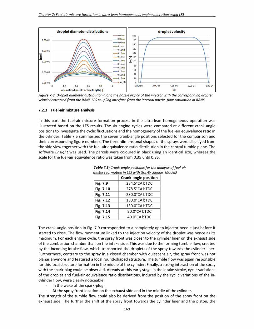
Chapter 7: Fuel-air mixture formation in ultra-lean homogeneous engine operation using LES _
169
Figure 7.8: Droplet diameter distribution along the nozzle orifice of the injector with the corresponding droplet velocity extracted from the RANS-LES coupling interface from the internal nozzle- flow simulation in RANS 7.2.3 Fuel-air mixture analysis In this part the fuel-air mixture formation process in the ultra-lean homogeneous operation was illustrated based on the LES results. The six engine cycles were compared at different crank-angle positions to investigate the cyclic fluctuations and the homogeneity of the fuel-air equivalence ratio in the cylinder. Table 7.5 summarizes the seven crank-angle positions selected for the comparison and their corresponding figure numbers. The three-dimensional shapes of the sprays were displayed from the side view together with the fuel-air equivalence ratio distribution in the central tumble plane. The software Ensight was used. The parcels were coloured in black using an identical size, whereas the scale for the fuel-air equivalence ratio was taken from 0.35 until 0.85.
Table 7.5: Crank-angle positions for the analysis of fuel-air mixture formation in LES with Gas-Exchange_Model5
Crank-angle position Fig. 7.9 284.5°CA bTDC Fig. 7.10 278.5°CA bTDC Fig. 7.11 230.0°CA bTDC Fig. 7.12 180.0°CA bTDC Fig. 7.13 130.0°CA bTDC Fig. 7.14 90.0°CA bTDC Fig. 7.15 40.0°CA bTDC
The crank-angle position in Fig. 7.9 corresponded to a completely open injector needle just before it started to close. The flow momentum linked to the injection velocity of the droplet was hence as its maximum. For each engine cycle, the spray front was closer to the cylinder liner on the exhaust side of the combustion chamber than on the intake side. This was due to the forming tumble flow, created by the incoming intake flow, which transported the droplets of the spray towards the cylinder liner. Furthermore, contrary to the spray in a closed chamber with quiescent air, the spray front was not planar anymore and featured a local round-shaped structure. The tumble flow was again responsible for this local structure formation in the middle of the cylinder. Finally, a strong interaction of the spray with the spark-plug could be observed. Already at this early stage in the intake stroke, cyclic variations of the droplet and fuel-air equivalence ratio distributions, induced by the cyclic variations of the in-cylinder flow, were clearly noticeable:
- In the wake of the spark-plug. - At the spray front location on the exhaust side and in the middle of the cylinder.
The strength of the tumble flow could also be derived from the position of the spray front on the exhaust side. The further the shift of the spray front towards the cylinder liner and the piston, the
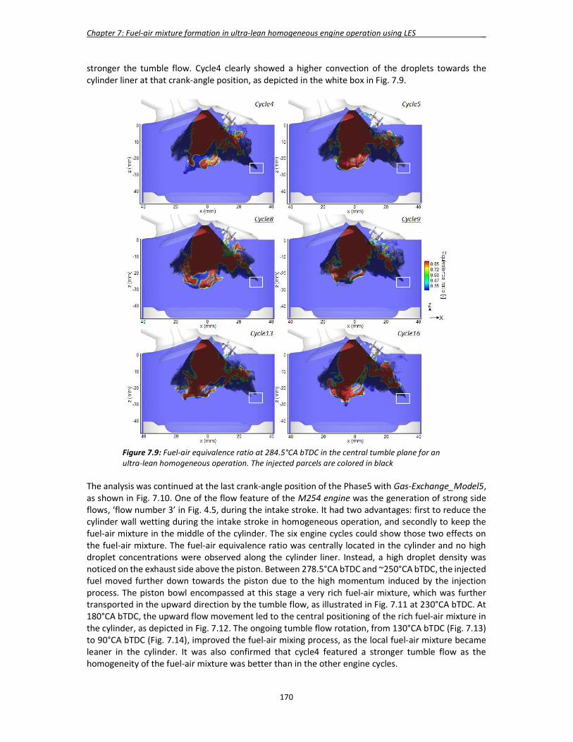
Chapter 7: Fuel-air mixture formation in ultra-lean homogeneous engine operation using LES _
170
stronger the tumble flow. Cycle4 clearly showed a higher convection of the droplets towards the cylinder liner at that crank-angle position, as depicted in the white box in Fig. 7.9.
Figure 7.9: Fuel-air equivalence ratio at 284.5°CA bTDC in the central tumble plane for an ultra-lean homogeneous operation. The injected parcels are colored in black The analysis was continued at the last crank-angle position of the Phase5 with Gas-Exchange_Model5, as shown in Fig. 7.10. One of the flow feature of the M254 engine was the generation of strong side flows, ‘flow number 3’ in Fig. 4.5, during the intake stroke. It had two advantages: first to reduce the cylinder wall wetting during the intake stroke in homogeneous operation, and secondly to keep the fuel-air mixture in the middle of the cylinder. The six engine cycles could show those two effects on the fuel-air mixture. The fuel-air equivalence ratio was centrally located in the cylinder and no high droplet concentrations were observed along the cylinder liner. Instead, a high droplet density was noticed on the exhaust side above the piston. Between 278.5°CA bTDC and ~250°CA bTDC, the injected fuel moved further down towards the piston due to the high momentum induced by the injection process. The piston bowl encompassed at this stage a very rich fuel-air mixture, which was further transported in the upward direction by the tumble flow, as illustrated in Fig. 7.11 at 230°CA bTDC. At 180°CA bTDC, the upward flow movement led to the central positioning of the rich fuel-air mixture in the cylinder, as depicted in Fig. 7.12. The ongoing tumble flow rotation, from 130°CA bTDC (Fig. 7.13) to 90°CA bTDC (Fig. 7.14), improved the fuel-air mixing process, as the local fuel-air mixture became leaner in the cylinder. It was also confirmed that cycle4 featured a stronger tumble flow as the homogeneity of the fuel-air mixture was better than in the other engine cycles.
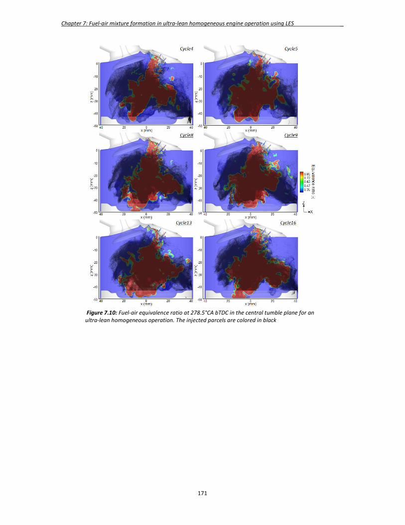
Chapter 7: Fuel-air mixture formation in ultra-lean homogeneous engine operation using LES _
171
Figure 7.10: Fuel-air equivalence ratio at 278.5°CA bTDC in the central tumble plane for an ultra-lean homogeneous operation. The injected parcels are colored in black

Chapter 7: Fuel-air mixture formation in ultra-lean homogeneous engine operation using LES _
172
Figure 7.11: Fuel-air equivalence ratio at 230.0°CA bTDC in the central tumble plane for an ultra-lean homogeneous operation. The injected parcels are clored in black
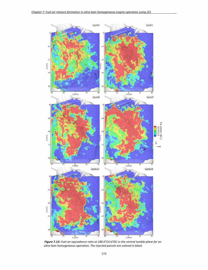
Chapter 7: Fuel-air mixture formation in ultra-lean homogeneous engine operation using LES _
173
Figure 7.12: Fuel-air equivalence ratio at 180.0°CA bTDC in the central tumble plane for an ultra-lean homogeneous operation. The injected parcels are colored in black
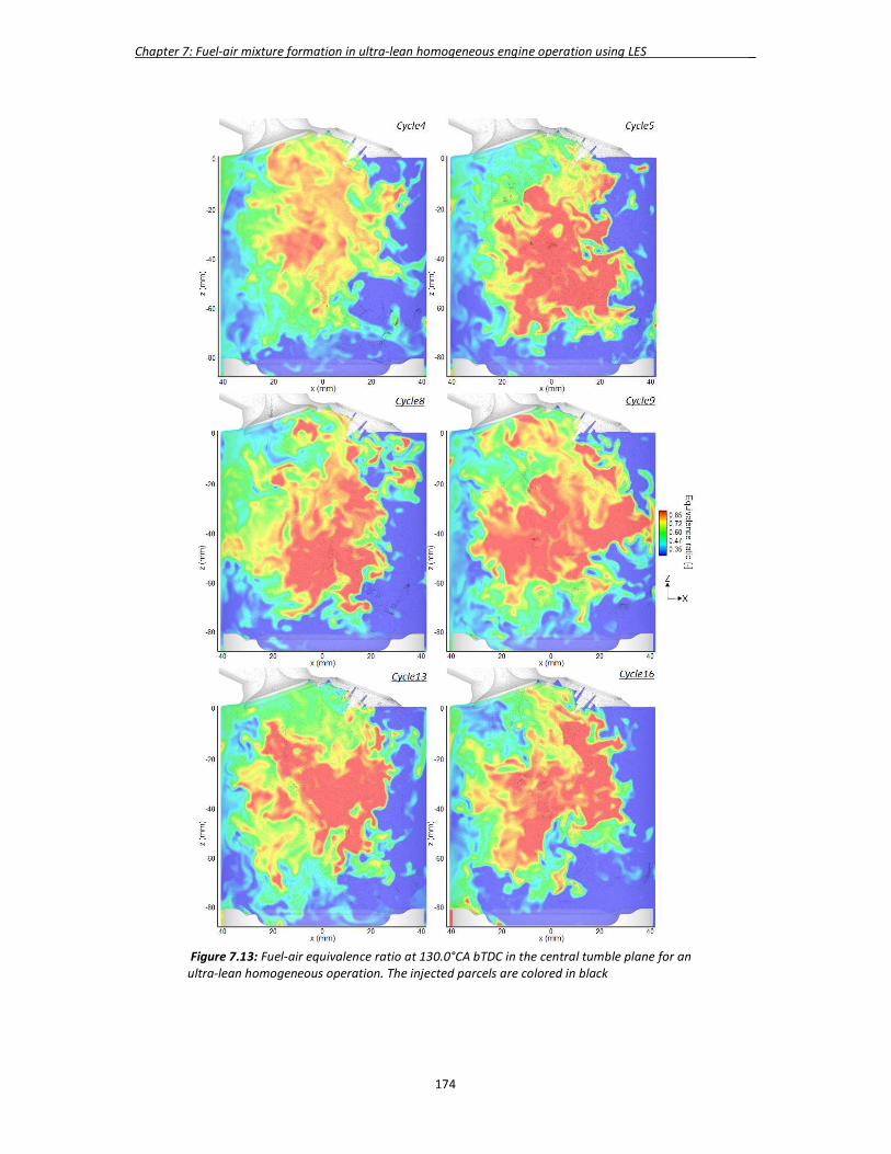
Chapter 7: Fuel-air mixture formation in ultra-lean homogeneous engine operation using LES _
174
Figure 7.13: Fuel-air equivalence ratio at 130.0°CA bTDC in the central tumble plane for an ultra-lean homogeneous operation. The injected parcels are colored in black
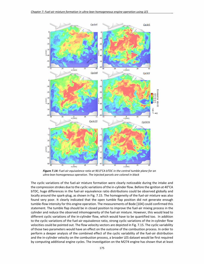
Chapter 7: Fuel-air mixture formation in ultra-lean homogeneous engine operation using LES _
175
Figure 7.14: Fuel-air equivalence ratio at 90.0°CA bTDC in the central tumble plane for an ultra-lean homogeneous operation. The injected parcels are colored in black The cyclic variations of the fuel-air mixture formation were clearly noticeable during the intake and the compression strokes due to the cyclic variations of the in-cylinder flow. Before the ignition at 40°CA bTDC, huge differences in the fuel-air equivalence ratio distributions could be observed globally and locally around the spark-plug, as shown in Fig. 7.15. The homogeneity of the fuel-air mixture was also found very poor. It clearly indicated that the open tumble flap position did not generate enough tumble-flow intensity for this engine operation. The measurements of Bode [104] could confirmed this statement. The tumble flap should be in closed position to improve the fuel-air mixing process in the cylinder and reduce the observed inhomogeneity of the fuel-air mixture. However, this would lead to different cyclic variations of the in-cylinder flow, which would have to be quantified too. In addition to the cyclic variations of the fuel-air equivalence ratio, strong cyclic variations of the in-cylinder flow velocities could be pointed out. The flow velocity vectors are depicted in Fig. 7.15. The cyclic variability of those two parameters would have an effect on the outcome of the combustion process. In order to perform a deeper analysis of the combined effect of the cyclic variability of the fuel-air distribution and the in-cylinder velocity on the combustion process, a broader LES dataset would be first required by computing additional engine cycles. The investigation on the M274 engine has shown that at least
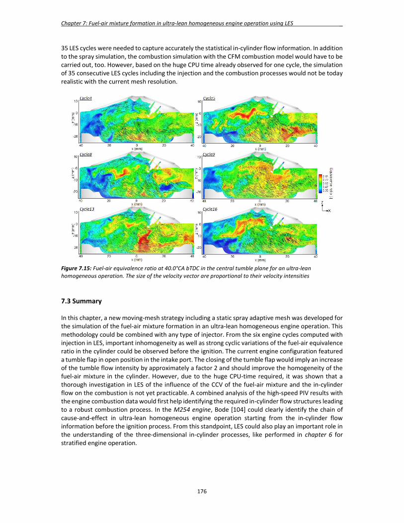
Chapter 7: Fuel-air mixture formation in ultra-lean homogeneous engine operation using LES _
176
35 LES cycles were needed to capture accurately the statistical in-cylinder flow information. In addition to the spray simulation, the combustion simulation with the CFM combustion model would have to be carried out, too. However, based on the huge CPU time already observed for one cycle, the simulation of 35 consecutive LES cycles including the injection and the combustion processes would not be today realistic with the current mesh resolution.
Figure 7.15: Fuel-air equivalence ratio at 40.0°CA bTDC in the central tumble plane for an ultra-lean homogeneous operation. The size of the velocity vector are proportional to their velocity intensities 7.3 Summary In this chapter, a new moving-mesh strategy including a static spray adaptive mesh was developed for the simulation of the fuel-air mixture formation in an ultra-lean homogeneous engine operation. This methodology could be combined with any type of injector. From the six engine cycles computed with injection in LES, important inhomogeneity as well as strong cyclic variations of the fuel-air equivalence ratio in the cylinder could be observed before the ignition. The current engine configuration featured a tumble flap in open position in the intake port. The closing of the tumble flap would imply an increase of the tumble flow intensity by approximately a factor 2 and should improve the homogeneity of the fuel-air mixture in the cylinder. However, due to the huge CPU-time required, it was shown that a thorough investigation in LES of the influence of the CCV of the fuel-air mixture and the in-cylinder flow on the combustion is not yet practicable. A combined analysis of the high-speed PIV results with the engine combustion data would first help identifying the required in-cylinder flow structures leading to a robust combustion process. In the M254 engine, Bode [104] could clearly identify the chain of cause-and-effect in ultra-lean homogeneous engine operation starting from the in-cylinder flow information before the ignition process. From this standpoint, LES could also play an important role in the understanding of the three-dimensional in-cylinder processes, like performed in chapter 6 for stratified engine operation.
177
Chapter 8
Conclusion and outlook The goal of this research work was to understand, via a joint analysis using high-speed PIV and LES, the three-dimensional flow phenomena in the chain of in-cylinder processes leading to the CCV of the IMEP in stratified engine operation. The optically-accessible single-cylinder, derived from the Mercedes-Benz’s M274 engine, was considered for these investigations as well as the LES research code AVBP. AVBP was chosen for its low-dissipative explicit acoustic LES solver and its high mesh quality standards. In order to fill the gap in the literature, a new LES validation strategy, called the PIV-guided LES validation strategy, was developed. The key in-cylinder flow patterns, affecting the combustion process in stratified engine operation, were isolated using a correlation analysis between the high-speed PIV flow fields and the engine combustion data. They were used to drive the validation process of the LES in-cylinder flow in terms of mean flow velocity and local CCV of the flow velocity. Using a global mesh sensitivity study, a robust methodology for the meshing and numerical setups were iteratively derived for AVBP. In order to assess the full potential of LES, the flow prediction using the 2nd and 3rd-order accurate in space and time convective schemes (Lax-Wendroff and TTGC) were investigated. The multi-cycle LES with the 3rd-order convective scheme was found to bring significant improvements. The mean flow structures and local CCV of the flow velocity were better captured. The efficient handling of the huge volume of data produced in high-speed PIV and LES, combined with the implementation of new analysis algorithms, were the key factors to extract the relevant flow information. A standard post-processing platform for LES and high-speed PIV was developed. It allowed the analysis and the graphical representation of the experimental and simulation results in the same manner. It was found mandatory in the LES validation process, where local flow structures had to be perfectly captured. Statistical analysis tools were applied for the first time to LES and important results could be derived. The conditional statistics was identically used in high-speed PIV and in LES so as to extract two groups of cycles linked to the extreme values of each key in-cylinder flow parameter. Using the validated LES flow fields, two crucial three-dimensional flow structures were isolated using conditional averaging and inputs from high-speed PIV. These flow structures were further quantified by the visual observation of the 3D rotation axis of the rotating tumble vortex, computed using an extension of the Г-criterion in 3D. The 3D rotation axis featuring a ‘croissant’ shape was found to be correlated with high CCV of the IMEP. In the experiments, the missing link between the CCV of the in-cylinder flow and the CCV of the IMEP is the global and local fuel-air mixture information in the cylinder. However, the spray simulation of the Piezo injector has never been addressed in LES, when it comes to model the primary droplet break-up using a coupling interface between the transient internal-nozzle flow simulation in RANS and LES. A new methodology featuring a spray adaptive region was derived and validated against cold closed-volume chamber spray measurements. Two different chamber pressures (𝑝 = 1 𝑏𝑎𝑟 and 𝑝 =6 𝑏𝑎𝑟) were investigated, in order to mimic the air density found in the engine cylinder before the start of injection in homogenous and stratified engine operations. Special care was put on the minimum cell size of the mesh and the total cell number, in view of a realistic integration of the derived meshing set-up into the gas-exchange model.

Chapter 8: Conclusion and outlook _
178
The integration of the validated spray-adaptive meshing setup into the gas-exchange mesh required the development of a new-moving mesh strategy adapted for the explicit acoustic LES solver. A multi-cycle fuel-air mixture formation was performed in stratified engine operation. A clear correlation was found between the CCV of the key in-cylinder flow parameters and the CCV of the fuel-air mixture distribution at the beginning of the combustion. These results confirmed that the fuel-air mixture information was the missing link in the experiments. Finally a new methodology for the simulation of the fuel-air mixture formation in ultra-lean homogeneous combustion was developed. The main goal was to create an innovative moving-mesh strategy, which kept the validated spray adaptive mesh undistorted during the injection process in the intake stoke with open intake valves. As a pilot application, few cycles were computed with the M254 engine geometry. Important inhomogeneity as well as strong CCV of the fuel-air equivalence ratio in the cylinder could be observed before the ignition. The results confirmed that the open tumble flap position in the intake port generated a too weak tumble flow intensity. At the end of this research project, the level of knowledge to quantify the flow phenomena involved in the CCV of the IMEP in stratified engine operation had significantly increased. From the LES results, a complete chain of cause-and-effect of the in-cylinder processes was derived. It started with the in-cylinder flow characteristics before the injection and included the injection process and the fuel-air mixture formation process until the start of combustion. The outcome of each process could be clearly understood following a change of the local key in-cylinder flow parameters before the injection. LES provided an added value concerning the understanding of the three-dimensional flow phenomena involved in the formation of the key in-cylinder flow parameters. This information was missing in high-speed PIV due to the measurement restrictions to planes. Furthermore, LES provided the missing link, i.e. the local fuel-air equivalence-ratio information around the spark-plug, between the CCV of the in-cylinder flow before the injection and the CCV of the IMEP observed experimentally. Finally, LES could extract very useful inputs to reduce the CCV of the IMEP in stratified engine operation, like the influence of the penetration length of the spark-plug in the combustion chamber. Outlook Based on the LES methodology developed for the stratified engine operation, other geometry variations could be potentially investigated. However, from the knowledge gained during the derivation of the chain of cause-and-effect, one could accurately assess any new engine design based on the information of the two key in-cylinder flow parameters before the start of injection. Indeed, it was clearly proved that the characteristics of in-cylinder flow before the injection was the reason for the CCV of the IMEP in stratified engine operation. The LES methodology would hence consist in running only a multi-cycle gas-exchange LES and analyse the flow field before the injection. First, it would drastically reduce the turn-around time for the evaluation of a new engine geometry; secondly, the overall complexity of the simulation process as well as the post-processing would be significantly reduced. Nevertheless, running a multi-cycle simulation with LES will still take much longer than with RANS. It will massively restrain the number of geometry variations to be assessed during an engine development project. As a comparison, the simulation of one engine cycle with RANS, presented in 4.2.1, took 18 hours on 64 cores, whereas 30 hours on 450 cores were required with LES. Even though nowadays the CPU resources are not an issue anymore, the overall computational time of LES to get access to enough statistical in-cylinder flow information is still prohibitive. In this research project, the use of a research explicit acoustic LES solver proved to be the right decision considering the level of flow understanding gained. However, such a low-dissipative centred-schemes code is very sensible to the mesh quality and cannot be run as easily as a commercial implicit LES code. The mesh preparation process is time consuming and requires extreme care and experience, especially in combination with moving meshes and complex geometries. Switching to a commercial implicit LES code would allow to obtain the final meshes within a couple of hours and the simulation would run in a more stable way
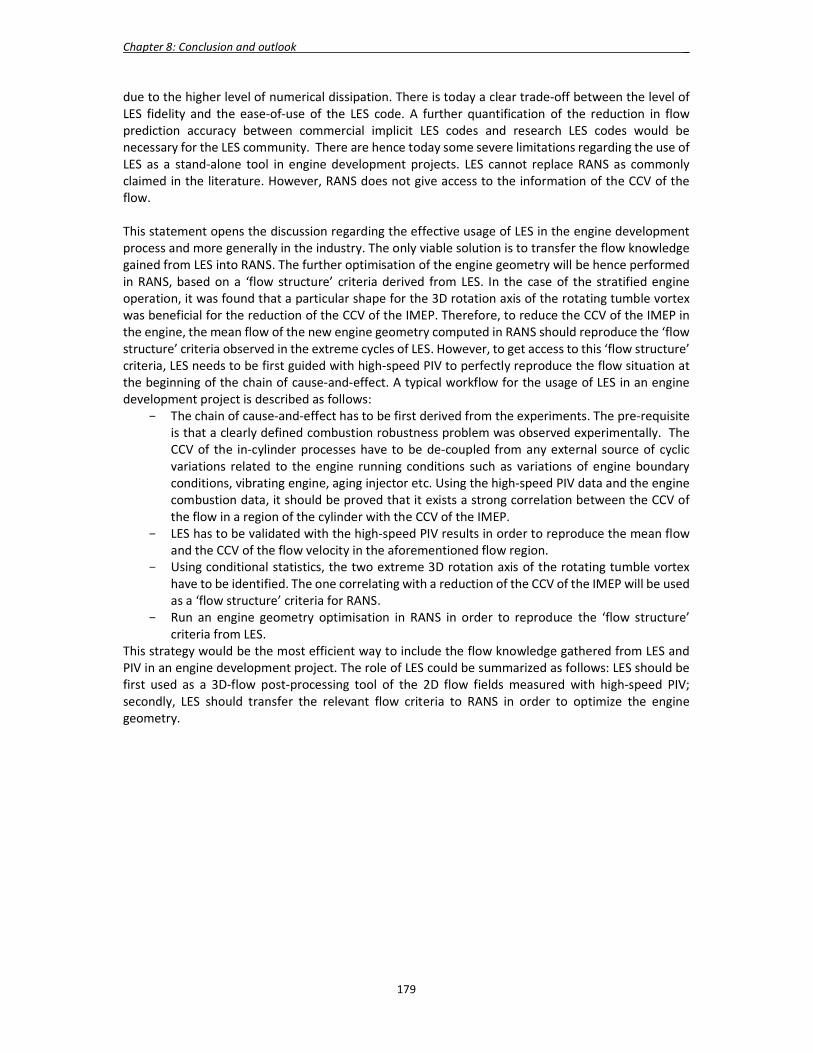
Chapter 8: Conclusion and outlook _
179
due to the higher level of numerical dissipation. There is today a clear trade-off between the level of LES fidelity and the ease-of-use of the LES code. A further quantification of the reduction in flow prediction accuracy between commercial implicit LES codes and research LES codes would be necessary for the LES community. There are hence today some severe limitations regarding the use of LES as a stand-alone tool in engine development projects. LES cannot replace RANS as commonly claimed in the literature. However, RANS does not give access to the information of the CCV of the flow. This statement opens the discussion regarding the effective usage of LES in the engine development process and more generally in the industry. The only viable solution is to transfer the flow knowledge gained from LES into RANS. The further optimisation of the engine geometry will be hence performed in RANS, based on a ‘flow structure’ criteria derived from LES. In the case of the stratified engine operation, it was found that a particular shape for the 3D rotation axis of the rotating tumble vortex was beneficial for the reduction of the CCV of the IMEP. Therefore, to reduce the CCV of the IMEP in the engine, the mean flow of the new engine geometry computed in RANS should reproduce the ‘flow structure’ criteria observed in the extreme cycles of LES. However, to get access to this ‘flow structure’ criteria, LES needs to be first guided with high-speed PIV to perfectly reproduce the flow situation at the beginning of the chain of cause-and-effect. A typical workflow for the usage of LES in an engine development project is described as follows:
- The chain of cause-and-effect has to be first derived from the experiments. The pre-requisite is that a clearly defined combustion robustness problem was observed experimentally. The CCV of the in-cylinder processes have to be de-coupled from any external source of cyclic variations related to the engine running conditions such as variations of engine boundary conditions, vibrating engine, aging injector etc. Using the high-speed PIV data and the engine combustion data, it should be proved that it exists a strong correlation between the CCV of the flow in a region of the cylinder with the CCV of the IMEP.
- LES has to be validated with the high-speed PIV results in order to reproduce the mean flow and the CCV of the flow velocity in the aforementioned flow region.
- Using conditional statistics, the two extreme 3D rotation axis of the rotating tumble vortex have to be identified. The one correlating with a reduction of the CCV of the IMEP will be used as a ‘flow structure’ criteria for RANS.
- Run an engine geometry optimisation in RANS in order to reproduce the ‘flow structure’ criteria from LES.
This strategy would be the most efficient way to include the flow knowledge gathered from LES and PIV in an engine development project. The role of LES could be summarized as follows: LES should be first used as a 3D-flow post-processing tool of the 2D flow fields measured with high-speed PIV; secondly, LES should transfer the relevant flow criteria to RANS in order to optimize the engine geometry.

Chapter 8: Conclusion and outlook _
180

181
Appendix A Influence of the initial droplet size distribution in LES The simulation of an outward-opening Piezo-actuated Pintle-type injector in AVBP was investigated by Habchi in 2011 [83]. A constant droplet diameter for the initialisation of the droplets and the SAB secondary break-up model was used. The author concluded that an extensive tuning of the initial droplet diameter was required to reproduce the experimental observations. He found out that a constant droplet diameter of 5 µm gave the best results. The critical point in his simulation was the underestimated air-entrainment leading to a wrong formation of the torus-shaped recirculation zone. In order to increase artificially the air entrainment-rate, the flow in the cell containing the injected droplet was initialised with the same velocity as the droplet one. This experience showed how crucial the accurate modelling of the primary break-up in LES is. It was often neglected in the literature, hence leading to a non-physical spray initialisation with excessive tuning parameters. In order to highlight the influence of the initial droplet size distribution for the spray simulation of the outward-opening Piezo-actuated Pintle-type injector, three different initialisation strategies were investigated:
- initialisation1: constant droplet diameter of 5 µm. - initialisation2: transient droplet diameter distribution with 𝐾 = 1. - initialisation3: transient droplet diameter equal to the hydraulic diameter, ranging from 2.5
µm to 22 µm.
Fig. A1-3 show a comparison of the three-dimensional shapes of the computed sprays from the side view at 𝑡 = 0.2, 0.3 and 0.4 𝑚𝑠. Finally a comparison with the experiments at 𝑡 = 0.5 𝑚𝑠 is depicted in Fig. A.4. The parcels were coloured by the value of their velocity and plotted using an identical size. Big differences could be noticed between the resulting spray shapes. With initialisation1, the dispersion of the spray could be reproduced but the size of the injected droplets was definitely too small leading to the wrong penetration length and thickness of the torus-shaped recirculation zone. Initialisation3 led to the opposite effect, although the maximal droplet size (22 µm) was closer to the one derived from the RANS-LES coupling interface (20.5 µm) in initialisation2. No spray dispersion at all could be noticed with initialisation3 and the penetration length was far too high. Initialisation2 encompassed the right balance between small droplets that tended to be dispersed easily and larger droplets that penetrated further down in the chamber. As a result, without the RANS-LES coupling interface, only an inappropriate tuning of the initial droplet size distribution combined with an increase of the secondary break-up sensitivity would bring the computed spray shape closer to the experimental one.
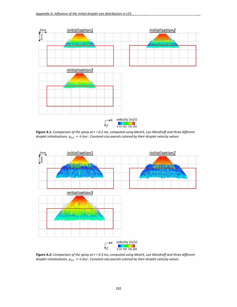
Appendix A: Influence of the initial droplet size distribution in LES__ _ _ _
182
Figure A.1: Comparison of the spray at t = 0.2 ms, computed using Mesh3, Lax-Wendroff and three different droplet initialisations. 𝑝 = 6 𝑏𝑎𝑟. Constant-size parcels colored by their droplet velocity values
Figure A.2: Comparison of the spray at t = 0.3 ms, computed using Mesh3, Lax-Wendroff and three different droplet initialisations. 𝑝 = 6 𝑏𝑎𝑟. Constant-size parcels colored by their droplet velocity values

Appendix A: Influence of the initial droplet size distribution in LES__ _ _ _
183
Figure A.3: Comparison of the spray at t = 0.4 ms, computed using Mesh3, Lax-Wendroff and three different droplet initialisations. 𝑝 = 6 𝑏𝑎𝑟. Constant-size parcels colored by their droplet velocity values
Figure A.4: Comparison of the spray at t = 0.5 ms, computed using Mesh3, Lax-Wendroff and three different droplet initialisations, with the experiments. 𝑝 = 6 𝑏𝑎𝑟 Simulation: the parcels are colored by their droplet velocity values Experiments: spray pattern using the shadowgraphy technique with background illumination

Appendix A: Influence of the initial droplet size distribution in LES__ _ _ _
184

185
Bibliography 1) A.N.Kolmogorov. Local Structure of Turbulence in Incompressible Viscous Fluid for Very Large Reynolds Number. Doklady AN., 30(1 and 2): pp.299-303, SSSR, 1941. 2) A.Favre. Statistical equations of turbulent gases. Problems of hydrodynamics and continuum mechanics: pp. 231-266, SIAM, Philadelphia, 1969. 3) W.P.Jones, B.E.Launder. The prediction of laminarization with a 2-equation model of turbulence. International Journal of Heat and Mass Transfer, 15: p301, 1972. 4) J.R.Bull, A.Jameson. Explicit filtering and exact reconstruction of the sub-filter stresses in large-eddy simulation. J. Comput. Phy. 30 pp.117-136, 2016. 5) M.Germano. Differential filters of elliptic type. Phys Fluids 29 (6) pp.1757-1758, 1986. 6) D.Carati, G.S.Winckelmans, H.Jeanmart. On the modelling of the subgrid-scale and filtered-scale stress tensors in large-eddy simulation. J. Fluid Mech. 441 pp.119-138, 2001. 7) T.S.Lund. The use of explicit filters in large-eddy simulation. Comput. Math. Appl. 46 pp.603-616, 2003. 8) S.Bose, P.Moin, D.You. Grid-independent large-eddy simulation using explicit filtering. Phy. Fluids 22 (10), 2010. 9) O.Colin, M.Rudgyard. Development of high-order Taylor-Galerkin schemes for LES. Journal of Computational Physics. 162(2) pp. 338-371, 2000. 10) M.Germano. Turbulence: the filtering approach. J. Fluid Mech. 238 pp.325-336, 1992 11) A.Yoshizawa. Statistical theory for compressible turbulent shear flows, with the application to subgrid modeling. Phys. Fluids 29 pp.2152-2164, 1986 12) J.Smagorinsky. General circulation experiments with the primitive equations. The basic experiment. Mon. Weather Rev. 91(3) pp.99-164, 1963 13) C.Bailly, G.Comte-Bellot. Turbulence. CNRS Editions, 2003. 14) J.W.Deardorff. A numerical study of the three-dimensional turbulent channel flow at large Reynolds numbers. Journal of Fluid Mechanics. 41(2) pp.453-480, 1970. 15) P.Moin, K.Squires, W.Cabot, S.Lee. A dynamic subgrid-scale model for compressible turbulence and scalar transport. Phys. Fluids. A 3(11) pp.2746-2757, 1991. 16) H.B.Toda, O.Cabrit, G.Balarac, S.Bose, J.Lee, H.Choi, F.Nicoud. A subgrid-scale model based on singular values for LES in complex geometries. NASA Ames/Stanford Univ. Center for Turbulence Research, editor, Proc. Of the Summer Programme, pp.193-202, 2000. 17) A.Misdariis, A.Robert, O.Vermorel, S.Richard, T.Poinsot. Numerical methods and turbulence modeling for LES of piston engines: impact on flow motion and combustion. Oil & Gas Science and Technology, 2010.

Bibliography _
186
18) J.P.Boris, F.F.Grinstein, E.S.Oran, R.L.Kolbe. New insights into large eddy simulation. Fluid Dyn. Res. 10 (4-6) pp.199-228, 1992 19) F.M.Denaro. What does finite volume-based implicit filtering really resolve in large-eddy simulation? J. Comput. Phys. 230 (10) pp.3849-3883, 2011. 20) S.B.Pope. Turbulent Flows. Cambridge university press, 2000. 21) M.Germano, U.Piomelli, P.Moin, W.H.Cabot. A dynamic subgrid-scale eddy viscosity model. Phy. Fluids. A 3 pp.1760-1765, 1991. 22) C.Meneveau, T.Lund. The dynamic Smagorinsky model and scale-dependent coefficients in the viscous range of turbulence. Phys. Fluids, 9(12) pp.3932-3934, 1997. 23) S.B.Pope. Ten questions concerning the large-eddy simulation of turbulent flows. New Journal of Physics, pp.6-35, 2004. 24) A.Aspden, N.Nikiforakis, S.Dalziel, J.B.Bell. Analysis of implicit LES methods. Comm. App. Math. and Comp. Sci. Vol.3,No1, 2008. 25) L.G.Margolin. Modeling of turbulent flow with implicit LES. Proceedings of the Joint Russian-American Five Laboratory Conference on Computational Mathematics/Physics. Vienna 19-23 June 2005. 26) M.Lesieur. Turbulence in Fluids. Fluid Mechanics and its applications. Kluwer Academic Publishers, 1990. 27) O.Colin. Simulations aux grandes échelles de la combustion turbulente prémélangée sur les statoréacteurs. PhD thesis, Université de Toulouse, 2000. 28) C.Angelberger. Development and application of Large-Eddy Simulation to study acyclic combustion in internal combustion engines. Habilitation, IFPEN, Université de Toulouse, 2011. 29) S.Buhl, F.Gleiss, M. Köhler, F.Hartmann, D.Messig, C.Brücker, C.Hasse. A combined numerical and experimental study of the 3D tumble structure and piston boundary layer development during the intake stroke of a gasoline engine. Flow Turb. Combutst. 98 pp.579-600, 2017. 30) E.Nicoud, O.Colin, C.Angelberger, F.Nicollet, C.Krüger. A no-slip implementation of a wall law boundary condition in a cell-vertex code for LES of internal aerodynamics on unstructured meshes. Conference LES4ICE, IFP Energies nouvelles, Rueil-Malmaison, 2016. 31) S.Ghosal, P.Moin. The basic equations for the large-eddy simulation of turbulent flows in complex geometries. J. Comput. Phys. 118(1) pp.24-37, 1995. 32) V.Moureau, O.Vasilyev, C.Angelberger, T.Poinsot. Proceedings of the summer program, center for turbulence research, NASA AMES/Stanford University, pp. 157-168, 2004. 33) J.Donea, A.Huerta, J.-Ph.Ponthot, A.Rodrígez-Ferran. Arbitrary Lagrangian-Eulerian Methods. Encyclopedia of Computational Mechanics, John Wiley & Sons, Volume 1: Fundamentals, Chapter 14, 2004 34) C.W. Hirt, A.A.Amsden, J.L.Cook. An arbitrary Lagrangian-Eulerian computing method for all flow speeds. Journal of Computational Physics, 14(3) pp.227:253, 1974.

Bibliography _
187
35) L.G.Margolin. Introduction to ‘an arbitrary Lagrangian-Eulerian computing method for all flow speeds’. Journal of Computational Physics, 135 pp.192-202, 1997. 36) V.Moureau, G.Lartigues, Y.Sommerer, C.Angelberger, O.Colin, T.Poinsot. Numerical methods for unsteady compressible multi-component reacting flow on fixed and moving grids. Journal of Computational Physics 202 pp.710-736, 2005. 37) O.Colin, M.Rudgyard. Development of High-Order Taylor-Galerkin Schemes for LES. Journal of Computational Physics 162 pp.338-371, 2000. 38) P.D.Lax, B.Wendroff. Systems of conservation laws. Communications in Pure and Applied Mathematics 13(2) pp.217-237, 1960. 39) J.Donea. A Taylor-Galerkin method for convective transport problems. Int. J. Numer. Methods Eng. 20 pp.95-101, 1984. 40) P.Sagaut. Large Eddy Simulation for incompressible flows. Scientific computation series. Springer-Verlag, 2000. 41) K. W.Thompson. Time Dependent Boundary Conditions for Hyperbolic Systems. Journal of Computational Physics, 68 pp.1-24, 1987. 42) K. W.Thompson. Time Dependent Boundary Conditions for Hyperbolic Systems II. Journal of Computational Physics, 89 pp.439-461, 1990. 43) T. J.Poinsot and S. K.Lele. Boundary Conditions for Direct Simulation of Compressible Viscous Flows. Journal of Computational Physics, 101 pp.104-129, 1992. 44) T. J.Poinsot and L.Selle. Actual Impedance of Non-reflecting Boundary Conditions: Implications for Computation of Resonators. AIAA Journal, 42(5) pp. 958-964, 2004. 45) R.Stiehl, J.Bode, J.Schorr, C.Krüger, A.Dreizler, B.Böhm. Influence of intake geometry variations on in-cylinder flow and flow–spray interactions in a stratified direct-injection spark-ignition engine captured by time-resolved particle image velocimetry. J. of engine research, 2016. 46) R.Stiehl, J.Schorr, C.Krüger, A.Dreizler, B.Böhm. In-Cylinder Flow and Fuel Spray Interactions in a Stratified Spray-Guided Gasoline Engine Investigated by High-Speed Laser Imaging Techniques. Flow Turbulence Combust, 91 pp.431–50, 2013. 47) C.Krüger, J.Schorr, F.Nicollet, J.Bode, A.Dreizler, B.Böhm. Cause-and-effect chain from flow and spray to heat release during lean gasoline combustion operation using conditional statistics. Int. J. of Engine Research, DOI: 10.1177/1468087416686721, 2017. 48) J.Bode, J.Schorr, C.Krüger, A.Dreizler, B.Böhm. Influence of three-dimensional in-cylinder flows on cycle-to-cycle variations in a fired stratified DISI engine measured by time-resolved dual-plane PIV. Proceedings of the Combustion Institute 36 (3), S. 3477–3485. DOI: 10.1016/j.proci.2016.07.106, 2016. 49) V.Moureau. Simulation aux grandes échelles de l’aérodynamique interne des moteurs à piston. PhD thesis, École centrale Paris, 2004. 50) L.Graftieaux, M.Michard, N.Grosjean. Combining PIV, POD and vortex identification algorithms for the study of unsteady turbulent swirling flows. Meas. Sci. Technol. 12(9), 1422, 2001.
Bibliography _
188
51) P.Janas, I.Wlaukas, B.Böhm, A.Kempf. On the Evolution of the Flow Field in a Spark Ignition Engine. Springer Science+Business Media Dordrecht, 2016. 52) L.Sachs. Applied Statistics a handbook of techniques. Springer-Verlag New York. DOI: 10.1007/978-1-4612-5246-7, 1984 53) R.A.Fischer. Statistical Methods for Research Workers. 13th edition, Hafner, 1958. 54) U.Schaupp, A.Waltner, A.Kaden, C.Krüger. Magere geschichtete Verbrennung mit strahlgeführtem Brennverfahren in Motoren mit hoher spezifischer Leistung. Aachener Symposium 2014. 55) C.Baumgarten. Mixture formation in internal combustion engines. Springer-Verlag New-York, 2005. 56) U.Michels. Euler-Strahlmodell für Düseninnenströmung und Strahlausbreitung. PhD thesis, Fakultät für Maschinenbau, Gottfried Wilhelm Leibniz Universität Hannover, 2008. 57) A.Hermann. Modellbildung für die 3D-Simulation der Gemischbildung und Verbrennung in Ottomotoren mit Benzin-Direkteinspritzung. PhD thesis, Fakultät für Maschinenbau, Universität Karlsruhe, 2008. 58) J.Ramos. Internal combustion engine modeling. Hemisphere publishing corporation, 1989. 59) FA.Williams. Combustion theory: Fundamental Theory of Chemically Reacting Flow Systems. Addion-Wesley Publishing Company Inc., Massachusetts, 1965. 60) JK.Dukowicz. A Particle-Fluid Numerical Model for Liquid Sprays. J. Comp. Physics, vol.35, pp.229-253, 1980. 61) G.P.Merker, C.Schwarz. Grundlagen Verbrennungsmotoren. Vieweg+Teubner, 4.Auflage, 2009. 62) G.Stiesch. Modeling Engine Spray and Combustion Processes. Springer, 2003. 63) G.G.Stokes. On the effect of the internal friction of fluids on the motion of pendulums, Pitt Press, volume9, 1851. 64) R.Clift, J.R.Grace, M.E.Weber. Bubbles, Drops and Particles. Academic press, 1978. 65) J.A.Mulholland, R.K.Shrivastava, J.O.L.Wendt. Influence of droplet spacing on drag coefficient in nonevaporating, monodisperse streams. AIAA Journal 26(10), pp.1231-1237, 1988. 66) J.F.Virepinte. Etude du comportement dynamique et thermique de gouttes en régime d’interaction dans le cas de jets rectilignes. PhD thesis, École National Supérieure de l’Aéronautique et de l’espace, 1999. 67) L.Schiller, A.Naumann. A drag coefficient correlation. VDI Zeitung 77 pp.318-320, 1935. 68) A.Massol. Simulation d’écoulement autour de réseaux de particules sphériques. PhD thesis, INP Toulouse, 2004. 69) N.Iafrate. Simulation aux grandes échelles diphasique dans les moteurs downsizés à allumage commandé. PhD thesis, INP Toulouse, 2016

Bibliography _
189
70) R.D.Reitz, R.Diwakar. Structure of High-Pressure Fuel Spray, SAE 870598, 1987. 71) N.Dombrowski, P.C. Hooper. The effect of Ambient Density on Drop Formation in Sprays. Chem. Eng. Science, Band 17, pp.291-305, 1962. 72) K.J.Wu, G.M.Faeth. Aerodynamic Effects on Primary Break-up in Gas/Liquid Mixing Layers for Turbulent Liquids. Atom. & Sprays, Band 2, pp.295-317, 1992. 73) K.Y.Huh, A.D.Gosman. A Phenomenological Model of Diesel Spray Atomization. Int. Conf. on Multiphase Flow, Tsukuba, 1991. 74) R.D.Reitz, R.Diwakar. Effect of Drop Breakup on Fuel Sprays. SAE 860469, 1986. 75) A.Wierzba. Deformation and Breakup of Liquid Drops in a Gas Stream at Nearly Critical Weber Numbers. Experiments in Fluids, vol 9, pp.59-64, 1993. 76) M.Pilch, C.A.Erdman. Use of Breakup Time Data and Velocity History Data to predict the Maximum Size of Stable Fragments for Acceleration-Induced Breakup of a Liquid Drop. Int. J. of Multiphase Flow, Band 13, pp.741-757, 1987. 77) R.D.Reitz. Modeling Atomization Process in High-Pressure Vaporizing Sprays. Atomization and Spray Technology 3, pp.309-337, 1987. 78) R.D.Reitz, F.V.Bracco. Mechanisms of Breakup of Round Liquid jets. In Encyclopedia of Fluid Mechanics, Gulf Pub, NJ 3, pp.233-249, 1986 79) W.Ohnesorge. Die Bildung von Tropfen an Düsen und die Auflösung flüssiger Strahlen. Zeitschrift für angewandte Mathematik und Mechanik, Bd. 16, Heft 6, pp.355-358, 1931. 80) C.Krueger. Validierung eines 1D-Spraymodells zur Simulation der Gemischbildung in direkteinspritzenden Dieselmotoren. PhD thesis, Rheinisch-Westfälische Technische Hochschule, Aachen, 2001. 81) D.B.Spalding. Experiments on the burning and extinction of liquid fuel spheres. Fuel. 32, pp.169-185, 1953. 82) W.E.Ranz, W.R.Marshall. Internal Combustion Engine Modeling. Hemisphere Publishing, New-York, 1952. 83) C.Habchi. Développement de modèles pout la Simulation aux grandes échelles des jets de carburants liquides dans les moteurs à combustion interne. ANR, ANR-07-PDIT-002, 2011. 84) J.Borée, P.C.Miles, D.Crolla, D.E.Foster, T.Kobayashi. Encyclopaedia of Automotive Engineering. John Wiley & Sons, Ltd, Chichester, UK, pp.1-31, 2014. 85) E.Baum, B.Peterson, B.Böhm, A.Dreizler. On The Validation of LES Applied to Internal Combustion Engine Flows: Part 1: Comprehensive Experimental Database. Flow Turbulence Combust 92 (1-2). DOI: 10.1007/s10494-013-9468-6, pp.269-297, 2014. 86) E.Baum, B.Peterson, C.Surmann, D.Michaelis, B.Böhm, A.Dreizler. Investigation of the 3D flow field in an IC engine using tomographic PIV. Proceedings of the Combustion Institute 34 (2). DOI: 10.1016/j.proci.2012.06.123, pp. 2903-2910, 2013.

Bibliography _
190
87) M.Buschbeck, N.Bittner, T.Halfmann, S.Arndt. Dependence of combustion dynamics in a gasoline engine upon the in-cylinder flow field, determined by high-speed PIV. Exp Fluids 53 (6). DOI: 10.1007/s00348-012-1384-3, pp.1701-1712, 2012 88) B.Peterson, D.Reuss, V.Sick. On the ignition and flame development in a spray-guided direct-injection spark-ignition engine. Combustion and Flame 161 (1). DOI: 10.1016/j.combustflame.2013.08.019, pp. 240-255, 2014. 89) E.Nicoud. Quantifying combustion stability in GDI engines by Large-Eddy Simulation. PhD thesis, École centrale Paris, 2017. 90) The International Council on clean transportation. CO2 emissions from new passenger cars in the EU: Car manufacturer’s performance in 2017. www.theicct.org. 91) G.Vent, C.Enderle, N.Merdes, F.Kreitmann, R.Weller. The New 2.0l Turbo Engine from the Mercedes-Benz 4-Cylinder Engine Family. 21st Aachen Colloquium Automobile and Engine Technology, 2012. 92) D.Haworth. Large-Eddy Simulation of in-cylinder flows. Oil & Gas Science and Technology 54(2), pp. 175-185, 1999. 93) M.Baumann, F.Di Mare, J.Janicka. On the Validation of Large-Eddy Simulation Applied to Internal Combustion Engine Flows Part II: Numerical Analysis. Flow Turbulence Combustion 92 (1-2), pp. 299-317. DOI: 10. 1007/s10494-013-9472-x, 2014. 94) A.Robert, S.Richard, O.Colin, L.Martinez, L.De Francqueville. LES prediction and analysis of knocking combustion in a spark-ignition engine. Proc. Combust. Inst., 35 (3), pp. 2941-2948, 2015. 95) A.Robert, S.Richard, O.Colin, T.Poinsot. LES study of deflagration to detonation mechanisms in a downsized spark-ignition engine. Combustion and Flame, Elsevier, 162 (7), pp. 2788-2807, 2015. 96) D.Goryntsev, A.Sadiki, J.Janicka. Towards Large-Eddy Simulation of Spray Combustion in Direct Injection Spark-Ignition Engine. SAE Technical Paper 2011-01-1884, 2011. 97) P.Abraham, K.Liu, D.Haworth, D.Reuss. Evaluating Large-Eddy Simulation (LES) and High-Speed Particle Image Velocimetry (PIV) with Phase-Invariant Proper Orthogonal Decomposition (POD). Oil & Gas Sci. Technol. – Rev. IFP Energies nouvelles 69(1), pp. 41-49, 2014. 98) L.Martinez, A.Benkenida, B.Cuenot. A model for the injection boundary conditions in the context of 3D Simulation of Diesel Spray. Methodology and Validation. Fuel, 89(1), pp. 219-228, 2010. 99) C.Habchi and G.Bruneaux. LES and Experimental investigation of Diesel sprays. 12th Triennial International Conference on Liquid Atomization and Spray Systems, Heidelberg, Germany, September 2-6 2012. 100) A.Robert, L.Martinez, J.Tillou, S.Richard. Eulerian-Eulerian Large-Eddy Simulation applied to transient Diesel Sprays. Oil & Gas Science and Technology – revue de l’IFP Energies Nouvelles, special issue “LES4ICE’12 conference”, 2013 101) BOSCH, ‘High-pressure piezo injector HDEV4’ – customer documentation, 2013.
Bibliography _
191
102) C.Ruhland, N.V.Dam, V.Sick, D.L.Reuss, D.Haworth, J.Oefelein, T.-W.Kuo and X.Yang. A common engine platform for engine LES development and validation, in LES4ICE, C. Angelberger, Editor, IFP Energies Nouvelles, Rueil-Malmaison, France, 2012. 103) La vision. Website: https://www.lavision.de 104) J.Bode. Untersuchung der Zyklus-zu-Zyklus Schwankungen in einem Ottomotor mit Hilfe mehrdimensionaler Strömungsdiagnostik. PhD thesis, Technische Universität Darmstadt, 2017. 105) L.Sachs and J.Hedderich. Angewandte Statistik: Methodensammlung mit R. Springer Berlin, Heidelberg, 2006. 106) R.A.Fisher. Statistical methods and scientific inference. Hafner Publishing Co., 1956. 107) K.Nording. Numerische Analyse der dieselmotorischen Gemischbildung, Verbrennung und Emissionsentstehung. PhD thesis, Universität Stuttgart, 2015. 108) P.J.O’Rourke. Statistical properties and numerical implementation of a model for droplet dispersion in a turbulent gas. Los Alamos National Laboratory report LA UR 87-2376, accepted by J. Comput. Phys, 1987. 109) AVBP: Property of CERFACS. Website: http://www.cerfacs.fr/avbp7x/. 110) R.Stiehl. Laserbasierte Untersuchung der Prozesse in einem Ottomotor mit strahlgeführtem Brennverfahren. PhD thesis, Technische Universität Darmstadt, 2015. 111) C.Brücker. 3D scanning PIV applied to an air flow in a motored engine using digital high-speed video. Measurement Science and Technology, 8(12):1480, 1997. 112) T. Li, J. Pareja, L. Becker, W. Heddrich, A. Dreizler and B. Böhm. Quasi-4d laser diagnostic using an acousto-optic deflector scanning system. Applied Physics B, 123(3):78, 2017. 113) HIP: Property of CERFACS. Website: http://www.cerfacs.fr/avbp7x/hip.php 114) B.E.Launder and D.B.Spalding. The numerical computation of turbulent flows. Comp. Methods Appl. Mech. Eng., 3:269-289, 1974. 115) A.Hatzipanagiotou. 3D-CFD-Simulation der Gemischbildung, Verbrennung und Emissions-Entstehung eines Hochdruck-Gas-Diesel-Brennverfahrens. PhD thesis, Karlsruher Institut für Technologie, 2018. 116) LES4ICE conference: LES for Internal Combustion Engine Flows LES4ICE, organized by IFP Energies Nouvelles and directed by C.Angelberger. Website: http://www.rs-les4ice.com. 117) CDP: The unstructured LES code. Center for integrated turbulence simulations, Stanford University. Website: http://web.stanford.edu/group/cits/research/combustor/cdp.html. 118) Centaur: Property of Centaursoft. Website: https://www.centaursoft.com/. 119) M.Lesieur. Turbulence in fluids. Fluid Mechanics and its applications. Kluwer Academic Publishers, 1990. 120) Star-CD: Property of Siemens. Website: https://mdx.plm.automation.siemens.com

Bibliography _
192
121) Star-CCM+: Property of Siemens. Website: https://mdx.plm.automation.siemens.com 122) Fire: Property of AVL. Website: https://www.avl.com/fire 123) CFX: Property of ANSYS. Website: https://www.ansys.com/products/fluids/ansys-cfx 124) FLUENT: Property of ANSYS. Website: https://www.ansys.com/Products/Fluids/ANSYS-Fluent 125) Converge: Property of Convergent science. Website: https://convergecfd.com/ 126) Open-Foam: Open source software. Website: https://www.openfoam.com/ 127) Kiva: Open source software. Website: http://www.lanl.gov/projects/feynman-center/deploying-innovation/intellectual-property/software-tools/kiva/download.php 128) CatiaV5: Property of Dassault Systèmes. Website: https://www.3ds.com/de/produkte-und-services/catia/ 129) The Paris climate agreement. United Nations Treaty collections, 2017. Website: https://treaties.un.org/pages/ViewDetails.aspx?src=TREATY&mtdsg_no=XXVII-7-d&chapter=27&clang=_en 130) Reducing C02 for passenger cars. European Commission. Website: https://ec.europa.eu/clima/policies/transport/vehicles/cars_en 131) Darmstadt Engine Workshop, RSM, Technische Universität Darmstadt. Website: http://www.rsm.tu-darmstadt.de/home_rsm/news_rsm/darmstadt_engine_workshop.de.jsp 132) Matlab: Property of Mathworks. Website: https://de.mathworks.com/products/matlab.html 133) Excel: Property of Microsoft. Website: https://products.office.com/de-de/excel 134) P.Chassaing. Turbulence en mécanique des fluides : analyse du phénomène en vue de sa modélisation à l’usage de l’ingénieur. Cépaduès, polytech edition, 48, 2000. 135) U.Piomelli, E.Balaras. Wall-layer models for large-eddy simulations. Annual Review of Fluid Mechanics, 34(1) pp. 349-374, 2002. 136) B.Wang, G.Zha. Detached-eddy simulation of a co-flow jet airfoil at high angle of attack. 39th AIAA Fluid Dynamics Conference, San Antonio USA, 22-25 June 2009. 137) O.Lehmkuhl, G.Chrysokentis, S.Gomez, H.Owen. Large-eddy simulation for automotive aerodynamics with Alya. Tenth International Conference on CFD, Barcelona Spain, July 9-13 2018. 138) C.Hasse, V.Sohm, B.Durst. Detached-eddy simulation of cyclic large scale fluctuations in a simplified engine setup. International Journal of Heat and fluid Flow, 30(1) pp. 32-43, 2009. 139) P.Spalart, W.H.Jou, M.Strelets, S.Allmaras. Comments on the feasibility of LES for wings, and on a hybrid RANS/LES approach. Proceedings of the first AFOSR international conference on DNS/LES, Louisiana Tech University USA, August 4-8 1997. 140) E.Balaras, C.Benocci, U.Piomelli. Two-layer approximate boundary conditions for large-eddy simulations. AIAA Journal, 34(6) pp. 1111-1119, 1996.

Bibliography _
193
141) W.Cabot. Near-wall models in large-eddy simulations of flow behind a backward-facing step. Annual research briefs. Center for Turbulence Research, NASA/Stanford Univ, pp. 199-210, 1996. 142) C.Jainski, L.Lu, A.Dreizler, V.Sick. High-Speed Micro Particle Image Velocimetry of boundary layer flows in a Direct-Injection engine. International Journal of Engine Research, 14(3) pp.247-259, 2013. 143) M.Ihme, P.C.Ma, M.Greene, V.Sick, C.Jainski, A.Dreizler. Non-equilibrium wall-modelling for Large-Eddy Simulation of internal combustion engines. THIESEL Conference on Thermo- and fluid Dynamic Processes in Direct Injection Engines, Valencia, Spain. 2016. 144) M.Gavaises, S.Tonini, A.Marchi, A.Theodorakakos, D.Bouris, L.Matteucci. Modelling of internal and near-nozzle flow of a pintle-type outwards-opening gasoline piezo-injector. Int. J. Engine Res. Vol7. DOI: 10.1243/14680874JER00306, 2006. 145) A.Marchi, J.M.Nouri, et al. Internal flow and spray characteristics of Pintle-type outwards opening Piezo injectors for gasoline direct-injection engines. SAE technical paper series 2007-01-1406, 2007. 146) B.Befrui, G.Corbinelli, D.Robart, W.Reckers. LES simulation of the internal flow and near-field spray structure of an outward-opening GDI injector and comparison with imaging data. SI combustion and direct injection SI engine technology, SP-2187, 2008. 147) Es-ice: Property of Siemens. Website: https://mdx.plm.automation.siemens.com.