arX

iv:a

stro

-ph/

0207

182v

1 8

Jul

200

2

1

Abstract. We present the analysis of a deep colour-magnitude diagram (CMD) of NGC 1831, a rich starcluster in the LMC. The data were obtained withHST/WFPC2 in the F555W (∼ V) and F814W (∼ I) fil-ters, reaching m555 ∼ 25. We discuss and apply a methodof correcting the CMD for sampling incompleteness andfield star contamination. Efficient use of the CMD datawas made by means of direct comparisons of the ob-served to model CMDs. The model CMDs are built byan algorithm that generates artificial stars from a singlestellar population, characterized by an age, a metallic-ity, a distance, a reddening value, a present day massfunction and a fraction of unresolved binaries. Photo-metric uncertainties are empirically determined from thedata and incorporated into the models as well. Statisti-cal techniques are presented and applied as an objectivemethod to assess the compatibility between the modeland data CMDs. By modelling the CMD of the centralregion in NGC 1831 we infer a metallicity Z = 0.012,8.75 ≤ log(τ) ≤ 8.80, 18.54 ≤ (m − M)0 ≤ 18.68 and0.00 ≤ E(B − V ) ≤ 0.03. For the position dependentPDMF slope (α = −d logΦ(M)/d log M), we clearly ob-serve the effect of mass segregation in the system: forprojected distances R ≤ 30 arcsec, α ≃ 1.7, whereas2.2 ≤ α ≤ 2.5 in the outer regions of NGC 1831.

Key words: galaxies: star clusters – Magellanic Cloud –globular clusters: individual: NGC 1831 – stars: statistics

A&A manuscript no.

(will be inserted by hand later)

Your thesaurus codes are:

missing; you have not inserted them

ASTRONOMYAND

ASTROPHYSICS

Analysis of colour-magnitude diagrams of rich LMC clusters:NGC1831

L. O. Kerber1, B. X. Santiago1, R. Castro1, and D. Valls-Gabaud2

1 Universidade Federal do Rio Grande do Sul, IF, CP15051, Porto Alegre 91501–970, RS, Brazil2 UMR CNRS 5572, Observatoire Midi-Pyrenees, 14, avenue Edouard Belin, 31400 Toulouse, France

Received 08 April 2002 / Accepted 06 May 2002

1. Introduction

The Large Magellanic Cloud (LMC) presents three essen-tial characteristics that make it an excellent complemen-tary laboratory for studying the formation and evolutionof galaxies and stellar systems in general: a) it is closeto the Galaxy; b) it has markedly different morphologi-cal, chemical and kinematical properties from our MilkyWay; c) it presents a large variety of stellar clusters, dis-playing distinct physical characteristics among themselvesand when compared to those in the Galaxy (Westerlund1990). Due to the diversity in ages and metallicities, LMCclusters are found at distinct evolutionary stages (Wester-lund 1990, Olszewski et al. 1991). The determination of acluster’s present physical properties, such as density pro-file, shape, internal velocity distribution and its positiondependent Present Day Mass Function (PDMF), provideus with essential links needed to assess the role of grav-itational dynamics, including effects of mass segregationand stellar evaporation (Heggie & Aarseth 1992, Spurzem& Aarseth 1996, de Oliveira et al. 2000). Thus, once thesepresent properties are known, modelling techniques like N-body simulations allow us to recover the initial conditionsunder which clusters formed (Goodwin 1997, Vesperini &Heggie 1997, Kroupa et al. 2001). In this context, the ini-tial mass function (IMF) and its possible universality, arekey pieces in the study of stellar contents of distant galax-ies (Kroupa 2001).

Through the analysis of colour-magnitude diagrams(CMDs) one has a great variety of physical informationabout a cluster. Isochrone fits help constraining the sys-tem’s age, metallicity, distance and reddening. Further-more, observational luminosity functions (LFs) have al-lowed derivation of the stellar mass function (Elson et al.1995, De Marchi & Paresce 1995, Santiago et al. 1996,Piotto et al. 1997, de Grijs et al. 2002a). However, thetransformation of luminosity into mass depends on ageand metallicity, the uncertainties in these parameters be-ing therefore incorporated into the inferred mass func-tion. Besides, the theoretical uncertainties in the mass-luminosity relation itself, specially for the low-mass stars

Send offprint requests to: kerber@if.ufrgs.br

(Piotto et al. 1997, Baraffe et al. 1998), added to the ef-fect of unresolved binarism, further hampers real massfunction determination through observational luminosityfunctions.

From both observational and theoretical points ofview, the advent of the Hubble Space Telescope (HST),associated with the constant improvement in theories ofstellar interiors, atmospheres and evolution, require evermore sophisticated methods of CMD analysis. In this con-text, computational modelling techniques have allowed awider use of CMDs as tools to constrain physical prop-erties of stellar populations and systems. Model CMDs,along with statistical methods of comparing them to ob-served ones, have been useful means to investigate thestar formation history within a galaxy (Gallart et al. 1996,Gallart et al. 1999, Hernandez et al. 1999, Holtzman et al.1999, Hernandez et al. 2000) or to constrain structural pa-rameters and the stellar luminosity function in the MilkyWay (Kerber et al. 2001).

With these issues in mind, our work aims at extract-ing as much physical information as possible about richLMC clusters, by means of objective comparison of theirobserved CMDs with artificial ones. The idea is to simul-taneously infer PDMF slope, age, metallicity, distance,reddening and unresolved binary fraction for each systemstudied. The present work introduces the techniques devel-oped for that purpose and shows the results for NGC 1831,one of the richest LMC clusters for which we have deepHST data.

Previous works are evidence of the large difficul-ties in extracting physical parameters for NGC 1831.Techniques based on CMDs from CCD photometry(Mateo 1987,1988; Chiosi 1989; Vallenari et al. 1992;Corsi et al. 1994), integrated spectroscopy or colours(Bica et al. 1986; Meurer et al. 1990; Cowley &Hartwick 1992; Girardi et al. 1995) and spectroscopyof individual giant stars (Olszewski et al. 1991) wereemployed with this aim, constraining the values of themain parameters: 8.50 <∼ log(τ) <∼ 8.80 (300 <∼ τ <∼ 650Myr); 0.002 <∼ Z <∼ 0.020 (−1.00 <∼ [Fe/H] <∼ 0.01);0.00 <∼ E(B − V ) <∼ 0.07. For the distance to NGC 1831,there are not reliable determinations, the standard

Kerber et al.: CMD analysis for NGC1831 3

procedure being the adoption of typical values of theintrinsic distance modulus, (m − M)0, for the LMCcentre. In this aspect, the most reliable estimate seemsto be that of Panagia et al. 1991, (m − M)0 = 18.51,since it is based on purely geometrical arguments appliedto high quality imaging and spectral data on supernovaSN1987a. In terms of dynamical evolution for this system,Elson et al. (1987) estimated 6.5 <∼ log(tcross) <∼ 7.0 and9.6 <∼ log(trh) <∼ 10.0 for the crossing time and two-bodyrelaxation time, respectively, the range quoted beingdue to different mass-luminosity relations. Comparingwith its estimated age values, these results suggest thatNGC 1831 is a system dynamically well mixed, butnot totally relaxed through stellar encounters. Hence,NGC 1831 is sufficiently old to have suffered mass segre-gation, affecting the PDMF slope at different distancesto its centre, but perhaps still young enough that theinitial conditions could be preserved in its outer regions.Similarly, external effects may not have had enough timeto affect the cluster dynamics either.

One of the main objectives of this paper is to verifythe effect of mass segregation in NGC 1831, quantifyingthe variation in PDMF slope with projected distance tothe cluster’s centre. This determination may yield stronglinks to IMF reconstruction efforts based on N-body mod-els. The paper is outlined as follows: in Sect. 2 we presentthe data and the methods of accounting for sample in-completeness and field star contamination in the observedCMD; in Sect. 3 we present the algorithm used for CMDmodelling and the statistical tools used for model vs. datacomparisons; in Sect. 4 we discuss control experimentsused for to verify the validity of the method; finally, inSect. 5 we present the results for the NGC 1831 data,which are discussed in Sect. 6.

2. The observed CMD

We have data taken with the Wide Field and Planetary

Camera 2 (WFPC2) on board HST for 8 rich LMC clus-ters and nearby fields. These data are part of the GO7307project, entitled “Formation and Evolution of Rich StarClusters in the LMC” (Beaulieu et al. 1999, Beaulieu etal. 2001, Johnson et al. 2001). For each cluster, imageswere obtained using the F555W (V) and F814W (I) fil-ters. Most of the photometry had been previously carriedout: cluster stellar LFs were built and analyzed by Santi-ago et al. (2001), de Grijs et al. (2002b); field stellar pop-ulations were studied by Castro et al. (2001). Exposuretimes, field coordinates, image reduction and photometryprocesses are described in detail by those authors.

Fig. 1 shows the observed WFPC2 CMD for stars inthe direction of NGC 1831 in panel (a) (hereafter the on-cluster field) and for a nearby field (hereafter the off-cluster field) studied by Castro et al. (2001) in panel (b).The on-cluster sample shown here is the final compositionof the CEN and HALF images described by Santiago et

Fig. 1. The on-cluster (a) and off-cluster (b) WFPC2CMDs for NGC 1831. The former contains 7801 stars ob-served in the cluster’s direction while the latter has 2030stars located in a field 7.3 arcmin away from the cluster’scentre.

al. (2001). These have the Planetary Camera (PC) centredon the cluster’s centre and half-light radius, respectively.The off-cluster field is located at about 7.3 arcmin awayfrom the cluster’s centre. A clear cluster main sequence(MS) is visible in the figure, stretching from m555 ≃ 18.5down to m555 ≃ 25. The cluster MS turn-off is also clearlyvisible at the upper MS end. Notice, however, that satura-tion becomes a problem in the HALF field for m555

<∼ 19(m555

<∼ 17.8 for the CEN field). Hence, all our subsequentanalysis will be based on the CMD fainter than this limit.A branch of evolved stars is seen as well, especially in therange 18 <∼ m555

<∼ 19, where the cluster red clump is lo-cated. The subgiant branch at fainter magnitudes is due tofield contamination and is largely made up of older (τ > 3Gyr) stars.

The on-cluster data suffer from two important effects:sample incompleteness and contamination by field stars.Our CMD modelling algorithm does not incorporate sucheffects. Therefore it is crucial to adequately correct the ob-served CMD for them in order to place models and dataon equal footing. Quantifying systematic and random pho-tometric uncertainties and either correcting for them orapplying them to model CMDs is extremely important aswell, as they are responsible for most of the observed CMDspread. These data corrections are the subject of the nextsubsections.

4 Kerber et al.: CMD analysis for NGC1831

2.1. Random photometric uncertainties

The random photometric uncertainties are the mainsource of spread in our HST/WFPC2 CMDs. Therefore,a suitable assessment of these uncertainties in both filtersis crucial for correctly incorporating this effect into theartificial CMDs.

For the on-cluster field, two independent photometricmeasurements were available for a fraction of the starsdue to the overlap region imaged by both the HALF andCEN fields (Santiago et al. 2001). Thus, we used the starsbelonging to this overlap region to estimate the typicalphotometric uncertainties in the data. For each filter andat each magnitude bin, we estimated the dispersion, σ′,in the distribution of differences between the independentmagnitude measurements. For simplicity we assume thatσ′ is the composition of two equally-sized realizations ofphotometric error, σ. Thus, we get σ′2 = 2σ2, and there-fore

σ =σ′

√2.

We emphasize that the two filters were treated as ab-solutely independent. As a consequence, the uncertaintyin colour m555 − m814, σcolour, will be the quadratic sumof the individual uncertainties:

σ2colour = σ2

555 + σ2814.

Fig. 2 shows the derived uncertainties for MS stars inthe two filters, σ555 and σ814, and for the colour, σcolour,using the expressions above.

For the off-clusters stars, we did not have two inde-pendent and overlapping WFPC2 images and, as a re-sult, we could not apply the same method to quantifytheir photometric uncertainties. The solution found wasto employ the same estimate as for the on-cluster stars.As the off-cluster image is deeper and sparser than theon-cluster ones, we can expect that this approximationyields an overestimate of the photometric uncertainties inthe off-cluster data. However, the off-cluster CMD is usedonly for statistical subtraction of field contamination fromthe on-cluster CMD. We will see later that this particularcorrection technique is fairly independent of the estimatedphotometric uncertainties.

2.2. Systematic photometric uncertainties

Systematic effects in WFPC2 data have been found byseveral authors. Johnson et al. (2001) measured an ex-posure time effect varying from 0.01 to 0.06 for differ-ent WFPC2 chips and filters in images of NGC 1805 andNGC 1818, as part of this project. de Grijs et al. (2002b)finds similar trends, but of slightly larger amplitude forthe same data. Previously, Casertano & Muchtler (1998)found an exposure time effect but in the opposite senseas Johnson et al. (2001). Colour shifts of ≃ 0.04 have also

Fig. 2. Estimated photometric uncertainties. Panel (a)shows the σ555 (solid circles) and σ814 (crosses) values asa function of apparent magnitude. Panel (b) shows theσcolour calculated for the MS stars as a function of m555.

been measured between different WFPC2 chips, possiblydue to errors in CTE and aperture corrections or in zero-points (see also Johnson et al. 1999).

Any photometric biases, as a function of either expo-sure time or chip, must be eliminated from our observedCMD, since the model CMDs which will be compared toit do not incorporate them.

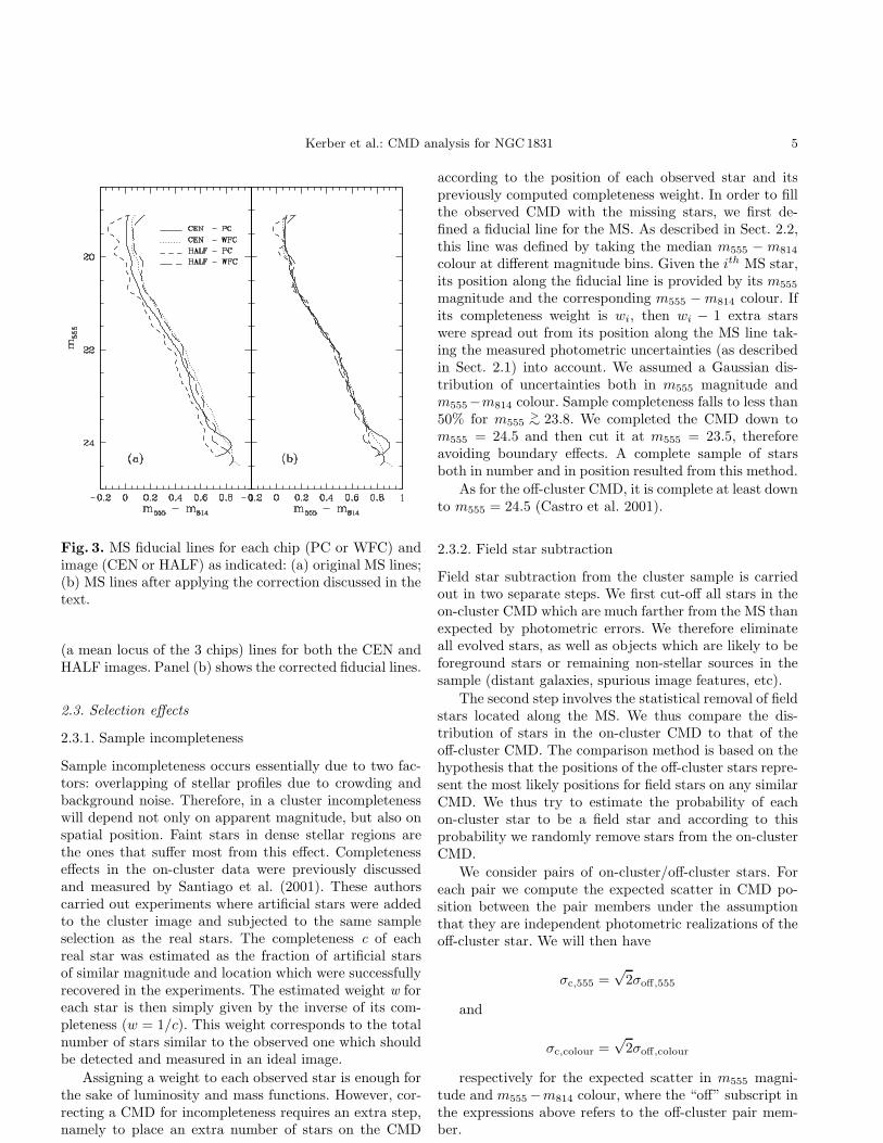
As there does not seem to exist a consensus on thecorrections to be applied, our approach was to empiricallymeasure such biases and to apply appropriate shifts tothe data when necessary. We searched for both exposuretime and chip vs. chip effects. No systematic effects werefound in the off cluster data. The main source of biasin the on-cluster data was found to be an offset betweenthe PC and the Wide Field Camera (WFC) chips in thesense that MS stars with the same m555 magnitude tendto be bluer by 0.05-0.10 mag when imaged with the PCthan with the WFC. This applies to both HALF and CENimages. As the PC in the HALF image is centered on thecluster half-light radius, this effect is unlikely to be due todifferences in crowding. In order to correct the data for thiseffect we first defined MS fiducial lines, taking the medianm555 −m814 colour at different magnitude bins. This wasdone separately for each chip and each image (CEN orHALF). We noticed that the WFC MS lines were morestable, always occupying loci in the CMD very close toeach other. Thus, we transposed the PC fiducial lines tothe corresponding WFC locus. The corrections are shownin Fig. 3. Panel (a) shows the uncorrected PC and WFC

Kerber et al.: CMD analysis for NGC1831 5

Fig. 3. MS fiducial lines for each chip (PC or WFC) andimage (CEN or HALF) as indicated: (a) original MS lines;(b) MS lines after applying the correction discussed in thetext.

(a mean locus of the 3 chips) lines for both the CEN andHALF images. Panel (b) shows the corrected fiducial lines.

2.3. Selection effects

2.3.1. Sample incompleteness

Sample incompleteness occurs essentially due to two fac-tors: overlapping of stellar profiles due to crowding andbackground noise. Therefore, in a cluster incompletenesswill depend not only on apparent magnitude, but also onspatial position. Faint stars in dense stellar regions arethe ones that suffer most from this effect. Completenesseffects in the on-cluster data were previously discussedand measured by Santiago et al. (2001). These authorscarried out experiments where artificial stars were addedto the cluster image and subjected to the same sampleselection as the real stars. The completeness c of eachreal star was estimated as the fraction of artificial starsof similar magnitude and location which were successfullyrecovered in the experiments. The estimated weight w foreach star is then simply given by the inverse of its com-pleteness (w = 1/c). This weight corresponds to the totalnumber of stars similar to the observed one which shouldbe detected and measured in an ideal image.

Assigning a weight to each observed star is enough forthe sake of luminosity and mass functions. However, cor-recting a CMD for incompleteness requires an extra step,namely to place an extra number of stars on the CMD

according to the position of each observed star and itspreviously computed completeness weight. In order to fillthe observed CMD with the missing stars, we first de-fined a fiducial line for the MS. As described in Sect. 2.2,this line was defined by taking the median m555 − m814

colour at different magnitude bins. Given the ith MS star,its position along the fiducial line is provided by its m555

magnitude and the corresponding m555 − m814 colour. Ifits completeness weight is wi, then wi − 1 extra starswere spread out from its position along the MS line tak-ing the measured photometric uncertainties (as describedin Sect. 2.1) into account. We assumed a Gaussian dis-tribution of uncertainties both in m555 magnitude andm555−m814 colour. Sample completeness falls to less than50% for m555

>∼ 23.8. We completed the CMD down tom555 = 24.5 and then cut it at m555 = 23.5, thereforeavoiding boundary effects. A complete sample of starsboth in number and in position resulted from this method.

As for the off-cluster CMD, it is complete at least downto m555 = 24.5 (Castro et al. 2001).

2.3.2. Field star subtraction

Field star subtraction from the cluster sample is carriedout in two separate steps. We first cut-off all stars in theon-cluster CMD which are much farther from the MS thanexpected by photometric errors. We therefore eliminateall evolved stars, as well as objects which are likely to beforeground stars or remaining non-stellar sources in thesample (distant galaxies, spurious image features, etc).

The second step involves the statistical removal of fieldstars located along the MS. We thus compare the dis-tribution of stars in the on-cluster CMD to that of theoff-cluster CMD. The comparison method is based on thehypothesis that the positions of the off-cluster stars repre-sent the most likely positions for field stars on any similarCMD. We thus try to estimate the probability of eachon-cluster star to be a field star and according to thisprobability we randomly remove stars from the on-clusterCMD.

We consider pairs of on-cluster/off-cluster stars. Foreach pair we compute the expected scatter in CMD po-sition between the pair members under the assumptionthat they are independent photometric realizations of theoff-cluster star. We will then have

σc,555 =√

2σoff,555

and

σc,colour =√

2σoff,colour

respectively for the expected scatter in m555 magni-tude and m555 −m814 colour, where the “off” subscript inthe expressions above refers to the off-cluster pair mem-ber.

6 Kerber et al.: CMD analysis for NGC1831

For the ith off-cluster CMD star we then consider theNi on-cluster stars inside a 3σc,555 x 3σc,colour box cen-tered on it. Using a Gaussian error distribution in mag-nitude and colour, we estimate the probability pi,j thatthe jth on-cluster CMD star, inside this box, is a secondphotometric measurement of the ith field star. Therefore,

pi,j ∝ exp[−(magi − magj)

2

2(σc,555)2]exp[

−(colouri − colourj)2

2(σc,colour)2]

where the normalization of pi,j is such that

Ni∑

j=1

pi,j = 1

Doing the same for all Noff off-cluster CMD stars, weestimate the probability Pj that the jth on-cluster CMDstar is any one of the Noff field stars. Hence,

Pj =

Noff∑

i=1

pi,j ,

whereNon∑

j=1

Pj = Noff

and Non is the total number of stars in the on-clusterCMD. In practice, not all off-cluster stars will have on-cluster stars within their 3σc,555 x 3σc,colour boxes. Theactual off-cluster stars taken into account will thereforebe N ′

off < Noff .Based on the Pj probabilities, and scaling the number

of field stars to the solid angle of the on-cluster field, werandomly remove

Nfield = N ′

off

Ωon

Ωoff

stars from the on-cluster CMD, where Ωon and Ωoff arethe solid angles covered by the on-cluster and off-clusterfields, respectively.

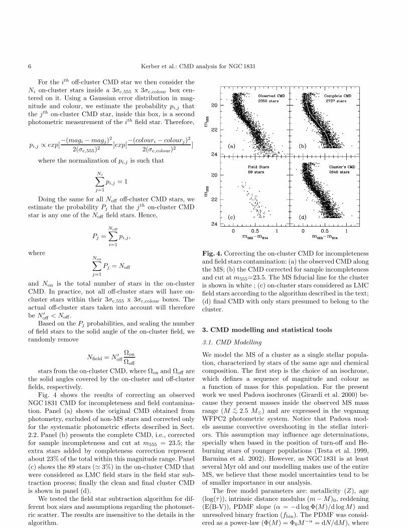
Fig. 4 shows the results of correcting an observedNGC 1831 CMD for incompleteness and field contamina-tion. Panel (a) shows the original CMD obtained fromphotometry, excluded of non-MS stars and corrected onlyfor the systematic photometric effects described in Sect.2.2. Panel (b) presents the complete CMD, i.e., correctedfor sample incompleteness and cut at m555 = 23.5; theextra stars added by completeness correction representabout 23% of the total within this magnitude range. Panel(c) shows the 89 stars (≃ 3%) in the on-cluster CMD thatwere considered as LMC field stars in the field star sub-traction process; finally the clean and final cluster CMDis shown in panel (d).

We tested the field star subtraction algorithm for dif-ferent box sizes and assumptions regarding the photomet-ric scatter. The results are insensitive to the details in thealgorithm.

Fig. 4. Correcting the on-cluster CMD for incompletenessand field stars contamination: (a) the observed CMD alongthe MS; (b) the CMD corrected for sample incompletenessand cut at m555=23.5. The MS fiducial line for the clusteris shown in white ; (c) on-cluster stars considered as LMCfield stars according to the algorithm described in the text;(d) final CMD with only stars presumed to belong to thecluster.

3. CMD modelling and statistical tools

3.1. CMD Modelling

We model the MS of a cluster as a single stellar popula-tion, characterized by stars of the same age and chemicalcomposition. The first step is the choice of an isochrone,which defines a sequence of magnitude and colour asa function of mass for this population. For the presentwork we used Padova isochrones (Girardi et al. 2000) be-cause they present masses inside the observed MS massrange (M <∼ 2.5 M⊙) and are expressed in the vegamagWFPC2 photometric system. Notice that Padova mod-els assume convective overshooting in the stellar interi-ors. This assumption may influence age determinations,specially when based in the position of turn-off and He-burning stars of younger populations (Testa et al. 1999,Barmina et al. 2002). However, as NGC 1831 is at leastseveral Myr old and our modelling makes use of the entireMS, we believe that these model uncertainties tend to beof smaller importance in our analysis.

The free model parameters are: metallicity (Z), age(log(τ)), intrinsic distance modulus (m− M)0, reddening(E(B-V)), PDMF slope (α = −d log Φ(M)/d log M) andunresolved binary fraction (fbin). The PDMF was consid-ered as a power-law (Φ(M) = Φ0M

−α = dN/dM), where

Kerber et al.: CMD analysis for NGC1831 7

the only free parameter is the slope α. fbin is defined asthe systemic binary fraction, fbin = Nbin/(Nbin + Nsing),where Nbin and Nsing are, respectively, the number of un-resolved pairs and single stars.

The process of generating artificial stars works as fol-lows:

(1) we fix Z and log(τ) for the stellar population bymeans of a chosen isochrone;

(2) we randomly draw a stellar mass according to thePDMF and get the absolute magnitudes in the two desiredfilters through the mass-luminosity relation given by theisochrone;

(3) for fbin randomly chosen cases, we repeat step (2),representing a companion star in a binary system, andcombine the two luminosities in both filters;

(4) we apply the intrinsic distance modulus (m−M)0and reddening vector(AV, E(B−V )) to the system, defin-ing its theoretical CMD position. For this purpose, we useRV = AV/E(B − V ) = 3.1 and the photometric trans-formation to the vegamag WFPC2 system according toHoltzman et al. 1995a;

(5) we introduce the photometric uncertainties byspreading the star with a Gaussian distribution of errorswith σ555 and σ814 as empirically determined (see Sect.2.1). This yields observational versions of the magnitudeand colour;

(6) finally, we verify if the star is inside the MS obser-vational ranges in magnitude and colour defined for thedata and throw it away if it is not.

For each model realization we generate the same num-ber of MS stars as observed in the real CMD, correctedfor sample incompleteness and field contamination, andlocated inside the 19.0 ≤ m555 ≤ 23.5 range. This rangein apparent magnitude corresponds to 0.5 <∼ M555

<∼ 5.0and 0.9 <∼ M <∼ 2.3 M⊙.

The best models are chosen by a direct comparison ofthe observed CMD with the artificial ones. The statisticaltools used in this comparison are presented in the nextsection. The model vs. observation comparison strategy isas follows:

(1) the global parameters for the cluster, log(τ), Z,E(B −V ) and (m−M)0, are determined using the CMDof the central cluster region (R ≤ 30 arcsec, where R is theprojected distance from the cluster’s centre), where fieldcontamination and statistical noise are minimized (see Ta-ble 1);

(2) for the best combinations of the global parameters,the position dependent parameters α and fbin are thenderived using the CMDs in concentric rings of variableradii.

Table 1 shows important information about the clusterregions used in this modelling process. The first columngives the range in R, Col. (2) the original number of CMD

Table 1. Number of points in the different cluster regionswhose CMDs are used in the CMD modelling as describedin Sect. 3.1.

Region (arcsec) observed complete field stars cluster

0 < R ≤ 30 2221 2737 89 26480 < R ≤ 15 1220 1506 27 147915 < R ≤ 30 1001 1216 62 115430 < R ≤ 60 1692 1972 240 1732R > 60 1673 1780 765 1015

stars in the 19.0 ≤ m555 ≤ 23.5 range, Col. (3) the num-ber of stars in the completeness corrected CMD (see Sect.2.3.1), Col. (4) the number of assigned field stars (Sect.2.3.2) and, finally, Col. (5) the number of stars in the CMDused in the modelling process. Notice that, not unexpect-edly, field contamination becomes a serious issue for theoutermost region, since statistical removal of field starsreduces the CMD numbers by about 40%. On the otherhand, crowding in the central regions yields larger photo-metric incompleteness, as reflected by the clear increasein the number of stars between Cols. (2) and (3).

This modelling strategy allows an efficient and system-atic search of best fit models in a 6-dimensional parame-ter space and makes use of the 2-dimensional informationprovided by the CMD data. Furthermore, this strategynaturally splits the parameters into those that define theposition of the MS in the CMD plane (the global ones) andthose that influence the way stars are distributed withinthe MS locus (the position dependent ones).

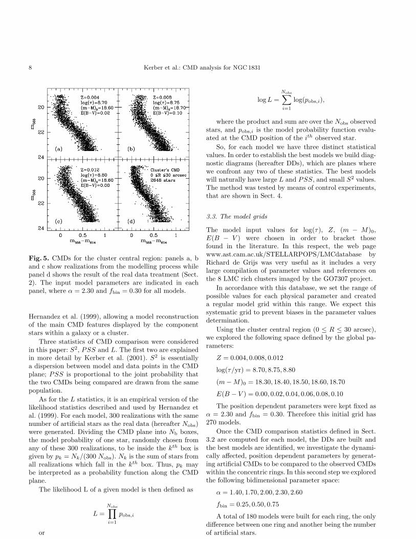
Fig. 5 shows four CMDs for the central cluster re-gion. The one in the bottom right (panel d) is the realdata, whereas the other three are realizations from differ-ent models generated by the modelling process describedabove. The input model parameters are shown in eachpanel. The three model CMDs do in fact look different,their MS ridge lines having different shapes and occupy-ing different positions along the CMD plane.

3.2. Statistical tools

One of the main goals of this paper is to establish anobjective comparison method between models and data.This required developing and applying statistical criteriathat discriminate the model CMDs that most adequatelyreproduce the observed one. Ideally these comparison cri-teria should be both simple and easy to implement butyet make use of as much information provided by the bidi-mensional colour-magnitude plane as possible. We stressthat these methods, in principle, are not restricted onlyto CMD analyses, but may be applied to the comparisonof any two bidimensional distributions of points. In simi-lar context as in this work, statistical techniques of CMDscomparison have been successfully applied by Kerber etal. (2001), Lastennet & Valls-Gabaud (1999), Saha (1998),

8 Kerber et al.: CMD analysis for NGC1831

Fig. 5. CMDs for the cluster central region: panels a, band c show realizations from the modelling process whilepanel d shows the result of the real data treatment (Sect.2). The input model parameters are indicated in eachpanel, where α = 2.30 and fbin = 0.30 for all models.

Hernandez et al. (1999), allowing a model reconstructionof the main CMD features displayed by the componentstars within a galaxy or a cluster.

Three statistics of CMD comparison were consideredin this paper: S2, PSS and L. The first two are explainedin more detail by Kerber et al. (2001). S2 is essentiallya dispersion between model and data points in the CMDplane; PSS is proportional to the joint probability thatthe two CMDs being compared are drawn from the samepopulation.

As for the L statistics, it is an empirical version of thelikelihood statistics described and used by Hernandez etal. (1999). For each model, 300 realizations with the samenumber of artificial stars as the real data (hereafter Nobs)were generated. Dividing the CMD plane into Nb boxes,the model probability of one star, randomly chosen fromany of these 300 realizations, to be inside the kth box isgiven by pk = Nk/(300 Nobs). Nk is the sum of stars fromall realizations which fall in the kth box. Thus, pk maybe interpreted as a probability function along the CMDplane.

The likelihood L of a given model is then defined as

L =

Nobs∏

i=1

pobs,i

or

log L =

Nobs∑

i=1

log(pobs,i),

where the product and sum are over the Nobs observedstars, and pobs,i is the model probability function evalu-ated at the CMD position of the ith observed star.

So, for each model we have three distinct statisticalvalues. In order to establish the best models we build diag-nostic diagrams (hereafter DDs), which are planes wherewe confront any two of these statistics. The best modelswill naturally have large L and PSS, and small S2 values.The method was tested by means of control experiments,that are shown in Sect. 4.

3.3. The model grids

The model input values for log(τ), Z, (m − M)0,E(B − V ) were chosen in order to bracket thosefound in the literature. In this respect, the web pagewww.ast.cam.ac.uk/STELLARPOPS/LMCdatabase byRichard de Grijs was very useful as it includes a verylarge compilation of parameter values and references onthe 8 LMC rich clusters imaged by the GO7307 project.

In accordance with this database, we set the range ofpossible values for each physical parameter and createda regular model grid within this range. We expect thissystematic grid to prevent biases in the parameter valuesdetermination.

Using the cluster central region (0 ≤ R ≤ 30 arcsec),we explored the following space defined by the global pa-rameters:

Z = 0.004, 0.008, 0.012

log(τ/yr) = 8.70, 8.75, 8.80

(m − M)0 = 18.30, 18.40, 18.50, 18.60, 18.70

E(B − V ) = 0.00, 0.02, 0.04, 0.06, 0.08, 0.10

The position dependent parameters were kept fixed asα = 2.30 and fbin = 0.30. Therefore this initial grid has270 models.

Once the CMD comparison statistics defined in Sect.3.2 are computed for each model, the DDs are built andthe best models are identified, we investigate the dynami-cally affected, position dependent parameters by generat-ing artificial CMDs to be compared to the observed CMDswithin the concentric rings. In this second step we exploredthe following bidimensional parameter space:

α = 1.40, 1.70, 2.00, 2.30, 2.60

fbin = 0.25, 0.50, 0.75

A total of 180 models were built for each ring, the onlydifference between one ring and another being the numberof artificial stars.

Kerber et al.: CMD analysis for NGC1831 9

4. Control Experiments

As mentioned in Sect. 3.2, we tested the validity of our sta-tistical methods using control experiments. These experi-ments consist of drawing one realization of some specificmodel and calling it the “observed CMD”. We then verifyif the DDs recover the generating model (hereafter inputmodel) as the best one describing the “observed CMD”.

Figs. 6 and 7 show the results of a control experi-ment involving the 270 models to be latter applied to theNGC 1831 central region. All panels show DDs of log S2

vs. log L, each point in the DD representing a particu-lar model. The panels on the right are blow-ups of thoseon the left, showing in detail the region where the bestmodels are located; this region corresponds to larger log Land smaller log S2 values. The different symbols in a sin-gle panel are coded according to the values of one of thefour global model parameters (Z, log(τ), (m − M)0 andE(B − V )), therefore allowing the effect of varying eachparameter to be separately assessed. Notice that the fig-ures do not show the entire model grid in order to avoidcluttering. The grid regions discarded from the DDs arethose of systematically high log S2 and low log L values.The “observed CMD” was taken to be a realization of themodel with Z = 0.008, log(τ) = 8.75, (m − M)0 = 18.50and E(B − V ) = 0.06. This input model is shown as thelarge star in the blowup panels.

A tight correlation between the two statistics is clearlyseen in all panels, adding reliability and stability to thechoice of the best fitting models. The control experimentsalso show that one is in fact capable of recovering the inputmodel based on the values of the statistics used: it is the

model with largest log L and smallest log S2, as ideally we

would expect.

Another important result from Figs. 6 and 7 is thecombining and/or canceling effect of some global parame-ters, yielding models of comparable quality. As an exam-ple, the effects of metallicity Z and reddening E(B − V )tend to cancel each other. Some models with Z (E(B−V ))lower (higher) than the input value, along with some highZ and low E(B − V ) ones, rank among the best modelsin the DDs. This degeneracy in the DDs is not surprisingsince the effect of increasing Z is to make stars redder andfainter at a given mass, roughly opposite to the effect ofdecreasing E(B − V ).

Fig. 8 presents similar DDs as in Figs. 6 and 7, butshows the model grid to be applied to the concentric re-gions of NGC 1831 (in a total of 180 models). The sym-bols now indicate different values of the PDMF slope α(panels (a) and (b)) and binary fraction fbin (panels (c)and (d)). As before, the panels on the right are blow-ups of the ones on the left, showing the best models only.The input model (large star), in this case, is the one withα = 2.00, fbin = 0.50 (and Z = 0.012, log(τ) = 8.75,(m − M)0 = 18.60, E(B − V ) = 0.02). It is again located

Fig. 6. DDs resulting from the control experiment forthe cluster’s central region, showing the effects of vary-ing metallicity (panels (a) and (b)) and age (panels (c)and (d)). The symbols are as indicated in the panels onthe left. The panels on the right show the best models indetail and use the same symbol notation.

Fig. 7. DDs resulting from the control experiment for thecluster’s central region, showing the effects of varying dis-tance (panels (a) and (b)) and reddening (panels (c) and(d)). The symbols are as indicated in the panels on theleft. The panels on the right show the best models in de-tail.

10 Kerber et al.: CMD analysis for NGC1831

Fig. 8. DDs resulting from the control experiment for the15 ≤ R ≤ 30 arcsec region. Panels (a) and (b) (the latter isa blowup of the former) show the effect of varying PDMFslope α, whereas panels (c) and (d) (the latter is a blowupof the former) show the effect of varying fbin. The inputmodel is represented by the large star.

at the extreme upper left corner of the DD, confirming theapplicability of our statistical approach.

However, the panels on the right show that the threebest models have the same α (= 2.00) but different fbin

values, revealing a larger difficulty in determining the lat-ter than the former. This occurs because the effect causedby binaries is of the same order as or smaller than thephotometric uncertainties in our WFPC2 CMDs. Conse-quently, as will be discussed in Sect. 5.2, the fbin determi-nation by means of our CMDs becomes a difficult task.

Notice that, in comparison with the DDs for the cen-tral region, the DDs in Fig. 8 present a larger dispersion.This is caused by the much smaller number of stars usedin the set of models with varying α and fbin; in this case,all model CMDs (including the “observed” one) have 1154stars, therefore mimicking the situation of the second con-centric region to be studied in NGC 1831 (see Table 1).

Fig. 9 shows DDs involving the PSS statistics. Theupper panels show PSS vs. log L and PSS vs. log S2 plotsfor the central region. The lower panels show the sameplots for one of the concentric rings. The same modelsas in Figs. 6, 7, and 8 are depicted but without symbolcoding as a function of parameter values. The correlationbetween PSS and the other statistics is again quite tight.In fact, the results based on the DDs are insensitive to theparticular choice of statistics to be plotted. This is a veryimportant result, since it further enhances the reliability

Fig. 9. DDs involving the PSS statistics in control exper-iments. The upper (lower) panels show PSS vs. log L andPSS vs. log S2 plots for the region inside 0 ≤ R ≤ 30(15 < R ≤ 30) arcsec.

of our statistical CMD modelling techniques. For the sakeof simplicity, we hereafter restrict ourselves to log L vs.log S2 DDs only.

5. Results

5.1. Central region

In this section we model the CMD of stars belonging to theregion within R ≤ 30 arcsec from the centre of NGC 1831.In accordance with Santiago et al. (2001), this correspondsroughly to R <∼ 7 pc or within 2 half-light radii. As indi-cated in Table 1, there are 2221 stars in this region inthe magnitude range 19.0 ≤ m555 ≤ 23.5. As also men-tioned earlier, this central cluster region suffers from in-significant contamination by LMC field stars. On the otherhand, due the high stellar density, incompleteness effectsbecome more important. The chosen faint magnitude cut-off represents the magnitude at which completeness fallsat 50%, in an attempt to reduce the relevance of this effecton our results.

The DDs for the model vs. real CMD comparison arepresented in Figs. 10 and 11. As in the control experi-ments, the correlation between log L and log S2 is quitenoticeable, the best models being again at the upper leftregion in the panels. These figures follow the same con-ventions and notations as Figs. 6 and 7, therefore allowingus to assess the effect of varying each global cluster pa-rameter separately. For example, panels 10(a) and 10(b)clearly show that the best models have Z = 0.012. The

Kerber et al.: CMD analysis for NGC1831 11

Fig. 10. DDs resulting from the CMD of the cluster’s cen-tral region, showing the effects of varying metallicity (pan-els (a) and (b)) and age (panels (c) and (d)). The symbolsare as indicated in the panels on the left. The panels onthe right show the best models in detail.

effects of the other parameters are not as striking as inthe case of metallicity. Yet, panels 10(c) and 10(d) favouran age in the range 8.75 ≤ log(τ) ≤ 8.80. Likewise, thethree lowest values of intrinsic distance modulus (two ofwhich are not even shown in the figure) can essentiallybe ruled out (panels 11(a) and 11(b)), placing NGC 1831near or beyond the distance to the LMC centre. Finally,E(B − V ) ≤ 0.02 is favoured by our modelling approach(panels 11(c) and 11(d)). Notice that this latter parameteris again anti-correlated with Z, in the sense that the mod-els in the blowup panels with Z = 0.008 (circles in panel10(b)) have larger E(B − V ) values (circles or crosses inpanel 11(d)).

These best choices of the global parameters, as dis-cussed in Sect. 3.1, besides being useful constraints bythemselves, serve as model inputs to the position depen-dent parameters α and fbin, whose modelling is based onthe concentric regions.

5.2. Concentric regions

We now analyze the NGC 1831 CMDs in the concentric re-gions listed in Table 1. As just mentioned, the free modelparameters in this case are the PDMF slope α and the un-resolved binary fraction fbin. For all regions we correctedthe observed CMD to the effects of sample incomplete-ness and field star contamination. Fig. 12 shows their final

Fig. 11. DDs resulting from the CMD of the cluster’s cen-tral region, showing the effects of varying distance (panels(a) and (b)) and reddening (panels (c) and (d)). The sym-bols are as indicated in the panels on the left. The panelson the right show the best models in detail.

CMDs. As mentioned before, Table 1 shows the number ofpoints in all the steps along the data correction process.

In the modelling, we apply the same model grid forevery region, only changing the number of artificial starsgenerated. The results from the previous section were usedto restrict the possible values of the clusters global param-eters, allowing us to investigate the dynamically depen-dent parameters for the system.

Figs. 13 and 14 present the DDs resulting from modelvs. data CMD comparison in the four regions. The differ-ent symbols in each panel correspond to different values ofα. As usual, the panels on the right show the best modelsin detail. The results for the two innermost regions arepresented in Fig. 13. Panels (a) and (b) indicate that thebest models for innermost region (R ≤ 15 arcsec) have1.40 ≤ α ≤ 1.70. In the ring 15 < R ≤ 30 arcsec, shownin panels (c) and (d) of the same figure, the best modelspresent similar α values: 1.40 ≤ α <∼ 1.70.

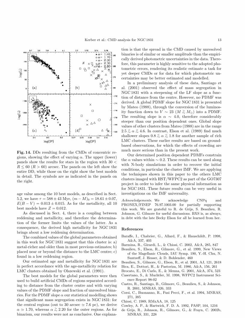
In Fig. 14 we have the results for the two outermostrings. Panels (a) and (b) show the DDs for the stars with30 < R ≤ 60 arcsec. Now, there is evidence for a sharpchange in the PDMFs slope: the best models have 2.30 ≤α ≤ 2.60. Finally, the DD for the most peripheric ring hasa large dispersion (panels 14(c) and 14(d) ). This spreadis also seen in the best PDMF slope: values in the range2.00 <∼ α ≤ 2.60 are seen in the upper left corner of theDD. This may reflect large uncertainties in the field star

12 Kerber et al.: CMD analysis for NGC1831

Fig. 12. The final NGC 1831 CMDs in four concentric re-gions: (a) 0 < R ≤ 15 arcsec; (b) 15 < R ≤ 30 arcsec;(c)30 < R ≤ 60 arcsec;(d) R > 60 arcsec.

Table 2. Best estimates of the slope α and its uncertaintyas a function of distance to the centre.

Region (arcsec) Region (pc) α σα

0 < R ≤ 15 0 < R ≤ 3.8 1.72 0.1515 < R ≤ 30 3.8 < R ≤ 7.6 1.68 0.1930 < R ≤ 60 7.6 < R ≤ 15.2 2.45 0.15R > 60 R > 15.2 2.19 0.33

subtraction, since it leads to a large reduction of CMDpoints in this ring.

For each ring, we assign a representative α and asso-ciated uncertainty using the 10 models with the largestvalues of likelihood L. The final slope is taken to be theweighted average value among these best models, and itsassociated uncertainty is the dispersion around the aver-age. The weight assigned to each model was the inverse ofthe difference in log L between the observed CMD and aCMD from a typical model realization. This difference is ameasure of the discrepancy between model and observedCMDs. Table 2 lists the final α values and uncertaintiesfor each ring (Cols. 3 and 4). The first 2 columns in thetable show the regions in arcsec and parsecs (assuming(m − M)0 = 18.61 for NGC 1831 as adopted in Sect. 6),respectively.

As for the fraction of unresolved binaries, fbin, the re-sults, as anticipated, are not conclusive in any ring, giventhe CMD spread. A more precise treatment of photometricerrors may help constrain this parameter.

Fig. 13. DDs resulting from the CMDs of concentric re-gions, showing the effect of varying α. The upper (lower)panels show the results for stars in the region with 0 ≤R ≤ 15 (15 < R ≤ 30) arcsec. The panels on the leftshow the entire DD, while those on the right show thebest models in detail. The symbols are as indicated in thepanels on the right.

6. Summary and Conclusions

In this work we analyzed a deep CMD of NGC 1831, arich LMC cluster, obtained from HST/WFPC2 images inthe F555W and F814W filters. We inferred physical pa-rameters such as metallicity, age, intrinsic distance modu-lus, reddening and PDMF slopes by comparing the clusterCMD with artificial ones. We presented in detail the tech-niques used to build the model CMDs, which use theseparameters as model input and take into account obser-vational uncertainties as in the real data. The parameterspace explored by our regular model grids bracketed thevalues found in the literature.

The model vs. data comparison required correcting theobserved CMD for selection effects caused by photometricincompleteness and CMD contamination by stars belong-ing to the LMC field. We also presented the statisticaltechniques used to compare the real CMD, corrected forthe aforementioned selection effects, to the artificial ones.These statistical tools allowed us to discriminate the mod-els that best reproduce the data. They are based on simpleand objective statistical quantities and make use of the fullbidimensional distribution of points in the CMD.

The best parameter values inferred for NGC 1831 arein the ranges 8.75 ≤ log(τ) ≤ 8.80, 18.50 ≤ (m − M)0 ≤18.70, 0.00 ≤ E(B − V ) ≤ 0.02. Using the weighted aver-

Kerber et al.: CMD analysis for NGC1831 13

Fig. 14. DDs resulting from the CMDs of concentric re-gions, showing the effect of varying α. The upper (lower)panels show the results for stars in the region with 30 <R ≤ 60 (R > 60) arcsec. The panels on the left show theentire DD, while those on the right show the best modelsin detail. The symbols are as indicated in the panels onthe right.

age value among the 10 best models, as described in Sect.5.2, we have τ = 588± 43 Myr, (m−M)0 = 18.61± 0.07,E(B − V ) = 0.013 ± 0.015. As for the metallicity, all 10best models have Z = 0.012.

As discussed in Sect. 4, there is a coupling betweenreddening and metallicity, and therefore the determina-tion of the former limits the values of the latter. As aconsequence, the derived high metallicity for NGC 1831brings about a low reddening determination.

The combined values of the global parameters obtainedin this work for NGC 1831 suggest that this cluster is: a)metal-richer and older than in most previous estimates; b)placed near or beyond the distance to the LMC centre; c)found in a low reddening region.

Our estimated age and metallicity for NGC 1831 arein perfect accordance with the age-metallicity relation forLMC clusters obtained by Olszewski et al. (1991).

The best models for the global parameters were thenused to build artificial CMDs of regions separated accord-ing to distance from the cluster centre and with varyingvalues of the PDMF slope and fraction of unresolved bina-ries. For the PDMF slope α our statistical modelling showsthat significant mass segregation exists in NGC 1831: forthe central regions (out to 30 arcsec ≃ 7.6 pc), we deriveα ≃ 1.70, whereas α >∼ 2.20 for the outer regions. As forbinarism, our results were not as conclusive. One explana-

tion is that the spread in the CMD caused by unresolvedbinaries is of similar or smaller amplitude than the empiri-cally derived photometric uncertainties in the data. There-fore, this parameter is highly sensitive to the adopted pho-tometric errors, rendering its realistic estimate a task foryet deeper CMDs or for data for which photometric un-certainties may be better estimated and modelled.

In a preliminary analysis of these data, Santiago etal. (2001) observed the effect of mass segregation inNGC 1831 with a steepening of the LF slope as a func-tion of distance from the centre. However, no PDMF wasderived. A global PDMF slope for NGC 1831 is presentedby Mateo (1988), through the conversion of the luminos-ity function down to V ∼ 23 (M >∼ M⊙) into a PDMF.The resulting slope is α ∼ 4.0, therefore considerablysteeper than our position dependent ones. Global slopevalues of other clusters from Mateo (1988) are in the range2.5 <∼ α <∼ 4.6. In contrast, Elson et al. (1989) find muchshallower slopes 0.8 <∼ α <∼ 1.8 for another sample of richLMC clusters. These earlier results are based on ground-based observations, for which the effects of crowding aremuch more serious than in the present work.

Our determined position dependent PDMFs constrainthe α values within ∼ 0.2. These results can be used alongwith N-body simulations in order to recover the initialconditions, in particular the cluster IMF. We are applyingthe techniques shown in this paper to the others LMCclusters imaged with HST/WFPC2 as part of the GO7307project in order to infer the same physical information asfor NGC 1831. These future results can be very useful ininvestigations on the IMF universality.

Acknowledgements. We acknowledge CNPq andPRONEX/FINEP 76.97.1003.00 for partially supportingthis work. We are grateful to R. de Grijs, S. Beaulieu, R.Johnson, G. Gilmore for useful discussions. BXS is, as always,in debt with the late Becky Elson for all he learned from her.

References

Baraffe, I., Chabrier, G., Allard, F., & Hauschildt, P. 1998,A&A, 337, 403

Barmina, R., Girardi, L., & Chiosi, C. 2002, A&A, 285, 847Beaulieu, S., Elson, R., Gilmore, G., et al. 1999, New Views

of the Magellanic Clouds, IAU Symp. 190, Y.-H. Chu, N.Suntzeff, J. Hesser, & D. Bohlender, 460

Beaulieu, S., Gilmore, G., Elson, R., et al. 2001, AJ, 121, 2618Bica, E., Dottori, H., & Pastoriza, M. 1986, A&A, 156, 261Brocato, E., Di Carlo, E., & Menna, G. 2001, A&A, 374, 523Casertano, S., & Muchtler, M. 1998, WFPC2 Instrument Sci-

ence Report 98-02Castro, R., Santiago, B., Gilmore, G., Beaulieu, S., & Johnson,

R. 2001, MNRAS, 326, 333Corsi, C., Buonanno, R., Fusi Pecci, F., et al. 1994, MNRAS,

271, 385Chiosi, C. 1989, RMxAA, 18, 125Cowley, A. P., & Hartwick, F. D. A. 1992, PASP, 104, 1216de Grijs, R., Johnson, R., Gilmore, G., & Frayn, C. 2002b,

MNRAS, 331, 228

14 Kerber et al.: CMD analysis for NGC1831

de Grijs, R., Gilmore, G., Johnson, R. & Mackey, A. D. 2002a,MNRAS, 331, 245

De Marchi, G., & Paresce, F. 1995, A&A, 304, 211de Oliveira, M. R., Bica, E., & Dottori, H. 2000, MNRAS, 311,

589Elson, R., Fall, S. M., & Freeman, K. C. 1987, ApJ, 323, 54Elson, R., Fall, S. M., & Freeman, K. C. 1989, ApJ, 336, 734Elson, R., Gilmore, G., Santiago, B., & Casertano, S. 1995, AJ,

110, 682Gallart, C., Aparicio, A., Bertelli, G., & Chiosi, C. 1996, AJ,

112, 1950Gallart, C., Freedman, W. L., Aparicio, A., Bertelli, G., &

Chiosi, C. 1999, AJ, 118, 2245Girardi, L., Chiosi, C., Bertelli, G., & Bressan A. 1995, A&A,

298, 87Girardi, L., Bressan, A., Bertelli, G., & Chiosi, C. 2000, A&AS,

141, 371Goodwin, S. P. 1997, MNRAS, 286, 669Heggie, D., & Aarseth, S. 1992, MNRAS, 257, 513Hernandez, X., Valls-Gabaud, D., & Gilmore G. 1999. MN-

RAS, 304, 705Hernandez, X., Gilmore, G., & Valls-Gabaud D. 2000, MN-

RAS, 317, 831Holtzman, J., Hester, J., Casertano, S., et al. 1995a, PASP,

107, 156Holtzman, J., Gallagher, J., Cole, A., et al. 1999, AJ, 118, 2262Johnson, J., Bolte, M., Stetson, P., Hesser, J., & Sommerville,

R. 1999, ApJ, 527, 199Johnson, R., Beaulieu, S., Gilmore, G., et al. 2001, MNRAS,

324, 367Kerber, L., Javiel, S., & Santiago, B. 2001, A&A, 365, 424Kroupa, P. 2001, MNRAS, 322, 231Kroupa, P., Aarseth, S., & Hurley, J. 2001, MNRAS, 321, 699Lastennet, E., & Valls-Gabaud, D. 1999, RMxA Conf. Ser., 8,

115Mateo, M. 1987, ApJ, 323, L41Mateo, M. 1988, ApJ, 331, 261Meurer G. R., Cacciari C., & Freeman K. C. 1990, AJ, 99, 1124Olszewski, E. W., Schommer, R. A., Suntzeff, N. B, & Harris,

H. C. 1991, AJ, 101, 515Panagia, N., Gilmozzi, R., Macchetto, F., Adorf, H.-M., & Kir-

shner, R. 1991, ApJ Letters, 380, L23Piotto, G., Cool, A., & King, I. 1997, AJ, 113, 1345Saha, P. 1998, AJ, 115, 1206Santiago, B., Elson, R., & Gilmore G. 1996, MNRAS, 281, 1363Santiago, B., Beaulieu, S., Johnson, R., & Gilmore, G. 2001,

A&A, 369, 74Spurzem, R., & Aarseth, S. 1996, MNRAS, 282, 19esta, V., Ferraro, F., Chieffi, A., et al. 1999, AJ, 118, 2864Vallenari, A., Chiosi, C., Bertelli, G., Meylan, G., & Ortolani,

S. 1992, AJ, 104, 1100Vesperini, E., & Heggie, D. 1997, MNRAS, 289, 898Westerlund, B. E. 1990, A&AR, 2, 29