Analysis of a Simple Model for Non-Preemptive Blocking-Free Scheduling

L. Almeida*, J. A. Fonseca {lda,jaf}@det.ua.pt

DET / IEETA

Universidade de Aveiro

P-3810-193 Aveiro, Portugal

* corresponding author

Abstract

Non-preemptive scheduling is known for its lower efficiency in meeting temporal constraints when

compared to preemptive scheduling. However, it is still used in certain cases such as in message

scheduling over serial broadcast buses and in light multi-tasking kernels for embedded systems based on

simple microprocessors. These cases are typically found in control applications requiring the periodic

execution (or transmission) of a set of tasks (or messages) with low jitter. This paper refers to a simple

execution strategy based on synchronised time-triggering and non-preemptive scheduling that allows to

eliminate the blocking factor commonly associated to non-preemption and thus reduce activation jitter.

The elimination of such blocking factor is achieved by using inserted idle-time. The paper focuses on the

schedulability analysis of a generic task set executed according to the referred model. In one part, a

specific response time-based analysis is presented which supports, under worst-case assumptions, a

necessary and sufficient schedulability assessment. In a following part, the paper presents a general

theorem that allows to adapt the existing analysis for preemptive scheduling to the referred model. In

particular, this theorem allows to develop adequate utilization bounds for guaranteed schedulability,

based on the well known bounds for rate-monotonic analysis.

1. Introduction

Non-preemptive scheduling is known for its lower efficiency in meeting temporal constraints when

compared to preemptive scheduling. In fact, non-preemption causes higher blocking factors that can easily

lead to non-schedulability. When applied to periodic tasks, it also imposes a well known limitation to the

tasks’ execution time, i.e. the largest task execution time must be shorter than the shortest task relative

deadline.

However, it is still used in certain cases such as in light multi-tasking kernels for embedded systems

based on simple microprocessors and, mainly, in message scheduling over serial broadcast buses. In the

former cases, it has the advantage of a lower run-time overhead and simple resource management, in the

latter, its use is imperative to support a coherent serial transfer of each message.

Many applications of both cases are in the control of physical devices normally requiring the periodic

execution (or transmission) of a set of tasks (or messages) with low jitter. One of the sources of jitter is the

blocking caused by non-preemptive scheduling but this can be reduced, or even eliminated, by adequately

using inserted idle-time and adjusting periods and relative phasing. In particular, this paper deals with the

use of inserted idle-time to delay the realease of any lower priority task (message) whenever a higher

priority one will become ready before the former one would finish. This is easily achieved in synchronised

systems where the activation of tasks (submission of messages) is performed by means of a periodic timer

interrupt. This paper refers to such a simple model based on synchronous time-triggering and inserted idle-

time to eliminate non-preemption blocking and reduce activation jitter. The paper presents a thorough

analysis of such model. Firstly, an accurate response time based analysis is developed according to what is

called the timeline approach. This analysis, under worst-case assumptions, supports a necessary and

sufficient schedulability assessment. Secondly, the paper presents a general theorem that allows to adapt

the existing analysis for preemptive scheduling to the referred model. Although the result in terms of

schedulability assessment is just sufficient and not necessary, it allows to develop utilization bounds for

guaranteed schedulability based on the well known bounds for Rate-Monotonic (RM) scheduling. This

fact facilitates the realization of fast schedulability tests that can be used to support on-line admission in

systems based on low processing-power CPUs.

2. Related work

It is known that non-preemptive scheduling causes a considerable schedulability penalty and many

systems which are schedulable preemptively cannot be timely scheduled with non-preemption [1].

Nevertheless, when tasks’ execution times are small compared to the respective periods then non-

preemption is not generally a serious drawback in terms of schedulability. In this case it is known that non-

preemptive scheduling approaches preemptive scheduling in terms of the level of schedulability [2].

Nevertheless, well-known results deduced for preemptive scheduling cannot be used directly in a non-

preemption situation. Either some degree of adaptation must be done on the existing preemptive analysis

or new analysis must be derived. For example, Jeffay et al. [3] use a new analysis to prove that the well-

known EDF algorithm is also optimal for non-preemptive task scheduling. On the other hand, Vasques [4]

suggests the use of an adequate blocking term in usual preemptive RM analysis to account for the effects

of non-preemption. The maximum such blocking that a task can suffer equals the duration of the longest

task among those with lower priority. Furthermore, this blocking also has a negative impact on the tasks’

release jitter which can be a drawback for example in control applications, with direct consequences either

in sampling and/or actuation jitter. Törngren [9] presents a detailed analyses of the temporal requirements

for such applications. Several important sources and characteristics of time variations (e.g. sampling jitter)

in distributed computer systems are identified and analysed.

A way to reduce non-preemption blocking and improve schedulability is to use idle-time insertion [5]. It

consists in delaying long non-preemptive tasks in order to wait for the release of tasks with shorter

deadlines and higher priority so that they can execute first. Otherwise such tasks would miss their

deadlines.

This technique can also be used to reduce the release jitter of high priority tasks. For example, consider a

synchronous system where tasks become ready synchronously with a timer interrupt. Moreover, consider

that a task is not released if it cannot finish before the next interrupt. Then, when the interrupt comes, such

task is rescheduled together with the remaining ones. Whenever this occurs, a small amount of idle-time

(implicitely inserted) may appear just before the interrupt (fig. 1). This simple execution strategy facilitates

the fulfillment of two typical requirements related to timing assumptions made in discrete-time control

theory [9], namely: constant sampling period, since it provides a means to reduce sampling jitter; and

activity synchronization, since a precise common clock is provided, based on the timer interrupt.

This technique has been proposed and discussed by the authors [6] for message scheduling in

synchronous fieldbus systems. Basically, two effects are referred concerning idle-time insertion: avoidance

of potential preemption instants, which makes it irrelevant whether the scheduling is preemptive or non-

-preemptive, and a bounded waste of bus-time (CPU in this case), corresponding to the inserted idle-time.

The former effect is responsible for the avoidance of blocking and guarantees a jitter-free periodic release

of the highest priority task (fig. 1). The latter effect means that the CPU may be kept idle while there are

ready tasks to be executed. This invalidates the direct applicability of the existing analysis for preemptive

scheduling (e.g [7] for fixed priorities or [10] for EDF), leading to the need for new analysis. In such

direction, two previous work-in-progress papers [11] and [12] have been presented by the authors which

contain the basis for the materials included in this paper. The former includes a new schedulability test

based on response times that, under worst-case assumptions, is necessary and suficient. The latter concerns

the adaptation of existing preemptive scheduling analysis resulting in a sufficient only schedulability

assessment. The interest in this adaptation is that it allows to use utilization-based tests which, despite

their pessimism, involve virtually no overhead. Such tests are, thus, useful for on-line admission control in

systems based on low processing power micro-controllers [13].

3. Task model

The analysis presented in the paper considers a set Γ of N independent periodic non-preemptive tasks.

Each task τ is an infinite succession of instances which are periodically activated. Nevertheless, no

instance is released for execution until the previous one is terminated.

The parameters that characterise a generic task τi are the computation time Ci, the period Ti, the relative

deadline Di which is equal to or shorter than the period, an initial phasing Φi expressing the activation

instant of the first instance, and a fixed priority Pi which can be, but not necessarily, derived from the

period, deadline or value in the context of the application. This is formalised in expression (1).

Γ ≡ { τi ( Ci , Ti , Di , Φi , Pi ), i = 1..N } (1)

The instances of each task are activated synchronously by a timer interrupt which has a period of E.

Each of such periods is called a tick interval, although the expressions micro-cycle and elementary-cycle

may occasionally be used with the same meaning. The periods of all tasks are expressed as integer

ττττ1 ττττ2 ττττ4 ττττ5 ττττ1 ττττ3 ττττ6

ττττ6

Time Xn

EXn - Inserted idle-timeτ1..6 – tasks

timer interrupts

tick interval n tick interval n+1

Figure 1. Inserting idle-time to prevent blocking.

multiples of E, i.e. ∀ i=1..N Ti=k*E, k≥1. The same constraint applies to the relative deadline Di and

initial phasing Φi, i.e. ∀ i=1..N Di=n*E, Φi=m*E, n,m≥1. Furthermore, it will be assumed that each task

must be short enough to execute within E, i.e. ∀ i=1..N Ci<E.

From the point of view of usual preemptive task scheduling, this last assumption is very restrictive,

indeed. Basically it does not allow for the coexistance of long tasks together with short and frequent ones.

From the point of view of non-preemptive task scheduling this assumption is still restrictive but not that

much. Non-preemption by itself constrains the execution times to be shorter than the shortest deadline.

However, in typical application areas for which this analysis is suited, this assumption is not restrictive.

For example, in fieldbus communication systems (e.g. CAN, Profibus, WorldFIP, ControlNet, Foundation

Fieldbus) typical messages are considerably shorter than the minimum broadcast period. In the control of

small autonomous robots using reflex behaviour approaches typical tasks are also short, with respect to the

minimum activation period. Also, in systems developed to manage the execution of finite state machines it

is typical to find a basic cycle within which several tasks, that correspond to state transitions, are executed.

For example, the Saphira system used in the Pioneer robots [14] has a basic cycle of 100ms within which

tasks (there called micro-tasks) are executed. A similar execution strategy is used in the Grape-II system,

developed for DSP applications [15].

In the analysis that follows, the task set Γ will be assumed to be ordered by decreasing priority, i.e.

∀ i,j=1..N i<j => Pi>Pj .

4. Worst-case phasing

In order to determine the worst-case scenario concerning the interference caused by higher priority tasks

to the release of lower priority ones, three aspects must be taken into account. Firstly, that tasks are

activated synchronously with the tick interrupt and that the initial phasings are also expressed as integer

multiples of the tick duration. Thus, no task becomes ready for execution in the middle of a tick interval.

Secondly, that tasks are not released for execution unless they can complete within the current tick interval

thus leading to a possible implicit idle-time insertion. Both previous aspects make it irrelevant whether the

scheduling is preemptive or not (fig. 1) since potential preemption instants are avoided. Thirdly, that the

order by which ready tasks are executed respects their relative priorities, i.e. a lower priority task cannot

execute if there is a higher priority one, ready for execution. Thus, whenever a portion of idle-time is

inserted no lower priority tasks can execute in that portion of time even if they fit in.

The previous three aspects altogether lead to a situation which is equivalent to the scheduling of fixed

priorities preemptive tasks in terms of worst-case scenario. In fact, the interference felt by each task is then

maximised when it is activated together with all higher priority tasks. Thus, to assess the schedulability of

a given task set, assuming fixed priorities, it suffices to consider all tasks in phase (without loss of

generality it will be assumed Φi = 0 ∀ i=1..N), i.e. all tasks activated at a given instant in time known as

the critical instant (t=0), and check whether the first instance of each task meets its deadline.

5. An accurate analysis (timeline)

In this section, an analysis specifically developed for this model is shown. Assuming worst-case phasing

(Φi=0 ∀ i=1..N), i.e. all tasks activated at the critical instant (t=0), as well as constant task execution time,

i.e. all task instances take exactly Ci time to complete, this analysis returns exact worst-case response

times (Rwci ∀ i=1..N) and thus supports a sufficient and necessary schedulability assessment (theorem 1).

Under different phasing (∃ i,j: Φi≠Φj) or varying execution times (but bounded by Ci ∀ i=1..N), the

analysis returns upper bounds to the worst-case response times that can be used to support a sufficient only

schedulability assessment (theorem 2). The use of this analysis for message scheduling in the WorldFIP

fieldbus was presented by the authors as work-in-progress in [11].

Theorem 1: Consider the synchronous model described in the previous sections in which the scheduler

uses inserted idle-time but enforces priority ordering in the execution of tasks. Also, consider a task set Γ

defined as in (1), with Di≤Ti ∀ i=1..N, worst-case phasing (Φi=0 ∀ i=1..N), constant execution times (Ci)

for each task, and any decreasing fixed priority assignment, i.e. i<j ⇒ Pi>Pj ∀ i,j=1..N. Then:

Rwci ≤ Di ∀ i=1..N ⇔⇔⇔⇔ Set Γ is schedulable

The proof is straight forward since the worst-case response times are exact and do occur in the first

instance of each task, activated at the critical instant. Thus, if ∃ i=1..N: Rwci>Di then a deadline has been

missed and the set is not schedulable. On the other hand, if the set Γ is not schedulable then a deadline

must have been missed and thus ∃ i=1..N: Rwci>Di (q.e.d.).

If a different phasing is used or if there are instances of any task i that take less than Ci to execute, then,

the effective worst-case response time of one or more tasks may be lower than the respective values Rwci

returned by the analysis. Thus the schedulability condition on the left becomes sufficient, only, and not

necessary. This is expressed as theorem 2.

Theorem 2: Consider again the same synchronous model with inserted idle-time and orderly execution

of tasks according to priorities. Also, consider a task set Γ as defined in (1), with Di≤Ti ∀ i=1..N and any

decreasing fixed priority assignment, i.e. i<j ⇒ Pi>Pj ∀ i,j=1..N. Then:

Rwci ≤ Di ∀ i=1..N ⇒⇒⇒⇒ Set Γ is schedulable under any phasing

The proof is again trivial since the effective worst-case response time of each task under any phasing is

lower than or equal to the respective value Rwci returned by the analysis. Then, if the condition on the left

is true the effective worst-case response times will also be lower than or equal to the respective deadlines

and thus the set is schedulable (q.e.d.).

It will now be shown how to exactly determine the worst-case response times (Rwci ∀ i=1..N) under a

worst-case phasing assumption. The particularity of this calculation resides in the need to exactly quantify

the amount of idle-time inserted in all the tick-intervals covered by the busy interval1 of each task. The

approach followed herein is called the timeline approach since it is based on building the schedule up to

the end of the longest busy interval, i.e. the interval [0,RwcN]. Starting from the critical instant (t=0), the

processor load in each tick-interval is built up taking into account the order in which tasks are processed,

thus allowing to determine the exact idle-time inserted.

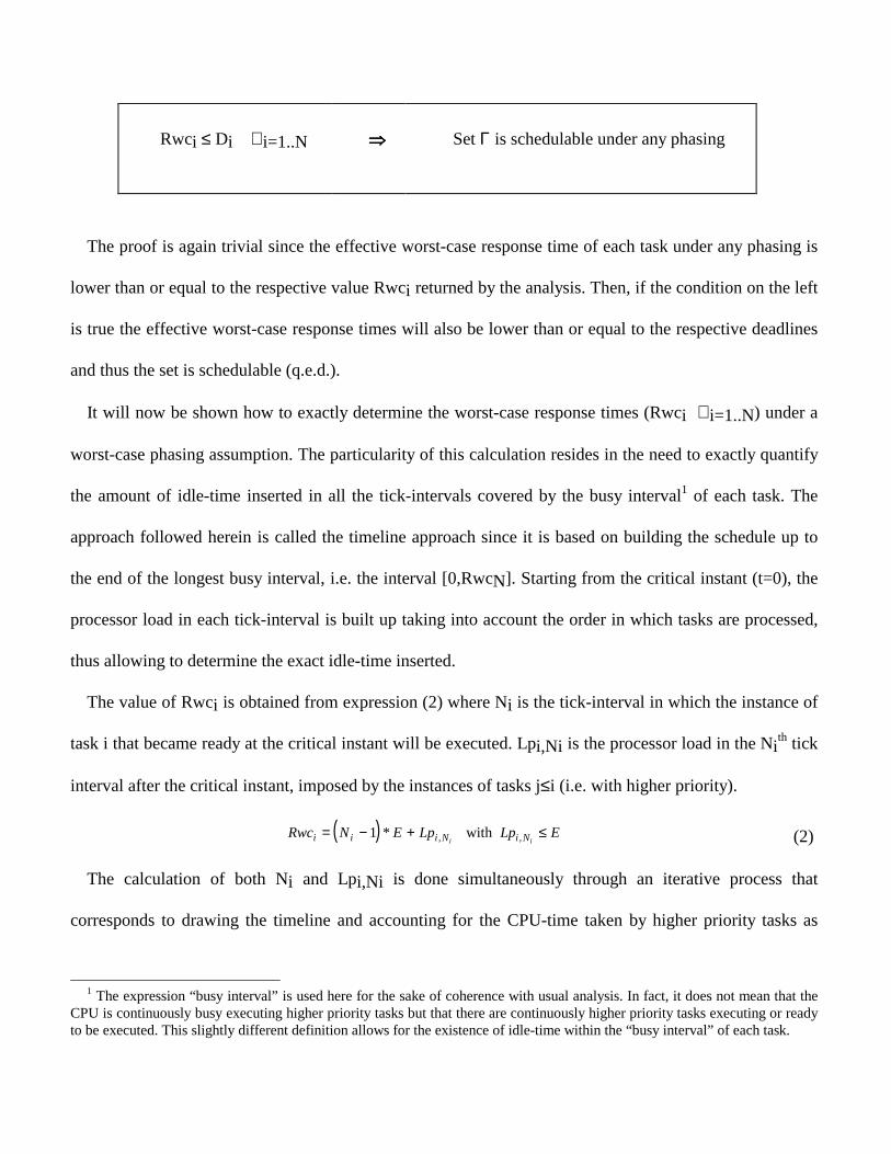
The value of Rwci is obtained from expression (2) where Ni is the tick-interval in which the instance of

task i that became ready at the critical instant will be executed. Lpi,Ni is the processor load in the Nith tick

interval after the critical instant, imposed by the instances of tasks j≤i (i.e. with higher priority).

( )Rwc N E Lp Lp Ei i i N i Ni i= − + ≤1 * , ,with (2)

The calculation of both Ni and Lpi,Ni is done simultaneously through an iterative process that

corresponds to drawing the timeline and accounting for the CPU-time taken by higher priority tasks as

1 The expression “busy interval” is used here for the sake of coherence with usual analysis. In fact, it does not mean that the

CPU is continuously busy executing higher priority tasks but that there are continuously higher priority tasks executing or ready to be executed. This slightly different definition allows for the existence of idle-time within the “busy interval” of each task.

they are processed. A boolean auxiliary function δk,n is used which becomes 1 whenever an instance of

task k is ready in the nth tick-interval and 0 otherwise. The auxiliary function δk,n is also calculated in the

same iterative process, knowing that, by the definition of critical instant, δk,1 = 1 ∀ k=1..N.(for a given n,

the vector δn represents the set δk,n ,for k=1..N).

The iterative process includes two cycles (fig. 2), an inner one on index k (lines 5-11), to account for the

processor load within a given tick interval, and an outer one on index n (lines 2-11), to pass from one tick

interval to the next until the instance of task i is processed.

1.

2.3.4.5.6.7.

8.mod

otherwise9. both cycles10. 11. cycle on k

δ

δ δ

δδ

δ

k

in

k n k n

n k n k

n n k n k

k nk

k N

n D ELoad

k Nk i

Load C ELoad Load C

n T E

k i

,

, ,

,

,

,

, ..

, ..

**

,,

,

1

1

1

1 1

10

11

1 00

= =

==

= ==

+ ≤= +

==

=

+

+

for to

for toif

if breakelse

break

Figure 2. Exact assessment of Rwci.

Line 1 represents the initialisation of the δk vector for the 1st tick interval and lines 3-4 represent the

initialisation of the processor load acumulator in the current tick interval and of the δk vector of next

interval. If the cycle on k does not complete when n reaches Di/E (exit through line 11) then Rwci grew

beyond Di and the transaction missed its deadline. Otherwise (exit through line 9), Rwci can be calculated

with Ni = n and Lpi,Ni = Loadn.

Notice that the calculation of RwcN can easily be used to generate Rwci ∀ i=1..N. Figure 3 shows the

calculation of Rwc9 for the set represented in table 1, in particular it allows to visualise the quantification

of Ni and Lpi,Ni as well as the evolution of the vector δn.

1

Rwc9

n=1

Critical instant (t=0)

2 3 4 1 5 1 2 3 4 1 58 9

n=4 ⇔ Ν =4

6 7

Lp9,N9

9

= δ 1111111111

100011111

111110001

= δ 2 = δ 3 100010001

= δ 4

n=2 n=3

Figure 3. The exact calculation of Rwc9 for the set in table 1.

In what concerns the time complexity of executing the algorithm, the inner loop has to be executed at

most N times (for the N tasks) and the outer loop has to be executed NN times (number of tick intervals

that contain RwcN). However, taking advantage of the δn vector, it is possible to scan only those tasks for

which δk,n is 1. Furthermore, the inner cycle breaks as soon as a task is found that does not fit in the

remaining time of that tick interval. Hence, the number of times the inner loop is executed is bounded by a

constant given by the maximum number of tasks that can be processed within any tick interval. Thus, the

Table 1. Task set with ∀∀∀∀ i=1..9 Di =Ti, ΦΦΦΦi=0, Pi=1/i

τi 1 2 3 4 5 6 7 8 9

Ci(ms) 0.21 0.21 0.2 0.2 0.2 0.2 0.2 0.14 0.14

Ti(ms) 1 2 2 2 2 4 4 4 4

algorithm time complexity is given by O(NN). Nevertheless, for a given set of execution times Ci which

are of the same order of magnitude, a realistic assumption at least in fieldbus systems, the value of NN is

approximately proportional to Σi=1N RwcN/Pi. When there are many tasks with period Pi shorther than

RwcN, the time complexity will be close to O(N2). On the other hand, if RwcN is shorter than a large subset

of the periods Pi the expression Σi=1N RwcN/Pi will be approximately proportional to N resulting in a

time complexity of O(N). In any case, the time complexity of this approach seems to be similar to that of

the iterative procedure proposed in [7] for response-time analysis of preemptive scheduling with fixed

priorities.

6. Adapting existing analysis for fixed priority preemptive systems

Although the accurate analysis developed in the preceding section does not incur in a particularly heavy

computational cost, there are situations in which the use of a simple utilization-based test is desirable,

even if more pessimistic. For example, in systems based on low processing-power microcontrollers that

follow the above model and support dynamic requirements with on-line admission control (e.g. [13]), it is

appealing to use a fast schedulability assessment that incurs in virtually no overhead. This can be achieved

with an utilization-based test where the current utilization is calculated in a recursive fashion. The

schedulability test is then reduced to one addition and one comparison, i.e. O(1) time complexity.

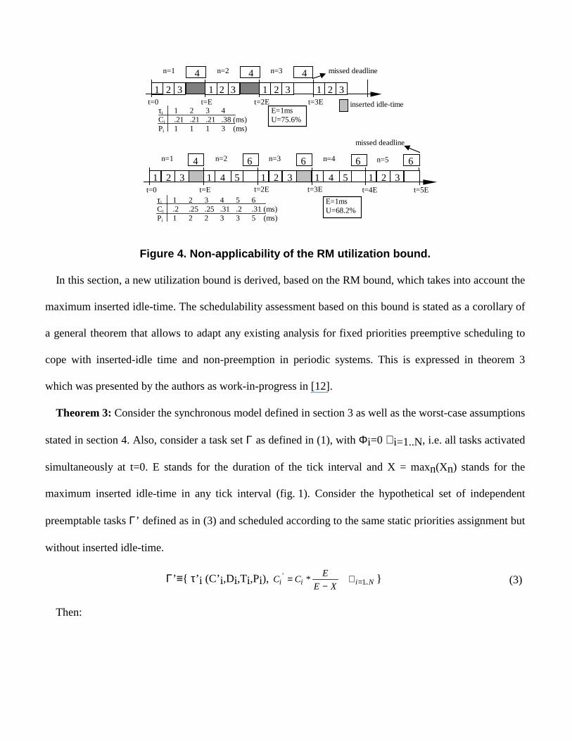
The question is, however, which utilization bound should be used. The Rate Monotonic bound cannot

be directly applied because of the existence of inserted idle-time. Figure 4 shows two examples in which

the RM utilization bound is met but the task set is not schedulable. In the first case task 4 never finds

enough time to execute and the same happens with task 6 in the second example.

1

n=1

t=0 2 3 1 1 2 3 1

4 2 3 2 3

n=2 4 n=3 4 missed deadline

t=E inserted idle-time τi 1 2 3 4 Ci .21 .21 .21 .38 (ms) Pi 1 1 1 3 (ms)

1

n=1

τi 1 2 3 4 5 6 Ci .2 .25 .25 .31 .2 .31 (ms) Pi 1 2 2 3 3 5 (ms)

t=0 2 3 1 1 1

4 n=2 n=3 missed deadline

t=E 4 5

6 2 3

6

4 5

6 1 2 3

6

t=2E t=3E t=4E

t=2E t=3E

t=5E

E=1ms U=75.6%

E=1ms U=68.2%

n=4 n=5

Figure 4. Non-applicability of the RM utilization bound.

In this section, a new utilization bound is derived, based on the RM bound, which takes into account the

maximum inserted idle-time. The schedulability assessment based on this bound is stated as a corollary of

a general theorem that allows to adapt any existing analysis for fixed priorities preemptive scheduling to

cope with inserted-idle time and non-preemption in periodic systems. This is expressed in theorem 3

which was presented by the authors as work-in-progress in [12].

Theorem 3: Consider the synchronous model defined in section 3 as well as the worst-case assumptions

stated in section 4. Also, consider a task set Γ as defined in (1), with Φi=0 ∀ i=1..N, i.e. all tasks activated

simultaneously at t=0. E stands for the duration of the tick interval and X = maxn(Xn) stands for the

maximum inserted idle-time in any tick interval (fig. 1). Consider the hypothetical set of independent

preemptable tasks Γ’ defined as in (3) and scheduled according to the same static priorities assignment but

without inserted idle-time.

Γ’≡{ τ’i (C’i,Di,Ti,Pi), C C EE Xi i i N

'..*=

−∀ =1 } (3)

Then:

Set Γ’ is guaranteed to be schedulable by

at least one sort of analysis for fixed

priority preemptive scheduling

⇒⇒⇒⇒ Set Γ is also schedulable

Proof: Define function Hi(t) as in expression (4), which represents the cumulative demand for CPU

time at instant t by the instances of tasks τ1 to τi. This function contains two terms, the former due to the

tasks effective processing and the latter due to the inserted idle-time. Starting from t=0+, the value of Hi(t)

raises in steps whenever a new task instance becomes ready. As long as there are uncompleted ready tasks,

the demand is higher than the effective CPU time, i.e. Hi(t) > t (see fig. 5 for task 9 of task set of table 1).

However, if the CPU has enough capacity to process all the tasks then Hi(t) will grow slower than t. When

t reaches Hi(t) it means that all the instances of tasks τ1 to τi that became ready in the interval [0,t) have

been completed (the interval [0,t) is then called the level i busy interval). Furthermore, such instant t also

corresponds to the response time of the first instance of task τi, or, more precisely, the worst-case response

time (Rwci) since all tasks are in phase. This is expressed in equation (5).

H t tT

C Xijj

ij n

n

tE

i N( ) * ..=

+ ∀= =

−

=∑ ∑1 1

1

1 (4)

Rwci = Hi(Rwci) , ∀ i=1..N (5)

On the other hand, a similar function, Η’i (t), can be established, as in expression (6), for set Γ’ which

represents the cumulative processor demand at instant t by the tasks τ’1 to τ’i. The worst-case response

time (Rwc’i) can also be written as the solution to equation (7).

H t tT

Cijj

ij i N' ( ) * ' ..=

∀=

=∑1

1 (6)

Rwc’i = H’i (Rwc’i) , ∀ i=1..N (7)

The proof of the theorem consists in showing that Rwc’i>Rwci, ∀ i=1..N Then, if set Γ’ is guaranteed to

be schedulable then Di≥Rwc’i, ∀ i=1..N. Consequently, Γ is also schedulable since Di≥Rwc’i≥Rwci,

∀ i=1..N.

To prove that Rwc’i>Rwci, ∀ i=1..N. consider the referred functions Ηi(t) and Η’i(t) restricted to the

interval (0,Rwci] or (0,Rwc’i] whichever is longer or until one of them grows beyond the deadline Di.

This latter situation corresponds to the non-schedulability of either Γ’ or Γ which is not relevant to this

proof. On the other hand, showing that Η’i(t) ≥ Ηi(t) in the interval (0,Rwc’i] leads to the desired result.

H t H tt

T Ct

T C Xi ijj

i

jjj

i

j nn

tE

' ( ) ( ) * ' *≥ ⇔

≥

+= = =

−

∑ ∑ ∑1 1 1

1

⇔

≥−

= =

−

∑ ∑tT C X

E XXjj

i

j nn

tE

1 1

1

* * (8)

By definition H’i (t) ≥ t in the interval (0,Rwc’i] yielding condition (9). Notice that, by the definition of

the ceiling and floor functions, x ≥ x ≥ x ≥ x −1.

( ) ( )tT

C tt

TC t

E XE

tE

E XtE

E Xjj

i

jjj

i

j

≥ ⇔

≥−

= − ≥

−

−

= =∑ ∑

1 11* ' * * * * (9)

Taking into account that X stands for maxn(Xn) the following inequality can be written

tE

X X nn

tE

−

≥

=

−

∑11

1

* (10)

Combining inequalities (9) and (10) proves the condition expressed in (8) and consequently, the

theorem (q.e.d.).

The above theorem represents a general result which can be exploited to enlarge the applicability of

several analysis based on fixed-priorities preemptive scheduling to non-preemptive scheduling of periodic

and synchronous tasks using inserted idle-time. However, any schedulability assessment resulting from the

use of this theorem is always sufficient and not necessary even when the analysis performed on the

t

H9’(t)

H9(t)

0 1 2 3 4 5 0

0.5

1

1.5

2

2.5

3

3.5

4

4.5

5

t (ms)

CPU Demand Functions

Rwc’9

Rwc9

t (ms)

Figure 5. CPU demand functions for task 9

within the set described in table 1.

hypothetical set Γ’ is necessary and sufficient. This is due to the fact that the theorem considers X, the

maximum inserted idle-time, and not the effective values Xn.

A practical difficulty resides in the determination of X = maxn(Xn) without actually building the

schedule to determine the values of Xn (the inserted idle-time in the nth tick interval). Hence, an upper

bound can be used given by (11). In fact, only the lower priority tasks that may not fit in the tick interval

where they became active (τi, i=k..N) can cause idle-time insertion. Nevertheless, for some particular

situations it is possible to determine the exact amount of idle-time that can be inserted.

ECECk

XXC

k

ii

k

ii

nnjNkj

>∧≤

≥≥

∑∑=

−

=

=

1

1

1

..

:

)(max)(max

(11)

The enlarged execution times are then given by (12).

NijNkj

ii CEECC ..1

..

'

)(max* =

=

∀−

= (12)

An interesting situation may happen when evaluating expression (11). If the sum of all the execution

times is less than or equal to E, then there is no inserted idle-time and index k cannot be computed.

However, in such situation the task set is obviously schedulable because all tasks fit within a single tick

interval and there can be no more than one instance of each task in that interval. For the same reason, the

first k-1 tasks are always guaranteed to be schedulable.

Two corollaries can now be established concerning the adaptation of two typical analysis: the

utilisation-based analysis for rate-monotonic scheduling [8] and the response time-based analysis for

fixed-priorities preemptive scheduling [7].

Corollary 1: Consider the synchronous model presented in section 3 and a set of tasks Γ as defined in

(1), with Di=Ti ∀ i=1..N and a priority assignment according to rate-monotonic, i.e. Ti<Tj ⇒ Pi>Pj

∀ i,j=1..N. Moreover, consider that N is larger than k-1 as obtained in (11) to force the existence of

inserted idle-time. Then:

−

−<

=∑

= EXN

TCU N

N

i i

i 1121

1

⇒⇒⇒⇒

Set Γ is schedulable

under any phasing

This corollary can be easily proved since the hypothetical set Γ’ (3) can be scheduled under RM if

UCT

Ni

ii

NN'

'=

< −

=∑

1

1

2 1

The schedulability of set Γ is then guaranteed by the theorem as long as Γ’ is schedulable in the

conditions referred. By transforming U’ into U=U’*(1-X/E) the corollary is then proved (q.e.d.).

Corollary 2: Again, consider the synchronous model presented in section 3 and a set of tasks Γ as

defined in (1), with Di=Ti ∀ i=1..N and any fixed decreasing priority assignment, i.e. i<j ⇒ Pi>Pj

∀ i,j=1..N. Moreover, consider that N is larger than k-1 as obtained in (11) to force the existence of

inserted idle-time. Then:

Rwc’i ≤ Di ∀ i=1..N ⇒⇒⇒⇒ Set Γ is schedulable

under any phasing

Rwc’i is the worst-case response time for an instance of τ’i in Γ’ (3) obtained by the usual response time

analysis for fixed priority preemptive scheduling [7]. Since when the left-hand side condition is true set Γ’

is schedulable, then, by the theorem, corollary 2 is proved (q.e.d.).

From these two corollaries, the latter one is presented just to illustrate the generality of theorem 3. In

fact, it incurs a computational cost similar to that of the timeline approach presented in the previous

section and its performance is worse, resulting in a more pessimistic schedulability assessment. In what

concerns corollary one, it allows to obtain the desired utilization bounds for guaranteed schedulability.

Figure 6 shows the variation of such bounds with N, the number of tasks, as well as with the ratio X/E

which represents the maximum fraction of CPU bandwidth that may be wasted with inserted idle-time.

The figure just shows values of X/E up to 30%. Beyond this threshold, the model becomes very restrictive

incuring in an excessive schedulability penalty (the utilization bound for large N drops below 50%). In

common situations where this model is applicable, values of X/E around 10% are typical. In this case, for

large N the utilization bound is about 63% which is close to the original RM bound. Notice that for small

values of N the sum of the Ci’s fits within E and thus, there is no inserted idle-time and the schedulability

is guaranteed. In general, taking X as the maximum of all execution times Ci, the schedulability is

guaranteed for N up to 1/(X/E). For a particular task set, such guarantee can be achieved for N up to k-1

obtained as in (11).

Several examples of pratical situations follow. Consider a WorldFIP fieldbus system with a

transmission rate of 1Mbit/s, 20µs of turnaround time, elementary cycle of 5ms and up to 32 data bytes per

transaction. In these circunstances, the maximum transaction duration is 418µs resulting in a rate X/E less

than 10%. Consider an FTT-CAN system operating at 250Kbit/s with an elementary cycle of 5ms. The

maximum transaction duration takes about 523µs (8 data bytes) corresponding to a ratio X/E smaller than

11%. Consider a simple robot controlled by a reflex behaviour approach, implemented on top of a

non-preemptive multitasking kernel running on an 8051 microcontroller with a 10ms tick interval. Since

most of the tasks execute simple arithmetic, conditional and data movement operations, it is very likely

that such tasks can execute in less than 1ms, resulting in a ratio X/E lower than 10%.

2 4 6 8 10 12 14 16 18 200

0.1

0.2

0.3

0.4

0.5

0.6

0.7

0.8

0.9

1

RM bound X/E=10% X/E=20% X/E=30%

N

U

Figure 6. Utilization bounds resulting from corollary 1.

Before concluding this section it is interesting to notice that the effect of using inserted idle-time can

also be accounted for, in the context of existing analysis for fixed priority preemptive scheduling, by

considering it as an extra virtual task with worst-case execution time of X and period E. This can easily be

proven in a similar way as for theorem 3. Then, it is also possible to modify the RM bound to guarantee

schedulability in this case. The resulting utilization bound is given by (13).

EXN

TC

U NN

i i

i −

−<

=∑

=12

1

1

(13)

However, it can easily be proved that this bound is always lower than the bound of corollary 1 and thus

it is more pessimistic. Figure 7 depicts this situation for a given task set with X=0.2ms and E=1ms

(X/E=20%). U(N) is the effective utilization (56.5% in this case with N=6). U’(N)=U(N)*E/(E-X) is an

enlarged utilization factor that accounts for X/E as in theorem 3 (71.5% in this case). U’’(N)=U(N)+X/E is

an extended utilization factor that accounts for X/E as in (13) resulting 77.5% in this case. Since the RM

bound for N=6 is 73.4%, according to the bound of corollary 1 the set is guaranteed to be schedulable.

However, according to the bound in (13) the schedulability of the set cannot be guaranteed.

1 2 3 4 5 6 0 0.1

0.2

0.3

0.4

0.5

0.6

0.7

0.8

0.91

U

N

U(N)

U’(N)U’’(N)

τi 1 2 3 4 5 Ci .21 .21 .2 .2 .2 (ms) Pi 1 2 2 2 4 (ms)

Figure 7. Using the adapted utilization factors.

Notice that comparing U’(N) and U’’(N) against the RM bound is equivalent to comparing U(N) against

the bounds of corollary 1 and (13) respectively.

7. Conclusions

Although non-preemptive scheduling does not seem very attractive due to the large blocking factors

normally associated to it, it is still used in some application areas such as message scheduling in fieldbus

communication systems and task scheduling in light multitasking kernels for embedded systems based on

simple microprocessors.

In this paper it is shown that by implicitely using idle-time insertion in synchronous systems, i.e. those

in which tasks are activated synchronously with a given clock tick, it is possible to eliminate the blocking

factor associated to non-preemption. The result is a jitter-free release of the highest priority task in the

system. If apropriate periods and initial phasing are chosen for the remaning tasks it might be possible to

obtain a jitter-free schedule for the whole task set.

Furthermore, the paper shows a thorough analysis of this scheduling model. An accurate response time-

based analysis is developed that, under worst-case conditions is necessary and sufficient. On the other

hand, the paper also presents a theorem that allows to adapt the existing analysis for fixed priorities

preemptive scheduling to cope with the inserted idle-time and non-preemption of this synchronous model.

The result is just a sufficient schedulability assessment. However, it allows to develop utilization bounds

for guaranteed schedulability that can be useful for on-line admission control in systems based on low

processing-power CPUs.

References

[1] Stankovic, J.A. et al.. Implications of Classical Scheduling Results for Real-Time Systems. IEEE

Computer, 28(6), 1995.

[2] Carderia, C.. Ordonnancement Temps Réel par Réseaux de Neurones. PhD Thesis, INPL, Nancy,

France, 1994.

[3] Jeffay, K. , D. Stanat and C.U. Martel. On Non-preemptive Scheduling of Periodic and Sporadic

Tasks. Proc. of IEEE RTSS’91. San Antonio, USA, 1991.

[4] Vasques, F.. Sur l’Intégration de Mécanismes d’Ordonnacement et de Communication dans la Sous-

Couche MAC de Réseaux Locaux Temps-Réel. PhD Thesis, LAAS-CNRS, Université Paul Sabatier,

Toulouse, France, 1996.

[5] Howell, R. and M. Venkatrao. On Non-Preemptive Scheduling of Recurring Tasks Using Inserted Idle

Times. Information and Computation, 117, 1995.

[6] Almeida, L. and José A. Fonseca. Schedulability Analysis in a Real-Time Fieldbus Network.

Proceedings of IFAC SICICA'97, Annecy, France, June 1997.

[7] Audsley, N., A. Burns, M. Richardson, K. Tindell and A. Wellings. Applying New Scheduling Theory

to Static Priority Pre-Emptive Scheduling. Software Engineering Journal, 8(5): 285-292, 1993.

[8] Liu C. L. and J. W. Layland. Scheduling Algorithms for Multiprogramming in a Hard Real-Time

Environment. Journal of ACM, 20(1): 46-61, 1973.

[9] Törngren, M. Fundamentals of Implementing Real-Time Control Applications in Distributed

Computer Systems. Real-Time Systems, 14: 219-250, 1998.

[10] Stankovic, J., M. Spuri, K. Ramamritham and G. Buttazzo. Deadline Scheduling for Real-Time

Systems. KluwerAcademic Publishers, 1998.

[11] Almeida, L. and J. A. Fonseca. Schedulability Analysis in the FIP Fieldbus Accounting for Inserted

Idle-Time. Proc. Work-in-Progress session of Euromicro RTS’99. York, UK, June 1999.

[12] Almeida, L. and J. A. Fonseca. Adapting Preemptive Scheduling Analysis to cope with Non-

Preemption and Inserted Idle-Time. Proc. Work-in-Progress session of IEEE RTSS 2000. Orlando,

USA, November 2000.

[13] Fonseca, J. A. and L. Almeida. Using a Planning Scheduler in the CAN Network. Proc. IEEE

ETFA’99. Barcelona, Spain, October 1999.

[14] Saphira - Software Manual (v6.1). Activ Media, Inc. 1998.

[15] Lauwereins, R., M. Engels, M. Adé and J.A. Peperstraete. Grape-II: A System-Level Prototyping

Environment for DSP Applications. IEEE Computer, February 1995.