Journal of Scheduling manuscript No.(will be inserted by the editor)

A Preemptive Bound for the Resource Constrained Project SchedulingProblem

Mohamed Haouari · Anis Kooli · Emmanuel Néron ·Jacques Carlier

Abstract The Resource Constrained Project Scheduling Problem (RCPSP) is one of the most intensively inves-tigated scheduling problems. It requires scheduling a set of interrelated activities, while considering precedencerelationships, and limited renewable resources allocation. The objective is to minimize the project duration. Wepropose a new destructive lower bound for this challenging NP-hard problem. Starting from a previously sug-gested LP model, we propose several original valid inequalities that aim at tightening the model representation.These new inequalities are based on precedence constraints, incompatible activity subsets and nonpreemptionconstraints. We present the results of an extensive computational study that was carried out on 2040 benchmarkinstances of PSPLIB, with up to 120 activities, and that provide strong evidence that the new proposed lowerbound exhibits an excellent performance. In particular, we report the improvement of the best known lowerbounds of 48 instances.

1 Introduction

The Resource Constrained Project Scheduling Problem (RCPSP) consists in scheduling activities submitted toboth precedence relationships and resource constraints in order to minimize the project duration. Formally,the RCPSP is defined as follows. A project consists of a set A = {A1, . . . , An} of nonpreemptive activities.Let G = (V,A) be the associated precedence graph. That is, the node set V includes the n activities as wellas two additional dummy zero-duration activities A0 and An+1 that represent the start and the end of theproject, respectively. An arc (i, j) ∈ A if and only if activity Ai is an immediate predecessor of activity Aj . Ris a set of K renewable resources that are required for processing the activities. Each resource k (k ∈ R) iscontinuously available from time zero onwards with resource capacity Bk. Each activity Aj ∈ A is characterizedby a deterministic processing time pj and resource requirements bjk (k ∈ R). The objective is to minimize theproject completion time. Actually, this challenging NP-hard problem is very appealing because it constitutesa formidable nut to crack. Indeed, despite intense research efforts, some benchmark instances with as manyas 60 activities remain desperately open since their inception about fifteen years ago. Moreover, and from apractical perspective, optimizing the project duration has become a crucial issue for most organizations, suchas construction engineering, manufacturing systems and software development projects, to quote just a few.

The RCPSP is a very renowned scheduling problem that has attracted an ever growing attention in theoperations research literature (see Demeulemeester and Herroelen (2002) for a comprehensive review). In thiscontext, several authors investigated mathematical programming formulations for the RCPSP. One of the firstmathematical models for the RCPSP was proposed by Pritsker et al. (1969) who proposed a time-indexed mixedinteger programming formulation. Later, Christofides et al. (1987) enhanced this formulation by expressing theprecedence constraints in a disaggregated form. This latter formulation was subsequently used by Möhringet al. (2003) to compute both Lagrangian-based lower bounds and feasible solutions. Mingozzi et al. (1998)

M. HaouariDepartment of Mechanical and Industrial Engineering, College of Engineering, Qatar University, Doha, Qatar.

A. KooliUniversité de Tunis, Ecole Supérieure des Sciences Economiques et Commerciales de Tunis, 4 Rue Abou Zakaria El Hafsi, 1089Montfleury, Tunisie.

A. Kooli · E. NéronUniversité François Rabelais de Tours, Laboratoire d’Informatique (EA 2101), Equipe Ordonnancement et Conduite (ERL CNRS6305), 64 avenue Jean Portalis, 37200 Tours, France.

J. CarlierUniversité de Technologie de Compiègne, Laboratoire HeuDiaSyC, CNRS UMR 7253, BP 20529, 60205 Compiègne, France.

2 Haouari et al.

proposed a clever 0-1 programming formulation with exponentially many columns. In this formulation, eachcolumn corresponds to a feasible subset (that is, a subset of activities that can simultaneously be executedwithout violating neither resource nor precedence constraints.) Alvarez-Valdés and Tamarit (1993) presenteda 0-1 programming formulation with exponentially many constraints that is based on the concept of minimalforbidden sets (that is, any subset of activities that cannot be in progress simultaneously and that is minimalfor inclusion). Recently, Koné et al. (2011) proposed two event-based formulations for the RCPSP where eventscorrespond to start or end times of activities. Finally, we note the work of Schutt et al. (2011) who presented newprocedures based on constraint programming. Experimental results demonstrate the very good performance ofthe proposed approach which delivered proven optimal solutions for several open instances.

Furthermore, a huge effort has been devoted to the design and analysis of lower bounds for the RCPSP.Lower bounds are extremely useful both from practical and theoretical points of view, especially for assessing theempirical performance of heuristics and for building effective branch-and-bound algorithms. Classically, lowerbounds are classified into two main classes: constructive lower bounds and destructive lower bounds. The firstclass includes bounds that are derived through optimally solving a relaxation of the genuine problem. We referto Artigues et al., (2008) for a comprehensive review of constructive RCPSP lower bounds. By contrast, thesecond class includes destructive lower bounds that are derived by using the following search strategy. Givenan initial trial value C of the makespan, a feasibility test is carried out to detect an infeasibility also called acontradiction. If an infeasibility occurs, then the trial value C is increased by 1 (or, alternatively a dichotomicsearch might be used), and the checking procedure is restarted (i.e., determining the largest value C whereinfeasibility can be proved. Thus, C+1 is the value of the destructive lower bound). This process is halted whenfor some value of C no infeasibility could be detected. Depending on how the checking procedure (for provinginfeasibility) is carried out, numerous destructive lower bounds have been proposed so far for the RCPSP. Inparticular, we quote the paper by Klein and Scholl (1999), where the idea of destructive bound was originallyintroduced, and those by Brucker and Knust (2000) and Baptiste and Demassey (2004) where destructive lowerbounds, that are the best lower bounds which are currently available for the RCPSP, are described. These latterbounds are based on solving LP relaxations that were derived from the formulation of Mingozzi et al. (1998)by partitioning the time horizon into time-windows and using the column generation technique to deal withthe exponential number of decision variables. Basically, the formulation of Brucker and Knust (2000) takes intoaccount release dates and deadlines of the activities and, for a given trial value C, attempts to prove that nopreemptive schedule with makespan shorter than C exists such that all resource constraints are satisfied. Theformulation of Brucker and Knust (2000) was subsequently enhanced by Baptiste and Demassey (2004) whoappended new cuts and used it to derive tight lower bounds. Furthermore, an additional approach using columngeneration was proposed by van den Akker et al. (2007). This approach requires reformulating the RCPSP intoan equivalent problem of minimizing the maximum lateness on a set of identical parallel machines. Anotheridea that was investigated uses the concept of energetic reasoning initially introduced by Lahrichi (1982). Later,Erschler et al. (1991) and Baptiste et al. (1999) used this concept to derive lower bounds for the RCPSP.Recently, Haouari et al. (2012) derived effective lower bounds based on several generalizations of the energeticreasoning.

In this paper, we propose a destructive lower bound where the checking procedure is based on solving anenhanced LP relaxation of the RCPSP. Even though the basic features of our approach are classic, they areenriched with some novel ideas which make it attractive. Indeed, starting from a relaxation from the literature,that is shown to perform poorly, we enhanced it with a variety of valid inequalities that enforce precedencerelationships, resource constraints, and nonpreemption. With few exceptions, all these valid inequalities areoriginal or dominate previously proposed cuts. Furthermore, a distinctive feature of the proposed lower bound isthat it requires the solution of a compact LP (that is, having a polynomial number of variables and constraints)and therefore does not require the implementation of a sophisticated column generation algorithm. A niceconsequence of this compactness feature is that our approach is scalable and therefore can be used for largescaled instances.

The remainder of the paper is organized as follows. In Section 2, we introduce a basic LP relaxation thatwas previously proposed in the literature and that will be used as a starting model for building an enhancedLP relaxation through appending several new valid constraints. To that aim, we begin with by presenting inSection 3 simple valid constraints. In Section 4, a new precedence constraint is presented. Incompatible activitysets-based cuts are presented in Section 5. Nonpreemptive cuts are presented in Section 6. The results of ourextensive computational experiments are presented in Section 7. Finally, some conclusive remarks as well asdirections for future research are presented in the last section.

2 A basic preemptive formulation

We define for each activity Aj ∈ A a release date rj and a deadline dj . For the sake of clarity, we briefly recallhow these values are computed. Let G = (V,A) be the precedence graph. Each arc (i, j) ∈ A is assigned the

A Preemptive Bound for the RCPSP 3

weight pi. Also, let l(i, j) be the weight of a longest path in G between nodes i and j. Thus, the release date ofAj ∈ A is given by rj = l(0, j). Furthermore, given a trial value C, (in the sequel, C is assumed to be a validlower bound of the makespan) the deadline of Aj ∈ A is given by dj = C + pj − l(j, n+ 1).

Now, we introduce a basic relaxation of the RCPSP that was originally proposed by Carlier and Néron (2003).This relaxation aims at checking whether there exists a feasible schedule having a makespan shorter than or equalto the trial value C. It is worth emphasizing that instead of considering an exact RCPSP feasibility problem wefocus on a relaxation of the RCPSP, where resource and precedence constraints are partially considered, thatis formulated as a linear program. Toward this end, we introduce the following notation. Let {t1, . . . , tL+1} bethe set containing all release dates and deadlines of all activities ranked in increasing order. A time intervalIl = [tl, tl+1) is defined for each l ∈ L where L = {1, . . . , L}. Hence, the time-horizon [0, C] (recall that C is atrial value of the makespan) is split into L consecutive time-intervals whose time-bounds correspond either toa release date or a deadline. Moreover, we define the following sets:

– Ij = {l ∈ L : Il ⊆ [rj , dj ]} the set of indices of time-intervals during which activity Aj can be processed,– Iji = {l ∈ L : max(ri, rj) ≤ tl < min(di, dj)} the set of indices of time-intervals during which both activitiesAi and Aj can be in progress simultaneously,

– Al = {Aj ∈ A : Il ⊆ [rj , dj ]} the set of activities that can be in progress during time-interval Il.

Also, we set ∆l = tl+1 − tl for l ∈ L, υ = maxAj∈A(dj − pj − rj + 1), and ρ = maxAj∈A∣∣Ij∣∣ . These latter

two parameters represent the maximum number of feasible starting times of an activity, and the maximumnumber of time-intervals during which an activity might be processed, respectively. Furthermore, we define thecontinuous decision variable xjl as the amount of time that is allocated to process activity Aj ∈ A during thetime interval Il ∈ Ij . Thus, the feasibility problem proposed by Carlier and Néron (2003) reads as follows:

(LP0) :Find x (1)s.t.∑l∈Ij

xjl = pj , ∀Aj ∈ A (2)

xjl ≤ ∆l, ∀Aj ∈ A,∀l ∈ Ij (3)∑Aj∈Al

bjkxjl ≤ Bk∆l, ∀k ∈ R, ∀l ∈ L (4)

∑s∈Ii:s≤l

xispi≥

l∑s=τ :tτ=rj

xjspj, ∀(i, j) ∈ A,∀l ∈ Iji (5)

xjl ≥ 0, ∀Aj ∈ A, ∀l ∈ Ij (6)

Constraints (2) state that each activity Aj must be processed within its specified time-window [rj , dj ].Constraints (3) require that any activity Aj could not be processed more than once at any time. Constraints(4) enforce that for any resource k and at any time-interval Il the total resource requirements do not exceed theresource capacity. Constraints (5) can be viewed as “pseudo-precedence” constraints. They enforce that if Ai isa predecessor of Aj then the total fraction of Ai that is processed from its release date ri up to the time-boundtl+1 is larger than or equal to the fraction of the successor activity Aj that is processed from its release date rjup to the same time-bound tl+1.

It is worth mentioning that, in a strict sense, LP0 does not correspond to the preemptive relaxation of theRCPSP. This is mainly due to the fact that (4) can be viewed as a relaxed version of the cumulative resourceconstraints.

Property 1 If for a given trial value C of the makespan, LP0 is infeasible then C + 1 is a valid lower bound onthe optimal makespan.

In the sequel, we denote LBCN the destructive bound that is based on Property 1. Interestingly, even thoughLBCN has been proposed few years ago, its computational performance has never been thoroughly assessed.Thus, we conducted a computational analysis of LBCN and compared it with the state-of-the-art lower bound ofBrucker and Knust (2000) (in the sequel, we shall refer to this latter bound by LBBK). In our implementation,we considered as an initial trial value the so-called critical path bound that is defined as follows:

LBC = l(0, n+ 1)

We considered a subset of 326 nontrivial 60- and 90-activity instances from the well-known PSPLIB testbedproposed by Kolisch et al. (1997) for which LBCN is strictly smaller than the best known upper bound. A

4 Haouari et al.

summary of the results is displayed in Table 1. In this table, each entry represents the total number of instancesthe equality (or inequality) that is stated in the first column of the corresponding row holds for the differentproblem sets, respectively. Not surprisingly, we observe that LBCN exhibits a poor performance and is largelydominated by LBBK . Actually, we found that LBCN is strictly outperformed by LBBK for 81.6% of theinstances.

60-activity 90-activityLBCN > LBBK 0 0LBCN = LBBK 29 31LBCN < LBBK 154 112

Table 1 Comparison between LBCN and LBBK on nontrivial instances.

In the sequel, we shall gradually append several valid constraints to LP0 and provide evidence that theseadditional cuts will have a dramatic effect on the performance of the resulting destructive bound. To that aim,we shall sequentially introduce the following four cut families: (i) simple valid cuts; (ii) precedence cuts; (iii)forbidden activity sets cuts, and (iv) nonpreemptive cuts.

3 Simple valid cuts

To begin with, we provide two simple, though computationally useful, cuts.

3.1 The concept of mandatory parts

The concept of a mandatory part of an activity has been defined within the framework of Energetic Reasoning(ER) (Lahrichi (1982); Erschler et al. (1991); Baptiste et al. (1999)). We recall that the mandatory part of anactivity Aj ∈ A during a time interval [t1, t2] ⊆ [0, C], hereafter denoted by p(j, t1, t2), is the part of Aj thatmust be processed within [t1, t2]. Thus, we have:

p(j, t1, t2) = min(t2 − t1, pj ,max(0, rj + pj − t1),max(0, t2 − dj + pj)

)Using these definitions, we straightforwardly derive the following valid variable bounds:

xjl ≥ p(j, tl, tl+1), ∀Aj ∈ A, ∀l ∈ Ij (7)

Clearly, (7) dominate (6) and can therefore replace these restrictions.

3.2 No idle-time

A second simple valid constraint requires that, in any optimal solution, there is at least one activity in progressat each time point: ∑

Aj∈Alxjl ≥ ∆l, ∀l ∈ L (8)

4 A precedence-based cut

Let x be a nonpreemptive schedule. We define αj =∑l∈Ij

tlxjl and βj =∑l∈Ij

(tl+1 − 1)xjl, for each activity

Aj ∈ A. Also, we denote by sj ∈ [rj , dj − pj ] the starting time of activity Aj . Thus, Aj is processed during theconsecutive time points sj , . . . , sj + pj − 1. Then, the mean time point during which the resources are allocatedto Aj is s̃j = sj + pj − 1

2 for Aj ∈ A. We have:

Proposition 1 We haveαjpj≤ s̃j ≤

βjpj

for Aj ∈ A. (9)

A Preemptive Bound for the RCPSP 5

Proof First, note that in this case the xjl’s are integers. Assume that xjl > 0 and that {sj , . . . , sj+pj−1}∩Il ={slj , . . . , slj + xjl − 1}. Thus, we have: tl ≤ slj + q ≤ tl+1 − 1 for q = 0, . . . , xjl − 1. Hence, we get:

tlxjl ≤xjl−1∑q=0

(slj + q) ≤ (tl+1 − 1)xjl, ∀Aj ∈ A, ∀l ∈ Ij (10)

After summing up all inequalities (10) for l ∈ Ij , we get:

∑l∈Ij

tlxjl ≤ sj + . . .+ (sj + pj − 1) ≤∑l∈Ij

(tl+1 − 1)xjl, ∀Aj ∈ A (11)

Finally, this yields

αjpj≤ s̃j ≤

βjpj, ∀Aj ∈ A

ut

Furthermore, for each Aj ∈ A and sj ∈ [rj , dj − pj ], we compute the corresponding values αj , βj , and s̃j ,

and we define the slack variables λj(sj) = s̃j −αjpj

and µj(sj) = βjpj− s̃j , respectively.

Lemma 1 The following inequality

βjpj− αipi≥ minsi∈[ri,di−pi], sj∈[rj ,dj−pj ]:si+pi≤sj

(λi(si) + µj(sj)) + pi2 + pj

2 , ∀(i, j) ∈ A (12)

is valid.

Proof Assume that (i, j) ∈ A. If activity Ai starts at si and activity Aj starts at sj then we have:

si + pi ≤ sj ⇒ s̃i + pi2 ≤ s̃j −

pj2

⇒ λi(si) + αipi

+ pi2 ≤

βjpj− pj

2 − µj(sj)

Hence, we derive the valid inequality

βjpj− αipi≥ (λi(si) + µj(sj)) + pi

2 + pj2 (13)

By considering all possible (compatible) starting times, we derive the valid inequality (12). ut

Clearly, for each Aj ∈ A and sj ∈ [rj , dj − pj ], the computation of λj(sj) and µj(sj) requires O(ρ)-time.Also, for each (i, j) ∈ A, the computation of the RHS of the corresponding inequality (12) requires O(υ2)-time.Thus, the overall effort for generating (12) is O(nρ+ |A| υ2).

5 Incompatible activity sets-based cuts

Now, we turn our attention to valid cuts that are based on incompatible activity sets. First, we describe twocuts from the literature. Next, we introduce the so-called clique cuts together with the associated separationprocedure. Finally, we show how to use the concept of dual feasible function (see Fekete and Schepers (1998))to derive from the capacity constraints (4) several valid inequalities.

6 Haouari et al.

5.1 Two cuts from the literature

For each resource k ∈ R, and each integer m, we define Emk = {Aj ∈ A : bjk ≥⌊

Bkm+ 1

⌋+ 1}. We observe that

in any feasible solution there must be at most m activities from Emk that can be processed in parallel (Carlierand Latapie (1991)). Hence, a valid constraint is:∑

Aj∈Al∩Emk

xjl ≤ m∆l, ∀l ∈ L, ∀k ∈ R (14)

In our tests, and for the sake of computational efficiency, we restrict these constraints to m ∈ {1, 2}.It is easy to see that for each k ∈ R, and each integer m, (14) can be derived in O(n)-time.Furthermore, Nabeshima (1973) introduced a more general concept of minimal forbidden set of activities.

Recall that this concept refers to activity subsets that include activities that cannot be in progress simultane-ously.

Let φ be a minimal forbidden set, and |φ| its cardinality. Then, a valid constraint is:∑Aj∈Al∩φ

xjl ≤ (|φ| − 1)∆l, ∀l ∈ L, ∀φ ∈ Φ (15)

where Φ is the set of all minimal forbidden sets.It is noteworthy that the number of minimal forbidden sets may be very large (see Artigues et al. (2008)).

Therefore, in the sequel, we shall restrict (15) only to minimal forbidden sets of cardinality 3. Hence, generatingthese cuts requires O(n3) time.

Remark 1 Notice that all the sets E2k of cardinality 3 (see Constraint 14) are included in the minimal forbidden

sets of cardinality 3. Thus, some cuts generated by (14) are also generated by (15). However, in general, a setE2k may be of cardinality larger than 3.

5.2 Clique cuts

In this section, we introduce a valid inequality that is based on subsets of mutually incompatible activities. Tothat aim, we define G′ = (V,E) an undirected incompatibility graph, presented for the RCPSP by Mingozzi etal. (1998), where each node i represents an activity Ai ∈ A, and where each edge {i, j} ∈ E is associated witha pair {Ai, Aj} of activities that cannot both be processed simultaneously. That is:

{i, j} ∈ E ⇐⇒

(i) Ai(Aj) is a predecessor of Aj(Ai)or(ii) bik + bjk > Bk for some k ∈ R

It is noteworthy that Condition (i) does not necessarily require an immediate precedence relationship.Let C denote the set of cliques of G′ . Clearly, a clique Cl ∈ C includes a set of mutually exclusive activities.

Hence, the following cut ∑Aj∈Al∩Cl

xjl ≤ ∆l, ∀l ∈ L,∀Cl ∈ C (16)

is valid.Clearly, it is sufficient to consider in (16) only the (nondominated) inclusionwise maximal cliques.Since (16) includes a very large (exponential) number of constraints, then the feasibility LP model is solved

using a constraint generation approach where violated clique constraints are iteratively generated on the fly.Hence, this approach requires iteratively solving |L| separation problems of the form:

(SP l): Given ( x̄jl)j=1,...,n the solution of LP0, find Cl ∈ C such that∑

Aj∈Al∩Cl

x̄jl > ∆l or verify that no

such clique exists.

Thus, (SP l) amounts to finding a clique Cl ∈ C such that∑

Aj∈Al∩Cl

x̄jl is maximal.

Therefore, we see that (SP l) requires solving a maximum weight clique problem (MWCP) in the subgraphGl = (V l, El) of G′ (where each node j from V l represents an activity Aj ∈ Al) and where each node is assigneda weight x̄jl. This latter problem is notoriously known to be NP-hard. In our implementation, we used theexact algorithm of Östergård (2001) to solve the MWCP.

A Preemptive Bound for the RCPSP 7

Alternatively, we tested a much faster (and significantly simpler) heuristic strategy where a restricted num-ber of clique cuts are only generated in a preprocessing step. Hence, in so doing, we avoid invoking a timeconsuming dynamic constraint generation procedure. It is noteworthy that since the clique cuts are now gener-ated prior to computing the xjl’s variables, then we cannot emphasize inclusionwise maximal cliques. Instead,the implemented heuristic is based on generating the cliques that are maximal w.r.t cardinality. More precisely,we implemented the following strategy:

– Step 1: Invoke an exact algorithm to generate the cliques that are maximal w.r.t cardinality(In our implementation, we used the algorithm of Östergård (2002) and we set the CPU time limit to 300s).

– Step 2: Sort the generated cliques in decreasing cardinality– Step 3: Select the largest #CC cliques and append them to the feasibility model (in our implementation,

we empirically set the parameter #CC to 80)

5.3 Dual feasible functions-based cuts

Dual Feasible Functions (DFFs) have been proposed in the context of bounding bin-packing problem by Feketeand Schepers (1998) and used in the context of bounding RCPSP by Carlier and Néron (2000, 2003). Basically,a DFF is a function f : [0, B] → [0, B′] satisfying the following property : Let, a1, . . . , ak ∈ [0, B] such thata1 + . . .+ ak ≤ B then f(a1) + . . .+ f(ak) ≤ f(B).

Given a feasible schedule x, and a DFF f , we denote by Alt the subset of activities that are in progress attime t ∈ Il (l ∈ L). We have: ∑

Aj∈Alt

bjk ≤ Bk, ∀t ∈ Il, ∀l ∈ L, ∀k ∈ R (17)

Since f is a DFF, then we get:∑Aj∈Alt

f(bjk) ≤ f(Bk), ∀t ∈ Il, ∀l ∈ L, ∀k ∈ R (18)

After summing up all inequalities for t ∈ Il, we derive:∑Aj∈Al

f(bjk)xjl ≤ f(Bk)∆l, ∀l ∈ L, ∀k ∈ R (19)

Hence, given a set F ={fh}h=1,...,ξ of DFFs, we can derive from (4) the following valid inequalities:∑Aj∈Al

fh(bjk)xjl ≤ fh(Bk)∆l, ∀l ∈ L, ∀k ∈ R, ∀fh ∈ F (20)

For the sake of computational efficiency, we performed extensive computational experiments to identify aneffective set of DFFs. We found that a good performance is obtained by implementing the following DFFs thatwere initially proposed by Fekete and Schepers (1998) and Carlier et al. (2007), respectively:

fs1 : [0, B]→ [0, B]

x 7→

{x if x(s+1)

B ∈ Z⌊x(s+1)B

⌋Bs otherwise

with s = 1, 2, and

fs2 : [0, B]→ [0,MB(B, I)]

x 7→

MB(B, I)−MB(B − x, I) if x >

B

21 if s ≤ x ≤ B

20 otherwise

for s = 1, . . . , B/2, and where MB(B, I) is the solution of the knapsack problem (KP) defined by the itemset I = {i ∈ [1, n] : s ≤ bik ≤ Bk/2}, capacity B, and where the objective is to maximize the number of selecteditems. This latter KP is trivially solved by ranking the items in nondecreasing weights. Thus, this computationcan be carried out in O(n logn)-time.

8 Haouari et al.

Remark 2 In a strict sense, fs2 is a Data Dependent Feasible Function, i.e., the function depends on the sizes ofthe bjk’s in the instance (see Carlier et al. (2007)).

We see that each cut that is based on fs1 can be generated in O(n)-time for each k ∈ R. Also, a cut that isbased on fs2 can be generated in O(n logn)-time for each k ∈ R.

6 Nonpreemptive cuts

In this section, we propose four families of cuts that are based on the requirement that a feasible RCPSPschedule is nonpreemptive.

6.1 First family

The first set of constraints is based on the fact that in a nonpreemptive schedule, an activity is continuouslyscheduled during a set of successive intervals. Thus, we have the following lemma.

Lemma 2 The following constraints

q−1∑l=p+1

xjl

q−1∑l=p+1

∆l

≥ xjp∆p

+ xjq∆q− 1, ∀Aj ∈ A,∀p, q ∈ Ij such that p+ 1 < q (21)

are valid.

Proof Assume that x represents a nonpreemptive schedule. We consider two cases:- Case 1: xjp

∆p+ xjq∆q

> 1. Thus, activity Aj is both processed during the intervals Ip and Iq (with p+ 1 < q).

Since x is nonpreemptive, then Aj is necessarily continuously processed during all the intermediate intervals

Ip+1, . . . , Iq−1 as well. Hence,

q−1∑l=p+1

xjl

q−1∑l=p+1

∆l

= 1 and therefore the constraint is valid.

- Case 2: xjp∆p

+ xjq∆q≤ 1. Then, the constraint is trivially valid. ut

Each constraint (21) can be generated in O(ρ)-time.

6.2 Second family

Let Rj = {p, p + 1, . . . , q} be the set of indices of time intervals during which activity Aj ∈ A must be inprogress if it starts at its release date rj . That is,

l ∈ Rj ⇔ [rj , rj + pj ] ∩ Il 6= ∅.

For convenience, we assume that∣∣Rj∣∣ > 1 (see Figure 1).

Fig. 1 Illustration of nonpreemptive cuts (second family)

A Preemptive Bound for the RCPSP 9

Lemma 3 We have

xjp∆p≤ . . . ≤ xj,q−1

∆q−1≤ εj

xjq∆q

, ∀Aj ∈ A (22)

where εj = ∆q

rj + pj − tq

Proof We consider two cases:Case 1: There exists h ∈ [p, q − 1] such that xjh

∆h> 0. Hence, xjl

∆l= 1 for l = h + 1, . . . , q − 1. Also,

xjq ≥ rj + pj − tq. Thus, the inequalities are valid.Case 2: xjl

∆l= 0, for l = p, . . . , q−1. In this case, the inequality reduces to εj

xjq∆q≥ 0 and is therefore trivially

valid. ut

Furthermore, let Dj = {p, p+ 1, . . . , q} be the set of indices of time intervals during which activity Aj ∈ Amust be in progress if it terminates at its deadline dj . That is,

l ∈ Dj ⇔ [dj − pj , dj ] ∩ Il 6= ∅.

Lemma 4 We have

ε′

j

xjp∆p≥ xj,p+1

∆p+1≥ . . . ≥ xjq

∆q, ∀Aj ∈ A (23)

where ε′

j = ∆p

tp+1 − dj + pj

Proof Similar to Lemma 3. ut

6.3 Third family

We define Sj(s) = {l ∈ L : [s, s+ pj ] ∩ Il 6= ∅} as the set that includes all the indices of those intervals duringwhich Aj must be in progress if it starts at s ( Aj ∈ A, s ∈ [rj , dj − pj ]). Also, let:

θjl(s) = min(tl+1, s+ pj)−max(tl, s)∆l

be the fraction of the interval [tl, tl+1) during which activity Aj is in progress if it starts at s.Thus, we have the following result:

Lemma 5 The following inequalities

mins∈[rj ,dj−pj ]

∑l∈Sj

θjl(s) ≤∑l∈Ij

xjl∆l≤ maxs∈[rj ,dj−pj ]

∑l∈Sj

θjl(s), ∀Aj ∈ A (24)

are valid.

Proof These inequalities trivially hold for any nonpreemptive schedule. ut

For each Aj ∈ A, and each s ∈ [rj , dj − pj ], the computation of∑l∈Sj θjl(s) requires O(ρ)-time. Hence, For

each Aj ∈ A, the generation of (24) requires O(υρ)-time.

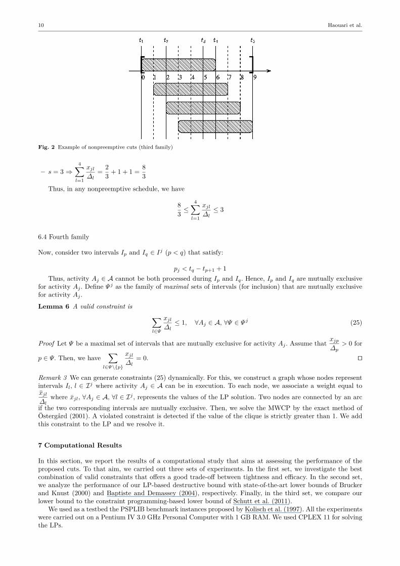
Example 1 Consider an activity Aj ∈ A with pj = 6, rj = 0, and dj = 9. Also, assume that the time intervalsthat overlap with [rj , dj) are the following: I1 = [0, 2), I2 = [2, 5), I3 = [5, 6), and I4 = [6, 9). The set of feasiblestart times is {0, 1, 2, 3}. We see from Figure 2 that:

– s = 0 ⇒4∑l=1

xjl∆l

= 1 + 1 + 1 = 3

– s = 1 ⇒4∑l=1

xjl∆l

= 12 + 1 + 1 + 1

3 = 176

– s = 2 ⇒4∑l=1

xjl∆l

= 1 + 1 + 23 = 8

3

10 Haouari et al.

Fig. 2 Example of nonpreemptive cuts (third family)

– s = 3 ⇒4∑l=1

xjl∆l

= 23 + 1 + 1 = 8

3

Thus, in any nonpreemptive schedule, we have

83 ≤

4∑l=1

xjl∆l≤ 3

6.4 Fourth family

Now, consider two intervals Ip and Iq ∈ Ij (p < q) that satisfy:

pj < tq − tp+1 + 1Thus, activity Aj ∈ A cannot be both processed during Ip and Iq. Hence, Ip and Iq are mutually exclusive

for activity Aj . Define Ψ j as the family of maximal sets of intervals (for inclusion) that are mutually exclusivefor activity Aj .

Lemma 6 A valid constraint is ∑l∈Ψ

xjl∆l≤ 1, ∀Aj ∈ A, ∀Ψ ∈ Ψ j (25)

Proof Let Ψ be a maximal set of intervals that are mutually exclusive for activity Aj . Assume that xjp∆p

> 0 for

p ∈ Ψ. Then, we have∑

l∈Ψ\{p}

xjl∆l

= 0. ut

Remark 3 We can generate constraints (25) dynamically. For this, we construct a graph whose nodes representintervals Il, l ∈ Ij where activity Aj ∈ A can be in execution. To each node, we associate a weight equal tox̄jl∆l

where x̄jl, ∀Aj ∈ A, ∀l ∈ Ij , represents the values of the LP solution. Two nodes are connected by an arcif the two corresponding intervals are mutually exclusive. Then, we solve the MWCP by the exact method ofÖstergård (2001). A violated constraint is detected if the value of the clique is strictly greater than 1. We addthis constraint to the LP and we resolve it.

7 Computational Results

In this section, we report the results of a computational study that aims at assessing the performance of theproposed cuts. To that aim, we carried out three sets of experiments. In the first set, we investigate the bestcombination of valid constraints that offers a good trade-off between tightness and efficacy. In the second set,we analyze the performance of our LP-based destructive bound with state-of-the-art lower bounds of Bruckerand Knust (2000) and Baptiste and Demassey (2004), respectively. Finally, in the third set, we compare ourlower bound to the constraint programming-based lower bound of Schutt et al. (2011).

We used as a testbed the PSPLIB benchmark instances proposed by Kolisch et al. (1997). All the experimentswere carried out on a Pentium IV 3.0 GHz Personal Computer with 1 GB RAM. We used CPLEX 11 for solvingthe LPs.

A Preemptive Bound for the RCPSP 11

7.1 Performance of the proposed cuts

In this first experiment, we restricted our attention to the 30- and 60-activity instances of PSPLIB (namely, setsKSD30 and KSD60). We only considered nontrivial instances for which the best known upper bound is strictlylarger than the lower bound LBRER yielded by the RER procedure that is described in Haouari et al. (2012).We implemented LBRER as an input for initializing the process (and also for adjusting initial ready times anddeadlines).

In this first phase, we analyzed the performance of the following bounds :– LBRER : the RER-based lower bound.– LB0 : the destructive lower bound based on Formulation LP0 along with the mandatory part constraint

(7), the no idle-time constraint (8) and the precedence-based cut (12).– LB1 : the destructive lower bound based on the formulation that is obtained after appending, in a prepro-

cessing step, 80 clique constraints (16) to the formulation that is used to compute LB0.– LB2 : the destructive lower bound based on the formulation that is obtained after appending the forbidden

activity sets constraints (14, 15 and the dual feasible functions-based constraints 20) to the formulation thatis used to compute LB1.

– LB3 : the destructive lower bound based on the formulation that is obtained after appending the nonpre-emptive constraints (21, 22, 23, 24 and 25) to the formulation that is used to compute LB2. For the sake ofefficiency, Constraints (25) are restricted to the particular (simple) case of pairwise exclusive intervals.

– LB4 : the destructive lower bound based on the formulation that is obtained after appending (on the fly) thefourth family of nonpreemptive cuts as described in Remark 3 to the formulation that is used to computeLB3.

– LB5 : the destructive lower bound based on the formulation that is obtained after appending (on the fly)the clique cuts (16) to the formulation that is used to compute LB3.

– LBall : the destructive lower bound based on the formulation that is obtained after both appending (onthe fly) the fourth family of nonpreemptive cuts as well as the clique cuts to the formulation that is used tocompute LB3.

Remark 4 We performed preliminary experiments that demonstrate that incremental search is faster than di-chotomous search. Thus, for the sake of efficacy, all the aforementioned destructive lower bounds are based onan incremental destructive search strategy.

Tables 2-3 display a summary of the computational results. For each lower bound, we provide: GAP : themean percentage deviation with respect to the best known upper bound, Time: the mean CPU time (in seconds)including the time for generating the cliques, #(LB = UB): number of times where the lower bound is equalto the best known upper bound, #(LB = maxLB) : number of times where the lower bound is maximal,#(LB > LBRER) : number of times where the lower bound outperforms the RER-based bound, and TAD :total absolute deviation from LBRER.

GAP (%) Time(s) #(LB = UB) #(LB = maxLB) #(LB > LBRER) TADLBRER 7.29 1.26 0 71 0 0LB0 7.29 1.28 0 71 0 0LB1 5.58 2.50 4 102 37 188LB2 5.57 2.98 4 103 37 189LB3 5.43 3.96 5 113 43 201LB4 5.43 4.86 5 113 43 201LB5 5.42 4.13 5 114 43 202LBall 5.42 5.03 5 114 43 202

Table 2 Results of the bounds on 114 non trivial KSD30 instances.

GAP (%) Time(s) #(LB = UB) #(LB = maxLB) #(LB > LBRER) TADLBRER 8.06 8.41 0 97 0 0LB0 8.06 8.86 0 97 1 1LB1 7.95 10.50 1 105 10 14LB2 7.95 11.31 1 106 11 15LB3 7.86 20.83 1 116 20 26LB4 7.86 73.65 1 116 20 26LB5 7.85 26.36 1 117 21 27LBall 7.84 83.26 1 118 21 28

Table 3 Results of the bounds on 118 non trivial KSD60 instances.

We observe that all the new proposed bounds both outperform the initial bound LBRER and the simpleLP-based bound LB0. Moreover, the results reveal that the new proposed bounds can be roughly classified into

12 Haouari et al.

two families {LB1, LB2} and {LB3, LB4, LB5, LBall}, where each family includes bounds that exhibit verysimilar performances. Clearly, bounds of the first family are the fastest, while those that belong to the secondfamily exhibit the best quality.

Interestingly, we observe that the best trade-off between efficiency and effectiveness is achieved by LB3.Therefore, in the sequel we shall use this bound as our reference bound.

7.2 Comparison with lower bounds of Brucker and Knust (2000) and Baptiste and Demassey (2004)

In this second experiment, we compare the performance of LB3 with respect to state-of-the-art bounds. Tothat aim, we consider the full set of benchmark instances of the PSPLIB. This testbed includes a total of 2040instances that are partitioned into four subsets: KSD30 (480 instances), KSD60 (480 instances), KSD90 (480instances), and KSD120 (600 instances). These subsets include 30, 60, 90, and 120 activities, respectively.

In Table 4, we display the results of LB3 as well as those provided by Brucker and Knust’s bound (LBBK).Moreover, we included for the set of instances KSD60 the results provided by the bound LBBD that wasproposed by Baptiste and Demassey (2004) (these authors tested their bound only on KSD60). The column’sheadings have the same meanings as those of Tables 2-3. It is noteworthy that the reported CPU times of LBBKwere obtained on a Sun Ultra 2 workstation 167 MHz using CPLEX 4.0 and those of LBBD on a HP OmnibookPentium III running at 720 MHz.

KSD30 KSD60GAP (%) Time(s) #(LB = UB) #(LB = maxLB) GAP (%) Time(s) #(LB = UB) #(LB = maxLB)

LB3 1.29 0.9 371 480 1.93 3.66 363 400LBBK 1.50 0.4 318 - 1.85 5 342 409LBBD - - - - 1.35 86.46 366 465

KSD90 KSD120LB3 1.58 10.97 371 444 3.41 96.57 236 539LBBK 1.62 72 353 436 3.62 355 (*) 214 474(*) Average calculated for 481 instances solved within 1 hour

Table 4 Comparison of the bounds on KSD instances.

Interestingly, we observe that LB3 exhibits an excellent performance both in terms of average gap as well asthe number of times it yields a proven optimal value. Indeed, it consistently exhibits the best performance onall problems sets, but KSD60, where LBBD is the champion bound. Nevertheless, we observe that for this latterproblem class, LBBD yields proven optimal values for 76.25% of the instances, while LB3 is only marginallyoutperformed as it provides proven optimal values for 75.62% of the instances. Notice that we have a "-" in therow LBBK and the column #(LB = maxLB) for KSD30 because the values of LBBK are not available onthis set of instances. Thus, we cannot make a comparison with the values of our lower bound to determine thenumber of times the lower bound is maximal.

Pushing our analysis a step further, we performed a pairwise comparison of the different lower bounds. Theresults are displayed in Table 5.

KSD60 KSD90 KSD120LB3 > LBBK 59 44 126LB3 = LBBK 369 400 413LB3 < LBBK 52 36 61LB3 > LBBD 15 - -LB3 = LBBD 385 - -LB3 < LBBD 80 - -

Table 5 Comparison between LB3, LBBK and LBBD on KSD instances.

Table 5 provides further evidence of the good performance of LB3. In particular, we observe that for 120-activity instances LB3 strictly dominates LBBK for 126 instances, while LBBK outperformed LB3 for only 61instances.

Overall, the computational experiments attest the efficacy of LB3. This performance is further demonstratedby the fact that LB3 provides a maximal lower bound for 1863 instances (91.32%).

To get a more accurate picture of the actual performance of our bound, we refined our analysis by consideringthe Resource Strength (RS) parameter. We briefly recall that RS is a normalized parameter on a 0Ű1 scalethat provides a measure of the tightness of resource constraints. Specifically, RS = 0 means that the resourceconstraints are very tight, while RS = 1 means that the available resource capacity fulfills the maximum activityrequirements when all activities are scheduled at the earliest start time. The sets KSD30, KSD60 and KSD90

A Preemptive Bound for the RCPSP 13

are generated with RS in {0.2, 0.5, 0.7, 1} whereas the set KSD120 is generated with RS in {0.1, 0.2, 0.3, 0.4,0.5}. Smaller the value of RS is, more the resource is constrained. RS value equal to 1 corresponds to instanceswhere the resource constraint plays no role, i.e., the instances are solved using the critical path. We focusedour investigation on KSD90 and KSD120. For KSD90, we found that 36 instances among the 44 instanceswhere LB3 dominates LBBK belong to the subset of tightly resource constrained instances with RS = 0.2.The remaining 8 instances belong to the set where RS is equal to 0.5. In Table 6, we report the percentage ofKSD120 instances where LB3 is greater than (less than or equal to) LBBK .

RS = 0.1 RS = 0.2 RS = 0.3 RS = 0.4 RS = 0.5LB3 > LBBK 31.67 39.17 17.50 11.67 5.00LB3 < LBBK 35.00 10.00 4.17 1.67 0.00LB3 = LBBK 33.33 50.83 78.33 86.67 95.00

Table 6 Resource strength analysis for LB3 vs LBBK on KSD120 instances

From this table, we see that:

– LB3 exhibits the best relative performance with respect to LBBK for RS = 0.2,– The absolute performance of LB3 increases as RS increases. Indeed, we see that LB3 ≥ LBBK for 65% of

the instances with RS = 0.1. On the other hand, LB3 ≥ LBBK for 100% of the instances with RS = 0.5.

7.3 Comparison with the approach of Schutt et al. (2011)

In this third experiment, we compare the performance of LB3 to the procedures that were proposed by Schuttet al. (2011). In this recently published paper, the authors implemented several exact methods that are basedon constraint programming. For all these procedures, the authors set the maximum CPU time to 10 minutes.However, if no proven optimal solution is found within the time limit, then a lower bound is computed using adestructive search procedure that starts from the best known lower bound found on the PSPLIB benchmark.Hence, to make a fair comparison with the approach of Schutt et al. (2011), we used for computing LB3 thissame start trial value for all unsolved instances.

Table 7 provides a pairwise comparison between LB3 and the lower bound of Schutt et al. (2011)(hereafter,denoted by LBCP ).

KSD60 KSD90 KSD120LB3 > LBCP 0 6 47LB3 = LBCP 391 429 453LB3 < LBCP 89 45 100

Table 7 Comparison between LB3 and LBCP on KSD instances.

Looking at Table 7, we see that for most instances (1273 out of 1560) both bounds are equal. On the otherhand, although LBCP often outperforms LB3, we see that LB3 strictly dominates LBCP for 53 instances.

As an indication, we compare the execution times of our lower bound LB3 to the exact methods of Schuttet al. (2011). For this, we look to the fastest procedures, on all instance sizes, among those implemented bySchutt et al. (2011). We note however that the execution times correspond to exact methods. The calculationof the lower bounds by Schutt et al. (2011) is not reported in the following. The authors used a Computer withan Intel Xeon CPU 2Ghz. The codes were written in Mercury using G12 constraint programming platform.

The best procedure of Schutt et al. (2011) on KSD60 has an average execution time of 66.01 seconds against3.66 seconds for our lower bound. On KSD120 instances, our lower bound shows a processing time of 96.57against 324.51 seconds on average for the best procedure of Schutt et al. (2011).

Table 8 displays the results of a detailed pairwise comparison between LB3 and LBCP onKSD120 instanceswith respect to parameter RS.

RS = 0.1 RS = 0.2 RS = 0.3 RS = 0.4 RS = 0.5LB3 > LBCP 5.83 17.50 9.17 5.83 0.83LB3 < LBCP 30.00 20.83 18.33 11.67 2.50LB3 = LBCP 64.17 61.67 72.50 82.50 96.67

Table 8 Resource strength analysis for LB3 vs LBCP on KSD120 instances

14 Haouari et al.

Interestingly, we observe that, similar to what we observed in Table 6, LB3 exhibits the best relativeperformance for RS = 0.2. Also, we see that the absolute performance of LB3 improves as RS increases.Indeed, LB3 is greater or equal to LBCP for 79.17% of the instances where RS = 0.1 and 97.50% of theinstances where RS = 0.5.

It is worth noting that after the present paper was submitted for publication, a novel constraint programming-based lower bound for the RCPSP was proposed by Vilim (2011). Computational results presented by the authoron the subset of 438 instances, show that this new bound is strictly outperformed by our bound for 5 instances(these new improved lower bounds and the corresponding instances are provided in Appendix A), yields a betterbound for 147 instances, and yields a similar bound for 286 instances. However, the author did not provide theCPU time that is required to compute this latter bound.

8 Conclusion

This paper describes a new destructive lower bound for the RCPSP. This bound is based on solving a sequenceof relaxed feasibility RCPSP models. Starting from a basic previously suggested LP model, we proposed severaloriginal valid inequalities that aim at tightening the model representation. These new inequalities are based onprecedence constraints, incompatible activity subsets and nonpreemption constraints. We presented the resultsof an extensive computational study that was carried out on 2040 benchmark instances with up to 120 activitiesand that provides evidence that, despite its deceptive simplicity, the new proposed lower bound exhibits anexcellent performance.

Future research needs to be focused on carrying out a thorough theoretical analysis of the strengths of therelaxations of the models of Mingozzi et al. (1998), Carlier and Néron (2003), Baptiste and Demassey (2004),as well as our model. We hope that our present contribution would stimulate research towards this excitingdirection. Furthermore, a second interesting research avenue is to implement the proposed model, together withseveral enhanced features, within an exact branch-and-bound algorithm for the RCPSP. We would expect thatthe good performance of the proposed valid inequalities would prove to be useful to achieve this goal, but thisrequires further investigation.

References

1. R. Alvarez-Valdés, M. Tamarit (1993). The project scheduling polyhedron: dimension, facets and lifting theorems. EuropeanJournal of Operational Research, 67, 204-220.

2. C. Artigues, S. Demassey, E. Néron (2008). Resource-constrained project scheduling : models, algorithms, extensions andapplications. Wiley.

3. P. Baptiste, S. Demassey (2004). Tight LP bounds for resource constrained project scheduling. OR Spectrum, 26, 251-262.4. P. Baptiste, C. Le Pape, W. Nuijten (1999). Satisfiability tests and time-bound adjustments for cumulative scheduling problems.

Annals of Operations Research, 92, 305-333.5. P. Brucker, S. Knust (2000). A linear programming and constraint propagation-based lower bound for the RCPSP. European

Journal of Operational Research, 127, 355-362.6. J. Carlier, F. Clautiaux, A. Moukrim (2007). New reduction procedures and lower bounds for the two-dimensional bin packing

problem with fixed orientation. Computers & Operations Research, 34, 2223-2250.7. J. Carlier, B. Latapie (1991). Une méthode arborescente pour résoudre les problèmes cumulatifs. RAIRO-RO, 25, 311-340.8. J. Carlier, E. Néron (2000). A new LP-based lower bound for the cumulative scheduling problem. European Journal of Opera-

tional Research, 127, 363-382.9. J. Carlier, E. Néron (2003). On linear lower bounds for the resource constrained project scheduling problem. European Journal

of Operational Research, 149, 314-324.10. N. Christofides, R. Alvarez-Valdes, J. Tamarit (1987). Project scheduling with resource constraints: A branch and bound

approach. European Journal of Operational Research, 29, 262-273.11. E. Demeulemeester, W. Herroelen (2002). Project scheduling: a research handbook, Vol. 49, Kluwer Academic Publisher.12. S. Demassey, C. Artigues, P. Michelon (2005). Constraint-propagation-based cutting planes: An application to the resource-

constrained project scheduling problem. INFORMS Journal on Computing, 17, 52-65.13. J. Erschler, P. Lopez, C. Thuriot (1991). Raisonnement temporel sous contraintes de ressources et problèmes d’ordonnancement.

Revue d’Intelligence Artificielle, 5, 7-32.14. S. Fekete, J. Schepers (1998). New classes of lower bounds for bin-packing problems. Lecture Notes in Computer Science, 1412,

257-270.15. M. Garey and D. Johnson (1979), Computers and Intractability: A Guide to the Theory of NP-completeness. Freeman, New

York.16. M. Haouari, A. Kooli, E. Néron (2012). Enhanced energetic reasoning-based lower bounds for the resource constrained project

scheduling problem. Computers & Operations Research, 39, 1187-1194.17. R. Klein and A. Scholl (1999). Computing lower bounds by destructive improvement: An application to resource-constrained

project scheduling. European Journal of Operational Research, 112, 322-346.18. R. Kolisch, A. Sprecher, A. Drexl (1997). PSPLIB-a project scheduling library. European Journal of Operational Research, 96,

205-216.19. O. Koné, C. Artigues, P. Lopez, M. Mongeau (2011). Event-based milp models for resource-constrained project scheduling

problems. Computers & Operations Research, 38, 3-13.20. A. Lahrichi (1982). Ordonnancements: La notion de parties obligatoires et son application aux problèmes cumulatifs. RAIRO-

RO, 16, 241-262.

A Preemptive Bound for the RCPSP 15

21. A. Mingozzi, V. Maniezzo, S. Ricciardelli, L. Bianco (1998). An exact algorithm for project scheduling with resource constraintsbased on a new mathematical formulation. Management Science, 44, 714-729.

22. R. Möhring, A. Schulz, F. Stork, M. Uetz (2003). Solving project scheduling problems by minimum cut computations. Man-agement Science, 49, 330-350.

23. I. Nabeshima (1973). Algorithms and reliable heuristics programs for multiproject scheduling with resource constraints andrelated parallel scheduling. University of Electro-Communications, Tokyo, Japan.

24. P. Östergård (2001). A new algorithm for the maximum-weight clique problem. Nordic Journal of Computing, 8, 424-436.25. P. Östergård (2002). A fast algorithm for the maximum clique problem. Discrete Applied Mathematics, 120, 197-207.26. A. Pritsker, L. Watters, P. Wolfe (1969). Multi-project scheduling with limited resources: A zero-one programming approach.

Management Science, 16, 93-108.27. A. Schutt, T. Feydy, P. Stuckey, M. Wallace (2011). Explaining the cumulative propagator. Constraints, 16, 250-282.28. J. van den Akker, G. Diepen, J. Hoogeveen (2007). A column generation based destructive lower bound for resource constrained

project scheduling problems. In Proceedings of CPAIOR, 376-390.29. P. Vilim (2011). Timetable Edge Finding Filtering Algorithm for Discrete Cumulative Resources. Integration of AI and OR

Techniques in Constraint Programming for Combinatorial Optimization Problems. Lecture Notes in Computer Science, 6697,230-245.

A New lower bounds

Table 9 lists all the improved lower bounds for the KSD instances of the PSPLIB benchmark.

Instance New valueKSD120_18_8 102KSD120_26_1 155KSD120_39_2 105KSD120_46_8 164KSD120_47_6 128

Table 9 New lower bounds for KSD instances