Analysis of a Cardiac Displacement Signal Recorded with an ...

Analysis of a Cardiac Displacement SignalRecorded with an Ultrasound Vibrometer

Master ThesisBiomedical Engineering and Informatics

Project Group: 18gr10407

Aalborg UniversitySchool of Medicine and Health

Fredrik Bajers Vej 7DK-9220 Aalborg Øst

School of Medicine and HealthFredrik Bajers Vej 7DK-9220 Aalborg Øhttp://smh.aau.dk

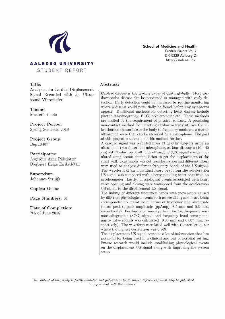
Title:Analysis of a Cardiac DisplacementSignal Recorded with an Ultra-sound Vibrometer

Theme:Master’s thesis

Project Period:Spring Semester 2018

Project Group:18gr10407

Participants:Ásgerður Arna PálsdóttirDagbjört Helga Eiríksdóttir

Supervisor:Johannes Struijk

Copies: Online

Page Numbers: 61

Date of Completion:7th of June 2018

Abstract:

Cardiac disease is the leading cause of death globally. Most car-diovascular disease can be prevented or managed with early de-tection. Early detection could be increased by routine monitoringwhere a disease could potentially be found before any symptomsappear. Traditional methods for detecting heart disease includephotoplethysmography, ECG, accelerometer etc. These methodsare limited by the requirement of physical contact. A promisingnon-contact method for detecting cardiac activity utilizes the vi-brations on the surface of the body to frequency modulate a carrierultrasound wave that can be recorded by a microphone. The goalof this project is to examine this method further.A cardiac signal was recorded from 13 healthy subjects using anultrasound transducer and microphone, at four distances (10 - 40cm) with T-shirt on or off. The ultrasound (US) signal was demod-ulated using arctan demodulation to get the displacement of thechest wall. Continuous wavelet transformation and different filterswere used to analyze different frequency bands of the US signal.The waveform of an individual heart beat from the accelerationUS signal was compared with a corresponding heart beat from anaccelerometer. Lastly, physiological events associated with heartvalve opening and closing were transposed from the accelerationUS signal to the displacement US signal.The linking of different frequency bands with movements causedby different physiological events such as breathing and heart beatscorresponded to literature in terms of frequency and amplitude(mean peak-to-peak amplitude (ppAmp), 3.5 mm and 0.3 mm,respectively). Furthermore, mean ppAmp for low frequency seis-mocardiographic (SCG) signals and frequency band correspond-ing to valve sounds was calculated (0.08 mm and 0.007 mm, re-spectively). The waveform correlated well with the accelerometerwhere the highest correlation was 0.969.The displacement US signal contains a lot of information that haspotential for being used in a clinical and out of hospital setting.Future research would include establishing physiological eventson the displacement US signal along with improving the systemsetup.

The content of this study is freely available, but publication (with source references) must only be publishedin agreement with the authors.

http://smh.aau.dk

PrefaceThis master’s thesis in Biomedical Engineering and Informatics was performed at AalborgUniversity during the period 1st of February - 7th of June. In this project, a novel non-contact method for recording cardiac events was examined. Vibrations on the surface of thechest wall were used to frequency modulate a carrier wave. The signal was demodulated toget the displacement of the chest wall followed by an examination of information in differentfrequency bands. The wavelet of an acceleration US signal was compared with an accelerom-eter, and lastly physiological events were transposed from the acceleration US signal to adisplacement US signal.Sources are referenced using the Vancouver method where the sources are given in chrono-logical order as they are used in the report. The full reference list can be found in the backof the report. References are used in the following fashion throughout the report:

• If the reference is located before a period in the end of a sentence, it refers to thatparticular sentence.

• If the reference is located after a period in the end of a paragraph, it refers to thatparagraph.

• If a reference is referenced by first author name in the beginning of a paragraph, itrefers to the rest of the paragraph unless a new reference is made.

• If a figure does not contain a reference the figure is made from data acquired in thisproject.

We would like to thank our supervisor from Aalborg University, Johannes Struijk for pro-viding the project and great supervision.

Aalborg University, 7th of June 2018

Ásgerður Arna Pálsdóttir<[email protected]>

Dagbjört Helga Eiríksdóttir<[email protected]>

v

Contents

I Problem Specification 1

1 Problem Analysis 31.1 Introduction . . . . . . . . . . . . . . . . . . . . . . . . . . . . . . . . . . . . . 31.2 The Cardiovascular System . . . . . . . . . . . . . . . . . . . . . . . . . . . . 3

1.2.1 The Cardiac Cycle . . . . . . . . . . . . . . . . . . . . . . . . . . . . . 41.2.2 The Atrioventricular and Semilunar Valves . . . . . . . . . . . . . . . 51.2.3 Heart Sounds . . . . . . . . . . . . . . . . . . . . . . . . . . . . . . . . 6

1.3 Diagnostic Techniques . . . . . . . . . . . . . . . . . . . . . . . . . . . . . . . 81.3.1 Auscultation . . . . . . . . . . . . . . . . . . . . . . . . . . . . . . . . 81.3.2 Seismocardiography . . . . . . . . . . . . . . . . . . . . . . . . . . . . 10

1.4 Alternative Techniques . . . . . . . . . . . . . . . . . . . . . . . . . . . . . . . 11

2 Problem Statement 13

II Problem Solution 15

3 Methods 173.1 Theoretical Background . . . . . . . . . . . . . . . . . . . . . . . . . . . . . . 17

3.1.1 Modulation . . . . . . . . . . . . . . . . . . . . . . . . . . . . . . . . . 173.1.2 Demodulation . . . . . . . . . . . . . . . . . . . . . . . . . . . . . . . . 183.1.3 Filtering . . . . . . . . . . . . . . . . . . . . . . . . . . . . . . . . . . . 20

3.2 Data Acquisition . . . . . . . . . . . . . . . . . . . . . . . . . . . . . . . . . . 223.2.1 Equipment Setup . . . . . . . . . . . . . . . . . . . . . . . . . . . . . . 233.2.2 Acquisition Protocol . . . . . . . . . . . . . . . . . . . . . . . . . . . . 23

3.3 Signal Processing and Analysis . . . . . . . . . . . . . . . . . . . . . . . . . . 243.3.1 Signal Processing . . . . . . . . . . . . . . . . . . . . . . . . . . . . . . 253.3.2 Frequency Band Examination . . . . . . . . . . . . . . . . . . . . . . . 273.3.3 Gold Standard Comparison . . . . . . . . . . . . . . . . . . . . . . . . 283.3.4 Locating Physiological Events . . . . . . . . . . . . . . . . . . . . . . . 28

4 Results 294.1 Frequency Band Examination . . . . . . . . . . . . . . . . . . . . . . . . . . . 29

4.1.1 Displacement signal . . . . . . . . . . . . . . . . . . . . . . . . . . . . 294.1.2 Velocity and Acceleration . . . . . . . . . . . . . . . . . . . . . . . . . 40

4.2 Comparison with Accelerometer . . . . . . . . . . . . . . . . . . . . . . . . . . 454.3 Fiducial Points Transposed to Displacement US Signal . . . . . . . . . . . . . 47

III Synthesis 49

5 Discussion 51

6 Conclusion 55

vii

CONTENTS

Bibliography 57

A Carrier Frequency Calculations 61

viii

Part I

Problem Specification

1

Chapter 1Problem Analysis

1.1 IntroductionIt is estimated that every year around 17 million people die from heart disease, making itthe leading cause of death globally [1]. Most cardiovascular diseases can be prevented ormanaged with early detection, which is thus of great benefit, causing the treatment to beeasier, more efficient and economical. Early detection could be increased by routine moni-toring, i.e. measurement of human physiological parameters on a periodic check up (e.g athome), where a disease could possibly be found before any symptoms appear. A lot has beenlearned in the past few years about heart disease, creating a possibility for early detection. [2]

There are many methods for detecting heart disease but the most used ones are in a clinicalsetting, such as auscultation, photoplethysmography (PPG) and electrocardiogram (ECG).Furthermore, some sensors have been developed to detect surface vibrations such as ac-celerometers and laser Doppler. All of these methods provide reliable results when properlyexecuted but are limited in some way, mostly because of the requirement for a physical con-tact. [3, 4, 5]

The drawbacks and limitations of the previous methods, combined with increasing possibil-ities in medical, research and commercial settings has led researchers worldwide to exploreother ways to optimize the measuring process and the possibility of non-contact measuringtechniques [3, 4, 5]. In contributing to the research of newly developed methods, it is im-portant to understand the functionality of the heart, it’s normality and abnormality, alongwith already used and new diagnostic techniques. This chapter will be devoted to deepenthe understanding of this functionality and introduce used and new diagnostic techniques.

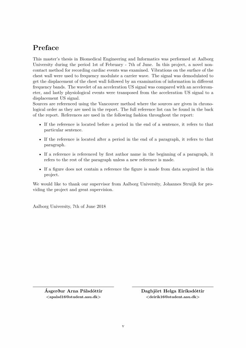
1.2 The Cardiovascular SystemThe cardiovascular system consists of the heart, the blood and the blood vessels. The heartis a hollow organ, located near the midline in the thoracic cavity of the body. It functionsas a pump that pushes the blood through the blood vessels into two closed circulations (thesystemic and pulmonary circulations), allowing an exchange of materials with the cells. Thetwo circulations are arranged in series where deoxygenated blood from the systematic circu-lation is an input to the pulmonary circulation and oxygenated blood from the pulmonarycirculation an input to the systematic circulation. [6, 7]

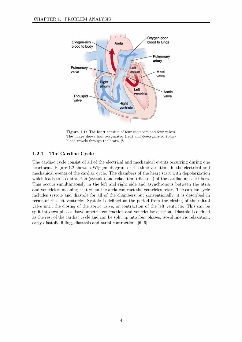
The heart consists of four chambers (left and right atria and ventricles) and four valves, asseen in figure 1.1. The four valves are controlled by pressure changes occurring as the heartcontracts and relaxes. Each valve helps to ensure a one way flow of blood, by opening toallow blood to flow through and then closing to prevent backflow. [6, 7]

3

CHAPTER 1. PROBLEM ANALYSIS

Figure 1.1: The heart consists of four chambers and four valves.The image shows how oxygenated (red) and deoxygenated (blue)blood travels through the heart. [8]

1.2.1 The Cardiac Cycle

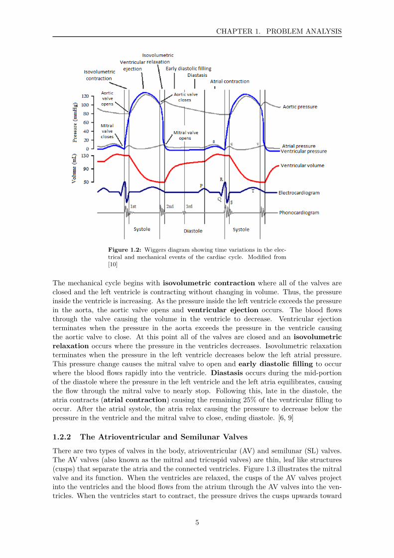
The cardiac cycle consist of all of the electrical and mechanical events occurring during oneheartbeat. Figure 1.2 shows a Wiggers diagram of the time variations in the electrical andmechanical events of the cardiac cycle. The chambers of the heart start with depolarizationwhich leads to a contraction (systole) and relaxation (diastole) of the cardiac muscle fibers.This occurs simultaneously in the left and right side and asynchronous between the atriaand ventricles, meaning that when the atria contract the ventricles relax. The cardiac cycleincludes systole and diastole for all of the chambers but conventionally, it is described interms of the left ventricle. Systole is defined as the period from the closing of the mitralvalve until the closing of the aortic valve, or contraction of the left ventricle. This can besplit into two phases, isovolumetric contraction and ventricular ejection. Diastole is definedas the rest of the cardiac cycle and can be split up into four phases; isovolumetric relaxation,early diastolic filling, diastasis and atrial contraction. [6, 9]

4


Figure 1.2: Wiggers diagram showing time variations in the elec-trical and mechanical events of the cardiac cycle. Modified from[10]

The mechanical cycle begins with isovolumetric contraction where all of the valves areclosed and the left ventricle is contracting without changing in volume. Thus, the pressureinside the ventricle is increasing. As the pressure inside the left ventricle exceeds the pressurein the aorta, the aortic valve opens and ventricular ejection occurs. The blood flowsthrough the valve causing the volume in the ventricle to decrease. Ventricular ejectionterminates when the pressure in the aorta exceeds the pressure in the ventricle causingthe aortic valve to close. At this point all of the valves are closed and an isovolumetricrelaxation occurs where the pressure in the ventricles decreases. Isovolumetric relaxationterminates when the pressure in the left ventricle decreases below the left atrial pressure.This pressure change causes the mitral valve to open and early diastolic filling to occurwhere the blood flows rapidly into the ventricle. Diastasis occurs during the mid-portionof the diastole where the pressure in the left ventricle and the left atria equilibrates, causingthe flow through the mitral valve to nearly stop. Following this, late in the diastole, theatria contracts (atrial contraction) causing the remaining 25% of the ventricular filling tooccur. After the atrial systole, the atria relax causing the pressure to decrease below thepressure in the ventricle and the mitral valve to close, ending diastole. [6, 9]

1.2.2 The Atrioventricular and Semilunar Valves

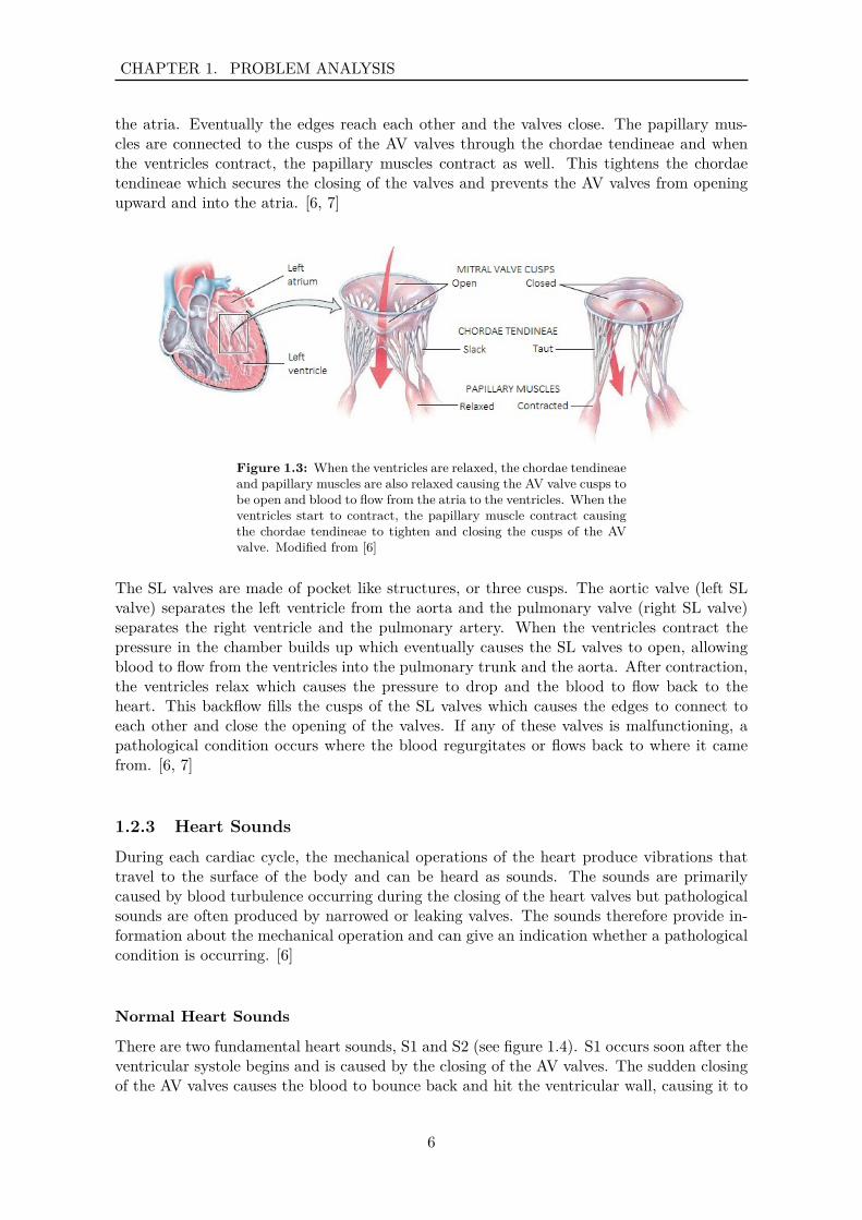
There are two types of valves in the body, atrioventricular (AV) and semilunar (SL) valves.The AV valves (also known as the mitral and tricuspid valves) are thin, leaf like structures(cusps) that separate the atria and the connected ventricles. Figure 1.3 illustrates the mitralvalve and its function. When the ventricles are relaxed, the cusps of the AV valves projectinto the ventricles and the blood flows from the atrium through the AV valves into the ven-tricles. When the ventricles start to contract, the pressure drives the cusps upwards toward

5


the atria. Eventually the edges reach each other and the valves close. The papillary mus-cles are connected to the cusps of the AV valves through the chordae tendineae and whenthe ventricles contract, the papillary muscles contract as well. This tightens the chordaetendineae which secures the closing of the valves and prevents the AV valves from openingupward and into the atria. [6, 7]

Figure 1.3: When the ventricles are relaxed, the chordae tendineaeand papillary muscles are also relaxed causing the AV valve cusps tobe open and blood to flow from the atria to the ventricles. When theventricles start to contract, the papillary muscle contract causingthe chordae tendineae to tighten and closing the cusps of the AVvalve. Modified from [6]

The SL valves are made of pocket like structures, or three cusps. The aortic valve (left SLvalve) separates the left ventricle from the aorta and the pulmonary valve (right SL valve)separates the right ventricle and the pulmonary artery. When the ventricles contract thepressure in the chamber builds up which eventually causes the SL valves to open, allowingblood to flow from the ventricles into the pulmonary trunk and the aorta. After contraction,the ventricles relax which causes the pressure to drop and the blood to flow back to theheart. This backflow fills the cusps of the SL valves which causes the edges to connect toeach other and close the opening of the valves. If any of these valves is malfunctioning, apathological condition occurs where the blood regurgitates or flows back to where it camefrom. [6, 7]

1.2.3 Heart Sounds

During each cardiac cycle, the mechanical operations of the heart produce vibrations thattravel to the surface of the body and can be heard as sounds. The sounds are primarilycaused by blood turbulence occurring during the closing of the heart valves but pathologicalsounds are often produced by narrowed or leaking valves. The sounds therefore provide in-formation about the mechanical operation and can give an indication whether a pathologicalcondition is occurring. [6]

Normal Heart Sounds

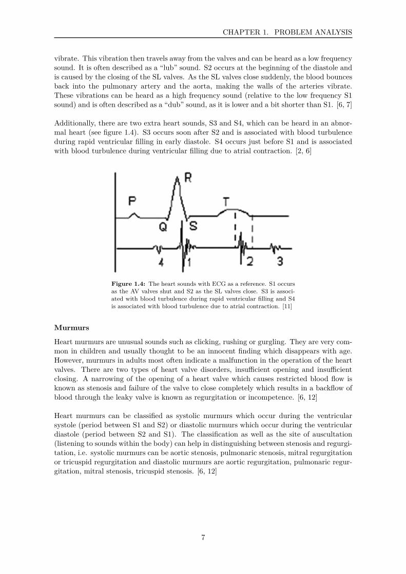
There are two fundamental heart sounds, S1 and S2 (see figure 1.4). S1 occurs soon after theventricular systole begins and is caused by the closing of the AV valves. The sudden closingof the AV valves causes the blood to bounce back and hit the ventricular wall, causing it to

6


vibrate. This vibration then travels away from the valves and can be heard as a low frequencysound. It is often described as a “lub” sound. S2 occurs at the beginning of the diastole andis caused by the closing of the SL valves. As the SL valves close suddenly, the blood bouncesback into the pulmonary artery and the aorta, making the walls of the arteries vibrate.These vibrations can be heard as a high frequency sound (relative to the low frequency S1sound) and is often described as a “dub” sound, as it is lower and a bit shorter than S1. [6, 7]

Additionally, there are two extra heart sounds, S3 and S4, which can be heard in an abnor-mal heart (see figure 1.4). S3 occurs soon after S2 and is associated with blood turbulenceduring rapid ventricular filling in early diastole. S4 occurs just before S1 and is associatedwith blood turbulence during ventricular filling due to atrial contraction. [2, 6]

Figure 1.4: The heart sounds with ECG as a reference. S1 occursas the AV valves shut and S2 as the SL valves close. S3 is associ-ated with blood turbulence during rapid ventricular filling and S4is associated with blood turbulence due to atrial contraction. [11]

Murmurs

Heart murmurs are unusual sounds such as clicking, rushing or gurgling. They are very com-mon in children and usually thought to be an innocent finding which disappears with age.However, murmurs in adults most often indicate a malfunction in the operation of the heartvalves. There are two types of heart valve disorders, insufficient opening and insufficientclosing. A narrowing of the opening of a heart valve which causes restricted blood flow isknown as stenosis and failure of the valve to close completely which results in a backflow ofblood through the leaky valve is known as regurgitation or incompetence. [6, 12]

Heart murmurs can be classified as systolic murmurs which occur during the ventricularsystole (period between S1 and S2) or diastolic murmurs which occur during the ventriculardiastole (period between S2 and S1). The classification as well as the site of auscultation(listening to sounds within the body) can help in distinguishing between stenosis and regurgi-tation, i.e. systolic murmurs can be aortic stenosis, pulmonaric stenosis, mitral regurgitationor tricuspid regurgitation and diastolic murmurs are aortic regurgitation, pulmonaric regur-gitation, mitral stenosis, tricuspid stenosis. [6, 12]

7


1.3 Diagnostic TechniquesAbnormal heart sounds or murmurs are often the first sign of a pathological condition and asin most disease early detection is favorable in giving an easier, more efficient and economicaltreatment [2]. Various measurements can be extracted for diagnostic purposes using differenttools and methods. Measurements including information about for example heart rate (HR)and heart rate variability (HRV) are widely used. [3]Additionally, displacement of the chest wall can give information about the hearts activity.The chest surface mainly moves because of respiratory activity but there are also smallervibrations occurring due to the cardiac activity. The movement of the chest wall caused byrespiratory activity ranges from 4 - 12 mm [13] at a frequency around 0.2 - 0.34 Hz [14].The movement of the chest wall due to cardiac activity ranges from 0.2 - 0.5mm [15] at afrequency around 1 - 1.34 Hz [14]. [16]

Multiple diagnostic tools and methods are available for observing these measurements suchas a stethoscope, seismocardiography, echocardiography and more.

1.3.1 Auscultation

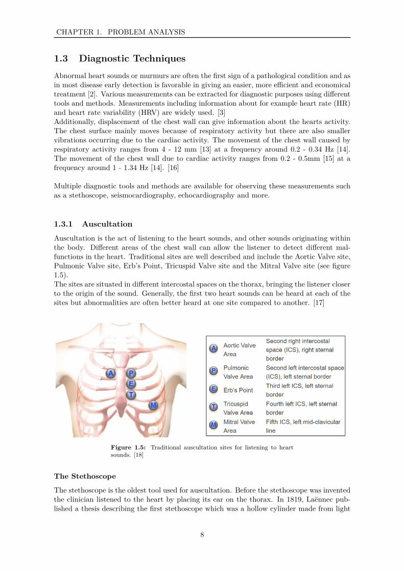
Auscultation is the act of listening to the heart sounds, and other sounds originating withinthe body. Different areas of the chest wall can allow the listener to detect different mal-functions in the heart. Traditional sites are well described and include the Aortic Valve site,Pulmonic Valve site, Erb’s Point, Tricuspid Valve site and the Mitral Valve site (see figure1.5).The sites are situated in different intercostal spaces on the thorax, bringing the listener closerto the origin of the sound. Generally, the first two heart sounds can be heard at each of thesites but abnormalities are often better heard at one site compared to another. [17]

Figure 1.5: Traditional auscultation sites for listening to heartsounds. [18]

The Stethoscope

The stethoscope is the oldest tool used for auscultation. Before the stethoscope was inventedthe clinician listened to the heart by placing its ear on the thorax. In 1819, Laënnec pub-lished a thesis describing the first stethoscope which was a hollow cylinder made from light

8


wood that should be placed on the patients chest, transmitting sound to one ear. [17, 19]Since then, the design of the stethoscope has made great progress with additional featuresas well as more quality and comfort for the user. A stethoscope placed on a patients chestpicks up vibrations at the thorax as pressure waves and directs them through a tube to theclinicians ears, where they are perceived as sound. These sounds usually have rather lowamplitude and can be hard to hear. [17, 20]

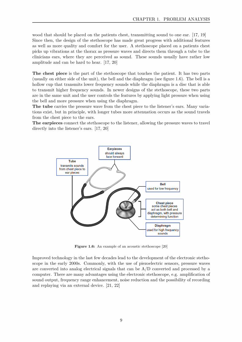
The chest piece is the part of the stethoscope that touches the patient. It has two parts(usually on either side of the unit), the bell and the diaphragm (see figure 1.6). The bell is ahollow cup that transmits lower frequency sounds while the diaphragm is a disc that is ableto transmit higher frequency sounds. In newer designs of the stethoscope, these two partsare in the same unit and the user controls the features by applying light pressure when usingthe bell and more pressure when using the diaphragm.The tube carries the pressure wave from the chest piece to the listener’s ears. Many varia-tions exist, but in principle, with longer tubes more attenuation occurs as the sound travelsfrom the chest piece to the ears.The earpieces connect the stethoscope to the listener, allowing the pressure waves to traveldirectly into the listener’s ears. [17, 20]

Figure 1.6: An example of an acoustic stethoscope [20]

Improved technology in the last few decades lead to the development of the electronic stetho-scope in the early 2000s. Commonly, with the use of piezoelectric sensors, pressure wavesare converted into analog electrical signals that can be A/D converted and processed by acomputer. There are many advantages using the electronic stethoscope, e.g. amplification ofsound output, frequency range enhancement, noise reduction and the possibility of recordingand replaying via an external device. [21, 22]

9


1.3.2 Seismocardiography

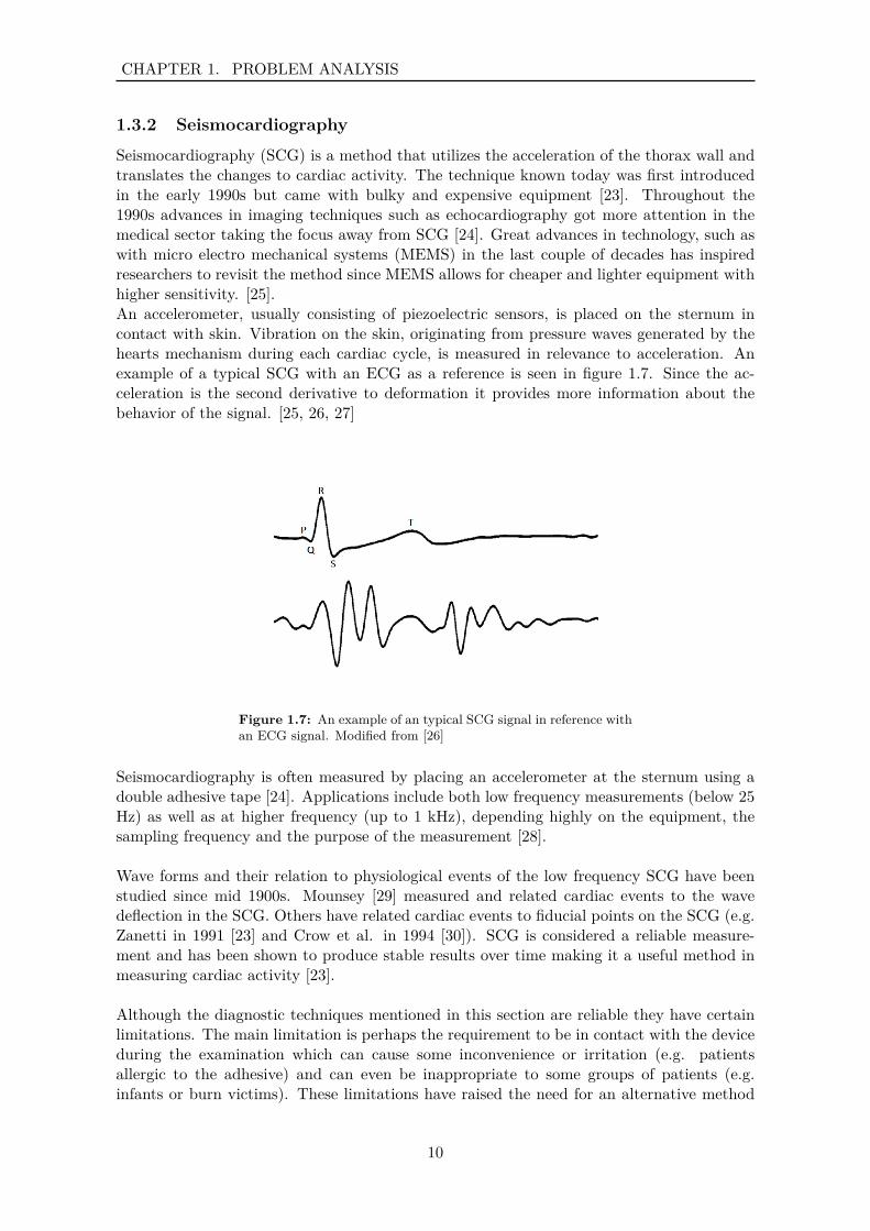
Seismocardiography (SCG) is a method that utilizes the acceleration of the thorax wall andtranslates the changes to cardiac activity. The technique known today was first introducedin the early 1990s but came with bulky and expensive equipment [23]. Throughout the1990s advances in imaging techniques such as echocardiography got more attention in themedical sector taking the focus away from SCG [24]. Great advances in technology, such aswith micro electro mechanical systems (MEMS) in the last couple of decades has inspiredresearchers to revisit the method since MEMS allows for cheaper and lighter equipment withhigher sensitivity. [25].An accelerometer, usually consisting of piezoelectric sensors, is placed on the sternum incontact with skin. Vibration on the skin, originating from pressure waves generated by thehearts mechanism during each cardiac cycle, is measured in relevance to acceleration. Anexample of a typical SCG with an ECG as a reference is seen in figure 1.7. Since the ac-celeration is the second derivative to deformation it provides more information about thebehavior of the signal. [25, 26, 27]

Figure 1.7: An example of an typical SCG signal in reference withan ECG signal. Modified from [26]

Seismocardiography is often measured by placing an accelerometer at the sternum using adouble adhesive tape [24]. Applications include both low frequency measurements (below 25Hz) as well as at higher frequency (up to 1 kHz), depending highly on the equipment, thesampling frequency and the purpose of the measurement [28].

Wave forms and their relation to physiological events of the low frequency SCG have beenstudied since mid 1900s. Mounsey [29] measured and related cardiac events to the wavedeflection in the SCG. Others have related cardiac events to fiducial points on the SCG (e.g.Zanetti in 1991 [23] and Crow et al. in 1994 [30]). SCG is considered a reliable measure-ment and has been shown to produce stable results over time making it a useful method inmeasuring cardiac activity [23].

Although the diagnostic techniques mentioned in this section are reliable they have certainlimitations. The main limitation is perhaps the requirement to be in contact with the deviceduring the examination which can cause some inconvenience or irritation (e.g. patientsallergic to the adhesive) and can even be inappropriate to some groups of patients (e.g.infants or burn victims). These limitations have raised the need for an alternative method

10


where contact is not needed and has led researchers throughout the world to examine othermethods [4, 31, 32].

1.4 Alternative TechniquesMultiple non-contact methods have been examined as an alternative to the more conven-tional contact methods. Most of the newest and most promising methods for measuring HRand HRV are based on the vibrations on the surface of the body during the cardiac cycle.Periodic movements caused by the pumping of blood from the heart are reflected at thesubjects surface and can give information, e.g. about the cardiac cycle frequency. Thesemovements can be detected by utilizing sensors of adequate resolution which typically workon the principle of the Doppler effect and sense waves that reflect (echo) as a result of activetransmission. [3, 4]

In 2014, Kranjec et al [4] performed a feasibility study where four promising non-contacttechniques were examined at different distances from the surface of the body and comparedto a reference ECG. The experiment was carried out simultaneously for all techniques, wherethe heart rate was measured using 6 different methods (lead I ECG (as a reference), CCECG,microwave radar, Ultrasound (US) radar, audio signal microphone and headphone audio con-tact method). The results showed that all of the methods were feasible. Furthermore, thesignal to noise ratio (SNR) was calculated where the microwave radar showed the best resultsfor distances below 10 cm and the US radar for distances above 10 cm.

The microwave and ultrasound measurement techniques are both based on the Doppler ef-fect and the principle of radar; a device sensing continuous electromagnetic or sound waves.The frequencies and output power are directly linked to the sensitivity of the system wherehigher quantities result in more sensitivity to small displacements occuring on the chestwall. Although these two methods work on the same principle, there are differences. USemitting sensors send out high frequency sound waves which need a medium to propagatethrough while microwave emitting sensors are based on electromagnetic waves propagatingat a higher speed than the US. [4, 5]

In 2017, Kranjec et al [5] followed up with his former study and performed a feasibility studywith proof of concept of an assembled non-contact HRV measuring device. This was done inan laboratory setting with healthy subjects and in a clinical environment with pathologicalsubjects. The measuring device was based on US radar where the jugular vein was mea-sured. They demonstrated that this method has great potential but that further researchand improvement is needed. Some of the factors that can be considered for improvementof their system were e.g. an inconvenient position of the patient, robustness of the system etc.

More studies have been conducted in investigating a similar method. Shirkovskiy et al [31]designed an ultrasonic diagnostic tool based on this method where 32 ultrasound transducerson 3 different panels were used to obtain a 3D seismocardiographic images of the thorax andabdomen. Jeger-Madiot et al [32] presented his method in 2017 where an ultrasound pulsewave was reflected off an elliptical acoustic mirror to get a focus point on the surface of thebody. They also showed that this method works through clothing.

These studies have shown that it is feasible to detect cardiac activity with this technique.This could be a valuable tool in clinical settings along with out-of-hospital use, lowering thetime and effort of cardiac activity recording. Furthermore, it could be of benefit in other

11


fields and applications, e.g. psycho-physiological studies of different groups of subjects (ath-letes, drivers or rehabilitation patients) [4].

The limitations these studies have in common is that the bandwidth of the system is verylimited and that there is not very much known about the information present in the receiveddisplacement signal. Furthermore, the knowledge of how that information translates tophysiological events is lacking. Apart from Shirkovskiy et al. [31], most of the studies useECG or laser-doppler as a validation method but wavelet comparison with known methodshas yet to happen. All of the previous studies commonly state that it needs more investigationon what potential and information it can contribute.

12

Chapter 2Problem Statement

What information do different frequency bands of a contactlessultrasound cardio-vibrometer signal contain in terms ofbreathing, heart rate and valve sounds; and how does itcompare with current seismocardiographic methods?

Based on this problem statement the following goals were set:

• Record contactless ultrasound cardio-vibrometer signals from different distances, withand without clothing.

• Obtain a baseband signal representing the displacement of the chest wall.

• Extract information from the displacement signal and interpret it with respect to phys-iological events in the cardiac cycle.

• Examine what effect different distances have on the signal’s quality and what effectclothing has on the signal’s quality.

• Examine how the obtained seismocardiographic waveform correlates with an accelerom-eter.

13

CHAPTER 2. PROBLEM STATEMENT

14

Part II

Problem Solution

15

Chapter 3MethodsAn experiment was performed to examine the information found in ultrasound vibrometersignals, which was encoded in a frequency modulated wave that had been reflected of asubject’s surface. This chapter describes the method used in this project, starting witha theoretical background (section 3.1), followed by a description of the data acquisitionprocedure (section 3.2) and finally a description of the signal processing done in analyzingthe signal (section 3.3).

3.1 Theoretical BackgroundThis section describes the theory used in the experimental part of this project. First thetheory behind modulating a signal is described, followed by an explanation of demodulation.Lastly, filters and filter design is explained.

3.1.1 Modulation

Modulation is a common method used in telecommunications and signal processing to trans-mit a baseband signal via a carrier wave with a fixed amplitude or frequency. There aremany ways to modulate a signal but in principle an analog signal can be modulated in termsof its amplitude, frequency or phase. [33]

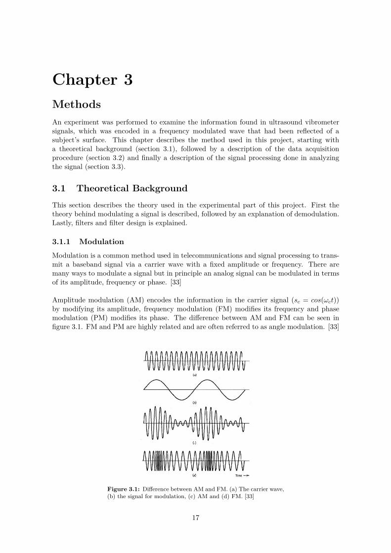
Amplitude modulation (AM) encodes the information in the carrier signal (sc = cos(ωct))by modifying its amplitude, frequency modulation (FM) modifies its frequency and phasemodulation (PM) modifies its phase. The difference between AM and FM can be seen infigure 3.1. FM and PM are highly related and are often referred to as angle modulation. [33]

Figure 3.1: Difference between AM and FM. (a) The carrier wave,(b) the signal for modulation, (c) AM and (d) FM. [33]

17

CHAPTER 3. METHODS

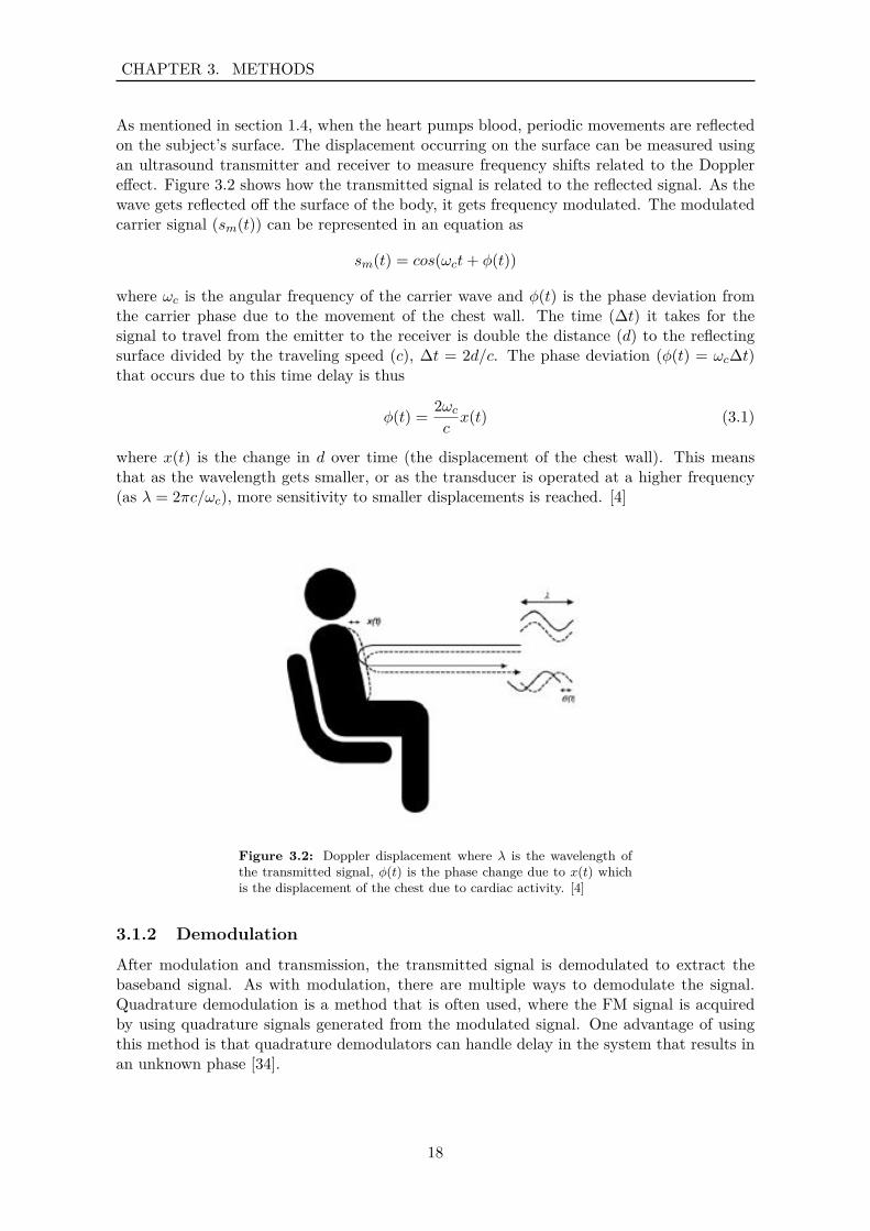
As mentioned in section 1.4, when the heart pumps blood, periodic movements are reflectedon the subject’s surface. The displacement occurring on the surface can be measured usingan ultrasound transmitter and receiver to measure frequency shifts related to the Dopplereffect. Figure 3.2 shows how the transmitted signal is related to the reflected signal. As thewave gets reflected off the surface of the body, it gets frequency modulated. The modulatedcarrier signal (sm(t)) can be represented in an equation as

sm(t) = cos(ωct+ φ(t))

where ωc is the angular frequency of the carrier wave and φ(t) is the phase deviation fromthe carrier phase due to the movement of the chest wall. The time (∆t) it takes for thesignal to travel from the emitter to the receiver is double the distance (d) to the reflectingsurface divided by the traveling speed (c), ∆t = 2d/c. The phase deviation (φ(t) = ωc∆t)that occurs due to this time delay is thus

φ(t) = 2ωc

cx(t) (3.1)

where x(t) is the change in d over time (the displacement of the chest wall). This meansthat as the wavelength gets smaller, or as the transducer is operated at a higher frequency(as λ = 2πc/ωc), more sensitivity to smaller displacements is reached. [4]

Figure 3.2: Doppler displacement where λ is the wavelength ofthe transmitted signal, φ(t) is the phase change due to x(t) whichis the displacement of the chest due to cardiac activity. [4]

3.1.2 Demodulation

After modulation and transmission, the transmitted signal is demodulated to extract thebaseband signal. As with modulation, there are multiple ways to demodulate the signal.Quadrature demodulation is a method that is often used, where the FM signal is acquiredby using quadrature signals generated from the modulated signal. One advantage of usingthis method is that quadrature demodulators can handle delay in the system that results inan unknown phase [34].

18

CHAPTER 3. METHODS

Quadrature Demodulation

A carrier signal which has been modulated, i.e. by reflecting off a subjects chest, representedby sm(t) can be written in the form

sm(t) = A(t)cos(2πfct+ φ(t)

)(3.2)

where A(t) is the amplitude of the signal, fc is the frequency of the carrier wave and φ(t)is the phase deviation from the instantaneous phase 2πfct (i.e. due to the movement of thechest wall). In an ideal case of an FM signal, A(t) is a constant. The phase deviation, φ(t),can be written in relation to the deviation in frequency as 2πf∆t. [33, 35]

A complex envelope of the modulated signal can be generated and represented in a rectan-gular form as

s̃m(t) = I(t) + jQ(t) (3.3)

The complex envelope, including the low pass in-phase (I) and quadrature (Q) components,contains all of the information found in the baseband signal. [33, 35]

In practise, I and Q components are obtained by multiplying xm(t) with sinusoids thathave the same frequency as the carrier wave. As stated in equation 3.4, sI(t) (containingthe I component and the carrier wave) is acquired by multiplying xm(t) with a sinusoidand, according to equation 3.5, sQ(t) (containing the Q component and the carrier wave) isacquired by multiplying xm(t) with a sinusoid which is phase shifted by 90 degrees from theprevious sinusoid (cosine and sinus).

sI(t) = xm(t) ∗ cos(2πfct) (3.4)

sQ(t) = xm(t) ∗ sin(2πfct) (3.5)

The heterodyne principle states that two sinusoidal signals of two different frequencies whichare mixed, can be written as the sum of two sinusoids where the frequencies are the sum anddifference of the original frequencies [34]. It is based on the trigonometric identities:

cos(θ1)cos(θ2) = 12cos(θ1 − θ2) + 1

2cos(θ1 + θ2)

cos(θ1)sin(θ2) = 12sin(θ1 + θ2) − 1

2sin(θ1 − θ2)

Utilizing this, the following can be derived:

sI(t) = 12A(t)

(cos(2π(2fc + f∆)t

)+ cos

(2πf∆t

))(3.6)

sQ(t) = 12A(t)

(sin(2πf∆t

)+ sin

(2π(2fc + f∆)t

))(3.7)

It is assumed that the carrier frequency is much higher than the deviation frequency, and asseen from equations 3.6 and 3.7 the carrier wave can easily be filtered out using a low passfilter, leaving only the frequency component related to the displacement of the chest wall.[33, 35]

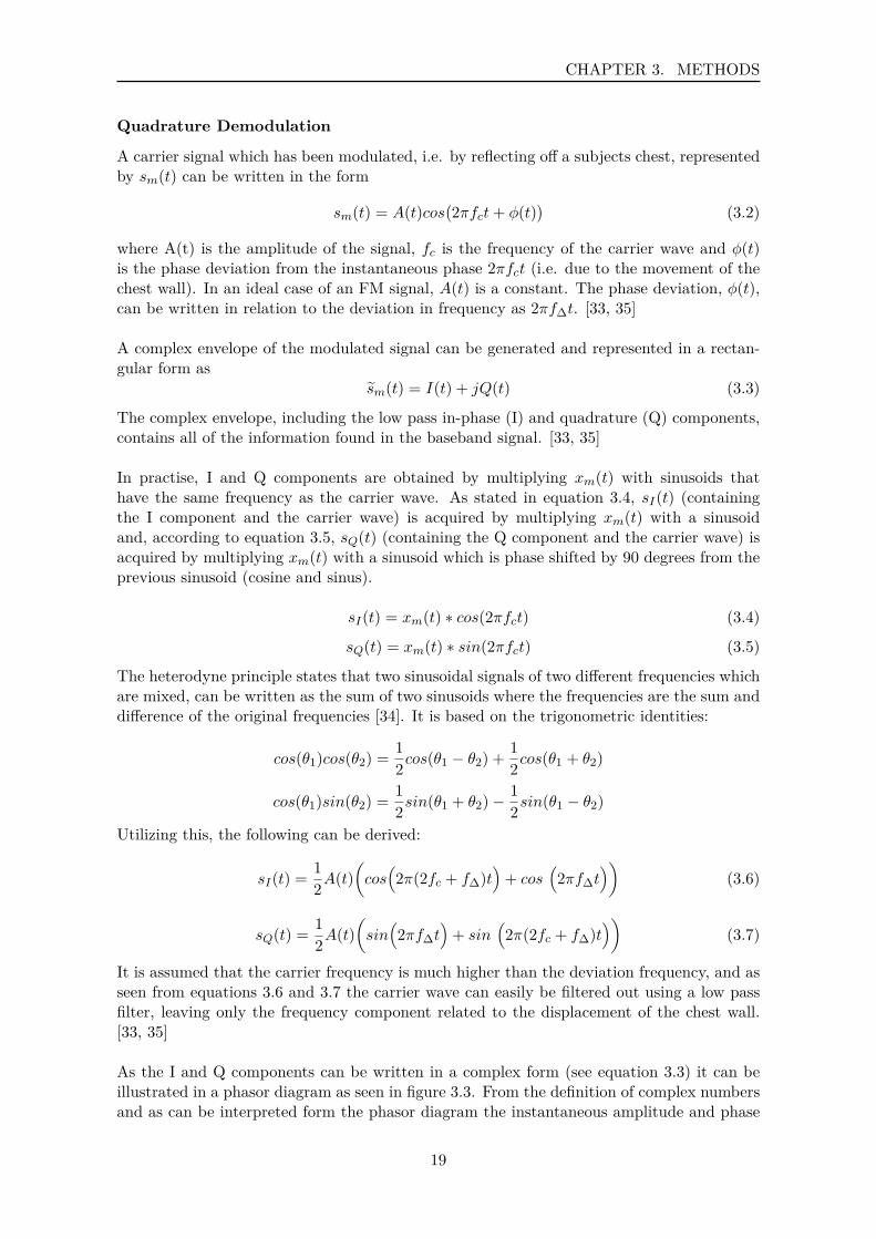
As the I and Q components can be written in a complex form (see equation 3.3) it can beillustrated in a phasor diagram as seen in figure 3.3. From the definition of complex numbersand as can be interpreted form the phasor diagram the instantaneous amplitude and phase

19

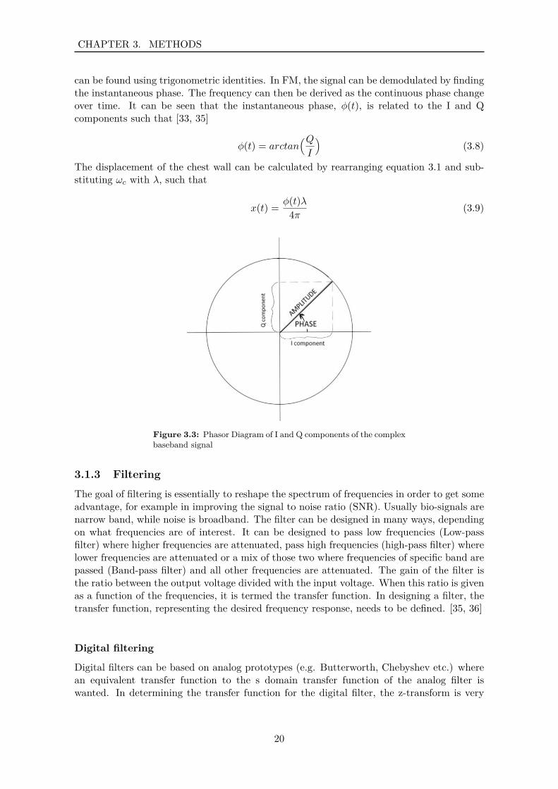
CHAPTER 3. METHODS

can be found using trigonometric identities. In FM, the signal can be demodulated by findingthe instantaneous phase. The frequency can then be derived as the continuous phase changeover time. It can be seen that the instantaneous phase, φ(t), is related to the I and Qcomponents such that [33, 35]

φ(t) = arctan(QI

)(3.8)

The displacement of the chest wall can be calculated by rearranging equation 3.1 and sub-stituting ωc with λ, such that

x(t) = φ(t)λ4π (3.9)

Figure 3.3: Phasor Diagram of I and Q components of the complexbaseband signal

3.1.3 Filtering

The goal of filtering is essentially to reshape the spectrum of frequencies in order to get someadvantage, for example in improving the signal to noise ratio (SNR). Usually bio-signals arenarrow band, while noise is broadband. The filter can be designed in many ways, dependingon what frequencies are of interest. It can be designed to pass low frequencies (Low-passfilter) where higher frequencies are attenuated, pass high frequencies (high-pass filter) wherelower frequencies are attenuated or a mix of those two where frequencies of specific band arepassed (Band-pass filter) and all other frequencies are attenuated. The gain of the filter isthe ratio between the output voltage divided with the input voltage. When this ratio is givenas a function of the frequencies, it is termed the transfer function. In designing a filter, thetransfer function, representing the desired frequency response, needs to be defined. [35, 36]

Digital filtering

Digital filters can be based on analog prototypes (e.g. Butterworth, Chebyshev etc.) wherean equivalent transfer function to the s domain transfer function of the analog filter iswanted. In determining the transfer function for the digital filter, the z-transform is very

20

CHAPTER 3. METHODS

useful because of its ability to define the digital equivalent of a transfer function. The digitaltransfer function is defined as

H(z) = Y (z)X(z)

where Y(z) is the output and X(z) is the input. [35, 36]The transfer function can be written in the form of a polynomials of z:

H(z) = b0 + b1z−1 + b2z

−2 + ...+ bNz−N

1 + a1z−1 + a2z−2 + ...+ aDz−D

From these two equations (assuming that a0 = 1), the relationship between the output givenany input can be determined as

Y (z)X(z) =

∑N−1k=0 bkz

−n∑D−1l=0 alz−n

By multiplying and transforming this equation, the output in time domain can be writtenas

y[n] =K∑

k=0bkx[n− k] −

L∑l=1

aly[n− l]

The designing of an appropriate filter is simply determining the a and b coefficients suchthat the desired spectrum is acquired. The frequency response can be found by Fouriertransforming the transfer function (H(jω)). [35, 36]The order of the filter, or the complexity of the filter, is determined by the number of poles(coefficients in the denominator) in the transfer function. As the order of the filter increasesthe slope of the filters transition from pass-band to attenuation increases, approaching anideal filter. However, approaching an ideal filter can cause a problem as the impulse responsemight become useless, causing a lot of ringing in the signal in time domain. A magnituderesponse of an ideal filter is seen in figure 3.4. The initial sharpness of the filter can beincreased without increasing the order of the filter but by doing so, some unevenness orripple will be present in the passband. In designing the filter, the order of the numerator(b-coefficients) must be equal or higher than the order of the denominator (a-coefficients) inorder for the filter to be stable. [35, 36]

FIR and IIR

Filters can be separated into two groups according to their approach in reshaping the spec-trum. These groups are finite impulse response (FIR) and infinite impulse response (IIR)filters. [35, 36]The transfer function of FIR filters only include a numerator, meaning there are no a co-efficients which operate on past values of the output. Thus, FIR filters only use the valueof the input. The main advantage of FIR filers is that they are always stable (the order ofthe numerator is always higher than the order of the denominator) and have a linear phaseshift. [35, 36]The transfer function of IIR filters contain both a numerator and a denominator, meaningthat the filter operates both on input values and past values of the output. [35, 36]The advantage of choosing IIR filters over FIR filter, is that they usually require a muchlower filter order in meeting a specific frequency criterion, and are more efficient in terms ofcomputation time and memory. [35, 36]

21

CHAPTER 3. METHODS

In each group of filters (FIR and IIR), there are multiple designs. IIR filters are usuallybased on analog prototypes (e.g. Butterworth, Chebyshev etc.) although several computeraided designs have been developed. On the other hand, FIR filters are usually developedwithout an analog prototype. [35, 36]

Butterworth

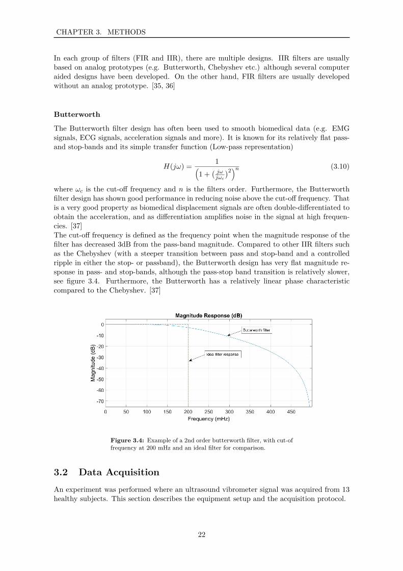
The Butterworth filter design has often been used to smooth biomedical data (e.g. EMGsignals, ECG signals, acceleration signals and more). It is known for its relatively flat pass-and stop-bands and its simple transfer function (Low-pass representation)

H(jω) = 1(1 +

( jωjωc

)2)n (3.10)

where ωc is the cut-off frequency and n is the filters order. Furthermore, the Butterworthfilter design has shown good performance in reducing noise above the cut-off frequency. Thatis a very good property as biomedical displacement signals are often double-differentiated toobtain the acceleration, and as differentiation amplifies noise in the signal at high frequen-cies. [37]The cut-off frequency is defined as the frequency point when the magnitude response of thefilter has decreased 3dB from the pass-band magnitude. Compared to other IIR filters suchas the Chebyshev (with a steeper transition between pass and stop-band and a controlledripple in either the stop- or passband), the Butterworth design has very flat magnitude re-sponse in pass- and stop-bands, although the pass-stop band transition is relatively slower,see figure 3.4. Furthermore, the Butterworth has a relatively linear phase characteristiccompared to the Chebyshev. [37]

Figure 3.4: Example of a 2nd order butterworth filter, with cut-offrequency at 200 mHz and an ideal filter for comparison.

3.2 Data AcquisitionAn experiment was performed where an ultrasound vibrometer signal was acquired from 13healthy subjects. This section describes the equipment setup and the acquisition protocol.

22

CHAPTER 3. METHODS

3.2.1 Equipment Setup

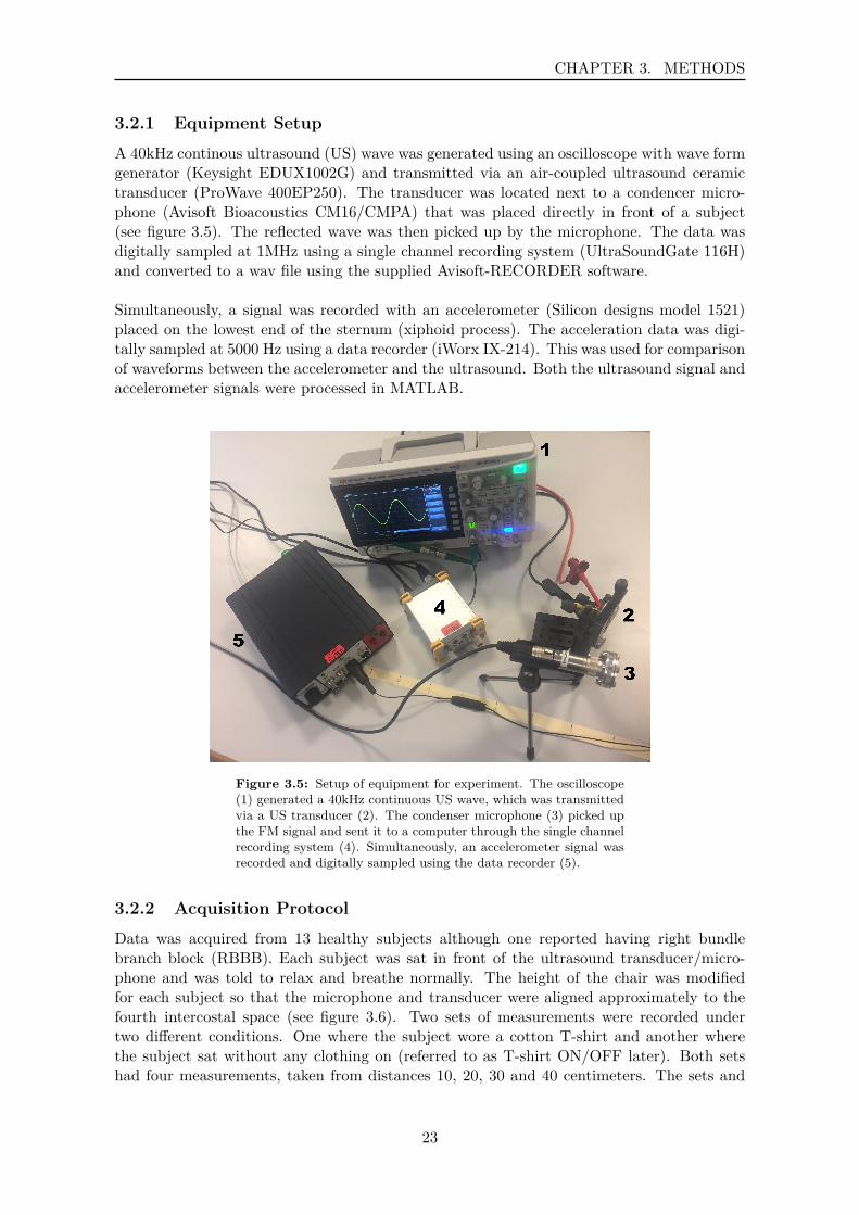
A 40kHz continous ultrasound (US) wave was generated using an oscilloscope with wave formgenerator (Keysight EDUX1002G) and transmitted via an air-coupled ultrasound ceramictransducer (ProWave 400EP250). The transducer was located next to a condencer micro-phone (Avisoft Bioacoustics CM16/CMPA) that was placed directly in front of a subject(see figure 3.5). The reflected wave was then picked up by the microphone. The data wasdigitally sampled at 1MHz using a single channel recording system (UltraSoundGate 116H)and converted to a wav file using the supplied Avisoft-RECORDER software.

Simultaneously, a signal was recorded with an accelerometer (Silicon designs model 1521)placed on the lowest end of the sternum (xiphoid process). The acceleration data was digi-tally sampled at 5000 Hz using a data recorder (iWorx IX-214). This was used for comparisonof waveforms between the accelerometer and the ultrasound. Both the ultrasound signal andaccelerometer signals were processed in MATLAB.

Figure 3.5: Setup of equipment for experiment. The oscilloscope(1) generated a 40kHz continuous US wave, which was transmittedvia a US transducer (2). The condenser microphone (3) picked upthe FM signal and sent it to a computer through the single channelrecording system (4). Simultaneously, an accelerometer signal wasrecorded and digitally sampled using the data recorder (5).

3.2.2 Acquisition Protocol

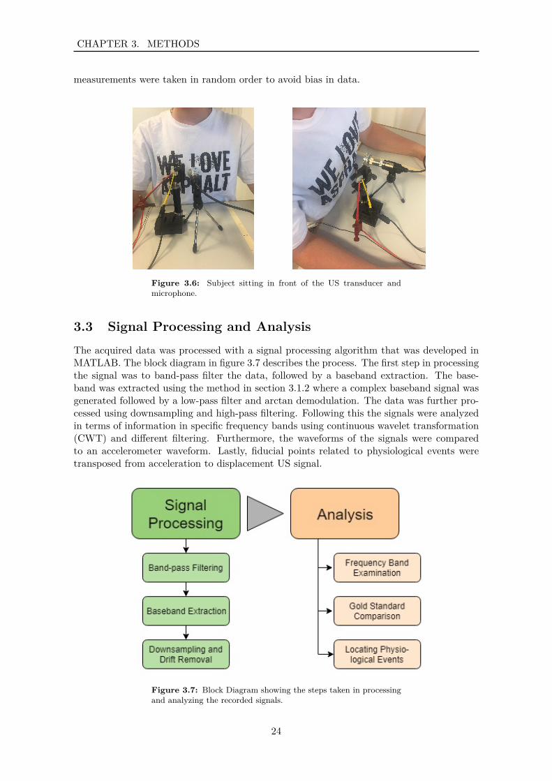
Data was acquired from 13 healthy subjects although one reported having right bundlebranch block (RBBB). Each subject was sat in front of the ultrasound transducer/micro-phone and was told to relax and breathe normally. The height of the chair was modifiedfor each subject so that the microphone and transducer were aligned approximately to thefourth intercostal space (see figure 3.6). Two sets of measurements were recorded undertwo different conditions. One where the subject wore a cotton T-shirt and another wherethe subject sat without any clothing on (referred to as T-shirt ON/OFF later). Both setshad four measurements, taken from distances 10, 20, 30 and 40 centimeters. The sets and

23

CHAPTER 3. METHODS

measurements were taken in random order to avoid bias in data.

Figure 3.6: Subject sitting in front of the US transducer andmicrophone.

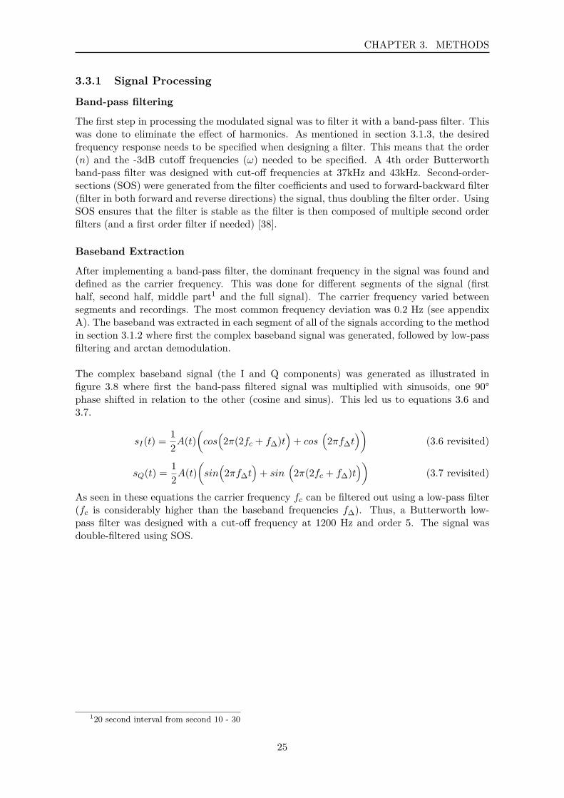
3.3 Signal Processing and AnalysisThe acquired data was processed with a signal processing algorithm that was developed inMATLAB. The block diagram in figure 3.7 describes the process. The first step in processingthe signal was to band-pass filter the data, followed by a baseband extraction. The base-band was extracted using the method in section 3.1.2 where a complex baseband signal wasgenerated followed by a low-pass filter and arctan demodulation. The data was further pro-cessed using downsampling and high-pass filtering. Following this the signals were analyzedin terms of information in specific frequency bands using continuous wavelet transformation(CWT) and different filtering. Furthermore, the waveforms of the signals were comparedto an accelerometer waveform. Lastly, fiducial points related to physiological events weretransposed from acceleration to displacement US signal.

Figure 3.7: Block Diagram showing the steps taken in processingand analyzing the recorded signals.

24

CHAPTER 3. METHODS

3.3.1 Signal Processing

Band-pass filtering

The first step in processing the modulated signal was to filter it with a band-pass filter. Thiswas done to eliminate the effect of harmonics. As mentioned in section 3.1.3, the desiredfrequency response needs to be specified when designing a filter. This means that the order(n) and the -3dB cutoff frequencies (ω) needed to be specified. A 4th order Butterworthband-pass filter was designed with cut-off frequencies at 37kHz and 43kHz. Second-order-sections (SOS) were generated from the filter coefficients and used to forward-backward filter(filter in both forward and reverse directions) the signal, thus doubling the filter order. UsingSOS ensures that the filter is stable as the filter is then composed of multiple second orderfilters (and a first order filter if needed) [38].

Baseband Extraction

After implementing a band-pass filter, the dominant frequency in the signal was found anddefined as the carrier frequency. This was done for different segments of the signal (firsthalf, second half, middle part1 and the full signal). The carrier frequency varied betweensegments and recordings. The most common frequency deviation was 0.2 Hz (see appendixA). The baseband was extracted in each segment of all of the signals according to the methodin section 3.1.2 where first the complex baseband signal was generated, followed by low-passfiltering and arctan demodulation.

The complex baseband signal (the I and Q components) was generated as illustrated infigure 3.8 where first the band-pass filtered signal was multiplied with sinusoids, one 90°phase shifted in relation to the other (cosine and sinus). This led us to equations 3.6 and3.7.

sI(t) = 12A(t)

(cos(2π(2fc + f∆)t

)+ cos

(2πf∆t

))(3.6 revisited)

sQ(t) = 12A(t)

(sin(2πf∆t

)+ sin

(2π(2fc + f∆)t

))(3.7 revisited)

As seen in these equations the carrier frequency fc can be filtered out using a low-pass filter(fc is considerably higher than the baseband frequencies f∆). Thus, a Butterworth low-pass filter was designed with a cut-off frequency at 1200 Hz and order 5. The signal wasdouble-filtered using SOS.

120 second interval from second 10 - 30

25

CHAPTER 3. METHODS

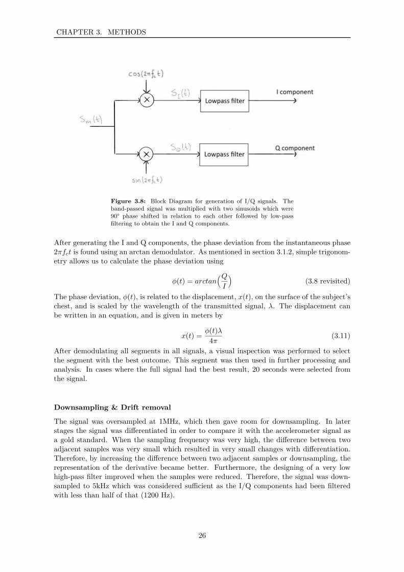
Figure 3.8: Block Diagram for generation of I/Q signals. Theband-passed signal was multiplied with two sinusoids which were90° phase shifted in relation to each other followed by low-passfiltering to obtain the I and Q components.

After generating the I and Q components, the phase deviation from the instantaneous phase2πfct is found using an arctan demodulator. As mentioned in section 3.1.2, simple trigonom-etry allows us to calculate the phase deviation using

φ(t) = arctan(QI

)(3.8 revisited)

The phase deviation, φ(t), is related to the displacement, x(t), on the surface of the subject’schest, and is scaled by the wavelength of the transmitted signal, λ. The displacement canbe written in an equation, and is given in meters by

x(t) = φ(t)λ4π (3.11)

After demodulating all segments in all signals, a visual inspection was performed to selectthe segment with the best outcome. This segment was then used in further processing andanalysis. In cases where the full signal had the best result, 20 seconds were selected fromthe signal.

Downsampling & Drift removal

The signal was oversampled at 1MHz, which then gave room for downsampling. In laterstages the signal was differentiated in order to compare it with the accelerometer signal asa gold standard. When the sampling frequency was very high, the difference between twoadjacent samples was very small which resulted in very small changes with differentiation.Therefore, by increasing the difference between two adjacent samples or downsampling, therepresentation of the derivative became better. Furthermore, the designing of a very lowhigh-pass filter improved when the samples were reduced. Therefore, the signal was down-sampled to 5kHz which was considered sufficient as the I/Q components had been filteredwith less than half of that (1200 Hz).

26

CHAPTER 3. METHODS

After phase extraction and downsampling, the data contained a drift which was eliminatedusing a very low high pass filter. A Butterworth high-pass filter was designed with a cut-offfrequency at 0.1 Hz and order 3. The signal was double-filtered using SOS.

3.3.2 Frequency Band Examination

For analysis of the signal, continuous wavelet transformation (CWT) was visualized on amagnitude scaleogram. Various high- and low-pass filters (see table 3.1) were designed basedon energy distribution and/or interesting frequency bands in the signal. The filters wherethen used to either extracted these areas from the signal for analysis or to filter them out ofthe signal that was then analyzed further. All filters were Butterworth design and appliedwith forward-backward filtering using SOS.

Filter Name Filter Type Wn [Hz] Filter OrderLP0.5 Low-pass 0.5 3LP1.5 Low-pass 1.5 5LP25 Low-pass 25 4LP86 Low-pass 86 7LPsub Low-pass subject dependant 4HP0.1 High-pass 0.1 5HP0.5 High-pass 0.5 3HP0.6 High-pass 0.6 5HP3 High-pass 3 5HP25 High-pass 25 4

Table 3.1: Filters used for frequency band examination. All filterswere Butterworth design and applied forward-backward, doublingthe order presented here.

Information found in four different frequency bands (0.1-0.5 Hz, 0.6-3 Hz, 3-25 Hz and 25-86Hz) of the signals were investigated in terms of amplitude. Average peak to peak amplitudein each signal was calculated by locating peaks in the signal associated to cardiac activity andfinding their mean. The average peak to peak amplitude was then analyzed using a linearmixed model with distance and T-shirt ON/OFF as fixed factors. A subject specific randomintercept was included in the model. P values < 0.05 were considered significant. In case ofan interaction, multiple comparisons with Bonferroni corrections were performed. This wasdone separately for each frequency band. Analysis of the studentized residuals of raw datashowed that assumption for normal distribution was violated (Shapiro-Wilk test, p < 0.05).Therefore, log transformation was applied to obtain normal distribution. Data is reportedas mean ± standard error. Three signals were excluded from the statistical comparison astheir mean peak to peak amplitude was largely influenced by demodulation errors and thusnot representing the true amplitude of the baseband signal.

In assessing the noise floor in the signal, fourier analysis was performed on the raw signal,for all distances as well as T-shirt ON/OFF.

27

CHAPTER 3. METHODS

3.3.3 Gold Standard Comparison

For the purpose of comparing the ultrasound vibrometer signal with the accelerometer, thesignal was double differentiated. Both the ultrasound vibrometer and accelerometer signalswere filtered using a low-pass and a high-pass filter to secure same frequency band-widthbetween the signals. Filters HP3 and LP25 were used. Both of the signals were forward-backward filtered using SOS.The US vibrometer and accelerometer signals were taken simultaneously although some delaywas introduced to the signals because of the software used and human variability. In order tocompare the waves of the signals, one heart beat was manually selected in each vibrometersignal (for each distance and T-shirt ON/OFF) and the corresponding heart complex fromthe accelerometer signal. Thereafter, the two waveforms were cross-correlated to examinethe similarities.

3.3.4 Locating Physiological Events

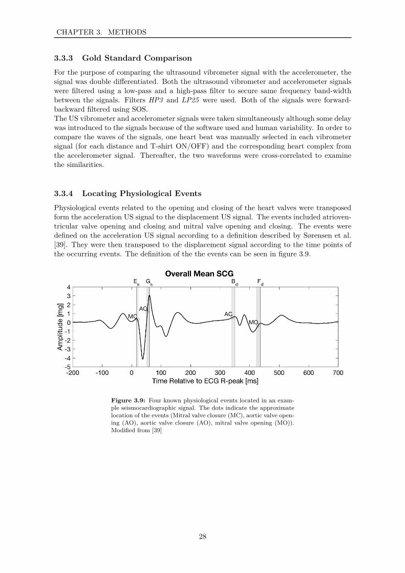
Physiological events related to the opening and closing of the heart valves were transposedform the acceleration US signal to the displacement US signal. The events included atrioven-tricular valve opening and closing and mitral valve opening and closing. The events weredefined on the acceleration US signal according to a definition described by Sørensen et al.[39]. They were then transposed to the displacement signal according to the time points ofthe occurring events. The definition of the the events can be seen in figure 3.9.

Figure 3.9: Four known physiological events located in an exam-ple seismocardiographic signal. The dots indicate the approximatelocation of the events (Mitral valve closure (MC), aortic valve open-ing (AO), aortic valve closure (AO), mitral valve opening (MO)).Modified from [39]

28

Chapter 4ResultsThe following sections present the results from the frequency band examination and theresult from the comparison of the US signal with the signal from an accelerometer as thegold standard.

4.1 Frequency Band Examination

The US signal’s frequency spectrum was first analyzed as recorded (displacement), followedby analysis after transformation to velocity and acceleration.

4.1.1 Displacement signal

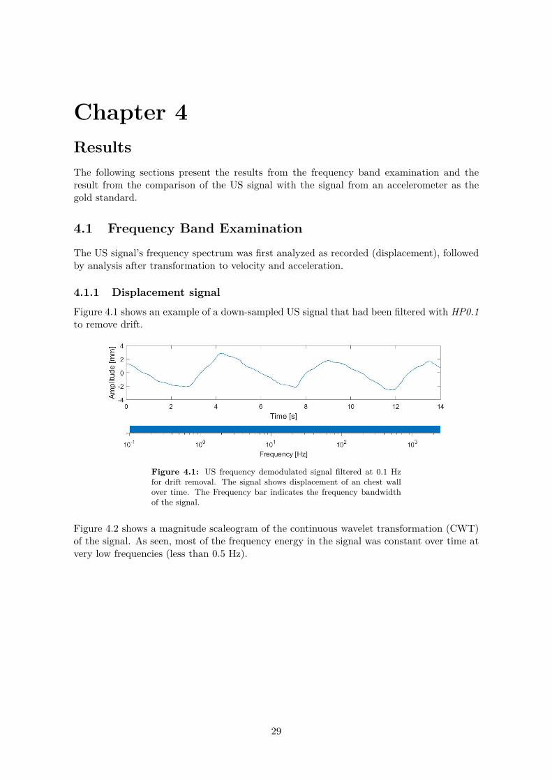
Figure 4.1 shows an example of a down-sampled US signal that had been filtered with HP0.1to remove drift.

Figure 4.1: US frequency demodulated signal filtered at 0.1 Hzfor drift removal. The signal shows displacement of an chest wallover time. The Frequency bar indicates the frequency bandwidthof the signal.

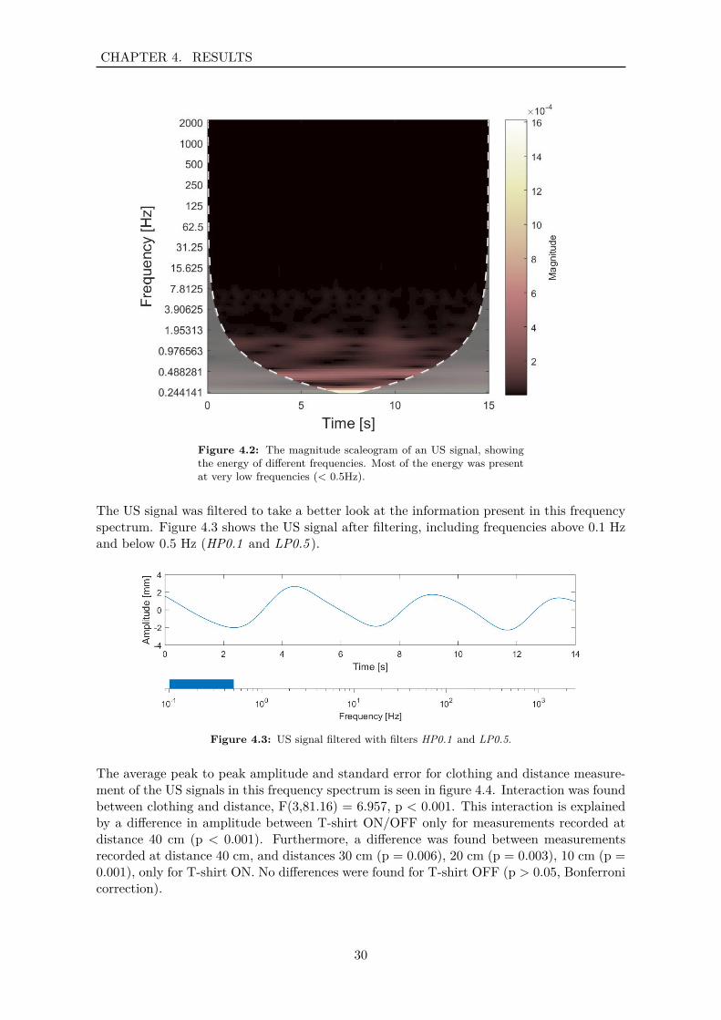
Figure 4.2 shows a magnitude scaleogram of the continuous wavelet transformation (CWT)of the signal. As seen, most of the frequency energy in the signal was constant over time atvery low frequencies (less than 0.5 Hz).

29

CHAPTER 4. RESULTS

Figure 4.2: The magnitude scaleogram of an US signal, showingthe energy of different frequencies. Most of the energy was presentat very low frequencies (< 0.5Hz).

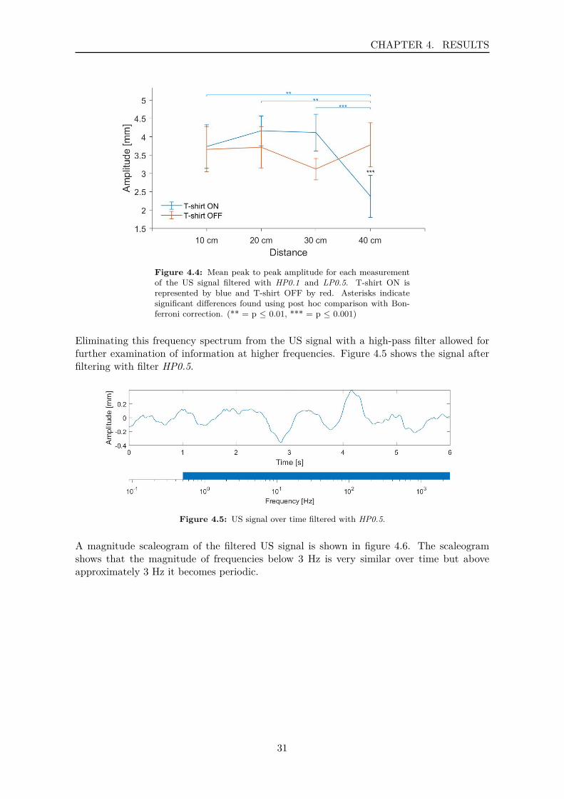
The US signal was filtered to take a better look at the information present in this frequencyspectrum. Figure 4.3 shows the US signal after filtering, including frequencies above 0.1 Hzand below 0.5 Hz (HP0.1 and LP0.5 ).

Figure 4.3: US signal filtered with filters HP0.1 and LP0.5.

The average peak to peak amplitude and standard error for clothing and distance measure-ment of the US signals in this frequency spectrum is seen in figure 4.4. Interaction was foundbetween clothing and distance, F(3,81.16) = 6.957, p < 0.001. This interaction is explainedby a difference in amplitude between T-shirt ON/OFF only for measurements recorded atdistance 40 cm (p < 0.001). Furthermore, a difference was found between measurementsrecorded at distance 40 cm, and distances 30 cm (p = 0.006), 20 cm (p = 0.003), 10 cm (p =0.001), only for T-shirt ON. No differences were found for T-shirt OFF (p > 0.05, Bonferronicorrection).

30

CHAPTER 4. RESULTS

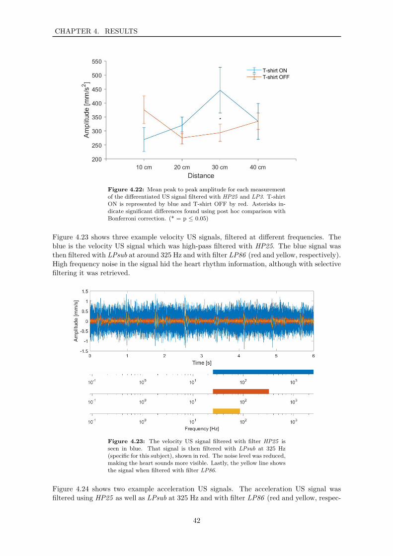
Figure 4.4: Mean peak to peak amplitude for each measurementof the US signal filtered with HP0.1 and LP0.5. T-shirt ON isrepresented by blue and T-shirt OFF by red. Asterisks indicatesignificant differences found using post hoc comparison with Bon-ferroni correction. (** = p ≤ 0.01, *** = p ≤ 0.001)

Eliminating this frequency spectrum from the US signal with a high-pass filter allowed forfurther examination of information at higher frequencies. Figure 4.5 shows the signal afterfiltering with filter HP0.5.

Figure 4.5: US signal over time filtered with HP0.5.

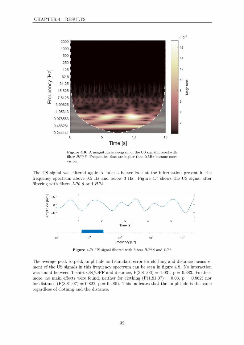
A magnitude scaleogram of the filtered US signal is shown in figure 4.6. The scaleogramshows that the magnitude of frequencies below 3 Hz is very similar over time but aboveapproximately 3 Hz it becomes periodic.

31

CHAPTER 4. RESULTS

Figure 4.6: A magnitude scaleogram of the US signal filtered withfilter HP0.5. Frequencies that are higher than 0.5Hz became morevisible.

The US signal was filtered again to take a better look at the information present in thefrequency spectrum above 0.5 Hz and below 3 Hz. Figure 4.7 shows the US signal afterfiltering with filters LP0.6 and HP3.

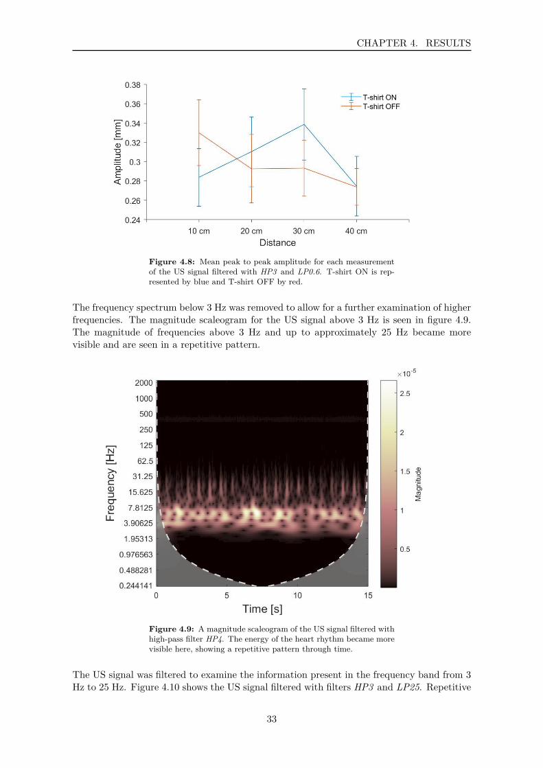
Figure 4.7: US signal filtered with filters HP0.6 and LP3.

The average peak to peak amplitude and standard error for clothing and distance measure-ment of the US signals in this frequency spectrum can be seen in figure 4.8. No interactionwas found between T-shirt ON/OFF and distance, F(3,81.06) = 1.031, p = 0.383. Further-more, no main effects were found, neither for clothing (F(1,81.07) = 0.03, p = 0.862) norfor distance (F(3,81.07) = 0.822, p = 0.485). This indicates that the amplitude is the sameregardless of clothing and the distance.

32

CHAPTER 4. RESULTS

Figure 4.8: Mean peak to peak amplitude for each measurementof the US signal filtered with HP3 and LP0.6. T-shirt ON is rep-resented by blue and T-shirt OFF by red.

The frequency spectrum below 3 Hz was removed to allow for a further examination of higherfrequencies. The magnitude scaleogram for the US signal above 3 Hz is seen in figure 4.9.The magnitude of frequencies above 3 Hz and up to approximately 25 Hz became morevisible and are seen in a repetitive pattern.

Figure 4.9: A magnitude scaleogram of the US signal filtered withhigh-pass filter HP4. The energy of the heart rhythm became morevisible here, showing a repetitive pattern through time.

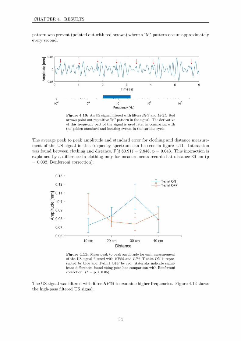
The US signal was filtered to examine the information present in the frequency band from 3Hz to 25 Hz. Figure 4.10 shows the US signal filtered with filters HP3 and LP25. Repetitive

33

CHAPTER 4. RESULTS

pattern was present (pointed out with red arrows) where a "M" pattern occurs approximatelyevery second.

Figure 4.10: An US signal filtered with filters HP3 and LP25. Redarrows point out repetitive "M" pattern in the signal. The derivativeof this frequency part of the signal is used later in comparing withthe golden standard and locating events in the cardiac cycle.

The average peak to peak amplitude and standard error for clothing and distance measure-ment of the US signal in this frequency spectrum can be seen in figure 4.11. Interactionwas found between clothing and distance, F(3,80.91) = 2.848, p = 0.043. This interaction isexplained by a difference in clothing only for measurements recorded at distance 30 cm (p= 0.032, Bonferroni correction).

Figure 4.11: Mean peak to peak amplitude for each measurementof the US signal filtered with HP25 and LP3. T-shirt ON is repre-sented by blue and T-shirt OFF by red. Asterisks indicate signif-icant differences found using post hoc comparison with Bonferronicorrection. (* = p ≤ 0.05)

The US signal was filtered with filter HP25 to examine higher frequencies. Figure 4.12 showsthe high-pass filtered US signal.

34

CHAPTER 4. RESULTS

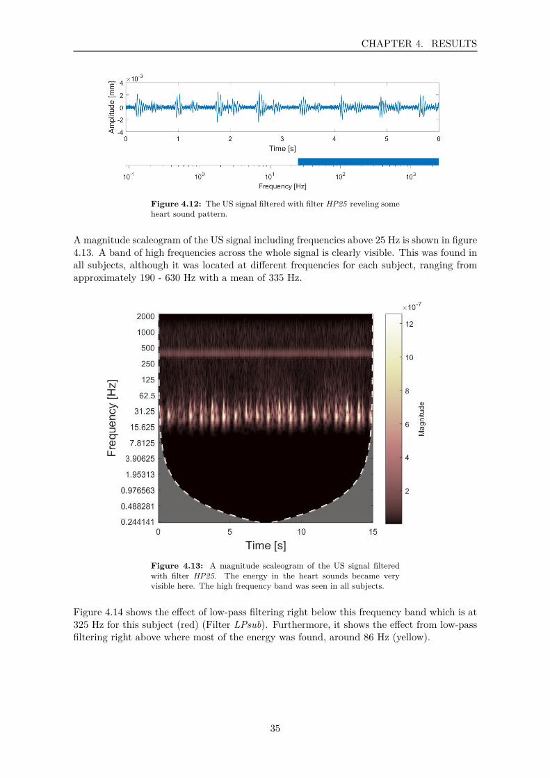
Figure 4.12: The US signal filtered with filter HP25 reveling someheart sound pattern.

A magnitude scaleogram of the US signal including frequencies above 25 Hz is shown in figure4.13. A band of high frequencies across the whole signal is clearly visible. This was found inall subjects, although it was located at different frequencies for each subject, ranging fromapproximately 190 - 630 Hz with a mean of 335 Hz.

Figure 4.13: A magnitude scaleogram of the US signal filteredwith filter HP25. The energy in the heart sounds became veryvisible here. The high frequency band was seen in all subjects.

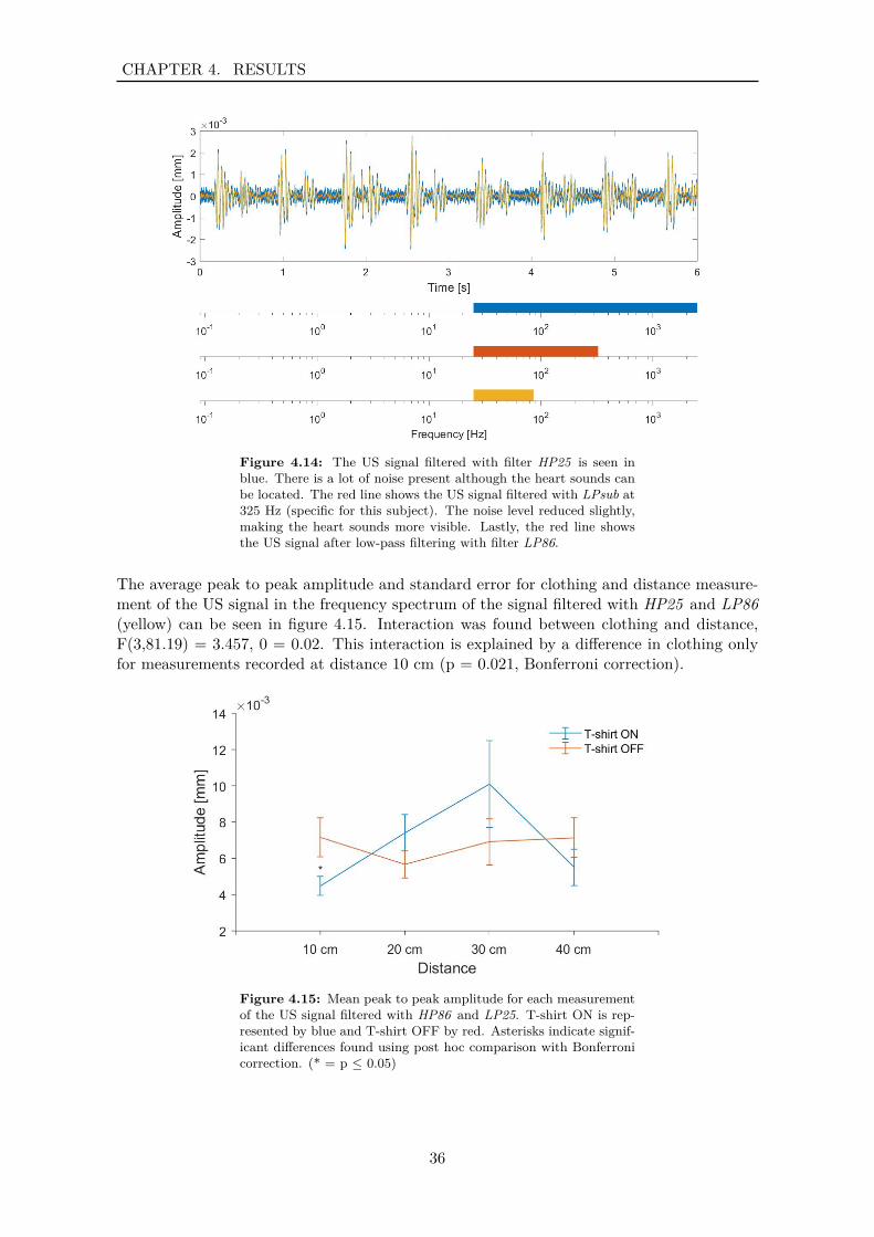
Figure 4.14 shows the effect of low-pass filtering right below this frequency band which is at325 Hz for this subject (red) (Filter LPsub). Furthermore, it shows the effect from low-passfiltering right above where most of the energy was found, around 86 Hz (yellow).

35

CHAPTER 4. RESULTS

Figure 4.14: The US signal filtered with filter HP25 is seen inblue. There is a lot of noise present although the heart sounds canbe located. The red line shows the US signal filtered with LPsub at325 Hz (specific for this subject). The noise level reduced slightly,making the heart sounds more visible. Lastly, the red line showsthe US signal after low-pass filtering with filter LP86.

The average peak to peak amplitude and standard error for clothing and distance measure-ment of the US signal in the frequency spectrum of the signal filtered with HP25 and LP86(yellow) can be seen in figure 4.15. Interaction was found between clothing and distance,F(3,81.19) = 3.457, 0 = 0.02. This interaction is explained by a difference in clothing onlyfor measurements recorded at distance 10 cm (p = 0.021, Bonferroni correction).

Figure 4.15: Mean peak to peak amplitude for each measurementof the US signal filtered with HP86 and LP25. T-shirt ON is rep-resented by blue and T-shirt OFF by red. Asterisks indicate signif-icant differences found using post hoc comparison with Bonferronicorrection. (* = p ≤ 0.05)

36

CHAPTER 4. RESULTS

Noise Floor and Distance Effect

An example showing the effect of distance on an US signal (T-shirt ON) which has beenfiltered with HP25 and LP86 is seen in figure 4.16. S1 and S2 can be seen at all distancesalthough when examining all of the subjects the signal lacked quality at larger distances,meaning that noise was introduced at random times.

(a) T-shirt ON, distance 10 cm

(b) T-shirt ON, distance 20 cm

(c) T-shirt ON, distance 30 cm

(d) T-shirt ON, distance 40 cm

Figure 4.16: The US signal (T-shirt ON) filtered with filters HP25and LP86. The effect of distance can be seen here. The quality ofthe signal is decreased at 40cm although heart sounds can be locatedat all distances.

37

CHAPTER 4. RESULTS

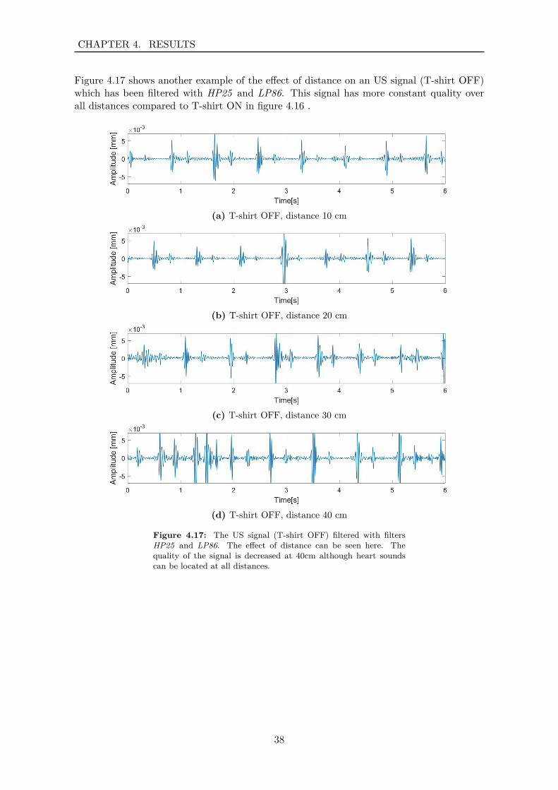
Figure 4.17 shows another example of the effect of distance on an US signal (T-shirt OFF)which has been filtered with HP25 and LP86. This signal has more constant quality overall distances compared to T-shirt ON in figure 4.16 .

(a) T-shirt OFF, distance 10 cm

(b) T-shirt OFF, distance 20 cm

(c) T-shirt OFF, distance 30 cm

(d) T-shirt OFF, distance 40 cm

Figure 4.17: The US signal (T-shirt OFF) filtered with filtersHP25 and LP86. The effect of distance can be seen here. Thequality of the signal is decreased at 40cm although heart soundscan be located at all distances.

38

CHAPTER 4. RESULTS

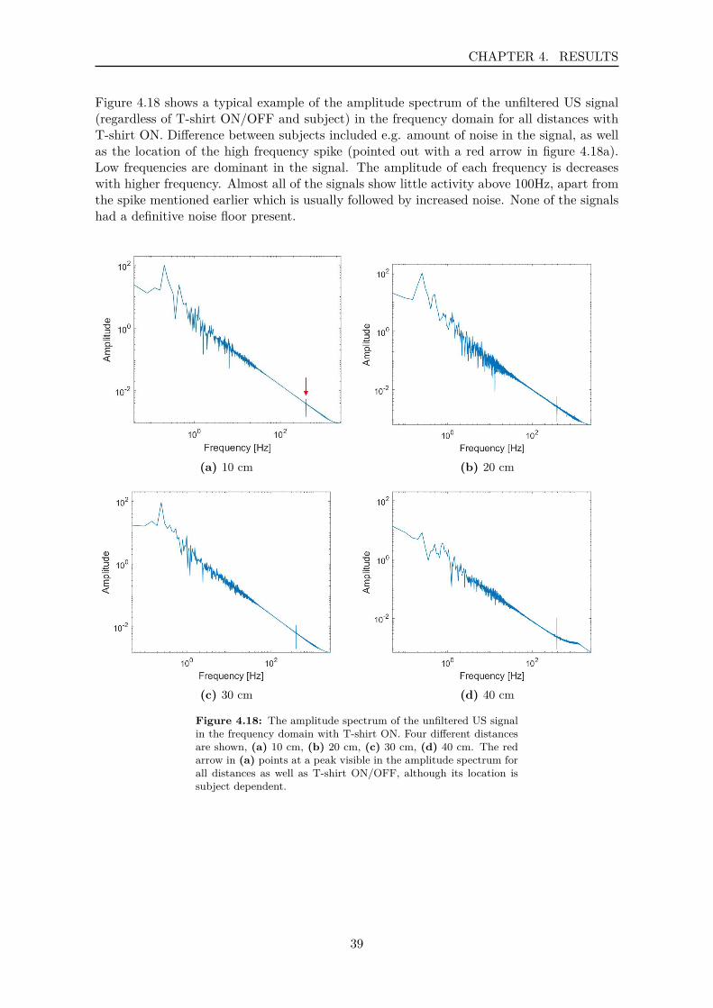
Figure 4.18 shows a typical example of the amplitude spectrum of the unfiltered US signal(regardless of T-shirt ON/OFF and subject) in the frequency domain for all distances withT-shirt ON. Difference between subjects included e.g. amount of noise in the signal, as wellas the location of the high frequency spike (pointed out with a red arrow in figure 4.18a).Low frequencies are dominant in the signal. The amplitude of each frequency is decreaseswith higher frequency. Almost all of the signals show little activity above 100Hz, apart fromthe spike mentioned earlier which is usually followed by increased noise. None of the signalshad a definitive noise floor present.

(a) 10 cm (b) 20 cm

(c) 30 cm (d) 40 cm

Figure 4.18: The amplitude spectrum of the unfiltered US signalin the frequency domain with T-shirt ON. Four different distancesare shown, (a) 10 cm, (b) 20 cm, (c) 30 cm, (d) 40 cm. The redarrow in (a) points at a peak visible in the amplitude spectrum forall distances as well as T-shirt ON/OFF, although its location issubject dependent.

39

CHAPTER 4. RESULTS

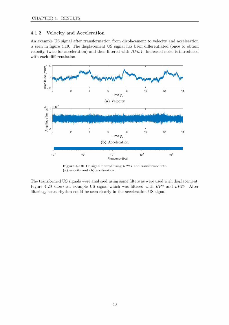
4.1.2 Velocity and Acceleration

An example US signal after transformation from displacement to velocity and accelerationis seen in figure 4.19. The displacement US signal has been differentiated (once to obtainvelocity, twice for acceleration) and then filtered with HP0.1. Increased noise is introducedwith each differentiation.

(a) Velocity

(b) Acceleration

Figure 4.19: US signal filtered using HP0.1 and transformed into(a) velocity and (b) acceleration

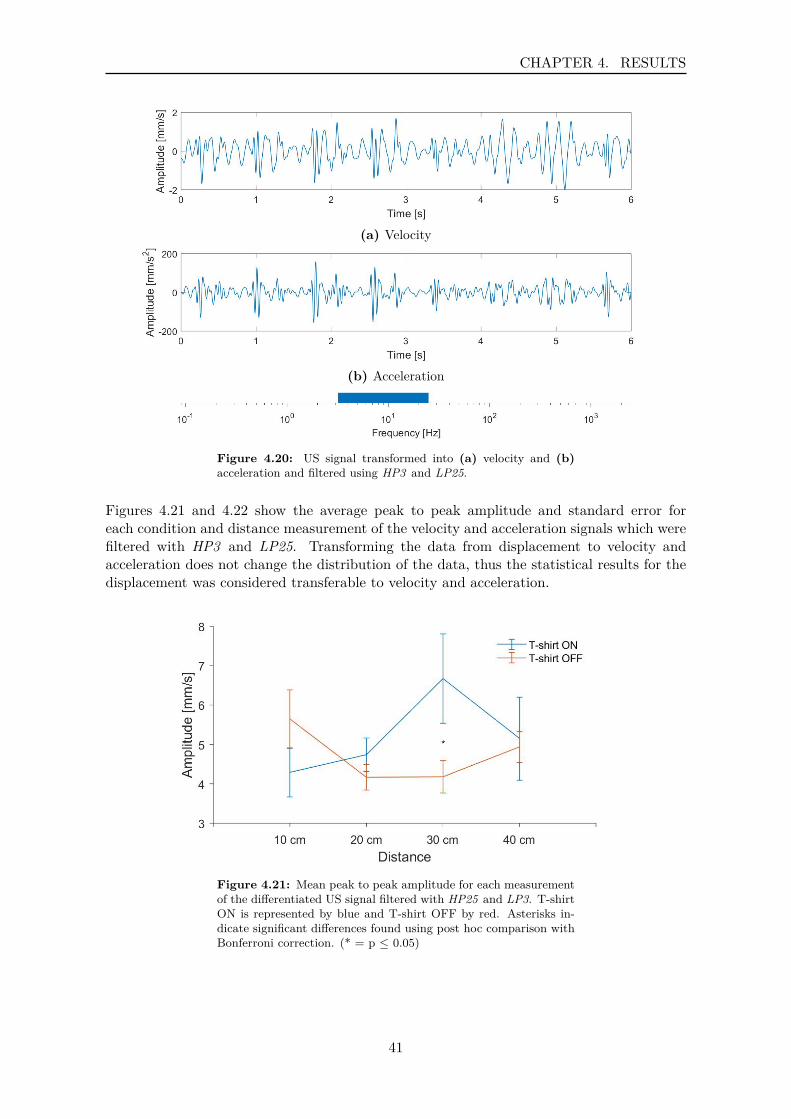
The transformed US signals were analyzed using same filters as were used with displacement.Figure 4.20 shows an example US signal which was filtered with HP3 and LP25. Afterfiltering, heart rhythm could be seen clearly in the acceleration US signal.

40

CHAPTER 4. RESULTS

(a) Velocity

(b) Acceleration

Figure 4.20: US signal transformed into (a) velocity and (b)acceleration and filtered using HP3 and LP25.

Figures 4.21 and 4.22 show the average peak to peak amplitude and standard error foreach condition and distance measurement of the velocity and acceleration signals which werefiltered with HP3 and LP25. Transforming the data from displacement to velocity andacceleration does not change the distribution of the data, thus the statistical results for thedisplacement was considered transferable to velocity and acceleration.

Figure 4.21: Mean peak to peak amplitude for each measurementof the differentiated US signal filtered with HP25 and LP3. T-shirtON is represented by blue and T-shirt OFF by red. Asterisks in-dicate significant differences found using post hoc comparison withBonferroni correction. (* = p ≤ 0.05)

41

CHAPTER 4. RESULTS

Figure 4.22: Mean peak to peak amplitude for each measurementof the differentiated US signal filtered with HP25 and LP3. T-shirtON is represented by blue and T-shirt OFF by red. Asterisks in-dicate significant differences found using post hoc comparison withBonferroni correction. (* = p ≤ 0.05)

Figure 4.23 shows three example velocity US signals, filtered at different frequencies. Theblue is the velocity US signal which was high-pass filtered with HP25. The blue signal wasthen filtered with LPsub at around 325 Hz and with filter LP86 (red and yellow, respectively).High frequency noise in the signal hid the heart rhythm information, although with selectivefiltering it was retrieved.

Figure 4.23: The velocity US signal filtered with filter HP25 isseen in blue. That signal is then filtered with LPsub at 325 Hz(specific for this subject), shown in red. The noise level was reduced,making the heart sounds more visible. Lastly, the yellow line showsthe signal when filtered with filter LP86.

Figure 4.24 shows two example acceleration US signals. The acceleration US signal wasfiltered using HP25 as well as LPsub at 325 Hz and with filter LP86 (red and yellow, respec-

42

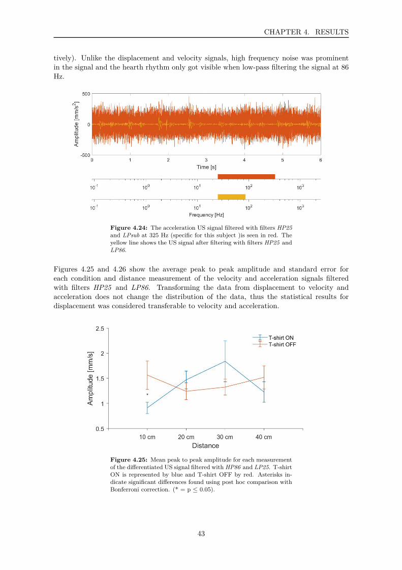
CHAPTER 4. RESULTS

tively). Unlike the displacement and velocity signals, high frequency noise was prominentin the signal and the hearth rhythm only got visible when low-pass filtering the signal at 86Hz.

Figure 4.24: The acceleration US signal filtered with filters HP25and LPsub at 325 Hz (specific for this subject )is seen in red. Theyellow line shows the US signal after filtering with filters HP25 andLP86.

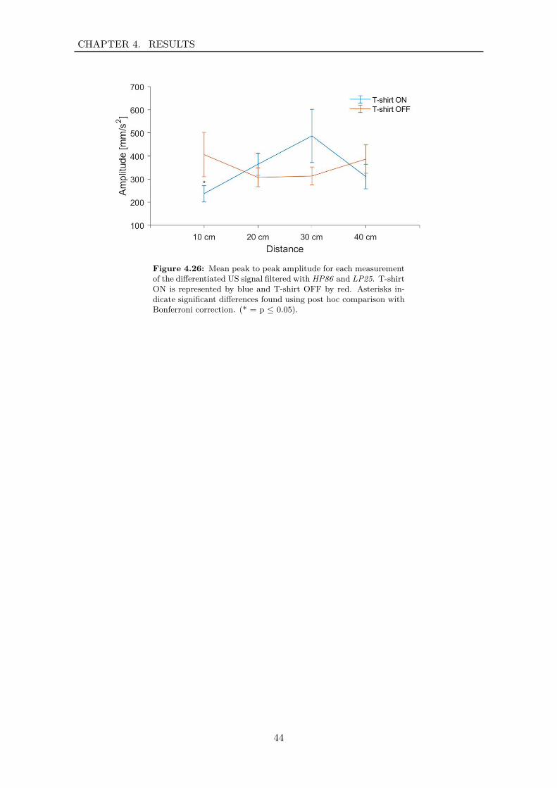
Figures 4.25 and 4.26 show the average peak to peak amplitude and standard error foreach condition and distance measurement of the velocity and acceleration signals filteredwith filters HP25 and LP86. Transforming the data from displacement to velocity andacceleration does not change the distribution of the data, thus the statistical results fordisplacement was considered transferable to velocity and acceleration.

Figure 4.25: Mean peak to peak amplitude for each measurementof the differentiated US signal filtered with HP86 and LP25. T-shirtON is represented by blue and T-shirt OFF by red. Asterisks in-dicate significant differences found using post hoc comparison withBonferroni correction. (* = p ≤ 0.05).

43

CHAPTER 4. RESULTS

Figure 4.26: Mean peak to peak amplitude for each measurementof the differentiated US signal filtered with HP86 and LP25. T-shirtON is represented by blue and T-shirt OFF by red. Asterisks in-dicate significant differences found using post hoc comparison withBonferroni correction. (* = p ≤ 0.05).

44

CHAPTER 4. RESULTS

4.2 Comparison with Accelerometer

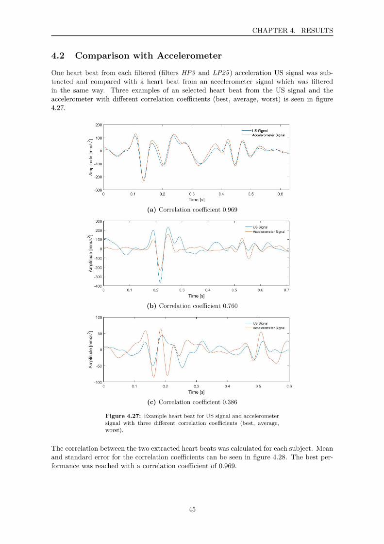
One heart beat from each filtered (filters HP3 and LP25 ) acceleration US signal was sub-tracted and compared with a heart beat from an accelerometer signal which was filteredin the same way. Three examples of an selected heart beat from the US signal and theaccelerometer with different correlation coefficients (best, average, worst) is seen in figure4.27.

(a) Correlation coefficient 0.969

(b) Correlation coefficient 0.760

(c) Correlation coefficient 0.386

Figure 4.27: Example heart beat for US signal and accelerometersignal with three different correlation coefficients (best, average,worst).

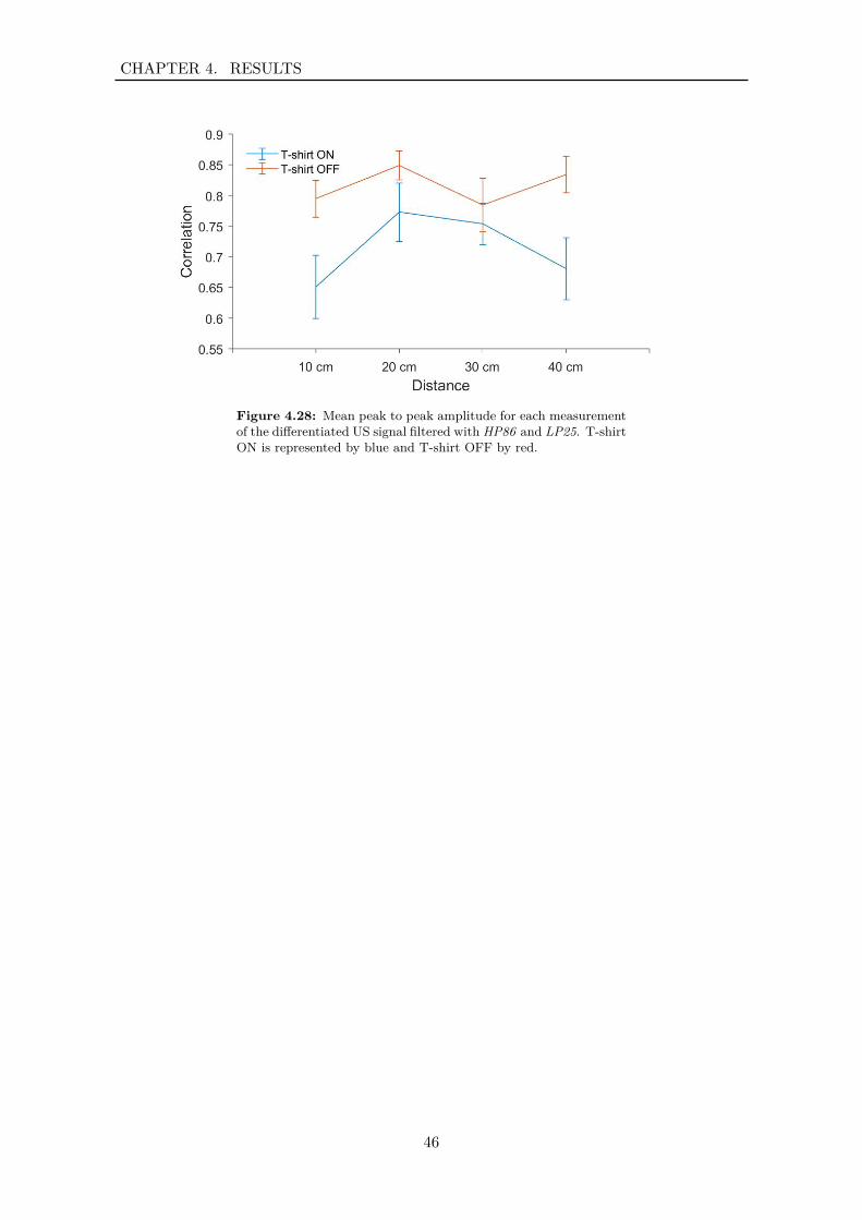
The correlation between the two extracted heart beats was calculated for each subject. Meanand standard error for the correlation coefficients can be seen in figure 4.28. The best per-formance was reached with a correlation coefficient of 0.969.

45

CHAPTER 4. RESULTS

Figure 4.28: Mean peak to peak amplitude for each measurementof the differentiated US signal filtered with HP86 and LP25. T-shirtON is represented by blue and T-shirt OFF by red.

46

CHAPTER 4. RESULTS

4.3 Fiducial Points Transposed to Displacement US Signal

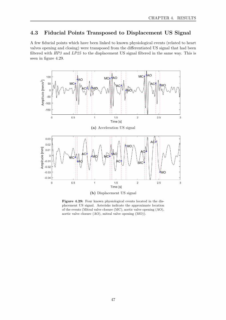
A few fiducial points which have been linked to known physiological events (related to heartvalves opening and closing) were transposed from the differentiated US signal that had beenfiltered with HP3 and LP25 to the displacement US signal filtered in the same way. This isseen in figure 4.29.

(a) Acceleration US signal

(b) Displacement US signal

Figure 4.29: Four known physiological events located in the dis-placement US signal. Asterisks indicate the approximate locationof the events (Mitral valve closure (MC), aortic valve opening (AO),aortic valve closure (AO), mitral valve opening (MO)).

47

CHAPTER 4. RESULTS

48

Part III

Synthesis

49

Chapter 5DiscussionMost cardiovascular diseases can be prevented or managed if detected early. Early detectionis therefore of great benefit, causing the treatment to be easier, more efficient and econom-ical. Many methods are available for detecting heart disease although most are limited tobeing contact methods. In this project, a novel method, where the principle of Doppler isutilized for detecting cardiac activity, was examined further. Cardiac signals were recordedusing an ultrasound vibrometer and analyzed in terms of different frequency spectra andcompared with an accelerometer. This chapter presents a discussion about the experimentalsetup and signal demodulation, followed by a discussion about the information found in thedisplacement signal and the comparison with an accelerometer.

Experimental Setup & Signal Demodulation

A subject was seated directly in front of a microphone which was directed at the septumof the subject. A transducer was placed next to the microphone, aiming at the subject ataround 20° angle. Multiple ways of setting up the equipment were assessed before this wasselected. All included that both the transducer and microphone were directed at the sub-ject. The setups were not experimentally tested, but the signals were visually analyzed bythe authors.The transducer emits at a 30° angle and as the wave reflects of the chest wall in differentdirections (depending on the angle of reflection) the microphone needed to be in the range ofthe reflection. The quality of the signal at short distances did not seem to be affected by thesetup. However, as the transducer emits at a 30° angle, the area affecting the carrier signalincreases as the distance increases. At smaller distances, the area affecting the carrier waveis very small, giving a certain focal point but at larger distances the area affected loses focus.The lack of a focal point seems to introduce some inconsistency in the signal, meaning addednoise in the signal and a reduction in the quality of the signal. The reduction of quality canbe explained by that the movement of the chest wall differs depending on the location andtime points during the respiration cycle [13] and cardiac cycle [15] and therefore when thewave is affected by a larger area, different movements are introduced to the signal, reducingthe quality. Furthermore, as the waves are reflected from different locations on the chest,they have different traveling distances and a longer traveling time that affects the phase de-viation of the carrier signal. This might lead to demodulation of a phase that is larger thanthe corresponding displacement of the chest wall, thus giving an incorrect representation ofthe movement.This could potentially be fixed with a setup introduced by Jeger-Madiot et al. [32] whodesigned an elliptical acoustic mirror that reflected the emitted signal, thus obtaining a focalpoint on the subject and eliminating the uncertainty of the precise origin of the cardiac signal.

A reoccurring and seemingly random problem was found when demodulating the signal wheresmall jumps (< π) occurred in some of the signals. This is thought to be explained by thecarrier frequency and instability in the oscillator. The dominant frequency was calculatedfrom the received signal. It varied between signals and even between parts of the same signal.

51

CHAPTER 5. DISCUSSION

The most frequent frequency was 0.2 Hz above the 40 kHz, although the deviation from 40kHz ranged from being 0.2 Hz below to 0.4 Hz above. This shows that the oscillator is notcompletely stable and at any given point the carrier frequency is little bit off from the domi-nant frequency. The dominant frequency was used in the demodulation process thus leavingthe system exposed to errors when the oscillator derived from that frequency. The effectthis had on the signal is that distortion was introduced to the signal (especially at higherfrequencies resulting in high amplitude peaks). This was solved to some degree by split-ting the signal into smaller segments to calculate the dominant frequency and demodulateeach segment separately. The drawback of doing this is that the demodulated signals werenow considerably shorter than the recorded signal. A possible improvement for this wouldbe to monitor the carrier frequency during the recording to have better knowledge aboutthese deviations from the 40 kHz and utilize that knowledge in calculating a more precisecarrier wave. Other methods of demodulation are worth considering, e.g. phase lock loopor slope detector, that do not use a local oscillator (used here to obtain the I/Q signals) assuch a demodulator might not be as affected by fluctuations in the oscillator as this system is.

Information in different frequency bands

A low frequency signal was extracted (0.1 - 0.5Hz), as this range had most of the energy inthe signal (see figure 4.2). Respiration is known to be in this range [14]. The movement ofthe chest wall due to breathing is larger than the movement due to heart beats (4-12 mm[13] vs 0.2-0.5 mm [15]), and therefore the energy stored in the signal due to breathing over-powers other frequency ranges. DeGroote et al [13] reported the displacement of the chestwall due to breathing in the range of 4-12 mm. This study, however, reports the amplitudea bit lower (overall mean around 3.5 mm, figure 4.4). This might be the effect of a smallsubject group as this study only had 13 subjects or because of the experimental setup, assubjects were asked not to move during the experiment. Breathing is a voluntary mechanismand was thus very variable between subjects.Significant difference was found between T-shirt ON and T-shirt OFF at 40 cm distanceindicating that clothing influences the signal at this distance. Furthermore, significant dif-ference was found between measurements taken at distance of 40 cm when subject is wearinga T-shirt, compared to other distances. This indicates that at this distance the energy oflow frequency factors in the signal is reduced. This could potentially be explained by thesystem setup as discussed earlier. As the distance is increased the focal point gets lost andthe carrier wave is influenced by a larger area which results in a reduced quality of signal.The energy in frequency spectrum above 0.5 Hz became more visible on the scaleogram afterthe frequency band related to the breathing had been filtered out, showing high energy infrequencies between 0.6 Hz and 3 Hz (see figure 4.6). Average heart rate during rest in adultsranges from 1 - 1.34 Hz [15], fitting well in the selected frequency range. The overall meanof displacement of the chest wall due to beating of the heart was reported in around 0.3 mm(figure 4.8), which fits well within the range 0.2 - 0.5 mm, reported by Ramachandran et al.[15]. No statistical difference between distances or clothing was found in this frequency rangeof the signal which indicates that neither distance nor clothing affected the measurement ofthe displacement.

The magnitude scaleogram of the signal where the heart rate had been filtered out (showingfrequencies above 3 Hz) showed that the energy in the signal became more periodic, espe-cially between 8 and 25 Hz. This periodic pattern is interpreted as the systolic and diastolicacoustic waves (corresponding to the valve sounds, S1 and S2). It is difficult to see clearrepetitive patterns in the signal in the time domain, although with effort, some repetition

52


can be observed. The overall mean of the amplitude of the signal that had been band-passfiltered between 3 Hz and 25 Hz was around 3 times less than in the signal showing the heartrate (approximately 0.08 mm, figure 4.11). There was no literature found on displacementof cardiac signal in this frequency range. However, the average amplitude of the accelerationUS signal was approximately 340 mm/s2. According to Rienzo et al [40] a typical seismo-cardiogram can have an amplitude of a few mg (where 10 mg ≈ 100 mm/s2), although theymention that a seismocardiogram signal can have a frequency range from 0.1 Hz and up to200 - 300 Hz, which is a larger range than this study explores. The significant differencefound in interaction between T-shirt ON/OFF at distance 30 cm might be explained by thereduced quality of the signal at greater distances as mentioned earlier.

Exploring the energy in the signal above 25 Hz showed a clear repetitive pattern between25 Hz and approximately 90 Hz. The valve sounds could now easily be located in the sig-nal, although some noise was present. Interestingly (and unexpectedly), high energy wasobserved in a band of rather high frequencies for all subjects although the precise frequencyband varied between subjects. We suggest that this could be due the skin’s natural reso-nance frequency. The skin is the last link in transmitting the sound waves from the heartto the surface and acts as an acoustic system. Acoustic systems all have their own naturalresonance frequency which should apply here as well. The suggestion is therefore that thisoccurs at different frequencies for each subject as the skin differs slightly between subjectsin terms of e.g. stiffness and elasticity. Silver et al [41] calculated the resonance frequencyof decellularized human skin, where he found that the frequency ranged from ca 150 Hz to350 Hz depending on the strain applied on the tissue. For our subjects this frequency rangedfrom 190 Hz - 630 Hz with a mean of 335 HzThe overall mean of the amplitude was decreased by a factor of 10 (was approximately 0.007mm, figure 4.15) compared to the amplitude of the signal with the frequencies between 3and 25 Hz. This is considered logical as the effect of the heart valves on the displacementof the chest wall is much smaller than the effect the ventricles have when contracting. Thesignificant difference found in in the amplitude between T-shirt ON/OFF at 10 cm might beexplained by a demodulation error that introduces a high peak in the signal that increasesthe mean amplitude (as discussed earlier).

Analysis of the whole frequency spectrum showed that no noise floor was present in the signaland thus indicating that the bandwidth of the signal could possibly be increased. Subjectselective low-pass filtering where the cut-off frequency was below the acoustic resonance fre-quency band reduced overall noise in the signal and made the heart sounds more visible. Asmost of the energy seen at these high frequencies was in this band, we suggest that locatingand filtering the resonance frequency band with a band-stop filter would allow for an increasein bandwidth of the system.

Wavelet comparison

Differentiating the US signal to obtain the velocity and acceleration is an important step ingetting the signal to a comparable form to an accelerometer signal. The downside of differ-entiating is that it introduces a lot of noise to the signal. However, with some filtering thecardiac activity was retrieved. Distinguishing between systolic and diastolic acoustic wavesin lower frequencies (3 - 25 Hz) got easier with each differentiation (see figure 4.20). Valvesounds were detectable for frequencies up to the resonance frequency in the velocity signal,although there was noise present. However, the valve sounds were only detectable in the

53


acceleration signal when a low-pass filter at 86 Hz was used.

Comparison of the waveforms of the acceleration US signal and the accelerometer signalshowed very promising results, with the highest correlation being 0.969 at distance 40cmfor T-shirt OFF. The mean correlation coefficient for signals recorded with T-shirt ON waslower than for T-shirt OFF (0.71 and 0.82, respectively) indicating that clothing reduces thequality of the signal. Despite this, cardiac activity was recognizable in all of the signals, forboth T-shirt ON/OFF and at all distances. The comparison was carried out by manuallyselecting one heartbeat complex (including both S1 and S2) from each US signal and thecorresponding complex from the accelerometer signal. Therefore, this does not reflect on theoverall outcome of the signals but rather the potential this system has in recording cardiacevents (i.e. the highest correlation occurring at 40 cm, indicating that a good quality can bereached at higher distances).

Cardiac events (MC, AO, AC and MO) were located on the acceleration US signal (see figure4.29) corresponding to the definition by Sørensen et al. [39]. After locating the events on theacceleration US signal, the corresponding time points on the US displacement signal weremarked. The MC and AO points seemed to always be located in valleys close and adjacent toeach other (forming a W pattern) that was followed by a deep valley and a high peak. Thispattern could potentially be used in locating these cardiac events. The AC and MO pointsseemed to be located at more random positions, although AC was always in the downslopeof a wave. This process shows the potential for examining the displacement signal further.More cardiac cycle events could easily be transferred to the displacement signal, giving moreinformation about the displacement signal, although this needs a more thorough examination.

As the results present, there is a lot of information on cardiac activity found in the displace-ment of the chest wall. Due to the information content and ease of execution of the method,it has great potential, both in clinical and out of hospital setting. In order for this method ofrecording cardiac activity to reach its full potential, additional noise in the signal would needto be reduced. This could be done to some extent by using calculations of a more precisecarrier wave and/or designing the hardware in such a way that the wave is directed at thechest wall with a well-defined focal point. Furthermore, recording at closer distances (10 -20 cm) results in recordings containing less noise than those of far distances.With these improvements and a suitable hardware design this could be of great benefit inrecording of cardiac activity, making the process less time consuming and more convenientfor the subject.

54

Chapter 6ConclusionIn this project a cardiac signal from 13 subjects was recorded. The signal was recordedusing an ultrasound transducer transmitting a 40 kHz ultrasound wave that got frequencymodulated when echoing off a subjects chest wall. The US signal was recorded using anultrasound microphone and processed digitally. It was demodulated using an arctan quadra-ture demodulator to get the displacement of the chest wall. The displacement US signal wasanalyzed using continuous wavelet transformation and high and low-pass filters of differentcut-off frequencies.

The US displacement signal contains information on different physiological events such asbreathing, chamber contraction, and heart valves opening and closing. The effect of distanceand clothing was tested and showed that the quality of the signal decreases with increaseddistance in such a way that the information in the signal due to cardiac activity was harder todetect. Furthermore, recording the signal with a T-shirt on does not reduce the informationin the signal.

The correlation of a heart complex from the US acceleration signal and an accelerometer sig-nal was calculated and showed good results with the highest correlation being 0.969. Lastly,physiological events associated with opening and closing of the heart valves were transposedfrom the acceleration US signal to the displacement US signal.

The displacement signal contains a lot of information on cardiac activity. Due to the infor-mation content and ease of execution of this method, it has great potential both in clinicaland out of hospital setting. In order to improve this method further, noise in the signal wouldneed to be reduced and the robustness of the system improved. This could be achieved e.g.with improved hardware in terms of getting a focal point on the chest wall, and/or systemdesign in terms of improving stability of the carrier wave and subject specific high frequencynoise.

55

CHAPTER 6. CONCLUSION

56

Bibliography[1] W. H. Organization, “Cardiovascular diseases (CVDs), year = 2017, url =

http://www.who.int/news-room/fact-sheets/detail/cardiovascular-diseases-(cvds), url-date = 2018-05-30.”

[2] M. Singh and A. Cheema, “Heart Sounds Classification using Feature Extraction ofPhonocardiography Signal,” International Journal of Computer Applications, vol. 77,no. 4, pp. 13–17, 2013.

[3] J. Kranjec, S. Beguš, G. Geršak, and J. Drnovšek, “Non-contact heart rate and heartrate variability measurements: A review,” Biomedical Signal Processing and Control,vol. 13, no. 1, pp. 102–112, 2014.

[4] J. Kranjec, S. Begus, J. Drnovsek, and G. Gersak, “Novel methods for noncontact heartrate measurement: A feasibility study,” IEEE Transactions on Instrumentation andMeasurement, vol. 63, no. 4, pp. 838–847, 2014.

[5] J. Kranjec, S. Beguš, G. Geršak, M. Šinkovec, J. Drnovšek, and D. Hudoklin, “Designand Clinical Evaluation of a Non-Contact Heart Rate Variability Measuring Device,”Sensors, vol. 17, no. 12, p. 2637, 2017.

[6] G. J. Tortora and B. Derrickson, Principles of anatomy and physiology. John Wiley &Sons, 13th ed., 2012.

[7] M. L. Entman, S. W. Jacob, and M. F. Oliver, “Human Cardiovascular System,” En-cyclopædia Britannica, pp. 1–10, 2014.

[8] “When Your Child Has a Hypoplastic Right Ventricle: Tricuspid Atresia.” https://www.fairview.org/patient-education/89171. Last accessed: March 2018.

[9] H. Fukuta and W. C. Little, “The Cardiac Cycle and the Physiologic Basis of LeftVentricular Contraction, Ejection, Relaxation, and Filling,” Heart Failure Clinics, vol. 4,no. 1, pp. 1–11, 2008.

[10] C. Webber and J. P. Zbilut, InTech Chapter 11 Nonlinear Cardiac Dynamics. 2012.

[11] D. S. M. Amin and F. Reguig, “Features for Heartbeat Sound Signal Normal and Patho-logical,” Recent Patents on Computer Science, vol. 1, pp. 1–8, 2010.

[12] M. Nabih-Ali, E. S. A. El-Dahshan, and A. S. Yahia, “A review of intelligent systems forheart sound signal analysis,” Journal of Medical Engineering and Technology, vol. 41,no. 7, pp. 553–563, 2017.

[13] A. De Groote, M. Wantier, G. Cheron, M. Estenne, and M. Paiva, “Chest wall motionduring tidal breathing,” Journal of Applied Physiology, vol. 83, no. 5, pp. 1531–1537,1997.

[14] W. Q. Lindh, M. S. Pooler, C. D. Tamparo, and B. M. Dahl, Delmar’s ComprehensiveMedical Assisting Administrative and Clinical Competencies. fouth ed.

57

https://www.fairview.org/patient-education/89171

https://www.fairview.org/patient-education/89171

BIBLIOGRAPHY

[15] C. Ramachandran and M. Singh, “Three-dimensional reconstruction of cardiac displace-ment patterns on the chest wall during the P, QRS and T-segments of the ECG by laserspeckle inteferometry,” Medical & Biological Engineering & Computing, vol. 27, no. 5,pp. 525–530, 1989.

[16] G. Shafiq and K. C. Veluvolu, “Surface chest motion decomposition for cardiovascularmonitoring,” Scientific Reports, vol. 4, pp. 1–9, 2014.

[17] A. K. Abbas and R. Bassam, Phonocardiography Signal Processing, vol. 4. Morgan &Claypool, 2009.

[18] J. Keroes, L. David, D. Wringley, and B. Erikson, “Heart Murmur,” 2017.

[19] L. A. Geddes, “Birth of the stethoscope,” IEEE Engineering in Medicine and BiologyMagazine, vol. 24, no. 1, pp. 84–86, 2005.

[20] A. J. Taylor, Learning Cardiac Auscultation. Springer, 2015.

[21] S. Leng, R. S. Tan, K. T. C. Chai, C. Wang, D. Ghista, and L. Zhong, “The electronicstethoscope,” BioMedical Engineering Online, vol. 14, no. 1, pp. 1–37, 2015.

[22] “Advantages / disadvantages of electronic stethoscopes.” http://www.nursetheory.com/advantages-disadvantages-of-electronic-stethoscopes/, 2018. (Last ac-cessed: March 2018).

[23] J. M. Zanetti and Salerno, “Seismocardiography: a technique for recording precordialacceleration,” Computer-Based Medical Systems, pp. 4–9, 1991.

[24] O. T. Inan, P.-f. Migeotte, K.-s. Park, M. Etemadi, K. Tavakolian, R. Casanella,J. Zanetti, J. Tank, I. Funtova, G. K. Prisk, and M. D. Rienzo, “Ballistocardiogra-phy and Seismocardiography : A Review of Recent Advances,” Journal of Biomedicaland Health Informatics, vol. 19, no. October, pp. 1414–1427, 2014.

[25] P. Castiglioni, A. Faini, G. Parati, and M. Di Rienzo, “Wearable seismocardiography,”Annual International Conference of the IEEE Engineering in Medicine and Biology -Proceedings, pp. 3954–3957, 2007.

[26] A. Akhbardeh, K. Tavakolian, V. Gurev, T. Lee, W. New, B. Kaminska, andN. Trayanova, “Comparative analysis of three different modalities for characteriza-tion of the seismocardiogram,” Proceedings of the 31st Annual International Conferenceof the IEEE Engineering in Medicine and Biology Society: Engineering the Future ofBiomedicine, EMBC 2009, pp. 2899–2903, 2009.

[27] A. Dinh, “Heart Activity Monitoring on Smartphone,” International Conference onBiomedical Engineering and Technology, vol. 11, pp. 45–49, 2011.

[28] J. M. Zanetti and K. Tavakolian, “Seismocardiography : Past , Present and Future,”pp. 7004–7007, 2013.

[29] P. Mounsey, “Praicordial ballistocardiography,” pp. 259–271, 1956.

[30] R. S. Crow, P. Hannan, D. Jacobs, L. Hedquist, and D. M. Salerno, “Relationship be-tween Seismovardiogram and Echoardiogram for Events in the Cardiac Cycle,” AmericanJournla of noninvasive Cardiology, vol. 8, pp. 39–46.

58

http://www.nursetheory.com/advantages-disadvantages-of-electronic-stethoscopes/

http://www.nursetheory.com/advantages-disadvantages-of-electronic-stethoscopes/

BIBLIOGRAPHY

[31] P. Shirkovskiy, A. Laurin, D. Chapelle, M. Fink, and R. K. Ing, “Contactless Mappingof Thoracic and Abdominal Motion : Applications for Seismocardiography,” Computingin Cardiology, 2017.

[32] N. Jeger-Madiot, J. Gateau, M. Fink, and R. Ing, “Non-contact and through-clothingmeasurement of the heart rate using ultrasound vibrocardiography,” Medical Engineer-ing and Physics, vol. 50, pp. 96–102, 2017.

[33] S. Haykin, Communication Systems. John Wiley & Sons, 2001.

[34] G.Verghese, “Chapter 14: Modulation and demodulation,” April 2012.

[35] W. Tranter, K. Shanmugan, T. Rappaport, and K. Kosbar, Principles of communicationsystems simulation with wireless applications. Prentice Hall, 2003.

[36] J. L. Semmlow, Biosignal and Biomedical Image Processing. Taylor & Francis Group,third ed., 2014.

[37] A. V. Oppenheim, Signals and Systems. Pretnice Hall, 1997.

[38] W. H. Press, W. T. Vetterling, S. A. Teukolsky, and B. P. Flannery, Numerical Recipesin Fortran 77: The art of scientific computing. Cambridge University Press, 2 ed., 1992.

[39] K. Sørensen, S. E. Schmidt, A. S. Jensen, P. Søgaard, and J. J. Struijk, “The seismo-cardiogram in normal subjects,” Unpublished.

[40] M. Di Rienzo, E. Vaini, P. Castiglioni, G. Merati, P. Meriggi, G. Parati, A. Faini, andF. Rizzo, “Wearable seismocardiography: Towards a beat-by-beat assessment of cardiacmechanics in ambulant subjects,” Autonomic Neuroscience: Basic and Clinical, vol. 178,no. 1-2, pp. 50–59, 2013.

[41] F. H. Silver and R. G. Shah, “Analysis of Mechanical Behavior of Composite TissuesUsing Vibrational Optical Coherence Tomography,” World Journal of Mechanics, no. 7,pp. 271–282, 2017.

59

BIBLIOGRAPHY

60

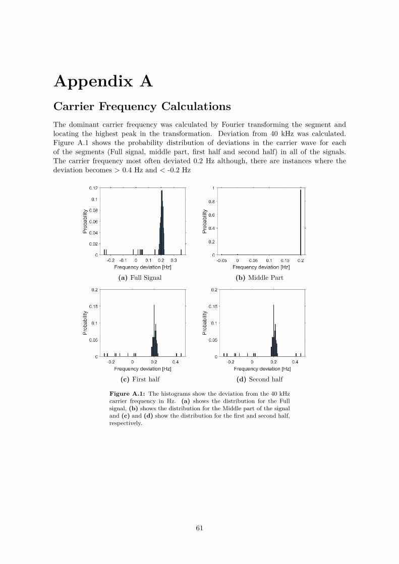
Appendix ACarrier Frequency CalculationsThe dominant carrier frequency was calculated by Fourier transforming the segment andlocating the highest peak in the transformation. Deviation from 40 kHz was calculated.Figure A.1 shows the probability distribution of deviations in the carrier wave for eachof the segments (Full signal, middle part, first half and second half) in all of the signals.The carrier frequency most often deviated 0.2 Hz although, there are instances where thedeviation becomes > 0.4 Hz and < -0.2 Hz

(a) Full Signal (b) Middle Part

(c) First half (d) Second half

Figure A.1: The histograms show the deviation from the 40 kHzcarrier frequency in Hz. (a) shows the distribution for the Fullsignal, (b) shows the distribution for the Middle part of the signaland (c) and (d) show the distribution for the first and second half,respectively.

61

Analysis of a Cardiac Displacement Signal Recorded with an ...

Documents

Transcript of Analysis of a Cardiac Displacement Signal Recorded with an ...