Singapore Management UniversityInstitutional Knowledge at Singapore Management University

Research Collection School of Social Sciences School of Social Sciences

1-2005

Analysis and Insights from a Dynamical Model ofNuclear Plant Safety RiskStephen HessSensortex, Inc.

Alfonso M. AlbanoSingapore Management University, alfonsoma@smu.edu.sg

John GaertnerElectronic Power Research institute

This Working Paper is brought to you for free and open access by the School of Social Sciences at Institutional Knowledge at Singapore ManagementUniversity. It has been accepted for inclusion in Research Collection School of Social Sciences by an authorized administrator of InstitutionalKnowledge at Singapore Management University. For more information, please email libIR@smu.edu.sg.

CitationHess, Stephen; Albano, Alfonso M.; and Gaertner, John, "Analysis and Insights from a Dynamical Model of Nuclear Plant Safety Risk"(2005). Research Collection School of Social Sciences. Paper 67.http://ink.library.smu.edu.sg/soss_research/67Available at: http://ink.library.smu.edu.sg/soss_research/67

ANY OPINIONS EXPRESSED ARE THOSE OF THE AUTHOR(S) AND NOT NECESSARILY THOSE OF THE SCHOOL OF ECONOMICS & SOCIAL SCIENCES, SMU

Analysis and Insights from a Dynamical Model of Nuclear Plant Safety Risk

Stephen M. Hess, Alfonso M. Albano, John P. Gaertner September 2005

Paper No. 14-2005

SSSMMMUUU EEECCCOOONNNOOOMMMIIICCCSSS &&& SSSTTTAAATTTIIISSSTTTIIICCCSSS WWWOOORRRKKKIIINNNGGG PPPAAAPPPEEERRR SSSEEERRRIIIEEESSS

To appear in: Reliability Engineering and System Safety

Analysis and Insights from a Dynamical Model of Nuclear Plant Safety Risk

Stephen M. Hess Sensortex, Inc.

515 Schoolhouse Road Kennett Square, PA, 19348, USA

Alfonso M. Albano* Visiting Professor

School of Economics and Social Sciences Singapore Management University

90 Stamford Road, Singapore 178903

John P. Gaertner Electric Power Research Institute

1300 Harris Boulevard Charlotte, NC, 28262, USA

* Permanent address: Department of Physics, Bryn Mawr College, Bryn Mawr, PA 19010, USA ABSTRACT

In this paper, we expand upon previously reported results of a dynamical systems model for

the impact of plant processes and programmatic performance on nuclear plant safety risk. We

utilize both analytical techniques and numerical simulations typical of the analysis of nonlinear

dynamical systems to obtain insights important for effective risk management. This includes use

of bifurcation diagrams to show that period doubling bifurcations and regions of chaotic

dynamics can occur. We also investigate the impact of risk mitigating functions (equipment

reliability and loss prevention) on plant safety risk and demonstrate that these functions are

capable of improving risk to levels that are better than those that are represented in a traditional

risk assessment. Next, we analyze the system response to the presence of external noise and

obtain some conclusions with respect to the allocation of resources to ensure that safety is

maintained at optimal levels. In particular, we demonstrate that the model supports the

importance of management and regulator attention to plants that have demonstrated poor

performance by providing an external stimulus to obtain desired improvements. Equally

important, the model suggests that excessive intervention, by either plant management or

regulatory authorities, can have a deleterious impact on safety for plants that are operating with

very effective programs and processes. Finally, we propose a modification to the model that

accounts for the impact of plant risk culture on process performance and plant safety risk. We

then use numerical simulations to demonstrate the important safety benefits of a strong risk

culture.

KEYWORDS: Nonlinear Dynamical Systems, Process Model, Risk Management

INTRODUCTION

In a previous paper [1], we presented an alternative approach to addressing the issue of the

impact of plant programmatic and process performance on nuclear power plant safety risk. We

developed a dynamical systems model that describes the interaction of important plant processes

on nuclear safety risk and discussed development of the mathematical model including the

identification and interpretation of significant inter-process interactions. We also performed a

preliminary analysis of the model that demonstrated that its dynamical evolution displays

features that have been observed at commercially operating plants. From this analysis, a few

significant insights were presented with respect to the effective control of nuclear safety risk, the

most important example being that significant benefits in effectively managing risk can be

obtained by integrating the plant operation and work management processes such that decisions

are made utilizing a multidisciplinary and collaborative approach. Finally, we noted that

although the model was developed specifically to be applicable to nuclear power plants, many of

the insights and conclusions obtained are likely applicable to other process industries.

In this previous paper, a dynamical systems model was developed that accounted for the

impact of the operations (O), work management (W), equipment reliability (E) and loss

prevention (L) functions on plant risk (R). These functions were defined as a mapping over the

domain space [-1, 1] with Xi = -1 defined to correspond to completely ineffective process

performance (i.e. a process for which there is no confidence that it will achieve its intended

function), Xi = 1 to completely effective process performance (i.e. a process for which there is

complete confidence that it will achieve its intended function) and Xi = 0 to be the point of

indifferent performance. Here we obtained the model (1)

R t O t W t( ) ( ) ( )+ = +1 O t O t W t W t O tWO WO( ) ( ) ( ) ( ) ( )+ = + +1 λ μ

W t W t O t E t L t O t W t E t W tOW EW LW OW EW( ) ( ) ( ) ( ) ( ) ( ) ( ) ( ) ( )+ = + + + + +1 λ λ λ μ μ (1)E t a E t a E t( ) ( ) ( )+ = +1 1 2

3 L t b L t b L t( ) ( ) ( )+ = +1 1 2

3 .

In this model, the coefficient λjk represents the linear coupling of process j on process k. As an

example, λOW represents the influence of the operations process on decisions made in the work

management process. Similarly, λWO represents the influence of the work management process

on decisions made in the operations process. The λjk thus provide a representation of how much

one process influences the other process in a unilateral manner. The coefficients μjk represent the

interactive (collaborative) coupling that occurs from process j on process k. Thus, μWO represents

the degree to which the operations and work management functions collaborate in operational

decision-making. In both cases, small values of the coupling coefficients (λ, μ ~ 0.01 – 0.05)

indicate minimal interaction between the processes, whereas large values (λ, μ ~ 1) indicate

significant levels of interaction.

As discussed in [1], we wish to reiterate that the primary benefit of this model is not in its

capacity to provide detailed quantitative estimates of changes in plant risk. The significance of

the model is that it provides a theoretical construct that can account for some of the features of

the impact of plant management and processes on commercial nuclear power plant safety risk.

As such, its analysis permits the development of insights that can be used to develop and

implement effective strategies to control safety risk at these facilities. As will be discussed in this

paper, the insights obtained from the model analysis qualitatively corroborate the results of

previous research and the opinion of numerous experts on the importance of management and

process factors to plant risk. Thus, the model can provide a construct from which these strategies

can be evaluated prior to implementation.

In the analysis of this model in [1], we demonstrated that the risk mitigating functions

(equipment reliability and loss prevention) possessed stable operating points at E = L = 0 (i.e. the

point of indifferent operation). Thus, we obtained an important simplification which permitted

use of analytical techniques. This simplification resulted in what we termed the “ROW” model

R t O t W t( ) ( ) ( )+ = +1 O t O t W t W t O tWO WO( ) ( ) ( ) ( ) ( )+ = + +1 λ μ (2)

W t W t O t O t W tOW OW( ) ( ) ( ) ( ) ( )+ = + +1 λ μ .

In addition to its utility in facilitating analysis, this simplified model also is important in that it is

generically applicable across a wide variety of process industries that either have not

implemented risk management functions and processes or where their impact is not significant.

BIFURCATIONS AND CHAOTIC DYNAMICS OF ROW SYSTEM

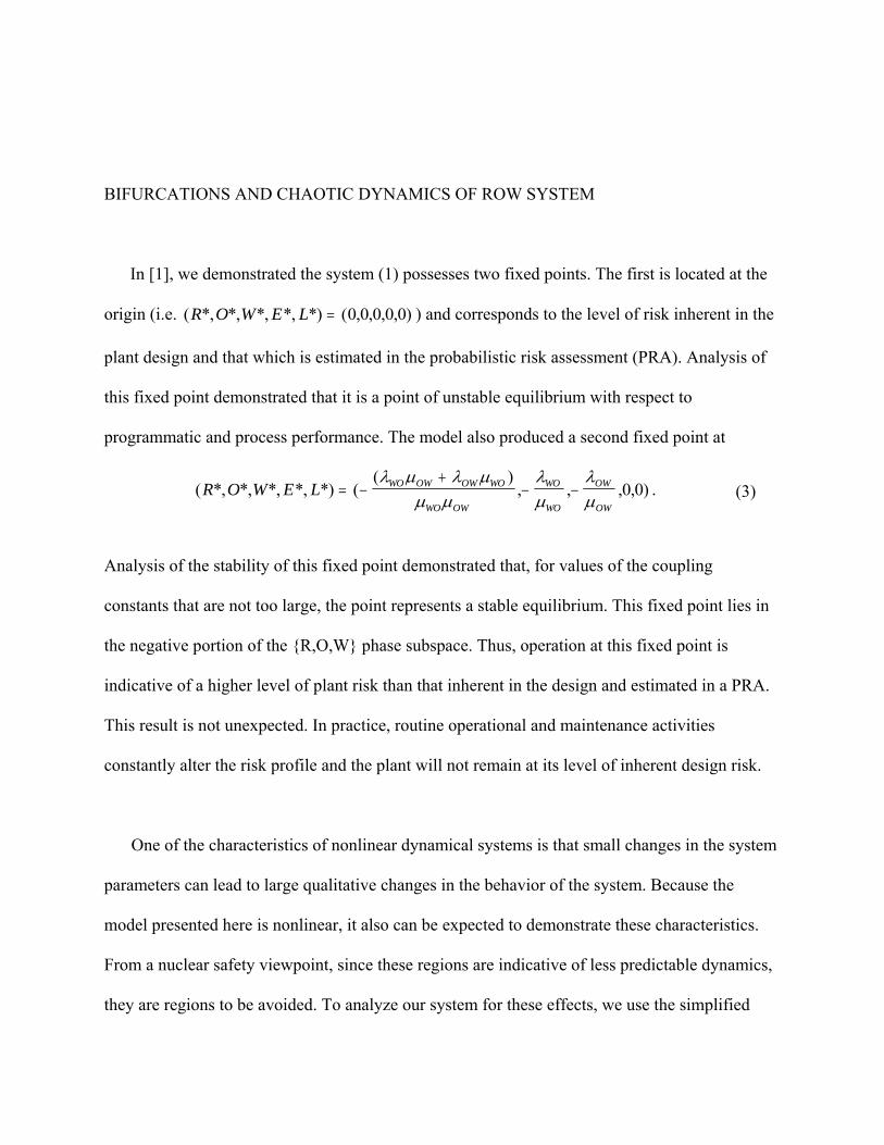
In [1], we demonstrated the system (1) possesses two fixed points. The first is located at the

origin (i.e. ( ) and corresponds to the level of risk inherent in the

plant design and that which is estimated in the probabilistic risk assessment (PRA). Analysis of

this fixed point demonstrated that it is a point of unstable equilibrium with respect to

programmatic and process performance. The model also produced a second fixed point at

*, *, *, *, *) ( , , , , )R O W E L = 0 0 0 0 0

( *, *, *, *, *) (( )

, , , , )R O W E L WO OW OW WO

WO OW

WO

WO

OW

OW= −

+− −

λ μ λ μμ μ

λμ

λμ

0 0 . (3)

Analysis of the stability of this fixed point demonstrated that, for values of the coupling

constants that are not too large, the point represents a stable equilibrium. This fixed point lies in

the negative portion of the {R,O,W} phase subspace. Thus, operation at this fixed point is

indicative of a higher level of plant risk than that inherent in the design and estimated in a PRA.

This result is not unexpected. In practice, routine operational and maintenance activities

constantly alter the risk profile and the plant will not remain at its level of inherent design risk.

One of the characteristics of nonlinear dynamical systems is that small changes in the system

parameters can lead to large qualitative changes in the behavior of the system. Because the

model presented here is nonlinear, it also can be expected to demonstrate these characteristics.

From a nuclear safety viewpoint, since these regions are indicative of less predictable dynamics,

they are regions to be avoided. To analyze our system for these effects, we use the simplified

ROW model (2) assuming the additional simplification in the interprocess couplings described in

[1]; i.e., we set λWO = λOW = λ and μWO = μOW = μ. With this simplification, the system of

equations becomes

R t O t W t( ) ( ) ( )+ = +1 O t O t W t W t O t( ) ( ) ( ) ( ) ( )+ = + +1 λ μ (4)

W t W t O t O t W t( ) ( ) ( ) ( ) ( )+ = + +1 λ μ .

For this system, the origin is an unstable fixed point and the second fixed point reduces to (-2λ/μ,

-λ/μ, -λ/μ). The primary motivation for this simplification is to facilitate analysis of the model

and develop useful insights. We note that setting the interprocess coupling parameters equal to

each other may not be appropriate for all applications of the model to real plants. However, there

are situations in which it is reasonable to expect the couplings between processes to be roughly

equal. As one example, when collaborative decision-making between processes is strong (i.e. μ

predominates over λ), it is likely that this collaboration will be reciprocal. Thus, if the work

management process inputs collaboratively in operational process decision-making, it is

reasonable that the converse also will apply.

For many dynamical systems, a stable fixed point can change stability as a control parameter

is varied. At a critical threshold of the parameter, this stable fixed point can become unstable and

be replaced by a system which oscillates between two points which are different from the

original stable point. For a system X(t), a period two solution occurs for X(t+2) = X(t) ≠ X(t+1)

[2]. Solving (4) for this condition indicates a period two bifurcation can occur for λ > 2. At

values greater than this, system bifurcations are possible. Thus, the model indicates that as the

individual processes are driven by internally generated objectives, their integrated impact on

other plant programs and safety risk can result in unanticipated results. Additionally, as this

linear coupling term is increased further, the system can undergo additional bifurcations leading

to the period doubling route to chaos. To provide an example of this behavior, Figure 1 shows a

bifurcation diagram for λ = 5 as the parameter μ is increased. In this diagram, performance of the

operations function (O) is displayed. Behavior of plant risk and the work management process is

similar.

In this diagram, the system bifurcates to a period two attractor at the value μ = 4.0. At

approximately μ = 4.74 the system bifurcates again into a period four attractor. This process

continues with further period doubling bifurcations. Between approximately 4.8 and 4.94, a

period three attractor is present. This region is particularly significant because existence of a

period three orbit implies chaotic dynamics [3]. This follows from Sharkovskii’s Theorem [4, 5].

This theorem provides a scheme for ordering the integers such that the existence of a period k

orbit implies the existence of periodic orbits for every higher ordered period. In this scheme,

consider the following ordering of all integers [12, p.135]

3 ► 5 ► 7 ► … ► 2·3 ► 2·5 ► 2·7 ► … ► 2n·3 ► 2n·5 ► 2n·7 ► … ► 2n ► … ►24 ► 23 ► 22 ►21 ► 1

(5)

with n ∞. In this sequence, the symbol ► should be understood to mean “follows” in the sequence.

Sharkovskii’s theorem states that the existence of a period j orbit implies the existence of all

periodic orbits of period k where k follows j in the ordering given in (5). For example, a period 8

orbit implies at least one period 4 orbit, which implies at least one of periods 2 and 1 also. Since three is

the last number in the sequence, existence of a period three orbit implies all other periodicities,

and thus chaotic dynamics. Thus, the presence of a period three orbit in Figure 1 indicates that

this system is capable of producing chaotic dynamics.

There are two additional items of significance with respect to this diagram. First, from a risk

management perspective, since performance changes rapidly in this region of the {R,O,W} phase

space, it will be difficult to effectively manage plant risk. Thus, these regions should be avoided.

Since values of λ this large are indicative of the individual process decision-makers driving the

decisions to meet their own objectives, these results indicate that individual departments and

work groups unilaterally pursuing their own agendas can have a detrimental impact on risk, with

the results of the decision-making process not always being adequately foreseen. However, a

second significant item relates to the behavior as μ is increased. At a sufficiently large value of μ,

which is indicative of the degree of collaboration between the operations and work management

processes, the results again become completely predictable (with significant risk reduction). This

is indicative of the collaboration between the majority of the organization’s members

outweighing the individual agendas of the few individuals attempting to control the decision

process. In the illustration presented here, μ is extremely large (μ = 5) which is indicative of an

extremely high level of interorganizational cooperation; and one which probably is not

achievable in practice. Thus, we obtain the insight that collaboration between the organizations

responsible for the operations and work management processes is an important component in

effectively managing plant risk and it can be concluded that it is not just the interaction between

the processes which is the important characteristic for managing risk, but the extent to which this

interaction is collaborative in nature. Therefore, to effectively control plant risk, organizations

should strive to maximize the degree of collaboration in the operations and work management

decision-making processes.

IMPACT OF RISK MITIGATION FUNCTIONS

In a commercial nuclear power plant, both the equipment reliability and loss prevention

functions are specifically intended to monitor performance, detect degraded conditions and

specify appropriate corrective actions for plant structures, systems and components. Thus, these

functions can be viewed as specifically addressing nuclear safety risk. Equipment reliability

encompasses those engineering and maintenance functions that specifically address the reliability

and availability of plant hardware. This function includes activities such as:

• developing and maintaining a long-term maintenance plan (preventive and predictive

maintenance programs),

• conducting surveillance and performance tests,

• analyzing performance and reliability of structures, systems and components,

• performing predictive maintenance.

Similarly, loss prevention encompasses those engineering and business functions that

specifically address the effectiveness of processes that prevent or mitigate safety consequences

that may occur due to unexpected events. This function includes activities such as:

• providing security measures,

• providing performance monitoring and improvement services,

• maintaining licenses and permits,

• performing emergency planning,

• providing fire protection.

The first question to be addressed is to what extent does good performance of either of these

programs compensate for poor performance in plant operations and work management. To

investigate this relationship, plant operations and work management performance were

simultaneously set to poor performance at a level which is representative of the lowest level

which likely would be tolerated by either plant management or the regulatory authorities. This

minimum level of acceptable performance was set at X = -0.1 for any of the modeled processes,

(i.e. X = {R,O,W,E,L}). This level was selected based on the following reasoning. Since the

industry is strictly regulated, the permitted level of plant performance will not be allowed to

deviate far from the level of inherent risk. Historical actions of the United States Nuclear

Regulatory Commission issuing shutdown orders to plants for management deficiencies and

plant operators taking similar self imposed actions when performance degradations are identified

lend support to the conclusion that significant performance degradation will not be tolerated.

Thus, choosing a negative 10% deviation within the domain space of one or more of the modeled

processes provides a reasonable estimate of the maximal degraded condition that would be

considered acceptable before significant corrective actions (i.e. plant shutdown by the plant

operator or regulatory body) would be taken.

The benefit of the risk mitigating functions can be shown explicitly by observing their effects

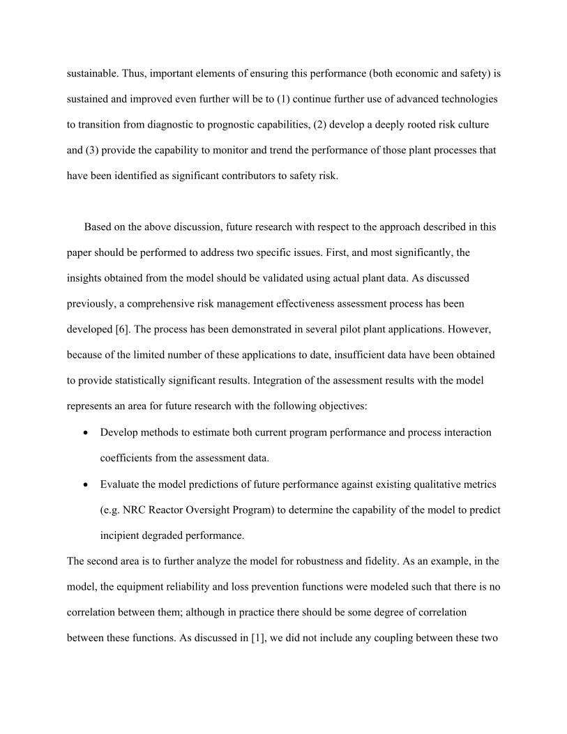
on plant risk. Figure 2 provides an example of where effective risk mitigating functions can

operate to overcome poor initial performance of the operations and work management functions.

In this simulation, the representative values for process couplings were chosen so that the

dominant interactions were linear; thus the beneficial impact of interactive decision-making was

present but not dominant. Also, the couplings of the risk mitigation functions were taken to be

only half that of the quadratic couplings between the operations and work management

processes. This led to the following selection of coupling parameters for the demonstration: λWO

= λOW = λ = 0.5, μWO = μOW = μ = 0.2, and λLO = λEW = λLW = μEW = 0.1. To permit illustration of

the effect of these functions, both were assumed to possess highly qualified staff with significant

plant experience (a1 = b1 = 0.8). For this case, increasing the initial performance of the equipment

reliability and loss prevention functions to E(0) = L(0) = 0.4474 results in these processes

eventually reversing the trend in increasing plant risk and reducing it below the inherent level.

Note that this initial value of E(0) / L(0) represents a critical value (to four significant figures).

For initial performance below this point, the loss prevention functions are not capable of

restoring risk performance to an acceptable level; whereas better initial performance of these

functions will restore performance faster. We note that we interpret R 1 for t > 30 as the risk

mitigating functions operating at a sufficiently high level of performance that they are capable of

reducing plant risk well below the inherent level. An example of this would be the case where

the plant’s predictive and preventive maintenance programs are functioning effectively so that

observed equipment failure rates are significantly below the levels that have been assumed in the

PRA.

The results displayed in Figure 2 provide an additional insight which is significant to the

management of nuclear plant safety risk. In this example, the equipment reliability and loss

prevention functions were capable of altering the performance of the operations and work

management processes sufficiently to reverse the deleterious trend in plant risk. However, these

dynamics required a significant period of time to occur. During this time, plant risk performance

remained in a degraded state. This behavior reinforces the conclusion that management must

continually focus on maintaining strong performance for those plant processes that provide a

direct impact on risk, i.e. operations and work management. It also indicates that the specific risk

mitigation processes will be maximally effective at controlling risk only if the operations and

work management functions are already operating at an effective level.

EFFECTS OF ADDITIVE NOISE

In any practical application of the dynamical risk model to analyze actual plant data, there is

anticipated to be a significant degree of uncertainty in the values of the estimated coupling

constants and in the actual level of process performance. This problem is exacerbated by the fact

that there do not exist any direct measures of these parameters. Currently, an assessment

approach has been developed [6] and preliminary results reported [7] that utilizes a structured

assessment to evaluate the effectiveness of risk management at operating plants. Further research

is being conducted to quantify these results so that they can be trended over time and used to

develop estimates of the model parameters. Because the model is nonlinear, system dynamics

possess strong sensitivity to initial conditions. Thus, these uncertainties will result in uncertainty

in the model predictions. Due to this, it is important to analyze these effects. An effective method

of simulating this effect is to introduce noise into the model equations. This noise can be viewed

as being from two distinct sources. First, the uncertainty of the values of the coupling constants

and actual performance provide a source that is internal to the system. This type of noise is

usually called “multiplicative noise” or “dynamical noise” and is expected to be random in

nature. Thus, it is well modeled as white noise. Second, the external environment also provides a

source of noise. This type of noise typically is referred to as additive noise. Sources of this type

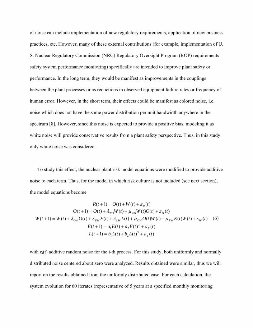
of noise can include implementation of new regulatory requirements, application of new business

practices, etc. However, many of these external contributions (for example, implementation of U.

S. Nuclear Regulatory Commission (NRC) Regulatory Oversight Program (ROP) requirements

safety system performance monitoring) specifically are intended to improve plant safety or

performance. In the long term, they would be manifest as improvements in the couplings

between the plant processes or as reductions in observed equipment failure rates or frequency of

human error. However, in the short term, their effects could be manifest as colored noise, i.e.

noise which does not have the same power distribution per unit bandwidth anywhere in the

spectrum [8]. However, since this noise is expected to provide a positive bias, modeling it as

white noise will provide conservative results from a plant safety perspective. Thus, in this study

only white noise was considered.

To study this effect, the nuclear plant risk model equations were modified to provide additive

noise to each term. Thus, for the model in which risk culture is not included (see next section),

the model equations become

)()()()1( ttWtOtR Rε++=+ )()()()()()1( ttOtWtWtOtO OWOWO εμλ +++=+

)()()()()()()()()()1( ttWtEtWtOtLtEtOtWtW WEWOWLWEWOW εμμλλλ ++++++=+ (6)

)()()()1( 321 ttEatEatE Eε++=+

)()()()1( 321 ttLbtLbtL Lε++=+

with εi(t) additive random noise for the i-th process. For this study, both uniformly and normally

distributed noise centered about zero were analyzed. Results obtained were similar, thus we will

report on the results obtained from the uniformly distributed case. For each calculation, the

system evolution for 60 iterates (representative of 5 years at a specified monthly monitoring

interval) was determined. At the end of this period, the systems were evaluated to ascertain if the

risk had increased or decreased at the end of the period. An ensemble of 1000 systems were

permitted to evolve for each set of noise over the range [-e, e] with e varied from 0 to 0.30 in

increments of 0.005. In all simulations, the plant initially was set at the inherent level of risk due

to its design (i.e. R(0) = 0) and all programs were set to the indifferent level of performance

(O(0) = W(0) = E(0) = L(0) = 0). The statistic measured was the fraction of systems which

achieved improved risk performance at the end of the simulated period, i.e.

S ≡ Number of systems with R(t=60)>0 / Total number of systems. (7)

We note that simulating system evolution over a 5 year timeframe without any modification to

the coupling parameters may be considered to be unrealistic. Changes in business and regulatory

conditions certainly require some response to plant operating practices over this time period.

However, as described in [1] (and additional references cited therein), nuclear power plant

operation has been characterized as a “machine bureaucracy”. Thus, any changes that are

implemented require significant periods of time to propagate through the system and the impact

of them to be made manifest. Experience with regulatory enforced shutdowns in the United

States indicates a long time is required to improve poor performance (typically two years

duration for the plant shutdown with several more years of closely monitored operation required

to attain strong levels of performance). Thus, by examining the evolution of the system over the

identified 5 year period, one can obtain some insight into the magnitude and relative timeframe

of a perturbation required to impact performance.

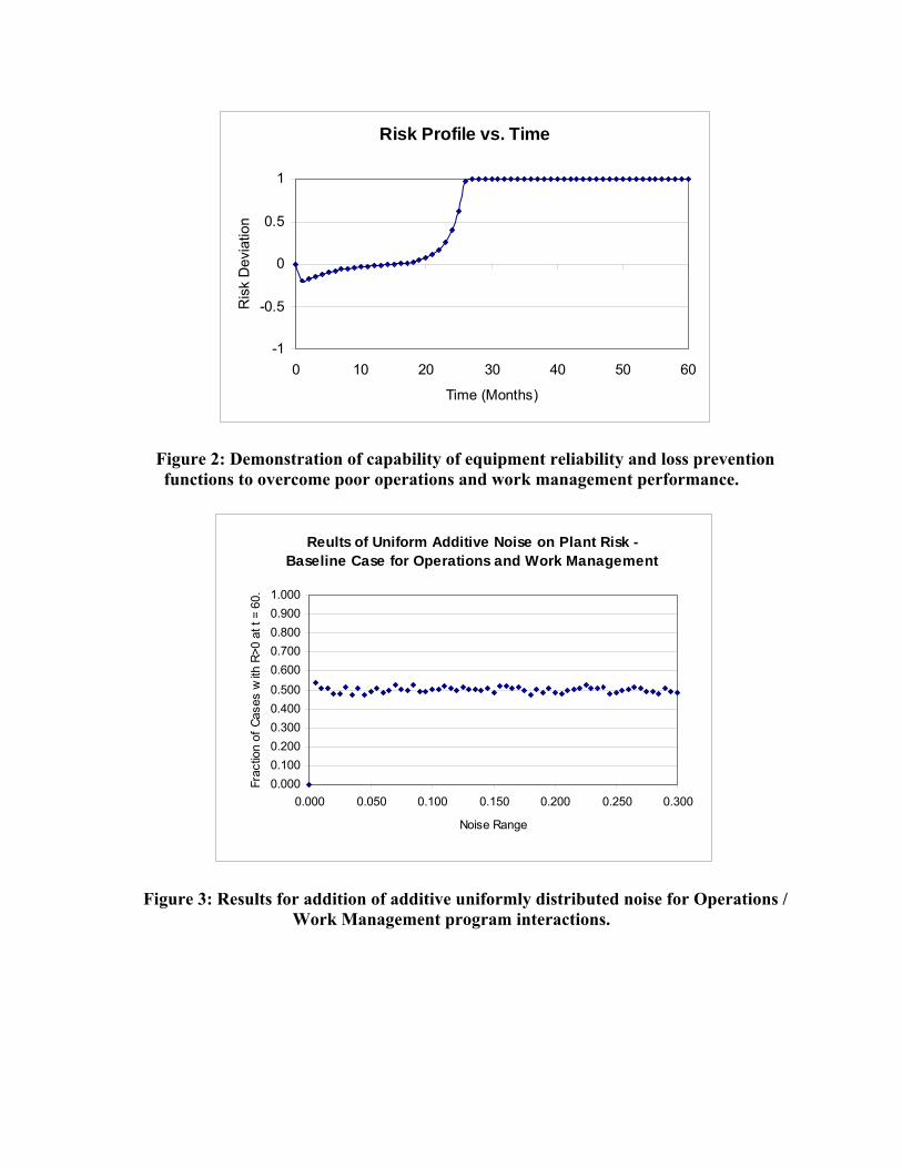
For the initial application of noise to the model, each program was assumed to operate

independently of every other program; i.e., all coupling constants were set equal to zero. As

expected, the system obtained a value of approximately 0.5 for the S statistic regardless of the

level of noise input. Next, the Operations and Work Management functions were assumed to be

present and interactive. However, the risk mitigating Equipment Reliability and Loss Prevention

functions were assumed to not contribute. As discussed earlier, this model is representative of a

much broader class of industrial facilities for which the risk mitigating functions are either not

present or only recently implemented. Direct couplings between O and W were assumed to be

moderate (λWO = λOW = 0.25) and the interactive coupling to be occasional (μWO = μOW = 0.1)

where the interpretation of the coupling values is as described in [1]. These values were selected

because they are believed to represent typical values for domestic commercial nuclear plants

currently in operation. They also are values which are well below that required for bifurcations to

occur. Since the additive noise is symmetrically distributed about zero, we expect the S statistic

also should be near S = 0.5 for all values of additive noise. This result was obtained via the

simulation and is shown in Figure 3. Similar results were obtained when the equipment

reliability and loss prevention functions were included under the same conditions.

Next, we investigated the impact of additive uniformly distributed noise for the case of an

initial positive performance of the risk mitigating Equipment Reliability and Loss Prevention

functions. Because these programs explicitly are intended to limit plant safety risk and improve

operational performance, they would be expected to increase the plant’s risk performance (R).

Thus, as E(0) and L(0) are increased, the statistic S also should increase with S 1 as the initial

performance of these functions becomes sufficiently effective. Since the noise is symmetrically

distributed about zero, higher amounts of noise would be expected to impact performance by

reducing S as the noise level increases. Figures 4(a) and (b) provide results for two of the cases

analyzed. Figure 4(a) displays results for the equipment reliability and loss prevention functions

initially slightly effective (E(0) = L(0) = 0.01) while Figure 4(b) provides results for the case of

moderately effective initial performance (E(0) = L(0) = 0.1). From these curves, one can see that

as the initial performance level of E or L increases, S also increases. However, for a given initial

condition, increasing the amount of noise limits the extent to which S increases; i.e. if εl

represents the low noise state and εh the high noise state with |εl| < |εh|, then S(εl) > S(εh)). Similar

calculations were performed for an initial negative performance of the risk mitigation functions

with results that basically mirrored those for the case of E and L having initially good

performance.

In the previous analyses, the additive noise was considered to be induced external to the

system and provide a stochastic component to performance. This noise can be interpreted as the

effects due to the external environment and includes factors such as perturbations due to the

general business climate and responses to regulatory mandates. The results obtained can be

interpreted in the following manner. For initial operation of the plant at indifferent levels of

performance and coupling parameters that are believed to be representative of current

commercial plants, deviation from the inherent risk level is sensitive to the external noise

imposed on the system. This result can be explained by the external environment having a

roughly equal potential to provide a positive or a negative effect. As an example of a negative

impact, a general economic slowdown can result in decreased operating revenue for the plant

owner. These business conditions will impose additional economic constraints on the plant that

can be manifest by items such as staff reductions or deferred maintenance. An example of a

positive effect would be the implementation of new information management software that

increases personnel efficiency and, thus, results in improved performance. However, there is

concern that some recent changes in the industry, particularly the effects due to the deregulation

of electrical generation, could result in economic pressures to reduce costs with potential for

concomitant reduction in effective risk management. This external influence could be modeled

by the addition of colored noise that provides a negative performance bias to each of the

processes. In contrast, programmatic and process changes that are intended to address identified

deficiencies can be modeled (at least in the short term) by the addition of colored noise that

provides a positive performance bias to each of the processes. These conditions were not

evaluated here and constitute a task for future research.

These results suggest several conclusions that could be drawn with respect to the effect of

external influences and the interactions with the specific risk management functions of

equipment reliability and loss prevention. For cases where performance of these functions is

poor, external perturbations typically produce a beneficial effect. This effect also increases as the

magnitude of the influence is increased. This result can be interpreted in the following manner.

Since performance of these functions is initially poor, externally induced events have a greater

likelihood of providing beneficial changes in performance. As an example, for plants with

identified degraded performance levels, either the plant owner or the regulatory authority will

attempt to identify the degradation and implement actions to address their basic causal factors.

Although not all of these changes will provide the intended effect, the majority will, and thus

overall performance can be anticipated to improve. Additionally, the poorer the initial

performance, the greater are the changes that are necessary to correct the situation. Thus, the

dynamical systems model provides support for the commonly accepted premise that, for complex

technologies which have the potential to impact public health and safety, regulation by an

unbiased external agency is an important element in ensuring that performance degradations that

can impact the public do not occur. Additionally, the result of these simulations also suggests

that these regulatory resources are best expended on facilities which demonstrate deficient

performance levels.

A second conclusion can be drawn from the case of effective performance of the risk

management functions. In this case, the addition of external noise typically produces a

detrimental effect which increases as the noise level increases. This result indicates that for well

functioning programs, most external stimuli are more likely to degrade performance than to

enhance it. This result also is not surprising. Systems that are operating at high efficiency

typically require significant effort to maintain this high level of effectiveness. For plants which

have developed effective risk management, the resources required to achieve these benefits need

to be used in a manner which is effective and efficient. Because these resources are limited,

responding to external perturbations will detract from performing the required beneficial risk

management functions. Since most of these external influences will not provide as much benefit

to performance as the functions typically performed by these resources, they will tend to detract

from the good overall performance. From a regulatory perspective, this suggests that the amount

of external intervention should be minimized at plants which exhibit effective risk management

and operational performance. For example, in the extreme case of a plant that possesses

comprehensive and effective risk management and demonstrates exemplary performance, the

regulatory function could theoretically be limited to monitoring and trending performance. We

note that this constitutes the basic premise of a regulatory structure that is risk-informed and

performance-based. Thus, this characteristic of the dynamical risk model provides additional

support to the safety and economic benefits that can be achieved by transforming to this

regulatory structure.

ADDITION OF RISK CULTURE TO THE MODEL

An important component to controlling plant risk is the development of a plant risk culture.

This culture can be characterized by understanding and awareness, by all plant personnel, of the

potential impact of operational and maintenance tasks on plant safety. Additionally, in an

effective risk culture, plant decision-making processes incorporate an explicit consideration of

the potential safety impact of plant activities and decisions and provide appropriate levels of

oversight and controls to mitigate risk. Although not formally demonstrated via specific results

obtained from traditional plant risk assessment models, it is logically consistent to assume that

the stronger the risk culture is made at a plant, the safer the plant will operate. In terms of the

dynamical systems model, this contribution should be manifest both directly in the coupling of

the risk mitigation processes to plant risk performance and also in the performance of the

individual processes themselves. In this section, we specifically address a modification to the

model (1) to address the impact of risk culture on performance.

In this discussion, we explicitly use the term “risk culture” as the defining characteristic that

impacts nuclear plant safety risk. The use of this terminology is deliberate. Recently, significant

research has been conducted throughout process industries, including nuclear power generation,

on the impact of what has been called a plant “safety culture”. However, although this

terminology has become accepted, it does not have a standard definition, meaning different

things to different researchers and across different industries [9, 10]. For applications to

commercial nuclear power plants, the term has been defined by the International Nuclear Safety

Advisory Group (INSAG). INSAG-4 [11] defines safety culture as “…that assembly of

characteristics and attitudes in organizations and individuals which establishes that, as an

overriding priority, nuclear plant safety issues receive the attention warranted by their

significance”. However, as discussed in [10], there are several problems with this approach; the

most significant being lack of development of a linkage between safety culture and how it

impacts human performance and reliability and the inability to establish the link between

achieving a “good” safety culture and safe plant performance. Additionally, from our

perspective, by including attitudes and values within the operational definition, safety culture

possesses a very broad context, for example including those attributes associated with normal

industrial safety practices. Because of this broad definition of the term safety culture, for the

dynamical systems model, we define a much more limited concept which we call risk culture. By

this term, we refer to the extent to which the plant considers nuclear safety risk as a fundamental

input into the various decision-making processes. Additionally, we consider the extent to which

this occurs to be measurable and demonstrable [7]. Thus, as defined here, risk culture can be

considered as a subset of safety culture with the specific objective of effectively controlling plant

safety risk.

Modeling of Risk Culture

We propose to incorporate the effect of risk culture in the dynamical systems model by

making the following assumptions. First, the extent to which an effective risk culture has been

achieved predominantly is a plant level effect. This is due to the organization’s culture being

strongly dependent upon the facility’s management philosophy and business practices. Thus, in

the model, the effect of the risk culture will apply to each plant process in the same way. Second,

the impact of risk culture is expected to have the following effects on the individual plant

processes. First, a point of operational indifference should be a fixed point of the system. This

assumption is due to a combination of economic and regulatory factors. From an economic

standpoint, implementing an effective risk culture is expensive in terms of resource application.

Providing appropriate personnel training, obtaining necessary technology and assigning qualified

personnel to analyze the risk associated with various activities all require a significant

commitment of human and monetary resources. Because these resources are limited by economic

considerations, there will be strong incentives to minimize their application, and thus limit their

effectiveness. This characteristic has been, in a qualitative sense, observed both at nuclear plants

and throughout industrial facilities in general, particularly in businesses in which competitive

pricing pressures are manifest. Conversely, poor operational performance can result in

significant regulatory pressure (including, if necessary, regulatory mandated plant shutdowns) to

force enhanced management effectiveness and improve operational performance. These

competing forces thus will tend to drive the risk culture to its point of indifferent performance,

i.e. one that utilizes a minimal level of resources to achieve a level of performance that is

acceptable from the viewpoint of both plant management and the regulatory authority. Second,

for a plant with an effective risk culture, this culture is expected to support maintaining effective

process performance, i.e. it should impede process performance from returning to the point of

indifference. Conversely, if process performance is poor, an effective risk culture should cause a

rapid improvement in the performance, at least back to a level of indifferent performance.

Finally, the model should revert to the previous model for a plant in which no discernable risk

culture has developed.

A mathematical function that provides the characteristics described above is a quadratic.

Thus, for each process, the effect of the plant risk culture can be incorporated into the process

model by including a term of the form

2)()1( tXtX cIc β=+ (8)

where XC represents the culture component of the I-th program performance (I = {O, W, E, L})

at the t-th iterate and βI represents the risk culture of the I-th process. Further, because a major

determinant of the risk culture possessed by different plant organizations is determined by global

management factors, the risk culture of each of the individual processes can be modeled as

)1( XX δβββ += (9)

where β is the global component of the risk culture and δβX is the deviation from this value for

the particular process. For this analysis of the impact of risk culture, we assume the culture is set

at the global level, thus we set δβX = 0 for all processes. With these modifications to incorporate

the effect of the plant risk culture, the dynamical systems risk model becomes

)()()1( tWtOtR +=+ 2)()()()()()1( tOtOtWtWtOtO WOWO βμλ +++=+

2)()()()()()()()()()1( tWtWtEtWtOtLtEtOtWtW EWOWLWEWOW βμμλλλ ++++++=+ (10)3

22

1 )()()()1( tEatEtEatE ++=+ β 3

22

1 )()()()1( tLbtLtLbtL ++=+ β .

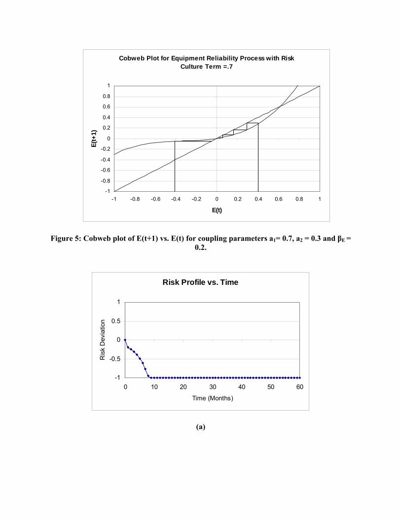
The effect of risk culture on a process function is shown in Figure 5 which shows a cobweb plot

[12] of the equipment reliability function with the cultural term included. Notice at these values

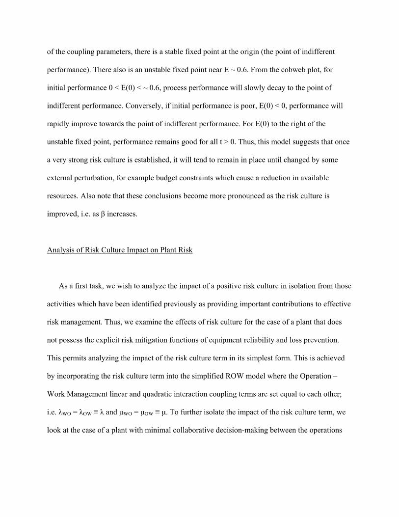
of the coupling parameters, there is a stable fixed point at the origin (the point of indifferent

performance). There also is an unstable fixed point near E ~ 0.6. From the cobweb plot, for

initial performance 0 < E(0) < ~ 0.6, process performance will slowly decay to the point of

indifferent performance. Conversely, if initial performance is poor, E(0) < 0, performance will

rapidly improve towards the point of indifferent performance. For E(0) to the right of the

unstable fixed point, performance remains good for all t > 0. Thus, this model suggests that once

a very strong risk culture is established, it will tend to remain in place until changed by some

external perturbation, for example budget constraints which cause a reduction in available

resources. Also note that these conclusions become more pronounced as the risk culture is

improved, i.e. as β increases.

Analysis of Risk Culture Impact on Plant Risk

As a first task, we wish to analyze the impact of a positive risk culture in isolation from those

activities which have been identified previously as providing important contributions to effective

risk management. Thus, we examine the effects of risk culture for the case of a plant that does

not possess the explicit risk mitigation functions of equipment reliability and loss prevention.

This permits analyzing the impact of the risk culture term in its simplest form. This is achieved

by incorporating the risk culture term into the simplified ROW model where the Operation –

Work Management linear and quadratic interaction coupling terms are set equal to each other;

i.e. λWO = λOW ≡ λ and μWO = μOW ≡ μ. To further isolate the impact of the risk culture term, we

look at the case of a plant with minimal collaborative decision-making between the operations

and work management processes, i.e. we set the quadratic operations to work management

coupling to zero (μ = 0). This results in the following simplified model

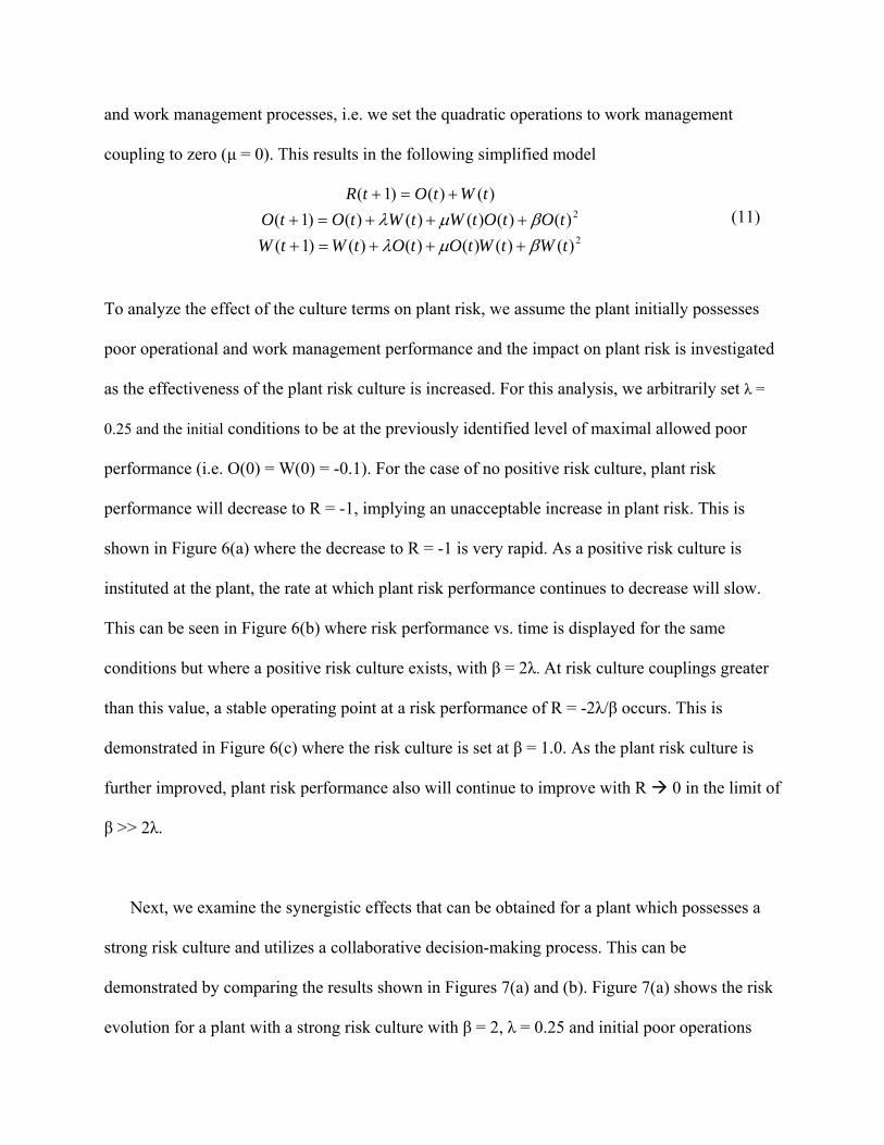
)()()1( tWtOtR +=+ 2)()()()()()1( tOtOtWtWtOtO βμλ +++=+ (11)2)()()()()()1( tWtWtOtOtWtW βμλ +++=+

To analyze the effect of the culture terms on plant risk, we assume the plant initially possesses

poor operational and work management performance and the impact on plant risk is investigated

as the effectiveness of the plant risk culture is increased. For this analysis, we arbitrarily set λ =

0.25 and the initial conditions to be at the previously identified level of maximal allowed poor

performance (i.e. O(0) = W(0) = -0.1). For the case of no positive risk culture, plant risk

performance will decrease to R = -1, implying an unacceptable increase in plant risk. This is

shown in Figure 6(a) where the decrease to R = -1 is very rapid. As a positive risk culture is

instituted at the plant, the rate at which plant risk performance continues to decrease will slow.

This can be seen in Figure 6(b) where risk performance vs. time is displayed for the same

conditions but where a positive risk culture exists, with β = 2λ. At risk culture couplings greater

than this value, a stable operating point at a risk performance of R = -2λ/β occurs. This is

demonstrated in Figure 6(c) where the risk culture is set at β = 1.0. As the plant risk culture is

further improved, plant risk performance also will continue to improve with R 0 in the limit of

β >> 2λ.

Next, we examine the synergistic effects that can be obtained for a plant which possesses a

strong risk culture and utilizes a collaborative decision-making process. This can be

demonstrated by comparing the results shown in Figures 7(a) and (b). Figure 7(a) shows the risk

evolution for a plant with a strong risk culture with β = 2, λ = 0.25 and initial poor operations

and work management performance (O(0) = W(0) = -0.1). As can be seen, this system will reach

a stable operating point at the very poor risk performance level of R = -0.25. For this plant,

improvement in risk performance above this level can be obtained by increasing the level of

collaboration in the operations and work management decision-making processes. Figure 7(b)

shows this improvement for a plant that possesses both a very strong risk culture and strongly

collaborative decision-making processes. For this case, (λ = 0.25, μ = β = 2), plant risk

performance is seen to be much improved above the level shown in Figure 7(a). Thus, the impact

of an effective risk culture can be viewed as similar to that due to effective collaboration between

the operations and work management decision processes. Note however, that because the

specific risk management processes (equipment reliability and loss prevention) are not present,

risk performance will still be below the inherent level due to the plant design. Thus, a significant

conclusion from this analysis is that a strong plant risk culture combined with effective

interactive decision-making in the operations and work management processes can result in a

significant improvement in plant safety risk with the two attributes combining to provide benefits

beyond those which can be obtained from either attribute by itself.

Effects of Positive Risk Culture

A question of fundamental importance with respect to risk culture is to what extent can it

impact (i.e. improve) safety performance. A second related question is what time frame is

required for this impact to be observed. A fruitful approach to evaluate these questions is to

apply the methods used in the analysis of dynamical systems to identify conditions necessary for

the system to remain in the region where R > 0. This analysis requires identification of the basin

of attraction for initial conditions and model coefficients to obtain performance such that R

remains positive and is similar to those which are employed to numerically generate the

Mandelbrot set. In this paper we provide a very brief discussion of the concept of basin of

attraction in the one-dimensional case. We then employ this concept to demonstrate how an

increasingly effective risk culture contributes to achieving effective risk management by driving

the system to operate in the region where R > 0.

An important question in the analysis of all physical systems is the determination of the

ultimate fate of an arbitrary initial point in the system. This question essentially asks what is the

behavior for an arbitrary point as t ∞. A system for which all initial conditions approach a

single point is termed globally stable. This can be demonstrated in a simple manner via the

elementary ordinary differential equation

axx −=& (12)

for a > 0 subject to the initial condition x(0) = x0. In this discussion, we illustrate the concepts

using differential equations because they are more familiar. However, they apply equally to maps

such as the dynamical risk model. One can solve (12) via elementary means to obtain the simple

exponential decay

atextx −= 0)( (13)

One can see from this solution that x 0 as t ∞ for any finite initial condition x0. Thus, the

basin of attraction for the origin is the entire interval (-∞, ∞).

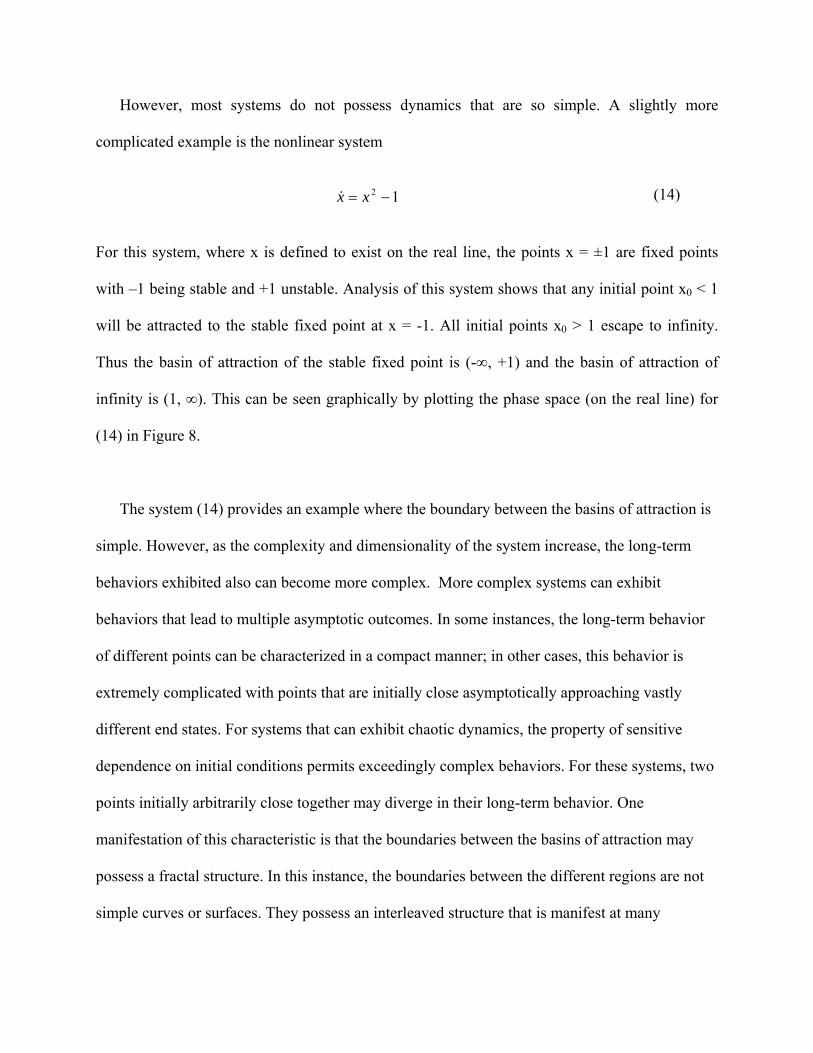
However, most systems do not possess dynamics that are so simple. A slightly more

complicated example is the nonlinear system

12 −= xx& (14)

For this system, where x is defined to exist on the real line, the points x = ±1 are fixed points

with –1 being stable and +1 unstable. Analysis of this system shows that any initial point x0 < 1

will be attracted to the stable fixed point at x = -1. All initial points x0 > 1 escape to infinity.

Thus the basin of attraction of the stable fixed point is (-∞, +1) and the basin of attraction of

infinity is (1, ∞). This can be seen graphically by plotting the phase space (on the real line) for

(14) in Figure 8.

The system (14) provides an example where the boundary between the basins of attraction is

simple. However, as the complexity and dimensionality of the system increase, the long-term

behaviors exhibited also can become more complex. More complex systems can exhibit

behaviors that lead to multiple asymptotic outcomes. In some instances, the long-term behavior

of different points can be characterized in a compact manner; in other cases, this behavior is

extremely complicated with points that are initially close asymptotically approaching vastly

different end states. For systems that can exhibit chaotic dynamics, the property of sensitive

dependence on initial conditions permits exceedingly complex behaviors. For these systems, two

points initially arbitrarily close together may diverge in their long-term behavior. One

manifestation of this characteristic is that the boundaries between the basins of attraction may

possess a fractal structure. In this instance, the boundaries between the different regions are not

simple curves or surfaces. They possess an interleaved structure that is manifest at many

different scales [12]. There are numerous examples of this behavior, the most famous of which is

that due to Mandelbrot (which results in the Mandelbrot set) [13].

The Mandelbrot set is obtained by consideration of the map [14]

ckzkz +=+ 2)()1( (15)

where z is a complex variable and c a complex constant. This system has fixed points at values

z* = [1 ± (1 – 4c)1/2 ] / 2. Fixed points z* for which –¾ < c < ¼ are stable. Iterates of the map for

values of c < -2 or c > ¼ escape to infinity. The dynamics of (15) can be analyzed by iterating

the initial value z(0) = 0 for many values of the constant c and observing whether the point

escapes to infinity. The result of this process produces the Mandelbrot set. This set exhibits a

complicated structure with increasing detail as we look at smaller regions of the parameter c. For

each point c in the set, there are orbits that remain bounded and orbits that do not. The boundary

of the basin of infinity is called a Julia set. We can analyze the points that are not in the

Mandelbrot set by characterizing their rate of divergence. For these points, we find their structure

to be fractal. We now make use of this technique to analyze the effect of plant risk culture on the

dynamics of the nuclear plant risk model.

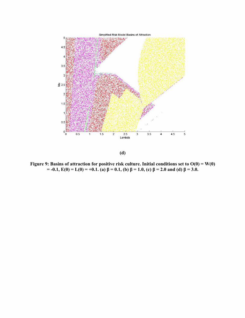
To analyze the impact of risk culture on the dynamical systems risk model, we perform a

numerical simulation to estimate the basin of attraction for R 1 assuming initial poor

operational and work management performance O(0) = W(0) = -0.1. Since these conditions are

expected to be near the limit of what would be permitted by either plant management or the

regulatory authority, they provide a very stringent test of the impact of a beneficial plant risk

culture. To simplify the calculations, we set model coefficients that are anticipated to be similar

equal to each other. This results in the following system of equations

)()()1( tWtOtR +=+ 2)()()()()()1( tOtOtWtWtOtO βμλ +++=+

2)()()()()()()()()()1( tWtWtEtWtOtLtEtOtWtW βωμωωλ ++++++=+ (16) 3

22

1 )()()()1( tEatEtEatE ++=+ β 3

22

1 )()()()1( tLbtLtLbtL ++=+ β .

In the simulations, like coefficients were set equal to each other with a1 = b1 = 0.7 and ω =

0.05. For each calculation, 50000 points were obtained and classified into the six categories

listed in Table 1. In the figure that displays the results (Figure 9), only orbits that reached the

“perfect” risk condition R = 1 within 60 iterations are shown. Thus, these points clearly are

within the basin of attraction of R = 1. Regions shown in white indicate that the system has not

evolved to R = 1 within this timeframe. Thus, it is indeterminate whether these points are within

this basin of attraction. Note that from a strictly risk management viewpoint, the objective would

be to avoid operation in these regions in preference to regions where R 1 much more rapidly.

The calculations shown here were conducted assuming good equipment reliability and loss

prevention performance E(0) = L(0) = +0.1. Results are provided in Figures 9(a) through (d) for

risk culture values of β = 0.1, 1.0, 2.0 and 3.0 respectively.

As expected, a small positive risk culture will provide a small impact on plant risk. This can

be seen in Figure 9(a) where a very large value of the operations – work management coupling

(μ) is required to drive risk performance to its maximal value within a reasonable time. Recall

that the iteration interval of the model was defined in [1] to be 1 month; thus at the small

beneficial risk culture assumed in this simulation (β = 0.1), μ must be very large (of the order 4

or more) to significantly improve plant risk within the space of a few years. However, this figure

provides an important insight into the importance of a strong risk culture. Notice that once we

enter the basin of attraction for R 1, small improvements in the operations – work

management collaborative interaction term result in a very rapid decrease in the time required to

reach R = 1. This is demonstrated in Figure 9(a) by the fact that the region where the time

required to reach R = 1 is long (50 < t < 60 iterations represented by the dark blue region) is very

thin. This effect is seen to persist as risk culture is improved as shown in Figures 9(b) through (d)

(β = 1, 2 and 3 respectively). This result suggests that there is a synergistic effect between a

strong risk culture, the plant decision-making processes and improved safety risk.

As plant risk culture improves further, it becomes readily apparent that a strong risk culture

can have a tremendous impact on improving plant risk performance. As expected, at modest

levels of plant risk culture, the operations and work management functions must be strongly

interactive to overcome the initial degree of poor performance assumed in these simulations.

However, as the plant risk culture becomes stronger, the degree to which this interaction must

occur diminishes. As plant risk culture further improves to a high level, e.g. β ~ 3, the culture is

strong enough to be effective at reducing plant risk in a very rapid manner. Notice that this effect

occurs regardless of the interactive coupling between the operations and work management

processes. From a practical standpoint, development of a strong risk culture also could be

expected to provide an impact on improving the dynamics of this interaction. Since this is not

included in the model (the interaction coefficients are treated as constants), the actual

effectiveness of the plant culture is most likely understated by the model for plants that have

developed a strong risk culture.

Finally, model simulations using this approach reveal a rich and complex structure inherent

in the system dynamics. Figure 10 provides results for a simulation for a plant where the risk

mitigating functions are assumed to operate at the indifferent level of performance. In this

simulation, the initial conditions were set to O(0) = 0.05 and W(0) = -0.025 and β was set to β =

0 (no risk culture). For this system, the operations process performance is sufficiently strong to

overcome the initial poor work management performance and permit the plant to evolve to a

state where risk performance can be sustained at R > 0. Figure 10 provides results for 25,000

trajectories over the subinterval 0 ≤ λ ≤ 0.2 and 0 ≤ μ ≤ 5. In this figure, we can see that different

combinations of λ and μ in this region can result in a wide range of the number of iterations

required to reach R = 1. This behavior of arbitrarily close points (in λ – μ space) resulting in

significantly different times required to reach R = 1 suggests the boundary of the basin of

attraction is fractal. This fact is important from a nuclear safety perspective. Because small

changes in the parameters can result in large changes in risk, operation in regions near the basin

boundary are unstable. Since this would be indicative of a potential loss of ability to effectively

control risk, these operational regimes should be avoided.

CONCLUSIONS

In this paper, we expanded upon previously reported results for a dynamical systems model

that accounts for the impact of plant processes and programmatic performance on nuclear plant

safety risk. We employed both analytical techniques and numerical simulations to obtain insights

from the model that identify important attributes of effective risk management. These insights

can be summarized as follows.

1) Use of collaborative decision-making between the operations and work management

processes provides important benefits to ensure plant risk impact is considered from

multiple viewpoints. This type of decision-making helps to ensure that operational and

maintenance decisions are well planned and robust with appropriate contingency plans

and management attention provided when anomalies are encountered.

2) The equipment reliability and loss prevention functions are capable of controlling plant

risk. For the case of some degradation in operations and / or work management

performance, these functions are capable of reversing these trends and restoring the plant

to an acceptable risk profile. However, because these functions require a significant

period of time for their impact to be observed, plant management and regulatory

authorities must be vigilant in ensuring the operations and work management functions

are effective. Contrariwise, for the case where the operations and work management

functions are already operating at an effective level, the equipment reliability and loss

prevention functions can provide additional risk mitigation and result in the plant

achieving risk levels that are less than the levels inherent in the plant design. In this

instance, the plant is capable of operating at a level of risk which is less than may be

inferred from the PRA.

3) Analysis of the model with additive noise indicates that regulation by an unbiased

external agency is an important element in ensuring that performance degradations that

can impact the public do not occur, or if they do, they are identified at an early stage

where the potential impact is minimal. This result also suggests that these resources

would best be expended on facilities which demonstrate deficient performance levels. For

plants which have achieved effective risk management, excessive intervention may result

in reduced efficiency and effectiveness and thus provide results that are the opposite of

what is desired. Thus, this model suggests that the amount of external intervention should

be limited at plants which exhibit effective risk management and operational

performance. Thus, the model supports the basic premise of a regulatory structure that is

risk-informed and performance-based. Additionally, it suggests that when high levels of

performance are achieved, both plant management and regulatory authorities should

carefully consider the potential impact on resource effectiveness and plant performance

before implementing any significant changes to plant processes or the resources required

to implement them.

4) Analysis of a modification to the model demonstrated the important impact and safety

benefits of a strong plant risk culture. Also, for plants with a very strong risk culture, the

model shows that the beneficial effects can perpetuate over long periods of time.

5) When a positive risk culture is combined with effective risk mitigation processes (i.e.

equipment reliability and loss prevention), the combined impact of these positive

influences provides significant safety benefits. Once good performance in all processes

that impact risk is in place, this level of performance can become self propagating and

persist for long periods of time.

Thus, the results obtained from the model provide useful insights and an underlying theoretical

construct which can be used to provide more effective risk management and help ensure

activities that are important to manage nuclear plant risk are performed in a manner that

maximizes their effectiveness.

We wish to close this paper with a few comments on how the insights obtained from the

model could be used to further the safe and efficient operation of commercial nuclear generating

stations. We also provide some ideas for future research to permit validation and application of

the model. At this time, the transition to a risk-informed, performance-based regulatory structure

is in the early stages of development and implementation. Additionally, the concept of risk

culture (or the more broadly defined safety culture) is only beginning to be understood and

incorporated into a plant management paradigm. However, as shown in Figure 11, over the past

decade both operational performance and plant safety have improved significantly at commercial

U. S. nuclear power plants [15]. These improvements can be attributed to many factors including

application of advanced technologies such as condition based maintenance approaches (e.g.

vibration, infrared thermographic analysis and ferrographic oil condition monitoring

technologies), use of analytical techniques such as reliability centered maintenance to specify

appropriate preventive and predictive maintenance activities, and implementation of

comprehensive work management information management systems. These systems (and others)

have contributed to reduced failure rates as observed in the various PRA updates. Additionally,

specific risk management processes (such as ORAM/SENTENEL, EEOS, etc.) coupled with

implementation of comprehensive system health and performance monitoring programs have

resulted in additional observed reductions in plant risk. Thus, there is significant evidence that

risk management is effective at controlling plant safety risk. The results obtained from analysis

of the dynamical systems model indicate that these improvements are both effective and

sustainable. Thus, important elements of ensuring this performance (both economic and safety) is

sustained and improved even further will be to (1) continue further use of advanced technologies

to transition from diagnostic to prognostic capabilities, (2) develop a deeply rooted risk culture

and (3) provide the capability to monitor and trend the performance of those plant processes that

have been identified as significant contributors to safety risk.

Based on the above discussion, future research with respect to the approach described in this

paper should be performed to address two specific issues. First, and most significantly, the

insights obtained from the model should be validated using actual plant data. As discussed

previously, a comprehensive risk management effectiveness assessment process has been

developed [6]. The process has been demonstrated in several pilot plant applications. However,

because of the limited number of these applications to date, insufficient data have been obtained

to provide statistically significant results. Integration of the assessment results with the model

represents an area for future research with the following objectives:

• Develop methods to estimate both current program performance and process interaction

coefficients from the assessment data.

• Evaluate the model predictions of future performance against existing qualitative metrics

(e.g. NRC Reactor Oversight Program) to determine the capability of the model to predict

incipient degraded performance.

The second area is to further analyze the model for robustness and fidelity. As an example, in the

model, the equipment reliability and loss prevention functions were modeled such that there is no

correlation between them; although in practice there should be some degree of correlation

between these functions. As discussed in [1], we did not include any coupling between these two

functions for several reasons. First, the SNPM provides a clear distinction between the two

processes (i.e. E represents engineering activities with direct and short term impact such as

preventive and predictive maintenance; whereas L represents those with longer term and more

indirect impact such as security and emergency planning). Thus, the degree of interaction

between them is assumed to be small compared with their interactions with O and W. Second,

both of these functions only impact risk indirectly through the O and W processes. These

assumptions should be investigated by analysis of the results obtained from plant risk

management assessments. They also can be validated by introducing coupling between these

functions in the model and determining at what level interactions impact the results.

REFERENCES

[1] S. M. Hess, A. M. Albano and J. P. Gaertner; “Development of A Dynamical Systems Model

of Plant Programmatic Performance on Nuclear Power Plant Safety Risk”; Reliability

Engineering and System Safety; 90 (2005) 62 - 74

[2] S. Strogatz; Nonlinear Dynamics and Chaos; 1994; Persius; Cambridge, MA

[3] T. Y. Li and J. A. Yorke; “Period Three Implies Chaos”; American Mathematical Monthly;

82 (1975) 985 - 992

[4] L.Block, J. Guckenheimer, M. Misiurewicz and L. S. Young; “Period Points of One-

dimensional Maps”; Springer Lecture Notes in Math.; 819 (1979); 18 - 34

[5] N. Tufillaro, T. Abbott and J. Reilly; An Experimental Approach to Nonlinear Dynamics and

Chaos; 1992; Addison Wesley; Redwood City, CA

[6] S. Hess; “Assessing Nuclear Power Plant Risk Management Effectiveness”; EPRI Report

1008242; 2004; Electric Power Research Institute; Palo Alto, CA

[7] J. Gaertner and S. Hess; “Assessing Nuclear Plant Risk Management Effectiveness”;

Proceedings of the Fourth American Nuclear Society International Topical Meeting on Nuclear

Plant Instrumentation, Controls and Human-Machine Interface Technologies; 2004; American

Nuclear Society; La Grange Park, IL

[8] R. E. Simpson; Introductory Electronics for Scientists and Engineers: 1974; Allyn and

Bacon; Boston, MA

[9] F. Guldenmund; “The Nature of Safety Culture: A Review of Theory and Research”; Safety

Science; 34 (2000); 215 - 257

[10] J. Sorensen; “Safety Culture: A Survey of the State-of-the-Art”; Reliability Engineering and

System Safety; 76 (2002); 189 - 204

[11] International Nuclear Safety Advisory Group; “Safety Culture”; Safety Series No. 75-

INSAG-4; (1991) International Atomic Energy Agency, Vienna, Austria

[12] K. Alligood, T. Sauer and J. Yorke; Chaos: An Introduction to Dynamical Systems; 1996;

Springer-Verlag; New York, NY

[13] B. Mandelbrot; The Fractal Geometry of Nature; 1983; W. H. Freeman and Company; New

York, NY

[14] D. Kaplan and L. Glass; Understanding Nonlinear Dynamics; 1995; Springer-Verlag; New

York, NY

[15] J. Gaertner, D. True and I. Wall; “Safety Benefits of Risk Assessment at U. S. Nuclear

Power Plants”; Nuclear News; Vol. 46, No. 1; January 2003; American Nuclear Society; La

Grange Park, IL

ACKNOWLEDGEMENTS

The authors wish to recognize the Electric Power Research Institute for providing the funding for

this research.

FIGURES

Simplified Risk Model Bifurcation Diagram

-1-0.8-0.6-0.4-0.2

00.20.40.60.8

1

3.9 4.1 4.3 4.5 4.7 4.9 5.1

Quadratic Coefficient μ

O

Figure 1: Example bifurcation diagram for simplified ROW risk model.

Risk Profile vs. Time

-1

-0.5

0

0.5

1

0 10 20 30 40 50 60

Time (Months)

Ris

k D

evia

tion

Figure 2: Demonstration of capability of equipment reliability and loss prevention functions to overcome poor operations and work management performance.

Reults of Uniform Additive Noise on Plant Risk - Baseline Case for Operations and Work Management

0.0000.1000.2000.3000.4000.5000.6000.7000.8000.9001.000

0.000 0.050 0.100 0.150 0.200 0.250 0.300

Noise Range

Frac

tion

of C

ases

with

R>0

at t

= 6

0.

Figure 3: Results for addition of additive uniformly distributed noise for Operations / Work Management program interactions.

Reults of Uniform Additive Noise on Plant Risk - E/L Performance Initially at +.01.

0.0000.1000.2000.3000.4000.5000.6000.7000.8000.9001.000

0.000 0.050 0.100 0.150 0.200 0.250 0.300

Noise Range

Frac

tion

of C

ases

with

R>0

at t

= 6

0.

(a)

Reults of Uniform Additive Noise on Plant Risk - E/L Performance Initially at +.1.

0.0000.1000.2000.3000.4000.5000.6000.7000.8000.9001.000

0.000 0.050 0.100 0.150 0.200 0.250 0.300

Noise Range

Frac

tion

of C

ases

with

R>0

at t

= 6

0.

(b)

Figure 4: Results for addition of additive uniformly distributed noise for plant with effective equipment reliability and loss prevention functions. (a) E(0) = L(0) = 0.01. (b) E(0)

= L(0) = 0.1.

Cobweb Plot for Equipment Reliability Process with Risk Culture Term =.7

-1

-0.8

-0.6

-0.4

-0.2

0

0.2

0.4

0.6

0.8

1

-1 -0.8 -0.6 -0.4 -0.2 0 0.2 0.4 0.6 0.8 1

E(t)

E(t+

1)

Figure 5: Cobweb plot of E(t+1) vs. E(t) for coupling parameters a1= 0.7, a2 = 0.3 and βE = 0.2.

Risk Profile vs. Time

-1

-0.5

0

0.5

1

0 10 20 30 40 50 60

Time (Months)

Ris

k D

evia

tion

(a)

Risk Profile vs. Time

-1

-0.5

0

0.5

1

0 10 20 30 40 50 60

Time (Months)

Ris

k D

evia

tion

(b)

Risk Profile vs. Time

-1

-0.5

0

0.5

1

0 10 20 30 40 50 60

Time (Months)

Ris

k D

evia

tion

(c)

Figure 6: Impact of risk culture for case of initial poor operational and work management performance. (a) No effective risk culture. (b) Risk culture sufficiently positive to slow the

rate of decay. (c) Risk culture sufficiently positive to limit the increase in plant risk.

Risk Profile vs. Time

-1

-0.5

0

0.5

1

0 10 20 30 40 50 60

Time (Months)

Ris

k D

evia

tion

(a)

Risk Profile vs. Time

-1

-0.5

0

0.5

1

0 10 20 30 40 50 60

Time (Months)

Ris

k D

evia

tion

(b)

Figure 7: (a) Evolution for plant with strong risk culture but with no collaboration between plant operations and work management processes. (b) Case of strong plant risk culture coupled with strong collaboration between operations and work management decision-

making processes.

x

x = -1 x = 1

Figure 8: Phase portrait for nonlinear differential equation (14).

(a)

(b)

(c)

(d)

Figure 9: Basins of attraction for positive risk culture. Initial conditions set to O(0) = W(0) = -0.1, E(0) = L(0) = +0.1. (a) β = 0.1, (b) β = 1.0, (c) β = 2.0 and (d) β = 3.0.

Figure 10: Basin of attraction for risk model without risk culture for 0 ≤ λ ≤ 0.2 and 0 ≤ μ ≤ 5.

0%

10%

20%

30%

40%

50%

60%

70%

80%

90%

100%

1992 1993 1994 1995 1996 1997 1998 1999 2000 YEAR

0%

10%

20%

30%

40%

50%

60%

70%

80%

90%

100%

INDUSTRY AVERAGE CAPACITY FACTOR

RELATIVE INDUSTRY AVERAGE CDF (Internal Events)

Figure 11: U. S. commercial nuclear power plant performance and relative calculated core

damage frequency 1992 – 2000.

TABLES

Time to Reach R = 1 Data Point Color t < 10 Yellow

10 < t < 20 Red 20 < t < 30 Magenta 30 < t < 40 Green 40 < t < 50 Cyan 50 < t < 60 Blue

Table 1: Classification scheme for basin of attraction R 1.