An X-ray CAD system with ribcage suppression for improved detection of lung lesion AronHorváth

An X-ray CAD system with ribcage suppression

for improved detection of lung lesions

Aron Horvath ∗, Gergely Orban †, Akos Horvath ‡, Gabor Horvath §

April 2, 2013

1 Abstract

The purpose of our study is to prove that eliminating bone shadows from chestradiographs can greatly improve the accuracy of automated lesion detection.To free images from rib and clavicle shadows, they are first segmented usinga dynamic programming approach. The segmented shadows are eliminated indifference space. The cleaned images are processed by a hybrid lesion detectorbased on gradient convergence, contrast and intensity statistics. False findingsare eliminated by a Support Vector Machine (SVM). Our method can eliminateapproximately 80% of bone shadows (84% of the posterior part) with an averagesegmentation error of 1 mm. With shadow removal the number of false findingsdropped from 2.94 to 1.23 at 63% of sensitivity for cancerous tumors. Theoutput of the improved system showed much less dependence on bone shadows.Our findings show that putting emphasis on bone shadow elimination can leadto great benefits for computer aided detection (CADe) systems.

Keywords: CAD, CADe, chest radiograph, bone shadow elimination, anatom-ical segmentation, lung nodule detection, lung cancer.

2 Introduction

Lung cancer is one of the most concerning health problems of the developedworld. Extremely high mortality makes it the most common cause of cancer

∗Department of Measurement and Information Systems, Budapest University of Technol-ogy and Economics, Magyar tudosok korutja 2. Budapest, 1117, Hungary, [email protected]†Department of Measurement and Information Systems, Budapest University of Tech-

nology and Economics, Magyar tudosok korutja 2. Budapest, 1117, Hungary, [email protected]‡Innomed Medical Zrt., Szabo Jozsef utca 12. Budapest, 1146, Hungary,

[email protected]§Department of Measurement and Information Systems, Budapest University of Tech-

nology and Economics, Magyar tudosok korutja 2. Budapest, 1117, Hungary, [email protected]

1

death. It was recently shown that mortality can be reduced with an early diag-nosis [18] but it should be done in a mostly symptomless stage of the disease.Therefore screening has the potential to increase the success rate of the treat-ment. A screening method has to be affordable and side effect-free while beingable to detect most lesions, in other words to have high sensitivity. One of thepossible methods for screening is chest radiography as it is widespread, cheapand poses the subject to only a low radiation dose. Its main disadvantage is themoderate sensitivity. According to previous studies, 30% of lung nodules can beoverlooked on chest radiographs [8]. Other results have shown that sensitivitycan be improved by using a CADe system [17], [22], [6].

An extensive amount of CADe systems have already been published for theproblem of lung nodule detection. Only a few of the recently published onesare [3], [31], [11], [2], [29], [4], [39]. A brief description of them can be found in[24]. The most important problem of existing CADe systems is the low positivepredictive value. In other words high sensitivity can only be reached at the costof many false detections. Most of these published systems can detect 60-70%of cancerous tumours, while they also mark roughly four false positive regionson each image. This detection capability allows them to be used only as asecond reader. Usability of CADe systems can be improved either by reducingthe number of false detections – to give the examiner less extra work –, orby finding more true lesions – to increase sensitivity. The detections of CADeshould be also complementary to the findings of radiologists, to better improvesensitivity when radiologists and CADe work in cooperation.

Low detection capability on chest radiographs is partly due to overlappinganatomical structures like shadows of bones. The presence of the ribcage andthe clavicles on the radiographs can cause two common detection errors. Theymay conceal the shadows of abnormalities by darkening the image thus reducingcontrast resulting in false negative cases. On the other hand, rib crossings onthe radiographs sometimes mimic convex structures appearing to be real lesions.This can introduce false positive findings. Both of the two effects seriously affecthuman examiners and CADe systems too; however, the hiding effect is problem-atic mostly to radiologists and physicians while the CADe system suffers ratherfrom false positives due to rib crossings. We claim that properly compensatingbone shadows has a great potential to reduce the number of a CADe system’sfalse findings.

Two main approaches are known for bone shadow removal. The first one is ahardware approach eliminating shadows based on two images taken. It is calleddual-energy subtraction radiography (DESR) and requires special hardware [1].This method is not discussed in this paper. The other approach does onlysoftware post-processing thus it works well together with conventional X-raymachines.

There were several previous attempts to eliminate bone shadows by software,although the problem is far from being solved. Two main approaches exist. Thefirst one directly suppresses bone shadows by applying a – usually learning –filter, like in [33] and [21]. This requires training samples from DESR methods;however, unsupervised methods also exist, like [27].

2

The second approach decomposes the problem into segmenting the boneshadows followed by the removal itself. Segmentation in its simplest form in-volves fitting of a ribcage model to the input image. [34] used a parabolic modeland least squares fitting. [38] preferred a mixed second order model and uti-lized the Hough transform for fitting. It is one of the few solutions targetingalso at the anterior part of ribs as most solutions only segment the more visi-ble posterior part. [7] was the first to restrict the search to the viewable lungfield and to use vertical intensity profiles for the search. They involved rule-based methods and introduced a refinement step after fitting the model. [41]was the first to utilize dynamic programming for fitting vertical profiles. Theirrefinement method used active contours. [36] created a statistical model for thewhole ribcage described by 10 parameters. [28] proposed to fit a point distribu-tion model. [35] suggested a pixel-wise classification method very different fromprevious approaches.

Bone shadow removal after segmentation usually involves the estimation ofthe bone intensity profile based on the contrast of the previously determinededges and then the subtraction of this estimated profile, like implemented in[37] and [25]. A refinement of this method is used in [30].

Recent studies confirmed that bone shadow suppression can help humanexaminers in finding lung nodules [9], [32], [20]. Although [23] recently comparedthe effect of different bone shadow elimination techniques to a commerciallyavailable CADe system, they took a different approach. They did not involvea solution completely omitting bone shadow removal as the CADe system theyused with unprocessed images suppressed the bones at a later point in theprocess. Therefore their method was not able to measure the general usefulnessof bone shadow removal. They also did not re-train the CADe system for thedifferent kind of images which is a fundamental step in our approach.

We expected that cleaning the images helps our existing CADe scheme toproduce fewer false positive findings. As the area originally hidden by bone shad-ows cannot be perfectly restored based on a single radiograph, we also createdfeatures helping a supervised classifier to eliminate falsely detected structurescaused by bones. In the sequel, we describe our existing CADe scheme, the boneshadow removal algorithm and the modifications to improve detection. After-wards, we demonstrate the results and compare the system to the one withoutshadow removal.

3 Materials and Methods

3.1 Overview

The main goal of our CADe system is to find as many lesions as possible onchest radiographs with the lowest number of false findings. The targeted le-sions are primarily lung nodules appearing as approximately round shaped darkshadows. These objects are often signs of cancerous tumors. We also try to findinfiltrated areas. These are irregularly shaped shadows with less definite border

3

and can also be signs of lung cancer or other interstitial lung diseases (ILD),often tuberculosis (TB).

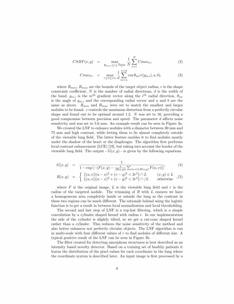
Our method for finding lung lesions can be separated into three major steps:image segmentation, image filtering and false positive reduction. Figure 1 showsan overview. First, the anatomical structures of the chest are segmented. Thisinvolves separating the viewable lung field and the segmentation of bone shad-ows including the clavicle and the full ribcage. There are several satisfactorysolutions for the problem of lung field segmentation [35], [40]. Our own algo-rithm delineates not only the outline of the lung fields, but provides the fullboundary of the ribcage as well, as described in [15]. The viewable area is usedto assist ribcage segmentation and to reduce the possible set of locations forlesions, as we only target the ones partly or completely inside this area.

The method we use for the segmentation of the clavicles is discussed in[13]. The ribcage segmentation algorithm is based on [16] and some details arediscussed in [14]. Here we only provide an overview and a detailed evaluationof ribcage segmentation.

In the second major step various image filters are run to enhance the vis-ibility of lung lesions. The first filter uses the result of bone segmentation tosuppress their shadows. Then three different filters are run in parallel to en-hance different types of lung lesions. A Constrained Sliding Band Filter (CSBF)is utilized to detect small and circular lung nodules. A method referenced asLarge Nodule Filter (LNF) is responsible for enhancing large and also circularnodules. Last, an Outlier Area Filter (OAF) identifies and segments amorphousbut high contrast suspicious areas. The enhanced regions of the image are thenextracted by thresholding and lesion borders are determined.

In the last step a large fraction of false findings are removed by supervisedlearning methods. A hierarchy of SVM-s classifies the candidates based on manytexture and geometry features.

3.2 Ribcage segmentation

Looking at chest X-ray images an apparent regularity can be observed at firstglance: the ribs have a quasi parallel arrangement. So it seems feasible to modelthe ribcage somehow. Even though the two sides of the ribcage appear to besymmetric, it is hard to select properties of this symmetry which stand for allthe instances of a wider image set, where occasional disorders and irregularitiesmay occur. Therefore we handle the two sides of the lungs independently.

To build a complete model - as in [28] and [36] - which is capable of enumer-ating the ribs one-by-one and to specify their positions would require too manyparameters and still would not be accurate enough to handle all the anomaliesthat may occur in a wider image set. The elimination requires high accuracy,thus we chose a different approach. We restrict our model only to the slopes ofribs. Our model assigns a slope to every point of the area of the bounding boxof a lung field, this way it neglects the position information of the ribs. Theseslopes can be described by a two dimensional function. Previously we inves-tigated the applicability of analytical functions like rational polynomials [16],

4

Figure 1: The main steps of the radiograph analysis.

5

(a) Averageslope field

(b) Fitted arcs (c) Fitted slopefield

(d) Possiblecurves

(e) Selectedcurves

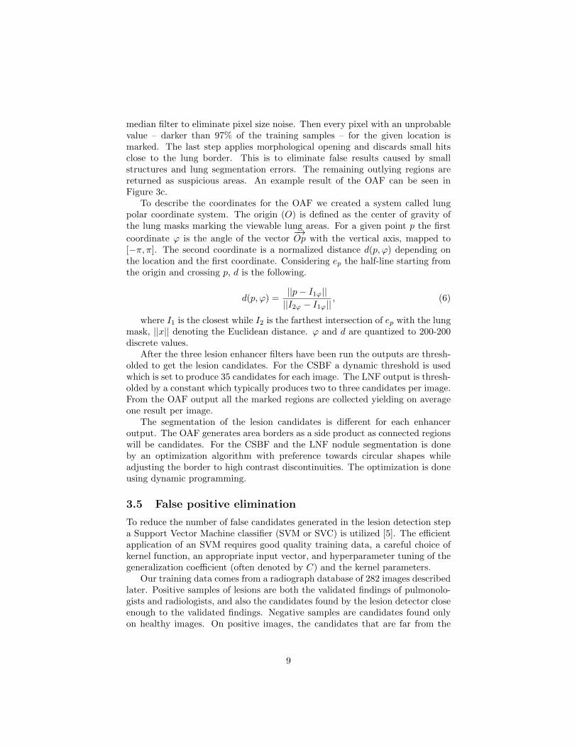
Figure 2: Overview of posterior ribcage segmentation. Arcs are fitted to theimage to fine tune an average slope field, then some of the curves generated fromthis slope field are selected. (The final refined rib borders are not included. Thedifference between 2c and 2a is difficult to notice, but it is significant for thefurther steps. )

but application of a simple smooth slope field map resulted in better overallperformance. The optimal slope field is searched around an average slope fieldby fitting small arcs to the image gradients.

This slope field can be applied to align and rescale vertical intensity profiles.This approach goes back to the early times of ribcage segmentation [7]. Byaligning these profiles we get a simple one dimensional signal on which localmaxima and minima selection gives the vertical positions of the upper andlower borders of ribs. This selection process is by no means straightforward,because there can be much more extrema than needed. To tackle this problemwe incorporated various correlations between the position of a rib border andthe distances between this and its neighbouring rib borders. This statisticswas then formulated into a dynamic programming problem, which provides thepositions of the rib borders. From these positions approximate rib borders canbe generated based on the aforementioned slope field. The final rib borders arethen obtained by refining these by a special dynamic programming based activecontour algorithm. The main steps can be followed in figure 2.

The main advantage of using a slope field over a global shape model is, thatthe slope field is almost independent of the rib thickness and spacing informationof the ribcage, therefore the search for the complete ribcage can be divided intotwo distinct subproblem, which reduces the complexity of the overall search.

This solution works well for the posterior part of the ribs, which is morevisible on chest radiographs, but for the anterior part we applied a differentprocedure. It launches a set of spiral curves from the ribcage boundary anditeratively fits them to the image contours by a dynamic programming activecontour algorithm. This finds the upper borders, while the lower borders areattached by a statistical point distribution model, and the final borders are

6

got after the same refinement step used for the posterior parts. The details ofthe whole complex ribcage segmentation algorithm is written in a forthcomingpublication.

3.3 Bone elimination

The segmentation data is used to remove the bone shadows from the images inorder to enhance the visibility of the lung structure. The elimination is based onSimko’s work [30]. He smoothed the bone borders on vertically differentiatedimages, then subtracted the smoothed areas from the original differentiatedimage. After an integration step he got the bone shadow free image. It workedquite fair on the clavicle, but close to the lateral parts of the ribs it fails. Toovercome this we differentiate perpendicular to the bones’ mid-line.

3.4 Lesion detection

The main steps of lesion detection are preprocessing, lesion enhancement bythe CSBF, LNF and OAF filters, thresholding and lesion segmentation. Inthe sequel we give a brief description of these methods, while a more detailedpresentation can be found in [24].

In the preprocessing step the bone shadow eliminated images are first sub-sampled to 512 lines of height while keeping the aspect ratio to reduce runningtime. Then, to spread pixel intensities in [0, 1], the median value of the pixelsin the segmented lung field and the deviation from the median is set to empir-ical values of 0.35 and 0.18 respectively by scaling and translation of the pixelvalues.

The first nodule enhancer, the CSBF is a gradient convergence based filter,also a member of the Convergence Index filter family. It is our slight modificationof the Sliding Band Filter described in [26]. It is mainly capable of enhancingsmall and circular structures. In our current setting it aims at structures witha diameter between 5 mm and 30 mm. The algorithm first generates imagegradients with a Sobel filter, then maps the gradient vector lengths by a boundedramp function r.

r(x, a, b) =

0 x < ax− a a ≤ x < bb− a b ≤ x

, (1)

where x is the original vector length, a and b are parameters. In our casea is set to 0 and b is set to 0.0025, a length above which the gradient vector isunlikely to be noise. After the mapping the CSBF filter output can be calculatedas follows.

7

CSBF (x, y) = maxRmin≤r≤Rmax

c

1

N

N∑i=1

Cmaxir, (2)

Cmaxir = maxr≤n≤r∗c

1

d

n+d∑m=n

cos θimr(|gm,i|, a, b), (3)

where Rmin, Rmax are the bounds of the target object radius, c is the shapeconstraint coefficient, N is the number of radial directions, d is the width ofthe band, gm,i is the mth gradient vector along the ith radial direction, θimis the angle of gm,i and the corresponding radial vector and a and b are thesame as above. Rmin and Rmax were set to match the smallest and largesnodules to be found. c controls the maximum distortion from a perfectly circularshape and found out to be optimal around 1.2. N was set to 16, providing agood compromise between precision and speed. The parameter d affects noisesensitivity and was set to 5.6 mm. An example result can be seen in Figure 3a.

We created the LNF to enhance nodules with a diameter between 30 mm and75 mm and high contrast, while letting them to lie almost completely outsideof the viewable lung field. The latter feature enables it to find nodules mostlyunder the shadow of the heart or the diaphragm. The algorithm first performslocal contrast enhancement (LCE) [19], but taking into account the border of theviewable lung field. The output - G(x, y) - is given by the following equations.

G(x, y) =1

1− exp [−(F (x, y)− 1|R(x,y)|

∑(u,v)∈R(x,y) F (u, v))]

, (4)

R(x, y) =

{{(u, v)|(u− x)2 + (v − y)2 < 2r2} ∩ L (x, y) ∈ L{(u, v)|(u− x)2 + (v − y)2 < 2r2} ∩ /L otherwise

, (5)

where F is the original image, L is the viewable lung field and r is theradius of the targeted nodule. The trimming of R with L ensures we havea homogeneous area completely inside or outside the lung as the contrast inthese two regions can be much different. The rationale behind using the logisticfunction is to get a result in between local normalization and local thresholding.

The second and last step of LNF is a top-hat filtering, which is a simpleconvolution by a cylinder shaped kernel with radius r. In our implementationthe side of the cylinder is slightly tilted, so we get a cut-cone shaped kernelrather than a cylinder. This reduces the noise sensitivity of the method andalso better enhances not perfectly circular objects. The LNF algorithm is runin multi-scale with four different values of r to find nodules of different size. Atypical positive result of the LNF can be seen in Figure 3b.

The filter created for detecting amorphous structures is best described as anintensity based novelty detector. Based on a training set of healthy patients itlearns the distribution of the pixel values for each coordinate in the lung wherethe coordinate system is described later. An input image is first processed by a

8

median filter to eliminate pixel size noise. Then every pixel with an unprobablevalue – darker than 97% of the training samples – for the given location ismarked. The last step applies morphological opening and discards small hitsclose to the lung border. This is to eliminate false results caused by smallstructures and lung segmentation errors. The remaining outlying regions arereturned as suspicious areas. An example result of the OAF can be seen inFigure 3c.

To describe the coordinates for the OAF we created a system called lungpolar coordinate system. The origin (O) is defined as the center of gravity ofthe lung masks marking the viewable lung areas. For a given point p the first

coordinate ϕ is the angle of the vector−→Op with the vertical axis, mapped to

[−π, π]. The second coordinate is a normalized distance d(p, ϕ) depending onthe location and the first coordinate. Considering ep the half-line starting fromthe origin and crossing p, d is the following.

d(p, ϕ) =||p− I1ϕ||||I2ϕ − I1ϕ||

, (6)

where I1 is the closest while I2 is the farthest intersection of ep with the lungmask, ||x|| denoting the Euclidean distance. ϕ and d are quantized to 200-200discrete values.

After the three lesion enhancer filters have been run the outputs are thresh-olded to get the lesion candidates. For the CSBF a dynamic threshold is usedwhich is set to produce 35 candidates for each image. The LNF output is thresh-olded by a constant which typically produces two to three candidates per image.From the OAF output all the marked regions are collected yielding on averageone result per image.

The segmentation of the lesion candidates is different for each enhanceroutput. The OAF generates area borders as a side product as connected regionswill be candidates. For the CSBF and the LNF nodule segmentation is doneby an optimization algorithm with preference towards circular shapes whileadjusting the border to high contrast discontinuities. The optimization is doneusing dynamic programming.

3.5 False positive elimination

To reduce the number of false candidates generated in the lesion detection stepa Support Vector Machine classifier (SVM or SVC) is utilized [5]. The efficientapplication of an SVM requires good quality training data, a careful choice ofkernel function, an appropriate input vector, and hyperparameter tuning of thegeneralization coefficient (often denoted by C) and the kernel parameters.

Our training data comes from a radiograph database of 282 images describedlater. Positive samples of lesions are both the validated findings of pulmonolo-gists and radiologists, and also the candidates found by the lesion detector closeenough to the validated findings. Negative samples are candidates found onlyon healthy images. On positive images, the candidates that are far from the

9

(a) A CSBF finding. (b) A LNF finding. (c) An OAF finding.

Figure 3: Typical findings of the three lesion detectors.

validated findings are not used for training. This was necessary as physicianstend to mark only some of the lung nodules when the image contains too manyof them. Keeping negative samples only from healthy images improved classifierperformance on independent test data. Exact thresholds used for training datageneration are described in [24]. As 30 times more negative samples were avail-able than positive ones, we used a cost-sensitive version of the SVM. Balancingis achieved by using different C values for positive and for negative samples.

As for the kernel, the isotropic Gaussian function was chosen for the SVM.The input vector of the kernel consists of various features describing texture,geometry and location. The final set of features described in section 3.5.1 is aresult of a simple forward selection algorithm selecting from 168 implementedfeatures. As the relevant features turned out to be different for the output of thethree nodule enhancing algorithms, separate classifiers are used for each resultset. This improves classification performance due to fewer irrelevant featuresand also reduces training time.

The two hyperparameters of the resulting SVM – C and the width parameter(σ) of the kernel – are tuned by an iteratively refining grid search. Cross-validation was used on image level to prevent overfitting.

3.5.1 The features for classification

The aforementioned feature selection algorithm identified 27 relevant featuresout of the total 168 we implemented. The short description of these features isthe following.

• Mean and maximum of the average fraction under the minimum (AFUM)filter inside nodule border [12].1, 2

• The linearity of nodule border transition. This considers the intensityprofiles perpendicular to the nodule border and calculates the error to thebest fitting linear approximation.1

• The contrast (average intensity fraction) close to the determined noduleborder.1

10

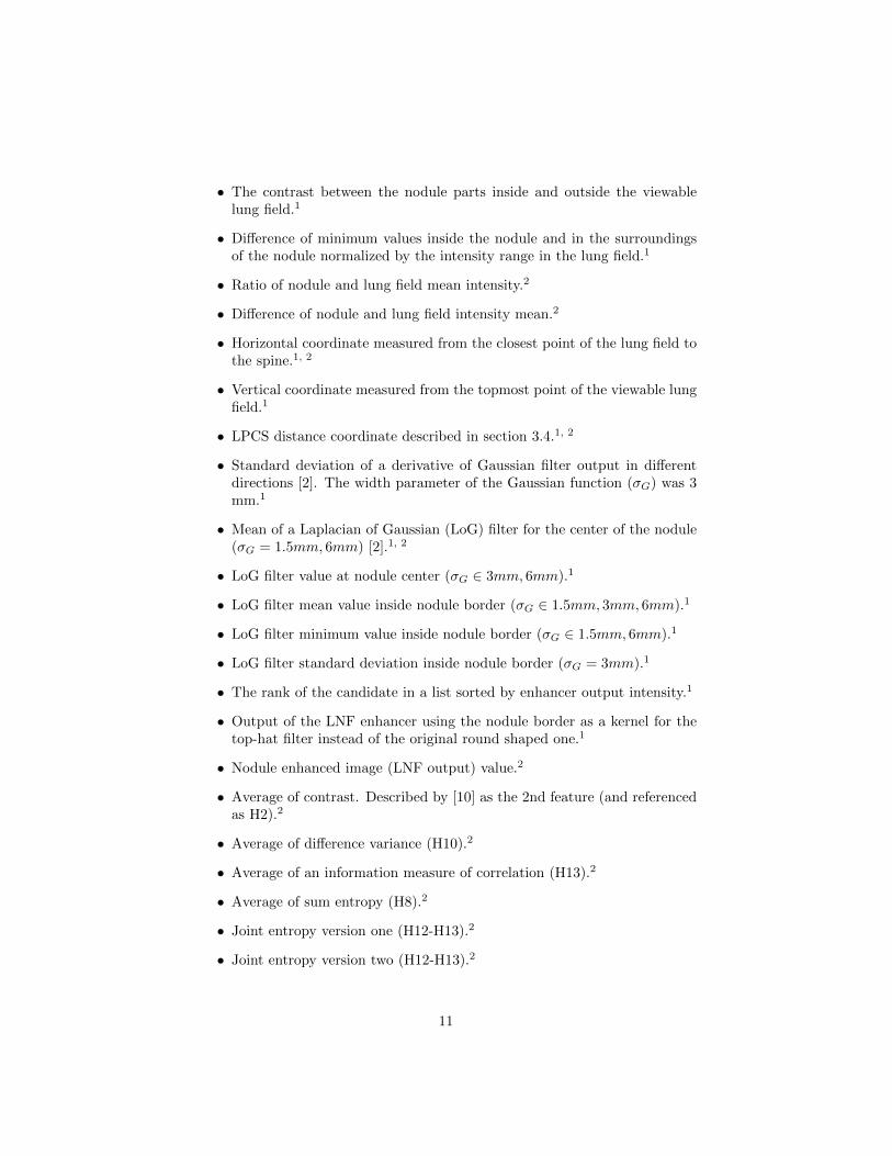
• The contrast between the nodule parts inside and outside the viewablelung field.1

• Difference of minimum values inside the nodule and in the surroundingsof the nodule normalized by the intensity range in the lung field.1

• Ratio of nodule and lung field mean intensity.2

• Difference of nodule and lung field intensity mean.2

• Horizontal coordinate measured from the closest point of the lung field tothe spine.1, 2

• Vertical coordinate measured from the topmost point of the viewable lungfield.1

• LPCS distance coordinate described in section 3.4.1, 2

• Standard deviation of a derivative of Gaussian filter output in differentdirections [2]. The width parameter of the Gaussian function (σG) was 3mm.1

• Mean of a Laplacian of Gaussian (LoG) filter for the center of the nodule(σG = 1.5mm, 6mm) [2].1, 2

• LoG filter value at nodule center (σG ∈ 3mm, 6mm).1

• LoG filter mean value inside nodule border (σG ∈ 1.5mm, 3mm, 6mm).1

• LoG filter minimum value inside nodule border (σG ∈ 1.5mm, 6mm).1

• LoG filter standard deviation inside nodule border (σG = 3mm).1

• The rank of the candidate in a list sorted by enhancer output intensity.1

• Output of the LNF enhancer using the nodule border as a kernel for thetop-hat filter instead of the original round shaped one.1

• Nodule enhanced image (LNF output) value.2

• Average of contrast. Described by [10] as the 2nd feature (and referencedas H2).2

• Average of difference variance (H10).2

• Average of an information measure of correlation (H13).2

• Average of sum entropy (H8).2

• Joint entropy version one (H12-H13).2

• Joint entropy version two (H12-H13).2

11

• Robustness of nodule border. It restarts nodule segmentation from centersnear the original one and compares the resulting borders.2

• Similarity of histograms inside and outside nodule, near the border. Simi-larity is simply the number of bins for which the difference between insideand outside is greater than a predefined value.2

In the list 1 and 2 means that the feature is used for the candidates of theCSBF and LNF respectively. For the OAF the feature selection could not berun due to the small number of positive samples. As the findings of the LNFand OAF have some similar properties, we decided to use the same feature setfor both algorithms (except for the ”robustness of nodule border” feature as theOAF has a different segmentation method).

To better exploit the results of bone segmentation, three new features werecreated based on the following observations. First, density variations in bonestructure can appear as intensity extrema and may produce false positive find-ings. Second, areas where bones overlap on the 2 dimensional summation imagesappear as dark, approximately rhomboid shaped structures frequently recog-nized by the system as lesions. Third, in the cases where bone shadows causefalse positive candidates, the border of the candidate follows the edge of the bonein a relatively large portion. These three observations motivated the followingthree features respectively.

The first feature calculates the area fraction of the nodule overlapping witha bone structure. The feature can be described formally as

BoneOverlapi =|{(x, y)|(x, y) ∈ Ci

⋂(⋃

j Bj)}||{(x, y)|(x, y) ∈ Ci}|

, (7)

where Ci contains the points of the ith candidate while Bj means the setof points inside the jth bone structure. |.| denotes the size of the sets. Thesecond feature calculates the overlap of candidates with bone crossings – theareas where two or more bone segments overlap with each other. Using theprevious notation, the formula is

BoneXOverlapi =|{(x, y)|(x, y) ∈ Ci

⋂(⋃

j,k(Bj

⋂Bk))}|

|{(x, y)|(x, y) ∈ Ci}|. (8)

The third feature calculates the fraction of the nodule perimeter that runsnear to a bone shadow border. It can be calculated as

FollowBoneEdgei =|{(x, y)|(x, y) ∈ δCi,minj d((x, y), δBj) < 1.5mm}|

|{(x, y)|(x, y) ∈ δCi}|, (9)

where δCi and δBj are the endpoint set of Ci and Bj , while d is the Euclideandistance.

12

3.6 The radiograph database

We tested the lesion detection on a private chest X-ray database containingimages of 407 patients where 259 of the cases contained at least one malignantlung nodule. Nodule diameter ranged from 2 mm to 98 mm, the average was23 mm. Most of the malignant cases were validated by CT. The images camefrom a TOP-X DR series digital X-ray machine by Innomed Medical Zrt. Thedetector used a maximal resolution of 3000 × 3000 pixels with 0.16 mm pixelsize in both dimensions.

For the evaluation of bone segmentation we used a subset of 30 images forwhich reference bone contours were available from a human observer. Out ofthese images five were segmented also by another independent observer for theinter-observer tests.

For the lesion detector we separated 282 images for training and cross-validated testing and kept the remaining 125 images purely for testing. Thisway we could generate results for all 407 images without overfitting.

4 Results

4.1 Bone segmentation

Numerous ways of measuring the quality of ribcage segmentation have beenapplied in the literature. Different measurements tell different things about theresults. To make our results comparable to others we had to evaluate themin various ways. First, we show detailed results when using a strict methodinvolving the pairing of found and reference bones. Then we show the resultsof a more permissive test also used in the literature, which simply uses overlapwith minimal pre-processing.

The first test was conducted on a set of 30 images. Previously these imageswere manually segmented by a human observer. His task was to delineate allthe visible ribs. 5 of these images were also segmented by another independentobserver. There was no accord between the two observers in how many ribs theyhave found on each image. The ribs in the abdominal region are often obscured,and some of them are cropped by the image borders.

Our current algorithm segments the anterior and posterior parts of the ribsindependently, but the human observers delineated the whole ones. There is

a problem with this difference: the Jaccard index (J(A,B) = |A∩B||A∪B| ) becomes

difficult to interpret, as the intersection between the areas will always be muchsmaller than their union, and the perfect solution will not get 100%. Thus wedecided to cut the manually segmented ribs into posterior and anterior parts byan automatic method, which uses the intersections of the rib mid-lines with theribcage boundary to cut them into posterior, anterior and even lateral parts (ifthere are more than one intersection).

The rib shadow elimination makes sense mainly above the lung fields, but tomake it comparable with some other results in ribcage segmentation [28], [35] wehave done two different measurements. First, we simply compared the posterior

13

and anterior parts by their manual counterparts, then we trimmed these by theapproximated complete lung field. In contrast to the general concept of visiblelung fields we included the area of the heart as well.

Our results can be seen in Figure 4. We ordered the images by their Jaccardindex, and selected the worst, the best and the median from the ordered list.We did this ordering separately for the posterior and the anterior parts, andseparately for the lung field trimmed and the full results as well.

We did some quantitative measurements as well, which can be seen on table1 (average values), and on table 2, 3, 4 for the worst, median and best im-ages respectively. To make these numbers easier to interpret we included therespective images as well (Figure 4).

The segmentation works independently on the left and right side, so wemeasured the results separately and the resulting numbers should be interpretedper lung side. The output of our algorithm does not provide a numbering for theribs, only returns a simple set of ribs. Therefore the evaluation process had tohandle the problem of finding the corresponding segmented rib for each referencerib. This pairing was done based on the Jaccard index. Every reference rib gota corresponding segmented rib, even if that segmented rib belonged to morethan one reference rib.

We were interested in how many of the 12 ribs our algorithm has found. Forthis we defined a rib being found when the Jaccard index was above a thresholdof 0.55. It may appear to be low, but even the inter-observer results werebetween 0.61 and 0.84. According to Table 1 our algorithm found on average5.93 posterior and 3.6 anterior ribs on an image, but when the considered areaof both the segmented and the reference bone are restricted to the lung fieldsthe numbers go up to 6.16 and 4.3 respectively. This increase can be explainedby the fact, that we got higher Jaccard indices for the restricted area, becausesome parts of the ribs (both the reference and the segmented) are trimmed bythe same curve (lung outline), which reduces the part of outline where the twoarea can differ.

We call a reference rib missed if there is no corresponding segmented ribwhich reached the threshold. We call a segmented rib false if there is no referencerib for which the Jaccard index is above the threshold. The average Jaccardindex in Table 5 is calculated by simply averaging the values over the ribs, buta smaller missing rib can cause less harm for the elimination than a longer one.To incorporate this effect we introduced a Weighted Jaccard index, which is thefollowing:

WeightedJaccardIndex =

∑i |Ri

⋂Si|∑

i |Ri

⋃Si|

, (10)

where Ri denotes the area of the ith reference, and Si denotes the area ofthe ith segmented rib. The simple averaged Jaccard index is the following:

AverageJaccardIndex =∑i

|Ri

⋂Si|

|Ri

⋃Si|

. (11)

14

Table 1: Average bone segmentation results when CADe compared with ob-server1.

Posterior Anteriorinside lung full image inside lung full image

Number of Reference Ribs 8,33 9,43 7,68 10,18Number of Segmented Ribs 7,15 7,53 6,10 7,18

Found 6,20 5,85 3,93 3,23Missed 2,13 3,58 3,75 6,95

Found per All 0,75 0,62 0,51 0,32False 0,95 1,68 2,18 3,95

False per Segmented Ribs 0,13 0,21 0,38 0,56Average Jaccard Index 0,62 0,52 0,48 0,34

Weighted Jaccard Index 0,62 0,48 0,44 0,33Average Sensitivity 0,71 0,63 0,59 0,52

Weighted Sensitivity 0,78 0,65 0,60 0,57

For the elimination it is important to have an accurate bone outline. One canget relatively high Jaccard indices with low outline accuracy, while if the outlineis exactly the same, but the reference rib is longer than the segmented one, theJaccard index degrades in a fast pace. To overcome this we introduced anothermeasure called Distance of Found. It is calculated by pairing the points of thereference borders by the segmented borders. The points without correspondingpairs are left out, and the average distance between the points are calculated.The pairing is carried out by launching perpendicular half-lines from the pointsof the midline of the two curves, and finding the intersecting points.

E.g. for the untrimmed posterior ribs we got an average of 5.2 pixels, whichmeans 0.83 mm in reality. These numbers are close to the ones calculated forthe inter-observer study, but it should be noted that these were averaged overonly the found ribs. The distribution of these distances are shown in Figure 5.

Another figure of merit we calculated is the specificity and sensitivity ofthe bone shadow segmentation based on area overlap. The area overlap is thesize of the area that is included in both the segmentation under investigationand the reference segmentation. Sensitivity of a method or observer versus thereference observer is the fraction of the overlap and the total area of the referencesegmentation, in other words the proportion of correctly identified bone areaaccording to the reference. Specificity is the fraction of the overlap and thetotal area of the method under investigation. One minus the specificity givesthe proportion of false positive bone area. We restricted the whole calculation tothe viewable lung field as the ribs below the diaphragm are often barely visible,misleading both the algorithm and the human observers.

Table 6 shows the results of the segmentation tests based on bone overlap.In the first column we compared the CADe results to a reference human ob-server locating only anterior ribs. In the second test the same human observerwas asked to segment the complete ribs including both anterior and posterior

15

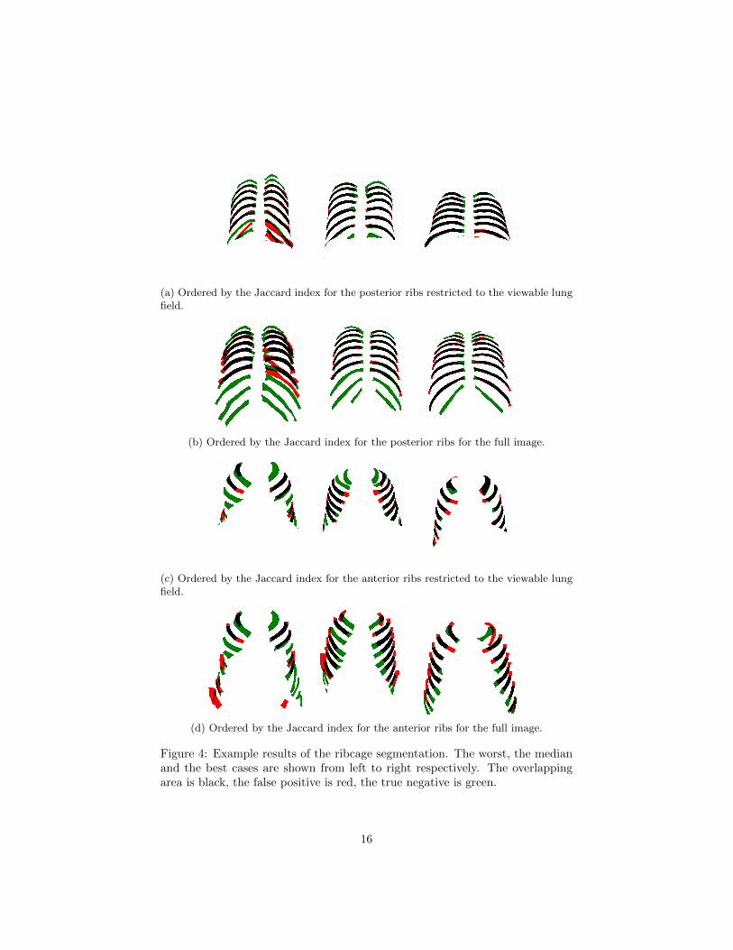
(a) Ordered by the Jaccard index for the posterior ribs restricted to the viewable lungfield.

(b) Ordered by the Jaccard index for the posterior ribs for the full image.

(c) Ordered by the Jaccard index for the anterior ribs restricted to the viewable lungfield.

(d) Ordered by the Jaccard index for the anterior ribs for the full image.

Figure 4: Example results of the ribcage segmentation. The worst, the medianand the best cases are shown from left to right respectively. The overlappingarea is black, the false positive is red, the true negative is green.

16

(a) Segmented vs observer1 ante-rior ribs.

(b) Segmented vs observer1 poste-rior ribs.

(c) Inter-observer anterior ribs. (d) Inter-observer posterior ribs.

Figure 5: Distribution of distances in pixel between the points of the referenceand segmented rib borders restricted to the viewable lung field.

Table 2: Worst case images of bone segmentation results when CADe comparedwith observer1. (Figure 6 left)



Found 5,00 5,50 0,00 0,00Missed 3,50 4,50 8,00 10,00





17

Table 3: Median case images of bone segmentation results when CADe comparedwith observer1. (Figure 6 middle)



Found 6,00 6,50 4,50 1,50Missed 3,00 3,00 3,00 9,00





Table 4: Best case images of bone segmentation results when CADe comparedwith observer1. (Figure 6 right)



Found 7,00 7,50 4,50 5,00Missed 0,00 2,50 2,00 4,00





18

Table 5: Inter-observer bone segmentation results between observer1 and ob-server2.



Found 8,00 8,00 7,00 8,50Missed 0,00 1,00 0,00 2,50





Table 6: Bone locator sensitivity and specificity in % based on overlap statistics.

CADe vs Observer1 CADe vs Observer1 Observer2 vs Observer1posterior ribs complete ribs complete ribs

Sensitivity 84.1 80.3 94Specificity 87.6 90.3 94.1

Sample size 30 30 5

parts. The third test involved two independent human observers both segment-ing complete ribs. This inter-observer comparison shows the obscurity of theproblem and gives an approximate upper bound to the achievable metrics forthe CADe algorithm.

Comparing the 80.3% sensitivity for full ribs with the 94% of the inter-observer result shows that the algorithm misses around 15% of the determinablepart of the bone which equals to approximately one bone per lung field. Seg-mentiation of the posterior part is even better with 84.1% sensitivity. Specificityof 90.3% ensures that the algorithm doesn’t produce much false areas. Further-more, the usual error here is that the anterior rib segmentation continues tofollow a bone towards the mediastinum even when it becomes hardly visibleor not visible at all for a human observer. In many of these cases the rib canbe identified retrospectively, thus these cases are rather the miss of the humanobserver. Furthermore, we observed that the rib parts where the CADe andobservers disagreed are barely visible so these sections hardly disturb lesiondetection. Sections with high contrast are segmented with higher accuracy.

Figure 6 shows example results for rib segmentation and elimination for theworst, an average and the best cases. It can be seen that even for the worstsegmentation the bone shadow eliminated image is adequate. Bone shadows arehardly visible and other fine details are kept.

19

It is almost impossible to compare our results with other published numbersas both the test samples and the methodology are different. As an example in[28] the authors published 50% to 80% sensitivity for the posterior and 50% forthe anterior part of the ribs. These numbers best correspond to the WeightedSensitivity row in Table 1; however, only the first 10 ribs were assessed in thatstudy. In [36], where the 2nd to 10th posterior ribs were included, the authorsreached an accuracy of 0.787. Their measurement method was most similarto the one used in the first column of Table 6. Based on these numbers wecannot state that our solution is better or worse, we can only say it performscomparably.

4.2 Lesion detection

For the following measurements 10-fold cross validation with 30 repetitions wasused. Results are demonstrated on free-response receiver operating characteris-tic (FROC) curves, showing the sensitivity as a function of average number offalse positives produced for each image. On the final output, a CADe drawingwas considered to be correct if its centroid – center of gravity – was locatedinside a physician’s marker; otherwise it was labeled as a false positive.

We evaluated our CADe system in three configurations to analyze the effectof bone localization and removal. The first configuration used no bone infor-mation at all, the second employed the bone shadow suppressed images on thelesion detector output but still excluding the three features based on bone out-lines, while the third configuration both used the bone shadow free images andthe new features. For each configuration we re-trained the lesion detector andgenerated FROC curves using the methodology described before. The resultscan be seen in Figure 7.

The improvement when using rib-shadow-free images is clear. At constant63% sensitivity the number of false positives could be reduced from 2.94 to 1.4.Utilizing the new features, the number of false positives falls further to 1.23.This means 52% of false detections could be eliminated which is a great benefitfor radiologists and physicians having to examine much less false CADe resultsat screening. Fixing the number of false detections to two yields sensitivityvalues of 57%, 66.7% and 68% for the unprocessed, the bone eliminated and thefeature including configurations respectively. Finding 19% more lesions is a hugebenefit in this case. Roughly the same improvement is valid for working pointsat lower false positive rates. Two example changes can be seen in Figure 8. Inthe first case a false negative changed into a true positive, while in the secondcase a false positive finding could be removed from the output. The majority ofthe changes were similar to these cases.

After seeing the benefits in detection accuracy we wanted to see how boneshadows and their removal affect the output distribution of the CADe system.We assumed that bone shadows and especially bone crossings cause many falsepositives for the original system and less or not at all for the new version. Weconducted two tests to support our hypothesis.

In the first test we investigated the overlap of the false findings with bone

20

Figure 6: The results of rib elimination. Original images (first row), result ofbone segmentation (second row), calculated bone shadows (third row) and boneeliminated images (fourth row). Left, center and right columns show the worst,the median and the best segmentation results respectively.

21

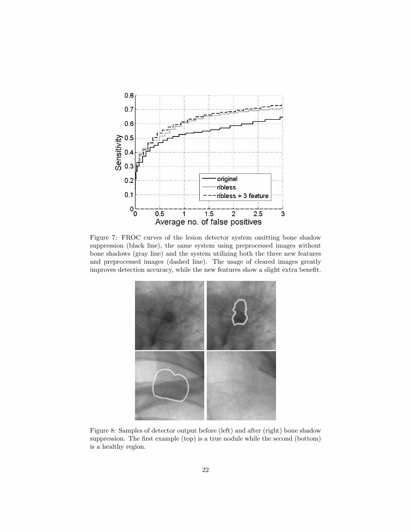
Figure 7: FROC curves of the lesion detector system omitting bone shadowsuppression (black line), the same system using preprocessed images withoutbone shadows (gray line) and the system utilizing both the three new featuresand preprocessed images (dashed line). The usage of cleared images greatlyimproves detection accuracy, while the new features show a slight extra benefit.

Figure 8: Samples of detector output before (left) and after (right) bone shadowsuppression. The first example (top) is a true nodule while the second (bottom)is a healthy region.

22

Table 7: Area fraction of false positive candidates overlapping with bone shad-ows.

Unprocessed Rib-shadow-free Rib-shadow-free+ 3 features

Total bone area 0.542 0.542 0.542FP area overl. bones 0.791 0.625 0.584Pearson’s correlation 0.0413 0.014 0.0078

Table 8: Area fraction of false positive candidates overlapping with shadows ofbone crossings.

Unprocessed Rib-shadow-free Rib-shadow-free+ 3 features

Total bone X area 0.121 0.121 0.121FP area overl. bone X-s 0.317 0.166 0.134

Pearson’s correlation 0.05 0.0119 0.0038

shadows. We expected the false findings to overlap less often with bones afterelimination. Moreover, in the ideal case when no bone shadows are present, theevent of falsely marking an area as a lesion should be independent from the areabeing overlapped by a bone shadow. To test this independence we considered asimple pixel-wise model. Let li be the indicator of marking the ith pixel falselyas a lesion and bi the indicator of the ith pixel belonging to a bone shadow.Let’s assume that li-s for all i are independent samples of the same indicatorrandom variable L and analogously bi-s are generated from the indicator randomvariable B 1. The probability P (B|L) should converge to P (B) if we weaken theconnection between the two variables and in the independent case they shouldbe equal. Also the Pearson’s correlation coefficient should be close to zero forweak dependency. P (B|L) = P (B,L)/P (L) can be estimated as the overlapbetween false positive lesions and bone shadows over the entire area of falsepositives. P (B) is simply the total area of bone shadows.

Table 7 shows the results of this test. The false positive area overlappingbones clearly decreases and approaches the total area of bone shadows as ex-pected; however, we can still see a gap suggesting that some false positive find-ings are still caused by bone shadows. The Pearson’s correlation coefficient getscloser to zero by an order of magnitude, although it was already small in theoriginal case. Table 8 shows the same numbers for bone crossings yielding thesame conclusion.

In the second test we analyzed the independence of a candidate being falsepositive and its overlap with bone shadows as two random variables. We decidedto use Pearson’s chi-squared test to test independence, so we needed to discretize

1This model is obviously incorrect as neither independence nor the identity of distributionshold, but for a big enough sample it is a close enough estimate of reality for the purposes ofthis test.

23

Table 9: Resulting p-values of independence tests between bone overlapping andfalse positiveness.

Original image Rib-shadow-free image Rib-free+ 3 features

Overlap w. bones 0.0001 0.0002 0.049Overlap w. bone X-s 0.0015 0.61 0.2

the variables. The first one is already binary while the overlap feature wasquantized to three bins: full overlap, partial overlap and no overlap with a 5%tolerance. We demonstrated the resulting p-values in Table 9. We ran the testsfor the same three configurations as above. Using a predefined significance levelof 1% the first two cases are clearly significant meaning that false positivenessdepends on – or at least correlates with – the overlap with bones while in thethird case we can no longer be sure that the relation exists. However, we shouldnote that a p-value of 0.049 suggests further investigation on a larger sample.We ran the same test using the bone crossing overlap as the second variable.Here, using the original system shows a clear correlation, while the results forthe versions exploiting bone information are insignificant. These results do notcontradict with our original hypothesis; however, the proof of independenceneeds more studies.

5 Conclusion and future work

To summarize our work, we developed a CADe system capable of automaticallydetecting various lung lesions. In our solution the ribcage and clavicle shadowsare removed before lesion detection. The cleaned images are analyzed by threedifferent filters for lesions and a hierarchy of SVM classifiers is used to reducethe number of false findings.

We evaluated the bone shadow segmentation algorithm and found that itcan detect approximately 80% of bone shadows with false findings around 10%.For the more disturbing posterior part it can detect as much as 84%. Accordingto our inter-observer tests, we cannot really hope for more than 94% sensitivity.When a bone is identified correctly, the segmentation border is accurate within1 mm. This is again close to the approximated lower bound determined by theinter observer analysis.

Our measurements showed that lesion detection performance can be greatlyimproved by removing bone shadows and also a bit more by using the bonesegmentation information as classifier input. The former reduced the numberof false findings by 52% from 2.94 to 1.4 at 63% sensitivity, while the latterresulted in a further decrease of 12% to 1.23 false positives per image.

We also tested if the remaining false findings are still dependent on the over-lap with bone shadows. The results confirmed that dependence is much weakeron the processed images, although we could not prove complete independence.

24

This means that some remainders of bone shadows are still causing a few falsefindings, but improving the accuracy of bone shadow removal is not likely toresult in further drastic improvements.

While evaluating our study we identified directions for further investigation.As some of the lung lesions are under the shadow of the heart and below thediaphragm it is a straightforward idea to extend the search for lesions to theseparts of the image. For this we would need to balance contrast in these areas.Fortunately the bone removal algorithm seems to be capable for this task withonly small modifications. Extending the search can hopefully lead to an increasein sensitivity.

Overall we believe our study contributes to the CADe community by show-ing the utility of bone shadow and more generally anatomic noise removal forthe purposes of automatic lung lesion detection. Although a few other researchgroups are also putting effort in this approach of image cleaning, a comprehen-sive performance comparison for automatic lesion detection has not been madeso far. We also believe our method for segmenting the bone shadows is perform-ing at least as good as alternative solutions due to its high accuracy and theinclusion of the anterior rib segments.

6 Acknowledgment

The authors express their thanks to all physicians of Pulmonological Clinic,Semmelweis University, who helped us with validated images and to the de-velopment staff of ImSoft ltd. This work was partly supported by the grantsTAMOP - 4.2.2.B-10/1–2010-0009 and KMR 12-1-2012-0122.

References

[1] William R Brody, Glenn Butt, Anne Hall, and Albert Macovski. A methodfor selective tissue and bone visualization using dual energy scanned pro-jection radiography. Medical physics, 8:353, 1981.

[2] P. Campadelli, E. Casiraghi, and D. Artioli. A fully automated methodfor lung nodule detection from postero-anterior chest radiographs. MedicalImaging, IEEE Transactions on, 25(12):1588–1603, 2006.

[3] S. Chen, K. Suzuki, and H. MacMahon. Development and evaluation ofa computer-aided diagnostic scheme for lung nodule detection in chest ra-diographs by means of two-stage nodule enhancement with support vectorclassification. Medical Physics, 38:1844, 2011.

[4] G. Coppini, S. Diciotti, M. Falchini, N. Villari, and G. Valli. Neural net-works for computer-aided diagnosis: detection of lung nodules in chestradiograms. Information Technology in Biomedicine, IEEE Transactionson, 7(4):344–357, 2003.

25

[5] C. Cortes and V. Vapnik. Support-vector networks. Machine learning,20(3):273–297, 1995.

[6] D.W. De Boo, M. Prokop, M. Uffmann, B. Van Ginneken, andCM Schaefer-Prokop. Computer-aided detection (CAD) of lung nodulesand small tumours on chest radiographs. European Journal of Radiology,72(2):218–225, 2009.

[7] P. de Souza. Automatic rib detection in chest radiographs. Computervision, graphics, and image processing, 23(2):129–161, 1983.

[8] K. Doi. Computer-aided diagnosis in medical imaging: historical review,current status and future potential. Computerized Medical Imaging andGraphics, 31(4-5):198–211, 2007.

[9] Matthew Thomas Freedman, Shih-Chung Benedict Lo, John C Seibel, andChristina M Bromley. Lung nodules: improved detection with software thatsuppresses the rib and clavicle on chest radiographs. Radiology, 260(1):265–273, 2011.

[10] R.M. Haralick, K. Shanmugam, and I.H. Dinstein. Textural features forimage classification. IEEE Transactions on systems, man and cybernetics,3(6):610–621, 1973.

[11] Russell C. Hardie, Steven K. Rogers, Terry Wilson, and Adam Rogers. Per-formance analysis of a new computer aided detection system for identifyinglung nodules on chest radiographs. Medical Image Analysis, 12(3):240–258,June 2008.

[12] M.D. Heath and K.W. Bowyer. Mass detection by relative image intensity.In Proceedings of the 5th International Workshop on Digital Mammography(IWDM-2000), pages 219–225, 2000.

[13] A. Horvath. Locating clavicles on chest radiographs. In Proceedings of the19th PhD Minisymposium, pages 62–63. Budapest University of Technologyand Economics, Department of Measurement and Information Systems,2012.

[14] A. Horvath. Statistical approach towards ribcage segmentation. In Proceed-ings of the 20th PhD Minisymposium, pages 26–29. Budapest University ofTechnology and Economics, Department of Measurement and InformationSystems, 2013.

[15] A. Horvath and G. Horvath. Segmentation of chest x-ray radiographs, anew robust solution. 5th European Conference of the International Feder-ation for Medical and Biological Engineering, pages 655–658, 2012.

[16] S. Juhasz, A. Horvath, L. Nikhazy, G. Horvath, and A Horvath. Segmen-tation of Anatomical Structures on Chest Radiographs. In Ratko Magjare-vic, Panagiotis D. Bamidis, and Nicolas Pallikarakis, editors, XII Mediter-ranean Conference on Medical and Biological Engineering and Computing

26

2010, volume 29 of IFMBE Proceedings, pages 359–362. Springer BerlinHeidelberg, 2010. 10.1007/978-3-642-13039-7 90.

[17] T. Kobayashi, X.-W. Xu, H. MacMahon, C. Metz, and K. Doi. Effectof acomputer-aided diagnosis scheme on radiologists’ performancein detectionof lung nodules on radiographs. Radiology, vol. 199, pp.843-848, 1996.

[18] Barnett S. Kramer, Christine D. Berg, Denise R. Aberle, and Philip C.Prorok. Lung cancer screening with low-dose helical CT: results fromthe national lung screening trial (NLST). Journal of Medical Screening,18(3):109–111, September 2011.

[19] J.S. Lee. Digital image enhancement and noise filtering by use of localstatistics. Pattern Analysis and Machine Intelligence, IEEE Transactionson, (2):165–168, 1980.

[20] F. Li, T. Hara, J. Shiraishi, R. Engelmann, H. MacMahon, and K. Doi.Improved detection of subtle lung nodules by use of chest radiographswith bone suppression imaging: Receiver operating characteristic analy-sis with and without localization. American Journal of Roentgenology,196(5):W535–W541, 2011.

[21] M. Loog, B. van Ginneken, and AMR Schilham. Filter learning: applicationto suppression of bony structures from chest radiographs. Medical imageanalysis, 10(6):826–840, 2006.

[22] H. MacMahon, R. Engelmann, F. M. Behlen, K. R. Hoffmann, T. Ishida,C. Roe, C. E. Metz, and Doi K. Computer-aided diagnosis of pulmonarynodules: Results of a large-scale observer test. Radiology. 1999;213:723-726., 1999.

[23] Ronald D Novak, Nicholas J Novak, Robert Gilkeson, Bahar Mansoori,and Gunhild E Aandal. A comparison of computer-aided detection (cad)effectiveness in pulmonary nodule identification using different methods ofbone suppression in chest radiographs. Journal of Digital Imaging, pages1–6, 2013.

[24] G. Orban and G. Horvath. Algorithm fusion to improve detection of lungcancer on chest radiographs. International Journal of Intelligent Computingand Cybernetics, 5(1):111–144, 2012.

[25] M. Park, J.S. Jin, and L.S. Wilson. Detection of abnormal texture in chestx-rays with reduction of ribs. In Proceedings of the Pan-Sydney area work-shop on Visual information processing, pages 71–74. Australian ComputerSociety, Inc., 2004.

[26] C. Pereira, A. Mendonca, and A. Campilho. Evaluation of contrast en-hancement filters for lung nodule detection. In ICIAR 2007 Proceedings,pages 878–888, Montreal, Canada, August 22–24 2007.

27

[27] Tahir Rasheed, Bilal Ahmed, MAU Khan, Maamar Bettayeb, SungyoungLee, and Tae-Seong Kim. Rib suppression in frontal chest radiographs:A blind source separation approach. In Signal Processing and Its Appli-cations, 2007. ISSPA 2007. 9th International Symposium on, pages 1–4.IEEE, 2007.

[28] Hideyuki Sakaida, Akira Oosawa, and Kazuo Shimura. Rib shape recog-nition in lung x-ray images for intelligent assistance. FUJI FILM RE-SEARCH AND DEVELOPMENT, 52:99, 2007.

[29] A.M.R. Schilham, B. Van Ginneken, and M. Loog. A computer-aided di-agnosis system for detection of lung nodules in chest radiographs with anevaluation on a public database. Medical Image Analysis, 10(2):247–258,2006.

[30] G. Simko, G. Orban, P. Maday, and G. Horvath. Elimination of clavicleshadows to help automatic lung nodule detection on chest radiographs. In4th European Conference of the International Federation for Medical andBiological Engineering, pages 488–491. Springer, 2009.

[31] P.R. Snoeren, G.J.S. Litjens, B. van Ginneken, and N. Karssemeijer. Train-ing a computer aided detection system with simulated lung nodules in chestradiographs.

[32] Elaheh Soleymanpour, Hamid Reza Pourreza, et al. Fully automatic lungsegmentation and rib suppression methods to improve nodule detection inchest radiographs. Journal of Medical Signals and Sensors, 1(3):191, 2011.

[33] K. Suzuki, H. Abe, H. MacMahon, et al. Image-processing technique forsuppressing ribs in chest radiographs by means of massive training arti-ficial neural network (mtann). Medical Imaging, IEEE Transactions on,25(4):406–416, 2006.

[34] J.I. Toriwaki, Y. Suenaga, T. Negoro, and T. Fukumura. Pattern recog-nition of chest x-ray images. Computer Graphics and Image Processing,2(3):252–271, 1973.

[35] B. Van Ginneken, M.B. Stegmann, and M. Loog. Segmentation of anatom-ical structures in chest radiographs using supervised methods: a compar-ative study on a public database. Medical Image Analysis, 10(1):19–40,2006.

[36] B. van Ginneken and B.M. ter Haar Romeny. Automatic delineation of ribsin frontal chest radiographs. In Proceedings of SPIE, volume 3979, page825, 2000.

[37] F. Vogelsang, F. Weiler, J. Dahmen, M. Kilbinger, B. Wein, andR. Gunther. Detection and compensation of rib structures in chest ra-diographs for diagnose assistance. In Proceedings of the International Sym-posium on Medical Imaging, volume 3338, page 1. Citeseer, 1998.

28

[38] H. Wechsler and J. Sklansky. Finding the rib cage in chest radiographs.Pattern Recognition, 9(1):21–30, 1977.

[39] Jun Wei, Y. Hagihara, A. Shimizu, and H. Kobatake. Optimal imagefeature set for detecting lung nodules on chest X-ray images. Proc. ofCARS2002, pages 706–711, 2002.

[40] Zhennan Yan, Jing Zhang, Shaoting Zhang, and Dimitris N Metaxas. Au-tomatic rapid segmentation of human lung from 2d chest x-ray images.

[41] Z. Yue, A. Goshtasby, and L.V. Ackerman. Automatic detection of ribborders in chest radiographs. Medical Imaging, IEEE Transactions on,14(3):525–536, 1995.

29

An X-ray CAD system with ribcage suppression for improved detection of lung lesion AronHorváth

Documents

Transcript of An X-ray CAD system with ribcage suppression for improved detection of lung lesion AronHorváth