(a) (b)

Figure 1. (a) Mesh NoC architecture (b) Quad-tree NoC

architecture

An Optimized NoC Architecture for Accelerating TSP Kernels in Breakpoint Median Problem

Turbo Majumder, Souradip Sarkar, Partha Pande and Anantharaman Kalyanaraman School of Electrical Engineering and Computer Science, Washington State University, USA

{tmajumde, ssarkar, pande, ananth}@eecs.wsu.edu

Abstract Traveling Salesman Problem (TSP) is a classical NP-

complete problem in graph theory. It aims at finding a least-cost Hamiltonian cycle that traverses all vertices of an input edge-weighted graph. One application of TSP is in breakpoint median-based Maximum Parsimony phylogenetic tree reconstruction, wherein a bounded edge-weight model is used. Exponential algorithms that apply efficient heuristics, such as branch-and-bound, to dynamically prune the search space are used. We adopted this approach in an NoC-based implementation for solving TSP targeted towards phylogenetics taking advantage of the fine-grained parallelism and efficient communication network. The largest fraction of the solution time for TSP is accounted for by a particular lower bound calculation operation that uses the graph’s adjacency matrix. In this paper, we present the design and implementation of the processing elements with a highly optimized lower bound computation kernel and evaluate its performance. Additionally, we explore two major NoC architectures – mesh and quad-tree – and show that the latter is more suitable for this application domain.

1. Introduction Traveling Salesman Problem [1] is a widely studied NP-

complete problem for which several heuristics have been explored [2-7,9] and the branch-and-bound based methods [8,9] continue to be the most popular among accurate solvers, owing to their effectiveness in reducing the exponential search space. The heuristic, which itself is computationally intensive is an ideal candidate for parallelization. An array of processing elements (PEs) working in parallel on distinct parts of the solution would naturally enhance performance. However, these PEs cannot work completely in isolation and need to communicate amongst themselves. This communication needs to be

efficient and synchronized with the computation operation of the PEs. To achieve this in an on-chip scenario, a platform possessing inherent fine-grained, large-scale parallelism and an efficient communication fabric needs to be chosen. A Network-on-Chip (NoC) provides the best fit to this requirement. On one hand, an NoC scales very well with increasing number of PEs; on the other, it offers the user the freedom to choose the communication architecture that is most apt for a target application.

The principal motivating application for us has been the breakpoint median problem that is at the heart of Maximum Parsimony-based phylogenetic reconstruction. It relies on breakpoint distance, which is a measure of how different two genomes are by their gene ordering. The pioneering work done on this in [10,11] reduces the problem to one of solving numerous instances of TSP on graphs with bounded integer edge weights. However, even this restricted version of the TSP problem has been shown to be NP-Hard [12]. A TSP solution of a graph with DIM vertices consists of a series of lower bound calculations, which could be implemented as a matrix reduction operation on the associated adjacency matrix. This operation has a time complexity of O(DIM2), which severely limits the scalability of the computational kernel with increasing input graph size. We designed an application-specific PE that achieves an O(DIM) matrix reduction, which in turn renders the entire computation to have a linear time complexity with graph size. Additionally, we explore two major NoC architectures – mesh, shown in Fig. 1(a) and a 4-way hierarchical star or quad-tree, shown in Fig. 1(b) – and demonstrate the superiority of the latter for our application. This is based on a comparison of network latency and power consumption across the two frameworks.

2. Related Work Broadly speaking, TSP algorithms can be classified into two groups – (a) approximation algorithms that run in polynomial time [2-5] and (b) accurate algorithms that run in exponential time [8,9]. Techniques used in approximation methods include the Kernighan-Lin heuristics, simulated annealing and genetic algorithms [2-6]. Among accurate methods, dynamic programming [8] is strictly exponential in practice whereas in branch-and-bound [8,9], one can expect significant pruning of search space. Coarse-level parallelization of TSP has been explored using genetic algorithms [6] and branch-and-bound [7,10].

Figure 3. PE architecture for one edge reduction

Figure 2. Flow diagram explaining branch-and-bound algorithm for solving the breakpoint median problem

On hardware acceleration targeted towards phylogenetics applications, substantial work has been carried out based on platforms like FPGA, Graphics Processing Unit (GPU), Cell Broadband Engine (CBE) and general-purpose multi-cores (traditional Intel/AMD dual-core, quad-core platforms). A hybrid hardware/software implementation proposed in [13] using Genetic Algorithm for Maximum Likelihood (GAML) approach reports a speedup of 30 over software. The phylogenetic likelihood function (PLF) has been accelerated around 8 times through the use of FPGA boards with built-in DSP slices in [14]. A whole genome phylogenetic reconstruction based on a parallelized version of the breakpoint median algorithm has been shown in [15]. Using a combination of software and FPGA, total execution has been reduced by a factor of 417 over single-thread

software implementation. In [16], a comparative evaluation of a program for Bayesian inference of phylogenetic trees is presented. While CBE and GPU are shown to have appreciable reduction in computation time, they introduce significant communication time penalty. The general purpose multi-cores have overall better performance. Currently, there are no custom multi-core NoC architectures targeting TSP or phylogenetics. Here, we present the design of a custom NoC for TSP computations typical in phylogenetic applications and evaluate its performance.

3. Algorithm In what follows, we present the core computation steps

of the TSP algorithm [8] used in our implementation. A graph is constructed out of DIM vertices, corresponding to the DIM reference genes, and with edges having a bounded weight – an integer cost between 0 and 3, or an edge with cost ∞ (representing nonexistent edges) [11].

Given an input graph G with DIM vertices, a conceptual computation tree is navigated in the depth first search order (DFS), one edge at a time. The tree has one unique path for each of the (DIM-1)! potential TSP tours. Every tree-edge (u,v) corresponds to a graph edge (i,j), and every path from the root to a leaf node encodes a completed TSP tour with cost equal to the sum of the edge weights along its path. An optimal TSP tour is a least-cost Hamiltonian cycle.

Initially, a variable called best_cost is initialized to ∞; this variable is dynamically updated to keep track of the least cost over all TSP tours examined so far at any stage of the algorithm. At every step, the algorithm evaluates the next eligible tree-edge in the DFS order as follows.

At any given step, let the newly included tree-edge be from node u to node v, and the newly included edge be (i,j)

Control logic

+

Counter(2*DIM+4)

S/P Decoder

clk

reset

row

col

TSP_matrix

(-)

LGMW

DIM

DIM

minval

adjCost

ReductionDone

matrix

DIM*DIM*LGMW

(DIM)*(DIM)*(LGMW)LGMW

LGMW

LGMW

LGMW

LGMW

LGMW

LGMW

LGMW = log2MW

MSB

Critical Path (In2Reg) (400ps)

Critical Path (Reg2Out)

(400ps)

Other non-critical timing paths (Reg2Reg)

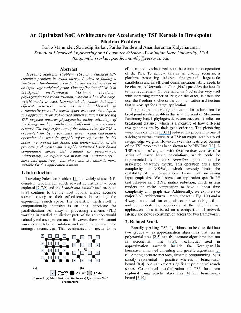
Figure 4. Efficient reduce (ρ) block for linear-time matrix reduction

with cost cij. Let c*(v) denote the cost of the least cost TSP tour passing through node v. If v is a leaf, then c*(v) is set equal to the net cost of the path from the root node to v. Subsequently, if c*(v)<best_cost then best_cost is updated to c*(v). If v is an internal node in the search tree, a lower bound for c*(v) is computed using a matrix reduction operation. If the lower bound computed (lbc(v)) is observed to be greater than or equal to best_cost, further exploration of the subtree under v is unnecessary and so it is pruned with the computation returning to node u; otherwise, the DFS is continued under v’s subtree.

We use the method shown in [8] for lower bound computation at each tree-edge. A DIM × DIM matrix called the reduction matrix (R) is maintained throughout execution. Initially, the matrix at the root node is set equal to the cost matrix defined by E. At any step of the DFS, lbc(v) is calculated as follows: 1) All entries in row i and column j of R is set to ∞; 2) R[j,1] is also set to ∞; 3) All rows and columns that contain at least one non-infinity value are reduced as follows: (a) Given row i, let mini = min{R[i,j]} for all 1≤j≤DIM; (b) Then for all 1≤j≤DIM, R[i,j] = R[i,j]-mini; (c) Similarly, given column j, let minj = min{R[i,j]} for all 1≤i≤DIM; (d) Then for all 1≤i≤DIM, R[i,j] = R[i,j]-minj As this is done, all subtracted values (i.e., the minimum values) are accumulated into another variable adjCost. 4) Subsequently, lbc(v) = lbc(u)+R[i,j]+adjCost. A flow chart for the algorithm is shown in Fig. 2.

4. NoC Design We seek to utilize NoC’s inherent parallel architecture,

customizability of the core and its efficient communication network to solve TSP. We designed and implemented the principal components of the NoC, namely the PEs and the communication network. We explored two different network architectures – the mesh and the quad-tree. In the following sub-sections, we describe in detail the design of the PE, switch and the overall network architecture.

4.1. PE Design The principal role of the PE is to handle the computation

along an edge as per the algorithm described in the previous section. Computational complexity being a major concern, our attempt has been to reduce the number of clock cycles required for this operation to make it scalable with increasing input graph size, DIM. The PE architecture has an integer datapath because the principal purported application, namely breakpoint median computation consists entirely of integer operations. The PE consists of a reduce block and peripheral control logic.We use the short-form lg k to denote log2k. The datapath consists of the following fields (DIM: number of vertices, MW: maximum edge weight).

a. x – the parent node (u) uses lg DIM bits b. y – the child node (v) uses lg DIM bits c. LBC – the lower bound cost (lbc(u)) estimate at an

edge; this requires lg DIM + lg MW + 1 bits d. EPC – the exact path cost (lbc(u)+R[i,j])

determined so far; takes lg DIM + lg MW + 1 bits

e. TSP – the TSP adjacency matrix (R), flattened. Its representation takes DIM2*lg MW bits.

f. VLST – the current list of vertices traversed; DIM*lg DIM + 1 bits are required to store this field.

g. CC – the candidate children at every stage; takes DIM bits

As is evident, the space complexity of the hardware is O(DIM2). A block diagram of the PE is shown in Fig. 3. We use valid weights 0 to 3 and 4 to denote ∞. A different range of weights just changes the number of bits for MW. Subsequent references in parentheses (e.g. ρ, φ, etc.) in this sub-section refer to this figure.

4.1.1. Reduction block. This block (ρ) carries out the matrix reduction operation described in Section 3. As is evident from the algorithm, the run-time of the operation should be a function of the matrix size, i.e., O(DIM2). The matrix is reduced using the new values of x and y in stage2 (see Peripheral control logic below) and the adjacency cost adjCost is obtained. This operation consumes the maximum fraction of the total time required for an edge computation. Hence, a significant amount of time is saved by suitably optimizing its design and implementation. Our implementation achieves O(DIM) cycle time. This has the effect of drastically reducing the total time as well as providing better time-scalability with increasing input graph size. Fig. 4 shows the architecture of reduce block. The flattened TSP matrix is initially reorganized into rows and columns in matrix. There are DIM rows and DIM columns with each entry taking up lg MW bits. The register bank minval of width DIM*(lg MW) is initialized with a bit pattern representing infinity. A counter is used as a state machine controller. There is a DIM-sized bank of comparators that compare one element from every row or column in every cycle. Minimum value calculation for all rows and the same for all columns take DIM cycles each. Additional cycles are required for subtraction of the minimum values and for calculation of the final adjCost. This step takes 2*(DIM+2) cycles to complete under the current implementation.

4.1.2. Peripheral control logic. The peripheral control logic is used for vertex selection, cost comparison, data management and bookkeeping. The register bank for the first stage is stage1, which has the same width as the datapath. The input control multiplexer initially switches to select the current vertex data. The CC field is computed (φ) from VLST in DIM cycles in the worst case. In the second stage, the candidate child is found by scanning (γ) CC of stage1. Again, this requires DIM clock cycles in the worst case. Using this candidate child, VLST is updated (B) for the child node in the graph. If it is not a leaf

node (A), the candidate child becomes the next child node, while the current node (y of stage1) becomes the parent node x of stage2. During the same stage, the data pertaining to the best case obtained so far is fetched into stage1. The input multiplexer now selects the lowest cost data (global best cost) available to the PE at this time. At this stage, TSP of stage1 gets the original TSP matrix. The current value of the exact cost of the path found so far, EPC is updated by adding to it the edge cost from x to y in the original adjacency matrix. The sum of adjCost (obtained from reduce operation) and EPC yields the lower bound cost, LBC, which is compared with the best cost found so far. If LBC is larger, the tree is pruned (E), the current child is aborted and the path through another child is explored. The data on stage2 is reloaded back to stage1 with the old value of x and a new calculation for the candidate child. If LBC is smaller and we have not reached a leaf node, normal operation continues (DFS) with the new set of data. If we have hit a leaf node with an LBC lower than the best cost globally found so far, this value (new global best cost data) is sent to the switch to be communicated with other PEs in the network.

4.1.3 Memory. There are two logical divisions in memory – global and local. However, all memory is physically distributed across all PEs. The global memory in a PE stores the TSP matrix that represents the subtree assigned to that PE. The local memory is implemented as a stack. During DFS, the new vertex data (path cost, vertex list) is pushed into the stack (Fig. 3). The stack is full only when the leaf node is reached. If there is pruning (before the leaf node is reached), the stack is popped. Every PE has a DIM-sized local memory stack. In order to introduce load-balancing to compensate for the variable effects of pruning, we reduce the solution space down to the third level of the tree by a single master thread. Subsequently, a list of all subtrees rooted at this level is maintained in memory. Once each thread completes one subtree reduction, it picks up the next available subtree and removes it from the list. This is achieved by maintaining a global array of flags and a mutually exclusive semaphore.

4.2 Network Design We explored two different kinds of network architecture – a mesh, shown in Fig. 1(a) and a quad-tree, shown in Fig. 1(b). The number of inter-switch links in a mesh increases faster than that in a quad-tree with increase in system size. The expected volume of inter-PE communication in our application is relatively low. Hence, by using an architecture with fewer links, there are potential savings in area and power without incurring a risk of network congestion.

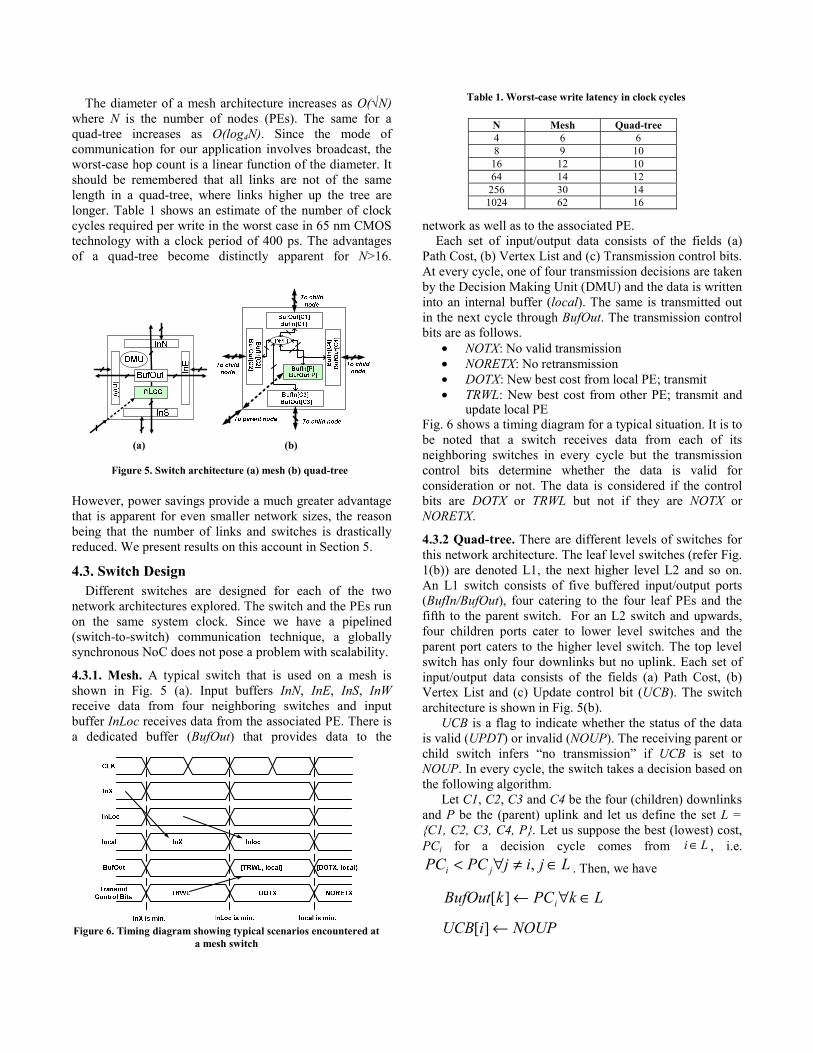
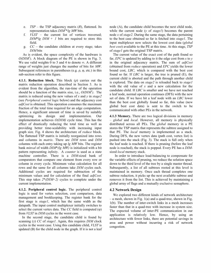
Figure 6. Timing diagram showing typical scenarios encountered at

a mesh switch

(a) (b)

Figure 5. Switch architecture (a) mesh (b) quad-tree

Table 1. Worst-case write latency in clock cycles

N Mesh Quad-tree 4 6 6 8 9 10

16 12 10 64 14 12

256 30 14 1024 62 16

The diameter of a mesh architecture increases as O(√N) where N is the number of nodes (PEs). The same for a quad-tree increases as O(log4N). Since the mode of communication for our application involves broadcast, the worst-case hop count is a linear function of the diameter. It should be remembered that all links are not of the same length in a quad-tree, where links higher up the tree are longer. Table 1 shows an estimate of the number of clock cycles required per write in the worst case in 65 nm CMOS technology with a clock period of 400 ps. The advantages of a quad-tree become distinctly apparent for N>16.

However, power savings provide a much greater advantage that is apparent for even smaller network sizes, the reason being that the number of links and switches is drastically reduced. We present results on this account in Section 5.

4.3. Switch Design Different switches are designed for each of the two network architectures explored. The switch and the PEs run on the same system clock. Since we have a pipelined (switch-to-switch) communication technique, a globally synchronous NoC does not pose a problem with scalability.

4.3.1. Mesh. A typical switch that is used on a mesh is shown in Fig. 5 (a). Input buffers InN, InE, InS, InW receive data from four neighboring switches and input buffer InLoc receives data from the associated PE. There is a dedicated buffer (BufOut) that provides data to the

network as well as to the associated PE. Each set of input/output data consists of the fields (a) Path Cost, (b) Vertex List and (c) Transmission control bits. At every cycle, one of four transmission decisions are taken by the Decision Making Unit (DMU) and the data is written into an internal buffer (local). The same is transmitted out in the next cycle through BufOut. The transmission control bits are as follows.

• NOTX: No valid transmission • NORETX: No retransmission • DOTX: New best cost from local PE; transmit • TRWL: New best cost from other PE; transmit and

update local PE Fig. 6 shows a timing diagram for a typical situation. It is to be noted that a switch receives data from each of its neighboring switches in every cycle but the transmission control bits determine whether the data is valid for consideration or not. The data is considered if the control bits are DOTX or TRWL but not if they are NOTX or NORETX.

4.3.2 Quad-tree. There are different levels of switches for this network architecture. The leaf level switches (refer Fig. 1(b)) are denoted L1, the next higher level L2 and so on. An L1 switch consists of five buffered input/output ports (BufIn/BufOut), four catering to the four leaf PEs and the fifth to the parent switch. For an L2 switch and upwards, four children ports cater to lower level switches and the parent port caters to the higher level switch. The top level switch has only four downlinks but no uplink. Each set of input/output data consists of the fields (a) Path Cost, (b) Vertex List and (c) Update control bit (UCB). The switch architecture is shown in Fig. 5(b).

UCB is a flag to indicate whether the status of the data is valid (UPDT) or invalid (NOUP). The receiving parent or child switch infers “no transmission” if UCB is set to NOUP. In every cycle, the switch takes a decision based on the following algorithm.

Let C1, C2, C3 and C4 be the four (children) downlinks and P be the (parent) uplink and let us define the set L = {C1, C2, C3, C4, P}. Let us suppose the best (lowest) cost, PCi for a decision cycle comes from Li ∈ , i.e.

LjijPCPC ji ∈≠∀< , . Then, we have

LkPCkBufOut i ∈∀←][

NOUPiUCB ←][

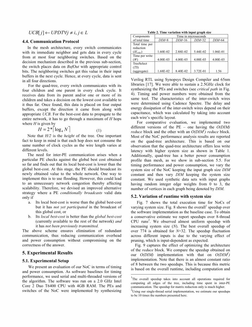
Table 2. Time variation with input graph size Components of total time

Time in microsecondsDIM=8 DIM=16 DIM=32 DIM=64

Total time per reduction (IEedge) 1.60E-02 2.88E-02 5.44E-02 1.06E-01 Time per write (W) 4.00E-03 4.00E-03 4.00E-03 4.00E-03 TreeSelect (TS) (aggregate) 1.68E-02 8.40E-02 3.72E-01 1.56

LjijUPDTjUCB ∈≠∀← ,][

4.4. Communication Protocol In the mesh architecture, every switch communicates with its immediate neighbor and gets data in every cycle from at most four neighboring switches. Based on the decision mechanism described in the previous sub-section, the switch places data on BufOut with appropriate control bits. The neighboring switches get this value in their input buffers in the next cycle. Hence, at every cycle, data is sent in all four directions.

For the quad-tree, every switch communicates with its four children and one parent in every clock cycle. It receives data from its parent and/or one or more of its children and takes a decision on the lowest cost available to it thus far. Once found, this data is placed on four output buffers, except the direction it came from along with appropriate UCB. For the best-cost data to propagate to the entire network, it has to go through a maximum of H hops where H is given by

⎡ ⎤NH 4log*2= (1) Note that H/2 is the height of the tree. One important fact to keep in mind is that each hop does not consume the same number of clock cycles as the wire length varies at different levels. The need for inter-PE communication arises when a particular PE checks against the global best cost obtained so far and finds out that its local best-cost is lower than the global best-cost. At this stage, the PE should broadcast its newly obtained value to the whole network. One way to implement this is to use flooding. However, this could lead to an unnecessary network congestion thereby affecting scalability. Therefore, we devised an improved alternative strategy where a PE conditionally broadcasts valid data only if

a. Its local best-cost is worse than the global best-cost but it has not yet participated in the broadcast of this global cost, or

b. Its local best-cost is better than the global best-cost (currently available to the rest of the network) and it has not been previously transmitted.

The above scheme ensures elimination of redundant communication, thus reducing communication overhead and power consumption without compromising on the correctness of the answer.

5. Experimental Results 5.1. Experimental Setup

We present an evaluation of our NoC in terms of timing and power consumption. As software baselines for timing performance, we used serial and multi-threaded versions of the algorithm. The software was run on a 2.0 GHz Intel Core 2 Duo T6400 CPU with 4GB RAM. The PEs and switches of the NoC were implemented by synthesizing

Verilog RTL using Synopsys Design Compiler and 65nm libraries [17]. We were able to sustain a 2.5GHz clock for synthesizing the PEs and switches (see critical path in Fig. 4). Timing and power numbers were obtained from the same tool. The characteristics of the inter-switch wires were determined using Cadence Spectre. The delay and energy dissipation of the inter-switch wires depend on their capacitance, which was calculated by taking into account each wire’s specific layout.

For comparative evaluation, we implemented two different versions of the PE – one having the O(DIM) reduce block and the other with an O(DIM2) reduce block. Most of the NoC performance analysis results are reported on the quad-tree architecture. This is based on our observation that the quad-tree architecture offers less write latency with higher system size as shown in Table 1. Additionally, quad-tree has a better power consumption profile than mesh, as we show in sub-section 5.5. For timing performance and power consumption, we vary the system size of the NoC keeping the input graph size DIM constant and then vary DIM keeping the system size constant. We used synthetic data sets with input graphs having random integer edge weights from 0 to 3, the number of vertices in each graph being denoted by DIM.

5.2. Variation of runtime with system size Fig. 7 shows the total execution time for NoCs of

varying system size. Fig. 8 shows the overall1 speedup over the software implementation as the baseline case. To obtain a conservative estimate we report speedups over 8-thread CPU runs2. We observed almost uniform speedup with increasing system size (N). The best overall speedup of over 774 is obtained for N=32. The speedup fluctuation across different inputs is due to the varying effect of pruning, which is input-dependent as expected. Fig. 9 captures the effect of optimizing the architecture of the reduce block. We compare the speedup obtained on our O(DIM) implementation with that on O(DIM2) implementation. Note that there is an almost constant ratio of 8 between the two speedups. This is because this metric is based on the overall runtime, including computation and 1The overall speedup takes into account all operations required for computing all edges of the tree, including time spent in inter-PE communication. The speedup for matrix reduction only is much higher. 2Using our single-thread serial implementation, we estimate our speedups to be 10 times the numbers presented here.

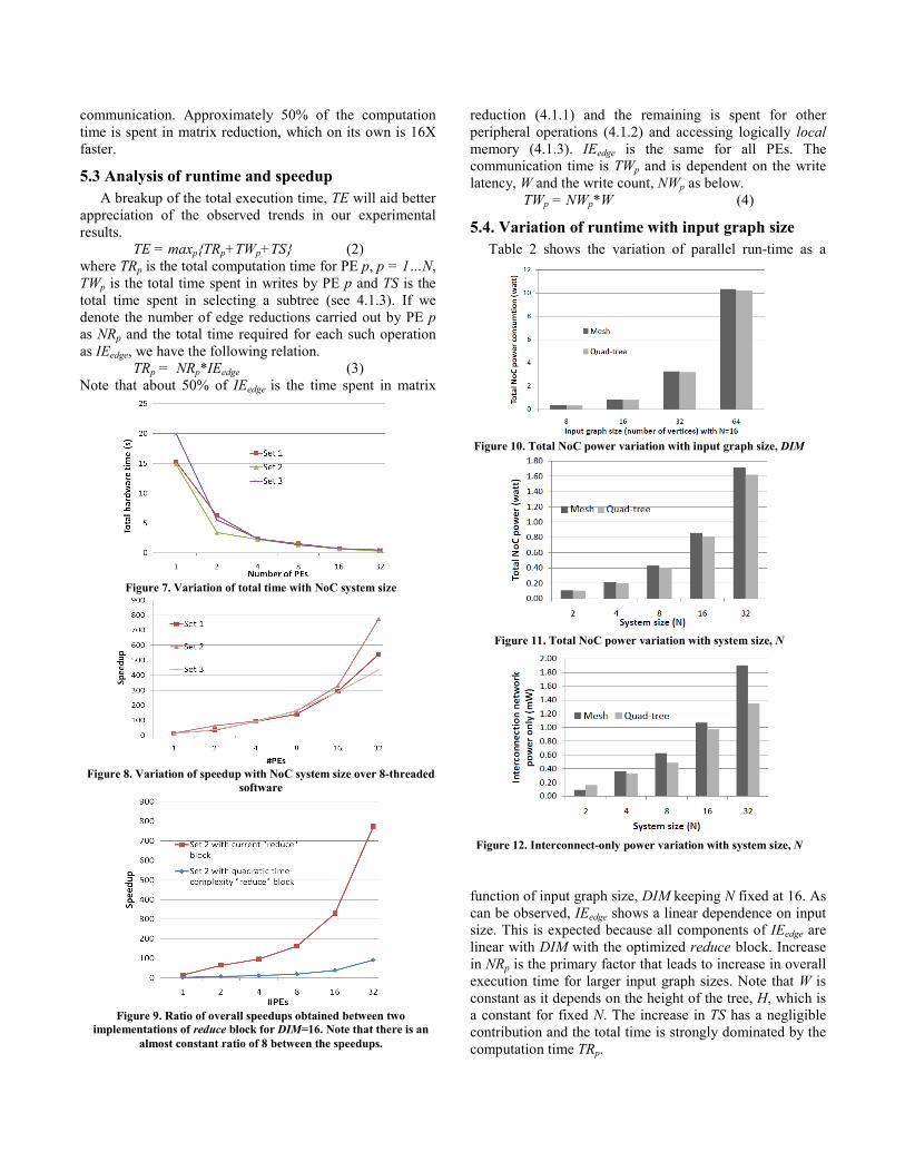
Figure 7. Variation of total time with NoC system size

Figure 8. Variation of speedup with NoC system size over 8-threaded

software

Figure 9. Ratio of overall speedups obtained between two

implementations of reduce block for DIM=16. Note that there is an almost constant ratio of 8 between the speedups.

Figure 10. Total NoC power variation with input graph size, DIM

Figure 11. Total NoC power variation with system size, N

Figure 12. Interconnect-only power variation with system size, N

communication. Approximately 50% of the computation time is spent in matrix reduction, which on its own is 16X faster.

5.3 Analysis of runtime and speedup A breakup of the total execution time, TE will aid better appreciation of the observed trends in our experimental results. TE = maxp{TRp+TWp+TS} (2) where TRp is the total computation time for PE p, p = 1…N, TWp is the total time spent in writes by PE p and TS is the total time spent in selecting a subtree (see 4.1.3). If we denote the number of edge reductions carried out by PE p as NRp and the total time required for each such operation as IEedge, we have the following relation.

TRp = NRp*IEedge (3) Note that about 50% of IEedge is the time spent in matrix

reduction (4.1.1) and the remaining is spent for other peripheral operations (4.1.2) and accessing logically local memory (4.1.3). IEedge is the same for all PEs. The communication time is TWp and is dependent on the write latency, W and the write count, NWp as below.

TWp = NWp*W (4)

5.4. Variation of runtime with input graph size Table 2 shows the variation of parallel run-time as a

function of input graph size, DIM keeping N fixed at 16. As can be observed, IEedge shows a linear dependence on input size. This is expected because all components of IEedge are linear with DIM with the optimized reduce block. Increase in NRp is the primary factor that leads to increase in overall execution time for larger input graph sizes. Note that W is constant as it depends on the height of the tree, H, which is a constant for fixed N. The increase in TS has a negligible contribution and the total time is strongly dominated by the computation time TRp.

5.5. Power Consumption One PE has a gate count of ~50K and a switch has

~1400 gates after synthesis. Fig. 10 depicts the variation in power consumption with increasing input graph size and system size constant at N=16. In Fig. 11, input graph size is constant at DIM=16 and system size varies. The PE and switch power numbers have been reported on 65nm standard cell libraries from CMP [12]. The interconnect power has been reported using Cadence Spectre. In each figure, we have compared the power consumption using mesh and that using quad-tree. Note that for fixed system size, N = 16, there is marginal power saving. This is because most of the power consumption occurs in the computation (PE) part and the benefit of using a quad-tree over a mesh is not readily apparent. In both cases for fixed N, the PE power consumption varies as O(DIM2) and the network (switch and interconnect) power consumption varies as O(lg DIM), though the mesh has a larger constant for the network power component. We observe larger savings in power when system size is varied with DIM kept fixed. Although, the total power consumption of the quad-tree NoC is 5% lower than the mesh, a closer look in Fig. 12 reveals the savings in interconnect-only power. Here we observe close to 30% savings in power consumption in the quad-tree. The interconnect power consumption difference between mesh and quad-tree does not follow a monotonic pattern. It narrows down when N is a power of 4 and increases in between. This is because the quad-tree is a complete tree and has the maximum number of links for a tree of that height when N is a power of 4.

6. Conclusion and Future Work In this paper we have undertaken the design,

implementation and performance evaluation of an NoC-based multi-core architecture for solving TSP targeted to breakpoint median problem in phylogeny. We show that the proposed NoC architecture reduces total execution time by a factor of 774 compared to a multi-threaded version of the corresponding software implementation. On the architecture front, we show that a quad-tree is better suited to this kind of application. To the best of our knowledge, this is the first NoC-based approach to tackle this problem.

We believe that our current implementation provides appreciable performance enhancement over comparable hardware accelerators and can serve as a basis for more NoC-based platforms with applications to life sciences. It also provides a paradigm for accelerating similar vector or matrix-based applications like image processing.

7. Acknowledgement This work is partially supported by NSF grant (IIS-

0916463).

8. References [1] E.L. Lawler, J. Lenstra, A.R. Kan and D. Shmoys. The

traveling salesman problem. John Wiley, 1985. [2] J. Bentley. Fast algorithms for geometric traveling salesman

problems. ORSA J. Computing, 4:387-411, 1992. [3] B. Golden, L. Bodin, T. Doyle, W. Stewart. Approximate

traveling salesman algorithms, Operations Research, 28:694-711, 1980.

[4] G. Reinelt. The traveling salesman problem: computational solutions for TSP applications. In LNCS 840, pp. 172-186, Springer-Verlag, Berlin, 1994.

[5] S. Lin and B. Kernighan. An effective heuristic algorithm for the traveling salesman problem. Operations Research, 21:498-516, 1973.

[6] P. Jog, J. Y. Suh, and D. Van Gucht. Parallel Genetic Algorithms Applied to the Traveling Salesman Problem, SIAM J. Optim. Volume 1, Issue 4, pp. 515-529 1991.

[7] D. L. Miller, J. F. Pekny. Results from a parallel branch and bound algorithm for the asymmetric traveling salesman problem, Operations Research Letters Volume 8, Issue 3, June 1989, Pages 129-135.

[8] E. Horowitz and S. Sahni, “Branch-and-bound” in Fundamentals of computer algorithms, Potomac, MD: Computer Science Press, 1984, pp. 370-421.

[9] M. Bellmore and G. Nemhauser, “The Traveling Salesman Problem: A Survey,” Operations Research, vol. 16, 1968, pp. 538-558

[10] D. A. Bader and M. Yan, “High-Performance Phylogeny Reconstruction” in Handbook of Computational Molecular Biology, Edited by S. Aluru, Chapman & Hall/CRC Computer and Information Science Series, 2005.

[11] M. Blanchette, G. Bourque, and D. Sankoff, “Breakpoint phylogenies,” Genome Informatics Workshop, Tokyo: University Academy Press, 1997, pp. 25-34.

[12] I. Pe'er and R. Shamir, “The median problems for breakpoints are NP-complete,” Elec. Colloq. on Comput. Complexity, 1998, p. 71.

[13] T. S. T. Mak and K. P. Lam, “High Speed GAML-based Phylogenetic Tree Reconstruction Using HW/SW Codesign,” Proc. Computational Systems Bioinformatics, 2003, pp. 470.

[14] N. Alachiotis et. al., “Exploring FPGAs for Accelerating the Phylogenetic Likelihood Function,” Proc. IEEE Intl. Sym. on Parallel and Distributed Processing 2009, pp 1-8.

[15] J. Bakos and P. Elenis, “A Special-Purpose Architecture for Solving the Breakpoint Median Problem,” IEEE Transactions on Very Large Scale Integration Systems, vol. 16, 2008, pp. 1666-1676.

[16] F. Patas et. al., “Fine-grain Parallelism using Multi-core, Cell/BE, and GPU Systems: Accelerating the Phylogenetic Likelihood Function,” Int. Conf. Parallel Processing, 2009, pp. 9-17.

[17] Circuits Multi-Projects (http://cmp.imag.fr/). Last date accessed: 20 Feb 2010.