An Online Tactical Metrics Applied to Football Game

Research Journal of Applied Sciences, Engineering and Technology 5(5): 1700-1719, 2013 ISSN: 2040-7459; e-ISSN: 2040-7467 © Maxwell Scientific Organization, 2013 Submitted: July 26, 2012 Accepted: August 28, 2012 Published: February 11, 2013

Corresponding Author: Filipe M. Clemente, RoboCorp, Department of Sport Sciences and Physical Education-University of

Coimbra, Estádio Universitário de Coimbra, Pavilhão 3, 3040-156 Coimbra, Portugal, Tel.: + 351 239 802770, Fax: + 351 239 802779

1700

An Online Tactical Metrics Applied to Football Game

1Filipe M. Clemente, 2Micael S. Couceiro, 3,4Fernando M.L. Martins and 3Rui Mendes

1RoboCorp, Department of Sport Sciences and Physical Education-University of Coimbra, Estádio Universitário de Coimbra, Pavilhão 3, 3040-156 Coimbra, Portugal

2RoboCorp at the Department of Electrical Engineering, Engineering Institute of Coimbra, Rua Pedro Nunes-Quinta da Nora, 3030-199 Coimbra, Portugal

3RoboCorp, Coimbra Department of Education-Polytechnic Institute of Coimbra, Rua Dom João III Solum, 3030-329 Coimbra, Portugal

4Instituto de Telecomunicações (IT), Covilhã, Convento Santo António, 6201-001 Covilhã, Portugal Abstract: In collective sports, the match analysis is fundamental in order to improve the quality of coaches’ intervention. Nevertheless, the generality of the systems are based on notational analysis which does not allow a deep understanding about the collective behaviour of the team. Therefore, the main goal of this study is to update and design new tactical metrics that allows an improved online knowledge about the teams’ behaviour. Tactical metrics such as the teams’ centroid, teams’ stretch index and teams’ effective play area will be presented throughout this study, validated by means of a single match experimental case study. Results suggest the potential of the herein proposed tactical metrics, providing relevant and online information to the coaches over time, thus allowing new opportunities to improve the quality of their intervention. Keywords: Collective performance evaluation, match analysis, sports performance, tactical metrics

INTRODUCTION

Match analysis refers to the objective of recording

and examining events occurring during competition (Carling et al., 2005). The main goal of match analysis is to provide to the coach relevant information about the team and/or the individual performance of each player (Franks and McGarry, 1996), thus allowing to improve the quality of future planning (Hughes and Franks, 2004). At the same time, the coach can analyze the performance of the opposing team in order to use the data to identify ways to overcome its strengths and exploit its weaknesses (Carling et al., 2009).

The traditional quantitative analysis (i.e., notational analysis) may not be suitable to establish the whole characteristics of a skill or tactical behaviour (Clemente et al., 2012a). Nevertheless, the use of new methods, such as artificial neural networks or tactical metrics (e.g., team’s centroid, team’s surface area or team’s stretch index) may allow to overcome the limitations inherent to notational analysis (Lees, 2002). Therefore, both notational and kinematical analysis need to be complemented with new methods to allow a further understanding of the team’s tactical dynamics (Clemente et al., 2012b). In fact, such information is vital to improve the knowledge of the game, quality of

training and intervention of the coach, thus improving the collective performance of teams.

Sport performance consists of a complex series of interrelationships between wide varieties of performance variables (Borrie et al., 2002). Therefore, structures and configurations of play should be considered as a whole rather than analysed in an individual manner (Passos, 2009). Systems with many dynamically interacting elements can produce rich and varied patterns of behaviours that are clearly different from the behaviour of individual players. In this line of though, McGarry et al. (2002) considered that the rich and varied patterns that arise in team sports are the result of the self-organization among many coupled oscillators (e.g., players).

The tactic concept is related with space-time dimension, being a consequence from the strategy and space-time constraints of match actions (Zerhouni, 1980). In other words, the tactic concept is an adaptation to new constraints of the match, such as to opposition or individual team’s constraints (Clemente, 2012). Tactics refers to the positions taken in reaction to the opposing team in the match and the adaptation of the team to the conditions of play (Gréhaigne and Godbout, 1995; Gréhaigne et al., 1999). Complementarily, to Smith et al. (1996) the tactic is the set of decisions and actions developed over the game.

Res. J. Appl. Sci. Eng. Technol., 5(5): 1700-1719, 2013

1701

The tactic states the relation among teammates that altogether forms the collective behaviour which can be divided into group tactic (i.e., clusters inside the team) or team tactic (i.e., all players of the team) (Zerhouni, 1980). In short, team’s tactic is related to the conception of unity, i.e., the ability that all players have to play as a team, coordinating their actions regarding the team’s needs.

Some collective sport games use specific methods and metrics in order to analyse and evaluate the dynamical collective behaviour. However, according to Neville et al. (2008), despite the large quantity of research methods and techniques to model performance in sport, used singly or in combination, results have been somehow disappointing. Simple frequency data cannot necessarily capture the full complexity of the performance (Borrie et al., 2002). Therefore, searching for identification and interpretation of substantial game behaviour, it is imperative to gather quantitative and qualitative information (Garganta, 2009). Consequently, it is necessary to develop novel concepts and tools, from the systems approach and computer science, to handle such complexity and allow a new understanding about tactical behaviour of teams (Balagué and Torrents, 2005), thus contributing to improve the knowledge of coaches, i.e., improving the potential of the match analysis.

Statement of contributions: Although recent studies analyse the team’s behaviour using collective metrics, the fact is that the most robust metrics to evaluate the sport performance analyse the individual behaviour of each player. However, collective sport games need to be understood as a collective phenomenon, i.e., the performance is not the sum of the parts, but the unique and specific cooperation of every part, i.e., the performance analysis need to be analysed as a whole: a team. In fact, at the football game, fewer studies had analysed the collective dynamic of teams through tactical metrics. However, football is a tactical sophisticated sport that requires the understanding of the coordination processes among players (Davids et al., 2005). One cannot expect the same performance from the same player in two different teams since the essence of style of play depends of each player specific properties (Deleplace, 1994). Hence, the sum of players’ performance within the same team has a preponderant influence in the performance and evolution of each player’s play style (Gréhaigne et al., 2005). For instance, the Portuguese football player Cristiano Ronaldo, considered the 2nd best player in the world, scored 46 goals in 38 games in 2011/2012 season in Real Madrid (1.21 goals per game). Nevertheless, in the national Portuguese team, he scored 35 goals in 94 matches (0.37 goals per game).

As previously addressed, until now, there are few studies dedicated exclusively to the study of tactical dynamics of teams, especially in 11-a-side football.

Therefore the main goal of this study is to propose new collective online metrics to the football game, thus improving the most pertinent information from a coach’s point-of-view and, at the same time, understand the factors that characterize the team’s performance.

In the present study, three online tactical metrics to analyse and evaluate the football game will be presented. The herein presented tactical metrics are defined as:

The team’s centroid The team’s stretch index The team’s effective area of play

The usefulness of the team’s centroid metric,

according to Bourbousson et al. (2010), may have the potential to compute the in-phase relation among the two opposing teams in longitudinal and lateral directions. This study proposes an updated version of the team’s centroid considering the distance of players in relation to the ball.

The team’s stretch index metric can give some information about the dispersion of the team in relation to the team’s centroid (Bourbousson et al., 2010). This information is important to improve the knowledge about the centrality of the game, thus allowing organizing the game based on such dispersion. Once again, this study proposes an updated version of the team’s stretch index which also considers the distance of players to the ball.

The team’s effective area of play metric allows obtaining the number of triangles of each team over time and the effective space to play. The number of effective triangles of each team may also characterize the efficiency of the tactical team organization. For instance, the effective area of a team may be used to evaluate both the defensive and offensive phases. Hence, this study also presents a computationally efficient algorithm to obtain and graphically present the effective area of each team in an online fashion using the high-level calculation tool MATLAB.

Paper organization: This study will be organized as it follows: Literature review: Discusses some collective

metrics applied to sport games in the literature Online metrics: Presents the online metrics

proposed giving the example of the 11-a-side football game

Case study: Results and Discussion, depicts the data obtained from a case study discussing the meaning of the results and how these metrics may provide useful information to coaches or other sport agents

Conclusion: Where a general overview of the present study is outlined


1702

LITERATURE REVIEW

Recently, many researchers developed new methods and metrics to analyse the team’s collective behaviour, thus increasing the quality and efficiency of the obtained results (Frencken et al., 2011; Passos et al., 2011a, b). Specifically, new metrics have been designed to better assess the collective performance of teams based on players’ tactical dynamic (Gréhaigne, 1992; Frencken and Lemmink, 2008; Bourbousson et al., 2010).

One of the first metrics applied to the football game was the effective play-space (Gréhaigne, 1992). According to some studies (Gréhaigne, 1992; Gréhaigne et al., 2005; Gréhaigne et al., 2010) this metric can verify the effectively occupied play-space by players of both teams. The effective play-space can be defined as the polygonal area obtained by a line that links all involved players positioned at the periphery of the play at specific instant. Nevertheless, the reported studies do not show a mathematical method to determine the metric and how to overtake the geometrical complexity related to the polygon computation. Also, this metric does not consider the influence of the occupied play-space of one team over the other. Hence, the claims about the effectiveness of the play-space proposed by Gréhaigne (1992) are not consistent with the ones considered in this study.

Frencken et al. (2011) and Frencken and Lemmink (2008) developed two metrics applied to small-sided football games (5-a-side) analysis:

The team’s centroid The team’s surface area

The team’s centroid metric was calculated as the mean position ̅ , of all outfield players (xn, yn) from one team. The results of Frencken et al. (2011) show that the correlations between both teams’ centroids are near perfect for the forward-backward oscillations for all analysed small-sided games. Although slightly lower, the correlation coefficients for the lateral oscillations of the teams’ centroids were still considerably high for the small-sided football games. These results confirm that team’s centroids tend to move in the same direction over the course of a game.

Bourbousson et al. (2010) presented two collective metrics applied in the basketball game:

The team’s spatial centre The team’s stretch index

The team’s spatial centre metric was calculated at the mean position of five players of each team as each player contributed equally to the team metrics. The data

Table 1: Description of the notation Notation Description (a b) The number of combinations of elements

from elements APol Polygon area P Polygon Δ Triangle formed by vertices (x1 , y1), (x2, y2)

and (x3, y3) Vector of triangles index ordinates through

perimeter by ascending order Γ Polygon from the triangles intersections DT Transpose of a matrix D Rq×r q×r real matrix δ; ζ Team A and B, respectively τ Counter of the non-overlapping triangles wi Weight based on the Euclidean distance from

each player to the ball dmax Maximal distance of one player to the ball Sind Stretch index di Euclidean distance between player i and the

team’s centroid

contained the longitudinal and lateral position of each player on the team. The team’s stretch index metric was obtained by computing the mean of the distances among each player and the spatial centre for that team. Therefore, this metric represented the mean deviation of each player on a team from its spatial centre (Bourbousson et al., 2010). The team’s spatial centre may allow to determinate the in-phase relation between the two teams in longitudinal and lateral directions. Regarding to the team’s stretch index, Bourbousson et al. (2010) suggested that it may provide an indication of whether a team was expanding or contracting at any instant.

Concerning the specificities of the 11-a-side football game, it is important to provide some updates to increase the quality and objectivity of the results. Therefore, given the reduced literature about the collective tactical dynamics on 11-a-side football, this study proposes a set of novel collective metrics, designed based on the needs of this sport, thus providing useful information to sport’s analysts.

ONLINE METRICS

Online tactical metrics can give to the coach or sport’s agent’s relevant information about how teams behave over time throughout the match. In fact, such metrics can be used as an important tool to improve the coach’s opportunities to make changes on the team’s tactic, easily detecting the strong or weak aspects of its performance during the match. Table 1 outlines the notation to allow an easier understands on the online metrics that will be presented and discussed.

Team’s centroid metric: For the football game, the centroid can be calculated through the geometric mean position ̅ , of all players (xn, yn) for each team. According to Frencken et al. (2011), the team’s centroid of both teams can provide three measures:


1703

Fig. 1: Spatial referential of the field The -distance (m) represented forward-backward

displacement (i.e., length of the field) y-distance (m) represented lateral displacement

(i.e., width of the field) Radial distance (m), comprising both forward-

backward and lateral displacement. These measures are obtained based on the centroid position relative to the origin , i.e., 0, 0 , defined at the centre of the field (Fig. 1):

xy =

1

∑ wiNi=1

∑ wixi11i=1

∑ wiyi11i=1

(1)

The position of the player is defined as (xi, yi).

The relevance of each player to the team’s centroid, i.e., wi weight, is based on the Euclidean distance from each player to the ball as:

wi=1-xi xb yi yb

dmax (2)

where, in , corresponds to the position of the ball and dmax is the Euclidean distance of the farthest player to the ball at each iteration (Fig. 1).

The usefulness of the team’s centroid, according to Bourbousson et al. (2010), may be the potential to compute the in-phase relation among the two opposing teams in longitudinal and lateral directions. Until now, the most relevant research focuses on the oscillation of each team in both the longitudinal and lateral directions, with strong coupling tendencies between them (Frencken et al., 2011). However, this kind of information can be of little use for the coach. In fact, the team’s centroid may provide useful information for field application, i.e., decreasing the systemic interpretation and increasing the potential application of the analysis of football to provide substantial information to the football scouts, thus improving the quality of teams’ analyses. Additionally, the centroid of each team can oscillate according to each variable in different moments (e.g., ball possession).

Therefore, the cumulative centroid position at the end of the game may reveal different tendencies over time. Thus, for the coach, analysing the teams’ centroid at different moments (e.g., ball possession) and how the team acts according to ball’s location or the opposing team’s centroid are important factors that allow determining how a team can improve its performance in order to achieve its goals, or how it can use the information about the opposing team to adequate a new tactical or strategic approach for the match. Nevertheless, the team’s centroid does not allow understanding the strategic distribution of players in the field. Therefore, it is important to propose a tactical metric that allows representing teams’ dispersion.

Team’s stretch index metric: The stretch index measures the space expansion or contraction of the team on the longitudinal a lateral directions (Bourbousson et al., 2010). Similarly to the team’s centroid, a weighted team’s stretch index metric may then be calculated as:

∑

∑ (3)

where,

= The Euclidean distance between player and the team’s centroid, i.e.:

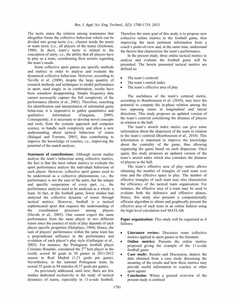
di= x x y y (4) within this context, the stretch index can be obtained by computing the mean of the distances between each player and the centroid of the team. Thus, this metric represents the mean deviation of each player on a team from its centroid (Fig. 2).

The team’s stretch index can give some information about the dispersion of the team in relation to the centroid. This information is important to improve the knowledge about the relation between players and the centrality of the game, thus allowing organizing the game in function of such dispersion.


1704

Fig. 2: Dispersion of the players in relation to centroid

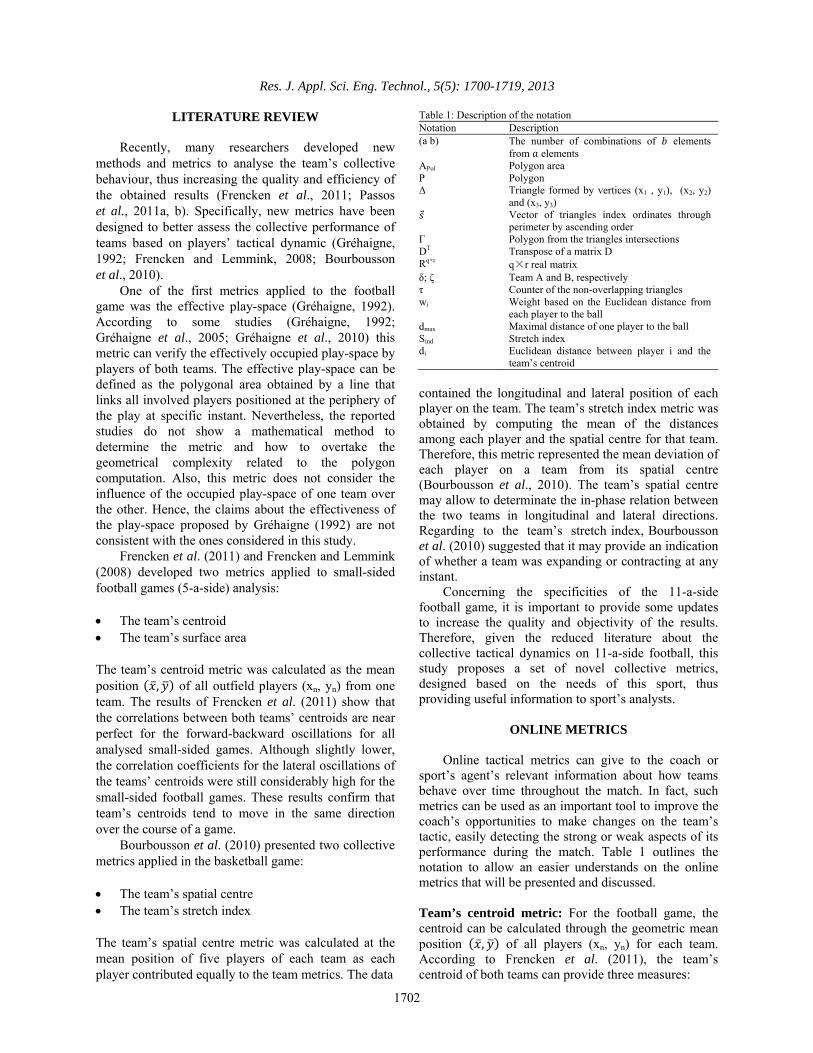
Fig. 3: An example of dispersion of the players in relation to centroid

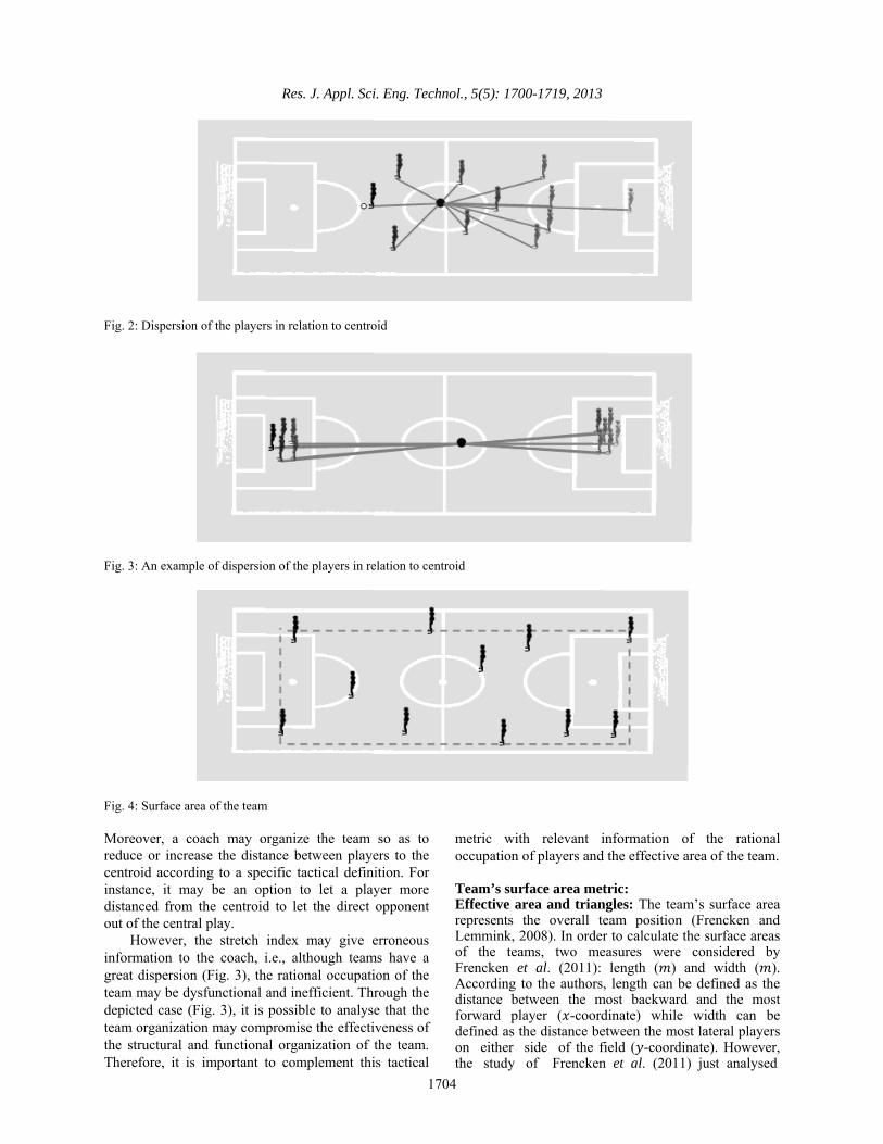
Fig. 4: Surface area of the team Moreover, a coach may organize the team so as to reduce or increase the distance between players to the centroid according to a specific tactical definition. For instance, it may be an option to let a player more distanced from the centroid to let the direct opponent out of the central play.

However, the stretch index may give erroneous information to the coach, i.e., although teams have a great dispersion (Fig. 3), the rational occupation of the team may be dysfunctional and inefficient. Through the depicted case (Fig. 3), it is possible to analyse that the team organization may compromise the effectiveness of the structural and functional organization of the team. Therefore, it is important to complement this tactical

metric with relevant information of the rational occupation of players and the effective area of the team.

Team’s surface area metric: Effective area and triangles: The team’s surface area represents the overall team position (Frencken and Lemmink, 2008). In order to calculate the surface areas of the teams, two measures were considered by Frencken et al. (2011): length ( ) and width ( ). According to the authors, length can be defined as the distance between the most backward and the most forward player ( -coordinate) while width can be defined as the distance between the most lateral players on either side of the field ( -coordinate). However, the study of Frencken et al. (2011) just analysed


1705

Fig. 5: Example of surface area

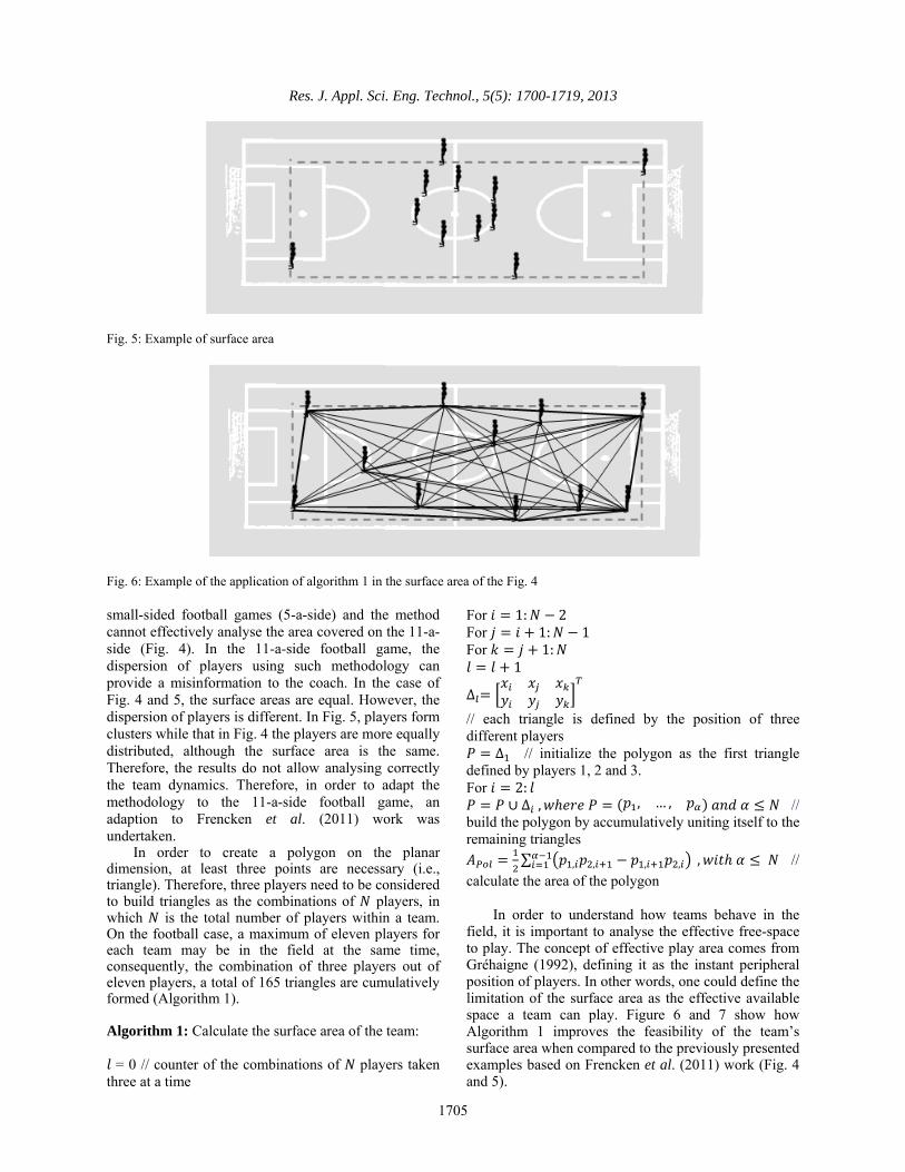
Fig. 6: Example of the application of algorithm 1 in the surface area of the Fig. 4 small-sided football games (5-a-side) and the method cannot effectively analyse the area covered on the 11-a-side (Fig. 4). In the 11-a-side football game, the dispersion of players using such methodology can provide a misinformation to the coach. In the case of Fig. 4 and 5, the surface areas are equal. However, the dispersion of players is different. In Fig. 5, players form clusters while that in Fig. 4 the players are more equally distributed, although the surface area is the same. Therefore, the results do not allow analysing correctly the team dynamics. Therefore, in order to adapt the methodology to the 11-a-side football game, an adaption to Frencken et al. (2011) work was undertaken.

In order to create a polygon on the planar dimension, at least three points are necessary (i.e., triangle). Therefore, three players need to be considered to build triangles as the combinations of players, in which is the total number of players within a team. On the football case, a maximum of eleven players for each team may be in the field at the same time, consequently, the combination of three players out of eleven players, a total of 165 triangles are cumulatively formed (Algorithm 1).

Algorithm 1: Calculate the surface area of the team: = 0 // counter of the combinations of players taken

three at a time

For 1: 2 For 1: 1 For 1:

1

∆

// each triangle is defined by the position of three different players

∆ // initialize the polygon as the first triangle defined by players 1, 2 and 3. For 2:

∪ ∆ , , … , // build the polygon by accumulatively uniting itself to the remaining triangles

∑ , , , , , //

calculate the area of the polygon

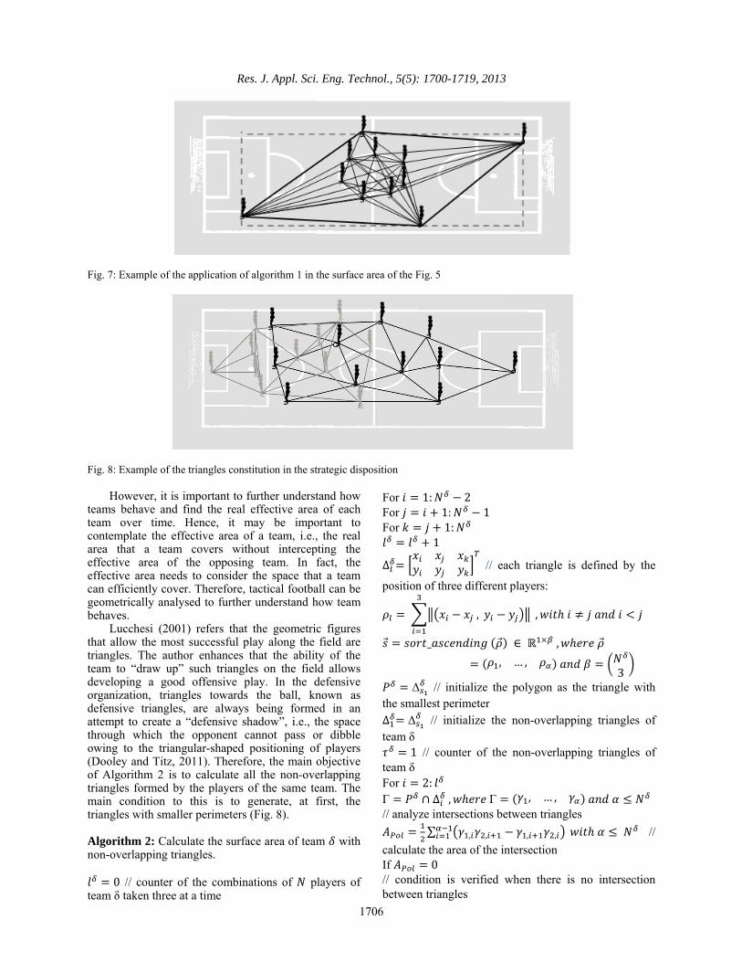
In order to understand how teams behave in the field, it is important to analyse the effective free-space to play. The concept of effective play area comes from Gréhaigne (1992), defining it as the instant peripheral position of players. In other words, one could define the limitation of the surface area as the effective available space a team can play. Figure 6 and 7 show how Algorithm 1 improves the feasibility of the team’s surface area when compared to the previously presented examples based on Frencken et al. (2011) work (Fig. 4 and 5).


1706

Fig. 7: Example of the application of algorithm 1 in the surface area of the Fig. 5

Fig. 8: Example of the triangles constitution in the strategic disposition

However, it is important to further understand how teams behave and find the real effective area of each team over time. Hence, it may be important to contemplate the effective area of a team, i.e., the real area that a team covers without intercepting the effective area of the opposing team. In fact, the effective area needs to consider the space that a team can efficiently cover. Therefore, tactical football can be geometrically analysed to further understand how team behaves.

Lucchesi (2001) refers that the geometric figures that allow the most successful play along the field are triangles. The author enhances that the ability of the team to “draw up” such triangles on the field allows developing a good offensive play. In the defensive organization, triangles towards the ball, known as defensive triangles, are always being formed in an attempt to create a “defensive shadow”, i.e., the space through which the opponent cannot pass or dibble owing to the triangular-shaped positioning of players (Dooley and Titz, 2011). Therefore, the main objective of Algorithm 2 is to calculate all the non-overlapping triangles formed by the players of the same team. The main condition to this is to generate, at first, the triangles with smaller perimeters (Fig. 8).

Algorithm 2: Calculate the surface area of team with non-overlapping triangles.

0 // counter of the combinations of players of team δ taken three at a time

For 1: 2 For 1: 1 For 1:

1

∆ // each triangle is defined by the

position of three different players:

, ,

_ ∈ ,

, … , 3

Δ // initialize the polygon as the triangle with the smallest perimeter ∆ Δ // initialize the non-overlapping triangles of team δ

1 // counter of the non-overlapping triangles of team δ For 2: Γ ∩ ∆ , Γ , … , // analyze intersections between triangles

∑ , , , , //

calculate the area of the intersection If 0 // condition is verified when there is no intersection between triangles


1707

Fig. 9: Number of effective triangles without overlapping

1 ∪ ∆ // build the polygon by accumulatively

uniting the non-overlapping triangles ∆ ∆ // non-overlapping τδtriangle of team δ

Therefore, as the number of formed triangles within a team increase, the less effective space is left for the opposing team. For instance, Trapattoni (1999) affirms that when players are pressured and cannot turn around and dribble, the ball must travel along triangles until a solution for forward play is found, i.e., the offensive triangles are annulled by the defensive triangles.

After generating all triangles of each team, the next step is to consider all triangles of each team without interception. Through this condition it is possible to calculate the area of each team without interception (Fig. 9). Hence, Algorithm 3 computes the triangles of each team that do not suffer from the intersection of the opposing team. Algorithm 3: Effective Area-Triangles of team that do not intersect the surface area of the opposing team .

0 // counter of the effective triangles of team δ 0 // effective area of team δ // polygon of the effective area of team δ is

initialized as an empty array For 1: Γ ∆ ∩ , Γ , … , 6 // analyse intersections between triangles

∑ , , , , 6 //

calculate the area of the intersection If 0 // condition is verified when there is no intersection between the triangle from team δ and the surface area of team ζ

∑ // calculate the area of

the triangle // cumulative effective area of team δ

(a) (b) Fig. 10: Example of triangles interception

1 // counter of the effective triangles of team δ

∪ ∆ // build the polygon of the effective area of team δ by accumulatively uniting its effective triangles

In Algorithm 3, both teams are simultaneously considered in which and are the team ID such that

1, 2 and 1, 2 with However, in the presence of interceptions between

opposing triangles and based on the supposition that effective defensive triangles can annul the offensive triangles (Trapattoni, 1999), the effective area to be considered is the one of the defensive triangles (Fig. 10a), thus reducing the effective area of the offensive team.

However, Dooley and Titz (2011) proves that in order to form effective defensive triangles, it is necessary to have an approximate distance of 12 m between each vertex (i.e., defensive players), i.e., a defensive triangle with a maximum perimeter of 36 m. Hence, if a defensive triangle has a perimeter superior to 36 m (Fig. 10 b), it will be nullified by the offensive triangles since there are no guarantees that the defensive players will be able to intercept the ball.

After considering the triangles without interception, it is necessary to consider all triangles of the team that does not have the ball possession (i.e., defensive team) with perimeters inferior to 36 m


1708

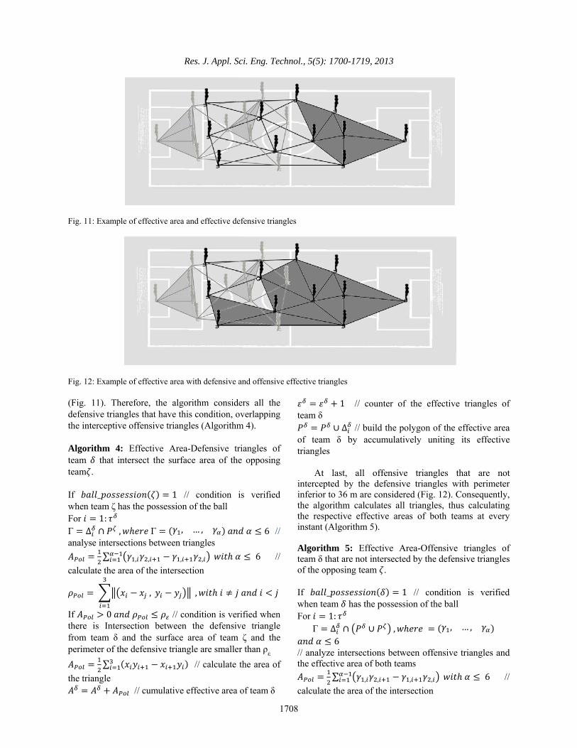
Fig. 11: Example of effective area and effective defensive triangles

Fig. 12: Example of effective area with defensive and offensive effective triangles (Fig. 11). Therefore, the algorithm considers all the defensive triangles that have this condition, overlapping the interceptive offensive triangles (Algorithm 4).

Algorithm 4: Effective Area-Defensive triangles of team that intersect the surface area of the opposing team .

If _ 1 // condition is verified when team ζ has the possession of the ball For 1: Γ ∆ ∩ , Γ , … , 6 // analyse intersections between triangles

∑ , , , , 6 //

calculate the area of the intersection

, ,

If 0 // condition is verified when there is Intersection between the defensive triangle from team δ and the surface area of team ζ and the perimeter of the defensive triangle are smaller than ρε


the triangle // cumulative effective area of team δ

1 // counter of the effective triangles of team δ

∪ ∆ // build the polygon of the effective area of team δ by accumulatively uniting its effective triangles

At last, all offensive triangles that are not intercepted by the defensive triangles with perimeter inferior to 36 m are considered (Fig. 12). Consequently, the algorithm calculates all triangles, thus calculating the respective effective areas of both teams at every instant (Algorithm 5).

Algorithm 5: Effective Area-Offensive triangles of team δ that are not intersected by the defensive triangles of the opposing team . If _ 1 // condition is verified when team has the possession of the ball For 1:

Γ ∆ ∩ ∪ , , … , 6

// analyze intersections between offensive triangles and the effective area of both teams

∑ , , , , 6 //

calculate the area of the intersection


1709

If 0 // condition is verified when there is intersection between the defensive triangle from team and the surface area of team and the perimeter of the defensive triangle is smaller than


the triangle // cumulative effective area of team

1 // counter of the effective triangles of team

∪ ∆ // build the polygon of the effective area of team by accumulatively uniting its effective triangles

Through this tactical metric, i.e., the effective team’s surface area, a coach may analyse if the team, in the defensive phase, acts as a defensive “block”, i.e., the union of the defensive triangles form a defensive polygon that constrains the opponents to loss the ball. Also, over time, the coach or the assistant may analyse if, the midfielders’ triangles are large enough to allow that offensive triangle moves forward without effective opposition. Therefore, the effective area can give to the coach important information about how teams behave and where mistakes or weakness in relation to the opponent may emerge from a specific tactical definition.

Through this metric it is possible to obtain other results, i.e., additionally to the team’s effective area it is possible to count the number of effective triangles of each team over time. The number of effective triangles of each team may characterize the efficiency of the team’s tactical organization. Hence, the effective area and the number of triangles can give different and complementary information, since a team with the same number of effective triangles may have a different effective area in different situations.

Computational requirements: The computation of the metrics previously proposed needs to be undertaken in real-time while the football game is running, thus requiring the use of high-speed algorithm (Ghamisi et al., 2012). To compute the team’s centroid a computational complexity of needs to be considered. However, since both teams in the game needs to be considered, a total of will be necessary to compute both centroids. Similarly, the necessary computational requirements for the stretch index will be for both teams.

Before computing the team’s effective area, one needs to compute the surface area with non-overlapping triangles (Algorithm 2). To form a triangle between the players from team , a 3-combination of the players may be considered as a subset of 3 distinct players of

. Hence, the time complexity to compute the team’s

surface area is 33

as one also needs to sort the

perimeters of all triangles (Algorithm 2). For a list of computationally efficient sorting algorithm please refer to Bhalchandra et al. (2009). The team’s effective area is divided into three algorithms. The first (Algorithm 3) and the third (Algorithm 5) linearly depends on the number of non-overlapping triangles from team , i.e.,

. On the other hand, the second algorithm (Algorithm 4) depends on the number of non-overlapping triangles from the opposing team, i.e., . Therefore, the total time complexity to compute the effective area, without considering the pre-computation of the surface area, is 2 . This results in a computational

requirement of 33

2 for each team.

As the computation from the effective area from both teams depends with one another, the total time complexity to compute the effective area for both teams

and is:

33

33

3

Basically, integrating all metrics, the computing

requirements, for both teams, can be mathematically described as:

33

33

3 2

(5)

In order to optimize the algorithm processing, the 11-a-side football specificities will be considered. Note that the same analysis may be carried out for the other football modalities.

Let us first consider the following results (Berg et al., 2008): Definition 1: Let the maximal planar subdivision be a subdivision S such that no edge connecting two players can be added to S without destroying its planarity. Hence, any edge that is not in S intersects one of the existing edges. Definition 2: Let a triangulation of P be a maximal planar subdivision whose vertex set is P . Also, any segment connecting two consecutive players on the boundary of the convex hull of P is an edge in any triangulation T . Theorem 1: Let P be a set of the N football players of team X in the plane, not all collinear and let N


1710

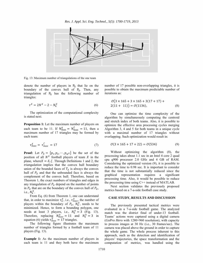
Fig. 13: Maximum number of triangulations of the one team denote the number of players in P that lie on the boundary of the convex hull of P . Then, any triangulation of P has the following number of triangles: 2 2 (6)

The optimization of the computational complexity is stated next.

Proposition 1: Let the maximum number of players on each team to be 11. If N N 11, then a maximum number of 17 triangles may be formed by each team:

17 (7) Proof: Let , , ⋯ , be the set of the position of all football players of team in the plane, where , . Through Definitions 1 and 2, the triangulation implies that the convex hull boundary union of the bounded faces of is always the convex hull of and that the unbounded face is always the complement of the convex hull. Therefore, based on Theorem 1, the exact numbers of triangles and edges in any triangulation of depend on the number of points in that are on the boundary of the convex hull of , i.e., .

From Eq. (6) from Theorem 1, one can understand that, in order to maximize , i.e., , the number of players within the boundary of , , needs to be minimized. Hence, to form a bounding polygon, one needs at least 3 players, i.e., 3 (Fig. 13). Therefore, replacing 11 and 3 in equation (6) yields 17 triangles.

The following figure illustrates the maximum number of triangles formed by a football team of 11 players (Fig. 13).

Example 1: As the maximum number of players in each team is 11 and they both have the maximum

number of 17 possible non-overlapping triangles, it is possible to obtain the maximum predictable number of iterations as:

3 165 3 165 3 17 172 11 11 1136 , (8)

One can optimize the time complexity of the

algorithm by simultaneously computing the centroid and stretch index of both teams. Also, it is possible to optimize the effective area processing cycles merging Algorithm 3, 4 and 5 for both teams in a unique cycle with a maximal number of 17 triangles without overlapping. Such optimization would result in:

3 165 17 22 534 (9)

Without optimizing the algorithm (8), the

processing takes about 1.1 sec in an Intel 4 core 2 quad cpu q900 processor 2.0 GHz and 4 GB of RAM. Considering the optimized version (9), it is possible to reduce the time to 0.98 sec. It is important to consider that the time is not substantially reduced since the graphical representation requires a significant processing time. Also, it would be possible to reduce the processing time using C++ instead of MATLAB.

Next section validates the previously proposed metrics based on a 7-a-side football case study.

CASE STUDY, RESULTS AND DISCUSSION

The previously presented tactical metrics were

evaluated in a 7-a-side football game. The analyzed match was the district final of under-13 football. Teams’ actions were captured using a digital camera (GoPro Hero with 1280×960 resolution), with capacity to process images at 30 Hz (i.e., 30 frames/sec). The camera was placed above the ground in order to capture the whole game. The whole process inherent to this approach, such as the detection and identification of players’ trajectories, the space transformation and the computation of metrics, was handled using the


1711

Fig. 14: Centroid of teams A and B in the -axis high-level calculation tool MATLAB. To compute the correlations between tactical metrics and teams it was used the r-Pearson test for positive variables and Spearman test to positive and negative variables in the same analysis. The correlation tests were performed using the IBM SPSS program (version 19) for a significance level of 5%.

After capturing the football match through the camera, the physical space was calibrated using direct linear transformation (i.e., DLT), which transforms elements’ position (i.e., players and ball) to the metric space (Duarte et al., 2010). After calibration, the tracking of players was accomplished, thus resulting in the Cartesian positioning of players and the ball over time.

Considering the online tactical metrics, the correct collective position of players may indicate a greater tactical effectiveness depending of their functional organization, with or without the ball possession. As previously defined, one of the most important online indicators is the team’s centroid that allows to analyse the average position of team players in the field. The team’s centroid, according to the studies presented in the literature applied in the basketball game (Bourbousson et al., 2010), must be analysed in both -axis and -axis. The online analysis of this metric allows the observer to detect any non-conformity of the teams, depending on the opponent and the team who possesses the ball. In fact, the teams’ centroids allows observing if teams are in-phase or not, been expected that, when functionally arranged, the team’s centroids of both teams are positively correlated.

Through Fig. 14, it may be observed that both teams’ centroids have in-phase behaviour. Moreover, considering Spearman’s correlation test, it is possible to observe a strong evidence of the positive relation between teams’ centroids over time ( 0.959), thus a large effect. Additionally, it is possible to verify a

regular oscillation of the teams’ centroids between the positive and the negative values of the -axis, in which teams try to unbalance the defensive equilibrium of their opponent, in order to remove it from the centre of the field where teams usually try to avoid the offensive attempts of the opponents. One proof of the unbalance importance can be seen in the sequence that led to the goal of Team A (Fig. 14), where the team starts having the ball possession on one side of the field, i.e., negative values of -axis, subsequently changing to the other side, i.e., positive values of -axis and immediately back to the other side again, thus unbalancing the defensive organization of the opponents. Hence, one can then observe that, while in the offensive phase, the lateral attacks are fundamental to overcome the defensive team (Lucchesi, 2001).

Similarly to the teams’ centroid in the -axis, it can be verified a large positive correlation between both centroids ( 0.908) in the -axis (i.e., length of the field) confirming the tendency for the in-phase relation between both teams over time, since they try to maintain a defensive balance to protect their goal (Frencken et al., 2011). It is important to consider that the positive values in the graph are related to the defensive side of Team B and the negative values are related to the defensive side of Team A. Nevertheless, through Fig. 15 it is possible to verify that Team A defends maintaining a larger distance in relation to the opponent and, inversely, Team B allows a higher approximation of Team A.

In the case where Team A is defending, the capability on maintaining a higher distance between teams’ centroids may suggest a smaller dispersion of Team A players or a higher dispersion of Team B players. This would represent a play style with less players involved in the offensive phase and, consequently, with higher dispersion in the -axis. Thus, it is possible to conclude that the centroid metric

-20

-15

-10

-5

0

5

10

15

20

25

1.2

61.2

121.

218

1.2

241.

230

1.2

361.

242

1.2

481.

254

1.2

601.

266

1.2

721.

278

1.2

841.

290

1.2

961.

210

21.2

1081

.211

41.2

1201

.212

61.2

1321

.213

81.2

1441

.215

01.2

1561

.216

21.2

1681

.217

41.2

1801

.2

Cen

troi

d P

osit

ion

[met

ers]

Time

Centroid (y-axis)

Team A

Team B


1712

Fig. 15: Centroid of teams A and B in the -axis

Fig. 16: Stretch index of teams A and B in the -axis needs to be merged with an indicator that allows verifying the dispersion of players during the match. Therefore, the teams’ stretch index metric allows a dispersion notion in function their centroid.

The dispersion of players according to the centroid can be understood as the collective behaviour of the team. Globally, the stretch index gives an average of 8.611 for Team B and 8.229 for Team A, i.e., a higher stretch index confirms the hypothesis previously suggested about the strategy adopted by Team B. Indeed, Team B presents a higher dispersion, thus resulting in a collective strategy that explores the forward players without a higher level of collective involvement during the offensive process. The inverse can also be verified, i.e., the forward players do not closely participate in the defensive phase. Therefore, the stretch index metric provides an indication of whether a team is expanding or contracting at any instant (Bourbousson et al., 2010). Equally, the stretch index may be related to the surface area of a team. Through the Person correlation process, it is possible to prove a correlation between the play area of Team A and its stretch index ( 0.745), thus a medium effect. The same evidence is verified in the Team B (rp = 0.779).

Considering Fig. 16, Team B has a higher play area (approximately 381 m2) comparing to the team A (approximately 370 m2 originated by the higher dispersion of players within the field with an average stretch index of 8.6 , in comparison to Team A with an average stretch index of 8.2 m. Hence, the surface

area can predict an increase of the possibilities of team’s behaviour. Nevertheless, the surface area cannot predict the real efficacy of the team. In fact, if one team presents a higher surface area it may suggest the opportunity that opponents may have to explore the middle and danger zones. Therefore, the collective efficacy may only be considered if the team is able to form real offensive and defensive triangulations. Considering that the game is a sum of offensive and defensive triangulations formed by each team, the effective play area developed in this study can allow a better understand about tactical and strategic behaviour of the team and, consequently, their collective efficacy.

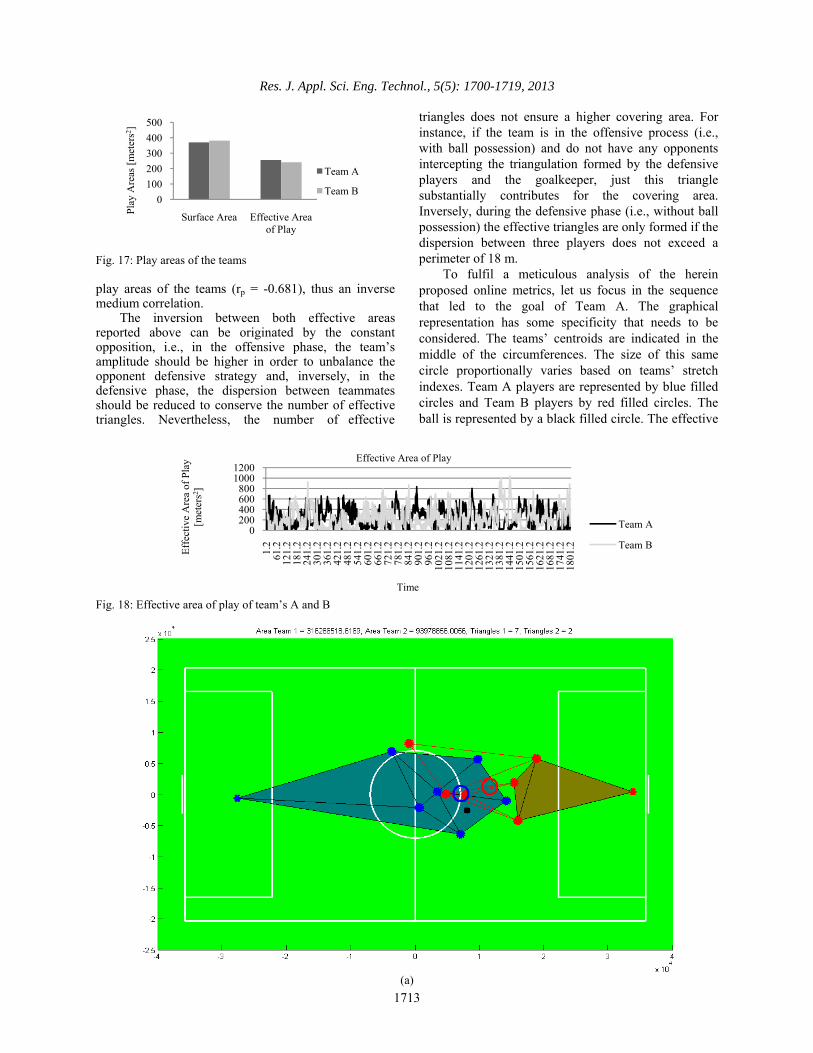
Based on the effective play area, it is possible to observe an inversion of each team’s areas (Fig. 17). Considering the effective play area, it is possible observe that Team A shows a higher efficacy in both offensive and defensive triangulations with a mean of 256 m2 when compared to Team B that presents a mean of 241 m2. Additionally, the effective play area shows that the classical surface area do not corresponds to a superior efficiency of the team.

Analysing the effective play area over time (Fig. 18), it is possible to observe permanent inverse cycles of teams. The quality of the opposition and the response provided by the opposing team can be reported as the rapport of strength that characterizes the football game (Gréhaigne et al., 2005). This rapport of strength may be seen as the relation between the effective areas of both teams. Thus, the Pearson’s correlation revealed a correlation between the effective

-40

-30

-20

-10

0

10

20

30

40

1.2

61.2

121.

218

1.2

241.

230

1.2

361.

242

1.2

481.

254

1.2

601.

266

1.2

721.

278

1.2

841.

290

1.2

961.

210

21.2

1081

.211

41.2

1201

.212

61.2

1321

.213

81.2

1441

.215

01.2

1561

.216

21.2

1681

.217

41.2

1801

.2

Cen

troi

d P

osit

ion

[met

ers]

Time

Centroid (x-axis)

Team A

Team B

0

5

10

15

20

25

1.2

61.2

121.

218

1.2

241.

230

1.2

361.

242

1.2

481.

254

1.2

601.

266

1.2

721.

278

1.2

841.

290

1.2

961.

210

21.2

1081

.211

41.2

1201

.212

61.2

1321

.213

81.2

1441

.215

01.2

1561

.216

21.2

1681

.217

41.2

1801

.2

Lev

el o

f S

tret

ch I

ndex

[m

eter

s]

Time

Stretch Index

Team ATeam B


1713

Fig. 17: Play areas of the teams play areas of the teams (rp = -0.681), thus an inverse medium correlation.

The inversion between both effective areas reported above can be originated by the constant opposition, i.e., in the offensive phase, the team’s amplitude should be higher in order to unbalance the opponent defensive strategy and, inversely, in the defensive phase, the dispersion between teammates should be reduced to conserve the number of effective triangles. Nevertheless, the number of effective

triangles does not ensure a higher covering area. For instance, if the team is in the offensive process (i.e., with ball possession) and do not have any opponents intercepting the triangulation formed by the defensive players and the goalkeeper, just this triangle substantially contributes for the covering area. Inversely, during the defensive phase (i.e., without ball possession) the effective triangles are only formed if the dispersion between three players does not exceed a perimeter of 18 m.

To fulfil a meticulous analysis of the herein proposed online metrics, let us focus in the sequence that led to the goal of Team A. The graphical representation has some specificity that needs to be considered. The teams’ centroids are indicated in the middle of the circumferences. The size of this same circle proportionally varies based on teams’ stretch indexes. Team A players are represented by blue filled circles and Team B players by red filled circles. The ball is represented by a black filled circle. The effective

Fig. 18: Effective area of play of team’s A and B

(a)

0

100

200

300

400

500

Surface Area Effective Area of Play

Pla

y A

reas

[m

eter

s2 ]

Team A

Team B

0200400600800

10001200

1.2

61.2

121.

218

1.2

241.

230

1.2

361.

242

1.2

481.

254

1.2

601.

266

1.2

721.

278

1.2

841.

290

1.2

961.

210

21.2

1081

.211

41.2

1201

.212

61.2

1321

.213

81.2

1441

.215

01.2

1561

.216

21.2

1681

.217

41.2

1801

.2Eff

ecti

ve A

rea

of P

lay

[met

ers2 ]

Time

Effective Area of Play

Team A

Team B


1714

(b)

(c)


1715

(d)

(e)


1716

(f)

(g)

Fig. 19: Graphical representation of the goal scored by team A (blue circles)


1717

Fig. 20: Tactical metrics during the play that result in goal areas of Team A and B are represented by the blue and red regions, respectively.

The above graphical representation (Fig. 19) shows that it is possible to verify a progressive tendency of Team A to increase the effective area of play, as well as the number of effective triangles. Effectively, this tendency can be explained by the defensive unbalance of Team B originated by their stretch level in the field. Players A and B of the Team B do not participated closely on their teammates defensive process, originating an opportunity for the offensive process of Team A exploring both sides of the field and, after this oscillation, taking advantage of the defensive unbalance. The dispersion of the defensive players of Team B reduced the opportunities to create effective triangles giving an opportunity for Team A to score.

The effective areas of play (Fig. 20) confirm the progressive improvement of Team A during the offensive attempt and, inversely, Team B shows a decrease of the effective area of play. These results originated an opportunity for Team A to concretize the offensive process and score. Considering the stretch index graph, it is possible to observe an instant where the level of dispersion is closer between the teams, with a stretch index of approximately 7 m for each team. This instant represents a danger unbalance for the defensive team, because it may be expected that defensive teams show lower stretch index levels in order to approximate the teammates, thus originating efficient triangles. This is observed in time = 3 sec, where a lower level of Team B stretch index (4.4 m) reduces the effective area of the opponent team (200

m2) because the effective defensive triangles intercepts and void the offensive triangles. Equally, in the same second, it is possible to observe the same number of four effective triangles for each team, i.e., the capability to reduce the stretch index level in the defensive phase improves the opportunity to void the effective triangles of team with ball possession.

Nevertheless, the increase of Team B stretch index originated by the dispersion of players A and B can be an explanation for the defensive unbalance observed in this specific case the third second. Additionally, the oscillation of the centroid taken by Team A may have contributed to the defensive unbalance of Team B and consequent efficacy of Team A during the offensive process, thus increasing their effective play area. It is important to consider that the stretch index of Team A does not substantially increases because the goal scored is achieved by an individual play from player C. In

8 sec, the same number of four effective triangles for both teams may be observed. Nevertheless, this specific case can be explained because the attacker players were in the middle of Team B triangles, thus reducing the capability to increase the number of offensive triangles. Thus, player C opted by an individual play to overtake the opposition and, after this process, the number of effective triangles of Team B reduced again due to their defensive unbalance. However, it is fundamental to emphasize that the individual process just happens after the efficacy of the collective behaviour, creating the opportunity to achieve the main goal.

0

2

4

6

8

10

12

1 2 3 4 5 6 7 8 9 10 11

Str

etch

Ind

ex [

met

ers]

Time

Stretch Index

Team A

Team B

0

1000

2000

3000

4000

5000

1 2 3 4 5 6 7 8 9 10 11Eff

ecti

ve A

rea

of P

lay

[met

ers2 ]

Time

Effective Area of Play

Team A

Team B

0

2

4

6

8

10

1 2 3 4 5 6 7 8 9 10 11

Number of Effective Triangles

Team A Team B


1718

CONCLUSION

In this study, the main goal was to update and design novel tactical and strategic online metrics that would allow coaches and other staff improving their potentialities of intervention during the match. Through this study, it was possible to explain the pertinence of the team’s centroid, the team’s stretch index and the team’s effective play area as metrics that allow understanding the tactical collective behaviour of football teams. The team’s centroid confirms the pertinence to understand the collective position of teammates in the field showing the strong point of the team. The statistical analysis between the team’s centroid showed a higher level of positive and linear correlation. Considering the team’s stretch index, it is possible understand the level of teammate’s dispersion in relation to the centroid during the match complementing the centroid metrics. Finally, the team’s effective play area allows an optimal solution to analyse the strategic and tactical efficiency of the collective behaviour. The effective play area of teams are inversely related between them, i.e., in the offensive phase the team with ball possession generally have higher levels of triangulations and effective area and, inversely, without the ball possession the team in defensive phase reduces the number of effective area justified by the lower levels of dispersion. The herein analysed metrics complement each other and their online analysis can improve the opportunities to organize the team and provide relevant feedbacks for players so as to achieve higher levels of performance. As future research direction, the online tactical metrics will be used in 11-a-side professional football during a whole season. Additionally, it will be important to design new tactical post-match metrics providing complementary information to the coaches in relation to the team’s evolution.

ACKNOWLEDGMENT

This study was supported by a PhD scholarship (SFRH/BD /73382/2010) by the Portuguese Foundation for Science and Technology (FCT). Furthermore, this study was made possible by the support and assistance of Carlos Figueiredo and Monica Ivanova for their cooperation and advice that were vital to fulfill some works of technical nature.

REFERENCES Balagué, N. and C. Torrents, 2005. Thinking before

computing: Changing approaches in sports performance. Int. J. Comp. Sci. Sport, 4(1): 5-13.

Berg, M., O. Cheong, M. Kreveld and M. Overmars, 2008. Computational Geometry: Algorithms and Applications. Springer, Heidelberg.

Bhalchandra, P., N. Deshmukh, S. Lokhande and S. Phulari, 2009. A comprehensive note on complexity issues in sorting algorithms. Adv. Comput. Res., 1(2): 1-9.

Borrie, A., G. Jonsson and M. Magnusson, 2002. Temporal pattern analysis and its applicability in sport: An explanation and exemplar data. J. Sports Sci., 20: 845-852.

Bourbousson, J., C. Sève and T. McGarry, 2010. Space-time coordination dynamics in basketball: Part 2. The interaction between the two teams. J. Sports Sci., 28(3): 349-358.

Carling, C., A.M. Williams and T. Reilly, 2005. Handbook of Soccer Match Analysis: A Systematic Approach to Improving Performance. Routledge, Abingdon, UK.

Carling, C., T. Reilly and A. Williams, 2009. Performance Assessment for Field Sports. Routledge, London.

Clemente, F.M., 2012. Pedagogical principles of teaching games for understanding and nonlinear pedagogy in the physical education teaching. Movimento, 18(2): 315-335.

Clemente, F., M. Couceiro, F. Martins and R. Mendes, 2012a. Team’s performance on FIFA U17 World Cup 2011: Study based on Notational Analysis. J. Phys. Educ. Sport, 12(1): 13-17.

Clemente, F., M. Couceiro, F. Martins, G. Dias and R. Mendes, 2012b. The influence of task constraints on attacker trajectories during 1v1 sub-phase in soccer practice. Sport Logia, 8(1): 13-20.

Davids, K., D. Araújo and R. Shuttleworth, 2005. Applications of Dynamical Systems Theory to Football. In: Reilly, T., J. Cabri and D. Araújo (Eds.), Science and Football V. Routledge Taylor & Francis Group, Oxon, pp: 556-569.

Deleplace, R., 1994. The Notion of Matrix Share for Complex Motor. In: Bouthier, D. and J. Griffet (Eds.), Representation and Action in Sport and Physical Activity. Proceedings of the 15th, University Paris XI, Orsay.

Dooley, T. and C. Titz, 2011. Soccer-The 4-4-2 System. Meyer & Meyer Sport, Germany.

Duarte, R., D. Araújo, O. Fernandes, C. Fonseca, V. Correia, V. Gazimba, B. Travassos, P. Esteves, L. Vilar and J. Lopes, 2010. Capturing complex human behaviors in representative sports contexts with a single camera. Med. Kaunas, 46(6): 408-414.

Franks, I.M. and T. McGarry, 1996. The Science of Match Analysis. In: Reilly, T. (Ed.), Science and Soccer. Spon Press Taylor & Francis Group, Oxon, pp: 363-375.

Frencken, W. and K. Lemmink, 2008. Team Kinematics of Small-Sided Soccer Games: A Systematic Approach. In: Reilly, T. And F. Korkusuz (Eds.), Science and Football VI. Routledge Taylor & Francis Group, Oxon, pp: 161-166.


1719

Frencken, W., K. Lemmink, N. Delleman and C. Visscher, 2011. Oscillations of centroid position and surface area of soccer teams in small-sided games. Euro. J. Sport Sci., 11(4): 215-223.

Garganta, J., 2009. Trends of tactical performance analysis in team sports: Bridging the gap between research, training and competition. Portuguese J. Sport Sci., 9(1): 81-89.

Ghamisi, P., M.S. Couceiro, J.A. Benediktsson and N.M.F. Ferreira, 2012. An efficient method for segmentation of images based on fractional calculus and natural selection. Exp. Syst. Appl., DOI: org/10. 1016 /j.eswa. 2012.04.078.

Gréhaigne, J.F., 1992. The Organization of the Game in Football. Joinville-le-Pont, Editions Actio, France.

Gréhaigne, J.F., 2008. A Dialectic Approach of some Concepts in the Learning of Invasion Games. In: Brandl-Bredenbeck, H.P. (Ed.), Exercise, Play Sports UN in Childhood and Adolescence-A European Perspective. Meyer & Meyer Verlag, Aachen, pp: 78-91.

Gréhaigne, J.F. and P. Godbout, 1995. Tactical knowledge in team sports from a constructivist and cognitivist perspective. Quest, 47: 490-505.

Gréhaigne, J.F., P. Godbout and D. Bouthier, 1999. The foundations of tactics and strategy in team sports. J. Teach. Phys. Educ., 18: 159-174.

Gréhaigne, J.F., J.F. Richard and L. Griffin, 2005. Teaching and Learning Team Sports and Games. Routledge Falmar, New York.

Gréhaigne, J.F., D. Caty and P. Godbout, 2010. Modelling ball circulation in invasion team sports: A way to promote learning games through understanding. Phys. Educ. Sport Pedagogy, 15(3): 257-270.

Hughes, M. and I.M. Franks, 2004. Notational Analysis-a Review of the Literature. In: Hughes, M. and I.M. Franks (Eds.), Notational Analysis of Sport: Systems for Better Coaching and Performance in Sport. Routledge, New York, pp: 59-106.

Lees, A., 2002. Technique analysis in sports: A critical review. J. Sports Sci., 20(10): 813-828.

Lucchesi, M., 2001. Attacking Soccer: A Tactical Analysis. Reedswain Publishing, Auburn, Michigan.

McGarry, T., D. Anderson, S. Wallace, M. Hughes and I. Franks, 2002. Sport competition as a dynamical self-organizing system. J. Sports Sci., 20(10): 771-781.

Neville, A., G. Atkinson and M. Hughes, 2008. Twenty-five years of sport performance research in the journal of sport science. J. Sport Sci., 26(4): 413-426.

Passos, P., 2009. Identifying Interpersonal Coordination Patterns in Rugby Union. VDM Publishing, Saarbrucken, pp: 164, ISBN: 3639203771.

Passos, P., K. Davids, D. Araújo, N. Paz, J. Minguéns and J. Mendes, 2011a. Networks as a novel tool for studying team ball sports as complex social systems. J. Sci. Med. Sport, 14: 170-176.

Passos, P., J. Milho, S. Fonseca, J. Borges, D. Araújo and K. Davids, 2011b. Interpersonal distance regulates functional grouping tendencies of agents in team sports. J. Motor Behav., 43(2): 155-163.

Smith, N., C. Handford and N. Priestley, 1996. Sports Analysis in Coaching. Department of Exercise and Sport Science, Alsager, pp: 63, ISBN: 0952474255.

Trapattoni, G., 1999. Coaching High Performance Soccer. Reedswain Inc., Spring City, Pensylvania.

Zerhouni, M., 1980. The Basics of Football Contemporary. Orges, Fleury.

An Online Tactical Metrics Applied to Football Game

Documents

Transcript of An Online Tactical Metrics Applied to Football Game