Regaining Spiritual Experience : Conserving Sacred Architecture by Intuitive Method
Upload
independentCategory
view
0download
0
INTERNATIONAL JOURNAL FOR NUMERICAL METHODS IN ENGINEERINGInt. J. Numer. Meth. Engng 2002; 54:1683–1716 (DOI: 10.1002/nme.486)
An objective �nite element approximation of the kinematicsof geometrically exact rods and its use in the formulationof an energy–momentum conserving scheme in dynamics
I. Romero and F. Armero∗;†
Department of Civil and Environmental Engineering; Structural Engineering; Mechanics and Materials;University of California; Berkeley; CA 94720; U.S.A.
SUMMARY
We present in this paper a new �nite element formulation of geometrically exact rod models in the three-dimensional dynamic elastic range. The proposed formulation leads to an objective (or frame-indi�erentunder superposed rigid body motions) approximation of the strain measures of the rod involving �niterotations of the director frame, in contrast with some existing formulations. This goal is accomplishedthrough a direct �nite element interpolation of the director �elds de�ning the motion of the rod’s cross-section. Furthermore, the proposed framework allows the development of time-stepping algorithms thatpreserve the conservation laws of the underlying continuum Hamiltonian system. The conservation lawsof linear and angular momenta are inherited by construction, leading to an improved approximation ofthe rod’s dynamics. Several numerical simulations are presented illustrating these properties. Copyright? 2002 John Wiley & Sons, Ltd.
KEY WORDS: geometrically exact rods; dynamics; �nite elements; objectivity; energy–momentumconserving algorithms
1. INTRODUCTION
A rod can be de�ned as a slender solid with two characteristic dimensions much smallerthan the third one, the latter de�ning the axial direction. This characterization leads to theconsideration of a general curve in the three-dimensional space with a plane section attachedto each of its material points. The plane of the section is then de�ned through two vectors, theso-called directors. Non-linear models of rods as directed continua have been considered bya large number of authors in the past; see the classical works of Cosserat and Cosserat [1]Green and Laws [2], Ericksen and Truesdell [3] Reissner [4] and the review of Antman [5],among others. This geometric characterization allows the de�nition of the di�erent components
∗Correspondence to: F. Armero, Structural Engineering, Mechanics and Materials, Department of Civil and Envi-ronmental Engineering, 713 Davis Hall, University of California, Berkeley, CA 94720-1710, U.S.A.
†E-mail: [email protected]
Contract=grant sponsor: AFOSR; contract=grant number: F49620-00-1-0360
Received 5 February 2001Copyright ? 2002 John Wiley & Sons, Ltd. Revised 21 September 2001
1684 I. ROMERO AND F. ARMERO
of the rod’s response of interest in structural applications. In this way, we talk of the axial, thetransverse shear, the bending and the torsional strain measures, with their associated conjugatestress resultants (i.e. the axial and the transverse shear forces, the bending moments and thetorques, respectively).Perhaps the main motivation behind the consideration of these structural members as general
directed continua in contrast, for example, of simpler in�nitesimal theories is the formulationof models that comply with the accepted principle of frame indi�erence while allowing�nite motions of the aforementioned geometric entities (hence, their common denominationas ‘geometrically exact theories’). Namely, the aforementioned measures of strain and stressresultants (or, in other words, the constitutive relation in the rod model) should not be a�ectedby a superposed rigid motion, even if the �nal equations of motion are only invariant in theclassical Galilean sense. The presence of di�erent constraints in the director �elds may leadto complex requirements for this property to hold. A typical example is given by the consid-eration of two orthonormal directors modelling a non-distorting cross-section. This situationforces the consideration of the �nite group of rotations in the con�guration space de�ning thestate of the rod. This case is sometimes referred as the special theory of Cosserat rods [5]and it is the focus of the developments presented in this paper.The strong non-linearity of the resulting theories leads almost inevitably to the consideration
of numerical methods for the integration of the �nal equations. To this purpose, Simo [6]presented a three-dimensional framework extending the plane model proposed in Reissner [4]that is particularly well-suited for its �nite element implementation. This implementation waslater developed by Simo and Vu-Quoc [7; 8] for the static and dynamic cases. An extensionincorporating the warping of the cross-sections due to shear and torsion was also presentedby Simo, Vu-Quoc [9]. Additional contributions in this �eld include the works of Cardonaand Geradin [10] and Ibrahimbegovic [11], amongst others. See the review in Cris�eld [12].The appropriate treatment of the rich geometric structure of the underlying continuum sys-
tem in the general dynamic range, a non-linear Hamiltonian system in the elastic case con-sidered herein, is of the main interest in the integration of the resulting dynamical systems.In this way, the presence of the conservation laws of linear and angular momentum and thelaw of conservation of energy is thought to be important properties to be inherited by thediscrete model. The correct approximation of the continuum systems is not the only motiva-tion behind, since it is commonly accepted that the conservation of energy by a numericalscheme leads to an added stability of the numerical simulations when compared with moretraditional non-conserving schemes. Newmark schemes, for example, are known to lead tonumerical instabilities in the non-linear range. Furthermore, these schemes do not conservethe angular momentum of the physical system either, leading to a distorted approximation ofthe phase dynamics. A complete recent study of these shortfalls can be found in Armero andRomero [13] and references therein. Some authors have indicated, however, that Newmarkschemes can be derived from a variational principle, preserving a numerically de�ned mo-mentum and leading eventually to a good energy behaviour for small time steps; see Kaneet al. [14].In any case, the formulation of alternative schemes that incorporate the conservation laws
of the underlying physical system by construction has been observed to lead to an improvednumerical performance avoiding the aforementioned shortfalls of standard (non-conserving)schemes. This observation has motivated the development of such schemes in Simoet al. [15]. Galvanetto and Cris�eld [16], Bauchau and Theron [17] and Botasso and Borri
Copyright ? 2002 John Wiley & Sons, Ltd. Int. J. Numer. Meth. Engng 2002; 54:1683–1716
INTEGRATION SCHEMES FOR THE DYNAMICS OF GEOMETRICALLY EXACT RODS 1685
[18], to mention just a few references in the context of geometrically exact rod formula-tions only. Variations of these schemes that show also energy decaying schemes to handlethe numerical sti�ness of the systems at hand have been also considered in the last of thesereferences.However, the recent developments in Cris�eld and Jeleni�c [19] have identi�ed the lack of
objectivity of commonly used �nite element approximations of the model of Simo [6] in thegeneral three-dimensional range, even if the model itself is frame indi�erent. Moreover, thesenumerical solutions become even path dependent for hyperelastic models in the quasi-staticrange. The reason for these limitations was traced back to the considered �nite element inter-polations in the �nite rotation group, even if parameterized through the (locally) linear spacesof the total or incremental rotation vectors, and not to the continuum formulation. Hence,these shortfalls disappear in the limit as the �nite element mesh is re�ned. However, the clearnon-physical component that these de�ciencies add to the computed solution, always witha �nite size mesh, strongly motivates their correction. To this purpose, Cris�eld and Jeleni�c[19; 20] proposed a numerical implementation for rod statics, and dynamics in the second ofthese references, based on the co-rotational concept that preserved the objectivity of the con-tinuum theory and the history independence characteristic of elastic solutions. The formulationof energy–momentum conserving integration schemes seem to be lacking in this framework,as indicated in Jeleni�c and Cris�eld [21]. In fact, we have observed that the original conserv-ing time-stepping algorithm presented in Simo et al. [15] is not conserving despite its claim,due again to the spatial �nite element interpolations as discussed in Appendix B.In the present work, we propose a �nite element implementation of the rod model presented
in Reference [6] that corrects this lack of objectivity and path dependence, and leads to awell-suited framework for the formulation of energy-conserving schemes. The goals of thispaper are then twofold, as re�ected in the title:
(i) The development of a �nite element formulation of the special theory of geometricallyexact rods that involves an objective approximation of the strain measures characterizingthese theories in terms of the rotational and translational generalized degrees of freedom,even in the quasi-static case, and
(ii) The formulation of energy–momentum conserving algorithms for the integration of therod dynamics in this framework.
The starting point in the development of the proposed formulation is the parameterization ofthe equations of motion of the rod directly in terms of the director �eld and their variations.The resulting formulation is totally equivalent to the original one but it allows to accomplishthe two aforementioned goals. The proposed �nite element formulation considers a direct in-terpolation of the director �elds (or, equivalently, the rotation tensor associated to the directorframe) and their variations, including the so-called director velocities. The orthonormal char-acter of the directors is enforced nodally with the appropriate rotational updates, assuring theconservation properties of the �nal numerical model in addition. Even though the rotationalcharacter of the interpolation is only enforced at the nodes of the �nite element model, theimproved properties of the �nal numerical methods (especially its conservation properties)makes the proposed approach very much worth its consideration. In fact, this situation iscommon to similar formulations of geometrically exact shells, allowing also the use of simi-lar arguments for the development of energy–momentum conserving time-stepping algorithms,as considered by Simo and Tarnow [22].
Copyright ? 2002 John Wiley & Sons, Ltd. Int. J. Numer. Meth. Engng 2002; 54:1683–1716
1686 I. ROMERO AND F. ARMERO
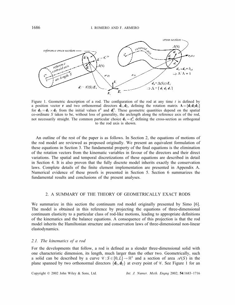
Figure 1. Geometric description of a rod. The con�guration of the rod at any time t is de�ned bya position vector r and two orthonormal directors d1; d2, de�ning the rotation matrix �=[d1d2d3]for d3 = d1× d2 from the initial values r0 and d0i . These geometric quantities depend on the spatialco-ordinate S taken to be, without loss of generality, the arclength along the reference axis of the rod,not necessarily straight. The common particular choice d3 = r0; s de�ning the cross-section as orthogonal
to the rod axis is shown.
An outline of the rest of the paper is as follows. In Section 2, the equations of motions ofthe rod model are reviewed as proposed originally. We present an equivalent formulation ofthese equations in Section 3. The fundamental property of the �nal equations is the eliminationof the rotation vectors from the kinematic variables in favour of the directors and their directvariations. The spatial and temporal discretizations of these equations are described in detailin Section 4. It is also proven that the fully discrete model inherits exactly the conservationlaws. Complete details of the �nite element implementation are presented in Appendix A.Numerical evidence of these proofs is presented in Section 5. Section 6 summarizes thefundamental results and conclusions of the present analyses.
2. A SUMMARY OF THE THEORY OF GEOMETRICALLY EXACT RODS
We summarize in this section the continuum rod model originally presented by Simo [6].The model is obtained in this reference by projecting the equations of three-dimensionalcontinuum elasticity to a particular class of rod-like motions, leading to appropriate de�nitionsof the kinematics and the balance equations. A consequence of this projection is that the rodmodel inherits the Hamiltonian structure and conservation laws of three-dimensional non-linearelastodynamics.
2.1. The kinematics of a rod
For the developments that follow, a rod is de�ned as a slender three-dimensional solid withone characteristic dimension, its length, much larger than the other two. Geometrically, sucha solid can be described by a curve C : S ∈ [0; L]→R3 and a section of area A(S) in theplane spanned by two orthonormal directors {d1; d2} at every point of C. See Figure 1 for an
Copyright ? 2002 John Wiley & Sons, Ltd. Int. J. Numer. Meth. Engng 2002; 54:1683–1716
INTEGRATION SCHEMES FOR THE DYNAMICS OF GEOMETRICALLY EXACT RODS 1687
illustration of these ideas. We denote by S and L the arclength and total length of the rod,respectively, in a certain reference con�guration.The location of a material point of the rod at time t¿ 0 is de�ned by the position vector
x(t) :A× [0; L]→R3 given by
x(�1; �2; S; t)= r(S; t) + ^(S; t) with ^(S; t)= ��d�(S; t) (1)
(summation implied over repeated indices �=1; 2) in terms of the position vector of themiddle axis r(t) : [0; L]→R3 and the two co-ordinates (�1; �2; S)∈A(S) (�xed in time) inthe section basis {d1; d2}. The parametrization (1) is assumed to hold at any time t and,in particular, in the reference con�guration which we take, without loss of generality, tobe the initial con�guration of the rod. We denote the variables associated to this referencecon�guration by r0(S) and d0�(S) (�=1; 2).We assume, for simplicity, that the curve C connects the centroids of the di�erent sections
A(S). This property holds for any time t given (1), given the assumed orthonormal char-acter of the directors. These considerations correspond to the classical assumption of planecross-sections remaining plane and undistorted after deformation, hence the assumption oforthonormal directors. Higher-order kinematics can be incorporated to the basic kinematicsdescribed here. For example, the warping of the cross-section due to shear and torsion can beincorporated to these considerations through the superposition of a warping function, as pre-sented by Simo and Vu-Quoc [9]. The developments in this work can be similarly extendedto this case by superposing these e�ects to the new parameterization developed in Section 3.We do not pursue these extensions here for the sake of brevity.We de�ne the director con�guration space
D= {(d1; d2); d�(S; t)=�(S; t)E� for �=1; 2; and �= �� on �u} (2)
with �(S; t)∈SO(3), the group of (proper) orthogonal transformations in R3, and {Ei}3i=1a �xed orthonormal basis in R3. Here, �u denotes the part of the boundary where the positionof the middle axis curve and the cross-section of the rod are constrained to certain �xedvalues; see (18) below. The rotation tensors appearing in this de�nition have the form
�=[d1d2d3] for d3 = d1× d2 (3)
with ‘× ’ denoting the cross product of vectors in R3. From the previous geometric descriptionit follows that the con�guration space Q of the rod is the product manifold
Q= {(r;�); r∈R3; �∈SO(3); and r= �r;�= �� on �u} (4)
Elements of the con�guration space Q correspond to the generalized displacements of the rodand are denoted by �=(r;�) in what follows.A typical choice for the de�nition of the cross-section in the reference con�guration is
given by the orthogonal cross-section of the rod middle axis, so r0; s= d03 where (·); s=d(·)=dS;see Figure 1. In a deformed con�guration, the directors d� remain orthonormal to one anotherbut not necessarily to the tangent of the rod axis r; s as a result of transverse shear. To ruleout the non-physical situation of in�nite transverse shear the restriction
d3 · r; s¿0 (5)
is imposed on the admissible con�gurations.
Copyright ? 2002 John Wiley & Sons, Ltd. Int. J. Numer. Meth. Engng 2002; 54:1683–1716
1688 I. ROMERO AND F. ARMERO
The tangent space to the con�guration space Q, denoted by TQ, is de�ned by the vectorspace
TQ= {��=(�r; ��)�; �∈Q; �r∈TR3∼ R3; ��= �X�; �X∈ so(3)} (6)
with so(3), the linear space of skew tensors in R3. This linear space is isomorphic to R3 andthere exists a bijection between the two spaces such that for any vector a in R3
�Xa= �X× a; �X∈ so(3) and �X∈R3 (7)
de�ning the axial vector �X=axial[�X] of the skew tensor �X. The rates of the generalizeddisplacements � belong to the tangent space TQ. Hence, we de�ne the generalized velocityW∈TQ
W= ˙�=(v;�) with r= v; �= �� (8)
where the dot stands for the material time derivative. In the terminology of classical mechan-ics, � is the spatial angular velocity of the cross-section.The motion of the rod is characterized through the introduction of the classical notions of
linear and angular momentum. In this way, the total linear momentum L of the rod can bewritten as
L(t)=∫ L
0
∫A
�0(S; ^)x(S; ^; t) dA dS=∫ L
0A�r dS=
∫ L
0p dS (9)
after using (1). Here we have introduced the reference density �0 of the material, and de�nedthe reference section density A�=
∫A�0 dA and the linear momentum density p=A�r. Note
that the �rst area moment∫A�� dA vanishes, since the curve r(S) is assumed to pass through
the centroid of the cross-section,In the same fashion, the total angular momentum of the rod J relative to the origin is
de�ned as the integral over the rod of the moment of momentum, and leads, after somealgebraic manipulations, to the expression
J(t) =∫ L
0
∫A
x×�0x dA dS=∫ L
0r× p dS +
∫ L
0
∫A
�0^× (�× ^) dA dS =∫ L
0(r× p+ �) dS
(10)
where we have de�ned the section spatial angular momentum �= i�� and the section spatialinertia
i�=∫A
�0(‖^21− ^⊗ ^) dA (11)
This inertia is con�guration dependent and is related to the (constant in time) body inertia
I�=�T i��=
∫A
�0(‖�‖21− �⊗ �) dA; �= ��E� (12)
with I�= I�(S), in general. Here, ‖a‖=√a · a denotes the norm based on the standard
Euclidean product ‘·’ in R3.
Copyright ? 2002 John Wiley & Sons, Ltd. Int. J. Numer. Meth. Engng 2002; 54:1683–1716
INTEGRATION SCHEMES FOR THE DYNAMICS OF GEOMETRICALLY EXACT RODS 1689
The dynamics of the rod are then de�ned in the canonical phase space P=T ∗Q (thecotangent space of the con�guration space Q) given by
T ∗Q = T ∗R3×T ∗SO(3)= {��=(p; �)�; �∈Q; p∈T ∗R3 ∼ R3; �∈T ∗SO(3) ∼ SO(3)}(13)
with � being the generalized momentum. The proper de�nition of the strain and stress mea-sures allows then the characterization of the rod’s mechanical response, leading to the gov-erning equations as discussed next.
2.2. The strain measures and the stress resultants
The following material strain measures characterize the deformation of the rod
�=�T r; s −�0r0; s and �=axial [�T�; s −�0�0; s] (14)
A careful look at these expressions identi�es the components of the vector � with the trans-verse shear and axial deformations, and the vector � with the bending and torsional strains.A straightforward calculation shows that a superposed rigid deformation (i.e. (r∗;�∗)= (a +Qr;Q�) for a∈R3 and Q∈SO(3) constant in S) leaves the vectors (14) invariant (i.e. �∗=�and �∗=�). This property is a re�ection of the frame indi�erence of the rod model underconsideration.We consider the stress resultants N and M conjugate to the strain measures (14), the
axial=transverse shear force and bending=torsional moment. Our interest in this paper liesin hyperelastic rod models. In this context, the constitutive relations are given in terms ofa stored energy functional W (�;�) as
N=@W@�
and M=@W@�
(15)
The objectivity of these stress resultants follows easily from the frame indi�erence of thestrain measures themselves. The numerical simulations of Section 5 consider a quadratic storedenergy function energy function, i.e.
W (�;�)= 12� · C��+ 1
2� · C�� (16)
with section sti�nesses of the form
C� =
GA1 0 00 GA2 00 0 EA
and C� =[EI 00 GJ
](17)
for the Young and shear modulus E and G of the material (isotropic response), the shearreduced sections A1; A2 in the reference directions E1 and E2, the area A, the second momentaarea I and the torsional constant J of the reference cross-section, following standard argumentsin strength of materials.
Copyright ? 2002 John Wiley & Sons, Ltd. Int. J. Numer. Meth. Engng 2002; 54:1683–1716
1690 I. ROMERO AND F. ARMERO
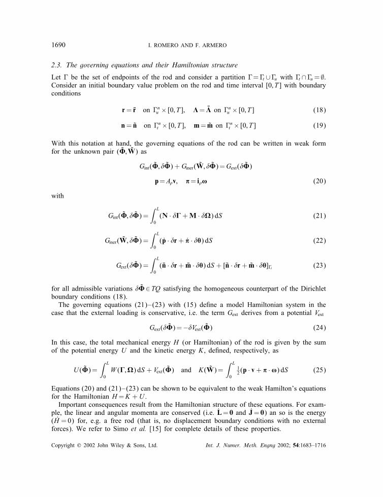
2.3. The governing equations and their Hamiltonian structure
Let � be the set of endpoints of the rod and consider a partition �=�t ∪�u with �t ∩�u= ∅.Consider an initial boundary value problem on the rod and time interval [0; T ] with boundaryconditions
r= �r on �nu × [0; T ]; �= �� on �nu × [0; T ] (18)
n= n on �nt × [0; T ]; m= m on �nt × [0; T ] (19)
With this notation at hand, the governing equations of the rod can be written in weak formfor the unknown pair (�; W) as
Gint(�; ��) +Giner(W; ��)=Gext(��)
p=A�v; �= i�� (20)
with
Gint(�; ��) =∫ L
0(N · ��+M · ��) dS (21)
Giner(W; ��) =∫ L
0(p · �r+ � · �X) dS (22)
Gext(��) =∫ L
0(�n · �r+ �m · �X) dS + [n · �r+ m · �X]�t (23)
for all admissible variations ��∈TQ satisfying the homogeneous counterpart of the Dirichletboundary conditions (18).The governing equations (21)–(23) with (15) de�ne a model Hamiltonian system in the
case that the external loading is conservative, i.e. the term Gext derives from a potential Vext
Gext(��)=−�Vext(�) (24)
In this case, the total mechanical energy H (or Hamiltonian) of the rod is given by the sumof the potential energy U and the kinetic energy K , de�ned, respectively, as
U (�)=∫ L
0W (�;�) dS + Vext(�) and K(W)=
∫ L
0
12 (p · v+ � · �) dS (25)
Equations (20) and (21)–(23) can be shown to be equivalent to the weak Hamilton’s equationsfor the Hamiltonian H=K +U .Important consequences result from the Hamiltonian structure of these equations. For exam-
ple, the linear and angular momenta are conserved (i.e. L= 0 and J= 0) an so is the energy(H =0) for, e.g. a free rod (that is, no displacement boundary conditions with no externalforces). We refer to Simo et al. [15] for complete details of these properties.
Copyright ? 2002 John Wiley & Sons, Ltd. Int. J. Numer. Meth. Engng 2002; 54:1683–1716
INTEGRATION SCHEMES FOR THE DYNAMICS OF GEOMETRICALLY EXACT RODS 1691
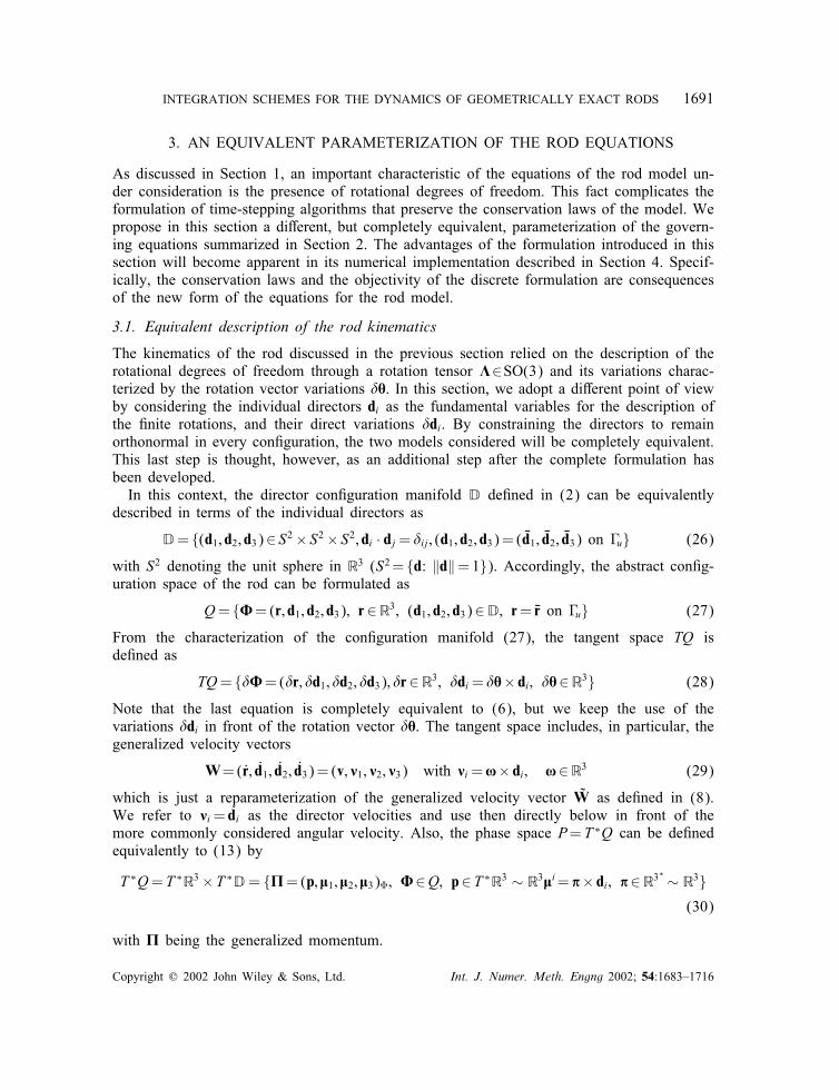
3. AN EQUIVALENT PARAMETERIZATION OF THE ROD EQUATIONS
As discussed in Section 1, an important characteristic of the equations of the rod model un-der consideration is the presence of rotational degrees of freedom. This fact complicates theformulation of time-stepping algorithms that preserve the conservation laws of the model. Wepropose in this section a di�erent, but completely equivalent, parameterization of the govern-ing equations summarized in Section 2. The advantages of the formulation introduced in thissection will become apparent in its numerical implementation described in Section 4. Specif-ically, the conservation laws and the objectivity of the discrete formulation are consequencesof the new form of the equations for the rod model.
3.1. Equivalent description of the rod kinematics
The kinematics of the rod discussed in the previous section relied on the description of therotational degrees of freedom through a rotation tensor �∈SO(3) and its variations charac-terized by the rotation vector variations �X. In this section, we adopt a di�erent point of viewby considering the individual directors di as the fundamental variables for the description ofthe �nite rotations, and their direct variations �di. By constraining the directors to remainorthonormal in every con�guration, the two models considered will be completely equivalent.This last step is thought, however, as an additional step after the complete formulation hasbeen developed.In this context, the director con�guration manifold D de�ned in (2) can be equivalently
described in terms of the individual directors as
D= {(d1; d2; d3)∈ S2× S2× S2; di · dj= �ij; (d1; d2; d3)= ( �d1; �d2; �d3) on �u} (26)
with S2 denoting the unit sphere in R3 (S2= {d: ‖d‖=1}). Accordingly, the abstract con�g-uration space of the rod can be formulated as
Q= {�=(r; d1; d2; d3); r∈R3; (d1; d2; d3)∈D; r= �r on �u} (27)
From the characterization of the con�guration manifold (27), the tangent space TQ isde�ned as
TQ= {��=(�r; �d1; �d2; �d3); �r∈R3; �di= �X× di ; �X∈R3} (28)
Note that the last equation is completely equivalent to (6), but we keep the use of thevariations �di in front of the rotation vector �X. The tangent space includes, in particular, thegeneralized velocity vectors
W=(r; d1; d2; d3)= (v; ]1; ]2; ]3) with ]i=�× di ; �∈R3 (29)
which is just a reparameterization of the generalized velocity vector W as de�ned in (8).We refer to ]i= di as the director velocities and use then directly below in front of themore commonly considered angular velocity. Also, the phase space P=T ∗Q can be de�nedequivalently to (13) by
T ∗Q=T ∗R3×T ∗D= {�=(p; \1; \2; \3)�; �∈Q; p∈T ∗R3 ∼ R3\i= �× di ; �∈R3∗ ∼ R3}(30)
with � being the generalized momentum.
Copyright ? 2002 John Wiley & Sons, Ltd. Int. J. Numer. Meth. Engng 2002; 54:1683–1716
1692 I. ROMERO AND F. ARMERO
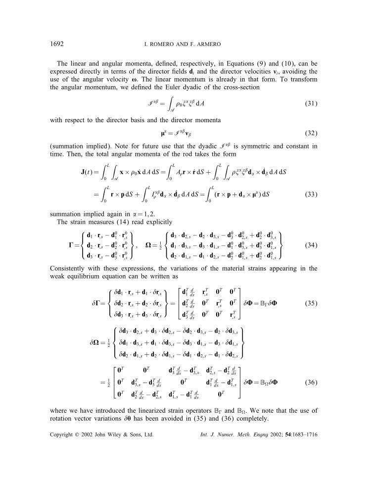
The linear and angular momenta, de�ned, respectively, in Equations (9) and (10), can beexpressed directly in terms of the director �elds di and the director velocities ]i, avoiding theuse of the angular velocity �. The linear momentum is already in that form. To transformthe angular momentum, we de�ned the Euler dyadic of the cross-section
I��=∫A
�0���� dA (31)
with respect to the director basis and the director momenta
\�=I��]� (32)
(summation implied). Note for future use that the dyadic I�� is symmetric and constant intime. Then, the total angular momenta of the rod takes the form
J(t) =∫ L
0
∫A
x×�0x dA dS=∫ L
0A�r× r dS +
∫ L
0
∫A
�����d�× d� dA dS
=∫ L
0r× p dS +
∫ L
0I ��� d�× d� dA dS=
∫ L
0(r× p+ d�× \�) dS (33)
summation implied again in �=1; 2.The strain measures (14) read explicitly
�=
d1 · r; s − d01 · r0; sd2 · r; s − d02 · r0; sd3 · r; s − d03 · r0; s
; �= 12
d3 · d2; s − d2 · d3; s − d03 · d02; s + d02 · d03; sd1 · d3; s − d3 · d1; s − d01 · d03; s + d03 · d01; sd2 · d1; s − d1 · d2; s − d02 · d01; s + d02 · d01; s
(34)
Consistently with these expressions, the variations of the material strains appearing in theweak equilibrium equation can be written as
��=
�d1 · r; s + d1 · �r; s�d2 · r; s + d2 · �r; s�d3 · r; s + d3 · �r; s
=dT1
dds rT; s 0T 0T
dT2dds 0T rT; s 0T
dT3dds 0T 0T rT; s
��=B��� (35)
��= 12
�d3 · d2; s + d3 · �d2; s − �d2 · d3; s − d2 · �d3; s�d1 · d3; s + d1 · �d3; s − �d3 · d1; s − d3 · �d1; s�d2 · d1; s + d2 · �d1; s − �d1 · d2; s − d1 · �d2; s
= 12
0T 0T dT3
dds − dT3; s dT2; s − dT2 d
ds
0T dT3; s − dT3 dds 0T dT1
dds − dT1; s
0T dT2dds − dT2; s dT1; s − dT1 d
ds 0T
��=B��� (36)
where we have introduced the linearized strain operators B� and B�. We note that the use ofrotation vector variations �X has been avoided in (35) and (36) completely.
Copyright ? 2002 John Wiley & Sons, Ltd. Int. J. Numer. Meth. Engng 2002; 54:1683–1716
INTEGRATION SCHEMES FOR THE DYNAMICS OF GEOMETRICALLY EXACT RODS 1693
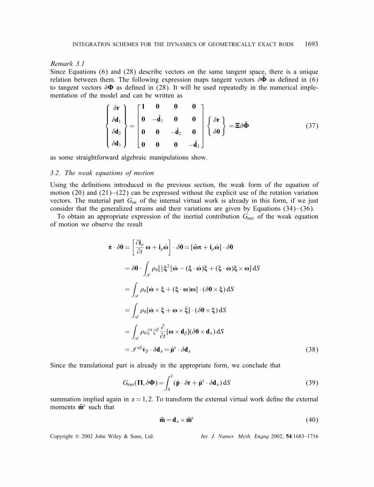
Remark 3.1Since Equations (6) and (28) describe vectors on the same tangent space, there is a uniquerelation between them. The following expression maps tangent vectors �� as de�ned in (6)to tangent vectors �� as de�ned in (28). It will be used repeatedly in the numerical imple-mentation of the model and can be written as
�r
�d1
�d2
�d3
=
1 0 0 0
0 −d1 0 0
0 0 −d2 0
0 0 0 −d3
{�r
�X
}=��� (37)
as some straightforward algebraic manipulations show.
3.2. The weak equations of motion
Using the de�nitions introduced in the previous section, the weak form of the equation ofmotion (20) and (21)–(22) can be expressed without the explicit use of the rotation variationvectors. The material part Gint of the internal virtual work is already in this form, if we justconsider that the generalized strains and their variations are given by Equations (34)–(36).To obtain an appropriate expression of the inertial contribution Giner of the weak equation
of motion we observe the result
� · �X=[@i�@t�+ i��
]· �X=[��+ i��] · �X
= �X ·∫A
�0[‖^2‖�− (^ · �)^+ (^ · �)^×�] dS
=∫A
�0[�× ^+ (^ · �)�] · (�X× ^) dS
=∫A
�0[�× ^+ �× ˙] · (�X× ^) dS
=∫A
�0����@@t[�× d�](�X× d�) dS
=I��]� · �d�= \� · �d� (38)
Since the translational part is already in the appropriate form, we conclude that
Giner(�; ��)=∫ L
0(p · �r+ \� · �d�) dS (39)
summation implied again in �=1; 2. To transform the external virtual work de�ne the externalmoments �m� such that
�m= d�× �m� (40)
Copyright ? 2002 John Wiley & Sons, Ltd. Int. J. Numer. Meth. Engng 2002; 54:1683–1716
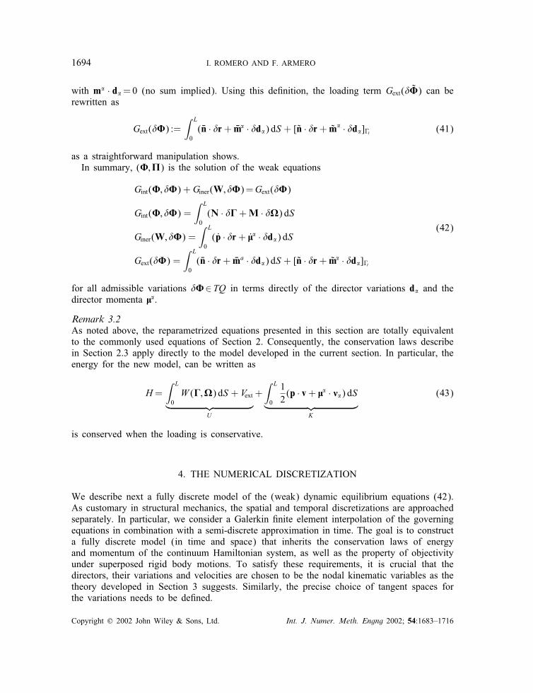
1694 I. ROMERO AND F. ARMERO
with m� · d�=0 (no sum implied). Using this de�nition, the loading term Gext(��) can berewritten as
Gext(��) :=∫ L
0(�n · �r+ �m� · �d�) dS + [n · �r+ m� · �d�]�t (41)
as a straightforward manipulation shows.In summary, (�;�) is the solution of the weak equations
Gint(�; ��) +Giner(W; ��)=Gext(��)
Gint(�; ��) =∫ L
0(N · ��+M · ��) dS
Giner(W; ��) =∫ L
0(p · �r+ \� · �d�) dS
Gext(��) =∫ L
0(�n · �r+ �ma · �d�) dS + [n · �r+ m� · �d�]�t
(42)
for all admissible variations ��∈TQ in terms directly of the director variations d� and thedirector momenta \�.
Remark 3.2As noted above, the reparametrized equations presented in this section are totally equivalentto the commonly used equations of Section 2. Consequently, the conservation laws describein Section 2.3 apply directly to the model developed in the current section. In particular, theenergy for the new model, can be written as
H=∫ L
0W (�;�) dS + Vext︸ ︷︷ ︸
U
+∫ L
0
12(p · v+ \� · ]�) dS︸ ︷︷ ︸
K
(43)
is conserved when the loading is conservative.
4. THE NUMERICAL DISCRETIZATION
We describe next a fully discrete model of the (weak) dynamic equilibrium equations (42).As customary in structural mechanics, the spatial and temporal discretizations are approachedseparately. In particular, we consider a Galerkin �nite element interpolation of the governingequations in combination with a semi-discrete approximation in time. The goal is to constructa fully discrete model (in time and space) that inherits the conservation laws of energyand momentum of the continuum Hamiltonian system, as well as the property of objectivityunder superposed rigid body motions. To satisfy these requirements, it is crucial that thedirectors, their variations and velocities are chosen to be the nodal kinematic variables as thetheory developed in Section 3 suggests. Similarly, the precise choice of tangent spaces forthe variations needs to be de�ned.
Copyright ? 2002 John Wiley & Sons, Ltd. Int. J. Numer. Meth. Engng 2002; 54:1683–1716
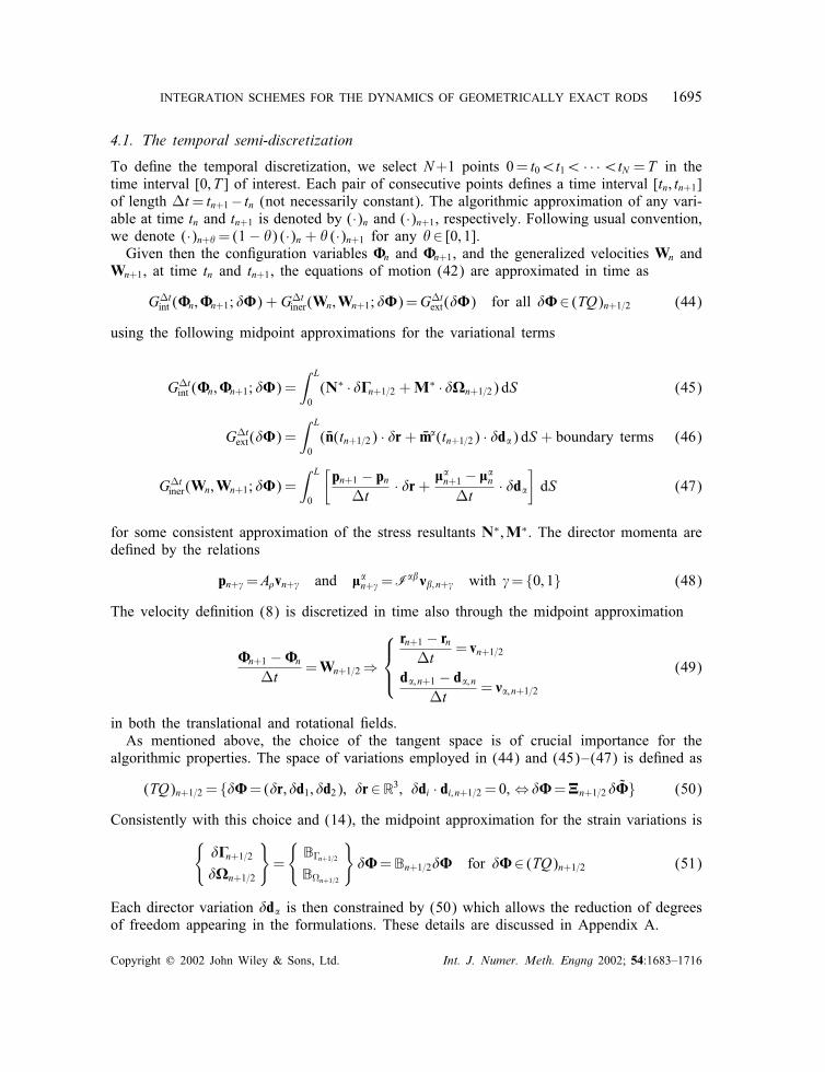
INTEGRATION SCHEMES FOR THE DYNAMICS OF GEOMETRICALLY EXACT RODS 1695
4.1. The temporal semi-discretization
To de�ne the temporal discretization, we select N+1 points 0= t0¡t1¡ · · ·¡tN =T in thetime interval [0; T ] of interest. Each pair of consecutive points de�nes a time interval [tn; tn+1]of length t= tn+1− tn (not necessarily constant). The algorithmic approximation of any vari-able at time tn and tn+1 is denoted by (·)n and (·)n+1, respectively. Following usual convention,we denote (·)n+�=(1− �) (·)n + � (·)n+1 for any �∈ [0; 1].Given then the con�guration variables �n and �n+1, and the generalized velocities Wn and
Wn+1, at time tn and tn+1, the equations of motion (42) are approximated in time as
Gtint (�n;�n+1; ��) +Gtiner(Wn;Wn+1; ��)=Gtext(��) for all ��∈ (TQ)n+1=2 (44)
using the following midpoint approximations for the variational terms
Gtint (�n;�n+1; ��) =∫ L
0(N∗ · ��n+1=2 +M∗ · ��n+1=2) dS (45)
Gtext(��) =∫ L
0(�n(tn+1=2) · �r+ �m�(tn+1=2) · �d�) dS + boundary terms (46)
Gtiner(Wn;Wn+1; ��) =∫ L
0
[pn+1 − pnt
· �r+ \�n+1 − \�nt
· �d�]dS (47)
for some consistent approximation of the stress resultants N∗;M∗. The director momenta arede�ned by the relations
pn+�=A�vn+� and \�n+�=I��]�; n+� with �= {0; 1} (48)
The velocity de�nition (8) is discretized in time also through the midpoint approximation
�n+1 −�nt
=Wn+1=2⇒
rn+1 − rnt
= vn+1=2
d�; n+1 − d�; nt
= ]�; n+1=2(49)
in both the translational and rotational �elds.As mentioned above, the choice of the tangent space is of crucial importance for the
algorithmic properties. The space of variations employed in (44) and (45)–(47) is de�ned as
(TQ)n+1=2 = {��=(�r; �d1; �d2); �r∈R3; �di · di; n+1=2 = 0; ⇔ ��=�n+1=2��} (50)
Consistently with this choice and (14), the midpoint approximation for the strain variations is{��n+1=2��n+1=2
}=
{B�n+1=2B�n+1=2
}��=Bn+1=2�� for ��∈ (TQ)n+1=2 (51)
Each director variation �d� is then constrained by (50) which allows the reduction of degreesof freedom appearing in the formulations. These details are discussed in Appendix A.
Copyright ? 2002 John Wiley & Sons, Ltd. Int. J. Numer. Meth. Engng 2002; 54:1683–1716
1696 I. ROMERO AND F. ARMERO
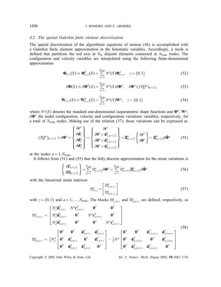
4.2. The spatial Galerkin �nite element discretization
The spatial discretization of the algorithmic equations of motion (44) is accomplished witha Galerkin �nite element approximation in the kinematic variables. Accordingly, a mesh isde�ned that partitions the rod axis in Nel disjoint elements connected at Nnode nodes. Thecon�guration and velocity variables are interpolated using the following �nite-dimensionalapproximation
�n+�(S) ≈ �hn+�(S) =
Nnode∑a=1Na(S)�a
n+�; �= {0; 1} (52)
��(S) ≈ ��h(S) =Nnode∑a=1Na(S)��a; ��a∈(TQa)n+1=2 (53)
Wn+�(S) ≈Whn+�(S) =
Nnode∑a=1Na(S)Wa; �= {0; 1} (54)
where Na(S) denotes the standard one-dimensional isoparametric shape functions and �a, Wa,��a the nodal con�guration, velocity and con�guration variations variables, respectively, fora total of Nnode nodes. Making use of the relation (37), these variations can be expressed as
(TQa)n+1=2 ��a=
�ra
�da1�da2�da3
=
�ra
�Xa× da1; n+1=2�Xa× da2; n+1=2�Xa× da3; n+1=2
=�an+1=2
{�ra
�Xa
}=�an+1=2��
a (55)
at the nodes a=1; Nnode.It follows from (51) and (55) that the fully discrete approximation for the strain variations is{
��n+1=2��n+1=2
}=Nnode∑a=1
Ban+1=2��a=
Nnode∑a=1
Ban+1=2�an+1=2��
a (56)
with the linearized strain matrices
Ban+�=[Ba�; n+�Ba�; n+�
](57)
with �= {0; 1} and a=1; : : : ; Nnode. The blocks Ba�; n+� and Ba�; n+� are de�ned, respectively, as
Ba�; n+� =
Na; sd
T1; n+� N arT; s; n+� 0T 0T
Na; sdT2; n+� 0T NarT; s; n+� 0T
Na; sdT3; n+� 0T 0T NarT; s; n+�
Ba�; n+� = 12N
a; s
0T 0T dT3; n+� dT2; n+�
0T dT3; n+� 0T dT1; n+�
0T dT2; n+� dT1; n+� 0T
− 12N
a
0T 0T dT3; s; n+� dT2; s; n+�
0T dT3; s; n+� 0T dT1; s; n+�
0T dT2; s; n+� dT1; s; n+� 0T
(58)
Copyright ? 2002 John Wiley & Sons, Ltd. Int. J. Numer. Meth. Engng 2002; 54:1683–1716

INTEGRATION SCHEMES FOR THE DYNAMICS OF GEOMETRICALLY EXACT RODS 1697
A straightforward calculation shows that the superposition of a rigid deformation leadsinvariant the discretized strain measures and their variations (56). We point out again that theorthonormality constraints of the directors are imposed on the nodal values da only. This isaccomplished through the introduction of the nodal rotation vectors in (55) and the use of theproper nodal rotational updates, as discussed again in Appendix A. Remarkably the assumeddirect interpolation of the directors di and their variations �di leads naturally to a conservingobjective approximation regardless of the particular nodal director update employed in theinterpolation, as proven in the following developments.
4.3. The discrete conservation properties
We show in this section that the algorithm de�ned in Sections 4.1 and 4.2 preserves theconservation laws of momenta and energy of the continuum model described in Section 2.3.We point out that the proofs below consider the �nal discrete equations in both time and space.This last consideration is crucial since the conservation properties of a temporal approximationcan be disturbed by the spatial �nite element interpolations in these problems involving a non-linear con�guration manifold, as observed in Appendix B for the schemes presented in Simoet al. [15].The linear momentum, angular momentum and total energy of the approximate, space–time
discrete solution (�hn ;Wh
n ) at time tn are de�ned, respectively, as
Ln=∫ L
0pn dS (59)
Jn=∫ L
0(rhn × pn + dh�; n× \�n) dS (60)
Hn=∫ L
0
(U + 1
2pn · vhn + 12\�n · ]h�; n
)dS (61)
with the momenta pn; \�n de�ned pointwise as described in (48). For the sake of conciseness,we consider the particular case of a free rod in the following developments, that is, with noconstrained generalized displacements on the boundary conditions and with no external forces(Gtext = 0). For this problem the time-discrete solution exhibits the following properties.
Property 1The total linear momentum is conserved.
ProofIn the discrete weak equilibrium equation choose admissible variations
(�rh; �dh1; �dh2; �d
h3)= (c; 0; 0; 0)∈TQ (62)
with c constant. By assumption Gtext = 0, and it is easily veri�ed that also Gtint = 0. ThereforeGtiner= 0 and thus
0=∫ L
0
pn+1 − pnt
· c dS= 1tc ·
∫ L
0(pn+1 − pn) dS= 1
tc · (Ln+1 − Ln) (63)
This last equation must hold for every c∈R3 therefore Ln+1 =Ln.
Copyright ? 2002 John Wiley & Sons, Ltd. Int. J. Numer. Meth. Engng 2002; 54:1683–1716
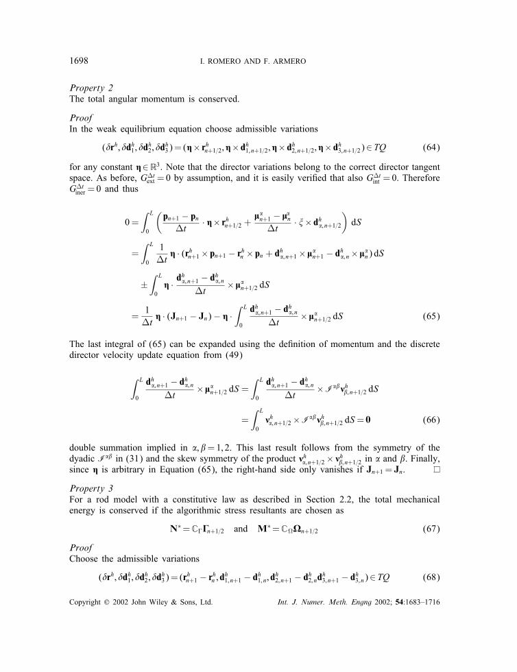
1698 I. ROMERO AND F. ARMERO
Property 2The total angular momentum is conserved.
ProofIn the weak equilibrium equation choose admissible variations
(�rh; �dh1; �dh2; �d
h3)= (W× rhn+1=2; W× dh1; n+1=2; W× dh2; n+1=2; W× dh3; n+1=2)∈TQ (64)
for any constant W∈R3. Note that the director variations belong to the correct director tangentspace. As before, Gtext = 0 by assumption, and it is easily veri�ed that also G
tint = 0. Therefore
Gtiner = 0 and thus
0 =∫ L
0
(pn+1 − pnt
· W× rhn+1=2 +\�n+1 − \�nt
· �× dh�; n+1=2)dS
=∫ L
0
1t
W · (rhn+1× pn+1 − rhn × pn + dh�; n+1× \�n+1 − dh�; n× \�n) dS
±∫ L
0W · d
h�; n+1 − dh�; nt
× \�n+1=2 dS
=1t
W · (Jn+1 − Jn)− W ·∫ L
0
dh�; n+1 − dh�; nt
× \�n+1=2 dS (65)
The last integral of (65) can be expanded using the de�nition of momentum and the discretedirector velocity update equation from (49)
∫ L
0
dh�; n+1 − dh�; nt
× \�n+1=2 dS =∫ L
0
dh�; n+1 − dh�; nt
×I��]h�; n+1=2 dS
=∫ L
0]h�; n+1=2×I��]h�; n+1=2 dS= 0 (66)
double summation implied in �; �=1; 2. This last result follows from the symmetry of thedyadic I�� in (31) and the skew symmetry of the product ]h�; n+1=2× ]h�; n+1=2 in � and �. Finally,since W is arbitrary in Equation (65), the right-hand side only vanishes if Jn+1 =Jn.
Property 3For a rod model with a constitutive law as described in Section 2.2, the total mechanicalenergy is conserved if the algorithmic stress resultants are chosen as
N∗=C��n+1=2 and M∗=C��n+1=2 (67)
ProofChoose the admissible variations
(�rh; �dh1; �dh2; �d
h3)= (r
hn+1 − rhn ; dh1; n+1 − dh1; n; dh2; n+1 − dh2; ndh3; n+1 − dh3; n)∈TQ (68)
Copyright ? 2002 John Wiley & Sons, Ltd. Int. J. Numer. Meth. Engng 2002; 54:1683–1716

INTEGRATION SCHEMES FOR THE DYNAMICS OF GEOMETRICALLY EXACT RODS 1699
in the weak dynamic equilibrium. Note that �dai · dai; n+1=2 = 0 (i=1; 2; 3) at the nodes andtherefore they are valid director variations. Since Gtext = 0, the sum Gtint + G
tiner must vanish.
Using the discrete velocity de�nitions (49), it follows that
Gtiner =∫ L
0
[pn+1 − pnt
· (rhn+1 − rhn ) +\�n+1 − \�nt
· (dh�; n+1 − dh�; n)]dS
=∫ L
0[(pn+1 − pn) · vhn+1=2 + (\�n+1 − \�n) · ] h�; n+1=2] dS = Kn+1 − Kn (69)
To prove properties 1 and 2, no speci�c form was needed for the algorithmic approximationsof the convected stresses N∗ and M∗. The choice
N∗=C��n + �n+1
2; M∗=C�
�n +�n+1
2(70)
is a second-order approximation to the stresses at the midpoint con�guration. The algorithmicapproximation for the stresses (70) is the same as the one in Simo et al. [15]; the approachdescribed by Gonz�alez [23] can be employed to obtain conserving approximations to thestress for more general constitutive models than the quadratic model considered herein. Forthe rod model described in Section 2.2, a simple manipulation proves then that these stressapproximations and variations (68) give
Gtint =∫ L
0
{N∗
M∗
}·{�n+1 − �n�n+1 −�n
}dS=Un+1 −Un (71)
Adding (69) and (71), the conservation property
0=Gtint +Gtiner =Un+1 + Kn+1 −Un − Kn=Hn+1 −Hn (72)
is recovered.
5. REPRESENTATIVE NUMERICAL SIMULATIONS
We present in this section several numerical simulations that illustrate the properties of theproposed formulation. Particular emphasis is placed in showing the objectivity and the preser-vation of conservation laws of the new implementation.
5.1. Example 1. Objectivity test: rigid motion of bent rod under quasi-static conditions
We compare the performance of the standard geometrically exact rod formulation of Simoand Vu-Quoc [8] and the newly proposed formulation. In particular, the following quasi-staticexample con�rms that the original rod discretization looses the objectivity of the continuumtheory while the implementation presented in the current work retains this fundamental prop-erty. This example was proposed by Cris�eld and Jeleni�c [19].A straight rod, discretized with nine linear rod elements, is placed in its undeformed con-
�guration with one end at the point A with Cartesian co-ordinates (0; 0; 2) and the other end
Copyright ? 2002 John Wiley & Sons, Ltd. Int. J. Numer. Meth. Engng 2002; 54:1683–1716
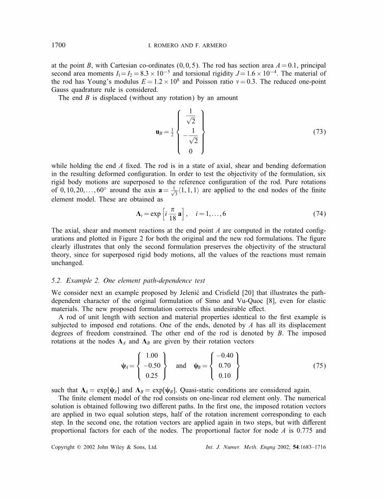
1700 I. ROMERO AND F. ARMERO
at the point B, with Cartesian co-ordinates (0; 0; 5). The rod has section area A=0:1, principalsecond area moments I1= I2 = 8:3× 10⁻⁵ and torsional rigidity J=1:6× 10⁻⁴. The material ofthe rod has Young’s modulus E=1:2× 10⁸ and Poisson ratio �=0:3. The reduced one-pointGauss quadrature rule is considered.The end B is displaced (without any rotation) by an amount
uB= 12
1√2
− 1√2
0
(73)
while holding the end A �xed. The rod is in a state of axial, shear and bending deformationin the resulting deformed con�guration. In order to test the objectivity of the formulation, sixrigid body motions are superposed to the reference con�guration of the rod. Pure rotationsof 0; 10; 20; : : : ; 60◦ around the axis a= 1√
3〈1; 1; 1〉 are applied to the end nodes of the �nite
element model. These are obtained as
�i=exp[i18a]; i=1; : : : ; 6 (74)
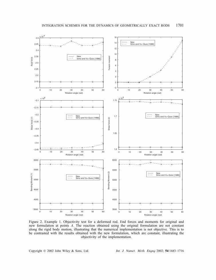
The axial, shear and moment reactions at the end point A are computed in the rotated con�g-urations and plotted in Figure 2 for both the original and the new rod formulations. The �gureclearly illustrates that only the second formulation preserves the objectivity of the structuraltheory, since for superposed rigid body motions, all the values of the reactions must remainunchanged.
5.2. Example 2. One element path-dependence test
We consider next an example proposed by Jeleni�c and Cris�eld [20] that illustrates the path-dependent character of the original formulation of Simo and Vu-Quoc [8], even for elasticmaterials. The new proposed formulation corrects this undesirable e�ect.A rod of unit length with section and material properties identical to the �rst example is
subjected to imposed end rotations. One of the ends, denoted by A has all its displacementdegrees of freedom constrained. The other end of the rod is denoted by B. The imposedrotations at the nodes �A and �B are given by their rotation vectors
�A=
1:00−0:500:25
and �B=
−0:400:700:10
(75)
such that �A= exp[�A] and �B= exp[�B]. Quasi-static conditions are considered again.The �nite element model of the rod consists on one-linear rod element only. The numerical
solution is obtained following two di�erent paths. In the �rst one, the imposed rotation vectorsare applied in two equal solution steps, half of the rotation increment corresponding to eachstep. In the second one, the rotation vectors are applied again in two steps, but with di�erentproportional factors for each of the nodes. The proportional factor for node A is 0.775 and
Copyright ? 2002 John Wiley & Sons, Ltd. Int. J. Numer. Meth. Engng 2002; 54:1683–1716
INTEGRATION SCHEMES FOR THE DYNAMICS OF GEOMETRICALLY EXACT RODS 1701
0 10 20 30 40 50 602.1
2.15
2.2
2.25
2.3
2.35
2.4
2.45
2.5x 10⁴
Axi
al fo
rce
Rotation angle (rad)
NewSimo and Vu-Quoc [1986]
0 10 20 30 40 50 60 _2
0
2
4
6
8
10
12
14
16
Rotation angle (rad)
Tor
sion
mom
ent
NewSimo and Vu- Quoc [1986]
0 10 20 30 40 50 60 _2.45
_2.4
_2.35
_2.3
_2.25
_2.2
_2.15
_2.1x 104
Rotation angle (rad)
She
ar fo
rce
(1) New
Simo and Vu- Quoc [1986]
0 10 20 30 40 50 601.6
1.65
1.7
1.75x 10⁵
Rotation angle (rad)
She
ar fo
rce
(2)
NewSimo and Vu- Quoc [1986]
0 10 20 30 40 50 603500
4000
4500
5000
5500
6000
Ben
ding
Mom
ent (
1)
Rotation angle (rad)
NewSimo and Vu-Quoc [1986]
0 10 20 30 40 50 603500
4000
4500
5000
5500
6000
Rotation angle (rad)
Ben
ding
Mom
ent (
2) NewSimo and Vu- Quoc [1986]
Figure 2. Example 1. Objectivity test for a deformed rod. End forces and moments for original andnew formulation at points A. The reaction obtained using the original formulation are not constantalong the rigid body motion, illustrating that the numerical implementation is not objective. This is tobe contrasted with the results obtained with the new formulation, which are constant, illustrating the
objectivity of the implementation.
Copyright ? 2002 John Wiley & Sons, Ltd. Int. J. Numer. Meth. Engng 2002; 54:1683–1716

1702 I. ROMERO AND F. ARMERO
Table I. Example 2. Single element problem with two solution paths (I and II). Numericalcomparison of strains and displacements obtained by the original rod formulation of Simo and
Vu-Quoc [8] and the current one.
�1 �2 �3 uB1 uB2 uBx
Solution I [8] −1:27464 1.26756 −0:40350 −0:02009 0.18605 −0:07187Solution II [8] −1:28872 1.25182 −0:41280 −0:01701 0.16401 −0:08261Solution I (Current) −0:66123 0.66499 0.22128 0.11370 −0:40047 0.57033Solution II (Current) −0:66123 0.66499 0.22128 0.11370 −0:40047 0.57033
0.4 for node B in the �rst step. The total proportional factor for both nodes is 1 in thesecond step.The nodal rotations at the end of the two solution strategies are identical, and both the
displacement of node B and the strains at the midpoint should be identical, but Table I showsthat the original formulation does not hold this property. The new one does.
5.3. Example 3. Buckling of a hinged frame
This next example involves the quasi-static simulation of the buckling of a hinged planeframe. This example was considered by Simo and Vu-Quoc [8] to assess the performanceof the numerical implementation under large displacements and strains. Figure 3 shows theundeformed con�guration and the deformed states for several load values, including the initialcon�guration. Each member of the frame has a length of 120 and it is discretized with �ve 3-node quadratic elements. The reduced two-point Gauss quadrature rule is considered to avoidthe shear locking of fully integrated elements. The assumed properties of the material areYoung’s modulus E=7:2× 10⁶ and Poisson’s ratio �=0:3. Each member of the frame haslength 120, inertia Ix= Iy=2 and cross-section A=6.
F = 0
F ~ 13600
F ~ 17800
F ~ - 5800
F~ -7700
F~ 15600
Figure 3. Example 3. Buckling of a hinged frame. Reference and deformed con�gurations.
Copyright ? 2002 John Wiley & Sons, Ltd. Int. J. Numer. Meth. Engng 2002; 54:1683–1716

INTEGRATION SCHEMES FOR THE DYNAMICS OF GEOMETRICALLY EXACT RODS 1703
0 10 20 30 40 50 60 70 80 90 100
_2
_1
0
1
2
3
4
5x 10
4
Displacement
For
ce
Vertical displacementHorizontal displacement
Figure 4. Example 3. Buckling of a hinged frame. Force displacement solution.
The load displacement solution is depicted in Figure 4. An arc-length solution strategy isemployed to follow the post-buckling deformation. The large �nite deformations and rotationsof the rods are to be noted, which allows us to conclude the robustness of the newly proposed�nite element formulation in this range. In particular, we observe a very similar response tothe performance of the formulation presented by Simo and Vu-Quoc [8] for this non-linearexample, with added properties of frame indi�erence in this quasi-static limit. A detailedcomparison is presented in the next example in the context of a three dimensional problem.
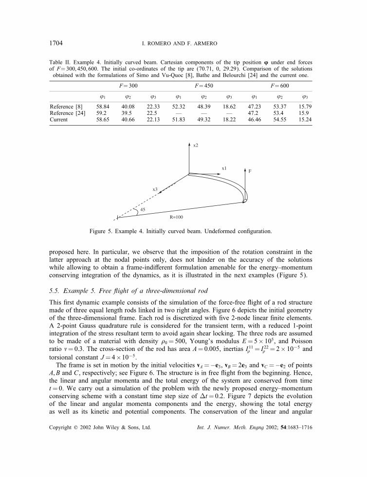
5.4. Example 4. Three-dimensional deformation of initially curved beam
We now illustrate the performance of the new formulation with a three-dimensional exampleproposed by Bathe and Belourchi [24]. The example considers the response of a cantilevercurved rod under a concentrate load in its tip, leading to a fully three-dimensional deformation.The rod has a unit square section and its material has Young’s modulus E=107 and Poisson’sratio �=0. The rod is discretized with eight linear �nite 2-noded linear elements. A one-pointGauss reduced integration rule is considered.We compare the formulations presented in Bathe and Belourchi [24] and in Simo and
Vu-Quoc [8] with the new formulation proposed herein. The deformed positions of the tipof the beam are compared in Table II for these three di�erent formulations. We observe, inparticular, a good agreement of the solution obtained with the formulation proposed hereinwith the solution obtained with the original formulation of Simo and Vu-Quoc [8]. We noteagain that the di�erence between the two formulations stands in the di�erent �nite ele-ment interpolation of the rotation �eld, through either a rotation vector or the directors as
Copyright ? 2002 John Wiley & Sons, Ltd. Int. J. Numer. Meth. Engng 2002; 54:1683–1716
1704 I. ROMERO AND F. ARMERO
Table II. Example 4. Initially curved beam. Cartesian components of the tip position � under end forcesof F=300; 450; 600. The initial co-ordinates of the tip are (70.71, 0, 29.29). Comparison of the solutionsobtained with the formulations of Simo and Vu-Quoc [8], Bathe and Belourchi [24] and the current one.
F=300 F=450 F=600
’1 ’2 ’3 ’1 ’2 ’3 ’1 ’2 ’3
Reference [8] 58.84 40.08 22.33 52.32 48.39 18.62 47.23 53.37 15.79Reference [24] 59.2 39.5 22.5 — — — 47.2 53.4 15.9Current 58.65 40.66 22.13 51.83 49.32 18.22 46.46 54.55 15.24
R=100
45
Fx1
x3
x2
Figure 5. Example 4. Initially curved beam. Undeformed con�guration.
proposed here. In particular, we observe that the imposition of the rotation constraint in thelatter approach at the nodal points only, does not hinder on the accuracy of the solutionswhile allowing to obtain a frame-indi�erent formulation amenable for the energy–momentumconserving integration of the dynamics, as it is illustrated in the next examples (Figure 5).
5.5. Example 5. Free �ight of a three-dimensional rod
This �rst dynamic example consists of the simulation of the force-free �ight of a rod structuremade of three equal length rods linked in two right angles. Figure 6 depicts the initial geometryof the three-dimensional frame. Each rod is discretized with �ve 2-node linear �nite elements.A 2-point Gauss quadrature rule is considered for the transient term, with a reduced 1-pointintegration of the stress resultant term to avoid again shear locking. The three rods are assumedto be made of a material with density �0 = 500, Young’s modulus E=5× 10⁵, and Poissonratio �=0:3. The cross-section of the rod has area A=0:005, inertias I 11� = I 22� =2× 10⁻⁵ andtorsional constant J=4×10⁻⁵.The frame is set in motion by the initial velocities vA=−e3, vB=2e3 and vC =−e2 of points
A; B and C, respectively; see Figure 6. The structure is in free �ight from the beginning. Hence,the linear and angular momenta and the total energy of the system are conserved from timet=0. We carry out a simulation of the problem with the newly proposed energy–momentumconserving scheme with a constant time step size of t=0:2. Figure 7 depicts the evolutionof the linear and angular momenta components and the energy, showing the total energyas well as its kinetic and potential components. The conservation of the linear and angular
Copyright ? 2002 John Wiley & Sons, Ltd. Int. J. Numer. Meth. Engng 2002; 54:1683–1716

INTEGRATION SCHEMES FOR THE DYNAMICS OF GEOMETRICALLY EXACT RODS 1705
3
3
3
e2e1
e3
A
B
C
Figure 6. Example 5. Free �ight of a three-dimensional rod. Geometry of the rod structure.
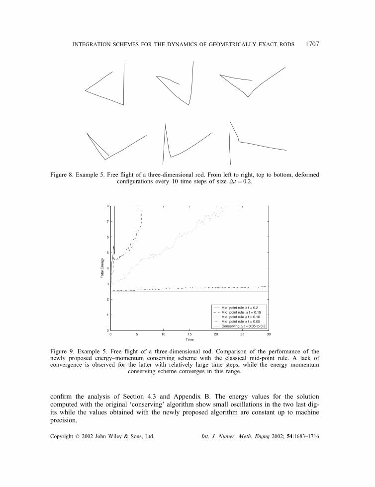
momenta and of the total energy is observed, con�rming the properties shown in the analysisof Section 4.3. The solution has large displacements and strains as illustrated in Figure 8. Thedeformed con�guration of the frame is shown every 10 time steps for a typical time interval.We have included in Figure 9 the evolution of the energy for the solution obtained by the
classical mid-point rule (that is, the stress resultants are obtained from the strain measurescorresponding to rn+1=2 and din+1=2 ; i=1; 3). This scheme conserves the momenta but not theenergy, as it can be concluded easily from the proofs in Section 4.3. Figure 9 depicts theevolution of the total energy for di�erent time step t. We can observe that for the previouslyconsidered value of t=0:2 the Newton–Raphson solution procedure ceases to convergeafter a few time steps, being unable to compute the simulation. The performance improvesfor smaller time steps, but still a lack of convergence is observed at some point, with thevalue of the energy being unphysically high. This situation is typical of commonly used non-conserving schemes. In contrast, the energy–momentum developed in this work converges inall the cases. These results show that a signi�cant improvement is obtained over a wide rangeof time steps where existing standard schemes fail to perform.
5.6. Example 6. Dynamic motion of a cantilever rod
In this example we solve the motion of a straight cantilever rod with a concentrated load andmoment on its free end. The goal of this simulation is to illustrate that the original ‘conserving’formulation of Simo et al. [15] exhibits oscillations in the energy evolution, and it is hence notconserving. As explained in Appendix B, the reason for these oscillations is the approximationof the rotational degrees of freedom of the motion by the �nite element interpolation. This isin contrast with the solution obtained using the newly proposed formulation, which exactlyconserves energy during the force free phase of the solution.The rod has length 10 and it is modelled with 10 identical 2-node linear rod elements
as considered in the previous example. The material has a Young’s modulus E=2× 10¹⁰,a Poisson’s ratio �=0:3 and a density �=15× 103. The cross-section has an area A=5× 10⁻⁴,
Copyright ? 2002 John Wiley & Sons, Ltd. Int. J. Numer. Meth. Engng 2002; 54:1683–1716

1706 I. ROMERO AND F. ARMERO
0 1 2 3 4 5 6 7 8 9 10 _1
_0.5
0
0.5
1
1.5
2
2.5
3
Time
Line
ar m
omen
tum
L xL yL z
0 1 2 3 4 5 6 7 8 9 10 _10
_8
_6
_4
_2
0
2
4
Time
Ang
ular
mom
entu
m
J xJ yJ z
0 1 2 3 4 5 6 7 8 9 100
0.5
1
1.5
2
2.5
3
Time
Ene
rgy
TotalKineticPotential
Figure 7. Example 5. Free �ight of a three-dimensional rod. Linear, angular and energy evolution.
moments of inertia I 11� = I 22� =12× 10−7 and torsional constant J=5× 10⁻⁷. All the degreesof freedom of one end are constrained and there is a concentrated load and moment at theother end. The load has value F=(1; 1; 1) · g(t) and the moment M=(1; 1; 1) · g(t), whereg(t) is the function
g(t)=
100t6
for 06t66
0 for 6¡t(76)
The rod lies along the x-axis in the Cartesian reference system employed in the de�nition ofthe forces. The rod then vibrates with no external loads after t¿6 around the �xed end. Thetotal energy of the system is therefore constant for the physical system after t¿6.We obtain the numerical solution for 20 time steps of constant time step size t=1.
Table III shows the total mechanical energy from time t=7 to 20 computed both by thescheme of Simo et al. [15] and the one proposed in this work. The numerical results
Copyright ? 2002 John Wiley & Sons, Ltd. Int. J. Numer. Meth. Engng 2002; 54:1683–1716
INTEGRATION SCHEMES FOR THE DYNAMICS OF GEOMETRICALLY EXACT RODS 1707
Figure 8. Example 5. Free �ight of a three-dimensional rod. From left to right, top to bottom, deformedcon�gurations every 10 time steps of size t=0:2.
0 5 10 15 20 25 300
1
2
3
4
5
6
7
8
Time
Tot
al E
nerg
y
Mid point rule ∆ t = 0.2Mid point rule ∆ t = 0.15Mid point rule ∆ t = 0.10Mid point rule ∆ t = 0.05Conserving ∆ t = 0.05 to 0.2
Figure 9. Example 5. Free �ight of a three-dimensional rod. Comparison of the performance of thenewly proposed energy–momentum conserving scheme with the classical mid-point rule. A lack ofconvergence is observed for the latter with relatively large time steps, while the energy–momentum
conserving scheme converges in this range.
con�rm the analysis of Section 4.3 and Appendix B. The energy values for the solutioncomputed with the original ‘conserving’ algorithm show small oscillations in the two last dig-its while the values obtained with the newly proposed algorithm are constant up to machineprecision.
Copyright ? 2002 John Wiley & Sons, Ltd. Int. J. Numer. Meth. Engng 2002; 54:1683–1716
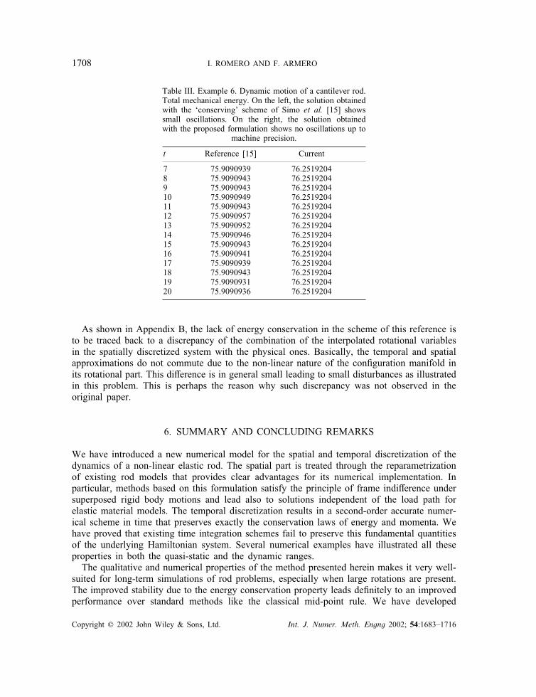
1708 I. ROMERO AND F. ARMERO
Table III. Example 6. Dynamic motion of a cantilever rod.Total mechanical energy. On the left, the solution obtainedwith the ‘conserving’ scheme of Simo et al. [15] showssmall oscillations. On the right, the solution obtainedwith the proposed formulation shows no oscillations up to
machine precision.
t Reference [15] Current
7 75.9090939 76.25192048 75.9090943 76.25192049 75.9090943 76.251920410 75.9090949 76.251920411 75.9090943 76.251920412 75.9090957 76.251920413 75.9090952 76.251920414 75.9090946 76.251920415 75.9090943 76.251920416 75.9090941 76.251920417 75.9090939 76.251920418 75.9090943 76.251920419 75.9090931 76.251920420 75.9090936 76.2519204
As shown in Appendix B, the lack of energy conservation in the scheme of this reference isto be traced back to a discrepancy of the combination of the interpolated rotational variablesin the spatially discretized system with the physical ones. Basically, the temporal and spatialapproximations do not commute due to the non-linear nature of the con�guration manifold inits rotational part. This di�erence is in general small leading to small disturbances as illustratedin this problem. This is perhaps the reason why such discrepancy was not observed in theoriginal paper.
6. SUMMARY AND CONCLUDING REMARKS
We have introduced a new numerical model for the spatial and temporal discretization of thedynamics of a non-linear elastic rod. The spatial part is treated through the reparametrizationof existing rod models that provides clear advantages for its numerical implementation. Inparticular, methods based on this formulation satisfy the principle of frame indi�erence undersuperposed rigid body motions and lead also to solutions independent of the load path forelastic material models. The temporal discretization results in a second-order accurate numer-ical scheme in time that preserves exactly the conservation laws of energy and momenta. Wehave proved that existing time integration schemes fail to preserve this fundamental quantitiesof the underlying Hamiltonian system. Several numerical examples have illustrated all theseproperties in both the quasi-static and the dynamic ranges.The qualitative and numerical properties of the method presented herein makes it very well-
suited for long-term simulations of rod problems, especially when large rotations are present.The improved stability due to the energy conservation property leads de�nitely to an improvedperformance over standard methods like the classical mid-point rule. We have developed
Copyright ? 2002 John Wiley & Sons, Ltd. Int. J. Numer. Meth. Engng 2002; 54:1683–1716
INTEGRATION SCHEMES FOR THE DYNAMICS OF GEOMETRICALLY EXACT RODS 1709
extensions of these methods that accommodate a controlled high-frequency dissipation tohandle the high numerical sti�ness of these systems along the lines presented in Armero andRomero [24]. We plan to present these extensions in a forthcoming publication.
ACKNOWLEDGEMENTS
Financial support for this research was provided by the AFOSR under contract no. F49620-00-1-0360with UC Berkeley. This support is gratefully acknowledged.
APPENDIX A. THE NUMERICAL IMPLEMENTATION
The numerical implementation of the proposed rod formulation is described next. The dy-namic solution is discussed in detail �rst and the quasi-static case is mentioned at the end asa particular instance.
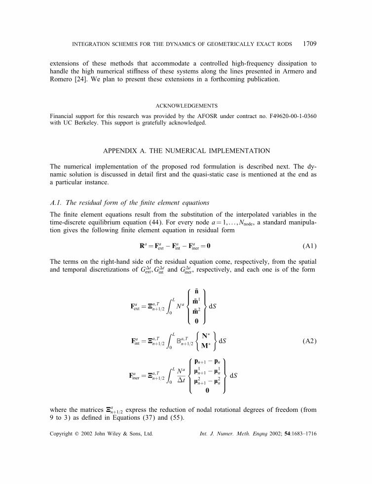
A.1. The residual form of the �nite element equations
The �nite element equations result from the substitution of the interpolated variables in thetime-discrete equilibrium equation (44). For every node a=1; : : : ; Nnode, a standard manipula-tion gives the following �nite element equation in residual form
Ra=Faext − Faint − Fainer = 0 (A1)
The terms on the right-hand side of the residual equation come, respectively, from the spatialand temporal discretizations of Gtext ; G
tint and G
tiner, respectively, and each one is of the form
Faext =�a; Tn+1=2
∫ L
0Na
�n�m1
�m2
0
dS
Faint =�a; Tn+1=2
∫ L
0Ba; Tn+1=2
{N∗
M∗
}dS (A2)
Fainer =�a; Tn+1=2
∫ L
0
Na
t
pn+1 − pn\1n+1 − \1n\2n+1 − \2n
0
dS
where the matrices �an+1=2 express the reduction of nodal rotational degrees of freedom (from9 to 3) as de�ned in Equations (37) and (55).
Copyright ? 2002 John Wiley & Sons, Ltd. Int. J. Numer. Meth. Engng 2002; 54:1683–1716
1710 I. ROMERO AND F. ARMERO
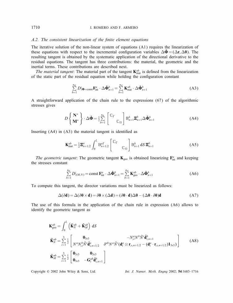
A.2. The consistent linearization of the �nite element equations
The iterative solution of the non-linear system of equations (A1) requires the linearization ofthese equations with respect to the incremental con�guration variables �=(r;X). Theresulting tangent is obtained by the systematic application of the directional derivative to theresidual equations. The tangent has three contributions: the material, the geometric and theinertial terms. These contributions are described next.The material tangent: The material part of the tangent Kabmat is de�ned from the linearization
of the static part of the residual equation while holding the con�guration constant
nel∑b=1D|�=constFaint ·�b
n+1 =nel∑b=1Kabmat ·�b
n+1 (A3)
A straightforward application of the chain rule to the expressions (67) of the algorithmicstresses gives
D
{N∗
M∗
}·�= 1
2
nel∑b=1
[C�
C�
]Bbn+1�
bn+1�
bn+1 (A4)
Inserting (A4) in (A3) the material tangent is identi�ed as
Kabmat =12�
an+1=2
∫ L
0BaTn+1=2
[C�
C�
]Bbn+1 dS �
bn+1 (A5)
The geometric tangent: The geometric tangent Kgeo is obtained linearizing Faint and keepingthe stresses constant
nel∑b=1D|(M;N ) = const Faint ·�b
n+1 =nel∑b=1Kabgeo ·�b
n+1 (A6)
To compute this tangent, the director variations must be linearized as follows:
(�d)=(�X× d)= �X× (d)= (�X · d)X− (X · �X)d (A7)
The use of this formula in the application of the chain rule in expression (A6) allows toidentify the geometric tangent as
Kabgeo =∫ L
0
(KabN + K
abM
)dS
KabN =3∑i=1
12
[03x3 −Na; sN bN idbi; n+1
NaNb; s Nidai; n+1=2 �abNaN i(dai ⊗ r; s; n+1=2 − (dai · r; s; n+1=2)13x3)
](A8)
KabM =3∑i=1
12
[03x3 03x303x3 −Gabi dbi; n+1
]
Copyright ? 2002 John Wiley & Sons, Ltd. Int. J. Numer. Meth. Engng 2002; 54:1683–1716
INTEGRATION SCHEMES FOR THE DYNAMICS OF GEOMETRICALLY EXACT RODS 1711
with N i, the ith component of the stress vector N. The 3× 3 matrices Gabi appearing in KabMare de�ned as
Gabi =12M
i3∑
j; k=1jik[(Na; sN
b − NaNb; s)dak; n+1=2 + �ab(Na; s dk; n+1=2 − Nadk; s; n+1=2)] (A9)
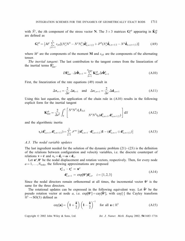
where Mi are the components of the moment M and ijk are the components of the alternatingtensor.The inertial tangent: The last contribution to the tangent comes from the linearization of
the inertial terms Fainer.
DFainer ·�n+1 =Nnodes∑b=1
Kabiner�bn+1 (A10)
First, the linearization of the rate equations (49) result in
vn+1 =2trn+1 and ]i; n+1 =
2tdi; n+1 (A11)
Using this last equation, the application of the chain rule in (A10) results in the followingexplicit form for the inertial tangent
Kabiner =2t2
∫ L
0
[NaNbA�13x3
NaNbY�(db�; n+1; da�; n+1=2)
]dS (A12)
and the algorithmic inertia
Y�(db�; n+1; da�; n+1=2)=2∑�=1
I�� [(db�; n+1 · da�; n+1=2)1− (db�; n+1 ⊗ da�; n+1=2)] (A13)
A.3. The nodal variable updates
The last ingredient needed for the solution of the dynamic problem (21)–(23) is the de�nitionof the relations between con�guration and velocity variables, i.e. the discrete counterpart ofrelations v= r and ]�= d�=�× d�.Let ua; Xa be the nodal displacement and rotation vectors, respectively. Then, for every node
a=1; : : : ; Nnode, the following approximations are proposedran+1 − ran = ua
dai; n+1 = exp[Xa]dai; n; i= {1; 2; 3}(A14)
Since the nodal directors remain orthonormal at all times, the incremental vector Xa is thesame for the three directors.The rotational updates can be expressed in the following equivalent way. Let �Xa be the
pseudo rotation vector at node a, i.e. exp[Xa]= cay[�Xa], with cay[·] the Cayley transformR3→SO(3) de�ned as
cay[a]=(1+
a2
)(1− a
2
)−1for all a∈R3 (A15)
Copyright ? 2002 John Wiley & Sons, Ltd. Int. J. Numer. Meth. Engng 2002; 54:1683–1716

1712 I. ROMERO AND F. ARMERO
Then, update (A14)2 can also be written as
dai; n+1 = cay[�Xa]dai; n=(1+
�Xa2
)(1−
�Xa2
)−1da�; n
=
(1−
�Xa2
)−1(1+
�Xa2
)dai; n
⇒ dai; n+1 − dai; n= �Xa× dai; n+1=2 (A16)
at each node a=1; Nnode.Note however that two elements which connect at a node but are not aligned may have
di�erent section directors and thus update (A16) must be modi�ed accordingly. For this, lete=1; : : : ; nelem be an element number and denote by d
(e)li ; �(e)li the director and director velocity
at the local node l of element e. The global-to-local nodal numbering map is customarily givenin terms of the ID matrix. Using this common notation, the global number of a node with localnumber l in an element e is a=ID(e; l). The following modi�cation of (A16) is proposed,which accounts for di�erent section directors in connecting elements
d(e); li; n+1 = cay[�Xa]d(e); li; n ; i= {1; 2; 3} with a=ID(e; l) (A17)
To approximate the velocity de�nitions at the nodes, the following midpoint approximationsare proposed for each global node
ua
t= van+1=2 and
�Xat= �a (A18)
Finally, at the element level, the director velocities are approximated by the following midpointrule
](e)li; n+1 = − ](e)li; n + 2�a× d(e)li; n+1=2 with a=ID(e; l) (A19)
for i= {1; 2; 3}.
A.4. Summary of the implementation
The steps for advancing the kinematic and velocity nodal variables from tn to tn+1 are summa-rized. Since the global equations are non-linear, a iterative (Newton–Raphson type) proceduremust be employed. Given the solution nodal variables (�a
n ;Wan ) (a=1; : : : ; Nnode) at time tn
as follows.1. Obtain a predictor for the solution at tn+1
(�a; (o)n+1 ;W
a; (o)n+1 )= (�
an ;W
an ) (A20)
2. Solve the non-linear �nite element equation (A2) by an iterative Newton–Raphson pro-cedure (denote by (k) the iteration count)2.1. Solve the linearized residual equation with unknown the incremental con�guration
variables �=(u;�X).
Copyright ? 2002 John Wiley & Sons, Ltd. Int. J. Numer. Meth. Engng 2002; 54:1683–1716
INTEGRATION SCHEMES FOR THE DYNAMICS OF GEOMETRICALLY EXACT RODS 1713
2.2. Update the nodal con�guration variables as described in (A3). For every nodea=1; : : : ; nnode
ra; (k+1)n+1 = ra; (k)n+1 +ua
�a; (k+1)n+1 = cay[�Xa]�a; (k)n+1
(A21)
2.3. Update the nodal velocity variables as described in (A3). For every node a=1; : : : ;nnode
va; (k+1)n+1 = va; (k)n+1 +2tua
�Xa = cay−1[�a; (k+1); Tn+1 �an]
�a; (k+1) = 2t�Xa
(A22)
2.4. Update the director and director velocities at the element (e) for every node in theelement
�(e); l; (k+1)n+1 = �a; (k+1)n+1 �(e); l0
](e); l; (k+1)i; n+1 = −](e)li; n + 2�a; (k+1)× d(e); l; (k+1)i; n+1=2
(A23)
2.5. Check for convergence in the solution of the system of non-linear equations and goback to 2.1 if not converged.
3. Advance time step counter n and goto 1.
A.5. A note on the implementation of the quasi-static case
The implementation of the quasi-static problem is obtained as above, but enforcing the equi-librium at the end of the time step tn+1 for n=1; 2; : : : instead of the midpoint con�guration.The dynamic contribution to the residual Fainer is discarded and accordingly, the inertial tangentKabiner. The �nal tangent in this quasi-static case consists then of the material tangent (A5),which is symmetric in this case, and the geometric tangent (A8). The latter exhibits thestandard non-symmetry due to the geometrically exact treatment of the �nite rotations.Since the equilibrium equations are imposed at the end of every time step, the exponential
map update (A14)2 may be used instead of the (equivalent) Cayley transform. The translationaland director velocities do not enter the formulation so their updates can be ignored in thiscontext. The linearization of the equations for this choice is almost identical to the onedescribed in Section A.2. Details are therefore omitted.
APPENDIX B. THE ENERGY CONSERVATION ARGUMENT IN SIMO ET AL. [15]
The �rst �nite element implementation of a dynamic rod model that preserved the conservationlaws of momenta and energy was proposed in Simo et al. [15]. It is shown below that, ingeneral, the law of energy conservation is not exactly preserved by the fully discrete model.The reason for the lack of energy conservation can be traced down to the evolution of therotational part of the kinetic energy. The reason why this fact may have passed unnoticed isprobably the small contribution of the rotational kinetic energy to the total mechanical energyof the rod, as illustrated in the numerical example of Section 5.6.
Copyright ? 2002 John Wiley & Sons, Ltd. Int. J. Numer. Meth. Engng 2002; 54:1683–1716
1714 I. ROMERO AND F. ARMERO
The implementation presented in Simo et al. [15] involves the nodal update equations
ran+1 − ran =t2(van+1 + v
an ) (B1)
Xa = t2(�an+1 + cay[Xa]�an) (B2)
�an+1 = cay[Xa]�an (B3)
for the nodal position of the middle axis ran+�, the nodal translational velocity van+�, the nodal
incremental rotational vector Xa, the nodal angular velocities �an+� and the nodal rotationtensors �an+� for �=0; 1. The �nite element interpolations de�ne the incremental rotationvector Xh(^g) and the angular velocity �hn+�(^g) (�=0; 1) at the quadrature points ^g fromtheir corresponding nodal values in (B1)–(B3). The total rotation tensor �n+�(^g) (�=0; 1)at the quadrature point ^g is not the interpolation of any nodal quantity, but it is obtainedinstead by the local rotational update (B3) applied directly at the quadrature points from theinterpolated rotation vector, that is
�n+1(^g)= cay[Xh(^g)]�n(^g) where Xh(^g)=nnode∑a=1Na(^g)Xa (B4)
for the �nite element shape functions Na(^) (a=1; nnode). This situation is to be contrastedwith the formulation proposed herein. Then, the spatial momenta �n+�(^g) at the quadraturepoint ^g for �=0; 1 are obtained as
�n+�(^g)= i�; n+�(^g)�n+�(^g) for i�; n+�(^g)=�n+�(^g)I��n+�(^g)T (B5)
the spatial inertia at the Gauss point ^g and time tn+� (�=0; 1), where I� is the (�xed) bodyinertia.The weak equilibrium equation of the formulation has the same form as (44)1 and (45)–
(47), although some of the terms have di�erent forms. In particular, the inertial term is ofthe form
Gtiner(Wn; Wn+1; ��)=∫ L
0
[phn+1 − phnt
· �rh + �n+1 − �nt
· �Xh]dS (B6)
in terms, in particular, of the interpolated variations �Xh of the incremental rotation vectorsand the above spatial momenta n+� (�=0; 1). The integrals are to be understood, as usual,in terms of the values of these quantities at the quadrature points, as de�ned above.To obtain the evolution of the energy in this discrete setting we follow the same arguments
considered in Section 4.3. For Gtext = 0, we choose the admissible variations �rh= rhn+1 − rhnand �Xh= Xh. As in that section, the internal work term yields the change in potential energyfor this choice of admissible variations. Thus
0 =Gtint (�n+1; �n; rhn+1 − rhn) +Gtkine(Wn+1; Wn; rhn+1 − rhn)
=Un+1 −Un +∫ L
0
[phn+1 − phnt
· (rhn+1 − rhn ) +�n+1 − �nt
· Xh]dS
Copyright ? 2002 John Wiley & Sons, Ltd. Int. J. Numer. Meth. Engng 2002; 54:1683–1716

INTEGRATION SCHEMES FOR THE DYNAMICS OF GEOMETRICALLY EXACT RODS 1715
=Un+1 −Un +∫ L
0
[(phn+1 − phn) · vhn+1=2 + (�n+1 − �n) ·
Xht
]dS
=Un+1 −Un + Kvn+1 − Kvn +∫ L
0(�n+1 − �n) · X
h
tdS (B7)
where we have denoted by Kv the translational part of the kinetic energy in (25)2, that is
Kv :=∫ L
0
12p · v dS=
∫ L
0
12A�v · v dS (B8)
Similarly, we de�ne
K! :=K − Kv=∫ L
0
12� · � dS=
∫ L
0
12� · i�� dS (B9)
for the rotational part of the kinetic energy.The energy conservation character of the algorithm would follow then if the last integral
in (B7) was the change in the rotational part of the kinetic energy K!. However, after using(B1)–(B3) the integrand in this integral is given by
(�n+1(^g)− �n(^g)) · Xh(^g)t
= 12(�n+1(^g)− �n(^g)) ·
nnode∑a=1Na(^g)(�an+1 + cay[Xa]�an)
= 12(�n+1(^g)− �n(^g)) · (�hn+1(^g) +
nnode∑a=1Na(^g)cay[Xa]�an)
= 12�n+1(^g) · i�(^g)�n+1(^g)− 1
2�n(^g) · i�(^g)�n(^g)
− (�n+1(^g)− �n(^g)) ·(cay[X(^g)]�n(^g)−
nnode∑a=1Na(^g)cay[Xa]�an
)(B10)
after some algebraic manipulations involving the properties of the Cayley transform (A15)(e.g. cay[X]X= X). Hence, we have
Kwn+1 − Kwn −∫ L
0(�n+1 − �n) · X
h
tdS
=ngauss∑g=1
[(�n+1(^g)− �n(^g)) ·
(cay[X(^g)]�n(^g)−
nnode∑a=1Na(^g)cay[Xa]�an
)]�=0 (B11)
in general. The e�ects of the spatial �nite element interpolation become apparent in this lastexpression, since the right-hand side vanishes for the exact �elds without this interpolation.This di�erence in the change of rotational kinetic energy has been observed to be small,though, as the numerical simulations of Section 5 illustrate.
Copyright ? 2002 John Wiley & Sons, Ltd. Int. J. Numer. Meth. Engng 2002; 54:1683–1716

1716 I. ROMERO AND F. ARMERO
The direct interpolation of the director �elds advocated in this paper can be seen thento avoid the diculties associated to the direct interpolation of the rotational vectors. Thesimplicity of the proof of the discrete conservation result (72) is also to be noted.
REFERENCES
1. Cosserat E, Cosserat F. Th�eorie des corps d�eformables. Trait�e de Physique. Paris (2nd edn), 1909.2. Green AE, Laws N. A general theory of rods. Proceedings of the Royal Society of London, Series A 1966;293:145–155.
3. Ericksen JL, Truesdell C. Exact theory of stress and strain in rods and shells. Archive for Rational Mechanicsand Analysis 1958; (1):195–323.
4. Reissner E. A one-dimensional �nite strain beam theory: the plane problem. Journal of Applied Mathematicsand Physics (ZAMP) 1972; 23:795–804.
5. Antman SS. Nonlinear Problems of Elasticity. Springer: Berlin, 1992.6. Simo JC. A �nite strain beam formulation. Part I. The three-dimensional dynamic problem. ComputationalMethods in Applied Mechanics and Engineering 1985; 49:55–70.
7. Simo JC. A three-dimensional �nite-strain rod model. Part II: Computational aspects. Computational Methodsin Applied Mechanics and Engineering 1986; 58;79–116.
8. Simo JC, Vu-Quoc L. On the dynamics in space of rods undergoing large motions—a geometrically exactapproach. Computational Methods in Applied Mechanics and Engineering 1988; 66(2):125–161.
9. Simo JC, Vu-Quoc L. A geometrically-exact beam model incorporating shear and torsion warping deformation.International Journal of Solids and Structures 1991; 27:371–393.
10. Cardona A, Geradin M. Time integration of the equations of motion in mechanism analysis. Computers andStructures 1989; 33(3):801–820.
11. Ibrahimbegovic A. On �nite element implementation of geometrically non-linear Reissner’s beam theory: three-dimensional curved beam elements. Computational Methods in Applied Mechanics and Engineering 1995; 122:11–26.
12. Cris�eld MA. Non-linear �nite element analysis of solids and structures. Advanced Topics. vol. 2. 1997; Wiley:Chichester.
13. Armero F, Romero I. On the formulation of high-frequency dissipative time-stepping algorithms for non-lineardynamics. I: Low order methods for two model problems and nonlinear elastodynamics. Computational Methodsin Applied Mechanics and Engineering 2001; 190:2603–2649.
14. Kane C, Marsden JE, Ortiz M, West M. Variational integrators and the Newmark algorithm for conservativeand dissipative mechanical systems. International Journal for Numerical Methods in Engineering 2000; 49:1295–1325.
15. Simo JC, Tarnow N, Doblar�e M. Non-linear dynamics of three-dimensional rods: exact energy and momentumconserving algorithms. International Journal for Numerical Methods in Engineering 1995; 38(9):1431–1473.
16. Galvanetto U, Cris�eld MA. An energy-conserving co-rotational procedure for the dynamics of planar beamstructures. International Journal for Numerical Methods in Engineering 1996; 39:2265–2282.
17. Bauchau OA, Theron NJ. Energy decaying scheme for non-linear beam models. Computational Methods inApplied Mechanics and Engineering 1996; 134:37–56.
18. Botasso CL, Borri M. Energy preserving=decaying schemes for non-linear beam dynamics using the helicoidalapproximation. Computational Methods in Applied Mechanics and Engineering 1997; 143:393–415.
19. Cris�eld MA, Jeleni�c G. Objectivity of strain measures in geometrically exact 3D beam theory and its �niteelement implementation. Proceedings of Royal Society of London 1998; 455:1125–1147.
20. Jeleni�c G, Cris�eld MA. Geometrically exact 3d beam theory: implementation of a strain-invariant �nite elementfor statics and dynamics. Computational Methods in Applied Mechanics and Engineering 1999; 171:141–171.
21. Jeleni�c G, Cris�eld MA. Dynamic analysis of 3D beams with joints in presence of large rotations. ComputationalMethods in Applied Mechanics and Engineering 2001; 190:4195–4230.
22. Simo JC, Tarnow N. A new energy and momentum conserving algorithm for the nonlinear dynamics of shells.International Journal for Numerical Methods in Engineering 1994; 37:2527–2549.
23. Gonz�alez O. Exact energy-momentum conserving algorithms for general models in non-linear elasticity.Computational Methods in Applied Mechanics and Engineering 2000; 190:1763–1783.
24. Bathe KJ, Belourchi S. Large displacement analysis of three-dimensional beam structures. International Journalfor Numerical Methods in Engineering 1979; 14:961–986.
25. Armero F, Romero I. On the formulation of high-frequency dissipative time-stepping algorithms for non-lineardynamics. II: Second order methods. Computational Methods in Applied Mechanics and Engineering 2001;190:6783–6824.
Copyright ? 2002 John Wiley & Sons, Ltd. Int. J. Numer. Meth. Engng 2002; 54:1683–1716
Copyright © 2022 FDOKUMEN