An MDP-based Approach for Multipath Data

Transmission over Wireless Networks

Vinh Bui and Weiping Zhu

The University of New South Wales, Australia

{v.bui, w.zhu}@adfa.edu.au

Alessio Botta and Antonio Pescape

University of Napoli “Federico II”, Italy

{a.botta, pescape}@unina.it

Abstract—Maintaining performance and reliability in wirelessnetworks is a challenging task due to the nature of wire-less channels. Multipath data transmission has been used inwired scenarios to reduce latency, improve throughput, and -when/where possible - balance the load. In this paper, we proposean approach for multipath data transmission over wirelessnetworks. We demonstrate that the problem under study canbe formulated as a Markov Decision Process (MDP) and wepropose an algorithm called On-line Policy Iteration (OPI), tosolve the formulated MDP in real time. We verified the proposedapproach using simulations with ns-2 and data collected fromreal heterogeneous wired/wireless networks. The results indicatethat we improve both delay and loss characteristics of end-to-endwireless communications outperforming the classical multi-pathschemes including Round Robin and Join the Shortest Queue.

I. INTRODUCTION

Wireless networks are noisy and unreliable communication

environments. Unlike in wired networks where data losses

are mainly caused by traffic congestions, losses in wireless

networks are due to both traffic congestions and transmis-

sion errors. If traffic congestions are somewhat predictable,

transmission errors are subject to the variation of the wireless

propagation environment, and therefore much harder to predict

and control. As a result, providing Quality of Service (QoS)

in wireless networks is more challenging.

Recently, multipath data transmission has been proposed as

a promising solution to overcome the bandwidth limitation,

end-to-end delay fluctuations, and consecutive losses in the

wired Internet environment [3], [6], [9], [11], [14], [21], [23],

[24], [25]. Nonetheless, the proposed approaches revealed

a number of limitations: (i) protocol specific; (ii) excessive

computation; (iii) requirements of explicit knowledge of the

network characteristics; (iv) optimal only for specific network

configurations. In addition, the significant difference in data

transmission characteristics of wired and wireless networks

suggests the necessity of further investigation.

Therefore, in this paper we present an analytical approach

to optimally transfer data over multiple wireless network

paths. In particular, our contributions are the following. First,

thanks to the Imbedded Markov Chain technique [15], we

demonstrate that the system under study can be modeled as

a Markov chain. Second, by using such results we formulate

0This work is supported by University of New South Wales at AustralianDefence Force Academy. This work has been partially supported by PRINRECIPE and CONTENT NoE, OneLab and NETQOS EU projects.

the multipath data transmission problem as a Markov Decision

Process (MDP) [20], a powerful mathematical framework for

making decisions in control environments exhibiting dynamic

behaviors e.g. transmission errors in wireless networks. Third,

we introduce a simple path state monitoring mechanism.

Fourth, an algorithm called OPI (On-line Policy Iteration),

which has a low computational complexity, is proposed to

select transmission paths on the fly by using the MPD. Fifth,

through simulations and real data, we show the feasibility of

our approach as well as its capability to obtain better per-

formance than classical approaches such as Round Robin and

Join-the-Shortest-Queue. In addition, our approach is general

enough to be applied for improving other QoS metrics such

as the throughput or a function of multiple QoS parameters.

Attempts to improve QoS in wireless networks by means

of multipath data transmission were made by [5] and [8].

In [5], the authors proposed a multipath routing mechanism,

which adaptively searches for available network paths from a

source to a destination, and optimally routes traffic among the

paths. However in [5], the routing problem was formulated

as a static optimization problem, using the average value of

some network parameters. On the contrary, we formulate the

problem using a dynamic optimization framework, which is

more capable of reflecting the network dynamics. In [8], a Join

the Shortest Queue (JSQ)-like algorithm was used to reduce

the cost of data alignment at the receiver side while spreading

traffic among multiple TCP connections. Meanwhile in this

paper, we focus on reducing end-to-end delay fluctuations and

improving packet loss characteristics while showing that our

approach performs better than the JSQ algorithm in various

simulation scenarios. Furthermore, compared to [8], we are

not tied to a specific transport protocol.

The rest of the paper is organized as follows. In Section

II and III, the problem under study is defined and the system

model is established. The formulation of the MDP is presented

in Section IV while Section V details a novel algorithm

to solve the formulated MDP. In Section VI, the numerical

verification of the proposed approach is presented. Finally,

concluding remarks are made in Section VII.

II. PROBLEM DEFINITION

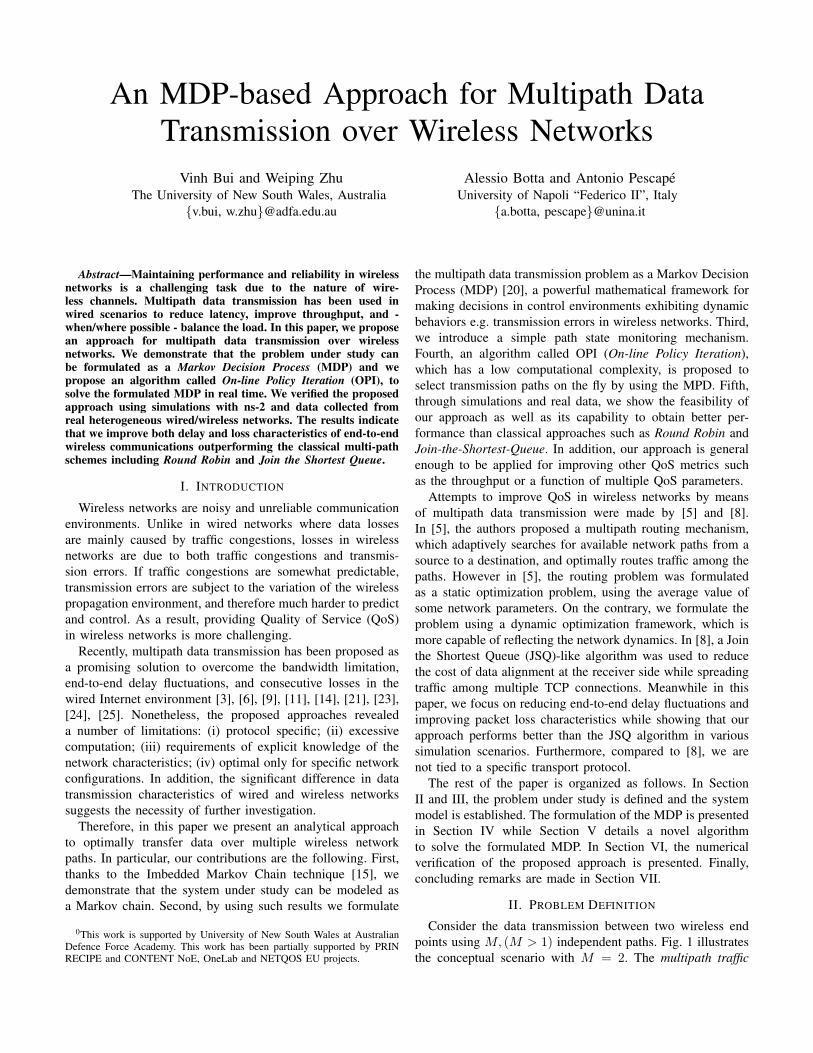
Consider the data transmission between two wireless end

points using M, (M > 1) independent paths. Fig. 1 illustrates

the conceptual scenario with M = 2. The multipath traffic

distributor is an abstract module (see Section VI-B1 for a

proof of concept scenario), which is implemented to optimally

distribute traffic over the paths.

path 1

path 2MultipathTraffic Distributor

Wireless bridge Wireless bridge

MultipathTraffic Distributor

Fig. 1. Multipath data transmission with 2 independent paths.

Assume that data arrives at the traffic distributor in a stream

of constant-length bins (i.e packets)1, with an average rate of

λ. Since the arrival process is discrete, we approximate it using

a Poisson process [12] with inter-arrival time between consec-

utive bins following an exponential i.i.d. random variable.2

The traffic distributor has to decide the path over which

to send the bins according to a predefined policy. We are

interested in finding a policy, which is optimal in terms of

minimizing the average transmission delay and loss rate. Since

delays and losses are dynamic characteristics, which exhibit

randomness to some degrees, static distribution policies are not

suitable. A powerful framework to cope with such stochastic

optimization problems is Markov Decision Processes (MDPs)

[1]. Nonetheless, before the framework can be applied, the

problem under study has to be formulated as a MDP.

III. SYSTEM AND STATES

In this section, we explain what do we mean by the system

states, and how do we monitor them. We also demonstrate the

system under study at specific instances can be modeled as a

Markov chain where the MDP framework is applicable.

A. System Model: basic idea

Previous studies on similar problems ([13], [18]) when ap-

plying decision frameworks, often assume the perfect knowl-

edge of the network path characteristics e.g. loss, delay

and throughput. To avoid this assumption, we design a path

state monitoring mechanism, which reveals loss and delay

conditions of the path by keeping track of data bins being

transmitted. The mechanism works as follows. Before the

distributor sends a bin over the selected path (i.e. it delivers

the bin to the related Access Point), the bin ID and a time

stamp are recorded on a list of size K. This information is

kept until the bin is correctly received by the other end of the

wireless link (i.e. the other Access Point). In this manner, given

the data stream, the evolution of the number of bins on the

list will implicitly reflect the path state in terms of Round Trip

1The constant length is assumed to simplify the formulation of the modelwhich can be, however, easily generalized for variable sized packets.

2In general, any discrete arrival process, e.g. packet streams, can beapproximated using the Poisson arrival process (see Faddy MJ (1997a)Extended Poisson process modelling and analysis of count data for example).Nonetheless, our arrival process is not purely Poisson but Markov ModulatedPoisson like. The reason is we consider the arrival process is Poisson(λ) onlyin a short period of time. After this period, λ may change to another value.

Time (RTT) and loss. In a real implementation, the information

regarding the transmission success can be retrieved directly

from the Access Point by using protocols e.g. CAPWAP [7].

At a first glance, this can be seen as a considerable overhead.

However we have verified that, even if this information is

obtained every 10/15 bins, the results presented in Section VI

remain almost unchanged (here, due to the space constraints,

we do not present this analysis).

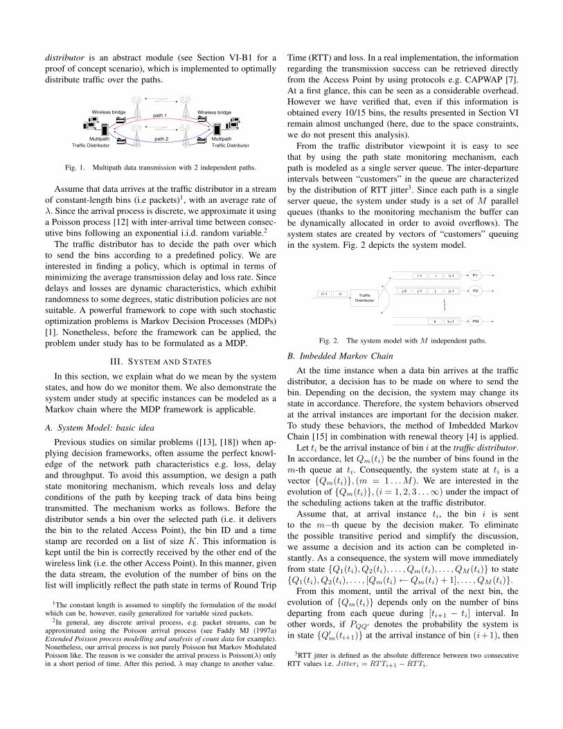
From the traffic distributor viewpoint it is easy to see

that by using the path state monitoring mechanism, each

path is modeled as a single server queue. The inter-departure

intervals between “customers” in the queue are characterized

by the distribution of RTT jitter3. Since each path is a single

server queue, the system under study is a set of M parallel

queues (thanks to the monitoring mechanism the buffer can

be dynamically allocated in order to avoid overflows). The

system states are created by vectors of “customers” queuing

in the system. Fig. 2 depicts the system model.

i i+1i-1 P1

j j+1j-1 P2j-2

k k+1 PM

TrafficDistributor

nn-1

Fig. 2. The system model with M independent paths.

B. Imbedded Markov Chain

At the time instance when a data bin arrives at the traffic

distributor, a decision has to be made on where to send the

bin. Depending on the decision, the system may change its

state in accordance. Therefore, the system behaviors observed

at the arrival instances are important for the decision maker.

To study these behaviors, the method of Imbedded Markov

Chain [15] in combination with renewal theory [4] is applied.

Let ti be the arrival instance of bin i at the traffic distributor.

In accordance, let Qm(ti) be the number of bins found in the

m-th queue at ti. Consequently, the system state at ti is a

vector {Qm(ti)}, (m = 1 . . .M). We are interested in the

evolution of {Qm(ti)}, (i = 1, 2, 3 . . .∞) under the impact of

the scheduling actions taken at the traffic distributor.

Assume that, at arrival instance ti, the bin i is sent

to the m−th queue by the decision maker. To eliminate

the possible transitive period and simplify the discussion,

we assume a decision and its action can be completed in-

stantly. As a consequence, the system will move immediately

from state {Q1(ti), Q2(ti), . . . , Qm(ti), . . . , QM (ti)} to state

{Q1(ti), Q2(ti), . . . , [Qm(ti)← Qm(ti) + 1], . . . , QM (ti)}.From this moment, until the arrival of the next bin, the

evolution of {Qm(ti)} depends only on the number of bins

departing from each queue during [ti+1 − ti] interval. In

other words, if PQQ′ denotes the probability the system is

in state {Q′m(ti+1)} at the arrival instance of bin (i+1), then

3RTT jitter is defined as the absolute difference between two consecutiveRTT values i.e. Jitteri = RTTi+1 −RTTi.

PQQ′ equals to the probability there are Q1(ti) − Q′

1(ti+1)bins departing from the first queue, Q2(ti) − Q

′

2(ti+1) bins

departing from the second queue, and so on during [ti+1− ti]interval. Since these departure processes are independent, we

can obtain PQQ′ by taking product of the probabilities.

To compute the probability there are Qm(ti) − Q′

m(ti+1)bins departing from the m-th queue, we utilize some results

from renewal theory. Let τk and τk+1 subsequently denote the

departure instances of bins k and k+ 1 from the m-th queue.

Assuming that, the inter-departure intervals [τk+1 − τk] are

i.i.d. random variables4 with a general distribution gm(x) =P (τk+1 − τk ≤ x). As a consequence, the sequence of

departure points {τk} fully forms an ordinary renewal process.

Suppose the queuing process has attained a steady state.

Subsequently, the sequence of departure points {τk}, started

from the arrival instance ti, forms the equilibrium renewal

process of the above ordinary renewal process [4] (Fig. 3).

E(ti)

t

arrivalsdepartures

the equilibrium renewal process

i i+1k+1 k+3k k+2

x0 x1

t i+1t i

Fig. 3. The queuing process of the m-th queue.

According to renewal theory, for the equilibrium renewal

process, the number of bins departing from the queue in

[ti+1− ti] interval is proportional to the length of the interval

and does not depend on ti. Hence, Qm(ti+1) is fully deter-

mined by Qm(ti) and does not depend on E(ti), which is the

elapsed time since the last departure observed at ti. Thus, the

random variable Qm(ti) forms a discrete-state Markov chain

imbedded in the queuing process. The state space of the chain

is comprised of all possible numbers of bins in the queue.

Let βj denote the probability of j bins, j = 0 . . .K ,

departing from the queue in [ti+1 − ti] interval. Since by

assumption [ti+1 − ti] are exponentially distributed, we have:

βj =

Z

∞

0

P [N(t) = j]λe−λtdt (1)

Recall that the inter-departure intervals [τk+1−τk] are i.i.d.

random variables with a general PDF gm(x). Let Gm(x) be

the corresponding cumulative distribution function of the inter-

departure intervals, and G(n)m (x) be the n-fold convolution of

Gm(x). Let µm ≡ E[τk+1−τk] be the mean value of the inter-

departure times. Subsequently, as shown in [4], the probability

of having j renewals during interval (0, t) of the equilibrium

renewal process P [N(t) = j] is:

P [N(t) = j] =1

µ

Z t

0

(P [No(u) = j − 1]− P [No(u) = j])du

=1

µ

Z t

0

[(G(j−1)m (u)−G(j)

m (u))− (G(j)m (u)−G(j+1)

m (u))]du

4we only assume i.i.d in a period of time since Internet Path Properties e.g.delays, throughputs are stationary in scale of minutes [27].

where P [No(u) = r] = G(r)m (u) − G

(r+1)m (u) is the

probability of having r renewals during interval (0, u) of the

corresponding ordinary renewal process. Substituting received

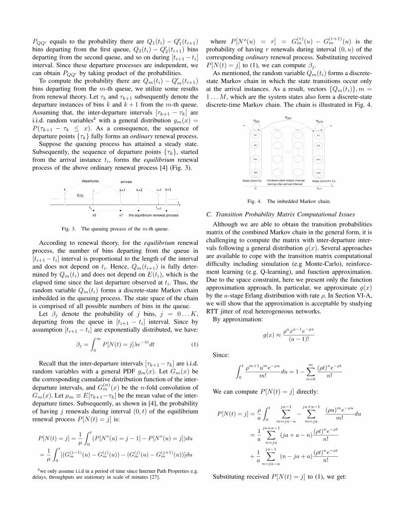
P [N(t) = j] to (1), we can compute βj .As mentioned, the random variable Qm(ti) forms a discrete-

state Markov chain in which the state transitions occur only

at the arrival instances. As a result, vectors {Qm(ti)},m =1 . . .M , which are the system states also form a discrete-state

discrete-time Markov chain. The chain is illustrated in Fig. 4.

Q2

Q1

Qm

QM

Q’2

Q’1

Q’m

Q’M

State {Qm(Ti)} State {Q’m(Ti+1)}Unobservable states change during inter-arrival interval

QQPQQ’P

Q’Q’P

t

Ti+1Ti

Fig. 4. The imbedded Markov chain.

C. Transition Probability Matrix Computational Issues

Although we are able to obtain the transition probabilities

matrix of the combined Markov chain in the general form, it is

challenging to compute the matrix with inter-departure inter-

vals following a general distribution g(x). Several approaches

are available to cope with the transition matrix computational

difficulty including simulation (e.g Monte-Carlo), reinforce-

ment learning (e.g. Q-learning), and function approximation.

Due to the space constraint, here we present only the function

approximation approach. In particular, we approximate g(x)by the a-stage Erlang distribution with rate ρ. In Section VI-A,

we will show that the approximation is acceptable by studying

RTT jitter of real heterogeneous networks.

By approximation:

g(x) ≈ρaxa−1e−ρx

(a− 1)!

Since:

Z t

0

ρm+1ume−ρu

m!du = 1−

mX

n=0

(ρt)ne−ρt

n!

We can compute P [N(t) = j] directly:

P [N(t) = j] =ρ

a

Z t

0

¡ ja−1X

m=ja−a

−

ja+a−1X

m=ja

¿

(ρu)me−ρu

m!du

=1

a

ja+a−1X

n=ja

(ja+ a− n)(ρt)ne−ρt

n!

+1

a

ja−1X

n=ja−a

(n− ja+ a)(ρt)ne−ρt

n!

Substituting received P [N(t) = j] to (1), we get:

βj =

Z

∞

0

P [N(t) = j]λe−λtdt

=1

a

ů ja+a−1X

n=ja

(ja+ a− n)( ρλ

)n

(1 + ρ

λ)n+1

+

ja−1X

n=ja−a

(n− ja+ a)( ρλ

)n

(1 + ρ

λ)n+1

ÿ

Given ρ/λ ratio5, we can be compute βj directly by using

the above formula. Obtaining βj for each queue, we can

compute the transition probability matrix of the Markov chain.

IV. MDP FORMULATION FOR MULTIPATH

TRANSMISSIONS

In previous section we demonstrated that the system under

study can be modeled as a Markov chain. Now, we show how

such a problem is formulated as a MDP.

Consider a time homogeneous MDP with a countable state

space S, a finite action space A where A(s) ∈ A, s ∈ S is a

set of admissible actions in state s, a non-negative immediate

reward function R : S×A(S)→ <+, and a set of conditional

probabilities P (s′|s, a), which is the probability of moving

from state s to state s′ if action a, a ∈ A(s) is taken. In

context of the problem under study, the MDP objective is to

minimize the average reward, which is a function of the path

delay/loss states over a period of time. The four-component

tuple {S,A, P,R} of the MDP is subsequently made of:

• S which is the state space of the defined system consisting ofM, (M ≥ 1) paths. It is clear that S is the state space of thecombined Markov chain.

• A = {a1, a2 . . . aM} is the set of actions each of which corre-sponds to the action of scheduling a data bin to one of M paths.

• P is the state transition probability matrix of the combinedMarkov chain, which can be calculated from the transition prob-abilities of each path in the system.

• R is the immediate reward function, which should be able toreflect the minimum average transmission loss/delay objective.Thanks to the path monitoring mechanism, the number of queu-ing bins on each path is a proportional function of the pathdelay/loss states [17]. Hence, we define the immediate rewardfunction R(s, a) = (µas + da)(1 − plosss,a ) where µa is thecommon inter-departure interval of the path chosen by actiona; s ∈ {1, 2 . . .K} is the state of the path; da is the pathpropagation delay; and plosss,a is the probability the packet is lostif the path is in state s. In practice, da can be estimated as a halfof the minimum RTT delay, and plosss,a can be estimated from thehistorical data using the frequency count technique.

A Markov policy is a description of behaviors, which

specifies the action to be taken in correspondence to each

system state and time step. If a policy is stationary, it specifies

only the action to be taken in each state independently of the

time steps. Given policy π and initial state s of the system, one

can quantitatively evaluate π based on the expected long-term

average reward, which is defined as follows:

vπ(s) ≡ lim sup

N→∞

1

N

NX

t=1

Eπs

ľ

R(S(t), aπ(S(t)))ł

(2)

5In practical implementation, ρ/λ ratio can be periodically estimated onthe fly from the historical evolution of the path queue lengths.

where R(S(t), aπ(S(t)) denotes the immediate expected

reward received by the decision maker at time t, when taking

action aπ(S(t)) in accordance with the policy π, while the

system is in state S(t). An optimal policy is the one that

minimizes the average reward vπ . Note that, it is sufficient

to find an optimal policy in the Markov policy space since,

for any history-dependent policy there is a Markov policy that

yields the same average reward [20]. In unconstrained MDP

formulation, it is possible to find a stationary optimal policy.

V. OPTIMAL DATA DISTRIBUTION ALGORITHM

Optimal data distribution can be achieved by solving the

formulated MDP. To obtain the MDP optimal policies, differ-

ent approaches can be used e.g. dynamic programming and

linear programming. However, we pay more attention on the

solving time since the problem under study is time sensitive

and we are interested, as next step of this work, in building

a real implementation. Therefore, we implement an algorithm

called On-line Policy Iteration (OPI) to gradually approach

the optimal policy of the formulated MDP on the fly.

A. Scheduling with On-line Policy Iteration

On-line Policy Iteration is based on the idea of the Pol-

icy Iteration (PI) algorithm [20] and asymmetric dynamic

programming. Two key factors, which potentially make OPI

a preferable algorithm for time sensitive problems are the

incremental on-line policy improvement and the computational

efficiency. The first factor comes naturally since OPI is based

on the PI algorithm, which iteratively improves a given random

policy until an ε-optimal policy is found. The second factor

however is resulted from a smart choice of the starting policy

and the improvement strategy. Particularly, instead of choosing

a random policy for improvement, like in the PI algorithm, we

select the Join the Shortest Queue (JSQ) policy to be the start-

ing policy for OPI. Since the JSQ policy is an optimal policy

for 2 parallel symmetric queues and an acceptable policy for

several other cases [16], we can save a lot of iterations by

starting from it, on the way to reach an ε-optimal policy. The

policy improvement strategy also plays an important role in

saving computational efforts. It is common in practice that

some states of a system are more frequently visited than the

others. These states are usually more important to the decision

maker as they contribute more to the final outcome. Therefore,

instead of equally evaluating and improving the policy for

every state, as in Policy Iteration algorithm, we could spend

more time on evaluating and improving the policy for those

important states. This policy improvement strategy is known

as prioritized sweeping, which still guarantees an ε-optimal

policy will be found if all system states are visited infinitely

often [20]. The OPI algorithm is detailed below:

• Step 1: Evaluate JSQ policy to obtain vopi(s) = vjsq(s).• Step 2: Obtain the system current state s. Take action a ∈ A that

maximizes vopi(s) and update vopi(s) with the maximum value:

vopi(s) = max

a∈A{R(s, a) +

X

s′∈S

pa(s′|s)vopi(s′)} (3)

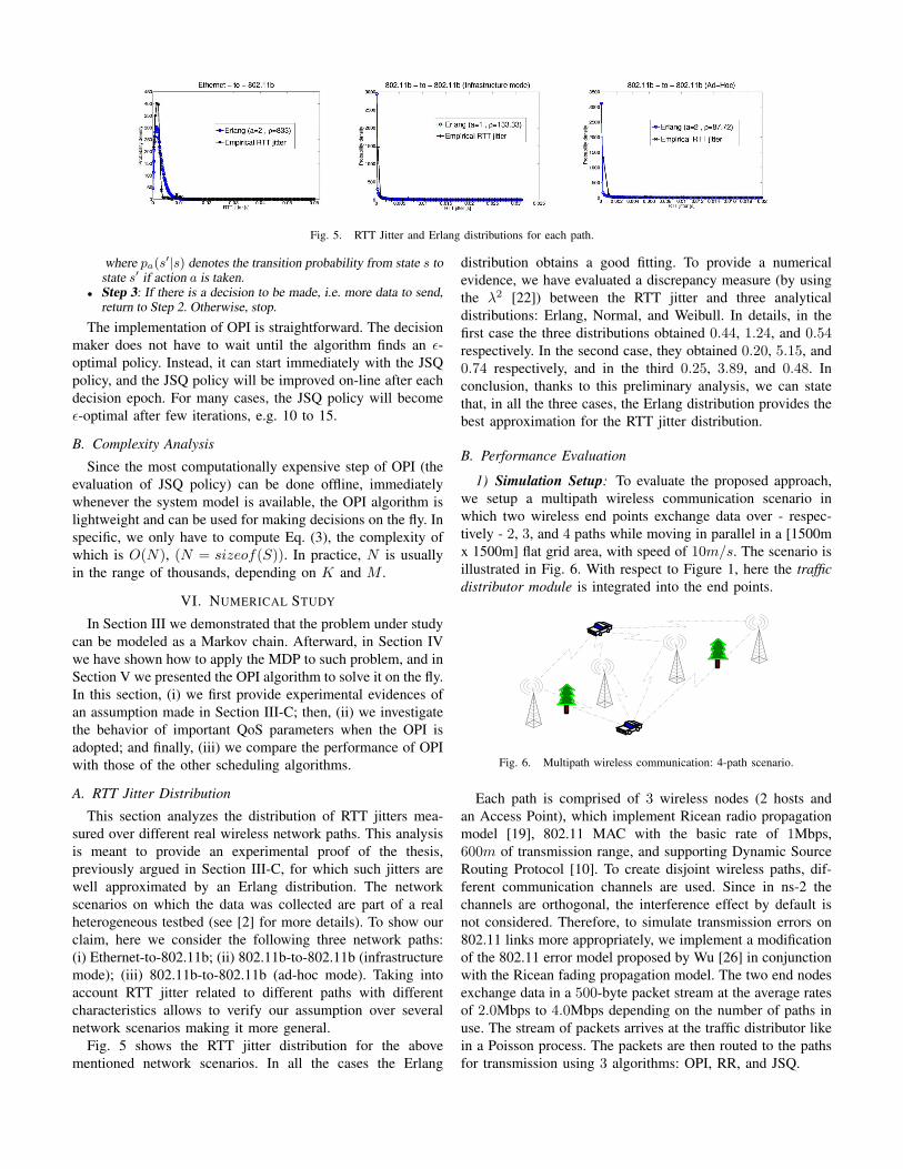
Fig. 5. RTT Jitter and Erlang distributions for each path.

where pa(s′|s) denotes the transition probability from state s tostate s′ if action a is taken.

• Step 3: If there is a decision to be made, i.e. more data to send,return to Step 2. Otherwise, stop.

The implementation of OPI is straightforward. The decision

maker does not have to wait until the algorithm finds an ε-optimal policy. Instead, it can start immediately with the JSQ

policy, and the JSQ policy will be improved on-line after each

decision epoch. For many cases, the JSQ policy will become

ε-optimal after few iterations, e.g. 10 to 15.

B. Complexity Analysis

Since the most computationally expensive step of OPI (the

evaluation of JSQ policy) can be done offline, immediately

whenever the system model is available, the OPI algorithm is

lightweight and can be used for making decisions on the fly. In

specific, we only have to compute Eq. (3), the complexity of

which is O(N), (N = sizeof(S)). In practice, N is usually

in the range of thousands, depending on K and M .

VI. NUMERICAL STUDY

In Section III we demonstrated that the problem under study

can be modeled as a Markov chain. Afterward, in Section IV

we have shown how to apply the MDP to such problem, and in

Section V we presented the OPI algorithm to solve it on the fly.

In this section, (i) we first provide experimental evidences of

an assumption made in Section III-C; then, (ii) we investigate

the behavior of important QoS parameters when the OPI is

adopted; and finally, (iii) we compare the performance of OPI

with those of the other scheduling algorithms.

A. RTT Jitter Distribution

This section analyzes the distribution of RTT jitters mea-

sured over different real wireless network paths. This analysis

is meant to provide an experimental proof of the thesis,

previously argued in Section III-C, for which such jitters are

well approximated by an Erlang distribution. The network

scenarios on which the data was collected are part of a real

heterogeneous testbed (see [2] for more details). To show our

claim, here we consider the following three network paths:

(i) Ethernet-to-802.11b; (ii) 802.11b-to-802.11b (infrastructure

mode); (iii) 802.11b-to-802.11b (ad-hoc mode). Taking into

account RTT jitter related to different paths with different

characteristics allows to verify our assumption over several

network scenarios making it more general.

Fig. 5 shows the RTT jitter distribution for the above

mentioned network scenarios. In all the cases the Erlang

distribution obtains a good fitting. To provide a numerical

evidence, we have evaluated a discrepancy measure (by using

the λ2 [22]) between the RTT jitter and three analytical

distributions: Erlang, Normal, and Weibull. In details, in the

first case the three distributions obtained 0.44, 1.24, and 0.54respectively. In the second case, they obtained 0.20, 5.15, and

0.74 respectively, and in the third 0.25, 3.89, and 0.48. In

conclusion, thanks to this preliminary analysis, we can state

that, in all the three cases, the Erlang distribution provides the

best approximation for the RTT jitter distribution.

B. Performance Evaluation

1) Simulation Setup: To evaluate the proposed approach,

we setup a multipath wireless communication scenario in

which two wireless end points exchange data over - respec-

tively - 2, 3, and 4 paths while moving in parallel in a [1500m

x 1500m] flat grid area, with speed of 10m/s. The scenario is

illustrated in Fig. 6. With respect to Figure 1, here the traffic

distributor module is integrated into the end points.

Fig. 6. Multipath wireless communication: 4-path scenario.

Each path is comprised of 3 wireless nodes (2 hosts and

an Access Point), which implement Ricean radio propagation

model [19], 802.11 MAC with the basic rate of 1Mbps,

600m of transmission range, and supporting Dynamic Source

Routing Protocol [10]. To create disjoint wireless paths, dif-

ferent communication channels are used. Since in ns-2 the

channels are orthogonal, the interference effect by default is

not considered. Therefore, to simulate transmission errors on

802.11 links more appropriately, we implement a modification

of the 802.11 error model proposed by Wu [26] in conjunction

with the Ricean fading propagation model. The two end nodes

exchange data in a 500-byte packet stream at the average rates

of 2.0Mbps to 4.0Mbps depending on the number of paths in

use. The stream of packets arrives at the traffic distributor like

in a Poisson process. The packets are then routed to the paths

for transmission using 3 algorithms: OPI, RR, and JSQ.

0

10

20

30

40

50

60

70

0 5000 10000 15000 20000

queu

e le

ngth

(pac

kets

)The evolution of queue length (RR)

path 1path 2path 3path 4

0

10

20

30

40

50

60

70

0 5000 10000 15000 20000

queu

e le

ngth

(pac

kets

)

packet sequence numbers

The evolution of queue length (JSQ)path 1path 2path 3path 4

0

10

20

30

40

50

60

70

0 5000 10000 15000 20000

queu

e le

ngth

(pac

kets

)

packet sequence numbers

The evolution of queue length (OPI)path 1path 2path 3path 4

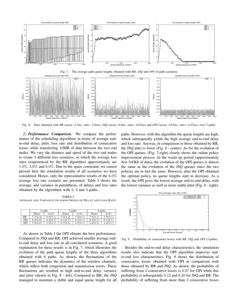
Fig. 7. The average path queue lengths obtained with RR, JSQ and OPI (4-path scenario).

0

0.001

0.002

0.003

0.004

0.005

0.006

0.007

0.008

0.009

0.01

0.011

0.012

0 2000 4000 6000 8000 10000 12000 14000 16000 18000 20000

jitter

(s)

packet sequence numbers

Wireless end-to-end jitter (RR)jitter

0

0.001

0.002

0.003

0.004

0.005

0.006

0.007

0.008

0.009

0.01

0.011

0.012

0 2000 4000 6000 8000 10000 12000 14000 16000 18000 20000

jitter

(s)

packet sequence numbers

Wireless end-to-end jitter (JSQ)jitter

0

0.001

0.002

0.003

0.004

0.005

0.006

0.007

0.008

0.009

0.01

0.011

0.012

0 2000 4000 6000 8000 10000 12000 14000 16000 18000 20000

jitter

(s)

packet sequence numbers

Wireless end-to-end jitter (OPI)jitter

Fig. 8. Jitter obtained with RR (mean: 2.1ms, stdev: 2.0ms), JSQ (mean: 0.8ms, stdev: 0.65ms) and OPI (mean: 0.67ms, stdev: 0.47ms), over 3 paths.

2) Performance Comparison: We compare the perfor-

mance of the scheduling algorithms in terms of average end-

to-end delay, jitter, loss rate and distribution of consecutive

losses while transferring 10MB of data between the two end

nodes. We vary the distance and speed of the two end nodes

to create 3 different loss scenarios, in which the average loss

rates (experienced by the RR algorithm) approximately are

1.0%, 3.0% and 6.0%. Due to the space constraint, we cannot

present here the simulation results of all scenarios we have

considered. Hence, only the representative results of the 6.0%average loss rate scenario are presented. Table I shows the

average, and variance in parenthesis, of delays and loss rates

obtained by the algorithms with 2, 3 and 4 paths.

TABLE IAVERAGE AND VARIANCE (IN PARENTHESIS) OF DELAY AND LOSS RATE.

2 paths 3 paths 4 paths

D(ms) L(%) D(ms) L(%) D(ms) L(%)

RR 7.7(2.4) 6.0(0.1) 7.4(2.3) 5.8(0.1) 7.6(2.1) 5.9(0.1)JSQ 8.3(0.9) 6.2(0.1) 8.1(0.7) 6.5(0.1) 8.2(0.7) 6.1(0.1)OPI 7.2(0.6) 5.9(0.1) 6.7(0.5) 4.7(0.1) 5.9(0.5) 4.2(0.1)

As shown in Table I the OPI obtains the best performance.

Compared to JSQ and RR, OPI achieved smaller average end-

to-end delay and loss rate in all considered scenarios. A good

explanation for these results is in Fig. 7, which illustrates the

evolution of the path queue lengths of the three algorithms

obtained with 4 paths. As shown, the fluctuations of the

RR queues indicates the dynamics of the wireless channels,

which reflect both congestion and transmission errors. These

fluctuations are resulted in high end-to-end delay variance

and jitter (shown in Fig. 8 - left). Compared to RR, the JSQ

managed to maintain a stable and equal queue length for all

paths. However, with this algorithm the queue lengths are high,

which subsequently yields the high average end-to-end delay

and loss rate. Anyway, in comparison to those obtained by RR,

the JSQ jitter is lower (Fig. 8 - center). As for the evolution of

the OPI queues, (Fig. 7-right) clearly shows the online policy

improvement process. In the warm up period (approximately

first 500Kb of data), the evolution of the OPI queues is almost

the same as the evolution of the JSQ queues since the two

policies are in fact the same. However, after the OPI obtained

the optimal policy, its queue lengths start to decrease. As a

result, the OPI gives the lowest average end-to-end delay, with

the lowest variance as well as more stable jitter (Fig. 8 - right).

0

0.1

0.2

0.3

0.4

0.5

0.6

0.7

0.8

0.9

1

1 2 3 4 5 6 7 8 9 10 11 12

proba

bility

consecutive losses

The average loss rate of 6%loss distribution (RR)

loss distribution (JSQ)loss distribution (OPI)

Fig. 9. Probability of consecutive losses with RR, JSQ and OPI (3-paths).

Besides the end-to-end delay characteristics, the simulation

results also indicate that the OPI algorithm improves end-

to-end loss characteristics. Fig. 9 shows the distribution of

consecutive losses obtained with OPI in comparison with

those obtained by RR and JSQ. As shown, the probability of

suffering from 2 consecutive losses is 0.07 for OPI while this

probability is subsequently 0.12 and 0.20 for JSQ and RR. The

probability of suffering from more than 2 consecutive losses

is 0.01 for OPI, 0.07 for JSQ and 0.10 for RR.

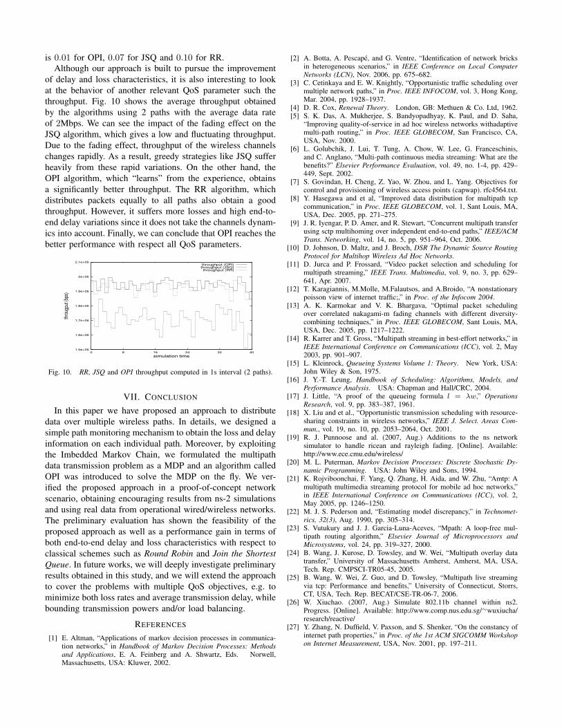
Although our approach is built to pursue the improvement

of delay and loss characteristics, it is also interesting to look

at the behavior of another relevant QoS parameter such the

throughput. Fig. 10 shows the average throughput obtained

by the algorithms using 2 paths with the average data rate

of 2Mbps. We can see the impact of the fading effect on the

JSQ algorithm, which gives a low and fluctuating throughput.

Due to the fading effect, throughput of the wireless channels

changes rapidly. As a result, greedy strategies like JSQ suffer

heavily from these rapid variations. On the other hand, the

OPI algorithm, which “learns” from the experience, obtains

a significantly better throughput. The RR algorithm, which

distributes packets equally to all paths also obtain a good

throughput. However, it suffers more losses and high end-to-

end delay variations since it does not take the channels dynam-

ics into account. Finally, we can conclude that OPI reaches the

better performance with respect all QoS parameters.

1.5e+06

1.6e+06

1.7e+06

1.8e+06

1.9e+06

2e+06

2.1e+06

4032241680

throu

gput

(bps)

simulation time

throughput (OPI)throughput (JSQ)throughput (RR)

Fig. 10. RR, JSQ and OPI throughput computed in 1s interval (2 paths).

VII. CONCLUSION

In this paper we have proposed an approach to distribute

data over multiple wireless paths. In details, we designed a

simple path monitoring mechanism to obtain the loss and delay

information on each individual path. Moreover, by exploiting

the Imbedded Markov Chain, we formulated the multipath

data transmission problem as a MDP and an algorithm called

OPI was introduced to solve the MDP on the fly. We ver-

ified the proposed approach in a proof-of-concept network

scenario, obtaining encouraging results from ns-2 simulations

and using real data from operational wired/wireless networks.

The preliminary evaluation has shown the feasibility of the

proposed approach as well as a performance gain in terms of

both end-to-end delay and loss characteristics with respect to

classical schemes such as Round Robin and Join the Shortest

Queue. In future works, we will deeply investigate preliminary

results obtained in this study, and we will extend the approach

to cover the problems with multiple QoS objectives, e.g. to

minimize both loss rates and average transmission delay, while

bounding transmission powers and/or load balancing.

REFERENCES

[1] E. Altman, “Applications of markov decision processes in communica-tion networks,” in Handbook of Markov Decision Processes: Methods

and Applications, E. A. Feinberg and A. Shwartz, Eds. Norwell,Massachusetts, USA: Kluwer, 2002.

[2] A. Botta, A. Pescape, and G. Ventre, “Identification of network bricksin heterogeneous scenarios,” in IEEE Conference on Local Computer

Networks (LCN), Nov. 2006, pp. 675–682.[3] C. Cetinkaya and E. W. Knightly, “Opportunistic traffic scheduling over

multiple network paths,” in Proc. IEEE INFOCOM, vol. 3, Hong Kong,Mar. 2004, pp. 1928–1937.

[4] D. R. Cox, Renewal Theory. London, GB: Methuen & Co. Ltd, 1962.[5] S. K. Das, A. Mukherjee, S. Bandyopadhyay, K. Paul, and D. Saha,

“Improving quality-of-service in ad hoc wireless networks withadaptivemulti-path routing,” in Proc. IEEE GLOBECOM, San Francisco, CA,USA, Nov. 2000.

[6] L. Golubchik, J. Lui, T. Tung, A. Chow, W. Lee, G. Franceschinis,and C. Anglano, “Multi-path continuous media streaming: What are thebenefits?” Elsevier Performance Evaluation, vol. 49, no. 1-4, pp. 429–449, Sept. 2002.

[7] S. Govindan, H. Cheng, Z. Yao, W. Zhou, and L. Yang. Objectives forcontrol and provisioning of wireless access points (capwap). rfc4564.txt.

[8] Y. Hasegawa and et al, “Improved data distribution for multipath tcpcommunication,” in Proc. IEEE GLOBECOM, vol. 1, Sant Louis, MA,USA, Dec. 2005, pp. 271–275.

[9] J. R. Iyengar, P. D. Amer, and R. Stewart, “Concurrent multipath transferusing sctp multihoming over independent end-to-end paths,” IEEE/ACM

Trans. Networking, vol. 14, no. 5, pp. 951–964, Oct. 2006.[10] D. Johnson, D. Maltz, and J. Broch, DSR The Dynamic Source Routing

Protocol for Multihop Wireless Ad Hoc Networks.[11] D. Jurca and P. Frossard, “Video packet selection and scheduling for

multipath streaming,” IEEE Trans. Multimedia, vol. 9, no. 3, pp. 629–641, Apr. 2007.

[12] T. Karagiannis, M.Molle, M.Falautsos, and A.Broido, “A nonstationarypoisson view of internet traffic;,” in Proc. of the Infocom 2004.

[13] A. K. Karmokar and V. K. Bhargava, “Optimal packet schedulingover correlated nakagami-m fading channels with different diversity-combining techniques,” in Proc. IEEE GLOBECOM, Sant Louis, MA,USA, Dec. 2005, pp. 1217–1222.

[14] R. Karrer and T. Gross, “Multipath streaming in best-effort networks,” inIEEE International Conference on Communications (ICC), vol. 2, May2003, pp. 901–907.

[15] L. Kleinrock, Queueing Systems Volume 1: Theory. New York, USA:John Wiley & Son, 1975.

[16] J. Y.-T. Leung, Handbook of Scheduling: Algorithms, Models, and

Performance Analysis. USA: Chapman and Hall/CRC, 2004.[17] J. Little, “A proof of the queueing formula l = λw,” Operations

Research, vol. 9, pp. 383–387, 1961.[18] X. Liu and et al., “Opportunistic transmission scheduling with resource-

sharing constraints in wireless networks,” IEEE J. Select. Areas Com-

mun., vol. 19, no. 10, pp. 2053–2064, Oct. 2001.[19] R. J. Punnoose and al. (2007, Aug.) Additions to the ns network

simulator to handle ricean and rayleigh fading. [Online]. Available:http://www.ece.cmu.edu/wireless/

[20] M. L. Puterman, Markov Decision Processes: Discrete Stochastic Dy-

namic Programming. USA: John Wiley and Sons, 1994.[21] K. Rojviboonchai, F. Yang, Q. Zhang, H. Aida, and W. Zhu, “Amtp: A

multipath multimedia streaming protocol for mobile ad hoc networks,”in IEEE International Conference on Communications (ICC), vol. 2,May 2005, pp. 1246–1250.

[22] M. J. S. Pederson and, “Estimating model discrepancy,” in Technomet-

rics, 32(3), Aug. 1990, pp. 305–314.[23] S. Vutukury and J. J. Garcia-Luna-Aceves, “Mpath: A loop-free mul-

tipath routing algorithm,” Elsevier Journal of Microprocessors and

Microsystems, vol. 24, pp. 319–327, 2000.[24] B. Wang, J. Kurose, D. Towsley, and W. Wei, “Multipath overlay data

transfer,” University of Massachusetts Amherst, Amherst, MA, USA,Tech. Rep. CMPSCI-TR05-45, 2005.

[25] B. Wang, W. Wei, Z. Guo, and D. Towsley, “Multipath live streamingvia tcp: Performance and benefits,” University of Connecticut, Storrs,CT, USA, Tech. Rep. BECAT/CSE-TR-06-7, 2006.

[26] W. Xiuchao. (2007, Aug.) Simulate 802.11b channel within ns2.Progress. [Online]. Available: http://www.comp.nus.edu.sg/∼wuxiucha/research/reactive/

[27] Y. Zhang, N. Duffield, V. Paxson, and S. Shenker, “On the constancy ofinternet path properties,” in Proc. of the 1st ACM SIGCOMM Workshop

on Internet Measurement, USA, Nov. 2001, pp. 197–211.