NATL INST OF STAND & TECH R.I.C.

NIST

PUBLICATIONS

AlllDM 3T1DDS

Nisr United States Department of CommerceTechnology AdministrationNational Institute of Standards and Technology

NIST Technical Note 1366

Analytical Estimation of Carrier

Multipath Bias on GPSPosition Measurements

C. Michael VolkJudah Levine

Analytical Estimation of Carrier

Multipath Bias on GPSPosition Measurements

C. Michael Volk

Judah Levine

Time and Frequency Division

Plnysics Laboratory

National Institute of Standards and Technology

325 BroadwayBoulder, Colorado 80303-3328

April 1994

"s—sr;

—

7

*^4TES O* '^

U.S. DEPARTMENT OF COMMERCE, Ronald H. Brown, SecretaryTECHNOLOGY ADMINISTRATION, Mary L. Good, Under Secretary for Technology

NATIONAL INSTITUTE OF STANDARDS AND TECHNOLOGY, Arati Prabhakar, Director

National Institute of Standards and Technology Technical NoteNatl. Inst. Stand. Technol., Tech. Note 1366, 68 pages (April 1994)

CODEN:NTNOEF

U.S. GOVERNMENT PRINTING OFFICEWASHINGTON: 1994

For sale by the Superintendent of Documents, U.S. Governnnent Printing Office, Washington, DC 20402-9325

CONTENTS

CHAPTER

1. I^^^RODUcnoN 2

1.1 Brief Introduction to GPS 3

1.2 The GPS Experiment "EDM" 4

1.3 Multipath Signatures in GPS Data 7

2. GENERAL APPROACH 9

2.1 The Multipath Error Phase 9

2.2 Position Bias Resulting from Phase Error 13

2.2.1 The Least Squares Adjustment 13

2.2.2 Parameterization for Analytical Treatment 15

2.3 Generic Calculation for Azimuthal Symmetry 17

2.3.1 Reducing to the Case of Azimuthal Symmetry 17

2.3.2 Numerical Integration 20

2.3.3 Approximating the Elevation Integrals 20

2.4 Generalization to Dual Frequency Observations 26

3. CALCULATIONS FOR SIMPLE REFLECTOR GEOMETRIES 31

3.1 Outline of the Strategy 31

3.2 Multipath from Flat Ground 33

3.2.1 Full Azimuthal Symmetry 33

3.2.2 Disturbed Symmetry 34

3.3 Multipath from Nearby Objects 35

3.4 Multipath from Tilted Ground 39

4. APPLICATION OF THE MODEL 43

4.1 Limitations of the Applicability 43

4.1.1 Non-uniform Satellite Distribution 44

4.1.2 Other Unmodelled Effects 47

4.2 Estimating the Amplitudes 48

4.3 Position Bias at "nist" 50

4.4 Position Bias at"eril" 52

5. SUMMARY AND CONCLUSIONS 54

REFERENCES 59

111

FIGURES

Figure

1 .

1

Horizontal components of the baselines nistrfcr and platrfcr in four

processing runs with varying minimum satellite elevation h^jn 6

1 .2 L3 (upper plot) and L4 (lower plot) postfit double-difference

residuals of the baseline nistrfcr 8

2.1 General geometry and variable definitions used in this chapter 10

2.2 Multipath error phase M versus satellite angle above the reflector

plane h' for relative multipath amplitudes (a) A—>1 and (b) A = 0.5 12

2.3 Multipath error phase contours as function of satellite elevation h

above the horizon and azimuth a as seen from the receiver for a

reflector surface tilted 45° with respect to the horizon 19

2.4 Numerical integration of the integrals (a) Io,y = l,y(h^in=0) and

(b) Iqz = lxy(hmui=0) as functions of upper integration limit hn,„ 21

2.5 M(x) normalized to amplitude 1 for varying A's 22

2.6 Exact integrals (black lines) and approximated integrals (gray lines):

(a) lo^y and Igxy , (b) Iqz and Iqz as functions of their upper

integration limit hn^g^ 26

2.7 Exact integrals (black lines) and approximated integrals (gray lines):

(a) I3oxy and I3oxy , (b) Bqz and I3oz as functions of their upper

integration limit hn,„ 29

3.1 Asymmetrical multipath region for flat ground as reflector 34

3.2 Multipath from a nearby planar reflector parallel to the y-axis,

horizontally symmetrical with respect to the x-axis, and at an angle

a from the horizon 36

3.3 Multipath from a vertical reflector 38

IV

3.4 Multipath from the ground tilted at an angle a from the horizon 40

4.1 Satellite elevations (upper plot) and azimuths (lower plot) in

degrees as functions of time for station rfcr 45

4.2 L3 postfit double difference residuals for the baselines nisteril

(upper plot) and eri2eril (lower plot) at day 078 (the first day of

the"EDM" experiment) 49

4.3 Geometry at the receiver site nist 51

4.4 Geometry at the receiver site eril 52

Analytical Estimation of Carrier Multipath Bias

on GPS Position Measurements

Michael Volk

Joint Institute for Laboratory Astrophysics

University of ColoradoBoulder, Colorado 80309

and

Judah Levine

Time and Frequency Division

National Institute of Standards and TechnologyBoulder, Colorado 80303

Multipath is one of the factors degrading the accuracy of position measurements

obtained with the Global Positioning System (GPS). We investigate the effects of mul-

tipath on the carrier phase measurement and the resulting bias on relative GPS posi-

tions for observation times longer than several hours.

A short-range GPS network was surveyed with day-long observation sessions.

The data display obvious multipath signatures and the position results indicate the

presence of site-specific errors at the level of several millimeters. This led us to sus-

pect multipath bias and motivated the quantitative estimation presented here. We first

model the phase error due to multipath from a single plane reflector in terms of satel-

lite-reflector geometry. The effect of this error on position is then derived by perform-

ing a simplified least squares adjustment under the assumption of uniform satellite

distribution. After several steps of approximations and manipulations we arrive at sim-

ple expressions for the bias in terms of general receiver-reflector geometry and a fewother variables. The results are generalized to dual frequency observations that are

commonly used for high accuracy observations.

The model is then employed to estimate upper limits of the multipath bias for gen-

eral receiver environments. We consider bias due to multipath from the flat ground,

from nearby objects, and from a tilted ground, obtaining formulae for each situation

that depend only on reflector characteristics and geometry. Finally, these results are

applied to the GPS experiment. Limitations of the applicability due to model assump-

tions and unmodelled effects are discussed. The two stations thought to be most

affected by multipath in the experiment are examined. We find that the multipath

phase error as inferred from the observations can give rise only to vertical biases

smaller than 2 mm and horizontal biases smaller than 1 mm. It is thus concluded that

bias due to multipath-induced carrier phase error is effectively reduced by averaging if

observation intervals are at least several hours long and som . basic precautions are

taken regarding the receiver environment.

Keywords: GPS geodesy; GPS measurements; multipath bias

* Current affiliation: Cooperative Inslilulc for Research in Environmcnial Sciences and Department of

Physics, University of Colorado, Boulder, CO 80309.** Fellow, Joint InsUtulc for Laboratory Astrophysics, University of Colorado, Boulder, CO 80309.

CHAPTER 1

INTRODUCTION

"Multipath" has long been recognized as a significant error source in high accu-

racy applications of the Navigation Satellite Timing and Ranging (NAVSTAR) Global

Positioning System (GPS). It occurs when a satellite signal is reflected from objects in

the vicinity of the receiver causing multiple arrivals of the same signal. Interference of

these arrivals corrupts the "true" (direct) signal with time-dependent signatures. Many

studies on multipath have focused on how to detect and reduce it (e.g., [1]). Consider-

able effort has been undertaken to design antennas and backplane configurations that

minimize the sensitivity of the receiver's antenna in the direction of reflectors at low

elevation angles [2,3].

Because multipath signamres on the carrier phase tend to oscillate with periods

shorter than 10 to 20 min, it is clear that their effect is most serious for GPS applica-

tions with short observing sessions and for kinematic applications. Several authors

have stated that observations over several hours are likely to average out most of the

effect on relative positioning [4,5,6].

This work developed out of a continuous discussion about how big the net bias on

relative positions due to multipath could be in a recent GPS experiment using observa-

tion sessions of 23 h. The experiment and some results hinting at multipath problems

are discussed later in this chapter, preceding is an (ultra-)brief introduction to GPS.

The main part of this report is of a rather theoretical nature: In Chapter 2 we develop

the mathematical frame and tools. These are used in the third chapter to estimate the

multipath-induced bias for several simple reflector-receiver geometries. Chapter 4

attempts to quantify the analysis and to apply the results to two receiver sites of the

GPS experiment mentioned above. Conclusions are drawn in the final fifth chapter.

1.1 Brief Introduction to GPS

GPS satellites orbiting at 20,000 km altitude transmit two carrier radio signals LI

and L2 at frequencies of about 1.23 and 1.58 GHz (wavelengths of about 19 and

24 cm). These are modulated with lower frequency codes, most importantly the

pseudo-random P-code at 10.23 MHz. The codes are used to simultaneously measure

the time delay of signals from several satellites at the receiver ("pseudorange measure-

ment")- An instantaneous receiver position with meter accuracy is thus obtained, e.g.,

for navigational applications (the original purpose of GPS). Even before the system

was operational, the potential use of the carrier signals for precise relative positioning

was realized and several methods were suggested on how to extract vector baselines at

centimeter-level accuracy [7].

In principle, the phase from at least two satellites (usually more than four) is mea-

sured at two (or more) receivers simultaneously, thus eliminating systematic receiver

and satellite clock offsets by common mode cancellation. The simultaneous phases of

each pair of receivers and each pair of satellites are substracted from each other to

arrive at "double difference" observations. The double differenced satellite ranges are

ambiguous by an unknown number of carrier wavelengths and left with errors due to

differential propagation delays. The latter are corrected by various methods. Since the

ionosphere is dispersive in the radio band, dual frequency observations (LI and L2)

allow elimination of major ionospheric effects. The ionosphere corrected range is an

appropriate linear combination of LI and L2 called L3. The non-dispersive atmo-

spheric delay (mainly due to the troposphere) must be corrected by modelling using

surface measurements. This method works well for the dry air which is approximately

in hydrostatic equilibrium, but is less satisfactory for the water vapor contribution.

Often water vapor radiometers are used to measure the wet delay; sometimes stochas-

tic estimation techniques are invoked. There is some argument as to which method

produces better results [8].

If the differenced satellite ranges are tracked while maintaining lock with the sig-

nal, the baseline vector can be obtained provided that the satellite orbits and the initial

cycle ambiguities (or "phase biases") are known. Nowadays the orbits are determined

by continuously tracking the satellites from a continental-sized or even global network

of "fiducial stations" whose coordinates are well known from other techniques (VLBI

or SLR). The phase ambiguities and relative station positions are then solved for using

a least-squares adjustment of all observations starting from a priori coordinates that

are usually known to within a few centimeters from pseudorange measurements. For

baselines shorter than 100 km most of the cycle ambiguities can usually be constrained

to their integer values. In a repeated adjustment the known ambiguities are constants

and only the station coordinates are estimated (usually relative to one fixed station). It

is actually not required that the ambiguities be fixed to integers since the best fitting

real numbers determined by the least squares adjustment are sufficient to yield mean-

ingful posidon results. However, the precision of the measurement increases if the

biases can be fixed. A comprehensive discussion of the fundamentals of GPS has been

given by Rocken [9].

Most errors affecting GPS relative posidoning are proportional to the baseline

length, e.g., orbit errors, atmospheric path delay errors, errors in the absolute position

of the fixed stadon (e.g., [10]). Besides receiver setup errors, the dominant length-

independent error sources are muldpath and two even more complex phenomena,

antenna phase center variations and imaging [11]. The latter of these two effects is

related to muldpath and is difficult to disdnguish from it. Phase center variadons and

imaging will be ignored in this work, yet it ought to be kept in mind that they may be

non-negligible.

1.2 The GPS Experiment "EDM"

A GPS experiment dded "EDM" was conducted in cooperadon with the Univer-

sity NAVSTAR Consortium (UNAVCO), Boulder, in March 1993. The objective was

to compare distances measured by GPS and the JILA three-wavelength electromag-

netic distance-measuring (EDM) instrument [12]. We had been tesdng the latter sys-

tem during several months in a two-wavelength mode over a baseline between the top

of a mesa west of the NIST facilides in Boulder and the base of a meteorological tower

operated by NOAA near Erie, Colorado. The EDM yielded a precision of better than

2 mm over this distance of 24 km, i.e., better than 0.1 ppm.

The GPS data were acquired at a sampling rate of 15 seconds during 3 daily ses-

sions each lasdng 23 h starting at GPS dme 17:00 on March 19, 20, and 21, respec-

tively. Four sites were occupied with Trimble 4000 SST dual-frequency receivers: the

two benchmarks at the NIST mesa ("nist") and at the tower base at Erie ("eril") used

for the EDM tests; another benchmark on NOAA land some 200 m from eril ("eri2");

and a benchmark on top of the UNAVCO building in Boulder ("rfcr"). A fifth receiver

at Platteville, Colorado ("plat") is operated permanendy by UNAVCO and served as a

reference position. The receivers at rfcr and plat were hard-mounted, whereas nist,

eril, and eri2 were subject to a daily setup error.

The data were then processed with the Bernese 3.3 software that uses double dif-

ference observables in one least squares adjustment in the way described above. In

general, more than 95 percent of the ambiguities for any given baseline and day could

be fixed to their integer values. Initially, baselines from nist to eril, eri2, and rfcr were

included in a series of processing runs under varying processing parameters. The

results showed good agreement between the distances on the first and third day but a

consistent 3 to 5 mm increase in the nist-to-eri baselines for the second day mainly due

to an apparent offset of nist to the west. In a second series of runs we processed base-

lines from rfcr to all other stations, including plat, in order to discriminate between

potential error sources. Surprisingly, the longest baseline of 47 km from rfcr to plat

("platrfcr") showed the best horizontal repeatability over the three days while horizon-

tal scatter in the distance from rfcr to nist ("nistrfcr") was biggest, up to 4 mm peak-to-

peak. Consequently, the main contributing error sources must be length-independent.

In fact, baseline nistrfcr is so short (5.5 km) that scale errors should be negligible alto-

gether.

In order to investigate if the unexpected high scatter in the horizontal components

of nistrfcr was likely to be due to setup errors at nist, we split up the data into three

(approximately) 8-h sessions for each day. Figure 1.1 shows the "time series" of the

resulting nine sessions for four processing runs in which the minimum satellite eleva-

tion above the horizon ("h^i^") was varied from 20° to 35°. It can be seen that: (i) the

scatter in nistrfcr is as big or bigger as in platrfcr, (ii) scatter within one day is not

smaller than scatter between days (which would have been expected for setup errors);

and (iii) that the minimum satellite elevation has quite an influence on the result, in

particular for baseline nistrfcr.

We thus arrive at the conclusion that site-specific problems giving rise to system-

atic bias of the position are likely to be present at nist. Multipath is one of the prime

candidates for such problems. While these results certainly motivated the discussion

that led to this work, they should by no means be considered as proof for the "multi-

path case".

Several ambiguous and unexplained factors not mentioned so far remain:

• The site most suffering from multipath is clearly eril . As will be discussed in Chap-

ter 4, this benchmark is surrounded by nearby trailers and the noise in the post-fit

double difference residuals is about twice that of all other baselines. However, this

is not apparent in the position results. In fact, the two Erie sites consistently yield

results very similar to each other in all the processing runs and there is no evidence

for site-dependent bias at eri 1

.

baseline nistrfcr

486

484

E 482

oi 480oco« 478T3

CO

> 476

474

472

. <>

•

<

/ ^L

.If

^. /S

[ ^} A\ yi ^ ^ </ V y

.^i

X

^^

k

^

VI

.^ A.'/^

5

<> Affi

r .

A/,

?e 1^ ,

-

? f

-

»

1 1

-\ ^ -

-

< >

-

boseline plotrfcr

1 23456789session

baseline nistrfcr

1 23456789runs:XXX hnnin = 20 session

ODD hmin = 25AAA hmin = 30000 hnnin = 35 baseline plotrfcr

Figure 1.1. Horizontal components of the baselines nistrfcr and platrfcr in four pro-

cessing runs with varying minimum satellite elevation h^j^. Sessions are approxi-

mately 8 h. The setup at nist was changed daily, i.e., after sessions 3 and 6, but

remained unchanged at rfcr and plat.

• Judging from the noise in the double difference post-fit residuals, nist is no worse

than any of the other sites.

• There were, however, mysterious receiver outages reoccurring daily at nist around

0:00 GPS time. The resulting gaps of up to one hour in the data caused unexplained

problems in the processing. Special data editing during preprocessing was required

to arrive at meaningful results at all.

No attempt is made in this work to further investigate any of these points. Instead

of trying to find out just what the problem at nist is, we will content ourselves with

estimating how much of a problem multipath could be in the given environment.

1.3 Multipath Signatures in GPS Data

Phase multipath is relatively easy to detect if dual frequency observations are

available. Other noise sources that can leave similar signatures in the data are highly

time-variable ionosphere noise, tropospheric delay errors, and different sorts of geo-

metric errors (satellite and receiver positions, clock errors). Ionospheric delay is elimi-

nated in the ionosphere-free linear combination L3 (section 1.1) while geometric

errors and tropospheric effects are common to both frequencies and thus cancelled by

forming the "geometry-free" linear combination L4 = LI - L2. L4 is simply the differ-

ential range of LI and L2 that is due to the ionosphere and other effects not common to

both frequencies like multipath.

As pointed out by Rocken [9], any correlation between L3 and L4 post-fit residu-

als must be due to measurement noise (3 mm) or multipath and related effects (imag-

ing, phase center variations). Hence, a simple inspection by eye will usually reveal

multipath signatures. An example from the baseline nistrfcr is given in figure 1.2.

Another indicator for multipath is noise signatures that repeat from day to day.

Because the satellite-receiver geometry repeats daily (shifted by 4 min), the multipath

does, too. This was evident in nearly all of the experimental data from the "EDM"

campaign. Indeed, we made use of the repetitive nature of multipath during data edit-

ing to distinguish cycle slips (which would not repeat daily) from high frequency high

amplitude multipath noise. This was especially helpful for baselines including eril

where the program in automatic mode frequently mistook "jumps" in the residuals

caused by multipath as cycle slips.

nisWcr«7903p 19t27

i| I I I I

I

I I I I

I

I I II I

I

I I I I

I

400.0 500.0 M.O 700.0 800.0

TIIC [epochs]

900.0 1000,0 1100.

ni$trfcf079Wf 19:27

0.5-

f o.o-

0-O.i-

i -

-1.0-

-1.5 T

400.0 500.0 600.0 700.0 800.0

TIIC [tfodrn]

Figure 1.2. L3 (upper plot) and L4 (lower plot) postfit double-difference residuals

of the baseline nistrfcr. Any correlation between the two plots is due to multipath.

CHAPTER 2

GENERAL APPROACH

The goal of this chapter is to express the bias of GPS derived positions resulting

from multipath in terms of receiver-reflector geometry and a few other variables. We

start out by modelling the multipath error phase in terms of geometry. In a second step

we derive the position bias due to this error phase. The analytical expressions thus

found will then be approximated in order to simplify the calculations for a given envi-

ronment. The discussion will be restricted to a single planar reflector.

2.1 The Multipath Error Phase

Consider a signal from a satellite that arrives at a receiver R via two different

paths: the direct path and the multipath due to reflection from a nearby planar object.

This causes the arrival of two signals at the receiver which are out of phase because

the two paths have different lengths. We start out by calculating the pathlength differ-

ence between the two paths. For a plane reflector at a perpendicular distance d from

the receiver the length of the multipath is equivalent to the length of a path from the

satellite to a (stationary) image receiver R' an equal perpendicular distance behind the

reflecting surface. The general geometry and variables used in the following are intro-

duced in figure 2.1.

As s and s' are essentially parallel, the pathlength difference As is simply the

length of R'R = 2dn projected on s':

As = 2dn-s'= 2dns (2.1)

where s is the unit vector in direction of s. If A. is the wavelength of the signal, then the

resulting phase difference between the direct and the multipath signal is

satellite S

coordinate

system:

R: receiver

R': image receiver

s: vector RSs': vector R'S

n: normal unit vector from

reflector to Rd: perpendicular distance

from R to reflector

AS = s'-s

h': satellite elevation angle

above reflector plane

in

,

arbitrary coordinate system:

h: elevation angle above the

x-y plane

a: azimuth angle from x-axis

Figure 2.1. General geometry and variable definitions used in this chapter.

.. 2n 47cd .

A<j) = Y^s = -y-n -s (2.2)

The two signals arriving at the receiver are

Sdireci = A,5/>i(a)t) and S^^^^i = A25m(cot+A(l)),

CO = 27CcA being the angular frequency of the satellite signal. They combine at the

receiver phase center yielding the total signal:

Sioui = Ai5/>i(cot) + A25/«(a)t+A(t)). (2.3)

This can be expressed as Sio^i = Aio,ai sinicot + M), where

A^otai = jAJ + Al + lA^A^cosAi^

and

tanM =A2sinA^

AJ

+ A2CosA<^

(2.4)

(2.5)

With the relative multipath signal amplitude A = A2/A, < 1 we thus arrive at an

expression for the error phase due to multipath,

10

M = atan

. f4nd .

A + cos\ -T—n s

(2.6)

M has the following features:

• For the special case A = 1 the right hand side of eq (2.5) becomes tan(A())/2) and

thus M = A(j)/2. Because of equal amplitudes, signals S^^a ^^^ Sn,uiij are indistin-

guishable resulting in a phase of S^a^^ equal to the average of their phases, cot+A(})/2.

This case is obviously of no practical relevance.

• For A < 1 M is amplitude limited: IMI <7i/2 or smaller than a quarter of a cycle. The

maximum amplitude ofM is determined exclusively by A.

• As the satellite moves, M undergoes cyclic variations. The periodicity of M is the

same as that of the sine in the numerator of eq (2.6), i.e., it oscillates with an angu-

lar frequency -r-^^ •

• It follows from eq (2.2) that the multipath oscillation frequency is proportional to

dA and to

— (n • s) = —sinh = cosh • —h ,

dt dt dt

i.e., it increases with the distance to the reflector, decreases for longer wavelengths,

and increases with the rate of change and the cosine of the satellite elevation angle

h' above the reflector plane.

A derivation similar to the preceding one has been given by Georgiadou and

Kleusberg [5]. They obtain an oscillation j)eriod of 3.2 min for h' = 45°, d = 10 m, and

an average rate of change of the satellite elevation angle. This number is within the

typical range of oscillation periods evident in experimental GPS data.

Figure 2.2 shows M as a function of h' for A —> 1 and for A = 0.5. In the case

A = 1 M would simply be wrapped, i.e., instead of the jumps of -1/2 cycles visible in

figure 2.1a, the sections would be appended one to the next to give a smooth function.

For small A, M becomes more harmonic. Changing X or d would have no influence on

the shape of M, but simply change the scale on the h' axis.

11

M [cycles](a)A^l

0.2

0.1

1 1 1

1j 1 111 /

-0.1

-0.2

[

1 [ r

)

1

1 r1

60 / 80 j^ h' [deg]

(b)A=0.5M [cycles]

0.075

0.05

0.025

-0.025

-0.05 •

-0.075

h' [deg]

Figure 2.2. Multipath error phase M versus satellite angle above the reflector plane

h' for relative multipath amplitudes (a) A—> 1 and (b) A = 0.5. In both cases the j)er-

pendicular distance from receiver to reflector d = 1 m and the wavelength X, = 20 cm.

12

2.2 Position Bias Resulting from Phase Error

2.2.1 The Least Squares Adjustment

To be able to calculate how an error in the phase affects the GPS position result,

we must understand how GPS infers position from the observed phase. The following

discussion of the least squares adjustment is a simplified version of the one given by

Rocken [9]. A rigorous general treatment of least squares solutions can be found for

example in Vanicek and Krakiwsy [13]. We will use the following variables which

each correspond to an observation:

s: is the true vector from the receiver to a satellite.

SqI is the vector from an a priori receiver f)osition to the satellite.

(j)(s): in cycles is the modeled phase expected at the receiver due to the true receiver

and satellite positions.

<|)': in cycles is the actual observed phase which is different from the modelled phase

because of unmodelled effects.

V = <j>- (j)': is called the residual.

r = s - SqI is a small correction to the a priori receiver position to be found in the adjust-

ment; it is constant for all observations.

We assume here that the only unknowns to be estimated in the adjustment are the

three components of the receiver position correction. This is actually the case in prac-

tice if the phase ambiguities have been fixed to integer values, precise orbits are used,

and no other parameters (e.g., tropospheric delay) are estimated. For each observation

there is a set of known model parameters; in the simplified treatment given here it con-

sists only of So and constants. Our phase model is simply geometrical neglecting all

sorts of errors that would in reality have to be modeled:

<|)(s) =1 = L^ . (2.7)

To be able to solve for r we have to linearize eq (2.7). For a priori coordinates close

enough to the true positions, r is very small and so

s„ s„ • r

0(8) = ^° + -^. (2.8)

13

It is also

(|)(s) = <|)' + v (2.9)

and thus

s s • rv = ^ + ^-<t)' (2.10)

For n<jb, observations included in the adjustment there are n^b, equations (2.10)

and only three unknowns. The number of observations, e.g., for a daily session in the

"EDM" campaign, is on the order of 5000, leading to a highly overdetermined system

of equations. In a least squares solution we solve for a correction to the a priori coordi-

nates by requiring the sum of the squares of the residuals to be minimized. Omitting in

the following the observation indices present for all variables except r, this require-

ment is written as

2 — /"s^ s„ • r

obs obs

^v = XIt"*""T ^'J= fninimum, (2.11)

where the sum runs over all observations included in the adjustment.

The minimum is found by differentiation:

^ Ay^2^ = y 5 (^o.

So-"*

obs obs

^ .,'S_ S_ • ror

obs

^fl^1 = lf.rf^V-*'j = » ^^^^>

lii^v-*'J-o=«- <^">

The term (s^ • r) • s^ can be expressed as S^ • r where Sq is the 3x3 matrix

Sn = s S„. (2.14)O.. O; Oj

Summarizing all the known terms in

b = (^-f}s, (2.15)

we arrive at

IsVr = Ib. (2.16)

obs ^ obs

V S^I

is a regular 3x3 matrix and we can finally solve for r:

obs ^

14

^obs ' obs

Let US now examine the effect of an unmodelled error like multipath on r The

only term affected by the error is the observations. In our case, we simply have to addM

the error phase resulting in biased observations <}) = (|)' + M » where M = ;:^ denotes

the multipath error phase in cycles. The biased position correction is then

r = r + 5r = ;i.rXSoVT(>>-M§o) = '•->^-f!§ V • iMs,. (2.18)

^obs J obs ^obs -' obs

We have thus deduced a general expression for the position bias due to multipath:

Sr = -^-fSS V.£M§o (2.19)

^obs ^ obs

where M is given by eq (2.6).

2.2.2 Parameterization for Analytical Treatment

We now face the task of actually calculating 8r for a given receiver-reflector

geometry. All terms of eq (2.19) have been parameterized except the summation over

all observations. The direct approach would be to actually perform the summation for

a specific GPS session. The matrix So is determined by the known satellite position for

each observation; likewise M can be calculated from the satellite position for each

observation. This approach would amount to a GPS simulation experiment in which

many error sources are neglected.

We are interested here in a generic solution that may not yield details applicable to

a S[)ecific practical situation but give some insight to the nature of multipath bias and

an order of magnitude estimate of its size. The approach taken is based on the assump-

tion of a uniform satellite distribution throughout the observation session. This

assumption is frequently made for the deduction of simple formulae for GPS errors

and has been shown to yield results agreeing to within 50 percent with simulation

experiments, even for the incomplete satellite test configuration of GPS prior to 1987

[10]. The validity of the assumption will be further discussed in Chapter 4.

The assumption of uniform satellite distribution has to be further defined here: We

assume that the satellite positions at the times of observations are evenly distributed in

the observation region, defined as angular space covered by the satellites as seen ft-om

the receiver in question. In mathematical language this means that the vectors s = s^

15

belonging to the observations, expressed in spherical coordinates h (elevation angle)

and a (azimuth angle) for any coordinate system centered on receiver R (or R*), are

distributed in (h,a)-space with a constant density function c.

For a sufficiendy high density c we can then parametrize the sum over all observa-

tions of any function f depending on s as integral over the observation region:

^f(s(h, a)) -»cI

f(s(h, a)) cosh dhda.obs T.

obs

(2.20)

Consequently, eq (2.19) becomes:

Sr = -A.|JS„co5hdhda| •

JVobs / mul

MKcosh • dh • da (2.21)

multi

where "multi" denotes the multipath region, i.e., the part of the observation region for

which M is nonvanishing.

Let us next calculate the 3x3 matrix

.-1S^cosh • dh • da = B

Jobs

Since the observation region is a cone about the vertical axis, we choose the z-axis of

our coordinate system to be vertical and obtain (replacing s^ by s for convenience):

2Jt90

BMl'.', cosh • dh • da (2.22)

h.

where h^u, is the minimum satellite elevation angle allowed in the adjustment and we

assume that there are no obstructing objects within the observation region.

With s =cosh cos a.

cosh • sin a

sinh

(2.23)

the azimuthal integral vanishes when its integrand is cosa., sina, and cosa sina. Hence,

the only non-zero components are:

B

90° 2n

cos^ hdh • I cos^ ada[^

= cos^hdh • (2.24)

16

B

90° 271

(2.25)

B

90° 271

= I ^m^hco^hdh da. (2.26)

All three components are positive with a maximum value of 2/37C at h^,^ = 0. For a typ-

ical elevation cutoff of hn^ = 20°, B' becomes the diagonal matrix

B-' =.06

1.06

2.01_

(2.27)

Inverting B'and inserting the result, B, into eq (2.21) yields the following analytical

formula for the position bias:

5r ="5x 1

5y= -X-

1

Sz P 0.5

JmMs^co^h • dh • da (2.28)

multi

2.3 Generic Calculation for Azimuthal Symmetry

While we succeeded in finding a compact analytical expression for the position

bias in terms of receiver-reflector geometry, we are now confronted with the problem

that the integral in eq (2.28) is in general very difficult to calculate. The goal of this

section is thus to develop a method to simplify eq (2.28) without restricting the appli-

cability of the approach.

2.3.1 Reducing to the Case of Azimuthal Symmetry

In order to obtain eq (2.28) we already chose a coordinate system with vertical z-

axis. In this coordinate system M from eq (2.6) becomes

17

M (h, a) = atan

sin47cd

n

1\

cosh • cos a.

cosh • sin a.

sinh )

.-1A + cos

47cdn

-l

\

cosh • cos a

cosh • sina.

sinh J

(2.29)

and is thus generally dependent on both satellite elevation angle and azimuth in a com-

plicated way. We are still free to rotate the coordinate system about the z-axis and can

achieve ny = by choosing the y-axis to be parallel to the reflector surface. Figure 2.3

shows phase contours ofM in (h,a)-space for the case of a reflector surface tilted from

the horizontal plane by 45°. Numerical integration of the two-dimensional integral in

eq (2.28) can be very time consuming (depending on the size of the integration

region).

If n is in z-direction, i.e., the reflector parallel to the horizontal plane, M becomes

independent of azimuth. We can reduce the problem to the case of azimuthal symme-

try by evaluating the integral in eq (2.28) in a coordinate system in which the z-axis is

in direction of n, i.e., by defining the horizontal plane as parallel to the reflector sur-

face. In this primed coordinate system it is

n = z = and s =cosh' • cos a'

cosh' sina'

sinh'

and thus eq (2.28) becomes

M (h*) = atan

. f^nd . .

.

sin\ -Y-sinh

.-1 (And . .,A + cos\ -;— 5mhV X

(2.30)

The dependence of M on h', the satellite elevation above the reflector plane, has

already been shown in figure 2.2. With this step we succeeded in separating the depen-

dencies on azimuth and elevation angle in the integral of eq (2.28), which is now

m =

Jmulli

M(h')

cosh' cos a'

cosh' • sina'

sinh'

cMh'dh'daV (2.31)

18

a [deg]

80 h[degj

Figure 2.3. Multipath error phase contours as function of satellite elevation h abovethe horizon and satellite azimuth a as seen from the receiver for a reflector surface

tilted 45° with respect to the horizon. Y-axis (a = 90°) is parallel to reflector surface.

Perpendicular distance to reflector is d = 0.5 m, relative multipath amplitude A = 0.5,

and wavelength X, = 20 cm. Ragged features are an artifact of the plotting routine.

19

The components of m' are given as x,y,z components in the primed coordinate

system. As eq (2.28) is given in coordinates of the unprimed system, m' has to be mul-

tiplied by the appropriate rotation matrix T that transforms from the primed to the

unprimed system. The position bias as defined in eq (2.28) is then

6r = -X B T m' . (2.32)

23.2 Numerical Integration

The major task in evaluating eq (2.31) now will be to calculate the following inte-

grals that are part of the components of m':

inm'andmv': L„

max

Jatan

sin\ -;r—sinn

.-1 f4Kd . ,,A + cosl —r-sinhV X

cos2h'dh' (2.33)

and in m^':

^n»

i^ ^

Jatan

. (4nd . .

,

sin\ —r—sinh

.-1 (And . ,,A -I- cos\ -y-j/nh

co^h'^mh'dh', (2.34)

where h^u, and h^^ are limits of the multipath region and have no geometrical mean-

ing at this point.

We first integrate both integrals numerically using the "mathematica" software.

The results are shown in figure 2.4 in form of plots of loxy and Iqz as functions of hn,ax'

where the index "0" denotes that h^„ = (thus I(h^^,hn,,s) = Io(hn,ax) - lo(hmin))- Not

surprisingly, the integrals Io(hn,ax) oscillate with the same periodicity as M(h') (com-

pare with figure 2.2). From eq (2.30) one infers that M performs 2dA cycles as h' goes

from to 90° (and sinh' from to 1). Hence, the average oscillation period in h'-space

is X/ild) • 90°; for d = 1 m it is approximately 9°. From now on, all terms concerning

oscillation parameters (period, frequency, cycle, etc.) shall refer to the oscillations in

h'.

2J.3 Approximating the Elevation Integrals

Given the apparent sinusoidal features of M and the integrals Io,y and Iqz, it is

templing to simply approximate them by harmonic functions of appropriate amplitude

20

(a)loxy

0.015

0.0125 •

0.01

0.0075

0.005 •

0.0025

* nmax

(b)loz

0.0075

0.005

0.0025

-0.0025

0.005 •

-0.0075 »

hmax

Figure 2.4. Numerical integration of the integrals (a) loxy = lxy(hm,n=0) and

(b) I(fe= lxy(hp,u,=0) as functions of upper integration limit h^^^. Relative multipath

amplitude is A = 0.5, perpendicular distance to reflector d = 1 m, and wavelength

X. = 20 cm.

21

and frequency to facilitate analytic expressions for the integrals. We will now investi-

gate how far such approximations would yield meaningful results.

M(h') is different from a sine function in two ways: Its shape within one period is

not quite harmonic and its frequency in h'-space varies with h'. The latter is due to the

sinh's in eq (2.30). Let us look at the shape first and examine instead of M(h') the func-

tion

M(x) =atanLA + cosxj

(2.35)

whose periodicity in x is, of course, constant. It is easily seen that for A —> 0,

M(x) —> Aisinx. For larger A we may still attempt to apply this approximation; how-

ever, the amplitude of the oscillation may be notably different from A. It can be shown

that the maximum value ofM for a given A is simply

M„„, = osinA.max (2.36)

The shape of M(x) is shown in figure 2.5 for different A's together with the approxi-

mation, M^^sinx. In practice, A is likely to be small. At any rate, the exact shape ofMhas no influence on the maximum amplitude of integrals I,y and I^ which will be our

main concern here.

M[x]/Mmax

A—K) (sinx) A-^l

0.5

X [deg]

-0.5 •

Figure 2^. M(x) normalized to amplitude 1 for varying A's: Plots are progressing

from A —> (= the approximation ^mx) over A = 0.2, 0.4, 0.6, 0.8 to A —> 1.

22

Having approximated M(x) with M„^^sinx, we now return to M(h') which has

become

M (h-) = M^„ . 5/«(^5mh']. (2.37)

Unfortunately, there is still no simple analytic expression for the integrals if eq (2.37)

is used instead of M(h'). To gain some insight into the factors determining the shape of

the integrals lo^y and lo^ we further simplify this expression by replacing the inside sine

with a linear function that yields the same number of cycles ofM in a satellite pass. In

other words, we approximate M (h') by a sine function with a constant frequency

equal to the average frequency of M(h') . As already deduced above, the average

period is — • - and thus the average angular frequency is

n = y. (2.38)

This results in

M(h') = M^^^^i/ifih' = asinAsin(^h'\ (2.39)

2Note that with this step we just replaced sinh' by - • h' , its average slope in the interval

[0,7i/2] to which h' is confined.

The integrals containing M (h') instead of M(h') can easily be evaluated. The

solutions in the limit Q » 1 are:

loxy "J

Mmax^^«"h'(C05h')2dh' ^ -^[l - COsClh^^^COS^h^J (2.40)

JM.

1

In. =IM^^sinQh' cosh'sinh'dh' -^ —^ ^cosClh^^sinlh^^. (2.41)

Oz J max Q 2 max max ^'

General features of the integrals apparent from eqs (2.40) and (2.41) are:

• They oscillate with frequency il.

• Their maximum amplitude is proportional to M^^/Q.

• The oscillation amplitudes vary as cos^h^ax ^d sinlh^^Mx for Iq and Iq^ , respec-

tively.

Comparing these integrals with the exact integrals of figure 2.4 we find:

23

• Using the values of A = 0.5, d = 1 m, and X. = 20 cm, the maximum amplitudes of

Iq and I^ are 0.013 and 0.0065. Thus, the approximation somewhat overesti-

mates the maximum value for I^y and underestimates it for I^^. This is due to the

fact that the region of faster-than-average oscillations (small h') is weighted by

cos^h'=\ in lojy, i.e., relatively overweighted, but by sinh' cosh' = h' in Iq^, i.e., rela-

tively underweighted.

• There are significant deviations in the shapes of the oscillation envelopes, particu-

larly obvious in Iq^. This integral differs much more strongly because the region

near h' = 90°, which deviates most strongly from the average frequency (oscillation

frequency —> 0), receives the most weight.

We now argue that these general results, and especially the envelope shapes of the

exact integrals, are not dependent on the particular values of A and dA:

• A will only influence the shape of the oscillation and determine the scale of the ver-

tical axis proportional to M^ax = asink.

• dA « Q is proportional to the number of cycles on the horizontal axis. Integrals of

oscillating functions scale with the inverse frequency of the integrand. Thus, the

vertical scale of the exact integrals will be proportional to X/d.

We may thus construct approximations to Io,y and Iqz by simulating the features as

apparent in figure 2.4. Starting from eqs (2.40) and (2.41) we make the following "cor-

rections":

(1) Scale the amplitudes to the correct values of lo^y and Iqz. These are found numeri-

cally to be both approximately 0.016 for the values A = 0.5, d = 1 m, and

X = 20 cm used in figure 2.4.

(2) Observe from figure 2.4. that the envelope shapes of the exact integrals are very

close to cosh^u. and sirih^^, respectively.

(3) Include the frequency dependence; as the integrals display the same frequency

dependence as their integrand M(h'), we can simply replace Qh by the original

argument, —r—sinh.

We thus arrive at our final (empirical) approximations to lo^y and Iqz^

ioxy - 0.62 !!^[l - co5h„„co.(^5mh„„)] (2.42)

loz ^ -0.61 • -j^sinh^^^cos\^^sinh^^^j. (2.43)

24

Plots of these approximations together with the exact integrals are shown in

figure 2.6. The agreement is quite surprising; one might presume that the empirically

constructed approximations could be obtained through more rigorous mathematical

reasoning as well. We will not follow that path but accept that the lack of mathematical

scrutiny requires us to be critical of the approximations. Clearly, their quality will

decline for small d (we assumed Q» 1 in eqs (2.40) and (2.41)). The real bias in the

limit d = obviously has to vanish, while according to eqs (2.42) and (2.43) it

becomes infinite. Intuitively, it is clear that these expressions will only be meaningful

as long as the integrals perform at least one full cycle between and 90°. This is the

case for 2dA = 1, i.e., d = X/2. In particular, the integrals will start to grow slower than

oc 1/d when d is on the order of or smaller than one wavelength; finally they vanish for

very small d. We will take the approximations as valid in that they give a good esti-

mate for the amplitude and frequency of the oscillations for a given h^^, and d bigger

than 1 m (the value chosen in figure 2.6); for smaller d they overestimate the ampli-

tudes. This will be sufficient for our purpose.

Summarizing, we state that the elevation integrals Ig^y and Iqz oscillate in h^„ with

an average period of 2k/Q = 45°Ayd under (approximately) cosine and sine envelopes,

respectively. The maximum amplitude reached is about 0.077 M^g,X/d for both inte-

grals, loxy is always positive while Iq^ oscillates about zero.

2.4 Generalization to Dual Frequency Observations

The treatment so far has been restricted to a single frequency while most experi-

ments today (and the "EDM" experiment) use dual frequency observations of the LI

and L2 carriers to correct for the ionospheric delay. It is clear that the ionosphere free

linear combination L3 will be contaminated by multipath from both LI and L2 and

thus be noisier than the single frequency signals. This now has to be quantified.

The ionosphere corrected phase in cycles of LI is defined as (e.g., [9])

h = <l>i-c"i

<>i-,-:r^20)2

= 2.545(1), -1.9844)2 (2.44)

where (j), and <^2 ^^ both in cycles of their respective wavelengths and

2

C = ^-^ = -1.545. (2.45)

(Oo-O),

25

(a)Ixy

0.015

0.0125

0.01

0.0075

0.005

0.0025

' ' ' hmax

(b)

Iz

0.0075

0.005

0.0025 •

-0.0025

-0.005

-0.0075

hmax

Figure 2.6._ Exact integrals (black lines) and approximated integrals (gray lines):

(a) Io,y and loxy , (b) Iqz and Iq,. as functions of their upj)er integration limit h^^x- R^^"

ative multipath amplitude is A = 0.5, perpendicular distance to reflector d = 1 m, andwavelength X, = 20 cm.

26

It follows that the multipath error phase in L3 is

M3 = 2.545Mi-1.984M2, (2.46)

Mj and M2 being defined by eq (2.6) with X equal to Xi and X2, respectively. Assuming

equal relative amplitudes Aj = A2 = A of the reflected signals of LI and L2 and using

approximation eq (2.37) this becomes

M3(h') = Ml2M5sin(^sinh'^-\.9%4sin(^sin\\'^'\ . (2.47)

Let

Vj = ^sinh\ Ay = Vi-Vj' ^i= 2.545, Cj = 1.984

then eq (2.47) can be expressed as

M̂ 3 atanl -^ ^-^—^ ^ (2.48)

\^Cj cos\\f^ + C2C05V2 jj

where D = M^^^Jcfi^C^^^lC^C^cosA^. (2.49)

This means that the maximum amplitude of M3 is

D„„ = M„„ (C, + C,) = osinA 4.529 (2.50)

as long as Ay reaches the value n. For a satellite that passes h' = 90° this is the case if

47td(lAi - IA2) > n, i.e., d > 23 cm which is usually satisfied in practice. In other

words, the multipath noise of the L3 linear combination is in general about 4.5 times

as large as for the single frequencies unless the receiver is mounted very close to the

ground and no other reflectors are present.

We have to examine now how this translates into the position bias. If L3 is used as

observable, then the simple phase model eq (2.7) becomes

<|)3(s) = f . (2.51)

It follows that the corresponding formula for the position bias is obtained by simply

replacing M with M3 and X with >., in eq (2.28):

6r = -XiB- { M^K^oshdhda. (2.52)

multi

27

Hence, the problem only amounts to calculating differences of integrals that have been

solved already. Any integral 13 involving M3 in the integrand is calculated from the

respective integrals II and 12 with Mj and M2 as 13 = Cjll - CjH:

[C X, C "I

= -0.62-max 1

gdcosh^^^ (2.545 co^Vj - 2.506 cos\^2) » (2.53)

13Oz I3oz = CiIlo.-C2l2,

= -0.61M( C

max

^2^2

Q max t1 X Q. max t2

Mmax>^l= -0.61 "'":

sinh^^^{2,545cos\\f^ - 2.506cos\\f2) (2.54)

Plots of I3oxy ^"d ^^oz are shown in figure 2.7 together with the exact (numeri-

cally integrated) integrals I3o,y and Bq^ for the usual parameters of A = 0.5 and

d = 1 m. The envelopes, simply coshj^^ and sinh^^ for single wavelengths, arc now

modified through the interference of the two wavelengths that is dependent on d. This

modification is calculated in the same way as the amplitude of M3 above in eq (2.49):

2.545 co5\|/j - 2.506CO5V2 = Eco^O, (2.55)

where the amplitude

E = V2.5452 + 2.5062 - 2 • 2.545 • 2.506co5Ay

« J2 2.545 • 2.506 • JT^TosA^ = 5.055m^ (2.56)

and <I> is the phase of the fast oscillations with an average period on the order of

27C _ 47C ^ 10° ^ _ .

p - n "«i + a2-d[m] •

^^-^'^

The periodicity of the amplitude variation, on the other hand, is on the order of

P = 47t 80

AQ ~ d[m]• (2.58)

28

-0.02

-0.03

I3z

0.02

0.01

-0.01

-0.02 •

hmax

Figure 2.7. _Exact integrals (black lines) and approximated integrals (gray lines):

(a) Boxv, and ISoxy , (b) Bq^ and I3oz ^^ functions of their upper integration limit hn,„.

Dashea lines are the amplitude envelopes calculated from the approximations. Rela-

tive multipath amplitude is A = 0.5, perpendicular distance to reflector d = 1 m, and

wavelengths A,, = 19 cm and X2 = 24 cm.

29

The resulting envelopes, also shown in figure 2.7, are:

I3oxy(hmax) = ^-l—g^^O^h^.^^m-^ (2.59)

K:(KJ = 3.1%^^/'^h^ax««^ (2.60)

with

^ = 27cdfr^-J-Vmh„„ = 6.9'd[m]sinh^. (2.61)2 l^Xj Xjj *"" I J max V

/

Comparing these results with the ones of the preceding section for single fre-

quency observations (X = Xi) we find:

• The elevation integrals I3oxy and I3oz oscillate in hn,„ with about the same period as

the corresponding single-frequency integrals, i.e., 10°/d[m].

• The oscillation envelopes are still cosine and sine functions, respectively, that now

undergo sinusoidal variations with an average period of 80°/d[m].

• The maximum amplitude reached is about five times as big as in the single fre-

quency case, namely 3AM^JKi/Sd = 0.074Mn,„/d.

• Both integrals oscillate about zero.

30

CHAPTER 3

CALCULATIONS FOR SIMPLE REFLECTOR GEOMETRIES

3.1 Outline of the Strategy

With the tools developed in the previous chapter we are now able to calculate the

position bias due to multipath for simple reflector-receiver geometries. The general

strategy, whenever applicable, will be:

(1) Define the reflector geometry in a coordinate system with vertical z-axis (the

unprimed system or "u-system"). We will generally define the y-axis parallel to

the reflector surface and assume a reflector horizontally symmetrical with respect

to the X-axis, which reduces the problem to two dimensions.

(2) Define a suitable coordinate system centered on the image receiver R' with the z-

axis in the direction of the normal vector of the reflector surface (the primed sys-

tem or "p-system") to reduce the calculation to the case of azimuthal symmetry.

(3) Determine the rotation matrix T that transforms from the p- to the u-system.

(4) Parameterize the multipath region (defined in section 2.2.2) in terms of elevation

angle h' and azimuth a' of the p-system.

(5) The position bias in the u-system is then calculated according to eq (2.32) as

8r, /3

5x

5y

5z

= -?i, •iB TJ

M, /3(h')

mulli

cosh' • cosd!

cos h' • sin a'

sinh'

cosh' dh' d^' (3.1)

where the index "1/3" stands for either single frequency (LI) observations or dual

frequency (L3) observations.

(6) The values of the elevation integrals Kh^i^, h^^) occurring in eq (3.1) are in prin-

ciple calculated from the approximations developed in the last chapter as

l(h„,i„.h„„) Hi„{h„„)-i„(h„,„). (3.2)

31

(7) These integrals oscillate in h^yn and !!„,„ with frequencies (and in the L3-case also

amplitude variations) depending on d as discussed in chapter 2. We are neither

interested in the position bias for narrowly defined values of d or h^in/max» ^^^

would it be justified on the basis of the approximations made to attempt such a

calculation. Instead, we will generally only estimate an upper limit to the magni-

tude of an elevation integral as

-max ,. -max|>(h„i„,h„„)| <Io <h„J+Io (h„„), (3.3)

-max -maxwhere Iq ("„,{„) ^ ^ and Iq (hn^^x' ^ ^ are the oscillation amplitudes of the

corresponding Iq integral for the particular values of hmin and h^,aJ^ (ignoring the

envelope variations in the L3-case). These oscillation amplitudes are

- for single frequency observations (deduced from eqs (2.42) and (2.43)):

max 1 max , n rn c max"oxy (h„,,) s 0.6—̂ cosh^,, s 0.015 -f-cojh„„ (3.4)

>lM „ . . .... M,r. max max . , n nt e- max"^ ^ max' 0/^ max A max ^ '

- for dual frequency observations (deduced from eqs (2.59) to (2.60)):

X,MI3o:; (KJ = ^-ji^cosh^.. ^ 5 • 110.7 (h^,,) (3.6)

max ,, , ^1 max . - -,max

i3oT (h..x) ^ 3^./«h„„ ^ 5 . nr (h^„) . (3.7)

The sign of the bias cannot be inferred in these estimates because the integrals

oscillate about zero (with the only exception of Il^y which is always positive). We-max -max ,, .

keep in mind that the maximum value Iq ("min^"''

o (hmax^ ^^y "^

reached whenever h^^, and hn,^, are more than a quarter cycle of the oscillations

apart, i.e.,

2°Ah = h - h . > -^ . (3.8)max min d f ml

This may as well be viewed as a condition for d. In the L3 case the integrals do

not oscillate at their highest values unless also the first maximum of the amplitude

variations is reached (compare figure 2.7) which requires

32

.

min '- '(3.9)

Note that the integrals do not grow any further for decreasing d if eqs (3.8) and

(3.9) are not satisfied and in fact vanish for very small d. The highest possible val-

ues are thus approximately reached for d =2°/Ah and d =20°/h^„ for the LI- and

L3-case, resj)ectively. Remember, however, that the calculations are no longer

useful if d becomes comparable to a wavelength, i.e., about 20 cm.

In this chapter M (without underscore) shall be in units of cycles. All definitions

and calculations of integrals from the last chapter will remain valid by simply express-

ing M,n„ = osinK in units of cycles, too. This means that the maximum value M^j^ can

assume is now 1/4. Whenever unidess lengths occur in equations they are understood

as numbers in meters.

3.2 Multipath from Flat Ground

3.2.1 Full Azimuthal Symmetry

Consider the ideal receiver site; a f)erfectly flat ground and no objects anywhere

nearby. Even in this case there exists multipath from ground reflections that reach the

antenna phase center from the backplane. The geometry is elementary; d is the antenna

height above the ground. The normal vector of the reflector plane (the ground) is verti-

cal, thus the u- and p- coordinate systems are identical. Moreover, there are reflections

for any satellite position within the observation region; thus the multipath region is

identical to the observation region. Consequently, the position bias is calculated as

5r =5x

5y

5z

= ->., B

2n90

w M(h')

h.

cosh' • cosdi'

co5h' • 5/na'

5m h'

cosh' dh" • da' (3.10)

where h^n is the minimum satellite elevation included in the adjustment, typically 20°.

As expected due to the azimuthal symmetry of the multipath region, there is no hori-

zontal bias; the azimuthal integral vanishes for 5x and 5y. The vertical bias for single

frequency observations is

33

|5z,| = Xj • 0.5 • 2n • 11^1^20°,90°J

r- max/ o\ - maxf © ^T^ Xi7c[lloz

|^20°J+ Ilo. [90°J]

= (>.i7c)0.015-^[5m20%5m90°j=12M

mm max

d V""'-" • J-'- d •

For dual frequency observations the bias may be five times as large:

M.|5z3| <, 60 mm max

(3.11)

(3.12)

3.2.2 Disturbed Symmetry

The non-existence of horizontal bias in the preceding section is due to the azi-

muthal symmetry of the multipath region; the effects of muMpath from all sides cancel

each other. Consider now the effect if this symmetry is disturbed because multipath in

a particular region is eliminated, e.g., by some obstructing object or by decreased

ground reflectivity or simply "missing ground" due to a nearby cliff. The geometry is

illustrated in figure 3.1.

The vertical bias calculated in the preceding section is not expected to change

much due to the region of missing multipath. However, a horizontal bias is now intro-

duced. Instead of integrating over the multipath region we can as well integrate over

multipathregion

Figure 3.1. Asymmetrical multipath region for flat ground as reflector.

34

the region of missing multipath knowing that the integral over both together vanishes.

Let us assume that this region is horizontally symmetrical with respect to the x-axis,

has a maximum angular height h^^ at a = 0, and a maximum azimuthal extent from

+2n,iui to -a^,^ (a^M ^ 7c/2) as seen from the image receiver R'. While the integration

limits of the elevation angle are, in general, functions of azimuth depending on the

exact shape of the region of missing multipath, we can obtain an upper limit to the bias

by separating the elevation and azimuthal integrals and integrating each over the max-

imum extent of the region:

J ysinsijmulti

f

JM(h')cosh'dh

Jcos Si

sin ada .(3.13)

This inequality has to be understood in an upper-limit sense, i.e., the elevation integral

on the right hand side really should be thought of as its oscillation amplitude as esti-

mated by the method described in section 3.1. We thus assign the elevation integral its

maximum value for its limits at a = throughout all the azimuthal integration. In most

practical situations the elevation integral will go through several maxima and minima

as its limits as functions of azimuth span an interval of several times 2°/d. When

applying these calculations to the practice, it ought to be kept in mind that eq (3.13)

may be quite an overestimate.

The choice of symmetry about the x-axis causes the integral over sina and thus the

bias in the y-direction to vanish. The bias along the x-axis is for LI observations

^ I . r~ max - max ~\

|5Xi| < X, Isina^^^ • [lloxy iKJ + IlOxy (h^ax)

J

sina^,Acos)^^,, + cos\\.)= 6 mm maxmax max (3.14)

The result for dual frequency observations is five times as big:

15x^1 < 30 mm. —r^ .Si>ia„„ (co^h^^ + co5h„- )I 5\ A max '^ max min' (3.15)

3.3 Multipath from Nearby Objects

Multipath from nearby objects is in practice potentially more serious than ground

multipath because it cannot be reduced by antenna design or absorbing material; the

reflected signals may be received at the same elevation angles as the direct signals. Of

35

course, nearby objects can often be avoided; the ground cannot. For our purpose, the

only fundamental differences between nearby objects and the ground are the facts that

objects are of limited extent and arbitrary position with respect to the receiver. The

geometry displayed in figure 3.2 will be applicable to many cases in practice. The y-

axis is chosen parallel to the reflector surface and the reflector is horizontally symmet-

rical with respect to the x-axis, giving a zero bias in y-direction. The multipath region

is identical to the region obstructed by the reflector as seen from the image receiver R',

where we assume for the moment that this region lies completely within the observa-

tion region.

First we need to express the limits of the multipath region in the primed system in

terms of known variables. In the x-z-plane (a = a' = 0) we deduce from the figure that

h' . +h„„ = a.min max (3.16)

Consequently the limits in the primed system are

L.I -^ L.

min ~ max (3.17)

and

h' „, = h' . +Ah = a-h„„ +Ahmax mm max (3.18)

where we do not allow cases that yield h'^ax ^ 90°. Again, these limits are really func-

tions of azimuth a' depending on the exact shape of the reflector. We assume here that

maximum angular height

of reflector in the

unprimed system as seen

from receiver R

vertical angular extent of

reflector as seen fromreceivers R and R'

„,„,: minimum angular height

of reflector in the primedsystem as seen fromimage receivcer R".

a < 90°: reflector ult with

respect to the horizon

Figure 3.2. Multipath from a nearby planar reflector parallel to the y-axis, horizon-

tally symmetrical with respect to the x-axis, and at an angle a from the horizon.

36

we are dealing with objects of rather limited azimuthal extent ±a'n,„ and obtain an

estimate of the integrals over the multipath region by separating the elevation and azi-

muthal parts in much the same way as eq (3.13):

m'Ix J

Mj(h')co52h*co5a'dh'da'

multi

h'™,(a=0) a-

JMj (h') cM^h'dh'

Jco^a'da'

h' i„(a= 0)

= 2sind.'„, • III,., (h' • , h' „,)|maxI

xy ^ mm' max'|

r- max - max "|

M— ^ Ah^i Ah< 2a' „• 0.015 ^max A

max2cos\a-h^^^ + —jcos—, (3.19)

mIz

f Mj (h') co^h'5mh'dh'da'

multi

h'm.,(a"= 0) a'„„

JM^mcosh'sinh'dh' f da'

= 2a',ax|Ilz(hWh.ax)|

^ 2a'^axPCr(«-h^J+Iir(oc-h,,,-HAh)]

a< 2a'„„, • 0.015 ^max ^

max Ah^ Ah.^o, -:r- \cos-—max / 2

• 2sin\ a-h + —^ jcos (3.20)

The transformation matrix from the primed system to the unprimed system is:

T =cosa -sina

1

sina cosa

(3.21)

With this we can calculate upp)er Umits to the single-frequency bias in the x- and z-

directions:

37

|5xJ < Xj • (Im'j lco5a + Im'jJ^ma)

= X, ^a' OmS-^cos^-1 max d 2

[cosacosl a-h„„, + ^^ + sinasinl a-h„„, + -r- 1i^ max 2 y V '"'"' 2 ;J

Ah r1 « max max= 11 mm • : COSd 2 V "*" 2

(3.22)

|5zj| < A,j • 0.5 • (|m'jj^|5/na + |m'jJco5a)

= X, ^a- • 0.015-5^co5^-1 max d 2

[sinacosl a - h„,, + ^r- + cosasinl a - h„,,I max 2 y v

max

^ ^'max^max Ah . f ^ , . Ah^= 6mm cos—sin\^2a-h^^^ + —j.

n(3.23)

For big angles a, i.e., near vertical reflector surfaces, the above parametrization is

not valid as parts or even the whole of the potential multipath region may lie outside

the observation region. Of particular interest in practice is the case of a vertical reflec-

tor as shown in figure 3.3. The total vertical angular extent of the reflector does not

h^a,: maximum angular height of reflec-

tor in the unprimed system as seen

from receiver R

minimum satellite elevation in

observation region

nun = 90° - h^ax and h' = 90° - h^inare the corresjxMidmg limits of the

multipath region in the primedsystem.

Figure 3.3. Multipath from a vertical reflector. The multipath region is determined

by the angular height of the reflector h^^^ and the minimum satellite elevation

included in the fit h„i„.

38

matter now, but only the extent above the minimum satellite elevation. Hence, vertical

reflectors can in principal be rendered harmless by choosing an elevation cutoff h^^^^

higher than the angular elevation h„„ of the reflector.

The integration limits in the primed system are now h'„^ = 90° - h^„ and

h'm« = 90° - h^. Thus, in analogy to eqs (3.19) and (3.20):

Kul S 2««a„„-[iC"(90°-h_]^lC.-;(90''-h„J]

M<, 2jma' „ • 0.015—j^ • (sinh^ + sinh.) , (3.24)max A ^ max min' ' ^ '

K.J ^ 2a_. [iloT(90°-h_].nr(90»-h„J]

^ 2a' „, • 0.015-^ • (cosh^^^ + cosh.) . (3.25)max A ^ max mm' ^ '

The vertical bias in the p-system is the horizontal bias in the u-system and vice versa:

M|Sxi| = ^1 • |m'j J < 6 mm • -^ • ^'^.Jcosh^^^ + cosh^J , (3.26)

M|5zi| = ^1 •

h'lxl ^ 6 mm • -^ • sin^'^^Jsinh^^^ + ^^^KJ • (3.27)

Note the analogy between eqs (3.26) and (3.14) where the bias is caused by a region of

missing multipath of the same extent as the multipath region in this calculation. The

corresponding estimates for dual frequency observations are again obtained by multi-

plying all results by a factor of five.

3.4 Multipath from Tilted Ground

As demonstrated in section 3.2, position bias due to multipath arises as a conse-

quence of asymmetry. A relatively small disturbance of vertical angular extent

Ah = 2°/d can cause the full effect. Since a perfectly flat ground is rather the exception

than the rule for a receiver site, it is of interest to examine how big a horizontal bias

can be introduced by a small ground tilt. Figure 2.4 illustrates the situation. The multi-

path region is identical to the observation region as long as the tilt is smaller than the

minimum satellite elevation, which we will assume here. A horizontal bias is intro-

duced by the ground tilt for two reasons: the vertical bias in the primed system pro-

duces a horizontal bias in the unprimed system as 6x = bz'sina, and the horizontal bias

39

multipathregion

Figure 3.4. Multipath from the ground tilted at an angle a from the horizon. Themultipath region is identical to the observation region.

in the primed system is non-zero because of the asymmetry of the multipath region in

that system. If we assume that 5z' is of the same order as that for the flat ground calcu-

lated in section 3.2, then 5x due to it becomes significant only for tilt angles greater

than, say 20°. We suspect that the second reason might yield an appreciable horizontal

bias for much smaller ground tilts, which shall be estimated now.

We have to evaluate the integral over the multipath region

"^'ix=

J ^1 ('i') co52h'co5a'dh'da' (3.28)

multi

The method of decoupling the elevation and azimuthal integrals eq (3.13) is of no use

in this case as the azimuthal extent of the multipath region is not limited; in fact,

applying it would give zero as the result. We have to actually parameterize the depen-

dencies of the limits on each other:

2n ( 90° N

m\^ =J J

Mj (h') co^^h'dh'

^hV„(a')

co^a'da' (3.29)

Inserting the approximated solution of the elevation integral, eq (2.42), we are con-

fronted with

40

2n

m\. = 0.62 "*" '

IX-"-- 8dj^^^h'^i„(aVo5(^5mh'^.„(a'))co.a-da'. (3.30)

It is easy to derive that, for small tilts a, the proper function of the minimum satellite

elevation as a function of azimuth in the primed system is

hmin(a') =h^.„-aco5a\ (3.31)

Rather than attempting to solve eq (3.30), we will now make some crude approxima-

tions and intuitive arguments that let us estimate an upper limit for it:

(1) h'^ is small, so cosh'^ = 1 and sinh'^ = h'^in

(2) linearize eq (3.31) in a' e [0,7c]:

h'in

(a') = h^. + a • ?f a' - ^1 (3.32)mm ^ ' min jrV 9 y^ '

(3) the integral in eq (3.30) thus becomes

n n

2fco5rY^fh^j„ + a?fa'-^]j co5a'da'= 2jco5 (D + Fa') co^a'da' (3.33)

with D^^(h^j„-a) (3.34)

and F.^(^a.-J = ^. (3.35)

Expression (3.33) reaches its maximum value of n when D is a multiple of 2n and

F = 1. With the angles in degrees and d in m, the first condition translates to

0.18d(h^i„-a) = integer (3.36)

which is satisfied e.g., for d = 1 m and h^ = 20° by a = 14.4°, 8.9°, 3.3°. The

second condition is

14°a = -^ , (3.37)

which is in fact on the order expected from the preceding sections.

Expressed in words, we have just defined conditions under which the elevation

integral of figure 2.6a goes from a maximum to the next minimum while the azimuth

41

in the primed system goes from to 180°. The horizontal bias is maximized when

these conditions are satisfied. We have also found that the conditions can be satisfied

for reasonable values of d, h,njn' ^"^ a.

Note that ground tilts smaller as well as larger than 1.47d create a smaller bias.

The exact solution for integral eq (3.33) is

n

if cos (D + Fa') cos&'da! = -^ • cos¥^ • siniu + F^l (3.38)

4which can be constrained to first order as < 4F for small F = 0.73(xd« 1 and ^ -

for large F» 1. Both limits yield the value 4 for F = 1 instead of the exact value of n.

These considerations result in the following upper estimates for the horizontal

bias Sxji

• maximum bias at a = 1 .4°/d:

M M|5xi| = |5x'j| = >.im'j^<Xj- 0.015-^7: = 9 mm-^ (3.39)

• for a < 1 .47d (a in degrees):

|5xi| < Xj • 0.015-^4 0.73ad = 8 mm • aM^^^ (3.40)

• for a> 1 .47d (a in degrees):

|5x,| < X, • 0.015^'—^ = 16 mm •^^

. (3.41)I

i|^ d 0.73ad ad^

For dual frequency observations the bias may be five times as large whenever

d > 20°/hmin = 1 ni. This limits the absolute maximum to about 10 mm. Also remem-

ber that the approximations were obtained under the assumption of a small ground tilt.

42

CHAPTER 4

APPLICATION OF THE MODEL

4.1 Limitations of the Applicability

Before applying the calculations of the previous chapter to the real world and spe-

cifically to the "EDM" campaign, it needs to be discussed how much the theoretical

results are distorted by real world effects disregarded in the model. The fact that the

object of this study, the position bias, shows a rather erratic behavior even in theory (it

oscillates) already forces us to confine quantitative statements to upper limit estimates.

Therefore we are now mainly concerned with the possibility that these estimates may

be too small in real situations.

Let us recall the essential formulae derived for the model in Chapter 2:

M = atan

. (And .

6r = -^rfjs.obs

A-1 MTcd -A + cos\ "Y"" *

/ multi

cosh • dh • da cosh • dh • da.

(2.6)

(2.21)

From this we calculated the position bias in Chapter 3 and obtained results of the form

M.|5r| < 3 mm max G (4.1)

where G is a factor dependent on geometry whose components are smaller than 4k for

single frequency observations. In the L3-case this result is multiplied by about five.

43

4.1.1 Non-uniform Satellite Distribution

If we assume for the moment that eq (2.6) gives the real error phase, the biggest

shortcoming of the model is the assumption of a uniform satellite distribution in the

derivation of eq (2.21). The actual satellite distribution is dependent only on the

receiver site and repeats daily. The satellite elevation angles and azimuths as functions

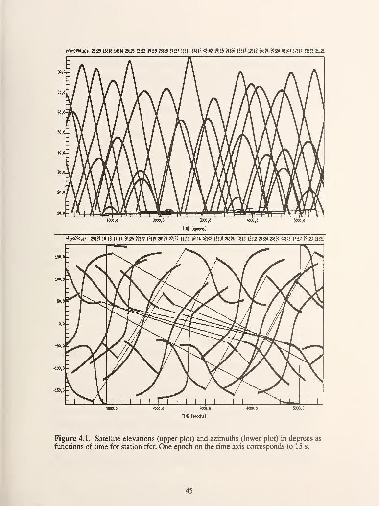
of time for the rfcr station are shown in figure 4.1. While these plots are not quite the

ideal means to examine the observation density in elevation and azimuth space, they

do reveal the most obvious deviations from a uniform distribution, that the density

decreases with increasing elevation angle; this is expected as a satellite zenith pass is a

rare event The azimuth plot displays two types of curves: those similar to inverse tan-

gents corresponding to east-west satellite passes, and those similar to inverse tangents

of the inverse argument corresponding to north-south passes. The predominance of

north-south passes over North America is well known to be responsible for the better

precision in the north-south direction often observed in GPS experiments if ambigu-

ities are not resolved (e.g., [14]). Our interest here is not in the characteristics of satel-

lite passes but only in the overall observation density throughout the session.

Essentially, we imagine a horizontal grid across the angle plots and require an equal

amount of data points in each row.

Formally, the non-uniformity of the satellite distribution would be introduced into

the calculations simply as a non-constant density function c(h, a) of azimuth and ele-

vation in the integrals of eq (2.21). The real density is different from the assumed con-

stant value in two ways:

(1) There will be large scale variations corresponding to a systematic asymmetry

depending on the receiver site. The most pronounced large-scale structure of c for

almost any site is the smaller number of high elevation observations. Because

both integrands in eq (2.21) are weighted by cosh, any variability of c in the

region h = 90° has little effect on the result.

To get an idea of the size of the influence, consider the extreme case of a den-

sity function that is unity for h < 60° and zero for h > 60°. The effect on the first

integral (the matrix B) is rather small; it becomes the matrix

B =1

1

0.8

(4.2)

44

rferO790,»U 29:29 18jl8 M:l4 25:25 22:22 19:19 28;28 27;27 11:11 16:16 02:02 15:15 24:26 13:13 12:12 24:24 20;20 C3:(l3 17:17 23:23 21:21

1000.0 2000.0 3000.0

TIIC [epochs]

4000.0 5O0O.0

rfcr0790.i2i 29:29 18:18 14:14 25;25 22:22 19:19 28:28 27:27 11:11 16:16 02:02 15:15 26:26 13:13 12:12 24:24 20:20 03:03 17:17 23:23 21:21

1000.0 2000.0 3000.0

TItC [tfxicht]

4000.0 5000.C

Figure 4.1. Satellite elevations (upper plot) and azimuths Qower plot) in degrees as

functions of time for station rfcr. One epoch on the time axis corresponds to 15 s.

45

which differs from eq (2.28) only in the zz-component by about 60 j)ercenL The

second integral is only affected in cases where the multipath region extends above

h = 60°. Of course, any azdmuthal non-homogeneity results in non-zero off-diago-

nal elements that lead, for example, to a small horizontal bias even in the case of a

perfecdy flat ground without obstacles.

In practice, observation times are sufficientiy long to sample all directions of

the sky. The large scale asymmetry is thus hardly of concern to us; it may influ-

ence the geometry factor G somewhat but will not affect the order of magnitude

of our estimates given by M^„/d.

(2) The density, of course, also fluctuates strongly on the small scale as the satellite

orbits are discrete lines in (h, a)- space. The condition for the applicability of the

model is that these fluctuations can be regarded as random for the particular

receiver-reflector geometry. We could construct an extreme case of non-random-

ness where all observations yield the same multipath error phase so that the bias

adds up instead of decreasing by averaging. This happens, for example, when all

observations have an equal elevation h' above the reflector plane.

Imagine the flat ground as a reflector and satellites circling the receiver at a

constant elevation h causing the (constant) error phase M. Then eq (2.21)

becomes

Vif

•MJ

s^da (4.3)^r=-X,.\ S„da

-obs multi

and thus

5z = -X, (Insin^h)-^ M (2Ksinh) = -]— (4.4)^ sinh

which is independent of the distance to the reflector and could become quite big.

While this hypothetical case might bear no resemblance with any real situation,

the problem of non-randomness is not completely irrelevant. A satellite pass par-

allel to a long vertical reflector may cause an almost constant or very slowly

changing error phase. If observation times are short, this particular set of observa-

tions may receive much more weight than would be predicted by our model,

resulting in a larger bias. Long observation times will obviously decrease such

systematic effects, but once present never completely eliminate them as no addi-

tional improvement is obtained if the observations span more than one day. It is

beyond the scope of this work to quantify the influence of non-random satellite

distributions on the position bias. Since general statements are hard to obtain, the

46

easiest way for such an evaluation would probably be a simulation using actual

satellite orbit data and calculating the bias from eq (2.19). Because of the neces-

sity of very particular geometry, situations as the one described above should be

very rare. Intuitively, one would assume that the satellite distribution is suffi-

ciently random for the model to be valid if observations include more than, say, 10

satellites, i.e., for observation times of several hours.

4.1.2 Other Unmodelled Effects

Other unmodelled effects that are of concern to us refer exclusively to the error

phase, M. In chapter 2 we made the following assumptions:

Single Reflector. Multiple reflections of the same signal would occur mostly from

the ground and a nearby object, whereas simultaneous reflections from two objects

would be rare due to their limited extent. Thus the two reflected signals would enter

the antenna from very different elevation angles (positive from the object, negative

from the ground). Because of the gain pattern of the antenna, it is likely that the ampli-

tudes differ by an order of magnitude or more, since reflection from the object pre-

vails. It is thus a good approximation for most practical cases to calculate the error

phase in a region of multiple reflections from the strongest reflection alone.

No Phase Change at Reflector. The phase difference between the direct and the

multipath signal was set equal to the pathlength difference divided by the wavelength.

Here we disregarded a phase change of n occurring at a conducting surface. This fac-

tor is inconsequential for the model results that employ the sinusoidal approximation

eq (2.37). It will only reverse the sign of the multipath phase.

Planar Reflector. Many reflectors in practice actually are close to plane surfaces

(trucks, ground, water, etc.). The effect of deviations from a perfect plane depend on

their scale: roughness on a scale much smaller than a wavelength can be disregarded;

roughness on the order of a wavelength will cause loss of the coherency of the

reflected signal, i.e., the error phase will average to zero. The only case that would

affect the model results would be a reflector that is bent on a scale larger than a wave-

length. The whole derivation of the error phase is not applicable then, as the image

receiver is not stationary and the calculated oscillation frequency becomes incorrect.

The model will still be a good approximation for slight curvature.

Constant Reflection Amplitude. In reality, A varies for several reasons, most

notably for the antenna gain pattern. Most modem antennas designed for high accu-

racy applications (among them the one used in the "EDM" experiment) feature a gain

47

drop between 10 and 20 dB from the zenith to the horizon, and down to 30 or even 40

dB at the backplane zenith (e.g., [15]). The amplitude of the reflected signal before

entering the antenna varies as a function of incidence on the reflector (and position of

the reflection point). Most importantly, reflections only occur if h' is smaller than the

Brewster angle = asin- , n being the index of refraction of the reflecting material.n

The variability of the amplitude could be included in the model simply as a func-

tion of elevation and azimuth in the second integral of eq (2.21), just as the observa-

tion density in the previous section. In practice it would vary slowly, i.e., slower than

the error phase itself. Therefore it would only influence the shape of the oscillation

envelope of this integral and thus the geometry factor G in eq (4,1), The scale of the

bias, M^„/d, remains correct, and we can estimate an upper limit by assuming the

maximum amplitude occurring for the particular reflector.

4.2 Estimating the Amplitudes

Without question, the most important variables determining the position bias are

the distance to the reflector and the maximum amplitude of the error phase. While the

former is readily obtained once a reflector is identified, the latter is very difficult to

model. Even if the variability as discussed in the previous section is disregarded, the

calculation of the amplitude requires knowledge of the antenna gain pattern, the index

of refraction, and the conductivity of the reflecting material. Needless to say, any

attempt to estimate the amplitudes is subject to substantial error. As our goal here will

be an upper estimate of the bias for a particular station in a particular experiment, it is

probably preferable (and certainly easier) to first consult the data itself.

The postfit residuals of the double differences contain the combined noise of both

stations of a baseline. This includes in the L3 case orbit errors, tropospheric errors,

clock terms, and multipath noise. We will in the following section focus on two sta-

tions of the "EDM" experiment, nist and eril: the former because its position showed

unexpectedly high scatter as discussed in the first chapter, the latter because it is by all

standards an extreme multipath site as will be evident below. TTie tactics will be the

following: we compare the L3 postfit double difference residuals of the baselines con-

taining nist and eril and select for each of the two the baseline and day with the small-

est noise. The amplitude of the multipath noise from any reflector must be smaller than

the overall noise amplitude for the particular day and, because multipath repeats daily,

on any of the days. The selected plots are shown in figure 4.2, namely nisteri2 and

eri2eril, both on the first day of the experiment. Eri2 is the station with the smallest

48

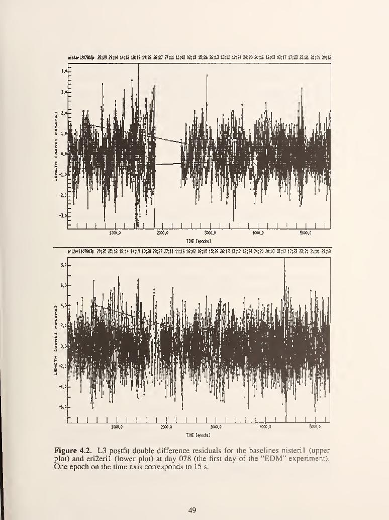
niiUri2e79Mp 25:29 29ji4 14:18 18:19 19:28 28:27 27:11 11:02 02:1! 15:26 24:13 13:12 12;24 24:20 20:14 14:03 M:17 17;23 23:21 h'M 29:18

iOOO.O 20CC,0 30O0.0

TM [epochs]

4000.0 5000,0

»ri2«ril07903p 29:25 25:18 18:14 14:19 19:28 28:27 27:11 11:16 14:02 02:15 15:24 24:13 13:12 12:24 24:20 20:03 03:17 17:23 23:21 21:C4 29:18

1000.0 2000.0 3000.0 4000.0 5000.0

TI)€ [(fochi]

Figure 4.2. L3 postfit double difference residuals for the baselines nisteril (upper

plot) and erileril (lower plot) at day 078 (the first day of the "EDM" experiment).

One epoch on the time axis corresponds to 15 s.

49

multipath noise (the receiver is located in an open field). From the plots we conserva-

tively estimate a maximum multipath noise amplitude smaller than 3 cm at nist (and

eri2) and smaller than 6 cm at eril. The fact that the two Erie sites differ from each

other only in their near environments also allows the conclusion that multipath at eril

is the dominant noise source for the baseline erileril. Since the amplitude of the error

phase is about 4.5 times as big for L3 observations as for LI observations (see section

2.4) we infer that

at nist: M^^^ < ||^ = 0.035 cycles <=> A < 0.22 (4.5)

at eril: M^^^ < ||^ = 0.07 cycles <=> A ^ 0.44 . (4.6)

At least the amplitude eq (4.6) must be quite an overestimate for reflections from

the ground; the antenna gain pattern is such that the strongest ground signals (lowest

elevation angle 20°) arc received at a sensitivity of less than -20 dB rclative to the

zenith while the gain for the corresponding direct signal is about 10 dB stronger. Even

for a perfectly reflecting ground the relative strength of the reflected signal must thus

be smaller than 0.3. We conclude that the high amplitude at eril is due to reflections

from several of the nearby objects. Assuming identical ground properties at the sta-

tions eril and eri2 we can reasonably choose eq (4.5) as upper limit for ground reflec-

tions at eril.

4.3 Position Bias at '*nist"

The environment of the nist site is drawn in figure 4.3. We consider the following

causes for bias due to multipath:.

Vertical Bias due to Ground Reflections. From eq (3.12) with M^^x < 0.035 and

d = 1.2 m we obtain:

ic I ^ 60 mm • 0.035 ,0 /a n\6Z3 < — = 1.8 mm. (4.7)

Hori7X)ntal Bias due to Ground Reflections Plus Asymmetry Induced by the

Tree. The angular height of the tree as seen from the receiver is approximately 22°,

i.e., for a minimum satellite elevation of 20° the tree disturbs the symmetry of the mul-

tipath region. TTie tree's azimuthal extent is about 25°. Assuming that eq (3.15) derived

for a flat ground approximately holds for the slight ground tilt, we thus infer

50

ground drops toward

east at -5° tilt

Rangular height

<20° as seen

from R

Figure 4.3. Geometry at the receiver site nist. Antenna height of R was 1.2 m above

ground. All numbers given in the sketch are estimates to within about 10 percent.

|8x.. 30 mm • 0.035 . ^^o _ _„ ^ _< -— sinl^ • 2c<9^20° = 0.7 mm

1.2(4.8)

Horizontal Bias due to Tilted Ground. The ground tilt in the vicinity of the

receiver is about 5°. In this case a = 4 x 1.4°/d, so eq (3.41) applies, yielding

|5xJ < 5 16 mm -5:^ = 0.4 mm (4.9)

Horizontal Bias Induced by Reflections From the Flatirons. The Flatirons

were initially suspected to be the main cause of bias. According to our model reflec-

tions off them cannot be a problem; even if the rock surface could be regarded as a

plane reflector (in reality it is rough on the order of a wavelength), the error phase

oscillates so fast due to the large distance that it averages out. However, this leads to a

different consideration; if the reflections from the Flatirons are much stronger than the

ground reflections, then they dominate the multipath phase in the region in which both

reflections are present simultaneously. Hence, multipath in this region averages out,

which effectively amounts to a region of missing ground multipath causing horizontal

bias according to section 3.2.

We estimate the essential parameters of the Flatirons as seen from nist as follows:

they arc tilted at an angle of about a = 45° from the horizontal, have a vertical angular

51

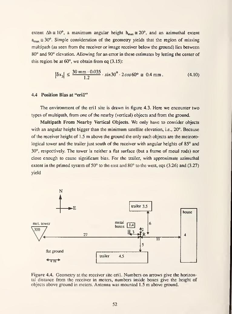
extent Ah = 10°, a maximum angular height h„„ = 20°, and an azimuthal extent

an,,, = 30°. Simple consideration of the geometry yields that the region of missing

multipath (as seen from the receiver or image receiver below the ground) lies between

80° and 90° elevation. Allowing for an error in these estimates by letting the center of

this region be at 60°, we obtain from eq (3.15):

5 I^ 30 mm • 0.035 . ^^o ^ ,^- „ .

0x3 < — 5m 30 • 2co560° = 0.4 mm (4.10)

4.4 Position Bias at ^^eril"

The environment of the eril site is drawn in figure 4.3. Here we encounter two

types of multipath, from one of the nearby (vertical) objects and from the ground.

Multipath From Nearby Vertical Objects. We only have to consider objects

with an angular height bigger than the minimum satellite elevation, i.e., 20°. Because

of the receiver height of 1 .5 m above the ground the only such objects are the meteoro-

logical tower and the trailer just south of the receiver with angular heights of 85° and

30°, respectively. The tower is neither a flat surface (but a frame of metal rods) nor

close enough to cause significant bias. For the trailer, with approximate azimuthal

extent in the primed system of 50° to the east and 80° to the west, eqs (3.26) and (3.27)

yield

Ni

met tower

flat ground

^ 4m ^

trailer 3.5

metal

boxes 1.4

27 ia.i->tA11

U-ailer 4.5

Figure 4.4. Geometry at the receiver site eril. Numbers on arrows give the horizon-

tal distance from the receiver in meters, numbers inside boxes give the height of

objects above ground in meters. Antenna was mounted 1.5 m above ground.

52

0.07 sin50° + sinSO°{ . ^^oOZj^ 30 mm •

—— • r l^mzO + 5zn30 I = 0.3 mm (4.11)

|6xJ ^ 30 mm • 5:5Z .^ 50° + 80°

^ ^^^^0° + co530°l = 0.9 mm . (4.12)

Hereby we slightly modified the equations to take into account the asymmetrical azi-

muthal extent of the trailer. Also note that because of this asymmetry, eq (4.12) is not

strictly a bias in the direction of the trailer.

Multipath from the Ground. The vertical bias caused by ground reflections is

similar in size as calculated above for nist (eq (4.7)), i.e., 1.8 mm, if we assume similar

ground reflectivity. Horizontal bias is introduced by objects that obstruct the ground

multipath region ("missing multipath"), i.e., objects with an angular height larger than

20° as seen from the image receiver 1.5 m below the ground. As is easily recognized,

all objects shown in figure 4.4 qualify; we will here only calculate the largest bias that

can be caused by a single object. Recalling the corresponding eq (3.15),

15x^1 < 30 mm • —^ • 5ma„„ (cosh^,^ + cosh-„) ,I

j| A max ^ max min' '

we find that the potentially most harmful objects are those of large azimuthal extent

and low angular height h^^, (but remember that hn^ - h^u, > 2°/d is required for the

full effect). The obvious candidate is again the long trailer to the south of the receiver

with azimuthal extent (now in the unprimed system) of approximately 20° to the east

and 70° to the west:

IS \ ^ nn 0035 sin20° + sinlO°( ^^o o^ /^ i-ix6x3 < 30 mm • • r 1 cos30 + coszO I = 0.8 mm . (4.13)

53

CHAPTER 5

SUMMARY AND CONCLUSIONS

In this work we estimate the bias on GPS position measurements caused by carrier

signal multipath. While the effect is known to be severe for short observation times

and kinematic GPS applications, it is expected to significantly decrease through aver-

aging for observation times much longer than the period of multipath signatures. Typi-

cal multipath periods are on the order of several minutes while high accuracy static

GPS applications usually require observations of several hours to facilitate satisfactory

ambiguity resolution.

The GPS Experiment "EDM" is introduced in the first chapter. It comprised

three days of observations on five receiver sites with inter-station distances between

200 m and 47 km. While the purpose of this experiment did not include testing multi-

path, concern over a possible multipath-induced bias arose after it was observed that

site-specific length-independent error sources strongly affected at least one of the sta-

tions. Some of the summarized results show an unsatisfactorily high scatter of the

shortest baseline in comparison with the longer ones. The presence of multipath signa-

tiu^es in the data is demonstrated as well.

A Mathematical Model of Carrier Multipath Bias is develoj)ed in Chapter 2.

We first model the error phase due to multipath in terms of satellite-receiver-reflector

geometry. This multipath phase is smaller than a quarter of a cycle of the carrier wave-

length and oscillates with the satellite elevation angle at a frequency proportional to

the reflector distance and the inverse carrier wavelength. In a second step we invoke

the method of least squares to calculate the position bias from an arbitrary set of obser-

vations corrupted by multipath error. Assuming a uniform satellite distribution allows

us to express the bias in terms of general geometrical parameters. The expression

involves integrals of the error phase that cannot be solved analytically. We simplify in

several steps: the transformation into a coordinate system in which the error phase is

azimuthally symmetrical reduces the integrals to one dimension; comparison of

54

numerical solutions with a sinusoidal approximation and some mathematical reason-

ing finally lead to simple formulae that simulate the most important features of the

integrals. The model is then generalized to dual frequency observations that are nowa-

days the standard in high accuracy applications of GPS. The main effect is a factor of

about five enhancement of the maximum multipath phase amplitude.

Not surprisingly, the bias is found to be roughly proportional to the reflection

amplitude. A, and inversely proportional to the perpendicular distance, d, from the

reflector. Somewhat less expected is the fact that the magnitude and even the direction

of the bias are very sensitive to the exact angular extent of the region in which multi-

path signals are received and to the distance from the reflector. The bias oscillates

depending on the elevation angle above the reflector plane with a period on the order

of 45°Xyd, i.e., for carrier wavelengths of 20 cm about 9°/d[ml. This means, for exam-

ple, that the bias sign reverses if the angular extent of the multipath region changes by

5° under otherwise identical conditions. More importantly, it also implies that the bias

is dependent on setup. In particular, a 10 percent change of the antenna height will

reverse the sign of the bias due to ground reflections. This explains why multipath

contributes to the day-to-day scatter when the setup and antenna height are varied

daily as is common practice in many GPS experiments. This practice should therefore

be recommended as it will allow multipath error to be represented in the repeatability

rather than remaining a systematic error with unknown magnitude.

Basic Receiver Environments are examined in Chapter 3 employing the model.

We obtain upp)er limits to the exj)ected multipath bias in terms of the reflection ampli-

tude, perpendicular distance from the reflector, and one or more angles characteristic

of the geometry. The general rule for any geometry is that multipath bias is a product

of multipath and asymmetry. Uniform multipath from all directions would in theory

not cause any bias. The concept of the image receiver at an equal distance behind the

(planar) reflector proves very useful within this context. To examine whether a partic-

ular environment might cause bias, all that needs be done is to identify reflectors and

determine whether the multipath region as seen from the image receiver is asymmetri-

cal.

Multipath from the flat ground causes vertical bias because it is non-symmetrical

in the vertical direction (no satellites are below the ground). The azimuthal symmetry

(about a vertical axis), however, precludes horizontal bias. Any azimuthal asymmetry

in the field of view of an image receiver, however, introduces horizontal bias. This

asymmetry could be due to any object (not necessarily a reflecting one) that obstructs a

small part of the observation region of the image receiver below the ground

55

(corresponding to ground reflections). A reflecting surface itself effectively acts as an

obstruction for the image receiver behind it. Thus, a nearby reflector will cause

horizontal bias unless it is completely outside the observation region of the image

receiver. Finally, an antenna placed above tilted ground results in horizontal bias

because the azimuthal symmetry of ground multipath is destroyed. Of concern hereby

is only the portion of ground within the observation region of the image receiver, i.e.,

the ground surrounding the antenna within a radius of d/tan20° = 2.7d for a satellite

elevation cutoff of 20° and an antenna height d. A very small ground tilt of 1 .4°/d,

however, is sufficient for the maximum bias. Therefore, horizontal bias due to ground

reflections can hardly be avoided despite careful site selection.

The maximum bias is of the general form and order

0.075

—

:^-G, i.e., 3mm—^Gd d[m]

for X^ = 19 cm. Here the maximum (single wavelength) error phase in cycles,

M„„ = asinA/ln, is smaller than 1/4, and G, which is dependent on geometry, is

smaller than 47C for single frequency observations and smaller than 207C for dual fre-

quency observations. The formula is an overestimate if d is on the order of or smaller

than a carrier wavelength.

These results suggest two principal ways to decrease or eliminate multipath bias:

(1) Antenna positioning: Reflectors that could create bias must either be avoided or

be distant enough to be harmless. While the ground cannot be avoided, we find

that carrier multipath bias due to ground reflections is inversely proportional to

the antenna height. This result appears to contradict recommendations by other

authors to place the antenna as close to the ground as possible [1,15]. The

argument for a very small antenna height is to yield a multipath error phase

oscillating so slowly with the satellite elevation, that it remains well below the

first maximum during a satellite pass. The first maximum, however, occurs at an

elevation angle of approximately 2°/d, implying an antenna height smaller than

about 2 cm to suppress it in a satellite zenith pass and well below that to actually

reduce the bias. This can hardly be achieved in practice due to the physical

dimensions of the antenna and its phase center location; one might have to place

part of the antenna below the ground. We argue that a very small antenna height

will likely reduce carrier multipath noise apparent in the postfit residuals, but only

because the slowly varying error is absorbed by the estimated parameters and thus

not visible in the adjustment residuals. This is precisely the result that is not

desired. In contrast, a large antenna height will increase the multipath oscillation

56

frequency, preventing the error from being absorbed in the parameters for

sufficiently long observation intervals. Thus the multipath signatures can be

detected in the postfit residuals and the bias will be decreased by averaging over

many multipath periods.

The picture is completely different for pseudorange multipath since the fun-

damental wavelength of the code modulations is 154 (P-code) or 1540 (C/A-code)

times bigger than the carrier wavelength. Thus, pseudorange multipath error can

be reduced to a small part of a cycle by placing the antenna very close to the

ground. This is an effective method for minimizing the resulting bias. Note that

the work presented here is not applicable to pseudorange because its signal struc-

ture and the methods to retrieve geometrical information from it are inherently

different than those of the carrier signal.

(2) Minimizing the reflection amplitude: This is usually possible only for ground

reflections. Methods tested include adding absorption material or a "choke ring"

to the antenna to reduce the strength of the reflected signal. Experimental tests

suggest that multipath rejection measures are most effective and practical if they

are designed into the antenna itself [1]. Most antennas in use for high precision

measurements today feature a strongly reduced sensitivity in the backplane reduc-

ing ground multipath effects.

Application of the Model is the subject of Chapter 4. We discuss the assumption

of uniform satellite distribution and unmodelled effects and conclude that the simple

model is applicable to most practical situations in that it discloses the nature of multi-

path error and yields an upper limit estimate of its magnitude. We examine in detail the

two stations of the experiment "EDM" that are thought to be most affected by multi-

path (nist and eril). The reflection amplitudes are estimated from the postfit residuals.

The model yields horizontal biases smaller than 1 mm and vertical biases smaller than

2 mm for all sources of multipath considered. We thus infer that even for these less

than ideal receiver sites, multipath bias is essentially averaged out due to the long

observation times. The remaining bias is comparable to setup errors and thus hardly

reason for concern. In any case, it cannot account for the high length-independent scat-

ter encountered in the experiment.

Inasmuch as the conditions in the "EDM" experiment are typical for non-ideal

receiver environments, we conclude that carrier multipath bias can be reduced to

harmless levels by: (i) the use of antennas with a gain drop bigger than 10 dB between

direct and backplane low-elevation signals (at 20°), (ii) an antenna height greater than

about 1 m, (iii) no large reflective objects closer than about 5 m to the antenna, and

57

(iv) observation times of more than several hours. These points should be satisfied in a

typical GPS campaign. The most critical issue may be the reflectivity of the ground.

Note that a nearly perfectly reflecting ground would yield biases about four times as

large as calculated here. In this extreme case the use of multipath suppressing devices

external to the antenna would be appropriate.

Potentially more harmful than multipath bias directly induced by a carrier phase

error, as examined in this work, are the effects of multipath on the data quality. Strong

multipath typically gives rise to problems during data preprocessing. Fast oscillations

may be misinterpreted as cycle slips by the software. Multipath can also cause loss of

lock and cycle slips during the observation. Finally, multipath becomes a major limita-

tion to the accuracy of long baselines when ambiguity resolution is attempted with the

help of pseudorange information.

58

REFERENCES

[1] Evans, A. G., and Hermann, B. R, A comparison of several technices to reduce

signal multipath from the Global Positioning System, in Global Positioning Sys-

tem: An Overview, edited by Y. Bock and N. Leppard, Springer-Veriag, NewYork,74-81, 1990.

[2] Meehan, T. K., Dinardo, S. J., and Young, L.E. GPS multipath reduction using

absorbing backplanes, EOS, Trans. AGU, 70, 1047, 1989.

[3] Young, L.E., and Meehan, T. K., GPS multipath on code-using receivers, EOS,

Trans. AGU, 69,324, 1988.

[41 Wells, D. E., Beck, N., Delikaraoglou, D., Kleusberg, A., Krakiwsky, E. J.,

Lachapelle, G., Langley, R. B., Nakiboglou, M., Schwarz, K. P., Tranquilla, J.

M., and Vanicek, P. Guide to GPS Positioning, Canadian GPS Associates, Fre-

dericton, NB, 1986.

[5] Georgiadou, Y, and Kleusberg, A. On carrier signal multipath effects in relative

GPS positioning, Manuscripta Geodaetica, 13, 172-179, 1988.

[61 Dixon, T. H., An introduction to the Global Positioning System and some geo-

logical applications. Rev. of Geophysics, 29, 249-276, 1991.

[7] Bossier, J. D., Goad, C, and Bender, P. L. Using the Global Positioning System

(GPS) for geodetic positioning. Bull. Geod., 54, 553-563, 1980.

[81 Lichten, S. M., and Komreich, S. Stochastic GPS estimation of tropospheric path

delays, EOS, Trans. AGU, 68, 1238, 1987.

[9] Rocken, C. The Global Positioning System: A new tool for tectonic studies,

PhD. thesis. University of Colorado, Boulder, 1988.

[101 Beutler, G., Bauerisma, I., Botton, S., Gurtner, W., Rothacher, M., Schildknecht,

T., Geiger, A. Atmospheric refraction and other important biases in GPS carrier

phase observations, lUGG XIX General Assembly, Vancouver Aug. 9-22, 1987.

59

[11] Tranquilla, J. M. Multipath and imaging problems in GPS receiver antennas,

Proc. 4th Intern. Symp. Sat. Pos., Austin, TX, April 28 - May 2, 557-571, 1986.

[12] Levine, J. Multiple wavelength electromagnetic distance measurements, Geo-

detic Refraction, edited by F. K. Brunner, Springer-Verlag, 45-51, 1984.

[13] Vanicek, P., and Krakiwsky, E. Geodesy: The concepts, 2nd edition, Elsevier Sci-

ence Publishers B.V., Amsterdam, 1986.

[14] Larson, K. M., and Agnew, D. C. Application of the Global Positioning System

to crustal deformation measurement - 1. Precision and accuracy, /. Geophys.

Res.,96, \6541-\6565, \99\.

[15] Clark, T. GPS antennas: De-mystifying multipath, NASA/GSFC unpublished

memo, March 5, 1992.

*U.S. GOVERNMENT PRINTING OFFICE: 1994-573-013/00026

60

NIST Technical Publications

Periodical

Journal of Research of the National Institute of Standards and Technology— Reports NIST research

and development in those disciplines of the physical and engineering sciences in which the Institute is

active. These include physics, chemistry, engineering, mathematics, and computer sciences. Paperscover a broad range of subjects, with major emphasis on measurement methodology and the basic

technology underlying standardization. Also included from time to time are survey articles on topics

closely related to the Institute's technical and scientific programs. Issued six times a year.

Nonperiodicals

Monographs—Major contributions to the technical literature on various subjects related to the Institute's

scientific and technical activities.

Handbooks—Recommended codes of engineering and industrial practice (including safety codes)

developed in cooperation with interested industries, professional organizations, and regulatory bodies.

Special Publications—Include proceedings of conferences sponsored by NIST, NIST annual reports, andother special publications appropriate to this grouping such as wall charts, pocket cards, andbibliographies.

Applied Mathematics Series—Mathematical tables, manuals, and studies of special interest to physicists,

engineers, chemists, biologists, mathematicians, computer programmers, and others engaged in scientific

and technical work.

National Standard Reference Data Series—Provides quantitative data on the physical and chemical

properties of materials, compiled from the world's literature and critically evaluated. Developed under a

worldwide program coordinated by NIST under the authority of the National Standard Data Act (Public

Law 90-396). NOTE: The Journal of Physical and Chemical Reference Data (JPCRD) is published bi-

monthly for NIST by the American Chemical Society (ACS) and the American Institute of Physics (AIP).

Subscriptions, reprints, and supplements are available from ACS, 1155 Sixteenth St., NW, Washington,

DC 20056.

Building Science Series—Disseminates technical information developed at the Institute on building

materials, components, systems, and whole structures. The series presents research results, test

methods, and performance criteria related to the structural and environmental functions and the durability

and safety characteristics of building elements and systems.

Technical Notes—Studies or reports which are complete in themselves but restrictive in their treatment

of a subject. Analogous to monographs but not so comprehensive in scope or definitive in treatment of

the subject area. Often serve as a vehicle for final reports of work performed at NIST under the

sponsorship of other government agencies.

Voluntary Product Standards—Developed under procedures published by the Department of Commercein Part 10, Title 15, of the Code of Federal Regulations. The standards establish nationally recognized

requirements for products, and provide all concerned interests with a basis for common understanding of

the characteristics of the products. NIST administers this program in support of the efforts of private

sector standardizing organizations.

Consumer Information Series— Practical information, based on NIST research and experience, covering

areas of interest to the consumer. Easily understandable language and illustrations provide useful

background knowledge for shopping in today's technological marketplace.

Order the above NIST publications from: Superintendent of Documents, Government Printing Office,

Washington. DC 20402.

Order the following NIST publications—FIPS and NISTIRs—from the National Technical Information

Service. Springfield. VA 22 1 61.

Federal Information Processing Standards Publications (FIPS PUB)—Publications in this series

collectively constitute the Federal Information Processing Standards Register. The Register serves as the

official source of information in the Federal Government regarding standards issued by NIST pursuant to

the Federal Property and Administrative Services Act of 1949 as amended, Public Law 89-306 (79 Stat.

1127), and as implemented by Executive Order 11717 (38 FR 12315, dated May 11, 1973) and Part 6 of

Title 15 CFR (Code of Federal Regulations).

NIST Interagency Reports (NISTIR)—A special series of interim or final reports on work performed by

NIST for outside sponsors (both government and non-government). In general, initial distribution is

handled by the sponsor; public distribution is by the National Technical Information Service, Springfield.

VA 22161, in paper copy or microfiche form.

TJ

3o^1

^* oD)

O00

TJ c2, w<0) 3

(DW

C Wv>

n

•(/>•

bdoo

CD COO MC C7I

S- COCD -,

r" o

n Q.

O 0)

5-<Q.OCOo00owCOCON)C»

z c^ (/)

o3 aQ) (t)

5-9J

CD '*

O O

C/) O<-> o

"^^ 3

^20)

DaHCDO3"3o_

oCO<