Proceedings of the Spatial Science Institute Biennial International Conference (SSC2007), Hobart, Tasmania, Australia, 14-18 May 2007 (peer-reviewed paper)

177

GPS-VIEW: VISUALISING GEODETIC GPS TIME SERIES ANALYSES

Christopher Watson and Bryn Roberts Centre for Spatial Information Science

School of Geography and Environmental Studies University of Tasmania

Private Bag 76, Hobart TAS 7001, Australia cwatson@utas.edu.au, bryn@brynr.ath.cx

ABSTRACT Local, regional and worldwide Global Positioning System (GPS) networks have long been used to monitor geophysical processes which vary spatially throughout the temporal and frequency domains. Geodetic GPS time series often exhibit complex non-linear behaviour which is a combination of real world geophysical signals and systematic artefacts caused by such things as aliasing of high frequency periodic motion and errors within the processing models or solution strategies. In this paper, we describe a beta version of an online, interactive tool designed to assist in the visualisation of geodetic GPS time series analyses. The tool, referred to as GPS-View, allows for interactive viewing of GPS time series parameter estimates for any given GPS analysis centre solution, or their differences. Using both numeric and chart output from Matlab time series analyses performed in advance, the viewer utilises the open source MapServer application as a web-mapping engine to visualise the spatial distribution of the time series output. GPS-View aids in the understanding of recent advances in GPS analysis strategies, helping to minimise the error contribution to geodetic GPS time series and further understand global geophysical processes.

BIOGRAPHY OF PRESENTER Christopher joined the academic staff at the University of Tasmania within the Centre for Spatial Information Science in 2004. Christopher’s research interests are centred in the disciplines of geodesy and geodynamics, with an emphasis on GPS applied to global climate change and sea level studies.

INTRODUCTION Global Positioning System (GPS) networks are commonly used to monitor various geophysical phenomena on global, regional and local scales. Typical processing strategies for GPS analyses involve processing 24 hours of data sampled at 30 second epochs (see Herring (1999) for a review). Parameterisation for these standard processing approaches includes a single station coordinate per 24 hour observation session, satellite orbital parameters, Earth orientation parameters and tropospheric zenith delays (typically 1 or 2-hourly). Processing consecutive 24 hour sessions yields a “daily” coordinate time series, often transformed into local topocentric coordinate components (North, East, Up) for subsequent interpretation. Coordinate time series and associated variance covariance information form the basic data structure used in the

Proceedings of the Spatial Science Institute Biennial International Conference (SSC2007), Hobart, Tasmania, Australia, 14-18 May 2007 (peer-reviewed paper)

178

analysis of geophysical phenomena such as tectonic motion, subduction / uplift, and earthquake displacement. These data also often contribute to refinements in reference frames (Altamimi et al., 2002) and national coordinate datums (Morgan et al., 1996).

The analysis of global scale geodetic GPS networks for geophysical applications dates back to the early 1990’s. Since these early experiments, densification of global networks combined with consistent developments in hardware and software have lead to incremental improvements in GPS positioning accuracy and associated time series repeatability. Updated time series are regularly computed by analysis centres and research laboratories using refined processing strategies and algorithms. This mode of incremental advancement within the geodetic GPS community continues, with regular contributions to the literature. Recently, notable progress has been made in understanding the impact of mismodelling periodic geophysical signals such as the solid Earth tide, ocean tide loading and other mass loading phenomena. Penna and Stewart (2003) and Penna et al. (2006) have shown theoretically and through the use of simulated data how unmodelled periodic signals propagate into GPS coordinate time series at different frequencies. Further development has been made in understanding the impact of improvements in solid Earth tide models (Watson et al., 2006), atmospheric pressure loading (Tregoning and van Dam, 2005), ocean tide loading (Urschl et al., 2005) and tropospheric mapping functions (Boehm et al., 2006) to name a few.

Different coordinate time series are generated depending on the analysis centre’s processing strategy and choice of incremental processing enhancements. Quantifying the systematic differences between different time series, both within and between analysis centres helps understand and progress geodetic GPS analyses. This translates to a reduced uncertainty in the geophysical interpretation of coordinate time series. In this paper, we outline an interactive, online tool referred to as GPS-View that is designed to assist in the visualisation of geodetic GPS time series analyses. The primary aim of the tool is to simplify the systematic comparison of different time series, through the improved visualisation of time series in the temporal and frequency domains, and time series parameters in the spatial domain.

Geodetic GPS Time Series The linear rate or velocity at which a GPS station moves has historically been the fundamental time series parameter of geophysical interest. Horizontal velocity differences at the ~100 mm/yr level exist across areas of active tectonic activity, with vertical rates of change as high as ~10 mm/yr in active areas. Geodetic GPS coordinate time series are therefore historically modelled with a simple offset and linear rate model. Following incremental developments in the field as previously discussed, additional, more complicated components to the time series were identified. In addition to the dominant linear velocity, seasonal displacements were observed (Blewitt et al, 2001), and in many cases added to the time series parameterisation. Coordinate time series are also affected by co-seismic and post-seismic displacements, modelled by time dependent offsets and logarithmic decay terms. Additional time dependent offsets have been observed to occur at times of GPS antenna and receiver / firmware changes (Tregoning et al. 2004). Neglecting co-seismic and post-seismic deformation, the motion of any GPS coordinate component, y, at time t, can be described according to the linear relation in Eqn 1.

Proceedings of the Spatial Science Institute Biennial International Conference (SSC2007), Hobart, Tasmania, Australia, 14-18 May 2007 (peer-reviewed paper)

179

( ) ( )

( ) ( )

( )

,

1

1

...

sin 2 cos 2 ...c d

jumps

j

i i

n

p i p p i pp

n

j i jumps ij

y t a b t

c t freq d t freq

jumps H t T v

π π=

=

= +

+ × + ×

+ − +

∑

∑

Eqn. 1

where H is the Heaviside step function. Parameters a and b define the coordinate position (offset) and linear rate (velocity). Parameter vectors c and d define the amplitude and phase of any number (n) of periodic terms with frequencies freq. Finally, the parameter vector jumps defines any number (njumps) of time dependent offsets occurring at times Tjumps. The remaining error in the model is described by v. Parameter estimation using weighted least squares techniques together with uncorrelated white noise or more sophisticated coloured noise models can be undertaken in a range of software suites. Examples include the QOCA (Dong, 2005) and CATS (Williams, 2005) suites originating from the Jet Propulsion and Proudman Oceanographic Laboratories respectively. The time series analyses undertaken for this paper were performed using the author’s custom software (see Watson, 2005), developed in Matlab and customised to read data from the various major scientific GPS analysis suites (such as GAMIT, Bernese and Gipsy).

The primary output for any given time series analysis includes time series parameter estimates (a, b and vectors c, d and jumps from Eqn 1) and uncertainties for each coordinate component, for each station in the network under investigation. Various statistics assessing the noise characteristics of the time series and the quality of the model fit are also output. These may include statistics such as the weighted root-mean-square (wrms) scatter, and normalised root-mean-square (nrms) or ratio of the scatter to the expected scatter based on the input uncertainty information. Quantitative statistics such as the number of data samples, number of parameters estimated and the numbers of outliers removed in pre-processing may also be output from any given analysis. This combined numeric output provides an analysis centre and solution specific picture of the perceived motion of the GPS station, suitable for geophysical interpretation.

Additional pictorial output is also generally produced when undertaking a time series analysis on any given GPS solution. Graphical plots of the residual time series, typically undertaken in both the time and frequency domains can help provide further insight into additional non-linear behaviour such as interesting site motions or erroneous processing artefacts. Further insight into the complex structure of the residual time series can be achieved using wavelet techniques (Keller, 2004) and output to graphical plots. These pictorial outputs further assist the interpretation and solution comparison process. Any attempt to compare two or more GPS solutions requires a detailed analysis of both numeric and pictorial output from each time series analysis. The automated and interactive visualisation of both the numeric output (time series parameters and analysis statistics) and pictorial output facilitates these comparisons and is the focus of the tool presented in this paper.

Proceedings of the Spatial Science Institute Biennial International Conference (SSC2007), Hobart, Tasmania, Australia, 14-18 May 2007 (peer-reviewed paper)

180

Existing tools for Visualising Geodetic GPS Output A considerable number of software tools have been previously developed to assist in visualising output from geodetic GPS time series analysis. Many of these tools are designed solely for the “end-user” and hence are analysis centre and solution specific, i.e., only time series output from a single GPS solution is presented (in one or more reference frames). Two specific examples include the Scripps Online Mapping Interface (SOMI) from the Scripps Orbit and Permanent Array Centre (SOPAC, 2006) and a similar project from the Japanese Geographical Survey Institute (GSI, 2006). The SOMI tool provides a web-based mapping interface enabling users to visualise the linear horizontal velocities from stations in the Southern California Integrated GPS Network (SCIGN). The GSI tool provides a similar service for users wishing to investigate any of the 1000+ GPS stations located in Japan. This particular tool has the additional functionality of allowing users to visualise the station velocities relative to any user-selected station, hence enabling the visualisation of strain.

Herring (2003) presents a series of customisable tools allowing the interactive viewing and manipulation of both time series and velocity information. Written using Matlab, the suite known as GGMatlab allows visualisation and detailed analysis of up to two velocity fields. A powerful feature of this suite is the ability to plot a velocity profile along a user-specified transect. Users also have the ability to view plots of the time series in the time domain for any specified site.

These and many other visualisation tools have the following limitations:

• The tools are generally analysis centre specific, allowing the viewing of results from a single time series analysis (with the exception of GGMatlab).

• Each tool is designed to visualise simply velocity information. There is no ability to view the spatial distribution of other numeric output from the time series analysis (WRMS, NRMS, periodic signals etc).

• Most tools have no direct link to move from visualisation in the spatial (map) domain, to viewing pictorial output of the time series analysis in the time, frequency (including wavelet) domains.

• Each tool provides a static visualisation experience; there is no ability to animate to assist comparative analysis.

GPS-VIEW: CONCEPTUAL DESIGN The conceptual design of GPS-View was conceived around the desire to view GPS time series output from multiple analysis centre solutions in the spatial, time and frequency (including wavelet) domains, both statically and in animated form. The tool was designed from the outset to be web-based to facilitate collaborative research and efficient distribution of results. Importantly, GPS-View was conceived to operate independently from specific time series analysis software. GPS-View simply requires a generic database of time series output and a directory structure of pictorial plot files. This initial “generic” processing required to generate the input data for GPS-View is shown in schematic form in Figure 1. In the case of this paper, all time series analysis is undertaken in the author’s custom analysis software written in Matlab.

Proceedings of the Spatial Science Institute Biennial International Conference (SSC2007), Hobart, Tasmania, Australia, 14-18 May 2007 (peer-reviewed paper)

181

Fig. 1: Data flow and “generic” time series analysis process.

To facilitate the different visualisation tasks required, the design of GPS-View is focused around a central “output” window with several expandable interface panes for control and customisation. Each interface pane (Map-View, Plot-View, Chart-View and Text-View) controls a particular visualisation task that is viewed in the central output window as shown schematically in Figure 2.

Fig. 2: Schematic view of the conceptual design of GPS-View consisting of a central

output window and associated interface panes.

The core conceptual functionality of each interface pane is provided in Table 1.

Tab.1: Core functionality of each interface section.

Proceedings of the Spatial Science Institute Biennial International Conference (SSC2007), Hobart, Tasmania, Australia, 14-18 May 2007 (peer-reviewed paper)

182

GPS-VIEW: IMPLEMENTATION To facilitate the implementation of an online tool with spatial mapping capabilities, a web-map server was required as the fundamental GPS-View engine. The open source MapServer suite (MapServer, 2006) was implemented as discussed below.

System Configuration MapServer (incorporating MapServer CGI v4.8.4 and MapScript v4.8.4) was configured with the Apache HTTP server (v2.0.58) and PHP (v5.1.4) with MySQL (v5.0.22) as the database engine. Data flow between the various components is shown in Figure 3.

Fig. 3: Schematic view showing the dataflow between HTML transfer, script processing

and data storage tiers of the GPS-View tool.

Database Design The numeric output from the generic time series analysis is required in a database structure for access by PHP and MapServer. A simple MySQL database was implemented utilising four tables. With reference to Table 2, the database is capable of storing time series output from multiple GPS analysis centre solutions (the solutions table). Each solution has many sites (the sites table), each of which has latitude and longitude values, and a file link to a pictorial plot of horizontal position over time or of the entire time series in the frequency domain. Each site then has time series analysis parameter estimates, uncertainties and output statistics for coordinate components N, E and U (the components table). Finally, any coordinate component record may have many parameters defining periodic signals (the periodic terms table).

Proceedings of the Spatial Science Institute Biennial International Conference (SSC2007), Hobart, Tasmania, Australia, 14-18 May 2007 (peer-reviewed paper)

183

Tab. 2: GPS-View database schema.

Interface Design The GPS-View interface was designed around the central output window and interface panes defined in Table 1. The interface was designed to be completely ‘theme-able’, providing the ability to operate under a number of different conditions, providing support for specific web browsers, screen resolutions and operating systems. Two of the beta release themes provide different output window configurations. The first offers a static output window size of 798 x 400 pixels. The second theme provides a wide screen version that automatically resizes the output window for users with larger screen resolutions and faster internet connections.

Each interface pane described in Table 1 was designed and implemented using a combination of javascript and cascading style sheets. Each pane may be minimised to show only the controls required for the specific visualisation task. Each interface section, including the output window, is described below.

Output Window The output window is the primary focus of the interface as the display area for all map, pictorial plot, dynamic chart and textual output to the user. As shown in Figure 4, the base of the output window incorporates a metadata panel and animation controls for the animated displays. These controls allow users to change the play direction, alter the speed, pause, re-start and move frame by frame through any given animation. The metadata panel provides a summary of the current contents of the output window.

Proceedings of the Spatial Science Institute Biennial International Conference (SSC2007), Hobart, Tasmania, Australia, 14-18 May 2007 (peer-reviewed paper)

184

Fig. 4: The output window with a map view of horizontal velocities from a global

solution. Note the metadata panel and animation controls below the output window.

Map-View Each of the cascading interface components are positioned below the output window and can be maximised or minimised at the user’s discretion. The Map-View interface (Figure 5) provides the spatial domain visualisation functionality as described in Table 1. The interface pane is divided into sections dealing with data selection (i.e., selecting which analysis centre time series data will be visualised), map parameter/statistic selection (i.e., selecting which information within a given solution will be plotted onto the map) and customisation (i.e., changing the appearance and content of the map output). Interface controls are a mixture of check boxes and pick lists, with some options unavailable depending on previous choices. When selecting time series parameters or statistics to visualise, the interface is subdivided into velocity, periodic terms or miscellaneous statistics. The list of available periodic constituents is updated dynamically based on the contents of the periodic terms database table for the selected analysis centre solution(s). For the visualisation of all time series parameters, the user has the choice to filter the available data based on sigma tolerances (1σ, 2σ, or 3σ significance). Symbol scaling is partially automated (based on the median value of the attribute being mapped) and controlled by a user selection of small, medium or large.

Proceedings of the Spatial Science Institute Biennial International Conference (SSC2007), Hobart, Tasmania, Australia, 14-18 May 2007 (peer-reviewed paper)

185

Fig. 5: The Map-View interface pane.

The map customisation controls are available within a sub-interface that cascades within the Map-View interface (Figure 6). The map customisation is divided into components detailing projection and extent, layers and text labelling.

Fig. 6: The map customisation interface pane.

Proceedings of the Spatial Science Institute Biennial International Conference (SSC2007), Hobart, Tasmania, Australia, 14-18 May 2007 (peer-reviewed paper)

186

Within the beta release, only a standard geographic projection is supported (latitude and longitude plotted purely as x,y Cartesian coordinates). Various predefined geographic regions are supported in addition to custom entry of map extents. Various map layers are available to enhance the visualisation as shown in Figure 6. Text labels are available for GPS site names and the latitude / longitude graticule.

Plot-View The Plot-View interface (Figure 7) enables users to view static or animated pictorial plot files that are produced during the time series analysis (see Table 1). The pictorial files are stored on the web-server and displayed within the output window.

Fig. 7: The Plot-View interface pane.

The interface allows users to first select which sites(s) and solution(s) are to be viewed (either statically or in animated format). The subsequent controls define which pictorial plot file(s) are displayed in the output window for the given solution(s)/site(s) previously defined. The plot files include plots of the time series (N, E or U coordinate component) in the time and frequency domains. Plots are also available showing the wavelet decomposition and wavelet power for each coordinate component. A typical example may be a user wishing to view all time domain plots (for all available analysis centre solutions) for an individual site, in the “U” component. Plot-View allows this request to be presented in an animated loop in the output window. Each time a new pictorial plot file is displayed in the output window, the metadata string is updated to ensure the user knows which plot is being displayed. If a range of solutions are loaded (perhaps each varying in terms of a different ocean tide loading model), the user is able to quickly visualise the impact of each model change.

Chart-View and Text-View Chart-View provides the ability to dynamically generate a scatter plot between any two fields within the database. Text-View provides a basic SQL query builder to enable user query of the database with textual output directed to the output window. An application of Chart-View is provided in the following case study. The interface is shown in Figure 8.

Proceedings of the Spatial Science Institute Biennial International Conference (SSC2007), Hobart, Tasmania, Australia, 14-18 May 2007 (peer-reviewed paper)

187

Fig. 8: The Chart-View interface pane.

CASE STUDY – IMPACT OF SOLID EARTH TIDE MODELS To assess the usability of GPS-View, a series of global GPS solutions generated as part of a study by Watson et al. (2006) were utilised. Watson et al. (2006) investigated the impact of solid Earth tide models on GPS coordinate and tropospheric time series by generating two GPS solutions differing only by the choice of solid Earth tide model (IERS 2003 and IERS 1992). Time series analysis on each respective solution and their differences provides an ideal test dataset for GPS-View.

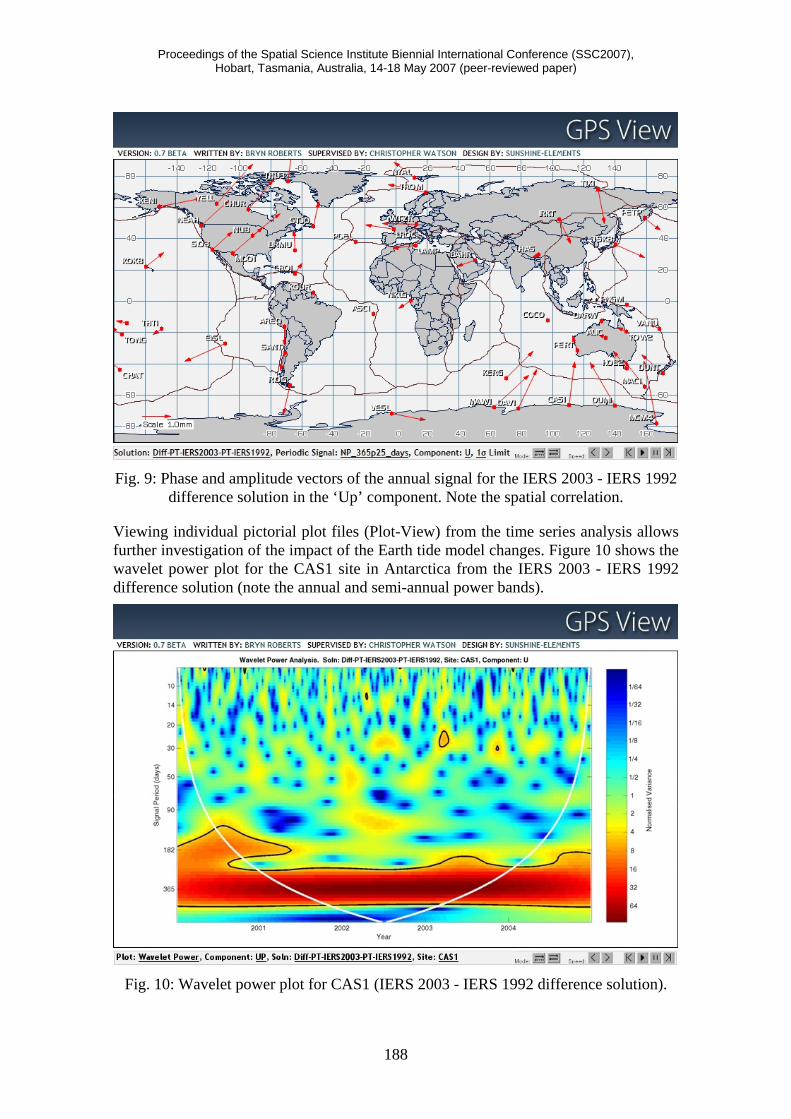
The Watson et al. (2006) study used real data to confirm the theoretical predictions made by Penna and Stewart (2003) and Stewart et al. (2005), i.e., that unmodeled, sub-daily periodic signals can propagate into time series at very low frequencies. Specifically, a mis-modelled diurnal signal introduced a spurious signal within the time series with an annual period. Given the potential for such a signal to mask geophysical signals of interest, Watson et al. (2006) investigated the spatial variability of the annual term. Within GPS-View, this visualisation is simplified considerably. Using the Map-View interface, the primary solution is set to the IERS 2003 - IERS 1992 difference analysis (designated PT-IERS2003-PT-IERS1992 in this case). The periodic term relating to an annual frequency is selected for the vertical component. The map in the output window then displays the amplitude and phase data (Figure 9) which shows a clear latitudinal and longitudinal dependence.

Proceedings of the Spatial Science Institute Biennial International Conference (SSC2007), Hobart, Tasmania, Australia, 14-18 May 2007 (peer-reviewed paper)

188

Fig. 9: Phase and amplitude vectors of the annual signal for the IERS 2003 - IERS 1992

difference solution in the ‘Up’ component. Note the spatial correlation.

Viewing individual pictorial plot files (Plot-View) from the time series analysis allows further investigation of the impact of the Earth tide model changes. Figure 10 shows the wavelet power plot for the CAS1 site in Antarctica from the IERS 2003 - IERS 1992 difference solution (note the annual and semi-annual power bands).

Fig. 10: Wavelet power plot for CAS1 (IERS 2003 - IERS 1992 difference solution).

Proceedings of the Spatial Science Institute Biennial International Conference (SSC2007), Hobart, Tasmania, Australia, 14-18 May 2007 (peer-reviewed paper)

189

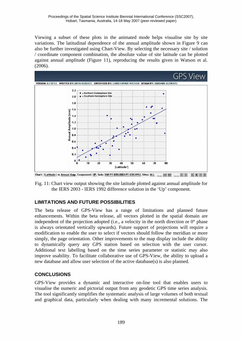
Viewing a subset of these plots in the animated mode helps visualise site by site variations. The latitudinal dependence of the annual amplitude shown in Figure 9 can also be further investigated using Chart-View. By selecting the necessary site / solution / coordinate component combination, the absolute value of site latitude can be plotted against annual amplitude (Figure 11), reproducing the results given in Watson et al. (2006).

Fig. 11: Chart view output showing the site latitude plotted against annual amplitude for

the IERS 2003 - IERS 1992 difference solution in the ‘Up’ component.

LIMITATIONS AND FUTURE POSSIBILITIES The beta release of GPS-View has a range of limitations and planned future enhancements. Within the beta release, all vectors plotted in the spatial domain are independent of the projection adopted (i.e., a velocity in the north direction or 0° phase is always orientated vertically upwards). Future support of projections will require a modification to enable the user to select if vectors should follow the meridian or more simply, the page orientation. Other improvements to the map display include the ability to dynamically query any GPS station based on selection with the user cursor. Additional text labelling based on the time series parameter or statistic may also improve usability. To facilitate collaborative use of GPS-View, the ability to upload a new database and allow user selection of the active database(s) is also planned.

CONCLUSIONS GPS-View provides a dynamic and interactive on-line tool that enables users to visualise the numeric and pictorial output from any geodetic GPS time series analysis. The tool significantly simplifies the systematic analysis of large volumes of both textual and graphical data, particularly when dealing with many incremental solutions. The

Proceedings of the Spatial Science Institute Biennial International Conference (SSC2007), Hobart, Tasmania, Australia, 14-18 May 2007 (peer-reviewed paper)

190

ability to animate results such as pictorial plot files or map views of a given time series parameter or statistic provides a powerful exploratory tool. Further development of GPS-View should augment these existing functionalities, providing an effective tool for geodetic GPS analysis and quality assurance processes within the geodetic community.

Readers wishing to view a beta release version of the software are directed to follow the links to the author’s website under staff at http://www.utas.edu.au/spatial/.

ACKNOWLEDGEMENTS Aslak Grinsted is thanked for the use of his wavelet coherence package used in this paper (http://www.pol.ac.uk/home/research/waveletcoherence/). We wish to thank the online MapServer community for answering several technical questions. Two anonymous reviewers are thanked for their reviews of this manuscript.

REFERENCES Altamimi, Z., Sillard, P., and Boucher, C. (2002). "ITRF2000: A New Release of the

International Terrestrial Reference Frame for Earth Science Applications." Journal of Geophysical Research B: Solid Earth, 107(10).

Blewitt, G., Lavalee, D., Clarke, P., and Nurutdinov, K. (2001). "A New Global Mode of Earth Deformation: Seasonal Cycle Detected." Science, 294(5550), pp2342-2345.

Boehm, J., Werl, B., and Schuh, H. (2006). "Troposphere Mapping Functions for GPS and Very Long Baseline Interferometry from European Centre for Medium-Range Weather Forecasts Operational Analysis Data." Journal of Geophysical Research-Solid Earth, 111(B2).

Dong, D. (2005). "Quasi-Observation Calculation Analysis (QOCA), Version 1.3" Jet Propulsion Laboratory, California, Available at: http://gipsy.jpl.nasa.gov/qoca/.

GSI (2006). "Crustal Movement in Japan: Map Viewer." Geographical Survey Institute, Japan, Available at: http://mekira.gsi.go.jp/ENGLISH/index.html.

Herring, T. (1999). "Geodetic Applications of GPS." Proceedings of the IEEE, 87(1), pp92-110.

Herring, T. (2003). "Matlab Tools for Viewing GPS Velocities and Time Series." GPS Solutions, 7(3), pp194-199.

Keller, W. (2004). "Wavelets in Geodesy and Geodynamics." Walter de Gruyter, Berlin, 279pp.

MapServer (2006). "Mapserver, Version 4.8.4." University of Minnesota, Minnesota, Available at: http://mapserver.gis.umn.edu/.

Morgan, P., Bock, Y., Coleman, R., Feng, P., Garrard, D., Johnston, G. M., Luton, G., McDowall, B., Pearse, M., Rizos, C., and Tiesler, R. (1996). "A Zero Order GPS Network for the Australian Region." Unisurv S-46, University of New South Wales, School of Geomatic Engineering, Sydney, 187pp.

Penna, N. T., and Stewart, M. P. (2003). "Aliased Tidal Signatures in Continuous GPS Height Time Series." Geophysical Research Letters, 30(23).

Penna, N. T., King, M., and Stewart, M. P. (2006). "GPS Height Time Series: Short Period Origins of Spurious Long Period Signals." Journal of Geophysical Research, in press.

Proceedings of the Spatial Science Institute Biennial International Conference (SSC2007), Hobart, Tasmania, Australia, 14-18 May 2007 (peer-reviewed paper)

191

SOPAC (2006). "Scripps Online Mapping Interface (SOMI), Version 4." Scripps Orbit and Permanent Array Center, University of California, San Diego, Available at: http://sopac.ucsd.edu/cgi-bin/dbMapserver.cgi?service=array&topic=scign.

Stewart, M.P., Penna, N.T. and Lichti, D.D. (2005). “Investigating the propagation mechanism of unmodelled systematic errors on coordinate time series estimated using least squares”, Journal of Geodesy, 79(8), 479–489.

Tregoning, P., Morgan, P., and Coleman, R. (2004). "The Effect of Receiver Firmware Upgrades on GPS Vertical Timeseries." Cahiers du Centre Européen de Géodynamique et de Séismologie, 23, pp37-46.

Tregoning, P., and van Dam, T. (2005). "Atmospheric Pressure Loading Corrections Applied to GPS Data at the Observation Level." Geophysical Research Letters, 32(22).

Urschl, C., Dach, R., Hugentobler, U., Schaer, S., and Beutler, G. (2005). "Validating Ocean Tide Loading Models Using GPS." Journal of Geodesy, 78(10), pp616-625.

Watson, C. S. (2005). "Satellite Altimeter Calibration and Validation Using GPS Buoy Technology." Thesis for Doctor of Philosophy, University of Tasmania, Hobart, Australia, 264pp. Available: http://adt.lib.utas.edu.au/public/adt-TU20060110.152656/.

Watson, C., Tregoning, P., and Coleman, R. (2006). "Impact of Solid Earth Tide Models on GPS Coordinate and Tropospheric Time Series." Geophysical Research Letters, 33(8).

Williams, S. (2005). "Create and Analyse Time Series (CATS), Version 3.1.1." Proudman Oceanogrpahic Laboratory, United Kingdom, Available at: http://www.pol.ac.uk/home/staff/WillSimo_cats.html.