An Intrinsic Framework for Analysis of Facial Surfaces

Noname manuscript No.(will be inserted by the editor)

An Intrinsic Framework for Analysis of Facial Surfaces

Chafik Samir1, Anuj Srivastava2, Mohamed Daoudi1, Eric Klassen3

1 GET/Telecom Lille1, LIFL (UMR USTL/CNRS 8022), France2 Department of Statistics, Florida State University, Tallahassee, FL 32306, USA3 Department of Mathematics, Florida State University, Tallahassee, FL 32306, USA

The date of receipt and acceptance will be inserted by the editor

Abstract A quantitative analysis of shapes of facial surfaces can play an important role inbiometric authentication. The main difficulty in comparing shapes of surfaces is the lack of acanonical system to represent all surfaces. This paper overcomes that problem by proposinga specific coordinate system, on facial surfaces, that enables comparisons of geometries offaces. In this system, a facial surface is represented as a path on the space of closed curves,called facial curves, where each curve is a level curve of distance function from the tip of thenose. Defining H to be the space of paths on the space of closed curves, the paper studies thedifferential geometry of H and endows it with a Riemannian. Using numerical techniques,it computes geodesic paths between elements of H that represent individual facial surfaces.This Riemannian analysis of faces is then used to: (i) find an optimal deformation fromone face to another, (ii) define and compute an average face for a given set of faces, and(iii) compute distances between faces to quantify differences in their shapes. Experimentalresults are presented to demonstrate and support these ideas.

1 Introduction

There has been an increasing interest in recent years in analyzing shapes of 3D objects.Advances in shape estimation algorithms, 3D scanning technology, hardware-accelerated3D graphics, and related tools, are enabling access to high quality 3D data. As technologiescontinue to improve, the need for automated methods for analyzing shapes of 3D objects willalso grow. In terms of characterizing 3D objects, for detection, classification, and recognition,their shape is naturally an important feature. It already plays important roles in areas suchas medical diagnostics, object designs, database search, and biometrics. Focusing on thelast topic, our goal in this paper is to develop a framework for analyzing shapes of facialsurfaces. Shape analysis involves computing metrics and “optimal deformations” betweenany two given objects in a manner that is invariant to certain similarity transformations.Typically, similarity transformations consists of the (rigid) translations and rotations, andthe (non-rigid) uniform scalings of the objects involved. For the problem of shape analysisof facial surfaces, we have chosen the similarity group to consist only of translations androtations; changes in scale of a facial surface will change the resulting deformations and themetrics. Restating our goals, we want to develop a mathematical framework for representingand comparing shapes of facial surfaces using metrics that are invariant to rotations and

2 Chafik Samir et al.

translations. In this process, we will also define and compute optimal deformations of facialsurfaces, from one into another. Our mathematical representations of surfaces will be suchthat the ensuing face comparisons are stable with respect to deformations of facial surfacesthat occur during changes in facial expressions. This is an important advantage of thisrepresentation, especially when it is used for recognizing people using shapes of their facialsurfaces.

What is the main difficulty in comparing shapes of two surfaces? Shape analysis shouldideally be invariant to the choice of parameterizations, i.e. one should get the same compar-ison irrespective of parametrization of the two surfaces. To highlight this issue, consider theproblem of analyzing shapes of curves in R

n. In this case, there is a fixed ordering of pointsalong the curves which helps us in parameterizing them (even though the parametrizationis not unique). Therefore, one directly works with the parameterized curves and developsmetrics that are invariant to re-parameterizations. For instance, if the curves are assumedto be parameterized by s ∈ [0, 1], then the space of automorphisms of [0, 1] can be iden-tified with the space of all possible re-parameterizations of curves. (An automorphism isa smooth, invertible map from a set to itself.) So, one seeks a method to compare shapesof any two curves that is invariant to re-parametrization of one or both curves. Althoughseemingly difficult, this issue has been resolved by several authors [15,11,10,12,16,21]. Thekey idea is that there exists an efficient computational solution, namely the dynamic pro-gramming algorithm, that can find the optimal re-parametrization for matching any twocurves, at arbitrarily fine samplings. Returning to the problem of comparing facial surfaces,this problem is made difficult by the fact that there is no natural ordering of points ona surface. Therefore, the space of all possible re-parameterizations of a surface is a largerset, i.e. the automorphisms of [0, 1]2, and an efficient analysis of shapes that is invariantto all re-parameterizations remains elusive. As explained later, our solution is to impose anatural hierarchy (or ordering) of points on a surface, using the idea of facial curves. Thisadditional structure results in dividing the re-parameterizations into two smaller sets, eachconsisting of automorphisms of [0, 1], each of which is relatively easier to solve using dynamicprogramming.

1.1 Current Approaches

– 3D Face Analysis: There has been a number of papers in recent years in 3D shapematching. A common theme in this literature has been to represent facial surfaces bycertain feature sets that are geometrical, such as the convex parts, areas with highcurvatures, saddle points, etc [3], [2]. Although such feature definitions are intuitivelymeaningful, the computation of curvatures involves numerical approximation of secondderivatives and is very susceptible to observation noise. Other approaches, such as thosebased on shape distribution [13] and conformal geometry [19], have also been proposed.Most of those works compare 3D shapes by comparing some corresponding features whileour goal is to compare the facial surfaces themselves. One exception is Glaunes et al. [5]where the authors have studied diffeomorphic matching of a given pair of distributions(of points) in a general setting, with applications to various matching problems includingcurves, surfaces, and unlabeled points-sets.

– Shape Analysis of Curves: There has been a significant amount of research in ana-lyzing shapes of open and closed curves, especially in a plane [15,11,10,12,16,21]. Thecommon theme has been to represent an infinite-dimensional moduli space of curves,with curves being represented in one of many possible ways, and to study the differen-tial geometry of this space modulo the space of re-parameterizations. In case of closedcurves, one uses an additional constraint to ensure closure; this results in the set of rele-vant curves being a nonlinear sub-manifold inside a larger Hilbert space. To compare any

An Intrinsic Framework for Analysis of Facial Surfaces 3

two curves, one imposes a Riemannian structure on the quotient space, and computesgeodesic paths under the chosen metric. The choice of a metric is important and differentauthors have advocated different metrics.

– Facial Surfaces Using Facial Curves: An important line of work in face analysishas been to use shapes of curves that lie on facial surfaces. Similar ideas have beenpursued in brain surface analysis: shapes of sulcal curves have been used to study shapesof brain surfaces [8]. Curves on surfaces are usually defined using level sets of functionson these surfaces. For example, one can use the curvature tensor on a surface to obtainparabolic and ridge curves [6], or use surface gradients to extract crest lines[20]. However,computations of gradients and curvatures both involve higher order derivatives and, asmentioned above, are numerically unstable. In an attractive approach, Bronstein et al. [1]use a surface distance function to define level curves that are invariant to rigid motions.In [14], Samir et al. suggested the use of level sets of the height function (z coordinates) ascurves of interest for face analysis. For comparing shapes of two facial surfaces, the basicidea is to extract level curves of the height function on each surface and to comparethe corresponding curves using techniques from planar shape analysis [10]. Althoughthe resulting metrics were reasonably successful in recognizing faces, there are somefundamental limitations with this representation. Firstly, the definition of level curveschanges with the global orientation of a face and, therefore, this shape analysis is notcompletely invariant to rotation. Secondly, this work was intended for face recognitiononly and not for a Riemannian analysis of facial surfaces. In other words, it lacked aformal definition of a space of facial surfaces and a proper Riemannian structure thatcan lead to formal geodesic paths (or optimal deformations) between faces. Consequently,interesting statistical quantities such as the mean face are neither defined nor computed.

1.2 Our Approach

Our approach is to represent facial surfaces as an indexed collection of closed curves onfaces, termed facial curves, and to apply tools from shape analysis of curves. This paper isan extension of the framework introduced in [14] in two ways: (i) the representations,metrics, and analysis is now completely invariant to rigid rotations and translations of thefacial surfaces, and (ii) there is a formal Riemannian analysis on space representing facialsurfaces, with precise mathematical definitions for spaces, metrics, geodesics, and statisticsof facial surfaces. The representation of a facial surface is based on facial curves, as in [14],but the definition of facial curves is now different. Facial curves are defined here as levelcurves of a surface distance function. This function, at a point on the surface, is defined tobe the length of the shortest path between that point and a fixed reference point (taken tobe the tip of the nose) along the facial surface. Shapes of level curves of this function areinvariant to rotation and translation of the facial surface. Visually these curves seem to befull of facial features that can prove to be important in face classification and recognition.Bronstein et al. [1] have argued that these level curves are stable with respect to changesin facial expressions and, hence, are useful in classification. These are closed curves in R

3

while the curves used in [14] are planar. An indexed collection of such curves will be used tomathematically represent the corresponding facial surface. Denoting this indexed collectionas a parameterized path on the space of closed curves in R

3, we formalize a mathematicalrepresentation of facial surfaces and focus on the space of all such representations. Choosinga Riemannian metric, we endow this space with a Riemannian structure and derive analgorithm for computing geodesic paths between given facial surfaces on this space. Thistool for computing geodesic is shown to be useful in finding optimal deformations betweenfaces, for registering points of facial surfaces, and for computing “average faces”.


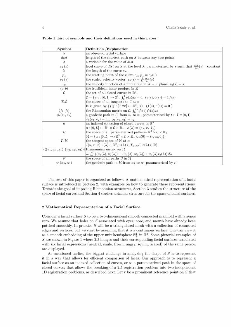
Table 1 List of symbols and their definitions used in this paper.

Symbol Definition /Explanation

S an observed facial surfacedist length of the shortest path on S between any two pointsλ a variable for the value of dist

cλ (s) level curve of dist on S at the level λ, parameterized by s such that dcλ

ds(s) =constant.

lλ the length of the curve cλ.pλ the starting point of the curve cλ, pλ = cλ(0)

vλ (s) the scaled velocity vector, vλ(s) = 1lλ

dcλ

ds(s)

v0 the velocity function of a unit circle in X − Y plane, v0(s) = s

(a, b) the Euclidean inner product in R3

C the set of all closed curves in R3,

C = {v|v : [0, 1] 7→ S2,∫ 1

0v(s)ds = 0, (v(s), v(s)) = 1, ∀s}

TvC the space of all tangents to C at vIt is given by {f |f : [0, 2π] 7→ R

3, ∀s, (f(s), v(s)) = 0 }

〈f1, f2〉 the Riemannian metric on C,∫ 2π

0f1(s)f2(s)ds

φt(v1, v2) a geodesic path in C, from v1 to v2, parameterized by t ∈ I ≡ [0, 1]φ0(v1, v2) = v1, φ1(v1, v2) = v2

α an indexed collection of closed curves in R3

α : [0, L] 7→ R3 × C × R+, α(λ) = (pλ, vλ, lλ)

H the space of all parameterized paths in R3 × C × R+

H = {α : [0, L] 7→ (R3 × C × R+), α(0) = (r, v0, 0)}TαH the tangent space of H at α

{(u,w, x)|u(λ) ∈ R3, w(λ) ∈ Tα(λ)C, x(λ) ∈ R}

〈〈(u1, w1, x1), (u2, w2, x2)〉〉 Riemannian metric on H

=∫ L

0((u1(λ), u2(λ)) + 〈w1(λ), w2(λ)〉 + x1(λ)x2(λ)) dλ

P the space of all paths β in Hψt(α1, α2) the geodesic path in H from α1 to α2 parameterized by t.

The rest of this paper is organized as follows. A mathematical representation of a facialsurface is introduced in Section 2, with examples on how to generate these representations.Towards the goal of imposing Riemannian structures, Section 3 studies the structure of thespace of facial curves and Section 4 studies a similar structure for the space of facial surfaces.

2 Mathematical Representation of a Facial Surface

Consider a facial surface S to be a two-dimensional smooth connected manifold with a genuszero. We assume that holes on S associated with eyes, nose, and mouth have already beenpatched smoothly. In practice S will be a triangulated mesh with a collection of connectededges and vertices, but we start by assuming that it is a continuous surface. One can view itas a smooth embedding of the upper unit hemisphere S

2+ in R

3. Some pictorial examples ofS are shown in Figure 1 where 2D images and their corresponding facial surfaces associatedwith six facial expressions (neutral, smile, frown, angry, squint, scared) of the same personare displayed.

As mentioned earlier, the biggest challenge in analyzing the shape of S is to representit in a way that allows for efficient comparison of faces. Our approach is to represent afacial surface as an indexed collection of curves, or as a parameterized path in the space ofclosed curves; that allows the breaking of a 2D registration problem into two independent1D registration problems, as described next. Let r be a prominent reference point on S that


Fig. 1 2D images and their corresponding facial surfaces of same person under different facialexpressions: neutral, smile, frown, angry, squint, and scared.

is easily detectable. In this paper, we have chosen r as the tip of the nose. Then, definea function dist to be the surface distance function from r to any point on the facialsurface. In other words, dist(r, q) is the length of the shortest path connecting r and q whilestaying on S. Using this function, one can define facial curves as the level sets of dist:

cλ = {q ∈ S|dist(r, q) = λ} ⊂ S , λ ∈ [0,∞). (1)

For large values of λ, the set cλ can be expected to be empty. On the other hand, for λ = 0,the set cλ is the singleton {r}. For values of λ in between those two extremes, we expect cλ

to capture of certain local geometry of the surface S. So far cλ is just a collection of pointsbut they can be ordered easily and we consider cλ(s) as a parameterized, closed curve thatis parameterized by constant speed over the interval [0, 1], i.e. dcλ

ds(s) = constant. Three sets

of variables describe this curve:

– Initial Position: We will denote the starting point on this curve by pλ ∈ R3, i.e.

cλ(0) = pλ.– Length: Let lλ denote the length of the curve cλ.– Direction function: The unit velocity vector vλ(s) ≡ 1

‖dcλ

ds(s)‖

dcλ

ds(s). Note that vλ(s) ∈

S2.

We will represent the original curve cλ(s) by the triple (pλ, vλ, lλ). For λ = 0, cλ collapsesinto the point r and we will use the convention that c0(s) = (r, v0(s), 0) where v0(s) =[− sin(s) cos(s) 0]′ is the velocity function of a unit circle in the X − Y plane. We willchoose an upper bound L of λ so that cλ for λ ≤ L is a continuous, smooth, closed curve inR

3. This helps in cropping some erroneous and unreliable data at the boundaries.

Next we need to specify the space in which these representations take values. Define aset:

C = {v : [0, 1] 7→ S2|

∫ 1

0

v(s)ds = 0, (v(s), v(s)) = 1, ∀s} .

C is the set of all velocity functions that correspond to constant-speed, closed curves in R3.

For a given triple (p, v, l), one can re-construct the curve using c(τ) = p + l∫ τ

0v(s)ds.

Before we proceed, we illustrate some computational steps needed to extract cλ froma given observation of S. We summarize the extraction and the parametrization of facialcurves in the following algorithm:


Algorithm 1 : Facial curve extraction and parametrization

Given a facial surface S, the cλs are determined as follows:

1- Preprocess the surface according to Section 2.1.2- Calculate dist value on all the vertices of the mesh according to Section 2.2.3- Crop the mesh at dist value L.4- Extract the level set of dist (collection of unordered points) at the level λ ∈ [0, L] according toSection 2.3.5- Order these points and smooth the resulting curve cλ.6- Uniformly resample cλ.7- Compute the tangent vector function vλ(s) and the curve length lλ; and set the parametrizationcλ = (pλ, vλ, lλ).

2.1 Surface Pre-Processing

The extraction part involves several steps to ensure robustness. Firstly, we remove discon-nected parts so that the surface distance function dist is well defined. Secondly, we fill holesby applying a linear interpolation, and then make the meshes regular by fixing the lengthof all edges equal to a standard value, resulting in a Delaunay triangulation. Finally, weincrease the number of vertices while keeping the mesh regular so that the surface is smoothand the resolution is finer. Shown in the top row of Figure 2 is an illustration of prepro-cessing a facial surface. Note that the hole on the nose was filled and the mesh has beenregularized. Shown in the bottom row are examples of refining a non-uniform mesh into adense, uniform mesh.

2.2 Surface Distance Function

Once the facial surface is pre-processed, the tip of the nose can be easily detected. Denotethis point as r ∈ R

3. A surface distance function dist : S → R+ is then defined as the lengthof the shortest path (on S) from r to any vertex q in the mesh. This function has been usedpreviously in many surface matching methods. For instance, Hilaga [7] used this functionto construct a Reeb graph and Bronstein et al. [1] used it to crop facial surfaces at theirboundaries. Several methods have been proposed to compute dist on S; a summary andcomparison of those methods is presented in [18]. We will use the Dijkstra’s algorithm [4]to compute dist that has a computational cost of O(n) with n being the number of verticesin the mesh. The resulting dist is invariant to rigid rotations and translations. As verifiedexperimentally later, it is also relatively robust to the deformations resulting from changesin facial expressions.

2.3 Facial Curves Extraction

For a λ ∈ [0, L], we seek the level set cλ in a given surface S. For practical purposes, wemodify the definition of cλ to consist of all the points whose distance dist from r is in[λ−δ, λ+δ], where δ is a pre-determined error value. A smaller value of δ ensures continuityand smoothness of the extracted curves. Shown in Figure 3 are examples of extracted facialcurves corresponding to two different value of δ, the left picture is for a larger δ while theright one is for a smaller δ. Figure 4 shows more examples of extracted facial curves. Thetop row shows some facial curves drawn on the facial surface while the bottom row showsincreasing number of curves extracted from a facial surface.


(a) (b) (c)

(d) (e) (f) (g)

Fig. 2 (a), (b): An example of facial surface before pre-processing and (c) same surface after pre-processing. (d) A facial surface, (e) its corresponding nonuniform mesh before regularization,(f)uniform mesh after regularization, (g) a part of that mesh enlarged to show uniformity.

Fig. 3 Left: extracted level set on an irregular mesh. Right: an extracted level set on the regularmesh after refinement.

2.4 Representations Using Facial Curves

Now we are ready to state our mathematical representation of a facial surface. Consider apath α : [0, L] 7→ (R3 × C × R+), such that α(λ) = (pλ, vλ, lλ) for λ ∈ [0, L]. Additionally,fix the starting point of α to be (r, v0, 0). Let H be the set of all such paths, i.e.

H = {α : [0, L] 7→ (R3 × C × R+)|α(0) = (r, v0, 0)} . (2)


Fig. 4 Top: An example of facial surface (left), an extracted level set curve drawn on the surface.Bottom: Increasing number of facial curves extracted from the surface in the left panel.

We will represent facial surfaces and analyze them as elements of H. Shown in Figure 5are examples of a facial surface represented using a large number of facial curves. The toppicture shows the original surface S while the bottom row shows a rendering of cλs for anincreasing number of λs as we go from left to right. From an implementation point of view,one has to settle for a finite number of curves in representing S. The actual choice of whichand how many curves are used in the analysis will ultimately depend on the application.

We note the following properties of this representations:

1. Invariance to Rotation and Translation: A good representation of S should beinvariant to translation and rotation of S. The choice of the surface distance functiondist to define facial curves ensures the invariance of level curves cλ. Since α is simply acollection of facial curves cλs, it is also invariant to these transformations.

2. Surface Reconstruction: In representing S by α, have we lost any information aboutS? For an arbitrary point p ∈ S, there exists a λ such that p lies on the curve cλ.Therefore, all points on S are present in α on one level curve or another. The facialcurves cλs are non-overlapping and, hence, no point p is represented twice in α. Thus,each point p is present once and only once in the set α. Therefore, considered as acollection of points S and α are identical. Shown in Figure 5 are some examples of αassociated with several faces. Each face in this figure is of the same person but at differentfacial expression. Can we reconstruct a facial surface using its representation α ∈ H? Toreconstruct, we first generate the Delaunay triangulation of the set of points containedin α and, then, use this triangulation to render a surface. An example is shown in Figure6 which pictorially shows an α or a collection of facial curves (left), the correspondingmesh generated using a delaunay triangulation (middle), and the resulting smooth facialsurface (right).

We have represented facial surfaces as elements of H. The next step is to impose aRiemannian structure on H and to compute geodesic paths between observed facial surfaces.Towards that goal, we first study the differential geometry of C and present algorithms forcomputing geodesics between given facial curves.


Fig. 5 Facial surfaces of the same person under different facial expressions, their correspondentsrepresentations in H.

(a) (b) (c) (d)

Fig. 6 Reconstruction example: (a) an original facial surface, (b) its representation as a large col-lection of curves in H, (c) a dense triangulated mesh formed from curves, and (d) the reconstructedsurface.

3 Riemannian Analysis of Facial Curves

A facial curve defined in the previous section is represented by: (i) a starting point p ∈ R3,

(ii) a velocity function v ∈ C, and (iii) a length l ∈ R+. Given two such facial curves, weaddress the question: How to form a geodesic path between them in an appropriate space ofcurves under a chosen Riemannian metric? While the parts dealing with the starting pointsand the lengths are simple, the main difficulty lies in computing a geodesic path betweenthe velocity functions of the two given curves in C. This exact problem has been solved inKlassen et al. [9], and we will adapt their solution to the study of facial curves. For thebenefit of readers, the main idea behind that approach has been summarized in this section.

To develop a geometric framework for analyzing elements of C, it is important understandits tangent bundle and to impose a Riemannian structure on it. Recall that v(s) ∈ S

2 and,consequently, v is a curve on S

2; a vector f tangent to C at v can also be viewed as a fieldof vectors tangent to S

2 along v. The space of all such tangent vectors, denoted by Tv(C),is given by:

Tv(C) = {f |f : [0, 1] 7→ R3,∀s (f(s) · v(s)) = 0,

∫ 1

0

f(s)ds = 0 } . (3)


To impose a Riemannian structure on C, we will assume the following inner product onTv(C): for f, g ∈ Tv(C),

〈f, g〉 =

∫ 1

0

(f(s) · g(s))ds . (4)

For any two closed curves, denoted by v0 and v1 in C, we are interested in finding ageodesic path between them in C under the metric given in Eqn. 3. This is accomplishedusing a path-straightening approach presented in [9]. The basic idea is to start with any pathφ(t) connecting v0 and v1. That is φ : [0, 1] 7→ C such that φ(0) = v0 and φ(1) = v1. Then,one iteratively “straightens” φ until it achieves a local minimum of the energy:

Ec(φ) ≡1

2

∫ 1

0

⟨

dφ

dt(t),

dφ

dt(t)

⟩

dt , (5)

over all paths from v0 to v1. The iteration is performed using a gradient approach, i.e. up-date φ iteratively in the direction of negative gradient of E till the gradient becomes zero.It has been shown in [17] that a critical point of E is a geodesic on C. Shown in Figure 7 isan example of the geodesic path between two facial curves and the evolution of Ec duringpath straightening.

Remark: One major difference between the framework in [9] and here is that the startingpoint on the individual facial curves are kept fixed here. In [9], the variability due to differentplacements of starting points, on a closed curve, was modeled using the action of unit circleS

1 on C and the geodesics were actually computed in the quotient space C/S1. However, in

the current paper, we use the vertical plane containing the bridge of the nose to determinethe starting points on each facial curve, and we fix them. Hence, the geodesics here arecomputed in C and not in the quotient space C/S

1. In computational terms, this involvesless work than was done to find geodesics in [9].

4 Riemannian Analysis of Faces on H

Next, we describe our approach to construct an ”optimal” deformation from one facial sur-face to another. Since facial surfaces are represented as elements of H, a natural formulationof ”optimal” is to consider the two corresponding elements in H and to construct a geodesicpath connecting them in H. The definition of geodesic is with respect to a Riemannianmetric that measures bending of facial surfaces. To actually compute geodesics, we need tostudy the differential geometry of H and to explain our choice of a Riemannian structureon it. The tangent space of H is given by:

Tα(H) = {(u,w, x)| ∀λ ∈ [0, L], u(λ) ∈ R3, w(λ) ∈ Tvλ

(C), x(λ) ∈ R} , (6)

where Tvλ(C) is as specified in Eqn. 3. H is an infinite non linear manifold, and to impose

a Riemannian structure on it, we define the Riemannian metric as follows:

〈〈(u1, w1, x1), (u2, w2, x2)〉〉 =

∫ L

0

((u1(λ), u2(λ)) + 〈w1(λ), w2(λ)〉 + x1(λ)x2(λ)) dλ . (7)

The inner product on tangent spaces of C is defined in Eqn. 4.Let S0 and S1 be any two given facial surfaces, and α0 and α1 be the correspond-

ing elements in H, respectively. Our goal is to construct a geodesic path Ψ(t) in H, pa-rameterized by time t, such Ψ(0) = α0 and Ψ(1) = α1. For each λ ∈ [0, L], we have


02

46

810

1214

1618

−10

12

3

−1

0

1

0 2 4 6 8 10 12 14 160.91

0.92

0.93

0.94

0.95

0.96

0.97

0.98

02

46

810

1214

1618

−10

12

3

−1.5−1

−0.50

0.5

0 2 4 6 8 10 12 14 150.905

0.91

0.915

0.92

0.925

0.93

0.935

0.94

Fig. 7 The geodesic path between two facial curves c1λ and c2λ, and the corresponding evolution ofthe energy Ec.

αi(λ) = (pi,λ, vi,λ, li,λ) ∈ (R3 × C × R+). For each of the components we compute thegeodesic paths independently by defining:

Ψ(t) = {Ψλ(t), λ ∈ [0, L]}, where Ψλ(t) = (Ψpλ(t), Ψv

λ(t), Ψ lλ(t)) . (8)

Ψλ is the geodesic path between the corresponding facial curves; it is composed of threecomponents. Ψp

λ is the geodesic on the initial position component, Ψvλ is over the shape com-

ponent, and Ψ lλ is over the length component. These individual components are computed

as follows:

1. Shape of Curves: Let Ψvλ(t) be a geodesic path in C, constructed using path straight-

ening [9], such that Ψvλ(0) = v0,λ and Ψv

λ(1) = v1,λ. This is accomplished as described inSection 3.

2. Initial Position: The geodesic path between the starting points p0,λ and p1,λ in R3 is

given by a straight line in R3. That is, Ψp

λ : [0, 1] → R3, t 7→ tp1,λ + (1 − t)p0,λ.

3. Length: The geodesic path between the lengths l0,λ and l1,λ in R is given by a straightline in R

+. That is, Ψ lλ : [0, 1] → R

+, t 7→ tl1,λ + (1 − t)l0,λ.

Proposition 1 The path Ψ defined in Eqn. 8 is a geodesic in H, such that Ψ(0) = α0 and

Ψ(1) = α1.

Proof: For a fixed λ, the three components (Ψpλ , Ψv

λ , Ψ lλ) are individually geodesics in spaces

R3, C, and R+, respectively, by construction. Thus, Ψλ is a geodesic in the product space

with respect to the metric given in Eqn. 7. As shown in Appendix, the full set of suchgeodesics Ψ is a geodesic if each one of Ψλ is a geodesic.

Next, we summarize the main steps required in computation of a geodesic path betweengiven two facial surfaces.

We performed a number of experiments using facial surfaces of same and different personsunder a variety of facial expressions, and studied the resulting geodesic paths. Some examplesare shown in Figures 8 - 11. Figures 8(a),(b) show facial surfaces S1 and S2 of the same


Given two different surfaces S1 and S2, this algorithm summarizes computational steps to constructa geodesic path between their representations in H.

1- Extract level curves c1λ and c2λ, for each λ, using Algorithm 1.2- Represent each surface as an element of H and denote them by α0 and α1, respectively.3- Compute the geodesics Ψλ(t), at each level λ ∈ [0, L], in R × C × R+.4- Combine these geodesic paths to form a path Ψ(t) in H.5- Reconstruct a facial surface for finitely spaced samples of t ∈ [0, 1], using the collection{Ψλ(t), λ ∈ [0, L]}.

person under neutral expression and smiling, respectively. Figure 8(c) shows the geodesicpath between S1 (shown in far left) and S2 (shown in far right). Drawn in between are facialsurfaces denoting equally spaced points along the geodesic path. In terms of the Riemannianmetric chosen, these paths denote the optimal deformations in going from the first face tothe second and the path lengths quantify the amount of deformations. In Figure 9(a), weshow two examples of geodesic paths between facial surfaces of the same people underdifferent facial expressions.In Figure 9(b), we show two examples of geodesic paths betweenfacial surfaces of the same different people. Figures 9(a) show geodesic path between thesame person under different expressions, while the figures 9(c) show geodesic paths betweendifferent persons. Each of the path has been shown from two different views.

To give more details about the deformation of facial surfaces, figures 9(b,d) display a pathof facial surfaces from different viewpoints, it can be shown in 9(b) that strong deformationsare obtained near the mouth that start to be close and then slowly opened during the path.However, the figure 9(d) shows strong deformations near eyes, mouth, nose and chin. Figures10 and 11 show many more examples of these geodesic paths.

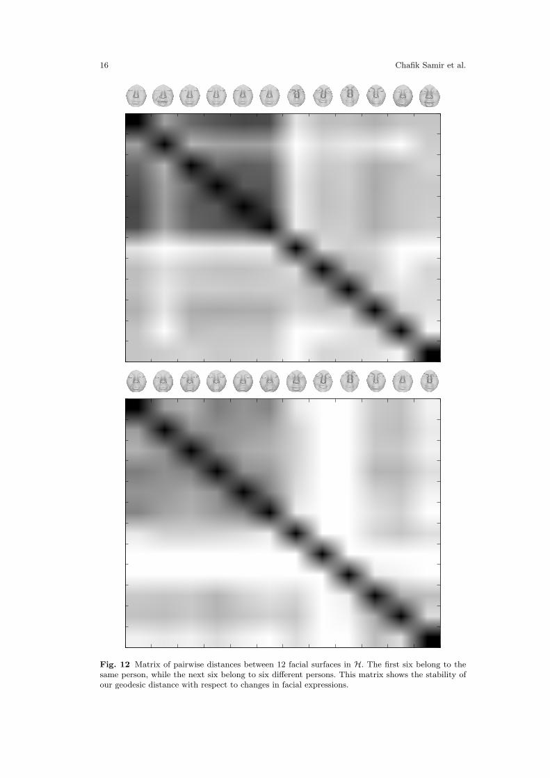
Experiments show that the proposed geodesic distance is relatively stable to changesin facial expressions. That is, the deformation caused by changes in expressions is muchsmaller in terms of the geodesic distances, when compared to the distances between faces ofdifferent people. Shown in Figure ?? are two examples of such experiments. Each of 12× 12the matrix shows pairwise distances between 12 facial surfaces, where the first six belongto the same person (under different expressions) and the next six belong to six differentpersons. The resulting distances are shown as a matrix in Figure ??. In this visualizationof the matrix, the lightness of each element (i; ) is proportional to the magnitude of thedistances between faces i and j. That is, each row and column represent the distances for aface when compared to all 12 faces. Darker elements represent better matches, while lighterelements indicate worse matches. The larger values of distances (lighter elements) involvingthe last six faces confirms that geodesic distances are smaller when the faces of the sameperson are involved.

5 Karcher Means of Facial Surfaces

For future statistical analysis, we are interested in defining a notion of “mean” for a givenset of facial surfaces. The Riemannian structure defined on H enables us to perform suchstatistical analysis for computing faces mean and variance. There are at least two ways ofdefining a mean value for a random variable that takes values on a nonlinear manifold. Thefirst definition, called extrinsic mean, involves embedding the manifold in a larger vectorspace, computing the Euclidean mean in that space, and then projecting it down to themanifold. The other definition, called the intrinsic mean or the Karcher mean utilizes theintrinsic geometry of the manifold to define and compute a mean on that manifold. It isdefined as follows: Let d(Si, Sj) denote the length of the geodesic from Si to Sj in H. To


0 5 10 15 2020

20.5

21

21.5

22

22.5

Number of Iteration

Pat

h E

nerg

y

(a) (b) (d)

(c)

Fig. 8 (a) and (b): Facial surfaces S1 and S2 of the same person under neutral and smile, respec-tively. (c): The geodesic paths between S1 far left and S2 far right; drawn in between are facialsurfaces denoting equally spaced point along this geodesic path. (d): The evolution of the pathenergy as a function of straightening iterations.

calculate the Karcher mean of facial surfaces {S1, ..., Sn} in H, define the variance function:

V : H → R,V(S) =

n∑

i=1

d(Si, Sj)2 (9)

The Karcher mean is then defined by:

S = arg minµ∈H

(V(µ)) (10)

Since H is complete, the intrinsic mean as defined above always exist. However, it may notbe unique, i.e. there may be a set of points in H for which the minimizer of V is obtained.To interpret geometrically, S is an element of H, that has the smallest deformation from allthe given facial shapes.

We present a commonly used algorithm for finding Karcher mean for a given set of facialsurfaces. This algorithm uses the gradient of V, in the space Tµ(H), to update the currentmean µ. If the points {S1, ..., Sn} are clustered fairly close together it has been proven that

Algorithm 2 : Gradient search

Set k = 0. Choose some time increment ǫ ≤ 1n. Choose a point µ0 ∈ H as an initial guess of the

mean. (For example, one could just take µ0 = S1.)

1- For each i = 1, ..., n choose the tangent vector fi ∈ Tµk(H) which is tangent to the geodesic

from µk to Si, and whose norm is equal to the length of this shortest geodesic. The vectorg =

∑i=n

i=1 fi is proportional to the gradient at µk of the function V.2- Flow for time ǫ along the geodesic which starts at µk and has velocity vector g. Call the pointwhere you end up µk+1, i.e. µk+1 = Ψ(µk; ǫ; g).3- Set k = k + 1 and go to step 1.


(a)

(b)

(c)

(d)

Fig. 9 Geodesic Paths between: (a) same person under different facial expressions, viewed fromdifferent viewpoints in (b). Different persons in (c) viewed from different viewpoints in (d).

the Karcher mean exists, is unique, and can be found by the above algorithm.

An example of using Karcher mean to compute the average face is shown in Figure 14.Here the sample set consists of six facial surfaces of the same person under different facialexpressions, and the mean face is shown in the far right panel. We have magnified the displayof Karcher mean to study the features retained by this surfaces from the original set. Figure15 shows the Karcher mean face for six facial surfaces of different persons. Note that thefacial surfaces of the same person, under different facial expressions, which are close to eachother in terms of geodesic distances, are quite close to their Karcher mean. For a clusteringor an identification purposes, they could be accurately been represented by their Karchermean. However, the Karcher mean of faces of different people is far, in term of geodesicdistance, to each of the faces, and appears to be a blurred version of the individual faces.


Fig. 10 Geodesic Paths between facial surfaces of same people under different expressions.

Fig. 11 Geodesic Paths between facial surfaces of different people.


Fig. 12 Matrix of pairwise distances between 12 facial surfaces in H. The first six belong to thesame person, while the next six belong to six different persons. This matrix shows the stability ofour geodesic distance with respect to changes in facial expressions.


Fig. 13 The same person, at each row, under six facial expressions in the left panel, and thecorresponding Karcher mean in the right panel.

Fig. 14 Karcher mean (far right) for the six different people in the left panel.

18

6 Summary

In this paper we introduce a new computational framework for analyzing shapes of facialsurfaces. The basic idea is to impose a specific coordinate system on facial surfaces usinglevel curves of the surface distance function (measured from the tip of nose). Then, eachsurface can be represented as a path on the space of closed curves in R

3. We focus on the setof such paths and impose a Riemannian metric on it for defining geodesic paths. The maintool presented in this paper is the construction of geodesic paths between arbitrary two facialsurfaces in the aforementioned set. There are multiple uses of this geodesic construction. Thelength of a geodesic between any two facial surfaces quantifies differences in their shapes;it also provides an optimal deformation from one to the other. Using Riemannian structureone can define simple statistics such as the sample mean, as is demonstrated for facialsurfaces in this paper. A future application of this framework is in biometrics, for examplein recognition of humans using shapes of their facial surfaces.

The central idea here is to decompose a surface into an indexed collection of closed curvesand to compute geodesics between the corresponding curves on two faces. This geodesic iscomputed using the idea of path-straightening present in [9] which allows only the bending(and not stretching/compressing) of curves. There are other metrics and methods in theliterature for computing geodesics between closed curves. An important idea is the use ofelastic curves where the curves are allowed to stretch and compress for computing geodesicpaths [12]. In future we propose to apply the framework of elastic curves to analyze facialcurves; it requires extending the notion of elastic curves to curves in R

3.

Appendices

Let C be a Riemannian manifold. Denote by I the unit interval [0, 1]. Denote by F the spaceof measurable functions [0, L] → C. F is a manifold; its tangent space is understood asfollows. If α ∈ F , then

TαF ={

w : [0, L] → TC : ∀λ ∈ [0, L], w(λ) ∈ Tα(λ)C}

Clearly, this is just the set of first-order deformations of α ∈ F . We now make F into aRiemannian manifold. If w1, w2 ∈ TαF , define

〈w1, w2〉 =

∫ L

0

〈w1(λ), w2(λ)〉 dλ

Theorem 1 Suppose we are given a path in F represented as φ : [0, L] × I → F . For each

λ ∈ [0, L], define φλ : I → C by φλ(t) = φ(λ, t). Then φ is a geodesic in F if ∀λ ∈ [0, L], φλ

is a geodesic in C.

Proof:

First, we review a useful characterization of geodesics in C. Suppose v0 and v1 are two pointsin C. Let B denote the space of all paths in C, parameterized by I, which start at v0 andend at v1:

B = {γ : I → C | γ(0) = v0 and γ(1) = v1} .

Define an energy functional E : B → R by

E(γ) ≡1

2

∫ 1

0

〈γ′(t), γ′(t)〉 dt,

19

Then, γ is a geodesic in C, connecting v0 and v1, if and only if the gradient of E with respectto γ is zero. In other words, γ is a critical point of the energy function E [17].

Now suppose that φ : [0, L] × I × (−ǫ, ǫ) → C is an arbitrary variation of φ in the spaceof curves in F , i.e., we are assuming that for all λ ∈ [0, L] and t ∈ I, φ(λ, t, 0) = φ(λ, t) andfor all λ ∈ [0, L] and h ∈ (−ǫ, ǫ), φ(λ, 0, h) = φ(λ, 0) and φ(λ, 1, h) = φ(λ, 1). For each valueof h ∈ (−ǫ, ǫ), we calculate the energy of the path φ(., ., h) in F as follows:

E(φ(., ., h)) =1

2

∫ 1

0

∫ L

0

⟨

∂φ

∂t(λ, t, h) ,

∂φ

∂t(λ, t, h)

⟩

dλdt

=1

2

∫ L

0

∫ 1

0

⟨

∂φ

∂t(λ, t, h) ,

∂φ

∂t(λ, t, h)

⟩

dtdλ

Differentiating with respect to h at h = 0 gives:

d

dhh=0E(φ(., ., h)) =

1

2

∫ L

0

d

dhh=0

(

∫ 1

0

⟨

∂φ

∂t(λ, t, h) ,

∂φ

∂t(λ, t, h)

⟩

dt

)

dλ

If we assume that φλ is a geodesic in C for every λ ∈ [0, L], then it follows immediately thatthe function we are integrating over [0, L] in the right hand side of the above expression is0 for every λ, proving that φ is a geodesic in F .

References

1. A. M. Bronstein, M.M. Bronstein, and R. Kimmel. Three-dimensional face recognition. Inter-national Journal of Computer Vision, 64(1):5–30, 2005.

2. K. I. Chang, K. W. Bowyer, and P. J. Flynn. An evaluation of multimodal 2D+3D facebiometrics. IEEE Trans. Pattern Anal. Mach. Intell., 27(4):619–624, 2005.

3. K. I. Chang, K. W. Bowyer, and P. J. Flynn. Multiple nose region matching for 3D facerecognition under varying facial expression. IEEE Pattern Transactions on Pattern Analysisand Machine Intelligence, 28(10):1695– 1700, 2006.

4. E. W. Dijkstra. A note on two problems in connection with graphs. Numerische Mathematik,1959.

5. J. Glaunes, A. Trouve, and L. Younes. Diffeomorphic matching of distributions: A new approachfor unlabelled point-sets and sub-manifolds matching. In CVPR (2), pages 712–718, 2004.

6. P.W. Hallinan, G. Gordon, A. L. Yuille, P. Giblin, and D. Mumford. Two- and Three-Dimensional Patterns of Face. A. K. Peters, 1999.

7. M. Hilaga, S. T. Kohmura, and T. L. Kunii. Topology matching for fully automatic similarityestimation of 3d shapes. In ACM SIGGRAPH, Annual Conference Series, page 203212, 2001.

8. N. Khaneja, M. I. Miller, and U. Grenander. Dynamic programming generation of curves onbrain surfaces. IEEE Transactions on Pattern Analysis and Machine Intelligence, 20(11):1260–1265, 1998.

9. E. Klassen and A. Srivastava. Geodesic between 3D closed curves using path straightening .In European Conference on Computer Vision (ECCV), page ??, 2006.

10. E. Klassen, A. Srivastava, W. Mio, and S. Joshi. Analysis of planar shapes using geodesic pathson shape spaces. IEEE Patt. Analysis and Machine Intell., 26(3):372–383, March, 2004.

11. P. W. Michor and D. Mumford. Riemannian geometries on spaces of plane curves. Journal ofthe European Mathematical Society, 8:1–48, 2006.

12. W. Mio, A. Srivastava, and S. Joshi. On shape of plane elastic curves. International Journalof Computer Vision, 73(3):307 – 324, July 2007.

13. R. Osada, T. Funkhouser, B. Chazells, and D. Dobkin. Matching 3D models with shape dis-tributions. In IEEE Shape Modeling International, May 2001.

14. C. Samir, A. Srivastava, and M. Daoudi. Three-dimensional face recognition using shapes offacial curves. IEEE Trans. Pattern Anal. Mach. Intell., 28(11):1847–1857, 2006.

20

15. T. B. Sebastian, P. N. Klein, and B. B. Kimia. On aligning curves. IEEE Transactions onPattern Analysis and Machine Intelligence, 25(1):116–125, 2003.

16. J. Shah. An H2 type riemannian metric on the space of planar curves. In Workshop on theMathematical Foundations of Computational Anatomy, MICCAI2006, October, 2006.

17. Michael Spivak. A Comprehensive Introduction to Differential Geometry, Vol I & II. Publishor Perish, Inc., Berkeley, 1979.

18. V. Surazhsky, T. Surazhsky, D. Kirsanov, S. Gortler, and H. Hoppe. Fast exact and approximategeodesics on meshes. In ACM SIGGRAPH, pages 553–560, 2005.

19. S. Wang, Y. Wang, M. Jin, Xianfeng Gu, and Dimitris Samaras. 3D surface matching andrecognition using conformal geometry. In CVPR (2), pages 2453–2460, 2006.

20. S. Yoshizawa, A. G. Belyaev, and H.-P. Seidel. Fast and robust detection of crest lines onmeshes. In Proc. of ACM Symposium on Solid and Physical Modeling, pages 227–232, 2005.

21. L. Younes. Computable elastic distance between shapes. SIAM Journal of Applied Mathematics,58:565–586, 1998.

An Intrinsic Framework for Analysis of Facial Surfaces

Documents

Transcript of An Intrinsic Framework for Analysis of Facial Surfaces