Nembhard, Ferrier, Oswald, and Sanz-Uribe (2002) 1

AN INTEGRATED MODEL FOR STATISTICAL AND VISION

MONITORING IN MANUFACTURING TRANSITIONS

Harriet Black Nembhard* Dept. of Industrial Engineering

University of Wisconsin-Madison 1513 University Ave. Madison WI 53706

Office: 608-265-9776 Fax: 608-262-8454

Email: hbnem@engr.wisc.edu *corresponding author

Nicola J. Ferrier Dept. of Mechanical Engineering University of Wisconsin-Madison

1513 University Ave. Madison WI 53706

Office: 608-265-8793 Email: ferrier@engr.wisc.edu

Tim A. Osswald

Dept. of Mechanical Engineering University of Wisconsin-Madison

1513 University Ave. Madison WI 53706

Office: (608) 263-9538 Email: osswald@engr.wisc.edu

Juan R. Sanz-Uribe

Dept. of Mechanical Engineering University of Wisconsin-Madison

1513 University Ave. Madison WI 53706

Office: (608) 265-2405 Email: jrsanzuribe@students.wisc.edu

July 2002

To appear in Quality and Reliability Engineering International

Nembhard, Ferrier, Oswald, and Sanz-Uribe (2002) 2

SUMMARY

Manufacturing transitions have been increasing due to higher pressures for product

variety. One dimension of this variety is color. A major quality control challenge is to

regulate the color by capturing data on color in real-time during the operation and to use

it to assess the opportunities for good parts. Control charting, when applied to a stable

state process, is an effective monitoring tool to continuously check for process shifts or

upsets. However, the presence of transition events can impede the normal performance of

a traditional control chart. In this paper, we present an integrated model for statistical and

vision monitoring using a tracking signal to determine the start of the transition and a

confirmation signal to ensure that any process oscillation has concluded. We also

developed an Automated Color Analysis and Forecasting System (ACAFS) that we can

adjust and calibrate to implement this methodology in different production processes. We

use a color transition process in plastic extrusion to illustrate a transition event and

demonstrate our proposed methodology.

KEY WORDS: Statistical Process Control; Tracking Signal; EWMA; Color Transition;

Image Processing; Polymer Processing; Extrusion.

Nembhard, Ferrier, Oswald, and Sanz-Uribe (2002) 3

1 INTRODUCTION AND MOTIVATION

Increased product variety is one of the major reasons that many manufacturing

organizations have shifted to move to a make-to-order production policy. One outcome of

this policy is an increase in the number of scheduled manufacturing transition events,

such as product grade change, recipe change, and raw material change. For example, in

recent years, the plastic industry has witnessed an increase in the demand of more

diversified and customized products. This industry is concerned with converting polymer

materials into usable plastic products, from simple to complex shapes and of different

colors and sizes. Injection molding and extrusion are the two most common plastic

processing methods. Customers are more concerned with surface quality and outward

appearance of the plastic parts than ever before.

Color has become an important aesthetic element of quality to plastic

manufacturers. Accordingly, plastic products are usually made in various colors to appeal

to the consumers. The attending problem is to regulate the color by capturing data on

color in real-time during the operation. Automated measurement of color is, however, a

difficult problem in that the data (an image) requires processing to measure the desired

information (color). In the computer vision, the perception of color is difficult because

the color measured by the sensor can vary greatly. The ambient light sources (e.g.,

infrared energy present in nature daylight, fluorescent light, and incandescent light) and

other energy sources can affect the sensed color. (Monet painted the same scene at

different times of day and in different weather conditions. The scenes, in terms of the raw

Nembhard, Ferrier, Oswald, and Sanz-Uribe (2002) 4

colors used to paint them, are dramatically different, while the scene content is identical

for all images.)

In addition to the usual color constancy problem, the color of the extruded

polymer varies based on thickness and temperature. As the polymer cools, the color

changes and the color intensity varies with thickness, especially while the polymer is hot.

Furthermore, a change in the plastic resin color will tend to produce a period of mixed-

colored parts due to mixing with the previous colored resin residuals. In other words, a

transient period is expected before the plastic parts fully assumed the new targeted color,

and hence the parts do not conform to specifications.

During a transition, the output process necessarily moves from one constant level

to another. Statistical process control (SPC) techniques in the form of control charts are

normally applied to these processes at different constant levels to identify quality

improvement opportunities. The SPC methods are reasonable under the assumptions that

the process mean is constant and the observations are independent. The observations can

be modeled by

tty εµ += (1)

where µ is the process mean and tε is an independent and identically distributed (iid)

random variable. For processes that follow Equation (1), the traditional Shewhart charts

and even the cumulative sum (CUSUM) chart or the exponentially weighted moving

average (EWMA) chart are appropriate SPC tools.

Nembhard, Ferrier, Oswald, and Sanz-Uribe (2002) 5

The presence of autocorrelation, however, will violate the independence

assumption of the traditional control chart. Autocorrelation means that consecutive

measurements of an output characteristic will be directly related to the previous ones.

This is a common consequence of processes that are driven by inertia and frequent

sampling (e.g., see [1]). Alwan [2] investigates the impact of autocorrelated data on the

traditional Shewhart chart and reported an increased number of false alarms. There are

also circumstances in which the process does not reach the new desired operating level

instantaneously as a result of these scheduled process transitions. Instead an induced

transient period, i.e., a dynamic but temporary trend that is inherent to the process, exists

such that the production is impeded and that the normal operation of control charts

applied prior to the transition also suffers with increased false alarms.

In quality engineering, there has been a resurgence of research activity on process

monitoring and control (e.g., see [3], [4], and [5]). For the specific problem of process

transitions, Nembhard and Mastrangelo [6] and Nembhard, Mastrangelo, and Kao [7]

proposed an integrated process control (IPC) technique that combines engineering

process control (EPC) and SPC on noisy dynamic systems. Nembhard and Kao [8] (NK)

develop a statistical methodology to recognize when the transition event has ended. That

work uses a sign test to continuously track the “change of slope” on a tracking signal

statistic as a means of detecting when the transient period is over. The tracking signal

statistic is commonly used to monitor the quality of a forecasting system. The NK

methodology is meant to supplement the SPC application – forecast-based EWMA and

Shewhart chart of the forecast errors for autocorrelated data that has been operating on

the process prior to the transition.

Nembhard, Ferrier, Oswald, and Sanz-Uribe (2002) 6

In this paper, we present an integrated model for statistical and vision monitoring.

We extend the NK methodology in two ways. First, we use the tracking signal to also

determine the start of the transition. (In their earlier work, NK assume that the start is

known to the user and only the end need be determined.) We recognized here that

particularly for a color target in automatic processing system, the start of the transition

may not necessarily be known (i.e., there may be an unknown delay time between when

color pellets are added to the system and when the new color appears in the product).

Secondly, we design a confirmation signal to ensure that the recognized starting and

ending points of the transition also coincides with the conclusion of any oscillation that

may be present. A further contribution of this work is the development of an Automated

Color Analysis and Forecasting System (ACAFS) that we can adjust and calibrate to

implement this technology in different production processes.

Manufacturing application of the proposed methodology could potentially reduce

the dollar and product losses due to transitions. It provides a holistic approach that

acknowledges transition monitoring as well as color image processing. Although we

employ a plastic manufacturing process as a context for illustration, we note that there are

other areas where statistical modeling and vision recognition for transitions may be

advantageous. For example, in a fabric web application, the web must be pleated

precisely between two colors without color “bleed-over.” Another practical application is

when temperature transitions are monitored with optical pyrometers.

The remainder of this paper is organized as follows. In Section 2, we discuss the

specifics of the research issues associated with the color transition problem and our

experimental design for collecting data. In Section 3, we discuss our development of the

Nembhard, Ferrier, Oswald, and Sanz-Uribe (2002) 7

automated color analysis and forecasting system (ACAFS) and present the signal test

designs that comprise the integrated statistical and vision methodology as well as the

tracking methodology. We demonstrate and evaluate the performance of our proposed

methodology in Section 4. We conclude the paper in Section 5.

2 RESEARCH ISSUES AND APPROACH

The residence time distribution (RTD) of a polymer is typically used to give a picture of

how the polymer will behave and progress through the equipment (e.g., extruder). The

RTD is a function of the temperature, the extruder speed, and the ratio of the polymer

components (e.g., a 50-50 blend versus a 75-25 blend of polystyrene and high density

polyethylene). Given this distribution, the analyst can start to get a theoretical estimate of

how long a particular transition may take to complete. In practice, however, a “margin of

safety” is often added to this estimate and that quantity of polymer is often dumped or

scrapped. This waste may be especially significant when it is necessary to switch

products several times during a shift. One source of motivation for our work is that an on-

line determination of the start and end of the transition can avoid this waste. Such an on-

line approach, however, will require the collection of observational data. In general, when

observational data are taken in discrete time order, autocorrelation is usually present.

During transitions, we must also address the dynamic behavior in the process. And for

color transitions, we must address the image collection and processing issues. In this

section, we first provide a description of the experimental setup, followed by a

description of the color transition event and explanation of the data collection.

Nembhard, Ferrier, Oswald, and Sanz-Uribe (2002) 8

2.1 Experimental Setup

An extrusion process is used here to demonstrate the transient phenomenon due to

a color transition and to address the process monitoring problems. This process is

commonly used to manufacture plastic products that are infinite in one direction - for

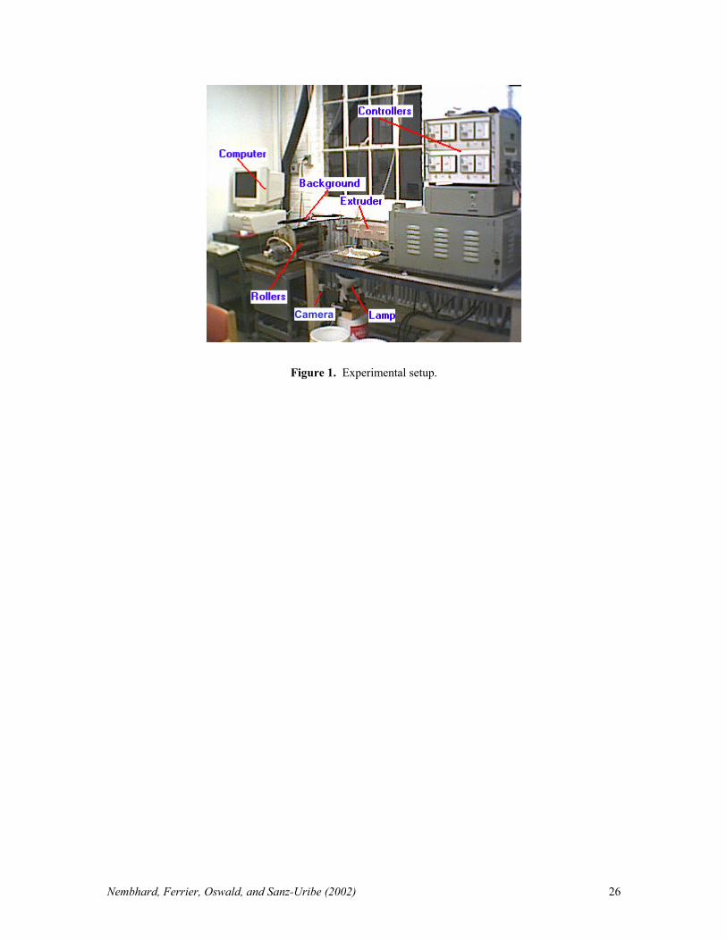
instance, wires, cables, tubes, pipes and films. Our experiments were conducted using a

laboratory scale single-screw extruder (Figure 1). The single-screw extruder used in our

experimentation is made by C. W. Brabender, with a screw diameter of 19.05 mm (3/4”)

and a length to diameter (L/D) ratio of 25:1. A slit die is attached to the end of the

extruder to form a strip of HDPE tape. We also use a CCD camera, a microcomputer with

a frame grabber to convert camera output to digital format, a 22 Watt fluorescent lamp

for illumination, a set of rollers to pull the extruded product, and a black-fabric

background panel.

There are four temperature control zones covering the barrel sections and the die

section. High-density polyethylene (HDPE) resin is used as the extrudate material. The

major processing parameters are the screw speed and barrel temperature profile. The

temperature zones 1 through 4 are set at 170, 180, 190, and 200 ºC respectively. The

screw speed is a controlled variable. The screw speeds used in the different color

transitions are 40 and 60 rpm. To color the resin red, blue and yellow colorants are used

to mix with the raw material at a 25:1 ratio.

[insert Figure 1 here]

Nembhard, Ferrier, Oswald, and Sanz-Uribe (2002) 9

2.2 Color Transition in Plastic Extrusion

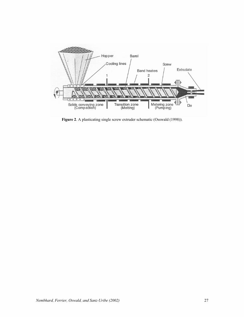
During extrusion, polymer pellets are first transformed into flowable melt by a

plasticating extruder. The plastic melt is then pushed through a metal die that

continuously shapes the melt into a desired profile. Osswald’s [9] schematic of a

plasticating single screw extruder is shown in Figure 2.

A change in the plastic resin color will tend to produce a period of mixed-colored

parts due to mixing with the previous colored resin residuals. A plasticating extruder is

typically divided into three main zones, namely, the solids conveying zone, transition

zone, and metering zone. As the name suggests, the solids conveying zone carries the

polymer pellets from the hopper to the screw channel. The polymer pellets are then

melted when advanced into the transition zone. Finally, the polymer melt is homogenized

and pumped into the die section through the metering zone.

To achieve a color transition during the extrusion of HDPE tape, the following

changeover strategy is applied. Prepare two 200g batches of raw material mixed with 8g

of colorant each. Run the machine with 200g of colorless HDPE to remove previous

materials and colors. Add the first colored mixture just when the colorless HDPE reaches

the feed throat. Add the second mixture once the first mixture reaches the feed throat.

During the processing of the color transition event, a molten strip of the HDPE extrudate

is continuously pushed out from the slit die.

[insert figure 2 here]

Nembhard, Ferrier, Oswald, and Sanz-Uribe (2002) 10

2.3 Data Collection

As the strip of HDPE appears, we collect an image of the strip at predetermined intervals

and process that image to establish a numerical value of its color. The red, green, blue

(RGB) system of color representation is perhaps most common. However, in order to

work with a single variable, we focus on using the hue as the color metric. Ideally, hue is

invariant to changes in lighting. In practice, as the intensity of the color darkens, the

reliability of a vision system to extract hue decreases (i.e., as the intensity decreases

( 0≈v ) then hue becomes undefined). The relationship between the RGB system and the

hue, saturation, and value (which is sometimes referred to as intensity or luminance)

(HSV) system is given by Equations (2a), (2b) and (2c):

3bgrv ++

= (2a)

[ ]

[ ][ ]

[ ]

>

−−+−

−+−−

≤

−−+−

−+−

=

−

−

vg

vbfor

bgbrgr

brgr

vg

vbfor

bgbrgr

brgr

h

,))(()(

)()(21

cos211

,))(()(

)()(21

cos21

21

2

1

21

2

1

π

π

(2b)

{ }bgrbgr

s ,,min31++

−= (2c)

where r is red, g is green, b is blue, h is hue, s is saturation, and v is value (derivations are

given in Gonzalez and Woods [10]). These formulae assume that both measurements are

normalized, i.e., 1,,0 ≤≤ bgr and 1,,0 ≤≤ vsh or 255,,0 ≤≤ bgr and

Nembhard, Ferrier, Oswald, and Sanz-Uribe (2002) 11

255,,0 ≤≤ vsh . Notice that if gbr == then the hue, h, is undefined, and if 0=v , then

s is also undefined.

3. INTEGRATED STATISTICAL AND VISION METHODOLOGY

In this section we discuss the proposed methodology for obtaining color data on-line and

tracking the transition process. To implement the proposed methodology, we developed a

program, called the automated color analysis and forecasting system (ACAFS), which

executes an integrated statistical and vision methodology, as shown in Figure 3. In this

program, we start by asking if a new color has been added in order to direct our color

data toward the transition analysis or toward the Shewhart chart (steady state). In this

research project we focus only in the transition analysis, which is the left hand flow path

of the flow diagram shown in Figure 3. The first part of this section describes the vision

methodology used in this research. The second part presents the forecast-based EWMA

statistic. The third part defines the tracking signal statistic leading to the computation of

the sign test.

3.1 Vision Methodology

The ACAFS is a C++ program developed to capture images of the polymer in

predetermined intervals or sample time, convert that image to a measurement of hue, and

statistically forecast the next observation.

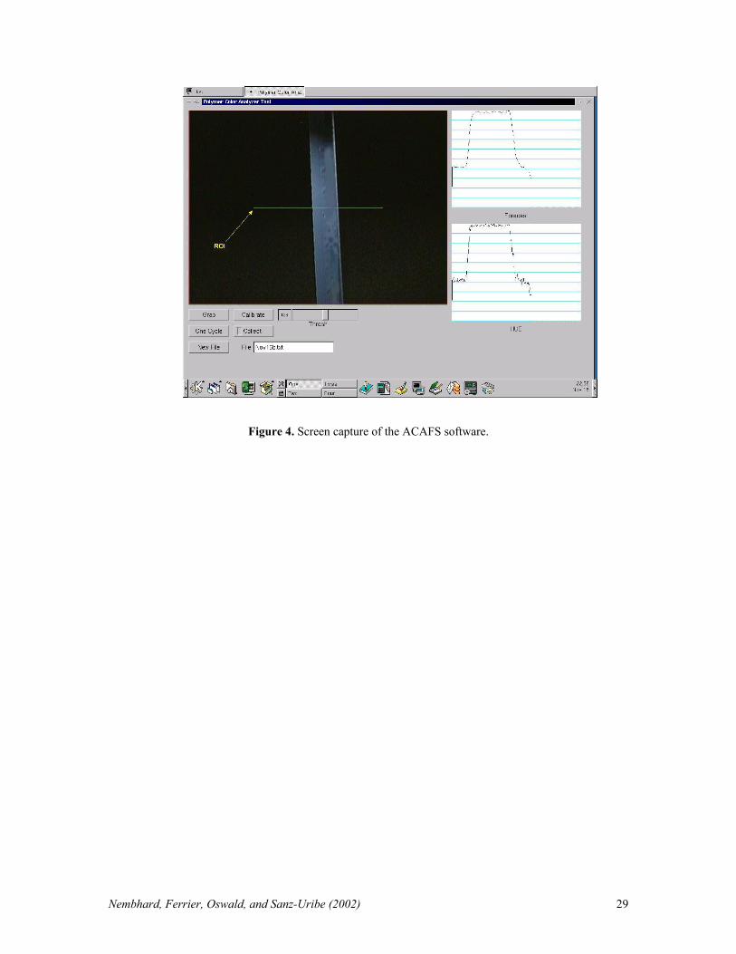
Figure 4 shows a screen capture of the ACAFS program while acquiring color

data in real time. In this figure, a 480 x 640-pixel image is shown as it is captured by the

CCD camera, with a 5 x 320 pixel region of interest (ROI) that can be dragged with the

mouse to a preferred position. The program takes color data only from the ROI every

Nembhard, Ferrier, Oswald, and Sanz-Uribe (2002) 12

sample time and reduces the original array to a 1 x 160-pixel array to facilitate the

analysis. As the camera and driver acquire color information in the RGB color

representation, the program converts the data to the HSV color representation by using

Equations (2a), (2b), and (2c).

Because the extrudate tape width is smaller than the ROI length, the program has

a subroutine that eliminates the background information determining the two edges of the

tape by making a threshold at 75 for the variable value ( 2550 ≤≤ v ). Figure 5 shows a

typical graph of intensity of v along the ROI. In this example, the information of interest

is for ROI values between 78 and 114 and the information between 0 and 77 and between

115 and 160 is considered background.

[insert figure 4 here]

[insert figure 5 here]

At each sampling time, once the tape edges are obtained, the program averages

the variable hue (h) within these two limits. This mean value is used to forecast h

following the forecast-based EWMA and tracking signal methodologies explained below.

3.2 Forecast-based EWMA

The EWMA chart was first suggested by Roberts [11]. In the SPC community, the

EWMA control chart is known for its ability to detect small process shifts more

effectively than the traditional Shewhart charts (e.g., see [12] and [13]). The EWMA

statistic is defined as

Nembhard, Ferrier, Oswald, and Sanz-Uribe (2002) 13

1)1( −−+= ttt zyz λλ (3)

where zt is the new value of the variable of interest, λ is the smoothing constant that

varies between 0 and 1, yt is the output and zt-1 is the input. The typical values for λ are

between 0.05 and 0.25 in SPC applications.

The EWMA also has a long history in forecasting and inventory control (see [14]

and [15]). It is well known in time series modeling and analysis that the EWMA with

θλ −= 1 is the optimal one-step ahead forecast of the integrated moving average

IMA(1,1) nonstationary time series model with parameter θ ([16]). Suppose )1(ˆ ty is the

one-step-ahead forecast made at the end of period t for the future observation 1+ty , then

tt zy =)1(ˆ . So the value of EWMA in Equation (3) calculated at time t is in fact the

optimal forecast. Hunter [17] advocates the use of EWMA and demonstrates the ease of

charting the EWMA scheme when viewed as the forecast of the next observation.

In order to deal with the autocorrelated data, several authors have suggested a

forecast-based monitoring procedure including Berthouex, Hunter, and Pallesen [18],

Alwan and Roberts [19], Harris and Ross [20], and Montgomery and Mastrangelo [21].

The forecast-based approach involves the following two steps: (1) identify and fit an

appropriate time series model to the process data and plot a run chart of the fitted values

and (2) apply traditional control charts to the one-step-ahead forecast errors or residuals.

The sequence of residuals is defined as

)1(ˆ 1−−= ttt yye . (4)

Nembhard, Ferrier, Oswald, and Sanz-Uribe (2002) 14

Lin and Adams [22] suggest using a combination of EWMA and Shewhart control charts

on the forecast errors for better average run length (ARL) performance. Adams and

Tseng [23] also investigate the robustness of the forecast-based monitoring procedures.

The EWMA forecast is in many cases a good approximation of the exact time-series

forecast (e.g., see [17] and [24]).

As the process of a transition event develops, the process data can either progress

up or down depending on the new target level. In event of a trend, the current EWMA

forecast accuracy tends to deteriorate resulting in a sudden increase in the forecast errors.

In fact, the EWMA tends to follow the data and will lag behind a linear trend

Montgomery and Mastrangelo [21]. Nevertheless, the EWMA scheme will improve in

accuracy once the process begins to level off. In due course, the tracking signal statistic

can be exploited to provide a signal on when the beginning and end of the transient

period has been reached.

3.3 Tracking Signal Methodology

In forecasting analysis, forecast errors are often used to assess the accuracy of a

forecasting system. Normally, we would desire a forecasting system to produce forecast

errors that are close to zero. The tracking signal is the usual form of statistic that draws

information from the forecast errors to monitor a forecasting system (e.g., see [15] and

[25]). Mastrangelo and Montgomery [26] proposed supplementing the tracking signals on

the moving centerline EWMA control chart for efficient process shift detection. A

tracking signal measures the deviation of the estimated forecast error from zero relative

Nembhard, Ferrier, Oswald, and Sanz-Uribe (2002) 15

to the variation of this statistic. Large deviations suggest that the performance of the

forecasting system has deteriorated and that the underlying form of the time series has

changed.

There are two forms of tracking signals: cumulative error tracking signal (CETS)

and smoothed error tracking signal (SETS) ([27]). This research project focuses only in

the SETS because in previous work it has shown better performance for this application

due to its high sensitivity to the most recent forecast errors ([8]).

The SETS statistic is the absolute value of the fraction given by the weighted sum

of all past one-step-ahead forecast errors, )1(tQ , divided by the standard deviation of the

one-step-ahead forecast errors, t∆̂

t

tt

QS∆

= ˆ)1( (5)

where )1(tQ is given by

)1()1()1()1( 1−−+= ttt QeQ αα (6)

and standard deviation of the one-step-ahead forecast error is estimated using the mean

absolute deviation (MAD) given by

1ˆ)1(|)1(|ˆ

−∆−+=∆ ttt e αα (7)

Nembhard, Ferrier, Oswald, and Sanz-Uribe (2002) 16

in the above equations α is the smoothing constant, 0 < α < 1, with different value for

each variable. For the MAD α is chosen between 0.05 and 0.15. The rationale behind this

statistic is to give more weight to the recent forecast errors than older ones by applying

the exponential smoothing concept.

In order to provide a statistical signal for the end of a transient period as the transition

process develops, we have devised an empirical method involving a sign test that

identifies a “change in the slope” on the tracking signals. Such a test procedure is

analogous to the first derivative test for finding the local maximum points of a continuous

differentiable function. For discrete-time application, the first derivative translates into

the first finite difference. The purpose here is to “track” the change in the tracking signal

statistics. When the forecasts become less accurate due to a trend, the tracking signal

statistic increases. However, the tracking signal statistic tends to decrease once the

forecasts become more accurate again. This characteristic is more prominent for SETS in

that it eventually forgets about the past big errors. To state the matter another way, the

SETS statistic is very sensitive to the most recent forecast errors.

The first finite difference of SETS at time period t is

1−−=∇ ttt SSS (8)

where ∇ is the backward difference operator. Using Equation (8) we can approximate

the end of a transient period as the transition process develops.

The indication that a transition is starting is inverse to the indication that a transition

is finishing. In this case, the first derivative is ideally infinite and can be obtained in

Nembhard, Ferrier, Oswald, and Sanz-Uribe (2002) 17

practice determining the point where is a sudden increase in the slope and continued

upward trend.

In summary, the integration of SPC technique with transition tracking procedure is

best elucidated by the flowchart in Figure 3. Before a transition event, the usual control

chart operates at the current process level. When the new colored material is charged to

the process, the current control chart is no longer useful because the transition is about to

start. At that time the ACAFS software starts acquiring and processing color information

from the process. The program assesses the trend of the slope of the SETS to determine

the transition’s beginning and end. When the transition has started the product is rejected

and when the transition has finished the product is newly accepted.

4 RESULTS AND DISCUSSION

The methodology was evaluated with two double transitions: the Yellow to Red and Red

to Yellow (YRY) transition in one run, and the Blue to Yellow and Yellow to Blue

(BYB) transition in another run.

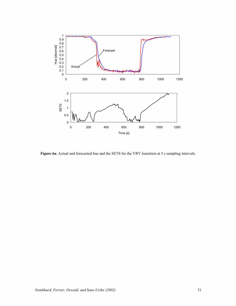
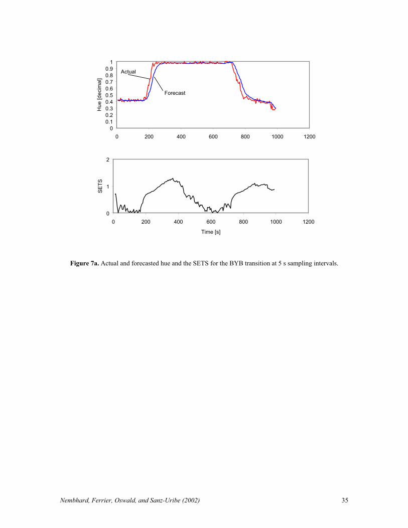
Figures 6 shows the results for hue and SETS in a YRY transition at a 40 rpm screw

speed with observation time intervals of 5 s, 10 s, 15 s, and 20 s. Figure 7 shows the

results for hue and SETS in a BYB transition at the same conditions. All of the graphs

were made using the smoothing constant λ equal to 0.25, the smoothing constant α for

the mean absolute deviation t∆̂ equal to 0.1, and the smoothing constant α for the

weighted sum of all past one-step-ahead forecast errors Qt(1) equal to 0.07. These

settings gave the best results because local maximum points were close to the start and

Nembhard, Ferrier, Oswald, and Sanz-Uribe (2002) 18

end of every transition. These values were obtained after several evaluations by simple

iteration (i.e., changing the values of these smoothing constants within the ranges

expressed in Sections 3.2 and 3.3).

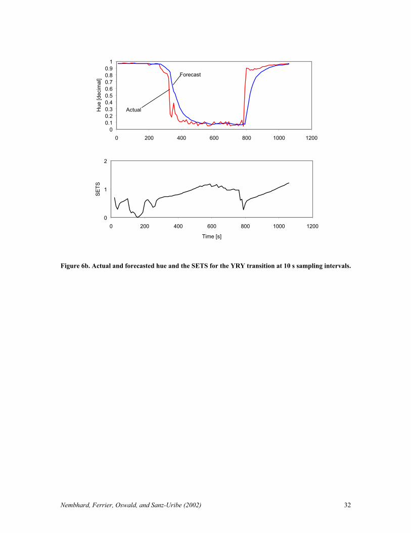
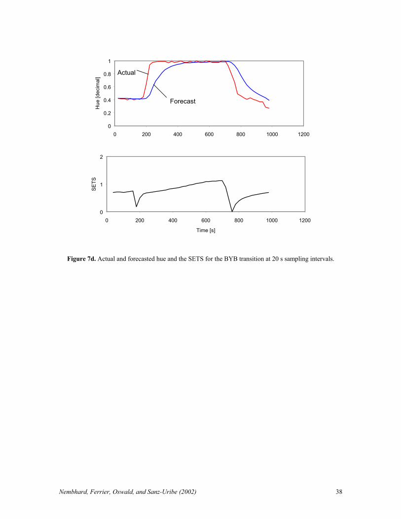
As the transitions in Figures 6a and 7a show, the forecast is close to the actual

data with sample times of 5s. As the sample times increase to 10 s in Figures 6b and 7b,

then to 15 s in Figures 6c and 7c, and finally to 20 s in Figures 6d and 7d, the forecast is

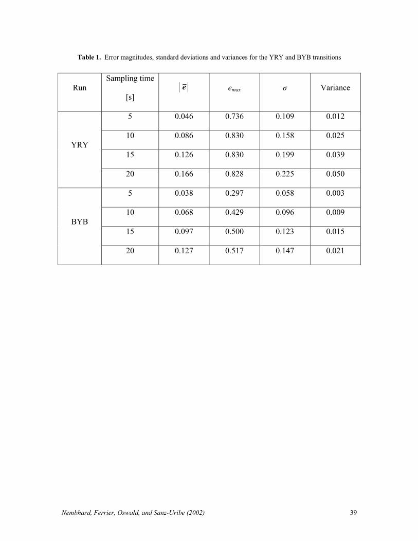
further away from the actual data. The mean magnitude of the errors, maximum errors,

standard deviations and variances for the two double transitions are shown in Table 1.

We can observe that the forecasting errors and the variance in the BYB transition are

lower than those in the YRY transition. We believe the reason for this difference is that

the camera used in the experiment showed its lowest repeatability when working with red

color, probably because of infrared perturbations caused by daylight conditions. This low

repeatability is most likely the source of the higher errors, standard deviations and

variances in the transitions involving red color. Even so, we can obtain smaller errors

when we use smaller time intervals, as we would generally expect in forecasting.

The tradeoff, however, from considering smaller errors is that the SETS is more

oscillatory. Recall that we are looking for the signal regarding the end of the transition

from the SETS. That is, Figure 3 shows that we will accept the product when the

transition has ended. More specifically, we will approximate the end of the transition

according to Equation (8). From this standpoint, we get the clearest signal about the

transition with the larger sample times as shown in Figures 6d and 7d. The YRY

transition starts at 180 s and ends at 820 seconds (Figure 6d). The BRB transition starts at

180 s and ends at 700 s.

Nembhard, Ferrier, Oswald, and Sanz-Uribe (2002) 19

[insert figure 6a here]

[insert figure 6b here]

[insert figure 6c here]

[insert figure 6d here]

[insert figure 7a here]

[insert figure 7b here]

[insert figure 7c here]

[insert figure 7d here]

[insert table 1 here]

Unfortunately, we cannot make such definitive statements at the other sampling

intervals. Even so, we can still discern a certain pattern of increasing slope in the SETS

where we can estimate local maximum and minimum values. Given this observation, in

our future work we may consider filtering methods that could potentially complement or

extend the proposed methodology. Nevertheless, we believe some tradeoff in the decision

of smaller errors versus clearer signal will still be required.

5 CONCLUSION

In this paper, we have presented a methodology that integrates statistical control

and vision monitoring to analyze transitions in a dynamic system. The statistical

component of the proposed methodology is the forecast-based EWMA combined with a

smoothed error tracking signal (SETS) that serves to determine the start and end of every

Nembhard, Ferrier, Oswald, and Sanz-Uribe (2002) 20

transition. The vision component is based on obtaining the transversal hue mean of the

extrudate tape in real time using a camera and software system. We also developed an

Automated Color Analysis and Forecasting System (ACAFS) that we can adjust and

calibrate to implement this methodology in different production processes.

To illustrate the methodology, we used two different color transitions that

occurred in a plastic extrusion process. We found that there was a tradeoff regarding

forecasting errors on the hue and the SETS to signal the transition that was based on the

size of the sampling interval. With larger sampling intervals, the tracking methodology is

very effective determining the point where the transition occurs. As mentioned above,

one aspect of our future work will involve investigating filtering or smoothing

approaches of the inlet signal in order to improve the forecasting and tracking functions

and thus improve the methodology.

On a broader scale, we believe this work to have applications in improving output

quality and reducing the economic and environmental impact of in-process waste. For

example, if our methodology can be applied to a process to reduce the amount of polymer

that is dumped or scrapped after a transition based on a mere guess or safe estimate of the

end of the transition, it could mean significant savings. Therefore, another aspect of our

future work will involve ways of quantifying the potential benefits in industrial

application.

ACKNOWLEDGEMENTS

The authors are grateful for the University of Wisconsin-Madison Graduate School

Awards 135-8090 and 135-8084 that supported our work on this project.

Nembhard, Ferrier, Oswald, and Sanz-Uribe (2002) 21

REFERENCES

[1] Montgomery DC. The use of statistical process control and design of experiments in

product and process improvement. IIE Transactions 1992 24: 4-17.

[2] Alwan LC. Effects of autocorrelation on control chart performance. Communications

in Statistics—Theory and Methods 1992 21: 1025-1049.

[3] MacGregor JF. On-line statistical process control. Chemical Engineering Progress

1988, 21-31.

[4] Vander Wiel SA, Tucker WT, Faltin FW, and Doganaksoy N. Algorithmic statistical

process control: concepts and an application. Technometrics 1992 34: 286-297.

[5] Box GEP and Luceño A. Statistical Control by Monitoring and Feedback Adjustment;

John Wiley & Sons: New York, NY, 1997.

[6] Nembhard HB and Mastrangelo CM. Integrated process control for startup operations.

Journal of Quality Technology 1998 30(3): 201-211.

[7] Nembhard HB, Mastrangelo CM, and Kao, MS. Statistical monitoring performance

for startup operations in a feedback control system. Quality and Reliability Engineering

International 2001 17(5): 379-390.

Nembhard, Ferrier, Oswald, and Sanz-Uribe (2002) 22

[8] Nembhard HB and Kao, M-S. A forecast-based monitoring methodology for process

transitions. Quality and Reliability Engineering International 2001 17(4): 307-321.

[9] Osswald TA. Polymer Processing Fundamentals; Hanser Publishers: Munich, 1998.

[10] Gonzalez RC and Woods R. Digital Image Processing, 3rd Edition; Addison-

Wesley: Reading, MA, 1992.

[11] Roberts SW. Control chart tests based on geometric moving averages.

Technometrics 1959 1: 239-250.

[12] Crowder SV. Design of exponentially weighted moving average schemes. Journal of

Quality Technology 1989 21(2): 155-162.

[13] Lucas JM and Saccucci MS. Exponentially weighted moving average control

schemes: properties and enhancements. Technometrics 1990 32: 1-12.

[14] Muth JF. Optimal properties of exponentially weighted forecasts. Journal of

American Statistical Association 1960 55: 299-306.

[15] Brown RG. Smoothing, Forecasting and Prediction of Discrete-Time Series;

Prentice-Hall, Inc.: Englewood Cliffs, NJ, 1962.

Nembhard, Ferrier, Oswald, and Sanz-Uribe (2002) 23

[16] Box GEP, Jenkins GM and Reinsel GC. Time Series Analysis, Forecasting and

Control, Third Edition; Prentice Hall: Englewood Cliffs, NJ, 1994.

[17] Hunter JS. The exponentially weighted moving average. Journal of Quality

Technology 1986 18: 203-210.

[18] Berthouex PM, Hunter WG and Pallesen L. Monitoring sewage treatment plants:

some quality control aspects. Journal of Quality Technology 1978 10: 139-149.

[19] Alwan, LC and Roberts HV. Time series modeling for statistical process control.

Journal of Business & Economic Statistics 1988 6: 87-95.

[20] Harris TJ and Ross WH. Statistical process control procedures for correlated

observations. Canadian Journal of Chemical Engineering 1991 69: 48-57.

[21] Montgomery DC and Mastrangelo CM. Some statistical process control methods for

autocorrelated data. Journal of Quality Technology 1991 23: 179-193.

[22] Lin WSW and Adams BM. Combined control charts for forecast-based monitoring

schemes. Journal of Quality Technology 1996 28: 289-301.

Nembhard, Ferrier, Oswald, and Sanz-Uribe (2002) 24

[23] Adams BM and Tseng IS. Robustness of forecast-based monitoring schemes.

Journal of Quality Technology 1998 30: 328-339.

[24] Montgomery DC. Introduction to Statistical Quality Control, Third Edition; John

Wiley and Sons: New York, NY, 1997.

[25] Trigg DW. Monitoring a forecasting system. Operational Research Quarterly 1964

15: 271-274.

[26] Mastrangelo CM and Montgomery DC. SPC with correlated observations for the

chemical and process industries. Quality and Reliability Engineering International 1995

11: 78-89.

[27] Montgomery DC, Johnson LA, and Gardiner LS. Forecasting and Time Series

Analysis, Second Edition; McGraw-Hill: New York, NY, 1990.

Nembhard, Ferrier, Oswald, and Sanz-Uribe (2002) 25

AUTHORS’ BIOGRAPHIES

Harriet Black Nembhard is an Assistant Professor of Industrial Engineering at the

University of Wisconsin-Madison. She has previously held manufacturing positions with

Dow Chemical, General Mills, and Pepsi-Cola. Her Ph.D. degree is in Industrial and

Operations Engineering from The University of Michigan. She is a member of ASQ, IIE,

and INFORMS.

Nicola J. Ferrier is an Assistant Professor of Mechanical Engineering at the University

of Wisconsin-Madison. Her research interests include the integration of computer vision

and motion control (robotics), real-time image analysis, dynamic tracking, and active

vision systems. Her Ph.D. degree is from the Division of Applied Sciences at Harvard

University. She is a member of IEEE, SME, and ARVO.

Tim A. Osswald is a Professor of Mechanical Engineering and the Director of the

Polymer Engineering Center at the University of Wisconsin-Madison. He is a member of

PPS, SPE, the Society of Rheology, the German Scientific Alliance of Polymer

Technology Professors and the Deutsche Rheologische Gesellschaft. He is Editor for the

Americas for the Polymer Engineering Journal and the Polymer Manufacturing Editor for

the SME Journals.

Juan R. Sanz-Uribe is a Ph.D. student in the Department of Mechanical Engineering at

the University of Wisconsin-Madison.

Nembhard, Ferrier, Oswald, and Sanz-Uribe (2002) 26

Figure 1. Experimental setup.

Camera

Nembhard, Ferrier, Oswald, and Sanz-Uribe (2002) 27

Figure 2. A plasticating single screw extruder schematic (Osswald (1998)).

Nembhard, Ferrier, Oswald, and Sanz-Uribe (2002) 28

Has the new color been

added?

Capture Image

Eliminate Background

Average Hue: 1

n

ii

t

yy

n==∑

n : Number of pixels of interestyt : Current hue value

1ˆ (1)ty + : Next step forecast

ˆ (1)ty : Previous step forecast

Find one-step-ahead EWMA

1ˆ ˆ(1) (1 ) (1)t tty y yλ λ+ = + −

Obtain Forecast Error ˆ (1)t t te y y= −

Apply the smoothing error tracking signal (1)

ˆt

tt

QS =∆

Has transition started?

Has transition finished?

No Yes

Accept Product

Capture Image

Eliminate Background

Average Hue: 1

n

ii

t

yy

n==∑

Find one-step-ahead EWMA

1ˆ ˆ(1) (1 ) (1)t tty y yλ λ+ = + −

Obtain Forecast Error ˆ (1)t t te y y= −

Shewhart Chart

Yes

No

Figure 3. Flow diagram of the ACAFS software.

Reject productYes

No

Nembhard, Ferrier, Oswald, and Sanz-Uribe (2002) 29

Figure 4. Screen capture of the ACAFS software.

Nembhard, Ferrier, Oswald, and Sanz-Uribe (2002) 30

0

50

100

150

200

250

0 20 40 60 80 100 120 140 160

Position in the ROI

Inte

nsity

of v

(0-2

55)

Threshold

Figure 5. Typical graph for intensity of v in the 0-255 scale.

Nembhard, Ferrier, Oswald, and Sanz-Uribe (2002) 31

00.10.20.30.40.50.60.70.80.9

1

0 200 400 600 800 1000 1200

Hue

[dec

imal

]Forecast

Actual

0

0.5

1

1.5

2

0 200 400 600 800 1000 1200

Time [s]

SETS

Figure 6a. Actual and forecasted hue and the SETS for the YRY transition at 5 s sampling intervals.

Nembhard, Ferrier, Oswald, and Sanz-Uribe (2002) 32

00.10.20.30.40.50.60.70.80.9

1

0 200 400 600 800 1000 1200

Hue

[dec

imal

] Forecast

Actual

0

1

2

0 200 400 600 800 1000 1200

Time [s]

SETS

Figure 6b. Actual and forecasted hue and the SETS for the YRY transition at 10 s sampling intervals.

Nembhard, Ferrier, Oswald, and Sanz-Uribe (2002) 33

0

0.2

0.4

0.6

0.8

1

0 200 400 600 800 1000 1200

Hue

[dec

imal

] Forecast

Actual

0

1

2

0 200 400 600 800 1000 1200

Time [s]

SETS

Figure 6c. Actual and forecasted hue and the SETS for the YRY transition at 15 s sampling intervals.

Nembhard, Ferrier, Oswald, and Sanz-Uribe (2002) 34

00.10.20.30.40.50.60.70.80.9

1

0 200 400 600 800 1000 1200

Hud

e [d

ecim

al]

Forecast

Actual

0

1

2

0 200 400 600 800 1000 1200

Time [s]

SETS

Figure 6d. Actual and forecasted hue and the SETS for the YRY transition at 20 s sampling intervals.

Nembhard, Ferrier, Oswald, and Sanz-Uribe (2002) 35

00.10.20.30.40.50.60.70.80.9

1

0 200 400 600 800 1000 1200

Hue

[dec

imal

]Forecast

Actual

0

1

2

0 200 400 600 800 1000 1200

Time [s]

SETS

Figure 7a. Actual and forecasted hue and the SETS for the BYB transition at 5 s sampling intervals.

Nembhard, Ferrier, Oswald, and Sanz-Uribe (2002) 36

00.10.20.30.40.50.60.70.80.9

1

0 200 400 600 800 1000 1200

Hue

[dec

imal

]Forecast

Actual

0

1

2

0 200 400 600 800 1000 1200

Time [s]

SETS

Figure 7b. Actual and forecasted hue and the SETS for the BYB transition at 10 s sampling intervals.

Nembhard, Ferrier, Oswald, and Sanz-Uribe (2002) 37

00.10.20.30.40.50.60.70.80.9

1

0 200 400 600 800 1000 1200

Hue

[dec

imal

]Forecast

Actual

0

1

2

0 200 400 600 800 1000 1200

Time [s]

SETS

Figure 7c. Actual and forecasted hue and the SETS for the BYB transition at 15 s sampling intervals.

Nembhard, Ferrier, Oswald, and Sanz-Uribe (2002) 38

0

0.2

0.4

0.6

0.8

1

0 200 400 600 800 1000 1200

Hue

[dec

imal

]

Actual

Forecast

0

1

2

0 200 400 600 800 1000 1200

Time [s]

SETS

Figure 7d. Actual and forecasted hue and the SETS for the BYB transition at 20 s sampling intervals.

Nembhard, Ferrier, Oswald, and Sanz-Uribe (2002) 39

Table 1. Error magnitudes, standard deviations and variances for the YRY and BYB transitions

Run Sampling time

[s] e emax σ Variance

5 0.046 0.736 0.109 0.012

10 0.086 0.830 0.158 0.025

15 0.126 0.830 0.199 0.039 YRY

20 0.166 0.828 0.225 0.050

5 0.038 0.297 0.058 0.003

10 0.068 0.429 0.096 0.009

15 0.097 0.500 0.123 0.015 BYB

20 0.127 0.517 0.147 0.021