
A Framework for Parallelizing Hierarchical Clustering Methods
Upload
khangminh22Category
view
3download
0
An Integrated Clustering AnalysisFramework for Heterogeneous Data
Aalaa Mojahed
A thesis submitted for the Degree ofDoctor of Philosophy
University of East AngliaSchool of Computing Sciences
August 26, 2016
c©This copy of the thesis has been supplied on condition that anyone who consults it is understood torecognise that its copyright rests with the author and that no quotation from the thesis, nor any informationderived therefrom, may be published without the author’s prior written consent.

Abstract
Big data is a growing area of research with some important research challenges that mo-
tivate our work. We focus on one such challenge, the variety aspect. First, we introduce
our problem by defining heterogeneous data as data about objects that are described by
different data types, e.g., structured data, text, time-series, images, etc. Through our work
we use five datasets for experimentation: a real dataset of prostate cancer data and four
synthetic dataset that we have created and made them publicly available. Each dataset
covers different combinations of data types that are used to describe objects. Our strategy
for clustering is based on fusion approaches. We compare intermediate and late fusion
schemes. We propose an intermediary fusion approach, Similarity Matrix Fusion (SMF),
where the integration process takes place at the level of calculating similarities. SMF pro-
duces a single distance fusion matrix and two uncertainty expression matrices. We then
propose a clustering algorithm, Hk-medoids, a modified version of the standard k-medoids
algorithm that utilises uncertainty calculations to improve on the clustering performance.
We evaluate our results by comparing them to clustering produced using individual el-
ements and show that the fusion approach produces equal or significantly better results.
Also, we show that there are advantages in utilising the uncertainty information as Hk-
medoids does. In addition, from a theoretical point of view, our proposed Hk-medoids
algorithm has less computation complexity than the popular PAM implementation of the
k-medoids algorithm. Then, we employed late fusion that aggregates the results of clus-
tering by individual elements by combining cluster labels using an object co-occurrence
matrix technique. The final cluster is then derived by a hierarchical clustering algorithm.
We show that intermediate fusion for clustering of heterogeneous data is a feasible and
efficient approach using our proposed Hk-medoids algorithm.
i

Publications and presentations
A copy of all the followings is presented in Appendix D. The main work in all the pub-
lications was conducted by the first author including: proposing solutions, running the
experiments, writing the first draft of the papers, creating the datasets used, analysing
the results, etc. All the others co-authors efforts have enriched the quality of the work
produced.
Publications :
1. We have published a paper [181] titled "A fusion approach to computing dis-
tance for heterogeneous data" accepted in KDIR 2014, the 6th International
Conference in Knowledge Discovery and Information Retrieval which took
place in Rome, Italy between the 21st and the 24th of October 2014. KDIR is
a part of IC3K conferences, the International Joint Conference on Knowledge
Discovery, Knowledge Engineering and Knowledge Management. The con-
ference proceedings are indexed by Citation Index (ISI), INSPEC, DBLP, EI
(Elsevier Index) and Scopus.
2. We have published a paper [183] titled "Applying Clustering Analysis to Het-
erogeneous Data Using Similarity Matrix Fusion (SMF)" as part of MLDM
2015, the 11th International Conference on Machine Learning and Data Min-
ing which took place in Hamburg, Germany between the 20th and the 23ed of
July 2015. The paper was published by Springer Verlag in volume 9166 of the
Lecture Notes in Computer Science series in the book "Machine Learning and
Data Mining in Pattern Recognition" .
ii

iii
3. We have also successfully published a paper [182] titled "An adaptive ver-
sion of k-medoids to deal with the uncertainty in clustering heterogeneous
data using an intermediary fusion approach" as a regular paper in the Inter-
national Journal of Knowledge and Information Systems (KAIS). the paper is
submitted on 07 October 2015, revised on 02 January 2016 and accepted on
28 Februray 2016.
4. We are also at the moment targeting the International Journal of Data Mining
and Knowledge Discovery (DMKD) with a regular paper titled "Clustering
heterogeneous data using fusion".
Presentations :
1. A 20 minutes oral presentation of our paper, "A fusion approach to computing
distance for heterogeneous data", in KDIR 2014.
2. A 30 minutes oral presentation of our paper, "Applying Clustering Analysis
to Heterogeneous Data Using Similarity Matrix Fusion (SMF)", in MLDM
2015.
3. A a poster representation of the research proposal in the CMP Postgraduate
day on the 29th of November 2013 with a research abstract published within
the event’s abstract booklet.
4. A a poster representation of the research progress in the CMP Postgraduate
day on the 31st of October 2014 with a research abstract published within the
event’s abstract booklet.
5. A poster representation of the research in the 8th Saudi Students Conference
which takes place at the hosting university, Imperial College London, UK
between 31st of January and the 1st of February 2015. The research abstract
is published by the Imperial College Press.
6. A a poster representation of the research progress in the CMP Postgraduate
day on the 23ed of October 2015 with a research abstract published within the
event’s abstract booklet.

iv
I dedicate the 3 years effort to the one person who personifies everyone in my life;parents, sisters, brothers, children and friends. I know myself, but you know me more. I
trust myself, but you trust me more. I love myself, but you love me more. I love youdearly my soul-mate and I love our commitment and determination to each other.
It is always you who give me everything I need and it is only you...

Acknowledgements
First and foremost, I would like to express my deep debt of gratitude and greatest appre-
ciation to my supervisor, Dr. Beatriz de la Iglesia, for supervising my graduate study for
three and a half years. I feel blessed to have her as my advisor. She helped me not only
accomplish my dream of becoming a professional in data mining but also develop a more
mature personality. I thank her for every piece of her intensive efforts that have been put
into this research work. I also thank her for introducing me to the field of data mining
at the first place in 2006 when I was a Master student at the UEA in which I found great
interests of doing my PhD in this area.
I would like to thank Dr. Wenja Wang for sharing with me a lot of knowledge in doing
this work. He has been instrumental with Beatriz in finding the topic of this dissertation.
I would also like to recognize his helpful comments and advice in improving the quality
of my work.
I gratefully acknowledge the funding sources that made my Ph.D. work possible. I was
funded by King Abdulaziz University, Jeddah, KSA for my 3 years study period which is
supported in the UK by the Saudi Cultural Bureau in London.
All the love and thanks goes to the best person out there for me, the only and unique
man in my life since I was 14, my sweetheart Bader. He was a marvellous half during the
last 14 years, we are really linked heart to heart. I cannot remember one thing in my life
without him; he is always the light that leads the way. He sacrificed to let me be what I
v

vi
want to be and showed the world how much he loves me and believes in me. You helped
me to achieve my goals as quick as I can to get back to your arms simply by your faith in
me.
My adorable kids, Azoz, Lamar and Aziz, you gave me the most in my life and I owe
you a lot. I cannot imagine my days without you; you are the smile, peace and safe, thank
you. My special hero Azoz, you always stand by me when things look bleak, you inhabit
my heart and I cannot force myself to forget you or stop loving you. If the only place
where I can see you is in my dreams, I will sleep forever. I miss you son. Lamar and
Aziz, you are the reason for the sparkle in my eye, smile on my face and bounce in my
step, I love you.
Also, I am very grateful to my beloved family, parents, sisters and brothers. Their
sincerest love has given me courage to overcome the most difficult times in my way of
pursuing my dream of studying abroad and doing my PhD. Special thanks are due to my
special sisters: Sahar and Nouf. It was their unconditional and consistent care, support
and understanding that helped me sustain. No matter where I go, how old I become, I
will never forget that I owe my childhood to a unique mother, Sahar, who was and still is
my backbone. Nouf, we both are so varied yet alike, so diverse yet so unified, at different
places yet always by each others side. All I can say is I love you both.
Last but not least, special thanks due to my studying mate, Abdurrahman. He shares
with me the long cold and disparate nights until the sun shines again. I appreciate your
patience, support and love.
Thank you all

Contents
Acknowledgements v
List of Figures x
List of Tables xiii
1 Introduction 11.1 Background and motivation . . . . . . . . . . . . . . . . . . . . . . . . . 1
1.2 Research hypothesis . . . . . . . . . . . . . . . . . . . . . . . . . . . . . 3
1.3 Research objectives . . . . . . . . . . . . . . . . . . . . . . . . . . . . . 4
1.4 Research limitations and boundaries . . . . . . . . . . . . . . . . . . . . 5
1.5 Research contributions . . . . . . . . . . . . . . . . . . . . . . . . . . . 6
1.6 Thesis structure . . . . . . . . . . . . . . . . . . . . . . . . . . . . . . . 7
2 The Task of Clustering in Data Mining 82.1 Introduction to clustering . . . . . . . . . . . . . . . . . . . . . . . . . . 8
2.2 Distance measures . . . . . . . . . . . . . . . . . . . . . . . . . . . . . 11
2.2.1 Types of distance measures . . . . . . . . . . . . . . . . . . . . . 13
2.2.2 Weaknesses of existing distance measures . . . . . . . . . . . . 25
2.2.3 Selecting distance measures . . . . . . . . . . . . . . . . . . . . 25
2.3 Cluster analysis . . . . . . . . . . . . . . . . . . . . . . . . . . . . . . . 27
2.3.1 Notation definitions . . . . . . . . . . . . . . . . . . . . . . . . . 27
2.3.2 Clustering solutions . . . . . . . . . . . . . . . . . . . . . . . . 29
2.3.3 Number of clusters . . . . . . . . . . . . . . . . . . . . . . . . . 31
2.4 Clustering algorithms . . . . . . . . . . . . . . . . . . . . . . . . . . . . 35
2.4.1 Classification of clustering algorithms . . . . . . . . . . . . . . . 35
2.4.2 Representation of clusters . . . . . . . . . . . . . . . . . . . . . 45
vii

CONTENTS viii
2.4.3 Overview on existing clustering algorithms . . . . . . . . . . . . 46
2.5 Evaluation of clustering solutions . . . . . . . . . . . . . . . . . . . . . . 47
2.5.1 Internal validation methods . . . . . . . . . . . . . . . . . . . . . 50
2.5.2 External validation methods . . . . . . . . . . . . . . . . . . . . 56
2.5.3 Relative validation methods . . . . . . . . . . . . . . . . . . . . 58
2.6 Cluster ensemble . . . . . . . . . . . . . . . . . . . . . . . . . . . . . . 60
2.6.1 Generation mechanism . . . . . . . . . . . . . . . . . . . . . . . 61
2.6.2 Consensus function . . . . . . . . . . . . . . . . . . . . . . . . . 63
2.7 Chapter summary . . . . . . . . . . . . . . . . . . . . . . . . . . . . . . 65
3 Clustering Framework for Heterogeneous Data 663.1 Introduction to Heterogeneous data definition . . . . . . . . . . . . . . . 66
3.2 Defining heterogeneous data . . . . . . . . . . . . . . . . . . . . . . . . 69
3.3 Problem statement . . . . . . . . . . . . . . . . . . . . . . . . . . . . . 71
3.4 Related work on clustering heterogeneous data . . . . . . . . . . . . . . 77
3.5 Proposed methodology for applying cluster analysis to heterogeneous data 80
3.5.1 The intermediate fusion approach . . . . . . . . . . . . . . . . . 81
3.5.2 The proposed Hk-medoids clustering . . . . . . . . . . . . . . . 87
3.5.3 The late fusion approach . . . . . . . . . . . . . . . . . . . . . . 92
3.6 Validating the proposed clustering framework for heterogeneous data . . . 98
3.7 The sets of heterogeneous data used to validate the proposed methodology 99
3.7.1 The cancer dataset . . . . . . . . . . . . . . . . . . . . . . . . . 100
3.7.2 The plants dataset . . . . . . . . . . . . . . . . . . . . . . . . . . 104
3.7.3 The journals dataset . . . . . . . . . . . . . . . . . . . . . . . . 106
3.7.4 The papers dataset . . . . . . . . . . . . . . . . . . . . . . . . . 109
3.8 The celebrities dataset . . . . . . . . . . . . . . . . . . . . . . . . . . . . 110
3.9 Chapter summary . . . . . . . . . . . . . . . . . . . . . . . . . . . . . . 112
4 Results of applying the similarity matrix fusion 1134.1 Experimental set up . . . . . . . . . . . . . . . . . . . . . . . . . . . . . 113
4.2 Computing DMs . . . . . . . . . . . . . . . . . . . . . . . . . . . . . . 118
4.3 The results of the cancer dataset . . . . . . . . . . . . . . . . . . . . . . 119
4.3.1 A worked example of the SMF approach . . . . . . . . . . . . . 119
4.3.2 DMs and FM calculation results . . . . . . . . . . . . . . . . . . 121

CONTENTS ix
4.3.3 Clustering results . . . . . . . . . . . . . . . . . . . . . . . . . . 126
4.3.4 Statistical testing . . . . . . . . . . . . . . . . . . . . . . . . . . 133
4.4 The results of the plants dataset . . . . . . . . . . . . . . . . . . . . . . . 136
4.4.1 DMs and FM calculation results . . . . . . . . . . . . . . . . . . 136
4.4.2 Clustering results . . . . . . . . . . . . . . . . . . . . . . . . . . 141
4.4.3 Statistical testing . . . . . . . . . . . . . . . . . . . . . . . . . . 145
4.5 The results of the journals dataset . . . . . . . . . . . . . . . . . . . . . 147
4.5.1 DMs and FM calculation results . . . . . . . . . . . . . . . . . . 147
4.5.2 Clustering results . . . . . . . . . . . . . . . . . . . . . . . . . . 149
4.5.3 Statistical testing . . . . . . . . . . . . . . . . . . . . . . . . . . 153
4.6 The results of the papers dataset . . . . . . . . . . . . . . . . . . . . . . 155
4.6.1 DMs and FM calculation results . . . . . . . . . . . . . . . . . . 155
4.6.2 Clustering results . . . . . . . . . . . . . . . . . . . . . . . . . . 157
4.6.3 Statistical testing . . . . . . . . . . . . . . . . . . . . . . . . . . 161
4.7 The results of the celebrities dataset . . . . . . . . . . . . . . . . . . . . 162
4.7.1 DMs and FM calculation results . . . . . . . . . . . . . . . . . . 162
4.7.2 Clustering results . . . . . . . . . . . . . . . . . . . . . . . . . . 164
4.7.3 Statistical testing . . . . . . . . . . . . . . . . . . . . . . . . . . 167
4.8 Chapter summary . . . . . . . . . . . . . . . . . . . . . . . . . . . . . . 168
5 Results of applying the Hk-medoids algorithm 1705.1 Experimental set up . . . . . . . . . . . . . . . . . . . . . . . . . . . . . 170
5.2 The results of the cancer dataset . . . . . . . . . . . . . . . . . . . . . . 174
5.3 The results of the plants dataset . . . . . . . . . . . . . . . . . . . . . . . 175
5.4 The results of the journals dataset . . . . . . . . . . . . . . . . . . . . . 178
5.5 The results of the papers dataset . . . . . . . . . . . . . . . . . . . . . . 180
5.6 The results of the celebrities dataset . . . . . . . . . . . . . . . . . . . . 181
5.7 Time complexity of Hk-medoids . . . . . . . . . . . . . . . . . . . . . . 183
5.7.1 Time complexity of Hk-medoids . . . . . . . . . . . . . . . . . . 183
5.7.2 Thresholds parameter sensitivity . . . . . . . . . . . . . . . . . . 186
5.8 Chapter summary . . . . . . . . . . . . . . . . . . . . . . . . . . . . . . 188
6 Clustering heterogeneous data using late fusion 1906.1 Experimental set up . . . . . . . . . . . . . . . . . . . . . . . . . . . . . 190

CONTENTS x
6.2 The results of the cancer dataset . . . . . . . . . . . . . . . . . . . . . . 194
6.3 The results of the plants dataset . . . . . . . . . . . . . . . . . . . . . . . 196
6.4 The results of the journals dataset . . . . . . . . . . . . . . . . . . . . . 200
6.5 The results of the papers dataset . . . . . . . . . . . . . . . . . . . . . . 202
6.6 The results of the celebrities dataset . . . . . . . . . . . . . . . . . . . . 205
6.7 Results evaluation . . . . . . . . . . . . . . . . . . . . . . . . . . . . . . 207
6.8 Chapter summary . . . . . . . . . . . . . . . . . . . . . . . . . . . . . . 210
7 Conclusions and further research 2127.1 Conclusions . . . . . . . . . . . . . . . . . . . . . . . . . . . . . . . . . 212
7.2 Limitations and future work . . . . . . . . . . . . . . . . . . . . . . . . 217
Bibliography 219
Appendices 241
Appendix A: Data Dictionary 242
Appendix B: Full results of the late fusion approach 250
Appendix C:The detailed results of the celebrities dataset 255
Appendix D: Publications 257

List of Figures
2.1 Computers increasingly do the legwork work as we move towards the datamining era . . . . . . . . . . . . . . . . . . . . . . . . . . . . . . . . . . 9
2.2 k-means clustering algorithm . . . . . . . . . . . . . . . . . . . . . . . . 39
2.3 PAM clustering algorithm . . . . . . . . . . . . . . . . . . . . . . . . . . 41
2.4 CLARA clustering algorithm . . . . . . . . . . . . . . . . . . . . . . . . 41
2.5 CLARANS clustering algorithm . . . . . . . . . . . . . . . . . . . . . . 42
2.6 Representation of clusters by points schemes . . . . . . . . . . . . . . . 45
2.7 Representation of clusters using classification tree and conjunctive state-ments schemes . . . . . . . . . . . . . . . . . . . . . . . . . . . . . . . 46
2.8 Diagram of the clustering ensemble approach . . . . . . . . . . . . . . . 62
3.1 RGB image element representation . . . . . . . . . . . . . . . . . . . . . 75
3.2 Heterogeneous data representation . . . . . . . . . . . . . . . . . . . . . 76
3.3 Conceptual framework for clustering heterogeneous datasets comprisingM elements and producing three clusters following the proposed interme-diate fusion approach . . . . . . . . . . . . . . . . . . . . . . . . . . . . 83
3.4 Hk-medoids clustering algorithm . . . . . . . . . . . . . . . . . . . . . . 89
3.5 A graphical representation of the cluster ensemble . . . . . . . . . . . . . 94
4.1 FM for the data sample and its combined uncertainty filter . . . . . . . . 121
4.2 Heatmap representation for DMs and FM-1 calculated for the prostatecancer dataset . . . . . . . . . . . . . . . . . . . . . . . . . . . . . . . . 123
4.3 Heatmap representation for the filtered fused matrix (FM-1) calculatedfor the prostate cancer dataset . . . . . . . . . . . . . . . . . . . . . . . . 124
4.4 Summary of the performance of k-medoids clustering obtained using theindividual DMs for the prostate cancer dataset . . . . . . . . . . . . . . . 128
4.5 Summary of the performance of k-medoids clustering obtained on fusionmatrices for prostate cancer dataset . . . . . . . . . . . . . . . . . . . . . 130
xi

LIST OF FIGURES xii
4.6 Summary of the performance of k-medoids clustering obtained on bothelements’ DMs and fusion matrices for prostate cancer dataset . . . . . . 131
4.7 Heatmap representation for DMs and FMs-1 calculated for the plants dataset138
4.8 Heatmap representation for the filtered fused matrices, FM-1, FM-NoRare-1, FM-NoRare-Reduced-1 and FM-Reduced-1, calculated for the plantsdataset . . . . . . . . . . . . . . . . . . . . . . . . . . . . . . . . . . . . 139
4.9 Summary of the performance of k-medoids clustering obtained using theindividual DMs for the plants dataset . . . . . . . . . . . . . . . . . . . . 142
4.10 Summary of the performance of k-medoids clustering obtained by fusionmatrices for plants dataset . . . . . . . . . . . . . . . . . . . . . . . . . 143
4.11 Summary of the performance of k-medoids clustering obtained on bothelements’ DMs and best and worst fusion matrices for plants dataset . . . 144
4.12 Heatmap representation for DMs and FM-1 calculated for the journalsdataset . . . . . . . . . . . . . . . . . . . . . . . . . . . . . . . . . . . . 148
4.13 Heatmap representation for the filtered fused matrix (FM-1) calculatedfor the journals dataset . . . . . . . . . . . . . . . . . . . . . . . . . . . 149
4.14 Summary of the performance of k-medoids clustering obtained using theindividual DMs for the journals dataset . . . . . . . . . . . . . . . . . . . 150
4.15 Summary of the performance of k-medoids clustering obtained on fusionmatrices for journals dataset . . . . . . . . . . . . . . . . . . . . . . . . 152
4.16 Summary of the performance of k-medoids clustering obtained on bothelements’ DMs and fusion matrices for journals dataset . . . . . . . . . . 153
4.17 Heatmap representation for DMs and FMs-1 calculated for the papersdataset . . . . . . . . . . . . . . . . . . . . . . . . . . . . . . . . . . . . 156
4.18 Heatmap representation for the filtered fused matrices, FM-1 and FM-NoRare-1 calculated for the papers dataset with grey representing uncer-tainty . . . . . . . . . . . . . . . . . . . . . . . . . . . . . . . . . . . . 157
4.19 Summary of the performance of k-medoids clustering obtained using theindividual DMs for the papers dataset . . . . . . . . . . . . . . . . . . . 158
4.20 Summary of the performance of k-medoids clustering obtained on fusionmatrices for papers dataset . . . . . . . . . . . . . . . . . . . . . . . . . 159
4.21 Summary of the performance of k-medoids clustering obtained on bothelements’ DMs and best and worst fusion matrices for papers dataset . . . 160
4.22 Heatmap representation for DMs and FM-1 calculated for the celebritiesdataset . . . . . . . . . . . . . . . . . . . . . . . . . . . . . . . . . . . . 163
4.23 Heatmap representation for the filtered fused matrices, FM-1 calculatedfor the celebrities dataset . . . . . . . . . . . . . . . . . . . . . . . . . . 164

LIST OF FIGURES xiii
4.24 Summary of the performance of k-medoids clustering obtained using theindividual DMs for the celebrities dataset . . . . . . . . . . . . . . . . . 165
4.25 Summary of the performance of k-medoids clustering obtained on fusionmatrices for celebrities dataset . . . . . . . . . . . . . . . . . . . . . . . 166
4.26 Summary of the performance of k-medoids clustering obtained on bothelements’ DMs and fusion matrices for celebrities dataset . . . . . . . . . 167
5.1 The average execution time measured in seconds of Hk-medoids and PAMimplementation of the standard k-medoids calculated for the heteroge-neous datasets ordered in ascending number or objects . . . . . . . . . . 185
6.1 Visualization of post-hoc Nemenyi test for the performance of differentclustering approaches . . . . . . . . . . . . . . . . . . . . . . . . . . . . 210
List of Tables
2.1 The main four quantities of binary features to compare two m-dimensionalobjects . . . . . . . . . . . . . . . . . . . . . . . . . . . . . . . . . . . . 14
2.2 The main differences between the typical hierarchical clustering algorithms 38
2.3 The main differences in computational complexity between the typicalpartitioning clustering algorithms. . . . . . . . . . . . . . . . . . . . . . 43
2.4 Notation in validity indices . . . . . . . . . . . . . . . . . . . . . . . . . 50
3.1 Main characteristics of our heterogeneous datasets . . . . . . . . . . . . . 100
3.2 NICE risk group classification system for localised prostate cancer . . . . 102
3.3 The classification systems for the journals dataset . . . . . . . . . . . . . 108
4.1 Correlation coefficients between DMs and FM-1 calculated for prostatecancer dataset . . . . . . . . . . . . . . . . . . . . . . . . . . . . . . . . 125
4.2 NICE risk groups for prostate cancer dataset . . . . . . . . . . . . . . . . 126
4.3 Gleason grade risk group classification system for localised prostate cancer 126
4.4 Mortality conditions grouping for prostate cancer dataset . . . . . . . . . 127
4.5 The performance of clustering prostate cancer dataset using certainty filters 133
4.6 Statistical analysis of SMF performance on the prostate cancer dataset . . 134
4.7 The Dunn index values from the results of clustering the prostate cancerdataset . . . . . . . . . . . . . . . . . . . . . . . . . . . . . . . . . . . . 135
4.8 Correlation coefficients between DMs and FMs-1 calculated for plantsdataset . . . . . . . . . . . . . . . . . . . . . . . . . . . . . . . . . . . . 140
4.9 The performance of clustering plants dataset using certainty filters . . . . 144
4.10 Statistical analysis of SMF performance on the plants dataset . . . . . . . 145
4.11 The Dunn index values from the results of clustering the plants dataset . . 146
4.12 Classification systems for journals dataset . . . . . . . . . . . . . . . . . 150
4.13 The performance of clustering journals dataset using certainty filters . . . 152
4.14 Statistical analysis of SMF performance on the journals dataset . . . . . . 154
xiv

LIST OF TABLES xv
4.15 The Dunn index values from the results of clustering the journals dataset . 154
4.16 Correlation coefficients between DMs and FMs-1 calculated for papersdataset . . . . . . . . . . . . . . . . . . . . . . . . . . . . . . . . . . . . 157
4.17 The performance of clustering papers dataset using certainty filters . . . . 161
4.18 Statistical analysis of SMF performance on the papers dataset . . . . . . . 161
4.19 The Dunn index values from the results of clustering the papers dataset . . 162
4.20 Correlation coefficients between DMs and FM-1 calculated for celebritiesdataset . . . . . . . . . . . . . . . . . . . . . . . . . . . . . . . . . . . . 164
4.21 The Dunn index values from the results of clustering the celebrities dataset 168
5.1 A comparison between the performance of SMF and Hk-medoids cluster-ing for the prostate cancer dataset . . . . . . . . . . . . . . . . . . . . . 175
5.2 A comparison between the performance of SMF, Hk-medoids, cluster-ing by SD element alone and by the best TS element in the four naturalgrouping systems of the prostate cancer dataset. . . . . . . . . . . . . . . 176
5.3 A comparison of SMF and Hk-medoids clustering for the plants dataset . 177
5.4 A comparison between SMF and Hk-medoids clustering and the best in-dividual element for the plants dataset. . . . . . . . . . . . . . . . . . . . 178
5.5 A comparison between SMF and Hk-medoids clustering for the journalsdataset . . . . . . . . . . . . . . . . . . . . . . . . . . . . . . . . . . . . 179
5.6 A comparison between SMF, Hk-medoids and the best individual DM forthe journals dataset in all the three classification systems. . . . . . . . . . 180
5.7 A comparison between SMF and Hk-medoids clustering for the papersdataset . . . . . . . . . . . . . . . . . . . . . . . . . . . . . . . . . . . . 181
5.8 A comparison between SMF, Hk-medoids and best individual DMs forthe celebrities dataset . . . . . . . . . . . . . . . . . . . . . . . . . . . . 182
5.9 A comparison between SMF and Hk-medoids clustering for the celebri-ties dataset . . . . . . . . . . . . . . . . . . . . . . . . . . . . . . . . . . 182
5.10 A comparison between SMF , Hk-medoids clustering and the best DMsfor the celebrities dataset. The best results for each validation measureand grouping are highlighted in bold. . . . . . . . . . . . . . . . . . . . . 183
5.11 The execution time measured in seconds of Hk-medoids and PAM imple-mentation of the standard k-medoids for all the experiments. . . . . . . . 184
5.12 Certainty thresholds sensitivity and their effect on Hk-medoids performance187
5.13 Certainty thresholds sensitivity and their effect on Hk-medoids executioncost . . . . . . . . . . . . . . . . . . . . . . . . . . . . . . . . . . . . . 187
6.1 The ensemble settings that produced the best aggregation clustering results 193

LIST OF TABLES xvi
6.2 Summary of the performance of the clustering ensemble for the cancerdataset . . . . . . . . . . . . . . . . . . . . . . . . . . . . . . . . . . . . 195
6.3 Summary of the performance of individual DMs, intermediate and late fu-sion approaches which were examined in order to apply the cluster anal-ysis to the cancer dataset . . . . . . . . . . . . . . . . . . . . . . . . . . 196
6.4 Summary of the Dunn index that was calculated for the plants dataset . . 198
6.5 Summary of the performance of clustering the ensemble for the plantsdataset . . . . . . . . . . . . . . . . . . . . . . . . . . . . . . . . . . . . 198
6.6 Summary of the performance of individual DMs, intermediate and latefusion approaches for the plants dataset . . . . . . . . . . . . . . . . . . 199
6.7 Summary of the performance of the clustering ensembles for the journalsdataset . . . . . . . . . . . . . . . . . . . . . . . . . . . . . . . . . . . . 201
6.8 Summary of the performance of individual DMs, intermediate and latefusion approaches for the journals dataset . . . . . . . . . . . . . . . . . 201
6.9 Summary of the Dunn index for the papers dataset . . . . . . . . . . . . . 203
6.10 Summary of the performance of the clustering ensemble for the papersdataset . . . . . . . . . . . . . . . . . . . . . . . . . . . . . . . . . . . . 204
6.11 Summary of the performance of individual DMs, intermediate and latefusion approaches for the papers dataset . . . . . . . . . . . . . . . . . . 204
6.12 Summary of the performance of the clustering ensemble for the celebritiesdataset . . . . . . . . . . . . . . . . . . . . . . . . . . . . . . . . . . . . 206
6.13 Summary of the performance of individual DMs, intermediate and latefusion approaches on the celebrities dataset . . . . . . . . . . . . . . . . 206
6.14 Ranked measure of the performance of individual DMs, intermediate andlate fusion approaches . . . . . . . . . . . . . . . . . . . . . . . . . . . . 207

List of Abbreviations
H a heterogeneous datasetOi the ith object ∈ HN the total number of objects ∈ HE j
Oithe jth element of the ith object
M the total number of elements of Oik number of clustersDM distance matrix represents the pair-wise distances between objectsFM a fusion matrix reporting fused distancesCV a certainty vectorUFM matrix expressing the degree of uncertainty from missing elementsDFM matrix expressing the standard deviation of similarity values in the DMsSD a structured data elementTS a time-series elementTE a free text elementIE an image elementdist distance measureCTS Connected-Triple-based Similarity, a co-occurrence similarity methodSRS SimRankbased Similarity, a co-occurrence similarity methodASRS Approximate SimRank-based Similarity, a co-occurrence similarity methodSL single-linkage, a hierarchical clustering algorithmCL Complete-linkage, a hierarchical clustering algorithmAL Average-linkage, a hierarchical clustering algorithmDTW Dynamic Time Wrapping, a distance measure for Time-seriesNICE The risk classification system of the National Institute
for Health and Care Excellence for prostate cancerGS-1 Gleason score 1, a risk classification system for the cancer datasetGS-2 Gleason score 2, a risk classification system for the cancer datasetMC Mortality condition, a classification system for the cancer datasetIF The Impact Factor score, a classification system for the journal datasetES The Eigenfactor Score, a classification system for the journal datasetIF The Article Influence score, a classification system for the journal dataset
xvii

Chapter 1
Introduction
This chapter serves as an introduction to the research. In Section 1.1 we give some general
background on big data and direct the discussion towards heterogeneous data and the
motivation of dealing with it. Section ?? gives the research hypothesis, while Section
1.3 summarises the objectives of this study as well as its road-map. Boundaries and
limitation are presented in Section 1.4 and the main contributions of the research are
stated in Section 1.5. The chapter ends in Section 1.6 with the structure of the remaining
parts of the thesis.
1.1 Background and motivation
Big data is produced daily by digital technology such as social networks, web logs, traffic
sensors, broadcast audio streams, online banking transactions, music file hosting services,
financial markets, and so on. Big data is not only huge in volume but also has the prop-
erties of velocity and variety [147]. The three Vs of volume, velocity and variety refer
to different aspects of big data that overwhelm the processing capacity of conventional
systems. Volume describes massive datasets (e.g. terabytes, petabytes of data); velocity
refers to the increasing rate at which data flows (e.g. continuously streaming data); and
variety defines data variability which does not fit the conventional structured database
(e.g. images, free text, video, sound). The three categories can also overlap in some
1

CHAPTER 1. INTRODUCTION 2
context to provide real challenges for data analysis. Interestingly, valuable patterns and
information lie within this data complexity. However, exploiting the value in such data
requires new processing methods.
The research presented in this thesis tries to explore big data. Given the large scope of
such enterprise, we narrow our investigation to the variety aspect of big data. We inter-
pret variety as referring to the presence of heterogeneous data types such as text, images,
audio, structured data, time series etc. In this research, we set out to deal explicitly with
variety in the data. In particular, we address the complexity that occurs when objects to
be analysed are described by multiple data types. For example, in a hospital environment,
a patient may be characterised by structured data from the administrative systems, images
from radiology, text reports that accompany images, others text reports containing, for
example, discharge information, results of blood tests which may be interpreted as time
series, etc. The analysis of such complex objects may sometimes be beneficial as mining
them may reveal interesting associations that would remain concealed if researchers in-
vestigate only one type of data. This area of development is currently under-addressed in
data mining so there is a gap to fill.
Two popular data mining tasks are clustering and classification. Although they share
some similarities and common analysis purposes, they are different approaches. Classifi-
cation is the most common representative of supervised learning techniques (i.e. prede-
fined classes are required). Classification models are build so that the class of an object
can be determined given the values of some decision (or dependent) variables. On the
other hand, clustering analysis is used to represent unsupervised knowledge discovery
tasks (i.e. where no supervisor has established predefined classes) [124] [257]. In cluster-
ing, a set of patterns or objects are clustered into related groups based on some measures
of (dis)similarity. The aim is to form groups or clusters where the objects within one
cluster are similar to one another and different from the objects in other clusters. Given
the exponential growth in the generation of big data (expected to be over 35 trillion GB
by 2020), clustering is receiving renewed attention and is used in many applications. Fur-
thermore, in the context of heterogeneous data unlabelled objects are likely and the task

CHAPTER 1. INTRODUCTION 3
is often to investigate if there is any relationships among objects. Thus, in this research
we focus on clustering analysis.
The measure of similarity plays a critical role in pattern analysis, including cluster-
ing. Applying appropriate measures results in more accurate configurations of the data
[227]. Accordingly, several measures have been proposed and tested in the literature.
These range from simple approaches which reflect the level of dissimilarity between two
attribute values, to others such as those that categorize conceptual similarity [131]. Dif-
ferent data types (i.e., graphs, text, time series, etc.) rely on different similarity measures.
Most of the available, reliable and widely-used measures can only be applied to one type
of data. In this context, it is essential to construct an appropriate similarity measure for
comparing complex objects that are described by components from diverse data types.
Once a measure of distance is defined, and a Distance Matrix (DM) representing the dis-
tance between the objects can be obtained, complex objects can be manipulated by means
of any of the popular clustering algorithms, including partitioning (e.g. k-means [166],
Partitioning Around Medoids (PAM) [133] or Clustering LARge Applications (CLARA)
[135]) and hierarchical algorithms (e.g. BIRCH. [274], CURE [92] or ROCK [93]). Fur-
thermore, it may also be possible to perform other data mining tasks, e.g., classifica-
tion analysis using distance-based techniques such as k-nearest neighbor algorithms [42].
Thus, experimenting and comparing different approaches to measure the (dis)similarity
between heterogeneous objects is one of the main objectives of this study.
1.2 Research hypothesis
We hypothesise that heterogeneous objects are complex and properly defined by all of
their constituent elements, hence clustering of complex objects should take account of all
of the constituent data types. For example, clustering patients on the basis of all of their
available data (e.g. images, time series with results of blood tests, text reports, etc) should
produce better configurations than clustering patients based on any one individual piece
of information or data type. Our hypothesis is that the process of fusion of information

CHAPTER 1. INTRODUCTION 4
from each object’s element could compensate for possible errors in a single element’s
clustering result, hence the decision of a group should be more reliable than the decision
of any individual element.
1.3 Research objectives
Mining heterogeneous data is complex in terms of having mixed data types, various data
representation schemes, and miscellaneous methods to measure similarity. Limited at-
tempts in the literature cover the processing of heterogeneous data; there is big room for
improvement in this area of research. Our main aim, therefore, is to define the problem of
mining heterogeneous data and to propose different approaches to efficiently apply clus-
tering to such data. Some emphasis is given to calculating robust similarity measures as
they are crucial for clustering, and in addition considerable attention is paid to carrying
out clustering validation in order to asses the efficiency of the proposed approaches. Six
key objectives structure the road-map of this research, and these are:
1. State the problems and challenges in mining heterogeneous data and review all the
preceding efforts and related research in this context.
2. Identify a data representation scheme for heterogeneous data that is capable of de-
scribing complex objects which include structured data along with other unstruc-
tured data types, e.g., text, time-series, images, etc. The representation scheme
should be extendable to allow for the introduction of more complexity in the ob-
jects such as other unstructured data types.
3. Propose a framework to cluster heterogeneous objects following intermediate and
late fusion approaches:
• Intermediate fusion can operate by combining distances between the con-
stituent parts of the objects. Hence heterogeneous objects are compared with
regards to each data type separately using selected distance measures and then

CHAPTER 1. INTRODUCTION 5
the distances are fused. Clustering operates on the fused distances. The fusion
occurs as as part of the modelling.
• Late fusion approaches can operate via ensemble methods to combine the re-
sults of applying clustering analysis on each dataset separately. Hence objects
are clustered according to each data type and the clustering results are fused
to produce the final clustering. Fusion occurs after models production.
4. Collect and prepare several heterogeneous datasets. In each dataset, objects should
be described by a different collection of data types in order to examine the ap-
proaches on different combinations. Preferably, objects should have labels that can
be used to assess the results using external cluster quality measures.
5. Test the results of operating both intermediate and late fusion clustering on the
prepared datasets. Moreover, examine the benefit of clustering objects by means of
different data types compared to clustering them by means of only one single data
type. This would address the main research hypothesis.
6. Interpret, evaluate and compare the results using clustering validation techniques
and multiple statistical tests.
1.4 Research limitations and boundaries
The limitations and boundaries of our study are:
• Although heterogeneous data is growing in popularity, there is no formal univer-
sal definition of it and it therefore means different things to different groups of
researchers.
• Mining heterogeneous data is a relatively new research area. This may hinder
progress as very limited experience can be exploited and approaches we can com-
pare against may not be readily available.

CHAPTER 1. INTRODUCTION 6
• There are difficulties in finding appropriate public datasets. The alternative for
finding suitable published or accessible datasets is to create synthetic heterogeneous
datasets from various sources.
• The complications in mining mixed data types, created by semantic gaps as well as
the fact that multimedia data are subject to varying interpretations (e.g. a particular
colour can represent different things in different cultures).
• The problem of uncertainty in measuring and combining similarity calculations due
to missing data, disagreement between distance calculations, etc.
1.5 Research contributions
The main contributions of this research are:
1. To provide a detailed and extensible definition of heterogeneous data. Our formal
data heterogeneity definition was published in [183].
2. To propose an intermediate data fusion approach, SMF, as a part of the proposed
solution which incorporates uncertainty. This appeared in [181]
3. To propose a new Hk-medoids algorithm for clustering heterogeneous data that uses
uncertainty in the fusion process to produce better clustering configurations. This
algorithm was published as a journal article in [182].
4. To propose a framework to investigate clustering performance in an integrative
manner including internal and external validation methods as well as statistical sig-
nificance tests and provide extensive experimental results under this framework.
5. To provide a comparison of intermediate and late data fusion approaches for clus-
tering heterogeneous data. This comparison has been submitted for publication

CHAPTER 1. INTRODUCTION 7
1.6 Thesis structure
The thesis incorporates seven chapters, below is a brief explanation of them:
Chapter 1 Discusses the importance of the research and the motivation to conduct the
study. It also, summarises the aims and objectives of the research as well as its
boundaries and limitations.
Chapter 2 Discusses in details the task of clustering in data mining; it defines clustering
analysis and describes all the issues related to implementing this task. In addition,
it outlines the most widely-used distance measures categorised by the data types
that they deal with. At the end of the chapter, the evaluation of clustering solutions
is described along with the available internal and external validation methods.
Chapter 3 Reviews how the literature describes heterogeneous data and some of the key
related work. Then, it covers our definition of heterogeneous data. Next, it dis-
cusses the proposed methods to apply clustering analysis on this type of data includ-
ing intermediate and late fusion approaches. Finally, it describe the heterogeneous
datasets that are experimented with to evaluate the proposed techniques.
Chapter 4 Presents the results of applying the proposed intermediate fusion approach,
SMF, on five different datasets and evaluates the results using external clustering
validation methods.
Chapter 5 Shows the results of applying the proposed Hk-medoids clustering algorithm
which takes account of uncertainty calculations.
Chapter 6 Demonstrates the results of applying late fusion schemes on the five heteroge-
neous datasets and evaluates the results using external clustering validation meth-
ods.
Chapter 7 Provides conclusions by discussing the results of all the proposed solutions.
In addition, it recommends some ideas for future work.

Chapter 2
The Task of Clustering in Data Mining
This chapter provides background on clustering. It starts in Section 2.1 with a general
introduction to data mining and then the focus is narrowed to cluster analysis as one of
the main data mining tasks. Next in Section 2.2 we discuss how to measure distances in
datasets as this plays a critical role in many pattern analysis tasks including clustering.
Other important related issues such as the possible clustering solutions and number of
clusters are investigated in Section 2.3. This is followed by a discussion on existing clus-
tering algorithms in Section 2.4. Then, a review on clustering result assessment methods
is summarise in Section 2.5. A cluster ensemble discussion is then given in Section 2.6.
In Section 2.7, the chapter ends with a summary.
2.1 Introduction to clustering
Data mining is a combination of techniques, methods and algorithms used to extract hid-
den knowledge from massive databases in order to help decision makers. It is applicable
to several fields: sciences [143], engineering [91], medicine [185], healthcare [196], eco-
nomics [20], social sciences [105], business [30] and many others. Therefore, it is quickly
becoming a powerful tool for expanding our knowledge of the physical and social worlds
[233]. Figure 2.1. illustrates the assistance that data mining offers. There are many clas-
sifications for what data mining can do, for example, Shaw et al. [212] group data mining
8

CHAPTER 2. THE TASK OF CLUSTERING IN DATA MINING 9
tasks into the following broad categories:
• Predictive modeling (e.g., classification and regression)
• Class identification (e.g., clustering and mathematical taxonomy)
• Dependency analysis (e.g., discovering association rules and frequent sequences)
• Dependency modeling and causality, i.e. data visualization (e.g., graphical models,
geometric projection and density estimation)
• Deviation detection/modeling (e.g., anomalies and changes)
• Concept description (e.g., summarisation, discrimination and comparison)
Figure 2.1: Computers increasingly do the legwork work as we move towards the datamining era
Different tasks may require different data mining models. For instance, association
rules would be needed to discover relationships between items, while a clustering algo-
rithm would be required to group similar data into clusters. It should be noted here that
choosing the best algorithm for each data problem is a considerable challenge. Data min-
ing uses a family of computational tools (e.g., statistical analysis, decision trees, neural
networks, rule induction and graphic visualization) that were developed during the last
years. Recent improvements and changes in computer H/W, S/W and data types have

CHAPTER 2. THE TASK OF CLUSTERING IN DATA MINING 10
made data mining even more attractive. In this research we study one of the main data
mining tasks, clustering, to solve a growing present challenge: mining heterogeneous
data. Therefore, clustering is described in detail in this chapter. The discussion covers
most related issues including clustering definition, areas of application, different types of
clustering solutions, similarity measures and existing clustering techniques. Afterwards,
in Chapter 3, a discussion on heterogeneous data is presented.
Clustering is an unsupervised classification technique where a set of patterns (obser-
vations, data items or feature vectors), are clustered into related groups or clusters based
on some similarity or dissimilarity measure without using predefined class labels [102].
If the dataset, D, comprises N objects such D = {O1,O2, . . . ,ON} and the ith object in
D is denoted Oi = {A1,A2, . . . ,AM} where the jth component, A j, is a data feature or an
attribute and its value is denoted as Oi.A j and M is the object’s dimensionality, then the
N objects are clustered into k groups where k ≤ N. Normally, to achieve the goal of clus-
tering the number of clusters has to be k � N. Typically the dataset D to be clustered
is viewed as a N X M object-feature matrix. The partition of D into k sub-groups is de-
noted as C = {C1,C2, . . . ,Ck}. Apart from using class labells, when available, to verify
how well the clustering worked, clustering does not use previously assigned class labels
during data processing. This is why it is considered as unsupervised learning [227]. In
contrast to classification analysis where the objective is to predict the class to which a
new pattern belongs, clustering seeks to discover the number and compositions of natural
partitions or clusters in the data. One of the drawbacks of unsupervised learning is the
probability of generating highly undesirable clusters. Using some form of supervision can
improve the clustering quality. For example, semi-supervised clustering clusters objects
based on user feedback or guidance constraints that lead the algorithm towards a better
partitioning [102].
Data from different application areas and different data types has been analyzed us-
ing clustering algorithms. Data in different application areas includes: geoscientific data,
e.g. satellite images [144]; biological data, e.g. microarray gene expression [129]; World
Wide Web data [156] and multimedia data [109]. Examples of different data types that

CHAPTER 2. THE TASK OF CLUSTERING IN DATA MINING 11
were used in clustering tasks are: Text [228]; time-series [155] and structured data [7].
Clustering is also a highly effective tool in spatial database applications [187], information
retrieval [158], Web analysis [270], marketing [95], medical diagnostics [89], computa-
tional biology [17], image segmentation [261], outlier detection [161] and many other
applications.
Clustering contains assumptions about the meaning of similarity as it is based on com-
parisons of objects. A reliable and accurate similarity measure is an essential requirement
for effective clustering performance. Most clustering algorithms then try to maximize the
inter-cluster similarity and minimize the intra-cluster similarity. In other words, they try
to combine objects that are similar to objects within their clusters and dissimilar to objects
of other clusters [73]. A more detailed discussion on similarity and dissimilarity measures
can be found in Section 2.2.
The problem of clustering can be described as an optimization problem with respect
to some clustering criteria. Two commonly used criteria are compactness and separation.
Compactness is a measure of object similarity within a cluster and separation is a measure
of isolation between clusters [172]. These criteria are used to assess the results of applying
a clustering algorithm to group some data. To use these criteria, there are several validity
measures that can be optimized for better clustering performance but no single measure
can be considered as the best for all clustering problems. Moreover, it is possible to
optimize multiple measures either separately or combined as a single measure to evaluate
the clustering solution. This is known as multi-objective clustering [140]. All possible
solutions along with validity index values describe the complete search space [172]. The
process of evaluating the complete search space is called cluster validity assessment and
is presented in Section 2.5.
2.2 Distance measures
Distance or similarity measures are essential to solve many pattern recognition problems
such as classification, clustering, outlier detection, noise removal and retrieval problems

CHAPTER 2. THE TASK OF CLUSTERING IN DATA MINING 12
[132]. The similarity of patterns in any clustering technique is typically reflected by a dis-
tance measure. Jain [124] defined the "distance measure" term as a metric or quasi-metric
on the space of features utilized to calculate and represent the similarity between patterns
or objects. Synonyms for distance measures include "similarity measures" and "similar-
ity coefficients". There is a variety of similarity/dissimilarity measures that have been
developed and are in use at present [32]. These measures range from simple approaches
which reflect the dissimilarity between two patterns based on their attribute values (e.g.
Euclidean) to others like those that categorize the conceptual similarity [131]. The im-
portance of these indices comes from their critical impact on the quality of the clustering
output [227]. Therefore, with a good distance measure the construction of the learning
models becomes easier and its accuracy usually improves [260].
A distance measure (e.g., Minkowski method) is simply called a "metric" (function) if
it satisfies four mathematical properties [227, 113]. If Oi, Oj and Oz are the objects and
dist is the distance metric, then the four properties are:
1. Reflexivity: the metric function produces zero, if and only if, the two examined
objects are identical, i.e. dist(Oi,Oj) = 0↔ Oi = Oj ∀i∧ j ∈ {1 : N}.
2. Symmetry: the distance from an objects Oi to an object Oj is the same as the dis-
tance from Oj to Oi, i.e. dist(Oi,Oj) = dist(Oj,Oi) ∀i∧ j ∈ {1 : N}.
3. Triangle inequality: this property is denoted by dist(Oi,Oz)≤ dist(Oi,Oj)+dist(Oj,
Oz) ∀i∧ j∧ z ∈ {1 : N}, where the equality happens when Oj lies on the line that
connects Oi and Oz.
4. Non-negativity: the metric function does not produce negative distances, i.e. dist(Oi,
Oj)≥ 0 ∀i∧ j ∈ {1 : N}.
In contrast, other distance measure, for example, some methods used with binary data
are not metrics, thus they do not satisfy these mathematical properties [227]. Also, there
are multiple distance measures for numeric data that are not metrics such as the Cosine
similarity method (defined in the next section). Non-metric distance measures are occa-
sionally referred to as "divergence" [32].

CHAPTER 2. THE TASK OF CLUSTERING IN DATA MINING 13
2.2.1 Types of distance measures
The diversity of problems, data types and their scales makes picking the most appropriate
distance measure(s) a major challenge. In this section we present some of the widely-used
distance measures classified according to the data types that they deal with.
1. Distance measure for structure data: The typical feature types in structured data
are binary, discrete nominal or ordinal and continuous [254]. Whereas binary at-
tributes may take the value 0 or 1, a discrete attribute can take one of a set of values
while a continuous feature gets a real value [227]. The similarity/dissimilarity of
objects is typically defined by some measure of distance of the individual attributes
that create these objects. Considering a dataset containing N objects, {O1, O2,
. . . ,ON}, where each object Oi is described by a single attribute A which is denoted
as Oi.A, the dissimilarity between Oi and Oj are defined by Tan et al. [231] accord-
ing to the attributes type as follows:
dist(Oi,O j) =
Binary or nominal attributes
0 i f Oi.A = O j.A
1 i f Oi.A 6= O j.A
Ordinal attributes |Oi.A−O j.A|/(N−1)
Continuous attributes |Oi.A−O j.A|
The common distance measures described below are more complex calculations as
they measure the distance between objects that are described by multiple attributes.
They calculate the distance between two structured objects defined as Oi = {Oi.A1,
Oi.A2, . . . ,Oi.Ap, . . . , OiAz} and Oj = {Oj.A1,Oj.A2, . . . ,Oj.Ap, . . . , Oj.Az}. The
following measures are classified according to the attributes type of the structured
data.
• Distance measures for binary data
The group of measures developed for this category of data is known as match-
ing coefficients [57]. The approach underlying these techniques is that two ob-
jects are viewed as similar to the degree that they share a common pattern of at-

CHAPTER 2. THE TASK OF CLUSTERING IN DATA MINING 14
tribute values among the binary variables. Typically, the matching coefficients
range between 0 for not similar at all and 1 for completely similar [73]. The
comparison between two objects, Oi and Oj, that are represented by the binary
vector feature form with z attributes leads to four quantities called Operational
Taxonomic Units (OTUs). Those are listed below and shown in Table 2.1 [32]:
a = the number of positions where Oi.Ap was 1 and Oj.Ap was 1.
b = the number of positions where Oi.Ap was 1 and Oj.Ap was 0.
c = the number of positions where Oi.Ap was 0 and Oj.Ap was 1.
d = the number of positions where Oi.Ap was 0 and Oj.Ap was 0.
Presence of i Absence of i sumPresence of j a c a + cAbsence of j b d b + d
sum a + c b + d p = a + b + c + d
Table 2.1: The main four quantities of binary features to compare two m-dimensionalobjects
There are multiple similarity measures for this type of data proposed in the
literature. The four most popular measures are discussed in this section. The
first one is Russell/Rao Index [201] which is the default for binary similarity
measure. It can be expressed in terms of the previous four quantities as:
aa+b+ c+d
(2.1)
This index is the proportion of cases in which both binary vectors are posi-
tively matched to the total number of features. In contrast, the Jaccard coef-
ficient [123], sometimes referred to as Tanimoto coefficient [221], excludes d
from consideration which represents joint absences where neither Oi nor Oj
were 1:
aa+b+ c
(2.2)
The third calculation is the Matching coefficient [223], sometimes referred to

CHAPTER 2. THE TASK OF CLUSTERING IN DATA MINING 15
as Rand [200] , which includes both matched cells a and d in the numerator:
a+da+b+ c+d
(2.3)
The fourth measure is Dice’s coefficient [54]. It is similar to the Jaccard coef-
ficient, with an additional weight given to cases where Oi and Oj were 1:
2a2a+b+ c
(2.4)
The distance between two vectors is determined by subtracting each of the
previous calculations from 1. Once distances are calculated for the whole data
they are combined into a matrix that is an input for the selected clustering
algorithm [73].
To illustrate this, assume the following two binary vectors, Oi and Oj.
Oi = {1, 1, 0, 0, 1, 0, 0, 1}
Oj = {0, 1, 0, 1, 1, 1, 0, 1}
Then, the four quantities are equal to: a = 3, b = 1, c = 2 and d = 2. Conse-
quently, the four described measures equal to:
Russell/Rao = 23+1+2+2 = 1
4a f tersubtraction→ 1-1
4=34
Jaccard = 33+1+2 = 1
2a f tersubtraction→ 1-1
2=12
Rand = 3+23+1+2+2 = 5
8a f tersubtraction→ 1-5
8=38
Dice = 2.32.3+1+2 = 2
3a f tersubtraction→ 1-2
3=13
It is obvious that the four indexes have different values; this is due to the
differences in the definition of each of the measures. Russell/Rao index and
matching correlation include negative matches, the d value, while Jaccard and
Dice’s coefficient do not. Furthermore, Dice’s coefficient uses a weighting
scheme. According to Sokal and Sneath [224], the d value does not reflect

CHAPTER 2. THE TASK OF CLUSTERING IN DATA MINING 16
necessarily any similarity between objects as a large proportion of the binary
dimensions in two objects are more likely to have negative matches. Some
other researchers [68] considered the negative matches but they see positive
matches as more significant, thus they give the former less weight comparing
to the latter.
Though a variety of binary similarity measures have been developed, only
a few studies have compared their performance. For example, Jakson et al.
[125] compared eight different similarity measures to evaluate the distances
between fish species. In handwriting identification practice, Zhang and Sri-
hari [273] compared seven binary measures which have been summarised by
Tubbs [238] to solve a matching problem. A large number of experiments
were conducted in these studies and they end up with different conclusions,
however, in regards to the measures we have mentioned, Jaccard and Dice’s
coefficients were the best performers. In addition, a recent survey conducted
by Choi et al. [37] has compared 76 binary similarity measures and classi-
fied them hierarchically to observe close relationships among them. This type
of study has lead researchers to choose the more accurate measures for their
problems.
• Distance measures for discrete and continuous data
Several distance measures for continuous data have been developed. The most
popular and widely-used methods are given below:
A. Minkowski metric family
The most popular proximity measure for this data category is the Minkowski
metric, P (Oi,Oj), which is a generalization of other well-known simi-
larity measures. Based on the Pythagorean Theorem, Euclid stated that
the shortest distance between two points is a straight line connect them,
consequently, this definition is known as the Euclidean distance [32].
Minkowski in the late 19th century considered other distance measures
and generalized this idea to form this family of measures [141]. The
Minkowski measure is the rth root of the sum of the absolute differences

CHAPTER 2. THE TASK OF CLUSTERING IN DATA MINING 17
to the rth power between the values of the objects’ attributes. It is calcu-
lated using the following formula [124]:
P (Oi,O j) = (z
∑p=1|Oi.Ap−O j.Ap|)
1r
(2.5)
where, Oi, Oj are respectively the ith and the jth objects in the dataset, r
is a parameter, z is the data dimensionality (number of attributes) and
Oi.Ap andOj.Ap are the pth attribute of Oi and Oj. The parameter, r,
should not be confused with the dimensionality, z. Special cases of the
Minkowski metric arise when r has different assignments. This includes
the city block (Manhattan) distance (L1norm) and the Euclidean distance
(L2norm) and the max norm (L∞norm). They occur whenr = 1, r = 2 and
r→ ∞ respectively.
The Euclidean distance is defined as the square root of the sum of squared
differences between two patterns. It runs from zero (in the case of iden-
tical objects) to an undetermined maximum. It has to be mentioned here
that, in practice, the square root in the Euclidean distance function is
often not computed because if the square root is taken or not, similar ob-
jects will still be similar anyway. Euclidean distance is the most widely
used metric as it works efficiently with different data types in different
dimensional space. Moreover, it has proved its effectiveness in the case
of data that has compact or isolated clusters [169]. On the other hand, it
sometimes needs data rescaling to get a common range of values [254] or
a weighting scheme [11] in order to solve the drawback of large-scaled
features due to its sensitivity to the scale of numbers.
Data rescaling is required for a fair comparison when manipulating data
with different measurement units and scales. An example will be a case
of measuring the distance between objects based on age and income fea-
tures. Unless these two attributes are rescaled, the distance between
objects will be dominated by income. To rescale a dataset, there are

CHAPTER 2. THE TASK OF CLUSTERING IN DATA MINING 18
two well-known techniques: data normalization and data standardiza-
tion. Data normalization scales the numbers in the range between zero
and one. The normalization rescales the value of the pth dimension of the
ith object, Oi.Ap, by dividing the difference between the original value,
Oi.Aporg, and the minimum of the pth dimension, Ap
min, by the difference
between the maximum of the same dimension, Apmax, and its minimum
Apmin. The following formula defines data normalization of Ox
i :
Oi.Apnorm =
Oi.Aporg−Ap
min
Apmax−Apmin(2.6)
Data standardization rescales the dataset by ignoring the level and ampli-
tude aspects and transforming the numbers to have zero mean and unit
variance. The level is the general size of the values which is measured
by the mean and the amplitude is the extremeness or variability of the
values, which is measured by the standard deviation. The standardization
rescales the value of the pth dimension of the ith object, Oi.Ap, using the
mean value, Apmean, and the standard deviation, Ap
std, of pth dimension
following the next formula:
Oi.Apstd =
Oi.Aporg−Ap
mean
Apstd
(2.7)
In addition, the Standardized Euclidean distance (SEuclidean) is also
used in practice and might be defined as the Euclidean distance measure
that is calculated on standardized data. The SEuclidean distance between
structured data objects requires computing the standard deviation vector
S = {s1,s2, . . . ,sp, . . . ,sz}, where sp is the standard deviation calculated
over the pth attribute, Ap, of the structure data. SEuclidean between two
objects, Oi and O j, is:
SEuclideanOi,O j =z
∑p=1
(Oi.Ap−O j.Ap)2/sp (2.8)

CHAPTER 2. THE TASK OF CLUSTERING IN DATA MINING 19
B. Salton’s Cosine Similarity
It is a measure of similarity between two vectors suggested by [209]
which measures the cosine of the angle between these vectors. It is a
judgment of orientation and not magnitude, so for vectors with the same
orientation the value will be 1; for vectors at 90o angle it will be 0. Thus,
its values lie in the range from 0 to 1 in positive spaces [262]. Cosine
similarity is expressed by the following equation to measure the similar-
ity between two z-dimensional objects Oi and Oj:
cos(Oi,O j) =∑
zp=1 Oi.Ap×O j.Ap√
∑zp=1 (Oi.Ap)2×
√∑
zp=1 (O j.Ap)2
(2.9)
Cosine similarity is one of the most popular similarity measure applied to
text documents [148]. This is due to its efficiency in the evaluations for
sparse vectors or matrices in particular as only the non-zero dimensions
will be calculated. Additionally, it works independently of the document
length, i.e., it considers two documents as identical objects if they have
the same set of words even if they occur in different frequencies [67].
2. Distance measure for text: The bag of words is one of the most popular rep-
resentation models for text mining. In this scheme words are assumed to appear
independently and the order is immaterial. Each word corresponds to a dimension
in the term-frequency-matrix, TFM, and each document then becomes a vector of
non-negative t values,#»D. TFM is a mathematical d x t matrix that represents the
frequency of a list of t terms in a set of d documents. Term frequency-inverse doc-
ument frequency (tf-idf) [113] is a weighting scheme used to determine the value
of each entry in TFM such that wi, j represent the value of the jth term in the ith
document#»Di.
For the text data type we can use the Euclidean distance and Cosine calculation
described earlier. Also, the Jaccard coefficient which measures similarity of binary
data can be used. For text documents, it compares the sum weight of shared terms

CHAPTER 2. THE TASK OF CLUSTERING IN DATA MINING 20
to the sum weight of terms that are present in either of the two document but are
not the shared terms. In addition, the following methods are other alternatives:
A. Pearson Correlation Coefficient
A decade after Francis Galton defined regression for the first time in 1885, Karl
Pearson developed a correlation index that is known by his name and still in
use until today [206]. In contrast to most of the similarity methods which are
bounded between [0,1], the Person Correlation Coefficient is measured from -1
to +1. The extremes +1 and -1 means the two objects are perfectly correlated in
the case of +1 in a positive manner and in the case of -1 in a negative manner. 0
reflects uncorrelated objects while the in-between values indicating intermediate
similarity or dissimilarity. When dealing with positive values only, the Pearson
coefficient can be transformed linearly by adding 1 to it and dividing the total
by 2. In general, Pearson coefficient measures the degree of linear dependency
[67]. There are several forms of the Pearson correlation coefficient formula. The
commonly used metric to measure the similarity between two text documents#»Di and
#»Di is [254]:
Pearson(#»Di,
#»D j) =
t ∑tx=1 wi,xw j,x−T Fi×T Fj√
[t ∑tx=1 (wi,x)
2−T F2i ][t ∑
tx=1 (w j,x)2−T F2
j ],
where, T Fi = ∑tx=1 wi,x and T Fj = ∑
tx=1 w j,x.
B. Averaged Kullback-Leibler Divergence
The Kullback-Leibler divergence [142], also called the relative entropy, is a
non-metric, non-symmetric measure widely applied for evaluating the differ-
ences between two probability distributions. Since, a document is considered
as a probability distribution of terms, we calculate the distance between the
two corresponding probability distributions to reflect the similarity between two
documents. Given two distributions of words#»Di and
#»D j the KL-divergence is

CHAPTER 2. THE TASK OF CLUSTERING IN DATA MINING 21
defined as:
DKL(#»Di ‖
#»D j) =
t
∑x=1
wi,x× log(
wi,x
w j,x
)(2.10)
The average KL-divergence, DavgKL, is sometimes used instead, for example
in text clustering [235], to overcome the non-symmetric problem. It can be
computed with the following formula:
DavgKL(#»Di ‖
#»D j) =
t
∑x=1
π1×DKL(wi,x ‖ wt)+π2×DKL(wi,x ‖ wt), (2.11)
where, π1 =wi,x
wi,x+w j,x, π2 =
w j,xwi,x+w j,x
and wt = π1×wi,x +π2×w j,x
3. Distance measure for time-series data type: To understand how we can mea-
sure the distance between Oi and Oj that are described by time-series data, we
need to know what is a time-series. A time-series is a temporally ordered set
of r values which are typically collected in successive intervals of time such as
{(t1,v1), . . . ,(tl,vl), . . . ,(tr,vr)}. Thus time-series can be represented as a vector of
r time/value pairs, however, r is not fixed, and thus the length of two objects of that
type can be different.
The similarity between two time-series may be computed as similarity in time, sim-
ilarity in shape and/or similarity in change. The time-based similarity compares the
underling shape in the time dimension, thus, this type of assessment ignores the
time component and deals with the values recorded as structured data. Correlation
measures, for example the previously described Euclidean distance, can be used for
this type of comparison [136]. The shape-based similarity has two types of assess-
ment: strict time dependent and weak time dependent. The strict time dependent
assessment is similar to the time-based similarity with the difference of mitigat-
ing noise in the index to capture similarity even when the data are not aligned in
time; the literature suggests the Dynamic Time Warping (DTW) approach (DTW
discussed below) for this type. The weak time dependent assessment compares

CHAPTER 2. THE TASK OF CLUSTERING IN DATA MINING 22
the similarity between the local sub-sequences of two Time-series, i.e., recognises
the similarity in the shape without requiring the time alignment. The time-series
shapelets method [263] is the most popular approach for measuring these simi-
larities. The change-based similarity measures how time-series change over time.
Auto-correlation functions were used in most research to transform data in order to
assess the similarity rather than comparing the actual values, where similarity arises
when we have a similar form of auto-correlation. To do this, researchers, normally,
fit a generative model, e.g. Auto-regressive Moving Average [16].
Here, we focus on measuring the shape similarity using an elastic approach such
as DTW, first introduced into the data mining community in 1996 [19]. DTW is a
non-linear (elastic) technique that allows similar shapes to match even if they are
out of phase in the time axis. Researchers [202] have investigated the ability of
DTW to handle sequences of variable lengths and concluded that re-interpolating
sequences into equal lengths does not produce a statistically significant difference
to comparing them directly using DTW. Others [106] have argued that interpolating
sequences into equal lengths is detrimental. In our practice, we believe that we can
assess time-series objects using their original lengths. However, the calculated dis-
tances are normalized and this is achieved by normalizing through the sum of both
series’ lengths. To explain how to align two time-series using DTW, suppose the
lengths of time-series which represent Oi and O j are r1 and r2 respectively. First,
we need to construct an r1× r2 piecewise squared distance matrix. The (zth, lth)
element of this matrix corresponds to the squared distance (Oi.vz−O j.vl)2, which
represents alignment between the values, vz and vl , of the two time-series, Oi and
O j, respectively. Then the DTW distance for Oi and O j is defined by the shortest
path through this matrix which is the best match between these two sequences. The
optimal path can be found using dynamic programming [202] that minimises the
warping cost:
DTWOi,O j = min
{√√√√ K
∑k=1
Wk (2.12)
where Wk is the matrix element (zth, lth)k that also belongs to the kth element of a

CHAPTER 2. THE TASK OF CLUSTERING IN DATA MINING 23
warping path, W. W is a set of contiguous matrix elements that represent a mapping
between Oi and O j.
4. Distance measure for image data type: There are many methods that have been
formulated in the literature to measure similarity between images and these meth-
ods depend on the representation of images. Images can be compared using, for
example, pixel-based [65], feature-based [50] and structural-based [31] methods.
In addition, we may use different versions of the image representation data such as:
the raw image, normalized image intensities, ranked intensities or joint probabili-
ties of corresponding intensities. Lets say that we want to measure the similarity
between two 2-dimensional m×n 24-bit RGB images, IMGX and IMGY , which are
stored as 3-dimensional matrices that are m×n×3. The sequences can be consid-
ered as intensities of corresponding pixels in the images in a raster-scan order such
as: IMGX = {imgX1,1,1, imgX1,1,2, imgX1,1,3, imgX1,2,1, imgX1,2,2, . . ., imgX1,n,3, . . .,
imgX2,1,1, . . ., imgXm,n,3} and IMGY = {imgY1,1,1, imgY1,1,2, imgY1,1,3, imgY1,2,1,
imgY1,2,2, . . ., imgY1,n,3, . . ., imgY2,1,1, . . ., imgYm,n,3}. In this representation, the
first two dimensions of the matrix, m and n, are the image dimensions while the
third dimension is used to define colour components for each individual pixel. The
colour of every pixel is determined by the combination of red, green, and blue in-
tensities. For a particular pixel, colours intensities are stored in each of the three
colour planes at the pixel’s position as a number between 0 and 1. In our defini-
tion of similarity, we do not consider rotational and scaling differences. Therefore,
if images IMGX and IMGY match, corresponding pixels in the images will show
the same scene point. Within this scenario, considerable efforts have been made to
define similarities between images using popular methods such as Pearson Correla-
tion Coefficient[206], Tanimoto measure[123], and any of the Minkowski measures
family [141] including (L1norm) and (L2norm). However, it was found that many
of these metrics suffer from one or more of the following disadvantages:
• It is difficult to combine the metric with powerful image recognition tech-
niques such as SVM [242], LDA [25], PCA [195], etc.

CHAPTER 2. THE TASK OF CLUSTERING IN DATA MINING 24
• The measure is sophisticated and its computation is complicated.
• It does not obey the triangle inequality in all cases, therefore, it is possible to
have two highly dissimilar images that can be both very similar to a third one.
Instead, multimedia data mining researchers take advantage of using image descrip-
tor systems that facilitate classification, indexing and image retrieval such as QBIC
[75], Netra [165], MARS [190] and VisualSEEK [220]. All of these systems work
fully automatically based on the images’ low-level features including colour, tex-
ture and shape. One of the image descriptors that has recently shown good perfor-
mance in different image tasks (e.g., image retrieval [153] and image completion
[104]) is GIST[189]. GIST is a global descriptor that does not need any form of
image segmentation and works using a similar approach to the popular local SIFT
descriptor [162]. In a preliminary stage, each image is re-sized in a way that does
not affect the aspect ratio of the original image. More precisely, a centered crop
is conducted and then the image is re-sized so that the cropped region preserves as
much as possible from the original input image. Researchers who have proposed
this model have also determined a set of perceptual dimensions that represent the
dominant spatial structure of an image. These are: naturalness, openness, rough-
ness, expansion and ruggedness. These dimensions can be estimated using spectral
and coarsely localized information. The images are divided to 4× 4 grids for which
orientation histograms are extracted. In more detail, this model uses the expression
"Spatial Envelop" to define the low dimensional representation of the images. This
term comes from a similar idea to what is employed in architecture to describe a
composite set of boundaries. For example, the special boundaries of most freeway
images look like a large surface stretching to the horizon line, filled-in with con-
cavities such as vehicles whereas an image of a jungle would look very different
from this perspective. Therefore, spatial envelope is represented by the relationship
between the outlines of the surfaces and their properties, including the inner tex-
tured pattern generated by different objects like windows, trees, cars, people etc.
Afterwards, when the GIST descriptions are generated, they are compared using

CHAPTER 2. THE TASK OF CLUSTERING IN DATA MINING 25
the L2norm distance (described within the Minkowski metric family).
2.2.2 Weaknesses of existing distance measures
Distance measures reflect the degree of similarity or dissimilarity between objects and
this measuring procedure should correspond to the data characteristics that might help
distinguish the clusters. Since, in many cases, if not all, these characteristics are depen-
dent on the problem context; there is no measure that is universally best for all types of
clustering problems [113] Nevertheless, understanding the effectiveness of each existing
measures is of importance in helping to choose the best one for the task in hand. Gen-
erally speaking, each of the methods developed through the years to measure similarity
between objects has its own strengths and weaknesses. One of the general drawbacks
of the existing measures, for instance, is the situation when the objects have features of
mixed types. Nevertheless, researchers have developed distance measures for this hetero-
geneity. Examples of measures proposed to represent qualitative and quantitative features
together are HVDM [254] and generalized Minkowski [121]. The generalized Minkowski
manipulates all attribute types together performing one cluster analysis using weighting
structure to add significance to the meaningful attributes [102]. Defining an appropriate
effective distance measure for a heterogeneous data obtained from different media types
is a big challenge discussed in Section 3.5.
It has to be noted that, some data mining techniques that use similarity measures such
as clustering analysis, deal with a matrix of proximities instead of the original data. This
matrix represents the proximities between objects in the form of an object-by-object prox-
imity. Thus, in such cases, the N(N− 1)/2 pairwise distance calculations for the N pat-
terns are pre-computed and stored in a symmetric proximity matrix in advance [124].
2.2.3 Selecting distance measures
Tan et al. [231] have pointed out some general helpful observations in choosing the simi-
larity between objects, these are:

CHAPTER 2. THE TASK OF CLUSTERING IN DATA MINING 26
1. The type of similarity/dissimilarity measure should fit the data.
2. Similarity between continuous attributes is most often expressed in terms of differ-
ences, e.g. Euclidean.
3. The data should be rescaled when needed before measuring distances.
4. In the case of sparse data, which often consists of symmetric attributes such as tf-
idf matrices that are used to represent free text, similarity measure that ignore 0-0
matches should be employed, e.g. Cosine and Jaccard coefficients.
5. In the case of time-series, there are some characteristics of the data vectors that
may need to be considered such as the nature of the task and the data domain which
specify the notion of similarity:
a. If the magnitude of the time-series is important, for instance, each time-series
represent total sales of the same product for a different year, then Euclidean
distance is optimal.
b. If the shape of the time-series is important which occurs when time-series repre-
sent different quantities, for instance, blood pressure and oxygen consumption,
then correlation which uses a built-in normalization that accounts for differences
in magnitude and level would be appropriate.
In addition, there are other issues related to time-series that we need to be aware of
as they significantly impact similarity calculations including:
a. They have trends or periodic patterns.
b. Sometime time lags need to be taken into account.
c. Two time-series may be similar over a specific period of time, e.g. the relation
between temperature and natural gas used in heating seasons is a case in point.

CHAPTER 2. THE TASK OF CLUSTERING IN DATA MINING 27
2.3 Cluster analysis
This section describes different aspects related to clustering analysis. It starts with some
definitions of important notations in Section 2.3.1. Possible clustering solutions are given
in Section 2.3.2. Section 2.3.3 investigates how to determine the number of clusters in
a clustering analysis problem as the number of clusters to be formed is one important
feature of a good clustering; few clusters achieve simplification but unavoidably lose the
fine detail of the data and vice versa [43]. After that, the available clustering techniques
and algorithms as well as how the clusters can be represented are discussed in Sections
2.4.1 and 2.4.2 respectively. The clustering analysis review ends up with an overview of
existing algorithm in Section 2.4.3.
2.3.1 Notation definitions
Some important notation in the context of clustering analysis is defined below as well as
some general shared properties of the possible solutions:
• A cluster’s centroid, CC, is the center of a cluster. In the feature space, it is the
point with coordinates equal to the average values, mean or median, of the variables
for the objects in a particular cluster. This is usually defined by the mean of the
numerical attributes and the mode of the categorical attributes. Thus, it almost
never corresponds to an actual data object. For a particular numerical attribute, Ai,
of objects belonging to the xth cluster, Cx, the mean is often calculated using the
formula below where |Cx| is number of objects in the xth cluster:
1|Cx| ∑
O∈Cx
Ai (2.13)
For a particular categorical attribute, A j, of objects belonging to Cx, the mode is
often assigned to the most frequently represented value of attribute A j of all objects
∈ Cx. Accordingly a cluster’s centroid, CCx , can be allocated by calculating the
mean and/or mode for every single attribute of the objects within the xthcluster. To

CHAPTER 2. THE TASK OF CLUSTERING IN DATA MINING 28
illustrate, the CCx that groups three 2-dimensional points, e.g., (2,3), (6,2) and (4,4)
is ((2+6+4)/3,(3+2+4)/3) =(4,3).
• The cluster’s medoid is considered as the most representative point within a cluster
as it is the most centrally located object in the cluster. The average dissimilarity to
all the objects in the cluster to the medoid is minimal [18]. In the case of data with
categorical attributes, the medoid is often used. A medoid is calculated by finding
object Oi ∈ cluster Cx that minimizes the following formula:
∑O j∈Cx
dist(Oi,O j) (2.14)
where dist(Oi,O j) is the distance between each object O j ∈ Cx and a particular
object in the same cluster, Oi, which could be allocated as the cluster medoid.
• The within-cluster variation, WCx, is the squared sum of the distances between
objects, Oi, that belong to a specific cluster, Cx, and the centre of this cluster, CCx:
WCx = ∑Oi∈Cx
dist(Oi,CCx)2 (2.15)
It reflects how compact and tight the clusters are.
• The total-cluster variation, TC, is the squared sum of the distances of each object,
Oi, to all objects’ average, µO, such:
TC = ∑Oi∈D
dist(Oi,µO)2 (2.16)
• The between-cluster variation, BC, is the squared sum of the distances of the centre
of each cluster Cx ∈ C, CCx , and all objects’ average, µO, such:
BC = ∑Cx∈C
|Cx|dist(µCx ,µO)2 (2.17)
where |Cx| is the number of objects in cluster Cx. BC reflects how separated and far

CHAPTER 2. THE TASK OF CLUSTERING IN DATA MINING 29
the clusters are. It is also calculated for a particular cluster Cx by subtracting WCx
from TC as BCx = TC - WCx.
2.3.2 Clustering solutions
Clustering can be complete or partial. Complete clustering allocates every object in the
dataset to at least one cluster such ∀Oi∈N ∈D, ∃Cx∈k ∈ C where Oi ∈Cx, thus C1∪ . . .∪
Cx ∪ . . .∪Ck = D. Partial clustering produces clusters by grouping some of the objects
and not all such ∃Oi∈N ∈ D ∧ Oi /∈ Cx where x = 1,2, . . . .k. An example for partial
clustering is the practice of partitioning a dataset excluding the uninteresting background,
noise or outlier objects [232].
Moreover, clusters can be exclusive or overlapping (probabilistic) [199]. Exclusive
clusters are defined when an object is arbitrarily assigned to a single sub-group. Each
object must belong to at most one cluster, i.e. Cx ∩Cy = φ,∀Cx,Cy ∈ C. Overlapping
clusters are defined when the clustering process allocates an object to several clusters si-
multaneously such that ∃Oi∈N ∈ D and Oi belongs to z clusters where 1≤ z≤ k. In other
situations, objects can belong to all the clusters with a specific membership probability,
γ, that is between 0 and 1 such Cx = {γO1,γO2, . . . ,γON},∀Cx∈k ∈ C where γ is the de-
gree of membership and 0 ≤ γ ≤ 1. The clusters are known as probabilistic clusters or
fuzzy clusters. In fuzzy clustering, unlike crisp or hard clustering, each object is given a
membership degree that indicates the strength of the object’s association to all or some of
the clusters, i.e. the object is not assigned to a unique single cluster [128]. This type of
clustering, which allows overlapping clusters, is therefore appropriate for imprecise and
noisy data [22].
Clustering techniques define clusters differently according to how each works, i.e.
depending on the distance, density, distribution, etc. The following points describe how
the common clustering solutions define clusters [227, 232, 199]:
• Well-separated clustering: defines a cluster as a set of objects where each of them
is more similar to every other object in the cluster, Cx, than to objects in other

CHAPTER 2. THE TASK OF CLUSTERING IN DATA MINING 30
clusters, Cy. That is, ∀Oi, Oj ∈ Cx, Oz ∈ Cy,→ dist(Oi,Oj) < dist(Oi,Oz) ∧
dist(Oi,Oj)< dist(Oj,Oz). This definition of clusters occurs when the dataset con-
tains natural separated clusters. The formed clusters may have any shape. More-
over, well-separated clusters sometimes use a threshold, θ, to satisfy that the dis-
tance between any pair of objects in different clusters is larger than the distance
between any two in the same cluster.
• Centre-based clustering: defines a cluster as a set of objects where objects are more
similar to the centre that defines their cluster, CCx , than to the centre of other clus-
ters, CCy , such ∀Oi ∈ Cx→ dist(Oi, CCx)< dist(Oi, CCy), Cx,Cy ∈ C. The centre of
a particular cluster is either a centroid or a medoid. Centre-based clusters tend to
be spherical.
• Graph-based clustering: this clustering solution is used when the data is represented
by graphs where nodes denote objects and links denote connections. A graph-based
solution defines a cluster as a set of connected objects that are not connected to other
objects outside their cluster. The connection between nodes differs according to the
clustering algorithm. Contiguity-based clusters are an important example of this
type where a pair of objects are connected if the distance between the objects is
within a determined threshold, θ. This is useful in the case of irregular or inter-
twined clusters. Clique clusters [6] are another example of graphic-based clusters
where all the nodes in the graph are completely connected to each other. Not sur-
prisingly, such cluster tends to be spherical.
• Density-based clustering: defines a cluster as a dense region of objects that are
separated by low-density regions from other clusters. This approach is useful in the
case of data with noise and outliers or irregular/entwined clusters where other types
of clusters such as contiguity-based cluster would tend to form bridges between
clusters in the presence of noise.
• Conceptual-based clustering: defines a cluster as a set of objects that creates a re-

CHAPTER 2. THE TASK OF CLUSTERING IN DATA MINING 31
gion with a uniform property (such as a specific density or a determined shape)
or that presents a specific concept. This definition encompasses all the other men-
tioned definitions but the shared property approach is more general and may also
include other types of clusters.
In addition, to produce a clustering solution, we can either consider only inputs or
consider both inputs (or a small set of it) and outputs. Inputs mean the distribution of
the input data and outputs mean the associate output mappings of these inputs. In those
algorithms that allow output information to contribute, outputs are utilized as a guidance
for clustering and approximation in different manners. Although, most of the available
clustering algorithms work on the input information only, however, there are some efforts
[87, 149] to consider both input and output information. Some researchers [248] are
working on algorithms that can produce clustering configuration using both input and
output information and also can determine the optimal number of clusters at the same
time. Specifying the number of clusters is a big problem in clustering which is discussed
in the next section (Section 2.3.3).
To apply any of the above solutions, there are many well-developed clustering algo-
rithms in the literature, Section 2.4 introduces some of the most widely-used at present.
2.3.3 Number of clusters
One common problem for clustering algorithms is the choice of an appropriate number
of clusters, which has a deterministic effect on the clustering output. In several clustering
algorithms, e.g. k-means [166] and k-medoids [133], the number of clusters to be created
is a parameter determined by the user. There are other algorithms, e.g. hierarchical tech-
niques [275, 92], that avoid this problem by searching for the optimal choice. The optimal
choice may depend on the dataset distribution and the resolution of the clustering output
required. Thus, the number of clusters ranges between two extremes: one cluster (max-
imum data compression) and N clusters where N is the number of objects in the dataset.
A prior understanding of the dataset at hand might help in estimating the number of clus-

CHAPTER 2. THE TASK OF CLUSTERING IN DATA MINING 32
ters [18]. However, a variety of methods have been proposed to estimate the number of
clusters, especially in the absence of preceding knowledge. The most common methods
are:
• Calinski and Harabasz’s pseudo-F method
This is a global method [29] also known as the Variance Ration Criterion (VRC). It
determines the optimal estimate of a number of clusters, k, by maximizing the index
VRCk∗ over the proposed number of clusters, k∗. The larger the index value, the
more distinct cluster structure and the smaller index value, the less clearly defined
structure. The Calinski and Harabasz’s pseudo-F index, VRCk∗ , for k∗ clusters and
N objects is given by:
VRCk∗ =BCk∗/(k∗−1)WCk∗/(N− k∗)
(2.18)
where BCk∗ and WCk∗ are the overall between-cluster variation and within-cluster
variation, respectively.
VRCk∗ is only defined for k∗ > 1 since BCk∗ is not defined when k∗ = 1 as the
maximum would never occur at k∗ = 1. Moreover, no one is interested in k∗ = 1.
Milligan and Cooper [177] evaluated thirty different methods for estimating the
optimal number of clusters. They stated that the method worked well in many
different cases and was one of the best examined approaches.
• Hartigan’s method
This is an empirical method [103], which depends on the idea that, for k∗< k, where
k is the optimal number of clusters and k∗ is the nominated number of clusters, a
(k∗+1) - cluster should be the k∗ - cluster with one of its clusters divided into two.
On the other hand, at k∗ > k, both k∗- cluster and (k∗+1) - cluster will be equal to
the optimal clustering with some of the clusters divided. Thus, there is not a great
difference between the within-cluster variation in the case of k∗-clusters, WCk∗ and
the within-cluster variation in the case of (k∗+1)-clusters, WCk∗+1. Hence, Hartigan

CHAPTER 2. THE TASK OF CLUSTERING IN DATA MINING 33
proposed the following calculation:
Hk∗ =
(WCk∗
WCk∗+1−1)(N− k∗−1) (2.19)
where N is the number of objects. The idea now is to increase k∗ and calculate the
Hartigan index, Hk∗ . A simple decision rule suggested by Hartigan is to stop adding
clusters (increasing the value of k∗ when Hk∗ > 10. Hence, k∗ is best estimated as
the smallest k∗ that satisfies Hk∗ ≤ 10.
• Silhouette
This method [134] is defined as the average of silhouette, S(Oi) for every object
Oi in the dataset D. It reflects the within-cluster compactness and between-cluster
separation. A silhouette, S(Oi), close to 1 implies that Oi is in the appropriate
cluster, while a silhouette, S(Oi), close to -1 implies that Oi is in the wrong cluster.
To calculate S(Oi), two quantities needs to be computed these are:
a(Oi) the average dissimilarity, Λavr, of object Oi to all other objects in its cluster,
Cx, such:
Λavr =1|Cx|∑Oj∈Cx dist(Oi,Oj) where |Cx| is the number of objects in cluster Cx.
and
b(Oi) the minimum average dissimilarity of object Oi to all other objects in cluster
Cy, minΛavr, where Cy ∈ C∧Cy 6= Cx ∀y ∈ {1 : k}, such that:
minΛavr =min{ 1|Cy|∑Oj∈Cy dist(Oi,Oj)}where |Cy| is the number of objects in clus-
ter Cy.
Any measure of dissimilarity from those described in Section 2.2. can be used to
measure dist(Oi, Oj).
The silhouette, S(Oi), of the ithobject, for each object in D is calculated as:
S(Oi) =b(Oi)−a(Oi)
max{a(Oi),b(Oi)}(2.20)
This can be rewritten as:

CHAPTER 2. THE TASK OF CLUSTERING IN DATA MINING 34
S(Oi) =
1−a(Oi)/b(Oi) if a(Oi)< b(Oi)
0 if a(Oi) = b(Oi)
b(Oi)/a(Oi)−1 if a(Oi) > b(Oi)
The average of S(Oi) over all data is a measure of how to determine the natural
number of clusters within a dataset. It is calculated by assuming a different number
of clusters, i.e. 1, 2, 3, . . . , etc. Then the number of clusters is chosen as that which
maximizes the average value of S(Oi)∀Oi ∈ D.
• Gap method
Tibshirani et al. [234] proposed a general method that is applicable to any clustering
technique and distance measure. The method compares WCk∗ , the previously de-
fined within-cluster variation, as k∗ increases to that expected under an appropriate
null reference distribution of the data. The optimal value of clusters, k, is the esti-
mated number of cluster when the log(WCk∗) falls the farthest below the expected
curve. This occurs when the value of k∗ maximizes the GAPN(k∗) which is defined
as:
GAPN(k∗) = EN{log(Wk∗)}− log(Wk∗) (2.21)
where EN{log(Wk∗)} denotes the expected value of log(Wk∗) under the null distri-
bution of a sample of size N.
To sum up, estimation of the number of clusters in the data should be based on several
methods instead of one. While most of the previously mentioned methods are designed to
work for any clustering technique, the performance of a method may depend on different
application situations. If the methods do not agree on the number of clusters, then the
diverse results should be interpretable in the context of the clustering application [259].

CHAPTER 2. THE TASK OF CLUSTERING IN DATA MINING 35
2.4 Clustering algorithms
Clustering techniques can be distinguished into various categories [227]:
1. They may cluster on all attributes, which is called polytheistic clustering, or cluster
using one attribute at a time, which is called monotheistic clustering.
2. They may work incrementally by clustering object by object or non-incrementally
where all objects are processed at once.
3. They may be overlapping where an object belongs to a single cluster or non-overlapping
where an object belongs to multiple clusters at the same time.
Multiple surveys of clustering techniques exist in the literature such as [124], [257]
and [18]. A review of these algorithms is provided below and organized by classifying
the different clustering techniques into multiple categories.
2.4.1 Classification of clustering algorithms
• Hierarchical clustering
Hierarchical algorithms create clusters recursively by dividing a database D of N
objects into a number of levels of nested partitioning, denoted by a dendrogram.
A dendrogram is a two-dimensional diagram or tree and gives a complete hierar-
chical description of how objects are similar to each other on different levels. It
can be examined at a particular level to represent a different clustering of the data
[124]. There are two types of hierarchical algorithms: agglomerative algorithms
and divisive algorithms. Agglomerative algorithms build the tree bottom-up, i.e.
merging the N objects into groups. Divisive algorithms build the tree up-bottom
by separating the N objects into finer clusters [199]. Bottom-up or agglomerative
clustering, the more commonly used technique, treats each object as a cluster of
size 1. Then, it merges the two nearest objects in a cluster of size 2 and so on to
reach one cluster combining all the objects unless other termination condition is

CHAPTER 2. THE TASK OF CLUSTERING IN DATA MINING 36
satisfied [219]. The up-bottom or divisive strategy does the reverse by starting with
all of the N objects in one cluster and subdividing them into smaller groups until a
termination condition is met such as a desired number of clusters or it stops when
each object forms a cluster. This strategy of hierarchical algorithms, up-bottom,
is used less often. Kaufman and Rousseeuw [134] remarked that divisive methods
have been largely ignored in the literature mostly due to computational limitations.
The computational demands of these techniques is O(2N) so grow exponentially as
the number of objects, N, raises.
Hierarchical algorithms differ in the ways they determine the similarity between
two clusters. There are three main ways to consider the distance between the two
clusters: the single-linkage method, the complete-linkage method and the average-
linkage method. The following formulas define four distance measures required
to distinguish between the three linkages. They measure the distance between two
clusters, Cx and Cy that have |Cx| and |Cy| objects respectively, where dist(Oi,O j)
is the distance between two objects Oi and Oj and dist(µCx ,µCy) is the distance
between the mean values of objects belonging to cluster Cx and cluster Cy [102]:
Minimum distance:
Λmin(Cx,Cy) = minOi∈Cx,O j∈Cydist(Oi,O j)
Maximum distance:
Λmax(Cx,Cy) = maxOi∈Cx,O j∈Cydist(Oi,O j)
Mean distance:
Λmean(Cx,Cy) = dist(µCx ,µCy)
Average distance:
Λavr(Cx,Cy) = | 1|Cx|−|Cy| |∑Oi∈Cx ∑O j∈Cy dist(Oi,O j)
The single-linkage takes the shortest pairwise distance between objects in two dif-
ferent clusters by using the minimum distance. In contrast, complete-linkage takes
the longest distance between the objects by using the maximum distance, while
the average-linkage takes the average of the pairwise distances between all pairs

CHAPTER 2. THE TASK OF CLUSTERING IN DATA MINING 37
of objects coming from each of the two clusters [259]. The latter type of linkage,
average-linkage, may use the mean or the average distance. Whereas the mean dis-
tance is simpler to calculate, the average distance is advantageous as it can be used
to deal with categorical data.
The complete-linkage methods often generate more compact clusters and more use-
ful hierarchical structure than the single-linkage methods. Having said that, the
latter methods are more versatile [207]. Guha et al. [92] have discussed the disad-
vantages of single-linkage and average-linkage methods. They stated that chaining
effect is the main drawback of single-linkage clustering. This happens when a
few points form a bridge between two clusters which enforce this type of meth-
ods to unify the two clusters. Elongated clusters mislead average-linkage clustering
according to Guha et al. [92] because this type of methods may split elongated
clusters.
Most of the hierarchical algorithms join two clusters or divide a cluster into two sub-
clusters. However, some algorithms work in a similar manner but with more than
two clusters or sub-clusters. Thus, hierarchical clustering merges smaller clusters
into larger ones or splits larger clusters into smaller ones recursively.
Steinbach et al. [227] reported some advantages and disadvantages of Hierarchical
clustering. The advantages are their applicability to any attributes types, ability
to handle any forms of similarity or distance and flexibility regarding the level of
granularity. The disadvantages are the ambiguity of their termination criteria and
the fact that most of them do not revisit the clusters for enhancement. In other
words, most of the hierarchical algorithms cannot backtrack or correct any executed
split or merge even if it later seems to be a poor decision. Classical examples of
hierarchical clustering algorithms are BIRCH [275], CURE [92] and ROCK [93].
Table 2.2 summarises the main differences between these clustering algorithms with
regards to the data type they support and the computational cost, where N is the
number of objects in the dataset. In addition, it includes the shape of clusters they
handle as well as the input and output of the algorithms. The arbitrary shaped

CHAPTER 2. THE TASK OF CLUSTERING IN DATA MINING 38
clusters may be ellipsoidal, spiral or cylindrical, for example.
Algorithm Data type Complexity Shapes of Input Outputclusters
BIRCH numerical O(N) non-convex clusters’ radius + no. of objects in clustersassignments of data values +linear sum of objects
+square sum of objects
CURE numerical O(N2 logN) arbitrary no. of clusters + assignments of data valuesno. of clusters representatives
ROCK categorical O(N2 +Nmmma +N2 logN); arbitrary no. of clusters assignments of data valuesmm: max no. of neighboursma: average no. of neighbours
Table 2.2: The main differences between the typical hierarchical clustering algorithms,Adapted from [97]
• Partitioning clustering
In contrast to hierarchical techniques, partitioning clustering carves up the set of ob-
jects into disjoint clusters at a single level [228]. It constructs a one-level not nested
partition of a database D of N objects into a set of k clusters. k is normally prede-
termined. Partitioning techniques such as k-means, k-medoids, PAM and CLARA,
which are described below, run over the search space multiple times. In each it-
eration, the algorithms start with different states and make changes to optimize
a certain criterion and get the best configuration to improve the clustering output
quality [140]. Descriptions of the most popular partitioning algorithms follow.
A. k-means
This popular algorithm was introduced by MacQueen [166] and has been used
in hundreds of contexts over the last 50 years. It is still one of the most widely
used clustering algorithms. In fact, it is often used as a first algorithm to cluster
a dataset [225]. k-means is based on the idea that a centroid can represent a
cluster. Specifically, it uses the notion of a centroid to denote a cluster centre.
k-means divides N objects where D = {O1, O2, . . . , ON} in M dimensional
space into a specified number of clusters, k [152]. The result is a set of k cen-
troids, each of which is located at the centre of the partitioned dataset [Dalal
et al., 2011]. Therefore, if Oi is the ith object and CCj is the jth cluster centroid,

CHAPTER 2. THE TASK OF CLUSTERING IN DATA MINING 39
k-means attempts to minimise the squared error between the empirical mean
of a cluster and the points in the cluster. This is represented by the following
objective function:
F =k
∑j=1
N
∑i=1
[dist(Oi,CC j)]2 (2.22)
where dist(Oi,CCj) is the chosen distance measure between a data object, Oi,
and a cluster centroid, CCj . Distance measures are discussed in details in Sec-
tion 2.2. The pseudo code of this clustering technique is presented below in
Figure 2.2 [166].
Input: D: a dataset containing N objectsk: the number of clusters
Output: a set of k clustersMethod:
1: arbitrary choose k initial centroids, clustering seeds, randomly or according to some heuristic.2: repeat3: assign all the remaining objects in D to the closest centroid.4: re-compute the centroid of each cluster by assuming the allocation in step 3 is correct.
Figure 2.2: k-means clustering algorithm
In order to find the optimal partition for k-means clustering, various algorithms
have been developed. The two most popular k-means algorithms are Forgy’s
[77] and MacQueen’s [166]. The main difference between the two algorithms
is in the way of updating the initial clustering seeds. Forgy’s assigns all re-
maining objects to one of the nearest seed locations and iterates the k-means
algorithm until convergence. MacQueen’s assigns one object at a time, in the
order they occur in the dataset, to the nearest seed and runs the algorithm af-
ter each assignment. Although the latter is computationally expensive, when
several iterations of the procedure are required, it is the most widely used al-
gorithm. Irrespective of the algorithm in use, k-means is the default option for
clustering since it can be easily implemented and it can converge to a local
minimum. Nevertheless, there are some shortcomings mentioned in several
articles, for example, [155, 192, 53] which are:
(1) Its tendency to favour spherical clusters when a Euclidean distance mea-

CHAPTER 2. THE TASK OF CLUSTERING IN DATA MINING 40
sure is used, as this assumes that clusters are naturally spherical.
(2) Its requirements for prior knowledge on the number of clusters.
(3) It does not work well with categorical data.
(4) It strongly depends on the initial guess of centroids.
(5) It can be negatively affected by a single outlier.
(6) The local optimum does not need to be a global optimum for overall clus-
tering.
(7) It may produce unbalance-sized or even empty structures, especially in
Forgy’s version.
B. k-medoids
Instead of using the mean value of data objects in a cluster to represent the
centre of this cluster, k-medoids, a variation of k-means, calculates the medoid
of the objects in each cluster. Once medoids are selected, clusters are shaped
by grouping objects that are close to respective medoids. For each cluster Cx ∈
k clusters, a medoid is calculated by finding object Oi ∈ Cx that minimizes the
following formula:
∑O j∈Cx
dist(Oi,O j) (2.23)
where dist(Oi,O j) is the distance between each object Oj ∈ Cx and a partic-
ular object in the same cluster, Oi, which could be the cluster medoid. To
determine the closeness between a medoid and an object, a valid similar-
ity/dissimilarity metric is used as an objective function. The commonly used
measures are Euclidean distance and Manhattan distance which are described
in detail with some other popular distance measures in Section 2.2. Rai and
Singh [199] stated two advantages of using this technique. Namely, it presents
no limitations on attributes types and it is less sensitive to the presence of out-
liers. This is due to the fact that the choice of medoids is dictated by the
location of objects inside a cluster rather than using a distorted mean value.

CHAPTER 2. THE TASK OF CLUSTERING IN DATA MINING 41
The k-medoid technique has different versions: PAM (Partitioning Around
Medoids) [133], CLARA (Clustering LARge Applications) [134] and CLARANS
(Clustering Large Applications based upon RANdomized Search) [187]. Pseudo
codes of these k-medoid algorithms are given below in Figure 2.3, Figure 2.4
and Figure 2.5 respectively1.
Input: D: a dataset containing N objectsk: the number of clusters
Output: a set of k clustersMethod:
1: arbitrary choose k objects from D as representative objects, seeds2: repeat3: assign each remaining object in D to the cluster with the nearest representative object.4: for each representative object, Oi, randomly select a non-representative object, Orandom5: Compute the total cost, S, of swapping Oi, with Orandom6: if S < 0, then replace Oi, with Orandom7: until no changes
Figure 2.3: PAM clustering algorithm
Input: D: a dataset containing N objectsk: the number of clusters
Output: a set of k clustersMethod:
1: i=12: repeat3: draw a sample of 40+2k objects randomly from D4: call Pam algorithm to find k medoids of the sample5: for each object in D, determine the most similar medoid of the k selected in step 4.6: Calculate the average dissimilarity of the clustering obtained in step 5;
if this value < current minimum, use it as the current minimum andretain the medoids found in step 4 as the best set of medoids obtained so far.
7: until i=5
Figure 2.4: CLARA clustering algorithm
PAM uses a medoids swap mechanism to enhance the clustering output and
since the medoids calculation is independent of noise, PAM is more robust
than k-means in terms of handling outliers. Nonetheless, according to Pande
et al. [192] it performs well on small datasets but does not work efficiently
with large datasets due to its computational complexity.
Ng and Han [187] reported that this is due to the expensive calculation needed
to find the medoids in PAM as it compares an object with the entire dataset
each time it swaps medoids. In larger datasets, CLARA can produce better1Experiments[134] indicate that 5 samples of size 40 + 2k give satisfactory results in CLARA.

CHAPTER 2. THE TASK OF CLUSTERING IN DATA MINING 42
Input: D: a dataset containing N objectsnl: the number of local minima obtainedmn: maximum number of neighbours examined
Output: a set of k clustersMethod:
1: i = 1 and Minimum cost, mc= large number.2: set current to an arbitrary object.3: j=1.4: Consider a random neighbour S of the current and calculate the cost
differential of the two objects.5: if S has a lower cost, set current toS and go to step 3.6: Otherwise, increment j by 1. If j ≤ mn, go to step 4.7: Otherwise, when j > mn, if the cost of current < mc,
set mc to the cost of current and set bestobj to the current.8: Increment i by 1. If i > nl, output bestobj. Otherwise go to step 2.
Figure 2.5: CLARANS clustering algorithm
clustering output than PAM. That is because PAM searches the whole sets of
k medoids, while CLARA compares very few neighbours corresponding to a
fixed small sample. CLARA is designed to draw a small sample of the dataset
and apply the PAM algorithm to create medoids instead of generating them for
the entire dataset. The drawback of this idea is that a local optimum clustering
of samples may not be the global optimum for the whole dataset.
Ng and Han [187] explained the medoids allocations in PAM and CLARA
as searching k sub-graphs from an N-points graph, then based on this under-
standing, they proposed the CLARANS algorithm in the context of clustering
in spatial databases. The CLARANS algorithm does not confine itself to any
sample at any given time, unlike CLARA that has a fixed sample at all the
search stages. CLARANS draws a sample of neighbours dynamically. The
clustering process can be presented as searching a graph where every node is
a potential solution, that is, a set of k medoids. If the local optimum is found,
CLARANS starts with a new randomly selected node in search for a new local
optimum. Consequently, the multiple sampling of medoids verification con-
sumes time. Thus clustering very large datasets in an acceptable time is one
of CLARANS limitations [192].

CHAPTER 2. THE TASK OF CLUSTERING IN DATA MINING 43
To sum up, k-means, k-medoids, PAM, CLARA and CLARANS share the
following properties:
(1) In general, they are not good at handling noise and outliers.
(2) They handle clusters that are non-convex shaped in the geometry space.
(3) They need the number of clusters as an input parameter, except CLARANS
which requires the maximum number of neighbours to be examined.
(4) They all are medoid based, except k-means which produces cluster cen-
troids.
(5) They support numerical data types, excluding k-medoids which works on
both numerical and categorical data.
Table 2.3 summarises the main differences between the mentioned partition-
ing clustering techniques in regards to the computational cost where N is the
number of objects in the dataset and k is the number of clusters defined.
Algorithm Complexityk-means O(N)k-medoids O(N)PAM O(k(N− k)2)CLARA O(k(40+ k)2 + k(N-k))CLARANS O(k)
Table 2.3: The main differences in computational complexity between the typical parti-tioning clustering algorithms.
• Grid clustering
Kovacs et al. [140] stated that this type of clustering quantities the space into a
number of rectangular cells, and then works with objects belonging to these cells.
It does not reposition them; rather, it builds multiple hierarchical levels of clus-
ters. This technique works fast as it is dependent on the number of cells rather
than the number of objects. Unlike other conventional clustering algorithms, grid
clustering does not use any of the distance measures such as Euclidean distance to
merge the cells properly. Instead similarity is determined using a predefined pa-
rameter, for instance, eliminating cells whose density is below a certain threshold,

CHAPTER 2. THE TASK OF CLUSTERING IN DATA MINING 44
θ [199]. Examples of Grid clustering algorithms are: OptiGrid [109], STING [250],
BANG-clustering [210] and WaveCluster [213]. OptiGrid is based on constructing
an optimal grid-partitioning by calculating the best hyperplanes for each dimen-
sion using certain data projections. STING explores statistical information stored
in the grid cells. BANG-clustering uses a multi-dimensional grid data structure to
organize the value space surrounding objects. WaveCluster clusters objects using
a wavelet transformation method to transform the original feature space. It should
be mentioned that some researchers classify grid clustering under the hierarchical
clustering techniques.
• Density-based clustering
Rai and Singh [199] defined density as the number of objects in a particular neigh-
bourhood of data objects. A density-based clustering technique groups objects de-
pending on a specific density objective function. A particular cluster continues
growing as long as the density does not exceeds some parameter [140]. By this
technique, clusters in data space are defined as high-density regions that exceed
a threshold, θ, and separated by other low-density regions. This type of cluster-
ing is able to discover clusters of arbitrary shapes and it has a natural protection
against outliers [255]. The typical density-based clustering algorithms are Density-
Based Spatial Clustering of Applications with Noise (DBSCAN) [66] and DEN-
CLUE [107] algorithm [225]. Both algorithms support numerical data types, have
O(N logN) computational complexity and require the cluster radius as well as the
minimum number of objects to be specified by the user.
• Model-based clustering
This technique is based on the assumption that the data are generated by a mixture
of underlying probability distributions [225]. The idea is to optimise a fit between
data and a mathematical model including, for instance, statistical models and neural
network models. It is a big challenge to choose a suitable model in the case of an
unknown data distribution. Moreover, the method suffers from high computational
cost, particularly in the case of data belong to a wide range of values [192].

CHAPTER 2. THE TASK OF CLUSTERING IN DATA MINING 45
2.4.2 Representation of clusters
The construction of generated clusters’ representation is an important issue in represent-
ing and understanding the results of clustering analysis. Duran and Odell [64] has in-
troduced the notion of cluster representation. Subsequently, the following representation
schemes were suggested by other researchers [55, 174] examining this issue more closely:
1. Using points, either clusters centroid or distant points.
2. Using nodes in a classification tree.
3. Using conjunctive logical expressions.
Figure 2.6: Representation of clusters by points schemes[124]
A discussion of the three clusters representation mentioned above is given by Jain
et al. [124] and is summarised here. The most popular scheme to represent clusters
is by using their centroids. This way of representation is ideal in the case of compact
clusters. In contrast, it fails to represent elongated clusters properly. The alternative
solution is to use boundary points of clusters, paying attention to the number of points
needed to represent clusters. This number must be increased when the complexity of
clusters’ shapes increases to describe the correct shape. Figure 2.6 shows both how to
represent a cluster using its centroid and using some of its distant points. The other two
schemes are illustrated by an example given in Figure 2.7, where both representations
denote the same set of clusters. Every path from the root to a leaf in the classification tree

CHAPTER 2. THE TASK OF CLUSTERING IN DATA MINING 46
corresponds to a conjunctive statement. The main limitation of using the third scheme is
that it can only represent rectangular or isotropic clusters.
Figure 2.7: Representation of clusters using classification tree and conjunctive statementsschemes [124]
2.4.3 Overview on existing clustering algorithms
Based on the previous material, even though the clustering algorithms mentioned are effi-
cient, they have some drawbacks that influence the feasibility of the analysis. For exam-
ple, some of them (e.g. partitioning clustering algorithms) often get stuck at some local
optimum because of the choice of the preliminary cluster centres or the order of the raw
data. Additionally, other algorithms work on enhancing only one cluster validity index
(e.g. compactness or separation), thus, they do not produce good clusters according to dif-
ferent criteria [172]. Another main problem with the current algorithms is their weakness
on dealing with arbitrarily shaped data distributions of the dataset to be clustered [192].
In general, most of the clustering algorithms deal with data features as equally in-
fluential factors on the clustering process [266] which does not allow for user domain
knowledge to be incorporated into the clustering process. However, there are a number
of recent researchers that have considered weighting schemes to extend and improve the
existing methods including Modha and Spangler [178], Huang et al. [114], Wang et al.
[252] and Hung et al. [118]. Moreover, the users’ knowledge as well as their specific re-
quirements cannot be used in most of the algorithms as they tend to produce the clustering

CHAPTER 2. THE TASK OF CLUSTERING IN DATA MINING 47
results without allowing the user to do any adjustments[192].
Clustering in high dimensional data is another challenge since there are difficulties
in interpreting data embedded in high-dimensional space. Dalal et al. [43] mentioned
that most of the existing clustering algorithms suffer from scalability as the size and the
dimensions of the data increase. Scalability, the ability to work well on small data sets as
well as large databases containing millions of objects, is one of the necessary properties
to have an efficient and effective clustering algorithm. Important properties according to
some authors [44, 199] include:
1. Scalability.
2. Detection of clusters with arbitrary shape.
3. Minimal requirements for domain knowledge to determine input parameters.
4. Handling of noise.
5. Insensitivity to the order of input records.
6. High dimensionality.
7. Analyse a mixture of attributes types.
Besides the ability to manipulate a mixture of data types in an efficient clustering
algorithm, Han and Kamber [102] state that one of the main challenges of data mining is
dealing with "mixed media data". They described this term as a combination of multiple
media, such as numeric, symbolic, text, images, time series, etc. One of the objectives of
this research is to stretch and extend the capability of the existing clustering algorithms to
handle such problem.
2.5 Evaluation of clustering solutions
The existence of a wide variety of clustering algorithms makes the analysis more flexible,
but it raises a major question: which clustering output best fits the application at hand?

CHAPTER 2. THE TASK OF CLUSTERING IN DATA MINING 48
Different algorithms or different parameter settings may give dissimilar clustering output
for the same dataset [115]. Dissimilar clusters may differ in their features including their
number, sizes, densities, shapes, objects they group etc. Furthermore, clustering analysis
ends up with a set of clusters even if the dataset does not contain any structure [176]. To
tackle these problems, assessing the results of a clustering algorithm(s) is desired [192].
The procedure of evaluating the quality of the clustering output to interpret the clustering
patterns and to find the best appropriate algorithm for a specific application is known as
clustering validation [98]. Bonner [26], to the best of the researcher’s knowledge, is the
first to argue that there is no standard and universal description of what a good clustering
is.
Multiple cluster validation methods have been developed in the last years. They eval-
uate the quality of generated clusters with respect to the two following criteria or both as
described by Dubed and Jain [61]:
• Cluster compactness: evaluates closeness of cluster’s members. Variance is the
common measure of compactness which should be minimized.
• Cluster separation: evaluates the clusters’ isolation by computing the distance be-
tween two clusters to reflect how distinct they are. This is evaluated by measuring
the distance between the closest member, between the most distant members or
between the representatives of the clusters. The latter calculation has been widely
used as it is efficient computationally and effective for hyper-sphere shaped clusters
which are the most favourable shape for most validity measures [14].
Compactness and separation are the fundamental objectives of any clustering algo-
rithms. Algorithms aim to satisfy these criteria based on preliminary assumption like ini-
tial location of centres, or input parameters such as number of clusters, number of objects
in clusters and minimum cluster diameter [100]. High quality generated clusters are those
which have minimum within-cluster scatter (well-compacted) and maximum between-
cluster distances (well-separated) as measured by validation methods. Almost all of the
most common validation methods measure compactness and separation and relate them to

CHAPTER 2. THE TASK OF CLUSTERING IN DATA MINING 49
one another. For example, Baarsch and Celebi tried to do that by maximizing/minimizing
a ratio between both quantities [14]. Furthermore, most of these validity methods are de-
veloped on the idea of testing a hypothesis. The methods first adopt a null hypothesis of
randomness, H◦, by assuming that the dataset has no structure. Then after applying a clus-
tering algorithm, the methods assess H◦ by testing the distribution of a selected statistical
model, T. H◦ will be rejected if the probability of T is low at certain significance level
which implies that the dataset contains clusters [115]. Furthermore, some of these vali-
dation methods employ graphical visualization to verify the clustering validation [208].
However, data visualization may not be effective in the case of large multidimensional
datasets (i.e. more than three dimensions). Nevertheless, the key drawback of utilizing a
clustering validation method is its high computational cost, especially when dealing with
large and/or complex datasets [116]. In addition to this drawback, they cannot assess arbi-
trary shaped clusters as they often calculate distances and other parameters, e.g. variance,
based on the chosen representative points of each cluster [140].
The existing approaches to study cluster validity are classified into three board cat-
egories by many researchers [203, 140, 100, 124]. These are: internal validation ap-
proaches, external validation approaches and relative validation approaches. Other re-
searchers categorized validity indices into only two groups; external approaches and rel-
ative approaches [14] or internal approaches and external approaches [207]. They have
limited their prescription to the categories that have received attention from the research
community, according to what they stated. However, our research considers the three
categories as the majority of researchers. Each category of validity methods has its own
advantages and limitations. These are described in the following sections. Table 2.4
demonstrates the common used notation in validity indices which are described below.
It has to be noted that the presented validation methods are often suitable for crisp clus-
tering, i.e. clustering with no overlap partitions [140]. Under each category, there are
dozens of validation measures, some of them have been selected and described. The se-
lection was made based on three characteristics: the success and efficiency of the method
in the literature, the method’s popularity and implementation simplicity.

CHAPTER 2. THE TASK OF CLUSTERING IN DATA MINING 50
Notation MeaningCi The ith clusterOj The jth object|Ci| Number of objects in the ith clusterN Number of objects in the datasetM Dataset dimensionalityk Number of clustersCCi Representative point of the ith cluster|Cj
i| Number of objects in the jth dimension of the ith clusterOj The mean value of values in the jth dimension|Oj| Number of objects in the jth dimension of the whole datasetOj
z The value of the jth dimension in the zth object.
Table 2.4: Notation in validity indices
2.5.1 Internal validation methods
Internal validation uses statistics on data objects to evaluate the generated clusters ex-
cluding any other information beyond the dataset itself. In other words, based on some
metrics and the dataset, internal validation indices evaluate the quality of clustering results
by measuring the intra-cluster homogeneity [192].
• Dunn Index (DI)
This index measures the ratio of the smallest distance between any two clusters and
the largest intra-cluster distance. It was first introduced by Dunn [63] and defined
by:
DI =min
i ∈ k{
minj ∈ k, j 6= i
{Λmin(Ci,C j)
min{Λmax(Cz)}
}}(2.24)
where,
Λmin(Ci,C j) = min{dist(Ox,Oy)|Ox ∈Ci,Oy ∈C j}

CHAPTER 2. THE TASK OF CLUSTERING IN DATA MINING 51
Λmax(Cz) = max{dist(Ox,Oy)|Ox,Oy ∈Cz}
Λmin(Ci,Cj) defines the inter-cluster distance between the ith and jth clusters, Ci and
Cj while Λmax(Cz) defines the intra-cluster distance of cluster zth cluster, Cz. Large
values of Dunn’s measure correspond to good clustering solution. This is because in
well-separated clusters, the distance among the clusters is large and their diameters
are supposed to be small. Dunn index is the most frequently cited measure [14].
It suffers from two main disadvantages, one is the time consuming calculations,
especially when N and k increase. The other one is its sensitivity to noise where the
maximum cluster diameter can be large in such cases [99]. Three versions of the
original index have been proposed in the literature and known as Dunn-like indices
[23, 191]. The researchers in the new versions have used different definition for
cluster distance and cluster diameter to make the index more robust to the presence
of noise. New versions use the concept of the Minimum Spanning Tree (MST), the
Relative Neighbourhood Graph (RNG) and the Gabriel Graph (GG).
• DaviesBouldin index (DB)
DB was proposed by Davis and Bouldin [47]. This index measures the average
similarity between each cluster and the one that most resembles it. It is the ratio
of the sum of within-cluster scatter to between-cluster separation. The difference
between DB and DI is that DB considers the average case by using the average
error of each class. Also in order to measure separation, unlike DI, DB uses cluster
centroids to represent clusters. The Davies-Bouldin index defined as:
DB =1k
k
∑i=1
maxj ∈ k, j 6= i
{Λavr(Ci)+Λavr(C j)
dist(CCi,CC j)
}(2.25)
where,
Λavr(Ci) =1|Ci|
|Ci|
∑x=1
dist(Oz,CCi)

CHAPTER 2. THE TASK OF CLUSTERING IN DATA MINING 52
Λavr(Cj) =1|Cj|
|Cj|
∑x=1
dist(Oz,CCj)
Λavr(Ci) and Λavr(Cj) are the average distance of all the objects in cluster Ci and
Cj to their respective centroid CCi and CCj. dist(CCi ,CCj) measures the distance
between the centroids of the ith and jth clusters, CCiand CCj . According to the above
definition of DB compacted and separated clusters give lower values of DB [140].
Alternative definitions of the dissimilarity between clusters and the dispersion of a
cluster are given by Davies and Bouldin [47]. In addition, Pal and Biswas [191] in
a similar way to the Dunn-like indices have proposed three variants of DB based on
MST, RNG and GG approaches.
• Root Mean Squared Standard Deviation (RMSSTD)
RMSSTD was proposed by [211]. It evaluates the homogeneity of the clusters, thus
the lower the RMSSTD value is, the better the clustering results. It is defined as:
RMSST D =
√√√√√√∑ i=1...kj=1...M
∑|C j
i |z=1(|C
jz |−O j)2
∑ i=1...kj=1...M
(|C ji |−1)
(2.26)
Hierarchical clustering algorithms often use this index. It can also be used for mea-
suring the quality of clustering solutions from other algorithms [140]. In hierar-
chical clustering, RMSSTD measures the variance of the generated clusters at each
step of the algorithm, therefore, if the value of the index in a particular step is higher
than in the previous one this means the new formed clusters are not homogeneous
[97].
• Rsquare (RS)
RS is also proposed by Sharma [211] but unlike RMSSTD which measure homo-
geneity within a cluster, RS indicates the extent to which clusters are different from
each other. Its values range between 0 and 1; where 0 means there are no difference
among the clusters and 1 indicates that there are significant differences between the

CHAPTER 2. THE TASK OF CLUSTERING IN DATA MINING 53
clusters. R-square index is defined using the within cluster sum of squares, SSw,
and the total sum of squares of the whole dataset, SSt as follows:
RS =SSt−SSw
SSt(2.27)
where,
SSt =M
∑i=1
|Oj|
∑z=1
(Ojz−Oj)2
SSw = ∑i=1...kj=1...M
|Cji|
∑z=1
(Ojz−Oj)2
• SD validity index
The idea of the SD index [96] is to evaluate the cluster validity based on the average
scattering of clusters and total separation between clusters. SD validity is defined
by:
SD(k) = γ.Scat(k)+Dis(k), (2.28)
where, Scat(k), the average scattering for clusters is evaluated by variance of the
clusters, σ(CCi), i=1. . . k and variance of the dataset, D, which is noted as σ(O),
and defined by:
Scat(k) =1k
k
∑i=1
‖ σ(CCi) ‖‖ σ(O) ‖
, (2.29)
where, σ(O) and σ(CCi), ∀i ∈ {1 . . .k} are calculated for each of the M dimensions
as below:

CHAPTER 2. THE TASK OF CLUSTERING IN DATA MINING 54
σ(O) =
σ1
O
σ2O...
σMO
such it is calculated for the jth dimension as:
σjO =
1N ∑(Oj
z−Oj)2, ∀j ∈ {1 . . .M},z ∈ {1 . . .N}
and
σ(CCi) =
σ1CCi
σ2CCi...
σMCCi
such it is calculated for the jth dimension as:
σjCCi
=1|Ci|∑
(Ojz−C
jCi)2, ∀j ∈ {1 . . .M},z ∈ {1...|Ci|}
In SD (k), the total separation of clusters, Dis(k), is measured by the distances of
cluster centre points by the following formula:
Dis(k) =Λmax(CC)
Λmin(CC)
k
∑i=1
(k
∑j=1, j 6=i
‖ CCi−CC j ‖
)−1
(2.30)
where, Λmax(CC) and Λmin(CC) are the maximum distance between cluster centers
and the minimum distance between cluster centers, respectively. They are calcu-
lated ∀i, j ∈ {1,2, ...k} as follows:
Λmax(CC) = max ‖ CCi−CCj ‖,
Λmin(CC) = min ‖ CCi−CCj ‖
γ in SD (k) is a weighting factor that is equal to Dis parameter in case of maxi-
mum number of clusters, Dis(kmax). Lower value of SD means more quality of the
clustering solution, hence the clusters are compacted and separated.

CHAPTER 2. THE TASK OF CLUSTERING IN DATA MINING 55
• S_Dbw validity index
S_Dbw method has been proposed by [100]. The difference between SD and
S_Dbw is that the latter takes into consideration the density of the clusters, yet both
indices evaluate cluster compactness and separation. Lower index values indicate
better clustering schema. Mathematically, S_Dbw is defined by:
S_Dbw(k) = Scat(k)+Dens_bw(k) (2.31)
This index measures two quantities which are:
1. The intra-cluster variance, Scat(k), which indicates the average scattering of
clusters. The smaller value of Scat(k), the more compact clusters. Scat(k) is
calculated by evaluating the variance of the clusters, σ(CCi) where i=1...k, and
variance of the dataset, D, which is denoted as σ(O). As previously described
in SD validity index, Scat(k) is described by the following formula:
Scat(k) =1k
k
∑i=1
‖ σ(CCi) ‖‖ σ(O) ‖
, (2.32)
2. The inter-cluster variance, Dens_bw (k), which represents the average number
of points between the k clusters in relation with density within clusters. A
small value of Dens_bw (k) reflects well-separated clusters. Dens_bw (k) is
defined as:
Dens_bw (k) =1
k.(k−1)
k
∑i=1
k
∑j=1, j 6=i
den(uCiC j)
max{den(CCi),den(CC j)}(2.33)
where, ucicj is the middle point of the line segment between the centres of
the clusters Ci and Cj which is defined by CCi and CCj . The density function
around a point, den(u), is defined as follows:
den(u) =mp
∑z=1
f (Oz,u), (2.34)

CHAPTER 2. THE TASK OF CLUSTERING IN DATA MINING 56
where mp is the number of tuples that belong to the clusters Ci and Cj such that
Oz ∈ Ci∪Cj ⊆ S. This represents the number of points in the neighbourhood
of u. It counts the number of points in a hyper-sphere whose radius is equal to
the average standard deviation, astd, of clusters which is calculated using the
formula below:
astd =1k
√√√√ k
∑i=1‖ σ(CCi) ‖ (2.35)
The function f(O,u) is defined as:
f(O,u) =
0, if dist(O,u)> astd
1, otherwise
2.5.2 External validation methods
External validation indices imply evaluating the generated clusters based on a pre-determined
structure or user specific intuition for the dataset [100].
There are two ways of evaluating the clustering results of a dataset D composed of N
objects using an external validation approach. The first technique compares the clustering
result, C = {C1,C2, ...,Ck}, with an independent partition, p= {p1,p2, ...,ps}, that is build
based on intuition about the dataset structure (k and s do not need to be the same). This
comparison scheme is not applicable for hierarchical clustering algorithms. The second
technique compares p with the distance matrix, DM.
• Comparison of C with p
This assumes the clustering results is C and the defined partitioning p. The steps
below described how to evaluate the clustering results using the definitions of C and
p [97, 98]:
1. Test each of the maximum number, mp, of possible pairs of objects, (Oi,Oj)∈
D, where mp = N(N-1)/2 and update the corresponding counter, a, b, c or d

CHAPTER 2. THE TASK OF CLUSTERING IN DATA MINING 57
such:
a: if Oi∧Oj ∈ Cx and Oi∧Oj ∈ py
⇒ Cx ∈ C, py ∈ p
b: if Oi∧Oj ∈ Cx and Oi ∈ py∧Oj ∈ pz
⇒ Cx ∈ C, py,pz ∈ p
c: if Oi ∈ Cx∧Oj ∈ Cy and Oi∧Oj ∈ py
⇒ Cx, Cz ∈ C, py ∈ p
d: if Oi ∈ Cx∧Oj ∈ Cy and Oi ∈ py∧Oj ∈ pz
⇒ Cz ∈ C, py, pz ∈ p
where the summation of the four counters equal to the number of maximum
pairs of objects, a + b + c + d = mp.
2. To define the degree of similarity between C and p, select and calculate an
appropriate binary data similarity measure, some of the most popular indices
are explained with examples in Section 2.2.3. Below is a brief summary of
those measures:
Russell/Rao [201] aa + b + c + d
Jaccard coefficient [123] aa + b + c
Rand statistic [200] a + da + b + c + d
Dice’s coefficient [54] 2a2a + b + c
Fowlkes and Mallows index [78] a√ aa + b .
aa + c
The higher the values of theses indices are the more similarity between C and
p.
• Comparison of p with DM
According to Halkidi [98], the independent partitioning of the dataset, p, can be
considered as a mapping function f such that f : O→{C1, C2, ..., Ck} ∀O∈D. The
following steps demonstrate how to compare p with DM ∀i, j ∈ {1...N}:

CHAPTER 2. THE TASK OF CLUSTERING IN DATA MINING 58
1. Based on p generate the matrix Y which is defined as:
Y(Oi,Oj) =
0, if f(Oi) 6= f(Oj)
1, if f(Oi) = f(Oj)
2. Evaluate the similarity statistically between the two matrices DM and Y using
huberts statistic, Γ, or normalized huberts, Γ. The calculated index value is an
indication of the clustering performance. High values of these indices indicate
a strong similarity between DM and Y. Moreover, Γ produces values between
-1 and +1. The Γ and Γ indices are defined below where, mp is the maximum
number of all pairs, (Oi,Oj), in the dataset [117]:
Huberts statistic (Γ):
Γ =1
mp
N−1
∑i=1
N
∑j=i+1
DM(Oi,O j)Y (Oi,O j) (2.36)
Normalized huberts statistic (Γ):
It uses the mean, µDM, µY, and standard deviation, σDM, σY, of the matrices
DM and Y respectively.
Γ =
[1
mp ∑N−1i=1 ∑
Nj=i+1
(DM(Oi,O j)−µDM
)(Y (Oi,O j)−µDM
)]σDMσY
(2.37)
2.5.3 Relative validation methods
Relative validation methods evaluate the clustering output by comparing it with other
clustering schemes. On the same dataset, a clustering algorithm(s) is executed repeat-
edly with different input parameter and then the results are compared to find the optimal
solution [203]. It is also known under the term of cluster stability.
Relative validation differs from internal and external validation methods because it

CHAPTER 2. THE TASK OF CLUSTERING IN DATA MINING 59
does not involve specific statistical tests, rather it has two approaches. Since the main
idea of relative validation is to find the optimal clustering configuration among some
obtained solutions, the selected algorithm will run on the dataset R times with different
set of parameter, Palg. Accordingly, there are two cases [97]:
• Number of clusters is not a required input, k /∈ Palg
In this situation, the choice of the best Palg is as follows:
1. Run the selected clustering algorithm for a wide range of different Palg.
2. Take into consideration the largest range of Palg for which k remains constant
that is often�N.
3. Choose, as appropriate, a set of Palg that correspond to the middle of this
range.
This approach can be utilized to identify the optimal number of clusters that fit the
dataset at hand.
• Number of clusters is a required input k ∈ Palg
This case involves choosing a suitable performance index, π, and follows the steps
below:
1. Run the selected clustering algorithm for all possible values of k, denoted as
k∗, that range between the maximum, kmax, and minimum number of clusters,
kmin, which is determined by the user as kmax, kmin ∈ Palg.
2. ∀k∗ where kmin ≤ k∗ ≤ kmax, run the clustering algorithm R times using differ-
ent set of Palg for the other parameters of the algorithm.
3. Plot the best values of the picked validity index, π, obtained for each possible
number of clusters, k∗ when trying different set of Palg.
4. Identify the best clustering scheme using the plot. There are two cases in
regards to the behaviour of T with respect to k∗. In the first case, we seek
the maximum of the plot if π does not show increasing or decreasing trend as

CHAPTER 2. THE TASK OF CLUSTERING IN DATA MINING 60
k∗changes. In the second case, we seek the significant local change, occurring
as a "knee" in the plot, in the case that π exhibit an increasing or decreasing
trend as k∗ increases. It has to be stressed that the absence of a "knee" in the
plot may be an indication that there is no clustering structure for the dataset.
Through the past 40 years and still to the present, cluster validity has been a strong area
of research. Most of the research which proposed new methods such as [277] compared
the performance of their ideas with the existing techniques. Having said that, there are a
few independent attempts that have compared and measured validation methods against
each other. Independent researchers [177, 247] are often more reliable as they have no
agenda of their own. In these papers, a number of early validation methods have been
shown to be the most efficient indices. However, the behaviour of validation indices may
change if different data structures were dealt with. This is because, for example, Milligan
and Cooper [177] have compared thirty methods but that was based on a well-separated
small datasets where each was about only 50 objects [97].
2.6 Cluster ensemble
Cluster ensemble, also called consensus or aggregation of clustering, has emerged as an
important elaboration of the classical clustering problem. It consists of generating a set of
clusterings from a particular dataset and combining them into a single final solution which
is a better fit. The purpose behind this process is to improve the performance of the results
obtained by each individual clustering. In the literature, several studies demonstrate that
the performance efficiency of a cluster ensemble exceeds single clustering [94, 70, 79].
Moreover, the result of a clustering ensemble practice is expected to be: consistent, ro-
bust, novel and stable which endorses the use of this kind of technique. When the en-
semble result fulfills the previous properties we ensure that we have very similar solution
(consistency) with better average performance than the combined results (robustness). In
addition, this guarantees that the final configuration is not achievable by single clustering
(novelty) and it comes with lower sensitivity to outliers/noise (stability). There is a big

CHAPTER 2. THE TASK OF CLUSTERING IN DATA MINING 61
variety of problems in which the clustering ensemble techniques can be applied. For ex-
ample: in image segmentation [76, 34, 218], document clustering [258, 86, 215], feature
extraction [110, 110, 130], bioinformatics [12, 111, 268] and physics problems [256].
Many cluster ensemble methods have been proposed over the past years and there
are potential and also shortcomings for each one. There are a number of survey papers
[246, 83, 151] with the purpose of reviewing these existing techniques. In general, every
cluster ensemble technique consists of two principle steps: generation and consensus
function. Generation is the phase of creating multiple clustering (partitions), this step
is discussed in Section 2.6.1. Consensus function is the process of integrating all the
clusterings that result from the previous step into a new final partition. Section 2.6.2
covers this phase.
The dataset, D, comprises N objects such D = {O1,O2, . . . ,ON}, where each ith object
in D, Oi, is a tuple in the M dimensional feature space for all i=1, 2, . . .,N. P ={P1, P2,
. . . ,Pp} is a set of partitions, where each ith partition, Pi={C1i ,C
2i , . . . ,C
kii }, is a partition
of the set of objects D with ki clusters such the Cji is the jth cluster of the ith partition
for all i=1, 2, . . ., p. The results of a cluster ensemble is the consensus partition, P∗ ∈ P,
which better represents the properties of each individual partition ∈ P. The first step in
any cluster ensemble method, generation, produces P while the second one, outputs P∗.
Figure 2.8 is a diagram of the general outline of any cluster ensemble method.
2.6.1 Generation mechanism
There are no restrictions on how P can be produced. It can be generated in numerous
ways, for example:
• Using different clustering algorithms [112] including partitioning, hierarchical, grid
clustering algorithms, etc.
• Using different parameters to initialize the same algorithm [119], e.g., varying the
number and/or location of initial cluster centers in iterative algorithms. Also, dif-
ferent distance measures can be used.

CHAPTER 2. THE TASK OF CLUSTERING IN DATA MINING 62
Figure 2.8: Diagram of the clustering ensemble approach
• Using different representations of objects [56], e.g., images can be represented by
their pixels, histograms, location and parameters of perceptual primitives or 3D
scene coordinates.
• Using objects projections such as different subspaces [70], choosing different sub-
sets of features ([269]), or data sampling [62]. It is intuitively assumed that each
clustering algorithm can provide different levels of performance for different parti-
tions of a dataset.

CHAPTER 2. THE TASK OF CLUSTERING IN DATA MINING 63
• Varying the order of data presentation in on-line methods [56] such as in some
implementation of BIRCH and k-means.
Since, the output of this step is a set of clusterings that will be combined in the next
step, we need it to be informative for the consensus function. Thus, it is advisable to
use different generation mechanism [246] in order to obtain large diversity in the set of
partitions P.
2.6.2 Consensus function
This function is used to aggregate the results of the ensemble components into a single
final partition, P∗. Thus, it is the core step in any clustering ensemble task. However, the
idea here is to define a function that is capable of improving the results of each involved
single clustering.
There is ambiguity in determining the best consensus function as it depends on sev-
eral aspects including: the nature of the problem, what we expect from the results and
the validation methods in use. A recent useful experimental comparison of clustering
ensemble methods [246] helps the selection of an appropriate consensus function. The
authors explore the general behavior of the functions, presented in Figure 2.8, regarding
six properties. These are:
1. the ability to combine partitions with different number of clusters, i.e. ki is not
necessarily equal for all partitions in P;
2. the dependency of the consensus function on a particular type of generation mech-
anism that are presented in Figure 2.8;
3. whether the functions consider the original dataset of objects, D, and the object
similarity values or only include the set of partitions, P;
4. the capability of determining the optimum number of cluster in P∗, i.e. weather the
number of clusters is a parameter for the consensus function or not;

CHAPTER 2. THE TASK OF CLUSTERING IN DATA MINING 64
5. the theoretical strength of the consensus function definitions. In general, methods
that fall into median partition approach are theoretically stronger;
6. the computational cost. They use three indicators: low, high and heuristic depen-
dent. The latter is used for cases when it is very difficult to determine the level as it
depends on the problem and the convergence criteria.
The available consensus functions can be divided (according to [246]) into two main
approaches: object co-occurrence and median partitions. The first approach, object co-
occurrence, analyzes how many times an object, or two objects together, belong(s) to
one specific cluster. Explicitly, this approach lets the objects vote for the clusters that
they seem they can fit within. Consensus functions that fall under this approach can
be divided into subgroups of methods: Relabeling and voting. Voting includes Voting-
Merging [58], Plurality Voting [74], Cumulative Voting [13] and Voting Active Clusters
[5]. Co-association matrix includes: Co-Association Single Link [124], Connected Triple
Based Similarity [119] and Probability Accumulation Matrix [251]. Graph and hyper-
graph methods include: Cluster-based Similarity Partitioning Algorithm [229] and Hybrid
Bipartite Graph Formulation [71]. Locally adaptive clustering algorithms include: WSPA
and WBPA [60]. Fussy methods include: sCSPA, sMCLA and sHBGF [198]. Information
theory methods include category utility function [237]; and finally, there is a finite mix
model CE-EM [236].
The second approach, median partition, is an optimization problem that aims to maxi-
mize the similarity with all partitions, formally defined by:
P∗ = max∀Pi,Pj∈P
p
∑i=1j=1
dist(Pi, Pj) (2.38)
dist is the similarity measure between partitions. There are many published methods
to measure (dis)similarity between partitions. They can be categorised into:
• counting pairs measures: count the pairs on which partitions agree or disagree;
• set matching measures: set cardinality comparisons;

CHAPTER 2. THE TASK OF CLUSTERING IN DATA MINING 65
• information theory based measures: quantify the information shared between two
clustering results;
• and kernel measures: these methods were developed specially for median partition
consensus functions.
With the big variety of existing measures, we need to study the properties of each one
to be able to select an appropriate method for our problem. Researchers [10, 173, 197]
have already conducted in-depth analysis of these measures, which might be helpful in
the selection process. The most popular clustering ensemble techniques that obtain the
solution based on median partition can be divided into: Generic algorithms: IT-GA [163]
and HCE [264]; Non-negative matrix factorization based methods: NMFC [38]; Kernel
methods: WKF [243], WPCK [244] and GWKF [245]; and Mirkin distance algorithms:
SAOM [72], FURTH [84] and CC-Pivot [8].
2.7 Chapter summary
In this chapter we review distance measures and organises them according to the data
type that they work on. Next we introduce clustering, including notation (e.g. cluster
centroids) and how to select the appropriate number of clusters. We also describe clus-
tering algorithms themselves including mathematical definitions and pseudo code as well
as drawbacks of different methods. Validation methods are also explored using internal,
external and relative validation calculations. The chapter ends with the cluster ensemble
section which outlines the two main steps of this technique: members generations and
ensemble consensus.
Thus, through this chapter we have explored clustering in depth and we have described
methods that will be used to develop and test our clustering approach for heterogeneous
data. Having covered the background literature on clustering we are now ready to define
our research ideas for clustering heterogeneous data.

Chapter 3
Clustering Framework for
Heterogeneous Data
This chapter covers heterogeneous data and all related issues that need to be discussed to
be able to deal with this type of data. The chapter starts with a review of how the literature
has defined heterogeneous data in Section 3.1. Our own definition is presented in Section
3.2 and Section 3.3 presents formally the research problem. Next, a discussion about the
related work is given in Section 3.4, and this is followed by our proposed approach to
apply cluster analysis to heterogeneous data in Section 3.5. Then, in Section 3.6, a set of
heterogeneous datasets, that we used to assess methodology for our approach. At the end,
the chapter summary is giving in Section 3.8.
3.1 Introduction to Heterogeneous data definition
In the literature, most descriptions, definitions and categorizations of data heterogeneity
reflect each researcher’s perspective. For example, some address the problems from a
structural point [138] and others from a semantic perspective [85]. Liu and Dou [157]
described the difference between these perspectives. They stated that structural hetero-
geneity refers to data gathered from multiple sources and stored in different structures
(e.g., relational databases vs. spread-sheet forms), while semantic heterogeneity means
66

CHAPTER 3. CLUSTERING FRAMEWORK FOR HETEROGENEOUS DATA 67
that there are differences in the data content and the supposed meaning. Taniar and Rusu
[233] described the latter perspective by stating that it refers to datasets that have dif-
ferent data types (e.g., image, time-series, structured data, etc.), different specifications,
and/or different interpretation of the same structure, for instance, different assignments
(e.g., character and string) to domains in a one-to-one relation between two tables.
Another viewpoint of the definition of heterogeneous data can be found in a study
[219] which described the data complexity properties that hinder straightforward data
mining techniques. It describes complexity as arising from two sources: these are from
data gathered from multiple processes and from data that have multiple interrelationships
among attributes and between the target attribute and the others. On the other hand, Han
and Kamber [102] defined a heterogeneous database as a collection of components that
are interconnected databases, such that each component holds objects that greatly differ
from objects in other components. Furthermore, they talk about databases that come
together grouping different types of data, e.g., spreadsheets, multimedia, hierarchical and
relational databases. The resulted combination is called a heterogeneous database.
Additionally, some researchers [271] view the Web as a huge source of heterogeneous
data, as the Web comprises different types of objects: web pages, links, queries, items,
documents, etc. Chelcea et al. [36] conducted supplementary research that supports the
previous definition. They determined the characteristics of complex data as large, multi-
source, heterogeneous and temporal data (e.g. time period-based clickstreams).
Hence, data from mixed media sources may be called heterogeneous data, but it can
also be termed as "complex data". Mining complex data via pattern detection was dis-
cussed in [216]. The paper referred to three types of datasets as complex data: semi-
structured collections, DNA and multimedia data. Similar research [175] aimed to shape
a complex environment by integrating heterogeneous data sources; these were structured,
semi-structured and unstructured data. The researchers stressed that, it is necessary to
design a unified data approach, e.g., a multi-database/warehouse system in order to ad-
dress the diversity of data types. By looking closely at the these data types, structured
data is the most common data type in conventional databases. Relational databases and

CHAPTER 3. CLUSTERING FRAMEWORK FOR HETEROGENEOUS DATA 68
object-oriented databases are two examples of the more commonly used conventional
structures. On the other hand, unstructured data cannot be directly indexed or represented
in these types of structures, however, this can be done if needed by a way or another. One
of the most popular ways of categorizing unstructured data is by representing in terms
of its space dimensionality. Zhang and Zhang [276] stated that typical examples of 0-
dimensional, 1-dimensional, 2-dimensional and 3-dimensional unstructured data are free
text (alphanumeric data), audio, graphics (imagery data) and video (animation), respec-
tively. Even though Zhang and Zhang considered audio, images and videos as unstruc-
tured data, many other researchers called them multimedia data [e.g., [81]]. Akeem et al.
[9] pointed out that multimedia data are unstructured or semi-structured by nature, and
they defined such data as sets of audio, speech, text, web objects, images or videos, or a
mixture of different types. Unlike structured data, semi-structured data have an irregular
or altering organization [39]. Nonetheless, semi-structured data enforces hierarchies of
records and fields by separating semantic elements using tags or other markers. Popu-
lar examples of semi-structured data are XML (the standard for data representation and
exchange on the World Wide Web) [150], e-mail and Electronic Data Interchange (EDI)
(a method for transferring data between computer systems or networks). It is possible
to transform data from unstructured into semi-structured or fully structured data [217].
Other researchers [3] believe that structured and semi-structured data can be treated as
unstructured data.
Returning back to the term of complex data, Ras et al. [278] described the specifics of
this data heterogeneity by summarising three points:
• Each object in the dataset is represented by different data types, i.e. numerical,
categorical, symbolic descriptor, text, images, audio and video;
• The data sources are numerous, e.g., in medical context, they could come from
textual reports, measures, surveys, radio-graphs, etc; and
• The data are particular to distinct times or places, e.g., patient data that may relate
to different doctors who provided certain information at different times.

CHAPTER 3. CLUSTERING FRAMEWORK FOR HETEROGENEOUS DATA 69
It thus is clear from all of the different types of heterogeneity that complexity is inher-
ent in heterogeneous data and that data analysis methods that address homogeneous data
may need some form of adaptation to work with heterogeneous data. In this research,
we define heterogeneity in a narrow sense as relating to real world complex objects that
are described by different elements where each element may be of a different data type.
Section 3.2. gives a precise formal description of our definition of heterogeneous data.
3.2 Defining heterogeneous data
A heterogeneous dataset in this research is defined as a set of objects described by a
combination of a number of elements. Each element may be an instance of a specific
data category. For example, in hospital environment, a ’patient’ may be described by
elements containing: structured data (e.g. a set of values for demographic attributes);
semi-structure data ( e.g. a diagnostic text report); time series data (e.g. a set of blood
test results over a period of time); and some image data (e.g. an x-ray image). Note that
an object may have entire elements missing (e.g. a complete set of values for a particular
blood test that the patient did not take) or values within the element missing (e.g. some
demographic values are not recorded). This type of heterogeneity makes no assumptions
about the source of the data. It could be an individual homogeneous database system
or multiple heterogeneous datasets. However, all available data represents a different
description, an element, of the same object. We are not referring to relationships between
classes of entities or objects but to relationships between objects of the same class. Each
element could be generated from a different process but the elements are understood as
being complementary to one another and describing the object in full. Thus they all are
characterised by sharing the same Object Identifier (O.ID).
The data categories that might compose our heterogeneous object are:
• Structured data
According to Losee [160], structured data refers to data systematized in a highly
predefined schema (e.g. tables and relations) where the regularities apply to the

CHAPTER 3. CLUSTERING FRAMEWORK FOR HETEROGENEOUS DATA 70
whole dataset. The schema has to be well-defined before the content is created by
determining the data types, structures and relations. A typical example for fully
structured data is a relational database system. An advantage of relational database
applications is the presence of several practical tools to maintain, manage and ad-
ministrate this type of data structure.
• Unstructured data
Unlike structured data, this kind of data does not have a pre-defined data model
[217]. A typical example of this category is free text. Unstructured data is also
described in [2] as data that cannot be shaped in rows and columns in a similar
way to relational databases. The lack of controlling navigation within unstructured
content is one of the big limitations in the analysis of this data type [217], thus it
is often very difficult to analyze unstructured data. Moreover, data in this format is
growing significantly and experts estimate that 80 to 90 percent of the data in any
organization is unstructured.
• Semi-structure data
In this category, the data is controlled by a regular structure that is applied to the
whole content to make it self-describing [160]. The data is interpreted with struc-
tural information supplied as tags, for example, name = "Mark"’ and city = "Lon-
don". To convert the unstructured data to semi-structured data, these tags can be
allocated manually or automatically [217]. Instances of semi-structure data are:
mark-up languages (e.g., XML), Electronic Data Interchange (EDI) which is a
communication system that provides standards for exchanging data electronically,
Electronic Mails (E-mail) and Resource Description Framework (RDF) which is a
language that provides meta-data to web resources in the WWW.
Abiteboul [2] reported that one of the strengths of this data category is the possibil-
ity of creating its semi-structure according to precise specifications to make it serve
a particular application, for example, allowing redundant or missing fields.
• Sequence data

CHAPTER 3. CLUSTERING FRAMEWORK FOR HETEROGENEOUS DATA 71
Sequence data refers to a successive ordered set of variables such that S= s1,s2, . . . ,sm
[108] where s1 is the first value, s2 is the second value and so on. The typical in-
stance of sequence data is time-series where it has a temporal order and events are
measured in uniform intervals and expressed numerically [108]. Other examples
of sequence data made of characters include acid sequences, protein sequences and
DNA sequences.
• Multimedia data
This category includes one or more of the data media that can be represented, pro-
cessed, stored and transmitted digitally. Zhang and Zhang [276] stated that this type
of data is at least 1-dimensional in the space. Images, audio and videos are common
examples of these digital media. Still images are sequences of pixels that represent
a region in the graphical display. Image resolution, size, complexity and compres-
sion scheme control the space needed to store them. Audio files are sound recording
files that use compressing schemes in order to minimize the space required to store
them as one minute of sound can take up to 2-3 Mbs of space. Full-motion videos
are stored as sequences of frames. They are the most space intensive multimedia
data type. However, that depends on the resolution and size of the frames, were a
single frame may need up to 1 MB to be stored.
3.3 Problem statement
In this research, the formal definition of a heterogeneous dataset, H, is a set of objects such
that H = {O1, O2, . . . , Oi, . . . , ON}, where N is the total number of objects in H and Oi
is the ith object in H. Each object, Oi, is defined by a unique Object Identifier, Oi.ID. We
use the dot notation to access the identifier and other component parts of an object. In our
heterogeneous dataset objects are also defined by a number of components or elements
Oi = {E1Oi, . . . ,E j
Oi, . . . ,EM
Oi}, where M represents the total number of elements and E j
Oi
represents the data relating to E j for Oi . Each full element, E j, for 1 ≤ j ≤M, may be
considered as representing and storing a different data type. Hence, we can view H from

CHAPTER 3. CLUSTERING FRAMEWORK FOR HETEROGENEOUS DATA 72
two different perspectives: as a set of objects containing data for each element or as a set
of elements containing data for each object. Either representation will allow us to extract
the required information. For example, O3 would refer to all the elements available for
object 3 (e.g a specific patient with a given ID); O3.E2 would refer to the second element
for object three (e.g. a set of hemoglobin blood test results for a specific patient); E2
would refer to all of the objects’ values for element 2 (e.g. all of the hemoglobin blood
results for all patients) .
We begin by considering a number of data types:
SD A heterogeneous dataset may contain a (generally only one) SD element, ESD. In
this case, there is a set of attributes ESD = {A1,A2, . . . ,Ap} defined over p domains
with the expectation that every object, Oi, contains a set of values for some or all of
the attributes in ESD. Hence, ESD is a N× p matrix in which the columns represent
the different attributes in ESD and the rows represent the values of each object, Oi,
for the set of attributes in ESD. For example, Oi.ESD.A3 refers to the value of A3
for Oi in the SD element. The domains for SD are those considered in relational
databases, e.g.:
• Primitive domains: there are a number of data types that can be considered
as primitive domains, for example: boolean, numeric, character and string.
Boolean values can be either true or false. A numerical value may be an
integer or a real number. A character value could be any uni-code character
such as a letter, number, symbol, space, etc. A strings domain, consists of or
a sequence of Unicode characters.
• Date or partial date domains: an instance of date as used in human communi-
cation; it is represented by all or a combination of year, month, day.
• Time domain: used to specify time in the following form "hh:mm:ss" where
hh indicates hours, mm indicates minutes and ss indicates seconds and all the
components are required. Thus it denotes a time ranging from 00 : 00 : 00 to
23 : 59 : 59.

CHAPTER 3. CLUSTERING FRAMEWORK FOR HETEROGENEOUS DATA 73
SD attributes may take one of a fixed number of possible values for each data entry.
This is known as a categorical data type, where the values are drawn from the pre-
viously mentioned domains (e.g. integer, char, string). In contrast, other attributes
may contain continuous values drawn from the numeric domain.
TS The heterogeneous dataset may also contain one or more time-series elements:
ETS1, . . . ,ETSg, . . . ,ETSq. A TS is a temporally ordered set of r values which
are typically collected in successive (possibly fixed) intervals of time: ETSg =
{(t1,v1), . . . ,(tl,vl), . . . ,(tr,vr)} such that v1 is the first recorded value at time t1,
vl is the lth recorded value at time tl , etc., ∀l,vl ∈ℜ. Any TS element, ETSg, can be
represented as a vector of r time/value pairs. Note, however, that r is not fixed, and
thus the length of the same time-series element can vary among different objects.
TE A heterogeneous object may be described using one or more distinct text elements.
A text element refers to an unstructured or a semi-structured segment of text form-
ing a document and modelled as a vector of t values that belongs to the term-
frequency-matrix, TFM. A term is a word(s) or set of words or a phrase (a word
in our case) that exists in a document and is extracted using one of the string match-
ing algorithms. TFM is a mathematical d x t matrix that represents the frequency
of a list of t terms in a set of d documents. Rows correspond to documents and
columns correspond to terms. The term frequency-inverse document frequency (tf-
idf) [113] is a weighting scheme that was used to determine the value of each entry
in TFM. This scheme uses a statistic weighting factor that reflects how important a
word is to a particular document that belongs to a set of documents. Although more
frequent words are assumed to be more important, in practice this is not the case.
Probably the most frequent words that appear in English text, e.g. "a" and "the", are
not descriptive or important in the text mining task.

CHAPTER 3. CLUSTERING FRAMEWORK FOR HETEROGENEOUS DATA 74
TFM =
w1,1 w1,2 · · · w1,t
w2,1 w2,2 · · · w2,t...
... . . . ...
wd,1 wd,2 · · · wd,t
wi,j, is the weight based on tf-idf scheme of the jth term in the ith document. But
we have to apply several standard transformations on the basic term vector rep-
resentation before constructing TFM. The stop words such as ’the’, ’and’, ’are’
and ’do’ have to be removed. Also, since the different morphological variations of
words with the same stem are similar, words with different endings, they need to be
mapped into a single word. For example, ’introduction’, ’introduce’, ’introducing’
and ’introduces’ are mapped to be the stem ’introduc’ and they should be treated as
a single word. In addition, including rare terms may introduce noise and add more
cost to the similarity computations. Thus, words that appear with less than a given
threshold frequency may be discarded.
Note that, in the case of having more than one TE for the same object, they might
be viewed as distinct elements or as one element after merging them.
IE A heterogeneous object may be described by one or more m×n 24-bit RGB im-
ages, sometimes known as a true colour image. An RGB image is stored as a
3-dimensional matrix which is m×n×3 such as IMG = {img1,1,1, img1,1,2, img1,1,3,
img1,2,1, img1,2,2, . . ., img1,n,3, . . ., img2,1,1, . . ., imgm,n,3}. The first two dimen-
sions of the matrix, m and n, are the image dimensions where m×n is the number of
pixels. The third dimension of the matrix, 3, are used to define red, green, and blue
colour components for each individual pixel. The colour of each pixel is determined
by the combination of the three colours intensities. For a particular pixel, colours
intensities are stored in each of the three colour planes at the pixel’s position as a
number between 0 and 1. The colour components for a black pixel are 0, 0, and 0
for the red, green and blue plane, while a pixel whose colour components are 1, 1,
and 1 is displayed as white. The three colour components for each pixel are stored

CHAPTER 3. CLUSTERING FRAMEWORK FOR HETEROGENEOUS DATA 75
along the third dimension of the RGB matrix. For example, the red, green, and
blue colour components of the pixel (6,15) are stored in the following position of
the RGB matrix: (6,15,1), (6,15,2), and (6,15,3), respectively, see figure 3.1. In a
24-bit RGB images, every colour plane: the red, green, and blue components, is 8
bits which produces up to 16 million different colours, 224 combinations.
Figure 3.1: RGB image element representation: The value and the position of storing thered, green, and blue colour components of the pixel (6,15) in the 3-dimensional matrixthat represents the RGB image
As a general comment, this definition of an object is extensible and allows for the in-
troduction of further data types such as video, sounds, etc. Moreover, it can be concluded
from the above definition that any object Oi ∈ H might contain more than one element
drawn from the same data category. In other words, a particular object Oi may be com-
posed of a number of DSs and/or TSs and/or images. Moreover, incomplete objects are
permitted, where one or more of their elements are absent. Figure 3.2 demonstrates two
different views of our heterogeneous dataset: an elements’ view and an objects’ view.

CHAPTER 3. CLUSTERING FRAMEWORK FOR HETEROGENEOUS DATA 76
The data can be stored in a way that allows easily to alternate between these two views,
Figure 3.2: Heterogeneous data representation: The red dashed rectangle shows the datarelating to a particular object,O2, whereas the matrices show various elements includinga SD element,E1, and two TS elements,E2 and EM.
i.e. the data of a particular element, say E1, can be accessed as well as the data for a par-
ticular object, say O2. It may be possible, for example to store the data as sets of tuples
< O.ID,E .ID,Data Type, f ield,value > where for a SD element the field contains the
name of the Attribute to be stored with its corresponding value, whereas for a TS element
the field corresponds to the time with its corresponding value and for TE element the field
corresponds to the term and the value reflecting the frequency from TFM. A simplified
example of a patient data recorded in this way may be similar to:
< Pat123,HISData,age,57 >,
< Pat123,HISData,weight,66 >,
< Pat123,HISData, tumourStage,3 >
< Pat123,BloodVitaminD,0,13.2 >
< Pat123,BloodVitaminD,30,13.6 >
< Pat123,BloodVitaminD,65,13.8 >
< Pat123,BloodCalcium,0,39 >
< Pat123,BloodCalcium,30,42 >
< Pat123,BloodCalcium,65,40 >
< Pat123,report1, ’tumour’,2 >
< Pat123,report1, ’MRI’,4 >
< Pat123,report1, ’diagnosed’,1 >
< Pat123,report1, ’positive’,1 >

CHAPTER 3. CLUSTERING FRAMEWORK FOR HETEROGENEOUS DATA 77
< Pat123,report2, ’cancer’,6 >
< Pat123,report2, ’medication’,2 >
< Pat123,report2, ’prostate’,5 >
< Pat123,report2, ’drugs’,3 >
In this scenario, it is possible to distribute the data using a distributed file system and
it is also possible to then retrieve the whole dataset for an object or for an element as
required by an algorithm.
For a heterogeneous dataset, H, comprising N objects as defined above, then the target
is to cluster the N objects into k groups where k ≤ N. Normally, to achieve the clustering
goal, the number of clusters has to be k� N. The partition of H into k clusters is denoted
as C = {C1,C2, . . . ,Ck} where each Ci is formed by grouping similar heterogeneous ob-
jects based on similarity measures.
Few attempts have been made to apply data mining techniques on such mixture of data
types. The next section (Section 3.4) describes what has been achieved in this area so far.
In particular, it details how previous researchers have tried to apply clustering techniques
on heterogeneous data and afterwards the discussion lead us to our proposed approach to
perform this task in Section 3.5.
3.4 Related work on clustering heterogeneous data
Nowadays, modern digital technologies can generate heterogeneous, complex and pecu-
liar data. This creates some challenges for data mining techniques. Thus, more data
mining research is needed [9]. Clustering, as discussed in Section 2.2, is the process of
grouping similar objects into meaningful clusters without prior knowledge. In the com-
munity of data mining and machine learning, clustering homogeneous data has been stud-
ied a great deal; comparatively, clustering of heterogeneous data is not a well-developed
area of research [82]. Few researchers have ventured into this field, discarding the basic
assumption that only homogeneous data objects can be successfully clustered, although

CHAPTER 3. CLUSTERING FRAMEWORK FOR HETEROGENEOUS DATA 78
nothing substantial has been achieved yet. Two recent surveys have appeared on mining
multimedia data (i.e. data containing mixed data types): [167] and [9]. They discuss
various data mining approaches and techniques, including clustering. However, as review
papers, detailed procedures are not provided; instead, they focus only on defining the
problem including the nature of this challenging data.
Clustering two data types simultaneously, documents and terms, is tackled in two sim-
ilar studies [51, 272]. In both studies, researchers clustered documents and terms as ver-
tices in a bipartite graph with the edges of the graph indicating their co-occurrence, using
edge weights to indicate the frequency of this co-occurrence. There was a restriction in
these papers: each word cluster was associated with a document cluster. The underlying
assumption here was that words that typically appear together should be associated with
same/similar concept which means similar documents. Considering this assumption as
a limitation, Dhillon et al. [52] worked on the same problem but they did not impose
such a restriction in their study. In addition to clustering a mixture of data types at the
same time, a reinforcement approach was suggested by other researchers [249], which
might help to address the problem of clustering a set of interrelated objects with different
types. The idea behind this approach is to cluster multiple data types separately. Inter-
type links are used to iteratively project the clustering results from one type onto another.
The researchers applied their scheme on multi-type interrelated web objects, and they
noted that their experiment results proved the effectiveness of this approach; significant
improvements in clustering accuracy were delivered compared to the result obtained by
a standard "flat" clustering scheme. Their idea might have been inspired by a former
study conducted by Zeng et al. [271], which attempted to develop a unified framework
for clustering heterogeneous web objects. It can be concluded from both studies that re-
lationships between objects can be represented as additional attributes of data and used in
the clustering. From the previously presented studies, it can be observed that much of the
work in this area relates to the clustering of multi-class interrelated objects, that is, objects
defined by multiple data types and belonging to different classes that are connected to one
another.

CHAPTER 3. CLUSTERING FRAMEWORK FOR HETEROGENEOUS DATA 79
On the other hand, by reviewing the literature, it seems that fusion approaches [27, 4]
are often used to deal with this mix of data as they can combine diverse data sources even
when they differ in terms of representation. General speaking, fusion approaches focus
on the analysis of multiple matrices and formulate data fusion as a collective factorisa-
tion of matrices. For example, Long et al. [159] proposed a spectral clustering algorithm
that uses the collective factorisation of related matrices to cluster multi-type interrelated
objects. The algorithm discovers the hidden structures of multi-class/multi-type objects
based on both feature information and relation information. Ma et al. [164] also used fu-
sion in the context of a collaborative filtering problem. They propose a new algorithm that
fuses a user’s social network graph with a user-item rating matrix using factor analysis
based on probabilistic matrix factorisation in order to find more accurate recommenda-
tions. Some recent work on data fusion [4] has sought to understand when data fusion
is useful and when the analysis of individual data sources may be more advantageous.
Data fusion approaches have become popular for heterogeneous data. It is referred to
as the process of integration of multiple data and knowledge from the same real-world
object into a consistent, accurate, and useful representation. In practice, data fusion has
been evolving for a long time in multi-sensor research [101, 137] and other areas such as
robotics and machine learning[1, 69]. However, there has been little interaction with data
mining research until recently [45].
According to the stage at which the fusion procedure takes place in the modelling
process, data fusion approaches are classified into three categories [170, 194, 90]: early
integration, late integration and intermediate integration. In early integration, data from
different modalities are concatenated to form a single dataset. According to Žitnik and Zu-
pan [239], this fusion method is theoretically the most powerful approach but it neglects
the modular structure of the data and relies on procedures for feature construction. Inter-
mediate integration is the newest method. It retains the structure of the data and concate-
nates different modalities at the level of a predictive model. In other words, it addresses
multiplicity and merges the data through the inference of a joint model. The negative as-
pect of intermediate integration is the requirement to develop a new inference algorithm
for every given model type. However, according to some researchers [239, 241, 194, 145]

CHAPTER 3. CLUSTERING FRAMEWORK FOR HETEROGENEOUS DATA 80
the intermediate data fusion approach is very accurate for prediction problems and may
be very promising for clustering. In late integration, each data modality gives rise to a
distinct model and models are fused using different weightings.
Though many studies (e.g. [146, 24, 214]) have examined data fusion in classification
there is less work in the clustering domain. However, in one hand a recent work on in-
termediate fusion for data clustering was conducted by Yu et al. [267] and found to be
promising. On the other hand, Greene and Cunningham [90], for example, present an ap-
proach to clustering with late integration using matrix factorisation. Others have derived
clustering using various ensemble methods [59, 229, 249, 82] to arrive at a consensus
clustering.
3.5 Proposed methodology for applying cluster analysis
to heterogeneous data
Our proposed solution for clustering heterogeneous data is to explore intermediate fusion
as well as late fusion and then compare the results of both. On the one hand, intermediate
fusion could be used to examine ways to merge Distance Matrices (DMs) prior to the
application of clustering algorithms. A number of DMs can be produced to assess the
similarity between heterogeneous objects; each matrix represents distance with regards to
a single element. We then fuse the DMs for the different elements together to generate
a single fused DM for the objects. We merge the DMs using a weighted linear scheme
to allow different elements to contribute to the clustering according to their importance.
In the machine learning community, these weights are sometimes assigned based on a
subjective process supported by domain knowledge. This subjective weighting process
may be feasible only in an environment where data is stable (i.e., not subject to a constant
change). Alternatively, weights can be determined automatically. Attention has been paid
to this topic and a number of weight setting methods were proposed [126, 41, 179, 226]. In
this research, we employ a systematic, but not automatic, manual approach in weighting
different elements (see section 3.5.1).

CHAPTER 3. CLUSTERING FRAMEWORK FOR HETEROGENEOUS DATA 81
A problem may arise when the different distance measures work on very different
scales. However, here we tackle this issue by normalising the pre-calculated values within
the individual DMs by scaling them to a range between 0 and 1. That makes the assump-
tion that the values in the final single distance matrix are directly comparable since they
can be considered as measured using the same "unit". Additionally, in our fusion process
we combine metric measures with non-metric ones and this could be considered a prob-
lem. However, we have no specific evidence to say these are non-commensurable with
each other. The differences between metric and non-metric measures are given in Section
2.2. In general, a metric is a distance measure that satisfies four mathematical properties:
reflexivity, symmetry, triangle inequality and non-negativity. In contrast, non-metric mea-
sure lack one or more of these properties. Although, it is desirable to satisfy the metric
properties, there are advantages in using the non-metric measures. An example to illus-
trate this claim is the case of using non-metric measures that are insensitive to radiometric
changes in the scene or invariant to sensor parameters like those that are used to compare
images which are captured under different lighting conditions [32]. Additionally, there
are multiple distance measures that do not satisfy the triangle inequality property.
Previous research [4, 194] has found that combining data types is not always useful
to knowledge extraction because some data types may introduce noise into the model.
Accordingly, we need to measure how useful each element is to our clustering results.
Moreover, other uncertainty issues need to be addressed too. On the other hand, a late
fusion solution could be designed by applying clustering algorithms multiple times, each
time trying to cluster heterogeneous objects with regards to a single element. The result-
ing clusters can then be fused using some form of voting scheme as part of an ensemble.
The late fusion idea has not been explored yet in our research so we currently focus on
the intermediary fusion.
3.5.1 The intermediate fusion approach
We propose to use a Similarity Matrix Fusion (SMF) approach, as follows:

CHAPTER 3. CLUSTERING FRAMEWORK FOR HETEROGENEOUS DATA 82
1. Define a suitable data representation to both describe the dataset and apply suitable
distance measures;
2. Calculate the DMs for each element independently;
3. Consider how to address data uncertainty;
4. Fuse the DMs efficiently into one Fusion Matrix (FM), taking account of uncer-
tainty;
5. Use the FM to apply clustering algorithms to the heterogeneous objects; and
6. Validate the resulting clusters.
The main idea of SMF is to create a comprehensive view of distances for heterogeneous
objects. SMF computes DMs obtained from each of the elements separately, taking ad-
vantage of the complementarity in the data. It also computes uncertainty in order to
use it with the FM to reflect the reliability of the distance calculations. Once we have
a FM representing distances between complex objects and values of uncertainty for the
calculations, we can proceed to cluster heterogeneous objects using standard algorithms
which were introduced in Section 2.4. Figure 3.3 illustrates the phases of this proposed
approach.
Construction of DMs for each element
For every pair of objects, Oi and Oj, we begin by calculating entries for each individual
DM corresponding to one of the elements in the heterogeneous database, E z, as follows:
DME z
Oi,O j= dist(Oi.E z,O j.E z), (3.1)
where in each case dist represents an appropriate distance measure for the given data
type. The most widely-used distance measures were explored in Section 2.2, and were
classified by the data types they can deal with. All the computed distances in the M DMs
need to be normalized to lie in the range [0− 1] since this is essential in handling data
uncertainty which is discussed later. For each DM, we use the following formula to scale

CHAPTER 3. CLUSTERING FRAMEWORK FOR HETEROGENEOUS DATA 83
Figure 3.3: Conceptual framework for clustering heterogeneous datasets comprising M el-ements and producing three clusters following the proposed intermediate fusion approach
the calculations between 0 and 1:
DME z
Oi,O j=
dist(Oi.E z,O j.E z)−min{
DME z}max
{DME z}−min
{DME z} , (3.2)
where min{
DME z}is the minimum distance calculation that is recorded in the DM which
corresponds to element E z and max{
DME z}is the maximum distance calculation that is
recorded in the DM which corresponds to element E z.
Once we have constructed the M DMs, they are later fused into one matrix, FM, which
expresses the distances between heterogeneous objects. Below is the explanation of our
proposed fusion technique.
Computing the Fusion Matrix
Fusion of the M DMs for each element can be achieved using a weighted average ap-
proach. Weights are used to allow emphasis on those elements that may have more influ-
ence on discriminating the objects. The fused matrix representing the distance between

CHAPTER 3. CLUSTERING FRAMEWORK FOR HETEROGENEOUS DATA 84
two objects, FMOi,O j , can be defined ∀i, j ∈ {1,2, . . . ,N} as:
FMOi,O j =
M∑
z=1wz×dist(Oi.E z,O j.E z)
M∑
z=1wz
(3.3)
The weight for the zth element, wz, can be estimated manually by analysing all con-
structed DMs using the heatmap visualization technique, and then evaluating the impor-
tance of each element in clustering our heterogeneous objects. Other automatic alterna-
tives might also be utilized. For example, for each DM we operate a clustering algorithm
to group our objects into k clusters and then assess the performance via one of the clus-
tering validation calculations, using the resulting value as a weight for that particular
element. One should remark here that weights are a convenient inclusion because there
might be substantive reasons for up-weighting or down-weighting the importance of a
specific element. For example, an element might not be significant from the end-user per-
spective, or its effects needed to be masked while clustering the dataset. In addition, one
or more of the weights might have a zero-value in some cases such as trying to measure
the similarity between the objects while masking out a particular element. This means
that the weighting scheme might include some user-defined weights.
Along with the process of fusing DMs, uncertainty needs to be addressed. This in-
cludes two main problems:
1. Incomplete objects: i.e. objects with missing elements which result in a missing
value in the DMs; for example, a patient could have a missing blood test resulting
in a missing distance with respect to another patient for that element; and
2. Disagreement between matrices: i.e. divergence with respect to how similar objects
are according to the different DMs. It is important to also measure this because
according to equation 3.3 two objects which have elements with middling values
for their distance measures may give raise to a fused distance value which would be

CHAPTER 3. CLUSTERING FRAMEWORK FOR HETEROGENEOUS DATA 85
very similar to two objects with widely differing distance values. Yet in the second
case, we may be less confident that the objects are similar than in the first case.
Below is our suggested solution to represent certainty in our fused calculations, FM.
How to handle uncertainty
Uncertainty is inseparably associated with learning from data. Cormode and McGregor
[40] reported that combining data values, can be considered as a source of uncertainty. In
fact, traditionally, uncertainty in data analysis, has been described in probabilistic terms,
and this approach has been applied in the data mining field. Many of clustering and classi-
fication algorithms have been extended correspondingly, e.g., UK-means clustering [35],
fuzzy c-means clustering [171] and nearest-neighbour classification [49, 265]. However,
we need to bear in mind that although there are accuracy and reliability benefits to han-
dling uncertainty appropriately there are also often increased computational costs.
In our research the process of measuring similarity can be affected by uncertainty in
a number of ways. First, as explained, we may be comparing incomplete objects which
brings uncertainty to any similarity calculations. Secondly, a lack of coincidence in judg-
ing/assessing the distance between objects when using different elements may also intro-
duce uncertainty in the FM. For instance, Oi and Oj may be considered as similar objects
in some of the pre-computed DMs but not in others, making the overall similarity of the
objects uncertain.
The question that arises here is how to define the uncertainty in our fused calculations
in an appropriate manner. We propose a general probabilistic description of both types
of uncertainty. For each pair of objects,Oi and Oj, we compute the uncertainty associated
with the FM arising from missing information, UFM, as follows:
UFMOi,O j =1M
M
∑z=1
1, DME z
Oi,O j6= null
0, otherwise(3.4)

CHAPTER 3. CLUSTERING FRAMEWORK FOR HETEROGENEOUS DATA 86
With regards to the disagreement between DMs judgments, we compute the uncer-
tainty associated with the FM, DFM, for each pair of objects,Oi and Oj, as follows:
DFMOi,O j =
(1M
M
∑z=1
(DME z
Oi,O j−DMOi,O j)
2) 1
2
, (3.5)
where,
DMOi,O j =1M
M
∑z=1
DME z
Oi,O j
In other words, UFM, calculates the proportion of missing distance values in the DMs
associated with all elements for objects Oi and Oj, while UFM, calculates the standard
deviation of distance values in the DMs associated with all elements for objects Oi and
Oj. We now have two expressions of uncertainty, UFM and DFM associated with each
value of the fusion matrix, FM. They may be used separately to filter data or combined
together. We may wish to use UFM and DFM individually or we may wish to report
both values together, for example by calculating the average of both measures as the
uncertainty associated with a given value of FM. To filter out values we can set thresholds
for each calculation individually, i.e., ignoring cases where UFM ≥ φ1 or DFM ≥ φ2.
Furthermore, we can produce adapted versions of the standard clustering algorithms such
as k-medoids which use the uncertainty information in the cluster formation process. This
will be part of our research.
General comment
Our proposed approach, SFM, for measuring the distances between objects in a heteroge-
neous dataset is flexible because of the following reasons:
1. It is extendable to other types of object elements as long as there is a distance
measure that can be used to compare this data type in a homogenous dataset.
2. It is applicable if there is more than one object’s component of the same type. For
instance, a heterogeneous object composed of structured data, four images, three
different text documents, a sound file and two distinct time-series. This can be
done either by dealing with every type separately as a collection of elements of a

CHAPTER 3. CLUSTERING FRAMEWORK FOR HETEROGENEOUS DATA 87
particular type or by dealing with every component distinctly.
3. It is flexible with regards to the choice of distance measure of each individual type
of data.
4. It is modifiable in terms of the clustering validity indicator used in determining the
weight of each object’s component.
5. It is simple when the researcher desires to modify or mask the effect of a particular
component on the overall clustering results by changing the weight of the compo-
nents.
6. It can incorporate uncertainty in the calculations.
3.5.2 The proposed Hk-medoids clustering
The standard k-medoids [133] is one of the most popular clustering techniques in use.
Several versions of this algorithm have been proposed in the literature. For example:
PAM (Partitioning Around Medoids) [133], CLARA (Clustering LARge Applications)
[134] and CLARANS (Clustering Large Applications based upon RANdomized Search)
[187]. Although, several versions of this algorithm were proposed and experimented
with in the literature, they are not able to handle data heterogeneity as we have defined
it nor the related uncertainty that arises in similarity calculations. Thus, with a view
toward an integrated analysis of certain and uncertain heterogeneous data, we introduce
Hk-medoids, an optimized version of the standard k-medoids algorithm that can address
the aforementioned problems.
Similar to the standard k-medoids, the proposed Hk-medoids makes multiple iterative
passes through the dataset and allows object membership to change based on distance
from medoids. It seeks to minimize the total variance of the clusters, i.e., the sum of the
distances from each object to its assigned cluster medoid. In both algorithms, we need to
update the objects assignments and the medoids allocations.
For the update stage, in some k-medoids implementations that works in a similar way

CHAPTER 3. CLUSTERING FRAMEWORK FOR HETEROGENEOUS DATA 88
to the k-means, two update phases iterative algorithm is applied over all k clusters. The
literature often describes the two update phases as batch update and PAM-like online
update. For example, the implementation that we have used in this paper, called ’small’,
which employs a variant of the Lloyd’s iterations based on [193]. During the batch update,
each iteration consists of reassigning objects to their closest medoid, all at once, followed
by recalculation of cluster medoids. During the PAM-like online update, for each cluster,
a small subset of data objects that are normally the furthest from and nearest to the medoid
are chosen. For each chosen data object, the algorithm reassigns the clustering of the
whole dataset and checks if doing so will reduce the sum of distances. This approach
is similar to what PAM does, however, the swap considerations are limited to the points
near the medoids and far from the medoids. When both update phases operate that tends
to improve the quality of solutions generated where the online update seems to produces
better solution than those found by the full batch updates [154].
Thus, in Hk-medoids, we exploited the difference between batch and PAM-like on-
line update phases; however, we use a different subset selection condition. We restrict
the PAM-like swap step to uncertain objects only, then reallocate the objects to the new
medoids. The pseudo code of Hk-medoids is presented below in Figure 3.4.
It is clear from Figure 3.4 that the proposed algorithm requires some calculations prior
to applying it to heterogeneous data. We have to fuse the distances between the individ-
ual data types using pre-calculated distance matrices, DMs. This is to produce a single
pairwise matrix of fused distances, FM, between heterogeneous objects that can be used
to produce a clustering configuration. In addition, we need to have some uncertainty
expressions. To compute these calculations, we benefit from the proposed intermediary
fusion approach, SMF, which is described in Section 3.5.1. SMF computes the fusion
matrix, FM, and two uncertainty expressions, UFM and DFM. UFM reflects uncertainty
arising from assessing incomplete objects and DFM expresses the degree of disagreement
between DMs. We then define certainty criteria by setting threshold(s) for one or both
of the UFM and DFM expressions, for example, UFM ≥ φ1 and/or DFM ≥ φ2. Our pa-
rameter experimentations lead to thresholds associated with between 10% and 35% of

CHAPTER 3. CLUSTERING FRAMEWORK FOR HETEROGENEOUS DATA 89
Input: FM: N×N pairwise distance fusion matrix for N objects, O1,O2, . . . ,ONk: number of clustersCV:certainty vector for N objects, CV = {CVOi}
Ni=1
Output: a set of k clusters’ medoids, M={M j}k
j=1label assignments ∀Oi, L = {LOi}
Ni=1
Method:1: Choose k initial objects as medoids, M1,M2, . . . ,Mk randomly2: Assign the remaining N− k objects to the closest medoids using the FM:
foreach Oi ∈ the remaining N− k objectsLOi ← jFM(Oi,M j), j ∈ {1 . . .k}
end3: Begin the batch-updating phase using certain objects only:
repeat%% calculate medoids using certain objects
foreach Mp ∈M do
x← 1≤ j≤NN∑
i=1FM(Oi,O j),∀ certainOi,certainO j ∈Mp, i.e. CV Oi = 1, CV O j = 1
if (Ox 6=Mp) thenMp = Ox
%% assign certain objects to the nearest medoidsforeach Oi, i ∈ {1 . . .N}
if CV Oi = 1 thenLOi ← jFM(Oi,M j), j ∈ {1 . . .k}if (LOi 6= LOi) then
LOi ←LOi
endend
enduntil none of the LOi change
4: Begin the PAM-like online-updating phase to deal with uncertain objects:%% assign uncertain objects to the nearest medoidsforeach Oi, i ∈ {1 . . .N}
if CV Oi = 0 thenLOi ← jFM(Oi,M j), j ∈ {1 . . .k}if (LOi 6= LOi) then
LOi ←LOi
endend
end%% operate PAM-like swap step using uncertain objects onlydo
foreach Mp ∈M do
x← 1≤ j≤NN∑
i=1FM(Oi,O j),∀ Oi,uncertainO j ∈Mp, i.e. CV Oi = 0||1,CV O j = 0
if (Ox 6=Mp) thenMp← Ox
endend
%% if any M j change, assign all objects to the nearest medoidsforeach Oi, i ∈ {1 . . .N}
LOi ← jFM(Oi,M j), j ∈ {1 . . .k}if (LOi 6= LOi) then
LOi ←LOi
endend
until none of the M j change5: return M and L
Figure 3.4: Hk-medoids clustering algorithm

CHAPTER 3. CLUSTERING FRAMEWORK FOR HETEROGENEOUS DATA 90
objects being considered as uncertain because between those margins we saw little effect
on performance. However, when going outside those margins, clustering performance
deteriorates. We practically illustrate the sensitivity of this parameter in Section 5.7.2.
Accordingly, we can determine pairs of objects for which FM calculations are uncertain,
given defined thresholds:
Certain(Oi,O j) = 1 ∀Oi,O j |UFMOi,O j ≥ φ1and/orDFMOi,O j ≥ φ2 (3.6)
For a given object, Oi, the certainty is defined in relation to all the other objects:
Certainty(Oi) = ∑1≤ j≤N
Certain(Oi,O j) (3.7)
We can then produce a certainty vector, CV , such that:
CV = {CV O1,CV O2, . . . ,CV ON} where CVOi =
0, Certainty(Oi)≥ N2
1, otherwise(3.8)
In other words, CV is a N binary vector indicating which of the N objects have uncer-
tain fused calculations according to the UFM and/or DFM thresholds, φ1 and φ2. CV Oi is
created for Oi by analysing the uncertainty calculations that are defined for Oi in relation
to all the other objects. When the number of objects that hold uncertain calculations with
Oi is greater than half of the total number of objects in the dataset, CV considers it as an
object with uncertain calculations and vice versa.
The main differences between the standard k-medoids and Hk-medoids are outlined
below:
1. The ability of Hk-medoids to deal with heterogeneous datasets.
2. Hk-medoids uses the uncertainty expressions generated in relation to the fused dis-
tances.
3. Fusion matrix, FM, and uncertainty expressions, UFM and DFM, must be computed

CHAPTER 3. CLUSTERING FRAMEWORK FOR HETEROGENEOUS DATA 91
before applying Hk-medoids.
4. Hk-medoids assigns the objects that are associated with certain calculations in the
batch phase only.
5. Hk-medoids allocates the objects that are associated with a high degree of uncer-
tainty in the online phase.
In fact, the most consuming part of any standard k-medoids implementation is the cal-
culation of the distances between objects. However, this is not the case in our algorithm
as it takes the pairwise fused distance matrix as an input. Thus we assume that as a pre-
liminary step we have used O(M×N2) steps to calculate FM, where M is the number
of elements and N is the number of heterogeneous objects. To compare the efficiency
of our proposed algorithm to the most popular k-medoids implementation, PAM, we can
discuss their computational complexity. We are interested in comparing our work to PAM
because our algorithm has a main iterative step that works similarly to PAM. Also, we
have analysed the complexity of ’small’ for the same reason. The complexity of PAM is
O(k(N− k)2), where k is number of clusters. However, other k-means like implementa-
tions, e.g. ’small’, are O(kN). By analysing the pseudo code of Hk-medoids in Figure 3.4
we can observe that the iterative parts of the algorithm are in step 3 (similar to ’small’) and
step 4 (similar to PAM). The computational complexity of step 3 is O(k(N−n)) where n
is the number of uncertain objects, while the complexity of Step 4 is O(k(N− n− k)2).
Thus, the cost of step 3 is less than the cost of ’small’ and the cost of step 4 is less than
the cost of PAM. The differences become more noticeable when we use specific uncer-
tainty thresholds that control the number of certain/uncertain objects. In other words, if
we come to a point where n = 0 or n is a very small number, the cost of step 3 will be
equivalent to the cost of ’small’ and step 4 will not be executed at all, hence the behaviour
of our algorithm will approximate that of ’small’. On the other hand, with a reasonable
number of uncertain objects n, Hk-medoids will be more efficient in term of execution
time compared to the standard PAM as the number of swaps in step 4 will be n and not N.
Thus, we overcome a main drawback of PAM which works inefficiently for large datasets
due to its swap complexity. In summary, Hk-medoids consists of two different iterative

CHAPTER 3. CLUSTERING FRAMEWORK FOR HETEROGENEOUS DATA 92
steps, but it is still less expensive than PAM +’small’. This is true even in worse scenario,
i.e. when n = N.
3.5.3 The late fusion approach
The justification for employing this type of methods to our problem can be linked to
the definition of a clustering ensemble. We can define it as the problem of reconciling
multiple clustering information about the same dataset but coming from different sources
(elements in our case). Then, building a clustering ensemble seems a natural solution
to clustering heterogeneous data. The results of applying a clustering algorithm to a set
of heterogeneous objects depend on many factors, for example, the characteristics of the
used dis/similarity function(s) and the structure of our objects according to each element.
Thus, when we apply clustering analysis to the same set of heterogeneous objects, we
may obtain very dissimilar configurations by comparing the results achieved based on the
different elements. Consequently, we can aggregate clustering results of all individual
elements to attain a more accurate and stable final clustering result. Relaying on this
interpretation, we endorse the use of clustering ensemble methods.
We chose one of the well-established ensemble methods: the pairwise similarity ap-
proach [79, 229]. It is one of the ensemble approaches that makes use of co-occurrence
relationships between all pairs of data objects that are represented in a similarity matrix.
The co-occurrence matrix denotes the proportion of base clusterings in which each pair of
objects are assigned to the same cluster. This way of reporting associations between ob-
jects was criticized [71, 119] because the matrix ignores the similarity amongst clusters.
In response to this criticism, new methods for generating two link-based pairwise similar-
ity matrices were proposed: Connected-Triple-based Similarity (CT S) [139], SimRank-
based Similarity (SRS) [127] and Approximate SimRank-based Similarity (ASRS) [120]
matrices. These matrices consider both the associations among objects as well as those
among clusters using link-based similarity measures (e.g. [28, 127]). The aforementioned
approach has proved its effectiveness in many different application domains such as: gene
expression data analysis [184, 230] and satellite image analysis [144].

CHAPTER 3. CLUSTERING FRAMEWORK FOR HETEROGENEOUS DATA 93
In our heterogeneous dataset, H, with N objects such that H = {O1, O2, . . . , Oi, . . . ,
ON}, each ith object in H, Oi, is defined by M elements for all i=1, 2, . . ., N such that
Oi = {E1Oi, . . . ,E j
Oi, . . . ,EM
Oi}. P ={P1, P2, . . . ,PM} is a set of M partitions, where each kth
partition, Pk={C1k ,C
2k , . . . ,C
xkk }, is a partition of the set of heterogeneous objects H with
xk clusters such the Clk is the lth cluster of the kth partition for all k=1, 2, . . ., M and Pk
groups the objects according to the kth element, Ek. Note that, for each Oi ∈ H, C(Oi)
denotes the cluster label assigned to the data object Oi, i.e. in the kth partitions, C(Oi) = l
if Oi ∈ Clk. The results of cluster ensemble is the consensus partition, P∗, which aggre-
gates the assessment of all pre-produced partitions, P, that were obtained by considering
the M elements individually. To do this, we need to conduct two steps: generation and
aggregation. The first step in the cluster ensemble techniques, the generation, produces P
while the second step, the aggregation, outputs P∗.
The peculiarities of our definition of heterogeneous data demand that we apply cluster
ensemble techniques according to the requirements of our application. Thus, in the gener-
ation step, we use k-medoids algorithm to produce the M partitions, P ={P1, P2, . . . ,PM}.
We select k-medoids in order to be able to compare the results of the intermediate and
the late fusion approaches, as k-medoids algorithm was the base clustering technique in
the intermediate fusion solution. Thus, we produce here a homogeneous ensemble where
base clusterings are established using repeated runs of k-medoids, each with a unique
element of those that define our heterogeneous objects.
In the aggregation step, we selected the link-base cluster ensemble approach. Explic-
itly, we use CTS, SRS and ASRS matrices in order to refine the evaluation of similarity
values among objects using three different similarity measures, instead of employing the
conventional method to establish the similarity calculations.
• How to create CT S matrix: CT S works using the connected-triple technique,
which assumes that if two nodes in a graph have a link to a third one, then this indi-
cates a similarity between those two nodes. The formal definition of the connected-
triple technique is given below. However, to understand the general idea, Figure
3.5 is a graphical representation of a clustering ensemble P. Square nodes represent

CHAPTER 3. CLUSTERING FRAMEWORK FOR HETEROGENEOUS DATA 94
clusters in each clustering Pk, k = 1, 2, . . . , M, whilst circle nodes denote data ob-
jects, Ox where x = 1, 2, . . . , N. In a partition Pk, object Ox is linked to cluster Ci if
Ox is assigned to Ci according to Pk. For example, O1 is assigned to C3 in P1 and to
to C2 in P3. The figure illustrates that O1 and O3 are similar because in clustering
P2 and P3 they have the same allocation (C32 and C2
3 respectively). P1 on the other
hand gives them a different allocation to clusters C31 and C4
1 respectively. However,
clusters C31 and C4
1 may be perceived as similar using the connected-triple technique
because they have two connected-triples for C32 and C2
3 .
Figure 3.5: A graphical representation of the cluster ensemble: an example of the appli-cation of CT S on P
In the application of CT S to the cluster ensemble problem, the idea is to build a
weighted graph G = (V,W ), where V is the set of vertices each corresponding to a

CHAPTER 3. CLUSTERING FRAMEWORK FOR HETEROGENEOUS DATA 95
cluster ∈ P and W is a set of weighted edges between clusters. The proportion of
overlapping members between two clusters, Ci and C j ∈ V , is used to estimate the
weight, wi j, which is assigned to the edge that connects the two clusters, Ci and C j
such as:
wi j =|OCi
⋂OC j |
|OCi⋃
OC j |,
where OCi ⊂ H represents a subset of objects assigned to Ci. Since, CT S works on
the concept that if two nodes have a link to a third one, then this indicates a sim-
ilarity between those two nodes, we are required to study the involved connected-
triples. A connected-triple is a sub-graph of G containing three vertices, Ci, C j and
Cz ⊂V and two weighted edges wiz and w jz ⊂W , while wi j /∈W . Here we compute
the minimum weight of the two involved edges instead of counting the number of
connected-triples as a whole number because we want to take into account shared
data members among clusters. Thus, the count of the connected-triple between Ci
and C j where Cz is their neighbor, WCT zi j, and the count of all q triples between Ci
and C j, WCTi j, can be calculated respectively as follows:
WCT zi j = min(wiz,w jz), WCTi j =
q
∑z=1
WCT zi j,where 1≤ q < ∞
Following that, the similarity between two data objects Ox and Oy that belong to
the kth ensemble member, Pk, is calculated as:
Sk(Ox,Oy) =
1 if C(Ox) =C(Oy)
WCTC(Ox),C(Oy)/WCTmax×DC otherwise
where C(Ox) is the cluster label to which Ox is assigned according to the kth par-
tition. WCTmax is the maximum WCT value of any two clusters within the cluster
ensemble P. DC is a constant decay factor ∈ (0,1]; which is the confidence level
of considering two non-identical objects as similar. To understand why we need
DC, consider a simple scenario where there is some similarity between Ox and Oy.
We can say that the similarity of Ox with itself is Sk(Ox,Ox)=1, but we most likely

CHAPTER 3. CLUSTERING FRAMEWORK FOR HETEROGENEOUS DATA 96
cannot conclude that Sk(Ox,Oy) = Sk(Ox,Ox) = 1 even if Ox and Oy are very similar.
Instead, we simply let Sk(Ox,Oy) = DC . Sk(Ox,Ox), which means that we are less
confident about the similarity between Oi and O j than we are between Oi and itself.
Accordingly, to construct CT S matrix, each entry is calculated as:
CT S(Ox,Oy) = 1/MM
∑k=1
Sk(Ox,Oy)
• How to create SRS matrix: Although the SRS method considers the ensemble
problem as a network of clusters similar to the CT S method, SRS goes beyond the
context of adjacent neighbours. It extends the assumption because it assumes that
neighbours are similar if their neighbours are similar as well. Thus, for our graph
G = (V,E), V corresponds to both objects and clusters in P, while E represents
edges between objects and the clusters to which they are allocated. Explicitly, sim-
ilarity between two objects is the average similarity between the clusters to which
they belong, and likewise, the similarity between clusters is the average similarity
between their members. SRS(i, j), the similarity between any pair of objects or any
two clusters, can be found by:
SRS(i, j) =
1 if i = j
DC|Ni||N j| ∑
i′∈Ni
∑j′∈N j
SRS(i′, j′) otherwise
where DC is constant factor ∈ (0,1], similar to DC described for the CT S matrix.
Ni⊂V , N j ⊂V are neighbour sets whose members are connected to vertices i and j,
respectively. The optimal similarity between two vertices i and j, could be obtained
through the iterative refinement of similarity values to a fixed-point and that can be
found after r iterations by:
limr→∞
SRSr(i, j) = SRS(i, j)
• How to create ASRS matrix: ASRS is an improved version of SRS working in

CHAPTER 3. CLUSTERING FRAMEWORK FOR HETEROGENEOUS DATA 97
a similar manner but without the iterative process of similarity refinement. We
represent the problem as a graph G = (V,E), where V represents objects as well
as clusters and E denotes edges between objects and their clusters. The similarity
between vertices i, j ∈V is calculated as follows:
ASRS(i, j) =
1 if i = j
1|Ni||N j| ∑
i′∈Ni
∑j′∈N j
Simclus(i′, j′) otherwise
where Ni⊂V , N j ⊂V are set of vertices connecting to i and j, respectively. In other
words, Ni are a set of clusters to which i is allocated. Simclus is the function used
to estimate similarity value between clusters. This function relays on a Weighted
SimRank (wSR) technique that also represents the ensemble problem as a graph.
However, wSR graph G = (V,W ) is similar to the CT S graph where V denotes only
clusters and W represents weighted edges between these clusters. Again here we
estimate the weight of the edge between clusters Ci and C j using the proportion of
the overlapping members among Ci and C j:
wi j =|OCi
⋂OC j |
|OCi⋃
OC j |,
where OCi ⊂ H represents a subset of objects assigned to Ci ∈ V . To measure the
similarity between any two vertices (i.e. clusters) Ci and C j, denoted as Simclus, we
use the formula:
Simclus(Ci,C j) =
1 if Ci =C j
wSR(Ci,C j)/wSRmax×DC otherwise
where DC ∈ (0,1] is a constant decay factor, the same idea of DC described for the
CT S matrix. wSRmax is the maximum wSR value of any two clusters Cx,Cy ∈ V ,

CHAPTER 3. CLUSTERING FRAMEWORK FOR HETEROGENEOUS DATA 98
which is calculated as:
wSR(Cx,Cy) =1
|NCx ||NCy| ∑Cx′∈NCx
∑Cy′∈NCy
(wxx′,wyy′)
where NCx , NCy ∈ V are the set of clusters to which clusters Cx and Cy are linked,
respectively.
To yield the final clustering solution, we use the obtained three similarity matrices as
an input to any similarity-based clustering algorithm. The literature suggest employing
hierarchical agglomeration clustering algorithms. Therefore, we selected single-linkage,
complete-linkage and average linkage techniques. Each of those takes a similarity matrix
and a number of clusters as an input, builds the model and outputs the final ensemble
result as set of N labels.
3.6 Validating the proposed clustering framework for het-
erogeneous data
Using clustering validity over this research involves exploiting internal and external ap-
proaches. These indicators can be used as follows:
Situation 1: Internal clustering validation can be used when clustering heterogeneous
datasets that have no pre-determined labels for the objects. Here, we evaluate our
data using internal assessment to validate the results of clustering. Internal valida-
tion methods use statistics that are calculated from the dataset itself by measuring
the intra-cluster homogeneity or compactness and inter-cluster separation. In Sec-
tion 2.5.1, several popular internal validity methods were presented.
Situation 2: External validation indices can be used to assess our results in the case of
having semi-supervised tasks. This happens when we are testing the approach on
objects that have pre-determined structure or user specific intuition for the dataset.

CHAPTER 3. CLUSTERING FRAMEWORK FOR HETEROGENEOUS DATA 99
Thus, we can compare clusters produced by our scheme with the original labels.
Section 2.5.2 discussed the available methods in detail.
After that, we conduct statistical tests in order to assess whether the difference in perfor-
mances that are calculated using external validation methods are statistically significant.
All the selected validation measures and details of the chosen statistical tests are given in
the experimental set up sections and in the results chapters (i.e. 4.1, 5.1 and 6.1).
3.7 The sets of heterogeneous data used to validate the
proposed methodology
This section gives descriptions of the heterogeneous datasets that we have compiled for
these experiments. As unfortunately, there are no readily available large datasets that we
could find containing data heterogeneity as we define it, we have started compiling our
own collection. It is not easy to construct these datasets as it is a semi manual process.
Hence, although the number of objects we have gathered is limited in our datasets, they
are complex as they are composed of several different types of elements. Moreover, the
number of objects in the cancer dataset is large compared to the other datasets and the
data comes from a real world problem. Note also that it was not possible to gain access
to the datasets that were examined by other researchers who studied similar problems.
The datasets we have compiled are publicly available at [180]. They comprise different
mixtures of elements, e.g. multiple TSs and SD, text and SD, etc. We propose five het-
erogeneous datasets: the prostate cancer dataset, the plants dataset, the papers dataset, the
journals dataset and the celebrities dataset. Table 3.1 summarises the main characteristics
of these datasets and we follow with some additional descriptions.

CHAPTER 3. CLUSTERING FRAMEWORK FOR HETEROGENEOUS DATA 100
dataset no. of objects no. of elements type of elements no. of groupings no. of FMs
Cancer 1,598 24 1 SD, 23 TSs 4 1Plants 100 3 1 SD, 1 TE, 1 IE 1 4Journals 135 3 1 SD, 2 TSs 3 1Papers 300 3 1 SD, 1 TS, 1 TE 1 2Celebrities 100 3 1 SD, 2 TSs 1 1
Table 3.1: Main characteristics of our heterogeneous datasets
3.7.1 The cancer dataset
This is a real dataset on a total of 1,904 patients diagnosed with prostate cancer during a
period of seven years from 2004 to 2010 at the Norwich and Norfolk University Hospital
(NNUH), UK. The dataset was created by Bettencourt-Silva et al. [21] by integrating
data from nine different hospital information systems. The data represents the follow
up of patients diagnosed with prostate cancer from the time of diagnosis until various
points, so in some cases it covers more than eight years after diagnosis. In addition, it
also includes pre-diagnosis description data for a period that ranges between 1 day to, in
some patients, more than 38 years before the day of discovering this medical condition.
The data dictionary is presented in Appendix A. Each patient’s data is represented by 26
attributes describing demographics (e.g. age, death indicator), disease states (e.g. Gleason
score, tumor staging) and kinds of treatments that the patient has had (e.g. Hormone
Therapy, radiology, surgery). In addition, 23 different blood test results (e.g. Vitamin
D, MCV, Urea) are recorded over time and may be indicative of the health of the patient
over the period of observation. Time is considered as 0 at the day of diagnosis and then
reported as number of days from that day. Data for all blood test results before time = 0
is recorded with corresponding negative numbers which represent number of days before
diagnosis. There are also outcome indicator attributes which record if the patient is dead
or alive at the end of the study period, as well as the causes of death.
In the preparation stage we have changed the data representation and conducted some
modifications. The 26 attributes are considered as forming the SD element. We have

CHAPTER 3. CLUSTERING FRAMEWORK FOR HETEROGENEOUS DATA 101
added categories in attributes with missing data in order to represent patients that fall in
the same category but were left blank. For example, in the death indicator attribute, there
are two values and both of them represent dead patients; 1 corresponds to patients that
died because of other reasons and 2 corresponds to those that died because of prostate
cancer. The values in this attribute were left blank for patients that survived to the end
of the study, thus we recorded them as group 3. This type of logical replacement method
was used in other cases, for example when missing data are categorical and objects with
blank values represent one possible group of patients. We end up with 100% completed
SD elements for all the 1,598 patients.
With regards to the blood test results, we put them in the form of 23 distinct TS ele-
ments. For every TS, data reported at time < 0 was discarded. Before starting distance
calculations, we wanted to restrict ourselves to have an analysis time window of three
years after diagnose period, in order to have comparable objects. Ideally, we would look
at five years follow up period, yet according to one of the dataset creators, this would
reduce the cohort considerably (we will end up with ≈600 patients only). Therefore,
we look at a three year period so that all patients are followed up for not more than this
amount of time, thus we kept patients with insufficient follow up as well (i.e. patients with
data for three years or less). In other words, patients that either past away during the three
years period or the day of their last check was when time < 1095 are included. For the
patients that are retained, all the data in the TSs corresponding to time > 1095 (i.e. three
years after diagnosis) was excluded and the death indicator attribute was modified to have
the value of the third group (i.e. survived) even if they died after the three years to note
three year survival. For three objects, we found patients that died just one to three days af-
ter the three years period and we included them as died within three years. This is because
there is usually some delay in reporting dates and that was an acceptable delay according
to the dataset generator(s). For patients with data for less than three years, on one hand,
we kept the original values of the death indicator attribute (i.e. 1 or 2) for those that died
before the three years period. On the other hand, the death indicator was changed to have
the value of 4, which represents a forth group for some other patients. This group repre-
sent patients with insufficient follow up (i.e. less than three years) but with an indicator of

CHAPTER 3. CLUSTERING FRAMEWORK FOR HETEROGENEOUS DATA 102
3 (i.e. the patient was alive) at the last check. After this, z-normalization was conducted
on all values remaining in the TSs before calculating the distance matrices. This was done
for each TS separately, i.e. each TS then has values that have been normalised for that
TS to achieve mean equal to 0 and unit variance. Also, we cleaned the data by discarding
blood tests where there were mostly missing values for all patients, and removed patients
which appeared to hold invalid values for some attributes, etc. At the end of this stage,
we still had 1,598 patient objects with SD for 26 attributes and 22 distinct TSs.
The natural grouping systems for patients were suggested by the data donors. They are
as follows:
• NICE system for risk stratification
There are a number of approaches used to classify risk groups for prostate cancer
patients. A widely used system is a composite risk score. It uses three data vari-
ables: Prostate-Specific Antigen (PSA), Gleason Grade, and Clinical Stage (Tu-
mour Stage). Risk assessment is conducted at the time of diagnosis or as soon as
possible thereafter. This stratification reflects the clinicians’ belief that patients with
the same risk have a similar clinical outcome and may follow a similar trajectory
through the disease pathway. The National Institute for Health and Care Excellence
(NICE) [188] provides the following guidance, presented in Table 3.2 for the risk
stratification of men with localised prostate cancer.
level of risk PSA ng/ml Gleason score clinical stageLow risk <10 and ≤6 and T1-T2aMedium risk 10 -20 or 7 or T2bHigh risk >20 or 8-10 or ≥T2c
Table 3.2: NICE risk group classification system for localised prostate cancer [188]
Our dataset requires some adaptation to apply this guidance, and advice on this was
obtained from the data creators. PSA is recorded as a TS. What we have done is
consider the value at diagnosis, and if there is nothing recorded at time = 0, then
the closest value before any type of treatments. Gleason score is divided into two
values; primary and secondary, thus we use the sum of both scores. The clinical

CHAPTER 3. CLUSTERING FRAMEWORK FOR HETEROGENEOUS DATA 103
stage is reported using numbers. We considered the following: clinical stage <2 as
low, clinical stage = 2 as medium and clinical stage > 2 as high risk.
• Gleason score risk classification system
Another well-known risk classification can be obtained by using Gleason grade
alone to classify patients diagnosed with prostate cancer. Gleason grade shows the
level of differentiation of the cancer cells under the microscope. High differenti-
ation is associated with worst prognosis which indicates more aggressive tumors
[33]. Gleason grade is computed as a sum of two or sometimes three scores: pri-
mary, secondary and tertiary (if applicable). Primary is the most commonly seen
level of differentiation under the microscope, secondary is second most common
and so on. The level of differentiation for these three scores is given from 1 to
5 and then summed together. The totals of Gleason scores in our dataset are all
> 5 as all the cases are definite cancer patients. We have defined two ways of
groupings patients according to their Gleason score:Gleason-score-1 and Gleason-
score-2. The first way of grouping, Gleason-score-1, has three groups: low, medium
and high risk. Gleason-score-2, classifies patients into four groups: low, medium-
1, medium-2 and high risk. The difference between the two groupings is in the
medium risk group. In Gleason-score-2 the medium group is divided into two sub-
groups depending on the exact values of the primary and secondary scores and not
only their sum.
• Mortality grouping
This labeling procedure classifies patients according to the outcome at the end of
the study period, rather than looking at the potential risk of patients at diagnosis.
For this grouping we used death indicators after conducting some changes on the
values of the corresponding attribute as discussed in Section 3.7.1.
The previous grouping systems are used to evaluate clustering configurations. From
now on we refer to them as: NICE, GS-1, GS-2 and MG respectively.

CHAPTER 3. CLUSTERING FRAMEWORK FOR HETEROGENEOUS DATA 104
3.7.2 The plants dataset
The data was derived from the website of the Royal Horticultural Society (RHS), the UK’s
leading gardening charity [222]. We have developed the dataset by choosing objects
from three different plant types in order to have labeled objects which are categorized
into distinct groups. The dataset consists of 100 objects in total; these are 42 kinds of
fruits, 22 different roses and 36 types of grass. Each plant has a description in form of
structured data and another in form of free text, in addition to an image representation
of it. Consequently, each object is composed of three elements: SD, TE and an IE. The
structured data element, SD, includes data for eight attributes, e.g. the plant’s height, rate
of growth, colour, flowering period etc. The data dictionary is presented in Appendix A.
The text element, TE, is a general free text description about the plant. The image element,
IE, is a picture of the plant in Joint Photographic Experts Group, JPEG, image format.
Note that, there are no incomplete objects so we do not have either missing element or
missing data within an element. The analysis for this dataset will not address uncertainty
in terms of missing data. However we are still expected to deal with uncertainty related
to the disagreement between the various distance calculations.
In the preparation stage, we have coded some attributes of the SD element in an al-
ternative way. We did this for attributes that can not be considered as categorical nor
numerical. For example, there are eight different types of soil and some plants can grow
in multiple types like: fertile, humus rich and/or well drained soil. As each plant has the
ability to live in a different combination of theses types, we have constructed eight binary
variable each represents a different soil type to report this information. Another example
is the flowering period attribute that we have also divided it into seven binary variables
where they represent the calendar months between April and October. This is because in
some cases the flowering period is extended for more than one season.
The TE element was processed according to the standard of text mining. We used the
bag of words representation, where words are assumed to appear independently and the
order is immaterial and the tf-idf weighting scheme was utilized to report the frequencies
of terms per document. In order to do that we used the TextPipe workbench [46] to do

CHAPTER 3. CLUSTERING FRAMEWORK FOR HETEROGENEOUS DATA 105
the text transformation, conversion, cleansing and extraction. Explicitly, we modified all
TE elements by removing punctuations, converting to small-case text and then extracting
the terms to generate the word list. The word list (term vector representation) originally,
after discarding duplications, consisted of 1720 unique words. From this list we removed
stop words which are the non-descriptive common terms such as ’a’, ’and’, ’are’ and ’do’.
Following common practices, we used the one implemented in the Weka machine learning
workbench, which contains 524 stop words. In addition, we have deleted all the numbers
from the word list as well and ended up with 1455 terms. Since, different morphological
variations of words with the same root (stem) are thematically similar, i.e. supposed to
be treated as a single word, we applied a stemming algorithm. We used Porter stemming
algorithm,’Porter stemmer’, [240] which maps words with different endings into a single
word. For example production, produce, produces and product will be mapped to the stem
produc. As a result of the stemming and removing duplications, we cut down the list to
1189 words. Another normalisation process, that is sometimes done when preparing text
data for data mining and information retrieval tasks, is applying a basic frequency based
term selection to remove rare terms (infrequent terms). The idea behind this practice is
that we are aware of the effect of including rare terms in the document representation
on the overall clustering performance. Including these terms can introduce noise into
the clustering process and add more cost to similarity computations. Consequently, we
decided to discover the effect of removing infrequent terms that make little contribution
to the similarity between two documents by discarding words that appear only in one
document. The word list after applying this term selection includes 631 words. Next, the
tf-idf weighting was used to construct a 100× 631 matrix that represents the TE element,
where rows correspond to the 100 plant objects.
For IE element, we considered both the original true colour images and another colour
modified version. The original images are true colour 24-bit images which can display
up to 224 colours defined by the RGB colour cube. This cube is a 3-dimensional array
that represents the colours by defining values for the three colour planes: red, green and
blue. In order to produce the reduced version of IE elements, we might do a uniform
quantization which involves dividing the RGB colour cube into equal-sized smaller cubes.

CHAPTER 3. CLUSTERING FRAMEWORK FOR HETEROGENEOUS DATA 106
The size of the smaller cubes can be determined by setting a tolerance value where the
allowable range is between 0 and 1. The tolerance value of 0.2, for example, means
the edge of the smaller cubes is one-fifth the length of the original RGB cube. When
the colour cube is cut up into smaller boxes, quantization process maps all colours that
fall within each box to the colour value at the centre of that box. Since the problem of
finding optimal palette is computationally expensive, other approaches can be used. In
our experiment, it was appropriate to use k-means clustering algorithm since the problem
of colour reduction may be considered as a clustering problem. We performed image
conversion to 16 colours by finding the optimal positions of 16 clusters in RGB space that
represent the image so that the global error after picture conversion is minimized.
The type of plant is the natural grouping system that we have used here. We have relied
on this grouping scheme when we structured the dataset. The 100 objects are classified
according to plant type into three classes. We have 42 different fruits, 22 different roses
and 36 kinds of grass.
3.7.3 The journals dataset
The data was obtained from the Journal Citation Reports (JCR) in the ISI Web of Knowl-
edge website [204]. JCR offers a systematic, objective means to critically evaluate the
world’s leading journals, with quantifiable, statistical information based on citation data.
We adopt a dataset from 2013 JCR Science Edition, which is the latest version of the
published reports. We have selected the journals from two fields of research: computer
science and information systems. When we were creating the dataset, we have sorted the
the journals by the Impact Factor (IF) in order to include journals with variation in the IF
scores. We have developed the dataset by choosing 135 journals where the IF ranges be-
tween 0.179 and 9.39. The number of articles in the chosen set of journals is 11,383 with
196,770 total citations. Each journal has a description in the form of structured data and
another in the form of two distinct time-series. Consequently, each object is composed of
three elements: SD and two TSs. The structured data element, SD, includes data for 11
attributes, e.g. number of citations, number of issues published by the journals per year,

CHAPTER 3. CLUSTERING FRAMEWORK FOR HETEROGENEOUS DATA 107
language of scripts, number of articles, etc. The data dictionary is presented in Appendix
A. The two time-series elements, TSs, report the annual number of citations for 10 years
period which is from 2004 to 2013. One TS element defines the changes in the number
of citations to articles published in the journal and the other TS is to report the number
of citations from articles published in the journal. There are 16 journals that have some
missing values within their SD element. Thus, the analysis here will address uncertainty
in terms of missing data as uncertainty that is related to the disagreement between the
various distance calculations.
In the preparation stage, we have coded some attributes of the SD element in an alter-
native way. We did this for categorical attributes with string values such as the issuing
country of journals and the languages of articles published in the journals. In other words,
we use numbers to define categorical values instead of the alphabetical original values.
For example, we use the numbers between 1 and 17 to code 17 different countries.
We have defined three grouping systems for our 135 journals. All the grouping systems
use citation data to assess and track the influence of a journal in relation to other journals.
They are as follows:
• The Impact Factor score
The journal impact factor is calculated by dividing the number of citations in the
JCR year by the total number of articles published in the two previous years. An
Impact Factor of 1.0 means that, on average, the articles published one or two year
ago have been cited one time. An Impact Factor of 2.5 means that, on average,
the articles published one or two year ago have been cited two and a half times.
The citing works may be articles published in the same journal. However, most
citing works are from different journals, proceedings, or books indexed by Web of
Science. The journals in our dataset are divided into five categories, presented in
Table 3.3.
• The Eigenfactor Score
This score is based on the number of times articles from the journal published in
the past five years have been cited in the JCR year, but it also considers which

CHAPTER 3. CLUSTERING FRAMEWORK FOR HETEROGENEOUS DATA 108
journals have contributed these citations so that highly cited journals will influence
the network more than lesser cited journals. References from one article in a journal
to another article from the same journal are removed, so that Eigenfactor Scores are
not influenced by journal self-citation. Our objects are divided into three categories,
presented in Table 3.3.
• The Article Influence score
This score determines the average influence of a journal’s articles over the first five
years after publication. It is calculated by dividing a journal’s Eigenfactor Score
by the number of articles in the journal, normalized as a fraction of all articles in
all publications. This measure is roughly analogous to the five-Year Journal Impact
Factor in that it is a ratio of a journal’s citation influence to the size of the journal’s
article contribution over a period of five years. The mean Article Influence Score
is 1.00. A score greater than 1.00 indicates that each article in the journal has
above-average influence. A score less than 1.00 indicates that each article in the
journal has below-average influence. The journals in our dataset are divided into
three categories, presented in Table 3.3.
The previous grouping systems are used to evaluate SMF clustering configurations.
From now on we refer to them as: IF, ES and AI respectively.
grouping group definition number of objectsIF IF≤0.5 28
0.5<IF≤1.0 361.0<IF≤1.5 291.5<IF≤2.0 22
IF>2.0 20ES ES≤0.0025 84
0.0025<ES≤0.0 30ES>0.0 21
AI AI≤0.4 620.4<AI≤0.8 41
AI>0.8 32
Table 3.3: The classification systems for the journals dataset

CHAPTER 3. CLUSTERING FRAMEWORK FOR HETEROGENEOUS DATA 109
3.7.4 The papers dataset
We adopt a dataset containing research papers published in year 2002. The dataset is
obtained from the Web of Science [205] by Thomson Scientific. The Web of Science
is a premier research platform that gives an access to high quality literature through a
unified platform that links a wide variety of content with one seamless search. In our
obtained dataset, 300 papers are selected from three different research fields (computing
sciences, business and healthcare services); for each field we chose 100 papers. For each
research field, we obtain the papers’ data from a specific research topic and those were:
data mining in computing sciences, economics in business and medical in health care
services. Before choosing the papers of each topic, we put all the available articles in
the website in an ascending order according to the total number of citations. Then we
choose papers with high, medium and low number of citations in order to have data that
varies from the scientometrics point of view. Each research paper has a description in the
form of structured data and another in the form of time-series, in addition to a free text
description. Consequently, each object is composed of three elements: SD, TS and an
TE. The structured data element, SD, includes data for seven attributes, e.g. number of
pages, total number of citations, number of authors, month of publication, etc. The data
dictionary for SD is presented in Appendix A. The time-series, TS, is supplementary data
for the paper’s citations spanning 16 years. It reports the annual number of citations to the
paper from the publication year, i.e. 2000, to year 2015. The text element, TE, is basically
the paper’s abstract. There are five papers that have some missing values within their SD
element. Thus, the analysis here will address uncertainty in terms of missing data as
uncertainty that is related to the disagreement between the various distance calculations.
In the preparation stage, we have coded some attributes of the SD element in an al-
ternative way. For example, in the month of publication attribute, we used the numbers
from 1 to 12 to represent the 12 calendar months instead of using the complete names of
the months. Another similar example is reporting the number of the paper’s author(s) as a
more beneficial replacement for their names. Also, as an alternative to using the numbers
of the beginning and end pages of the paper, we convert this into the number of pages. By

CHAPTER 3. CLUSTERING FRAMEWORK FOR HETEROGENEOUS DATA 110
looking at the missing data in the SD, we found that most missing data is in the attribute
that reports the issue number of the journal that published the paper. Thus, in the analysis
we discarded this attribute because it is not very informative for the analysis and in its
place we create an alternative attribute to report whether the article is a conference paper
or not. This is because, the missing data in the attribute that records the issue number is
only missing in the case of conference papers.
The TE element was processed according to the standard of text mining similarly to
how we dealt with the text element of the plant dataset (see section 3.7.2). After doing
all preparations using the TextPipe workbench, the word list consisted of 7,376 unique
words. We cut this number to 6,582 terms by removing stop words and deleting all the
numbers. Then, by applying a stemming process, the list included 4,351 words. As we did
previously with the plants dataset, we also applied a basic frequency based term selection
to remove rare terms. We discarded words that appear only in a single document and we
ended up with 1080 words in the list. Next, the tf-idf weighting was used to construct
a 300 × 1,080 matrix that represent the TE element where rows correspond to the 300
paper objects.
For the TS, we specifically chose papers that were published in the same year to unify
the citation span to be from year 2000 to year 2015. As a result, the citation TSs for all
the papers start and end at the same point on the time-axis.
The research field of the papers is the natural grouping system that we have used for
this data. We have relied on this grouping scheme to construct the dataset. The 300 papers
are classified into three different research fields. We have 100 computing sciences papers,
100 business papers and 100 healthcare services papers.
3.8 The celebrities dataset
We have created a dataset about celebrities. The data was obtained from multiple web
sources: Forbes [122], Wikipedia [253] and Google trends [88]. In one hand, Forbes is a
leading source for reliable business news and financial information. It is well known for

CHAPTER 3. CLUSTERING FRAMEWORK FOR HETEROGENEOUS DATA 111
its lists and rankings such as the lists of the richest Americans and rankings of world’s
top companies. From Forbes, we have borrowed the list of the 2014 raking of the world’s
most powerful celebrities. After that, we have obtained some data about those celebrities
from both Forbes and Wikipedia. On the other hand, Google Trends analyses a percent-
age of Google searches to determine how many searches have been done for the terms we
are interested in compared to the total number of Google searches done during the same
time. Numbers in Google Trends are normalized in order to make it easier to compare
search data. From Google trends website, we have obtained data on measuring search
interest for people in our celebrities’ list during a two year period. We have looked at
the searches in English language and limited ourselves to analyse UK searches only that
happened between January 2013 and January 2015. We chose the data in these particular
two years to be consistent with the results of the 2014 ranking that we have selected to
determine our celebrity list. We have developed the dataset by collecting data about the
100 celebrities that we have in our list. They are divided into three groups of professions:
actors/actresses (30), musicians (24) and 46 other celebrity personalities including ath-
letes, directors, producers and authors. Each celebrity has a description in the form of
structured data and another in the form of two distinct time-series. Consequently, each
object is composed of three elements: SD and two TSs. The structured data element, SD,
includes data for 12 attributes, e.g. age, gender, number of awards, the year of activation,
etc. The data dictionary is presented in Appendix A. The two time-series elements, TSs,
report the weekly normalized number of searches about the celebrity that have been done
from the first week in January 3013 to the first week in January 2015. One TS element
defines the interest of people in the UK through web searches and the other TS is to report
their interest using Youtube searches. Note that, there are no incomplete objects so we do
not have missing elements. Thus, the analysis of uncertainty here will refer only to the
disagreement between the various distance calculations.
In the preparation stage, we have coded some attributes of the SD element in an alter-
native way. We did this for categorical attributes with string values such as the gender,
Marital Status and country of origin of the celebrity. In other words, we use numbers
to define categorical values instead of the alphabetical original values. For example, we

CHAPTER 3. CLUSTERING FRAMEWORK FOR HETEROGENEOUS DATA 112
use the numbers between 1 and 3 to code the marital status: 1 for married, 2 for single
and 3 for divorced where these three conditions are the only marital status that appear
in the data. We also, calculate the active age using the date of birth and the year of ac-
tivation attributes. Also, the country of origin of the celebrity has been amended; only
20% of celebrities in the list are not American and they come from 11 different countries.
Thus, we have grouped them all in a single category of non-American celebrities while
the remains 80 personalities are in the American group.
The natural grouping system we have chosen is the professional grouping. The 100
celebrities are classified into three different groups of professions. We have 30 actors/actress,
24 musicians and 46 other celebrity personalities.
3.9 Chapter summary
The purpose of this chapter is to establish a suitable definition of heterogeneous data and
to propose a reliable framework to apply cluster analysis to this kind of data. Related
to that effort, it was necessary to start with an understanding of data heterogeneity as
defined in the literature. We formalise our definition of heterogeneous data, and also
identify the need for further research in this area, in particular in relation to clustering.
We also look at data fusion techniques as they may be the best approach for our work.
Next, we suggest an intermediate fusion approach, SMF, which fuses distances between
individual elements and records the uncertainty attached to the fusion. Then we propose
an algorithm, Hk-medoids, which can utilise the output of the SMF approach including
the uncertainty information. We also suggest how late fusion methods (ensemble) can be
implemented. We discuss how to statistically validate the results obtained by the proposed
methodology in order to make comparisons between the different approaches. We also
introduce a set of five heterogeneous datasets that will be used in the experimental work
in order to examine and validate the proposed methodology. Hence, this chapter presents
all the methods we propose for clustering heterogeneous data. The next few chapters will
then present the results of testing those approaches on the selected heterogeneous datasets.

Chapter 4
Results of applying the similarity
matrix fusion
The performance of the proposed intermediate integration technique is evaluated on five
heterogeneous datasets: the prostate cancer dataset, the plants dataset, the papers dataset,
the journals dataset and the celebrities dataset. Section 3.7 gives descriptions of the five
datasets as well as the data preparation process for each experiment, while here we give
the experimental set up in Section 4.1. This is followed by the similarity measure choices
in Section 4.2. The experiment results come in the next sections and they are demonstrated
for each dataset separately. The results include: clustering configurations, performance
comparisons and validation assessment using statistical significance tests. Finally, we
sum up everything in the conclusions in Section 4.8.
4.1 Experimental set up
In order to apply and validate our proposed Similarity Matrix Fusion approach, SMF,
described in Section 3.5.1, on the five heterogeneous datasets we describe here the exper-
imental set up. We can make evaluations when applying cluster analysis to heterogeneous
objects by measuring (dis)similarities in relation to a single element compared to the inte-
grated (fused) assessment for all elements. In other words, we can judge the performance
113

CHAPTER 4. RESULTS OF APPLYING THE SIMILARITY MATRIX FUSION 114
of SMF by studying the relation between elements that composed the heterogeneous ob-
jects, their distances and the distances between the objects themselves. We can also use
naturally groupings of objects into categories, which gives the study a semi-supervised
analysis environment, and we can investigate how clustering using individual elements
compares to clustering using the fused matrix.
After defining a suitable data representation for our objects along with the data pre-
processing, the first step in SMF is to calculate DMs for each element independently. For
each dataset we discuss the choices of the distance measures that we used and all related
issues in order to construct the pairwise DM, where each DM reports distances between
objects in relation to an individual element. At the fusion phase and by means of using
the pre-calculated DMs, we apply the next stage in our SMF approach and compute the
primary fusion matrix, FM. We set an initial equal weight for all the elements (i.e. wi = 1
for every element) and from here on we refer to this fusion matrix using the notation
FM-1. In addition, we have calculated the two primary uncertainty matrices UFM-1 and
DFM-1, which report the level of uncertainty related to the fused distances in FM-1. We
can also created more than one fusion matrix by making some changes to the weighting
scheme of the components. As presented later on, we define a second fusion matrix as
FM-2. In this matrix, the weights are not equal but are instead selected based on some
criteria. We propose to use clustering performance obtained on each individual element in
order to set new weights for DMs. Accordingly, we have to produce amended uncertainty
calculation matrices which can be referred to as UFM-2 and DFM-2.
We used heatmap visualisations to exemplify our approach. That leads us to present
the pre-computed pairwise distance matrices using heatmap visualisation for each element
of each dataset. Our visualisation also takes into consideration uncertainty as represented
by UFM-1 and DFM-1. Accordingly, we can observe the correlation between the dif-
ferent distance matrices corresponding to different elements. In addition, we calculate
correlation between DMs. Since most of the currently available comparison techniques
are based on the Mantel test [168], we used the standard test to express the significance
of the correlation. The Mantel test is a non-parametric statistical method that computes

CHAPTER 4. RESULTS OF APPLYING THE SIMILARITY MATRIX FUSION 115
the correlation between two distance matrices. The coefficients fall between −1, strong
negative correlation, and +1, strong positive correlation, where a value of 0 indicates no
correlation.
Next, we apply k-medoids clustering on the distance matrices and the results are pre-
sented for each heterogeneous dataset. We feed the algorithm with the pre-calculated
DMs as well as several versions of Fusion Matrices, FMs, independently. The perfor-
mance of the SMF approach is then evaluated in comparison to the results of applying
the same clustering algorithm to each element separately and to FMs. Our hypothesis is
that the combined information contained in the FMs produces better clustering than the
individual elements.
For every heterogeneous dataset, we evaluate clustering in relation to the possible
grouping(s) of the objects in the dataset. Each experiment consists of the following steps:
1. Choose a grouping system, in case we have more than one. The possible groupings
are described within the definition of each dataset in Section 3.7.
2. Set the number of clusters, k, to be equal to the number of categories existing in the
grouping system.
3. Produce a clustering solution using k-medoids with one of the pre-computed DMs.
4. Use external validation methods to evaluate the solution taking advantage of the
labels and evaluate also using an internal method.
5. Repeat step 3 and step 4 for each DM and for the FMs.
Hence for each dataset and grouping system we apply k-medoids algorithm on each
individual DM and on the FM(s). We divided our experimental work into three main sets
of experiments:
1. Apply cluster analysis to distance calculations of all the objects by means of using
the DMs for different elements. Since objects of each heterogeneous dataset are
described by SD element and one or two other data types, we report the performance

CHAPTER 4. RESULTS OF APPLYING THE SIMILARITY MATRIX FUSION 116
of the results generated by clustering DMs that are related to SD. We also report the
performance of the best and the worst performing element that is drawn from other
data types and in some cases the average performance of all the other types where
it is suitable.
2. Apply cluster analysis to cluster fused distance calculations using the initial FM-1
and the amended versions of the fused matrix and compare it to the previous set of
experiments. Since in SMF we can use weights in the fusion step, we have exam-
ined different weightings. However, it may not always be possible to establish the
degree of relevance of each element and hence weighted fusion may not be an op-
tion. Having said that, in our experiment, we used clustering performance of each
individual element to specify elements’ weights and produced several amended
FMs. The influence of playing with these weights on the fused distance calcula-
tions is reported in FM-2.
3. A repetition of the previous experiment using only certain distances (i.e. we filter
FM-1 using UFM-1 and DFM-1). We use a filtering approach to remove objects
that are related to uncertain distances and then apply k-medoids to the remaining
objects. We set out thresholds for UFM-1 and DFM-1 in order to filter out objects.
We then eliminate objects that exceed these thresholds when they are compared to
half or more of the other objects. For example, if the dataset consists of 100 objects,
then we may remove an object if it holds uncertain fused distances between the
object itself and 50 or more of the other 99 objects. Moreover, in some cases we
have used more than one filter. For example, in the prostate cancer dataset, we set
three filters: in filter 1 we used UFM-1 and DFM-1 expressions together, whereas
in filters 2 and 3 we used UFM-1 and DFM-1 individually. As a second step we
can use the clustering results of the certain objects to cluster the uncertain ones. In
other words, we use the medoids that were generated with the filtering approach
to assign the residual objects that were removed from the analysis to the produced
clusters.
In all these experiments, we aim to examine if fused DMs are more informative to the

CHAPTER 4. RESULTS OF APPLYING THE SIMILARITY MATRIX FUSION 117
k-medoids algorithm than using individual DMs. In cluster evaluation, we use the ground-
truth labels that we previously gave to the objects in order to calculate the external valida-
tion indices. To evaluate the results we calculate three different external validation tests:
Jaccard coefficients, Rand statistic and Dice’s index. We choose these three methods as
they are defined differently. Rand statistic includes negative matches whereas Jaccard
and Dice’s coefficient do not. Also, Dice’s considers the positive matches as more signif-
icant in the calculation and thus it gives them more weight. With regards to the choice
of an internal validation method, we use the Dunn index as it measures both compact-
ness (i.e. maximum distance between data objects of clusters) and clusters separation (i.e.
minimum distance between clusters). Large values indicate the presence of compact and
well-separated clusters.
Finally, we demonstrate the significance of SMF performance using statistical testing.
Note that as the nature of k-medoids implies that we may get different results with dif-
ferent initialisations, we applied each algorithm 50 times. Each run was executed with
random initialization. In the results we report the best outcome for each experiment out
of 50 runs.
In the thesis we present experimental results by selecting the best run, since there
are little differences among multiple runs for most of the cases including FMs and in-
dividual DMs. We attached the full detailed performance of 50 clustering runs for one
of our dataset (the celebrities dataset) using jaccard coefficient in Appendix C. The re-
sults confirm a stable clustering performance as the variances calculated over the 50 runs
were small. The variance of the 50 results obtained by clustering DMSD, DMT SWeb and
DMT SUtube and FM-1 were 0.004568314, 0.007842824, 0.006584078 and 0.006383843,
respectively. In addition, the main conclusions holds equally when we analyse the results
based on either the average or the best of the 50 runs. In this context, by clustering DMSD,
DMT SWeb and DMT SUtube and FM-1, the averages of performances were 0.322745098,
0.371764706, 0.368627451 and 0.42627451, while the best obtained results for these ma-
trices respectively were, 0.41, 0.53, 0.50 and 0.54. Thus, both statistics lead to the same
conclusions in terms of what methods lead to best clustering performances.

CHAPTER 4. RESULTS OF APPLYING THE SIMILARITY MATRIX FUSION 118
4.2 Computing DMs
In order to construct DMs, we have chosen one similarity measure for each data type.
For the SD element, Standardized Euclidean distance was employed since it is well estab-
lished and works efficiently in countless experiments. For TE, we used Cosine calculation
as it is a widely studied and examined method in text mining problems and it has proved
its efficiency. With regards to TSs, we used a Dynamic Time Warping (DTW) approach
for several reasons:
1. DTW has been used before to measure the similarities between TSs in the field of
data mining; it was first introduced into this community in 1996 [19].
2. DTW is a non-linear (elastic) technique that allows similar shapes to match even if
they are out of phase in the time axis.
3. The ability of DTW to handle sequences of variable lengths has been investigated
by Keogh and Ratanamahatana [202] and they concluded that re-interpolating se-
quences into equal lengths does not produce a statistically significant difference to
comparing them using their original lengths directly by means of DTW.
Accordingly, we used DTW to assess the TS elements since we want our calculations
to reflect that two TSs are close to each other if they have a similar behavior through the
time-line regardless of the actual timing and the TSs’ lengths. Every calculated distance
for the TSs was computed by dividing the cumulative distance by the sum of both series’
lengths. This normalization step is especially important in DTW when comparing align-
ments between time series of different lengths and also when performing partial matches,
which is applicable in some cases like the prostate cancer dataset.
For IE, following what the multimedia data mining researchers do, we have taken the
advantage of using a recent image descriptor system. We used GIST which has shown
good performance in different image mining tasks.
By applying those similarity measures on our data, we have constructed the pairwise
DMs, one for each element. Note that, the DM for element i has no null values in the

CHAPTER 4. RESULTS OF APPLYING THE SIMILARITY MATRIX FUSION 119
case of having all the objects with a present element i. However, the null value occurs
when comparing incomplete objects. As previously explained, UFM and DFM address
this problem.
4.3 The results of the cancer dataset
We begin our experiments with a real dataset that satisfies our definition of heterogeneous
data, including the objects’ description and the presence of cases with different levels and
types of uncertainty. This dataset can be considered as a set of independent, but clinically
related, measurements on patients that aid our goal of deriving consistent and relevant
clustering configurations from heterogeneous data. A description of the data is given in
Section 3.7.1 while the experimental results are given in the following sections. Before
proceeding to apply SMF on the whole dataset, we present first a worked example. It
examines the proposed approach on a smaller scale as this was our first experimental
data.
4.3.1 A worked example of the SMF approach
Before proceeding to apply clustering algorithms, we present here a worked example that
examines the proposed approach for calculating distances of heterogeneous objects in the
context of different scenarios. We selected a small sample of 16 patients that represent
the following scenarios:
S1 4 patients, O1 : O4, that are described as complete heterogeneous objects, with 22
TSs and SD element with 26 recorded values. Manual examination of the raw data
indicated they are very similar (but not identical) in all of their elements. Thus, we
are certain that they represent a cohort of similar patients.
S2 4 patients, O5 : O8, that are described as complete heterogeneous objects, with 22
TSs and SD element with 26 recorded values. Manual examination of the raw
data shows they are dissimilar, and all their DMs reported concordant large values

CHAPTER 4. RESULTS OF APPLYING THE SIMILARITY MATRIX FUSION 120
(associated with dissimilarity). Thus, we are certain that this patients are dissimilar
according to all their elements.
S3 The same four patients in S1 are used with some of their elements discarded to create
uncertainty, O9 : O12. They all hold a complete SD element but are described by
different number of TSs as we have removed some. The no. of present TSs are
O9=14, O10=16, O11=13 and O12=15. Thus, they are similar but we are uncertain
as the objects are incomplete.
S4 O13 : O16, the same four patients in S2 but with some added noise to the raw data
so that they reported large but divergent similarity according to the different DMs.
Also we discarded some of the TSs so the no. of TSs present are: O13=15, O14=16,
O15=17 and O17=12. Thus, they are dissimilar but we are uncertain as disagreement
and objects’ incompleteness are present.
Note that in the process of removing TSs, we sometimes deleted the same TS element,
ETSi, from two objects and other times we discarded different TSs, ETSi and ETSj, in
order to test both cases.
Patients in the sample were compared to each other following our SMF approach. Fig-
ure 4.1 provides a visulisation of our results for the small sample of data. Objects in S1
reported dissimilarity values in the FM < 0.2 while the FM dissimilarities for patients in
S2 were > 0.7. Both had all associated variance values, DFM, ≤ 0.1 and incomplete-
ness values, UFM, equal to 0. Patients in S3 reported dissimilarity values in FM < 0.2
with variances reported in DFM ≤ 0.2 and incompleteness values in UFM > 0.4. Pa-
tients in S4 reported dissimilarity values > 0.7 in FM with variances in DFM > 0.2 and
incompleteness in UFM > 0.4.
In Figure 4.1 the UFM and DFM are used to report uncertainty in the right hand
heatmap (coloured in grey). We can see in the heatmap on the right that patients from
S1 and S2 are similar/dissimilar respectively but in both cases the similarity reported in
the FM is certain according to the companion uncertainty heatmap. On the other hand,
patients in S3 are still similar (as they related to S1 patients) but report higher levels of

CHAPTER 4. RESULTS OF APPLYING THE SIMILARITY MATRIX FUSION 121
Figure 4.1: FM for the data sample (A, to the left) and its combined uncertainty filter (B,to the right): The uncertainty filter reports the average of UFM and DFM. In A, dark bluereflects strong similarity (FM≤0.1) and then it scales through green until it reaches brightyellow to reflect dissimilarity (FM=0.9). In B, the scales of grey colour report uncertainty,the darker the colour the higher the level of uncertainty. The white area in B supports theFM calculations for S1 and S2 cases with combined uncertainty values ≤ 0.05. The othercalculations are subject to varying levels of uncertainty.
uncertainty, whereas the S4 patients are both dissimilar (as they relate to S2) and uncer-
tain.
The worked example on a small sample of patients shows what we were expecting
from SMF. Moreover, it shows how the distance and uncertainty calculations may be
visualised via heatmaps.
4.3.2 DMs and FM calculation results
DMs were calculated for SD element and for every TS. Next, We fused DMs and con-
structed FM-1 along with the associated uncertainty matrices UFM-1 and DFM-1. In all
the results, we refer to the elements using their names. More information about them can
be found in the data dictionary in Appendix A.
Since the size of each generated DM is very large (1598×1598), we use the heatmap
graphical representation to provide an immediate visual summary of distance calcula-
tions. Figure 4.2 shows visualization of our distance matrices using colours to represent
distance values in a two-dimensional graph for each individual element. As before, we

CHAPTER 4. RESULTS OF APPLYING THE SIMILARITY MATRIX FUSION 122
use dark blue to reflect strong similarity and then the colour scales through green until
it reaches bright yellow to reflect strong dissimilarity. In addition, we use red to report
null values that appear in DMs when comparing incomplete objects. For FM-1, in Figure
4.2 we represent the entire fused calculations for all the objects while in Figure 4.3 we
use the grey colour to represent all patients that report uncertain distance values in FM-1
due to exceeding one or both of the determined thresholds for UFM-1 and DFM-1. The
thresholds were set up as UFM-1=0.4 and DFM-1=0.2, thus we omitted fused distances
for patients (represented in grey colour) that have UFM-1 values ≥ 0.4 or DFM-1 ≥ 0.2.
We present FM-1 before and after filtering objects because we will use both matrices in
the application of k-medoids algorithm in the next section (Section 4.3.3). Note that, in
both figures patients are reported in ascending order using their identifiers from left to
right on the x-axis and from up to down on the y-axis.
The visualisations allow us to draw some initial conclusions about DMs that seem to
be related to each other. However, to explore this in more detail, we used the Mantel test
as a DM comparison technique. Calculated correlation coefficients that reflects the degree
of the relationships between the DMs and FM-1 are summarised in Table 4.1. By looking
at the calculations in the table, we can conclude that B20, B22, B23 and B26 are all well-
correlated elements as the coefficients between every pair is ≥ 0.5750. This is confirmed
also by the heatmap visualisations in Figure 4.2. Moreover, the degree of associations
between B20-B22 and between B22-B23 is very strong with values of 0.8296 and 0.9809
respectively. Another strong correlation (0.8074) appears to be between B2 and B3, in
addition to a moderate association that correlates both P-B1 as well as B10-B12. One
interesting observation from these statistics is the relationship between SD and both B22
and B23 as the coefficients here reflect the only negative correlations in the table. The
heatmap visualisations in Figure 4.2 confirms all these stated associations. These findings
may have some medical relevance which we will explore with the domain expert as all
the blood tests that we analyse are not always associated with prognosis or risk in prostate
cancer; our analysis may reveal some unknown correlations that may be of interest and is
novel in its own way.

CHAPTER 4. RESULTS OF APPLYING THE SIMILARITY MATRIX FUSION 123
Figure 4.2: Heatmap representation for DMs and FM-1 calculated for the prostate cancerdataset: DMs for SD and TSs use red colour to represent missing values; blue indicatessimilarity and yellow indicates dissimilarity. The fusion matrix, FM-1, represent the fuseddistances without taking into account uncertainty.
It is also worth observing that the FM maintains a higher degree of correlation with
some elements than with others. For example, elements B10 to B20, B22 and B23, and
B25-B27 appear well represented in terms of the correlation measure. Hence the well
correlated elements are able to exert a stronger influence in the FM.

CHAPTER 4. RESULTS OF APPLYING THE SIMILARITY MATRIX FUSION 124
Figure 4.3: Heatmap representation for the filtered fused matrix (FM-1) calculated for theprostate cancer dataset

CHAPTER 4. RESULTS OF APPLYING THE SIMILARITY MATRIX FUSION 125
SDP
B1
B2
B3
B4
B5
B7
B8
B9
B10
B11
B12
B13
B19
B20
B21
B22
B23
B24
B25
B26
B27
FM-1
SD0.
0195
0.00
250.
0544
0.09
800.
0720
0.03
000.
0723
0.04
580.
0649
0.03
460.
0205
0.04
220.
0231
0.03
650.
0043
0.01
84-0
.013
0-0
.018
70.
0272
0.04
470.
0010
0.05
940.
1521
P0.
4355
0.20
630.
1648
0.12
460.
3778
0.24
760.
0344
0.22
230.
0056
0.11
670.
0361
0.02
220.
0238
0.14
790.
3677
0.10
470.
1096
0.14
100.
1489
0.13
390.
1172
0.24
74B
10.
2169
0.18
510.
1348
0.56
040.
3491
0.04
140.
3155
0.06
420.
1660
0.07
920.
0726
0.07
810.
2156
0.39
450.
1838
0.18
420.
2090
0.21
060.
2691
0.15
710.
3457
B2
0.80
740.
1404
0.20
760.
4054
0.03
300.
3649
0.06
670.
1920
0.11
810.
0989
0.09
060.
2620
0.19
350.
1754
0.17
110.
2425
0.17
330.
2546
0.17
360.
3976
B3
0.13
680.
1726
0.36
970.
0139
0.33
180.
0629
0.16
210.
1045
0.08
460.
0674
0.23
070.
1423
0.12
630.
1231
0.21
920.
1678
0.19
860.
1531
0.36
26B
40.
1404
0.11
670.
1212
0.09
860.
1575
0.12
170.
1567
0.13
570.
0220
0.04
720.
1351
0.06
600.
1655
0.06
810.
0523
0.36
310.
1569
0.19
89B
50.
1403
0.08
650.
3689
0.08
660.
2009
0.11
490.
0969
0.10
730.
2179
0.47
940.
2376
0.23
730.
2547
0.26
670.
3369
0.21
910.
4020
B7
0.14
350.
0917
0.00
580.
1598
0.05
880.
0583
0.06
040.
1649
0.00
350.
1662
0.16
570.
0682
0.05
240.
0633
0.05
700.
1991
B8
0.39
290.
1619
0.19
180.
1635
0.16
650.
1595
0.16
940.
0804
0.20
000.
1950
0.28
140.
1988
0.17
260.
2724
0.43
65B
90.
1529
0.00
550.
0054
0.05
380.
1555
0.05
860.
1321
0.06
000.
0596
0.06
260.
0477
0.15
760.
0513
0.19
10B
100.
3757
0.54
240.
1589
0.25
860.
1529
0.10
500.
1603
0.15
530.
1410
0.23
420.
1864
0.25
160.
5781
B11
0.36
770.
2422
0.25
280.
2701
0.18
210.
2737
0.27
200.
1433
0.29
000.
2858
0.25
540.
5932
B12
0.24
800.
3642
0.17
470.
1140
0.18
610.
1832
0.14
190.
2326
0.21
520.
2305
0.58
73B
130.
2610
70.
1794
0.10
560.
1835
0.18
030.
2421
0.21
180.
1882
0.20
030.
5818
B19
0.16
360.
1058
0.16
860.
1649
0.24
220.
2312
0.18
830.
1996
0.60
38B
200.
1500
0.82
960.
8258
0.36
750.
3016
0.57
500.
3768
0.64
93B
210.
1700
0.16
910.
2184
0.21
390.
2842
0.15
050.
3457
B22
0.98
090.
3727
0.31
850.
6464
0.35
780.
6631
B23
0.36
960.
3159
0.63
850.
3538
0.65
75B
240.
1385
0.03
680.
0331
0.16
63B
250.
6634
0.29
740.
5176
B26
0.38
410.
6333
B27
0.57
27FM
-1
Tabl
e4.
1:C
orre
latio
nco
effic
ient
sbe
twee
nD
Ms
and
FM-1
calc
ulat
edfo
rpro
stat
eca
ncer
data
set

CHAPTER 4. RESULTS OF APPLYING THE SIMILARITY MATRIX FUSION 126
4.3.3 Clustering results
This section presents the results of applying a k-medoids algorithm to each of the pre-
calculated DMs and also to several constructed fused matrices starting with the initial
fused calculations, FM-1. The section is organized to report the clustering experimental
work in the three sets of experiments that we have designed in Section 4.1. The main aim
of these experiments is to examine if the FMs are more informative for the k-medoids
algorithm than using individual DMs. NICE, GS-1, GS-2 and MG grouping systems
(defined in Section 3.7.1) were used to evaluate SMF clustering configurations in all the
experiments. Consequently, we started with patients labeling following all the different
classification systems.
We applied the NICE guidance to label our patients. Table 4.2 shows number and
percentage of patients in each risk category following the NICE categorisation system.
level of risk number of patients percentageLow risk 16 1.0%Medium risk 806 50.43%High risk 776 48.56%
Table 4.2: NICE risk groups for prostate cancer dataset
As can be observed, the ’Low risk’ category presents low numbers in our data.
With regards to GS-1 and GS-2 groupings, table 4.3 presents the difference between
both systems as well as number and percentage of patients that were assigned to each risk
category.
level of risk Gleason scores number of patients percentageGleason-score-1Low risk primary + secondary ≤ 6 70 4.38%Medium risk primary + secondary = 7 1142 71.46%High risk primary + secondary ≥ 8 386 24.16%Gleason-score-2Low risk primary + secondary ≤ 6 70 4.38%Medium-1 risk primary =3 and secondary =4 594 37.17%Medium-2 risk primary =4 and secondary =3 548 34.29%High risk primary + secondary ≥ 8 386 24.16%
Table 4.3: Gleason grade risk group classification system for localised prostate cancer

CHAPTER 4. RESULTS OF APPLYING THE SIMILARITY MATRIX FUSION 127
Similarly, GS-1 and GS-2 categorisation has assigned a minority group of patients
to the ’Low risk’ class. In addition, we can observe that GS-2 system has divided the
’medium risk’ patients into approximately two equal subgroups.
The last possible groupings, MG, is quite different because it looks at the patients’
outcome at the end of the study period, instead of the assessment of risk at the beginning
of the study period. Since our TS represent bio-markers of the patient health status for the
follow up period, they may be informative in establishing the outcome hence we though
we would study this. The four mortality categories after we have made our changes on the
death indicator as described in Section 3.7.1 are: died due to prostate cancer, died because
of other reasons, survived for three years and insufficient follow up to establish three year
outcome (i.e. undetermined). Table 4.4 presents number and percentage of patients that
are classified in each mortality group.
mortality conditions number of patients percentageDied due to prostate cancer 158 9.89%Died due to other reasons 28 1.75%Survived 902 56.45%Undetermined 510 31.91%
Table 4.4: Mortality conditions grouping for prostate cancer dataset
It can be concluded from the table that the majority of our cancer patients survived
for three years, while a small percent of the patients died due to reasons other rather than
prostate cancer.
For the next step of applying k-medoids, the number of clusters, k, was determined de-
pending on the selected grouping system, i.e. we set k=3 for NICE and GS-1 experiments
and k=4 in GS-2 and MG experiments. The presentation of clustering results are divided
below into the three main sets of experiments that we have designed in the experiment set
up section:
1. Results of applying k-medoids to cluster distance calculations of all objects by
means of using the DMs calculated for elements. Figure 4.4 shows the performance
of clustering evaluated according to the four possible groupings, NICE, GS-1, GS-2

CHAPTER 4. RESULTS OF APPLYING THE SIMILARITY MATRIX FUSION 128
and MC. The figure includes a summary of the statistics calculated using the three
external validation indices: Jaccard, Rand and Dice’s coefficients. The indices eval-
uate the clustering configurations produced by k-medoids using: SD and TSs DMs.
In the figure we report SD and the best TS performer (Max TS), the worst(Min TS)
and the average of all 22 TSs (Average TS).
Figure 4.4: Summary of the performance of k-medoids clustering obtained using the in-dividual DMs for the prostate cancer dataset
It can be observed from the figure that although the SD element contains the in-
formation that defines four groupings, it does not seem to be the best performer.
According to two of the validation methods, Dice’s and Jaccard, the SD element
alone performs worse than the Max TS and the average TS. The Rand coefficient,
however, evaluates the clustering performance obtained by the SD as competitive,
and better in the case of GS-2. The other two validation methods make different
judgments. In general, the Jaccard and Dice methods behave similarly whereas the
Rand index reports different results. When we compare SD and Min TS, for both
Dice and Jaccard, Min SD performs better than SD, except for the calculation of
Dice’s index in the MC groupings.
In most cases, SD has worse performance than the Min TS, average TS and the

CHAPTER 4. RESULTS OF APPLYING THE SIMILARITY MATRIX FUSION 129
Max TS, hence some of the TSs appear to have good information for the clustering
process.
2. For the second set of experiments, in addition to the initial FM-1, we produced
another version of the fused matrix, FM-2. Since in SMF we can use weights in
the fusion step, we have examined different weightings. In our experiment, we
used clustering performance of each individual element to establish weights. For
each classification system, we have selected the top five elements that produced
the highest averaged evaluation coefficients. The elements that we have selected
for NICE system are P, B1, B9, B21 and B27 and for GS-1 they are B1, B8, B10,
B12 and B25 elements. For GS-2 classification, we use B2, B3, B7, B12 and B26
elements. For MC groupings, we chose B1, B10, B13, B19 and B20 elements.
By looking at the DMs heatmap visualisations in Figure 4.2, we can observe the
degree of association between some of the elements selected here. For example, P,
B1 and B21 (used for NICE); B8, B10, B12 and B25 (used for GS-1); B10, B13
and B19 (used for GS-2) and B10, B13 and B19 (used for MC) seem to be similar
DMs. Some of these associations are also supported by the calculations of Mantel
test in Table 4.1. For example, NICE uses B1 which is moderately related to P,
B21 and B9 with 0.4355, 0.3945 and 0.3155 correlation values respectively, also P
has a moderate correlation value (0.3677) with B21. A strong relation is estimated
between B10 and B12, used as top performers for GS-1. With regards to GS-2, we
found that B2 and B3 show a strong relation with values of 0.8074. Other moderate
correlations are estimated between B3 and B7 (0.3697) also between B2 and B7
(0.4054). Another interesting finding that can be discussed with the domain expert
is having B7 and B9 as good elements to classify patients according to NICE and
GS-2 even though they have a large number of missing values. The number of
patients that lack the two elements respectively is 1584 and 1394. For MC, B13
and B19 are also correlated with value of 0.3642. Note that what we have done
here may not be appropriate in a real scenario as we may not be able to establish
the worth of each element in clustering the data, specially in the absence of external

CHAPTER 4. RESULTS OF APPLYING THE SIMILARITY MATRIX FUSION 130
assessment. However, we consider it a worthwhile exercise in order to understand
how privileged information about the best contributors could affect the clustering
outcome.
We calculate FM-2 for each grouping system by giving the selected DMs a dou-
ble weight compared to the remain 18 DMs. The influence of playing with these
weights on the clustering performance is demonstrated in Figure 4.5. This com-
pares FM-2, the weighted fusion matrix, to FM-1 that fuses DMs by giving equal
weights for all the elements. Again, the performance here is evaluated and pre-
sented according to the three external indices.
Figure 4.5: Summary of the performance of k-medoids clustering obtained on fusionmatrices for prostate cancer dataset
By looking at Figure 4.5, it is obvious, and perhaps expected, that FM-2 produces
better clustering results than FM-1. Therefore, prior knowledge about the most
important contributors could be exploited positively. Having said that, we need to
remember that such information may not be available.
Figure 4.6 summarises the comparison between the clustering performance when
using individual DMs, FM-1 and FM-2. The figure shows the evaluation of clus-
tering using SD, Min TS, Average TS, Max TS, FM-1 and FM-2. The performance

CHAPTER 4. RESULTS OF APPLYING THE SIMILARITY MATRIX FUSION 131
here is reported with regards to the four grouping systems, and for the purpose of
presentation simplification, by Jaccard coefficients only as a representative of the
three calculated external indices. We chose Jaccard as there is seems to be an agree-
ment between its calculations and Dice’s judgment, in contrast with Rand statistics
in some occasions.
Figure 4.6: Summary of the performance of k-medoids clustering obtained on both ele-ments’ DMs and fusion matrices for prostate cancer dataset
The results show that by combining DMs (i.e. using FM-1 or FM-2), we obtained
better performance than Min TS and than SD. This is interesting in the context that
the ground-truth labels are contained within SD. For example, although Gleason
scores are part of the SD element and they are key factors of the first all three clas-
sification systems, NICE, GS-1 and GS-2, FM-1 and FM-2 produced better clus-
tering results compared to the SD element. Also interestingly, for all classification
systems, Average TS seems to be better than SD element. Hence the information
contained in the blood test time series aids in defining our groupings more accu-
rately than the information contained in SD. Also, by experimenting with FM-1
and FM-2, we obtain better or comparable performance to the Average of individ-
ual TSs. Thus, the SMF approach combines data from the different type of elements

CHAPTER 4. RESULTS OF APPLYING THE SIMILARITY MATRIX FUSION 132
to give an accurate configurations and since it may not be possible a priori to know
which TS is the best performer it is reassuring that the combination approach is
within some acceptable deviation from the Average of TSs and the best TSs.
3. The third set of experiments is concerned with applying k-medoids to cluster certain
data only. As described in Section 4.1, we filtered all the uncertain data to perform
the clustering and then assigned the uncertain data as a separate step. In order to
screen the objects, we set three filters. In filter 1, we remove records and columns
from FM-1 that correspond to 175 patients, as those patients have UFM-1 values
≥ 0.4 and DFM-1 ≥ 0.3. In filter 2, we set a threshold only for UFM-1 to remove
objects that miss≥ 30% of the calculations in FM-1. In filter 3 we used DFM-1 only
by setting a threshold of 0.1. As a result, by using filter 2 we removed 405 patients
while by using filter 3 we excluded 383 patients. Table 4.5 shows a summary of the
experiments compared to the results of clustering using all objects (from experiment
2). We report Jaccard coefficient as a representative for the clustering validity for all
the approaches and the calculations presented evaluate the results of applying filter
1. The results indicate that the k-medoids algorithm applied to the filtered data
does not produce better clustering performance. The accuracy of our model has
decreased by experimenting with all three filters compared to the results previously
reported for using the full FM-1. In addition to what is presented in Table 4.5, a
similar deterioration occurs when we used the medoids of the generated clusters
to assign the residual objects, 175, 405 and 383 patients, that were removed by
the three filters respectively. Filtering is therefore not a suitable approach. Note
that Rand and Dice’s indices concurred with the same conclusion, moreover, the
results of trying the other two filters came up with the same interpretation. We
can concluded here that uncertain fused calculations that are related to incomplete
objects and/or objects with high degree of disagreement between their elements in
the similarity assessments seem to have information that aids the clustering process.
Thus, we can say that they need to be included in the analysis, however, we may use
the uncertainty information in a different manner. Our plan is to produce a modified
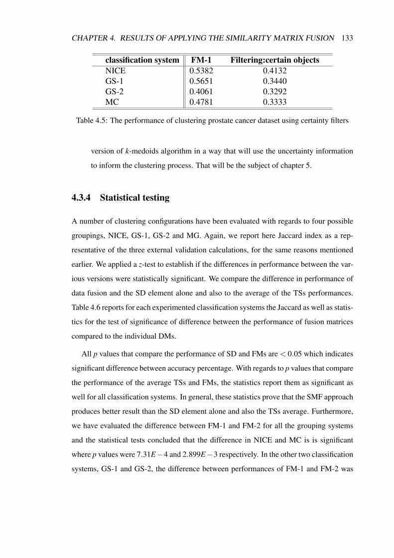
CHAPTER 4. RESULTS OF APPLYING THE SIMILARITY MATRIX FUSION 133
classification system FM-1 Filtering:certain objectsNICE 0.5382 0.4132GS-1 0.5651 0.3440GS-2 0.4061 0.3292MC 0.4781 0.3333
Table 4.5: The performance of clustering prostate cancer dataset using certainty filters
version of k-medoids algorithm in a way that will use the uncertainty information
to inform the clustering process. That will be the subject of chapter 5.
4.3.4 Statistical testing
A number of clustering configurations have been evaluated with regards to four possible
groupings, NICE, GS-1, GS-2 and MG. Again, we report here Jaccard index as a rep-
resentative of the three external validation calculations, for the same reasons mentioned
earlier. We applied a z-test to establish if the differences in performance between the var-
ious versions were statistically significant. We compare the difference in performance of
data fusion and the SD element alone and also to the average of the TSs performances.
Table 4.6 reports for each experimented classification systems the Jaccard as well as statis-
tics for the test of significance of difference between the performance of fusion matrices
compared to the individual DMs.
All p values that compare the performance of SD and FMs are < 0.05 which indicates
significant difference between accuracy percentage. With regards to p values that compare
the performance of the average TSs and FMs, the statistics report them as significant as
well for all classification systems. In general, these statistics prove that the SMF approach
produces better result than the SD element alone and also the TSs average. Furthermore,
we have evaluated the difference between FM-1 and FM-2 for all the grouping systems
and the statistical tests concluded that the difference in NICE and MC is is significant
where p values were 7.31E−4 and 2.899E−3 respectively. In the other two classification
systems, GS-1 and GS-2, the difference between performances of FM-1 and FM-2 was

CHAPTER 4. RESULTS OF APPLYING THE SIMILARITY MATRIX FUSION 134
groupings system SD FM-1 FM-2 TSs FM-1 FM-2NICEJaccard 0.3335 0.5381 0.5939 0.4712 0.5381 0.5939z score – +−11.663 +−14.76 – +−3.782 +−6.951p value – < 1.0E−5 < 1.0E−5 – 7.8E−5 < 1.0E−5GS-1Jaccard 0.4230 0.5651 0.5882 0.4746 0.5651 0.5882z score – +−8.034 +−9.34 – +−5.12 +−6.435p value – < 1.0E−5 < 1.0E−5 – < 1.0E−5 < 1.0E−5GS-2Jaccard 0.2829 0.4061 0.4205 0.3229 0.4061 0.4205z score – +−7.328 +−8.145 – +−4.886 +−5.709p value – < 1.0E−5 < 1.0E−5 – < 1.0E−5 < 1.0E−5MCJaccard 0.3191 0.4781 0.5269 0.3403 0.4781 0.5269z score – +−9.18 +−11.889 – +−7.922 +−10.643p value – < 1.0E−5 < 1.0E−5 – < 1.0E−5 < 1.0E−5
Table 4.6: Statistical analysis of SMF performance on the prostate cancer dataset. Thetable reports statistics for Jaccard coefficient of k-medoids clustering obtained with re-gards to four possible groupings of the prostate cancer dataset. The first group of columnsprovides the statistical test that calculates the significance of SMF performance comparedto using SD and the second group of columns compares to the average performance of allTSs
not significant with 0.093084 and 0.204119 p values.
It is also interesting to see the TSs that are particularly good performers, i.e. those
that have the highest values according to the previous set of experiments as they are blood
tests that may either be indicative of risk or mortality. They are PSA test (P, 0.5119), HDL
Cholesterol (B12, 0.5569), Aspartate transaminase (B4, 0.3767) and Haemoglobin (B20,
0.3899) for NICE, GS-1, GS-2 and MC, respectively, where the figures in the brackets are
the Jaccard external evaluation coefficients of the blood tests.
We also computed the Dunn internal index for every single DM and FMs using the
results of applying clustering in relation to the four groupings. Table 4.7 shows the coeffi-
cients that have evaluated SD element, FM-1, FM-2 and the best individual DM for each
classification system. The best individual DM represented in the table are the ones that
have been chosen according to the internal validation calculations.
In general, Dunn index considers B3, B21, B23 and B26 as the top TSs that have poten-
tial to produce good quality clustering results (i.e. well separated and compact clusters).
In ascending order the top five DMs according to Dunn evaluations for NICE system are:
SD, FM-2, FM-1 and B23 and B4; for GS-1: SD, FM-1, FM-2, B23 and B4; for GS-2:
SD, FM-1, FM-2, B26 and B21; and for MC: SD, FM-1, FM-2, B26 and B21. For all the

CHAPTER 4. RESULTS OF APPLYING THE SIMILARITY MATRIX FUSION 135
DM NICE GS-1 GS-2 MCSD 0.025244647 0.039554437 0.035023101 0.035023101B23 0.002995108 0.002440136 – –B4 0.001565763 0.001668239 – –B21 0.000350434 – 0.000784296 0.005162134B26 – – 0.002904887 0.010576913FM-1 0.008457828 0.023813098 0.009207189 0.016180151FM-2 0.008720526 0.020815176 0.008968838 0.014523745
Table 4.7: The Dunn index values from the results of clustering the prostate cancerdataset: the statistics are reported for SD and FMs as well as the top TS that are cho-sen by internal validation calculations. We use – to represent the case when the DM is notassociated with the top informative TS for a particular grouping.
experiments that we have conducted, the Dunn index ranks SD as the best and FM-1 as
the second best DM, except for NICE where FM-1 ranks third after FM-2. FM-2 holds
the third top position in terms of quality of the clustering that might be obtained using this
matrix. Accordingly, in general, Dunn evaluates FM-1 as more informative than FM-2.
Moreover, it does not rate DMs that were considered as the best performers according to
external validation indices as one of the top informative DM, except in the case of NICE
(they agree on B21) and GS-2 (they agree on B26). Hence interestingly, external and in-
ternal validation metrics do not agree on the same conclusion, but their judgment of FM-1
and FM-2 for all groupings as top performers were the same. Thus, the fused matrices
seem to have reasonable performance according to both internal and external validation.
In other words, DMs that have been evaluated as good performers using external and in-
ternal methods are not the same, except for the two fusion matrices, FM-1 and FM-2,
for all the four groupings. This may be a positive result for the SMF approach when we
do not have external information. In real clustering problems, we are not expected to
have the ground truth labels, thus, the only way to examine different elements is by using
internal quality measures. From our results and supposing that we agree with external
evaluation as guidance on the true clusters, internal validation may not produce a good
ranking of elements in terms of their ability to produce good clusters. Hence in many
clustering exercises it would not be possible to know a prior which elements to use to
produce good clustering. However, the FMs may provide a combined evidence approach
that aids the clustering towards producing good results. Thus, when we cannot establish

CHAPTER 4. RESULTS OF APPLYING THE SIMILARITY MATRIX FUSION 136
which elements to use or give more weight to, the fusion matrix can be used to produce
clustering results that are not very far from what we could obtain using the best elements.
4.4 The results of the plants dataset
We have created a dataset about plants. Objects in this dataset are also described by a
mixture of data types, but different from those in the prostate cancer patients and hence
providing us with new challenges. It will enable us to further validate the feasibility of our
approach on different combinations of data types. In addition, all objects are classified
into pre-defined classes which is beneficial at the stage of assessing and comparing the
performance. A description of the data is given in Section 3.7.2 while the experiment is
giving in the following next sections.
4.4.1 DMs and FM calculation results
A plant object is defined by three data types: structured data, SD, free text element, TE,
and an image, IE. We selected three distance measures, as described in Section 4.2, and
then generated pairwise DMs for each of the three elements. We calculated DMSD, DMT E ,
DMT ENoRare, DMIE and DMIEReduced . These matrices are for the following respectively:
SD, TE, TE element represented without rare terms, IE and IE element represented with
reduced colours. Next, we fused DMs and constructed the initial FMs along with the
associated uncertainty matrices DFMs-1 where there was no need to calculate UFM-1
as in this dataset we do not compare incomplete objects. We computed four FMs; by
fusing all possible combination of DMs and including all the three data types. FM-1
fuses DMSD, DMT E and DMIE ; FM-NoRare-1 fuses DMSD, DMT ENoRare and DMIE ;
FM-NoRare-Reduced-1 fuses DMSD, DMT ENoRare and DMIEReduced; and FM-Reduced-1
fuses DMSD, DMT E and DMIEReduced . In all the results, we may refer to the elements
using their names. More information about them is available in the data dictionary in
Appendix A.

CHAPTER 4. RESULTS OF APPLYING THE SIMILARITY MATRIX FUSION 137
Since the size of each generated DM is large (100×100) to be compared, we use the
heatmap graphical representation to provide an immediate visual summary of distance
calculations. Figure 4.7 shows visualization of our distance matrices using colours to
represent distance values in a two-dimensional graph for each individual element. As
before, we use dark blue to reflect strong similarity and then the colour scales through
green until it reaches bright yellow to reflect strong dissimilarity. For the four FMs, in
Figure 4.7 we represent the entire fused calculations for all the objects while in Figure
4.8 we use the gray colour to represent all plants that report uncertain distance values in
FMs due to exceeding the determined threshold for DFM-1. The threshold was set up as
DFM-1=0.4 for the the four FMs, thus we omitted fused distances for plants (represented
in grey colour) that have DFM-1 ≥ 0.4. We present FMs before and after filtering objects
because we will use both matrices in the application of k-medoids algorithm in the next
section (Section 4.4.2). Note that, in both figures, plants are reported in ascending order
using their identifiers from left to right on the x-axis and from up to down on the y-axis.
We have the 42 fruits first then the 22 roses and finally the 36 types of grass at the end.
The visualisations allow us to draw some initial conclusions about DMs that seem to
be related to each other. However, to explore this in more detail, we used the Mantel test
as a DM comparison technique. Calculated correlation coefficients that reflects the degree
of the relationships between the DMs and FM-1 are summarised in Table 4.8. By looking
at the calculations in the table, we can conclude that SD, TE and TE-NoRare are all well-
correlated elements as the coefficients between every pair is ≥ 0.4183. Moreover, the
degree of associations between TE-TE-NoRare and between IE-IE-Reduced is very strong
with values of 0.9950 and 0.9727 respectively. However, this is to be expected as those
represent the same data element. This is confirmed also by the heatmap visualisations in
Figure 4.7. In addition, all the statistics indicate positive relationship between elements
as there are no negative coefficients.
It is also worth observing that the four FMs maintains a higher degree of correlation
with some elements than with others. The SD and both DMs that report the similarity
calculations for TE element appear well represented in terms of the correlation measure.

CHAPTER 4. RESULTS OF APPLYING THE SIMILARITY MATRIX FUSION 138
Figure 4.7: Heatmap representation for DMs and FMs-1 calculated for the plants dataset:DMs for SD, TE, TE-NoRare, IE and IE-Reduced. We use blue colour to indicate similar-ity and yellow to indicate dissimilarity. The fusion matrices, FMs-1, represent the fuseddistances without taking into account uncertainty.
However, the text element seems to be the most correlated to the FMs. Hence the well
correlated elements are able to exert a stronger influence in the FM. In addition, by look-
ing at all DMs and FMs in figures 4.7 and 4.8, the representation reflect some expected
similarities among plants of the same type. For example, given that the objects are ordered
by class, the dark blue square at the right bottom corner of the DMs and FMs correlate to
the expected strong similarity between grass objects. Also, strong similarity was reported
among fruits objects, in contrast to the calculated distances between roses.

CHAPTER 4. RESULTS OF APPLYING THE SIMILARITY MATRIX FUSION 139
Figure 4.8: Heatmap representation for the filtered fused matrices, FM-1, FM-NoRare-1,FM-NoRare-Reduced-1 and FM-Reduced-1, calculated for the plants dataset

CHAPTER 4. RESULTS OF APPLYING THE SIMILARITY MATRIX FUSION 140
SDT
ET
E-N
oRar
eIE
IE-R
educ
edFM
-1FM
-N
oRar
e-1
FM-
NoR
are-
Red
uced
-1
FM-
Red
uced
-1
SD0.
4183
0.41
980.
1953
0.18
370.
7697
0.76
410.
7666
0.77
25T
E0.
9950
0.22
190.
2194
0.79
060.
8007
0.80
660.
7967
TE
-NoR
are
0.22
200.
2190
0.79
020.
8053
0.81
100.
7960
IE0.
9727
0.59
650.
5867
0.56
540.
5748
IE-R
educ
ed0.
5791
0.56
940.
5683
0.57
82FM
-10.
9985
0.99
430.
9959
FM-N
oRar
e-1
0.99
610.
9946
FM-N
oRar
e-R
educ
ed-1
0.99
84
FM-R
educ
ed-1
Tabl
e4.
8:C
orre
latio
nco
effic
ient
sbe
twee
nD
Ms
and
FMs-
1ca
lcul
ated
forp
lant
sda
tase
t

CHAPTER 4. RESULTS OF APPLYING THE SIMILARITY MATRIX FUSION 141
4.4.2 Clustering results
Here we present the results of applying the standard k-medoids algorithm to individual
DMs and also to FMs; including FM-1 and FM-2. Our main aim is to examine if the FMs
lead the k-medoids algorithm to produce better clustering results than using individual
DMs. To do this we conducted three sets of experiments that we have designed in Section
4.1. The plant type is the grouping system that was used to evaluate SMF clustering
configurations in all the experiments. This categorisation has 22 % of the objects classed
as ‘roses’. In addition, the ‘fruits’ class contains approximately half of our objects (42%),
while the remaining 36 plants belonging to the class ‘grass’.
The number of clusters, k, was determined depending on this grouping system, thus,
for this experiments we set k=3. The results are presented below and divided into three
sets according to the experiment set up section:
1. First we present the results of applying k-medoids to cluster our heterogeneous
objects by means of using the individual DMs. Figure 4.9 shows the performance
of clustering evaluated according to the truth-labels of the plants. As before, three
external validation indices: Jaccard, Rand and Dice’s coefficients are presented in
the figure. They were calculated to evaluate the results produced by k-medoids
using: SD, TE, TE-NoRare, IE and IE-Reduced DMs.
It can be observed from the figure that the TE-NoRare element alone performs better
than the other four elements with regards to all coefficients. In general, text element
and structured data seem to be perform better than the image element. Thus, the IE
element is the least informative for the grouping. However, Jaccard and Dice’s
indices put IE-Reduced slightly ahead of the other version of the image element,
IE.
2. The second set of experiments, examines the initial fusion matrices, FMs-1, and the
special weighted fusion matrices, FMs-2. Here we produced the following versions
of the FM-1: FM-1, FM-NoRare-1, FM-NoRare-Reduced-1 and FM-Reduced-1.
All those combine DMs with equal weight. We also produced FM-2 using differ-

CHAPTER 4. RESULTS OF APPLYING THE SIMILARITY MATRIX FUSION 142
Figure 4.9: Summary of the performance of k-medoids clustering obtained using the in-dividual DMs for the plants dataset
ent weights: FM-2, FM-NoRare-2, FM-NoRare-Reduced-2 and FM-Reduced-2. In
order to determine these weights, we used clustering performance of each individ-
ual DM. Note that in the absence of external assessment, we may not be able to
establish the worth of each element using the approach that we propose here.
We calculate FMs-2 by giving the text element, which is the best performer, a dou-
ble weight compared to the remaining two DMs. The influence of playing with
these weights on the clustering performance is demonstrated in Figure 4.10 which
compares FMs-2 to FMs-1. The figure demonstrates the results for each of the
four different ways of grouping individual DMs: FM, FM-NoRare, FM-NoRare-
Reduced and FM-Reduced. Again, the performance here is evaluated using the
three external indices.
As it was expected, Figure 4.10, shows that FM-2 produces better clustering results
than FM-1. Nevertheless, examining different weighting has not improved the per-
formance of FM-NoRare-Reduced. This fuses: SD, TE-NoRare and IE-Reduced.
In addition, we can conclude from Figure 4.10 that the best fusion of the three ele-
ments that compose our objects is by combining: SD, TE-NoRare and IE Reduced.

CHAPTER 4. RESULTS OF APPLYING THE SIMILARITY MATRIX FUSION 143
Figure 4.10: Summary of the performance of k-medoids clustering obtained by fusionmatrices for plants dataset
We conducted a comparison between the clustering performance when using in-
dividual DMs, FMs-1 and FMs-2 and the results are summarised in Figure 4.11.
The figure shows the evaluation of clustering using SD, TE, TE-NoRare, IE and
IE-Reduced. It compares these matrices to the best FMs-1 performer (Max FM-1)
and the worst (Min FMs-1) and the same for FMs-2 matrices (Max FM-2 and Min
FM-2). The best fusion matrix was FM-NoRare-Reduced and the worst was FM.
The performance here is reported, for the purpose of presentation simplification, by
Jaccard coefficients only as a representative of the three calculated external indices.
In general, the results show that FM-1 and FM-2 produced better performance than
individual DMs. Min FM-1 and Min FM-2 seem better than the individual DMs,
except for TE-NoRare when compared to Min FM-1. Thus, we conclude that our
results are reassuring as the combination approach is within some acceptable devi-
ation from the best individual matrices even when it is not possible to determine the
best performer.
3. To conduct the third set of experiment, as described in Section 4.1, we filter all the

CHAPTER 4. RESULTS OF APPLYING THE SIMILARITY MATRIX FUSION 144
Figure 4.11: Summary of the performance of k-medoids clustering obtained on both ele-ments’ DMs and best and worst fusion matrices for plants dataset
uncertain data to perform the clustering and then assign the uncertain data as a sepa-
rate experiment. Accordingly, we removed 14, 24, 25 and 20 plants, as those plants
have DFM-1 values ≥ 0.3 in all FMs-1. Table 4.9 shows a summary of the exper-
iments reported by Jaccard coefficient compared to the results of clustering using
all objects. The results indicate that when we applied k-medoids algorithm to the
filtered data, the perfomance of clustering configuration has decreased compared to
the results reported for the full FMs-1.
Fusion matrix FMs-1 Filtering:certain objectsFM-1 0.69 0.4651FM-NoRare-1 0.73 0.4468FM-NoRare-Reduced-1 0.85 0.5761FM-Reduced-1 0.69 0.4375
Table 4.9: The performance of clustering plants dataset using certainty filters
In addition to what is presented in Table 4.9, a worse deterioration was reported when
we used the generated medoids using certain data only to assign the residual objects that

CHAPTER 4. RESULTS OF APPLYING THE SIMILARITY MATRIX FUSION 145
fusion matrix SD FMs-1 FMs-2 text FMs-1 FMs-2 image FMs-1 FMs-2FMJaccard 0.66 0.69 0.77 0.64 0.69 0.77 057 0.69 0.77z score – +−0.453 +−1.723 – +−0.749 +−2.016 – +−1.757 +−3.008p value – 0.325274 4.2444E−2 – 0.226929 2.19E−2 – 3.9459E−2 1.315E−3FM-NoRareJaccard 0.66 0.73 0.81 0.76 0.73 0.81 0.57 0.73 0.81z score – +−1.075 +−2.403 – +−0.487 +−0.861 – +−2.372 +−3.669p value – 0.141187 8.131E−3 – 0.313129 0.194619 – 8.846E−3 1.22E−4FM-NoRare-ReducedJaccard 0.66 0.85 0.86 0.76 0.85 0.86 0.58 0.85 0.86z score – +−3.124 +−3.311 – +−1.606 +−1.802 – +−4.229 +−4.41p value – 8.92E−4 4.65E−4 – 0.054137 3.5773E−2 – 1.2E−5 < 1.0E−5FM-ReducedJaccard 0.66 0.69 0.83 64.00 0.69 0.83 0.58 0.69 0.83z score – +−0.453 +−2.758 – +−0.749 +−3.044 – +−1.616 +−3.876p value – 0.325274 2.908E−3 – 0.226929 1.167E−3 – 0.053047 5.3E−5
Table 4.10: Statistical analysis of SMF performance on the plants dataset. The tablereports statistics for Jaccard coefficient of k-medoids clustering obtained with regards tothe different fusion combinations. The first set of columns provides the statistical test thatcalculates the significance of SMF performance compared to using structured data, thesecond set of columns compares to the performance of the text element while the last setof columns is for the image element. – means that the statistic can not be calculated
were removed. Thus, we can concluded here that uncertain fused calculations seem to
have information that aids the clustering process. Thus, we need to include them but in a
different manner. This confirms our previous conclusion in Section 4.3.3. Note that Rand
and Dice’s indices concurred with the same conclusion.
4.4.3 Statistical testing
The performance of clustering were evaluated here to examine the significance of the dif-
ferences between Jaccard calculations that were computed for clustering results obtained
using FMs and individual DMs. We applied a z-test to establish if the differences in per-
formance were statistically significant. Table 4.10 shows the Jaccard values and statistics
for the test of significance.
The p values confirm that the difference between the performance of FMs-2 and each
of the individual element: SD, text and image is significant, except for FM-NoRare-2
when compared to the text element. With regards to p values that compare the perfor-
mance of FMs-1 to text (TE or TE-NoRare) and SD, the statistics report them as not
significant apart from the one that compares FM-NoRare-Reduced-1 and SD. The statisti-

CHAPTER 4. RESULTS OF APPLYING THE SIMILARITY MATRIX FUSION 146
SD 0.181775611 FM-1 0.275899167 FM-2 0.092507311TE 0.327597615 FM-NoRare-1 0.226079578 FM-NoRare-2 0.162051703TE-NoRare 0.114691349 FM-NoRare-Reduced-1 0.168005112 FM-NoRare-Reduced-2 0.158479823IE 0.154771467 FM-Reduced-1 0.184643632 FM-Reduced-2 0.178111331IE-Reduced 0.116527353 – – – –
Table 4.11: The Dunn index values from the results of clustering the plants dataset: thestatistics are reported for the different representation of the three elements, DMS. Also,the two versions of the FMs for the different combinations of data fusion.
cal test also considers that FMs-1 perform significantly better than the image element (IE
or IE-Reduced), except for one fusion matrix, FM-Reduced-1. Although, some of these
statistics are not significant, the SMF approach produces at least comparable results, and
some times significantly better results, to the individual elements separately, especially
in the case of using weights. We have also evaluated the difference between FMs-1 and
FMs-2. For each fusion combination, statistical tests concluded that the difference is not
significant; except for FM-Reduced combination with 1.0225E−1 p value. Thus, in the
case of just combining everything together without weightings (i.e. using FMs-1), SMF
can be used to produce clustering results that are not very far from what we could obtain
using the best elements.
We also computed the Dunn internal index for every single DM and FMs. Table 4.11
shows the coefficients that have evaluated SD element, text, image, FMs-1 and FMs-2.
Dunn index considers text element as the top individual DMs that have potential to
produce good quality clustering results. It evaluates FM-1 and FM-NoRare-1 as the next
best distance matrices. In general, for all the experiments that we have conducted, the
Dunn index ranks FMs-1 as better matrices in terms of quality of the clustering that might
be obtained over FMs-2. Accordingly, Dunn evaluates FMs-1 as more informative than
FMs-2. Therefore, external and internal validation metrics do not agree on the same
conclusion. In addition, external validation evaluates TE-NoRare as the best performer
whereas the internal index points at TE.

CHAPTER 4. RESULTS OF APPLYING THE SIMILARITY MATRIX FUSION 147
4.5 The results of the journals dataset
We have created a dataset of journals in the context of scientometrics analysis. Objects
in this dataset are described by two different data types, similar to the mixture of data
types in the prostate cancer patients but with some changes. In addition, all objects are
classified into pre-defined classes which facilitates the process of assessing and comparing
clustering performances. A description of the data is given in Section 3.7.3 while the
experiment is giving in the following sections.
4.5.1 DMs and FM calculation results
A journal object is defined by two data types composed of three elements: structured data,
SD, and two Time-series, TSs. We selected two distance measures, as described in Section
4.2, and then generated pairwise DMs for each of the three elements. We calculated
DMSD, DMT StoJ and DMT S f romJ . These matrices are for the following respectively: SD,
TS to the journal and TS from the journal. Next, we fused DMs and constructed the
initial FM-1 along with the associated uncertainty matrices DFM-1 and UFM-1. In all
the results, we refer to the elements using their names. More information about them is
presented as a data dictionary in Appendix A.
Since the size of each generated DM is large (135×135), we use the heatmap graphical
representation to provide an immediate visual summary of distance calculations. Figure
4.12 shows a visualization of our distance matrices using colours to represent distance
values in a two-dimensional graph for each individual element. Colours are mapped as
previously.
For FM-1, in Figure 4.12 we represent the entire fused calculations for all the objects
while in Figure 4.13 we use the grey colour to represent all objects that report uncertain
distance values in FM-1 due to exceeding one or both of the determined thresholds for
UFM-1 and DFM-1. The thresholds were set up as UFM-1=0.33 and DFM-1=0.1, thus
we omitted fused distances for journals that have UFM-1 values ≥ 0.33 or DFM-1 ≥ 0.1.
We present FM-1 before and after filtering objects because we will use both matrices in

CHAPTER 4. RESULTS OF APPLYING THE SIMILARITY MATRIX FUSION 148
the application of k-medoids algorithm in the next section (Section 4.5.2). Note that, in
both figures, journals are reported in ascending order using their identifiers from left to
right on the x-axis and from up to down on the y-axis.
Figure 4.12: Heatmap representation for DMs and FM-1 calculated for the journalsdataset: DMs for SD and two TSs with red colour to represent missing values; blue in-dicates similarity and yellow indicates dissimilarity. The fusion matrix, FM-1, representthe fused distances without taking into account uncertainty.
The visualisations allow us to draw some initial conclusions about DMs but we will
also use the Mantel test as before. The calculated correlation coefficients reflects a strong
degree of the relationships between TStoJ and TSfromJ with 0.9950. This is confirmed
also by the heatmap visualisations in Figure 4.12. By looking at the other calculations,
we can conclude a moderate association that correlates both SD-TStoJ as well as SD-
TSfromJ with 0.4183 and 0.4198 respectively. The heatmap visualisations in Figure 4.12
confirms all these stated associations. In addition, all the statistics indicate positive rela-
tionship between elements as there is no negative coefficients.
It is also worth observing that the FM maintains a higher degree of correlation with
some elements than with others. For example, SD appear to be the least representative

CHAPTER 4. RESULTS OF APPLYING THE SIMILARITY MATRIX FUSION 149
Figure 4.13: Heatmap representation for the filtered fused matrix (FM-1) calculated forthe journals dataset
element in terms of the correlation measure while the others are more correlated elements
which means they may have a stronger influence on the FM-1.
4.5.2 Clustering results
In order to examine our FMS approach, we applied k-medoids to DMs and FMs to eval-
uate and compare the generated clustering configurations. Three sets of experiments,
designed in Section 4.1, were conducted and their results are presented below. The plant
type is the grouping system that was used to validate the results. For evaluation, we used
IF, ES and AI grouping systems that are defined in Section 3.7.3.
We started with journals labeling following all the different classification systems.
Table 4.12 shows number and percentage of journals in each category following the three
categorisation system.
As can be observed, each of the three classification assigned a minority group of jour-
nals to the last category. In IF labeling system, the data is well distributed in the middle
clusters while in ES and AI groupings much of the data belongs to the first category.

CHAPTER 4. RESULTS OF APPLYING THE SIMILARITY MATRIX FUSION 150
IF ES AIcluster no. % cluster no. % cluster no. %IF≤0.5 28 20.74% ES≤0.0025 84 62.22% AI≤0.4 62 45.93%0.5<IF≤1.0 36 26.67% 0.0025<ES≤0 30 22.22% 0.4<AI≤0.8 41 30.37%1.0<IF≤1.5 29 21.48% ES>0 21 15.56% AI>0.8 32 23.70%1.5<IF≤2.0 22 16.30% – – – – – –IF>2.0 20 14.81% – – – – – –
Table 4.12: Classification systems for journals dataset
For this experiment, we set k=5 for IF grouping and k=3 in ES and AI grouping. The pre-
sentation of clustering results are divided below into the three main sets of experiments
as before:
1. Results of applying k-medoids to cluster distance calculations of all objects by
means of using the DMs calculated for elements. Figure 4.14 shows the perfor-
mance of clustering evaluated according to the three possible groupings, IF, ES
and AI. The figure includes a summary of the statistics calculated using the three
external validation indices: Jaccard, Rand and Dice’s coefficients to evaluate the
clustering configurations. In the figure we report SD, TStoJ and TSfromJ.
Figure 4.14: Summary of the performance of k-medoids clustering obtained using theindividual DMs for the journals dataset

CHAPTER 4. RESULTS OF APPLYING THE SIMILARITY MATRIX FUSION 151
From figure 4.14, it can be observed that with regards to Jaccard and Dice’s coef-
ficients in ES and AI classification systems, the order of the best performances is
TStoJ, TSfromJ and SD. Rand agrees with this ordering in the ES groupings. How-
ever, Rand has different judgment in the other classifications, IF and AI, where SD
seemed to be more informative than TSfromJ. The other two indices, Jaccard and
Dice’s evaluate our DMs similarly for IF classification. Again, we confirm here that
the Jaccard and Dice’s methods behave similarly whereas the Rand index reports
different results. Nevertheless, all the three validation methods rank TStoJ as the
best performer for all three grouping systems.
2. For the second set of experiments, we produced a weighted fusion matrix, FM-
2, for each grouping system by giving the best performer, TStoJ, a double weight
compared to the remain two DMs. The influence of playing with these weights on
the clustering performance is demonstrated in Figure 4.15 which compares FM-2
to FM-1. Again, the performance here is evaluated and presented according to the
three external indices.
By looking at Figure 4.15, the biggest improvement in the performance seems to be
in IF and AI classification while for ES the improvement is marginal. This applies
for all three validation coefficients.
We compare the performance of individual DMs and FMs, Figure 4.16 summarises
this comparison. The figure shows the evaluation of clustering using every element
alone, FM-1 and FM-2. The performance here is compared by Jaccard coefficients
only, for the purpose of presentation simplification.
The results show that by combining DMs, using FM-1 and FM-2, we obtained
stable performance that is better than individual DMs in all groupings, except AI.
For AI grouping, the best individual DM, TStoJ, seems to be more informative for
the clustering algorithm than FM-1, however, FM-2 outperformed TStoJ. All these
findings are very similar to the conclusions that are suggested by the other two
external calculations.
3. In this set of experiments, we were interested in clustering certain data. We fil-

CHAPTER 4. RESULTS OF APPLYING THE SIMILARITY MATRIX FUSION 152
Figure 4.15: Summary of the performance of k-medoids clustering obtained on fusionmatrices for journals dataset
tered out 41 journals that exceeded the thresholds UFM-1=0.33 and DFM-1=0.1.
The results indicate that the k-medoids algorithm applied to the filtered data does
not produce better clustering performance. A deterioration occurs when we fil-
tered uncertain journals. Moreover, worst results are produced when we assigned
the residual journals to medoids that are generated when clustering certain objects
only. Table 4.13 compares Jaccard coefficients that are calculated for the results
of clustering certain objects compared to the results of clustering all objects. In
general, we concluded here, as previously, that filtering is not a suitable approach.
Thus, we need to use certainty calculations in a different manner.
classification system FM-1 Filtering:certain objectsIF 0.355555556 0.3085106383ES 0.792592593 0.4468085106AI 0.533333333 0.4361702128
Table 4.13: The performance of clustering journals dataset using certainty filters

CHAPTER 4. RESULTS OF APPLYING THE SIMILARITY MATRIX FUSION 153
Figure 4.16: Summary of the performance of k-medoids clustering obtained on both ele-ments’ DMs and fusion matrices for journals dataset
4.5.3 Statistical testing
With regards to three possible groupings, IF, ES and AI, a number of clustering config-
urations have been evaluated. We applied a z-test to establish if the differences in per-
formance as before are statistically significant. Table 4.14 reports for each experimented
classification systems the Jaccard as well as statistics for the test of significance of dif-
ference between the performance of fusion matrices compared to the individual DMs. p
values indicate that the differences between fusion matrices and TStoJ is not significant.
This is not very surprising as TStoJ is the individual DM with best performance and there
are not many additional pieces of information that can be combined in the FMs. When we
compared the performances of FMs with SD, we found that the differences are significant
in ES and AI. p values also suggest a significant difference between FMs and TSfromJ
for both IF and ES. Thus, we may conclude that when the number of elements is low,
the SMF approach produces comparable result to the best individual elements alone. Fur-
thermore, we have evaluated the difference between FM-1 and FM-2 for all the grouping
systems and the statistical tests concluded that the difference is not significant.

CHAPTER 4. RESULTS OF APPLYING THE SIMILARITY MATRIX FUSION 154
groupings system SD FM-1 FM-2 TStoJ FM-1 FM-2 TSfromJ FM-1 FM-2IFJaccard 0.325925926 0.355555556 0.414814815 0.340740741 0.355555556 0.414814815 0.311111111 0.355555556 0.414814815z score – +−0.514 +−1.512 – +−0.256 +−1.255 – +−0.775 +−1.772p value – 0.303626 0.065267 – 0.398975 0.104739 – 0.21917 3.8197E−2ESJaccard 0.62962963 0.792592593 0.807407407 0.733333333 0.792592593 0.807407407 0.688888889 0.792592593 0.807407407z score – +−2.954 +−3.248 – +−1.145 +−1.447 – +−1.944 +−2.243p value – 1.568E−3 5.81E−4 – 0.126105 0.073948 – 2.5948E−2 2.448E−2AIJaccard 0.42962963 0.533333333 0.57037037 0.548148148 0.533333333 0.57037037 0.511111111 0.533333333 0.57037037z score – +−1.705 +−2.313 – +−0.244 +−0.368 – +−0.366 +−0.977p value – 4.4097E−2 1.0361E−2 – 0.403615 356437 – 0.357183 0.16428
Table 4.14: Statistical analysis of SMF performance on the journals dataset. The tablereports statistics for Jaccard coefficient of k-medoids clustering obtained with regards tothree possible groupings of the journals dataset. The first set of columns provides thestatistical test that calculates the significance of SMF performance compared to using SD,the second set of columns compares to the TStoJ and the third set of columns to TSfromJ
DM IF ES AISD 0.019812955 0.014436103 0.038107798TStoJ 0.006900568 0.053354258 0.009976748TSfromJ 0.021527789 0.065227503 0.065227503FM-1 0.012628299 0.01562139 0.08445345FM-2 0.004698804 0.017382167 0.034164988
Table 4.15: The Dunn index values from the results of clustering the journals dataset: thestatistics are reported for SD and FMs.
In addition to the external validation, we also computed the Dunn internal index for
every single DM and FMs using the results of applying clustering in relation to the three
groupings. Table 4.15 shows the coefficients that have evaluated individuals elements,
FM-1 and FM-2 for each classification system.
With regards to individual DMs, the Dunn index considers TStfromJ as the top individ-
ual element that has the potential to produce good quality clustering results. That applies
for each classification systems. However, this was not the same conclusion that we have
reached by the external coefficients. Moreover, the Dunn index does not rank FMs (FM-1
and FM-2) as highly effective in terms of quality of the clustering that might be obtained
except in the case of the AI classification.

CHAPTER 4. RESULTS OF APPLYING THE SIMILARITY MATRIX FUSION 155
4.6 The results of the papers dataset
We have constructed a dataset about research papers. Objects in this dataset are also
described by a mixture of data types. In order to have further validation of our approaches,
the arrangements for this data were different from the previous datasets, which allows
us to examine different combinations of data types. In addition, like the other datasets,
all objects here are classified into pre-defined classes which is beneficial at the stage of
assessing and comparing the performance. A description of the data is given in Section
3.7.4 while the experimental result are given in the following sections.
4.6.1 DMs and FM calculation results
A paper object is defined by three data types: structured data, SD, time-series, TS and free
text element, TE. We selected three distance measures, as described in Section 4.2, and
then generated pairwise DMs for each of the three elements. We calculated DMSD, DMT S,
DMT E and DMT ENoRare. These matrices are for the following respectively: SD, TS, TE
and TE element represented discounting rare terms. Next, We fused DMs and constructed
the initial FMs along with the associated uncertainty matrices UFM-1 and DFMs-1. We
computed two FMs by fusing all possible combination of DMs and including all the three
data types. FM-1 fuses DMSD, DMT S and DMT E ; FM-NoRare-1 fuses DMSD, DMT S
and DMT ENoRare. In all the results, we refer to the elements using their names. More
information about them can be found in the data dictionary in Appendix A.
We use the heatmap graphical representation to provide an immediate visual summary
of distance calculations as the size of each generated DM is large (300×300). Figure 4.17
shows visualization of our distance matrices using colours to represent distance values in
a two-dimensional graph for each individual element. As before, we use dark blue to
reflect strong similarity and then the colour scales through green until it reaches bright
yellow to reflect strong dissimilarity. For the two FMs, in Figure 4.17 we represent the
entire fused calculations for all the objects while in Figure 4.18 we use the gray colour to
represent all plants that report uncertain distance values in FMs due to exceeding one or

CHAPTER 4. RESULTS OF APPLYING THE SIMILARITY MATRIX FUSION 156
both of the determined thresholds for UFM-1 and DFM-1. The thresholds were set up as
UFM-1=0.33 and DFM-1=0.4, thus we omitted fused distances for papers (represented in
grey colour) that have UFM-1 values≥ 0.33 or DFM-1≥ 0.4. We present FMs before and
after filtering objects because we will use both matrices in the application of k-medoids
algorithm in the next section (Section 4.6.2). Note that, in both figures, papers are reported
in ascending order using their identifiers from left to right on the x-axis and from up to
down on the y-axis. However, we have the 100 computer science papers first then the 100
business economics articles and finally the last 100 papers represent research in health
care services.
Figure 4.17: Heatmap representation for DMs and FMs-1 calculated for the plants dataset:DMs for SD, TS, TE and TE-NoRare with red colour to represent missing values. We useblue colour to indicate similarity and yellow to indicate dissimilarity. The fusion matrices,FMs-1, represent the fused distances without taking into account uncertainty.
The visualisations together with Mantel test results allow us to draw some initial con-
clusions about DMs that seem to be related to each other. Calculated correlation co-
efficients that reflects the degree of the relationships between the DMs and FMs-1 are
summarised in Table 4.16. By looking at the calculations in the table, we can conclude
that the degree of associations between TS-TE is very strong with values of 0.9989. This
is confirmed also by the heatmap visualisations in Figure 4.17 where we have the dark
blue in both DMs in the diagonal positions. Another moderate association seem to be be-

CHAPTER 4. RESULTS OF APPLYING THE SIMILARITY MATRIX FUSION 157
tween SD and TE-NoRare with a degree of 0.4939. In addition, all the statistics indicate
positive relationship between elements as there is no negative coefficients.
Figure 4.18: Heatmap representation for the filtered fused matrices, FM-1 and FM-NoRare-1 calculated for the papers dataset with grey representing uncertainty
Again we observe that the two FMs maintain a higher degree of correlation with some
elements than with others. The SD and TE-NoRare appear well represented in terms of
the correlation measure. Thus, the text element that is represented without taking into
account the rare words seems to be the most correlated to the FMs. Hence the well
correlated elements are able to exert a stronger influence in the FM. Consequently, they
might produce a better clustering configuration.
SD TS TE TE-NoRare FM-1 FM-NoRare-1
SD 0.0519 0.0537 0.4939 0.6787 0.6780TS 0.9989 0.0508 0.1897 0.2010TE 0.0508 0.1895 0.2014TE-NoRare 0.8663 0.8649FM-1 0.9999FM-NoRare-1
Table 4.16: Correlation coefficients between DMs and FMs-1 calculated for papersdataset
4.6.2 Clustering results
We present in this section the results of applying the k-medoids algorithm to DMs and
FMs. We report the clustering experimental work in the three sets of experiments that
we have designed in Section 4.1. The paper research field is the grouping system that
was used to evaluate SMF results in all the experiments. This categorisation has assigned
100 papers to each of the three categories we have: computing sciences, business and

CHAPTER 4. RESULTS OF APPLYING THE SIMILARITY MATRIX FUSION 158
healthcare services. According to the grouping system, we set k=3 for the next step of
applying k-medoids. The results were:
1. The results of applying k-medoids to cluster distance calculations of all objects by
means of using the DMs calculated for elements are shown in Figure 4.19. As
before, we report three external validation indices: Jaccard, Rand and Dice’s coef-
ficients. The indices evaluate the clustering configurations produced by k-medoids
using: SD, TS, TE and TE-NoRare DMs.
Figure 4.19: Summary of the performance of k-medoids clustering obtained using theindividual DMs for the papers dataset
It can be observed from the figure that the TS DM performs marginally better than
the other three DMs with regards to all coefficients. TE and TE-NoRare produced
similar results. The three indices agreed that SD is marginally less informative for
the grouping.
2. For the second set of experiments, we constructed: FM-1, FM-NoRare-1, FM-2
and FM-NoRare-2. According to the evaluations in the first set of experiment, we

CHAPTER 4. RESULTS OF APPLYING THE SIMILARITY MATRIX FUSION 159
constructed FMs-2 by giving the TS element, which is the best performer, a double
weight compared to the remain two DMs. Figure 4.20 compares FMs-2 to FMs-1
using the three external indices.
Figure 4.20: Summary of the performance of k-medoids clustering obtained on fusionmatrices for papers dataset
By looking at Figure 4.20, it is obvious that FMs-2 produced better clustering con-
figurations than FMs-1 for both combination of DMs. Thus, including weights
has improved the performance of the initial fused matrices according to all three
coefficients. In addition, we can conclude from Figure 4.20 that from the fusion
point of view, the best combination of the three elements includes the TE-NoRare
representation. This conclusions were confirmed by the three validation indices.
Figure 4.21 summarises the comparison between the clustering performance when
using individual DMs, FMs-1 and FMs-2 and is reported for the purpose of presen-
tation simplification by Jaccard coefficients only.
The results show that by combining DMs, we obtained moderately better perfor-
mance compared to the results obtained using individual DMs. This is especially

CHAPTER 4. RESULTS OF APPLYING THE SIMILARITY MATRIX FUSION 160
Figure 4.21: Summary of the performance of k-medoids clustering obtained on both ele-ments’ DMs and best and worst fusion matrices for papers dataset
true, for the FMs-2. When it is not be possible a prior to know which element is the
best performer it is reassuring that the combination approach is producing similar
results to the best individual performer, TS.
3. The third set of experiments is concerned with applying k-medoids to cluster certain
data by using certainty filters. As described in Section 4.1, we filtered all the uncer-
tain data to perform the clustering and then assign the uncertain data as a separate
experiment. We remove records from FMs-1 that correspond to 99 papers in both
FM-1 and FM-NoRare-1, as those papers have UFM-1 values ≥ 0.33 or DFM-1
values≥ 0.4. Table 4.17 reports Jaccard calculations that evaluate the results of our
experiment and compares them to the results of clustering all objects, from exper-
iment 2. Note that Rand and Dice’s indices concurred with the same conclusions.
The results indicate as before that filtering data in this way is not appropriate.

CHAPTER 4. RESULTS OF APPLYING THE SIMILARITY MATRIX FUSION 161
Fusion matrix FMs-1 Filtering:certain objectsFM-1 0.683333333 0.4246031746FM-NoRare-1 0.683333333 0.5238095238
Table 4.17: The performance of clustering papers dataset using certainty filters
4.6.3 Statistical testing
Table 4.18 shows the Jaccard as well as statistics (z-test ) for the test of significance of the
difference between the performance of FMs compared to the individual DMs.
fusion matrix SD FMs-1 FMs-2 TS FMs-1 FMs-2 text FMs-1 FMs-2FMJaccard 0.62 0.683333333 0.723333333 0.67 0.683333333 0.723333333 0.656666667 0.683333333 0.723333333z score – +−1.628 +−2.695 – +−0.349 +−1.421 – +−0.695 +−1.765p value – 0.051762 3.519E−3 – 0.363545 0.077658 – 0.243528 3.8782E−2FM-NoRareJaccard 0.62 0.683333333 0.763333333 0.67 0.683333333 0.763333333 0.663333333 0.683333333 0.763333333z score – +−1.628 +−3.801 – +−0.349 +−2.537 – +−0.522 +−2.708p value – 0.051762 7.2E−5 – 0.363545 5.59E−3 – 0.300835 3.385E−3
Table 4.18: Statistical analysis of SMF performance on the papers dataset. The tablereports statistics for Jaccard coefficient of k-medoids clustering obtained with regardsto the different fusion combinations. The first column provides the statistical test thatcalculates the significance of SMF performance compared to using structured data, thesecond column compares to the performance of time-series element while the last columnis for the text element. – means that the statistic can not be calculated
p values confirm that the difference between the performance of FMs-2 and the indi-
vidual elements (SD, TS and TE) is significant. Differences between FMs-1 and DMs
are not significant. Furthermore, we evaluated the difference between FMs-1 and FMs-
2 for both fusion combinations. The statistical tests concluded that the difference be-
tween performances in the first combination was not significant with p value 0.141636.
The differences between FM-NoRare-1 and FM-NoRare-2 were significant with p value
of 0.014262.
We also computed the Dunn internal index for every single DM and all FMs. Table
4.19 shows the coefficients that have evaluated SD element, time-series, text, FMs-1 and
FMs-2. We can observe that Dunn index considers the text elements as the top individual
DMs. In ascending order the top three DMs according to Dunn evaluations are: text
matrices, FMs-2 and FMs-1. For all the experiments, the Dunn index ranks FMs-2 as the

CHAPTER 4. RESULTS OF APPLYING THE SIMILARITY MATRIX FUSION 162
SD 0.018373434 TE-NoRare 0.286613925 FM-2 0.278251405TS 0.026078378 FM-1 0.270661232 FM-NoRare-2 0.266406871TE 0.33819674 FM-NoRare-1 0.244223864 – –
Table 4.19: The Dunn index values from the results of clustering the papers dataset:the statistics are reported for the different representation of the three elements and thedifferent combinations of data fusion.
second of the top matrices in terms of quality of the clustering obtained and then FMs-1.
Accordingly, Dunn evaluates FMs-2 as more informative than FMs-1.
4.7 The results of the celebrities dataset
We have created a dataset about celebrities. Objects in this dataset are described by two
data types, namely structured data and time-series. Like the previous datasets, all ob-
jects here are classified into pre-defined classes which is beneficial when assessing and
comparing clustering configurations. A description of the data is given in the Section 3.8
while the experimental results are given in the sections below.
4.7.1 DMs and FM calculation results
A celebrity object has a description in form of SD and another in form of two distinct TSs.
We selected two distance measures, as described in Section 4.2, and then generated three
pairwise DMs for each of the three elements. More information about them can be found
in the data dictionary in Appendix A. We calculated DMSD, DMT SWeb and DMT SUtube.
These matrices are for the following respectively: SD, TS for the trends of web searches
and TS for the trends of youtube searches. Next, we fused DMs and constructed the initial
FM, FM-1, along with the associated uncertainty matrix DFM-1 where there was no need
to calculate UFM-1 as in this dataset we do not compare incomplete objects.
Figure 4.22 shows the heatmap graphical representation of our distance matrices as
before. In Figure 4.22 we represent the entire fused calculations for all the objects while
in Figure 4.23 we use the grey colour to represent all celebrities that report uncertain

CHAPTER 4. RESULTS OF APPLYING THE SIMILARITY MATRIX FUSION 163
distance values in FM-1. We omitted fused distances for celebrities (represented in grey
colour) that have DFM-1 ≥ 0.2. Since we will use FM-1 before and after filtering objects
in the application of k-medoids algorithm in the next section (Section 4.6.2), we present
both. Note that, in both figures, celebrities are ordered so that we have 30 actors/actresses
first, then 34 musicians, and finally 46 other celebrity personalities including athletes,
directors, producers and authors.
Figure 4.22: Heatmap representation for DMs and FM-1 calculated for the celebritiesdataset: DMs for SD, TSWeb and TSUtube. We use blue colour to indicate similarity andyellow to indicate dissimilarity. The fusion matrix, FM-1, represent the fused distanceswithout taking into account uncertainty.
We also calculated the Mantel test as before. Calculated correlation coefficients that
reflect the degree of the relationships between the DMs and FM-1 are summarised in Ta-
ble 4.20. The degree of associations between TSWeb and TSUtube is the strongest with
values of 0.4549. This is also confirmed by the heatmap visualisations in Figure 4.22. An-
other interesting association appears to be between SD and TSUtube where the statistic
reports negative coefficient. Also, the heatmap visualisation confirms this stated associa-

CHAPTER 4. RESULTS OF APPLYING THE SIMILARITY MATRIX FUSION 164
tion.
Figure 4.23: Heatmap representation for the filtered fused matrices, FM-1 calculated forthe celebrities dataset
FM-1 maintains a higher degree of correlation with the TSs, more so than with SD.
Hence the well correlated elements are able to exert a stronger influence in the FM-1.
SD TSWeb TSUtube FM-1SD 0.01890 -0.0074 0.3482TSWeb 0.4549 0.7817TSUtube 0.8163FM-1
Table 4.20: Correlation coefficients between DMs and FM-1 calculated for celebritiesdataset
4.7.2 Clustering results
The results of clustering each of the individual DMs and also the fused matrices are pre-
sented in this section. The type of the celebrity’s profession classification (defined in
Section 3.7.3) was used to evaluate SMF clustering configurations in all the experiments.
The 100 celebrities are classified into three different groups of professions. Consequently,

CHAPTER 4. RESULTS OF APPLYING THE SIMILARITY MATRIX FUSION 165
for the next step of applying k-medoids, we set k=3 for experiments. We have 30 ac-
tors/actress, 24 musicians and 46 other celebrity personalities. The clustering perfor-
mance was:
1. Results of applying k-medoids using the DMs calculated for elements. Figure
4.24 includes a summary of the three external validation indices: Jaccard, Rand
and Dice’s coefficients. In the figure we report the performance of clustering SD,
TSWeb and TSUtube.
Figure 4.24: Summary of the performance of k-medoids clustering obtained using theindividual DMs for the celebrities dataset
For Jaccard and Dice’s calculations, TSs are better than SD and both TSs perform
equally. Rand ranks the SD element higher and TSWeb seems to produce better
performance than TSUTube.
2. For the second set of experiments, we produced a weighted version of the fusion
matrix, FM-2. In FM-2 we give TSWeb more weight as the internal validation using
Dunn put it ahead in terms of performance. The difference between the performance

CHAPTER 4. RESULTS OF APPLYING THE SIMILARITY MATRIX FUSION 166
of FM-1 and FM-2 that is evaluated using the three external indices is demonstrated
in Figure 4.25. Figure 4.25 shows that FM-2 produces better clustering results than
FM-1 according to Jaccard and Dice’s methods, but not according to Rand.
Figure 4.25: Summary of the performance of k-medoids clustering obtained on fusionmatrices for celebrities dataset
In figure 4.26 we present a comparison between the clustering performance when
using individual DMs and FMs. Jaccard and Dice’s coefficients show that by com-
bining DMs in FM-1 and FM-2, we obtained better performance than by using the
individual elements. However, Rand still shows that SD is a strong element with a
comparable performance to FMs.
3. To work on certain objects, we filtered 23 celebrities with a DFM-1 threshold of
0.2. According to all the external validity, the results indicate that the k-medoids al-
gorithm applied to the filtered data does not produce better clustering performance.
The accuracy of our model according to Jaccard index has decreased (0.42) com-
pared to the results previously reported for using the full FM-1 (0.54). A further
deterioration occurs when we used the generated medoids to cluster the remain 23
uncertain objects. This confirm our previous conclusion that uncertain objects need

CHAPTER 4. RESULTS OF APPLYING THE SIMILARITY MATRIX FUSION 167
Figure 4.26: Summary of the performance of k-medoids clustering obtained on both ele-ments’ DMs and fusion matrices for celebrities dataset
to be involved in the analysis as they seem to have information that aids the cluster-
ing algorithm.
4.7.3 Statistical testing
We tested the significance of differences in the performance of FMs (as measured by Jac-
card) compared to the individual DMs by applying a z-test. We found that the differences
between the SD and FMs were significant with 3.2811E − 2 and 5.448E − 3 p values
when we compared SD to FM-1 and FM-2, respectively. For the other elements, TSs, the
differences have not been considered as significant according to our calculations. Further-
more, we have evaluated the difference between FMs-1 and FMs-2 and concluded that it
was not significant with 0.237923 p value.
In addition, we also computed the Dunn internal index for every single DM and FMs.
Table 4.21 shows the coefficients that have evaluated SD element, TSs and FMs.

CHAPTER 4. RESULTS OF APPLYING THE SIMILARITY MATRIX FUSION 168
SD 0.111833878 FM-1 0.084541164TSWeb 0.059412059 FM-2 0.169743689TSUtube 0.173080824 – –
Table 4.21: The Dunn index values from the results of clustering the celebrities dataset:the statistics are reported for all DMs and FMs
We can observe that Dunn index considers TSUtube as the most informative DMs. In
ascending order the top three DMs according to Dunn evaluations are: TSUtube, FM-2
and then SD. This is a very different result from what we have concluded from the external
calculations.
4.8 Chapter summary
In this chapter, we investigated the challenge of clustering heterogeneous data using an
intermediate fusion approach. We have presented some results to evaluate our proposed
SMF approach. For the experimental work, we have examined five datasets. These are:
prostate cancer, plants, journals, papers and celebrities. They are composed of different
combinations of data types. The results are reported in a novel way using a graphical
representation and statistical calculations.
In general, one of our main findings is that by using intermediary fusion we may gain
significant advantage on clustering performance in comparison to using only one data
element. This may be true even when the data labels may be derived from one element
(e.g. structured data in the prostate cancer dataset). Also using the fused distances does
not result in deterioration of clustering results so it is a safe approach when objects are
described by different elements and we are not sure as to which element may best describe
the objects.
With our approach, we are able to identify which elements behave similarly with re-
spect to distance between objects. We can also identify the elements that may produce the
best clustering results. In the prostate cancer dataset in particular, the results may have
some clinical relevance. For example, knowing that the progression of certain blood re-

CHAPTER 4. RESULTS OF APPLYING THE SIMILARITY MATRIX FUSION 169
sults over time enable us to group patients according to risk or mortality more accurately
may be of interest to clinicians.
We have found that time series data is often able to produce good clustering results.
With regards to text data, the removal of rare terms seems to be beneficial. Structured
data seemed to be less able to produce good clustering results than other modalities. We
did not have enough image elements to make any conclusions for this data modality.
We have also found that external and internal clustering validity indices do not often
agree on their judgment of cluster quality. Internal validity indices may lead to differ-
ent choices than external validity indices in terms of elements to use in the clustering.
However, both indices tend to judge fusion matrices as delivering good clustering. Even
among external validity indices there is not always agreement. For example, the Jaccard
and Dice’s indices behave similar to each other but differently from the Rand index.
Although we have so far found a method for recording uncertainty in the fusion pro-
cess, we have not yet used this information to our advantage. We need to explore varia-
tions in the standard clustering algorithms that may enable us to produce more accurate
results, taking uncertainty into account. We are therefore planning a modified implemen-
tation of the k-medoids clustering algorithm.
In addition, there are many issues that could be addressed in our approach, for example,
the introduction of additional data types, or the identification of the optimal number of
clusters for applications with no external knowledge of the clustering. Other problems
include appropriate weighting schemes. What we have done here in terms of deriving
weights may not be appropriate in a real scenario as we may not be able to establish
the worth of each element in clustering the data, specially in the absence of external
assessment. However, we consider it a worthwhile exercise in order to understand how
privileged information about the best contributors could affect the clustering outcome. An
alternative that can be used in the absence of external assessment is to base the weights
on internal indices instead, but as we saw external and internal methods rarely agreed on
the same conclusions.

Chapter 5
Results of applying the Hk-medoids
algorithm
The performance of the proposed clustering algorithm, Hk-medoids is evaluated on five
heterogeneous datasets: the prostate cancer dataset, the plant dataset, the papers dataset,
the journals dataset and the celebrities dataset. Section 3.7 gives descriptions of the five
datasets as well as the data preparation process for each experiment. Here we give the ex-
perimental set up in Section 5.1 and that is followed by the experimental results on clus-
tering configurations, performance validation assessment and comparisons to the results
obtained by SMF. Then, in Section 5.7, the time complexity of executing the Hk-medoids
is presented by comparing the cost of our algorithm to a PAM implementation in Section
5.7.1. The sensitivity of setting the thresholds is practically discussed in Section 5.7.2
because it has an effect on Hk-medoids in terms of running time and performance. At the
end of the chapter we summarise our findings.
5.1 Experimental set up
This section describes the experimental set up in order to validate the potential of our
adaptive k-medoids algorithm, Hk-medoids, described in Section 3.5.2. We can evaluate
Hk-medoids against our previously proposed SMF approach as it represents an extension
170

CHAPTER 5. RESULTS OF APPLYING THE HK-MEDOIDS ALGORITHM 171
of it. The results of applying SMF to the five heterogeneous datasets are reported in
Chapter 4. SMF benefited from the semi-supervised analysis environment (i.e. the natural
groupings of objects into categories) to investigate clustering results and Hk-medoids also
uses those groupings.
k-medoid algorithms use a distance matrix to represent dis/similarities between ob-
jects. Since SMF produces such matrix for heterogeneous objects, as well as uncertainty
measurements, we use those in Hk-medoids. Hence Hk-medoids is an extension of SMF
to better incorporate uncertainty in the clustering process. The experimental process in-
volves the following steps:
1. Implement SMF first to calculate the fused distances in FM and the uncertainty
expressions, UFM and DFM.
2. Define certainty criteria by setting threshold(s) for one or both of the UFM and
DFM expressions, for example, UFM≥ φ1 and/or DFM≥ φ2. Accordingly, we can
establish objects for which FM calculations are certain, given defined thresholds,
and produce a certainty vector, CV such as CV = {CV O1,CV O2, . . . ,CV ON}, where:
CVOi =
0, UFMOi ≥ φ1 and/or DFMOi ≥ φ2
1, otherwise(5.1)
3. Execute Hk-medoids.
4. Validate the resulting clusters using external assessment methods.
5. Compare the results obtained by SMF to those obtained by Hk-medoids.
As previously, in order to compute DMs for the SD element in all the experimented
datasets, we chose the Standardized Euclidean distance, which requires computing the
standard deviation vector. With regards to TE elements, we used the standard in text min-
ing to measure similarities, the Cosine calculation [209] as this measure is widely used
and reported to be effective with text, such as in numerous information retrieval appli-
cations [15] and in clustering [148]. For TSs, we use Dynamic Time Warping (DTW),

CHAPTER 5. RESULTS OF APPLYING THE HK-MEDOIDS ALGORITHM 172
first introduced into the data mining community in 1996 [19]. DTW can cope with TSs
of different lengths. Its ability to do this was tested by many researchers (e.g., [202]).
However, our calculated distances are normalized through the sum of the lengths of the
TSs that we are comparing. For IE, we use the GIST [189] descriptor as it is easy to com-
pute, provides a compact representation of the images and it is not prone to segmentation
errors. Also, it has recently shown good performance in different image tasks (e.g., image
retrieval [153] and image completion [104]).
By choosing the above similarity calculations, we were able to obtain individual DMs
as the first step of SMF. Afterwards, we combined the individual DM as proposed in
section 3.5.1 to calculate the FMs, then we calculated UFMs, DFMs and CVs. Using
all these calculations, we first applied a standard k-medoids algorithm to the FMs using
all objects. A second phase focused on certain objects only to find the clusters using
k-medoids with specified thresholds for UFMs and DFMs, and then assigned uncertain
objects to the closest generated medoids. We tried to use settings for UFM and DFM that
resulted in a reasonable number of uncertain objects. Thus, we neither asses a very big
nor a very small proportion of objects as uncertain. Specifically, we looked for threshold
that considered less than 35% and more than of 10% of the total number of objects for
each dataset as uncertain. In addition, for the plants dataset and the celebrities dataset
only DFM was considered as all objects are complete so we deal only with uncertainty
that arises from the disagreement between DMs. We designed the second experiment to
examine the effect of eliminating uncertain objects from the analysis. Third, we imple-
ment our proposed Hk-medoids algorithm using all the required pre-calculated matrices
and specified settings. Finally, we assess all the obtained clustering solutions.
With regards to the results assessment, the five heterogeneous datasets we have com-
piled have one or more natural grouping system(s). Thus, we can benefit from the ground
truth labels when evaluating clustering performance. To evaluate the results we calculate
three different external validation tests: Jaccard coefficient [123], Rand statistic [200] and
Dice’s index [54]. Finally, we demonstrate the significance of Hk-medoids performance
using statistical testing. We apply a z-test to establish if the differences in performance

CHAPTER 5. RESULTS OF APPLYING THE HK-MEDOIDS ALGORITHM 173
between Hk-medoids and the best individual DM and between Hk-medoids and SMF
are statistically significant. We compare the difference in performance using the Jaccard
calculations as a representative of the external validation coefficients in order to be con-
sistent.
A generic outline that describes Hk-medoids algorithm is given below:
1. Begin with a random start to initialize the algorithm by selecting k objects as clus-
tering seeds (i.e. initial medoids).
2. Assign all the remaining N-k objects to the closest centroids using the FM matrix.
the batch-updating phase for certain objects only. The batch-updating phase is an
iterative process that is repeated until convergence. Convergence can be, for exam-
ple: maximum number of iteration, minimal decrease in squared error or no more
changes in membership of clusters. In each pass of the batch-updating phase, the
algorithm works on certain objects, all at once, in the following way:
• New medoids are calculated using only certain memberships.
• Certain objects are reassigned to other medoids if this minimises the average
squared Euclidean distance between certain objects and the clusters’ medoids.
3. Begin the PAM-like online-updating phase for uncertain objects only: it is called
sometimes the adaptive training and it studies uncertain objects one by one as fol-
lows:
• Reassign the uncertain membership to the closest medoids, if needed.
• Recompute the medoids each time a single uncertain object is reassigned.
• Reassign all objects, of medoids changed.
Note that as the nature of Hk-medoids implies that we may get different results with
different initialisations. Hence, we applied each algorithm 50 times. Each run was exe-
cuted with random initialisation. In the results we report the best outcome,measured by
the chosen external validation methods, for each experiment out of 50 runs.

CHAPTER 5. RESULTS OF APPLYING THE HK-MEDOIDS ALGORITHM 174
5.2 The results of the cancer dataset
We begin our experiments with a real dataset that satisfies our definition of heterogeneous
data, including the objects’ description and the presence of cases with different levels
and types of uncertainty. A description of the data is given in Section 3.7.1. Briefly,
this dataset, after the preparation stage, is about 1,598 patients that were diagnosed with
prostate cancer. A patient is described by SD element and 23 distinct TSs. Patients are
classified into groups following four different categorization systems: NICE, GS-1, GS-2
and MC. Patients are grouped into three classes according to the first two systems and
four classes following the other two.
First, we implemented SMF, as explained in Section 4.3. SMF produced 24 DMs that
reflect the distances for each element separately in addition to FM-1 which fuses all the 24
elements with equal weights. Uncertainty related to FM-1 was calculated in UFM-1 and
DFM-1. Thresholds were set as UFM-1=0.4 and DFM-1=0.3, as a result we considered
175 patients as uncertain objects which is about 11%of the total number of objects. Note
that he same patients were excluded using the filter approach in the third set of clustering
experiment in Chapter 4.
Next, Hk-medoids was executed to produce a clustering solution using FM-1, UFM-1,
DFM-1 and their respective thresholds. Table 5.1 shows the performance of Hk-medoids
using the fused matrix for all patients. Also it compares SMF applied to all patients
and to certain objects only. We report here Jaccard coefficient as a representative for the
clustering validity. All the other external validity indices gave similar results.
In general, the results in Table 5.1 suggest that although using uncertainty to filter out
objects does not work well, the Hk-medoids approach to using uncertainty has produced
better clustering performance for all the groupings. To validate this important conclusion,
we have tested if the differences in performances are significant. All p values that compare
the performance of SMF with certainty filters and Hk-medoids are < 0.05 which indicates
significant difference between Jaccard calculations. With regards Hk-medoids and SMF
without certainty filters, differences are also significant. p values were < 0.00001, 2.305,

CHAPTER 5. RESULTS OF APPLYING THE HK-MEDOIDS ALGORITHM 175
grouping SMF SMF Hk-medoidssystem without certainty filter with certainty filterNICE 0.5382 0.4132 0.7021GS-1 0.5651 0.3440 0.6358GS-2 0.4061 0.3292 0.4431MC 0.4781 0.3990 0.5307
Table 5.1: A comparison between the performance of SMF and Hk-medoids clustering forthe prostate cancer dataset: Jaccard coefficients are reported to validate clustering resultsusing ground truth labels for the four classification systems. The table consists of threecolumns, the first two report the accuracy of SMF (all objects versus complete objects)and that is compared to the results of the Hk-medoids in the third one.
0.017172 and 0.00147 for NICE, GS-1, GS-2 and MC grouping respectively.
Table 5.2 compares the results of SMF and Hk-medoids to the ones obtained by SD
element alone as well as to the results of the best individual TS in all the four grouping
systems. For the cancer dataset, the proposed Hk-medoids outperformed clustering on
the SD alone in all cases according to Jaccard and Dice’s and in two of the groupings
for the Rand index. In addition, in comparison to the best individual TSs, Hk-medoids
also performed well. With regards to the significant testing, all p values that compare
the performance of SMF and Hk-medoids to the SD element and to the best TS using
the Jaccard index are < 0.05 which shows significant differences (indicated by + in the
table). Hence in terms of using individual elements to cluster versus using the combined
information used in the SMF approach, for the cancer dataset the proposed Hk-medoids
outperforms using the SD alone, despite the groupings being derived from information
contained in the SD, and also it outperforms using the best TS.
5.3 The results of the plants dataset
We have created a dataset about 100 plants. Objects in this dataset are described by
SD, TE and IE which is a different combination of data types that provides us with new
challenges. Plants objects are classified into pre-defined classes which is beneficial for
assessing and comparing performances. We have 42 fruit plants, 22 kinds of roses and 36

CHAPTER 5. RESULTS OF APPLYING THE HK-MEDOIDS ALGORITHM 176
grouping system SD best TS SMF Hk-medoids
Jaccard Rand Dice’s Jaccard Rand Dice’s Jaccard Rand Dice’s Jaccard Rand Dice’s
NICE 0.3335 0.5037 0.4002 0.5119 0.5195 0.5059 0.5382+ 0.5072 0.5184 0.7021*+ 0.5807 0.58407GS-1 0.4230 0.4860 0.4583 0.5569 0.5065 0.5269 0.5651+ 0.51751 0.5306 0.6358*+ 0.5480 0.5598GS-2 0.2829 0.5985 0.3613 0.3767 0.5975 0.4297 0.4061+ 0.5828 0.4482 0.4431*+ 0.5502 0.4698MC 0.3191 0.5412 0.3896 0.3899 0.5263 0.4381 0.4781+ 0.5209 0.4888 0.5307*+ 0.4878 0.5172
Table 5.2: A comparison between the performance of SMF, Hk-medoids, clustering bySD element alone and by the best TS element in the four natural grouping systems of theprostate cancer dataset. The best results for each validation measure and grouping arehighlighted in bold. * denotes statistically significant difference of the Jaccard indiceswith respect to the standard SMF approach. A + indicates statistical difference betweenthe value of Jaccard coefficients for the Hk-medoids algorithm and DMs including SDand best TS.
types of grass. A full description of the data is given in Section 3.7.2.
First, we implemented SMF as explained in section 4.4. SMF produced five DMs for:
SD, TE, TE without rare terms, IE and IE with reduced colours. In addition we have four
FMs by fusing all possible combination of the five DMs to combine the three elements
and give them equal weights.
• FM fuses DMSD, DMT E and DMIE ;
• FM-NoRare fuses DMSD, DMT ENoRare and DMIE ;
• FM-NoRare-Reduced fuses DMSD, DMT ENoRare and DMIEReduced;
• FM-Reduced fuses DMSD, DMT E and DMIEReduced .
Uncertainty related to FMs was calculated using DFMs-1 only as there were no incom-
plete objects. Using DFMs-1=0.3 filter, we had 14, 24, 25 and 20 incomplete objects
in the analysis using FM-1, FM-NoRare-1, FM-NoRare-Reduced-1 and FM-Reduced-1
respectively. The number of uncertain objects according to this filter was in all cases
≤ 25% of the total number of plants objects. These plants were excluded using the same
threshold as in Chapter 4 for the plants dataset.

CHAPTER 5. RESULTS OF APPLYING THE HK-MEDOIDS ALGORITHM 177
After that, we implemented Hk-medoids. Table 5.3 summarises the results. We report
here Jaccard coefficient as a representative for the clustering validity but similar results
were given by the other external validity indices.
fusion SMF SMF Hk-medoidsmatrix without certainty filter with certainty filterFM-1 0.6900 0.4651 0.7200
FM-NoRare-1 0.7300 0.4468 0.8500FM-NoRare-Reduced-1 0.8500 0.5761 0.8600
FM-Reduced-1 0.6900 0.4375 0.8300
Table 5.3: A comparison of SMF and Hk-medoids clustering for the plants dataset: Jac-card coefficients are reported to validate clustering results using ground truth labels for thefour fusion matrices.The table consists of three columns, the first two report the accuracyof SMF (all objects and certain objects) and the third reports Hk-medoids.
The results in table 5.3 are similar to the previous dataset. Hk-medoids shows an
increase in clustering performance. Filtering uncertain objects is again not an appropriate
practice. We have tested if the differences between performances are significant. All p
values indicate significant difference between SMF with certainty filters compared to Hk-
medoids. Difference in performance of Hk-medoids and SMF without certainty filters was
significant in two of the FMs: FM-NoRare-1 (p value= 0.018626) and FM-Reduced-1
(p value= 0.010225).
Table 5.4 compared the performances of SMF and Hk-medoids to the one obtained
by the best individual DMs for all the four different FMs. Hk-medoids outperformed the
best individual DM for all the four fusion matrices in the majority of cases. SMF has
performed better than the best individual matrices according to Jaccard and Dice’s but not
to Rand. As in other experiments, Jaccard and Dice’s conclude the same outcome while
Rand agreed on their judgment for Hk-medoids only. Thus, all three external validation
techniques agreed that Hk-medoids outperforms the best individual DM in all four cases.
However, The significance tests between Jaccard index of Hk-medoids and the best indi-
vidual DM, represented by + in the table, show that the difference is significant only for
FM-NoRare-Reduced-1 and FM-Reduced-1.

CHAPTER 5. RESULTS OF APPLYING THE HK-MEDOIDS ALGORITHM 178
fusion matrix best DM SMF Hk-medoids
Jaccard Rand Dice’s Jaccard Rand Dice’s Jaccard Rand Dice’s
FM-1 0.6600 0.6778 0.5690 0.6900 0.6469 0.5798 0.7200 0.6778 0.5902FM-NoRare-1 0.7600 0.7251 0.6032 0.7300 0.7101 0.5935 0.8500* 0.8103 0.6296FM-NoRare-Reduced-1 0.7600 0.7251 0.6032 0.8500 0.6296 0.6324 0.8600+ 0.8319 0.6323FM-Reduced-1 0.6600 0.6778 0.5690 0.6900 0.6477 0.5798 0.8300*+ 0.7826 0.6241
Table 5.4: A comparison between SMF and Hk-medoids clustering and the best indi-vidual element for the plants dataset. The best results for each validation measure andgrouping are highlighted in bold. * denotes statistically significant differences betweenHk-medoids and the standard SMF approach using Jaccard calculations. + indicates sta-tistical difference between the value of Jaccard coefficients for the Hk-medoids algorithmand the best DM.
5.4 The results of the journals dataset
We have created a dataset about 135 journals in a context of scientometrics analysis ap-
plication. A description of the data is given in Section 3.7.3. Objects in this dataset are
described by two different data types, SD and two TSs. All objects are classified into
pre-defined classes according to three different classification systems. IF groups journals
into five classes while each of ES and AI groups them into three classes.
We began by implementing the SMF approach, Section 4.3 describes the experiment
and the results. All the required matrices calculations were produced by SMF; three DMs
that reflect the distances for each element separately in addition to FM-1 which fuses
all the three elements with equal weights. We also computed UFM-1 and DFM-1 to
report uncertainty. The thresholds were set up as UFM-1=0.33 and DFM-1=0.1, thus we
considered fused distances for journals that have UFM-1 values ≥ 0.33 or DFM-1 ≥ 0.1.
By applying this filter, we considered 41 journals as uncertain which is about 30% of the
135 journals that we have. These journals were removed using the same filter when we
conducted the third set of clustering experiment for the journals dataset in Chapter 4.
Then, we executed Hk-medoids to produce a clustering configuration using FM-1,
UFM-1, DFM-1 and their thresholds. Table 5.5 compares the performances of three ex-
periments. These are SMF when applied to all journals objects, SMF when applied to

CHAPTER 5. RESULTS OF APPLYING THE HK-MEDOIDS ALGORITHM 179
certain objects and Hk-medoids. The representative for the clustering validity in the table
is the Jaccard coefficient. All the other external validity indices gave similar results.
grouping SMF SMF Hk-medoidssystem without certainty filter with certainty filter
IF 0.3556 0.3085 0.4222ES 0.7926 0.4468 0.8222AI 0.5111 0.4362 0.5926
Table 5.5: A comparison between SMF and Hk-medoids clustering for the journalsdataset: Jaccard coefficients are reported to validate clustering results using ground truthlabels. There are more than one natural grouping system for the objects and are repre-sented in the table using their names. The table consists of three columns, the first tworeport the accuracy of SMF (all objects versus certain objects), the last reports on Hk-medoids.
As before, filtering uncertain objects results in deterioration against the results reported
using the full FM-1. On the other hand, Hk-medoids produced better clustering perfor-
mance compared to the other two approaches. Using uncertainty information within the
clustering algorithm is therefore a promising approach. The same conclusions were de-
rived also by the other two external validation indices. When we tested for significance,
p values were all < 0.05 when we compared standard SMF with certainty filters (Jac-
card index) to Hk-medoids. However, when comparing to the standard SMF approach , p
values reported the difference as not significant, except for AI classification (0.024477).
Table 5.6 shows the performances of SMF and Hk-medoids as well as TStoJ for all the
three groupings. We found that in each classification system Hk-medoids outperformed
the best performer which was TStoJ. In general, Jaccard and Dice’s conclude the same
outcome. Rand agreed on their judgment when we compare the best individual performer
to the results of Hk-medoids in IF and ES but not AI. Although there are improvements
in performance, the statistical tests indicate that the differences are significant only in the
case of ES when comparing the Jaccard index for Hk-medoids to the one TStoJ. This is
signified in the table using + symbol. With regards to comparing SMF to TStoJ, in IF and
ES SMF produces similar or better results than those obtained by the best individual ma-
trix, however that was not the case in AI. This conclusion is driven by all three validation
coefficients and the difference between Jaccard indexes was not significant in any case.

CHAPTER 5. RESULTS OF APPLYING THE HK-MEDOIDS ALGORITHM 180
grouping system best DM SMF Hk-medoids
Jaccard Rand Dice’s Jaccard Rand Dice’s Jaccard Rand Dice’s
IF 0.3407 0.6977 0.4053 0.3556 0.6816 0.4156 0.4222 0.7216 0.4578ES 0.7333 0.6986 0.5946 0.7926 0.8292 0.6132 0.8222+ 0.7703 0.6218AI 0.5481 0.6646 0.5230 0.5111 0.4779 0.5161 0.5926* 0.6524 0.5424
Table 5.6: A comparison between SMF, Hk-medoids and the best individual DM for thejournals dataset in all the three classification systems. The best results for each valida-tion measure and grouping are highlighted in bold. * signifies statistically significantdifferences between Hk-medoids and the standard SMF approach using only Jaccard cal-culations. A + indicates statistical difference between Hk-medoids algorithm and the bestDM.
5.5 The results of the papers dataset
We have established a dataset about 300 research papers, a description of the data is given
in Section 3.7.4. Objects in this dataset are also described by a mixture of data types, SD,
TS and TE. Like the other datasets, all objects here are classified into pre-defined classes
which are three fields of research. We have 100 papers from each research area: computer
science, business economics and health care service.
First, we implemented SMF, full details of the experiment is given in Section 4.6. SMF
produced four DMs for: SD, TS, TE and TE element without rare words. In addition we
also produced two FMs by fusing all possible combination of the four DMs to combine
the three elements and give them equal weights:
• FM fuses DMSD, DMT S and DMT E ;
• FM-NoRare fuses DMSD, DMT S and DMT ENoRare.
Uncertainty thresholds were set up as UFM = 0.33 and DFMs = 0.4. Using those filters,
99 papers were considered in both FM and FM-NoRare as uncertain objects or < 0.33 of
the total number of objects. These papers were excluded using the same threshold when
we used when we conducted the third set of clustering experiment in Chapter 4 for the
plants dataset.

CHAPTER 5. RESULTS OF APPLYING THE HK-MEDOIDS ALGORITHM 181
Next, we implemented Hk-medoids to apply cluster analysis using FMs-1, UFM-1,
DFMs-1 and their thresholds. Table 5.7 presents results as for the other datasets. The Jac-
card coefficient is reported as a representative for the external clustering validity indices.
A similar conclusion was obtained by the other external validity coefficients, Rand and
Dice’s index.
fusion SMF SMF Hk-medoidsmatrix without certainty filter with certainty filterFM-1 0.6833 0.4246 0.7233
FM-NoRare-1 0.6833 0.5238 0.7333
Table 5.7: A comparison between SMF and Hk-medoids clustering for the papers dataset:Jaccard coefficients are reported to validate clustering results using ground truth labels.The table consists of three columns, the first two report the accuracy of SMF (all objectsversus incomplete objects) and that is compared to the results of the Hk-medoids in thethird one.
Results for these database agree with previous result. Hk-medoids shows an increase
in clustering performance compared to the results obtained by clustering the full FMs-1.
Differences are statistically significant for SMF with certainty filters versus Hk-medoids,
as all p values were < 0.05. On the other hand, p values that compare the performance of
Hk-medoids and the standard SMF that did not show statistical significance.
Table 5.8 shows comparisons with individual DMs. SMF and Hk-medoids show in-
creased clustering performance compared to the results obtained by clustering the individ-
ual matrices in all cases. According to Jaccard and Dice’s indices the increase obtained by
SMF is marginal. All three validation calculations agreed that Hk-medoids outperforms
the best individual DM, however, the statistical tests do not show significant improve-
ments.
5.6 The results of the celebrities dataset
We have created a dataset about the 100 most popular celebrities in 2013. A description
of the data is given in the Section 3.8 . Objects in this dataset are described by two data
types, namely SD and two TSs. Celebrities objects are classified into pre-defined classes,

CHAPTER 5. RESULTS OF APPLYING THE HK-MEDOIDS ALGORITHM 182
fusion matrix best DM SMF Hk-medoids
Jaccard Rand Dice’s Jaccard Rand Dice’s Jaccard Rand Dice’s
FM-1 0.6700 0.7313 0.5726 0.6833 0.7265 0.5775 0.7233 0.7526 0.5902FM-NoRare-1 0.6700 0.7313 0.5726 0.6833 0.7265 0.5775 0.7333 0.7603 0.5946
Table 5.8: A comparison between SMF, Hk-medoids and best individual DMs for thecelebrities dataset. The best results for each validation measure and grouping are high-lighted in bold.
we have 30 actors/actresses, 34 musicians and 46 other celebrity personalities including
athletes, directors, producers and authors.
We follow same process as in previous experiments. There were three DMs that reflect
the distances for each element separately and FM-1 which fuses all the three elements
with equal weights. DFM-1 was computed but UFM-1 was not calculated as there is no
incomplete objects in the dataset. The threshold was set up as DFM-1=0.2. As a result of
applying this filter, we dealt with 23% objects as uncertain. These objects were removed
also in the third set of clustering experiment for the celebrities dataset in Chapter 4. After
that, we executed Hk-medoids to generate a clustering configuration using FM-1, DFM-1
and its threshold. Results are presented in Table 5.9 using Jaccard calculations, however,
similar results were obtained by the other two external indices.
fusion SMF SMF Hk-medoidsmatrix without certainty filter with certainty filterFM-1 0.5400 0.4286 0.6200
Table 5.9: A comparison between SMF and Hk-medoids clustering for the celebritiesdataset: Jaccard coefficients are reported to validate clustering results using ground truthlabels. The table consists of three columns, the first two report the accuracy of SMF (allobjects versus incomplete objects) and that is compared to the results of the Hk-medoidsin the third one.
Using the filtered data, as before, performance has decreased compared the standard
SMF approach. However, Hk-medoids produced better results. The differences in perfor-
mances between the filtered SMF and Hk-medoids are significant according to statistical
tests. However, the p value for Hk-medoids and standard SMF performance difference is

CHAPTER 5. RESULTS OF APPLYING THE HK-MEDOIDS ALGORITHM 183
fusion matrix best DM SMF Hk-medoids
Jaccard Rand Dice’s Jaccard Rand Dice’s Jaccard Rand Dice’s
FM-1 0.5300 0.5469 0.5146 0.5400 0.5921 0.5192 0.6200 0.6374 0.5536
Table 5.10: A comparison between SMF , Hk-medoids clustering and the best DMs forthe celebrities dataset. The best results for each validation measure and grouping arehighlighted in bold.
not significant.
Table 5.10 shows that SMF performed slightly better than the best individual matrix,
TSWeb. For this dataset, Hk-medoids outperformed all the DMs including the best per-
former but not with a significant difference according to a z-test.
5.7 Time complexity of Hk-medoids
In this section, we review the time complexity of Hk-medoids. In order to do this, we need
to also look at the thresholds for certainty as those have a main bearing on the running of
the algorithm. The specifications of the processor we used to run our implementations are:
Intel(R) Core(TM) i5-3337U CPU, 1.8 GHz, 64-bit windows 8.1 operating system with
6 GB installed RAM. Section 5.7.1 discusses the costs of the Hk-medoids and Section
5.7.2 tests the impact of the certainty thresholds on the results in terms of clustering
performance and elapsed time needed to produce the outcome.
5.7.1 Time complexity of Hk-medoids
With regards to the time cost of Hk-medoids, we said that our Hk-medoids is, theoreti-
cally, faster than the standard PAM implementation of the k-medoids. To back this with
empirical evidence, we compared the elapsed time needed to produce the results by both
algorithms for all the previous experiments over the five datasets. Table 5.11 compares
the actual running time measured in seconds for all the 14 experiments. To demonstrate

CHAPTER 5. RESULTS OF APPLYING THE HK-MEDOIDS ALGORITHM 184
grouping system/ Hk-medoids PAMfused matrices
The cancer datasetNICE 0.090856 2.696481GS-1 0.091641 2.697643GS-2 0.094189 2.781021MC 0.092765 2.764705
The plants datasetFM 0.006175 0.011016FM-NoRare 0.00603 0.011506FM-NoRare-Reduced 0.005926 0.011456FM-Reduced 0.00635 0.012425
The journals datasetIF 0.006851 0.018278ES 0.007501 0.01645AI 0.006707 0.01404
The papers datasetFM 0.008335 0.033052FM-NoRare 0.008053 0.03301
The celebrities datasetFM 0.006441 0.013363
Table 5.11: The execution time measured in seconds of Hk-medoids and PAM implemen-tation of the standard k-medoids for all the experiments.
how Hk-medoids behaves in relation to the number of objects in datasets compared to
PAM, a summarised graph of the running times is shown in Figure 5.1. The figure shows
the average time needed to execute both algorithms on each of the datasets. Note that the
graph orders the datasets according to the number of objects in an ascending order: Plants,
celebrities, journals, papers and cancer dataset. Table 5.11 and Figure 5.1 are empirical
evidence of our claim about the time complexity of our algorithm, discussed in Section
3.5.2. The difference in the running time between the two algorithms is substantial when
the number of objects changes from the minimum in the plants/celebrities datasets (100)
to the maximum in the cancer dataset (1589). Hence, for real world datasets such as the
cancer dataset our approach holds some promise.

CHAPTER 5. RESULTS OF APPLYING THE HK-MEDOIDS ALGORITHM 185
Figure 5.1: The average execution time measured in seconds of Hk-medoids and PAMimplementation of the standard k-medoids calculated for the heterogeneous datasets or-dered in ascending number or objects where the percentages of uncertain objects are 25%,23%, 30%, 33% and 11%, for the plants, celebrities, journals, papers and cancer dataset,respectively.

CHAPTER 5. RESULTS OF APPLYING THE HK-MEDOIDS ALGORITHM 186
5.7.2 Thresholds parameter sensitivity
In this section, we study the sensitivity of UFM and DFM and the impact of setting differ-
ent thresholds on clustering performance and running time. As we discussed in Section
3.5.2, we want to set the thresholds in a way that considers a reasonable number of objects
as uncertain, thus, we neither assess a very big nor a very small proportion of objects as
uncertain. Our parameter experimentations lead to thresholds associated with between
10% and 35% of objects being considered as uncertain because between those margins
we saw little effect on clustering performance. However, when going outside those mar-
gins, clustering performance deteriorates. We illustrate the sensitivity of this parameter
using all the five dataset in Table 5.12. It compares Jaccard coefficients for Hk-medoids
when we set different thresholds for UFM and DFM. We can see that thresholds leading to
less than 10%, and greater than 35% of objects being considered as uncertain gave worse
results for Hk-medoids. In contrast, when we observed performances between 10% and
35% by examining two points within those margins: one in 10%-20% and one in 20%-
35% we obtained the best reported results. This conclusion is achieved for each set of
experiments, i.e. grouping system/fusion matrix represented in each row of the table. For
clarification, since the UFM and DFM calculations vary from one dataset to another and
also the number of objects is different in each dataset, we could not test every point in
the margins given. Instead, for each grouping system/fusion we tested one unique point
within the margins given in the table header and report the results in the table so the
margins are just indicative.
Hence, when we examine the influence of thresholds (showed in Table 5.12 and Table
5.13 ) on the performance of Hk-medoids we meet our expectations. The cost of the Hk-
medoids increases as the percentage of uncertain objects rises (see section 3.5.2) as shown
in Table 5.13. Table 5.13 has the actual running time measured in seconds for all the 14
set of experiments including four grouping systems for the cancer dataset, four fusion
matrices for the plants dataset, three grouping systems for the journal dataset, two fusion
matrices for the papers dataset and one fusion matrix for the celebrities dataset.
This section gives us some empirical justification for our selected thresholds consider-

CHAPTER 5. RESULTS OF APPLYING THE HK-MEDOIDS ALGORITHM 187
margins limits objects≤5% 5%<objects≤10% 10%<objects≤20% 20%<objects≤35% 35%<objects≤50% 50%<objects≤75%for uncertain objects
The cancer datasetNICE 0.4685 0.53250 0.7021 0.7494 0.5891 0.5325GS-1 0.4850 0.51583 0.6358 0.7325 0.6616 0.5969GS-2 0.3085 0.36660 0.4431 0.4850 0.3785 0.4230MC 0.4066 0.48250 0.5307 0.5004 0.4875 0.5494
The plants datasetFM 0.51 0.52 0.57 0.72 0.58 0.60
FM-NoRare 0.62 0.62 0.74 0.85 0.76 0.66FM-NoRare-Reduced 0.57 0.58 0.63 0.86 0.71 0.71
FM-Reduced 0.58 0.61 0.78 0.83 0.81 0.77
The journals datasetIF 0.3200 0.3926 0.3907 0.4222 0.3800 0.3841ES 0.6852 0.7062 0.7259 0.8222 0.6296 0.6444AI 0.4893 0.4963 0.5337 0.5926 0.5333 0.5093
The papers datasetFM 0.4233 0.5300 0.6300 0.7233 0.5000 0.3500
FM-NoRare 0.4633 0.5833 0.6133 0.7333 0.6567 0.4300
The celebrities datasetFM 0.32 0.41 0.62 0.62 0.45 0.52
Table 5.12: Certainty thresholds sensitivity and their effect on Hk-medoids performance:performance on the five datasets: cancer, plants, journals, papers and celebrities dataset ismeasured by Jaccard coefficients. The first raw indicates the thresholds margins range.
margins limits objects≤5% 5%<objects≤10% 10%<objects≤20% 20%<objects≤35% 35%<objects≤50% 50%<objects≤75%
for uncertain objects
The cancer datasetNICE 0.0200238 0.0358446 0.090856 0.265991 1.069387 2.392394GS-1 0.0360720 0.0634855 0.091641 0.220607 1.001270 2.021214GS-2 0.0283484 0.0546670 0.094189 0.193269 0.950642 2.158189MC 0.0572720 0.0760780 0.092765 0.175929 0.904731 1.915334
The plants datasetFM 0.005024 0.005178 0.006314 0.006175 0.009408 0.018353
FM-NoRare 0.00405 0.005885 0.006004 0.006030 0.009114 0.012870FM-NoRare-Reduced 0.041581 0.004302 0.005233 0.005926 0.008987 0.010787
FM-Reduced 0.004051 0.004775 0.005941 0.006350 0.008064 0.011980
The journals datasetIF 0.006392 0.006967 0.007379 0.006851 0.012160 0.015225ES 0.006164 0.007556 0.007441 0.007501 0.015331 0.016213AI 0.005092 0.005972 0.006317 0.006707 0.011062 0.016044
The papers datasetFM 0.004942 0.006105 0.009425 0.008335 0.015062 0.019532
FM-NoRare 0.003167 0.004965 0.007044 0.008053 0.015740 0.031405
The celebrities datasetFM 0.004353 0.005043 0.00687 0.006441 0.010893 0.010587
Table 5.13: Certainty thresholds sensitivity and their effect on on Hk-medoids executioncost. Running time is computed in seconds for the five datasets: cancer, plants, journals,papers and celebrities. The first raw indicates the thresholds margins range.

CHAPTER 5. RESULTS OF APPLYING THE HK-MEDOIDS ALGORITHM 188
ing between 10% and 35% of the objects as uncertain. Our choice gives a balance between
performance and execution time. Moreover, the same conclusion was drawn for the SMF
approach when we studied the effect of different thresholds on the performance.
5.8 Chapter summary
In this chapter, we investigated the challenge of clustering heterogeneous data using our
proposed clustering algorithm. We introduced Hk-medoids, an adapted version of the
standard k-medoids algorithm. The adaptation refers to the capability to handle the prob-
lem of clustering objects that are described by a diversity of data types, heterogeneous
data, while utilising the uncertainty information generated by the distance measuring pro-
cess. The implementation proposed here incorporates uncertainty expressions initially
suggested by the intermediate fusion approach, SMF, into the k-medoids algorithm. Al-
though in SMF we found a method for recording uncertainty in the fusion process, in
Chapter 4 we did not used this information to our advantage. Hk-medoids, explores a
variation in the standard clustering algorithm that has enabled us to produce more accu-
rate results by taking the uncertainty into account while also speeding up the clustering
process.
We have experimentally evaluated the potential of our proposed algorithm using five
datasets. These are: prostate cancer, plants,journals, papers and celebrities. Our hetero-
geneous objects are represented by standard data, text, time series and images in various
combinations. Also, these five dataset that are compiled for our experimentation all are
available to other researchers.
The results are reported using external validity coefficients and differences are tested
for statistical significance. Our results showed that Hk-medoids produced equal or better
performance compared to the standard SMF approach. In some cases, though not in
all, Hk-medoids produces significantly better result than SMF. Additionally, Hk-medoids
outperformed clustering using the best individual matrix in a majority of cases. It is still
worth noting that identifying the best individual DM may not be feasible in real scenarios,

CHAPTER 5. RESULTS OF APPLYING THE HK-MEDOIDS ALGORITHM 189
hence for those the SMF approach would hold promise. Another important feature in our
implementation is that we adapted k-medoids that is known as less sensitive to outliers
compared to other popular clustering techniques. Moreover, our proposed algorithm deals
with uncertainty that arises from the disagreement between DMs, calculated as DFM,
which may tackle noise in the data. All this increases the credibility of our proposal.
With regards to the comparisons between the time cost of our proposed Hk-medoids
against the standard PAM implementation of k-medoids, our algorithm performs better
in terms of computation time, in all cases. Since the certainty parameter plays an es-
sential role in our proposal, we tested practically how we can set up this parameter to
gain a performance advantage. Our experimentation leads us to conclude that values that
correspond to 10%-35% uncertain objects showed good results so we consider those the
acceptable margins. Nonetheless, others implementing our approach may wish to experi-
ment within those margins but also possibly outside those margins.
We have experimented with intermediate data fusion to cluster heterogeneous data
through both SMF and Hk-medoids. The next step is to investigate how a late data fusion
approach can deal with this kind of problem. In late fusion we will perform clustering
analysis separately on each data type and then at a later stage we arrive to the final clus-
tering result by some form of ensemble.

Chapter 6
Clustering heterogeneous data using
late fusion
The performance of the late data fusion approach on heterogeneous data is examined here
on five heterogeneous datasets: the prostate cancer dataset, the plant dataset, the papers
dataset, the journals dataset and the celebrities dataset. Descriptions of the experimented
datasets are given in Section 3.7, in addition to information about how the data prepara-
tion process was conducted on each dataset. In this chapter, we explain the experimental
set up for late fusion in section 6.1. This is followed by the experimental results for
each dataset. The results include clustering configurations, performance validation as-
sessment and comparisons to the results obtained by the intermediate fusion approach.
We then present a comparison summary of all experimented clustering approaches along
with comprehensive statistical tests in Section 6.7. Section 6.8, provides a summary of
this chapter.
6.1 Experimental set up
The aim of these set of experiments is to examine if cluster ensembles can be used to
boost the quality of clustering results, that is, we will combine a set of partitions obtained
from applying clustering analysis to a partial definition of the heterogeneous objects. In
190

CHAPTER 6. CLUSTERING HETEROGENEOUS DATA USING LATE FUSION 191
this sense, we will be performing late fusion as the fusion will occur after the model
development. To test this scenario, we run a clustering algorithm several times, each
time we cluster according to an individual element from those that define the objects
in full. Nevertheless, each clustering algorithm has access to all objects. We produced
these partitions for two reasons: as a generational step to begin the ensemble method and
also to compare the results of the individual clustering to the aggregated configurations
according to both intermediate and late fusion techniques. We begin by discussing the
cluster ensembles including the design of the individual ensemble members, the methods
by which the individual clustering results are combined and how the final configurations
are assessed.
In the generation stage, we employ the standard k-medoids algorithm in order to be
consistent and to produce comparable results to those previously obtained by the inter-
mediate fusion approaches. k-medoids is applied several times to cluster objects in the
heterogeneous dataset; each run is intended to build the clustering model in relation to
an individual element (e.g. a text element or an image element). The algorithm in each
run works on a pre-computed DM for the selected element. In order to create DMs, we
select the same distance measures that we previously used in the intermediate fusion ap-
proach for all the experimented datasets as all the selected methods have shown good
performance in different clustering tasks. As a reminder to the reader, for SD element, we
choose the Standardized Euclidean distance; for TE elements, we use the Cosine calcula-
tion; for TSs, we use Dynamic Time Warping (DTW); and for IE, we use the GIST.
Hence, for each experimented dataset we apply k-medoids to every DM that represents
similarity calculations between objects by means of one of its element. Thus, we produced
M lists of clustering labels, each reporting how the algorithm allocates objects to clusters
according to an individual element. Next, we move to the aggregation stage, in which we
combined the generated M lists of labels in order to create the final clustering results.
In the aggregation stage, individual results are integrated to recover the full structure
of the data by applying an object co-occurrence matrix technique. Object co-occurrence
matrix technique is explained in details in Section 2.6.2. In general, this type of ensemble

CHAPTER 6. CLUSTERING HETEROGENEOUS DATA USING LATE FUSION 192
technique analyses the pre-produced M label lists and examines how many times an object
belongs to one cluster or how many times two objects belong together in the same cluster.
Explicitly, it maps the partitions (i.e. M lists) in the cluster ensemble into an intermediate
representation, called the co-association similarity matrix. This matrix can be considered
as a N ×N new matrix that measures pair-wise similarity between the N objects ∈ H.
Generally speaking, the more objects appear in the same clusters, the more similar they
are considered. We use three different methods to estimate similarities between objects
using the M label lists: Connected-Triple-based Similarity (CT S) [139], SimRank-based
Similarity (SRS) [127] and Approximate SimRank-based Similarity (ASRS) [120] matri-
ces. A description of these three similarity matrices can be found in Section 3.5.3. CT S,
SRS and ASRS are all improved techniques to measure the similarity compared to the orig-
inal co-occurrence matrix [79], which ignores in its calculations the similarity amongst
clusters.
Using the co-association matrices, CT S, SRS and ASRS, as the similarity measure, we
estimate the aggregated similarity between the objects. The constant decay factor or the
level of confidence with which two non-identical clusters can be accepted as similar is ∈
(0,1]. In our work, it was set to 0.8. The choice of the constant decay factor was made
according to its definition and role in the calculations. Moreover, it has been set it to 0.8
in several works [127, 120].
After acquiring the final similarity matrices, their quality is typically assessed using
internal validity indices, which evaluate the potential of the matrices to produce good con-
figuration using only quantities and features of the clustering solution measurable from
the dataset without reference to external information. In order to be consistent with the
previous experiments, we use the Dunn index. A large value of the Dunn index signifies
compact and well-separated clusters.
The final clustering solution is obtained by applying any similarity-based clustering
algorithm to the similarity matrices obtained in the previous step. According to the
recent literature, researchers tend to employ hierarchical clustering algorithms with the
co-occurrence matrix techniques. Therefore, we evaluate three different hierarchical ag-

CHAPTER 6. CLUSTERING HETEROGENEOUS DATA USING LATE FUSION 193
glomerative clustering variants: single-linkage (SL), complete-linkage (CL) and average-
linkage (AL). We applied them using the CT S, SRS and ASRS similarity matrices.
To validate the final clustering results, we use external indices Jaccard, Rand and
Dice’s, to be consistent with validation of intermediate fusion. Since, in the ensemble
process we examine three different similarity matrices with three different hierarchical
clustering algorithms, we need to show the results in an appropriate way for simplifica-
tion reasons. Thus we report only the outcomes of the settings that generated the best
configurations for each external index. This is so that we can compare the best late fu-
sion performance with intermediate fusion. So for each validation index, the combination
of similarity matrix and clustering algorithm that produced best results for all databases
becomes number 1, then 2, etc. This ranking system therefore decides on the best set-
tings by investigating the results of all the five datasets and all their classifications (or a
combination between the individual DMs). Table 6.1 shows the results of ranking in this
way.
Jaccard Dice’s RandCT S SRS ASRS CT S SRS ASRS CT S SRS ASRS
SL 1 1 1AL 2 2 3CL 3 3 2
Table 6.1: The ensemble settings that produced the best clustering results: clustering al-gorithm are presented in rows, similarity matrices are presented in columns. The rankingis given for each external index individually.
Based on, Table 6.1, all three validation methods put CT S matrix with single-linkage
as best ensemble for all the conducted experiments. Also, we can observe that Jaccard
and Dice’s coefficients rank ASRS and average-linkage hierarchical algorithms in posi-
tion 2. For Rand, positions 2 and 3 are different from the other two validity measures.
Subsequently, we presented the late fusion results in the following sections according to
the majority judgment (Jaccard and Dice’s). Full results of all experiments for all the five
evaluated datasets are presented in Appendix B.
Finally, we apply a z-test and calculate p values in order to establish if the differences

CHAPTER 6. CLUSTERING HETEROGENEOUS DATA USING LATE FUSION 194
in performance between the late fusion and other approaches are statistically significant.
We compare the difference in performance using the Jaccard calculations in order to be
consistent with the previous chapters. Note that as the nature of k-medoids implies that
we may get different results with different initialisations, we applied each algorithm 50
times. In the results we report the best outcome for each experiment out of 50 runs.
6.2 The results of the cancer dataset
A description of the cancer heterogeneous dataset is given in Section 3.7.1. In brief, after
the data preparation processes, this dataset includes about 1,598 male patients diagnosed
with prostate cancer. Every patient is described by 24 elements derived from two data
types: one SD element and 23 distinct TSs. There are four different categorization sys-
tems that were used to label the patients. These are: NICE, GS-1, GS-2 and MC. Patients
are grouped into three classes according to the first two systems and four classes following
the other two.
First, we produce 24 DMs that reflect the distances between objects using the selected
distance measures, mentioned in Section 6.1. We compute the DMs for each of the 24
elements to express separately the distance between objects in relation to the 24 elements.
Next, we start the generation process by applying k-medoids clustering algorithm to each
of the pre-calculated 24 DMs. The process is repeated to generate k = 3 and k = 4 clusters
to match our grouping systems. The result of the generation step is 24 distinct lists of ob-
ject labels used then in the aggregation step. After that, we conduct the aggregation step,
as explained earlier, using different settings, including both different similarity measures
and different hierarchical clustering algorithms. The Dunn index was examined for the
three matrices, when k = 3, and the coefficients were 0.38440, 0.01669 and 0.19897, for
CT S, SRS and ASRS respectively. The same was concluded when k = 4. The hierarchical
clustering algorithms used SL, CL and AL to produce the aggregated configuration.
We then measured performances on the aggregated clustering results by computing
Jaccard, Dice’s and Rand index for every one of the nine experimented combinations

CHAPTER 6. CLUSTERING HETEROGENEOUS DATA USING LATE FUSION 195
between the similarity matrices and the clustering algorithms. This was done for each
of the categorization systems, NICE, GS-1, GS-2 and MC, separately. In Table 6.2 we
present results of the clustering ensemble for the combination settings that produced the
best results for all the experimented datasets according to the ranking presented in Table
6.1. Appendix B gives the full representation of the results of all the nine settings.
grouping ensemble Jaccard Dice’s Randsystem setting
SL + CT S 0.50501 0.50249 0.49007NICE CL + CT S 0.43680 0.46627 0.49441
AL + ASRS 0.50313 0.50156 0.48998SL + CT S 0.71464 0.58836 0.57082
GS-1 CL + CT S 0.61577 0.55188 0.54675AL + ASRS 0.71339 0.58793 0.56964SL + CT S 0.37109 0.42600 0.31690
GS-2 CL + CT S 0.28223 0.36080 0.5068AL + ASRS 0.37234 0.42683 0.31679SL + CT S 0.01814 0.03502 0.43149
MC CL + CT S 0.41927 0.45609 0.46802AL + ASRS 0.01877 0.03619 0.43088
Table 6.2: Summary of the performance of clustering ensemble for the cancer dataset:the table reports Jaccard, Dice’s and Rand coefficients for the selected ensemble settingcombinations. The statistics are organised by the four grouping systems, NICE, GS-1,GS-2 and MC. Best performance for every grouping system and index is highlighted inbold
From Table 6.2, we can observe that Jaccard and Dice’s indices coincide in their as-
sessment and show similar good performance for the SL and CT S combinations. Rand
index favours CL+ CT S more often.
In addition, in Table 6.3, we compare late fusion with the SMF approach (see Section
4.3) and Hk-medoids (see Section 5.2) using Jaccard as a representative index. The table
also reports the performances of the SD element and the best time-series element. There-
fore, Table 6.3 summarises the difference in performances of the intermediate and the late
fusion approaches when they were executed on the prostate cancer dataset compared to
the performance of individual DMs.

CHAPTER 6. CLUSTERING HETEROGENEOUS DATA USING LATE FUSION 196
grouping Individual DMs Intermediate fusion Late fusionsystem SD best TS SMF Hk-medoids ensembleNICE 0.3335 0.5119 0.5382* 0.7021 0.5050GS-1 0.4230 0.5569 0.5651 0.6358* 0.7146GS-2 0.2829 0.3767 0.4061* 0.4431 0.3723MC 0.3191 0.3899 0.4781* 0.5307 0.4193
Table 6.3: Summary of the performance of individual DMs intermediate and late fu-sion approaches which were examined in order to apply cluster analysis to the cancerdataset: the table compares the performances, calculated by Jaccard coefficients, of theSD element, best TS element, SMF approach, Hk-medoids algorithm and the best re-sults obtained by late fusion for the cancer dataset. The statistics are organised by thefour grouping systems. The best results for each grouping system are highlighted in boldwhile the second best approach is highlighted with *.
In general, Table 6.3 suggests that Hk-medoids algorithm outperforms all the other ap-
proaches, except for GS-1 classification system. Also, we can observe that SMF comes in
second place for the experimented approaches after Hk-medoids (highlighted with * in the
table). Thus, we can conclude that for this database intermediate fusion including SMF
and Hk-medoids produces better clustering results than the best individual DMs and the
late fusion approach. To validate this important conclusion, we have tested if the differ-
ences between performances are significant. All p values that compare the performance
of late fusion and the best two approaches (highlighted in bold or by * in the table) are
< 0.05 which indicates significant difference between Jaccard calculations. In the case of
GS-1 grouping, the significant difference in favor of the late fusion.
6.3 The results of the plants dataset
The plants dataset has 100 plants. Each plant in this dataset is described by three data
types: SD, TE and IE. A full description of the data is given in Section 3.7.2. Plants
objects are classified into three pre-defined classes. We have 42 fruit plants, 22 roses
and 36 types of grass. The labelled objects will enable us to assess and compare the
performances using external validation methods.
The first step of the cluster ensemble framework is to establish cluster ensemble mem-

CHAPTER 6. CLUSTERING HETEROGENEOUS DATA USING LATE FUSION 197
bers. In order to do that, we first produced five individual DMs using the selected mea-
sures (see Section 6.1). Each one was used to estimate similarities between objects in
relation to: SD, TE, TE elements without rare terms, IE and IE element with reduced
colours. Second, we created five lists of labels using k-medoids as a base clustering al-
gorithm with k = 3 clusters. The output produced from this step is a 100× 5 matrix of
cluster labels for 100 data objects from five base clusterings.
With the cluster ensemble produced from the generation stage, the relationship be-
tween any pair of objects is calculated using link-based measures. As before, we ex-
amined three similarity matrices (CT S, SRS and ASRS) and three hierarchical clustering
methods (SL, CL and AL). These algorithms were applied to all possible combinations of
the five DMs in order to combine the three elements in each experiment. We called each
of these combinations as follows:
• comb1: DMSD, DMT E and DMIE ;
• comb2: DMSD, DMT ENoRare and DMIE ;
• comb3: DMSD, DMT ENoRare and DMIEReduced; and
• comb4: DMSD, DMT E and DMIEReduced .
The Dunn index for CT S, SRS and ASRS matrices was calculated for each DMs combi-
nation where k = 3. Table 6.4 shows the calculations that were made for all the combina-
tions: comb1, comb2, comb3 and comb4. From the table, CT S matrix seems to produce
the best clustering results according to Dunn index, while SRS seems to be not useful for
this task.
For each of the four combinations and for each similarity matrix, we ended up with
a 100× 3 matrix (of cluster labels for 100 objects) produced by three different methods
(SL, CL and AL). Next, we computed the external validation methods but we present this
here only for the settings that are best ranked as discussed in Section 6.1. In table 6.5, we
show the performances using Jaccard, Dice’s and Rand index. The full results of all the
nine settings is given in Appendix B.

CHAPTER 6. CLUSTERING HETEROGENEOUS DATA USING LATE FUSION 198
DMs CT S SRS ASRScombination matrix matrix matrix
comb1 0.28291 0.0 0.10660comb2 0.27238 0.0 0.23303comb3 0.35560 0.0 0.12084comb4 0.43441 0.0 0.12084
Table 6.4: Summary of the Dunn index that was calculated for the plants dataset: Dunnindex was calculated in order to examine the ability of the computed similarity matrices:CT S, SRS and ASRS to produce good results by applying cluster ensemble analysis. Thebest results for each DMs combinations are highlighted in bold.
DMs ensemble Jaccard Dice’s RandCombination setting
SL + CT S 0.38000 0.43182 0.59252comb1 CL + CT S 0.38000 0.43182 0.64424
AL + ASRS 0.57000 0.53271 0.63172SL + CT S 0.08000 0.13793 0.64141
comb2 CL + CT S 0.32000 0.39024 0.72505AL + ASRS 0.04000 0.07407 0.63152SL + CT S 0.53000 0.51456 0.63657
comb3 CL + CT S 0.09000 0.15254 0.63495AL + ASRS 0.37000 0.42529 0.36343SL + CT S 0.49000 0.49495 0.43172
comb4 CL + CT S 0.08000 0.13793 0.64343AL + ASRS 0.25000 0.33333 0.40263
Table 6.5: Summary of the performance of clustering ensemble for the plants dataset:the table reports Jaccard, Dice’s and Rand coefficients for the selected ensemble settingswhich combine a hierarchical clustering algorithm (SL, CL or AL) with a similarity matrix(CT S or ASRS). The statistics are organised by the four combinations of DMs. We usedthe bold to highlight the setting with the best performance for every DMs combinationand according to each validity method. The second best approach is highlighted with *
From Table 6.5, we can conclude that in a majority of experiments CT S with CL or
SL algorithms produced the best results. However, for comb1 Jaccard and Dice’s put AL
algorithm with ASRS matrix in the lead.
We compare Jaccard coefficients in Table 6.6 for the late fusion, SMF approach (see
Section 4.4) and Hk-medoids (see Section 5.3). The table also presents the best results
obtained by an individual element. Accordingly, Table 6.6 summarises the performances

CHAPTER 6. CLUSTERING HETEROGENEOUS DATA USING LATE FUSION 199
of the intermediate and late fusion approaches when they were executed on the plants
dataset compared to the performance of individual DMs.
DMs Individual DMs Intermediate fusion Late fusioncombinations best DM SMF Hk-medoids ensemble
comb1 0.64 0.69* 0.72 0.57comb2 0.76* 0.73 0.85 0.64comb3 0.76 0.85* 0.86 0.53comb4 0.64 0.69* 0.83 0.54
Table 6.6: Summary of the performance of individual DMs, intermediate and late fusionapproaches for the plants dataset: Jaccard coefficients of the best element, SMF approach,Hk-medoids algorithm and the best results obtained by a clustering ensemble setting. Thestatistics are organised by the four combinations of DMs. The best results for each DMscombination are highlighted in bold while the second best is highlighted by *.
Table 6.6 shows that Hk-medoids algorithm outperforms all the other approaches for
all the DMs combinations. In addition, we can observe that late fusion is the worse
approach for all the combinations. SMF seems to be the second best after the Hk-
medoids for all DMs combinations, except for comb2. For comb2, the best individual
DM, DMT ENoRare, comes in second place after the Hk-medoids algorithm. Accordingly,
in general, the results obtained by intermediate fusion approaches (i.e. SMF and Hk-
medoids) are better than the best individual DMs and the late fusion approach. We have
tested if the differences between performances are significant in order to validate these
results. All p values indicate significant difference between performance of late fusion
and the best two other approaches, i,e. all p values, calculated using Jaccard index, are
<0.05. The p values for differences between late fusion and best approach (highlighted in
bold in the table) are 0.013312, 0.000328, <0.00001 and <0.00001 for the four DMs com-
binations respectively. p values that compare the late fusion and the second best approach
(highlighted with * in the table) were 0.039459, 0.032013, < 0.00001 and 0.014629 for
comb1, comb2, comb3 and comb4 respectively.

CHAPTER 6. CLUSTERING HETEROGENEOUS DATA USING LATE FUSION 200
6.4 The results of the journals dataset
We have created a dataset of 135 journals in the context of scientometrics analysis. A full
description of the data is given in Section 3.7.3. Briefly, objects in this dataset are de-
scribed by two different data types composed of three elements: structured data, SD, and
two time-series, TStoJ and TSfromJ. All objects are classified into pre-defined classes,
which facilitates the process of assessing and comparing clustering performances. The
objects are classified according to three different classification systems: IF, ES and AI. IF
groups journals into five classes while ES and AI group them into three classes.
As a first step, we generated three pair-wise DMs using the selected distance measures,
described in Section 6.1. We calculated DMSD, DMT StoJ and DMT S f romJ for SD, TS to the
journal and TS from the journal. Next, we established the cluster ensemble members by
creating a list of labels for each element using k-medoids as a base clustering algorithm.
The number of clusters was k = 5 for the IF grouping, and k = 3 for the ES and AI
classifications. The output produced from this step is a 135× 3 matrix of cluster labels
for 135 journals from three clusterings.
After the generation step, we begin the late integration strategy as before. Dunn index
was computed for these matrices twice, for k = 3 and for k = 5. However, the values were
the same for CT S, SRS and ASRS: 0.14632, 0.0 and 0.0322, respectively. Next, these
similarity matrices were used with three hierarchical clustering algorithms: SL, CL and
AL.
For the evaluation, we compute three external validation methods: Jaccard, Dice’s and
Rand indices. Table 6.7 shows the results for the chosen clustering ensemble settings
according to the ranking system described in Section 6.1. The full results for all the nine
settings are given in Appendix B.
From the statistics presented in Table 6.5, we can observe that the best results for all
indices for IF and ES grouping systems were obtained by applying CL and SL algorithms,
respectively, with CT S. For AI classification, Jaccard and Dice’s indices have CT R matrix
with SL algorithm as best. Rand index puts AL algorithm with ASRS matrix in the lead.

CHAPTER 6. CLUSTERING HETEROGENEOUS DATA USING LATE FUSION 201
grouping ensemble Jaccard Dice’s Randsystem setting
SL + CT S 0.20741 0.29319 0.29895IF CL + CT S 0.21481 0.30052 0.31940
AL + ASRS 0.20741 0.29319 0.30072SL + CT S 0.65185 0.56592 0.69585
ES CL + CT S 0.06667 0.11765 0.61979AL + ASRS 0.08148 0.14013 0.66081SL + CT S 0.32593 0.39462 0.38795
AI CL + CT S 0.23704 0.32161 0.49033AL + ASRS 0.23704 0.32161 0.49563
Table 6.7: Summary of the performance of clustering ensembles for the journals dataset:the table reports Jaccard, Dice’s and Rand coefficients for the selected ensemble settings,which combine a hierarchical clustering algorithm (SL, CL or AL) with a similarity ma-trix (CT S or ASRS). The statistics are organised by the three grouping systems: IF, ESand AI. We used bold to highlight the setting with the best performance for every DMscombination and according to each validity method.
It is worth noting that the biggest difference between the results obtained by the best
ensemble setting and others occurred for the ES classification.
We compare late fusion and intermediate fusion through the Jaccard coefficients in Ta-
ble 6.8. The table compares the performances of the clustering ensemble, SMF approach
(see Section 4.5) and Hk-medoids (see Section 5.4). Also, the table presents the best
results obtained by clustering individual elements.
grouping Individual DMs Intermediate fusion Late fusionsystem best DM SMF Hk-medoids ensemble
IF 0.34074 0.35556* 0.42222 0.25926ES 0.73333 0.79259* 0.82222 0.68889AI 0.54815* 0.53333 0.59259 0.46667
Table 6.8: Summary of the performance of individual DMs, intermediate and late fusionapproaches for the journals dataset: Jaccard coefficients are presented for the best ele-ment, SMF approach, Hk-medoids algorithm and best results obtained by a clusteringensemble. The statistics are organised by the three grouping systems: IF, ES and AI.The best results for each DMs combination are highlighted in bold while the second bestapproach is highlighted as *.
Based on Table 6.8, we observe that Hk-medoids algorithm is the overall best strategy

CHAPTER 6. CLUSTERING HETEROGENEOUS DATA USING LATE FUSION 202
in all tested systems. The other intermediate approach, SMF, outperformed late fusion and
clustering based on individual elements for IF and ES. For AI grouping, the best individual
DM, DMDMToJ , comes in second place after the Hk-medoids algorithm. Accordingly,
in general, the results obtained by intermediate fusion approaches including both: SMF
and Hk-medoids, are promising. Interestingly, clustering ensembles produced the worse
performances for all the classification systems. The differences between Jaccard indices
for late fusion and Hk-medoids, show statistical significance with 0.002371, 0.005386
and 0.01904 p values. Comparison between ensemble and the second best approach gave
p values > 0.05 for two grouping systems: IF (0.043173) and ES (0.025827). However,
for AI it was 0.08996. Thus, the difference in performance between late fusion and the
second best clustering approach was significant, except for AI classification.
6.5 The results of the papers dataset
We have established a dataset of about 300 research papers. A paper object is defined
by three data types: structured data, SD, time-series, TS and a free text element, TE. A
more detailed description of the data is given in Section 3.7.4 and the data dictionary
is available in Appendix A. Like the other datasets, all objects here are classified into
pre-defined classes. The classes are three research fields: computer science, business
economics and health care service. The number of papers belong to each research area is
equal.
We used the selected distance measures, as described in Section 6.1, to generate the
pairwise DMs, which estimate the distances between objects in relation to the three ele-
ments. We calculated DMSD, DMT S, DMT E and DMT ENoRare. These matrices are for the
SD, TS, TE and TE element without rare terms.
After that, there were two steps leading to the final consensus clustering. First, we
ran the base clustering algorithm, k-medoids, to get a set of base clustering results. Sec-
ond, various settings of the cluster ensemble were examined, combining the link-based
similarity measures with the similarity-based clustering algorithms. In the first step, we

CHAPTER 6. CLUSTERING HETEROGENEOUS DATA USING LATE FUSION 203
created four lists of labels. The output produced from this step is a 300× 4 matrix of
cluster labels for 300 data objects from four base clusterings (i.e. four individual DMs).
In the second step, we examined three similarity matrices: CT S, SRS and ASRS with three
hierarchical clustering techniques: SL, CL and AL. These algorithms were applied to all
possible combinations of the four DMs in a way that combined the three elements in each
ensemble experiment. We called each of these combination, comb, and they were:
• comb1: DMSD, DMT S and DMT E ;
• comb2: DMSD, DMT S and DMT ENoRare.
The Dunn index for CT S, SRS and ASRS matrices was calculated for both combi-
nations where k = 3. Table 6.9 shows the calculations that were made for comb1 and
comb2. It is clear that CT S has the potential to perform better than the other two matrices
according to Dunn index.
DMs CT S SRS ASRScombination matrix matrix matrix
comb1 0.37376 0.0 0.20678comb2 0.35005 0.0 0.22615
Table 6.9: Summary of the Dunn index for the papers dataset for similarity matrices:CT S, SRS and ASRS. The best results for each DMs combinations are highlighted in bold.
For both combinations and for each similarity matrix, we ended up with a 300× 3
matrix of cluster labels for 300 objects produced by three different clustering algorithms.
To evaluate the ensemble results, we computed three external validation methods. Here
we only present in Table 6.10 the results of the chosen ensemble settings according to
our ranking. The full results of all the nine experimented ensemble settings are given in
Appendix B.
By analysing Table 6.10, we can conclude that all the three validation methods agree
that CT S with SL algorithm produced the best results for comb2. A similar conclusion
can be made for comb1 according to Jaccard and Dice’s methods.
In Table 6.11 we compare Jaccard coefficients for the tested fusion approaches. Also,
we included the performance of the individual element that produced the best results. This

CHAPTER 6. CLUSTERING HETEROGENEOUS DATA USING LATE FUSION 204
DMs ensemble Jaccard Dice’s RandCombination setting
SL + CT S 0.49000 0.49495 0.68832comb1 CL + CT S 0.26667 0.34783 0.72109
AL + ASRS 0.32000 0.39024 0.34029SL + CT S 0.84667 0.62871 0.82305
comb2 CL + CT S 0.27333 0.35345 0.75483AL + ASRS 0.10333 0.17127 0.63534
Table 6.10: Summary of the performance of clustering ensemble for the papers dataset:the table reports Jaccard, Dice’s and Rand coefficients for the selected ensemble settingswhich combine a hierarchical clustering algorithm (SL, CL or AL) with a similarity matrix(CT S or ASRS). The statistics are organised by two combinations of DM. We used bold tohighlight best performance for every combination and according to each validity method.
element was TS, which is one of the DMs that is involved in both combinations and that
was also used as one of the ensemble members.
DMs Individual DMs Intermediate fusion Late fusioncombinations best DM SMF Hk-medoids ensemble
comb1 0.67000 0.68333* 0.72000 0.49000comb2 0.67000 0.68333 0.73333* 0.84667
Table 6.11: Summary of the performance of individual DMs, intermediate and late fu-sion approaches for the papers dataset: Jaccard coefficients for the best element, SMFapproach, Hk-medoids algorithm and the best results obtained by a clustering ensemblesetting. The statistics are organised by two possible combinations of DMs. The bestresults for each combination are highlighted in bold while the second best approach ishighlighted with *.
Table 6.11 shows that the Hk-medoids algorithm outperforms all the other approaches
for comb1, while the late fusion approach produced better results for comb2. Intermediate
fusion techniques worked better than the late fusion strategy for comb1 experiments. For
comb1, the z-test and the calculated p values reported the difference in performance of
late fusion compared to the best approach as significant with < 0.00001 p value. Also, for
comb2 the test indicated significant difference with 0.000521 p value; however that was
in favor of the late fusion.

CHAPTER 6. CLUSTERING HETEROGENEOUS DATA USING LATE FUSION 205
6.6 The results of the celebrities dataset
We have created a dataset of the 100 most powerful celebrities in 2013. A celebrity
object has a description in the form of SD and another in the form of two distinct TSs.
A description of the data is given in Section 3.8 and the data dictionary is presented in
Appendix A. Again, the objects here are classified into classes and have ground truth
labels. We have 30 actors/actresses, 34 musicians and 46 other celebrity personalities
including athletes, directors, producers and authors.
Using the two selected distance measures, as described in Section 6.1, we constructed
three DMs that reflect the distances according to each element separately. We calculated
DMSD, DMT SWeb and DMT SUtube. These matrices are for the following respectively: SD,
TS for the trends of Web searches and TS for the trends of Youtube searches.
Next, we started the ensemble generation process by applying k-medoids clustering
algorithm to the pre-calculated three DMs. The result of the generation step was three
distinct lists of 100 object labels. Each list allocated the celebrities to the generated clus-
ters according to one of the three elements. It should be noted that, number of clusters, k,
was three as stated in the categorisation system. We then conducted the aggregation step
using these lists as ensemble members. Different ensemble settings were experimented
with. These are described in Section 6.1. We calculated CT S, SRS and ASRS similarity
measures in the ensemble step with values of 0.41893, 0.0 and 0.21653 for the Dunn in-
dex respectively. After this, we used SL, CL and AL clustering algorithms in order to find
the final aggregated configuration.
After that, we measured the performances by computing Jaccard, Dice’s and Rand
indices. Table 6.12 shows the results of the late fusion strategy for the three chosen
ensemble settings (see Section 6.1). Appendix B gives the full representation of the results
for all the nine settings.
From Table 6.12, two of the external validation methods assessed two ensemble set-
tings as equivalent for the celebrities dataset. Explicitly, SL algorithm with CT S and AL
algorithm with ASRS produced the same quality of aggregated configurations according

CHAPTER 6. CLUSTERING HETEROGENEOUS DATA USING LATE FUSION 206
ensemble Jaccard Dice’s Randsetting
SL + CT S 0.50000 0.50000 0.42162CL + CT S 0.15000 0.23077 0.48505AL + ASRS 0.50000 0.50000 0.42162
Table 6.12: Summary of the performance of clustering ensemble for the celebritiesdataset. The table reports Jaccard, Dice’s and Rand coefficients for the selected ensem-ble settings which combine a hierarchical clustering algorithm (SL, CL or AL) with asimilarity matrix (CT S or ASRS). We used the bold to highlight the setting with the bestperformance for every DMs combination and according to each validity method.
to Jaccard and Dice’s statistics. Again, Rand has a different conclusion putting CL al-
gorithm with CT S at the lead. Therefore, we can conclude that all the three validation
methods agree that CT S similarity helped to produce the best clustering ensemble results.
Furthermore, in Table 6.13 we compare the performances of the intermediate and the
late fusion approaches when they were executed on the celebrities dataset. Here we
summarise the results of the clustering ensemble, SMF approach (see Section 4.7), Hk-
medoids (see Section 5.6) and the best results obtained by individual elements. The table
shows Jaccard calculations as a representative of the external validation indices.
Individual DMs Intermediate fusion Late fusionbest DM SMF Hk-medoids ensemble
0.53 0.54* 0.62 0.50
Table 6.13: Summary of the performance of individual DMs, intermediate and late fu-sion approaches on the celebrities dataset: Jaccard coefficients of the best element, SMFapproach, Hk-medoids algorithm and the best results obtained by a clustering ensemblesetting. The best results for each DMs combination are highlighted in bold while thesecond best approach is highlighted by *.
Table 6.13 indicates that the cluster ensemble generated the worst performance. In
contrast, intermediate fusion techniques seemed to be the best approaches. In particular,
for the Hk-medoid algorithm the difference was considered as significant by the z-test
with 0.043725 p value.

CHAPTER 6. CLUSTERING HETEROGENEOUS DATA USING LATE FUSION 207
6.7 Results evaluation
The Friedman test [80] is a non-parametric test for testing the difference between several
related samples. This test with the corresponding post-hoc tests was recommended by a
comprehensive recent study by Demsar [48] when conducting comparisons between mul-
tiple algorithms over multiple datasets. In his study, Demsar theoretically and empirically
examined several parametric and non-parametric statistical methods.
First, the Friedman test ranks the examined approaches separately for each experiment
(in each row) from low to high. The best performing approach getting the rank of 1, the
second best rank 2, . . ., etc. Next, it computes the average rank of approaches, as shown in
Table 6.14. From the table, we can see that the ranks themselves give a rough conclusion
about the comparison.
Original performance measures Ranked performance measuresDataset grouping system/ Individual DMs Intermediate fusion Late fusion Individual DMs Intermediate fusion Late fusion
DMs combination best DM SMF Hk-medoids ensemble best DM SMF Hk-medoids ensemblecancer NICE 0.5119 0.5382 0.7021 0.5050 3 2 1 4
GS-1 0.5569 0.5651 0.6358 0.7146 4 3 2 1GS-2 0.3767 0.4061 0.4431 0.3723 3 2 1 4MC 0.3899 0.4781 0.5307 0.4193 4 2 1 3
plants comb1 0.6400 0.6900 0.7200 0.5700 3 2 1 4comb2 0.7600 0.7300 0.8500 0.6400 2 3 1 4comb3 0.7600 0.8500 0.8600 0.5300 3 2 1 4comb4 0.6400 0.6900 0.8300 0.5400 3 2 1 3
journals IF 0.3407 0.3556 0.4222 0.2593 3 2 1 4ES 0.7333 0.7926 0.8222 0.6889 3 2 1 4AI 0.5482 0.5333 0.5926 0.4667 2 3 1 4
papers comb1 0.67000 0.68333 0.72000 0.49000 3 2 1 4comb2 0.67000 0.68333 0.73333 0.84667 4 3 2 1
celebrities 0.5300 0.5400 0.6200 0.5000 3 2 1 4rank sum 43 32 16 48
average rank 3.0714 2.2857 1.1429 3.4286
Table 6.14: Ranked measure of the performance of individual DMs intermediate and latefusion approaches: results are summarised for the five datasets. Numbers in the first fourcolumns compare performance calculated by Jaccard coefficients of the best individualDM, SMF approach, Hk-medoids algorithm and the best results obtained by late fusion.In the last four columns, we rank the performances from 1 to 4 for each experimentseparately. The last two rows compute the sum and average of ranks for each clusteringapproach.
The null hypothesis for the Friedman test is that there are no differences between the
performances of our approaches, i.e. their average ranks should be equal. We reject the
null-hypothesis if the Friedman statistics, FF , is greater than the critical value of the de-
grees of freedom for the α value, which can be obtained from any statistical book. When
the null-hypothesis is rejected, it can be concluded that at least one of the approaches dif-

CHAPTER 6. CLUSTERING HETEROGENEOUS DATA USING LATE FUSION 208
fers from the rest significantly. Then we look at post-hoc test results to see which approach
differs from others. Technically, Friedman test checks whether the average ranks (the last
row in the table) are significantly different from the mean of the ranks. For any particular
approach, the mean of the ranks of the 14 experiments is (number of approaches+1)/2,
Thus, it is (4+1)/2=2.5. The Friedman statistics are:
χ2F =
12×144× (4+1)
[(3.07142 +2.28572 +1.14292 +3.42862)− 4× (4+1)2
4
]= 22.84296
FF =(14−1)× (22.84296)
[14× (4−1)]−22.84296= 15.5013
We had four approaches: apply clustering using individual DMs, SMF, Hk-medoids
and clustering ensemble. We also had 14 experiments including different grouping sys-
tems/DMs combinations, conducted on five datasets. FF is distributed according to the
F-distribution with 4−1 = 3 and (4−1)× (14−1) = 39 degrees of freedom. The criti-
cal value of F(3.39) for the confidence level α = 0.05 is 2.85. Since 15.5013 > 2.85, we
reject the null-hypothesis.
Now, we can proceed with a post-hoc test using the Nemenyi test [186] for pairwise
comparisons. According to this test, the performance of two experiments is significantly
different if the corresponding average rank difference is ≥ critical difference, CD, where
critical values are based on the Studentized range statistic divided by√
2. The critical
value of Nemenyi test for the confidence level α = 0.05 when we want to study the dif-
ferences in performances of four approaches is 2.569 and critical difference is:
CD = 2.569
√4× (4+1)
6×14= 1.25
Based on CD value calculated for the confidence level α = 0.05, we can identify the
following:
• The best individual DM performed significantly worse than Hk-medoids: 3.0714−
1.1429 = 1.9285 > 1.25.

CHAPTER 6. CLUSTERING HETEROGENEOUS DATA USING LATE FUSION 209
• Late fusion performed significantly worse than Hk-medoids: 3.4286− 1.1429 =
2.2857 > 1.25.
• The difference between Hk-medoids and SMF was just below CD value so not
significant (2.2857−1.1429 = 1.1428 < 1.25).
• The difference between SMF and the late fusion ensemble was below the CD value
so not significant (3.4286−2.2857 = 1.1429 < 1.25)
• The difference between SMF and individual DMs was also below the CD value so
not significant (3.0714−2.2857 = 0.7857 < 1.25).
• The difference between late fusion and individual DMs was also below the CD
value (3.4286−3.0614 = 0.3672 < 1.25).
At the α = 0.10 confidence level the critical value of Nemenyi test for the four ap-
proaches in comparison is 2.291 and the critical difference is:
CD = 2.291
√4× (4+1)
6×14= 1.12
According to this CD value, Hk-medoids performs significantly better than all the other
approaches including SMF. In addition, at the confidence level of α = 0.10, we found that
the difference between the performances of SMF and the late fusion is also significant
(3.4286−2.2857 = 1.1429 > 1.12).
A Critical Difference (CD) diagram for the post-hoc Nemenyi test can be established
in the form defined by Demsar [48]. These diagrams provide an interesting visualization
of the statistical significance in order to compare all approaches against each other. Figure
6.1 shows a diagrams of the results of a Nemenyi post-hoc test. In the resulting graph, the
X-axis represents the average rank position of the respective approach across all the five
datasets. Horizontal bold lines connect the approaches for which we cannot exclude the
hypothesis that their average rank is equal. Any pair of unconnected approaches can be
considered as having an average rank that is different with statistical significance. On top
of the graph an horizontal line is shown with the critical difference.

CHAPTER 6. CLUSTERING HETEROGENEOUS DATA USING LATE FUSION 210
Figure 6.1: Visualization of post-hoc Nemenyi test for the performance of different clus-tering approaches: In A, groups of approaches that are not significantly different at theconfidence level α= 0.05 are connected in red horizontal line. In B, groups of approachesthat are not significantly different at the confidence level α = 0.10 are also connected witha red line.
6.8 Chapter summary
In this chapter we experimented with a late fusion approach. We examined five datasets
that fit within our definition of heterogeneous data in which objects are described by M
elements derived from different data types.
We created clustering ensemble in which the individual M ensemble members were
obtained from the M data elements separately using the k-medoids algorithm to be con-
sistent with the experiments in the previous chapters. The aggregation step was then con-
ducted using agglomerative hierarchical clustering algorithms including single-linkage,
complete-linkage and average-linkage. Those were applied to consensus similarity ma-
trices CT S, SRS and ASRS. These matrices fuse the generated M ensemble members to
estimate the similarity between the objects. Next, we computed Dunn index to evaluate
the goodness of clustering structures that can be acquired using these consensus similar-
ity matrices. We also calculated external validation indices, Rand, Jaccard and Dice’s
statistics, to evaluate the performances of the cluster ensembles.
According to the Dunn index, CT S produced similarity calculations that could lead to

CHAPTER 6. CLUSTERING HETEROGENEOUS DATA USING LATE FUSION 211
the best ensemble configurations. On the other hand, external validation methods pro-
duced two divided perspectives on the best ensemble settings. Jaccard and Dice’s always
had similar assessments, as previously, while Rand produced different conclusions in
about half of the experiments. CT S with single-linkage algorithm was preferred by Jac-
card and Dice’s in 70% of the experiments compared to the other ensemble settings, while
Rand put CT S with complete-linkage in the lead for its preferred settings. Consequently,
external assessment methods validate the Dunn index results about the potential of CT S
to obtain good performances.
For all the reported results, the intermediate integration strategies presented previously
in this thesis proved to be the better than late fusion and than the best results obtained by
individual DMs (see Chapter 4). More specifically, our proposed Hk-medoids (see Chap-
ter 5) produced better results for all the experimented datasets including their different
grouping systems and DMs combinations compared to the best results obtained by the
ensemble settings except in two cases. These cases were: GS-1 grouping system in the
cancer dataset and comb2 DMs combination in the papers dataset. Nevertheless, in these
cases, Hk-medoids was the second best approach after the late fusion. Also, in these com-
parisons intermediate fusion approaches were generally better than the individual DMs.
Thus, intermediate fusion has emerged as a good approach for clustering heterogeneous
data. Most importantly, all these results were validated statistically via different statistical
tests including z-test, and then different approaches were compared on the five databases
using a Friedman test and its post-hoc Nemenyi test. The test confirmed that the proposed
Hk-medoids performs statistically significantly better than the other approaches with a
confidence level of α = 0.10.

Chapter 7
Conclusions and further research
In this chapter we look back at the aims of the research and the hypotheses initially for-
mulated and we review how the research undertaken has achieved aims and objective and
answered the initial hypothesis. We also report on the recommendations that resulted
from this study. Section 7.1 discusses the work undertaken, the findings, and recom-
mendations while Section 7.2 discusses some of the limitations of our research. It also
provides pointers to additional related research that should be conducted in the field of
applying knowledge discovery techniques to heterogeneous data.
7.1 Conclusions
The goal of clustering is to find the underlying structure of a dataset following specific
criteria. In this study, we consider the problem of clustering heterogeneous data. Simply
stated, the aim of our work is to cluster a set of heterogeneous objects that are defined
by a set of elements drawn from different data types. Applying data mining techniques
on heterogeneous data has been considered a very challenging machine learning problem
recently. The literature covers a few examples but they have not been extensive and many
experiments were not verified statistically. Hence till now studies have employ partial or
unsatisfactory solutions.
212

CHAPTER 7. CONCLUSIONS AND FURTHER RESEARCH 213
This kind of problem is very dependent on data manipulation, and in particular distance
measures used for different data types. There are widely-known methods that can work
effectively for each data type and those are the ones we apply and recommend here. An in-
depth study of distance measures was considered outside the scope of this research. Hence
our research departs from a set of distance measures calculated for objects described by
different data types and it focuses on how to amalgamate the information embedded in
the distance measure to produce a coherent clustering configuration.
We address the problem of clustering heterogeneous data by trying to find a clustering
configuration that uses, as much as it may be beneficial, all of the objects’ components.
Our assumption is that analysing complex objects using an individual data type may miss
some hidden relationships which can be uncovered by looking at the overall description
of the object using all available data. In other words, complex (heterogeneous) objects
are properly defined by all of their constituent elements, hence clustering of complex
objects should take account of all of the data types that inform us of the overall object
configuration. We pose the overall objectives of our work in Section 1.3 in terms of
examining this hypothesis.
Chapter 2 of this thesis provides background and a literature review of relevant ma-
terial to our work in relation to clustering. It defines distance measures, the clustering
problem clustering evaluation, etc. It gives a summary of some important issues includ-
ing basic notations (e.g. cluster centroids) and how to select the appropriate number of
clusters. This is followed by a comprehensive discussion about clustering algorithms
themselves including mathematical definitions and pseudo code. The assessment meth-
ods are then explored so that we can validate clustering configurations. In particular, we
discussed internal, external and relative validation calculations. The chapter ends with the
cluster ensemble section which outlined the two main steps of this technique: members
generations and ensemble consensus. After reviewing work on clustering we identified
suitable distance measures, clustering algorithms and evaluation methods so we are ready
to implement clustering for heterogeneous data.
In Chapter 3 we formally define the problem of clustering heterogeneous data and

CHAPTER 7. CONCLUSIONS AND FURTHER RESEARCH 214
present a suitable representation for heterogeneous objects. Our initial definition of het-
erogeneous objects covers element descriptors of types such as text, image and time series
as well as structured data. However, we make our definition extensible to other data types
as long as suitable distance measures can be established for them.
In Chapter 3 we also show the connection of our problem with data fusion. This en-
ables us to propose an intermediate fusion approach, Similarity Matrix Fusion or SFM,
which includes uncertainty calculations to record the uncertainty arising in the fusion pro-
cess. SMF provides a fusion of distance measures calculated for the different elements
that define an object. The fusion approach can utilise weights to allow certain elements
to become more prominent in the distance calculations. The output of SMF is a fused
distance matrix, FM, which can be directly fed into a standard clustering algorithm such
as k-medoids. We then extend this idea further by modifying k-medoids to take advantage
of the uncertainty arising from the fusion process. We propose a new algorithm called
Hk-medoids which has an initial phase using only certain objects, and a second phase in
which uncertain objects are also considered when the medoids are updated. The result-
ing algorithm is not only promising in terms of clustering results but theoretically more
efficient that the popular PAM implementation of the standard k-medoids algorithm.
As unfortunately we did not find many readily available large datasets that containing
data heterogeneity as we defined it, we have started compiling our own collection and
making them publicly available. Note that it is not easy to construct these datasets as it is
a semi manual process. Hence, although the number of objects we have gathered is lim-
ited in our datasets, they are complex as they are composed of several different elements.
Moreover, each dataset comprises different mixtures of elements, e.g. multiple TSs, im-
ages, text and SD, etc. Although there are some related similar work in the literature, it
was not possible to gain access to the datasets that were examined by other researchers.
This was additional motivation to publish our collection to the machine learning research
community.
The SMF approach is empirically tested in Chapter 4. In this chapter, we apply SMF
to each of the five databases we have compiled for this purpose. SMF is one of our

CHAPTER 7. CONCLUSIONS AND FURTHER RESEARCH 215
main contributions so we need to test it extensively. We aggregate multiple pre-calculated
distance matrices for our objects before applying a clustering algorithm. We calculated
individual dis/similarity measures for each element that defines the object and fuse them
to find a single fused matrix. Thus, the fusion takes place within the step of producing
a clustering configuration. We present the results obtained by SMF in comparison to the
results produced using individual elements to cluster the objects. We experiment with
assigning weights to different element by using three external validity indices to establish
the best elements. Those elements are then assigned greater weights. Even though in
practice this may not be possible, it enables to compare against a best case scenario. We
compare results using both external and internal evaluation methods for all datasets. Our
findings are that SMF produces results that are equivalent or better to those produced
by the best individual elements, even when an element is the one that defines the cluster
labels. This is a very positive outcome because in real life we may not know which are the
best individual elements so if our combination approach produces equal or better results
it should be a preferred option.
Another of our main contributes is the proposed Hk-medoids algorithm. This cluster-
ing algorithm is a modified version of the standard k-medoids. The modification extends
the algorithm for the problem of clustering complex heterogeneous objects. In this algo-
rithm, we use SMF to calculate fused similarities between objects. The fused approach
entails uncertainty for incomplete objects or for objects which have diverging distances
according to the different component. Our implementation of Hk-medoids proposed here
works with the fused distances and deals with the uncertainty in the fusion process. We
experimentally evaluate the potential of our proposed algorithm and compare its results to
those obtained by SMF in Chapter 5. In addition, from a theoretical point of view, we ar-
gue that our proposed algorithm has lower computation complexity than the popular PAM
implementation of the standard k-medoids. Our results show that Hk-medoids produces
equal or better performance compared to the standard SMF approach. In some cases,
though not in all, Hk-medoids produces significantly better results than SMF. Addition-
ally, Hk-medoids outperformed clustering using the best individual matrix in a majority
of cases. We also validate our claim that Hk-medoids is more efficient that PAM by pro-

CHAPTER 7. CONCLUSIONS AND FURTHER RESEARCH 216
ducing practical evidence on time cost analysis.
Finally and to provide a good comparison, late fusion techniques are experimented
with. We study thee different similarity methods with three different hierarchical algo-
rithms. Their results are compared to those obtained following both proposed interme-
diate data fusion approaches. In Chapter 6 we report on the experimental comparison of
intermediate and late fusion techniques. The results are followed by statistical tests using
the Friedman test and its post-hoc analysis counterpart, to examine the difference between
the performances of all the experimented approaches. Our findings are that the proposed
intermediary fusion approaches proposed outperform late fusion in most cases. We need
to stress on that this conclusion is based on the particular settings that we have arranged
for the late fusion experiments. The arrangements include: the ensemble members’ gen-
eration mechanism, the distance measure used, the aggregation technique, etc. This may
indicates to the importance of further investigation on late fusion.
The main outcome of all three results chapters suggest that the intermediate approaches
seem to be better than the late fusion techniques implemented. In particularly, Hk-
medoids results show the feasibility of the our algorithm and also they show a perfor-
mance enhancement when comparing to the application of the SMF approach in combi-
nation with k-medoids. We therefore conclude that an intermediate fusion approach is
appropriate for clustering heterogeneous data and that using uncertainty that results from
the fusion process can enhance performance and efficiency.
From the above, we conclude we have met the objectives of this study. We provide an
extensible definition of data heterogeneity which accepts incomplete objects. We propose
intermediate approaches (SMF and Hk-medoids) and practice late fusion (cluster ensem-
ble) techniques to analyse this kind of data complexity. The main contribution of SMF,
besides combining distances when evaluating similarities, is the proposed ways to record
uncertainty (UFM and DFM). Furthermore, these calculations are advantageously used
in the Hk-medoids algorithm. The complexity of Hk-medoids is less than PAM +’small’
algorithms as we observed in Chapter 3 (Section 3.5.2) and in practical experiments in
Chapter 5 (Section 5.7.1). The flexibility of our definition of heterogeneous data and the

CHAPTER 7. CONCLUSIONS AND FURTHER RESEARCH 217
resilience of our proposed clustering framework allows us to fuse the data derived from
diverse data types without substantial pre-processing and the clustering results are as good
as or better than those obtained from clustering on an individual data type.
7.2 Limitations and future work
Despite some researchers working on related studies, they either have a different defi-
nition of data heterogeneity (e.g. relaying on the inter-linking of data types), work on
other data mining tasks (e.g. collaborative filtering), or their approaches are not fully
explained. Thus, a comparison against other state-of-art intermediary fusion approaches
on the same problem was not possible. This was a limitation of our work. However, we
have tried to provide a comprehensive comparison including experiments of our two pro-
posed intermediate fusion techniques, late fusion methods as well as on applying cluster
analysis separately to individual data types. Also, to counteract this limitation, we have
constructed a number of datasets that are available to other researchers so our results are
both reproducible and so that other researchers can in the future produce comparisons
with our proposed techniques.
Some of the databases we provided are relatively small because of the laborious pro-
cess to collect the data. However, the cancer dataset is a larger, real world dataset which
gives a glimpse into the behaviour of our algorithms for larger data. We have also pro-
vided different elements, e.g. text, images, etc., but there is the potential to experiment
much wider with larger datasets containing different data types (e.g. movies, audio clips,
etc).
We did not attempt to produce an early fusion strategy as that would have meant mod-
ifying the original data to fuse all data elements into one representation. We believe
intermediate or late fusion is more applicable and more extendable. However, further
research could consider a comparison to an early fusion strategy.
The identification of the optimal number of clusters for applications with no external
knowledge of the clustering is an open research issue. We assumed a scenario in which

CHAPTER 7. CONCLUSIONS AND FURTHER RESEARCH 218
external knowledge was available but to make the method more applicable to real world
data, experimentation when the number of clusters is not know may need to be undertaken.
Although we experimented with some weighting schemes for the different elements
this was based on clustering performance. It may be necessary to consider more appro-
priate weighting schemes for the fusion of distances. A systematic way of giving weights
to the elements should be examined, specially for the cases of unlabelled objects. What
we have done here, again, may not be appropriate in a real scenario as we may not be able
to establish the worth of each element in clustering the data, specially in the absence of
external assessment. However, we considered it a worthwhile exercise in order to under-
stand how privileged information about the best contributors could affect the clustering
outcome.
We could also examine different techniques for the initialisation of cluster medoids as
those can have an effect on overall performance.
Considering the development a consensus function in the late fusion technique that
exploits the uncertainty expressions, which we have proposed in the SMF approach, is
also one of our future work. In this way, late fusion could perhaps become comparable to
Hk-medoids which makes use of that information.
We could also examine intermediate and late fusion techniques on other knowledge
discovery tasks, for example for classification problems. This could be easily achieved if
we use classification algorithms that take advantage of distance between objects, such as
k-nearest neighbour algorithms.

Bibliography
[1] M. A. Abidi and R. C. Gonzalez. Data fusion in robotics and machine intelligence.Academic Press Professional, Inc., San Diego, CA, USA, 1992.
[2] S. Abiteboul, P. Buneman, and D. Suciu. Data on the web: from relations to semi-structured data and XML. Morgan Kaufmann Publishers Inc. San Francisco, CA,USA, 1999.
[3] S. Abiteboul, D. Quass, J. McHugh, J. Widom, and J. I. Wiener. The lorel querylanguage for semistructured data. Decision Support Systems, 1(1):68–88, 1997.
[4] E. Acar, M. A. Rasmussen, F. S., T. Naes, and R. Bro. Understanding data fusionwithin the framework of coupled matrix and tensor factorizations. Chemometricsand Intelligent Laboratory Systems, 129(1):53 – 63, 2013.
[5] A. K. Agogino and K. Tumer. Ensemble clustering with voting active labels. Pat-tern Recognition Letters, 29(14):1947–1953, 2008.
[6] Rakesh Agrawal, Johannes Gehrke, Dimitrios Gunopulos, and Prabhakar Ragha-van. Automatic subspace clustering of high dimensional data for data mining ap-plications. SIGMOD Rec., 27(2):94–105, June 1998.
[7] A. B. Ahafeeq and K. S. Hareesha. Dynamic clustering of data with modifiedk-means algorithm. International Conference on Information and Computer Net-works (ICICN), 27(1):221–225, 2012.
[8] N. Ailon, M. Charikar, and A. Newman. Aggregating inconsistent information:Ranking and clustering. J. ACM, 55(5):23:1–23:27, November 2008.
[9] O. A. Akeem, T. K. Ogunyinka, and B. L. Abimbola. A framework for multime-dia data mining in information technology environment. International Journal ofComputer Science and Information Security (IJCSIS), 10(5):69–77, 2012.
[10] E. Amigó, J. Gonzalo, J. Artiles, and F. Verdejo. A comparison of extrinsic clus-tering evaluation metrics based on formal constraints. Inf. Retr., 12(4):461–486,August 2009.
[11] C. Atkeson, A. Moore, and S. Schaal. Locally weighted learning. Artificial Intelli-gence Review, 11(1):11–73, 1996.
219

BIBLIOGRAPHY 220
[12] R. Avogadri and G. Valentini. Ensemble clustering with a fuzzy approach. InO. Okun and G. Valentini, editors, Supervised and unsupervised ensemble methodsand their applications, volume 126 of Studies in Computational Intelligence, pages49–69. Springer Berlin Heidelberg, 2008.
[13] H. G. Ayad and M. S. Kamel. Cumulative voting consensus method for partitionswith variable number of clusters. Pattern Analysis and Machine Intelligence, IEEETransactions on, 30(1):160–173, January 2008.
[14] J. Baarsch and M. E. Celebi. Investigation of internal validity measures for k-means clustering. In Proceedings of the International MultiConference Engineersand Computer Scientists (IMECS), pages 471–476, Hong Kong, China, 2012.
[15] R. A. Baeza-Yates and B. Ribeiro-Neto. Modern information retrieval. Addison-Wesley Longman Publishing Co., Inc., Boston, MA, USA, 1999.
[16] A. J. Bagnall and G. J. Janacek. Clustering time series from arma models withclipped data. In Proceedings of the Tenth ACM SIGKDD International Conferenceon Knowledge Discovery and Data Mining, KDD ’04, pages 49–58, New York,NY, USA, 2004. ACM.
[17] A. Ben-Dor, R. Shamir, and Z. Yakhini. Clustering gene expression patterns. Jour-nal of Computational Biology, 6(3):281–297, 1999.
[18] A. Berkhin. A survey of clustering data mining techniques. In J. Kogan,C. Nicholas, , and M. Teboulle, editors, Grouping multimedimentional data, re-cent advances in clustering, pages 25–71. Springer Berlin Heidelberg, 2006.
[19] D. J. Berndt and J. Clifford. Finding patterns in time series: A dynamic program-ming approach. In U. M. Fayyad, G. Piatetsky-Shapiro, P. Smyth, and R. Uthu-rusamy, editors, Advances in knowledge discovery and data mining, pages 229–248. American Association for Artificial Intelligence, Menlo Park, CA, USA, 1996.
[20] M. J. A. Berry. Data mining techniques: for marketing, sales and customer rela-tionship management. Indianapolis, Wiley, 2ed edition, 2004.
[21] J. H. Bettencourt-Silva, B. de la Iglesia, S. Donell, and V. Rayward-Smith. Oncreating a patient-centric database from multiple hospital information systems in anational health service secondary care setting. Methods of Information in Medicine,51(3):6730–6737, 2012.
[22] J. C. Bezdek. Numerical taxonomy with fuzzy sets. Journal of MethematicalBiology, 1(1):57–71, 1974.
[23] J. C. Bezdek and N. R. Pal. Numerical taxonomy with fuzzy sets. IEEE Transac-tions on System, Man and Cybernetics, Part B: Cybernetics, 28(3):301–315, 1998.

BIBLIOGRAPHY 221
[24] T. D. Bie, L. Tranchevent, L. M. M. van Oeffelen, and Y. Moreau. Kernel-baseddata fusion for gene prioritization. In Proceedings of ISMB/ECCB Conference,volume 23, pages 125–132, 2007.
[25] D. M. Blei, A. Y. Ng, and M. I. Jordan. Latent dirichlet allocation. Journal ofMachine Learning Research, 3(1):993–1022, March 2003.
[26] R. Bonner. On some clustering techniques. IBM Journal of Research and Devel-opment, 8(1):22–32, 1964.
[27] H. Boström, S. F. Andler, M. Brohede, R. Johansson, A. Karlsson, J. van Laere,L. Niklasson, M. Nilsson, A. Persson, and T. Ziemke. On the definition of informa-tion fusion as a field of research. Technical report, Institutionen för kommunikationoch information, 2007.
[28] P. Calado, M. Cristo, M. A. Gonçalves, E. S. de Moura, B. A. Ribeiro-Neto,and N. Ziviani. Link-based similarity measures for the classification of web docu-ments. Journal of the American Society for Information Science and Technology,57(2):208–221, 2006.
[29] T. Calinski and J. Harabasz. A dendrite method for cluster analysis. Communica-tions in Statistics, 3(1):1–27, 1974.
[30] Longbing Cao, Philip S. Yu, Chengqi Zhang, and Huaifeng Zhang. Data miningfor business applications. Springer Publishing Company, Incorporated, 1 edition,2008.
[31] S. Carrato and S. Marsi. Parallel structure based on neural networks for imagecompression. Electronics Letters, 28(12):1152–1153, June 1992.
[32] S. H. Cha. Comprehensive survey on distance/similarity measures between proba-bility density functions. International Journal of Mathematical Models and Meth-ods in Applied Sciences, 4(1):300–307, 2007.
[33] T. Y. Chan, A. W. Partin, P. C. Walsh, and J. I. Epstein. Prognostic significanceof gleason score 3+4 versus gleason score 4+3 tumor at radical prostatectomy.Urology, 56(5):823 – 827, 2000.
[34] Y. Chang, D. Lee, Y. Hong, J. K. Archibald, and D. Liang. A robust color imagequantization algorithm based on knowledge reuse of k-meansclustering ensemble.Journal of Multimedia, 3(2):20–27, 2008.
[35] M.l Chau, R. Cheng, B. Kao, and J. Ng. Uncertain data mining: An example inclustering location data. In Proceedings of the 10th Pacific-Asia Conference onAdvances in Knowledge Discovery and Data Mining, PAKDD’06, pages 199–204,Berlin, Heidelberg, 2006. Springer-Verlag.

BIBLIOGRAPHY 222
[36] S. Chelcea, A. Silva, Y. Lechevallier, D. Tanasa, and B. Trousse. Pre-processingand clustering complex data in e-commerce domain. In Proceedings of the First In-ternational Workshop on Mining Complex Data, pages 1–7, Houston, Texas, 2005.
[37] S. S. Choi, S. H. Cha, and C. C. Tappert. A survey of binary similarity and distancemeasures. Pattern Recognition, 22(4):43–48, 2010.
[38] A. Cichocki, R.l Zdunek, A. H. Phan, and S. Amari. Nonnegative matrix and ten-sor factorizations: applications to exploratory multi-way data analysis and blindsource separation. Wiley Publishing, 2009.
[39] B. F. Cooper, N. Sample, M. J. Franklin, G. R. Hjaltason, and M. Shadmon. A fastindex for semistructured data. In Proceedings of the 27th VLDB Conference, pages341–350, Roma, Italy, 2001.
[40] G. Cormode and A. McGregor. Approximation algorithms for clustering uncertaindata. In Proceedings of the Twenty-seventh ACM SIGMOD-SIGACT-SIGART Sym-posium on Principles of Database Systems, PODS ’08, pages 191–200, New York,NY, USA, 2008. ACM.
[41] S. Cost and S. Salzberg. A weighted nearest neighbor algorithm for learning withsymbolic features. Machine Learning, 10:57–78, 1993.
[42] T. Cover and P. Hart. Nearest neighbor pattern classification. IEEE Transactionson Information Theory, 13(1):21–27, January 1967.
[43] M. A. Dalal, N. D. Harale, and U. L. Kulkarni. An iterative improved k-meansclustering. ACEE International Journal on Network Security, 2(3):45–48, 2011.
[44] M. A. Dalal and U. L. Kulkarani. Data clustering. In Proceeding of the Interna-tional Conference on Computing Applications - Database Systems, pages 57–62,Pondicherry, India, 2011.
[45] B. V. Dasarathy. Information fusion, data mining, and knowledge discovery. Infor-mation Fusion, 4(1):1–2, 2003.
[46] DataMystic. textpipe. http://www.datamystic.com/textpipe. Accessed:2015-06-12.
[47] D. L. Davies and D. W. Bouldin. A cluster seperation measure. IEEE Transactionon Pattern Analysis and Machine Intelligence, 1(2):224–227, 1979.
[48] J. Demšar. Statistical comparisons of classifiers over multiple data sets. The Jour-nal of Machine Learning Research, 7(1):1–30, December 2006.
[49] T. Denoeux. A k-nearest neighbor classification rule based on dempster-shafertheory. IEEE transactions on systems, man and cybernetics, 25(5):804–813, 1995.
[50] T. Deselaers, D.l Keysers, and H. Ney. Features for image retrieval: An experi-mental comparison. Information retrieval, 11(2):77–107, April 2008.

BIBLIOGRAPHY 223
[51] I. S. Dhillon and S. Inderjit. Co-clustering documents and words using bipartitespectral graph partitioning. In Proceedings of the Seventh ACM SIGKDD Inter-national Conference on Knowledge Discovery and Data Mining, KDD ’01, pages269–274, New York, NY, USA, 2001. ACM.
[52] I. S. Dhillon, S. Mallela, and D. Modha. Information-theoretic c-oclustering. InProceedings of the 9th ACM SIGKDD International Conference on KnowledgeDiscovery and Data Mining, pages 89–98, Washington, DC, USA, 2003.
[53] I. S. Dhillon and D. Modha. A data clustering algorithm on distributed memorymultiprocessors. In 5th ACM SIGKDD, Large-scale Parallel KDD Systems Work-shop, pages 245–260, San Diego, CA, 1999.
[54] L. R. Dice. Measures of the amount of ecologic association between species. Ecol-ogy, 26(3):297–302, 1945.
[55] E. Diday and J. C. Simon. Clustering anaslysis. In K. S. Fu, editor, Digital PatternRecognition, pages 47–94. Springer-Verlag, Secaucus, NJ, 1976.
[56] T. G. Dietterich. Ensemble methods in machine learning. In Proceedings of thefirst International Workshop on Multiple Classifier Systems, MCS ’00, pages 1–15,London, UK, UK, 2000. Springer-Verlag.
[57] W. R. Dillon and M. Goldstein. Multivariate Analysis: Methods and Applications.John Wiley and Sons, 1984.
[58] E. Dimitriadou, A. Weingessel, and K. Hornik. Voting-merging: an ensemblemethod for clustering. In G. Dorffner, H. Bischof, and K. Hornik, editors, Arti-ficial neural networks-ICANN 2001, volume 2130 of Lecture Notes in ComputerScience, pages 217–224. Springer Berlin Heidelberg, 2001.
[59] E. Dimitriadou, A. Weingessel, and K. Hornik. A combination scheme for fuzzyclustering. In N. Pal and M. Sugeno, editors, Advances in Soft Computing(AFSS 2002), volume 2275 of Lecture Notes in Computer Science, pages 332–338.Springer Berlin Heidelberg, 2002.
[60] C. Domeniconi and M. Al-Razgan. Weighted cluster ensembles: Methods andanalysis. ACM Transactions on Knowledge Discovery from Data, 2(4):17:1–17:40,January 2009.
[61] R. Dubes and A.K. Jain. Validity studies in clustering methodologies. PatternsRecognition, 11(1):235–234, 1979.
[62] S Dudoit and J Fridlyand. Bagging to improve the accuracy of a clustering proce-dure. Bioinformatics, 19(9):1090–1099, 2003.
[63] J. C. Dunn. A fuzzy relative of the isodata process and its use in detecting compactwell-separated clusters. Journal of Cybernetica, 3(1):32–57–, 1973.

BIBLIOGRAPHY 224
[64] B. S. Duran and P. L. Odell. Cluster Analysis: a Survey. Springer-Verlag, NewYork, 1974.
[65] D. C. Duro, S. E. Franklin, and M. G. Dubé. A comparison of pixel-based andobject-based image analysis with selected machine learning algorithms for the clas-sification of agricultural landscapes using spot-5 {HRG} imagery. Remote Sensingof Environment, 118(3):259 – 272, 2012.
[66] M. Easter, H. P. Kriegel, J. Sander, and X. Xiaowei. A density-based algorithmfor discovering clusters in large spatial databases with noise. In Proceedings of the2ed International Conference on Knowledge Discovery and Data Mining (KDD),pages 266–231, Portland, Oregon, 1996. AAAI Press.
[67] L. Egghe and L. Leydesdorff. The relation between pearson’s correlation coeffi-cient and salton’s cosine measure. Journal of the American Society for InformationScience and Technology, 60(5):1027–1036, 2009.
[68] D. P. Faith, P. R. Minchin, and L. Belbin. Compositional dissimilarity as a robustmeasure of ecological distance. Journal of Plant Ecology, 69(1):57–68, 1987.
[69] N. El Faouzi, H. Leung, and A. Kurian. Data fusion in intelligent transportationsystems: progress and challenges-a survey. Information Fusion, 12(1):4 – 10, 2011.Special Issue on Intelligent Transportation Systems.
[70] X. Z. Fern and C. E. Brodley. Random projection for high dimensional data clus-tering: A cluster ensemble approach. In T. Fawcett and N. Mishra, editors, ICML,pages 186–193. AAAI Press, 2003.
[71] X. Z. Fern and C. E. Brodley. Solving cluster ensemble prob-lems by bipartite graph partitioning. In Proceedings of the21st internationalcon f erenceonmachinelearning,Ban f f ,Alberta,Canada,2004.
[72] V. Filkov and S. Skiena. Integrating microarray data by consensus clustering. InProceedings of the 15th IEEE International Conference on Tools with ArtificialIntelligence, pages 418–426, Sacramento, California, Nov 2003.
[73] H. Finch. Comparison of distance measure in cluster analysis with dichotomousdata. Journal of Data Science, 3(1):85–100, 2005.
[74] B. Fischer and J. M. Buhmann. Bagging for path-based clustering. IEEE Transac-tions on Pattern Analysis and Machine Intelligence, 25(11):1411–1415, November2003.
[75] M. Flickner, H. Sawhney, W. Niblack, J. Ashley, Q. Huang, B. Dom, M. Gorkani,J. Hafner, D. Lee, D. Petkovic, D. Steele, and P. Yanker. Query by image and videocontent: The QBIC system. Computer, 28(9):23–32, September 1995.

BIBLIOGRAPHY 225
[76] G. Forestier, C. Wemmert, and P. Gançarski. Collaborative multi-strategical clus-tering for object-oriented image analysis. In O. Okun and G. Valentini, editors, Su-pervised and unsupervised ensemble methods and their applications, volume 126of Studies in Computational Intelligence, pages 71–88. Springer Berlin Heidelberg,2008.
[77] E. W. Forgy. Cluster analysis of multivariate data: effciency vs. interpretability ofclassification. Biometrics, 21(1):768–769, 1965.
[78] E. B. Fowlkes and C. L. Mallows. A method for comparing two hierarchical clus-tering. Journal of the American Statistical Association, 78(383):553–569, 1983.
[79] A. L. N. Fred and A. K. Jain. Combining multiple clusterings using evidenceaccumulation. IEEE Transactions on Pattern Analysis and Machine Intellegence,27(6):835–850, June 2005.
[80] M. Friedman. The use of ranks to avoid the assumption of normality implicit in theanalysis of variance. Journal of the American Statistical Association, 32(200):675–701, December 1937.
[81] W. Fu. Multi-media data mining technology for the systematic framework. The3ed IEEE International Conference on Software Engineering and Service Science(ICSESS), pages 570–572, 2012.
[82] B. Gao, T. Liu, X. Zheng, Q. Cheng, and W. Ma. Consistent bipartite graph co-partitioning for star structured high-order heterogeneous data co-clustering. In Pro-ceedings of the 6th IEEE International Conference on Data Mining (ICDM), pages1–31, Hong Kong, China, 2006.
[83] R. Ghaemi, N. Sulaiman, H. Ibrahim, and N. Mustapha. A survey: clusteringensembles techniques. Proceedings of World Academy of Science, Engineeringand Technology, 38(1):636–645, February 2009.
[84] A. Gionis, H. Mannila, and P. Tsaparas. Clustering aggregation. ACM Trans.Knowl. Discov. Data, 1(1):1–30, March 2007.
[85] C. H. Goh. Representing and reasoning about semantic conflicts in heterogeneousinformation systems. PhD thesis, School of Management, Massachusetts Instituteof Technology, Madnick, Aloan, 1997. Supervisor: E. Stuart.
[86] E. Gonzàlez and Jordi Turmo. Comparing non-parametric ensemble methods fordocument clustering. In E. Kapetanios, V. Sugumaran, and M. Spiliopoulou, edi-tors, Natural Language and Information Systems, volume 5039 of Lecture Notes inComputer Science, pages 245–256. Springer Berlin Heidelberg, 2008.
[87] J. González, H. Rojas, J. Ortega, and A. Prieto. A new clustering technique forfunction approximation. IEEE Transactions on Neural Networks, 13(1):132–142,2002.

BIBLIOGRAPHY 226
[88] Google. Explore trends. http://www.google.com/trends/?hl=en-GB, 2015.Accessed: 2015-04-24.
[89] D. Greene, A. Tsymbal, N. Bolshakova, and P. Cunningham. Ensemble clusteringin medical diagnostics. In Proceedings of the 17th IEEE Symposium on Computer-Based Medical Systems, pages 576–581, Dublin, UK, 2004.
[90] P. Greene and P. Cunningham. A matrix factorization approach for integrating mul-tiple data views. In Proceedings of the European Conference on Machine Learningand Knowledge Discovery in Databases: Part I, pages 423–438, Berlin, Heidel-berg, 2009.
[91] R. Grossman. Data mining for scientific and engineering applications. KluwerAcademic, Dordrecht, London, UK, 2001.
[92] S. Guha, R. Rastogi K., and Shim. Cure: an efficient clustering algorithim for largedatasets. In Proceedings of ACM SIGMOD International Conference on Manage-ment of Data, pages 73–84, New York,USA, 1998.
[93] S. Guha, R. Rastogi K., and Shim. Rock: A robust clstering algorithm for categor-ical attributes. Information Systems, 25(5):345–366, 2000.
[94] S. T. Hadjitodorov, L. I. Kuncheva, and L. P. Todorova. Moderate diversity forbetter cluster ensembles. Information Fusion, 7(3):264–275, September 2006.
[95] P. Haider, L. Chiarandini, and U. Brefeld. Discriminative clustering for marketsegmentation. In Proceedings of 18th ACM SIGKDD International Conference OnKnowledge Discovery and Data Mining, pages 417–452, New York, USA, 2012.
[96] M. Halkidi, Y. Batistakis, and M. Vazirgiannis. Quality scheme assessment in theclustering process. In Proceeding of the 4th European Conference on Principles ofData Mining and Knowledge Discovery, pages 265–276, 2000.
[97] M. Halkidi, Y. Batistakis, and M. Vazirgiannis. On clustering validation techniques.Journal of Intelligent Information Systems, 17(2):107–145, 2001.
[98] M. Halkidi, Y. Batistakis, and M. Vazirgiannis. Cluster validity methods: Part 1.SIGMOD Record, 31(2):40–45, 2002.
[99] M. Halkidi, Y. Batistakis, and M. Vazirgiannis. Cluster validity methods: Part 2.SIGMOD Record, 31(3):19–27, 2002.
[100] M. Halkidi and M. Vazirgiannis. Clustering validity sssessment: finding the opti-mal partitioning of a data set. In Proceedings of IEEE International ConferenceOn Data Mining, pages 187–194, San Jose, California, USA, 2001.
[101] D.L. Hall and J. Llinas. An introduction to multisensor data fusion. Proceedingsof the IEEE, 85(1):6–23, 1997.

BIBLIOGRAPHY 227
[102] J. Han and M. Kamber. Data Mining Concepts And Techniques. Morgan Kauf-mann, San Francisco, 2ed edition, 2006.
[103] J. A. Hartigan. Clustering Algorithms. Wiley and Sons, New York, 1975.
[104] J. Hays and A. A. Efros. Scene completion using millions of photographs. In ACMSIGGRAPH 2007, San Diego, California, USA, 2007. ACM.
[105] W. He. Examining students online interaction in a live video streaming envi-ronment using data mining and text mining. Computers in Human Behaviour,29(1):90–102, 2013.
[106] O. Henniger and S. Muller. Effects of time normalization on the accuracy of dy-namic time warping. In First IEEE International Conference on biometrics: theory,applications, and systems, pages 1–6, Washington DC, USA, September 2007.
[107] M. Herbin, N. Bonnet, and P. Vautrot. Estimation of the number of clusters andinfluence zones. Pattern Recognition Letters, 22(14):1557–1568, 2001.
[108] J. Hills, J. Lines, E. Baranauskas, J. Mapp, and A. Bagnall. Classification of timeseries by shapelet transformation. Data Mining and Knowledge Discovery, 28(4),2013.
[109] A. Hinneburg and D. Keim. An efficient approach to clutering large multimediadatabases with noise. In Proceedings of the 4th ACM SIGKDD, pages 58–65, NewYork, USA, 1998.
[110] Yi Hong, Sam Kwong, Yuchou Chang, and Qingsheng Ren. Unsupervised featureselection using clustering ensembles and population based incremental learningalgorithm. Pattern Recognition, 41(9):2742 – 2756, 2008.
[111] X. Hu, E. K. Park, and X. Zhang. Microarray gene cluster identification and an-notation through cluster ensemble and em-based informative textual summariza-tion. IEEE Transactions on Information Technology in Biomedicine, 13(5):832–840, 2009.
[112] X. Hu and I. Yoo. Cluster ensemble and its applications in gene expression analysis.In Proceedings of the Second Conference on Asia-Pacific Bioinformatics, APBC’04, pages 297–302, Darlinghurst, Australia, Australia, 2004. Australian ComputerSociety, Inc.
[113] A. Huang. Similarity measures for text document clustering. In J. Holland,A. Nicholas, and D. Brignoli, editors, The 6th New Zealand Computer Science Re-search Student Conference, pages 49–56, Christchurch, New Zealand, April 2008.
[114] J. Z. Huang, M. K. Ng, H. Rong, and Z. Li. Automated variable weighting ink-means type clustering. IEEE Transactions on Pattern Analysis and MachineIntelligence, 27(1):657– 668, 2005.

BIBLIOGRAPHY 228
[115] Z. Huang, D. W. Chenug, and M. K. Ng. An empirical study on the visual clustervalidation methods with fastmap. In Proceedings the 7th International ConferenceOn Database Systems for Advanced Applications, pages 84–91, Hong Kong, China,2001.
[116] Z. Huang and T. Lin. A visual method of cluster validation with fastmap. InProceedings of the 4th Pacific-Asia Conference on Knowledge Discovery and DataMining, pages 153–164, Kyoto, Japan, 2000.
[117] L. J. Hubert and P. Arabie. Comparing partitions. Journal of Classification,2(1):193–218, 1985.
[118] W. L. Hung, M. S. Yang, and D. H. Chen. Bootstrapping approach to feature-weight selection in fuzzy c-means algorithms with an application in colour imagesegmentation. Pattern Recognition Letters, 29(9):1317–1325, 2008.
[119] N. Iam-on, T. Boongoen, and S. Garrett. Refining pairwise similarity matrix forcluster ensemble problem with cluster relations. In J. Boulicaut, M.l R. Berthold,and T. Horvàth, editors, Discovery Science, volume 5255 of Lecture Notes in Com-puter Science, pages 222–233. Springer, 2008.
[120] N. Iam-on and S. Garrett. LinkCluE: a MATLAB package for link-based clusterensembles. Journal of Statistical Software, 36(9):1–36, 2010.
[121] M. Ichino and H. Yaguchi. Generalized minkowski metrics for mixed feature-typedata analysis. IEEE Transactions on Systems Man and Cybernetics, 24(1):698–708, 1994.
[122] Forbes Inc. The world’s most powerful celebrities. http://www.forbes.com/,2015. Accessed: 2015-04-24.
[123] S. Jaccard. Nouvelles researches sur la distribution florale. Bulletin de la SocièteVaudense des Sciences Naturelles, 44:223–270, 1908.
[124] A. K. Jain, M. N. Murty, and P. J. Flynn. Data clustering: a review. ACM Comput-ing Surveys, 31(3):264–323, 1999.
[125] D. A. Jakson, K. M. Somers, and H. H. Harvey. Similarity cofficients: measuresof co-occurance and association or simply measures of occurrence? The AmericanNat1uralist, 133(3):436–453, 1998.
[126] K James. A hybrid genetic algorithm for classification. In In Proceedings ofthe Twelfth International Joint Conference on Artificial Intelligence (pp. 645–650,pages 645–650. Morgan Kaufmann, 1991.
[127] G. Jeh and J. Widom. SimRank: A measure of structural-context similarity. InProceedings of the 18th ACM SIGKDD International Conference on KnowledgeDiscovery and Data Mining, KDD ’02, pages 538–543, New York, NY, USA, 2002.ACM.

BIBLIOGRAPHY 229
[128] R. J.Hathaway and J. C. Bezdek. Recent convergence results for the fuzzy c-meansclustering algorithms. Journal of Classification, 5(2):237–247, 1988.
[129] D. Jiang, C. Tang, and A. Zhang. Cluster analysis for gene expression data: asurvey. IEEE Transactions on Knowledge and Data Engineering, 16(11):1370–1386, 2007.
[130] E. L. Johnson and H. Kargupta. Collective, hierarchical clustering from distributed,heterogeneous data. Large-Scale Parallel Data Mining, 1759:221–224, 1999.
[131] R. A. Johnson and D. W. Wichern. Applied Multivariate Statistical Analysis. Pear-son Prentice Hall, USA, 6th edition, 2007.
[132] K. Kalpakis, D. Gada, and V. Puttagunta. Distance measures for effective clusteringof arima time-series. In Proceedings of the 2001 IEEE International Conferenceon Data Mining, pages 273–280, San Jose, California, USA, 2001.
[133] L. Kaufman and P. J. Rousseeuw. Clustering by means of medoids. In Y. Dodge,editor, Statistical Data Analysis Based on the L1 - Norm and Related Methods,pages 405–416. Springer Berlin Heidelberg, North-Holland, 1987.
[134] L. Kaufman. and P. J. Rousseeuw. Finding groups in data: an introduction tocluster analysis. Wiley-Interscience, New York, 1990.
[135] L. Kaufman and P.r J. Rousseeuw. Clustering Large Applications (ProgramCLARA), pages 126–163. John Wiley and Sons, Inc., 2008.
[136] E. Keogh and S. Kasetty. On the need for time series data mining benchmarks:a survey and empirical demonstration. Data Mining and Knowledge Discovrey,7(4):349–371, October 2003.
[137] B. Khaleghi, A. Khamis, F. O. Karray, and S. N. Razavi. Multisensor data fusion:A review of the state-of-the-art. Information Fusion, 14(1):28 – 44, 2013.
[138] W. Kim and J. Seo. Classifying schematic and data heterogeneity in multidatabasesystems. IEEE Computer, 24(12):12–18, 1991.
[139] S. Klink, P. Reuther, A. Weber, B. Walter, and M. Ley. Analysing social networkswithin bibliographical data. In Proceedings of the 17th International Conference onDatabase and Expert Systems Applications, DEXA’06, pages 234–243. Springer-Verlag, Berlin, Heidelberg, 2006.
[140] F. Kovács, C. Legány, and A. Babos. Cluster validity measurement techniques. InProceedings of the 5th WSEAS International Conference on Artificial Intelligence,Knowledge Engineering and DataBases, pages 388–393, Wisconsin, USA, 2006.
[141] E. F. Krause. Taxicab geometry an adventure in non-euclidean geometry. Addison-Wesley Publishing Company, Menlo Park, California, 1975.

BIBLIOGRAPHY 230
[142] S. Kullback. Information Theory And Statistics. Wiley and Sons, New York, NY,USA, 1959.
[143] A. Kusiak and A. Verma. Analysing bearing faults in wind turbines: a data-miningapproach. Renewable Energy, 48(1):110–116, 2012.
[144] I. O. Kyrgyzov, H. Maitre, and M. Campedel. A method of clustering combina-tion applied to satellite image analysis. In Proceedings of the 14th InternationalConference on Image Analysis and Processing (ICLAP), pages 81–86, Modena,2007.
[145] G. R. G. Lanckriet, T. D. Bie, N. Cristianini, M. I. Jordan, and W. S. Noble. Astatistical framework for genomic data fusion. Bioinformatics, 20(16):2626–2635,2004.
[146] G. R. G. Lanckriet, N. Cristianini, P. Bartlett, L. Ghaoui, and M. I. Jordan. Learn-ing the kernel matrix with semidefinite programming. The Journal of MachineLearning Research, 5:27–72, December 2004.
[147] D. Laney. 3D data management: controlling data volume, velocity, and variety.Technical report, META Group, February 2001.
[148] B. Larsen and C. Aone. Fast and effective text mining using linear-time documentclustering. In Proceedings of the Fifth ACM SIGKDD International Conference onKnowledge Discovery and Data Mining, KDD ’99, pages 16–22, New York, NY,USA, 1999. ACM.
[149] J. M. Leski. Generalized weighted conditional fuzzy clustering. IEEE Transactionson Fuzzy Systems, 11(6):709–715, Dec 2003.
[150] Q. Li and B. Moon. Indexing and querying xml data for regular path expressions.In Proceedings of the 27th VLDB Conference, pages 361–370, Roma, Italy, 2001.
[151] T. Li, M. Ogihara, and S. Ma. On combining multiple clusterings: an overview anda new perspective. Applied Intelligence, 33(2):207–219, 2010.
[152] W. Li. Modified k-means clustering algorithm. Congress on image and signalprocessing Conference, 4:618–621, 2008.
[153] X. Li, C. Wu, C. Zach, S. Lazebnik, and J. Frahm. Modeling and recognition oflandmark image collections using iconic scene graphs. In Proceedings of the 10thEuropean Conference on Computer Vision: Part I, ECCV ’08, pages 427–440,Berlin, Heidelberg, 2008. Springer-Verlag.
[154] P. Liang and D. Klein. Online EM for unsupervised models. In Proceedings ofHuman Language Technologies: The 2009 Annual Conference of the North Ameri-can Chapter of the Association for Computational Linguistics, NAACL ’09, pages611–619, Stroudsburg, PA, USA, 2009.

BIBLIOGRAPHY 231
[155] J. Lin, M. Vlachos, E. Keogh, and D. Gunopulos. Iterative incremental clusteringof time series. In E. Bertino, S. Christodoulakis, D. Plexousakis, V. Christophides,M. Koubarakis, K. Bohm, and E. Ferrari, editors, Advances in Database Technol-ogy, volume 2992, pages 106–122. Springer Berlin Heidelberg, 2004.
[156] A. Lipai. World wide web metasearch clustering algorithm. Revista InformaticaEconomica, 2(26):5–11, 2008.
[157] H. Liu and D. Dou. An exploration of understanding heterogeneity through datamining. In The 2ed KDD Workshop on Mining Multiple Information Sources(MMIS), pages 24–27, Las Vegas, Nevada, USA, 2008.
[158] X. Liu and W. B. Croft. Cluster-based retrieval using language models. In Pro-ceedings of the 27th Annual International ACM SIGIR Conference on Research andDevolopment Kin Information Retrieval, pages 186–193, New York, USA, 2004.
[159] B. Long, Z. Zhang, X. Wu, and P. S. Yu. Spectral clustering for multi-type re-lational data. In International Conference on Machine Learning, pages 585–592,Pittsburgh, USA, 2006.
[160] R. M. Losee. Browsing mixed structured and unstructured data. Information Pro-cessing and Management, 42(2):440–452, 2006.
[161] A. Loureiro, L. Torgo, and C. Soares. Outlier detection using clustering methods: adata cleaning application. In Proceedings of the KDNet Symposium on Knowledge-Based Systems for the Public Sector, Germany, 2004.
[162] D. G. Lowe. Distinctive image features from scale-invariant keypoints. Interna-tional Journal of Computer Vision, 60(2):91–110, 2004.
[163] H. Luo, F. Jing, and X. Xie. Combining multiple clusterings using informationtheory based genetic algorithm. In The International Conference on ComputationalIntelligence and Security, volume 1, pages 84–89, Guangzhou, China, Nov 2006.
[164] H. Ma, H. Yang, M. R. Lyu, and I. King. SoRec: Social recommendation usingprobabilistic matrix factorization. In Proceedings of the 17th ACM Conference onInformation and Knowledge Management, CIKM ’08, pages 931–940, New York,NY, USA, 2008. ACM.
[165] W. Ma and B. S. Manjunath. Netra: a toolbox for navigating large image databases.In Proceedings of the 1997 International Conference on Image Processing (ICIP’97), volume 3, pages 568–571, Washington, DC, USA, 1997. IEEE ComputerSociety.
[166] J. MacQueen. Some methods for classification and analysis of multivariate obser-vations. In Proceedings of the 5th Berkeley Symposium on Mathematical Statisticsand Probability, volume 1, pages 281–297, California, USA, 1967.

BIBLIOGRAPHY 232
[167] T. N. Manjunath, R. S. Hegadi, and G. K. Ravikumar. A survey on multimediadata mining and its relevance today. International Journal Of Computer Scienceand Network Security (IJCSNS), 10(11):165–170, 2010.
[168] N. Mantel. The detection of disease clustering and a generalized regression ap-proach. Cancer research, 27(2):209 – 220, 1967.
[169] J. Mao and A. K. Jain. A self-organization network for hyper-ellipsoidal clustering(hec). IEEE Transaction on Neural Network, 7(1):16–29, 1996.
[170] P. Maragos, P. Gros, A. Katsamanis, and G. Papandreou. Cross-modal integrationfor performance improving in multimedia: a review. In P. Maragos, A. Potami-anos, and P. Gros, editors, Multimodal Processing and Interaction, volume 33 ofMultimedia Systems and Applications, pages 1–46. Springer US, 2008.
[171] M. Masson and T. Denoeux. ECM: An evidential version of the fuzzy c-meansalgorithm. Pattern Recognition, 41(4):1384 – 1397, 2008.
[172] U. Maulik, S. Bandyopadhyay, and A. Mukhopadhyay. Multiobjective genetic al-gorithms for clustering applications in data mining and bioinformatics. SpringerHeidelberg Dordrecht, New York, 2004.
[173] M. Meila. Comparing clusterings-an information based distance. Journal of Mul-tivariate Analysis, 98(5):873 – 895, 2007.
[174] R. Michalski, R. E. Stepp, and E. Diday. A recent advance in data analysis: clus-tering objects into classes characterized by conjunctive concepts. In L. Kanal andA. Rosenfeld, editors, Progress in Partial Recognition, volume 1, pages 33–56.North-Holland Publishing Co., The Netherlands, 1981.
[175] L. L. Miller, V. Honavar, and T. Barata. Warehousing structured and unstructureddata for data mining. In Proceedings of the ASIS Annual Meeting, volume 34, pages215–240, California, USA, 1997.
[176] G. W. Milligan. A monte carlo study of thirty internal criterion measures for clus-tering analysis. Psychmetrika, 46(2):187–199, 1981.
[177] G. W. Milligan and M. Cooper. An examination of procedures for determining thenumber of clusters in a data set. Psychmetrika, 50(2):159–179, 1985.
[178] D. S. Modha and W. S. Spangler. Feature weighting in k-means clustering. Ma-chine Learning, 52(1):217–237, 2003.
[179] T. Mohri and H. Tanaka. An optimal weighting criterion of case indexing for bothnumeric and symbolic attributes, 1994.
[180] A. Mojahed. Heterogeneous data: data mining solutions. http://amojahed.wix.com/heterogeneous-data, 2015. Accessed: 2015-08-30.

BIBLIOGRAPHY 233
[181] A. Mojahed and B. de la Iglesia. A fusion approach to computing distance forheterogeneous data. In KDIR 2014 - Proceedings of the International Conferenceon Knowledge Discovery and Information Retrieval, Rome, Italy, 21 - 24 October,2014, pages 269–276, 2014.
[182] A. Mojahed and B. de la Iglesia. An adaptive version of k-medoids to deal withthe uncertainty in clustering heterogeneous data using an intermediary fusion ap-proach. Knowledge and Information Systems, pages 1–26, 2016.
[183] A. Mojahed, J. H. Bettencourt-Silva, W. Wang, and B. de la Iglesia. Applyingclustering analysis to heterogeneous data using similarity matrix fusion (SMF). InMachine Learning and Data Mining in Pattern Recognition - 11th InternationalConference, MLDM 2015, Hamburg, Germany, July 20-21, 2015, Proceedings,pages 251–265, 2015.
[184] S. Monti, P. Tamayo, J. Mesirov, and T. Golub. Consensus clustering: a resampling-based method for class discovery and visualization of gene expression microarraydata. Machine Learning, 52(1-2):91–118, July 2003.
[185] S. Neil. Digging for drug facts. Communications of the ACM, 55(10):11–13, 2012.
[186] P. Nemenyi. Distribution-free multiple comparisons. PhD thesis, Princeton Uni-versity, New Jersey, USA, 1963.
[187] R. Ng and J. Han. Efficient and effective clustering methods for spatial data mining.In Proceedings of the 20th Conference on VLDB, pages 144–155, Santiago, 1994.
[188] NICE. Prostate cancer: diagnosis and treatment. NICE clinical guideline 175,pages 1–48, 2014.
[189] A. Oliva and A. Torralba. Modeling the shape of the scene: a holistic representationof the spatial envelope. International Journal for Computer Vision, 42(3):145–175,May 2001.
[190] M.l Ortega, Y. Rui, K. Chakrabarti, S. Mehrotra, and T. S. Huang. Supporting sim-ilarity queries in MARS. In Proceedings of the 5th ACM International Conferenceon Multimedia, MULTIMEDIA ’97, pages 403–413, New York, NY, USA, 1997.ACM.
[191] N. R. Pal and J. Biswas. Cluster validation using graph theoritic concepts. PatternRecognition, 30(6):847– 857, 1997.
[192] R. S. Pande, S. S. Sambare, and V. M. Thakre. Data clustering using data miningtechniques. International Journal of Advanced Research in Computer and Com-munication Engineering, 1(8):494 –499, 2012.
[193] H. Park and C. Jun. A simple and fast algorithm for k-medoids clustering. ExpertSystems Applications, 36(2):3336–3341, March 2009.

BIBLIOGRAPHY 234
[194] P. Pavlidis, J. Weston, J. Cai, and W. S. Noble. Learning gene functional classifica-tions from multiple data types. Journal of Computational Biology, 9(2):401–411,2002.
[195] K. Pearson. On lines and planes of closest fit to systems of points in space. Philo-sophical Magazine, 2(6):559–572, 1901.
[196] K. Penny and G. D. Smith. The use of data-mining to identify indicators of health-related quality of life in patients with irritable bowel syndrome. Journal of ClinicalNursing, 21(19):2761–2771, 2012.
[197] D. Pfitzner, R. Leibbrandt, and D. Powers. Characterization and evaluation ofsimilarity measures for pairs of clusterings. Knowledge Information Systems,19(3):361–394, May 2009.
[198] K. Punera and J. Ghosh. Consensus-based ensembles of soft clusterings. AppliedArtificial Intelligence, 22(7-8):780–810, 2008.
[199] P. Rai and S. Singh. A survey of clustering techniques. International Journal ofComputer Applications, 7(12):1–5, 2010.
[200] W. M. Rand. Objective criteria foe the evaluation of clustering methods. Journalof the American Statistical Association, 66(336):846–850, 1958.
[201] C. R. Rao. The utilization of multiple measurements in problems of biologicalclassification. Journal of the Royal Statistical Society, Series B, 10(2):159–193,1948.
[202] C. A. Ratanamahatana and E. Keogh. Three myths about dynamic time warpingdata mining. In Proceedings of SIAM International Conference on Data Mining(SDM05), pages 506–510, Newport Beach, CA, USA, 2005.
[203] E. Rendón, I. Abundez, and A. Arizmendi andE. M. Quiroz. Internal versus exter-nal cluster validation indexes. International Journal Of Computers And Communi-cations, 1(5):27–34, 2011.
[204] Thomson Reuters. ISI Web of Knowledge: Journal Citation Reports. http://wokinfo.com/products_tools/analytical/jcr/, 2015. Accessed: 2015-04-14.
[205] Thomson Reuters. Web of Science. http://apps.webofknowledge.com/WOS_GeneralSearch_input.do?product=WOS&SID=P1JvWUMqY5wYpc8EIER&search_mode=GeneralSearch, 2015. Accessed: 2015-04-14.
[206] J. L. Rodgers and W. A. Nicewander. The relation between pearson’s correlationcoefficient and salton’s cosine measure. Journal of the American Society for Infor-mation Science and Technology, 60(5):1027–1036, 1988.

BIBLIOGRAPHY 235
[207] L. Rokach and O. Maimon. Clustering methods. In O. Maimon and L. Rokach,editors, The Data Mining And Knowledge Discovery Handbook, pages 321–352.Springer Science + Businesses Media Inc., USA, 2005.
[208] P. J. Rousseeuwi. Sihouettes: a graphical aid to the interpretation and validation ofcluster analysis. Journal Of Computational And Applied Mathematics, 20(1):23–65, 1987.
[209] G. Salton and M. J. McGill. Introduction to Modern Information Retrieval.McGraw-Hill, New York, NY, USA, 1987.
[210] E. Schikuta and M. Erhart. The bang-clustering system: grid-based data analysis.In Proceeding of Advances in Intelligent Data Analysis, Reasoning about Data,2nd International Symposium, pages 513–524, London, UK, 1997.
[211] S. Sharma. Applied Multivariate Techniques. John Wiley and Sons, Inc, 1996.
[212] M. J. Shaw, C. Subramaniam, G. W. Tan, and M. E. Welge. Knowledge manage-ment and data mining for marketing. Decision Support Systems, 31(1):127–137,2001.
[213] G. Sheikholeslami, S. Chatterjee, and A. Zhang. Wavecluster: A multi resolutionclustering approach for very large spatial databases. In Proceedings of the 24thConference on VLDB, pages 428–439, New York, USA, 1998.
[214] Y. Shi, T. Falck, A. Daemen, L. Tranchevent, J. A. K. Suykens, B. De Moor, andY. Moreau. L2-norm multiple kernel learning and itsapplication to biomedical datafusion. BMC Bioinformatics, 11(1):309 – 332, 2010.
[215] H. Shinnou and M. Sasaki. Ensemble document clustering using weighted hy-pergraph generated by (NMF). In Proceedings of the 45th Annual Meeting of theAssociation for Computational Linguistics, Prague, 2007.
[216] A. Siebes and Z. Struzik. Complex data: mining using patterns. In D. J. Hand,N. M. Adams, and R. J. Bolton, editors, Pattern Detection And Discovery, volume2447, pages 24–35. Springer Berlin Heidelberg, 2002.
[217] R. Sin, S. Schaffert, S. Stroka, and R. Ferstl. Combining unstructured, fully struc-tured and semi-structured information in semantic wikis. In Proceedingsthe of the4th Workshop on Semantic Wikis (SemWiki 2009) at ESWC09, pages 1–15, Herak-lion, Greece, 2009.
[218] V. Singh, L. Mukherjee, J. Peng, and J. Xu. Ensemble clustering using semidefiniteprogramming with applications. Machine Learning, 79(1-2):177–200, 2010.
[219] D. Skillicorn. Understanding complex datasets data mining with matrix decompo-sitions. Taylor and Francis Group, LLC, USA, 2007.

BIBLIOGRAPHY 236
[220] J. R. Smith and S. Chang. VisualSEEk: a fully automated content-based imagequery system. In Proceedings of the 4th ACM International Conference on Multi-media, MULTIMEDIA ’96, pages 87–98, New York, NY, USA, 1996. ACM.
[221] P. H. A. Sneath. Some thoughts on bacterial classification. Journal of GeneralMicrobiology, 17(1):184–200, 1957.
[222] The Royal Horticultural Society. Plants, Septmber 2014. URL:https://www.rhs.org.uk/.
[223] R. R. Sokal and C. D. Michener. A statistical method for evaluating systematicrelationships. University of Kansas Science Bulletin, 28(1):1409–1438, 1958.
[224] R. R. Sokal and P. H. Sneath. Principles of Numeric Taxonomy. W. H. Freeman,San Francisco, 1963.
[225] A. N. Sravya and M. N. Sri. A novel approach of temporal data clustering viaweighted clustering ensemble with different representations. International Journalof Computer Trends and Technology (IJCTT), 41(4):642–629, 2013.
[226] C. Stanfill and D. Waltz. Toward memory-based reasoning. Commun. ACM,29(12):1213–1228, December 1986.
[227] M. Steinbach, L. Ertfoz, and V. Kumar. The challenges of clustering high di-mensional data. In L. Wille, editor, New Directions in Statistical Physics, pages273–309. Springer Berlin Heidelberg, 2004.
[228] M. Steinbach, G. Karypis, and V. Kumar. A comparison of document clusteringtechniques. In KDD Workshop on Text Mining, pages 1–20, 2000.
[229] A. Strehl and J. Ghosh. Cluster ensembles — a knowledge reuse frameworkfor combining multiple partitions. Journal of Machine Learning and Research,3(1):583–617, March 2003.
[230] S. Swift, A. Tucker, V. Vinciotti, N. Martin, C. Orengo, X. Liu, and P. Kellam. Con-sensus clustering and functional interpretation of gene-expression data. GenomeBiology, 5(11):1–16, 2004.
[231] P. Tan, M. Steinbach, and V. Kumar. Data Mining. Pearson, Addison Wesley,Boston, San Francisco, New York, 2005.
[232] P. Tan, M. Steinbach, and V. Kumar. Introduction To Data Mining. Pearson Edu-cation Inc., Boston, 2005.
[233] D. Taniar and L. I. Rusu. Strategic Advancements in Utilizing Data Mining andWarehousing Technologies: new Concepts and Developments. IGI Global, YurchakPrinting Inc, 2010.
[234] R. Tibshirani, G. Walther, and T. Hastie. Estimating the number of data clustersvia the gap statistic. Journal of the Royal Statistical Society, 63(1):411–423, 2001.

BIBLIOGRAPHY 237
[235] N. Z. Tishby, F. Pereira, and W. Bialek. The information bottleneck method. In Pro-ceedings of the 37th Allerton Conference on Communication, Control and Comput-ing, pages 22–24, USA, 1999.
[236] A. P. Topchy, A. K. Jain, and W. F. Punch. A mixture model for clustering en-sembles. In M. W. Berry, U. Dayal, C. Kamath, and D. B. Skillicorn, editors, Pro-ceedings of the SIAM International Conference on Data Mining, pages 379–390.SIAM, 2004.
[237] Alexander Topchy, Anil K. Jain, and William Punch. Clustering ensembles: modelsof consensus and weak partitions. IEEE Transactions on Pattern Analysis andMachine Intelligence, 27(12):1866–1881, 2005.
[238] J. D. Tubbs. A note on binary template matching. Pattern Recognition, 22(4):159–365, 1989.
[239] M. Žitnik and B. Zupan. Data fusion by matrix factorization. ArXiv e-prints,37(1):41–53, July 2013.
[240] C.J. van Rijsbergen, S.E. Robertson, and M.F. Porter. New models in probabilisticinformation retrieval. Technical report, Computer Laboratory, Cambridge (Eng-land), 1980.
[241] M. H. van Vliet, H. M. Horlings, M. J. van de Vijver, M. J. T. Reinders, and L. F. A.Wessels. Integration of clinical and gene expression data has a synergetic effect onpredicting breast cancer outcome, 2012.
[242] V. N. Vapnik. The Nature of Statistical Learning Theory. Springer-Verlag NewYork, Inc., New York, NY, USA, 1995.
[243] S. Vega-Pons, J. Correa-Morris, and J. Ruiz-Shulcloper. Weighted cluster ensem-ble using a kernel consensus function. In J. Ruiz-Shulcloper and W. G. Kropatsch,editors, Progress in Pattern Recognition, Image Analysis and Applications, vol-ume 5197 of Lecture Notes in Computer Science, pages 195–202. Springer BerlinHeidelberg, 2008.
[244] S. Vega-Pons, J. Correa-Morris, and J. Ruiz-Shulcloper. Weighted partition con-sensus via kernels. Pattern Recognition, 43(8):2712 – 2724, 2010.
[245] S. Vega-Pons and J. Ruiz-Shulcloper. Clustering ensemble method for heteroge-neous partitions. In E. Bayro-Corrochano and J. Eklundh, editors, Progress inPattern Recognition, Image Analysis, Computer Vision, and Applications, volume5856 of Lecture Notes in Computer Science, pages 481–488. Springer Berlin Hei-delberg, 2009.
[246] S. Vega-Pons and J. Ruiz-Shulcloper. A survey of clustering ensemble algorithms.IJPRAI, 25(3):337–372, 2011.

BIBLIOGRAPHY 238
[247] L. Vendramin, R. J. G. B. Campello, and E. R. Hruschka. Relative clusteringvalidity criteria: a comparative overview. Statistical Analysis And Data Mining,3(4):209–235, 2010.
[248] D. Wang, X. Zeng, and J. A. Keane. An input-output clustering method for fuzzysystem identification. In Proceedings of IEEE International Conference on FuzzySystems, pages 1–6, Imperial College, London, UK, 2007.
[249] J. Wang, H. Zeng, Z. Chen, H. Lu, L. Tao, and W. Ma. Recom: reinforcement clus-tering of multi-type interrelated data objects. In Proceedings of the 26th AnnualInternational ACM SIGIR Conference on Research and Development in Informa-tion Retrieval, pages 274–281, New York, NY, USA, 2003.
[250] W. Wang, J. Yang, and R. Muntz. Sting: a statistical information grid approachto spatial data mining. In Proceedings of 23rd International Conference on VeryLarge Data Base (VLDB), pages 186–195, Greece, 1997.
[251] X. Wang, C. Yang, and J. Zhou. Clustering aggregation by probability accumula-tion. Pattern Recognition, 42(5):668 – 675, 2009.
[252] X. Z. Wang, Y. D. Wang, and L. J. Wang. Improving fuzzy c-means clusteringbased on feature-weight learning. Pattern Recognition Letters, 25(1):1123 –1132,2004.
[253] Wikipedia. Wikipedia: The free encycipedia. https://en.wikipedia.org/wiki/Main_Page, 2015. Accessed: 2015-04-24.
[254] D. R. Wilson and T. R. Martinez. Improved heterogeneous distance functions.Journal of Artificial Intelligence Research, 6(1):1–34, 1997.
[255] M. A. Wong. A hybrid clustering method for identifying high-density clusters.Journal of the American Statistical Association, 77(1):841–847, 1982.
[256] A. Wouterse and A. P. Philipse. Geometrical cluster ensemble analysis of randomsphere packings. The Journal of Chemical Physics, 125(19), 2006.
[257] R. Xu and D. Wunsch. Survey of clustering algorithms. IEEE Transactions onNeural Networks, 16(3):645–678, May 2005.
[258] S. Xu, Z. Lu, and G. Gu. An efficient spectral method for document cluster en-semble. In The 9th International Conference for Young Computer Scientists, pages808–813. IEEE Computer Society, 2008.
[259] M. Yan. Methods of determining the number of clusters in a data set and a newclustering criterion. PhD thesis, Faculty of the Virginia Polytechnic Institute andState University, Virginia, 2005. Supervisor: K. Y. Chair.
[260] Liu Yang and Rong Jin. Distance metric learning: a comprehensive survey. Michi-gan State Universiy, 2, 2006.

BIBLIOGRAPHY 239
[261] Y. Yang and S. Huang. Image segmentation by fuzzy c-means clustering algorithmwith a novel penalty term. Computing and Informatics, 26(1):17–31, 2007.
[262] Jun Ye. Cosine similarity measures for intuitionistic fuzzy sets and their applica-tions. Mathematical and Computer Modelling, 53(1-2):91–97, January 2011.
[263] L. Ye and E. Keogh. Time series shapelets: a new primitive for data mining. InProceedings of the 15th ACM SIGKDD International Conference on KnowledgeDiscovery and Data Mining, KDD ’09, pages 947–956, New York, NY, USA, 2009.ACM.
[264] H. Yoon, S. Ahn, S. Lee, S. Cho, and J. Kim. Heterogeneous clustering ensemblemethod for combining different cluster results. In J. Li, Qiang Y., and A. Tan,editors, BioDM, volume 3916 of Lecture Notes in Computer Science, pages 82–92.Springer, 2006.
[265] Z. Younes, F. Abdallah, and T. Denoeux. An evidence-theoretic k-nearest neighborrule for multi-label classification. In L. Godo and A. Pugliese, editors, ScalableUncertainty Management, volume 5785 of Lecture Notes in Computer Science,pages 297–308. Springer Berlin Heidelberg, 2009.
[266] J. Yu, M. Yang, and E. Lee. Sample-weighted clustering methods. Computer andMathematics with Applications, 62(1):2200–2208, 2001.
[267] S.i Yu, B. Moor, and Y. Moreau. Clustering by heterogeneous data fusion: frame-work and applications. In Learning from Multiple Sources Workshop (NIPS),Whistler, BC, Canada, 2009.
[268] Z. Yu and H. Wong. Class discovery from gene expression data based on perturba-tion and cluster ensemble. IEEE Transactions on NanoBioscience, 8(2):147–160,June 2009.
[269] Z Yu, H Wong, and H Wang. Graph-based consensus clustering for class discoveryfrom gene expression data. Bioinformatics, 23(21):2888–2896, 2007.
[270] O. Zamir and O. Etzioni. Web document clustering: a feasibility demonstration.In Proceedings of 21st Annual International ACM SIGIR Conference on Researchand Development in Information Retrieval, pages 46–54, New York, 1998.
[271] H. Zeng, Z. Chen, and W. Ma. A unified framework for clustering heterogeneousweb objects. In Proceedings of the 3rd International Conference on Web Informa-tion Systems Engineering (WISE), pages 161–172, Singapore, 2002.
[272] H. Zha, C. Ding, and M. Gu. Bipartite graph partitioning and data clustering. InProceedings of the 10th International Conference on Information and KnowledgeManagement, pages 25–32, New York, NY, USA, 2001.

BIBLIOGRAPHY 240
[273] B. Zhang and S. N. Srihari. Binary vector dissimilarity for handwriting identifi-cation. In Proceedings of SPIE, Document Recognition And Retrieval X, pages15–166, Santa Clara, California, USA, 2003.
[274] T. Zhang, R. Ramakrishnan, and M. Livny. BIRCH: an efficient data clusteringmethod for very large databases. In Proceedings of the 1996 ACM SIGMOD Inter-national Conference on Management of Data, SIGMOD ’96, pages 103–114, NewYork, NY, USA, 1996. ACM.
[275] T. Zhang, R. Ramakrishnman, M., and Linvy. BIRCH: an efficient method for largedatabases. ACM SIGMOD, 25(2):103–114, 1996.
[276] Z. Zhang and R. Zhang. Multimedia data mining: a systematic introduction toconcepts theory. Chapman and Hall/CRC, Taylor and Francis Group, USA, 2008.
[277] Q. Zhao, M. Xu, and P. Franti. Sum-of-squares based cluster validity index andsignificance analysis. In Proceedings Of The International Conference On Adap-tive And Natural Computing Algorithms (ICANNGA), Lecturer Notes In ComputerScience 5495, pages 313–322, Berlin, Heidelberg, 2009.
[278] D. A. Zighed, S. Tsumoto, Z. W. Ras, and H. Hacid, editors. Mining ComplexData, volume 165 of Studies in Computational Intelligence. Springer, 2009.

Appendices
241

Appendix A: Data Dictionary
242

APPENDIX A: DATA DICTIONARY 243
Dat
adi
ctio
nary
ofth
epr
osta
teca
ncer
data
set
vari
able
desc
ript
ion
type
valu
esor
rang
eno
rmal
rang
eA
.Att
ribu
tesr
epre
sent
edas
ast
ruct
ured
data
elem
ent
idpa
tient
iden
tifier
inte
ger
1:19
04–
time
time
inda
ysin
tege
r-1
4170
:327
8–
Zde
ath
indi
cato
rca
tego
rica
l1-
any
caus
es,
2-pr
osta
teca
ncer
–
Qde
priv
atio
nsc
ore
cate
gori
cal
1:5
–D
Dye
arof
diag
nose
cate
gori
cal
2004
:201
0–
Aag
edi
agno
sis
deci
mal
[41.
3:94
.9]
–D
diag
nosi
stu
mou
rsta
ging
cate
gori
cal
1:6
–G
1G
leas
ongr
ade
prim
ary
cate
gori
cal
3:10
–G
2G
leas
ongr
ade
seco
ndar
yca
tego
rica
l3:
5–
G3
Gle
ason
grad
ete
rtia
ryca
tego
rica
l3:
7–
STr
eatm
ent:
surg
ery
bina
ry1-
appl
ied
–H
Trea
tmen
t:ho
rmon
eth
erap
ybi
nary
1-ap
plie
d–
RTr
eatm
ent:
radi
olog
ybi
nary
1-ap
plie
d–
WTr
eatm
ent:
wat
chfu
lwai
ting
bina
ry1-
appl
ied
–C
1is
chae
mic
hear
tdis
ease
bina
ry1-
appl
ied
–C
2ce
rebr
ovas
cula
rdis
ease
sbi
nary
1-ap
plie
d–
C3
lung
canc
erbi
nary
1-ap
plie
d–
C4
chro
nic
low
erre
spir
ator
ydi
seas
esbi
nary
1-ap
plie
d–
C5
influ
nza
and
pneu
mon
iabi
nary
1-ap
plie
d–
C6
mal
igna
ntne
opla
smof
colo
n,si
gmoi
d,re
ctum
anus
bina
ry1-
appl
ied
–
C7
dem
entia
bina
ry1-
appl
ied
–
C8
mal
igna
ntne
opla
smly
mph
oid,
haem
atop
oiet
icbi
nary
1-ap
plie
d–

APPENDIX A: DATA DICTIONARY 244
C9
dise
ases
ofliv
erbi
nary
1-ap
plie
d–
C10
Gen
itour
inar
y:re
nalf
ailu
rebi
nary
1-ap
plie
d–
C11
Gen
itour
inar
y:in
flam
ator
ydi
seas
eof
pros
tate
bina
ry1-
appl
ied
–C
12G
enito
urin
ary:
pros
tate
hype
rpla
sia
bina
ry1-
appl
ied
–C
13G
enito
urin
ary:
othe
rbi
nary
1-ap
plie
d–
C14
othe
rdia
gnos
esbi
nary
1-ap
plie
d–
B.E
lem
ents
repr
esen
ted
astim
e-se
ries
data
type
PPS
Ate
stde
cim
al0.
05:1
0000
.0–
B1
Alk
alin
ePh
osph
atas
e:hi
gh-l
iver
dise
ase,
bone
cond
ition
s(m
etas
tase
sto
bone
),bi
liary
obst
ruct
ion;
low
-mal
nutr
ition
,vita
min
defic
ienc
yin
tege
r21
:708
538
-126
B2
Cre
atin
ine:
high
-uri
nary
trac
tpro
blem
s,ki
dney
dise
ase;
low
-mus
cle
prob
lem
sin
tege
r29
:232
555
-125
B3
Ure
a:ki
dney
,ren
alfu
nctio
n,de
hydr
atio
nde
cim
al0.
9:68
.01.
7-7.
1
B4
Asp
arta
tetr
ansa
min
ase:
enzy
mes
prod
uced
inth
eliv
er;l
iver
dise
ase
inte
ger
16:7
70<4
0
B5
Bili
rubi
n:liv
erfu
nctio
n,bi
liary
obst
ruct
ion
inte
ger
2:47
8<2
2B
6G
amm
a-gl
utam
yltr
ansp
eptid
ase:
Liv
erdi
seas
eno
tdet
erm
ined
allm
issi
ng<6
0B
7V
itam
inD
:vita
min
defic
ienc
y,w
eake
rbon
esin
tege
r11
:670
50-1
20B
8C
alci
um:b
ones
deci
mal
1.24
:4.1
82.
5-7.
5
B9
Test
oste
rone
:hor
mon
efu
els
pros
tate
canc
er,
mak
esit
grow
quic
ker
deci
mal
0.1:
39.9
9.9-
27.8
B10
Cho
lest
erol
(tot
al):
athe
rosc
lero
sis,
stro
kes,
etc
deci
mal
1.4:
10.2
3.6-
5.0
B11
Trig
lyce
ride
s:nu
triti
on/o
besi
ty,d
iabe
tes,
kidn
eydi
seas
ede
cim
al0.
31:1
3.86
0.5-
1.7
B12
HD
LC
hole
ster
olde
cim
al0.
35:3
.46
0.85
-2.0
B13
LD
LC
hole
ster
olde
cim
al0.
0:7.
20.
4-3.
0B
19To
talc
hole
ster
oldi
vide
dby
LD
Lde
cim
al0.
0:9.
7N
/A

APPENDIX A: DATA DICTIONARY 245
B20
Hae
mog
lobi
n:lo
w-b
leed
ing
orki
dney
failu
re;
high
-poo
rhea
rt/lu
ngfu
nctio
nor
liver
and
kidn
eyca
ncer
deci
mal
3.8:
22.7
13-1
8
B21
Whi
teB
lood
Cou
nt:h
igh
-bac
teri
alin
fect
ions
,al
lerg
ies,
etc;
low
-vir
alin
fect
ions
,HIV
,che
mo
deci
mal
0.0:
510.
64-
11
B22
Mea
nco
rpus
cula
rvol
ume:
aver
age
volu
me
ofa
red
bloo
dce
ll;in
dica
tes
anem
iain
tege
r55
:128
77-9
5
B23
Mea
nco
rpus
cula
rHae
mog
lobi
n:m
ass
ofH
bin
bloo
dce
ll;al
soin
dica
tes
anem
iade
cim
al14
.0:4
5.0
27-3
2
B24
Fast
ing
Glu
cose
:dia
bete
s;hy
pogl
ycae
mia
deci
mal
2.1:
20.9
3.5-
6.1
B25
Ran
dom
Plas
ma
Glu
cose
:dia
bete
s;hy
pogl
ycae
mia
deci
mal
1.3:
49.4
3.5-
7.8
B26
Sodi
um:l
ow-k
idne
yfa
ilure
,hea
rtfa
ilure
;hi
gh-d
ehyd
ratio
n,di
abet
esin
tege
r10
9:17
313
4-14
5
B27
Alb
umin
:low
-kid
ney
orliv
erdi
seas
e;hi
gh-d
ehyd
ratio
n,di
et(h
igh
prot
ein)
inte
ger
10:5
635
-50

APPENDIX A: DATA DICTIONARY 246
Dat
adi
ctio
nary
ofth
epl
ants
data
set
vari
able
desc
ript
ion
type
valu
esor
rang
eA
.Att
ribu
tesr
epre
sent
edas
ast
ruct
ured
data
elem
ent
posi
tion
posi
tion
ofgr
owth
cate
gori
cal
full
sun
full
sun
orpa
rtia
lsha
deso
ilty
peof
the
soil
cate
gori
cal
fert
ile,m
oist
,hum
usri
ch,
wel
l-dr
aine
d,ac
idic
,alk
alin
e,co
mpo
stan
d/or
wel
ltel
orat
era
teof
grow
thth
egr
owth
rate
ofth
epl
ant
cate
gori
cal
slow
,ave
rage
orfa
stha
rdne
ssth
eha
rdne
ssty
peof
the
plan
tca
tego
rica
lfu
llyor
fros
the
ight
the
heig
htde
cim
al0.
15-1
0sp
read
the
spre
adde
cim
al0.
15-1
0co
lor
the
colo
roft
hepl
ant’s
flow
ers
cate
gori
cal
6di
ffer
entc
olor
spe
riod
the
plan
t’sflo
wer
ing
peri
odca
tego
rica
lse
tofc
alen
derm
onth
sB
.Ele
men
trep
rese
nted
aste
xtda
taty
pede
scri
ptio
na
gene
ralf
ree
text
desc
ript
ion
abou
tthe
plan
tfr
eete
xt–
C.E
lem
entr
epre
sent
edas
imag
eda
taty
peim
age
api
ctur
eof
the
plan
t24
-bit
JPE
Gim
age
–

APPENDIX A: DATA DICTIONARY 247
Dat
adi
ctio
nary
ofth
ejo
urna
lsda
tase
tva
riab
lede
scri
ptio
nty
peva
lues
orra
nge
A.A
ttri
bute
srep
rese
nted
asa
stru
ctur
edda
tael
emen
tto
talc
ites
tota
lnum
bero
fcita
tion
toth
ejo
urna
lin
2013
inte
ger
26-3
1522
IFth
eim
pact
fact
orof
the
jour
nal
deci
mal
0.17
9-9.
395y
-IF
the
5ye
arim
pact
fact
orde
cim
al0.
21-8
.504
IIth
eIm
med
iacy
Inde
xof
the
jour
nal.
deci
mal
0-1.
251
artic
les2
013
the
tota
lnum
bero
fart
icle
sin
inte
ger
0-60
2th
ejo
urna
lpub
lishe
din
2013
chl
The
cite
dha
lf-l
ife
ofth
ejo
urna
lde
cim
al1.
7-15
Eig
enfa
ctor
Scor
esi
mila
rto
IFbu
titc
onsi
ders
whi
chjo
urna
lsde
cim
al0.
0000
1-0.
0620
4ha
veco
ntri
bute
dth
ese
cita
tions
and
isno
tinfl
uenc
edby
jour
nals
elf-
cita
tions
Art
icle
Influ
ence
Scor
eth
eav
erag
ein
fluen
ceof
ajo
urna
l’sar
ticle
sde
cim
al0.
056-
3.5
artic
les
over
the
first
five
year
saf
terp
ublic
atio
nco
untr
yth
eor
igin
coun
try
cate
gori
cal
17di
ffer
entc
ount
ries
lang
uage
the
acce
pted
lang
uage
(s)
cate
gori
cal
Eng
lish
orm
ulti-
lang
uage
sis
sue/
year
noof
issu
espu
blis
hed
pery
ear
inte
ger
0-24
B.E
lem
entr
epre
sent
edas
time-
seri
esto
jour
nal
annu
alnu
mbe
rofc
itatio
nsto
the
jour
nal
inte
ger
–fr
omjo
urna
lan
nual
num
bero
fcita
tions
from
the
jour
nal
inte
ger
–

APPENDIX A: DATA DICTIONARY 248
Dat
adi
ctio
nary
ofth
epa
pers
data
set
vari
able
desc
ript
ion
type
valu
esor
rang
eA
.Att
ribu
tesr
epre
sent
edas
ast
ruct
ured
data
elem
ent
noof
auth
ors
num
bero
fthe
pape
r’s
auth
ors
inte
ger
1-18
mon
thth
epu
blic
atio
nm
onth
ofth
epa
per
cate
gori
cal
1-12
volu
me
the
volu
me
ofth
ejo
urna
ltha
tthe
pape
ris
publ
ishe
din
inte
ger
1-19
10co
nfer
ence
the
artic
leis
aco
nfer
ence
pape
rbi
nary
1-ap
plie
dpa
ges
the
tota
lnum
bero
fthe
pape
r’s
page
sin
tege
r3-
58ci
tatio
nto
taln
umbe
rofc
itatio
nto
the
pape
rsin
cepu
blic
atio
nin
tege
r20
-237
2av
erag
epe
ryea
rav
erag
enu
mbe
rofc
itatio
npe
ryea
rde
cim
al1.
25-1
48.3
1B
.Ele
men
trep
rese
nted
astim
e-se
ries
data
type
cita
tion
the
annu
alnu
mbe
rofc
itatio
nsfr
om20
00to
2015
inte
ger
0-29
9C
.Ele
men
trep
rese
nted
aste
xtda
taty
peab
stra
ctth
epa
per’
sab
stra
ctfr
eete
xt–

APPENDIX A: DATA DICTIONARY 249
Dat
adi
ctio
nary
ofth
ece
lebr
ities
data
set
vari
able
desc
ript
ion
type
valu
esor
rang
eA
.Att
ribu
tesr
epre
sent
edas
ast
ruct
ured
data
elem
ent
age
the
age
ofth
ece
lebr
ityin
tege
r21
-72
DO
Bth
ece
lebr
ity’s
year
ofbi
rth
date
1942
-199
4ac
tive-
year
the
year
whe
nth
ece
lebr
ityst
arte
dth
eca
reer
date
1957
-201
1ac
tive-
age
the
cele
brity
’sag
ew
hen
s/he
star
ted
the
care
erda
te4-
40ge
nder
the
cele
brity
’sge
nder
cate
gori
cal
1-fe
mal
e,2-
mal
eM
SM
arita
lSta
tus
ofth
ece
lebr
ityca
tego
rica
l1-
mar
ried
,2-s
ingl
e,3-
divo
rced
child
ren
noof
the
cele
brity
’sch
ildre
nin
tege
r0-
7co
untr
yth
eor
igin
ofth
ece
lebr
itybi
nary
1-A
mer
ican
rela
tives
whi
ther
ifs/
heha
sa
cele
brity
rela
tive
bina
ry1-
appl
ied
awar
dsnu
mbe
rofa
war
dss/
heha
sw
onin
tege
r0-
177
nom
inat
ions
num
bero
fnom
inat
ions
inte
ger
0-25
9ea
rnin
gsho
wm
any
mill
ion
s/he
earn
sde
cim
al3.
5-62
0B
.Ele
men
trep
rese
nted
astim
e-se
ries
data
type
web
the
norm
aliz
ednu
mbe
rofw
eekl
yw
ebin
tege
r0-
100
sear
ches
over
two
year
suT
ube
the
norm
aliz
ednu
mbe
rofw
eekl
yyo
utub
ein
tege
r0-
100
sear
ches
over
two
year
s

Appendix B: Full results of the latefusion approach
250

APPENDIX B: FULL RESULTS OF THE LATE FUSION APPROACH 251
1. The performance of clustering ensemble for the cancer dataset
grouping similarity clustering External validationsystems measures algorithm methods
Rand Jaccard Dice’sNICE CT S SL 0.490069381 0.505006258 0.502490660
CL 0.494407145 0.436795995 0.466265865AL 0.491453390 0.500625782 0.500312695
SRS SL 0.490069381 0.505006258 0.502490660CL 0.504295836 0.224655820 0.310017271AL 0.491766869 0.501251564 0.500625000
ASRS SL 0.489975337 0.503128911 0.501559576CL 0.489994146 0.010638298 0.020833333AL 0.489975337 0.503128911 0.501559576
GS-3 CT S SL 0.570823109 0.714643304 0.588356517CL 0.546750282 0.615769712 0.551878856AL 0.561345075 0.693992491 0.581236897
SRS SL 0.569639727 0.713391740 0.587931924CL 0.522627298 0.202127660 0.287878788AL 0.540198573 0.108260325 0.177983539
ASRS SL 0.569639727 0.713391740 0.587931924CL 0.568572331 0.243429287 0.327441077AL 0.569639727 0.713391740 0.587931924
GS-4 CT S SL 0.316901293 0.371088861 0.426005747CL 0.506774671 0.282227785 0.360800000AL 0.328163022 0.366708385 0.423104693
SRS SL 0.316901293 0.370463079 0.425593098CL 0.459324939 0.309762203 0.382534776AL 0.343909850 0.360450563 0.418909091
ASRS SL 0.316794710 0.372340426 0.426829268CL 0.323411465 0.046933667 0.085812357AL 0.316794710 0.372340426 0.426829268
MC CT S SL 0.431488797 0.018147685 0.035024155CL 0.468027113 0.419274093 0.456092580AL 0.433310893 0.559449312 0.528056704
SRS SL 0.431488797 0.017521902 0.033857316CL 0.501232364 0.152065081 0.233205374AL 0.462612549 0.025031289 0.047675805
ASRS SL 0.430875946 0.018773467 0.036188179CL 0.430875946 0.018773467 0.036188179AL 0.430875946 0.018773467 0.036188179

APPENDIX B: FULL RESULTS OF THE LATE FUSION APPROACH 252
2. The performance of clustering ensemble for the plants dataset
DMs similarity clustering External validationcombination measures algorithm methods
Rand Jaccard Dice’scomb1 CT S SL 0.592525253 0.38 0.431818182
CL 0.644242424 0.38 0.431818182AL 0.659797980 0.15 0.230769231
SRS SL 0.356969697 0.22 0.305555556CL 0.657171717 0.12 0.193548387AL 0.729898990 0.22 0.305555556
ASRS SL 0.358989899 0.24 0.324324324CL 0.633333333 0.26 0.342105263AL 0.631717172 0.57 0.53271028
comb2 CT S SL 0.641414141 0.08 0.137931034CL 0.725050505 0.32 0.390243902AL 0.744848485 0.14 0.218750000
SRS SL 0.649292929 0.64 0.561403509CL 0.744848485 0.14 0.218750000AL 0.791313131 0.09 0.152542373
ASRS SL 0.354949495 0.37 0.425287356CL 0.667070707 0.24 0.324324324AL 0.631515152 0.04 0.074074074
comb3 CT S SL 0.636565657 0.53 0.514563107CL 0.634949495 0.09 0.152542373AL 0.744848485 0.14 0.218750000
SRS SL 0.363030303 0.25 0.333333333CL 0.867474747 0.03 0.056603774AL 0.867474747 0.35 0.411764706
ASRS SL 0.363434343 0.23 0.315068493CL 0.615353535 0.38 0.431818182AL 0.363434343 0.37 0.425287356
comb4 CT S SL 0.431717172 0.49 0.494949495CL 0.643434343 0.08 0.137931034AL 0.622020202 0.54 0.519230769
SRS SL 0.356969697 0.24 0.324324324CL 0.662424242 0.02 0.038461538AL 0.647474747 0.05 0.090909091
ASRS SL 0.354949495 0.23 0.315068493CL 0.629292929 0.02 0.038461538AL 0.402626263 0.25 0.333333333

APPENDIX B: FULL RESULTS OF THE LATE FUSION APPROACH 253
3. The performance of clustering ensemble for the journals dataset
grouping similarity clustering External validationsystem measures algorithm methods
Rand Jaccard Dice’sAI CT S SL 0.298949696 0.207407407 0.293193717
CL 0.319402985 0.214814815 0.300518135AL 0.389718076 0.207407407 0.293193717
SRS SL 0.228745163 0.259259259 0.341463415CL 0.476616915 0.185185185 0.270270270AL 0.476616915 0.185185185 0.270270270
ASRS SL 0.220453289 0.259259259 0.341463415CL 0.348590381 0.207407407 0.293193717AL 0.300718629 0.207407407 0.293193717
ES CT S SL 0.695854063 0.651851852 0.565916399CL 0.619789939 0.066666667 0.117647059AL 0.619789939 0.066666667 0.117647059
SRS SL 0.495632946 0.614814815 0.551495017CL 0.663681592 0.133333333 0.210526316AL 0.619789939 0.066666667 0.117647059
ASRS SL 0.473963516 0.222222222 0.307692308CL 0.663681592 0.688888889 0.579439252AL 0.660807076 0.081481481 0.140127389
IF CT S SL 0.387949143 0.325925926 0.394618834CL 0.490326147 0.237037037 0.321608040AL 0.482365948 0.318518519 0.389140271
SRS SL 0.358982863 0.318518519 0.389140271CL 0.561636263 0.518518519 0.509090909AL 0.568048646 0.466666667 0.482758621
ASRS SL 0.371807629 0.303703704 0.377880184CL 0.508678828 0.214814815 0.300518135AL 0.495632946 0.237037037 0.321608040

APPENDIX B: FULL RESULTS OF THE LATE FUSION APPROACH 254
4. The performance of clustering ensemble for the papers dataset
DMs similarity clustering External validationcombination measures algorithm methods
Rand Jaccard Dice’scomb1 CT S SL 0.688316611 0.490000000 0.494949495
CL 0.721092531 0.266666667 0.347826087AL 0.708606466 0.163333333 0.246231156
SRS SL 0.340289855 0.320000000 0.390243902CL 0.792173913 0.276666667 0.356223176AL 0.703879599 0.423333333 0.458483755
ASRS SL 0.335629877 0.326666667 0.39516129CL 0.698483835 0.056666667 0.101796407AL 0.340289855 0.320000000 0.390243902
comb2 CT S SL 0.823054627 0.846666667 0.628712871CL 0.754827202 0.273333333 0.353448276AL 0.829832776 0.303333333 0.377593361
SRS SL 0.342541806 0.323333333 0.392712551CL 0.797703456 0.286666667 0.36440678AL 0.636633222 0.510000000 0.504950495
ASRS SL 0.335585284 0.330000000 0.397590361CL 0.773088071 0.776666667 0.608355091AL 0.635340022 0.103333333 0.171270718
5. The performance of clustering ensemble for the celebrities dataset
similarity clustering External validationmeasures algorithm methods
Rand Jaccard Dice’sCT S SL 0.421616162 0.50 0.500000000
CL 0.485050505 0.15 0.230769231AL 0.495959596 0.21 0.295774648
SRS SL 0.374343434 0.22 0.305555556CL 0.546868687 0.31 0.382716049AL 0.546868687 0.19 0.275362319
ASRS SL 0.397373737 0.20 0.285714286CL 0.421616162 0.50 0.500000000AL 0.421616162 0.50 0.500000000

Appendix C:The detailed results of thecelebrities dataset
255

APPENDIX C:THE DETAILED RESULTS OF THE CELEBRITIES DATASET 256
Run no. DMSD DMT SWeb DMT SUTube FM-1 K-medoids1 0.35 0.34 0.31 0.39 0.442 0.28 0.52 0.33 0.35 0.563 0.31 0.4 0.3 0.35 0.424 0.23 0.29 0.33 0.33 0.595 0.25 0.29 0.27 0.5 0.36 0.28 0.3 0.5 0.35 0.357 0.38 0.36 0.37 0.4 0.428 0.34 0.3 0.31 0.53 0.389 0.39 0.36 0.27 0.36 0.44
10 0.41 0.24 0.5 0.38 0.5911 0.26 0.3 0.28 0.51 0.5412 0.28 0.19 0.33 0.49 0.5813 0.19 0.36 0.51 0.48 0.3214 0.28 0.24 0.3 0.47 0.4415 0.21 0.29 0.38 0.31 0.316 0.26 0.43 0.27 0.46 0.4217 0.41 0.34 0.31 0.33 0.418 0.4 0.29 0.5 0.4 0.3319 0.25 0.36 0.37 0.38 0.5520 0.3 0.35 0.38 0.23 0.6221 0.35 0.19 0.37 0.49 0.5922 0.34 0.34 0.3 0.53 0.4223 0.2 0.36 0.37 0.33 0.5824 0.28 0.51 0.29 0.54 0.5725 0.35 0.5 0.37 0.44 0.3226 0.26 0.4 0.37 0.37 0.3627 0.41 0.36 0.48 0.41 0.4828 0.33 0.51 0.3 0.54 0.429 0.41 0.51 0.5 0.39 0.3730 0.4 0.34 0.38 0.48 0.5831 0.25 0.39 0.41 0.37 0.2732 0.38 0.3 0.51 0.54 0.5233 0.28 0.34 0.31 0.44 0.3834 0.32 0.38 0.47 0.3 0.3435 0.39 0.29 0.48 0.52 0.4236 0.41 0.41 0.3 0.27 0.3237 0.38 0.39 0.38 0.43 0.4238 0.41 0.34 0.41 0.5 0.4439 0.38 0.51 0.47 0.49 0.5940 0.26 0.49 0.31 0.43 0.6241 0.21 0.51 0.3 0.53 0.6142 0.31 0.36 0.37 0.51 0.3643 0.34 0.5 0.31 0.48 0.5544 0.38 0.48 0.28 0.44 0.3245 0.41 0.51 0.21 0.32 0.5946 0.21 0.24 0.5 0.46 0.5447 0.34 0.36 0.35 0.39 0.548 0.38 0.46 0.41 0.43 0.4549 0.32 0.4 0.3 0.36 0.5950 0.3 0.39 0.5 0.54 0.37

Appendix D: Publications
257
Copyright © 2022 FDOKUMEN