An infectious diseases hazard map for India based on mobility

and transportation networks

Onkar Sadekar, Mansi Budamagunta, G. J. Sreejith, Sachin Jain, and M. S. Santhanam

Indian Institute of Science Education and Research, Pune 411 008, India.

August 5, 2021

Abstract

We propose a risk measure and construct an infectious diseases hazard map for India. Given an

outbreak location, a hazard index is assigned to each city using an effective distance that depends on

inter-city mobilities instead of geographical distance. We demonstrate its utility using an SIR model

augmented with air, rail, and road data between top 446 cities. Simulations show that the effective

distance from outbreak location reliably predicts the time of arrival of infection in other cities. The

hazard index predictions compare well with the observed spread of SARS-CoV-2. The hazard map

can be useful in other outbreaks also.

Keywords: Hazard Map, Infectious Diseases, Indian Transportation Network, Effective Distance, Covid-

19.

1 Introduction

As of July 2021, more than 19 Crore people – about one in every 40 humans – have been infected by the

SARS-CoV-2, and about 39 Lakh have deceased [1]. COVID-19 has escalated from a cluster of cases in

China in late 2019 into an unprecedented global public health crisis. In India, starting with a few cases

in February 2020, the infection had spread to about 65 Lakh people in a span of about eight months

when the first wave peaked. With the resurgence of the second wave in India since March 2021, the

number of infections and deaths have witnessed a steep increase [2].

The Spanish Flu of 1918 was one of the biggest pandemics to hit India, arriving in Bombay with the

British-Indian army returning from the first world war in Europe [3]. The then annual report of the

Sanitary Commissioner to the Government of India observed that “There is ample evidence during the

first epidemic of the introduction of infection into a locality from another infected locality. The railway

played a prominent part, as was inevitable. During the panic caused by the epidemic, the trains were

filled with emigrants from infected centres, many of them being ill. The Post office also was an important

1

arX

iv:2

105.

1512

3v3

[q-

bio.

PE]

4 A

ug 2

021

agency in disseminating infection, also very largely through the Railway Postal Service. Lucknow, Lahore,

Simla and other cities are said to have been infected in this manner” [4]. Further, the report states that

“there is ample evidence to prove that infection in India during the second epidemic was carried from

province to province and place to place within each province by travelers by rail, riverboats, carts and

on foot”. This mode of spread is also confirmed by other studies based on detailed data recorded then in

Bombay and other provinces of British India [3]. Nearly one century after the Spanish Flu, long-distance

travel is even more common. This has resulted in rapid spread of infections to remote corners of the

world [5, 6, 7]. It is expected that irrespective of the virus’ innate capacity to infect, the spread from

one geographical area to another is primarily caused by the mobility of the people [8, 9, 10, 11].

The influence of transportation on the pattern of infection spread is evident in SARS-CoV-2 and

earlier infectious diseases [12, 13, 14, 15]. One might identify two concurrent but distinct processes –

(a) evolution of infection within a small well-mixed geographical region (city/town), and (b) the inter-

city transmission between the regions. The latter will depend crucially on the transport networks and

the mobility patterns of people within the country [16, 17, 18, 19]. A rather impractical limit is when

transportation systems are entirely stopped leading to suppression of infection spread. Most modeling

efforts focused on prediction of caseloads in India [20, 21, 22, 23, 24, 25], rather than geographical

spreading patterns.

In this work, we propose an infectious diseases hazard map for India based on a reliable predictor

of the arrival time of infections from a known outbreak location [12]. Though first official COVID-19

cases were detected in Kerala, significant outbreaks (several hundred cases) were reported in April 2020

from Mumbai and Delhi [2]. Being large transport hubs, infection quickly spread into rest of India from

these two cities. While Mumbai or Delhi could be the outbreak location now, in a general scenario, the

outbreak location can be anywhere. It is natural to define hazard indices for every city/town based on

different potential outbreak locations.

The question can be posed as follows – in a network of M cities/towns (X1, X2, X3, · · ·XM ), and if

the outbreak location is X1, can a hazard value be assigned to other cities/towns reflecting, not their

geographical proximity but an “effective proximity” incorporating mobility patterns? We discuss one

solution and validate it using models incorporating extensive transportation networks data.

Note that the proposed hazard index (on which the hazard map is based) depends on the outbreak

location and mobility patterns. The latter is a time-dependent factor. However, as the number of cases

do not appreciably change in less than a day, and the data is made public only on a granularity of a

day, we construct the hazard map assuming mobility averaged over few days to be representative for all

times. For a hazard map at a subcontinental spatial scale such as India, each city/town is assumed to

be well-mixed. In this work, the mobility data is applied to obtain a hazard map for 446 cities/towns

with a population greater than one Lakh [26].

2

2 Augmented SIR model framework

Our framework is based on the susceptible-infected-recovered (SIR) compartmental model augmented

with connectivity information between towns and cities [12, 27]. For a well-mixed population, the SIR

model [28, 29] is given as

∂S(t)

∂t= −αS(t)I(t)

N,

∂I(t)

∂t= +α

S(t)I(t)

N− βI(t),

∂R(t)

∂t= +βI(t). (1)

In this, S(t), I(t) and R(t) denote the susceptible, infected, and recovered population respectively at

time t. α and β denote the infection and recovery rates. The total population N = S(t) + I(t) + R(t)

remains constant over time. However, the population in a large region like India is not well-mixed. Thus,

in a network of M cities/towns, Eqs. (1) apply inside each city/town as the population within can be

assumed to be well-mixed. A small part of this population can travel between cities/towns according to

∂Nn(t)

∂t=

M∑

m=1

[Fnm − Fm

n ] , n,m = 1, 2, · · ·M, (2)

where Nn(t) denotes the population of nth city/town at time t, and Fmn denotes the rate of people

traveling from n to m. Fmn together with the convention Fn

n = 0 defines the traffic matrix. A city’s

population will be a constant if its total influx and outflux are equal. In this work the traffic matrix

is inferred from limited, available real-life data, and generally they do not strictly satisfy this balance.

However the time scales over which our simulations are performed are small enough that the small

imbalances in fluxes do not change the city populations appreciably, accordingly, we assume them to be

constant in the rest of the work.

There is very little reliable data about infection acquired during transit. The probability of getting

infected during transit is assumed to be zero. In our model, a susceptible traveler leaving city n would

remain so upon reaching city m (similarly for infected or recovered travelers). With these assumptions,

the SIR model incorporating the inter-city mobilities can be written as [30]

∂Sn(t)

∂t= −αSn(t)In(t)

Nn+∑

m

[ Fnm

NmSm(t)− Fm

n

NnSn(t)

],

∂In(t)

∂t= +α

Sn(t)In(t)

Nn− βIn(t) +

∑

m

[ Fnm

NmIm(t)− Fm

n

NnIn(t)

],

∂Rn(t)

∂t= +βIn(t) +

∑

m

[ Fnm

NmRm(t)− Fm

n

NnRn(t)

], n,m = 1, 2, · · ·M. (3)

Upon adding the equations, we find that the total city population Sn(t) + In(t) + Rn(t) = Nn is a

constant upto small deviations on account of the imbalance between influxes and outfluxes. These

equations extend the SIR model to a network in which population is well mixed only within each city.

These equations provide one of the well-studied among several models of large scale infection spread

[31, 32]

3

Note that the Eqs. (3) are not India specific and have been applied on a global scale [12, 30]. In

rest of the work, Eqs. (3) will be the central framework supplemented with India-specific traffic matrix.

Estimating F is particularly difficult due to the insufficient availability of real data, the details of which

are elaborated in the supplement [33].

3 Transportation network and data

Hereafter the discussion will be India specific. We include air, rail and road data in the traffic matrix;

inland waterways and other modes are ignored. A directed network of cities/towns with a population

above 1 Lakh (according to 2011 census [26]) and having at least one of air, rail or road connectivity is

created. The network has M = 446 nodes (cities/towns), and 46448 weighted edges. Each pair of cities

can have upto two oppositely directed edges between them, with weights representing the total traffic

(all modes) in that direction. Further details of the edge data are given in the supplement [33].

The air, rail and road transportation data are combined to obtain the averaged daily traffic matrix

F, whose element Fmn represents the net direct traffic (number of people) from city n to m on a “typical”

day. We ignore any effect of the differences in the travel times associated with different modes of traffic

(for instance air travel being faster than road travel). Figure 1 shows the busiest 500 inter-city routes

based on sum of forward and backward traffic.

The matrix F constructed from real data is not symmetric Fmn 6= Fn

m, i.e., the forward and backward

traffic between n and m is unequal. The line thickness indicates its weight – thicker lines represent more

traffic.

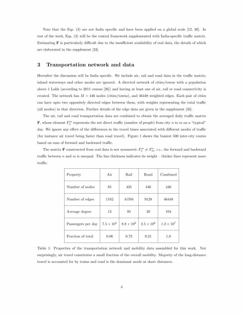
Property Air Rail Road Combined

Number of nodes 85 435 446 446

Number of edges 1182 41594 9128 46448

Average degree 13 95 20 104

Passengers per day 7.5× 105 8.8× 106 2.5× 106 1.2× 107

Fraction of total 0.06 0.73 0.21 1.0

Table 1: Properties of the transportation network and mobility data assembled for this work. Not

surprisingly, air travel constitutes a small fraction of the overall mobility. Majority of the long-distance

travel is accounted for by trains and road is the dominant mode at short distances.

4

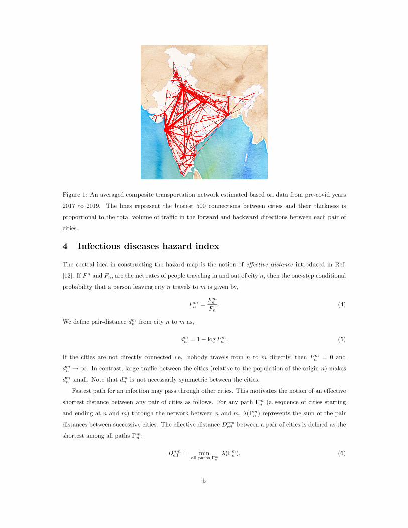
Figure 1: An averaged composite transportation network estimated based on data from pre-covid years

2017 to 2019. The lines represent the busiest 500 connections between cities and their thickness is

proportional to the total volume of traffic in the forward and backward directions between each pair of

cities.

4 Infectious diseases hazard index

The central idea in constructing the hazard map is the notion of effective distance introduced in Ref.

[12]. If Fn and Fn, are the net rates of people traveling in and out of city n, then the one-step conditional

probability that a person leaving city n travels to m is given by,

Pmn =

Fmn

Fn. (4)

We define pair-distance dmn from city n to m as,

dmn = 1− logPmn . (5)

If the cities are not directly connected i.e. nobody travels from n to m directly, then Pmn = 0 and

dmn →∞. In contrast, large traffic between the cities (relative to the population of the origin n) makes

dmn small. Note that dmn is not necessarily symmetric between the cities.

Fastest path for an infection may pass through other cities. This motivates the notion of an effective

shortest distance between any pair of cities as follows. For any path Γmn (a sequence of cities starting

and ending at n and m) through the network between n and m, λ(Γmn ) represents the sum of the pair

distances between successive cities. The effective distance Dnmeff between a pair of cities is defined as the

shortest among all paths Γmn :

Dnmeff = min

all paths Γmn

λ(Γmn ). (6)

5

Infection spread between the cities is likely to depend on the traffic between cities rather than ge-

ographical distances. The effective distance depends on the mobilities rather than the geographical

distance. By definition it takes into account the multiple paths that may connect a pair of cities, just as

the infection may reach a city through another one rather than directly from the outbreak. It is therefore

natural to expect a high correlation between aspects of infection spread and Deff .

To make this precise, we define the “time of arrival” TnmA of the infection in a city m (from a given

outbreak location n) as the first time when the number of (active) infected cases cross a predefined

threshold Ic. In studies of infection spread through global air-traffic patterns, time of arrival at location

m from an outbreak location n was found to be proportional to the effective distance Dnmeff between

them.[12]. Naively TnmA between cities, which is obtained from solution of the Eq.3 is expected to have

a complex dependence on the traffic. It is surprising that TnmA can instead be reliably predicted from a

simple functional Dnmeff .

Extensive simulations performed in this work and summarized in Fig. 2 show that, for a wide range

of realistic α and β and Indian traffic patterns, TA has a high linear correlation with Deff . Predicting the

arrival of infection at a given location is not only of academic interest but is also of immense practical

value. In the rest of the paper, we present our analysis of this idea using Indian traffic data.

Given an outbreak location, the risk of infection in another location can be quantified in many

ways, time of arrival being a natural one. Under reasonable and realistic assumptions including uniform

infection parameters, Deff provides a reliable and robust predictor of TA, as evident from our simulations.

Deff can be mapped using available transportation data unlike TA that can be obtained either from

extensive simulations or a posteriori knowledge of the infection spread.

5 Results

In order to validate the utility of the effective distance, we numerically evolve the coupled differential

equations (3) using fourth-order Runge-Kutta method. The initial infected population Ii0(t = 0) in the

outbreak city i0 is taken to be a fraction (0.0001) of the local population. We perform such simulations

for different choices of the outbreak locations and infection parameters. TA for each city is evaluated in

each case by finding the time when the city’s infected population crosses a threshold, Ic taken to be 10.

Qualitative results are independent of choices of Ii0 and Ic.

In Fig. (2) we show the results assuming infection parameters α = 1.5, β = 1.0 giving R0 = 1.5,

a typical value that was witnessed for SARS-CoV-2 [34]. In Fig. (2) (left panel), the effective distance

Di0meff , where i0 is the outbreak location, is plotted against the time of arrival at city m. This is shown

for four different outbreak locations of varying sizes, namely, Delhi, Mumbai, Patna, and Tirupati. We

find a good linear relation between Di0meff and T i0m

A , as indicated by high R2 & 0.94. These are in striking

contrast to the right panels which show TA against the geographical distances from the outbreak.

Similar observations were made in Ref.[12] which considered key global air traffic patterns alone.

6

2 4 6 8 10 12 14 16Time of Arrival (in days)

4

6

8

10

12

14

Def

f

R2 = 0.951

2 4 6 8 10 12 14 16Time of Arrival (in days)

0

500

1000

1500

2000

Dge

o (in

km

s)

R2 = 0.005

2 4 6 8 10 12 14Time of Arrival (in days)

4

6

8

10

12

14

Def

f

R2 = 0.948

2 4 6 8 10 12 14Time of Arrival (in days)

0500

10001500200025003000

Dge

o (in

km

s)

R2 = 0.001

5 10 15 20Time of Arrival (in days)

468

10121416

Def

f

R2 = 0.946

5 10 15 20Time of Arrival (in days)

0

500

1000

1500

2000

2500

Dge

o (in

km

s)R2 = 0.002

5 10 15 20 25Time of Arrival (in days)

2468

10121416

Def

f

R2 = 0.956

5 10 15 20 25Time of Arrival (in days)

0

500

1000

1500

2000

2500

Dge

o (in

km

s)

R2 = 0.0

Figure 2: Plots showing strong linear correlation between effective distance Deff and time of arrival TA.

Left column shows Di0meff plotted against TA of the infection at city m from outbreak at city i0. TA is

obtained by solving Eq. (3) with infection parameters α = 1.5, β = 1.0, Ic = 10. Outbreak locations

considered in the rows from top to bottom are Delhi, Mumbai, Patna, and Tirupati. The right column

shows the geographical distance Di0mgeo from i0 plotted against TA. R2 indicated in the plots is a measure

of goodness of the linear fits (red lines), R2 = 1 being a perfect linear fit.

7

Remarkably, within India, considering multiple modes of transport, with air travel being the least pop-

ular mode accounting for less than 10% of relevant mobility, the linearity holds good. Smaller Deff to

the outbreak then suggests a higher risk to a city, manifested as earlier arrival of the infection. The

demonstration of the ability of the Deff to predict the time of arrival is a key result of this work.

Table 2 shows the TA for the same outbreak locations as in Fig. 2. In each case, the list of the

top cities in terms of risk (i.e. smallest Deff) is also listed. For outbreaks from poorly connected cities,

the surrounding regions face the first brunt of infection; followed by bigger cities. On the other hand,

outbreaks from big metros which are well connected, quickly reach far corners. For instance, infection

from Tirupati reaches Bangalore in ∼ 5 days, while outbreak from Mumbai or Delhi, spreads to Bangalore

in ∼ 2.5 days. The hazard map in Fig. 3 shows this visually for the same four outbreak locations. The

size of circles represent the hazard (larger the circle, greater the risk). The hazard (i.e Deff) is easily

estimated for all the cities; only the top 10 cities are shown to avoid clutter.

It is interesting to consider the hazard map assuming only one mode of transport is operating. The

transportation-mode-specific hazard map is shown for two outbreak locations, Bangalore (Fig. 4),and

Guwahati (Fig. 5). As expected air traffic takes the infection to distant big cities while the roads restrict

the infection in geographical proximity. When all data is combined, the map (Fig. 4d, Fig. 5d) is largely

influenced by rail and road traffic patterns due to their higher contribution to the total traffic.

Earlier works which used mobility to study the spread have exclusively used airline mobility, which

is justified in the global context [12]. India has not just one of the largest railway networks but is also

used by a significant fraction of people. Hence, an analysis of this type presented here is most desirable

in the Indian context.

Finally, in Table (3), the results of our framework are compared with real data of TA for the first

wave of the SARS-CoV-2 pandemic.

District-wise data is available from 26th April, 2020 [2]. Mumbai crossed the threshold first and is

taken to be the outbreak location. There were ∼ 4000 active cases in Mumbai on 26th April 2020. The

TA at a city is when its three-day average caseload crosses a threshold taken to be Ic = 4000. Table

(3) presents a comparison of the real data with predictions from Deff . Table (3) (left) has the top 12

at-most risk cities based on the Deff framework. This is compared with their rank in terms of real-life

time of arrival of infections TA. We find that 9 out the 12 cities also appear in the top-12 based on

estimates from TA. To present a different means of comparison, Table (3) (right) has the top-12 cities

based on time of arrival. Again we find that 9 out of these 12 appear in the top-12 based on Deff . It

is remarkable, given the uncertainties in the traffic data and the approximations made to fill in missing

data, that ∼ 75% of cities obtained from simulations match with those in the list obtained from real

data This provides the proof-of-concept that it is possible to create a systematic predictive framework

to objectively estimate the risk in Indian cities [35].

8

Delhi

City Deff TOA

Kanpur 3.96 1.62

Mumbai 4.06 1.69

Gurgaon 4.25 1.94

Lucknow 4.33 2.00

Faridabad 4.34 2.00

Jhansi 4.54 2.19

Rohtak 4.58 2.31

Ludhiana 4.70 2.38

Moradabad 4.70 2.44

Bangalore 4.71 2.38

Mumbai

City Deff TOA

Thane 2.89 1.00

Pune 3.17 1.19

Delhi 3.7 1.62

Surat 4.07 2.00

Ahmedabad 4.08 2.00

Pimpri Chinchwad 4.25 2.19

Nashik 4.33 2.25

Vasai 4.43 2.38

Vasco Da Gama 4.47 3.00

Bangalore 4.49 2.38

Patna

City Deff TOA

Gaya 2.98 2.06

Dinapur Nizamat 3.32 2.50

Arrah 3.58 2.75

Delhi 3.75 2.81

Bhagalpur 3.99 3.25

Kolkata 4.09 3.25

Darbhanga 4.44 3.88

Jehanabad 4.47 3.94

Begusarai 4.57 4.00

Biharsharif 4.60 3.94

Tirupati

City Deff TOA

Chittoor 2.41 2.88

Chennai 2.53 2.88

Hyderabad 3.04 3.50

Vellore 4.23 5.31

Bangalore 4.25 5.06

Tiruvannamalai 4.50 5.81

Kadapa 4.84 6.50

Vijayawada 4.89 6.62

Anantapur 5.00 6.75

Madanapalle 5.01 6.75

Table 2: Time of Arrival (TA), in days, for each of the four outbreak locations in Fig. 2, showing cities

with largest 10 values of TA. The parameters are α = 1.5, β = 1.0, and Ic = 10.

6 Conclusion

If an infectious disease breaks out in one city, how long does it take to reach other cities and towns?

This length of time can be a simple measure of the risk in other cities – the longer it takes, the lesser the

risk. One may estimate this from careful simulations involving detailed traffic patterns. However this

time is easily predicted by a quantity called the effective distance, which can be calculated if we know

the prevailing traffic patterns. Larger the effective distance of a city from an outbreak location, lower is

its risk of early infection.

9

Rank

based

on Deff

City Deff

Rank

based

on TA

Rank

based

on TA

CityTA

(in days)

Rank

based

on Deff

1 Thane 2.88 4 1 Delhi 11 3

2 Pune 3.18 5 2 Ahmedabad 13 5

3 Delhi 3.70 1 3 Chennai 16 12

4 Surat 4.06 222 4 Thane 25 1

5 Ahmedabad 4.08 2 5 Pune 46 2

6 Nashik 4.29 10 6 Hyderabad 57 10

7 Vasai 4.42 No Data 7 Bangalore 65 9

8 Vasco Da Gama 4.47 No Data 8 Guwahati 70 55

9 Bangalore 4.49 7 9 Kolkata 79 11

10 Hyderabad 4.62 6 10 Nashik 85 6

11 Kolkata 4.91 9 11 Guntur 88 141

12 Chennai 4.93 3 12 Kurnool 89 131

Table 3: Comparison of the time of arrival of infection for real data and that from the simulation

framework proposed in this work. The Time of Arrival TA is given in days. The table shows top-12

at most risk cities obtained through Deff and real-life data. The ranks based on TA for top-12 cities

according to Deff are given. Correspondingly, a list is prepared for top-12 cities based on TA. The rows

in bold denote the cities common to both lists. Note that 9 out of 12 cities (∼ 75 %) are common to

both the lists, showing that the proposed framework has predictive capability. Mumbai is taken to be

the outbreak location and the real-life data is at the granularity of districts.

Based on this idea, we have constructed an infectious disease hazard map for India using the data

from the inter-city transportation network in India. Further details about the map can be found at

https://www.iiserpune.ac.in/~hazardmap/.

Real data from air, road, and rail transportation networks between the most populous 446 Indian cities

was used in this calculation. We relied on publicly available data sources and used simple assumptions

and algorithms to fill-in the missing attributes of typical Indian traffic patterns.

We used extensive simulations to validate the usefulness of the idea. We find, in agreement with

similar past studies, that the effective distance of a city from the origin is proportional to the time of

appearance of first infections in that city and is thus a reliable measure of its risk. Comparison with

the early patterns of spread of COVID-19 in India showed surprisingly good agreement between the

predictions from effective distances and real data. This adds further credence to the idea of effective

distance.

The results here prompt several interesting questions both of academic and practical value. While

effective distance predicts relative order in which cities are affected, the rate of spread through this

10

sequence is determined by the details of the infection parameters (α, β) as well as average mobility.

A conceptual framework that explains the empirical observations regarding these (from simulations) is

missing. Moreover a good explanation for the linear relationship between the effective distance and time

of arrival may be needed in order to know the limits of its applicability. Lastly, a generalization of the

notion of effective distance to a scenario of multiple outbreak locations will make this an invaluable tool

in designing efficient mitigation measures – for instance in determining which traffic routes to close down

with higher priority.

Acknowledgments

This work was funded by a special MATRICS grant MSC/2020/000122 given by SERB, Government

of India to MSS, GJS and SJ. OS would like to thank Aanjaneya Kumar and Suman Kulkarni for

the discussions. OS and MB acknowledge the INSPIRE grant from the Department of Science and

Technology, India. Map plots in the paper are made using Leaflet [36]

References

[1] https://covid19.who.int/, https://coronavirus.jhu.edu/map.html

[2] https://www.covid19india.org/

[3] I. D. Mills, The 1918-1919 influenza pandemic - The Indian experience, The Indian Economic and

Social History Review 23, 1 (1986). https://doi.org/10.1177%2F001946468602300102

[4] The Annual Report of the Sanitary Commissioner with the Government of India (1918), (Calcutta,

1920).

[5] Gautreau, A., Barrat, A., Barthelemy, M., Global disease spread: statistics and estimation of arrival

times. Journal of theoretical biology 251, 509–522. (2008)

[6] Barthelemy, M., Spatial networks. Physics Reports 499, 1–101. (2011)

[7] Feng, L., Zhao, Q., Zhou, C., Epidemic in networked population with recurrent mobility pattern.

Chaos, Solitons & Fractals 139, 110016. (2020)

[8] Belik, V., Geisel, T., Brockmann, D., Natural human mobility patterns and spatial spread of infec-

tious diseases. Physical Review X 1, 011001. (2011)

[9] Coltart, C.E., Behrens, R.H., The new health threats of exotic and global travel. British Journal of

General Practice 62, 512–513. (2012)

[10] Helbing, D., Globally networked risks and how to respond. Nature 497, 51–59. (2013)

11

[11] Barbosa, H., Barthelemy, M., Ghoshal, G., James, C.R., Lenormand, M., Louail, T., Menezes, R.,

Ramasco, J.J., Simini, F., Tomasini, M., 2018. Human mobility: Models and applications. Physics

Reports 734, 1–74. (2018)

[12] Brockmann, D., Helbing, D., The Hidden Geometry of Complex, Network-Driven Contagion Phe-

nomena. Science 342, 1337–1342. (2013)

[13] Arenas, A., Cota, W., Gomez-Gardenes, J., Gomez, S., Granell, C., Matamalas, J.T., Soriano-

Panos, D., Steinegger, B., Modeling the Spatiotemporal Epidemic Spreading of COVID-19 and the

Impact of Mobility and Social Distancing Interventions. Physical Review X 10, 041055. (2020)

[14] Althouse, B.M., Wenger, E.A., Miller, J.C., Scarpino, S.V., Allard, A., Hebert-Dufresne, L., Hu, H.,

Stochasticity and heterogeneity in the transmission dynamics of SARS-CoV-2. arXiv:2005.13689.

(2020)

[15] Garcia-Gasulla, D., Napagao, S.A., Li, I., Maruyama, H., Kanezashi, H., P’erez-Arnal, R., Miyoshi,

K., Ishii, E., Suzuki, K., Shiba, S., Global Data Science Project for COVID-19 Summary Report.

arXiv:2006.05573. (2020)

[16] Mishra, R., Gupta, H.P., Dutta, T., Analysis, Modeling, and Representation of COVID-19

Spread: A Case Study on India, in IEEE Transactions on Computational Social Systems, doi:

10.1109/TCSS.2021.3077701. (2021)

[17] Sarkar, K., Khajanchi, S., Nieto, J.J., Modeling and forecasting the COVID-19 pandemic in India.

Chaos, Solitons & Fractals 139, 110049. (2020)

[18] Pujari, B.S., Shekatkar, S., Multi-city modeling of epidemics using spatial networks: Application to

2019-nCov (COVID-19) coronavirus in India. medRxiv. https://doi.org/10.1101/2020.03.13.

20035386 (2020)

[19] Gupta, S., Shah, S., Chaturvedi, S., Thakkar, P., Solanki, P., Dibyachintan, S., Roy, S., Sushma,

M.B., Godbole, A., Jaseem, N. et. al., An India-specific compartmental model for Covid-19: pro-

jections and intervention strategies by incorporating geographical, Infrastructural and response het-

erogeneity. arXiv:2007.14392. (2020)

[20] R. Gopal, V. K. Chandrasekar and M. Lakshmanan, Dynamical modelling and analysis of COVID-19

in India, Current Science 120 1342 (2021).

[21] Bedi, P., Dhiman, S., Gole, P., Jindal, V., Prediction of COVID-19 Trend in India and Its Four

Worst-Affected States Using Modified SEIRD and LSTM Models. SN COMPUT. SCI. 2, 224 (2021)

[22] Khajanchi, S., Sarkar, K., Forecasting the daily and cumulative number of cases for the COVID-19

pandemic in India. Chaos: An Interdisciplinary Journal of Nonlinear Science 30, 071101. (2020)

12

[23] Das, A., Dhar, A., Goyal, S., Kundu, A., Pandey, S., COVID-19: Analytic results for a modified

SEIR model and comparison of different intervention strategies. Chaos, Solitons & Fractals 110595.

(2021)

[24] Jha, V., Forecasting the transmission of Covid-19 in India using a data driven SEIRD model.

arXiv:2006.04464. (2020)

[25] Khajanchi, S., Sarkar, K., Mondal, J., Perc, M., Dynamics of the COVID-19 pandemic in India.

arXiv:2005.06286. (2020)

[26] https://censusindia.gov.in/2011-common/censusdata2011.html

[27] Gong, Y., Song, Y., Jiang, G., Epidemic spreading in metapopulation networks with heterogeneous

infection rates, Physica A: Statistical Mechanics and its Applications, 416, 208-218. (2014)

[28] Ronald, R., and Hilda, P., An application of the theory of probabilities to the study of a priori

pathometry.–Part IIIProc. R. Soc. Lond. A 93: 225–240. (1917)

[29] Kermack, W. O. and McKendrick, A. G., A contribution to the mathematical theory of epidemics,

Proc. R. Soc. Lond. A 115:700–721. (1927)

[30] Colizza, V., Pastor-Satorras, R., and Vespignani, A. Reaction-diffusion processes and metapopula-

tion models in heterogeneous networks. Nature Phys 3, 276–282 (2007).

[31] Taylor, D., Klimm, F., Harrington, H.A., Kramar, M., Mischaikow, K., Porter, M.A., Mucha, P.J.,

2015. Topological data analysis of contagion maps for examining spreading processes on networks.

Nature communications 6, 1–11. (2015)

[32] Tolic, D., Kleineberg, K.-K., Antulov-Fantulin, N., Simulating SIR processes on networks using

weighted shortest paths. Scientific reports 8, 1–10. (2018)

[33] Please refer to the Supplementary material.

[34] Marimuthu S., Joy M.,Malavika B., Nadaraj A., Asirvatham E., Jeyaseelan L., Modelling of repro-

duction number for COVID-19 in India and high incidence states. Clinical Epidemiology and Global

Health, 9, 57-61. (2021)

[35] For more information, visit https://www.iiserpune.ac.in/~hazardmap/

[36] Leaflet — Map tiles by Stamen Design, under CC BY 3.0. Data by © OpenStreetMap, under CC

BY SA.

13

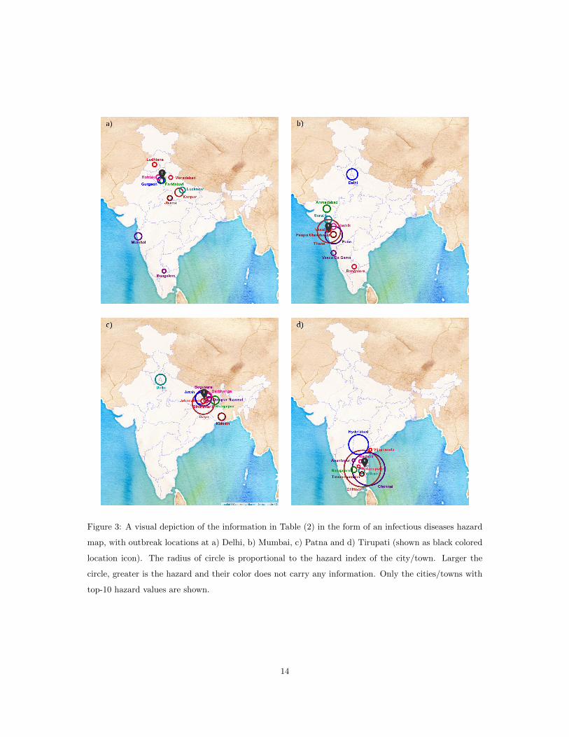
Figure 3: A visual depiction of the information in Table (2) in the form of an infectious diseases hazard

map, with outbreak locations at a) Delhi, b) Mumbai, c) Patna and d) Tirupati (shown as black colored

location icon). The radius of circle is proportional to the hazard index of the city/town. Larger the

circle, greater is the hazard and their color does not carry any information. Only the cities/towns with

top-10 hazard values are shown.

14

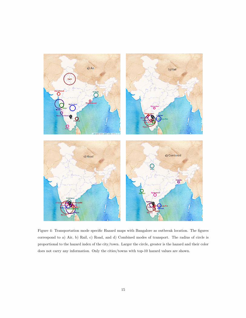
Figure 4: Transportation mode specific Hazard maps with Bangalore as outbreak location. The figures

correspond to a) Air, b) Rail, c) Road, and d) Combined modes of transport. The radius of circle is

proportional to the hazard index of the city/town. Larger the circle, greater is the hazard and their color

does not carry any information. Only the cities/towns with top-10 hazard values are shown.

15

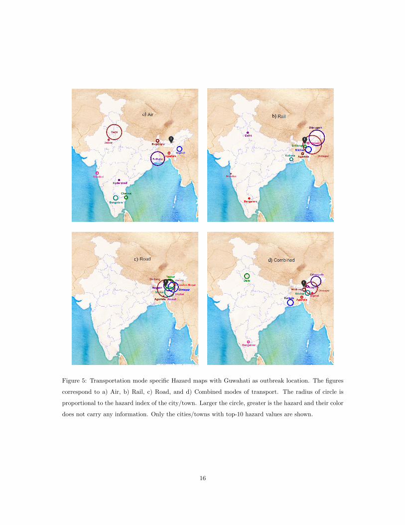
Figure 5: Transportation mode specific Hazard maps with Guwahati as outbreak location. The figures

correspond to a) Air, b) Rail, c) Road, and d) Combined modes of transport. The radius of circle is

proportional to the hazard index of the city/town. Larger the circle, greater is the hazard and their color

does not carry any information. Only the cities/towns with top-10 hazard values are shown.

16

Supplemental Material for

An infectious diseases hazard map for India based on mobility and

transportation networks

Onkar Sadekar, Mansi Budamagunta, G. J. Sreejith, Sachin Jain, and M. S. Santhanam

Indian Institute of Science Education and Research, Pune 411 008, India.

1 Transportation network and data

In this supplementary material, network creation and data sources used in estimating the traffic matrix F

are discussed. For the purposes of this work, we focus on data from air, railway and road transportation

while ignoring inland waterways and other modes.

Based on the 2011 census data [1], a network of cities/towns in India whose population is more than

1 Lakh and having at least one of air, rail or road connectivity is created. By this criterion, a directed

network with M = 446 nodes (cities/towns), and 46448 edges (routes) is created. In this, the edges

corresponding to air, railway and road links are combined if they connect the same pair of cities and

are counted as one edge. Some important network properties are listed in Table (1). In the table, mean

degree refers to the out-degree (which is the same as in-degree for this dataset) and gives a measure of

the average number of cities each city is connected to. This table also shows coarse mobility data. By

‘route symmetry index’ in the context of pair of cities a and b, it is indicated if route a→ b has the same

traffic as the reverse route b → a or not. The index is defined for a given dataset as ‘1− the maximum

absolute fractional traffic difference with respect to the city’s population averaged over all cities’. The

index can mathematically be expressed as

Route Symmetry Index = 1−⟨

maxj|F ji − F i

j |Ni

⟩

i

. (1)

The locality of mobility indicates if the fraction of people who travel out of a city, i.e. Fi

Ni, is the same

across all cities or not. As is evident, air travel contributes far less to the overall mobility of people in

India though it might become somewhat important if the speed of transportation is taken into account.

As road travel is a locally (< 300 km) dominant mode, most of the meaningful long-distance connections

and mobility arise from railways.

Railway data : The data of trains and railway stations was obtained from the Indian Railways website,

and travel planning websites [2, 3]. In all, Indian railway network has about 8000 railway stations through

which about 3000 express/mail/passenger trains are run daily [4]. The weekly schedule of each of these

trains is drawn from the railway timetable [4]. Even though there are studies conducted to analyse the

Indian railway network [5, 6, 7], none of them considered the number of passengers travelling between

two cities. The data of the number of trains run is converted into passenger traffic through an algorithm

1

arX

iv:2

105.

1512

3v3

[q-

bio.

PE]

4 A

ug 2

021

Property Airway Railway Roadway Combined

Number of Nodes 85 435 446 446

Number of Edges 1182 41594 9128 46448

Average Degree 13 95 20 104

Route symmetry index 1 0.9875 1 0.9878

Locality of Mobility Same Different Same Different

Passengers/day 7.5× 105 8.8× 106 2.5× 106 1.2× 107

Fraction of total 0.06 0.73 0.21 1.0

Table 1: Properties of the transportation network and mobility data assembled for this work. Not

surprisingly, air travel constitutes a miniscule fraction of the overall mobility. Bulk of long distance travel

is accounted for by trains, though at short distances roads might also have significant contribution.

described in the next sections. The algorithm relies on two simple assumptions – that the train is always

full (almost always true in India), and the number of passengers travelling between two cities on some

route is proportional to the population of the two cities. Based on this algorithm, the daily passengers

on the train comes to about 88 Lakh [Table (1)]. As we are only concerned with long-distance traffic,

the suburban traffic in several cities such as Mumbai and Chennai, which have a dense suburban train

network, is also ignored.

Airline data : The passenger data on domestic routes, based on the data available on the Directorate

General of Civil Aviation, Govt. of India (DGCA), was obtained [8] for 85 Indian cities with an airport

and with a population of 1 Lakh or more. Passenger traffic was collected for pairs of cities for the year

2018, from which daily traffic was arrived at. According to the DGCA, the total domestic air traffic in

India for 2018-2019 was 2851 Lakhs [9]. This implies that about 7.8 Lakhs people use air transport daily

on an average, which upon correcting for the ignored airports for small cities with a population less than

1 Lakh, comes to approximately 7.5 Lakhs per day, the value indicated in Table (1).

Road data : Compared to the other two modes of transport, very little reliable information is available

for road transport in India. The National Highways Authority of India (NHAI) provides some minimal

data only for national highways, which typically carry traffic over long-distances of >300-400 Kms.

However, we ignore the long-distance road traffic by assuming that people mostly prefer train or air for

long-distance travel. Further, the significant passenger flux over short distances of about <400 km is

2

mainly accounted for by public transport and in some cases by private vehicles. Since there is no reliable

data available to estimate the short distance (<400 Kms) travel (or even the long-distance traffic) between

any two given cities, we estimate these numbers using our algorithm given in the next section. The basic

idea behind the algorithm is that most people prefer road for distances of < 300 Kms. This algorithm

gives us daily traffic of around 25 Lakhs per day.

All these data are assembled together to obtain the averaged daily traffic matrix F, whose element

F ji represents the mean composite volume of traffic (number of people) in the route from city i to j in a

“typical” day. Note that the data is mainly drawn from or estimated for pre-covid years, 2017 to 2019.

Based on this dataset, we find that F ji 6= F i

j , i.e., it is a directed network, implying that the number

of people travelling from city i to j and vice-versa are not equal. In this paper, we will also neglect the

time-scales associated with various modes of transport (e.g., the air is faster than train or road travel)

and focus only on the average number of people travelling in a day.

2 Algorithms

The raw data that we have collected is not in the format of number of passengers travelling from city i

to city j except for the airway. The rail data is in the form of travel routes, while there is no reliable

source for road data. In this supplemental material, we will look at two algorithms to estimate the road

and rail traffic matrices entries by making some reasonable assumptions.

2.1 Railways

The raw data for railways is in the format of the train routes with stops [2, 3]. We have the population

for each of the stop on all routes. The raw data set consists of 4480 routes, including both forward

and backward routes [4]. To make the data-analysis tractable, we include only those cities that have a

population of more than 1 Lakh as per the 2011 census in India [1]. Thus, few smaller sub-stations in

the vicinity of major metropolitan cities are also treated as separate cities.

To extract data from train routes and population of cities, we rely on the two assumptions,

1. The train is always full while travelling between any two consecutive cities.

2. The number of people travelling between any two cities (not necessarily consecutive) on a route is

proportional to their individual populations.

In addition to the information about the route and population, we also have the information about

the weekly frequency and the type of train on each of the routes. We use the knowledge about the train

type to fix the capacity of each train. We will now delve into the details of the algorithm.

Let us consider a particular route Ω with k stations labelled by indices 1, 2, ..., k. The population

of the cities is N1, N2, ..., Nk respectively. Assumption 1 tells us that the train starts with full capacity

from city 1, which we denote by C. According to the assumption 2 these C number of people will get

3

down at remaining stations proportional to the population. Going back to our first assumption; the

number of people getting on the train at any city j (j ≥ 2) would be the same as number of people

getting down at that station. Let F denote the traffic matrix, where F ji corresponds to number of people

going from city i to city j in unit time. Similarly, Fi represents the total number of people moving out

of city i in a unit amount of time.

Now, the number of people getting on the train at city 2, will again get down at cities j (j ≥ 3),

proportional to their population. The number of people getting down at city 3 would be dependent on

number of people who got on the train in city 1 and 2. Thus, we continue this process until city k − 1,

and finally C number of people will get down at city k. The total outgoing/incoming number of people

for the cities on the route Ω can be expressed mathematically as,

F1(Ω) = C,

F2(Ω) = F1N2∑kj=2Nj

,

F3(Ω) = F1N3∑kj=2Nj

+ F2N3∑kj=3Nj

,

F4(Ω) = F1N4∑kj=2Nj

+ F2N4∑kj=3Nj

+ F3N4∑kj=4Nj

,

...

Fa(Ω) =a−1∑

i=1

[Fi

Na∑kj=i+1Nj

]. (2)

We note that these equations have a recursive form. Luckily, we can simplify each of them to get a

simple form for Fa, which denotes the total number of people leaving city a for route Ω,

Fa(Ω) = F1Na∑kj=aNj

= CNa∑kj=aNj

, for, 2 ≤ a ≤ k − 1,

Fa(Ω) = F1 = C, for, a = 1. (3)

For instance the expression for F3(Ω) can be simplified as,

F3(Ω) = F1N3∑kj=2Nj

+ F2N3∑kj=3Nj

,

F3(Ω) = F1N3∑kj=2Nj

+ F1N2∑kj=2Nj

N3∑kj=3Nj

,

F3(Ω) = F1N3∑kj=2Nj

[1 +

N2∑kj=3Nj

],

F3(Ω) = F1N3∑kj=2Nj

[∑kj=2Nj

∑kj=3Nj

],

4

F3(Ω) = F1N3∑kj=3Nj

. (4)

The number of people going from city a to city b (2 ≤ a < b ≤ k) for the route Ω would be,

F ba(Ω) =

[C

Na∑kj=aNj

][Nb∑k

j=a+1Nj

], for, 2 ≤ a < b ≤ k,

F ba(Ω) =

[C

Nb∑kj=a+1Nj

], for, 1 = a < b ≤ k. (5)

Thus, we have obtained the expression for number of people travelling from city a to city b for a given

route. There is only one free parameter in the above expression F1 = C, which we fix by knowing the

type of train and its capacity [2]. We can run the same algorithm for all the routes in our raw data-set

to get the full F-matrix for railway as the mode of transport. We illustrate this algorithm in a more

visual and simple way, using an imaginary toy route and population in Fig. (1).

Let us consider a train route going through 4 cities A, B, C, and D having equal population N . We

will also assume that the capacity of train is 120. Figure. (1) shows the final results after running the

algorithm for the forward and backward routes. As we can readily see the F-matrix is not symmetric

even if we consider the simplest case of just one route through cities of equal population. It is also

worth noting that the total number of people travelling in/out of a city is not proportional to the city

population. The assymetricity of F-matrix and unequal local mobility becomes more pronounced when

we consider all cities and all the routes.

2.2 Road

In this section, we will look at the algorithm used to generate the road traffic. To our knowledge, there

is no systematic source of road traffic connecting almost all cities in India with population above 1 Lakh.

The only available data is about toll booths on national highways [10]. This data is not useful as it leaves

out most of the short-distance routes. Thus, we have to estimate the traffic data by using the available

information.

As a simplest case, we assume that the final F-matrix is symmetric. We can move away from this

assumption, however, the process to make sure that the population of each city remains constant becomes

more complex.

The next assumption we make is that most people use road travel for a short distance and long-

distance travel is usually undertaken through railways or by aeroplane. And we make the final assumption

that the total number of people travelling by road is proportional to the population of the city. We will

later see how these specific assumptions help us fix the free parameters in our algorithms under the given

set of constraints.

First we construct a graph of the cities. We consider cities within a specified distance as adjacent

in this graph and construct an adjacency matrix for this graph. The distances are calculated using the

5

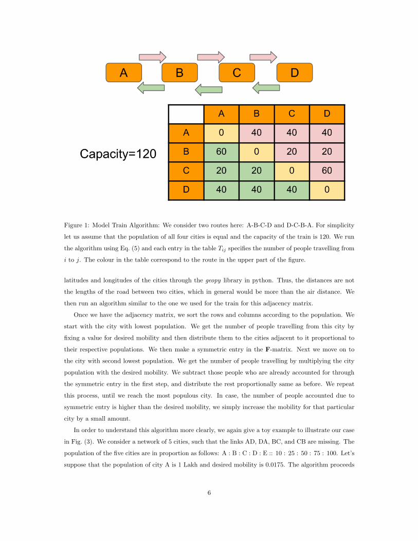
Figure 1: Model Train Algorithm: We consider two routes here: A-B-C-D and D-C-B-A. For simplicity

let us assume that the population of all four cities is equal and the capacity of the train is 120. We run

the algorithm using Eq. (5) and each entry in the table Tij specifies the number of people travelling from

i to j. The colour in the table correspond to the route in the upper part of the figure.

latitudes and longitudes of the cities through the geopy library in python. Thus, the distances are not

the lengths of the road between two cities, which in general would be more than the air distance. We

then run an algorithm similar to the one we used for the train for this adjacency matrix.

Once we have the adjacency matrix, we sort the rows and columns according to the population. We

start with the city with lowest population. We get the number of people travelling from this city by

fixing a value for desired mobility and then distribute them to the cities adjacent to it proportional to

their respective populations. We then make a symmetric entry in the F-matrix. Next we move on to

the city with second lowest population. We get the number of people travelling by multiplying the city

population with the desired mobility. We subtract those people who are already accounted for through

the symmetric entry in the first step, and distribute the rest proportionally same as before. We repeat

this process, until we reach the most populous city. In case, the number of people accounted due to

symmetric entry is higher than the desired mobility, we simply increase the mobility for that particular

city by a small amount.

In order to understand this algorithm more clearly, we again give a toy example to illustrate our case

in Fig. (3). We consider a network of 5 cities, such that the links AD, DA, BC, and CB are missing. The

population of the five cities are in proportion as follows: A : B : C : D : E :: 10 : 25 : 50 : 75 : 100. Let’s

suppose that the population of city A is 1 Lakh and desired mobility is 0.0175. The algorithm proceeds

6

Figure 2: The relative size of 200 Kms circle for scale on map of India. On left hand side, we draw the

circles around Mumbai, Pune, Delhi, Secennai, Guwahati, and Port-Blair. The right hand figure shows

the circle for Pune. We can identify few of the important cities in Maharashtra which are connected to

Pune by road from our algorithm.

as follows:

• First we get the adjacency matrix whose indices are sorted according to the population. We start

with lowest population city, i.e. A and distribute the desired number of people into all possible

connections (blue coloured).

• We make symmetric entries in the first column (blue), subtract that number from desired traffic

for city B and distribute the rest into possible connections (red). We make similar symmetric entry

in red.

• For city C, we proceed as before, subtract, distribute, and make symmetric entry (yellow).

• We continue the algorithm until the table is fully filled.

Coming back to our algorithm for a network of 446 cities, the parameter values that we used in our

algorithm are,

• desired mobility γ = 0.015.

• radius of circle of proximity = 200 Kms.

• The increase in traffic to distribute in case the symmetric entries already sum up more than the

desired traffic was (0.5× desired traffic).

According to [11], the total yearly road traffic in India is around 822 crore passengers. If we consider

the average daily road traffic it comes out to be around 2.25 crore passengers. At a gross level, if we

7

Figure 3: Road Algorithm: The F-matrix for the toy model is symmetric and the final traffic, matches

exactly with desired traffic for most cities.

calculate the global mobility for India considering that the current population of 130 crores, we get the

global mobility to be around 0.017. We take it to be 0.015 in order to compensate for fluctuations and

other uncertainties.

We now mention few of the main results of the F-matrix for road transport.

1. We increased the mobility of only 6 (out of 446) cities to account for overflow of traffic due to

symmetric entries.

2. The cities have 20 connections on an average.

3. 92% (or ≈ 410) cities have a local mobility of 0.015. The average (global) mobility is 0.0115 and

the standard deviation of it is 0.0021.

References

[1] https://censusindia.gov.in/2011-common/censusdata2011.html

[2] https://indianrailways.info/all_trains/

[3] https://www.makemytrip.com/railways/list-of-indian-railway-stations.html

[4] https://enquiry.indianrail.gov.in/mntes/

[5] Rajput, N.K., Badola, P., Arora, H., Grover, B.A., Complex Network Analysis of Indian Railway

Zones. arXiv:2004.04146. (2020)

8

[6] Gopalakrishnan, R., Rangaraj, N., Capacity management on long-distance passenger trains of Indian

Railways. Interfaces 40, 291–302. (2010)

[7] Sen, P., Dasgupta, S., Chatterjee, A., Sreeram, P.A., Mukherjee, G., Manna, S.S., Small-world

properties of the Indian railway network. Physical Review E 67, 036106. (2003)

[8] http://www.knowindia.net/aviation.html

[9] https://www.civilaviation.gov.in/sites/default/files/MoCA_Annual_Report_2018_19.

pdf, Page No. 49

[10] https://tis.nhai.gov.in/

[11] https://en.wikipedia.org/wiki/Transport_in_India

9